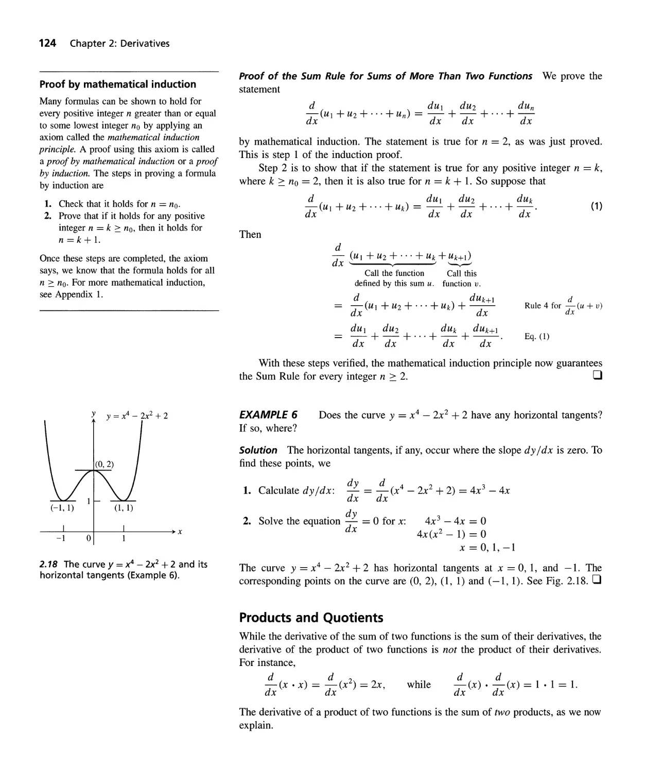
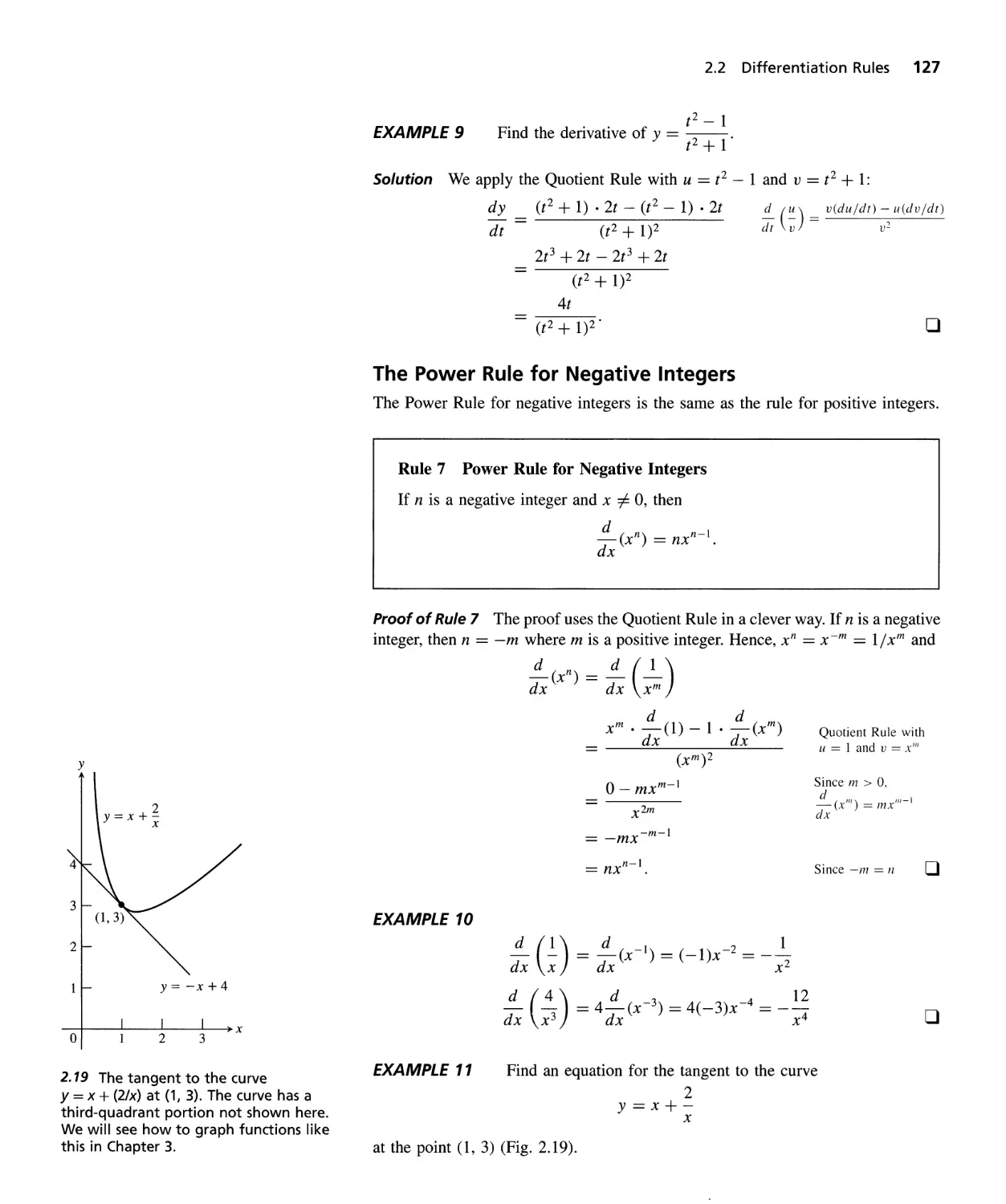
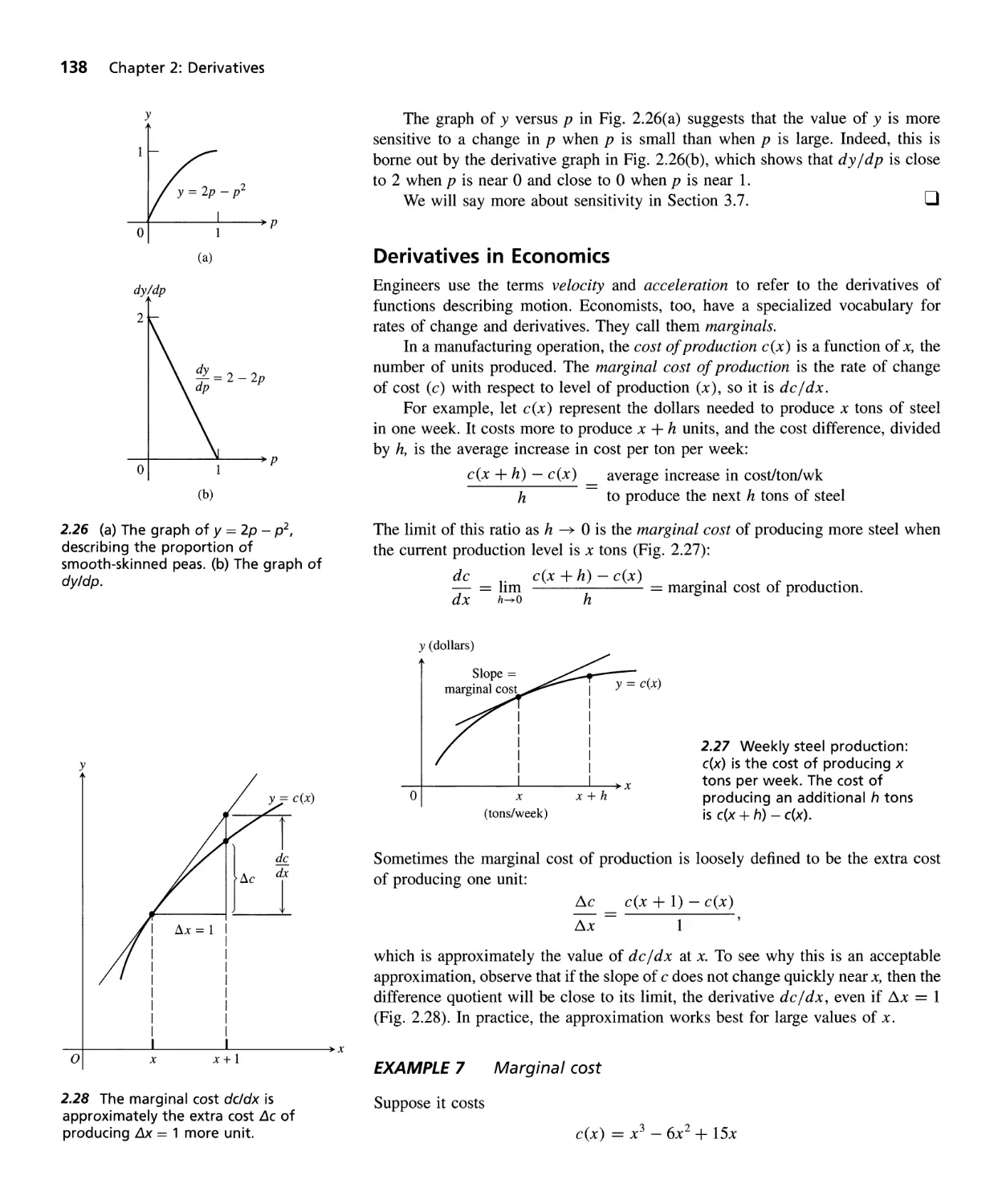
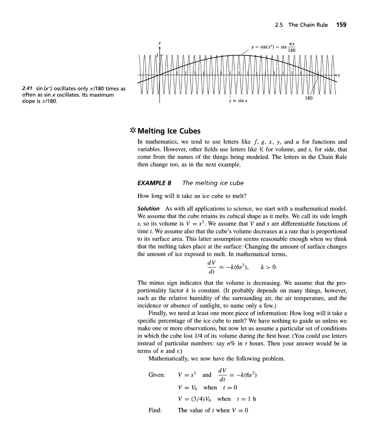
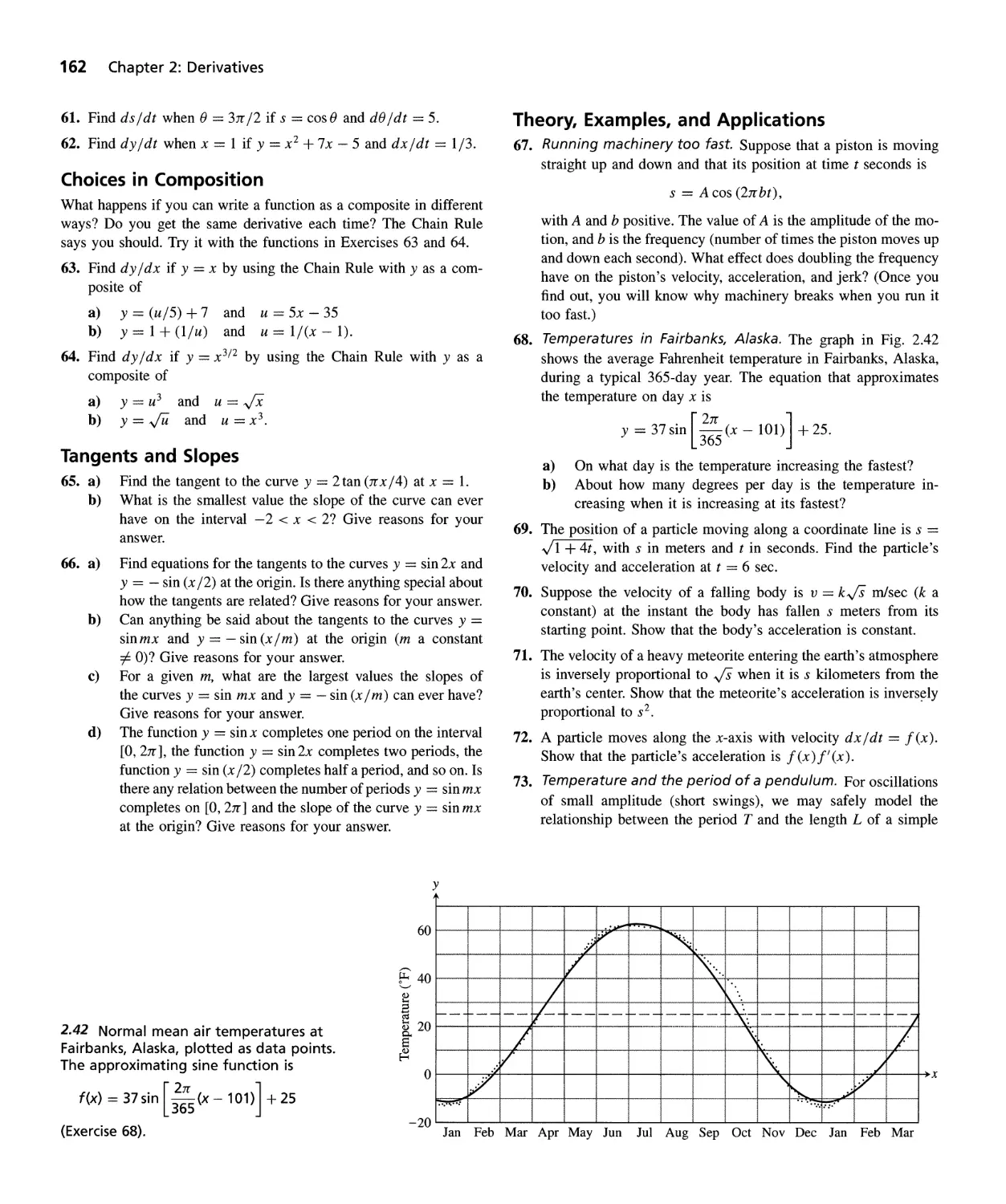
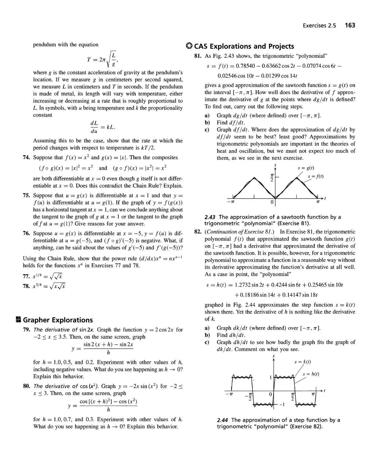
/


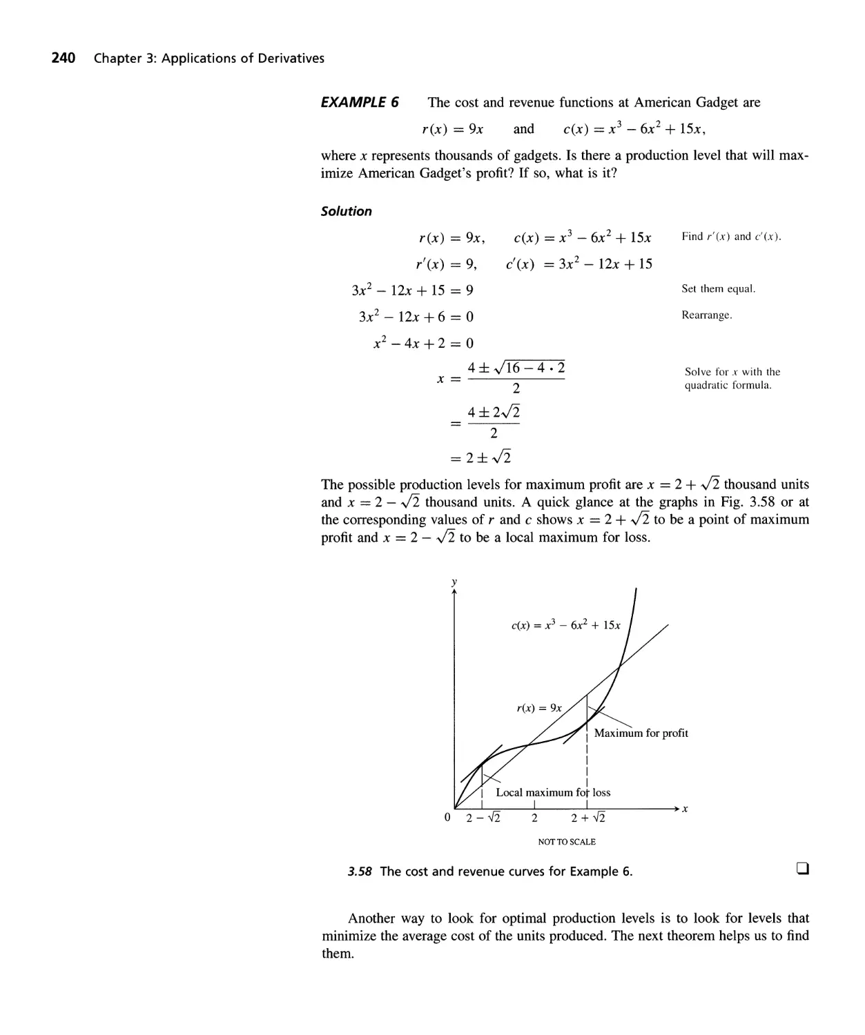


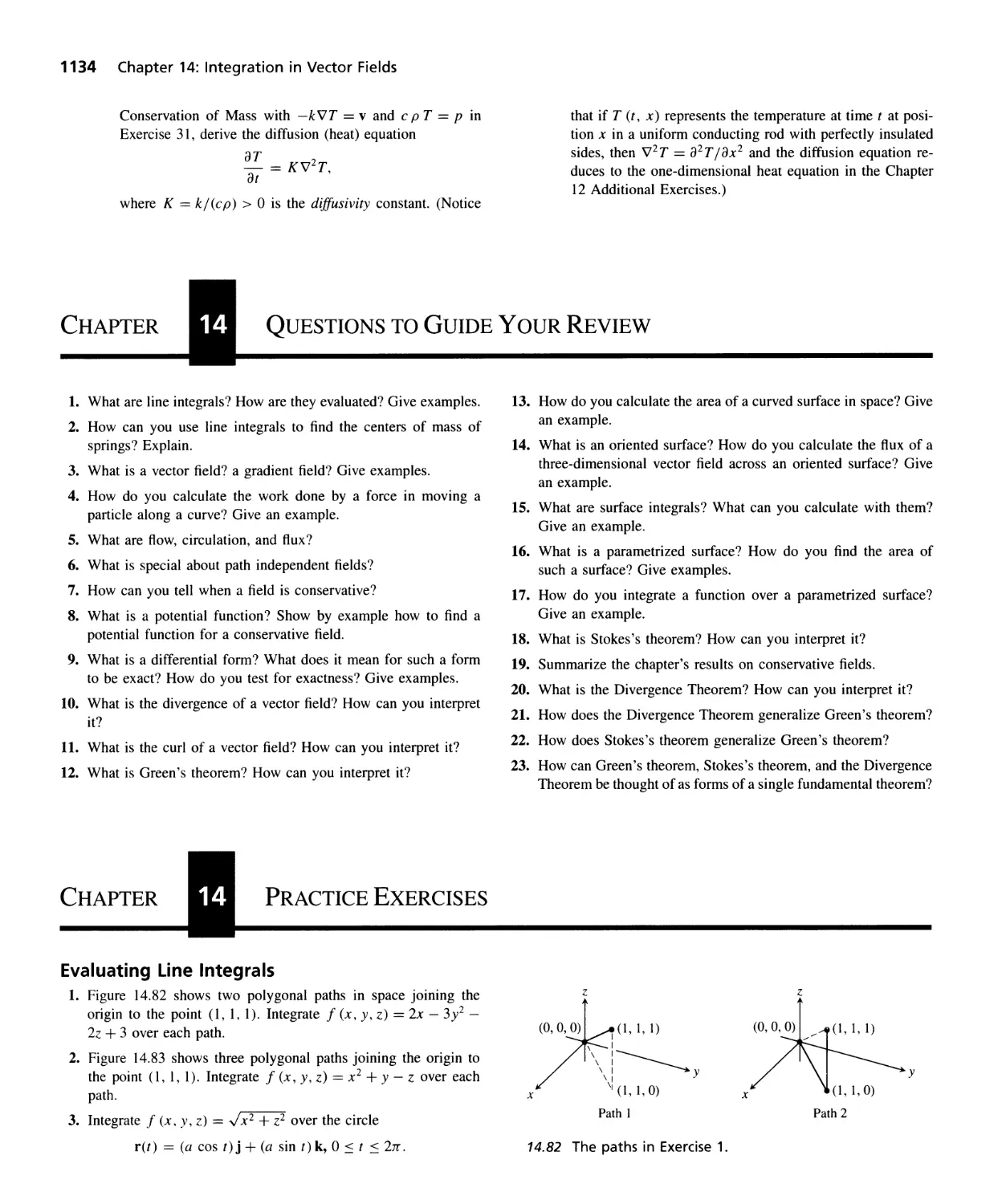
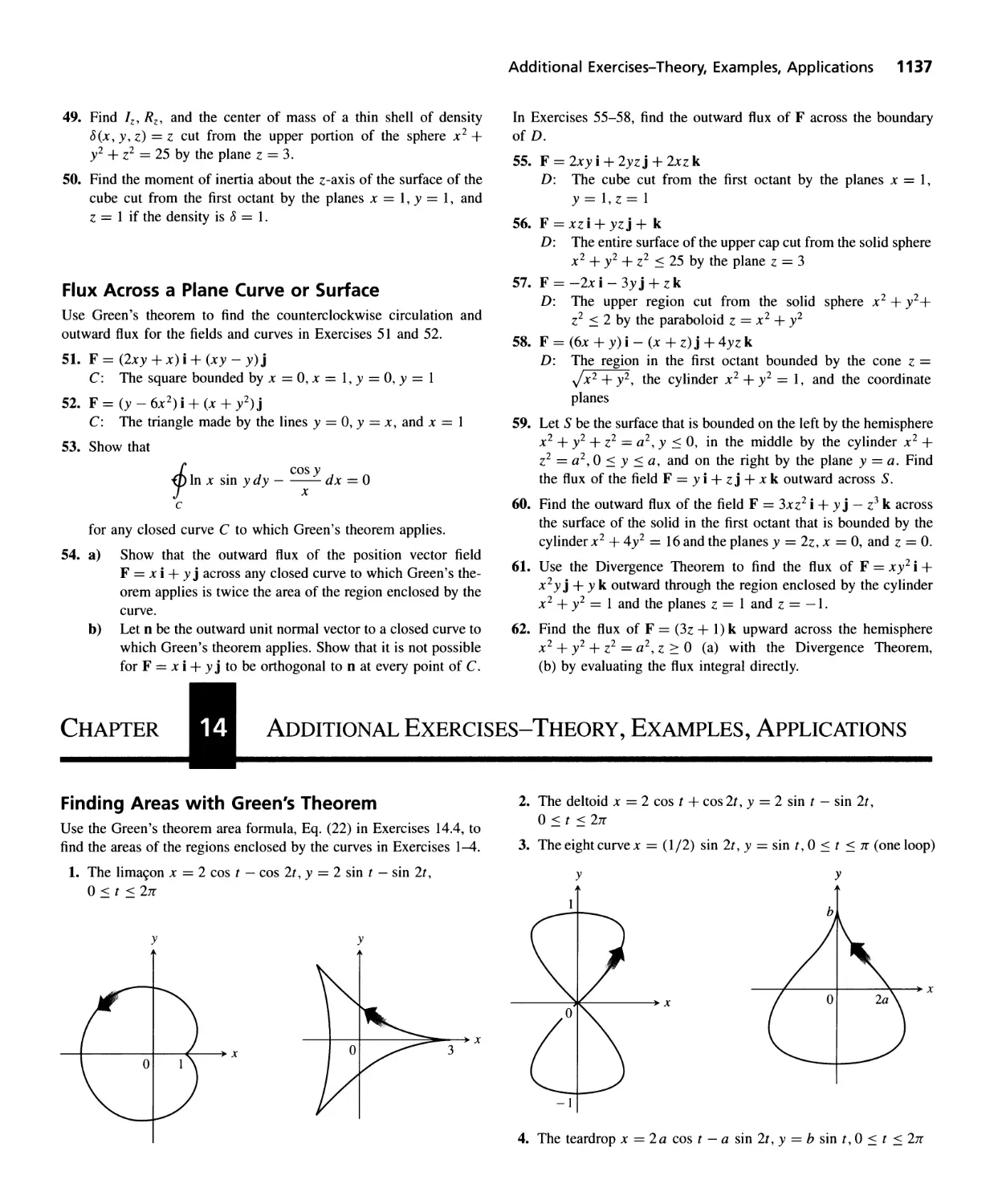


Текст
9TH EDITION
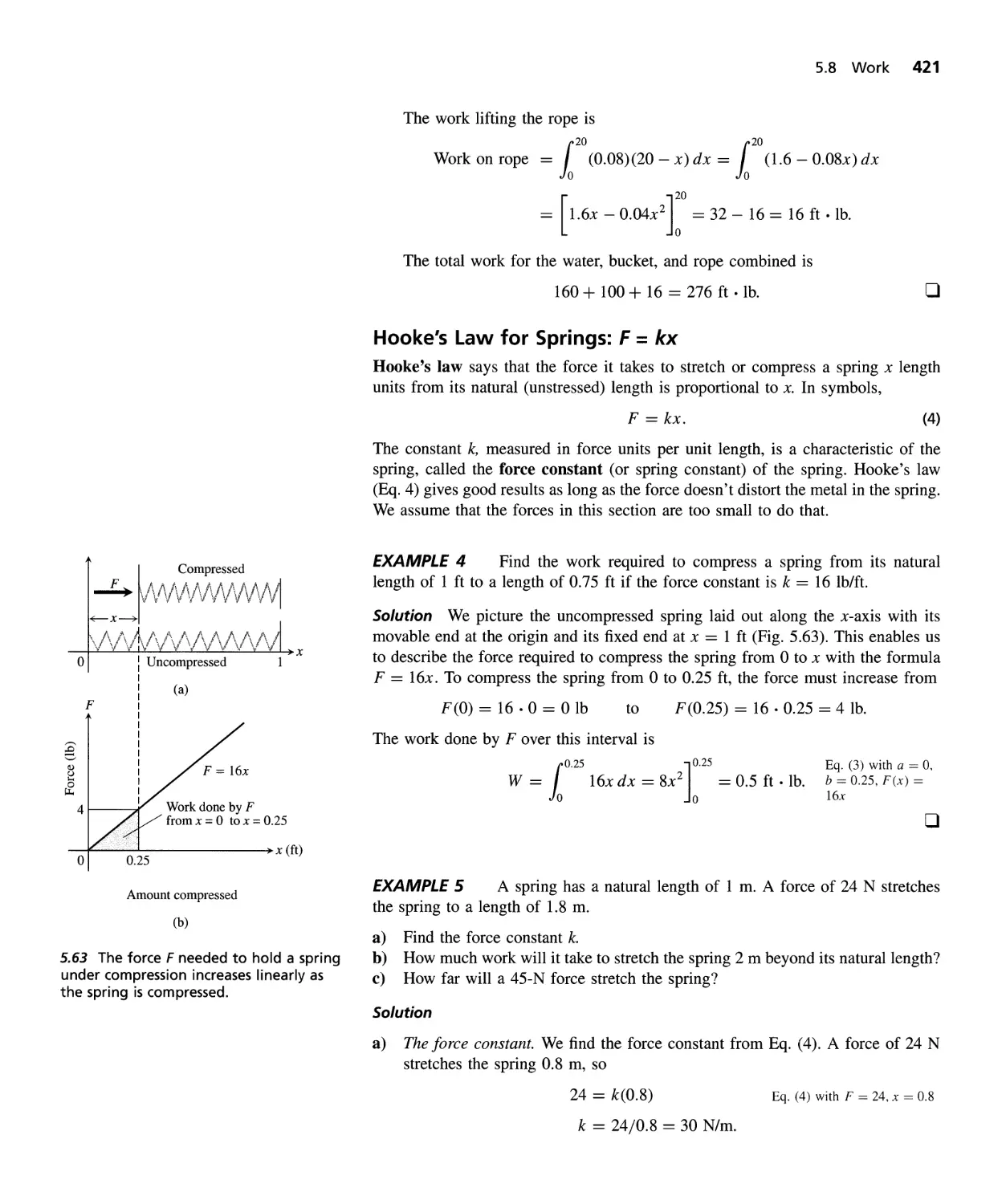
Calculus and
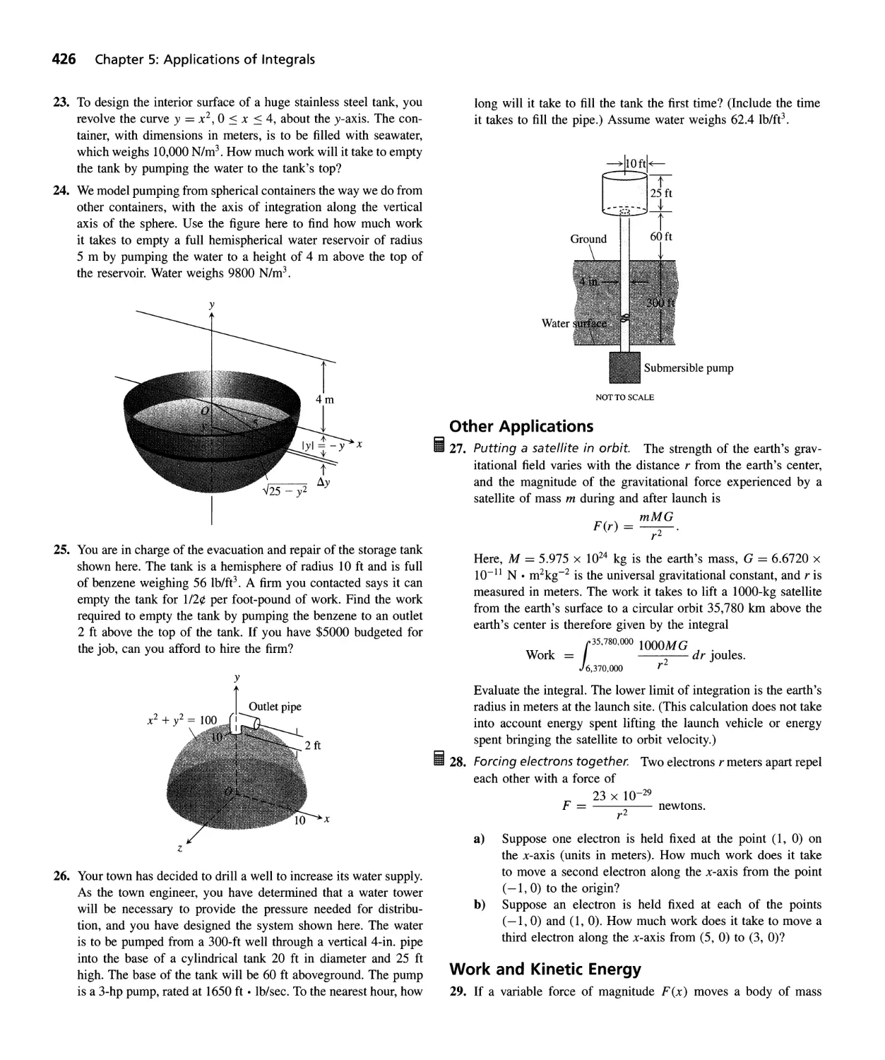
Analytic
Geometry
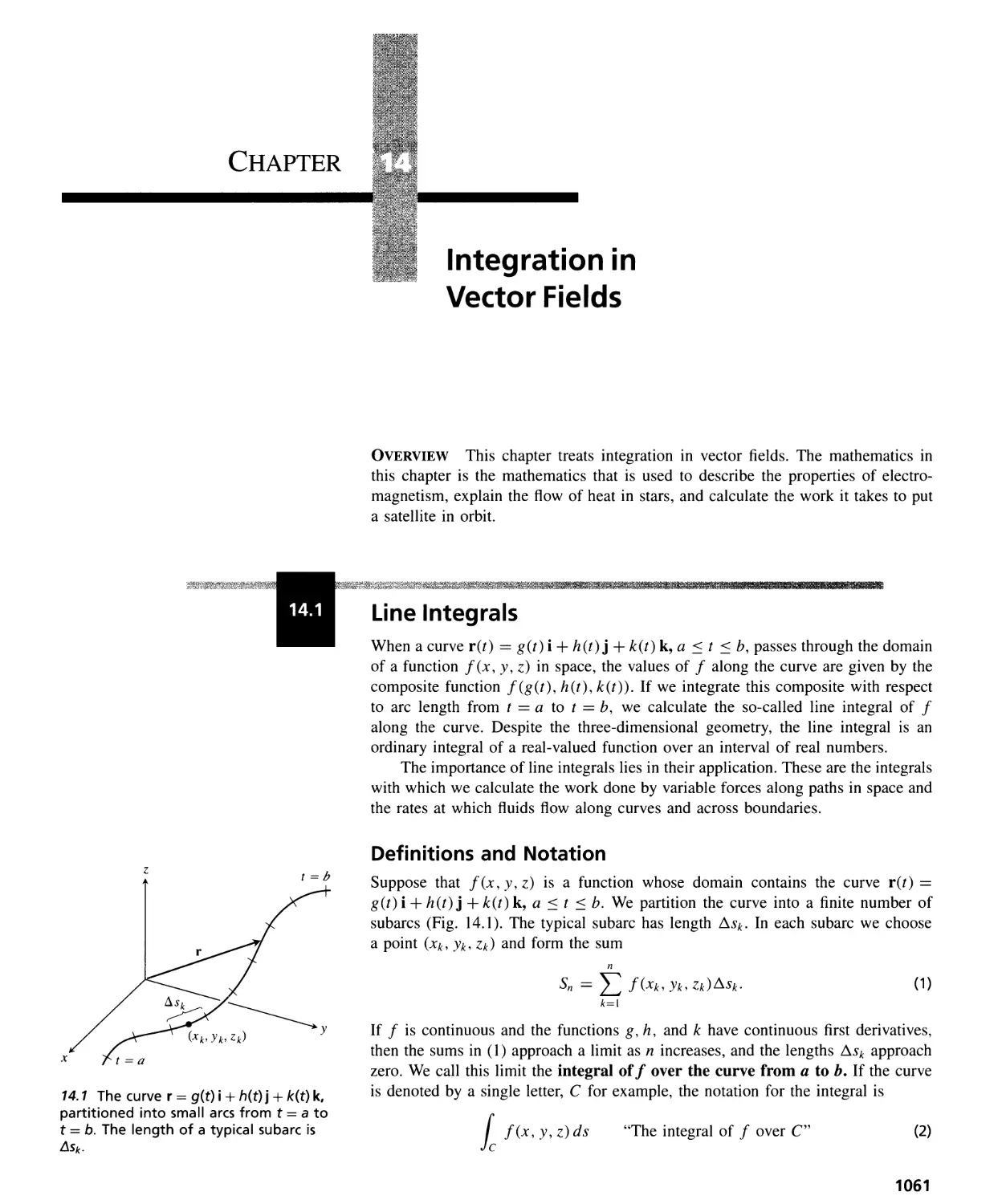
George B. Thomas, Jr.
Massachusetts Institute of Technology
Ross L. Finney
With the collaboration of
Maurice D. Weir
Naval Postgraduate School
\SON -Wf'J'
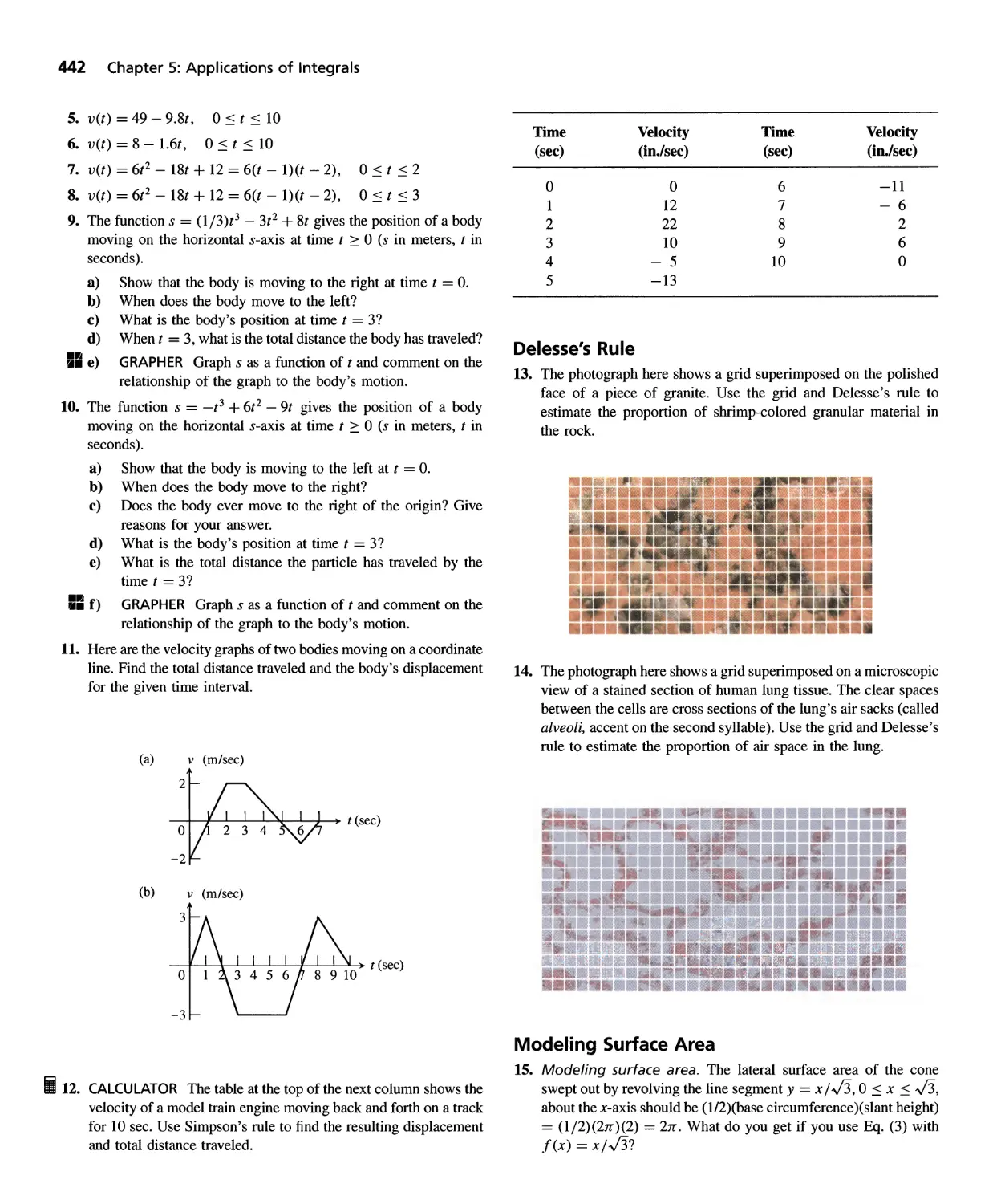
'4
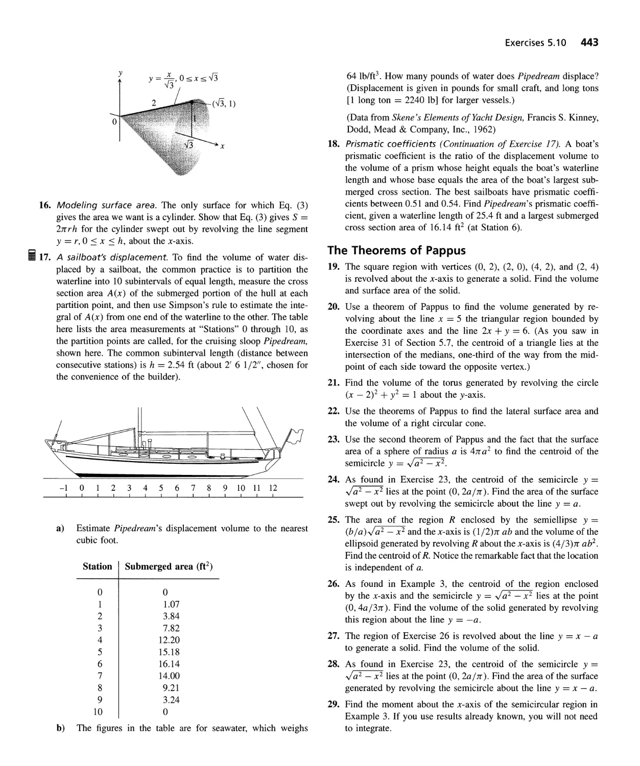
'."$ Addison-Wesley Publishing Company
SrUD£.
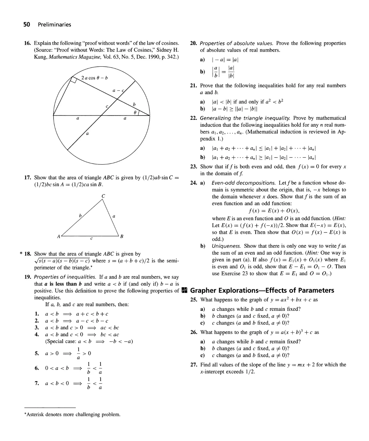
Reading, Massachusetts · Menlo Park, California · New York
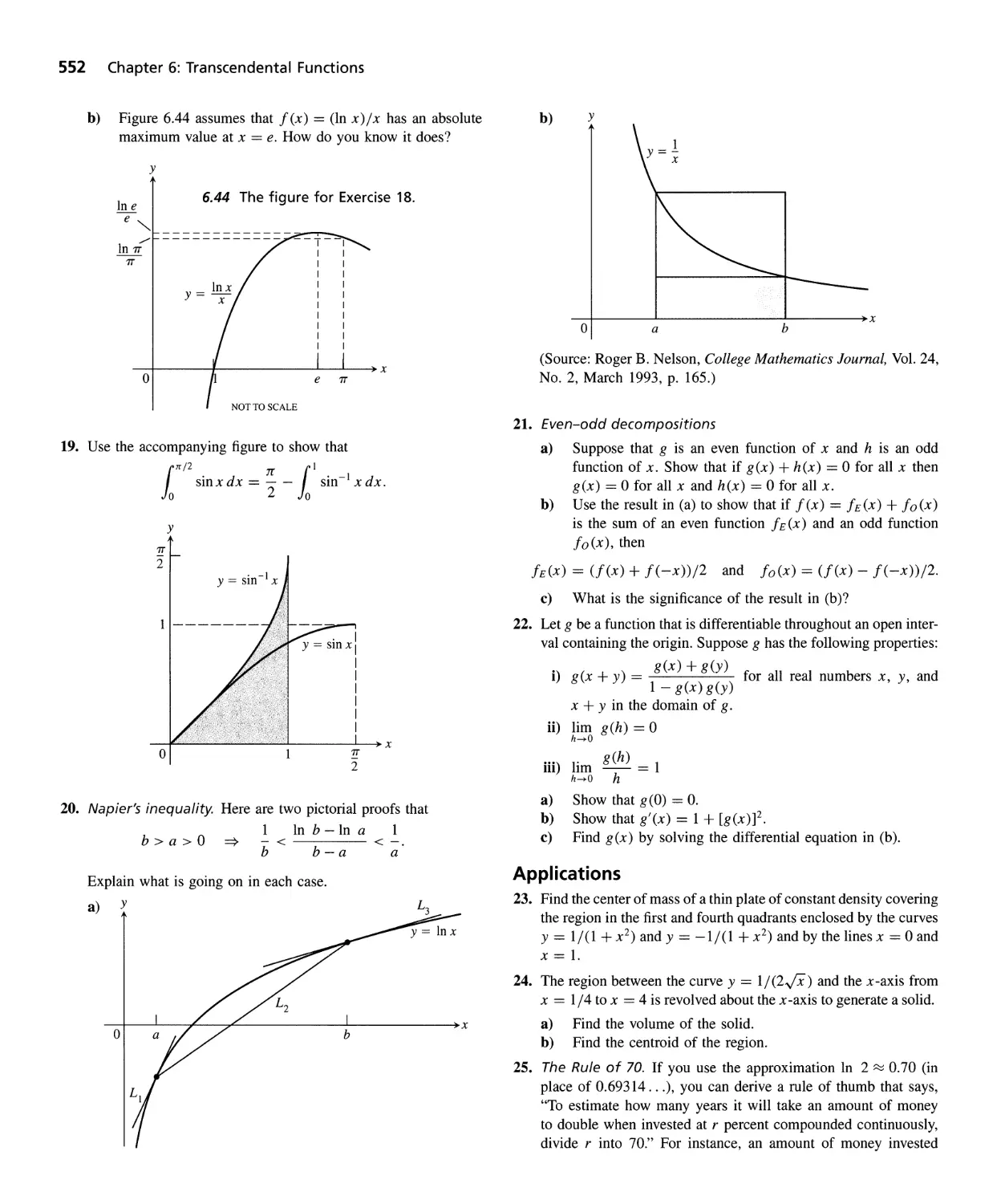
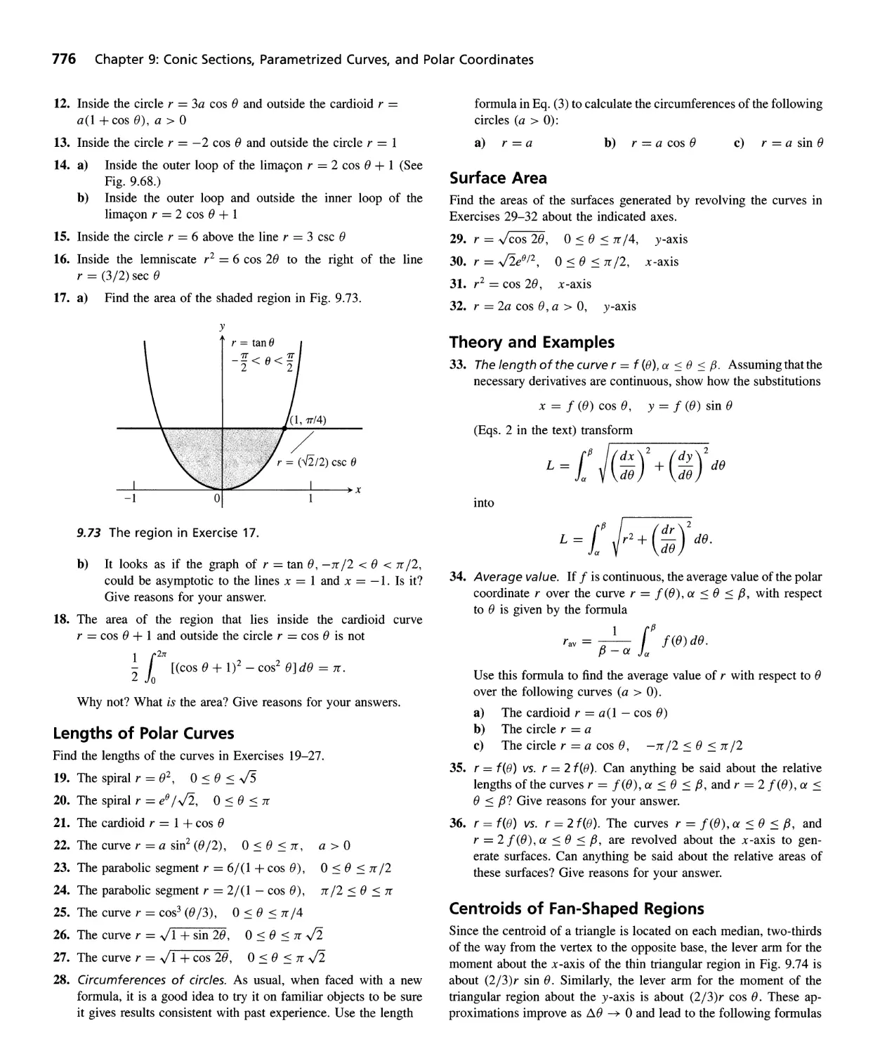
Don Mills, Ontario · Wokingham, England · Amsterdam
Bonn · Sydney · Singapore · Tokyo · Madrid
San Juan · Milan · Paris
Acquisitions Editor
Development Editor
Managing Editor
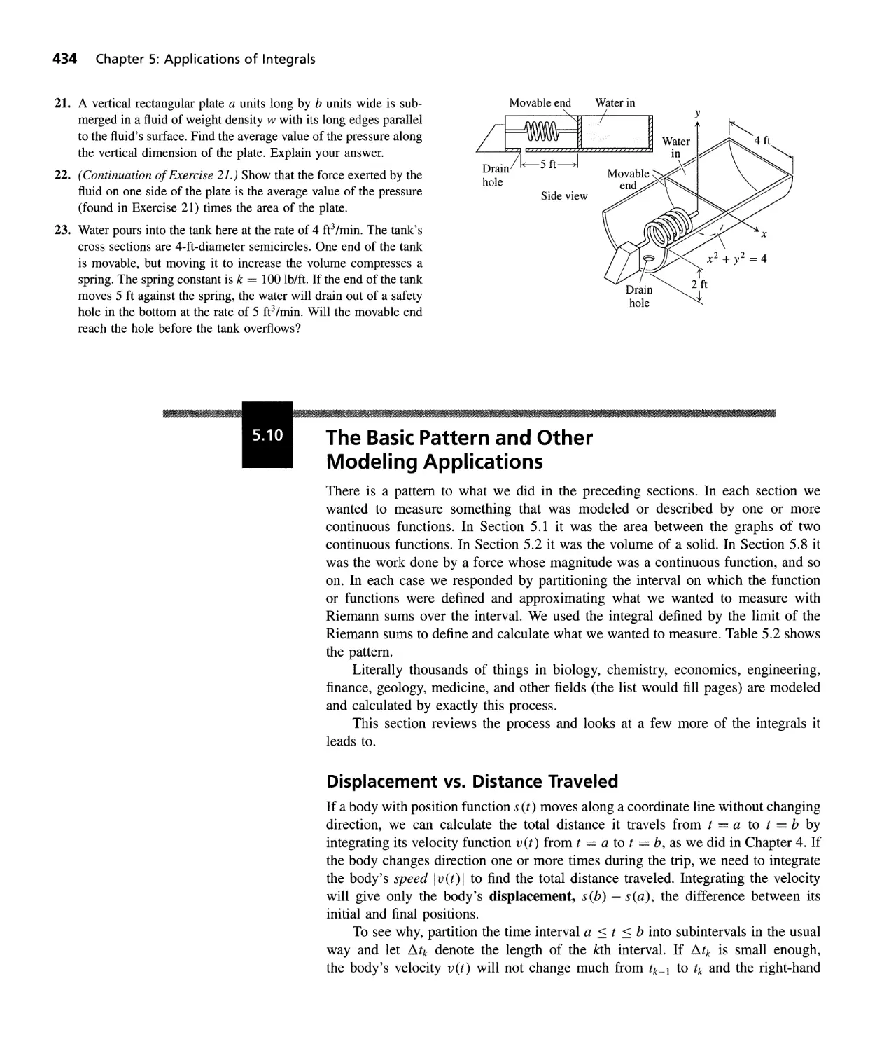
Senior Production Supervisor
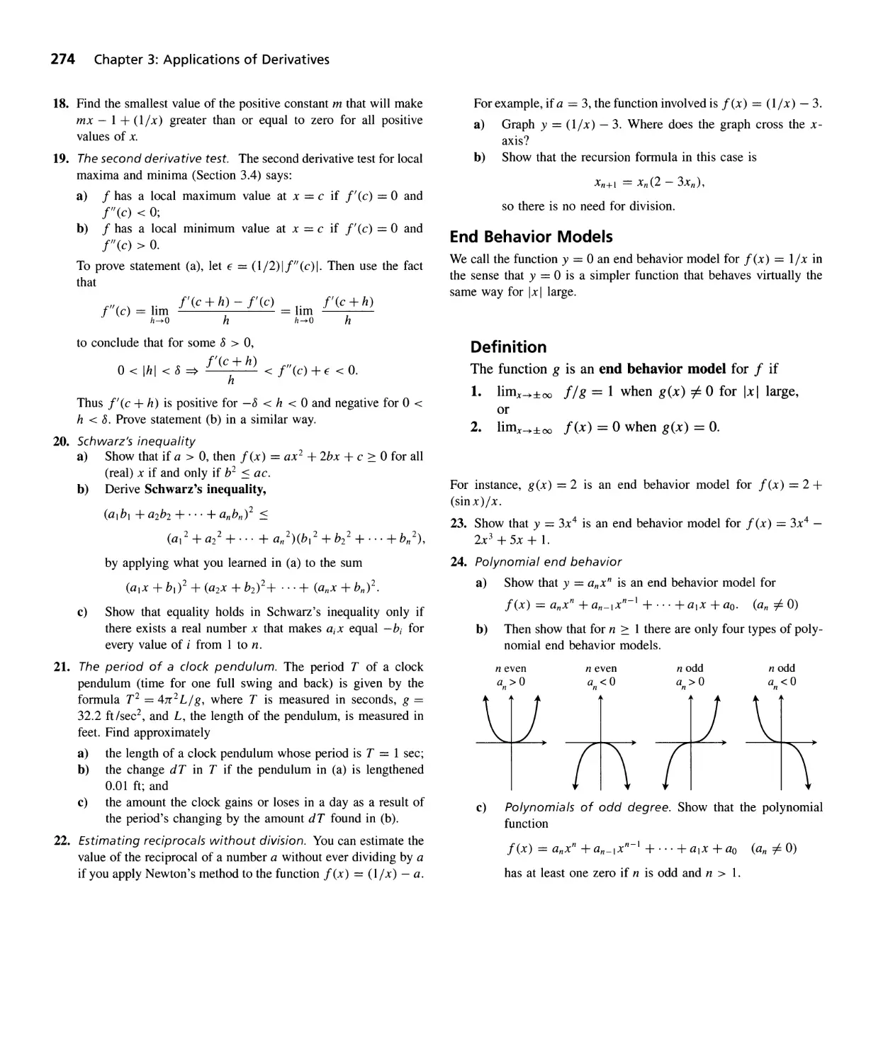
Senior Marketing Manager
Marketing Coordinator
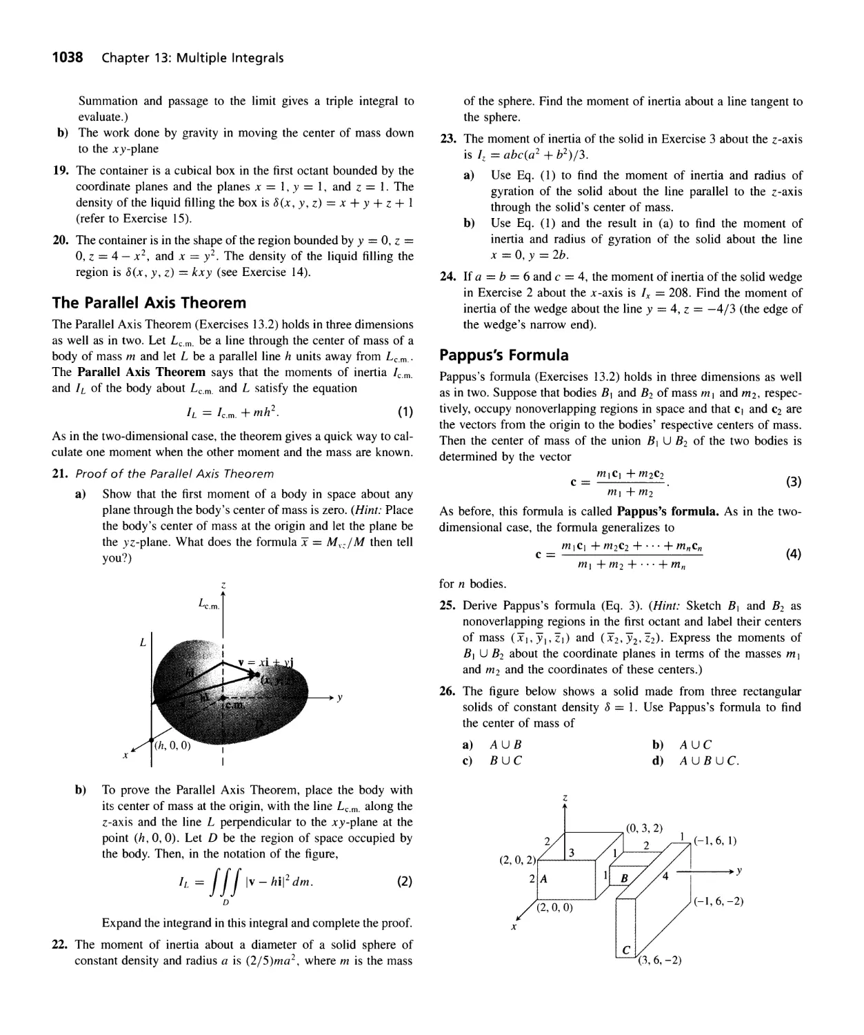
Prepress Buying Manager
Art Buyer
Senior Manufacturing Manager
Manufacturing Coordinator
SON -Wf'
9 4 1 J'(<<,
;-:£1
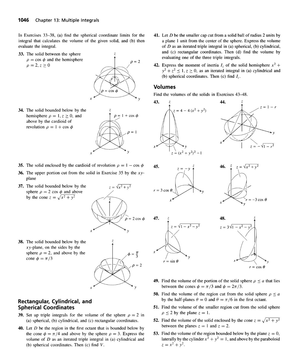
'4 (t
SrUD£ '\
World Student Series
Laurie Rosatone
Marianne Lepp
Karen Guardino
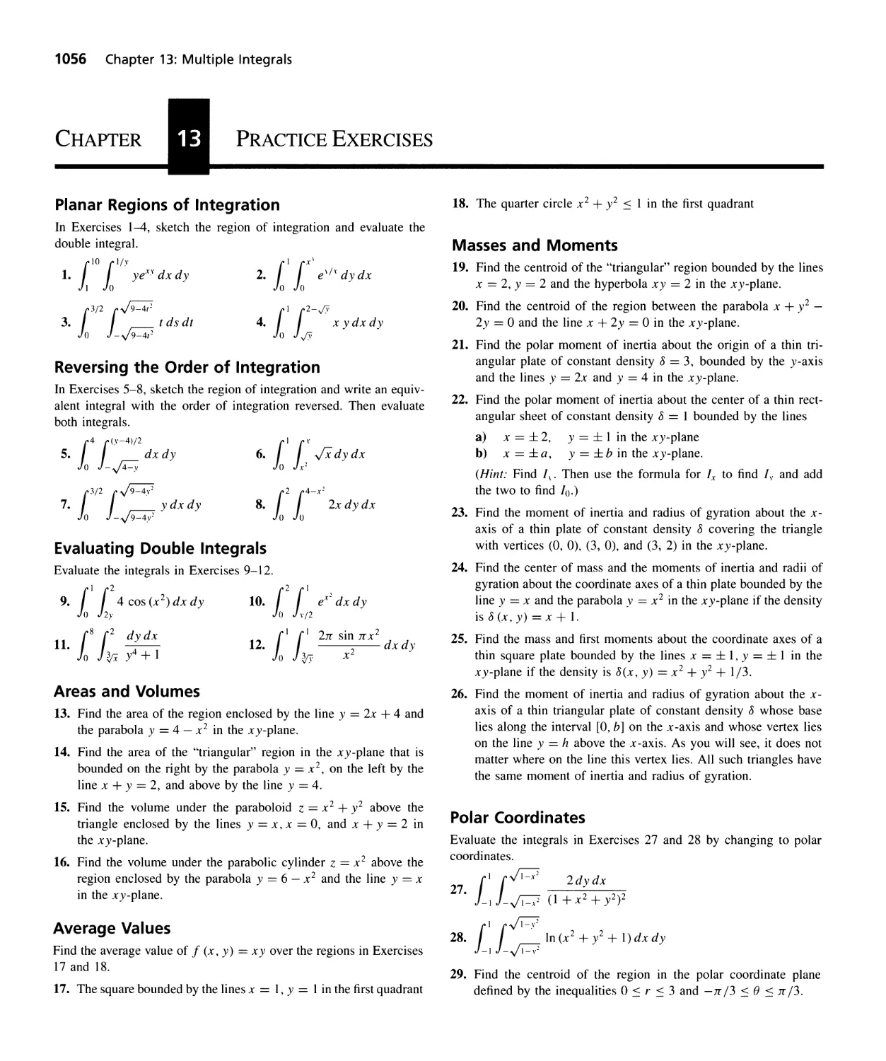
Jennifer Bagdigian
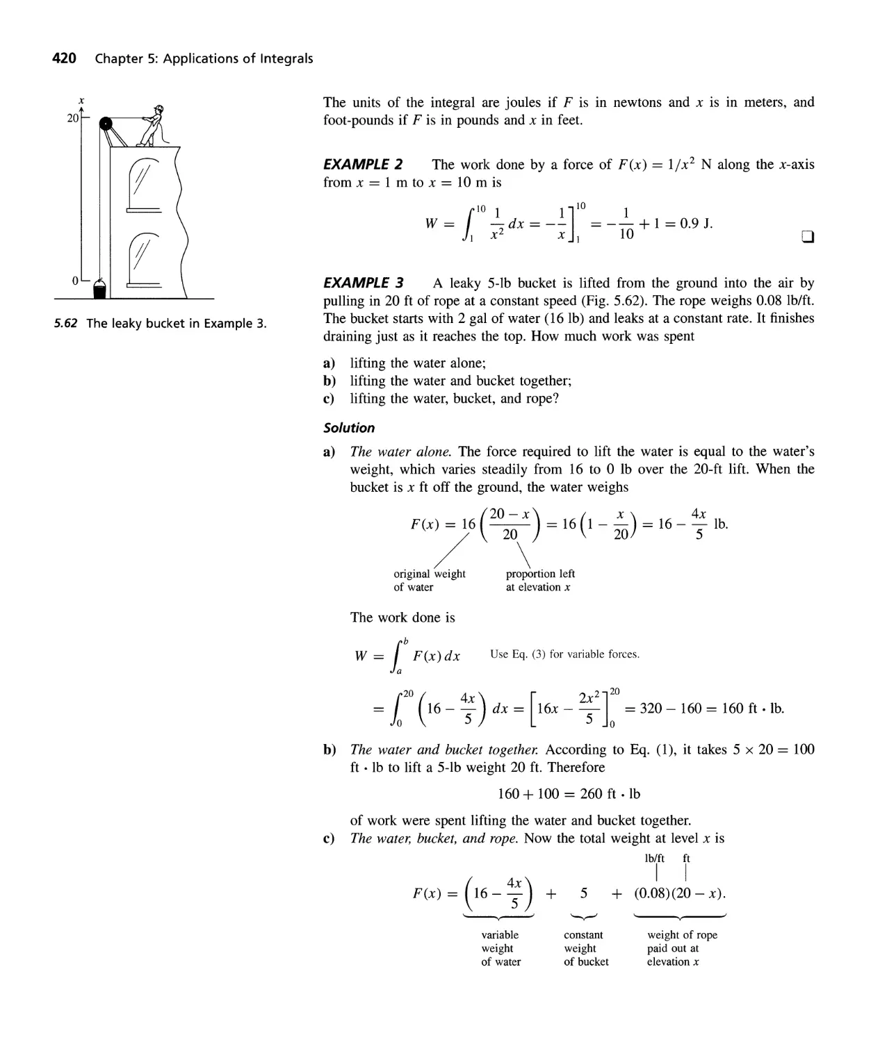
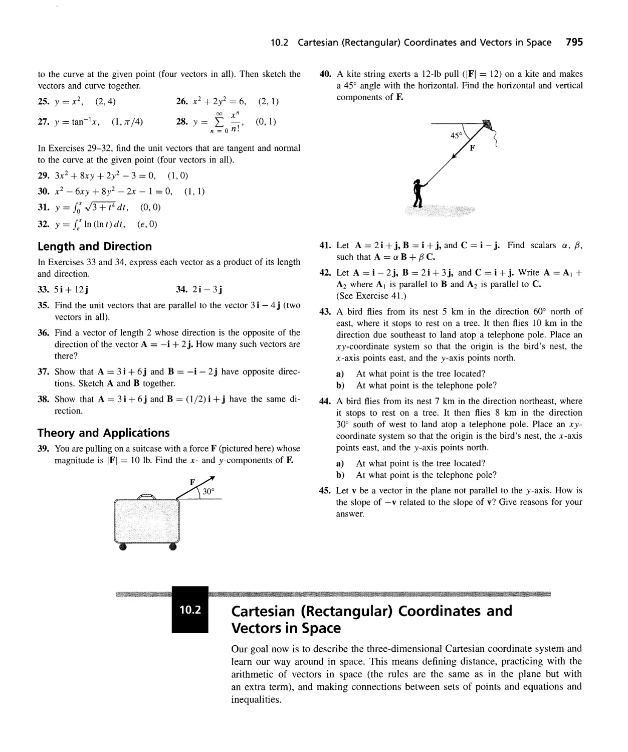
Andrew Fisher
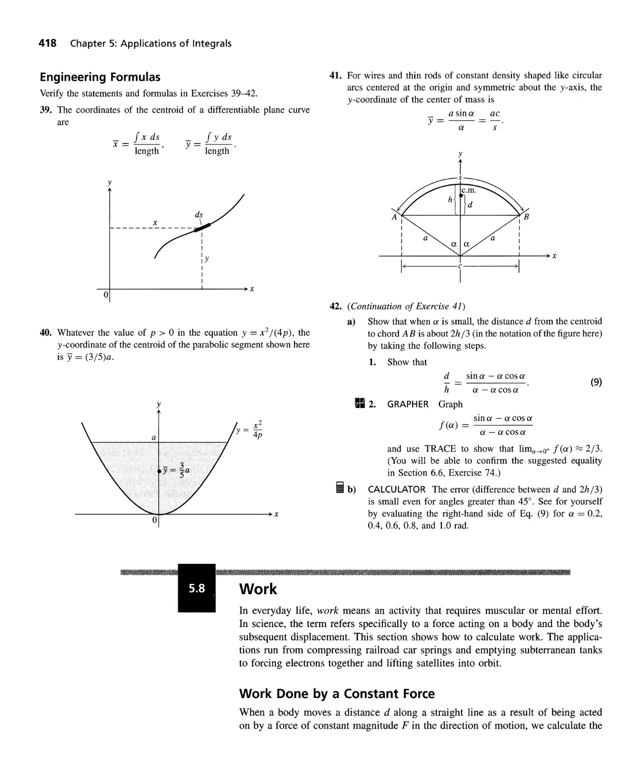
Benjamin Rivera
Sarah McCracken
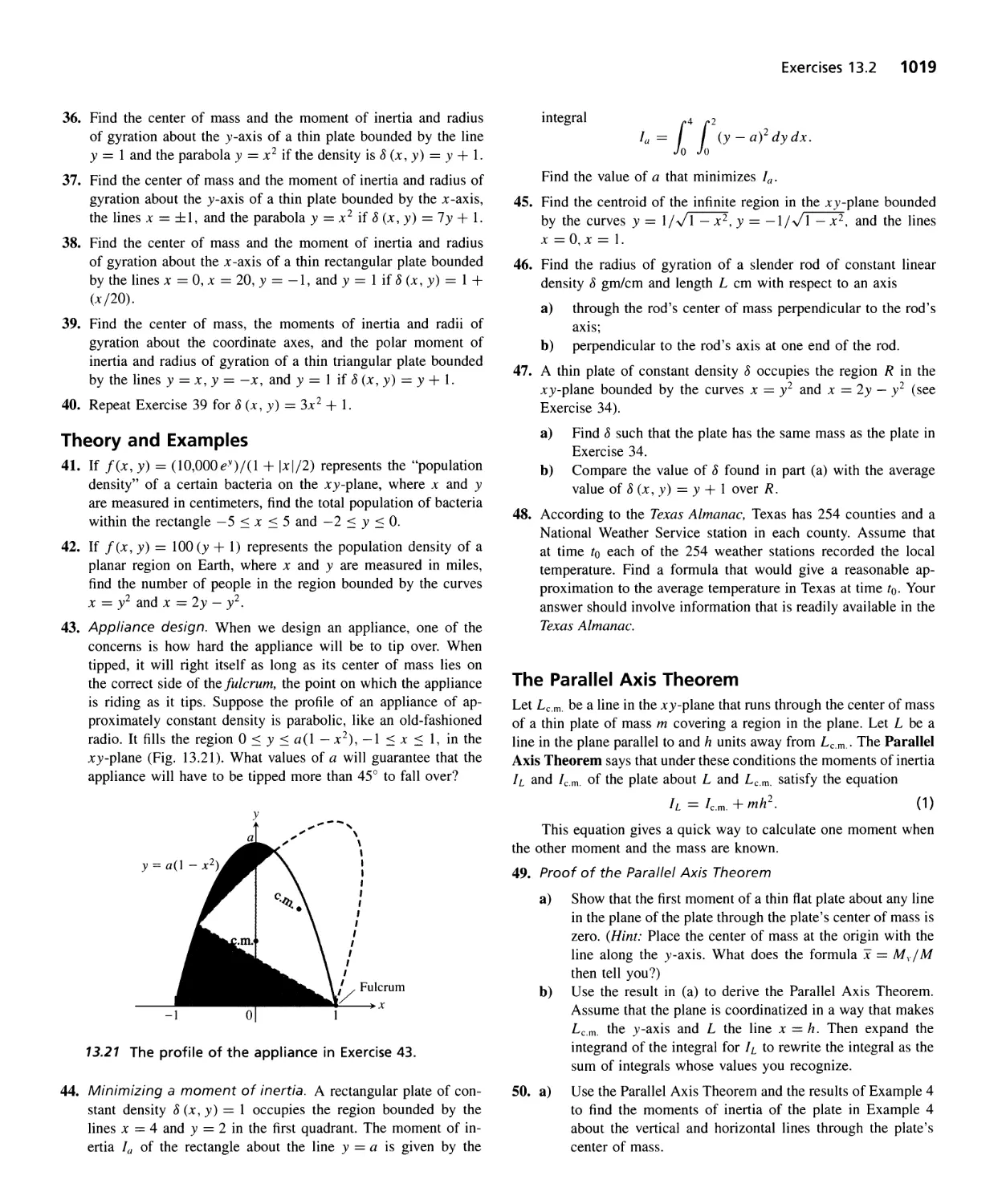
Joseph Vetere
Roy Logan
Evelyn Beaton
Production Editorial Services
Art Editors
Copy Editor
Proofreader
Text Design
Cover Design
Cover Photo
Composition
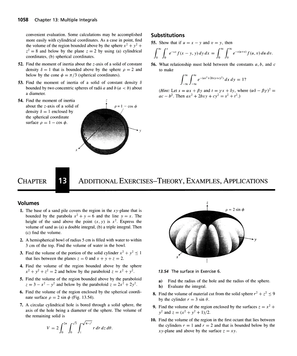
Technical Illustration
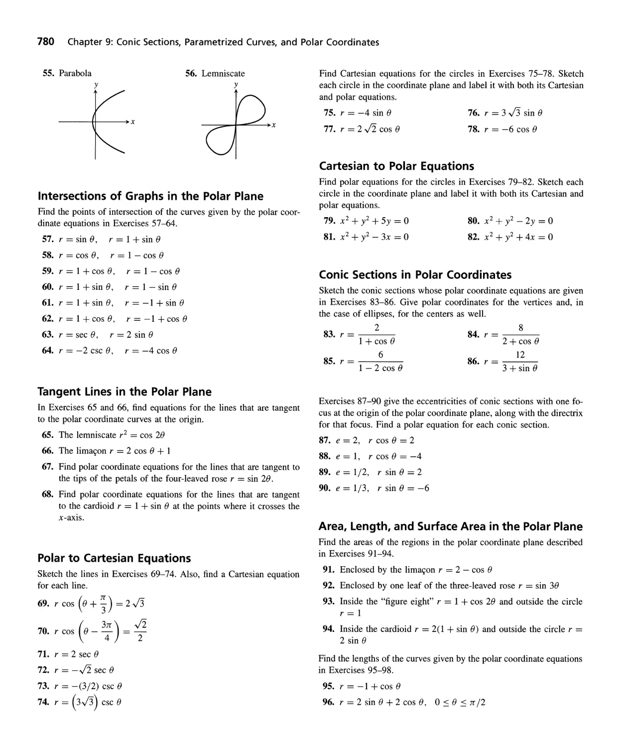
Barbara Pendergast
Susan London-Payne, Connie Hulse
Barbara Flanagan
Joyce Grandy
Martha Podren, Podren Design;
Geri Davis, Quadrata, Inc.
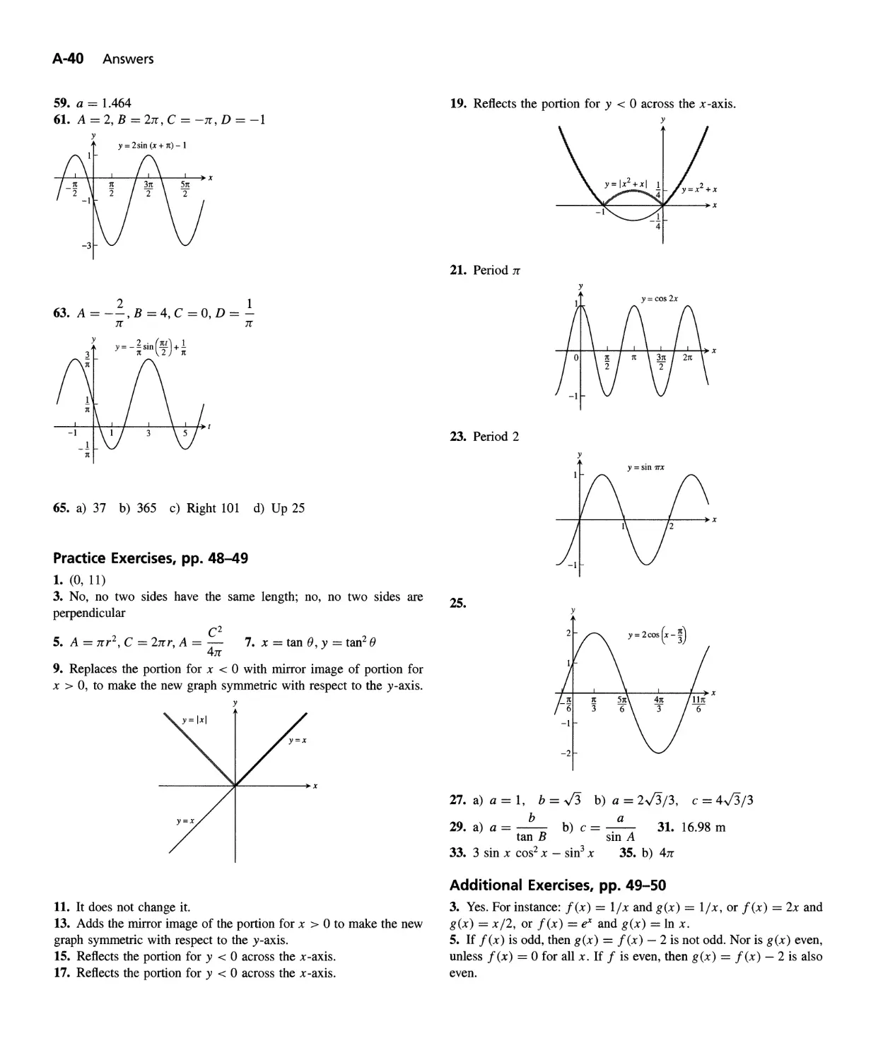
Marshall Henrichs
John Lund/Tony Stone Worldwide
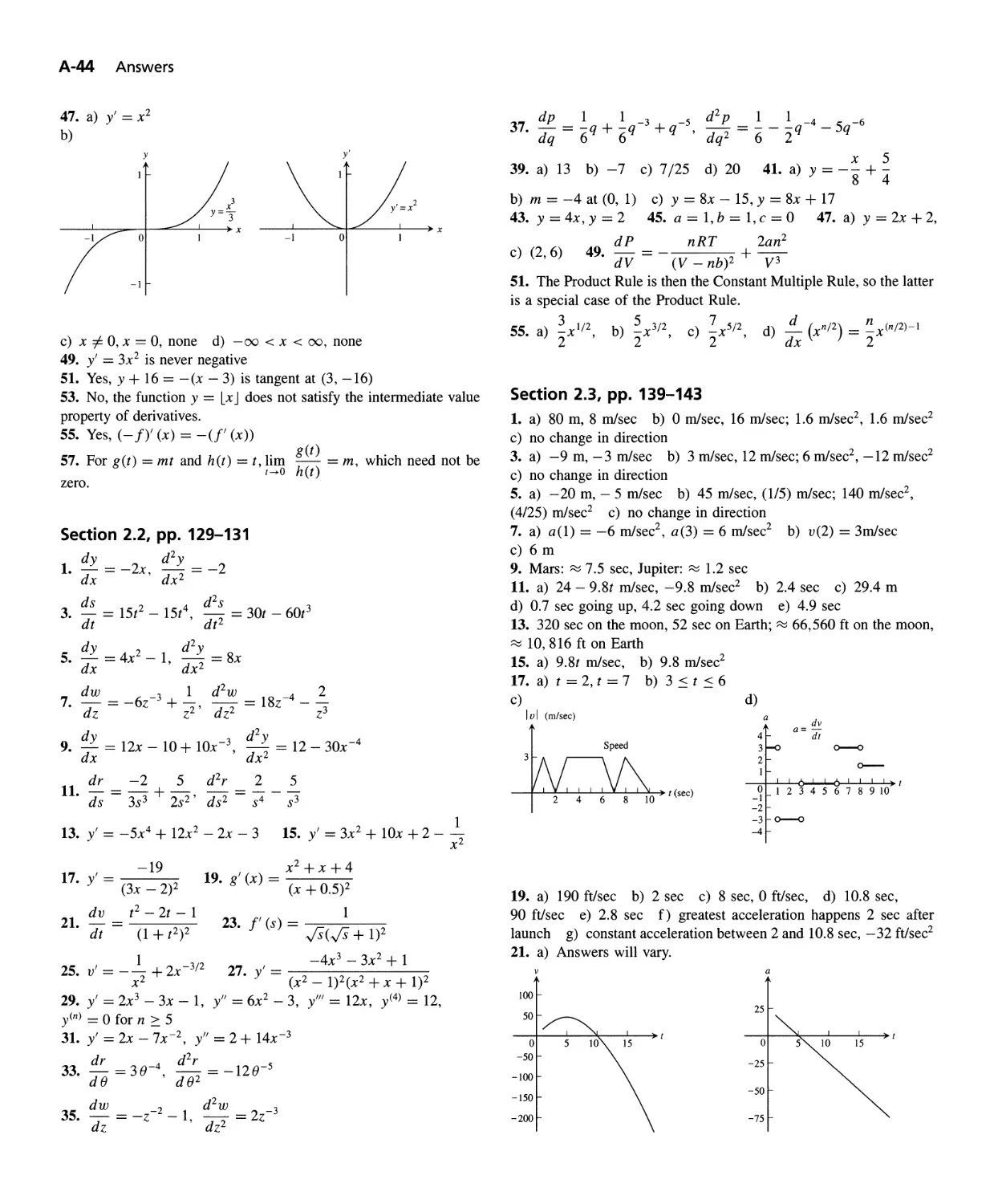
TSI Graphics, Inc.
Tech Graphics
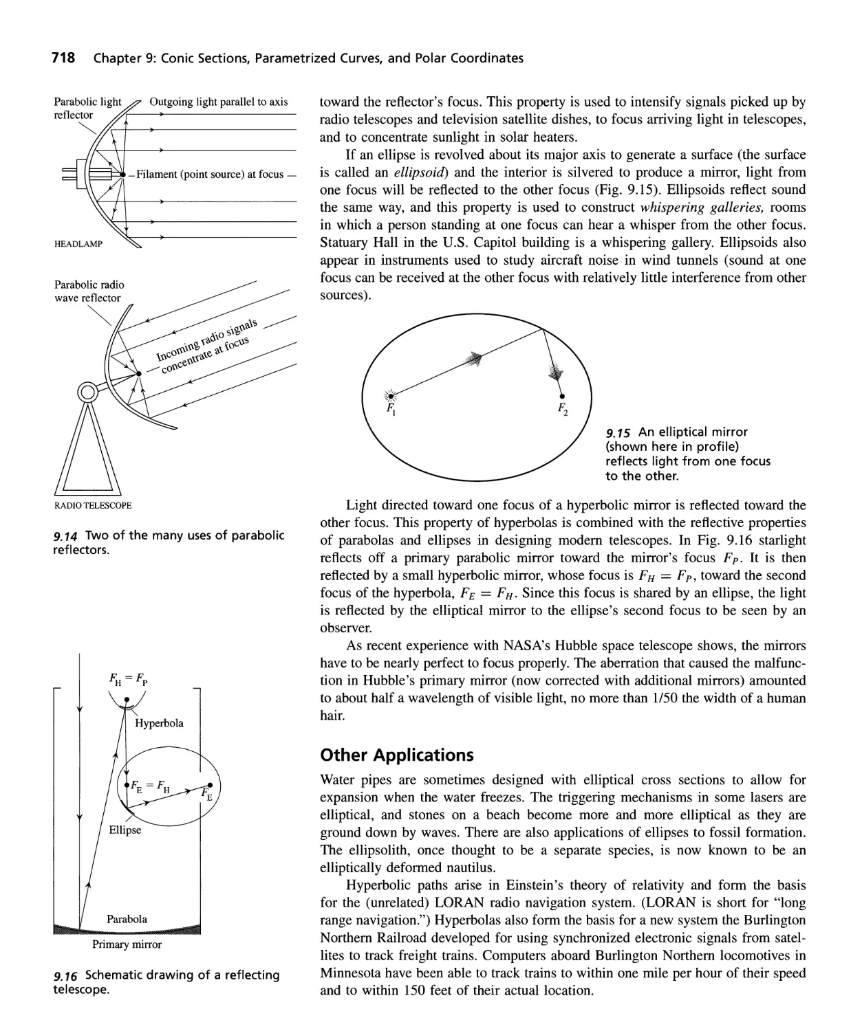
Photo Credits: 142,238,408,633, 722, 875, 899, From PSSC Physics 21e, 1965; D.C. Heath
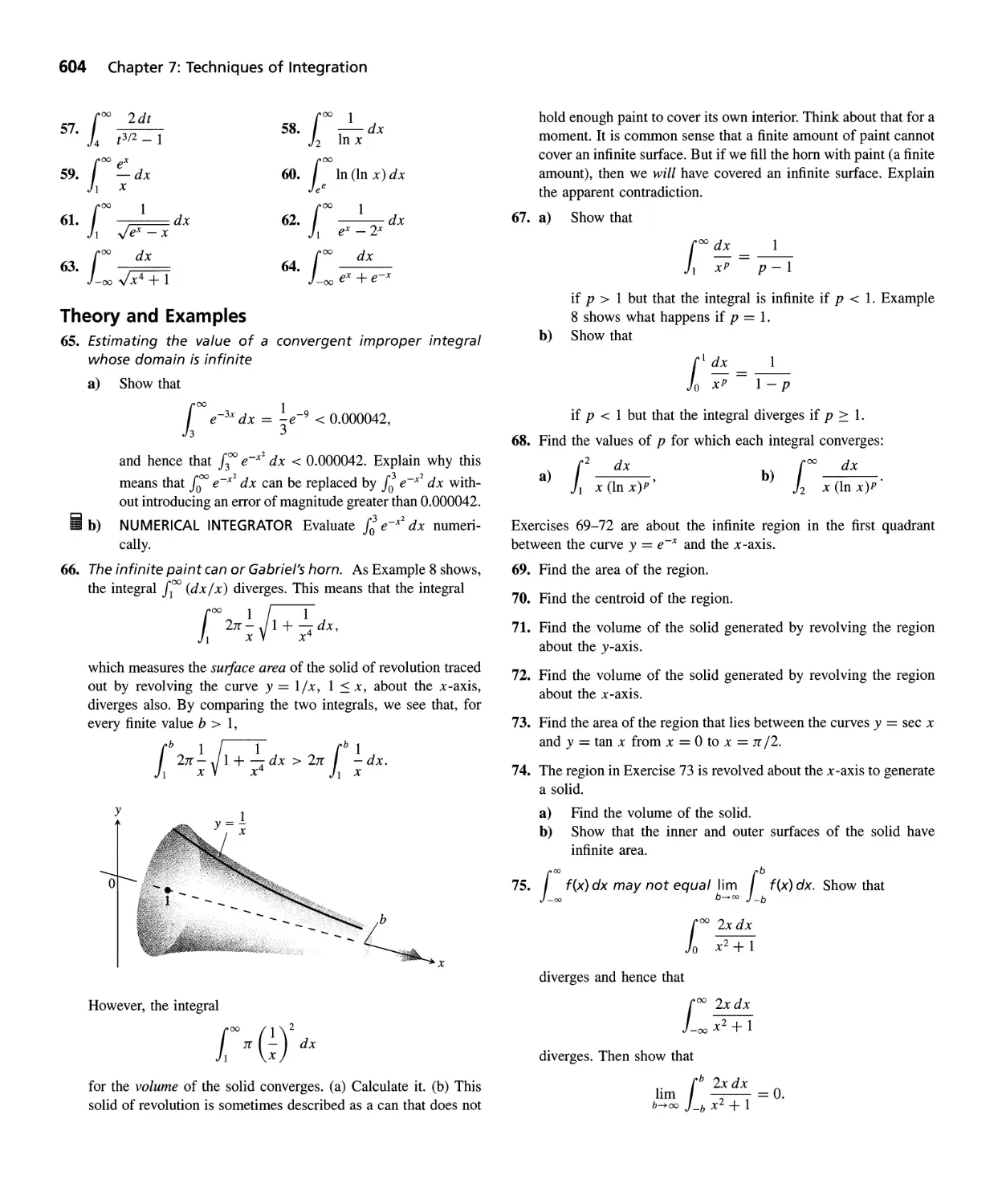
& Co. with Education Development Center, Inc., Newton, MA. Reprinted with permission
186, APIWide World Photos 266, Scott A. Burns, Urbana, IL 287, Joshua E. Barnes, Univer-
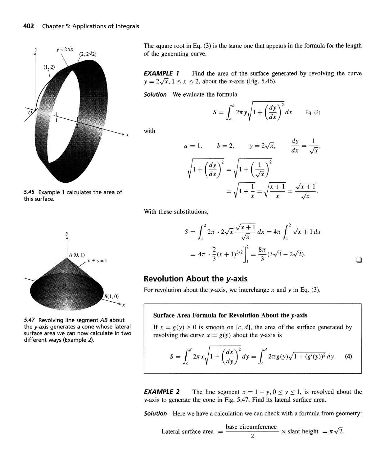
sity of Hawaii 354, Marshall Henrichs 398, @ Richard F. Voss/IBM Research 442, @ Susan
Van Etten 872, APIWide World Photos 889, @ 1994 Nelson L. Max, University of Califor-
nia/Biological Photo Service; Graphic by Alfred Gray 938, ND Roger- Viollet 1068,
NASA/Jet Propulsion Laboratory
Reprinted with corrections, June, 1998.
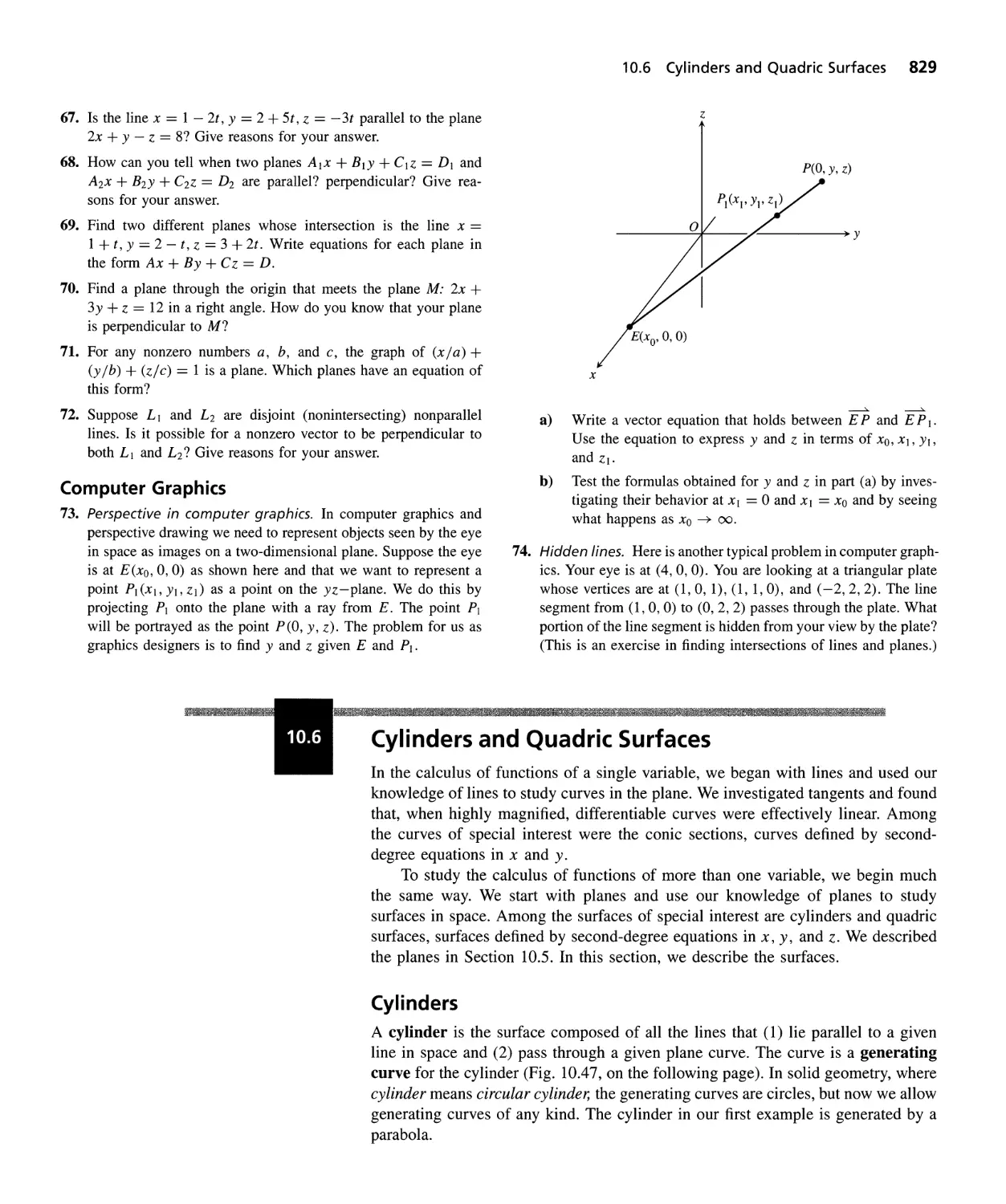
Cogyright @ 1996 by Addison-Wesley Publishing Company, Inc. All rights reserved. No
part' of this publication may be reproduced, stored in a retrieval system, or transmitted,
in any form or by any means, electronic, mechanical, photocopying, or otherwise,
without the prior written permission of the publisher. Printed in the United States of
America.
45678910-VH-9998
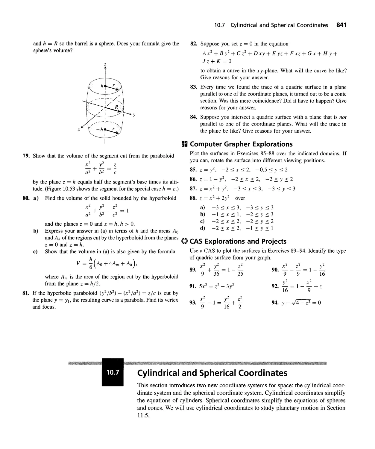
ISBN 0-201-40015-4
Contents
To the Instructor VIII
To the Student XVII
Preliminaries
1
2
3
4
5
Limits and
Continuity
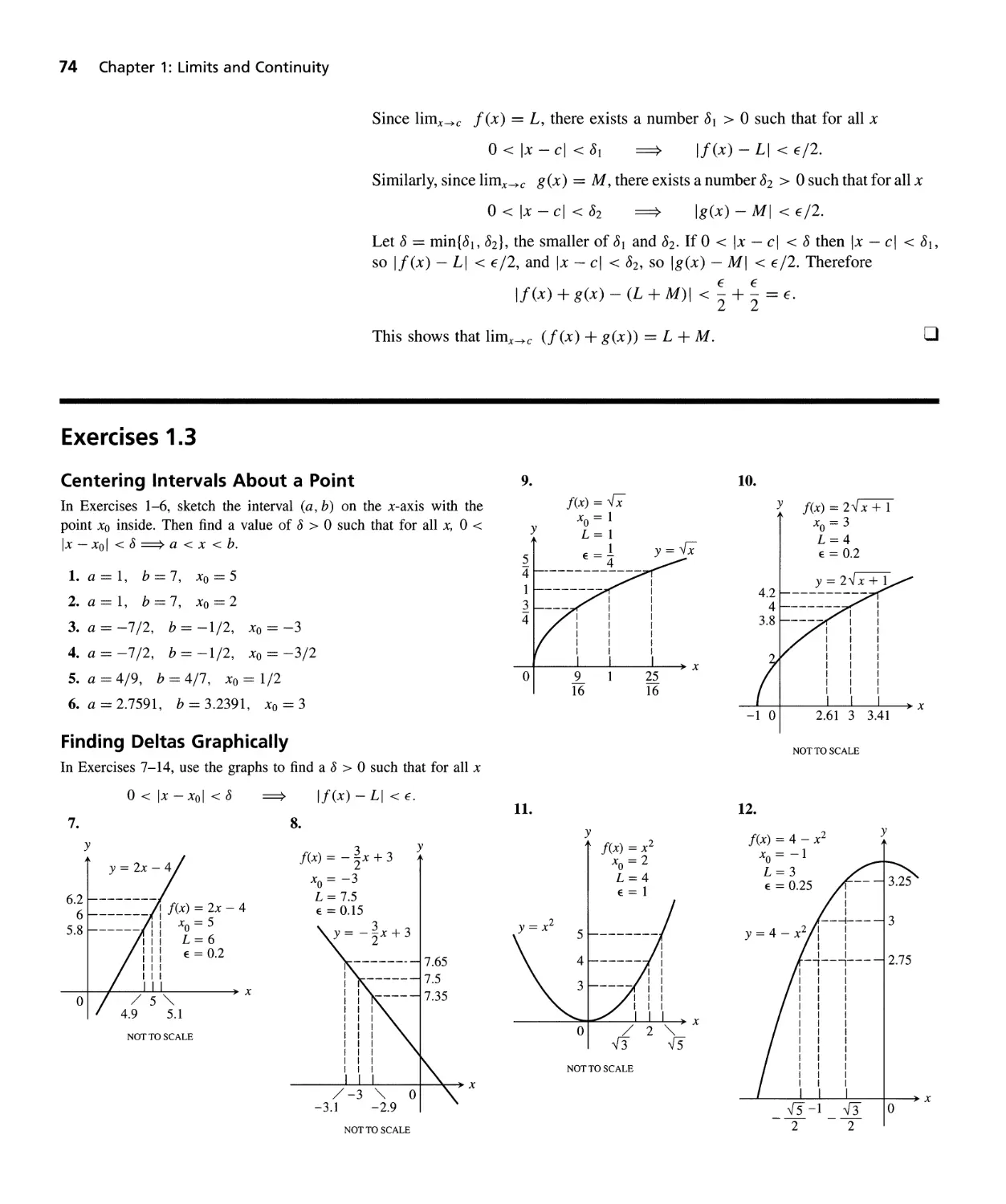
1.1
1.2
1.3
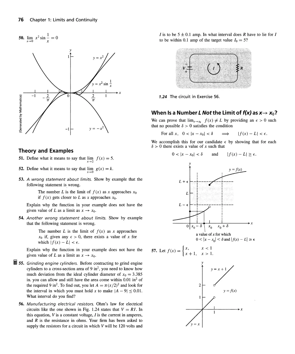
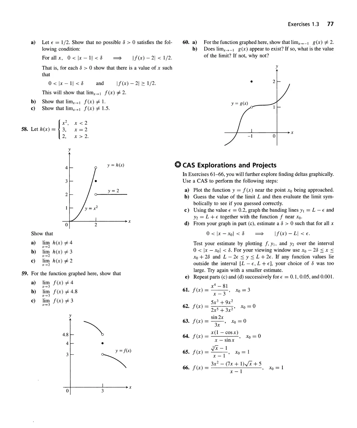
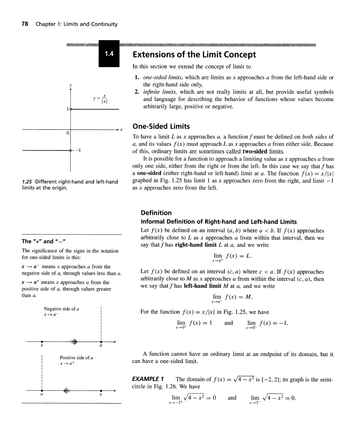
1.4
1.5
1.6
Derivatives
2.1
2.2
2.3
2.4
2.5
2.6
2.7
Applications of
Derivatives
3.1
3.2
3.3
Real Numbers and the Real Line 1
Coordinates, Lines, and Increments 8
Functions 17
Shifting Graphs 27
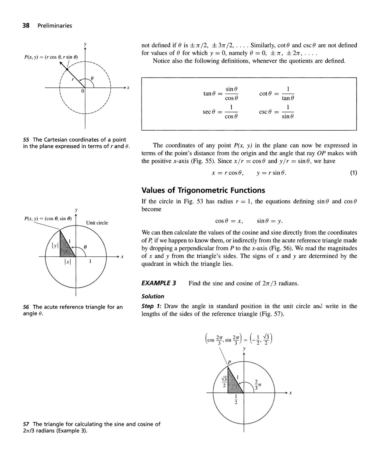
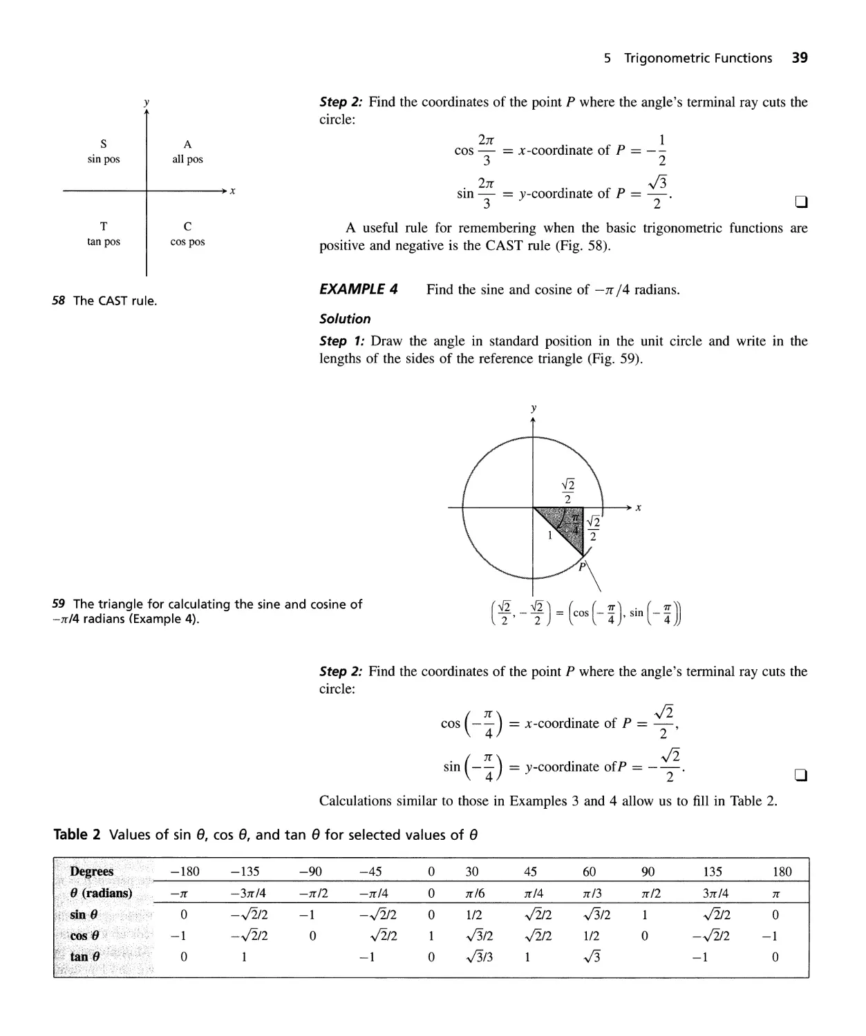
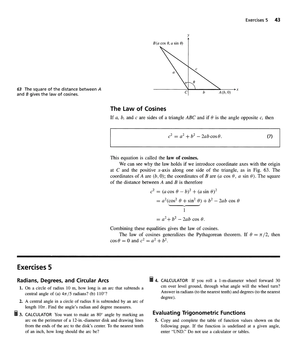
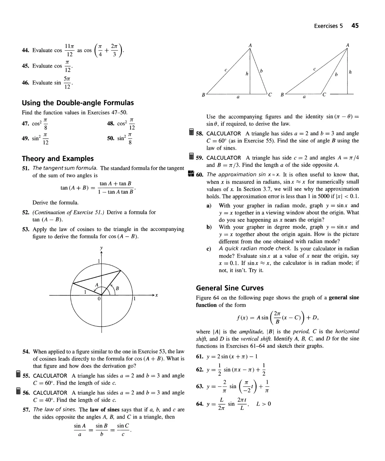
Trigonometric Functions 35
QUESTIONS TO GUIDE YOUR REVIEW 47 PRACTICE EXERCISES 48
ADDITIONAL EXERCISES-THEORY, EXAMPLES, ApPLICATIONS 49
Rates of Change and Limits 51
Rules for Finding Limits 61
Target Values and Formal Definitions of Limits 66
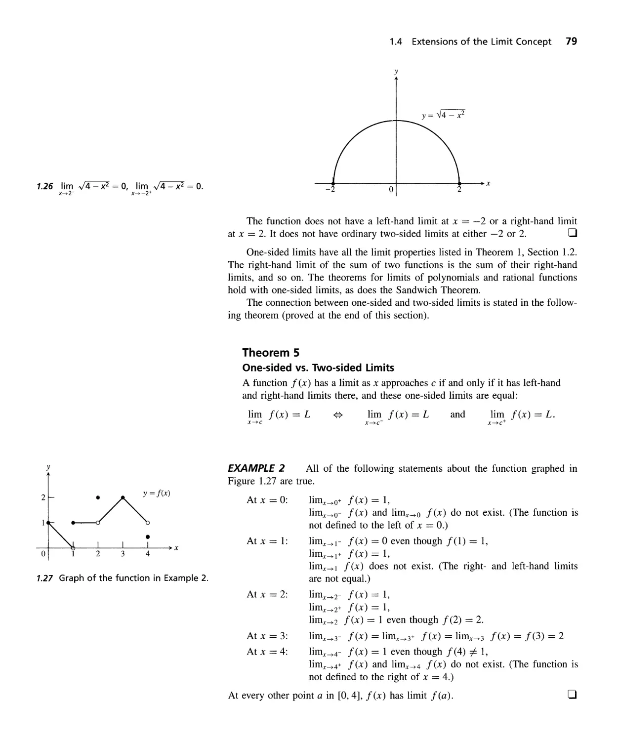
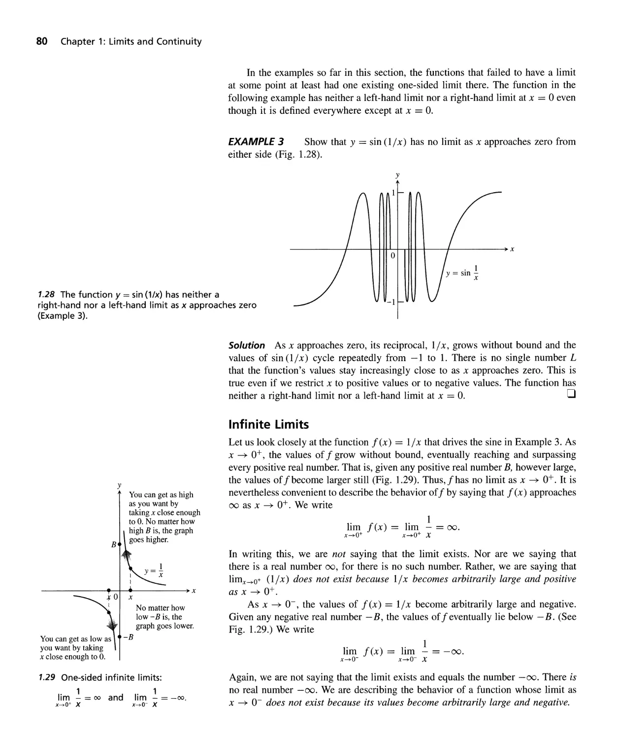
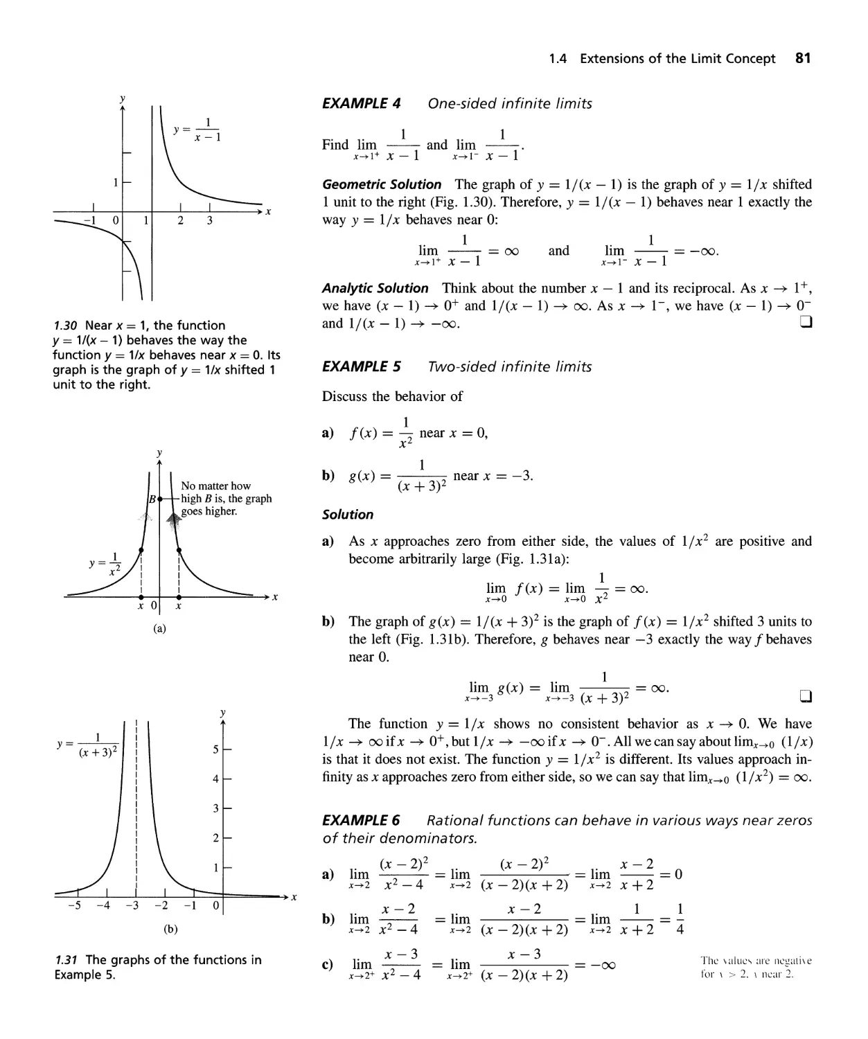
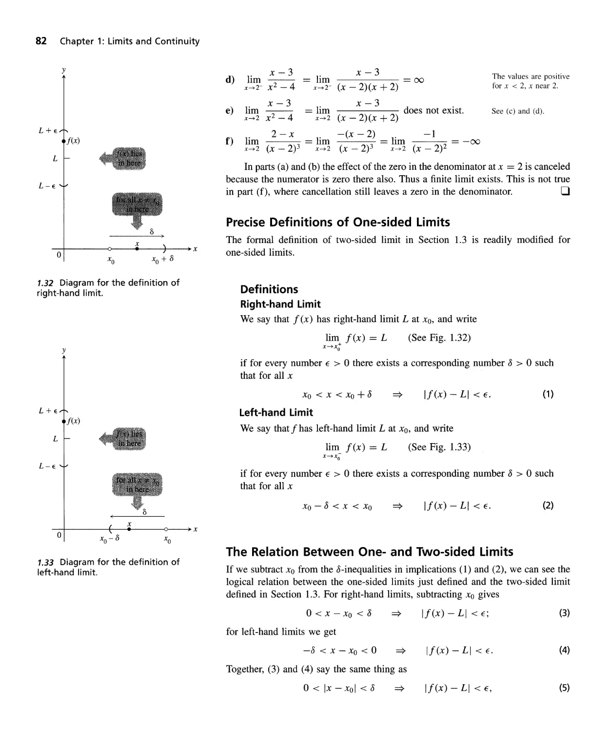
Extensions of the Limit Concept 78
Continuity 87
Tangent Lines 97
QUESTIONS TO GUIDE YOUR REVIEW 103 PRACTICE EXERCISES 104
ADDITIONAL EXERCISES-THEORY, EXAMPLES, APPLICATIONS 105
The Derivative of a Function 109
Differentiation Rules 121
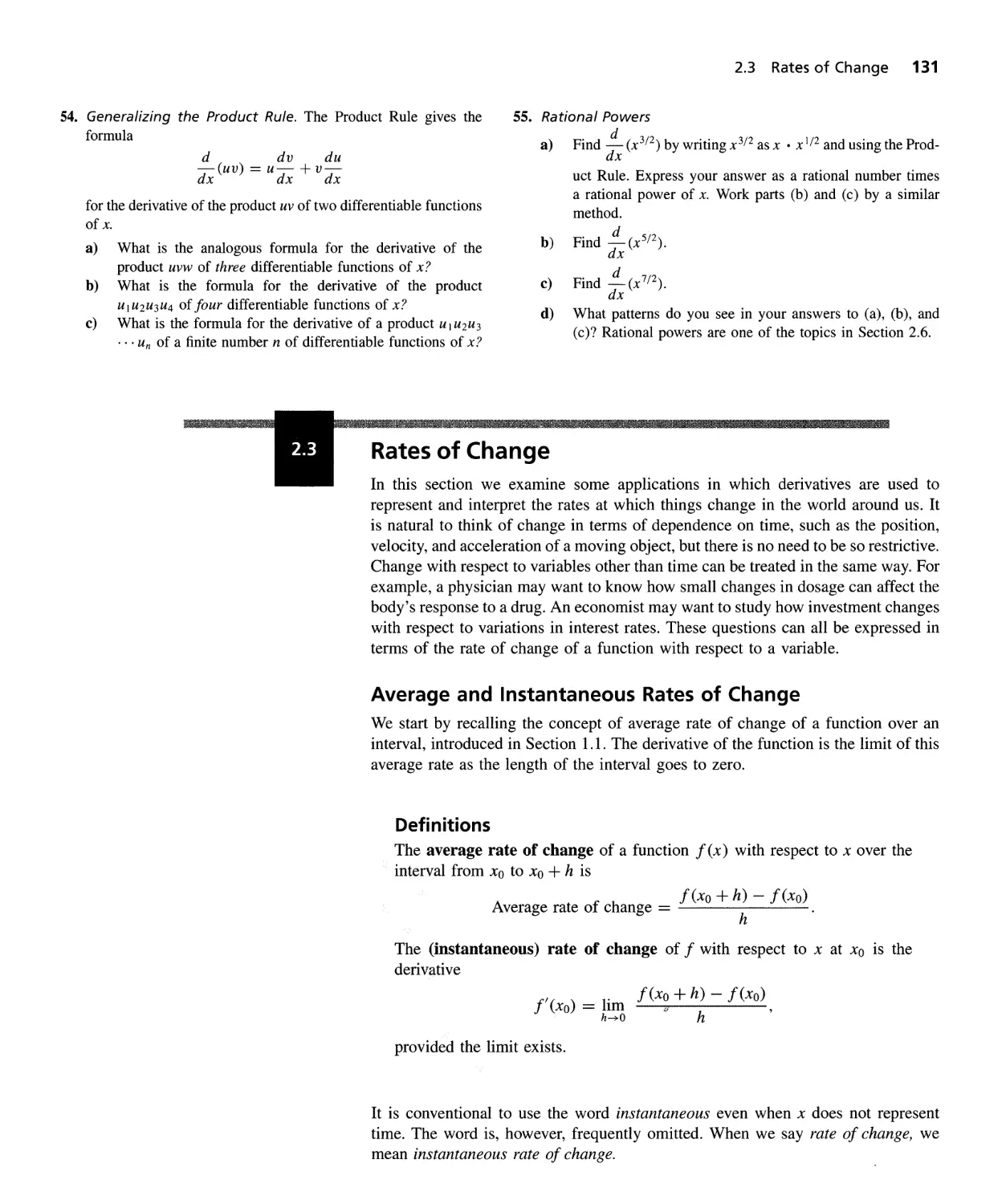
Rates of Change 131
Derivatives of Trigonometric Functions 143
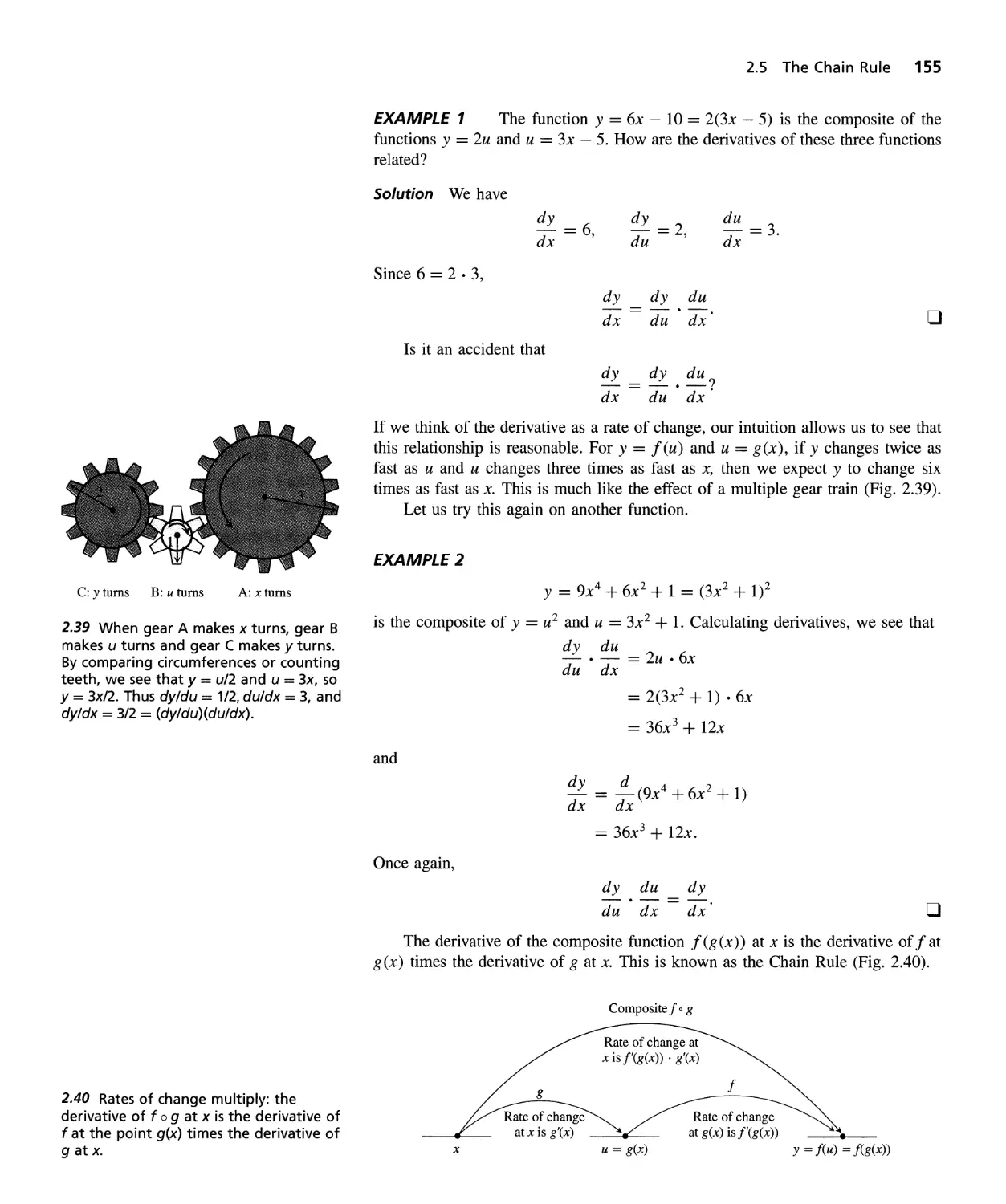
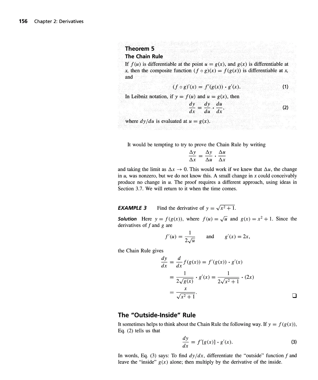
The Chain Rule 154
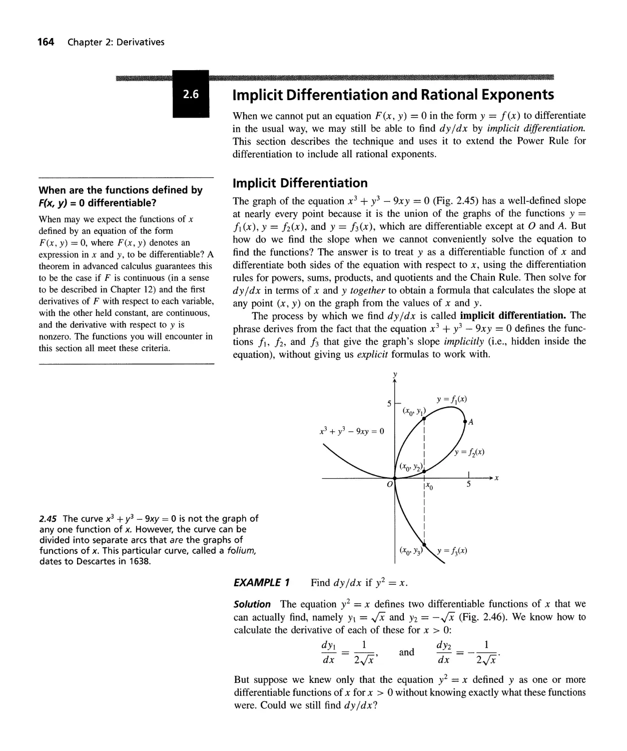
Implicit Differentiation and Rational Exponents 164
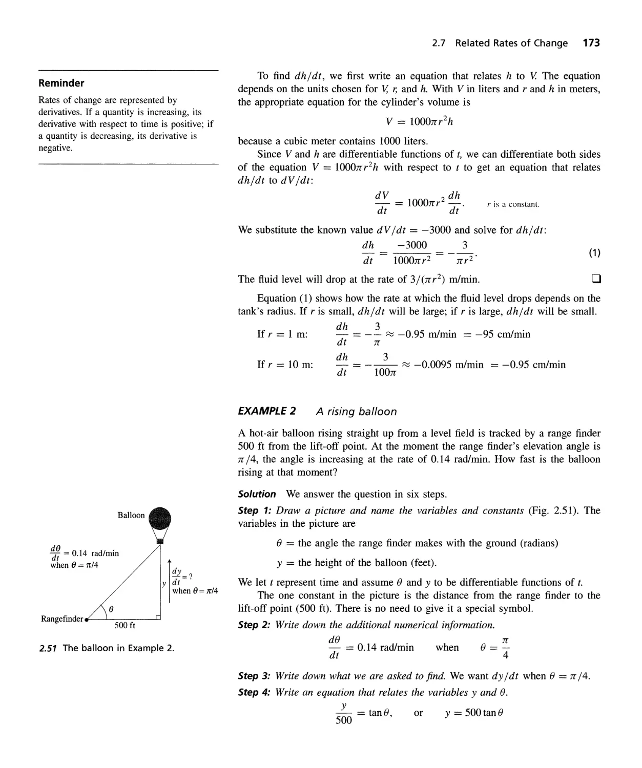
Related Rates of Change 172
QUESTIONS To GUIDE YOUR REVIEW 180 PRACTICE EXERCISES 181
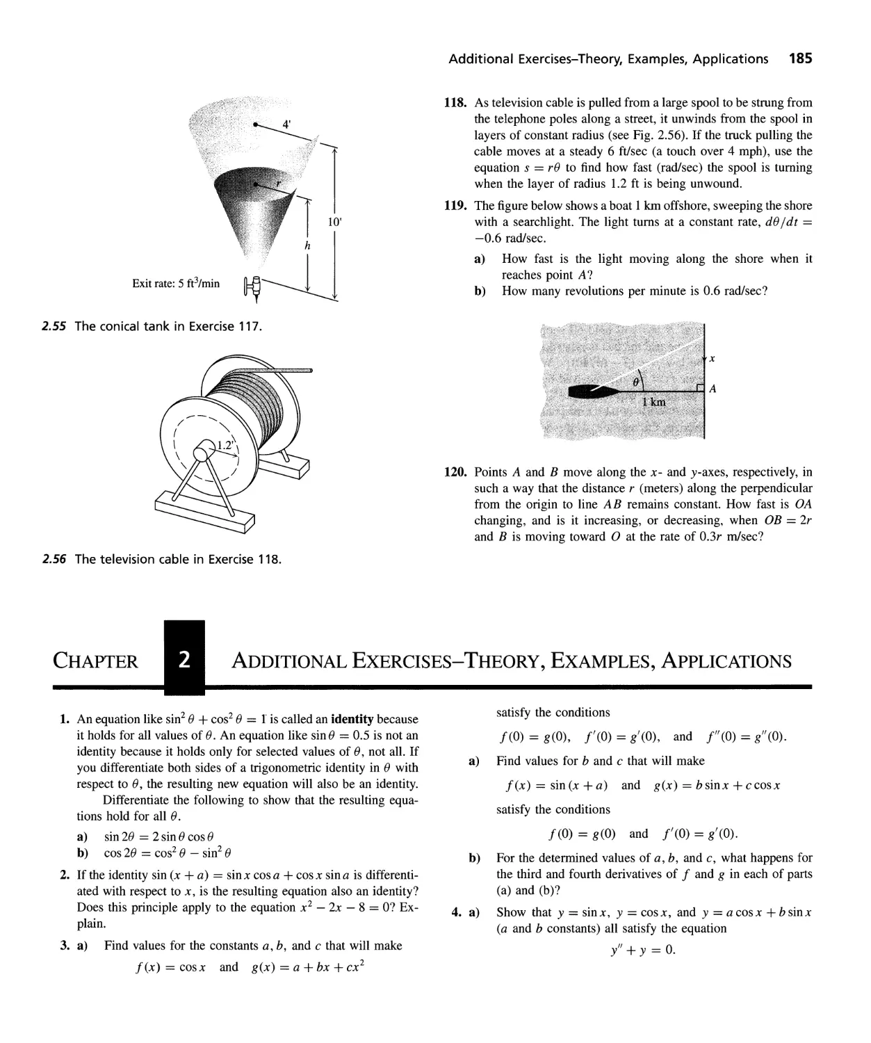
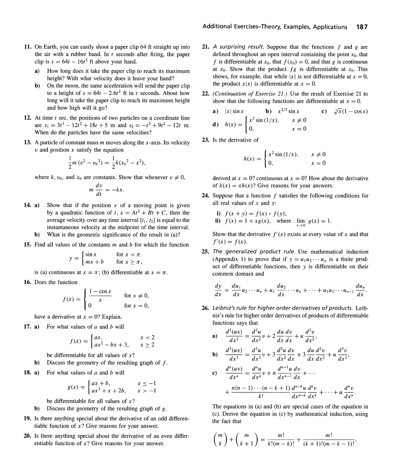
ADDITIONAL EXERCISES-THEORY, EXAMPLES, ApPLICATIONS 185
Extreme Values of Functions 189
The Mean Value Theorem 196
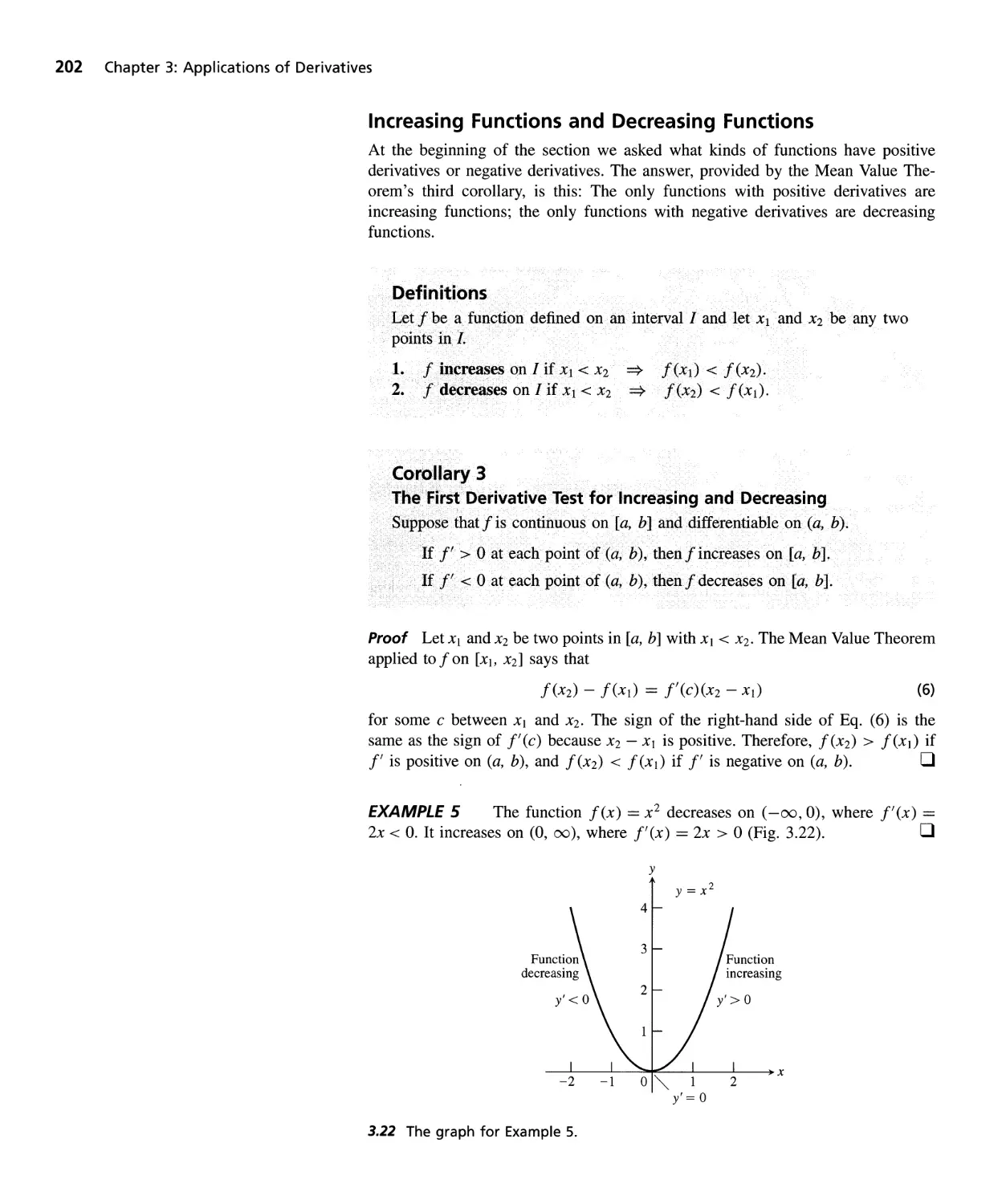
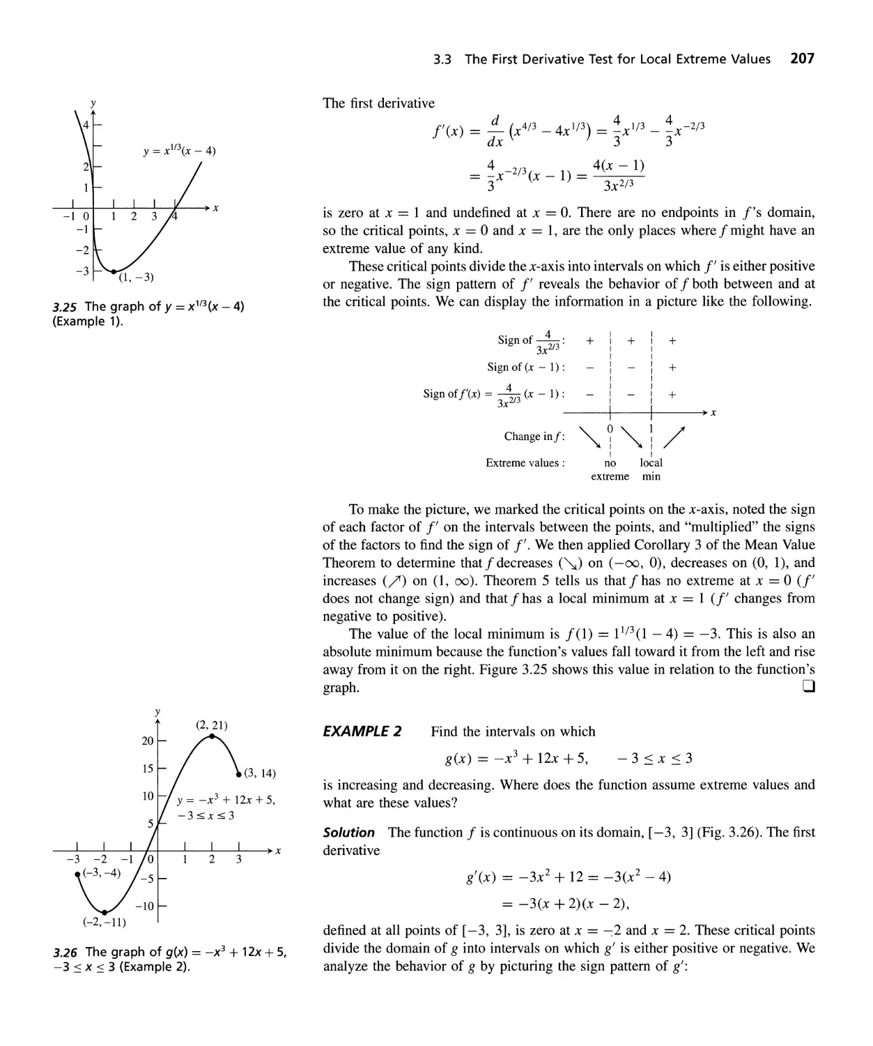
The First Derivative Test for Local Extreme Values 205
iii
IV Contents
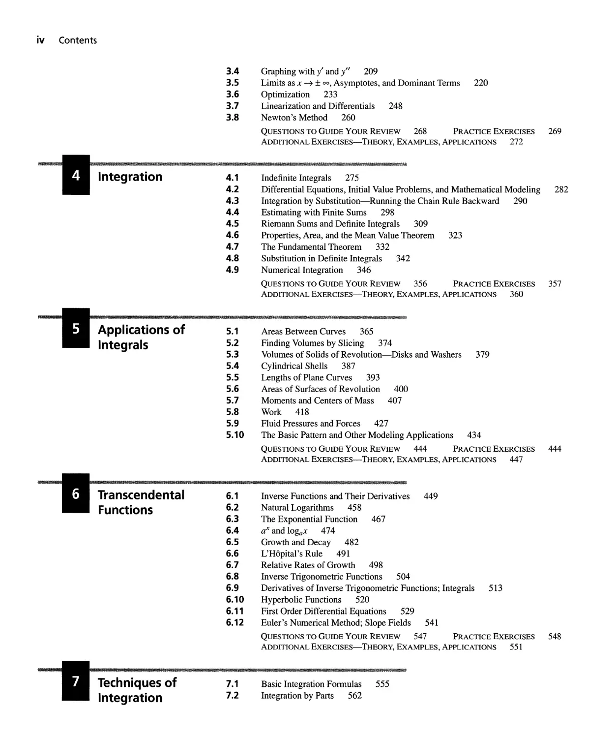
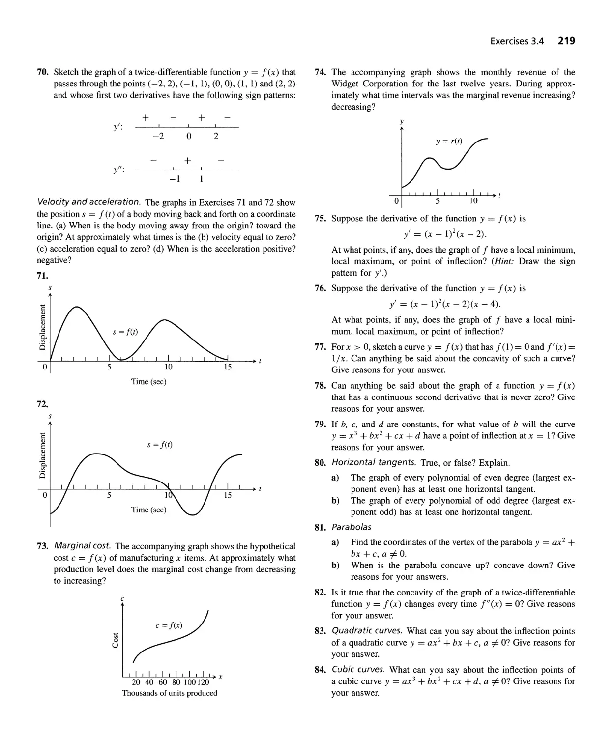
3.4 Graphing with y' and y" 209
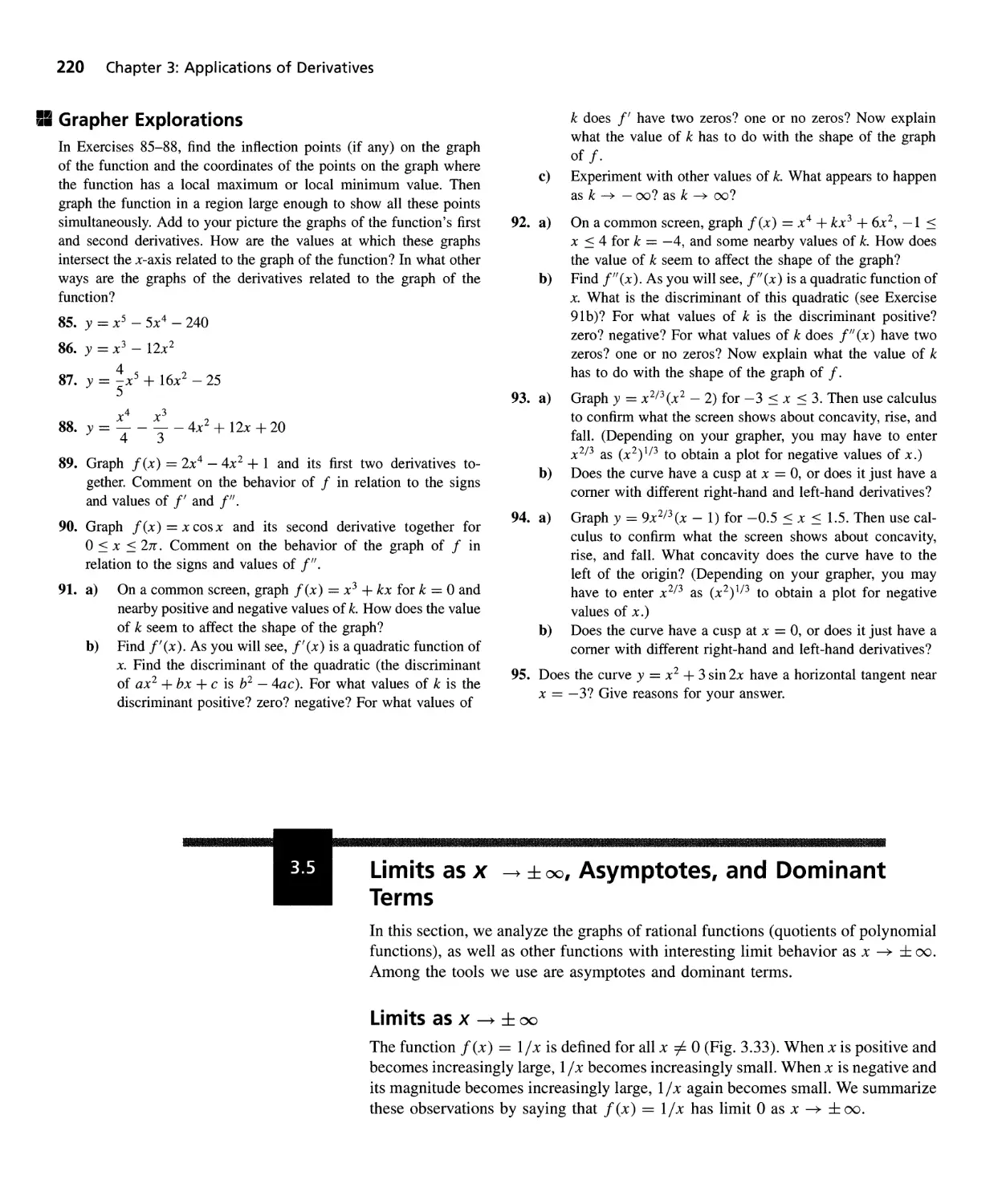
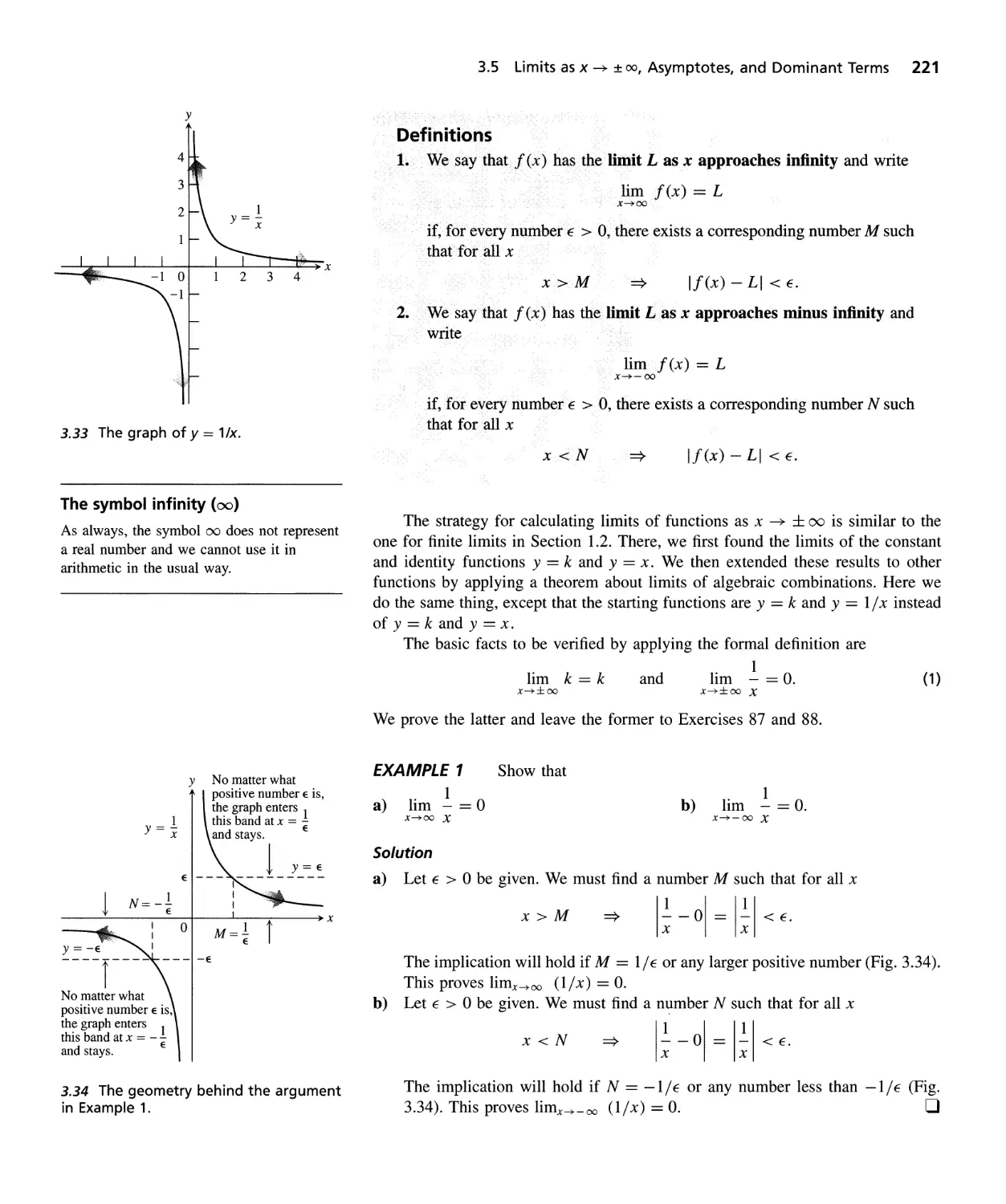
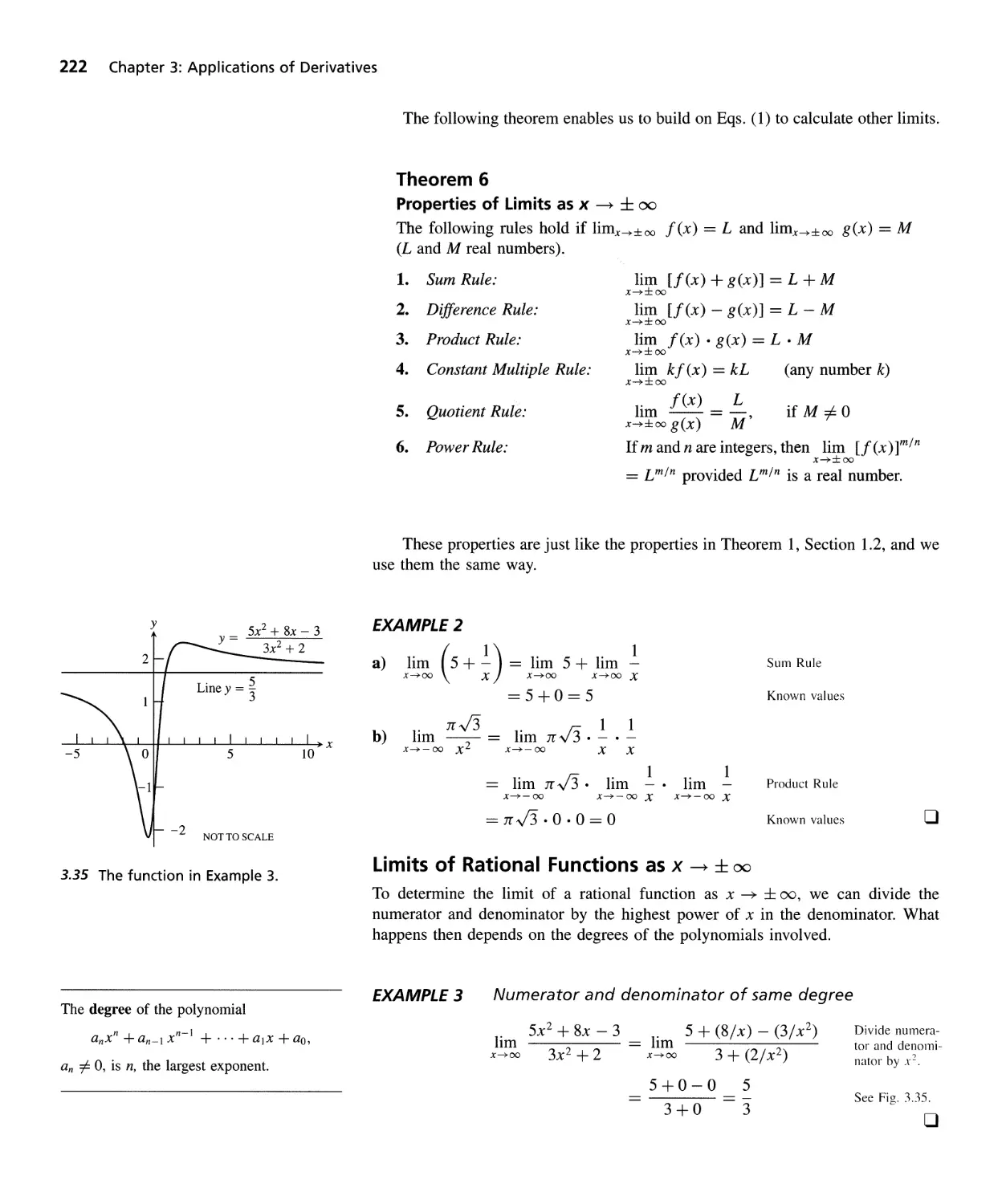
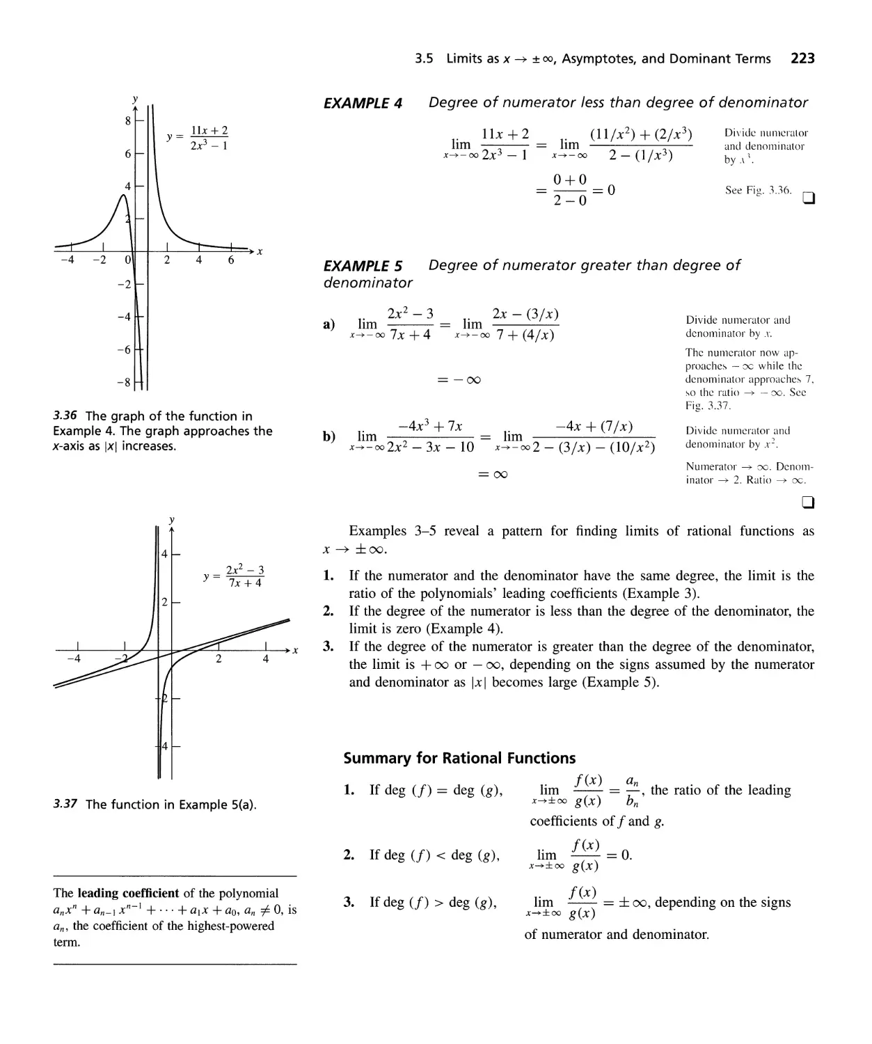
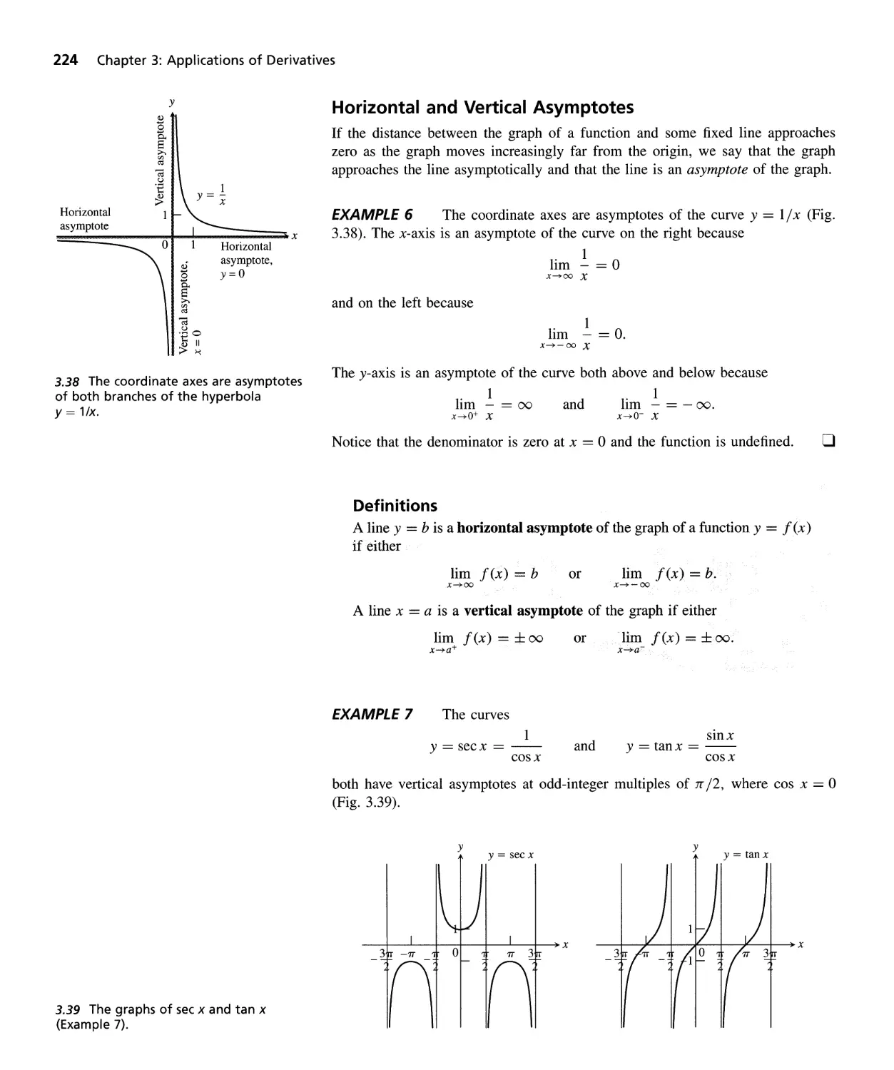
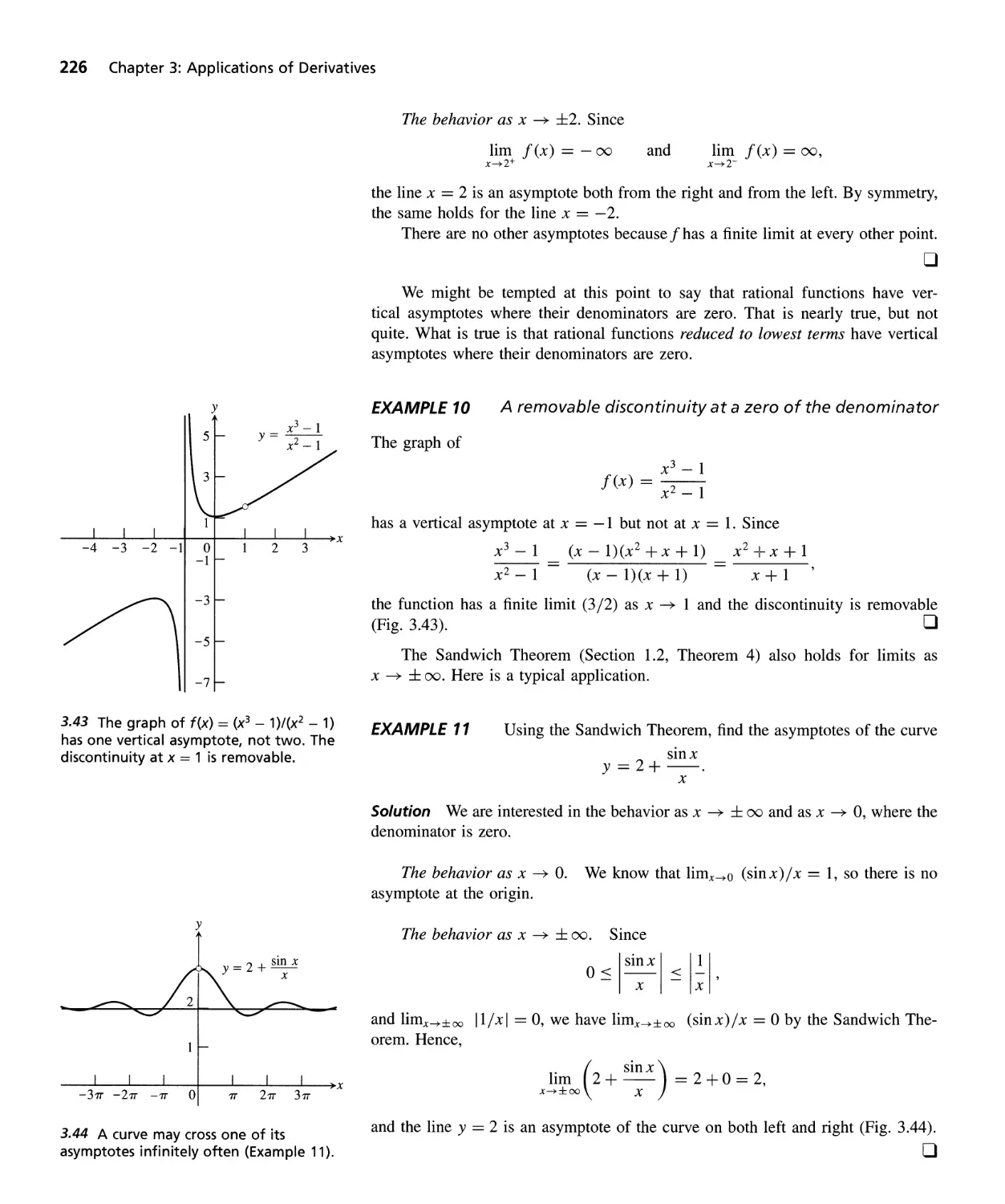
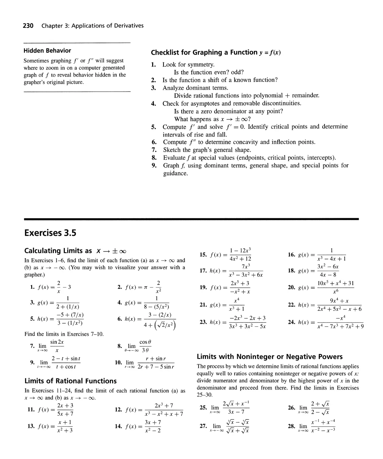
3.5 Limits as x :!: 00, Asymptotes, and Dominant Terms 220
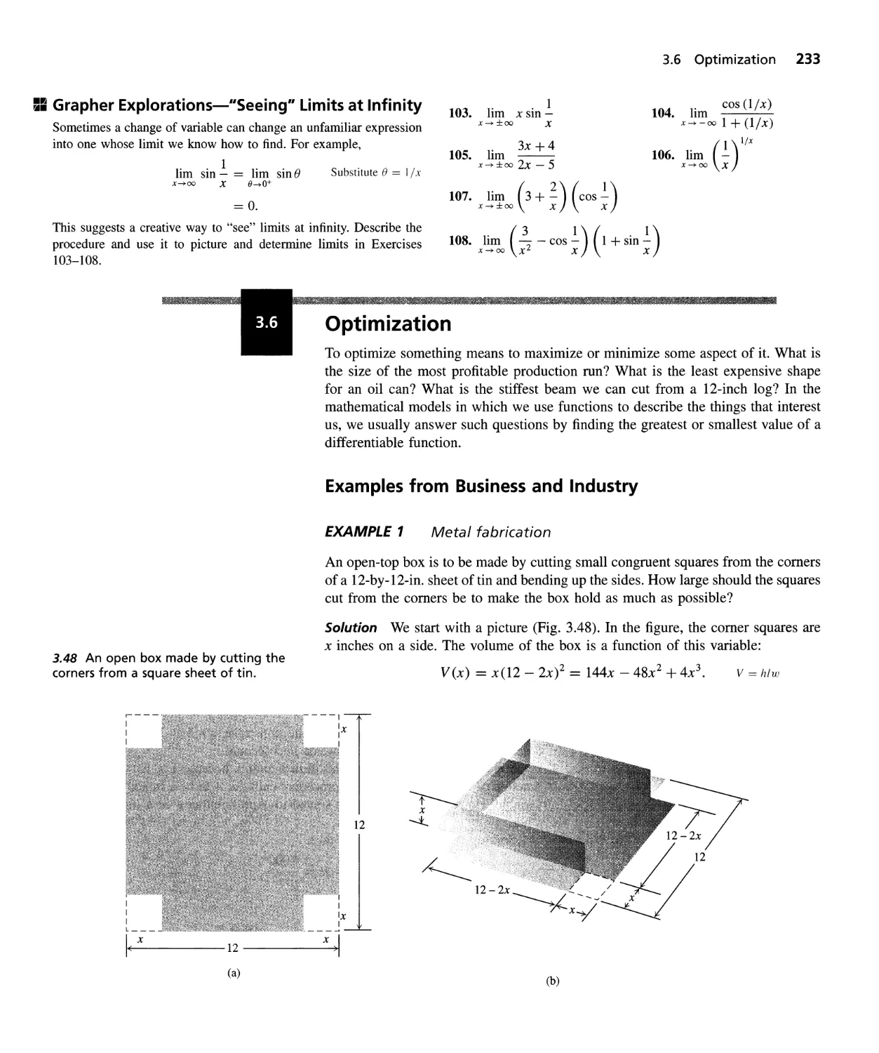
3.6 Optimization 233
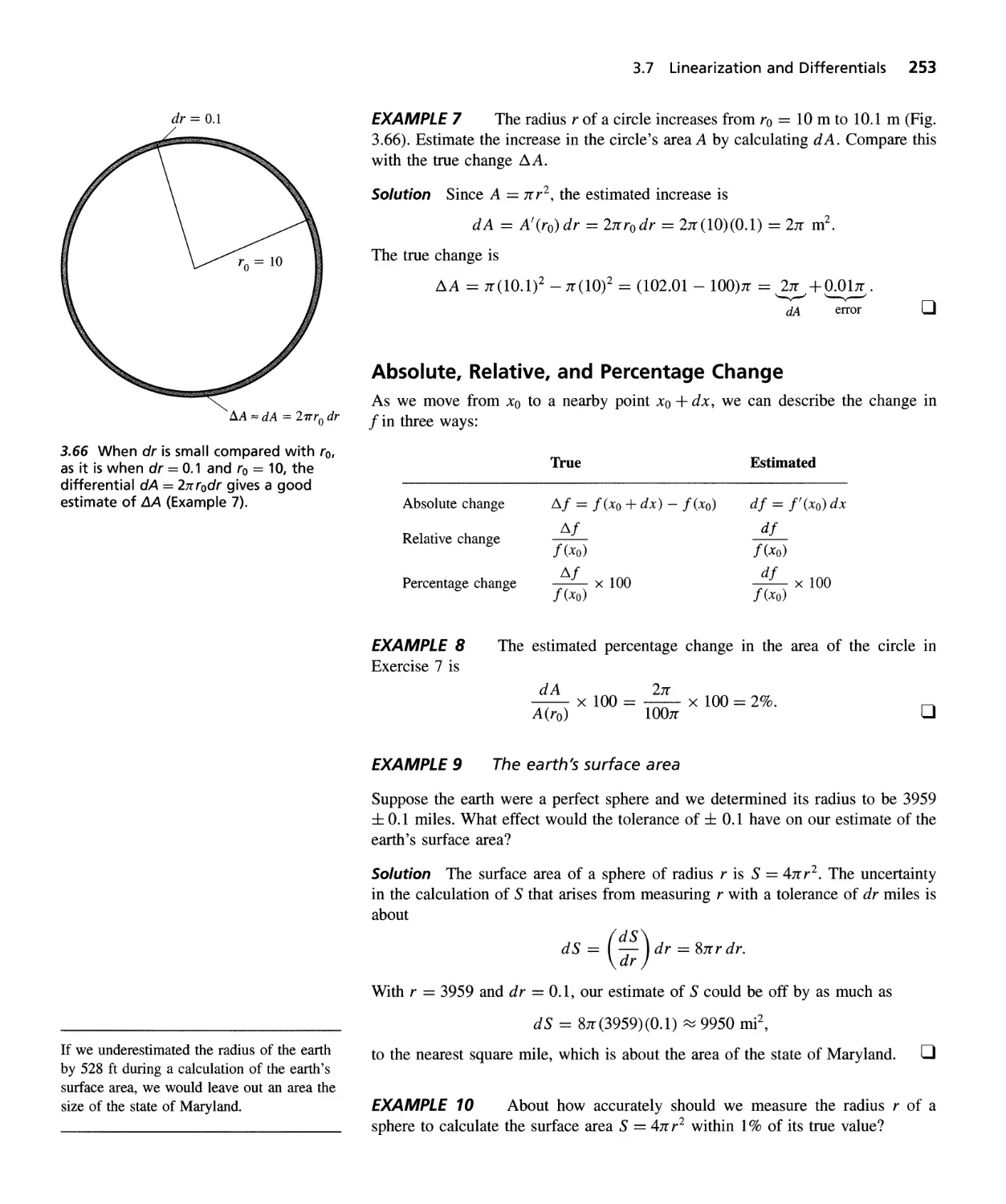
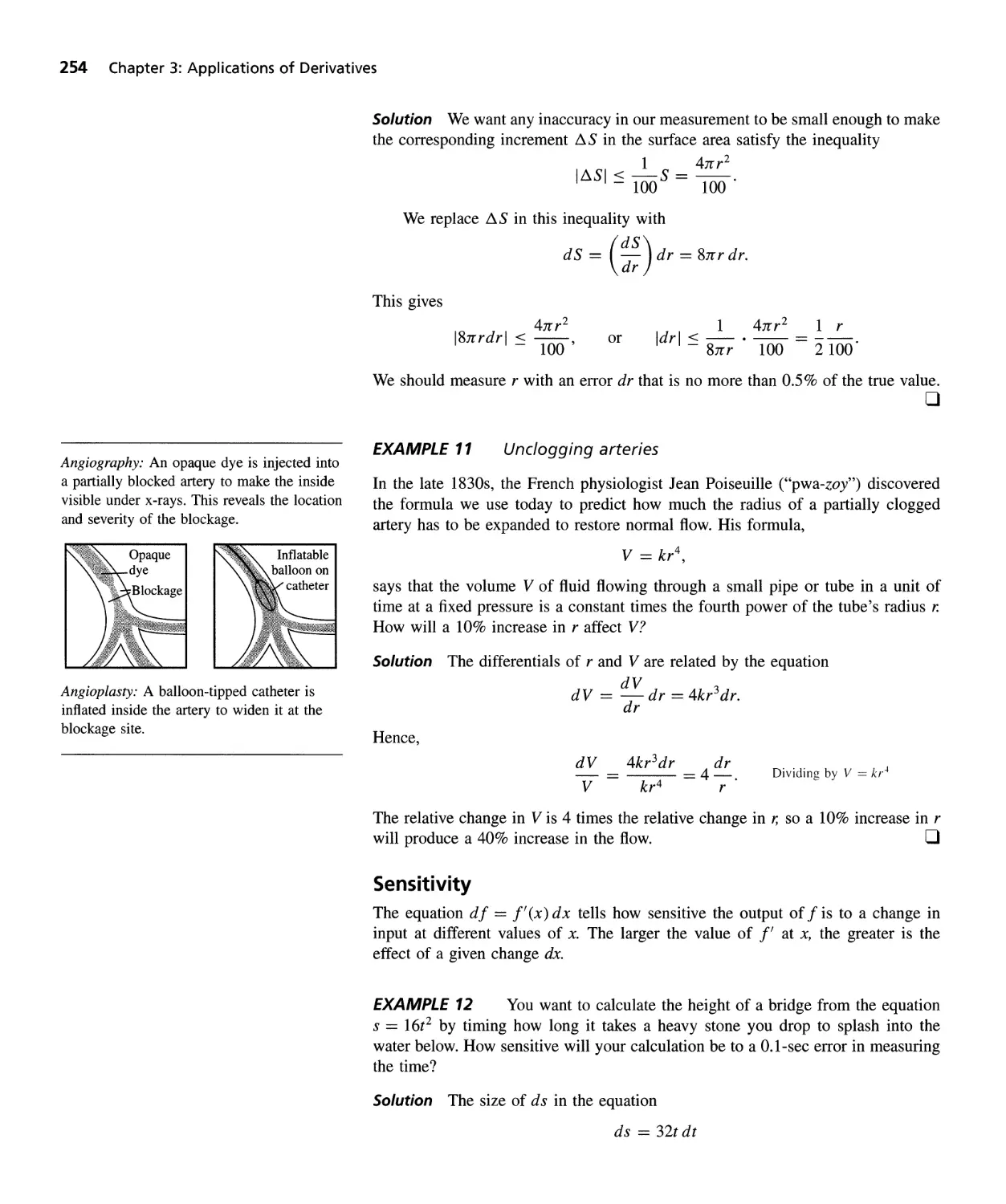
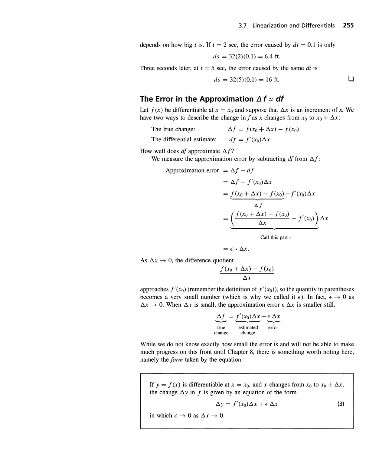
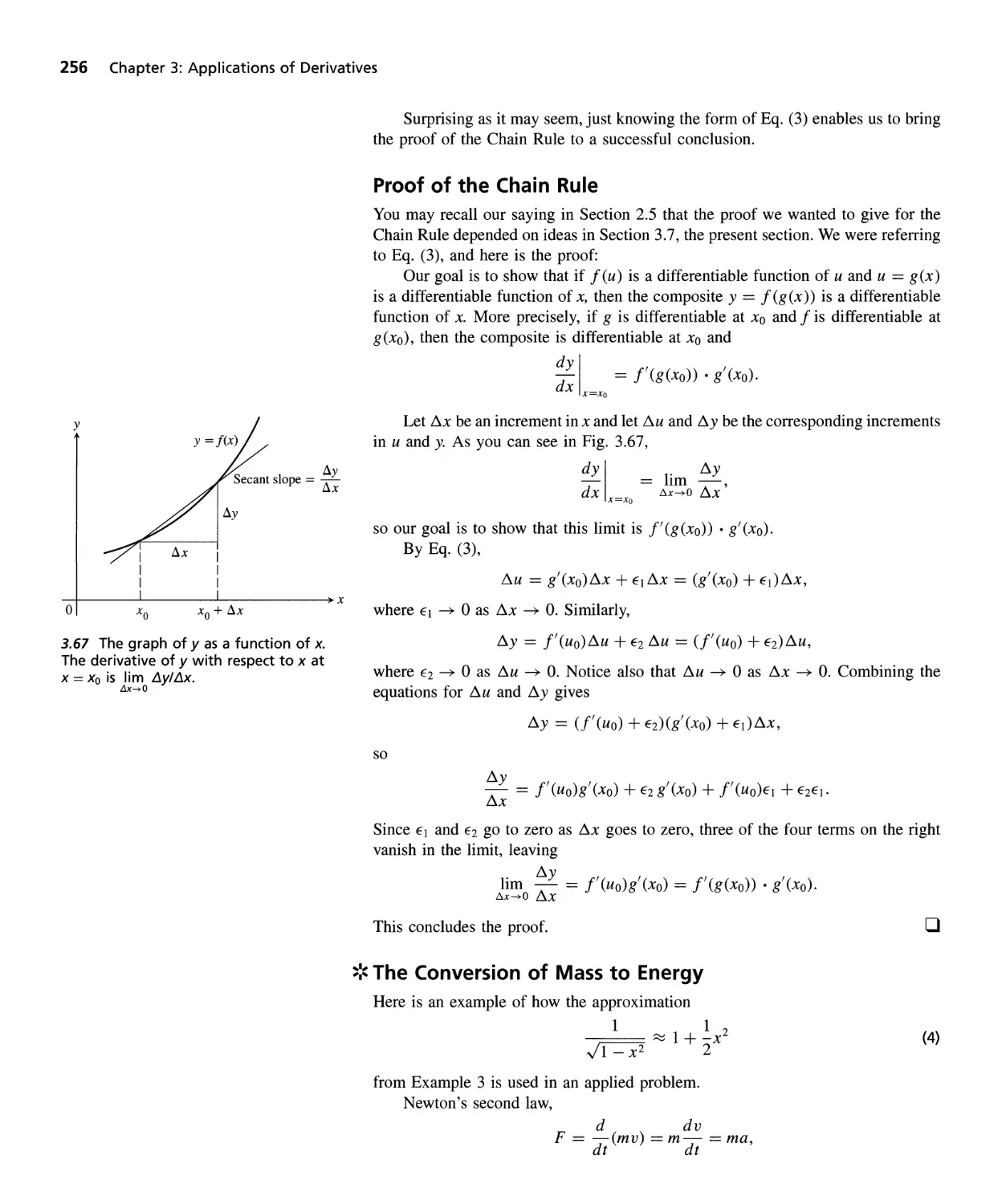
3.7 Linearization and Differentials 248
3.8 Newton's Method 260
QUESTIONS TO GUIDE YOUR REVIEW 268 PRACTICE EXERCISES 269
ADDITIONAL EXERCISES-THEORY, EXAMPLES, ApPLICATIONS 272
Integration
4.1
4.2
4.3
4.4
4.5
4.6
4.7
4.8
4.9
Applications of
Integrals
5.1
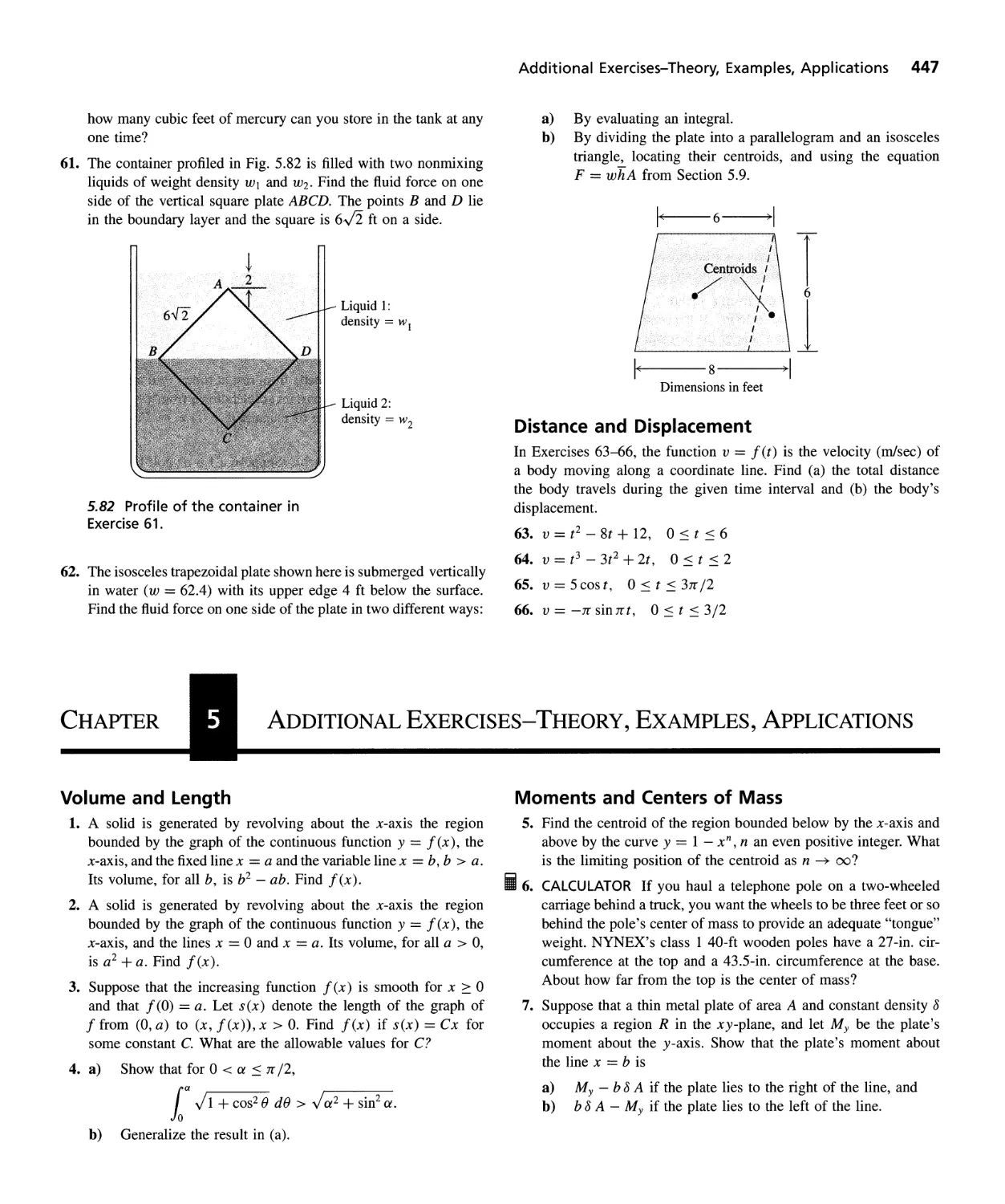
5.2
5.3
5.4
5.5
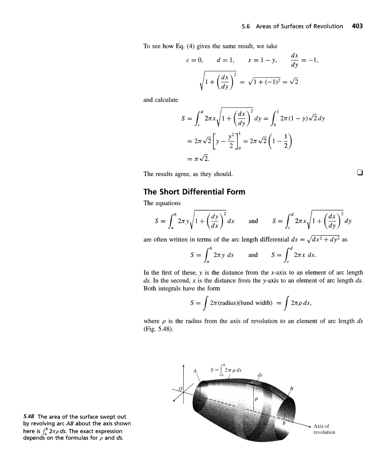
5.6
5.7
5.8
5.9
5.10
Transcendental
Functions
6.1
6.2
6.3
6.4
6.5
6.6
6.7
6.8
6.9
6.10
6.11
6.12
Techniques of
Integration
7.1
7.2
Indefinite Integrals 275
Differential Equations, Initial Value Problems, and Mathematical Modeling 282
Integration by Substitution-Running the Chain Rule Backward 290
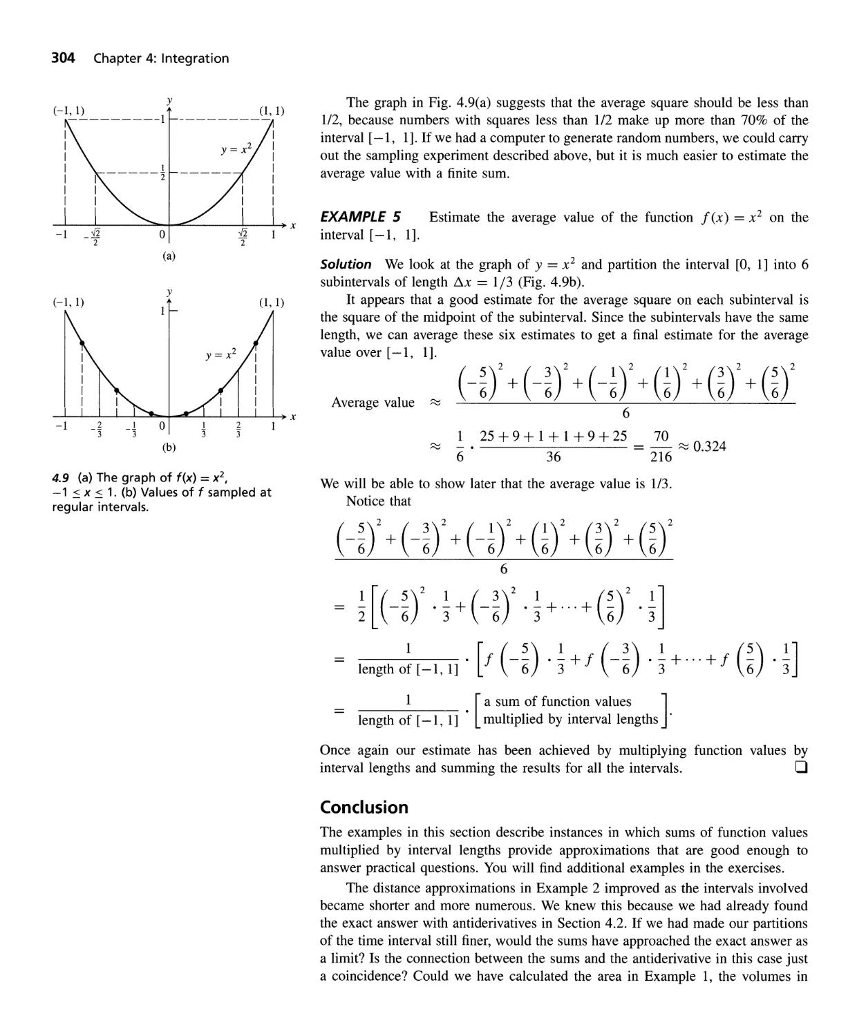
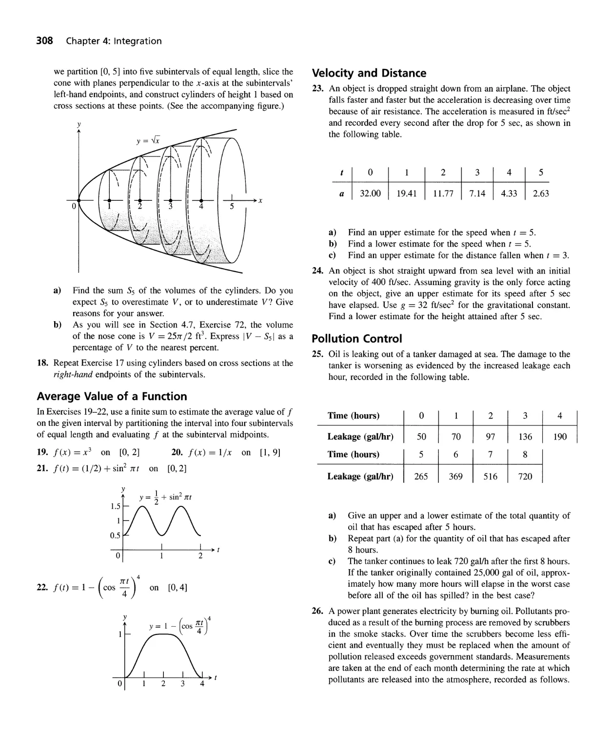
Estimating with Finite Sums 298
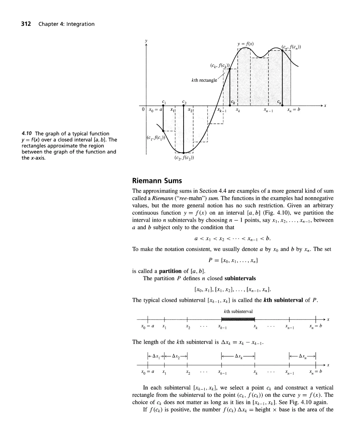
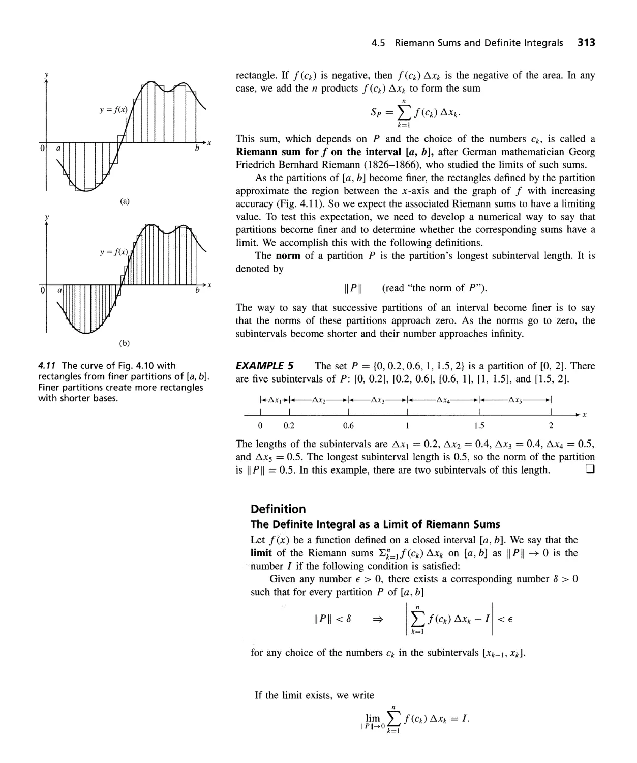
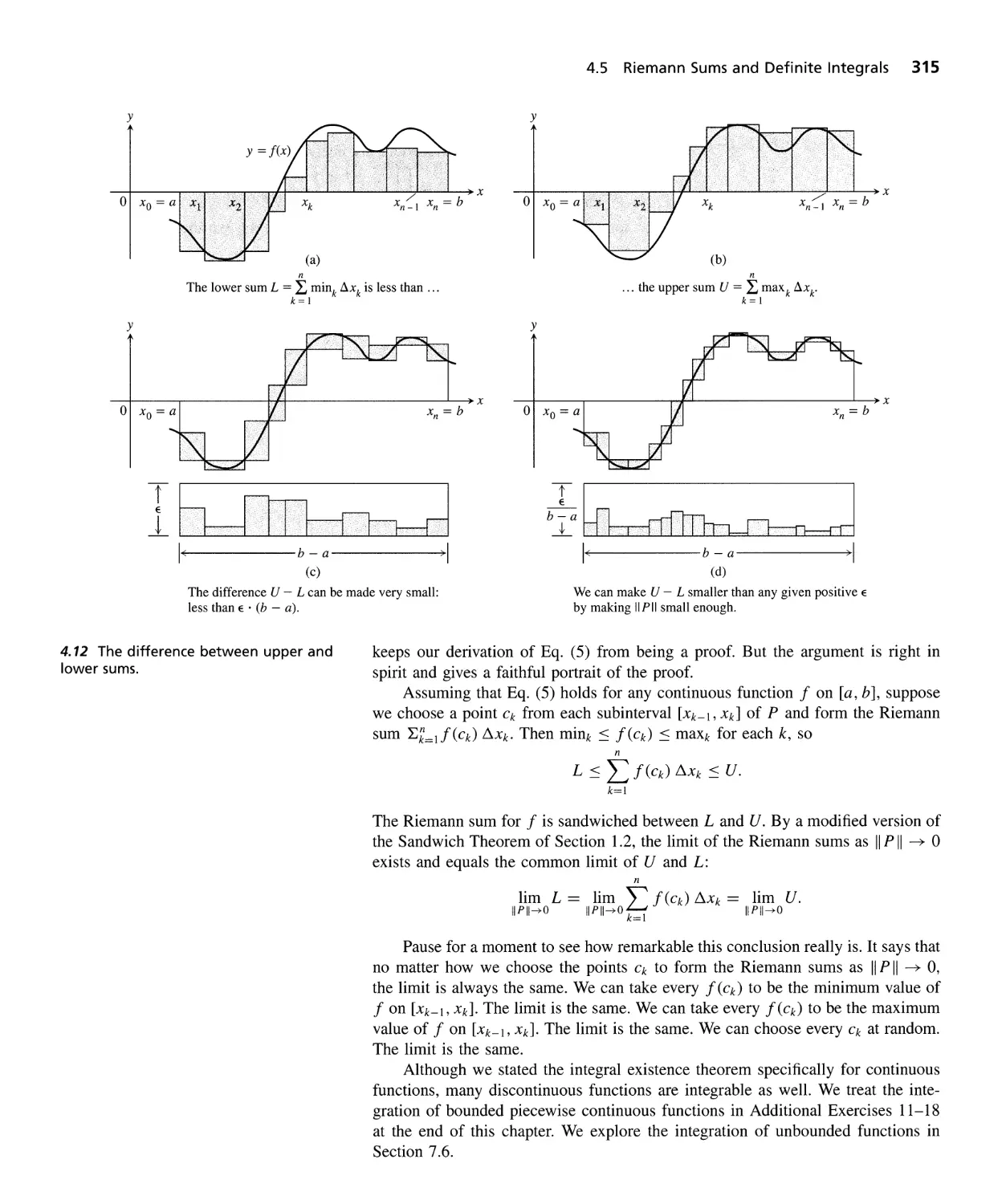
Riemann Sums and Definite Integrals 309
Properties, Area, and the Mean Value Theorem 323
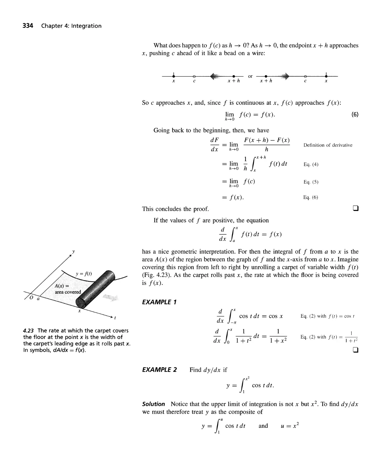
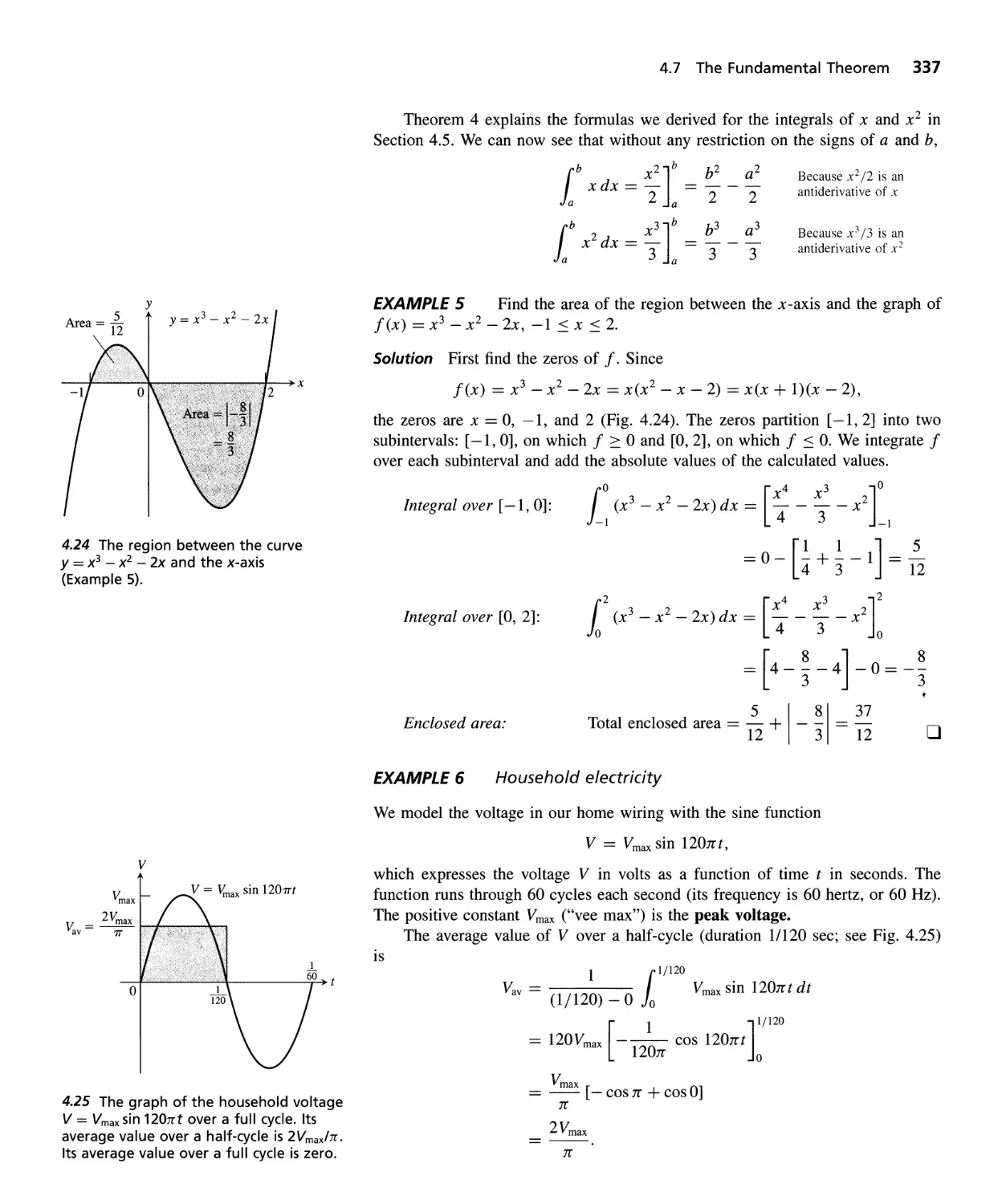
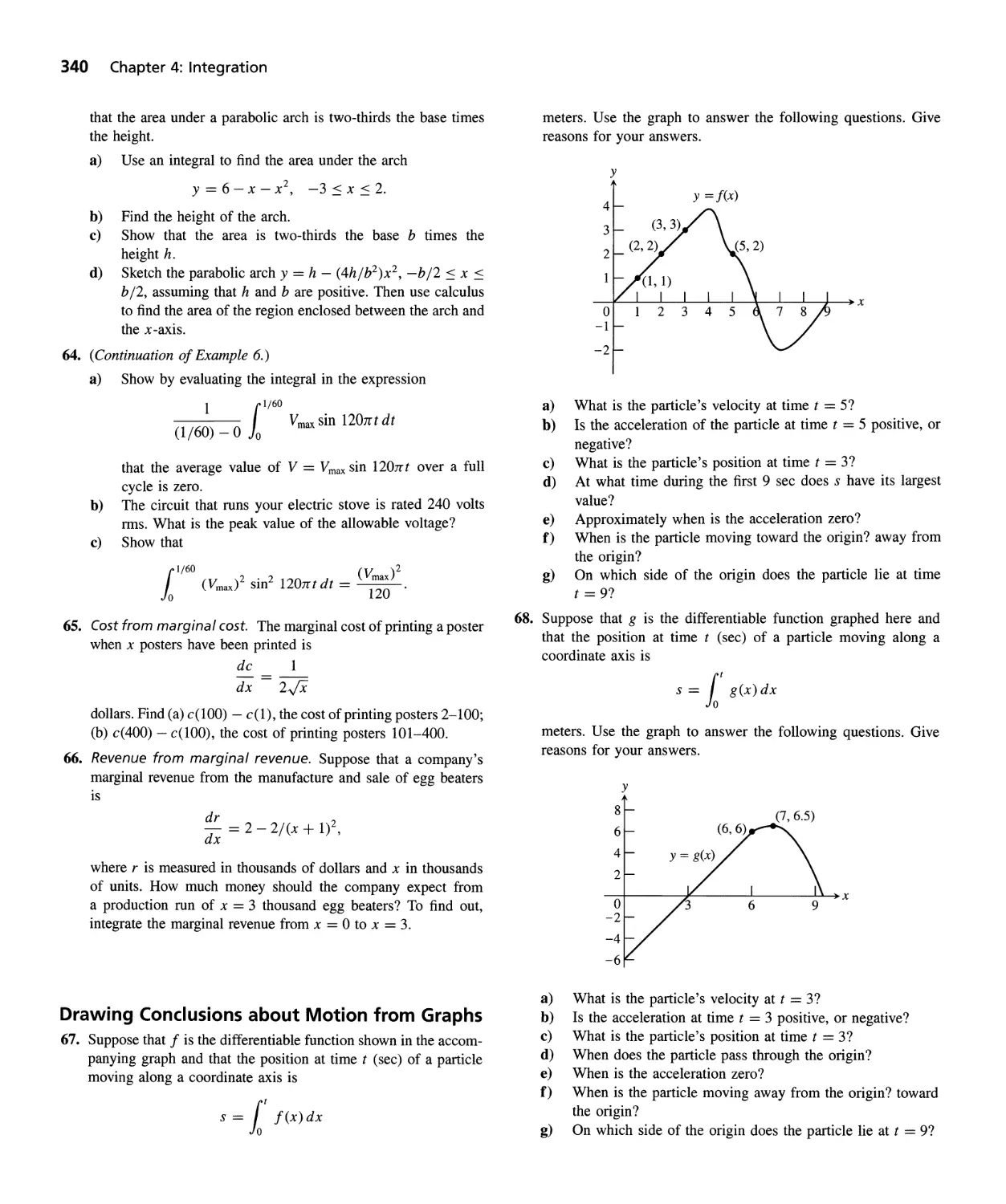
The Fundamental Theorem 332
Substitution in Definite Integrals 342
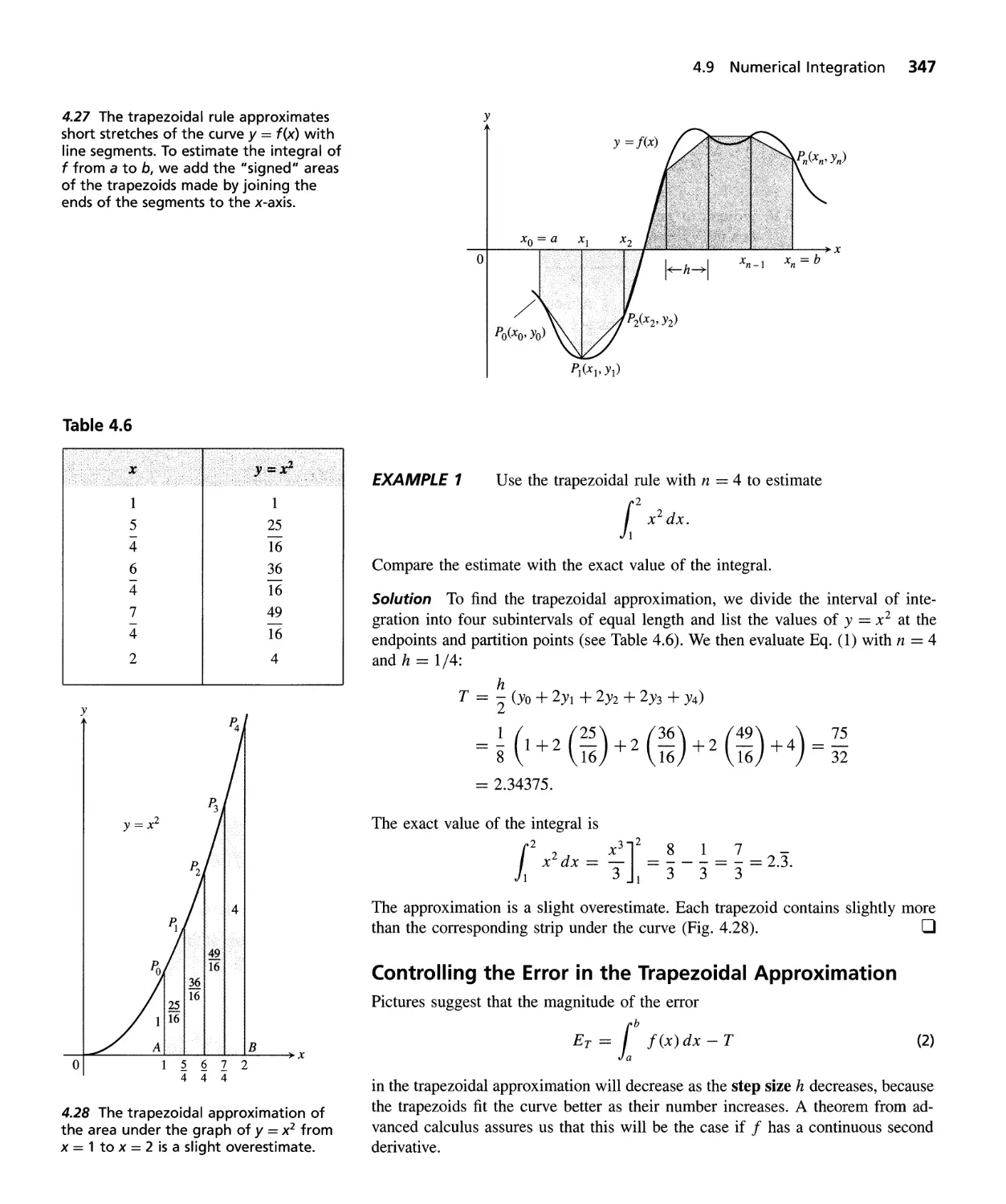
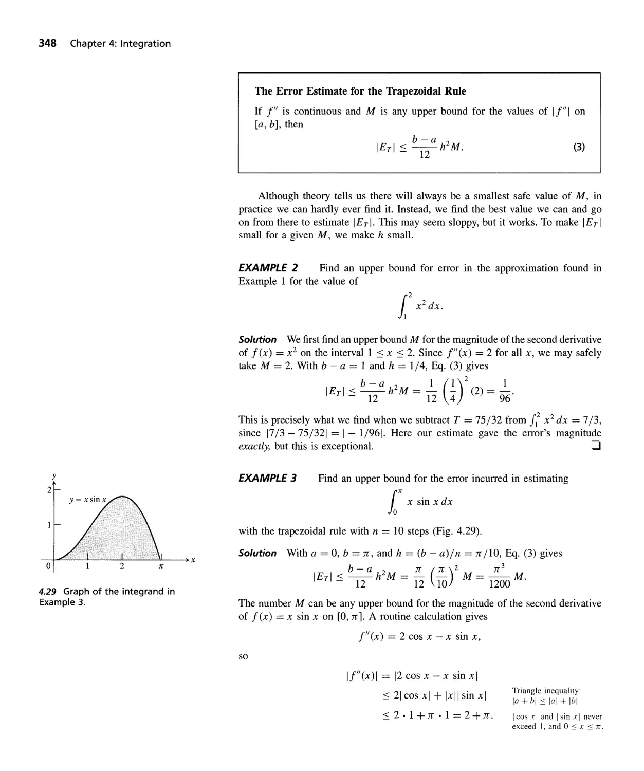
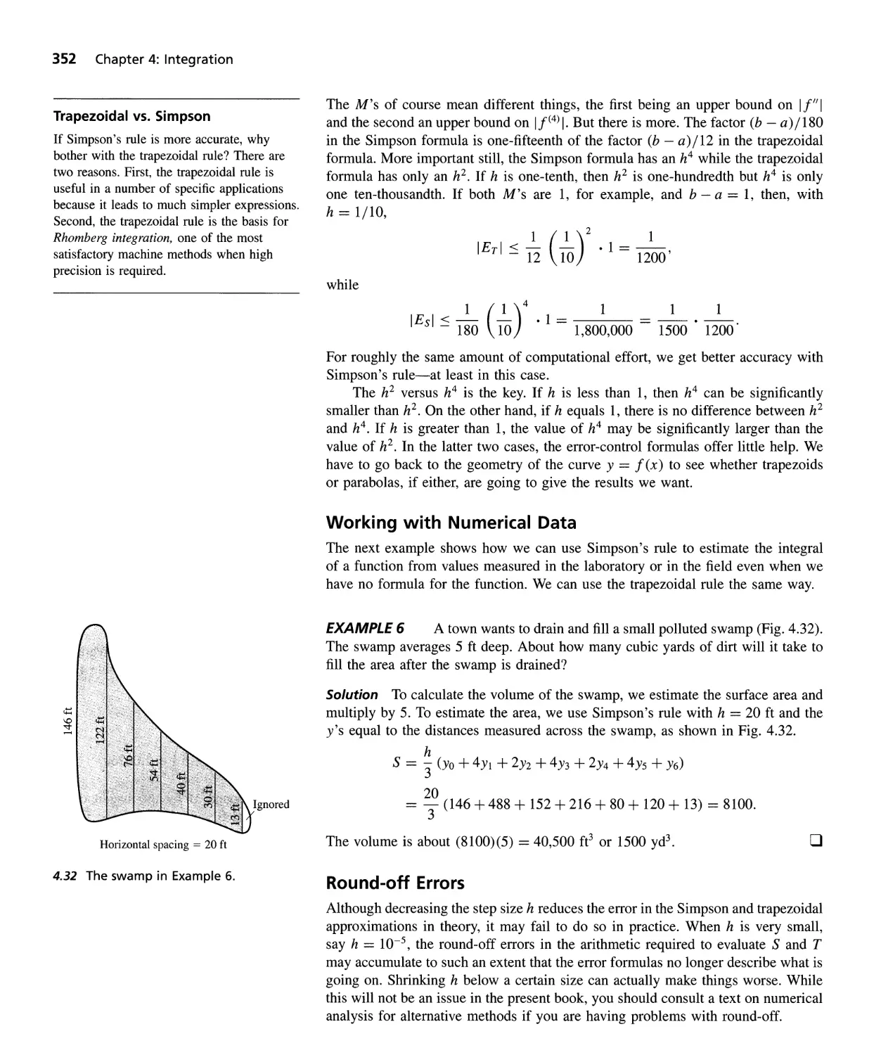
Numerical Integration 346
QUESTIONS TO GUIDE YOUR REVIEW 356 PRACTICE EXERCISES 357
ADDITIONAL EXERCISES-THEORY, EXAMPLES, ApPLICATIONS 360
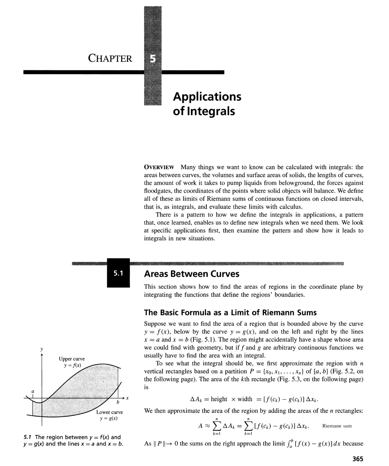
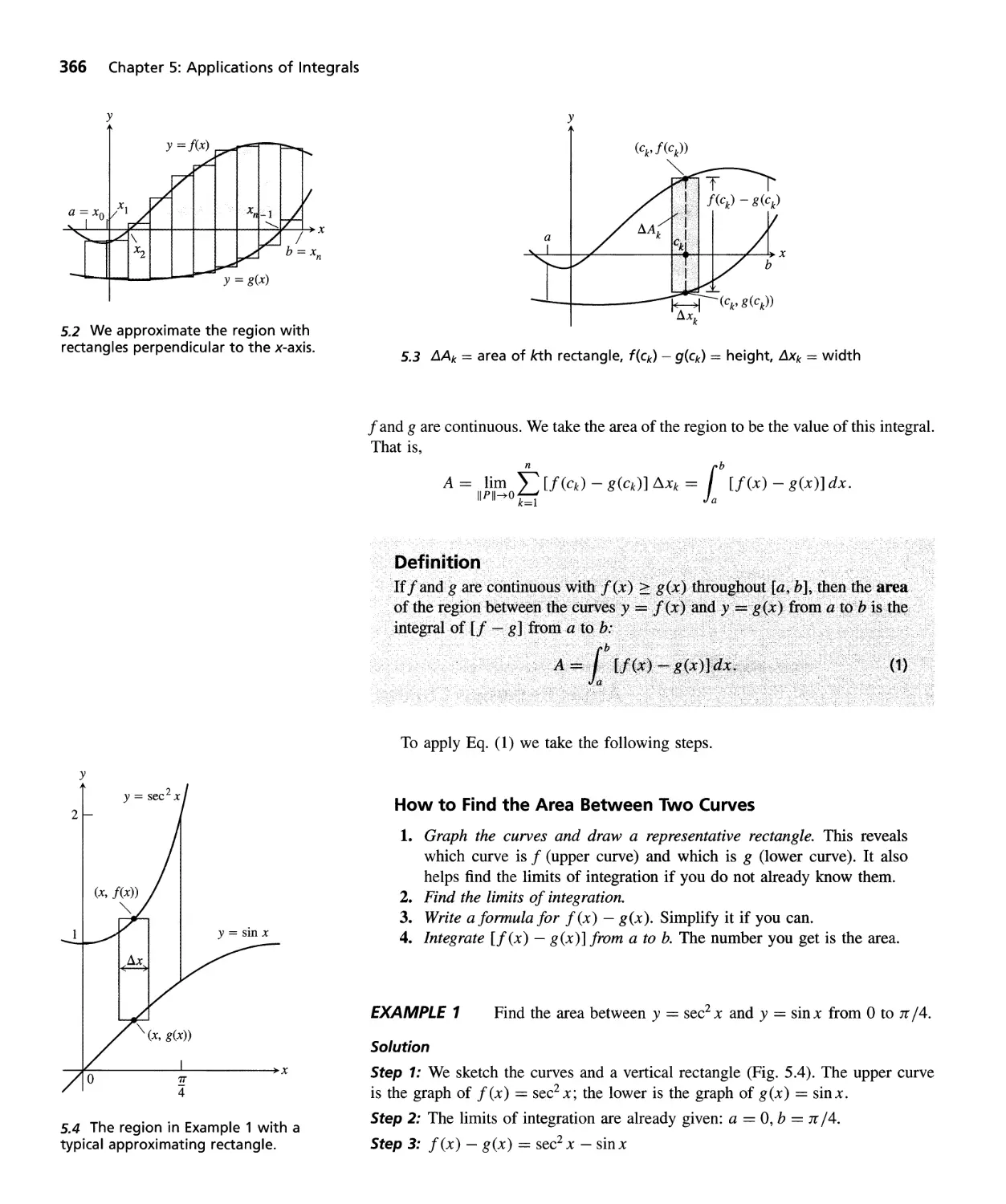
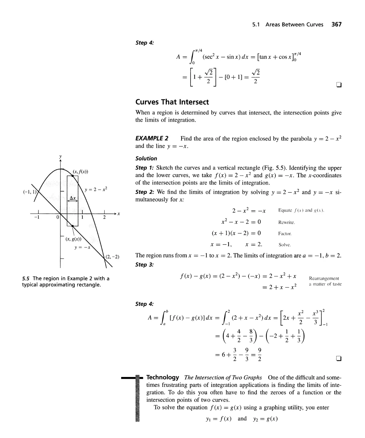
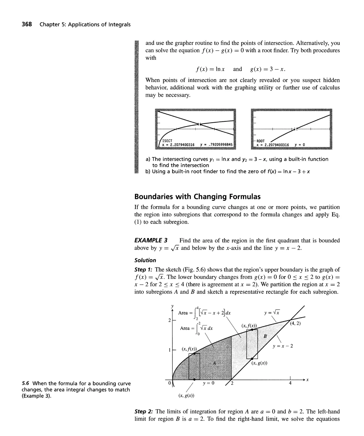
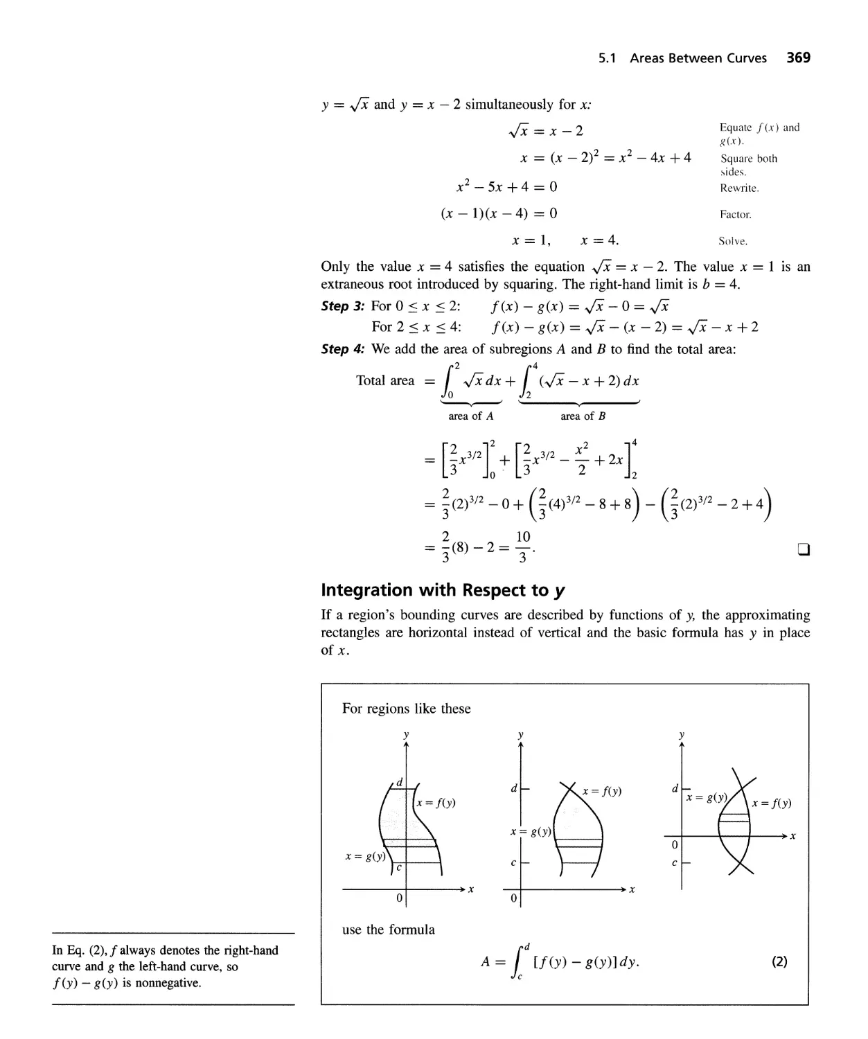
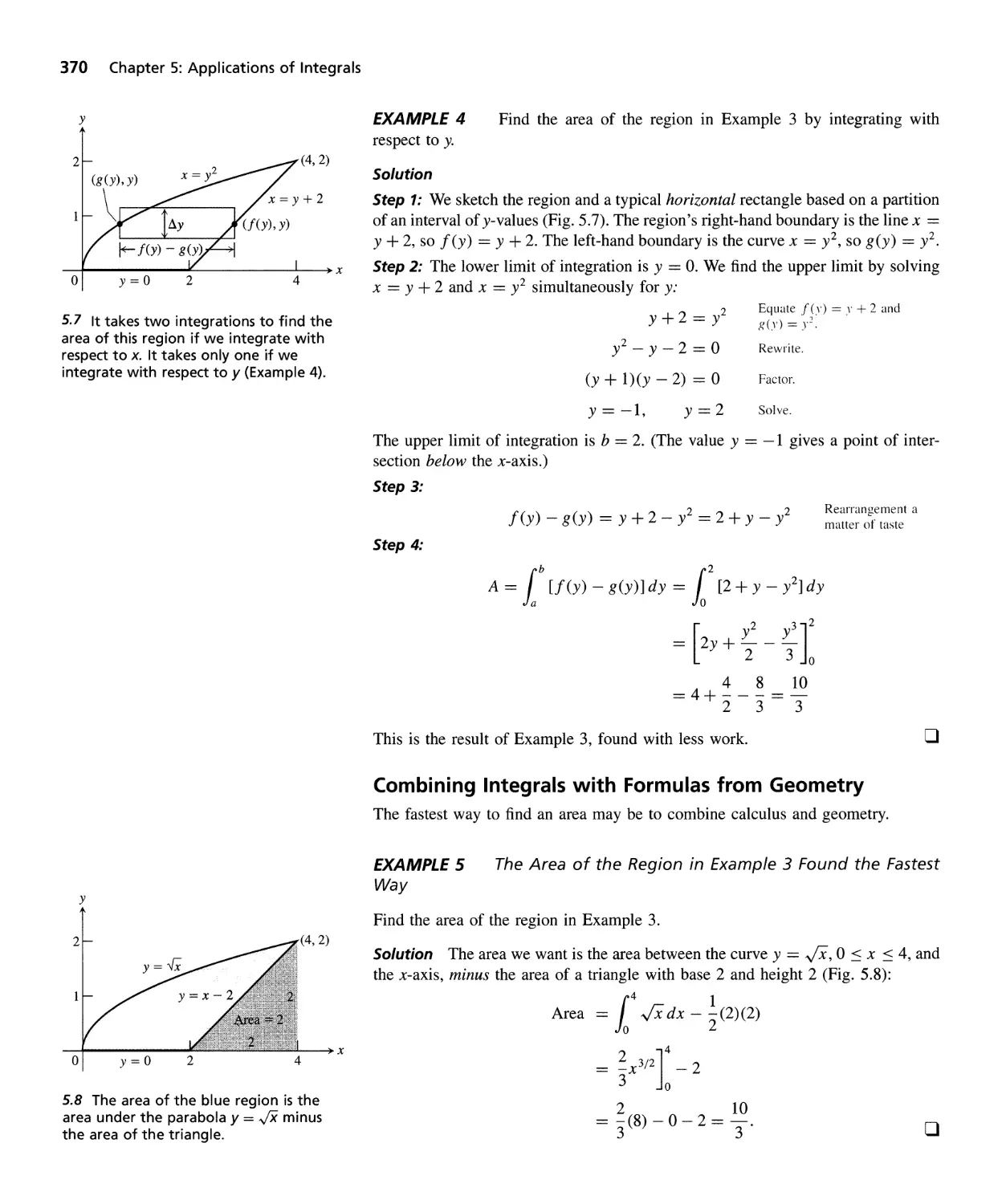
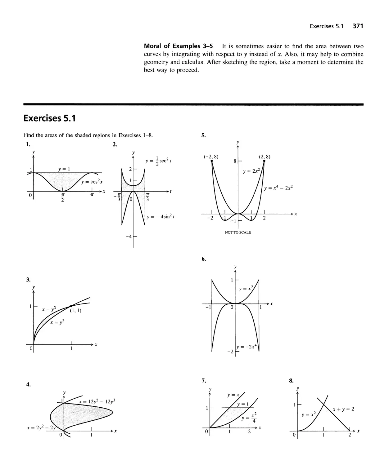
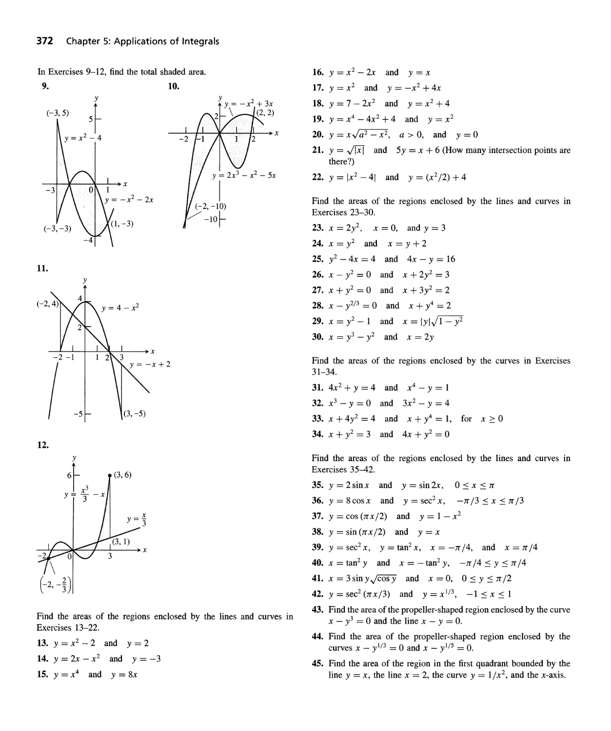
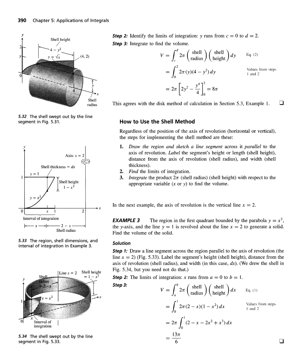
Areas Between Curves 365
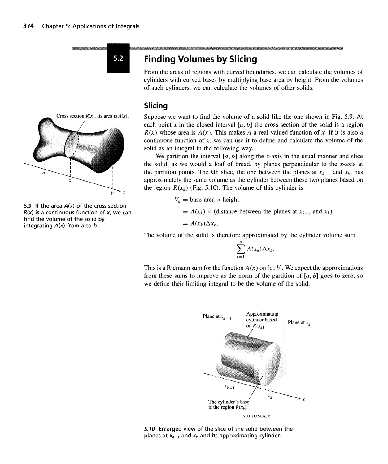
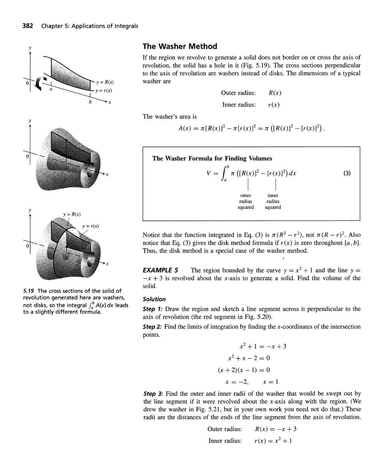
Finding Volumes by Slicing 374
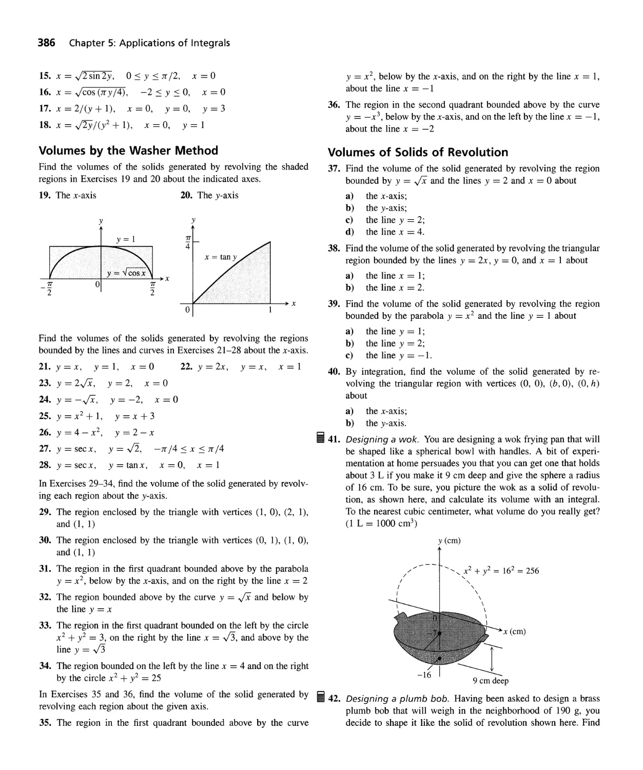
Volumes of Solids of Revolution-Disks and Washers 379
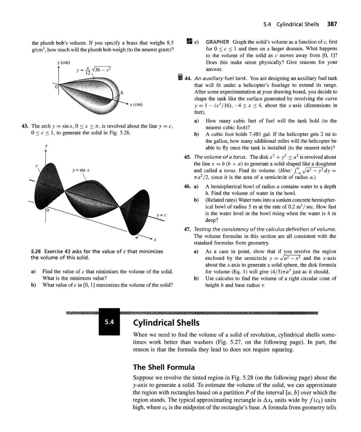
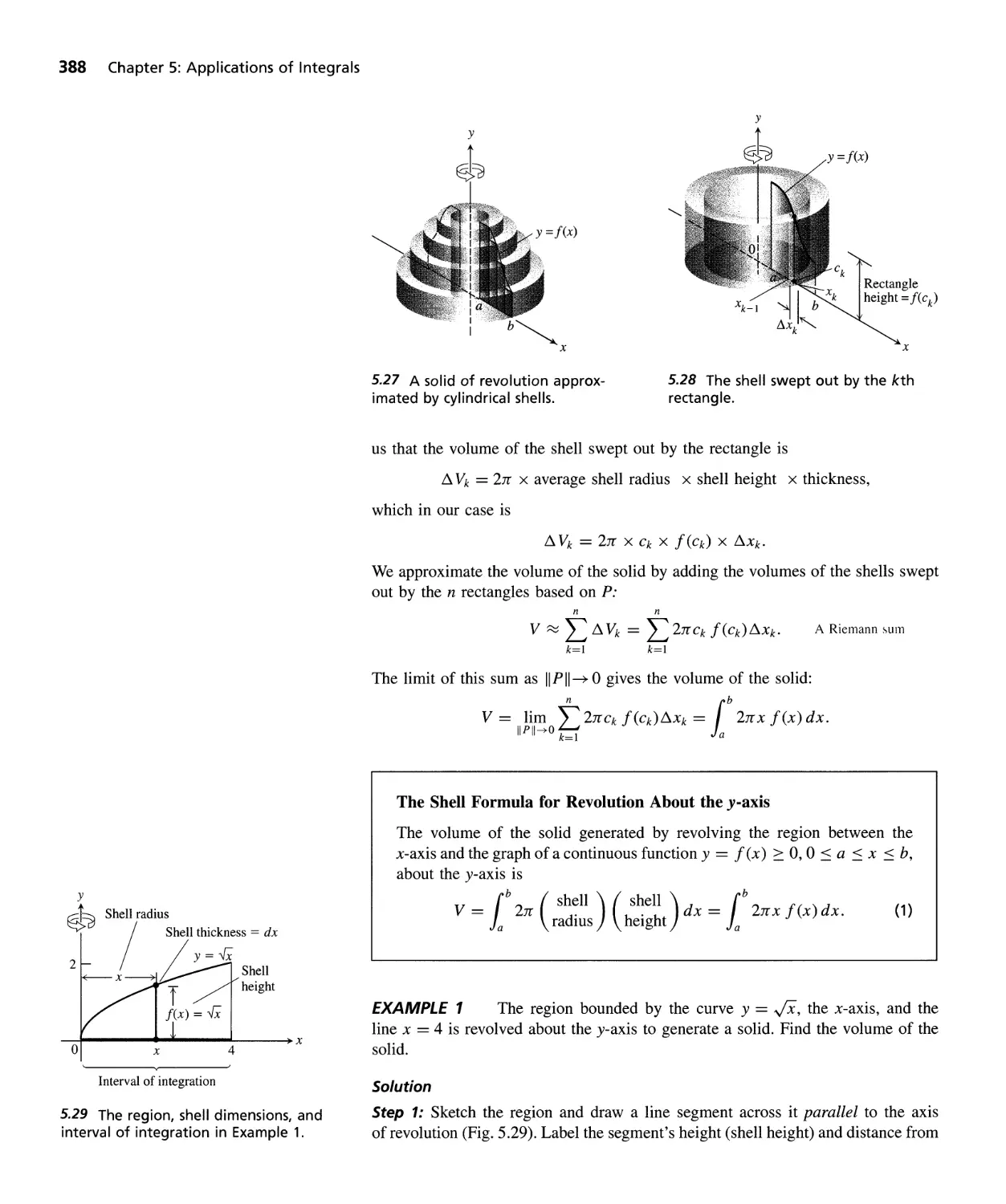
Cy lindrical Shells 387
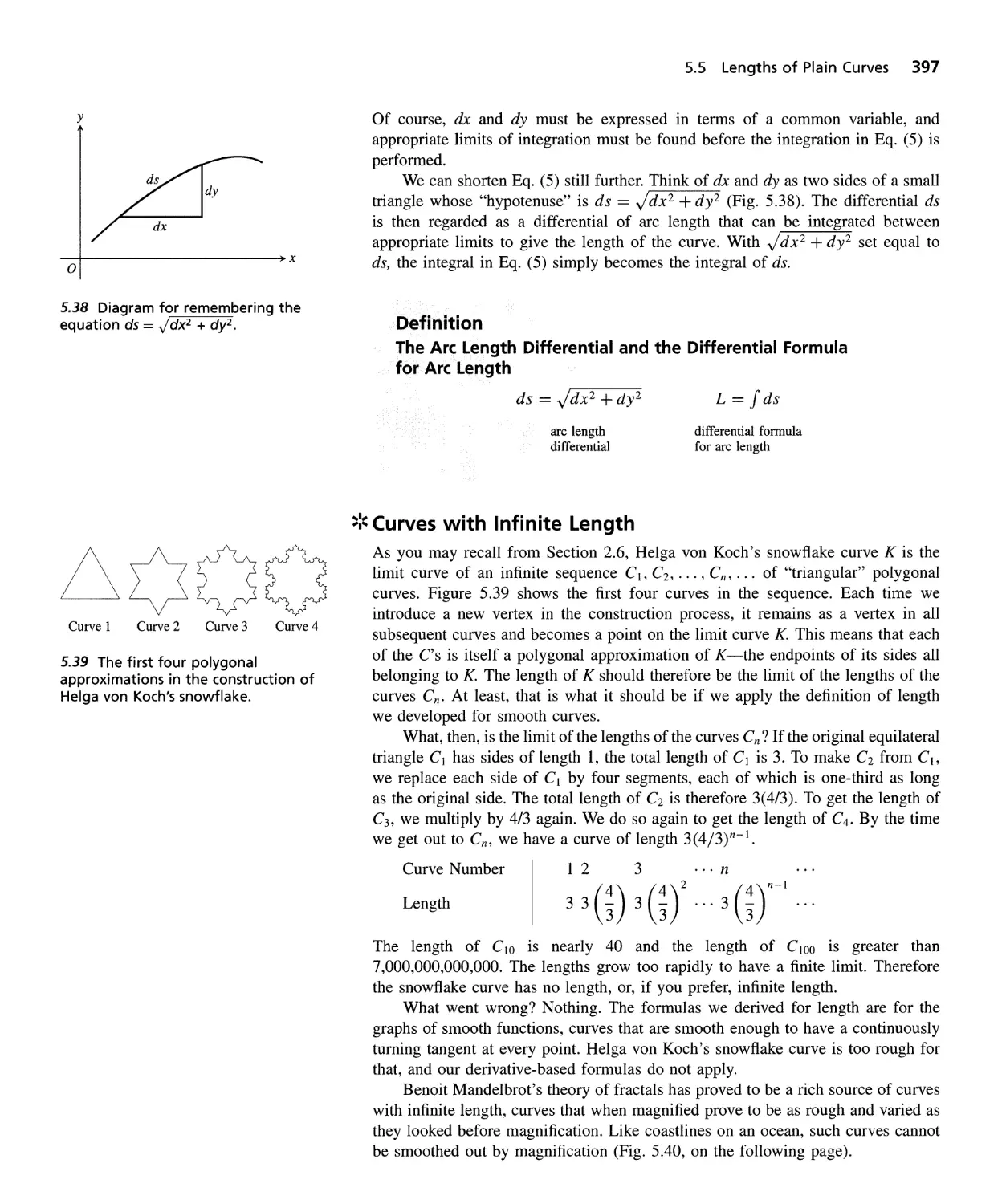
Lengths of Plane Curves 393
Areas of Surfaces of Revolution 400
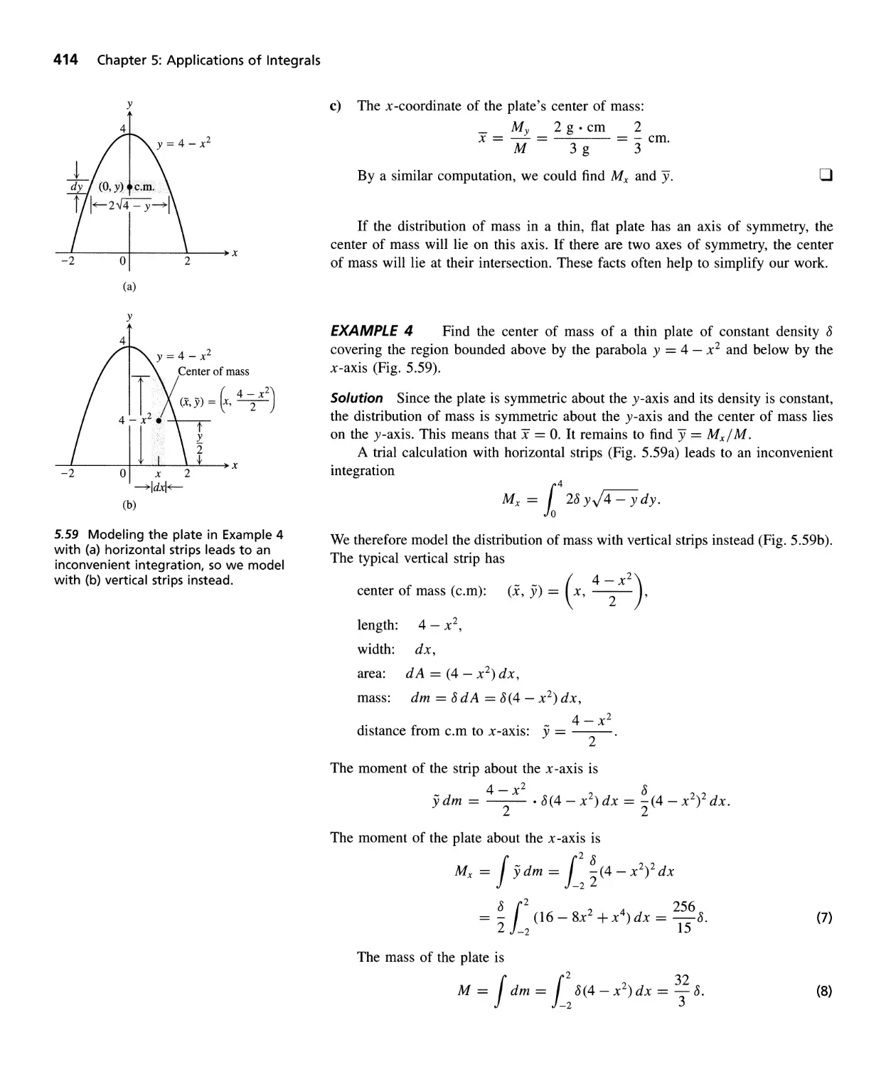
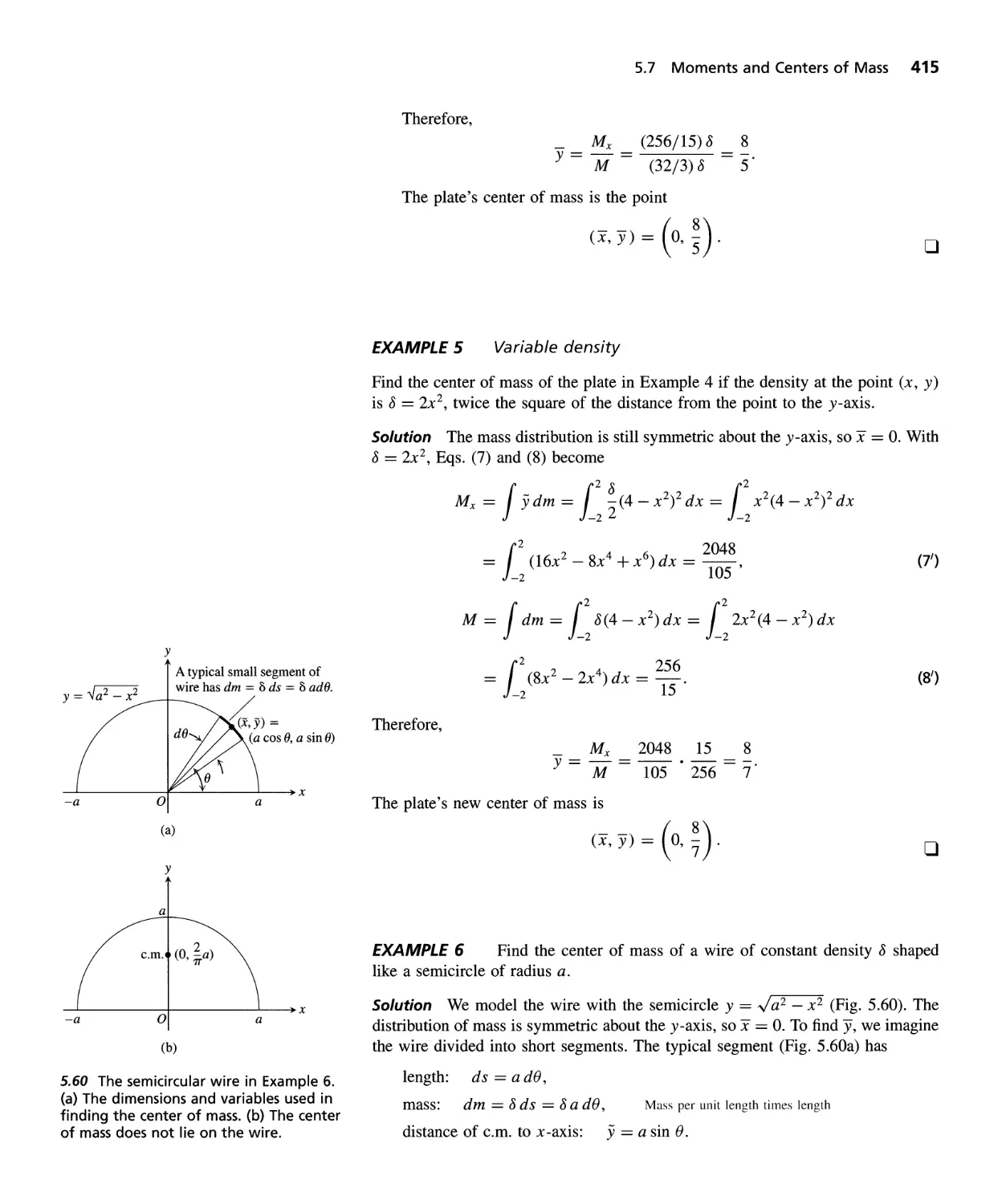
Moments and Centers of Mass 407
Work 418
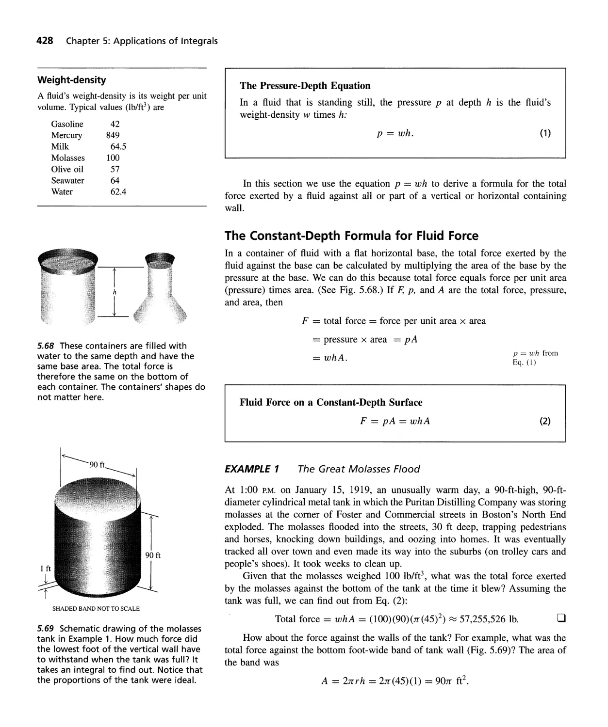
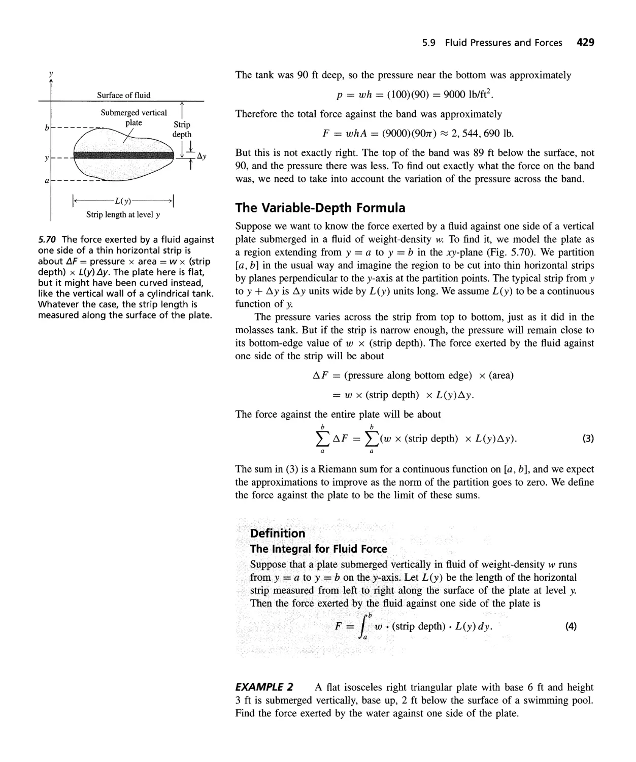
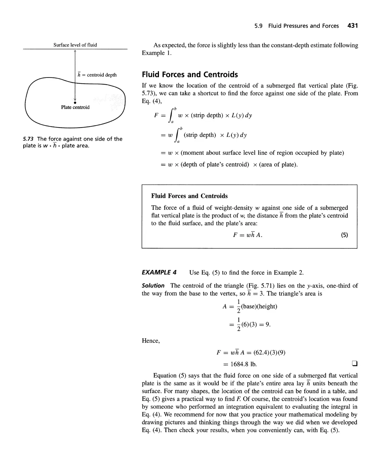
Fluid Pressures and Forces 427
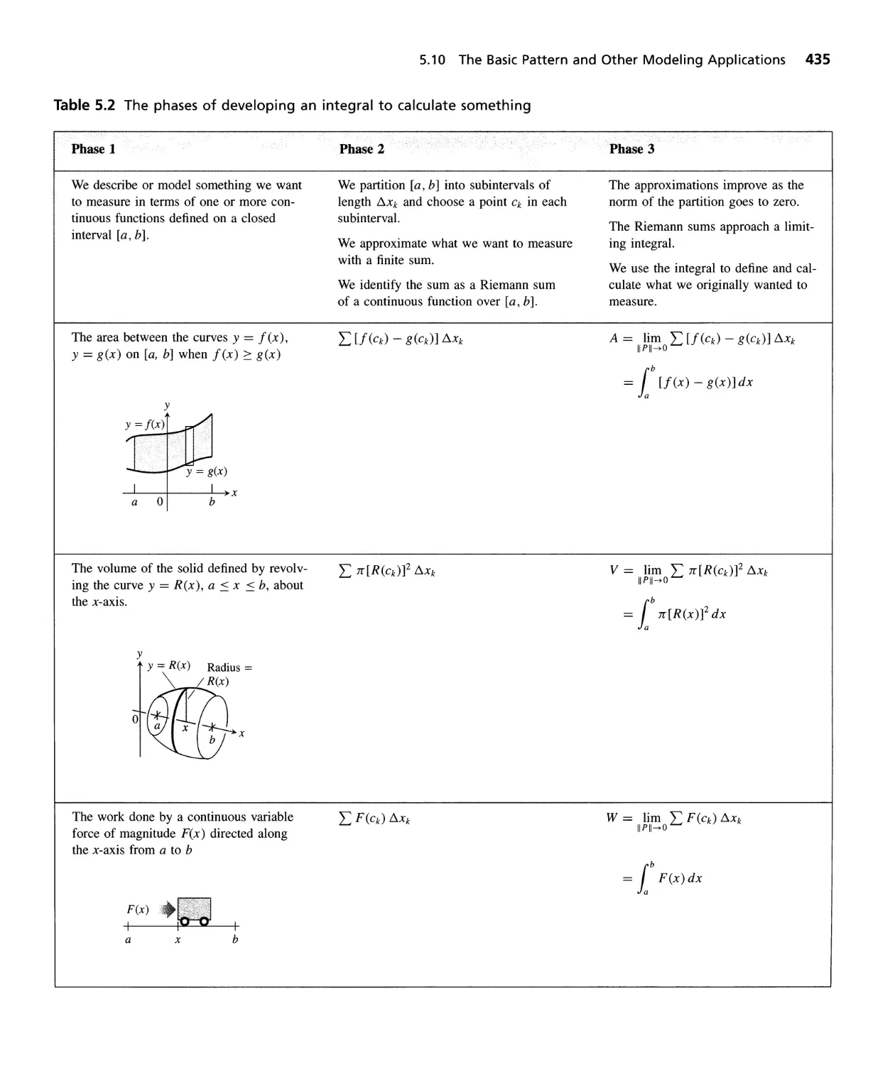
The Basic Pattern and Other Modeling Applications 434
QUESTIONS TO GUIDE YOUR REVIEW 444 PRACTICE EXERCISES 444
ADDITIONAL EXERCISES-THEORY, EXAMPLES, ApPLICATIONS 447
Inverse Functions and Their Derivatives 449
Natural Logarithms 458
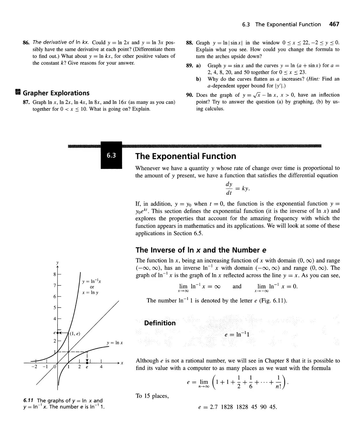
The Exponential Function 467
aX and loga x 474
Growth and Decay 482
L'Hopital's Rule 491
Relative Rates of Growth 498
Inverse Trigonometric Functions 504
Derivatives of Inverse Trigonometric Functions; Integrals 513
Hyperbolic Functions 520
First Order Differential Equations 529
Euler's Numerical Method; Slope Fields 541
QUESTIONS TO GUIDE YOUR REVIEW 547 PRACTICE EXERCISES 548
ADDITIONAL EXERCISES-THEORY, EXAMPLES, ApPLICATIONS 551
Basic Integration Formulas 555
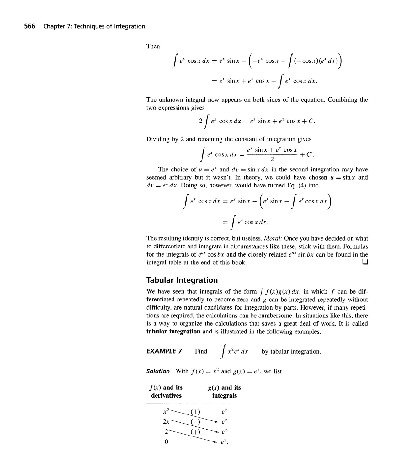
Integration by Parts 562
Infinite Series
Conic Sections,
Parametrized
Curves, and Polar
Coordinates
Vectors and
Analytic Geometry
in Space
Vector-Valued
Functions and
Motion in Space
Contents v
7.3 Partial Fractions 569
7.4 Trigonometric Substitutions 578
7.5 Integral Tables and CAS 583
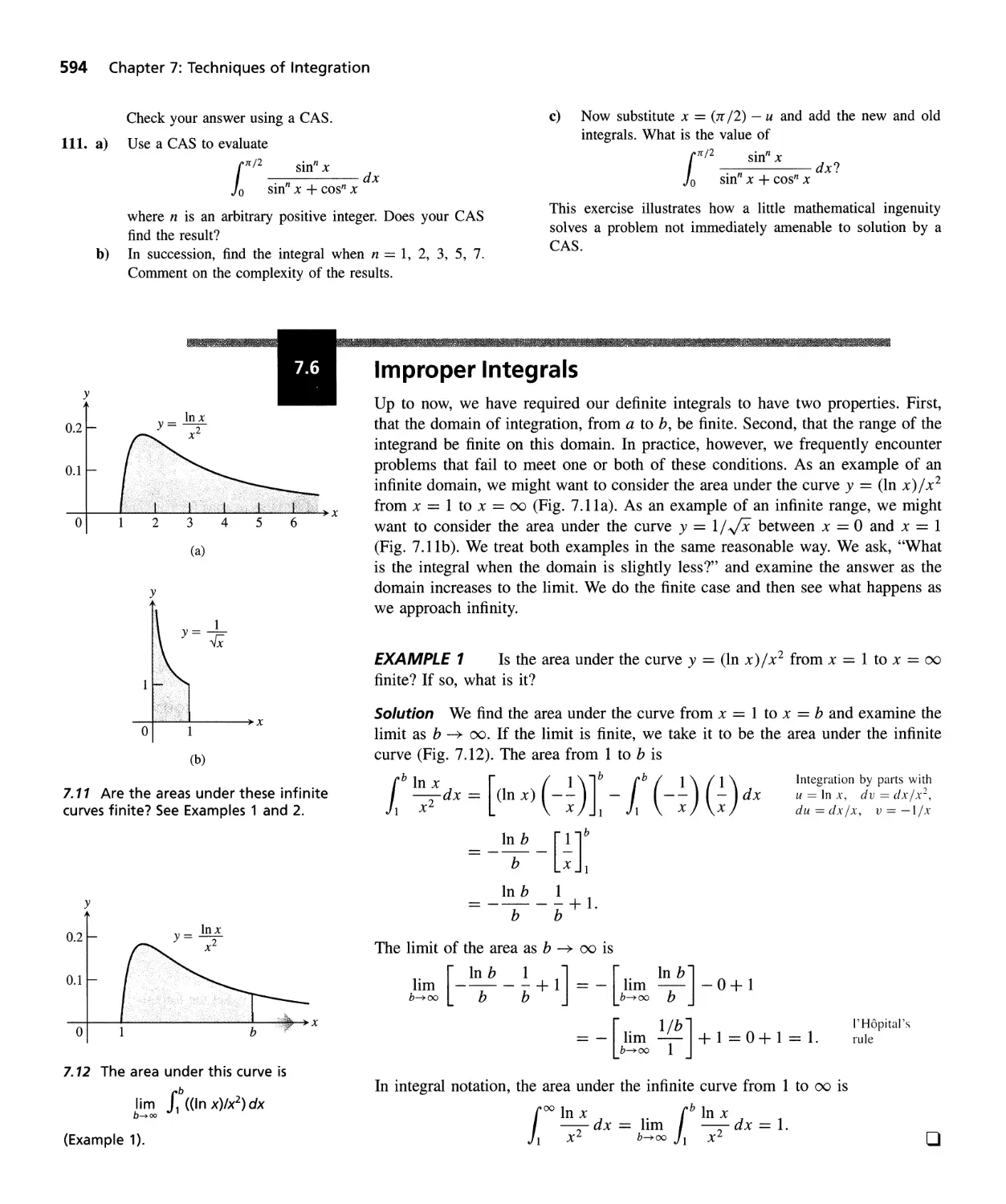
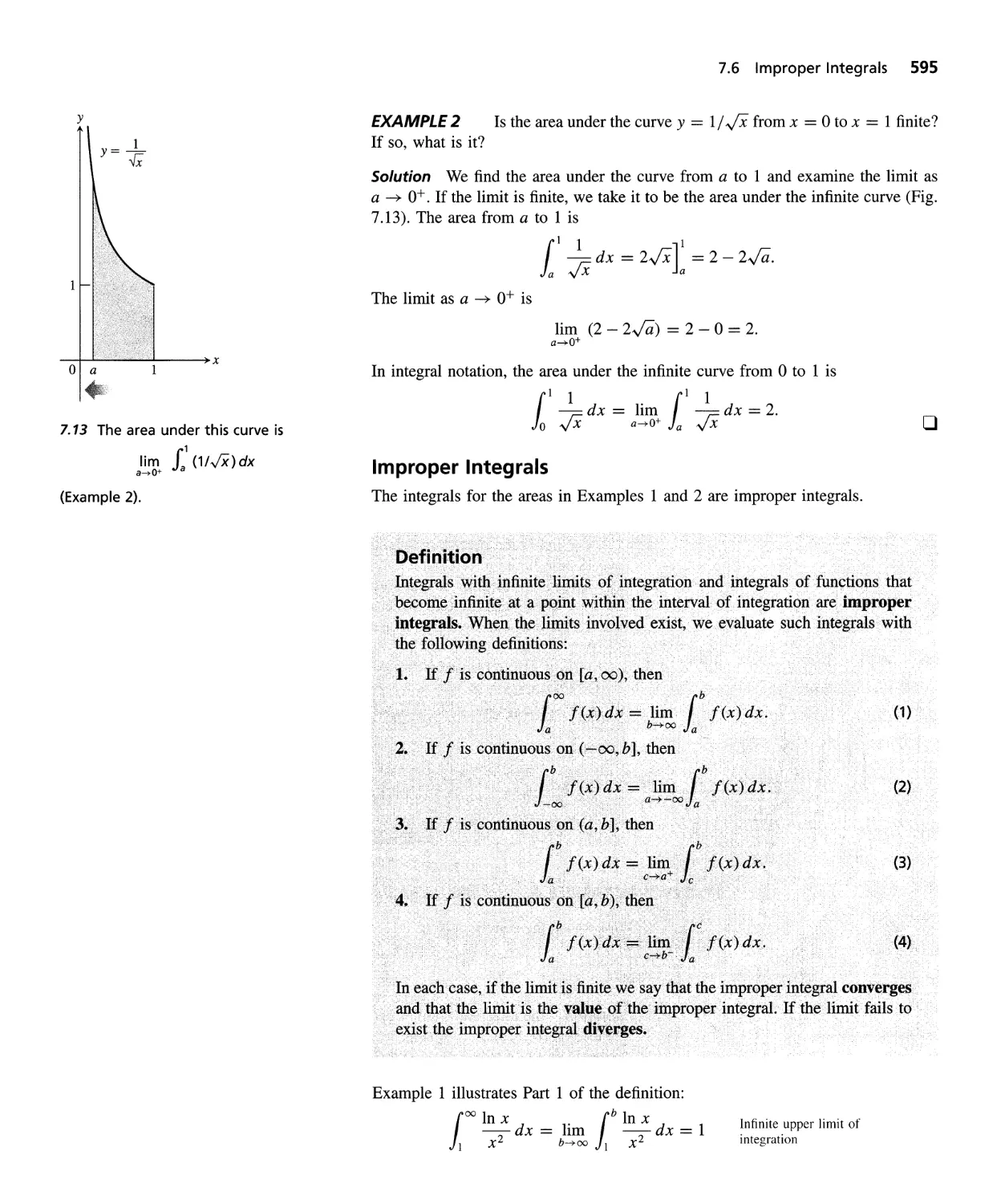
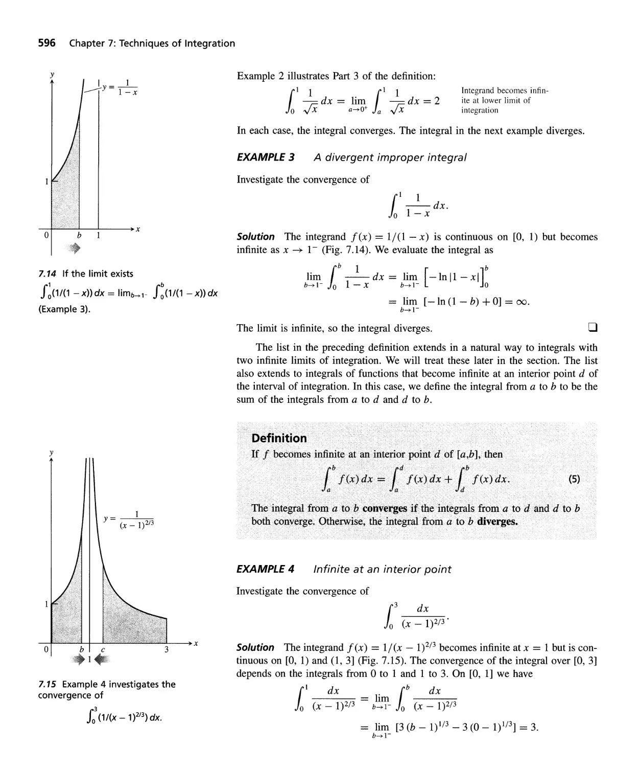
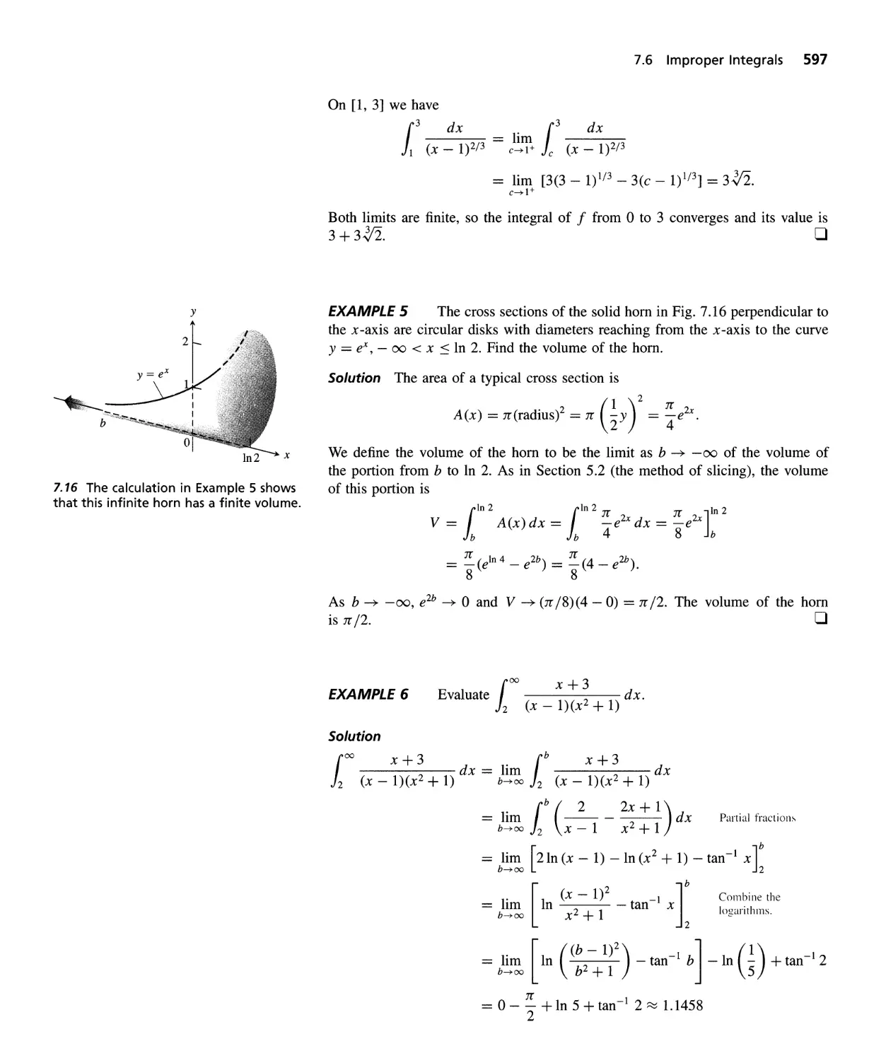
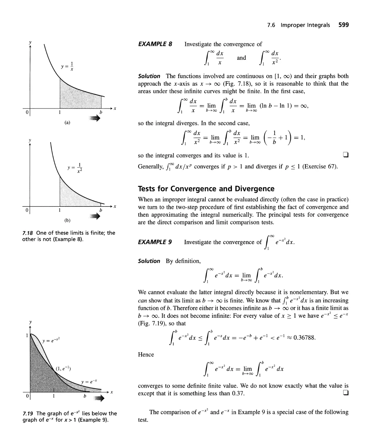
7.6 Improper Integrals 594
QUESTIONS TO GUIDE YOUR REVIEW 606 PRACTICE EXERCISES 606
ADDITIONAL EXERCISES-THEORY, EXAMPLES, ApPLICATIONS 609
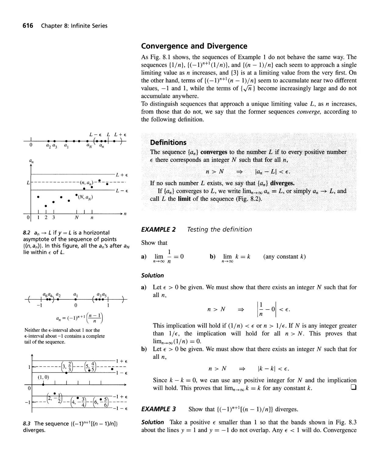
8.1
8.2
8.3
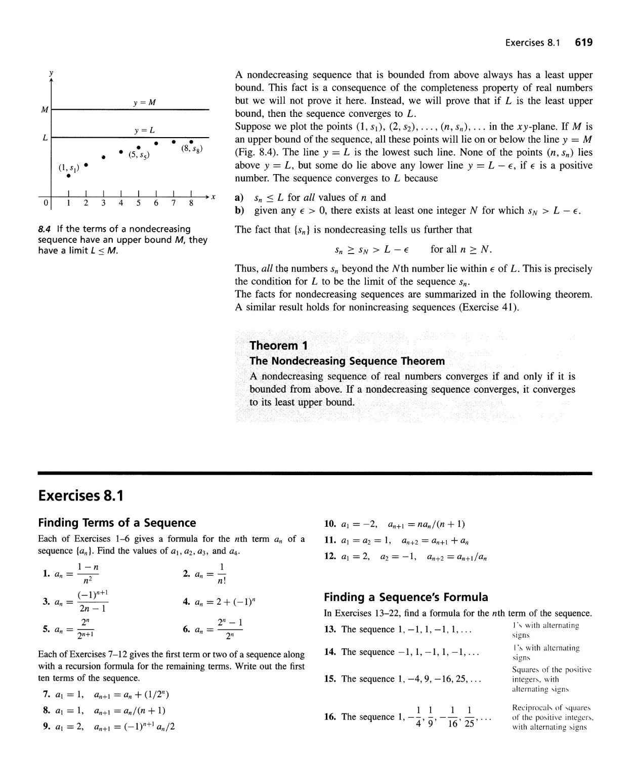
8.4
8.5
8.6
8.7
8.8
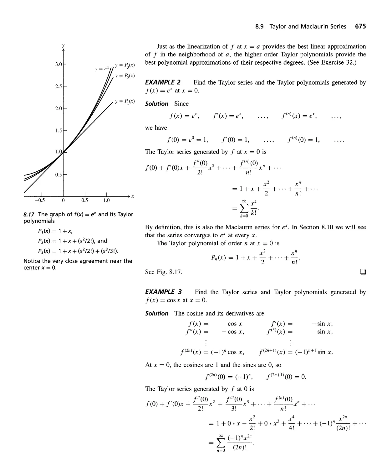
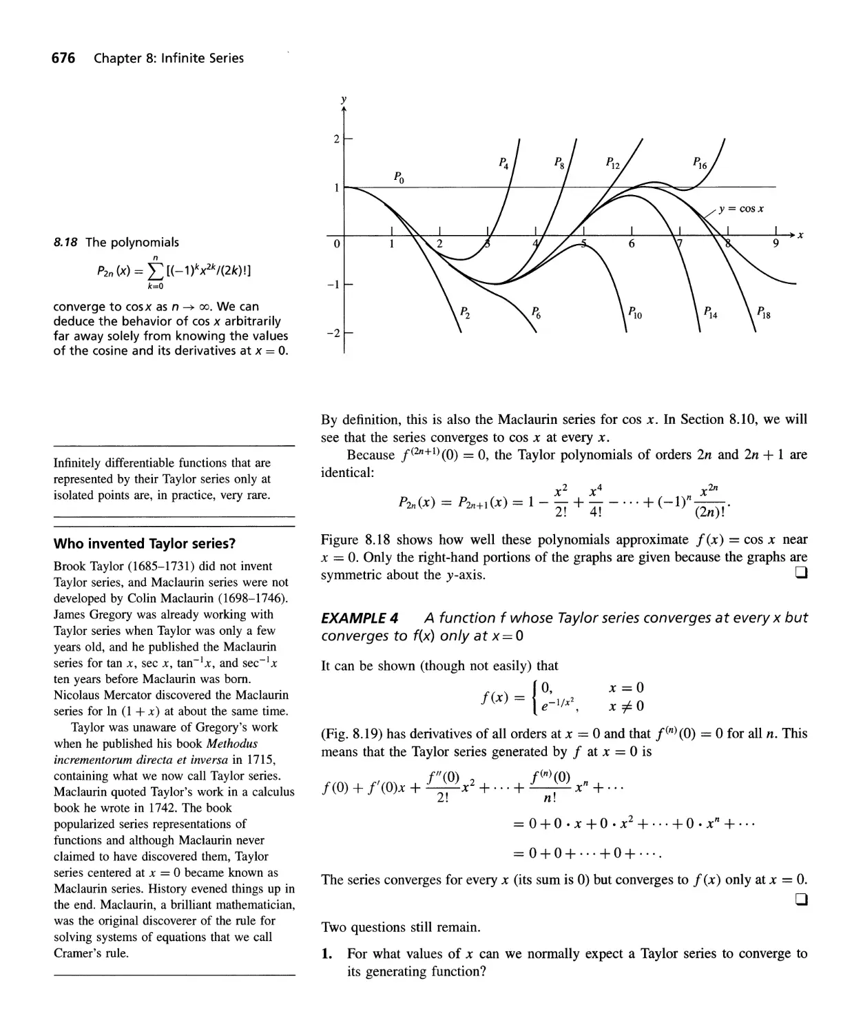
8.9
8.10
8.11
9.1
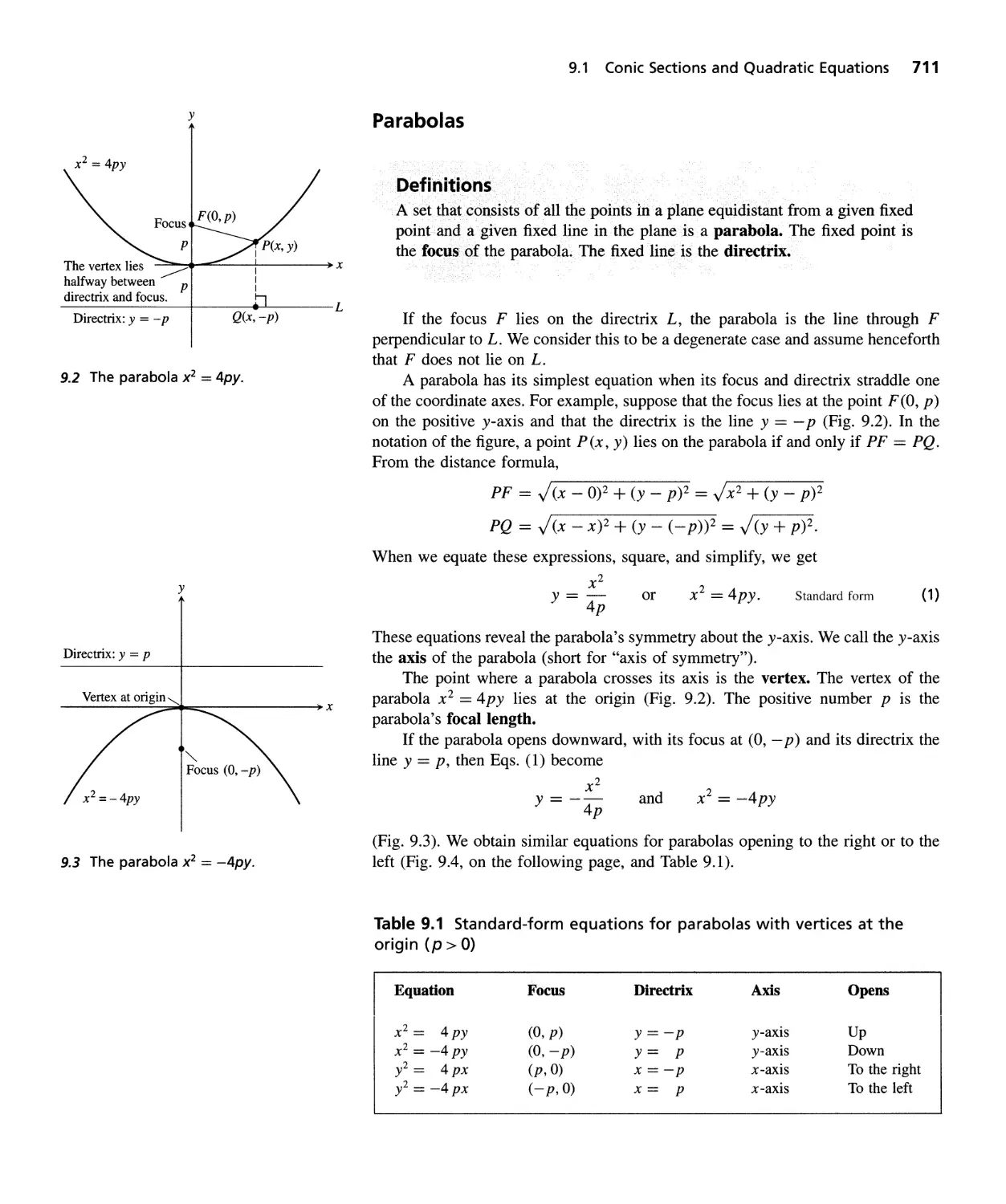
9.2
9.3
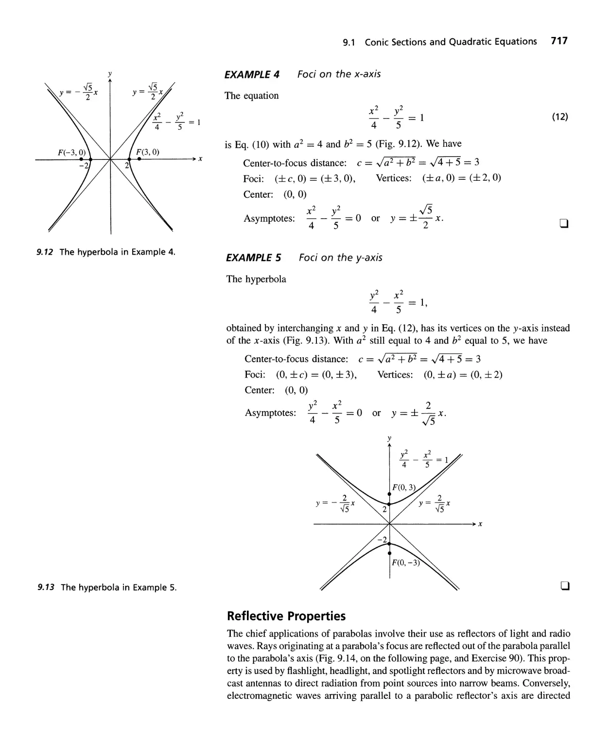
9.4
9.5
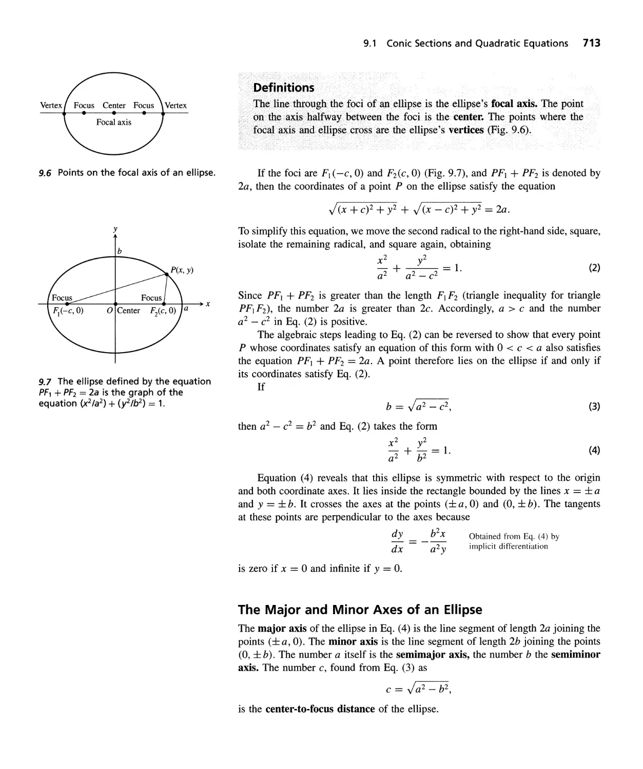
9.6
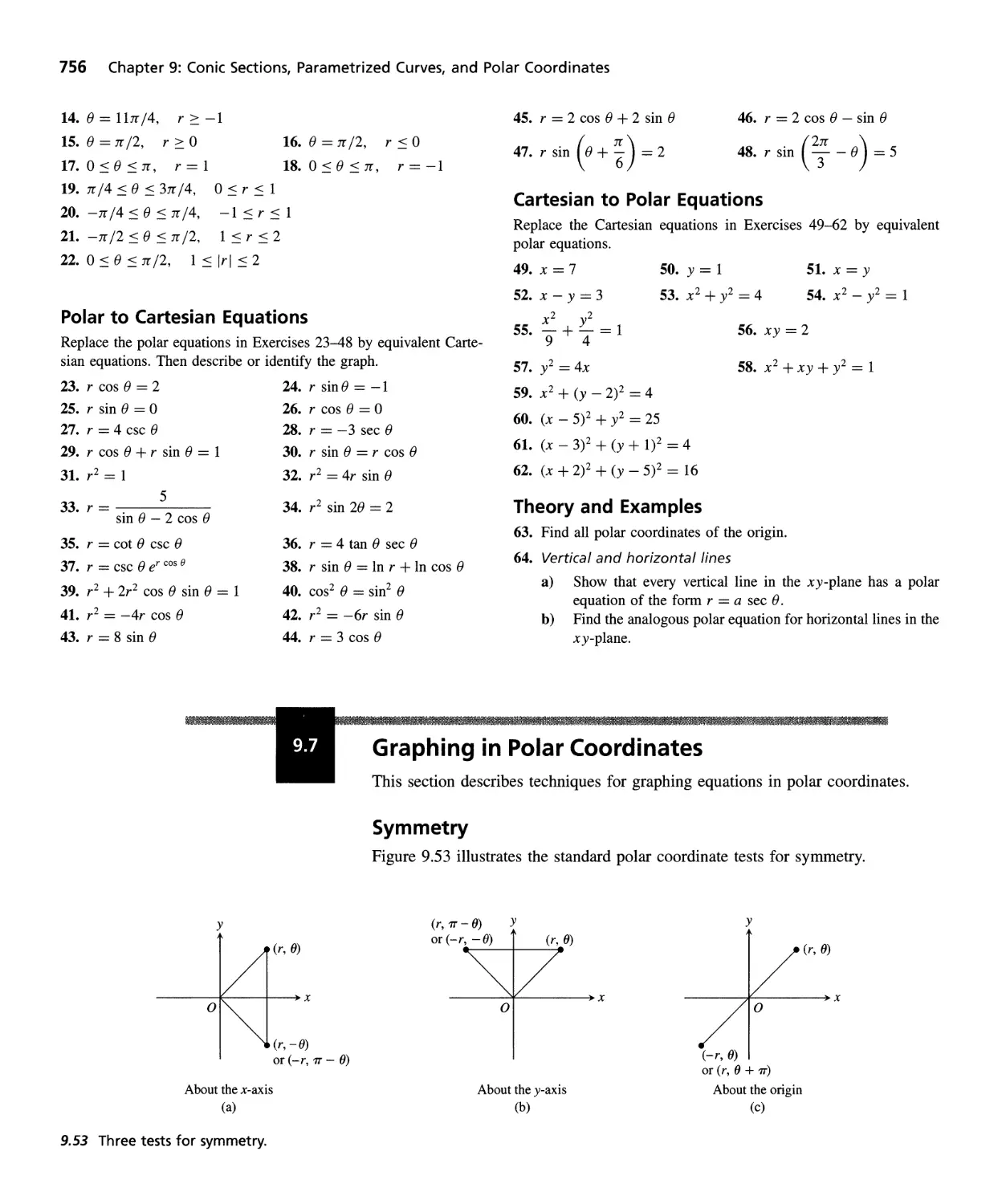
9.7
9.8
9.9
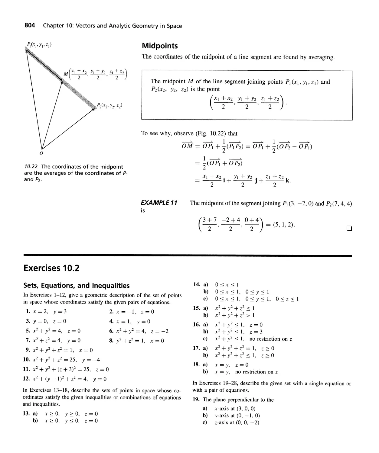
10.1
10.2
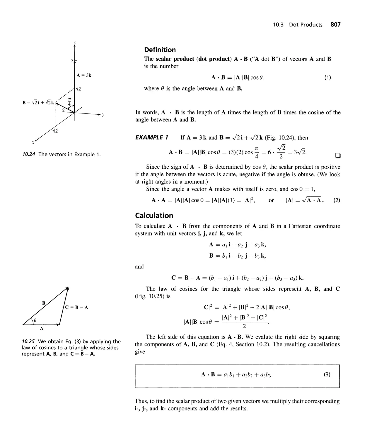
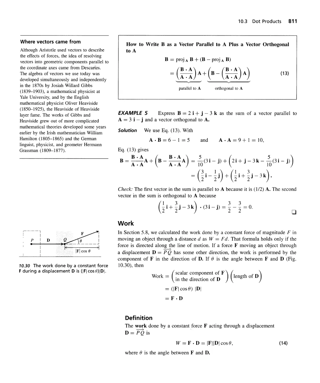
10.3
10.4
10.5
10.6
10.7
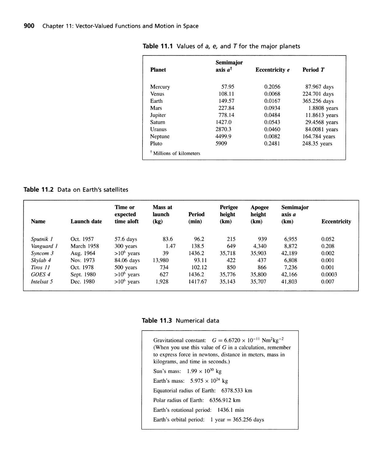
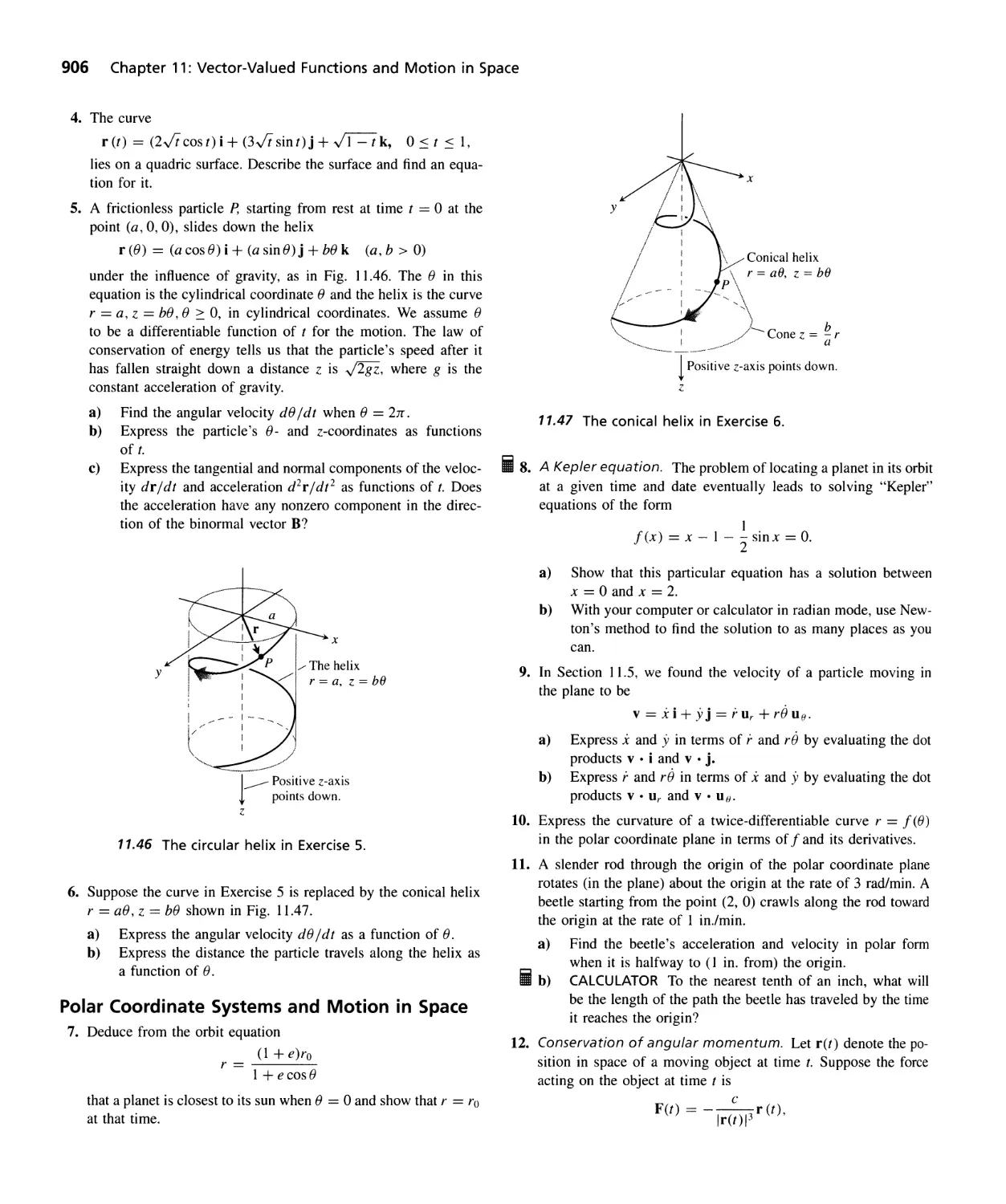
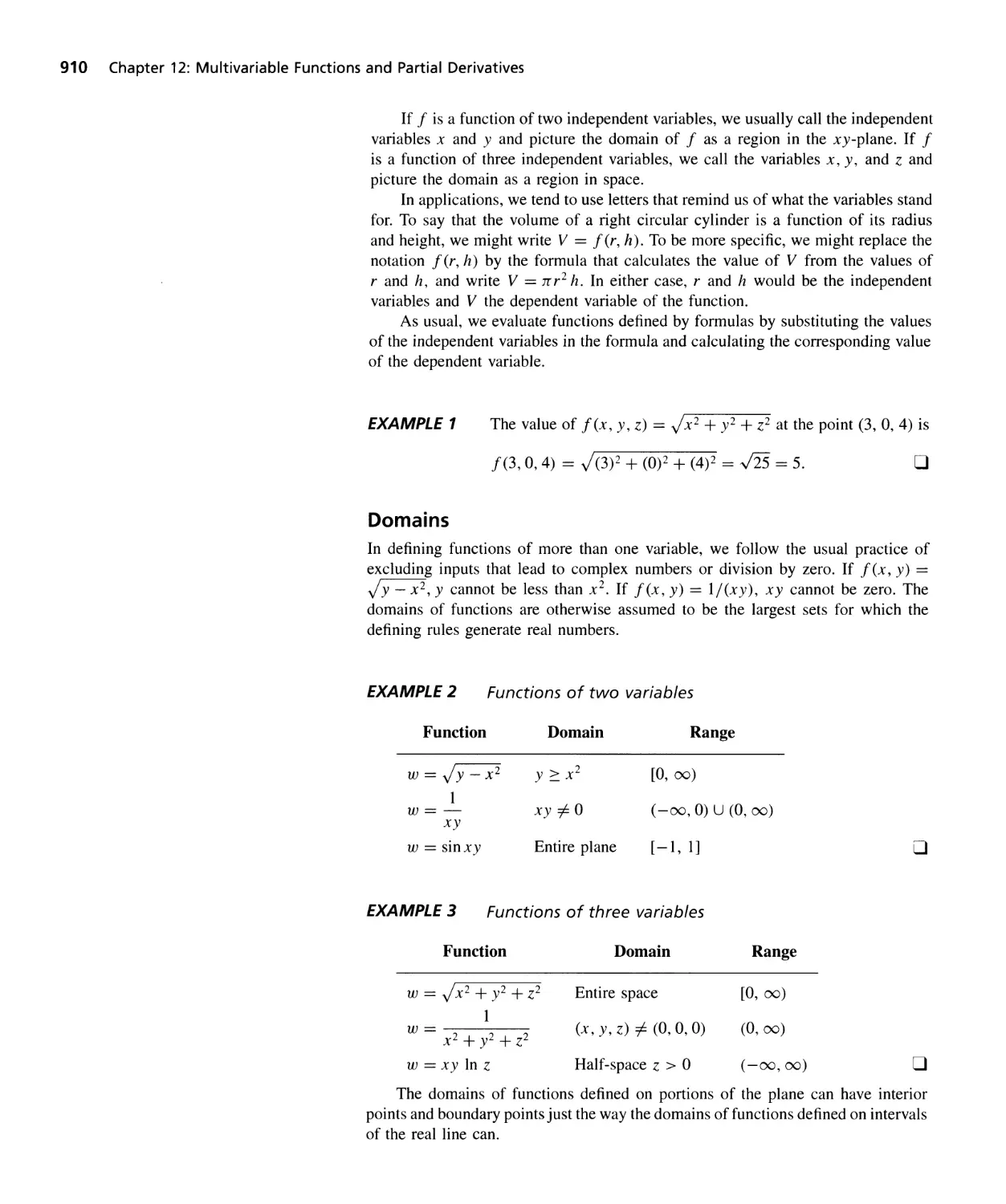
11.1
11.2
11.3
11.4
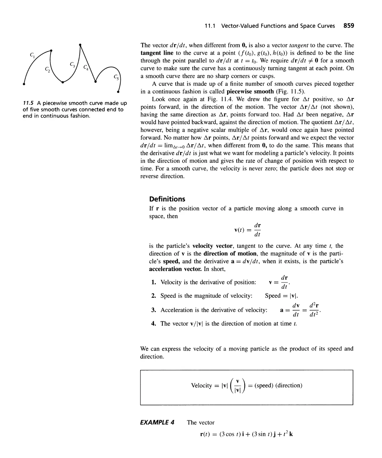
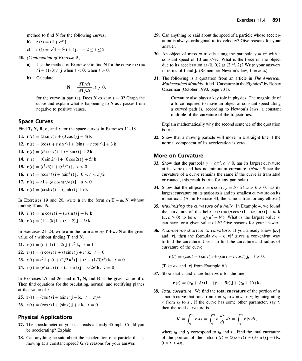
11.5
.' "ili!J!ffj!jfjlil! i!/Iif/JUiiPi!t!$fI!i!JI!k Mi1!i!/i B!i£
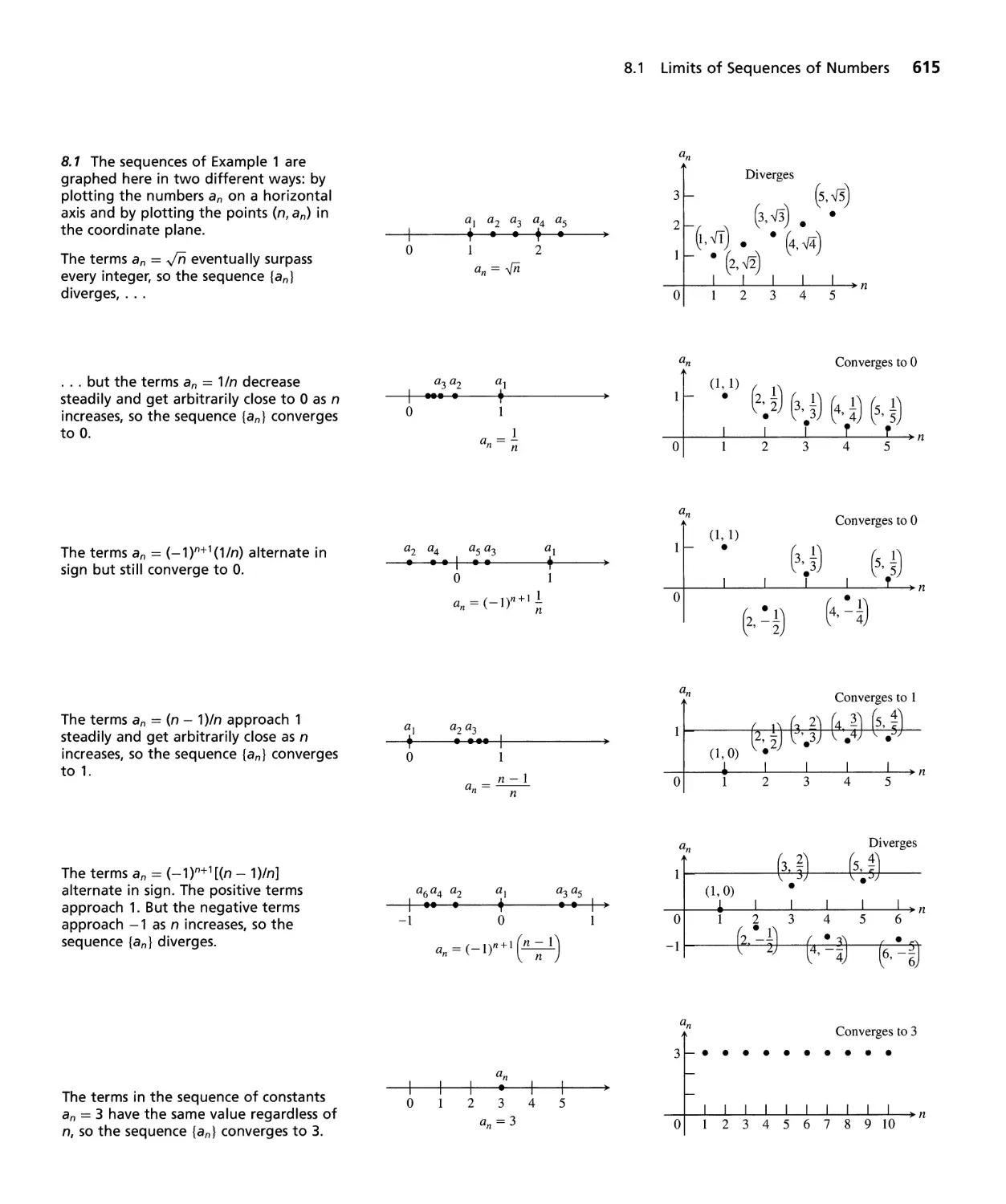
Limits of Sequences of Numbers 613
Theorems for Calculating Limits of Sequences 622
Infinite Series 630
The Integral Test for Series of Nonnegative Terms 640
Comparison Tests for Series of Nonnegative Terms 644
The Ratio and Root Tests for Series of Nonnegative Terms 649
Alternating Series, Absolute and Conditional Convergence 655
Power Series 663
Taylor and Maclaurin Series 672
Convergence of Taylor Series; Error Estimates 678
Applications of Power Series 688
QUESTIONS TO GUIDE YOUR REVIEW 699 PRACTICE EXERCISES 700
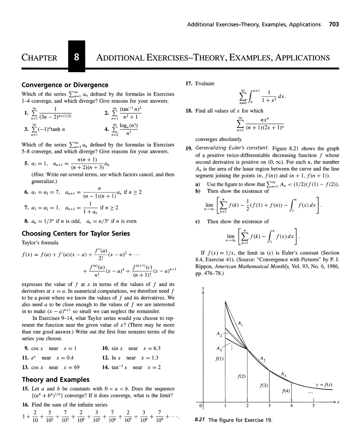
ADDITIONAL EXERCISES-THEORY, EXAMPLES, ApPLICATIONS 703
1NIf1ifil'
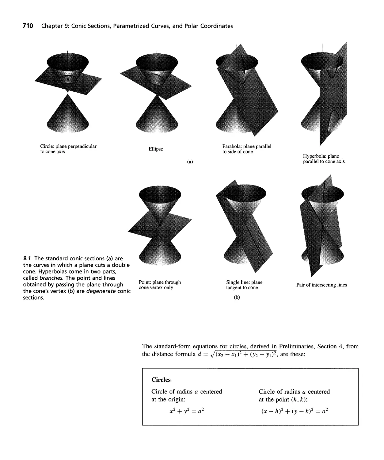
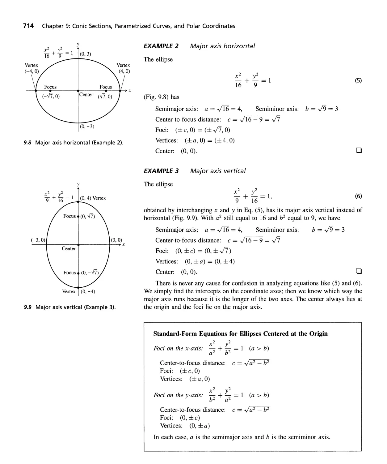
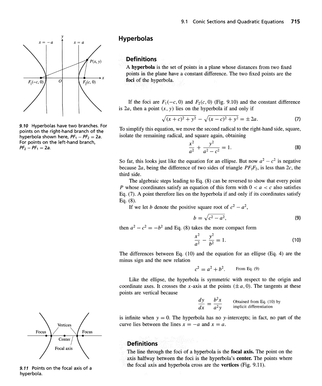
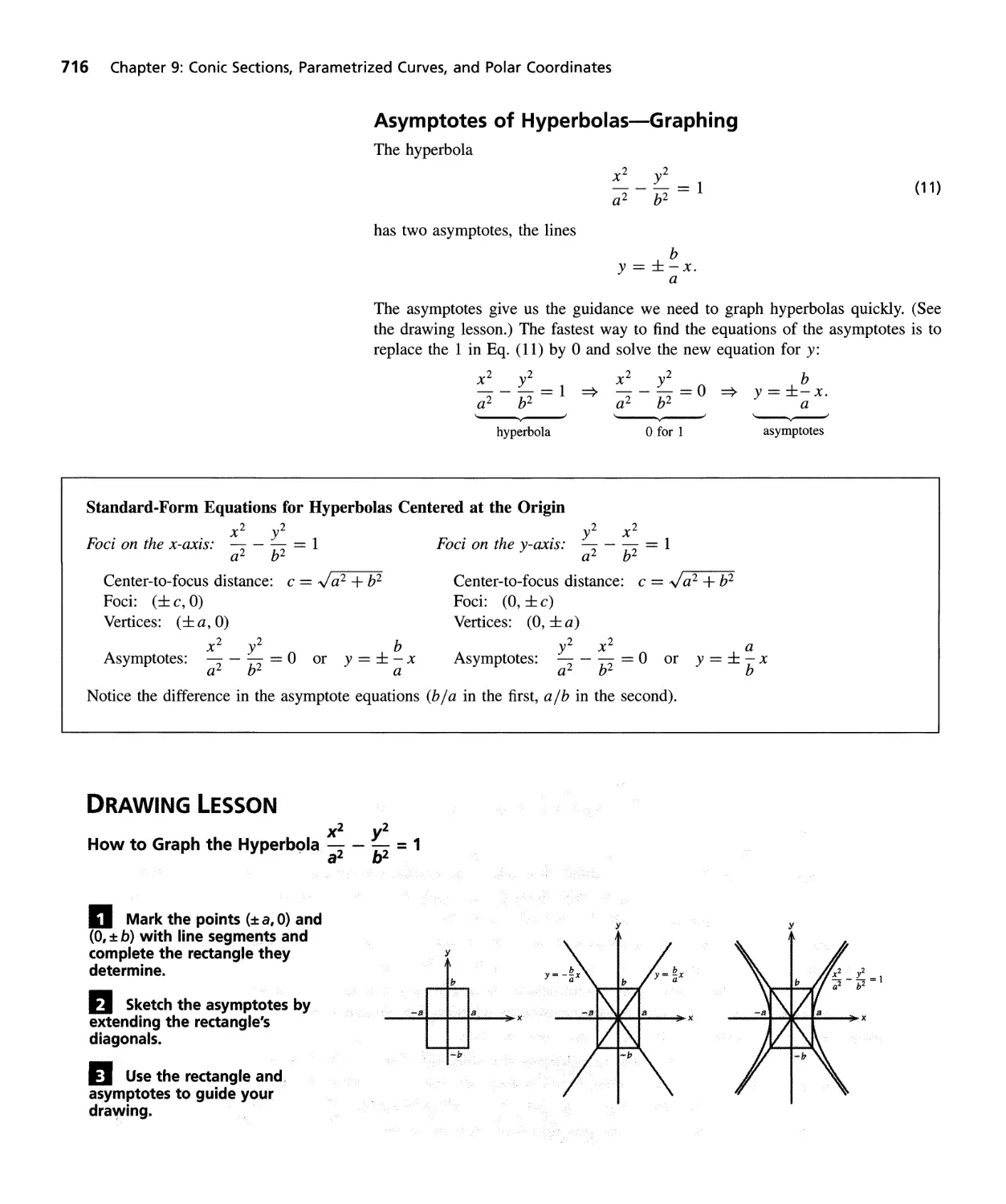
Conic Sections and Quadratic Equations 709
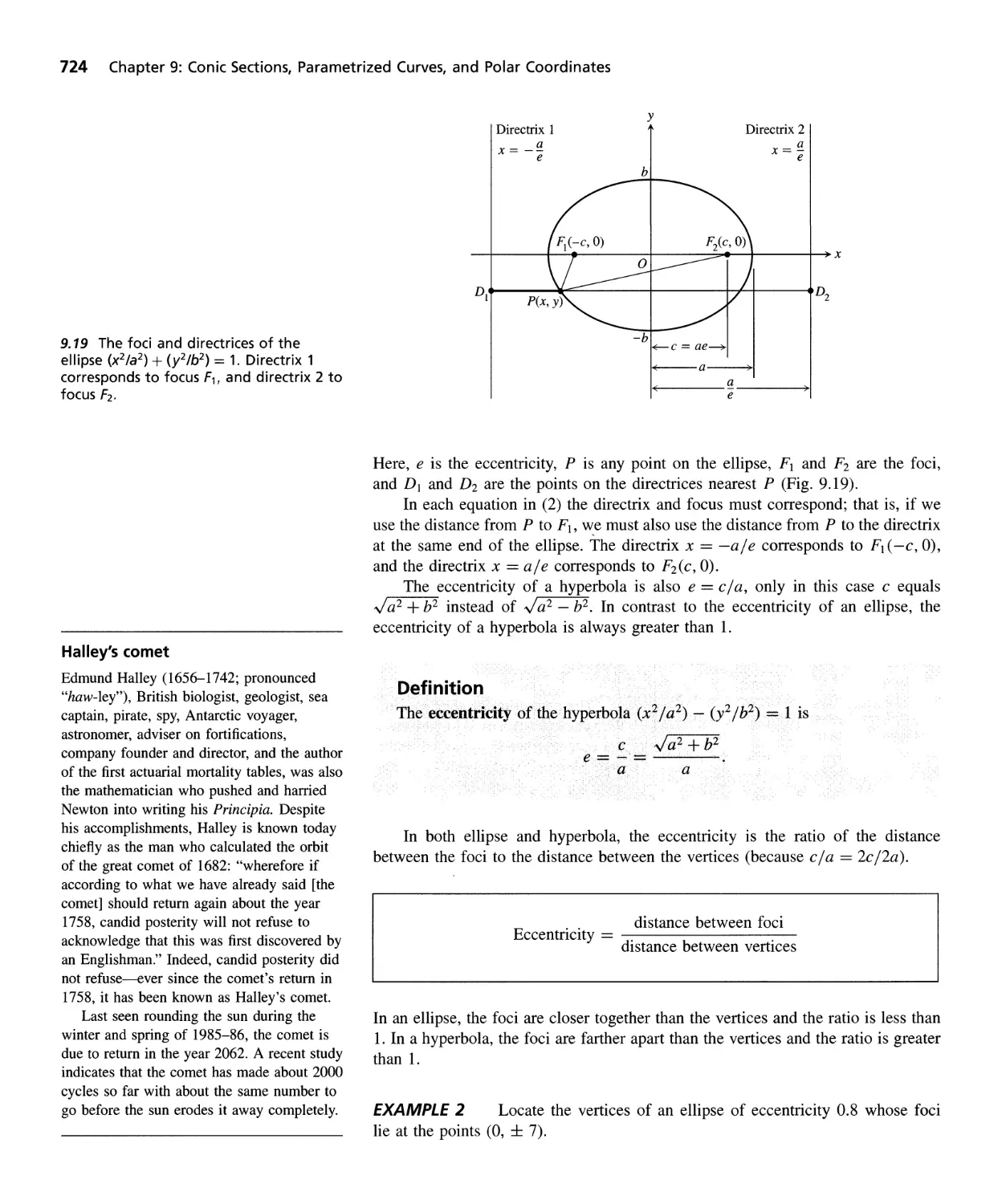
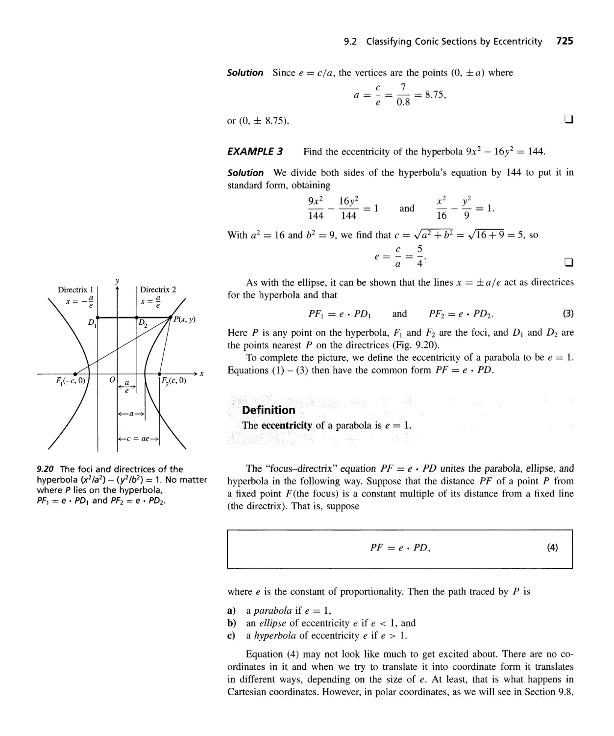
Classifying Conic Sections by Eccentricity 723
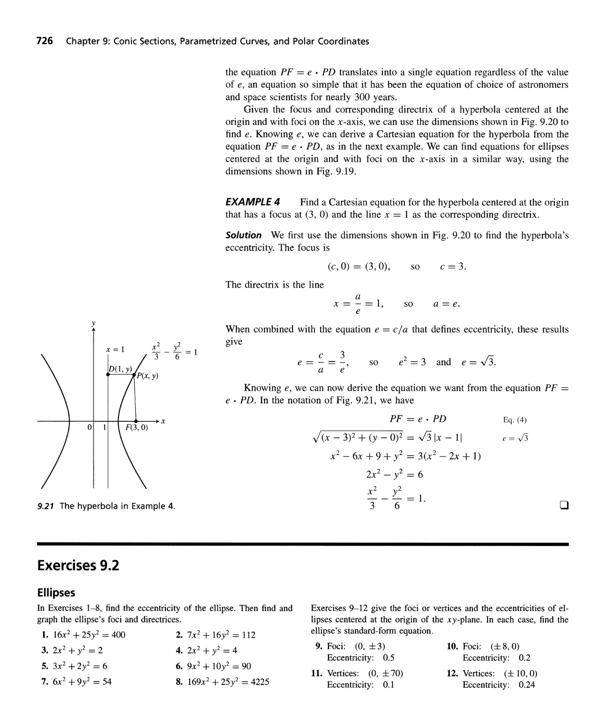
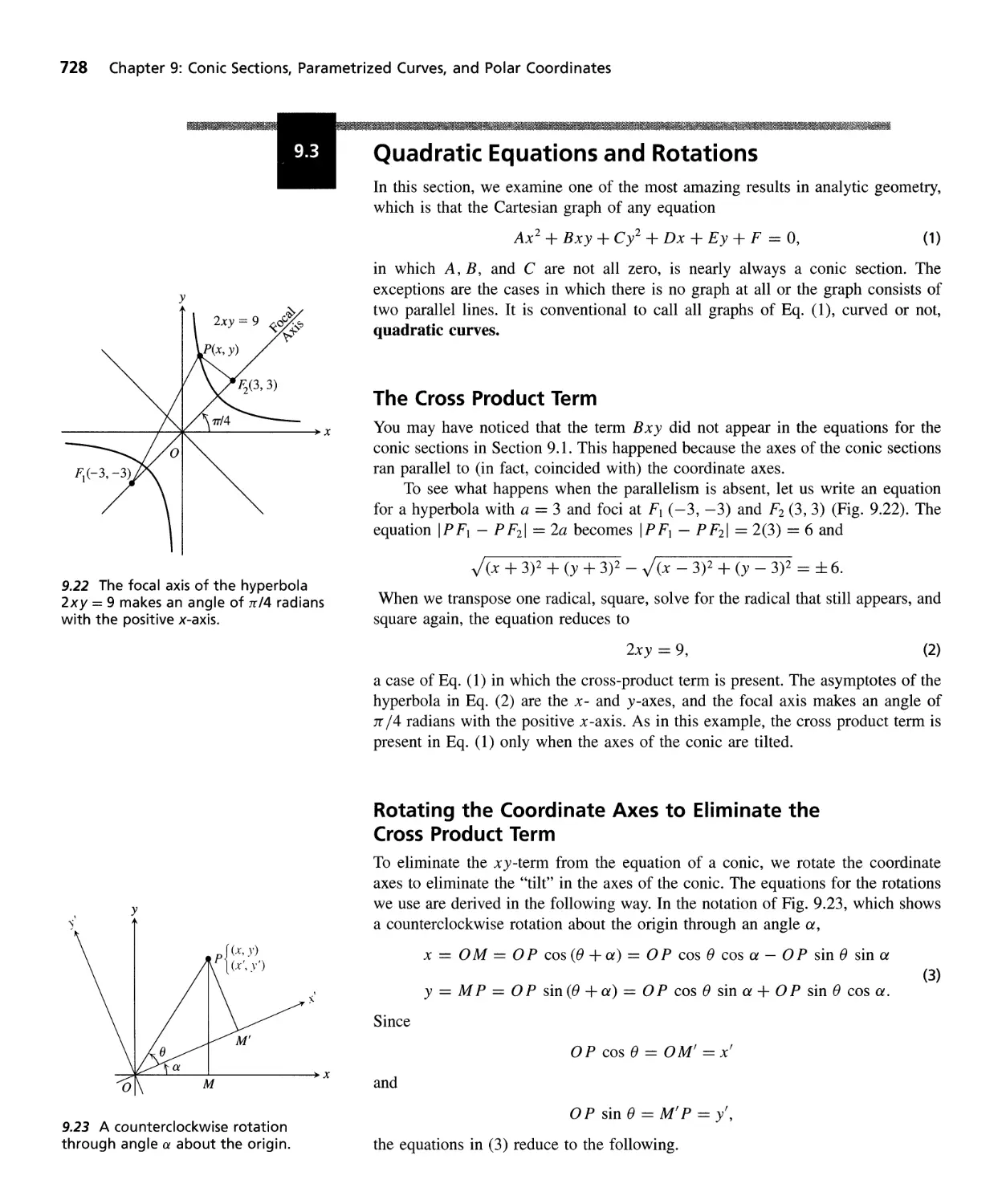
Quadratic Equations and Rotations 728
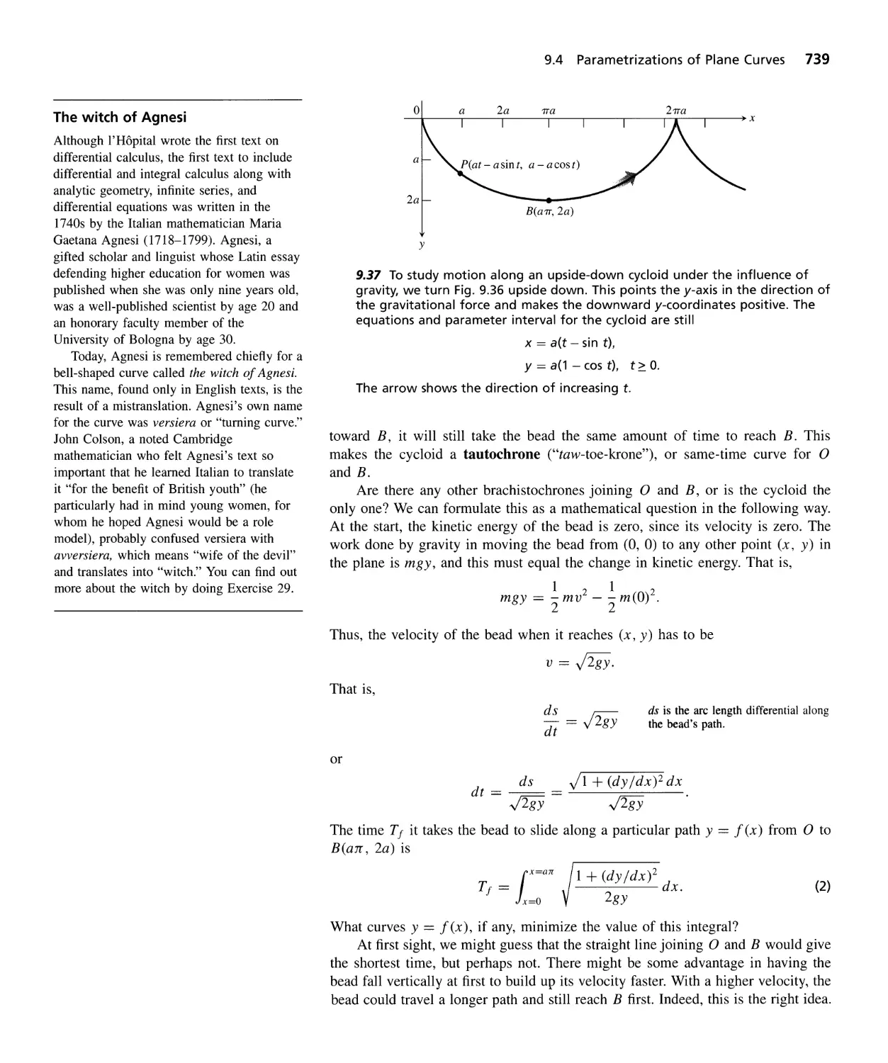
Parametrizations of Plane Curves 734
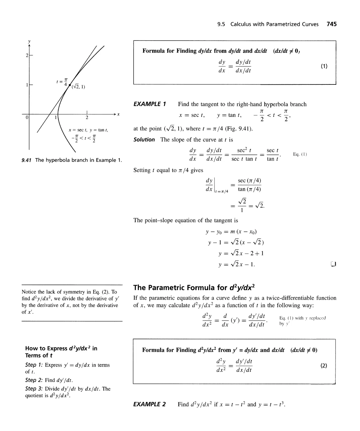
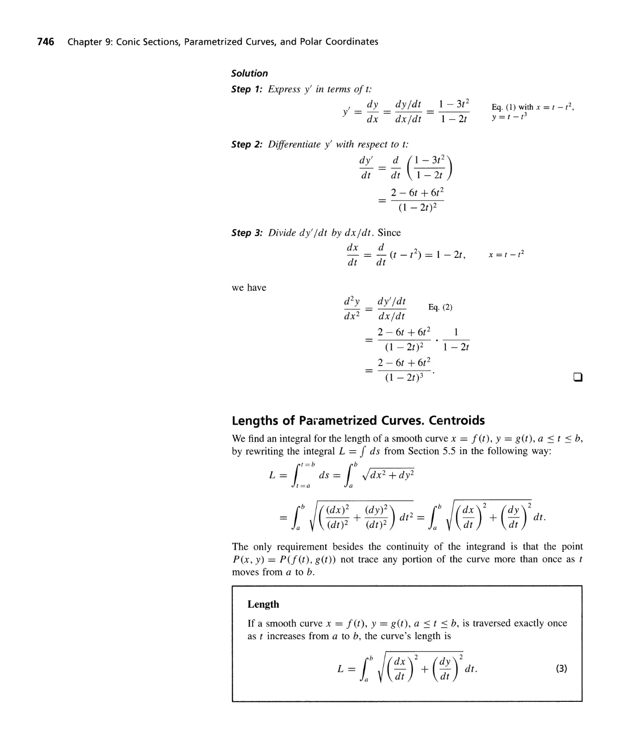
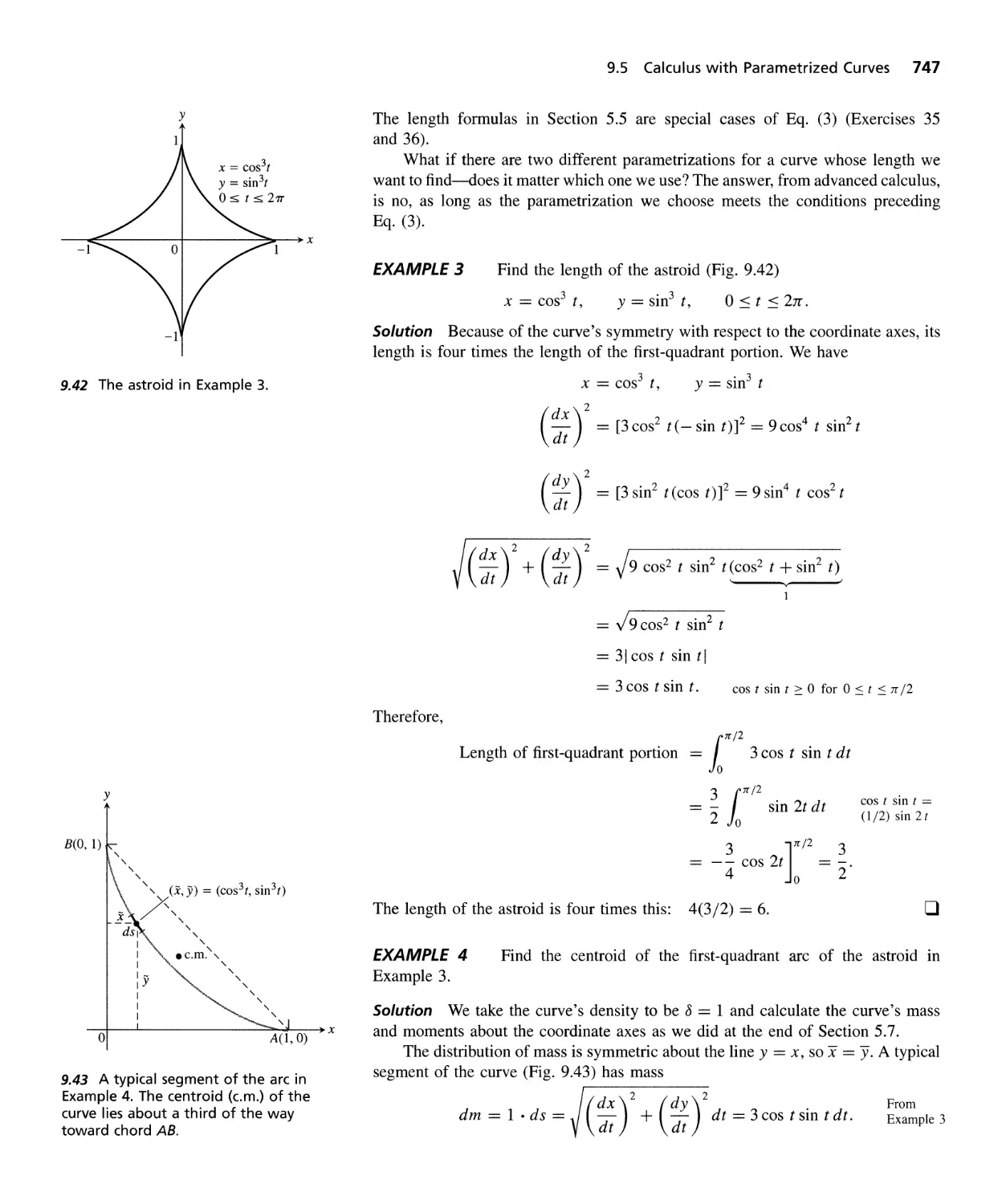
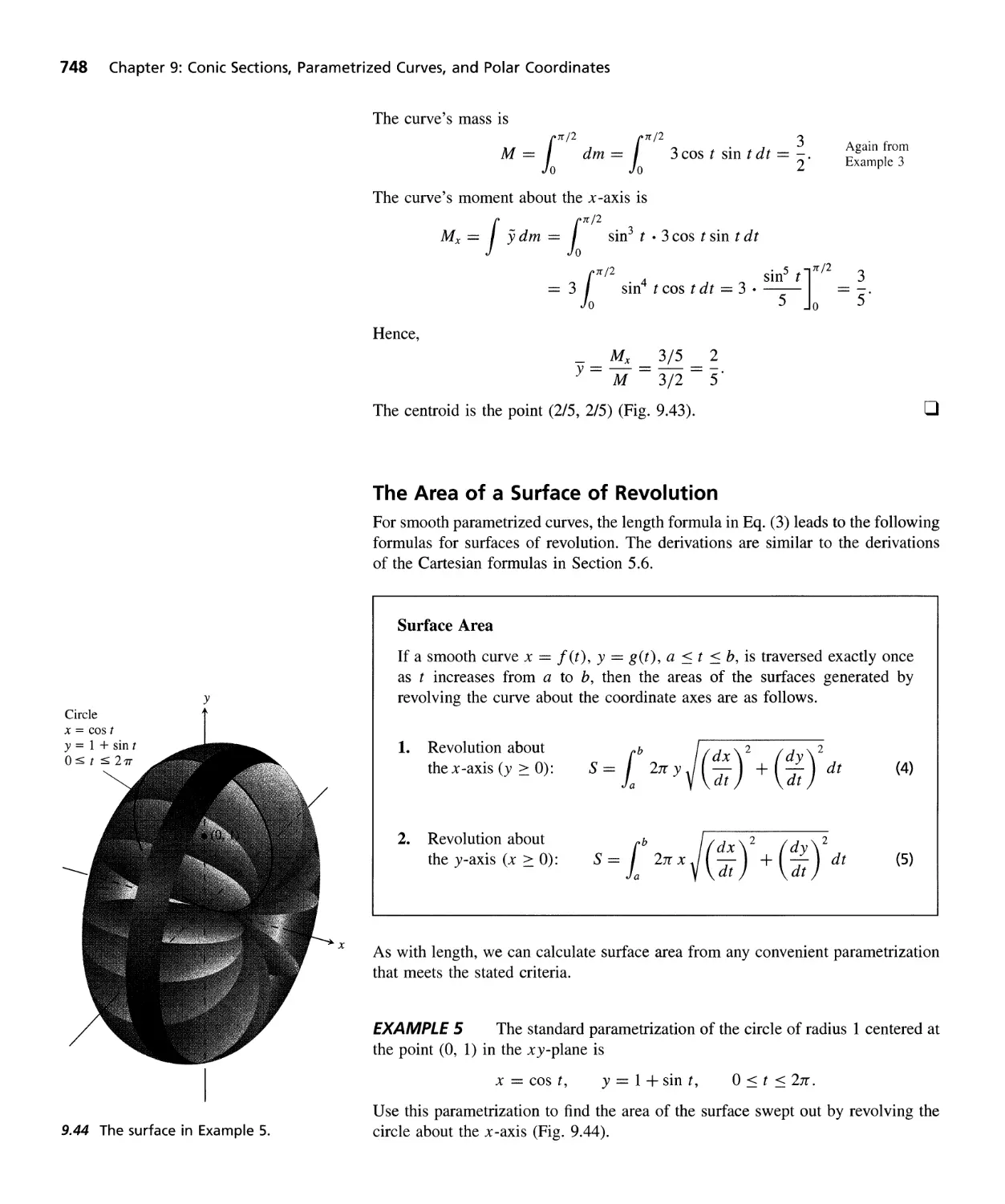
Calculus with Parametrized Curves 744
Polar Coordinates 751
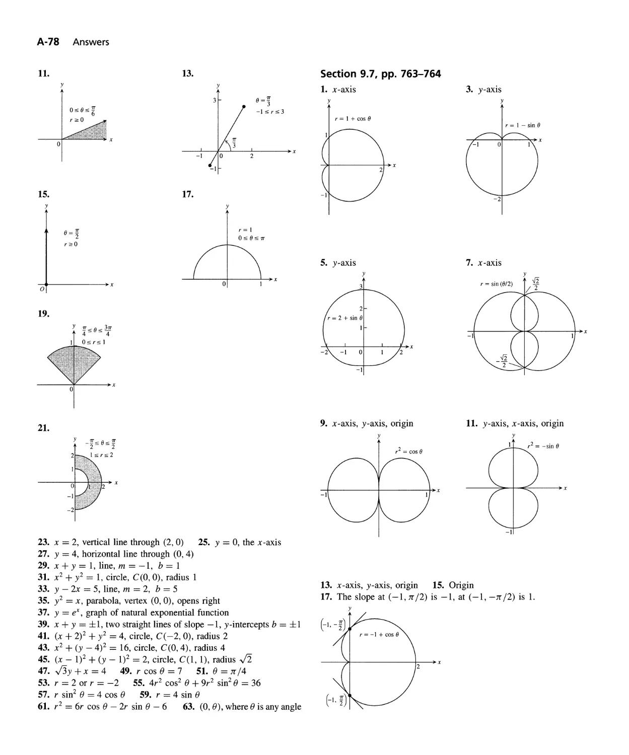
Graphing in Polar Coordinates 756
Polar Equations for Conic Sections 764
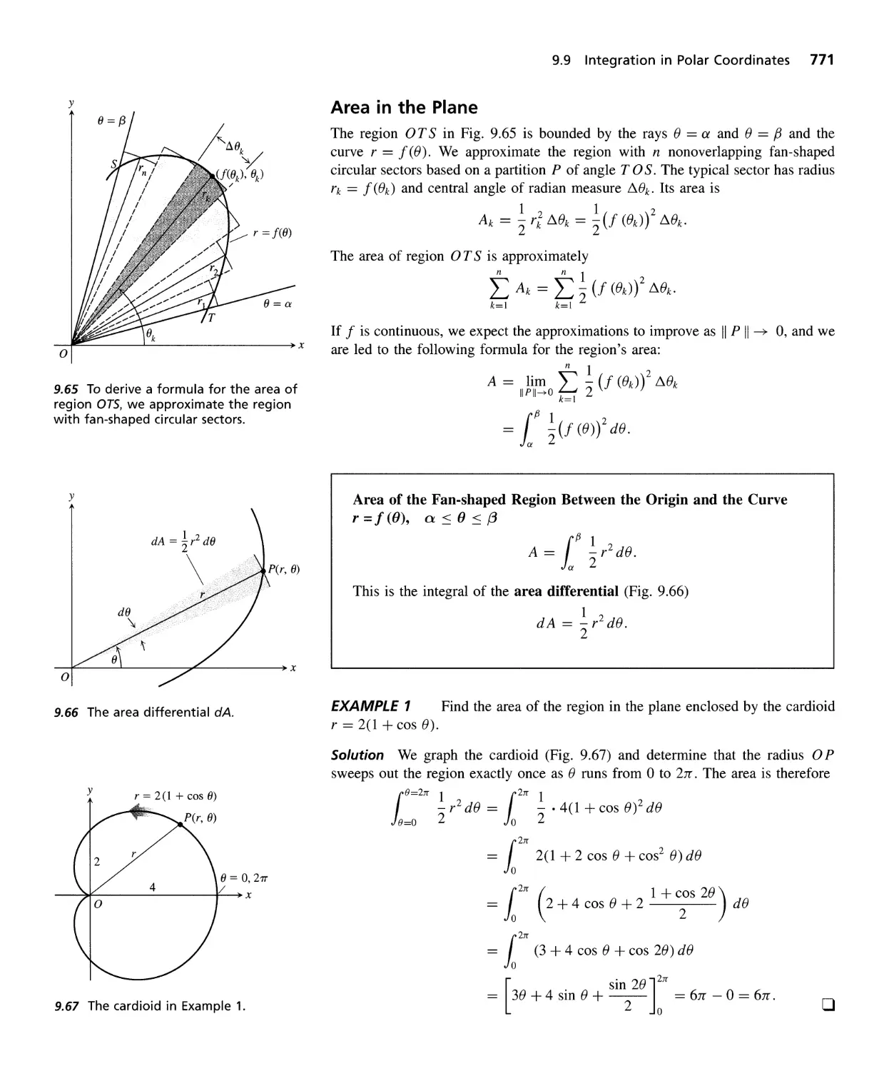
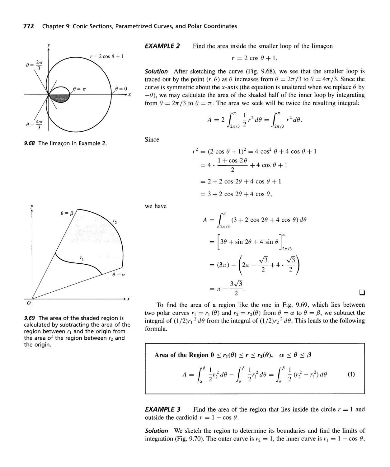
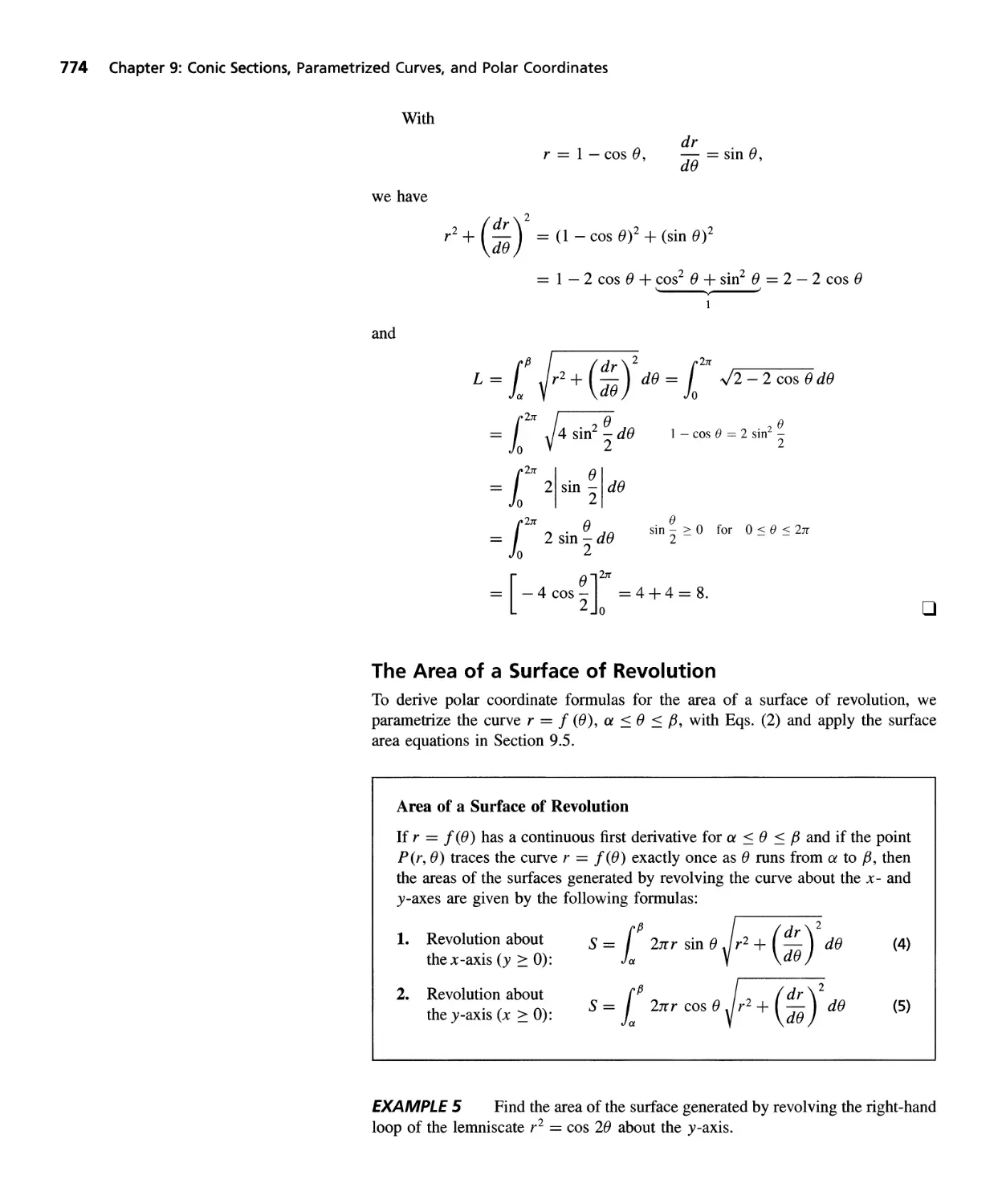
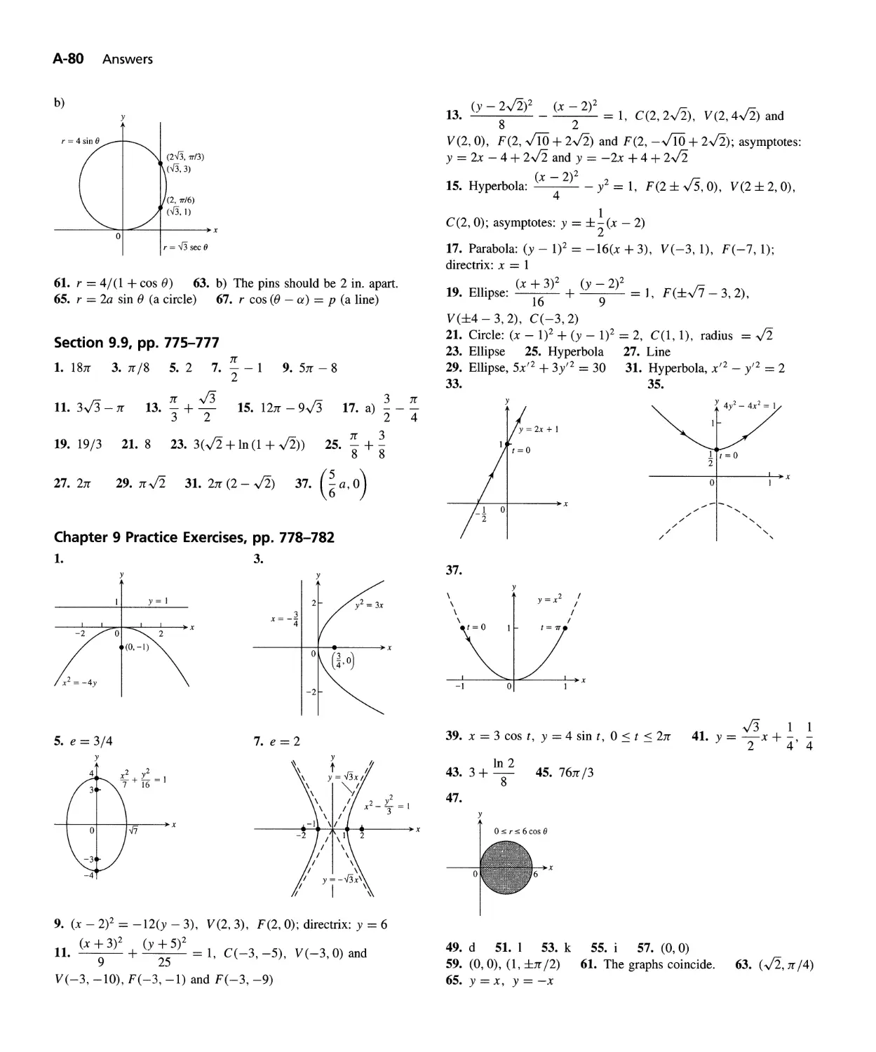
Integration in Polar Coordinates 770
QUESTIONS TO GUIDE YOUR REVIEW 777 PRACTICE EXERCISES 778
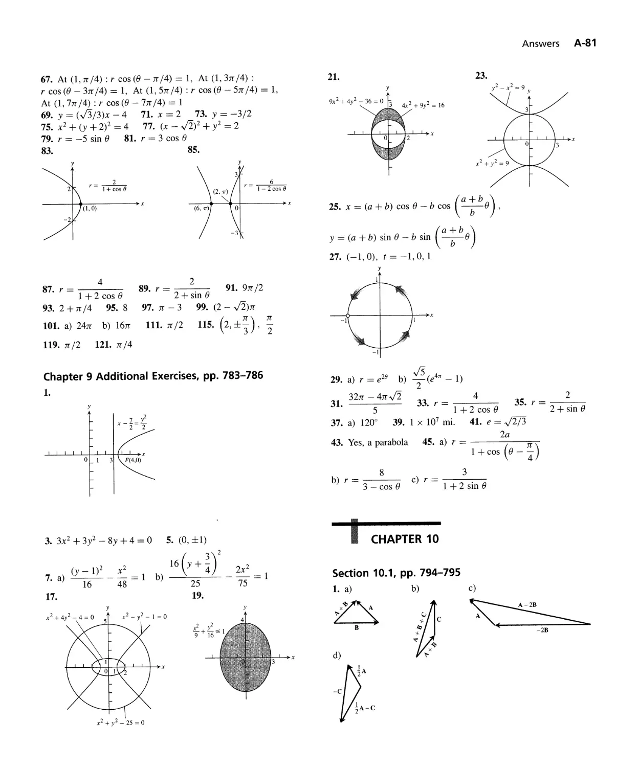
ADDITIONAL EXERCISES-THEORY, EXAMPLES, ApPLICATIONS 783
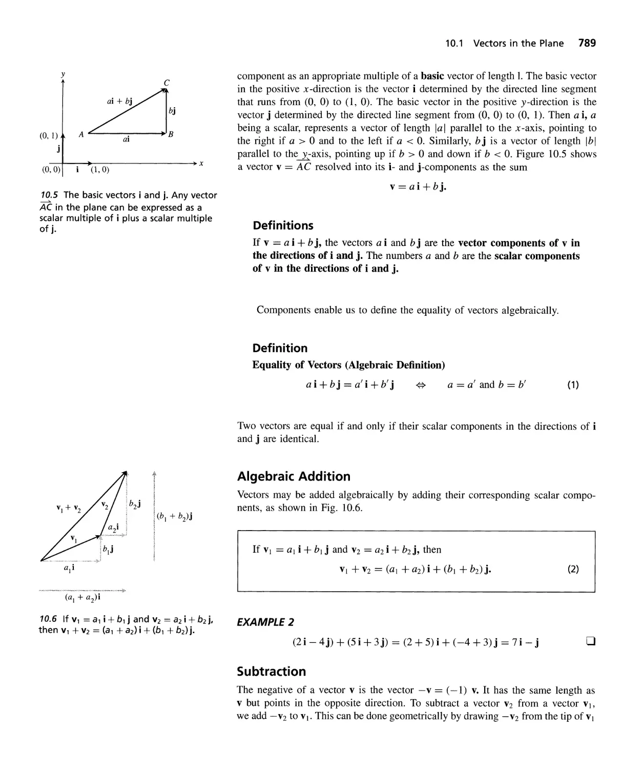
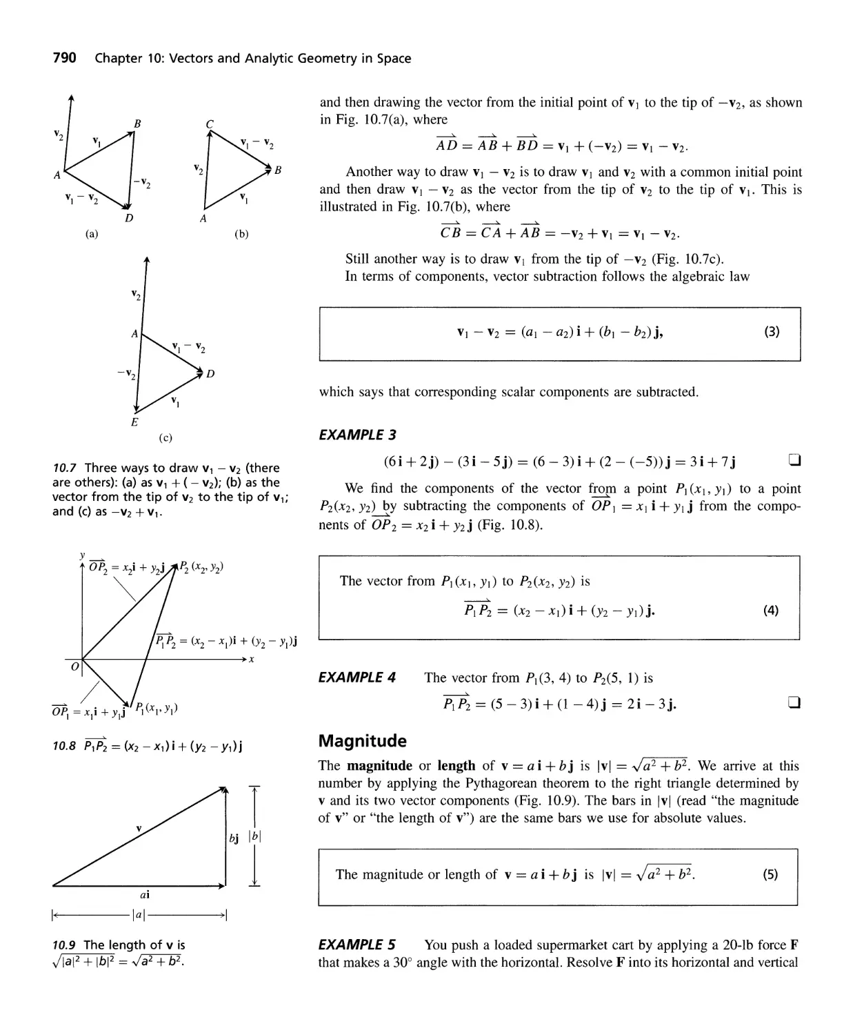
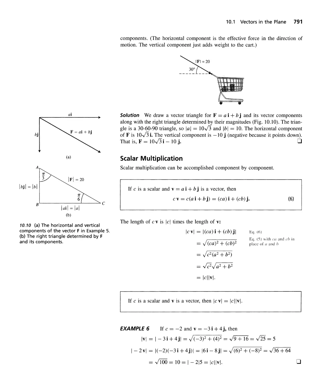
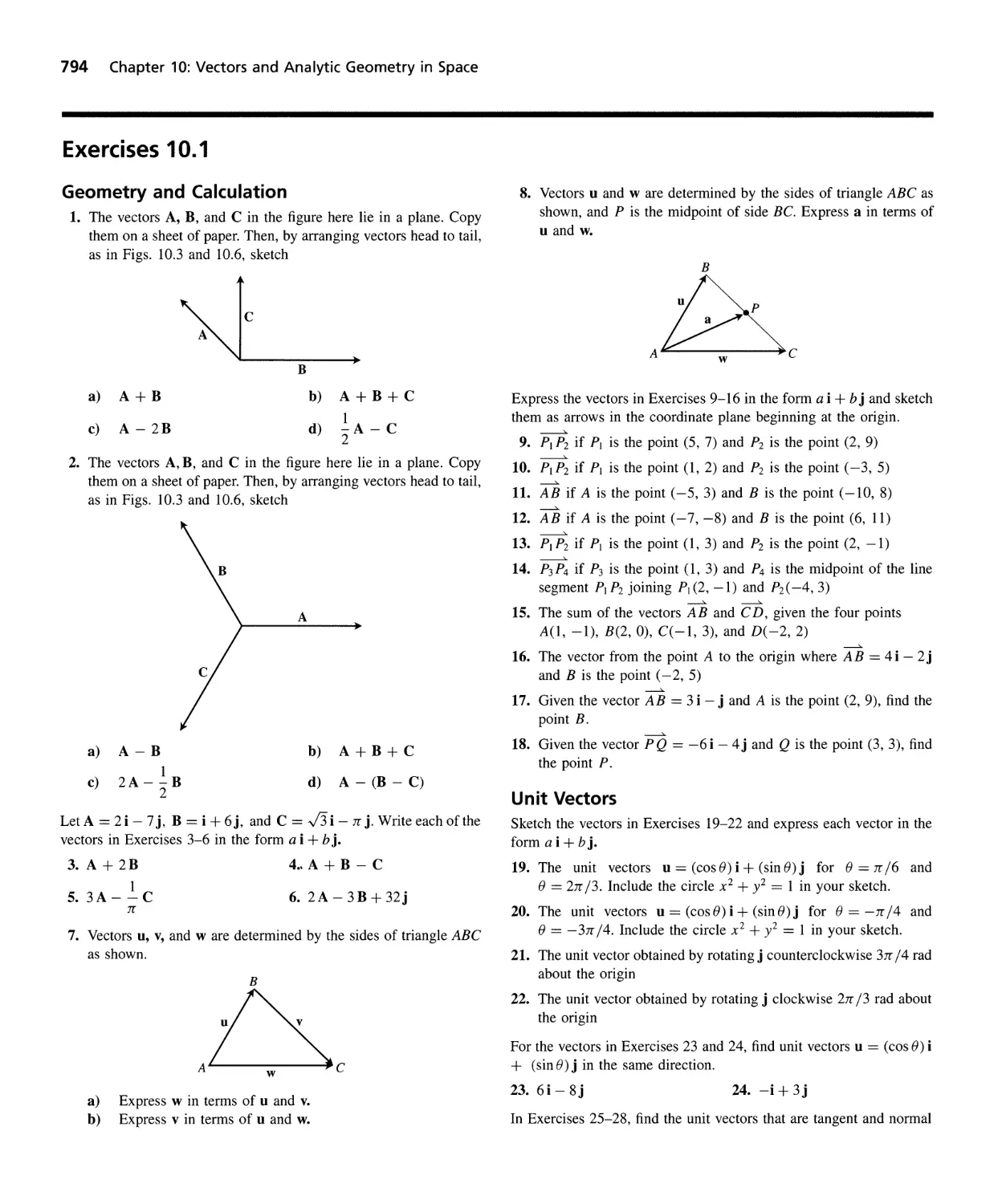
Vectors in the Plane 787
Cartesian (Rectangular) Coordinates and Vectors in Space 795
Dot Products 806
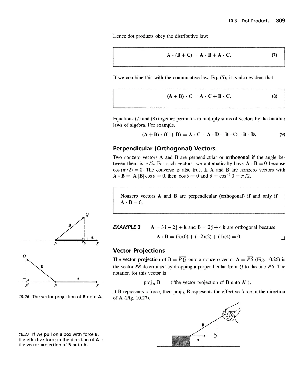
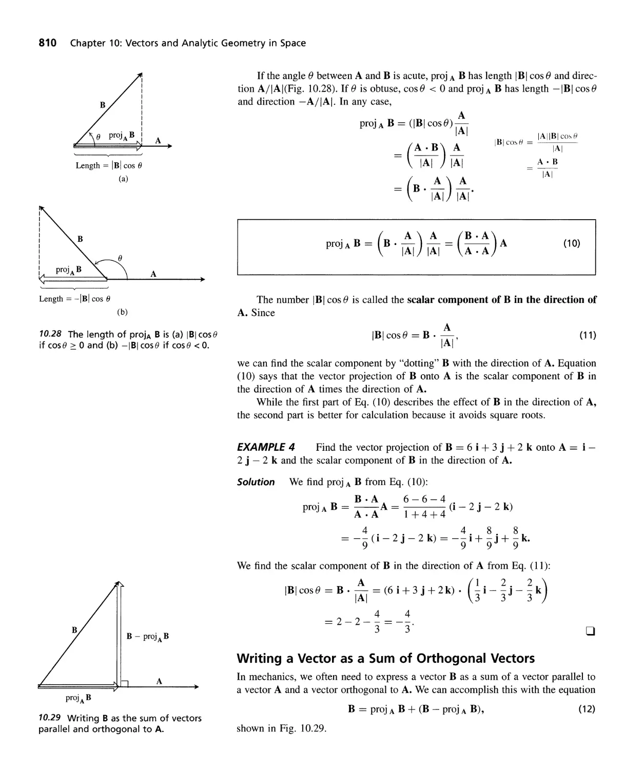
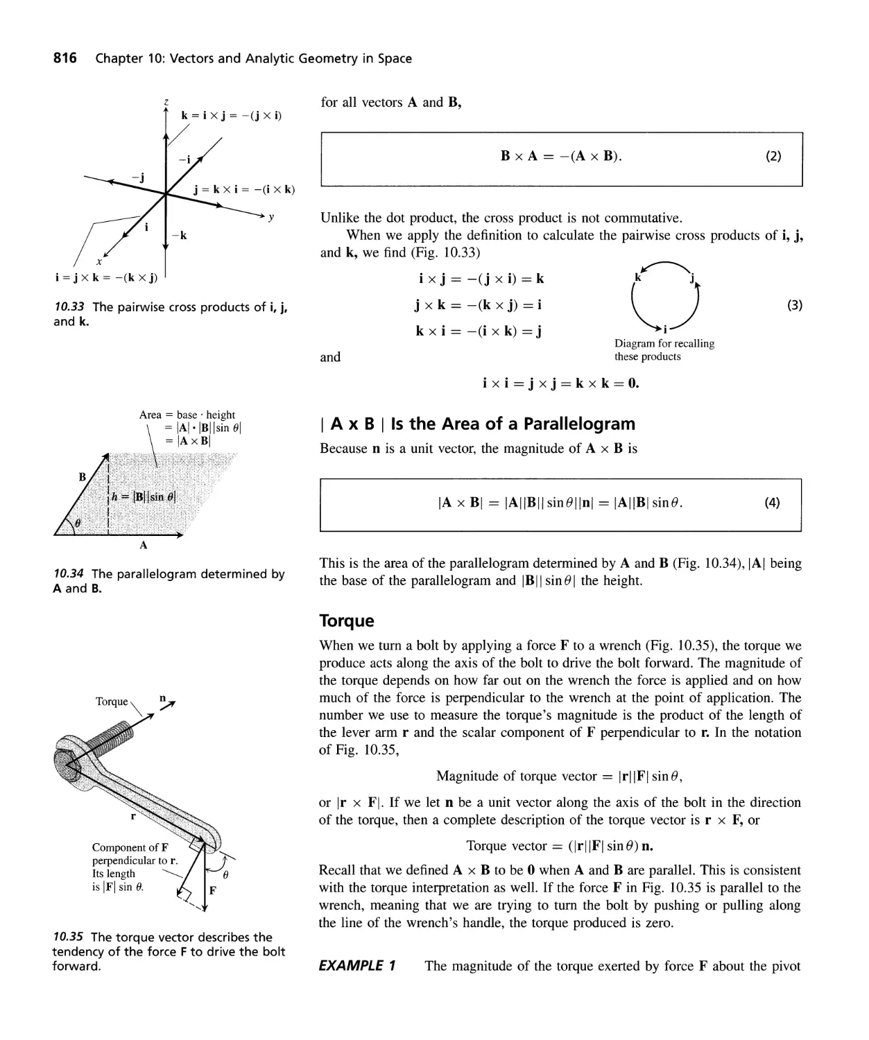
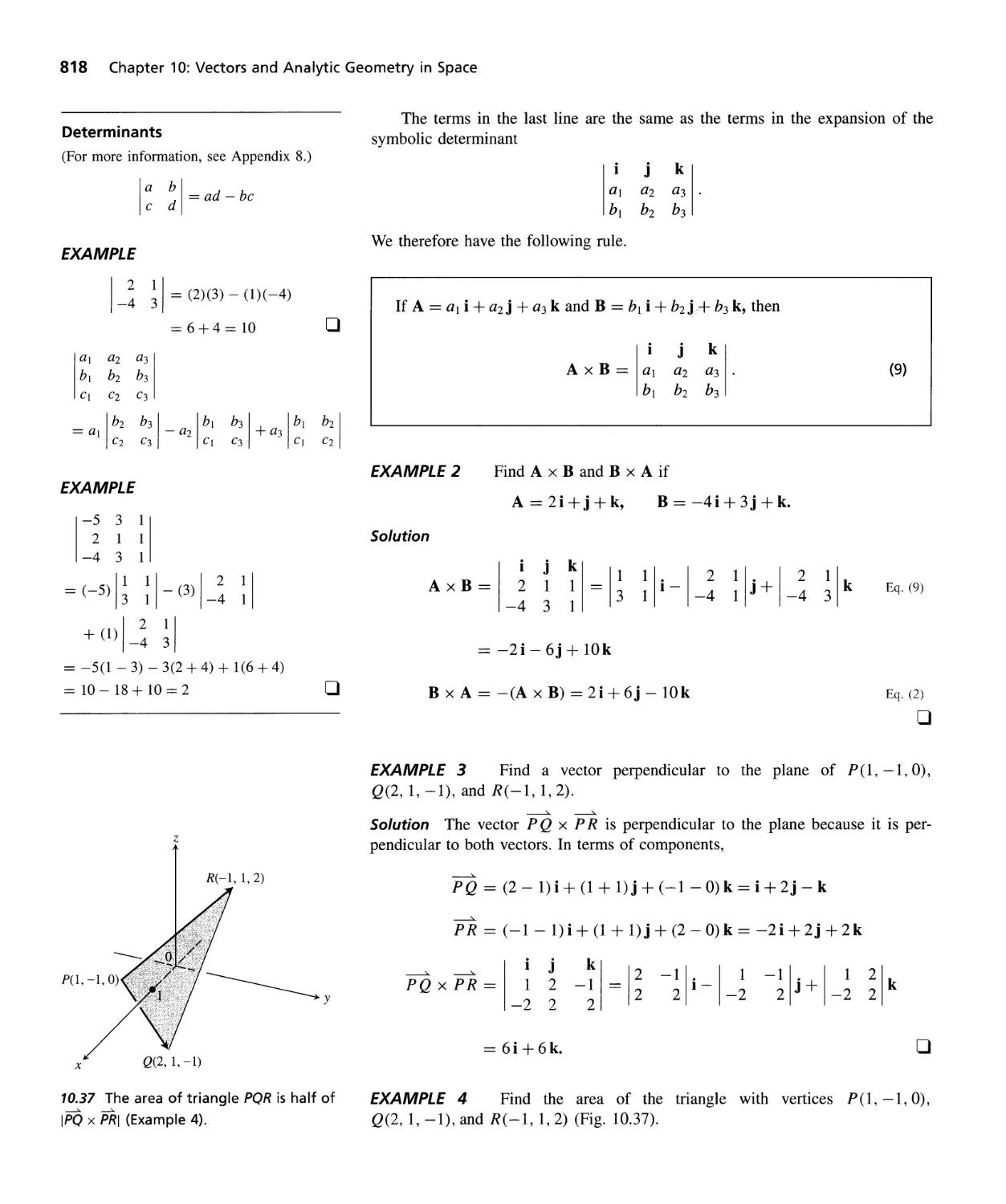
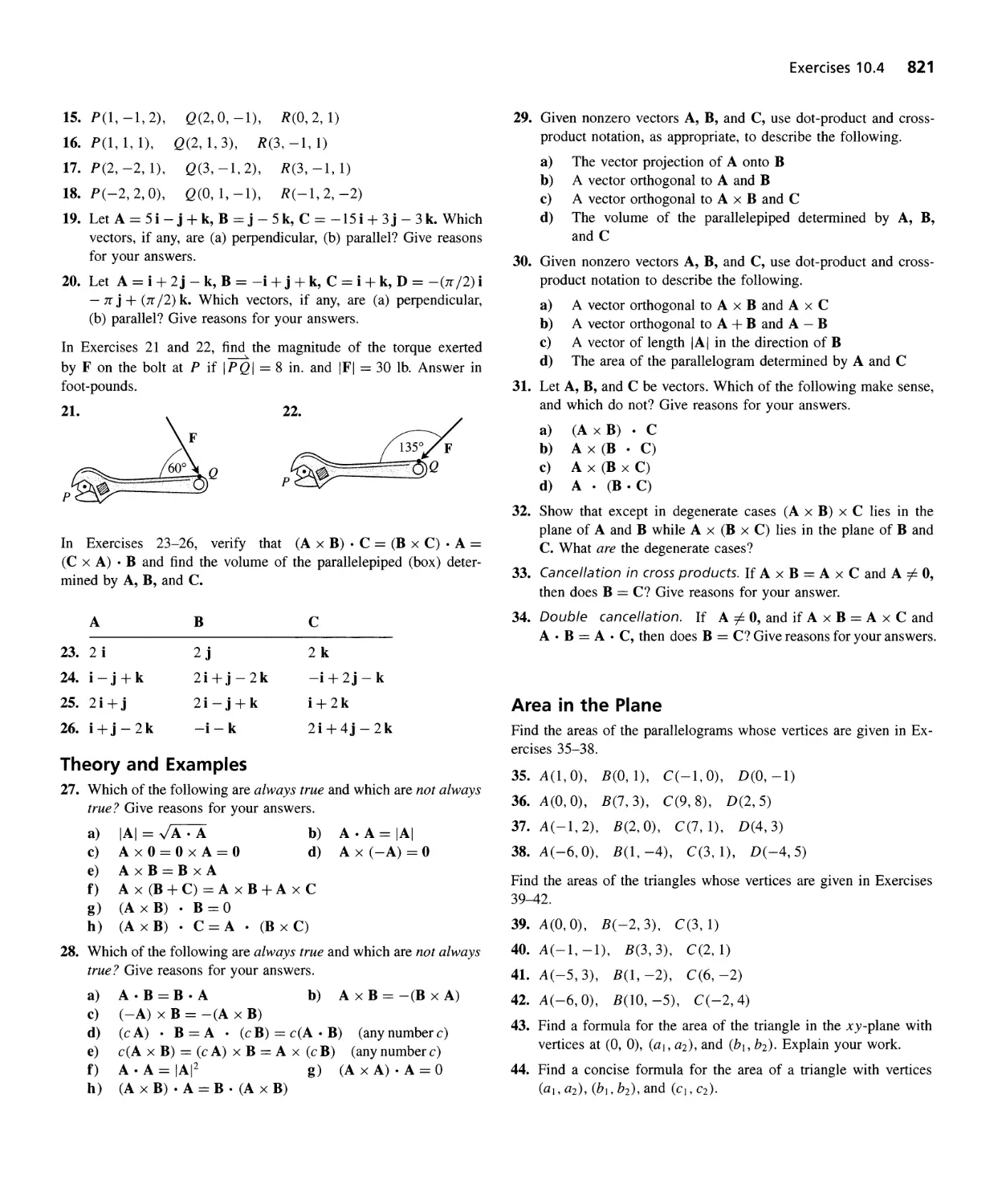
Cross Products 815
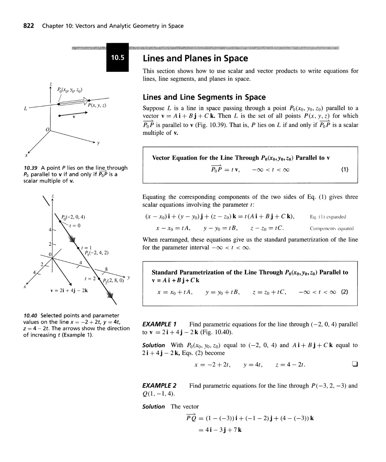
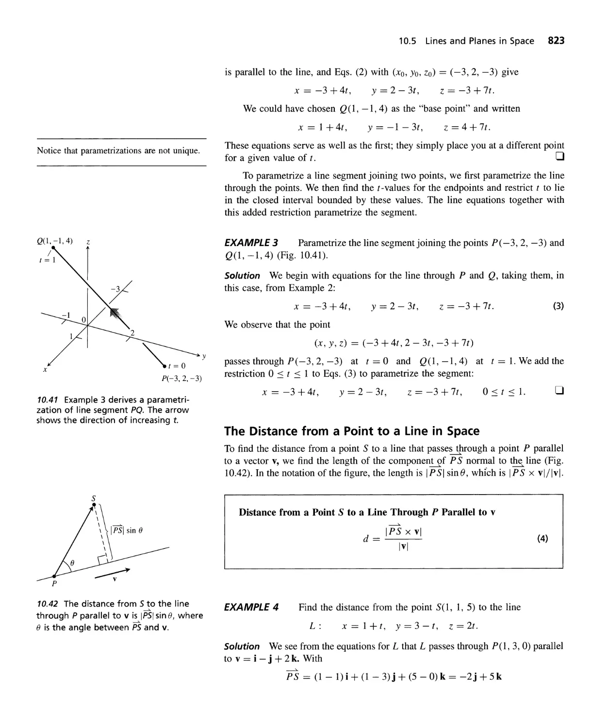
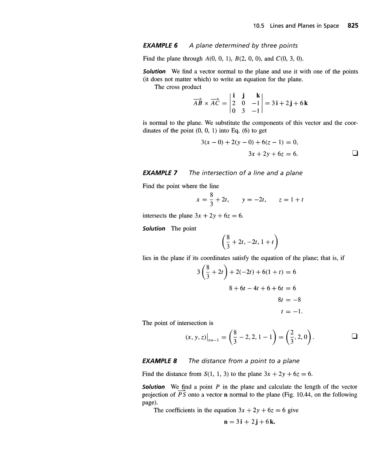
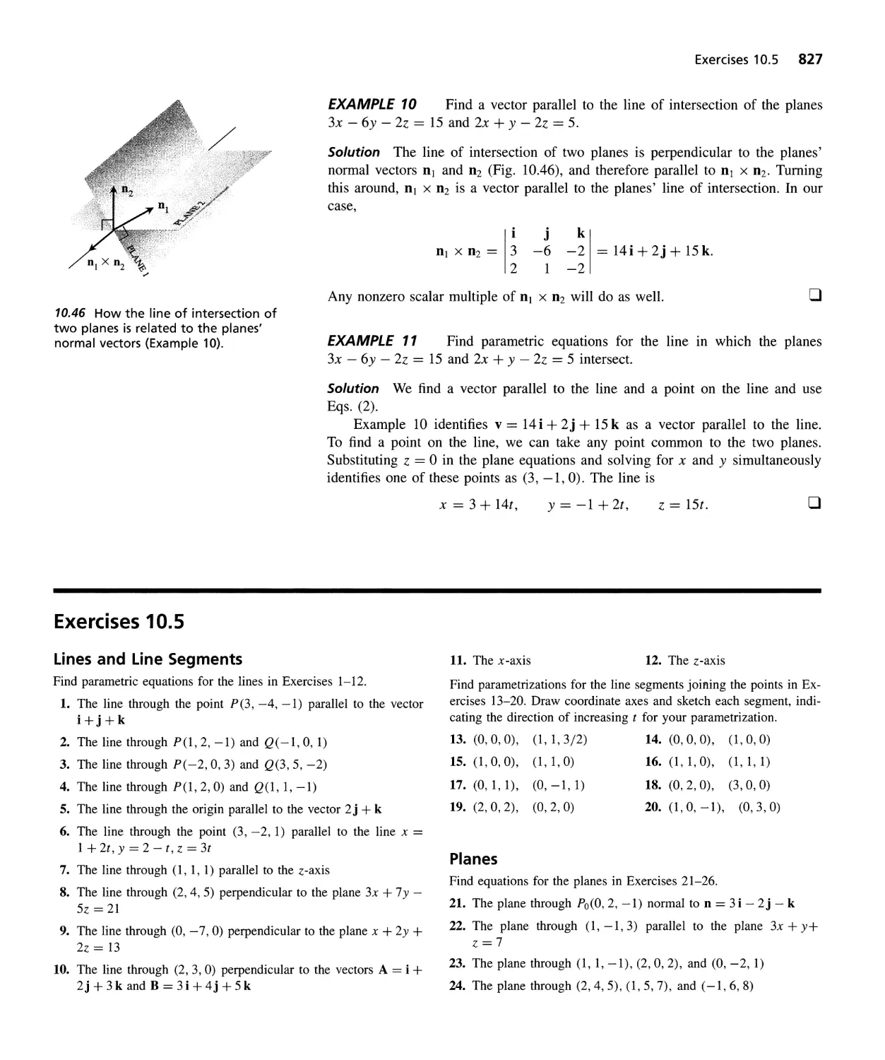
Lines and Planes in Space 822
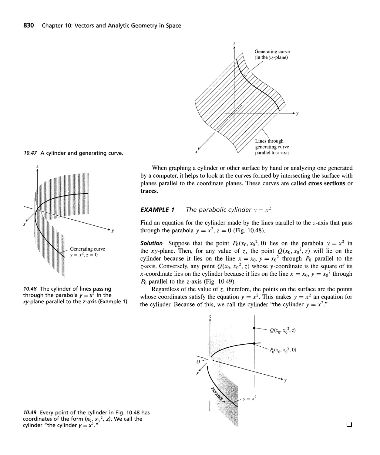
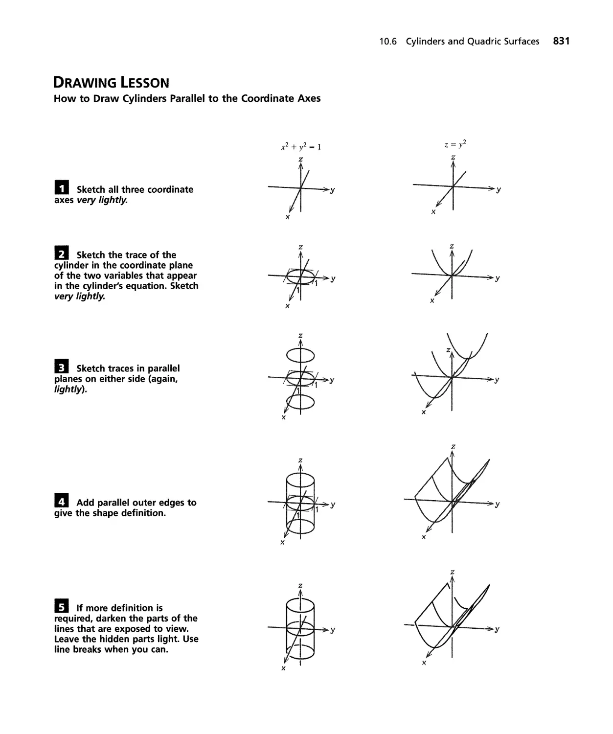
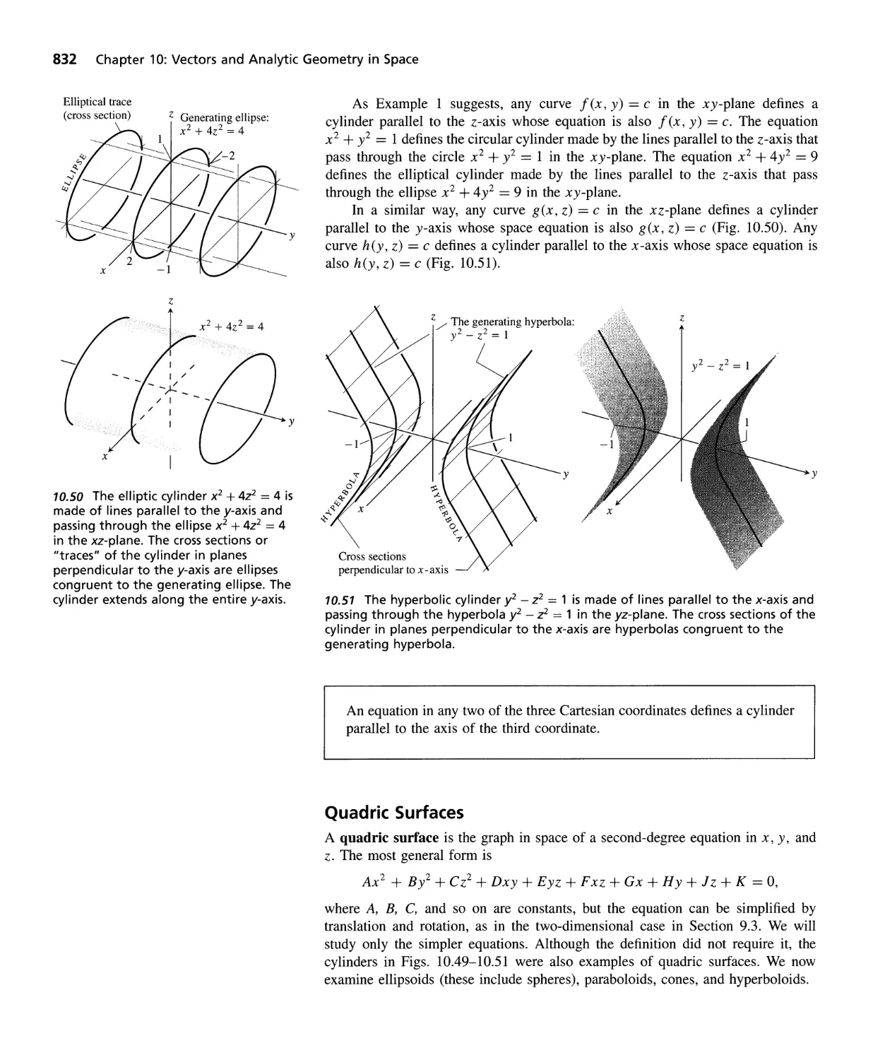
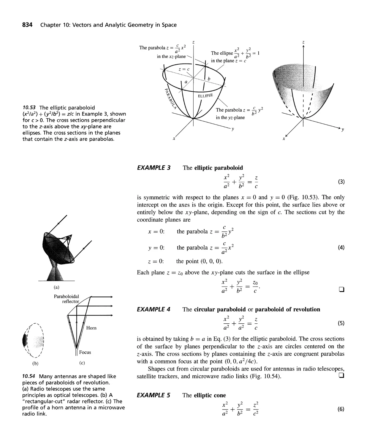
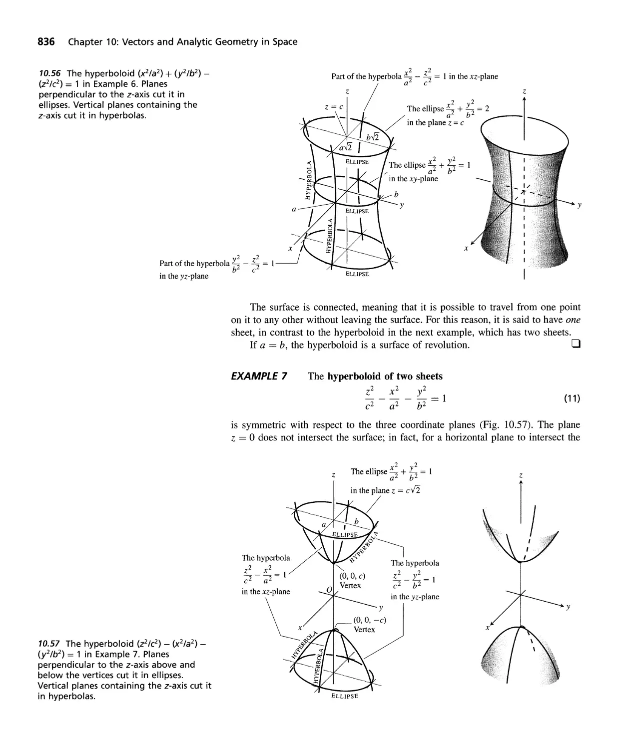
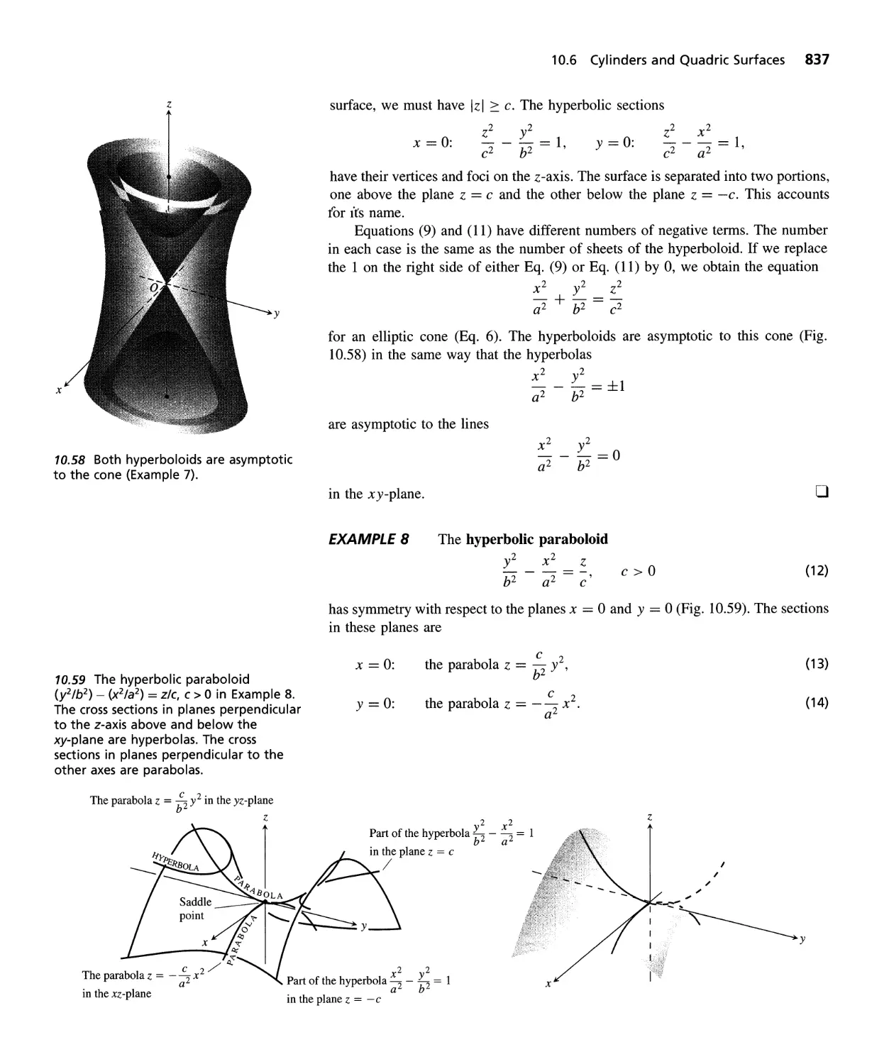
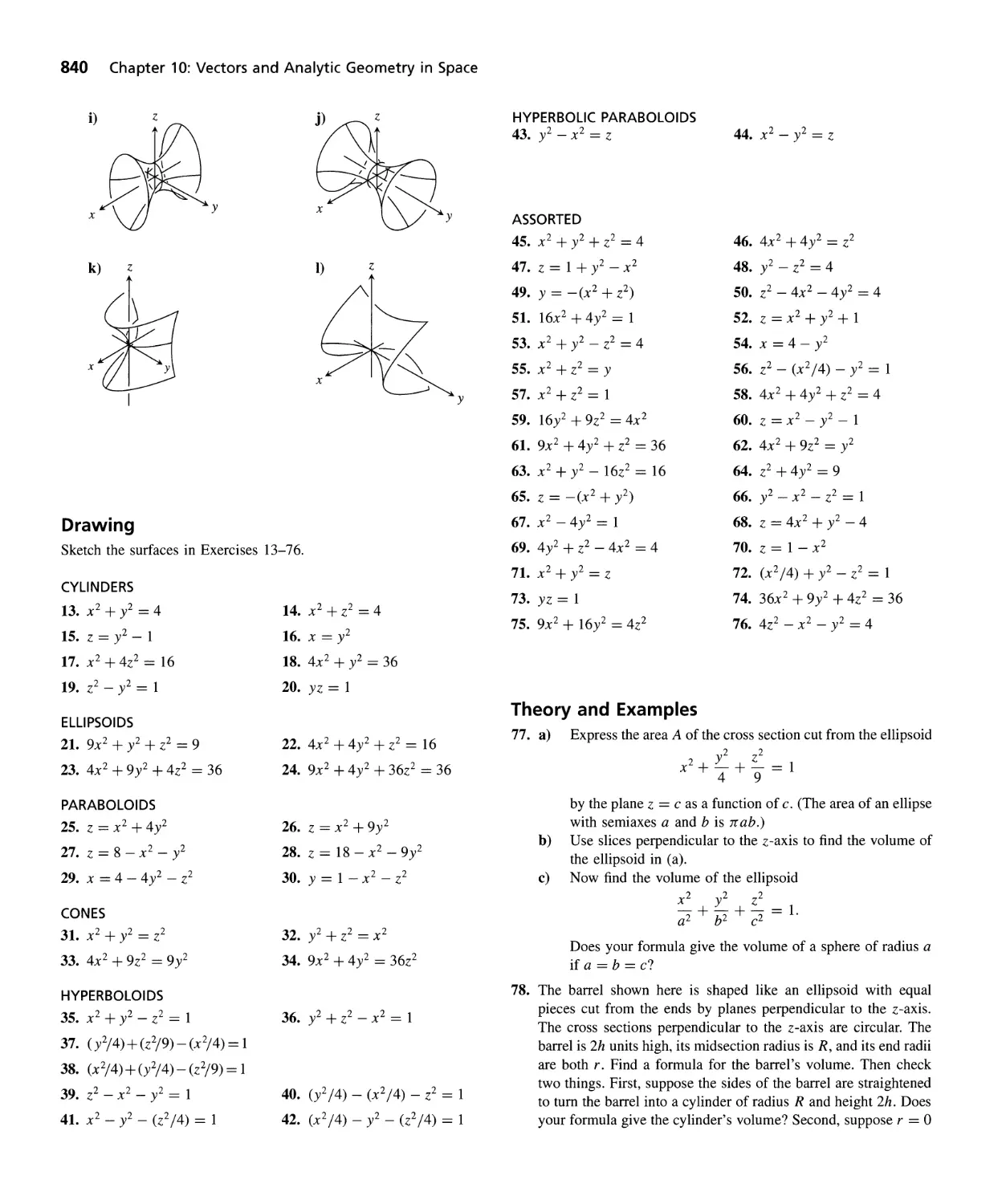
Cylinders and Quadric Surfaces 829
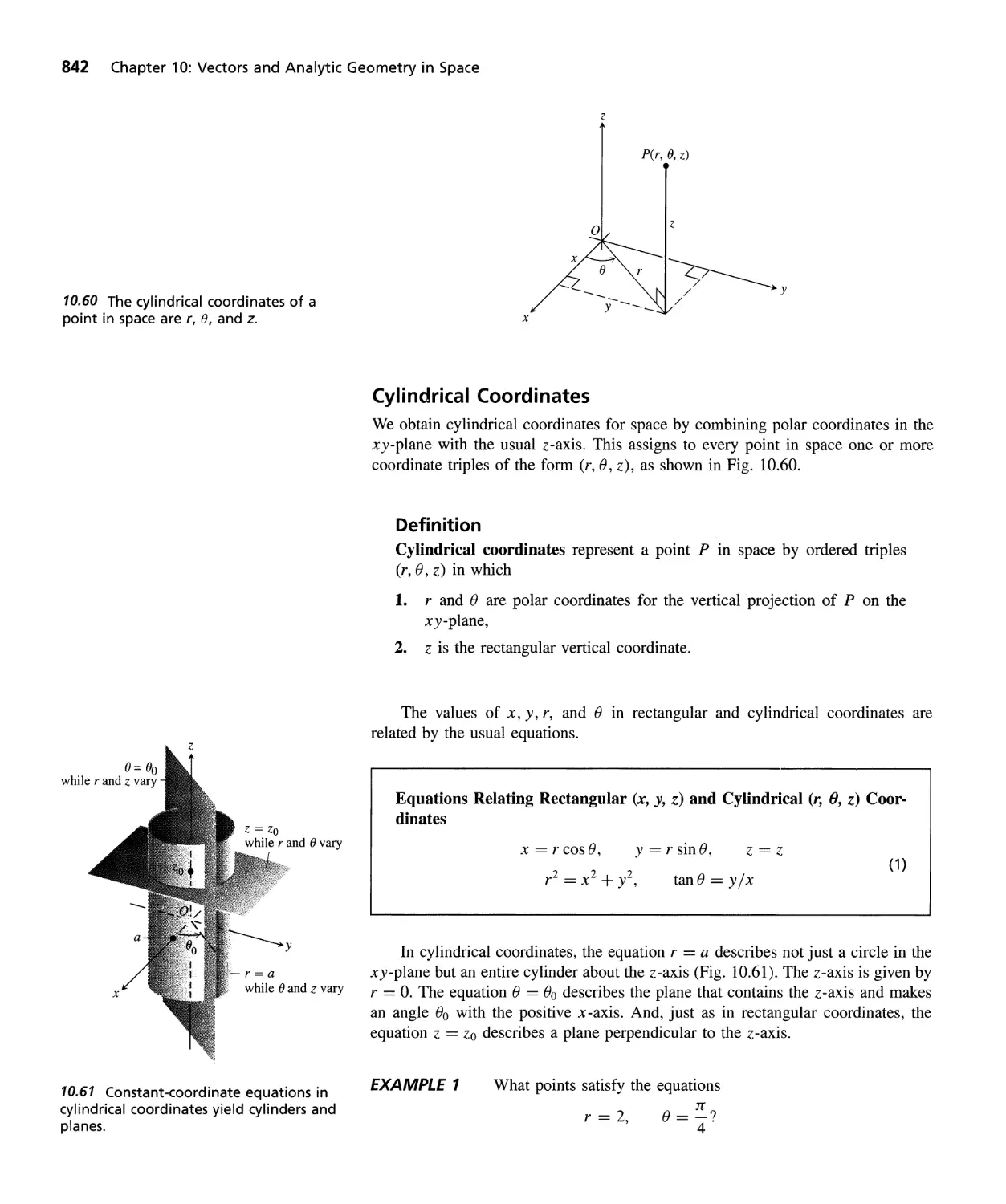
Cylindrical and Spherical Coordinates 841
QUESTI9NS TO GUIDE YOUR REVIEW 847 PRACTICE EXERCISES 848
ADDITIONAL EXERCISES-THEORY, EXAMPLES, ApPLICATIONS 851
.' .iIi!i!Jl/iPiRiFi€_'!iffI!if__ f!ifii!f'#l/ iJI
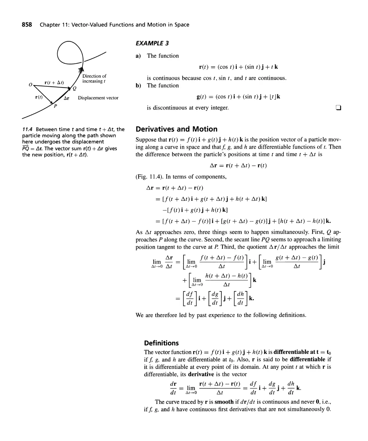
Vector- Valued Functions and Space Curves 855
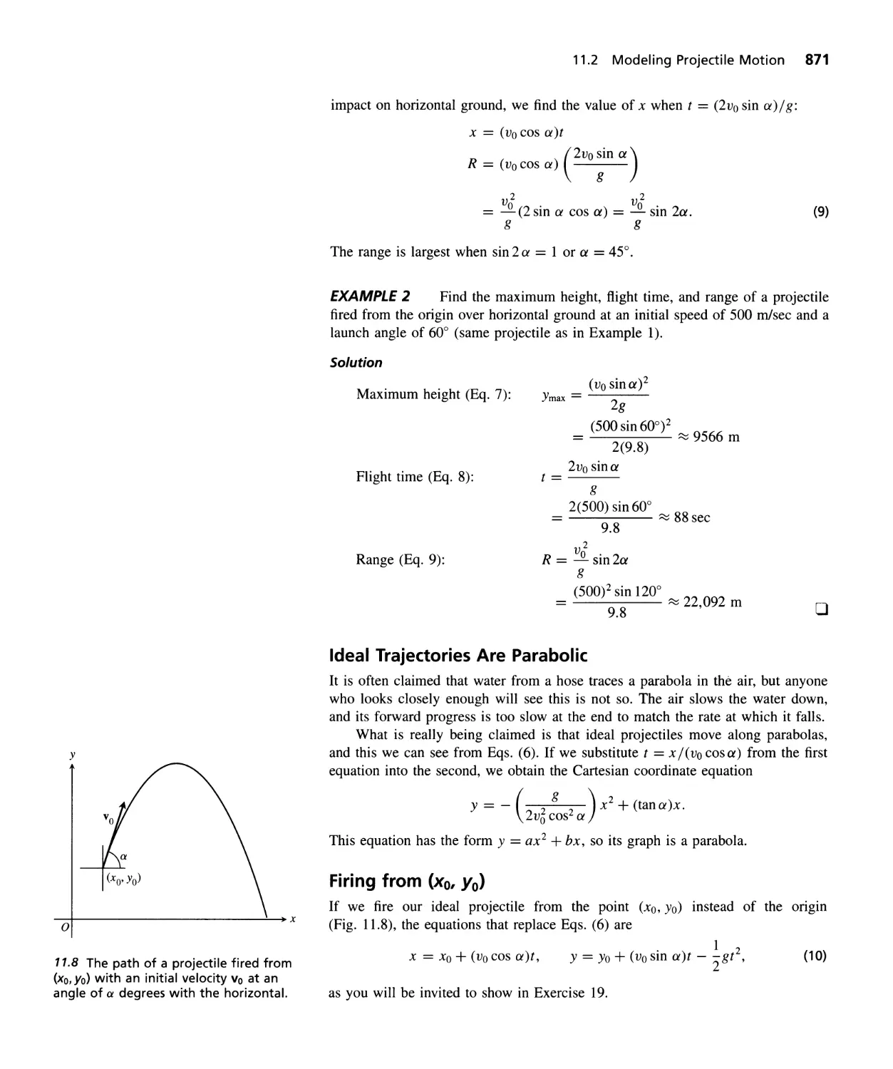
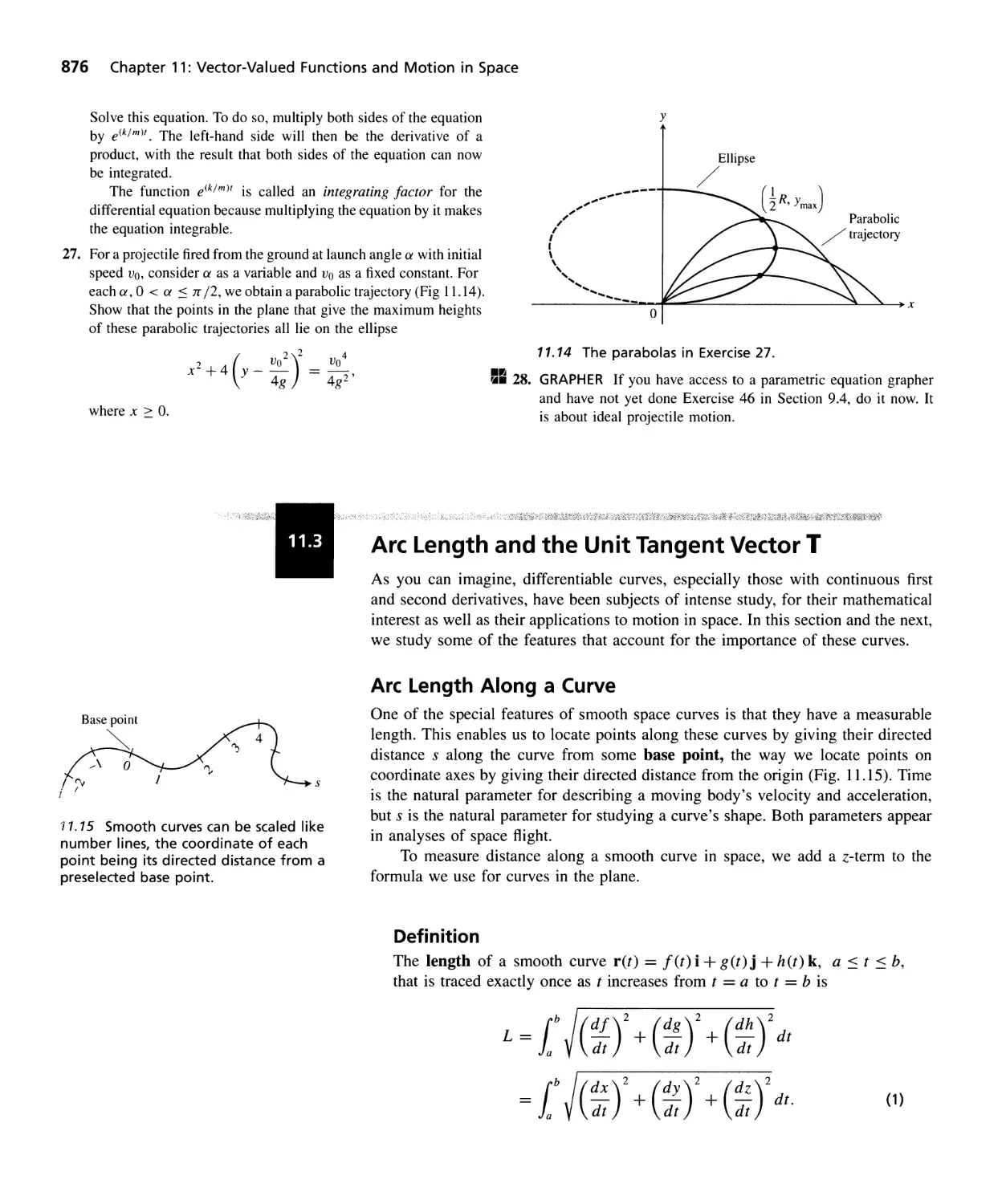
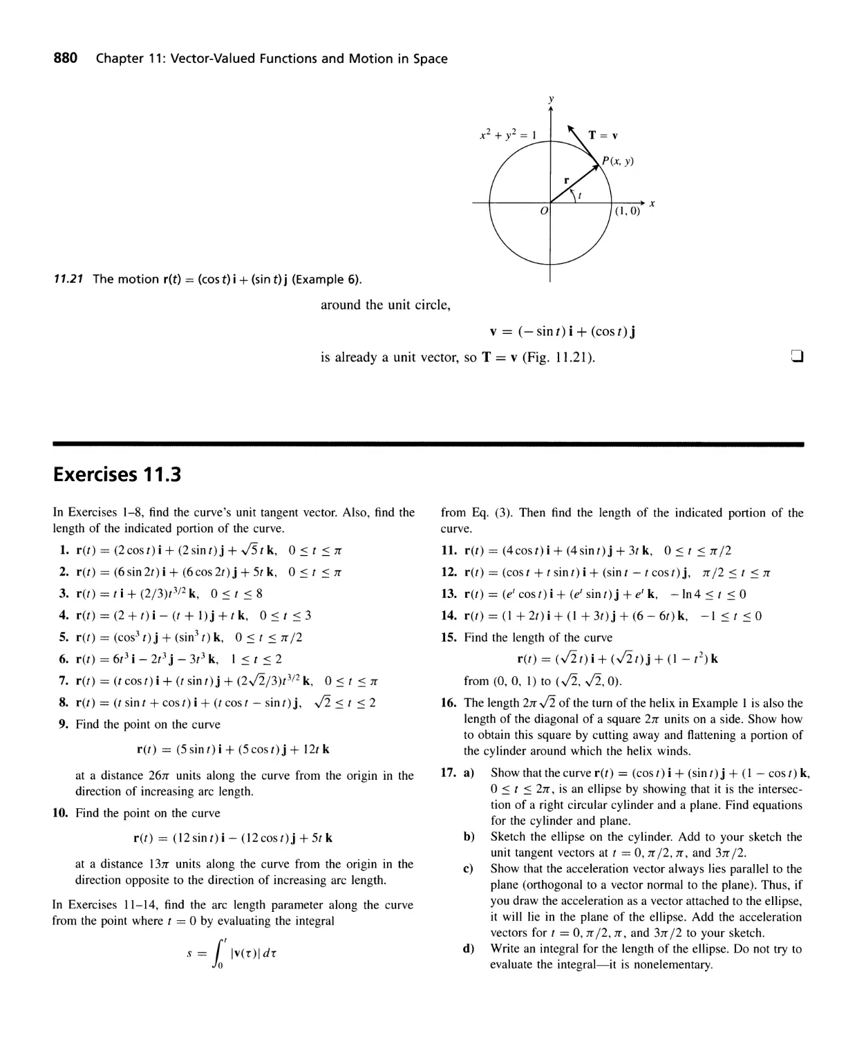
Modeling Projectile Motion 868
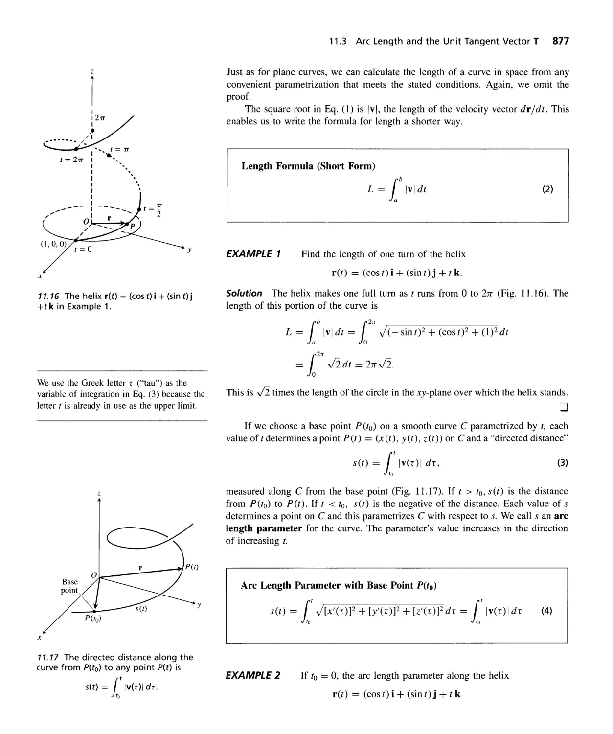
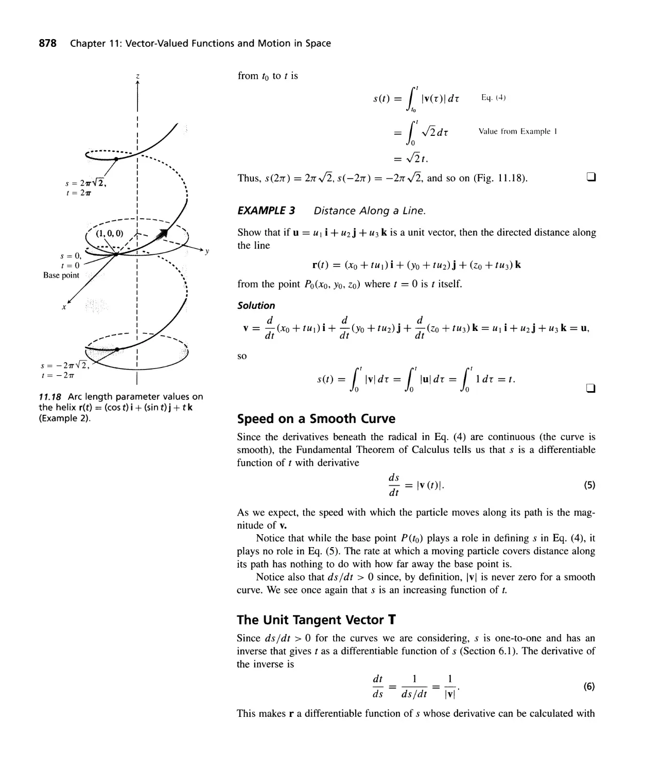
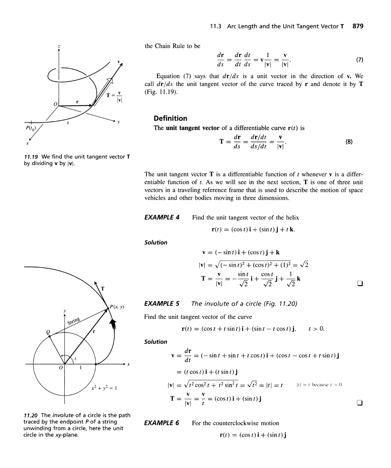
Arc Length and the Unit Tangent Vector T 876
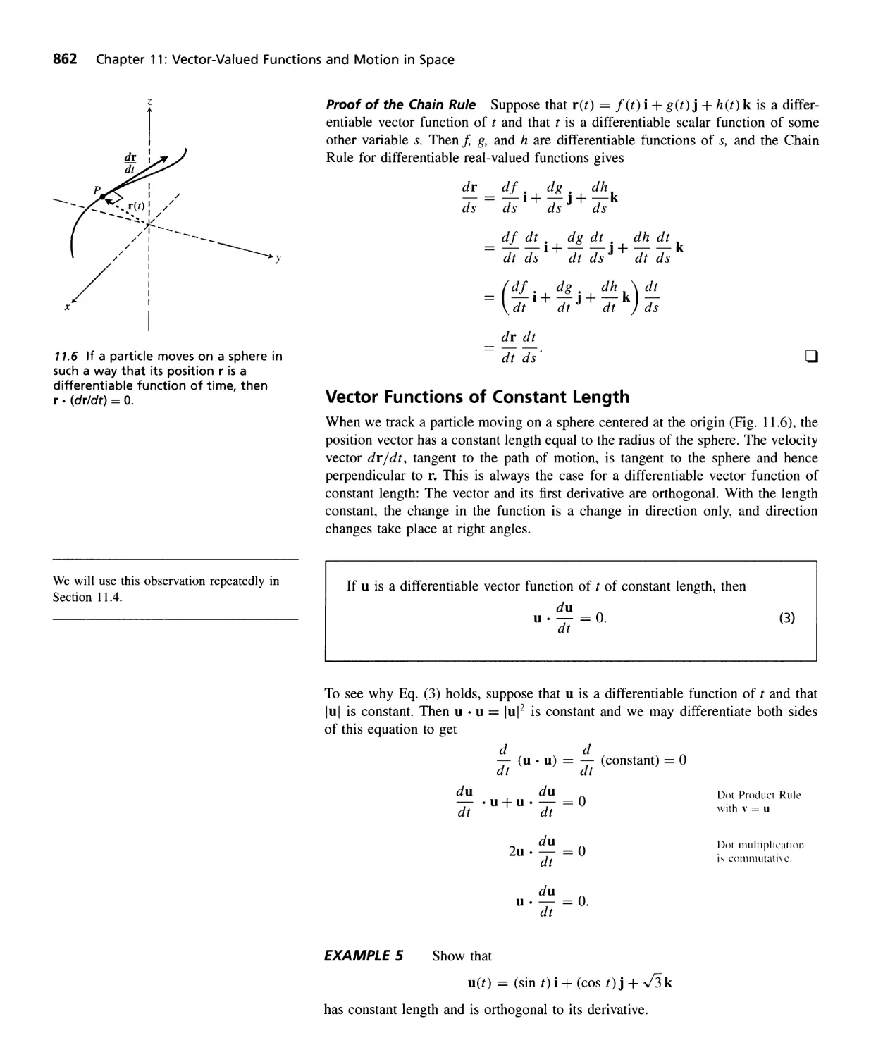
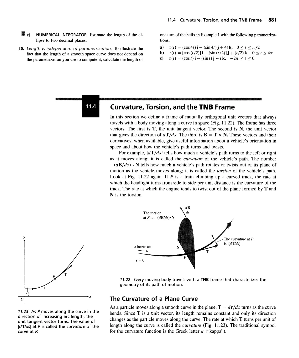
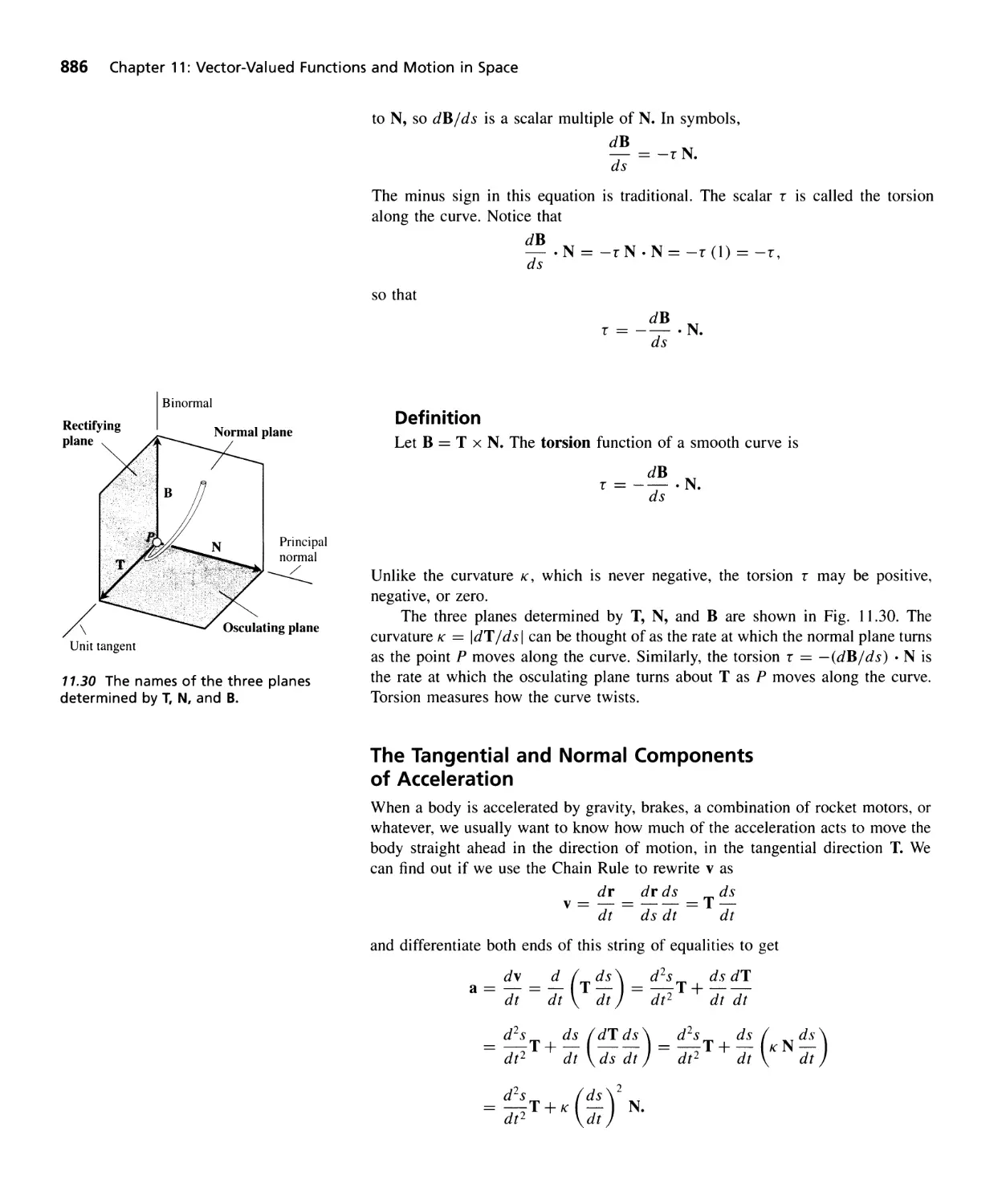
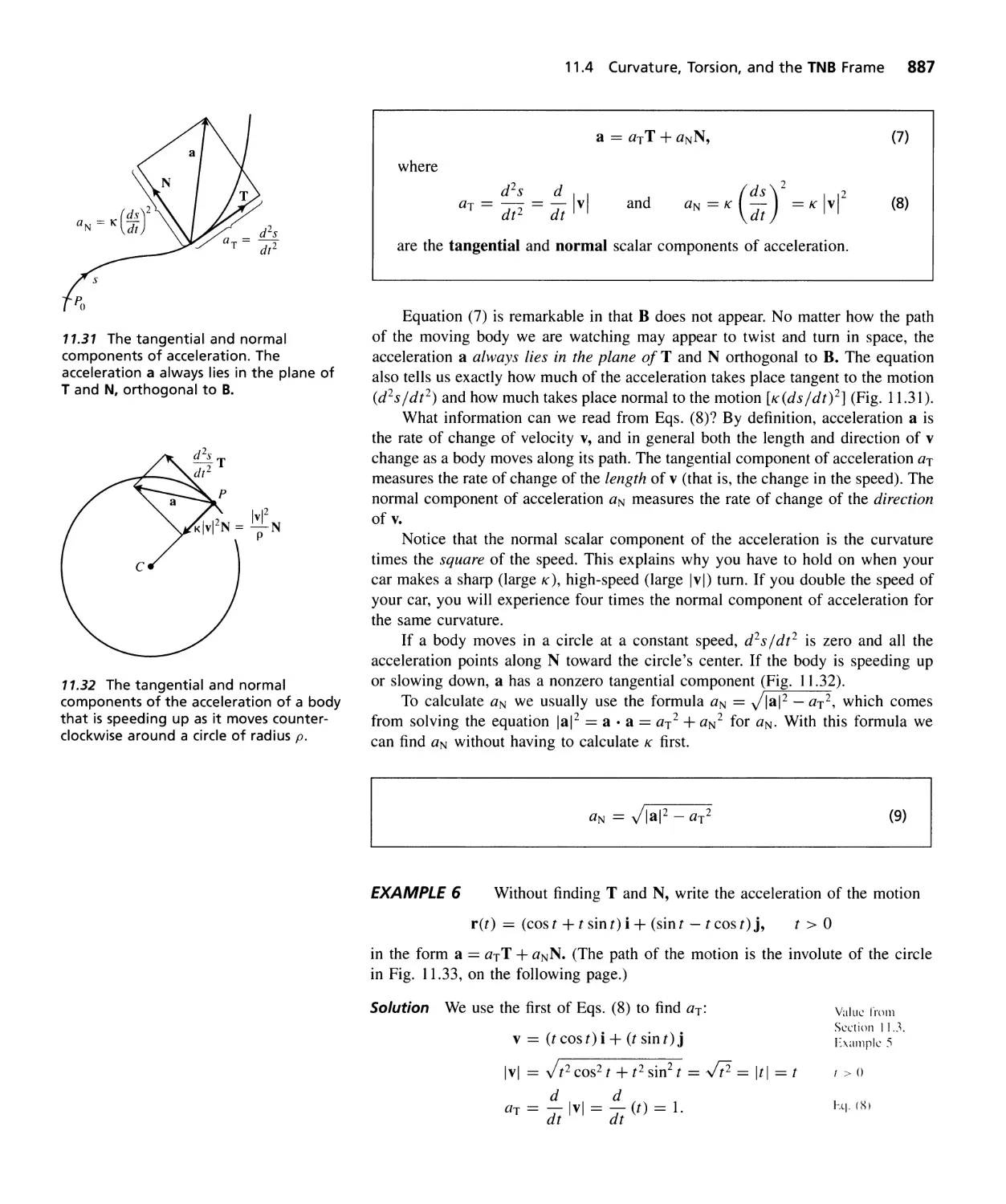
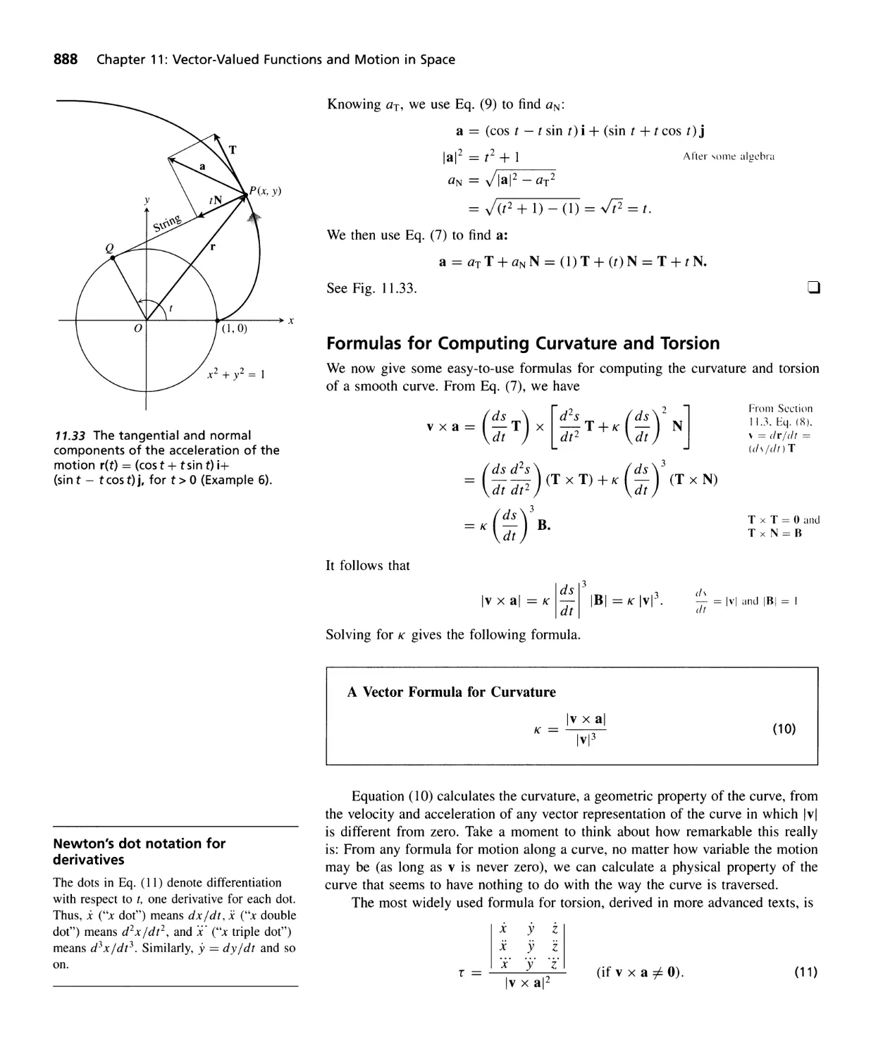
Curvature, Torsion, and the TNB Frame 881
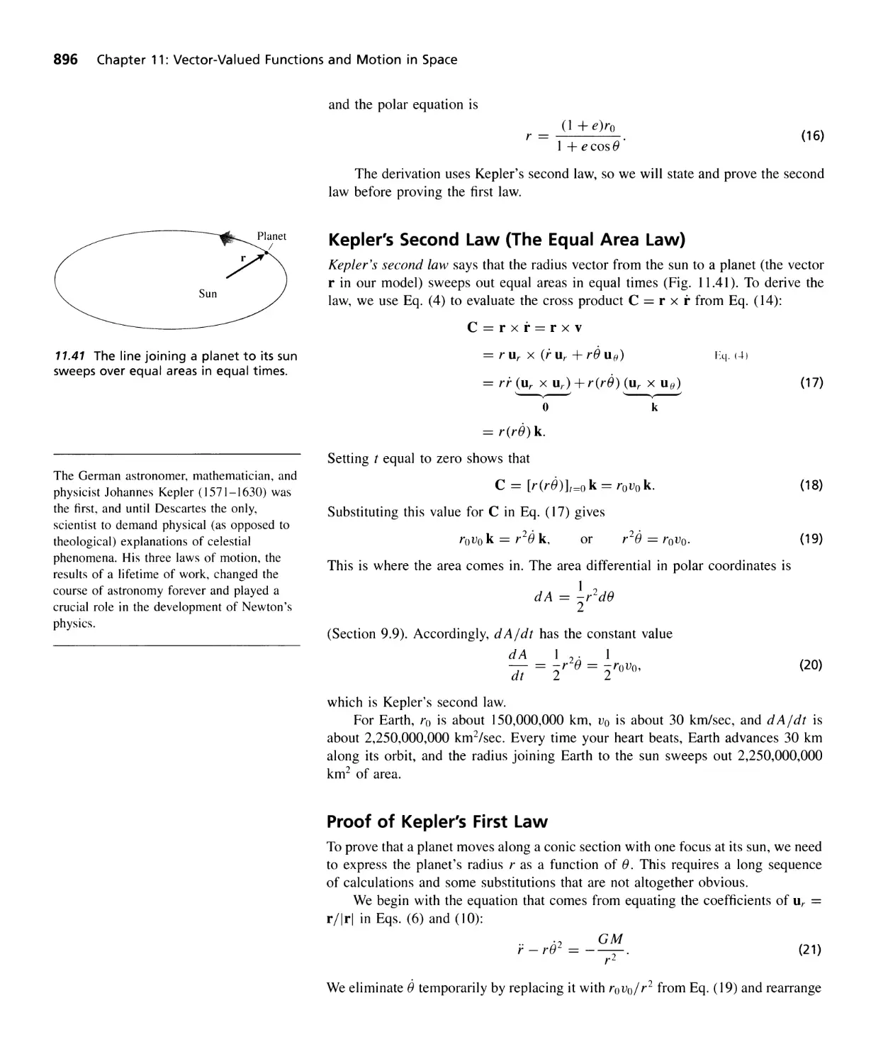
Planetary Motion and Satellites 893
QUESTIONS TO GUIDE YOUR REVIEW 902 PRACTICE EXERCISES 902
ADDITIONAL EXERCISES-THEORY, EXAMPLES, ApPLICATIONS 905
vi Contents
Multivariable
Functions and
Partial Derivatives
Multiple Integrals
Integration in
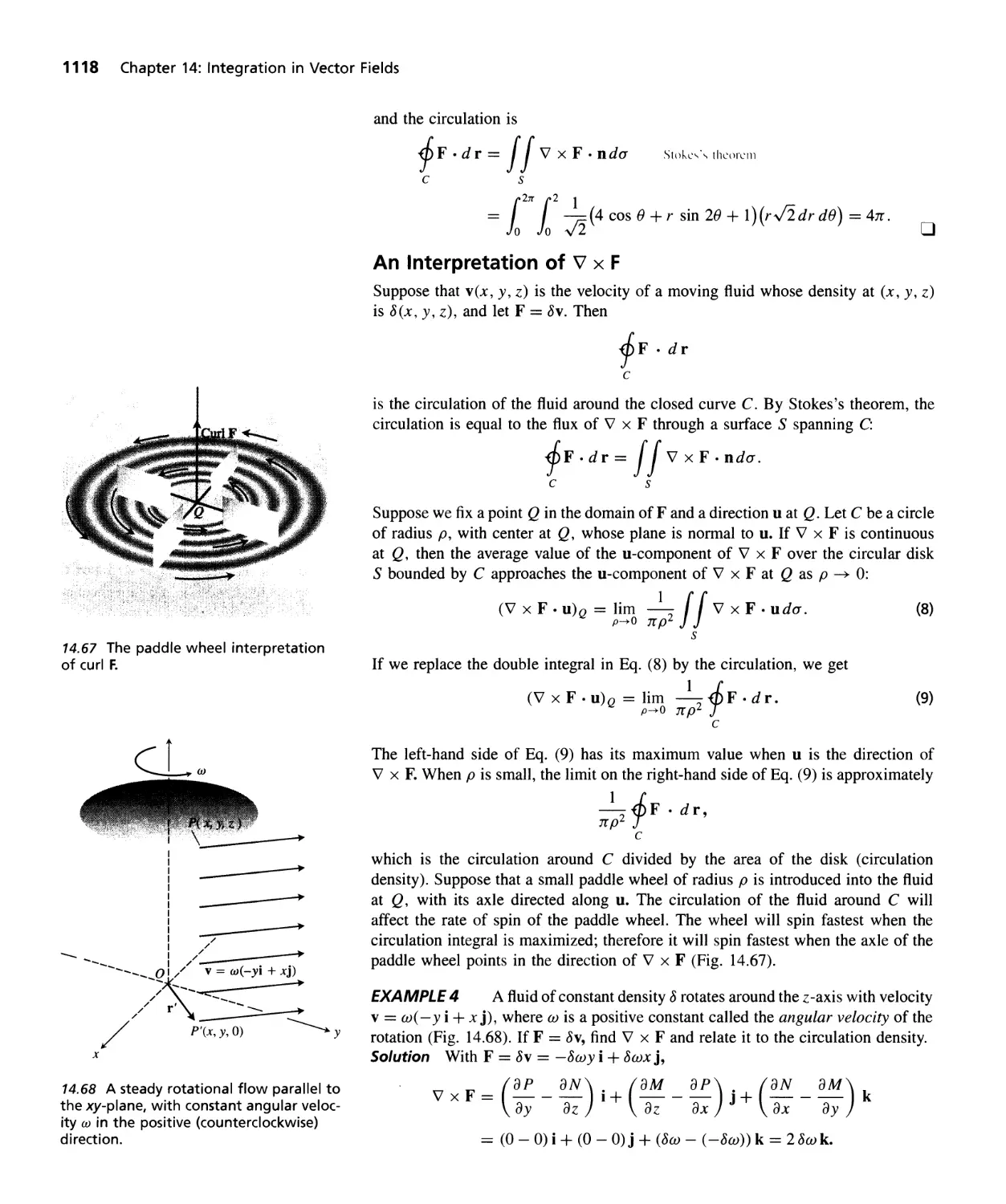
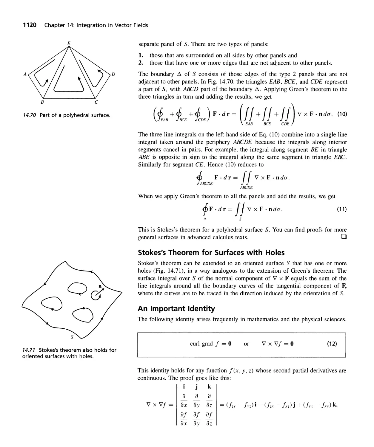
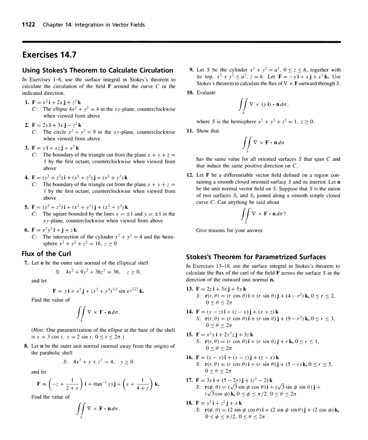
Vector Fields
Appendices
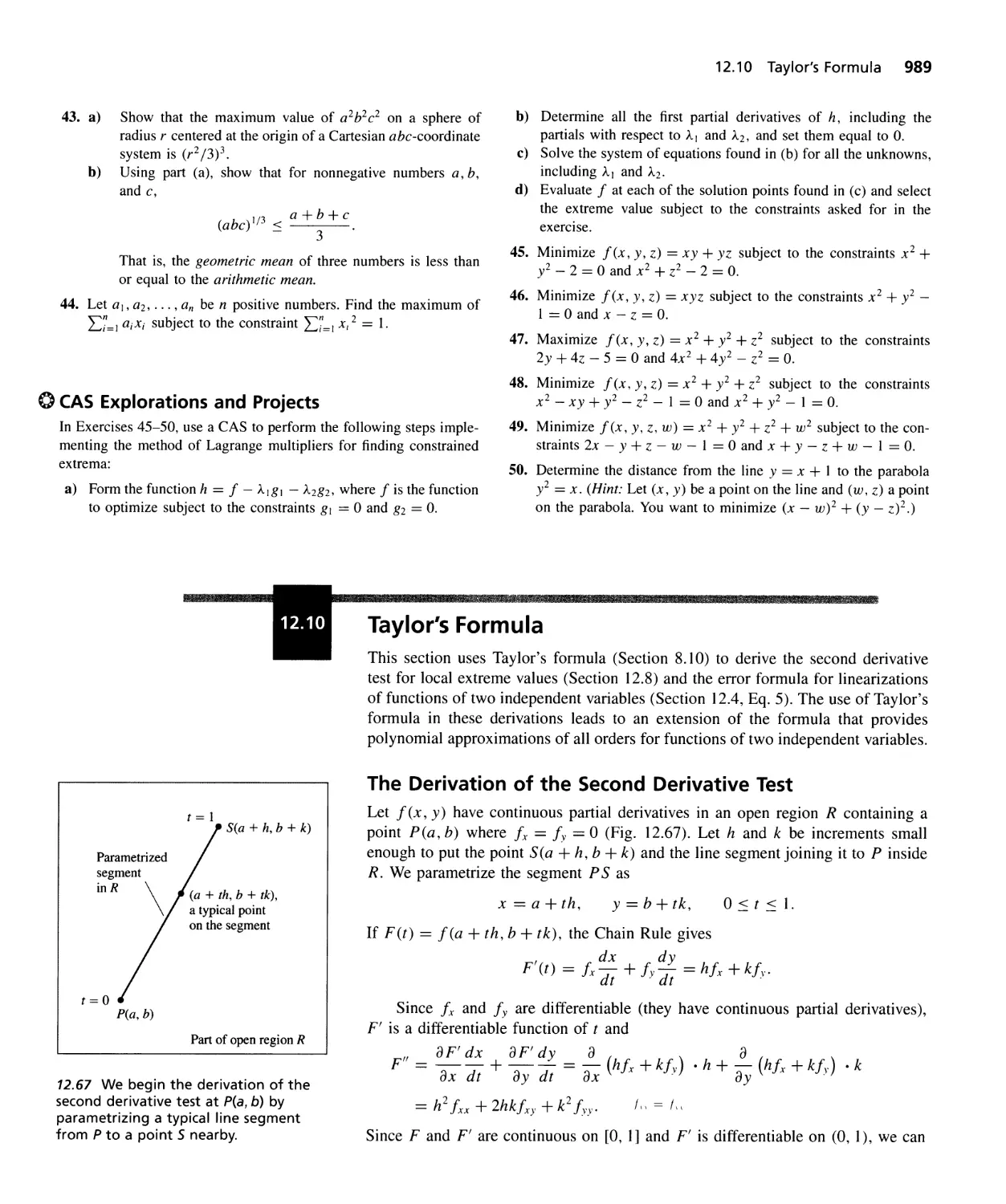
12.1
12.2
12.3
12.4
12.5
12.6
12.7
12.8
12.9
12.10
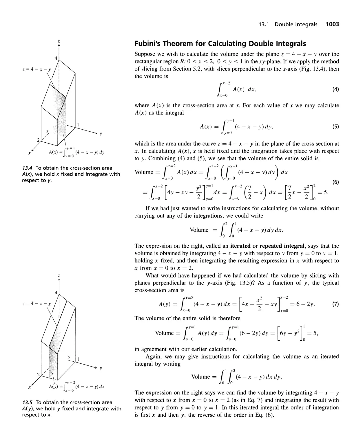
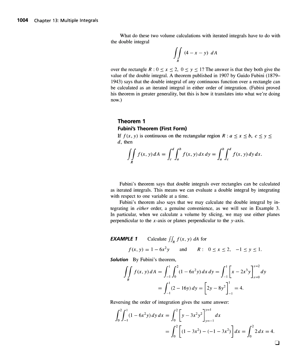
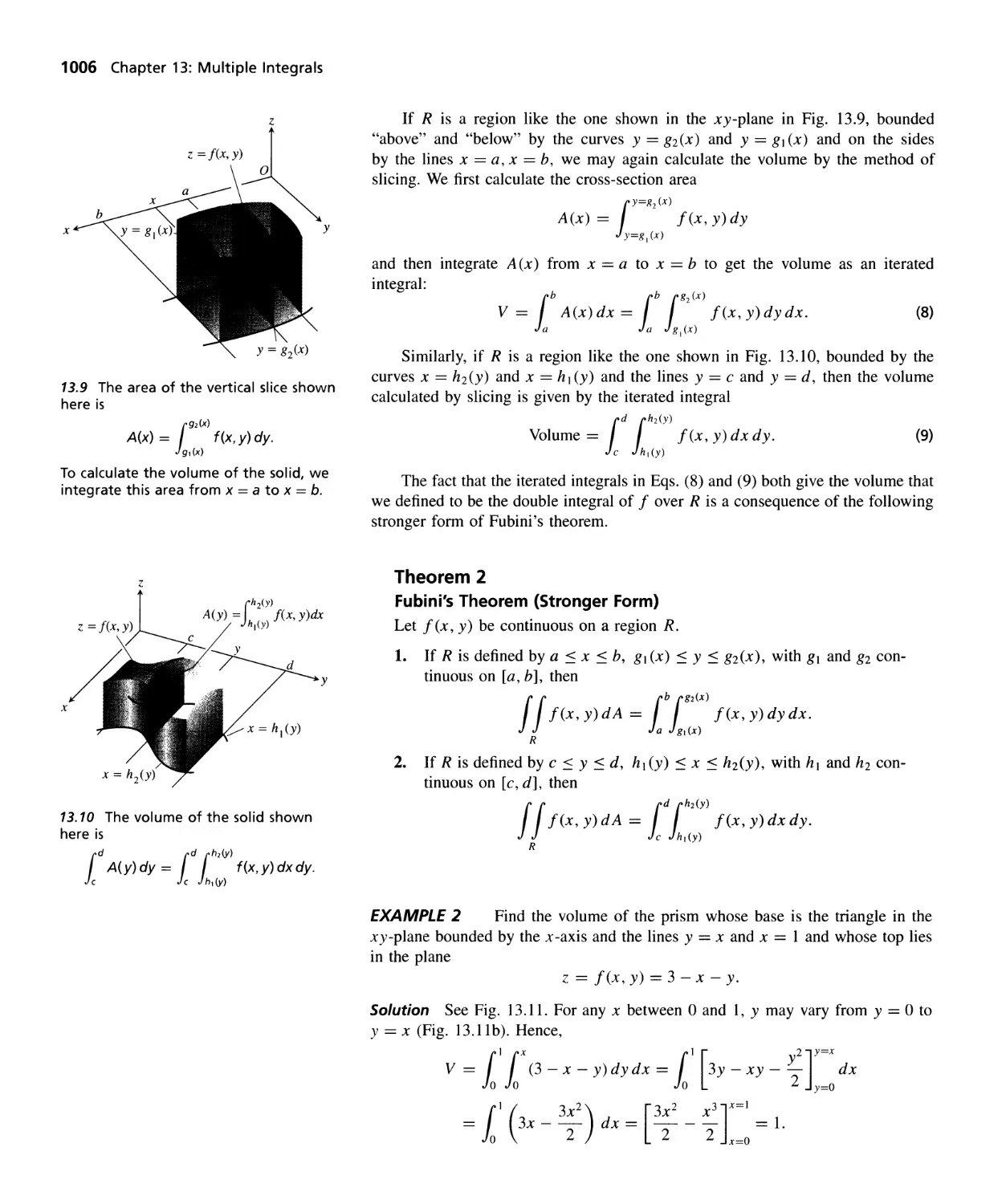
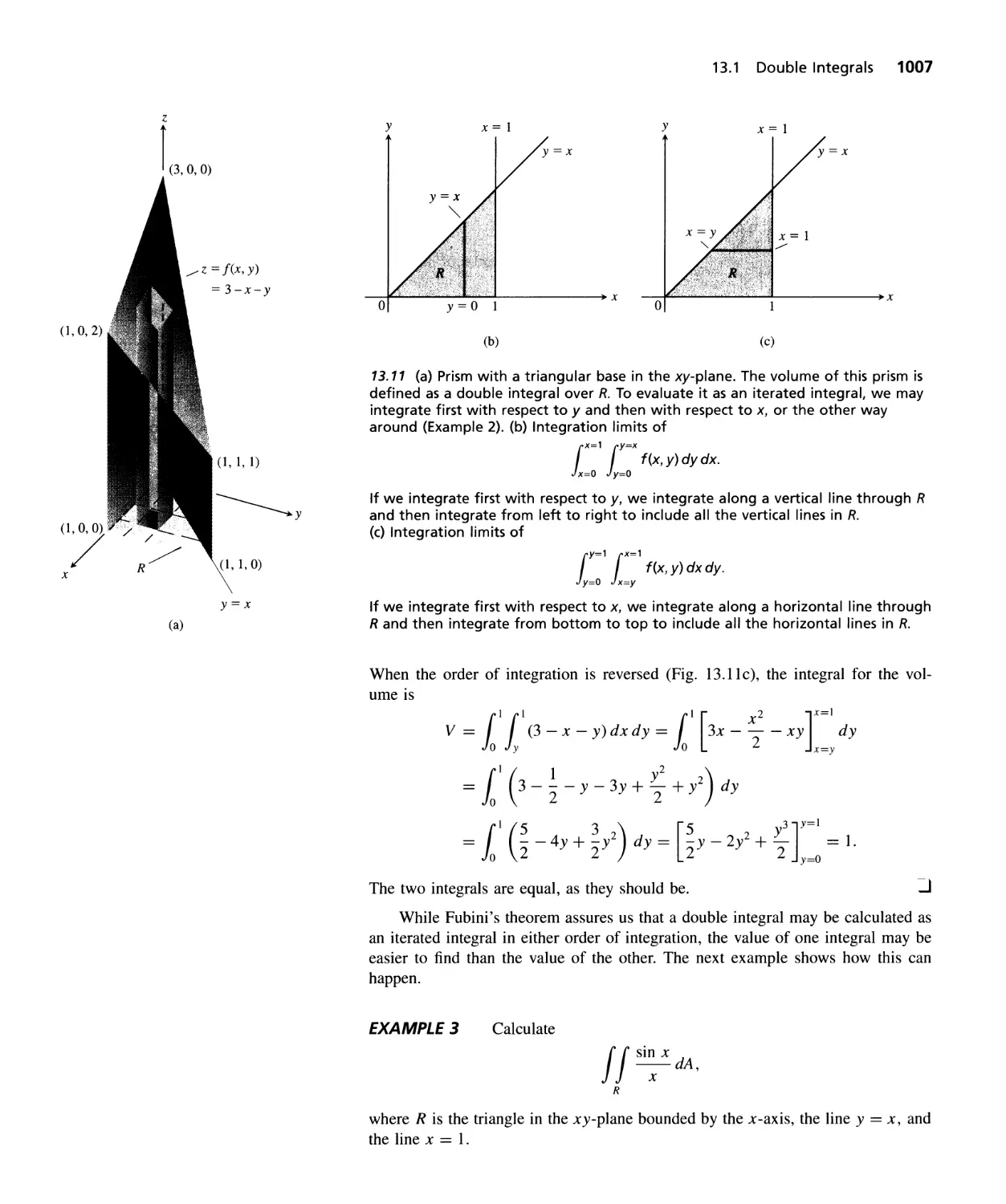
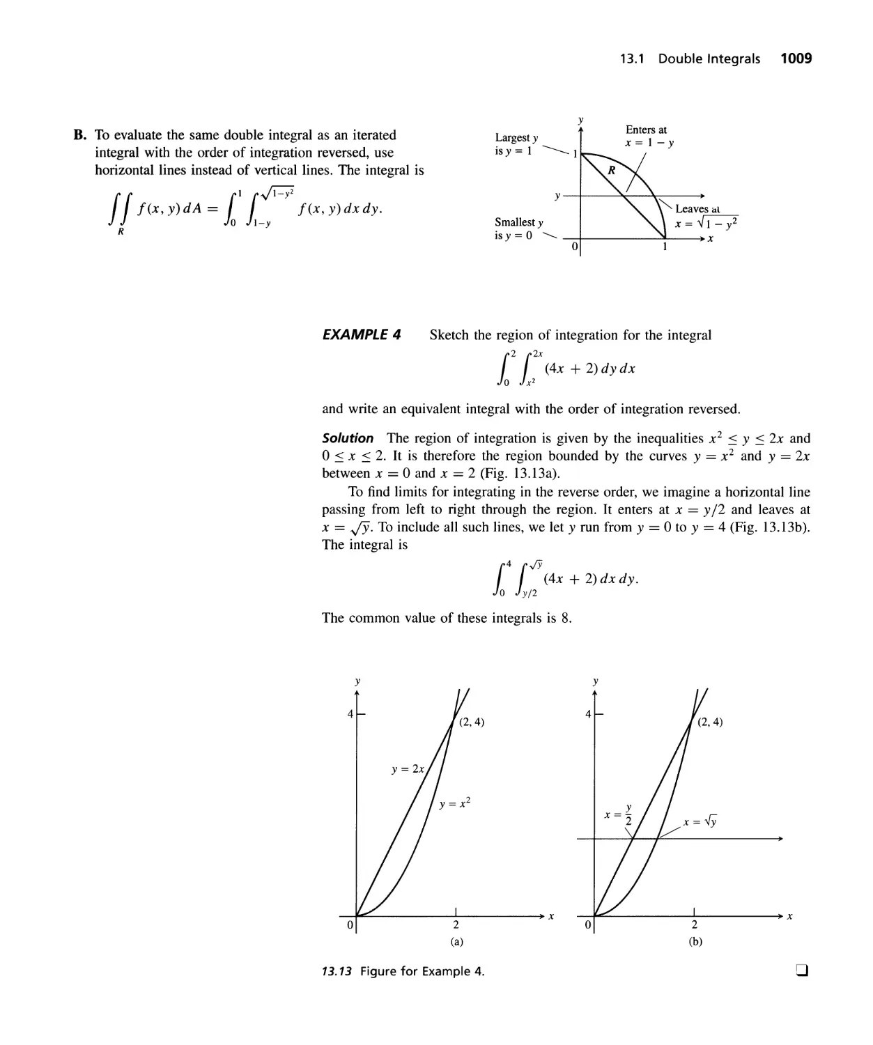
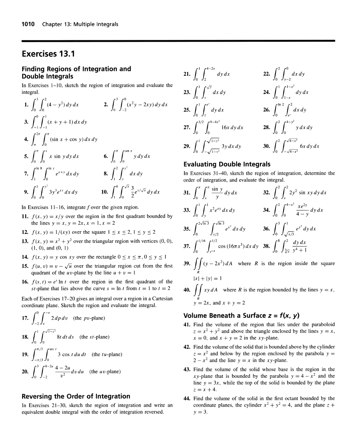
13.1
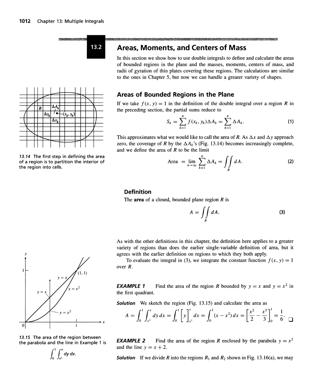
13.2
13.3
13.4
13.5
13.6
13.7
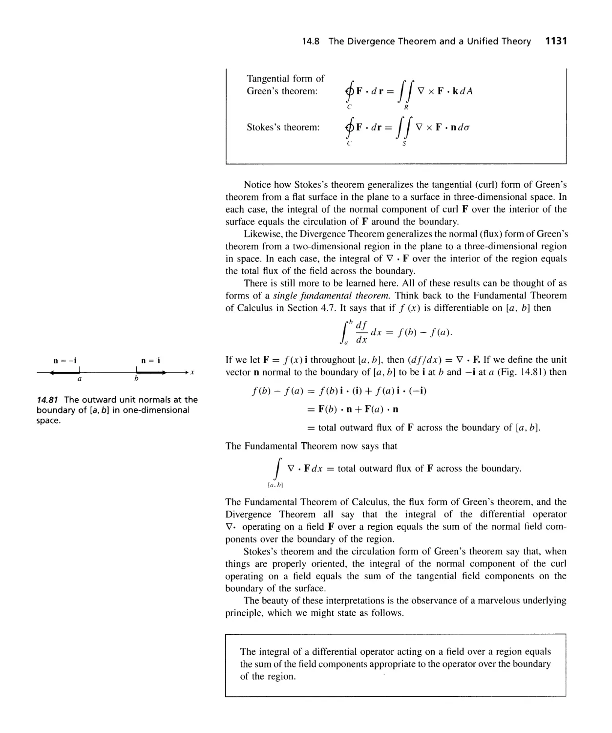
14.1
14.2
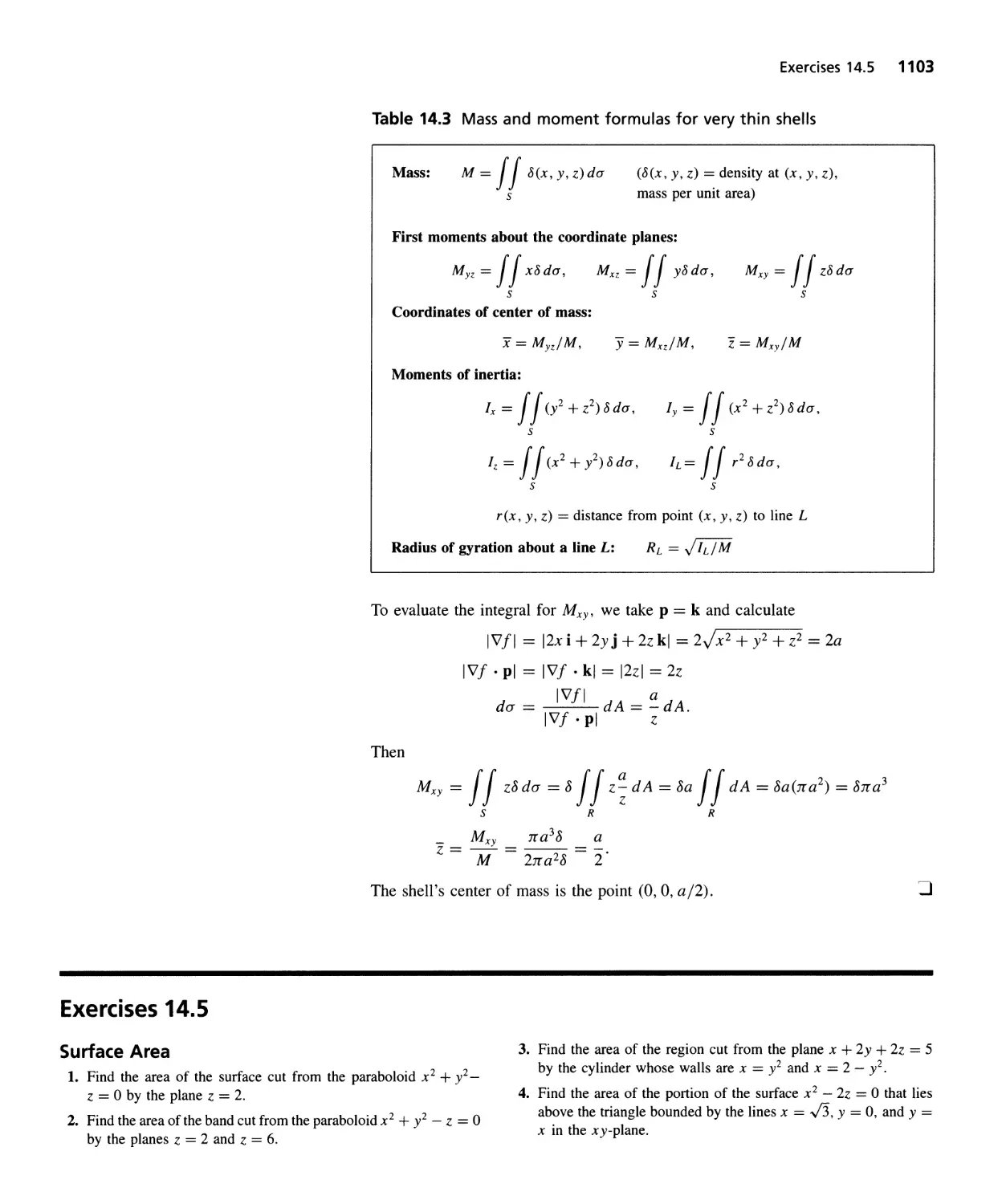
14.3
14.4
14.5
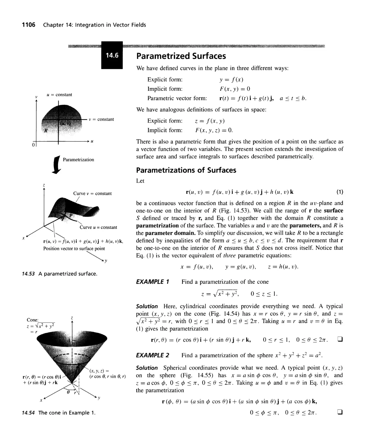
14.6
14.7
14.8
A.1
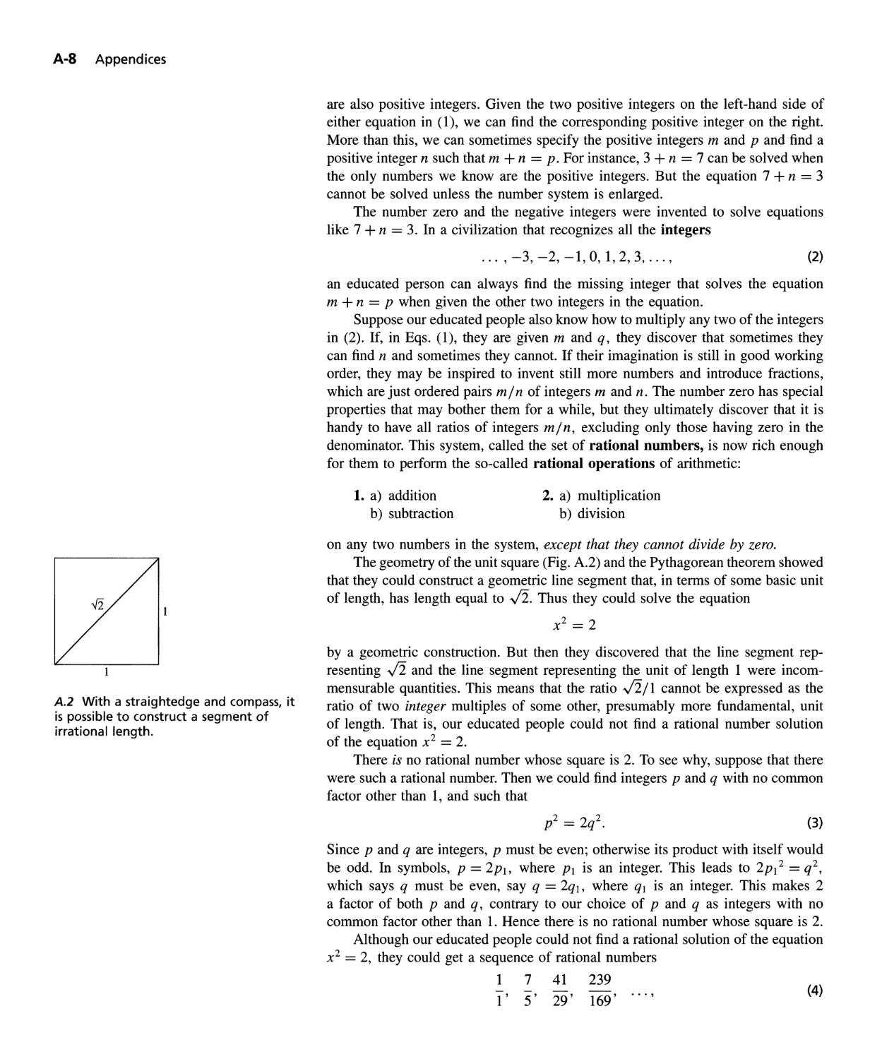
A.2
A.3
A.4
A.5
A.6
A.7
A.8
A.9
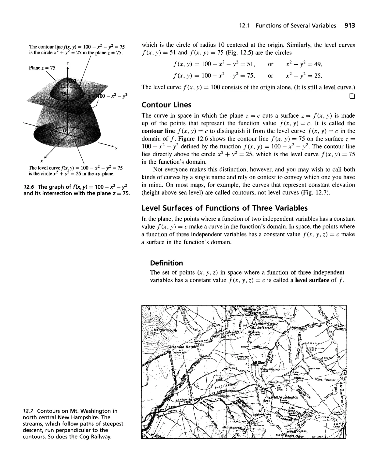
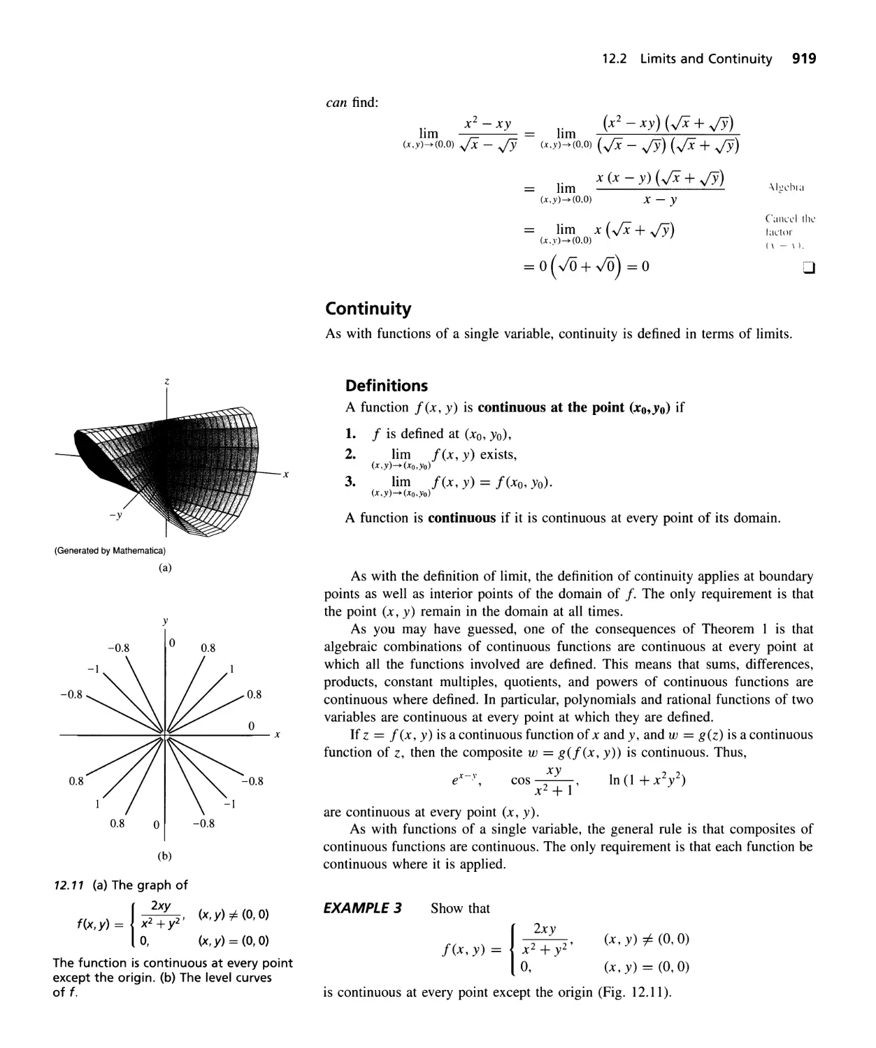
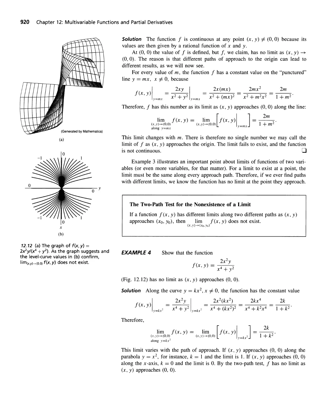
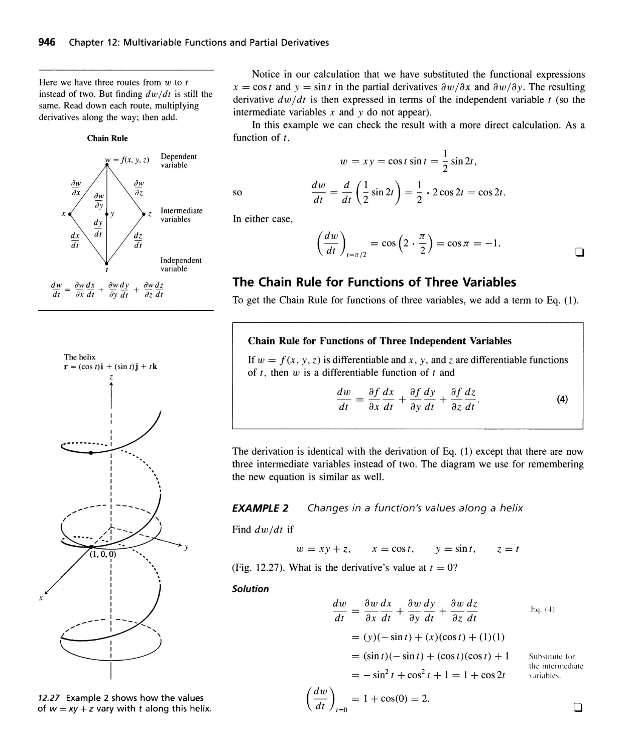
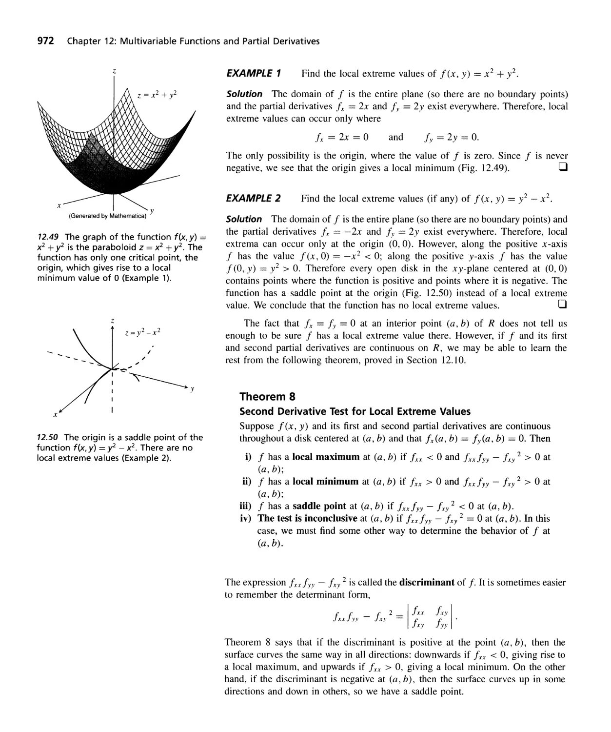
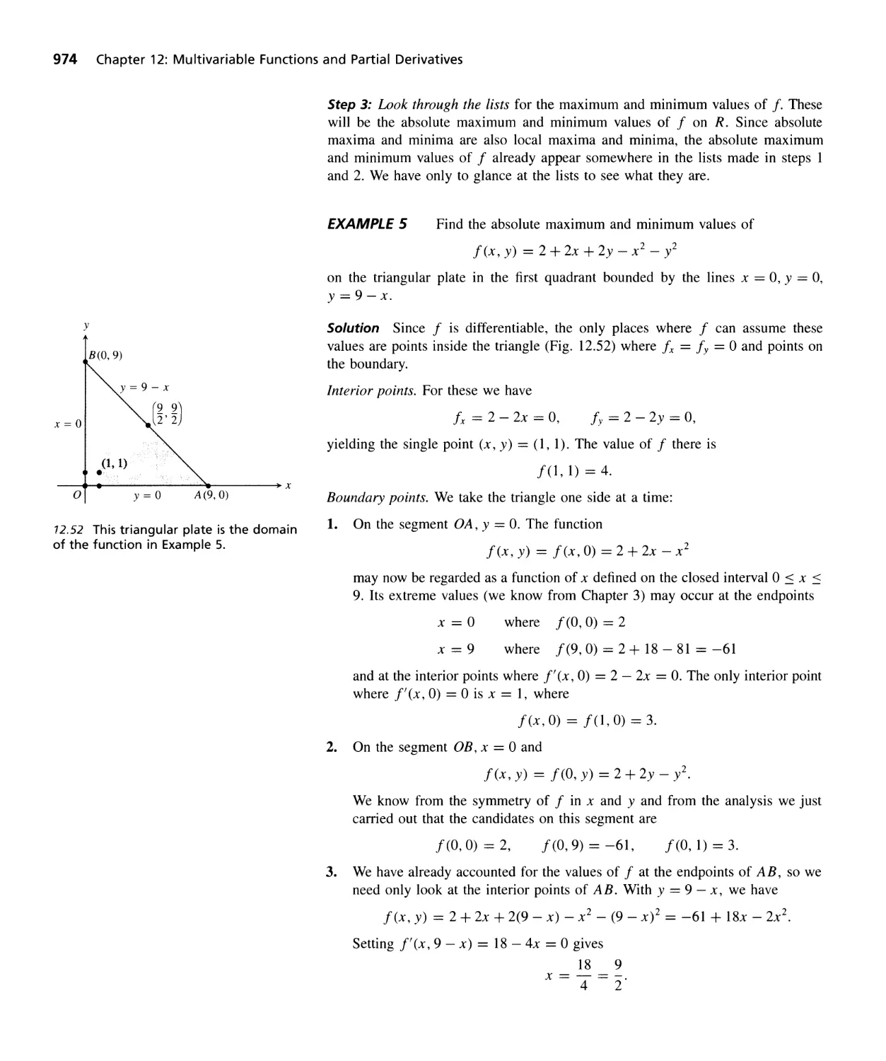
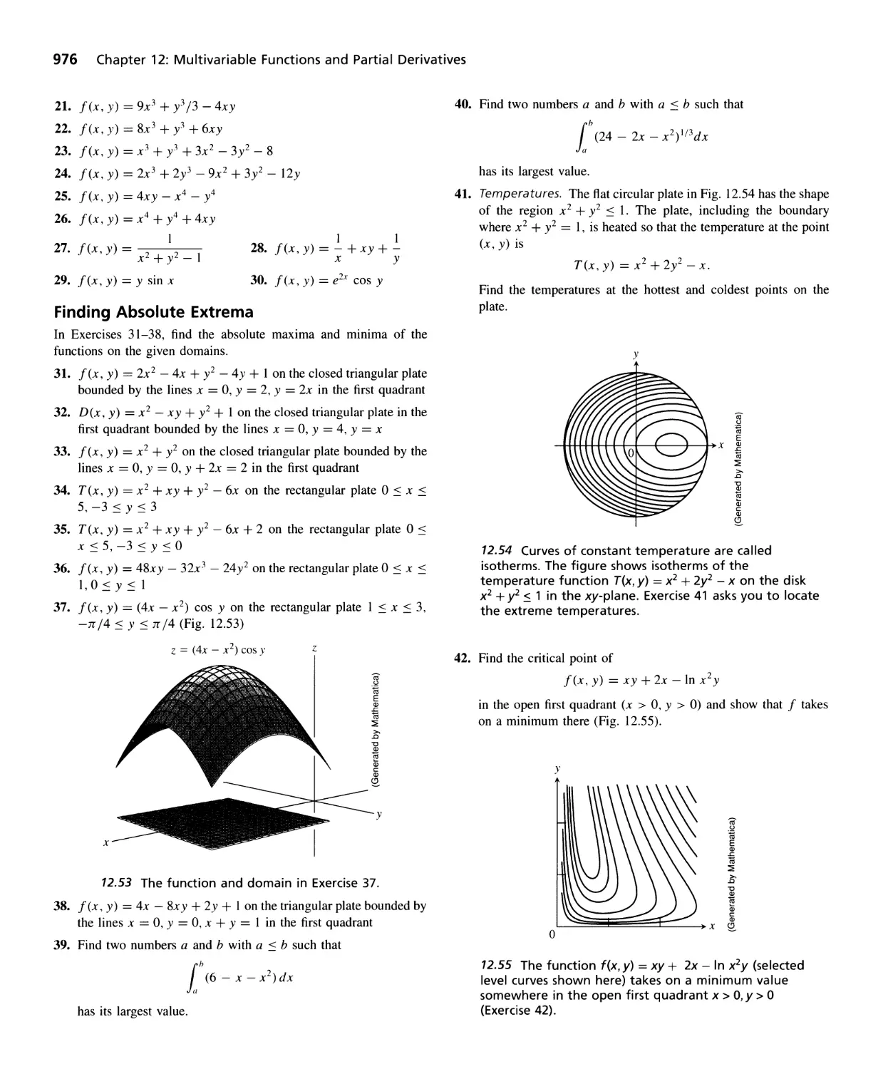
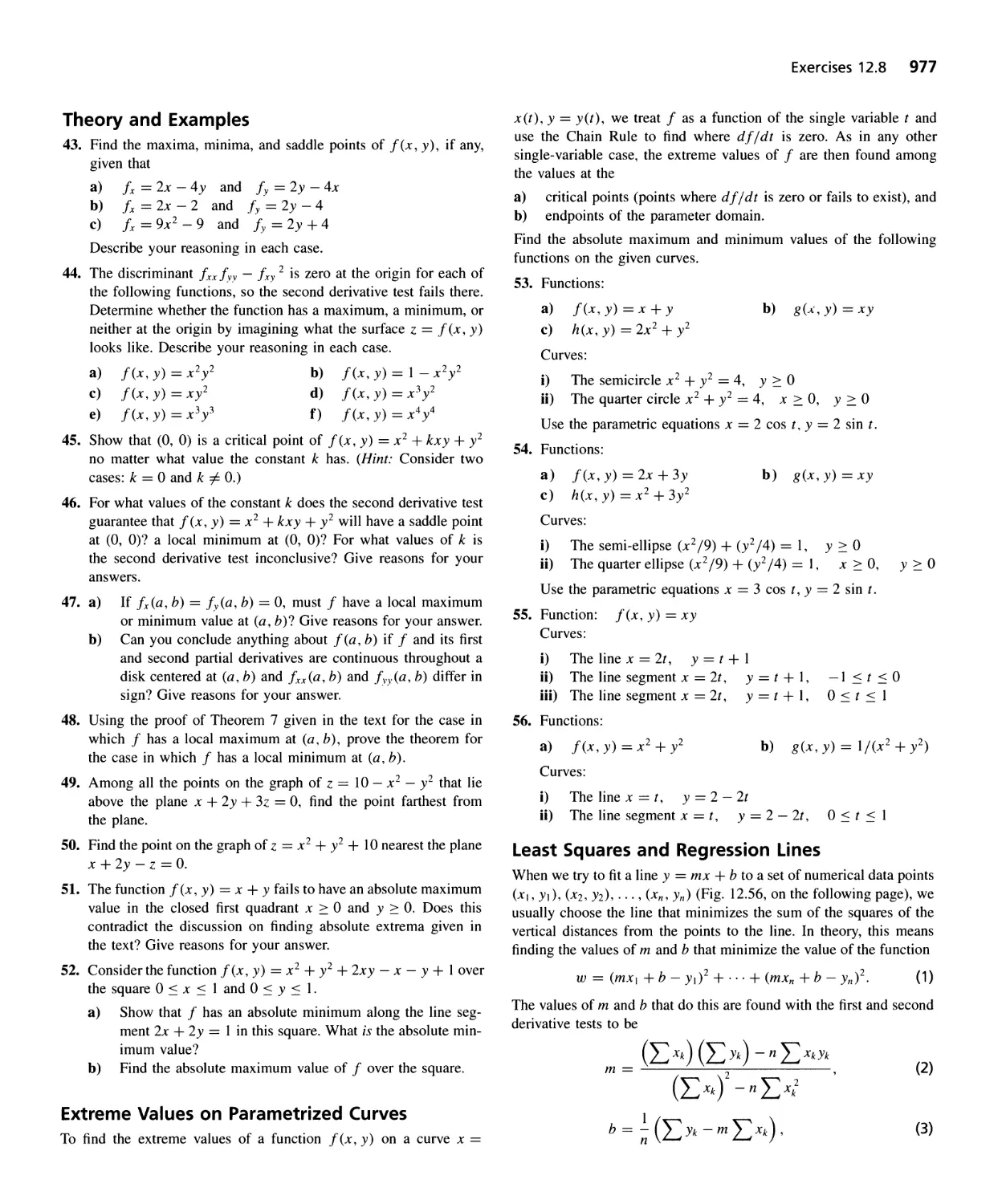
Functions of Several Variables 909
Limits and Continuity 917
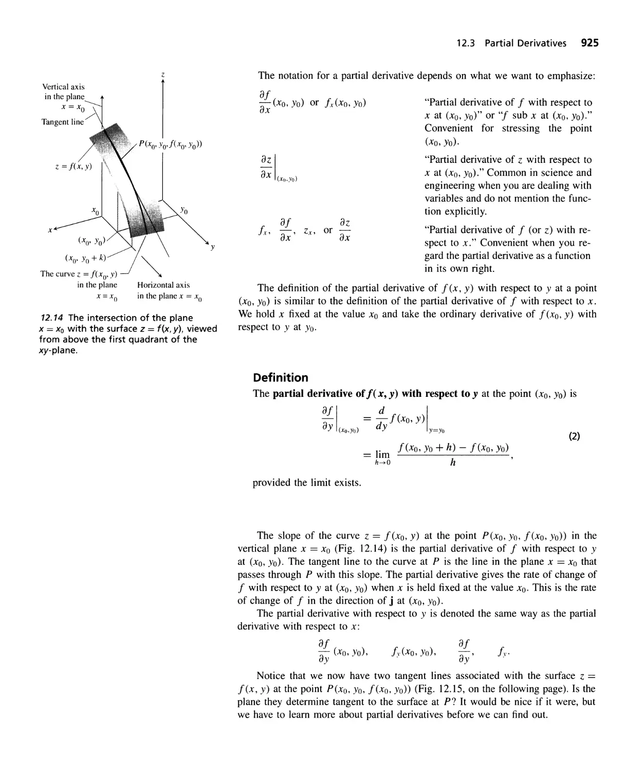
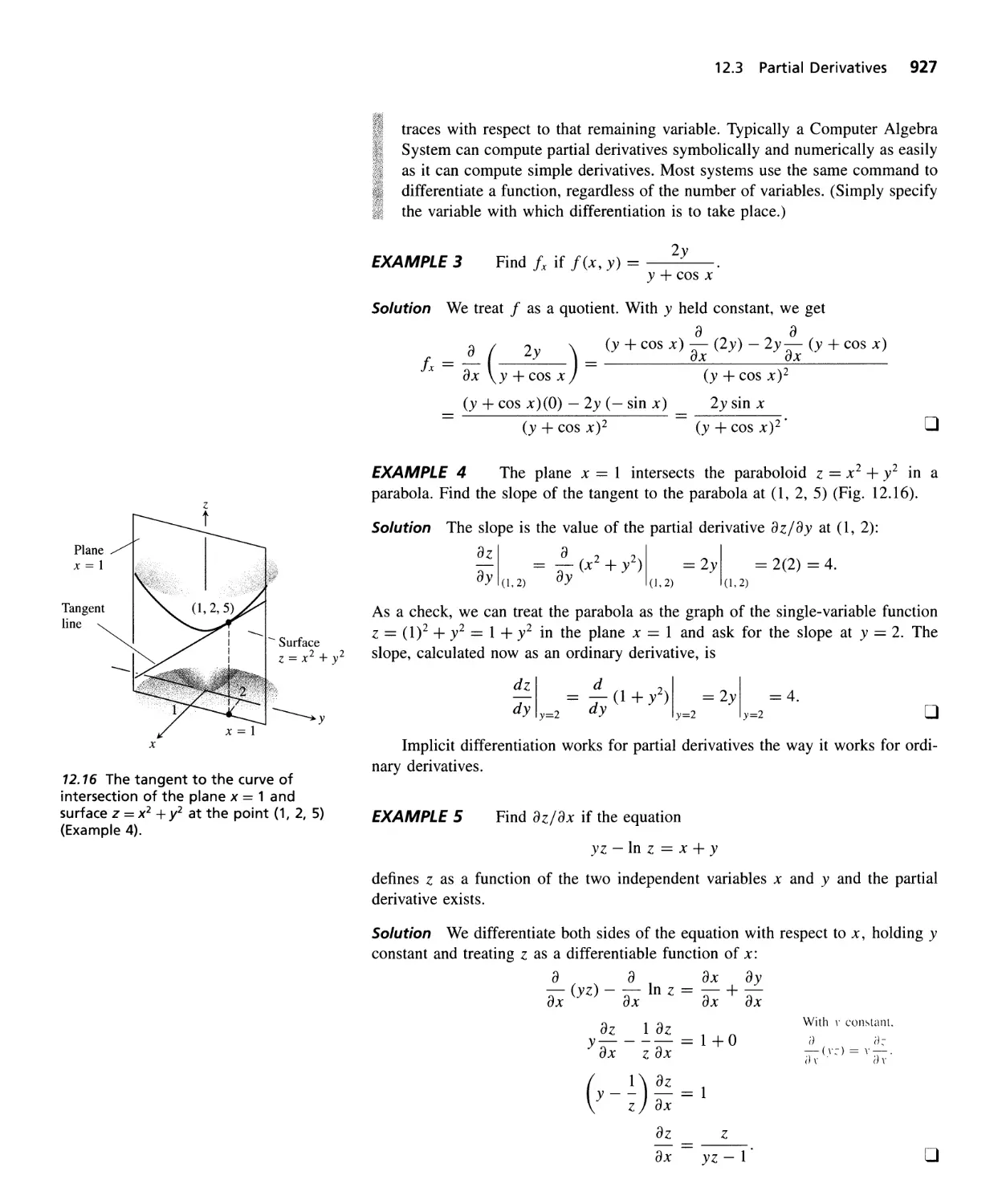
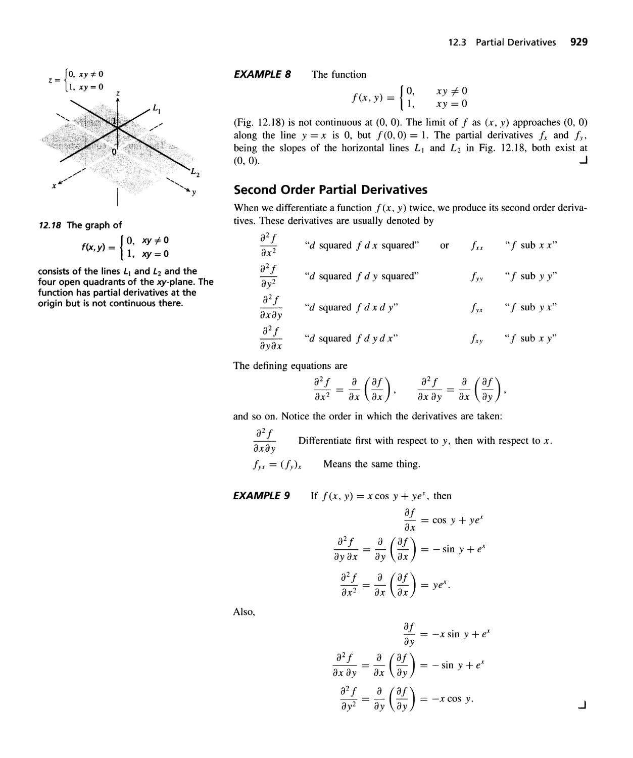
Partial Deri vati ves 924
Differentiability, Linearization, and Differentials 933
The Chain Rule 944
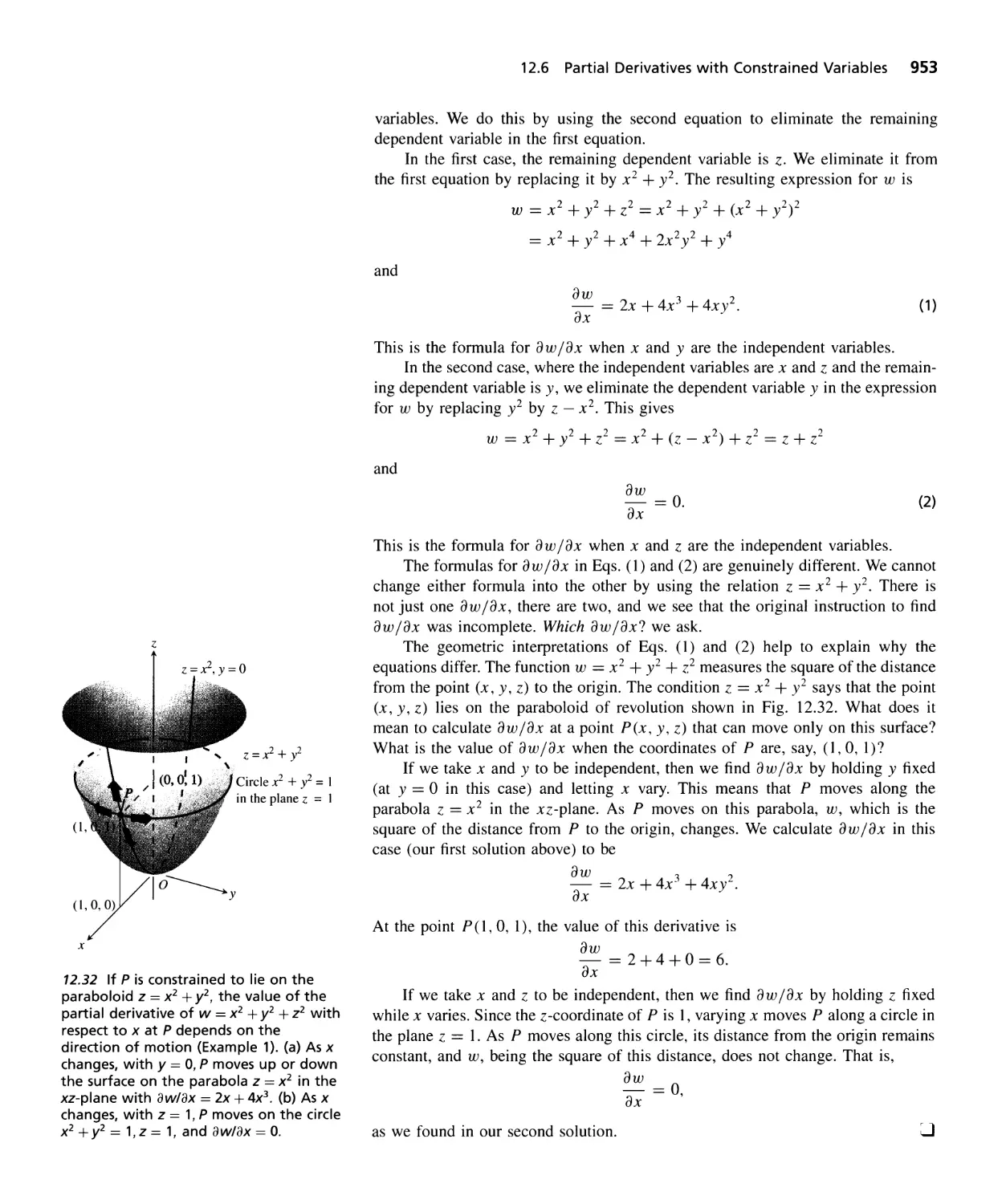
Partial Derivatives with Constrained Variables 952
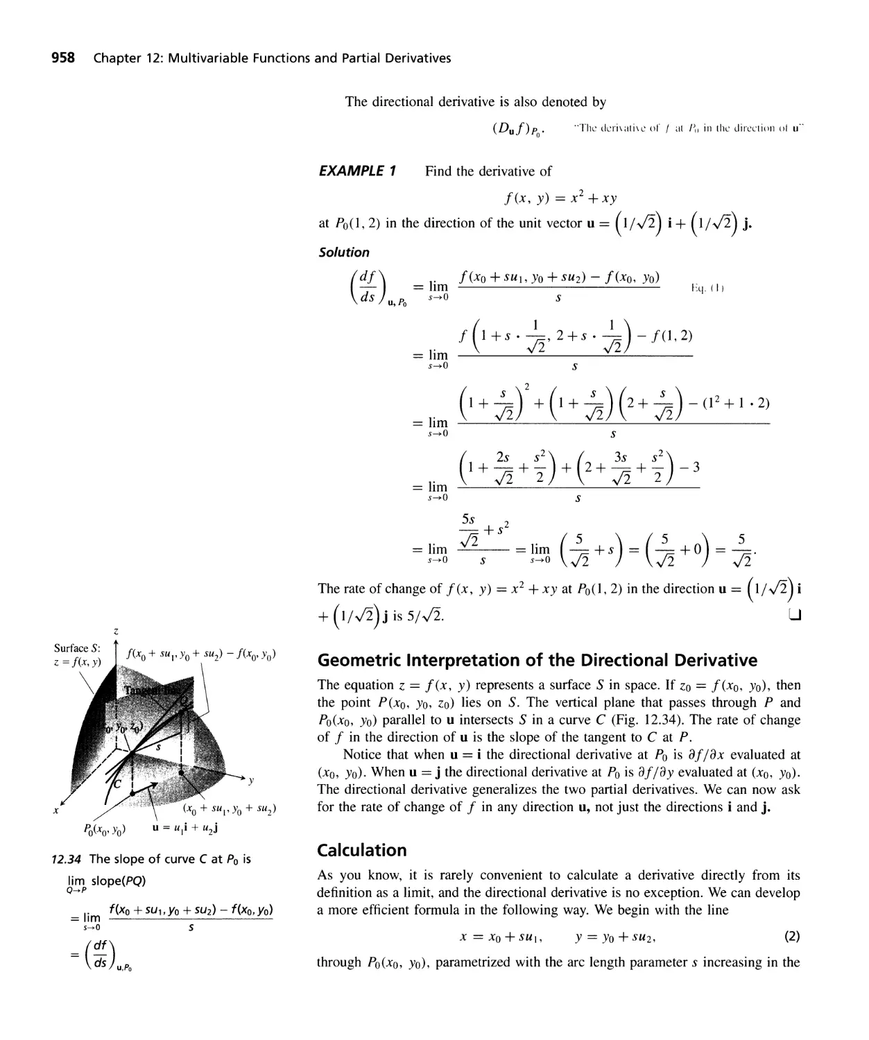
Directional Derivatives, Gradient Vectors, and Tangent Planes 957
Extreme Values and Saddle Points 970
Lagrange Multipliers 980
Taylor's Formula 989
QUESTIONS TO GUIDE YOUR REVIEW 993 PRACTICE EXERCISES 994
ADDITIONAL EXERCISES-THEORY, EXAMPLES, ApPLICATIONS 998
Double Integrals 1001
Areas, Moments, and Centers of Mass 1012
Double Integrals in Polar Form 1020
Triple Integrals in Rectangular Coordinates 1026
Masses and Moments in Three Dimensions 1034
Triple Integrals in Cylindrical and Spherical Coordinates 1039
Substitutions in Multiple Integrals 1048
QUESTIONS TO GUIDE YOUR REVIEW 1055 PRACTICE EXERCISES 1056
ADDITIONAL EXERCISES-THEORY, EXAMPLES, APPLICATIONS 1058
Line Integrals 1061
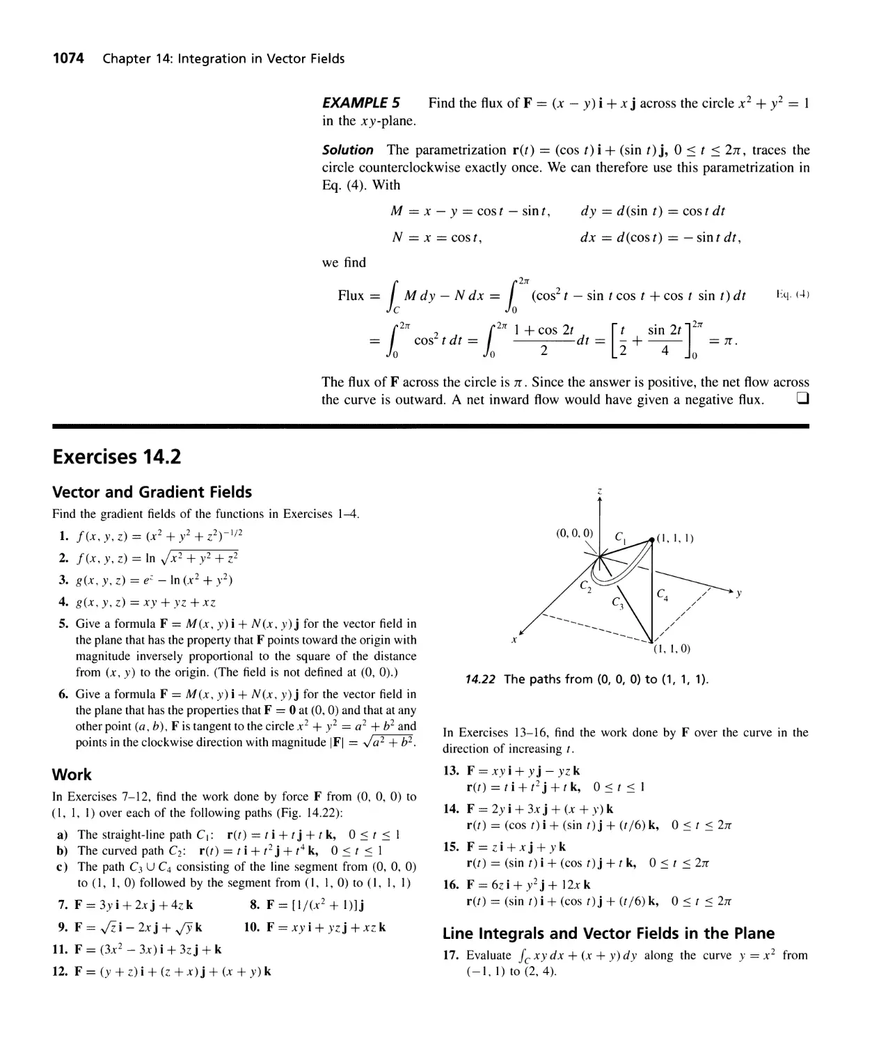
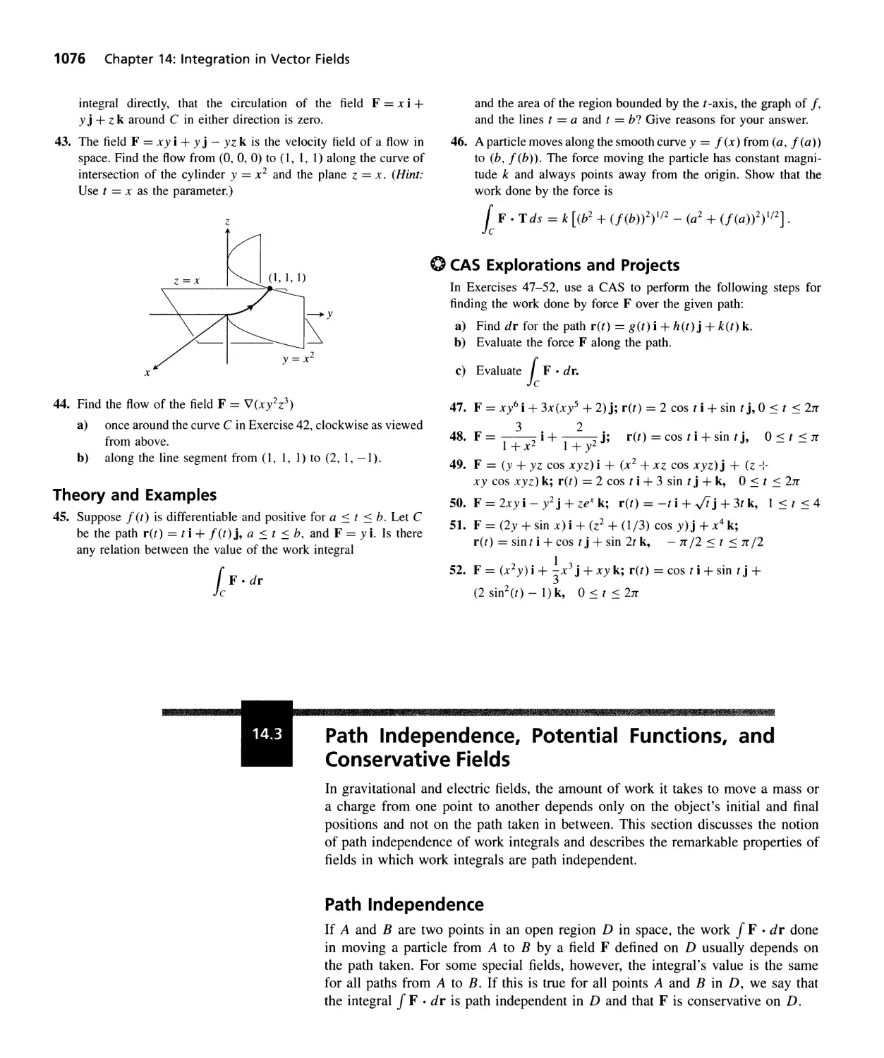
Vector Fields, Work, Circulation, and Flux 1067
Path Independence, Potential Functions, and Conservative Fields 1076
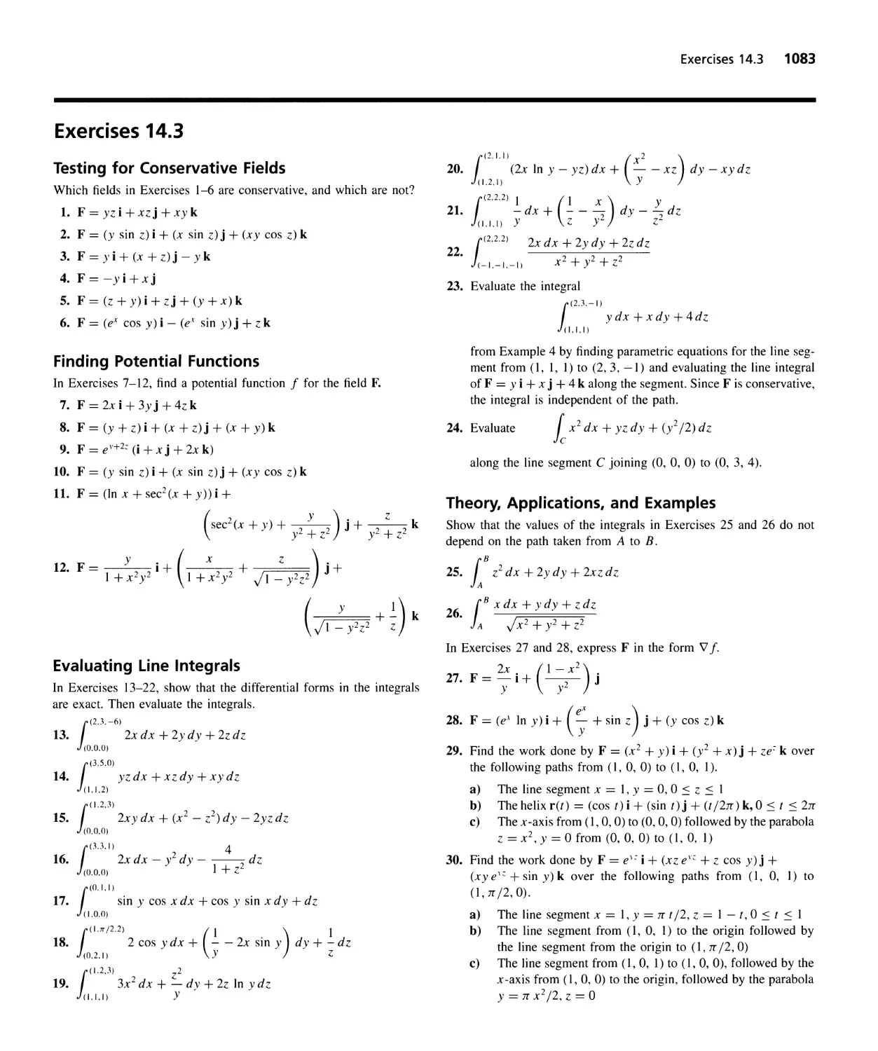
Green's Theorem in the Plane 1084 /
Surface Area and Surface Integrals 1096
Parametrized Surfaces 1106
Stokes's Theorem 1114
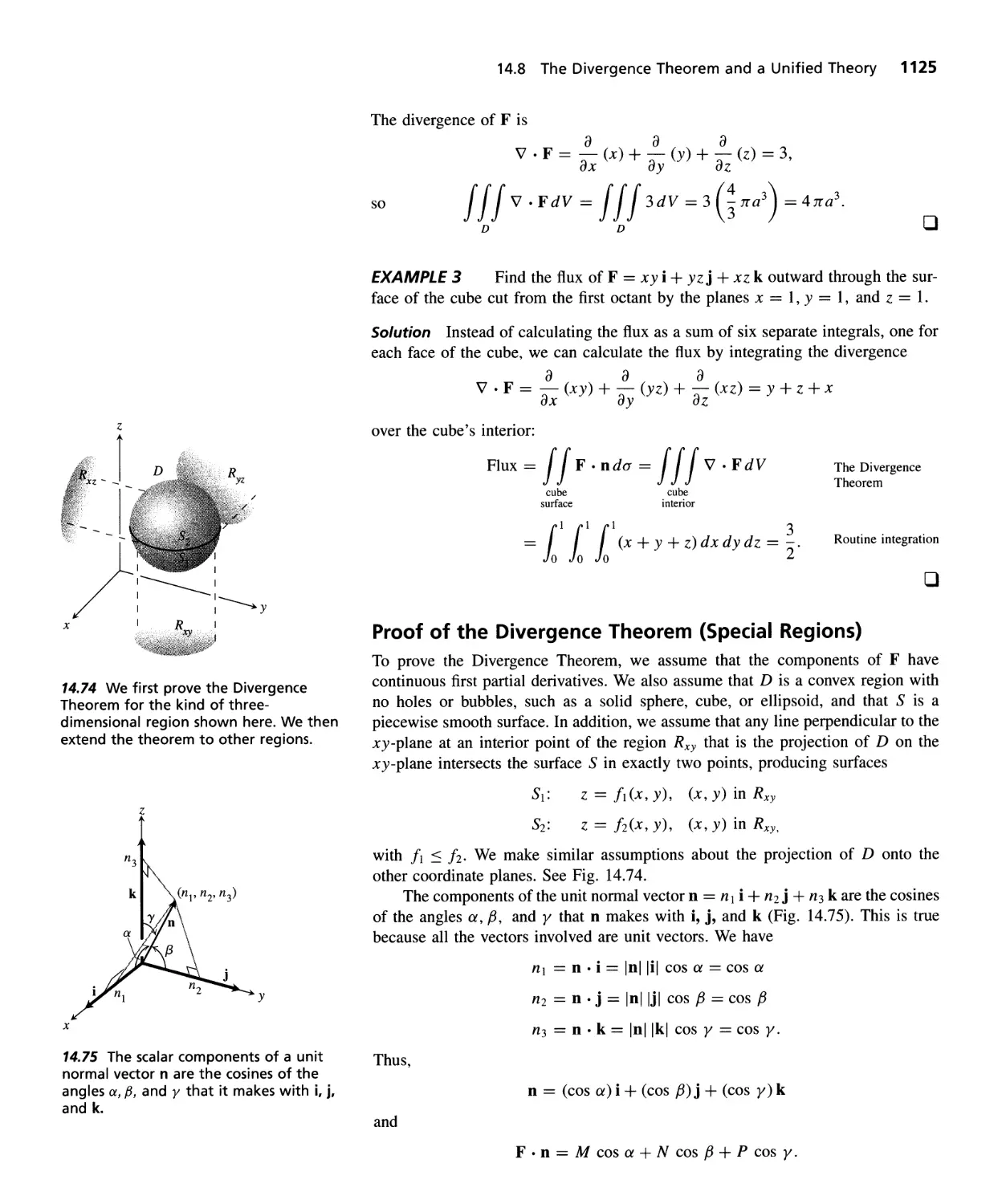
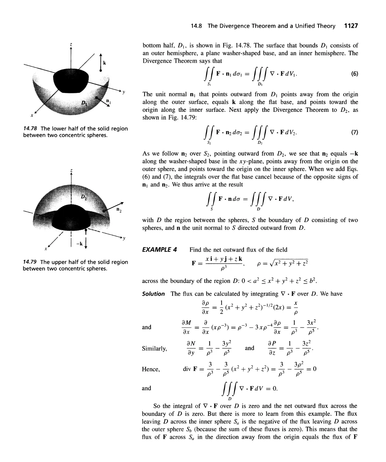
The Divergence Theorem and a Unified Theory 1123
QUESTIONS TO GUIDE YOUR REvIEW 1134
PRACTICE EXERCISES 1134 ADDITIONAL EXERCISES-THEORY,
EXAMPLES, ApPLICATIONS 1137
Mathematical Induction A-I
Proofs of Limit Theorems in Section 1.2 A-4
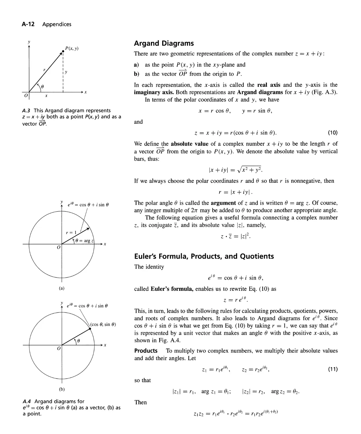
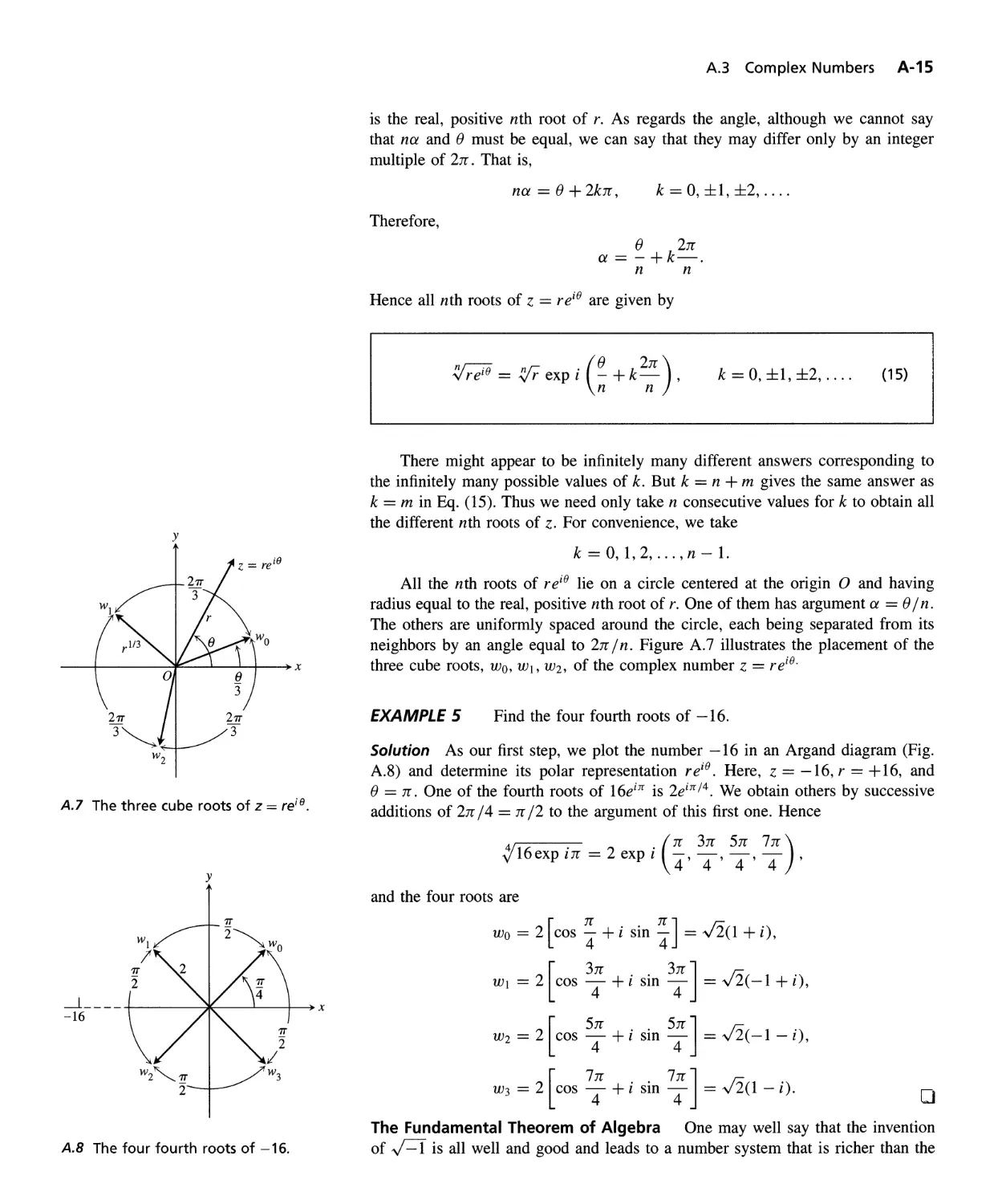
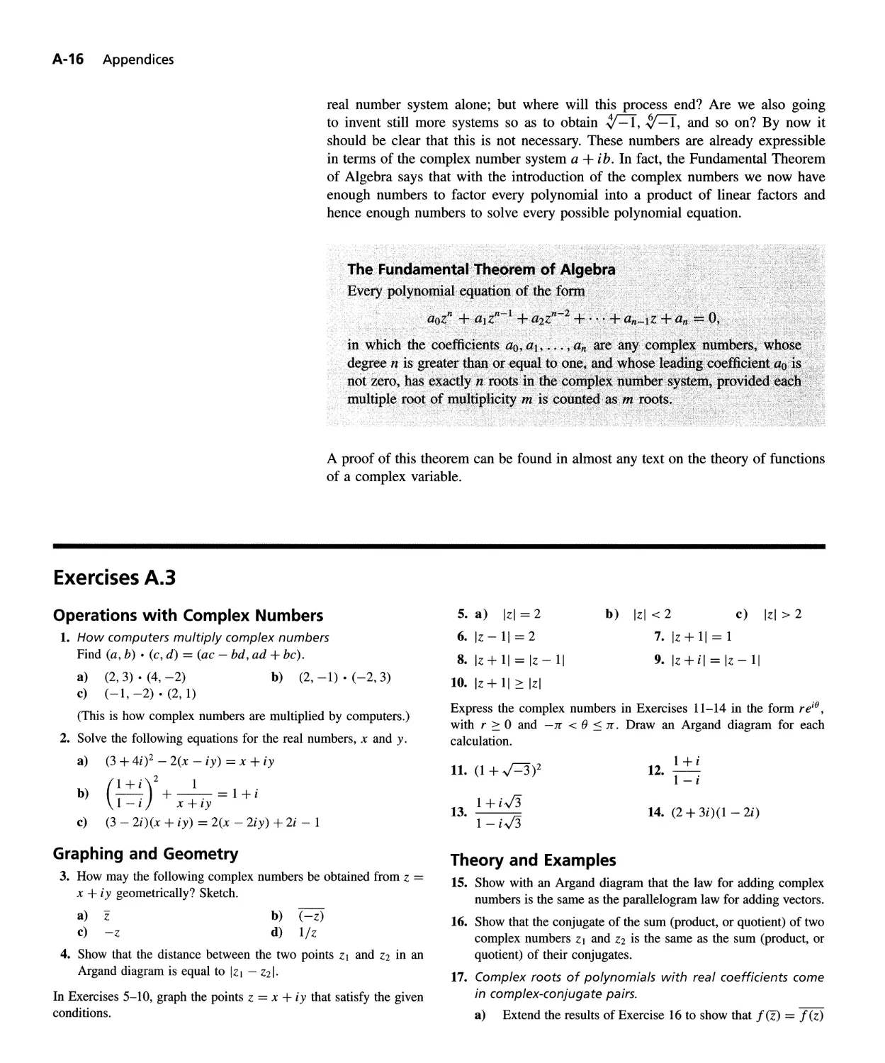
Complex Numbers A-7
Simpson' s One-Third Rule A -17
Cauchy's Mean Value Theorem and the Stronger Form of l'Hopital's Rule A-18
Limits That Arise Frequently A-20
The Distributive Law for Vector Cross Products A-21
Determinants and Cramer's Rule A-22
Euler's Theorem and the Increment Theorem A-29
Answers A-35
Index 1-1
A Brief Table of Integrals T-1
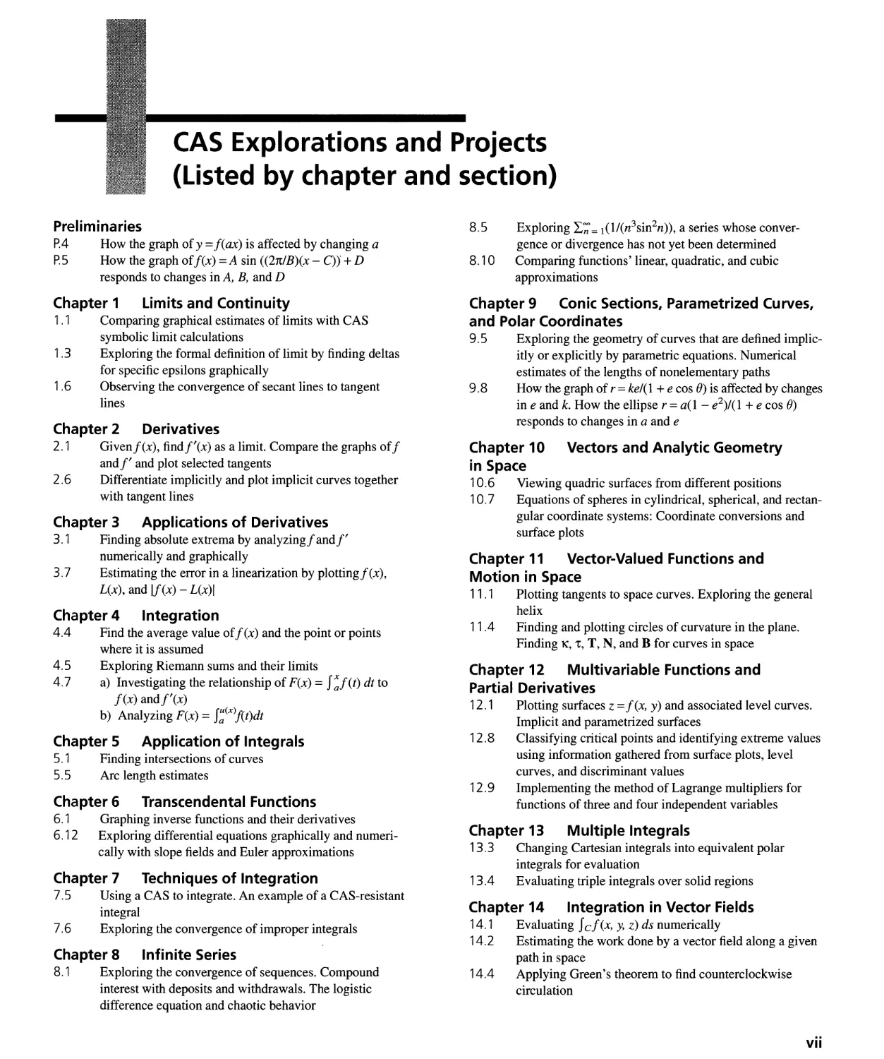
CAS Explorations and Projects
(Listed by chapter and section>
Preliminaries
P.4 How the graph of y = f(ax) is affected by changing a
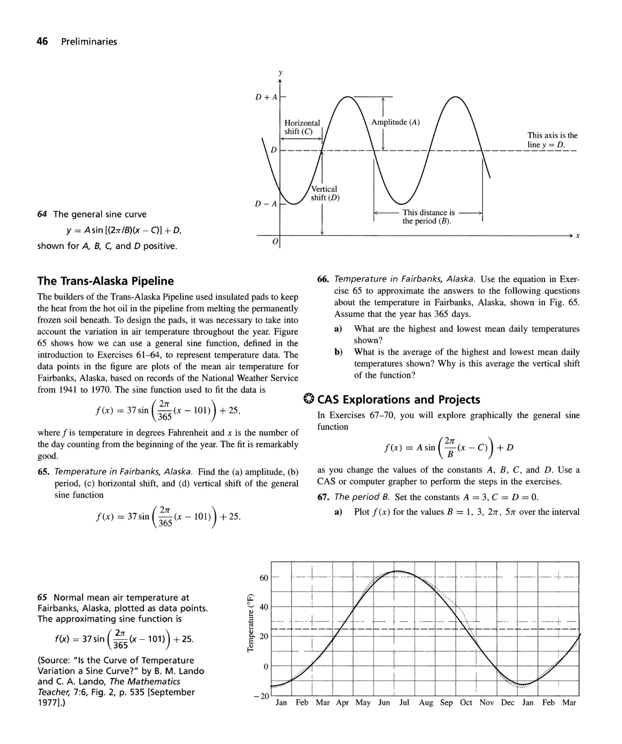
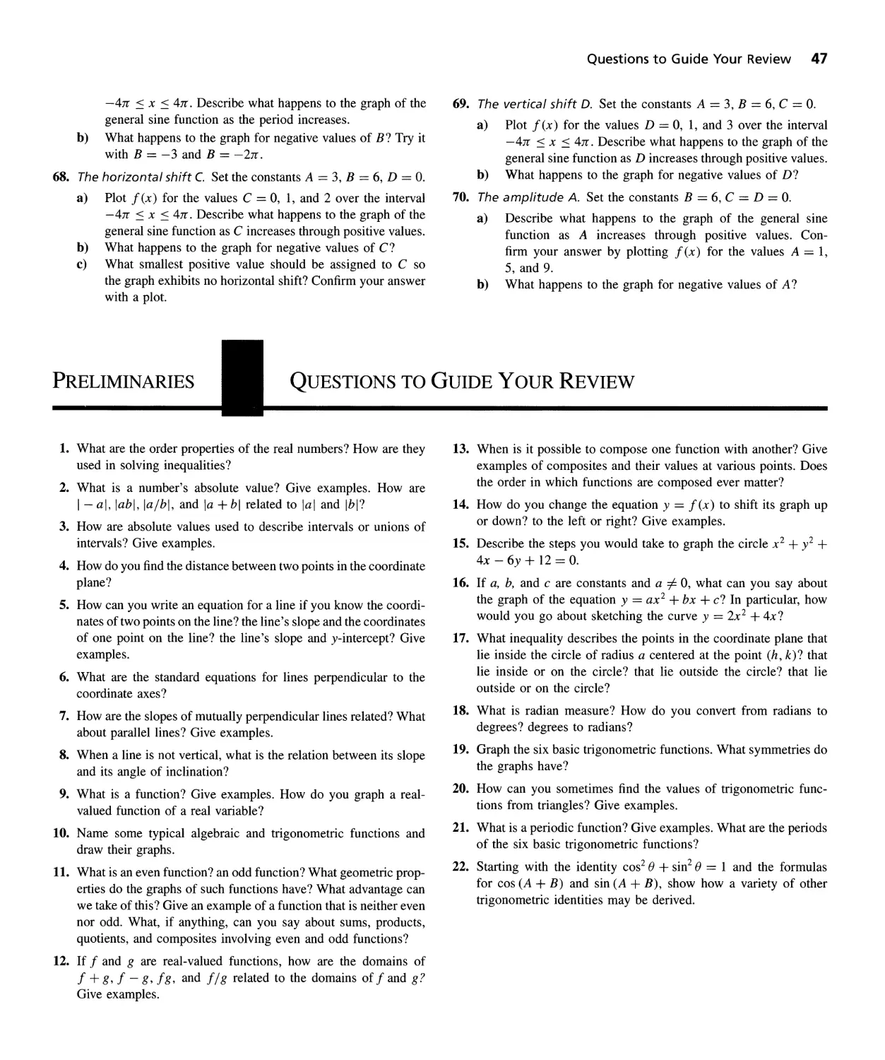
P.5 How the graph off(x) = A sin «2n/B)(x - C)) + D
responds to changes in A, B, and D
8.5 Exploring Ie; = 1(1/(n 3 sin 2 n)), a series whose conver-
gence or divergence has not yet been determined
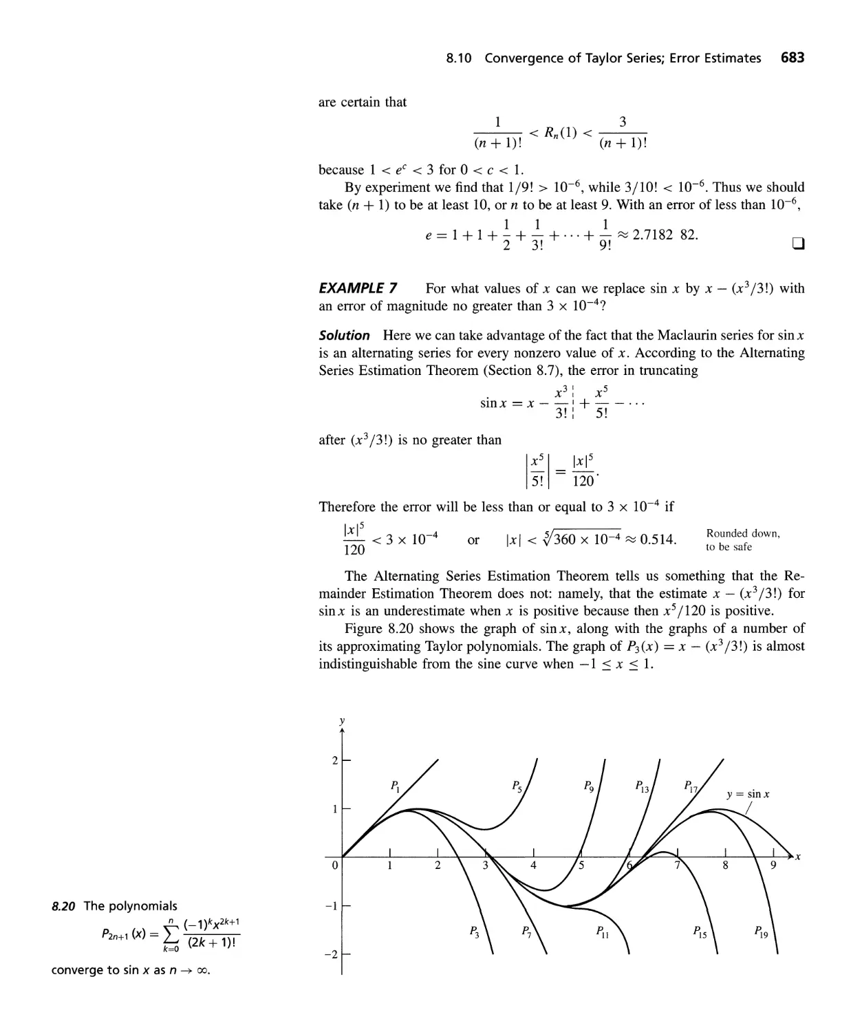
8.10 Comparing functions' linear, quadratic, and cubic
approximations
Chapter 1 limits and Continuity
1 . 1 Comparing graphical estimates of limits with CAS
symbolic limit calculations
1.3 Exploring the formal definition of limit by finding deltas
for specific epsilons graphically
1 .6 Observing the convergence of secant lines to tangent
lines
Chapter 9 Conic Sections, Parametrized Curves,
and Polar Coordinates
9.5 Exploring the geometry of curves that are defined implic-
itly or explicitly by parametric equations. Numerical
estimates of the lengths of nonelementary paths
9.8 How the graph of r = ke/( 1 + e cos ()) is affected by changes
in e and k. How the ellipse r = a( 1 - e 2 )/( 1 + e cos ())
responds to changes in a and e
Chapter 2 Derivatives
2.1 Givenf(x), findf'(x) as a limit. Compare the graphs off
and f' and plot selected tangents
2.6 Differentiate implicitly and plot implicit curves together
with tangent lines
Chapter 10 Vectors and Analytic Geometry
in Space
1 0.6 Viewing quadric surfaces from different positions
10.7 Equations of spheres in cylindrical, spherical, and rectan-
gular coordinate systems: Coordinate conversions and
surface plots
Chapter 3 Applications of Derivatives
3.1 Finding absolute extrema by analyzingf andf'
numerically and graphically
3.7 Estimating the error in a linearization by plottingf(x),
L(x), and If (x) - L(x)1
Chapter 4 Integration
4.4 Find the average value off (x) and the point or points
where it is assumed
4.5 Exploring Riemann sums and their limits
4.7 a) Investigating the relationship of F(x) = I f(t) dt to
f(x) andf'(x)
b) Analyzing F(x) = I;(X)f(t)dt
Chapter 5 Application of Integrals
5. 1 Finding intersections of curves
5.5 Arc length estimates
Chapter 11 Vector-Valued Functions and
Motion in Space
11.1 Plotting tangents to space curves. Exploring the general
helix
11.4 Finding and plotting circles of curvature in the plane.
Finding K, 't, T, N, and B for curves in space
Chapter 6 Transcendental Functions
6.1 Graphing inverse functions and their derivatives
6.12 Exploring differential equations graphically and numeri-
cally with slope fields and Euler approximations
Chapter 12 Multivariable Functions and
Partial Derivatives
1 2. 1 Plotting surfaces z = f (x, y) and associated level curves.
Implicit and parametrized surfaces
12.8 Classifying critical points and identifying extreme values
using information gathered from surface plots, level
curves, and discriminant values
12.9 Implementing the method of Lagrange multipliers for
functions of three and four independent variables
Chapter 7 Techniques of Integration
7.5 Using a CAS to integrate. An example of a CAS-resistant
integral
7.6 Exploring the convergence of improper integrals
Chapter 13 Multiple Integrals
13.3 Changing Cartesian integrals into equivalent polar
integrals for evaluation
13.4 Evaluating triple integrals over solid regions
Chapter 8 Infinite Series
8.1 Exploring the convergence of sequences. Compound
interest with deposits and withdrawals. The logistic
difference equation and chaotic behavior
Chapter 14 Integration in Vector Fields
14.1 Evaluating I cf(x, y, z) ds numerically
14.2 Estimating the work done by a vector field along a given
path in space
14.4 Applying Green's theorem to find counterclockwise
circulation
..
VII
To the Instructor
This Is a Major Revision
Throughout the 40 years that it has been in print, Thomas/Finney has been used to
support a variety of teaching methods from traditional to experimental. In response
to the many exciting currents in teaching calculus in the 1990s, the new edition is the
most extensive revision of Thomas/Finney ever. We have built on the traditional
strengths of the book-excellent exercises, sound mathematics, variety in applica-
tions-to produce a flexible text that contains all the elements needed to teach the
many different kinds of courses that exist today.
A book does not make a course: The instructor and the students do. With this in
mind we have added features to Thomas/Finney 9th edition to make it the most flex-
ible calculus teaching resource yet.
· The exercises have been reorganized to facilitate assigning a subset of the
material in a section.
· The grapher explorations, all accessible with any graphing calculator, many
suitable for in-class and group work, have been expanded.
· New Computer Algebra System (CAS) explorations and projects that re-
quire a CAS have been included. Some of these can be done quickly while
others require several hours. All are suitable for either individual or group
work. You will find a list of CAS exercise topics following the Table of
Contents.
· Technology Connection notes appear throughout the text suggesting experi-
ments students might do with a grapher to supplement their understanding
of a given topic. These notes are meant to encourage students to think of
their grapher as a casually available tool, like a pencil.
· We revised the entire first semester and large parts of the second and third
semesters to provide what we believe is a cleaner, more visual, and more ac-
cessible book.
With all these changes, we have not compromised our belief that the fundamental
goal of a calculus book is to prepare students to enter the scientific community.
viii
Students Will Find Even More Support for
Creative Problem Solving
Throughout this book, we have included examples and discussions that encourage
students to think visually and numerically. Almost every exercise set has easy to
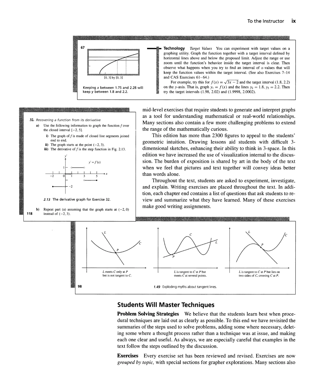
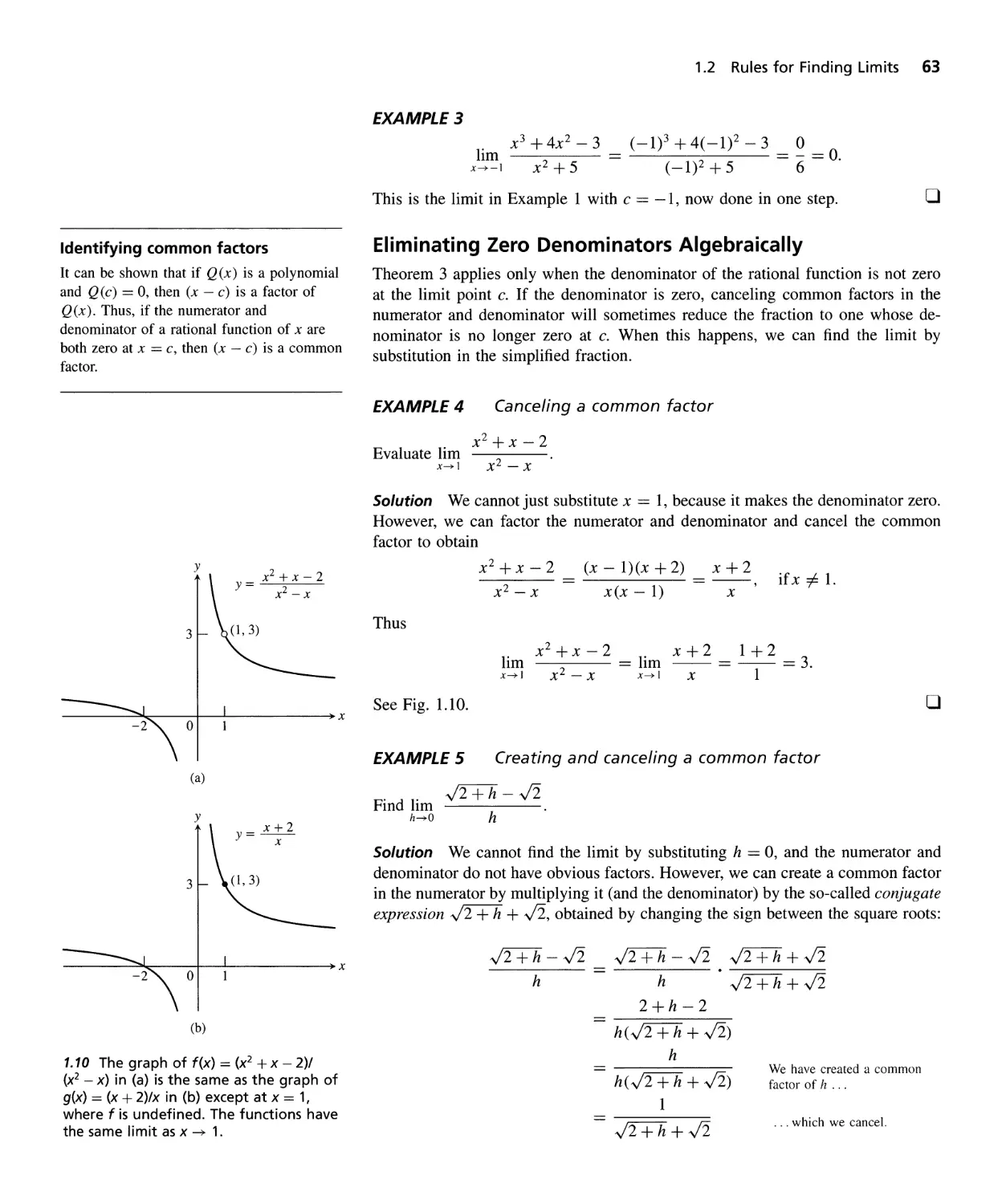
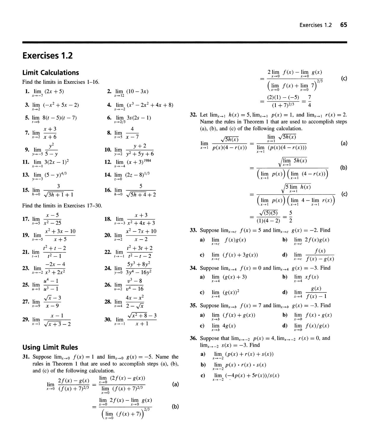
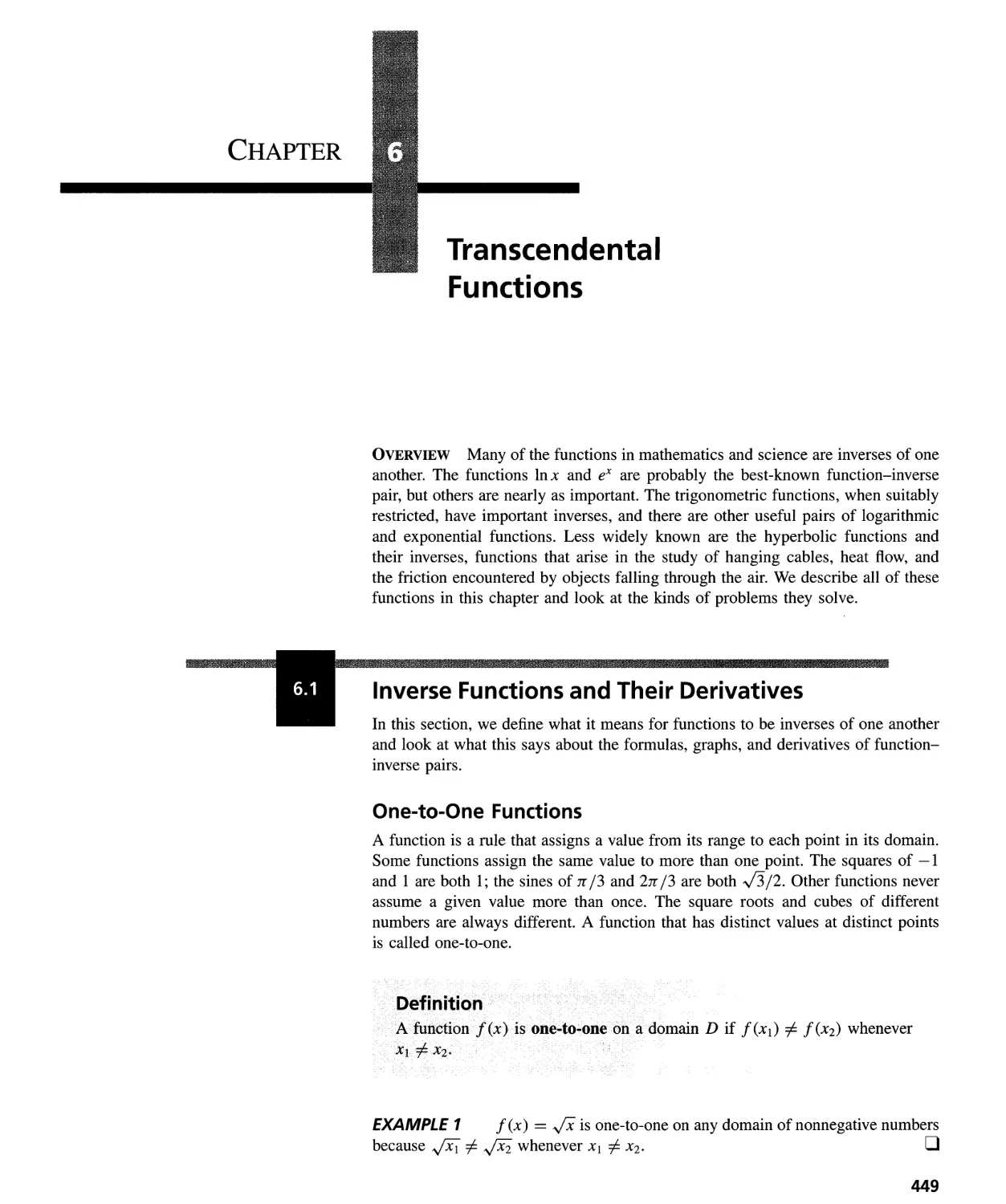
67
[0,3] by [0, 3]
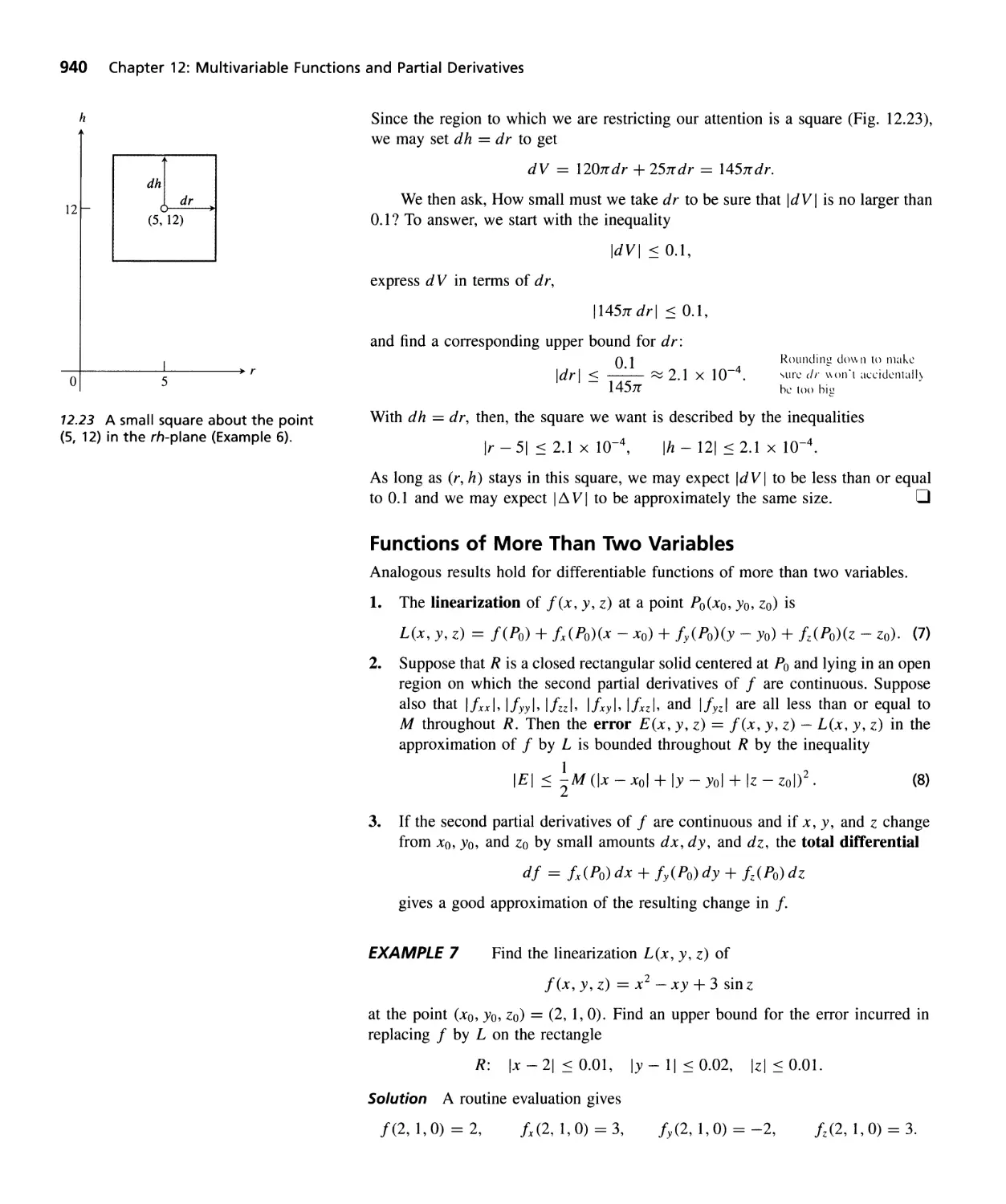
Keeping x between 1.75 and 2.28 will
keep y between 1.8 and 2.2.
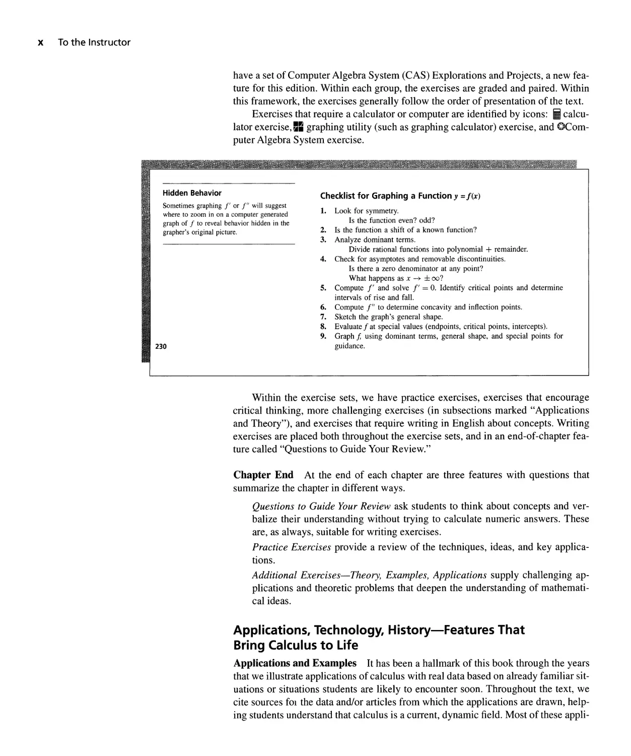
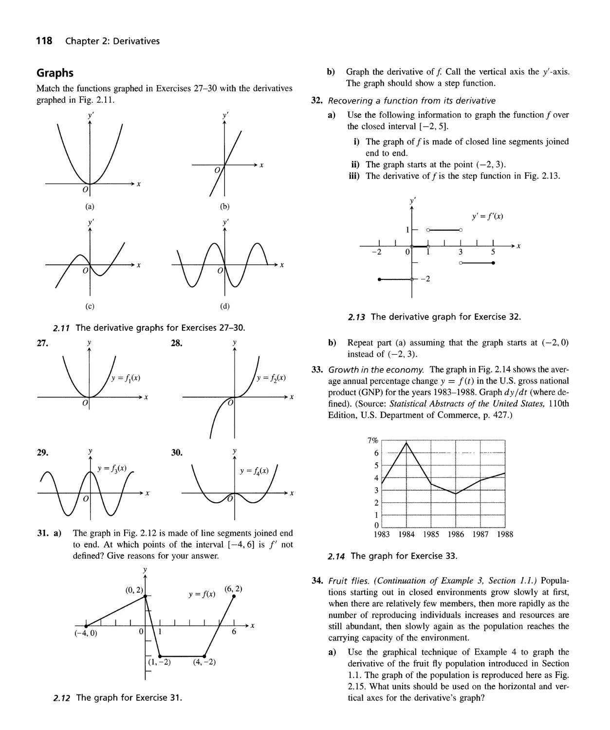
32. Recovering a function from its derivative
a) Use the following information to graph the function f over
the closed interval [-2,5].
i) The graph of f is made of closed line segments joined
end to end.
ii) The graph starts at the point (-2,3).
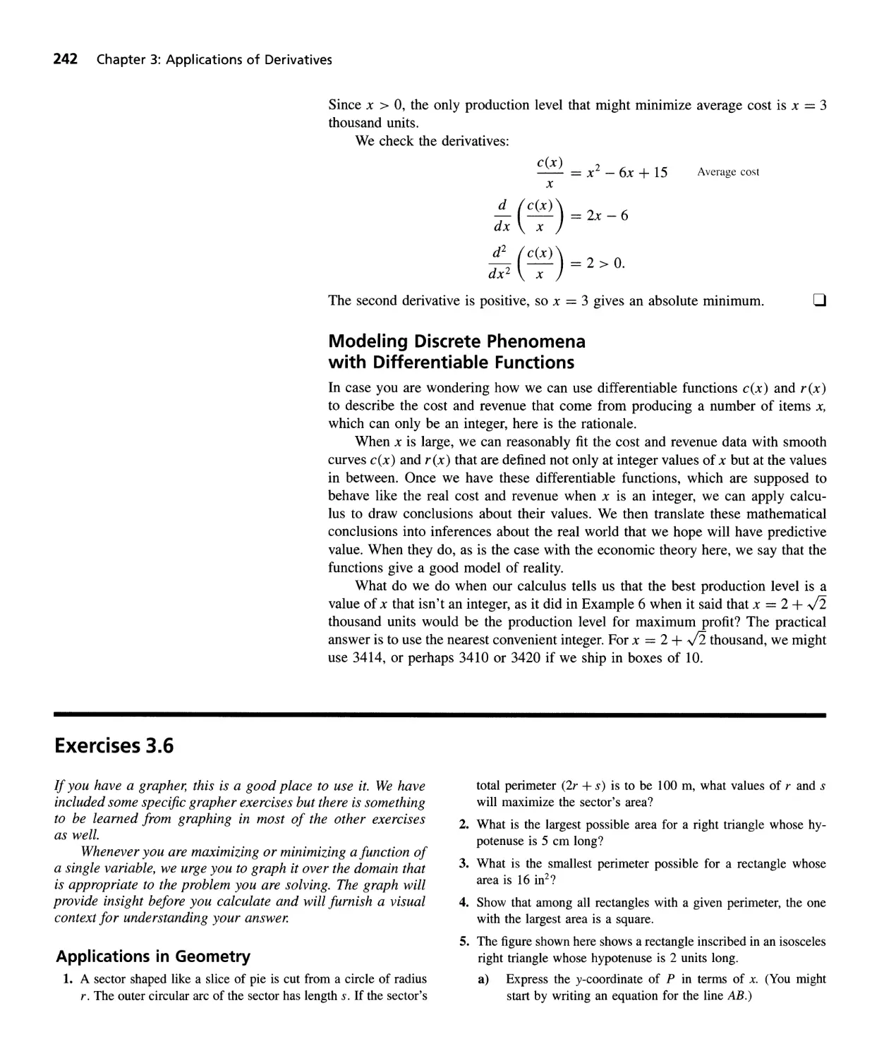
iii) The derivative of f is the step function in Fig. 2.13.
y ,
y' = J'{x)
C :J
x
-2 0 3 5
0 .
-2
2.13 The derivative graph for Exercise 32.
b) Repeat part (a) assuming that the graph starts at (-2,0)
118 instead of (-2, 3).
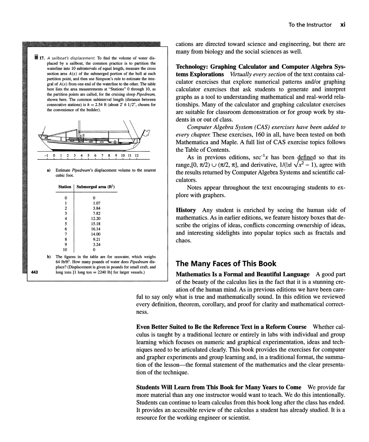
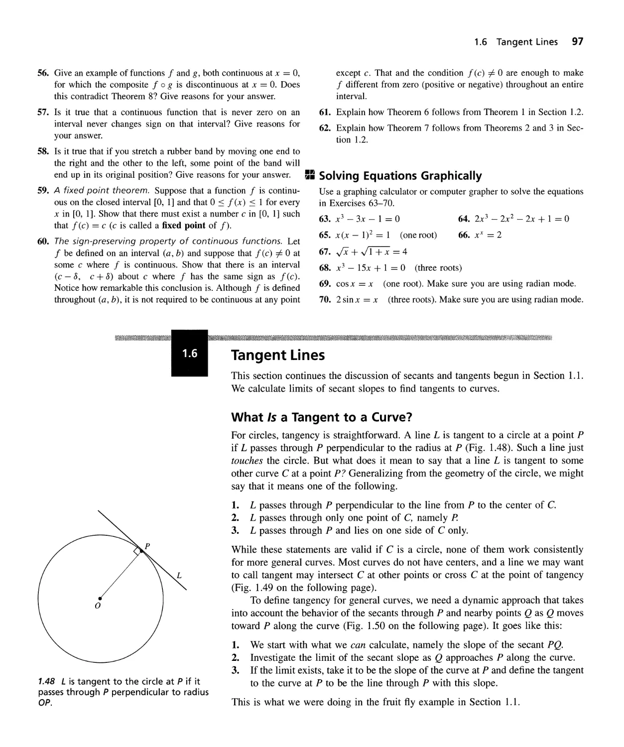
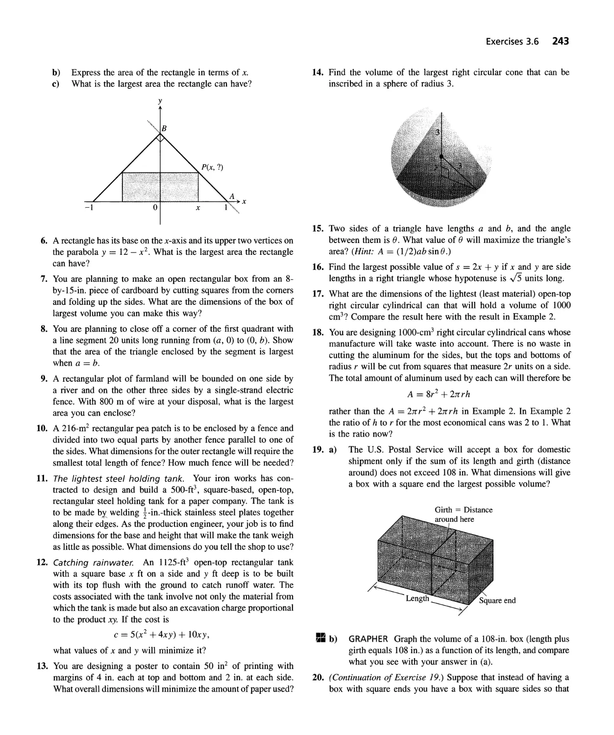
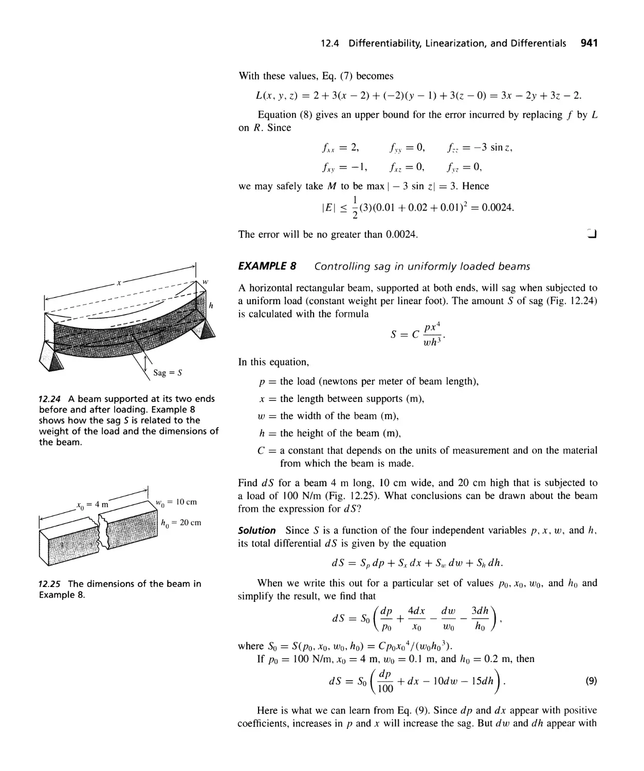
L meets C only at P
but is not tangent to C.
98
To the I nstructor IX
Technology Target Values You can experiment with target values on a
graphing utility. Graph the function together with a target interval defined by
horizontal lines above and below the proposed limit. Adjust the range or use
zoom until the function's behavior inside the target interval is clear. Then
observe what happens when you try to find an interval of x-values that will
keep the function values within the target interval. (See also Exercises 7-14
and CAS Exercises 61- 64.)
For example, try this for I (x) = .J 3x - 2 and the target interval (1.8, 2.2)
on the y-axis. That is, graph YI = I(x) and the lines Y2 = 1.8, Y3 = 2.2. Then
try the target intervals (1.98, 2.02) and (1.9998, 2.0002).
mid-level exercises that require students to generate and interpret graphs
as a tool for understanding mathematical or real-world relationships.
Many sections also contain a few more challenging problems to extend
the range of the mathematically curious.
This edition has more than 2300 figures to appeal to the students'
geometric intuition. Drawing lessons aid students with difficult 3-
dimensional sketches, enhancing their ability to think in 3-space. In this
edition we have increased the use of visualization internal to the discus-
sion. The burden of exposition is shared by art in the body of the text
when we feel that pictures and text together will convey ideas better
than words alone.
Throughout the text, students are asked to experiment, investigate,
and explain. Writing exercises are placed throughout the text. In addi-
tion, each chapter end contains a list of questions that ask students to re-
view and summarize what they have learned. Many of these exercises
make good writing assignments.
C
L is tangent to Cat P but
meets C at several points.
L is tangent to C at P but lies on
two sides of C, crossing Cat P.
1.49 Exploding myths about tangent lines.
Students Will Master Techniques
Problem Solving Strategies We believe that the students learn best when proce-
dural techniques are laid out as clearly as possible. To this end we have revisited the
summaries of the steps used to solve problems, adding some where necessary, delet-
ing some where a thought process rather than a technique was at issue, and making
each one clear and useful. As always, we are especially careful that examples in the
text follow the steps outlined by the discussion.
Exercises Every exercise set has been reviewed and revised. Exercises are now
grouped by topic, with special sections for grapher explorations. Many sections also
x To the Instructor
have a set of Computer Algebra System (CAS) Explorations and Projects, a new fea-
ture for this edition. Within each group, the exercises are graded and paired. Within
this framework, the exercises generally follow the order of presentation of the text.
Exercises that require a calculator or computer are identified by icons: it calcu-
lator exercise, == graphing utility (such as graphing calculator) exercise, and OCom-
puter Algebra System exercise.
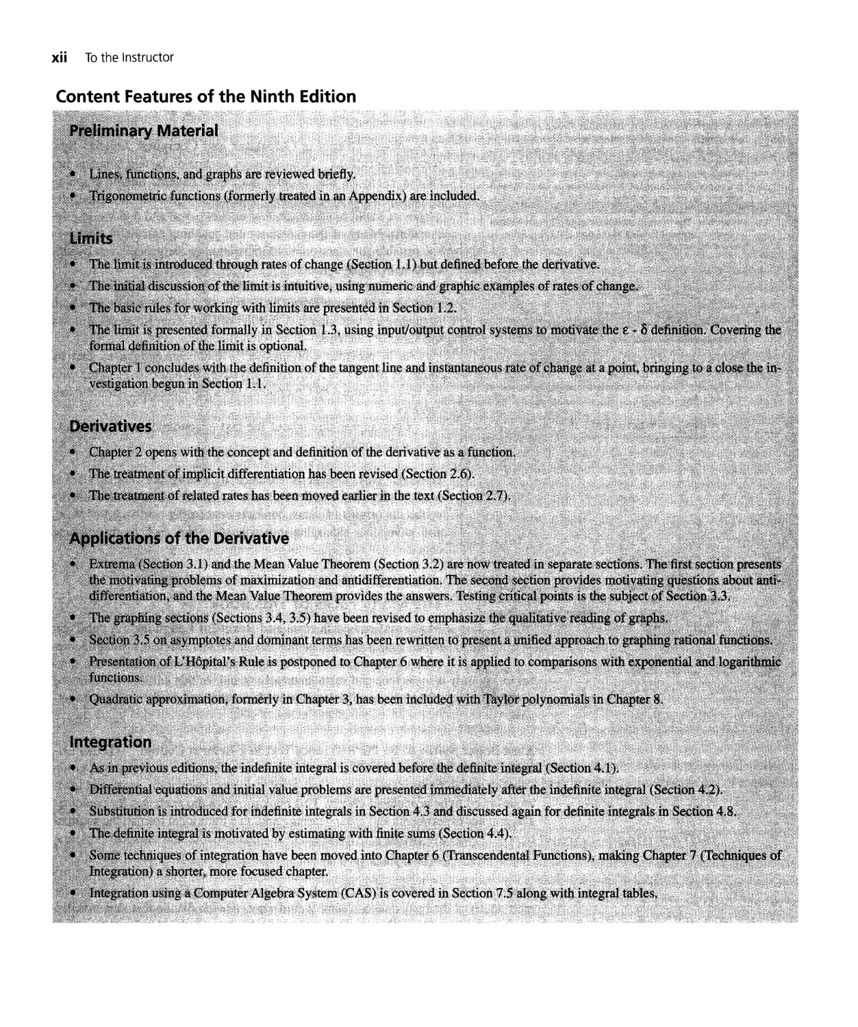
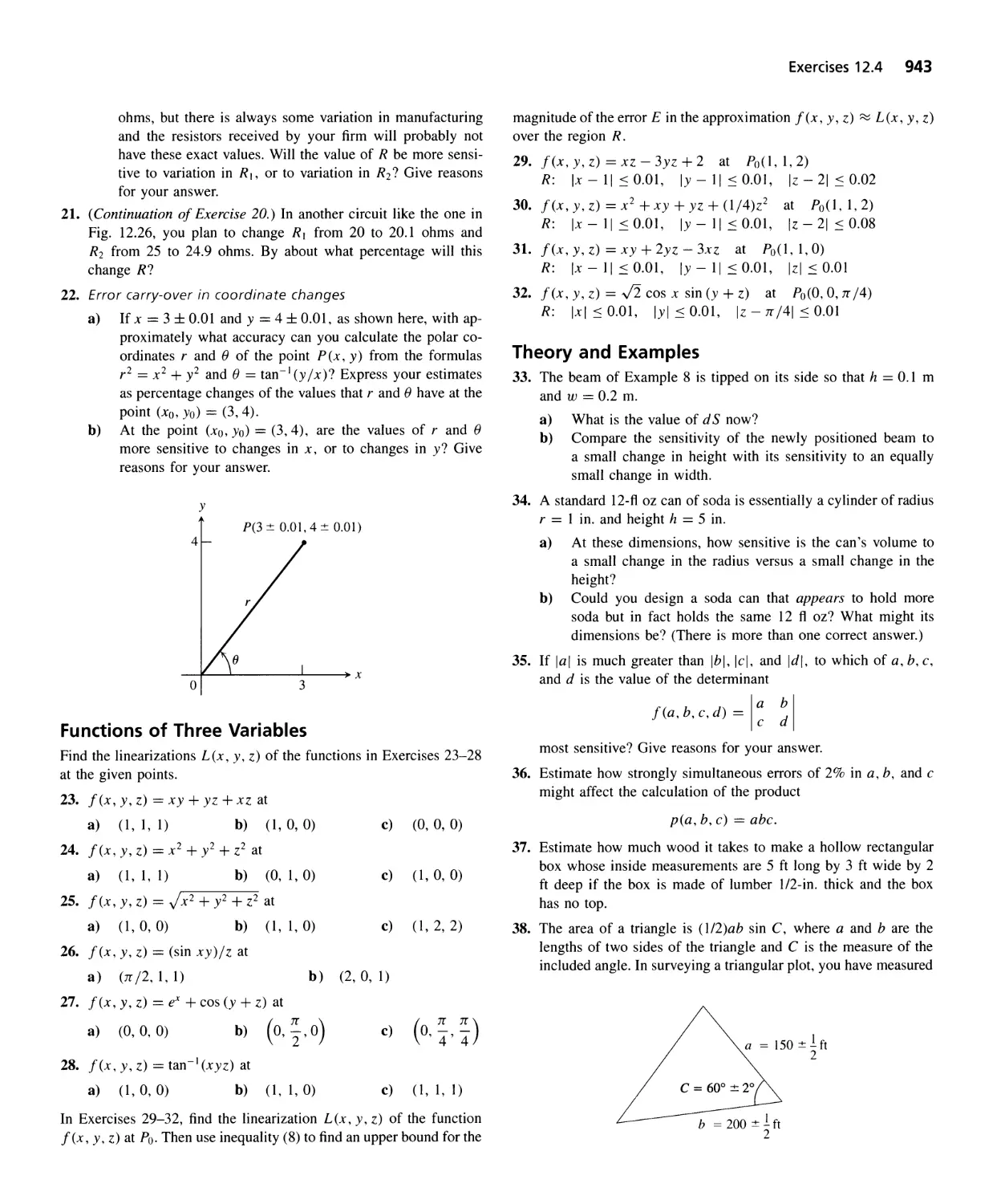
Hidden Behavior
Checklist for Graphing a Function y = f(x)
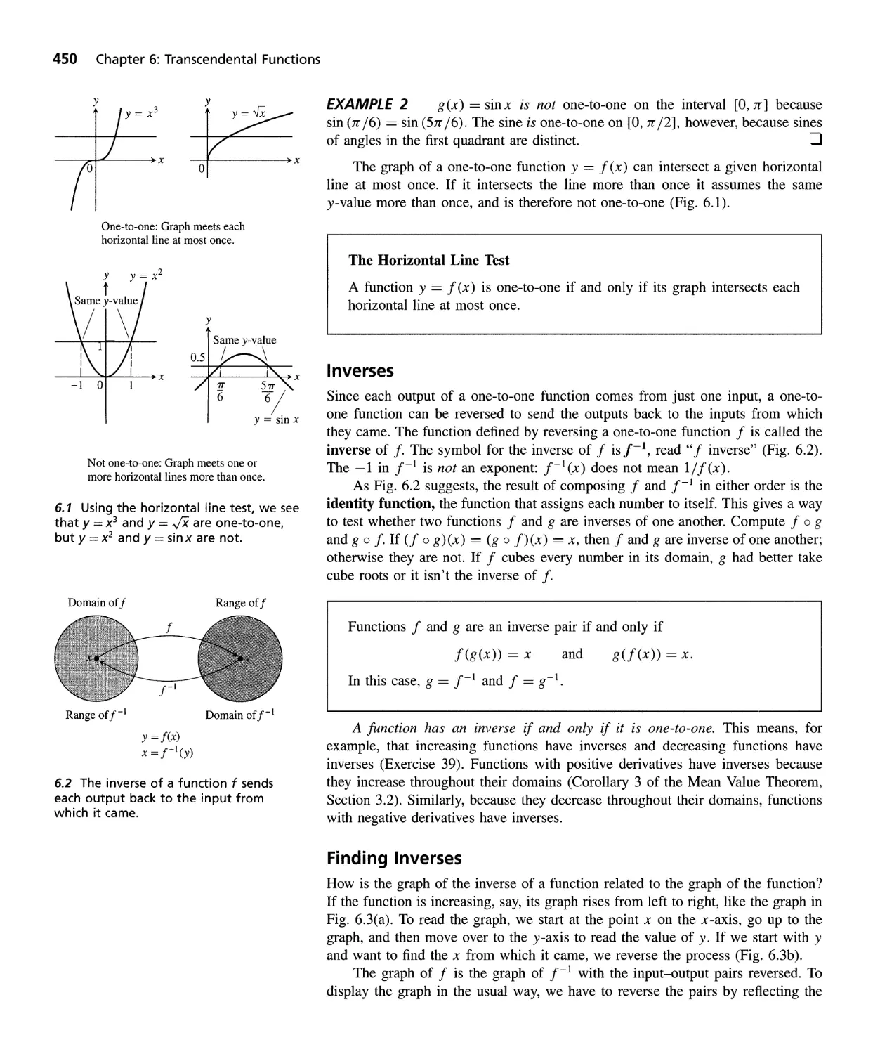
1. Look for symmetry.
Is the function even? odd?
2. Is the function a shift of a known function?
3. Analyze dominant terms.
Divide rational functions into polynomial + remainder.
4. Check for asymptotes and removable discontinuities.
Is there a zero denominator at any point?
What happens as x --+ :i: oo?
5. Compute I' and solve I' = O. Identify critical points and determine
intervals of rise and fall.
6. Compute I" to determine concavity and inflection points.
7. Sketch the graph's general shape.
8. Evaluate I at special values (endpoints, critical points, intercepts).
9. Graph f, using dominant terms, general shape, and special points for
guidance.
Sometimes graphing f' or I" will suggest
where to zoom in on a computer generated
graph of f to reveal behavior hidden in the
grapher's original picture.
Within the exercise sets, we have practice exercises, exercises that encourage
critical thinking, more challenging exercises (in subsections marked "Applications
and Theory"), and exercises that require writing in English about concepts. Writing
exercises are placed both throughout the exercise sets, and in an end-of-chapter fea-
ture called "Questions to Guide Your Review."
Chapter End At the end of each chapter are three features with questions that
summarize the chapter in different ways.
Questions to Guide Your Review ask students to think about concepts and ver-
balize their understanding without trying to calculate numeric answers. These
are, as always, suitable for writing exercises.
Practice Exercises provide a review of the techniques, ideas, and key applica-
ti on s.
Additional Exercises-Theory, Examples, Applications supply challenging ap-
plications and theoretic problems that deepen the understanding of mathemati-
cal ideas.
Applications, Technology, History-Features That
Bring Calculus to Life
Applications and Examples It has been a hallmark of this book through the years
that we illustrate applications of calculus with real data based on already familiar sit-
uations or situations students are likely to encounter soon. Throughout the text, we
cite sources fOl the data and/or articles from which the applications are drawn, help-
ing students understand that calculus is a current, dynamic field. Most of these appli-
To the I nstructor xi
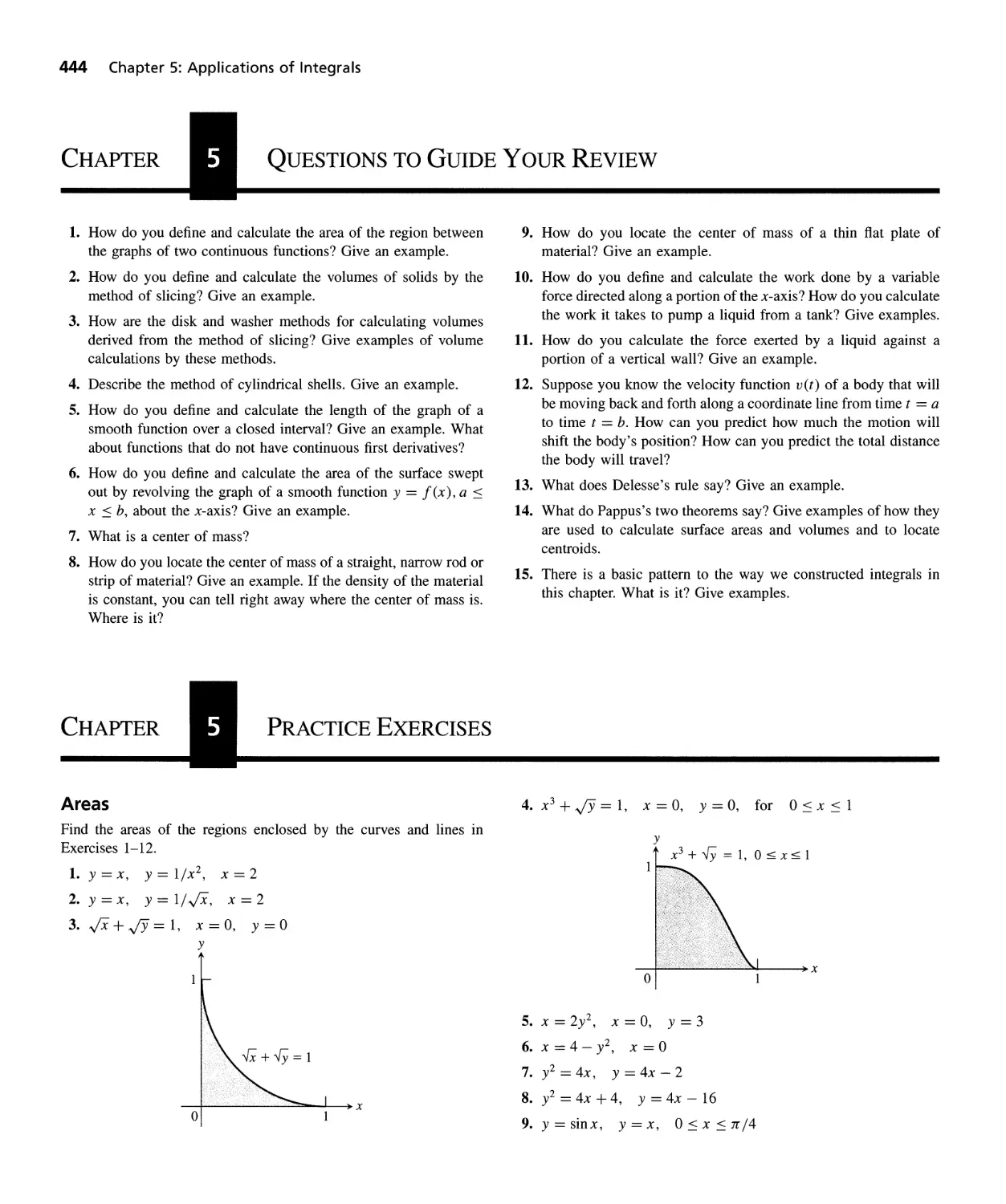
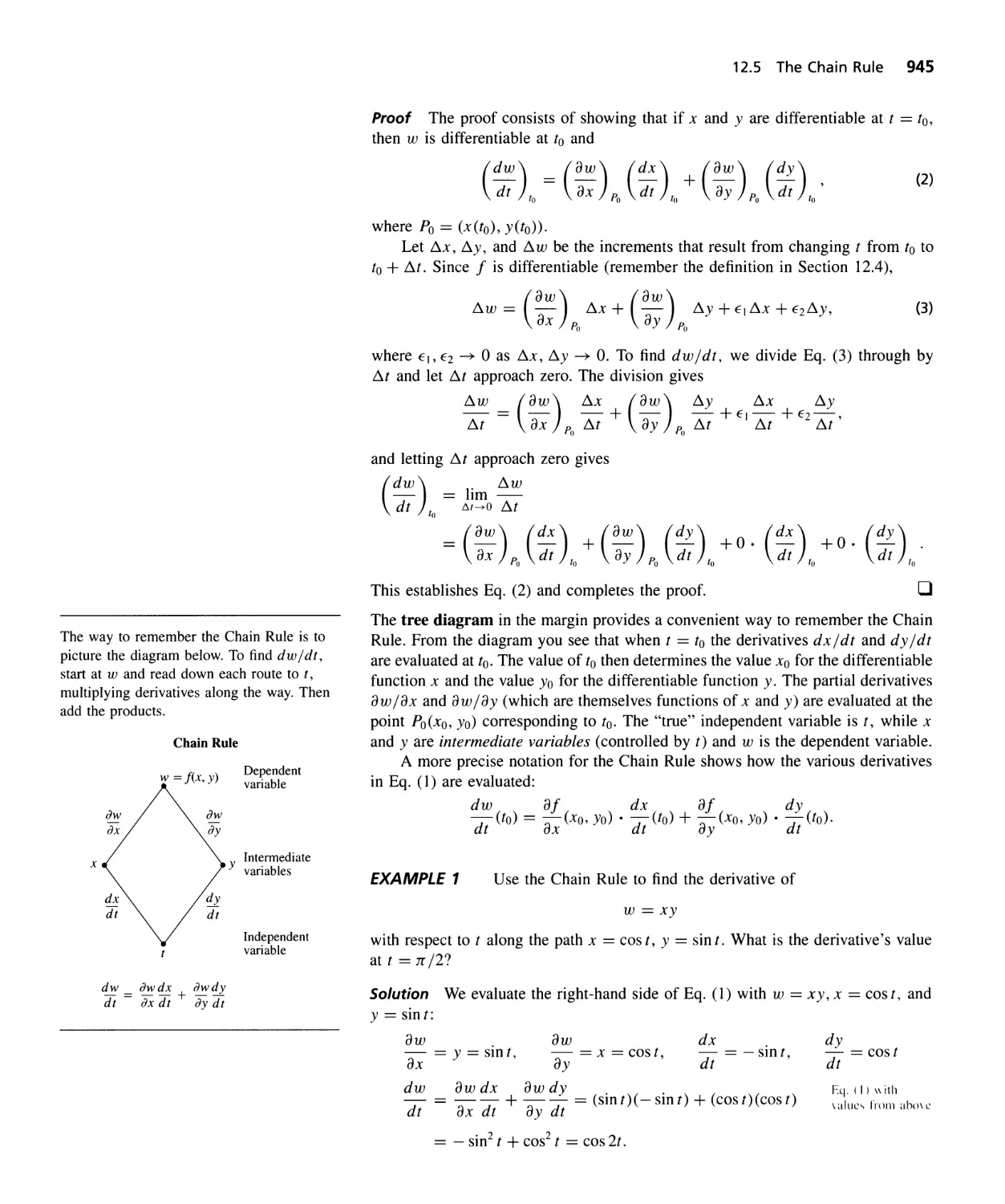
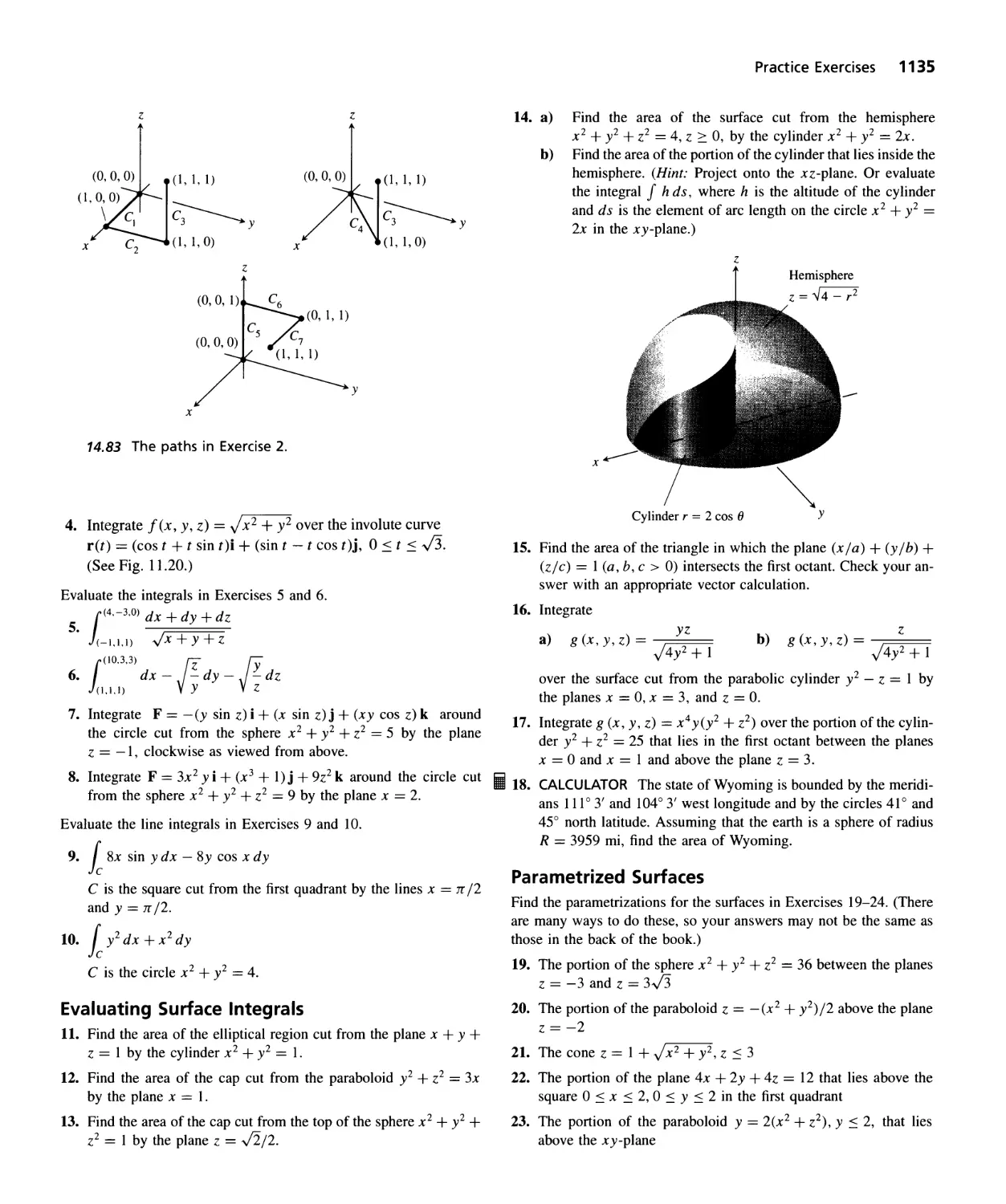
Ii 17. A sailboat's displacement. To find the volume of water dis-
placed by a sailboat, the common practice is to partition the
waterline into 10 subintervals of equal length, measure the cross
section area A (x) of the submerged portion of the hull at each
partition point, and then use Simpson's rule to estimate the inte-
gral of A(x) from one end of the waterline to the other. The table
here lists the area measurements at "Stations" 0 through 10, as
the partition points are called, for the cruising sloop Pipedream,
shown here. The common subinterval length (distance between
consecutive stations) is h = 2.54 ft (about 2' 6 1/2", chosen for
the convenience of the builder).
cations are directed toward science and engineering, but there are
many from biology and the social sciences as well.
Technology: Graphing Calculator and Computer Algebra Sys-
tems Explorations Virtually every section of the text contains cal-
culator exercises that explore numerical patterns and/or graphing
calculator exercises that ask students to generate and interpret
graphs as a tool to understanding mathematical and real-world rela-
tionships. Many of the calculator and graphing calculator exercises
are suitable for classroom demonstration or for group work by stu-
dents in or out of class.
Computer Algebra System (CAS) exercises have been added to
every chapter. These exercises, 160 in all, have been tested on both
Mathematica and Maple. A full list of CAS exercise topics follows
the Table of Contents.
As in previous editions, sec-Ix has been define d so that its
range,[O, n/2) u (n/2, n], and derivative, 1/(lxl .J x 2 - 1), agree with
the results returned by Computer Algebra Systems and scientific cal-
culators.
Notes appear throughout the text encouraging students to ex-
plore with graphers.
<:::> <:::>
-1 0 1 2 3 4 5 6 7 8 9 10 11 12
I I I I I I I I I I I I I I
a) Estimate Pipedream's displacement volume to the nearest
cubic foot.
Station Submerged area (ft 2 )
o 0
1 1.07
2 3.84
3 7.82
4 12.20
5 15.18
6 16.14
7 14.00
8 9.21
9 3.24
10 0
History Any student is enriched by seeing the human side of
mathematics. As in earlier editions, we feature history boxes that de-
scribe the origins of ideas, conflicts concerning ownership of ideas,
and interesting sidelights into popular topics such as fractals and
chaos.
443
b) The figures in the table are for seawater, which weighs
64 Ib/ft 3 . How many pounds of water does Pipedream dis-
place? (Displacement is given in pounds for small craft, and
long tons [1 long ton = 2240 lb] for larger vessels.)
The Many Faces of This Book
Mathematics Is a Formal and Beautiful Language A good part
of the beauty of the calculus lies in the fact that it is a stunning cre-
ation of the human mind. As in previous editions we have been care-
ful to say only what is true and mathematically sound. In this edition we reviewed
every definition, theorem, corollary, and proof for clarity and mathematical correct-
ness.
Even Better Suited to Be the Reference Text in a Reform Course Whether cal-
culus is taught by a traditional lecture or entirely in labs with individual and group
learning which focuses on numeric and graphical experimentation, ideas and tech-
niques need to be articulated clearly. This book provides the exercises for computer
and grapher experiments and group learning and, in a traditional format, the summa-
tion of the lesson-the formal statement of the mathematics and the clear presenta-
tion of the technique.
Students Will Learn from This Book for Many Years to Come We provide far
more material than anyone instructor would want to teach. We do this intentionally.
Students can continue to learn calculus from this book long after the class has ended.
It provides an accessible review of the calculus a student has already studied. It is a
resource for the working engineer or scientist.
xii To the Instructor
Content Features of the Ninth Edition
To the Instructor xiii
Supplements for the Instructor
OmniTest 3 in DOS-Based Format: This easy-to-use software is developed ex-
clusively for Addison-Wesley by ips Publishing, a leader in computerized testing
and assessment. Among its features are the following.
· DOS interface is easy to learn and operate. The windows look-alike inter-
face makes it easy to choose and control the items as well as the format for
each test.
· You can easily create make-up exams, customized homework assign-
ments, and multiple test forms to prevent plagiarism. OmniTest 3 is
xiv To the Instructor
algorithm driven-meaning the program can automatically insert new num-
bers into the same equation-creating hundreds of variations of that equa-
tion. The numbers are constrained to keep answers reasonable. This allows
you to create a virtually endless supply of parallel versions of the same test.
This new version of OmniTest also allows you to "lock in" the values shown
in the model problem, if you wish.
. Test items are keyed by section to the text. Within the section, you can se-
lect questions that test individual objectives from that section.
· You can enter your own questions by way of OmniTest 3 ,s sophisticated
editor-complete with mathematical notation.
Instructor's Solutions Manual by Maurice D. Weir (Naval Postgraduate School).
This two-volume supplement contains the worked-out solutions for all the exercises
in the text.
Answer Book contains short answers to most exercises in the text.
Supplements for the Instructor and Student
Student Study Guide by Maurice D. Weir (Naval Postgraduate School). Orga-
nized to correspond with the text, this workbook in a semi programmed format in-
creases student proficiency with study tips and additional practice.
Student Solutions Manual by Maurice D. Weir (Naval Postgraduate School).
This manual is designed for the student and contains carefully worked-out solutions
to all of the odd-numbered exercises in the text.
Differential Equations Primer A short, supplementary manual containing ap-
proximately a chapter's-worth of material. Available should the instructor choose to
cover this material within the calculus sequence.
Technology-Related Supplements
Analyzer* This program is a tool for exploring functions in calculus and many
other disciplines. It can graph a function of a single variable and overlay graphs of
other functions. It can differentiate, integrate, or iterate a function. It can find roots,
maxima and minima, and inflection points, as well as vertical asymptotes. In addi-
tion, Analyzer* can compose functions, graph polar and parametric equations, make
families of curves, and make animated sequences with changing parameters. It ex-
ploits the unique flexibility of the Macintosh wherever possible, allowing input to be
either numeric (from the keyboard) or graphic (with a mouse). Analyzer* runs on
Macintosh II, Plus, or better.
The Calculus Explorer Consisting of 27 programs ranging from functions to vec-
tor fields, this software enables the instructor and student to use the computer as an
"electronic chalkboard." The Explorer is highly interactive and allows for manipula-
tion of variables and equations to provide graphical visualization of mathematical
relationships that are not intuitively obvious. The Explorer provides user-friendly
operation through an easy-to-use menu-driven system, extensive on-line documenta-
tion, superior graphics capability, and fast operation. An accompanying manual in-
To the Instructor xv
eludes sections covering each program, with appropriate examples and exercises.
Available for IBM PC/compatibles.
InSight A calculus demonstration software program that enhances understanding
of calculus concepts graphically. The program consists of ten simulations. Each pre-
sents an application and takes the user through the solution visually. The format is
interactive. Available for IBM PC/compatibles.
Laboratories for Calculus I Using Mathematica By Margaret Haft, The Univer-
sity of Michigan-Dearborn. An inexpensive collection of Mathematica lab experi-
ments consisting of material usually covered in the first term of the calculus se-
quence.
Math Explorations Series Each manual provides problems and explorations in
calculus. Intended for self-paced and laboratory settings, these books are an excel-
lent complement to the text.
Exploring Calculus with a Graphing Calculator, Second Edition, by Char-
lene E. Beckmann and Ted Sundstrom of Grand Valley State University.
Exploring Calculus with Mathematica, by James K. Finch and Millianne
Lehmann of the University of San Francisco.
Exploring Calculus with Derive, by David C. Arney of the United States Mili-
tary Academy at West Point.
Exploring Calculus with Maple, by Mark H. Holmes, Joseph G. Ecker,
William E. Boyce, and William L. Seigmann of Rensselaer Polytechnic Insti-
tute.
Exploring Calculus with Analyzer*, by Richard E. Sours of Wilkes Univer-
sity.
Exploring Calculus with the IBM PC Version 2.0, by John B. Fraleigh and
Lewis I. Pakula of the University of Rhode Island.
xvi To the Instructor
Acknowledgments
We \vould like to express our thanks for the many valuable contri-
butions of the people who reviewed this book as it developed
through its various stages:
Exercises
In addition, we thank the following people who reviewed the exer-
cise sets for content and balance and contributed many of the in-
teresting new exercises:
Jennifer Earles Szydlik, University of Wisconsin-Madison
Aparna W. Higgins, University of Dayton
William Higgins, Wittenberg University
Leonard F. Klosinski, Santa Clara University
David Mann, Naval Postgraduate School
Kirby C. Smith, Texas A & M University
Kirby Smith was also a pre-revision reviewer and we wish to
thank him for his many helpful suggestions.
We would like to express our appreciation to David Canright,
Naval Postgraduate School, for his advice and his contributions to
the CAS exercise sets, and Gladwin Bartel, at Otero Junior Col-
lege, for his maflY helpful suggestions.
Manuscript Reviewers
Erol Barbut, University of Idaho
Neil E. Berger, University of Illinois at Chicago
George Bradley, Duquesne University
Thomas R. Caplinger, Memphis State University
Curtis L. Card, Black Hills State University
James C. Chesla, Grand Rapids Community College
P.M. Dearing, Clemson University
Maureen H. Fenrick, Mankato State University
Stuart Goldenberg, cA Polytechnic State University
Johnny L. Henderson, Auburn University
James V. Herod, Georgia Institute of Technology
Paul Hess, Grand Rapids Community College
Alice J. Kelly, Santa Clara University
Jeuel G. LaTorre, Clemson University
Pamela Lowry, Lawrence Technological University
John E. Martin, III, Santa Rosa Junior College
James Martino, Johns Hopkins University
James R. McKinney, California State Polytechnic University
Jeff Morgan, Texas A & M University
F. J. Papp, University of Michigan-Dearborn
Peter Ross, Santa Clara University
Rouben Rostamian, University of Maryland-Baltimore County
William L. Siegmann, Rensselaer Polytechnic Institute
John R. Smart, University of Wisconsin-Madison
Dennis C. Smolarski, S. 1., Santa Clara University
Bobby N. Winters, Pittsburgh State University
Answers
We would like to thank Cynthia Hutcherson for providing answers
for exercises in some of the chapters in this edition. We also ap-
preciate the work of an outstanding team of graduate students at
Stanford University, who checked every answer in the text for ac-
curacy: Miguel Abreu, David Cardon, Tanya Kalich, Jeffrey D.
Oldham, and Julie Roskies. Jeffrey D. Oldham also tested all the
CAS exercises, and we thank him for his many helpful sugges-
tions.
Technology Notes Reviewers
Lynn Kamstra Ipina, University of Wyoming
Robert Flagg, University of Southern Maine
Jeffrey Stephen Fox, University of Colorado at Boulder
James Martino, Johns Hopkins University
Carl W. Morris, University of Missouri-Columbia
Robert G. Stein, California State University-San Bernardino
Other Contributors
We are particularly grateful to Maurice D. Weir, Naval Postgradu-
ate School, who shared his teaching ideas throughout the prepara-
tion of this book. He produced the final exercise sets and wrote
most of the CAS exercises for this edition. We appreciate his con-
stant encouragement and thoughtful advice.
We thank Richard A. Askey, University of Wisconsin-Madi-
son, David McKay, Oregon State University, and Richard G.
Montgomery, Southern Oregon State College, for sharing their
teaching ideas for this edition.
We are also grateful to Erich Laurence Hauenstein, College
of DuPage, for generously providing an improved treatment of
chaos in Newton's method, and to Robert Carlson, University of
Colorado, Colorado Springs, for improving the exposition in the
section on relative rates of growth of functions.
Accuracy Checkers
Steven R. Finch, Massachusetts Bay Community College
Paul R. Lorczak, MathSoft, Inc.
John R. Martin, Tarrant County Junior College
Jeffrey D. Oldham, Stanford University
To the Student
What Is Calculus?
Calculus is the mathematics of motion and change. Where there is motion or growth,
where variable forces are at work producing acceleration, calculus is the right math-
ematics to apply. This was true in the beginnings of the subject, and it is true today.
Calculus was first invented to meet the mathematical needs of the scientists of
the sixteenth and seventeenth centuries, needs that were mainly mechanical in na-
ture. Differential calculus dealt with the problem of calculating rates of change. It
enabled people to define slopes of curves, to calculate velocities and accelerations of
moving bodies, to find firing angles that would give cannons their greatest range,
and to predict the times when planets would be closest together or farthest apart. In-
tegral calculus dealt with the problem of determining a function from information
about its rate of change. It enabled people to calculate the future location of a body
from its present position and a knowledge of the forces acting on it, to find the areas
of irregular regions in the plane, to measure the lengths of curves, and to find the
volumes and masses of arbitrary solids.
Today, calculus and its extensions in mathematical analysis are far reaching in-
deed, and the physicists, mathematicians, and astronomers who first invented the
subject would surely be amazed and delighted, as we hope you will be, to see what a
profusion of problems it solves and what a range of fields now use it in the mathe-
matical models that bring understanding about the universe and the world around us.
The goal of this edition is to present a modern view of calculus enhanced by the use
of technology.
How to Learn Calculus
Learning calculus is not the same as learning arithmetic, algebra, and geometry. In
those subjects, you learn primarily how to calculate with numbers, how to simplify
algebraic expressions and calculate with variables, and how to reason about points
lines, and figures in the plane. Calculus involves those techniques and skills but de-
velops others as well, with greater precision and at a deeper level. Calculus intro-
duces so many new concepts and computational operations, in fact, that you will no
longer be able to learn everything you need in class. You will have to learn a fair
amount on your own or by working with other students. What should you do to
learn ?
1. Read the text. You will not be able to learn all the meanings and connections
you need just by attempting the exercises. You will need to read relevant
XVII
xviii To the Student
passages in the book and work through examples step by step. Speed reading
will not work here. You are reading and searching for detail in a step-by-step
logical fashion. This kind of reading, required by any deep and technical con-
tent, takes attention, patience, and practice.
2. Do the homework, keeping the following principles in mind.
a) Sketch diagrams whenever possible.
b) Write your solutions in a connected step-by-step logical fashion, as if you
were explaining to someone else.
c) Think about why each exercise is there. Why was it assigned? How is it re-
lated to the other assigned exercises?
3. Use your calculator and computer whenever possible. Complete as many gra-
pher and CAS (Computer Algebra System) exercises as you can, even if they are
not assigned. Graphs provide insight and visual representations of important
concepts and relationships. Numbers can reveal important patterns. A CAS
gives you the freedom to explore realistic problems and examples that involve
calculations that are too difficult or lengthy to do by hand.
4. Tryon your own to write short descriptions of the key points each time you
complete a section of the text. If you succeed, you probably understand the ma-
terial. If you do not, you will know where there is a gap in your understanding.
Learning calculus is a process-it does not come all at once. Be patient, perse-
vere, ask questions, discuss ideas and work with classmates, and seek help when you
need it, right away. The rewards of learning calculus will be very satisfying, both in-
tellectually and professionally.
G.B.T., Jr., State College, PA
R.L.F., Monterey, CA
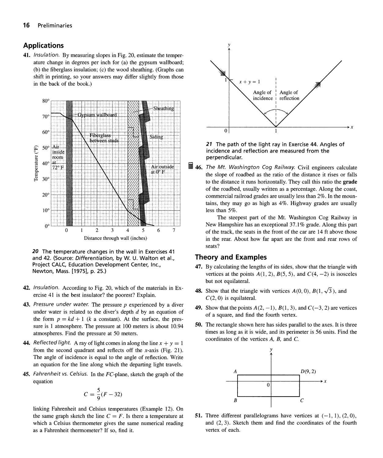
Preliminaries
Overview This chapter reviews the main things you need to know to start calculus.
The topics include the real number system, Cartesian coordinates in the plane,
straight lines, parabolas, circles, functions, and trigonometry.
Real Numbers and the Real Line
This section reviews real numbers, inequalities, intervals, and absolute values.
Real Numbers and the Real Line
Much of calculus is based on properties of the real number system. Real numbers
are numbers that can be expressed as decimals, such as
3
- - == -0.75000. . .
4
1
- == 0.33333 . . .
3
h == 1.4142...
The dots ... in each case indicate that the sequence of decimal digits goes on
forever.
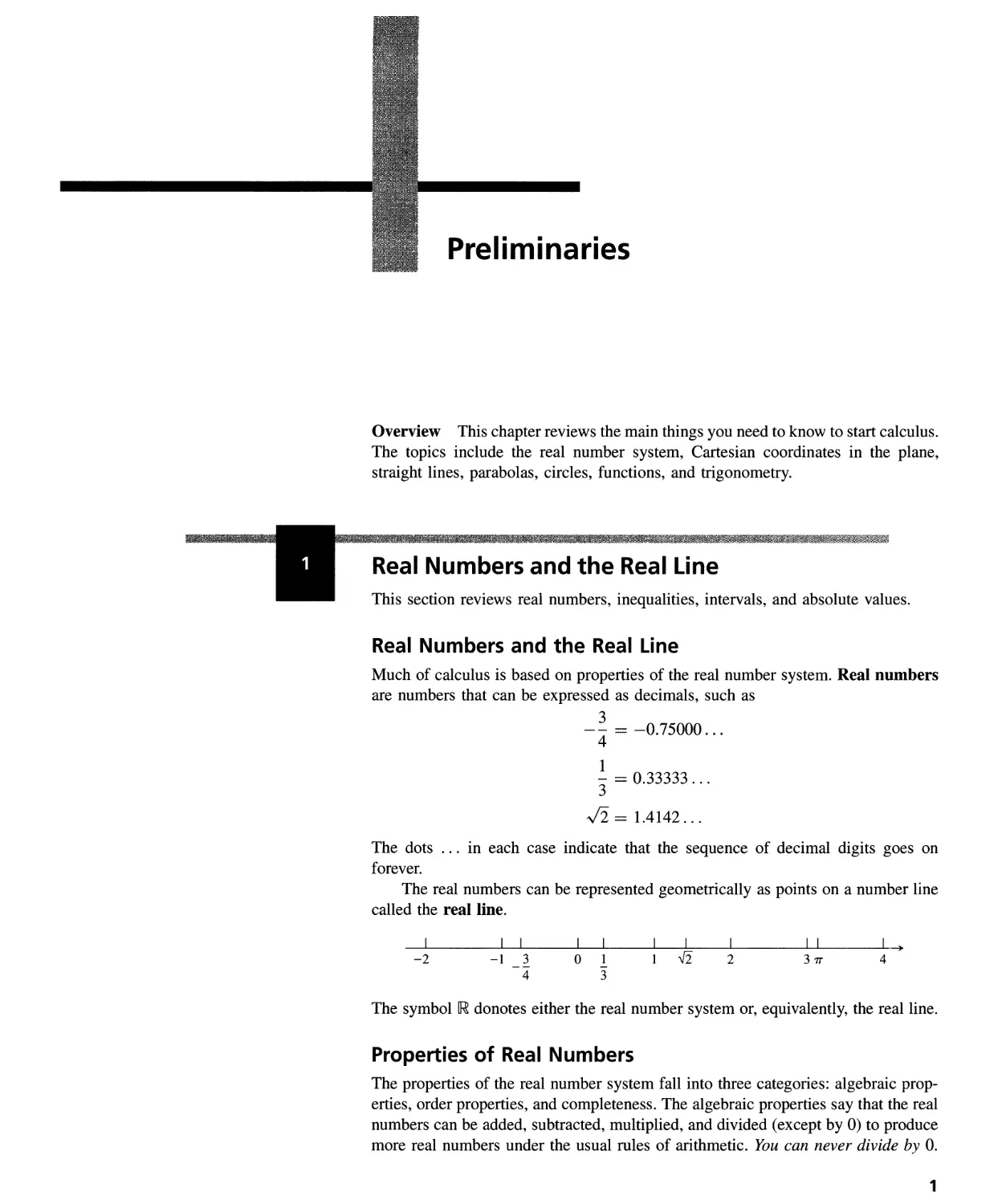
The real numbers can be represented geometrically as points on a number line
called the real line.
I
-2
I I
-1 3
4
I I
o 1
3
I I
1 -fi
I
2
I I
31T
I
4
The symbol donotes either the real number system or, equivalently, the real line.
Properties of Real Numbers
The properties of the real number system fall into three categories: algebraic prop-
erties, order properties, and completeness. The algebraic properties say that the real
numbers can be added, subtracted, multiplied, and divided (except by 0) to produce
more real numbers under the usual rules of arithmetic. You can never divide by O.
1
2 Preliminaries
The symbol =} means "implies."
Notice the rules for multiplying an
inequality by a number. Multiplying by a
positive number preserves the inequality;
multiplying by a negative number
reverses the inequality. Also,
reciprocation reverses the inequality for
numbers of the same sign.
The order properties of real numbers are summarized in the following list.
Rules for Inequalities
If a, b, and c are real numbers, then:
1.
2.
3.
4.
a<b=}a+c<b+c
a<b=}a-c<b-c
a < band c > 0 =} ac < bc
a < band c < 0 =} bc < ac
Special case: a < b =} -b < -a
1
a>O=}->O
a
1 1
If a and b are both positive or both negative, then a < b =} - < -
b a
5.
6.
The completeness property of the real number system is deeper and harder to
define precisely. Roughly speaking, it says that there are enough real numbers to
"complete" the real number line, in the sense that there are no "holes" or "gaps"
in it. Many of the theorems of calculus would fail if the real number system were
not complete, and the nature of the connection is important. The topic is best saved
for a more advanced course, however, and we will not pursue it.
Subsets of
We distinguish three special subsets of real numbers.
1. The natural numbers, namely 1, 2, 3, 4, . . .
2. The integers, namely 0, :I: 1, :1:2, :1:3, . . .
3. The rational numbers, namely the numbers that can be expressed in the form
of a fraction m/n, where m and n are integers and n i= O. Examples are
1 4 200 57
- and 57 == -.
3' 9' 13' 1
The rational numbers are precisely the real numbers with decimal expansions
that are either
a) terminating (ending in an infinite string of zeros), for example,
3
- == 0.75000. . . == 0.75 or
4
b) repeating (ending with a block of digits that repeats over and over), for example
23 -
- == 2.090909 . . . == 2.09.
11
The bar indicates the
block of repeating
digits.
The set of rational numbers has all the algebraic and order properties of
the real numbers but lacks the completeness property. For example, there is no
rational number whose square is 2; there is a "hole" in the rational line where h
should be.
1 Real Numbers and the Real Line 3
Real numbers that are not rational are called irrational numbers. They are char-
acterized by having nonterminating and nonrepeating decimal expansions. Examples
are 7T:, h, , and loglO 3.
Intervals
A subset of the real line is called an interval if it contains at least two numbers and
contains all the real numbers lying between any two of its elements. For example,
the set of all real numbers x such that x > 6 is an interval, as is the set of all x such
that -2 < x < 5. The set of all nonzero real numbers is not an interval; since 0 is
absent, the set fails to contain every real number between -1 and 1 (for example).
Geometrically, intervals correspond to rays and line segments on the real line,
along with the real line itself. Intervals of numbers corresponding to line segments
are finite intervals; intervals corresponding to rays and the real line are infinite
intervals.
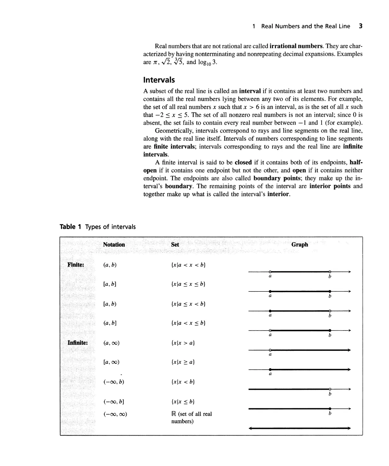
A finite interval is said to be closed if it contains both of its endpoints, half-
open if it contains one endpoint but not the other, and open if it contains neither
endpoint. The endpoints are also called boundary points; they make up the in-
terval's boundary. The remaining points of the interval are interior points and
together make up what is called the interval's interior.
Table 1 Types of intervals
Graph
(a, b) {xla < x < b}
8 8 )
a b
[a, b] {xla < x < b}
. . )
a b
[a, b) {xla < x < b}
. 8 )
a b
(a, b] {xla < x < b}
e . )
a b
(a, (0) {xix> a}
e )
a
[a, (0) {xix > a}
. )
a
(-00, b) {xix < b}
8 )
b
(-00, b] {xix < b}
. )
(-00, (0) (set of all real b
numbers)
( )
4 Preliminaries
I I
o 1
c
3
7
I
o
(a)
I
o
(b)
c
1
(c)
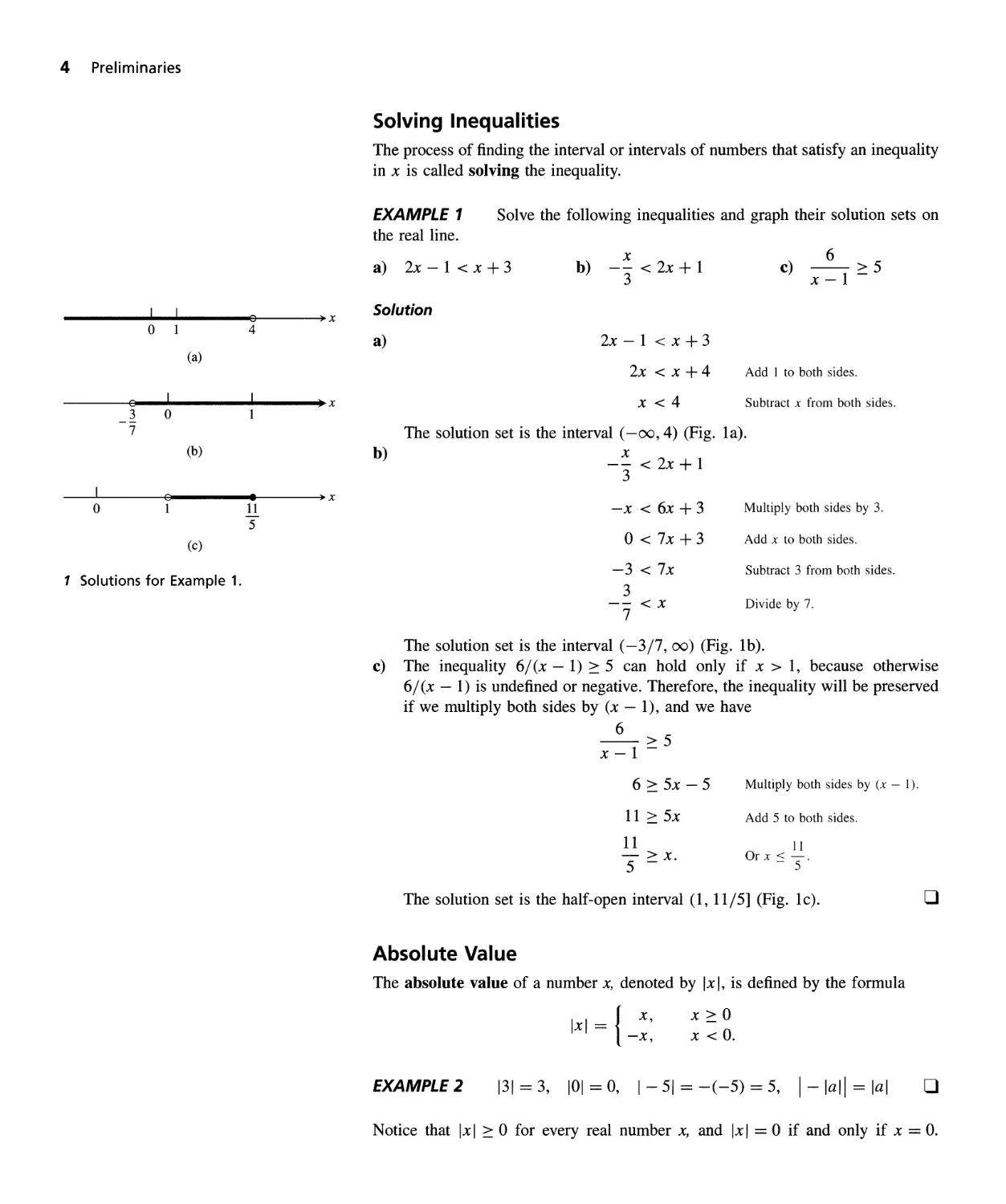
1 Solutions for Example 1.
e
4
) x
I
1
) x
.
11
5
) x
Solving Inequalities
The process of finding the interval or intervals of numbers that satisfy an inequality
in x is called solving the inequality.
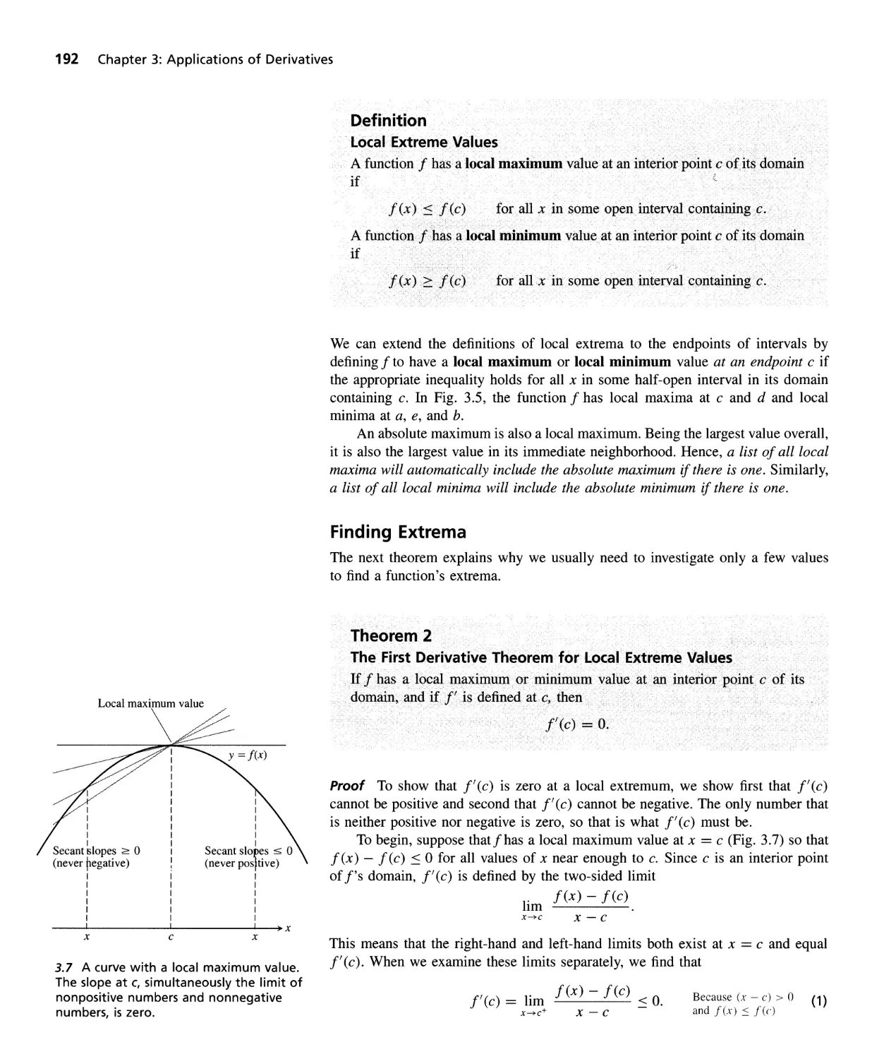
EXAMPLE 1
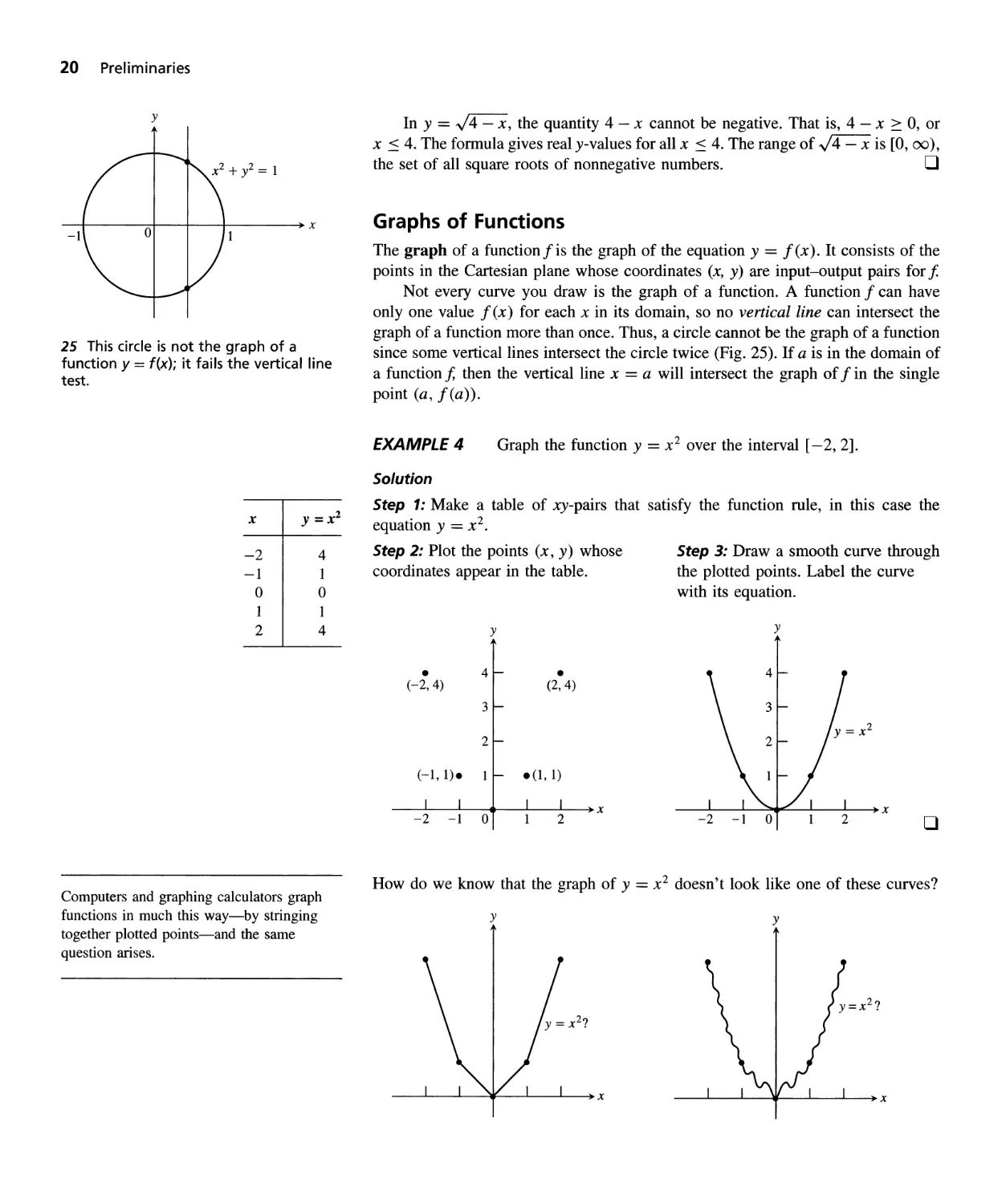
the real line.
Solve the following inequalities and graph their solution sets on
a) 2x - 1 < x + 3
x
b) -- < 2x + 1
3
6
c) > 5
x-l-
Solution
a)
2x-l <x+3
2x < x +4
Add 1 to both sides.
x<4
Subtract x from both sides.
b)
The solution set is the interval (-00, 4) (Fig. la).
x
-- < 2x + 1
3
-x < 6x + 3
o < 7x + 3
-3 < 7x
3
-- < x
7
Multiply both sides by 3.
Add x to both sides.
Subtract 3 from both sides.
Divide by 7.
The solution set is the interval (-3/7, (0) (Fig. 1 b).
c) The inequality 6/(x - 1) > 5 can hold only if x > 1, because otherwise
6/ (x - 1) is undefined or negative. Therefore, the inequality will be preserved
if we multiply both sides by (x - 1), and we have
6
>5
x-l-
6 > 5x - 5
11 > 5x
11
- > x.
5 -
Multiply both sides by (x - 1).
Add 5 to both sides.
11
Or x < -.
- 5
The solution set is the half-open interval (1,11/5] (Fig. lc).
o
Absolute Value
The absolute value of a number x, denoted by Ix I, is defined by the formula
Ix I == { X,
-x,
x > O
x < O.
EXAMPLE 2
131==3, 101=0, 1-51=-(-5)==5, 1-lall==lal
o
Notice that Ix I > 0 for every real number x, and Ix I = 0 if and only if x = O.
It is important to remember that
Ja2 == lal. Do not write Ja2 == a unless
you already know that a ::: O.
1-51 = 5 131
-1 I
-5 0 3
14-11 = 11-41 = 3
I I
1 4
)
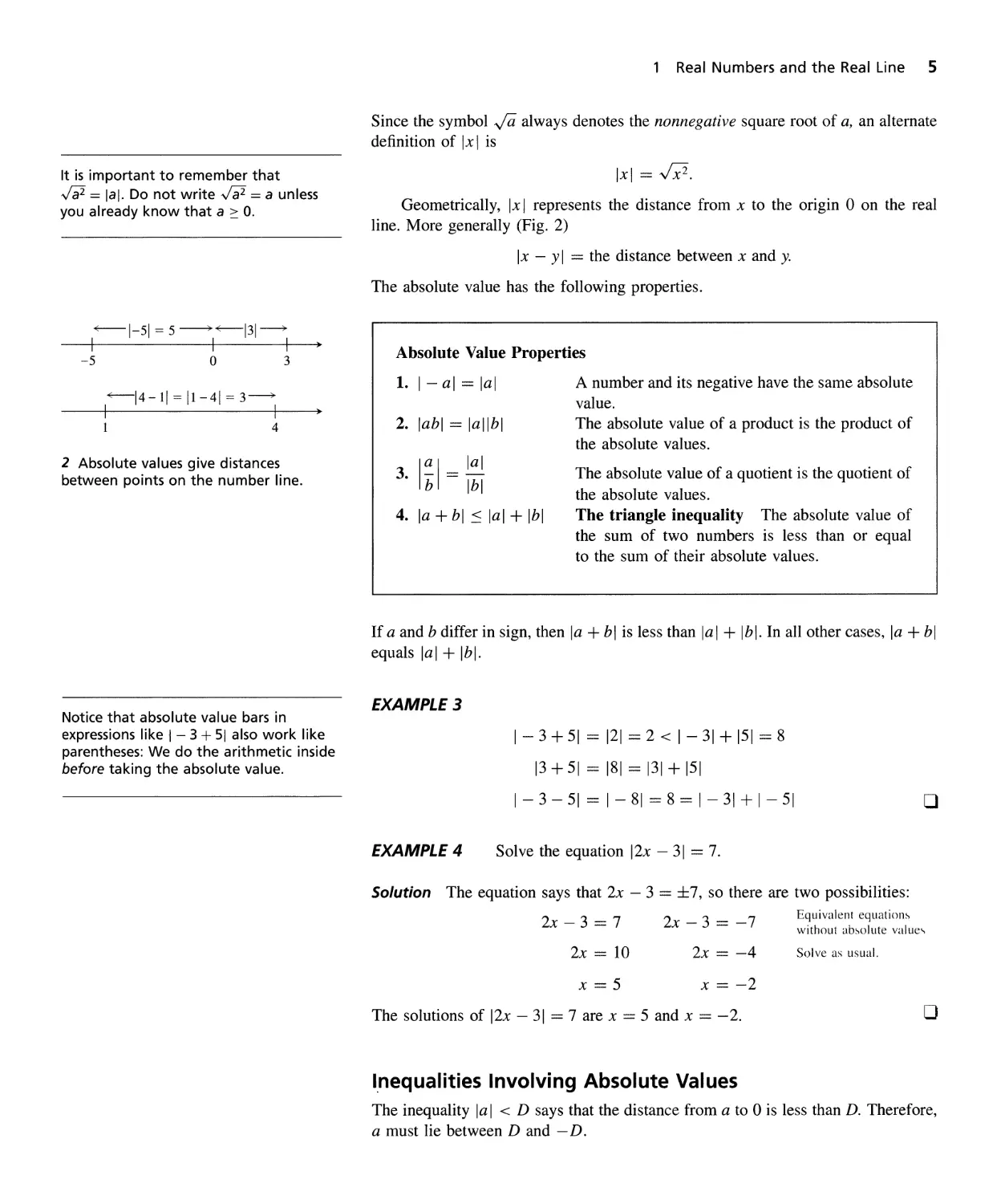
2 Absolute values give distances
between points on the number line.
Notice that absolute value bars in
expressions like i - 3 + 51 also work like
parentheses: We do the arithmetic inside
before taking the absolute value.
1 Real Numbers and the Real Line 5
Since the symbol ,Ja always denotes the nonnegative square root of a, an alternate
definition of Ix I is
Ix I == R.
Geometrically, Ix I represents the distance from x to the origin 0 on the real
line. More generally (Fig. 2)
Ix - y I == the distance between x and y.
The absolute value has the following properties.
Absolute Value Properties
1. 1- al == lal
A number and its negative have the same absolute
value.
The absolute value of a product is the product of
the absolute values.
The absolute value of a quotient is the quotient of
the absolute values.
The triangle inequality The absolute value of
the sum of two numbers is less than or equal
to the sum of their absolute values.
2. labl == la Ilbl
3. I : I = :::
4. la + bl < lal + Ibl
If a and b differ in sign, then la + bl is less than lal + Ibl. In all other cases, la + bl
equals lal + Ibl.
EXAMPLE 3
I - 3 + 51 == 121 == 2 < I - 31 + 151 == 8
13 + 51 == 181 == 131 + 151
I - 3 - 51 == I - 81 == 8 == I - 31 + I - 51
o
EXAMPLE 4
Solve the equation 12x - 31 == 7.
Solution The equation says that 2x - 3 == :1:7, so there are two possibilities:
2x-3==7
2x == 10
Equivalent equati()n
without ab o]ute value
2x-3==-7
2x == -4
Solve as usual.
x==5
x == -2
The solutions of 12x - 31 == 7 are x == 5 and x == -2.
o
I,nequalities Involving Absolute Values
The inequality la I < D says that the distance from a to 0 is less than D. Therefore,
a must lie between D and - D.
6 Preliminaries
The symbol {:} means "if and only if," or
"implies and is implied by."
c
-4
I
5
8 ) x
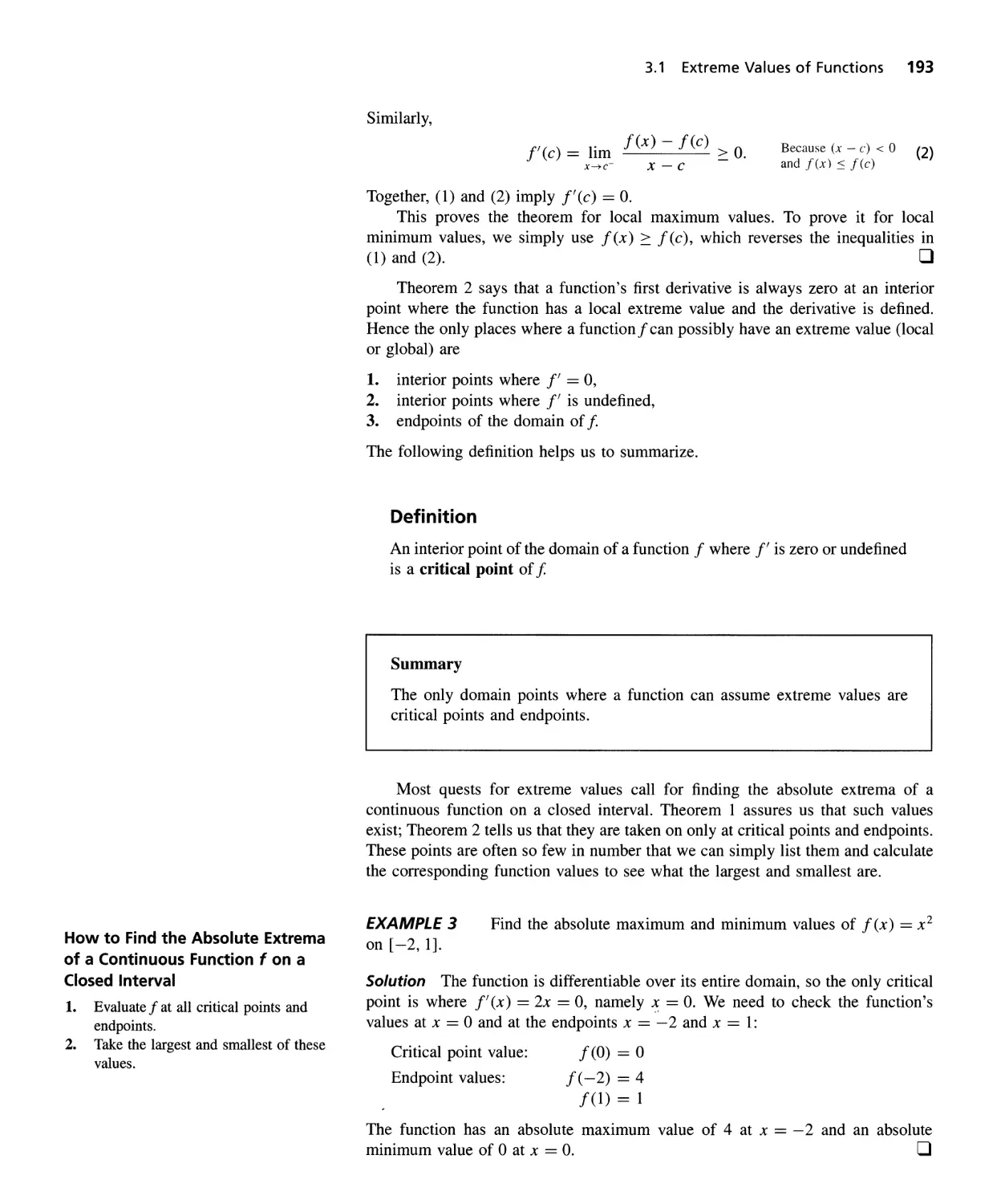
14
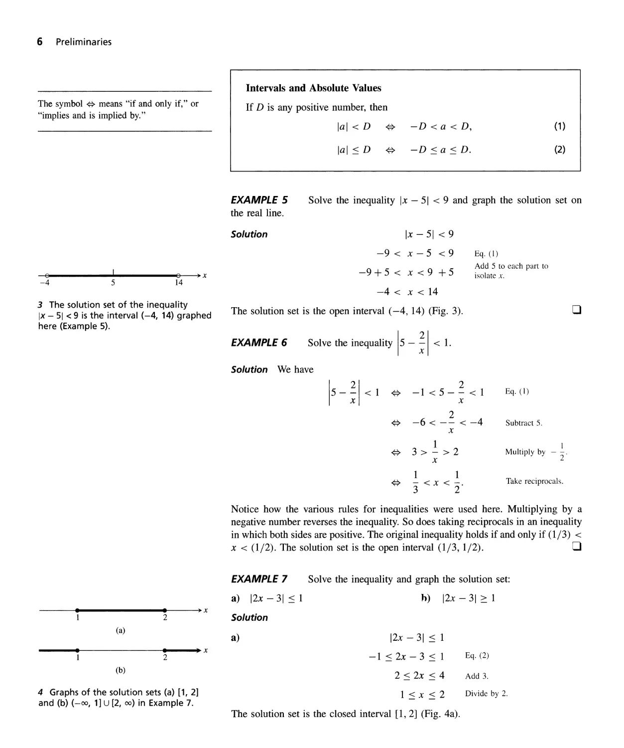
3 The solution set of the inequality
Ix - 51 < 9 is the interval (-4, 14) graphed
here (Example 5).
.
1
.
2
) X
(a)
.
1
) x
.
2
(b)
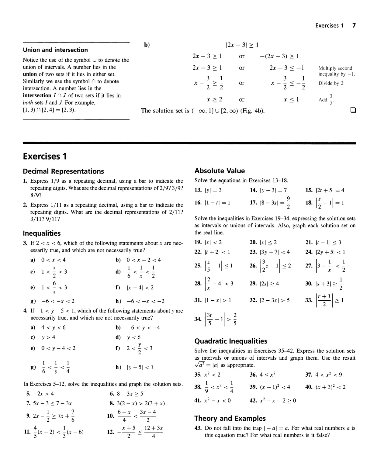
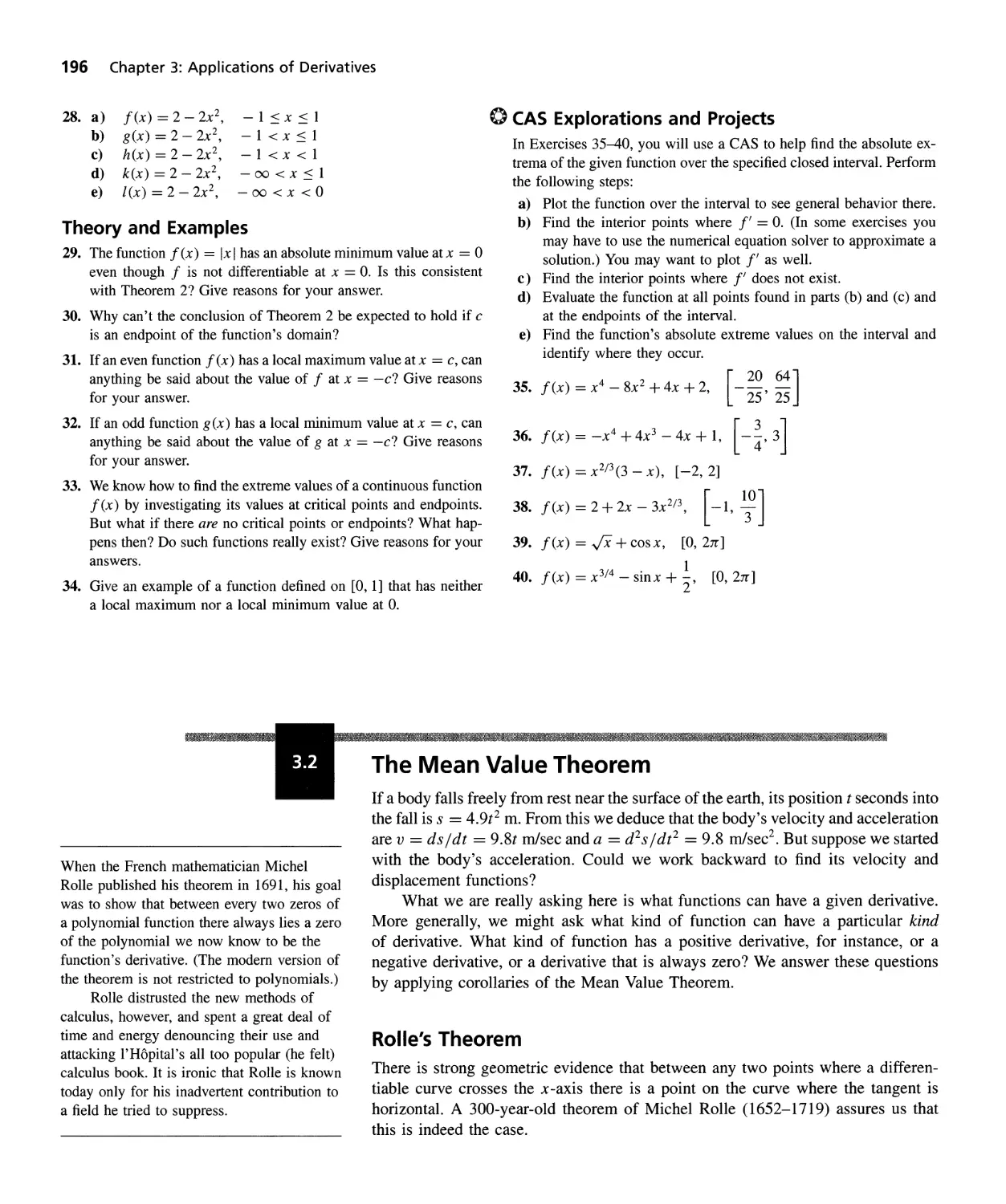
4 Graphs of the solution sets (a) [1, 2]
and (b) (-00, 1] U [2, 00) in Example 7.
Intervals and Absolute Values
If D is any positive number, then
lal < D {:} -D < a < D,
lal < D {:} -D < a < D.
(1 )
(2)
EXAMPLE 5
the real line.
Solve the inequality Ix - 51 < 9 and graph the solution set on
Ix - 51 < 9
-9 < x - 5 < 9
-9 + 5 < x < 9 + 5
-4 < x < 14
The solution set is the open interval (-4, 14) (Fig. 3).
Solution
Eq. (1)
Add 5 to each part to
isolate x.
EXAMPLE 6
2
Solve the inequality 5 - - < 1.
x
Solution We have
2
5-- <1
x
2
{:} -1<5--<1
x
Eq. (I)
2
{:} -6 < -- < -4
x
Subtract 5,
{:}
1
3>->2
x
Multiply by
{:}
1 1
- < x < -.
3 2
Take reciprocals.
o
1
2
Notice how the various rules for inequalities were used here. Multiplying by a
negative number reverses the inequality. So does taking reciprocals in an inequality
in which both sides are positive. The original inequality holds if and only if (1/3) <
x < (1/2). The solution set is the open interval (1/3, 1/2). 0
EXAMPLE 7
a) 12x - 31 < 1
Solve the inequality and graph the solution set:
h) 12x - 31 > 1
Solution
a)
12x - 31 < 1
-1 < 2x-3 < 1
2 < 2x < 4
l < x < 2
Divide by 2.
Eq. (2)
Add 3.
The solution set is the closed interval [1, 2] (Fig. 4a).
b)
Union and intersection
Notice the use of the symbol U to denote the
union of intervals. A number lies in the
union of two sets if it lies in either set.
Similarly we use the symbol n to denote
intersection. A number lies in the
intersection I n J of two sets if it lies in
both sets I and J. For example,
[1,3) n [2,4] = [2,3).
Exercises 1 7
12x - 31 > 1
2x - 3 > 1 or -(2x - 3) > 1
2x-3 > 1
3 1
x-->-
2 - 2
2x-3 < -1
3 1
x - - < --
2 - 2
Multiply econd
inequality by -1.
Divide by 2.
or
or
x > 2
3
Add -.
2
or
x < 1
The solution set is (- 00, 1] U [2, (0) (Fig. 4b).
o
Exercises 1
Decimal Representations
1. Express 1/9 as a repeating decimal, using a bar to indicate the
repeating digits. What are the decimal representations of 2/9? 3/9?
8/9?
2. Express 1/11 as a repeating decimal, using a bar to indicate the
repeating digits. What are the decimal representations of 2/11?
3/11? 9/11?
Inequalities
3. If 2 < x < 6, which of the following statements about x are nec-
essarily true, and which are not necessarily true?
a) O<x<4 b) O<x-2<4
x d) 1 1 1
c) 1<-<3 -<-<-
2 6 x 2
6 f) Ix - 41 < 2
e) 1<-<3
x
g) -6 < -x < 2 h) -6 < -x < -2
4. If -1 < y - 5 < 1, which of the following statements about yare
necessarily true, and which are not necessarily true?
a) 4<y<6 b) -6 < y < -4
c) y>4 d) y<6
e) O<y-4<2 f) y
2<-<3
2
1 1 1 h)
g) -<-<- ly-51 < 1
6 y 4
In Exercises 5-12, solve the inequalities and graph the solution sets.
5. -2x > 4
7. 5x - 3 < 7 - 3x
1 7
9. 2x - - > 7x + -
2 - 6
4 1
11. 5 (x - 2) < 3 (x - 6)
6. 8 - 3x > 5
8. 3(2 - x) > 2(3 + x)
6 - x 3x - 4
10. <
4 2
x + 5 12 + 3x
12. <
2 4
Absolute Value
Solve the equations in Exercises 13-18.
13. I y I = 3
16. 11 - tl = 1
14. Iy - 31 = 7
9
17. 18 - 3s1 = -
2
15. 12t + 51 = 4
18. I - 11 = 1
Solve the inequalities in Exercises 19-34, expressing the solution sets
as intervals or unions of intervals. Also, graph each solution set on
the real line.
19. Ix I < 2 20. Ix I < 2 21. It - 11 < 3
22. It + 21 < 1 23. 13y - 71 < 4 24. 12 y + 51 < 1
I -II < I 3 1 1
25. 26. -z - 1 < 2 27. 3 -- <-
2 x 2
2 1
28. - -4 <3 29. 12s1 > 4 30. Is + 31 > 2
x
31. 11 - x I > 1 32. 12 - 3x I > 5 33. r+l > 1
-
2
3r 2
34. - -1 >-
5 5
Quadratic Inequalities
Solve the inequalities in Exercises 35-42. Express the solution sets
as intervals or unions of intervals and graph them. Use the result
R = lal as appropriate.
35. x 2 < 2 36. 4 < x 2 37. 4 < X 2 < 9
1 2 1 2 2
38. - < x < - 39. (x - 1) < 4 40. (x + 3) < 2
9 4
41. x 2 - x < 0
42. x 2 - x - 2 > 0
Theory and Examples
43. Do not fall into the trap I - al = a. For what real numbers a is
this equation true? For what real numbers is it false?
8 Preliminaries
la + bl 2 = (a + b)2
= a 2 + Zab + b 2
< a 2 + 21allbl + b 2
< lal 2 + 21allbl + Ibl 2
= (Ial + Ibl)2
la + bl < lal + Ibl
46. Prove that labl = lallbl for any numbers a and b.
47. If Ix I < 3 and x > -1/2, what can you say about x?
(1 )
48. Graph the inequality Ix I + I y I < 1.
== 49. GRAPHER
a) Graph the functions f(x) = x/2 and g(x) = 1 + (4/x) to-
gether to identify the values of x for which
x 4
- > 1 + -.
2 x
44. Solve the equation Ix - 11 = 1 - x.
45. A proof of the triangle inequality. Give the reason justifying
each of the numbered steps in the following proof of the triangle
inequality.
(2) b) Confirm your findings in (a) algebraically.
(3) 1= 50. GRAPHER
a) Graph the functions f(x) = 3/(x - 1) and g(x) =
2/ (x + 1) together to identify the values of x for which
3 2
<
x+l
(4)
x-I
b)
Confirm your findings in (a) algebraically.
i/f!!flj(1fJ{f!!ltlI W!J'i$;fI1!tt'l/. .
Coordinates, Lines, and Increments
This section reviews coordinates and lines and discusses the
notion of increment.
y
Cartesian Coordinates in the Plane
b --------1 Pea, b)
Negative x-axis
-3 -2 -1
Origin
/
o I \ 2 a3
-1
x
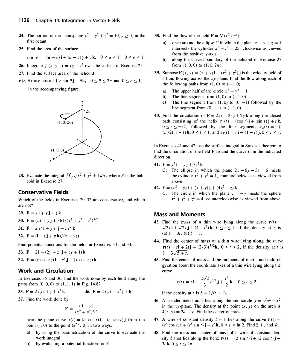
The positions of all points in the plane can be measured with respect to two
perpendicular real lines in the plane intersecting in the O-point of each (Fig. 5).
These lines are called coordinate axes in the plane. On the horizontal x-axis,
numbers are denoted by x and increase to the right. On the vertical y-axis, numbers
are denoted by y and increase upward. The point where x and yare both 0 is the
origin of the coordinate system, often denoted by the letter O.
If P is any point in the plane, we can draw lines through P perpendicular to
the two coordinate axes. If the lines meet the x-axis at a and the y-axis at b, then a
is the x-coordinate of P, and b is they-coordinate. The ordered pair (a, b) is the
point's coordinate pair. The x-coordinate of every point on the y-axis is O. The
y-coordinate of every point on the x-axis is O. The origin is the point (0, 0).
The origin divides the x-axis into the positive x-axis to the right and the
negative x-axis to the left. It divides the y-axis into the positive and negative y-
axis above and below. The axes divide the plane into four regions called quadrants,
numbered counterclockwise as in Fig. 6.
Positive y-axis 3
2
Positive x-axis
Negative y-axis
-3
5 Cartesian coordinates.
A Word About Scales
When we plot data in the coordinate plane or graph formulas whose variables have
different units of measure, we do not need to use the same scale on the two axes. If
we plot time vs. thrust for a rocket motor, for example, there is no reason to place
the mark that shows 1 sec on the time axis the same distance from the origin as the
mark that shows 1 lb on the thrust axis.
When we graph functions whose variables do not represent physical measure-
ments and when we draw figures in the coordinate plane to study their geometry
and trigonometry, we try to make the scales on the axes identical. A vertical unit
2 Coordinates, Lines, and Increments 9
6 The points on the axes all have coordinate pairs,
but we usually label them with single numbers.
Notice the coordinate sign patterns in the quadrants.
y
3 (0, 3)
Second First
quadrant 2 (0, 2) quadrant
(-, +) (+, +)
1 (0, 1)
(-2,0) (0, 0) (1, 0) (2, 0)
x
-2 -1 0 1 2
Third -1 (0, -1) Fourth
quadrant quadrant
(-, -) -2 (0, - 2) (+, -)
6
C(5, 6)
of distance then looks the same as a horizontal unit. As on a surveyor's map or a
scale drawing, line segments that are supposed to have the same length will look
as if they do and angles that are supposed to be congruent will look congruent.
Computer displays and calculator displays are another matter. The vertical
and horizontal scales on machine-generated graphs usually differ, and there are
corresponding distortions in distances, slopes, and angles. Circles may look like
ellipses, rectangles may look like squares, right angles may appear to be acute
or obtuse, and so on. Circumstances like these require us to take extra care in
interpreting what we see. High-quality computer software usually allows you to
compensate for such scale problems by adjusting the aspect ratio (ratio of vertical
to horizontal scale). Some computer screens also allow adjustment within a narrow
range. When you use a grapher, try to make the aspect ratio 1, or close to it.
.J
B (2, 5)
y = 8
Increments and Distan'ce
5
3
x= 0
y = - 5 f
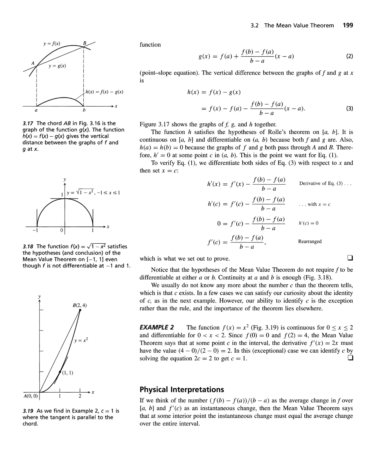
When a particle moves from one point in the plane to another, the net changes
in its coordinates are called increments. They are calculated by subtracting the
coordinates of the starting point from the coordinates of the ending point.
4
2
EXAMPLE 1 In going from the point A(4, -3) to the point B(2, 5) (Fig. 7),
the increments in the x- and y-coordinates are
1
D(5, 1)
dx = 2 - 4 = -2,
dy = 5 - (-3) = 8.
o
o 1
x
-1
-2
-3
x = -2
(2, - 3)
EXAMPLE 2
From C(5, 6) to D(5, 1) (Fig. 7) the coordinate increments are
7 Coordinate increments may be
positive, negative, or zero.
dx == 5 - 5 = 0,
dy = 1 - 6 == -5.
o
10 Preliminaries
Y This distance is
d = " IX 2 -x 1 1 2 + I Y 2 - Yl1 2
Y2 = " (x 2 -x l )2 + (Y2 - YI)2
\
Y I P(x l , YI )' v
IX 2 -xII
0 Xl
Q(X 2 , Y2)
I Y 2- Y II
, C(X 2 , YI)
X 2
8 To calculate the distance between
P(X" y,) and Q(X2, Y2), apply the
Pythagorean theorem to triangle PCQ.
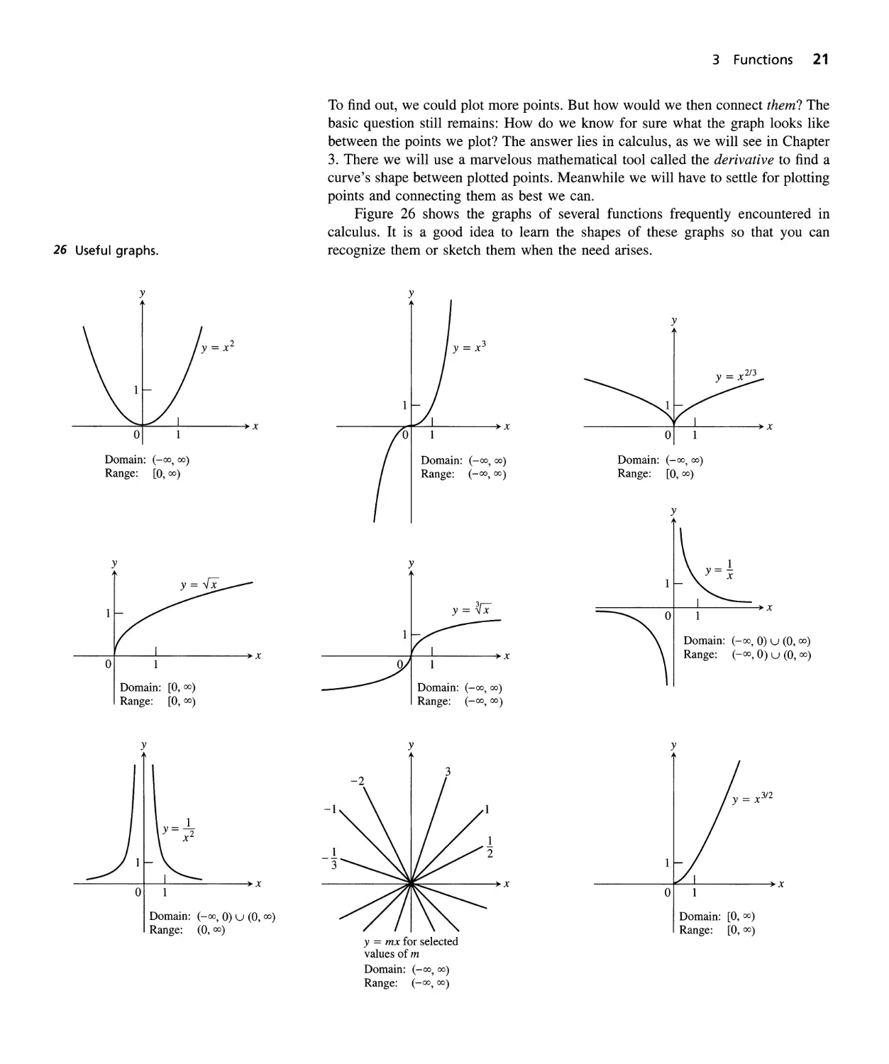
The distance between points in the plane is calculated with a formula that
comes from the Pythagorean theorem (Fig. 8).
Distance Formula for Points in the Plane
The distance betw een P(Xl, Yl) a nd Q(X2, Y2) is
d = J (dX)2 + (dy)2 = J (X2 - Xl)2 + (Y2 - Yl)2.
X
EXAMPLE 3
a) Th e distance between P( -1,2 ) and Q(3, 4) is
J (3 - (-1»)2 + (4 - 2)2 = J (4)2 + (2)2 = JW = J4:5 = 2.J5.
b) The distance from the origin to P (x, y ) is
J (x - 0)2 + (y - 0)2 = J x2 + y2.
o
Graphs
The graph of an equation or inequality involving the variables x and y is the set of
all points P (x, y) whose coordinates satisfy the equation or inequality.
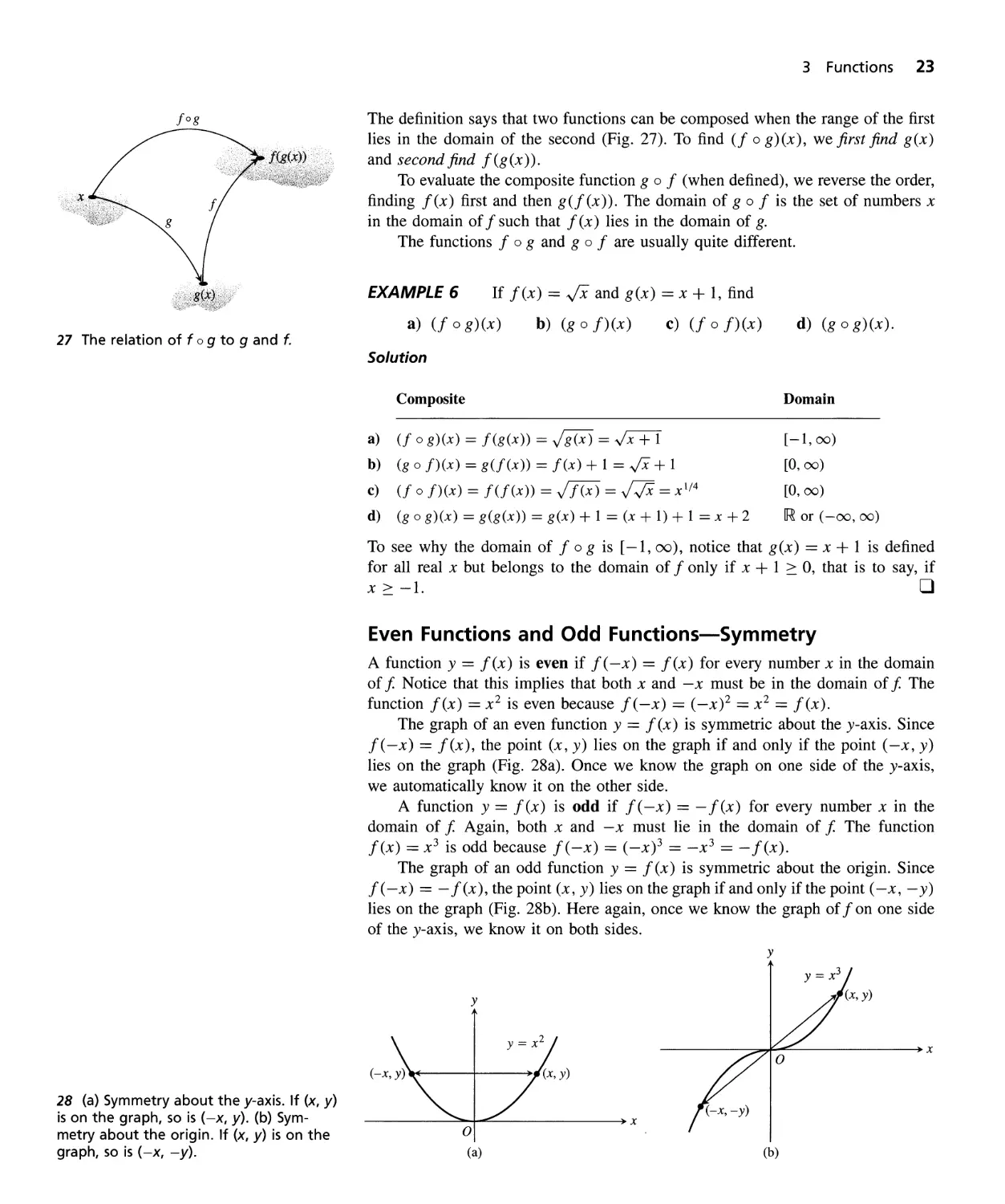
EXAMPLE 4
Circles centered at the origin
a) If a > 0, the equation x 2 + y2 = a 2 represents all points P (x, y) whose dis-
tance from the origin is J x 2 + y2 = # = a. These points lie on the circle
of radius a centered at the origin. This circle is the graph of the equation
x 2 + '-y2 = a 2 (Fig. 9a).
b) Points (x, y) whose coordinates satisfy the inequality x 2 + y2 < a 2 all have
distance < a from the origin. The graph of the inequality is therefore the circle
of radius a centered at the origin together with its interior (Fig. 9b).
Y
Y
X2 + y2 = a 2
a
x 2 + y2 S a 2
X
x
a
(a)
(b)
9 Graphs of (a) the equation and (b) the inequality in Example 4.
o
The circle of radius 1 unit centered at the origin is called the unit circle.
2 Coordinates, Lines, and Increments 11
y
(2, 4)
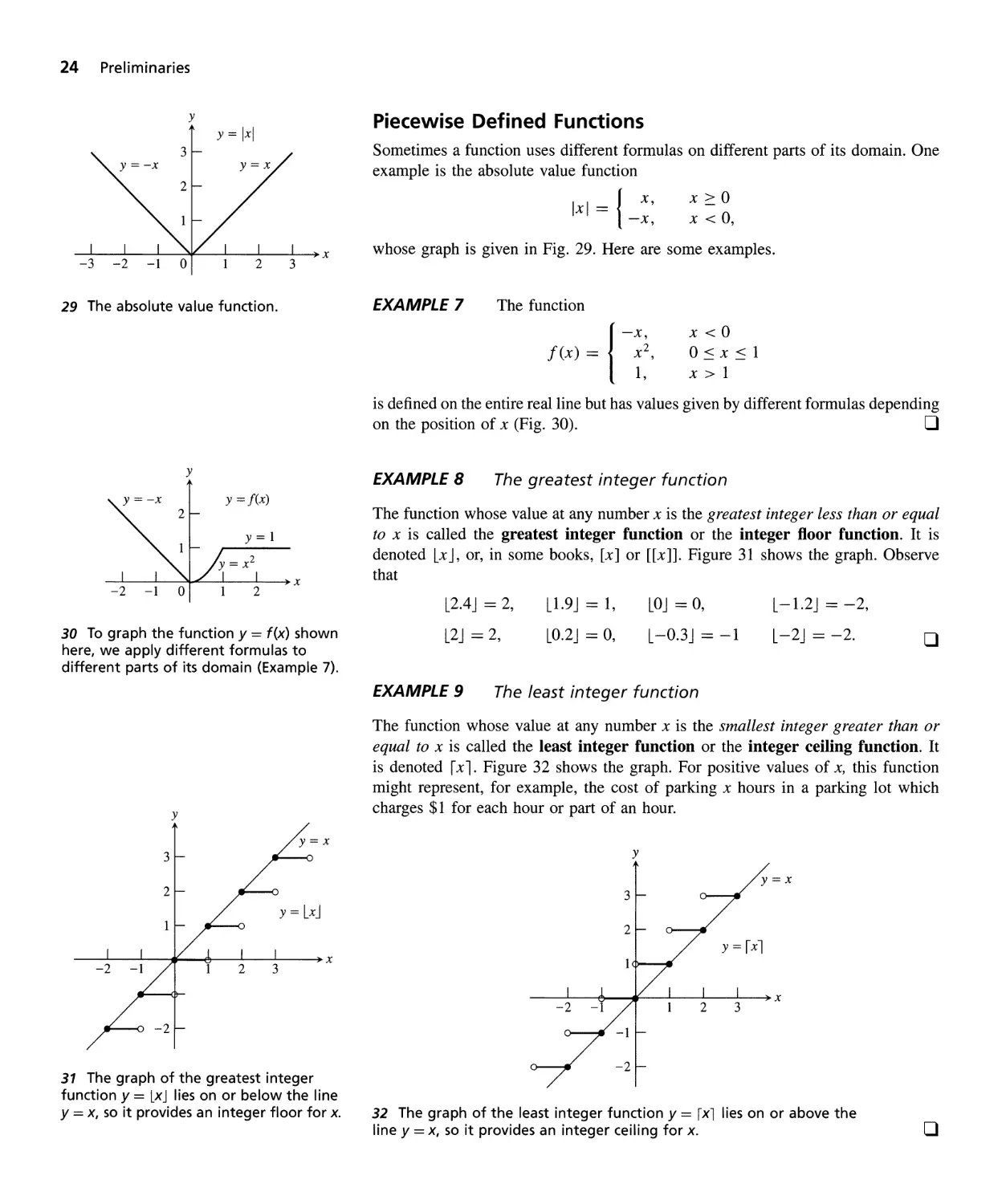
EXAMPLE 5 Consider the equation Y == x z . Some points whose coordinates
satisfy this equation are (0,0), (1,1), (-1,1), (2,4), and (-2,4). These points
(and all others satisfying the equation) make up a smooth curve called a parabola
(Fig. 10). 0
y = x 2
-2 -1 0 1
x
Straight Lines
Given two points PI (Xl, YI) and Pz (xz, yz) in the plane, we call the increments
X == Xz - Xl and Y == Yz - Yl the run and the rise, respectively, between PI
and Pz. Two such points always determine a unique straight line (usually called
simply a line) passing through them both. We call the line PI Pz.
Any nonvertical line in the plane has the property that the ratio
rise Y Yz - YI
m==-==-=
run X Xz - Xl
2
10 The parabola y == x 2 .
y
L
has the same value for every choice of the two points PI (Xl, YI) and Pz (xz, yz) on
the line (Fig. 11).
Definition
The constant
rise Y Yz - Yl
m=-=-==
run X Xz - Xl
isthe..slope of the nonverticalline PI Pz.
x
The slope tells us the direction (uphill, downhill) and steepness of a line. A line
with positive slope rises uphill to the right; one with negative slope falls downhill
to the right (Fig. 12). The greater the absolute value of the slope, the more rapid
the rise or fall. The slope of a vertical line is undefined. Since the run X is zero
for a vertical line, we cannot form the ratio m.
o
11 Triangles P1 QP 2 and P Q'P are
similar, so
L\y' L\y
----m
&' - & - .
y
12 The slope of L 1 is
_ L\y _ 6 - (-2) _
m- - - .
L\x 3-0 3
x
That is, y increases 8 units every time x increases 3
units. The slope of L 2 is
L\y 2 - 5 -3
m == - == - == -.
& 4-0 4
That is, y decreases 3 units every time x increases 4
units.
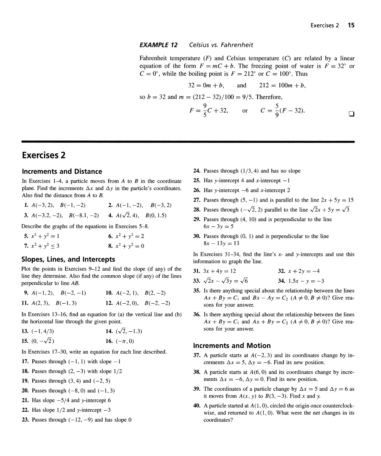
16 The standard equations for the vertical and
horiz0ntal lines through (2, 3) are x == 2 and y == 3.
12 Preliminaries
/
/ h .
"""...... ./ / not t IS
---
x x
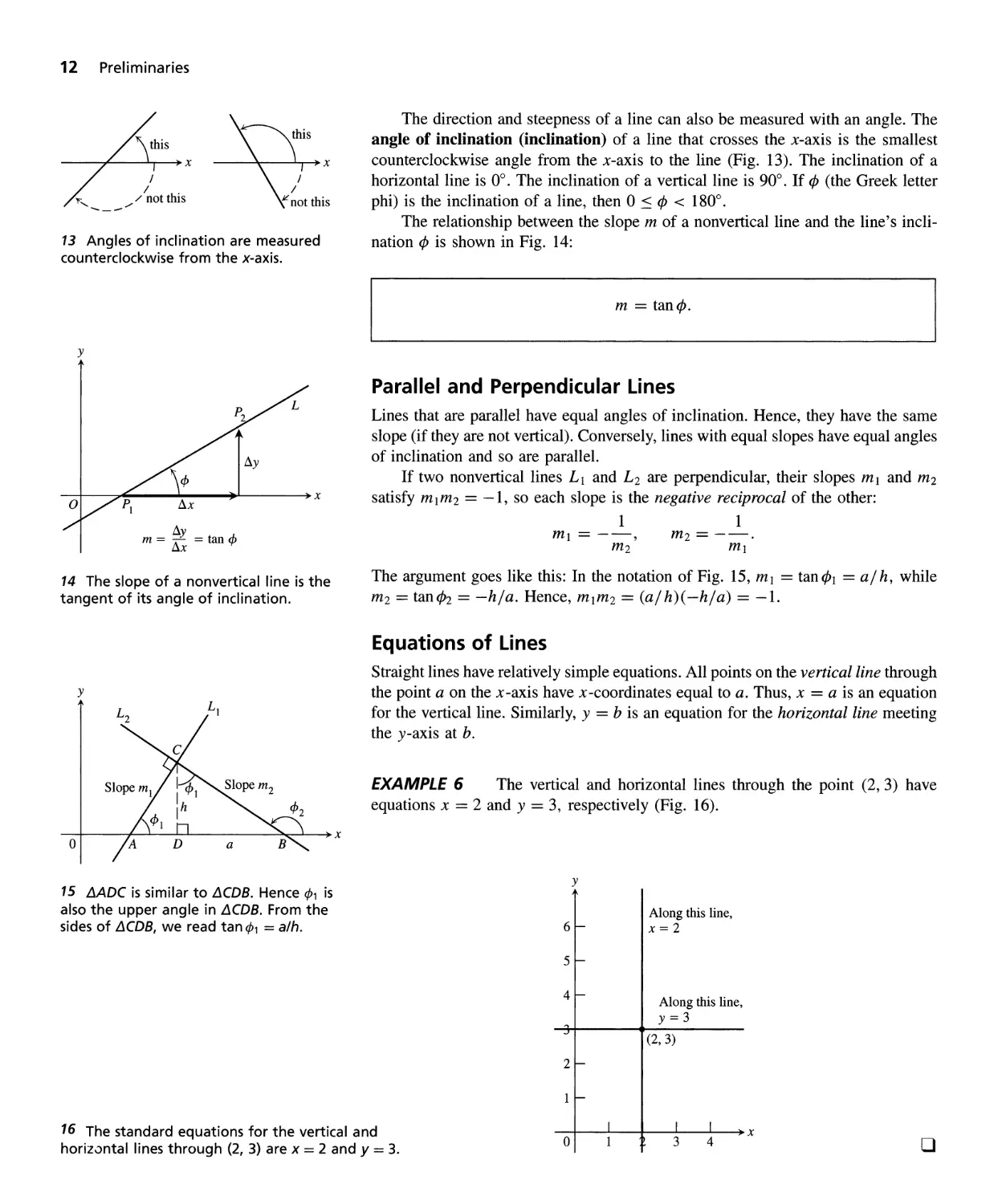
13 Angles of inclination are measured
counterclockwise from the x-axis.
y
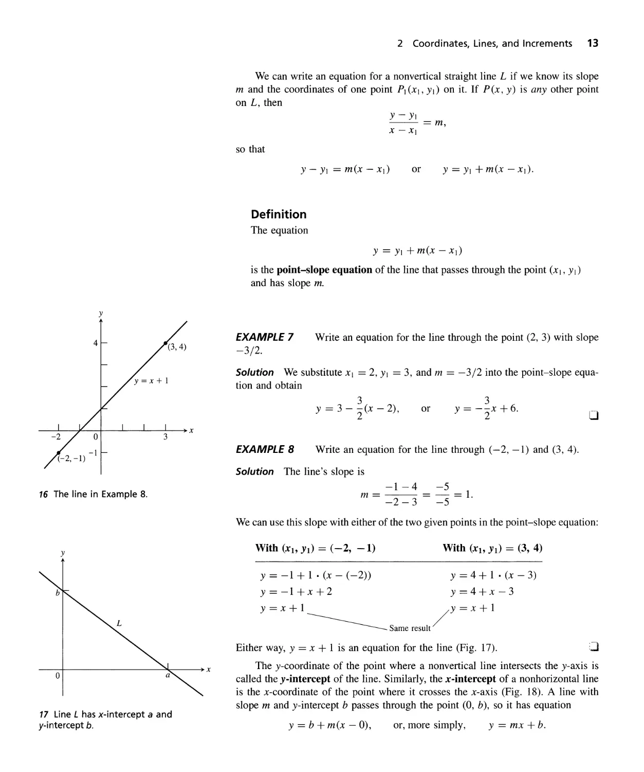
Lly
x
m = Lly = tan cP
Llx
14 The slope of a nonvertical line is the
tangent of its angle of inclination.
y
o
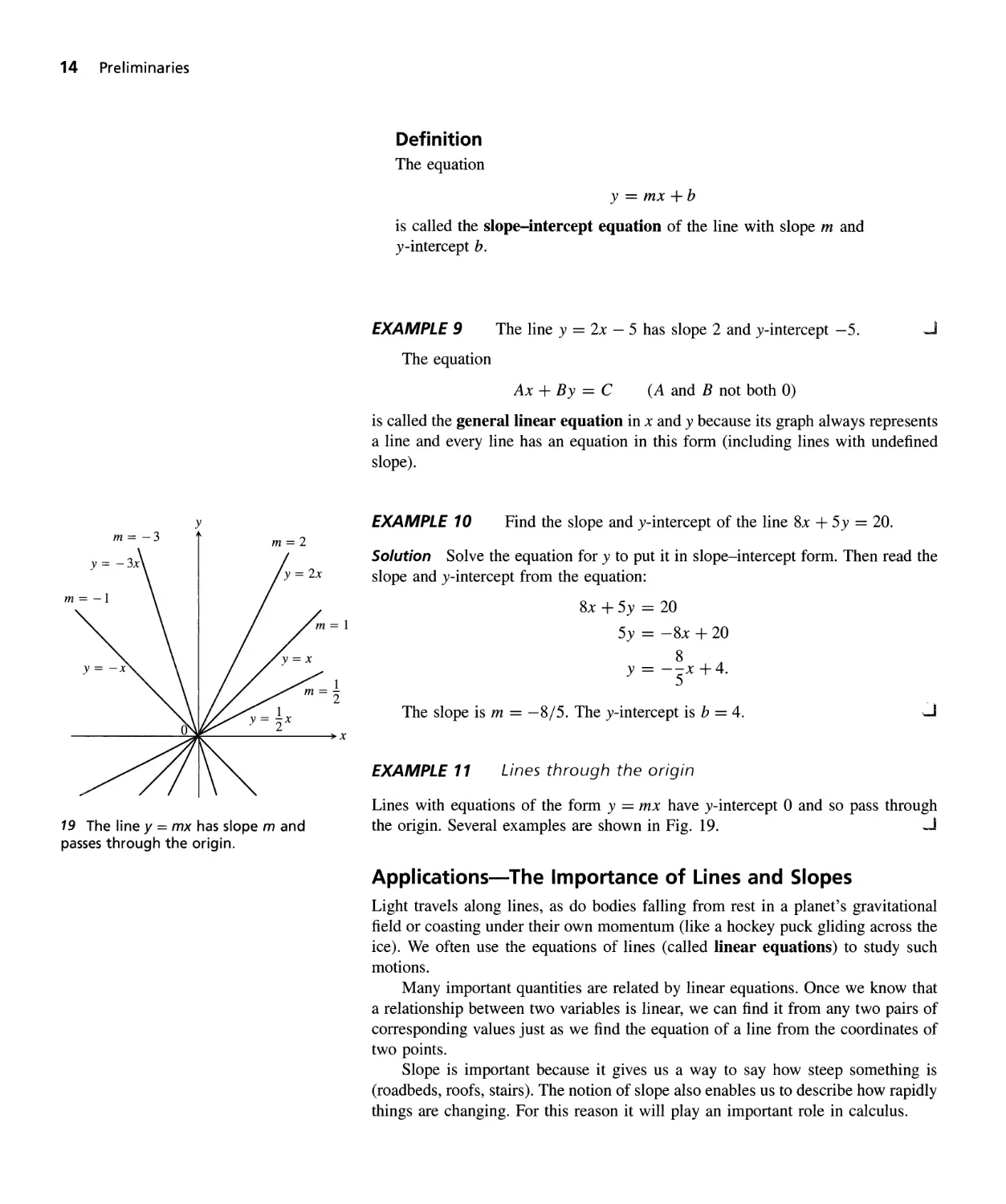
15 l1ADC is similar to l1CDB. Hence 11 is
also the upper angle in l1CDB. From the
sides of l1CDB, we read tan 11 == a/h.
The direction and steepness of a line can also be measured with an angle. The
angle of inclination (inclination) of a line that crosses the x-axis is the smallest
counterclockwise angle from the x-axis to the line (Fig. 13). The inclination of a
horizontal line is 0°. The inclination of a vertical line is 90°. If f/J (the Greek letter
phi) is the inclination of a line, then 0 < f/J < 180°.
The relationship between the slope m of a nonverticalline and the line's incli-
nation f/J is shown in Fig. 14:
m = tan f/J.
Parallel and Perpendicular Lines
Lines that are parallel have equal angles of inclination. Hence, they have the same
slope (if they are not vertical). Conversely, lines with equal slopes have equal angles
of inclination and so are parallel.
If two nonvertical lines L 1 and L 2 are perpendicular, their slopes m 1 and m2
satisfy m 1 m2 = -1, so each slope is the negative reciprocal of the other:
1 1
ml = --, m2 = --.
m2 ml
The argument goes like this: In the notation of Fig. 15, ml = tan f/Jl = a/ h, while
m2 = tanf/J2 = -h/a. Hence, mlm2 = (a/h)(-h/a) = -1.
Equations of Lines
Straight lines have relatively simple equations. All points on the vertical line through
the point a on the x -axis have x -coordinates equal to a. Thus, x = a is an equation
for the vertical line. Similarly, y = b is an equation for the horizontal line meeting
the y-axis at b.
EXAMPLE 6 The vertical and horizontal lines through the point (2,3) have
equations x = 2 and y = 3, respectively (Fig. 16).
x
y
6
Along this line,
x=2
5
4
Along this line,
y=3
(2, 3)
2
1
o
o
x
y
16 The line in Example 8.
y
17 Line L has x-intercept a and
y-intercept b.
x
2 Coordinates, Lines, and Increments 13
We can write an equation for a nonvertical straight line L if we know its slope
m and the coordinates of one point PI (Xl, YI) on it. If P (x, y) is any other point
on L, then
Y - YI
m,
X - Xl
so that
Y-YI =m(x-xI)
or
Y = YI +m(x -Xl),
Definition
The equation
Y==YI+m(X-XI)
is the point-slope equation of the line that passes through the point (Xl, YI)
and has slope m.
EXAMPLE 7
-3/2.
Write an equation for the line through the point (2, 3) with slope
Solution We substitute Xl == 2, YI == 3, and m == -3/2 into the point-slope equa-
tion and obtain
3
Y == 3 - 2 (x - 2),
3
Y == --x +6.
2
or
o
EXAMPLE 8
Write an equation for the line through (- 2, -1) and (3, 4).
Solution The line's slope is
-1 - 4 -5
m== ---1
-2-3--5- .
We can use this slope with either of the two given points in the point-slope equation:
With (Xl' YI) == (-2, -1)
With (Xl' YI) == (3, 4)
Y = -1 + 1 · (x - (-2»
y=-I+x+2
Y = 4 + 1 · (x - 3)
y==4+x-3
y=x+l /Y=X+l
--------------- Same result
Either way, Y == X + 1 is an equation for the line (Fig. 17).
:.J
x
The y-coordinate of the point where a nonvertical line intersects the y-axis is
called the y-intercept of the line. Similarly, the x-intercept of a nonhorizontalline
is the x-coordinate of the point where it crosses the x-axis (Fig. 18). A line with
slope m and y-intercept b passes through the point (0, b), so it has equation
Y = b + m(x - 0),
or, more simply,
Y == mx + b.
14 Preliminaries
y
m =-3
m=2
m =-1
19 The line y == mx has slope m and
passes through the origin.
Definition
The equation
y = mx + b
is called the slope-intercept equation of the line with slope m and
y-intercept b.
EXAMPLE 9
-'
The line y = 2x - 5 has slope 2 and y-intercept -5.
The equation
Ax + By = C
(A and B not both 0)
is called the general linear equation in x and y because its graph always represents
a line and every line has an equation in this form (including lines with undefined
slope ).
EXAMPLE 10
Find the slope and y- intercept of the line 8x + 5 y = 20.
Solution Solve the equation for y to put it in slope-intercept form. Then read the
slope and y-intercept from the equation:
8x + 5 y = 20
5 y = - 8x + 20
8
y = --x+4.
5
The slope is m = -8/5. The y-intercept is b = 4.
x
EXAMPLE 11
Lines through the origin
Lines with equations of the form y = mx have y-intercept 0 and so pass through
the origin. Several examples are shown in Fig. 19. -.J
Applications-The Importance of Lines and Slopes
Light travels along lines, as do bodies falling from rest in a planet's gravitational
field or coasting under their own momentum (like a hockey puck gliding across the
ice). We often use the equations of lines (called linear equations) to study such
motions.
Many important quantities are related by linear equations. Once we know that
a relationship between two variables is linear, we can find it from any two pairs of
corresponding values just as we find the equation of a line from the coordinates of
two points.
Slope is important because it gives us a way to say how steep something is
(roadbeds, roofs, stairs). The notion of slope also enables us to describe how rapidly
things are changing. For this reason it will play an important role in calculus.
EXAMPLE 12
Exercises 2 15
Celsius vs. Fahrenheit
Fahrenheit temperature (F) and Celsius temperature (C) are related by a linear
equation of the form F == me + b. The freezing point of water is F = 32° or
e == 0°, while the boiling point is F == 212° or e = 100°. Thus
32 == Om + b,
and
212 == 100m + b,
so b = 32 and m = (212 - 32)/100 == 9/5. Therefore,
9 5
F = 5 e + 32, or e == 9 (F - 32).
o
Exercises 2
Increments and Distance
In Exercises 1-4, a particle moves from A to B in the coordinate
plane. Find the increments x and y in the particle's coordinates.
Also find the distance from A to B.
1. A(-3,2), B(-I, -2)
3. A(-3.2, -2), B(-8.1, -2)
2. A( -1, -2), B( -3, 2)
4. A( v0., 4), B(O, 1.5)
Describe the graphs of the equations in Exercises 5-8.
5. x 2 + y2 = 1 6. x 2 + y2 = 2
7. x 2 + y2 < 3 8. x 2 + y2 = 0
Slopes, Lines, and Intercepts
Plot the points in Exercises 9-12 and find the slope (if any) of the
line they determine. Also find the common slope (if any) of the lines
perpendicular to line AB.
9. A(-1,2), B(-2, -1)
11. A(2,3), B( -1, 3)
10. A( -2, 1), B(2, -2)
12. A( -2,0), B( -2, -2)
In Exercises 13-16, find an equation for (a) the vertical line and (b)
the horizontal line through the given point.
13. (-1,4/3) 14. ( , -1.3)
15. (0, - ) 16. (-T(, 0)
In Exercises 17-30, write an equation for each line described.
17. Passes through (-1, 1) with slope -1
18. Passes through (2, -3) with slope 1/2
19. Passes through (3,4) and (-2,5)
20. Passes through (-8, 0) and (-1, 3)
21. Has slope -5/4 and y-intercept 6
22. Has slope 1/2 and y-intercept -3
23. Passes through (-12, -9) and has slope 0
24. Passes through (1/3, 4) and has no slope
25. Has y-intercept 4 and x-intercept -1
26. Has y-intercept -6 and x-intercept 2
27. Passes through (5, -1) and is parallel to the line 2x + 5 y = 15
28. Passes through (-v0., 2) parallel to the line v0.x + 5 y = ,J3
29. Passes through (4, 10) and is perpendicular to the line
6x - 3y = 5
30. Passes through (0, 1) and is perpendicular to the line
8x - 13 y = 13
In Exercises 31-34, find the line's x- and y-intercepts and use this
information to graph the 'line.
31. 3x + 4y = 12 32. x + 2y = -4
33. v0.x - ,J3y = J6 34. 1.5x - y = -3
35. Is there anything special about the relationship between the lines
Ax + By = C 1 and Bx - Ay = C 2 (A i= 0, B i= O)? Give rea-
sons for your answer.
36. Is there anything special about the relationship between the lines
Ax + By = C 1 and Ax + By = C 2 (A i= 0, B i= O)? Give rea-
sons for your answer.
Increments and Motion
37. A particle starts at A( -2,3) and its coordinates change by in-
crements x = 5, y = -6. Find its new position.
38. A particle starts at A(6, 0) and its coordinates change by incre-
ments x = -6, y = O. Find its new position.
39. The coordinates of a particle change by x = 5 and y = 6 as
it moves from A(x, y) to B(3, -3). Find x and y.
40. A particle started at A(I, 0), circled the origin once counterclock-
wise, and returned to A(l, 0). What were the net changes in its
coordinates?
16 Preliminaries
Applications
41. Insulation. By measuring slopes in Fig. 20, estimate the temper-
ature change in degrees per inch for (a) the gypsum wallboard;
(b) the fiberglass insulation; (c) the wood sheathing. (Graphs can
shift in printing, so your answers may differ slightly from those
in the back of the book.)
80°
70°
60°
50°
°
'-"
Q)
40°
......
<\:S
Q)
O-t
8
30°
20°
10°
0°
! ' \ .... .... ..;..
! !.... ....:..... .....o).....:.....
-- '['-1 \, .L ..r e.a..t1.f.ttlg
. .J)
, ,...., . W ..... .... .... ..,
'I J ,II
-n-'; !V ,\ -'. '\ . .
i.....,..... ......,....,.......... '\ ' .
, ,........... \'\ ?\ ....r..1T.. ..:.
X.... J .L..j..;.. ...,...
, r. 1_ _1 : i :
. , ! ....t'.t!.......... .!:-:e:.'+"'Jtl ; . i / '.J di 1 , ...
Inc r I ,
:\ :r .+...;..... .. !\{.. 1....,..... r i 1% lC T. .
\. . i / 'J . ;
, I;
..,.. i\ . ...,...
room, ,.... ,....,.....,... ;
\
dt r . < !\. ; . ......
"r2° 'F " ,... I....'.....,... . LAir outsiqe .........
." I , -,...
.::T. UO ::flIrT "
C.::!.....'. ; \. ...,..... .........,... '% ....; ...f......f.....j.... .......
" ,
......... ; "- ///,' ...:..... .....;.. ................ .........
, ...,..... ...;.....,... v ..... j....f ...
f......... ......... ...,.....,... : ! :
v ;.. .....,..t.... .,..
!\. . ....r... ,-
, ,
; ,...-;..... .. "'f\.' j}0 ......f-....
r/I r
............... ,....-:..... I....:... I.....t... +.. '......... < ......./............
;.....'M .. \. . .
;.....,.... ..!.... v4 .
; .......;\ r\' . T....
;.......... I........ i........... ...... ,....'.........
....,.... ! .... .......,... ......... ..............
!-'''c''''
............... ............ ...c.... ,.............. . ....
o
2
7
3
1
4
6
5
Distance through wall (inches)
20 The temperature changes in the wall in Exercises 41
and 42. (Source: Differentiation, by W. U. Walton et aI.,
Project CALC, Education Development Center, Inc.,
Newton, Mass. [1975], p. 25.)
42. Insulation. According to Fig. 20, which of the materials in Ex-
ercise 41 is the best insulator? the poorest? Explain.
43. Pressure under water. The pressure p experienced by a diver
under water is related to the diver's depth d by an equation of
the form p = kd + 1 (k a constant). At the surface, the pres-
sure is 1 atmosphere. The pressure at 100 meters is about 10.94
atmospheres. Find the pressure at 50 meters.
44. Reflected light. A ray of light comes in along the line x + y = 1
from the second quadrant and reflects off the x-axis (Fig. 21).
The angle of incidence is equal to the angle of reflection. Write
an equation for the line along which the departing light travels.
45. Fahrenheit vs. Celsius. In the FC-plane, sketch the graph of the
equation
5
C = -(F - 32)
9
linking Fahrenheit and Celsius temperatures (Example 12). On
the same graph sketch the line C = F. Is there a temperature at
which a Celsius thermometer gives the same numerical reading
as a Fahrenheit thermometer? If so, find it.
y
Angle of
incidence
x
o
1
Ii 46.
21 The path of the light ray in Exercise 44. Angles of
incidence and reflection are measured from the
perpendicular.
The Mt. Washington Cog Railway. Civil engineers calculate
the slope of roadbed as the ratio of the distance it rises or falls
to the distance it runs horizontally. They call this ratio the grade
of the roadbed, usually written as a percentage. Along the coast,
commercial railroad grades are usually less than 2%. In the moun-
tains, they may go as high as 4%. Highway grades are usually
less than 5%.
The steepest part of the Mt. Washington Cog Railway in
New Hampshire has an exceptional 37.1 % grade. Along this part
of the track, the seats in the front of the car are 14 ft above those
in the rear. About how far apart are the front and rear rows of
seats?
Theory and Examples
47. By calculating the lengths of its sides, show that the triangle with
vertices at the points A(I, 2), B(5, 5), and C(4, -2) is isosceles
but not equilateral.
48. Show that the triangle with vertices A(O, 0), B(I, .J3), and
C (2, 0) is equilateral.
49. Show that the points A(2, -1), B(I, 3), and C( -3,2) are vertices
of a square, and find the fourth vertex.
50. The rectangle shown here has sides parallel to the axes. It is three
times as long as it is wide, and its perimeter is 56 units. Find the
coordinates of the vertices A, B, and C.
y
I'
A D(9, 2)
0
B C
x
51. Three different parallelograms have vertices at (-1, 1), (2, 0),
and (2,3). Sketch them and find the coordinates of the fourth
vertex of each.
3 Fu nctions 17
(-2, -3)
54. Find the line that passes through the point (I, 2) and through
the point of intersection of the two lines x + 2 Y = 3 and 2x -
3y = -1.
Show that the point with coordinates
( Xl +X2 YI + Y2 )
2 ' 2
is the midpoint of the line segment joining P (x I , YI) to Q (X2, Y2).
The distance from a point to a line. We can find the distance
from a point P(xo, Yo) to a line L: Ax + By = C by taking the
following steps (there is a somewhat faster method in Section
10.5):
1. Find an equation for the line M through P perpendicular to L.
2. Find the coordinates of the point Q in which M and L in-
tersect.
3. Find the distance from P to Q.
52. A 90° rotation counterclockwise about the origin takes (2, 0) to
(0, 2), and (0, 3) to (-3,0), as shown in Fig. 22. Where does it
take each of the following points?
a) (4, I) b) (-2, -3) c) (2, -5) 55.
d) (x, 0) e) (0, y) f) (x, y)
g) What point is taken to (10, 3)?
y
56.
(4, 1)
.
x
(- 3, 0) (2, 0)
.
(2, - 5)
Use these steps to find the distance from P to L in each of the
following cases.
a) P(2,1), L:y=x+2
b) P(4,6), L: 4x + 3y = 12
c) P(a,b), L:x=-I
d) P(xo, Yo), L: Ax + By = C
22 The points moved by the 90° rotation in Exercise 52.
53. For what value of k is the line 2x + ky = 3 perpendicular to the
line 4x + y = I? For what value of k are the lines parallel?
Functions
Functions are the major tools for describing the real world in mathematical terms.
This section reviews the notion of function and discusses some of the functions
that arise in calculus.
Functions
The temperature at which water boils depends on the elevation above sea level (the
boiling point drops as you ascend). The interest paid on a cash investment depends
on the length of time the investment is held. In each case, the value of one variable
quantity, which we might call y, depends on the value of another variable quantity,
which we might call x. Since the value of y is completely determined by the value
of x, we say that y is a function of x.
The letters used for variable quantities may come from what is being described.
When we study circles, we usually call the area A and the radius r. Since A = 7T: r 2 ,
we say that A is a function of r. The equation A = 7T: r 2 is a rule that tells how to
calculate a unique (single) output value of A for each possible input value of the
radius r.
The set of all possible input values for the radius is called the domain of the
function. The set of all output values of the area is the range of the function. Since
circles cannot have negative radii or areas, the domain and range of the circle area
function are both the interval [0, (0), consisting of all nonnegative real numbers.
The domain and range of a mathematical function can be any sets of objects;
they do not have to consist of numbers. Most of the domains and ranges we will
encounter in this book, however, will be sets of real numbers.
18 Preliminaries
Leonhard Euler (1707-1783)
Leonhard Euler, the dominant mathematical
figure of his century and the most prolific
mathematician who ever lived, was also an
astronomer, physicist, botanist, chemist, and
expert in Oriental languages. He was the first
scientist to give the function concept the
prominence in his work that it has in
mathematics today. Euler's collected books
and papers fill 70 volumes. His introductory
algebra text, written originally in German
(Euler was Swiss), is still read in English
translation.
D = domain set
R = set containing
the range
23 A function from a set D to a set R
assigns a unique element of R to each
element in D.
x
I(x)
)
Input
(Domain)
Output
(Range)
24 A "machine" diagram for a function.
In calculus we often want to refer to a generic function without having any
particular formula in mind. Euler invented a symbolic way to say "y is a function
of x" by writing
y == f(x)
("y equals f of x")
In this notation, the symbol f represents the function. The letter x, called the in-
dependent variable, represents an input value from the domain of f, and y, the
dependent variable, represents the corresponding output value f (x) in the range
of f. Here is the formal definition of function.
Definition
A function from a set D to...aset..R is.arulethatassigns<a.uniqUe.....element
f(x) in R to each. element xinD.
In this definition, D = D(f) (read "D off") is the domain of the function f and R
is a set containing the range of f. See Fig. 23.
Think of a function f as a kind of machine that produces an output value f(x)
in its range whenever we feed it an input value x from its domain (Fig. 24).
In this book we will usually define functions in one of two ways:
1. by giving a formula such as y = x 2 that uses a dependent variable y to denote
the value of the function, or
2. by giving a formula such as f (x) = x 2 that defines a function symbol f to
name the function.
Strictly speaking, we should call the function f and not f (x), as the latter denotes
the value of the function at the point x. However, as is common usage, we will often
refer to the function as f (x) in order to name the variable on which f depends.
It is sometimes convenient to use a single letter to denote both a function and
its dependent variable. For instance, we might say that the area A of a circle of
radius r is given by the function A (r) == 7T: r 2 .
Evaluation
As we said earlier, most of the functions in this book will be real-valued functions
of a real variable, functions whose domains and ranges are sets of real numbers.
We evaluate such functions by substituting particular values from the domain into
the function's defining rule to calculate the corresponding values in the range.
EXAMPLE 1
function
The volume V of a ball (solid sphere) of radius r is given by the
4
VCr) = -7T:r 3 .
3
The volume of a ball of radius 3 m is
4
V(3) == -7T:(3)3 = 367T: m 3 .
3
o
Most of the functions we encounter will have
domains that are either intervals or unions of
intervals.
3 Functions 19
EXAMPLE 2
the formula
Suppose that the function F is defined for all real numbers t by
F(t) = 2(t - 1) + 3.
Evaluate F at the input values 0, 2, x + 2, and F (2).
Solution In each case we substitute the given input value for t into the formula
for F:
F(O) = 2(0 - 1) + 3 == -2 + 3 == 1
F(2) = 2(2 - 1) + 3 == 2 + 3 == 5
F(x + 2) == 2(x + 2 - 1) + 3 = 2x + 5
F(F(2» == F(5) = 2(5 - 1) + 3 = 11.
o
The Domain Convention
When we define a function y = f(x) with a formula and the domain is not stated
explicitly, the domain is assumed to be the largest set of x-values for which the
formula gives real y-values. This is the function's so-called natural domain. If we
want the domain to be restricted in some way, we must say so.
The domain of the function y = x 2 is understood to be the entire set of real
numbers. The formula gives a real y-value for every real number x. If we want
to restrict the domain to values of x greater than or equal to 2, we must write
" == 2 X > 2 "
Y x, _ .
Changing the domain to which we apply a formula usually changes the range
as well. The range of y == x 2 is [0,(0). The range of y == x 2 , X > 2, is the set of
all numbers obtained by squaring numbers greater than or equal to 2. In symbols,
the range is {x 2 lx > 2} or {yly > 4} or [4, (0).
EXAMPLE 3
Function Domain (x) Range (y)
y = -J I - x 2 [-1,1] [0, 1]
1
y= - (-00,0) U (0, (0) (-00,0) U (0, (0)
x
y= [0, (0) [0, (0)
y = -J 4 - x (-00,4] [0, (0)
The formula y == V I - x 2 gives a real y-value for every x in the closed interval
from -1 to 1. Beyond this domain, 1 - x 2 is negative and its square root is not a
real number. The values of 1 - x 2 vary from 0 to 1 on th e give n domain, and the
square roots of these values do the same. The range of V I - x 2 is [0, 1].
The formula y = l/x gives a real y-value for every x except x == O. We cannot
divide any number by zero. The range of y = 1/ x, the set of reciprocals of all
nonzero real numbers, is precisely the set of all nonzero real numbers.
The formula y == ,JX gives a real y-value only if x > O. The range of y = ,JX
is [0, (0) because every nonnegative number is some number's square root (namely,
it is the square root of its own square).
20 Preliminaries
y
-1
x
1
25 This circle is not the graph of a
function y == f(x}; it fails the vertical line
test.
x y =x 2
-2 4
-1 1
0 0
1 1
2 4
Computers and graphing calculators graph
functions in much this way-by stringing
together plotted points-and the same
question arises.
In y = ,J 4 - x, the quantity 4 - x cannot be negative. That i s, 4 - x > 0, or
x < 4. The formula gives real y-values for all x < 4. The range of ,J 4 - x is [0, (0),
the set of all square roots of nonnegative numbers. 0
Graphs of Functions
The graph of a function I is the graph of the equation y = I (x). It consists of the
points in the Cartesian plane whose coordinates (x, y) are input-output pairs for f
Not every curve you draw is the graph of a function. A function I can have
only one value I (x) for each x in its domain, so no vertical line can intersect the
graph of a function more than once. Thus, a circle cannot be the graph of a function
since some vertical lines intersect the circle twice (Fig. 25). If a is in the domain of
a function f, then the vertical line x = a will intersect the graph of I in the single
point (a, I(a)).
EXAMPLE 4
Graph the function y = x 2 over the interval [-2,2].
Solution
Step 1: Make a table of xy-pairs that satisfy the function rule, in this case the
equation y = x 2 .
Step 2: Plot the points (x, y) whose
coordinates appear in the table.
Step 3: Draw a smooth curve through
the plotted points. Label the curve
with its equation.
y
. 4 .
( - 2, 4) (2, 4)
3
2
(-1, o. 1 . (1, 1)
x
-2 -1 0 1 2
y
x
-2 -1 0
2
1
o
How do we know that the graph of y = x 2 doesn't look like one of these curves?
y
y
x
x
3 Functions 21
26 Useful graphs.
To find out, we could plot more points. But how would we then connect them? The
basic question still remains: How do we know for sure what the graph looks like
between the points we plot? The answer lies in calculus, as we will see in Chapter
3. There we will use a marvelous mathematical tool called the derivative to find a
curve's shape between plotted points. Meanwhile we will have to settle for plotting
points and connecting them as best we can.
Figure 26 shows the graphs of several functions frequently encountered in
calculus. It is a good idea to learn the shapes of these graphs so that you can
recognize them or sketch them when the need arises.
y
y
x
y
y = x 3
o
x
x
1
o 1
Domain: (-00, 00)
Range: [0, 00)
Domain: (-00, 00)
Range: (-00, (0)
Domain: (-00, 00)
Range: [0, 00)
y
o
x
1
y
y
1
y={fX
x
1
x
Domain: (-00, 0) u (0, 00)
Range: (-00, 0) u (0, (0)
1
Domain: [0, (0)
Range: [0, 00)
Domain: (-00, 00)
Range: (-00, 00)
y
y
y
1
1
3
1
x
3
-1
x
x
o 1
o 1
y = mx for selected
values of m
Domain: (-00, (0)
Range: (-00, 00)
Domain: [0, (0)
Range: [0, (0)
Domain: (-00, 0) u (0, 00)
Range: (0, (0)
22 Preliminaries
Sums, Differences, Products, and Quotients
Like numbers, functions can be added, subtracted, multiplied, and divided (except
where the denominator is zero) to produce new functions. If I and g are functions,
then for every x that belongs to the domains of both I and g, we define functions
I + g, I - g, and Ig by the formulas
(I + g) (x) == I(x) + g(x)
(I - g) (x) = I(x) - g(x)
(Ig)(x) = I(x)g(x).
At any point of D(!) n D(g) at which g(x) i= 0, we can also define the function
1/ g by the formula
( I ) (x) = f(x) (where g(x) # 0).
g g(x)
Functions can also be multiplied by constants: If c is a real number, then the
function cl is defined for all x in the domain of I by
(c/)(x) == c/(x).
EXAMPLE 5
Function
Formula
Domain
f(x) =
g(x) = -vi I - x
3g(x) = 3 -v1 I - x
(f + g)(x) = + -viI - x
(f - g)(x) = - -vi I - x
(g - f)(x) = -vi I - x -
(f · g)(x) = f(x)g(x) = -vl x(I - x)
f (x) = f(x) = m
g g(x) v
f x _ g(x) _
f ( ) - f(x) - V --;-
Composite Functions
f
[0, (0)
(-00, 1]
(-00, 1]
[0, 1] = D(f) n D(g)
[0, 1]
[0, 1]
[0, 1]
g
3g
f+g
f-g
g-f
f.g
fig
[0, 1) (x = 1 excluded)
glf
(0, 1] (x = 0 excluded) 0
Composition is another method for combining functions.
Definition
If I and g are functions, the composite function log ("I circle g") is defined
by
(log) (x) = I (g (x) ) .
The domain of log consists of the numbers x in the domain of g for which
g(x) lies in the domain off.
fog
27 The relation of fog to 9 and f.
28 (a) Symmetry about the y-axis. If (x, y)
is on the graph, so is (-x, y). (b) Sym-
metry about the origin. If (x, y) is on the
graph, so is (-x, -y).
3 Functions 23
The definition says that two functions can be composed when the range of the first
lies in the domain of the second (Fig. 27). To find (f 0 g) (x), we first find g(x)
and second find f(g(x».
To evaluate the composite function g 0 f (when defined), we reverse the order,
finding f (x) first and then g (f (x». The domain of g 0 f is the set of numbers x
in the domain of f such that f (x) lies in the domain of g.
The functions fog and g 0 f are usually quite different.
EXAMPLE 6 If f(x) = Vi and g(x) == x + 1, find
a) (f 0 g) (x) b) (g 0 f) (x) c) (f 0 f) (x)
d) (g 0 g) (x).
Solution
Composite
Domain
a) (f 0 g)(x) = f(g(x)) = Jg(x) = x + 1
b) (g 0 f)(x) = g(f(x)) = f(x) + 1 = + 1
c) (f 0 f)(x) = f(f(x)) = J f(x) = J = X 1 / 4
d) (g 0 g)(x) = g(g(x)) = g(x) + 1 = (x + 1) + 1 = x + 2
[-1,(0)
[0, 00)
[0, (0)
or (-00, (0)
To see why the domain of fog is [-1, (0), notice that g (x) = x + 1 is defined
for all real x but belongs to the domain of f only if x + 1 > 0, that is to say, if
x > -1. 0
Even Functions and Odd Functions-Symmetry
A function y == f (x) is even if f ( - x) = f (x) for every number x in the domain
of f Notice that this implies that both x and -x must be in the domain of f The
function f(x) == x 2 is even because fe-x) = (_X)2 == x 2 == f(x).
The graph of an even function y == f(x) is symmetric about the y-axis. Since
f( -x) == f(x), the point (x, y) lies on the graph if and only if the point (-x, y)
lies on the graph (Fig. 28a). Once we know the graph on one side of the y-axis,
we automatically know it on the other side.
A function y == f (x) is odd if f ( -x) = - f (x) for every number x in the
domain of f Again, both x and -x must lie in the domain of f The function
f(x) = x 3 is odd because fe-x) == (_X)3 == -x 3 = - f(x).
The graph of an odd function y == f (x) is symmetric about the origin. Since
f ( -x) = - f (x), the point (x, y) lies on the graph if and only if the point ( -x, - y)
lies on the graph (Fig. 28b). Here again, once we know the graph of f on one side
of the y-axis, we know it on both sides.
y
y
x
x
o
(a)
(b)
24 Preliminaries
y
y = Ixl
x
-3 -2 -1 0
1
2 3
29 The absolute value function.
y
y = I(x)
y=1
x
-2 -1 0
1
2
30 To graph the function y == f{x} shown
here, we apply different formulas to
different parts of its domain {Example 7}.
y
y = LxJ
x
-2
31 The graph of the greatest integer
function y = LxJ lies on or below the line
y == x, so it provides an integer floor for x.
Piecewise Defined Functions
Sometimes a function uses different formulas on different parts of its domain. One
example is the absolute value function
Ix I = { X,
-x,
x > O
x < 0,
whose graph is given in Fig. 29. Here are some examples.
EXAMPLE 7
The function
{ -x
f(x) = x;,
1,
x<o
O < x < 1
x > 1
is defined on the entire real line but has values given by different formulas depending
on the position of x (Fig. 30). 0
EXAMPLE 8
The greatest integer function
The function whose value at any number x is the greatest integer less than or equal
to x is called the greatest integer function or the integer floor function. It is
denoted Lx j, or, in some books, [x] or [[x ]]. Figure 31 shows the graph. Observe
that
L2.4j = 2,
L2j = 2,
Ll.9j = 1,
LO.2j = 0,
LOj = 0,
L -0.3j = -1
L -1.2j = -2,
L-2j=-2.
o
EXAMPLE 9
The least integer function
The function whose value at any number x is the smallest integer greater than or
equal to x is called the least integer function or the integer ceiling function. It
is denoted r xl. Figure 32 shows the graph. For positive values of x, this function
might represent, for example, the cost of parking x hours in a parking lot which
charges $1 for each hour or part of an hour.
y
x
32 The graph of the least integer function y = rxl lies on or above the
line y = x, so it provides an integer ceiling for x.
o
Exercises 3 25
Exercises 3
Functions
In Exercises 1-6, find the domain and range of each function.
1. f(x) = 1 + x 2 2. f(x) = 1 - JX
1 1
3. F(t) = Jt 4. F(t) = 1 + Jt
1
5. g(z) = v' 4 - Z2 6. g(z) =
v' 4 - Z2
In Exercises 7 and 8, which of the graphs are graphs of functions of
x, and which are not? Give reasons for your answers.
7. a)
b)
y
y
x
x
o
o
8. a)
b)
y
y
x
x
o
o
Finding Formulas for Functions
9. Express the area and perimeter of an equilateral triangle as a
function of the triangle's side length x.
10. Express the side length of a square as a function of the length d
of the square's diagonal. Then express the area as a function of
the diagonal length.
11. Express the edge length of a cube as a function of the cube's
diagonal length d. Then express the surface area and volume of
the cube as a function of the diagonal length.
12. A point P in the first quadrant lies on the graph of the function
f (x) = JX. Express the coordinates of P as functions of the
slope of the line joining P to the origin.
Functions and Graphs
Graph the functions in Exercises 13-24. What symmetries, if any, do
the graphs have? Use the graphs in Fig. 26 for guidance, as needed.
1
13. y=-x 3 14. y=--
x 2
1 1
15. y = - - 16. y = -
x Ixl
17. y = M 18. y =
19. y = x 3 /8 20. y = -4JX
21. y = _x 3 / 2 22. y = (_x)3/2
23. y = (_x)2/3 24. y = _x 2 / 3
25. Graph the following equations and explain why they are not
graphs of functions of x.
a) Iyl =x
b) y2=x2
26. Graph the following equations and explain why they are not
graphs of functions of x.
a) Ixl+lyl=1
b) Ix + yl = 1
Even and Odd Functions
In Exercises 27-38, say whether the function is even, odd, or neither.
27. f(x) = 3 28. f(x) = x- 5
29. f(x) = x 2 + 1 30. f(x) = x 2 + x
31. g(x)=x 3 +x 32. g(x)=x 4 +3x 2 -1
1 x
33. g (x) = X 2 _ 1 34. g (x) = X 2 - 1
1
35. h(t) = - 36. h(t) = It 3 1
t - 1
37. h(t) = 2t + 1 38. h(t) = 21tl + 1
Sums, Differences, Products, and Quotients
In Exercises 39 and 40, find the domains and ranges of f, g, f + g,
and f · g.
39. f(x) = x, g(x ) = v' x - 1
40. f(x) = v' x + 1, g(x) = v' x - 1
In Exercises 41 and 42, find the domains and ranges of f, g, fig,
and gl f.
41. f(x) = 2, g(x) = x 2 + 1
42. f(x) = 1, g(x) = 1 + JX
26 Preliminaries
Composites of Functions
43. If f (x) = x + 5 and g (x) = x 2 - 3, find the following.
a) f(g(O)) b) g(f(O))
c) f(g(x)) d) g(f(x))
e) f(f(-5)) f) g(g(2))
g) f(f(x)) h) g(g(x))
44. If f(x) = x-I and g(x) = 1/(x + 1), find the following.
a) f(g(I/2)) b) g(f(I/2))
c) f(g(x)) d) g(f(x))
e) f(f(2)) f) g(g(2))
g) f(f(x)) h) g(g(x))
45. If u(x) = 4x - 5, v(x) = x 2 , and f(x) = l/x, find formulas for
the following.
a) u(v(f(x))) b) u(f(v(x)))
c) v(u(f(x))) d) v(f(u(x)))
e) f(u(v(x))) f) f(v(u(x)))
46. If f(x) = JX, g(x) = x/4, and h(x) = 4x - 8, find formulas
for the following.
a) h(g(f(x)))
c) g(h(f(x)))
e) f(g(h(x)))
b) h(f(g(x)))
d) g(f(h(x)))
f) f(h(g(x)))
Let f(x) = x - 3, g(x) = JX, h(x) = x 3 , and j (x) = 2x. Ex-
press each of the functions in Exercises 47 and 48 as a composite
involving one or more of f, g, h, and j.
You can see what is going on if you let x be your original
number and follow the steps to make a formula f (x) for the
number you end up with.
Piecewise Defined Functions
Graph the functions in Exercises 51-54.
51. f (x) = { X, 0 < x < 1
2-x, l<x < 2
{ 1-X O < x < 1
52. g(x) = 2 _ x ' ,
l<x < 2
53. F (x) = { 3 - x, x < 1
2x, x > 1
54. G (x) = { I / x, x < 0
x, 0 < x
55. Find a formula for each function graphed.
a)
y
b)
y
1
(1, 1)
f--'9
I I
I I
I I
I I
I I
I I
t
1 2 3 4
2
x
o
o
2
56. Find a formula for each function graphed.
47. a) y=JX-3 b) y = 2JX a)
c) y = X 1/4 d) y =4x y
e) y = J (x - 3)3 f) y = (2x - 6) 3
48. a) y=2x-3 b) y = x 3 / 2 1
c) Y =x 9 d) y=x-6
e) y = 2 -J x - 3 f) y = -J x 3 - 3
49. Copy and complete the following table.
g(x) f(x)
a) x -7 JX
b) x+2 3x
c) -J x - 5
d) x x
x-I x-I
e) 1
1 +-
x
f) 1
x
(f 0 g) (x)
-J x 2 - 5
x
x
50. A magic trick. You may have heard of a magic trick that goes
like this: Take any number. Add 5. Double the result. Subtract 6.
Divide by 2. Subtract 2. Now tell me your answer, and I'll tell
you what you started with.
Pick a number and try it.
o
b)
y
(T, 1)
A ........-0
I I
I I
I I
I I
t
0 T T 3iI' 2T
I I -- I
I 1 I
I I
-A .........
x
T T
2
The Greatest and Least Integer Functions
57. For what values of x is (a) LxJ = O? (b) r xl = O?
58. What real numbers x satisfy the equation Lx J = r xl?
59. Does r -xl = - Lx J for all real x? Give reasons for your answer.
60. Graph the function
f(x) = { LxJ,
r xl,
x > O
x<O
Why is f(x) called the integer part of x?
Even and Odd Functions
61. Assume that f is an even function, g is an odd function, and
both f and g are defined on the entire real line . Which of the
following (where defined) are even? odd?
a) fg
d) f2 = ff
g) g a f
b) fig
e) g2 = gg
h) f a f
4 Shifting Graphs 27
c) glf
f) fag
i) gag
== Grapher
63. (Continuation of Ex ample 5.) Graph the functions f (x) = ,JX
and g(x) = .v I - x together with their (a) sum, (b) product,
(c) two differences, (d) two quotients.
64. Let f(x) = x - 7 and g(x) = x 2 . Graph f and g together with
fag and g a f.
62. Can a function be both even and odd? Give reasons for your
answer.
y = x 2 + 2
y = x 2 + 1
y = x 2
y = x 2 - 2
x
33 To shift the graph of f(x} == x 2 up (or
down), we add positive (or negative)
constants to the formula for f.
Shifting Graphs
This section shows how to change an equation to shift its graph up or down or
to the right or left. Knowing about this can help us spot familiar graphs in new
locations. It can also help us graph unfamiliar equations more quickly. We practice
mostly with circles and parabolas (because they make useful examples in calculus),
but the methods apply to other curves as well. We will revisit parabolas and circles
in Chapter 9.
How to Shift a Graph
To shift the graph of a function y == f (x) straight up, we add a positive constant
to the right-hand side of the formula y = f (x).
EXAMPLE 1 Adding 1 to the right-hand side of the formula y = x 2 to get
y == x 2 + 1 shifts the graph up 1 unit (Fig. 33). 0
To shift the graph of a function y = f (x) straight down, we add a negative
constant to the right-hand side of the formula y = f (x).
EXAMPLE 2 Adding -2 to the right-hand side of the formula y == x 2 to get
y = x 2 - 2 shifts the graph down 2 units (Fig. 33). 0
To shift the graph of y = f (x) to the left, we add a positive constant to x.
EXAMPLE 3 Adding 3 to x in y == x 2 to get y = (x + 3)2 shifts the graph 3
units to the left (Fig. 34). 0
Add a positive
constant to x.
Add a negative
constant to x.
y
o 1 2
x
34 To shift the graph of y == x 2 to the left, we add a positive constant to x. To shift
the graph to the right, we add a negative constant to x.
28 Preliminaries
y
y = (x + 1)3 + 3
y = X 3 Y = (x - 2)3
y = (x - 2)3 - 2
35 The graph of y = x 3 shifted to three
new positions in the xy-plane.
y
/P(X, y)
C(h, k)
(x - h)2 + (y - k)2 = a 2
x
o
36 A circle of radius a in the xy-plane,
with center at (h, k).
To shift the graph of y = f (x) to the right, we add a negative constant to x.
EXAMPLE 4 Adding -2 to x in y = x 2 to get y = (x - 2)2 shifts the graph 2
units to the right (Fig. 34). 0
Shift Formulas
VERTICAL SHIFfS
y - k = I(x) or
y = I (x) + k
Shifts the graph up k units if k > 0
Shifts it down Ikl units if k < 0
x HORIZONTAL SHIFfS
y == f(x - h)
Shifts the graph right h units if h > 0
Shifts it left Ih I units if h < 0
EXAMPLE 5 The graph of y = (x - 2)3 - 2 is the graph of y = x 3 shifted 2
units to the right and 2 units down. The graph of y = (x + 1)3 + 3 is the graph of
y = x 3 shifted 1 unit to the left and 3 units up (Fig. 35). 0
Equations for Circles
A circle is the set of points in a plane whose distance from a given fixed point
in the plane is constant (Fig. 36). The fixed point is the center of the circle; the
constant distance is the radius. We saw in Section 2, Example 4, that the circle of
radius a centered at the origin has equation x 2 + y2 = a 2 . If we shift the circle to
place its center at the point (h, k), its equation becomes (x - h)2 + (y - k)2 = a 2 .
The Standard Equation for the Circle of Radius a Centered at the Point
(h, k)
(x - h)2 + (y - k)2 = a 2
(1 )
EXAMPLE 6 If the circle x 2 + y2 = 25 is shifted 2 units to the left and 3 units
up, its new equation is (x + 2)2 + (y - 3)2 = 25. As Eq. (1) says it should be, this
is the equation of the circle of radius 5 centered at (h, k) = (-2, 3). 0
EXAMPLE 7
(3, 4) is
The standard equation for the circle of radius 2 centered at
(x - 3)2 + (y - 4)2 = (2)2
or
(x - 3) 2 + (y - 4) 2 == 4.
4 Shifting Graphs 29
There is no need to square out the x- and y-terms in this equation. In fact, it is
better not to do so. The present form reveals the circle's center and radius. 0
EXAMPLE 8
Find the center and radius of the circle
(x - 1)2 + (y + 5)2 = 3.
Solution Comparing
(x - h)2 + (y - k)2 = a 2
with
(x - 1)2 + (y + 5)2 = 3
shows that h = 1, k = -5, and a = J3. The center is the point (h, k) = (1, -5);
the radius is a = J3. 0
Technology Square Windows We use the term "square window" when the
units or scalings on both axes are the same. In a square window graphs are
true in shape. They are distorted in a nonsquare window.
The term square window does not refer to the shape of the graphic dis-
play. Graphing calculators usually have rectangular displays. The displays of
Computer Algebra Systems are usually square. When a graph is displayed,
the x-unit may differ from the y-unit in order to fit the graph in the display,
resulting in a distorted picture. The graphing window can be made square by
shrinking or stretching the units on one axis to match the scale on the other,
giving the true graph. Many systems have built-in functions to make the win-
dow "square." If yours does not, you will have to do some calculations and set
the window size manually to get a square window, or bring to your viewing
some foreknowledge of the true picture.
On your graphing utility, compare the perpendicular lines YI = x and
Y2 = -x + 4 in a square window and a nons quare one such as [-10, 10]
by [10, 10]. Graph the semicircle y = .v S - x 2 in the same windows.
Two perpendicular lines and a
semicircle graphed distorted by a
rectangular window.
If an equation for a circle is not in standard form, we can find the circle's
center and radius by first converting the equation to standard form. The algebraic
technique for doing so is completing the square (see inside front cover).
EXAMPLE 9
Find the center and radius of the circle
x 2 + y2 + 4x - 6y - 3 = O.
30 Preliminaries
y
Exterior: (x - h)2 + (y - k)2 > a 2
h) + (y --... /.
)<
?
k
x
o
h
37 The interior and exterior of the circle
(x - h}2 + (y - k}2 = a 2 .
x
38 Besides determining the direction in
which the parabola y == ax 2 opens, the
number a is a scaling factor. The parabola
widens as a approaches zero and narrows
as lal becomes large.
Solution We convert the equation to standard form by completing the squares in
x and y:
x 2 + y2 + 4x - 6y - 3 = 0
(x 2 + 4x
Start with the given equation,
Gather terms. Move the
constant to the right-hand
side.
) + (y2 _ 6y
)=3
(X2 + 4x + ( )) + (l - 6y + ( 2 6 )) =
3 + ( y + ( 2 6 Y
Add the square of half the
coefficient of x to each
side of the equation. Do
the same for y. The
parenthetical expressions
on the left-hand side are
now perfest squares.
(x 2 + 4x + 4) + (y2 - 6y + 9) = 3 + 4 + 9
(x + 2)2 + (y - 3)2 = 16
Write each quadratic as a
squared I inear expression.
With the equation now in standard form, we read off the center's coordinates and
the radius: (h, k) = (-2,3) and a = 4. 0
Interior and Exterior
The points that lie inside the circle (x - h)2 + (y - k)2 = a 2 are the points less
than a units from (h, k). They satisfy the inequality
(x - h)2 + (y - k)2 < a 2 .
They make up the region we call the interior of the circle (Fig. 37).
The circle's exterior consists of the points that lie more than a units from
(h, k). These points satisfy the inequality
(x - h)2 + (y - k)2 > a 2 .
EXAMPLE 10
Inequality
Region
x 2 + y2 < 1
x 2 + y2 < 1
x 2 + y2 > 1
x 2 + y2 > 1
Interior of the unit circle
Unit circle plus its interior
Exterior of the unit circle
Unit circle plus its exterior
o
Parabolic Graphs
The graph of an equation like y = 3x 2 or y = -5X2 that has the form
y = ax 2
is a parabola whose axis (axis of symmetry) is the y-axis. The parabola's vertex
(point where the parabola and axis cross) lies at the origin. The parabola opens
upward if a > 0 and downward if a < O. The larger the value of lal, the narrower
the parabola (Fig. 38).
If we interchange x and y in the formula y = ax 2 , we obtain the equation
2
x = ay .
y
y2
x=-
2
2
39 The parabola x == ay2 is symmetric
about the x-axis. It opens to the right if
a > 0 and to the left if a < O.
y
o
40 The graphs of the functions y == ,JX
and y == -,JX join at the origin to make
the graph of the equation x == y2
(Example 11).
y
y = a(x - h)2 + k
,\
I New vertex
I is (h, k)
I
I
X
0 h
41 The parabola y == ax 2 , a > 0, shifted h
u'nits to the right and k units up.
4 Shifting Graphs 31
With x and y now reversed, the graph is a parabola whose axis is the x-axis and
whose vertex lies at the origin (Fig. 39).
EXAMPLE 11 The formula x == y2 gives x as a function of y but does not give
y as a function of x. If we solve for y, we find that y = :I:.JX. For each positive
value of x we get two values of y instead of the required single value.
When taken separately, the formulas y == .JX and y == -.JX do define functions
of x. Each formula gives exactly one value of y for each possible value of x. The
graph of y == .JX is the upper half of the parabola x == y2. The graph of y = -.JX
is the lower half (Fig. 40). 0
The Quadratic Equation y = ax 2 + bx + c, a 0
To shift the parabola y = ax 2 horizontally, we rewrite the equation as
y == a(x - h)2.
To shift it vertically as well, we change the equation to
y-k=a(x-h)2.
(2)
The combined shifts place the vertex at the point (h, k) and the axis along the line
x = h (Fig. 41).
Normally there would be no point in multiplying out the right-hand side of
Eq. (2). In this case, however, we can learn something from doing so because the
resulting equation, when rearranged, takes the form
y = ax 2 + bx + c. (3)
This tells us that the graph of every equation of the form y = ax 2 + bx + c, a i= 0,
is the graph of y = ax 2 shifted somewhere else. Why? Because the steps that take
us from Eq. (2) to Eq. (3) can be reversed to take us from (3) back to (2). The
curve y = ax 2 + bx + c has the same shape and orientation as the curve y == ax 2 .
The axis of the parabola y == ax 2 + bx + c turns out to be the line x == -b / (2a).
The y- intercept, y = c, is obtained by setting x = O.
The Graph of y = ax 2 + bx + c, a 'I 0
The graph of the equation y = ax 2 + bx + c, a i= 0, is a parabola. The
parabola opens upward if a > 0 and downward if a < O. The axis is the
line
b
x = --.
2a
(4)
The vertex of the parabola is the point where the axis and parabola intersect.
Its x-coordinate is x = -b /2a; its y-coordinate is found by substituting
x = -b/2a in the parabola's equation.
EXAMPLE 12
Graphing a parabola
. 1
Graph the equatIon y = - - x 2 - x + 4.
2
32 Preliminaries
Intercept at y = 4
/
(0,4)
Solution We take the following steps.
Step 1: Compare the equation with y = ax 2 + bx + c to identify a, b, and c.
1
a=-- b=-I , c=4
2'
Vertex is (-1, ) I
P . . \ 1
oInt symmetnc I
with y-intercept I
(-2 I
-I
I I I 1 3
I
001 2
I
I 1
y
1 2 4
y=--x -x+
2
Step 2: Find the direction of opening. Down, because a < O.
Step 3: Find the axis and vertex. The axis is the line
x==- =- (-1) =-1, Eq.(4)
2a 2( -1/2)
x so the x-coordinate of the vertex is -1. The y-coordinate is
1 2 9
y=-2(-I) -(-1)+4==2'
Intercepts at
x = -4 and x = 2
The vertex is (-1,9/2).
Step 4: Find the x-intercepts (if any).
1 2
--x -x+4==0
2
x 2 + 2x - 8 == 0
Set y = 0 in the
parabola's equation,
42 The parabola in Example 12.
Solve a usual.
(x - 2)(x + 4) = 0
x = 2,
x =-4
Step 5: Sketch the graph. We plot points, sketch the axis (lightly), and use what
we know about symmetry and the direction of opening to complete the graph
(Fig. 42). 0
Exercises 4
Shifting Graphs
1. Figure 43 shows the graph of y == - x 2 shifted to two new posi-
tions. Write equations for the new graphs.
2. Figure 44 shows the graph of y == x 2 shifted to two new positions.
Write equations for the new graphs.
x
x
y
Position (a)
Position (b)
43 The parabolas in Exercise 1.
44 The parabolas in Exercise 2.
3. Match the equations listed in (a)-(d) to the graphs in Fig. 45.
a) y = (x - 1)2 - 4 b) y = (x - 2)2 + 2
c) y = (x + 2)2 + 2 d) y = (x + 3)2 - 2
y
Position 2
Position 1
x
(1, -4)
45 The parabolas in Exercise 3.
4. Figure 46 shows the graph of y = -x 2 shifted to four new posi-
tions. Write an equation for each new graph.
y
x
46 The parabolas in Exercise 4.
Exercises 5-16 tell how many units and in what directions the graphs
of the given equations are to be shifted. Give an equation for the
shifted graph. Then sketch the original and shifted graphs together,
Exercises 4 33
labeling each graph with its equation. Use the graphs in Fig. 26 for
reference as needed.
5. x 2 + y2 = 49 Down 3, left 2
6. x 2 + y2 = 25 Up 3, left 4
7. y = x 3 Left 1, down 1
8. y = x 2/3 Right 1, down 1
9. y =,jX Left 0.81
10. y = -,jX Right 3
11. y = 2x - 7 Up 7
1
12. y = 2 (x + 1) + 5 Down 5, right 1
13. x = y2 Left 1
15. y = l/x Up 1, right 1
14. x = -3y2 Up 2, right 3
16. y = l/x 2 Left 2, down 1
Graph the functions in Exercises 17-36. Use the graphs in Fig. 26
for reference as needed.
17. y = y' x + 4
19. y = Ix - 21
21. y = 1 + y' x - 1
23. y = (x + 1)2 / 3
25. y = 1 - X 2/3
27. y = x - 1 - 1
1
29. y =
x-2
1
31. y = - + 2
x
18. y = y' 9 - x
20. y = 11 - x I - 1
22. y = 1 - ,jX
24. y = (x - 8)2 / 3
26. y + 4 = x 2/3
28. y = (x + 2)3 / 2 + 1
1
30. y = - - 2
x
1
32. y =
x+2
1
34.y=--1
x 2
1
33. y =
(x - 1)2
1
35. y = 2 + 1
x
1
36.y=
(x + 1)2
37. The accompanying figure shows the graph of a function f (x )
with domain [0, 2] and range [0, 1]. Find the domains and ranges
of the following functions, and sketch their graphs.
y
1
x
o
2
a) f(x)+2
c) 2f(x)
e) f(x+2)
g) f( -x)
b) f (x) - 1
d) - f(x)
f) f (x - 1)
h) - f(x + 1) + 1
34 Preliminaries
38. The accompanying figure shows the graph of a function g(t) with
domain [-4,0] and range [-3,0]. Find the domains and ranges
of the following functions, and sketch their graphs.
y
t
a) g( -t) b) -g(t)
c) g(t) + 3 d) 1 - g(t)
e) g(-t + 2) f) g(t - 2)
g) g(1 - t) h) -g(t - 4)
Ci rcles
In Exercises 39-44, find an equation for the circle with the given
center C (h, k) and radius a. Then sketch the circle in the xy-plane.
Include the circle's center in your sketch. Also, label the circle's x-
and y-intercepts, if any, with their coordinate pairs.
39. C(0,2), a = 2
41. C(-1,5), a == 00
43. C( -,J3, -2), a = 2
40. C ( - 3, 0), a = 3
42. C(I,I), a =
44. C(3, 1/2), a = 5
Graph the circles whose equations are given in Exercises 45-50. Label
each circle's center and intercepts (if any) with their coordinate pairs.
45. x 2 + y2 + 4x - 4y + 4 = 0
46. x 2 + y2 - 8x +4y + 16 = 0
47. x 2 + y2 - 3y - 4 == 0
48. x 2 + y2 - 4x - (9/4) == 0
49. x 2 + y2 - 4x + 4y = 0
50. x 2 + y2 + 2x == 3
Parabolas
Graph the parabolas in Exercises 51-58. Label the vertex, axis, and
intercepts in each case.
51. y == x 2 - 2x - 3 52. y = x 2 + 4x + 3
53. y == -x 2 + 4x 54. y = -x 2 + 4x - 5
55. y = - x 2 - 6x - 5 56. y = 2X2 - x + 3
1 1
57. y = -x 2 + x + 4 58. y = --x 2 + 2x + 4
2 4
59. Graph the pa rabola y == x - x 2 . Then find the domain and range
of f(x) = .v x - x 2 .
60. Graph the parabola y = 3 - 2x - x 2 . Then find the domain and
range of g(x) = .v 3 - 2x - x 2 .
Inequalities
Describe the regions defined by the inequalities and pairs of inequal-
ities in Exercises 61-68.
61. x 2 + y2 > 7
62. x 2 + y2 < 5
63. (x - 1) 2 + y2 < 4
64. x 2 + (y - 2)2 > 4
65. x 2 + y2 > 1, x 2 + y2 < 4
66. x 2 + y2 < 4, (x + 2)2 + y2 :s 4
67. x 2 + y2 + 6y < 0, y > -3
68. x 2 + y2 - 4x + 2y > 4, x > 2
69. Write an inequality that describes the points that lie inside the
circle with center (-2, 1) and radius ,J6.
70. Write an inequality that describes the points that lie outside the
circle with center (-4, 2) and radius 4.
71. Write a pair of inequalities that describe the points that lie inside
or on the circle with center (0, 0) and radius , and on or to
the right of the vertical line through (1, 0).
72. Write a pair of inequalities that describe the points that lie outside
the circle with center (0, 0) and radius 2, and inside the circle
that has center (1, 3) and passes through the origin.
Shifting Lines
73. The line y = mx, which passes through the origin, is shifted
vertically and horizontally to pass through the point (xo, Yo).
Find an equation for the new line. (This equation is called the
line's point-slope equation.)
74. The line y = mx is shifted vertically to pass through the point
(0, b). What is the new line's equation?
Intersecting Lines, Circles, and Parabolas
In Exercises 75-82, graph the two equations and find the points in
which the graphs intersect.
75. y = 2x, x 2 + y2 = 1
76. x + y == 1, (x - 1)2 + y2 = 1
77. y - x = 1, y = X 2
78. x + y = 0, y = -(x - 1)2
79. y=-x 2 , y=2x 2 -1
1
80. y = 4: x 2 , Y = (x - 1) 2
81. x 2 + y2 = 1, (x - 1)2 + y2 = 1
82. x 2 + y2 = 1, X 2 + y = 1
o CAS Explorations and Projects
In Exercises 83-86, you will explore graphically what happens to the
graph of y = f(ax) as you change the value of the constant a. Use
a CAS or computer grapher to perform the following steps.
a) Plot the function y == f(x) together with the function y == f(ax)
for a == 2, 3, and 10 over the specified interval. Describe what
happens to the graph as a increases through positive values.
b) Plot the function y == f (x) and y == f (ax) for the negative values
a == -2, -3. What happens to the graph in this situation?
c) Plot the function y == f (x) and y == f (ax) for the fractional
values a == 1/2,1/3,1/4. Describe what happens to the graph
when lal < 1.
5 Trigonometric Functions 35
5x
83. f(x) == 2 ' [-10, 10]
x +4
2x(x - 1)
84. f (x) == 2 ' [-3, 2]
x + 1
x+l
85. f(x) == 2 ' [-2,2]
2x + 1
x 4 - 4x 3 + 10
86. f (x) == x 2 + 4 ' [-1, 4]
Trigonometric Functions
This section reviews radian measure, trigonometric functions, periodicity, and basic
trigonometric identities.
Radian Measure
In navigation and astronomy, angles are measured in degrees, but in calculus it is
best to use units called radians because of the way they simplify later calculations
(Section 2.4).
Let ACB be a central angle in a unit circle (circle of radius 1), as in Fig. 47.
The radian measure () of angle ACB is defined to be the length of the circular arc
AB. Since the circumference of the circle is 2Jr and one complete revolution of a
circle is 360°, the relation between radians and degrees is given by the following
equation.
Degrees
Radians
1
1
1
1
47 The radian measure of angle ACB is
the length of the arc AB.
1'( radians = 180°
EXAMPLE 1
Conversions (Fig. 48)
1'( 1'(
45 · - == - rad
180 4
1'( 180
- . - = 30°
6 1'(
1
1
Convert 45° to radians:
48 The angles of two common triangles,
in degrees and radians.
1'(
Convert - rad to degrees:
6
o
36 Preliminaries
y
Positive
measure
49 Angles in standard position in the xy-plane.
Conversion formulas
Jr .
1 degree == - ( 0.02) radIans
180
Jr
Degrees to radians: multiply by -
180
d . 180 5
1 ra Ian == - ( 7) degrees
Jr
180
Radians to degrees: multiply by -
Jr
Circle of radius r
51 The radian measure of angle ACB is
the length () of arc A' B ' on the unit circle
centered at C. The value of () can be
found from any other circle as sIr.
y
x
x
Negative
measure
An angle in the xy-plane is said to be in standard position if its vertex lies at
the origin and its initial ray lies along the positive x-axis (Fig. 49). Angles measured
counterclockwise from the positive x-axis are assigned positive measures; angles
measured clockwise are assigned negative measures.
When angles are used to describe counterclockwise rotations, our measurements
can go arbitrarily far beyond 2Jr radians or 360 0 . Similarly, angles describing
clockwise rotations can have negative measures of all sizes (Fig. 50).
y
y
x
x
91T
4
y
y
x
x
50 Nonzero radian measures can be positive or negative.
There is a useful relationship between the length s of an arc AB on a circle
of radius r and the radian measure () of the angle the arc subtends at the circle's
center C (Fig. 51). If we draw a unit circle with the same center C, the arc A' B'
cut by the angle will have length (), by the definition of radian measure. From the
similarity of the circular sectors ACB and A' CB', we then have s / r = () /1.
opposite
adjacent
sin () = opp
hyp
d'
cas () = h a J
yp
csc () = hyp
opp
sec () = hy
ad]
d'
cot () =
opp
tan () = opp
adj
52 Trigonometric ratios of an acute
angle.
y
x
r
53 The trigonometric functions of a
general angle () are defined in terms of x,
}I, and r.
y
x
54 The new and old definitions agree for
acute angles.
5 Trigonometric Functions 37
Radian Measure and Arc Length
s
-=()
,
r
or
s = r()
Notice that these equalities hold precisely because we are measuring the angle in
radians.
Angle Convention: Use Radians
From now on in this book it is assumed that all angles are measured in
radians unless degrees or some other unit is stated explicitly. When we talk
about the angle ]( /3, we mean ]( /3 radians (which is 60°), not n /3 degrees.
When you do calculus, keep your calculator in radian mode.
EXAMPLE 2 Consider a circle of radius 8. (a) Find the central angle subtended
by an arc of length 2n on the circle. (b) Find the length of an arc subtending a
central angle of 3n /4.
Solution
s 2n n
a) () == - == - == -
r 8 4
b) s = re = 8 ( 3; ) = 6n
o
The Six Basic Trigonometric Functions
You are probably familiar with defining the trigonometric functions of an acute
angle in terms of the sides of a right triangle (Fig. 52). We extend this definition to
obtuse and negative angles by first placing the angle in standard position in a circle
of radius r. We then define the trigonometric functions in terms of the coordinates
of the point P(x, y) where the angle's terminal ray intersects the circle (Fig. 53).
Sine:
. () y
SIn =-
r
Cosecant:
r
csc() = -
y
Cosine:
x
cos () = -
r
Secant:
r
sec() = -
x
Tangent:
y
tan () == -
x
Cotangent:
x
cot () = -
y
These extended definitions agree with the right-triangle definitions when the angle
is acute (Fig. 54).
As you can see, tan () and sec () are not defined if x = O. This means they are
38 Preliminaries
y
P(x, y) = (r cas (), r sin ()
I --
,./
/'
-...... ,
,
"
'\
\
\
\
\
\
I
I
I
/
/
/
/'
,.
-_/
\
\
\
\
\
'\
"
"
---
not defined if () is :I: n /2, :I: 3n /2, . . . . Similarly, cot () and csc () are not defined
for values of () for which y = 0, namely () == 0, :I: n, :I: 2n, . . . .
Notice also the following definitions, whenever the quotients are defined.
x
sin ()
tan () ==
cos ()
1
1
cot() = -
tan ()
1
csc() = -
sin ()
sec () ==
cos ()
55 The Cartesian coordinates of a point
in the plane expressed in terms of rand e.
y
P(x, y) = (cas 8, sin 8)
---------
U nit circle
56 The acute reference triangle for an
angle e.
The coordinates of any point P( x, y) in the plane can now be expressed in
terms of the point's distance from the origin and the angle that ray OP makes with
the positive x-axis (Fig. 55). Since x / r = cos () and y / r = sin (), we have
x = r cos () ,
(1 )
y == r sin () .
Values of Trigonometric Functions
If the circle in Fig. 53 has radius r = 1, the equations defining sin () and cos ()
become
cos () = x,
sin () == y.
We can then calculate the values of the cosine and sine directly from the coordinates
of P, if we happen to know them, or indirectly from the acute reference triangle made
by dropping a perpendicular from P to the x-axis (Fig. 56). We read the magnitudes
x of x and y from the triangle's sides. The signs of x and yare determined by the
quadrant in which the triangle lies.
EXAMPLE 3
Find the sine and cosine of 2n /3 radians.
Solution
Step 1: Draw the angle in standard position in the unit circle anu write in the
lengths of the sides of the reference triangle (Fig. 57).
( 21T. 21T ) ( 1 i3 )
cas 3' SIn""3 = - "2' T
\p y
x
57 The triangle for calculating the sine and cosine of
2TC/3 radians (Example 3).
s
SIn pas
5 Trigonometric Functions 39
y
Step 2: Find the coordinates of the point P where the angle's terminal ray cuts the
circle:
A
all pas
2n 1
cos - = x-coordinate of P = --
3 2
. 2n .
SIn - = y-coordlnate of P = -.
3 2
o
x
T
tan pas
58 The CAST rule.
c
A useful rule for remembering when the basic trigonometric functions are
positive and negative is the CAST rule (Fig. 58).
cas pas
EXAMPLE 4
Find the sine and cosine of -n /4 radians.
Solution
Step 1: Draw the angle in standard position in the unit circle and write in the
lengths of the sides of the reference triangle (Fig. 59).
y
x
P\
( 1 , - 1 ) = (cos ( - ), sin ( - ))
59 The triangle for calculating the sine and cosine of
-TC/4 radians (Example 4).
Step 2: Find the coordinates of the point P where the angle's terminal ray cuts the
circle:
cos ( - : ) = x-coordinate of P = ,
. ( n ) . h
SIn -4 = y-coordinate ofP = -T'
Calculations similar to those in Examples 3 and 4 allow us to fill in Table 2.
o
Table 2 Values of sin a, cos a, and tan a for selected values of a
-180 -135 -90 -45 0 30 45 60 90 135 180
-Jr -3Jr/4 - Jr /2 -Jr /4 0 Jr/6 Jr/4 Jr/3 Jr/2 3Jr /4 Jr
0 - /2 -1 - /2 0 1/2 /2 /2 1 /2 0
-1 - /2 0 /2 1 /2 /2 1/2 0 - /2 -1
0 1 -1 0 /3 1 -1 0
40 Preliminaries
y
y = SIn x
Domain: (-00, (0)
Range: [-1, 1]
y
x
Domain: x =1= j: '!I, j: 31T , . . .
2 2
Range: (-00, -1] u [1, (0)
60 The graphs of the six basic
trigonometric functions as functions of
radian measure. Each function's
periodicity shows clearly in its graph.
Periods of trigonometric functions
Period 1T: tan (x +;rr) == tan x
cot (x +;rr) == eotx
Period 21T:
sin (x + 2;rr) == sin x
eos (x + 2;rr) == eos x
see (x + 2;rr) == see x
ese (x + 2;rr) == ese x
y
y
y = cas x
x
x
x
Domain: (-00, (0)
Range: [-1, 1]
Domain: All real numbers except odd
integer multiples of 1T/2
Range: (-00, (0)
y
y
y = csc x
x
x
Domain: x =1= 0, j: 1T, j:21T, . . .
Range: (-00, -1] u [1, (0)
Domain: x =1= 0, j:1T, j:21T, . . .
Range: (-00, (0)
Graphs
When we graph trigonometric functions in the coordinate plane, we usually denote
the independent variable by x instead of (). See Fig. 60.
Periodicity
When an angle of measure x and an angle of measure x + 2]'( are in standard posi-
tion, their terminal rays coincide. The two angles therefore have the same trigono-
metric values. For example, cos (x + 2]'() = cos x. Functions like the trigonometric
functions whose values repeat at regular intervals are called periodic.
Definition
A function f(x) is. periodic ifthereisi. a positive numberp such that
f(x+ p) =f(x}forallx.'Thesmallestsuchvalueofp is the period off.
As we can see in Fig. 60, the tangent and cotangent functions have period p = ]'(.
The other four functions have period 2]'(.
Figure 61 shows graphs of y == cos 2x and y = cos(x /2) plotted against the
graph of y = cos x. Multiplying x by a number greater than 1 speeds up a trigono-
metric function (increases the frequency) and shortens its period. Multiplying x by
a positive number less than 1 slows a trigonometric function down and lengthens
its period.
y
(a)
61 (a) Shorter period: cos 2x. (b) Longer
period: cos (x/2)
y
1
62 The reference triangle for a general
angle fJ.
5 Trigonometric Functions 41
y
x
x
(b)
The importance of periodic functions stems from the fact that much of the
behavior we study in science is periodic. Brain waves and heartbeats are periodic,
as are household voltage and electric current. The electromagnetic field that heats
food in a microwave oven is periodic, as are cash flows in seasonal businesses and
the behavior of rotational machinery. The seasons are periodic-so is the weather.
The phases of the moon are periodic, as are the motions of the planets. There is
strong evidence that the ice ages are periodic, with a period of 90,000-100,000
years.
If so many things are periodic, why limit our discussion to trigonometric func-
tions? The answer lies in a surprising and beautiful theorem from advanced calculus
that says that every periodic function we want to use in mathematical modeling can
be written as an algebraic combination of sines and cosines. Thus, once we learn
the calculus of sines and cosines, we will know everything we need to know to
model the mathematical behavior of periodic phenomena.
Even vs. Odd
The symmetries in the graphs in Fig. 60 reveal that the cosine and secant functions
are even and the other four functions are odd:
Even
Odd
cos (-x) = cosx
sec (-x) == secx
sin (-x) == - sin x
tan (-x) = -tan x
csc (-x) = -cscx
cot (-x) = -cot x
Identities
x
Applying the Pythagorean theorem to the reference right triangle we obtain by
dropping a perpendicular from the point P (cos e, sin e) on the unit circle to the
x-axis (Fig. 62) gives
cos 2 e + sin 2 e = 1.
(2)
This equation, true for all values of e, is probably the most frequently used identity
in trigonometry.
42 Preliminaries
All the trigonometric identities you will need
in this book derive from Eqs. (2) and (3).
Instead of memorizing Eqs. (3) you might
find it helpful to remember Eqs. (4), and then
recall where they came from.
Dividing Eq. (2) in turn by cos 2 () and sin 2 () gives the identities
1 + tan 2 () == sec 2 () ,
1 + cot 2 () = csc 2 () .
You may recall the following identities from an earlier course.
Angle Sum Formulas
cos (A + B) = cos A cos B - sin A sin B
sin (A + B) = sin A cos B + cos A sin B
(3)
These formulas hold for all angles A and B. There are similar formulas for
cos (A - B) and sin (A - B) (Exercises 35 and 36).
Substituting () for both A and B in the angle sum formulas gives two more
useful identities:
Double-angle Formulas
cos 2() == cos 2 () - sin 2 ()
(4)
sin 2() == 2 sin () cos ()
Additional formulas come from combining the equations
cos 2 () + sin 2 () == 1, cos 2 () - sin 2 () == cos 2().
We add the two equations to get 2 cos 2 () = 1 + cos 2() and subtract the second
from the first to get 2 sin 2 () = 1 - cos 2().
Additional Double-angle Formulas
1 + cos 2()
cos 2 () =
2
1 - cos 2()
sin 2 () =
2
(5)
(6)
When e is replaced by () /2 in Eqs. (5) and (6), the resulting formulas are called
half-angle formulas. Some books refer to Eqs. (5) and (6) by this name as well.
63 The square of the distance between A
and B gives the law of cosines.
Exercises 5 43
y
B (a cas 0, a sin 0)
x
c
b
A (b, 0)
The Law of Cosines
If a, b, and c are sides of a triangle ABC and if () is the angle opposite c, then
c 2 = a 2 + b 2 - 2abcos().
(7)
This equation is called the law of cosines.
We can see why the law holds if we introduce coordinate axes with the origin
at C and the positive x-axis along one side of the triangle, as in Fig. 63. The
coordinates of A are (b, 0); the coordinates of B are (a cos (), a sin (). The square
of the distance between A and B is therefore
c 2 == (a cos e - b)2 + (a sin ()2
= a 2 (cos 2 e + sin 2 e) + b 2 - 2ab cos e
\.. .J
v
1
= a 2 + b 2 - 2ab cos e.
Combining these equalities gives the law of cosines.
The law of cosines generalizes the Pythagorean theorem. If e == 7T: /2, then
cose = 0 and c 2 == a 2 + b 2 .
Exercises 5
Radians, Degrees, and Circular Arcs
1. On a circle of radius 10m, how long is an arc that subtends a
central angle of (a) 4n /5 radians? (b) 110°?
2. A central angle in a circle of radius 8 is subtended by an arc of
length IOn. Find the angle's radian and degree measures.
113. CALCULATOR You want to make an 80° angle by marking an
arc on the perimeter of a 12-in.-diameter disk and drawing lines
from the ends of the arc to the disk's center. To the nearest tenth
of an inch, how long should the arc be?
i 4. CALCULATOR If you roll a 1-m-diameter wheel forward 30
cm over level ground, through what angle will the wheel turn?
Answer in radians (to the nearest tenth) and degrees (to the nearest
degree ).
Evaluating Trigonometric Functions
5. Copy and complete the table of function values shown on the
following page. If the function is undefined at a given angle,
enter "UND." Do not use a calculator or tables.
44 Prelim inaries
(J
-7r
- 27r/3
37r/4
o
7r/2
sin (;}
cos (;}
tan (;}
cot (;}
sec (;}
csc (;}
6. Copy and complete the following table of function values. If the
function is undefined at a given angle, enter "UND." Do not use
a calculator or tables.
(J
-7r/3
57r/6
- 37r/2
-7r/6
7r/4
sin (;}
cos (;}
tan (;}
cot (;}
sec (;}
csc (;}
In Exercises 7-12, one of sin x, cos x, and tan x is given. Find the
other two if x lies in the specified interval.
3 in [ ' n ]
7. SIn x == -, x
5
8. tan x == 2, x in [0, ]
1 x in [ - ' 0 ]
9. cosx == -,
3
10. 5 x in [ ' n ]
cosx == --
13'
1 x in [n, 3; ]
11. tanx == -,
2
12. 1 . [ 3n ]
sIn x == -- x In n, 2
2'
Graphing Trigonometric Functions
Graph the functions in Exercises 13-22. What is the period of each
function?
13. sin 2x
15. cos n x
1 . nx
7. - SIn -
3
19. cos (x - )
14. sin (x /2)
nx
16. cos-
2
18. - cos 2nx
20. sin (x + )
21. sin (x - : ) + 1
22. cos (x + : ) - 1
Graph the functions in Exercises 23-26 in the ts-plane (t-axis hor-
izontal, s-axis vertical). What is the period of each function? What
symmetries do the graphs have?
23. s == cot 2t 24. s == - tan nt
25. s = see ( n; ) 26. s = csc G)
1= 27. GRAPHER
a) Graph y == cos x and y == sec x together for - 3n /2 < x <
3n /2. Comment on the behavior of sec x in relation to the
signs and values of cos x.
b) Graph y == sin x and y == csc x together for -n < x < 2n.
Comment on the behavior of csc x in relation to the signs
and values of sin x.
1= 28. GRAPHER Graph y == tan x and y == cotx together for -7 <
x < 7. Comment on the behavior of cot x in relation to the signs
and values of tan x.
29. Graph y == sin x and y == Lsin x J together. What are the domain
and range of Lsin x J?
30. Graph y == sin x and y == r sin x 1 together. What are the domain
and range of r sin xl?
Additional Trigonometric Identities
Use the angle sum formulas to derive the identities in Exercises 31-36.
31. cos (x - ) = sin x 32. cos (x + ) = - sin x
33. sin (x + ) = cos x
34. sin (x - ) = - cosx
35. cos (A - B) == cos A cos B + sin A sin B
36. sin (A - B) == sin A cos B - cos A sin B
37. What happens if you take B == A in the identity cos (A - B) ==
cos A cos B + sin A sin B? Does the result agree with something
you already know?
38. What happens if you take B == 2n in the angle sum formulas?
Do the results agree with something you already know?
Using the Angle Sum Formulas
In Exercises 39-42, express the given quantity in terms of sin x and
cos x.
39. cos (n + x) 40. sin (2n - x)
41. sin c; - x ) 42. cos C; + x )
43. Evaluate sin 7 n as sin ( n + n ) .
12 4 3
Evaluate cos Iln as cos ( n + 2n ) .
12 4 3
n
Evaluate cos -.
12
46 I . 5n
. Eva uate SIn -.
12
44.
45.
Using the Double-angle Formulas
Find the function values in Exercises 47-50.
n n
47. cos 2 - 48. cos 2 -
8 12
49 . 2 n
. SIn -
12
O . 2 n
5 . SIn -
8
Theory and Examples
51. The tangent sum formula. The standard formula for the tangent
of the sum of two angles is
tanA+tanB
tan (A + B) =
1 - tan A tan B
Derive the formula.
52. (Continuation of Exercise 51.) Derive a formula for
tan (A - B).
53. Apply the law of cosines to the triangle in the accompanying
figure to derive the formula for cos (A - B).
y
1
1
x
54. When applied to a figure similar to the one in Exercise 53, the law
of cosines leads directly to the formula for cos (A + B). What is
that figure and how does the derivation go?
II 55. CALCULATOR A triangle has sides a = 2 and b = 3 and angle
C = 60°. Find the length of side c.
II 56. CALCULATOR A triangle has sides a = 2 and b = 3 and angle
C = 40°. Find the length of side c.
57. The law of sines. The law of sines says that if a, b, and care
the sides opposite the angles A, B, and C in a triangle, then
sin A sin B sin C
a
b
c
Exercises 5 45
A
A
B
h
C B
a
a
Use the accompanying figures and the identity sin (n - 8) =
sin 8, if required, to derive the law.
i 58. CALCULATOR A triangle has sides a = 2 and b = 3 and angle
C = 60° (as in Exercise 55). Find the sine of angle B using the
law of sines.
i 59. CALCULATOR A triangle has side c = 2 and angles A = n /4
and B = n /3. Find the length a of the side opposite A.
.
.. 60. The approximation sin x;:::: x. It is often useful to know that,
when x is measured in radians, sin x x for numerically small
values of x. In Section 3.7, we will see why the approximation
holds. The approximation error is less than 1 in 5000 if Ix I < 0.1.
a) With your grapher in radian mode, graph y = sin x and
y = x together in a viewing window about the origin. What
do you see happening as x nears the origin?
b) With your grapher in degree mode, graph y = sin x and
y = x together about the origin again. How is the picture
different from the one obtained with radian mode?
c) A quick radian mode check. Is your calculator in radian
mode? Evaluate sin x at a value of x near the origin, say
x = 0.1. If sin x x, the calculator is in radian mode; if
not, it isn't. Try it.
General Sine Curves
Figure 64 on the following page shows the graph of a general sine
function of the form
f(x) = A sin ( (x - C)) + D,
where I A I is the amplitude, I B I is the period, C is the horizontal
shift, and D is the vertical shift. Identify A, B, C, and D for the sine
functions in Exercises 61-64 and sketch their graphs.
61. y = 2 sin (x + n) - 1
1 1
62. y = - sin (nx - n) + -
2 2
63. y = - sin ( t ) +
n -2 n
L . 2nt
64. y = 2n SIn L' L > 0
46 Preliminaries
y
D+A
Horizontal
,s hift (C) ) I
64 The general sine curve
y == A sin [(2Jl' /B)(x - C)] + D,
shown for A, B, C, and D positive.
o
The Trans-Alaska Pipeline
The builders of the Trans-Alaska Pipeline used insulated pads to keep
the heat from the hot oil in the pipeline from melting the permanently
frozen soil beneath. To design the pads, it was necessary to take into
account the variation in air temperature throughout the year. Figure
65 shows how we can use a general sine function, defined in the
introduction to Exercises 61-64, to represent temperature data. The
data points in the figure are plots of the mean air temperature for
Fairbanks, Alaska, based on records of the National Weather Service
from 1941 to 1970. The sine function used to fit the data is
f(x) = 37 sin ( 2][ (x - 101) ) + 25,
365
where f is temperature in degrees Fahrenheit and x is the number of
the day counting from the beginning of the year. The fit is remarkably
good.
65. Temperature in Fairbanks, Alaska. Find the (a) amplitude, (b)
period, (c) horizontal shift, and (d) vertical shift of the general
sine function
. ( 2][ )
f(x) = 37 SIn -(x -101) +25.
365
60 -
65 Normal mean air temperature at
Fairbanks, Alaska, plotted as data points.
The approximating sine function is
f(x) == 37 sin ( 2Jl' (x - 101 » ) + 25.
365
(Source: "Is the Curve of Temperature
Variation a Sine Curve?" by B. M. Lando
and C. A. Lando, The Mathematics
Teacher, 7:6, Fig. 2, p. 535 [September
1977] .)
----
o 40
o
$-<
::3
....
C'\S
$-<
o
20
S
This axis is the
line y = D.
Vertical
shift (D)
j
This distance is
the period (B).
x
66. Temperature in Fairbanks, Alaska. Use the equation in Exer-
cise 65 to approximate the answers to the following questions
about the temperature in Fairbanks, Alaska, shown in Fig. 65.
Assume that the year has 365 days.
a) What are the highest and lowest mean daily temperatures
shown?
b) What is the average of the highest and lowest mean daily
temperatures shown? Why is this average the vertical shift
of the function?
o CAS Explorations and Projects
In Exercises 67-70, you will explore graphically the general SIne
function
f(x) = A sin c: (x - C)) + D
as you change the values of the constants A, B, C, and D. Use a
CAS or computer grapher to perform the steps in the exercises.
67. The period B. Set the constants A = 3, C = D = O.
a) Plot f (x) for the values B = 1, 3, 2][, 5][ over the interval
- - " .....l-...-- ".........- _........
. _.... - -t ..........--....
,
i
t ..-
o
-20
Jan Feb Mar Apr May Jun Jul Aug Sep Oct Nov Dec Jan Feb Mar
... ...
i
-+-
!
-4n < x < 4n. Describe what happens to the graph of the
general sine function as the period increases.
b) What happens to the graph for negative values of B? Try it
with B == -3 and B == -2n.
68. The horizontal shift C. Set the constants A == 3, B == 6, D == O.
a) Plot f (x) for the values C == 0, 1, and 2 over the interval
-4n < x < 4n. Describe what happens to the graph of the
general sine function as C increases through positive values.
b) What happens to the graph for negative values of C?
c) What smallest positive value should be assigned to C so
the graph exhibits no horizontal shift? Confirm your answer
with a plot.
PRELIMINARIES
Questions to Guide Your Review 47
69. The vertical shift D. Set the constants A == 3, B == 6, C == O.
a) Plot f (x) for the values D == 0, 1, and 3 over the interval
-4n < x < 4n. Describe what happens to the graph of the
general sine function as D increases through positive values.
b) What happens to the graph for negative values of D?
70. The amplitude A. Set the constants B == 6, C == D == O.
a) Describe what happens to the graph of the general sine
function as A increases through positive values. Con-
firm your answer by plotting f (x) for the values A == 1,
5, and 9.
b) What happens to the graph for negative values of A?
QUESTIONS TO GUIDE YOUR REVIEW
1. What are the order properties of the real numbers? How are they
used in solving inequalities?
2. What is a number's absolute value? Give examples. How are
I - ai, lab\, la/bl, and la + bl related to lal and Ibl?
3. How are absolute values used to describe intervals or unions of
intervals? Give examples.
4. How do you find the distance between two points in the coordinate
plane?
5. How can you write an equation for a line if you know the coordi-
nates of two points on the line? the line's slope and the coordinates
of one point on the line? the line's slope and y-intercept? Give
examples.
6. What are the standard equations for lines perpendicular to the
coordinate axes?
7. How are the slopes of mutually perpendicular lines related? What
about parallel lines? Give examples.
8. When a line is not vertical, what is the relation between its slope
and its angle of inclination?
9. What is a function? Give examples. How do you graph a real-
valued function of a real variable?
10. Name some typical algebraic and trigonometric functions and
draw their graphs.
11. What is an even function? an odd function? What geometric prop-
erties do the graphs of such functions have? What advantage can
we take of this? Give an example of a function that is neither even
nor odd. What, if anything, can you say about sums, products,
quotients, and composites involving even and odd functions?
12. If f and g are real-valued functions, how are the domains of
f + g, f - g, fg, and fig related to the domains of f and g?
Give examples.
13. When is it possible to compose one function with another? Give
examples of composites and their values at various points. Does
the order in which functions are composed ever matter?
14. How do you change the equation y == f (x) to shift its graph up
or down? to the left or right? Give examples.
15. Describe the steps you would take to graph the circle x 2 + y2 +
4x-6y+12==0.
16. If a, b, and c are constants and a =I- 0, what can you say about
the graph of the equation y == ax 2 + bx + c? In particular, how
would you go about sketching the curve y == 2x2 + 4x?
17. What inequality describes the points in the coordinate plane that
lie inside the circle of radius a centered at the point (h, k)? that
lie inside or on the circle? that lie outside the circle? that lie
outside or on the circle?
18. What is radian measure? How do you convert from radians to
degrees? degrees to radians?
19. Graph the six basic trigonometric functions. What symmetries do
the graphs have?
20. How can you sometimes find the values of trigonometric func-
tions from triangles? Give examples.
21. What is a periodic function? Give examples. What are the periods
of the six basic trigonometric functions?
22. Starting with the identity cos 2 () + sin 2 () == 1 and the formulas
for cos (A + B) and sin (A + B), show how a variety of other
trigonometric identities may be derived.
48 Preliminaries
PRELIMINARIES
PRACTICE EXERCISES
Geometry
1. A particle in the plane moved from A ( - 2, 5) to the y-axis in
such a way that y equaled 3 x. What were the particle's new
coordinates?
2. a) Plot the points A(8, 1), B(2, 10), C(-4, 6), D(2, -3), and
E(14/3,6).
b) Find the slopes of the lines AB, BC, CD, DA, CE, and BD.
c) Do any four of the five points A, B, C, D, and E form a
parallelogram?
d) Are any three of the five points collinear? How do you
know?
e) Which of the lines determined by the five points pass through
the origin?
3. Do the points A(6, 4), B(4, -3), and C( -2, 3) form an isosceles
triangle? a right triangle? How do you know?
4. Find the coordinates of the point on the line y == 3x + 1 that is
equidistant from (0, 0) and (-3, 4).
Functions and Graphs
5. Express the area and circumference of a circle as functions of
the circle's radius. Then express the area as a function of the
circumference.
6. Express the radius of a sphere as a function of the sphere's surface
area. Then express the surface area as a function of the volume.
7. A point P in the first quadrant lies on the parabola y == x 2 . Express
the coordinates of P as functions of the angle of inclination of
the line joining P to the origin.
8. A hot -air balloon rising straight up from a level field is tracked
by a range finder located 500 ft from the point of lift-off. Express
the balloon's height as a function of the angle the line from the
range finder to the balloon makes with the ground.
Composition with absolute values. In Exercises 9-14, graph II and
12 together. Then describe how applying the absolute value function
before applying II affects the graph.
II (x) 12(X) = II (Ixl)
9. x Ixl
10. x 3 Ixl 3
11. x 2 Ixl 2
12. 1
-
x Ixl
13. M
14. sin x sin Ixl
Composition with absolute values. In Exercises 15-20, graph gl
and g2 together. Then describe how taking absolute values after ap-
plying g I affects the graph.
gl (x) g2(X) = IgI(x)1
15. x 3 Ix 3 1
16. I I
1 1
17. -
x x
18. 4 - x 2 14 - x 2 1
19. x 2 + x Ix 2 +xl
20. sin x I sin xl
Trigonometry
In Exercises 21-24, sketch the graph of the given function. What is
the period of the function?
21. y == cos 2x
. x
22. y == SIn -
2
nx
23. y == SInnx 24. y == cos-
2
25. Sketch the graph y = 2 cos (x - ).
26. Sketch the graph y = 1 + sin (x + : ).
In Exercises 27-30, ABC is a right triangle with the right angle at C.
The sides opposite angles A, B, and C are a, b, and c, respectively.
27. a)
b)
28. a)
b)
29. a)
b)
30. a)
b)
Find a and b if c == 2, B == n /3.
Find a and c if b == 2, B == n /3.
Express a in terms of A and c.
Express a in terms of A and b.
Express a in terms of Band b.
Express c in terms of A and a.
Express sin A in terms of a and c.
Express sin A in terms of band c.
i 31. CALCULATOR Two guy wires stretch from the top T of a vertical
pole to points Band C on the ground, where C is 10m closer to
the base of the pole than is B. If wire BT makes an angle of 35°
with the horizontal, and wire CT makes an angle of 50° with the
horizontal, how high is the pole?
i 32. CALCULATOR Observers at positions A and B 2 kIn apart simul-
taneously measure the angle of elevation of a weather balloon to
Additional Exercises-Theory, Examples, Applications 49
.
be 40° and 70°, respectively. If the balloon is directly above a .. 35. a)
point on the line segment between A and B, find the height of b)
the balloon. c)
a)
b)
c)
33. Express sin 3x in terms of sin x and cos x.
34. Express cos 3x in terms of sin x and cos x.
PRELIMINARIES
GRAPHER Graph the function f(x) = sin x + cos (xI2).
What appears to be the period of this function?
Confirm your finding in (b) algebraically.
GRAPHER Graph f(x) = sin (11 x).
What are the domain and range of f?
Is f periodic? Give reasons for your answer.
.
.. 36.
ADDITIONAL EXERCISES-THEORY, EXAMPLES, ApPLICATIONS
Geometry
1. An object's center of mass moves at a constant velocity v along
a straight line past the origin. The accompanying figure shows
the coordinate system and the line of motion. The dots show
positions that are 1 sec apart. Why are the areas AI, A 2 , . . . , As
in the figure all equal? As in Kepler's equal area law (see Section
11.5), the line that joins the object's center of mass to the origin
sweeps out equal areas in equal times.
y
10
(J)
$-<
0
....
0
S
.9
Q 5
,
,
x
0 5 10 15
Kilometers
2. a) Find the slope of the line from the origin to the midpoint
P of side AB in the triangle in the accompanying figure
(a, b > 0).
y
B(O, b)
x
o
A (a, 0)
b) When is 0 P perpendicular to AB?
Functions and Graphs
3. Are there two functions f and g such that fog = g 0 f? Give
reasons for your answer.
4. Are there two functions f and g with the following property? The
graphs of f and g are not straight lines but the graph of fog is
a straight line. Give reasons for your answer.
5. If f(x) is odd, can anything be said of g(x) = f(x) - 2? What
if f is even instead? Give reasons for your answer.
6. If g (x) is an odd function defined for all values of x, can anything
be said about g (O)? Give reasons for your answer.
7. Graph the equation Ixl + Iyl = 1 + x.
8. Graph the equation y + Iyl = x + Ixl.
Trigonometry
In Exercises 9-14, ABC is an arbitrary triangle with sides a, b, and c
opposite angles A, B, and C, respectively.
9. Find b if a = ,J3, A = n 13, B = n 14.
10. Find sin B if a = 4, b = 3, A = n 14.
11. Find cos A if a = 2, b = 2, c = 3.
12. Find c if a = 2, b = 3, C = n 14.
13. Find sin B if a = 2, b = 3, c = 4.
14. Find sin C if a = 2, b = 4, c = 5.
Derivations and Proofs
15. Prove the following identities.
1 - cos x sIn x
a) 1 + cos x
sIn x
1 - cos x x
b) = tan 2 -
1 + cos x 2
50 Preliminaries
16. Explain the following "proof without words" of the law of cosines.
(Source: "Proof without Words: The Law of Cosines," Sidney H.
Kung, Mathematics Magazine, Vol. 63, No.5, Dec. 1990, p. 342.)
20. Properties of absolute values. Prove the following properties
of absolute values of real numbers.
a) l-al=lal
b) I
I = :::
c
21. Prove that the following inequalities hold for any real numbers
a and b.
a) lal < Ibl if and only if a 2 < b 2
b) la - bl > Iial-Ibil
22. Generalizing the triangle inequality. Prove by mathematical
induction that the following inequalities hold for any n real num-
bers aI, a2, . . . , an. (Mathematical induction is reviewed in Ap-
pendix 1.)
a) I a 1 + a2 + . . . + an I < I a 11 + I a21 + . . . + I an I
b) lal + a2 + . . . + an I > laII - la21 - . . . - Ian I
23. Show that if f is both even and odd, then f (x) = 0 for every x
in the domain of f.
24. a) Even-odd decompositions. Let f be a function whose do-
main is symmetric about the origin, that is, -x belongs to
the domain whenever x does. Show that f is the sum of an
even function and an odd function:
17. Show that the area of triangle ABC is given by (1 /2)ab sin C ==
(1/2)bc sin A = (1/2)ca sin B.
b)
f(x) = E(x) + O(x),
where E is an even function and 0 is an odd function. (Hint:
Let E(x) = (f(x) + f( -x))/2. Show that E( -x) = E(x),
so that E is even. Then show that 0 (x) = f (x) - E (x) is
odd. )
Uniqueness. Show that there is only one way to write f as
the sum of an even and an odd function. (Hint: One way is
given in part (a). If also f(x) = EI(X) + OI(X) where EI
is even and 0 1 is odd, show that E - E 1 = 0 1 - O. Then
use Exercise 23 to show that E = E I and 0 = 0 1 ,)
A
c
B
* 18.
S how that the area of tri angle ABC is given by
,J s(s - a)(s - b)(s - c) where s = (a + b + c)/2 is the semi-
perimeter of the triangle. *
19. Properties of inequalities. If a and b are real numbers, we say
that a is less than b and write a < b if (and only if) b - a is
positive. Use this definition to prove the following properties of == Grapher Explorations-Effects of Parameters
inequalities. 25. What happens to the graph of y = ax 2 + bx + c as
If a, b, and c are real numbers, then:
a) a changes while band c remain fixed?
b) b changes (a and c fixed, a #- O)?
c) c changes (a and b fixed, a #- O)?
26. What happens to the graph of y = a (x + b)3 + c as
a) a changes while band c remain fixed?
b) b changes (a and c fixed, a #- O)?
c) c changes (a and b fixed, a #- O)?
Find all values of the slope of the line y = mx + 2 for which the
x-intercept exceeds 1/2.
1.
2.
3.
4.
a<b ===} a+c<b+c
a<b ===} a-c<b-c
a < band c > 0 ===} ac < bc
a < band c < 0 ===} bc < ac
(Special case: a < b ===} -b < -a)
1
a>O ===} ->0
a
5.
1 1 27.
6. O<a<b ===} -<-
b a
1 1
7. a<b<O ===} -<-
b a
* Asterisk denotes more challenging problem.
CHAPTER
Free fall
Near the surface of the earth, all bodies fall
with the same constant acceleration. The
distance a body falls after it is released from
rest is a constant multiple of the square of
the time elapsed. At least, that is what
happens when the body falls in a vacuum,
where there is no air to slow it down. The
square-of-time rule also holds for dense,
heavy objects like rocks, ball bearings, and
steel tools during the first few seconds of
their fall through air, before their velocities
build up to where air resistance begins to
matter. When air resistance is absent or
insignificant and the only force acting on a
falling body is the force of gravity, we call
the way the body falls free fall.
Limits and Continuity
OVERVIEW The concept of limit of a function is one of the fundamental ideas
that distinguishes calculus from algebra and trigonometry.
In this chapter we develop the limit, first intuitively and then formally. We use
limits to describe the way a function f varies. Some functions vary continuously;
small changes in x produce only small changes in f (x). Other functions can have
values that jump or vary erratically. We also use limits to define tangent lines
to graphs of functions. This geometric application leads at once to the important
concept of derivative of a function. The derivative, which we investigate thoroughly
in Chapter 2, quantifies the way a function's values change.
Rates of Change and Limits
In this section we introduce two rates of change, speed and population growth. This
leads to the main idea of the section, the idea of limit.
Speed
A moving body's average speed over any particular time interval is the amount of
distance covered during the interval divided by the length of the interval.
EXAMPLE 1 A rock falls from the top of a 150-ft cliff. What is its average
speed (a) during the first 2 sec of fall? (b) during the I-sec interval between second
1 and second 2?
Solution Physical experiments show that a solid object dropped from rest to fall
freely near the surface of the earth will fall
y == 16t 2 ft
during the first t sec. The average speed of the rock during a given time interval is
the change in distance, y, divided by the length of the time interval, t.
y 16(2)2 - 16(0)2 ft
a) For the first 2 sec: - == 32-
t 2 - 0 sec
b) From second 1 to second 2:
y
t
16 (2) 2 - 16 ( 1 ) 2 ft
== 48-
2- 1 sec
o
51
52 Chapter 1: Limits and Continuity
Geometrically, an average rate of change
is a secant slope.
Table 1.1 Average speeds over short time intervals
y 16(to + h)2 - 16to2
Average speed: - =
t h
Length of
time interval
h
Average speed over
interval of length h
starting at to = 1
Average speed over
interval of length h
starting at to = 2
1
0.1
0.01
0.001
0.0001
48
33.6
32.16
32.016
32.0016
80
65.6
64.16
64.016
64.0016
EXAMPLE 2
Find the speed of the rock at t == 1 and t == 2 sec.
Solution We can calculate the average speed of the rock over a time interval
[to, to + h], having length t == h, as
y 16(to + h)2 - 16t02
t h
We cannot use this formula to calculate the "instantaneous" speed at to by sub-
stituting h == 0, because we cannot divide by zero. But we can use it to calculate
average speeds over increasingly short time intervals starting at to == 1 and to == 2.
When we do so, we see a pattern (Table 1.1).
The average speed on intervals starting at to == 1 seems to approach a lim-
iting value of 32 as the length of the interval decreases. This suggests that the
rock is falling at a speed of 32 ft/sec at to == 1 sec. Similarly, the rock's speed at
to == 2 sec would appear to be 64 ft/sec. 0
Average Rates of Change and Secant Lines
Given an arbitrary function y == ! (x), we calculate the average rate of change of
y with respect to x over the interval [Xl, X2] by dividing the change in value of
y, y == !(X2) - !(XI), by the length of the interval X == X2 - Xl == h over which
the change occurred.
Definition
The average rate ofchangeofy == f(x) with respect to x over the interval
[Xl, X2] is
y
X
!(X2) - !(XI)
!(Xt+ h ) - !(XI)
h
X2 - Xl
Notice that the average rate of change of ! over [Xl, X2] is the slope of the line
through the points P(XI' !(XI» and Q(X2, !(X2» (Fig. 1.1). In geometry, a line
joining two points of a curve is called a secant to the curve. Thus, the average rate
of change of ! from X I to X2 is identical with the slope of secant PQ.
1.1 A secant to the graph y = f(x). Its slope is
IJyll1x, the average rate of change of f over the
interval [Xl, X2].
1.1 Rates of Change and Limits 53
y
y
P(xl'!(x I ))
X --,
I
I
I
X
0 Xl X 2
Experimental biologists often want to know the rates at which populations grow
under controlled laboratory conditions.
EXAMPLE 3
The average growth rate of a laboratory population
Figure 1.2 shows how a population of fruit flies (Drosophila) grew in a 50-day
experiment. The number of flies was counted at regular intervals, the counted
values plotted with respect to time, and the points joined by a smooth curve. Find
the average growth rate from day 23 to day 45.
Solution There were 150 flies on day 23 and 340 flies on day 45. Thus the num-
ber of flies increased by 340 - 150 == 190 in 45 - 23 == 22 days. The average
rate of change of the population from day 23 to day 45 was
p 340 - 150 190
Average rate of change: - == == - 8.6 flies/day.
t 45 - 23 22
This average is the slope of the secant through the points P and Q on the graph in
Fig. 1.2. 0
The average rate of change from day 23 to day 45 calculated in Example 3
does not tell us how fast the population was changing on day 23 itself. For that we
need to examine time intervals closer to the day in question.
1.2 Growth of a fruit fly population in a controlled
experiment. (Source: Elements of Mathematical
Biology by A. J. Lotka, 1956, Dover, New York, p. 69.)
P
350
300
rJJ
(])
i:5 250
t.+-t
0
$-0 200
(])
.D
E 150 ..
::s
Z
100
50
0
: 190
i
t
10
20 30
Time (days)
40
50
54 Chapter 1: Limits and Continuity
p
Slope of PQ = p/ t
Q (flies/day) 350 ........ - f-..
!
300
340 - 150 en
(45,340) 8.6 Q)
45 - 23 i:5 250
t.+-t
0
330 - 150 $-0 200
(40, 330) 10.6 Q)
.D
40 - 23 E 150
::s
310 - 150 z
(35,310) 13.3
35 - 23
265 - 150 50
(30, 265) 16.4
30 - 23
0
/ 1 \ 20 30
A(14,0) Time (days)
t
40
50
1.3 The positions and slopes of four
secants through the point P on the fruit
fly graph.
EXAMPLE 4 How fast was the number of flies in the population of Example
3 growing on day 23 itself?
Solution To answer this question, we examine the average rates of change over
increasingly short time intervals starting at day 23. In geometric terms, we find
these rates by calculating the slopes of secants from P to Q, for a sequence of
points Q approaching P along the curve (Fig. 1.3).
The values in the table show that the secant slopes rise from 8.6 to 16.4 as
the t-coordinate of Q decreases from 45 to 30, and we would expect the slopes to
rise slightly higher as t continued on toward 23. Geometrically, the secants rotate
about P and seem to approach the red line in the figure, a line that goes through
P in the same direction that the curve goes through P. We will see that this line
is called the tangent to the curve at P. Since the line appears to pass through the
points (14, 0) and (35, 350), it has slope
350 - 0
35 _ 14 == 16.7 flies/day (approximately).
On day 23 the population was increasing at a rate of about 16.7 flies/day. 0
The rates at which the rock in Example 2 was falling at the instants t == 1
and t == 2 and the rate at which the population in Example 4 was changing on
day t == 23 are called instantaneous rates of change. As the examples suggest, we
find instantaneous rates as limiting values of average rates. In Example 4, we also
pictured the tangent line to the population curve on day 23 as a limiting position
of secant lines. Instantaneous rates and tangent lines, intimately connected, appear
in many other contexts. To talk about the two constructively, and to understand
the connection further, we need to investigate the process by which we determine
limiting values, or limits, as we will soon call them.
Limits of Function Values
Before we give a definition of limit, let us look at another example.
EXAMPLE 5
x 2 - 1
How does the function f (x) == behave near x == I?
x-I
y
o
y
x 2 - 1
y = f(x) =
x-I
1
2
o
y=x+l
1
1.4 The graph of f is identical with the
line y = x + 1 except at x = 1, where f is
not defined.
1.1 Rates of Change and Limits 55
Solution The given formula defines f for all real numbers x except x == 1 (we
cannot divide by zero). For any x =1= 1 we can simplify the formula by factoring
the numerator and canceling common factors:
« x - 1) (x + 1)
fx)== ==x+l
x-I
for x =1= 1.
x
The graph of f is thus the line y == x + 1 with one point removed, namely the
point (1, 2). This removed point is shown as a "hole" in Fig. 1.4. Even though f (1)
is not defined, it is clear that we can make the value of f (x) as close as we want
to 2 by choosing x close enough to 1 (Table 1.2).
We say that f (x) approaches arbitrarily close to 2 as x approaches 1, or, more
simply, f (x) approaches the limit 2 as x approaches 1. We write this as
x 2 - 1
lim
X I x-I
lim f(x) == 2,
x 1
_ 2
- .
or
o
Table 1.2 The closer x gets to 1, the closer f(x) = (x 2 - 1 )/(x - 1) seems
to get to 2.
x
Values of x
below and'
above 1
x 2 -1
f(x) = = x + 1, x 1
x-I
0.9
1.1
0.99
1.01
0.999
1. 001
0.999999
1.000001
1.9
2.1
1.99
2.01
1.999
2.001
1.999999
2.000001
Definition
Informal Definition of Limit
Let f (x) be defined on an open interval about Xo, except possibly at Xo
itself. If f (x) gets arbitrarily close to L for all x sufficiently close to Xo, we
say that f approaches the limit L as x approaches Xo, and we write
lim f(x) == L.
x xo
This definition is "informal" because phrases like arbitrarily close and sufficiently
close are imprecise; their meaning depends on the context. To a machinist man-
ufacturing a piston, close may mean within a few thousandths of an inch. To an
astronomer studying distant galaxies, close may mean within a few thousand light-
years. The definition is clear enough, however, to enable us to recognize and evaluate
limits of specific functions. We will need the more precise definition of Section
1.3, however, when we set out to prove theorems about limits.
56 Chapter 1: Limits and Continuity
1.5 lim f(x) = lim g(x) = lim h(x) = 2.
x 1 x 1 x 1
y
(a) Identity function
y
k
y=k
o
xo
(b) Constant function
1.6 The functions in Example 8.
y
y
y
(a) f(x) = X; 11
(b) g(x) = f X; 11 , x"* 1
1 1, x = 1
(c) hex) = x + 1
EXAMPLE 6 The existence of a limit as x Xo does not depend on how the
function may be defined at Xo. The function f in Fig 1.5 has limit 2 as x 1
even though f is not defined at x == 1. The function g has limit 2 as x 1 even
though 2 =1= g (1). The function h is the only one whose limit as x 1 equals its
value at x == 1. For h we have lim x -+ I h (x) == h (1). This kind of equality of limit
and function value is special, and we will return to it in Section 1.5. 0
Sometimes lim x -+ xo f (x) can be evaluated by calculating f (xo). This holds, for
example, whenever f (x) is an algebraic combination of polynomials and trigono-
metric functions for which f (xo) is defined. (We will say more about this in Sections
1.2 and 1.5.)
EXAMPLE 7
a) lim (4) = 4
x-+2
b)
c)
lim (4) == 4
x-+-13
lim x == 3
x-+3
x
d) lim (5x - 3) == 10 - 3 == 7
x-+2
. 3x + 4 -6 + 4 2
e) 11m
x-+-2 X + 5 -2 + 5 3
o
EXAMPLE 8
a) If f is the identity function f (x) == x, then for any value of Xo (Fig. 1.6a),
lim f(x) == lim x == Xo.
X-+Xo X-+Xo
x
b) If f is the constant function f (x) == k (function with the constant value k),
then for any value of Xo (Fig. 1.6b),
lim f(x) == lim k == k
X-+Xo X-+Xo
o
Some ways that limits can fail to exist are illustrated in Fig. 1.7 and described
in the next example.
y
y = { 0, x < 0
1, x > 0
1
o
(a) Unit step function Vex)
1.7 The functions in Example 9.
x
(b) g(x)
EXAMPLE 9
Exercises 1.1 57
y
y
y= ! ' x*O
0, x = 0
1
x
x
o
! 0, x < 0
y = 1
sin x' x > 0
-1
(c)f(x)
A function may fail to have a limit at a point in its domain.
Discuss the behavior of the following functions as x o.
x<o
x > o
Limits from Graphs
1. For the function g(x) graphed here, find the following limits or
explain why they do not exist.
a) lim g(x) b) lim g(x)
x l x 2
U(x) == { 0,
1,
b) g(x) == { Ijx,
0,
I 0,
f (x) == . 1
SIn -,
x
a)
c)
x#o
x==o
x < o
x>o
Solution
a) It jumps: The unit step function U (x) has no limit as x 0 because its values
jump at x == O. For negative values of x arbitrarily close to zero, U (x) == O.
For positive values of x arbitrarily close to zero, U (x) == 1. There is no single
value L approached by U(x) as x 0 (Fig. 1.7a).
b) It grows too large: g (x) has no limits as x 0 because the values of g grow
arbitrarily large in absolute value as x 0 and do not stay close to any real
number (Fig. 1.7b).
c) It oscillates too much: f(x) has no limit as x 0 because the function's
values oscillate between + 1 and -1 in every open interval containing O. The
values do not stay close to anyone number as x 0 (Fig. 1.7 c). 0
c)
lim g(x)
x 3
Exercises 1.1
y
y = g(x)
x
58 Chapter 1: Limits and Continuity
2. For the function f(t) graphed here, find the following limits or
explain why they do not exist.
a)
b)
lim f(t)
t -l
c)
lim f (t)
t O
lim f(t)
t -2
s
s = f(t)
1
t
o 1
-1
3. Which of the following statements about the function y = f (x)
graphed here are true, and which are false?
y
y = f(x)
x
a) lim f(x) exists b) lim f(x) == 0
x o x o
c) lirn f(x) == 1 d) lim f(x) == 1
x o x l
e) lim f(x) = 0
x l
f) lim f (x) exists at every point xo in (-1, 1)
x xo
4. Which of the following statements about the function y = f (x)
graphed here are true, and which are false?
y
y = f(x)
x
-2
a) lim f(x) does not exist
x 2
b) lim f(x) == 2
x 2
c) lim f (x) does not exist
x l
d) lim f (x) exists at every point xo in (-1, 1)
x xo
e) lim f (x) exists at every point xo in (1, 3)
x xo
Existence of Limits
In Exercises 5 and 6, explain why the limits do not exist.
x 1
5. lim - 6. lim
x O Ix I x I x-I
7. Suppose that a function f (x) is defined for all real values of
x except x = xo. Can anything be said about the existence of
limx xo f (x)? Give reasons for your answer.
8. Suppose that a function f(x) is defined for all x in [-1,1].
Can anything be said about the existence of limx o f(x)? Give
reasons for your answer.
9. If limx I f (x) = 5, must f be defined at x = I? If it is, must
f (1) = 5? Can we conclude anything about the values of f at
x = I? Explain.
10. If f(l) = 5, must limx l f(x) exist? If it does, then must
limx l f(x) = 5? Can we conclude anything about limx l f(x)?
Explain.
Calculator/Grapher Exercises-Estimating Limits
11. Let f(x) = (x 2 - 9)/(x + 3).
Ii a) CALCULATOR Make a table of the values off at the points
x == -3.1, -3.01, -3.001, and so on as far as your calcula-
tor can go. Then estimate limx -3 f(x). What estimate do
you arrive at if you evaluatefat x = -2.9, -2.99, -2.999,
. . . instead?
II b) GRAPHER Support your conclusions in (a) by graphing f
near xo = -3 and using ZOOM and TRACE to estimate
y-values on the graph as x -3.
c) Find limx _3 f(x) algebraically.
12. Let g(x) = (x 2 - 2)/(x - -J2).
Ii a) CALCULATOR Make a table of the values of g at the points
x = 1.4, 1.41, 1.414, and so on through successive decimal
approximations of -J2. Estimate limx V2 g(x).
II b) GRAPHER Support your conclusion in (a) by graphing g
near xo = -J2 and using ZOOM and TRACE to estimate
y-values on the graph as x -J2.
c) Find limx V2 g(x) algebraically.
13. Let G(x) = (x + 6)/(x 2 + 4x - 12).
Ii a) CALCULATOR Make a table of the values of G at x =
-5.9, -5.99, -5.999.. .. Then estimate limx _6 G(x).
What estimate do you arrive at if you evaluate G at x =
-6.1, -6.01, -6.001, ... instead?
II b) GRAPHER Support your conclusions in (a) by graphing G
and using ZOOM and TRACE to estimate y-values on the
graph as x -6.
c) Find limx _6 G(x) algebraically.
14. Let h(x) = (x 2 - 2x - 3)/(x 2 - 4x + 3).
Ii a) CALCULATOR Make a table of the values of h at x =
2.9, 2.99, 2.999, and so on. Then estimate limx 3 h(x).
What estimate do you arrive at if you evaluate h at x =
3.1, 3.01, 3.001, . . . instead?
1= b) GRAPHER Support your conclusions in (a) by graphing
h near Xo = 3 and using ZOOM and TRACE to estimate
y- values on the graph as x --+ 3.
e) Find limx 3 h(x) algebraically.
15. Let f (x) = (x 2 - 1) 1 (I x I - 1).
Ii a) CALCULATOR Make tables of the values of f at values
of x that approach Xo = -1 from above and below. Then
estimate limx--+_l f(x).
1= b) GRAPHER Support your conclusion in (a) by graphing f
near Xo = -1 and using ZOOM and TRACE to estimate
y-values on the graph as x --+ -1.
e) Find limx--+_l f(x) algebraically.
16. Let F(x) = (x 2 + 3x + 2)/(2 - I xl).
Ii a) CALCULATOR Make tables of values of F at values of x
that approach Xo = - 2 from above and below. Then estimate
limx _2 F(x).
1= b) GRAPHER Support your conclusion in (a) by graphing F
near Xo = -2 and using ZOOM and TRACE to estimate
y-values on the graph as x --+ -2.
e) Find limx _2 F(x) algebraically.
17. Let g(e) = (sin e) Ie.
Ii a) CALCULATOR Make tables of values of g at values of e
that approach eo = 0 from above and below. Then estimate
lime o g(e).
1= b) GRAPHER Support your conclusion in (a) by graphing g
near eo = o.
18. Let G(t) = (1 - cos t)lt 2 .
Ii a) CALCULATOR Make tables of values of G at values of t
that approach to = 0 from above and below. Then estimate
limt o G(t).
1= b) GRAPHER Support your conclusion in (a) by graphing G
near to = O.
19. Let f(x) = xl/(l-x).
Ii a) CALCULATOR Make tables of values off at values of x that
approach Xo = 1 from above and below. Does f appear to
have a limit as x --+ I? If so, what is it? If not, why not?
1= b) GRAPHER Support your conclusions in (a) by graphing f
near Xo = 1.
20. Let f(x) = (3 X - l)lx.
Ii a) CALCULATOR Make tables of values of f at values of x
that approach Xo = 0 from above and below. Does f appear
to have a limit as x --+ O? If so, what is it? If not, why not?
1= b) GRAPHER Support your conclusions in (a) by graphing f
near Xo = O.
Limits by Substitution
In Exercises 21-28, find the limits by substitution. Support your an-
swers with a grapher or calculator if available.
21. lim 2x
x 2
22. lim 2x
x o
Exercises 1. 1 59
23. lim (3x - 1)
x--+1/3
-1
24. lim
x--+ I (3x - 1)
3x 2
26. lim
x --+ - I 2x - 1
cosx
28. lim
x--+n 1 - JT
25. lim 3x(2x - 1)
x--+ -I
27. lim x sin x
x--+n /2
Average Rates of Change
In Exercises 29-34, find the average rate of change of the function
over the given interval or intervals.
29. f(x) = x 3 + 1;
(a) [2,3], (b) [-1,1]
30. g(x) = x 2 ;
(a) [-1,1], (b) [-2,0]
31. h(t) = cott;
( a) [JT 14, 3 JT 14], (b) [JT 16, JT 12]
32. g(t) = 2 + cos t;
( a ) [0, JT ], (b) [ - JT , JT]
33. R(e) = ,J 4e + 1; [0,2]
34. p(e) = e 3 - 4e 2 + 5e; [1,2]
35. Figure 1.8 shows the time-to-distance graph for a 1994 Ford
Mustang Cobra accelerating from a standstill.
a) Estimate the slopes of secants P QI, P Q2, P Q3, and P Q4,
arranging them in order in a table. What are the appropriate
units for these slopes?
b) Then estimate the Cobra's speed at time t = 20 sec.
s
650 P
600
500
,-.,
-5 400
(])
u
s::
...... 300
en
0
200
100
t
0 5 10 15 20
Elapsed time (see)
1.8 The time-to-distance graph for Exercise 35.
!iHIl 0 CAS Explorations and Projects
II 37. CALCULATOR The profits of a small company for each of the. .
first five years of its operation are given in the following table: In Exercises 41-46, use a CAS to perform the following steps:
a) Plot the function near the point Xo being approached.
b) From your plot guess the value of the limit.
e) Evaluate the limit symbolically. How close was your guess?
x 4 - 16
41. lim
x 2 x - 2
x 3 - x 2 - 5x - 3
42. lim
x -l (x + 1)2
1 + x-I
43. lim
x O
60 Chapter 1: limits and Continuity
36. Figure 1.9 shows the plot of distance fallen (m) vs. time for a
wrench that fell from the top platform of a communications mast
on the moon to the station roof 80 m below.
a) Estimate the slopes of the secants P Q I, P Q2, P Q3, and
P Q4, arranging them in a table like the one in Fig. 1.3.
b) About how fast was the wrench going when it hit the roof?
-'
-,,'
y
80
p
---
5 60
c _ .
"-._n_nr--'-" _ 1 Q 2 - n__
i : - = :==t-= :== tt = -= =EJ
(5 1 [
t
o
5
Elapsed time (see)
10
1.9 The time-to-distance graph for Exercise 36.
Year
Profit in $1000s
1990
1991
1992
1993
1994
6
27
62
III
174
a)
Plot points representing the profit as a function of year, and
join them by as smooth a curve as you can.
What is the average rate of increase of the profits between
1992 and 1994?
b)
e) Use your graph to estimate the rate at which the profits were
changing in 1992.
i 38. CALCULATOR Make a table of values for the function F(x) =
(x + 2)/(x - 2) at the points x = 2, x = 11/10, x = 101/100,
x = 1001/1000, x = 10001/10000, and x = 1.
a) Find the average rate of change of F(x) over the intervals
[1, x] for each x i= 1 in your table.
b) Extending the table if necessary, try to determine the rate
of change of F(x) at x = 1.
i 39. CALCULATOR Let g(x) = ,JX for x > o.
a) Find the average rate of change of g(x) with respect to x
over the intervals [1,2], [1, 1.5], and [1, 1 + h].
b) Make a table of values of the average rate of change of g with
respect to x over the interval [1, 1 + h] for some values of h
approaching zero, say h = 0.1, 0.01, 0.001, 0.0001, 0.00001,
and 0.000001.
e) What does your table indicate is the rate of change of g(x)
with respect to x at x = I?
d) Calculate the limit as h approaches zero of the average
rate of change of g (x) with respect to x over the interval
[1,1 +h].
i 40. CALCULATOR Let 1(1) = 1/1 for 1 i= O.
a) Find the average rate of change of 1 with respect to lover
the intervals (i) from 1 = 2 to 1 = 3, and (ii) from 1 = 2 to
1 = T.
b) Make a table of values of the average rate of change of 1
with respect to lover the interval [2, T], for some values of
T approaching 2, say T = 2.1, 2.01, 2.001, 2.0001, 2.00001,
and 2.000001.
e) What does your table indicate is the rate of change of 1 with
respect to 1 at 1 = 2?
d) Calculate the limit as T approaches 2 of the average rate of
change of 1 with respect to lover the interval from 2 to T.
You will have to do some algebra before you can substitute
T = 2.
x 2 -9
44. lim
x 3 ,J x 2 +7-4
2x2
46. lim
x O 3 - 3cosx
x
1 - cos x
45. lim
x O x sin x
1.2 Rules for Finding Limits 61
Rules for Finding Limits
This section presents theorems for calculating limits. The first three let us build
on the results of Example 8 in the preceding section to find limits of polynomials,
rational functions, and powers. The fourth prepares for calculations later in the text.
Limits of Powers and Algebraic Combinations
Theorem 1
Properties of limits
Thefollowingrulesholdiflimx
c f(x) == L and limx
c g(x) = M (L and
.Mreal. nu l11.bers) .
8umRule:
2. Difference Rule:
3. Product Rule:
COl1stantMultiple Rule.
lim [f{x) + g(x)] = L + M
x
c
lim [f(x) - g(x)] = L - M
x
c
lim f(x) · g(x) = L · M
x
c
lim kf(x) - kL (any number k)
x
c
lim f(x) _.£, M =I- 0
x
c g(x) M
If m .and n. are integers, then
lim [f(x)]mjn = Lmjn,
x-'+c
provided L mjn is a real number.
In words, the formulas in Theorem 1 say:
1. The limit of the sum of two functions is the sum of their limits.
2. The limit of the difference of two functions is the difference of their limits.
3. The limit of the product of two functions is the product of their limits.
4. The limit of a constant times a function is that constant times the limit of the
function.
5. The limit of the quotient of two functions is the quotient of their limits, provided
the limit of the denominator is not zero.
6. The limit of any rational power of a function is that power of the limit of the
function, provided the latter is a real number.
We will prove the Sum Rule in Section 1.3. Rules 2-5 are proved in Appendix 2.
Rule 6 is proved in more advanced texts.
EXAMPLE 1
x 3 + 4x 2 - 3
Find !
x 2 + 5 .
Solution Starting with the limits limx
c x == c and limx
c k == k from Section
1.1, Example 8, and combining them using various parts of Theorem 1, we obtain:
62 Chapter 1: Limits and Continuity
a) lim x 2 == ( lim X ) ( lim X ) == C · C == c 2
x c x c x c
Product or Power
b) lim (x 2 + 5) == lim x 2 + lim 5 == c 2 + 5
x c x c x c
Sum and (a)
c) lim 4x 2 == 4lim x 2 == 4c 2
Constant Multiple and (a)
x c x c
d) lim (4x 2 - 3) == lim 4x 2 - lim 3 == 4c 2 - 3
x c x c x c
Difference and (c)
e) lim x 3 == ( lim x 2 ) ( lim X ) == c 2 · C == c 3
x c x c x c
Product and (a), or Power
f) lim (x 3 + 4x - 3) == lim x 3 + lim (4x 2 - 3)
x c x c x c
Sum
x 3 + 4x 2 - 3
g) lim
x c x 2 + 5
== c 3 + 4c 2 - 3
lim (x 3 + 4x 2 - 3)
x c
Quotient
(d) and (e)
lim (x 2 + 5)
x c
c 3 + 4c 2 - 3
c 2 + 5
(f) and (b)
o
EXAMPLE 2
Find lim -J 4X2 - 3.
x -2
Solution
lim ) 4x 2 - 3 == ) 4(-2)2 - 3
x -2
Example I (d) and
Power Rule with n = 1/2
== -J 16 - 3
==m
o
Two consequences of Theorem 1 further simplify the task of calculating limits of
polynomials and rational functions. To evaluate the limit of a polynomial function
as X approaches c, merely substitute c for X in the formula for the function. To
evaluate the limit of a rational function as x approaches a point c at which the
denominator is not zero, substitute c for x in the formula for the function.
Theorem 2
limits of Polynomials Can Be Found by Substitution
If P(x) == anx n + an_lx n - l + . . . + ao, then
lim P (x) == P (c) == an c n + an -I c n -I + . . . + aO.
x c
Theorem 3
limits of Rational Functions Can Be Found by Substitution
If the limit of the Denominator Is Not Zero
If P(x) and Q(x) are polynomials and Q(c) #- 0, then
I . P(x) P(c)
1m
x c Q(x) Q(c)
Identifying common factors
It can be shown that if Q (x) is a polynomial
and Q(c) = 0, then (x - c) is a factor of
Q(x). Thus, if the numerator and
denominator of a rational function of x are
both zero at x = c, then (x - c) is a common
factor.
y
x 2 + x - 2
x 2 -x
3
y=
o
(a)
y
x+2
y=
x
3
o 1
(b)
1.10 The graph of f(x) = (x 2 + x - 2)/
(x 2 - x) in (a) is the same as the graph of
g(x) = (x + 2)/x in (b) except at x = 1,
where f is undefined. The functions have
the same limit as x -+ 1.
1.2 Rules for Finding Limits 63
EXAMPLE 3
. x 3 +4x 2 -3 (-1)3+4(-1)2-30
11m == == - == o.
x-+-l x 2 +5 (-1)2+5 6
This is the limit in Example 1 with c == -1, now done in one step.
o
Eliminating Zero Denominators Algebraically
Theorem 3 applies only when the denominator of the rational function is not zero
at the limit point c. If the denominator is zero, canceling common factors in the
numerator and denominator will sometimes reduce the fraction to one whose de-
nominator is no longer zero at c. When this happens, we can find the limit by
substitution in the simplified fraction.
EXAMPLE 4
Canceling a common factor
x 2 + x - 2
Evaluate lim 2 .
x-+ 1 X - X
Solution We cannot just substitute x == 1, because it makes the denominator zero.
However, we can factor the numerator and denominator and cancel the common
factor to obtain
x 2 + x - 2
(x - 1) (x + 2)
x(x - 1)
x
x+2
if x #- 1.
x 2 -x
Thus
x 2 + x - 2 x + 2
lim == lim
x-+I x 2 - X x-+l X
1+2
== 3.
1
x
See Fig. 1.10.
o
EXAMPLE 5
Creating and canceling a common factor
2 + h -
Find lim
h-+O h
Solution We cannot find the limit by substituting h == 0, and the numerator and
denominator do not have obvious factors. However, we can create a common factor
in the numer ator by multiplying it (and the denominator) by the so-called conjugate
expression 2 + h + , obtained by changing the sign between the square roots:
x
2 + h -
h
2 + h - 2 + h +
h 2+h+
2+h-2
h( 2+h+ )
h
h( 2+h+ )
1
2 + h +
We have created a common
factor of h . . .
. . . which we cancel.
Y Therefore,
Q (2 + h, -J 2 + h )
64 Chapter 1: Limits and Continuity
o
2
2+h
1
1.11 The limit of the slope of secant PQ
as Q -+ P along the curve is 1/(2J2)
(Example 5).
Y
L
o
x
c
1. 12 The graph of f is sandwiched
between the graphs of g and h.
Y
-1
o
1
1.13 Any function u(x) whose graph lies
in the region between y = 1 + (x 2 /2) and
y = 1 - (x 2 /4) has limit 1 as x -+ O.
x
y' 2 + h - . 1
lim == 11m
h O h h O y' 2 + h +
1
y' 2+0+
1
2 '
The denominator is no
longer 0 at h = 0,
so we can substitute.
Notice that the fraction ( y' 2 + h - ) / h is the slope of the secant through the
point P(2, ) and the point Q(2 + h, y' 2 + h) nearby on the curve y == -JX.
Figure 1.11 shows the secant for h > O. Our calculation shows that the limiting
value of this slope as Q P along the curve from either side is 1 / (2 ). 0
The Sandwich Theorem
The following theorem will enable us to calculate a variety of limits in subsequent
chapters. It is called the Sandwich Theorem because it refers to a function f whose
values are sandwiched between the values of two other functions g and h that have
the same limit L at a point c. Being trapped between the values of two functions
that approach L, the values of f must also approach L (Fig. 1.12). You will find a
proof in Appendix 2.
EXAMPLE 6
Gi ven that
x 2 x 2
1 - - < U ( x ) < 1 + - for all x -t.. 0
4 - - 2 I ,
find lim u(x).
x o
Solution Since
limx o (1 - (x 2 /4)) == 1 and limx o (1 + (x 2 /2) == 1,
the Sandwich Theorem implies that limx o u (x) == 1 (Fig. 1.13). 0
x
EXAMPLE 7
Show that if limx c I f (x) I = 0, then limx c f (x) = O.
Solution Since -If(x)1 < f(x) < If(x)l, and -If(x)1 and If(x)1 both have limit
o as x approaches c, limx c f(x) = 0 by the Sandwich Theorem. 0
Exercises 1.2 65
Exercises 1.2
Limit Calculations
Find the limits in Exercises 1-16.
1. lim (2x + 5) 2. lim (10 - 3x)
x -7 x 12
3. lim (- x 2 + 5x - 2) 4. lim (x 3 - 2X2 + 4x + 8)
x 2 x -2
5. lim 8(t - 5)(t - 7)
t 6
7 I . x + 3
. Im-
x 2 X + 6
y2
9. lim
y -5 5 - y
11. lim 3(2x - 1)2
x -l
13. lim (5 - y)4/3
y -3
3
15. lim
h O ,J 3h + 1 + 1
6. lim 3s(2s - 1)
s 2/3
4
8. lim
x 5 x - 7
10. lim y + 2
y 2 y2 + 5y + 6
12. lim (x + 3) 1984
x -4
14. lim (2z - 8) 1/3
z O
5
16. lim
h O ,J 5h + 4 + 2
Find the limits in Exercises 17-30.
17. lim x-5 x+3
18. lim
x 5 x 2 - 25 x -3 x 2 + 4x + 3
19. lim x 2 + 3x - 10 20. lim x 2 -7x+10
x -5 x+5 x 2 x-2
21. lim t 2 + t - 2 22. lim t 2 + 3t + 2
t l t 2 - 1 t -l t 2 - t - 2
23. lim -2x - 4 5 y 3 + 8y2
24. lim
x -2 x 3 + 2x2 y O 3 y 4 - 16y2
25. lim u 4 - 1 v 3 - 8
26. lim
u l u 3 - 1 v 2 v 4 - 16
27. lim vX-3 28. lim 4x - x 2
x 9 x-9 x 4 2-vX
29. lim x-I ,Jx 2 + 8 - 3
30. lim
x 1 ,J x+3-2 x -l x+1
Using Limit Rules
31. Suppose limx o f(x) = 1 and limx o g(x) = -5. Name the
rules in Theorem 1 that are used to accomplish steps (a), (b),
and (c) of the following calculation.
I . 2f(x) - g(x) l (2f(x) - g(x))
1m
x O (f(x) + 7)2/3 lim (f(x) + 7)2/3
x O
lim 2f(x) - lim g(x)
x O x O
( lim (f(x) + 7) ) 2/3
x O
(a)
(b)
2lim f(x) - lim g(x)
x O x O
( lim f(x) + lim 7 ) 2/3
x O x O
(2)(1) - (-5) 7
(1 + 7)2/3 4
32. Let limx l hex) = 5, limx l p(x) = 1, and limx l rex) = 2.
Name the rules in Theorem 1 that are used to accomplish steps
(a), (b), and (c) of the following cal culati on.
,J5h(x) l ,J 5h(x)
lim (a)
x l p(x)(4 - rex)) lim (p(x)(4 - rex)))
x l
(c)
J! 5h(x)
(! p(x)) (! (4- r(x)))
J5! h(x)
( lim p(x) ) ( lim 4 - lim rex) )
x l x l x l
(b)
(c)
,J(5)(5) 5
(1)(4 - 2) 2
33. Suppose limx c f (x) = 5 and limx c g (x) = -2. Find
a) lim f(x)g(x) b) lim 2f(x)g(x)
x c x c
c) lim (f(x) + 3g(x)) d) lim f(x)
x c x c f(x) - g(x)
34. Suppose limx 4 f(x) = 0 and limx 4 g(x) = -3. Find
a) lim (g(x) + 3) b) lim xf(x)
x 4 x 4
c) lim (g(x))2 d) lim g(x)
x 4 x 4 f(x) - 1
35. Suppose limx b f (x) = 7 and limx b g (x) = - 3. Find
a) lim (f(x) + g(x)) b) lim f(x) · g(x)
x b x b
c) lim 4g(x) d) lim f(x)/g(x)
x b x b
36. Suppose that limx _2 p(x) = 4, limx -2 rex) = 0, and
limx -2 sex) = -3. Find
a) lim (p(x) + rex) + sex))
x -2
b) lim p(x) · rex) · sex)
x -2
c) lim (-4p(x) + 5r(x))/s(x)
x -2 .
66 Chapter 1: Limits and Continuity
Limits of Average Rates of Change
Because of their connection with secant lines, tangents, and instanta-
neous rates, limits of the form
I - f(x + h) - f(x)
1m
h O h
occur frequently in calculus. In Exercises 37-42, evaluate this limit
for the given value of x and function f
37. f (x) == x 2 , X == 1
38. f(x)==x 2 , x=-2
39. f (x) == 3x - 4, x = 2
40. f(x) = l/x, x == -2
41. f(x) == , x = 7
42. f(x) = ,J 3x + 1, x == 0
Using the S andwich Theo rem
43. If ,J 5 - 2x2 :S f(x) :s ,J 5 - x 2 for -1 < x :s 1, find
limx o f(x).
44. If2-x 2 < g(x):S 2cosx for all x, find limx o g(x).
45. a) It can be shown that the inequalities
x 2 x sIn x
1--< <1
6 2 - 2 cos x
hold for all values of x close to zero. What, if anything,
does this tell you about
x sIn x
lim 7
x O 2 - 2cosx
.. b)
.
Give reasons for your answer.
GRAPHER Graph
y = 1 - (x 2 /6), y = (x sinx)/(2 - 2cosx), and y = 1
together for -2 < x < 2. Comment on the behavior of the
graphs as x ---+ o.
Suppose that the inequalities
1 x 2 1 - cos x 1
---< <-
2 24 x 2 2
46. a)
hold for values of x close to zero. (They do, as you will see
in Section 8.10.) What, if anything, does this tell you about
1 - cos x
lim 7
x O x 2
.. b)
.
Give reasons for your answer.
GRAPHER Graph the equations y = (1/2) - (x 2 /24), y =
(1 - cos x) / x 2 , and y = 1/2 together for -2 < x < 2.
Comment on the behavior of the graphs as x ---+ O.
Theory and Examples
47. Ifx 4 :s f(x) :sx 2 for x in [-1,1] andx 2 < f(x) < x 4 for x <
-1 and x > 1, at what points c do you automatically know
limx c f (x) 7 What can you say about the value of the limit
at these points 7
48. Suppose that g(x) < f(x) < h(x) for all x i= 2 and suppose that
lim g(x) = lim h(x) = -5.
x 2 x 2
Can we conclude anything about the values of f, g, and h at
x = 27 Could f (2) = 07 Could limx 2 f (x) = 07 Give reasons
for your answers.
_ f(x) - 5 .
49. If hm = 1, find 11m f(x).
x 4 X - 2 x 4
50. If lim f(:) = 1, find (a) lim f(x) and (b) lim f(x) .
x -2 X x -2 x -2 X
f(x) - 5 _
51. a) If lim = 3, find hm f(x).
x 2 X - 2 x 2
b) If lim f(x) - 5 = 4, find lim f(x).
x 2 x - 2 x 2
52. If lim f(:) = 1, find (a) lim f(x) and (b) lim f(x)
x O x x O x O X
..
.. 53. a)
b)
..
. 54. a)
GRAPHER Graph g(x) = x sin (l/x) to estimate
limx o g(x), zooming in on the origin as necessary.
Confirm your estimate in (a) with a proof.
GRAPHER Graph h(x) = x 2 cos (l/x 3 ) to estimate
limx o h (x), zooming in on the origin as necessary.
Confirm your estimate in (a) with a proof.
b)
Target Values and Formal Definitions of Limits
In this section we give a formal definition of the limit introduced in the previous
two sections. We replace vague phrases like "gets arbitrarily close" in the informal
definition with specific conditions that can be applied to any particular example.
To do this we first examine how to control the input of a function to ensure that
the output is kept within preset bounds.
Keeping Outputs near Target Values
We sometimes need to know what input values x will result in output values of the
function y == f (x) near a particular target value. How near depends on the context.
1.3 Target Values and Formal Definitions of Limits 67
A gas station attendant, asked for $5.00 worth of gas, will try to pump a volume of
gas worth $5.00 to the nearest cent. An automobile mechanic grinding a 3.385-in.
cylinder will not let the bore exceed this value by more than 0.002 in. A pharmacist
making ointments will measure ingredients to the nearest milligram.
EXAMPLE 1
Controlling a linear function
How close to Xo == 4 must we hold the input x to be sure that the output y == 2x - 1
lies within 2 units of Yo == 7?
Solution We are asked: For what values of x is Iy - 71 < 2? To find the answer
we first express 1 y - 71 in terms of x:
Iy - 71 == 1(2x - 1) - 71 == 12x - 81.
The question then becomes: What values of x satisfy the inequality 12x - 81 < 2?
To find out, we solve the inequality:
12x - 81 < 2
-2 < 2x - 8 < 2
6 < 2x < 10
3<x<5
-1<x-4<1.
Keeping x within 1 unit of Xo == 4 will keep y within 2 units of Yo == 7 (Fig. 1.14).
y
T control !
thIS
5
Upper bound: y = 9
Lower bound: y = 5
x
1.14 Keeping x within 1 unit of Xo = 4 will keep y
within 2 units of Yo = 7.
o
Technology Target Values You can experiment with target values on a
graphing utility. Graph the function together with a target interval defined by
horizontal lines above and below the proposed limit. Adjust the range or use
zoom until the function's behavior inside the target interval is clear. Then
observe what happens when you try to find an interval of x-values that will
keep the function values within the target interval. (See also Exercises 7-14
and CAS Exercises 61-64.)
For example, try this for f (x) == ,J 3x - 2 and the target interval (1.8, 2.2)
on the y-axis. That is, graph YI == f (x) and the lines Y2 == 1.8, Y3 == 2.2. Then
try the target intervals (1.98, 2.02) and (1.9998, 2.0002).
[0, 3] by [0, 3]
Keeping x between 1.75 and 2.28 will
keep y between 1.8 and 2.2.
68 Chapter 1: Limits and Continuity
Stripes
about
lmm
wide
(a)
r=6cm
f
h
1
Liquid volume
V = 361Th
(b)
1.15 A 1-L measuring cup (a), modeled as
a right circular cylinder (b) of radius
r = 6 cm (Example 2).
y
I
L + 10
f(x)
L
I
L--
10
( 0 0 )
x
x
0 x - 8 xo xo + 8
0
1.16 A preliminary stage in the
development of the definition of limit.
EXAMPLE 2 Why the stripes on a 1-liter kitchen measuring cup are
about a millimeter wide
The interior of a typical 1-L measuring cup is a right circular cylinder of radius 6
cm (Fig. 1.15). The volume of water we put in the cup is therefore a function of
the level h to which the cup is filled, the formula being
V = n6 2 h == 36nh.
How closely must we measure h to measure out 1 L of water (1000 cm 3 ) with an
error of no more than 1 % (10 cm 3 )?
Solution We want to know in what interval to hold values of h to make V satisfy
the inequality
IV - 10001 == 136nh - 10001 < 10.
To find out, we solve the inequality:
136nh - 10001 < 10
-10 < 36nh - 1000 < 10
990 < 36nh < 1010
990 < h < 1010
36n - - 36n
8.8 < h < 8.9
/ \
rounded up, rounded down,
to be safe to be safe
The interval in which we should hold h is about 8.9 - 8.8 = 0.1 cm wide (1 mm).
With stripes 1 mm wide, we can expect to measure a liter of water with an accuracy
of 1 %, which is more than enough accuracy for cooking. 0
The Precise Definition of Limit
In a target-value problem, we determine how close to hold a variable x to a particular
value Xo to ensure that the outputs f (x) of some function lie within a prescribed
interval about a target value L. To show that the limit of f (x) as x --* Xo actually
equals L, we must be able to show that the gap between f(x) and L can be made
less than any prescribed error, no matter how small, by holding x close enough to
Xo.
Suppose we are watching the values of a function f (x) as x approaches Xo
(without taking on the value of Xo itself). Certainly we want to be able to say that
f (x) stays within one-tenth of a unit of L as soon as x stays within some distance
8 of Xo (Fig. 1.16). But that in itself is not enough, because as x continues on its
course toward Xo, what is to prevent f (x) from jittering about within the interval
from L - 1/10 to L + 1/10 without tending toward L?
We can be told that the error can be no more than 1/100 or 1/1000 or 1/100,000.
Each time, we find a new 8-interval about Xo so that keeping x within that interval
satisfies the new error tolerance. And each time the possibility exists that f (x)
jitters away from L at the last minute.
The following figures illustrate the problem. You can think of this as a quarrel
between a skeptic and a scholar. The skeptic presents E -challenges to prove that
1.3 Target Values and Formal Definitions of Limits 69
the limit does not exist or, more precisely, that there is room for doubt, and the
scholar answers every challenge with a 8-interval around Xo.
y
y
y
x
1
L + 100
L
1
L - 100
x
o
Xo
I
I
I
I
/ \ x
o Xo
Xo - 81/10 Xo + 81/10
Response:
Ix - xol < 81/10 (a number)
o
Xo
The challenge:
1
Make If(x) - LI < € = 10
New challenge:
1
Make If(x) - LI < € = 100
y
y
y
1
L + 100
L
1
L - 100
I
I
I
I
o / Xo \
Xo - 8 1 / 100 Xo + 8 11100
Response:
Ix - Xo 1 < 8 11100
x
x
x
o Xo
New challenge:
1
€ = 1000
o
Xo
Response:
Ix - Xo 1 < 81/1000
y
y
y
L
/
1
L - 100,000
1
L + 100 000
'
L
/
1
L - 100,000
x
x
1
L + 1 00 000
,
x
o
Xo
o
Xo
o
Xo
New challenge:
1
€ = 100,000
Response:
Ix - Xo 1 < 81/100,000
New challenge:
€ = ...
How do we stop this seemingly endless series of challenges and responses?
By proving that for every error tolerance E that the challenger can produce, we can
find, calculate, or conjure a matching distance 8 that keeps x "close enough" to Xo
to keep f (x) within that tolerance of L (Fig. 1.17 on the following page).
70 Chapter 1: Limits and Continuity
y
L+E
L
L-E
x
x
1.17 The relation of 8 and E in the definition of limit. 0 Xo - 8 Xo Xo + 8
Here, at last, is a mathematical way to say that the closer x gets to Xo, the
closer y == f (x) gets to L.
The Weierstrass definition
The concepts of limit and continuity (and,
indeed, real number and function) did not
enter mathematics overnight with the great
discoveries of Sir Isaac Newton (1642-1727)
and Baron Gottfried Wilhelm Leibniz
(1646-1716). Mathematicians had an
imperfect understanding of these fundamental
ideas even as late as the last century.
Definitions of the limit given by French
mathematician Augustin-Louis Cauchy
(1789-1857) and others referred to variables
"approaching indefinitely" a fixed value and
frequently made use of "infinitesimals,"
quantities that become infinitely small but
not zero. The now accepted E -8 definition of
limit was formulated by German
mathematician Karl Weierstrass (1815-1897)
in the middle of the nineteenth century as
part of his attempt to put mathematical
analysis on a sound logical foundation.
Definition
A Formal Definition of limit
Let f (x) be defined on an open interval about Xo, except possibly at Xo
itself. We say that f(x) approaches the limit L as x approaches Xo, and
write
lim f(x) = L,
x--+ Xo
if, for every number E > 0, there exists a corresponding number 8 > 0 such
that for all x
o < Ix - xol < 8 =:::::} If (x) - LI < E.
To return to the idea of target values, suppose you are machining a generator
shaft to a close tolerance. You may try for diameter L, but since nothing is perfect,
you must be satisfied with a diameter f(x) somewhere between L - E and L + E.
The 8 is the measure of how accurate your control setting for x must be to guarantee
this degree of accuracy in the diameter of the shaft. Notice that as the tolerance for
error becomes stricter, you may have to adjust 8. That is, the value of 8, how tight
your control setting must be, depends on the value of E, the error tolerance.
Examples: Testing the Definition
The formal definition of limit does not tell how to find the limit of a function, but it
enables us to verify that a suspected limit is correct. The following examples show
how the definition can be used to verify limit statements for specific functions.
(The first two examples correspond to parts of Examples 7 and 8 in Section 1.1.)
However, the real purpose of the definition is not to do calculations like this, but
rather to prove general theorems so that the calculation of specific limits can be
simplified.
y
y = 5x - 3
2+E
2 ------------
2-E
x
o
1 +
5
1.18 If f(x) = Sx-3, then 0 < Ix-11 <E/S
guarantees that 1 f(x) - 21 < E (Example 3).
y
o
Xo + E
Xo + 8
Xo
x - 8
o
Xo - E
Xo - 8 Xo Xo + 8
1.19 For the function f(x) = x, we find
that 0 < Ix - xol < 8 will guarantee
If(x) - xol < E whenever 8 < E
(Example 4a).
y
k+E
k
k-E
y=k
x
o
Xo - 8 Xo Xo + 8
1.20 For the function f(x) = k, we find
that If(x) - kl < E for any positive 8
(Example 4b).
1.3 Target Values and Formal Definitions of Limits 71
EXAMPLE 3
Show that limx I (5x - 3) == 2.
Solution Set Xo == 1, f (x) == 5x - 3, and L == 2 in the definition of limit. For any
given E > 0 we have to find a suitable 8 > 0 so that if x =I=- 1 and x is within distance
8 of Xo == 1, that is, if
o < Ix - 11 < 8,
then f (x) is within distance E of L == 2, that is
If(x) - 21 < E.
We find 8 by working backwards from the E-inequality:
1(5x - 3) - 21 == 15x - 51 < E
5Ix-ll<E
Ix-11<E/5
Thus we can take 8 == E/5 (Fig. 1.18). If 0 < Ix - 11 < 8 == E/5, then
1(5x - 3) - 21 == 15x - 51 == 51x - 11 < 5(E/5) == E.
This proves that limx 1 (5x - 3) == 2.
The value of 8 == E /5 is not the only value that will make 0 < Ix - 11 < 8
imply 15x - 51 < E. Any smaller positive 8 will do as well. The definition does not
ask for a "best" positive 8, just one that will work. 0
EXAMPLE 4
Two important limits
Verify: (a) lim x == Xo (b) lim k == k (k constant).
x xo x xo
Solution
a) Let E > 0 be given. We must find 8 > 0 such that for all x
x
implies
o < Ix - xol < 8
Ix - xol < E.
The implication will hold if 8 equals E or any smaller positive number (Fig.
1.19). This proves that limx xo x == Xo.
b) Let E > 0 be given. We must find 8 > 0 such that for all x
o < Ix - xol < 8
implies
Ik-kl<E.
Since k - k == 0, we can use any positive number for 8 and the implication will
hold (Fig. 1.20). This proves that limx xo k == k. 0
Finding Deltas Algebraically for Given Epsilons
In Examples 3 and 4, the interval of values about Xo for which I f (x) - L I was less
than E was symmetric about Xo and we could take 8 to be half the length of the
interval. When such symmetry is absent, as it usually is, we can take 8 to be the
distance from Xo to the interval's nearer endpoint.
EXAMPLE 5 For the limit limx 5 -V x-I == 2, find a 8 > 0 that works for
E == 1. That is, find a 8 > 0 such that for all x
0< Ix -51 < 8 :::==:} I -V x -1-21 < 1.
72 Chapter 1: Limits and Continuity
3 3
1 i;,,:...1 1""'i,; 1
2 ;",,:,..".',: ";":"' "" 8
I
10
) x
1.21 An open interval of radius 3 about
Xo = 5 will lie inside the open interval
(2, 10).
y
y=
3 -------------- ------
2
x
1
012
8
5
NOT TO SCALE
10
1.22 The function and intervals in
Example 5.
So lution We organize the search into two steps. First we solve the inequality
I -v x - 1 - 21 < 1 to find an interval (a, b) about Xo = 5 on which the inequality
holds for all x =I=- Xo. Then we find a value of 8 > 0 that places the interval 5 - 8 <
x < 5 + 8 (centered at Xo == 5) inside the interval (a, b).
Step 1: Solve the inequality I -v x-I - 21 < 1 to find an interval about Xo == 5 on
which the inequality holds for aU x =I=- Xo .
I -v x - 1 - 2 1 < 1
-1< -vx-I -2<1
1 < -v x - 1 < 3
1<x-1<9
2 < x < 10
The inequality holds for all x in the open interval (2, 10), so it holds for all x =I=- 5
in this interval as well.
Step 2: Find a value of 8 > 0 that places the centered interval 5 - 8 < x < 5 + 8
inside the interval (2, 10). The distance from 5 to the nearer endpoint of (2, 10) is 3
(Fig. 1.21). If we take 8 == 3 or any smaller positive number, then the inequ ality 0 <
Ix - 51 < 8 will automatically place x between 2 and 10 to make I -v x - 1 - 21 < 1
(Fig. 1.22):
o < Ix - 51 < 3
I -V x - 1 - 21 < 1.
o
::::=:}
How to Find a 6 for a Given f, L, Xo, and € > 0 Algebraically
The process of finding a 8 > 0 such that for all x
o < Ix - xol < 8
===}
If(x) - LI < E
can be accomplished in two steps.
Step 1 Solve the inequality If (x) - LI < E to find an open interval (a, b)
about Xo on which the inequality holds for all x =I=- Xo.
Step 2 Find a value of 8 > 0 that places the open interval (xo - 8, Xo + 8)
centered at Xo inside the interval (a, b). The inequality If (x) - LI < E will
hold for all x =I=- Xo in this 8 - interval.
EXAMPLE 6
Prove that limx 2 f(x) == 4 if
f(x) = { x 2 , X =I=- 2
1, x == 2.
Solution Our task is to show that given E > 0 there exists a 8 > 0 such that for
all x
o < Ix - 21 < 8
===}
If (x) - 41 < E.
Step 1: Solve the inequality I f (x) - 41 < E to find an open interval about Xo == 2
on which the inequality holds for aU x =I=- Xo.
y
y = X 2
o / 2 '"
4-E 4+E
1.23 The function in Example 6.
1.3 Target Values and Formal Definitions of Limits 73
For x =I- Xo == 2, we have f (x) == x 2 , and the inequality to solve is Ix 2 - 41 < E:
Ix 2 - 41 < E
- E < x 2 - 4 < E
4 - E < x 2 < 4 + E
,J4-E < Ixl< ,J4+ E
,J 4-E < x < ,J 4+E.
A sume E: < 4; ee below.
An open interval about Xo = 2
that solves the inequality
x
T he ine quality I f (x) - 41 < E holds for all x =I- 2 in the open interval ( ,J 4 - E,
,J 4 + E) (Fig. 1.23).
Step 2: Find a value of 8 > 0 that places the centered interval (2 - 8, 2 + 8) inside
the interval ( ,J 4 - E, ,J 4 + E).
Tak e 8 to be the distance from Xo == 2 to the n ear er en dpoint of ( ,J 4 - E,
,J 4 + E). In other words, take 8 == min {2 - ,J 4 - E, ,J 4 + E - 2}, the minimum
(the smaller) of the two numbers 2 - ,J 4 - E and ,J 4 + E - 2. If 8 has this or any
smaller po sitive value, the in equality 0 < Ix - 21 < 8 will automatically place x
between ,J 4 - E and ,J 4 + E to make If (x) - 41 < E. For all x,
o < Ix - 21 < 8
::::==}
If (x) - 41 < E.
This completes the proof.
Why was it all right to assume E < 4? Because, in finding a 8 such that for all
x, 0 < Ix - 21 < 8 implied If (x) - 41 < E < 4, we found a 8 that would work for
any larger E as well.
Fin ally, notice the freedom we gained in letting 8 == min {2 - ,J 4 - E,
,J 4 + E - 2}. We did not have to spend time deciding which, if either, number
was the smaller of the two. We just let 8 represent the smaller and went on to finish
the argument. 0
Using the Definition to Prove Theorems
We do not usually rely on the formal definition of limit to verify specific limits such
as those in the preceding examples. Rather we appeal to general theorems about
limits, in particular the theorems of Section 1.2. The definition is used to prove
these theorems. As an example, we prove part 1 of Theorem 1, the Sum Rule.
EXAMPLE 7
Proving the rule for the limit of a sum
Given that limx c f (x) == L and limx c g (x) == M, prove that
lim (f(x) + g(x» == L + M.
x c
Solution Let E > 0 be given. We want to find a positive number 8 such that for
all x
o < Ix - cl < 8
::::==}
If'(x) + g(x) - (L + M)I < E.
Regrouping terms, we get
If (x) + g(x) - (L + M)I == I(f(x) - L) + (g(x) - M)I
< If (x) - LI + Ig(x) - MI.
Triangle Inequality:
10 +hl::: 1([1 + 1171
74 Chapter 1: Limits and Continuity
Since limx c f(x) == L, there exists a number 8 1 > 0 such that for all x
o < Ix - cl < 8 1
::::=:}
If (x) - LI < E/2.
Similarly, since limx c g(x) == M, there exists a number 8 2 > 0 such that for all x
o < Ix - cl < 8 2
::::=:}
Ig(x) - MI < E/2.
Let 8 == min{81, 8 2 }, the smaller of 8 1 and 8 2 . If 0 < Ix - cl < 8 then Ix - cl < 8 1 ,
so If(x) - LI < E/2, and Ix - cl < 8 2 , so Ig(x) - MI < E/2. Therefore
E E
If(x) +g(x) - (L + M)I < - + - == E.
2 2
This shows that limx c (f(x) + g(x» == L + M.
o
Exercises 1.3
Centering Intervals About a Point
In Exercises 1-6, sketch the interval (a, b) on the x-axis with the
point Xo inside. Then find a value of 8 > 0 such that for all x, 0 <
Ix - xol < 8 ===} a < x < b.
9.
10.
y
f(x) =-vi
x = 1
o
L=1
E=!
4
Y f(x) = 2 "./ x + 1
Xo = 3
L=4
E = 0.2
1. a = 1, b = 7, Xo = 5
2. a = 1, b = 7, Xo = 2
3. a = -7/2, b = -1/2, Xo =-3
4. a = -7/2, b = -1/2, Xo = -3/2
5. a = 4/9, b = 4/7, Xo = 1/2
6. a = 2.7591, b = 3.2391, Xo = 3
5
4
1
3
4
x
x
o
9 25
16 16
-1 0 2.61 3 3.41
Finding Deltas Graphically
In Exercises 7-14, use the graphs to find a 8 > 0 such that for all x
NOT TO SCALE
o < Ix - xol < 8
===}
If(x) - LI < E.
11.
12.
6.2
6
5.8
8.
f(x) = - x +3 y
Xo = - 3
L = 7.5
E = 0.15
Y = - x + 3
Y
7.
NOT TO SCALE
o
x
/2""
13 {5
f(x) = 4 - x 2
X - -1
0-
L=3
E = 0.25
y
Y
f(x) = x 2
X = 2
o
L=4
E = 1
I
I
I
I
----1--- 3
I I
I I
I I
I I
-1----,---
2.75
x
7.65
7.5
7.35
o
NOT TO SCALE
x
NOT TO SCALE
{5 -1
2
13
2
x
o
13.
14. y
y
2.01
1
f(x) = X
1
Xo = 2
L=2
E = 0.01
y=-L
-v=x
f(x) = _l:--
\J-X
x =-1
o
L=2
E = 0.5
2.5
I
I
I
I
2 ___.1
I
I I
I I
I I
1.99 ---I-+-
I
I
__L___ 2
I I
I I
I I
_____+-__L___
I I
I I
I I
I I
I I
I I
I I
I I
I I
I I
1.5
x
o 1/! ""1
- 2-
2.01 1.99
16
9
-1 16 0
25
NOT TO SCALE
Finding Deltas Algebraically
Each of Exercises 15-30 gives a function f(x) and numbers L, Xo,
and E > O. In each case, find an open interval about Xo on which the
inequality I f (x) - L I < E holds. Then give a value for 8 > 0 such that
for all x satisfying 0 < Ix - Xo I < 8 the inequality I f (x) - L I < E
holds.
15. f(x)=x+1, L=5, xo=4, E=O.Ol
16. f(x) = 2 x - 2, L = -6, Xo = -2, E = 0.02
17. f(x) = y' x + 1, L = 1, Xo = 0, E = 0.1
18. f(x) = ,jX, L = 1/2, Xo = 1/4, E = 0.1
19. f(x) = y'19 - x, L = 3, Xo = 10, E = 1
20. f(x)= y' x-7, L=4, xo=23, E=l
21. f(x) = 11 x, L = 1/4, Xo = 4, E = 0.05
22. f(x)=x 2 , L=3, xo=J3, E=O.l
23. f (x) = x 2 , L = 4, Xo = -2, E = 0.5
24. f(x) = 11 x, L = -1, Xo = -1, E = 0.1
25. f(x) = x 2 - 5, L = 11, Xo = 4, E = 1
26. f(x) = 1201x, L = 5, Xo = 24, E = 1
27. f(x) = mx, m > 0, L = 2m, Xo = 2, E = 0.03
28. f(x) = mx, m > 0, L = 3m, Xo = 3, E = C > 0
29. f(x) = mx +b, m > 0, L = (mI2) +b, Xo = 1/2,
E=C>O
30. f(x)=mx+b, m>O, L=m+b, xo=l, E=0.05
More on Formal limits
Each of Exercises 31-36 gives a function f(x), a point Xo, and a
positive number E. Find L = lim f (x). Then find a number 8 > 0
x ---+ xo
such that for all x
o < Ix - xol < 8
Exercises 1.3 75
==>
If (x) - LI < E.
31. f(x)=3-2x, xo=3, E=0.02
32. f(x)=-3x-2, xo=-l, E=0.03
x 2 - 4
33. f (x) = , Xo = 2, E = 0.05
x-2
x 2 + 6x + 5
34. f(x) = , Xo = -5, E = 0.05
x+5
35. f(x) = y' 1 - 5x, Xo = -3, E = 0.5
36. f(x) = 41x, Xo = 2, E = 0.4
Prove the limit statements in Exercises 37-50.
37. lim (9 - x) = 5
x---+4
X y' x-5=2
39. lim
x---+9
41. lim f(x) = 1 if
x---+l
42. lim f(x) = 4 if
x---+-2
1
43. lim - = 1
x---+l X
44. 1 1
lim - - -
x---+ x 2 3
x 2 - 9
45. lim = -6
x---+-3 X + 3
x 2 - 1
46. lim = 2
x---+ I x-I
47. lim f(x) = 2 if
x---+l
48. lim f(x) = 0 if
x---+o
1
49. lim x sin - = 0
x---+o X
38. lim (3x - 7) = 2
x---+3
40. lim y' 4 - x = 2
x---+o
f(x) = { '
f(x) = { x2,
1,
x =F 1
x=l
x =F -2
x =-2
f (x) = { 4 - 2x, x < 1
6x - 4, x > 1
f (x) = { 2x, x < 0
x 12, x > 0
y
. 1
y = x SIn -
x
x
(Generated by Mathematica)
76 Chapter 1: Limits and Continuity
1
50. lim x 2 sin - = 0
x o X
y
1
(?
u
E
Q)
.r::.
rn
:2
.c
"U
Q)
rn
CD
c:
Q)
Q.
x
Theory and Examples
51. Define what it means to say that lim f(x) = 5.
x 2
52. Define what it means to say that lim g(x) = k.
x o
53. A wrong statement about limits. Show by example that the
following statement is, wrong.
The number L is the limit of f (x) as x approaches Xo
if f (x) gets closer to L as x approaches Xo.
Explain why the function in your example does not have the
given value of L as a limit as x Xo.
54. Another wrong statement about limits. Show by example
that the following statement is wrong.
The number L is the limit of f (x) as x approaches
Xo if, given any E > 0, there exists a value of x for
which If (x) - LI < E.
Explain why the function in your example does not have the
given value of L as a limit as x Xo.
i 55. Grinding engine cylinders. Before contracting to grind engine
cylinders to a cross-section area of 9 in 2 , you need to know how
much deviation from the ideal cylinder diameter of Xo = 3.385
in. you can allow and still have the area come within 0.01 in 2 of
the required 9 in 2 . To find out, you let A = n (x /2)2 and look for
the interval in which you must hold x to make IA - 91 < 0.01.
What interval do you find?
56. Manufacturing electrical resistors. Ohm's law for electrical
circuits like the one shown in Fig. 1.24 states that V = R I. In
this equation, V is a constant voltage, 1 is the current in amperes,
and R is the resistance in ohms. Your firm has been asked to
supply the resistors for a circuit in which V will be 120 volts and
1 is to be 5 ::I:: 0.1 amp. In what interval does R have to lie for 1
to be within 0.1 amp of the target value 10 = 5?
1.24 The circuit in Exercise 56.
When Is a Number L Not the Limit of f(x) as x xo?
We can prove that limx xo f (x) :j:. L by providing an E > 0 such
that no possible 8 > 0 satisfies the condition
For all x, 0 < Ix - Xo I < 8
If (x) - LI < E.
===}
We accomplish this for our candidate E by showing that for each
8 > 0 there exists a value of x such that
o < Ix - xol < 8
and
If(x) - LI > E.
y
I I
I
I I
..,.. +-- -........... - - -+--.........,..-
I J
I I
J I
I I
I I
I I
I I
I. .. I
.......L...........=.;... .;.._...... _ .......L....;..;.;. _......
I I
I I
I
I
I
I
x
o Xo - 8 \ Xo Xo + 8
a value of x for which
o < Ix - xol < 8 and If(x) - LI ;;::: E
57. Let f (x) = { X, 1
x + ,
x < 1
x>1.
y
2
y = f(x)
x
a)
Let E = 1/2. Show that no possible 8 > 0 satisfies the fol-
lowing condition:
For all x, 0 < Ix - 11 < 8
===}
If (x) - 21 < 1/2.
That is, for each 8 > 0 show that there is a value of x such
that
o < Ix - 11 < 8
If(x) - 21 > 1/2.
and
This will show that lim x --+ I f (x) :j:. 2.
b) Show that limx--+l f(x):j:. 1.
c) Show that lim x --+ I f (x) :j:. 1.5.
58. Let h (x) = I ' <
2, x > 2.
y
4
y = hex)
3
x
2
y=2
1
o
2
Show that
a)
b)
c)
lim h (x) :j:. 4
x--+2
lim hex) :j:. 3
x--+2
lim hex) :j:. 2
x--+2
59. For the function graphed here, show that
a) lim f(x):j:. 4
x--+3
b) lim f(x):j:. 4.8
x--+3
c) lim f (x) :j:. 3
x--+3
y
4.8
4
.
3
y = f(x)
x
o
3
Exercises 1.3 77
60. a)
b)
For the function graphed here, show that lim x --+ -1 g (x) :j:. 2.
Does limx--+_l g(x) appear to exist? If so, what is the value
of the limit? If not, why not?
y
.
2
1
x
o
o CAS Explorations and Projects
In Exercises 61-66, you will further explore finding deltas graphically.
Use a CAS to perform the following steps:
a) Plot the function y = f (x) near the point Xo being approached.
b) Guess the value of the limit L and then evaluate the limit sym-
bolically to see if you guessed correctly.
c) Using the value E = 0.2, graph the banding lines YI = L - E and
Y2 = L + E together with the function f near Xo.
d) From your graph in part (c), estimate a 8 > 0 such that for all x
o < Ix - xol < 8
If(x) - LI < E.
===}
Test your estimate by plotting f, YI, and Y2 over the interval
o < Ix - xol < 8. For your viewing window use Xo - 28 < x <
Xo + 28 and L - 2E < Y < L + 2E. If any function values lie
outside the interval [L - E, L + E], your choice of 8 was too
large. Try again with a smaller estimate.
e) Repeat parts (c) and (d) successively for E = 0.1,0.05, and 0.001.
x 4 - 81
61. f(x) = , Xo = 3
x-3
5x 3 + 9x 2
62. f (x) = 2x 5 + 3x 2 ' Xo = 0
sin 2x
63. f(x) = , Xo = 0
3x
x (1 - cos x)
64. f (x) = . , Xo = 0
x - SIn x
JX -1
65. f(x) = , Xo = 1
x-I
3x 2 - (7x + 1),JX + 5
66. f (x) = , Xo = 1
x-I
78 Chapter 1: Limits and Continuity
itl!f!ll!lItWiJJliflll '
y
x
Y=I I
1
o
-1
1.25 Different right-hand and left-hand
limits at the origin.
The II +" and 11_"
The significance of the signs in the notation
for one-sided limits is this:
x a - means x approaches a from the
negative side of a, through values less than a.
x a+ means x approaches a from the
positive side of a, through values greater
than a.
Negative side of a
x a-
I
I
I
I
I
I
I
I
I
I
I
.
a
)
.
x
w+
),\\.
I
I
I
I
I
I
I
I
I
I
I
.
a
Positive side of a
x a+
<d e;"
, \\ :.\;-
'\" ,
.
x
)
Extensions of the Limit Concept
In this section we extend the concept of limit to
1. one-sided limits, which are limits as x approaches a from the left-hand side or
the right-hand side only,
2. infinite limits, which are not really limits at all, but provide useful symbols
and language for describing the behavior of functions whose values become
arbitrarily large, positive or negative.
x
One-Sided Limits
To have a limit L as x approaches a, a function f must be defined on both sides of
a, and its values f (x) must approach L as x approaches a from either side. Because
of this, ordinary limits are sometimes called two-sided limits.
It is possible for a function to approach a limiting value as x approaches a from
only one side, either from the right or from the left. In this case we say that f has
a one-sided (either right -hand or left-hand) limit at a. The function f (x) == x / Ix I
graphed in Fig. 1.25 has limit 1 as x approaches zero from the right, and limit -1
as x approaches zero from the left.
Definition
Informal Definition of Right-hand and Left-hand Limits
Let f(x) be defined on an interval (a, b) where a < b. If f(x) approaches
arbitrarily close to L as x approaches a from within that interval, then we
say that f has right-hand limit L at a, and we write
lim f(x) == L.
x-+a+
Let f(x) be defined on an interval (c, a) where c < a. If f(x) approaches
arbitrarily close to M as x approaches a from within the interval (c, a), then
we say that f has left-hand limit M at a, and we write
lim f(x) == M.
x-+a-
For the function f (x) == x / Ix I in Fig. 1.25, we have
lim f(x) == 1
x ---+ 0+
and
lim f(x) == -1.
x-+o-
A function cannot have an ordinary limit at an endpoint of its domain, but it
can have a one-sided limit.
EXAMPLE 1 The domain of f (x) == .J 4 - x 2 is [-2, 2]; its graph is the semi-
circle in Fig. 1.26. We have
lim j 4 - x 2 == 0
x---+-2+
and
lim j 4 - x 2 == O.
x---+ 2-
1.26 lim 4-X2=O, lim 4-X2=O.
x 2- x -2+
y
2
y = f(x)
.
x
o
1
3
1.27 Graph of the function in Example 2.
1.4 Extensions of the Limit Concept 79
y
y = 4 - x 2
x
-2
o
2
The function does not have a left-hand limit at x == -2 or a right-hand limit
at x == 2. It does not have ordinary two-sided limits at either -2 or 2. 0
One-sided limits have all the limit properties listed in Theorem 1, Section 1.2.
The right-hand limit of the sum of two functions is the sum of their right-hand
limits, and so on. The theorems for limits of polynomials and rational functions
hold with one-sided limits, as does the Sandwich Theorem.
The connection between one-sided and two-sided limits is stated in the follow-
ing theorem (proved at the end of this section).
Theorem 5
One-sided vs. Two-sided Limits
A function f (x) has a limit as x approaches c if and only if it has left-hand
and right-hand limits there, and these one-sided limits are equal:
lim f(x) == L
x c
lim f(x) == L
X C-
and
lim f(x) == L.
x c+
<=>
EXAMPLE 2 All of the following statements about the function graphed in
Figure 1.27 are true.
At x == 0:
limx o+ f (x) == 1,
limx o- f (x) and limx o f (x) do not exist. (The function is
not defined to the left of x == 0.)
limx l- f(x) == 0 even though f(l) == 1,
limx l+ f(x) == 1,
limx 1 f (x) does not exist. (The right- and left-hand limits
are not equal.)
limx 2- f (x) == 1,
limx 2+ f (x) == 1,
limx 2 f (x) == 1 even though f (2) == 2.
limx 3- f(x) == limx 3+ f(x) == limx 3 f(x) == f(3) == 2
limx 4- f(x) == 1 even though f(4) =I- 1,
limx 4+ f (x) and limx 4 f (x) do not exist. (The function is
not defined to the right of x == 4.)
At x == 1:
At x == 2:
At x == 3:
At x == 4:
At every other point a in [0,4], f(x) has limit f(a).
o
80 Chapter 1: Limits and Continuity
In the examples so far in this section, the functions that failed to have a limit
at some point at least had one existing one-sided limit there. The function in the
following example has neither a left-hand limit nor a right-hand limit at x == 0 even
though it is defined everywhere except at x == O.
EXAMPLE 3 Show that y == sin (ljx) has no limit as x approaches zero from
either side (Fig. 1.28).
y
1.28 The function y = sin (1/x) has neither a
right-hand nor a left-hand limit as x approaches zero
(Example 3).
1
x
o
-1
Solution As x approaches zero, its reciprocal, 1 j x, grows without bound and the
values of sin (1 j x) cycle repeatedly from -1 to 1. There is no single number L
that the function's values stay increasingly close to as x approaches zero. This is
true even if we restrict x to positive values or to negative values. The function has
neither a right-hand limit nor a left-hand limit at x == O. 0
You can get as low as
you want by taking
x close enough to O.
You can get as high
as you want by
taking x close enough
to O. No matter how
high B is, the graph
goes higher.
Infinite Limits
Let us look closely at the function f (x) == 1 j x that drives the sine in Example 3. As
x ---+ 0+, the values of f grow without bound, eventually reaching and surpassing
every positive real number. That is, given any positive real number B, however large,
the values off become larger still (Fig. 1.29). Thus, f has no limit as x ---+ 0+. It is
nevertheless convenient to describe the behavior off by saying that f (x) approaches
00 as x ---+ 0+. We write
y
1
lim f(x) == lim - == 00.
x---+o+ x---+o+ X
x
In writing this, we are not saying that the limit exists. Nor are we saying that
there is a real number 00, for there is no such number. Rather, we are saying that
limx---+o+ (1 j x) does not exist because 1 j x becomes arbitrarily large and positive
as x ---+ 0+.
As x ---+ 0-, the values of f (x) == 1 j x become arbitrarily large and negative.
Given any negative real number - B, the values off eventually lie below - B. (See
Fig. 1.29.) We write
No matter how
low - B is, the
graph goes lower.
-B
. 1
lim f(x) == hm - == -00.
x---+o- x---+o- X
1.29 One-sided infinite limits:
I . 1 d I . 1
1m - = 00 an 1m - = -00.
x o+ X x o- X
Again, we are not saying that the limit exists and equals the number -00. There is
no real number -00. We are describing the behavior of a function whose limit as
x ---+ 0- does not exist because its values become arbitrarily large and negative.
y
1
y=-
x-I
2 3
1.30 Near x = 1, the function
y = 1/(x - 1) behaves the way the
function y = 1/x behaves near x = O. Its
graph is the graph of y = 1/x shifted 1
unit to the right.
y
No matter how
high B is, the graph
goes higher.
x 0 x
(a)
y
1
y = (x + 3)2 5
4
3
2
1
-5 -4 -3 -2 -1 0
(b)
1.31 The graphs of the functions in
Example 5.
1.4 Extensions of the Limit Concept 81
EXAMPLE 4
One-sided infinite limits
1
1
Find lim
x-+l+ x-I
and lim
x-+l- x-I
x
Geometric Solution The graph of y == 1/(x - 1) is the graph of y == l/x shifted
1 unit to the right (Fig. 1.30). Therefore, y == 1/ (x - 1) behaves near 1 exactly the
way y == l/x behaves near 0:
1
lim
x-+l+ x-I
1
and
lim
x-+l- x-I
== 00
== -00.
Analytic Solution Think about the number x-I and its reciprocal. As x -+ 1 +,
we have (x - 1) -+ 0+ and 1/(x - 1) -+ 00. As x -+ 1-, we have (x - 1) -+ 0-
and 1/(x - 1) -+ -00. 0
EXAMPLE 5
Two-sided infinite limits
Discuss the behavior of
a)
1
f(x) == 2: near x = 0,
x
1
b) g(x) = (x + 3)2 near x = -3.
Solution
a) As x approaches zero from either side, the values of 1/ x 2 are positive and
become arbitrarily large (Fig. 1.31 a):
x
1
lim f (x) == lim _ 2 == 00.
x-+o x-+o X
b) The graph of g(x) == 1/(x + 3)2 is the graph of f(x) = l/x 2 shifted 3 units to
the left (Fig. 1.31b). Therefore, g behaves near -3 exactly the way fbehaves
near O.
1
lim g(x) == lim 2 = 00.
x-+-3 x-+-3 (x + 3)
o
The function y == l/x shows no consistent behavior as x -+ O. We have
l/x -+ 00 if x -+ O+,butl/x -+ -00 if x -+ 0-. All we can say aboutlimx-+o (l/x)
is that it does not exist. The function y = l/x 2 is different. Its values approach in-
finity as x approaches zero from either side, so we can say that limx-+o (1/x 2 ) == 00.
EXAMPLE 6 Rational functions can behave in various ways near zeros
of their denominators.
a) lim (x - 2)2 = lim (x - 2)2 x-2
== lim ==0
x-+2 x 2 -4 x-+2 (x - 2)(x + 2) x-+2 x+2
x
b) lim x-2 x-2 1 1
== lim == lim -
x-+2 x 2 -4 x-+2 (x - 2) (x + 2) x-+2 x+2 4
c) lim x-3 lim x-3 The valLlC are I1cgati\ e
- = -00
x-+2+ X 2 - 4 x-+ 2+ (X - 2) (x + 2) for \ > 2. \ ncar 2.
82 Chapter 1: Limits and Continuity
y
L+E
f(x)
L
L-E
o )
x
x
o
xo
xo + 8
1.32 Diagram for the definition of
right-hand limit.
y
L+E
f(x)
L
L-E
x
x
o
x -8
o
xo
1.33 Diagram for the definition of
left-hand limit.
x-3 x-3 The values are positive
d) lim == lim == 00
x--+2- x 2 - 4 x 2- (x - 2)(x + 2) for x < 2, x near 2.
x-3 x-3
e) lim x 2 -4 == lim does not exist. See (c) and (d).
x 2 x--+2 (x - 2)(x + 2)
f) 2-x -(x - 2) == lim -1
lim == lim (x - 2)3 (x - 2)2 == -00
x 2 (x - 2)3 x 2 x--+2
In parts (a) and (b) the effect of the zero in the denominator at x == 2 is canceled
because the numerator is zero there also. Thus a finite limit exists. This is not true
in part (f), where cancellation still leaves a zero in the denominator. 0
Precise Definitions of One-sided Limits
The formal definition of two-sided limit in Section 1.3 is readily modified for
one-sided limits.
Definitions
Right-hand Limit
We say that f (x) has right-hand limit L at Xo, and write
lim f(x) == L
x x+
o
(See Fig. 1.32)
if for every number E > 0 there exists a corresponding number 8 > 0 such
that for all x
Xo < x < Xo + 8
If(x) - LI < E.
(1 )
:::}
Left-hand Limit
We say that f has left-hand limit L at Xo, and write
lim f(x) == L
x xo
(See Fig. 1.33)
if for every number E > 0 there exists a corresponding number 8 > 0 such
that for all x
Xo - 0 < x < Xo
If (x) - LI < E.
(2)
:::}
The Relation Between One- and Two-sided Limits
If we subtract Xo from the o-inequalities in implications (1) and (2), we can see the
logical relation between the one-sided limits just defined and the two-sided limit
defined in Section 1.3. For right-hand limits, subtracting Xo gives
o < x - Xo < 8
for left-hand limits we get
-0 < x - Xo < 0
If(x) - LI < E;
(3)
:::}
:::}
If (x) - LI < E.
(4)
Together, (3) and (4) say the same thing as
o < Ix - xol < 0
If (x) - LI < E,
(5)
:::}
Exercises 1.4 83
y
the implication required for two-sided limit. Thus, f has limit L at Xo if and only if
f has right-hand limit L and left-hand limit L at Xo.
Precise Definitions of Infinite Limits
B
Instead of requiring f (x) to lie arbitrarily close to a finite number L for all x
sufficiently close to Xo, the definitions of infinite limits require f (x) to lie arbitrarily
far from the origin. Except for this change, the language is identical with what we
have seen before. Figures 1.34 and 1.35 accompany these definitions.
/
x - B
o
\
Xo + B
x
Definitions
Infinite Limits
1. We say that f(x) approaches infinity as x approaches Xo, and write
lim f(x) == 00,
x -+ xo
1.34 lim f(x) = 00,
x xo
y
if for every positive real number B there exists a corresponding 8 > 0
such that for all x
x - B
o
\
Xo + B
/
o < Ix - xol < 8
::::}
f(x) > B.
x
2. We say that f(x) approaches minus infinity as x approaches Xo, and
write
lim f(x) == -00,
X-+Xo
-B
if for every negative real number - B there exists a corresponding 8 > 0
such that for all x
o < Ix - xol < 8
:::}
f(x) < -B.
1.35 lim f(x) = -00.
x xo
The precise definitions of one-sided infinite limits at Xo are similar and are
stated in the exercises.
Exercises 1.4
Finding Limits Graphically
1. Which of the following statements about the function y = f (x)
graphed here are true, and which are false?
x
a) lim f(x) = 1 b) lim f(x) = 0
x -l+ x o-
c) lim f(x) = 1 d) lim f(x) = lim f(x)
x o- x o- x o+
e) lim f(x) exists f) lim f(x) = 0
x o x o
g) lim f(x) = 1 h) lim f(x) = 1
x o x I
i) lim f(x) = 0 j) lim f(x) = 2
x I x 2-
k) lim f (x) does not exist. I) lim f(x) = 0
x -I- x 2+
y
y = f(x)
84 Chapter 1: Limits and Continuity
2. Which of the following statements about the function y = f (x)
graphed here are true, and which are false?
y
y = f(x)
x
-1
o
2
3
1
a)
c)
lim f(x) = 1
x-+-l+
lim f(x) = 2
x-+2
e) lim f(x) = 1
x-+ 1+
g) lim f(x) = lim f(x)
x-+o+ x-+o-
h) lim f (x) exists at every c in the open interval ( -1, 1).
x-+c
lim f(x) exists at every c in the open interval (1, 3).
b)
d)
f)
lim f (x) does not exist.
x-+2
lim f(x) = 2
x-+ 1-
lim f(x) does not exist.
x-+l
i)
x-+c
j) lim f(x) = 0
x-+ -1-
k) lim f (x) does not exist.
x-+3+
1 3 -x
3. Let f (x) = x '
- + 1
2 '
x<2
x>2
y
/=:;4
x
o
2
4
a)
b)
c)
d)
Find lim x -+2+ f(x) and lim x -+2- f(x).
Does lim x -+2 f (x) exist? If so, what is it? If not, why not?
Find lim x -+4- f(x) and lim x -+4+ f(x).
Does lim x -+4 f (x) exist? If so, what is it? If not, why not?
x<2
x=2
1 3-X
4. Let f(x) = '
2'
x > 2.
y
x
-2 0
2
a) Find lim x -+2+ f(x),lim x -+2- f(x), and f(2).
b)
c)
d)
Does lim x -+2 f (x) exist? If so, what is it? If not, why not?
Find limx-+-l- f(x) and limx-+_l+ f(x).
Does limx-+_l f(x) exist? If so, what is it? If not, why not?
x:SO
{ 0,
5. Let f (x) = . 1
SIn -,
x
x > O.
y
1
x
o
/ 0, x < 0
y = 1
sin x' x > 0
-1
a) Does limx-+o+ f (x) exist? If so, what is it? If not, why not?
b) Does limx-+o- f (x) exist? If so, what is it? If not, why not?
c) Does limx-+o f (x) exist? If so, what is it? If not, why not?
6. Let g(x) = JX sin (l/x).
Y
1
_r-. 1
y = "X SIn -
x
x
0
C? -
(.) 7T
+:i
ctS
E
Q)
.!:
-
ctS
>-
.0
"'C
Q)
C5
CD
c:
Q)
-1
a) Does limx-+o+ g(x) exist? If so, what is it? If not, why not?
b) Does limx-+o- g (x) exist? If so, what is it? If not, why not?
c) Does limx-+o g(x) exist? If so, what is it? If not, why not?
{ x3 x -# 1
7. a) Graph f(x) = 0,' x = 1.
b) Find limx-+l- f(x) and limx-+l+ f(x).
c) Does lim x -+ I f (x) exist? If so, what is it? If not, why not?
8. a)
G h f( ) _ { 1-X2, x#l
rap x - 2 - 1
, x - .
Find limx l+ I(x) and limx l- f(x).
Does limx 1 f (x) exist? If so, what is it? If not, why not?
b)
e)
Graph the functions in Exercises 9 and 10. Then answer these ques-
tions.
a) What are the domain and range of f?
b) At what points c, if any, does limx c f (x) exist?
e) At what points does only the left-hand limit exist?
d) At what poi nts doe s only the right-hand limit exist?
I ,J I - x 2 if O:s x < 1
9. I(x) = 1 if 1 < x < 2
2 if x = 2
10. f (x) = I
if - 1 :S x < 0, or 0 < x < 1
if x = 0
if x < -1, or x > 1
Finding Limits Algebraically
Find the limits in Exercises 11-20.
11. lim {X+2 12. lim
x -0.5- V x l+ V
( X ) ( 2X+5 )
13. lim
x -2+ X + 1 x 2 + x
( 1 )( X+6 )( 3-X )
14. lim
x 1- X + 1 x 7
" ,J h 2 + 4h + 5 - J5
15. 11m
h O+ h
- ,J 5h 2 + 11h + 6
16. lim
h O- h
17. a) lim (x + 3) Ix + 21
x -2+ X + 2
. J2X(x - 1)
18. a) 11m
x l+ lx-II
19. a) lim LB J
B 3+ B
b)
lim (x + 3) Ix + 21
x -2- X + 2
J2X(x - 1)
lim
x l- Ix - 11
I " LB J
1m -
B 3- B
b)
b)
20. a) lim (t - LtJ)
t 4+
b) Ii m (t - L t J )
t 4-
Infinite Limits
Find the limits in Exercises 21-32.
. 1
21. 11m -
x O+ 3x
. 5
22. 11m -
x O- 2x
3
23. lim
x 2- x - 2
1
24. lim
x 3+ x - 3
2x
25. lim
x -8+ X + 8
3x
26. lim
x -5- 2x + 10
Exercises 1.4 85
4 -1
27. lim (x - 7)2 28. lim x 2 (x + 1)
x 7 x O
2 2
29. a) lim - b) lim -
x O+ 3x 1/3 x O- 3x 1/3
2 2
30. a) lim - b) lim -
x O+ X liS x O- x liS
4 1
31. lim x 2/5 32. lim x 2/3
x O x O
Find the limits in Exercises 33-36.
33. lim tan x 34. lim sec x
x (TCI2)- x (-TCI2)+
35. lim (l+cscB) 36. lim (2-cotB)
B O- B O
Additional Calculations
Find the limits in Exercises 37-42.
1
37. lim x 2 - 4 as
a) x 2+
e) x -2+
b) x 2-
d) x -2-
38. lim x
x 2 - 1 as
a) x 1+ b) x I-
e) x -1+ d) x -1-
39. lim c; - ) as
a) x 0+ b) x 0-
e) x -V2 d) x -1
40. lim x 2 - 1
as
2x+4
a) x -2+ b) x -2-
e) x 1+ d) x 0-
41. lim x 2 - 3x + 2
x 3 - 2x 2 as
a) x 0+ b) x 2+
e) x 2- d) x 2
e) What, if anything, can be said about the limit as x O?
42. lim x 2 - 3x + 2
x 3 - 4x as
a) x 2+ b) x -2+
e) x 0- d) x 1+
e) What, if anything, can be said about the limit as x O?
Find the limits in Exercises 43-46.
43. lim ( 2 - t 3 ) as
a) t 0+ b) t 0-
86 Chapter 1: Limits and Continuity
44. lim C}/5 + 7) as
a) t 0+
b) t 0-
45. ( 1 2)
lim --- + as
X 2/3 (x - 1 )2/3
a) x 0+
b) x 0-
c) x 1+
d) x 1-
( 1 1)
46. lim --- - as
Xl/3 (x-1)4/ 3
a) x 0+
b) x 0-
c) x 1+
d) x 1-
Theory and Examples
47. Once you know limx a+ f(x) and limx a- f(x) at an interior
point of the domain off, do you then know limx a f (x)? Give
reasons for your answer.
48. If you know that limx c f (x) exists, can you find its value by
calculating limx c+ f (x)? Give reasons for your answer.
49. Suppose that f is an odd function of x. Does knowing that
limx o+ f (x) == 3 tell you anything about limx o- f (x)? Give
reasons for your answer.
50. Suppose that f is an even function of x. Does knowing that
limx r f(x) == 7 tell you anything about either limx -r f(x)
or limx _2+ f(x)? Give reasons for your answer.
Formal Definitions of One-sided limits
51. Given E > 0, find an int erval/ == (5, 5 + 8), 8 > 0, such that if
x lies in /, then x - 5 < E. What limit is being verified and
what is its value?
52. Given E > 0, find an int erval / == (4 - 8, 4), 8 > 0, such that if
x lies in /, then 4 - x < E. What limit is being verified and
what is its value?
Use the definitions of right-hand and left-hand limits to prove the
limit statements in Exercises 53 and 54.
x
53. lim - = -1
x o- Ix I
x-2
54. lim == 1
x 2+ Ix - 21
55. Find (a) limx 4oo+ Lx J and (b) limx 400- Lx J; then use limit def-
initions to verify your findings. (c) Based on your conclusions
in (a) and (b), can anything be said about limx 400 LxJ? Give
reasons for your answers.
56. Let f(x) = { X2 sin(l/x), x < 0
, x > o.
Find (a) limx o+ f(x) and (b) limx o- f(x); then use limit
definitions to verify your findings. (c) Based on your conclusions
in (a) and (b), can anything be said about limx o f(x)? Give
reasons for your answer.
The Formal Definition of Infinite limit
Use formal definitions to prove the limit statements In Exercises
57-60.
1
57. lim - = 00
x O x 2
-1
58. lim - == -00
x O x 2
-2
59. lim = -00
x 3 (x - 3)2
1
60. lim == 00
x -5 (x + 5)2
Formal Definitions of Infinite One-sided limits
61. Here is the definition of infinite right-hand limit.
We say that f (x) approaches infinity as x approaches Xo from
the right, and write
lim f(x) = 00,
x x;
if, for every positive real number B, there exists a correspond-
ing number 8 > 0 such that for all x
Xo < x < Xo + 8
=}
f(x) > B.
Modify the definition to cover the following cases.
a) lim f(x) == 00
x x;;
b) lim f(x) = -00
x x(
c) lim f(x) = -00
x x(
Use the formal definitions from Exercise 61 to prove the limit state-
ments in Exercises 62-67.
62. lim = 00
x O+ X
1
63. lim - == -00
x O- X
64. lim
x 2-
1
65. lim
x 2+ X - 2
= 00
1
= -00
x-2
. 1
66. hm 2 = -00
x 1+ 1 - x
. 1
67. hm 2 = 00
x l- 1 - x
1.5 Continuity 87
Continuity
When we plot function values generated in the laboratory or collected in the field,
we often connect the plotted points with an unbroken curve to show what the
function's values are likely to have been at the times we did not measure. In doing
so, we are assuming that we are working with a continuous function, a function
whose outputs vary continuously with the inputs and do not jump from one value
to another without taking on the values in between.
So many physical processes proceed continuously that throughout the eigh-
teenth and nineteenth centuries it rarely occurred to anyone to look for any other
kind of behavior. It came as quite a surprise when the physicists of the 1920s
discovered that the vibrating atoms in a hydrogen molecule can oscillate only at
discrete energy levels, that light comes in particles, and that, when heated, atoms
emit light at discrete frequencies and not in continuous spectra. As a result of these
and other discoveries, and because of the heavy use of discrete functions in com-
puter science and statistics, the issue of continuity has become one of practical as
well as theoretical importance.
In this section, we define continuity, show how to tell whether a function
is continuous at a given point, and examine the intermediate value property of
continuous functions.
Continuity at a Point
In practice, most functions of a real variable have domains that are intervals or
unions of separate intervals, and it is natural to restrict our study of continuity to
functions with these domains. This leaves us with only three kinds of points to
consider: interior points (points that lie in an open interval in the domain), left
endpoints, and right endpoints.
Definition
A function f is continuous at an interior point x == c of its domain if
lim f(x) == f(c).
x-+c
In Fig. 1.36 on the following page, the first function is continuous at x == O.
The function in (b) would be continuous if it had f (0) = 1. The function in ( c)
would be continuous if f (0) were 1 instead of 2. The discontinuities in (b) and
(c) are removable. Each function has a limit as x -+ 0, and we can remove the
discontinuity by setting f (0) equal to this limit.
The discontinuities in parts (d)-(f) of Fig. 1.36 are more serious: limx-+o f (x)
does not exist and there is no way to improve the situation by changing f at O.
The step function in (d) has a jump discontinuity: the one-sided limits exist but
have different values. The function f (x) == 1/ x 2 in (e) has an infinite discontinuity.
Jumps and infinite discontinuities are the ones most frequently encountered, but there
are others. The function in (f) is discontinuous at the origin because it oscillates
too much to have a limit as x -+ O.
88 Chapter 1: Limits and Continuity
y
y
x
(a)
(b)
1.36 The function in (a) is continuous at
x = 0; the functions in (b)-(f) are not.
" /
+
.
"
./
.
"'- -
" -
> . .- ""....". > .
, , ,
a) y, = x*int x incorrectly graphed in
connected mode.
b) y, = x*int x correctly graphed in dot
mode.
y
y
x
o
y =f(x)
1
x
x
(c)
(d)
y
y
1
y=f(x)=-
x 2
1
x
-1
o
x
o
(e)
(f)
Technology Deceptive Pictures A graphing utility (calculator or Computer
Algebra System-CAS*) plots a graph much as you do when plotting by hand:
by plotting points, or pixels, and then connecting them in succession. The
resulting picture may be misleading when points on opposite sides of a point
of discontinuity in the graph are incorrectly connected. To avoid incorrect
connections some systems allow you to use a "dot mode," which plots only the
points. Dot mode, however, may not reveal enough information to portray the
true behavior of the graph. Try the following four functions on your graphing
device. If you can, plot them in both "connected" and "dot" modes.
YI == x*int x
at x == 2
jump discontinuity
,..
...(?
..'(
. 1
Y2 == SIn -
x
at x == 0
oscillating discontinuity
. ...
1
Y3 == at x == 2
x-2
x 2 - 2
Y4 == at x == 2
x-y'2
removable discontinuity
infinite discontinuity
* Rhymes with class.
Continuity
from the right
Two-sided
continuity
I
I
I y = f(x)
I
I
I
I
I
C
Continuity
from the left
I
I
I
I
I
I
I
I ) x
b
a
1.37 Continuity at points a, b, and c.
y
2 y = "'-i 4 - x 2
-2
o
2
1.38 Continuous at every domain point.
y
y = Vex)
1
o
1.39 Right-continuous at the origin.
y
2 . Y = f(x)
1
x
0 1 2 3 4
1.40 This function, defined on the closed
interval [0, 4], is discontinuous at x = 1, 2,
and 4. It is continuous at all other points
of its domain.
1.5 Continuity 89
Continuity at endpoints is defined by taking one-sided limits.
Definition
.A<Junctionfiscontinuousataleft endpoint x = a of its domainif
lim.. f(x} -- ...f{a)
x'--+a+
andcol1tinuollsat ariglttendpointx .... b of its domain if
Hm>! (x) - f (b).
X-4b
x
In general, a function f is right-continuous (continuous from the right) at a
point x == c in its domain if limx c+ f (x) == f (c). It is left-continuous (continuous
from the left) at c if limx c- f(x) == f(c). Thus, a function is continuous at a
left endpoint a of its domain if it is right-continuous at a and continuous at a right
endpoint b of its domain if it is left-continuous at b. A function is continuous
at an interior point c of its domain if and only if it is both right-continuous and
left-continuous at c (Fig. 1.37).
EXAMPLE 1 The function f (x) == ,.J 4 - x 2 is continuous at every point of its
domain, [-2,2] (Fig. 1.38). This includes x == -2, where f is right-continuous,
and x == 2, where f is left-continuous. 0
EXAMPLE 2 The unit step function U (x), graphed in Fig. 1.39, IS right-
continuous at x == 0, but is neither left-continuous nor continuous there. 0
We summarize continuity at a point in the form of a test.
x
Continuity Test
A function f (x) is continuous at x == c if and only if it meets the following
three conditions.
1. f (c) exists
2. limx c f(x) exists
3. limx c f(x) == f(c)
(c lies in the domain of f)
(f has a limit as x -+ c)
(the limit equals the function value)
For one-sided continuity and continuity at an endpoint, the limits in parts 2
and 3 of the test should be replaced by the appropriate one-sided limits.
EXAMPLE 3 Consider the function y == f(x) in Fig. 1.40, whose domain is
the closed interval [0, 4]. Discuss the continuity of f at x == 0, 1, 2, 3, and 4.
90 Chapter 1: Limits and Continuity
Solution The continuity test gives the following results:
a) f is continuous at x == 0 because
i) f (0) exists (f (0) == 1),
ii) limx o+ f(x) == 1 (the right-hand limit exists at this left endpoint),
iii) limx o+ f(x) == f(O) (the limit equals the function value).
b) f is discontinuous at x == 1 because limx I f (x) does not exist. Part 2 of the
test fails: f has different right- and left-hand limits at the interior point x == 1.
However, f is right -continuous at x == 1 because
i) f(l) exists (f(l) == 1),
ii) limx 1+ f (x) == 1 ( the right-hand limit exists at x == 1),
iii) limx l+ f(x) == f(l) (the right-hand limit equals the function value).
c) f is discontinuous at x == 2 because limx 2 f (x) =1= f (2). Part 3 of the test
fails.
d) f is continuous at x = 3 because
i) f(3) exists (f(3) == 2),
ii) limx 3 f(x) == 2 (the limit exists at x == 2),
iii) limx 3 f(x) == f(3) (the limit equals the function value).
e) f is discontinuous at the right endpoint x == 4 because limx 4- f(x) =1= f(4).
The right-endpoint version of Part 3 of the test fails. 0
Rules of Continuity
It follows from Theorem 1 in Section 1.2 that if two functions are continuous at
a point, then various algebraic combinations of those functions are continuous at
that point.
Theorem 6
Continuity of Algebraic Combinations
If functions f andg are continuous at x == c, then the following functions
are continuous at x - c:
1. f + g and f - g
2. fg
3. kf, where k is any number
4. f / g (provided g( c) =1= 0)
5. (f(x»m/n (provided f(x»m/n is defined on an interval containing c,
and m and n areintegers)
As a consequence, polynomials and rational functions are continuous at every
point where they are defined.
y = Ixl
x
-3 -2 -1 0
1
2 3
1.41 The sharp corner does not prevent
the function from being continuous at
the origin (Example 5).
1.42 The continuity of composites.
1.5 Continuity 91
Theorem 7
Continuity of Polynomials and Rational Functions
Every polynomial is continuous at every point of the real line. Every rational
function is continuous at every point where its denominator is different from
zero.
EXAMPLE 4 The functions f(x) == x 4 + 20 and g(x) == 5x(x - 2) are contin-
uous at every value of x. The function
f(x) x 4 + 20
r(x) == - ==
g(x) 5x(x - 2)
is continuous at every value of x except x == 0 and x == 2, where the denominator
is O. 0
EXAMPLE 5
Continuity of f(x) == Ixl
The function f(x) == Ixl is continuous at every value of x (Fig. 1.41). If x > 0, we
have f(x) == x, a polynomial. If x < 0, we have f(x) == -x, another polynomial.
Finally, at the origin, limx-+o Ix I == 0 == 101. 0
EXAMPLE 6
Continuity of trigonometric functions
We will show in Chapter 2 that the functions sin x and cos x are continuous at every
value of x. Accordingly, the quotients
SIn x cos x
tan x == cot x ==
cosx sIn x
1
1
csc x == ---:--
sIn x
sec x ==
cosx
are continuous at every point where they are defined.
o
Theorem 8 tells us that continuity is preserved under the operation of compo-
sition.
Theorem 8
Continuity of Composites
If f is continuous at c, and g is continuous at f (c), then g 0 f is continuous
at c(see Fig. 1.42).
gof
g
Continuous
at f( c )
c
g(f(c))
92 Chapter 1: Limits and Continuity
y = x 2 + x - 6
x 2 - 4
x
-1
o
2
3
4
1
(a)
x+3
y=
x+2
x
-1
o
2
3
4
1
(b)
1.43 (a) The graph of
f(x) = x 2 + x - 6
x 2 -4
and (b) the graph of its continuous
extension
F(x) = x + 3 =
x+2
x 2 +x-6
x 2 _ 4 ' x i= 2
5
4'
x=2
(Example 8).
The continuity of composites holds for any finite number of functions. The only
requirement is that each function be continuous where it is applied. For an outline
of the proof of Theorem 8, see Exercise 6 in Appendix 2.
EXAMPLE 7 The following functions are continuous everywhere on their re-
spective domains.
a) y = v'X
b) y == v' X2 - 2x - 5
X cOS(x 2 / 3 )
c) Y == 1 + x 4
x-2
d) y ==
x 2 - 2
ThcorcIn\ 6 and 7 (rational power of a polynomial)
Theorcm 6 and 7, or (a) plu Thcorcm\ 7 and g ( power
of a polynomial or compo ition with the quare root)
TheoreJll 6, 7, and g (power, compo itc, product polynomial.
and quotient)
Thcorcm 7 and g (cornpo ite or ab olute value and a rational
function) 0
Continuous Extension to a Point
As we saw in Section 1.2, a rational function may have a limit even at a point
where its denominator is zero. If f (c) is not defined, but lim x -+ c f (x) = L exists,
we can define a new function F(x) by the rule
{ f(x) if x is in the domain of f
F(x) = .
L If x == c.
The function F is continuous at x == c. It is called the continuous extension of
f to x == c. For rational functions f, continuous extensions are usually found by
canceling common factors.
EXAMPLE 8
Show that
x 2 + x - 6
f(x) = x2 - 4
has a continuous extension to x == 2, and find that extension.
Solution Although f (2) is not defined, if x =1= 2 we have
f X2 + x - 6 (x - 2)(x + 3) x + 3
(x) == ==
x 2 - 4 (x - 2)(x + 2) x + 2
The function
x+3
F(x) ==
x+2
is equal to f (x) for x =1= 2, but is also continuous at x == 2, having there the value
of 5/4. Thus F is the continuous extension of f to x == 2, and
. x 2 + x - 6 5
l x 2 - 4 == l f(x) == 4.
The graph of f is shown in Fig. 1.43. The continuous extension F has the same
graph except with no hole at (2, 5/4). 0
Continuity on Intervals
A function is called continuous if it is continuous everywhere in its domain. A
function that is not continuous throughout its entire domain may still be continuous
when restricted to particular intervals within the domain.
y
y = f(x)
ftb)-------------- ---
f(a)
Yo - - - - - - - - - --
o
b
x
a
c
1.44 The function f, being continuous on
[a, b], takes on every value between f(a)
and f(b).
y
1
y = lxJ,
O < x < l
.
x
o
1
1.45 The function f(x) = LxJ,O < x < 1,
does not take on any value between
f(O) = 0 and f(1) = 1.
1.5 Continuity 93
A function f is said to be continuous on an interval/in its domain if
lim x -+ c f (x) == f (c) at every interior point c and if the appropriate one-sided limits
equal the function values at any endpoints / may contain. A function continuous on
an interval/is automatically continuous on any interval contained in /. Polynomials
are continuous on every interval, and rational functions are continuous on every
interval on which they are defined.
EXAMPLE 9
Functions continuous on intervals
y
y
2
y = 4 - x 2
x
1
y= -
x
x
-2
o
2
(a) Continuous on [-2, 2]
y
(b) Continuous on (-00, 0) and (0, 00)
y
y = Vex)
x
y = cos x
1
x
o
(c) Continuous on (-00, 0) and [0,00)
o
(d) Continuous on (- 00, 00)
Functions that are continuous on intervals have properties that make them partic-
ularly useful in mathematics and its applications. One of these is the intermediate
value property. A function is said to have the intermediate value property if it
never takes on two values without taking on all the values in between.
Theorem 9
TheJnterrnediateiValue he J'erY1
Supp()sef(.x) iscontinuousonaninterval./,and aandb are any two points
. of I. Then if Yo isanl1mber betw.eenf(a)and f(b), there exists a number
cbetweenaandb suchthat f(c}. ...... yo (Fig. 1.44).
The proof of the Intermediate Value Theorem depends on the completeness
property of the real number system and can be found in more advanced texts.
The continuity of f on / is essential to the theorem. If f is discontinuous at
even one point of /, the theorem's conclusion may fail, as it does for the function
graphed in Fig. 1.45.
94 Chapter 1: Limits and Continuity
1.46 A graphical solution of the
equation x 3 - x - 1 = O. We graph the
function f(x) = x 3 - X - 1 and, with
successive screen enlargements, estimate
the coordinates of the point where the
graph crosses the x-axis.
First we make a graph with a relatively
large scale. It reveals a root (zero)
between x = 1 and x = 2.
We change the window to
1.32 ::; x ::; 1.33, -0.01 ::; y ::; 0.01.
The root lies between 1.324 and 1.325.
A Consequence for Graphing: Connectivity Theorem 9 is the reason the
graph of a function continuous on an interval I cannot have any breaks. It will
be connected, a single, unbroken curve, like the graph of sin x. It will not have
jumps like the graph of the greatest integer function Lx J or separate branches like
the graph of l/x.
The Consequence for Root Finding We call a solution of the equation f(x) ==
o a root or zero of the function f. The Intermediate Value Theorem tells us that
if f is continuous, then any interval on which f changes sign must contain a zero
of the function.
This observation is the basis of the way we solve equations of the form f(x) ==
o with a graphing calculator or computer grapher (when f is continuous). The
solutions are the x-intercepts of the graph of f. We graph the function y == f (x)
over a large interval to see roughly where its zeros are. Then we zoom in on the
intersection points one at a time to estimate their coordinates. Figure 1.46 shows a
typical sequence of steps in a graphical solution of the equation x 3 - x-I == O.
Graphical procedures for solving equations and finding zeros of functions,
while instructive, are relatively slow. We usually get faster results from numerical
methods, as you will see in Section 3.8.
We change the viewing window to
1 ::; x ::; 2, -1 ::; y ::; 1. We now see
that the root lies between 1.3 and 1.4.
We change the window to
1.3 ::; x ::; 1.35, -0.1 ::; y ::; 0.1.
The root lies between 1.32 and 1.33.
1.324719
1.324717
We change the window to
1.324 ::; x ::; 1.325, -0.001 ::; y ::; 0.001.
The root lies between 1.3247 and 1.3248.
After two more enlargements, we arrive
at a screen that shows the root to be
approximately 1.324718.
Exercises 1.5 95
EXAMPLE 10
Is any real number exactly 1 less than its cube?
Solution This is the question that gave rise to the equation we just solved. Any
such number must satisfy the equation x == x 3 - 1 or x 3 - x-I == O. Hence, we
are looking for a zero of f (x) == x 3 - x-I. By trial, we find that f (1) == -1 and
f (2) == 5 and conclude from Theorem 9 that there is at least one number in [1, 2]
where f is zero. So, yes, there is a number that is 1 less than its cube, and we just
estimated its value graphically to be about 1.3247 18. 0
Exercises 1.5
Continuity from Graphs
In Exercises 1--4, say whether the function graphed is continuous on
[-1, 3]. If not, where does it fail to be continuous and why?
y = f(x)
y = g(x)
y
y = f(X
y = 2x
1
1.
2.
y
y
x
1.47 The graph for Exercises 5-10.
x x
-} 0 2 3 -} 0 1 2 3
3. 4.
y y
y = hex) y = k(x)
x
7. a) Is f defined at x = 2? (Look at the definition of f.)
b) Is f continuous at x = 2?
8. At what values of x is f continuous?
9. What value should be assigned to f (2) to make the extended func-
tion continuous at x = 2?
x
10. To what new value should f (1) be changed to remove the dis-
continuity?
-1 0
2
3
-} 0
2
3
Exercises 5-10 are about the function
x 2 - 1
,
2x,
1,
-2x + 4,
0,
f(x) =
-1 < x < 0
O<x<I
x = 1
l<x<2
2<x<3
Applying the Continuity Test
At which points do the functions in the following exercises fail to be
continuous? At which points, if any, are the discontinuities removable?
not removable? Give reasons for your answers.
11. Exercise 1, Section 1.4
12. Exercise 2, Section 1.4
graphed in Fig. 1.47.
5. a) Does f ( -1) exist?
b) Does limx _l+ f(x) exist?
c) Does limx _l+ f(x) = f(-I)?
d) Is f continuous at x = -I?
6. a) Does f (1) exist?
b) Does limx 1 f (x) exist?
c) Does limx l f(x) = f(l)?
d) Is f continuous at x = I?
At what points are the functions in Exercises 13-28 continuous?
1
13. y = - 3x
x-2
x+l
15. y =
x 2 - 4x + 3
1
14. y = 2 + 4
(x + 2)
x+3
16. y =
x 2 - 3x - 10
9 _ cos x
1.y--
x
1
18. y =
Ix I + I
x+2
20. y =
cosx
')
x-
17. y = Ix - 11 + sin x
2
96 Chapter 1: Limits and Continuity
21. y = csc 2x
nx
22. y = tan -
2
24 _ .J x 4 + 1
· y - 1 + sin 2 x
26. y = 3x - 1
28. y = (2 - X)I/5
x tan x
23. y = x 2 + 1
25. y = .J 2x + 3
27. y = (2x - 1)1/3
Limits of Composite Functions
Find the limits in Exercises 29-34.
29. lim sin (x - sin x)
30. ! sin G eos(tan t))
X 7T
31. lim sec (y sec 2 y - tan 2 y - 1)
y l
32. lim tan ( n cos (sin x 1/3 » )
x o 4
33. hm cos ( )
t O .J19 _ lf 3 see 2t
34. lim J csc 2 x + 5,J3 tan x
X 7T /6
Continuous Extensions
35. Define g(3) in a way that extends g(x) = (x 2 - 9)/(x - 3) to be
continuous at x = 3.
36. Define h(2) in a way that extends h(t) = (t 2 + 3t - 10)/(t - 2)
to be continuous at t = 2.
37. Define f(I) in a way that extends f(s) = (s3 - I)/(s2 - 1) to
be continuous at s = 1.
38. Defineg(4)inawaythatextendsg(x) = (x 2 - 16)/(x 2 - 3x - 4)
to be continuous at x = 4.
39. For what value of a is
f(x) = { x2 - 1,
2ax,
x < 3
x > 3
continuous at every x?
40. For what value of b is
g(x) = { 2,
continuous at every x?
x <-2
x > -2
== Grapher Explorations-Continuous Extension
In Exercises 41--44, graph the function f to see whether it appears to
have a continuous extension to the origin. If it does, use TRACE and
ZOOM to find a good candidate for the extended function's value at
x = O. If the function does not appear to have a continuous extension,
can it be extended to be continuous at the origin from the right or
from the left? If so, what do you think the extended function's value(s)
should be?
lOX - 1
41. f(x) =
IOlx l - 1
42. f(x) =
x
x
sIn x
43. f(x) = -
Ix I
44. f (x) = (1 + 2x) 1/ X
Theory and Examples
45. A continuous function y = f (x) is known to be negative at x = 0
and positive at x = 1. Why does the equation f (x) = 0 have at
least one solution between x = 0 and x = I? Illustrate with a
sketch.
46. Explain why the equation cos x = x has at least one solution.
47. Show that the equation x 3 - 15x + 1 = 0 has three solutions in
the interval [-4, 4].
48. Show that the function F (x) = (x - a)2 (x - b)2 + x takes on
the value (a + b)/2 for some value of x.
49. If f (x) = x 3 - 8x + 10, show that there are values e for which
fee) equals (a) n; (b) -,J3; (c) 5,000,000.
50. Explain why the following five statements ask for the same in-
formation.
a) Find the roots of f (x) = x 3 - 3x - 1.
b) Find the x-coordinates of the points where the curve y = x 3
crosses the line y = 3x + 1.
e) Find all the values of x for which x 3 - 3x = 1.
d) Find the x-coordinates of the points where the cubic curve
y = x 3 - 3x crosses the line y = 1.
e) Solve the equation x 3 - 3x - 1 = O.
51. Give an example of a function f (x) that is continuous for all
values of x except x = 2, where it has a removable discontinuity.
Explain how you know that f is discontinuous at x = 2, and how
you know the discontinuity is removable.
52. Give an example of a function g (x) that is continuous for all
values of x except x = -1, where it has a nonremovable discon-
tinuity. Explain how you know that g is discontinuous there and
why the discontinuity is not removable.
* 53. * A function discontinuous at every point.
a) Use the fact that every nonempty interval of real numbers
contains both rational and irrational numbers to show that
the function
f(x) = { 1 f x s ati nal
o If x IS IrratIonal
is discontinuous at every point.
b) Is f right-continuous or left-continuous at any point?
54. If functions f (x) and g (x) are continuous for 0 < x < 1, could
f(x)/ g(x) possibly be discontinuous at a point of [0, I]? Give
reasons for your answer.
55. If the product function h (x) = f (x) · g (x) is continuous at x = 0,
must f (x) and g (x) be continuous at x = O? Give reasons for your
answer.
* Asterisk denotes a challenging problem.
56. Give an example of functions f and g, both continuous at x = 0,
for which the composite fog is discontinuous at x = O. Does
this contradict Theorem 8? Give reasons for your answer.
57. Is it true that a continuous function that is never zero on an
interval never changes sign on that interval? Give reasons for
your answer.
58. Is it true that if you stretch a rubber band by moving one end to
the right and the other to the left, some point of the band will
end up in its original position? Give reasons for your answer.
59. A fixed point theorem. Suppose that a function f is continu-
ous on the closed interval [0, 1] and that 0 < f (x) < 1 for every
x in [0, 1]. Show that there must exist a number e in [0, 1] such
that fee) = e (e is called a fixed point of f).
60. The sign-preserving property of continuous functions. Let
f be defined on an interval (a, b) and suppose that fee) =1= 0 at
some e where f is continuous. Show that there is an interval
(e - 8, e + 8) about e where f has the same sign as fee).
Notice how remarkable this conclusion is. Although f is defined
throughout (a, b), it is not required to be continuous at any point
fli l J#: ;tlld I
1.6 Tangent Lines 97
except e. That and the condition f (e) =1= 0 are enough to make
f different from zero (positive or negative) throughout an entire
interval.
61. Explain how Theorem 6 follows from Theorem 1 in Section 1.2.
62. Explain how Theorem 7 follows from Theorems 2 and 3 in Sec-
tion 1.2.
== Solving Equations Graphically
Use a graphing calculator or computer grapher to solve the equations
in Exercises 63-70.
63. x 3 - 3x - 1 = 0 64. 2x 3 - 2x2 - 2x + 1 = 0
65. x(x - 1) 2 = 1 (one root) 66. XX = 2
67. JX + y' 1 + x = 4
68. x 3 - 15x + 1 = 0 (three roots)
69. cos x = x (one root). Make sure you are using radian mode.
70. 2 sin x = x (three roots). Make sure you are using radian mode.
Tangent Lines
This section continues the discussion of secants and tangents begun in Section 1.1.
We calculate limits of secant slopes to find tangents to curves.
What Is a Tangent to a Curve?
For circles, tangency is straightforward. A line L is tangent to a circle at a point P
if L passes through P perpendicular to the radius at P (Fig. 1.48). Such a line just
touches the circle. But what does it mean to say that a line L is tangent to some
other curve C at a point P? Generalizing from the geometry of the circle, we might
say that it means one of the following.
1. L passes through P perpendicular to the line from P to the center of C.
2. L passes through only one point of C, namely P.
3. L passes through P and lies on one side of Conly.
While these statements are valid if C is a circle, none of them work consistently
for more general curves. Most curves do not have centers, and a line we may want
to call tangent may intersect C at other points or cross C at the point of tangency
(Fig. 1.49 on the following page).
To define tangency for general curves, we need a dynamic approach that takes
into account the behavior of the secants through P and nearby points Q as Q moves
toward P along the curve (Fig. 1.50 on the following page). It goes like this:
1. We start with what we can calculate, namely the slope of the secant PQ.
2. Investigate the limit of the secant slope as Q approaches P along the curve.
3. If the limit exists, take it to be the slope of the curve at P and define the tangent
to the curve at P to be the line through P with this slope.
This is what we were doing in the fruit fly example in Section 1.1.
1.48 L is tangent to the circle at P if it
passes through P perpendicular to radius
OP.
,,'
//,/' Secants
".-',#'r'./.... ...---
/"/,,,,/ ------- --------
/r'/,#' .,.,.,..
,..,,#' ....,.,.....r
,#'/ ......r""
",/
98 Chapter 1: Limits and Continuity
L meets C only at P
but is not tangent to C.
How do you find a tangent to a
curve?
This was the dominant mathematical question
of the early seventeenth century and it is hard
to overestimate how badly the scientists of
the day wanted to know the answer. In
optics, the tangent determined the angle at
which a ray of light entered a curved lens. In
mechanics, the tangent determined the
direction of a body's motion at every point
along its path. In geometry, the tangents to
two curves at a point of intersection
determined the angle at which the curves
intersected. Descartes went so far as to say
that the problem of finding a tangent to a
curve was "the most useful and most general
problem not only that I know but even that I
have any desire to know."
L is tangent to C at P but
meets C at several points.
L is tangent to C at P but lies on
two sides of C, crossing C at P.
1.49 Exploding myths about tangent lines.
1.50 The dynamic approach to tangency. The tangent to the curve at P is the line
through P whose slope is the limit of the secant slopes as Q --+ P from either side.
EXAMPLE 1 Find the slope of the parabola y == x 2 at the point P(2, 4). Write
an equation for the tangent to the parabola at this point.
Solution We begin with a secant line through P(2, 4) and Q(2 + h, (2 + h)2)
nearby. We then write an expression for the slope of the secant PQ and investigate
what happens to the slope as Q approaches P along the curve:
y
Secant slope ==-
x
(2 + h)2 - 2 2
h
h 2 + 4h + 4 - 4
h
h 2 + 4h = h + 4.
h
If h > 0, Q lies above and to the right of P, as in Fig. 1.51. If h < 0, Q lies to
the left of P (not shown). In either case, as Q approaches P along the curve, h
approaches zero and the secant slope approaches 4:
lim (h + 4) == 4.
h---+O
We take 4 to be the parabola's slope at P.
1.51 Diagram for finding the slope of
the parabola y = x 2 at the point
P(2, 4) (Example 1).
y
o
I
P(x o ' f(x o )) I
------____J
h I
I
I
Xo Xo + h
1.52 The tangent slope is
lim f(xo + h) - f(xo)
h O h
How to Find the Tangent to the
Curve y = f(x) at (xo, Yo)
1. Calculate f (xo) and f (xo + h).
2. Calculate the slope
m = lim f(xo + h) - f(xo) .
h O h
3. If the limit exists, find the tangent
line as Y = Yo + m(x - xo).
1.6 Tangent Lines 99
y
Secant slope is (2 + h)2 - 4 = h + 4
h
Tangent slope = 4
y = (2 + h)2 - 4
x
2+h
NOT TO SCALE
The tangent to the parabola at P is the line through P with slope 4:
y == 4 + 4(x - 2)
y == 4x - 4.
Point-slope equation
o
Finding a Tangent to the Graph of a Function
To find a tangent to an arbitrary curve y == f (x) at a point P (xo, f (xo» we use
the same dynamic procedure. We calculate the slope of the secant through P and
a point Q (xo + h, f (xo + h». We then investigate the limit of the slope as h -+ 0
(Fig. 1.52). If the limit exists, we call it the slope of the curve at P and define the
tangent at P to be the line through P having this slope.
x
Definitions
The slope of the curve y == f(x) at the point P(xo, f(xo» is the number
. f(xo + h) - f(xo)
m == hm (provided the limit exists).
h-+O h
The tangent line to the curve at P is the line through P with this slope.
Whenever we make a new definition it is a good idea to try it on familiar
objects to be sure it gives the results we want in familiar cases. The next example
shows that the new definition of slope agrees with the old definition when we apply
it to nonverticallines.
EXAMPLE 2
Testing the definition
Show that the line y == mx + b is its own tangent at any point (xo, mxo + b).
Solution We let f(x) == mx + b and organize the work into three steps.
Step 1: Find f(xo) and f(xo + h).
f(xo) == mxo + b
f(xo + h) == m(xo + h) + b == mxo + mh + b
100 Chapter 1: Limits and Continuity
Pierre de Fermat (1601-1665)
The dynamic approach to tangency, invented
by Fermat in 1629, proved to be one of the
seventeenth century's major contributions to
calculus.
Fermat, a skilled linguist and one of his
century's greatest mathematicians, tended to
confine his writing to professional
correspondence and to papers written for
personal friends. He rarely wrote completed
descriptions of his work, even for his
personal use. His famous "last theorem" (that
an + b n = en has no positive integer solutions
for a, b, and e if n is an integer greater than
2) is known only from a note he jotted in the
margin of a book. His name slipped into
relative obscurity until the late 1800s, and it
was only from a four-volume edition of his
works published at the beginning of this
century that the true importance of his many
achievements became clear.
Besides the work in physics and number
theory for which he is best known, Fermat
found the areas under curves as limits of
sums of rectangle areas (as we do today) and
developed a method for finding the centroids
of shapes bounded by curves in the plane.
The standard formula for the first derivative
of a polynomial function, the formulas for
calculating arc length and for finding the area
of a surface of revolution, and the second
derivative test for extreme values of functions
can all be found in his papers. We will see
what these are as the text continues.
y
1
y=-
x
--
x
The two tangent lines to y = 1/x
having slope -1/4.
Step 2: Find the slope lim (f(xo + h) - f(xo»1 h.
h O
lim f(xo + h) - f(xo) == lim (mxo + mh + b) - (mxo + b)
h O h h O h
mh
== lim - == m
h O h
Step 3: Find the tangent line using the point-slope equation. The tangent line at
the point (x, mxo + b) is
y == (mxo + b) + m(x - xo)
y == mxo + b + mx - mxo
y == mx + b.
o
EXAMPLE 3
a) Find the slope of the curve y == 11 x at x == a.
b) Where does the slope equal -1/4?
c) What happens to the tangent to the curve at the point (a, 11 a) as a changes?
Solution
a) Here f(x) == 11x. The slope at (a, lla) is
1 1
lim f(a + h) - f(a) == lim a+h a
h O h h O h
== lim la-(a+h)
-
h O h a(a + h)
-h
== lim
h O ha(a + h)
-1 1
== lim 2 .
h O a(a + h) a
Notice how we had to keep writing "limh o" at the beginning of each line
until the stage where we could evaluate the limit by substituting h == O.
b) The slope of y == 11 x at the point where x == a is -11 a 2 . It will be -1/4
provided
1
1
4
a 2
This equation is equivalent to a 2 == 4, so a == 2 or a == -2. The curve has slope
-1/4 at the two points (2,1/2) and (-2, -1/2) (Fig. 1.53).
c) Notice that the slope -11 a 2 is always negative. As a -+ 0+, the slope ap-
proaches -00 and the tangent becomes increasingly steep (Fig. 1.54). We see
this again as a -+ 0-. As a moves away from the origin, the slope approaches
0- and the tangent levels off. 0
Rates of Change
The expression
f(xo + h) - f(xo)
h
y
x
1.54 The tangent slopes, steep near the
origin, become more gradual as the point
of tangency moves away.
All of these refer to the same thing.
1. The slope of y = f(x) at x = Xo
2. The slope of the tangent to y = f(x)
at x = Xo
3. The rate of change of f (x) with
respect to x at x = Xo
4. The derivative of f at x = Xo
f(xo + h) - f(xo)
5. lim
h O h
Exercises 1.6 101
is called the difference quotient of f at Xo. If the difference quotient has a limit
as h approaches zero, that limit is called the derivative of fat Xo. If we interpret
the difference quotient as a secant slope, the derivative gives the slope of the curve
and tangent at the point where x == xo. If we interpret the difference quotient as an
average rate of change, as we did in Section 1.1, the derivative gives the function's
rate of change with respect to x at the point x == Xo. The derivative is one of the
two most important mathematical objects considered in calculus. We will begin a
thorough study of it in Chapter 2.
EXAMPLE 4 Instantaneous speed (Continuation of Section 1.1,
Examples 1 and 2)
In Examples 1 and 2 in Section 1.1, we studied the speed of a rock falling freely
from rest near the surface of the earth. We knew that the rock fell y == 16t 2 feet
during the first t seconds, and we used a sequence of average rates over increasingly
short intervals to estimate the rock's speed at the instant t == 1. Exactly what was
the rock's speed at this time?
Solution We let f (t) == 16t 2 . The average speed of the rock over the interval
between t == 1 and t == 1 + h seconds was
f(l + h) - f(l)
h
16(1 + h)2 - 16(1)2
h
16(h 2 + 2h) = 16(h + 2).
h
The rock's speed at the instant t == 1 was
y
)
\
I
h £2
V "\
- _ ---- J; _ \t- -
11 It-
IJ. I i \!
, i -.t.... r 1
\: ..... -- f- - -:f ......
! r\J 1\ ,
- -
, 7 I
1\ (
\?, JJ. i
1
\. "I _.. ou_ I
_ .--. _ . '" -- !
j
I i
I ! _ L_ _.. L
- ...,.. 1..... .. ..1........ ..... -
lim 16(h + 2) == 16(0 + 2) == 32 ft/sec.
h-+O
Our original estimate of 32 ft/sec was right.
o
2.
x
Slopes and Tangent Lines
In Exercises 1-4, use the grid and a straight edge to make a rough estimate of the slope of the curve (in y-units per x-unit) at the points PI
and P 2 . Graphs can shift during a press run, so your estimates may be somewhat different from those in the back of the book.
3.
4.
)
.........L..- - -- A -
-roo -- /JIIf' "- .- - - .-
J \.
! If ..., ,
i A J \1 i
.. .- "" _ -- \r- oo _ . i
II j
i '"'
I "" \
'p, - - -. .. . ..... .....- ,
j
1 1 1 , ..
,-4 00 J. \
_00 ..-
I-
L 1 () 1 j I ;
l.l . ...... .. . 06...0. ......... - -- -- -. ..... ..1 w._ 1
x
Exercises 1.6
1.
y
I'
i
:
I
"'" 1
T 2
oo ...... _ . I
i ,
!
II
......}- t.... !
- i--.. .. - - _00 - 'i-- -
;
I- i
.... / -
I n
, I /j
i/ 01
/ _ -. _...
J
1-.. I... ..... 1 .- ..... ... .... - - -.
J J.
I i
y
y
x
)
j
.. ... -.. -.
I"" :
'" /' -, ;
! / "" '"
I J ,
J -... -
1 p .P- _..
J. j j "-'1"00'2
, j
, I ! j
-I i
.......0......... -- - .... .. . ..... ..... .............. oo
i I
I
J 0 i ! ,
I t ... -
i
x
102 Chapter 1: Limits and Continuity
In Exercises 5-10, find an equation for the tangent to the curve at the
given point. Then sketch the curve and tangent together.
5. y=4-x 2 , (-1,3) 6. y=(x-1)2+1, (1,1)
1
7. y =2 , (1,2) 8. y = 2' (-1,1)
x
9. y = x 3 , (-2, -8)
10. y = :3 ' (-2,-D
In Exercises 11-18, find the slope of the function's graph at the given
point. Then find an equation for the line tangent to the graph there.
11. f(x) = x 2 + 1, (2,5)
12. f(x) = x - 2x2, (1, -1)
x
13. g(x) = -, (3,3)
x-2
8
14. g(x) = 2' (2,2)
x
15. h (t) = t 3 , (2, 8)
16. h(t)=t 3 +3t, (1,4)
17. f(x) = , ( 4,2)
18. f(x) = y' x + 1, (8,3)
In Exercises 19-22, find the slope of the curve at the point indicated.
19. y = 5x 2 , X = -1
20. y = 1 - x 2 , X = 2
1
21. y = _ 1 ' x = 3
x-
x-I
22. y = x + l ' x = 0
Tangent Lines with Specified Slopes
At what points do the graphs of the functions in Exercises 23 and 24
have horizontal tangents?
23. f (x) = x 2 + 4x - 1 24. g (x) = x 3 - 3x
25. Find equations of all lines having slope -1 that are tangent to
the curve y = 1/(x - 1).
26. Find an equation of the straight line having slope 1/4 that is
tangent to the curve y = .
Rates of Change
27. An object is dropped from the top of a 100-m-high tower. Its
height aboveground after t seconds is 100 - 4.9t 2 m. How fast
is it falling 2 sec after it is dropped?
28. At t seconds after lift-off, the height of a rocket is 3t 2 ft. How
fast is the rocket climbing after 10 sec?
29. What is the rate of change of the area of a circle (A = nr 2 ) with
respect to its radius when the radius is r = 3?
30. What is the rate of change of the volume of a ball (V = (4/3)nr 3 )
with respect to the radius when the radius is r = 2?
Testing for Tangents
31. Does the graph of
f(x) = { x2 sin
0,
(l/x), x i- 0
x=O
have a tangent at the origin? Give reasons for your answer.
32. Does the graph of
( ) = { X sin ( 1 / x) , x i- 0
gx 0 x=O
,
have a tangent at the origin? Give reasons for your answer.
Vertical Tangents
We say that the curve y = f (x) has a vertical tangent at the point
where x = Xo if limh o (f(xo + h) - f(xo»/ h = 00 or -00.
Vertical tangent at x = 0:
lim f(O+h)-f(O) =lim h 1/3 _0
h O h h O h
1
= 1 h 213 = 00
y
x
o
No vertical tangent at x = 0:
lim g(O + h) - g(O) = lim h 2/3 - 0
h O h h O h
1
= lim
h O h 1/3
does not exist, because the limit is 00 from the right and -00
from the left.
y
x
o
33.
Does the graph of
1 -1, x<O
f(x) = 0, x=O
1, x > 0
Questions to Guide Your Review 103
43. y = { -M,
,
x < O
x>O
44. y = -J 14 - x I
o CAS Explorations and Projects
have a vertical tangent at the origin? Give reasons for your answer.
34. Does the graph of
U (x) = { 0,
1,
x<O
x > O
have a vertical tangent at the point (0, I)? Give reasons for your
answer.
== Grapher Explorations-Vertical Tangents
a) Graph the curves in Exercises 35-44. Where do the graphs appear
to have vertical tangents?
b) Confirm your findings in (a) with limit calculations.
35. y = x 2 / 5
37. y = X 1/5
39. y = 4x 2 / 5 - 2x
41. y = x 2 / 3 - (x - 1)1/3
36. y = x 4 / 5
38. y = x 3 / 5
40. y = x 5 / 3 - 5x 2 / 3
42. y == x 1j3 + (x - 1)1/3
CHAPTER
Use a CAS to perform the following steps for the functions in Exer-
cises 45-48.
. 1
a) Plot y = f(x) over the Interval Xo - 2 < x < Xo + 3.
b) Define the difference quotient q at Xo as a function of the general
step size h.
c) Find the limit of q as h --+ O.
d) Define the secant lines y = f (xo) + q* (x - xo) for h = 3, 2,
and 1. Graph them together with f and the tangent line over the
interval in part (a).
45. f (x) = x 3 + 2x, Xo = 0
5
46. f (x) = x + -, Xo = 1
x
47. f(x) = x + sin (2x), Xo = n /2
48. f(x) = cos x + 4 sin (2x), Xo = n
QUESTIONS TO GUIDE YOUR REVIEW
1. What is the average rate of change of the function g(t) over the
interval from t = a to t = b? How is it related to a secant line?
2. What limit must be calculated to find the rate of change of a
function g(t) at t = to?
3. Does the existence and value of the limit of a function f (x) as
x approaches c ever depend on what happens at x = c? Explain,
and give examples.
4. What theorems are available for calculating limits? Give examples
of how the theorems are used.
5. How are one-sided limits related to limits? How can this rela-
tionship sometimes be used to calculate a limit or prove it does
not exist? Give examples.
6. How is the problem of controlling the input x of a function f
so that the output y = f (x) will be within a certain specified
tolerance E of a target value Yo = f (xo) related to the problem
of proving that f has limit Yo as x --+ xo?
7. What exactly does limx xo f(x) = L mean? Give an example in
which you find a 8 > 0 for a given f, L, Xo, and E > 0 in the
formal definition of limit.
8. Give formal definitions of the following statements.
a) limx 2- f(x) = 5
b) limx 2+ f(x) = 5
c) limx 2 f(x) = 00
d) limx 2 f(x) = -00
9. What conditions must be satisfied by a function if it is to be
continuous at an interior point of its domain? at an endpoint?
10. How can looking at the graph of a function help you tell where
the function is continuous?
11. What does it mean for a function to be right-continuous at a
point? left-continuous? How are continuity and one-sided conti-
nuity related?
12. What can be said about the continuity of polynomials? of rational
functions? of trigonometric functions? of rational powers and
algebraic combinations of functions? of composites of functions?
of absolute values of functions?
13. Under what circumstances can you extend a function f (x) to be
continuous at a point x = c? Give an example.
14. What does it mean for a function to be continuous on an interval?
15. What does it mean for a function to be continuous? Give examples
to illustrate the fact that a function that is not continuous on its
entire domain may still be continuous on selected intervals within
the domain.
104 Chapter 1: Limits and Continuity
16. What property must a function f that is continuous on an interval
[a, b] have? Show by examples that f need not have this property
if it is discontinuous at some point of the interval.
17. It is often said that a function is continuous if you can draw its
graph without having to lift your pen from the paper. Why is
that?
CHAPTER
PRACTICE EXERCISES
limit Calculations and Continuity
1. Graph the function
18. What does continuity have to do with solving equations?
19. When is a line tangent to a curve C at a point P?
20. What is the significance of the formula
lim f(x + h) - f(x) ?
h O h .
In Exercises 7-10, find the limit of g(x) as x approaches the indicated
value.
1, x < -1 7. lim (4g(X»1/3 = 2 1
8. lim =2
-x, -1 < x < 0 x o+ x v'5 x + g(x)
f(x) = 1, x=O 3x 2 + 1 5 - x 2
-x, O<x<1 9. lim = 00 10. lim = 0
x l g(x) x -2 ,J g(x)
1, x > 1.
Then discuss, in complete detail, limits, one-sided limits, continu-
ity, and one-sided continuity of f at each of the points x = -1, 0,
and 1. Are any of the discontinuities removable? Explain.
2. Repeat the instructions of Exercise 1 for
0, x < -1
f(x) = Ijx, 0 < Ixl < 1
0, x = 1
1, x > 1.
3. Suppose that f(x) and g(x) are defined for all x and that
limx c f(x) = -7 and limx c g(x) = O. Find the limit as x ---+ c
of the following functions.
a) 3f(x) b) (f(X»2
c) f(x). g(x) d) f(x)
g(x) - 7
e) cos(g(x» f) If(x)1
4. Suppose that f (x) and g (x) are defined for all x and that
limx o f(x) = 1/2 and limx o g(x) = ,Ji. Find the limits as
x ---+ 0 of the following functions.
a) -g(x)
c) f(x) + g(x)
e) x + f(x)
b)
d)
f)
g(x) · f(x)
1If(x)
f(x) · cosx
x-I
In Exercises 5 and 6, find the value that limx o g (x) must have if the
given limit statements hold.
5.1im ( 4- g (x» ) = 1
x O x
6. lim ( X lim g(x» ) = 2
x -4 x O
In Exercises 11-18, find the limit or explain why it does not exist.
x 2 - 4x + 4
11. lim (a) as x ---+ 0, (b) as x ---+ 2
x 3 + 5x 2 - 14x
x 2 +x
12. lim (a) as x ---+ 0, (b) as x ---+ -I
x 5 + 2x 4 + x 3
13. lim
x l
1- JX 14. lim x 2 - a 2
I-x x a x 4 - a 4
(x + h)2 - x 2 16. lim (x + h)2 - x 2
h x O h
1 1
- - (2 + x)3 - 8
2+x 2 18. lim
x x O x
15. lim
h O
17. lim
x O
19. On what intervals are the following functions continuous?
a) f(x) = x l / 3 b) g(x) == X 3 / 4
c) h(x) = x- 2 / 3 d) k(x) = x- I / 6
20. Can f (x) = X (x 2 - 1) I Ix 2 - 11 be extended to be continuous
at x = 1 or -I? Give reasons for your answers. (Graph the
function-you will find the graph interesting.)
== Grapher Explorations-Continuous Extensions
In Exercises 21-24, graph the function to see whether it appears to
have a continuous extension to the given point a. If it does, use
TRACE and ZOOM to find a good candidate for the extended func-
tion's value at a. If the function does not appear to have a continuous
extension, can it be extended to be continuous from the right or left?
If so, what do you think the extended function's value should be?
x-I
21. f(x) = ' a = 1
x - 4 X
5 cos ()
22. g «() = , a = n 12
4() - 2n
23. h(t) = (1 + Itl)l/l, a = 0
x
24. k (x) = I I ' a = 0
1 - 2 x
== Grapher Explorations-Roots
25. Let f(x) =x 3 -x-I.
a) Show that f must have a zero between -1 and 2.
b) Solve the equation f (x) = 0 graphically with an error of at
most 10- 8 .
c) It can be shown that the exact value of the solution in (b)
CHAPTER
Additional Exercises-Theory, Examples, Applications 105
IS
( J69 ) 1/3 ( _ J69 ) 1/3 .
2 + 18 + 2 18
Evaluate this exact answer and compare it with the value
determined in (b).
26. Let f(x) = x 3 - 2x + 2.
a) Show that f must have a zero between -2 and O.
b) Solve the equation f (x) = 0 graphically with an error of at
most 10- 4 .
c) It can be shown that the exact value of the solution in (b)
IS
( ) 113 ( ) 1/3
/¥i -I - /¥i + I
Evaluate this exact answer and compare it with the value
determined in (b).
ADDITIONAL EXERCISES-THEORY, EXAMPLES, ApPLICATIONS
1. a) If limx c f(x) = 5, must f(c) = 5?
b) If f(c) = 5, must limx c f(x) = 5?
Give reasons for your answers.
2. Can limx c (f(x)lg(x» exist even if limx c f(c) = 0 and
limx c g (x) = O? Give reasons for your answer.
3. Assigning a value to 0°. The rules of exponents tell us that
a O = 1 if a is any number different from zero. They also tell us
that on = 0 if n is any positive number.
If we tried to extend these rules to include the case 0 0 , we
would get conflicting results. The first rule would say 0 0 = 1
while the second would say 0 0 = O.
We are not dealing with a question of right or wrong here.
Neither rule applies as it stands, so there is no contradiction. We
could, in fact, define 0 0 to have any value we wanted as long as
we could persuade others to agree.
What value would you like 0 0 to have? Here are two exam-
ples that might help you to decide. (See Exercise 4 for another
example.)
II a) CALCULATOR Calculate XX for x = 0.1,0.01,0.001, and
so on as far as your calculator can go. Write down the value
you get each time. What pattern do you see?
== b) GRAPHER Graph the function y = XX (as y = x A x) for 0 <
x < 1. Even though the function is not defined for x < 0, the
graph will approach the y-axis from the right. Toward what
y-value does it seem to be headed? Zoom in to estimate the
value more closely. What do you think it is?
4. A reason you might want 0° to be something other thafl
o or 1. As the number x increases through positive values, the
numbers II x and liOn x) both approach zero. What happens
to the number
( 1 ) liOn x)
f(x) = -
x
as x increases? Here are two ways to find out.
II a) CALCULATOR Evaluate f for x = 10, 100, 1000, and so
on, as far as your calculator can reasonably go. What pattern
do you see?
== b) GRAPHER Graph f in a variety of graphing windows, in-
cluding windows that contain the origin. What do you see?
Use TRACE to read y-values along the graph. What do you
find? Chapter 6 will explain what is going on.
5. Lorentz contraction. In relativity theory the length of an object,
say a rocket, appears, to an observer, to depend on the speed at
which the object is traveling with respect to the observer. If the
observer measures the rocket's length as Lo at rest, then at speed
v the rocket's length will appear to be
L = Lo J I v 2 .
c 2
Thl' I,OIL'ntl
C011llacll0l1 IO!II'll!,
Here, c 3 X 10 8 m/sec is the speed of light in a vacuum. What
happens to L as v increases? Find limv c- L. Why was the left-
hand limit needed?
106 Chapter 1: Limits and Continuity
6. Roots of a quadratic equation that is almost linear. The equa-
tion ax 2 + 2x - 1 = 0, where a is a constant, has two roots if
a > -1 and a i- 0, on e pos itive and one negative:
-l+ l+a -1- l+a
r+(a) = , r_(a) = .
a a
What happens to r + (a) as a --+ o? as a --+ -1 +?
What happens to r _ (a) as a --+ o? as a --+ -1 +?
GRAPHER Support your conclusions by graphing r +(a) and
r _ (a) as functions of a. Describe what you see.
== d) GRAPHER For added support, graph f(x) = ax 2 + 2x - 1
simultaneously for a = 1, 0.5, 0.2, 0.1, and 0.05.
7. If limx o+ f(x) = A and limx o- f(x) = B, find
a) limx o+ f (x 3 - x)
b) limx o- f(x 3 - x)
c) limx o+ f (x 2 - x 4 )
d) limx o- f (x 2 - x 4 )
a)
b)
..
r.4I. c)
8. Which of the following statements are true, and which are false?
If true, say why; if false, give a counterexample (that is, an
example confirming the falsehood).
a) If limx a f (x) exists but limx a g (x) does not exist, then
limx a (f(x) + g(x» does not exist.
b) If neither limx a f (x) nor limx a g (x) exists, then
limx a (f(x) + g(x» does not exist.
c) If f is continuous at a, then so is 1 f I.
d) If 1 f 1 is continuous at a, then so is f.
9. Show that the equation x + 2 cas x = 0 has at least one solution.
10. Explain why the function f (x) = sin( 1 Ix) has no continuous
extension to x = o.
11. Controlling the flow from a draining tank. Torricelli's law
says that if you drain a tank like the one in the figure below,
the rate y at which water runs out is a constant times the square
root of the water's depth x. The constant depends on the size of
the exit valve. Suppose that y = ,JX 12 for a certain tank. You
are trying to maintain a fairly constant exit rate by pouring more
water into the tank with a hose from time to time. How deep
must you keep the water if you want to maintain the exit rate
(a) within 0.2 ft 3 1 min of the rate Yo = 1 ft 3 /min? (b) within
0.1 ft3/min of the rate Yo = 1 ft 3 /min?
Exit rate y ft 3 / min
12. Thermal expansion in precise equipment. As you may know,
most metals expand when heated and contract when cooled. The
dimensions of a piece of laboratory equipment are sometimes so
critical that the temperature in the shop where it is made and the
laboratory where it is used must not be allowed to vary. A typical
aluminum bar that is 10 cm wide at 70°F will be
y = 10 + (t - 70) x 10- 4
centimeters wide at a nearby temperature t. Suppose you are
using a bar like this in a gravity wave detector, where its width
must stay within 0.0005 cm of the ideal 10 cm. How close to
to = 70°F must you maintain the temperature to ensure that this
tolerance is not exceeded?
13. Antipodal points. Is there any reason to believe that there is
always a pair of antipodal (diametrically opposite) points on the
earth's equator where the temperatures are the same? Explain.
14. Uniqueness of limits. Show that a function cannot have two
different limits at the same point. That is, if limx xo f (x) = L 1
and limx xo f(x) = L 2 , then L] = L 2 .
In Exercises 15-18, use the formal definition of limit to prove that
the function is continuous at Xo.
15. f(x) = x 2 - 7, Xo = 1
16. g(x) = Ij (2x), Xo = 1/4
17. h (x) = 2x - 3, Xo = 2
18. F(x)= 9-x, xo=5
In Exercises 19 and 20, use the formal definition of limit to prove
that the function has a continuous extension to the given value of x.
x 2 - 1
19. f (x) = , x = -1
x+1
x 2 - 2x - 3
20. g(x) = , x = 3
2x - 6
21. Max {a, b} and min {a, b}.
a) Show that the expression
a + b la - bl
max {a, b} = +
2 2
equals a if a > b and equals b if b > a. In other words,
max (a, b) gives the larger of the two numbers a and b.
b) Find a similar expression for min {a, b}, the sInaller of a
and b.
*22. A function continuous at only one point. Let
f(x) = { x f x s ati nal
o If x IS IrratIonal.
a) Show that f is continuous at x = O.
b) Use the fact that every non empty open interval of real num-
bers contains both rational and irrational numbers to show
that f is not continuous at any nonzero value of x.
*23. Bounded functions. A real-valued function 1 is bounded from
above on a set D if there exists a number N such that 1 (x) < N
for all x in D. We call N, when it exists, an upper bound for 1
on D and say that 1 is bounded from above by N. In a similar
manner, we say that 1 is bounded from below on D if there
exists a number M such that I(x) > M for all x in D. We call
M, when it exists, a lower bound for 1 on D and say that 1 is
bounded from below by M. We say that 1 is bounded on D if
it is bounded from both above and below.
a) Show that 1 is bounded on D if and only if there exists a
number B such that I/(x)1 < B for all x in D.
b) Suppose that 1 is bounded from above by N. Show that if
lim x -+ xo f(x) = L, then L < N.
c) Suppose that 1 is bounded from below by M. Show that if
lim x -+ xo I(x) = L, then L > M.
*24. The Dirichlet ruler function. If x is a rational number, then
x can be written in a unique way as a quotient of integers m In
Additional Exercises-Theory, Examples, Applications 107
where n > 0 and m and n have no common factors greater than
1. (We say that such a fraction is in lowest terms. For example,
6/4 written in lowest terms is 3/2.) Let I(x) be defined for all
x in the interval [0, 1] by
1 (x) = { II n f x . In. is a rational number in lowest terms
o If x IS IrratIonal.
For instance, f(O) = 1(1) = 1,/(1/2) = 1/2, f(1/3) = f(2/3)
= 1/3,/(1/4) = 1(3/4) = 1/4, and so on.
a) Show that 1 is discontinuous at every rational number in
[0, 1].
b) Show that 1 is continuous at every irrational number in
[0, 1]. (Hint: If E is a given positive number, show that
there are only finitely many rational numbers r in [0, 1]
such that I(r) > E.)
c) Sketch the graph of I. Why do you think 1 is called the
"ruler function"?
CHAPTER
Derivatives
OVERVIEW In Chapter 1 we defined the slope of a curve at a point as the limit of
secant slopes. This limit, called a derivative, measures the rate at which a function
changes and is one of the most important ideas in calculus. Derivatives are used
widely in science, economics, medicine, and computer science to calculate velocity
and acceleration, to explain the behavior of machinery, to estimate the drop in water
levels as water is pumped out of a tank, and to predict the consequences of making
errors in measurements. Finding derivatives by evaluating limits can be lengthy
and difficult. In this chapter we develop techniques to make calculating derivatives
eaSIer.
The Derivative of a Function
At the end of Chapter 1, we defined the slope of a curve y == f (x) at the point
where x == xo to be
. f(xo + h) - f(xo)
m == hm .
h-+O h
We called this limit, when it existed, the derivative of f at xo. In this section, we
investigate the derivative as a function derived from f by considering the limit at
each point of f's domain.
Definition
The derivative of the function f with respect to the variable x is the function
fl whose value at x is
f'ex) = lim f(x + h) - f(x)
h-+O h
provided the limit exists.
The domain of fl, the set of points in the domain of f for which the limit exists,
may be smaller than the domain off If fl (x) exists, we say that f has a derivative
(is differentiable) at x.
109
110 Chapter 2: Derivatives
Why all these notations?
The "prime" notations y' and I' come from
notations that Newton used for derivatives.
The d / dx notations are similar to those used
by Leibniz. Each has its own strengths and
weaknesses.
Input: Ou put: , df
function y = f(x) Operation denvatlve y = dx
) d )
dx
2.1 Flow diagram for the operation of
taking a derivative with respect to x.
Steps for Calculating f'ex) from the
Definition of Derivative
1. Write expressions for I (x) and
I(x + h).
2. Expand and simplify the difference
quotient
I(x + h) - I(x)
h
3. U sing the simplified quotient, find
I' (x) by evaluating the limit
I' (x) = lim I(x + h) - I(x) .
h O h
Notation
There are many ways to denote the derivative of a function y == f (x). Besides
f' (x), the most common notations are these:
y'
"y prime"
Nice and brief but does not name the
independent variable
N ames the variables and uses d for
deri vati ve
dy
dx
"dy dx"
df
dx
"df dx"
Emphasizes the function's name
d
- f(x)
dx
"ddx of f(x)"
Emphasizes the idea that differentiation
is an operation performed on f (Fig. 2.1)
A common operator notation
One of Newton's notations, now common
for time derivatives
Dxf
y
"dx of f"
"y dot"
We also read dy / dx as "the derivative of y with respect to x," and df / dx and
(d / dX).f (x) as "the derivative of f with respect to x."
Calculating Derivatives from the Definition
The process of calculating a derivative is called differentiation. Examples 2 and
3 of Section 1.6 illustrate the process for the functions y == mx + band y == 1/ x.
Example 2 shows that
d
-(mx + b) == m.
dx
In Example 3, we see that
:x ( ) = - :2 '
Here are two more examples.
EXAMPLE 1
x
a) Differentiate f (x) == .
x-I
b) Where does the curve y == f (x) have slope -I?
Solution
a) We take the three steps listed in the margin.
x
Step 1: Here we have f(x) ==
x-I
and
f x h _ (x + h)
( + ) - (x + h) - l ' so
2.1 The Derivative of a Function 111
y x
y= x-I
3
2
Slope -1
1 Slope -1
x
-1
b)
-2
f(x + h) - f(x)
Step 2: h
x +h x
x+h-l x-I
h
1 (x + h)(x - 1) - x(x + h - 1)
== - .
h (x + h - 1) (x - 1)
1 -h
== - · and
h (x + h - l)(x - 1)'
-1 -1
Step 3: fl (x) == lim ==.
h-+O (x + h - 1) (x - 1) (x - 1)2
The slope of y == f (x) will be -1 provided
1
- --1
(x - 1)2 - .
This equation is equivalent to (x - 1)2 == 1, so x == 2 or x == 0 (Fig. 2.2). 0
a c
ad - ch
- --
b d
hd
2.2 yl = -1 at x = 0 and x = 2.
EXAMPLE 2
a) Find the derivative of y == ,JX for x > O.
b) Find the tangent line to the curve y == ,JX at x == 4.
Solution
Step 3: f' (x) == lim
h-+O
f(x +h) == -J x+h
-Jx+h-,JX
h
(x+h)-x
h( -J x + h + ,JX)
1
-J x+h+,JX
1 1
-J x + h +,JX 2,JX
You will often need to know the derivative of
,JX for x > 0:
d 1
-,JX = -.
dx 2,JX
a) Step 1: f(x) ==,JX and
f(x + h) - f(x)
Step 2: h
vx+h +JX
Multiply by
x+h+JX
Try to remember it.
See Fig. 2.3.
y
Il )
\
trt y=
y'
o
x
, 1
y = 2
x
x
o
x
(a)
(b)
2.3 The graphs of (a) y = and (b) y' = 1/(2 ), x > 0 (Example 2). The function
is defined at x = 0, but its derivative is not.
112 Chapter 2: Derivatives
y
1
y = 4x + 1
\
x
o
4
2.4 The curve y = ,JX and its tangent at
(4, 2). The tangent's slope is found by
evaluating dyldx at x = 4 (Example 2).
The symbol for evaluation
In addition to
f'ea) = lim f(a + h) - f{a) ,
h-+O h
the value of the derivative of y = f (x) with
respect to x at x = a can be denoted in the
following ways:
I dy d
y Ix=a = - = - f{x) .
dx x=a dx x=a
Here the symbol Ix=a, called an evaluation
symbol, tells us to evaluate the expression to
its left at x = a.
Daedalus's flight path on April 23, 1988.
b) The slope of the curve at x == 4 is
dy 1 1
-
dx x=4 2,JX x=4 4
The tangent is the line through the point (4, 2) with slope 1/4 (Fig. 2.4).
1
y == 2 + 4 (x - 4)
1
y== 4 x + 1 0
Graphing f' from Estimated Values
When we measure the values of a function y == I (x) in the laboratory or in the
field (pressure vs. temperature, say, or population vs. time) we usually connect the
data points with lines or curves to picture the graph of f. We can often make a
reasonable plot of I' by estimating slopes on this graph. The following examples
show how this is done and what can be learned from the process.
EXAMPLE 3
Medicine
On April 23, 1988, the human-powered airplane Daedalus flew a record-breaking
119 Ian from Crete to the island of Santorini in the Aegean Sea, southeast of
mainland Greece. During the 6-h endurance tests before the flight, researchers
monitored the prospective pilots' blood-sugar concentrations. The concentration
graph for one of the athlete-pilots is shown in Fig. 2.5(a), where the concentration
in milligrams/deciliter is plotted against time in hours.
The graph is made of line segments connecting data points. The constant slope
of each segment gives an estimate of the derivative of the concentration between
measurements. We calculated the slope of each segment from the coordinate grid
and plotted the derivative as a step function in Fig. 2.5(b). To make the plot for the
first hour, for instance, we observed that the concentration increased from about
79 mg/dL to 93 mg/dL. The net increase was y == 93 - 79 == 14 mg/dL. Dividing
this by t == 1 h gave the rate of change as
y 14
t == T == 14 mg/dL per h. 0
Athens
"i,':';""".' ·
,
-, .
-> oO '"
.. tP-
<Q
", "
...'
, ,
TURKEY
GREECE
..
., ,." ",
" It
.,
.
..
SANTORINI, ·
,
Sea of 'Crete
,
,
" ,
....
,.JI RHODES
,I
Mediterranean
Sea
Heraklion
o 50 100 150
1..... I I km
CRETE
y
110
OJ)
E,,100
c::
.9
.....
90
c::
u
c::
o
U
I
--,-"-'
I
o
2 3 4
Time (h)
(a)
5
6
1
y'
..s:::
OJ)
E 15
d
0
.
10
I-t
.....
c::
u 5
c::
0
U
4-1
0 t
OJ) 0 1 2 3 4 5 6
c::
..s::: -5
u
4-1
0
-10
.....
Time (h)
(b)
2.5 (a) The sugar concentration in the
blood of a Daedalus pilot during a 6-h
preflight endurance test. (b) The
derivative of the pilot's blood-sugar
concentration shows how rapidly the
concentration rose and fell during various
portions of the test. (Source: The
Daedalus Project: Physiological Problems
and Solutions by Etha n R. Nadel and
Steven R. Bussolari, American Scientist,
Vol. 76, No.4, July-August 1988, p. 358.)
2.6 We made the graph of y' = f'(x) in
(b) by plotting slopes from the graph of
y = f(x) in (a). The vertical coordinate of
B' is the slope at B, and so on. The graph
of y' = f'(x) is a visual record of how the
slope of f changes with x.
2.1 The Derivative of a Function 113
Notice that we can make no estimate of the concentration's rate of change at
times t == 1, 2, . . . , 5, where the graph we have drawn for the concentration has a
corner and no slope. The derivative step function is not defined at these times.
When we have so many data that the graph we get by connecting the data
points resembles a smooth curve, we may wish to plot the derivative as a smooth
curve. The next example shows how this is done.
EXAMPLE 4
Graph the derivative of the function y == f (x) in Fig. 2.6(a).
t
Solution We draw a pair of axes, marking the horizontal axis in x-units and the
vertical axis in y'-units (Fig. 2.6b). Next we sketch tangents to the graph of f at
frequent intervals and use their slopes to estimate the values of y' == f' (x) at these
points. We plot the corresponding (x, y') pairs and connect them with a smooth
curve.
From the graph of y' == f' (x) we see at a glance
1. where f's rate of change is positive, negative, or zero;
2. the rough size of the growth rate at any x and its size in relation to the size of
f(x);
3. where the rate of change itself is increasing or decreasing. 0
y
Slope 0
A
... ....... '.
Slope
= 2 y-un' six-unit
8 y-units
5
x
o
(a)
y'
Slope
4
Slope 3
units 2
1
x
B'
Vertic a coordinate 1
(b)
114 Chapter 2: Derivatives
Slope =
I . f(a + h) - f(a)
1m
h O+ h
Slope =
I ' f(b + h) - f(b)
1m
h O- h
I I
I I
I I
I I
I I
I I
I I
I I
I I
b + h b
h<O
I
I
I
a a+h
h>O
) X
2.7 Derivatives at endpoints are
one-sided limits.
y
0\
y' not defined:
right-hand derivative
=1= left-hand derivative
2.8 Not differentiable at the origin.
Differentiable on an Interval; One-sided Derivatives
A function y == f (x) is differentiable on an open interval (finite or infinite) if it
has a derivative at each point of the interval. It is differentiable on a closed interval
[a, b] if it is differentiable on the interior (a, b) and if the limits
lim
h -+ 0+
f(a + h) - f(a)
h
f(b + h) - f(b)
h
Left-hand derivative at b
Right-hand derivative at a
lim
h-+O-
exist at the endpoints (Fig. 2.7).
Right-hand and left-hand derivatives may be defined at any point of a function's
domain. The usual relation between one-sided and two-sided limits holds for these
derivatives. Because of Theorem 5, Section 1.4, a function has a derivative at a point
if and only if it has left-hand and right-hand derivatives there, and these one-sided
derivatives are equal.
EXAMPLE 5 The function y == Ix I is differentiable on (-00, 0) and (0, (0) but
has no derivative at x == O. To the right of the origin,
d d d
-(Ixl) == -(x) == -(1 · x) == 1.
dx dx dx
d
-(mx+b)=m
dx
To the left,
d d d
-(Ixl) == -(-x) == -(-1 · x) == -1
dx dx dx
x
(Fig. 2.8). There can be no derivative at the origin because the one-sided derivatives
differ there:
. . . . 10 + hi - 101 . Ih I
RIght-hand denvatIve of Ixl at zero == hm == hm -
h-+O+ h h-+O+ h
h
== lim - Ih I = h when h > 0
h -+ 0+ h
== lim 1 == 1
h -+ 0+
10+hl-101 .Ihl
Left-hand derivative of Ix I at zero == lim == 11m -
h-+O- h h-+O- h
-h
== lim -
h-+O- h
Ihl = -h when h < 0
== lim - 1 == -1.
h-+O-
o
When Does a Function Not Have a Derivative
at a Point?
A function has a derivative at a point xo if the slopes of the secant lines through
P(xo, f(xo)) and a nearby point Q on the graph approach a limit as Q approaches
P. Whenever the secants fail to take up a limiting position or become vertical as Q
approaches P, the derivative does not exist. A function whose graph is otherwise
2.1 The Derivative of a Function 115
smooth will fail to have a derivative at a point where the graph has
1. a corner, where the one-sided
derivatives differ
2. a cusp, where the slope of PQ
approaches 00 from one side and
-00 from the other
3. a vertical tangent, where the slope of PQ approaches 00 from both sides or
approaches -00 from both sides (here, -(0)
4. a discontinuity.
.....
116 Chapter 2: Derivatives
How rough can the graph of a
continuous function be?
The absolute value function fails to be
differentiable at a single point. Using a
similar idea, we can use a sawtooth graph to
define a continuous function that fails to have
a derivative at infinitely many points.
y
y = I (x)
x
o
But can a continuous function fail to have a
derivative at every point?
The answer, surprisingly enough, is yes,
as Karl Weierstrass (1815-1897) found in
1872. One of his formulas (there are many
like it) was
00 ( 2 ) n
f(x) = :3 cas (9 n nx),
a formula that expresses I as an infinite sum
of cosines with increasingly higher
frequencies. By adding wiggles to wiggles
infinitely many times, so to speak, the
formula produces a graph that is too bumpy
in the limit to have a tangent anywhere.
Continuous curves that fail to have a
tangent anywhere playa useful role in chaos
theory, in part because there is no way to
assign a finite length to such a curve. We
will see what length has to do with
derivatives when we get to Section 5.5.
y
1
y = Vex)
o
2.9 The unit step function does not have
the intermediate value property and
cannot be the derivative of a function on
the real line.
Differentiable Functions Are Continuous
A function is continuous at every point where it has a derivative.
Theorem 1
Iff has a derivative at x== c, then f is continuous at x = c.
Proof Given that f'(c) exists, we must show that lim x -+ c f(x) == f(c), or, equiv-
alently, that limh-+o f(c + h) == f(c). If h #- 0, then
f(c + h) == f(c) + (f(c + h) - f(c))
= fee) + f(e + h) - fee) . h.
h
Now take limits as h -+ O. By Theorem 1 of Section 1.2,
lim f(e + h) = lim fee) + lim f(e + h) - fee) . lim h
h-+O h-+O h-+O h h-+O
== f(c) + f'(c) · 0
==f(c)+O
== f(c). 0
Similar arguments with one-sided limits show that if f has a derivative from one
side (right or left) at x == c, then f is continuous from that side at x == c.
Caution The converse of Theorem 1 is false. A function need not have a deriva-
tive at a point where it is continuous, as we saw in Example 5.
The Intermediate Value Property of Derivatives
Not every function can be some function's derivative, as we see from the following
theorem.
Theorem 2
If a and b are any two points in an interval on which f is differentiable, then
f' takes on every value between f'(a) and f'(b).
x
Theorem 2 (which we will not prove) says that a function cannot be a deriva-
tive on an interval unless it has the intermediate value property there (Fig. 2.9).
The question of when a function is a derivative is one of the central questions in
all calculus, and Newton's and Leibniz's answer to this question revolutionized the
world of mathematics. We will see what their answer was when we reach Chapter 4.
Exercises 2.1 117
Exercises 2.1
Finding Derivative Functions and Values
Using the definition, calculate the derivatives of the functions in Ex-
ercises 1-6. Then find the values of the derivatives as specified.
1. f(x) = 4 - x 2 ; f'e -3), f'(O), f'(l)
2. F(x) = (x - 1)2 + 1; F'(-l), F'(O), F ' (2)
1 I , ,r;;
3. g(t) = t 2 ; g(-1),g(2),g(v3)
1-z
4. k(z) = ; k'(-l), k'(1), k'(vIz)
5. pee) = ; p'(l), p'(3), p'(2j3)
6. res) = y' 2s + 1; r'(O), r'(l), r'(lj2)
In Exercises 7-12, find the indicated derivatives.
dy y =2x 3 8. dr s3
7. - if - if r=-+l
dx ds 2
ds t 10. dv 1
9. - if s= - if v=t--
dt 2t + 1 dt t
11 dp 1 dz 1
if p = y' q + 1 12. - if z=
· dq dw y' 3w - 2
Slopes and Tangent Lines
In Exercises 13-16, differentiate the functions and find the slope of
the tangent line at the given value of the independent variable.
9
13. f(x)=x+-, x=-3
x
1
14. k (x) = , x = 2
2+x
15. s = t 3 - t 2 , t = -1
16. y = (x + 1) 3 , X = - 2
In Exercises 17-18, differentiate the functions. Then find an equation
of the tangent line at the indicated point on the graph of the function.
8
17. y=f(x)= , (x,y)=(6,4)
-J x - 2
18. w = g (z) = 1 + -J 4 - z, (z, w) = (3, 2)
In Exercises 19-22, find the values of the derivatives.
19. ds if s = 1 - 3t 2
dt t=-1
20. dy 1
- if y=l--
dx x=J3 x
dr 2
21. - if r=
de 8=0 y' 4 - e
22. dw if w=z+-JZ
dz z=4
An Alternative Formula for Calculating
Derivatives
The formula for the secant slope whose limit leads to the derivative
depends on how the points involved are labeled. In the notation of
Fig. 2.10, the secant slope is (f(x) - f(e))/(x - e) and the slope of
the curve at P is
f'(e) = lim f(x) - fee)
x c x - e
Secant slope is
f(x) - f(e)
x-e
T
f(x) - fee)
I+-h=x-e
I I
! .,i" !
e x
Derivative off at e is
f ' ( ) - I ' f(e + h) - f(e)
e - 1m h
h O
_ lim f(x) - f(e)
x c X - e
2.10 The way we write the difference quotient for the
derivative of a function f depends on how we label the
points involved.
The use of this formula simplifies some derivative calculations. Use it
in Exercises 23-26 to find the derivative of the function at the given
value of e.
1
23. f(x) = , e = -1
x+2
1
24. f (x) = (x _ 1) 2 ' e = 2
t
25. g(t)=-, e=3
t - 1
26. k (s) = 1 + JS, e = 9
118 Chapter 2: Derivatives
Graphs
Match the functions graphed in Exercises 27-30 with the derivatives
graphed in Fig. 2.11.
y'
y'
x
x
o
(a)
(b)
y'
y'
x
x
(c)
(d)
2.11 The derivative graphs for Exercises 27-30.
27. y 28. y
x
o
29.
30.
y
y
x
y = (x)
31. a)
The graph in Fig. 2.12 is made of line segments joined end
to end. At which points of the interval [-4, 6] is f' not
defined? Give reasons for your answer.
y
(0, 2) y = f(x) (6, 2)
x
(1, -2) (4, -2)
2.12 The graph for Exercise 31.
b) Graph the derivative of f Call the vertical axis the y' -axis.
The graph should show a step function.
32. Recovering a function from its derivative
a) Use the following information to graph the function f over
the closed interval [-2, 5].
i) The graph of f is made of closed line segments joined
end to end.
ii) The graph starts at the point (-2, 3).
iii) The derivative of f is the step function in Fig. 2.13.
,
y
y' = f'(x)
1 c 0
x
-2 0 1 3 5
c .
-2
2.13 The derivative graph for Exercise 32.
x
b) Repeat part (a) assuming that the graph starts at (-2, 0)
instead of (-2, 3).
33. Growth in the economy. The graph in Fig. 2.14 shows the aver-
age annual percentage change y = f (t) in the U.S. gross national
product (GNP) for the years 1983-1988. Graph dy jdt (where de-
fined). (Source: Statistical Abstracts of the United States, 110th
Edition, U,S. Department of Commerce, p. 427.)
x
7%
6 ..... . ........... ................-
5
4
3
2
1
o
1983 1984 1985 1986 1987 1988
2.14 The graph for Exercise 33.
34. Fruit flies. (Continuation of Example 3, Section 1.1.) Popula-
tions starting out in closed environments grow slowly at first,
when there are relatively few members, then more rapidly as the
number of reproducing individuals increases and resources are
still abundant, then slowly again as the population reaches the
carrying capacity of the environment.
a) Use the graphical technique of Example 4 to graph the
derivative of the fruit fly population introduced in Section
1.1. The graph of the population is reproduced here as Fig.
2.15. What units should be used on the horizontal and ver-
tical axes for the derivative's graph?
p Give reasons for your answers.
350 39. 40.
- ....-- --r'- 1
y = f(x) y y y = f(x)
300
D: - 3 < x < 2 D: -2 < x < 3
250 2
200 1
i. ,
;
150 ........ . ......... ...........r.. X X
I j
100
50 -2 -2
(
! t
0 10 20 30 40 50
Time (days)
41. 42.
2.15 The graph for Exercise 34. y y
y = f(x) y = f(x)
D: - 3 < x < 3
D: -2 < x 3
b) During what days does the population seem to be increasing
fastest? slowest?
Compare the right-hand and left-hand derivatives to show that the
functions in Exercises 35-38 are not differentiable at the point P.
35.
36.
y
y = f(x)
Exercises 2.1 119
x
x
-2 -1 0
123
43. 44.
y y
y=2 2
P(1, 2)
1
x x
0 1 2 x
x
-1 0 1 2
P(O, 0)
37.
38.
y
y = f(x)
y
y = f(x)
1
P(1, 1)
1
1 P(1,l)
y = --r;-
o 1
x
Each figure in Exercises 39-44 shows the graph of a function over a
closed interval D. At what domain points does the function appear to
be
a) differentiable?
b) continuous but not differentiable?
c) neither continuous nor differentiable?
x
Theory and Examples
In Exercises 45-48,
a) Find the derivative y' = f'(x) of the given function y = f(x).
b) Graph y = f (x) and y' = f' (x) side by side using separate sets
of coordinate axes, and answer the following questions.
c) For what values of x, if any, is y' positive? zero? negative?
d) Over what intervals of x-values, if any, does the function y =
f (x) increase as x increases? decrease as x increases? How is
this related to what you found in (c)? (We will say more about
this relationship in ,Chapter 3.)
45. y = -x 2 46. y = -l/x
47. y = x 3 /3 48. y = x 4 /4
49. Does the curve y = x 3 ever have a negative slope? If so, where?
Give reasons for your answer.
50. Does the curve y = 2,jX have any horizontal tangents? If so,
where? Give reasons for your answer.
61. Weierstrass's nowhere differentiable continuous function.
The sum of the first eight terms of the Weierstrass function
I(x) = L:o(2/3)n cos(gn Jrx ) is
g(x) = cos(JTx) + ( ) 1 cos(9JTX) + ( ) 2 cos(9 2 JTx)
+ ( y cos(9 3 JTx) +... + ( r cos(9 7 JTx).
Graph this sum. Zoom in several times. How wiggly and bumpy
54. Graph the derivative of I(x) = Ixl. Then graph y = (Ixl - 0)1
( 0) I I I Wh I d ? is this graph? Specify a viewing window in which the displayed
x - = x x. at can you conc u e. . f h h . h
portIon 0 t e grap IS smoot .
55. Does knowing that a function I (x) is differentiable at x = Xo
tell you anything about the differentiability of the function - I 0 CAS Explorations and Projects
at x = xo? Give reasons for your answer. Use a CAS to perform the following steps for the functions in Exer-
56. Does knowing that a function get) is differentiable at t = 7 tell cises 62-67.
you anything about the differentiability of the function 3g at a) Plot y = I (x) to see that function's global behavior.
t = 7? Give reasons for your answer, b) Define the difference quotient q at a general point x, with general
step size h.
c) Take the limit as h -+ O. What formula does this give?
d) Substitute the value x = Xo and plot the function together with
its tangent line at that point.
e) Substitute various values for x larger and smaller than Xo into
the formula obtained in part (c). Do the numbers make sense
with your picture?
f) Graph the formula obtained in part (c). What does it mean when
its values are negative? zero? positive? Does this make sense
with your plot from part (a)? Give reasons for your answer.
62. I (x) = x 3 + x 2 - x, Xo = 1
63. I(x) = x l/3 + x 2/3 , Xo = 1
4x
64. I(x) = x 2 + l ' Xo = 2
66. I(x) = sin 2x, Xo = Jr 12
120 Chapter 2: Derivatives
51.
Does the parabola y = 2X2 - 13x + 5 have a tangent whose slope
is -1 ? If so, find an equation for the line and the point of tangency.
If not, why not?
Does any tangent to the curve y = ,JX cross the x-axis at x = -I?
If so, find an equation for the line and the point of tangency. If
not, why not?
Does any function differentiable on (-00, (0) have y = Lx J as
its derivative? Give reasons for your answer,
52.
53.
57. Suppose that functions get) and h(t) are defined for all values
of t and that g(O) = h(O) = O. Can limt o(g(t))/(h(t)) exist? If
it does exist, must it equal zero? Give reasons for your answers.
58. a)
Let I (x) be a function satisfying I I (x) I < x 2 for -1 < x <
1. Show that I is differentiable at x = 0 and find I' (0).
Show that
b)
{ 2 . 1
I (x) = x SIn x ' x =I- 0
0, x = 0
is differentiable at x = 0 and find I' (0).
II Grapher Explorations
59. Graph y = 1 I (2,JX) in a window that has 0 < x < 2. Then, on
the same screen, graph
v' x + h - ,JX
y=
h
60.
for h = 1, 0.5, 0.1. Then try h = -1, -0.5, -0,1. Explain what
IS gOIng on.
Graph y = 3x 2 in a window that has -2 < x < 2,0 < y < 3.
Then, on the same screen, graph
(x + h)3 - x 3
h
for h = 2, 1, 0.2. Then try h = -2, -1, -0.2. Explain what is
gOIng on.
y=
x-I
65. I (x) = 2 '
3x + 1
67. I(x) = x 2 cosx,
Xo = -1
Xo = Jr 14
y
e
(x, c) (x + h, c)
I I
I I
I I
I I
I I
I I
I h I
I I
x x+h
o
y=e
x
2.16 The rule (dldx)(c) = 0 is another
way to say that the values of constant
functions never change and that the
slope of a horizontal line is zero at every
point.
2.2 Differentiation Rules 121
Differentiation Rules
This section shows how to differentiate functions without having to apply the
definition each time.
Powers, Multiples, Sums, and Differences
The first rule of differentiation is that the derivative of every constant function is
zero.
Rule 1 Derivative of a Constant
. d
If C IS constant, then - C == O.
dx
EXAMPLE 1
d
dx (8) == 0,
( - ) ==o
dx 2 '
o
( ) = 0
Proof of Rule 1 We apply the definition of derivative to f (x) == c, the function
whose outputs have the constant value c (Fig. 2.16). At every value of x, we find
that
f'ex) = lim f(x + h) - f(x) = lim c - c = lim 0 = O.
h-+O h h-+O h h-+O 0
The next rule tells how to differentiate x n if n is a positive integer.
Rule 2 Power Rule for Positive Integers
If n is a positive integer, then
d
dx x n = nxn-l.
To apply the Power Rule, we subtract 1 from the original exponent (n) and
multiply the result by n.
EXAMPLE 2
f I x I X2 I x3 I X4 I ...
fl 1 2x 3x 2 4x 3 . . .
o
Proof of Rule 2 If f (x) == x n , then f (x + h) == (x + h)n. Since n is a positive
integer, we can use the fact that
an - b n == (a - b)(a n - l + a n - 2 b +... + ab n - 2 + b n - l )
122 Chapter 2: Derivatives
y
y = 3x 2
3
Slope = 3(2x)
y =6x
(1,3) =6(1)=6
2
1
Slope = 2x
= 2(1) = 2
x
o
1
2
2.17 The graphs of y = x 2 and y = 3x 2 .
Tripling the y-coordinates triples the
slope (Example 3).
to simplify the difference quotient for f Taking x + h == a and x == b, we have
a - b == h. Thus
f(x + h) - f(x)
h
(x + h)n - x n
h
(h)[(x + h)n-l + (x + h)n-2x +... + (x + h)x n - 2 + xn-l]
h
== (x + h)n-l + (x + h)n-2x + . . . + (x + h)x n - 2 + xn-l.
\.. J
y
n terms, each with limit xn-l as h -+ 0
Hence
!£xn == lim f(x + h) - f(x) == nxn-l.
dx h-+O h
o
The next rule says that when a differentiable function is multiplied by a constant,
its derivative is multiplied by the same constant.
Rule 3 The Constant Multiple Rule
If u is a differentiable function of x, and c is a constant, then
d du
-(cu) == c-.
dx dx
In particular, if n is a positive integer, then
d
dx (ex n ) = en xn-I,
EXAMPLE 3
The derivative formula
d 2
- (3x ) == 3 · 2x == 6x
dx
says that if we rescale the graph of y == x 2 by multiplying each y-coordinate by 3,
then we multiply the slope at each point by 3 (Fig. 2.17). 0
EXAMPLE 4
A useful special case
The derivative of the negative of a differentiable function is the negative of the
function's derivative. Rule 3 with c == -1 gives
d d d du 0
dx (-u) == dx (-1 · u) == -1 · dx (u) == - dx '
Proof of Rule 3
d
-cu == lim
dx h-+O
cu(x + h) - cu(x)
h
u(x + h) - u(x)
h
Derivative definition
with f(x) = cu(x)
Limit property
== c lim
h-+O
du
== c-
dx
u is differentiable.
o
Denoting functions by u and v
The functions we are working with when we
need a differentiation formula are likely to be
denoted by letters like f and g. When we
apply the formula, we do not want to find it
using these same letters in some other way.
To guard against this, we denote the functions
in differentiation rules by letters like u and v
that are not likely to be already in use.
2.2 Differentiation Rules 123
The next rule says that the derivative of the sum of two differentiable functions
is the sum of their derivatives.
Rule 4 The Sum Rule
If U and v are differentiable functions of x, then their sum u + v is differen-
tiable at every point where u and v are both differentiable. At such points,
d du dv
-(u + v) == - + -.
dx dx dx
Combining the Sum Rule with the Constant Multiple Rule gives the equivalent
Difference Rule, which says that the derivative of a difference of differentiable
functions is the difference of their derivatives.
d d du dv du dv
-(u - v) == -[u + (-I)v] == - + (-1)- == - - -
dx dx dx dx dx dx
The Sum Rule also extends to sums of more than two functions, as long as
there are only finitely many functions in the sum. If u 1, U2, . . . , Un are differentiable
at x, then so is UI +U2+"'+Un, and
d dUl dU2 dUn
- (UI + U2 + ... + Un) == - + - + ... + -.
dx dx dx dx
EXAMPLE 5
a)
y == x 4 + 12x b)
4
y == x 3 + _x 2 - 5x + 1
3
dy d 3 d ( 4 2 ) d d
- == -x + - -x - -(5x) + -(1)
dx dx dx 3 dx dx
dy d 4 d
- == -(X) + -(12x)
dx dx dx
== 4x 3 + 12
4
== 3x 2 + - . 2x - 5 + 0
3
8
== 3x 2 + -x - 5
3
o
Notice that we can differentiate any polynomial term by term, the way we
differentiated the polynomials in Example 5.
Proof of Rule 4 We apply the definition of derivative to f (x) == u (x) + v (x):
d . [u(x + h) + vex + h)] - [u(x) + vex)]
- [u(x) + vex)] == hm h
dx h-+O
[ U(X + h) - u(x) vex + h) - vex) ]
== lim h + h
h-+O
u(x + h) - u(x) . vex + h) - vex) du dv
== l h + l h == dx + dx '
o
124 Chapter 2: Derivatives
Proof by mathematical induction
Many formulas can be shown to hold for
every positive integer n greater than or equal
to some lowest integer no by applying an
axiom called the mathematical induction
principle. A proof using this axiom is called
a proof by mathematical induction or a proof
by induction. The steps in proving a formula
by induction are
1. Check that it holds for n = no.
2. Prove that if it holds for any positive
integer n = k > no, then it holds for
n=k+1.
Once these steps are completed, the axiom
says, we know that the formula holds for all
n > no. For more mathematical induction,
see Appendix 1.
Y Y = x 4 - 2x2 + 2
(-1,1)
(1, 1)
x
-1 0
1
2.18 The curve y = x 4 - 2x 2 + 2 and its
horizontal tangents (Example 6).
Proof of the Sum Rule for Sums of More Than Two Functions We prove the
statement
d dUI dU2 dUn
-(UI + U2 +... + Un) == - + - +... + -
dx dx dx dx
by mathematical induction. The statement is true for n == 2, as was just proved.
This is step 1 of the induction proof.
Step 2 is to show that if the statement is true for any positive integer n == k,
where k > no == 2, then it is also true for n == k + 1. So suppose that
d dUI dU2 dUk
-CUI + U2 +... + Uk) == - + - +... + -. (1)
dx dx dx dx
Then
d
- (UI + U2 + . . . + Uk + Uk+l)
dx v J
Call the function Call this
defined by this sum u. function v.
d dUk+1
-CUI + U2 + . . . + Uk) +
dx dx
dUI dU2 dUk dUk+1
-+-+...+-+
dx dx dx dx
d
Rule 4 for -(u + v)
dx
Eq, (1)
With these steps verified, the mathematical induction principle now guarantees
the Sum Rule for every integer n > 2. 0
EXAMPLE 6
If so, where?
Does the curve y == x 4 - 2X2 + 2 have any horizontal tangents?
Solution The horizontal tangents, if any, occur where the slope dy fdx is zero. To
find these points, we
dy d 4 2 3
1. Calculate dyfdx: - == -(x - 2x + 2) == 4x - 4x
dx dx
2 S . dy
. olve the equatIon - == 0 lor x:
dx
4x 3 - 4x == 0
4x(x 2 - 1) == 0
x==O,I,-1
The curve y == x 4 - 2X2 + 2 has horizontal tangents at x == 0, 1, and -1. The
corresponding points on the curve are (0, 2), (1, 1) and (-1, 1). See Fig. 2.18. 0
Products and Quotients
While the derivative of the sum of two functions is the sum of their derivatives, the
derivative of the product of two functions is not the product of their derivatives.
For instance,
d d 2
-(x · x) == -(x) == 2x,
dx dx
while
d d
- (x) · - (x) == 1 · 1 == 1.
dx dx
The derivative of a product of two functions is the sum of two products, as we now
explain.
Picturing the product rule
If u(x) and vex) are positive and increase
when x increases, and if h > 0,
vex + h)
-
dv
/'"
v (x)
I
I
I I
v(x) du
I I
I I
I I
u(x) vex)
o
/ du \
u(x) u(x+ h)
the total shaded area in the picture is
u(x + h)v(x + h) - u(x)v(x) =
u(x + h) v + vex + h) u - u v.
Dividing both sides of this equation by h
gIves
u(x + h)v(x + h) - u(x)v(x)
h
v u v
= u(x + h) h + vex + h) h - u h'
v dv
Ash -+ 0+, u · - -+ 0 · - = 0, leaving
h dx
d dv du
-(uv) = u- + V-.
dx dx dx
2.2 Differentiation Rules 125
Rule 5 The Product Rule
If u and v are differentiable at x, then so is their product u v, and
d dv du
-(uv) == u- + v-.
dx dx dx
The derivative of the product uv is u times the derivative of v plus v times the
derivative of u. In prime notation, (uv)' == uv' + vu'.
Proof of Rule 5
d . u(x + h)v(x + h) - u(x)v(x)
-(uv) == hm
dx h-+O h
To change this fraction into an equivalent one that contains difference quotients for
the derivatives of u and v, we subtract and add u (x + h) v (x) in the numerator:
d .
-(uv) == hm
dx h-+O
u(x + h)v(x + h) - u(x + h)v(x) + u(x + h)v(x) - u(x)v(x)
h
[ vex + h) - vex) u(x + h) - U(X) ]
u(x+h) h +v(x) h
h . vex + h) - vex) . u(x + h) - u(x)
u(x + ). hm + vex) · hm .
h-+O h h-+O h
== lim
h-+O
== lim
h-+O
As h approaches zero, u(x + h) approaches u(x) because u, being differentiable
at x, is continuous at x. The two fractions approach the values of d v f dx at x and
dufdx at x. In short,
d dv du
-(uv) == u- + V-.
dx dx dx
o
EXAMPLE 7
Find the derivative of y == (x 2 + 1)(x 3 + 3).
Solution From the Product Rule with u == x 2 + 1 and v == x 3 + 3,
we find
d
-[(x 2 + 1)(x 3 + 3)] == (x 2 + 1)(3x 2 ) + (x 3 + 3)(2x)
dx
== 3x 4 + 3x 2 + 2x 4 + 6x
== 5x 4 + 3x 2 + 6x.
o
Example 7 can be done as well (perhaps better) by multiplying out the original
expression for y and differentiating the resulting polynomial. We now check:
y == (x 2 + 1)(x 3 + 3) == x 5 + x 3 + 3x 2 + 3
dy == 5x4 + 3x 2 + 6x.
dx
This is in agreement with our first calculation.
126 Chapter 2: Derivatives
There are times, however, when the Product Rule must be used. In the following
example, we have only numerical values to work with.
EXAMPLE 8
Let y == u v be the product of the functions u and v. Find y' (2) if
u(2) == 3,
u' (2) == -4,
v(2) == 1,
and
v' (2) == 2.
Solution From the Product Rule, in the form
, ( ) ' , ,
y == uv == uv + vu ,
we have
y' (2) == u(2)v' (2) + v(2)u' (2)
== (3)(2) + (1)( -4) == 6 - 4 == 2.
o
Quotients
Just as the derivative of the product of two differentiable functions is not the product
of their derivatives, the derivative of the quotient of two functions is not the quotient
of their derivatives. What happens instead is this:
Rule 6 The Quotient Rule
If u and v are differentiable at x, and v (x) i= 0, then the quotient u f v is
differentiable at x, and
:x C ) =
du dv
v- - u-
dx dx
v 2
Proof of Rule 6
u(x + h)
( U ) == lim vex + h)
dx v h-+O h
u(x)
--
vex)
v(x)u(x + h) - u(x)v(x + h)
== lim
h-+O hv(x + h)v(x)
To change the last fraction into an equivalent one that contains the difference
quotients for the derivatives of u and v, we subtract and add v(x)u(x) in the
numerator. We then get
( U ) == Hm v(x)u(x + h) - v(x)u(x) + v(x)u(x) - u(x)v(x + h)
dx v h-+O hv(x + h)v(x)
== lim
h-+O
u(x + h) - u(x) vex + h) - vex)
vex) - u(x)
h h
vex + h)v(x)
Taking the limit in the numerator and denominator now gives the Quotient Rule.
D
y
2
y=x+-
x
1
o
y = -x + 4
x
2
3
2.19 The tangent to the curve
y = x + (2/x) at (1, 3). The curve has a
third-quadrant portion not shown here.
We will see how to graph functions like
this in Chapter 3.
2.2 Differentiation Rules 127
EXAMPLE 9
. d d . t 2 - 1
FIn the erlvative of y == 2 .
t + 1
Solution
We apply the Quotient Rule with u == t 2 - 1 and v == t 2 + 1:
d y (t 2 + 1) · 2t - (t 2 - 1) · 2t
dt (t 2 + 1)2
2t 3 + 2t - 2t 3 + 2t
(t 2 + 1)2
4t
(t 2 + 1)2 .
o
( ) = v(du/dt) u(dv/dt)
dt v v-
The Power Rule for Negative Integers
The Power Rule for negative integers is the same as the rule for positive integers.
Rule 7 Power Rule for Negative Integers
If n is a negative integer and x i= 0, then
d
-(x n ) == nxn-l.
dx
Proof of Rule 7 The proof uses the Quotient Rule in a clever way. If n is a negative
integer, then n == -m where m is a positive integer. Hence, x n == x- m == l/x m and
d n d ( 1 )
-(x) == - -
dx dx x m
d d m
x m . -(1) - 1 · -(x )
dx dx
(xm)2
Quotient Rule with
u = 1 and v = XIII
o - mxm-l
Since 111 > 0,
d
- (XIII) = 111X IlI - 1
dx
X2m
-m-l
== -mx
== nx n - 1 .
Since -111 = II
o
EXAMPLE 10
d ( 1 ) d -I -2 1
- - == -(x ) == (-I)x ==--
dx x dx x 2
d ( 4 ) d -3 -4 12
- - ==4-(x )==4(-3)x ==--
dx x 3 dx x 4
o
EXAMPLE 11
Find an equation for the tangent to the curve
2
y==x+-
x
at the point (1, 3) (Fig. 2.19).
128 Chapter 2: Derivatives
Notice that
:x ( )
does not mean multiplication. It means "the
derivative of the derivative."
Solution The slope of the curve is
dy = (x)+2 ( ) == 1 +2 ( - ) == 1- .
dx dx dx X x 2 x 2
The slope at x == 1 is
dy == [ 1 - 2 2 ] == 1 - 2 == -1.
dx x=1 x x=1
The line through (1, 3) with slope m == -1 is
y - 3 == (-I)(x - 1)
y == -x + 1 + 3
y == -x+4.
Point-slope equation
o
Choosing Which Rules to Use
The choice of which rules to use in solving a differentiation problem can make a
difference in how much work you have to do. Here is an example.
EXAMPLE 12
Rather than using the Quotient Rule to find the derivative of
(x - 1)(x 2 - 2x)
y==
x 4
expand the numerator and divide by x 4 :
(x - 1)(x 2 - 2x) x 3 - 3x 2 + 2x -1 -2 -3
Y == 4 == X - 3x + 2x .
x 4 X
Then use the Sum and Power Rules:
dy = _x-2 _ 3(-2)x-3 + 2(-3)x- 4
dx
166
- -- + - - -
- x 2 x 3 x 4 .
o
Second and Higher Order Derivatives
The derivative y' == dy j dx is the first (first order) derivative of y with respect to
x. This derivative may itself be a differentiable function of x; if so, its derivative
y" = dy' = ( d Y ) == d 2 y
dx dx dx dx 2
is called the second (second order) derivative of y with respect to x.
If y" is differentiable, its derivative, ylll == dy" j dx == d 3 Y j dx 3 is the third
(third order) derivative of y with respect to x. The names continue as you imagine,
with
d
y(n) == _ y(n-l)
dx
denoting the nth (nth order) derivative of y with respect to x, for any positive
integer n.
Exercises 2.2 129
How to read the symbols for
derivatives
EXAMPLE 13 The first four derivatives of y == x 3 - 3x 2 + 2 are
First derivative: y' == 3x 2 - 6x
Second derivative: y" == 6x - 6
y'
d 2 y
dx 2
"y prime"
y" "y double prime"
"d squared y dx squared"
Third derivative:
Fourth derivative:
ylll == 6
y(4) == o.
ylll "y triple prime"
y(n) "y super n"
The function has derivatives of all orders, the fifth and later derivatives all being
zero. []
dny
dx n
"d to the n of y by dx to the n"
Exercises 2.2
Derivative Calculations
Find the derivatives of all orders of the functions in Exercises 29 and
30.
In Exercises 1-12, find the first and second derivatives.
1. y = -x 2 + 3 2. y = x 2 + x + 8
3. s = 5t 3 - 3t 5 4. W = 3Z7 - 7Z3 + 21z2
4x 3 x 3 x 2 X
5. y = 3 - x 6. y = 3 + 2 + 4
1 4
7. w = 3z- 2 - - 8. s = -2t- 1 + -
Z t 2
x 4 3
29. y = - - _x 2 - x
2 2
x 5
30. y = 120
Find the first and second derivatives of the functions in Exercises
31-38.
31 _ x 3 + 7
. y-
x
9. y = 6x 2 - lOx - 5x- 2
1 5
11. r = - - -
3s 2 2s
33. r = «() - 1)«()2 + () + 1)
()3
( 1 + 3Z )
35. w = 3z (3 - z)
_ ( q2+ 3 ) ( q4-1 )
37. p - 12q q 3
10. y = 4 - 2x - x- 3
12 4 1
12. r = - - - + -
() ()3 e4
In Exercises 13-16, find y' (a) by applying the Product Rule and
(b) by multiplying the factors to produce a sum of simpler terms to
differentiate.
13. y = (3 - x 2 )(x 3 - x + 1)
15. y = (x 2 + 1) (x + 5 + D
14. y = (x - 1) (x 2 + x + 1)
16. y = (x + ) (x - + 1 )
32 _ t 2 + 5 t - 1
. s -
t 2
34. u = (x 2 + x) (x 2 - X + 1)
x 4
36. w = (z + l)(z - 1)(z2 + 1)
q2 + 3
38. p=
(q - 1)3 + (q + 1)3
Find the derivatives of the functions in Exercises 17-28.
Using Numerical Values
39. Suppose u and v are functions of x that are differentiable at
x = 0 and that
17 _ 2x + 5
. y-
3x -2
x 2 - 4
19. g(x) =
x + 0.5
21. v = (1 - t)(l + t 2 )-1
-1
23. f(s) = r;
VS + 1
2 1 + x - 4,JX
5. v =
x
18. z = 2x + 1
x 2 - 1
t 2 - 1
20. f(t) = t2 + t - 2
22. w = (2x - 7) -1 (x + 5)
24. u = 5x + 1
2,JX
26. r=2( Je +Je)
28. y = (x + 1) (x + 2)
(x - 1) (x - 2)
b) ( )
dx v
u(O) =5, u'(O) =-3, v(O)=-l, v'(O) =2.
Find the values of the following derivatives at x = O.
40. Suppose u and v are differentiable functions of x and that
u(l) = 2, u'(l) = 0, v(l) = 5, v'(l) = -1.
d
a) -(uv)
dx
b) ( )
dx v
c) ( )
dx u
d
d) -(7v - 2u)
dx
Find the values of the following derivatives at x = 1.
d
a) -(uv)
dx
1
27. y =
(x 2 -1)(x 2 +x + 1)
c) ( )
dx u
d
d) -(7v - 2u)
dx
130 Chapter 2: Derivatives
Slopes and Tangents
41. a) Find an equation for the line perpendicular to the tangent to
the curve y = x 3 - 4x + 1 at the point (2, 1).
b) What is the smallest slope on the curve? At what point on
the curve does the curve have this slope?
c) Find equations for the tangents to the curve at the points
where the slope of the curve is 8.
42. a) Find equations for the horizontal tangents to the curve
y = x 3 - 3x - 2. Also find equations for the lines that are
perpendicular to these tangents at the points of tangency.
b) What is the smallest slope on the curve? At what point on
the curve does the curve have this slope? Find an equation
for the line that is perpendicular to the curve's tangent at this
point.
43. Find the tangents to Newton's Serpentine (graphed here) at the
origin and the point (1,2).
y
4x
Y = x 2 + 1
x
44. Find the tangent to the Witch of Agnesi (graphed here) at the
point (2, 1). There is a nice story about the name of this curve
in the marginal note on Agnesi in Section 9.4.
Y
8
Y = x 2 + 4
x
023
45.
The curve y = ax 2 + bx + c passes through the point (1, 2) and
is tangent to the line y = x at the origin. Find a, b, and c.
The curves y = x 2 + ax + band y = cx - x 2 have a common
tangent line at the point (1, 0). Find a, b, and c.
46.
47. a)
Find an equation for the line that is tangent to the curve
y = x 3 - x at the point (-1, 0).
GRAPHER Graph the curve and tangent line together. The
tangent intersects the curve at another point. Use ZOOM
and TRACE to estimate the point's coordinates.
GRAPH E R Confirm your estimates of the coordinates of
the second intersection point by solving the equations for
the curve and tangent simultaneously (SOLVER key).
Find an equation for the line that is tangent to the curve
y = x 3 - 6x 2 + 5x at the origin,
GRAPHER Graph the curve and tangent together, The tan-
gent intersects the curve at another point. Use ZOOM and
TRACE to estimate the point's coordinates.
.. b)
..
..
.. c)
48. a)
.. b)
..
II c) GRAPHER Confirm your estimates of the coordinates of
the second intersection point by solving the equations for
the curve and tangent simultaneously (SOLVER key).
Physical Applications
49. Pressure and volume. If the gas in a closed container is main-
tained at a constant temperature T, the pressure P is related to
the volume V by a formula of the form
nRT an 2
P = V - nb - V2 '
in which a, b, n, and R are constants. Find d P I d V,
50. The body's reaction to medicine. The reaction of the body to
a dose of medicine can sometimes be represented by an equation
of the form
R = M 2 ( C _ M )
2 3 '
where C is a positive constant and M is the amount of medicine
absorbed in the blood. If the reaction is a change in blood pres-
sure, R is measured in millimeters of mercury. If the reaction is
a change in temperature, R is measured in degrees, and so on.
Find d Rid M. This derivative, as a function of M, is called
the sensitivity of the body to the medicine. In Section 3,6, we
will see how to find the amount of medicine to which the body is
most sensitive. (Source: Some Mathematical Models in Biology,
Revised Edition, R. M Thrall, J. A. Mortimer, K, R. Rebman, R.
F, Baum, eds., December 1967, PB- 202 364, p. 221; distributed
by NTIS, U.S. Department of Commerce.)
Theory and Examples
51. Suppose that the function v in the Product Rule has a constant
value c. What does the Product Rule then say? What does this
say about the Constant Multiple Rule?
52. The Reciprocal Rule
a) The Reciprocal Rule says that at any point where the func-
tion v (x) is differentiable and different from zero,
( ) - - :2 : .
Show that the Reciprocal Rule is a special case of the Quo-
tient Rule.
b) Show that the Reciprocal Rule and the Product Rule together
imply the Quotient Rule.
53. Another proof of the Power Rule for positive integers. Use
the algebra formula
x n - c n = (x - c)(x n - 1 + xn- 2 c + . . . + xc n - 2 + c n - 1 )
together with the derivative formula
f'(c) = lim f(x) - f(c)
x c X - C
from Exercises 2.1 to show that (dldx)(x n ) = nx n - 1 ,
54. Generalizing the Product Rule. The Product Rule gives the
formula
d dv du
-(uv) = u- + v-
dx dx dx
for the derivative of the product uv of two differentiable functions
of x.
a) What is the analogous formula for the derivative of the
product uvw of three differentiable functions of x?
b) What is the formula for the derivative of the product
u 1 U2U3u4 of four differentiable functions of x?
c) What is the formula for the derivative of a product U I U2U3
. . 'Un of a finite number n of differentiable functions of x?
2.3 Rates of Change 131
55. Rational Powers
d
a) Find - (x 3/2 ) by writing x 3/2 as x · x 112 and using the Prod-
dx
uct Rule. Express your answer as a rational number times
a rational power of x. Work parts (b) and (c) by a similar
method.
b) Find (X 5/2 ),
dx
, d
c) FInd _(x 7/2 ).
dx
d) What patterns do you see in your answers to (a), (b), and
(c)? Rational powers are one of the topics in Section 2.6.
Rates of Change
In this section we examine some applications in which derivatives are used to
represent and interpret the rates at which things change in the world around us. It
is natural to think of change in terms of dependence on time, such as the position,
velocity, and acceleration of a moving object, but there is no need to be so restrictive.
Change with respect to variables other than time can be treated in the same way. For
example, a physician may want to know how small changes in dosage can affect the
body's response to a drug. An economist may want to study how investment changes
with respect to variations in interest rates. These questions can all be expressed in
terms of the rate of change of a function with respect to a variable.
Average and Instantaneous Rates of Change
We start by recalling the concept of average rate of change of a function over an
interval, introduced in Section 1.1. The derivative of the function is the limit of this
average rate as the length of the interval goes to zero.
Definitions
The average rate of change of a function f (x) with respect to x over the
interval from Xo to Xo + h is
f(xo + h) - f(xo)
Average rate of change == .
h
The (instantaneous) rate of change of f with respect to x at xo is the
derivative
f(xo + h) - f(xo)
f' (xo) == lim l h
h-+O
provided the limit exists.
It is conventional to use the word instantaneous even when x does not represent
time. The word is, however, frequently omitted. When we say rate of change, we
mean instantaneous rate of change.
132 Chapter 2: Derivatives
Position at time t ..,
'I
. i . ., . . . \1 .
.) I\
S = f(t)
and at time t + t
II
. ) s
s + s = f(t + t)
2.20 The positions of a body moving
along a coordinate line at time t and
shortly later at time t + J1t.
s
700
, ---1
1- 1 -1
E 500 -S-eca s Tope - t -I
'-' average velo41ty
g 400 furinteryaLfJiom Q ,----,-" --,-l----
300 t = 5 o t = t5.. -. n t l P is
speedpmeter !
: 4 a :o 5
veloc t:y). ----i
j
600
200
100
o
10
20
5
15
25
Elapsed time (sec)
2.21 The time-to-distance data for
Example 2.
EXAMPLE 1
The area A of a circle is related to its diameter by the equation
A == n D 2 .
4
How fast is the area changing with respect to the diameter when the diameter is
10 m?
Solution The (instantaneous) rate of change of the area with respect to the diameter is
dA n nD
- == -2D == -.
dD 4 2
When D == 10 m, the area is changing at rate (n 12) 10 == 5n m 2 /m. This means
that a small change D m in the diameter would result in a change of about 5n D
m 2 in the area of the circle. 0
Motion Along a Line-Displacement, Velocity, Speed,
and Acceleration
Suppose that an object is moving along a coordinate line (sayan s-axis) so that we
know its position s on that line as a function of time t:
s == f(t).
The displacement of the object over the time interval from t to t + t (Fig. 2.20) is
s == f(t + t) - f(t),
and the average velocity of the object over that time interval is
displacement s f(t + t) - f(t)
Vav == -
travel time t t
To find the body's velocity at the exact instant t, we take the limit of the average
velocity over the interval from t to t + t as t shrinks to zero. This limit is the
derivative of f with respect to t.
Definition
The (instantaneous) velocity is the derivative of the position function
s == f (t) with respect to time. At time t the velocity is
vet) = ds = lim f(t + f}.1) - f(t) .
d t t-+O t
t
EXAMPLE 2 Figure 2.21 shows a distance-time graph of a 1994 Ford Mustang
Cobra. The slope of the secant PQ is the average velocity for the 10-sec interval
from t == 5 to t == 15 sec, in this case 35.5 m/sec or 128 kmlh. The slope of the
tangent at P is the speedometer reading at t == 5 sec, about 20 m/sec or 72 km/h.
The car's top speed is 220 kmlh (about 137 mph). (Source: Car & Driver, April
1994.) 0
2.3 Rates of Change 133
Technology Parametric Functions To graph curves y == f(x), where y is
a function of x, your graphing utility should be set in function mode. Not
all curves can be represented in that mode, so most graphing utilities have
a parametric mode as well. In this mode you plot the points (x(t), yet))
whose coordinates are functions of the varying "time" parameter t. Thus you
can think of the curve as the path of a moving particle as it changes its (x, y)
position over time (see Section 9.4). A curve y == f(x) can be graphed in
parametric mode using the equations x == t, Y == f (t). Set your graphing utility
to parametric mode and try the following equations.
Relation
Parametrization
y == x 2 (y a function of x)
x 2 + y2 == 4 (y not a function of x)
x(t) == t, yet) == t 2 , -00 < t < 00
x (t) == 2 cos t , Y (t) == 2 sin t ,
o < t < 2n
The parabola x(t) == t,
y(t) = t 2 , for t 2: -2
Besides telling us how fast the object is moving, the velocity also tells us in what
direction it is moving. When the object is moving forward (s increasing) the velocity
is positive; when the body is moving backward (s decreasing) the velocity is negative
(Fig. 2.22).
s
s
s = f(t)
ds >0
dt
ds <0
dt
o
t
o
t
. .
s IncreasIng:
positive slopes
s decreasing:
negative slopes
2.22 V = dsldt is positive when 5 increases and negative when 5 decreases.
If we drive to a friend's house and back at 30 mph, say, the speedometer will
show 30 on the way over but it will not show -30 on the way back, even though our
distance from home is decreasing. The speedometer always shows speed, which
is the absolute value of velocity. Speed measures the rate of forward progress
regardless of direction.
134 Chapter 2: Derivatives
2.23 The velocity graph for Example 3.
Definition
Speed is the absolute value of velocity.
Speed Iv(t)1 = I : I
EXAMPLE 3 Figure 2.23 shows the velocity v == f' (t) of a particle moving on a
coordinate line. The particle moves forward for the first 3 seconds, moves backward
for the next 2 seconds, stands still for a second, and moves forward again. Notice
that the particle achieves its greatest speed at time t == 4, while moving backward.
v
MOVES FORWARD
(v> 0)
I
I
FORWARD I
AGAIN I
(v > 0) I
I
I
I Speeds I
I I
I up I
I I
I I
I I
I I I
!, Stands I I
0 11 I I
I Stl I I
I I I
I (v = 0) I I
I I
15 6 7
I
I
I
I
I
I
I
I
I
I
I
I I
I .......... . ...... .. ..... . . ... .... .. ....... ... I
t(... .......S peed s...) .(..................Sl ow s.................;\
I . Up> I. down I
I I I
I I I
\ MOVES BACKWARD \
I (v < 0) I
t (sec)
I
I
I
I
I
I
I I I
r I I
Speeds I Steady I Slows I I
I -+
I(V =const)1 down
I I
v = f'(t)
o
1
o
The rate at which a body's velocity changes is called the body's acceleration.
The acceleration measures how quickly the body picks up or loses speed.
Definition
Acceleration is the derivative of velocity with respect to time. If a body's
position at time t is s == f(t), then the body's acceleration at time t is
dv d 2 s
aCt) ==---- . - -.
dt dt 2
We can illustrate all this with free fall. As we mentioned at the beginning
of Chapter 1, near the surface of the earth all bodies fall with the same constant
acceleration. When air resistance is absent or insignificant and the only force acting
2.3 Rates of Change 135
on a falling body is the force of gravity, we call the way the body falls free fall.
The mathematical description of this type of motion captured the imagination of
many great scientists, including Aristotle, Galileo, and Newton. Experimental and
theoretical investigations revealed that the distance a body released from rest falls
in time t is proportional to the square of the amount of time it has fallen. We express
this by saying that
1
s == - g t 2
2 '
where s is distance and g is the acceleration due to Earth's gravity. This equation
holds in a vacuum, where there is no air resistance, but it closely models the fall
of dense, heavy objects, such as rocks or steel tools, for the first few seconds of
their fall, before air resistance starts to slow them down.
The value of g in the equation s == (1/2)gt 2 depends on the units used to
measure t and s. With t in seconds (the usual unit), we have the following values:
Free-Fall Equations (Earth)
ft
English units: g == 32 ,
sec
m
g == 9.8 ,
sec
1
s == - (32)t 2 == 16t 2 (s in feet)
2
1
s == - (9.8)t 2 == 4.9t 2 (s in meters)
2
Metric units:
The abbreviation ft/sec 2 is read "feet per second squared" or "feet per second
per second," and mlsec 2 is read "meters per second squared."
This description allows us to answer many questions concerning the position
and velocity of a falling object.
t (seconds) s (meters)
t = 0 e 0
t = 1 I \ 5
,_/
10
15
t = 2 I \ 20
'- /
25
30
35
40
t = 3 I \ 45
,_/
EXAMPLE 4 Figure 2.24 shows the free fall of a heavy ball bearing released
from rest at time t == 0 sec.
a) How many meters does the ball fall in the first 2 sec?
b) What is its velocity, speed, and acceleration then?
Solution
a) The metric free-fall equation is s == 4.9t 2 . During the first 2 sec, the ball falls
s (2) == 4.9(2)2 == 19.6 m.
b) At any time t, velocity is the derivative of displacement:
, d 2
vet) == s (t) == -(4.9t ) == 9.8t.
dt
At t == 2, the velocity is
2.24 A ball bearing falling from rest
(Example 4).
v(2) == 19.6 mlsec
in the downward (increasing s) direction. The speed at t == 2 is
speed == I v (2) I == 19.6 mlsec.
136 Chapter 2: Derivatives
__ 256
4-<
'-"
..c
00
'Q3
::c
s=o
s, v
400
160
o
s
Smax
v=O
I I
I I
I I
I I
r l t = ?
I '
I
I
I
I
I
I
I
I
(a)
S = 160t - 16t 2
-160
ds
v = - = 160 - 32t
dt
(b)
2.25 (a) The rock in Example 5. (b) The
graphs of 5 and v as functions of time; 5 is
largest when v = dsldt = O. The graph of
5 is not the path of the rock: it is a plot of
height vs. time. The slope is the rock's
velocity.
The acceleration at any time t is
aCt) == v'(t) == sl/(t) == 9.8 mlsec 2 .
At t == 2, the acceleration is 9.8 mlsec 2 .
o
EXAMPLE 5 A dynamite blast blows a heavy rock straight up with a launch
velocity of 160 ft/sec (about 109 mph) (Fig. 2.25a). It reaches a height of s ==
160t - 16t 2 ft after t sec.
a) How high does the rock go?
b) What is the velocity and speed of the rock when it is 256 ft above the ground
on the way up? on the way down?
c) What is the acceleration of the rock at any time t during its flight (after the
blast)?
d) When does the rock hit the ground again?
t
Solution
a) In the coordinate system we have chosen, s measures height from the ground
up, so the velocity is positive on the way up and negative on the way down.
The instant the rock is at its highest point is the one instant during the flight
when the velocity is O. Therefore, to find the maximum height, all we need to
do is to find when v == 0 and evaluate s at this time.
At any time t, the velocity is
ds d
v == - == -(160t - 16t 2 ) == 160 - 32t ft/sec.
dt dt
The velocity is zero when
160 - 32t == 0,
or
t == 5 sec.
The rock's height at t == 5 sec is
Smax == s(5) == 160(5) - 16(5)2 == 800 - 400 == 400 ft.
See Fig. 2.25(b).
b) To find the rock's velocity at 256 ft on the way up and again on the way down,
we find the two values of t for which
set) == 160t - 16t 2 == 256.
To solve this equation we write
16t 2 - 160t + 256 == 0
16(t 2 - lOt + 16) == 0
(t - 2) (t - 8) == 0
t == 2 sec, t == 8 sec.
The rock is 256 ft above the ground 2 sec after the explosion and again 8 sec
after the explosion. The rock's velocities at these times are
v(2) == 160 - 32(2) == 160 - 64 == 96 ft/sec,
v(8) == 160 - 32(8) == 160 - 256 == -96 ft/sec.
At both instants, the rock's speed is 96 ft/sec.
c) At any time during its flight following the explosion, the rock's acceleration
Why peas wrinkle
British geneticists have recently discovered
that the wrinkling trait comes from an extra
piece of DNA that prevents the gene that
directs starch synthesis from functioning
properly. With the plant's starch conversion
impaired, sucrose and water build up in the
young seeds. As the seeds mature, they lose
much of this water, and the shrinkage leaves
them wrinkled.
2.3 Rates of Change 137
IS
dv d
a == - == -(160 - 32t) == -32 ft/sec 2 .
dt dt
The acceleration is always downward. When the rock is rising, it is slowing
down; when it is falling, it is speeding up.
d) The rock hits the ground at the positive time t for which s == O. The equation
160t - 16t 2 == 0 factors to give 16t (10 - t) == 0, so it has solutions t == 0 and
t == 10. At t == 0 the blast occurred and the rock was thrown upward. It returned
to the ground 10 seconds later. 0
Technology Simulation of Motion on a Vertical Line The parametric equa-
tions
x(t) == c,
yet) == f(t)
will illuminate pixels along the vertical line x == c. If f (t) denotes the height
of a moving body at time t, graphing (x(t), yet)) == (c, J(t)) will simulate
the actual motion. Try it for the rock in Example 5 with x (t) == 2, say, and
yet) == 160t - 16t 2 , in dot mode with tStep == 0.1. Why does the spacing of
the dots vary? Why does the grapher seem to stop after it reaches the top? (Try
the plots for 0 < t < 5 and 5 < t < 10 separately.)
For a second experiment, plot the parametric equations
x(t) == t,
yet) == 160t - 16t 2
together with the vertical line simulation of the motion, again in dot mode.
Use what you know about the behavior of the rock from the calculations of
Example 5 to select a window size that will display all the interesting behavior.
{ x(t) = 2
y( t) = 160t - 16 t 2
and
{ X(t) = t
y(t) = 160t - 16t 2
: ---'---'"
I.../" '-'"
! ....... ......
j... .....
:
... : ...
I : ::' .....
.: ....
: ;, ,,'
I < , I
in dot mode
Sensitivity to Change
When a small change in x produces a large change in the value of a function f(x),
we say that the function is relatively sensitive to changes in x. The derivative f' (x)
is a measure of the sensitivity to change at x.
EXAMPLE 6
Sensitivity to change
The Austrian monk Gregor Johann Mendel (1822-1884), working with garden
peas and other plants, provided the first scientific explanation of hybridization. His
careful records showed that if p (a number between 0 and 1) is the frequency of
the gene for smooth skin in peas (dominant) and (1 - p) is the frequency of the
gene for wrinkled skin in peas, then the proportion of smooth-skinned peas in the
population at large is
y == 2p(1 - p) + p2 == 2p _ p2.
138 Chapter 2: Derivatives
y
1
0 1 P
(a)
dy/dp
2
p
o
1
(b)
2.26 (a) The graph of y = 2p - p2,
describing the proportion of
smooth-skinned peas. (b) The graph of
dyldp.
y
de
dx
1
dx = 1
o
x
x+l
2.28 The marginal cost dcldx is
approximately the extra cost c of
producing L1x = 1 more unit.
The graph of y versus p in Fig. 2.26(a) suggests that the value of y is more
sensitive to a change in p when p is small than when p is large. Indeed, this is
borne out by the derivative graph in Fig. 2.26(b), which shows that dy I dp is close
to 2 when p is near 0 and close to 0 when p is near 1.
We will say more about sensitivity in Section 3.7. 0
Derivatives in Economics
Engineers use the terms velocity and acceleration to refer to the derivatives of
functions describing motion. Economists, too, have a specialized vocabulary for
rates of change and derivatives. They call them marginals.
In a manufacturing operation, the cost of production c(x) is a function of x, the
number of units produced. The marginal cost of production is the rate of change
of cost (c) with respect to level of production (x), so it is dcldx.
For example, let c(x) represent the dollars needed to produce x tons of steel
in one week. It costs more to produce x + h units, and the cost difference, divided
by h, is the average increase in cost per ton per week:
c(x + h) - c(x) average increase in cost/ton/wk
h to produce the next h tons of steel
The limit of this ratio as h 0 is the marginal cost of producing more steel when
the current production level is x tons (Fig. 2.27):
de = lim e(x + h) - e(x) = marginal cost of production.
dx h-+O h
y (dollars)
y = c(x)
2.27 Weekly steel production:
c(x) is the cost of prod uci ng x
tons per week. The cost of
producing an additional h tons
is c(x + h) - c(x).
x
o
x
(tons/week)
x+h
Sometimes the marginal cost of production is loosely defined to be the extra cost
of producing one unit:
c c(x + 1) - c(x)
x 1
which is approximately the value of dc I dx at x. To see why this is an acceptable
approximation, observe that if the slope of c does not change quickly near x, then the
difference quotient will be close to its limit, the derivative dc I dx, even if x == 1
(Fig. 2.28). In practice, the approximation works best for large values of x.
x
EXAMPLE 7
Marginal cost
Suppose it costs
c(x) == x 3 - 6x 2 + 15x
Choosing functions to illustrate
economics
In case you are wondering why economists
use polynomials of low degree to illustrate
complicated phenomena like cost and
revenue, here is the rationale: While formulas
for real phenomena are rarely available in any
given instance, the theory of economics can
still provide valuable guidance. The functions
about which theory speaks can often be
illustrated with low degree polynomials on
relevant intervals. Cubic polynomials provide
a good balance between being easy to work
with and being complicated enough to
illustrate important points.
Exercises 2.3 139
dollars to produce x radiators when 8 to 30 radiators are produced. Your shop
currently produces 10 radiators a day. About how much extra will it cost to produce
one more radiator a day?
Solution The cost of producing one more radiator a day when 10 are produced
is about c' (10):
c'(x) = .!!..-(x 3 - 6x 2 + 15x) = 3x 2 - 12x + 15
dx
c' (10) == 3(100) - 12(10) + 15 == 195.
The additional cost will be about $195.
o
EXAMPLE 8
Marginal tax rate
To get some feel for the language of marginal rates, consider marginal tax rates. If
your marginal income tax rate is 28% and your income increases by $1,000, you can
expect to have to pay an extra $280 in income taxes. This does not mean that you
pay 28% of your entire income in taxes. It just means that at your current income
level I, the rate of increase of taxes T with respect to income is dT I d I == 0.28.
You will pay $0.28 out of every extra dollar you earn in taxes. Of course, if you
earn a lot more, you may land in a higher tax bracket and your marginal rate will
increase. 0
EXAMPLE 9
If
Marginal revenue
rex) == x 3 - 3x 2 + 12x
gives the dollar revenue from selling x thousand candy bars, 5 < x < 20, the
marginal revenue when x thousand are sold is
r'(x) = .!!..-(x 3 - 3x 2 + 12x) = 3x 2 - 6x + 12.
dx
As with marginal cost, the marginal revenue function estimates the increase in
revenue that will result from selling one additional unit. If you currently sell 10
thousand candy bars a week, you can expect your revenue to increase by about
r' (10) == 3(100) - 6(10) + 12 = $252
if you increase sales to 11 thousand bars a week.
o
Exercises 2.3
Motion Along a Coordinate Line
Exercises 1-6 give the position s = f(t) of a body moving on a
coordinate line for a < t < b, with s in meters and t in seconds.
a) Find the body's displacement and average velocity for the given
time interval.
b) Find the body's speed and acceleration at the endpoints of the
interval.
c) When during the interval does the body change direction (if
ever)?
1. s = 0.8t 2 , 0 < t < 10 (free fall on the moon)
2. s = 1.86t 2 , 0 < t < 0.5 (free fall on Mars)
3. s = -t 3 + 3t 2 - 3t, 0 < t < 3
4. s = (t 4 /4) - t 3 + t 2 , 0 < t < 2
140 Chapter 2: Derivatives
25 5
5. s - - - - 1 < t < 5
- t 2 t '
25
6. s = - , - 4 < t < 0
t+5 --
7. At time t, the position of a body moving along the s-axis is
s = t 3 - 6t 2 + 9t m. (a) Find the body's acceleration each time
the velocity is zero. (b) Find the body's speed each time the
acceleration is zero. (c) Find the total distance traveled by the
body from t = 0 to t = 2.
8. At time t > 0, the velocity of a body moving along the s-axis
is v = t 2 - 4t + 3. (a) Find the body's acceleration each time
the velocity is zero. (b) When is the body moving forward?
moving backward? (c) When is the body's velocity increasing?
decreasing?
Free-Fall Applications
9. The equations for free fall at the surfaces of Mars and Jupiter (s
in meters, t in seconds) are s = 1.86t 2 on Mars, s = l1.44t 2 on
Jupiter. How long would it take a rock falling from rest to reach
a velocity of 27.8 m1sec (about 100 kmIh) on each planet?
10. A rock thrown vertically upward from the surface of the moon
at a velocity of 24 m1sec (about 86 kmIh) reaches a height of
s = 24t - 0.8t 2 meters in t seconds.
a) Find the rock's velocity and acceleration at time t. (The
acceleration in this case is the acceleration of gravity on the
moon. )
b) How long does it take the rock to reach its highest point?
c) How high does the rock go?
d) How long does it take the rock to reach half its maximum
height?
e) How long is the rock aloft?
11. On Earth, in the absence of air, the rock in Exercise 10 would
reach a height of s = 24t - 4.9t 2 meters in t seconds.
a) Find the rock's velocity and acceleration at time t.
b) How long would it take the rock to reach its highest point?
c) How high would the rock go?
d) How long would it take the rock to reach half its maximum
height?
e) How long would the rock be aloft?
12. Explorers on a small airless planet used a spring gun to launch
a ball bearing vertically upward from the surface at a launch
velocity of 15 m1sec. Because the acceleration of gravity at the
planet's surface was gs m1sec 2 , the explorers expected the ball
bearing to reach a height of s = 15t - (1/2)gst 2 meters t seconds
later. The ball bearing reached its maximum height 20 sec after
being launched. What was the value of g s ?
13. A 45-caliber bullet fired straight up from the surface of the moon
would reach a height of s = 832t - 2.6t 2 feet after t seconds. On
Earth, in the absence of air, its height would be s = 832t - 16t 2
feet after t seconds. How long will the bullet be aloft in each
case? How high would the bullet go?
14. (Continuation of Exercise 13.) On Jupiter, in the absence of air,
the bullet's height would be s = 832t - 37.53t 2 feet after t sec-
onds. On Mars it would be s = 832t - 6.1t 2 feet after t seconds.
How high would the bullet go in each case?
15. Galileo's free-fall formula. Galileo developed a formula for a
body's velocity during free fall by rolling balls from rest down
increasingly steep inclined planks and looking for a limiting for-
mula that would predict a ball's behavior when the plank was
vertical and the ball fell freely (part a of the accompanying fig-
ure). He found that, for any given angle of the plank, the ball's
velocity t seconds into the motion was a constant multiple of t.
That is, the velocity was given by a formula of the form v = kt.
The value of the constant k depended on the inclination of the
plank.
Free fall
position
f"""j /--',
I ' \
I I
I' I
I '-;:..._....
I II
I II
I II
I II ?
I II .
I II
I II
I
I "
(a)
(b)
In modem notation (part b of the figure), with distance in
meters and time in seconds, what Galileo determined by experi-
ment was that, for any given angle (), the ball's velocity t seconds
into the roll was
v = 9.8(sin ())t m1sec.
a) What is the equation for the ball's velocity during free fall?
b) Building on your work in (a), what constant acceleration
does a freely falling body experience near the surface of
the earth?
16. Free fall from the tower of Pisa. Had Galileo dropped a can-
nonball from the tower of Pisa, 179 ft above the ground, the
ball's height aboveground t seconds into the fall would have
been s = 179-16t 2 .
a) What would have been the ball's velocity, speed, and accel-
eration at time t?
b) About how long would it have taken the ball to hit the
ground?
c) What would have been the ball's velocity at the moment of
impact?
Conclusions About Motion from Graphs
17. The accompanying figure shows the velocity v = ds Idt = f(t)
(m1sec) of a body moving along a coordinate line.
v (m1sec)
v = f(t)
3
t (sec)
o
-3
a) When does the body reverse direction?
b) When (approximately) is the body moving at a constant
speed?
c) Graph the body's speed for 0 < t < 10,
d) Graph the acceleration, where defined.
18. A particle P moves on the number line shown in part (a) of
the accompanying figure. Part (b) shows the position of P as a
function of time t.
2
o
-2
-4
I
o
p
.
) s (cm)
:' .
',:,\:.
. :; . ,,:
\'.:'
(a)
s (cm)
s = f( t)
t (sec)
(6, - 4)
(b)
a) When is P moving to the left? moving to the right? standing
still ?
b) Graph the particle's velocity and speed (where defined).
19. When a model rocket is launched, the propellant bums for a few
seconds, accelerating the rocket upward. After burnout, the rocket
coasts upward for a while and then begins to fall. A small ex-
plosive charge pops out a parachute shortly after the rocket starts
down. The parachute slows the rocket to keep it from breaking
when it lands.
The figure here shows velocity data from the flight of the
model rocket. Use the data to answer the following.
200
150
-- 100
u
Q)
r/)
........
......
'-" 50
......
'u
0
0
-50
-100
o
I\. ! . "'i'" ! . ...,..... -'.. .....-
I....... ! I........ i ....>.... ... ....
r- - ! ! .. .....+ ... ..+... - ,-- -
I....... 1......\ , , .......
...>.... I........ I......... , .... ... ... ....
! ,
! i I.. ....+.. ..+. .m.,..... _ "Tr- .. 1
, i r-- -I- -;.... i i -
: : , , '
h :Ij 1\.1 -
' :+m 'x' i ::.j:::. i
! ! ..... ..J... ,
I...t.... ...+... ....,.... I....... ...t......... ..t...
I........ J.... ....,.... ... \!.... ...; I........ .......
I........ .... .....,..... ....... ...t\...., I........ ........
:::1 .... ...>......... I....... ........ .'t...
.... ... ;_. ....,..... , ........ I........
I.... ...- .... - ..... .... ... .... .. N-.. .........
f....... .... l...oo'
I........ .... .. .... . , -.,..... ,.-.....
\:
f.... .... -.>.... ,..... -....
f........ .... I........ ....,.... 1\..
..... .... ...,.... I
I........ .... ..... .... ...,.... ':1
2 4 6 8 10
Time after launch (sec)
12
a)
b)
c)
How fast was the rocket climbing when the engine stopped?
For how many seconds did the engine bum?
When did the rocket reach its highest point? What was its
velocity then?
Exercises 2.3 141
d) When did the parachute pop out? How fast was the rocket
falling then?
e) How long did the rocket fall before the parachute opened?
f) When was the rocket's acceleration greatest?
g) When was the acceleration constant? What was its value
then (to the nearest integer)?
20. The accompanying figure shows the velocity v = f (t) of a par-
ticle moving on a coordinate line.
v
o
t (sec)
v = f(t)
a) When does the particle move forward? move backward?
speed up? slow down?
b) When is the particle's acceleration positive? negative? zero?
c) When does the particle move at its greatest speed?
d) When does the particle stand still for more than an instant?
21. The graph here shows the position s of a truck traveling on a
highway. The truck starts at t = 0 and returns 15 hours later at
t = 15.
500
-- 400
]
'-"
ci 300
.9
,
r/)
0
200
100
o
5 10
Elapsed time, t (h)
15
a) Use the technique described in Section 2.1, Example 4, to
graph the truck's velocity v = ds Idt for 0 < t < 15. Then
repeat the process, with the velocity curve, to graph the
truck's acceleration d v I d t .
b) Suppose s = 15t 2 - t 3 . Graph dsldt and d 2 sldt 2 and com-
pare your graphs with those in (a).
22. The multiflash photograph in Fig. 2.29 on the following page
shows two balls falling from rest. The vertical rulers are marked
142 Chapter 2: Derivatives
in centimeters. Use the equation s = 490t 2 (the free-fall equation
for s in centimeters and t in seconds) to answer the following
questions.
a) How long did it take the balls to fall the first 160 cm? What
was their average velocity for the period?
b) How fast were the balls falling when they reached the
160-cm mark? What was their acceleration then?
c) About how fast was the light flashing (flashes per second)?
2.29 Two balls falling
from rest (Exercise 22).
23. The graphs in Fig. 2.30 show the position s, velocity v = ds I dt,
and acceleration a = d 2 s I dt 2 of a body moving along a coor-
dinate line as functions of time t. Which graph is which? Give
reasons for your answers.
24. The graphs in Fig. 2.31 show the position s, the velocity v =
dsldt, and the acceleration a = d 2 sldt 2 of a body moving along
the coordinate line as functions of time t. Which graph is which?
Give reasons for your answers,
Economics
25. Marginal cost. Suppose that the dollar cost of producing x wash-
ing machines is c(x) = 2000 + 100x - 0.lx 2 .
a) Find the average cost per machine of producing the first
100 washing machines.
b) Find the marginal cost when 100 washing machines are
produced.
y
y
o
@
@
t
o
@
t
2.30 The graphs for
Exercise 23.
2.31 The graphs for
Exercise 24.
c) Show that the marginal cost when 100 washing machines
are produced is approximately the cost of producing one
more washing machine after the first 100 have been made,
by calculating the latter cost directly.
26. Marginal revenue. Suppose the revenue from selling x custom-
made office desks is
r (x) = 2000 ( 1 _ 1 )
x+1
dollars.
a) Find the marginal revenue when x desks are produced.
b) Use the function r' (x) to estimate the increase in revenue
that will result from increasing production from 5 desks a
week to 6 desks a week.
c) Find the limit of r' (x) as x 00. How would you interpret
this number?
Additional Applications
27. When a bactericide was added to a nutrient broth in which bacte-
ria were growing, the bacterium population continued to grow for
a while, but then stopped growing and began to decline. The size
of the population at time t (hours) was b = 10 6 + 10 4 t - 103t 2 .
Find the growth rates at (a) t = 0; (b) t = 5; and (c) t = 10 hours,
28. The number of gallons of water in a tank t minutes after the
tank has started to drain is Q (t) = 200(30 - t)2. How fast is the
water running out at the end of 10 min? What is the average rate
at which the water flows out during the first 10 min?
29. It takes 12 hours to drain a storage tank by opening the valve
at the bottom. The depth y of fluid in the tank t hours after the
valve is opened is given by the formula
y = 6 (1 - I t 2 r m.
a) Find the rate dy /dt (mIh) at which the tank is draining at
time t.
b) When is the fluid level in the tank falling fastest? slowest?
What are the values of d y / d t at these times?
.
.. c) GRAPHER Graph y and dy /dt together and discuss the
behavior of y in relation to the signs and values of d y / d t .
30. The volume V = (4/3)nr 3 of a spherical balloon changes with
the radius.
a) At what rate does the volume change with respect to the
radius when r = 2 ft?
b) By approximately how much does the volume increase when
the radius changes from 2 to 2.2 ft?
31. Suppose that the distance an aircraft travels along a runway before
takeoff is given by D = (10/9)t 2 , where D is measured in meters
from the starting point and t is measured in seconds from the time
the brakes are released. If the aircraft will become airborne when
its speed reaches 200 kmlhr, how long will it take to become
airborne, and what distance will it travel in that time?
II 32. Volcanic lava fountains. Although the November 1959 Kilauea
Iki eruption on the island of Hawaii began with a line of fountains
along the wall of the crater, activity was later confined to a single
vent in the crater's floor, which at one point shot lava 1900 ft
straight into the air (a world record). What was the lava's exit
velocity in feet per second? in miles per hour?
ft!fflllfilfII_'fitlil..
2.4 Derivatives of Trigonometric Functions 143
(Hint: If Vo is the exit velocity of a particle of lava, its height t
seconds later will be s = vot - 16t 2 feet. Begin by finding the
time at which ds/dt = O. Neglect air resistance.)
== Grapher Explorations
Exercises 33-36 give the position function s = f(t) of a body moving
along the s-axis as a function of time t. Graph f together with the
velocity function vet) = ds/dt = f'(t) and the acceleration function
aCt) = d 2 s/dt 2 = f"(t). Comment on the body's behavior in relation
to the signs and values v and a. Include in your commentary such
topics as the following.
a) When is the body momentarily at rest?
b) When does it move to the left (down) or to the right (up)?
c) When does it change direction?
d) When does it speed up and slow down?
e) When is it moving fastest (highest speed)? slowest?
f) When is it farthest from the axis origin?
33. s = 200t - 16t 2 , 0 < t < 12,5 (A heavy object fired straight
up from the earth's surface at 200 ftlsec)
34. s = t 2 - 3t + 2, 0 < t < 5
35. s = t 3 - 6t 2 + 7t, 0 < t < 4
36. s = 4 - 7 t + 6t 2 - t 3 , 0 < t < 4
Derivatives of Trigonometric Functions
Trigonometric functions are important because so many of the phenomena we
want information about are periodic (electromagnetic fields, heart rhythms, tides,
weather). A surprising and beautiful theorem from advanced calculus says that
every periodic function we are likely to use in mathematical modeling can be
written as an algebraic combination of sines and cosines, so the derivatives of sines
and cosines play a key role in describing important changes. This section shows
how to differentiate the six basic trigonometric functions.
Some Special Limits
Our first step is to establish some inequalities and limits. It is assumed throughout
that angles are measured in radians.
Theorem 3
If e is measured in radians, then
-I e I < sin e < I e I
and
- lei < 1 - cos e < lei.
144 Chapter 2: Derivatives
y
x
2.32 From the geometry of this figure,
drawn for () > 0, we get the inequality
sin 2 () + (1 - cos (})2 < (}2.
Proof To establish these inequalities, we picture e as an angle in standard position
(Fig. 2.32). The circle in the figure is a unit circle, so Ie I equals the length of the
circular arc A The length of line segment AP is therefore less than I e I.
Triangle APQ is a right triangle with sides of length
QP == I sin el,
AQ == 1 - cos e.
From the Pythagorean theorem and the fact that AP < lei, we get
sin 2 e + (1 - cos e)2 == (AP)2 < e 2 .
(1 )
The terms on the left side of Eq. (1) are both positive, so each is smaller than their
sum and hence is less than e 2 :
sin 2 e < e 2
and
(1 - cos e)2 < e 2 .
By taking square roots, we can see that this is equivalent to saying that
I sine I < lei
and
11 - cos e I < Ie I
or
-lei < sine < lei
o
and
- lei < 1 - cose < lei.
EXAMPLE 1
Show that sin e and cos e are continuous at e == O. That is,
lim sine == 0
8-+0
and
lim cos e == 1.
8-+0
Solution As e --* 0, both Ie I and -Ie I approach O. The values of the limits there-
fore follow immediately from Theorem 3 and the Sandwich Theorem. 0
The function f (e) == (sin e) Ie graphed in Fig. 2.33 appears to have a removable
discontinuity at e == O. As the figure suggests, liI11e-+o fee) == 1.
y
1
sin () .
y = -0 (radIans)
()
NOT TO SCALE
2.33 The graph of f«(}) = (sin (})/().
.... .........:..<; . ... .... ......... . .... .:.:.. .................. .:.....::. ..Y d .......... ....,... ..... .... .':
:) :...::....,.
-<u.." 'C> ......:.. ....i< :.....:... ::..
'II" ..... .'. "::.'. ":':'i:.' ..........< . ...../ ...:
: > ...<t" " ..... ..i<.\ ...: ..,..:i.<
.'. .......i«. " .......:. : .-i '...... »>,
::.::. ....., ':'
.,.: .'
...u'<j.........
< ). :.:., i::; . .... ......:H.i
i'.C< ".
.,:.'
,'. "',.< ",). ..'
;,,/. ...:.:....:...:.......
if :.:.......?... .........
: . ". :. ......).
....:. ......././ .'.... ....... .............. ':'.'. ...... ...........<....:
.. ......:.,/ .......',< ........:.:
c i . ..:
, * d'/
< ..
.... '.' .... ....... .:........ '....
) :':
/......,'y....,..........
...... ..<...... :.....
..
""': ........:.............
":'.':'.
.:... ,"..:
.. ....
:...
'<' i............ ......
: ,'.' ............:.,...
.t.... :........,;:< .:::.......
. ....:,/.
Proof The plan is to show that the right-hand and left-hand limits are both 1. Then
we will know that the two-sided limit is 1 as well.
Equation (3) is where radian measure comes
in: The area of sector OAP is () /2 only if () is
measured in radians.
y
T
1
x
o
Q
A (1, 0)
v
1
2.34 The figure for the proof of
Theorem 4. TAIOA = tan 8, but OA = 1, so
TA=tan8.
2.4 Derivatives of Trigonometric Functions 145
To show that the right-hand limit is 1, we begin with values of e that are
positive and less than 7r /2 (Fig. 2.34 ). Notice that
Area OAP < area sector OAP < area OAT.
We can express these areas in terms of e as follows:
1 1 1
Area OAP == -base x height == -(I)(sine) == - sine
222
lIe
Area sector OAP == -r 2 e == -(1)2e == -
2 2 2
1 1 1
Area OAT == -base x height == -(I)(tane) == - tane,
2 2 2
(3)
so
1 1 1
- sin e < - e < - tan e .
222
This last inequality will go the same way if we divide all three terms by the positive
number (1/2) sine:
e 1
1<- <
sin e cos e
We next take reciprocals, which reverses the inequalities:
sine
1 > - > cos e.
e
Since limB-+o+ cos e == 1, the Sandwich Theorem gives
sine
lim - == 1.
B -+ 0+ e
Finally, observe that sin e and e are both odd functions. Therefore, fee) ==
(sin e) Ie is an even function, with a graph symmetric about the y-axis (see Fig.
2.33). This symmetry implies that the left-hand limit at 0 exists and has the same
value as the right-hand limit:
sin e sin e
lim - == 1 == lim
e e '
B-+O- B-+O+
so limB-+o (sin e) /e == 1 by Theorem 5 of Section 1.4.
o
Theorem 4 can be combined with limit rules and known trigonometric identities
to yield other trigonometric limits.
EXAMPLE 2
cos h - 1
Show that lim == O.
h-+O h
Solution Using the half-angle formula cos h = 1 - 2 sin 2 (h /2), we calculate
cos h - 1 . 2 sin 2 (h/2)
lim = 11m -
h-+O h h-+O h
sine
= - lim - sin e
B-+O e
== -(1)(0) == O.
Let () = h/2,
o
146 Chapter 2: Derivatives
Y1 = sin x, -2n :::; x :::; 2n
Y2 = d(Y1 )/dx, -2n :::; x :S 2n
Technology Conjectures Based on Grapher Images What you see in the
window of a graphing utility can suggest conjectures, sometimes rather strongly.
Graph the functions
YI == sIn x
Y2 == d(YI) I dx
(This is computed by a built-in differentiation utility.)
Does the graph of Y2 look familiar? What function do you think it is? Test
your conjecture by adding the function's graph to the screen.
The Derivative of the Sine
To calculate the derivative of Y == sin x, we combine the limits in Example 2 and
Theorem 4 with the addition formula
sin (x + h) == sin x cosh + cosx sinh.
(4)
We have
dy . sin (x + h) - sin x
- == 11m
dx h-+O h
(sin x cos h + cos x sin h) - sin x
== lim
h-+O h
sin x (cos h - 1) + cos x sin h
= lim
h-+O h
Derivative definition
Eq. (4)
== lim ( sin x . cos h - 1 ) + lim
h-+O h h-+O
cos h - 1
= sIn x · lim + cosx ·
h-+O h
== sin x · 0 + cos x · 1
( cos x . Si h )
sinh
lim
h-+O h
Example 2 and
Theorem 4
== cos x .
In short, the derivative of the sine is the cosine.
d
- (sin x) == cosx
dx
EXAMPLE 3
a) Y ==x 2 - sin x:
dy d
- == 2x - -(sin x)
dx dx
== 2x - cosx
dy d
- == x 2 -(sinx) + 2x sin x
dx dx
==x 2 cosx+2xsinx
Product Rule
Difference Rule
b) y == x 2 sin x:
Radian measure in calculus
In case you are wondering why calculus uses
radian measure when the rest of the world
seems to use degrees, the answer lies in the
argument that the derivative of the sine is
the cosine. The derivative of sin x is cos x
only if x is measured in radians. The
argument requires that when h is a small
increment in x,
lim (sin h) / h = 1.
h O
This is true only for radian measure, as we
saw during the proof of Theorem 4. You will
see what the degree-mode derivatives of the
sine and cosine are if you do Exercise 76,
y = cos x
x
y'
I
I
I
I
I
y' = - sin x
I
x
2.35 The curve y' = - sin x as the graph
of the slopes of the tangents to the curve
y = cosx.
2.4 Derivatives of Trigonometric Functions 147
sIn x
c) y == -:
x
dy
dx
d
x · - (sin x) - sin x · 1
dx
x 2
X COSX - sIn x
x 2
Quotient Rule
The Derivative of the Cosine
With the help of the addition formula,
cos (x + h) == cos x cos h - sin x sin h,
we have
d I . cos (x + h) - cos x
-(cosx) == 1m h
dx h-+O
( cos x cos h - sin x sin h) - cos x
== lim
h-+O h
cos x (cos h - 1) - sin x sin h
== lim
h-+O h
cos h - 1 I . . sin h
== lim cosx · - 1m sIn x · -
h-+O h h-+O h
cos h - 1 sin h
== cos x · lim - SIn x · lim
h-+O h h-+O h
== cos x · 0 - sin x · 1
== - SIn x.
In short, the derivative of the cosine is the negative of the sine.
o
(5)
Derivative
definition
Eq. (5)
Example 2 and
Theorem 4
d .
- (cosx) == - sIn x
dx
Figure 2.35 shows another way to visualize this result.
EXAMPLE 4
a) y == 5x +cosx
dy d d
- == -(5x) + -(cosx)
dx dx dx
== 5 - sin x
SUll1 Rule
b) y == sIn x cosx
dy . d d .
- == sIn x -(cosx) + cosx -(sIn x)
dx dx dx
== sin x ( - sin x) + cos x (cos x)
== cos 2 X - sin 2 x
Product Rule
148 Chapter 2: Derivatives
-s.
">
">
">
..
<;.
<;.
<;.
<;.
<;.
<;.
<;.
<;.
<;.
<;.
.
<
<
<
<
<
<
<
<
<
<
<
.
-5
0 Rest
position
5 Position at
t = 0
s
2.36 The body in Example 5.
s, v
o
2.37 The graphs of the position and
velocity of the body in Example 5.
t
c)
cosx
y==
1 - sin x
. d d.
(1 - sInx)-(cosx) - cosx-(1 - sInx)
dx dx
(1 - sinx)2
(1 - sinx)( - sinx) - cosx(O - cosx)
(1 - sinx)2
dy
dx
Quotient Rule
1 - sin x
(1 - sinx)2
1
1 - sin x
sin 2 x + cos 2 x = 1
o
Simple Harmonic Motion
The motion of a body bobbing up and down on the end of a spring is an example
of simple harmonic motion. The next example describes a case in which there are
no opposing forces like friction or buoyancy to slow the motion down.
EXAMPLE 5 A body hanging from a spring (Fig. 2.36) is stretched 5 units
beyond its rest position and released at time t == 0 to bob up and down. Its position
at any later time t is
s == 5 cos t.
What are its velocity and acceleration at time t?
Solution We have
Position:
s == 5 cos t
ds d d .
v == - == -(5cost) == 5-(cost) == -5sInt
dt dt dt
dv d 5 . d. 5
a == - == -(- sInt) = -5-(slnt) == - cost.
dt dt dt
Velocity:
Accelerati on:
Here is what we can learn from these equations:
1. As time passes, the body moves up and down between s == 5 and s == -5 on
the s-axis. The amplitude of the motion is 5. The period of the motion is 2n,
the period of cos t.
2. The function sin t attains its greatest magnitude (1) when cos t == 0, as the
graphs of the sine and cosine show (Fig. 2.37). Hence, the body's speed,
I v I == 51 sin t I, is greatest every time cos t == 0, i.e., every time the body passes
its rest position.
The body's speed is zero when sin t = O. This occurs at the endpoints of
the interval of motion, when cos t == ::i:: 1.
3. The acceleration, a == - 5 cos t, is zero only at the rest position, where the
cosine is zero. When the body is anywhere else, the spring is either pulling
on it or pushing on it. The acceleration is greatest in magnitude at the points
farthest from the origin, where cos t == ::i:: 1. 0
2.4 Derivatives of Trigonometric Functions 149
Jerk
A sudden change in acceleration is called a "jerk." When a ride in a car or a bus
is jerky, it is not that the accelerations involved are necessarily large but that the
changes in acceleration are abrupt. Jerk is what spills your soft drink. The derivative
responsible for jerk is d 3 S I dt 3 .
Definition
Jerk isthe..derivativeofacceleration....lfabody's...position..at time t is s ==
f (t), the. body's jerk at timet is
da d 3 s
. ..dt 3 .
Recent tests have shown that motion sickness comes from accelerations whose
changes in magnitude or direction take us by surprise. Keeping an eye on the road
helps us to see the changes coming. A driver is less likely to become sick than a
passenger reading in the backseat.
EXAMPLE 6
a) The jerk of the constant acceleration of gravity (g == 32 ft/sec 2 ) is zero:
d
j == -(g) == O.
dt
We don't experience motion sickness if we are just sitting around.
b) The jerk of the simple harmonic motion in Example 5 is
da d
j == d t == d t ( - 5 cos t)
== 5 sin t .
It has its greatest magnitude when sin t == :I:: 1, not at the extremes of the
displacement but at the origin, where the acceleration changes direction and
sign. 0
The Derivatives of the Other Basic Functions
Because sin x and cos x are differentiable functions of x, the related functions
SIn x 1
tan x == sec x ==
cosx cosx
cosx 1
cot x == cscx ==
sIn x sIn x
are differentiable at every value of x at which they are defined. Their derivatives,
calculated from the Quotient Rule, are given by the following formulas.
150 Chapter 2: Derivatives
Notice the minus signs in the derivative
formulas for the cofunctions.
d
- (tan x) == sec 2 x (6)
dx
d
-(cot x) == - csc 2 x (8)
dx
d
-(see x) == see x tan x (7)
dx
d
-(cscx) == - cscx cot x (9)
dx
To show how a typical calculation goes, we derive Eq. (6). The other derivations
are left to Exercises 67 and 68.
EXAMPLE 7
Find dy I dx if y == tan x.
Solution
d. . d
d d ( Sinx ) cOsx-(slnx) - slnx-(cosx)
-(tanx) == _ == dx dx
dx dx cos X cos 2 X
COS X cos x - sin x ( - sin x)
cos 2 X
cos 2 x + sin 2 x
cos 2 x
1
== sec 2 x
cos 2 x
EXAMPLE 8
Find y" if y == see x.
Solution
y == secx
,
y == secx tan x
" d
y == -(secx tanx)
dx
Eg. (7)
d d
== secx-(tanx) + tanx-(secx)
dx dx
== see x (sec 2 x) + tan x (see x tan x)
== sec 3 x + see x tan 2 x
Product Rule
EXAMPLE 9
d d
-(3x + cot x) == 3 + -(cot x) == 3 - csc 2 X
dx dx
( ) = (2cscx) = 2 (cscx)
dx sIn x dx dx
== 2(-cscxcotx) == -2cscxcotx
a)
b)
Quotient
Rule
o
o
o
2.4 Derivatives of Trigonometric Functions 151
Continuity of Trigonometric Functions
Since the six basic trigonometric functions are differentiable throughout their do-
mains they are also continuous throughout their domains by Theorem 1, Section
2.1. This means that sin x and cos x are continuous for all x, that see x and tan x are
continuous except when x is a nonzero integer multiple of 7T 12, and that csc x and
cot x are continuous except when x is an integer multiple of n. For each function,
lim x -+ c f (x) == f (c) whenever f (c) is defined. As a result, we can calculate the
limits of many algebraic combinations and composites of trigonometric functions
by direct substitution.
EXAMPLE 10
-J2 + see x
cos (n - tan x)
-J2+secO
cos (n - tan 0)
-J 2 + 1 J3
== - == -J3
cos (n - 0) -1
o
iim
x-+o
Other Limits Calculated with Theorem 4
The equation lime-+o(sin 8) 18 == 1 holds no matter how 8 may be expressed:
SIn x sin 7 x
lim - == 1, 8 == x; lim == 1, 8 == 7 x;
x-+o X x-+o 7x
As x ---+ 0, e ---+ 0
As x ---+ 0, e ---+ 0
I . sin (2/3)x _ _ I f) (2/3)
1m 0 == X
x-+o (2/3)x '
y
As x ---+ 0, e ---+ 0
3
Knowing this helps us calculate related limits involving angles in radian measure.
y = tan 2x
5x
2
EXAMPLE 11
X
1T 0 1T
4 4
-1
b)
-2
sin 2x
a) lim == lim
x-+o 5x x-+o
2. si n 2x
== - hm
5 x-+o 2x
2 2
== -(1) == -
5 5
tan 2x
lim == lim
x-+o 5x x-+o
(2/5) · sin 2x
(2/5) · 5x
Eq. (2) doc,", not apply to the original
fraction. We need a 2.\ in the denominator.
not a 5.\. We producc it by multiplying
numcrator and dcnominator by 2/5.
Now Eq. (2) applic
( sin 2x 1 )
5x · cos 2x
( sin 2X ) ( 1 )
== lim lim
x-+o 5x x-+o cos 2x
in 2x
tan2x = -
C(h 2x
-3
= ( ) Co o ) =
Part (a) and continuity of co .\
2.38 The graph of y = (tan 2x)/5x steps
across the y-axis at y = 2/5 (Example 11).
See Fig. 2.38.
o
152 Chapter 2: Derivatives
EXAMPLE 12
Applications
The occurrence of the function (sin x) / x in
calculus is not an isolated event. The function
arises in such diverse fields as quantum
physics (where it appears in solutions of the
wave equation) and electrical engineering (in
signal analysis and signal filter design) as
well as in the mathematical fields of
differential equations and probability theory.
sin (t _ Jr )
lim 2
t-+(n/2) t _ T[
2
Set () = t - (n /2).
Then () ---+ 0 as
t ---+ (n /2).
sine
== lirn 1
8-+0 e
o
Exercises 2.4
Derivatives
In Exercises 1-12, find dy /dx.
1. y=-10x+3cosx
3 .
2. y = - + 5 SIn x
x
Limits
Find the limits in Exercises 27-32.
27. lim sin ( - )
x 2 X 2
3. y = csc x - 4,JX + 7
1
4. y = x 2 cot x - -
x 2
28. lim ..J 1 + COS (11: CSC x)
x -7r /6
29. lim sec [ cos x + 11: tan ( 11: ) - 1 ]
x o 4secx
5. y = (sec x + tan x)(sec x - tan x)
6. y = (sin x + cos x) sec x
cotx
7. y =
1 + cot x
4 1
9. y=-+-
cosx tan x
cosx
8. y =
1 + sin x
30. ! sin ( tan 7f x t;::c x )
cos x x
10. y = - + -
x cos x
( sin 1 )
31. lim tan 1 - -
t O 1
11. y = x 2 sin x + 2x cosx - 2 sin x
12. y = x 2 cosx - 2x sin x - 2cosx
32. lim cos ( () )
e o SIn ()
In Exercises 13-16, find d s / d 1.
13. s = tan 1 - 1
1 + csc 1
15. s =
1 - csc 1
16. s =
1 - cos 1
sin 1
Find the limits in Exercises 33-48.
sin ,J2()
33. lim
e o ,J2()
sin k 1
34. lim
t O 1
(k constant)
14. s = 1 2 - sec 1 + 1
2 tan q
4. p =
1 + tan q
sin 3 y h
35. lim 36. lim
y O 4y h O- sin 3h
tan 2x 21
37. lim 38. lim
x o x t O tan 1
39. lim x csc 2x 40. lim 6x 2 (cotx)(csc 2x)
x o cos5x x o
41. lim x + x cos x 42. lim x 2 - x + sin x
x O SIn x cos x x O 2x
43. lim sin (1 - cos 1) 44. lim sin (sin h)
t O 1 - cos t h O sin h
sin () 46. lim sin 5x
45. lim
e o sin 2() x o sin 4x
In Exercises 17-20, find dr /d().
17. r = 4 - ()2 sin()
19. r = sec () csc ()
18. r = () sin () + cos ()
20. r = (1 + sec ()) sin ()
In Exercises 21-24, find dp/dq.
1
21. p = 5 + -
cotq
2 sinq + cosq
3. p =
cosq
25. Find y" if (a) y = csc x, (b) y = sec x.
26. Find y(4) = d 4 y/dx 4 if (a) y = -2sinx,
22. p = (1 + csc q) cos q
(b) y = 9 cos x.
47. lim tan 3x
x o sin 8x
48. lim sin 3y cot 5y
y O Y cot 4 y
Tangent Lines
In Exercises 49-52, graph the curves over the given intervals, together
with their tangents at the given values of x. Label each curve and
tangent with its equation.
49. y = sin x, - 3n/2 < x < 2n
x = -n, 0, 3n /2
50. y = tan x, - n /2 < x < n /2
x = -n /3, 0, n /3
51. y = sec x, - n /2 < x < n /2
x = -n /3, n /4
52. y = 1 + cos x, - 3n /2 < x < 2n
x = -n /3, 3n /2
Do the graphs of the functions in Exercises 53-56 have any horizontal
tangents in the interval 0 < x < 2n? If so, where? If not, why not?
You may want to visualize your findings by graphing the functions
with a grapher.
53. y = x + sin x
55. y = x - cot x
54. y = 2x + sin x
56. y = x + 2 cos x
57. Find all points on the curve y = tan x, -n /2 < x < n /2, where
the tangent line is parallel to the line y = 2x. Sketch the curve
and tangent( s) together, labeling each with its equation.
58. Find all points on the curve y = cot x, 0 < x < n, where the
tangent line is parallel to the line y = -x. Sketch the curve and
tangent(s) together, labeling each with its equation.
In Exercises 59 and 60, find an equation for (a) the tangent to the
curve at P and (b) the horizontal tangent to the curve at Q.
59.
60.
y
y
2
x
1
4
o 1T
2
y = 4 + cot x - 2 csc x
(Generated by Mathematica)
o 1 2 3
4
y = 1 + Y2 csc x + cot x
(Generated by Mathematica)
Exercises 2.4 153
Simple Harmonic Motion
The equations in Exercises 61 and 62 give the position s = I (t) of
a body moving on a coordinate line (s in meters, t in seconds). Find
the body's velocity, speed, acceleration, and jerk at time t = n /4 sec.
61. s = 2 - 2 sin t 62. s = sin t + cos t
Theory and Examples
63. Is there a value of c that will make
f(x) = I Si: 2 3X , x =1= 0
c, x = 0
continuous at x = o? Give reasons for your answer.
64. Is there a value of b that will make
{ X + b, x < 0
g(x) = cosx, x > 0
continuous at x = o? differentiable at x = o? Give reasons for
your answers.
d 999 d 725
65. Find dx 999 (cosx) 66. Find dX 725 (sin x)
67. Derive the formula for the derivative with respect to x of
a) sec x
b) csc x.
68. Derive the formula for the derivative with respect to x of cot x.
== Grapher Explorations
69. Graph y = cos x for -n < x < 2n. On the same screen, graph
sin (x + h) - sin x
h
y=
for h = 1, 0.5, 0.3, and 0.1. Then, in a new window, try h =
-1, -0.5, and -0.3. What happens as h --+ o+? as h --+ o-?
What phenomenon is being illustrated here?
70. Graph y = - sin x for -n < x < 2n. On the same screen, graph
cos (x + h) - cosx
y=
h
for h = 1, 0.5, 0.3, and 0.1. Then, in a new window, try h =
-1, -0.5, and -0.3. What happens as h --+ o+? as h --+ o-?
What phenomenon is being illustrated here?
71. Centered difference quotients. The centered difference quo-
tient
fex + h) - f(x - h)
2h
x
is used to approximate f' (x) in numerical work because (1) its
limit as h --+ 0 equals f' (x) when f' (x) exists, and (2) it usually
gives a better approximation of f' (x) for a given value of h than
Fermat's difference quotient
I(x + h) - f(x)
h
154 Chapter 2: Derivatives
See the figure below.
y
Slope = f'(x)
Sl f(x + h) - f(x)
ope =
h
y = f(x)
B
I
Sl - f(x + h) - f(x - h)
I ope - 2h
I
I
I
I
I
I
I
I
h
h
x
o
x-h
x+h
x
a) To see how rapidly the centered difference quotient for
f (x) = sin x converges to f' (x) = cos x, graph y = cos x
together with
sin (x + h) - sin (x - h)
y = 2h
over the interval [ -Jr, 2Jr] for h = 1, 0.5, and 0.3. Compare
the results with those obtained in Exercise 69 for the same
values of h.
b) To see how rapidly the centered difference quotient for
f (x) = cos x converges to f' (x) = - sin x, graph y =
- sin x together with
cos (x + h) - cos (x - h)
y = 2h
72.
over the interval [-Jr, 2Jr] for h = 1,0,5, and 0.3. Compare
the results with those obtained in Exercise 70 for the same
values of h.
A caution about centered difference quotients. (Continua-
tion of Exercise 71.) The quotient
f(x + h) - f(x - h)
2h
may have a limit as h --+ 0 when f has no derivative at x. As a
case in point, take f (x) = Ix I and calculate
lim 10+hl-10-hl
h O 2h
As you will see, the limit exists even though f (x) = Ix I has no
derivative at x = O.
73. Graph y = tan x and its derivative together on (-Jr /2, Jr /2). Does
the graph of the tangent function appear to have a smallest slope?
a largest slope? Is the slope ever negative? Give reasons for your
answers.
74. Graph y = cot x and its derivative together for 0 < x < Jr. Does
the graph of the cotangent function appear to have a smallest
slope? a largest slope? Is the slope ever positive? Give reasons
for your answers.
75. Graph y = (sinx)/x, y = (sin2x)/x, and y = (sin4x)/x to-
gether over the interval -2 < x < 2. Where does each graph
appear to cross the y-axis? Do the graphs really intersect the
axis? What would you expect the graphs of y = (sin 5x)/x and
y = (sin (-3x))/x to do as x --+ O? Why? What about the graph
of y = (sin kx) / x for other values of k? Give reasons for your
answers.
76. Radians vs. degrees. What happens to the derivatives of sin x
and cos x if x is measured in degrees instead of radians? To find
out, take the following steps.
a) With your graphing calculator or computer grapher in degree
mode, graph
sin h
f(h) == -
h
and estimate limh o f(h), Compare your estimate with
Jr /180. Is there any reason to believe the limit should be
Jr /180?
b) With your grapher still in degree mode, estimate
cos h - 1
lim .
h O h
c) Now go back to the derivation of the formula for the deriva-
tive of sin x in the text and carry out the steps of the deriva-
tion using degree-mode limits. What formula do you obtain
for the derivative?
d) Work through the derivation of the formula for the derivative
of cos x using degree-mode limits. What formula do you
obtain for the derivative?
e) The disadvantages of the degree-mode formulas become
apparent as you start taking derivatives of higher order. Try
it. What are the second and third degree-mode derivatives
of sin x and cos x?
The Chain Rule
We now know how to differentiate sin x and x 2 - 4, but how do we differentiate a
composite like sin (x 2 - 4)? The answer is, with the Chain Rule, which says that
the derivative of the composite of two differentiable functions is the product of their
derivatives evaluated at appropriate points. The Chain Rule is probably the most
widely used differentiation rule in mathematics. This section describes the rule and
how to use it. We begin with examples.
C: y turns B: u turns
A: x turns
2.39 When gear A makes x turns, gear B
makes u turns and gear C makes y turns.
By comparing circumferences or counting
teeth, we see that y = u/2 and u = 3x, so
Y = 3x/2. Thus dyldu = 112, duldx = 3, and
dyldx = 312 = (dyldu)(duldx).
2.40 Rates of change multiply: the
derivative of fog at x is the derivative of
f at the point g(x) times the derivative of
9 at x.
2.5 The Chain Rule 155
EXAMPLE 1 The function y == 6x - 10 == 2(3x - 5) is the composite of the
functions y == 2u and u == 3x - 5. How are the derivatives of these three functions
related?
Solution We have
dy
- == 6,
dx
dy == 2
du '
du
-- 3
dx - .
Since 6 == 2 e 3,
dy dy du
-==-e-
dx du dx
o
Is it an accident that
dy dy du
- - - e -?
dx - du dx'
If we think of the derivative as a rate of change, our intuition allows us to see that
this relationship is reasonable. For y == feu) and u == g(x), if y changes twice as
fast as u and u changes three times as fast as x, then we expect y to change six
times as fast as x. This is much like the effect of a multiple gear train (Fig. 2.39).
Let us try this again on another function.
EXAMPLE 2
y == 9x 4 + 6x 2 + 1 == (3x 2 + 1)2
is the composite of y == u 2 and u == 3x 2 + 1. Calculating derivatives, we see that
dy du
- e - == 2u e 6x
du dx
== 2(3x 2 + 1) · 6x
== 36x 3 + 12x
and
dy d
- == -(9x 4 + 6x 2 + 1)
dx dx
== 36x 3 + 12x.
Once again,
dy du dy
-e---
du dx - dx.
o
The derivative of the composite function f (g (x)) at x is the derivative of f at
g (x) times the derivative of g at x. This is known as the Chain Rule (Fig. 2.40).
Composite fog
g
Rate of change at
x is f'(g(x)) . g'(x)
f
Rate of change
at g(x) is f'(g(x))
.
y = feu) = f(g(x))
x
u = g(x)
156 Chapter 2: Derivatives
Theorem'.....s
' 1 . " . h . . ., .. . " . e . . . ... . .. . C . . ... . .. h , . .. . . . . . . ai .. . . n , . ., R " " . , u .. le . . .,. . , . .... ... . . . ... .. ...... . . . .., . . . ' . ... . .... . ' ,. . . ... . .. ... . . ......,.., ..... . . . '.. . . . .... . . . ' . . .... . < . '.... .. . . . '... . ...'. . ' . . ;. . .. . . . ... . . , '< , .. . . ,. .. . . . . . ' . . .. ,' . . .. ' . .. . . . ' . . . , . . . ' ..., . . . . ... . .. . . . '.. . .. . ' .. . . .. . . . ' . . . ' ., .. ... .. . . .. .. '.. ., .. . '..; , .., . . . . ,. .. .
.. .' . .'. '-', ,,-- ,-- Y' --.' _- _. - ,--, - - -__,-- - . .-, - -, - -- ___ .', -,' ..,' . .
_. H"H' __,--_', ___,_ - ,',,__ ,-,_--,
,,- -" ,:::- . - .:-: ,-.: ,,' " "" "" , ,- - -,- - -- -
lr£(tl)1 ...diffet€inti;l61 tthe.p(jinttl.... ........i g(x)'and... ( )...i$d11Ierentiabte..at
x,thep. the.compositefunction>ff.. og){x) ... ............ .... f{g{x)} is 'differentiable at.. x,
and..
,. .(.f....'()....g.)l.{.x:)........ ................. .......jl...(g..(x,.)..)..........'..gl.(X..)'.
Leibniznotatio Il ,.if>y... ' f(u)al1d.u...... ....'. ..,... ...g(x),then
ilyt1yau
'- >.: - ';--"", :,-:--;: T ': --,' :-<_. - _:<- ::: :,_:::':: :'::-: :- ,-':-: ,-; ::,::: '_,
dx au dx
.wh re...aylau...'is.,..evalllate{ratu.... ...... ..... .g(x).....,.,'.,
It would be tempting to try to prove the Chain Rule by writing
y y u
-==-e-
x u x
and taking the limit as x -+ O. This would work if we knew that u, the change
in u, was nonzero, but we do not know this. A small change in x could conceivably
produce no change in u. The proof requires a different approach, using ideas in
Section 3.7. We will return to it when the time comes.
EXAMPLE 3
Find the derivative of y == -J x 2 + 1.
Solution Here y == f(g(x)), where feu) == -JU and g(x) == x 2 + 1.
derivatives of f and g are
1
f'(u) = 2-JU
Since the
and
g' (x) == 2x,
the Chain Rule gives
dy d
dx == dx f(g(x)) == f'(g(x)) e g'(x)
1, 1
2.Jg(X) · g (x) = 2.Jx 2 + 1 · (2x)
x
-J x 2 + 1
o
The "Outside-Inside" Rule
It sometimes helps to think about the Chain Rule the following way. If y == f (g (x)),
Eq. (2) tells us that
dy, ,
dx == f [g(x)] e g (x).
In words, Eq. (3) says: To find d y I dx, differentiate the "outside" function f and
leave the "inside" g(x) alone; then multiply by the derivative of the inside.
(3)
2.5 The Chain Rule 157
EXAMPLE 4
derivative of
outside the outside
d I I
- sin (x 2 + x) == cos (x 2 + x) e (2x + 1)
dx '--v-' '--v-' '-v-'
inside
inside derivative
left alone of the inside
o
Repeated Use of the Chain Rule
We sometimes have to use the Chain Rule two or more times to find a derivative.
Here is an example.
EXAMPLE 5
Find the derivative of get) == tan (5 - sin 2t).
Solution
d .
g' (t) == - (tan (5 - SIn 2t))
dt
= sec 2 (5 - sin2t) · (5 - sin2t)
dt
= sec 2 (5 - sin 2t). (0 - (cos 2t) · :t (2t))
== sec 2 (5 - sin 2t) e (- cos 2t) e 2
== -2(cos 2t) sec 2 (5 - sin 2t)
Derivative of
tan u with
u == 5 - sin 2t
Derivative of
5 - sin u
with u == 2t
o
Differentiation Formulas That Include the Chain Rule
Many of the differentiation formulas you will encounter in your scientific work
already include the Chain Rule.
If f is a differentiable function of u, and u is a differentiable function of x, then
substituting y == f (u) in the Chain Rule formula
dy dy du
-==-e-
dx du dx
leads to the formula
d ,du
dx feu) == f (u) dx . (4)
For example, if u is a differentiable function of x, n is an integer, and y == un,
then the Chain Rule gives
dy d n du
- == -(u ) e -
dx du dx
n-l du
== nu -
dx
Differentiating u ll with respect
to u itself gives null-I.
158 Chapter 2: Derivatives
sinn X is short for (sin X)n, n =1= -1.
Power Chain Rule
If u (x) is a differentiable function and n is an integer, then un is differentiable
and
d n n-l du
-u == nu -
dx dx
(5)
EXAMPLE 6
d d
- sin 5 x == 5 sin 4 x-(sinx)
dx dx
a)
Eq. (5) with II = sin x. 11 = 5
== 5 sin 4 x cos X
d d
b) -(2x + 1)-3 == -3(2x + 1)-4 -(2x + 1)
dx dx
== -3(2x + 1)-4 (2)
== -6(2x + 1)-4
d d
c) - (5x 3 - x 4 ) 7 == 7 (5x 3 - x 4 )6 - (5x 3 - x 4 )
dx dx
== 7(5x 3 - x 4 )6 (5 . 3x 2 - 4x 3 )
== 7(5x 3 - x 4 )6 (15x 2 - 4x 3 )
d ( 1 ) d -1
d) dx 3x _ 2 == dx (3x - 2)
-2 d
== -1(3x - 2) -(3x - 2)
dx
== -1 (3x - 2)-2 (3)
3
(3x - 2)2
In part (d) we could also have found the derivative with the Quotient Rule. 0
Eq. (5) with u = 2x + I, /l = - 3
Eq. (5) with u = 5x' -X 4 .11 = 7
Eq. (5) with II = 3x - 2. /1 = -I
EXAMPLE 7
Radians vs. degrees
It is important to remember that the formulas for the derivatives of sin x and cos x
were obtained under the assumption that x is measured in radians, not degrees.
The Chain Rule brings new understanding to the difference between the two. Since
180° == Jr radians, XO == Jrx/180 radians. By the Chain Rule,
d. ° d. ( JrX ) Jr ( JrX ) Jr °
-sIn(x) == -SIn - == -cos - == -cos(x).
dx dx 180 180 180 180
See Fig. 2.41. Similarly, the derivative of cos (XO) is -(Jr /180) sin (XO).
The factor Jr /180, annoying in the first derivative, would compound with re-
peated differentiation. We see at a glance the compelling reason for the use of
radian measure. 0
2.41 sin (xo) oscillates only n/180 times as
often as sin x oscillates. Its maximum
slope is n/180.
2.5 The Chain Rule 159
y
y sine 0)
. 1TX
SIn
= x = -
/ 180
, ,,1 7\- " " " II -A-A....... " A A A " " "
_104- 11
,...- r-.
, .......10'1""""" ....."'r--- ....
...... , 1'0... .....
""" ."." I I I I I I 1"'0 .........
."." ......""" / ...... ........:-..
,
lt1
v V v v V v v V v v v v V v V v v V Iv v v \
I 180
Y = SIn x
x
;):=: Melting Ice Cubes
In mathematics, we tend to use letters like f, g, x, y, and u for functions and
variables. However, other fields use letters like for volume, and s, for side, that
come from the names of the things being modeled. The letters in the Chain Rule
then change too, as in the next example.
EXAMPLE 8
The melting ice cube
How long will it take an ice cube to melt?
Solution As with all applications to science, we start with a mathematical model.
We assume that the cube retains its cubical shape as it melts. We call its side length
s, so its volume is V == S3. We assume that V and s are differentiable functions of
time t. We assume also that the cube's volume decreases at a rate that is proportional
to its surface area. This latter assumption seems reasonable enough when we think
that the melting takes place at the surface: Changing the amount of surface changes
the amount of ice exposed to melt. In mathematical terms,
dV 2
dt == -k(6s ), k > O.
The minus sign indicates that the volume is decreasing. We assume that the pro-
portionality factor k is constant. (It probably depends on many things, however,
such as the relative humidity of the surrounding air, the air temperature, and the
incidence or absence of sunlight, to name only a few.)
Finally, we need at least one more piece of information: How long will it take a
specific percentage of the ice cube to melt? We have nothing to guide us unless we
make one or more observations, but now let us assume a particular set of conditions
in which the cube lost 1/4 of its volume during the first hour. (You could use letters
instead of particular numbers: say n% in r hours. Then your answer would be in
terms of nand r.)
Mathematically, we now have the following problem.
dV 2
and - == -k(6s )
dt
when t == 0
Given:
V == S3
V == V o
V == (3/4)V o when t == 1 h
Find: The value of t when V == 0
160 Chapter 2: Derivatives
We apply the Chain Rule to differentiate V == s3 with respect to t:
dV 2 ds
- == 3s -.
dt dt
We set this equal to the given rate, -k(6s 2 ), to get
ds
3s 2 - == -6ks2
dt
ds
- == -2k.
dt
The side length is decreasing at the constant rate of 2k units per hour. Thus, if
the initial length of the cube's side is so, the length of its side one hour later is
SI == So - 2k. This equation tells us that
2k == So - SI .
The melting time is the value of t that makes 2kt == so. Hence,
So So 1
tmelt == - ==
2k So - s 1 1 - (S 1 Iso)
But
SI
So
( 3 ) 1/3
4VO _ ( ) 1/3
1/3 - 0.91.
(V o ) 4
Therefore,
tmelt ==
1
11 h.
1 - 0.91
If 1/4 of the cube melts in 1 h, it will take about 10 h more for the rest of it to melt.
o
If we were natural scientists interested in testing the assumptions on which
our mathematical model is based, our next step would be to run a number of
experiments and compare their outcomes with the model's predictions. One practical
application might lie in analyzing the proposal to tow large icebergs from polar
waters to offshore locations near southern California, where the melting ice could
provide fresh water. As a first approximation, we might imagine the iceberg to be
a large cube or rectangular solid, or perhaps a pyramid. We will say more about
mathematical modeling in Section 4.2.
Exercises 2.5
Derivative Calculations
2. y = 2u 3 , U = 8x - 1
4. y = cos u, u = -x /3
5. y = cos u, u = SIn x
6. y = sin u, u = x - cos x
7. y = tan u, u = lOx - 5
8. y=-secu, u=x 2 +7x
In Exercises 1-8, given y = feu) and u = g(x), find dy /dx =
f' (g(x) )g' (x),
1. y = 6u - 9, u = (1/2)x 4
3. y = sin u, u = 3x + 1
In Exercises 9-18, write the function in the form y = f (u) and u =
g(x). Then find dy/dx as a function of x.
9. y = (2x + 1)5 10. y = (4 - 3x) 9
11. y = (1 - r 7 12. y = G - 1 r lO
13. y = ( X 2 + x _ ) 4 14. y = ( X + ) 5
8 x 5 5x
15. y = see (tan x) 16. y = eot (1T - )
17. y = sin 3 x 18. y = 5 cos- 4 x
Find the derivatives of the functions in Exercises 19-38.
19. p =
4 4
21. s = - sin3t + - cos5t
3n 5n
( 3nt ) ( 3nt )
22. s = sin 2 + cos 2
23. r = (csc 0 + cot 0) -1
25. y = x 2 sin 4 x + x cos- 2 x
1 ( 1 ) -1
27.y=-(3x-2)7+ 4- 2
21 2x
1 ( 2 ) 4
28. y = (5 - 2x)-3 + 8 x + 1
29. y = (4x + 3)4(X + 1)-3
31. hex) = x tan (2,jX) + 7
33. f(O) = ( sinO ) 2
1 + cos 0
35. r = sin (0 2 ) cos (20)
37. q = sin ( )
In Exercises 39-48, find dy /dt.
39. y = sin 2 (nt - 2)
41. y = (1 + cos 2t)-4
43. y = sin (cos (2t - 5))
45. y = ( 1 + tan 4 (f2 ) Y
47. y = V I + COS (t 2 )
Find y" in Exercises 49-52.
49. y = (1 + y
20. q = .J 2r - r 2
24. r = -(sec 0 + tan 0)-1
1 5 X 3
26. y = - sin - x - - cos x
x 3
30. y = (2x - 5)-1 (x 2 - 5x)6
32. k(x) = x 2 see ( )
( 1 + cos t ) -1
34. get) = .
SIn t
36. r = see .JB tan ( )
( sin t )
38. q = cot t
40. y = sec 2 nt
42. y = (1 + cot (t /2))-2
44. y = eos (5 sin G ) )
1 2 3
46. y = - (1 + cos (7 t) )
6
48. y = 4 sin ( } 1 + .Jt)
50. y = (1 - ,jX)-I
Exercises 2.5 161
1
51. y = - cot (3x - 1)
9
52. y = 9 tan G )
Finding Numerical Values of Derivatives
In Exercises 53-58, find the value of (f 0 g)' at the given value of x.
53. feu) = u 5 + 1, u = g(x) =,jX, x = 1
1 1
54. f (u) = 1 - -, u = g (x) = , x = -1
u I-x
nu
55. feu) = cot 10' u = g(x) = 5y'X, x = 1
1
56. f (u) = u + 2 ' U = g (x) = n x, x = 1/4
cos u
2u
57. f (u) = 2 ' U = g (x) = lOx 2 + x + 1, x = 0
u + 1
58. feu) = ( u - 1 ) 2, U = g(x) = - 1, x = -1
u + 1 x
59. Suppose that functions f and g and their derivatives with respect
to x have the following values at x = 2 and x = 3.
x f(x) g(x) f'(x) g'(x)
2 8 2 1/3 -3
3 3 -4 2n 5
Find the derivatives with respect to x of the following combina-
tions at the given value of x.
b) f(x) + g(x), x = 3
d) f(x)/ g(x), x = 2
f) .J f(x) , x = 2
a) 2f(x), x = 2
c) f(x). g(x), x = 3
e) f(g(x)), x = 2
g) 1 /g 2 (x), X = 3
h) V f2(X) + g2(X), x = 2
60. Suppose that the functions f and g and their derivatives with
respect to x have the following values at x = 0 and x = 1.
x . f(x) g(x) f' (x) g' (x)
0 1 1 5 1/3
1 3 -4 -1/3 -8/3
Find the derivatives with respect to x of the following combina-
tions at the given value of x,
a) 5f(x) - g(x), x=l b) f(x)g3(x), x=o
c) f(x) x=l d) f(g(x)), x=o
,
g(x) + 1
e) g(f(x)), x=O f) (xlI + f(X))-2, x=l
g) f(x + g(x)), x=O
1
.' -
"
j ;i'" ,.
.'
/ '"
/ \
\.
--- ,....-- -- 1-- -- -- --- -- --- -\. -- ......-- -- -- --I
/ \
1\.'
,/' "\ /
. /
V '\ '- V
r. ...... 'o' ..,. d
162 Chapter 2: Derivatives
61. Find d5 I dt when e = 3n 12 if 5 = cos e and de I dt = 5.
62. Find dYldt when x = 1 if Y = x 2 + 7x - 5 and dxldt = 113.
Choices in Composition
What happens if you can write a function as a composite in different
ways? Do you get the same derivative each time? The Chain Rule
says you should. Try it with the functions in Exercises 63 and 64.
63. Find dy Idx if y = x by using the Chain Rule with y as a com-
posite of
a) y = (uI5) + 7 and u = 5x - 35
b) y = 1 + (1 I u) and u = 1 I (x - 1).
64. Find dy I dx if y = X 3 / 2 by using the Chain Rule with y as a
composite of
a) y = u 3 and u = ,JX
b) y =,JU and u = x 3 .
Tangents and Slopes
65. a) Find the tangent to the curve y = 2 tan (n x 14) at x = 1.
b) What is the smallest value the slope of the curve can ever
have on the interval - 2 < x < 2? Give reasons for your
answer.
66. a) Find equations for the tangents to the curves y = sin 2x and
y = - sin (x 12) at the origin. Is there anything special about
how the tangents are related? Give reasons for your answer.
b) Can anything be said about the tangents to the curves y =
sin mx and y = - sin (x 1m) at the origin (m a constant
=I O)? Give reasons for your answer.
c) For a given m, what are the largest values the slopes of
the curves y = sin mx and y = - sin (x 1m) can ever have?
Give reasons for your answer.
d) The function y = sin x completes one period on the interval
[0, 2n], the function y = sin 2x completes two periods, the
function y = sin (x 12) completes half a period, and so on. Is
there any relation between the number of periods y = sin mx
completes on [0, 2n] and the slope of the curve y = sin mx
at the origin? Give reasons for your answer.
y
60
2.42 Normal mean air temperatures at
Fairbanks, Alaska, plotted as data points.
The approximating sine function is
f(x} = 37 sin [ ::5 (x - 101)] + 25
(Exercise 68).
,-..
40
'---'
:3
.....
20
0..
8
Theory, Examples, and Applications
67. Running machinery too fast. Suppose that a piston is moving
straight up and down and that its position at time t seconds is
5 = A cos (2nbt),
with A and b positive. The value of A is the amplitude of the mo-
tion, and b is the frequency (number of times the piston moves up
and down each second). What effect does doubling the frequency
have on the piston's velocity, acceleration, and jerk? (Once you
find out, you will know why machinery breaks when you run it
too fast.)
68. Temperatures in Fairbanks, Alaska. The graph in Fig. 2.42
shows the average Fahrenheit temperature in Fairbanks, Alaska,
during a typical 365-day year. The equation that approximates
the temperature on day x is
y = 37 sin [ :; (x - 101)] + 25.
a) On what day is the temperature increasing the fastest?
b) About how many degrees per day is the temperature in-
creasing when it is increasing at its fastest?
69. T he posi tion of a particle moving along a coordinate line is 5 =
.v I + 4t, with 5 in meters and t in seconds. Find the particle's
velocity and acceleration at t == 6 sec.
70. Suppose the velocity of a falling body is v = k,JS m1sec (k a
constant) at the instant the body has fallen 5 meters from its
starting point. Show that the body's acceleration is constant.
71. The velocity of a heavy meteorite entering the earth's atmosphere
is inversely proportional to ,JS when it is 5 kilometers from the
earth's center. Show that the meteorite's acceleration is invers ly
proportional to 52.
72. A particle moves along the x-axis with velocity dx I dt = f (x).
Show that the particle's acceleration is f (x) f' (x).
73. Temperature and the period of a pendulum. For oscillations
of small amplitude (short swings), we may safely model the
relationship between the period T and the length L of a simple
o x
-20
Jan Feb Mar Apr May Jun Jul Aug Sep Oct Nov Dec Jan Feb Mar
pendulum with the equation
T = 2n /f
where g is the constant acceleration of gravity at the pendulum's
location. If we measure g in centimeters per second squared,
we measure L in centimeters and T in seconds. If the pendulum
is made of metal, its length will vary with temperature, either
increasing or decreasing at a rate that is roughly proportional to
L. In symbols, with u being temperature and k the proportionality
constant
dL
- = kL.
du
Assuming this to be the case, show that the rate at which the
period changes with respect to temperature is k T 12.
74. Suppose that f(x) = x 2 and g(x) = lxi, Then the composites
(f 0 g) (x) = Ixl 2 = x 2 and (g 0 f) (x) = Ix 2 1 = x 2
are both differentiable at x = 0 even though g itself is not differ-
entiable at x = O. Does this contradict the Chain Rule? Explain.
75. Suppose that u = g(x) is differentiable at x == 1 and that y =
feu) is differentiable at u = g(l). If the graph of y = f(g(x))
has a horizontal tangent at x = 1, can we conclude anything about
the tangent to the graph of g at x = 1 or the tangent to the graph
of fat u = g(l)? Give reasons for your answer.
76. Suppose u = g(x) is differentiable at x = -5, y = feu) is dif-
ferentiable at u = g(-5), and (f og)'(-5) is negative. What, if
anything, can be said about the values of g' ( - 5) and f' (g ( - 5))?
Using the Chain Rule, show that the power rule (dldx)x n = nx n - l
holds for the functions x n in Exercises 77 and 78.
77. X I / 4 = J,JX
78. X 3 / 4 = J x,JX
II Grapher Explorations
79. The derivative of si n 2x. Graph the function y = 2 cos 2x for
-2 < x < 3.5. Then, on the same screen, graph
sin2 (x + h) - sin2x
y=
h
for h = 1.0, 0,5, and 0.2. Experiment with other values of h,
including negative values. What do you see happening as h --+ O?
Explain this behavior.
80. The derivative of cos (x 2 ). Graph y = -2x sin (x 2 ) for -2 <
x 3. Then, on the same screen, graph
cos [(x + h)2] - cos (x 2 )
y=
h
for h = 1.0,0.7, and 0.3. Experiment with other values of h.
What do you see happening as h --+ O? Explain this behavior.
Exercises 2.5 163
o CAS Explorations and Projects
81. As Fig. 2.43 shows, the trigonometric "polynomial"
s = f (t) = 0.78540 - 0.63662 cos 2t - 0,07074 cos 6t -
0.02546 cos lOt - 0.01299 cos 14t
gives a good approximation of the sawtooth function s = get) on
the interval [-JT, JT]. How well does the derivative of f approx-
imate the derivative of g at the points where dg I dt is defined?
To find out, carry out the following steps.
a) Graph dg I dt (where defined) over [-JT, JT],
b) Find dfldt,
c) Graph df I dt. Where does the approximation of dg I dt by
d f I d t seem to be best? least good? Approximations by
trigonometric polynomials are important in the theories of
heat and oscillation, but we must not expect too much of
them, as we see in the next exercise.
s
s = get)
/ s = f(t)
/
t
-1T
o
1T
2.43 The approximation of a sawtooth function by a
trigonometric "polynomial" (Exercise 81).
82. (Continuation of Exercise 81.) In Exercise 81, the trigonometric
polynomial f(t) that approximated the sawtooth function get)
on [-JT, JT] had a derivative that approximated the derivative of
the sawtooth function. It is possible, however, for a trigonometric
polynomial to approximate a function in a reasonable way without
its derivative approximating the function's derivative at all well.
As a case in point, the "polynomial"
s = h (t) = 1.2732 sin 2t + 0.4244 sin 6t + 0.25465 sin lOt
+0.18186sin 14t +0.14147sin 18t
graphed in Fig. 2.44 approximates the step function s = k(t)
shown there. Yet the derivative of h is nothing like the derivative
of k.
a)
b)
c)
Graph dkldt (where defined) over [-JT, JT].
Find dhldt.
Graph dhldt to see how badly the graph fits the graph of
dkldt. Comment on what you see.
s
1
t
-1T
o 1T
2
1T
1T
2
-1
2.44 The approximation of a step function by a
trigonometric "polynomial" (Exercise 82).
164 Chapter 2: Derivatives
When are the functions defined by
F(x, y) = 0 differentiable?
When may we expect the functions of x
defined by an equation of the form
F(x, y) = 0, where F(x, y) denotes an
expression in x and y, to be differentiable? A
theorem in advanced calculus guarantees this
to be the case if F is continuous (in a sense
to be described in Chapter 12) and the first
derivatives of F with respect to each variable,
with the other held constant, are continuous,
and the derivative with respect to y is
nonzero. The functions you will encounter in
this section all meet these criteria.
Implicit Differentiation and Rational Exponents
When we cannot put an equation F (x, y) == 0 in the form y == f (x) to differentiate
in the usual way, we may still be able to find dy I dx by implicit differentiation.
This section describes the technique and uses it to extend the Power Rule for
differentiation to include all rational exponents.
Implicit Differentiation
The graph of the equation x 3 + y3 - 9x y == 0 (Fig. 2.45) has a well-defined slope
at nearly every point because it is the union of the graphs of the functions y ==
fleX), y == f2(X), and y == f3(X), which are differentiable except at 0 and A. But
how do we find the slope when we cannot conveniently solve the equation to
find the functions? The answer is to treat y as a differentiable function of x and
differentiate both sides of the equation with respect to x, using the differentiation
rules for powers, sums, products, and quotients and the Chain Rule. Then solve for
dy Idx in terms of x and y together to obtain a formula that calculates the slope at
any point (x, y) on the graph from the values of x and y.
The process by which we find dy I dx is called implicit differentiation. The
phrase derives from the fact that the equation x 3 + y3 - 9xy == 0 defines the func-
tions fl, f2, and f3 that give the graph's slope implicitly (i.e., hidden inside the
equation), without giving us explicit formulas to work with.
y
5
Y = flex)
A
x 3 + y3 - 9xy = 0
x
5
2.45 The curve x 3 + y3 - 9xy = 0 is not the graph of
anyone function of x. However, the curve can be
divided into separate arcs that are the graphs of
functions of x. This particular curve, called a folium,
dates to Descartes in 1638.
EXAMPLE 1
Find dy Idx if y2 == X.
Solution The equation y2 == x defines two differentiable functions of x that we
can actually find, namely Yl == ,JX and Y2 == -,JX (Fig. 2.46). We know how to
calculate the derivative of each of these for x > 0:
dYl 1 dY2 1
- and - --
dx 2,JX' dx 2,JX .
But suppose we knew only that the equation y2 == x defined y as one or more
differentiable functions of x for x > 0 without knowing exactly what these functions
were. Could we still find dy Idx?
o
y2 = x
y
1 1
Slope = - = -
2
I P(x, 1X)
I
I
I
I
I
I (x, -1X)
1
Slope = - = --
2Y2 21X
x
2.46 The equation y2 - X = 0, or y2 = X
as it is usually written, defines two
differentiable functions of x on the
interval x 2: O. Example 1 shows how to
find the derivatives of these functions
without solving the equation y2 = x for }I.
y
-5
5
/ (3, -4)
x 3
Slope = - - = -
y 4
2.47 The circle combines the graphs of
two functions. The graph of Y2 is the
lower semicircle and passes through
(3, -4).
Solving polynomial equations in x
andy
The quadratic formula enables us to solve a
second degree equation like y2 - 2xy +
3x 2 = 0 for y in terms of x. There are
somewhat more complicated formulas for
solving equations of degree three and four.
But there are no general formulas for solving
equations of degree five or higher. Finding
slopes on curves defined by such equations
usually requires implicit differentiation.
2.6 Implicit Differentiation and Rational Exponents 165
The answer is yes. To find dy Idx we simply differentiate both sides of the
equation y2 == x with respect to x, treating y = f (x) as a differentiable function
of x:
y2 == X
dy
2y- == 1
dx
d
The Chain Rule gives _ y2 =
dx
d 2 I dy
-[f(x)] = 2f(x)f (x) = 2y-.
dx dx
dy 1
dx 2y
This one formula gives the derivatives we calculated for both of the explicit solutions
Yl == ,JX and Y2 == -,JX:
dYl 1 1
- - - - -,
dx 2Yl 2,JX
dY2
dx
1
2Y2
o
1
2( -,JX)
1
--
2,JX'
EXAMPLE 2
Find the slope of circle x 2 + y2 = 25 at the point (3, -4).
Solution The circle is not the graph of a single func tion of x . Rather it is t he com-
bined graphs of two differentiable functions, YI == -J 25 - x 2 and Y2 == - ,J 25 - x 2
(Fig. 2.47). The point (3, -4) lies on the graph of Y2, so we can find the slope by
calculating explicitly:
dY2
dx x=3
-2x
2 -J 25 - x 2 x=3
-6
2 -J 25 - 9
3
4
(1 )
x
But we can also solve the problem more easily by differentiating the given equation
of the circle implicitly with respect to x:
d 2 d 2 d
dx (x ) + dx (y ) == dx (25)
dy
2x + 2y- == 0
dx
dy x
-
dx y
3 3
-- -
-4 4
The slope at (3, -4) is _ x
Y (3, -4)
Notice that unlike the slope formula in Eq. (1), which applies only to points
below the x -axis, the formula d y I dx == -xl y applies everywhere the circle has a
slope. Notice also that the derivative involves both variables x and y, not just the
independent variable x. 0
To calculate the derivatives of other implicitly defined functions, we proceed
as in Examples 1 and 2: We treat y as a differentiable implicit function of x and
apply the usual rules to differentiate both sides of the defining equation.
EXAMPLE 3
Find dy Idx if 2y = x 2 + sin y.
166 Chapter 2: Derivatives
Implicit Differentiation Takes Four
Steps
1. Differentiate both sides of the
equation with respect to x, treating y
as a differentiable function of x.
2. Collect the terms with d y / dx on one
side of the equation.
3. Factor out dy I dx.
4. Solve for dy / dx by dividing.
The word normal
When analytic geometry was developed in
the seventeenth century, European scientists
still wrote about their work and ideas in
Latin, the one language that all educated
Europeans could read and understand. The
word normalis, which scholars used for
"perpendicular" in Latin, became normal
when they discussed geometry in English.
Solution
2y == x 2 + siny
d d 2 .
-(2y) == -(x + sIny)
dx dx
d 2 d.
== -(x) + -(SIn y)
dx dy
dy dy
2 - == 2x + cos y-
dx dx
dy dy
2- - cosy- == 2x
dx dx
dy
(2 - cos y)- == 2x
dx
dy
dx
Differentiate both side
with respect to x ...
. . . treating y a a function
of x and using the Chain
Rule.
Collect terms with dy j dx . . .
. . . and factor out dyj dx.
2x
2 - cos y
Solve for dyjdx by dividing.
o
Lenses, Tangents, and Normal Lines
In the law that describes how light changes direction as it enters a lens, the important
angles are the angles the light makes with the line perpendicular to the surface of
the lens at the point of entry (angles A and B in Fig. 2.48). This line is called the
normal to the surface at the point of entry. In a profile view of a lens like the one
in Fig. 2.48, the normal is the line perpendicular to the tangent to the profile curve
at the point of entry.
Tangent
Curve of lens
surface
2.48 The profile of a lens, showing the bending (refraction) of a ray of light as it
passes through the lens surface.
A line is normal to a curve at a point ifitisperpendicular to. the curve's
tang ntthere.Theline. isqalledthe normal t() the curve atthat point.
The profiles of lenses are often described by quadratic curves. When they are,
we can use implicit differentiation to find the tangents and normals.
y
x
2.49 The graph of x 2 - xy + y2 = 7 is an
ellipse. Example 4 shows how to find
equations for the tangent and normal
lines at the point (-1, 2).
Helga von Koch's snowflake curve
( 1904)
Start with an equilateral triangle, calling it
curve 1. On the middle third of each side,
build an equilateral triangle pointing outward.
Then erase the interiors of the old middle
thirds. Call the expanded curve curve 2. Now
put equilateral triangles, again pointing
outward, on the middle thirds of the sides of
curve 2. Erase the interiors of the old middle
thirds to make curve 3. Repeat the process,
as shown, to define an infinite sequence of
plane curves. The limit curve of the sequence
is Koch's snowflake curve.
The snowflake curve is too rough to have
a tangent at any point. In other words, the
equation F (x, y) = 0 defining the curve does
not define y as a differentiable function of x
or x as a differentiable function of y at any
point. We will encounter the snowflake again
when we study length in Section 5.5.
Curve 1
Curve 2
Curve 3
Curve 4
2.6 Implicit Differentiation and Rational Exponents 167
EXAMPLE 4 Find the tangent and normal to the curve x 2 - xy + y2 = 7 at
the point (-1, 2) (Fig. 2.49).
Solution We first use implicit differentiation to find dy Idx:
x 2 - xy + y2 == 7
d 2 d d 2 d
dx (x ) - dx (xy) + dx (y ) == dx (7)
( dy dX ) dy
2x- x-+y- +2y- ==0
dx dx dx
dy
(2y - x)- == y - 2x
dx
dy y - 2x
dx 2y - x
Differentiate both
sides with respect to x, . . .
. , . treating xy as a product
and y as a function of x.
Collect terms.
Solve for dy/dx.
We then evaluate the derivative at (x, y) == (-1, 2) to obtain
dy y - 2x 2 - 2(-1) 4
dx (-1.2) 2y - X (-1,2) 2(2) - (-1) 5
The tangent to the curve at (-1, 2) is the line
4
y = 2 + 5" (x - (-1»
4 14
y == -x + -.
5 5
The normal to the curve at (-1,2) is
5
y == 2 - - (x - (-1»
4
5 3
y = --x + -.
4 4
o
Using Implicit Differentiation to Find Derivatives
of Higher Order
Implicit differentiation can also produce derivatives of higher order.
EXAMPLE 5
Find d 2 y Idx 2 if 2x 3 - 3y2 == 7.
Solution To start, we differentiate both sides of the equation with respect to x to
find y' == dy Idx:
2x 3 - 3y2 = 7
d 3 d 2 d
dx (2x ) - dx (3y ) == dx (7)
6x 2 - 6yy' == 0
x 2 - yy' == 0
x 2
y' == - (if y # 0).
y
168 Chapter 2: Derivatives
We differentiate the equation x 2 - yy' == 0 again to find y":
d 2 , d
dx (x - yy ) = dx (0)
2x - y' y' - yy" == 0 Product Rule with u = y, v = y'
yy" = 2x _ (y')2
" 2x (y')2
Y == - - - (y # 0).
y y
Finally, we substitute y' == x 2 1Y to express y" in terms of x and y:
" 2x (x 2 Iy)2 2x x 4
Y == - - - - - (y # 0).
y y Y y3
o
Rational Powers of Differentiable Functions
We know that the Power Rule
d
- x n == nx n - l
dx
(2)
holds when n is an integer. We can now show that it holds when n is any rational
number.
Theorem 6
Power Rule for Rational Powers
If n is a rational number, then x n is differentiable at every interior point x
of the domain of xn-l, and
d
_ x n == nxn-l.
dx
(3)
Proof Let p and q be integers with q > 0 and suppose that y == = x p / q . Then
yq==x p .
This equation is an algebraic combination of powers of x and y, so the advanced
theorem we mentioned at the beginning of the section assures us that y is a differ-
entiable function of x. Since p and q are integers (for which we already have the
Power Rule), we can differentiate both sides of the equation implicitly with respect
to x and obtain
qyq-l dy = px p - 1 .
dx
If y # 0, we can then divide both sides of Eq. (4) by qyq-l to solve for dy Idx,
obtaining
(4)
dy
dx
px p - l
q yq-l
P x p - 1
= -.
q (x(p/q))q-l
Eg. (4) divided by qyq-I
y = x p / q
2.6 Implicit Differentiation and Rational Exponents 169
p
== - .
q
p-l
x
X p - p / q
p p
-(q-l)==p--
q q
== P . X(p-l)-(p-p/q)
q
== P . X(p/q)-l .
q
A law of exponents
This proves the rule.
o
EXAMPLE 6
(Xl/2) = X-l/2 =
dx I 2 2,JX ""
1
Eq. (3) with n == -
2
a)
function
defined for x 0
derivative defined
only for x > 0
b)
d 1
_(X I / 5 ) = _X- 4 / 5
dx I 5
1
Eq, (3) with n == -
5
function
defined for all x
derivative not
defined at x == 0
o
A version of the Power Rule with a built-in application of the Chain Rule states
that if n is a rational number, u is differentiable at x, and (u (x) )n-l is defined, then
un is differentiable at x, and
d n n-l du
-u ==nu -.
dx dx
(5)
EXAMPLE 7
d 1
_(1_X 2 )1/4 = -(I-x 2 )-3/4(-2x)
dx / 4
Eq, (5) with u == 1 - X 2
and n == 1/4
a)
function defined
on [-1, 1]
-x
2( 1 - x 2 )3/4
\
derivative defined
only on (-1, 1)
b)
dId
-(COSX)-1/5 == --(cosx)-6/5 -(cosx)
dx 5 dx
1
= -- (cos x)-6/5( - sin x)
5
1
== - sin x(cos x)-6/5
5
o
170 Chapter 2: Derivatives
Exercises 2.6
Derivatives of Rational Powers
Find dy Idx in Exercises 1-10,
1. y = X 9 / 4
3. y = J2X
5. y = 7 y' x + 6
7. y = (2x + 5)-1/2
9. y = x(x 2 + 1)1/2
2. y = X- 3 / 5
4. y =
6. y = - 2 y' x-I
8. y = (1 - 6X)2/3
10. y = x(x 2 + 1)-1/2
Find the first derivatives of the functions in Exercises 11-18.
11. s = ;(i2
13. y = sin [( 2t + 5)- 2/3]
15. f(x) = )1 - ,JX
17. h«()) = 1 + cos (2())
12. r = ()-3
14. Z = cos [(1 - 6t)2/3]
16. g(x) = 2(2x- I / 2 + 1)-1/3
18. k«()) = (sin «() + 5))5/4
Differentiating Implicitly
Use implicit differentiation to find dy I dx in Exercises 19-32.
19. x 2 y + xy2 = 6 20. x 3 + y3 = 18xy
21. 2xy + y2 = X + y 22. x 3 - xy + y3 = 1
23. x 2 (x - y)2 = x 2 - y2 24. (3xy + 7)2 = 6y
x-I x-y
25. y2 = - 26. x 2 =
x+l x+y
27. x = tan y 28. x = sin y
29. x + tan (x y) = 0
31. y sin ( ) = 1 - xy
Find dr I d() in Exercises 33-36.
30. x + sin y = xy
32. y2 cos C ) = 2x + 2 y
33. ()1/2 + r l / 2 = 1
3 4
34. r - 2,J"e = - ()2/3 + _ ()3/4
2 3
3 ' 1
5. SIn (r()) = -
2
36. cos r + cos () = r()
Higher Derivatives
In Exercises 37-42, use implicit differentiation to find dy I dx and then
d 2 yldx 2 .
37. x 2 + y2 = 1 38. x 2 / 3 + y2/3 = 1
39. y2 = x 2 + 2x 40. y2 - 2x = 1 - 2y
41. 2 = x - y 42. xy + y2 = 1
43. If x 3 + y3 = 16, find the value of d 2 y I dx 2 at the point (2, 2).
44. If xy + y2 = 1, find the value of d 2 y Idx 2 at the point (0, -1).
Slopes, Tangents, and Normals
In Exercises 45 and 46, find the slope of the curve at the given points.
45. y2 + x 2 = y4 - 2x at (-2, 1) and (-2, -1)
46. (x 2 + y2)2 = (x - y)2 at (1,0) and (1, -1)
In Exercises 47-56, verify that the given point is on the curve and
find the lines that are (a) tangent and (b) normal to the curve at the
given point.
47. x 2 + xy - y2 = 1, (2,3)
48. x 2 + y2 = 25, (3, -4)
49. x 2 y2=9, (-1,3)
50. y2-2x-4y-l=0, (-2,1)
51. 6x 2 + 3xy + 2 y 2 + 17y - 6 = 0, (-1,0)
52. x 2 - J3xy + 2 y 2 = 5, (J3,2)
53. 2xy + n sin y = 2n, (1, n 12)
54. x sin 2y = y cos 2x, (n 14, n 12)
55. y = 2 sin (n x - y), (1,0)
56. x 2 cos 2 y - sin y = 0, (0, n)
57. Find the two points where the curve x 2 + xy + y2 = 7 crosses
the x-axis, and show that the tangents to the curve at these points
are parallel. What is the common slope of these tangents?
58. Find points on the curve x 2 + xy + y2 = 7 (a) where the tangent
is parallel to the x-axis and (b) where the tangent is parallel to
the y-axis. In the latter case, dy I dx is not defined, but dx I dy is.
What value does dx I dy have at these points?
59. The eight curve. Find the slopes of the curve y4 = y2 - x 2 at
the two points shown here.
y
1
x
-1
60. The cissoid of Diocles (from about 200 B.C.). Find equations for
the tangent and normal to the cissoid of Diocles y2 (2 - x) = x 3
at (1, I).
y
y2(2 - x) = x 3
x
61. The devil's curve (Gabriel Cramer [the Cramer of Cramer's
rule], 1750). Find the slopes of the devil's curve y4 - 4y2 =
x 4 - 9x 2 at the four indicated points.
Y y4 _ 4y2 = x 4 - 9x 2
2
-3
3
x
-2
62. The folium of Descartes. (See Fig. 2,45.)
a) Find the slope of the folium of Descartes, x 3 + y3 - 9x y =
o at the points (4, 2) and (2,4),
b) At what point other than the origin does the folium have a
horizontal tangent?
c) Find the coordinates of the point A in Fig. 2,45, where the
folium has a vertical tangent.
Theory and Examples
63. Which of the following could be true if f"(x) = x- I /3?
a)
3
f(x) = _x 2 /3 - 3
2
b)
9
f(x) = _x 5 /3 - 7
10
3
f '(x) = _x 2 /3 + 6
. 2
c)
I
f"'(x) = __x- 4 /3
3
d)
Exercises 2.6 171
64. Is there anything special about the tangents to the curves 2X2 +
3 y2 = 5 and y2 = x 3 at the points (1, :f: I)? Give reasons for your
answer.
y
y2 = x3
x
65. The line that is normal to the curve x 2 + 2x y - 3 y2 = 0 at (1, I)
intersects the curve at what other point?
66. Find the normals to the curve x y + 2x - y = 0 that are parallel
to the line 2x + y = O.
67. Show that if it is possible to draw these three normals from the
point (a, 0) to the parabola x = y2 shown here, then a must be
greater than 1/2. One of the normals is the x-axis. For what value
of a are the other two normals perpendicular?
y
x = y2
o
x
68. What is the geometry behind the restrictions on the domains of
the derivatives in Example 6 and Example 7(a)?
In Exercises 69 and 70 find both d y j d x (treating y as a function of x)
and dxjdy (treating x as a function of y). How do dyjdx and dx/dy
seem to be related? Can you explain the relationship geometrically in
terms of the graphs?
69. xy3+x 2 y=6 70. x 3 +y2 =sin 2 y
== Grapher Explorations
71. a) Given that x 4 + 4y2 = 1, find dy jdx two ways: (1) by solv-
ing for y and differentiating the resulting functions in the
usual way and (2) by implicit differentiation. Do you get
the same result each way?
172
72. a)
Solve the equation x 4 + 4y2 = 1 for y and graph the re- 0 CAS Explorations and Projects
suiting functions together to produce a complete graph of U CAS -+ h ,f: 11 ' ' E ' 73 80
h . 4 4 2 1 Th dd h h f h fi se a to peuorm t e 10 oWIng steps In xercIses - .
t e equatIon x + y =. en ate grap sot erst
derivatives of these functions to your display. Could you a) Plot the equation with the implicit plotter of CAS. Check to see
have predicted the general behavior of the derivative graphs that the given point P satisfies the equation.
from looking at the graph of x 4 + 4y2 = I? Could you have b) Using implicit differentiation find a formula for the derivative
predicted the general behavior of the graph of x 4 + 4 y2 = 1 d y I dx and evaluate it at the given point P.
by looking at the derivative graphs? Give reasons for your c) Use the slope found in part (b) to define the equation of the
answers. tangent line to the curve at P. Then plot the implicit curve and
tangent line together on a single graph.
73. x 3 -xy + y3 = 7, P(2,1)
74. x 5 +y 3 X+yx 2 +y4 =4, P(l,l)
2+x
75. y2 + y = , P (0, 1)
I-x
Chapter 2: Derivatives
b)
b)
Given that (x - 2)2 + y2 = 4, find dy Idx two ways: (1) by
solving for y and differentiating the resulting functions with
respect to x and (2) by implicit differentiation. Do you get
the same result each way?
Solve the equation (x - 2)2 + y2 = 4 for y and graph the
resulting functions together to produce a complete graph of
the equation (x - 2)2 + y2 = 4. Then add the graphs of the
functions' first derivatives to your picture. Could you have
predicted the general behavior of the derivative graphs from
looking at the graph of (x - 2)2 + y2 = 4? Could you have
predicted the general behavior of the graph of (x - 2)2 +
y2 = 4 by looking at the derivative graphs? Give reasons
for your answers.
76. y3+cosxy=x2, P(l,O)
77.x+tan C )=2, p(l, : )
78. x y3 + tan (x + y) = 1, P ( : ' 0 )
79. 2 y 2 + (xy )1/3 = x 2 + 2, P(l, 1)
80. x -J 1 + 2y + y = x 2 , P(l,O)
Related Rates of Change
How rapidly will the fluid level inside a vertical cylindrical storage tank drop if we
pump the fluid out at the rate of 3000 L/min?
A question like this asks us to calculate a rate that we cannot measure directly
from a rate that we can. To do so, we write an equation that relates the variables
involved and differentiate it to get an equation that relates the rate we seek to the
rate we know.
EXAMPLE 1
Pumping out a tank
How rapidly will the fluid level inside a vertical cylindrical tank drop if we pump
the fluid out at the rate of 3000 L/min?
Solution We draw a picture of a partially filled vertical cylindrical tank, calling
its radius r and the height of the fluid h (Fig. 2.50). Call the volume of the fluid \<'
As time passes, the radius remains constant, but V and h change. We think of
V and h as differentiable functions of time and use t to represent time. We are told
that
dh =? 1
dt .
dV
- == -3000.
dt
; = - 3000 L/min
We are asked to find
2.50 The cylindrical tank in Example 1.
We pump out at the rate of 3000 L/min. The rate
is negative because the volume is decreasing,
dh
dt
How fast will the fluid level drop?
Reminder
Rates of change are represented by
derivatives. If a quantity is increasing, its
derivative with respect to time is positive; if
a quantity is decreasing, its derivative is
negative.
Balloon
= 0.14 rad/min
when () = 1t/4
Rangefinder
500 ft
2.51 The balloon in Example 2.
j d Y _ ?
Y dt -.
when () = n/4
2.7 Related Rates of Change 173
To find d h j d t, we first write an equation that relates h to \<' The equation
depends on the units chosen for r, and h. With V in liters and rand h in meters,
the appropriate equation for the cylinder's volume is
V == 1000nr 2 h
because a cubic meter contains 1000 liters.
Since V and h are differentiable functions of t, we can differentiate both sides
of the equation V == 1 OOOn r 2 h with respect to t to get an equation that relates
dhjdt to dV jdt:
dV 2 dh
- == 1000nr -.
dt dt
We substitute the known value dV jdt == -3000 and solve for dhjdt:
dh -3000 3
--
dt 1 OOOn r 2 n r 2 .
r is a constant.
(1 )
The fluid level will drop at the rate of 3j(nr 2 ) m/min.
o
Equation (1) shows how the rate at which the fluid level drops depends on the
tank's radius. If r is small, dhjdt will be large; if r is large, dh/dt will be small.
dh 3
- == -- -0.95 m/min = -95 cm/min
dt n
dh
dt
If r == 1 m:
If r == 10m:
3 .
-0.0095 m/mln == -0.95 cm/min
lOOn
EXAMPLE 2
A rising balloon
A hot-air balloon rising straight up from a level field is tracked by a range finder
500 ft from the lift-off point. At the moment the range finder's elevation angle is
n j 4, the angle is increasing at the rate of 0.14 rad/min. How fast is the balloon
rising at that moment?
Solution We answer the question in six steps.
Step 1: Draw a picture and name the variables and constants (Fig. 2.51). The
variables in the picture are
() = the angle the range finder makes with the ground (radians)
y == the height of the balloon (feet).
We let t represent time and assume () and y to be differentiable functions of t.
The one constant in the picture is the distance from the range finder to the
lift-off point (500 ft). There is no need to give it a special symbol.
Step 2: Write down the additional numerical information.
d() / . h n
- == 0.14 rad mln w en () == -
dt 4
Step 3: Write down what we are asked to find. We want dy /dt when () = n /4.
Step 4: Write an equation that relates the variables y and ().
y
- == tan(), or y == 500tan()
500
174 Chapter 2: Derivatives
y
Situation when
x = 0.8, y = 0.6
dy = _ 60
dt 9>
:r--J )
o
dx _?
dt -
2.52 Figure for Example 3.
. ) x
Step 5: Differentiate with respect to t using the Chain Rule. The result tells how
dy Idt (which we want) is related to de Idt (which we know).
dy ') de
- == 500 sec- e -
dt dt
Step 6: Evaluate with e == Jr 14 and de Idt == 0.14 to find dy Idt.
dy = 500ej2)2(0.14) = (1000)(0.14) = 140
dt
-:r j
\L'C - =
-+
At the moment in question, the balloon is rising at the rate of 140 ft/min.
Strategy for Solving Related Rate Problems
1. Draw a picture and name the variables and constants. Use t for time.
Assume all variables are differentiable functions of t.
2. Write down the numerical information (in terms of the symbols you
have chosen).
3. Write down what you are asked to find (usually a rate, expressed as a
derivative ).
4. Write an equation that relates the variables. You may have to combine
two or more equations to get a single equation that relates the variable
whose rate you want to the variable whose rate you know.
5. Differentiate with respect to t. Then express the rate you want in terms
of the rate and variables whose values you know.
6. Evaluate. Use known values to find the unknown rate.
EXAMPLE 3
A highway chase
A police cruiser, approaching a right-angled intersection from the north, is chasing
a speeding car that has turned the corner and is now moving straight east. When
the cruiser is 0.6 mi north of the intersection and the car is 0.8 mi to the east, the
police determine with radar that the distance between them and the car is increasing
at 20 mph. If the cruiser is moving at 60 mph at the instant of measurement, what
is the speed of the car?
Solution We carry out the steps of the basic strategy.
Step 1: Picture and variables. We picture the car and cruiser in the coordinate
plane, using the positive x-axis as the eastbound highway and the positive y-axis
as the southbound highway (Fig. 2.52). We let t represent time and set
x == position of car at time t,
y == position of cruiser at time t,
s == distance between car and cruiser at time t.
We assume x, y, and s to be differentiable functions of t.
Step 2: Numerical information. At the instant in question,
dy
x == 0.8 mi, y == 0.6 mi, dt == -60 mph,
ds
- == 20 mph.
dt
(dy I dt is negative because y is decreasing.)
dV = 9 ft 3 /min
dt
1 dy = ?
dt .
when y = 6 ft
10 ft
2.53 The conical tank in Example 4.
2.7 Related Rates of Change 175
Step 3: To find:
dx
dt
Step 4: How the var iables a re related: S2 == x 2 + y2
(The equation s == j x 2 + y2 would also work.)
Step 5: Differentiate with respect to t.
ds dx dy
2s - == 2x - + 2y -
dt dt dt
ds = ( x dX +y dY )
dt s dt dt
== 1 ( x dX +y dY )
j x 2 +y2 dt dt
Step 6: Evaluate, with x == 0.8, y == 0.6, dy Idt == -60, ds Idt == 20, and solve for
dx/dt.
Pythagorean theorem
Chain Rule
1 ( dx )
20 = 0.8 - + (0.6)( -60)
j (0.8)2 + (0.6)2 dt
\.. j
v
1
dx
20 == 0.8 - - 36
dt
dx 20 + 36
- == = 70
dt 0.8
At the moment in question, the car's speed is 70 mph.
o
EXAMPLE 4 Water runs into a conical tank at the rate of 9 ft 3 /min. The tank
stands point down and has a height of 10ft and a base radius of 5 ft. How fast is
the water level rising when the water is 6 ft deep?
Solution We carry out the steps of the basic strategy.
Step 1: Picture and variables. We draw a picture of a partially filled conical tank
(Fig. 2.53). The variables in the problem are
V == volume (ft 3 ) of water in the tank at time t (min),
x == radius (ft) of the surface of the water at time t,
y == depth (ft) of water in the tank at time t.
We assume x, and y to be differentiable functions of t. The constants are the
dimensions of the tank.
Step 2: Numerical information. At the time in question,
dV .
y == 6 ft, - = 9 ft 3 /mln.
dt
Step 3: To find:
dy
dt
Step 4: How the variables are related.
1
V == -nx 2 y
3
Cone volume formula
(2)
176 Chapter 2: Derivatives
This equation involves x as well as V and y. Because no information is given about
x and dx I d t at the time in question, we need to eliminate x. Using similar triangles
(Fig. 2.53) gives us a way to express x in terms of y:
x 5 y
- or x - -
y 10' -2'
Therefore,
1 ( Y ) 2 T( 3
V == 3 T( 2 Y == 12 Y .
(3)
Step 5: Differentiate with respect to t. We differentiate Eq. (3), getting
dV _ T( 2 dy _ T( 2 dy
- - - · 3y - - -y -
dt 12 dt 4 dt .
(4)
We then solve for dyldt to express the rate we want (dyldt) in terms of the rate
we know (dV Idt):
dy 4 dV
dt - T( y2 dt .
Step 6: Evaluate, with y = 6 and dV Idt == 9.
dy 4 . 9 == 0.32 ft/min
dt T( (6)2 T(
At the moment in question, the water level is rising at about 0.32 ft/min. 0
Exercises 2.7
1. Suppose that the radius r and area A = nr 2 of a circle are dif-
ferentiable functions of t. Write an equation that relates dAI dt
to dr Idt.
2. Suppose that the radius r and surface area S = 4nr 2 of a sphere
are differentiable functions of t. Write an equation that relates
dS Idt to dr Idt.
3. The radius r and height h of a right circular cylinder are related
to the cylinder's volume V by the formula V = nr 2 h.
a) How is dV Idt related to dhldt if r is constant?
b) How is dV Idt related to dr Idt if h is constant?
c) How is dV Idt related to drldt and dhldt if neither r nor
h is constant?
4. The radius r and height h of a right circular cone are related to
. the cone's volume V by the equation V = (1/3)nr 2 h.
a) How is dV Idt related to dhldt if r is constant?
b) How. is d V I d t related to d rid t if h is constant?
c) How is dV Idt related to drldt and dhldt if neither r nor
h is constant?
5. Changing voltage, The voltage V (volts), current I (amperes),
and resistance R (ohms) of an electric circuit like the one shown
here are related by the equation V = I R. Suppose that V is
increasing at the rate of 1 volt/sec while I is decreasing at the
rate of 1/3 amp/sec. Let t denote time in seconds.
R
a) What is the value of dV Idt?
b) What is the value of dlldt?
c) What equation relates dRldt to dV Idt and dlldt?
d) Find the rate at which R is changing when V = 12 volts
and I = 2 amp. Is R increasing, or decreasing?
6. The power P (watts) of an electric circuit is related to the circuit's
resistance R (ohms) and current i (amperes) by the equation P =
R ' 2
l .
a) How are d P I dt, d R I dt, and di I dt related if none of P, R,
and i are constant?
b) How is d Rid t related to d i I dt if P is constant?
7. Let x and y be differentiable functions of t and let s = J x 2 + y2
be the distance between the points (x, 0) and (0, y) in the xy-
plane.
a) How is ds/dt related to dx/dt if y is constant?
b) How is ds/dt related to dx/dt and dy/dt if neither x nor
y is constant?
c) How is dx/dt related to dy/dt if s is constant?
8. If x, y, and z are lengths of the edges of a rect angular box, the
common length of the box's diagonals is s = J x 2 + y2 + Z2.
a) Assuming that x, y, and z are differentiable functions of t,
how is ds/dt related to dx/dt, dy/dt, and dz/dt?
b) How is ds/dt related to dy/dt and dz/dt if x is constant?
c) How are dx/dt, dy/dt, and dz/dt related if s is constant?
9. The area A of a triangle with sides of lengths a and b enclosing
an angle of measure e is
1
A = -ab sine.
2
a) How is dA/dt related to de /dt if a and b are constant?
b) How is dAjdt related to de Jdt and daJdt if only b is
constant?
c) How is dA/dt related to de /dt, da/dt, and db/dt if none
of a, b, and e are constant?
10. Heating a plate. When a circular plate of metal is heated in an
oven, its radius increases at the rate of 0.01 cmlmin. At what
rate is the plate's area increasing when the radius is 50 cm?
11. Changing dimensions in a rectangle. The length I of a rect-
angle is decreasing at the rate of 2 cmlsec while the width w is
increasing at the rate of 2 cmlsec. When I = 12 cm and w = 5
cm, find the rates of change of (a) the area, (b) the perimeter,
and (c) the lengths of the diagonals of the rectangle. Which of
these quantities are decreasing, and which are increasing?
12. Changing dimensions in a rectangular box. Suppose that the
edge lengths x, y, and z of a closed rectangular box are changing
at the following rates:
dx dy dz
- = 1 m1sec - = -2 m1sec - = 1 m1sec.
dt ' dt ' dt
Find the rates at which the bo x's (a) volu me, (b) surface area,
and (c) diagonal length s = J x 2 + y2 + Z2 are changing at the
instant when x = 4, y = 3, and z = 2.
13. A sliding ladder. A 13-ft ladder is leaning against a house when
its base starts to slide away. By the time the base is 12 ft from
the house, the base is moving at the rate of 5 ft/sec.
y
x
Exercises 2.7 177
a) How fast is the top of the ladder sliding down the wall then?
b) At what rate is the area of the triangle formed by the ladder,
wall, and ground changing then?
c) At what rate is the angle e between the ladder and the
ground changing then?
14. Commercial air traffic. Two commercial airplanes are flying at
40,000 ft along straight-line courses that intersect at right angles,
Plane A is approaching the intersection point at a speed of 442
knots (nautical miles per hour; a nautical mile is 2000 yd). Plane
B is approaching the intersection at 481 knots. At what rate is
the distance between the planes changing when A is 5 nautical
miles from the intersection point and B is 12 nautical miles from
the intersection point?
15. Flying a kite. A girl flies a kite at a height of 300 ft, the wind
carrying the kite horizontally away from her at a rate of 25 ft/sec.
How fast must she let out the string when the kite is 500 ft away
from her?
16. Boring a cylinder. The mechanics at Lincoln Automotive are
reboring a 6-in.-deep cylinder to fit a new piston. The machine
they are using increases the cylinder's radius one-thousandth of an
inch every 3 min. How rapidly is the cylinder volume increasing
when the bore (diameter) is 3.800 in,?
17. A growing sand pi/e. Sand falls from a conveyor belt at the
rate of 10 m 3 /min onto the top of a conical pile. The height of
the pile is always three-eighths of the base diameter. How fast
are the (a) height and (b) radius changing when the pile is 4 m
high? Answer in cmlmin.
18. A draining conical reservoir. Water is flowing at the rate of
50 m 3 /min from a shallow concrete conical reservoir (vertex
down) of base radius 45 m and height 6 m. (a) How fast is
the water level falling when the water is 5 m deep? (b) How fast
is the radius of the water's surface changing then? Answer in
cmlmin.
19. A draining hemispherical reservoir. Water is flowing at the
rate of 6 m 3 /min from a reservoir shaped like a hemispherical
bowl of radius 13 m, shown here in profile. Answer the following
questions, given that the volume of water in a hemispherical bowl
of radius R is V = (n /3)y2(3R - y) when the water is y units
deep.
Center of sphere
/
Water level
y
a) At what rate is the water level changing when the water is
8 m deep?
b) What is the radius r of the water's surface when the water
is y m deep?
178 Chapter 2: Derivatives
c) At what rate is the radius r changing when the water is 8 m
deep?
20. A growing raindrop. Suppose that a drop of mist is a perfect
sphere and that, through condensation, the drop picks up moisture
at a rate proportional to its surface area. Show that under these
circumstances the drop's radius increases at a constant rate.
21. The radius of an inflating balloon. A spherical balloon is
inflated with helium at the rate of lOOn ft 3 /min. How fast is
the balloon's radius increasing at the instant the radius is 5 ft?
How fast is the surface area increasing?
22. Hauling in a dinghy. A dinghy is pulled toward a dock by a
rope from the bow through a ring on the dock 6 ft above the
bow. The rope is hauled in at the rate of 2 ft/sec. (a) How fast
is the boat approaching the dock when 10ft of rope are out?
(b) At what rate is angle () changing then (see the figure)?
Ring at edge
of dock
23. A balloon and a bicycle. A balloon is rising vertically above a
level, straight road at a constant rate of 1 ft/sec. Just when the
balloon is 65 ft above the ground, a bicycle moving at a constant
rate of 17 ft/sec passes under it. How fast is the distance between
the bicycle and balloon increasing 3 sec later?
y
x
x(t)
24. Making coffee. Coffee is draining from a conical filter into a
cylindrical coffeepot at the rate of 10 in 3 /min. (a) How fast is
the level in the pot rising when the coffee in the cone is 5 in,
deep? (b) How fast is the level in the cone falling then?
r--
6"
6"
How fast
is this
level falling?
I
6"
How fast
is th i s
level rising?
25. Cardiac output. In the late 1860s, Adolf Fick, a professor of
physiology in the Faculty of Medicine in Wiirtzberg, Germany,
developed one of the methods we use today for measuring how
much blood your heart pumps in a minute. Your cardiac output
as you read this sentence is probably about 7 liters a minute. At
rest it is likely to be a bit under 6 L lmin. If you are a trained
marathon runner running a marathon, your cardiac output can be
as high as 30 L lmin.
Your cardiac output can be calculated with the formula
Q
y = D '
where Q is the number of milliliters of CO 2 you exhale in a
minute and D is the difference between the CO 2 concentration
(mIlL) in the blood pumped to the lungs and the CO 2 concentra-
tion in the blood returning from the lungs. With Q = 233 mVmin
and D = 97 - 56 = 41 mIlL,
233 mllmin
y = 41 milL 5.68 L/min,
fairly close to the 6 L Imin that most people have at basal (resting)
conditions. (Data courtesy of 1. Kenneth Herd, M.D., Quillan
College of Medicine, East Tennessee State University.)
Suppose that when Q = 233 and D = 41, we also know
that D is decreasing at the rate of 2 units a minute but that Q
remains unchanged. What is happening to the cardiac output?
26. Cost, revenue, and profit. A company can manufacture x items
at a cost of e(x) dollars, a sales revenue of r (x) dollars, and a
profit of p(x) = rex) - e(x) dollars (everything in thousands).
Find de / dt, dr / dt, and dp / dt for the following values of x and
dx/dt.
a) r (x) = 9 x, e (x) = X 3 - 6x 2 + 15 x, and dx / d t = 0.1
when x = 2
b) rex) = 70x, e(x) = x 3 - 6x 2 + 45/x, and dx/dt =
0.05 when x = 1.5
27. Moving along a parabola. A particle moves along the parabola
y = x 2 in the first quadrant in such a way that its x-coordinate
(measured in meters) increases at a steady 10 mlsec. How fast is
the angle of inclination () of the line joining the particle to the
origin changing when x = 3 m?
28. Moving along another parabola. A particle moves from right
to left along the parabola y = in such a way that its x-
coordinate (measured in meters) decreases at the rate of 8 mlsec.
How fast is the angle of inclination () of the line joining the
particle to the origin changing when x = -4?
29. Motion in the plane. The coordinates of a particle in the met-
ric xy-plane are differentiable functions of time t with dx / d t =
-1 mlsec and dy / dt = -5 mlsec. How fast is the particle's
distance from the origin changing as it passes through the point
(5, 12)?
30. A moving shadow. A man 6 ft tall walks at the rate of 5 ftlsec
toward a streetlight that is 16 ft above the ground. At what rate
is the tip of his shadow moving? At what rate is the length of his
shadow changing when he is 10ft from the base of the light?
31. Another moving shadow. A light shines from the top of a pole
50 ft high. A ball is dropped from the same height from a point
30 ft away from the light. How fast is the shadow of the ball
moving along the ground 1/2 sec later? (Assume the ball falls a
distance s = 16t 2 ft in t sec.)
Light
'-I Ball at time t = 0
50-ft
pole
NOT TO SCALE
32. You are videotaping a race from a stand 132 ft from the track,
following a car that is moving at 180 mph (264 ftlsec). How fast
will your camera angle () be changing when the car is right in
front of you? A half second later?
Camera
()!
!
I
I
I
I 132'
I
j
!
!
!
!
Exercises 2.7 179
33. A melting ice layer. A spherical iron ball 8 in. in diameter is
coated with a layer of ice of uniform thickness. If the ice melts
at the rate of 10 in 3 /min, how fast is the thickness of the ice
decreasing when it is 2 in. thick? How fast is the outer surface
area of ice decreasing?
34. Highway patrol. A highway patrol plane flies 3 mi above a level,
straight road at a steady 120 milh. The pilot sees an oncoming
car and with radar determines that at the instant the line-of-sight
distance from plane to car is 5 mi the line-of-sight distance is
decreasing at the rate of 160 milh. Find the car's speed along the
highway.
II 35. A building's shadow. On a morning of a day when the sun will
pass directly overhead, the shadow of an 80-ft building on level
ground is 60 ft long. At the moment in question, the angle () the
sun makes with the ground is increasing at the rate of 0.27° lmin.
At what rate is the shadow decreasing? (Remember to use radians.
Express your answer in inches per minute, to the nearest tenth.)
36. Walkers. A and B are walking on straight streets that meet at
right angles. A approaches the intersection at 2 mlsec; B moves
away from the intersection 1 mlsec. At what rate is the angle ()
changing when A is 10m from the intersection and B is 20 m
from the intersection? Express your answer in degrees per second
to the nearest degree,
B
37. A baseball diamond is a square 90 ft on a side. A player runs
from first base to second at a rate of 16 ftlsec.
a) At what rate is the player's distance from third base changing
when the player is 30 ft from first base?
b) At what rates are angles ()1 and ()2 (see the figure) changing
at that time?
180 Chapter 2: Derivatives
c) The player slides into second base at the rate of 15 ft/sec.
At what rates are angles (h and (h changing as the player
touches base?
Second base
Third
base
First
base
Home
38. A second hand. At what rate is the distance between the tip
of the second hand and the 12 0' clock mark changing when the
second hand points to 4 o'clock?
CHAPTER
II 39. Ships. Two ships are steaming straight away from a point 0 along
routes that make a 120 0 angle. Ship A moves at 14 knots (nautical
miles per hour; a nautical mile is 2000 yd). Ship B moves at
21 knots. How fast are the ships moving apart when OA = 5 and
OB = 3 nautical miles?
QUESTIONS TO GUIDE YOUR REVIEW
1. What is the derivative of a function f? How is its domain related
to the domain of f? Give examples.
2. What role does the derivative play in defining slopes, tangents,
and rates of change?
3. How can you sometimes graph the derivative of a function when
all you have is a table of the function's values?
4. What does it mean for a function to be differentiable on an open
interval? on a closed interval?
5. How are derivatives and one-sided derivatives related?
6. Describe geometrically when a function typically does not have
a derivative at a point.
7. How is a function's differentiability at a point related to its con-
tinuity there, if at all?
8. Could the unit step function
Vex) = { 0, x < 0
1, x > 0
possibly be the derivative of some other function on [-1, I]?
Explain.
9. What rules do you know for calculating derivatives? Give some
examples.
10. Explain how the three formulas
d
a) dx (x n ) = nXn-I,
11.
d du
dx (cu) = c dx '
d dUI dU2 dUn
-(UI + U2 +.,. + Un) = - + - +,., + -
dx dx dx dx
enable us to differentiate any polynomial.
What formula do we need, in addition to the three listed In
question 10, to differentiate rational functions?
What is a second derivative? a third derivative? How many deriva-
tives do the functions you know have? Give examples,
What is the relationship between a function's average and instan-
taneous rates of change? Give an example.
b)
c)
12.
13.
14. How do derivatives arise in the study of motion? What can you
learn about a body's motion along a line by examining the deriva-
tives of the body's position function? Give examples.
15. How can derivatives arise in economics?
16. Give examples of still other applications of derivatives.
17. What is the value of lime o(sine)/e? Does it matter whether e
is measured in degrees or radians? Explain.
18. What do the limits limh o(sin h)/ h and limh o(cos h - 1)/ h
have to do with the derivatives of the sine and cosine functions?
What are the derivatives of these functions?
19. Once you know the derivatives of sin x and cos x, how can you
find the derivatives of tan x, cot x, sec x, and csc x? What are
the derivatives of these functions?
20. At what points are the six basic trigonometric functions contin-
uous? How do you know?
21. What is the rule for calculating the derivative of a composite of
two differentiable functions? How is such a derivative evaluated?
Give examples.
CHAPTER
Derivatives of Functions
PRACTICE EXERCISES
Find the derivatives of the functions in Exercises 1-36.
1. y = x 5 - 0.125x 2 + O,25x
2. y = 3 - 0.7x 3 + 0.3x 7
3. y = x 3 - 3(x 2 + n 2 )
1
4. y =x 7 +v'7x-
n + 1
5. y = (x + 1)2(x 2 + 2x)
6. y = (2x - 5)(4 - X)-1
7. y = «() 2 + sec () + 1) 3
8. y = ( -1 _ CS II _ y
o
9. s =
1+0
11. y = 2 tan 2 x - sec 2 x
13. s = cos 4 (1 - 2t)
15. s = (s ec t + t an t)5
17. r = -vl 2() sin ()
19. r = sin v'2e
1 2 2
21. y = -x csc-
2 x
23. y = X- 1 / 2 sec (2X)2
25. y = 5 cotx 2
27. y = x 2 sin 2 (2x 2 )
( 4t ) -2
29. s = t + 1
( ,JX ) 2
31. y =
l+x
1
10. s = r;
yt - 1
1 2
12. y = . 2 --
sIn x sIn x
14. s = cot 3 G)
16. s = csc 5 (1 - t + 3t 2 )
18. r = 2() -vi cos ()
20. r = sin «() + -vi () + 1 )
22. y = 2,JX sin ,JX
24. y = ,JX csc (x + 1)3
26. y = x 2 cot5x
28. y = x- 2 sin 2 (x 3 )
-1
30. s =
15(15t - 1)3
( 2,JX ) 2
32. y = ,JX
2 x + 1
Practice Exercises 181
22. If u is a differentiable function of x, how do you find (d/dx)(u n )
if n is an integer? if n is a rational number? Give examples.
23. What is implicit differentiation? When do you need it? Give
examples.
24. How do related rate problems arise? Give examples.
25. Outline a strategy for solving related rate problems. Illustrate
with an example.
J x 2 + x
33. y = x 2
( sin () ) 2
35. r =
cos () - 1
In Exercises 37-48, find dy /dx.
37. y = (2x + 1) -vl 2x + 1
38. y = 20(3x - 4)1/4(3x - 4)-1/5
3
39. y =
(5x 2 + sin 2x )3/2
40. y = (3 + cos 3 3X)-1/3
41. xy + 2x + 3y = 1
42. x 2 + xy + y2 - 5x = 2
43. x 3 + 4xy - 3 y 4/3 = 2x
44. 5X 4 / 5 + 10y6/5 = 15
45. = 1
46. x 2 y2 = 1
x
47. y2 =
x+l
48. y2 = {f+X
V
34. y = 4x J x +,JX
( 1 + sin () ) 2
36. r =
1 - cos ()
In Exercises 49 and 50, find dp/dq.
49. p3 + 4pq - 3q2 = 2
50. q = (5 p 2 + 2p)-3/2
In Exercises 51 and 52, find dr/ds.
51. r cos 2s + sin 2 s = n 52. 2r s - r - s + S2 = -3
53. Find d 2 y / dx 2 by implicit differentiation:
a) x 3 + y3 = 1
2
b) y2 = 1 - -
x
54. a) By differentiating x 2 - y2 = 1 implicitly, show that
dy/dx = x/yo
b) Then show that d 2 y /dx 2 = -1/y3.
182 Chapter 2: Derivatives
Numerical Values of Derivatives
55. Suppose that functions f (x) and g (x) and their first derivatives
have the following values at x = 0 and x = l.
x I(x) g(x) I' (x) g' (x)
0 1 1 5 1/3
1 3 -4 -1/3 -8/3
Find the first derivatives of the following combinations at the
given value of x.
a) 5f(x) - g(x), x = 1 b) f(x)gJ(x), X = 0
c) f(x) x = 1 d) f(g(x», x = 0
g(x) + 1 '
e) g(f(x»), x = 0 f) (x + f(X»J / 2, x = 1
g) f(x + g(x», x = 0
56. Suppose that the function f (x) and its first derivative have the
following values at x = 0 and x = 1.
x I(x) I' (x)
0 9 -2
1 -3 1/5
Find the first derivatives of the following combinations at the
given value of x.
a)
c)
,JX f (x ) , x = 1
f(,JX), x=1
f(x) x = 0
2 + cos x '
b) ,J f(x) , x = 0
d) f (1 - 5 tan x) , x = 0
e)
f) 10 sin c r ; ) f2(x), x = I
57. Find the value of dy/dt at t = 0 if y = 3 sin 2x and x = t 2 + Jr.
58. Find the value of ds/du at u = 2 if s = t 2 +5t and
t = (u 2 + 2U)1/3.
59. Find the value of dwjds at s = 0 if 11) = sine,jr - 2) and r =
8 sin (s + Jr /6).
60. Find the value of dr/dt at t = 0 if r = «(}2 + 7)1/3 and
()2t +8 = l.
61. If y3 + y = 2 cos x, find the value of d 2 y / dx 2 at the point
(0, 1).
62. If x 1/3 + Y 1/3 = 4, find d 2 y /dx 2 at the point (8, 8).
Derivative Definition
In Exercises 63 and 64, find the derivative using the definition.
1
63. f(t) = 2t + 1 64. g(x) = 2X2 + 1
65. a) Graph the function
{ x 2 ,
f(x) = -x 2 ,
-1 < x < 0
O < x < l.
b) Is f continuous at x = 07
c) Is f differentiable at x = 07
Give reasons for your answers.
66. a) Graph the function
{ X,
f (x) = tan x ,
-1 < x < 0
o < x < Jr /4.
b) Is f continuous at x = O?
c) Is f differentiable at x = 07
Give reasons for your answers.
67. a) Graph the function
f(x) = { X,
2 - x,
b) Is f continuous at x = 1 7
c) Is f differentiable at x = 17
Give reasons for your answers.
68. For what value or values of the constant m, if any, is
O < x < 1
1 < x < 2.
f (x) = { si n 2x ,
mx,
x < O
x>O
a) continuous at x = O?
b) differentiable at x = O?
Give reasons for your answers.
Slopes, Tangents, and Normals
69. Are there any points on the curve y = (x /2) + 1/ (2x - 4) where
the slope is -3/27 If so, find them.
70. Are there any points on the curve y = x-I / (2x) where the
slope is 37 If so, find them.
71. Find the points on the curve y = 2x J - 3x 2 - I2x + 20 where
the tangent is parallel to the x-axis.
72. Find the x- and y-intercepts of the line that is tangent to the
curve y = x J at the point (-2, -8).
73. Find the points on the curve y = 2x 3 - 3x 2 - 12x + 20 where
the tangent is
a) perpendicular to the line y = 1 - (x /24);
b) parallel to the line y = v'2 - 12x.
74. Show that the tangents to the curve y = (Jr sin x) / x at x = Jr
and x = -Jr intersect at right angles.
75. Find the points on the curve y = tan x, -Jr /2 < x < Jr /2, where
the normal is parallel to the line y = -x /2, Sketch the curve
and normals together, labeling each with its equation.
76. Find equations for the tangent and normal to the curve y =
I + cos x at the point (Jr /2, 1). Sketch the curve, tangent, and
normal together, labeling each with its equation,
77. The parabola y = x 2 + C is to be tangent to the line y = x.
Find C.
78. Show that the tangent to the curve y = x 3 at any point (a, a 3 )
meets the curve again at a point where the slope is four times
the slope at (a, a 3 ).
79. For what value of c is the curve y = c / (x + 1) tangent to the
line through the points (0, 3) and (5, -2)?
80. Show that the normal line at any point of the circle x 2 + y2 = a 2
passes through the origin.
In Exercises 81-86, find equations for the lines that are tangent and
normal to the curve at the given point.
81. x 2 + 2 y 2 = 9, (1,2) 82. x 3 + y2 = 2, (1, 1)
83. xy+2x-5y=2, (3,2) 84. (y-x)2=2x+4, (6,2)
85. x + JXY = 6, (4,1) 86. X 3 / 2 + 2 y 3/2 = 17, (1,4)
87. Find the slope of the curve x 3 y3 + y2 = X + y at the points
( 1, 1) and (1, -1).
88. The graph below suggests that the curve y = sin (x - sin x)
might have horizontal tangents at the x-axis. Does it? Give rea-
sons for your answer.
y
1
y = sin (x - sin x)
x
(Generated by Mathematica) -1
Analyzing Graphs
Each of the figures in Exercises 89 and 90 shows two graphs, the
graph of a function y = f (x) together with the graph of its derivative
f' (x). Which graph is which? How do you know?
89. y 90. y
4
3
2
1
x 0
@
1
2
@
-2
Practice Exercises 183
91. Use the following information to graph the function y = f(x)
for -1 < x < 6.
i) The graph off is made of line segments joined end to end,
ii) The graph starts at the point (-1, 2).
iii) The derivative of f, where defined, agrees with the step
function shown here.
y
y = f'(x)
x
-1
-1
1 2 3 456
-2
92. Repeat Exercise 91, supposing that the graph starts at (-1, 0)
instead of (-1, 2).
Exercises 93 and 94 are about the graphs in Fig. 2.54. The graphs
in part (a) show the numbers of rabbits and foxes in a small arctic
2000
.......L......T
._. i ; ; .. I i i i ; , i
! i ! 'Nufu b,
r-'..' .......t....:.... : ; : :
: , r , ; i ,
1 . I i
! /" ""'I .o
.raJ ihfts. 1 -
; ;
; " ; ,
r ; ; I
.......i.... ..... A
...........t...r.....r... .,.\
t
t!i
t
tiin
- =
- f++
:
:
.... .....V. i ( d.,..!lV.
{ ) :
i.- I.....r.r ..r-, . .. i
f........-.. ; :
i !!f j - !
1
$!?t
..i....:....i...+.. .....J.....:.....
...+ ffffl:!: ,J:!1
: : :: ::::
;;l
f }l
= JO=
lH :
E
F1$
:':- ';;;;:-;:;;;"f
1000
00
150
200
50
100
Time (days)
(a)
+100
i ; ; ; I ; i ...!......... ....t.. ...t.......+.. ; i ; ; ; ;
....i.... I i : i
i
! i ! : i ; . ;
, , , , , : <
.. : ' :
i L : i
r' ....
......,.... i : ;
: i ; ; i
- 41 J
--:\1- i
, I
!\. i , i i
..J1 . :
i , /. ;
!\.
i i ;
\.. '1 ; : ;
]=.:- : ; ... ;-.,... , ....t..:.. . i
. : : ! :
. i : i :
i ; ; j ; : ;
, i i
50
o
-50
-100
o
50 100 150
Time (days)
Derivative of the rabbit population
(b)
200
x
2.54 Rabbits and foxes in an arctic predator-prey food
chain. (Source: Differentiation by W. U. Walton et aI.,
Project CALC, Education Development Center, Inc.,
Newton, Mass, 1975, p. 86.)
184 Chapter 2: Derivatives
population. They are plotted as functions of time for 200 days.
The number of rabbits increases at first, as the rabbits reproduce.
But the foxes prey on the rabbits and, as the number of foxes in-
creases, the rabbit population levels off and then drops. Figure 2.54(b)
shows the graph of the derivative of the rabbit population. We made
it by plotting slopes, as in Example 4 in Section 2.1.
93. a) What is the value of the derivative of the rabbit population
in Fig. 2.54 when the number of rabbits is largest? smallest?
b) What is the size of the rabbit population in Fig. 2.54 when
its derivative is largest? smallest?
94. In what units should the slopes of the rabbit and fox population
curves be measured?
Limits
Find the limits in Exercises 95-104.
95. lim sin (s /2)
--+O s/3
97. lim slnx
X--+O 2x2 - x
98. lim 3x - tan 7 x
X--+O 2x
9 . sin 2 (e + n)
6. hm
8--+ -Jr e + n
99. lim sIn r
r--+O tan 2r
100. lim sin (sine)
8--+0 e
101. lim 4 tan 2 e + tan e + 1
8--+ (Jr/2)- tan 2 e + 5
102. lim 1 - 2 cot 2 e
8--+0-t 5 cot 2 e - 7 cot e - 8
10 x sIn x
3. lim
X--+O 2 - 2cosx
1 - cos e
104. lim 2
H--+O e
Show how to extend the functions in Exercises 105 and 106 to be
continuous at the origin.
105 tan (tan x) tan (tan x)
. g(x) = 106. f(x) = . .
tan x sIn (sIn x)
107. Is there any value of k that will make
f(x) = I s
:x, x -# 0
k, x = 0
continuous at x = O? If so, what is it? Give reasons for your
answer.
== 108. a)
GRAPHER Graph the function
I x2
f(x) = sin 2 2x '
c,
x =0.
x#O
b) Find a value of c that makes f continuous at x = O. Justify
your answer.
Related Rates
109. The total surface area S of a right circular cylinder is related to
the base radius r and height h by the equation S = 2n r 2 + 2n rho
a) How is dS/dt related to dr/dt if h is constant?
b) How is dS/dt related to dh/dt if r is constant?
c) How is dS/dt related to dr/dt and dh/dt if neither r nor
h is constant?
d) How is dr/dt related to dh/dt if S is constant?
110. The lateral surface area S of a right circular cone is r elated t o
the base radius r and height h by the equation S = n r ,J r 2 + h 2 .
a) How is dS/dt related to dr/dt if h is constant?
b) How is dS/dt related to dh/dt if r is constant?
c) How is dS/dt related to dr/dt and dh/dt if neither r nor
h is constant?
111. The radius of a circle is changing at the rate of -2/n m/sec. At
what rate is the circle's area changing when r = 10m?
112. The volume of a cube is increasing at the rate of 1200 cm 3 /min
at the instant its edges are 20 em long. At what rate are the
edges changing at that instant?
113. If two resistors of R I and R 2 ohms are connected in parallel in
an electric circuit to make an R-ohm resistor, the value of R can
be found from the equation
1 1 1
---+-
R - RI R 2 .
If R I is decreasing at the rate of 1 ohm/see and R 2 is increasing
at the rate of 0.5 ohm/see, at what rate is R changing when
RI = 75 ohms and R 2 = 50 ohms?
+
r----
1
1
1
1
1
1
1
1
1
1____-
------,
1
1
1
1
1
R 2 1 R
1
I
1
1
_____J
114.
The impedance Z (ohms) in a series circuit is related to the
re sistance R (ohms) and reactance X (ohms) by the equation Z =
,J R2 + X2. If R is increasing at 3 ohms/see and X is decreasing
at 2 ohms/see, at what rate is Z changing when R = 10 ohms
and X = 20 ohms?
The coordinates of a particle moving in the metric x y-plane
are differentiable functions of time t with dx / d t = -I m/sec
and d y / d t = -5 m/sec. How fast is the particle approaching
the origin as it passes through the point (5, 12)?
A particle moves along the curve y = x 3 / 2 in the first quadrant
in such a way that its distance from the origin increases at the
rate of 11 units per second. Find dx/dt when x = 3.
Water drains from the conical tank shown in Fig. 2.55 at the
rate of 5 ft 3 /min. (a) What is the relation between the variables
hand r in the figure? (b) How fast is the water level dropping
when h = 6 ft?
115.
116.
117.
---
Exit rate: 5 ft 3 /min
1 10 '
h
-----L
2.55 The conical tank in Exercise 117.
2.56 The television cable in Exercise 118.
CHAPTER
Additional Exercises-Theory, Examples, Applications 185
118. As television cable is pulled from a large spool to be strung from
the telephone poles along a street, it unwinds from the spool in
layers of constant radius (see Fig. 2.56). If the truck pulling the
cable moves at a steady 6 ftlsec (a touch over 4 mph), use the
equation s = r() to find how fast (rad/sec) the spool is turning
when the layer of radius 1.2 ft is being unwound.
119. The figure below shows a boat 1 Ian offshore, sweeping the shore
with a searchlight. The light turns at a constant rate, d() / dt =
-0.6 radlsec.
a) How fast is the light moving along the shore when it
reaches point A?
b) How many revolutions per minute is 0.6 rad/sec?
x
A
120. Points A and B move along the x- and y-axes, respectively, in
such a way that the distance r (meters) along the perpendicular
from the origin to line A B remains constant. How fast is OA
changing, and is it increasing, or decreasing, when OB = 2r
and B is moving toward 0 at the rate of 0.3r mlsec?
ADDITIONAL EXERCISES-THEORY, EXAMPLES, ApPLICATIONS
1. An equation like sin 2 () + cos 2 () = 1 is called an identity because
it holds for all values of (). An equation like sin () = 0.5 is not an
identity because it holds only for selected values of (), not all. If
you differentiate both sides of a trigonometric identity in () with
respect to (), the resulting new equation will also be an identity.
Differentiate the following to show that the resulting equa-
tions hold for all ().
a) sin 2() = 2 sin () cos ()
b) cos 2() = cos 2 () - sin 2 ()
2. If the identity sin (x + a) = sin x cos a + cos x sin a is differenti-
ated with respect to x, is the resulting equation also an identity?
Does this principle apply to the equation x 2 - 2x - 8 = O? Ex-
plain.
3. a) Find values for the constants a, b, and c that will make
f(x) = cosx and g(x) = a + bx + cx 2
satisfy the conditions
f (0) = g(O), f' (0) = g' (0), and f" (0) = g" (0).
a) Find values for band c that will make
f (x) = sin (x + a) and g (x) = b sin x + c cos x
satisfy the conditions
f(O) = g(O) and f' (0) = g' (0).
b) For the determined values of a, b, and c, what happens for
the third and fourth derivatives of f and g in each of parts
(a) and (b)?
4. a) Show that y = sin x, y = cosx, and y = a cosx + b sinx
(a and b constants) all satisfy the equation
y" + y = O.
186 Chapter 2: Derivatives
b) How would you modify the functions in (a) to satisfy the
equation
y
8 ft
Suspension cables {-
Gondola
I I+- Width
x
y" + 4 y == O?
Generalize this result.
5. An osculating circle. Find the values of h, k, and a that make
the circle (x - h)2 + (y - k)2 == a 2 tangent to the parabola y ==
x 2 + 1 at the point (1, 2) and that also make the second deriva-
tives d 2 y / dx 2 have the same value on both curves there. Circles
like this one that are tangent to a curve and have the same sec-
ond derivative as the curve at the point of tangency are called
osculating circles (from the Latin osculari meaning "to kiss").
We will encounter them again in Chapter 11.
6. Marginal revenue. A bus will hold 60 people. The number x
of people per trip who use the bus is related to the fare charged
(p dollars) by the law p == [3 - (x/40)]2. Write an expression
for the total revenue r (x) per trip received by the bus company.
What number of people per trip will make the marginal revenue
dr / dx equal to zero? What is the corresponding fare? (This is
the fare that maximizes the revenue, so the bus company should
probably rethink its fare policy.)
7. Industrial production
a) Economists often use the expression "rate of growth" in rel-
ative rather than absolute terms. For example, let u == f (t)
be the number of people in the labor force at time t in a
given industry. (We treat this function as though it were dif-
ferentiable even though it is an integer-valued step function.)
Let v == g(t) be the average production per person in
the labor force at time t. The total production is then y == u v.
If the labor force is growing at the rate of 4% per year
(du/dt == 0.04u) and the production per worker is growing
at the rate of 5% per year (dv/dt == 0.05v), find the rate of
growth of the total production, y.
b) Suppose that the labor force in (a) is decreasing at the rate
of 2% per year while the production per person is increasing
at the rate of 3% per year. Is the total production increasing,
or is it decreasing, and at what rate?
8. The designer of a 30- ft -diameter spherical hot-air balloon wants
to suspend the gondola 8 ft below the bottom of the balloon with
cables tangent to the surface of the balloon (Fig. 2.57). Two of
the cables are shown running from the top edges of the gondola
to their points of tangency, (-12, -9) and (12, -9). How wide
should the gondola be?
9. Pisa by parachute. The accompanying photograph shows Mike
McCarthy parachuting from the top of the Tower of Pisa on
August 5, 1988. Make a rough sketch to show the shape of the
graph of his speed during the jump.
10. The position at time t > 0 of a particle moving along a coordinate
line is
i
15 ft
1
NOT TO SCALE
2.57 The balloon and gondola in Exercise 8.
'"
.
f: }i!,i' :,;,
. 1 tJ » ,' ,
" 4','
I P. "}c
r.., . "
-1. "
<
"I' . ,.;...
{tgA;,-: ...
. >.
? :..
1'D :" ; .,: ': <f'\
. "; ..0( . ._ ....: .;.
t;:f \{ \
,;
Mike McCarthy of London jumped from the Tower of
Pisa and then opened his parachute in what he said
was a world record low-level parachute jump of 179
feet. Source: Boston Globe, Aug. 6, 1988.
s == 10 cos (t + IT /4).
b) What are the points farthest to the left and right of the origin
reached by the particle?
c) Find the particle's velocity and acceleration at the points in
question (b).
d) When does the particle first reach the origin? What are its
velocity, speed, and acceleration then?
a) What is the particle's starting position (t == O)?
11. On Earth, you can easily shoot a paper clip 64 ft straight up into
the air with a rubber band. In t seconds after firing, the paper
clip is s = 64t - 16t 2 ft above your hand.
a) How long does it take the paper clip to reach its maximum
height? With what velocity does it leave your hand?
b) On the moon, the same acceleration will send the paper clip
to a height of s = 64t - 2.6t 2 ft in t seconds. About how
long will it take the paper clip to reach its maximum height
and how high will it go?
12. At time t sec, the positions of two particles on a coordinate line
are Sl = 3t 3 - 12t 2 + 18t + 5 m and S2 = -t 3 + 9t 2 - 12t m.
When do the particles have the same velocities?
13. A particle of constant mass m moves along the x -axis, Its velocity
v and position x satisfy the equation
1 2 2 1 2 2
2 m (v - vo ) = 2k(xo - x ),
where k, vo, and Xo are constants. Show that whenever v #- 0,
dv
m - = -kx.
dt
14. a) Show that if the position x of a moving point is given
by a quadratic function of t, x = At 2 + Bt + C, then the
average velocity over any time interval [t1, t2] is equal to the
instantaneous velocity at the midpoint of the time interval.
b) What is the geometric significance of the result in (a)?
15. Find all values of the constants m and b for which the function
{ SIn x for x < Jr
Y = mx + b for x > Jr,
is (a) continuous at x = Jr; (b) differentiable at x = Jr.
16. Does the function
I
-
os x
f(x) =
for x #- 0,
for x = 0,
have a derivative at x = O? Explain.
17. a) For what values of a and b will
I(x) = { :
; _ bx + 3,
x<2
x > 2
b)
18. a)
be differentiable for all values of x?
Discuss the geometry of the resulting graph of f.
For what values of a and b will
{ ax + b,
g(x) = ax 3 +x + 2b,
x < -1
x > -1
be differentiable for all values of x?
b) Discuss the geometry of the resulting graph of g.
19. Is there anything special about the derivative of an odd differen-
tiable function of x? Give reasons for your answer.
20. Is there anything special about the derivative of an even differ-
entiable function of x? Give reasons for your answer.
Additional Exercises-Theory, Examples, Applications 187
21. A surprising result. Suppose that the functions f and g are
defined throughout an open interval containing the point Xo, that
f is differentiable at Xo, that f (xo) = 0, and that g is continuous
at Xo. Show that the product f g is differentiable at xo. This
shows, for example, that while Ix I is not differentiable at x = 0,
the product x Ix I is differentiable at x = 0,
22. (Continuation of Exercise 21,) Use the result of Exercise 21 to
show that the following functions are differentiable at x = O.
a) Ixl sin x b) x 2 / 3 sin x c) -fi(1 - cosx)
{ x 2 Sin(I/X), x#-0
d) hex) =
0, x = 0
23. Is the derivative of
{ x2 sin (l/x),
h (x) =
0,
x#-0
x=O
24.
derived at x = O? continuous at x = O? How about the derivative
of k (x) = x h (x)? Give reasons for your answers,
Suppose that a function f satisfies the following conditions for
all real values of x and y:
i) f(x + y) = f(x) · fey);
ii) f(x) = 1 + xg(x), where lim g(x) = 1.
x
o
25.
Show that the derivative f' (x) exists at every value of x and that
f'(x) = f(x).
The generalized product rule. Use mathematical induction
(Appendix 1) to prove that if y = u I U2 . . . Un is a finite prod-
uct of differentiable functions, then y is differentiable on their
common domain and
dy dU1 dU2 dUn
- = -U2'" Un + U1 - ". Un + ... + Ut U 2'" Un-l -.
dx dx dx dx
26.
Leibniz's rule for higher order derivatives of products. Leib-
niz's rule for higher order derivatives of products of differentiable
functions says that
d 2 (uv) d 2 u du dv d 2 v
a) = -v+2-- +U-
dx 2 dx 2 dx dx dx 2 '
d 3 (uv) d 3 u d 2 u dv du d 2 v d 3 v
b) = -v+3--+3--+u-
dx 3 dx 3 dx 2 dx dx dx 2 dx 3 '
dn(uv) dnu d n - 1 u dv
=-v+n -+.,.
dx n dx n dx n - 1 dx
c)
n(n-1)...(n-k+l)d n - k ud k v dnv
+ -+...+u-.
> k! dx n - k dx k dx n
The equations in (a) and (b) are special cases of the equation in
(c). Derive the equation in (c) by mathematical induction, using
the fact that
( m ) ( m ) m! m!
k + k+l = k!(m-k)!+ (k+1)!(m-k-l)!'
CHAPTER
Appl ications of
Derivatives
OVERVIEW This chapter shows how to draw conclusions from derivatives. We use
derivatives to find extreme values of functions, to predict and analyze the shapes of
graphs, to find replacements for complicated formulas, to determine how sensitive
formulas are to errors in measurement, and to find the zeros of functions numerically.
The key to many of these accomplishments is the Mean Value Theorem, a theorem
whose corollaries provide the gateway to integral calculus in Chapter 4.
Extreme Values of Functions
This section shows how to locate and identify extreme values of continuous func-
tions.
The Max-Min Theorem
A function that is continuous at every point of a closed interval has an absolute
maximum and an absolute minimum value on the interval. We always look for these
values when we graph a function, and we will see the role they play in problem
solving (this chapter) and in the development of the integral calculus (Chapters 4
and 5).
,'.',;,,,:,,,:-,:-, ""'.-'-:":'",.,,-,-,,.,....:.-.:-;:--.:: :' . ,. '" """" , '" ,
,::,'":';"-,':-:::":"",,:,,,,:,".;',::.:<::.<::;,::',-;',.>'';,::':'::::''::', :::'..;;:;
..: . . ...,... ' ..,. " ','., . ... . . . . . ..,.,. . .. ' .. . . " ..... . '..,. . ,'.. .. .....,. ': .,,., . . , '""... " '.... . ", ' ..... ' . . ,,'.. ' . " .. " '.:. " '.. " .. " '. ' .',," " " . ,.,. . " . '.. . .,. " ."... . ,.. . '.', . .. ' '.,. . .., .. ,. . .'.' . ". . .". . .:,. . ""., . ... . ,..,. " ,. " ......... . ... ' .. " ... . . . .. . .... ' .... . .... . '. . .... .. .,.,.. . .,.. . .... . ... . .. . . . ... ' .. . .. . . . ... . ... . .. .. ... ' .. . ,.. . . . .. . . .. ... . . . .." . . . , ' . . ,. . . . ,.,...,, ' . ' ,.. " ....'.', . ," ,."...'",..,., ' .:..,'.'",'". . ....,... ' ...... . .""..". . .,.. . .,'. . .. . .. . ... ' ."". . .......... . .. . ",., . ... . ........... ' .,.. ' .. . .. . ...,.", ' ... ' .... ' ,......,..',. ' ... . .. ' ".., . .,'",. . ., ' ,.... ' ",.... . ,'",.... . ." ' .,..','". . :...'" . .". . .., ' ,,",.'... . ", . .. ' .. . ....,. ' .... . ..,.... . ... . ... . ... ' ...,.. . .. . ... . ..... . .... . .... . " . ...,....,. . . . ... . ............. . .... . ..,.... . ..... . ... . .. ' . . ..... . .... . .. . ..,... . .. . ..'..... . .""., . ."..,.." . ,... . .", . ." . ... ' ...... . .,., ' ...... . .'.,. . .... . .. . ... . .. . ... . ... . ... . ..". . ...... . ... ' ..... . .. . ... . ... . . . ... . ... . ... . .. . ..... . . . . . .., . .....,..,.,.."....'. . ...
. .,' .....". ,., '" '" ,..... ...,.... ... ,"' "',',"'.,",,"., '".',.- .," ... ..','," ... .
, : -:- ,':> ,':. "., "", :"".. ":,' ,"....".;
· .............. . . ... ......:..i...i...........i.......::. ............... ...>....:...........i.................
... ..I'! 0m.i ... .. c.1I'... . . i ... (ti()n$
.i. .;_ .. -I.. . .:! $ l. '. J)iU}u ....m$Qrnewher
. .... . . . .,... ' .. ' .. . ., . . . ,'. . . . .. .. . . . . . . . . . . . : .. . . . .. . . . .. . . . . . . . . . . . . 1 . . . . . . . . . . . ; . B . . .. . . . . . . . , . , . ,. . . . . : . : . ' . . , .. ,. ' . 1 . .: . : .. .. , . . ' ,. . .. . ., ' .. . . . , ' . TI1 . .' , . . . . ' . . . . .. . ... . .. .' .. . . [ .. . .. . . . .. . . . , . . .' . . . , . . .. . .,. a ,. . . . . .. , . . . . . . . . .. . t . ' . . ., . .. . .. .. . . . . . . .. . . . , ' . . . . . . .. i ,. , . ,. . ' .. s . : . . . . . : . . . ' . ' . ' . . ., .. . ' . . .. . , : . . . t . . ... . . . . D . . .. . .. . , . . .. .. ' . : . . . . . e .. . . .. .. : .. ' . . .. f . . . . .. .. . . . e .. . . . . . . . .. . .. . , . . . .. . . . .. ., . : . ar . ., .. : ,. ,... . . . .' . .. . .. ., e , . . .. . ' . ... . " . ..' . . , . . .. . . . . . . . n .. . . . . .. . .. . . . . . . . u . . . . ., .. . : . .. ... . .. . . . .. ID . .. . . ,. . . ' .. . ... . . ' . . . .. . . .. . . 15. . .. ." .. .. ,.. . e .: .. . ... .. r .. .. ,. . . s .. . . . . . . . .. . . . . ' . . . .. . . . . . .' .. . . x . . . . . . . .. .. . . .. . . . 1 . . . . . . . . .. . . . . ., . . .. . .. . a ... .. . .. . . . n . , . .. . ' . . , . .. .. ' , . .. . . . . . . . . . .. . . x . . . . . . .. . . . ., ... . . . 2 . . . . .. . .. . . . . .... .. 1 .. . .. . . . .,. .. . n . . .. .. . . . . . ... . . . . .. . . . . l ... .. . .... . . . w . ....... . . . . . . .. . . i . .. . t . h . .. . . . . . ... . . . . . . . . . ! ... .. .. .. . . . ( . . .. Xl) . . ... . . .. .. . . . . . . . . ... .. . . . . .. . .' . . . . m .. .. .. . . ' . . . f . ' . ( . . . . . x . ..... . . . . . .. . 2 . .. .. . . ) . ' . . . ... . .... . M . . . . .. . . .. '
l:.iLi. JJ. ..trtL. Jj{ ) <t. AJ.:.f() . ¥ ry....o her...x..in.l....(Fig.... :).1... .on....tl1e....following....page).
The proof of Theorem 1 requires a detailed knowledge of the real number system
and we will not give it here.
189
190 Chapter 3: Applications of Derivatives
3.1 Typical arrangements of a continuous
function's absolute maxima and minima
on a closed interval [a, b].
y
y = SIn X
x
3.2 Figure for Example 1.
y
No largest value
"'"
y=x
O<x<1
0"'" I
No smallest value
x
3.3 On an open interval, a continuous
function need not have either a
maximum or a minimum value. The
function f(x) = x has neither a largest nor
a smallest value on (0, 1).
(x 2 , M)
1 m
) X
x
a
b
Maximum and minimum
at endpoints
(xl,m)
Maximum and minimum
at interior points
1 M
I
I
,m
I
a x 2 b
Maximum at interior point,
minimum at endpoint
) x
) X
b
a
XI
Minimum at interior point,
maximum at endpoint
EXAMPLE 1 On [-Jr /2, Jr /2], I(x) = cosx takes on a maximum value of 1
(once) and a minimum value of 0 (twice). The function g(x) = sin x takes on a
maximum value of 1 and a minimum value of -1 (Fig. 3.2). 0
As Figs. 3.3 and 3.4 show, the requirements that the interval be closed and the
function continuous are key ingredients of Theorem 1. Without them, the conclusion
of the theorem need not hold.
y
_ Graph has no
highest point
x
-I
o
y=x-I
O<x 1
_ Graph has no
lowest point
3.4 Even a single point of discontinuity can keep a function from having either a
maximum or a minimum value on a closed interval. The function
I x + 1,
y = 0,
x - 1,
-1 :sx<O
x=O
0<x:s1
is continuous at every point of [-1,1] except x = 0, yet its graph over [-1, 1] has
neither a highest nor a lowest point.
!
y = X 2
D = (-00,00)
2
(a) abs min only
!
y = x 2
D = [0, 2]
2
(b) abs max and min
!
y = x 2
D = (0, 2]
2
(c) abs max only
!
y = x 2
D = (0, 2)
2
(d) no abs max or min
3.6 Graphs for Example 2.
3.1 Extreme Values of Functions 191
Local maximum.
No greater value of
/nearby.
Absolute maximum.
No greater value of/ anywhere.
Also a local maximum.
Local minimum.
I No smaller
! value of/ nearby.
!
j
I
I
!
!
!
!
b
a c
{
)
\
I
I
I
!
I
! Local minimu.p.
I No smaller valu r of
! / nearby. !
! !
e d
) x
x
Absolute minimum.
No smaller value
of/anywhere. Also a j
local minimum. !
I
3.5 How to classify maxima and minima.
Local vs. Absolute (Global) Extrema
Figure 3.5 shows a graph with five extreme points. The function's absolute minimum
occurs at a even though at e the function's value is smaller than at any other point
nearby. The curve rises to the left and falls to the right around e, making f (e) a
maximum locally. The function attains its absolute maximum at d.
x
Definition
Absolute Extreme Values
Letfbea function n with domain D. Then f has an absolute maximum
valueonD at a point e if
fex) < fee)
for all x in D
and an absolute minimum value onD at e if
f(x) > fee)
for all x in D.
x
Absolute maximum and minimum values are called absolute extrema (plural of
the Latin extremum). Absolute extrema are also called global extrema.
Functions with the same defining rule can have different extrema, depending
on the domain.
x
EXAMPLE 2 (See Fig. 3.6.)
Function Domain Absolute extrema
rule D on D (if any)
a) y == x 2 (-00, (0) No absolute maximum. Absolute
minimum of 0 at x == o.
b) y == x 2 [0, 2] Absolute maximum of (2)2 == 4 at x == 2.
Absolute minimum of 0 at x == o.
c) y == x 2 (0, 2] Absolute maximum of 4 at x == 2.
No absolute minimum.
d) y == x 2 (0, 2) No absolute extrema. 0
192 Chapter 3: Applications of Derivatives
Local maximum value
\?
o
I
I
I
I
Secant slopes 2:: 0
(never pegative)
I
I
I
I
I
I
I
X
I
I
I
I
I
I
Secant slo es < 0
(never posttive)
I
I
I
I
I
I
I ) x
X
c
3.7 A curve with a local maximum value.
The slope at c, simultaneously the limit of
nonpositive numbers and nonnegative
numbers, is zero.
We can extend the definitions of local extrema to the endpoints of intervals by
defining f to have a local maximum or local minimum value at an endpoint c if
the appropriate inequality holds for all x in some half-open interval in its domain
containing c. In Fig. 3.5, the function f has local maxima at c and d and local
minima at a, e, and b.
An absolute maximum is also a local maximum. Being the largest value overall,
it is also the largest value in its immediate neighborhood. Hence, a list of all local
maxima will automatically include the absolute maximum if there is one. Similarly,
a list of all local minima will include the absolute minimum if there is one.
Finding Extrema
The next theorem explains why we usually need to investigate only a few values
to find a function's extrema.
Proof To show that f' (c) is zero at a local extremum, we show first that f' (c)
cannot be positive and second that f'(C) cannot be negative. The only number that
is neither positive nor negative is zero, so that is what f' (c) must be.
To begin, suppose thatfhas a local maximum value at x = c (Fig. 3.7) so that
f (x) - f (c) < 0 for all values of x near enough to c. Since c is an interior point
of f' s domain, f' (c) is defined by the two-sided limit
. f(x) - f(c)
11m .
x c x - c
This means that the right-hand and left-hand limits both exist at x = c and equal
f' (c). When we examine these limits separately, we find that
f'(c) = lim f(x) - f(c) < O.
x c+ X - C
Because (x - c) > 0 (1)
and f(x) :s fee)
How to Find the Absolute Extrema
of a Continuous Function f on a
Closed Interval
1. Evaluate f at all critical points and
endpoints.
2. Take the largest and smallest of these
values.
3.1 Extreme Values of Functions 193
Similarly,
f'(e) = Hm I(x) - I(e) > o.
x c X - e
Because (x - c) < 0 (2)
and f(x) f(c)
Together, (1) and (2) imply f'(e) == O.
This proves the theorem for local maximum values. To prove it for local
minimum values, we simply use f(x) > fee), which reverses the inequalities in
(1) and (2). 0
Theorem 2 says that a function's first derivative is always zero at an interior
point where the function has a local extreme value and the derivative is defined.
Hence the only places where a function f can possibly have an extreme value (local
or global) are
1. interior points where f' == 0,
2. interior points where f' is undefined,
3. endpoints of the domain of f
The following definition helps us to summarize.
Definition
An interior point of the domain of a function f where f' is zero or undefined
is a critical point off.
Summary
The only domain points where a function can assume extreme values are
critical points and endpoints.
Most quests for extreme values call for finding the absolute extrema of a
continuous function on a closed interval. Theorem 1 assures us that such values
exist; Theorem 2 tells us that they are taken on only at critical points and endpoints.
These points are often so few in number that we can simply list them and calculate
the corresponding function values to see what the largest and smallest are.
EXAMPLE 3
on [-2, 1].
Find the absolute maximum and minimum values of f (x) == x 2
Solution The function is differentiable over its entire domain, so the only critical
point is where f' (x) == 2x == 0, namely == O. We need to check the function's
values at x == 0 and at the endpoints x == - 2 and x == 1:
Critical point value:
Endpoint values:
f(O) == 0
f(-2) ==4
f(l) == 1
The function has an absolute maximum value of 4 at x == - 2 and an absolute
minimum value of 0 at x == O. 0
194 Chapter 3: Applications of Derivatives
y
(1, 7)
;J:i, ' '":1"-1ffl., ,::
q,1:t'1:.. .
",
''';t'
y = 8t - t 4
-32
3.8 The extreme values of g(t) = St - t4
on [-2, 1] (Example 4).
y
y = x 2/3 , - 2 x 3
Local
Absolute maximum;
also a local maximum
x
-2
o 1 2 3
Absolute minimum;
also a local minimum
-1
3.9 The extreme values of h(x) = X 2/3 on
[-2, 3] occur at x = 0 and x = 3 (Exam-
ple 5).
y
3.10 f(x) = X 1/3 has no extremum at
x = 0, even though f'(x) = (1/3)x- 2/3 is
undefined at x = o.
EXAMPLE 4
Find the absolute extrema values of get) = 8t - t 4 on [-2, 1].
t
Solution The function is differentiable on its entire domain, so the only critical
points occur where g/ (t) = O. Solving this equation gives
8 - 4t 3 = 0
t 3 = 2
t = 2 1 / 3 ,
a point not in the given domain. The function's local extrema therefore occur at
the endpoints, where we find
g( -2) = -32
g(l) = 7.
(Absolute minimum)
(Absolute maximum)
See Fig. 3.8.
o
EXAMPLE 5
Find the absolute extrema of hex) = X 2 / 3 on [-2,3].
Solution The first derivative
2 2
h'(x) = _X- 1 / 3 =
3 3x 1/3
has no zeros but is undefined at x = O. The values of h at this one critical point
and at the endpoints x = - 2 and x = 3 are
h(O) = 0
h( -2) = (_2)2/3 = 4 1 / 3
h(3) = (3)2/3 = 91/3.
The absolute maximum value is 9 1 / 3 , assumed at x = 3; the absolute minimum is
0, assumed at x = 0 (Fig. 3.9). 0
While a function's extrema can occur only at critical points and endpoints, not
every critical point or endpoint signals the presence of an extreme value. Figures
3.10 and 3.11 illustrate this for interior points, and Exercise 34 asks you for a
function that fails to assume an extreme value at an endpoint of its domain.
x
3.11 g(x) = x 3 has no extremum at x = 0 even though g'(x) = 3x 2 is zero at x = o.
Exercises 3.1 195
As we will see in Section 3.3, we can determine the behavior of a functionf at
a critical point c by further examining f', but we must look beyond what f' does
at c itself.
Exercises 3.1
Finding Extrema from Graphs
In Exercises 1-6, determine from the graph whether the function has
any absolute extreme values on [a, b]. Then explain how your answer
is consistent with Theorem 1.
1.
y
2.
y
y = f(x)
y = h(x)
x x
0 a c) c 2 b 0 a c b
3. 4.
y y
y = h(x)
x
0 a c b 0 a c b
5. 6.
y y
y = g(x) y = g(x)
.
x x
0 a c b 0 a c b
Absolute Extrema on Closed Intervals
In Exercises 7-22, find the absolute maximum and minimum values of
each function on the given interval. Then graph the function. Identify
the points on the graph where the absolute extrema occur, and include
their coordinates.
2
7. f(x) = "3x - 5, - 2 x 3
8. f(x) = -x - 4, - 4 < x < 1
9. f(x) = x 2 - 1, - 1 < x < 2
10. f(x) =4-x 2 , -3 < x < 1
1
11. F(x) = -2' 0.5 < x < 2
x
1
12. F (x) = - -, - 2 < x < -1
x
13. hex) = , - 1 < x < 8
14. hex) = - 3x 2 / 3 , - 1 x 1
15. g(x) = v' 4 -x 2 , -2 < x < 1
16. g(x)=- v' 5-x 2 , - x < O
1r 51r
17. f (()) = sin () , -"2 < () 6
18. f (()) = tan (),
19. g(x) = cscx,
20. g(x) = secx,
21. f(t) = 2 - Itl,
22. f(t) = It - 51,
1r 1r
--<()<-
3 - - 4
1r 21r
- <x <-
3 - - 3
1r 1r
--<x<-
3 - - 6
-1 < t < 3
4 < t < 7
In Exercises 23-26, find the function's absolute maximum and mini-
mum values and say where they are assumed.
23. f(x) =x 4 / 3 , -1 < x < 8
24. f(x) = x 5 /3, - 1 x < 8
25. g(()) = ()3/5, - 32 < () < 1
26. h(()) = 3()2/3, - 27 < () < 8
Local Extrema in the Domain
In Exercises 27 and 28, find the values of any local maxima and
minima the functions may have on the given domains, and say where
they are assumed. Which extrema, if any, are absolute for the given
domain?
27. a)
b)
c)
d)
e)
f(x)=x 2 -4,
g(x)=x 2 -4,
h (x) = x 2 - 4,
k(x)=x 2 -4,
I (x) = x 2 - 4,
-2 < x < 2
-2 < x<2
-2<x<2
-2 < x<oo
O<x<oo
196 Chapter 3: Applications of Derivatives
28. a) f(x) = 2 - 2x2, -1 x < 1
b) g(x) = 2 - 2x 2 , -1<x < 1
c) hex) = 2 - 2X2, -1<x<1
d) k(x) = 2 - 2x 2 , -oo<x 1
e) I (x) = 2 - 2x 2 , -oo<x<o
Theory and Examples
29. The function f (x) = Ix I has an absolute minimum value at x = 0
even though f is not differentiable at x = O. Is this consistent
with Theorem 2? Give reasons for your answer.
30. Why can't the conclusion of Theorem 2 be expected to hold if c
is an endpoint of the function's domain?
31. If an even function f (x) has a local maximum value at x = c, can
anything be said about the value of f at x = -c? Give reasons
for your answer.
32. If an odd function g (x) has a local minimum value at x = c, can
anything be said about the value of g at x = -c? Give reasons
for your answer.
33. We know how to find the extreme values of a continuous function
f (x) by investigating its values at critical points and endpoints.
But what if there are no critical points or endpoints? What hap-
pens then? Do such functions really exist? Give reasons for your
answers.
34. Give an example of a function defined on [0, 1] that has neither
a local maximum nor a local minimum value at O.
When the French mathematician Michel
Rolle published his theorem in 1691, his goal
was to show that between every two zeros of
a polynomial function there always lies a zero
of the polynomial we now know to be the
function's derivative. (The modern version of
the theorem is not restricted to polynomials.)
Rolle distrusted the new methods of
calculus, however, and spent a great deal of
time and energy denouncing their use and
attacking l'Hopital's all too popular (he felt)
calculus book. It is ironic that Rolle is known
today only for his inadvertent contribution to
a field he tried to suppress.
o CAS Explorations and Projects
In Exercises 35-40, you will use a CAS to help find the absolute ex-
trema of the given function over the specified closed interval. Perform
the following steps:
a) Plot the function over the interval to see general behavior there.
b) Find the interior points where f' = O. (In some exercises you
may have to use the numerical equation solver to approximate a
solution.) You may want to plot f' as well.
c) Find the interior points where f' does not exist.
d) Evaluate the function at all points found in parts (b) and (c) and
at the endpoints of the interval.
e) Find the function's absolute extreme values on the interval and
identify where they occur.
35. f(x)=x4-8x2+4x+2, [ 20 64 ]
25' 25
4 3 [ 3 ]
36.f(x)=-x+4x-4x+l, -4,3
37. f(x) = x 2 / 3 (3 - x), [-2, 2]
38. f(x) = 2 + 2x - 3X 2 / 3 , [-1, 13° ]
39. f(x) = + cosx, [0,2n]
. 1
40. f(x) = X 3 / 4 - sIn x + 2' [0,2n]
The Mean Value Theorem
If a body falls freely from rest near the surface of the earth, its position t seconds into
the fall is s = 4.9t 2 m. Prom this we deduce that the body's velocity and acceleration
are v = dsjdt = 9.8t mlsec and a = d 2 sjdt 2 = 9.8 mlsec 2 . But suppose we started
with the body's acceleration. Could we work backward to find its velocity and
displacement functions?
What we are really asking here is what functions can have a given derivative.
More generally, we might ask what kind of function can have a particular kind
of derivative. What kind of function has a positive derivative, for instance, or a
negative derivative, or a derivative that is always zero? We answer these questions
by applying corollaries of the Mean Value Theorem.
Rolle's Theorem
There is strong geometric evidence that between any two points where a differen-
tiable curve crosses the x-axis there is a point on the curve where the tangent is
horizontal. A 300-year-old theorem of Michel Rolle (1652-1719) assures us that
this is indeed the case.
y
f'(c) = 0
o
x
(a)
y
f'(c 3 ) = 0
o
x
(b)
3. 12 Rolle's theorem says that a
differentiable curve has at least one
horizontal tangent between any two
points where it crosses the x-axis. It may
have just one (a), or it may have more (b).
y
x
a
b
(a) Discontinuous at an endpoint
3.13 No horizontal tangent.
3.2 The Mean Value Theorem 197
Theorem 3
Rolle's Theorem
Suppose that y = f (x) is continuous at every point of the closed interval
[a, b 1. and differentiable atevery point of its interior (a, b). If
I(a) = f(b) = 0,
then there is at least one number e in ( a, b) at which
f'(e) = o.
See Fig. 3.12.
Proof Being continuous, f assumes absolute maximum and minimum values on
[a, b]. These can occur only
1. at interior points where I' is zero,
2. at interior points where f' does not exist,
3. at the endpoints of the function's domain, in this case a and b.
By hypothesis, I has a derivative at every interior point. That rules out (2), leaving
us with interior points where f' = 0 and with the two endpoints a and b.
If either the maximum or the minimum occurs at a point e inside the interval,
then f' (e) = 0 by Theorem 2 in Section 3.1, and we have found a point for Rolle's
theorem.
If both maximum and minimum are at a or b, then f is constant, f' = 0, and
e can be taken anywhere in the interval. This completes the proof. 0
The hypotheses of Theorem 3 are essential. If they fail at even one point, the
graph may not have a horizontal tangent (Fig. 3.13).
y
y
y = f(x)
y = f(x)
x
x
a
b
xo
b
a
xo
(b) Discontinuous at an interior point
(c) Continuous on [a, b] but not differentiable
at some interior point
EXAMPLE 1
The polynomial function
x 3
f(x) = - - 3x
3
graphed in Fig. 3.14 (on the following page) is continuous at every point of [-3,3]
and is differentiable at every point of (-3,3). Since f( -3) = f(3) = 0, Rolle's
198 Chapter 3: Applications of Derivatives
3.14 As predicted by Rolle's theorem, this
curve has horizontal tangents between
the points where it crosses the x-axis
(Example 1).
y
Tangent parallel to chord
/
A
I
o \ a
y = f(x)
I
Slope f(b) - f(a)
I b - a
I
I
I
b
x
c
3.15 Geometrically, the Mean Value
Theorem says that somewhere between A
and B the curve has at least one tangent
parallel to chord AB.
3.16 The graph of f and the chord AS
over the interval [a, b].
y
(- , 2 )
x 3
Y = - - 3x
3
x
( , -2 )
theorem says that f' must be zero at least once in the open interval between a == - 3
and b == 3. In fact, f'ex) == x 2 - 3 is zero twice in this interval, once at x == -J3
and again at x == J3. 0
The Mean Value Theorem
The Mean Value Theorem is a slanted version of Rolle's theorem (Fig. 3.15). There
is a point where the tangent is parallel to chord AB.
Theorem 4
The Mean Value Theorem
Suppose y == fex) is continuous on a closed interval [a, b] and differentiable
on the interval's interior (a, b). Then there"' is at least one point c in (a, b)
at which
f(b) - f(a) = f'(c).
b-a
(1)
Proof We picture the graph of f as a curve in the plane and draw a line through
the points A(a, f(a)) and B(b, f(b)) (see Fig. 3.16). The line is the graph of the
) x
a
b
A
I
I
I
I
I
I
a
I
I
I
I
I
I
I
I
h(X) = f(x) - g(x)
) X
b
3. 17 The chord AB in Fig. 3.16 is the
graph of the function g(x). The function
h(x) = f(x) - g(x) gives the vertical
distance between the graphs of f and
9 at x.
y
1 y = ...J 1 - x 2 , - 1 :::; x :::; 1
x
-1
o
1
3.18 The function f(x) = -J 1 - x 2 satisfies
the hypotheses (and conclusion) of the
Mean Value Theorem on [-1, 1] even
though f is not differentiable at -1 and 1.
y
B(2, 4)
x
A(O, 0)
1
2
3.19 As we find in Example 2, C = 1 is
where the tangent is parallel to the
chord.
3.2 The Mean Value Theorem 199
function
g(x) = f(a) + f(b) - f(a) (x - a)
b-a
(2)
(point-slope equation). The vertical difference between the graphs of f and g at x
IS
hex) == f(x) - g(x)
= f(x) - f(a) - f(b) - f(a) (x - a).
b-a
Figure 3.17 shows the graphs of f, g, and h together.
The function h satisfies the hypotheses of Rolle's theorem on [a, b]. It is
continuous on [a, b] and differentiable on (a, b) because both f and g are. Also,
h(a) == h(b) == 0 because the graphs of f and g both pass through A and B. There-
fore, h' == 0 at some point e in (a, b). This is the point we want for Eq. (1).
To verify Eq. (1), we differentiate both sides of Eq. (3) with respect to x and
then set x == e:
(3)
h'(x) = f'ex) _ f(b) - f(a)
b-a
h'(e) = f'ee) _ f(b) - f(a)
b-a
o = f'ee) _ f(b) - f(a)
b-a
f'(e) = f(b) - f(a) ,
b-a
Derivative of Eq. (3) . . .
. . . with x = c
h'(c) = 0
Rearranged
which is what we set out to prove.
o
Notice that the hypotheses of the Mean Value Theorem do not require f to be
differentiable at either a or b. Continuity at a and b is enough (Fig. 3.18).
We usually do not know any more about the number c than the theorem tells,
which is that e exists. In a few cases we can satisfy our curiosity about the identity
of e, as in the next example. However, our ability to identify e is the exception
rather than the rule, and the importance of the theorem lies elsewhere.
EXAMPLE 2 The function f(x) == x 2 (Fig. 3.19) is continuous for 0 < x < 2
and differentiable for 0 < x < 2. Since f (0) == 0 and f (2) == 4, the Mean Value
Theorem says that at some point c in the interval, the derivative f' (x) == 2x must
have the value (4 - 0) / (2 - 0) == 2. In this (exceptional) case we can identify e by
solving the equation 2e == 2 to get c == 1. 0
Physical Interpretations
If we think of the number (f(b) - f(a))/(b - a) as the average change inf over
[a, b] and f'(e) as an instantaneous change, then the Mean Value Theorem says
that at some interior point the instantaneous change must equal the average change
over the entire interval.
200 Chapter 3: Applications of Derivatives
EXAMPLE 3 If a car accelerating from zero takes 8 sec to go 352 ft, its
average velocity for the 8-sec interval is 352/8 == 44 ft/sec. At some point during
the acceleration, the Mean Value Theorem says, the speedometer must read exactly
30 mph (44 ft/sec) (Fig. 3.20). 0
s
400
2 320
'-"
Q)
u 240
s=
00
a 160
80
0
t
5
Time (see)
3.20 Distance vs. elapsed time for the car in Example 3.
Corollaries and Some Answers
At the beginning of the section, we asked what kind of function has a zero derivative.
The first corollary of the Mean Value Theorem provides the answer.
Cdrollary1
functions with Zero Derivatives Are Constant
If.... fl (x).. .. ....... . 0 'at each point of an. int (\l(.dJ,th llf(x} ; Cf()rflll.x... in 1,
where Cis.a constant.
We know that if a function f has a constant value on an interval I, then f is
differentiable on I and f' (x) == 0 for all x in I. Corollary 1 provides the converse.
Proof of Corollary 1 We want to show thatfhas a constant value on I. We do so
by showing that if Xl and X2 are any two points in I, then f(XI) == f(X2).
Suppose that Xl and X2 are two points in I, numbered from left to right so that
Xl < X2. Then f satisfies the hypotheses of the Mean Value Theorem on [Xl, X2]: It
is differentiable at every point of [Xl, X2], and hence continuous at every point as
well. Therefore,
!(X2) - !(x]) = f'ee)
X2 - Xl
at some point c between Xl and X2. Since f' == 0 throughout I, this equation trans-
lates successively into
!(X2) - !(x]) = 0, !(X2) - !(x]) = 0, and !(x]) = !(X2).
X2 - Xl 0
At the beginning of the section, we also asked if we could work backward
from the acceleration of a body falling freely from rest to find the body's velocity
and displacement functions. The answer is yes, and it is a consequence of the next
corollary.
y=x 2 +C
y
C=2
C=l
C=o
C =-1
C=-2
3.2 The Mean Value Theorem 201
Corollary 2
Functions with the Same Derivative Differ by a Constant
If f' (x) == g' (x) at each point of an interval I, then there exists a constant
C such that f(x) == g(x) + C for all x in I.
Proof At each point x in I the derivative of the difference function h == f - g is
h'(x) == f'(x) - g'(x) == O.
Thus, hex) == C on I (Corollary 1). That is, f(x) - g(x) == C on I, so f(x) ==
g(x)+c. 0
x Corollary 2 says that functions can have identical derivatives on an interval only
if their values on the interval have a constant difference. We know, for instance, that
the derivative of f (x) == X 2 on (- 00, (0) is 2x. Any other function with derivative
2x on (-00, (0) must have the formula x 2 + C for some value of C (Fig. 3.21).
-2
3.21 From a geometric point of view,
Corollary 2 of the Mean Value Theorem
says that the graphs of functions with
identical derivatives can differ only by a
vertical shift. The graphs of the functions
with derivative 2x are the parabolas
y = x 2 + C, shown here for selected
values of C.
EXAMPLE 4 Find the function f(x) whose derivative is sin x and whose graph
passes through the point (0, 2).
Solution Since f (x) has the same derivative as g (x) == - cos x, we know that
f(x) == - cosx + C for some constant C. The value of C can be determined from
the condition that f (0) == 2 (the graph of f passes through (0, 2)):
f (0) == - cos (0) + C = 2,
The formula for fis f(x) = - cosx + 3.
so
C = 3.
o
Finding Velocity and Position from Acceleration
Here is how to find the velocity and displacement functions of a body falling freely
from rest with acceleration 9.8 mlsec 2 .
We know that vet) is some function whose derivative is 9.8. We also know
that the derivative of get) = 9.8t is 9.8. By Corollary 2,
vet) == 9.8t + C
for some constant C. Since the body falls from rest, v (0) == O. Thus
(4)
9.8(0) + C == 0,
and
C == O.
The velocity function must be vet) == 9.8t. How about the position function set)?
We know that set) is some function whose derivative is 9.8t. We also know
that the derivative of h(t) == 4.9t 2 is 9.8t. By Corollary 2,
set) == 4.9t 2 + C (5)
for some constant C. Since s (0) == 0,
4.9(0)2 + C == 0,
and
C == O.
The position function must be set) = 4.9t 2 .
The ability to find functions from their rates of change is one of the great
powers we gain from calculus. As we will see, it lies at the heart of the mathematical
developments in Chapter 4. We will continue the story there.
202 Chapter 3: Applications of Derivatives
Increasing Functions and Decreasing Functions
At the beginning of the section we asked what kinds of functions have positive
derivatives or negative derivatives. The answer, provided by the Mean Value The-
orem's third corollary, is this: The only functions with positive derivatives are
increasing functions; the only functions with negative derivatives are decreasing
functions.
Definitions
Eetfbea;:funQtion.defined.'onanintervalI andletxl....and..X2 be any two
';p6il1ts'in;1.
.fil1. re}l Qn.,lifxl.<X2 => f(XIJ....< ..f{X2)..
>f'd reasesonlifxL«x2 ==> f(X2)<f(Xl).
r< :I ... ... ... . . ....iii.< ............
. ... : j i.[)eri ti,, !est.fc.1rrln(feasin ...... . d...De aSing
$l1pPOS thjt{ is{onti uo s o 10blan4 ff re tiableon.: (a, b),
Iff1>Oateachpoint..of{a, .b)," then! increa.seson[a, .b].
If fAsO.at..each.pointof(a,. .,.b),.thenfdecreases '.on[a,. ...b].
Proof Let Xl and X2 be two points in [a, b] with Xl < X2. The Mean Value Theorem
applied to f on [Xl, X2] says that
f(X2) - f(XI) == f'(C)(X2 - Xl)
(6)
for some c between Xl and X2. The sign of the right-hand side of Eq. (6) is the
same as the sign of f'(e) because X2 - Xl is positive. Therefore, f(X2) > f(XI) if
f' is positive on (a, b), and f (X2) < f (Xl) if f' is negative on (a, b). 0
EXAMPLE 5 The function f(x) ==x 2 decreases on (-00,0), where f'ex) ==
2x < O. It increases on (0, (0), where f' (x) == 2x > 0 (Fig. 3.22). 0
y
y = x 2
4
Function
. .
IncreasIng
-2 -1 0 1 2
y' = 0
x
3.22 The graph for Example 5.
Exercises 3.2 203
Exercises 3.2
Finding c in the Mean Value Theorem
Find the value or values of e that satisfy the equation
f(b) - f(a) = f'(e)
b-a
in the conclusion of the Mean Value Theorem for the functions and
intervals in Exercises 1-4.
1. f (x) = X 2 + 2x - 1, [0, 1]
2. f(x) = x 2 / 3 , [0, 1]
3. f(x)=x + , [ ,2]
4. f(x) = x - 1, [1,3]
Checking and Using Hypotheses
Which of the functions in Exercises 5-8 satisfy the hypotheses of the
Mean Value Theorem on the given interval, and which do not? Give
reasons for your answers.
5. f(x) = x 2 / 3 , [-1 ,8] 6. f(x) = x 4 / 5 , [0,1]
7. f(x) = x(1 - x), [0,1]
I -Jr < X < 0
8. f(x) = Sl:X,
0, x = 0
9. The function
f(x) = { X, 0 < x< 1
0, x = 1
is zero at x = 0 and x = 1 and differentiable on (0, 1), but its
derivative on (0, 1) is never zero. How can this be? Doesn't
Rolle's theorem say the derivative has to be zero somewhere in
(0, I)? Give reasons for your answer.
10. For what values of a, m, and b does the function
{ 3, x = 0
f(x) = -x 2 + 3x + a, 0 < x < 1
mx + b, 1 < x < 2
satisfy the hypotheses of the Mean Value Theorem on the interval
[0, 2]?
Roots (Zeros)
11. a) Plot the zeros of each polynomial on a line together with
the zeros of its first derivative.
i) y = x 2 - 4
ii) y = x 2 + 8x + 15
iii) y = x 3 - 3x 2 + 4 = (x + 1) (x - 2)2
iv) y = x 3 - 33x 2 + 216x = x(x - 9)(x - 24)
b) Use Rolle's theorem to prove that between every two zeros
.
of x n + an_IX n - 1 + . . . + alX + ao there lies a zero of
nx n - l + (n - l)a n _IX n - 2 + . . . + al.
12. Suppose that f" is continuous on [a, b] and that f has three
zeros in the interval. Show that f" has at least one zero in
(a, b). Generalize this result.
13. Show that if f" > 0 throughout an interval [a, b], then f' has
at most one zero in [a, b]. What if f" < 0 throughout [a, b]
instead?
14. Show that a cubic polynomial can have at most three real zeros.
Theory and Examples
15. Show that at some instant during a 2-h automobile trip the car's
speedometer reading will equal the average speed for the trip.
16. Temperature change. It took 14 sec for a thermometer to rise
from -19°C to 100°C when it was taken from a freezer and
placed in boiling water. Show that somewhere along the way the
mercury was rising at exactly 8.5°C/sec.
17. Suppose thatfis differentiable on [0, 1] and that its derivative is
never zero. Show that f(O) i= f(I).
18. Show that Isin b - sinal < Ib - al for any numbers a and b.
19. Suppose thatfis differentiable on [a, b] and that f(b) < f(a).
Can you then say anything about the values of f' on [a, b]?
20. Suppose that f and g are differentiable on [a, b] and that f (a) =
g(a) and f(b) = g(b). Show that there is at least one point be-
tween a and b where the tangents to the graphs of f and g are
parallel.
21. Let f be differentiable at every value of x and suppose that
f(l) = 1, that f' < 0 on (-00, 1), and that f' > 0 on (1, (0).
a) Show that f(x) > 1 for all x.
b) Must f' (1) = O? Explain.
22. Let f(x) = px 2 + qx + r be a quadratic function defined on
a closed interval [a, b]. Show that there is exactly one point e
in (a, b) at which f satisfies the conclusion of the Mean Value
Theorem.
II 23. A surprising graph. Graph the function
f(x) = sin x sin (x + 2) - sin 2 (x + 1).
What does the graph do? Why does the function behave this way?
Give reasons for your answers.
24. If the graphs of two functions f(x) and g(x) start at the same
point in the plane and the functions have the same rate of change
at every point, do the graphs have to be identical? Give reasons
for your answer.
25. a) Show that g (x) = 1/ x decreases on every interval in its
domain.
204 Chapter 3: Applications of Derivatives
b) If the conclusion in (a) is really true, how do you explain
the fact that g ( 1) = 1 is actually greater than g ( - 1) = - 1 ?
26. Let f be a function defined on an interval [a, b]. What conditions
could you place on f to guarantee that
. f ' < f(b) - f(a) < f '
mIn max ,
- b-a -
where min f' and max f' refer to the minimum and maximum
values of f' on [a, b]? Give reasons for your answer.
Ii 27. CALCULATOR Use the inequalities in Exercise 26 to estimate
f(O.1) if f'ex) = 1/(1 + x 4 cosx) for 0 < x < 0.1 and f(O) = 1.
Ii 28. CALCULATOR Use the inequalities in Exercise 26 to estimate
f(O.I) if f'ex) = 1/(1 - x 4 ) for 0 < x < 0.1 and f(O) = 2.
29. The geometric mean of a and b. The geometric mean of two
positive numbers a and b is the number,Jab. Show that the value
of c in the conclusion of the Mean Value Theorem for f (x) = 1/ x
on an interval [a, b] of positive numbers is c = ,Jab.
30. The arithmetic mean of a and b. The arithmetic mean of two
numbers a and b is the number (a + b) /2. Show that the value
of c in the conclusion of the Mean Value Theorem for f(x) = x 2
on any interval [a, b] is c = (a + b) /2.
Finding Functions from Derivatives
31. Suppose that f ( -1) = 3 and that f' (x) = 0 for all x. Must
f (x) == 3 for all x? Give reasons for your answer.
32. Suppose that f (0) = 5 and that f' (x) = 2 for all x. Must f (x) =
2x + 5 for all x? Give reasons for your answer.
33. Suppose that f'ex) = 2x for all x. Find f(2) if
a) f(O) = 0 b) f(l) = 0 c) f(-2) = 3.
34. What can be said about functions whose derivatives are constant?
Give reasons for your answer.
In Exercises 35-40, find all possible functions with the given deriva-
tive.
35. a) y' =x b) y' = x 2 c) y' = x 3
36. a) y' = 2x
b) y' = 2x - 1
c) y' = 3x 2 + 2x - 1
37. a) I 1
y =--
x 2
b) I 1
y =1--
x 2
1
c) y' = 5 + -
x 2
38. a) I 1
y = 2
b) I 1
y =-
c) I 1
y = 4x - -
39. a)
t
y' = cos -
2
y' = sin 2t
b)
c)
. t
y' = SIn 2t + cos -
2
40. a) y' = sec 2 ()
b) y' =
c) y' = - sec 2 ()
In Exercises 41-44, find the function with the given derivative whose
graph passes through the point P.
41. f' (x) = 2x - 1, P(O,O)
42. g'(x) = + 2x, P( -1, 1)
x
43. r' (e) = 8 - csc 2 e, P ( ' 0)
44. r'(t) = sect tant - 1, P(O,O)
Counting Zeros
When we solve an equation f(x) = 0 numerically, we usually want to
know beforehand how many solutions to look for in a given interval.
With the help of Corollary 3 we can sometimes find out.
Suppose that
1. f is continuous on [a, b] and differentiable on (a, b),
2. f(a) and f(b) have opposite signs,
3. f' > 0 on (a, b) or f' < 0 on (a, b).
Then f has exactly one zero between a and b: It cannot have more
than one because it is either increasing on [a, b] or decreasing on
[a, b]. Yet it has at least one, by the Intermediate Value Theorem
(Section 1.5). For example, f (x) = x 3 + 3x + 1 has exactly one zero
on [-1, 1] because f is differentiable on [-1, 1], f( -1) = -3 and
f (1) = 5 have opposite signs, and f' (x) = 3x 2 + 3 > 0 for all x
(Fig. 3.23).
y
I
-1
x
y = x 3 + 3x + 1
1
3.23 The only real zero of the polynomial y == x 3 + 3x + 1
is the one shown here between -1 and O.
Show that the functions in Exercises 45-52 have exactly one
zero in the gi ven in terval.
45. f(x)=x 4 +3x+1, [-2, -1]
3 4
46. f(x)=x +2+7, (-00,0)
x
Absolute min
I
a
47. g(t) = + vT+t - 4, (0, (0)
48. get) = + vT+t - 3.1, (-1, 1)
1 - t
49. r(O) = 0 + sin 2 ( ) - 8, (-00,00)
50. r«()) = 2() - cos 2 () + ,)2, (-00, (0)
1
51. r«()) = sec () - ()3 + 5, (0, n /2)
52. r«()) = tan () - cot() - (), (0, n /2)
3.24 A function's first derivative tells
how the graph rises and falls.
3.3 The First Derivative Test for Local Extreme Values 205
o CAS Exploration
53. Rolle's original theorem
a) Construct a polynomial f(x) that has zeros at x = -2, -1,
0, 1, and 2.
b) Graph f and its derivative f' together. How is what you see
related to Rolle's original theorem? (See the marginal note
on Rolle.)
c) Do g(x) = sin x and its derivative g' illustrate the same
phenomenon?
d) How would you state and prove Rolle's original theorem in
light of what we know today?
The First Derivative Test for Local
Extreme Values
This section shows how to test a function's critical points for the presence of local
extreme values.
The Test
As we see once again in Fig. 3.24, a function f may have local extrema at some
critical points while failing to have local extrema at others. The key is the sign of
f' in the point's immediate vicinity. As x moves from left to right, the values of f
increase where f' > 0 and decrease where f' < O.
At the points where f has a minimum value, we see that f' < 0 on the interval
immediately to the left and f' > 0 on the interval immediately to the right. (If the
point is an endpoint, there is only the interval on the appropriate side to consider.)
This means that the curve is falling (values decreasing) on the left of the minimum
value and rising (values increasing) on its right. Similarly, at the points where f
has a maximum value, f' > 0 on the interval immediately to the left and f' < 0
on the interval immediately to the right. This means that the curve is rising (values
increasing) on the left of the maximum value and falling (values decreasing) on its
right.
These observations lead to a test for the presence of local extreme values.
Absolute max
j' undefined
No extreme
j'= 0
I
I
I
I
I
I
I
I
I
I
I
c 1
j'<O
I
I Local min
I j'= 0
I
I
I
I
c 3 S c 5
C 2
I Local min
I
I
I
I
I
I
b
) x
206 Chapter 3: Applications of Derivatives
Theorem 5
The First Derivative Test for Local Extreme Values
The following test applies to a continuous function f (x).
A t a critical point c:
1. If f' changes from positive to negative at c ( f' > 0
for x < c and f' < 0 for x > c), then f has a local
maximum value at c.
local max
I
I
I
I
I f'< 0
I
I
I
local max
2. If f' changes from negative to positive at c (f' < 0
for x < c and f' > 0 for x > c), then'f has a local
minimum value at c.
f' < 0 I f' > 0
I
I
I
c
(a) f'(c) = 0
3.
(b) f'( c) undefined
EXAMPLE 1
Find the critical points of
f(x) == x 1 / 3 (x - 4) == x 4 / 3 - 4x 1 / 3 .
Identify the intervals on which f is increasing and decreasing. Find the function's
local and absolute extreme values.
Solution The functionfis defined for all real numbers and is continuous (Fig. 3.25).
y
y = XI/ 3 (X - 4)
x
3.25 The graph of y = X 1 / 3 (X - 4)
(Example 1).
y
(2, 21)
20
(3, 14)
y = - X 3 + 12x + 5,
-3::s;x::s;3
x
-10
(-2, -11)
3.26 The graph of g(x) = -x 3 + 12x + 5,
-3 ::: x ::: 3 (Example 2).
3.3 The First Derivative Test for Local Extreme Values 207
The first derivative
d 4 4
f'ex) == - (X4/3 - 4x I / 3 ) == _x I / 3 _ _x- 2 / 3
dx 3 3
_ 4 -2/3 _ 4(x - 1)
- -x (x - 1) - 2/3
3 3x
is zero at x == 1 and undefined at x == O. There are no endpoints in f's domain,
so the critical points, x == 0 and x == 1, are the only places where f might have an
extreme value of any kind.
These critical points divide the x-axis into intervals on which f' is either positive
or negative. The sign pattern of f' reveals the behavior of f both between and at
the critical points. We can display the information in a picture like the following.
Sign of /3 :
3x
Sign of (x - 1) :
Sign of !'(x) = /3 (x - 1) :
3x
I
+ + I +
I
I
I +
I
I
)
I +
I
I I
i i/
I I
no local
extreme min
) x
Change in!:
Extreme values:
To make the picture, we marked the critical points on the x-axis, noted the sign
of each factor of f' on the intervals between the points, and "multiplied" the signs
of the factors to find the sign of f'. We then applied Corollary 3 of the Mean Value
Theorem to determine that f decreases ( ) on (-00, 0), decreases on (0, 1), and
increases (/) on (1, (0). Theorem 5 tells us that f has no extreme at x == 0 (f'
does not change sign) and that f has a local minimum at x == 1 (f' changes from
negative to positive).
The value of the local minimum is f(I) == 1 1 / 3 (1 - 4) == -3. This is also an
absolute minimum because the function's values fall toward it from the left and rise
away from it on the right. Figure 3.25 shows this value in relation to the function's
graph. 0
EXAMPLE 2
Find the intervals on which
g(x) == -x 3 + 12x + 5,
-3 < x < 3
is increasing and decreasing. Where does the function assume extreme values and
what are these values?
Solution The function f is continuous on its domain, [-3, 3] (Fig. 3.26). The first
derivative
g'(X) == -3x 2 + 12 == -3(x 2 - 4)
== -3(x + 2)(x - 2),
defined at all points of [-3, 3], is zero at x == -:2 and x == 2. These critical points
divide the domain of g into intervals on which g' is either positive or negative. We
analyze the behavior of g by picturing the sign pattern of g/:
208 Chapter 3: Applications of Derivatives
Sign of -3(x + 2) : +
Sign of (x - 2) : +
Sign of g '(x) = - 3(x + 2)(x - 2) : +
endpoint endpoint
I I
Change in g(x) : -3 -2 / 2 3
I I I I
I I I I
I I I I
Extrema: local local local local
max min max min
We conclude that g has local maxima at x = -3 and x = 2 and local minima at
x = -2 and x = 3. The corresponding values of g(x) = -x 3 + 12x + 5 are
Local maxima:
Local minima:
g( -3) = -4,
g(-2)=-11,
g(2) = 21
g(3) = 14.
Since g is defined on a closed interval, we also know that g ( - 2) is the absolute
minimum and g(2) is the absolute maximum. Figure 3.26 shows these values in
relation to the function's graph. 0
Exercises 3.3
Analyzing f Given f
Answer the following questions about the functions whose derivatives
are given in Exercises 1-8:
a) What are the critical points off?
b) On what intervals is f increasing or decreasing?
c) At what points, if any, does f assume local maximum and mini-
mum values?
1. f'ex) = x(x - 1)
3. f'ex) = (x - 1)2(x + 2)
5. f'ex) = (x - 1)(x + 2)(x - 3)
6. f'ex) = (x - 7)(x + 1)(x + 5)
7. f' (x) = x- 1 / 3 (X + 2)
2. f'ex) = (x - 1)(x + 2)
4. f' (x) = (x - 1)2(x + 2)2
8. f' (x) = x-I /2 (x - 3)
Extremes of Given Functions
In Exercises 9-28:
a) Find the intervals on which the function is increasing and de-
creasIng.
b) Then identify the function's local extreme values, if any, saying
where they are taken on.
c) Which, if any, of the extreme values are absolute?
== d) GRAPHER You may wish to support your findings with a graph-
ing calculator or computer grapher.
9. get) = -t 2 - 3t + 3 10. get) = -3t 2 + 9t + 5
11. hex) = -x 3 + 2x2
13. f «()) = 3()2 - 4()3
15. fer) = 3r 3 + 16r
17. f(x) = x 4 - 8x 2 + 16
3
19. H(t) = -t 4 - t 6
2
21. g(x) = x v' 8 - x 2
x 2 - 3
23. f (x) = , x i= 2
x-2
25. f(x) = x 1 / 3 (x + 8)
27. hex) = x 1 / 3 (x 2 - 4)
12. hex) = 2x 3 - 18x
14. f «()) = 6() - ()3
16. her) = (r + 7)3
18. g(x) = x 4 - 4x 3 + 4x 2
20. K (t) = 15t 3 - t 5
22. g(x) = x 2 v' 5 - x
x 3
24. f(x) = 3x2 + 1
26. g(x) = x 2 / 3 (x + 5)
28. k(x) = x 2 / 3 (x 2 - 4)
Extremes on Half-Open Intervals
In Exercises 29-36:
a) Identify the function's local extreme values in the given domain,
and say where they are assumed.
b) Which of the extreme values, if any, are absolute?
.
.. c) GRAPHER You may wish to support your findings with a graph-
ing calculator or computer grapher.
29. f(x)=2x-x 2 , -00<x < 2
30. f (x) = (x + 1) 2 , - 00 < x < 0
31. g(x) = x 2 - 4x + 4, 1 < x < 00
32. g(x) = -x 2 - 6x - 9, -4 < x < 00
33. f(t) = 12t - t 3 , -3 < t < 00
34. f (t) = t 3 - 3t 2 , - 00 < t < 3
x 3
35. hex) = - - 2X2 + 4x, 0 < x < 00
3
36. k(x) = x 3 + 3x 2 + 3x + 1, -00 < x < 0
Graphing Calculator or Computer Grapher
In Exercises 37-40:
a) Find the local extrema of each function on the given interval,
and say where they are assumed.
GRAPHER Graph the function and its derivative together. Com-
ment on the behavior of f in relation to the signs and values
of f'.
x . x
f (x) = 2" - 2 SIn 2"' 0 < x < 2Jr
.. b)
..
37.
38. f(x) = -2cosx - cos 2 x, -Jr < x < Jr
39. f(x) = csc 2 X - 2cotx, 0 < x < Jr
40. f(x) = sec 2 x - 2 tanx,
-Jr Jr
- <x <-
2 2
Theory and Examples
Show that the functions in Exercises 41 and 42 have local extreme
values at the given values of e, and say which kind of local extreme
the function has.
e
41. h(e) = 3 cos -, 0 < e < 2Jr, at e = 0 and e = 2Jr
2
3.4 Graphing with y' and y" 209
42. h (e) = 5 sin , 0 < e < JT, at e = 0 and e = JT
43. Sketch the graph of a differentiable function y = f (x) through
the point (1, 1) if f'(I) = 0 and
a) f'(x) > 0 for x < 1 and f'(x) < 0 for x > 1;
b) f' (x) < 0 for x < 1 and f' (x) > 0 for x > 1;
c) f'(x»Oforxi=l;
d) f'(x) < 0 for x i= 1.
44. Sketch the graph of a differentiable function y = f (x) that has
a) a local minimum at (1, 1) and a local maximum at (3, 3);
b) a local maximum at (1, 1) and a local minimum at (3, 3);
c) local maxima at (1, 1) and (3, 3);
d) local minima at (1, 1) and (3, 3).
45. Sketch the graph of a continuous function y = g (x) such that
a) g(2) = 2, 0 < g' < 1 for x < 2, g'(x) ---+ 1- as x ---+ 2-,
-1 < g' < 0 for x > 2, and g' (x) ---+ -1 + as x ---+ 2+;
b) g(2) = 2, g' < 0 for x < 2, g'(x) ---+ -00 as x ---+ 2-,
g' > 0 for x > 2, and g'(x) ---+ 00 as x ---+ 2+.
46. Sketch the graph of a continuous function y = h (x) such that
a) h(O) = 0, -2 < hex) < 2 for all x, h'(x) ---+ 00 as x ---+ 0-,
and h' (x) ---+ -00 as x ---+ 0+;
b) h(O) = 0, -2 < hex) < 0 for all x, h'(x) ---+ 00 as x ---+ 0-,
and h' (x) ---+ -00 as x ---+ 0+.
47. As x moves from left to right through the point c = 2, is the graph
of f (x) = x 3 - 3x + 2 rising, or is it falling? Give reasons for
your answer.
48. Find the intervals on which the function f(x) = ax 2 + bx + c,
a i= 0, is increasing and decreasing. Describe the reasoning be-
hind your answer.
Graphing with Y' and Y"
In Section 3.1, we saw the role played by the first derivative in locating a function's
extreme values. A function can have extreme values only at the endpoints of its
domain and at its critical points. We also saw that critical points do not necessarily
yield extreme values. In Section 3.2, we saw that almost all the information about
a differentiable function is contained in its derivative. To recover the function
completely, the only additional information we need is the value of the function at
anyone single point. If a function's derivative is 2x and the graph passes through
the origin, the function must be x 2 . If a function's derivative is 2x and the graph
passes through the point (0, 4), the function must be x 2 + 4.
In Section 3.3, we extended our ability to recover information from a function's
first derivative by showing how to use it to tell exactly what happens at a critical
point. We can tell whether there really is an extreme value there or whether the
graph just continues to rise or fall.
In the present section, we show how to determine the way the graph of a
210 Chapter 3: Applications of Derivatives
function y == f (x) bends or turns. We know that the information must be contained
in y', but how do we find it? The answer, for functions that are twice differentiable
except perhaps at isolated points, is to differentiate y'. Together y' and y" tell us
the shape of the function's graph. We will see in Chapter 4 how this enables us to
sketch solutions of differential equations and initial value problems.
Concavity
As you can see in Fig. 3.27, the curve y == x 3 rises as x increases, but the portions
defined on the intervals (-00, 0) and (0, 00) turn in different ways. As we come
in from the left toward the origin along the curve, the curve turns to our right and
falls below its tangents. As we leave the origin, the curve turns to our left and rises
above its tangents.
To put it another way, the slopes of the tangents decrease as the curve ap-
proaches the origin from the left and increase as the curve moves from the origin
into the first quadrant.
Definition
The graph of a differentiable function y == f (x) is concave up on an in-
terval where y' is increasing and concave down on an interval where y' is
decreasing.
If y == f (x) has a second derivative, we can apply Corollary 3 of the Mean Value
Theorem to conclude that y' increases if y" > 0 and decreases if y" < O.
The Second Derivative Test for Concavity
Let y == f (x) be twice differentiable on an interval I.
1. If y" > 0 on I, the graph of f over I is concave up.
2. If y" < 0 on I, the graph of f over I is concave down.
EXAMPLE 1
a) The curve y == x 3 (Fig. 3.27) is concave down on (-00, 0) where y" == 6x < 0
and concave up on (0, 00) where y" == 6x > O.
y
y' decreases
/ /
I '
/'
y' increases
x
3.27 The graph of f(x) == x 3 is concave
down on (-00, 0) and concave up on
(0, (0).
s
s = 2 + cos t
3
2
1
o
7T
2
37T
T
3.29 The motion in Example 2.
y
Cost function y = c(x)
t;
e
o
$
0'
G
COST
o\ \.. S\ G
c
x
o
3.30 The point of inflection on a typical
cost curve separates the interval of
decreasing marginal cost from the interval
of increasing marginal cost. This is the
point where the marginal cost is smallest
(Example 3).
3.4 Graphing with y' and y" 211
b) The parabola y == x 2 (Fig. 3.28) is concave up on every interval because yl! ==
2 > O.
y
x
3.28 The graph of f(x) = x 2 on any interval is concave up.
o
Points of Inflection
To study the motion of a body moving along a line, we often graph the body's
position as a function of time. One reason for doing so is to reveal where the body's
acceleration, given by the second derivative, changes sign. On the graph, these are
the points where the concavity changes.
t
Definition
A point where the graph of a function has a tangent line and where the
concavity changes is called a point of inflection.
Thus a point of inflection on a curve is a point where ylf is positive on one side
and negative on the other. At such a point, yl! is either zero (because derivatives
have the intermediate value property) or undefined.
On the graph of a twice-differentiable function, y" == 0 at a point of inflec-
tion.
EXAMPLE 2
Simple harmonic motion
The graph of s == 2 + cos t, t > 0 (Fig. 3.29), changes concavity at t == n /2, 3n /2,
. . . , where the acceleration sl! == - cos t is zero. 0
EXAMPLE 3
Marginal cost
Inflection points have applications in some areas of economics. Suppose that y ==
c (x) is the total cost of producing x units of something (Fig. 3.30). The point of
inflection at P is then the point at which the marginal cost (the approximate cost
of producing one more unit) changes from decreasing to increasing. 0
212 Chapter 3: Applications of Derivatives
y
y" does not
exist.
o
3.31 A point where y" fails to exist can
be a point of inflection.
The graph of y == 2 cos x -.J2 x and its
first derivative.
y' = 0, y" < 0
local max
y' = 0, y" > 0
local min
EXAMPLE 4
An inflection point where y" does not exist
The curve y == x 1 / 3 has a point of inflection at x == 0 (Fig. 3.31), but yll does not
exist there.
x
/I _ d 2 ( 1/3 ) _ d ( 1 -2/3 ) _ 2 -5/3
Y - - x - - -x - --x
dx 2 dx 3 9
o
EXAMPLE 5
No inflection where y"== 0
The curve y == x 4 has no inflection point at x == 0 (Fig. 3.32). Even though yll ==
12x2 is zero there, it does not change sign.
y
x
-1
1
3.32 The graph of y == x4 has no inflection point at the origin, even
though y" == 0 there. 0
Technology Graphing a Function with Its Derivatives When we graph a
function y == f (x), it may be difficult to identify the inflection points exactly by
zooming in. Try it on the curve y == 2cosx - ,J2x, -n: < x < 3n:/2. Adding
the graph of f' to the display can help to identify inflection points more closely,
but the strongest visual evidence comes from graphing f and fll together.
It is interesting to watch all three functions, f, f', and fll, being graphed
simul taneo usl y.
The Second Derivative Test for Local Extreme Values
Instead of examining y' for sign changes at a critical point, we can sometimes use
the following test to determine the presence of a local extremum.
The Second Derivative Test for Local Extreme Values
If f'(C) == 0 and fll(C) < 0, thenfhas a local maximum at x == c.
If f'(C) == 0 and fll(C) > 0, thenfhas a local minimum at x == c.
Testing the critical points in
Example 6
As a quick test to see if any of the critical
points are local extreme values, we could
try the second derivative test.
At x = 3, y" > 0:
We now know that this point is
definitely a local minimum.
At x = 0, y" = 0:
Test fails, and so we will need to check
the signs of y' to know whether this
point gives a local extreme value.
3.4 Graphing with y' and y" 213
Notice that the test requires us to know yll only at c itself, and not in an interval
about c. This makes the test easy to apply. That's the good news. The bad news is
that the test is inconclusive if y'l == 0 or if yll does not exist. When this happens,
use the first derivative test for local extreme values.
Graphing with y' and y"
We now apply what we have learned to sketch the graphs of functions.
EXAMPLE 6
Graph the function
y == x 4 - 4x 3 + 10.
Solution
Step 1: Find yl and yll.
y == x 4 - 4x 3 + 10
yl == 4x 3 - 12x2 == 4x 2 (x - 3)
yll == 12x2 - 24x == 12x(x - 2)
Critical points: .x = 0,
x=3
Possible inflection
points: x = 0, x = 2
Step 2: Rise and fall. Sketch the sign pattern for yl and use it to describe the
behavior of y.
4x 2 : + + +
(x - 3) : +
4x 2 (x - 3) : +
) x
o /
I I
I I
no local
extreme mln
Step 3: Concavity. Sketch the sign pattern for yll and use it to describe the way
the graph bends.
12x: + +
(x - 2) : +
12x(x - 2) : + +
) x
cone 0 conc 2 conc
LIP I down I LIP
I I
infl infl
point point
214 Chapter 3: Applications of Derivatives
Step 4: Summary and general shape. Summarize the information from steps 2 and
3. Show the shape over each interval. Then combine the shapes to show the curve's
general form.
I I
i !/
I I
I cone I cone
I I
i up i up
:
infl local
point min
) x
cone
up i
infl
point
cone
down
Step 5: Specific points and curve. Plot the curve's intercepts (if convenient) and the
points where yl and y" are zero. Indicate any local extreme values and inflection
points. Use the general shape in step 4 as a guide to sketch the curve. (Plot additional
points as needed.)
y
20
15
y = x 4 - 4x 3 + 10
x
-1 0
-5
inflection
-10 point
-15
-20
(3, -17)
local
minimum
o
The steps in Example 6 give a general procedure for graphing by hand.
Strategy for Graphing y = f(x)
1. Find y' and y".
2. Find the rise and fall of the curve.
3. Determine the concavity of the curve.
4. Make a summary and show the curve's general shape.
5. Plot specific points and sketch the curve.
EXAMPLE 7
Graph y = x 5 / 3 - 5x 2 / 3 .
Cusps
The graph of a continuous function y = f (x)
has a cusp at a point x = c if the concavity is
the same on both sides of c and either
1. lim f'(x) = 00 and lim f'(x) = -00
X C- X C+
y
o
y = f(x)
lim f'(x) = -00
x c+
lim f'(x) = 00
x c-
or
2. lim f'(x) = -00 and lim f'(x) = 00.
X C- x c+
y
y = f(x)
o
c
A cusp can be either a local maximum (1) or
a local minimum (2).
3.4 Graphing with y' and y" 215
Solution
Step 1: Find y' and yfl.
y == x 5 / 3 - 5x 2 / 3 == x 2 / 3 (x - 5)
I 5 10 5
y == _X 2 / 3 _ _x- 1 / 3 == _X- 1 / 3 (X - 2)
333
10 10 10
yfl == _x- 1 / 3 + _x- 4 / 3 == _x- 4 / 3 (X + 1)
9 9 9
The x-intercepts
are at x = 0 and
x = 5.
Critical poinb:
x = 0, x = 2
Possible inflection
points: x = 0,
x =-1
Step 2: Rise and fall.
X -l/3 .
3 .
(x - 2) :
y' = x-l/3(X - 2) :
+
+
+
+
+
) x
/?
I
I
( y' do sn't )
eXIst
I
local max
2
I
I
I
/
(y' = 0)
I
I
local min
Step 3: Concavity.
10 X - 4/3 .
9 .
(x + 1) :
y" = 19 0 x- 4 / 3 (x + 1) :
I
+ + I +
I
I
+ I +
I I
I I
I I
I + I +
I I
I I ) x
-1 0
cone I cone I cone
down I up I up
I I
I I
infl point
x
Prom the sign pattern for yll, we see that there is an inflection point at x == -1, but
not at x == O. However, knowing that
1. the function y == x 5 / 3 - 5X 2 / 3 is continuous,
2. yl -+ 00 as x -+ 0- and yl -+ -00 as x -+ 0+ (see the formula for yl in step
2), and
3. the concavity does not change at x == 0 (step 3) tells us that the graph has a
cusp at x == O.
x
Step 4: Summary. General shape.
I I
/ I / I /
I I
I I
I I
conc I conc conc I conc
down I I
I up up I up
I I ) x
-1 0 2
( i
I
infl cusp local
point local max mIn
216 Chapter 3: Appl ications of Derivatives
1
local
max
-1 (0, 0)
y
y = x 5 / 3 - 5x 2 / 3 = x 2 / 3 (x - 5)
2
Step 5: Specific points and curve. See the figure to the left.
o
x
Learning About Functions from Derivatives
Pause for a moment to see how remarkable the conclusions in Examples 6 and 7
really are. In each case, we have been able to recover almost everything we need
to know about a differentiable function y == f (x) by examining y'. We can find
where the graph rises and falls and where the local extremes are assumed. We can
differentiate y' to learn how the graph bends as it passes over the intervals of rise
and fall. We can determine the shape of the function's graph. The only information
we cannot get from the derivative is how to place the graph in the xy-plane. That
requires evaluating the formula for f at various points. Or so it seems. But as we
saw in Section 3.2, even that is nearly superfluous. All we really need, in addition
to y', is the value of f at a single point.
2
infl
point
(-1,-6)
\
-6
What Derivatives Tell Us About Graphs
a)
b)
c)
Differentiable ::::}
smooth, connected;
may rise and fall
y' > 0 ::::} rises from
left to right;
may be wavy
y' < 0 ::::} falls from
left to right;
may be wavy
d)
e)
f)
/or (or\
ange
y" > 0 ::::} concave up
throughout; no waves;
may rise or fall
y" < 0 ::::} concave down ::::} Inflection point (iff
throughout; no waves; is twice differentiable)
may rise or fall
g)
h) i)
orV
y' = 0 and y" < 0
at a point
y' = 0 and y" > 0
at a point
y' changes sign ::::}
local maximum or
local minimum
=> Local maximum
=> Local minimum
Exercises 3.4 217
Exercises 3.4
Analyzing Graphed Functions
Identify the inflection points and local maxima and minima of the
functions graphed in Exercises 1-8. Identify the intervals on which
the functions are concave up and concave down.
1.
2.
x 3 x 2 1
y=----2x+-
3 2 3
y
x 4
y = - - 2x2 + 4
4
y
x
x
o
(Generated by Mathematica)
(Generated by Mathematica)
3.
4.
y = (x2 _ 1)2/3
4 y
y = xl/ 3 (x 2 - 7)
14
y
x
x
o
5.
6.
. 27T 27T
y = x + SIn 2x, - 3 < x < 3
y
4 7T 7T
Y = tan x - x, - 2 < x < 2
y
27T 27T
3 3
x
x
(Generated by Mathematica)
7.
8.
y = sin lxi, -27T < x < 27T
Y
_ 37T
Y = 2 cos x - ,,2x, -7T < x < 2
y
NOT TO SCALE
37T
2
x
x
(Generated by Mathematica)
Graphing Equations
Use the steps of the graphing procedure on page 214 to graph the
equations in Exercises 9-40. Include the coordinates of any local
extreme points and inflection points.
9. y = x 2 - 4x + 3
11. y = x 3 - 3x + 3
13. y = -2x 3 + 6x 2 - 3
15. y = (x - 2) 3 + 1
17. y = x 4 - 2X2 = X 2 (X 2 - 2)
18. y = -x 4 + 6x 2 - 4 = x2(6 - x 2 ) - 4
19. y = 4x 3 - x 4 = x 3 (4 - x)
20. y = x 4 + 2x 3 = x 3 (x + 2)
21. y = x 5 - 5x 4 = x 4 (x - 5)
22. y=x G -Sr
23. y = x + sin x, 0 < x < 2n
24. y = x - SIn x, O:s x < 2n
25. Y=X I / 5
27. y = X 2 / 5
29. y = 2x - 3X 2 / 3
31. y = X 2/3 G - x )
10. y = 6 - 2x - x 2
12. y = x(6 - 2X)2
14. y = 1 - 9x - 6x 2 - x 3
16. y = 1 - (x + 1)3
26. y = X 3 / 5
28. y = X 4 / 5
30. y = 5x 2 / 5 - 2x
32. y = X 2 / 3 (X - 5)
33. y = x -J 8 - x 2
x 2 - 3
35. y = , x i= 2
x-2
37. y = /x 2 - 11
{ FX ,
39. y = M = fi,
40. y = -J lx - 41
34. y = (2 - x 2 )3/2
x 3
36. y = 2
3x + 1
38.y=/x 2 -2xl
x < O
x>O
218 Chapter 3: Applications of Derivatives
Sketching the General Shape Knowing y'
Each of Exercises 41-62 gives the first derivative of a continuous
function y = f (x). Find y" and then use steps 2-4 of the graphing
procedure on page 214 to sketch the general shape of the graph of f.
41. y' = 2 + x - x 2 42. y' = x 2 - X - 6
43. y' = x(x - 3)2 44. y' = x 2 (2 - x)
45. y' = x(x 2 - 12) 46. y' = (x - 1)2(2x + 3)
47. y' = (8x - 5x 2 )(4 - X)2 48. y' = (x 2 - 2x)(x - 5)2
JT JT
49. y' = sec 2 x, - - < x < -
2 2
50. y' = tan x,
JT JT
--<x<-
2 2
e
51. y' = cot -, 0 < e < 2JT
2
, 2 e 2
52. y = csc - , 0 < e < JT
2
53. y' = tan 2 e - 1,
JT JT
--<e<-
2 2
54. y' = 1 - cot 2 e, 0 < e < JT
55. y' = cos t, 0 < t < 2JT
56. y' = sin t, 0 < t < 2JT
57. y' = (x + 1)-2/3
58. y' = (x - 2)-1/3
59. y' = X- 2 / 3 (X - 1)
60. y' = x- 4 / 5 (x + 1)
, 21 I { - 2x , x < 0
61. y = x = 2x, x > 0
{ -x2 X < 0
62. y' = 2' - 0
x, x >
Sketching y from Graphs of y' and y"
Each of Exercises 63-66 shows the graphs of the first and second
derivatives of a function y = f(x). Copy the picture and add to it
a sketch of the approximate graph of f, given that the graph passes
through the point P.
63.
64.
y
y
x
y = j"(x)
65.
y
p
y = j'(x)
o
x
66.
y
x
Theory and Examples
67. The accompanying figure shows a portion of the graph of a
twice-differentiable function y = f (x). At each of the five la-
beled points, classify y' and y" as positive, negative, or zero.
y
y = j(x) S
o
x
68. Sketch a smooth connected curve y = f (x) with
f( -2) = 8, f'(2) = f'( -2) = 0,
f(O) = 4, f'(x) < 0 for Ix I < 2,
f(2) = 0, f"(x) < 0 for x < 0,
f'(x) > 0 for Ix I > 2, f"(x) > 0 for x > o.
69. Sketch the graph of a twice-differentiable function y = f (x) with
the following properties. Label coordinates where possible.
x
Derivatives
y
x
x < 2
2
2<x<4
4
4<x<6
6
x>6
7
1
y' < 0, y" > 0
, 0 Y " > 0
Y = ,
y' > 0, y" > 0
y' > 0, y" = 0
y' > 0, y" < 0
, 0 Y " < 0
Y = ,
y' < 0, y" < 0
4
+ + y
-2 0 2 y = r(t)
+
-1 1
77.
t
5 10 15
Time (see) 78.
70. Sketch the graph of a twice-differentiable function y = I (x) that
passes through the points (-2, 2), (-1,1), (0,0), (1,1) and (2,2)
and whose first two derivatives have the following sign patterns:
y/ :
y" :
Velocity and acceleration. The graphs in Exercises 71 and 72 show
the position s = I (t) of a body moving back and forth on a coordinate
line. (a) When is the body moving away from the origin? toward the
origin? At approximately what times is the (b) velocity equal to zero?
(c) acceleration equal to zero? (d) When is the acceleration positive?
negative?
71.
s
.....
c::
Q)
8
Q)
u
rJ:J
0
0
72.
s
.......
c::
Q)
8
Q)
u
rJ:J
o
s = f( t)
t
o
Time (sec)
73. Marginal cost. The accompanying graph shows the hypothetical
cost c = I (x) of manufacturing x items. At approximately what
production level does the marginal cost change from decreasing
to increasing?
c
.......
rJ:J
o
U
c = f(x)
x
20 40 60 80 100120
Thousands of units produced
Exercises 3.4 219
74. The accompanying graph shows the monthly revenue of the
Widget Corporation for the last twelve years. During approx-
imately what time intervals was the marginal revenue increasing?
decreasing?
t
o
10
5
75. Suppose the derivative of the function y = I (x) is
y/ = (x - 1)2(x - 2).
At what points, if any, does the graph of I have a local minimum,
local maximum, or point of inflection? (Hint: Draw the sign
pattern for y/.)
76. Suppose the derivative of the function y = I (x) is
y/ = (x - 1)2(x - 2)(x - 4).
At what points, if any, does the graph of I have a local mini-
mum, local maximum, or point of inflection?
For x > 0, sketch a curve y = I(x) that has 1(1) = 0 and I/(x) =
l/x. Can anything be said about the concavity of such a curve?
Give reasons for your answer.
Can anything be said about the graph of a function y = I (x)
that has a continuous second derivative that is never zero? Give
reasons for your answer.
79. If b, c, and d are constants, for what value of b will the curve
y = x 3 + bx 2 + cx + d have a point of inflection at x = I? Give
reasons for your answer.
80. Horizontal tangents. True, or false? Explain.
a) The graph of every polynomial of even degree (largest ex-
ponent even) has at least one horizontal tangent.
b) The graph of every polynomial of odd degree (largest ex-
ponent odd) has at least one horizontal tangent.
81. Parabolas
a) Find the coordinates of the vertex of the parabola y = ax 2 +
bx + c, a =f. O.
b) When is the parabola concave up? concave down? Give
reasons for your answers.
82. Is it true that the concavity of the graph of a twice-differentiable
function y = I (x) changes every time I" (x) = O? Give reasons
for your answer.
83. Quadratic curves. What can you say about the inflection points
of a quadratic curve y = ax 2 + bx + c, a =f. O? Give reasons for
your answer.
84. Cubic curves. What can you say about the inflection points of
a cubic curve y = ax 3 + bx 2 + cx + d, a =f. O? Give reasons for
your answer.
220 Chapter 3: Appl ications of Derivatives
II Grapher Explorations
In Exercises 85-88, find the inflection points (if any) on the graph
of the function and the coordinates of the points on the graph where
the function has a local maximum or local minimum value. Then
graph the function in a region large enough to show all these points
simultaneously. Add to your picture the graphs of the function's first
and second derivatives. How are the values at which these graphs
intersect the x-axis related to the graph of the function? In what other
ways are the graphs of the derivatives related to the graph of the
function?
85. y = x 5 - 5x 4 - 240
86. y = x 3 - 12x2
4
87. y = - x 5 + 16x 2 - 25
5
x 4 x 3
88. y = - - - - 4x 2 + 12x + 20
4 3
89. Graph f(x) = 2x 4 - 4x 2 + 1 and its first two derivatives to-
gether. Comment on the behavior of f in relation to the signs
and values of f' and fl/.
90. Graph f (x) = x cos x and its second derivative together for
o < x < 2n. Comment on the behavior of the graph of f in
relation to the signs and values of fl/.
91. a) On a common screen, graph f (x) = x 3 + kx for k = 0 and
nearby positive and negative values of k. How does the value
of k seem to affect the shape of the graph?
b) Find f'ex). As you will see, f'ex) is a quadratic function of
x. Find the discriminant of the quadratic (the discriminant
ofax 2 + bx + c is b 2 - 4ac). For what values of k is the
discriminant positive? zero? negative? For what values of
k does f' have two zeros? one or no zeros? Now explain
what the value of k has to do with the shape of the graph
of f.
c) Experiment with other values of k. What appears to happen
as k - oo? as k oo?
92. a) On a common screen, graph f(x) = x 4 + kx 3 + 6x 2 , -1 <
x < 4 for k = -4, and some nearby values of k. How does
the value of k seem to affect the shape of the graph?
b) Find fl/(x). As you will see, fl/(x) is a quadratic function of
x. What is the discriminant of this quadratic (see Exercise
91 b)? For what values of k is the discriminant positive?
zero? negative? For what values of k does fl/(x) have two
zeros? one or no zeros? Now explain what the value of k
has to do with the shape of the graph of f.
93. a) Graph y = x 2/3 (X 2 - 2) for -3 < x < 3. Then use calculus
to confirm what the screen shows about concavity, rise, and
fall. (Depending on your grapher, you may have to enter
x 2/3 as (x 2 ) 1/3 to obtain a plot for negative values of x.)
b) Does the curve have a cusp at x = 0, or does it just have a
corner with different right-hand and left-hand derivatives?
94. a) Graph y = 9x 2/3 (x - 1) for -0.5 < x < 1.5. Then use cal-
culus to confirm what the screen shows about concavity,
rise, and fall. What concavity does the curve have to the
left of the origin? (Depending on your grapher, you may
have to enter x 2/3 as (x 2 )I/3 to obtain a plot for negative
values of x.)
b) Does the curve have a cusp at x = 0, or does it just have a
corner with different right-hand and left-hand derivatives?
95. Does the curve y = x 2 + 3 sin 2x have a horizontal tangent near
x = -3? Give reasons for your answer.
Limits as x :!: 00, Asymptotes, and Dominant
Terms
In this section, we analyze the graphs of rational functions (quotients of polynomial
functions), as well as other functions with interesting limit behavior as x ::l:: 00.
Among the tools we use are asymptotes and dominant terms.
Limits as x :!: 00
The function f(x) == l/x is defined for all x =I 0 (Fig. 3.33). When x is positive and
becomes increasingly large, 1/ x becomes increasingly small. When x is negative and
its magnitude becomes increasingly large, 1/ x again becomes small. We summarize
these observations by saying that f (x) == 1/ x has limit 0 as x ::l:: 00.
y
4
3
2
1
y=-
x
x
3.33 The graph of y = 1 Ix.
The symbol infinity (<X)
As always, the symbol 00 does not represent
a real number and we cannot use it in
arithmetic in the usual way.
1
y=-
x
y No matter what
positive number E is,
the graph enters 1
this band at x = E
and stays.
1 Y=E
1
1
N=--
E
x
o
M= r
y =-E
----f----
No matter what
positive number E is,
the graph enters 1
this band at x = --
E
and stays.
3.34 The geometry behind the argument
in Example 1.
3.5 Limits as x --+ :!: 00, Asymptotes, and Dominant Terms 221
Definitions
1. l We say thatf(x) has the limit Lasx approaches infinity and write
lim.f(x) == L
x oo
if,f6reveryriumbefE > 0, there exists a corresponding number M such
thafforallx
::::} II (x) - LI < E.
2. We say that f{x} has the limit Las x approaches minus infinity and
write
lim /f(x) == L
x -oo
if, for everynumberE >0, there exists a corresponding number N such
,....that for all x
II (x) - LI < E.
x<N
=>
The strategy for calculating limits of functions as x ::f:: 00 is similar to the
one for finite limits in Section 1.2. There, we first found the limits of the constant
and identity functions y == k and y == x. We then extended these results to other
functions by applying a theorem about limits of algebraic combinations. Here we
do the same thing, except that the starting functions are y == k and y == 1/ x instead
of y == k and y == x.
The basic facts to be verified by applying the formal definition are
1
lim k == k and lim - == O. (1)
x :l::oo x :l::oo x
We prove the latter and leave the former to Exercises 87 and 88.
EXAMPLE 1 Show that
1
a) lim - == 0
x oo X
b)
. 1
11m - == O.
x -oo X
Solution
a) Let E > 0 be given. We must find a number M such that for all x
1 1
x > M => - - 0 == - < E.
X X
The implication will hold if M == 1/ E or any larger positive number (Fig. 3.34).
This proves limx oo (l/x) == O.
b) Let E > 0 be given. We must find a n mber N such that for all x
1 1
x < N ==> - - 0 == - < E.
X X
The implication will hold if N == -1/ E or any number less than -1/ E (Fig.
3.34). This proves limx _oo (l/x) == O. 0
222 Chapter 3: Applications of Derivatives
The following theorem enables us to build on Eqs. (1) to calculate other limits.
Theorem 6
Properties of Limits as x :f: 00
The following rules hold if limx-+:l::oo f(x) = Land limx-+:f:oo g(x) = M
(L and M real numbers).
1. Sum Rule:
2. Difference Rule:
3. Product Rule:
4. Constant Multiple Rule:
5. Quotient Rule:
6. Power Rule:
lim [I (x) + g(x)] = L + M
x-+:I: 00
lim [f(x) - g(x)J = L - M
x :!: 00
lim f(x). g(x) = L · M
x :!: 00
lim kf(x) = kL (any number k)
x :l:oo
lirn f(x) = !::.., if M =1= 0
X-7:1:oo g(x) M
If m and n are integers, then lim [f (x) ]m/n
x :I:: 00
= L m / n provided Lm/n is a real number.
These properties are just like the properties in Theorem 1, Section 1.2, and we
use them the same way.
EXAMPLE 2
a) lim ( 5 + ) = lim 5 + lim
X-7oo X x-+oo X-7oo x
=5+0=5
. J( . 1 1
b) 11m - = 11m J(,J3 · - · -
X-7- 00 x 2 x-+- 00 X X
y
5x 2 + 8x - 3
3x 2 + 2
2
1
Line y =
x
Sum Rule
Known values
1 1
== lim J( . lim -. lim
x-+- 00 X-7- 00 X x-+- 00 X
==J( .O.O=O
- 2 NOT TO SCALE
Product Rule
Known values
o
3.35 The function in Example 3.
Limits of Rational Functions as x :f: 00
To determine the limit of a rational function as x ::f:: 00, we can divide the
numerator and denominator by the highest power of x in the denominator. What
happens then depends on the degrees of the polynomials involved.
EXAMPLE 3
Numerator and denominator of same degree
The degree of the polynomial
n + n-I +
anX an-IX ...+a\x+ao,
I . 5X2 + 8x - 3
1m
x-+oo 3x 2 + 2
an =f. 0, is n, the largest exponent.
== lim 5 + (8Ix) - (3/x 2 )
X-7oo 3 + (2Ix 2 )
5+0-0 5
3 +0 3
o
Divide numera-
tor and denOlni-
natoI' by x 2 .
See Fig. 3.35.
y
8
6
llx + 2
y = 2x 3 - 1
x
-4 -2 0 2 4 6
-2
-4
-6
-8
3.36 The graph of the function in
Example 4. The graph approaches the
x-axis as Ixl increases.
y
4
2x 2 - 3
y = 7x + 4
2
4
3.37 The function in Example 5(a).
The leading coefficient of the polynomial
anx n + an-l xn-l + . . . + alX + aO, an =J. 0, is
an, the coefficient of the highest-powered
term.
3.5 Limits as x :!: 00, Asymptotes, and Dominant Terms 223
EXAMPLE 4
Degree of numerator less than degree of denominator
. 1lx + 2 . (11/x 2 ) + (2/x 3 )
hm = hm
x--+ - 00 2x 3 - 1 x --+ - 00 2 - (1 / x 3 )
0+0
=0
2-0
Divide numerator
and denominator
by .\ '\.
See Fig. 3.36. 0
EXAMPLE 5 Degree of numerator greater than degree of
denominator
2X2 - 3
a) lim
x--+- 00 7x + 4
. 2x - (3/x)
hm
x--+-oo 7 + (4/x)
Divide numerator and
denominator by x.
The numerator now ap-
proache - x while the
denominator approache 7,
o the ratio ---7 - CX). See
Fig. 3.37.
= -00
-4x 3 + 7x
b) lim
x--+- 00 2X2 - 3x - 10
. -4x + (7 / x)
11m
x--+-002 - (3/x) - (10/x 2 )
Divide nUlllcrator and
denominator by x 2 .
= 00
Numerator ---7 CX). Denom-
inator ---7 2. Ratio ---7 oc.
o
Examples 3-5 reveal a pattern for finding limits of rational functions as
x ::f:: 00.
x
1. If the numerator and the denominator have the same degree, the limit is the
ratio of the polynomials' leading coefficients (Example 3).
2. If the degree of the numerator is less than the degree of the denominator, the
limit is zero (Example 4).
3. If the degree of the numerator is greater than the degree of the denominator,
the limit is + 00 or - 00, depending on the signs assumed by the numerator
and denominator as Ix I becomes large (Example 5).
Summary for Rational Functions
1 If d ( f ) d ( ) I . f (x) an h . f h I d .
. eg = eg g, 1m - = -, t e ratIo 0 t e ea Ing
x--+:J:oo g(x) b n
coefficients of f and g.
lim f(x) = O.
x--+:J: 00 g(x)
2. If deg (f) < deg (g),
3. If deg (f) > deg (g),
I . f (x) ::f:: d d . h .
1m - = 00, epen Ing on t e sIgns
x--+:J: 00 g (x)
of numerator and denominator.
224 Chapter 3: Applications of Derivatives
Horizontal
asymptote
y
Q)
o
....
8
r/1
ro
u
'€ 1
y = :x
1
x
Horizontal
as asymptote,
o y=O
....
8
r/1
ro
. 0
t: II
3.38 The coordinate axes are asymptotes
of both branches of the hyperbola
y = 1/x.
3.39 The graphs of sec x and tan x
(Example 7).
Horizontal and Vertical Asymptotes
If the distance between the graph of a function and some fixed line approaches
zero as the graph moves increasingly far from the origin, we say that the graph
approaches the line asymptotically and that the line is an asymptote of the graph.
EXAMPLE 6 The coordinate axes are asymptotes of the curve y = 1/ x (Fig.
3.38). The x-axis is an asymptote of the curve on the right because
1
lim - = 0
x---+oo X
and on the left because
1
lim - = o.
x---+ - 00 x
The y-axis is an asymptote of the curve both above and below because
1 1
lim - = 00 and lim - = - 00.
x o+ X x o- X
Notice that the denominator is zero at x = 0 and the function is undefined. 0
Definitions
A line y = b is a horizontal asymptote of the graph .of a function y = f(x)
if either
lim f(x) = b
x oo
lim f(x) = b.
x---+ - 00
or
A line x = a is a vertical asymptote of the graph if either
lim f(x) - :1: 00
x---+a+
lim f(x) = :1:00.
x'-'+a -
or
EXAMPLE 7
The curves
1
y = secx = -
cosx
sIn x
and
y=tanx=
cosx
both have vertical asymptotes at odd-integer multiples of J( /2, where cos x = 0
(Fig. 3.39).
y
y
y = tan x
y = see x
x
x
y
Vertical
asymptote,
x =-2
6
5
y = x+ 3
x+2
1
=1+-
x+2
Horizontal
asymptote,
y = 1
x
-2
-3
-4
3.41 The lines y = 1 and x = -2 are
asymptotes of the curve y = (x + 3)/(x + 2)
(Example 8).
y
8
y = - 2 4
x -
Vertical
asymptote, x = 2
Horizontal
asymptote, y = 0
/ x
3
3.42 The graph of y = -8/(x 2 - 4)
(Example 9). Notice that the curve
approaches the x-axis from only one side.
Asymptotes do not have to be two-sided.
3.5 Limits as x :t 00, Asymptotes, and Dominant Terms 225
The graphs of
1
y == csc x == ----:--
Slnx
cosx
y == cotx == .
Slnx
and
have vertical asymptotes at integer multiples of J(, where sin x == 0 (Fig. 3.40).
y
y
y = cot x
y = csc x
x
x
3.40 The graphs of csc x and cot x (Example 7).
o
EXAMPLE 8
Find the asymptotes of the curve
x+3
y == .
x+2
Solution We are interested in the behavior as x ::f:: 00 and as x -2, where
the denominator is zero.
The asymptotes are quickly revealed if we recast the rational function as a
polynomial with a remainder, by dividing (x + 2) into (x + 3).
1
x + 2 )x + 3
x+2
1
This enables us to rewrite y:
1
y==l+
x+2
From this we see that the curve in question is the graph of y == 1/ x shifted 1 unit
up and 2 units left (Fig. 3.41). The asymptotes, instead of being the coordinate
axes, are now the lines y == 1 and x == - 2. 0
EXAMPLE 9
Find the asymptotes of the graph of
8
f(x) == - 2 .
x -4
Solution We are interested in the behavior as x ::f:: 00 and as x ::f::2, where
the denominator is zero. Notice that f is an even function of x, so its graph is
symmetric with respect to the y-axis.
The behavior as x ::f:: 00. Since limx oo f (x) == 0, the line y == 0 is an
asymptote of the graph to the right. By symmetry it is an asymptote to the left as
well (Fig. 3.42).
226 Chapter 3: Applications of Derivatives
y
5
x 3 - 1
y = 2 1
x -
-4 -3 -2 -1 0
-1
2 3
-3
-5
-7
3.43 The graph of f(x) = (x 3 - 1)/(x 2 - 1)
has one vertical asymptote, not two. The
discontinuity at x = 1 is removable.
y
y = 2 + SIn x
x
-31T -21T -1T 0
1T 21T 31T
3.44 A curve may cross one of its
asymptotes infinitely often (Example 11).
The behavior as x :f::2. Since
lim f(x) == - 00
x---+ 2+
and
lim f(x) == 00,
x---+ 2-
the line x == 2 is an asymptote both from the right and from the left. By symmetry,
the same holds for the line x == -2.
There are no other asymptotes because f has a finite limit at every other point.
o
We might be tempted at this point to say that rational functions have ver-
tical asymptotes where their denominators are zero. That is nearly true, but not
quite. What is true is that rational functions reduced to lowest terms have vertical
asymptotes where their denominators are zero.
EXAMPLE 10
A removable discontinuity at a zero of the denominator
The graph of
x 3 - 1
f(x) == x2 _ 1
x
has a vertical asymptote at x == -1 but not at x == 1. Since
x 3 -I (x-I)(x 2 +x+I) x2+x+I
x 2 -I (x-I)(x+I) x+I
the function has a finite limit (3/2) as x 1 and the discontinuity is removable
(Fig. 3.43). 0
The Sandwich Theorem (Section 1.2, Theorem 4) also holds for limits as
x :f:: 00. Here is a typical application.
EXAMPLE 11
Using the Sandwich Theorem, find the asymptotes of the curve
sIn x
y == 2 +-.
x
Solution We are interested in the behavior as x :f:: 00 and as x 0, where the
denominator is zero.
The behavior as x O. We know that limx---+o (sin x) / x == 1, so there is no
asymptote at the origin.
The behavior as x :f:: 00. Since
SIn x 1
0 < - <
x x
and limx---+:l::oo II/xl == 0, we have limx---+:J:oo (sinx)/x == 0 by the Sandwich The-
orem. Hence,
x
( SIn x )
lim 2 + - == 2 + 0 == 2,
x ---+ :J: 00 X
and the line y == 2 is an asymptote of the curve on both left and right (Fig. 3.44).
o
y
x 2 - 3 x 1
y = 2x - 4 = 2" + 1 + 2x - 4
The vertical distance
between curve and
line goes to zero as x -t 00
6
-2
Vertical
asymptote,
x=2
-3
3.45 The graph of f(x) == (x 2 - 3)/(2x - 4)
(Example 12).
3.5 Limits as x :t 00, Asymptotes, and Dominant Terms 227
Oblique Asymptotes
If the degree of the numerator of a rational function is one greater than the degree
of the denominator, the graph has an oblique asymptote, that is, a linear asymptote
that is neither vertical nor horizontal.
EXAMPLE 12
Find the asymptotes of the graph of
x 2 - 3
f(x) = .
2x -4
Solution We are interested in the behavior as x ::f:: 00 and also as x 2, where
the denominator is zero. We divide (2x - 4) into (x 2 - 3):
x
- + 1
2
2x - 4 )x 2 3
x 2 - 2x
2x - 3
2x -4
1
This tells us that
x 2 - 3 x 1
f(x) = 2x _ 4 = 2 + 1 + 2x - 4
'-v-'
linear remainder
(2)
Since lim x --+2+ f (x) = 00 and lim x --+2- f (x) = - 00, the line x = 2 is a two-sided
asymptote. As x ::f:: 00, the remainder approaches 0 and f (x) (x /2) + 1. The
line y = (x /2) + 1 is an asymptote both to the right and to the left (Fig. 3.45). 0
Graphing with Asymptotes and Dominant Terms
Of all the observations we can make quickly about the function
x 2 - 3
f(x) =
2x -4
in Example 12, probably the most useful is that
x 1
f(x) = 2 + 1 + 2x - 4 .
This tells us immediately that
x
f(x) - + 1
2
1
f(x)
2x -4
for x numerically large
for x near 2
If we want to know how f behaves, this is the way to find out. It behaves like
y = (x/2) + 1 when x is numerically large and the contribution of 1/(2x - 4) to
the total value of f is insignificant. It behaves like 1/ (2x - 4) when x is so close
to 2 that 1/ (2x - 4) makes the dominant contribution.
We say that (x /2) + 1 dominates when x is numerically large, and we say that
1/ (2x - 4) dominates when x is near 2. Dominant terms like these are the key to
predicting a function's behavior.
228 Chapter 3: Applications of Derivatives
EXAMPLE 13
Graph the function
x 3 + 1
y=
x
Solution We investigate symmetry, dominant terms, asymptotes, rise, fall, extreme
values, and concavity.
Step 1: Symmetry. There is none.
Step 2: Find any dominant terms and asymptotes. We write the rational function
as a polynomial plus remainder:
2 1
y = x +-.
x
(3)
For Ixllarge, y x 2 . For x near zero, y l/x.
Equation (3) reveals a vertical asymptote at x = 0, where the denominator of
the remainder is zero.
Step 3: Find y' and analyze the function's critical points. Where does the curve
rise and fall?
The first derivative
, 1 2x 3 - 1
y =2x--=
x 2 x 2
From Eg. (3)
is undefined at x = 0 and zero when
1 2x 3 - 1 : I
I +
2x--=0 I
x 2 I
x 2 : I
+ I + +
2x 3 - 1 = 0 I
, 2x 3 - 1 I
Y = I +
3 1 x 2 I
X =- I ) x
2 o 0.8 /
I I
1 I I
X = .V2 0.8. I I
no local
extreme mIn
value
Step 4: Find y" and determine the curve's concavity. The second derivative
" 2 2x 3 + 2
y = 2+ - =
x 3 x 3
is undefined at x = 0 and zero when
2
2+ - = 0
x 3
2x 3 + 2 : + +
x 3 : +
" 2x 3 + 2 . + +
y = x 3
2x 3 + 2 = 0
x 3 = -1
) x
x = -1.
cone -1 cone 0 cone
up : down: up
I I
infl
point
3.5 Limits as x :t 00, Asymptotes, and Dominant Terms 229
Step 5: Summarize the information from the preceding steps and sketch the curve's
general shape.
I I I
I I I /
I I I
I I I
I I I
cone I cone I cone I cone
I down I I
up I I up I up
I I I ) x
"'- -I \ 0 "'- G i 8
I I
I I
infl vert local
point asmt mIn
Step 6: Plot the curve's intercepts, mark any horizontal tangents, and graph the
dominant terms. See Fig. 3.46. This provides a framework for graphing the curve.
y
y=l
x
x
o 0.8 3
-2
-3
-4
-5
-6
-7
3.46 The dominant terms and horizontal tangent provide a framework for
graphing the function.
Step 7: Now add the final curve to your figure, using the framework and the curve's
general shape as guides. See Fig. 3.47. 0
Graph close
toy= l/x
for x near 0
y
Graph close
to y = x 2
for Ixllarge
y=l
x
x
-2
-3
-4
-5
-6
3.47 The function, graphed with the aid of the framework in Fig. 3.46.
Checklist for Graphing a Function y = f(x)
1. Look for symmetry.
Is the function even? odd?
2. Is the function a shift of a known function?
3. Analyze dominant terms.
Divide rational functions into polynomial + remainder.
4. Check for asymptotes and removable discontinuities.
Is there a zero denominator at any point?
What happens as x :i: oo?
5. Compute ff and solve ff = O. Identify critical points and determine
intervals of rise and fall.
6. Compute f" to determine concavity and inflection points.
7. Sketch the graph's general shape.
8. Evaluate f at special values (endpoints, critical points, intercepts).
9. Graph f, using dominant terms, general shape, and special points for
guidance.
230 Chapter 3: Applications of Derivatives
Hidden Behavior
Sometimes graphing f' or f" will suggest
where to zoom in on a computer generated
graph of f to reveal behavior hidden in the
grapher's original picture.
Exercises 3.5
Calculating limits as x --* :I:: 00
In Exercises 1-6, find the limit of each function (a) as x 00 and
(b) as x - 00. (You may wish to visualize your answer with a
grapher. )
2
1. f(x) = - - 3
x
1
3. g(x) == 2 + (l/x)
5 h _ - 5 + (7 / x)
· (x) - 3 _ (1/x2)
2
2. f(x) = 11: - -
x 2
1
4. g(x) == 8 _ (5/x 2 )
6. h(x) == 3 - (2/x)
4 + (v12/x 2 )
Find the limits in Exercises 7-10.
sin 2x
7. lim
x oo x
cose
8. lim-
(j -oo 3e
10. lim r + sin r
r oo 2r + 7 - 5 sin r
2 - t + sin t
9. lim
t -oo t + cos t
limits of Rational Functions
In Exercises 11-24, find the limit of each rational function (a) as
x 00 and (b) as x - 00.
2x +3
11. f(x) ==
5x +7
x+1
13. f(x) == 2
x +3
2x 3 + 7
12. f(x) == 3 2
X -x +x+7
3x +7
14. f(x) == 2
x -2
1 - 12x 3
15. f(x) == 2
4x + 12
7x 3
17. h(x) == 3 2
X - 3x + 6x
2x 5 + 3
19. f(x) == 2
-x +x
x 4
21. g(x) == x 3 + 1
23. h(x) == -2x 3 - 2x + 3
3x 3 + 3x 2 - 5x
1
16. g(x) == x 3 _ 4x + 1
3x 2 - 6x
18. g(x) ==
4x - 8
2 0 10x5 + x 4 + 31
· g (x) == 6
X
9x 4 + x
22. h(x) ==
2x 4 + 5x 2 - x + 6
-x 4
24. h(x) ==
x 4 - 7 x 3 + 7 x 2 + 9
limits with Noninteger or Negative Powers
The process by which we determine limits of rational functions applies
equally well to ratios containing noninteger or negative powers of x:
divide numerator and denominator by the highest power of x in the
denominator and proceed from there. Find the limits in Exercises
25-30.
25. lim 2,JX + X-I
x oo 3x - 7
26. lim 2 + ,JX
x oo 2 - ,JX
27. lim 4X - -fi
x -oo 4X +-fi
- I + -4
. X x
28. } x- 2 _ x- 3
2x 5/3 - X I/3 + 7
29. lim
x oo x 8/5 + 3x + ,JX
30. lim -YX - 5x + 3
x -oo 2x + x 2/3 - 4
Inventing Graphs from Values and Limits
In Exercises 31-34, sketch the graph of a function y = f (x) that
satisfies the given conditions. No formulas are required-just label
the coordinate axes and sketch an appropriate graph. (The answers
are not unique, so your graphs may not be exactly like those in the
answer section.)
31. f(O) = 0, f(I) = 2, f( -1) = -2, lim f(x) = -1, and
x -oo
lim f(x) = 1
x oo
32. f(O) = 0, lim f(x) = 0, lim f(x) = 2, and
x :I:: 00 x O+
lim f(x) = -2
x O-
33. f(O) = 0, lim f(x) = 0, lim f(x) = lim f(x) = 00,
x :l::oo x I- x -I+
lim f(x) = - 00, and lim f(x) = - 00
x I+ x -I-
34. f(2) = 1, fe-I) = 0, lim f(x) = 0, lim f(x) = 00,
x oo x O+
lim f(x) = - 00, and lim f(x) = 1
x O- x - 00
1
51. y = 2
x-I
x 2 - 2
53. y = - 2
x-I
x 2
55. y =
x-I
x 2 - 4
57. y =
x-I
x 2 - x + 1
59. y =
x-I
x 3 - 3x 2 + 3x - 1
61. y =
x 2 + x - 2
x
63. y = 2
x-I
8
65. y = 2
X +4
4x
66. y = 2
x +4
(Agnesi's witch)
Exercises 3.5 231
x 2
52. y = 2
x -1
x 2 -4
54. y = 2
x -2
x 2
56. y = -
x+I
x 2 - 4
58. y = -
x+I
60 _ _ x 2 - x + 1
.y- x-I
x 3 + x - 2
62. y = 2
x-x
x-I
64. y =
x 2 (x - 2)
== Grapher Explorations
Graph the curves in Exercises 67-72 and explain the relation between
the curve's formula and what you see.
Inventing Functions
In Exercises 35-38, find a function that satisfies the given conditions
and sketch its graph. (The answers here are not unique. Any function
that satisfies the conditions is acceptable. Feel free to use formulas
defined in pieces if that will help.)
35. lim f(x) = 0, lim f(x) = 00, and lim f(x) = 00
x :I:: 00 x 2- x 2+
36. lim g(x) = 0, lim g(x) = - 00, and lim g(x) = 00
x :l::oo x 3- x 3+
37. lim hex) = -1, lim hex) = 1, lim hex) = -1, and
x - 00 x oo x O-
lim hex) = 1
x O+
38. lim k(x) = 1, lim k(x) = 00, and lim k(x) = - 00
x :l::oo x I- x I+
Graphing Rational Functions
Graph the rational functions in Exercises 39-66. Include the graphs
and equations of the asymptotes and dominant terms.
1 1
39. y = 40. y =
x-I x+I
1 -3
41. y = 42. y =
2x+4 x-3
x+3 h
.y= «.y=
x+2 x+I
4 2x2 + x-I x 2 - 49
5. y = 46. y =
x 2 -I x 2 +5x-I4
x 2 - 1 x 2 + 4
.y= .y=
x 2x
x 4 + 1 x 3 + 1
49. y = 2 50. y = 2
X X
(N ewton's serpentine)
x
67. y =
-J 4 - x 2
_ 2/3
69. y - x + x 1/3
71. y = sin C2: 1 )
-1
68. y =
-J 4 - x 2
2
70. y = 2,JX + ,JX - 3
72. y = -cos ( x 2 : 1 )
Graphing Terms
Each of the functions in Exercises 73-76 is given as the sum or
difference of two terms. First graph the terms (with the same set of
axes). Then, using these graphs as guides, sketch in the graph of the
function.
1 J( J(
73. y = sec x + -, -- < x < -
x 2 2
74. 1 J( J(
y = sec x - - -- < x < -
2 ' 2 2
x
1 J( J(
75. y=tanx+ 2 , -- < x < -
x 2 2
1 J( J(
76. y=--tanx, -- < x < -
x 2 2
Theory and Examples
77. Let f(x) = (x 3 + X 2 )/(x 2 + 1). Show that there is a value of e
for which fee) equals
a) -2 b) cos 3 c) 5,000,000.
232 Chapter 3: Applications of Derivatives
78. Find lim ( v' x 2 + x - v' x2 - X ) .
x oo
79. Symmetry. Suppose an odd function is known to be increasing
on the interval x > O. What can be said of its behavior on the ..
interval x < O? ..
80. Symmetry. Suppose an even function is known to be increasing
on the interval x < O. What can be said of its behavior on the
interval x > O?
81. Suppose that f (x) and g (x) are polynomials in x and that
limx oo (f (x) j g (x» = 2. Can you conclude anything about
limx - 00 (f (x) j g (x»? Give reasons for your answer.
82. Suppose that f(x) and g(x) are polynomials in x. Can the graph
of f(x)jg(x) have an asymptote if g(x) is never zero? Give
reasons for your answer.
83. How many horizontal asymptotes can the graph of a given ra-
tional function have? Give reasons for your answer.
84. How many vertical asymptotes can the graph of a given rational
function have? Give reasons for your answer.
85. a) The word asymptote derives from an old Greek word for
"never touching." In practice, however, a curve may cross
one of its asymptotes a finite number of times or even in-
finitely often, as does the curve y = 2 + (sin x) j x in Ex-
ample 11. Show that the slope of the curve nevertheless
approaches the slope of the asymptote as x 00.
b) Give an example of a function f (x) with the following
properties:
i) f is differentiable for x > O.
ii) limx oo f (x) = 2.
iii) limx oo f' (x) does not exist.
86. A puzzle. Suppose we want to identify the oblique asymptote
of the curve
x 2 + 3x + 7
y= x+2
If we recast the rational function as a polynomial plus remainder,
we find
x 2 + 3x + 7 5
=x+l+
x+2 x+2
The oblique asymptote should be the line y = x + 1.
But suppose, instead, that we divide both numerator and
denominator by x, to obtain
x 2 + 3x + 7
x+2
x + 3 + (7 j x)
1 + (2jx)
For x large, the value is approximately x + 3, so the asymptote
should be the line y = x + 3.
Which line is the real asymptote, and why?
Use the formal definitions of limits as x :t: 00 to establish the
limits in Exercises 87 and 88.
87. If fhas the constant value f(x) = k, then lim f(x) = k.
x oo
88. If fhas the constant value f(x) = k, then lim f(x) = k.
x -oo
More Grapher Explorations
Graph the functions in Exercises 89-92. What asymptotes do the
graphs have? Why are the asymptotes located where they are?
x 2 - 4 x 2 + x - 6
89. y = - 90. y =
x+l 2x-2
x 3 - x 2 - 1 x 3 - 2x2 + x + 1
91. y = 2 92. y = 2
x-I x-x
Graph the functions in Exercises 93-98 together with their dominant
terms. Comment on the relation of the graphs of the dominant terms
to the graphs of the functions.
3
93. y = x 3 + -
x
3
94. y = x 3 - -
X
1
95. y = 2 sin x + -
x
1
96. y = 2 cos x - -
x
x 2
97 · y = "2 + 3 sin 2x
98. y = (x - 1) 11 + 2 sin 2]'( x
Graph the functions in Exercises 99 and 100. Then answer the fol-
lowing questions.
a) How does the graph behave as x O+? as x O-?
b) How does the graph behave as x :t: oo?
c) How does the graph behave as x = 1 and x = -I?
Give reasons for your answers.
3 ( 1 ) 2/3
99. y = 2 x - x
3 ( X ) 2/3
100. y = -
2 x-I
101. Graph the function
x 3 - 2
y = - x 2 + 1
over the following intervals.
a) -9 < x < 9
b) -90 < x < 90
c) -900 < x < 900
The graph in (a) should be good. The graph in (b) may indicate
some activity near the origin but will not show what. The graph
in (c) will look just like the graph of the line y = -x. Why?
102. Graph the function y = x 2 / 3 j(x 2 - 1) over the interval -2 <
x < 2. The curve will appear to be concave down between x =
-1 and x = 1, with no sign of a cusp at the origin. Zoom in on
the origin and watch the true shape of the graph emerge. Why
do you think the cusp fails to appear in the first view of the
graph?
== Grapher Explorations-IISeeing" Limits at Infinity
Sometimes a change of variable can change an unfamiliar expression
into one whose limit we know how to find. For example,
I . 0 1 1 0 0 L) S b L) I /
1m sin - = 1m sin (7 u stitute (7 = x
X-HX) X 8 O+
= o.
This suggests a creative way to "see" limits at infinity. Describe the
procedure and use it to picture and determine limits in Exercises
103-108.
Optimization
3.6 Optimization 233
03 1 0 0 1
1 . 1m x sin -
x :l::oo X
104. lim cos (ljx)
x -00 1 + (ljx)
( 1 ) Ijx
106. lim -
x oo x
1 0 3x + 4
105. 1m
x :I:: 00 2x - 5
107. lim ( 3 + 2 ) ( cos )
x :l::oo X X
108. lim ( 32 - cas .!.. ) ( 1 + sin )
x oo x x x
To optimize something means to maximize or minimize some aspect of it. What is
the size of the most profitable production run? What is the least expensive shape
for an oil can? What is the stiffest beam we can cut from a 12-inch log? In the
mathematical models in which we use functions to describe the things that interest
us, we usually answer such questions by finding the greatest or smallest value of a
differentiable function.
Examples from Business and Industry
EXAMPLE 1
Metal fabrication
An open-top box is to be made by cutting small congruent squares from the comers
of a 12-by-12-in. sheet of tin and bending up the sides. How large should the squares
cut from the comers be to make the box hold as much as possible?
Solution We start with a picture (Fig. 3.48). In the figure, the comer squares are
x inches on a side. The volume of the box is a function of this variable:
3.48 An open box made by cutting the
corners from a square sheet of tin.
12
I
I
I
L____
I x
(
12
x )1
(a)
Vex) = x(12 - 2x)2 = 144x - 48x 2 + 4x 3 .
v = hlw
12 - 2x /-- -- __ -J//
x /
(b)
234 Chapter 3: Applications of Derivatives
y
Maximum
/
<!)
E
::s
y = x(12 - 2x)2,
0 x < 6
mIn
/ x
2 6
NOT TO SCALE
3.49 The volume of the box in Fig. 3.48
graphed as a function of x.
2r )
T
h
1
3.50 This 1-L can uses the least material
when h = 2r (Example 2).
Since the sides of the sheet of tin are only 12 in. long, x < 6 and the domain of V
is the interval 0 < x < 6.
A graph of V (Fig. 3.49) suggests a minimum value of 0 at x == 0 and x == 6
and a maximum near x == 2. To learn more, we examine the first derivative of V
wi th respect to x:
dV
- == 144 - 96x + 12x2 == 12(12 - 8x + x 2 ) == 12(2 - x)(6 - x).
dx
Of the two zeros, x == 2 and x == 6, only x == 2 lies in the interior of the function's
domain and makes the critical-point list. The values of V at this one critical point
and two endpoints are
Critical-point value: V (2) == 128
Endpoint values: V (0) == 0, V (6) == O.
The maximum volume is 128 in 3 . The cut-out squares should be 2 in. on a side.
D
EXAMPLE 2
Product design
You have been asked to design a 1-L oil can shaped like a right circular cylinder.
What dimensions will use the least material?
Solution We picture the can as a right circular cylinder with height h and diameter
2r (Fig. 3.50). If rand h are measured in centimeters and the volume is expressed
as 1000 cm 3 , then rand h are related by the equation
n r 2 h == 1000. I L = 1000 em 3 (1 )
How shall we interpret the phrase "least material"? One possibility is to ignore
the thickness of the material and the waste in manufacturing. Then we ask for
dimensions rand h that make the total surface area
A == 2nr 2 + 2nrh
ey linder ey linder
ends wall
(2)
as small as possible while satisfying the constraint n r 2 h == 1000. (Exercise 18
describes one way we might take waste into account.)
We are not quite ready to find critical points because Eq. (2) gives A as a
function of two variables and our procedure calls for A to be a function of a single
variable. However, Eq. (1) can be solved to express either r or h in terms of the
other.
Sol ving for h is easier, so we take
1000
h == .
nr
This changes the formula for A to
1000 2000
A == 2nr 2 + 2nrh == 2nr 2 + 2nr == 2nr 2 + -.
nr r
For small r (a tall thin container, like a pipe), the term 2000/r dominates and
A is large. For larger r (a short wide container, like a pizza pan), the term 2nr 2
3.51 The graph of A = 2n r 2 + 2000lr is
concave up.
3.6 Optimization 235
dominates and A is again large. If A has a minimum, it must be at a value of r that
is neither too large nor too small.
Since A is differentiable throughout its domain (0, (0) and the domain has no
endpoints, A can have a minimum only where dAldr == O.
2000
A == 2nr 2 + -
r
d A 2000
- == 4nr - -
dr r 2
Find dA/dr.
2000
4nr - - == 0 Set it equal to o.
r 2
4n r 3 == 2000 Solve for r.
r _ _ 5 O
Jc, Critical point
So something happens at r == .J 500 In, but what?
If the domain of A were a closed interval, we could find out by evaluating A
at this critical point and the endpoints and comparing the results. But t he dom ain
is not a closed interval, so we must learn what is happening at r == 5001n by
determining the shape of A's graph. We can do this by investigating the second
derivative, d 2 AI dr 2 :
d A 2000
- == 4nr - -
dr r 2
d 2 A 4000
----;:;- == 4 n + _ 3 .
dr r
The se cond d erivative is positive throughout the domain of A. The value of A at
r == 5001n is therefore an absolute minimum because the graph of A is concave
up (Fig. 3.51).
A
Tall
and thin
Short
and wide
A = 27rr 2 + 2000 10
r '
o
5 0
r
When
r == 500In,
1000 3
h == - == 2 5001n == 2r.
nr 2
After some arithmetic (3)
Equation (3) tells us that the most efficient can has its height equal to its diameter.
With a calculator we find
r 5.42 cm,
o
h 10.84 cm.
236 Chapter 3: Applications of Derivatives
y
max
100
x
50
o
10
20
3.52 The product of x and (20 - x)
reaches a maximum value of 100 when
x == 10 (Example 3).
y
x 2 + y2 = 4
(x, 4 - x 2 )
/
x
-2 -x
o
x 2
3.53 The rectangle and semicircle in
Example 4.
Strategy for Solving Max-Min Problems
1. Read the problem. Read the problem until you understand it. What is
unknown? What is given? What is sought?
2. Draw a picture. Label any part that may be important to the problem.
3. Introduce variables. List every relation in the picture and in the problem
as an equation or algebraic expression.
4. Identify the unknown. Write an equation for it. If you can, express the
unknown as a function of a single variable or in two equations in two
unknowns. This may require considerable manipulation.
5. Test the critical points and endpoints. Use what you know about the
shape of the function's graph and the physics of the problem. Use the
first and second derivatives to identify and classify critical points (where
f' == 0 or does not exist).
Examples from Mathematics
EXAMPLE 3
Products of numbers
Find two positive numbers whose sum is 20 and whose product is as large as
possible.
Solution If one number is x, the other is (20 - x). Their product is
f(x) == x(20 - x) == 20x - x 2 .
We want the value or values of x that make f(x) as large as possible. The domain
of f is the closed interval 0 < x < 20.
We evaluate f at the critical points and endpoints. The first derivative,
f' (x) == 20 - 2x,
is defined at every point of the interval 0 < x < 20 and is zero only at x == 10.
Listing the values of f at this one critical point and the endpoints gives
Critical-point value:
Endpoint values:
f(10) == 20(10) - (10)2 == 100
f (0) == 0, f (20) == O.
We conclude that the maximum value is f(10) == 100. The corresponding numbers
are x == 10 and (20 - 10) == 10 (Fig. 3.52). 0
EXAMPLE 4
Geometry
A rectangle is to be inscribed in a semicircle of radius 2. What is the largest area
the rectangle can have, and what are its dimensions?
Solution To describe the dimensions of the rectangle, we place the circle and
rectangle in the coordinate plane (Fig. 3.53). The length, height, and area of the
rectangle can then be expressed in terms of the position x of the lower right-hand
corner:
Length: 2x
Height: ) 4 - x 2
Area: 2x · ) 4 - x 2 .
y
Medium 2
3.54 A light ray refracted (deflected from
its path) as it passes from one medium to
another. 8, is the angle of incidence and
8 2 is the angle of refraction.
3.6 Optimization 237
Notice that the values of x are to be found in the interval 0 < x < 2, where the
selected corner of the rectangle lies.
Our mathematical goal is now to find the absolute maximum value of the
continuous function
A(x) == 2x J 4 - x 2
on the domain [0, 2]. We do this by examining the values of A at the critical points
and endpoints. The derivative
dA
dx
_2X2
+ 2 J 4 - x 2
,J 4 - x 2
is not defined when x = 2 and is equal to zero when
_2X2
+ 2 J 4 - x 2 = 0
,J 4 - x 2
_2X2 + 2(4 - x 2 ) == 0 Multiply both idcs by J 4 -x 2 .
8 - 4x 2 == 0
x 2 = 2
x == ::I:: J2.
Of the two zeros, x = ,J2 and x == -,J2, only x == ,J2 lies in the interior of A's
domain and makes the critical-point list. The values of A at the endpoints and at
this one critical point are
Critical-point value: A (,J2) = 2,J2 ,J 4 - 2 = 4
Endpoint values: A (0) == 0, A (2) == O.
The area has a maximum value of 4 when the rectangle is ,J 4 - x 2 == ,J2 units
high and 2x = 2,J2 units long. 0
):C Fermat's Principle and Snell's Law
The speed of light depends on the medium through which it travels and tends to be
slower in denser media. In a vacuum, it travels at the famous speed c = 3 x 10 8
m/sec, but in the earth's atmosphere it travels slightly slower than that, and in glass
slower still (about two-thirds as fast).
Fermat's principle in optics states that light always travels from one point to
another along the quickest route. This observation enables us to predict the path
light will take when it travels from a point in one medium (air, say) to a point in
another medium (say, glass or water).
x
EXAMPLE 5 Find the path that a ray of light will follow in going from a point
A in a medium where the speed of light is Cl across a straight boundary to a point
B in a medium where the speed of light is C2.
Solution Since light traveling from A to B will do so by the quickest route, we
look for a path that will minimize the travel time.
We assume that A and B lie in the xy-plane and that the line separating the two
media is the x-axis (Fig. 3.54).
In a uniform medium, where the speed of light remains constant, "shortest
time" means "shortest path," and the ray of light will follow a straight line. Hence
238 Chapter 3: Applications of Derivatives
dt/ dx dt/ dx dt/ dx
negative zero positive
/ / /
,-----;+++++++++1 ) X
o 0 d
3.55 The sign pattern of dt/dx in
Example 5.
3.56 For air and water at room
temperature, the light velocity ratio is
1.33 and Snell's law becomes
sin 8 1 == 1.33 sin 8 2 . In this laboratory
photograph, 8 1 == 35.5° ,8 2 == 26°, and
(sin 35.5°/sin 26°) 0.581/0.438 1.33, as
predicted.
This photograph also illustrates that
angle of reflection = angle of incidence
(Exercise 39).
the path from A to B will consist of a line segment from A to a boundary point P,
followed by another line segment from P to B. From the formula distance equals
rate times time, we have
distance
time ==
rate
The time required for light to travel from A to P is therefore
AP ,J a 2 +x2
tl == - ==
C1 C1
From P to B the time is
PB j b 2 +(d-x)2
t2 == - == .
C2 C2
The time from A to B is the sum o f these:
,J a 2 +x2 j b 2 +(d-x)2
t == tl + t2 == +
CI C2
(4)
Equation (4) expresses t as a differentiable function of x whose domain is
[0, d], and we want to find the absolute minimum value of t on this closed interval.
We find
dt
dx
x (d - x)
cI ,J a 2 +x 2 c2 j b 2 +(d-x)2
(5)
In terms of the angles ()1 and ()2 in Fig. 3.54,
dt sin ()1 sin ()2
dx c) C2
(6)
We can see from Eq. (5) that dtjdx < 0 at x == 0 and dtjdx > 0 at x == d. Hence,
dt j dx == 0 at some point Xo in between (Fig. 3.55). There is only one such point
because dt j dx is an increasing function of x (Exercise 52). At this point,
sin ()I sin ()2
C1 C2
This equation is Snell's law or the law of refraction.
We conclude that the path the ray of light follows is the one described by
Snell's law. Figure 3.56 shows how this works for air and water. 0
Cost and Revenue in Economics
Here we want to point out two of the many places where calculus makes a contri-
bution to economic theory. The first has to do with the relationship between profit,
revenue (money received), and cost.
Suppose that
rex) == the revenue from selling x items
c(x) == the cost of producing the x items
p(x) == rex) - c(x) == the profit from selling x items.
Developing a physical law
In developing a physical law, we typically
observe an effect, measure values and list
them in a table, and then try to find a rule by
which one thing can be connected with
another. The Alexandrian Greek Claudius
Ptolemy (c. 100-c. 170 A.D.) tried to do this
for the refraction of light by water. He made
a table of angles of incidence and
corresponding angles of refraction, with
values very close to the ones we find for air
and water today.
Angle
in air
(degrees)
Ptolemy's
angle
in water
(degrees)
Modern
angle
in water
(degrees)
10
20
30
40
50
60
70
80
8
15.5
22.5
28
35
40.5
45
50
7.5
15
22
29
35
40.5
45
47.6
The rule that connected these angles,
however, eluded him, as it did everyone else
for the next 1400 years. The Dutch
mathematician Willebrord Snell (1580 -1626)
found it in 1621.
Finding a rule is nice, but the real glory
of science is finding a way of thinking that
makes the rule evident. Fermat discovered it
around 1650. His idea was this: Of all the
paths light might take to get from one point
to another, it follows the path that takes the
shortest time. In Example 5, you see how
this principle leads to Snell's law. The
derivation we give is Fermat's own.
For more on marginal revenue and cost, see
the end of Section 2.3.
3.6 Optimization 239
The marginal revenue and cost at this production level (x items) are
dr
- = marginal revenue
dx
de
- = marginal cost.
dx
The first theorem is about the relationship of the profit p to these derivatives.
..Theorerri.7
-MaximUt11profit{ifaI1y)occl1fS at a production level<at which marginal
revenueequalsffiarginal" cost.
Proof We assume that rex) and e(x) are differentiable for all x > 0, so if p(x) =
r (x) - e(x) has a maximum value, it occurs at a production level at which p' (x) = O.
Since p' (x) = r' (x) - e' (x), p' (x) = 0 implies
r'(x) - e'(x) = 0 or r'(x) = e'(x).
This concludes the proof (Fig. 3.57).
y
r/:J
l2
o
Q
Break-even
B
I
: Maximum profit, c'(x) = r'(x)
I
I
I
I
I
I Local maximum for loss:(minimum profit), c'(x) = r'(x)
x
o
Items produced
3.57 The graph of a typical cost function starts concave down and later turns
concave up. It crosses the revenue curve at the break-even point B. To the left of B,
the company operates at a loss. To the right, the company operates at a profit,
with the maximum profit occurring where c'(x) = r'(x). Farther to the right, cost
exceeds revenue (perhaps because of a combination of market saturation and rising
labor and material costs) and production levels become unprofitable again.
o
What guidance do we get from Theorem 7? We know that a production level
at which p' (x) = 0 need not be a level of maximum profit. It might be a level of
minimum profit, for example. But if we are making financial projections for our
company, we should look for production levels at which marginal cost seems to
equal marginal revenue. If there is a most profitable production level, it will be one
of these.
240 Chapter 3: Applications of Derivatives
EXAMPLE 6
The cost and revenue functions at American Gadget are
rex) == 9x
and
c(x) == x 3 - 6x 2 + 15x,
where x represents thousands of gadgets. Is there a production level that will max-
imize American Gadget's profit? If so, what is it?
Solution
rex) == 9x,
r'(x) == 9,
3x 2 - 12x + 15 == 9
3x 2 - 12x + 6 == 0
x 2 - 4x + 2 == 0
c(x) == x 3 - 6x 2 + 15x
c' (x) == 3x 2 - 12x + 15
Find r'(x) and c'(x).
Set them equal.
Rearrange.
x==
4::i:,J16-4. 2
2
4 ::i: 2
2
== 2 ::i: ,J2
Solve for x with the
quadratic formula.
The possible production levels for maximum profit are x == 2 + thousand units
and x == 2 - thousand units. A quick glance at the graphs in Fig. 3.58 or at
the corresponding values of rand c shows x == 2 + to be a point of maximum
profit and x == 2 - to be a local maximum for loss.
y
c(x) = x 3 - 6x 2 + 15x
o
2
2 + fi
x
NOT TO SCALE
3.58 The cost and revenue curves for Example 6.
o
Another way to look for optimal production levels is to look for levels that
minimize the average cost of the units produced. The next theorem helps us to find
them.
3.6 Optimization 241
Proof We start with
c(x) = cost of producing x items, x > 0
c(x) . .
- = average cost of producIng x Items,
x
assumed differentiable.
If the average cost can be minimized, it will be at a production level at which
( C(X) ) = 0
dx x
xc' (x) - c(x) = 0
x 2
Quotient Rule
xc' (x) - c(x) = 0
, c(x)
c (x) = - .
X
marginal average
cost cost
Multiplied by x
This completes the proof.
o
Again we have to be careful about what Theorem 8 does and does not say.
It does not say that there is a production level of minimum average cost-it says
where to look to see if there is one. Look for production levels at which average
cost and marginal cost are equal. Then check to see if any of them gives a minimum
average cost.
EXAMPLE 7 The cost function at American Gadget is c(x) = x 3 - 6x 2 + 15x
(x in thousands of units). Is there a production level that minimizes average cost?
If so, what is it?
Solution We look for levels at which average cost equals marginal cost.
Cost: c(x) = x 3 - 6x 2 + 15x
Marginal cost: c'(x) = 3x 2 - 12x + 15
A c(x) - -x 2 -6x+15
verage cost:
x
3x 2 - 12x + 15 = x 2 - 6x + 15
2X2 - 6x = 0
MC = AC
2x(x - 3) = 0
x=o
or
x=3
242 Chapter 3: Appl ications of Derivatives
Since x > 0, the only production level that might minimize average cost is x = 3
thousand units.
We check the derivatives:
c(x) 2
- = X - 6x + 15
x
Average cost
( C(X) ) =2x-6
dx x
( C(X) ) = 2 > O.
dx 2 X
The second derivative is positive, so x = 3 gives an absolute minimum. 0
Modeling Discrete Phenomena
with Differentiable Functions
In case you are wondering how we can use differentiable functions c(x) and r (x)
to describe the cost and revenue that come from producing a number of items x,
which can only be an integer, here is the rationale.
When x is large, we can reasonably fit the cost and revenue data with smooth
curves c(x) and r (x) that are defined not only at integer values of x but at the values
in between. Once we have these differentiable functions, which are supposed to
behave like the real cost and revenue when x is an integer, we can apply calcu-
lus to draw conclusions about their values. We then translate these mathematical
conclusions into inferences about the real world that we hope will have predictive
value. When they do, as is the case with the economic theory here, we say that the
functions give a good model of reality.
What do we do when our calculus tells us that the best production level is a
value of x that isn't an integer, as it did in Example 6 when it said that x = 2 + -J2
thousand units would be the production level for maximum profit? The practical
answer is to use the nearest convenient integer. For x = 2 + -J2 thousand, we might
use 3414, or perhaps 3410 or 3420 if we ship in boxes of 10.
Exercises 3.6
If you have a grapher, this is a good place to use it. We have
included some specific grapher exercises but there is something
to be learned from graphing in most of the other exercises
as well.
Whenever you are maximizing or minimizing a function of
a single variable, we urge you to graph it over the domain that
is appropriate to the problem you are solving. The graph will
provide insight before you calculate and will furnish a visual
context for understanding your answer.
Applications in Geometry
1. A sector shaped like a slice of pie is cut from a circle of radius
r. The outer circular arc of the sector has length s. If the sector's
total perimeter (2r + s) is to be 100 m, what values of rand s
will maximize the sector's area?
2. What is the largest possible area for a right triangle whose hy-
potenuse is 5 cm long?
3. What is the smallest perimeter possible for a rectangle whose
area is 16 in 2 ?
4. Show that among all rectangles with a given perimeter, the one
with the largest area is a square.
5. The figure shown here shows a rectangle inscribed in an isosceles
right triangle whose hypotenuse is 2 units long.
a) Express the y-coordinate of P in terms of x. (You might
start by writing an equation for the line AB.)
b) Express the area of the rectangle in terms of x.
c) What is the largest area the rectangle can have?
y
-1
x
6. A rectangle has its base on the x-axis and its upper two vertices on
the parabola y = 12 - x 2 . What is the largest area the rectangle
can have?
7 . You are planning to make an open rectangular box from an 8-
by-IS-in. piece of cardboard by cutting squares from the comers
and folding up the sides. What are the dimensions of the box of
largest volume you can make this way?
8. You are planning to close off a comer of the first quadrant with
a line segment 20 units long running from (a, 0) to (0, b). Show
that the area of the triangle enclosed by the segment is largest
when a = b.
9. A rectangular plot of farmland will be bounded on one side by
a river and on the other three sides by a single-strand electric
fence. With 800 m of wire at your disposal, what is the largest
area you can enclose?
10. A 216-m 2 rectangular pea patch is to be enclosed by a fence and
divided into two equal parts by another fence parallel to one of
the sides. What dimensions for the outer rectangle will require the
smallest total length of fence? How much fence will be needed?
11. The lightest steel holding tank. Your iron works has con-
tracted to design and build a 500-ft 3 , square-based, open-top,
rectangular steel holding tank for a paper company. The tank is
to be made b welding -in.-thick stainless steel plates together
along their edges. As the production engineer, your job is to find
dimensions for the base and height that will make the tank weigh
as little as possible. What dimensions do you tell the shop to use?
12. Catching rainwater. An 1125-ft 3 open-top rectangular tank
with a square base x ft on a side and y ft deep is to be built
with its top flush with the ground to catch runoff water. The
costs associated with the tank involve not only the material from
which the tank is made but also an excavation charge proportional
to the product xy. If the cost is
c = 5(x 2 + 4xy) + IOxy,
what values of x and y will minimize it?
13. You are designing a poster to contain 50 in 2 of printing with
margins of 4 in. each at top and bottom and 2 in. at each side.
What overall dimensions will minimize the amount of paper used?
Exercises 3.6 243
14. Find the volume of the largest right circular cone that can be
inscri bed in a sphere of radius 3.
15. Two sides of a triangle have lengths a and b, and the angle
between them is (). What value of () will maximize the triangle's
area? (Hint: A = (I/2)ab sin ().)
16. Find the largest possible value of s = 2x + y if x and yare side
lengths in a right triangle whose hypotenuse is ,J5 units long.
17. What are the dimensions of the lightest (least material) open-top
right circular cylindrical can that will hold a volume of 1000
cm 3 ? Compare the result here with the result in Example 2.
18. You are designing IOOO-cm 3 right circular cylindrical cans whose
manufacture will take waste into account. There is no waste in
cutting the aluminum for the sides, but the tops and bottoms of
radius r will be cut from squares that measure 2r units on a side.
The total amount of aluminum used by each can will therefore be
A = 8r 2 + 2nrh
rather than the A = 2n r 2 + 2n r h in Example 2. In Example 2
the ratio of h to r for the most economical cans was 2 to 1. What
is the ratio now?
19. a) The U.S. Postal Service will accept a box for domestic
shipment only if the sum of its length and girth (distance
around) does not exceed 108 in. What dimensions will give
a box with a square end the largest possible volume?
1= b) GRAPHER Graph the volume of a I08-in. box (length plus
girth equals 108 in.) as a function of its length, and compare
what you see with your answer in (a).
20. (Continuation of Exercise 19.) Suppose that instead of having a
box with square ends you have a box with square sides so that
244 Chapter 3: Applications of Derivatives
its dimensions are h by h by w and the girth is 2h + 2 w. What
dimensions will give the box its largest volume now?
Girth
h
----- --- -----
",."" ",.""
",."" ",.
",."" ",.",.""
h
21. Compare the answers to the following two construction problems.
a) A rectangular sheet of perimeter 36 cm and dimensions x
cm by y cm is to be rolled into the cylinder shown here (a).
What values of x and y give the largest volume?
b) The rectangular sheet of perimeter 36 cm and dimensions
x by y is to be revolved about one of the sides of length y
to sweep out the cyclinder shown here (b). What values of
x and y give the largest volume?
y
x
Circumference = x
y
(a)
(b)
22. A right triangle whose hypotenuse is ,J3 m long is revolved about
one of its legs to generate a right circular cone. Find the radius,
height, and volume of the cone of greatest volume that can be
made this way.
23. Circle VS. square
a) A 4-m length of wire is available for making a circle and
a square. How should the wire be distributed between the
two shapes to maximize the sum of the enclosed areas?
== b) GRAPHER Graph the total area enclosed by the wire as a
function of the circle's radius. Reconcile what you see with
your answer in (a).
..
.. c) GRAPHER Now graph the total area enclosed by the wire
as a function of the square's side length. Again, reconcile
what you see with your answer in (a).
24. If the sum of the surface areas of a cube and a sphere is held
constant, what ratio of an edge of the cube to the radius of the
sphere will make the sum of the volumes (a) as small as possible,
(b) as large as possible?
25. A window is in the form of a rectangle surmounted by a semi-
circle. The rectangle is of clear glass while the semicircle is of
tinted glass that transmits only half as much light per unit area
as clear glass does. The total perimeter is fixed. Find the propor-
tions of the window that will admit the most light. Neglect the
thickness of the frame.
///
/
/ /
/
26. A silo (base not included) is to be constructed in the form of a
cylinder surmounted by a hemisphere. The cost of construction
per square unit of surface area is twice as great for the hemisphere
as it is for the cylindrical sidewall. Determine the dimensions to
be used if the volume is fixed and the cost of construction is
to be kept to a minimum. Neglect the thickness of the silo and
waste in construction.
27. The trough here is to be made to the dimensions shown. Only
the angle () can be varied. What value of () will maximize the
trough's volume?
\ W r
l'- /'I
28.
A rectangular sheet of 8 -by-ll-in. paper shown here is placed
on a flat surface, and one of the comers is placed on the opposite
longer edge. The other comers are held in their original positions.
With all four comers now held fixed, the paper is smoothed flat.
The problem is to make the length of the crease as small as
possible. Call the length L.
D
R
c
Q (originally at A)
...J L 2 - x 2
x
A
p
B
a) Try it with paper.
b) Show that L 2 = 2x 3 /(2x - 8.5).
c) What value of x minimizes L 2 ?
Ii d) CALCULATOR Find the minimum value of L to the nearest
tenth of an inch.
== e) GRAPHER Graph L as a function of x and compare what
you see with your answer in (d).
Physical Applications
29. The height of a body moving vertically is given by
1 2
S = --gt + vot + So, g > 0,
2
with s in meters and t in seconds. Find the body's maximum
height.
Ii 30. CALCULATOR The 8-ft wall shown here stands 27 ft from the
building. Find the length of the shortest straight beam that will
reach to the side of the building from the ground outside the wall.
Building
8' wall
I (
27'
) I
31. The strength of a beam. The strength S of a rectangular wooden
beam is proportional to its width w times the square of its
depth d.
a) Find the dimensions of the strongest beam that can be cut
from a 12-in.-diameter cylindrical log.
== b) GRAPHER Graph S as a function of the beam's width w,
assuming the proportionality constant to be k = 1. Reconcile
what you see with your answer in (a).
== c) GRAPHER On the same screen, or on a separate screen,
graph S as a function of the beam's depth d, again taking
k = 1. Compare the graphs with one another and with your
answer in (a). What would be the effect of changing to some
other value of k? Try it.
32. The stiffness of a beam. The stiffness S of a rectangular beam
is proportional to its width times the cube of its depth.
a) Find the dimensions of the stiffest beam that can be cut
from a 12-in.-diameter log.
== b) GRAPHER Graph S as a function of the beam's width w,
assuming the proportionality constant to be k = 1. Reconcile
what you see with your answer in (a).
== c) GRAPHER On the screen, or on a separate screen, graph
S as a function of the beam's depth d, again taking k = 1.
Compare the graphs with one another and with your answer
in (a). What would be the effect of changing to some other
value of k? Try it.
Exercises 3.6 245
33. Suppose that at any given time t (sec) the current i (amp) in
an alternating current circuit is i = 2 cos t + 2 sin t. What is the
peak current for this circuit (largest magnitude)?
34. A small frictionless cart, attached to the wall by a spring, is pulled
10 cm from its rest position and released at time t = 0 to roll
back and forth for 4 sec. Its position at time t is s = 10cosnt.
a) What is the cart's maximum speed? When is the cart moving
that fast? Where is it then? What is the magnitude of the
acceleration then?
b) Where is the cart when the magnitude of the acceleration
is greatest? What is the cart's speed then?
5
35. Two masses hanging side by side from springs have positions
SI = 2 sin t and S2 = sin 2t, respectively.
a) At what times in the interval 0 < t do the masses pass each
other? (Hint: sin 2t = 2 sin t cos t.)
b) When in the interval 0 < t < 2n is the vertical distance
between the masses the greatest? What is this distance?
(Hint: cos 2t = 2 cos 2 t - 1.)
51
o
52
5
36. The positions of two particles on the s-axis are SI = sin t and
S2 = sin (t + n 13).
a) At what time(s) in the interval 0 < t < 2n do the particles
meet?
b) What is the farthest apart the particles ever get?
c) When in the interval 0 < t < 2n is the distance between
the particles changing the fastest?
37. Suppose that at time t > 0 the position of a particle moving on
the x-axis is x = (t - 1)(t - 4)4.
a) When is the particle at rest?
b) During what time interval does the particle move to the left?
246 Chapter 3: Applications of Derivatives
What is the fastest the particle goes while moving to the
left?
GRAPHER Graph x as a function of t for 0 < t < 6. Graph
dx / dt over the same interval, in another color if possible.
Compare the graphs with one another and with your an-
swers in (a)-(c).
38. At noon, ship A was 12 nautical miles due north of ship B.
Ship A was sailing south at 12 knots (nautical miles per hour-a
nautical mile is 2000 yd) and continued to do so all day. Ship B
was sailing east at 8 knots and continued to do so all day.
a) Start counting time with t = 0 at noon and express the dis-
tance s between the ships as a function of t.
b) How rapidly was the distance between the ships changing
at noon? One hour later?
Ii c) CALCULATOR The visibility that day was 5 nautical miles.
Did the ships ever sight each other?
II d) GRAPHER Graph sand ds/dt together as functions of t
for -1 < t < 3, using different colors if possible. Compare
the graphs and reconcile what you see with your answers
in (b) and (c).
e) The graph of ds /dt looks as if it might have a horizontal
asymptote in the first quadrant. This in turn suggests that
ds /dt approaches a limiting value at t 00. What is this
value? What is its relation to the ships' individual speeds?
39. Fermat's principle in optics states that light always travels from
one point to another along a path that minimizes the travel time.
Figure 3.59 shows light from a source A reflected by a plane
mirror to a receiver at point B. Show that for the light to obey
Fermat's principle, the angle of incidence must equal the angle
of reflection. (This result can also be derived without calculus.
There is a purely geometric argument, which you may prefer.)
c)
.. d)
..
Normal
Light
receIver
Light
source
Angle of
incidence
Plane mirror
3.59 In studies of light reflection, the angles of incidence
and reflection are measured from the line normal to the
reflecting surface. Exercise 39 asks you to show that if
light obeys Fermat's "least-time" principle, then 8 1 = 8 2 .
40. Tin pest. Metallic tin, when kept below 13°C for a while, be-
comes brittle and crumbles to a gray powder. Tin objects eventu-
ally crumble to this gray powder spontaneously if kept in a cold
climate for years. The Europeans who saw the tin organ pipes
in their churches crumble away years ago called the change tin
pest because it seemed to be contagious. And indeed it was, for
the gray powder is a catalyst for its own formation.
A catalyst for a chemical reaction is a substance that controls
the rate of the reaction without undergoing any permanent change
in itself. An autocatalytic reaction is one whose product is a cat-
alyst for its own formation. Such a reaction may proceed slowly
at first if the amount of catalyst present is small and slowly again
at the end, when most of the original substance is used up. But
in between, when both the substance and its catalyst product are
abundant, the reaction proceeds at a faster pace.
In some cases it is reasonable to assume that the rate v =
dx/dt of the reaction is proportional both to the amount of the
original substance present and to the amount of product. That is,
v may be considered to be a function of x alone, and
v = kx(a - x) = kax - kx 2 ,
where
x = the amount of product
a = the amount of substance at the beginning
k = a positive constant.
At what value of x does the rate v have a maximum? What is
the maximum value of v?
Mathematical Applications
41. Is the function f (x) = x 2 - x + 1 ever negative? Explain.
42. You have been asked to determine whether the function f(x) =
3 + 4 cos x + cos 2x is ever negative.
a) Explain why you need consider values of x only in the
interval [0, 2n].
b) Is f ever negative? Explain.
43. Find the points on the curve y = ,JX nearest the point (c, 0)
a) ifc > 1/2
b) if c < 1/2.
44. What value of a makes f(x) = x 2 + (a/x) have (a) a local min-
imum of x = 2; (b) a point of inflection at x = I?
45. What values of a and b make
f(x)=x 3 +ax 2 +bx
have (a) a local maximum at x = -1 and a local minimum at
x = 3; (b) a local minimum at x = 4 and a point of inflection at
x = I?
46. Show that f(x) = x 2 + (a/x) cannot have a local maximum for
any value of a.
47. a) The function y = cot x - ,J2 csc x has an absolute maxi-
mum value on the interval 0 < x < n. Find it.
1= b) GRAPHER Graph the function and compare what you see
with your answer in (a).
48. a) The function y = tan x + 3 cot x has an absolute minimum
value on the interval 0 < x < n /2. Find it.
II b) GRAPHER Graph the function and compare what you see
with your answer in (a).
49. How close does the curve y = ,JX come to the point (1/2, 16)?
50. Let f (x) and g (x) be the differentiable functions graphed here.
Point c is the point where the vertical distance between the curves
is the greatest. Is there anything special about the tangents to the
two curves at c? Give reasons for your answer.
) X
a c
51. Show that if a, b, c, and d are positive integers, then
(a 2 + I)(b 2 + I)(c 2 + I)(d 2 + 1)
> 16.
abcd -
52. The derivative dt/dx in Example 5
a) Show that
x
f(x) = .va 2 + x 2
is an increasing function of x.
b) Show that
d-x
g(x) =
J b 2 + (d - x)2
is a decreasing function of x.
c) Show that
dt x d - x
dx cl .v a 2 + x 2 c2 J b 2 + (d - x)2
is an increasing function of x.
Medicine
53. Sensitivity to medicine (Continuation of Exercise 50, Section
2.2). Find the amount of medicine to which the body is most
sensitive by finding the value of M that maximizes the derivative
dR/dM, where
R = M 2 ( - )
and C is a constant.
54. How we cough
a) When we cough, the trachea (windpipe) contracts to increase
the velocity of the air going out. This raises the questions
of how much it should contract to maximize the velocity
and whether it really contracts that much when we cough.
Under reasonable assumptions about the elasticity of
the tracheal wall and about how the air near the wall is
slowed by friction, the average flow velocity v can be mod-
eled by the equation
v = c(ro - r)r 2 cm/sec,
ro
-<r<r o
2 - - ,
Exercises 3.6 247
.. b)
..
where ro is the rest radius of the trachea in centimeters and
c is a positive constant whose value depends in part on the
length of the trachea.
Show that v is greatest when r = (2/3)ro, that is, when
the trachea is about 33% contracted. The remarkable fact
is that x-ray photographs confirm that the trachea contracts
about this much during a cough.
GRAPHER Take ro to be 0.5 and c to be 1, and graph v
over the interval 0 < r < 0.5. Compare what you see to the
claim that v is at a maximum when r = (2/3)ro.
Business and Economics
55. It costs you c dollars each to manufacture and distribute back-
packs. If the backpacks sell at x dollars each, the number sold
is given by n = a/ex - c) + b(IOO - x), where a and b are cer-
tain positive constants. What selling price will bring a maximum
profit?
56. You operate a tour service that offers the following rates:
a) $200 per person if 50 people (the minimum number to book
the tour) go on the tour.
b) For each additional person, up to a maximum of 80 people
total, everyone's charge is reduced by $2.
It costs $6000 (a fixed cost) plus $32 per person to conduct the
tour. How many people does it take to maximize your profit?
57. The best quantity to order. One of the formulas for inventory
management says that the average weekly cost of ordering, paying
for, and holding merchandise is
km hq
A(q) = q +cm+ 2'
where q is the quantity you order when things run low (shoes,
radios, brooms, or whatever the item might be), k is the cost of
placing an order (the same, no matter how often you order), c is
the cost of one item (a constant), m is the number of items sold
each week (a constant), and h is the weekly holding cost per item
(a constant that takes into account things such as space, utilities,
insurance, and security). Your job, as the inventory manager for
your store, is to find the quantity that will minimize A( q). What
is it? (The formula you get for the answer is called the Wilson
lot size formula.)
58. (Continuation of Exercise 57.) Shipping costs sometimes depend
on order size. When they do, it is more realistic to replace k by
k + bq, the sum of k and a constant multiple of q. What is the
most economical quantity to order now?
59. Show that if rex) = 6x and c(x) = x 3 - 6x 2 + I5x are your rev-
enue and cost functions, then the best you can do is break even
(have revenue equal cost).
60. Suppose c(x) = x 3 - 20x 2 + 20,000 x is the cost of manufac-
turing x items. Find a production level that will minimize the
average cost of making x items.
248 Chapter 3: Applications of Derivatives
3.60 The more we magnify the graph of
a function near a point where the
function is differentiable, the flatter the
graph becomes and the more it resembles
its tangent.
Linearization and Differentials
Sometimes we can approximate complicated functions with simpler ones that give
the accuracy we want for specific applications and are easier to work with. The
approximating functions discussed in this section are called linearizations. They
are based on tangent lines.
We introduce new variables dx and dy and define them in a way that gives
new meaning to the Leibniz notation dy / dx. We will use dy to estimate error in
measurement and sensitivity to change.
Linear Approximations
As you can see in Fig. 3.60, the tangent to a curve y == I (x) lies close to the curve
near the point of tangency. For a brief interval to either side, the y-values along the
tangent line give a good approximation to the y-values on the curve.
y = x 2 and its tangenty = 2x - 1 at (1,1).
Tangent and curve very close near (1, 1).
Tangent and curve very close throughout
entire x-interval shown.
Tangent and curve closer still. Computer
screen cannot distinguish tangent from
curve on this x-interval.
In the notation of Fig. 3.61, the tangent passes through the point (a, I( a)), so
its point-slope equation is
y == I(a) + I' (a)(x - a).
y
o
a
3.61 The equation of the tangent line is
y = f(a) + f'(a)(x - a).
1.1
y = 1 + (x/2)
7
y=
1.0
0.9
-0.1
o
0.1
0.2
3.63 Magnified view of the window in
Fig. 3.62.
3.7 Linearization and Differentials 249
Thus, the tangent is the graph of the function
L(x) == f(a) + f'(a)(x - a).
For as long as the line remains close to the graph off, L(x) gives a good approxi-
mation to f(x).
x
Definitions,
Iff is differentiable. at.x < a,then the> approximating function
L(x).. ' .... .f{a)-t..f'(a)(x --a)
(1)
is thelineanzation of f aLa. The approximation
j(x}'.. L(x)
ofjbyListhestandardlinearapproximation of j at a. The point x == a
isthe enterofthe approximation.
EXAMPLE 1
Find the linearization of f (x) == ,J l + x at x == o.
Solution We evaluate Eq. (1) for f at a == O. With
1
f'ex) == -(1 + X)-1/2,
2
we have f (0) == 1, f' (0) == 1/2, and
/ 1 x
L(x) == f(a) + f (a)(x - a) == 1 + -(x - 0) == 1 + -.
2 2
See Fig. 3.62.
3.62 The graph of y = v'T+X
and its linearizations at x = 0
and x = 3. Figure 3.63 shows a
magnified view of the small
window about 1 on the y-axis.
y
x
-1
o
1
2
3
4
o
The approximation ,J l + x 1 + (x/2) (Fig. 3.63) gives
0.2
v 1.2 1 + - == 1.10, Accurate to 2 decimals
2
0.05
v 1.05 1 + - == 1.025,
2
,J 1.005 1 + 0.005 == 1.00250.
2
Accurate to 3 decimals
Accurate to 5 decimals
250 Chapter 3: Appl ications of Derivatives
Do not be misled by these calculations into thinking that whatever we do with
a linearization is better done with a calculator. In practice, we would never use
a linearization to find a particular square root. The utility of a linearization is its
ability to replace a complicated fo rmula by a simpler one over an entire interval of
values. If we have to work with y' 1 + x for x close to 0 and can tolerate the small
amount of error involved, we can work with 1 + (x /2) instead. Of course, we then
need to know how much error there is. We will touch on this toward the end of the
section but will not have the full story until Chapter 8.
A linear approximation normall y lose s accuracy away from its center. As Fig.
3.62 suggests, the approximation y' 1 + x 1 + (x /2) will probably be too crude
to be useful near x == 3. There, we need the linearization at x == 3.
EXAMPLE 2
Find the linearization of 1 (x) == y' 1 + x at x == 3.
Solution We evaluate Eq. (1) for 1 at a == 3. With
1 1
1(3) == 2, 1'(3) == -(1 + X)-1/2 1 == -
2 x=3 4'
we have
1 5 x
L(x) == 2 + -(x - 3) == - +-.
4 4 4
o
At x == 3.2, the linearization in Example 2 gives
y'1 + x == y'1 + 3.2 + 3.2 == 1.250 + 0.800 == 2.050,
4 4
which differs from the true value J42 2.04939 by less than one one-thousandth.
The linearization in Example 1 gives
.vI + x = .vI + 3.2 1 + 3.2 = 1 + 1.6 = 2.6,
2
a result that is off by more than 25%.
EXAMPLE 3
The most important linear approximation for roots and powers is
(1 + X)k 1 + kx (x 0; any number k) (2)
(Exercise 20). This approximation, good for values of x sufficiently close to zero,
has broad application.
Common linear approximations,
x o
Approximation (x 0)
Source: Eq. (2) with . . .
sin x x
x
y' 1 + x 1 + -
2
1
== (1 - x)-l 1 + (-I)(-x) == 1 + x
I-x
1 5
1 + 5x 4 == (1 + 5X 4 )1/3 1 + -(5x 4 ) == 1 + _x 4
3 3
1 = (1 _ x2)-1/2 1 + ( _ ) ( _ x 2 ) = 1 + x 2
y' 1 - x 2 2 2
cosx 1
tan x x
(1 + X)k 1 + kx
(See the Exercises.)
k == 1/2
k==-1;-x
in place of x
k == 1/3; 5x 4
in place of x
k == -1/2; -x 2
in place of x
o
y
x
3.64 The graph of f(x) = cosx and its
linearization at x = n/2. Near x = n/2,
cos x - x + (n /2).
The meaning of dx and dy
In most contexts, the differential dx of the
independent variable is its change x, but
we do not impose this restriction on the
definition.
Unlike the independent variable dx, the
variable dy is always a dependent variable. It
depends on both x and dx.
Table 3.1 Formulas for differentials
de = 0
d(eu) = edu
d(u + v) = du + dv
d(uv) = udv + vdu
d ( ) = v du - u dv
V v 2
d(u n ) = nu n - 1 du
d(sin u) = cos u du
d(cos u) = - sin u du
d(tan u) = sec 2 u du
d(cot u) = - csc 2 U du
d(sec u) = sec u tan u du
d(csc u) = - csc u cot u du
3.7 Linearization and Differentials 251
EXAMPLE 4
Find the linearization of f (x) == cos x at x == n /2 (Fig. 3.64).
Solution With
f (n /2) == cos (n /2) == 0
f' (n /2) == - sin (n /2) == -1,
and
we have
L(x) == f(a) + f'(a)(x - a)
=O+(-l)(x- )
n
== -x + -.
2
o
Differentials
Definitions
Let y f (x) be a differentiable function. The differential dx is an inde-
pendent variable. The differential dy is
dy == f'(x) dx.
EXAMPLE 5 Find dy if
a) y==x 5 +37x
b) y == sin 3x .
Solution
a) dy == (5x 4 + 37) dx
b) dy == (3 cos 3x) dx
o
If dx =1= 0 and we divide both sides of the equation dy == f' (x) dx by dx, we
obtain the familiar equation
dy ,
- == f (x).
dx
This equation says that when dx =1= 0, we can regard the derivative dy / dx as a
quotient of differentials.
We sometimes write
df == f'(x) dx
in place of dy == f' (x) dx, and call df the differential off For instance, if f (x) ==
3x 2 - 6, then
df == d(3x 2 - 6) == 6xdx.
Every differentiation formula like
d(u + v) du dv
==-+-
dx dx dx
has a corresponding differential form like
d(u + v) == du +dv,
obtained by multiplying both sides by dx (Table 3.1).
252 Chapter 3: Applications of Derivatives
EXAMPLE 6
a) d(tan 2x) == sec 2 (2x) d(2x) == 2 sec 2 2x dx
b) d ( x ) == (x + 1) dx - x d (x + 1) == x dx + dx - x dx == dx
x + 1 (x + 1)2 (x + 1)2 (x + 1)2 0
Estimating Change with Differentials
Suppose we know the value of a differentiable function I (x) at a point Xo and we
want to predict how much this value will change if we move to a nearby point
Xo + dx. If dx is small, I and its linearization L at Xo will change by nearly the
same amount. Since the values of L are simple to calculate, calculating the change
in L offers a practical way to estimate the change in f
In the notation of Fig. 3.65, the change in I is
I == I(xo + dx) - I(xo).
y
dx
3.65 If dx is small, the change in the
linearization of f is nearly the same as
the change in f.
Tangent
line
When dx is a small change in x,
the corresponding change in
the linearization is precisely df
x
o xo
Xo + dx
The corresponding change in L is
L == L(xo + dx) - L(xo)
= f(xo) + f'(xo) [(xo +dx) -xo] - !Jj}.,
v L(xo)= f (Xo)
L(xo+dx)
== I' (xo) dx.
Thus, the differential dl == I' (x) dx has a geometric interpretation: When dl
is evaluated at x == Xo, dl == L, the change in the linearization of I corresponding
to the change d x .
The Differential Estimate of Change
Let I(x) be differentiable at x == Xo. The approximate change in the value
of I when x changes from Xo to Xo + dx is
dl == I' (xo) dx.
dr = 0.1
3.66 When dr is small compared with ro,
as it is when dr = 0.1 and ro = 10, the
differential dA = 2nr o dr gives a good
estimate of LlA (Example 7).
If we underestimated the radius of the earth
by 528 ft during a calculation of the earth's
surface area, we would leave out an area the
size of the state of Mary land.
3.7 Linearization and Differentials 253
EXAMPLE 7 The radius r of a circle increases from ro = 10m to 10.1 m (Fig.
3.66). Estimate the increase in the circle's area A by calculating dA. Compare this
with the true change A.
Solution Since A = TC r 2 , the estimated increase is
dA = A' (ro) dr = 2TCro dr = 2TC (10)(0.1) = 2TC m 2 .
The true change is
A = TC (10.1)2 - TC (10)2 = (102.01 - 100)TC = 2TC + O.OlTC .
'-v-' '-v-'
dA error 0
Absolute, Relative, and Percentage Change
As we move from Xo to a nearby point Xo + dx, we can describe the change in
f in three ways:
True
Estimated
Absolute change
baf = f(xo + dx) - f(xo)
baf
f(xo)
baf x 100
f (xo)
df = f' (xo) dx
df
f(xo)
df x 100
f (xo)
Relative change
Percentage change
EXAMPLE 8
Exercise 7 is
The estimated percentage change in the area of the circle in
dA 2TC
x 100 = x 100 = 2%.
A(ro) 100TC
o
EXAMPLE 9
The earth's surface area
Suppose the earth were a perfect sphere and we determined its radius to be 3959
:f: 0.1 miles. What effect would the tolerance of :f: 0.1 have on our estimate of the
earth's surface area?
Solution The surface area of a sphere of radius r is S = 4TC r 2 . The uncertainty
in the calculation of S that arises from measuring r with a tolerance of dr miles is
about
dS = ( : ) dr = 8nrdr.
With r = 3959 and dr = 0.1, our estimate of S could be off by as much as
d S = 8TC (3959) (0.1) 9950 mi 2 ,
to the nearest square mile, which is about the area of the state of Maryland. 0
EXAMPLE 10 About how accurately should we measure the radius r of a
sphere to calculate the surface area S = 4TC r 2 within 1 % of its true value?
254 Chapter 3: Applications of Derivatives
Angiography: An opaque dye is injected into
a partially blocked artery to make the inside
visible under x-rays. This reveals the location
and severity of the blockage.
Opaque
dye
Blockage
Angioplasty: A balloon-tipped catheter is
inflated inside the artery to widen it at the
blockage site.
Solution We want any inaccuracy in our measurement to be small enough to make
the corresponding increment S in the surface area satisfy the inequality
1 4Jl'r 2
I S I < -S ==
- 100 100
We replace S in this inequality with
dS = ( : ) dr = 8nr dr.
This gives
4Jl'r 2
1 8Jl'rdr l < ,
- 100
or
1 4Jl'r 2 1 r
Idr I < 8Jl'r · 100 - 2 100
We should measure r with an error dr that is no more than 0.5% of the true value.
D
EXAMPLE 11
Unclogging arteries
In the late 1830s, the French physiologist Jean Poiseuille ("pwa-zoy") discovered
the formula we use today to predict how much the radius of a partially clogged
artery has to be expanded to restore normal flow. His formula,
V == kr 4 ,
says that the volume V of fluid flowing through a small pipe or tube in a unit of
time at a fixed pressure is a constant times the fourth power of the tube's radius r.
How will a 10% increase in r affect V?
Solution The differentials of r and V are related by the equation
dV 3
dV == - dr == 4kr dr.
dr
Hence,
dV
V
4kr 3 dr dr
-4-
kr 4 - r.
Dividing by V = kr 4
The relative change in V is 4 times the relative change in r, so a 10% increase in r
will produce a 40% increase in the flow. D
Sensitivity
The equation dl == If (x) dx tells how sensitive the output of I is to a change in
input at different values of x. The larger the value of If at x, the greater is the
effect of a given change dx.
EXAMPLE 12 You want to calculate the height of a bridge from the equation
s == 16t 2 by timing how long it takes a heavy stone you drop to splash into the
water below. How sensitive will your calculation be to a O.l-sec error in measuring
the time?
Solution The size of ds in the equation
ds == 32t dt
3.7 Linearization and Differentials 255
depends on how big t is. If t == 2 sec, the error caused by dt == 0.1 is only
ds == 32(2) (0.1) == 6.4 ft.
Three seconds later, at t == 5 sec, the error caused by the same dt is
ds == 32(5)(0.1) == 16 ft.
o
The Error in the Approximation 1.\ f df
Let f (x) be differentiable at x == Xo and suppose that x is an increment of x. We
have two ways to describe the change in f as x changes from Xo to Xo + x:
The true change:
The differential estimate:
f == f(xo + x) - f(xo)
df == f'(xo) x.
How well does df approximate f?
We measure the approximation error by subtracting df from f:
Approximation error == f - df
== f - f' (xo) x
== f(xo + x) - f(xo) - f'(xo) x
\. J
v
f
= ( f(X O + : - f(xo) _ f'(x o ») x
\.. ,)
v
Call this part E
== E · x.
As x 0, the difference quotient
f(xo + x) - f(xo)
x
approaches f' (xo) (remember the definition of f' (xo)), so the quantity in parentheses
becomes a very small number (which is why we called it E). In fact, E 0 as
x O. When x is small, the approximation error E x is smaller still.
f == f'(xo) x +E x
'-v-'
true estimated error
change change
While we do not know exactly how small the error is and will not be able to make
much progress on this front until Chapter 8, there is something worth noting here,
namely the form taken by the equation.
If y == f (x) is differentiable at x == Xo, and x changes from Xo to Xo + x,
the change y in f is given by an equation of the form
y == f'(xo) x + E x
in which E 0 as x O.
(3)
256 Chapter 3: Applications of Derivatives
y
Secant slope =
y
X
o
Xo + X
Xo
3.67 The graph of y as a function of x.
The derivative of y with respect to x at
x == Xo is lim f1ylf1x.
Llx O
Surprising as it may seem, just knowing the form of Eq. (3) enables us to bring
the proof of the Chain Rule to a successful conclusion.
Proof of the Chain Rule
You may recall our saying in Section 2.5 that the proof we wanted to give for the
Chain Rule depended on ideas in Section 3.7, the present section. We were referring
to Eq. (3), and here is the proof:
Our goal is to show that if f (u) is a differentiable function of u and u == g(x)
is a differentiable function of x, then the composite y == f (g (x)) is a differentiable
function of x. More precisely, if g is differentiable at Xo and f is differentiable at
g (xo), then the composite is differentiable at Xo and
dy
== f'(g(xo)) · g'(xo).
dx X=Xo
Let x be an increment in x and let u and y be the corresponding increments
in u and y. As you can see in Fig. 3.67,
dy . y
== 11m -,
dx X=Xo x O x
so our goal is to show that this limit is f' (g (xo)) · g' (xo).
By Eq. (3),
x
u == g' (xo) x + El x == (g' (xo) + El) x,
where El 0 as x O. Similarly,
y == f' (uo) u + E2 u == (f' (uo) + E2) u,
where E2 0 as u O. Notice also that u 0 as x O. Combining the
equations for u and y gives
y == (f'(uo) + E2)(g'(Xo) + El) X,
so
t1y = f' (UO)g' (xo) + E2 g' (xo) + f' (Uo)E] + E2E].
x
Since El and E2 go to zero as x goes to zero, three of the four terms on the right
vanish in the limit, leaving
lim t1y = f' (UO)g' (xo) = f' (g(xo» · g' (xo).
x O x
This concludes the proof.
o
):C The Conversion of Mass to Energy
Here is an example of how the approximation
I I
I + _x 2
-V I - x 2 2
(4)
from Example 3 is used in an applied problem.
Newton's second law,
d dv
F == -(mv) == m- == ma,
dt dt
Exercises 3.7 257
is stated with the assumption that mass is constant, but we know this is not strictly
true because the mass of a body increases with velocity. In Einstein's corrected
formula, mass has the value
mo
m==
J 1 - v 2 / c 2 '
(5)
where the "rest mass" mo represents the mass of a body that is not moving and c is
the speed of light, which is about 300,000 km/sec. When v is very small compared
with c, v 2 / c 2 is close to zero and it is safe to use the approximation
1 1 ( V2 )
1+- -
J 1 - v 2 / c 2 2 c 2
(Eq. 4 with x == v / c) to write
mo [ 1 ( V2 ) ] 1 2 ( 1 )
m == mo 1 + - 2" == mo + - mo v 2" '
J 1 - v 2 / c 2 2 c 2 c
or
1 2 ( 1 )
m mo + 2 mo v c 2 .
(6)
Equation (6) expresses the increase in mass that results from the added velocity v.
In Newtonian physics, (1 /2)mo v 2 is the kinetic energy (KE) of the body, and
if we rewrite Eq. (6) in the form
2 1 2
(m - mo)c -mov ,
2
we see that
2 1 2 1 2 1 2
(m - mo)c -mov == -mov - -mo(O) == (KE),
2 2 2
or
( m)c2 (KE).
(7)
In other words, the change in kinetic energy (KE) in going from velocity 0 to
velocity v is approximately equal to ( m )c 2 .
With c equal to 3 x 10 8 m/sec, Eq. (7) becomes
(KE) 90,000,000,000,000,000 m joules
mass in kilograms
and we see that a small change in mass can create a large change in energy. The
energy released by exploding a 20- kiloton atomic bomb, for instance, is the result
of converting only 1 gram of mass to energy. The products of the explosion weigh
only 1 gram less than the material exploded. A U.S. penny weighs about 3 grams.
Exercises 3.7
Finding Linearizations
In Exercises 1-6, find the linearization L(x) of f(x) at x = a.
1. f (x) = x 4 at x = 1
2. f(x) = X-I at x = 2
258 Chapter 3: Applications of Derivatives
3. f(x)=x 3 -x at x=1
4. f(x) = x 3 - 2x + 3 at x = 2
5. f(x) = ,JX at x = 4
6. f(x) = x2 + 9 at x = -4
You want linearizations that will replace the functions in Exercises
7 -12 over intervals that include the given points Xo. To make your
subsequent work as simple as possible, you want to center each lin-
earization not at Xo but at a nearby integer x = a at which the given
function and its derivative are easy to evaluate. What linearization do
you use in each case?
7. f(x) = x 2 + 2x, Xo = 0.1
8. f(x) = X-I, Xo = 0.6
9. f(x) = 2X2 + 4x - 3, Xo = -0.9
10. f(x) = 1 +x, Xo = 8.1
11. f(x) = 4X, Xo = 8.5
x
12. f(x) = -, Xo = 1.3
x+l
Linearizing Trigonometric Functions
In Exercises 13-16, find the linearization of f at x = a. Then graph
the linearization and f together.
13. f(x) = sinx at (a) x = 0, (b) x = n
14. f(x) = cosx at (a) x = 0, (b) x = -n 12
15. f(x) = secx at (a) x = 0, (b) x = - n 13
16. f(x) = tan x at (a) x = 0, (b) x = n 14
The Approximation (1 + X)k 1 + kx
17. Use the formula (1 + X)k 1 + kx to find linear approximations
of the following functions for values of x near zero.
f(x) = (1 + X)2 1
a) b) f(x) = (1 + x)5
2 d) g(x) = (1 - x)6
c) g(x) =
I-x
hex) = 3(1 + X)I/3 1
e) f) hex) =
1 +x
18. Faster than a calculator. Use the approximation (1 + X)k
1 + kx to estimate
a) (1.0002)50
b) 1.009.
19. Find the linearization of f (x) = x + 1 + sin x at x = o. How
is it related to the individual linearizations for x + 1 and
sin x?
20. We know from the Power Rule that the equation
d
-(1 + X)k = k(1 + X)k-I
dx
holds for every rational number k. In Chapter 6, we will show
that it holds for every irrational number as well. Assuming this
result for now, show that the linearization of f (x) = (1 + X)k at
x = 0 is L(x) = 1 + kx for any number k.
Derivatives in Differential Form
In Exercises 21-32, find dy.
21. y = x 3 - 3,JX
2x
23. y = 2
l+x
25. 2 y 3/2 + xy - x = 0
27. y = sin (5,JX)
29. y = 4 tan (x 3 /3)
22. y = x 1 - x 2
2,JX
24. y = 3(1 + ,JX)
26. x y2 - 4X 3 / 2 - Y = 0
28. y = cos (x 2 )
30. y = sec (x 2 - 1)
32. y = 2 cot ( Jx )
31. y=3csc(I-2,JX)
Approximation Error
In Exercises 33-38, each function f (x) changes value when x changes
from Xo to Xo + dx. Find
a) the change /).f = f(xo + dx) - f(xo);
b) the value of the estimate df = f'(xo) dx; and
c) the approximation error I/).f - d fl.
y
r
f = f(x o + dx) - f(x o )
1
(x o ' f(x o ))
I dx
Tangent I
o Xo Xo + dx
x
33. f(x)=x 2 +2x, xo=O, dx=O.1
34. f(x) = 2X2 + 4x - 3, Xo = -1, dx = 0.1
35. f(x) = x 3 - x, Xo = 1, dx = 0.1
36. f(x) = x 4 , Xo = 1, dx = 0.1
37. f(x) = X-I, Xo = 0.5, dx = 0.1
38. f (x) = x 3 - 2x + 3, Xo = 2, dx = 0.1
Differential Estimates of Change
In Exercises 39-44, write a differential formula that estimates the
given change in volume or surface area.
39. The change in the volume V = (4/3)nr 3 of a sphere when the
radius changes from '0 to ro + dr
40. The change in the volume V = x 3 of a cube when the edge
lengths change from Xo to Xo + dx
41. The change in the surface area S = 6x 2 of a cube when the edge
lengths change from Xo to Xo + dx
42. The change in the lateral surface area S = n r -J r 2 + h 2 of a right
circular cone when the radius changes from ro to ro + dr and
the height does not change
43. The change in the volume V = nr 2 h of a right circular cylinder
when the radius changes from ro to ro + dr and the height does
not change
44. The change in the lateral surface area S = 2n r h of a right circular
cy linder when the height changes from ho to ho + d h and the
radius does not change
Applications
45. The radius of a circle is increased from 2.00 to 2.02 m.
a) Estimate the resulting change in area.
b) Express the estimate in (a) as a percentage of the circle's
original area.
46. The diameter of a tree was lOin. During the following year, the
circumference grew 2 in. About how much did the tree's diameter
grow? the tree's cross-section area?
47. The edge of a cube is measured as 10 cm with an error of 1 %.
The cube's volume is to be calculated from this measurement.
Estimate the percentage error in the volume calculation.
48. About how accurately should you measure the side of a square
to be sure of calculating the area within 2% of its true value?
49. The diameter of a sphere is measured as 100:f: 1 cm and the
volume is calculated from this measurement. Estimate the per-
centage error in the volume calculation.
50. Estimate the allowable percentage error in measuring the diameter
D of a sphere if the volume is to be calculated correctly to within
3%.
51. The height and radius of a right circular cylinder are equal, so the
cylinder's volume is V = n h 3 . The volume is to be calculated
from a measurement of h and must be calculated with an error
of no more than 1 % of the true value. Find approximately the
greatest error that can be tolerated in the measurement of h,
expressed as a percentage of h.
52. a) About how accurately must the interior diameter of a
10-m-high cylindrical storage tank be measured to calcu-
late the tank's volume to within 1 % of its true value?
b) About how accurately must the tank's exterior diameter be
measured to calculate the amount of paint it will take to
paint the side of the tank within 5% of the true amount?
53. A manufacturer contracts to mint coins for the federal govern-
ment. How much variation dr in the radius of the coins can be
tolerated if the coins are to weigh within 1/1000 of their ideal
weight? Assume that the thickness does not vary.
54. (Continuation of Example 11.) By what percentage should r be
increased to increase V by 50%?
55. (Continuation of Example 12.) Show that a 5% error in measuring
t will cause about a 10% error in calculating s from the equation
s = 16t 2 .
Exercises 3.7 259
56. The effect of flight maneuvers on the heart. The amount of
work done in a unit of time by the heart's main pumping chamber,
the left ventricle, is given by the equation
V8v 2
W = PV +-,
2g
where W is the work, P is the average blood pressure, V is the
volume of blood pumped out during the unit of time, 8 is the
density of the blood, v is the average velocity of the exiting
blood, and g is the acceleration of gravity.
When P, 8, and v remain constant, W becomes a function
of g and the equation takes the simplified form
b
W = a + - (a, b constant). (8)
g
As a member of NASA's medical team, you want to know how
sensitive W is to apparent changes in g caused by flight maneu-
vers, and this depends on the initial value of g. As part of your
investigation, you decide to compare the effect on W of a given
change dg on the moon, where g = 5.2 ftlsec 2 , with the effect
the same change dg would have on Earth, where g = 32 ft/sec 2 .
You use Eq. (8) to find the ratio of dW moon to dWEarth. What do
you conclude?
57. Sketching the change in a cube's volume. The volume V =
x 3 of a cube with edges of length x increases by an amount V
when x increases by an amount x. Show with a sketch how to
represent V geometrically as the sum of the volumes of
a) three slabs of dimensions x by x by x;
b) three bars of dimensions x by x by x;
c) one cube of dimensions x by x by x.
The differential formula dV = 3x 2 dx estimates the change in V
with the three slabs.
II 58. Measuring the acceleration of gravity. When the length L of
a clock pendulum is held constant by controlling its temperature,
the pendulum's period T depends on the acceleration of gravity g.
The period will therefore vary slightly as the clock is moved from
place to place on the earth's surface, depending on the change
in g. By keeping track of T, we can estimate the variation in
g from the equation T = 2n (L / g) 1/2 that relates T, g, and L.
a) With L held constant and g as the independent variable,
calculate dT and use it to answer (b) and (c).
b) If g increases, will T increase, or decrease? Will a pendulum
clock speed up, or slow down? Explain.
c) A clock with a 100-cm pendulum is moved from a location
where g = 980 cm/sec 2 to a new location. This increases
the period by dT = 0.001 sec. Find dg and estimate the
value of g at the new location.
Theory and Examples
59. Show that the approximation of -J 1 + x by its linearization at
the origin must improve as x 0 by showing that
lim -J 1 + x = 1.
x-+o 1 + (x /2)
260 Chapter 3: Applications of Derivatives
60. Show that the approximation of tan x by its linearization at the
origin must improve as x -+ 0 by showing that
I ' tan x
1m - = 1.
x-+o x
61. Suppose that the graph of a differentiable function I (x) has
a horizontal tangent at x = a. Can anything be said about the
linearization of I at x = a? Give reasons for your answer.
.
.. 62. Reading derivatives from graphs. The idea that differentiable
curves flatten out when magnified can be used to estimate the
values of the derivatives of functions at particular points. We
magnify the curve until the portion we see looks like a straight
line through the point in question, and then we use the screen's
coordinate grid to read the slope of the curve as the slope of the
line it resembles.
a) To see how the process works, try it first with the function
y = x 2 at x = 1. The slope you read should be 2.
b) Then try it with the curve y = eX at x = 1, x = 0, and x =
-1. In each case, compare your estimate of the derivative
with the value of eX at the point. What pattern do you see?
Test it with other values of x. Chapter 6 will explain what
IS gOIng on.
.
.. 63. Linearizations at inflection points. As Fig. 3.64 suggests,
linearizations fit particularly well at inflection points. You will
understand why if you do Exercise 40 in Section 8.10 later
in the book. As another example, graph Newton's serpentine,
I (x) = 4x / (x 2 + 1), together with its linearizations at x = 0 and
x = J3.
64. The linearization is the best linear approximation. (This is
why we use the linearization.) Suppose that y = I (x) is differen-
tiable at x = a and that g (x) = m (x - a) + c is a linear function
in which m and c are constants. If the error E (x) = I (x) - g (x)
were small enough near x = a, we might think of using g as
a linear approximation of I instead of the linearization L (x) =
I (a) + I' (a) (x - a). Show that if we impose on g the conditions
1. E (a) = 0 The approximation error is zero at x = a,
2. lim E(x) = 0 The error is negligible when compared
x-+a x - a with x - a,
then g(x) = I(a) + I'(a)(x - a). Thus, the linearization L(x)
gives the only linear approximation whose error is both zero at
x = a and negligible in comparison with x-a.
(fiI i7 "
The linearization, L(x):
y = f(a) + f'(a)(x - a)
\
Some other linear
approximation, g(x):
y = m(x - a) + c
) x
a
II 65. CALCULATOR Enter 2 in your calculator and take successive
square roots by pressing the square root key repeatedly (or raising
the displayed number repeatedly to the 0.5 power). What pattern
do you see emerging? Explain what is going on. What happens
if you take successive tenth roots instead?
II 66. CALCULATOR Repeat Exercise 65 with 0.5 in place of 2 as the
original entry. What happens now? Can you use any positive
number x in place of 2? Explain what is going on.
o CAS Explorations and Projects
In Exercises 67-70, you will use a CAS to estimate the magnitude
of the error in using the linearization in place of the function over a
specified interval I. Perform the following steps:
a) Plot the function lover I.
b) Find the linearization L of the function at the point a.
c) Plot I and L together on a single graph.
d) Plot the absolute error II (x) - L(x)1 over I and find its maxi-
mum value.
e) From your graph in part (d), estimate as large a 8 > 0 as you
can, satisfying
Ix - al < 8 => II (x) - L(x)1 < E
for E = 0.5, 0.1, and 0.01. Then check graphically to see if your
8-estimate holds true.
67.I(x)=X 3 +x 2 -2x, [-1,2], a=1
68. I( x ) = x - 1 [ - 1 ] a = !
4x 2 + 1 ' 4" 2
69. I(x) = x 2 / 3 (X - 2), [-2, 3], a = 2
70. I(x) = JX - sin x, [0,2:rr], a = 2
Newton's Method
We know simple formulas for solving linear and quadratic equations, and there are
somewhat more complicated formulas for cubic and quartic equations (equations
of degree three and four). At one time it was hoped that similar formulas might
be found for quintic and higher degree equations, but the Norwegian mathematician
y
o
x
Root
sought
'\
Fourth
APPROXIMATIONS
3.68 Newton's method starts with an
initial guess Xo and (under favorable
circumstances) improves the guess one
step at a time.
Tangent line
(graph of
linearization
of f at x n )
y
o
x
Point: (x n , f(x n ))
Slope: f'(x n )
Equation:
y - f(x n ) = f'(xn)(x - x n )
Root sought
\
(X n , f(x n ))
I
I
I
I
I
I
I
I
I
\
_ f(x n )
x n + 1 - x n - f'(x n )
3.69 The geometry of the successive
steps of Newton's method. From X n we go
up to the curve and follow the tangent
line down to find Xn+1.
3.8 Newton's Method 261
Neils Henrik Abel (1802-1829) showed that no formulas like these are possible for
polynomial equations of degree greater than four.
When exact formulas for solving an equation f (x) == 0 are not available, we
can turn to numerical techniques from calculus to approximate the solutions we
seek. One of these techniques is Newton's method or, as it is more accurately called,
the Newton-Raphson method. It is based on the idea of using tangent lines to replace
the graph of y == f (x) near the points where f is zero. Once again, linearization is
the key to solving a practical problem.
The Theory
The goal of Newton's method for estimating a solution of an equation f(x) == 0 is
to produce a sequence of approximations that approach the solution. We pick the
first number Xo of the sequence. Then, under favorable circumstances, the method
does the rest by moving step by step toward a point where the graph of f crosses
the x-axis (Fig. 3.68).
The initial estimate, Xo, may be found by graphing or just plain guessing. The
method then uses the tangent to the curve y == f (x) at (xo, f (xo)) to approximate
the curve, calling the point where the tangent meets the x-axis Xl. The number Xl
is usually a better approximation to the solution than is Xo. The point X2 where the
tangent to the curve at (Xl, f (Xl)) crosses the x-axis is the next approximation in
the sequence. We continue on, using each approximation to generate the next, until
we are close enough to the root to stop.
We can derive a formula for generating the successive approximations in the
following way. Given the approximation X n , the point-slope equation for the tangent
to the curve at (xn, f (xn)) is
y - f(x n ) == f'(xn)(x - x n )
(1 )
(Fig. 3.69). We find where the tangent crosses the x-axis by setting y equal to 0 in
this equation and solving for x, giving, in turn,
o - f (x n ) == f' (x n ) (x - x n )
- f(xn) == f'(xn)x - f'(xn)x n
f' (xn)x == f' (xn)x n - f (xn)
f(xn)
X == X n - , .
f (x n )
Eq. (]) with)' == 0
Assuming I' (An) #- 0
This value of X is the next approximation, x n + 1 .
The Strategy for Newton's Method
1. Guess a first approximation to a root of the equation f (x) == O. A graph
of y == f (x) will help.
2. Use the first approximation to get a second, the second to get a third,
and so on, using the formula
f(xn)
Xn+1 = X n - f' (x n ) , (f' (x n ) =f. 0) (2)
where f' (xn) is the derivative of f at Xn.
262 Chapter 3: Applications of Derivatives
Algorithm and iteration
It is customary to call a specified sequence of
computational steps like the one in Newton's
method an algorithm. When an algorithm
proceeds by repeating a given set of steps
over and over, using the answer from the
previous step as the input for the next, the
algorithm is called iterative and each
repetition is called an iteration. Newton's
method is one of the really fast iterative
techniques for finding roots.
x
3.70 The graph of f(x} = x 3 - X - 1
crosses the x-axis between x = 1 and
x = 2.
The Practice
In our first example we find decimal approximations to ,J2 by estimating the positive
root of the equation f(x) == x 2 - 2 == O.
EXAMPLE 1
Find the positive root of the equation
f(x) == x 2 - 2 == o.
Solution With f(x) == x 2 - 2 and f'(x) == 2x, Eq. (2) becomes
x n 2 - 2
Xn+l == X n -
2x n
To use our calculator efficiently, we rewrite this equation in a form that uses fewer
arithmetic operations:
x n 1
Xn+l == X n - - + -
2 X n
X n 1
--+-
- 2 X n .
The equation
X n 1
Xn+l == - + -
2 X n
enables us to go from each approximation to the next with just a few keystrokes.
With the starting value Xo == 1, we get the results in the first column of the following
table. (To 5 decimal places, ,J2 == 1.41421.)
Number of
Error correct figures
Xo == 1 -0.41421 1
Xl == 1.5 0.08579 1
X2 == 1.41667 0.00246 3
X3 == 1.41422 0.00001 5 0
Newton's method is the method used by most calculators to calculate roots
because it converges so fast (more about this later). If the arithmetic in the table
in Example 1 had been carried to 13 decimal places instead of 5, then going one
step further would have given ,J2 correctly to more than 10 decimal places.
EXAMPLE 2 Find the x-coordinate of the point where the curve y == X3 - X
crosses the horizontal line y == 1.
Solution The curve crosses the line when X3 - X == 1 or X3 - x-I == O. When
does f(x) == x3 - x-I equal zero? The graph off (Fig. 3.70) shows a single root,
located between x == 1 and x == 2. We apply Newton's method tofwith the starting
value Xo == 1. The results are displayed in Table 3.2 and Fig. 3.71.
At n.== 5 we come to the result X6 == Xs == 1.3247 17957. When Xn+l == X n ,
Eq. (2) shows that f(xn) == O. We have found a solution of f(x) == 0 to 9 decimals.
3.8 Newton's Method 263
Root sought f(x n ) f'(x n ) f(x n )
n x n X 1 -x -
n+ - n f'(x n )
X
0 1 -1 2 1.5
1 1.5 0.875 5.75 1.3478 26087
2 1.3478 26087 0.1006 82173 4.4499 05482 1.3252 00399
3 1.3252 00399 0.0020 58362 4.2684 68293 1.3247 18174
4 1.3247 18174 0.0000 00924 4.2646 34722 1. 3 247 17957
3.71 The first three x-values in Table 3.2. 5 1. 3 247 17957 -1.0437E-9 4.2646 32997 1.3247 17957
Table 3.2 The result of applying Newton's method to f(x) = x 3 - X - 1
with Xo = 1
y = x 3 - x-I
The equation x 3 - x-I == 0 is the equation we solved graphically in Section
1.5. Notice how much more rapidly and accurately we find the solution here. 0
In Fig. 3.72, we have indicated that the process in Example 2 might have
started at the point B o (3, 23) on the curve, with Xo == 3. Point Bo is quite far
from the x-axis, but the tangent at Bo crosses the x-axis at about (2.11, 0), so
Xl is still an improvement over Xo. If we use Eq. (2) repeatedly as before, with
f (x) == x 3 - x-I and f' (x) == 3x 2 - 1, we confirm the 9-place solution X6 ==
Xs == 1.3247 17957 in six steps.
The curve in Fig. 3.72 has a local maximum at x == -1 j J3 and a local mini-
mum at x == +ljJ3. We would not expect good results from Newton's method if
we were to start with Xo between these points, but we can start any place to the
right of x == 1 j J3 and get the answer. It would not be very clever to do so, but
we could even begin far to the right of Bo, for example with Xo == 10. It takes a bit
longer, but the process still converges to the same answer as before.
y
25
20
15
10
5
B} (2.11, 6.28)
Root sought I
1/-./3 \ :
1.6 2.11
x
Convergence Is Usually Assured
In practice, Newton's method usually converges with impressive speed, but since
this is not guaranteed you must test that convergence is actually taking place. One
way to do this would be to begin by graphing the function to find a good starting
value for Xo. It is important to test that you are getting closer to a zero of the
function, by evaluating If (x n ) I, and to check that the method is converging, by
evaluating IX n - xn+ll.
Theory does provide some help, however. A theorem from advanced calculus
says that if
3.72 Any starting value Xo to the right of
x = 1/ J3 wi II lead to the root.
y = f(x)
I
I
I
I
f(x)f"(x)
< 1
(f'(X))2
(3)
x'
o
x
for all x in an interval about a root r, then the method will converge to r for any
starting value Xo in that interval. In practice, the theorem is somewhat hard to apply
and convergence is evaluated by calculating f(x n ) and IX n - xn+ll.
Inequality (3) is a sufficient but not a necessary condition. The method can
and does converge in some cases where there is no interval about r on which
the inequality holds. Newton's method always converges if the curve y == f(x) is
convex ("bulges") toward the x -axis in the interval between Xo and the root sought.
See Fig. 3.73.
3.73 Newton's method will converge to r
from either starting point.
264 Chapter 3: Applications of Derivatives
(X n , f(x n ))
x
3.74 If f'{xn} = 0, there is no intersection
point to define X n +1'
y
x
o
3.75 Newton's method fails to converge.
3.76 Newton's method may miss the root
you want if you start too far away.
Under favorable circumstances, the speed with which Newton's method con-
verges to r is expressed by the advanced calculus formula
max If"l
IXn+1 - r 1 < . , Ix n - r 1 2 == constant · IXn - r I: (4)
2 mln If I '-v-'
error en+l error en
where max and min refer to the maximum and minimum values in an interval
surrounding r. The formula says that the error in step n + 1 is no greater than a
constant times the square of the error in step n. This may not seem like much, but
think of what it says. If the constant is less than or equal to 1, and IXn - r I < 10- 3 ,
then IXn+1 - rl < 10- 6 . In a single step the method moves from three decimal
places of accuracy to six!
The results in (3) and (4) both assume that f is "nice." In the case of (4), this
means that f has only a single root at r, so that f' (r) =1= O. If f has a multiple root
at r, the convergence may be slower.
But Things Can Go Wrong
Newton's method stops if f'(xn) == 0 (Fig. 3.74). In that case, try a new starting
point. Of course, f and f' may have a common root. To detect whether this is so,
you could first find the solutions of f' (x) == 0 and check f at those values. Or you
could graph f and f' together.
Newton's method does not always converge. For instance, if
I - -J r - x,
f(x) ==
-J x - r,
x < r
(5)
x > r,
the graph will be like the one in Fig. 3.75. If we begin with Xo == r - h, we get
Xl == r + h, and successive approximations go back and forth between these two
values. No amount of iteration brings us closer to the root than our first guess.
If Newton's method does converge, it converges to a root. In theory, that is. In
practice, there are situations in which the method appears to converge but there is
no root there. Fortunately, such situations are rare.
When Newton's method converges to a root, it may not be the root you have
in mind. Figure 3.76 shows two ways this can happen.
The solution then is to use everything you know about the curve-from graphs
drawn by computer or from calculus-based analysis-to get a feeling for the shape
of the curve near r and to choose an Xo close to r. Use Newton's method and test
its convergence as you go along. The chances are you will have no problems.
x
Root
found
\
x
\ x o "'"
Root Starting
sought point
3.8 Newton's Method 265
y
3.77 (a) Starting values in (- 00, - ,Ji/2), (- m17, mI7),
and (,Ji/2, 00) lead respectively to roots A, 8, and C. (b) The
values x = r.m17 lead only to each other. (c) Between ml7
and ,Ji/2 there are infinitely many open intervals of points
attracted to A alternating with open intervals of points
attracted to C. This behavior is mirrored in the interval
(- ,Ji/2, - m 17).
y = 4x 4 - 4x 2
Root A
-1
m
7"
o---o
Root C
/
1
x
(a)
(b)
o
2
/
o
)
o
(c)
:( Chaos in Newton's Method
The process of finding roots by Newton's method can be chaotic, meaning that for
some equations the final outcome can be extremely sensitive to the starting value's
location.
The equation 4x 4 - 4x 2 == 0 is a case in point (Fig. 3.77a). Starting values in
the blue zone on the x-axis lead to root A. Starting values in the black lead to
root B, and starting values in the red zone lead to root C. The points -:3=,J2/2 give
horizontal tangents. The points -:3=J2I 17 "cycle," each leading to the other, and
back (Fig. 3.77b).
The interval between J2I/7 and ,J2/2 contains infinitely many open intervals
of points leading to root A, alternating with intervals of points leading to root C (Fig.
3.77c). The boundary points separating consecutive intervals (there are infinitely
many) do not lead to roots, but cycle back and forth from one to another.
Here is where the "chaos" is truly manifested. As we select points that approach
J2I 17 from the right it becomes increasingly difficult to distinguish which lead to
root A and which to root C. On the same side of J2I 17, we find arbitrarily close
together points whose ultimate destinations are far apart.
If we think of the roots as "attractors" of other points, the coloring in Fig. 3.77
shows the intervals of the points they attract (the "intervals of attraction"). You
might think that points between roots A and B would be attracted to either A or
B, but, as we see, that is not the case. Between A and B there are infinitely many
intervals of points attracted to C. Similarly, between Band C lie infinitely many
intervals of points attracted to A.
We encounter an even more dramatic example of chaotic behavior when we
apply Newton's method to solve the complex-number equation Z6 - 1 == O. It has
six solutions: 1, -1, and the four numbers -:3=(1/2) -:3= (,/3/2)i. As Fig. 3.78 (on
the following page) suggests, each of the six roots has infinitely many "basins"
266 Chapter 3: Applications of Derivatives
3.78 This computer-generated initial
value portrait uses color to show where
different points in the complex plane end
up when they are used as starting values
in applying Newton's method to solve the
equation Z6 - 1 = o. Red points go to 1,
green points to (1/2) + (-J3/2)i, dark blue
points to (-1/2) + (-J3/2)i, and so on.
Starting values that generate sequences
that do not arrive within 0.1 units of a
root after 32 steps are colored black.
y
,.,.
-,4
.,
,.t ""
, >".'
,', .
" /Ii'"
, ,,'" \
. "o.
""
. .t
'LI ... I
".
'q, £: ,
" . t ,\, '-" k,
,\ . \' ,j .(!
,..t1=i
."7
--
"
,...'
'.",'
tJtC' ; _ '
,f, . \
';i: ----?- X
, .. \or/;"" r
'- .
"I '/' I',.
'f,... ,,
'
;i
...£. ,
\ \
I.
'Iro'(
,
.;" 1j;
,
,
)' .
;
. '\ .t
'- . \, ... ,J
<. ..
.:t
.... "\}' .. ._
,
" )>O#II,"..'
'1'
f'.. '..
\'"
,
- t'
} ,\-\" ,,-t
\' " .
.
1 r .... '1...."¥.:I
.
..,.
-4 .s.."
of attraction in the complex plane (Appendix 3). Starting points in red basins are
attracted to the root 1, those in the green basin to the root (1/2) + (.J3/2)i, and
so on. Each basin has a boundary whose complicated pattern repeats without end
under successive magnifications.
Exercises 3.8
Root Finding
1. Use Newton's method to estimate the solutions of the equation
X2 + x-I = O. Start with Xo = -1 for the left-hand solution
and with Xo = 1 for the solution on the right. Then, in each case,
find X2.
2. Use Newton's method to estimate the one real solution of x3 +
3x + 1 = O. Start with Xo = 0 and then find X2.
3. Use Newton's method to estimate the two zeros of the function
I(x) = x 4 + x - 3. Start with Xo = -1 for the left-hand zero and
with Xo = 1 for the zero on the right. Then, in each case, find X2.
4. Use Newton's method to estimate the two zeros of the function
I(x) = 2x - x 2 + 1. Start with Xo = 0 for the left-hand zero and
with Xo = 2 for the zero on the right. Then, in each case, find X2.
5. Use Newton's method to find the positive fourth root of 2 by
solving the equation x 4 - 2 = O. Start with Xo = 1 and find X2.
6. Use Newton's method to find the negative fourth root of 2 by
solving the equation x 4 - 2 = O. Start with Xo = -1 and find X2.
Ii 7. CALCULATOR At what value(s) of x does cosx = 2x?
Ii 8. CALCULATOR At what value(s) of x does cosx = -x?
Ii 9. CALCULATOR Use the Intermediate Value Theorem from Sec-
tion 1.5 to show that I (x) = x 3 + 2x - 4 has a root between
x = 1 and x = 2. Then find the root to 5 decimal places.
Ii 10. CALCULATOR Estimate Jr to as many decimal places as your
calculator will display by using Newton's method to solve the
equation tan x = 0 with Xo = 3.
Theory, Examples, and Applications
11. Suppose your first guess is lucky, in the sense that Xo is a root
of I (x) = O. Assuming that I' (xo) is defined and not 0, what
happens to Xl and later approximations?
12. You plan to estimate Jr /2 to 5 decimal places by using Newton's
method to solve the equation cos x = O. Does it matter what your
starting value is? Give reasons for your answer.
13. Oscillation. Show that if h > 0, applying Newton's method to
I(x) = { -JX, x > 0
.J x, x < 0
leads to Xl = -h if Xo = h and to Xl = h if Xo = -h. Draw a
picture that shows what is going on.
14. Approximations that get worse and worse. Apply Newton's
method to I(x) = x l / 3 with Xo = 1, and calculate Xl, x2, X3, and
X4. Find a formula for IX n I. What happens to IX n I as n --* oo?
Draw a picture that shows what is going on.
15. a) Explain why the following four statements ask for the same
information:
i) Find the roots of f(x) = x 3 - 3x - 1.
ii) Find the x-coordinates of the intersections of the
curve y = x 3 with the line y = 3x + 1.
iii) Find the x-coordinates of the points where the curve
y = x 3 - 3x crosses the horizontal line y = 1.
iv) Find the values of x where the derivative of g (x) =
(I/4)x 4 - (3/2)x 2 - x + 5 equals zero.
CALCULATOR Use Newton's method to find the two neg-
ative zeros of f (x) = x 3 - 3x - 1 to 5 decimal places.
GRAPHER Graph f(x) = x 3 - 3x - 1 for -2 < x < 2.5.
Use ZOOM and TRACE to estimate the zeros of f to 5
decimal places.
GRAPHER Graph g(x) = 0.25x 4 - 1.5x 2 - x + 5. Use
ZOOM and TRACE with appropriate rescaling to find, to
5 decimal places, the values of x where the graph has hor-
izontal tangents.
16. Locating a planet. To calculate a planet's space coordinates,
we have to solve equations like x = 1 + 0.5 sin x. Graphing the
function f (x) = x-I - 0.5 sin x suggests that the function has
a root near x = 1.5. Use one application of Newton's method to
improve this estimate. That is, start with Xo = 1.5 and find Xl'
(The value of the root is 1.49870 to 5 decimal places.) Remember
to use radians.
i 17. Finding an ion concentration. While trying to find the acidity
of a saturated solution of magnesium hydroxide in hydrochloric
acid, you derive the equation
3.64 x 10- 11 + -4
+ 2 = [H 3 0 ] + 3.6 x 10
[H 3 0 ]
II a)
.. b)
..
..
.. c)
for the hydronium ion concentration [H 3 0+]. To find the value
of [H 3 0+], you set x = I0 4 [H 3 0+] and convert the equation to
x 3 + 3.6x 2 - 36.4 = O.
You then solve this by Newton's method. What do you get for
x? (Make it good to 2 decimal places.) For [H 3 0+]?
18. Show that Newton's method cannot converge to a point x = c
where the function's graph has an upward pointing cusp above
the x-axis like the one in the margin on p. 215.
II 0 Computer or Programmable Calculator
Exercises 19-28 require a computer or programmable calculator.
19. The curve y = tan x crosses the line y = 2x between x = 0 and
x = T{ /2. Use Newton's method to find where.
20. Use Newton's method to find the two real solutions of the equa-
tion x 4 - 2x 3 - x 2 - 2x + 2 = O.
21. a) How many solutions does the equation sin 3x = 0.99 - x 2
have?
Use Newton's method to find them.
b)
22. a)
b)
Does cos 3x ever equal x?
Use Newton's method to find where.
Exercises 3.8 267
23.
24.
Find the four real zeros of the function f (x) = 2x 4 - 4x 2 + 1.
The sonobuoy problem. In submarine location problems it is
often necessary to find a submarine's closest point of approach
(CPA) to a sonobuoy (sound detector) in the water. Suppose that
the submarine travels on a parabolic path y = x 2 and that the
buoy is located at the point (2, -1/2).
a) Show that the value of x that minimizes the distance between
the submarine and the buoy is a solution of the equation
x = I/(x 2 + 1).
b) Solve the equation x = I/(x 2 + 1) with Newton's method.
y
Submarine track
in two dimensions
x
o
I " 2
"
sonobuo;(2, -
)
(Source: The Contraction Mapping Principle, by C. O. Wilde,
UMAP Unit 326
Arlington, MA, COMAP, Inc.)
25. Curves that are nearly flat at the root. Some curves are so flat
that, in practice, Newton's method stops too far from the root to
give a useful estimate. Try Newton's method on f(x) = (x - 1)40
with a starting value of Xo = 2 to see how close your machine
comes to the root x = 1.
y
y = (x - 1)40
Slope = -40
I
Slope = 40
(2, I)
Nearly flat
o I
x
2
26. Finding a root different from the one sought. All three roots
of f(x) = 4x 4 - 4x 2 can be found by starting Newton's method
near x = ,J2f/7. Try it. See Fig. 3.77.
268 Chapter 3: Applications of Derivatives
27. Find the approximate values of rl through r4 in the factorization
8x 4 - 14x 3 - 9x 2 + llx - 1
= 8(x - rd(x - r2)(x - r3)(x - r4).
y
y = 8x 4 - 14x 3 - 9x 2 + 11 x-I
C?
()
E
Q)
.c
1\3
>-
.Q
"C
Q)
1\3
Q;
c:
Q)
x
CHAPTER
28. Chaos in Newton's method. If you have a computer or a cal-
culator that can be programmed to do complex-number arith-
metic, experiment with Newton's method to solve the equation
Z6 - 1 = O. The recursion relation to use is
Z6 - 1 5 1
Zn+ I = Zn - 5 or Zn+ 1 = 6" Zn + 6 5 .
Zn zn
Try these starting values (among others): 2, i, ,J3 + i.
QUESTIONS TO GUIDE YOUR REVIEW
1. What can be said about the values of a function that is continuous
on a closed interval?
2. What does it mean for a function to have a local extreme value
on its domain? An absolute extreme value? How are local and
absolute extreme values related, if at all? Give examples.
3. What is the First Derivative Theorem for Local Extreme Values?
How does it lead to a procedure for finding a function's local
extreme values?
4. How do you find the absolute extrema of a continuous function
on a closed interval? Give examples.
5. What are the hypotheses and conclusion of Rolle's theorem? Are
the hypotheses really necessary? Explain.
6. What are the hypotheses and conclusion of the Mean Value The-
orem? What physical interpretations might the theorem have?
7. State the Mean Value Theorem's three corollaries.
8. How can you sometimes identify a function f (x) by knowing f'
and knowing the value of f at a point x = xo? Give an example.
9. What is the First Derivative Test for Local Extreme Values? Give
examples of how it is applied.
10. How do you test a twice-differentiable function to determine
where its graph is concave up or concave down? Give examples.
11. What is an inflection point? Give an example. What physical
significance do inflection points sometimes have?
12. What is the Second Derivative Test for Local Extreme Values?
Give examples of how it is applied.
13. What do the derivatives of a function tell you about the shape of
its graph?
14. List the steps you would take to graph a polynomial function.
Illustrate with an example.
15. What is a cusp? Give examples.
16. What exactly do lim x -+ oo f(x) = Land lim x -+_ oo f(x) = L
mean? Give examples.
17. What are limx-+:l:oo k (k a constant) and limx-+:l:oo (l/x)? How
do you extend these results to other functions? Give examples.
18. How do you find the limit of a rational function as x --+ ::f: oo?
What are the three basic possibilities? Give examples.
19. List the steps you would take to graph a rational function. Illus-
trate with an example.
20. Outline a general strategy for solving max-min problems. Give
examples.
21. What is the linearization L (x) of a function f (x) at a point
x = a? What is required of f at a for the linearization to exist?
How are linearizations used? Give examples.
22. If x moves from Xo to a nearby value Xo + dx, how do you
estimate the corresponding change in the value of a differentiable
function f (x)? How do you estimate the relative change? The
percentage change? Give an example.
23. How do you estimate the error in a linear approximation? Give
an example.
24. Describe Newton's method for solving equations. Give an exam-
ple. What is the theory behind the method? What are some of
the things to watch out for when you use the method?
CHAPTER
PRACTICE EXERCISES
Existence of Extreme Values
1. Does f (x) = x 3 + 2x + tan x have any local maximum or min-
imum values? Give reasons for your answer.
2. Does g (x) = csc x + 2 cot x have any local maximum values?
Give reasons for your answer.
3. Does f(x) = (7 + x)(11 - 3X)1/3 have an absolute minimum
value? An absolute maximum? If so, find them or give reasons
why they fail to exist. List all critical points of f
4. Find values of a and b such that the function
ax +b
f(x) = 2 1
x -
has a local extreme value of 1 at x = 3. Is this extreme value
a local maximum, or a local minimum? Give reasons for your
answer.
5. The greatest integer function f (x) = Lx J, defined for all values
of x, assumes a local maximum value of 0 at each point of [0, 1).
Could any of these local maximum values also be local minimum
values of f? Give reasons for your answer.
6. a) Give an example of a differentiable function f whose first
derivative is zero at some point c even though f has neither
a local maximum nor a local minimum at c.
b) How is this consistent with Theorem 2 in Section 3.1? Give
reasons for your answer.
7. The function y = 1 I x does not take on either a maximum or a
minimum on the interval 0 < x < 1 even though the function is
continuous on this interval. Does this contradict the Max - Min
Theorem for continuous functions? Why?
8. What are the maximum and minimum values of the function
y = Ix I on the interval -1 < x < I? Notice that the interval is
not closed. Is this consistent with the Max-Min Theorem for
continuous functions? Why?
..
r.4I. 9. Grapher A graph that is large enough to show a function's
global behavior may fail to reveal important local features. The
graph of f (x) = (x 8 /8) - (x 6 /2) - x 5 + 5x 3 is a case in point.
a) Graph f over the interval -2.5 < x < 2.5. Where does the
graph appear to have local extreme values or points of in-
flection?
b) Now factor fl(X) and show that f has a local maximum
at x = 45 1.70998 and local minima at x =::l:.J3
::l: 1.73205.
c) Zoom in on the graph to find a viewing window that shows
the presence of the extreme values at x = 45 and x = .J3.
The moral here is that without calculus the existence of two
of the three extreme values would probably have gone unnoticed.
Practice Exercises 269
On any normal graph of the function, the values would lie close
enough together to fall within the dimensions of a single pixel
on the screen.
(Source: Uses of Technology in the Mathematics Curriculum,
by Benny Evans and Jerry Johnson, Oklahoma State University,
published in 1990 under National Science Foundation Grant USE-
8950044. )
..
r.4I. 10. (Continuation of Exercise 9.)
a) Graph f(x) = (x 8 /8) - (2/5)x 5 - 5x - (5Ix 2 ) + 11 over
the interval - 2 < x < 2. Where does the graph appear to
have local extreme values or points of inflection?
b) Show thatfhas a local maximum value at x = ;f5 1.2585
and a local minimum value at x = -Vl 1.2599.
c) Zoom in to find a viewing window that shows the presence
of the extreme values at x = 45 and x = -Vl.
The Mean Value Theorem
11. a) Show that g (t) = sin 2 t - 3t decreases on every interval in
its domain.
b) How many solutions does the equation sin 2 t - 3t = 5 have?
Give reasons for your answer.
Show that y = tan () increases on every interval in its do-
maIn.
If the conclusion in (a) is really correct, how do you explain
the fact that tan n = 0 is less than tan (n 14) = I?
Show that the equation x 4 + 2X2 - 2 = 0 has exactly one
solution on [0, 1].
CALCULATOR Find the solution to as many decimal places
as you can.
Show that f(x) = xl (x + 1) increases on every interval in
its domain.
Show that f (x) = x 3 + 2x has no local maximum or min-
imum values.
Ii 15. CALCULATOR As a result of a heavy rain, the volume of water
in a reservoir increased by 1400 acre- ft in 24 h. Show that at some
instant during that period the reservoir's volume was increasing
at a rate in excess of 225,000 gaUmin. (An acre-foot is 43,560 fe,
the volume that would cover one acre to the depth of one foot.
A cubic foot holds 7.48 gal.)
16. The formula F (x) = 3x + C gives a different function for each
value of C. All of these functions, however, have the same deriva-
tive with respect to x, namely F I (x) = 3. Are these the only dif-
ferentiable functions whose derivative is 3? Could there be any
others? Give reasons for your answers.
12. a)
b)
13. a)
Ii b)
14. a)
b)
270 Chapter 3: Applications of Derivatives
17. Show that
:XC:l )= :X (- X l )
even though
x 1
x+l #- x+l '
Doesn't this contradict Corollary 2 of the Mean Value Theorem?
Give reasons for your answer.
18. Calculate the first derivatives of J(x) = x 2 j(x 2 + 1) and g(x) =
-lj(x 2 + 1). What can you conclude about the graphs of these
functions?
Graphs and Graphing
Graph the curves in Exercises 19-28.
19. y = x 2 - (x 3 j 6) 20. y = X 3 - 3x 2 + 3
21. y = -x 3 + 6x 2 - 9x + 3
22. y = (lj8)(x 3 + 3x 2 - 9x - 27)
23. y = x 3 (8 - x) 24. y = x 2 (2x 2 - 9)
25. y = x - 3x 2 / 3 26. y = x l / 3 (X - 4 )
27. y=x ,J 3-x 28. y=x ,J 4-x 2
Each of Exercises 29-34 gives the first derivative of a function y =
J(x). (a) At what points, if any, does the graph of J have a local
maximum, local minimum, or inflection point? (b) Sketch the general
shape of the graph.
29. y' = 16 - x 2 30. y' = x 2 - X - 6
31. y' = 6x(x + 1) (x - 2) 32. y' = x2(6 - 4x)
33. y' = x 4 - 2X2 34. y' = 4x 2 - x 4
II GRAPHER In Exercises 35-38, graph each function. Then use the
function's first derivative to explain what you see.
35. y = x 2 / 3 + (x - 1)1/3 36. y = x 2 / 3 + (x - 1)2/3
37. y = x l / 3 + (x - 1)1/3 38. y = x 2 / 3 - (x - 1)1/3
Sketch the graphs of the functions in Exercises 39-46.
x+l
39. y =
x-3
41 _ x 2 + 1
. y-
X
x 3 + 2
43. y =
2x
x 2 - 4
45. y = 2
X - 3
2x
40. y =
x+5
42 _ x 2 - x + 1
. y-
X
x 4 - 1
44. y = 2
X
x 2
46. y = 2
x -4
U sing the graphs of the dominant terms as a guide, sketch the graphs
of the equations in Exercises 47 and 48.
1
47. y = csc x - 2"' 0 < x < n
x
2
48. y = tan x - -,
x
n
-- < x < 0
2
Drawing Conclusions About Motion from Graphs
Each of the graphs in Exercises 49 and 50 is the graph of the position
function s = J(t) of a body moving on a coordinate line (t represents
time). At approximately what times (if any) is each body's (a) velocity
equal to zero? (b) acceleration equal to zero? During approximately
what time intervals does the body move (c) forward? (d) backward?
49.
s
o
t
50.
s
t
o
6
8
2
4
limits
Find the limits in Exercises 51-60.
2x +3
51. lim
x oo 5x + 7
x 2 - 4x + 8
53. lim 3
X -00 3x
x 2 - 7x
55. lim
x -oo x + 1
2X2 + 3
5x 2 + 7
52.
lim
x -oo
54. lim 1
x oo x 2 -7x + 1
x 4 + x 3
56. lim
x oo 12x 3 + 128
57. lim sIn x ( If you have a grapher, try graPhing )
x oo Lx J the function for -5 < x < 5.
. cos () _ 1 ( If you have a grapher, try graPhing )
58. hm J(x) = x(cos (ljx) - 1) near the
(} OO ()
origin to "see" the limit at infinity.
59. ll ' m x + sin x + 2y'X x 2 / 3 + X-I
60. lim
x + sin x x oo x 2 / 3 + cos 2 x
x oo
Optimization
61. The sum of two nonnegative numbers is 36. Find the numbers if
(a) the difference of their square roots is to be as large as possible,
(b) the sum of their square roots is to be as large as possible.
62. The sum of two nonnegative numbers is 20. Find the numbers
a) if the product of one number and the square root of the other
is to be as large as possible;
b) if one number plus the square root of the other is to be as
large as possible.
63. An isosceles triangle has its vertex at the origin and its base
parallel to the x-axis with the vertices above the axis on the
curve y = 27 - x 2 . Find the largest area the triangle can have.
64. A customer has asked you to design an open-top rectangular
stainless steel vat. It is to have a square base and a volume of
32 fe, to be welded from quarter-inch plate, and to weigh no
more than necessary. What dimensions do you recommend?
65. Find the height and radius of the largest right circular cylinder
that can be put in a sphere of radius J3.
66. The figure here shows two right circular cones, one upside down
inside the other. The two bases are parallel, and the vertex of the
smaller cone lies at the center of the larger cone's base. What
values of rand h will give the smaller cone the largest possible
volume?
r-
t':\:I"":,-,-:,;: : ,,
, " , , '1';"'"';
.:;--.._''-: -. ',' ,-
12'
1
67. A drilling rig 12 mi offshore is to be connected by a pipe to a
refinery onshore, 20 mi down the coast from the rig. If underwater
pipe costs $50,000 per mile and land-based pipe costs $30,000 per
mile, what values of x and y give the least expensive connection?
Refinery
(
) I ( 20 - Y
20mi
y
68. An athletic field is to be built in the shape of a rectangle x units
long capped by semicircular regions of radius r at the two ends.
The field is to be bounded by a 400-m racetrack. What values of
x and r give the rectangle the largest possible area?
Practice Exercises 271
69. Your company can manufacture x hundred grade A tires and y
hundred grade B tires a day, where 0 < x < 4 and
40 - lOx
y=
5-x
Your profit on grade A tires is twice your profit on grade B tires.
Find the most profitable number of each kind of tire to make.
70. Suppose a manufacturer can sell x items a week for a revenue
of r = 200x - 0.OIx 2 cents, and it costs c = 50x + 20,000 cents
to make x items. Is there a most profitable number of items to
make each week? If so, what is it? Explain.
Linearization
71. Find the linearizations of
72.
a) tan x at x = -1( /4 b) secx at x = -1( /4.
Graph the curves and linearizations together.
We can obtain a useful linear approximation of the function
f (x) = 1/( 1 + tan x) at x = 0 by combining the approximations
1
l+x
l-x
and
tan x x
to get
1
1 + tan x
Show that this result is the standard linear approximation of
1/(1 + tan x) at x = O.
73. Find the linearization of f (x) = ,J 1 + x + sin x - 0.5 at x = O.
74. Find the linearization of f (x) = 2/ (1 - x) + ,J I + x - 3.1 at
x = O.
1 - x.
Differential Estimates of Change
75. Write a formula that estimates the change that occurs in the
volume of a right circular cone when the radius changes from ro
to ro + d r and the height does not change.
v = !TTr 2 h
3
S = TTr r2 + h 2
(Lateral surface area)
76. Write a formula that estimates the change that occurs in the
lateral surface area of a cone when the height changes from ho
to ho + d h and the radius does not change.
272 Chapter 3: Applications of Derivatives
Applications of Differentials
77. a) How accurately should you measure the edge of a cube to
be reasonably sure of calculating the cube's surface area
with an error of no more than 2%?
b) Suppose the edge is measured with the accuracy required
in (a). About how accurately can the cube's volume be cal-
culated from the edge measurement? To find out, estimate
the percentage error in the volume calculation that would
result from using the edge measurement.
78. The circumference of a great circle of a sphere is measured as
10 cm with a possible error of 0.4 cm. The measurement is then
used to calculate the radius. The radius is then used to calculate
the surface area and volume of the sphere. Estimate the percentage
errors in the calculated values of (a) the radius, (b) the surface
area, and (c) the volume.
79. To find the height of a tree, you measure the angle from the
ground to the treetop from a point 100 ft away from the base. The
best figure you can get with the equipment at hand is 30° ::l: 1 0.
About how much error could the tolerance of ::l: 1 ° create in the
calculated height? Remember to work in radians.
CHAPTER
80. To find the height of a lamppost, you stand a 6-ft pole 20 ft from
the lamp and measure the length a of its shadow. The figure you
get for a is 15 ft, give or take an inch. Calculate the height of the
lamppost from the value a = 15 and estimate the possible error
in the result.
h
,
,
,
,
,
,
,
,
,
,
Newton's Method
Ii 81. CALCULATOR Let f(x) = 3x - x 3 . Show that the equation
f (x) = -4 has a solution in the interval [2, 3] and use New-
ton's method to find it.
82. Let f (x) = x 4 - x 3 . Show that the equation f (x) = 75 has a
solution in the interval [3, 4] and use Newton's method to
find it.
ADDITIONAL EXERCISES-THEORY, EXAMPLES, ApPLICATIONS
1. What can you say about a function whose maximum and min-
imum values on an interval are equal? Give reasons for your
answer.
2. Is it true that a discontinuous function cannot have both an ab-
solute maximum and an absolute minimum value on a closed
interval? Give reasons for your answer.
3. Can you conclude anything about the extreme values of a contin-
uous function on an open interval? on a half-open interval? Give
reasons for your answer.
4. Use the sign pattern for the derivative
df = 6(x _ 1) (x - 2)2(X - 3)3(x _ 4)4
dx
to identify the points where f has local maximum and minimum
values.
5. a) Suppose that the first derivative of y = f (x) is
y' = 6(x + 1)(x - 2)2.
At what points, if any, does the graph of f have a local
maximum, local minimum, or point of inflection?
b) Suppose that the first derivative of y = f (x) is
y' = 6x(x + 1) (x - 2).
At what points, if any, does the graph of f have a local
maximum, local minimum, or point of inflection?
6. If f' (x) < 2 for all x, what is the most the values off can increase
on [0, 6]? Give reasons for your answer.
7. Suppose thatfis continuous on [a, b] and that e is an interior point
of the interval. Show that if f'(x) < 0 on [a, e) and f'(x) > 0
on (e, b], then f(x) is never less than fee) on [a, b].
8. a)
b)
Show that -1/2 < x/(I + X 2 ) < 1/2 for every value of x.
Suppose that I is a function whose derivative is I' (x) =
x / (1 + x 2 ). Use the result in (a) to show that
1
I/(b) - l(a)1 < 21b - al
for any a and b.
9. The derivative of I (x) = x 2 is zero at x = 0, but I is not a
constant function. Doesn't this contradict the corollary of the
Mean Value Theorem that says that functions with zero deriv-
atives are constant? Give reasons for your answer.
Let h = I g be the product of two differentiable functions of x.
a) If I and g are positive, with local maxima at x = a, and if
I' and g' change sign at a, does h have local maximum
at a?
b) If the graphs of I and g have inflection points at x = a, does
the graph of h have an inflection point at a?
In either case, if the answer is yes, give a proof. If the answer is
no, give a counterexample.
10.
11.
Use the following information to find the values of a, b, and e
in the formula I(x) = (x + a)/(bx 2 + ex + 2).
i) The values of a, b, and e are either 0 or 1.
ii) The graph of I passes through the point (-1, 0).
iii) The line y = 1 is an asymptote of the graph of f
For what value or values of the constant k will the curve y =
x 3 + kx 2 + 3x - 4 have exactly one horizontal tangent?
Points A and B lie at the ends of a diameter of a unit circle and
point C lies on the circumference. Is it true that the perimeter of
triangle ABC is largest when the triangle is isosceles? How do
you know?
The ladder problem. What is the approximate length (ft) of the
longest ladder you can carry horizontally around the corner of
the corridor shown here? Round your answer down to the nearest
foot.
12.
13.
14.
y
6
x
o
8
15. You want to bore a hole in the side of the tank shown here at
a height that will make the stream of water coming out hit the
ground as far from the tank as possible. If you drill the hole near
the top, where the pressure is low, the water will exit slowly but
spend a relatively long time in the air. If you drill the hole near
the bottom, the water will exit at a higher velocity but have only
a short time to fall. Where is the best place, if any, for the hole?
(Hint: How long will it take an exiting particle of water to fall
from height y to the ground?)
Additional Exercises-Theory, Examples, Applications 273
Tank kept full, Y
top open
Ground
x
16.
An American football player wants to kick a field goal with the
ball being on a right hash mark. Assume that the goal posts are
b feet apart and that the hash mark line is a distance a > 0 feet
from the right goal post. (See the accompanying figure.) Find the
distance h from the goal post line that gives the kicker his largest
angle f3. Assume the football field is flat.
Goal posts
/ '\
b
Goal post line
Right hash mark line
h
Football
17.
A max-min problem with a variable answer. Sometimes the
solution of a max-min problem depends on the proportions of the
shapes involved. As a case in point, suppose that a right circular
cy linder of radius r and height h is inscribed in a right circular
cone of radius R and height H, as shown here. Find the value
of r (in terms of Rand H) that maximizes the total surface area
of the cylinder (including top and bottom). As you will see, the
solution depends on whether H < 2R or H > 2R.
274 Chapter 3: Applications of Derivatives
18. Find the smallest value of the positive constant m that will make
mx - 1 + (1/ x) greater than or equal to zero for all positive
val ues of x.
19. The second derivative test. The second derivative test for local
maxima and minima (Section 3.4) says:
a) f has a local maximum value at x == e if f'(e) == 0 and
f"(e) < 0;
b) f has a local minimum value at x == e if f'(e) == 0 and
f"(e) > O.
To prove statement (a), let E == (1/2)lf"(e)l. Then use the fact
that
f " ( ) 1 . f'(e+h) - f'(e) 1 .
e == 1m == 1m
h O h h O
f'(e+h)
h
to conclude that for some 8 > 0,
0< Ihl < 8 =} f'(e+h) < f"(e)+E < O.
h
Thus f' (e + h) is positive for -8 < h < 0 and negative for 0 <
h < 8. Prove statement (b) in a similar way.
20. Schwarz's inequality
a) Show that if a > 0, then f(x) == ax 2 + 2bx + e > 0 for all
(real) x if and only if b 2 < ae.
b) Derive Schwarz's inequality,
(alb l + a2b2 + . . . + a n b ll)2 <
(a1 2 + a2 2 + . . . + a1l 2 )(b I 2 + b 2 2 + . . . + b n 2),
by applying what you learned in (a) to the sum
(alx + b l )2 + (a2x + b 2 )2+ . . . + (anx + b n )2.
c) Show that equality holds in Schwarz's inequality only if
there exists a real number x that makes ai x equal -bi for
every value of i from 1 to n.
21. The period of a clock pendulum. The period T of a clock
pendulum (time for one full swing and back) is given by the
formula T 2 == 477: 2 L/ g, where T is measured in seconds, g ==
32.2 ft/sec 2 , and L, the length of the pendulum, is measured in
feet. Find approximately
a) the length of a clock pendulum whose period is T == 1 sec;
b) the change dT in T if the pendulum in (a) is lengthened
0.01 ft; and
c) the amount the clock gains or loses in a day as a result of
the period's changing by the amount dT found in (b).
22. Estimating reciprocals without division. You can estimate the
value of the reciprocal of a number a without ever dividing by a
if you apply Newton's method to the function f(x) == (l/x) - a.
For example, if a == 3, the function involved is f(x) == (I/x) - 3.
a) Graph y == (l/x) - 3. Where does the graph cross the x-
ax is?
b) Show that the recursion formula in this case is
Xn+1 == x n (2 - 3x n ),
so there is no need for division.
End Behavior Models
We call the function y == 0 an end behavior model for f (x) == 1/ x in
the sense that y == 0 is a simpler function that behaves virtually the
same way for Ix I large.
Definition
The function g is an end behavior model for f if
1. limx :i:oo fig = 1 when g(x) i- 0 for Ix I large,
or
2. limx :i:oo f(x) = 0 when g(x) = O.
For instance, g (x) == 2 is an end behavior model for f (x) == 2 +
(sin x) / x.
23. Show that y == 3x 4 is an end behavior model for f (x) == 3x 4 -
2x 3 + 5x + 1.
24. Polynomial end behavior
a) Show that y == anx n is an end behavior model for
f(x) == anx n + an_IX n - 1 + . . . + alx + ao. (an #- 0)
b) Then show that for n > 1 there are only four types of poly-
nomial end behavior models.
n even
a >0
11
n even
a <0
n
n odd
a >0
n
n odd
a <0
n
c)
Polynomials of odd degree. Show that the polynomial
function
f(x) == anx n + an_IX n - 1 + . . . + alx + ao (an #- 0)
has at least one zero if n is odd and n > I.
CHAPTER
Integration
OVERVIEW This chapter examines two processes and their relation to one another.
One is the process by which we determine functions from their derivatives. The
other is the process by which we arrive at exact formulas for such things as volume
and area through successive approximations. Both processes are called integration.
Integration and differentiation are intimately connected. The nature of the con-
nection is one of the most important ideas in all mathematics, and its independent
discovery by Leibniz and Newton still constitutes one of the greatest technical
advances of modern times.
Indefinite Integrals
One of the early accomplishments of calculus was predicting the future position of a
moving body from one of its known locations and a formula for its velocity function.
Today we view this as one of a number of occasions on which we determine a
function from one of its known values and a formula for its rate of change. It is
a routine process today, thanks to calculus, to calculate how fast a space vehicle
needs to be going at a certain point to escape the earth's gravitational field or to
predict the useful life of a sample of radioactive polonium-210 from its present
level of activity and its rate of decay.
The process of determining a function from one of its known values and its
derivative f (x) has two steps. The first is to find a formula that gives us all
the functions that could possibly have f as a derivative. These functions are the
so-called antiderivatives of f, and the formula that gives them all is called the
indefinite integral of f. The second step is to use the known function value to
select the particular anti derivative we want from the indefinite integral. The first
step is the subject of the present section; the second is the subject of the next.
Finding a formula that gives all of a function's anti derivatives might seem like
an impossible task, or at least to require a little magic. But this is not the case at
all. If we can find even one of a function's anti derivatives we can find them all,
because of the first two corollaries of the Mean Value Theorem of Section 3.2.
275
276 Chapter 4: Integration
Finding Antiderivatives-Indefinite Integrals
Definitions
AfunctionF(x) is anantiderivativeof a function f(x) if
P'(x)f(x)
forallxinthedomainofj.The set of all anti derivatives of f is the
indefinite.. integral.. of fwithrespect to x,....denotedby
11{X)dx.
'I11e Ytn ql.fi!) J . hefu Stion f is.the integrand of the
integ aliand....x.....is.....the...'V riabl.e..()f...integration.
According to Corollary 2 of the Mean Value Theorem (Section 3.2), once we
have found one anti derivative F of a function f, the other antiderivatives of f
differ from F by a constant. We indicate this in integral notation in the following
way:
1 f(x)dx = F(x) + c.
(1 )
The constant C is the constant of integration or arbitrary constant. Equation (1)
is read, "The indefinite integral of f with respect to x is F (x) + C." When we find
F(x) + C, we say that we have integrated f and evaluated the integral.
EXAMPLE 1
Evaluate f 2x dx.
Solution
/ an antiderivative of 2x
[ 2x dx = x 2 + C
J ----- the arbitrary constant
The formula x 2 + C generates all the antiderivatives of the function 2x. The func-
tions x 2 + 1, x 2 - JT, and x 2 + ,J2 are all antiderivatives of the function 2x, as you
can check by differentiation. 0
Many of the indefinite integrals needed in scientific work are found by reversing
derivative formulas. You will see what we mean if you look at Table 4.1, which
lists a number of standard integral forms side by side with their derivative-formula
sources.
In case you are wondering why the integrals of the tangent, cotangent, secant,
and cosecant do not appear in the table, the answer is that the usual formulas for
them require logarithms. In Section 4.7, we will see that these functions do have
antiderivatives, but we will have to wait until Chapters 6 and 7 to see what they
are.
4.1 Indefinite Integrals 277
Table 4.1 Integral formulas
J xn+l
1. x n dx = + C,
n+1
J dx = J I dx = x + C (special case)
n =I -I, n rational
( xn+l ) = x n
dx n + 1
J cos kx
2. sin kx dx = - k + C
d
dx (x) = 1
(_ CO:kx) = sin kx
:x (Sinkkx) = cos kx
d
- tanx = sec 2 x
dx
J sin kx
3. cos kx dx = k + C
4. J sec 2 xdx = tan x + C
5. J csc 2 X dx = - cot x + C
6. J see x tan x dx = see x + C
7. J csc x cot x dx = - csc x + C
d
- (- cot x) = csc 2 X
dx
d
- see x = see x tan x
dx
d
- (- csc x) = csc x cot x
dx
EXAMPLE 2
Selected integrals from Table 4. 1
f x6
x 5 dx = 6 + c
Formula I
with n = 5
a)
b) f )x dx = f x- I / 2 dx = 2xl/2 + C = 2-JX, + c
f cos 2x
sin 2x dx = - 2 + C
Formula I
withn=-1/2
c)
Formula 2
with k = 2
f X f 1 sin (1/2) x x
d) cos - dx = cos -x dx = + C = 2 sin - + C Formula 3
2 2 1/2 2 with k = 1/2
o
Finding an integral formula can sometimes be difficult, but checking it, once
found, is relatively easy: differentiate the right-hand side. The derivative should be
the integrand.
EXAMPLE 3
Right: f x cos x dx = x sin x + cos x + c
Reason: The derivative of the right-hand side is the integrand:
d
- (x sin x + cos x + C) = x cos x + sin x - sin x + 0 = x cos x.
dx
278 Chapter 4: Integration
Wrong: f x cos x dx = x sin x + C
Reason: The derivative of the right-hand side is not the integrand:
.!!:..- (x sin x + C) = x cos x + sin x + 0 i- x cos x. 0
dx
Do not worry about how to derive the correct integral formula in Example 3.
We will present a technique for doing so in Chapter 7.
Rules of Algebra for Antiderivatives
Among the things we know about anti derivatives are these:
1. A function is an antiderivative of a constant multiple kf of a function f if and
only if it is k times an anti derivative of f.
2. In particular, a function is an anti derivative of - f if and only if it is the
negative of an anti derivative of f.
3. A function is an anti derivative of a sum or difference f :f: g if and only if it
is the sum or difference of an antiderivative of f and an anti derivative of g.
When we express these observations in integral notation, we get the standard arith-
metic rules for indefinite integration (Table 4.2).
Table 4.2 Rules for indefinite integration
1. Constant Multiple Rule:
J kf(X)dX=kJ f(x)dx
(Does not work if k varies with x.)
2. Rule for Negatives:
J - f(x)dx = - J f(x)dx
(Rule 1 with k = -I)
3. Sum and Difference Rule:
J [f(x) :I: g(x)] dx = J f(x) dx:l: J g(x) dx
EXAMPLE 4 Rewriting the constant of integration
f 5 sec x tan x dx = 5 f sec x tan x dx Table 4.2, Rule I
= 5(sec X + C)
= 5 sec X + 5C
Table 4.1, Formula 6
Fir t form
= 5 sec X + C'
Shorter form, where C' is SC
= 5 sec X + C
Usual fonn-no prime. Since 5 times an
arbitrary constant i an arbitrary con tant,
we rename C'.
o
What about all the different forms in Example 4? Each one gives all the
antiderivatives of f (x) = 5 sec X tan x, so each answer is correct. But the least
4.1 Indefinite Integrals 279
complicated of the three, and the usual choice, is
f 5 see x tan x dx = 5 see x + c.
Just as the Sum and Difference Rule for differentiation enables us to differenti-
ate expressions term by term, the Sum and Difference Rule for integration enables
us to integrate expressions term by term. When we do so, we combine the individual
constants of integration into a single arbitrary constant at the end.
EXAMPLE 5
Term-by-term integration
Evaluate
f (x 2 - 2x + 5)dx.
Solution If we recognize that (x 3 /3) - x 2 + 5x is an anti derivative of x 2 - 2x +
5, we can evaluate the integral as
antiderivative arbitrary constant
A /
r "'
f x3
(x 2 - 2x + 5) dx = 3 - x 2 + 5x + C.
If we do not recognize the antiderivative right away, we can generate it term
by term with the Sum and Difference Rule:
f (x 2 - 2x + 5) dx = f x 2 dx - f 2x dx + f 5 dx
x 3
= - +C 1 -X 2 +C 2 +5x+C 3 .
3
This formula is more complicated than it needs to be. If we combine C 1, C 2 , and
C 3 into a single constant C = C 1 + C 2 + C 3 , the formula simplifies to
x 3
- - x 2 + 5x + C
3
and still gives all the antiderivatives there are. For this reason we recommend that
you go right to the final form even if you elect to integrate term by term. Write
f (x 2 - 2x + 5) dx = f x 2 dx - f 2x dx + f 5 dx
x 3
= - - x 2 + 5x + C.
3
Find the simplest antiderivative you can for each part and add the constant at the
end. 0
The Integrals of sin 2 x and cos 2 X
We can sometimes use trigonometric identities to transform integrals we do not
know how to evaluate into integrals we do know how to evaluate. The integral
formulas for sin 2 x and cos 2 x arise frequently in applications.
280 Chapter 4: Integration
EXAMPLE 6
a) f sin 2 x dx = f 1 - os 2x dx ...in 2 x = I - O, 2.1
= f (1 - cos 2x) dx = f dx - f COS 2x dx
1 1 sin 2x x sin 2x
= -x - - + c = - - + c
2 2 2 2 4
b)
f - - f 1 + C 2 0s 2x dx
cos 2 X dx
COI.., - r =
] + co 2.\
2
x sin 2x
= 2 + 4 +C
AI.., in part (a), but
with a ign change
o
Exercises 4.1
Finding Antiderivatives
In Exercises 1-18, find an antiderivative for each function. Do as
many as you can mentally. Check your answers by differentiation.
1. a) 2x b) x 2 c) x 2 - 2x + I
2. a) 6x b) X 7 c) X 7 - 6x + 8
3. a) - 3x -4 b) X -4 c) X -4 + 2x + 3
4. a)
5. a)
6. a)
7. a)
8. a)
9. a)
10. a)
11. a)
12. a)
13. a)
14. a)
2x- 3
I
x 2
2
x 3
3
-
2
$
3
2 -1/3
-x
3
I _ 1 /2
-x
2
-Jr SIn Jr x
Jr COS Jr X
sec 2 x
csc 2 X
b)
x- 3
_+x2
2
5
b)
x 2
b)
I
2x 3
I
2
1
30
I -2/3
-x
3
b)
b)
b)
b)
1 _ 3 /2
--x
2
b)
b)
3 sin x
Jr JrX
- cas -
2 2
2 2 X
- see -
3 3
3 2 3x
- - csc -
2 2
b)
b)
c)
-X- 3 + x-I
c)
5
2--
x 2
3 1
x--
x 3
I
+-
3 I
yx+ 0
I -4/3
--x
3
3 -5/2
--x
2
c)
c)
c)
c)
c)
c)
c)
sin Jr x - 3 sin 3x
JrX
COS - + Jr COS x
2
2 3x
- see -
2
c)
c)
I - 8 csc 2 2x
15. a)
c)
csc x cot x
JrX JrX
-Jr CSC - cot -
2 2
b) - csc 5x cot 5x
16. a)
c)
secx tan x
JrX JrX
see - tan -
2 2
b) 4 see 3x tan 3x
17. (sin x - COS X)2
18. (I + 2COSX)2
Evaluating Integrals
Evaluate the integrals in Exercises 19-58. Check your answers by
differentiation.
19. J (x + I) dx
21. J (3t 2 + D dt
23. J (2x 3 - 5x + 7) dx
25. J ( :2 - x 2 - D dx
27. J X- 1/3 dx
20. J (5 - 6x) dx
22. J ( +4t 3 ) dt
24. J (1 - x 2 - 3x 5 ) dx
26. J G - :3 + 2x ) dx
28. J x -5/4 dx
29. J ( +$) dx
31. J (sy- )/ 4 ) dy
30. J ( + Jx ) dx
32. J ( - )/ 4 ) dy
Checking Integration Formulas
Verify the integral formulas in Exercises 59-64 by differentiation. In
Section 4.3, we will see where formulas like these come from.
59. J (7X - 2)3 dx = (7x - 2)4 + c
28
60. J(3X+5)-2dX=_ (3X 5)-1 +C
61. J sec 2 (5x - I) dx = tan (5x - I) + C
J ( X - I ) ( X - I )
62. csc 2 3 dx = -3 cot 3 + c
J I I
63. dx = - + c
(x + 1)2 X + I
33. J 2x (I - x- 3 ) dx
3 J to+0
5. 2 dt
t
37. J (-2 cos t)dt
39. J 7 sin dO
41. J (-3 csc 2 x) dx
43. J csc O 2 cot 0 dO
45. J (4 see x tan x - 2 sec 2 x)dx
46. J (csc 2 X - csc x cot x) dx
47. J (sin 2x - csc 2 x) dx
48. J (2 cos 2x - 3 sin 3x) dx
49. J 4 sin 2 ydy
1 J I + cos 4t
5 . dt
2
53. J (1 + tan 2 0) dO
(Hint: I + tan 2 e = sec 2 e)
55. J cor xdx
(Hint: 1 + cot 2 x = csc 2 x)
57. J cos 0 (tan 0 + see 0) dO
Exercises 4.1 281
34. J x- 3 (x + I) dx
J 4+0
36. t 3 dt
38. J (-5 sin t) dt
40. J 3 cos 50 dO
42. J ( - see; X ) dx
44. J see 0 tan 0 dO
f Ix
64. dx = + c
(x + 1)2 x + I
65. Right, or wrong? Say which for each formula and give a brief
reason for each answer.
a) J x sin x dx = x; sin x + c
b) J x sin x dx = -x cos x + c
c) J x sin x dx = -x cos x + sin x + C
66. Right, or wrong? Say which for each formula and give a brief
reason for each answer.
J s 3e
a) tan e sec 2 e de = 3 + c
b) J tan 0 sec 2 0 dO = tan 2 0 + C
c) J tan 0 sec 2 0 dO = sec 2 0 + C
67. Right, or wrong? Say which for each formula and give a brief
reason for each answer.
a) J (2x + 1)2 dx = (2X; 1)3 + C
b) J 3(2x + 1)2 dx = (2x + 1)3 + C
c) J 6(2x + 1)2 dx = (2x + 1)3 + C
50. J CO 2 Y dy
2 J I - cos 6t
5 . dt
2
54. J (2 + tan 2 0) dO
56. J (1 - cot 2 x) dx
68. Right, or wrong? Say which for each formula and give a brief
reason for each answer.
J csc e
5& de
csc e - sin e
a) J .J2x + I dx = J x 2 + x + C
b) J .J2x+l dx= Jx 2 +x+ C
c) J .J 2x + I dx = ( .J 2x + I r + C
Theory and Examples
69. Suppose that
d
f(x) = -(I --IX)
dx
d
and g(x) = dx (x + 2).
Find:
a) J f(x) dx
c) J[-f(X)]dX
e) J [f(x) + g(x)] dx
b) J g(x) dx
d) J[-g(X)]dX
f) J [f(x) - g(x)] dx
282 Chapter 4: Integration
g) J [x + f(x)] dx
h) J [g(x) - 4] dx
70. Repeat Exercise 69, assuming that
d d .
f(x) = - eX and g(x) = - (x sIn x).
dx dx
Differential Equations, Initial Value Problems,
and Mathematical Modeling
This section shows how to use a known value of a function to select a particular
anti derivative from the functions in an indefinite integral. The ability to do this is
important in mathematical modeling, the process by which we, as scientists, use
mathematics to learn about reality.
Initial Value Problems
An equation like
dy
- = f(x)
dx
that has a derivative in it is called a differential equation. The problem of finding
a function y of x when we know its derivative and its value Yo at a particular point
Xo is called an initial value problem. We solve such a problem in two steps, as
demonstrated in Example 1.
EXAMPLE 1
velocity
Finding a body's velocity from its acceleration and initial
The acceleration of gravity near the surface of the earth is 9.8 m1sec 2 . This means
that the velocity v of a body falling freely in a vacuum changes at the rate of
dv 2
- = 9.8 m1sec .
dt
If the body is dropped from rest, what will its velocity be t seconds after it is
released?
Solution In mathematical terms, we want to solve the initial value problem that
consists of
The differential equation:
dv
- = 9.8
dt
v = 0 when t = 0 (abbreviated as v(O) = 0)
The initial condition:
We first solve the differential equation by integrating both sides with respect to t:
dv
- = 9.8 The differential equation
dt
f dt = f 9.8 dt Integrate with respect to t.
v + C 1 = 9.8t + C 2
v=9.8t+C.
Integrals evaluated
Constants combined as one
y
y = X 3 + C
4.1 The curves y == x 3 + C fill the
coordinate plane without overlapping. In
Example 2 we identify the curve
y == x 3 - 2 as the one that passes through
the given point (1, -1).
4.2 Differential Equations, Initial Value Problems, and Mathematical Modeling 283
This last equation tells us that the body's velocity t seconds into the fall is 9.8t +
C m/sec for some value of C. What value? We find out from the initial condition:
v = 9.8t + C
o = 9.8(0) + C
C = O.
v(O) = 0
Conclusion: The body's velocity t seconds into the fall is
v = 9.8t + 0 = 9.8t m/sec.
o
The indefinite integral F (x) + C of the function f (x) gives the general solu-
tion y = F (x) + C of the differential equation dy / dx = f (x). The general solution
gives all the solutions of the equation (there are infinitely many, one for each value
of C). We solve the differential equation by finding its general solution. We then
solve the initial value problem by finding the particular solution that satisfies the
initial condition y (xo) = Yo (y has the value Yo when x = xo).
EXAMPLE 2
Finding a curve from its slope function and a point
Find the curve whose slope at the point (x, y) is 3x 2 if the curve is required to
pass through the point (1, -1).
Solution In mathematical language, we are asked to solve the initial value problem
that consists of
The differential equation:
dy 2
-=3x
dx
y(l) = -1.
The curve's slope is 3x 2 .
The initial condition:
To solve it we first solve the differential equation:
x dy 2
- =3x
dx
f dx = f 3x 2 dx
y = x 3 + C.
Constants of integration
combined, givi ng the general
solution
This tells us that y equals x 3 + C for some value of C. We find that value from
the condition y(l) = -1:
y = x 3 + C
-1 = (1)3 + C
C = -2.
o
The curve we want is y = x 3 - 2 (Fig. 4.1).
In the next example, we have to integrate a second derivative twice to find the
function we are looking for. The first integration,
f d2S ds
-dt=-+C,
dt 2 dt
gives the function's first derivative. The second integration gives the function.
284 Chapter 4: Integration
s
EXAMPLE 3 Finding a projectile's height from its acceleration, initial
velocity, and initial position
.-..
8
'-"
"'0
c::
='
0
I-t
OJ:)
0
:>
0
.D
c;j
......
..c::
OJ:)
.0
::I:
3
....,
I
I
I
I
I
. Projectile
A heavy projectile is fired straight up from a platform 3 m above the ground, with
an initial velocity of 160 m1sec. Assume that the only force affecting the projectile
during its flight is from gravity, which produces a downward acceleration of 9.8
m1sec 2 . Find an equation for the projectile's height above the ground as a function
of time t if t = 0 when the projectile is fired. How high above the ground is the
projectile 3 sec after firing?
Ground level
Solution To model the problem, we draw a figure (Fig. 4.2) and let s denote
the projectile's height above the ground at time t. We assume s to be a twice-
differentiable function of t and represent the projectile's velocity and acceleration
with the derivatives
o
ds
v= -
dt
d V d 2 s
a - -
- dt - dt 2 .
4.2 The sketch for modeling the
projectile motion in Example 3.
and
Since gravity acts in the direction of decreasing s in our model, the initial value
problem to solve is the following:
d 2 s
The differential equation: - = -9.8
dt 2
ds
The initial conditions: dt (0) = 160 and s(O) = 3.
We integrate the differential equation with respect to t to find dsjdt:
f d2 s f
dt 2 dt = (-9.8) dt
ds
- = -9.8t + C 1 .
dt
We apply the first initial condition to find C 1 :
160 = -9.8(0) + C 1
C 1 = 160.
This completes the formula for ds j dt:
ds
- = -9.8t + 160.
dt
ds
- (0) = 160
dt
We integrate ds jdt with respect to t to find s:
f ; dt = f (-9.8t + 160) dt
s = -4.9t 2 + 160t + C 2 .
We apply the second initial condition to find C 2 :
3 = -4.9(0)2 + 160(0) + C 2
C 2 = 3.
This completes the formula for s as a function of t:
s = -4.9t 2 + 160t + 3.
s(O) = 3
4.2 Differential Equations, Initial Value Problems, and Mathematical Modeling 285
To find the projectile's height 3 sec into the flight, we set t = 3 in the formula
for s. The height is
s = -4.9(3)2 + 160(3) + 3 = 438.9 m.
o
When we find a function from its first derivative, we have one arbitrary constant,
as in Examples 1 and 2. When we find a function from its second derivative, we
have to deal with two constants, one from each antidifferentiation, as in Example
3. To find a function from its third derivative would require us to find the values of
three constants, and so on. In each case, the values of the constants are determined
by the problem's initial conditions. Each time we find an antiderivative, we need
an initial condition to tell us the value of C.
Sketching Solution Curves
The graph of a solution of a differential equation is called a solution curve (integral
curve). The curves y = x 3 + C in Fig. 4.1 are solution curves of the differential
equation dy/dx = 3x 2 . When we cannot find explicit formulas for the solution
curves of an equation dy /dx = f(x) (that is, we cannot find an antiderivative of
f), we may still be able to find their general shape by examining derivatives.
EXAMPLE 4
Sketch the solutions of the differential equation
1
y'
x 2 + 1 .
Solution
Step 1: y' and y". As in Section 3.4, the curve's general shape
is determined by y' and y". We already know y':
, 1
y = x 2 + 1 .
Step 2: Rise and fall. The domain of y' is (-00, (0). There
are no critical points, so the solution curves have no cusps or
extrema. The curves rise from left to right because y' > O. At
x = 0, the curves have slope 1.
We find y" by differentiation, in the usual way:
" d, d ( 1 )
y = dx (y ) = dx x 2 + 1
-2x
(x 2 + 1)2 .
Step 3: Concavity. The second derivative changes from (+)
to (-) at x = 0, so the curves all have an inflection point at
x = O.
1 I
y' = + I +
x 2 + 1 I
I ) x
/ 0 /
I
I
I
slope = 1
y" = - 2x .
(x 2 + 1)2 .
+
I
I
I
I
o conc
: down
I
infl point
) x
Step 4: Summary: / I /
I
I
I
I conc down
conc up I
I ) x
0 (
I
I
I
I
infl point slope = 1
conc
up
General shape:
286 Chapter 4: Integration
y Slope 1
\
4.3 The solution curve in Example 5.
x
The first derivative tells us still more:
1
lim y' = lim = 0,
X IOO X IOO x 2 + 1
so the curves level off as x :i: 00.
Step 5: Specific points and solution
curves. We plot an assortment of
points on the y-axis where we know
the curves' slope (it is 1 at x =
0), mark tangents with that slope
for guidance, and sketch "parallel"
curves of the right general shape.
y
x
o
EXAMPLE 5 Sketch the solution of the initial value problem
. , 1
DIfferential equation: y = x 2 + 1
Initial condition: y = 0 when x = o.
Solution We find the solution's general shape (Example 4) and sketch the solution
curve that passes through the point (0, 0) (Fig. 4.3). 0
The technique we have learned for sketching solutions is particularly helpful
when we are faced with an equation dy/dx = f(x) that involves a function whose
anti derivatives have no elementary formula. The antiderivatives of the function
f(x) = 1/(x 2 + 1) in Example 4 do have an e lement ary formula, as we will see in
Chapter 6, b ut the antiderivatives of g (x) = y' 1 + x 4 do not. To solve the equation
dy/dx = y' 1 +x 4 , we must proceed either graphically or numerically.
Mathematical Modeling
The development of a mathematical model usually takes four steps: First we observe
something in the real world (a ball bearing falling from rest or the trachea contracting
during a cough, for example) and construct a system of mathematical variables and
relationships that imitate some of its important features. We build a mathematical
metaphor for what we see. Next we apply (usually) existing mathematics to the
variables and relationships in the model to draw conclusions about them. After that
we translate the mathematical conclusions into information about the system under
study. Finally we check the information against observation to see if the model
has predictive value. We also investigate the possibility that the model applies to
other systems. The really good models are the ones that lead to conclusions that
are consistent with observation, that have predictive value and broad application,
and that are not too hard to use.
The natural cycle of mathematical imitation, deduction, interpretation, and con-
firmation is shown in the diagrams on the following page.
4.2 Differential Equations, Initial Value Problems, and Mathematical Modeling 287
. Observed: Things
falling from rest
In a vacuum
Assumptions about
how measurable
quantities are related
Confirmation
timer/video
1. The velocity at
time t should be 32t.
2. All bodies fall with
the same constant
acceleration; 32 ft/sec 2 .
Interpretation in
real-world terms
4.4 (a) The modeling cycle for the shapes
of colliding galaxies. (b) The computer's
image of how galaxies are reshaped by
the collision.
. Observed:
Oddly shaped
galaxies
Comparison:
The computer pictures
look like the photographs
of the observed galaxies.
Plausible conclusion: They
got this way by passing
through one another.
Assumptions about
how gravity would affect
stars of galaxies passing
through one another
Variables:
s = distance
t = time
Initial values:
s = 0 and v = 0
when t = 0
Assumed relation:
s = 16t 2
Assumptions about
how measurable
quantities are related
Variables:
Angles, light speeds,
distances, etc.
Assumed relations:
Fermat's principle
Time = distance/rate
. Observed: A light ray
bending as it passes
from one medium to
another
Refraction
of light
Apply extreme
value calculation of
Example 5, Section 3.6
Apply
calculus
Confirmation
measurement
Mathematical conclusion:
. c 2 .
SIn 8 2 = C SIn 8)
]
Mathematical
conclusions:
1. v = 32t
2. a = 32
Snell's law: The sine of
the angle of refraction
will always be c 2 /c]
times the sine of the
angle of incidence.
Interpretation in
real-world terms
Computer Simulation
When a system we want to study is complicated, we can sometimes experiment
first to see how the system behaves under different circumstances. But if this is
not possible (the experiments might be expensive, time-consuming, or dangerous),
we might run a series of simulated experiments on a computer-experiments that
behave like the real thing, without the disadvantages. Thus we might model the
effects of atomic war, the effect of waiting a year longer to harvest t
ees, the effect
of crossing particular breeds of cattle, or the effect of reducing atmospheric ozone
by 1 %, all without having to pay the consequences or wait to see how things work
out naturally.
We also bring computers in when the model we want to use has too many
calculations to be practical any other way. NASA's space flight models are run on
computers-they have to be to generate course corrections on time. If you want to
model the behavior of galaxies that contain billions and billions of stars, a computer
offers the only possible way. One of the most spectacular computer simulations in
recent years, carried out by Alar Toomre at MIT, explained a peculiar galactic shape
that was not consistent with our previous ideas about how galaxies are formed. The
galaxies had acquired their odd shapes, Toomre concluded, by passing through one
another (Fig. 4.4).
Variables and
force equations
Apply:
Shapes of galaxies \',i Computer simulation
of colliding galaxies
Interpretation: Pictures
of galaxies passing though
one another
Computer-generated
visual images
(a)
.
, .
.' ";- -
Data about
changing star
positions
(b)
288 Chapter 4: Integration
Exercises 4.2
Initial Value Problems
1. Which of the following graphs shows the solution of the initial
value problem
dy
- = 2x Y = 4 when x = I?
dx '
y
y
y
(1,4)
1
x
x
x
-1 0
-1 0
1
1
(a)
(b)
(c)
Give reasons for your answer.
2. Which of the following graphs shows the solution of the initial
value problem
dy
dx = -x, Y = I when x = -I?
y
y
x
x
x
(a)
(b)
(c)
Give reasons for your answer.
Solve the initial value problems in Exercises 3-22.
dy
3. - = 2x - 7, y(2) = 0
dx
dy
4. - = 10-x, y(O) =-1
dx
dy I
5. - = - + x, x > 0; y(2) = 1
dx x 2
dy 2
6. - =9x -4x+5, y(-I) =0
dx
7. dy = 3X- 2 / 3 , y(-I) = -5
dx
dy I
8. dx - 2,JX ' y(4) = 0
ds
9. - = I + cos t, s(O) = 4
dt
10 ds . ( ) 1
. - = cos t + SIn t, s Jr =
dt
11. dr = -Jr sin Jre, reO) = 0
de
dr
12. - = cos Jre, reO) = I
de
dv I
13. - = - see t tan t, v(O) = I
dt 2
dv 2 ( Jr )
14. - = 8t + csc t v - = -7
dt ' 2
d 2 y
15. dx 2 = 2 - 6x; y/(O) = 4, y(O) = I
d 2 y
16. dx 2 = 0;
d 2 r 2
17. - - -,
d t 2 t 3
y/(O) = 2, y(O) = 0
dr
dt
= I, r(l) = I
t=1
d 2 s 3t
18. - - 8 '
dt 2
19. d 3 y
- =6.
dx 3 '
20. d 3 e
-=0.
dt 3 '
ds
dt
= 3, s(4) = 4
t=4
y" (0) = -8, y/ (0) = 0, y(O) = 5
9"(0) = -2, 9'(0) = -
, 9(0) = ..fi
21. y(4) = - sin t + cos t;
y///(O) = 7, y"(O) = y/(O) = -1, y(O) = 0
22. y(4) = - cos x + 8 sin 2x;
y/// (0) = 0, y" (0) = y/ (0) = I, y(O) = 3
Finding Position from Velocity
Exercises 23-26 give the velocity v = ds / dt and initial position of
a body moving along a coordinate line. Find the body's position at
time t.
23. v = 9.8 t + 5, s (0) = 10
24. v=32t-2, s(I/2)=4
25. v = sinJrt, s(O) = 0
2 2t
26. v = - cos -, s(Jr 2 ) = I
Jr Jr
Finding Position from Acceleration
Exercises 27-30 give the acceleration a = d 2 s / dt 2 , initial velocity,
and initial position of a body moving on a coordinate line. Find the
body's position at time t.
27. a = 32; v(O) = 20, s(O) = 5
4
x
2
50.
x
0
-2
51.
28. a = 9.8; v(O) = -3, s(O) = 0
29. a = -4 sin 2t; v(O) = 2, s(O) = -3
9 3t
30. a = - cos -; v(O) = 0, s(O) = -1
Jr2 Jr
Finding Curves
31. Find the curve y = f (x) in the xy-plane that passes through the
point (9, 4) and whose slope at each point is 3 ,JX.
32. a) Find a curve y = f (x) with the following properties: .
d 2 y
i) - = 6x
dx 2
ii) Its graph passes through the point (0, I) and has a
horizontal tangent there.
b) How many curves like this are there? How do you know?
Solution (Integral) Curves
Exercises 33-36 show solution curves of differential equations. In
each exercise, find an equation for the curve through the labeled
point.
33.
34.
y
x
x
35.
36.
dy .
dx = SIn x - cos x
y
6
y
Use the technique described in Example 4 to sketch some of the
solutions of the differential equations in Exercises 37-40. Then solve
the equations to check on how well you did.
dy dy
37. - = 2x 38. - = -2x + 2
dx dx
Exercises 4.2 289
dy 2
39. - = 1 - 3x
dx
4 0 dy _ 2
. -x
dx
Use the technique described in Examples 4 and 5 to sketch the solu-
tions of the initial value problems in Exercises 41-44.
dy I
41. - - , -I < x < 1; y(O) = 0
dx -JI - x 2
42. = ,,/1 + x4, y(O) = I
dy 1
43. - = - I, y(O) = I
dx x 2 + I
dy x
44. - - , y(O) = 0
dx x 2 + 1
Applications
45. On the moon the acceleration of gravity is 1.6 mlsec 2 . If a rock
is dropped into a crevasse, how fast will it be going just before
it hits bottom 30 see later?
46. A rocket lifts off the surface of Earth with a constant acceleration
of 20 mlsec 2 . How fast will the rocket be going I min later?
47. With approximately what velocity do you enter the water if you
dive from a 10-m platform? (Use g = 9.8 mlsec 2 .)
i 48. CALCULATOR The acceleration of gravity near the surface of
Mars is 3.72 mlsec 2 . If a rock is blasted straight up from the
surface with an initial velocity of 93 mlsec (about 208 mph),
how high does it go? (Hint: When is the velocity zero?)
49. Stopping a car in time. You are driving along a highway at a
steady 60 mph (88 ft/sec) when you see an accident ahead and
slam on the brakes. What constant deceleration is required to stop
your car in 242 ft? To find out, carry out the following steps.
Step 1: Solve the initial value problem
d 2 s
Differential equation: - = -k (k constant)
dt 2
ds
Initial conditions: - = 88 and s = 0 when t = O.
dt
Measuring time and distance from
when the brakes are applied
Step 2: Find the value of t that makes ds jdt = O. (The answer
will involve k.)
Step 3: Find the value of k that makes s = 242 for the value of
t you found in step 2.
Stopping a motorcycle. The State of Illinois Cycle Rider Safety
Program requires riders to be able to brake from 30 mph (44
ft/sec) to 0 in 45 ft. What constant deceleration does it take to
do that?
Motion along a coordinate line. A particle moves on a co-
ordinate line with acceleration a = d 2 sjdt 2 = 15Jt - (3jJt),
subject to the conditions that ds j dt = 4 and s = 0 when t = 1.
Find
a) the velocity v = ds j dt in terms of t,
b) the position s in terms of t.
290 Chapter 4: Integration
i 52.
The hammer and the feather. When Apollo 15 astronaut David
Scott dropped a hammer and a feather on the moon to demon-
strate that in a vacuum all bodies fall with the same (constant)
acceleration, he dropped them from about 4 ft above the ground.
The television footage of the event shows the hammer and feather
falling more slowly than on Earth, where, in a vacuum, they would
have taken only half a second to fall the 4 ft. How long did it
take the hammer and feather to fall 4 ft on the moon? To find
out, solve the following initial value problem for s as a function
of t. Then find the value of t that makes s equal to O.
d 2 s
Differential equation: - = -5.2 ft/sec 2
dt 2
Initial conditions:
ds
- = 0 and s = 4 when t = 0
dt
53. Motion with constant acceleration. The standard equation for
the position s of a body moving with a constant acceleration a
along a coordinate line is
a 2
s = 2 t + Vo t + so, ( 1 )
where Vo and So are the body's velocity and position at time
t = O. Derive this equation by solving the initial value problem
d 2 s
Differential equation: - = a
dt 2
ds
Initial conditions: - = Vo and s = So when t = 0
dt
54. (Continuation of Exercise 53.) Free fall near the surface of
a planet. For free fall near the surface of a planet where the
acceleration of gravity has a constant magnitude of g length-
units/sec 2 , Eq. (I) takes the form
I 2
S = - - g t + Vo t + so,
2
(2)
where s is the body's height above the surface. The equation
has a minus sign because the acceleration acts downward, in the
direction of decreasing s. The velocity Vo is positive if the object
is rising at time t = 0, and negative if the object is falling.
Instead of using the result of Exercise 53, you can derive
Eq. (2) directly by solving an appropriate initial value problem.
What initial value problem? Solve it to be sure you have the right
one, explaining the solution steps as you go along.
Theory and Examples
55. Finding displacement from an antiderivative of velocity
a) Suppose that the velocity of a body moving along the
s -aXIS IS
ds
- = v = 9.8t - 3.
dt
1) Find the body's displacement over the time interval
from t = I to t = 3 given that s = 5 when t = o.
2) Find the body's displacement from t = I to t = 3 given
that s = -2 when t = o.
3) Now find the body's displacement from t = I to t = 3
given that s = So when t = O.
b) Suppose the position s of a body moving along a coordinate
line is a differentiable function of time t. Is it true that once
you know an antiderivative of the velocity function ds / dt
you can find the body's displacement from t = a to t = b
even if you do not know the body's exact position at either
of those times? Give reasons for your answer.
56. Uniqueness of solutions. If differentiable functions y = F (x)
and y = G (x) both solve the initial value problem
dy
dx = f(x), y(xo) = Yo,
on an interval I, must F (x) = G (x) for every x In I? Give
reasons for your answer.
Integration by Substitution-Running the
Chain Rule Backward
A change of variable can often turn an unfamiliar integral into one we can evaluate.
The method for doing this is called the substitution method of integration. It is one
of the principal methods for evaluating integrals. This section shows how and why
the method works.
The Generalized Power Rule in Integral Form
When u is a differentiable function of x and n is a rational number different from
-1, the Chain Rule tells us
( un+l ) = un du .
dx n + 1 dx
Equation (I) actually holds for any real
exponent n =1= -I, as we will see in
Chapter 6.
4.3 Integration by Substitution-Running the Chain Rule Backward 291
This same equation, from another point of view, says that u n + 1 j(n + 1) is one of
the antiderivatives of the function un(dujdx). Therefore,
f ( dU ) un+l
u n _ dx = +C.
dx n + 1
The integral on the left-hand side of this equation is usually written in the simpler
"differential" form,
f undu,
obtained by treating the dx' s as differentials that cancel. Combining the last two
equations gives the following rule.
If u is any differentiable function,
f un+l
undu = + c.
n+l
(n ;/= -1, n rational)
(1 )
In deriving Eq. (1) we assumed u to be a differentiable function of the variable
x, but the name of the variable does not matter and does not appear in the final
formula. We could have represented the variable with e, t, y, or any other letter.
Equation (1) says that whenever we can cast an integral in the form
f undu,
(n ;/= -1)
with u a differentiable function and du its differential, we can evaluate the integral
as [u n+ 1 j (n + 1)] + C.
EXAMPLE 1
Evaluate f (x + 2)5 dx.
Solution We can put the integral in the form
f undu
by substituting
u = x + 2,
d
du = d(x + 2) = -(x + 2) · dx
dx
= 1 · dx = dx.
Then
f (x + 2)5dx = f u 5 du
u 6
= 6+ C
(x + 2)6
+ c.
6
u = x + 2, du = dx
Integrate, using Eq. (I)
with n = 5.
Replace u by x + 2.
o
292 Chapter 4: Integration
EXAMPLE 2
f .v I + y2 · 2ydy = f U I / 2 du
U(l/2)+1
(1/2) + I + C
2
= _U 3 / 2 + C
3
2
= -(1 + y2)3/2 + C
3
EXAMPLE 3
Adjusting the i ntegrand by a constant
f .J 4t -Idt = f U I / 2 · dU
= f U I / 2 du
1 U 3 / 2
=-.-+C
4 3/2
1
= - U 3 / 2 + C
6
1
= -(4t - 1)3/2 + C
6
Let u = I + y 2 ,
du=2ydy.
Integrate, using
Eq. (I) wit h
11 = 1/2.
Sitnpler form
Replace u by
1+ y2.
o
Let u = 4t - I,
du = 4dt,
(1/4)du=dt.
With the 114 out front,
the integral is now in
standard form.
Integrate, using Eg. (1)
wi th n = I 12.
Simpler forrn
Replace u by 4t - 1.
o
Trigonometric Functions
If u is a differentiable function of x, then sin u is a differentiable function of x.
The Chain Rule gives the derivative of sin u as
d . du
- Slnu = cosu-.
dx dx
From another point of view, however, this same equation says that sin u is one of
the antiderivatives of the product cos u · (du/dx). Therefore,
f (cosu : ) dx = sinu + C.
A formal cancellation of the dx's in the integral on the left leads to the following
rule.
If u is a differentiable function, then
f cosudu = sinu + C.
(2)
4.3 Integration by Substitution-Running the Chain Rule Backward 293
Equation (2) says that whenever we can cast an integral in the form
f cosudu,
we can integrate with respect to u to evaluate the integral as sin u + c.
EXAMPLE 4
f cos (7() + 5) d() = f cas u · dU
= f cosudu
1 .
= - SIn u + c
7
1
= 7 sin(78 + 5) + C
Let u = 7e + 5,
du = 7 de,
(l/7)du=d8.
With (l/7) out front,
the integral is now
in standard form.
Integrate with
respect to u.
Replace u by
78 + 5. 0
The companion formula for the integral of sin u when u is a differentiable
function is
f sinudu = -cosu + C.
(3)
EXAMPLE 5
f x 2 sin (x 3 ) dx = f sin(x 3 ) · x 2 dx
= f sin u · du
= f sinudu
1
= 3" ( - cos u) + C
1
= - - cos (x 3 ) + C
3
Let u = x"
du = 3x 2 dx
(l/3)du =x 2 dx.
Integrate with respect
to u.
Replace u by x 3 .
o
The Chain Rule formulas for the derivatives of the tangent, cotangent, secant,
and cosecant of a differentiable function u lead to the following integrals.
f sec 2 u du = tan u + C (4)
f csc 2 u du = - cot u + C (5)
f sec utan udu = sec u + C (6)
f csc u cot u d u = - csc u + C (7)
294 Chapter 4: Integration
The Substitution Method of
Integration
Take these steps to evaluate the integral
J f (g(x »g' (x) dx,
when f and g/ are continuous functions:
Step 1: Substitute u = g (x) and
d u = g/ (x) dx to obtain the integral
J f(u) duo
Step 2: Integrate with respect to u.
Step 3: Replace u by g (x) in the result.
In each formula, u is a differentiable function of a real variable. Each formula can
be checked by differentiating the right-hand side with respect to that variable. In
each case, the Chain Rule applies to produce the integrand on the left.
EXAMPLE 6
f de = f sec2 28 d8
cos 28
f 2 1
= sec u. 2 du
= f sec 2 u du
1
=-tanu+C
2
1
= -tan28+C
2
sec 28 =
cos 28
Let u = 28,
du = 2d8,
d8=(1/2)du.
Integrate, using Eg. (4).
Replace u by 28.
Check:
d ( 1 ) 1 d
- - tan 28 + C = - · - (tan 28) + 0
d8 2 2 d8
1 ( 2 d )
= -. sec 28. - (28)
2 d8
1 2 1
= - · sec 28. 2 =
2 cos 2 28
Chain Rule
o
The Substitution Method of Integration
The substitutions in the preceding examples are all instances of the following general
rule.
f f(g(x» · g'(x) dx = f feu) du
= F(u)+C
1. Substitute u = g(x),
du = g'(x) dx.
2. Evaluate by finding an
anti derivative F (u) of
f(u). (Anyone will do.)
3. Replace u by g(x).
= F(g(x» + C
These three steps are the steps of the substitution method of integration. The method
works because F(g(x» is an antiderivative of f(g(x» · g/(x) whenever F is an
anti derivative of f:
li / /
-F(g(x» = F (g(x» · g (x)
dx
= f(g(x» · g/(x)
Chain Rule
Because F' = f
Implicit in the substitution method is the assumption that we are replacing x by a
function of u. Thus, the substitution u = g(x) must be solvable for x to give x as
a function x = g-l (u) ("g inverse of u"). The domains of u and x may need to be
restricted on occasion to make this possible. You need not be concerned with this
issue at the moment. We will discuss inverses in Section 6.1 and treat the theory
of substitutions in greater detail in Sections 7.4 and 13.7.
4.3 Integration by Substitution-Running the Chain Rule Backward 295
EXAMPLE 7
f (x 2 + 2x - 3)2(X + 1) dx = f u 2 · du
= f u 2 du
1 u 3 1
= - · - + c = - u 3 + c
236
1
= -(x 2 + 2x - 3)3 + c
6
EXAMPLE 8
f sin 4 t cos t dt = f u 4 du
u 5
= S+c
sin 5 t
5 +c
Let u = x 2 + 2x - 3,
du=2xdx+2dx
= 2(x + 1) dx,
(1/2)du = (x + I)dx.
Integrate with respect
to u.
Replace u.
o
Let u = sin f,
d u = COS f d f .
Integrate with respect to u.
Replace u.
o
The success of the substitution method depends on finding a substitution that
will change an integral we cannot evaluate directly into one that we can. If the first
substitution fails, we can try to simplify the integrand further with an additional
substitution or two. (You will see what we mean if you do Exercises 47 and 48.)
Alternatively, we can start afresh. There can be more than one good way to start,
as in the next example.
EXAMPLE 9
Evaluate
f 2z dz
Z2 + 1 .
Solution We can use the substitution method of integration as an exploratory tool:
substitute for the most troublesome part of the integrand and see how things work
out. For the integral here, we might try u = Z2 + 1 or we might even press our luck
and take u to be the entire cube root. Here is what happens in each case.
Solution 1 Substitute u = Z2 + 1.
f 2z dz f du
z2+1 = u 1/3
= f u- 1 / 3 du
u 2/3
= 2/3 + C
3
= - u 2/3 + c
2
3
= _(Z2 + 1)2 / 3 + c
2
Let u = Z2 + I,
d u = 22 d 2.
In the form lu'l du
Integrate with respect
to ll.
Replace u by Z2 + l.
Solution 2 Substitute u = Z2 + 1 instead.
f 2zdz = f 3U:dU
Z2 + 1
= 3 f U du
u 2
=3."2+ C
3
= _(Z2 + 1)2/3 + C
2
296 Chapter 4: Integration
Let u == ;'; Z2 + I,
U 1 = 7 2 + 1
.... ,
3u 2 du = 2z dz.
Integrate with respect
to u.
Replace u by
(2 2 + 1)ln.
o
Exercises 4.3
Evaluating Integrals
Evaluate the indefinite integrals in Exercises 1-12 by using the given
substitutions to reduce the integrals to standard form.
1. J sin 3x dx, U = 3x
2. J x sin (2x 2 ) dx, U = 2X2
3. J see 2t tan 2t dt, U = 2t
4. J (I - cos y sin dt, U = I - cos
5. J 28(7x - 2)-5 dx, U = 7x - 2
6. J X 3 (X 4 - 1)2dx, U = x 4 - I
J 9r2 dr
7. u = 1 - r 3
-J l-r 3 '
8. J 12(y4 + 4y2 + 1)2(y3 + 2y) dy, U = y4 + 4y2 + I
9. J..;; sin 2 (x 3/2 - 1) dx, U = X 3/2 - I
10. J :2 cos 2 ( ) dx, U =-
11. J csc 2 29 cot 29 d9
a) Using u = cot 2() b) Using u = csc 2()
J dx
12.
-J 5x + 8
a) Using u = 5x + 8
b) Using u = -J 5x + 8
Evaluate the integrals in Exercises 13-46.
13. J .../3 - 2s ds 14. J (2x + 1)3 dx
J 1 J 3 dx
15. ds 16. 2 )2
-J 5s + 4 ( - x
17. J 9 1 - 9 2 d9 18. J 89 ;; 9 2 - I d9
J J 4ydy
19. 3y .j 7 - 3y2 dy 20. .j
2 y 2 + 1
J (1 + ";;)3 d
22. ..;; x
24. J sin (8z - 5) dz
J 1
21. dx
";;(1 + ";;)2
23. J cos (3z + 4) dz
25. J sec 2 (3x + 2) dx
J x x
27. sin 5 - cos - dx
3 3
29. Jr2 c; -IY dr
31. J x 1/2 sin (X 3/2 + I) dx
26. J tan 2 x sec 2 x dx
J x x
28. tan 7 - sec 2 - dx
2 2
30. J r 4 ( 7 - ; Y dr
32. J x I/3 sin (x 4/3 - 8) dx
33. J see (v + )tan(v+ ) dv
34. J csc C 1f ) cot C 1f ) dv
J sin (2t + 1) d
35. t 36.
cos 2 (2t + 1)
37. J .Jcot y csc 2 y dy
39. J t COS G - I) dt
J 1 1 1
41. - sin - cos - de
e 2 e e
J cos,Je
42. ,Je' 2,Je de
e SIn e
43. J (s3 + 2S2 - 5s + 5)(3s 2 + 4s - 5) ds
44. J (8 4 - 28 2 + 88 - 2)(8 3 - 8 + 2) d8
45. J t 3 (1 + t 4 )3 dt
J (X=T
46. V dx
J 6 cos t
dt
(2 + sin t)3
J see z tan z d
38. r;:;:;:-; z
'\! see Z
40. J cos(..Ji + 3) dt
Simplifying Integrals Step by Step
If you do not know what substitution to make, try reducing the integral
step by step, using a trial substitution to simplify the integral a bit and
then another to simplify it some more. You will see what we mean
if you try the sequences of substitutions in Exercises 47 and 48.
J 18 tan 2 x sec 2 x
47. dx
(2 + tan 3 X)2
a) u = tan x, followed by v = u 3 , then by w = 2 + v
b) u = tan 3 x, followed by v = 2 + u
c) u = 2 + tan 3 x
48. J J l + sin 2 (x - I) sin (x - I) cos (x - I) dx
a) u = x-I, followed by v = sinu, then by w = 1 + v 2
b) u = sin (x - 1), followed by v = 1 + u 2
c) U = 1 + sin 2 (x - 1)
Evaluate the integrals in Exercises 4 9 and 50.
J (2r - I) cos J 3(2r - 1)2 + 6
49. dr
J 3(2r - 1)2 + 6
J sin,Je d
50. e
J e cos 3 ,Je
Exercises 4.3 297
Initial Value Problems
Solve the initial value problems in Exercises 51-56.
ds
51. - = 12t (3t 2 - 1)3, s (1) = 3
dt
52. dy = 4x (x 2 + 8)-1/3, y(O) = 0
dx
53. ds = 8 sin 2 ( t + ) , s (0) = 8
dt 12
dr 2 ( 1[ ) 1[
54. de = 3 cos 4" - e, r (0) = "8
55. : = -4 sin (2t - ), s'(O) = 100, s(O) = 0
d 2 y
56. - = 4 sec 2 2x tan 2x, y'(O) = 4, y(O) =-1
dx 2
57. The velocity of a particle moving back and forth on a line is
v = ds/dt = 6 sin 2t mlsec for all t. If s = 0 when t = 0, find
the value of s when t = 1[ /2 sec.
58. The acceleration of a particle moving back and forth on a line
is a = d 2 s /dt 2 = 1[2 cos 1[t mlsec 2 for all t. If s = 0 and v = 8
mlsec when t = 0, find s when t = 1 sec.
Theory and Examples
59. It looks as if we can integrate 2 sin x cos x with respect to x in
three different ways:
a) J2sinxcosxdX= J2UdU u=smx,
= u 2 + c 1 = sin 2 x + c 1
b) J2sinxcosxdX= J -2udu
u = cos x,
= -u 2 + c 2 = - cos 2 x + c 2
c) J 2 sin x cos xdx = J sin 2xdx
cos2x C
+ 3.
2
2 sin x cas x = sin 2x
Can all three integrations be correct? Give reasons for your an-
swer.
60. The substitution u = tan x gives
J J u2 tan 2 x
sec 2 x tan x dx = u du = 2 + c = 2 + c.
The substitution u = see x gives
J J u2 sec 2 x
sec 2 xtanxdx= udu=2+ c = 2 +c.
Can both integrations be correct? Give reasons for your answer.
298 Chapter 4: Integration
OJ)
8 8
'-"
s:::
.9
6
I-;
s:::
8 4
s:::
o
u
2
o
c
o
c = J(t)
4.5 The dye concentrations from Table
4.3, plotted and fitted with a smooth
curve. Time is measured with t = 0 at the
time of injection. The dye concentrations
are zero at the beginning, while the dye
passes through the lungs. They then rise
to a maximum at about t = 9 sec and
taper to zero by t = 31 see.
Estimating with Finite Sums
This section shows how practical questions can lead in natural ways to approxima-
tions by finite sums.
t
Area and Cardiac Output
The number of liters of blood your heart pumps in a minute is called your cardiac
output. For a person at rest, the rate might be 5 or 6 liters per minute. During
strenuous exercise the rate might be as high as 30 liters per minute. It might also
be altered significantly by disease.
Instead of measuring a patient's cardiac output with exhaled carbon dioxide, as
in Exercise 25 in Section 2.7, a doctor may prefer to use the dye-dilution technique
described here. You inject 5 to 10 mg of dye in a main vein near the heart. The dye
is drawn into the right side of the heart and pumped through the lungs and out the
left side of the heart into the aorta, where its concentration can be measured every
few seconds as the blood flows past. The data in Table 4.3 and the plot in Fig. 4.5
show the response of a healthy, resting patient to an injection of 5.6 mg of dye.
To calculate the patient's cardiac output, we divide the amount of dye by the
area under the dye concentration curve and multiply the result by 60:
amount of dye
Cardiac output = x 60. (1)
area under curve
You can see why the formula works if you check the units in which the various
quantities are measured. The amount of dye is in milligrams and the area is in
(milligrams/liter) x seconds, which gives cardiac output in liters/minute:
mg sec L sec L
· = mg · · -:- =
mg mIn mg · sec mIn mIn
- · sec
L
In the example that follows, we estimate the area under the concentration curve in
Fig. 4.5 and find the patient's cardiac output.
Table 4.3 Dye-dilution data
5 0 19 0.91
7 3.8 21 0.57
9 8.0 23 0.36
11 6.1 25 0.23
13 3.6 27 0.14
15 2.3 29 0.09
17 1.45 31 0
c
I'
8 J i
-I- , cl= (t
6 I \ !
4 \
2 I I'i
-I-
I
lA
0 v 5 7 9 11 15 19 23 27 31 ,
OJ)
8
'-'
I:
.9
b
I:
(])
u
I:
o
u
(])
o
Time (sec)
4.6 The region under the concentration
curve of Fig. 4.5 is approximated with
rectangles. We ignore the portion from
t = 29 to t = 31; its concentration is
negligible.
4.4 Estimating with Finite Sums 299
EXAMPLE 1 Find the cardiac output of the patient whose data appear in Table
4.3 and Fig. 4.5.
t
Solution We know the amount of dye to use in Eq. (1) (it is 5.6 mg), so all we
need is the area under the concentration curve. None of the area formulas we know
can be used for this irregularly shaped region. But we can get a good estimate of this
area by approximating the region between the curve and the t -axis with rectangles
and adding the areas of the rectangles (Fig. 4.6). Each rectangle omits some of the
area under the curve but includes area from outside the curve, which compensates.
In Fig. 4.6 each rectangle has a base 2 units long and a height that is equal to the
height of the curve above the midpoint of the base. The rectangle's height acts as a
sort of average value of the function over the time interval on which the rectangle
stands. After reading rectangle heights from the curve, we multiply each rectangle's
height and base to find its area, and then get the following estimate:
Area under curve sum of rectangle areas
f(6) · 2 + f(8) · 2 + f(10) · 2 + . . . + f(28) · 2
(1.4)(2) + (6.3)(2) + (7.5)(2) + ... + (0.1)(2)
(28.8)(2) = 57.6 mg · secjL.
(2)
Dividing this figure into the amount of dye and multiplying by 60 gives a corre-
sponding estimate of the cardiac output:
amount of dye 5.6 .
Cardiac output x 60 = - x 60 5.8 Ljmln.
area estimate 57.6
The patient's cardiac output is about 5.8 Ljmin.
o
Technology Using a Grapher to Calculate Finite Sums If your graphing
utility has a method for evaluating sums, you might want to use it in this
section. Later in the chapter, you will find it useful for approximating "definite"
integrals. There will be other uses still later in your study of calculus.
Distance Traveled
Suppose we know the velocity function v = ds j dt = f (t) mjsec of a car moving
down a highway and want to know how far the car will travel in the time interval
a < t < b. If we know an anti derivative F of f, we can find the car's position
function s = F (t) + C and calculate the distance traveled as the difference between
the car's positions at times t = a and t = b (as in Section 4.2, Exercise 55).
Ifwe do not know an anti derivative of v = f(t), we can approximate the answer
with a sum in the following way. We partition [a, b] into short time intervals on each
of which v is fairly constant. Since velocity is the rate at which the car is traveling,
we approximate the distance traveled on each time interval with the formula
Distance = rate x time = f(t) · l::1t
and add the results across [a, b]. To be specific, suppose the partitioned interval
looks like this
1+- t +- t I+- t
I . I . I . I
a t 1 t 2 t 3
I ) t (sec)
b
300 Chapter 4: Integration
with the subintervals all of length l::1t. Let tl be a point in the first subinterval. If
the interval is short enough so the rate is almost constant, the car will move about
f (tl) l::1t m during that interval. If t2 is a point in the second interval, the car will
move an additional f (t2) l::1t m during that interval, and so on. The sum of these
products approximates the total distance D traveled from t = a to t = b. If we use
n subintervals, then
D f(tl) l::1t + f(t2) l::1t +... + f(tn) l::1t.
(3)
Let's try this on the projectile in Example 3, Section 4.2. The projectile was
fired straight into the air. Its velocity t sec into the flight was v = f(t) = 160 - 9.8t
and it rose 435.9 m from a height of 3 m to a height of 438.9 m during the first
3 sec of flight.
EXAMPLE 2 The velocity function of a projectile fired straight into the air is
f(t) = 160 - 9.8t. Use the summation technique just described to estimate how
far the projectile rises during the first 3 sec. How close do the sums come to the
exact figure of 435.9 m?
Solution We explore the results for different numbers of intervals and different
choices of evaluation points.
3 subintervals of length 1, with f evaluated at left-hand endpoints:
t 1 t 2 t 3
t
o 1 2 3
1 L\t 1
With f evaluated at t = 0, 1, and 2, we have
D f (tl) l::1t + f (t2) l::1t + f (t3) l::1t Eg. (I)
[160 - 9.8(0)](1) + [160 - 9.8(1)](1) + [160 - 9.8(2)](1)
450.6.
3 subintervals of length 1, with f evaluated at right-hand endpoints:
t 1 t 2 t 3
t
o 123
1 L\t
With f evaluated at t = 1, 2, and 3, we have
D f (tl) l::1t + f (t2) l::1t + f (t3) l::1t Eg. (l)
[160 - 9.8(1)](1) + [160 - 9.8(2)](1) + [160 - 9.8(3)](1)
421.2.
With 6 subintervals of length 1/2, we get
t 1 t 2 t 3 t 4 t 5 t 6
t
o 123
I I
L\t
t 1 t 2 t 3 t 4 t 5 t 6
t
o 123
I I
L\t
4.4 Estimating with Finite Sums 301
Using left-hand endpoints:
Using right-hand endpoints:
D 443.25.
D 428.55.
These six-interval estimates are somewhat closer than the three-interval estimates.
The results improve as the subintervals get shorter.
Table 4.4 Travel-distance estimates
Nllniberof
.......s\lbintervals
Length of each
subinterval
. Left endp()jrit
sum.
Right-endpoint
sum
3
6
12
24
48
96
192
1
0.5
0.25
0.125
0.0625
0.03125
0.015625
450.6
443.25
439.58
437.74
436.82
436.36
436.13
421.2
428.55
432.23
434.06
434.98
435.44
435.67
Error magnitude =
Itrue value - calculated valuel
As we can see in Table 4.4, the left-endpoint sums approach the true value
435.9 from above while the right-endpoint sums approach it from below. The true
value lies between these upper and lower sums. The magnitude of the error in the
closest entries is 0.23, a small percentage of the true value.
0.23
Error percentage = 0.05%.
435.9
It would be safe to conclude from the table's last entries that the projectile rose
about 436 m during its first 3 sec of flight. 0
Notice the mathematical similarity between Examples 1 and 2. In each case,
we have a function f defined on a closed interval and estimate what we want to
know with a sum of function values multiplied by interval lengths. We can use
similar sums to estimate volumes.
Volume
Here are two examples using finite sums to estimate volumes.
EXAMPLE 3 A solid lies between planes perpendicular to the x-axis at x = -2
and x = 2. The cross sections of the solid perpendicular to the axis betwee n these
planes are vertical square s whos e base edges run from the semicircle y = - ,J 9 - x 2
to the semicircle y = y'9 - x 2 (Fig. 4.7a, on the following page). The height of
the square at x is 2 y' 9 - x 2 . Estimate the volume of the solid.
Solution We partition the interval [-2, 2] on the x -axis into four subintervals of
length x = 1. The solid's cross section at the left-hand endpoint of each subinterval
is a square (Fig. 4.7b). On each of these squares we construct a right cylinder (square
slab) of height 1 extending to the right (Fig. 4.7 c). We add the cylinders' volumes
to estimate the volume of the solid.
302 Chapter 4: Integration
/y
"y = ".j 9 - X 2
/
x
4.7 (a) The solid in Example 3. (b) Square
cross sections of the solid at x = -2, -1,
0, and 1. (c) Rectangular cylinders (slabs)
based on the cross sections to
approximate the solid.
/y
y= ".j 9-x 2
/
,;;,y
x
x
(b)
(c)
We calculate the volume of each cylinder with the formula V = Ah (base
area x hei ght). The area of the solid's cross section at x is A (x) = (side)2 =
(2 ,J 9 - x 2 )2 = 4 (9 - x 2 ), so the sum of the volumes of the cylinders is
S4 = A (c) x + A (C2) x + A (C3) x + A (C4) x
= 4 (9 - c)2)(I) + 4 (9 - c2 2 )(I) + 4 (9 - c3 2 )(I) + 4 (9 - c4 2 )(1)
= 4 [(9 - (_2)2) + (9 - (_1)2) + (9 - (0)2) + (9 - (1)2) 1
= 4 [ (9 - 4) + (9 - I) + (9 - 0) + (9 - 1) I
= 4 (36 - 6) = 120.
This compares favorably with the solid's true volume V = 368/3 122.67 (we
will see how to calculate V in Section 4.7). The difference between S and V is a
small percentage of V:
Error percentage
(368/3) - 120
(368/3)
IV - S41
V
8
= - 2.2%.
368
With a finer partition (more subintervals) the approximation would be even better.
EXAMPLE 4
Estimate the volume of a solid sphere of radius 4.
Solution We picture the spher e as if it s surface were generated by revolving the
graph of the function f (x) = ,J 16 - x 2 about the x-axis (Fig. 4.8a). We partition
the interval -4 < x < 4 into 8 subintervals of length x = I. We then approximate
the solid with right circular cylinders based on cross sections of the solid by planes
perpendicular to the x-axis at the subintervals' left-hand endpoints (Fig. 4.8b). (The
cylinder at x = -4 is degenerate because the cross section there is just a point.)
We add the cylinders' volumes to estimate the volume of a sphere.
4.4 Estimating with Finite Sums 303
y
C 1
y
y = "-1 16 -x 2
x
x
(a)
(b)
4.8 (a) The semicircle y = .J 16 - x 2
revolved about the x-axis to outline a
sphere. (b) The solid sphere approximated
with cross-section-based cylinders.
We calculate the volume of each cylinder with the formula V = nr 2 h. The
sum of the eight cylinders' volumes is
Sg = n [f( CI)]2 x + n [f(C2)]2 x + n [ f(C3)]2 x +. .. + n [f (cg)]2 x
=Jr [ J 16-c tZ r L'lx+ Jr [ J 16-c 2Z r L'lx+Jr [ J 16-c 32 r L'lx
+"'+Jr [ J 16-CgZr L'lx
= n [(16 - (_4)2) + (16 - (_3)2) + (16 - (_2)2) + . . . + (16 - (3)2)]
= n [0 + 7 + 12 + 15 + 16 + 15 + 12 + 7]
= 84 n .
This compares favorably with the sphere's true volume,
4 3 4 3 256n
V = -nr = -n(4) = .
333
The difference between Sg and V is a small percentage of V:
IV - Sgl (256/3)n - 84n
Error percentage = =
V (256/3)n
256 - 252 1
= = - 1.60/0.
256 64
o
The Average Value of a Nonnegative Function
To find the average of a finite set of values, we add them and divide by the number of
values added. But what happens if we want to find the average of an infinite number
of values? For example, what is the average value of the function f (x) = x 2 on
the interval [-1, I]? To see what this kind of "continuous" average might mean,
imagine that we are pollsters sampling the function. We pick random x's between
-1 and 1, square them, and average the squares. As we take larger samples, we
expect this average to approach some number, which seems reasonable to call the
average off over [-1, 1].
304 Chapter 4: Integration
y
(-1,1)
---------1
I
I
I
I
I
I
I
(1,1)
-1 _ {i
2
o
(a)
{i
2
(-1,1)
y
1
(1,1)
y = x 2
-1
o
(b)
1
3
2
3
2
3
1
-3
4.9 (a) The graph of f(x) = x 2 ,
-1 ::: x ::: 1. (b) Values of f sampled at
regular intervals.
1
1
The graph in Fig. 4.9(a) suggests that the average square should be less than
1/2, because numbers with squares less than 1/2 make up more than 700/0 of the
interval [-1, 1]. If we had a computer to generate random numbers, we could carry
out the sampling experiment described above, but it is much easier to estimate the
average value with a finite sum.
x
EXAMPLE 5 Estimate the average value of the function f(x) = x 2 on the
interval [-1, 1].
Solution We look at the graph of y = x 2 and partition the interval [0, 1] into 6
subintervals of length x = 1/3 (Fig. 4.9b).
It appears that a good estimate for the average square on each subinterval is
the square of the midpoint of the subinterval. Since the subintervals have the same
length, we can average these six estimates to get a final estimate for the average
value over [-1, 1].
Average value
(- y + (- y + (- y + ( y + ( y + ( y
6
1 25 + 9 + 1 + 1 + 9 + 25 70
- · = - 0.324
6 36 216
x
We will be able to show later that the average value is 1/3.
Notice that
(- y +(- y +(- y +( y +( y +( y
6
[(- y . +(- y . +...+( y . ]
length o [- 1, 1] · [f ( - ) · + f ( - ) · + .. . + f ( ) · ]
1 [ a sum of function values ]
length of [ -1, 1]. multiplied by interval lengths .
Once again our estimate has been achieved by multiplying function values by
interval lengths and summing the results for all the intervals. 0
Conclusion
The examples in this section describe instances in which sums of function values
multiplied by interval lengths provide approximations that are good enough to
answer practical questions. You will find additional examples in the exercises.
The distance approximations in Example 2 improved as the intervals involved
became shorter and more numerous. We knew this because we had already found
the exact answer with antiderivatives in Section 4.2. If we had made our partitions
of the time interval still finer, would the sums have approached the exact answer as
a limit? Is the connection between the sums and the antiderivative in this case just
a coincidence? Could we have calculated the area in Example 1, the volumes in
Exercises 4.4 305
Examples 3 and 4, and the average value in Example 5 with anti derivatives as well?
As we will see, the answers are "Yes, they would have," "No, it is not a coincidence,"
and "Yes, we could have."
Exercises 4.4
Cardiac Output
1. The table below gives dye concentrations for a dye-dilution cardiac-
output determination like the one in Example 1. The amount of dye
injected in this case was 5 mg instead of 5.6 mg. Use rectangles
to estimate the area under the dye concentration curve and then
go on to estimate the patient's cardiac output.
Seconds after
injection
t
Dye concentration
(adjusted for recirculation)
c
2
4
6
8
10
12
14
16
18
20
22
24
o
0.6
1.4
2.7
3.7
4.1
3.8
2.9
1.7
1.0
0.5
o
-4
00
E
'-"
c: 3
.9
.....
1-<
.....
c:
2
c:
o
u
(])
6 1
c
t
o 2 4 6 8 10 12 14 16 18 20 22 24
Time (sec)
2. The accompanying table gives dye concentrations for a cardiac-
output determination like the one in Example 1. The amount of
dye injected in this case was 10 mg. Plot the data and connect
the data points with a smooth curve. Estimate the area under the
curve and calculate the cardiac output from this estimate.
Seconds Dye concentration Seconds Dye concentration
after (adjusted for after (adjusted for
injection recirculation) injection recirculation)
t c t c
0 0 16 7.9
2 0 18 7.8
4 0.1 20 6.1
6 0.6 22 4.7
8 2.0 24 3.5
10 4.2 26 2.1
12 6.3 28 0.7
14 7.5 30 0
Distance
3. The table below shows the velocity of a model train engine mov-
ing along a track for 10 sec. Estimate the distance traveled by the
engine using 10 subintervals of length 1 with (a) left-endpoint
values and (b) right -endpoint values.
Time Velocity Time Velocity
(sec) (in./sec) (sec) (in./sec)
0 0 6 11
1 12 7 6
2 22 8 2
3 10 9 6
4 5 10 0
5 13
4. You are sitting on the bank of a tidal river watching the incoming
tide carry a bottle upstream. You record the velocity of the flow
every five minutes for an hour, with the results shown in the table
on the following page. About how far upstream did the bottle
travel during that hour? Find an estimate using 12 subintervals
of length 5 with (a) left-endpoint values and (b) right-endpoint
values.
Velocity (converted Velocity
Time to fUsec) Time (converted to fUsec)
(sec) (30 milh = 44 fUsec) (sec) (30 milh = 44 fUsec)
0 0 70 15
10 44 80 22
20 15 90 35
30 35 100 44
40 30 110 30
50 44 120 35
60 35 8.
Time Velocity Time Velocity
(h) (milh) (h) (milh)
0.0 0 0.006 116
0.00 I 40 0.007 125
0.002 62 0.008 132 9.
0.003 82 0.009 137
0.004 96 0.010 142
0.005 108
306 Chapter 4: Integration
Time Velocity Time Velocity
(min) (mlsec) (min) (mlsec)
0 I 35 1.2
5 1.2 40 1.0
10 1.7 45 1.8
15 2.0 50 1.5
20 1.8 55 1.2
25 1.6 60 0
30 1.4
5. You and a companion are about to drive a twisty stretch of dirt
road in a car whose speedometer works but whose odometer
(mileage counter) is broken. To find out how long this particular
stretch of road is, you record the car's velocity at 10-sec intervals,
with the results shown in the table below. Estimate the length
of the road (a) using left-endpoint values and (b) using right-
endpoint values.
6. The table below gives data for the velocity of a vintage sports
car accelerating from 0 to 142 mi/h in 36 see (10 thousandths of
an hour).
a) Use rectangles to estimate how far the car traveled during
the 36 see it took to reach 142 mi/h.
b) Roughly how many seconds did it take the car to reach the
halfway point? About how fast was the car going then?
mi/h
160
hours
140
120
1
j
i!
100
80
60
40
- - - - - -} ....+.. .....j
; l
,
20
o 0.002 0.004 0.006 0.008 0.01
Volume
7. (Continuation of Example 3.)
Suppose we use only two
square cylinders to estimate
the volume V of the solid in
Example 3, as shown in
profile in the figure here.
a) Find the sum 52 of the
volumes of the cylinders.
b) Express I V - 5 2 1 as a
percentage of V to the
nearest percent. - 2
x
o
2
(Continuation of Example 3.)
Suppose we use six square
cylinders to estimate the volume
V of the solid in Example 3, as
shown in the accompanying
profile view.
a) Find the sum 56 of the
volumes of the cylinders.
b) Express 1 V - 5 6 1 as
a percentage of V to the
nearest percent.
x
-2 _1 _2 0 2
3 3 3
4
3
2
(Continuation of Example 4.) Suppose we approximate the vol-
ume V of the sphere in Example 4 by partitioning the interval
-4 < x < 4 into four subintervals of length 2 and using cylin-
ders based on the cross sections at the subintervals' left-hand
endpoints. (As in Example 4, the leftmost cylinder will have a
zero radius.)
a) Find the sum 54 of the volumes of the cylinders.
b) Express 1 V - 5 4 1 as a percentage of V to the nearest percent.
10. To estimate the volume V of a solid sphere of radius 5 you
partition its diameter into five subintervals of length 2. You then
slice the sphere with planes perpendicular to the diameter at
the subintervals' left-hand endpoints and add the volumes of
cylinders of height 2 based on the cross sections of the sphere
determined by these planes.
a) Find the sum 55 of the volumes of the cylinders.
b) Express 1 V - 5 5 1 as a percentage of V to the nearest percent.
11. To estimate the volume V of a solid hemisphere of radius 4,
imagine its axis of symmetry to be the interval [0, 4] on the
x -axis. Partition [0, 4] into eight subintervals of equal length and
approximate the solid with cylinders based on the circular cross
sections of the hemisphere perpendicular to the x -axis at the
subintervals' left-hand endpoints. (See the accompanying profile
view.)
y
y= './ 16-x 2
x
o 1
2 3
12.
a) Find the sum 58 of the volumes of the cylinders. Do you
expect 58 to overestimate V, or to underestimate V? Give
reasons for your answer.
b) Express 1 V - 5 8 1 as a percentage of V to the nearest percent.
Repeat Exercise II using cylinders based on cross sections at the
right-hand endpoints of the subintervals.
Estimates with large error. A solid lies between planes per-
pendicular to the x -axis at x = 0 and x = 4. The cross sections
of the solid perpendicular to the axis between these planes are
vertical squares whose base edges run from the parabolic curve
y = - y'X to the parabolic curve y = y'X.
13.
a) Find the sum 54 of the volumes of the cylinders obtained
by partitioning 0 < x < 4 into four subintervals of length 1
Exercises 307
based on the cross sections at the subinterval's right-hand
endpoints.
b) The true volume is V = 32. Express 1 V - 5 4 1 as a percent-
age of V to the nearest percent.
c) Repeat parts (a) and (b) for the sum 58.
14. Estimates with large error. A solid lies between planes perpen-
dicular to the x -axis at x = 0 and x = 4. The cross sections of
the solid perpendicular to the axis between these planes are verti-
cal equilateral triangles whose base edges run from the parabolic
curve y = -y'X to the parabolic curve y = y'X.
a) Find the sum 54 of the volumes of the cylinders obtained
by partitioning 0 < x < 4 into four subintervals of length
I based on the cross sections at the subinterval's left-hand
endpoints.
b) The true volume is V = 8-J3. Express 1 V - 5 4 1 as a per-
centage of V to the nearest percent.
Ii c) CALCULATOR Repeat parts (a) and (b) for the sum 58.
15. A reservoir shaped like a hemispherical bowl of radius 8 m is
filled with water to a depth of 4 m. (a) Find an estimate 5
of the water's volume by approximating the water with eight
circumscribed solid cylinders. (b) As you will see in Section 4.7,
Exercise 71, the water's volume is V = 320n /3 m 3 . Find the
error 1 V - 51 as a percentage of V to the nearest percent.
16. A rectangular swimming pool is 30 ft wide and 50 ft long. The
table below shows the depth h(x) of the water at 5-ft intervals
from one end of the pool to the other. Estimate the volume of
water in the pool using (a) left-endpoint values of h; (b) right-
endpoint values of h.
Position Depth Position Depth
x ft h(x) ft x ft h(x) ft
0 6.0 30 11.5
5 8.2 35 11.9
10 9.1 40 12.3
15 9.9 45 12.7
20 10.5 50 13.0
25 11.0
17. The nose "cone" of a rocket is a paraboloid obtained by re-
volving the curve y = y'X, 0 < x < 5, about the x-axis, where
x is measured in feet. To estimate the volume V of the nose cone,
308 Chapter 4: Integration
we partition [0, 5] into five subintervals of equal length, slice the
cone with planes perpendicular to the x -axis at the subintervals'
left-hand endpoints, and construct cylinders of height I based on
cross sections at these points. (See the accompanying figure.)
o
) X
a) Find the sum Ss of the volumes of the cylinders. Do you
expect Ss to overestimate V, or to underestimate V? Give
reasons for your answer.
b) As you will see in Section 4.7, Exercise 72, the volume
of the nose cone is V = 251f /2 ft 3 . Express I V - Ssl as a
percentage of V to the nearest percent.
18. Repeat Exercise 17 using cylinders based on cross sections at the
right-hand endpoints of the subintervals.
Average Value of a Function
In Exercises 19-22, use a finite sum to estimate the average value of I
on the given interval by partitioning the interval into four subintervals
of equal length and evaluating I at the subinterval midpoints.
19. I(x) = x 3 on [0, 2]
21. l(t) = (1/2) + sin 2 1ft
20. I(x) = I/x
on [0, 2]
on [1,9]
y
1.5
1
0.5
o
t
1
2
22. J(t) = I - (cos :t r on [0,4]
y
y = 1 - (cos t r
1
t
o
1
2
3
4
Velocity and Distance
23. An object is dropped straight down from an airplane. The object
falls faster and faster but the acceleration is decreasing over time
because of air resistance. The acceleration is measured in ft/sec 2
and recorded every second after the drop for 5 see, as shown in
the following table.
t
o
1
2
4
5
3
a
32.00
11. 77
19.41
7.14
4.33
2.63
a) Find an upper estimate for the speed when t = 5.
b) Find a lower estimate for the speed when t = 5.
e) Find an upper estimate for the distance fallen when t = 3.
24. An object is shot straight upward from sea level with an initial
velocity of 400 ft/sec. Assuming gravity is the only force acting
on the object, give an upper estimate for its speed after 5 see
have elapsed. Use g = 32 ft/sec 2 for the gravitational constant.
Find a lower estimate for the height attained after 5 sec.
Pollution Control
25. Oil is leaking out of a tanker damaged at sea. The damage to the
tanker is worsening as evidenced by the increased leakage each
hour, recorded in the following table.
Time (hours) 0 1 2 3 4
Leakage (gallhr) 50 70 97 136 190
Time (hours) 5 6 7 8
Leakage (gallhr) 265 369 516 720
26.
a) Give an upper and a lower estimate of the total quantity of
oil that has escaped after 5 hours.
b) Repeat part (a) for the quantity of oil that has escaped after
8 hours.
e) The tanker continues to leak 720 gal/h after the first 8 hours.
If the tanker originally contained 25,000 gal of oil, approx-
imately how many more hours will elapse in the worst case
before all of the oil has spilled? in the best case?
A power plant generates electricity by burning oil. Pollutants pro-
duced as a result of the burning process are removed by scrubbers
in the smoke stacks. Over time the scrubbers become less effi-
cient and eventually they must be replaced when the amount of
pollution released exceeds government standards. Measurements
are taken at the end of each month determining the rate at which
pollutants are released into the atmosphere, recorded as follows.
4.5 Riemann Sums and Definite Integrals 309
Month Jan Feb Mar Apr May Jun Jul Aug Sep Oct Nov Dee
Pollutant
release rate 0.2 0.25 0.27 0.34 0.45 0.52 0.63 0.70 0.81 0.85 0.89 0.95
(tons/day)
a) Assuming a 30-day month and that new scrubbers allow
only 0.05 tons/day released, give an upper estimate of the
total tonnage of pollutant released by the end of June. What
is a lower estimate?
b) In the best case, approximately when will a total of 125
tons of pollutant have been released into the atmosphere?
o CAS Explorations and Projects
In Exercises 27-30, use a CAS to perform the following steps:
a) Plot the functions over the given interval.
b) Partition the interval into n = 100, 200, and 1000 subintervals of
equal length, and evaluate the function at the midpoint of each
subinterval.
c) Compute the average value of the function values generated in
part (b).
d) Solve the equation I(x) = (average value) for x using the aver-
age value calculated in (c) for the n = 1000 partitioning.
27. I(x) = sin x on [0, n] 28. I(x) = sin 2 x on [0, n]
29. f (x) = x sin on [ : ' 17: ]
30. f (x) = x sin 2 on [ : ' 17: ]
Riemann Sums and Definite Integrals
In the preceding section, we estimated distances, areas, volumes, and average values
with finite sums. The terms in the sums were obtained by multiplying selected
function values by the lengths of intervals. In this section, we say what it means for
sums like these to approach a limit as the intervals involved become more numerous
and shorter. We begin by introducing a compact notation for sums that contain large
numbers of terms.
Sigma Notation for Finite Sums
We use the capital Greek letter L ("sigma") to write an abbreviation for the sum
f(tl) t + f(t2) t + . . . + f(t n ) t
as L =I f (tk) t, "the sum from k equals 1 to n of f of tk times delta t." When
we write a sum this way, we say that we have written it in sigma notation.
Definitions
Sigma Notation for Finite Sums
The symbol L ==I ak denotes the sum at + a2+ . .. + an- The a's are the
terms of the sum: at is the first term, a2 is the second term, ak is the
kth term, and an is the nth and last term. The variable k is the index of
summation. The values of k run through the integers from 1 to n _ The
numb r 1 is the .lower limit of summation; the number n is the upper
limit of summation.
310 Chapter 4: Integration
EXAMPLE 1
The sum in
sigma notation
The sum written out-one
term for each value of k
The value of
the sum
5
Lk
k=l
3
L (-l)kk
k=1
2 k
k+l
1+2+3+4+5
15
(-1)1(1) + (-1)2(2) + (-1)3(3)
-1+2-3=-2
1 2
+
1+1 2+1
1 2 7
-+-=-
2 3 6
o
The lower limit of summation does not have to be 1; it can be any integer.
EXAMPLE 2
Express the sum 1 + 3 + 5 + 7 + 9 in sigma notation.
Solution
Starting with k = 2:
6
1 + 3 + 5 + 7 + 9 = L (2k - 3)
k=2
1
1 + 3 + 5 + 7 + 9 = L (2k + 7)
k=-3
Starting with k = -3:
The formula generating the terms changes with the lower limit of summation, but
the terms generated remain the same. It is often simplest to start with k = 0 or
k = 1.
Starting with k = 0:
4
1 + 3 + 5 + 7 + 9 = L (2k + 1)
k=O
5
1 + 3 + 5 + 7 + 9 = L (2k - 1)
k=1
o
Starting with k = 1:
Algebra with Finite Sums
We can use the following rules whenever we work with finite sums.
Algebra Rules for Finite Sums
1. Sum Rule:
n n n
L (ak + b k ) = L ak + L b k
k=1 k=1 k=1
2. Difference Rule:
n n n
L (ak - b k ) = L ak - L b k
k=1 k=1 k=1
3. Constant Multiple Rule:
n n
L cak = c. L ak
k=1 k=1
(Any number c)
4. Constant Value Rule:
n
Lc=n.c
k=1
(c is any constant value.)
4.5 Riemann Sums and Definite Integrals 311
There are no surprises in this list. The formal proofs can be done by mathe-
matical induction (Appendix 1).
EXAMPLE 3
n n n
a) L (3k - k 2 ) = 3 L k - L k 2
k=l k=l k=l
Difference Rule
and Constant
Multiple Rule
n n n n
b) L (-ak) = L (-1) · ak = -1 · L ak = - L ak
k=l k=l k=l k=l
3 3 3
C) L (k + 4) = L k + L 4
k=l k=l k=l
Constant
Multiple Rule
Sum Rule
= (1 + 2 + 3) + (3 · 4)
= 6 + 12 = 18
Constant
Value Rule
o
Sum Formulas for Positive Integers
Over the years people have discovered a variety of formulas for the values of finite
sums. The most famous of these are the formula for the sum of the first n integers
(Gauss discovered it at age 5) and the formulas for the sums of the squares and
cubes of the first n integers.
The first n integers:
t k = n(n + 1)
k=l 2
tk 2 = n(n + 1)(2n + 1)
k=l 6
tk 3 = ( n(n + 1» ) 2
k=l 2
(1 )
The first n squares:
(2)
The first n cubes:
(3)
EXAMPLE 4
4
Evaluate L (k 2 - 3k).
k=l
Solution We can use the algebra rules and known formulas to evaluate the sum
without writing out the terms.
444
L(k 2 -3k) = Lk 2 -3Lk
k=l k=l k=l
Difference Rule
and Constant
Multiple Rule
= 4(4 + 1 (8 + 1) _ 3 ( 4(4 : 1) )
= 30 - 30 = 0
Eq . (2) and (I)
wi th 11 = 4
o
312 Chapter 4: Integration
4.10 The graph of a typical function
y == f(x) over a closed interval [a, b]. The
rectangles approximate the region
between the graph of the function and
the x-axis.
y
y f(x)
=
r ..---- (C, f(c n »
}, ...... .............. .....>
/1\Y\ ....('!i y .. y.....y
,....... ......................'ii i ............................ ............... .......... :' "
. \i'i/ I )//.> ............... ........ ..... ...
( C k ' 'k ) : liiii iii ..........................ii ...............i ........ ......... :.............
i...............
i, ii i> ... ..iii ..........' ..... ..... .. ..... . ..ii......
:J /...... ................................. ...............,...........i . i..... ............. .....................
I. , . ...i....... ...................... '...ii//ii/... .... i.................................
Iii
kth rectangle 11)i/ I .............................>.. ii .....i»/........... I
..............................>/........ ....... ...................................... ........................... 1/
i. . ...Y. y..' ../ ..Y.
..............> .. .......... ... ..>/ii I..ii
li//. . ......i .... ................. ............./ ............ I).
· .......>. .........i. ..........
HYii./. i { i \\\i. Y. yicx 1\/\
c 1 c 2 i .............Tii./>. I'
.................. ............. ,. ............ ...........1............ ............../................ l.'i
0 I I I I x = b
Xo = a XII X21 I Xk_l X k X n -1 n
1 .... .... I I I
I I I I
..... I I I
\ t r ---
I I
f--- ........ . .... I
.. I
( C 1 ' f( C 1 » I ...... I
I ..... ...... __..J
I I
L ,.. ..J
x
(c 2 , f(c 2 »
Riemann Sums
The approximating sums in Section 4.4 are examples of a more general kind of sum
called a Riemann ("ree-mahn") sum. The functions in the examples had nonnegative
values, but the more general notion has no such restriction. Given an arbitrary
continuous function y = f (x) on an interval [a, b] (Fig. 4.10), we partition the
interval into n subintervals by choosing n - 1 points, say Xl, X2, . . . , Xn-l, between
a and b subject only to the condition that
a < Xl < X2 < . . . < Xn-l < b.
To make the notation consistent, we usually denote a by Xo and b by Xn. The set
p = {XO, Xl, . . . , Xn}
is called a partition of [a, b].
The partition P defines n closed subintervals
[xo, xtJ, [Xl, X2],..., [Xn-l, x n ].
The typical closed subinterval [Xk-l, Xk] is called the kth subinterval of P.
kth subinterval
---1
X
X = b
n
J'!I; I
n Int
x k
Xo = a xl
X 2
X k - 1
X n - 1
The length of the kth subinterval is Xk = Xk - Xk-l .
1 Xl-+- X2--4
---1 I I
xn 1
I x
X n - 1 xn=b
Xk--1
I I
Xo = a Xl X 2
X k - 1
X k
In each subinterval [Xk-l, Xk], we select a point Ck and construct a vertical
rectangle from the subinterval to the point (Ck, f(Ck» on the curve y = f(x). The
choice of Ck does not matter as long as it lies in [Xk-l, Xk]. See Fig. 4.10 again.
If f(Ck) is positive, the number f(Ck) Xk = height x base is the area of the
y
o a
b x
(a)
y
y = f(x)
o a
b x
(b)
4.11 The curve of Fig. 4.10 with
rectangles from finer partitions of [a, b].
Finer partitions create more rectangles
with shorter bases.
4.5 Riemann Sums and Definite Integrals 313
rectangle. If f(Ck) is negative, then f(Ck) Xk is the negative of the area. In any
case, we add the n products f(Ck) Xk to form the sum
n
Sp = Lf(Ck)l:1Xk.
k=l
This sum, which depends on P and the choice of the numbers Ck, is called a
Riemann sum for f on the interval [a, b], after German mathematician Georg
Friedrich Bernhard Riemann (1826-1866), who studied the limits of such sums.
As the partitions of [a, b] become finer, the rectangles defined by the partition
approximate the region between the x -axis and the graph of f with increasing
accuracy (Fig. 4.11). So we expect the associated Riemann sums to have a limiting
value. To test this expectation, we need to develop a numerical way to say that
partitions become finer and to determine whether the corresponding sums have a
limit. We accomplish this with the following definitions.
The norm of a partition P is the partition's longest subinterval length. It is
denoted by
II P II
(read "the norm of P").
The way to say that successive partitions of an interval become finer is to say
that the norms of these partitions approach zero. As the norms go to zero, the
subintervals become shorter and their number approaches infinity.
EXAMPLE 5 The set P = {O, 0.2, 0.6, 1, 1.5, 2} is a partition of [0, 2]. There
are five subintervals of P: [0,0.2], [0.2,0.6], [0.6,1], [1,1.5], and [1.5,2].
I... /::,. Xl +-I-+--- /::"x 2 ----+-I-+--- /::,. x 3 ----+-1 ..
I I I I
I "
I
1.5
/::,. X 4
/::,. X 5
I
I
2
x
o
0.2
0.6
1
The lengths of the subintervals are Xl = 0.2, X2 = 0.4, X3 = 0.4, X4 = 0.5,
and X5 = 0.5. The longest subinterval length is 0.5, so the norm of the partition
is II P II = 0.5. In this example, there are two subintervals of this length. 0
Definition
The Definite Integral as a Limit of Riemann Sums
Let f(x) be a function defined on a closed interval [a, b]. We say that the
limit of the Riemann sums "EZ=l!(Ck) l:1Xk on [a, b] as IIPII -+ 0 is the
number I if the following condition is satisfied:
Given any number E > 0, there exists a corresponding number 8 > 0
such that for every partition P of [a, b]
II P II < 8
n
L !(Ck) l:1xk - I < E
k=l
=}
for any choice of the numbers Ck in the subintervals [Xk-l, Xk].
If the limit exists, we write
n
lim L f(Ck) Xk = I.
IIPII O k=l
314 Chapter 4: Integration
We call I the definite integral of f over [a, b], we say that f is integrable over
[a, b], and we say that the Riemann sums of f on [a, b] converge to the num-
ber I.
We usually write I as f: f (x) dx, which is read "integral of f from a to b."
Thus, if the limit exists,
n l b
lim L f(Ck) (j,Xk = f(x) dx.
IIPII O k=I a
The amazing fact is that despite the variety in the Riemann sums 'Lf(Ck) (j,Xk
as the partitions change and the arbitrary choice of Ck' S in the intervals of each
new partition, the sums always have the same limit as II P II -+ 0 as long as f is
continuous. The need to establish the existence of this limit became clear as the
nineteenth century progressed, and it was finally established when Riemann proved
the following theorem in 1854. You can find a current version of Riemann's proof
in most advanced calculus books.
Theorem 1
The Existence of Definite Integrals
All continuous functions are integrable. That is, if a function f is continuous
on an interval [a,b], then its definite integral over [a,b] exists.
Why should we expect such a theorem to hold? Imagine a typical partition
P of the interval [a, b]. The function f, being continuous, has a minimum value
mink ("min kay") and a maximum value maxk ("max kay") on each subinterval.
The products mink (j,Xk associated with the minimum values (Fig. 4.12a) add up to
what we call the lower sum for f on P:
L = minI (j,XI + min2 (j,X2 + . . . + min n (j,x n .
The products maxk (j,Xk obtained from the maximum values (Fig. 4.12b) add up to
the upper sum for f on P:
U = maXI (j,XI + max2(j,X2 + . . . + max n (j,x n .
The difference U - L between the upper and lower sums is the sum of the areas of
the shaded blocks in Fig. 4.12( c). As II P II -+ 0, the blocks in Fig. 4.12( c) become
more numerous, narrower, and shorter. As Fig. 4.12( d) suggests, we can make the
nonnegative number U - L less than any prescribed positive E by taking II P II close
enough to zero. In other words,
lim (U - L) = 0,
IIPII O
(4)
and, as shown in more advanced texts,
lim L = lim U.
IIPII O IIPII O
(5)
The fact that Eqs. (4) and (5) hold for any continuous function is a consequence
of a special property, called uniform continuity, that continuous functions have on
closed intervals. This property guarantees that as II P II -+ 0 the blocks that make
up the difference between U and L in Fig. 4.12( c) become less tall as they become
less wide and that we can make them all as short as we please by making them
narrow enough. Passing over the E - 8 arguments associated with uniform continuity
4.5 Riemann Sums and Definite Integrals 315
y
y
o Xo
x
b
o Xo
x
n
The lower sum L = L mink xk is less than...
k = 1
n
... the upper sum U = L max k xk.
k = 1
y
y
x = b
n
o Xo = a
x
x
o Xo = a
x = b
n
11
I (
.
) I
b a . ... . .. . .... . . . .... . .... . ........ . ... . .. . ... . .. . .. . i . . . ... . . .
" lliI ; 01
I (
) I
b-a
(c)
The difference U - L can be made very small:
less than E . (b - a).
b-a
(d)
We can make U - L smaller than any given positive E
by making II P II small enough.
4.12 The difference between upper and
lower sums.
keeps our derivation of Eq. (5) from being a proof. But the argument is right in
spirit and gives a faithful portrait of the proof.
Assuming that Eq. (5) holds for any continuous function f on [a, b], suppose
we choose a point Ck from each subinterval [Xk-l, Xk] of P and form the Riemann
sum "EZ=lf(Ck) Xk. Then mink < f(Ck) < maxk for each k, so
n
L < L f(Ck) Xk < u.
k=1
The Riemann sum for f is sandwiched between Land U. By a modified version of
the Sandwich Theorem of Section 1.2, the limit of the Riemann sums as II P II --+ 0
exists and equals the common limit of U and L:
n
lim L = lim '" f(Ck) Xk = lim U.
IIPII O IIPII O IIPII O
k=1
Pause for a moment to see how remarkable this conclusion really is. It says that
no matter how we choose the points Ck to form the Riemann sums as II P II --+ 0,
the limit is always the same. We can take every f(Ck) to be the minimum value of
f on [Xk-l, Xk]. The limit is the same. We can take every f(Ck) to be the maximum
value of f on [Xk-l, Xk]. The limit is the same. We can choose every Ck at random.
The limit is the same.
Although we stated the integral existence theorem specifically for continuous
functions, many discontinuous functions are integrable as well. We treat the inte-
gration of bounded piecewise continuous functions in Additional Exercises 11-18
at the end of this chapter. We explore the integration of unbounded functions in
Section 7.6.
316 Chapter 4: Integration
Functions with No Riemann Integral
While some discontinuous functions are integrable, others are not. The function
{ I when x is rational
f (x) = 0 when x is irrational,
for example, has no Riemann integral over [0, 1]. For any partition P of [0, 1], the
upper and lower sums are
u = Lmaxk xk = L 1 · Xk = L Xk = 1,
Every ubinterval
contains a rational
number
Every subinterval
contains an irrational
number.
L = L mink xk = L 0 · Xk = o.
For the integral of f to exist over [0, 1], U and L would have to have the same
limit as II P II O. But they do not:
lim L = 0
IIPII O
while
lim U = 1.
IIPII O
Therefore, f has no integral on [0, 1]. No constant multiple kf has an integral
either, unless k is zero.
Terminology
There is a fair amount of terminology associated with the symbol f: f (x) dx.
Integral sign
The function is the integrand.
b / /X is the variable of integration.
f(x) dx
Upper limit of integration
a
Lower limit of integration /
v
Integral of f from a to b
When you find the value of the integral,
you have evaluated the integral.
The value of the definite integral of a function over any particular interval
depends on the function and not on the letter we choose to represent its independent
variable. If we decide to use t or u instead of x, we simply write the integral as
l bf (t)dt or l bf (U)dU instead of l bf (X)dx.
No matter how we write the integral, it is still the same number, defined as a
limit of Riemann sums. Since it does not matter what letter we use, the variable of
integration is called a dummy variable.
EXAMPLE 6
Express the limit of Riemann sums
n
lim L ( 3C k 2 - 2Ck + 5) Xk
IIPII O k=l
as an integral if P denotes a partition of the interval [-1, 3].
v
- 160 .... v = 160 - 9.8 t
iii "7' ............... .... "'" (3, 130.6)
........ .......<i .......... .........
< ............ :
............. \i ........... ........' r
120 ...... .........<
.......... ......... iii i I.
............ ... <
....i.. i\ : . .......... ..
.. ....i... ;...... .......
.................... . ........
< !...... ...
ase 80 ... ..... !. ........
................i ......<
i......... ii i base
..< .<
...... ........ ii ............. <
. ....... .........
40 ... i. .......... i. i
.<i ..< i
.. ................. i< ....... ........ . ................
........... ..........
....... ............ [< i
............ iii ... .. / ' .......... ........
............ ii ................ ...... .......
. ..
0 1 2 3
b
I (
height
) I
Region is a trapezoid with height = 3
base (top) = 130.6
base (bottom) = 160.
4.13 Rectangles for a Riemann sum of
the velocity function f(t) = 160 - 9.8t
over the interval [0, 3].
4.5 Riemann Sums and Definite Integrals 317
Solution The function being evaluated at Ck in each term of the sum is f (x) =
3x 2 - 2x + 5. The interval being partitioned is [-1, 3]. The limit is therefore the
integral of f from -1 to 3:
lim t ( 3C k 2 - 2Ck + 5) i"lxk = 1 3 (3x2 - 2x + 5) dx.
IIPII O k=I -1 0
Constant Functions
Theorem 1 says nothing about how to calculate definite integrals. Except for a few
special cases, that takes another theorem (Section 4.7). Among the exceptions are
constant functions. Suppose that f has the constant value f(x) = c over [a, b].
Then, no matter how the Ck' S are chosen,
n n
Lf(Ck) Xk = L C . Xk
k=I k=I
f(cd always equals c.
n
= C · L Xk
k=I
Constant Multiple Rule for Sums
= c(b - a).
1/
L Xk = length of interval [a. b] = b - a
k=1
Since the sums all have the value c(b - a), their limit, the integral, does too.
If f(x) has the constant value c on [a, b], then
l b f(x)dx = l b cdx = c(b - a).
EXAMPLE 7
a) [ 3dX = 3(4 - (-1» = (3)(5) = 15
b) [ (-3)dX = -3(4 - (-1» = (-3)(5) = -15
o
The Area Under the Graph of a Nonnegative Function
The sums we used to estimate the height of the projectile in Section 4.4, Example
2, were Riemann sums for the projectile's velocity function
t
v = f(t) = 160 - 9.8t
on the interval [0, 3]. We can see from Fig. 4.13 how the associated rectangles
approximate the trapezoid between the t -axis and the curve v = 160 - 9. 8t. As the
norm of the partition goes to zero, the rectangles fit the trapezoid with increasing
accuracy and the sum of the areas they enclose approaches the trapezoid's area,
which is
b I + b 2 160 + 130.6
Trapezoid area = h · = 3 · = 435.9.
2 2
318 Chapter 4: Integration
y
b
a
o
a b
I b - a
4.14 The region in Example 8.
This confirms our suspicion that the sums we were constructing in Section 4.4,
Example 2, approached a limit of 435.9. Since the limit of these sums is also the
integral of f from 0 to 3, we now know the value of the integral as well:
1 3 (160 - 9.8t) dt = trapezoid area = 435.9.
We can exploit the connection between integrals and area in two ways. When
we know a formula for the area of the region between the x-axis and the graph of a
continuous nonnegative function y = f (x), we can use it to evaluate the function's
integral. When we do not know the region's area, we can use the function's integral
to define and calculate the area.
Definition
Letf(x}. > 0 be continuous
graph .ofl and the x-axis.. is
Whenever we make a new definition, as we have here, consistency becomes an
issue. Does the definition that we have just developed for nonstandard shapes give
correct results for standard shapes? The answer is yes, but the proof is complicated
and we will not go into it.
EXAMPLE 8
Using an area to evaluate a definite integral
Evaluate
l b X dx,
o < a < b.
Solution We sketch the region under the curve y = x, a < x < b (Fig. 4.14), and
see that it is a trapezoid with height (b - a) and bases a and b. The value of the
integral is the area of this trapezoid:
l b a + b b 2 a 2
xdx=(b-a). =---.
a 2 2 2
Thus,
x
[../5 xdx = (J5)2 _ (1)2 = 2
Jt 2 2
and so on.
Notice that x 2 /2 is an anti derivative of x, further evidence of a connection
between antiderivatives and summation. 0
EXAMPLE 9
Using a definite integral to find an area
Find the area of the region between the parabola y = x 2 and the x-axis on the
interval [0, b].
y
b 2
(b, b 2 )
x
Xo = 0 Xl X 2 X 3
I x-+I x-+I x-+I
X n - 1 X n = b
I x-+I
4.15 The rectangles of the Riemann sums
in Example 9.
Notice that x 3 /3 is an anti derivative of x 2 .
4.5 Riemann Sums and Definite Integrals 319
Solution We evaluate the integral for the area as a limit of Riemann sums.
We sketch the region (a nonstandard shape) (Fig. 4.15) and partition [0, b] into
n subintervals of length X = (b - 0) / n = b / n. The points of the partition are
XO=o, XI= X, x2=2 x,
Xn-l = (n - 1) x, X n = n x = b.
We are free to choose the Ck'S any way we please. We choose each Ck to be the
right-hand endpoint of its subinterval, a choice that leads to manageable arithmetic.
Thus, CI = Xl, C2 = X2, and so on. The rectangles defined by these choices have
areas
f(CI) X = f( x) x = ( x)2 x = (12)( x)3
f(C2) x = f(2 x) x = (2 x)2 x = (22)( x)3
f(c n ) x = f(n x) x = (n x)2 x = (n2)( x)3.
The sum of these areas is
n
Sn = L f(Ck) x
k=l
n
= L k2( x)3
k=l
n
= ( x)3Lk2
k=l
( x)] is a constant.
b 3 n(n + 1)(2n + 1)
= -.
n 3 6
b 3 (n + 1)(2n + 1)
= -.
6 n 2
b 3 2n 2 + 3n + 1
= -.
6 n 2
b 3 (2+ 3 + ).
= -.
6 n n 2
x = bin, and Eq. (2)
(6)
We can now use the definition of definite integral
l b n
f(x) dx = lim L f(Ck) x
a IIPII-+O k=]
to find the area under the parabola from X = 0 to X = b as
{b x 2 dx = lim Sn
Jo n-+oo
In this example,
II P II .-+ 0 i equivalent
to 11 --+ 00.
lim b 3 . ( 2 + 3 + )
n-+oo 6 n n 2
Eq. (6)
b 3 b 3
= - · (2 + 0 + 0) = -.
6 3
320 Chapter 4: Integration
With different values of b, we get
t x 2 dx = = (5 x 2 dx = (1.5)3
Jo 3 3 ' Jo 3
and so on.
3.375
= 1. 125,
3
o
Exercises 4.5
Sigma Notation
Write the sums in Exercises 1-6 without sigma notation. Then evaluate
them.
1. t
k=] k + I
3 k - 1
2. L-
k=] k
5
4. L sin kn
k=]
4
6. L(-I)k coskn
k=]
4
3. L cos kn
k=]
3 n
5. L ( -I )k+] sin -
k=] k
7. Which of the following express 1 + 2 + 4 + 8 + 16 + 32 in sigma
notation?
6
a) L 2 k -]
k=]
5
b) L 2 k
k=O
4
c) L 2 k +]
k=-]
8. Which of the following express I - 2 + 4 - 8 + 16 - 32 in sigma
notation?
6
a) L(-2)k-1
k=]
3
c) L (_I)k+] 2k+2
k=-2
5
b) L(-I)k 2 k
k=O
9. Which formula is not equivalent to the other two?
4 (-I)k-] 2 (-I)k
a) k k _ I b) E k + I c)
1 (-l)k
L
k=-] k + 2
10. Which formula is not equivalent to the other two?
4 3
a) L (k - 1)2 b) L (k + 1)2 c)
k=] k=-]
-]
L k 2
k=-3
Express the sums in Exercises 11-16 in sigma notation. The form
of your answer will depend on your choice of the lower limit of
summation.
11. 1 + 2 + 3 + 4 + 5 + 6
1 I I I
13. - + - + - + -
2 4 8 16
I I I I
15. I - - + - - - + -
2 3 4 5
12. I + 4 + 9 + 16
14. 2 + 4 + 6 + 8 + 10
I 2 3 4 5
16. -- + - - - + - - -
55555
Values of Finite Sums
n n
17. Suppose that L ak = -5 and L b k = 6. Find the values of
k=l k=l
n n b k n
a) L 3a k b) L- c) L(ak + b k )
k=] k=] 6 k=]
n n
d) L(ak - b k ) e) L (b k - 2ak)
k=] k=]
n n
18. Suppose that L ak = 0 and L b k = I. Find the values of
k=1 k=]
n n
a) L 8ak b) L 250b k
k=l k=l
n n
c) L(ak+ l ) d) L(b k - I)
k=1 k=]
Use the algebra rules on p. 310 and the formulas in Eqs. (1)-(3) to
evaluate the sums in Exercises 19-28.
10 10
19. a) L k b) L k 2
k=] k=l
c)
10
Lk 3
k=]
13
20. a) L k
k=]
13
c) L k 3
k=]
13
b) L k 2
k=]
7
21. L (-2k)
k=]
6
23. L (3 - k 2 )
k=l
5
25. L k(3k + 5)
k=l
6
24. L(k 2 - 5)
k=1
7
26. L k(2k + I)
k=l
5 nk
22. "
k 15
( ) 3
5 k3 5
27. L - + L k
k=l 225 k=]
( 7 ) 2 7 k3
28. L k - L -
k=] k=] 4
Rectangles for Riemann Sums
In Exercises 29-32, graph each function f (x) over the given interval.
Partition the interval into four subintervals of equal length. Then
add to your sketch the rectangles associated with the Riemann sum
:=lf(Ck) f:1Xk, given that Ck is the (a) left-hand endpoint, (b) right-
hand endpoint, (c) midpoint of the kth subinterval. (Make a separate
sketch for each set of rectangles.)
29. f(x) = x 2 - I, [0,2]
30. f(x) = -x 2 , [0, I]
31. f(x) = sin x, [-J[, J[]
32. f(x)=sinx+l, [-J[,JT]
33. Find the norm of the partition P = {O, 1.2, 1.5, 2.3, 2.6, 3}.
34. Find the norm of the partition P = {- 2, -1.6, -0.5, 0, 0.8, I}.
Expressing Limits as Integrals
Express the limits in Exercises 35-42 as definite integrals.
n
35. lim L Ck 2 /1xk, where P is a partition of [0, 2]
IIPII--+O k=l
n
36. lim L 2Ck 3 /1xk, where P is a partition of [-I, 0]
lIP 11--+0 k=1
n
37. lim L (Ck 2 - 3Ck) /1xb where P is a partition of [-7, 5]
lIP 11--+0 k=1
38. lim t ( ) /1xk, where P is a partition of [1,4]
II PII--+O k=1 Ck
n I
39. lim L /1xk, where P is a partition of [2, 3]
IIPII--+0k=l I - Ck
n
40. Hm L J 4 - Ck 2 /1xk, where P is a partition of [0, 1]
IIPII--+°k=l
n
41. Hm L (sec Ck) /1xb where P is a partition of [-JT/4, 0]
IIPII--+°k=1
n
42. lim L (tan Ck) /1xb where P is a partition of [0, J[ /4]
IIPII--+°k=l
Constant Functions
Evaluate the integrals in Exercises 43-48.
43. 1 1 5 dx 44. 1 7 (-20) dx
-2 3
45. 1 3 (-160) dt 46. 1 1 de
47.1:',>.5ds 48. J: v'2dr
Using Area to Evaluate Integrals
In Exercises 49-56, graph the integrands and use areas to evaluate
the integrals.
49. 1 4 (:: + 3) dx
-2 2
51.1: J 9-x 2 dx
, 1
53. 121xI dx
f 3/2
50. ( - 2x + 4) dx
1/2
52.1: J l6-x 2 dx
54. 1: (1 - Ix I) dx
Exercises 4.5 321
55. 1: (2 - Ix I) dx
56.1: (I + J l-x 2 ) dx
Use areas to evaluate the integrals in Exercises 57- 60.
57.1 b xdx, b > 0 58.1 b 4xdx, b> 0
59. 1 b 2s ds, 0 < a < b 60. 1 b 3t dt, 0 < a < b
Evaluations
Use the results of Examples 8 and 9 to evaluate the integrals in
Exercises 61-72.
f 1 2 '5 1 2n
61. 1 xdx 62. xdx 63. n e de
0.5
15 0 1°'3
64. rdr 65. 1 x 2 dx 66. ° S2 ds
h
1 1 / 2 1" /2 1 2a
67. ° t 2 dt 68. ° e 2 de 69. a xdx
l a 1 3b
70. a X dx 71. 1 x 2 dx 72. ° x 2 dx
Finding Area
In Exercises 73-76, use a definite integral to find the area of the
region between the given curve and the x-axis on the interval [0, b],
as in Example 9.
73. y = 3x 2
75. y = 2x
74. y = JTX 2
x
76. y = - + I
2
Theory and Examples
77. What values of a and b maximize the value of
1 b (x - x 2 ) dx?
(Hint: Where is the integrand positive?)
78. What values of a and b minimize the value of
1 b (x 4 - 2x2) dx?
79. Upper and lower sums for increasing functions
a) Suppose the graph of a continuous function f (x) rises stead-
ily as x moves from left to right across an interval [a, b].
Let P be a partition of [a, b] into n subintervals of length
/1x = (b - a)/n. Show by referring to the accompanying
figure that the difference between the upper and lower sums
for f on this partition can be represented graphically as the
area of a rectangle R whose dimensions are [f(b) - f(a)]
by /1x. (Hint: The difference U - L is the sum of areas
322 Chapter 4: Integration
of rectangles whose diagonals Qo QI, QI Q2, . . . , Qn-I Qn
lie along the curve. There is no overlapping when these
rectangles are shifted horizontally onto R.)
b) Suppose that instead of being equal, the lengths f:1xk of the
subintervals of the partition of [a, b] vary in size. Show that
U - L < If(b) - f(a)lf:1x max ,
where f:1x max is the norm of P, and hence that limllPII O
(U - L) == O.
y
y = f(x)
1
f(b) - f(a)
]
I xl
Q3
Q2
QI
x
o Xo = a Xl X 2
X = b
n
80. Upper and lower sums for decreasing functions (Continua-
tion of Exercise 79)
a) Draw a figure like the one in Exercise 79 for a continuous
function f (x) whose values decrease steadily as x moves
from left to right across the interval [a, b]. Let P be a
partition of [a, b] into subintervals of equal length. Find an
expression for U - L that is analogous to the one you found
for U - L in Exercise 79( a).
b) Suppose that instead of being equal, the lengths f:1xk of the
subintervals of P vary in size. Show that the inequality
U - L < If(b) - f(a)lf:1x max
of Exercise 79(b) still
(U - L) = O.
81. Evaluate f x 2 dx, b > 0, by
carrying out the calculations
of Example 9 with inscribed
rectangles, as shown here,
instead of circumscribed
rectangles.
82. Let
1 [ 1 2 3 n-I ]
SI1 == - - + - + - + . . . + .
n n n n n
Calculate limn oo Sn by showing that Sn is an approximating
sum of the integral
1 1 xdx,
whose value we know from Example 8. (Hint: Partition [0, I]
into n intervals of equal length and write out the approximating
sum for inscribed rectangles.)
83. Let
1 2 2 2 (n - 1)2
Sn = - + - + . . . +
n 3 n 3 n 3
To calculate limn oo Sn, show that
I [ ( I ) 2 ( 2 ) 2 ( n _ I ) 2 ]
Sn = ;; ;; + ;; + . . . + n
and interpret Sn as an approximating sum of the integral
1 1 x 2 dx,
whose value we know from Example 9. (Hint: Partition [0, I]
into n intervals of equal length and write out the approximating
sum for inscribed rectangles.)
84. Use the formula
sin h + sin 2h + sin 3h + . . . + sin mh
cos (h/2) - cos (m + (1/2))h)
2 sin (h /2)
to find the area under the curve y = sin x from x = 0 to x = Jr /2,
in two steps:
a) Partition the interval [0, J[ /2] into n subintervals of equal
length and calculate the corresponding upper sum U; then
b) Find the limit of U as n 00 and f:1x = (b - a)/n O.
holds and hence that limllPII O
o CAS Explorations and Projects
y
X
X n - I \
X = b
n
If your CAS can draw rectangles associated with Riemann sums, use it
to draw rectangles associated with Riemann sums that converge to the
integrals in Exercises 85-90. Use n = 4, 10, 20, and 50 subintervals
of equal length in each case.
85. 1 1 (1 - x) dx =
o 2
86. 1 , (x2 + I) dx =
o 3
87. i: cosxdx=O
1 71: /4
88. 0 sec 2 x dx = I
4.6 Properties, Area, and the Mean Value Theorem 323
89. i: Ixldx = I
90. 1 2 .!. dx (The integral's value is In 2.)
I X
b) Use sigma notation to write the left-endpoint sum Sn for n
subintervals of length 4/ n.
c) Find limn oo SI1. How does this limit appear to be related
to the volume of the solid?
94. (Continuation of Section 4.4 Example 4.) In sigma notation, the
left-endpoint sum in Example 4, Section 4.4, is
8
S8 = L Jr [16 - (-4 + (k - 1))2].
k=1
91. a) Write the sum Sn in Exercise 82 in sigma notation and use
your CAS to find limn oo Sn.
b) Do the same for the sum Sn in Exercise 83.
92. Write the sum sin h + sin 2h + . . . + sin mh in Exercise 84 in
sigma notation and use your CAS to find limn 00 Sn.
93. (Continuation of Section 4.4, Example 3.) In sigma notation, the
left-endpoint sum in Example 3, Section 4.4, is
4
S4 = L 4 [9 - (-2 + (k - 1))2] .
k=1
a) Use sigma notation to write the analogous left-endpoint
sums S8 for eight subintervals of length 4/8 and S25 for
25 subintervals of length 4/25.
a) Use sigma notation to write the analogous left-endpoint
sums S16 for 16 subintervals of length 1/2 and S80 for 80
subintervals of length 1/10.
b) Use sigma notation to write the left -endpoint sum Sn for n
subintervals of length 8/ n.
c) Find limn oo Sn. How does this limit appear to be related
to the volume of the sphere?
vlf.'lIl/f".>'" ..
Properties, Area, and the Mean Value Theorem
This section describes working rules for integrals, examines the relationship between
the integral of an arbitrary continuous function and area, and takes a fresh look at
average value.
Properties of Definite Integrals
We often want to add and subtract definite integrals, multiply their integrands by
constants, and compare them with other definite integrals. We do this with the
rules in Table 4.5 (on the following page). All the rules except the first two follow
from the way integrals are defined with Riemann sums. You might think that this
would make them relatively easy to prove. After all, we might argue, sums have
these properties so their limits should have them, too. But when we get down to
the details we find that most of the proofs require complicated E -8 arguments with
norms of subdivisions and are not easy at all. We omit all but two of the proofs.
The remaining proofs can be found in more advanced texts.
Notice that Rule 1 is a definition. We want every integral over an interval of
zero length to be zero. Rule 1 extends the definition of definite integral to allow for
the case a = b. Rule 2, also a definition, extends the definition of definite integral
to allow for the case b < a. Rules 3 and 4 are like the analogous rules for limits and
indefinite integrals. Once we know the integrals of two functions, we automatically
know the integrals of all constant multiples of these functions and their sums and
differences. We can also use Rules 3 and 4 repeatedly to evaluate integrals of
arbitrary finite linear combinations of integrable functions term by term. For any
324 Chapter 4: Integration
y
/:;:
,/'
ff(X) dx
x
o
b
a
c
.1 16 Additivity for definite integrals:
lab f(x) dx + [f(X) dx = [f(x) dx
[ f(x) dx = [f(X) dx - lab f(x) dx.
Table 4.5 Rules for definite integrals
1. Zero:
1 a f(x) dx = 0 (A definition)
1 a f (x) dx = -l b f (x) dx (Also a definition)
1 b kf(x) dx = k 1 b f(x) dx (Any number k)
1 b -f(X)dx=-l b f(x)dx (k=-l)
1 b (f(x) :I: g(x)) dx = 1 b f(x) dx:l: 1 b g(x) dx
1 b f(x) dx + 1 c f(x) dx = 1 c f(x) dx
2. Order of Integration:
3. Constant Multiples:
4. Sums and Differences:
5. Additivity:
6. Max-Min Inequality: If max f and min f are the maximum and minimum values
of f on [a, b], then
minf · (b - a) < 1 b f(x) dx < maxf · (b - a).
7. Domination: f(x) > g(x) on [a, b] =} 1 b f(x) dx > 1 b g(x) dx
f(x) > 0 on [a, b] =} 1 b f(x) dx > 0
(S pecial case)
constants cI, . . . , C n , regardless of sign, and functions fl (x), . . . , fn (x), integrable
on [a, b],
l b (cdl (x) + ... + c n fn (x» dx = c] l b f] (x) dx + ... + C n l b fn(x) dx.
The proof, omitted, comes from mathematical induction.
Figure 4.16 illustrates Rule 5 with a positive function, but the rule applies to
any integrable function.
Proof of Rule 3 Rule 3 says that the integral of k times a function is k times the
integral of the function. This is true because
l b n
kf(x) dx = lim L kf(Ci) Xi
a IIPII O i=1
n
= lim k '""' f(Ci) Xi
IIPII O f::t
n l b
= k lim L f(Ci) Xi == k f(x) dx.
IIPII O i=1 a
o
4.6 Properties, Area, and the Mean Value Theorem 325
Proof of Rule 6 Rule 6 says that the integral of lover [a, b] is never smaller
than the minimum value of I times the length of the interval and never larger than
the maximum value of I times the length of the interval. The reason is that for
every partition of [a, b] and for every choice of the points Ck,
n
min I · (b - a) = min I · L Xk
k=1
11
L Xk = b - a
A=l
n
= L min I · Xk
k=1
n
< L I(Ck) Xk
k=1
min f ::s f(Ck)
n
< L max I · Xk
k=1
f(Ck) max f
n
= max I · L Xk
k=1
= max I · (b - a).
In short, all Riemann sums for I on [a, b] satisfy the inequality
n
min I · (b - a) < L I(Ck) Xk < max I · (b - a).
k=1
Hence their limit, the integral, does too.
o
EXAMPLE 1 Suppose that
i: f(x) dx = 5, 1 4 f(x) dx = -2,
/ 1 hex) dx = 7.
-1
Then
1. 1 1 f(x)dx = - 1 4 f(x)dx = -(-2) = 2
2. i: [2f(x) + 3h(x)] dx = 2 i: f(x) dx + 3 i: hex) dx
= 2 (5) + 3 (7) = 31
3. / 4 f(x)dx = / 1 f(x)dx + t f(x)dx = 5 + (-2) = 3
-1 -1 Jl
Rule 2
Rules 3 and 4
Rule 5
o
In Section 4.5 we learned to evaluate three general integrals:
l b cdx = c(b - a) (Any constant c)
l b b2 a 2
a X dx = 2: - 2: (0 < a < b)
{b x 2 dx = b 3 (b > 0).
Jo 3
The rules in Table 4.5 enable us to build on these results.
(1 )
(2)
(3)
326 Chapter 4: Integration
EXAMPLE 2
Evaluate 1 2 ( : - 7t + 5) dt.
Solution
[2 ( t2 ) 1 [2 [2 [2
10 "4 - 7t + 5 dt = 4" 10 t 2 dt - 7 10 t dt + 10 5 dt
Rules 3
and 4
1 ( (2)3 ) ( (2)2 (0)2 )
= 4 3 - 7 2 - 2 + 5(2 - 0)
2 10
= - - 14 + 10 = --
3 3
Eqs. (I )-(3)
o
EXAMPLE 3
Evaluate 1 3 x 2 dx.
Solution We cannot apply Eq. (3) directly because the lower limit of integration
is different from O. We can, however, use the Additivity Rule to express f: x 2 dx
as a difference of two integrals that can be evaluated with Eq. (3):
1 2 x 2 dx + 1 3 x 2 dx = 1 3 x 2 dx
1 3 x 2 dx = 1 3 x 2 dx -1 2 x 2 dx
Rule 5
Solve for
f 3 ? I
. 2 X-( x.
(3)3 (2)3 Eg. (3) now
---
3 3 appl ies.
27 8 19
--- -
3 3 3
In Section 4.7, we will see how to evaluate f: x 2 dx in a more direct way. 0
The Max-Min Inequality for definite integrals (Rule 6) says that min f · (b - a) is
a lower bound for the value of f: f(x) dx and that max f · (b - a) is an upper
bound.
EXAMPLE 4
Show that the value of
1 1 VI+cosx dx
cannot possibly be 2.
Solution The maximum value of .v I + cos x on [0, 1] is .v I + 1 = ,J2, so
[ 0 I VI + cos x dx < max VI + cos x . (1 - 0) Table 4.5,
Jo Rule 6
< ,J2 · 1 = ,J2.
The integral cannot exceed ,J2, so it cannot possibly equal 2.
o
EXAMPLE 5 Use the inequality cos x > (1 - x 2 /2), which holds for all x, to
find a lower bound for the value of fOl cos x dx.
4.17 (a) The Riemann sums are algebraic
sums of areas and so is the integral to
which they converge. (b) The value of the
integral of f from a to b is
l b l 1
f(x) dx = f(x) dx + f(x) dx
a a X1
+ l b f(x) dx = A 1 - A 2 + A3.
X2
y
4
x
y=4_X2
o
-5
4.18 Part of the region in Example 6 lies
below the x-axis.
4.6 Properties, Area, and the Mean Value Theorem 327
Solution
1 1 cos x dx > 1 1 (1 - X; ) dx
1 1 1 1 1
> 1 dx - - x 2 dx
o 2 0
1 (1)3 5
> 1 · ( 1 - 0 ) - - · - = - 0.83.
- 2 3 6
Rule 7
Rules 3 and 4
The value of the integral is at least 5/6.
o
Integrals and Total Area
If an integrable function y = f (x) has both positive and negative values on an
interval [a, b], then the Riemann sums for f on [a, b] add the areas of the rectangles
that lie above the x -axis to the negatives of the areas of the rectangles that lie below
it (Fig. 4.17). The resulting cancellation reduces the sums, so their limiting value
is a number whose magnitude is less than the total area between the curve and the
x-axis. The value of the integral is the area above the axis minus the area below
the axis.
This means that we must take special care in finding areas by integration.
y
y
Iff(ck) > O,f(ck)t:.x k is an area...
(Xl
J f(x)dx=A 1
a
r f(x) dx=A 3
X 2
o
J X2
f(x) dx = -A 2
xI
o
x
x
...but iff(ck) < O,f(ck)t:.x k is
the negative of an area.
(a)
(b)
EXAMPLE 6 Find the area of the regIon between the curve y = 4 - x 2 ,
o < x < 3, and the x-axis.
Solution The x-intercept of the curve partitions [0, 3] into subintervals on which
f (x) = 4 - x 2 has the same sign (Fig. 4.18). To find the area of the region between
the graph of f and the x-axis, we integrate f over each subinterval and add the
absolute values of the results.
Integral over [0, 2]:
1 2 (4 -x 2 )dx = 1 2 4dx -1 2 x 2 dx
(2)3
= 4(2 - 0) - 3
8 16
=8--=-
3 3
Eqs. (1)
and (3)
328 Chapter 4: Integration
How to Find the Area of the
Region Between a Curve y = f(x),
a < x < b, and the x-axis
1. Partition [a, b] with the zeros of f.
2. Integrate f over each subinterval.
3. Add the absolute values of the
integrals.
y
y = f(x)
x
4.19 A sample of values of a function on
an interval [a, b].
Integral over [2, 3]:
1 3 (4 - x 2 ) dx = 1 3 4dx -1 3 x 2 dx
The region's area:
( (3)3 (2)3 )
= 4(3 - 2) - 3 - 3
19 7
= 4 - - =--
3 3
7 23
3 3
o
Eg. (1) and
Example 3
16
Area = - +
3
The Average Value of an Arbitrary Continuous
Function
In Section 4.4, Example 5, we discussed the average value of a nonnegative con-
tinuous function. We are now ready to define average value without requiring f
to be nonnegative, and to show that every continuous function assumes its average
value at least once.
We start once again with the idea from arithmetic that the average of n numbers
is the sum of the numbers divided by n. For a continuous function f on a closed
interval [a, b] there may be infinitely many values to consider, but we can sample
them in an orderly way. We partition [a, b] into n subintervals of equal length (the
length is x = (b - a) / n) and evaluate f at a point Ck in each subinterval (Fig.
4.19). The average of the n sampled values is
f(CI) + f(C2) +... + f(c n )
n
L f(Ck)
k=l
The sum in sigma
notation
1
== - .
n
n
x
b-a
n
L f(Ck)
k=l
b-a
X=-
n
1 n
· L f(Ck) x
b-a
k=l
y
a Riemann sum for f on [a, b]
Thus, the average of the sampled values is always l/(b - a) times a Riemann sum
for f on [a, b]. As we increase the size of the sample and let the norm of the
partition approach zero, the average must approach (1/ (b - a» f: f (x) dx. We
are led by this remarkable fact to the following definition.
Definition
If f is integrable on [a, b], its average (mean) value on [a, b] is
1 l b
av (f) = f(x) dx.
b-a
a
EXAMPLE 7 Find the average value of f(x) = 4 - x 2 on [0, 3]. Does f
actually take on this value at some point in the given domain?
y
4
x
y = 4 - x 2
Average value of y
on [0,3] is assumed
1 -- at x = .J3
o
-5
4.20 The average value of f(x) = 4 - x 2
on [0, 3] occurs at x = J3 (Example 7).
y
r-------- ------,
I I I
I I I
I I I
I I I
I I
I I
x
o
c
b
a
4.21 Theorem 2 for a positive function:
At some point c in [a, b],
f(c) · (b - a) = l b f(x) dx.
y
y = f(x)
1
o
.
1
2 ---------------- Average value 1/2
not assumed
o
1
2
4.22 A discontinuous function need not
assume its average value.
4.6 Properties, Area, and the Mean Value Theorem 329
Solution
1 I b
av (I) = I(x) dx
b-a
a
= 1 t(4-X2)dX= ( f34dX- f3x2dX )
3 - 0 Jo 3 Jo Jo
1 ( (3)3 ) 1
= - 4(3 - 0) - - = - (12 - 9) = 1
333
The average value of I (x) = 4 - x 2 over the interval [0, 3] is 1. The function
assumes this value when 4 - x 2 = 1 or x = :!:J3. Since one of these points, x =
J3, lies in [0, 3], the function does assume its average value in the given domain
(Fig. 4.20). 0
The Mean Value Theorem for Definite Integrals
The statement that a continuous function on a closed interval assumes its average
value at least once in the interval is known as the Mean Value Theorem for Definite
Integrals.
Theorem 2
The Mean Value Theorem for.Definltelntegrals
If lis continuous on [a,b],thenat somepoint.cin [a, b],
. . .1.......... l b ...
f«(;) i/ . i .. ... . . . . 1 . . . . . .... (x}d1.
b-a .
a
(Fig.... 4.21)..
In Example 7, we found a point where I assumed its average value by setting
I (x) equal to the calculated average value and solving for x. But this does not
prove that such a point will always exist. It proves only that it existed in Example
7. To prove Theorem 2, we need a more general argument.
Proof of Theorem 2 If we divide both sides of the Max-Min Inequality (Rule 6)
by (b - a), we obtain
1 I b
min f < b _ a a f(x) dx < max f.
x
Since I is continuous, the Intermediate Value Theorem for Continuous Functions
(Section 1.5) says that I must assume every value between min I and max I. It
must therefore assume the value (1/(b - a» f: I(x) dx at some point c in [a, b].
o
The continuity of I is important here. A discontinuous function can step over
its average value (Fig. 4.22).
What else can we learn from Theorem 2? Here is an example.
330 Chapter 4: Integration
EXAMPLE 8
Show that if f is continuous on [a, b], a =1= b, and if
I b f(x) dx = 0,
then f(x) = 0 at least once in [a, b].
Solution The average value of f on [a, b] is
av (f) = 1 I b f(x) dx = 1 . 0 = O.
b-a a b-a
By Theorem 2, f assumes this value at some point c in [a, b].
o
Exercises 4.6
Using Properties and Known Values to Find Other
Integrals
1. Suppose that f and g are continuous and that
[2 f(x)dx = -4, [5 f(x)dx = 6, [5 g(x)dx = 8.
Use the rules in Table 4.5 to find
a) 1 2 g(x) dx
c) [2 3f (X)dX
e) [5 [f(x) - g(x)] dx
b) [g(X)dX
d) 1 5 f(x) dx
f) [5 [4f(x) - g(x)] dx
2. Suppose that f and h are continuous and that
[9 f(x)dx = -I, 1 9 f(x)dx = 5, 1 9 h(x)dx = 4.
Use the rules in Table 4.5 to find
a) [9 -2f(x)dx b)
c) 1 9 [2f(x) - 3h(x)] dx d)
e) [7 f(x)dx f)
3. Suppose that 11 2 f(x) dx = 5. Find
a) [2 f(u)du b)
c) [ f(t) dt d)
1 9 [f(x) + h(x)] dx
[ f(x)dx
1 7 [h(x) - f(x)] dx
[2.;3f(Z)dZ
[2 [_ f(x)] dx
4. Suppose that I 3 g(t) dt = v'2. Find
a) 1- 3 g(t) dt b) i: g(u) du
1 0 1 0 g(r)
c) [-g(x)] dx d) M dr
-3 -3 v2
5. Suppose that f is continuous and that I f (z) dz = 3 and
10 4 f(z) dz = 7. Find
a) 1 4 f(z) dz b) 1 3 f(t) dt
6. Suppose that h is continuous and that I I h (r) d r = 0 and
I I h(r) dr = 6. Find
a) [3 h(r)dr b) - [ h(u)du
Evaluate the integrals in Exercises 7-18.
1 1 1 -2
7. 3 7 dx 8. ° h dx
1 2 1 5 X
9. 5x dx 10. - dx
° 3 8
11. 1 2 (2t - 3) dt
13. [ (I + ) d z
15. [2 3u 2 du
17.1 2 (3x 2 +x - 5)dx
1 ../2
12. ° (t - h) dt
14. 1° (2z - 3) dz
16. {I 24 u 2 d u
11/2
18. [0 (3x 2 + x - 5) dx
Area
In Exercises 19-22, find the total shaded area.
19. 20.
y y
3 3
x
0
o
-1
x
-9
21.
22.
y
2.25
y
y = x 2 - 2x
3
[
-1 0 1
37. f(t) = sin t on [0, 2n]
x [ 4 Jr , : ]
38. f «()) = tan () on
x
0 4
0
-1
-4
In Exercises 23-26, graph the function over the given interval. Then
(a) integrate the function over the interval and (b) find the area of the
region between the graph and the x -axis.
23. y = x 2 - 6x + 8, [0, 3]
24. y = -x 2 + 5x - 4, [0, 2]
25. y = 2x - x 2 , [0, 3]
26. y = x 2 - 4 x, [0, 5]
Average Value
In Exercises 27-34, graph the function and find its average value over
the given interval. At what point or points in the given interval does
the function assume its average value?
27. f(x) = x 2 - I on [0,.J3]
x 2
28. f(x) = - 2 on [0,3]
29. f(x) = -3x2 - 1 on [0, I]
30. f(x) = 3x 2 - 3 on [0,1]
31. f(t) = (t - 1)2 on [0,3]
32. f(t) = t 2 - t on [-2, I]
33. g(x) = Ixl- 1 on (a) [-1,1], (b) [1,3], and (c) [-1,3]
34. h(x) = -Ixl on (a) [-1,0], (b) [0,1], and (c) [-1, I]
Exercises 4.6 331
In Exercises 35-38, find the average value of the function over the
given interval from the graph of f (without integrating).
35. f (x) = { X + 4, -4 ::s x ::s -Ion [-4, 2]
-x + 2, -I < x ::s 2
y
x
-4 0 2
36. f (t) = I - -J 1 - t 2 on [ -1, 1]
s
s = 1 - -'-i 1 - [2
Theory and Examples
39. Use the Max-Min Inequality to find upper and lower bounds for
the value of
[' I 2 dx.
10 1 + x
40. (Continuation of Exercise 39.) Use the Max-Min Inequality to
find upper and lower bounds for
1 0.5 1 1 I 1
2 dx and 2 dx.
a I + x 0.5 I + x
Add these to arrive at an improved estimate of
[' I 2 dx.
10 1 + x
41. Show that the value of fol sin (x 2 ) d x cannot possibly be 2.
42. Show that the value of fol -J x + 8 dx lies between 2V2 2.8
and 3.
43. Suppose that f is continuous and that fl 2 f (x) dx = 4. Show
that f (x) = 4 at least once on [1, 2].
44. Suppose that f and g are continuous on [a, b], a =I b, and that
f: (f(x) - g(x)) dx = O. Show that f(x) = g(x) at least once
in [a, b].
45. Integrals of nonnegative functions. Use the Max-Min Inequal-
ity to show that if f is integrable then
f(x) 0': 0 on [a, b] =} l b f(x) dx > O.
332 Chapter 4: Integration
46. Integrals of nonpositive functions. Show that if f is integrable
then
f(x) < 0 on [a, b] :::::} l b f(x)dx < O.
47. Use the inequality sin x < x, which holds for x > 0, to find an
upper bound for the value of Jo 1 sin x dx.
48. The inequality see x > I + (x 2 /2) holds on (-Jr /2, Jr /2). Use
it to find a lower bound for the value of Jo 1 see x dx.
49. If av (f) really is a typical value of the integrable function f (x)
on [a, b], then the number av(f) should have the same integral
over [a, b] that f does. Does it? That is, does
l b av(f)dx = l b f(x)dx?
Give reasons for your answer.
50. It would be nice if average values of integrable functions obeyed
the following rules on an interval [a, b]:
a) av (f + g) = av (f) + av (g)
b) av (kf) = k av (f) (any number k)
c) av (f) < av (g) if f(x) < g(x) on [a, b].
Do these rules ever hold? Give reasons for your answers.
51. If you average 30 mi/h on a 150-mi trip and then return over the
same 150 mi at the rate of 50 mi/h, what is your average speed
for the trip? Give reasons for your answer. (Source: David H.
Pleacher, The Mathematics Teacher, Vol. 85, No.6, pp. 445-446,
September 1992.)
52. A dam released 1000 m 3 of water at 10m 3 lmin and then released
another 1000 m 3 at 20 m 3 /min. What was the average rate at
which the water was released? Give reasons for your answer.
The Fundamental Theorem
This section presents the Fundamental Theorem of Integral Calculus. The inde-
pendent discovery by Leibniz and Newton of this astonishing connection between
integration and differentiation started the mathematical developments that fueled
the scientific revolution for the next two hundred years and constitutes what is still
regarded as the most important computational discovery in the history of the world.
The Fundamental Theorem, Part 1
If f (t) is an integrable function, the integral from any fixed number a to another
number x defines a function F whose value at x is
F(x) = l x f(t) dt.
(1 )
For example, if f is nonnegative and x lies to the right of a, F (x) is the area
under the graph from a to x. The variable x is the upper limit of integration of
an integral, but F is just like any other real-valued function of a real variable. For
each value of the input x there is a well-defined numerical output, in this case the
integral of f from a to x.
Equation (1) gives an important way to define new functions and to describe
solutions of differential equations (more about this later). The reason for mentioning
Eq. (1) now, however, is the connection it makes between integrals and derivatives.
For if f is any continuous function whatever, then F is a differentiable function of
x whose derivative is f itself. At every value of x,
d d l x
- F(x) = - f(t) dt = f(x).
dx dx a
This idea is so important that it is the first part of the Fundamental Theorem of
Calculus.
4.7 The Fundamental Theorem 333
Theorem 3
The Fundamental Theorem of Calculus, Part 1
If I. is continuous on [a,b], then F(x) = fax f(t)dt has a derivative at
everypoinrof [a, b].....and
d F d l x
- = - d . . . . . f . (t) dt = f(x),
dx x a
a < x < b.
(2)
This conclusion is beautiful, powerful, deep, and surprising, and Eq. (2) may
well be the most important equation in mathematics. It says that the differen-
tial equation d F / dx = I has a solution for every continuous function f. It says
that every continuous function I is the derivative of some other function, namely
fax f (t) d t. It says that every continuous function has an antiderivative. And it says
that the processes of integration and differentiation are inverses of one another.
Proof of Theorem 3 We prove Theorem 3 by applying the definition of derivative
directly to the function F (x). This means writing out the difference quotient
F(x + h) - F(x)
h
(3)
and showing that its limit as h -+ 0 is the number f (x).
When we replace F (x + h) and F (x) by their defining integrals, the numerator
in Eq. (3) becomes
l x + h l x
F(x + h) - F(x) = a f(t) dt - a f(t) dt.
The Additivity Rule for integrals (Table 4.5 in Section 4.6) simplifies the right-hand
side to
f X+h
x f(t)dt,
so that Eq. (3) becomes
F ( x + h ) - F ( x ) 1
== - [F(x + h) - F(x)]
h h
1 f X+h
=- f(t)dt.
h X
(4)
According to the Mean Value Theorem for Definite Integrals (Theorem 2 in the
preceding section), the value of the last expression in Eq. (4) is one of the values
taken on by f in the interval joining x and x + h. That is, for some number e in
this interval,
1 f X+h
- f(t) dt = fee).
h x
(5)
We can therefore find out what happens to (1/ h) times the integral as h -+ 0 by
watching what happens to fee) as h -+ o.
334 Chapter 4: Integration
y
4.23 The rate at which the carpet covers
the floor at the point x is the width of
the carpet's leading edge as it rolls past x.
In symbols, dA/dx = f(x).
What does happen to fee) as h O? As h 0, the endpoint x + h approaches
x, pushing e ahead of it like a bead on a wire:
0 . \" . or . N" . 0
".\,:\,...:: ,;,:,:t ; ir'
x c x + h x + h c x
So e approaches x, and, since f is continuous at x, f (e) approaches f (x):
lim fee) = f(x).
h-+O
(6)
Going back to the beginning, then, we have
dF . F(x+h)-F(x)
-=hm
dx h-+O h
1 j X+h
= lim - f(t) dt
h-+O h x
Definition of derivative
Eq. (4)
= lim fee)
h-+O
Eg. (5)
= f(x).
Eg. (6)
This concludes the proof.
If the values of f are positive, the equation
d l x
- f(t) dt = f(x)
dx a
o
has a nice geometric interpretation. For then the integral of f from a to x is the
area A(x) of the region between the graph of f and the x-axis from a to x. Imagine
covering this region from left to right by unrolling a carpet of variable width f (t)
(Fig. 4.23). As the carpet rolls past x, the rate at which the floor is being covered
is f(x).
EXAMPLE 1
d j x
- cos t d t = cos x
dx -Jr
Eg. (2) with f (t) = cas f
d [X
dx Jo
1 1
dt =
1 + t 2 1 + x 2
I
E g . (2) with t (t) =
. I + f.!.
o
EXAMPLE 2
Find dy/dx if
x2
y = J cos t dt.
Solution Notice that the upper limit of integration is not x but x 2 . To find dy / dx
we must therefore treat y as the composite of
y = JU cos t dt and u = x 2
4.7 The Fundamental Theorem 335
and apply the Chain Rule:
dy
dx
dy du
--
du dx
d l u du
= - cos t dt · -
du 1 dx
du
= cos u · -
dx
Chain Rule
Sub titute the formula
for Y.
Eq. (2) with f(t) = co l
= cos x 2 · 2x
1
II = X-
== 2x cos x 2 .
Usual form
o
EXAMPLE 3
integral.
Differential equation:
Express the solution of the following initial value problem as an
dy
-=tanx
dx
Initial condition:
y(l) = 5
Solution The function
F(x) = IX tan t dt
is an anti derivative of tan x. Hence the general solution of the equation is
y = IX tan t dt + C.
As always, the initial condition determines the value of C:
5 = I I tan t dt + C y(l) = 5
5=0+C
C = 5.
(7)
The solution of the initial value problem is
y = IX tan t dt + 5.
How did we know where to start integrating when we constructed F(x)? We
could have started anywhere, but the best value to start with is the initial value of
x (in this case x = 1). Then the integral will be zero when we apply the initial
condition (as it was in Eq. 7) and C will automatically be the initial value of y.
o
The Evaluation of Definite Integrals
We now come to the second part of the Fundamental Theorem of Calculus, the part
that describes how to evaluate definite integrals.
336 Chapter 4: Integration
How to Evaluate l b f(x) dx
1. Find an anti derivative F of f. Any
anti derivative will do, so pick the
simplest one you can.
2. Calculate the number F(b) - F(a).
This number will be l b f(x)dx.
Notation
The usual notation for the number
F(b) - F(a) is F(x)] when F(x) has
a single term, or [F(x)] for F(b) - F(a)
when F (x) has more than one term.
..:.....
.""".'
.' .'
:> .....
"
,....
........:..i..:,............:...
>.......'i' ...,.,'... ..in..'...
."..:..: H. .,' ..... ..H :.. ..: ..........
...... .....'.. ......,.......>< . 'n,....'...:.:...
.,' .,,{i
..... .:n'.:
, H..',..........
, .......{.....:
.., .......
i<';;i;/ .......};i..
>.',:
.>.:'.
" ....:..H
. .......: '. ,
i: H /< .................
.......... ....: ...>.>..,
:.i .;
'.
'.
:'
, .,..
..
::
,. ...
..... ;> :..; ..... ......:........
......
,.(
/,
..
. "
"
.......
.,..:.
.
..
... .. ..............
. .
d>.
.
.
:.
.;H' ........... '.
r
.. . ....; J2:
.r.
'. H' .... ..,. ....:......;;-' ,.....
.Hi .....;'.; :' ..,.:
,i: u . .,';t '.. ....
:i' ... ......:h .., ... ..,
, .......,,{,:>: ....
.:.......,.'. .." .........: ...:..::,
'i' ......... ::H'{
.... .. ......... ... ...... ....
..
i'.:
iF .':
:
::. .:
...
'" .
.....
:.;
..()
:i
.:
:.
.,.
...
...
, :
:.":..
,....
. ....
...
..;. ,:
..
...........;
,: ...
.,..
...
..
Theorem 4 says that to evaluate the definite integral of a continuous function
f from a to b, all we need do is find an anti derivative F of f and calculate the
number F(b) - F(a). The existence of the anti derivative is assured by the first part
of the Fundamental Theorem.
Proof of Theorem 4 To prove Theorem 4, we use the fact that functions with
identical derivatives differ only by a constant. We already know one function whose
derivative equals f, namely,
G(x) = l x f(t)dt.
Therefore, if F is any other such function, then
F(x) = G(x) + C
(9)
throughout [a, b] for some constant C. When we use Eq. (9) to calculate F(b) -
F(a), we find that
F(b) - F(a) = [G(b) + C] - [G(a) + C]
= G(b) - G(a)
= l b f(t) dt -l a f(t) dt
= l b f(t) dt - 0 = l b f(t) dt.
This establishes Eq. (8) and concludes the proof.
o
EXAMPLE 4
i Jf eas x dx = sin x I = sin 7r - sin 0 = 0 - 0 = 0
a)
b)
° ] 0
! see x tan x dx = see x = see 0 - see ( - 7r ) = 1 - ,J2
-]f /4 -]f /4 4
c)
[4 ( -IX - :2 ) dx = [X 3 / 2 + ; I
= [(4)3/2 + ] _ [(1)3/2 + ]
= [8 + 1] - [5] = 4.
o
y
5
Area = 12
3 2 2
y=x-x-x
x
4.24 The region between the curve
y = x 3 - x 2 - 2x and the x-axis
(Example 5).
v
V rnax
2 V rnax
V av = TT'
v = V rnax sin 120TT't
t
4.25 The graph of the household voltage
V = V max sin 120Jrt over a full cycle. Its
average value over a half-cycle is 2V max /Jr.
Its average value over a full cycle is zero.
4.7 The Fundamental Theorem 337
Theorem 4 explains the formulas we derived for the integrals of x and x 2 in
Section 4.5. We can now see that without any restriction on the signs of a and b,
b 2 ] b
1 x dx ==
a 2 a
b 3 ] b
1 x2 dx =
a 3 a
b 2 a 2
---
2 2
Because x 2 /2 is an
antiderivative of x
b 3 a 3
---
3 3
Because x 3 /3 is an
antiderivative of x 2
EXAMPLE 5 Find the area of the region between the x-axis and the graph of
f(x) = x 3 - x 2 - 2x, -1 < x < 2.
Solution First find the zeros of f. Since
f(x) = x 3 - x 2 - 2x == x(x 2 - X - 2) = x(x + 1) (x - 2),
the zeros are x = 0, -1, and 2 (Fig. 4.24). The zeros partition [-1, 2] into two
subintervals: [-1, 0], on which f > 0 and [0, 2], on which f < o. We integrate f
over each subinterval and add the absolute values of the calculated values.
Integral over [-1, 0]:
1 0 [ X4 x3 ] 0
(x 3 - x 2 - 2x) dx == - - - - x 2
-1 4 3 -1
=0-[ + -1]= :2
Integral over [0, 2]:
1 2 [ X4 x3 ] 2
(x 3 - x 2 - 2x) dx = - - - - x 2
0 43 0
= [4- -4] -0= -
.
5 8 37
Total enclosed area = - + - - - 0
12 3 12
Enclosed area:
EXAMPLE 6
Household electricity
We model the voltage in our home wiring with the sine function
V = V max sin 120nt,
which expresses the voltage V in volts as a function of time t in seconds. The
function runs through 60 cycles each second (its frequency is 60 hertz, or 60 Hz).
The positive constant V max ("vee max") is the peak voltage.
The average value of V over a half-cycle (duration 1/120 sec; see Fig. 4.25)
IS
1 1 1/120
V av == V max sin 120nt dt
(1/120) - 0 0
[ 1 ] 1/120
= 120V max - cos 120nt
120n 0
V max
= - [- cos n + cos 0]
n
2V max
n
338 Chapter 4: Integration
The average value of the voltage over a full cycle, as we can see from Fig. 4.25, is
zero. (Also see Exercise 64.) If we measured the voltage with a standard moving-coil
galvanometer, the meter would read zero.
To measure the voltage effectively, we use an instrument that measures the
square root of the average value of the sq uare of the voltage, namely
V rrns = J (V2)av.
The subscript "rms" (read the letters separately) stands for "root mean square."
Since the average value of V 2 = (V rnax )2 sin 2 120nt over a cycle is
1 1 1/60 ( IT ) 2
2 2 . 2 Y rnax
(V )av = (V rnax ) sIn 120nt dt =
( 1 /60) - 0 0 2
(10)
(Exercise 64c), the rms voltage is
" - J (V rnax )2 - V rnax
Yrrns - 2 -,J2 .
The values given for household currents and voltages are always rms values. Thus,
"115 volts ac" means that the rms voltage is 115. The peak voltage,
V rnax = ,J2 Vrms = ,J2 · 115 163 volts,
(11 )
obtained from Eq. (11), is considerably higher.
o
Evaluate the integrals in Exercises 1-26.
1. i>2X +5)dx 2. i: (5 - D dx
3.1 4 (3X- : )dX 4. i:(x 3 -2X+3)dX
5.1 1 (x 2 + ,JX)dx 6.1 5 X 3 / 2 dx
1 32 j -l 2
7. 1 x-6/5 dx 8. 2" dx
-2 X
9. 1" sin x dx 10. 1" (1 + cos x) dx
l TC / 3 1 5TC/6
11. 0 2 sec 2 x dx 12. csc 2 x dx
TC/6
1 3TC /4 l TC /3
13. csc e cot e de 14. 0 4 see u tan u du
TC/4
1 I + cos 2t
15. 0 dt
TC /2 2
Exercises 4.7
Evaluating Integrals
J TC /2
17. (8 y 2 + sin y) dy
- TC /2
19. I-I (r + 1)2 dr
1 1 ( u7 I )
21. - - - du
-J2 2 u 5
I -J2 S2 +
23. 2 d s
1 s
25. i: Ixl dx
j -TC/4
18. (4 sec 2 t + ) dt
-TC /3 t
j J3
20. (t + 1)(t2 + 4) dt
-J3
22. I I ( - ) dv
1/2 V V
[4 I -
24. 19 du
l TC I
26. - (cos x + I cos xl) dx
o 2
j TC/3 I - cos 2t
16. dt
-TC /3 2
Evaluating Integrals Using Substitutions
In Exercises 27-34, use a substitution to find an anti derivative and
then apply the Fundamental Theorem to evaluate the integral.
27. 1 1 (1 - 2X)3 dx 28. 1 2 ..;'3x + I dx
29. 1 1 t J t2 + I dt 3 0. j 2 t dt
o -1 ,J 2t 2 + 8
31. 1" sin 2 (I + ) dB
33. [:n: sin 2 cos dx
Jo 4 4
34. 1 :n: tan3 sec 2 dx
2:n:13 4 4
1 :n: 12
32. sec 2 (n - 2e) de
3:n: 18
Area
In Exercises 35-40, find the total area between the region and the
x -aXIS.
35. y = -x 2 - 2x, -3 < x < 2
36. y = 3x 2 - 3, -2 < x < 2
37. y = x 3 - 3x 2 + 2x, 0 < x < 2
38. y = x 3 - 4x, -2 < x < 2
39. y = x 1/ 3 , -I < x < 8
40. y = X 1/3 - x, -1 < x < 8
Find the areas of the shaded regions in Exercises 41-44.
41.
y
2
y=2
X=TT'
x
o
TT'
Exercises 4.7 339
Derivatives of Integrals
Find the derivatives in Exercises 45-48 (a) by evaluating the integral
and differentiating the result and (b) by differentiating the integral
directly.
45. .!!...- [-IX cos t d t
dx Jo
d l t4
47. - ,JU du
dt 0
Each of the following functions solves one of the initial value prob-
lems in Exercises 55-58. Which function solves which problem? Give
brief reasons for your answers.
f x 1
a) y = - dt - 3
1 t
c) y = i: see t dt + 4
Find dy /dx in Exerc ises 49-54.
49. y = l x J l + t 2 dt
51. y = lv'X sin (t 2 ) dt
l sin x dt n
53. y = , Ix I < _ 2
o .v I - t 2
l tan x dt
54. y = 2
o I + t
Initial Value Problems
46. .!!...- f sin x 3t 2 dt
dx 1
d l tan ()
48. - sec 2 y dy
de 0
f x 1
50. y = - d t , x > 0
1 t
52. y = lX' cos ..Ji dt
b)
y = l x see t dt + 4
I x I
y = - dt - 3
:n: t
d)
42. dy I
55. - y(n) = -3 56. y' = sec x, y(-I)=4
y dx x
y = SIn x 5 ' I
57. y' = sec x, y(O) = 4 8. y = - y(l) = -3
x
x
43.
44.
y
y
()
/1
y=sec 2 t /
y = 1 - t 2
TT' 0 1
4
t
-fi
Express the solutions of the initial value problems in Exercises 59-62
in terms of integrals.
dy
59. - = sec x, y(2) = 3
dx
60. dy = J I + x 2 , y(l) = -2
dx
ds
61. - = f(t), s(to) = So
dt
dv
62. - = g(t), v(to) = Vo
dt
Applications
63. Archimedes' area formula for parabolas. Archimedes (287-
212 B.C.), inventor, military engineer, physicist, and the greatest
mathematician of classical times in the western world, discovered
340 Chapter 4: Integration
that the area under a parabolic arch is two-thirds the base times
the height.
a) Use an integral to find the area under the arch
y = 6 - x - x 2 , -3 < x < 2.
b) Find the height of the arch.
c) Show that the area is two-thirds the base b times the
height h.
d) Sketch the parabolic arch y = h - (4h/b 2 )x 2 , -b/2 < x <
b /2, assuming that hand b are positive. Then use calculus
to find the area of the region enclosed between the arch and
the x -axis.
64. (Continuation of Example 6.)
a) Show by evaluating the integral in the expression
1 1 1/60
V rnax sin 120nt dt
(1/60) - 0 0
that the average value of V = V max sin 120n t over a full
cycle is zero.
b) The circuit that runs your electric stove is rated 240 volts
rms. What is the peak value of the allowable voltage?
c) Show that
1 1/60 2. 2 (V max )2
(V;nax) SIn 120n t dt =
o 120
65. Cost from marginal cost. The marginal cost of printing a poster
when x posters have been printed is
de I
- -
dx 2
dollars. Find (a) e(IOO) - e(I), the cost of printing posters 2-100;
(b) e(400) - c(IOO), the cost of printing posters 101-400.
66. Revenue from marginal revenue. Suppose that a company's
marginal revenue from the manufacture and sale of egg beaters
IS
dr
dx =2-2/(x+I)2,
where r is measured in thousands of dollars and x in thousands
of units. How much money should the company expect from
a production run of x = 3 thousand egg beaters? To find out,
integrate the marginal revenue from x = 0 to x = 3.
Drawing Conclusions about Motion from Graphs
67. Suppose that f is the differentiable function shown in the accom-
panying graph and that the position at time t (sec) of a particle
moving along a coordinate axis is
s = L f(x)dx
meters. Use the graph to answer the following questions. Give
reasons for your answers.
y
4
3
2
1
y = f(x)
o
-1
-2
x
a) What is the particle's velocity at time t = 5?
b) Is the acceleration of the particle at time t = 5 positive, or
negative?
c) What is the particle's position at time t = 3?
d) At what time during the first 9 sec does s have its largest
value?
e) Approximately when is the acceleration zero?
f) When is the particle moving toward the origin? away from
the origin?
g) On which side of the origin does the particle lie at time
t = 9?
68. Suppose that g is the differentiable function graphed here and
that the position at time t (sec) of a particle moving along a
coordinate axis is
s = l' g(x)dx
meters. Use the graph to answer the following questions. Give
reasons for your answers.
Y
8
6
4
2
0 x
-2
-4
-6
a) What is the particle's velocity at t = 3?
b) Is the acceleration at time t = 3 positive, or negative?
c) What is the particle's position at time t = 3?
d) When does the particle pass through the origin?
e) When is the acceleration zero?
f) When is the particle moving away from the origin? toward
the origin?
g) On which side of the origin does the particle lie at t = 9?
Volumes from Section 4.4
69. (Continuation of Section 4.4, Example 3.) The approximating
sum for the volume of the solid in Example 3, Section 4.4, was
a Riemann sum for an integral. What integral? Evaluate it to find
the volume.
70. (Continuation of Section 4.4, Example 4.) The approximating
sum for the volume of the sphere in Example 4, Section 4.4, was
a Riemann sum for an integral. What integral? Evaluate it to find
the volume.
71. (Continuation of Section 4.4, Exercise 15.) The approximating
sums for the volume of water in Exercise 15, Section 4.4, are
Riemann sums for an integral. What integral? Evaluate it to find
the volume.
Exercises 4.7 341
80. Suppose that f has a negative derivative for all values of x and
that f (I) = O. Which of the following statements must be true
of the function
h(x) = fox f(t) dt?
Give reasons for your answers.
a) h is a twice-differentiable function of x.
b) hand dh/dx are both continuous.
c) The graph of h has a horizontal tangent at x = I.
d) h has a local maximum at x = 1.
e) h has a local minimum at x = I.
f) The graph of h has an inflection point at x = I.
g) The graph of dh/dx crosses the x-axis at x = 1.
72. (Continuation of Section 4.4, Exercise 17.) The approximating
sums for the volume of the rocket nose cone in Exercise 17, II Grapher Explorations
Section 4.4, is a Riemann sum for an integral. What integral? 81. The Fundamental Theorem. If f is continuous, we expect
Evaluate it to find the volume. I l x+h
lim - f(t) dt
h-+O h x
Theory and Examples
73. Show that if k is a positive constant, then the area between the
x -axis and one arch of the curve y = sin kx is 2/ k.
74. Find
I fo x t2
lim - dt.
x-+o x 3 0 t 4 + I
75. Suppose ft f(t) dt = x 2 - 2x + 1. Find f(x).
76. Find f(4) if f; f(t) dt = x cos JrX.
77. Find the linearization of
l x + 1 9
f(x)=2- -dt
2 I + t
at x = I.
78. Find the linearization of
f X 2
g (x) = 3 + 1 sec (t - 1) d t
at x = -1.
to equal f (x), as in the proof of Part I of the Fundamental
Theorem. For instance, if f (t) = cos t, then
I l x + h _ sin (x + h) - sin x
- cos t d t - .
h x h
(12)
82.
The right-hand side of Eq. (12) is the difference quotient for the
derivative of the sine, and we expect its limit as h 0 to be
cos x.
Graph cos x for -Jr < x < 2Jr. Then, in a different color if
possible, graph the right-hand side of Eq. (12) as a function of x
for h = 2, I, 0.5, and 0.1. Watch how the latter curves converge
to the graph of the cosine as h O.
Repeat Exercise 81 for f (t) = 3t 2 . What is
I l x + h (x + h)3 - x 3
lim - 3t 2 d t = lim ?
h-+O h x h-+O h
Graph f (x) = 3x 2 for -I < x < I. Then graph the quotient
«x + h)3 - x 3 )/ h as a function of x for h = I, 0.5, 0.2, and
0.1. Watch how the latter curves converge to the graph of 3x 2 as
h O.
79. Suppose that f has a positive derivative for all values of x and
that f(l) =. O. Which of the following statements must be true 0 CAS Explorations and pro J . ects
of the functIon
x In Exercises 83-86, let F(x) = fax f(t) dt for the specified function
g(x) = 1 f(t) dt? f and interval [a, b]. Use a CAS to perform the following steps and
o answer the questions posed.
Give reasons for your answers.
a) g is a differentiable function of x.
b) g is a continuous function of x.
c) The graph of g has a horizontal tangent at x = I.
d) g has a local maximum at x = I.
e) g has a local minimum at x = I.
f) The graph of g has an inflection point at x = I.
g) The graph of dg /dx crosses the x-axis at x = 1.
a) Plot the functions f and F together over [a, b].
b) Solve the equation F' (x) = O. What can you see to be true about
the graphs of f and F at points where F' (x) = O? Is your obser-
vation borne out by Part I of the Fundamental Theorem coupled
with information provided by the first derivative? Explain your
answer.
c) Over what intervals (approximately) is the function F increasing
and decreasing? What is true about f over those intervals?
342 Chapter 4: Integration
d) Calculate the derivative f' and plot it together with F. What can
you see to be true about the graph of F at points where f' (x) =
O? Is your observation borne out by Part I of the Fundamental
Theorem? Explain your answer.
83. f(x) = x 3 - 4x 2 + 3x, [0,4]
84. f(x) = 2x 4 - 17x 3 + 46x 2 - 43x + 12, [0, n
. x
85. f(x) = SIn 2x cos 3' [0,2n]
86. f(x) = x cos nx, [0,2n]
In Exercises 87-90, let F(x) = faU(X) f(t) dt for the specified a, u,
and f. Use a CAS to perform the following steps and answer the
questions posed.
a) Find the domain of F.
b) Calculate F' (x) and determine its zeros. For what points in its
domain is F increasing? decreasing?
c) Calculate F" (x) and determine its zero. Identify the local ex-
trema and the points of inflection of F.
d) Using the information from parts (a)-(c), draw a rough hand-
sketch of y = F (x) over its domain. Then graph F (x) on your
CAS to support your sketch.
87. a = I, u (x) = x 2 , f (x) = 1 - x 2
88. a = 0, u (x) = X 2 , f (x) = 1 - x 2
89. a=O, u(x)=I-x, f(x)=x 2 -2x-3
90. a = 0, u (x) = I - X 2 , f (x) = x 2 - 2x - 3
d l U (X)
91. Calculate - f(t) dt and check your answer using a CAS.
dx a
d 2 l U (X)
92. Calculate f(t) dt and check your answer using
dx a
a CAS.
Substitution in Definite Integrals
There are two methods for evaluating a definite integral by substitution, and they
both work well. One is to find the corresponding indefinite integral by substitution
and use one of the resulting antiderivatives to evaluate the definite integral by the
Fundamental Theorem. The other is to use the following formula.
Substitution in Definite Integrals
THE FORMULA
This formula first appeared in a book written
by Isaac Barrow (1630-1677), Newton's
teacher and predecessor at Cambridge
University.
l b 1 9(b)
f (g(x» · g' (x) dx = feu) du
a g(a)
(1 )
How To USE IT
Substitute u = g (x), du = g/ (x) dx, and integrate from g(a) to g(b).
To use the formula, make the same u-substitution you would use to evaluate the
corresponding indefinite integral. Then integrate with respect to u from the value
u has at x = a to the value u has at x = b.
EXAMPLE 1
Evaluate f: 3x 2 J x 3 + I dx.
Solution We have two choices.
4.8 Substitution in Definite Integrals 343
Method 1: Transform the integral as an indefinite integral, integrate, change back
to x, and use the original x-limits.
f 3x \/x 3 + ldx = f .jUdu
2
= - u 3 / 2 + C
3
2
= - (x 3 + 1)3/2 + C
3
/ 1 2 ] 1
3x 2 J X 3 + 1 dx = _(x 3 + 1)3/2
-1 3_1
Le t u = r \ + I. d [( = 3 r d.r .
Integrate with respect to [(.
Replace u by x + I.
U e the integral ju,-t found.
with limih of integration for x.
2
= _ [((1)3 + 1)3/2 _ (( _1)3 + 1)3/2]
3
_ 2 [ 3/2 3/2 ] _ 2 [ ] _ 4,J2
- - 2 -0 - - 2v2 --
3 3 3
Method 2: Transform the integral and evaluate the transformed integral with the
transformed limits given by Eq. (1).
i: 3x 2 .JX 3 + I dx
= 1 2 .jUdu
= 2 U 3 / 2 ] 2
3 0
Let u = x \ + I. d u = 3_\ :2 dx.
When x = - L [( = (-I) + 1 = O.
When x = I. [( = (I) + I = 2.
Evaluate the new definite integral.
= 2 [2 3 / 2 _ 0 3 / 2 ] = [ 2h ] == 4,J2
333
o
Which method is better-transforming the integral, integrating, and transform-
ing back to use the original limits of integration, or evaluating the transformed
integral with transformed limits? In Example 1, the second method seems easier,
but that is not always the case. As a rule, it is best to know both methods and to
use whichever one seems better at the time.
Here is another example of evaluating a transformed integral with transformed
limits.
EXAMPLE 2
1 7(/2 cot e csc 2 e de = (o u . (-du)
n/4 Jl
= - 1° u du
= - [ I
_ [ (0)2 (1)2 ] _ 1
- --- -
- -
2 2 2
Let II = cot e. dlt = - csc f} df)
- du = csc 2 f) de.
When f) = n /4. II = cot (n /4) = I.
When f} = n /2. u = cot (n /2) = O.
o
344 Chapter 4: Integration
Technology Visualizing Integrals with Elusive Antiderivatives Many inte-
grable functions, such as the important
2
f (x) = e- X
from probability theory, do not have anti derivatives that can be expressed in
terms of elementary functions. Nevertheless, we know the anti derivative of f
exists by Part 1 of the Fundamental Theorem of Calculus. Use your graphing
utility to visualize the integral function
F (x) = l x e- t2 dt.
What can you say about F (x)? Where is it increasing and decreasing? Where
are its extreme values, if any? What can you say about the concavity of its
graph?
Exercises 4.8
Evaluating Definite Integrals
Evaluate the integrals in Exercises 1-24.
1. a) 1 3 J y+ Idy b)
2. a) 1 1 r J l-r 2 dr
3. a)
4. a)
5. a)
6. a)
7. a)
8. a)
9. a)
10. a)
i TC /4
o tan x sec 2 x dx
1" 3 cos 2 x sin x dx
1 1 t\l + t 4 )3 dt
[
Jo t(t 2 +1)I/3dt
L
[
l J3 4x
dx
o -vl x2+1
[ 0 1 x 3 dx
Jo -vl x 4 + 9
5r
dr
(4 + r 2 )2
IO,jV
dv
(I + v 3/2 )2
[TC 16
11. a) Jo (I - cos 3t) sin 3t dt
b)
1 TC 13
(I - cos 3t) sin 3t dt
TCI6
f o ( 2 + tan ) sec2 dt
- TC 12 2 2
f TC 12 ( t ) t
2 + tan - sec 2 - dt
-TC /2 2 2
b)
i J Y+ldY
f 1 r J l - r 2 dr
-1
f o tan x sec 2 x dx
-TC 14
1 3TC 3 cos 2 x sin x dx
2TC
f o sin w
14. a) 2 d w
-TC12 (3 +2 cos w)
b) [ O TC I 2 SIn w dw
Jo (3+2 cos W)2
15. 1 1 J t 5 + 2t(5t 4 + 2) dt
1 4 dy
16.
1 2 (1 + )2
12. a)
b)
1 2TC cas z
dz
o -vi 4 + 3 sin z
i:
cos z
dz
-vi 4 + 3 sin z
b)
13. a)
b)
b)
b)
i: t\l + t 4 )3 dt
f o t(t2 + 1)1/3 dt
-
b)
b)
[
1 4
i TCI6
17. 0 cos- 3 2e sin 2e de
18. 1 3 "/2 cot 5 ( ) sec 2 (n de
19. 1" 5(5 - 4 cos t)I/4 sin t dt
20. 1"/4 (1 - sin 2t)3/2 cos 2t dt
21. [(4 Y - y2 +4l + 1)-2/3 (12l- 2y +4)dy
b)
5r
dr
(4 + r 2 )2
IO,jV
dv
(I + v 3/2 )2
b)
f J3 4x
dx
-J3 -vl x2+1
b)
i
dx
-vi x 4 + 9
x 3
Exercises 4.8 345
22. 1 1 (l + 6l- 12y + 9)-1/2 (l + 4y - 4) dy
W
23. 1 " v'o cos 2 (e 3 / 2 ) de
32. a)
Show that
o
if h is odd
j -1/2 ( I )
24. -I r 2 sin 2 I + t dt
21 a hex) dx
b) Test the result in part (a) with h(x) = sin x and with h(x) =
cos x, taking a = n /2 in each case.
33. If f is a continuous function, find the value of the integral
I _ fa f (x) dx
Jo f(x) + f(a - x)
i: h(x)dx =
if h is even.
Area
Find the total areas of the shaded regions in Exercises 25-28.
25.
y
26.
y
y = (1 - cos x) sin x
34.
x x
0 TT
by making the substitution u = a - x and adding the resulting
integral to I.
By using a substitution, prove that for all positive numbers x
and y,
y = x 4 - x 2
l Xy I l y I
- dt = - dt.
x tIt
x
y = ¥(cos x)(sin( TT + TTsin x»
y
The Shift Property for Definite Integrals
A basic property of definite integrals is their invariance under trans-
lation, as expressed by the equation.
l b f(x) dx = l: c f(x + c) dx.
(2)
27.
28.
y
-3
x
The equation holds whenever f is integrable and defined for the
necessary values of x. For example (Fig. 4.26),
j -l 1 1
(x + 2)3 dx = x 3 dx.
-2 0
(3)
y
y = 3(sinx) " 1 + cosx
x
y = (x + 2)3
y = x 3
Theory and Examples
29. Suppose that F(x) IS an anti derivative of f(x) = (sin x)/x,
x > O. Express
{
sin 2x
dx
x
in terms of F.
30. Show that if f is continuous, then
[f(X)dX = [ f(l-x)dx.
o
1
4.26 The integrations in Eq. (3). The shaded regions,
being congruent, have equal areas.
31. Suppose that
[ f(x)dx = 3.
35. Use a substitution to verify Eq. (2).
36. For each of the following functions, graph f(x) over [a, b] and
f(x + c) over [a - c, b - c] to convince yourself that Eq. (2) is
reasonable.
a) f(x)=x 2 , a=O, b=l, c=1
b) f(x)=si nx, a=O, b=n, c=n/2
c) f(x) = -J x - 4, a = 4, b = 8, c = 5
Find
i: f(x) dx
if (a) f is odd, (b) f is even.
346 Chapter 4: Integration
The length h = (b - a) / n is called the step
size. It is conventional to use h in this
context instead of x.
Numerical Integration
As we have seen, the ideal way to evaluate a definite integral J: f (x) dx is to find
a formula F (x) for one of the antiderivatives of f (x) and calculate the number
F(b) - F(a). But some anti deriv atives are hard to find, and still others, like the
antiderivatives of (sin x) / x and .J 1 + x:+, have no elementary formulas. We do not
mean merely that no one has yet succeed ed in finding elementary formulas for the
anti derivatives of (sin x) / x and v' 1 + x 4 . We mean it has been proved that no such
formulas exist.
Whatever the reason, when we cannot evaluate a definite integral with an an-
tiderivative, we turn to numerical methods such as the trapezoidal rule and Simpson's
rule, described in this section.
The Trapezoidal Rule
When we cannot find a workable anti derivative for a function f that we have to
integrate, we partition the interval of integration, replace f by a closely fitting
polynomial on each subinterval, integrate the polynomials, and add the results to
approximate the integral of f. The higher the degrees of the polynomials for a given
partition, the better the results. For a given degree, the finer the partition, the better
the results, until we reach limits imposed by round-off and truncation errors.
The polynomials do not need to be of high degree to be effective. Even line
segments (graphs of polynomials of degree 1) give good approximations if we use
enough of them. To see why, suppose we partition the domain [a, b] of f into n
subintervals of length x = h = (b - a)/n and join the corresponding points on
the curve with line segments (Fig. 4.27). The vertical lines from the ends of the
segments to the partition points create a collection of trapezoids that approximate
the region between the curve and the x-axis. We add the areas of the trapezoids,
counting area above the x-axis as positive and area below the axis as negative:
1 1 1 1
T = 2 (Yo + Yl)h + 2 (YI + Y2)h + . . . + 2 (Yn-2 + Yn-l)h + 2 (Yn-l + Yn)h
= h ( YO + Yt + Y2 +... + Yn-l + Yn)
h
= 2 (Yo + 2YI + 2Y2 + . . . + 2Yn-1 + Yn),
where
Yo = f(a), YI = f(XI),
Yn-l = f(Xn-l),
Yn = f(b).
. . . ,
The trapezoidal rule says: Use T to estimate the integral of f from a to b.
The Trapezoidal Rule
To approximate J: f(x) dx, use
h
T = 2 (Yo + 2Yl + 2Y2 + . . . + 2Yn-1 + Yn)
(1 )
(for n subintervals of length h = (b - a)/n and Yk = f(Xk».
4.27 The trapezoidal rule approximates
short stretches of the curve y = f(x) with
line segments. To estimate the integral of
f from a to b, we add the "signed" areas
of the trapezoids made by joining the
ends of the segments to the x-axis.
Table 4.6
I
5
4
6
4
7
4
2
y
y = x 2
4
o
B
672
4 4
I
25
16
36
16
49
16
4
x
4.28 The trapezoidal approximation of
the area under the graph of y = x 2 from
x = 1 to x = 2 is a slight overestimate.
4.9 Numerical Integration 347
y
o
y = f(x)
x
I h--+I
Po(x o ' Yo)
P 1 (X 1 , Yl)
EXAMPLE 1
Use the trapezoidal rule with n = 4 to estimate
[2 x 2 dx.
Compare the estimate with the exact value of the integral.
Solution To find the trapezoidal approximation, we divide the interval of inte-
gration into four subintervals of equal length and list the values of Y = x 2 at the
endpoints and partition points (see Table 4.6). We then evaluate Eq. (1) with n = 4
and h = 1/4:
h
T = - (Yo + 2Yl + 2Y2 + 2Y3 + Y4)
2
1 ( ( 25 ) ( 36 ) ( 49 ) ) 75
= - 1 +2 - +2 - +2 - +4 =-
8 16 16 16 32
= 2.34375.
The exact value of the integral is
[2 x 2 dx = 3 I = - = = 2.3.
The approximation is a slight overestimate. Each trapezoid contains slightly more
than the corresponding strip under the curve (Fig. 4.28). 0
Controlling the Error in the Trapezoidal Approximation
Pictures suggest that the magnitude of the error
E T = l b f(x)dx - T
(2)
in the trapezoidal approximation will decrease as the step size h decreases, because
the trapezoids fit the curve better as their number increases. A theorem from ad-
vanced calculus assures us that this will be the case if f has a continuous second
derivative.
348 Chapter 4: Integration
y
2
1
o
1
2
1C
4.29 Graph of the integrand in
Example 3.
The Error Estimate for the Trapezoidal Rule
If f" is continuous and M is any upper bound for the values of I f" I on
[a, b], then
b-a
IETI < 12 h 2 M.
(3)
Although theory tells us there will always be a smallest safe value of M, in
practice we can hardly ever find it. Instead, we find the best value we can and go
on from there to estimate lET I. This may seem sloppy, but it works. To make lET I
small for a given M, we make h small.
EXAMPLE 2 Find an upper bound for error in the approximation found in
Example 1 for the value of
1 2 x 2 dx.
Solution We first find an upper bound M for the magnitude of the second derivative
of f (x) = x 2 on the interval 1 < x < 2. Since f" (x) = 2 for all x, we may safely
take M = 2. With b - a = 1 and h = 1/4, Eq. (3) gives
( ) 2
b-a 2 1 1 1
lET I < h M = - - (2) = -.
- 12 12 4 96
This is precisely what we find when we subtract T = 75/32 from 11 2 x 2 dx = 7 /3,
since 17/3 - 75/321 = I - 1/961. Here our estimate gave the error's magnitude
exactly, but this is exceptional. 0
EXAMPLE 3
Find an upper bound for the error incurred in estimating
lIT x sin x dx
x
with the trapezoidal rule with n = 10 steps (Fig. 4.29).
Solution With a = 0, b = n, and h = (b - a)/n = n /10, Eq. (3) gives
b-a 2 n ( n ) 2 n3
l E T I < h M - - - M - - M
- 12 - 12 10 - 1200 .
The number M can be any upper bound for the magnitude of the second derivative
of f (x) = x sin x on [0, n ]. A routine calculation gives
f"(x) = 2 cos x -x sin x,
so
If"(x)1 = 12 cos x - x sin xl
< 21 cos xl + Ixll sin xl
< 2.1+n.l=2+n.
Triangle inequality:
la +hl:::: lal + Ihl
I cos xl and I sin xl never
exceed I, and 0 :::: x :::: n.
4.9 Numerical Integration 349
We can safely take M = 2 + n. Therefore,
n 3 n 3 (2+n)
lET I < -M = < 0.133.
- 1200 1200
Rounded up to
be safe
The absolute error is no greater than 0.133.
For greater accuracy, we would not try to improve M but would take more
steps. With n = 100 steps, for example, h = n 1100 and
n ( n ) 2 n3(2+n) 3
lET I < - - M = < 0.00133 = 1.33 x 10- . 0
- 12 100 120,000
EXAMPLE 4 As we will see in Chapter 6, the value of In 2 can be calculated
from the integral
/ 2 1
In 2 = - dx.
1 X
How many subintervals (steps) should be used in the trapezoidal rule to approximate
the integral with an error of magnitude less than 10- 4 ?
Solution To determine n, the number of subintervals, we use Eq. (3) with
b - a 1
h=
b-a=2-1=1
,
n n
" d 2 -1 -3 2
f (x) = - (x ) = 2x =-.
dx 2 x 3
Then
E T <
b-a
h 2 max f" (x)
12
11 2 ( r max 2
3 '
X
where max refers to the interval [1, 2].
This is one of the rare cases where we can find the exact value of max I f" I.
On [1, 2], y = 21x 3 decreases steadily from a maximum of y = 2 to a minimum
of y = 1/4. Therefore,
1 ( 1 ) 2 1
lET I < 12 n · 2 = 6n 2 .
The error's absolute value will therefore be less than 10- 4 if
1 -4
6n 2 < 1 0 ,
10 4
_ <n 2
6 '
100
v'6 < Inl,
Multiply both sides by 10 4 /12.
Square roots of both sides
100
v'6
< n,
/1 is positive.
40.83 < n.
Rounded up, to be safe
350 Chapter 4: Integration
Simpson's one-third rule
The idea of using the formula
h
A = 3 (Yo + 4Yl + Y2)
to estimate the area under a curve is known
as Simpson's one-third rule. But the rule was
in use long before Thomas Simpson
(1720-1761) was born. It is another of
history's beautiful quirks that one of the
ablest mathematicians of eighteenth-century
England is remembered not for his successful
texts and his contributions to mathematical
analysis but for a rule that was never his, that
he never laid claim to, and that bears his
name only because he happened to mention
it in a book he wrote.
4.30 Simpson's rule approximates short
stretches of cu rve with pa ra bol ic arcs.
y
Y2)
Y = Ax 2 + Bx + C
x
4.31 By integrating from -h to h, we
find the shaded area to be
h
3 (Yo + 4Y1 + Y2).
The first integer beyond 40.83 is n = 41. With n = 41 subintervals we can guarantee
calculating In 2 with an error of magnitude less than 10- 4 . Any larger n win
wo , o. 0
Simpson's Rule
Simpson's rule for approximating f: f(x) dx is based on approximating f with
quadratic polynomials instead of linear polynomials. We approximate the graph
with parabolic arcs instead of line segments (Fig. 4.30).
Parabolic arc
x
./
ParabolIc arc
parabOliC
The integral of the quadratic polynomial Y = AX2 + Bx + C in Fig. 4.31 from
x = -h to x = h is
j h h
(Ax 2 + Bx + C) dx = - (Yo + 4YI + Y2)
-h 3
(4)
(Appendix 4). Simpson's rule follows from partitioning [a, b] into an even number
of subintervals of equal length h, applying Eq. (4) to successive interval pairs, and
adding the results.
Simpson's Rule
To approximate J: f (x) dx, use
h
S = 3 (Yo + 4YI + 2Y2 + 4Y3 + . . . + 2Yn-2 + 4Yn-I + Yn).
(5)
The y's are the values of f at the partition points
Xo = a, Xl = a + h, X2 = a + 2h, ..., Xn-l = a + (n - l)h, X n = b.
The number n is even, and h = (b - a)/n.
Error Control for Simpson's Rule
The magnitude of the Simpson's rule error,
Es = l b f(x)dx - S,
(6)
Table 4.7
o
I
4
2
4
3
4
I
o
5
256
80
256
405
256
5
4.9 Numerical Integration 351
decreases with the step size, as we would expect from our experience with the
trapezoidal rule. The inequality for controlling the Simpson's rule error, however,
assumes f to have a continuous fourth derivative instead of merely a continuous
second derivative. The formula, once again from advanced calculus, is this:
The Error Estimate for Simpson's Rule
If f(4) is continuous and M is any upper bound for the values of 1 f(4) 1 on
[a, b], then
b-a
I E 5 1 < h 4 M.
- 180
(7)
As with the trapezoidal rule, we can almost never find the smallest possible
value of M. We just find the best value we can and go on from there to estimate
IE 51.
EXAMPLE 5
Use Simpson's rule with n = 4 to approximate
1 1 5x 4 dx.
What estimate does Eq. (7) give for the error in the approximation?
Solution Again we have chosen an integral whose exact value we can calculate
directly:
1 1 5x 4 dx = x 5 I = 1.
To find the Simpson approximation, we partition the interval of integration
into four subintervals and evaluate f (x) = 5x 4 at the partition points (Table 4.7).
We then evaluate Eq. (5) with n = 4 and h = 1/4:
h
S = 3 (Yo + 4YI + 2Y2 + 4Y3 + Y4)
= ( 0+4 ( ) +2 ( 80 ) +4 ( 405 ) +5 ) 1.00260.
12 256 256 256
To estimate the error, we first find an upper bound M for the magnitude of
the fourth derivative of f (x) = 5x 4 on the interval 0 < x < 1. Since the fourth
derivative has the constant value f(4) (x) = 120, we may safely take M == 120.
With b - a = 1 and h = 1/4, Eq. (7) gives
( ) 4
b-a 1 1 1
IEsl < h 4 M = - - (120) = - < 0.00261.
- 180 180 4 384
o
Which Rule Gives Better Results?
The answer lies in the error-control formulas
b-a
lET I < 12 h 2 M,
b-a
IEsl < 180 h 4 M.
352 Chapter 4: Integration
Trapezoidal vs. Simpson
If Simpson's rule is more accurate, why
bother with the trapezoidal rule? There are
two reasons. First, the trapezoidal rule is
useful in a number of specific applications
because it leads to much simpler expressions.
Second, the trapezoidal rule is the basis for
Rhomberg integration, one of the most
satisfactory machine methods when high
precision is required.
.....
\0
Horizontal spacing = 20 ft
4.32 The swamp in Example 6.
The M's of course mean different things, the first being an upper bound on I f" I
and the second an upper bound on I f(4) I. But there is more. The factor (b - a) /180
in the Simpson formula is one-fifteenth of the factor (b - a) /12 in the trapezoidal
formula. More important still, the Simpson formula has an h 4 while the trapezoidal
formula has only an h 2 . If h is one-tenth, then h 2 is one-hundredth but h 4 is only
one ten-thousandth. If both M's are 1, for example, and b - a = 1, then, with
h = 1/10,
1 ( 1 ) 2 1
E <- - .1--
I T I - 12 10 - 1200'
while
IEsl < 1 0 ( /0 r · 1 = 1,80 ,000 = 15 0 · 1;00 '
For roughly the same amount of computational effort, we get better accuracy with
Simpson's rule-at least in this case.
The h 2 versus h 4 is the key. If h is less than 1, then h 4 can be significantly
smaller than h 2 . On the other hand, if h equals 1, there is no difference between h 2
and h 4 . If h is greater than 1, the value of h 4 may be significantly larger than the
value of h 2 . In the latter two cases, the error-control formulas offer little help. We
have to go back to the geometry of the curve Y = f (x) to see whether trapezoids
or parabolas, if either, are going to give the results we want.
Working with Numerical Data
The next example shows how we can use Simpson's rule to estimate the integral
of a function from values measured in the laboratory or in the field even when we
have no formula for the function. We can use the trapezoidal rule the same way.
EXAMPLE 6 A town wants to drain and fill a small polluted swamp (Fig. 4.32).
The swamp averages 5 ft deep. About how many cubic yards of dirt will it take to
fill the area after the swamp is drained?
Solution To calculate the volume of the swamp, we estimate the surface area and
multiply by 5. To estimate the area, we use Simpson's rule with h = 20 ft and the
y's equal to the distances measured across the swamp, as shown in Fig. 4.32.
h
S = 3 (Yo +4YI + 2Y2 +4Y3 + 2Y4 +4Y5 + Y6)
20
= 3 (146 + 488 + 152 + 216 + 80 + 120 + 13) = 8100.
The volume is about (8100) (5) = 40,500 ft 3 or 1500 yd 3 .
o
Round-off Errors
Although decreasing the step size h reduces the error in the Simpson and trapezoidal
approximations in theory, it may fail to do so in practice. When h is very small,
say h = 10- 5 , the round-off errors in the arithmetic required to evaluate Sand T
may accumulate to such an extent that the error formulas no longer describe what is
going on. Shrinking h below a certain size can actually make things worse. While
this will not be an issue in the present book, you should consult a text on numerical
analysis for alternative methods if you are having problems with round-off.
Exercises 4.9 353
Exercises 4.9
Estimating Integrals
The instructions for the integrals in Exercises 1-10 have two parts,
one for the trapezoidal rule and one for Simpson's rule.
I. Using the trapezoidal rule
a) Estimate the integral with n = 4 steps and use Eq. (3) to
find an upper bound for lET I.
b) Evaluate the integral directly, and use Eq. (2) to find I E T I.
i c) CALCULATOR Use the formula (IETI/true value) x 100
to express I E T I as a percentage of the integral's true value.
II. Using Simpson's rule
a) Estimate the integral with n = 4 steps and use Eq. (7) to
find an upper bound for IE s I.
b) Evaluate the integral directly, and use Eq. (6) to find IEsl.
i c) CALCULATOR Use the formula (IEsl/true value) x 100
to express IE s I as a percentage of the integral's true value.
1. 1. 2 xdx 2. 1. 3 (2x - l)dx
3. i: (x 2 + l)dx 4. i: (x 2 - l)dx
5 . 1 2 (t3 + t)dt 6. 1 1 (t3 + l)dt
o -1
7. 1. 2 ds 8. 1 4 I 2 ds
1 S 2 (s - I)
9. 1" sin t dt
10. 1 1 sin nt dt
In Exercises 11-14, use the tabulated values of the integrand to es-
timate the integral with (a) the trapezoidal rule and (b) Simpson's
rule with n = 8 steps. Round your answers to 5 decimal places. Then
(c) find the integral's exact value and the approximation error E T or
Es, as appropriate, from Eqs. (2) and (6).
11. 1 1 x J l - x 2 dx
x
x V I - x 2
o
0.125
0.25
0.375
0.5
0.625
075
0.875
1.0
0.0
0.12402
0.24206
0.34763
0.43301
0.48789
0.49608
0.42361
o
12. 1 3 () d()
-J 16 + ()2
1 lr / 2 3 cos t
13. . 2 d t
-lr/2 (2 + SIn t)
i lr /2
14. (csc 2 y) -Jcot y dy
lr/4
()
()/ y' 16 + ()2
o
0.375
0.75
1.125
1.5
1.875
2.25
2.625
3.0
0.0
0.09334
0.18429
0.27075
0.35112
0.42443
0.49026
0.58466
0.6
1
(3 cos 1)/(2 + sin 1)2
-1.57080
-1.17810
-0.78540
-0.39270
o
0.39270
0.78540
1.17810
1.57080
0.0
0.99138
1.26906
1.05961
0.75
0.48821
0.28946
0.13429
o
y
(csc 2 y) y'cot Y
0.78540
0.88357
0.98175
1.07992
1.17810
1.27627
1.37445
1.47262
1.57080
2.0
1.51606
1.18237
0.93998
0.75402
0.60145
0.46364
0.31688
o
The Minimum Number of Subintervals
In Exercises 15-26, use Eqs. (3) and (7), as appropriate, to estimate the
minimum number of subintervals needed to approximate the integrals
with an error of magnitude less than 10- 4 by (a) the trapezoidal rule
and (b) Simpson's rule. (The integrals in Exercises 15-22 are the
integrals from Exercises 1-8.)
15. 1. 2 xdx
17. i: (x 2 + I) dx
16. /3 (2x - 1) dx
18. i: (x 2 - I) dx
354 Chapter 4: Integration
19. 1 2 (t 3 + t) dt 20. i: (t 3 + 1) dt r
1 2 1 22. 1 4 1 ds 26"
21. 2" ds 1
1 S (s - 1)2
23.1 3 .Jx +ldx 1 3 1
24. dx
o -J x + 1 24" )
25. .1 2 sin (x + l)dx 26. i: cos (x + Jr) dx
Applications
27. As the fish-and-game warden of your township, you are respon-
sible for stocking the town pond with fish before fishing season.
The average depth of the pond is 20 ft. You plan to start the
season with one fish per 1000 ft 3 . You intend to have at least
25% of the opening day's fish population left at the end of the
season. What is the maximum number of licenses the town can
sell if the average seasonal catch is 20 fish per license?
Oft
III
I,'
. u.... ,fp
" if1
..:: , "I,j-
WI ,-- -b -
4.33 Solectria cars are produced by Selectron Corp.,
Arlington, MA (Exercise 29).
Vertical spacing = 200 ft
30. The accompanying table shows time-to-speed data for a 1994
Ford Mustang Cobra accelerating from rest to 130 mph. How far
had the Mustang traveled by the time it reached this speed?
Ii 28. CALCULATOR The design of a new airplane requires a gasoline
tank of constant cross-section area in each wing. A scale drawing
of a cross section is shown here. The tank must hold 5000 lb of
gasoline, which has a density of 42 Ib/ft 3 . Estimate the length of
the tank.
Speed change
Seconds
Zero to 30 mph
40 mph
50 mph
60 mph
70 mph
80 mph
90 mph
] 00 mph
110 mph
120 mph
130 mph
Yo = 1.5 ft, YI = 1.6 ft, Y2 = 1.8 ft, Y3 = 1.9 ft,
Y4 = 2.0 ft, Y s = Y 6 = 2.1 ft Horizontal spacing = 1 ft
Ii 29. CALCULATOR A vehicle's aerodynamic drag is determined in
part by its cross-section area and, all other things being equal,
engineers try to make this area as small as possible. Use Simp-
son's rule to estimate the cross-section area of James Worden's
solar-powered Solectria car at MIT (Fig. 4.33).
2.2
3.2
4.5
5.9
7.8
10.2
12.7
16.0
20.6
26.2
37.1
Source: Car and Driver, April 1994.
Theory and Examples
31. Polynomials of low degree. The magnitude of the error in the
trapezoidal approximation of J: f (x) dx is
b-a 2 "
lET 1 = h If (c) I,
12
where c is some point (usually unidentified) in (a, b). If f is a
linear function of x, then f" (c) == 0, so E T = 0 and T gives the
exact value of the integral for any value of h. This is no surprise,
really, for if f is linear, the line segments approximating the graph
of f fit the graph exactly. The surprise comes with Simpson's
rule. The magnitude of the error in Simpson's rule is
b-a
IEsl = 180 h 4 If(4) (c) I,
where once again c lies in (a, b). If f is a polynomial of degree
less than 4, then f(4) = 0 no matter what c is, so Es = 0 and S
gives the integral's exact value-even if we use only two steps.
As a case in point, use Simpson's rule with n = 2 to estimate
1 2 x 3 dx.
Compare your answer with the integral's exact value.
II 32. Usable values of the sine-integral function. The sine-integral
function,
l x sin t
Si(x) = -dt,
o t
is one of the many functions in engineering whose formulas
cannot be simplified. There is no elementary formula for the
antiderivative of (sin t)/t. The values of Si (x), however, are
readily estimated by numerical integration.
Although the notation does not show it explicitly, the func-
tion being integrated is
I sin t 0
f(t) == t' t l-
1, t = 0,
"Sine integral of x"
the continuous extension of (sin t)/t to the interval [0, x]. The
function has derivatives of all orders at every point of its domain.
Its graph is smooth (Fig. 4.34) and you can expect good results
from Simpson's rule.
y
sin t
y=-
t
Si (x) = (X sin t dt
Jo t
t
21T
4.34 The continuous extension of y = (sin t)/t. The
sine-integral function Si(x) is the subject of Exercise 32.
a) Use the fact that I f(4) I < 1 on [0, n /2] to give an upper
Exercises 4.9 355
bound for the error that will occur if
. ( n ) 1 77:/2 sin t
SI - = - dt
2 0 t
is estimated by Simpson's rule with n = 4.
b) Estimate Si (n /2) by Simpson's rule with n = 4.
c) Express the error bound you found in (a) as a percentage of the
value you found in (b).
Ii 33. (Continuation of Example 3.) The error bounds in Eqs. (3) and
(7) are "worst case" estimates, and the trapezoidal and Simpson
rules are often more accurate than the bounds suggest. The trape-
zoidal rule estimate of
1" x sin x dx x x sin x
0 0
in Example 3 is a case in (0.1 )n 0.09708
point. (0.2)n 0.36932
a) Use the trapezoidal (0.3 )n 0.76248
rule with n = 10 to (0.4 )n 1.19513
approximate the value (0.5)n 1.57080
of the integral. The (0.6)n 1.79270
table to the right gives (0.7)n 1.77912
the necessary y-values. (0.8)n 1.47727
(0.9)n 0.87372
n 0
b) Find the magnitude of the difference between n, the inte-
gral's value, and your approximation in (a). You will find
the difference to be considerably less than the upper bound
of 0.133 calculated with n = 10 in Example 3.
1= c) GRAPHER The upper bound of 0.133 for I E T I in Example
3 could have been improved somewhat by having a better
bound for
If" (x)1 = 12 cos x - x sin xl
on [0, n]. The upper bound we used was 2 + n. Graph
f" over [0, n] and use TRACE or ZOOM to improve this
upper bound.
Use the improved upper bound as M in Eq. (3) to
make an improved estimate of lET I. Notice that the trape-
zoidal rule approximation in (a) is also better than this
improved estimate would suggest.
Ii 34. CALCULATOR (Continuation of Exercise 33)
1= a) GRAPHER Show that the fourth derivative of f(x) =
x SIn x IS
f(4) (x) = -4 cos x + x sin x.
Use TRACE or ZOOM to find an upper bound M for the
values of I f(4) I on [0, n].
b) Use the value of M from (a) together with Eq. (7) to obtain
an upper bound for the magnitude of the error in estimating
the value of
1" x sin x dx
with Simpson's rule with n = 10 steps.
356 Chapter 4: Integration
c) Use the data in the table in Exercise 33 to estimate
Jo71: x sin x dx with Simpson's rule with n = 10 steps.
d) To 6 decimal places, find the magnitude of the difference
between your estimate in (c) and the integral's true value,
Jr . You will find the error estimate obtained in (b) to be
quite good.
You are planning to use Simpson's rule to estimate the values of the
integrals in Exercises 35 and 36. Before proceeding, you turn to Eq.
(7) to determine the step size h needed to assure the accuracy you
want. What happens? Can this be avoided by using the trapezoidal
rule and Eq. (3) instead? Give reasons for your answers.
35. 1 4 x 3 / 2 dx
36. 1 1 X 5 / 2 dx
CHAPTER
Ii Numerical Integrator
As we mentioned at the beginning of the section, the definite in-
tegrals of many continuous functions cannot be evaluated with the
Fundamental Theorem of Calculus because their antiderivatives lack
elementary formulas. Numerical integration offers a practical way to
estimate the values of these so-called nonelementary integrals. If your
calculator or computer has a numerical integration routine, try it on
the integra ls in E xercises 37-40.
37.1 1 V i +x 4 dx
1 71:/2 sin x
38. - dx
o x
A nonelementary integral that
came up in Newton's research
The integral from Exercise 32. To
avoid division by zero, you may
have to start the integration at a
small positive number like 10- 6
instead of O.
1 71: /2
39. 0 sin (x 2 ) dx
1 71: /2
40. 0 40 V l - O.64cos 2 t dt
An integral associated with the
diffraction of light
The length of the ellipse
(x 2 /25) + (y2/9) = 1
QUESTIONS TO GUIDE YOUR REVIEW
1. Can a function have more than one antiderivative? If so, how are
the antiderivatives related? Explain.
2. What is an indefinite integral? How do you evaluate one? What
general formulas do you know for evaluating indefinite integrals?
3. How can you sometimes use a trigonometric identity to transform
an unfamiliar intregal into one you know how to evaluate?
4. How can you sometimes solve a differential equation of the form
dyjdx = f (x)?
5. What is an initial value problem? How do you solve one? Give
an example.
6. If you know the acceleration of a body moving along a coordinate
line as a function of time, what more do you need to know to
find the body's position function? Give an example.
7. How do you sketch the solutions of a differential equation dy j dx
= f (x) when you do not know an antiderivative of f? How
would you sketch the solution of an initial value problem d y j dx =
f(x), y(xo) = Yo under these circumstances?
8. How can you sometimes evaluate indefinite integrals by substi-
tution? Give examples.
9. How can you sometimes estimate quantities like distance traveled,
area, volume, and average value with finite sums? Why might you
want to do so?
10. What is sigma notation? What advantage does it offer? Give
examples.
11. What rules are available for calculating with sigma notation?
12. What is a Riemann sum? Why might you want to consider such
a sum?
13. What is the norm of a partition of a closed interval?
14. What is the definite integral of a function f over a closed interval
[a, b]? When can you be sure it exists?
15. What is the relation between definite integrals and area? Describe
some other interpretations of definite integrals.
16. Describe the rules for working with definite integrals (Table 4.5).
Give examples.
17. What is the average value of an integrable function over a closed
interval? Must the function assume its average value? Explain.
18. What does a function's average value have to do with sampling
a function's values?
19. What is the Fundamental Theorem of Calculus? Why is it so
important? Illustrate each part of the theorem with an example.
20. How does the Fundamental Theorem provide a solution to the
initial value problem dy jdx = f(x), y(xo) = Yo, when f is con-
tinuous?
21. How does the method of substitution work for definite integrals?
Give examples.
22. How is integration by substitution related to the Chain Rule?
23. You are collaborating to produce a short "how-to" manual for
numerical integration, and you are writing about the trapezoidal
rule. (a) What would you say about the rule itself and how to
use it? how to achieve accuracy? (b) What would you say if you
were writing about Simpson's rule instead?
CHAPTER
PRACTICE EXERCISES
Finite Sums and Estimates
1. The accompanying figure shows the graph of the velocity (ft/sec)
of a model rocket for the first 8 see after launch. The rocket
accelerated straight up for the first 2 see and then coasted to
reach its maximum height at t = 8 sec.
200
,.-.. 150
u
Q.)
C/.)
.........
.....
'-' 100
.....
T>
0
- 50
"f'" f....:.... 1\...:.... ..+ .....:... ..+... 1.,+, ....:..
f...+.. I....f.... ......\ .....!... :....f.... i.....:... I.....:... ....f...
....:.... x... : [....t.. ....:...
; ; ;
: ....t.. ! ! f....:... ....t...
; ; " ;
,
" - -
f....j.... f....f} ....f.. .....!... ....t.... ....[\ I..... ....
I..t... I...I- ....j... ....f.. ...+.. ".f.'. v....... ....
f...-i-... Il.... ....f.. ....:... ....f.... ....:... I'C" ....
'\.
i ....:... ....f.. ....+.. :....t... I .... 1"+' ,....
'I ;
J '"
00
2
4
6
8
Time after launch (sec)
a) Assuming that the rocket was launched from ground level,
about how high did it go? (This is the rocket in Section 2.3,
Exercise 19, but you do not need to do Exercise 19 to do
the exercise here.)
b) Sketch a graph of the rocket's height aboveground as a
function of time for 0 < t < 8.
2. a) The accompanying figure shows the velocity (m1sec) of a
body moving along the s-axis during the time interval from
t = 0 to t = 10 sec. About how far did the body travel
during those 10 see?
b) Sketch a graph of s as a function of t for 0 < t < 10 as-
suming s (0) = O.
5
.....
'u 2
o
1
,.-..4
u
Q.)
C/.)
e 3
'-'
o
2 4 6 8 10
Time (sec)
Practice Exercises 357
24. How would you compare the relative merits of Simpson's rule
and the trapezoidal rule?
10 10
3. Suppose that L ak = -2 and L b k = 25. Find the value of
k=l k=l
a)
f ak
k=l 4
10
L (ak + b k - I)
k=l
d)
10 ( 5 )
L - - b k
k=l 2
b)
10
L (b k - 3ak)
k=l
c)
20 20
4. Suppose that L ak = 0 and L b k = 7. Find the values of
k=l k=1
20
a) L 3ak
k=l
20
b) L (ak + b k )
k=l
20
d) L (ak - 2)
k=l
c)
20 ( I 2b k )
L ---
k=l 2 7
Definite Integrals
In Exercises 5-8, express each limit as a definite integral. Then eval-
uate the integral to find the value of the limit. In each case, P is a
partition of the given interval and the numbers Ck are chosen from
the subintervals of P.
n
5. lim L (2Ck - 1)-1/2 xk, where P is a partition of [1,5]
IIPII-+O k=l
n
6. lim L Ck(Ck 2 - 1)1/3 xk, where P is a partition of [1,3]
IIPII-+O k=l
7. lim t ( cos ( Ck )) Xk, where P is a partition of [-Jr, 0]
IIPII-+O k=l 2
n
8. lim L (sin Ck)(COS Ck) Xk, where P is a partition of [0, Jr /2]
IIPII-+O k=l
9. If J 2 3 f(x) dx = 12, J 2 f(x) dx = 6, and J 2 g(x) dx = 2,
find the values of the following.
a) i: f(x) dx
c) 1- 2 g(x) dx
b)
[5 f(x) dx
i: (-lfg(X)) dx
d)
e) i: ( f(X); g(X) ) dx
358 Chapter 4: Integration
10. If J0 2 f(x) dx = IT, J0 2 7g(x) dx = 7, and Jo 1 g(x) dx = 2, find
the values of the following.
a) 1 2 g(x) dx
b) 1 2 g(x)dx
c) l° f (X)dX
d) 1\/2 f(x) dx
e) 1 2 (g(x) - 3f(x)) dx
Area
In Exercises 11-14, find the total area of the region between the graph
of f and the x -axis.
11. f(x) =x 2 -4x +3, 0 < x < 3
12. f(x) = 1 - (x 2 j4), -2:S x < 3
13. f(x) = 5 - 5x 2/3 , -I < x < 8
14. f(x) = I - yX, 0 < x < 4
Initial Value Problems
Solve the initial value problems in Exercises 15-18.
dy x 2 + 1
15. dx x 2 ' y(l) = -I
16. d y = ( X + ) 2, Y (1) = I
dx x
d 2 r 3
17. dt 2 = IS0 + 0 ; r' (I) = 8, r(l) = 0
d 3 r If'
18. dt 3 = - cos t; r (0) = r (0) = 0, reO) = -1
f x 1
19. Show that y = x 2 + - dt solves the initial value problem
I t
d 2 y I,
dx 2 = 2 - x 2 ; y (1) = 3, y(l) = 1.
20. Show that y = J; (1 + 2 ) dt solves the initial value
problem
d 2 y
dx 2 = ,Jsec x tan x; y' (0) = 3, y(O) = O.
Express the solutions of the initial value problems in Exercises 21
and 22 in terms of integrals.
d y sin x
21. dx = ' y(5 ) = -3
22. : = J 2-sin 2 x, y(-1)=2
Evaluating Indefinite Integrals
Evaluate the integrals in Exercises 23-44.
23. J (x 3 + Sx - 7) dx 24. J (8t 3 - t + t) dt
26. J ( - ) dt
20 t 4
J 6r2dr
28.
(r3 _ )3
J e2
30. de
9 ,J 73 + e 3
32. J (2 - x)3/5 dx
25. J (30 + ) dt
J rdr
27.
(r 2 + 5)2
29. J 3e J 2 - e 2 de
31. J x\l + x 4 )-1/4 dx
33. J sec2 ds
10
34. J csc 2 :n: s ds
36. J see tan de
3 3
38. J cos 2 dx
40. J (tan X)-3/2 sec 2 x dx
35. J csc he cot hede
37. J sin 2 dx
39. J 2(cos X)-1/2 sin x dx
41. J (2e + I + 2 cos(2e + I)) de
42. J ( 1 + 2 sec 2 (2e - IT» ) de
,J 2e - IT
43. J (t - D (t + D dt
J (t + 1)2 - I d
44. t 4 t
Evaluating Definite Integrals
Evaluate the integrals in Exercises 45-70.
45. 1 1 (3x2 - 4x + 7)dx 46. {I (8s 3 - 12s2 + S)ds
-I Jo
47. ( 4 2 dv 48. (7 X- 4 / 3 dx
J1 V JI
[4 dt [4 (I + ,JU) 1/2
49. JI to 50. J1 ,JU du
1 1 36dx 1 1 dr
51. 52.
o (2x + I) 3 0 ;; (7 - 5 r ) 2
1 I 1 1/2
53. x- 1/3 (1 - x 2/3 )3/2 dx 54. 0 x3(1 + 9x 4 )-3/2 dx
1/8
55. 1]( sin 2 Sr dr 56. 1](/4 cos 2 (4t - : ) dt
[71: 13
57. 10 sec 2 e de
1 371: 14
58. csc 2 x dx
71:14
1 3Jr X lIT e 76.
59. cot 2 - dx 60. tan 2 - de
JT 6 o 3
1° see x tan x dx 1 3IT 1 4
61. 62. csc zcot zdz
-JT 13 JTI4
1 IT 12 1 2x sin (1 - x 2 ) dx 77.
63. ° 5(sin X)3/2 cos x dx 64.
1 IT 12
65. 15 sin 4 3x cos 3x dx
-JT 12
l 2IT/3 C) C)
66. ° cos- 4 "2 sin "2 dx
1 IT 12 3 sin x cos x lIT 14 sec 2 x 78.
67. J I + 3 sin 2 x dx 68. dx
(1 + 7 tan X)2/3
1 IT 13 tan e l IT2/4 cos./i
69. 2 see e de 70. dt
0 JT2/36 J t sin ,Jt
Average Values
71. Find the average value of f (x) = mx + b
a) over [-I, I]
b) over [-k, k]
72. Find the average value of
a) y = over [0, 3]
b) y = J{iX over [0, a]
73. Let f be a function that is differentiable on [a, b]. In Chapter 1
we defined the average rate of change of f over [a, b] to be
f(b) - f(a)
b-a
and the instantaneous rate of change of f at x to be ff (x). In
this chapter we defined the average value of a function. For the
new definition of average to be consistent with the old one, we
should have
f(b) - f(a)
= average value of ff on [a, b].
b-a
Is this the case? Give reasons for your answer.
74. Is it true that the average value of an integrable function over
an interval of length 2 is half the function's integral over the
interval? Give reasons for your answer.
Numerical Integration
i 75. CALCULATOR According to the error-bound formula for Simp-
son's rule, how many subintervals should you use to be sure of
estimating the value of
In 3 = 1 3 dx
by Simpson's rule with an error of no more than 10- 4 in abso-
lute value? (Remember that for Simpson's rule, the number of
subintervals has to be even.)
Practice Exercises 359
A brief calculation sho ws tha t if 0 < x < I, then the second
derivative of f (x) = I + x 4 lies between 0 and 8. Based on
this, about how many subdivisions would you need to estimate
the integral of f from 0 to I with an error no greater than 10- 3
in absolute value using the trapezoidal rule?
A direct calculation shows that
lIT 2 sin 2 x dx = Jr:.
How close do you come to this value by using the trapezoidal
rule with n = 6? Simpson's rule with n = 6? Try them and find
out.
You are planning to use Simpson's rule to estimate the value of
the integral
1 2 f(x) dx
with an error magnitude less than 10- 5 . You have determined
that I f(4) (x) I < 3 throughout the interval of integration. How
many subintervals should you use to assure the required accuracy?
(Remember that for Simpson's rule the number has to be even.)
i 79. CALCULATOR Compute the average value of the temperature
function
f(x) = 37 sin ( 2:rr (x - 101» ) + 25
365
for a 365-day year. This is one way to estimate the annual mean
air temperature in Fairbanks, Alaska. The National Weather Ser-
vice's official figure, a numerical average of the daily normal
mean air temperatures for the year, is 25. 7°F, which is slightly
higher than the average value of f(x). Figure 2.42 shows why.
i 80. Specific heat of a gas. Specific heat C v is the amount of heat
required to raise the temperature of a given mass of gas with con-
stant volume by 1°C, measured in units of cal/deg-mole (calories
per degree gram molecule). The specific heat of oxygen depends
on its temperature T and satisfies the formula
C v = 8.27 + 10- 5 (26T - 1.87T 2 ).
Find the average value of C v for 20° < T < 675°C and the tem-
perature at which it is attained.
Theory and Examples
81. Is it true that every function y = f (x) that is differentiable on
[a, b] is itself the derivative of some function on [a, b]? Give
reasons for your answer.
82. Suppose th at F(x ) is an anti derivative of f(x) = I + x 4 . Ex-
press Jo 1 1 + x 4 dx in terms of F and give a reason for your
answer.
83. Find dy /dx if y = J; 1 + t 2 dt. Explain the main steps in your
calculation.
84. Find dy/dx if y = Jc sx (1/(1 - t 2 »dt. Explain the main steps
in your calculation.
360 Chapter 4: Integration
85. A new parking lot. To meet the demand for parking, your town
has allocated the area shown here. As the town engineer, you
have been asked by the town council to find out if the lot can
be built for $11,000. The cost to clear the land will be $0.10 a
square foot, and the lot will cost $2.00 a square foot to pave.
Can the job be done for $II,OOO?
Oft
Ignored
Vertical spacing = 15 ft
86. Skydivers A and B are in a helicopter hovering at 6400 ft.
Skydiver A jumps and descends for 4 see before opening her
parachute. The helicopter then climbs to 7000 ft and hovers
there. Forty-five seconds after A leaves the aircraft, B jumps
and descends for 13 see before opening her parachute. Both sky-
divers descend at 16 ft/sec with parachute open. Assume that
the skydivers fall freely (no effective air resistance) before their
parachutes open.
a) At what altitude does A's parachute open?
b) At what altitude does B's parachute open?
c) Which skydiver lands first?
CHAPTER
Average Daily Inventory
Average value is used in economics to study such things as average
daily inventory. If I (t) is the number of radios, tires, shoes, or what-
ever product a firm has on hand on day t (we call I an inventory
function), the average value of lover a time period [0, T] is called
the firm's average daily inventory for the period.
Average daily inventory = av (I) = i T I (t) dt.
T 0
If h is the dollar cost of holding one item per day, the product av(I) · h
is the average daily holding cost for the period.
87. As a wholesaler, Tracey Burr Distributors receives a shipment
of 1200 cases of chocolate bars every 30 days. TBD sells the
chocolate to retailers at a steady rate, and t days after a shipment
arrives, its inventory of cases on hand is I (t) = 1200 - 40t, 0 <
t < 30. What is TBD's average daily inventory for the 30-day
period? What is its average daily holding cost if the cost of
holding one case is 3 a day?
88. Rich Wholesale Foods, a manufacturer of cookies, stores its cases
of cookies in an air-conditioned warehouse for shipment every 14
days. Rich tries to keep 600 cases on reserve to meet occasional
peaks in demand, so a typical 14-day inventory function is I (t) =
600 + 600t, 0 < t < 14. The daily holding cost for each case is
4 per day. Find Rich's average daily inventory and average daily
holding cost.
89. Solon Container receives 450 drums of plastic pellets every 30
days. The inventory function (drums on hand as a function of
days) is I (t) = 450 - t 2 /2. Find the average daily inventory. If
the holding cost for one drum is 2 per day, find the average
daily holding cost.
90. Mitchell Mailorder receives a shipment of 600 cases of athletic
socks every 60 days. The number of cases on hand t days after
the shipment arrives is I (t) = 600 - 20J15t. Find the average
daily inventory. If the holding cost for one case is 1 /2 per day,
find the average daily holding cost.
ADDITIONAL EXERCISES-THEORY, EXAMPLES, ApPLICATIONS
Theory and Examples
1. a) If 1 1 7 f(x)dx =7, does [ f(x)dx = I?
b) If l' f(x)dx =4 and f(x) > 0, does [ Jf(X) dX=
=2?
Give reasons for your answers.
2. Suppose 1 2 f(x) dx = 4, 1 5 f(x) dx = 3, 1 5 g(x) dx = 2.
-2 2 -2
Which, if any, of the following statements are true?
a) 1 2 f(x) dx = -3
b) i: (f(x) + g(x» = 9
c) f(x) < g(x) on the interval -2 < x < 5
3. Show that
I l x
y = - f(t) sin a(x - t) dt
a 0
solves the initial value problem
d 2 y 2 d Y
dx 2 + a y = f(x), dx = 0 and y = 0 when x = O.
(Hint: sin (ax - at) = sin ax cos at - cos ax sin at.)
4. Suppose x and y are related by the equation
x = (Y I dt.
10 1 + 4t 2
Show that d 2 y 1 dx 2 is proportional to y and find the constant of
proportionality.
5. Find f(4) if
a) lX' f(t) dt = x cos :n:x,
( f(x)
b ) Jot 2 d t = x cos :n: x .
6. Find f (n 12) from the following information.
i) f is positive and continuous.
ii) The area under the curve y = f (x) from x = 0 to x = a is
a 2 a n
- + - sin a + - cos a.
222
7. The area of the region in the xy-plane enclosed by the x-axis,
the curve y = f( x), f(x) > 0, and the lines x = 1 and x = b is
equal to b2 + I - for all b > 1. Find f(x).
8. Prove that
l x (1" f(t)dt) du= l x f(u)(x-u)du.
(Hint: Express the integral on the right-hand side as the difference
of two integrals. Then show that both sides of the equation have
the same derivative with respect to x.)
9. Find the equation for the curve in the xy-plane that passes through
the point (1, -1) if its slope at x is always 3x 2 + 2.
10. You sling a shovelful of dirt up from the bottom of a hole with
an initial velocity of 32 ft/sec. The dirt must rise 17 ft above the
release point to clear the edge of the hole. Is that enough speed
to get the dirt out, or had you better duck?
Bounded Piecewise Continuous Functions
Although we are mainly interested in continous functions, many func-
tions in applications are piecewise continuous. All bounded piecewise
continuous functions are integrable (as are many unbounded functions,
as we will see in Chapter 7). Bounded on an interval I means that
for some finite constant M, I f (x) I < M for all x in I. Piecewise
continuous on I means that I can be partitioned into open or half
open subintervals on which f is continuous. To integrate a bounded
piecewise continuous function that has a continuous extension to each
Additional Exercises-Theory, Examples, Applications 361
closed subinterval of the partition, we integrate the individual exten-
sions and add the results. The integral of the function
{ I-X -1<x<O
f(x) = x 2 ,' 0 < x < 2
-I, 2 < x < 3,
(Fig. 4.35) over [-I, 3] is
1 3 f(X)dX= 1 °(1-X)dX+ t x 2 dx+ r 3 (_I)dx
-1 -1 10 12
= [x - 2 II + [ X; I + [ - x I
3 8 19
= - + - - 1 = -.
2 3 6
y
x
-1 0 1 2 3
y =-1
-1 . .
4.35 Piecewise continuous functions like this are
integrated piece by piece.
The Fundamental Theorem applies to bounded piecewise contin-
uous functions with the restriction that (dldx) J: f(t) dt is expected
to equal f (x) only at values of x at which f is continuous. There is
a similar restriction on Leibniz's rule below.
Graph the functions in Exercises 11-16 and integrate them over
their domains.
11. f(x) = { x 2/3 ,
-4,
-8 < x < 0
0<x<3
- - ,
12. f(x) = { ,
x - 4,
-4 < x < 0
0 < x < 3
13. get) = { in :n:t,
O < t<l
l < t < 2
{ vT=z
14. h(z) = ' 1/3
(7z - 6)- ,
O < z<1
1 < z < 2
362 Chapter 4: Integration
I 1,
15. f (x) = 1 - x 2 ,
2,
I r,
16. h(r) = 1 - r 2 ,
1,
-2 < x<-1
-1:sx<l
1 < x < 2
-1 < r < 0
O < r<1
I < r < 2
17. Find the average value of the function graphed in Fig. 4.36(a).
18. Find the average value of the function graphed in Fig. 4.36(b).
y
1
x
o
1 2
(a)
y
I ! : :
012
(b)
o
.
3
) x
4.36 The graphs for Exercises 17 and 18.
leibniz's Rule
In applications, we sometimes encounter functions like
x 2 j 2 -JX
f(x) = 1 (1 + t) dt and g(x) = sin t 2 dt,
SIn X ,JX
defined by integrals that have variable upper limits of integration and
variable lower limits of integration at the same time. The first integral
can be evaluated directly but the second cannot. We may find the
derivative of either integral, however, by a formula called Leibniz's
rule:
Leibniz's Rule
If f is continuous on [a, b], and u(x) and v(x) are differen-
tiable functions of x whose values lie in [a, b], then
d l V (X) dv du
- f(t)dt = f(v(x)) - - f(u(x))-.
dx u(x) dx dx
Figure 4.37 gives a geometric interpretation of Leibniz's rule. It
shows a carpet of variable width f (t) that is being rolled up at the
left at the same time x as it is being unrolled at the right. (In this
interpretation time is x, not t.) At time x, the floor is covered from
u(x) to v(x). The rate dujdx at which the carpet is being rolled up
need not be the same as the rate d v j dx at which the carpet is being
y
f(u(x) )
y = f(t)
i V(X)
A(x) = f(t) dt
u(x)
4.37 Rolling and unrolling a carpet: a geometric
interpretation of leibniz's rule:
dA dv du
dx = f{v{x)) dx - f{u{x)) dx .
laid down. At any given time x, the area covered by carpet is
l V (X)
A(x) = f(t) dt.
u(x)
At what rate is the covered area changing? At the instant x, A (x) is
increasing by the width f (v (x)) of the unrolling carpet times the rate
d v j dx at which the carpet is being unrolled. That is, A (x) is being
increased at the rate
dv
f(v(x)) -.
dx
At the same time, A is being decreased at the rate
du
f(u(x)) dx '
the width at the end that is being rolled up times the rate d u j dx. The
net rate of change in A is
dA dv du
dx = f(v(x)) dx - f(u(x)) dx '
which is precisely Leibniz's rule.
To prove the rule, let F be an antiderivative of f on [a, b]. Then
l V (X)
f(t) dt = F(v(x)) - F(u(x)).
u(x)
(1)
Differentiating both sides of this equation with respect to x gives the
equation we want:
l V (X) f(t) dt = [ F(V(X)) - F(U(X)) ]
dx u(x) dx
, dv , du
= F (v(x)) - - F (u(x)) - Chain Rule
dx dx
dv du
= f(v(x)) dx - f(u(x)) dx .
You will see another way to derive the rule in Chapter 12, Additional
Exercise 3.
Use Leibniz's rule to find the derivatives of the functions in
Exercises 19-21.
1 sin x 1
20. f(x) = 2 dt
cos x 1 - t
l x 1
19. f(x) = - dt
I/x t
21. g(y) = f 2 sin t 2 dt
22. Use Leibniz's rule to find the value of x that maximizes the value
of the integral
l x + 3
x t(5-t)dt.
Problems like this arise in the mathematical theory of politi-
cal elections. See "The Entry Problem in a Political Race," by
Steven J. Brams and Philip D. Straffin, Jr., in Political Equilib-
rium, Peter Ordeshook and Kenneth Shepfle, Editors, Kluwer-
Nijhoff, Boston, 1982, pp. 181-195.
Approximating Finite Sums with Integrals
In many applications of calculus, integrals are used to approximate
finite sums-the reverse of the usual procedure of using finite sums
to approximate integrals. Here is an example.
EXAMPLE 7 Estimate the sum of the square roots of the first
n positive integers, -JI + ,J2 + . . . + y'n.
Solution See Fig. 4.38. The integral
1 1 2 ] I
,JX dx = - x 3 / 2
0 3 0
is the limit of the sums
2
3
Sn = II. + G. + .. . + .
V n V n V n
-JI+ +...+y'n
n 3 / 2
y
y={X
x
o
1 2
n-l
n
- -
n n
4.38 The relation of the circumscribed rectangles to the
integral fo' JX dx leads to an estimate of the sum
J1 + J2 + J3 + .. . + 01.
Additional Exercises-Theory, Examples, Applications 363
Therefore, when n is large, Sn will be close to 2/3 and we will have
2
Root sum = -J1 + h + . . . + vn = Sn . n 3 / 2 - n 3 / 2 .
3
The following table shows how good the approximation can be.
n Root sum (2/3)n 3 / 2 Relative error
10 22.468 21.082 1.386/22.468 6%
50 239.04 235.70 1.4%
100 671.46 666.67 0.7%
1000 21,097 21,082 0.070/0
0
23. Evaluate
. 1 5 + 2 5 + 3 5 + . . . + n 5
hm 6
n---+oo n
by showing that the limit is
1 1 x 5 dx
and evaluating the integral.
24. See Exercise 23. Evaluate
lim (1 3 + 2 3 + 3 3 + . . . + n 3 ).
n--'" 00 n 4
25. Let f (x) be a continuous function. Express
} [f G) + f ( ) + .. . + f (;; ) ]
as a definite integral.
26. Use the result of Exercise 25 to evaluate
a)
I
lim 2 (2 + 4 + 6 + . . . + 2n),
n --'" 00 n
b)
1
lim 16 (1 15 + 2 15 + 3 15 + . . . + n 15) ,
n---+oo n
c)
1 ( n 2n 3 n n n )
lim - sin - + sin - + sin - + . . . + sin - .
n---+oo n n n n n
What can be said about the following limits?
I
d) lim _(115+215+315+...+nI5)
n--'" 00 n 17
e)
1
lim - (1 15 + 2 15 + 3 15 + . . . + n 15)
n--"'oo n l5
27. a) Show that the area An of an n-sided regular polygon in a
circle of radius r is
nr 2 2n
An = - sin -.
2 n
b) Find the limit of An as n 00. Is this answer consistent
with what you know about the area of a circle?
364 Chapter 4: Integration
28. The error function. The error function,
2 [X 2
erf(x) = .Jli 10 e- t dt,
important in probability and in the theories of heat flow and signal
transmission, must be evaluated numerically because there is no
elementary expression for the anti derivative of e- t2 .
a) Use Simpson's rule with n = 10 to estimate erf(l).
b) In [0, I] ,
d 4 ( e- t2 ) < 12.
dt 4 -
Give an upper bound for the magnitude of the error of the
estimate in (a).
CHAPTER
y
Upper curve
y = f(x)
x
Lower curve
y = g(x)
5.1 The region between y == f(x) and
y == g(x) and the lines x == a and x == b.
Applications
of Integrals
OVERVIEW Many things we want to know can be calculated with integrals: the
areas between curves, the volumes and surface areas of solids, the lengths of curves,
the amount of work it takes to pump liquids from below ground, the forces against
floodgates, the coordinates of the points where solid objects will balance. We define
all of these as limits of Riemann sums of continuous functions on closed intervals,
that is, as integrals, and evaluate these limits with calculus.
There is a pattern to how we define the integrals in applications, a pattern
that, once learned, enables us to define new integrals when we need them. We look
at specific applications first, then examine the pattern and show how it leads to
integrals in new situations.
Areas Between Curves
This section shows how to find the areas of regions in the coordinate plane by
integrating the functions that define the regions' boundaries.
The Basic Formula as a Limit of Riemann Sums
Suppose we want to find the area of a region that is bounded above by the curve
y == f(x), below by the curve y == g(x), and on the left and right by the lines
x == a and x == b (Fig. 5.1). The region might accidentally have a shape whose area
we could find with geometry, but if f and g are arbitrary continuous functions we
usuall y have to find the area with an integral.
To see what the integral should be, we first approximate the region with n
vertical rectangles based on a partition P == {XO, Xl, . . . , x n } of [a, b] (Fig. 5.2, on
the following page). The area of the kth rectangle (Fig. 5.3, on the following page)
IS
Ak == height x width == [f(Ck) - g(Ck)] Xk.
We then approximate the area of the region by adding the areas of the n rectangles:
n n
A L Ak == L [f(Ck) - g(Ck)] Xk.
k=l k=l
As II P II 0 the sums on the right approach the limit f: [f(x) - g(x)] dx because
Riemann sum
365
366 Chapter 5: Applications of Integrals
y
y = g(x)
5.2 We approximate the region with
rectangles perpendicular to the x-axis.
y
2
1
'\ (x, g(x))
x
7T
4
5.4 The region in Example 1 with a
typical approximating rectangle.
y
x
5.3 Ak == area of kth rectangle, f(Ck) - g(Ck) == height, Xk == width
f and g are continuous. We take the area of the region to be the value of this integral.
That is,
n I b
A= lim L[f(Ck)-g(Ck)] Xk== [f(x)-g(x)]dx.
"P,, O k=l a
To apply Eq. (1) we take the following steps.
How to Find the Area Between Two Curves
1. Graph the curves and draw a representative rectangle. This reveals
which curve is f (upper curve) and which is g (lower curve). It also
helps find the limits of integration if you do not already know them.
2. Find the limits of integration.
3. Write a formula for f (x) - g(x). Simplify it if you can.
4. Integrate [f(x) - g(x)] from a to b. The number you get is the area.
EXAMPLE 1
Find the area between y == sec 2 x and y = sinx from 0 to 1i /4.
Solution
Step 1: We sketch the curves and a vertical rectangle (Fig. 5.4). The upper curve
is the graph of f (x) == sec 2 x; the lower is the graph of g (x) = sin x.
Step 2: The limits of integration are already given: a == 0, b == 1i /4.
Step 3: f(x) - g(x) == sec 2 x - sin x
y
5.5 The region in Example 2 with a
typical approximating rectangle.
5.1 Areas Between Curves 367
Step 4:
{IT /4
A = 10 (sec 2 x - sin x) dx = [tan x + cosx ] /4
[ ]
== 1 + 2 - [0 + 1] == 2
o
Curves That Intersect
When a region is determined by curves that intersect, the intersection points give
the limits of integration.
EXAMPLE 2 Find the area of the region enclosed by the parabola y == 2 - x 2
and the line y == -x.
Solution
Step 1: Sketch the curves and a vertical rectangle (Fig. 5.5). Identifying the upper
and the lower curves, we take f(x) == 2 - x 2 and g(x) = -x. The x-coordinates
of the intersection points are the limits of integration.
Step 2: We find the limits of integration by solving y == 2 - x 2 and y == -x si-
multaneously for x:
x
2 - x 2 = -x
x 2 - X - 2 == 0
Rewrite.
Equate f C\ ) and g (.\ ).
(x + l)(x - 2) == 0
Factor.
x=-l,
x == 2.
Solve.
The region runs from x == -1 to x == 2. The limits of integration are a == -1, b == 2.
Step 3:
f(x) - g(x) == (2 - x 2 ) - (-x) == 2 - x 2 + x
== 2 + x - x 2
Rearrangement
a matter of ta te
Step 4:
A = t [f(x) - g(x)]dx = 1 2 (2+x -x 2 )dx = [ 2X + x 2 _ X 3 ] 2
Ja -I 2 3_ 1
= (4 + - ) - ( -2 + + )
3 9 9
=6+ 2 - 3 ==2 0
Technology The Intersection of Two Graphs One of the difficult and some-
times frustrating parts of integration applications is finding the limits of inte-
gration. To do this you often have to find the zeroes of a function or the
intersection points of two curves.
To solve the equation f (x) = g (x) using a graphing utility, you enter
Yl == f(x) and Y2 == g(x)
368 Chapter 5: Applications of Integrals
5.6 When the formula for a bounding curve
changes, the area integral changes to match
(Example 3).
and use the grapher routine to find the points of intersection. Alternatively, you
can solve the equation f (x) - g (x) == 0 with a root finder. Try both procedures
with
f(x) == In x and g(x) = 3 - x.
When points of intersection are not clearly revealed or you suspect hidden
behavior, additional work with the graphing utility or further use of calculus
may be necessary.
ROOT
x = 2.2079400316 y = 0
y = .79205996845
a) The intersecting curves Y1 == Inx and Y2 == 3 - x, using a built-in function
to find the intersection
b) Using a built-in root finder to find the zero of f(x) == In x - 3 + x
Boundaries with Changing Formulas
If the formula for a bounding curve changes at one or more points, we partition
the region into subregions that correspond to the formula changes and apply Eq.
(1) to each subregion.
EXAMPLE 3 Find the area of the region in the first quadrant that is bounded
above by y == -IX and below by the x-axis and the line y == x - 2.
Solution
Step 1: The sketch (Fig. 5.6) shows that the region's upper boundary is the graph of
f(x) == -IX. The lower boundary changes from g(x) == 0 for 0 < x < 2 to g(x) ==
x - 2 for 2 < x < 4 (there is agreement at x == 2). We partition the region at x == 2
into subregions A and B and sketch a representative rectangle for each subregion.
2
y 4
Area = t [ - x + 2]dx
Area = I: dx
1
x
4
Step 2: The limits of integration for region A are a == 0 and b == 2. The left-hand
limit for region B is a == 2. To find the right-hand limit, we solve the equations
In Eq. (2), f always denotes the right-hand
curve and g the left-hand curve, so
f (y) - g (y) is nonnegative.
5.1 Areas Between Curves 369
y = -IX and y = x - 2 simultaneously for x:
,jX=x-2
x == (x - 2)2 == x 2 - 4x + 4
x 2 - 5x + 4 == 0
Equate f(x) and
g(x).
Square both
ides.
Rewrite.
(x - l)(x - 4) == 0
Factor.
x = 1,
x = 4.
Solve.
Only the value x == 4 satisfies the equation -IX == x - 2. The value x == 1 IS an
extraneous root introduced by squaring. The right-hand limit is b == 4.
Step 3: For 0 < x < 2: f(x) - g(x) == -IX - 0 = -IX
For 2 < x < 4: f(x) - g(x) == -IX - (x - 2) == -IX - x + 2
Step 4: We add the area of subregions A and B to find the total area:
Total area = 1 2 ,jX dx + 1 4 (,jX - x + 2) dx
"-v-" I.. Y J
area of A area of B
= [ X3/2 ] 2 + [ X3/2 _ x 2 + 2X ] 4
3 0 3 2 2
= (2)3/2 - 0 + ( (4)3/2 - 8 + 8) - ( (2)3/2 - 2 + 4)
2 10
= 3 (8) - 2 == 3. 0
Integration with Respect to y
If a region's bounding curves are described by functions of y, the approximating
rectangles are horizontal instead of vertical and the basic formula has y in place
of x.
For regions like these
y
y
y
d
x = g(y)
x
o
c
c
x
x
o
o
use the formula
A = [d (f(y) - g(y)]dy.
(2)
370 Chapter 5: Applications of Integrals
y
2
(4, 2)
1
o
y=o
2
4
5.7 It takes two integrations to find the
area of this region if we integrate with
respect to x. It takes only one if we
integrate with respect to y (Example 4).
y
2
(4, 2)
1
o
2
y=o
4
5.8 The area of the blue region is the
area under the parabola y == JX minus
the area of the triangle.
x
x
EXAMPLE 4
respect to y.
Find the area of the region in Example 3 by integrating with
Solution
Step 1: We sketch the region and a typical horizontal rectangle based on a partition
of an interval of y-values (Fig. 5.7). The region's right-hand boundary is the line x ==
y + 2, so fey) == y + 2. The left-hand boundary is the curve x == y2, so g(y) == y2.
Step 2: The lower limit of integration is y == O. We find the upper limit by solving
x == y + 2 and x == y2 simultaneously for y:
y + 2 == y2
y2 _ Y _ 2 == 0
(y + 1) (y - 2) == 0
Equate fey) = y + 2 and
1
g(y) = y-.
Rewrite.
Factor.
y == -1,
y==2
Sol ve.
The upper limit of integration is b == 2. (The value y == -1 gives a point of inter-
section below the x-axis.)
Step 3:
fey) - g(y) == y + 2 - y2 == 2 + y _ y2
Rearrangement a
matter of taste
Step 4:
A = l b [f(y) - g(y)] dy = 1 2 [2 + y -l] dy
[ y2 y3 ] 2
= 2y + "2 - 3 0
4 8 10
=4+---==-
2 3 3
This is the result of Example 3, found with less work.
o
Combining Integrals with Formulas from Geometry
The fastest way to find an area may be to combine calculus and geometry.
EXAMPLE 5
Way
The Area of the Region in Example 3 Found the Fastest
Find the area of the region in Example 3.
Solution The area we want is the area between the curve y == -JX, 0 < x < 4, and
the x-axis, minus the area of a triangle with base 2 and height 2 (Fig. 5.8):
Area = t.;x dx - (2)(2)
Jo 2
= X3/2 ] 4 _ 2
3 0
2 10
= 3 (8) - 0 - 2 == 3.
o
Exercises 5.1 371
Moral of Examples 3-5 It is sometimes easier to find the area between two
curves by integrating with respect to y instead of x. Also, it may help to combine
geometry and calculus. After sketching the region, take a moment to determine the
best way to proceed.
Exercises 5.1
Find the areas of the shaded regions in Exercises 1-8.
5.
1.
2.
y
y
y
y = ! sec 2 t
2
(-2, 8)
(2, 8)
y = 1
x
t
o
7T
2
7T
y = -4sin 2 t
x
NOT TO SCALE
-4
6.
y
3.
y
1 x
-1 1
x
-2
o
1
4.
7.
8.
1
y
1
x
x
x
o
1
2
o
2
372 Chapter 5: Applications of Integrals
9.
In Exercises 9-12, find the total shaded area.
10.
y
(- 3, 5) 5
y = x 2 - 4
-3
x
(-3, -3)
11.
y
x
-5
(3, -5)
12.
y
6l (3, 6)
I x 3
y = - -x
3
x
x
y = 2x 3 - x 2 - 5x
I
(-2, -10)
Y -10
Find the areas of the regions enclosed by the lines and curves in
Exercises 13-22.
13. y = x 2 - 2 and y = 2
14. y = 2x - x 2 and y = -3
15. y = x 4 and y = 8x
16. y = x 2 - 2x and y = x
17. y == x 2 and y = -x 2 + 4x
18. y = 7 - 2x2 and y == x 2 + 4
19. y == x 4 - 4x 2 + 4 and y == x 2
20. y == x .v a 2 -x 2 , a > 0, and y == 0
21. y == M and 5y = x + 6 (How many intersection points are
there ?)
22. y == Ix 2 - 41 and y == (x 2 /2) + 4
Find the areas of the regions enclosed by the lines and curves in
Exercises 23-30.
23. x == 2 y2 , X == 0, and y == 3
24. x = y2 and x == y + 2
25. y2 - 4x == 4 and 4x - y = 16
26. x - y2 = 0 and x + 2 y 2 == 3
27. x + y2 = 0 and x + 3 y2 == 2
28. x - y2/3 = 0 and x + y4 == 2
29. x == y2 - 1 and x = lyl J l - y2
30. x == y3 - y2 and x = 2 y
Find the areas of the regions enclosed by the curves in Exercises
31-34.
31. 4x 2 + y == 4 and x 4 - y == 1
32. x 3 - y == 0 and 3x 2 - y == 4
33. x + 4 y2 == 4 and x + y4 == 1, for x > 0
34. x + y2 == 3 and 4x + y2 == 0
Find the areas of the regions enclosed by the lines and curves in
Exercises 35-42.
35. y = 2 sin x and y = sin 2x, 0 < x < n
36. y == 8 cosx and y == sec 2 x, -n /3 < x < n /3
37. y == cos (nx/2) and y == 1 - x 2
38. y = sin (nx/2) and y == x
39. y == sec 2 x, y = tan 2 x, x == -n /4, and x == n /4
40. x == tan 2 y and x == -tan 2 y, -n/4 < y < n/4
41. x = 3 sin y .vcos y and x == 0, 0 < y < n /2
42. y == sec 2 (n x /3) and y == x 1/3, -1 < x < 1
43. Find the area of the propeller-shaped region enclosed by the curve
x - y3 == 0 and the line x - y = o.
44. Find the area of the propeller-shaped region enclosed by the
curves x - yi/3 == 0 and x - yi/5 == o.
45. Find the area of the region in the first quadrant bounded by the
line y == x, the line x == 2, the curve y == 1/ x 2 , and the x-axis.
46. Find the area of the "triangular" region in the first quadrant
bounded on the left by the y-axis and on the right by the curves
y == sinx and y == cosx.
47. The region bounded below by the parabola y == x 2 and above by
the line y == 4 is to be partitioned into two subsections of equal
area by cutting across it with the horizontal line y == c.
a) Sketch the region and draw a line y == c across it that looks
about right. In terms of c, what are the coordinates of the
points where the line and parabola intersect? Add them to
your figure.
b) Find c by integrating with respect to y. (This puts c in the
limits of integration.)
c) Find c by integrating with respect to x. (This puts c into the
integrand as well.)
48. Find the area of the region between the curve y == 3 - x 2 and
the line y == -1 by integrating with respect to (a) x, (b) y.
49. Find the area of the region in the first quadrant bounded on the
left by the y-axis, below by the line y == x /4, above left by the
curve y == 1 + ,jX, and above right by the curve y == 2/,jX.
50. Find the area of the region in the first quadrant bounded on the
left by the y-axis, below by the curve x == 2,JY, above left by
the curve x == (y - 1)2, and above right by the line x == 3 - y.
y
x = (y - 1)2
2
x
1
o
1
2
51. The figure here shows triangle AOC inscribed in the region cut
from the parabola y == x 2 by the line y == a 2 . Find the limit of
the ratio of the area of the triangle to the area of the parabolic
region as a approaches zero.
y
y = x 2
x
Exercises 5.1 373
52. Suppose the area of the region between the graph of a positive
continuous function I and the x-axis from x == a to x == b is 4
square units. Find the area between the curves y == I (x) and
y == 2/(x) from x == a to x == b.
53. Which of the following integrals, if either, calculates the area of
the shaded region shown here? Give reasons for your answer.
a) f:<x - (-x»dx = f>XdX
b) f:(-X-(X»dX= f: -2xdx
y
x
54. True, sometimes true, or never true? The area of the region
between the graphs of the continuous functions y == I (x) and
y == g(x) and the vertical lines x == a and x == b (a < b) is
l b [J(x) - g(x)] dx.
Give reasons for your answer.
o CAS Explorations and Projects
In Exercises 55-58, you will find the area between curves in the plane
when you cannot find their points of intersection using simple algebra.
Use a CAS to perform the following steps:
a) Plot the curves together to see what they look like and how many
points of intersection they have.
b) Use the numerical equation solver in your CAS to find all the
points of intersection.
c) Integrate I I (x) - g (x) lover consecutive pairs of intersection
values.
d) Sum together the integrals found in part (c).
x 3 x 2 1
55. I(x) == 3 - 2 - 2x + 3' g(x) == x-I
x 4
56. I(x) == 2 - 3x 3 + 10, g(x) == 8 - 12x
57. I(x) == x + sin (2x), g(x) == x 3
58. I(x) == x 2 cosx, g(x) == x 3 - X
374 Chapter 5: Applications of Integrals
. .... ,
1- .:",: _ ..' _
x
5.9 If the area A(x) of the cross section
R(x) is a continuous function of x, we can
find the volume of the solid by
integrating A(x) from a to b.
Finding Volumes by Slicing
From the areas of regions with curved boundaries, we can calculate the volumes of
cylinders with curved bases by multiplying base area by height. From the volumes
of such cylinders, we can calculate the volumes of other solids.
Slicing
Suppose we want to find the volume of a solid like the one shown in Fig. 5.9. At
each point x in the closed interval [a, b] the cross section of the solid is a region
R(x) whose area is A(x). This makes A a real-valued function of x. If it is also a
continuous function of x, we can use it to define and calculate the volume of the
solid as an integral in the following way.
We partition the interval [a, b] along the x-axis in the usual manner and slice
the solid, as we would a loaf of bread, by planes perpendicular to the x-axis at
the partition points. The kth slice, the one between the planes at Xk-l and Xk, has
approximately the same volume as the cylinder between these two planes based on
the region R(xk) (Fig. 5.10). The volume of this cylinder is
V k == base area x height
== A (Xk) X (distance between the planes at Xk-l and Xk)
== A(Xk) Xk.
The volume of the solid is therefore approximated by the cylinder volume sum
n
L A(Xk) Xk.
k=l
This is a Riemann sum for the function A(x) on [a, b]. We expect the approximations
from these sums to improve as the norm of the partition of [a, b] goes to zero, so
we define their limiting integral to be the volume of the solid.
Plane at X k _ 1
Approximating
cy linder based
on R(Xk)
Plane at x k
--
--- --
--
The cylinder's base x
is the region R(xk).
NOT TO SCALE
5.10 Enlarged view of the slice of the solid between the
planes at Xk-1 and Xk and its approximating cylinder.
5.2 Finding Volumes by Slicing 375
Definition
Th volull1eof:asolidofkri()wn.. .integrable..cross-secti6n areaA(x) from
x .. lltox .... . b is theintegralofAfromatob:
V. ..... l bA (X)dx. (1)
To apply Eq. (1), we take the following steps.
How to Find Volumes by the Method of Slicing
1. Sketch the solid and a typical cross section.
2. Find a formula for A (x).
3. Find the limits of integration.
4. Integrate A (x) to find the volume.
EXAMPLE 1 A pyramid 3 m high has a square base that is 3 m on a side.
The cross section of the pyramid perpendicular to the altitude x m down from the
vertex is a square x m on a side. Find the volume of the pyramid.
Solution
Step 1: A sketch. We draw the pyramid with its altitude along the x-axis and its
vertex at the origin and include a typical cross section (Fig. 5.11).
5. 11 The cross sections of the pyramid in Example 1
are squares.
Typical cross
section
'\.
x(m)
Step 2: A formula for A (x). The cross section at x is a square x meters on a side,
so its area is
A(x) == x 2 .
Step 3: The limits of integration. The squares go from x == 0 to x == 3.
Step 4: The volume.
b 3 3 ] 3
V = ( A(x) dx = { x 2 dx = = 9.
Ja Jo 3 0
The volume is 9 m 3 .
o
376 Chapter 5: Applications of Integrals
Bonaventura Cavalieri (1598-1647)
Cavalieri, a student of Galileo's, discovered
that if two plane regions can be arranged to
lie over the same interval of the x-axis in
such a way that they have identical vertical
cross sections at every point, then the regions
have the same area. The theorem (and a letter
of recommendation from Galileo) were
enough to win Cavalieri a chair at the
University of Bologna in 1629. The solid
geometry version in Example 3, which
Cavalieri never proved, was given his name
by later geometers.
Cross sections have
the same length at
every point in [a, b]
a
I
b
)
x
-: ame v\e
Same cross-section
area at every level
5.13 Cavalieri's theorem: These solids
have the same volume. You can illustrate
this yourself with stacks of coins.
EXAMPLE 2 A curved wedge is cut from a cylinder of radius 3 by two planes.
One plane is perpendicular to the axis of the cylinder. The second plane crosses
the first plane at a 45° angle at the center of the cylinder. Find the volume of the
wedge.
Solution
Step 1: A sketch. We draw the wedge and sketch a typical cross section perpen-
dicular to the x-axis (Fig. 5.12).
2 "-1 9 - x 2
y
/3
x
\
(x, - "-1 9 - x 2 )
5.12 The wedge of Example 2, sliced perpendicular
to the x-axis. The cross sections are rectangles.
Step 2: The formula for A (x). The cross section at x is a re ctangle of area
A(x) = (height)(width) = (x) ( 2J9 - x 2 )
== 2x j 9 - x 2 .
Step 3: The limits of integration. The rectangles run from x == 0 to x == 3.
Step 4: The volume.
. b 3
V = 1 A(x)dx = 1 2x J 9 - x 2 dx
2 ] 3
== -- (9 - X 2 )3/2
3 0
2
== 0 + - (9)3/2
3
Let u = 9 - x 2 ,
du = -2x dx, integrate,
and substitute back.
== 18.
o
EXAMPLE 3
Cavalieri's Theorem
Cavalieri's theorem says that solids with equal altitudes and identical parallel cross-
section areas have the same volume (Fig. 5.13). We can see this immediately from
Eq. (1) because the cross-section area function A(x) is the same in each case. 0
Exercises 5.2 377
Exercises 5.2
Cross-Section Areas
In Exercises 1 and 2, find a formula for the area A (x) of the cross
sections of the solid perpendicular to the x-axis.
1. The solid lies between planes perpendicular to the x-axis at x =
-1 and x = 1. In each case, the cross sections perpendicular
to t he x-ax is between these planes run fro m the semicircle y =
- .J 1 - x 2 to the semicircle y = .J 1 - x 2 .
a) The cross sections are circular disks with diameters in the
xy-plane.
x
b) The cross sections are squares with bases in the xy-plane.
x
x 2 + y2 = 1
c) The cross sections are squares with diagonals in the xy-
plane. (The length of a square's diagonal is ,J2 times the
length of its sides.)
y
x
d) The cross sections are equilateral triangles with bases in the
xy-plane.
x
2. The solid lies between planes perpendicular to the x-axis at x = 0
and x = 4. The cross sections perpendicular to the x-axis between
these planes run from the parabola y = -,JX to the parabola
y = ,JX.
a) The cross sections are circular disks with diameters in the
xy-plane.
b) The cross sections are squares with bases in the xy-plane.
c) The cross sections are squares with diagonals in the xy-plane.
d) The cross sections are equilateral triangles with bases in the
xy-plane.
Volumes by Slicing
Find the volumes of the solids in Exercises 3-12.
3. The solid lies between planes perpendicular to the x-axis at x = 0
and x = 4. The cross sections perpendicular to the axis on the
interval 0 < x < 4 are squares whose diagonals run from the
parabola y = -,JX to the parabola y = ,JX.
378 Chapter 5: Applications of Integrals
4. The solid lies between planes perpendicular to the x-axis at x =
-1 and x = 1. The cross sections perpendicular to the x-axis are
circular disks whose diameters run from the parabola y = x 2 to
the parabola y = 2 - x 2 .
5. The solid lies between planes perpendicular to the x-axis at
x = -1 and x = 1. The cross sections perpendicular to the axis
between these planes are vertica l squa res whose base edges
ru n from the semicircle y = - ,J l - x 2 to the semicircle y =
,J l - x 2 .
6. The solid lies between planes perpendicular to the x-axis at x =
-1 and x = 1. The cross sections perpendicular to the x-axis
between these plan es are squares whose diagonals run fro m the
semicircle y = - ,J 1 - x 2 to the semicircle y = ,J 1 - x 2 . (The
length of a square's diagonal is ,J2 times the length of its sides.)
7. The base of the solid is the region between the curve y = 2 ,J sin x
and the interval [0, Jr] on the x-axis. The cross sections perpen-
dicular to the x-axis are
y = 2 --J sin x
x
a) vertical equilateral triangles with bases running from the
x-axis to the curve;
b) vertical squares with bases running from the x-axis to the
curve.
8. The solid lies between planes perpendicular to the x-axis at x =
-Jr 13 and x = Jr 13. The cross sections perpendicular to the x-
aXIs are
a) circular disks with diameters running from the curve y =
tan x to the curve y = sec x;
b) vertical squares whose base edges run from the curve y =
tan x to the curve y = sec x.
9. The solid lies between planes perpendicular to the y-axis at y = 0
and y = 2. The cross sections perpendicular to the y-axis are cir-
cular disks with diameters running from the y-axis to the parabola
x = J5y2.
10. The base of the solid is the disk x 2 + y2 < 1. The cross sections
by planes perpendicular to the y-axis between y = -1 and y = 1
are isosceles right triangles with one leg in the disk.
x
Cavalieri's Theorem
11. A twisted solid. A square of side length s lies in a plane per-
pendicular to a line L. One vertex of the square lies on L. As this
square moves a distance h along L, the square turns one revo-
lution about L to generate a corkscrew-like column with square
cross sections.
a) Find the volume of the column.
b) What will the volume be if the square turns twice instead
of once? Give reasons for your answer.
12. A solid lies between planes Y
perpendicular to the x-axis at
x = 0 and x = 12. The cross
sections by planes perpendicular
to the x-axis are circular disks
whose diameters run from the line
y = x 12 to the line y = x.
Explain why the solid has the
same volume as a right circular
cone with base radius 3 and
height 12.
13. Cavalieri's original theorem. Prove Cavalieri's original theo-
rem (marginal note, page 376), assuming that each region is
bounded above and below by the graphs of continuous functions.
14. The volume of a hemisphere (a classical application of Cav-
alieri's theorem). Derive the formula V = (2/3)Jr R 3 for the
volume of a hemisphere of radius R by comparing its cross sec-
tions with the cross sections of a solid right circular cylinder of
radius R and height R from which a solid right circular cone of
base radius R and height R has been removed.
--
y
Cross section perpendicular to
the axis at x is a disk of area
A(x) = n(radius)2 = n(R(x))2
y = R(x)
Axis of
revolution
5.14 The solid generated by revolving
the region between the curve y == R(x)
and the x-axis from a to b about the
x-axis.
5.3 Volumes of Solids of Revolution-Disks and Washers 379
Volumes of Solids of Revolution-Disks
and Washers
'rhe most common application of the method of slicing is to solids of revolution.
Solids of revolution are solids whose shapes can be generated by revolving plane
regions about axes. Thread spools are solids of revolution; so are hand weights
and billiard balls. Solids of revolution sometimes have volumes we can find with
formulas from geometry, as in the case of a billiard ball. But when we want to
find the volume of a blimp or to predict the weight of a part we are going to have
turned on a lathe, formulas from geometry are of little help and we turn to calculus
for the answers.
1Cl
Axis of
revolution
Generating region
-----
Axis of
revolution
If we can arrange for the region to be the region between the graph of a contin-
uous function y == R (x), a < x < b, and the x-axis, and for the axis of revolution
to be the x-axis (Fig. 5.14), we can find the solid's volume in the following way.
The typical cross section of the solid perpendicular to the axis of revolution is
a disk of radius R(x) and area
A(x) == n(radius)2 = n[R(x)]2.
The solid's volume, being the integral of A from x = a to x = b, is the integral of
n [R (X)]2 from a to b.
Volume of a Solid of Revolution (Rotation About the x-axis)
The volume of the solid generated by revolving about the x-axis the region
between the x-axis and the graph of the continuous function y == R (x), a <
x < b, is
v = l b n[radiusf dx = l b n[R(x)f dx.
(1 )
EXAMPLE 1 The region between the curve y == -JX, 0 < x < 4, and the x-axis
is revolved about the x-axis to generate a solid. Find its volume.
380 Chapter 5: Applications of Integrals
y
o
R(x) =
) x
X 4 W
(a)
y
y=
x
(b)
5.15 The region (a) and solid (b) in
Example 1.
y
1
y= 1
x W
x
0 1 4
(a)
y
R(x) = - 1
(b)
5.16 The region (a) and solid (b) in
Example 2.
Solution We draw figures showing the region, a typical radius, and the generated
solid (Fig. 5.15). The volume is
V = 1 b Jl' [R (x) f dx Eg. (I)
= 1 4 Jl' [JX]2 dx R(x) = -IX
= Jl' {4 X dx = Jl' x 2 ] 4 = Jl' (4)2 = 8Jl'.
Jo 2 0 2 0
How to Find Volumes Using Eq. (1)
1. Draw the region and identify the radius function R (x).
2. Square R(x) and multiply by 1i.
3. Integrate to find the volume.
The axis of revolution in the next example is not the x-axis, but the rule for
calculating the volume is the same: Integrate 1i (radius)2 between appropriate limits.
EXAMPLE 2 Find the volume of the solid generated by revolving the region
bounded by y == -JX and the lines y = 1, x = 4 about the line y = 1.
Solution We draw figures showing the region, a typical radius, and the generated
solid (Fig. 5.16). The volume is
V = [4 Jl'[R(x)f dx Eg. (I)
= [4 Jl' [-IX _ 1]2 dx R(x) = -IX - I
= Jl' [4 [x - 2-IX + 1] dx
== 1i [ X2 _ 2 . 2 x 3 /2 + X ] 4 71i
2 3 I 6 0
To find the volume of a solid generated by revolving a region between the
y-axis and a curve x = R(y), c < y < d, about the y-axis, we use Eq. (1) with x
replaced by y.
Volume of a Solid of Revolution (Rotation About the y-axis)
V = l d Jl'(radius)2 dy = l d Jl'[R(y)]2 dy
(2)
5.3 Volumes of Solids of Revolution-Disks and Washers 381
EXAMPLE 3 Find the volume of the solid generated by revolving the region
between the y-axis and the curve x == 2/ y, 1 < y < 4, about the y-axis.
2
x= -
y
Solution We draw figures showing the region, a typical radius, and the generated
solid (Fig. 5.17). The volume is
V = 1 4 .n[R(y)]2 d Y Eq.(2)
1
R(y) =
x
2
= 1 4 .n ( f dy
== n 1 4 dy = 4.n [ _ ] 4 = 4.n [ 3 ]
I y2 Y I 4
2
R()') = -
. .1'
o
(a)
y
== 3n.
o
EXAMPLE 4 Find the volume of the solid generated by revolving the region
between the parabola x = y2 + 1 and the line x == 3 about the line x == 3.
x
Solution We draw figures showing the region, a typical radius, and the generated
solid (Fig. 5.18). The volume is
1 ../2
V == n[R(y)]2 dy
-../2
1 ../2
= Jl' [2 - y2]2 dy
-../2
1 ../2
== n [4 - 4y2 + y4] dy
-../2
[ 4 5 ] ../2
== n 4y - _y3 + L
3 5_../2
64n
15
Eq. (2)
R(y) = 3 - (.1'2 + 1)
= 2 _ .1'2
(b)
5.17 The region (a) and solid (b) in
Example 3.
y R(y) = 3 - (y2 + 1)
= 2 - y2
fi \ (3, )
y
x=3
o 1
x
x
y
-fi
(3, - )
x = y2 + 1
(a)
I
(b)
5.18 The region (a) and solid (b) in
Example 4.
o
382
Chapter 5: Applications of Integrals
y
x
y
x
y
y = R(x)
x
5.19 The cross sections of the solid of
revolution generated here are washers,
not disks, so the integral J: A(x) dx leads
to a slightly different formula.
The Washer Method
If the region we revolve to generate a solid does not border on or cross the axis of
revolution, the solid has a hole in it (Fig. 5.19). The cross sections perpendicular
to the axis of revolution are washers instead of disks. The dimensions of a typical
washer are
Outer radius: R (x)
Inner radius:
rex)
The washer's area is
A(x) == 1i[R(X)]2 -1i[r(x)]2 == 1i ([R(X)]2 - [r(x)]2) .
The Washer Formula for Finding Volumes
V = l b :n: ([Rr)]2 - [r(t]2) dx
(3)
outer
radius
squared
Inner
radius
squared
Notice that the function integrated in Eq. (3) is 1i (R 2 - r 2 ), not 1i (R - r)2. Also
notice that Eq. (3) gives the disk method formula if r (x) is zero throughout [a, b].
Thus, the disk method is a special case of the washer method.
EXAMPLE 5 The region bounded by the curve y == x 2 + 1 and the line y ==
- x + 3 is revolved about the x-axis to generate a solid. Find the volume of the
solid.
Solution
Step 1: Draw the region and sketch a line segment across it perpendicular to the
axis of revolution (the red segment in Fig. 5.20).
Step 2: Find the limits of integration by finding the x-coordinates of the intersection
points.
x 2 + 1 == -x + 3
x 2 + x - 2 == 0
(x + 2) (x - 1) == 0
x =-2
,
x=l
Step 3: Find the outer and inner radii of the washer that would be swept out by
the line segment if it were revolved about the x-axis along with the region. (We
drew the washer in Fig. 5.21, but in your own work you need not do that.) These
radii are the distances of the ends of the line segment from the axis of revolution.
Outer radius:
R(x) == -x + 3
rex) == x 2 + 1
Inner radius:
y
(-2, 5)
-2/
Interval of x
integration
x
5.20 The region in Example 5 spanned by
a line segment perpendicular to the axis
of revolution. When the region is
revolved about the x-axis, the line
segment will generate a washer.
5.3 Volumes of Solids of Revolution-Disks and Washers 383
y
5.21 The inner and outer radii of the
washer swept out by the line segment in
Fig. 5.20.
Washer cross section
Outer radius: R(x) = - x + 3
Inner radius: rex) = x 2 + 1
Step 4: Evaluate the volume integral.
V = l b JC ([R(x)f - [r(x)f) dx
= i JC( -x + 3)2 - (x 2 + 1)2) dx
= 1 1 JC (8 - 6x - x 2 - x 4 ) dx
-2
Eq. (3)
Value from tcp
2 and 3
Exprc ion
sq uared and
combined
[ x3 x5 ] I
= JC 8x - 3x 2 - 3" - 5" -2
117n
5
o
How to Find Volumes by the Washer Method
1. Draw the region and sketch a line segment across it perpendicular to
the axis of revolution. When the region is revolved, 'this segment will
generate a typical washer cross section of the generated solid.
2. Find the limits of integration.
3. Find the outer and inner radii of the washer swept out by the line
segment.
4. Integrate to find the volume.
To find the volume of a solid generated by revolving a region about the y-axis,
we use the steps listed above but integrate with respect to y instead of x.
EXAMPLE 6 The region bounded by the parabola y = x 2 and the line y = 2x
in the first quadrant is revolved about the y-axis to generate a solid. Find the volume
of the solid.
384 Chapter 5: Applications of Integrals
5.22 The region, limits of integration,
and radii in Example 6.
y
s::
.9
......
$..0
bJ)
(!)
......
s::
t+-<
o
>
$..0
(!)
......
=
-
y
o
=
R(y) = ---l
y-- y = x 2 or x = {y
I 3
(oJY,y ) = 2 - oJY
I
x
1 3
2
5.24 The region, limits of integration,
and radii in Example 7.
Solution
Step 1: Draw the region and sketch a line segment across it perpendicular to the
axis of revolution, in this case the y-axis (Fig. 5.22).
Step 2: The line and parabola intersect at y == 0 and y == 4, so the limits of inte-
gration are c == 0 and d == 4.
Step 3: The radii of the washer swept out by the line segment are R(y) == -JY,
r(y) == y /2 (Figs. 5.22 and 5.23).
y
y
4
R(y) = ..ry
(2, 4)
=
.9
......
$..0
bJ)
(!)
......
.9
t+-<
o
>
$..0
(!)
......
=
-
x
5.23 The washer swept out by the line
segment in Fig. 5.22.
(
r(y) =
)1
y
y = x 2
or
x=..ry
x
o
2
Step 4:
v = I d :n: ([R(y)f - [r(y)]2) dy
Eg. (3) with y
in place of x
= 1 4 :n: ([ r - [ r) dy
=:n: t ( y _ y2 ) dy == 1i [ y2 _ y3 ] 4 = :n:
10 4 2 12 0 3
Val ues from
steps 2 and 3
o
EXAMPLE 7 The region in the first quadrant enclosed by the parabola y == x 2 ,
the y-axis, and the line y = 1 is revolved about the line x = 3/2 to generate a solid.
Find the volume of the solid.
Solution
Step 1: Draw the region and sketch a line segment across it perpendicular to the
axis of revolution, in this case the line x = 3/2 (Fig. 5.24).
Step 2: The limits of integration are y == 0 to Y == 1.
Step 3: The radii of the washer swept out by the line segment are R (y) == 3/2,
r(y) == (3/2) - -JY (Figs. 5.24 and 5.25).
5.25 The washer swept out by the line segment in
Fig. 5.24.
Step 4:
Exercises 5.3 385
y
/ ?y) = - Vi
x = 3/2
x
v = [d Jr ([R(y)]2 - [r(y)f) dy
Eq. (3) with
y in place
of x
= 1 1 Jr ([ f - [ - JY f) dy
= Jr 1 1 (3JY - y)dy = Jr [2 l / 2 - I
31i
2
o
Exercises 5.3
Volumes by the Disk Method
In Exercises 1-4, find the volume of the solid generated by revolving
the shaded region about the given axis.
1. About the x-axis 2. About the y-axis
y y
x
x
3. About the y-axis
y
4. About the x-axis
y
Y = SIn x cos x
1
x
x = tan ( Y)
x
o
Find the volumes of the solids generated by revolving the regions
bounded by the lines and curves in Exercises 5-10 about the x-axis.
5. y = x 2 , Y = 0, x = 2 6. y = x 3 , Y = 0, x = 2
7. y= .v 9-x 2 , y=O 8. y=x-x 2 , y=O
9. y = .vcosx , 0 < x < Jr /2, y = 0, x = 0
10. y = sec x, y = 0, x = -Jr /4, x = Jr /4
In Exercises 11 and 12, find the volume of the solid generated by
revolving the region about the given line.
11. The region in the first quadrant bounded above by the line y =
,J2, below by the curve y = sec x tan x, and on the left by the
y-axis, about the line y = ,J2
12. The region in the first quadrant bounded above by the line y = 2,
below by the curve y = 2 sin x, 0 < x < Jr /2, and on the left by
the y-axis, about the line y = 2
Find the volumes of the solids generated by revolving the regions
bounded by the lines and curves in Exercises 13-18 about the y-axis.
13. x = -J5 y2, X = 0, y = -1, y = 1
14. x = y3/2, X = 0, y = 2
386 Chapter 5: Applications of Integrals
15. x == .J2 sin 2y, 0 < y < n 12, x == 0
16. x == .J cos (n y 14) , - 2 < y < 0, x = 0
17. x == 2/(y + 1), x == 0, y == 0, y = 3
18. x == J2Y 1 (y2 + 1), x == 0, y == 1
Volumes by the Washer Method
Find the volumes of the solids generated by revolving the shaded
regions in Exercises 19 and 20 about the indicated axes.
19. The x-axis 20. The y-axis
y
y
y = 1
1T
4
x
x
1T
2
o
1T
2
o
1
Find the volumes of the solids generated by revolving the regions
bounded by the lines and curves in Exercises 21-28 about the x-axis.
21. y = x, y == 1, x = 0 22. y = 2x, y = x, x = 1
23. y = 2,JX, y == 2, x == 0
24. y == -,JX, y == - 2, x = 0
25. y == x 2 + 1, y == x + 3
26. y = 4 - x 2 , Y == 2 - x
27. y == secx, y ==,)2, -n14 < x < n14
28. y = sec x, y = tan x , x == 0, x == 1
In Exercises 29-34, find the volume of the solid generated by revolv-
ing each region about the y-axis.
29. The region enclosed by the triangle with vertices (1, 0), (2, 1),
and (1, 1)
30. The region enclosed by the triangle with vertices (0, 1), (1, 0),
and (1, 1)
31. The region in the first quadrant bounded above by the parabola
y = x 2 , below by the x-axis, and on the right by the line x = 2
32. The region bounded above by the curve y = ,JX and below by
the line y == x
33. The region in the first quadrant bounded on the left by the circle
x 2 + y2 == 3, on the right by the line x = ,)3, and above by the
line y = ,)3
34. The region bounded on the left by the line x == 4 and on the right
by the circle x 2 + y2 == 25
In Exercises 35 and 36, find the volume of the solid generated by
revolving each region about the given axis.
35. The region in the first quadrant bounded above by the curve
y == x 2 , below by the x-axis, and on the right by the line x == 1,
about the line x == -1
36. The region in the second quadrant bounded above by the curve
y = - x 3 , below by the x-axis, and on the left by the line x == -1,
about the line x = - 2
Volumes of Solids of Revolution
37. Find the volume of the solid generated by revolving the region
bounded by y = ,JX and the lines y = 2 and x = 0 about
a) the x-axis;
b) the y-axis;
c) the line y = 2;
d) the line x = 4.
38. Find the volume of the solid generated by revolving the triangular
region bounded by the lines y = 2x, y = 0, and x = 1 about
a) the line x = 1;
b) the line x = 2.
39. Find the volume of the solid generated by revolving the region
bounded by the parabola y = x 2 and the line y = 1 about
a) the line y = 1;
b) the line y = 2;
c) the line y = - 1.
40. By integration, find the volume of the solid generated by re-
volving the triangular region with vertices (0, 0), (b, 0), (0, h)
about
a) the x-axis;
b) the y-axis.
Ii 41. Designing a wok. You are designing a wok frying pan that will
be shaped like a spherical bowl with handles. A bit of experi-
mentation at home persuades you that you can get one that holds
about 3 L if you make it 9 cm deep and give the sphere a radius
of 16 cm. To be sure, you picture the wok as a solid of revolu-
tion, as shown here, and calculate its volume with an integral.
To the nearest cubic centimeter, what volume do you really get?
(1 L == 1000 cm 3 )
y (cm)
-- --
-', x 2 + y2 = 16 2 = 256
"-
"-
'\
\
\
\
\
\
I
I
,..
/
/
/
I
I
x (cm)
-1 I
---l
9 cm deep
Ii 42. Designing a plumb bob. Having been asked to design a brass
plumb bob that will weigh in the neighborhood of 190 g, you
decide to shape it like the solid of revolution shown here. Find
the plumb bob's volume. If you specify a brass that weighs 8.5
g/cm 3 , how much will the plumb bob weigh (to the nearest gram)?
y (cm)
x (cm)
43. The arch y = sin x, 0 < x < n, is revolved about the line y = c,
o < c < 1, to generate the solid in Fig. 5.26.
y
5.26 Exercise 43 asks for the value of c that minimizes
the volume of this solid.
a) Find the value of c that minimizes the volume of the solid.
What is the minimum value?
b) What value of c in [0, 1] maximizes the volume of the solid?
5.4 Cylindrical Shells 387
II c) GRAPHER Graph the solid's volume as a function of c, first
for 0 < C < 1 and then on a larger domain. What happens
to the volume of the solid as c moves away from [0, I]?
Does this make sense physically? Give reasons for your
answer.
II 44. An auxiliary fuel tank. You are designing an auxiliary fuel tank
that will fit under a helicopter's fuselage to extend its range.
After some experimentation at your drawing board, you decide to
shape the tank like the surface generated by revolving the curve
y = 1 - (x 2 /16), -4 < x < 4, about the x-axis (dimensions in
feet).
a) How many cubic feet of fuel will the tank hold (to the
nearest cubic foot)?
b) A cubic foot holds 7.481 gal. If the helicopter gets 2 mi to
the gallon, how many additional miles will the helicopter be
able to fly once the tank is installed (to the nearest mile)?
45. The volume of a torus. The disk x 2 + y2 < a 2 is revolved about
the line x = b (b > a) to generate a solid shaped li ke a dou ghnut
and called a torus. Find its volume. (Hint: f a J a 2 - y2 dy =
n a 2 12, since it is the area of a semicircle of radius a.)
46. a) A hemispherical bowl of radius a contains water to a depth
h. Find the volume of water in the bowl.
b) (Related rates) Water runs into a sunken concrete hemispher-
ical bowl of radius 5 m at the rate of 0.2 m 3 1 sec. How fast
is the water level in the bow I rising when the water is 4 m
deep?
47. Testing the consistency of the calculus definition of volume.
The volume formulas in this section are all consistent with the
standard formulas from geometry.
a) As a case in point, show that if you rev olve the region
enclosed by the semicircle y == y' a 2 - x 2 and the x-axis
about the x-axis to generate a solid sphere, the disk formula
for volume (Eg. 1) will give (4/3)na 3 just as it should.
b) Use calculus to find the volume of a right circular cone of
height h and base radius r.
Cylindrical Shells
When we need to find the volume of a solid of revolution, cylindrical shells some-
times work better than washers (Fig. 5.27, on the following page). In part, the
reason is that the formula they lead to does not require squaring.
The Shell Formula
Suppose we revolve the tinted region in Fig. 5.28 (on the following page) about the
y-axis to generate a solid. To estimate the volume of the solid, we can approximate
the region with rectangles based on a partition P of the interval [a, b] over which the
region stands. The typical approximating rectangle is Xk units wide by f (Ck) units
high, where Ck is the midpoint of the rectangle's base. A formula from geometry tells
388 Chapter 5: Applications of Integrals
y
Shell radius
/ Shell thickness = dx
/ y=
& Shell
f height
I(x) =
2
x
o
x 4
Interval of integration
5.29 The region, shell dimensions, and
interval of integration in Example 1.
"
x
5.27 A solid of revolution approx-
imated by cylindrical shells.
5.28 The shell swept out by the kth
rectangle.
us that the volume of the shell swept out by the rectangle is
V k == 2n x average shell radius x shell height x thickness,
which in our case is
V k == 2n x Ck x f(Ck) X Xk.
We approximate the volume of the solid by adding the volumes of the shells swept
out by the n rectangles based on P:
n n
V L V k == L 2nck f(Ck) Xk.
k=l k=l
A Riemann um
The limit of this sum as IIPII 0 gives the volume of the solid:
n I b
V= lim L2nckf(ck) Xk= 2nxf(x)dx.
IIPII O k=l a
The Shell Formula for Revolution About the y-axis
The volume of the solid generated by revolving the region between the
x-axis and the graph of a continuous function y = f (x) > 0, 0 < a < x < b,
about the y-axis is
I b ( ) ( ) I b
shell shell
V = 2n d . h . h d x == 2n x f (x) d x .
a ra IUS elg t a
(1 )
EXAMPLE 1 The region bounded by the curve y == -JX, the x-axis, and the
line x = 4 is revolved about the y-axis to generate a solid. Find the volume of the
solid.
Solution
Step 1: Sketch the region and draw a line segment across it parallel to the axis
of revolution (Fig. 5.29). Label the segment's height (shell height) and distance from
One way to remember Eq. (1) is to imagine
cutting and unrolling a cylindrical shell to get
a (nearly) flat rectangular solid.
dx
Inner circumference = 27TX
-
,
h = I(x)
l = 27TX
-L
y-
dx = thickness
Almost a rectangular solid
V = length X height X thickness
= 27TX ./(x) . dx
y
I (
4 _ y2
Shell height
) I
(4, 2)
2
) X
4-< c:
o 0
.;:
> Y
01)
<1.) <1.)
..... .....
c: c:
- .-
Shell
thickness = dy
o
4
5.31 The region, shell dimensions, and
interval of integration in Example 2.
5.4 Cylindrical Shells 389
the axis of revolution (shell radius). The width of the segment is the shell thickness
dx. (We drew the shell in Fig. 5.30, but you need not do that.)
y Shell radius
/
x
x
-4
5.30 The shell swept out by the line segment in Fig. 5.29.
Step 2: Find the limits of integration: x runs from a = 0 to b == 4.
V = {b 2n: ( sh ll ) ( s ell ) dx
Ja radIus heIght
= 1 42 n:(X)(v'X)dX
Eq. (I)
Val LlC'-I from '-Itep'-l
I and 2
= 2n: t X 3 / 2 dx = 2n: [ 2 X5/2 ] 4
Jo 5 0
128][
5
o
Equation (1) is for vertical axes of revolution. For horizontal axes, we replace the
x's with y's.
The Shell Formula for Revolution About the x-axis
v = j d 2n: ( sh ll ) ( s ell ) d == j d 2n: f( )d (2)
c radIus heIght y c y y y
(for fey) > 0 and 0 < c < y < d)
EXAMPLE 2 The region bounded by the curve y = v'X, the x-axis, and the
line x = 4 is revolved about the x-axis to generate a solid. Find the volume of the
solid.
Solution
Step 1: Sketch the region and draw a line segment across it parallel to the axis of
revolution (Fig. 5.31). Label the segment's length (shell height) and distance from
the axis of revolution (shell radius). The width of the segment is the shell thickness
dYe (We drew the shell in Fig. 5.32, shown on the following page, but you need not
do that.)
390 Chapter 5: Applications of Integrals
y
Shell height
/
4 - y2
Y / (4,2)
5.32 The shell swept out by the line
segment in Fig. 5.31.
y
Axis: x = 2
1
Shell thickness = dx
y=l /
I Shell height
1 - x 2
o
2
x 1
I
v
Interval of integration
l x l ( 2-x
Shell radius
5.33 The region, shell dimensions, and
interval of integration in Example 3.
Line x = 2
y
x"'"
Interval of
integration
5.34 The shell swept out by the line
segment in Fig. 5.33.
x
Step 2: Identify the limits of integration: y runs from c == 0 to d == 2.
Step 3: Integrate to find the volume.
V = j d 2n: ( sh ll ) ( s ell ) d
c radIus heIght y
= 1 2 2n:(y)(4 -i) dy
= 2n: [21- :4 I = 8n:
Eg. (2)
Values from '-Itep
I and 2
This agrees with the disk method of calculation in Section 5.3, Example 1. 0
How to Use the Shell Method
Regardless of the position of the axis of revolution (horizontal or vertical),
the steps for implementing the shell method are these:
1. Draw the region and sketch a line segment across it parallel to the
axis of revolution. Label the segment's height or length (shell height),
distance from the axis of revolution (shell radius), and width (shell
thickness).
2. Find the limits of integration.
3. Integrate the product 2n (shell radius) (shell height) with respect to the
appropriate variable (x or y) to find the volume.
In the next example, the axis of revolution is the vertical line x = 2.
EXAMPLE 3 The region in the first quadrant bounded by the parabola y == x 2 ,
the y-axis, and the line y == 1 is revolved about the line x = 2 to generate a solid.
Find the volume of the solid.
Solution
Step 1: Draw a line segment across the region parallel to the axis of revolution (the
line x == 2) (Fig. 5.33). Label the segment's height (shell height), distance from the
axis of revolution (shell radius), and width (in this case, dx). (We drew the shell in
Fig. 5.34, but you need not do that.)
Step 2: The limits of integration: x runs from a = 0 to b = 1.
Step 3: - l b ( Shell ) ( shell )
V - 2n d . h . h dx
a ra IUS eIg t
= 1 1 2n:(2 - x)(1 - x 2 ) dx
= 2n: 1 1 (2 - X - 2X2 + x 3 ) dx
13n
6
Eg. (I)
Values from step
I and 2
o
Table 5.1 Washers vs. shells
5.4 Cylindrical Shells 391
Table 5.1 summarizes the washer and shell methods for the solid generated by
revolving the region bounded by y == x and y == x 2 about the coordinate axes. For
this particular region, both methods work well for both axes of revolution. But this
is not always the case. When a region is revolved about the y-axis, for example,
and washers are used, we must integrate with respect to y. However, it may not be
possible to express the integrand in terms of y. In such a case, the shell method
allows us to integrate with respect to x instead.
The washer and shell methods for calculating volumes of solids of revolution
always agree. In Section 6.1 (Exercise 52), we will be able to prove the equivalence
for a broad class of solids.
The region bounded by
y = x, y = x 2
or
x = y, x = -{y
y
1
o
1
GENERATING SEGMENT .1 TO AXIS: WASHERS. GENERATING SEGMENT II TO AXIS: SHELLS.
y
y
1
x
r-- Shell height = -.ry - y
x
V = r 011T ((x)2 - (x 2 )2)dx
27T
15 -1
V = r :0 1 21T(Y)(-.ry - y)dy
27T
15
-1
=
y
y
1
Shell height
= x - x 2
R=
-.,.
r=y
Shell radius
x
x
y = 1
V = r 7T (( )2 - (y)2)dY = 1!
Jy = 0 6
V = r= >1T(X)(X - x 2 )dx =
392 Chapter 5: Applications of Integrals
Exercises 5.4
In Exercises 1-6, use the shell method to find the volumes of the
solids generated by revolving the shaded region about the indicated
aXIS.
1. 2.
y y
4 x 2 4
y=l+-
4 2
1
x
x
o
2
2
o
3.
4.
y
y
12
3 X
y = f3
f3
o
2 1]-X
o
5. The y-axis
y
6. The y-axis
y
9x
y=
x 3 + 9
5
2
1
x=-{3
x
x
o
f3
3
o
Use the shell method to find the volumes of the solids generated by
revolving the regions bounded by the curves and lines in Exercises
7-14 about the y-axis.
7. y = x, y == -xI2, x == 2
8. y = 2x, y == x 12, x = 1
9. y == x 2 , Y == 2 - x, x == 0, for x > 0
10. y = 2 - x 2 , Y = x 2 , X = 0
11. y = Vi, y == 0, x == 4
12. y = 2x - 1, y == Vi, x == 0
13. y == l/x, y == 0, x == 1/2, x = 2
14. y == 3/(2Vi), y == 0, x = 1, x = 4
Use the shell method to find the volumes of the solids generated by
revolving the regions bounded by the curves and lines in Exercises
15-22 about the x-axis.
15. x == , x == -y, y = 2
16. x = y2, X == -y, y = 2
17. x == 2y - y2, X = 0
19. y == Ix I, y = 1
21. y == Vi, y == O. y == x - 2
22. y = Vi, y == 0, y = 2 - x
18.x==2y-y2, x==y
20. y == x, y == 2x, y = 2
In Exercises 23 and 24, use the shell method to find the volumes of the
solids generated by revolving the shaded regions about the indicated
axes.
23. a)
b)
c)
d)
24. a)
b)
c)
d)
The x-axis
The line y == 1
The line y == 8/5
The line y == -2/5
y
1
x
y
x
o
2
o
The x-axis
The line y == 2
The line y == 5
The line y == -5/8
1
In Exercises 25-32, find the volumes of the solids generated by re-
volving the regions about the given axes. If you think it would be
better to use disks or washers in any given instance, feel free to do
so.
25. The triangle with vertices (1, 1), (1, 2), and (2, 2) about (a) the
x-axis; (b) the y-axis; (c) the line x == 10/3; (d) the line y = 1
26. The region in the first quadrant bounded by the curve x == y - y3
and the y-axis about (a) the x-axis; (b) the line y == 1
27. The region in the first quadrant bounded by x == y - y3, X == 1,
and y == 1 about (a) the x-axis; (b) the y-axis; (c) the line x == 1;
(d) the line y == 1
28. The triangular region bounded by the lines 2y == x + 4, y == x,
and x == 0 about (a) the x-axis; (b) the y-axis; (c) the line x == 4;
(d) the line y == 8
29. The region in the first quadrant bounded by y == x 3 and y == 4x
about (a) the x-axis; (b) the line y == 8
30. The region bounded by y == and y == x 2 /8 about (a) the x-
axis; (b) the y-axis
31. The region bounded by y == 2x - x 2 and y == x about (a) the
y-axis; (b) the line x == 1
32. The region bounded by y == , y == 2, x == 0 about (a) the x-
axis; (b) the y-axis; (c) the line x == 4; (d) the line y == 2
33. The region in the first quadrant that is bounded above by the
curve y == 1/ X 1/4, on the left by the line x == 1/16, and below by
the line y == 1, is revolved about the x-axis to generate a solid.
Find the volume of the solid by (a) the washer method; (b) the
shell method.
34. The region in the first quadrant that is bounded above by the
curve y == 1/ , on the left by the line y == 1/4, and below by
the line y == 1 is revolved about the y-axis to generate a solid.
Find the volume of the solid by (a) the washer method; (b) the
shell method.
35. Let f(x) = { i:in x)/x, < . < :n:
a) Show that xf(x) == sin x, 0 < x < Jr.
b) Find the volume of the solid generated by revolving the
shaded region about the y-axis.
y
{ sin x , 0 < x < 7T
Y = x
1, x = 0
1
x
o
7T
5.5 Lengths of Plane Curves 393
36.
L ( ) { (tan x) 2 / x , 0 < x < Jr /4
et g x == 0 - 0
, x - .
a) Show that xg(x) == (tanx)2, 0 < x < Jr /4.
b) Find the volume of the solid generated by revolving the
shaded region about the y-axis.
y
4
7T
{ tan 2 x 0 < < '!!
, x - 4
y = x
0, x = 0
x
37.
o 7T
4
The region shown here is to beJrevolved about the x-axis to
generate a solid. Which of the methods (disk, washer, shell) could
you use to find the volume of the solid? How many integrals
would be required in each case? Explain.
y
(1, 1)
x
-2
o
1
38.
The region shown here is to be revolved about the y-axis to
generate a solid. Which of the methods (disk, washer, shell) could
you use to find the volume of the solid? How many integrals
would be required in each case? Give reasons for your answers.
y
1
1
x
o
-1
39. Suppose that the function f (x) is nonnegative and continuous for
x > o. Suppose also that, for every positive number b, revolving
the region enclosed by the graph of f, the coordinate axes, and
the line x == b about the y-axis generates a solid of volume 2Jr b 3 .
Find f(x).
Lengths of Plane Curves
We approximate the length of a curved path in the plane the way we use a ruler to
estimate the length of a curved road on a map, by measuring from point to point
with straight-line segments and adding the results. There is a limit to the accuracy
of such an estimate, however, imposed in part by how accurately we measure and
in part by how many line segments we use.
394 Chapter 5: Applications of Integrals
Q
I
I Tangent
I parallel
I to chord
(ck,/(c k ))
I
I
I
I
I
I
I
I
I
I
X k - l
I (
) x
C k
Xk
X k
)1
5.36 Enlargement of the arc PQ in Fig.
5.35.
With calculus we can usually do a better job because we can imagine using
straight-line segments as short as we please, each set of segments making a poly-
gonal path that fits the curve more tightly than before. When we proceed this way,
with a smooth curve, the lengths of the polygonal paths approach a limit we can
calculate with an integral.
The Basic Formula
Suppose we want to find the length of the curve y = f(x) from x == a to x = b.
We partition [a, b] in the usual way and connect the corresponding points on the
curve with line segments to form a polygonal path that approximates the curve (Fig.
5.35). If we can find a formula for the length of the path, we will have a formula
for approximating the length of the curve.
y
y = I(x) B
A --V ( xk)2 + ( Yk)2 I
I
I I
I Q I
I Yk I
I I
I I
I I
I I
I I
I I
x
0 a x k _ l x k b
5.35 A typical segment PQ of a polygonal path approximating the curve AB.
The length of a typical line segment PQ (see the figure) is J ( Xk)2 + ( Yk)2.
The length of the curve is therefore approximated by the sum
n
L J ( Xk)2 + ( Yk)2.
k=l
(1 )
We expect the approximation to improve as the partition of [a, b] becomes finer,
and we would like to show that the sums in (1) approach a calculable limit as the
norm of the partition goes to zero. To show this, we rewrite the sum in (1) in a
form to which we can apply the Integral Existence Theorem from Chapter 4. Our
starting point is the Mean Value Theorem for derivatives.
Definition
A function with a continuous first derivative is said to be smooth and its
graph is called a smootbcurve.
If fis smooth, by the Mean Value Theorem there is a point (Ck, f(Ck)) on the
curve between P and Q where the tangent is parallel to the segment PQ (Fig. 5.36).
At this point
f' (cd = !:::..Yk ,
Xk
or
Yk = f'(Ck) Xk.
5.5 Lengths of Plain Curves 395
With this substitution for Yk, the sums in (1) take the form
n n
L ) ( Xk)2 + (f'(Ck) Xk)2 = L ) 1 + (f'(Ck))2 Xk.
k=l k=l
A Riemann
sum
Because ) 1 + (f'(X))2 is continuous on [a, b], th e limit of the sums on the right
as the norm of the partition goes to zero is f: ) 1 + (f'(X))2 dx. We define the
length of the curve to be the value of this integral.
Definition
Iffis smooth on [a, b],the length of the curve Y = f(x) from a to b is
L = l b 1+ ( r dx = l b Jl + (f'(x))2 dy. (2)
EXAMPLE 1
Find the length of the curve
4 3/2
Y == 3 x - 1,
Solution We use Eq. (2) with a = 0, b = 1, and
4 3/2
Y = 3 x - 1
dy = 4 . X1/2 = 2.fix 1 / 2
dx 3 2
( d ) 2 2
d = (2.fix 1 / 2 ) = 8x.
o < x < 1.
The length of the curve from x == 0 to x == 1 is
L = 1 1 1 + ( r dx = 1 1 1 + 8x dx
= . (1 + 8x)3/2 ] I 13
3 8 0 6
Eq. (2) with
(l = O. h = I
Let u = I + 8x,
integrate, and
replace u by
I + 8x. 0
Dealing with Discontinuities in dy/dx
At a point on a curve where dy / dx fails to exist, dx / dy may exist and we may be
able to find the curve's length by expressing x as a function of y and applying the
following analogue of Eq. (2):
Formula for the Length of a Smooth Curve x = g(y), c < Y < d
L = [d 1 + ( r dy = [d J l + (g'(y))2dy. (3)
396 Chapter 5: Applications of Integrals
y
1
x
( x ) 2/3
Y = 2: ' Os; x s; 2
(2, 1)
o
1
2
5.37 The graph of y == (X/2)2/3 from x == 0
to x == 2 is also the graph of x == 2 y 3/2
frnm " n tn v = 1
EXAMPLE 2
Find the length of the curve y = (x /2)2/3 from x = 0 to x = 2.
Solution The derivative
dy == ( X ) -1/3 ( ) = ( 2 ) 1/3
dx 3 2 2 3 x
is not defined at x == 0, so we cannot find the curve's length with Eq. (2).
We therefore rewrite the equation to express x in terms of y:
y = ( r/3
y3/2 == x
2
Raise both sides
to the power 3/2.
x = 2 y 3/2. Solve for x.
From this we see that the curve whose length we want is also the graph of x = 2 y 3/2
from y = 0 to Y = 1 (Fig. 5.37).
The derivative
dx = 2 ( ) yl/2 == 3yl/2
dy 2
is continuous on [0, 1]. We may therefore use Eq. (3) to find the curve's length:
L= I d l+( ; rdY= l1 Jl+9Y dY
1 2 3 / 2 ]
= -. -(1+9y) ]
9 3 0
= (lO.JiO - 1) 2.27.
27
Eg. (3) with
c = 0, d = I
Let u = ] + 9 y .
du /9 = d)',
integrate, and
substitute back.
o
The Short Differential Formula
The equations
L = l b 1 + ( r dx
L = I d 1 + ( ; r dy
and
(4)
are often written with differentials instead of derivatives. This is done formally by
thinking of the derivatives as quotients of differentials and bringing the dx and dy
inside the radicals to cancel the denominators. In the first integral we have
1 + ( d y ) 2 dx = Jl + d y2 2 dx = dx 2 + dy2 dx 2 = Jdx 2 +dy2 .
dx dx dx 2
In the second integral we have
( dx ) 2
1 + dy dy = V 1 + ij dy =
dx 2
dy2 + dy2 dl = J dx 2 +dy2.
Thus the integrals in (4) reduce to the same differential formula:
L = l b Jdx 2 +dy2 .
(5)
y
o
x
5.38 Diagram f or remem bering the
equation ds == vi dx 2 + dy2.
60
Cu el Cu e2 Cu e3
Curve 4
5.39 The first four polygonal
approximations in the construction of
Helga von Koch's snowflake.
5.5 Lengths of Plain Curves 397
Of course, dx and dy must be expressed in terms of a common variable, and
appropriate limits of integration must be found before the integration in Eq. (5) is
performed.
We can shorten Eq. (5) still further. Think of dx and dy as two sides of a small
triangle whose "hypotenuse" is ds = J dx 2 + dy2 (Fig. 5.38). The differential ds
is then regarded as a differential of arc length that can be integra ted between
appropriate limits to give the length of the curve. With J dx 2 + dy2 set equal to
ds, the integral in Eq. (5) simply becomes the integral of ds.
Definition
The Arc Length Differential and the Differential Formula
for. Arc length
ds == vi d x 2 + dy2 L == f ds
arc length
differential
differential formula
for arc length
):C Curves with Infinite Length
As you may recall from Section 2.6, Helga von Koch's snowflake curve K is the
limit curve of an infinite sequence C I , C 2 , . . . , Cn, . .. of "triangular" polygonal
curves. Figure 5.39 shows the first four curves in the sequence. Each time we
introduce a new vertex in the construction process, it remains as a vertex in all
subsequent curves and becomes a point on the limit curve K. This means that each
of the C's is itself a polygonal approximation of K -the endpoints of its sides all
belonging to K. The length of K should therefore be the limit of the lengths of the
curves Cn. At least, that is what it should be if we apply the definition of length
we developed for smooth curves.
What, then, is the limit of the lengths of the curves C n ? If the original equilateral
triangle C I has sides of length 1, the total length of C I is 3. To make C 2 from C 1,
we replace each side of C 1 by four segments, each of which is one-third as long
as the original side. The total length of C 2 is therefore 3(4/3). To get the length of
C 3 , we multiply by 4/3 again. We do so again to get the length of C 4 . By the time
we get out to Cn, we have a curve of length 3(4j3)n-l.
Curve Number
12 3 ...n
( 4 ) ( 4 ) 2 ( 4 ) n-1
33 3 3 3 ...3 3
Length
The length of C IO is nearly 40 and the length of C IOO is greater than
7,000,000,000,000. The lengths grow too rapidly to have a finite limit. Therefore
the snowflake curve has no length, or, if you prefer, infinite length.
What went wrong? Nothing. The formulas we derived for length are for the
graphs of smooth functions, curves that are smooth enough to have a continuously
turning tangent at every point. Helga von Koch's snowflake curve is too rough for
that, and our derivative-based formulas do not apply.
Benoit Mandelbrot's theory of fractals has proved to be a rich source of curves
with infinite length, curves that when magnified prove to be as rough and varied as
they looked before magnification. Like coastlines on an ocean, such curves cannot
be smoothed out by magnification (Fig. 5.40, on the following page).
cf,t "
.: . t. ' t
, .. .
. t, \;
, '. . .
"
" . "
w
_
." 't.,.. ",
398 Chapter 5: Applications of Integrals
:,
. ,
. '
t,' .".C
" :/:.'.
. ,,- }
., if
I
.
I\ i:
!' :." {:
. ......
> · ,
,', 4..:
" I
, . '" .
,
f
f . '1'1 ,;t
'I
,,' '\
<.
\ .
J.
_
'\'(.'
;' ;
'" J
'.' t . t'
f'
. ,
(.
f:
'l U1
:-' , 'II
. ,
"
J - I.. ....;,'
.'. . ,<0" 5:)
1-
, . -;' f.)ii ':{
.. . "-f.r .I'
':i,' f
{j\
1,,,
1. Ii .
,-,,.).
, J'
'
:< .
,,
: .
. .. ..
... "
..
.
,""
5.40 Repeated magnifications of a
fractal coastline. Like Helga Von Koch's
snowflake curve, coasts like these are too
rough to have a measurable length.
.
!
,
.,
'\'
, '.
. .
,
I
it
'"
/t y"i .' '
...
::
. t,
..., OJ
, 'fv
.
'*
W! t
'i
1;
, ' /1
::;.;-- ;r
r
\....: . .
'
\.
, . ,
..\, 1
'rth}
J .<
'rt '
u' k,};l
::"
; .tri k ¥ ' .
" ,',
'
:', .tf
.,"
-f' . t",'<i
, .
<.1!'- r
· " ,..;1.t,. '-\''''1
" k '
2
'
:" j t ,\ .
to. ':'\" ".'
.
,. iI .
, ,,
.
-1;\ : i.... _-II
. ,
-' " .
.' -of " '
'.'1. .ft: ,
l'
, , ,
,t ,
" ,",' . -- -. . ,-> .
.,. : 1
\' .. ;i' '.
,j, )
, .
'"'."
t "
( . '.
::' "," .1.. '
.;;
\ l" ,,/c,c. \
. . ,"..t-\f '". <...'-{ <
.
\' . t,
. c'J.
.
b:'
. «,
t .. :1,
\,,, \'. '
,
',,:
o "
f
.
c: ' '1 4
,c J' ! 1> .
: I.
h. t_ -"( " t
-,lit.;
"'('
. \ Ii: t
...
: lit > 110
. . .
. .
.. .
Exercises 5.5
Finding Integrals for Lengths of Curves
In Exercises 1-8:
a) Set up an integral for the length of the curve.
== Ob) Graph the curve to see what it looks like.
== 0 c) Use your grapher's or computer's integral evaluator to find the
curve's length numerically.
1. y == x 2 , -1 < x < 2
2. y == tan x, - Jr 13 < x < 0
3. x == si n y, 0 < y < Jr
4. x == J I - y2, -1/2 < y < 112
5. y2 + 2y == 2x + 1 from (-1, -1) to (7, 3)
6. y == SIn x - x cos x, 0 < x < Jr
7. y = l x t an t dt, 0 < x < JT 16
8. x = l Y J sec 2 t - 1 dt, -JT 13 < y < JT 14
Finding Lengths of Curves
Find the lengths of the curves in Exercises 9-18. If you have a grapher,
you may want to graph these curves to see what they look like.
9. y == (I/3)(x 2 + 2)3/2 from x == 0 to x == 3
10. y == X 3 / 2 from x == 0 to x == 4
11. x == (y3/3) + I/(4y) from y == 1 to Y == 3
(Hint: 1 + (dxldy)2 is a perfect square.)
12. x == (y3/2/3) - yl/2 from y == 1 to Y == 9
(Hint: 1 + (dxldy)2 is a perfect square.)
13. x == (y4/4) + I/(8 y 2) from y == 1 to Y == 2
(Hint: 1 + (dxldy)2 is a perfect square.)
14. x == (y3/6) + I/(2y) from y == 2 to Y == 3
(Hint: 1 + (dxldy)2 is a perfect square.)
15. y == (3/4)x 4 / 3 - (3/8)X 2 / 3 + 5, 1 < x < 8
16. y == (x 3 13 ) + x 2 + x + 11 (4x + 4), 0 < x < 2
17. x= l Y Jsec 4 t- ldt, -JTI4 < Y < JTI4
l S.y== j x J 3t4-Idt, -2 < x < -1
-2
19. a) Find a curve through the point (1, 1) whose length integral
(Eq. 2) is
L == j 4 J 1 + 1 dx.
1 4x
b) How many such curves are there? Give reasons for your
answer.
20. a) Find a curve through the point (0, 1) whose length integral
(Eq. 3) is
L= 12 )1+ ;4 dY.
b) How many such curves are there? Give reasons for your
answer.
21. Find the length of the curve
y = fox "; cos 2t dt
from x = 0 to x = n 14.
22. The length of an astroid. The graph of the equation x 2/3 +
y2/3 = 1 is one of a family of curves called astroids (not "as-
teroids") because of their starlike appearance (see the accom-
panying figure). Find the length of this particular astroid by
finding the length of half the first -quadrant portion, y =
(1 - x 2/3 )3/2, ,J2/4 < x < 1, and multiplying by 8.
y
1
-1
1
X 2/3 + y2/3 = 1
x
-1
Numerical Integration
Ii You may have wondered why so many of the curves we have been
workin g with have unusual formulas. The reason is that the square
root } 1 + (dy Idx)2 that appears in the integrals for length and sur-
face area almost never leads to a function whose anti derivative we
can find. In fact, the square root itself is a well-known source of
nonelementary integrals. Most integrals for length and surface area
have to be evaluated numerically, as in Exercises 23 and 24.
23. Your metal fabrication company is bidding for a contract to make
sheets of corrugated iron roofing like the one shown here. The
cross sections of the corrugated sheets are to conform to the curve
. 3n
y = SIn - x, O::s x < 20 in.
20
If the roofing is to be stamped from flat sheets by a process
that does not stretch the material, how wide should the original
material be? To find out, use numerical integration to approximate
the length of the sine curve to 2 decimal places.
Exercises 5.5 399
Original sheet
y
Corrugated sheet
o
/
y = sin 37T x
20
24.
Your engineering firm is bidding for the contract to construct
the tunnel shown here. The tunnel is 300 ft long and 50 ft wide
at the base. The cross section is shaped like one arch of the
curve y = 25 cos (n x 150). Upon completion, the tunnel's inside
surface (excluding the roadway) will be treated with a waterproof
sealer that costs $1.75 per square foot to apply. How much will
it cost to apply the sealer? (Hint: Use numerical integration to
find the length of the cosine curve.)
y y = 25 cos (7Tx/50)
x (ft)
NOT TO SCALE
Theory and Examples
25. Is there a smooth curve y = f (x) whose length over the interval
o ::s x ::s a is always ,J2a? Give reasons for your answer.
26. Using tangent fins to derive the length formula for curves.
Assumefis smooth on [a, b] and partition the interval [a, b] in
the usual way. In each subinterval [Xk-l, Xk] construct the tangent
fin at the point (Xk-l, f(Xk-I)), shown in the figure.
a) Show that the lengt h of the kth tangent fin o ver the interval
[Xk-I,Xk] equals } (b.Xk)2 + (f/(Xk-l)b. X k)2.
b) Show that
lim f-. (length of kth tangent fin) = l b J 1 + (/' (x ))2 dx,
n
oo
k=l a
which is the length L of the curve y = f (x) from a to b.
Xk
I
I
I
I
I
I
I
-----+- Tangent fin
I with slope
I 1'(x k _ 1 )
I
I
I
I
) X
X k - l
X k
o CAS Explorations and Projects
In Exercises 27-32, use a CAS to perform the following steps for the
given curve over the closed interval.
a) Plot the curve together with the polygonal path approximations
for n = 2, 4, 8 partition points over the interval. (See Fig. 5.35.)
b) Find the corresponding approximation to the length of the curve
by summing the lengths of the line segments.
c) Evaluate the length of the curve using an integral. Compare your
approximations for n = 2,4,8 to the actual length given by the
400 Chapter 5: Applications of Integrals
y
y = I(x)
5.41 The surface generated by revolving
the graph of a nonnegative function
y == f(x), a x < b, about the x-axis. The
surface is a union of bands like the one
swept out by the arc PQ.
----
x
5.42 The line segment joining P and Q
sweeps out a frustum of a cone.
integral. How does the actual length compare with the approxi-
mations as n increases? Explain your answer.
27. f(x) = .v I - x 2 ,
28. f(x) = x I/3 + x 2/3 ,
29. f(x) = sin (Jrx 2 ),
30. f(x) = x 2 cosx,
x-I
31. f(x) = 2 '
4x + 1
32. f (x) = x 3 - x 2 ,
-1 < x < 1
O < x < 2
O < x:::;.J2
O < x < Jr
1
-- < x < 1
2 - -
-I:::;x:::; 1
Areas of Surfaces of Revolution
When you jump rope, the rope sweeps out a surface in the space around you, a
surface called a surface of revolution. As you can imagine, the area of this surface
depends on the rope's length and on how far away each segment of the rope swings.
This section explores the relation between the area of a surface of revolution and
the length and reach of the curve that generates it. The areas of more complicated
surfaces will be treated in Chapter 14.
The Basic Formula
Suppose we want to find the area of the surface swept out by revolving the graph of
a nonnegative function y == f(x), a < x < b, about the x-axis. We partition [a, b]
in the usual way and use the points in the partition to partition the graph into short
arcs. Figure 5.41 shows a typical arc PQ and the band it sweeps out as part of the
graph of f
As the arc PQ revolves about the x-axis, the line segment joining P and Q
sweeps out part of a cone whose axis lies along the x-axis (magnified view in Fig.
5.42). A piece of a cone like this is called a frustum of the cone, frustum being
Latin for "piece." The surface area of the frustum approximates the surface area of
the band swept out by the arc PQ.
The surface area of the frustum of a cone (see Fig. 5.43) is 2n times the average
of the base radii times the slant height:
rl + r2
Frustum surface area = 2n · · L == n (rl + r2) L.
2
For the frustum swept out by the segment PQ (Fig. 5.4 4), this works ou t to be
Frustum surface area == n(f(xk-l) + f(Xk)) J ( Xk)2 + ( Yk)2.
The area of the original surface, being the sum of the areas of the bands swept
out by arcs like arc PQ, is approximated by the frustum area sum
n
Ln(f(xk-l) + f(Xk)) J ( Xk)2 + ( Yk)2.
k=l
(1 )
We expect the approximation to improve as the partition of [a, b] becomes finer,
and we would like to show that the sums in (1) approach a calculable limit as the
norm of the partition goes to zero.
5.6 Areas of Surfaces of Revolution 401
5.43 The important dimensions of the frustum in Fig.
5.42.
"
"
"
"
"
"
"
"
"
"
"
----
T
Yk
r l = I(x k -I) I
I
I
I
I
Xk_1
I(
Segm ent length:
L = ( xk)2 + ( Yk)2
Y = I(x)
Q
I
: r 2 = I(x k )
I
I
X k
) I
To show this, we try to rewrite the sum in (1) as the Riemann sum of some
function over the interval from a to b. As in the calculation of arc length, we begin
by appealing to the Mean Value Theorem for derivatives.
Iffis smooth, then by the Mean Value Theorem, there is a point (Ck, f(Ck)) on
the curve between P and Q where the tangent is parallel to the segment PQ (Fig.
5.45). At this point,
f' (Ck) = Il y k ,
Xk
Xk
Yk = f'(Ck) Xk.
With this substitution for Yk, the sums in (1) take the form
5.44 Dimensions associated with the arc
and segment PQ.
n
Ln(f(xk-l) + f(Xk)) ) ( Xk)2 + (f'(Ck) Xk)2
k=l
n
== L n(f(xk-l) + f(xk)) ) l + (f'(Ck))2 Xk. (2)
k=l
At this point there is both good news and bad news.
The bad news is that the sums in (2) are not the Riemann sums of any function
because the points Xk-l, k, and Ck are not the same and there is no way to make
them the same. The good news is that this does not matter. A theorem called Bliss's
theorem, from advanced calculus, assures us that as the norm of the partition of
[a, b] goes to zero, the sums in Eq. (2) converge to
l b 2n f(x) )1 + (f'(X))2 dx
T
Yk
1-
Tangent
parallel
to chord
just the way we want them to. We therefore define this integral to be the area of
the surface swept out by the graph of f from a to b.
Y = I(x)
Definition
The Surface Area Formula for the Revolution About the x-axis
If the function f (x» O is smooth on [a, b], the area of the surface gen-
erated by revolving the curve Y = f(x) about the x-axis is
s.= lb2ny 1 + ( y dx = l b 2nf(x) )1 + (f'(x))2 dx. (3)
X k _} c k
Ie xk
X k
) 1
5.45 If f is smooth, the Mean Value
Theorem guarantees the existence of a
point on arc PQ where the tangent is
parallel to segment PQ.
402 Chapter 5: Applications of Integrals
y
y=2-VX
5.46 Example 1 calculates the area of
th is su rface.
y
A (0, 1)
x+y=l
5.47 Revolving line segment AB about
the y-axis generates a cone whose lateral
surface area we can now calculate in two
different ways (Example 2).
The square root in Eq. (3) is the same one that appears in the formula for the length
of the generating curve.
EXAMPLE 1 Find the area of the surface generated by revolving the curve
y == 2-1X, 1 < x < 2, about the x-axis (Fig. 5.46).
Solution We evaluate the formula
S = i b 2n y 1 + ( Y dx Eq. (3)
with
x
y == 2 , dy 1
a == 1, b == 2, -
dx -IX'
1 + ( )x Y
1 + ( Y
- Ff - f¥ +1_ -J X + 1
- 1+-- - .
x x -IX
With these substitutions,
1 2 -J x + 1 1 2
S = I 2n. 2 -IX dx = 4n I -.I x + 1 dx
2 ] 2 8
= 4n · - (x + 1)3 / 2 = (3,)3 - 2h).
3 I 3
o
Revolution About the y-axis
For revolution about the y-axis, we interchange x and y in Eq. (3).
x
Surface Area Formula for Revolution About the y-axis
If x == g (y) > 0 is smooth on [c, d], the area of the surface generated by
revolving the curve x == g(y) about the y-axis is
s = [d 2nx 1 + ( Y dy = [d 2ng(y) ../ 1 + (g'(y))2dy. (4)
EXAMPLE 2 The line segment x == 1 - y, 0 < y < 1, is revolved about the
y-axis to generate the cone in Fig. 5.47. Find its lateral surface area.
Solution Here we have a calculation we can check with a formula from geometry:
base circumference
Lateral surface area == x slant height == n h.
2
5.48 The area of the surface swept out
by revolving arc AB about the axis shown
here is Jab 2n p ds. The exact expression
depends on the formu las for p and ds.
5.6 Areas of Surfaces of Revolution 403
To see how Eq. (4) gives the same result, we take
c == 0,
dx
d = 1, x = 1 - y, dy = -1,
1+( ; r = Jl+(-1)2 =h
and calculate
s = I d 21TX 1 + ( ; r dy = 1 1 21T(1 - y)hdy
= 21Th [y - y; l = 21Th ( 1 - )
== l[ h.
The results agree, as they should.
o
The Short Differential Form
The equations
S = l b 21T Y 1 + ( r dx
and
s= I d21TX 1+( ; rdY
are often written in terms of the arc length differential ds = J dx 2 + dy2 as
S = l b 21TY ds and S = I d 21TX ds.
In the first of these, y is the distance from the x-axis to an element of arc length
ds. In the second, x is the distance from the y-axis to an element of arc length ds.
Both integrals have the form
S = f 21T(radius)(band width) = f 21Tpds,
where p is the radius from the axis of revolution to an element of arc length ds
(Fig. 5.48).
s = i b 21T P ds
Axis of
revolution
404 Chapter 5: Applications of Integrals
If you wish to remember only one formula
for surface area, you might make it the short
differential form.
x
NOT TO SCALE
5.49 The surface generated by revolving
the curve y == x 3 , 0 < X < 1/2, about the
x-axis could be the design for a
champagne glass (Example 3).
Short Differential Form
s = f 21!pds
In any particular problem, you would then express the radius function p and the arc
length differential ds in terms of a common variable and supply limits of integration
for that variable.
EXAMPLE 3 Find the area of the surface generated by revolving the curve
y == x 3 , 0 < x < 1/2, about the x-axis (Fig. 5.49).
Solution We start with the short differential form:
S = f 21!pds
= f 21!yds
= f 21!y J dx 2 + dy2,
For revolution about
the x-axis, the radius
function is p = y.
ds = j dx'2 + dy2
We then decide whether to express dy in terms of dx or dx in terms of dYe The
original form of the equation, y == x 3 , makes it easier to express dy in terms of dx,
so we continue the calculation with
y == x 3 ,
dy == 3x 2 dx,
and
J dx 2 + dy2 == J dx 2 + ( 3x 2 dx)2
== J 1 + 9x 4 dx.
With these substitutions, x becomes the variable of integration and
l X =1/2
S = x=o 21!y Jdx 2 + dy2
[ 1/2
= 10 21!x 3 J l + 9x 4 dx
= 21! ( 3 1 6 ) ( ) (1 + 9X 4 )3/2 J:/ 2
n [( 9 ) 3/2 ]
= 27 1 + 16 - 1
== [( 25 ) 3/2 _ 1 ] == ( 125 _ 1 )
27 16 27 64
Substitute u =- 1 + 9x 4 , d U /36 =
x 1 dx, integrate, and substitute
back.
61n
1728
As with arc length calculations, even the simplest curves can provide a workout.
o
Exercises 5.6 405
Exercises 5.6
Finding Integrals for Surface Area
In Exercises 1-8:
a) Set up an integral for the area of the surface generated by re-
volving the given curve about the indicated axis.
! . A b)
r. V Graph the curve to see what it looks like. If you can, graph the
surface, too.
! . A c)
r. V Use your grapher's or computer's integral evaluator to find the
surface's area numerically.
1. y = tan x, 0 < x < n /4; x-axis
2. y = x 2 , 0 < x < 2; x-aXIS
3. xy = 1, 1 < y < 2; y-axIs
4. x = SIn y, 0 < y < n; y-axis
5. Xl/2 + yl/2 = 3 from (4, 1) to (1,4); x-aXIS
6. y + 2,JY == x, 1 < y < 2; y-axis
7. x= lYt antdt , O < y < lfj3; y-axis
8. y = l x .J t 2 - 1 dt, 1 < x < -vis; x-axis
Finding Surface Areas
9. Find the lateral (side) surface area of the cone generated by
revolving the line segment y = x /2, 0 < x < 4, about the x-axis.
Check your answer with the geometry formula
1
Lateral surface area = - x base circumference x slant height.
2
10. Find the lateral surface area of the cone generated by revolving
the line segment y = x /2, 0 < x < 4 about the y-axis. Check
your answer with the geometry formula
1
Lateral surface area = - x base circumference x slant height.
2
11. Find the surface area of the cone frustum generated by revolving
the line segment y = (x/2) + (1/2), 1 < x < 3, about the x-axis.
Check your result with the geometry formula
Frustum surface area = n (rl + r2) x slant height.
12. Find the surface area of the cone frustum generated by revolving
the line segment y = (x /2) + (1/2), 1 < x < 3, about the y-axis.
Check your result with the geometry formula
Frustum surface area = n (rl + r2) x slant height.
Find the areas of the surfaces generated by revolving the curves in
Exercises 13-22 about the indicated axes. If you have a grapher, you
may want to graph these curves to see what they look like.
13. y = x 3 /9, 0 < x < 2; x-axis
14. y = , 3/4 < x < 15/4; x-axis
15. y = -J2x - x 2 , 0.5 < x < 1.5; x-aXIS
16. y = -J x + 1, 1 < x < 5; x-axis
17. x = y3/3, 0 < y < 1; y-axis
18. x = (1/ 3)y3/2 - yl/2, 1 < y < 3; y-axIs
19. x = 2 -J 4 - y, 0 < y < 15/4; y-axIs
x
20. x = -J 2y - 1, 5/8 < y < 1; y-axIs
x
21. x = (y4 /4) + 1/(8 y2), 1 < y < 2; x-aXIS (Hint: Express
ds = J dx 2 + dy2 in terms of dy, and evaluate the integral S =
f 2ny ds with appropriate limits.)
22. y = (1/ 3) (x 2 + 2) 3/2, 0 < x < --/2; y-axis (Hint: Express
ds = J dx 2 + dy2 in terms of dx, and evaluate the integral S =
f 2nx ds with appropriate limits.)
23. Testing the new definition. Show that the surface area of a
sphere of radius a is still 4na 2 by using Eq. (3) to find the area
of the surface generated by revolving the curve y = -J a 2 - x 2 ,
-a < x < a, about the x -axis.
24. Testing the new definition. The lateral (side) surface area o f
a cone of height h and base radius r should be nr -J r 2 + h 2 ,
the semiperimeter of the base times the slant height. Show that
this is still the case by finding the area of the surface generated
by revolving the line segment y = (r / h)x, 0 < x < h, about the
x -aXIS.
25. a) Write an integral for the area of the surface generated by
revolving the curve y = cos x, -n /2 < x < n /2, about the
x-axis. In Section 7.4 we will see how to evaluate such
integrals.
1m b) CALCULATOR Find the surface area numerically.
406 Chapter 5: Applications of Integrals
26. The surface of an astroid. Find the area of the surface gen-
erated by revolving about the x-axis the portion of the astroid
X 2 / 3 + y2/3 = 1 shown here. (Hint: Revolve the first-quadrant
portion y = (1 - X 2 / 3 )3/2 , a < x < 1, about the x-axis and double
your result.)
y
X 2 / 3 + y2/3 = 1
x
-1
o
1
II 27. Enameling woks. Your company decided to put out a deluxe
version of the successful wok you designed in Section 5.3, Ex-
ercise 41. The plan is to coat it inside with white enamel and
outside with blue enamel. Each enamel will be sprayed on 0.5
nun thick before baking. (See diagram here.) Your manufacturing
department wants to know how much enamel to have on hand
for a production run of 5000 woks. What do you tell them? (Ne-
glect waste and unused material and give your answer in liters.
Remember that 1 cm 3 = 1 mL, so 1 L = 1000 cm 3 .)
y (cm)
---
./
/'
/
/
I
I
.......
"
"
"
'\
\
\
\
\
\
I
x (cm)
28.
T
I p
x 2 + y2 = 16 2 =256
Slicing bread. Did you know that if you cut a spherical loaf
of bread into slices of equal width, each slice will have the
sa me amo unt of crust? To see why, suppose the semicircle y =
,J r 2 - x 2 shown here is revolved about the x-axis to generate
a sphere. Let AB be an arc of the semicircle that lies above an
interval of length h on the x-axis. Show that the area swept out
by AB does not depend on the location of the interval. (It does
depend on the length of the interval.)
y
A
-r
r
o a a+h
Ihr-
) X
29. The shaded band shown here is cut from a sphere of radius R by
parallel planes h units apart. Show that the surface area of the
band is 2]'( Rh.
h
T
30. Here is a schematic drawing of the 90-ft dome used by the U.S.
National Weather Service to house radar in Bozeman, Mont.
a) How much outside surface is there to paint (not counting
the bottom)?
II b) CALCULATOR Express the answer to the nearest square
foot.
en
<t:
I
31.
Surfaces generated by curves that cross the axis of revolu-
tion. The surface area formula in Eq. (3) was developed under
the assumption that the function f whose graph generated the
surface was nonnegative over the interval [a, b]. For curves that
cross the axis of revolution, we replace Eq. (3) with the absolute
value formula
s= f 2npds= f 2nIJ(x)lds.
(5)
Use Eq. (5) to find the surface area of the double cone generated
by revolving the line segment y = x, -1 < x < 2, about the x-
aXIS.
32. (Exercise 31, continued.) Find the area of the surface generated
by revolving the curve y = x 3 /9, -,J3 < x < ,J3, about the x-
axis. What do you think will happen if you drop the absolute
value bars from Eq. (5) and attempt to find the surface area with
the formula S = f 2]'( f(x) ds instead? Try it.
Numerical Integration
Find, to 2 decimal places, the areas of the surfaces generated by
revolving the curves in Exercises 33-36 about the x-axis.
33. y == sin x, 0 < x < n
34. y == x 2 /4, 0 < x < 2
35. y = x + sin 2x, - 2n /3 < x < 2n /3 (the curve in Section
3.4, Exer cise 5)
36. y = ;2 .) 36 - x 2 , 0 < x < 6 (the surface of the plumb bob in
Section 5.3, Exercise 44)
37. An alternative derivation of the surface area formula. As-
sume f is smooth on [a, b] and partition [a, b] in the usual way.
In the kth subinterval [Xk-I, Xk] construct the tangent line to the
curve at the midpoint mk == (Xk-I + Xk) /2, as in the figure here.
, D..Xk
a) Show that '1 == f(mk) - f (mk)T and '2 = f(mk) +
, D..Xk
f (mk)T.
b) Show that the length L k o f the tangent line segm ent in the
kth subinterval is Lk = J (D..Xk)2 + (f'(mk)D..Xk)2.
Mass vs. weight
Weight is the force that results from gravity
pulling on a mass. If an object of mass m is
placed in a location where the acceleration of
gravity is g, the object's weight there is
F == mg
(as in Newton's second law).
5.7 Moments and Centers of Mass 407
r l
x
xk_1 m k x k
I ( xk ) I
c) Show that the lateral surface area of the frustum of the cone
swept out by the tangen t line segment as it revolves about
the x-axis is 2n f(mk) J l + (f'(mk»2 D..Xk.
d) Show that the area of the surface generated by revolving
y == f(x) about the x-axis over [a, b] is
lim t ( lateral surface area ) = l b 2lf I(x) .)! + (f'(X))2 dx.
n-1-OO k=1 of kth frustum a
Moments and Centers of Mass
Many structures and mechanical systems behave as if their masses were concentrated
at a single point, called the center of mass (Fig. 5.50, on the following page). It is
important to know how to locate this point, and doing so is basically a mathematical
enterprise. For the moment we deal with one- and two-dimensional objects. Three-
dimensional objects are best done with the multiple integrals of Chapter 13.
Masses Along a Line
We develop our mathematical model in stages. The first stage is to imagine masses
m I, m2, and m3 on a rigid x-axis supported by a fulcrum at the origin.
XI 0 X 2 X 3
X
m l m 2 m 3
Fulcrum
at origin
The resulting system might balance, or it might not. It depends on how large the
masses are and how they are arranged.
Each mass mk exerts a downward force mkg equal to the magnitude of the
mass times the acceleration of gravity. Each of these forces has a tendency to turn
the axis about the origin, the way you turn a seesaw. This turning effect, called
a torque, is measured by multiplying the force mkg by the signed distance Xk
from the point of application to the origin. Masses to the left of the origin exert
negative (counterclockwise) torque. Masses to the right of the origin exert positive
(clockwise) torque.
408 Chapter 5: Applications of Integrals
(a)
(b)
5.50 (a) The motion of this wrench gliding on ice seems haphazard until we notice
that the wrench is simply turning about its center of mass as the center glides in a
straight line. (b) The planets, asteroids, and comets of our solar system revolve
about their collective center of mass. (It lies inside the sun.)
The sum of the torques measures the tendency of a system to rotate about the
origin. This sum is called the system torque.
System torque == mlgxl + m2gx2 + m3gx3
The system will balance if and only if its torque is zero.
If we factor out the g in Eq. (1), we see that the system torque is
g(ml x l + m2 X 2 + m3 x 3).
/ \
a feature of the a feature of
environment the system
(1 )
Thus the torque is the product of the gravitional acceleration g, which is a fea-
ture of the environment in which the system happens to reside, and the number
(mlxl + m2X2 + m3x3), which is a feature of the system itself, a constant that stays
the same no matter where the system is placed.
The number (mlxl + m2x2 + m3x3) is called the moment of the system about
the origin. It is the sum of the moments mlXI, m2X2, m3x3 of the individual masses.
M 0 == Moment of system about origin == L m kXk
(We shift to sigma notation here to allow for sums with more terms. For L mkXk,
read "summation mk times Xk .")
We usually want to know where to place the fulcrum to make the system
balance, that is, at what point x to place it to make the torque zero.
-
Xl 0 X 2 X X 3
X
m l / \ m 2 m 3
/ \
'---
Special location
for balance
The torque of each mass about the fulcrum in this special location is
T f b - _ ( signed distance ) ( dOWnward )
torque 0 mk a out x - f f -
o mk rom x lorce
= (Xk - x )mkg.
When we write the equation that says that the sum of these torques is zero, we get
Density
A material's density is its mass per unit
volume. In practice, however, we tend to use
units we can conveniently measure. For
wires, rods, and narrow strips we use mass
per unit length. For flat sheets and plates we
use mass per unit area.
5.7 Moments and Centers of Mass 409
an equation we can solve for x :
L(Xk - x )mkg = 0
g L(Xk - x )mk == 0
L(mkXk - x mk) = 0
LmkXk - L x mk = 0
LmkXk == x Lmk
- L mkxk
x == L mk .
Sum of the torque
equals zero
Constant Multiple Rule
for Sums
g divided out, 111 f..
di tributed
Difference Rule for
SurTIS
Rearranged, Constant
Multiple Rule again
Solved for x
This last equation tells us to find x by dividing the system's moment about the
origin by the system's total mass:
_ L Xkmk system moment about origin
x- -
- L mk - system mass .
The point x is called the system's center of mass.
Wires and Thin Rods
In many applications, we want to know the center of mass of a rod or a thin strip
of metal. In cases like these where we can model the distribution of mass with a
continuous function, the summation signs in our formulas become integrals in a
manner we now describe.
Imagine a long, thin strip lying along the x-axis from x == a to x == b and cut
into small pieces of mass mk by a partition of the interval [a, b].
X k
1------------------.--------1 ) x
a m b
k
The kth piece is Xk units long and lies approximately Xk units from the origin.
Now observe three things.
First, the strip's center of mass x is nearly the same as that of the system of
point masses we would get by attaching each mass mk to the point Xk:
_ system moment
x .
system mass
Second, the moment of each piece of the strip about the origin is approximately
xk mk, so the system moment is approximately the sum of the xk mk:
System moment LXk mk.
Third, if the density of the strip at Xk is 8 (Xk), expressed in terms of mass
per unit length, and 8 is continuous, then mk is approximately equal to 8 (Xk) Xk
(mass per unit length times length):
mk 8(Xk) Xk.
Combining these three observations gives
system moment LXk mk LXk8(Xk) Xk
X .
system mass L mk L 8(Xk) Xk
(2)
410 Chapter 5: Applications of Integrals
To find a center of mass, divide moment by
mass.
x
b
5.51 The center of mass of a straight,
thin rod or strip of constant density lies
ha If way between its ends.
---1/
/()
x (m)
5.52 We can treat a rod of variable
thickness as a rod of variable density. See
Example 2.
The sum in the last numerator in Eq. (2) is a Riemann sum for the continuous
function x8(x) over the closed interval [a, b]. The sum in the denominator is a
Riemann sum for the function 8 (x) over this interval. We expect the approximations
in (2) to improve as the strip is partitioned more finely, and we are led to the equation
_ f: x8(x) dx
x = b .
fa 8(x) dx
This is the formula we use to find x .
Moment, Mass, and Center of Mass of a Thin Rod or Strip Along the
x-axis with Density Function 6(x)
Moment about the origin:
Mo = l b xo(x) dx
M = l b o(x)dx
Mo
x ==-
M
(3c)
(3a)
Mass:
(3b)
Center of mass:
EXAMPLE 1
Strips and rods of constant density
Show that the center of mass of a straight, thin strip or rod of constant density lies
halfway between its two ends.
Solution We model the strip as a portion of the x-axis from x == a to x == b (Fig.
5.51). Our goal is to show that x == (a + b)j2, the point halfway between a and b.
The key is the density's having a constant value. This enables us to regard the
function 8 (x) in the integrals in Eqs. (3) as a constant (call it 8), with the result
that
Mo = {b oxdx = 0 {b xdx = 0 [ X2 ] b = 0 (b 2 _ a 2 )
Ja Ja 2 a 2
M= lbodx=o lbdx=o[xI =o(b-a)
8
-(b 2 _ a 2 )
Mo 2
x==-==
M 8(b-a)
a+b
2
The 8's cancel in the
formula for x.
o
EXAMPLE 2
A variable density
The 10-m-Iong rod in Fig. 5.52 thickens from left to right so that its density, instead
of being constant, is 8(x) == 1 + (xj10) kg/me Find the rod's center of mass.
y
x
5.53 Each mass mk has a moment about
each axis.
y
5.54 A two-dimensional array of masses
balances on its center of mass.
5.7 Moments and Centers of Mass 411
Solution The rod's moment about the origin (Eq. 3a) is
Mo = 1 IOXO (X)dX= 1IO X (1+ ;O )dX= 1 10 (x+ ; )dX
[x 2 X 3 ] 10 1 00 250
The unit" or a moment
== _ 2 + 30 0 == 50 + _ 3 = _ 3 kg. m.
are mass x length.
The rod's mass (Eq. 3b) is
10 10 [ 2 ] 10
M = ( o(x) dx = { ( 1 + ) dx == x + == 10 + 5 == 15 kg.
10 10 10 20 0
The center of mass (Eq. 3c) is located at the point
_ M 0 250 1 50
x = - = - · - == - 5.56 m.
M 3 15 9
o
Masses Distributed over a Plane Region
Suppose we have a finite collection of masses located in the plane, with mass mk
at the point (Xk, Yk) (see Fig. 5.53). The mass of the system is
System mass: M == L mk.
Each mass mk has a moment about each axis. Its moment about the x-axis is mkYk,
and its moment about the y-axis is mkXk. The moments of the entire system about
the two axes are
Moment about x-axis:
Mx == LmkYk,
My = Lmkxk.
Moment about y-axis:
The x-coordinate of the system's center of mass is defined to be
_ My Lmkxk
x---
- M - Lmk .
(4)
With this choice of x , as in the one-dimensional case, the system balances about
the line x == x (Fig. 5.54).
The y-coordinate of the system's center of mass is defined to be
Mx L mkYk
Y - - - (5)
- M - L mk .
With this choice of Y , the system balances about the line Y = Y as well. The torques
exerted by the masses about the line Y == Y cancel out. Thus, as far as balance is
concerned, the system behaves as if all its mass were at the single point ( x , y ). We
call this point the system's center of mass.
Thin, Flat Plates
In many applications, we need to find the center of mass of a thin, flat plate: a
disk of aluminum, say, or a triangular sheet of steel. In such cases we assume the
distribution of mass to be continuous, and the formulas we use to calculate x and
Y contain integrals instead of finite sums. The integrals arise in the following way.
412 Chapter 5: Applications of Integrals
y
y ---
Strip of mass m
\
Imagine the plate occupying a region in the xy-plane, cut into thin strips parallel
to one of the axes (in Fig. 5.55, the y-axis). The center of mass of a typical strip
is (x, y). We treat the strip's mass m as if it were concentrated at (x, y). The
moment of the strip about the y-axis is then x m. The moment of the strip about
the x-axis is y m. Equations (4) and (5) then become
_ My Lx m Mx Ly m
x == M = L m ' Y = M == L m .
x
As in the one-dimensional case, the sums are Riemann sums for integrals and
approach these integrals as limiting values as the strips into which the plate is cut
become narrower and narrower. We write these integrals symbolically as
_ f x dm _ f y dm
x - and y -
- f dm - f dm .
o
x
5.55 A plate cut into thin strips parallel
to the y-axis. The moment exerted by a
typical strip about each axis is the
moment its mass m would exert if
concentrated at the strip's center of mass
(x, y) .
Moments, Mass, and Center of Mass of a Thin Plate Covering a Region
in the xy-plane
y (cm) Moment about the x-axis: Mx = f Y dm
2 (1, 2)
Moment about the y-axis: My = f idm (6)
Mass: M = f dm
x=l
Center of mass: _ My Mx
x ==- y== -
M' M
o
y=o
1
x (cm)
y
To evaluate these integrals, we picture the plate in the coordinate plane and
sketch a strip of mass parallel to one of the coordinates axes. We then express the
strip's mass dm and the coordinates (x, y) of the strip's center of mass in terms
of x or y. Finally, we integrate y dm, x dm, and dm between limits of integration
determined by the plate's location in the plane.
5.56 The plate in Example 3.
(1, 2)
2
Strip c.m.
is halfway.
(x,)I) = (x, x)
EXAMPLE 3 The triangular plate shown in Fig. 5.56 has a constant density of
8 == 3 g/cm 2 . Find (a) the plate's moment My about the y-axis, (b) the plate's mass
M, and (c) the x-coordinate of the plate's center of mass (c.m.).
Solution
Method 1: Vertical strips (Fig. 5.57).
a) The moment My: The typical vertical strip has
o Idxl 1
U nits in centimeters
x
center of mass (c.m.):
(x, y) == (x, x),
5.57 Modeling the plate in Example 3
with vertica I stri ps.
length: 2x,
width: dx,
distance of c.m. from y-axis:
area: dA == 2x dx,
mass: dm == 8 dA == 3 · 2x dx == 6x dx,
x == x.
y (cm)
2
x (cm)
y
Strip c.m.
is halfway.
_ _ ( y + 2
(x,y) = ,y)
(1, y) dy
T
o
1
5.58 Modeling the plate in Example 3
with horizontal strips.
How to Find a Plate's Center of
Mass
1. Picture the plate in the x y-plane.
2. Sketch a strip of mass parallel to one
of the coordinate axes and find its
dimensions.
3. Find the strip's mass dm and center
of mass (i, y).
4. Integrate y dm, i dm, and dm to find
M x , My, and M.
5. Divide the moments by the mass to
calculate x and y .
5.7 Moments and Centers of Mass 413
The moment of the strip about the y-axis is
x dm == x · 6x dx == 6x 2 dx.
The moment of the plate about the y-axis is therefore
I ] 1
My = f i dm = 1 6x 2 dx = 2x 3 0 = 2 g · em.
b) The plate's mass:
M = f dm = 1 1 6x dx = 3x 2 I = 3 g.
c) The x-coordinate of the plate's center of mass:
_ My 2 g · cm 2
x == - == == - cm.
M 3 g 3
By a similar computation we could find Mx and y == M x / M.
Method 2: Horizontal strips (Fig. 5.58).
a) The moment My: The y-coordinate of the center of mass of a typical horizontal
strip is y (see the figure), so
-
y == y.
The x-coordinate is the x-coordinate of the point halfway across the triangle.
This makes it the average of y /2 (the strip's left-hand x-value) and 1 (the strip's
right-hand x-value):
-
x=
(y /2) + 1 y 1 y + 2
2 == 4 + 2 == 4 .
We also have
length:
y 2 - Y
1--==
2 2'
width: dy,
2-y
area: dA == 2 dy,
2-y
mass: dm = 8 dA == 3. 2 dy,
distance of c.m. to y-axis:
y+2
4
-
x==
The moment of the strip about the y-axis is
_ y+2 2-y 3 2
xdm== .3. dy==-(4-y)dy.
428
The moment of the plate about the y-axis is
f - 1 2 3 2 3 [ y3 ] 2 3 ( 16 )
My== xdm== -(4-y)dy==- 4y-- ==- - ==2g.cm.
0 8 8 3 0 83
b) The plate's mass:
M == f dm = t \ 2- y)dy = 3 [ 2 Y _ y2 ] 2 = (4-2) =3 g.
Jo 2 2 2 0 2
414 Chapter 5: Applications of Integrals
y
x
-2
o
(a)
2
y
4
y = 4 - x 2
Center of mass
-2
( 4 - x 2 )
(x,)7) = ' 2
t
2
i
x 2
-+Idx,*-
(b)
x
o
5.59 Modeling the plate in Example 4
with (a) horizontal strips leads to an
inconvenient integration, so we model
with (b) vertical strips instead.
c) The x-coordinate of the plate's center of mass:
_ My 2 g · cm 2
x = - == == - cm.
M 3 g 3
By a similar computation, we could find Mx and y .
o
If the distribution of mass in a thin, flat plate has an axis of symmetry, the
center of mass will lie on this axis. If there are two axes of symmetry, the center
of mass will lie at their intersection. These facts often help to simplify our work.
EXAMPLE 4 Find the center of mass of a thin plate of constant density 8
covering the region bounded above by the parabola y == 4 - x 2 and below by the
x-axis (Fig. 5.59).
Solution Since the plate is symmetric about the y-axis and its density is constant,
the distribution of mass is symmetric about the y-axis and the center of mass lies
on the y-axis. This means that x == O. It remains to find y == Mx / M.
A trial calculation with horizontal strips (Fig. 5.59a) leads to an inconvenient
integration
Mx = 1 4 28 y J4 - y dy.
We therefore model the distribution of mass with vertical strips instead (Fig. 5.59b).
The typical vertical strip has
center of mass (c.m): (i, y) = (x, 4 x 2 ).
length: 4 - x 2 ,
width: dx,
area: dA == (4 - x 2 ) dx,
mass: dm == 8 dA == 8(4 - x 2 ) dx,
. ,.., 4 - x 2
dIstance from c.m to x-axis: y == .
2
The moment of the strip about the x-axis is
4 - x 2 8
ydm == .8(4-x 2 )dx == -(4-x 2 )2dx.
2 2
The moment of the plate about the x -axis is
Mx == f y dm == 1 2 8 (4 - X 2 )2 dx
-2 2
8 1 2 256
=- (16-8x 2 +x 4 )dx=-8.
2 -2 15
(7)
The mass of the plate is
f 1 2 32
M == dm == 8(4-x 2 )dx == -8.
-2 3
(8)
y = ...j a 2 - x 2
-a
-a
y
A typical small segment of
wire has dm = 0 ds = 0 adO.
y)=
(a cos 0, a sin 0)
x
o
(a)
a
y
a
2
(0, ;n-a)
x
o
a
(b)
5.60 The semicircular wire in Example 6.
(a) The dimensions and variables used in
finding the center of mass. (b) The center
of mass does not lie on the wire.
5.7 Moments and Centers of Mass 415
Therefore,
Alx (256/15)8 8
y == == (32/3)8 5
The plate's center of mass is the point
( x , y ) = (0, ) .
o
EXAMPLE 5
Variable density
Find the center of mass of the plate in Example 4 if the density at the point (x, y)
is 8 == 2x 2 , twice the square of the distance from the point to the y-axis.
Solution The mass distribution is still symmetric about the y-axis, so x == O. With
8 = 2X2, Eqs. (7) and (8) become
Alx == f y dm == 1 2 (4 - X 2 )2 dx = 1 2 x\4 - X 2 )2 dx
-2 2 -2
1 2 2M8
== (16x 2 - 8x 4 + x 6 ) dx = -,
-2 105
AI == f dm = 1 2 8(4-X2)dx = 1 2 2X2(4-X2)dx
-2 -2
(7')
1 2 2 4 256
== (8x - 2x ) dx = -.
-2 15
(8')
Therefore,
Alx 2048 15 8
y == = 105 · 256 = 7.
The plate's new center of mass is
( x , y ) = (0, ) .
o
EXAMPLE 6 Find the center of mass of a wire of constant density 8 shaped
like a semicircle of radius a.
Solution We model the wire with the semicircle y = -J a 2 - x 2 (Fig. 5.60). The
distribution of mass is symmetric about the y-axis, so x = O. To find y , we imagine
the wire divided into short segments. The typical segment (Fig. 5.60a) has
length: ds = a dO,
mass: dm == 8 ds = 8 a dO, Mass per unit length times length
distance of c.m. to x -axis: y == a sin O.
_ fydm
Y == f dm
416 Chapter 5: Applications of Integrals
Hence,
foIT a sin () · 8a d()
foIT 8a d ()
8a 2 [ - cos ()] 2
== - a.
8an n
The center of mass lies on the axis of symmetry at the point (0, 2a / n), about
two-thirds of the way up from the origin (Fig. 5.60b). 0
Centroids
When the density function is constant, it cancels out of the numerator and denom-
inator of the formulas for x and y . This happened in nearly every example in this
section. As far as x and y were concerned, 8 might as well have been 1. Thus,
when the density is constant, the location of the center of mass is a feature of the
geometry of the object and not of the material from which it is made. In such cases
engineers may call the center of mass the centroid of the shape, as in "Find the
centroid of a triangle or a solid cone." To do so, just set 8 equal to 1 and proceed
to find x and y as before, by dividing moments by masses.
Exercises 5.7
Thin Rods
1. An 80-lb child and a 100-lb child are balancing on a seesaw. The
80-lb child is 5 ft from the fulcrum. How far from the fulcrum
is the 100-lb child?
2. The ends of a log are placed on two scales. One scale reads 100
kg and the other 200 kg. Where is the log's center of mass?
3. The ends of two thin steel rods of equal length are welded together
to make a right-angled frame. Locate the frame's center of mass.
(Hint: Where is the center of mass of each rod?)
y
L
Right-angled weld
o
L x
4. You weld the ends of two steel rods into a right-angled frame.
One rod is twice the length of the other. Where is the frame's
center of mass? (Hint: Where is the center of mass of each rod?)
Exercises 5-12 give density functions of thin rods lying along various
intervals of the x-axis. Use Eqs. (3a-c) to find each rod's moment
about the origin, mass, and center of mass.
5. 8 (x) == 4, 0 < x < 2
6. 8(x) = 4, 1:S x :S 3
7. 8(x) == 1 + (xI3), 0 :S x < 3
8. 8 (x) = 2 - (x 14), 0 < x :s 4
9. 8(x) == 1 + (l/JX), 1:S x :s 4
10. 8(x) == 3(X- 3 / 2 + X- 5 / 2 ), 0.25:s x :s 1
11.8(X)== { 2-X, O < x<l
x, 1 < x :s 2
12. 8(x) == { X + 1, 0 < x < 1
2, 1 < x < 2
Thin Plates with Constant Density
In Exercises 13-24, find the center of mass of a thin plate of constant
density 8 covering the given region.
13. The region bounded by the parabola y == x 2 and the line y == 4
14. The region bounded by the parabola y = 25 - x 2 and the x-axis
15. The region bounded by the parabola y = x - x 2 and the line
y == -x
16. The region enclosed by the parabolas y == x 2 - 3 and y == _2X2
17. The region bounded by the y-axis and the curve x == y - y3,
O:sy < l
18. The region bounded by the parabola x == y2 - Y and the line
y==x
19. The region bounded by the x-axis and the curve y = cos x,
-Jr 12 :s x :S Jr 12
20. The region between the x-axis and the curve y = sec 2 x, -Jr /4 <
x:S Jr/4
21. The region bounded by the parabolas y = 2x2 - 4x and y =
2x - x 2
22. a) The region cut from the first quadrant by the circle x 2 +
y2 = 9
b) T he regi on bounded by the x -axis and the semicircle y =
.J 9 - x 2
Compare your answer with the answer in (a).
23. The "triangular" region in the first quadrant between the circle
x 2 + y2 = 9 and the lines x = 3 and y = 3. (Hint: Use geometry
to find the area.)
24. The region bounded above by the curve y = 1/ x 3 , below by the
curve y = -1/ x 3 , and on the left and right by the lines x = 1
and x = a > 1. Also, find lim a -+ oo x.
Thin Plates with Varying Density
25. Find the center of mass of a thin plate covering the region be-
tween the x-axis and the curve y = 2/ x 2 , 1 :S x :S 2, if the plate's
density at the point (x, y) is 8 (x) = x 2 .
26. Find the center of mass of a thin plate covering the region bounded
below by the parabola y = x 2 and above by the line y = x if the
plate's density at the point (x, y) is 8(x) = 12x.
27. The region bounded by the curves y = ::!:4/,jX and the lines
x = 1 and x = 4 is revolved about the y-axis to generate a solid.
a) Find the volume of the solid.
b) Find the center of mass of a thin plate covering the region
if the plate's density at the point (x, y) is 8(x) = l/x.
c) Sketch the plate and show the center of mass in your sketch.
28. The region between the curve y = 2/ x and the x -axis from x = 1
to x = 4 is revolved about the x-axis to generate a solid.
a) Find the volume of the solid.
b) Find the center of mass of a thin plate covering the region
if the plate's density at the point (x, y) is 8 (x) = ,jX.
c) Sketch the plate and show the center of mass in your sketch.
Centroids of Triangles
29. The centroid of a triangle lies at the intersection of the
triangle's medians (Fig. 5.61 a). You may recall that the point
inside a triangle that lies one-third of the way from each side
toward the opposite vertex is the point where the triangle's three
medians intersect. Show that the centroid lies at the intersection
of the medians by showing that it too lies one-third of the way
from each side toward the opposite vertex. To do so, take the
following steps.
1. Stand one side of the triangle on the x-axis as in Fig. 5.61 (b).
Express dm in terms of Land dy.
2. Use similar triangles to show that L = (b / h) (h - y). Sub-
stitute this expression for L in your formula for dm.
Exercises 5.7 417
X
\
\
\
\
\
\
\
" \ /'
" \ /'
" /'
Centroict
/' \ "
/' \ ""
/' "
/'/' \ ""
/' \ ""
v/' \ "
(a)
y
h-
h
x
b
(b)
) I
5.61 The triangle in Exercise 29. (a) The centroid.
(b) The dimensions and variables to use in locating
the center of mass.
3. Show that y = h/3.
4. Extend the argument to the other sides.
Use the result in Exercise 29 to find the centroids of the triangles
whose vertices appear in Exercises 30-34. (Hint: Draw each triangle
first. )
31. (0, 0), (1, 0), (0, 1)
33. (0, 0), (a, 0), (0, b)
30. (- 1, 0), (1, 0), (0, 3)
32. (0, 0), (a, 0), (0, a)
34. (0,0), (a, 0), (a /2, b)
Thin Wires
35. Find the moment about the x-axis of a wire of constant density
that lies along the curve y = ,jX from x = 0 to x = 2.
36. Find the moment about the x-axis of a wire of constant density
that lies along the curve y = x 3 from x = 0 to x = 1.
37. Suppose the density of the wire in Example 6 is 8 = k sin {}
(k constant). Find the center of mass.
38. Suppose the density of the wire in Example 6 is 8 = 1 + k I cos {} I
(k constant). Find the center of mass.
418 Chapter 5: Applications of Integrals
Engineering Formulas
Verify the statements and formulas in Exercises 39-42.
39. The coordinates of the centroid of a differentiable plane curve
are
41. For wires and thin rods of constant density shaped like circular
arcs centered at the origin and symmetric about the y-axis, the
y-coordinate of the center of mass is
a sIn a ac
y=
a s
_ f x ds
x=
length '
- f y ds
y= .
length
x
------------
I
I
I
:y
I
I
I
x
y
I (
c
1
) 1
o
x
40. Whatever the value of p > 0 in the equation y = x 2 1 (4 p), the
y-coordinate of the centroid of the parabolic segment shown here
is y = (3/5)a.
42. (Continuation of Exercise 41)
a) Show that when a is small, the distance d from the centroid
to chord A B is about 2h 13 (in the notation of the figure here)
by taking the following steps.
1. Show that
d sIn a - a cosa (9)
-
h a - a cos a
y .. 2 GRAPHER Graph
.. .
SIn a - a cos a
f(a) =
a - a cos a
o
x
and use TRACE to show that lima-+o+ f (a) 2/3.
(You will be able to confirm the suggested equality
in Section 6.6, Exercise 74.)
II b) CALCULATOR The error (difference between d and 2h13)
is small even for angles greater than 45°. See for yourself
by evaluating the right-hand side of Eq. (9) for a = 0.2,
0.4, 0.6, 0.8, and 1.0 rad.
Work
In everyday life, work means an activity that requires muscular or mental effort.
In science, the term refers specifically to a force acting on a body and the body's
subsequent displacement. This section shows how to calculate work. The applica-
tions run from compressing railroad car springs and emptying subterranean tanks
to forcing electrons together and lifting satellites into orbit.
Work Done by a Constant Force
When a body moves a distance d along a straight line as a result of being acted
on by a force of constant magnitude F in the direction of motion, we calculate the
Joules
The joule, abbreviated J and pronounced
"jewel," is named after the English physicist
James Prescott Joule (1818-1889). The
defining equation is
1 joule = (1 newton)(1 meter).
In symbols, 1 J = 1 N · m.
It takes a force of about 1 N to lift an
apple from a table. If you lift it 1 m you
have done about 1 J of work on the apple. If
you then eat the apple you will have
consumed about 80 food calories, the heat
equivalent of nearly 335,000 joules. If this
energy were directly useful for mechanical
work, it would enable you to lift 335,000
more apples up 1 m.
5.8 Work 419
work W done by the force on the body with the formula
W == Fd
(Constant-force formula for work).
(1 )
Right away we can see a considerable difference between what we are used to
calling work and what this formula says work is. If you push a car down the street,
you will be doing work on the car, both by your own reckoning and by Eq. (1).
But if you push against the car and the car does not move, Eq. (1) says you will
do no work on the car, even if you push for an hour.
From Eq. (1) we see that the unit of work in any system is the unit of force
multiplied by the unit of distance. In SI units (SI stands for Systeme International,
or International System), the unit of force is a newton, the unit of distance is a
meter, and the unit of work is a newton-meter (N · m). This combination appears
so often it has a special name, the joule. In the British system, the unit of work is
the foot-pound, a unit frequently used by engineers.
EXAMPLE 1 If you jack up the side of a 2000-lb car 1.25 ft to change a tire
(you have to apply a constant vertical force of about 1000 lb) you will perform
1000 x 1.25 = 1250 ft-Ib of work on the car. In SI units, you have applied a force
of 4448 N through a distance of 0.381 m to do 4448 x 0.381 1695 J of work.
o
Work Done by a Variable Force
If the force you apply varies along the way, as it will if you are lifting a leaking
bucket or compressing a spring, the formula W == F d has to be replaced by an
integral formula that takes the variation in F into account.
Suppose that the force performing the work acts along a line that we can model
with the x-axis and that its magnitude F is a continuous function of the position. We
want to find the work done over the interval from x == a to x == b. We partition [a, b]
in the usual way and choose an arbitrary point Ck in each subinterval [Xk-l, Xk]. If
the subinterval is short enough, F, being continuous, will not vary much from Xk-l
to Xk. The amount of work done across the interval will be about F (Ck) times the
distance Xk, the same as it would be if F were constant and we could apply Eq.
(1). The total work done from a to b is therefore approximated by the Riemann
sum
n
L F(ck) xk.
k=l
(2)
We expect the approximation to improve as the norm of the partition goes to zero,
so we define the work done by the force from a to b to be the integral of F from
a to b.
Definition
The work done by a variable. force F(x) directed along the x-axis from
x .. .. . a to.xbis
w = 1° F(x) dx.
(3)
420
Chapter 5: Applications of Integrals
x
20
o
5.62 The leaky bucket in Example 3.
The units of the integral are joules if F is in newtons and x is in meters, and
foot - pounds if F is in pounds and x in feet.
EXAMPLE 2 The work done by a force of F(x) = 1jx 2 N along the x-axis
from x = 1 m to x == 10m is
f lO 1 1 ] 10 1
W = - dx == -- == -- + 1 == 0.9 J.
I x 2 X I 10
o
EXAMPLE 3 A leaky 5-lb bucket is lifted from the ground into the air by
pulling in 20 ft of rope at a constant speed (Fig. 5.62). The rope weighs 0.08 lb/ft.
The bucket starts with 2 gal of water (16 lb) and leaks at a constant rate. It finishes
draining just as it reaches the top. How much work was spent
a) lifting the water alone;
b) lifting the water and bucket together;
c) lifting the water, bucket, and rope?
Solution
a) The water alone. The force required to lift the water is equal to the water's
weight, which varies steadily from 16 to 0 lb over the 20-ft lift. When the
bucket is x ft off the ground, the water weighs
( 20-X ) ( X ) 4x
F(X /6 20\ = 16 1 - 20 = 16 - 5 lb.
original weight proportion left
of water at elevation x
The work done is
w = l b F(x)dx
Use Eg. (3) for variable forces.
[20 ( 4 ) [ 2 2 ] 20
= 10 16 - ; dx = 16x - 0 = 320 - 160 = 160 ft · lb.
b) The water and bucket together. According to Eq. (1), it takes 5 x 20 == 100
ft · lb to lift a 5-lb weight 20 ft. Therefore
160 + 100 == 260 ft · lb
of work were spent lifting the water and bucket together.
c) The water, bucket, and rope. Now the total weight at level x is
lb/ft ft
I I
F(x) = (16 - ) + 5 + (0.08)(20 - x).
y '-v-' v
variable constant weight of rope
weight weight paid out at
of water of bucket elevation x
Compressed
F ) vvV0/VWVVV
x
'" f. J /' .\ 1\ Ii I i\. f\ l, f\
\/\/ \/\/ \/ \/ \1 'v \/ \/ \l v
x
o
Uncompressed 1
(a)
F
,,-..
.D
-
'-"
x (ft)
Q)
u
$...(
o
4
Work done by F
from x = 0 tox = 0.25
o
0.25
Amount compressed
(b)
5.63 The force F needed to hold a spring
under compression increases linearly as
the spring is compressed.
5.8 Work 421
The work lifting the rope is
Work on rope = 1 20 (0.08)(20 - x) dx = 1 20 (1.6 - 0.08x) dx
= [1.6X - 0.04x 2 I O = 32 - 16 = 16 ft · lb.
The total work for the water, bucket, and rope combined is
160 + 100 + 16 == 276 ft · lb.
o
Hooke's Law for Springs: F = kx
Hooke's law says that the force it takes to stretch or compress a spring x length
units from its natural (unstressed) length is proportional to x. In symbols,
F == kx.
(4)
The constant k, measured in force units per unit length, is a characteristic of the
spring, called the force constant (or spring constant) of the spring. Hooke's law
(Eq. 4) gives good results as long as the force doesn't distort the metal in the spring.
We assume that the forces in this section are too small to do that.
EXAMPLE 4 Find the work required to compress a spring from its natural
length of 1 ft to a length of 0.75 ft if the force constant is k = 16 lb/ft.
Solution We picture the uncompressed spring laid out along the x-axis with its
movable end at the origin and its fixed end at x == 1 ft (Fig. 5.63). This enables us
to describe the force required to compress the spring from 0 to x with the formula
F == 16x. To compress the spring from 0 to 0.25 ft, the force must increase from
F (0) = 16 · 0 = 0 lb
to
F(0.25) = 16 · 0.25 = 4 lb.
The work done by F over this interval is
fo.25 ] 0.25
W = 10 l6x dx = 8x 2 0 = 0.5 ft · lb.
Eg. (3) with a = 0,
b = 0.25, F(x) =
16x
o
EXAMPLE 5 A spring has a natural length of 1 m. A force of 24 N stretches
the spring to a length of 1.8 m.
a) Find the force constant k.
b) How much work will it take to stretch the spring 2 m beyond its natural length?
c) How far will a 45- N force stretch the spring?
Solution
a) The force constant. We find the force constant from Eq. (4). A force of 24 N
stretches the spring 0.8 m, so
24 == k(0.8)
k == 24/0.8 == 30 N/m.
Eg. (4) with F = 24, x = 0.8
422 Chapter 5: Applications of Integrals
x=o
.......
I
-' ;
<,
tr
",'
,,,
.... .,.":"'J Ii.
'" ..,',.
" '<"'"">
0.8 -----.
1
x(m)
24N
5.64 A 24-N weight stretches this spring
0.8 m beyond its unstressed length.
y
r--- 14
14[
T Y
5.65 To find the work it takes to pump
the water from a tank, think of lifting
the water one thin slab at a time.
How to Find Work Done During
Pumping
1. Draw a figure with a coordinate
system.
2. Find the weight F of a thin
horizontal slab of liquid.
3. Find the work l::1 W it takes to lift the
slab to its destination.
4. Integrate the work expression from
the base to the surface of the liquid.
b) The work to stretch the spring 2 m. We imagine the unstressed spring hanging
along the x-axis with its free end at x == 0 (Fig. 5.64). The force required to
stretch the spring x m beyond its natural length is the force required to pull
the free end of the spring x units from the origin. Hooke's law with k = 30
says that this force is
F(x) = 30x.
The work done by F on the spring from x == 0 m to x == 2 m is
W = 1 2 30xdx = 15X 2 J: = 60 1.
c) How far will a 45-N force stretch the spring? We substitute F = 45 in the
equation F == 30x to find
45 = 30x,
or
x == 1.5 m.
A 45-N force will stretch the spring 1.5 m. No calculus is required to find this.
o
Pumping Liquids from Containers
How much work does it take to pump all or part of the liquid from a container?
To find out, we imagine lifting the liquid out one thin horizontal slab at a time
and applying the equation W = F d to each slab. We then evaluate the integral this
leads to as the slabs become thinner and more numerous. The integral we get each
time depends on the weight of the liquid and the dimensions of the container, but
the way we find the integral is always the same. The next examples show what to
do.
EXAMPLE 6 How much work does it take to pump the water from a full
upright circular cylindrical tank of radius 5 m and height 10 m to a level of 4 m
above the top of the tank?
Solution We draw the tank (Fig. 5.65), add coordinate axes, and imagine the water
divided into thin horizontal slabs by planes perpendicular to the y-axis at the points
of a partition P of the interval [0, 10].
The typical slab between the planes at y and y + y has a volume of
V == n(radius)2(thickness) == n (5)2 y == 25n y m 3 .
The force F required to lift the slab is equal to its weight,
Water weighs
9800 N/m 3 .
F = 9800 V
== 9800(25n y) = 245,000n y N.
The distance through which F must act is about (14 - y) m, so the work done
lifting the slab is about
W = force x distance == 245,000n(14 - y) y J.
The work it takes to lift all the water is approximately
10 10
W L W == L 245,000n(14 - y) y J.
o 0
5.8 Work 423
y 1
y = 2x or x = - y
2
This is a Riemann sum for the function 245,000n(14 - y) over the interval 0 <
y < 10. The work of pumping the tank dry is the limit of these sums as II P II 0:
w = 1 10 245,OOOn(14 - y) dy = 245,OOOn 1 10 (14 - y) dy
= 245,OOOn [ 14y - I O = 245,OOOn[90]
69,272,118 69.3 x 10 6 J.
A I-horsepower output motor rated at 746 J/sec could empty the tank in a little
less than 26 h. 0
5.66 The olive oil in Example 7.
EXAMPLE 7 The conical tank in Fig. 5.66 is filled to within 2 ft of the top
with olive oil weighing 57 Ib/ft 3 . How much work does it take to pump the oil to
the rim of the tank?
Solution We imagine the oil divided into thin slabs by planes perpendicular to
the y-axis at the points of a partition of the interval [0, 8].
The typical slab between the planes at y and y + fly has a volume of about
V = n(radius)2(thickness) = n ( y r y = : y2 y ft 3 .
The force F (y) required to lift this slab is equal to its weight,
57n
F(y) == 57 V == - y2 fly lb.
4
Weight == weight per unit
vol ume x volume
The distance through which F (y) must act to lift this slab to the level of the
rim of the cone is about (10 - y) ft, so the work done lifting the slab is about
57n
W = -(10 - y)y2 y ft · lb.
4
The work done lifting all the slabs from y == 0 to Y == 8 to the rim is approximately
8 57n
W L -(10 - y)y2 y ft · lb.
o 4
This is a Riemann sum for the function (57n /4)(10 - y)y2 on the interval from
y == 0 to Y == 8. The work of pumping the oil to the rim is the limit of these sums
as the norm of the partition goes to zero.
1 8 57n
W == -(10 - y)y2 dy
o 4
57n 1 8
= - (10y2 - y3) dy
4 0
57n [ 10 y3 y4 ] 8
= - - - - 30 561 ft · lb.
434 '
o
o
424 Chapter 5: Applications of Integrals
Exercises 5.8
Work Done by a Variable Force
1. The workers in Example 3 changed to a larger bucket that held
5 gal (40 lb) of water, but the new bucket had an even larger
leak so that it, too, was empty by the time it reached the top.
Assuming that the water leaked out at a steady rate, how much
work was done lifting the water? (Do not include the rope and
bucket.)
2. The bucket in Example 3 is hauled up twice as fast so that there
is still 1 gal (8 lb) of water left when the bucket reaches the
top. How much work is done lifting the water this time? (Do not
include the rope and bucket.)
3. A mountain climber is about to haul up a 50-m length of hanging
rope. How much work will it take if the rope weighs 0.624 N/m?
4. A bag of sand originally weighing 144 lb was lifted at a constant
rate. As it rose, sand also leaked out at a constant rate. The sand
was half gone by the time the bag had been lifted 18 ft. How
much work was done lifting the sand this far? (Neglect the weight
of the bag and lifting equipment.)
5. An electric elevator with a motor at the top has a multi strand
cable weighing 4.5 lb/ft. When the car is at the first floor, 180 ft
of cable are paid out, and effectively 0 ft are out when the car is
at the top floor. How much work does the motor do just lifting
the cable when it takes the car from the first floor to the top?
6. When a particle of mass m is at (x, 0), it is attracted toward the
origin with a force whose magnitude is k / x Z . If the particle starts
from rest at x = b and is acted on by no other forces, find the
work done on it by the time it reaches x = a, 0 < a < b.
7. Suppose that the gas in a circular cylinder of cross-section area A
is being compressed by a piston. If P is the pressure of the gas in
pounds per square inch and V is the volume in cubic inches, show
that the work done in compressing the gas from state (PI, VI) to
state (pz, V z ) is given by the equation
j ( PZ, V Z )
Work = P dV.
( PI ,VI)
(Hint: In the coordinates suggested in the figure here, d V == A dx.
The force against the piston is pA.)
y
x
8. (Continuation of Exercise 7.) Use the integral in Exercise 7 to
find the work done in compressing the gas from VI == 243 in 3
to V z = 32 in 3 if PI = 50 Ib/in 3 and P and V obey the gas law
P V 1.4 == constant (for adiabatic processes).
Springs
9. It took 1800 J of work to stretch a spring from its natural length
of 2 m to a length of 5 m. Find the spring's force constant.
10. A spring has a natural length of lOin. An 800-lb force stretches
the spring to 14 in. (a) Find the force constant. (b) How much
work is done in stretching the spring from lOin. to 12 in.?
(c) How far beyond its natural length will a 1600-lb force stretch
the spring?
11. A force of 2 N will stretch a rubber band 2 cm (0.02 m). Assuming
Hooke's law applies, how far will a 4-N force stretch the rubber
band? How much work does it take to stretch the rubber band
this far?
12. If a force of 90 N stretches a spring 1 m beyond its natural length,
how much work does it take to stretch the spring 5 m beyond its
natural length?
13. Subway car springs. It takes a force of 21,714 lb to compress
a coil spring assembly on a New York City Transit Authority
subway car from its free height of 8 in. to its fully compressed
height of 5 in.
a) What is the assembly's force constant?
b) How much work does it take to compress the assembly the
first half inch? the second half inch? Answer to the nearest
in · lb.
(Data courtesy of Bombardier, Inc., Mass Transit Division, for
spring assemblies in subway cars delivered to the New York City
Transit Authority from 1985 to 1987.)
14. A bathroom scale is compressed 1/16 in. when a 150-lb person
stands on it. Assuming the scale behaves like a spring that obeys
Hooke's law, how much does someone who compresses the scale
1/8 in. weigh? How much work is done compressing the scale
1/8 in.?
Pumping Liquids from Containers
The Weight of Water
Because of variations in the earth's gravitational field, the
weight of a cubic foot of water at sea level can vary from
about 62.26 lb at the equator to as much as 62.59 lb near the
poles, a variation of about 0.5%. A cubic foot that weighs
about 62.4 lb in Melbourne and New York City will weigh
62.5 lb in Juneau and Stockholm. While 62.4 is a typical
figure and a common textbook value, there is considerable
variation.
15. The rectangular tank shown here, with its top at ground level, is
used to catch runoff water. Assume that the water weighs 62.4
Ib/ft 3 .
a) How much work does it take to empty the tank by pumping
the water back to ground level once the tank is full?
b) If the water is pumped to ground level with a (5/11 )-hp
motor (work output 250 ft · lb/sec), how long will it take
to empty the full tank (to the nearest minute)?
c) Show that the pump in part (b) will lower the water level
10ft (halfway) during the first 25 min of pumping.
d) What are the answers to parts (a) and (b) in a location where
water weighs 62.26 Ib/ft 3 ? 62.59 Ib/ft3?
GrOUl1d
Je\lel
y
16. The rectangular cistern (storage tank for rainwater) shown here
has its top 10ft below ground level. The cistern, currently full, is
to be emptied for inspection by pumping its contents to ground
level.
a) How much work will it take to empty the cistern?
b) How long will it take a (1/2)-hp pump, rated at 275 ft · lb/sec,
to pump the tank dry?
c) How long will it take the pump in part (b) to empty the
tank halfway? (It will be less than half the time required to
empty the tank completely.)
d) What are the answers to parts (a)-(c) in a location where
water weighs 62.26 Ib/ft 3 ? 62.59 Ib/ft 3 ?
Ground level
/
10 ft
y
17. How much work would it take to pump the water from the tank
in Example 6 to the level of the top of the tank (instead of 4 m
higher) ?
18. Suppose that, instead of being full, the tank in Example 6 is only
half full. How much work does it take to pump the remaining
water to a level 4 m above the top of the tank?
Exercises 5.8 425
19. A vertical right circular cylindrical tank measures 30 ft high and
20 ft in diameter. It is full of kerosene weighing 51.2 Ib/ft 3 . How
much work does it take to pump the kerosene to the level of the
top of the tank?
20. The cylindrical tank shown here can be filled by pumping water
from a lake 15 ft below the bottom of the tank. There are two
ways to go about it. One is to pump the water through a hose
attached to a valve in the bottom of the tank. The other is to
attach the hose to the rim of the tank and let the water pour in.
Which way will be faster? Give reasons for your answer.
Ii 21. CALCULATOR The truncated conical container shown here is
full of strawberry milkshake that weighs 4/9 oz/in 3 . As you can
see, the container is 7 in. deep, 2.5 in. across at the base, and
3.5 in. across at the top (a standard size at Brigham's in Boston).
The straw sticks up an inch above the top. About how much
work does it take to suck up the milkshake through the straw
(neglecting friction)? Answer in inch-ounces.
y
y = 14x - 17.5
(1.75, 7)
y + 17.5
x = 14
Dimensions in inches
22. a) Suppose the conical container in Example 7 contains milk
(weighing 64.5 Ib/ft3) instead of olive oil. How much work
will it take to pump the contents to the rim?
b) How much work will it take to pump the oil in Example 7
to a level 3 ft above the cone's rim?
426 Chapter 5: Applications of Integrals
23. To design the interior surface of a huge stainless steel tank, you
revolve the curve y == x 2 , 0 < x < 4, about the y-axis. The con-
tainer, with dimensions in meters, is to be filled with seawater,
which weighs 10,000 N/m 3 . How much work will it take to empty
the tank by pumping the water to the tank's top?
24. We model pumping from spherical containers the way we do from
other containers, with the axis of integration along the vertical
axis of the sphere. Use the figure here to find how much work
it takes to empty a full hemispherical water reservoir of radius
5 m by pumping the water to a height of 4 m above the top of
the reservoir. Water weighs 9800 N/m 3 .
25. You are in charge of the evacuation and repair of the storage tank
shown here. The tank is a hemisphere of radius 10ft and is full
of benzene weighing 56 Ib/ft 3 . A firm you contacted says it can
empty the tank for I/2 per foot-pound of work. Find the work
required to empty the tank by pumping the benzene to an outlet
2 ft above the top of the tank. If you have $5000 budgeted for
the job, can you afford to hire the firm?
Outlet pipe
x
z
26. Your town has decided to drill a well to increase its water supply.
As the town engineer, you have determined that a water tower
will be necessary to provide the pressure needed for distribu-
tion, and you have designed the system shown here. The water
is to be pumped from a 300-ft well through a vertical 4-in. pipe
into the base of a cylindrical tank 20 ft in diameter and 25 ft
high. The base of the tank will be 60 ft aboveground. The pump
is a 3-hp pump, rated at 1650 ft · lb/sec. To the nearest hour, how
long will it take to fill the tank the first time? (Include the time
it takes to fill the pipe.) Assume water weighs 62.4 Ib/ft 3 .
10 ftl+--
T
25 ft
...----- t
:::".. "'T
Ground 60 ft
t
Water
Submersible pump
NOT TO SCALE
Other Applications
i 27. Putting a satellite in orbit. The strength of the earth's grav-
itational field varies with the distance r from the earth's center,
and the magnitude of the gravitational force experienced by a
satellite of mass m during and after launch is
mMG
F(r) == 2 .
r
Here, M == 5.975 X 10 24 kg is the earth's mass, G == 6.6720 X
10- 11 N · m 2 kg- 2 is the universal gravitational constant, and r is
measured in meters. The work it takes to lift a IOOO-kg satellite
from the earth's surface to a circular orbit 35,780 kIn above the
earth's center is therefore given by the integral
1 35,780,000 IOOOMG
Work == 2 dr joules.
6,370,000 r
Ii 28.
Evaluate the integral. The lower limit of integration is the earth's
radius in meters at the launch site. (This calculation does not take
into account energy spent lifting the launch vehicle or energy
spent bringing the satellite to orbit velocity.)
Forcing electrons together. Two electrons r meters apart repel
each other with a force of
23 x 10- 29
F==
newtons.
r 2
a) Suppose one electron is held fixed at the point (1, 0) on
the x-axis (units in meters). How much work does it take
to move a second electron along the x-axis from the point
(-1, 0) to the origin?
b) Suppose an electron is held fixed at each of the points
(-1,0) and (1, 0). How much work does it take to move a
third electron along the x-axis from (5, 0) to (3, O)?
Work and Kinetic Energy
29. If a variable force of magnitude F (x) moves a body of mass
m along the x-axis from Xl to X2, the body's velocity v can be
written as dx/dt (where trepresents time). Use Newton's Second
Law of Motion F = m(dv/dt) and the Chain Rule
dv dv dx dv
- = --=v-
dt dx dt dx
to show that the net work done by the force in moving the body
from Xl to X2 is
l x2 1 1
W = F(x)dx = -mv - -mvi,
Xl 2 2
where VI and V2 are the body's velocities at Xl and X2. In physics
the expression (1 /2)m v 2 is called the kinetic energy of the body
moving with velocity v. Therefore, the work done by the force
equals the change in the body's kinetic energy, and we can find
the work by calculating this change.
In Exercises 30-36, use the result of Exercise 29.
30. Tennis. A 2-oz tennis ball was served at 160 ft/sec (about 109
mph). How much work was done on the ball to make it go this
fast? (To find the ball's mass from its weight, express the weight
in pounds and divide by 32 ft/sec 2 , the acceleration of gravity.)
31. Baseball. How many foot-pounds of work does it take to throw
a baseball 90 mph? A baseball weighs 5 oz = 0.3125 lb.
32. Golf. A 1.6-oz golf ball is driven off the tee at a speed of 280
ft/sec (about 191 mph). How many foot-pounds of work are done
getting the ball into the air?
i 33. Tennis. During the match in which Pete Sampras won the 1990
U.S. Open men's tennis championship, Sampras hit a serve that
5.9 Fluid Pressures and Forces 427
Weight vs. Mass
Weight is the force that results from gravity pulling on a mass.
The two are related by the equation in Newton's second law,
Weight = mass x acceleration.
Thus,
Newtons = kilograms x m/ sec 2 ,
Pounds = slugs x ft/ sec 2 .
To convert mass to weight, multiply by the acceleration of
gravity. To convert weight to mass, divide by the acceleration
of gravity.
was clocked at a phenomenal 124 mph. How much work did
Sampras have to do on the 2-oz ball to get it to that speed?
Ii 34. Football. A quarterback threw a 14.5-oz football 88 ft/sec (60
mph). How many foot-pounds of work were done on the ball to
get it to this speed?
i 35. Softball. How much work has to be performed on a 6.5-oz soft-
ball to pitch it 132 ft/sec (90 mph)?
36. A ball bearing. A 2-oz steel ball bearing is placed on a ver-
tical spring whose force constant is k = 18 lb/ft. The spring is
compressed 3 inches and released. About how high does the ball
bearing go?
Fluid Pressures and Forces
We make dams thicker at the bottom than at the top (Fig. 5.67) because the pressure
against them increases with depth. It is a remarkable fact that the pressure at any
point on a dam depends only on how far below the surface the point is and not on
how much the surface of the dam happens to be tilted at that point. The pressure,
in pounds per square foot at a point h feet below the surface, is always 62.4h. The
number 62.4 is the weight-density of water in pounds per cubic foot.
The formula, pressure == 62.4h, makes sense when you think of the units
invol ved:
5.67 To withstand the increasing
pressure, dams are built thicker as they
go down.
lb lb
2 = 3" x ft.
ft ft
As you can see, this equation depends only on units and not on the fluid involved. The
pressure h feet below the surface of any fluid is the fluid's weight-density times h.
428 Chapter 5: Applications of Integrals
Weight-density
A fluid's weight-density is its weight per unit
volume. Typical values (lb/ft 3 ) are
Gasoline
Mercury
Milk
Molasses
Olive oil
Seawater
Water
42
849
64.5
100
57
64
62.4
-r
h
5.68 These containers are filled with
water to the same depth and have the
same base area. The total force is
therefore the same on the bottom of
each container. The containers' shapes do
not matter here.
--- 90 ft------..
SHADED BAND NOT TO SCALE
5.69 Schematic drawing of the molasses
tank in Example 1. How much force did
the lowest foot of the vertical wall have
to withstand when the tank was full? It
takes an integral to find out. Notice that
the proportions of the tank were ideal.
The Pressure-Depth Equation
In a fluid that is standing still, the pressure p at depth h is the fluid's
weight -density w times h:
p == who
(1 )
In this section we use the equation p == w h to derive a formula for the total
force exerted by a fluid against all or part of a vertical or horizontal containing
wall.
The Constant-Depth Formula for Fluid Force
In a container of fluid with a flat horizontal base, the total force exerted by the
fluid against the base can be calculated by multiplying the area of the base by the
pressure at the base. We can do this because total force equals force per unit area
(pressure) times area. (See Fig. 5.68.) If F, p, and A are the total force, pressure,
and area, then
F == total force == force per unit area x area
== pressure x area == p A
== whA.
p = wh from
Eq. (l)
Fluid Force on a Constant-Depth Surface
F == pA == whA
(2)
EXAMPLE 1
The Great Molasses Flood
At 1:00 P.M. on January 15, 1919, an unusually warm day, a 90-ft-high, 90-ft-
diameter cylindrical metal tank in which the Puritan Distilling Company was storing
molasses at the corner of Foster and Commercial streets in Boston's North End
exploded. The molasses flooded into the streets, 30 ft deep, trapping pedestrians
and horses, knocking down buildings, and oozing into homes. It was eventually
tracked all over town and even made its way into the suburbs (on trolley cars and
people's shoes). It took weeks to clean up.
Given that the molasses weighed 100 Ib/ft 3 , what was the total force exerted
by the molasses against the bottom of the tank at the time it blew? Assuming the
tank was full, we can find out from Eq. (2):
Total force == whA == (100)(90)(1i(45)2) 57,255,526 lb. 0
How about the force against the walls of the tank? For example, what was the
total force against the bottom foot-wide band of tank wall (Fig. 5.69)? The area of
the band was
A == 21irh == 21i(45)(1) = 90n ft 2 .
y
Surface of fluid
Submerged vertical
plate Strip
depth
l{ y
y
I (
L(y) ) I
Strip length at level y
5.70 The force exerted by a fluid against
one side of a thin horizontal strip is
about F == pressure x area == w x (strip
depth) x L(y) y. The plate here is flat,
but it might have been curved instead,
like the vertical wall of a cylindrical tank.
Whatever the case, the strip length is
measured along the surface of the plate.
5.9 Fluid Pressures and Forces 429
The tank was 90 ft deep, so the pressure near the bottom was approximately
p = wh == (100)(90) == 9000 Ib/ft 2 .
Therefore the total force against the band was approximately
F == whA == (9000)(90Ti) 2,544,690 lb.
But this is not exactly right. The top of the band was 89 ft below the surface, not
90, and the pressure there was less. To find out exactly what the force on the band
was, we need to take into account the variation of the pressure across the band.
The Variable-Depth Formula
Suppose we want to know the force exerted by a fluid against one side of a vertical
plate submerged in a fluid of weight-density w. To find it, we model the plate as
a region extending from y == a to y == b in the xy-plane (Fig. 5.70). We partition
[a, b] in the usual way and imagine the region to be cut into thin horizontal strips
by planes perpendicular to the y-axis at the partition points. The typical strip from y
to y + y is y units wide by L(y) units long. We assume L(y) to be a continuous
function of y.
The pressure varies across the strip from top to bottom, just as it did in the
molasses tank. But if the strip is narrow enough, the pressure will remain close to
its bottom-edge value of w x (strip depth). The force exerted by the fluid against
one side of the strip will be about
F == (pressure along bottom edge) x (area)
== w x (strip depth) x L (y) y.
The force against the entire plate will be about
b b
L F == L(w x (strip depth) x L(y) y).
(3)
a a
The sum in (3) is a Riemann sum for a continuous function on [a, b], and we expect
the approximations to improve as the norm of the partition goes to zero. We define
the force against the plate to be the limit of these sums.
, :'Defin.ition
,-'.- - ,-'-' ------ '- '-' --,---. --'-'- .'-, - - - ----' -,' - .,--- --- - , ',. --,
The..lntegral....forFluid ..Force
J.1pp()sethataplatesubmergedvertically in .fl.uid of weight-density w runs
frgDlyatoy .... ....... bontl1e)'... Js.>LetL{y) be the length of the horizontal
stripJ11easJ.lreclfr()rnly t.tQ1figij.,along the surface of the plate at level y.
Thentheforceexert clbythe.fluidagainst one side of the plate is
,>.Yfj
l.w'(StriP depth) · L(y) dy. (4)
EXAMPLE 2 A flat isosceles right triangular plate with base 6 ft and height
3 ft is submerged vertically, base up, 2 ft below the surface of a swimming pool.
Find the force exerted by the water against one side of the plate.
430 Chapter 5: Applications of Integrals
Y (ft)
Pool surface at y = 5
y = x or x = y
/
/
t
Depth:
5-y
1
/
/
/
(3, 3)
(x, x) = (y, y)
x (ft)
5.71 To find the force on one side of the
submerged plate in Example 2, we can
use a coordinate system like the one here.
y (ft)
NOT TO SCALE
5.72 The molasses tank with the
coordinate origin at the bottom
(Example 3).
Solution We establish a coordinate system to work in by placing the origin at
the plate's bottom vertex and running the y-axis upward along the plate's axis of
symmetry (Fig. 5.71). (We will look at other coordinate systems in Exercises 3 and
4.) The surface of the pool lies along the line y == 5 and the plate's top edge along
the line y == 3. The plate' s right-hand edge lies along the line y = x, with the upper
right vertex at (3, 3). The length of a thin strip at level y is
L(y) == 2x == 2y.
The depth of the strip beneath the surface is (5 - y). The force exerted by the water
against one side of the plate is therefore
F = l b W X ( fh) x L(y) dy Eg. (4)
= 1 3 62.4(5 - y) 2y dy
= 124.81 3 (5y -l) dy
[ 5 3 ] 3
== 124.8 - y2 - L == 1684.8 lb.
23 0 []
How to Find Fluid Force
Whatever coordinate system you use, you can find the fluid force against
one side of a submerged vertical plate or wall by taking these steps.
1. Find expressions for the length and depth of a typical thin horizontal
s tri p.
2. Multiply their product by the fluid's weight-density wand integrate over
the interval of depths occupied by the plate or wall.
EXAMPLE 3 We can now calculate exactly the force exerted by the molasses
against the bottom 1-ft band of the Puritan Distilling Company's storage tank when
the tank was full.
The tank was a right circular cylindrical tank 90 ft high and 90 ft in diameter.
U sing a coordinate system with the origin at the bottom of the tank and the y-axis
pointing up (Fig. 5.72), we find that the typical horizontal strip at level y has
Strip depth:
Strip length:
90 - y,
Ti X tank diameter == 90Ti.
The force against the band is therefore
Force = 1 1 w(depth)(1ength)dy = 11100(90 - y)(90JT) dy
= 9000JT 1 1 (90 - y) dy 2,530,553 Ib.
For Inola cs,
w = 100
o
Surface level of fluid
h = centroid depth
.
Plate centroid
5.73 The f orc e against one side of the
plate is w · h · plate area.
5.9 Fluid Pressures and Forces 431
As expected, the force is slightly less than the constant-depth estimate following
Example 1.
Fluid Forces and Centroids
If we know the location of the centroid of a submerged flat vertical plate (Fig.
5.73), we can take a shortcut to find the force against one side of the plate. From
Eq. (4),
F = l b W x (strip depth) x L(y) dy
= W l b (strip depth) x L(y) dy
== w x (moment about surface level line of region occupied by plate)
= w x (depth of plate's centroid) x (area of plate).
Fluid Forces and Centroids
The force of a fluid of weight-density w against one side of a submerged
flat vertical plate is the product of w, the distance h from the plate's centroid
to the fluid surface, and the plate's area:
F == whA.
(5)
EXAMPLE 4
Use Eq. (5) to find the force in Example 2.
Solution The centroid of the triangle (Fig. 5.71) lies on the y-axis, one-third of
the way from the base to the vertex, so h == 3. The triangle's area is
1 .
A == -(base)(helght)
2
1
== -(6)(3) == 9.
2
Hence,
F == wh A == (62.4)(3)(9)
== 1684.8 lb.
o
Equation (5) says that the fluid force on one side of a submerged flat vertical
plate is the same as it would be if the plate's entire area lay h units beneath the
surface. For many shapes, the location of the centroid can be found in a table, and
Eq. (5) gives a practical way to find F. Of course, the centroid's location was found
by someone who performed an integration equivalent to evaluating the integral in
Eq. (4). We recommend for now that you practice your mathematical modeling by
drawing pictures and thinking things through the way we did when we developed
Eq. (4). Then check your results, when you conveniently can, with Eq. (5).
432 Chapter 5: Applications of Integrals
Exercises 5.9
The weight-densities of the fluids in the following exercises can be
found in the table on page 428.
1. What was the total fluid force against the cylindrical inside wall
of the molasses tank in Example 1 when the tank was full? half
full ?
2. What was the total fluid force against the bottom I-ft band of
the inside wall of the molasses tank in Example 1 when the tank
was half full?
3. Calculate the fluid force on one side of the plate in Example 2
using the coordinate system shown here.
y (ft)
I (
A
Surface level
4 ft ) 1
B
t
1 ft
T
4 ft
1
8. The plate in Exercise 7 is revolved 180 0 about line AB so that
part of the plate sticks out of the lake, as shown here. What force
does the water exert on one face of the plate now?
Surface of pool x (ft) T
t 0 5 3 ft
1
Depth Iyl
t
1 ft
AI , B
4 ft ) 1
4. Calculate the fluid force on one side of the plate in Example 2
using the coordinate system shown here.
y (ft)
Pool surface at y = 2
1
x (ft)
5. The plate in Example 2 is lowered another 2 ft into the water.
What is the fluid force on one side of the plate now?
6. The plate in Example 2 is raised to put its top edge at the surface
of the pool. What is the fluid force on one side of the plate now?
7. The isosceles triangular plate shown here is submerged vertically
1 ft below the surface of a freshwater lake.
a) Find the fluid force against one face of the plate.
b) What would be the fluid force on one side of the plate if
the water were seawater instead of freshwater?
9. The vertical ends of a watering trough are isosceles triangles like
the one shown here (dimensions in feet).
a) Find the fluid force against the ends when the trough is full.
Ii b) CALCULATOR How many inches do you have to lower the
water level in the trough to cut the fluid force on the ends
in half? (Answer to the nearest half inch.)
c) Does it matter how long the trough is? Give reasons for
your answer.
y (ft)
(2, 3)
x (ft)
o
2
10. The vertical ends of a watering trough are squares 3 ft on a side.
a) Find the fluid force against the ends when the trough is full.
Ii b) CALCULATOR How many inches do you have to lower the
water level in the trough to reduce the fluid force by 25%?
c) Does it matter how long the trough is? Give reasons for
your answer.
11. The viewing portion of the rectangular glass window in a typical
fish tank at the New England Aquarium in Boston is 63 in. wide
and runs from 0.5 in. below the water's surface to 33.5 in. below
the surface. Find the fluid force against this portion of the window.
The weight-density of seawater is 64 Ib/ft 3 . (In case you were
wondering, the glass is 3/4 in. thick and the tank walls extend 4
in. above the water to keep the fish from jumping out.)
12. A horizontal rectangular freshwater fish tank with base 2 x 4 ft
and height 2 ft (interior dimensions) is filled to within 2 in. of
the top.
a) Find the fluid force against each side and end of the tank.
b) If the tank is sealed and stood on end (without spilling), so
that one of the square ends is the base, what does that do
to the fluid forces on the rectangular sides?
i 13. CALCULATOR A rectangular milk carton measures 3.75 x 3.75
in. at the base and is 7.75 in. tall. Find the force of the milk on
one side wnen me canon 1 S" fuU.
II 14. CALCULATOR A standard olive oil can measures 5.75 by 3.5
in. at the base and is lOin. tall. Find the fluid force against the
base and each side when the can is full.
A semicircular plate 2 ft in diameter sticks straight down into
fresh water with the diameter along the surface. Find the force
exerted by the water on one side of the plate.
A tank truck hauls milk in a 6- ft -diameter horizontal right circular
cylindrical tank. How much force does the milk exert on each
end of the tank when the tank is half full?
17. The cubical metal tank shown here has a parabolic gate, held
in place by bolts and designed to withstand a fluid force of 160
lb without rupturing. The liquid you plan to store has a weight-
density of 50 Ib/ft 3 .
a) What is the fluid force on the gate when the liquid is 2 ft
deep?
b) What is the maximum height to which the container can be
filled without exceeding its design limitation?
15.
16.
y (ft)
(-1,1)
(1, 1)
x (ft)
o
-1
1
Parabolic gate
Enlarged view of
parabolic gate
18. The rectangular tank shown here has a 1 ft x 1 ft square window
1 ft above the base. The window is designed to withstand a fluid
force of 312 lb without cracking.
a) What fluid force will the window have to withstand if the
tank is filled with water to a depth of 3 ft?
b) To what level can the tank be filled with water without
exceeding the window's design limitation?
Exercises 5.9 433
II 19. CALCULATOR The end plates of the trough shown here were
designed to withstand a fluid force of 6667 lb. How many cubic
feet of water can the tank hold without exceeding this limitation?
Round down to the nearest cubic foot.
j' (l{)\
o
x (ft)
End view of trough
Dimensional
view of trough
20. Water is running into the rectangular swimming pool shown here
at the rate of 1000 ft3/h.
a) Find the fluid force against the triangular drain plate after
9 h of filling.
b) The drain plate is designed to withstand a fluid force of 520
lb. How high can you fill the pool without exceeding this
limitation?
10 ft
Triangular drain plate
Y (ft)
(-1, 1)
(1,1)
x (ft)
-1
o
1
Enlarged view of drain plate
434 Chapter 5: Applications of Integrals
21. A vertical rectangular plate a units long by b units wide is sub-
merged in a fluid of weight density w with its long edges parallel
to the fluid's surface. Find the average value of the pressure along
the vertical dimension of the plate. Explain your answer.
22. (Continuation of Exercise 21.) Show that the force exerted by the
fluid on one side of the plate is the average value of the pressure
(found in Exercise 21) times the area of the plate.
23. Water pours into the tank here at the rate of 4 ft 3 /min. The tank's
cross sections are 4-ft-diameter semicircles. One end of the tank
is movable, but moving it to increase the volume compresses a
spring. The spring constant is k == 100 lb/ft. If the end of the tank
moves 5 ft against the spring, the water will drain out of a safety
hole in the bottom at the rate of 5 ft3/min. Will the movable end
reach the hole before the tank overflows?
Movable end Water in
", """""I, \\I
Movable" >:::<' "\
hole end
Side view
The Basic Pattern and Other
Modeling Applications
There is a pattern to what we did in the preceding sections. In each section we
wanted to measure something that was modeled or described by one or more
continuous functions. In Section 5.1 it was the area between the graphs of two
continuous functions. In Section 5.2 it was the volume of a solid. In Section 5.8 it
was the work done by a force whose magnitude was a continuous function, and so
on. In each case we responded by partitioning the interval on which the function
or functions were defined and approximating what we wanted to measure with
Riemann sums over the interval. We used the integral defined by the limit of the
Riemann sums to define and calculate what we wanted to measure. Table 5.2 shows
the pattern.
Literally thousands of things in biology, chemistry, economics, engineering,
finance, geology, medicine, and other fields (the list would fill pages) are modeled
and calculated by exactly this process.
This section reviews the process and looks at a few more of the integrals it
leads to.
Displacement vs. Distance Traveled
If a body with position function s (t) moves along a coordinate line without changing
direction, we can calculate the total distance it travels from t = a to t == b by
integrating its velocity function vet) from t == a to t == b, as we did in Chapter 4. If
the body changes direction one or more times during the trip, we need to integrate
the body's speed I vet) I to find the total distance traveled. Integrating the velocity
will give only the body's displacement, s(b) - sea), the difference between its
initial and final positions.
To see why, partition the time interval a < t < b into subintervals in the usual
way and let tk denote the length of the kth interval. If tk is small enough,
the body's velocity vet) will not change much from tk-l to tk and the right-hand
5.10 The Basic Pattern and Other Modeling Applications 435
Table 5.2 The phases of developing an integral to calculate something
We describe or model something we want
to measure in terms of one or more con-
tinuous functions defined on a closed
interval [a, b].
We partition [a, b] into subintervals of
length Xk and choose a point Ck in each
subinterval.
The approximations improve as the
norm of the partition goes to zero.
The Riemann sums approach a limit-
ing integral.
We use the integral to define and cal-
culate what we originally wanted to
measure.
We approximate what we want to measure
with a finite sum.
We identify the sum as a Riemann sum
of a continuous function over [a, b].
The area between the curves y == f (x),
y == g(x) on [a, b] when f(x) > g(x)
L [f(Ck) - g(Ck)] Xk
A = lim L [f(Ck) - g(Ck)] Xk
IIPII-+O
= l b [f(x) - g(x)] dx
x
a 0 b
The volume of the solid defined by revolv-
ing the curve y == R(x), a < x < b, about
the x-axis.
L n[R(ck)]2 Xk
v = lim L n[R(ck)]2 Xk
IIPII-+O
= l b JT[R(x)f dx
y
y = R(x) Radius =
\ / R(x)
/
The work done by a continuous variable
force of magnitude F(x) directed along
the x-axis from a to b
L F(Ck) Xk
W = lim L F(Ck) Xk
IIPII-+O
= l b F(x) dx
a
x
b
436 Chapter 5: Applications of Integrals
endpoint value V(tk) will give a good approximation of the velocity throughout the
interval. Accordingly, the change in the body's position coordinate during the kth
time interval will be about
V(tk) tk.
The change will be positive if V(tk) is positive and negative if V(tk) is negative.
In either case, the distance traveled during the kth interval will be about
IV(tk)l tk.
The total trip distance will be approximately
n
L IV(tk)l tk.
k=l
(1 )
The sum in Eq. (1) is a Riemann sum for the speed Iv(t) I on the interval [a, b].
We expect the approximations to improve as the norm of the partition of [a, b] goes
to zero. It therefore looks as if we should be able to calculate the total distance
traveled by the body by integrating the body's speed from a to b. In practice, this
turns out to be the right thing to do. The mathematical model predicts the distance
correctly every time.
Distance traveled = l b Iv(t)1 dt
If we wish to predict how far up or down the line from its initial position a
body will end up when a trip is over, we integrate v instead of its absolute value.
To see why, let set) be the body's position at time t and let F be an antiderivative
of v. Then
set) = F(t) + C
for some constant C. The displacement caused by the trip from t == a to t = b is
s(b) - sea) = (F(b) + C) - (F(a) + C)
= F(b) - F(a) = l b v(t) dt.
Displacement = l b v(t) dt
EXAMPLE 1
3n /2 see was
The velocity of a body moving along a line from t = 0 to t =
vet) == 5 cos t m1sec.
Find the total distance traveled and the body's displacement.
m/sec
5
t (sec)
v(t) = 5 cos t
Velocity
--.
u
<L)
rJJ
--
8
"-'
. 0
u
o
-5
m
Shift
from s(O)
s(O) + 5
t (sec)
t::
.g
.....
.....
rJJ
0--'
0..8
8"-'
0°
II
..... ......
5 <L) s(O)
8 .5
<L) .....
u .....
C\S C\S
........
0..
rJJ
a
s(O) - 5
s(t) = 5 sin t + s(O)
5.74 The velocity and displacement of
the body in Example 1.
5.75 The steps leading to Delesse's rule:
(a) a slice through a sample cube; (b) the
granular material in the slice; (c) the slab
between consecutive slices determined by
a partition of [0, L].
(a)
5.10 The Basic Pattern and Other Modeling Applications 437
Solution
Distance traveled
{3:rr 12
= 10 15 cas t I d t Distance is the integral of speed.
1 :rr 12 1 3 :rr 12
== 5costdt+ (-5cost)dt
o :rr12
] :rr /2 ] 3:rr /2
= 5 sin t - 5 sin t
o :rr12
== 5(1 - 0) - 5( -1 - 1) = 5 + 10 = 15 m
(3:rr /2 Displacelnent is the integral
Displacement = 10 5 cas t dt of velocity.
] 3:rr 12
= 5 sin t 0 = 5( -1) - 5(0) == -5 m
During the trip, the body traveled 5 m forward and 10 m backward for a total
distance of 15 m. This displaced the body 5 m to the left (Fig. 5.74). 0
Delesse's Rule
As you may know, the sugar in an apple starts turning into starch as soon as the
apple is picked, and the longer the apple sits around, the starchier it becomes. You
can tell fresh apples from stale by both flavor and consistency.
To find out how much starch is in a given apple, we can look at a thin slice
under a microscope. The cross sections of the starch granules will show up clearly,
and it is easy to estimate the proportion of the viewing area they occupy. This
two-dimensional proportion will be the same as the three-dimensional proportion
of uncut starch granules in the apple itself. The apparently magical equality of these
proportions was first discovered by a French geologist, Achille Ernest Delesse, in
the 1840s. Its explanation lies in the notion of average value.
Suppose we want to find the proportion of some granular material in a solid
and that the sample we have chosen to analyze is a cube whose edges have length
L. We picture the cube with an x-axis along one edge and imagine slicing the
cube with planes perpendicular to points of the interval [0, L] (Fig. 5.75). Call the
proportion of the area of the slice at x occupied by the granular material of interest
(starch, in our apple example) r (x) and assume r is a continuous function of x.
x
(b)
(c)
438 Chapter 5: Applications of Integrals
Delesse's rule
Achille Ernest Delesse was a mid-nineteenth-
century mining engineer interested in
determining the composition of rocks. To
find out how much of a particular mineral a
rock contained, he cut it through, polished an
exposed face, and covered the face with
transparent waxed paper, trimmed to size. He
then traced on the paper the exposed portions
of the mineral that interested him. After
weighing the paper, he cut out the mineral
traces and weighed them. The ratio of the
weights gave not only the proportion of the
surface occupied by the mineral but, more
important, the proportion of the entire rock
occupied by the mineral. This rule is still
used by petroleum geologists today. A
two-dimensional analogue of it is used to
determine the porosities of the ceramic filters
that extract organic molecules in chemistry
laboratories and screen out microbes in water
purifiers.
Now partition the interval [0, L] into subintervals in the usual way. Imagine
the cube sliced into thin slices by planes at the subdivision points. The length f1Xk
of the kth subinterval is the distance between the planes at Xk-1 and Xk. If the
planes are close enough together, the sections cut from the grains by the planes
will resemble cylinders with bases in the plane at Xk. The proportion of granular
material between the planes will be about the same as the proportion of cylinder
base area in the plane at Xk, which in turn will be about r(xk). Thus the amount of
granular material in the slab between the two planes will be about
(Proportion) x (slab volume) = r(xk)L 2 f1Xk.
The amount of granular material in the entire sample cube will be about
n
L r(xk)L 2 Xk.
k=l
This sum is a Riemann sum for the function r (x) L 2 over the interval [0, L]. We
expect the approximations by sums like these to improve as the norm of the sub-
division of [0, L] goes to zero and therefore expect the integral
l L r(x)L 2 dx
to give the amount of granular material in the sample cube.
We can obtain the proportion of granular material in the sample by dividing
this amount by the cube's volume, L 3 . If we have chosen our sample well, this will
also be the proportion of granular material in the solid from which the sample was
taken. Putting it all together, we get
Proportion of granular _ Proportion of granular
material in solid material in the sample cube
l L r(x)L 2 dx L21L r(x) dx 1 l L
o 0 = _ rex) dx
L3 L3 L 0
= average value of rex) over [0, L]
= proportion of area occupied by granular
material in a typical cross section.
This is Delesse's rule. Once we have found r, the average of rex) over [0, L], we
have found the proportions of granular material in the solid.
In practice, r is found by averaging over a number of cross sections. There
are several things to watch out for in the process. In addition to the possibility
that the granules cluster in ways that make representative samples difficult to find,
there is the possibility that we might not recognize a granule's trace for what it
is. Some cross sections of normal red blood cells look like disks and ovals, while
others look surprisingly like dumbbells. We do not want to dismiss the dumbbells
as experimental error the way one research group did a few years ago.
Useless Integrals - Bad Models
Some of the integrals we get from forming Riemann sums do what we want, but
others do not. It all depends on how we choose to model the problems we want to
solve. Some choices are good; others are not. Here is an example.
5.76 The modeling cycle for surface area.
(a)
(b)
5.77 Why not use (a) cylindrical bands
instead of (b) conical bands to
approximate surface area?
5.10 The Basic Pattern and Other Modeling Applications 439
· A solid of revolution
whose surface area
we want to know
Modeled by revolving
an appropriate curve
y = I(x), a < x < b,
about the x-axis
The surface area of the
geometric model is
S = f21T f (X) 1 + (: r dx.
Compare
(It is S.)
Cone frustum approximation
The area of the
solid's surface
should be S.
We use the surface area formula
s = l b 2n f (x) 1 + ( ) 2 dx
(2)
because it has predictive value and always gives results consistent with information
from other sources. In other words, the model we used to derive the formula (Fig.
5.76) was a good one.
Why not find the surface area by approximating with cylindrical bands instead
of conical bands, as suggested in Fig. 5.77? The Riemann sums we get this way
converge just as nicely as the ones based on conical bands, and the resulting integral
is simpler. Instead of Eq. (2), we get
S = l b 2nf(x)dx. (3)
After all, we might argue, we used cylinders to derive good volume formulas, so
why not use them again to derive surface area formulas?
The answer is that the formula in Eq. (3) has no predictive value and almost
never gives results consistent with other calculations. The comparison step in the
modeling process fails for this formula.
There is a moral here: Just because we end up with a nice-looking integral
does not mean it will do what we want. Constructing an integral is not enough-we
have to test it too (Exercises 15 and 16).
The Theorems of Pappus
In the third century, an Alexandrian Greek named Pappus discovered two formulas
that relate centroids to surfaces and solids of revolution. The formulas provide
shortcuts to a number of otherwise lengthy calculations.
cTh;eorem 1
........;................;p .p.pt.l.$'s.....TI1.e().rem......f9. r ...... V ().I...u.l11.es
Ifa.planeregionis revolved.. onc.e.. about a lin.ein.. the< plane .... that does not
cut ,tb.rol1gh the region's interior; then the. volume. of the solid itgenerat s is
"equaltothe. region 'sarea.timesthedistance traveled by the region ' s centroid
duringtherevolution.If,olsthedistancefrom the axis of revolution to the
... centrolcl,thel1
(4)
440 Chapter 5: Applications of Integrals
y
y
o
) X
5.78 The region R is to be revolved
(once) about the x-axis to generate a
solid. A 1700-year-old theorem says that
the solid's volume can be calculated by
multiplying the region's area by the
distance traveled by its centroid during
the revolution.
5.79 With Pappus's first theorem, we can
find the volume of a torus without
having to integrate (Example 2).
y
a X
5.80 With Pappus's first theorem, we can
locate the centroid of a semicircular
region without having to integrate
(Example 3).
Proof We draw the axis of revolution as the x-axis with the region R in the first
quadrant (Fig. 5.78). We let L (y) denote the length of the cross section of R
perpendicular to the y-axis at y. We assume L (y) to be continuous.
By the method of cylindrical shells, the volume of the solid generated by
revolving the region about the x-axis is
V = [d 2JT(shell radius)(shell height) dy = 2JT [d Y L(y) dy. (5)
The y-coordinate of R's centroid is
_ [d Y dA
y==
A
[d Y L(y) dy
A
so that
[d Y L(y) dy = A y .
Substituting A y for the last integral in Eq. (5) gives V = 2n y A. With p equal to
y , we have V == 2npA. 0
EXAMPLE 2 The volume of the torus (doughnut) generated by revolving a
circular disk of radius a about an axis in its plane at a distance b > a from its
center (Fig. 5.79) is
V = 2n (b) (n a 2 ) = 2n 2 ba 2 .
o
Z Distance from axis of
revolution to centroid
/
b
a
y
Area: 7T a 2
Circumference: 2 7T a
x
EXAMPLE 3
Locate the centroid of a semicircular region.
Solution We model the region as the region between the semicircle y = ,J a 2 - x 2
(Fig. 5.80) and the x-axis and imagine revolving the region about the x-axis to
generate a solid sphere. By symmetry, the x-coordinate of the centroid is x = o.
With y = p in Eq. (4), we have
_ V (4/3)na 3 4
y = 2n A = 2n(1/2)na 2 == 3n a. 0
Exercises 5.10 441
The proof we give assumes that we can model the axis of revolution as the x-axis
and the arc as the graph of a smooth function of x.
Proof We draw the axis of revolution as the x-axis with the arc extending from
x == a to x == b in the first quadrant (Fig. 5.81). The area of the surface generated
by the arc is
y
y
s = l:: b 2ny ds = 2n l:: b y ds.
(7)
'tj-x
The y-coordinate of the arc's centroid is
j X=b j X=b
_ x=a y ds x=a y ds
y == l x =b ds - L
x=a
L = I ds is the arc's
length and y = y.
5.81 Figure for Pappus's area theorem.
Hence
j X=b
x=a yds = y L.
Substituting y L for the last integral in Eq. (7) gives S == 21i y L. With p equal to
y , we have S == 2npL.
EXAMPLE 4
The surface area of the torus in Example 2 is
S == 21i(b)(21ia) = 41i 2 ba.
o
Exercises 5.10
Distance and Displacement
In Exercises 1-8, the function v(t) is the velocity in meters per second
of a body moving along a coordinate line. (a) Graph v to see where it
is positive and negative. Then find (b) the total distance traveled by the
body during the given time interval and (c) the body's displacement.
1. v(t) = 5 cos t, o < t < 2n
2. v(t) = sin nt, 0 < t < 2
3. v (t) = 6 sin 3 t , o < t < n /2
4. v (t) = 4 cos 2t, O < t < n
442 Chapter 5: Applications of Integrals
5. v(t) = 49 - 9.8t, 0 < t < 10
6. v (t) = 8 - 1. 6t , 0 < t < 10
7. v(t) = 6t 2 - 18t + 12 = 6(t - 1)(t - 2), 0 < t < 2
8. v(t) = 6t 2 - 18t + 12 = 6(t - 1)(t - 2), 0 < t < 3
9. The function s = (1/3)t 3 - 3t 2 + 8t gives the position of a body
moving on the horizontal s-axis at time t > 0 (s in meters, t in
seconds ).
a) Show that the body is moving to the right at time t = O.
b) When does the body move to the left?
c) What is the body's position at time t = 3?
d) When t = 3, what is the total distance the body has traveled?
..
.. e) GRAPHER Graph s as a function of t and comment on the
relationship of the graph to the body's motion.
10. The function s = -t 3 + 6t 2 - 9t gives the position of a body
moving on the horizontal s-axis at time t > 0 (s in meters, t in
seconds ).
a) Show that the body is moving to the left at t = O.
b) When does the body move to the right?
c) Does the body ever move to the right of the origin? Give
reasons for your answer.
d) What is the body's position at time t = 3?
e) What is the total distance the particle has traveled by the
time t = 3?
II f) GRAPHER Graph s as a function of t and comment on the
relationship of the graph to the body's motion.
11. Here are the velocity graphs of two bodies moving on a coordinate
line. Find the total distance traveled and the body's displacement
for the given time interval.
(a) v (m/see)
2
0 t (see)
-2
(b) v (m/see)
3
o
-3
IE 12. CALCU LA TOR The table at the top of the next column shows the
velocity of a model train engine moving back and forth on a track
for 10 sec. Use Simpson's rule to find the resulting displacement
and total distance traveled.
Time Velocity Time Velocity
(see) (iD./see) (see) (iD./see)
0 0 6 -11
1 12 7 6
2 22 8 2
3 10 9 6
4 - 5 10 0
5 -13
Delesse's Rule
13. The photograph here shows a grid superimposed on the polished
face of a piece of granite. Use the grid and Delesse's rule to
estimate the proportion of shrimp-colored granular material in
the rock.
.. '.
,;:",.. "
.'
..' ,
,,, ,II
, "
., :!'
r,' ,,"'"
..
,I,' ,
'.' '
.
14. The photograph here shows a grid superimposed on a microscopic
view of a stained section of human lung tissue. The clear spaces
between the cells are cross sections of the lung's air sacks (called
alveoli, accent on the second syllable). Use the grid and Delesse's
rule to estimate the proportion of air space in the lung.
lit
'"
'
_ L,' _.,,: / '"
"
,," , .. .,.., ' ,
" : ',./ ," :,,; , Y', '
' ,...' ,,' ,:, ,( .. ..
. "', ' , ....' ',AI.: ,,>
','.'iI ."" I Jill ...... ..
....... ',,;,
0" }i
aI '.' ":i....."111 ....
," Y
... i ,..,
' .. '.1 ., "
..' .. :" II
"""1" '.'"
,
Modeling Surface Area
15. Modeling surface area. The lateral surface area of the cone
swept out by revolving the line segment y = x/
, 0 < x <
,
about the x-axis should be (1/2)(base circumference)(slant height)
= (1/2)(2Jr)(2) = 2Jr. What do you get if you use Eq. (3) with
f(x) = x/
?
y
y= .f3 ,o
x
13
x
16. Modeling surface area. The only surface for which Eq. (3)
gives the area we want is a cylinder. Show that Eq. (3) gives S ==
2nrh for the cylinder swept out by revolving the line segment
y == r, 0 < x < h, about the x-axis.
i 17. A sailboat's displacement. To find the volume of water dis-
placed by a sailboat, the common practice is to partition the
waterline into 10 subintervals of equal length, measure the cross
section area A (x) of the submerged portion of the hull at each
partition point, and then use Simpson's rule to estimate the inte-
gral of A (x) from one end of the waterline to the other. The table
here lists the area measurements at "Stations" 0 through 10, as
the partition points are called, for the cruising sloop Pipedream,
shown here. The common subinterval length (distance between
consecutive stations) is h == 2.54 ft (about 2/ 6 1/2//, chosen for
the convenience of the builder).
c=:::>
c=:::>
-1 0 1 2 3 4 5 6 7 8 9 10 11 12
a) Estimate Pipedream's displacement volume to the nearest
cubic foot.
Station Submerged area (ft 2 )
o 0
1 1.07
2 3.84
3 7.82
4 12.20
5 15.18
6 16.14
7 14.00
8 9.21
9 3.24
10 0
b) The figures In the table are for seawater, which weighs
Exercises 5.10 443
64 Ib/ft 3 . How many pounds of water does Pipedream displace?
(Displacement is given in pounds for small craft, and long tons
[1 long ton == 2240 lb] for larger vessels.)
(Data from Skene's Elements of Yacht Design, Francis S. Kinney,
Dodd, Mead & Company, Inc., 1962)
18. Prismatic coefficients (Continuation of Exercise 17). A boat's
prismatic coefficient is the ratio of the displacement volume to
the volume of a prism whose height equals the boat's waterline
length and whose base equals the area of the boat's largest sub-
merged cross section. The best sailboats have prismatic coeffi-
cients between 0.51 and 0.54. Find Pipedream's prismatic coeffi-
cient, given a waterline length of 25.4 ft and a largest submerged
cross section area of 16.14 ft 2 (at Station 6).
The Theorems of Pappus
19. The square region with vertices (0, 2), (2, 0), (4, 2), and (2, 4)
is revolved about the x-axis to generate a solid. Find the volume
and surface area of the solid.
20. Use a theorem of Pappus to find the volume generated by re-
volving about the line x = 5 the triangular region bounded by
the coordinate axes and the line 2x + y == 6. (As you saw in
Exercise 31 of Section 5.7, the centroid of a triangle lies at the
intersection of the medians, one-third of the way from the mid-
point of each side toward the opposite vertex.)
21. Find the volume of the torus generated by revolving the circle
(x - 2)2 + y2 == 1 about the y-axis.
22. Use the theorems of Pappus to find the lateral surface area and
the volume of a right circular cone.
23. Use the second theorem of Pappus and the fact that the surface
area of a sphere of radiu s a is 4n a 2 to find the centroid of the
semicircle y = ,J a 2 - x 2 .
24. A s found in Exercise 23, the centroid of the semicircle y =
,J a 2 - x 2 lies at the point (0, 2aln). Find the area of the surface
swept out by revolving the semicircle about the line y == a.
25. The ar ea of t he region R enclosed by the semiellipse y =
(bla) ,J a 2 - x 2 and the x-axis is (1/2)n ab and the volume of the
ellipsoid generated by revolving R about the x-axis is (4/3)n ab 2 .
Find the centroid of R. Notice the remarkable fact that the location
is independent of a.
26. As found in Example 3, the centroid of the region enclosed
by the x-axis and the semicircle y = ,J a 2 - x 2 lies at the point
(0, 4aI3n). Find the volume of the solid generated by revolving
this region about the line y = -a.
27. The region of Exercise 26 is revolved about the line y == x - a
to generate a solid. Find the volume of the solid.
28. A s found in Exercise 23, the centroid of the semicircle y ==
,J a 2 - x 2 lies at the point (0, 2a In). Find the area of the surface
generated by revolving the semicircle about the line y == x-a.
29. Find the moment about the x-axis of the semicircular region in
Example 3. If you use results already known, you will not need
to integrate.
444 Chapter 5: Applications of Integrals
CHAPTER
QUESTIONS TO GUIDE YOUR REVIEW
1. How do you define and calculate the area of the region between
the graphs of two continuous functions? Give an example.
2. How do you define and calculate the volumes of solids by the
method of slicing? Give an example.
3. How are the disk and washer methods for calculating volumes
derived from the method of slicing? Give examples of volume
calculations by these methods.
4. Describe the method of cylindrical shells. Give an example.
5. How do you define and calculate the length of the graph of a
smooth function over a closed interval? Give an example. What
about functions that do not have continuous first derivatives?
6. How do you define and calculate the area of the surface swept
out by revolving the graph of a smooth function y = f (x), a <
x < b, about the x-axis? Give an example.
7. What is a center of mass?
8. How do you locate the center of mass of a straight, narrow rod or
strip of material? Give an example. If the density of the material
is constant, you can tell right away where the center of mass is.
Where is it?
CHAPTER
PRACTICE EXERCISES
Areas
Find the areas of the regions enclosed by the curves and lines in
Exercises 1-12.
1. y == x, y == 11x 2 , X = 2
2. y == x, y = 1/,JX, x == 2
3. ,JX+JY==1, x==O, y==O
y
1
x
o
1
9. How do you locate the center of mass of a thin flat plate of
material? Give an example.
10. How do you define and calculate the work done by a variable
force directed along a portion of the x-axis? How do you calculate
the work it takes to pump a liquid from a tank? Give examples.
11. How do you calculate the force exerted by a liquid against a
portion of a vertical wall? Give an example.
12. Suppose you know the velocity function v (t) of a body that will
be moving back and forth along a coordinate line from time t = a
to time t = b. How can you predict how much the motion will
shift the body's position? How can you predict the total distance
the body will travel?
13. What does Delesse's rule say? Give an example.
14. What do Pappus's two theorems say? Give examples of how they
are used to calculate surface areas and volumes and to locate
centroids.
15. There is a basic pattern to the way we constructed integrals in
this chapter. What is it? Give examples.
4. x 3 + JY = 1, x == 0, y = 0, for 0 < x < 1
y
x 3 + -vy = 1, 0 < x < 1
x
5. x == 2 y 2, X == 0, y == 3
6. x = 4 - y2, X = 0
7. y2 == 4x, y == 4x - 2
8. y2 == 4x + 4, y == 4x - 16
9. y == sin x, y = x, 0 < x < l( 14
10. y = I sinxl,
11. y = 2 sinx,
12.
13.
y = 1,
-Jr /2 < x < Jr /2
y = sin 2x,
O < x < Jr
14.
y = 8 cos x, y = sec 2 x, - Jr /3 < x < Jr /3
Find the area of the "triangular" region bounded on the left by
x + y = 2, on the right by y = x 2 , and above by y = 2.
Find the area of the "triangular" region bounded on the left by
y = ,JX, on the right by y = 6 - x, and below by y = 1.
Find the extreme values of f (x) = x 3 - 3x 2 and find the area of
the region enclosed by the graph off and the x-axis.
Find the area of the region cut from the first quadrant by the
curve Xl /2 + y 1 /2 = a 1/2.
Find the total area of the region enclosed by the curve x = y2/3
and the lines x = y and y = -1.
Find the total area of the region between the curves y == sin x
and y = cos x for 0 < x < 3Jr /2.
15.
16.
17.
18.
Volumes
Find the volumes of the solids in Exercises 19-24.
19. The solid lies between planes perpendicular to the x-axis at x == 0
and x == 1. The cross sections perpendicular to the x-axis between
these planes are circular disks whose diameters run from the
parabola y = x 2 to the parabola y = ,JX.
20. The base of the solid is the region in the first quadrant between
the line y == x and the parabola y == 2,JX. The cross sections
of the solid perpendicular to the x-axis are equilateral triangles
whose bases stretch from the line to the curve.
21. The solid lies between planes perpendicular to the x-axis at
x = Jr /4 and x = 5Jr /4. The cross sections between these planes
are circular disks whose diameters run from the curve y = 2 cos x
to the curve y == 2 sin x.
22. The solid lies between planes perpendicular to the x-axis at x == 0
and x = 6. The cross sections between these planes are squares
whose bases run from the x-axis up to the curve x 1/2 + y 1/2 = ,)6.
y
6
xl/2 + yl/2 =
x
23. The solid lies between planes perpendicular to the x-axis at x == 0
and x = 4. The cross sections of the solid perpendicular to the
x-axis between these planes are circular disks whose diameters
run from the curve x 2 == 4y to the curve y2 == 4x.
24. The base of the solid is the region bounded by the parabola
Practice Exercises 445
y2 = 4x and the line x = 1 in the xy-plane. Each cross section
perpendicular to the x-axis is an equilateral triangle with one edge
in the plane. (The triangles all lie on the same side of the plane.)
25. Find the volume of the solid generated by revolving the region
bounded by the x-axis, the curve y = 3x 4 , and the lines x = 1
and x = -1 about (a) the x-axis; (b) the y-axis; (c) the line x = 1;
(d) the line y == 3.
26. Find the volume of the solid generated by revolving the "tri-
angular" region bounded by the curve y = 4/ x 3 and the lines
x = 1 and y == 1/2 about (a) the x-axis; (b) the y-axis; (c) the
line x == 2; (d) the line y = 4.
27. Find the volume of the solid generated by revolving the region
bounded on the left by the parabola x == y2 + 1 and on the right
by the line x = 5 about (a) the x-axis; (b) the y-axis; (c) the line
x = 5.
28. Find the volume of the solid generated by revolving the region
bounded by the parabola y2 = 4x and the line y == x about (a)
the x-axis; (b) the y-axis; (c) the line x == 4; (d) the line y = 4.
29. Find the volume of the solid generated by revolving the "trian-
gular" region bounded by the x-axis, the line x == Jr /3, and the
curve y == tan x in the first quadrant about the x-axis.
30. Find the volume of the solid generated by revolving the region
bounded by the curve y = sin x and the lines x = 0, x = Jr, and
y == 2 about the line y = 2.
31. Find the volume of the solid generated by revolving the region
between the x-axis and the curve y = x 2 - 2x about (a) the x-
axis; (b) the line y == -1; (c) the line x == 2; (d) the line y = 2.
32. Find the volume of the solid generated by revolving about the
x-axis the region bounded by y = 2 tan x, y = 0, x = -Jr /4, and
x = Jr /4. (The region lies in the first and third quadrants and
resembles a skewed bow tie.)
33. A round hole of radius -J3 ft is bored through the center of a
solid sphere of radius 2 f1. Find the volume of material removed
from the sphere.
Ii 34. CALCULATOR The profile of a football resembles the ellipse
shown here. Find the football's volume to the nearest cubic inch.
y
4x2 y2
121 + 12 = 1
x
Lengths of Curves
Find the lengths of the curves in Exercises 35-38.
35. y = x 1 / 2 - (1/3)x 3 / 2 , 1 < x < 4
36. x = y2/3, 1 < y < 8
446 Chapter 5: Applications of Integrals
37. y == (5/12)x 6 / 5 - (5/8)x 4 / 5 , 1 < x < 32
38. x == (y3/12) + (1Iy), 1 < y < 2
Areas of Surfaces of Revolution
In Exercises 39-42, find the areas of the surfaces generated by re-
volving the curves about the given axes.
39. y == y' 2x + 1, 0 < x < 3, x-axis
40. y == x 3 13, 0 < x < 1, x-axis
41. x == J 4y - y2, 1 < y < 2, y-axis
42. x == ,jY, 2 < y < 6, y-axis
Centroids and Centers of Mass
43. Find the centroid of a thin, flat plate covering the region enclosed
by the parabolas y == 2x2 and y == 3 - x 2 .
44. Find the centroid of a thin, flat plate covering the region enclosed
by the x-axis, the lines x == 2 and x == -2, and the parabola
y == x 2 .
45. Find the centroid of a thin, flat plate covering the "triangular"
region in the first quadrant bounded by the y-axis, the parabola
y == x 2 14, and the line y == 4.
46. Find the centroid of a thin, flat plate covering the region enclosed
by the parabola y2 == x and the line x == 2 y .
47. Find the center of mass of a thin, flat plate covering the region
enclosed by the parabola y2 == x and the line x == 2y if the density
function is 8(y) == 1 + y. (Use horizontal strips.)
48. a) Find the center of mass of a thin plate of constant density
covering the region between the curve y == 31 X 3 / 2 and the
x-axis from x == 1 to x == 9.
b) Find the plate's center of mass if, instead of being constant,
the density is 8(x) == x. (Use vertical strips.)
Work
49. A rock climber is about to haul up 100 N (about 22.5 lb) of
equipment that has been hanging beneath her on 40 m of rope
that weighs 0.8 newton per meter. How much work will it take?
(Hint: Solve for the rope and equipment separately; then add.)
50. You drove an 800-gal tank truck from the base of Mt. Washington
to the summit and discovered on arrival that the tank was only
half full. You started with a full tank, climbed at a steady rate, and
accomplished the 4750-ft elevation change in 50 min. Assuming
that the water leaked out at a steady rate, how much work was
spent in carrying water to the top? Do not count the work done
in getting yourself and the truck there. Water weighs 8 lb/U.S.
gal.
51. If a force of 20 lb is required to hold a spring 1 ft beyond its
unstressed length, how much work does it take to stretch the
spring this far? an additional foot?
52. A force of 200 N will stretch a garage door spring 0.8 m be-
yond its unstressed length. How far will a 300- N force stretch the
spring? How much work does it take to stretch the spring this
far?
53. A reservoir shaped like a right circular cone, point down, 20 ft
across the top and 8 ft deep, is full of water. How much work
does it take to pump the water to a level 6 ft above the top?
54. (Continuation of Exercise 53.) The reservoir is filled to a depth
of 5 ft, and the water is to be pumped to the same level as the
top. How much work does it take?
55. A right circular conical tank, point down, with top radius 5 ft
and height 10 ft is filled with a liquid whose weight-density is 60
Ib/ft3. How much work does it take to pump the liquid to a point
2 ft above the tank? If the pump is driven by a motor rated at
275 ft · lblsec (1/2-hp), how long will it take to empty the tank?
56. A storage tank is a right circular cylinder 20 ft long and 8 ft in
diameter with its axis horizontal. If the tank is half full of olive
oil weighing 57 Ib/n 3 , find the work done in emptying it through
a pipe that runs from the bottom of the tank to an outlet that is
6 ft above the top of the tank.
Fluid Force
57. The vertical triangular plate shown here is the end plate of a
trough full of water (w == 62.4). What is the fluid force against
the plate?
y
UNITS IN FEET
58. The vertical trapezoidal plate shown here is the end plate of a
trough full of maple syrup weighing 75 Ib/ft 3 . What is the force
exerted by the syrup against the end plate of the trough when the
syrup is 10 in. deep?
y
UNITS IN FEET
59. A flat vertical gate in the face of a dam is shaped like the parabolic
region between the curve y == 4x 2 and the line y == 4, with mea-
surements in feet. The top of the gate lies 5 ft below the surface
of the water. Find the force exerted by the water against the gate
(w == 62.4).
II 60. CALCULATOR You plan to store mercury (w == 849 Ib/ft3) in a
vertical right circular cylindrical tank of radius 1 ft whose inte-
rior side wall can withstand a total fluid force of 40,000 lb. About
how many cubic feet of mercury can you store in the tank at any
one time?
61. The container profiled in Fig. 5.82 is filled with two nonmixing
liquids of weight density WI and W2. Find the fluid force on one
side of the vertical square plate ABCD. The points B and D lie
in the boundary layer and the square is 6J2 ft on a side.
Liquid 1:
density = wI
Liquid 2:
density = w 2
5.82 Profile of the container in
Exercise 61.
62. The isosceles trapezoidal plate shown here is submerged vertically
in water (w = 62.4) with its upper edge 4 ft below the surface.
Find the fluid force on one side of the plate in two different ways:
CHAPTER
Additional Exercises-Theory, Examples, Applications 447
a)
b)
By evaluating an integral.
By dividing the plate into a parallelogram and an isosceles
triangle, locating their centroids, and using the equation
F = whA from Section 5.9.
I (
) I
6
1< 8
Dimensions in feet
T
6
1
) I
Distance and Displacement
In Exercises 63-66, the function v = f(t) is the velocity (m/sec) of
a body moving along a coordinate line. Find (a) the total distance
the body travels during the given time interval and (b) the body's
displacement.
63. v = t 2 - 8t + 12, 0 < t < 6
64. v = t 3 - 3t 2 + 2t, 0 < t < 2
65. v = 5 cos t, 0 < t < 3Jr /2
66. v = -Jr sin Jr t, 0 < t < 3/2
ADDITIONAL EXERCISES-THEORY, EXAMPLES, ApPLICATIONS
Volume and Length
1. A solid is generated by revolving about the x-axis the region
bounded by the graph of the continuous function y = f (x), the
x-axis, and the fixed line x = a and the variable line x = b, b > a.
Its volume, for all b, is b 2 - ab. Find f (x).
2. A solid is generated by revolving about the x-axis the region
bounded by the graph of the continuous function y = f (x), the
x-axis, and the lines x = 0 and x = a. Its volume, for all a > 0,
is a 2 + a. Find f(x).
3. Suppose that the increasing function f (x) is smooth for x > 0
and that f(O) = a. Let sex) denote the length of the graph of
f from (0, a) to (x, f(x)), x > O. Find f(x) if sex) = Cx for
some constant C. What are the allowable values for C?
4. a) Show that for 0 < ex Jr /2,
1" J 1 + cos 2 e de > J a 2 + sin 2 a.
b) Generalize the result in (a).
Moments and Centers of Mass
5. Find the centroid of the region bounded below by the x-axis and
above by the curve y = 1 - x n , n an even positive integer. What
is the limiting position of the centroid as n -+ oo?
II 6. CALCULATOR If you haul a telephone pole on a two-wheeled
carriage behind a truck, you want the wheels to be three feet or so
behind the pole's center of mass to provide an adequate "tongue"
weight. NYNEX's class 1 40-ft wooden poles have a 27-in. cir-
cumference at the top and a 43.5-in. circumference at the base.
About how far from the top is the center of mass?
7. Suppose that a thin metal plate of area A and constant density 8
occupies a region R in the xy-plane, and let My be the plate's
moment about the y-axis. Show that the plate's moment about
the line x = b is
a) My - b 8 A if the plate lies to the right of the line, and
b) b 8 A - My if the plate lies to the left of the line.
448 Chapter 5: Applications of Integrals
8. Find the center of mass of a thin plate covering the region bounded
by the curve y2 = 4ax and the line x = a, a = positive constant,
if the density at (x, y) is directly proportional to (a) x, (b) Iyl.
9. a) Find the centroid of the region in the first quadrant bounded
by two concentric circles and the coordinate axes, if the
circles have radii a and b, 0 < a < b, and their centers are
at the origin.
b) Find the limits of the coordinates of the centroid as a ap-
proaches b and discuss the meaning of the result.
10. A triangular comer is cut from a square 1 ft on a side. The area
of the triangle removed is 36 in 2 . If the centroid of the remaining
region is 7 in. from one side of the original square, how far is it
from the remaining sides?
Surface Area
11. At points on the curve y = 2,JX, line segments of length h = y
are drawn perpendicular to the xy-plane (Fig. 5.83). Find the
area of the surface formed by these perpendiculars from (0, 0)
to (3, 2-J3).
5.83 The surface in Exercise 11.
12. At points on a circle of radius a, line segments are drawn per-
pendicular to the plane of the circle, the perpendicular at each
point P being of length ks, where s is the length of the arc of
the circle measured counterclockwise from (a, 0) to P and k is
a positive constant, as shown here. Find the area of the surface
formed by the perpendiculars along the arc beginning at (a, 0)
and extending once around the circle.
x
Work
13. A particle of mass m starts from rest at time t = 0 and is moved
along the x-axis with constant acceleration a from x = 0 to x = h
against a variable force of magnitude F(t) = t 2 . Find the work
done.
14. Work and kinetic energy. Suppose a 1.6-oz golf ball is placed
on a vertical spring with force constant k = 2 lb/in. The spring
is compressed 6 in. and released. About how high does the ball
go (measured from the spring's rest position)?
Fluid Force
15. A triangular plate ABC is submerged in water with its plane
vertical. The side AB, 4 ft long, is 6 ft below the surface of the
water, while the vertex C is 2 ft below the surface. Find the force
exerted by the water on one side of the plate.
16. A vertical rectangular plate is submerged in a fluid with its top
edge parallel to the fluid's surface. Show that the force exerted
by the fluid on one side of the plate equals the average value of
the pressure up and down the plate times the area of the plate.
17. The center of pressure on one side of a plane region submerged in
a fluid is defined to be the point at which the total force exerted by
the fluid can be applied without changing its total moment about
any axis in the plane. Find the depth to the center of pressure (a)
on a vertical rectangle of height h and width b if its upper edge
is in the surface of the fluid; (b) on a vertical triangle of height
h and base b if the vertex opposite b is a ft and the base b is
(a + h) ft below the surface of the fluid.
CHAPTER
Transcendental
Functions
OVERVIEW Many of the functions in mathematics and science are inverses of one
another. The functions In x and eX are probably the best-known function-inverse
pair, but others are nearly as important. The trigonometric functions, when suitably
restricted, have important inverses, and there are other useful pairs of logarithmic
and exponential functions. Less widely known are the hyperbolic functions and
their inverses, functions that arise in the study of hanging cables, heat flow, and
the friction encountered by objects falling through the air. We describe all of these
functions in this chapter and look at the kinds of problems they solve.
Inverse Functions and Their Derivatives
In this section, we define what it means for functions to be inverses of one another
and look at what this says about the formulas, graphs, and derivatives of function-
. .
Inverse paIrs.
One-to-One Functions
A function is a rule that assigns a value from its range to each point in its domain.
Some functions assign the same value to more than one point. The squares of -1
and 1 are both 1; the sines of n /3 and 2n /3 are both ,J3 /2. Other functions never
assume a given value more than once. The square roots and cubes of different
numbers are always different. A function that has distinct values at distinct points
is called one-to-one.
Definition
'A function j(x}isoI1c-to-one oltadomain D if I(x}) =f. I(X2) whenever
.Xl=f..X2. ......
EXAMPLE 1 I (x) == -JX is one-to-one on any domain of nonnegative numbers
because JX1 =f. JX2 whenever Xl =f. X2. 0
449
450 Chapter 6: Transcendental Functions
y
y
y = X 3
x
o
One-to-one: Graph meets each
horizontal line at most once.
y = x 2
y
x
-1 0
1
51T
6/
y = sin x
Not one-to-one: Graph meets one or
more horizontal lines more than once.
6.1 Using the horizontal line test, we see
that y = x 3 and y = ,JX are one-to-one,
but y = x 2 and y = sin x are not.
Domain of I
Range of I
I
I-I
Range of I-I
Domain of I-I
y = I(x)
x=I-I(y)
6.2 The inverse of a function f sends
each output back to the input from
which it came.
EXAMPLE 2 g (x) == sin x is not one-to-one on the interval [0, n] because
sin (n /6) == sin (Sn /6). The sine is one-to-one on [0, n /2], however, because sines
of angles in the first quadrant are distinct. 0
The graph of a one-to-one function y == f (x) can intersect a given horizontal
line at most once. If it intersects the line more than once it assumes the same
y-value more than once, and is therefore not one-to-one (Fig. 6.1).
The Horizontal Line Test
A function y == f (x) is one-to-one if and only if its graph intersects each
horizontal line at most once.
x
Inverses
Since each output of a one-to-one function comes from just one input, a one-to-
one function can be reversed to send the outputs back to the inputs from which
they came. The function defined by reversing a one-to-one function f is called the
inverse of f. The symbol for the inverse of f is f-l, read "f inverse" (Fig. 6.2).
The -I in f-I is not an exponent: f-I(X) does not mean I/f(x).
As Fig. 6.2 suggests, the result of composing f and f- l in either order is the
identity function, the function that assigns each number to itself. This gives a way
to test whether two functions f and g are inverses of one another. Compute fog
and g 0 f. If (f 0 g) (x) == (g 0 f) (x) == x, then f and g are inverse of one another;
otherwise they are not. If f cubes every number in its domain, g had better take
cube roots or it isn't the inverse of f.
Functions f and g are an inverse pair if and only if
f(g(x)) == x
and
g(f(x)) == x.
In this case, g == f-I and f == g-l.
A function has an inverse if and only if it is one-to-one. This means, for
example, that increasing functions have inverses and decreasing functions have
inverses (Exercise 39). Functions with positive derivatives have inverses because
they increase throughout their domains (Corollary 3 of the Mean Value Theorem,
Section 3.2). Similarly, because they decrease throughout their domains, functions
with negative derivatives have inverses.
Finding Inverses
How is the graph of the inverse of a function related to the graph of the function?
If the function is increasing, say, its graph rises from left to right, like the graph in
Fig. 6.3(a). To read the graph, we start at the point x on the x-axis, go up to the
graph, and then move over to the y-axis to read the value of y. If we start with y
and want to find the x from which it came, we reverse the process (Fig. 6.3b).
The graph of f is the graph of f-I with the input-output pairs reversed. To
display the graph in the usual way, we have to reverse the pairs by reflecting the
6.3 The graph of f-1 (x).
How to Express (-1 as a Function
of x
Step 1: Solve the equation y == f (x)
for x in terms of y.
Step 2: Interchange x and y. The
resulting formula will be y == f- l (x).
6.1 Inverse Functions and Their Derivatives 451
y
y
x
x
o X
RANGE OF I-I
(b) The graph of I can also serve as a graph of I -I .
To find the x that gave y, we start at y and go over
to the curve and down to the x-axis. The domain
of I-I is the range of f The range of I-I is the
domain off
o X
DOMAIN OF I
(a) To find the value of I at x, we start at x
and go up to the curve and over to the y-axis.
x
y
I
t.l..
o
o
Z
<I:
o
y = I-I(x)
I
t.l..
o
o
Z
<I:
x
y
/
/
/
/
/
/
/
/
/
(c) To draw the graph of I -I in the
usual way, we reflect it in the line y = x.
(d) Then we interchange the letters x and y.
We now have a graph of I-I as a function of x.
graph in the 45° line y == x (Fig. 6.3c) and interchanging the letters x and y (Fig.
6.3d). This puts the independent variable, now called x, on the horizontal axis and
the dependent variable, now called y, on the vertical axis. The graphs of f (x) and
f- l (x) are symmetric about the line y == x.
The pictures in Fig. 6.3 tell us how to express f- l as a function of x, which
is stated at the left.
EXAMPLE 3
1
Find the inverse of y == - x + 1, expressed as a function of x.
2
Solution
1
y == 2x + 1
2y == x + 2
x == 2y - 2.
Step 2: Interchange x and y: y == 2x - 2.
The inverse of the function f (x) == (1 /2)x + 1 is the function f-I (x) == 2x - 2.
Step 1: Solve for x in terms of y:
452 Chapter 6: Transcendental Functions
y
x
6.4 Graphing f(x) = (1/2)x + 1 and
f-1 (x) = 2x - 2 together shows the
graphs' symmetry with respect to the line
y =x.
j-.t-
{ X1 (t) = t
Y1 (t) = t + cos t
{ x 3 (t)=t
Y3(t) = t
{ x 2 (t) = t+cost
Y2(t) = t
y
y = x 2 , X > 0
x
6.5 The functions Y = ,JX and Y = x 2 ,
X 2: 0, are inverses of one another.
To check, we verify that both composites give the identity function:
f-l(f(X» = 2 ( x + 1) - 2 = x + 2 - 2 = x
1
f (f -I (x)) == - (2x - 2) + 1 == x-I + 1 == x.
2
See Fig. 6.4.
o
EXAMPLE 4
function of x.
Find the inverse of the function y == x 2 , X > 0, expressed as a
Solution
Step 1: Solve for x in terms of y:
y == x 2
v'Y == == Ix I == x
Ixl = x because x 0
Step 2: Interchange x and y: y == -JX.
The inverse of the function y == x 2 , X > 0, is the function y == -JX. See Fig. 6.5.
Notice that, unlike the restricted function y == x 2 , X > 0, the unrestricted func-
tion y == x 2 is not one-to-one and therefore has no inverse. 0
Technology Using Parametric Equations to Graph Inverses (See the Tech-
nology Notes in Section 2.3 for a discussion of parametric mode.) It is easy to
graph the inverse of the function y == f (x), using the parametric form
x(t) == f(t),
yet) == t.
You can graph the function and its inverse together, using
Xl (t) == t, YI (t) == f(t)
X2(t) == f(t), Y2(t) == t
(the function)
( its inverse)
Even better, graph the function, its inverse, and the identity function y == x,
expressed parametrically as
X3(t) == t,
Y3 (t) == t
(the identity function)
The graphing is particularly effective if done simultaneously.
Try it on the functions y == x 5 /(X 2 + 1) and y == x + cosx. You will see
the symmetry best if you use a square window (one in which the x- and y-axes
are identically scaled).
Derivatives of Inverses of Differentiable Functions
If we calculate the derivatives of f(x) == (1/2)x + 1 and its inverse f-I (x) ==
2x - 2 from Example 3, we see that
f(x) = ( x + 1 ) ==
dx dx 2 2
dId
dx f- (x) == dx (2x - 2) == 2.
6.1 Inverse Functions and Their Derivatives 453
y
1 b y
y = -x --
m m
Slope = 1-
m
I(a) - - - (a,/(a»
I
I
I
I (/(a), a)
I
I Y = I-I(x)
I I
I I
X X
0 a 0
x
dl-I I 1
The slopes are reciprocal: dx f(a) = dl I
dx a
6.6 The slopes of nonvertical lines
reflected across the line y = x are
reciprocals of one another.
6.7 The graphs of inverse functions have reciprocal slopes at corresponding
points.
The derivatives are reciprocals of one another. The graph of f is the line y ==
(1/2)x + 1, and the graph of f- l is the line y == 2x - 2 (Fig. 6.4). Their slopes
are reciprocals of one another.
This is not a special case. Reflecting any nonhorizontal or nonvertical line
across the line y == x always inverts the line's slope. If the original line has slope
m =f. 0 (Fig. 6.6), the reflected line has slope 11m (Exercise 36).
The reciprocal relation between the slopes of graphs of inverses holds for other
functions as well. If the slope of y == f(x) at the point (a, f(a)) is ff (a) =f. 0, then
the slope of y == f-I (x) at the corresponding point (f(a), a) is Ilf f (a) (Fig. 6.7).
Thus, the derivative of f- l at f(a) equals the reciprocal of the derivative of f at
a. As you might imagine, we have to impose some mathematical conditions on f
to be sure this conclusion holds. The usual conditions, from advanced calculus, are
stated in Theorem 1.
Theore,m...1
The Derivative Ru Ie for Il'Ive rses
Iff> isdifferentiable.atevery..point of an interval I and df Idx is never
zeroohl,tben.f;.lis lferentiable at every point of the interval f(1). The
valueofdf__l/d atanyparticular point f (a) is the reciprocal of the value
of dfldxata:
( d f -- 1 )
>. dX. ... ... x=f(a)
1
(1 )
( d f ) .
dx x=a
V-I)' = ;, .
(2)
454 Chapter 6: Transcendental Functions
y
y = X 2 , X > 0
EXAMPLE 5
we have
df d 2
- == -(x) == 2x
dx dx
For f (x) == x 2 , X > 0, and its inverse f-I (x) == -JX (Fig. 6.8),
and
df-I d 1
== - == -, x > o.
dx dx 2-JX
4
x
The point (4, 2) is the mirror image of the point (2, 4) across the line y == x.
At the point (2,4): df = 2x = 2(2) = 4.
dx
df-I 1 1 1 1
At the point (4,2): - - 0
dx 2-JX 2J4 4 df/dx
Equation (1) sometimes enables us to find specific values of df-l/dx without
knowing a formula for f-I.
3
2
1
o
1
2
3
4
6.8 The derivative of f-1 (x) = ,JX at the
point (4, 2) is the reciprocal of the
derivative of f{x) = x 2 at (2, 4).
EXAMPLE 6 Let f(x) == x 3 - 2. Find the value of df-l /dx at x == 6 == f(2)
without finding a formula for f- l (x).
y
y = x 3 - 2
(2, 6) Slope 3x 2 = 3(2)2 = 12
Solution
6
df
== 3x 2
dx x=2
== 12
x=2
Reciprocal slope: /2
df-l 1
dx x=f(2) 12
Eq. (1)
(6, 2)
See Fig. 6.9.
o
x
Another Way to Look at Theorem 1
If y == f(x) is differentiable at x == a and we change x by a small amount dx, the
corresponding change in y is approximately
6
dy == f'(a) dx.
6.9 The derivative of f(x) = x 3 - 2 at
x = 2 tells us the derivative of f-1 at
x = 6.
This means that y changes about f' (a) times as fast as x and that x changes about
l/f'(a) times as fast as y.
Exercises 6.1
Identifying One-to-One Functions Graphically
Which of the functions graphed in Exercises 1-6 are one-to-one, and which are not?
1.
y
2.
y
3.
y y = tan x
4.
y
x
y = Lx J
...
..-0
..-0
..-0
y = - 3x 3
x
x
x
y = x 4 - x 2
I
..-0
..-0
..-0
-0
5.
6.
y
y
y=l
x
x
x
\
Graphing Inverse Functions
Each of Exercises 7-10 shows the graph of a function y == f(x).
Copy the graph and draw in the line y == x. Then use symmetry with
respect to the line y == x to add the graph of I-I to your sketch. (It
is not necessary to find a formula for I-I.) Identify the domain and
range of f-I.
7. y
y = f(x) = 2 1 , x > 0
x + 1
1
o
x
1
8.
y
1
y = f(x) = 1 - x' x > 0
1
o
x
9.
10.
y
y
y = f(x) = tan x,
1T 1T
-- < X < -
2 2
x
x
y = f(x) = sin x,
_'!I< x <'!I 1
2 - - 2
11. a) Graph the function I(x) == -J l - x 2 , 0 < X < 1. What sym-
metry does the graph have?
b) Show that I is its own inverse. (Remember that ,JXi == x
if x > 0.)
12. a) Graph the function f (x) == 1/ x. What symmetry does the
graph have?
b) Show that I is its own inverse.
Exercises 6.1 455
Formulas for Inverse Functions
Each of Exercises 13-18 gives a formula for a function y == I (x) and
shows the graphs of I and I-I. Find a formula for I-I in each case.
13. I(x) == x 2 + 1, x > 0
y
1
x
o
1
14. I (x) == X 2 , X < 0
y
y = f(x)
x
15. f(x) ==x 3 -1
y
y = f(x)
x
16. I (x) == X 2 - 2x + 1, x > 1
y
1
x
o
1
456 Chapter 6: Transcendental Functions
17. f(x) = (x + 1)2, x > -1
Y
18. f(x) = x 2 / 3 , X > 0
Y
Y=f-I(x)
x
1
x
o 1
Each of Exercises 19-24 gives a formula for a function y = f (x). In
each case, find f- I (x) and identify the domain and range of f-I. As
a check, show that f(f-I(x» = f-I(f(x» = x.
19. f(x) = x 5 20. f(x) = x 4 , X > 0
21. f(x) = x 3 + 1 22. f(x) = (1/2)x - 7/2
23. f(x) = l/x 2 , X > 0 24. f(x) = l/x 3 , X =1= 0
Derivatives of Inverse Functions
In Exercises 25-28:
a) Find f- I (x).
b) Graph f and f -I together.
c) Evaluate dfldx at x = a and df-I Idx at x = f(a) to show that
at these points df-Ildx = I/(dfldx).
25. f (x) = 2x + 3, a = -1
26. f(x) = (1/5)x + 7, a = -1
27. f(x) = 5 - 4x, a = 1/2
28. f (x) = 2x 2 , X > 0, a = 5
29. a) Show that f(x) = x 3 and g(x) = $ are inverses of one
another.
b) Graph f and g over an x-interval large enough to show
the graphs intersecting at (1, 1) and (-1, -1). Be sure the
picture shows the required symmetry in the line y = x.
c) Find the slopes of the tangents to the graphs of f and g at
(1, 1) and (-1, -1) (four tangents in all).
d) What lines are tangent to the curves at the origin?
30. a) Show that hex) = x 3 /4 and k(x) = (4X)I/3 are inverses of
one another.
b) Graph hand k over an x-interval large enough to show
the graphs intersecting at (2, 2) and (-2, -2). Be sure the
picture shows the required symmetry about the line y = x.
c) Find the slopes of the tangents to the graphs at hand k at
(2, 2) and (-2, -2).
d) What lines are tangent to the curves at the origin?
31. Let f(x) = x 3 - 3x 2 - 1, x > 2. Find the value of df-I Idx at
the point x = -1 = f(3).
32. Let f(x) = x 2 - 4x - 5, x > 2. Find the value of df-Ildx at
the point x = 0 = f(5).
33. Suppose that the differentiable function y = f (x) has an inverse
and that the graph of f passes through the point (2, 4) and has
a slope of 1/3 there. Find the value of df-l Idx at x = 4.
34. Suppose that the differentiable function y = g (x) has an inverse
and that the graph of g passes through the origin with slope 2.
Find the slope of the graph of g-I at the origin.
35. a) Find the inverse of the function f (x) = mx, where m is a
constant different from zero.
b) What can you conclude about the inverse of a function
y = f (x) whose graph is a line through the origin with
a nonzero slope m?
36. Show that the graph of the inverse of f(x) = mx + b, where m
and b are constants and m =1= 0, is a line with slope 1 I m and
y-intercept -b 1m.
37. a) Find the inverse of f (x) = x + 1. Graph f and its inverse
together. Add the line y = x to your sketch, drawing it with
dashes or dots for contrast.
b) Find the inverse of f(x) = x + b (b constant). How is the
graph of f- I related to the graph of f?
c) What can you conclude about the inverses of functions
whose graphs are lines parallel to the line y = x?
38. a) Find the inverse of f(x) = -x + 1. Graph the line y =
- x + 1 together with the line y = x. At what angle do the
lines intersect?
b) Find the inverse of f(x) = -x + b (b constant). What angle
does the line y = -x + b make with the line y = x?
c) What can you conclude about the inverses of functions
whose graphs are lines perpendicular to the line y = x?
Increasing and Decreasing Functions
39. Increasing functions and decreasing functions. As in Section
3.2, a function f (x) increases on an interval I if for any two
points XI and X2 in I,
X2 > XI f(X2) > f(xI).
Similarly, a function decreases on I if for any two points XI and
X2 in I,
X2 > XI f(X2) < f(xI).
Show that increasing functions and decreasing functions are one-
to-one. That is, show that for any XI and X2 in I, X2 =1= XI implies
f(X2) =1= f(xI).
Use the results of Exercise 39 to show that the functions in Exercises
40-44 have inverses over their domains. Find a formula for df-I Idx
using Theorem 1.
40. f(x) = (1/3)x + (5/6)
41. f(x) = 27x 3
42. f(x) = 1 - 8x 3
43. f(x) = (1 - X)3
44. f(x) = X 5/3 .
Theory and Applications
45. If f(x) is one-to-one, can anything be said about g(x) = - f(x)?
Give reasons for your answer.
Exercises 6.1 457
f JCf )
W(t) = n( (f-1 (y»2 - a 2 ) dy
J(a)
S(t) = [2nx(f(t) - f(x» dx.
Then show that the functions Wand S agree at a point of [a, b]
and have identical derivatives on [a, b]. As you saw in Section
4.2, Exercise 56, this will guarantee W (t) = S (t) for all t in
[a, b]. In particular, Web) = S(b). (Source: "Disks and Shells
Revisited," by Walter Carlip, American Mathematical Monthly,
Vol. 98, No.2, February 1991, pp. 154-156.)
46. If f (x) is one-to-one and f (x) is never 0, can anything be said
about hex) = l/f(x)? Give reasons for your answer.
47. Suppose that the range of g lies in the domain of f so that
the composite fog is defined. If f and g are one-to-one, can 0 CAS Explorations and Projects
anything be said about fog? Give reasons for your answer.
48. If a composite fog is one-to-one, must g be one-to-one? Give
reasons for your answer.
49. Suppose f (x) is positive, continuous, and increasing over the
interval [a, b]. By interpreting the graph of f show that
l b f(x) dx + t(b) r 1 (y) dy = bf(b) - af(a).
a J(a)
50. Determine conditions on the constants a, b, c, and d so that the
rational function
f(x) = ax + b
cx +d
has an inverse.
51. Still another way to view Theorem 1. If we write g(x) for
f- I (x), Eq. (1) can be written as
1
g'(f(a» = - f ' or g'(f(a». f'(a) = 1.
'(a)
If we then write x for a, we get
g'(f(x» · f'(x) = 1.
The latter equation may remind you of the Chain Rule, and indeed
there is a connection.
Assume that f and g are differentiable functions that are
inverses of one another, so that (g 0 f) (x) = x. Differentiate both
sides of this equation with respect to x, using the Chain Rule to
express (g 0 f), (x) as a product of derivatives of g and f. What
do you find? (This is not a proof of Theorem 1 because we assume
here the theorem's conclusion that g = f- I is differentiable.)
52. Equivalence of the washer and shell methods for finding
volume. Let f be differentiable on the interval a < x < b, with
a > 0, and suppose that f has a differentiable inverse, f-I. Re-
volve about the y-axis the region bounded by the graph of f
and the lines x = a and y = f (b) to generate a solid. Then the
values of the integrals given by the washer and shell methods for
the volume have identical values:
f J(b) l b
n( (f-1 (y»2 - a 2 )dY = 2nx(f(b) - f(x» dx.
J(a) a
To prove this equality, define
In Exercises 53-60, you will explore some functions and their inverses
together with their derivatives and linear approximating functions at
specified points. Perform the following steps using your CAS:
a) Plot the function y = f(x) together with its derivative over the
given interval. Explain why you know that f is one-to-one over
the interval.
b) Solve the equation y = f (x) for x as a function of y, and name
the resulting inverse function g.
c) Find the equation for the tangent line to f at the specified point
(xo, f (xo».
d) Find the equation for the tangent line to g at the point (f (xo), xo)
located symmetrically across the 45° line y = x (which is the
graph of the identity function). Use Theorem 1 to find the slope
of this tangent line.
e) Plot the functions f and g, the identity, the two tangent lines, and
the line segment joining the points (xo, f(xo» and (f(xo), xo).
Discuss the symmetries you see across the main diagonal.
2
53. y = ,J 3x - 2, 3" < x < 4, Xo = 3
3x +2
54. y = , -2 < x < 2, Xo = 1/2
2x - 11
4x
55. y = x 2 + l ' -1 < x < 1, Xo = 1/2
x 3
56. y = x 2 + l ' -1 < x < 1, Xo = 1/2
57. y = x 3 - 3x 2 - 1, 2 < x < 5,
27
Xo= -
10
3
Xo =-
2
58. y = 2 - x - x 3 ,
-2 < x < 2,
59. y = eX, - 3 < x < 5, Xo = 1
1r 1r
60. Y = sIn x , -- < x < - X o = 1
2- -2'
In Exercises 61 and 62, repeat the steps above to solve for the functions
y = f (x) and x = f- I (y) defined implicitly by the given equations
over the interval.
61. yl/3 - 1 = (x + 2)3, -5 < x < 5, Xo = -3/2
62. cos y = X I IS , 0 < x < 1, Xo = 1/2
458 Chapter 6: Transcendental Functions
6.10 The graph of y = In x and its
relation to the function y = 1 Ix, x > o.
The graph of the logarithm rises above
the x-axis as x moves from 1 to the right,
and it falls below the axis as x moves
from 1 to the left.
Natural Logarithms
The most important function-inverse pair in mathematics and science is the pair
consisting of the natural logarithm function In x and the exponential function eX.
The key to understanding eX is In x, so we introduce In x first. The importance
of logarithms came at first from the improvement they brought to arithmetic. The
revolutionary properties of logarithms made possible the calculations of the great
seventeenth-century advances in offshore navigation and celestial mechanics. Nowa-
days we do complicated arithmetic with calculators, but the properties of logarithms
remain as important as ever.
The Natural Logarithm Function
The natural logarithm of a positive number x, written as In x, is the value of an
integral.
Definition
The Natural Logarithm Function
I X.}
Inx. ...> dt,
1 t
>0
If x > 1, then In x is the area under the curve y == II t from t == 1 to t == x
(Fig. 6.10). For 0 < x < 1, In x gives the negative of the area under the curve from
y
y=l
x
If 0 < x < 1, then In x = f+ dt = -f+dt
gives the negative of this area.
1
x
If x > 1, then In x = i x + dt
gives this area.
o
1\ IX
If x = 1, then In x = i + dt = O.
6.2 Natural Logarithms 459
Typical 2-place values of In x
x In x
x to 1. The function is not defined for x < O. We also have
f 1 1
In 1 == - d t = O.
1 t
Upper and lower limits equal
o
0.05
0.5
1
2
3
4
10
undefined
- 3.00
-0.69
o
0.69
1.10
1.39
2.30
Notice that we show the graph of y == l/x in Fig. 6.10 but use y == l/t in the
integral. Using x for everything would have us writing
f x 1
lnx == - dx,
1 X
with x meaning two different things. So we change the variable of integration
to t.
The Derivative of y = In x
By the first part of the Fundamental Theorem of Calculus (in Section 4.6),
lnx == {X dt == .
dx dx 11 t x
For every positive value of x, therefore,
d 1
- In x == -.
dx x
If u is a differentiable function of x whose values are positive, so that In u is
defined, then applying the Chain Rule
dy
dx
dy du
--
dudx
to the function y == In u gives
d d du 1 du
- In u == - In u · - == - -.
dx du dx u dx
d 1 du
- In u == - -,
dx u dx
u>O
(1 )
EXAMPLE 1
dId 1 1
-ln2x == --(2x) == -(2) == -
dx 2x dx 2x x
o
Notice the remarkable occurrence in Example 1. The function y = In 2x has
the same derivative as the function y == In x. This is true of y = In ax for any
number a:
dId 1 1
- In ax = - · - (ax) == - (a) = -.
dx ax dx ax x
(2)
460 Chapter 6: Transcendental Functions
In the late 1500s, a Scottish baron, John
Napier, invented a device called the
logarithm that simplified arithmetic by
replacing multiplication by addition. The
equation that accomplished this was
In ax = In a + In x.
To multiply two positive numbers a and x,
you looked up their logarithms in a table,
added the logarithms, found the sum in the
body of the table, and read the table
backward to find the product ax.
Having the table was the key, of course,
and Napier spent the last 20 years of his life
working on a table he never finished (while
the astronomer Tycho Brahe waited in vain
for the information he needed to speed his
calculations). The table was completed after
Napier's death (and Brahe's) by Napier's
friend Henry Briggs in London. Base 10
logarithms subsequently became known as
Briggs's logarithms (what else?) and some
books on navigation still refer to them this
way.
Napier also invented an artillery piece that
could hit a cow a mile away. Horrified by the
weapon's accuracy, he stopped production
and suppressed the cannon's design.
EXAMPLE 2 Equation (1) with u == x 2 + 3 gives
dId 1 2x
- d In (x 2 + 3) == 2 · - (x 2 + 3) == 2 · 2x == . 0
x x + 3 dx x + 3 x 2 + 3
Properties of Logarithms
The properties that made logarithms the single most important improvement in
arithmetic before the advent of modem computers are listed in Table 6.1. The
properties made it possible to replace multiplication of positive numbers by addition,
and division of positive numbers by subtraction. They also made it possible to
replace exponentiation by multiplication. For the moment, we add the restriction
that the exponent n in Rule 4 be a rational number. You will see why when we
prove the rule.
EXAMPLE 3
a) In 6 == In (2 · 3) == In 2 + In 3 Product
4
b) In4 -InS == In - == InO.8 Quotient
S
C) 1
In - == - In 8 Reciprocal
8
== - In 2 3 == - 3 In 2 Power 0
EXAMPLE 4
a) In4 + In sin x == In (4 sin x) Product
b) In x+l Quotient
== In (x + 1) - In (2x - 3)
2x - 3
c) In sec x == In 1
== - In cos x Reciprocal
cosx
1
d) In x + 1 == In (x + 1)1/3 = -In (x + 1) Power 0
3
Proof that In ax = In a + In x The argument is unusual-and elegant. It starts
by observing that In ax and In x have the same derivative (Eq. 2). According to
Corollary 1 of the Mean Value Theorem, then, the functions must differ by a
Table 6.1 Properties of natural logarithms
For any numbers a > 0 and x > 0,
1. Product Rule: In ax = In a + In x
2. Quotient Rule: a
In - = In a-In x
x
3. 1
Reciprocal Rule: In - = -lnx Rule 2 with a = I
x
4. Power Rule: Inx n = n In x
6.2 Natural Logarithms 461
constant, which means that
In ax == In x + c
(3)
for some C. With this much accomplished, it remains only to show that C equals
lna.
Equation (3) holds for all positive values of x, so it must hold for x = 1. Hence,
In (a · 1) == In 1 + C
In a = 0 + C
C = In a.
In 1 = 0
Rearranged
Substituting C == In a in Eq. (3) gives the equation we wanted to prove:
In ax == In a + In x .
(4)
o
Proof that In (a/x) = In a - In x We get this from Eq. (4) in two stages. Equation
(4) with a replaced by l/x gives
In + In x = In ( · x )
= In 1 = 0,
so that
1
In - == - In x .
x
Equation (4) with x replaced by l/x then gives
a ( 1 ) 1
In - == In a. - == In a + In -
x x x
== In a -lnx. 0
Proof that In x n = n In x (assuming n rational) We use the same-derivative
argument again. For all positive values of x,
In x n = (x n ) Eg. (I) with u = x"
dx x n dx
1 d
== n · - == -en In x).
x dx
Here is where we need n
to be rational, at least for
now. We have proved the
Power Rule only for
rational exponents.
1
== -n xn-I
x n
Since In x n and n In x have the same derivative,
In x n == n In x + C
for some constant C. Taking x to be 1 identifies C as zero, and we're done. 0
As for using the rule In x n = n In x for irrational values of n, go right ahead
and do so. It does hold for all n, and there is no need to pretend otherwise. From
the point of view of mathematical development, however, we want you to be aware
that the rule is far from proved.
462 Chapter 6: Transcendental Functions
The Graph and Range of In x
The derivative d (In x) I dx == 1 I x is positive for x > 0, so In x is an increasing
function of x. The second derivative, -1 I x 2 , is negative, so the graph of In x is
concave down.
We can estimate In 2 by numerical integration to be about 0.69. We therefore
know that
In 2 n = n In 2 > n ( ) =
and
In2- n =-nIn2<-n( )=- .
It follows that
lim In x == 00
x oo
and
lim In x == -00.
x o+
The domain of In x is the set of positive real numbers; the range is the entire real
line.
Logarithmic Differentiation
The derivatives of positive functions given by formulas that involve products, quo-
tients, and powers can often be found more quickly if we take the natural logarithm
of both sides before differentiating. This enables us to use the rules in Table 6.1
to simplify the formulas before differentiating. The process, called logarithmic
differentiation, is illustrated in the next example.
EXAMPLE 5
(x 2 + 1) (x + 3)1/2
Find dyldx if y == , x > 1.
x-I
Solution We take the natural logarithm of both sides and simplify the result with
the rules in Table 6.1:
(x 2 + 1) (x + 3)1/2
In y == In
x-I
== In (x 2 + 1) (x + 3)1/2) - In (x - 1)
== In (x 2 + 1) + In (x + 3) 1/2 - In (x - 1)
1
== In(x 2 + 1) + -In (x + 3) -In (x - 1).
2
Quotient Rule
Product Rule
Power Rule
We then take derivatives of both sides with respect to x, using Eq. (1) on the left:
1 dy
ydx
Next we solve for dy I dx:
dy ( 2x 1 1 )
--y + -
dx - x 2 + 1 2x + 6 x-I .
111
.2x+-.
x 2 + 1 2 x + 3
1
x-I
6.2 Natural Logarithms 463
Finally, we substitute for y:
dy == (X 2 + 1) (x + 3)1/2 ( 2x + 1 _ 1 ) .
dx x-I x 2 + 1 2x + 6 x-I 0
How to Differentiate y = f(x) > 0 by Logarithmic Differentiation
1. In y == In f (x) Take logs of both side .
d d
2. dx lny == dx (In f(x))
3. dy = (lnf(x»
y dx dx
dy d
4. dx == Y dx (In f(x))
5. = f(x) :x (lnf(x))
Differentiate both side . . .
. . . using Eg. (I) on the left.
Solve for dy/dx.
Substitute y = f(x).
The Integral f (1Iu) du
Equation (1) leads to the integral formula
f du = In u + c
when u is a positive differentiable function, but what if u is negative? If u is
negative, then -u is positive and
(5)
f du = f 1 d(-u)
u (-u)
(6)
== In (-u) + c.
Eq. (5) with u replaced by -ll
We can combine Eqs. (5) and (6) into a single formula by noticing that in each case
the expression on the right is In I u I + C. In Eq. (5), In u == In I u I because u > 0;
in Eq. (6), In (-u) == In lul because u < o. Whether u is positive or negative, the
integral of (l/u) du is In lul + c.
If u is a nonzero differentiable function,
f du = In lul + c.
(7)
We know that
f un+I
undu == + c,
n+l
Equation (7) explains what to do when n equals -1.
n =f. -1.
464 Chapter 6: Transcendental Functions
Equation (7) says that integrals of a certain form lead to logarithms. That is,
f f'ex)
dx == In If(x)1 + c
f(x)
whenever f (x) is a differentiable function that maintains a constant sign on the
domain given for it.
EXAMPLE 6
1 2 2 1 -1 d ] -1
2 X dx = = In lul
o x - 5 -5 U -5
u = X 2 - 5, d u = 2x d x,
u(O) = -5, u(2) = -1
= In I - 11 - In I - 51 == In 1 - In 5 = -In 5 0
EXAMPLE 7
1 17:/2 4 cos e 1 5 2
de == - du
-17: /2 3 + 2 sin e 1 u
= 21n IUII
u = 3 + 2sine, du = 2 cos ede,
u( -Jr /2) = 1, u(Jr /2) = 5
== 2 In 151 - 2 In 111 == 2 In 5
o
The Integrals of tan x and cot x
Equation (7) tells us at last how to integrate the tangent and cotangent functions.
For the tangent,
f f sin x f -du
tanxdx == dx == -
cos x u
u = cosx,
du = - sin x dx
= - f d: = -In lul + C Eg. (7)
= -In I cosxl + C = In 1 + C Reciprocal Rule
Icosxl
== In I sec x I + C.
For the cotangent,
f d f COSXdX f dU
cot x x == . ==-
SIn x u
u = SIn x,
du = cosx dx
== In I u I + C == In I sin x I + C == -In I csc x I + C.
f tan u d u = -In I cos u I + C = In I see u I + C
f cot u d u = In I sin u I + C = -In I csc x I + C
Exercises 6.2 465
EXAMPLE 8
i T{ /6 i T{ /3 du 1 i T{ /3
tan2xdx == tanu · - = - tanudu
o 0 220
1 ] T{ /3 1 1
- In I sec u I == - (In 2 - In 1) == - In 2
2 0 2 2
Substitute u = 2x,
dx = dul2,
u(O) = 0,
U(lf 16) = If 13
o
Exercises 6.2
Using the Properties of Logarithms
1. Express the following logarithms in terms of In 2 and In 3.
a) In 0.75 b ) In (4/9) c) In (1/2)
d) In -V9 e) In 3J2 f) In
2. Express the following logarithms in terms of In 5 and In 7.
a) In (1/125) b) In 9.8 c) In 7,J7
d) In 1225 e) In 0.056
f) (In 35 + In (1/7)) I (In 25)
Use the properties of logarithms to simplify the expressions in Exer-
cises 3 and 4.
3. a) In sin e _ In ( Si e )
b) In (3x 2 - 9x) + In ( 3 )
1
c) -In (4t 4 ) -In 2
2
4. a) In sec 0 + In cos 0
b) In (8x + 4) - 2 In 2
c) 3 In t 2 - 1 - In (t + 1)
Derivatives of Logarithms
In Exercises 5-36, find the derivative of y with respect to x, t, or 0,
as appropriate.
5. y = In 3x
7. y = In (t 2 )
3
9. y = In -
x
6. y = In kx, k constant
8. y = In (t 3 / 2 )
10
10. y = In -
x
11. y = In (0 + 1)
13. y = In x 3
15. y = t (In t) 2
x 4 x 4
17.y==-lnx--
4 16
19 _ In t
. y-
t
12. y = In (20 + 2)
14. y = (In X)3
16. y = t.Jlnt
x 3 x 3
18. y = -In x - -
3 9
O 1 + In t
2 . y =
t
In x
21. y ==
1 + In x
23. y = In (In x)
25. y = 0 (sin (In 0) + cos (In 0))
1
27. y = In
x x + 1
29 _ 1 + In t
. y-
1 - In t
x In x
22. y =
1 + In x
24. y = In (In (In x))
26. y = In (sec 0 + tan 0)
1 1 +x
28. y == - In
2 1- x
30. y = J ln -Jt
32. y = In ( sin 0 cos 0 )
1 + 2 In 0
31. y = In (sec(In 0))
( (X2 + 1)5 )
33. y = In
1-x
l X 2
35. y == In ,Ji dt
x 2 /2
(x + 1)5
(x + 2)20
34. y = In
$
36. y = f In t d t
JX
Logarithmic Differentiation
In Exercises 37-50, use logarithmic differentiation to find the deriva-
tive of y w ith respe ct to the given independent variable.
37. y = x(x + 1) 38. y = J (x 2 + 1) (x - 1)2
39. y = 40. y = )1(1 1)
41. y = O + 3 sin 0 42. y = (tan 0) 20 + 1
1
44. y = t (t + 1) (t + 2)
6 0 sin 0
4 . y =
sec 0
(x + 1)10
48.y=
(2x + 1)5
43. y = t (t + 1) (t + 2)
45 _ 0+5
. y-
o cos 0
47. = x x2+1
y (x + 1)2/3
49. = 3 x (x - 2)
Y x2 + 1
50. == 3 x(x + 1)(x - 2)
Y (x 2 + 1)(2x + 3)
466 Chapter 6: Transcendental Functions
Integration
Evaluate the integrals in Exercises 51-68.
1 -2 dx 1 0 3dx
51. 52.
-3 X _13x-2
J 8rdr
54.
4r 2 - 5
J 2ydy
53. 2 2
y - 5
lIT sin t 1" /3 4 sin e
55. dt 56. de
o 2 - cos t 1 - 4 cos e
1 2 21n x 1 4 dx
57. dx 58. 2 X In x
I x
59. 1 4 dx 60. 1 16 dx
2 x(ln x)2 2 2x JInX
J 3 see 2 t 62. J seeytany dy
61. dt
6 + 3 tan t 2 + sec y
1 IT /2 X 1 IT /2
63. tan -dx 64. cot t dt
o 2 lr/4
lIT e 1" /12
65. 2 cot -de 66. o 6 tan 3x d x
lr /2 3
67. J dx 68. J see x dx
2JX + 2x .J ln (sec x + tan x)
Theory and Applications
69. Locate and identify the absolute extreme values of
a) In (cosx) on [-nI4, nI3],
b) cos (In x) on [1/2, 2].
70. a) Prove that f (x) = x - In x is increasing for x > 1.
b) Using part (a), show that In x < x if x > 1.
71. Find the area between the curves y = In x and y = In 2x from
x = 1 to x = 5.
72. Find the area between the curve y = tan x and the x -axis from
x = - n 14 to x = n 13.
73. The region in the first quadrant bounded by th e coordinate axes,
the line y = 3, and the curve x = 21 .J y + 1 is revolved about
the y-axis to generate a solid. Find the volume of the solid.
74. The region between the curve y = .J cot x and the x -axis from
x = n 16 to x = n 12 is revolved about the x -axis to generate a
solid. Find the volume of the solid.
75. The region between the curve y = l1x 2 and the x-axis from
x = 112 to x = 2 is revolved about the y-axis to generate a
solid. Find the volume of the solid.
76. In Section 5.4, Exercise 6, we revolve d about the y-axis the region
between the curve y = 9xl .J x 3 + 9 and the x-axis from x = 0
to x = 3 to generate a solid of volume 36n. What volume do
you get if you revolve the region about the x-axis instead? (See
Section 5.4, Exercise 6, for a graph.)
77. Find the lengths of the following curves.
a) y = (x 2 /8) - In x, 4 < x < 8
b) x=(YI4)2-21n(YI4), 4 < y < 12
78. Find a curve through the point (1, 0) whose length from x = 1
to x = 2 is
L = 1 2 J 1 + x 12 dx.
i 79. CALCULATOR
a) Find the centroid of the region between the curve y = 1 I x
and the x -axis from x = 1 to x = 2. Give the coordinates
to 2 decimal places.
b) Sketch the region and show the centroid in your sketch.
80. a) Find the center of mass of a thin plate of constant density
covering the region between the curve y = 1 I JX and the
x-axis from x = 1 to x = 16.
b) Find the center of mass if, instead of being constant, the
density function is 8 (x) = 41 JX.
Solve the initial value problems in Exercises 81 and 82.
81. dy = 1 + , y(l) = 3
dx X
d 2 y 2
82. _ 2 = sec x, y(O) = 0 and y'(O) = 1
dx
83. The linearization of In (1 + x) at x = o. Instead of approximat-
ing x near x = 1, we approximate In (1 + x) near x = O. We get
a simpler formula this way.
a) Derive the linearization In (1 + x) x at x = O.
i b) CALCULATOR Estimate to 5 decimal places the error in-
volved in replacing In (1 + x) by x on the interval [0, 0.1].
II c) GRAPHER Graph In (1 + x) and x together for 0 < x <
0.5. Use different colors, if available. At what points does
the approximation of In (1 + x) seem best? least good? By
reading coordinates from the graphs, find as good an upper
bound for the error as your grapher will allow.
84. Estimating values of In x with Simpson's rule. Although lin-
earizations are good for replacing the logarithmic function over
short intervals, Simpson's rule is better for estimating particular
values of In x.
As a case in point, the values of In (1.2) and In (0.8) to 5
places are
In (1.2) = 0.18232, In (0.8) = -0.22314.
Estimate In (1.2) and In (0.8) first with the formula In (1 + x) x
and then use Simpson's rule with n = 2. (Impressive, isn't it?)
85. Find
1 . In (x 2 )
1m .
x oo In x
Generalize this result.
86. The derivative of In kx. Could y == In 2x and y == In 3x pos-
sibly have the same derivative at each point? (Differentiate them
to find out.) What about y = In kx, for other positive values of
the constant k? Give reasons for your answer.
II Grapher Explorations
87. Graph In x, In 2x, In 4x, In 8x, and In 16x (as many as you can)
together for 0 < x < 10. What is going on? Explain.
y
6.11 The graphs of y = In x and
y = In- 1 x. The number e is In- 1 1.
6.3 The Exponential Function 467
88. Graph y = In I sin xl in the window 0 < x < 22, -2 < y < o.
Explain what you see. How could you change the formula to
turn the arches upside down?
89. a) Graph y = sin x and the curves y == In (a + sin x) for a =
2, 4, 8, 20, and 50 together for 0 < x < 23.
b) Why do the curves flatten as a increases? (Hint: Find an
a-dependent upper bound for Iytl.)
90. Does the graph of y == ,JX - In x, x > 0, have an inflection
point? Try to answer the question (a) by graphing, (b) by us-
ing calculus.
The Exponential Function
Whenever we have a quantity y whose rate of change over time is proportional to
the amount of y present, we have a function that satisfies the differential equation
dy _ k
dt - y.
If, in addition, y == Yo when t == 0, the function is the exponential function y ==
yoe kt . This section defines the exponential function (it is the inverse of In x) and
explores the properties that account for the amazing frequency with which the
function appears in mathematics and its applications. We will look at some of these
applications in Section 6.5.
The Inverse of In x and the Number e
The function In x, being an increasing function of x with domain (0, (0) and range
(-00, (0), has an inverse In- I x with domain (-00, (0) and range (0, (0). The
graph of In -1 x is the graph of In x reflected across the line y == x. As you can see,
lim In- I x == 00 and lim In- I x == o.
x oo
x -oo
The number In -1 1 is denoted by the letter e (Fig. 6.11).
Definitic)n
Although e is not a rational number, we will see in Chapter 8 that it is possible to
find its value with a computer to as many places as we want with the formula
( 1 1 1 )
e == lim 1 + 1 + - + - + . . . + - .
n oo 2 6 n!
x
To 15 places,
e == 2.7 1828 1828 45 90 45.
468 Chapter 6: Transcendental Functions
Typical Values of eX
x eX (rounded)
-1
o
1
2
10
100
0.37
1
2.72
7.39
22026
2.6881 x 10 43
The Function y = eX
We can raise the number e to a rational power x in the usual way:
e 2 = e . e, e- 2 = -.!..., e 1/2 = ,,;e,
e 2
and so on. Since e is positive, eX is positive too. This means that eX has a logarithm.
When we take the logarithm we find that
In eX == x In e = x · 1 == x.
(1 )
Since In x is one-to-one and In (In -1 x) == x, Eq. (1) tells us that
eX == In- I x
for x rational.
(2)
Equation (2) provides a way to extend the definition of eX to irrational values
of x. The function In -1 x is defined for all x, so we can use it to assign a value to
eX at every point where eX had no previous value.
Equations Involving In x and eX
Since In x and eX are inverses of one another, we have
Inverse Equations for eX and In x
e 1nx == x
(all x > 0)
(all x)
(3)
(4)
In (eX) == x
You might want to do parts of the next example on your calculator.
EXAMPLE 1
a) In e 2 == 2
b) In e- I == -1
1
c) ln,,;e == 2
d) In e sinx == sin x
e) e 1n2 == 2
f) e 1n (x 2 +1) == x 2 + 1
g) e 3ln2 == e 1n23 == e 1n8 == 8
h) e 3ln2 == (e 1n2 )3 == 2 3 == 8
One way
Another way
o
Useful Operating Rules
1. To remove logarithms from an
equation, exponentiate both sides.
2. To remove exponentials, take the
logarithm of both sides.
Table 6.2 Laws of exponents for eX
For all numbers x, XI, and X2,
1. e XI . e X2 = eXt +X2
1
2. e- X = -
eX
e XI
3. - = e X1 - X2
e X2
4. (eXt )X2 = e X \ X2 = (eX2 )XI
6.3 The Exponential Function 469
EXAMPLE 2
Find Y if In Y == 3t + 5.
Solution Exponentiate both sides:
e 1n Y == e 3t + 5
Y == e 3t + 5 .
Eq. (3)
o
EXAMPLE 3
Find k if e 2k == 10.
Solution Take the natural logarithm of both sides:
e 2k == 10
In e 2k == In 10
2k == In 10
1
k == - In 10.
2
Eq. (4)
o
Laws of Exponents
Even though eX is defined in a seemingly roundabout way as In-Ix, it obeys the
familiar laws of exponents from algebra (Table 6.2).
Proof of Law 1 Let
YI == eXt
Y - e X2
2 - .
(S)
and
Then
Xl == InYI and X2 == In Y2
XI + X2 == In YI + In Y2
== In YIY2
Take logs of both
ides of Eqs. (5).
Product Rule
eX1+X2 == e 1n YIY2
Exponentiate.
== YIY2
e 1nll = u
== eXt e X2 .
o
The proof of Law 4 is similar. Laws 2 and 3 follow from Law 1 (Exercise 78).
EXAMPLE 4
a) e X + 1n2 == eX . e 1n 2 == 2e x Law I
1 1
b) e- 1nx == _ - Law 2
e1n X X
2x
C) e 2x-I Law 3
-==e
e
d) (e 3 )X == e 3x == (e x )3 Law 4 0
470 Chapter 6: Transcendental Functions
Transcendental numbers and
transcendental functions
Numbers that are solutions of polynomial
equations with rational coefficients are called
algebraic: -2 is algebraic because it satisfies
the equation x + 2 = 0, and J3 is algebraic
because it satisfies the equation x 2 - 3 = O.
N umbers that are not algebraic are called
transcendental, a term coined by Euler to
describe numbers, like e and JT, that appeared
t "transcend the power of algebraic
methods." But it was not until a hundred
years after Euler's death (1873) that Charles
Hermite proved the transcendence of e in the
sense that we describe. A few years later
(1882), C. L. F. Lindemann proved the
transcendence of JT.
Today we call a function y = I(x)
algebraic if it satisfies an equation of the
form
Pnyn + . . . + PlY + Po = 0
in which the P's are polynomials in x with
rational coeffic ients. The function
y = 1/ -J x + 1 is algebraic because it
satisfies the equation (x + 1) y2 - 1 = O.
Here the polynomials are
P 2 = X + 1, PI = 0, and Po = -1.
Polynomials and rational functions with
rational coefficients are algebraic, as are all
sums, products, quotients, rational powers,
and rational roots of algebraic functions.
Functions that are not algebraic are
called transcendental. The six basic
trigonometric functions are transcendental, as
are the inverses of the trigonometric
functions and the exponential and logarithmic
functions that are the main subject of the
present chapter.
The Derivative and Integral of eX
The exponential function is differentiable because it is the inverse of a differentiable
function whose derivative is never zero. Starting with y == eX, we have, in order,
y == eX
In y == x
1 dy
-- == 1
ydx
dy
-==y
dx
dy X
- == e .
dx
Logarithms of both sides
Derivatives of both sides with respect
to x
y replaced by e \
The startling conclusion we draw from this sequence of equations is that eX is its
own derivative.
As we will see in Section 6.5, the only functions that behave this way are
constant multiples of eX.
d
- eX == eX
dx
(6)
EXAMPLE 5
d d
- (5e X ) == 5- eX
dx dx
== 5e x
o
The Chain Rule extends Eq. (6) in the usual way to a more general form.
If u is any differentiable function of x, then
d u u du
-e == e -.
dx dx
(7)
EXAMPLE 6
d d
- e- x == e- x - (-x) == e- X (-I) == -e- X
dx dx
Eq. (7) with u = -x
a)
d. . d .
- e smx == e smx - (sin x) = e smx . cosx
dx dx
The integral equivalent of Eq. (7) is
b)
Eg. (7) with u = sin x
o
6.3 The Exponential Function 471
f e U du = e U + c.
EXAMPLE 7
1 10 2 1 10 8 1
e 3x dx == e U . - du
o ° 3
1 1 10 8
== - eUdu
3 °
== eu ] IO 8
3 °
1 7
== 3 [8 - 1] == 3
EXAMPLE 8
[11: /2 ] 11:/2
10 e sinx cos x dx = e sinx 0
I
u = 3.\". - du = d.\. u(O) = 0,
3
u(ln 2) = 3 In 2 = In 2' = In 8
o
Anticlerivative from
Example 6
== e l - eO == e - 1
EXAMPLE 9
Solving an initial value problem
Solve the initial value problem
dy
e Y - == 2x
dx '
x > ,J3;
o
y(2) == O.
Solution We integrate both sides of the differential equation with respect to x to
obtain
e Y ==x 2 +C.
We use the initial condition to determine C:
C == eO - (2)2
== 1 - 4 == -3.
This completes the formula for e Y :
e Y == x 2 - 3.
To find y, we take logarithms of both sides:
In e Y == In (x 2 - 3)
y == In (x 2 - 3).
Notice that the solution is valid for x > ,J3.
(8)
(9)
472 Chapter 6: Transcendental Functions
It is always a good idea to check a solution in the original equation. From Eqs.
(8) and (9), we have
The solution checks.
e Y dy = e Y In (x 2 - 3)
dx dx
== e Y 2x
x 2 - 3
2x
= (x 2 - 3) 2 3
x -
Eg. (9)
Eg. (8)
== 2x.
o
Exercises 6.3
Algebraic Calculations with the Exponential and
Logarithm
Find simpler expressions for the quantities in Exercises 1-4.
1. a) eln 7.2 b) - In x 2 C) eln x-In y
e
2. a) In (x 2 +l) b) e-In 0.3 C) eln Jrx-In 2
e
3. a) 2ln b) In (In ee) c) In (e- x2 - l )
4. a) In (e see 0) b) In (e(e ) c) In (e 2Inx )
Solving Equations with Logarithmic or Exponen-
tial Terms
In Exercises 5-10, solve for y in terms of t or x, as appropriate.
5. In y = 2t + 4
7. In (y - 40) = 5 t
9. In (y - 1) - In 2 = x + In x
10. In (y2 - 1) -In (y + 1) = In (sin x)
6. In y = -t + 5
8. In (1 - 2 y) = t
In Exercises 11 and 12, solve for k.
11. a) e 2k =4 b) 100e lOk =200 c) ek/lOOO=a
1
12. a) e 5k = - b) 80e k = 1 c) e(lnO.8)k = 0.8
4
In Exercises 13-16, solve for t.
1
13. a) e- 0 . 3t = 27 b) e kt = -
2
c) e(lnO.2)t =0.4
14. a)
e- O . Olt = 1000
1
e kt = _
10
c)
1
e(ln2)t = _
2
b)
15. eO = x 2
16. e(x 2 )e(2x+1) = e t
Derivatives
In Exercises 17-36, find the derivative of y with respect to x, t, or
(), as appropriate.
17. y = e- 5x
19. y = e 5 - 7x
18. y = e 2x / 3
20. y = e (4JX+x2)
21. y = xe X - eX
23. y = (x 2 - 2x + 2) eX
25. y = eO (sin () + cos ()
27. y = cos (e- 02 )
29. y = In (3te- t )
31. y = In C: O eO )
22. y = (1 + 2x)e- 2x
24. y = (9x 2 - 6x + 2)e 3x
26. y = In (3()e- O )
28. y = ()3 e- 20 cos 5()
33. y = e(eost+lnt)
30. y = In (2e- t sin t)
32. y = In C : )
34. y = e sin t (In t 2 + 1)
36. y = l elx In t dt
e 4 ../i
l Inx
35. y = 0 sine'dt
In Exercises 37-40, find dy / dx.
37. In y = e Y sin x 38. In xy = e X + Y
39. e 2x = sin (x + 3y) 40. tany = eX + In x
Integrals
Evaluate the integrals in Exercises 41-62.
41. f (e 3x + 5e- X ) dx 42. f (2e X - 3e- 2x ) dx
l In3 1 0
43. eX dx 44. e -x dx
In 2 - In 2
45. f 8e(x+l) dx
46. f 2e(2x-l) dx
l ln 16
48. 0 e x / 4 dx
l 1n9
47. e x / 2 dx
In4
49. f e;; dr
51. f 2t e- t ' dt
f e I/x
53. dx
I n / 4
55. 0 (1 + e tano ) sec 2 e de
i n /2
56. (1 + e cot () csc 2 () d()
n/4
57. f esec"t see 7ft tan 7ft dt
58. f e Csc (,,+t) csc (7f + t) cot (7f + t) dt
l ln (n /2) 1 .Jfi1"JT 2 2
59. 2e v cos e V dv 60. 0 2x eX cos (eX) dx
In (n /6)
f -..[i
50. e..;r dr
52. f t 3 e(t4) dt
f -1/x2
54. e x 3 dx
f er
61. dr
1 + e r
2 f dx
6 .
1 + eX
Initial Value Problems
Solve the initial value problems in Exercises 63-66.
63. d y = e t sin (e t - 2), y (1n 2) = 0
dt
64. dy = e- t sec 2 (ne- t ), y(1n 4) = 2/n
dt
d 2 y
65. dx 2 = 2e- x , y(O) = 1 and y' (0) = 0
66. d 2 y = } - e 2t , y (1) = -} and y' (1) = 0
dt 2
Theory and Applications
67. Find the absolute maximum and minimum values of f(x) =
eX - 2x on [0, 1].
68. Where does the periodic function f (x) = 2e sin (x/2) take on its
extreme values and what are these values?
y
y = 2esin (x/2)
x
o
Exercises 6.3 473
69. Find the absolute maximum value of f(x) = x 2 1n (l/x) and say
where it is assumed.
1170. GRAPHER Graph f(x) = (x - 3)2e x and its first derivative to-
gether. Comment on the behavior of f in relation to the signs
and values of f'. Identify significant points on the graphs with
calculus, as necessary.
71. Find the area of the "triangular" region in the first quadrant that is
bounded above by the curve y = e 2x , below by the curve y = eX,
and on the right by the line x = In 3.
72. Find the area of the "triangular" region in the first quadrant that
is bounded above by the curve y = e X / 2 , below by the curve
y = e- x / 2 , and on the right by the line x = 2 In 2.
73. Find a curve through the origin in the xy-plane whose length
from x = 0 to x = 1 is
L = [ J} + ex dx.
74. Find the area of the surface generated by revolving the curve
x = (e Y + e- Y ) /2, 0 < y < In 2, about the y-axis.
y
e Y + e- Y
2
x=
x
75. a) Showthatflnxdx=xlnx-x+C.
b) Find the average value of In x over [1, e].
76. Find the average value of f(x) = l/x on [1, 2].
77. The linearization of eX at x = 0
a) Derive the linear approximation eX 1 + x at x = O.
i b) CALCULATOR Estimate to 5 decimal places the magnitude
of the error involved in replacing eX by 1 + x on the interval
[0, 0.2].
II c) GRAPHER Graph eX and 1 + x together for -2 < x < 2.
Use different colors, if available. On what intervals does the
approximation appear to overestimate eX? underestimate eX?
78. Laws of Exponents.
a) Starting with the equation eX, e X2 = eX, +X2, derived in the
text, show that e- X = l/e x for any real number x. Then
show that eX, / e X2 = e X1 - X2 for any numbers XI and X2.
b) Show that (e X1 )X2 = e X ,X2 = (e X2 )XI for any numbers XI andx2.
i 79. A decimal representation of e. Find e to as many decimal
places as your calculator allows by solving the equation In x = 1.
i 80. The inverse relation between eX and In x. Find out how good
your calculator is at evaluating the composites
e lnx and In (eX).
82. The geometric, logarithmic, and arithmetic mean inequality
a) Show that the graph of eX is concave up over every interval
of x-values.
b) Show, by reference to the accompanying figure, that if 0 <
a < b then
474 Chapter 6: Transcendental Functions
81. Show that for any number a > 1
fa In xdx + 1 1na eYdy = a In a.
(See accompanying figure.)
y
In a
x
o
l Inb
e(lna+Inb)/2 . (1n b - In a) < eX dx <
In a
c) Use the inequality in (b) to conclude that
< b-a < a+b
In b - In a 2
This inequality says that the geometric mean of two positive
numbers is less than their logarithmic mean, which in turn
is less than their arithmetic mean.
(For more about this inequality, see "The Geometric,
Logarithmic, and Arithmetic Mean Inequality" by Frank
Burk, American Mathematical Monthly, Vol. 94, No.6,
June-July 1987, pp. 527-528.)
I
In a + In b
2
IF
Ie
I
I
I
I
I
I
I
ID
In b
) x
NOT TO SCALE
e In a + e In b
· (1n b - In a).
2
ax and loga x
While we have not yet devised a way to raise positive numbers to any but rational
powers, we have an exception in the number e. The definition eX == In -I x defines
eX for every real value of x, irrational as well as rational. In this section, we show
how this enables us to raise any other positive number to an arbitrary power and
thus to define an exponential function y == aX for any positive number a. We also
prove the Power Rule for differentiation in its final form (good for all exponents)
and define functions like XX and (sin x ) tan X that involve raising the values of one
function to powers given by another.
Just as eX is but one of many exponential functions, In x is one of many loga-
rithmic functions, the others being the inverses of the function aX. These logarithmic
functions have important applications in science and engineering.
The Function aX
Since a == e ln a for any positive number a, we can think of aX as (e ln a)x == eX In a.
We therefore make the following definition.
Definition
For any numbers a > 0 and x ,
aX == eX Ina.
(1 )
Table 6.3 Laws of exponents
For a > 0, and any x and y:
1.
aX . a Y = aX+Y
2.
1
a-X = -
aX
3.
4.
X
a X- Y
-=a
a Y
(aX)Y = a XY = (aY)X
6.4 aX and I09ax 475
EXAMPLE 1
a) 2J3 == e J3In 2
b) 277: == e77: In 2
o
The function aX obeys the usual laws of exponents (Table 6.3). We omit the
proofs.
The Power Rule (Final Form)
We can now define x n for any x > 0 and any real number n as x n == en In X . Therefore,
the n in the equation In x n == n In x no longer needs to be rational-it can be any
number as long as x > 0:
In x n == In (en In X) == n In x . In e In ell = Lt, any u
== n In x.
Together, the law aX laY == a X - Y and the definition x n == en Inx enable us to
establish the Power Rule for differentiation in its final form. Differentiating x n with
respect to x gives
d n d n In X
-X ==-e
dx dx
d
= en In X . - (n In x)
dx
Definition of XII, x > 0
Chain Rule for e"
n n
== x .-
X
The definition again
= n xn-l.
Table 6.3, Law 3
In short, as long as x > 0,
xn == nx n - I .
dx
The Chain Rule extends this equation to the Power Rule's final form.
Power Rule (Final Form)
If u is a positive differentiable function of x and n is any real number, then
un is a differentiable function of x and
d n n_I du
-u == nu -.
dx dx
EXAMPLE 2
a) x./i = .J2X./i-1 (x > 0)
dx
b) (sinx)Jr = Jr (sin X)Jr-1 cos x
dx
(sin x > 0)
o
476 Chapter 6: Transcendental Functions
y = (l r y
y=Gr
y=Gr
y = IX
-1
o
x
1
6.12 Exponential functions decrease if
o < a < 1 and increase if a > 1. As x 00,
we have aX 0 if 0 < a < 1 and aX 00 if
a > 1. As x -00, we have aX 00 if
o < a < 1 a nd aX 0 if a > 1.
The Derivative of aX
We start with the definition aX == eX In a:
d d d
_ax == -eX In a ==e xlna . -(x In a)
dx dx dx
Chain Rule
== aX In a.
If a > 0, then
d
_ax == aX In a.
dx
With the Chain Rule, we get a more general form.
If a > 0 and u is a differentiable function of x, then aU is a differentiable
function of x and
d du
-au == aU In a -.
dx dx
(2)
Equation (2) shows why eX is the exponential function preferred in calculus. If
a == e, then In a == 1 and Eq. (2) simplifies to
d
- eX == eX In e == eX.
dx
EXAMPLE 3
a) 3 x = 3 x In 3
dx
d d
b) -3- x == 3- x In 3-(-x) == -3- x In 3
dx dx
d. . d .
c) _3 sm X == 3 sm X In 3- (sin x) == 3 sm X (In 3) cos x
dx dx
o
From Eq. (2), we see that the derivative of aX is positive if In a > 0, or a > 1,
and negative if In a < 0, or 0 < a < 1. Thus, aX is an increasing function of x if
a > 1 and a decreasing function of x if 0 < a < 1. In each case, aX is one-to-one.
The second derivative
d 2 d
-(aX) == -(aX In a) == (In a)2a x
dx 2 dx
is positive for all x, so the graph of aX is concave up on every interval of the real
line (Fig. 6.12).
Other Power Functions
The ability to raise positive numbers to arbitrary real powers makes it possible
to define functions like XX and x In X for x > O. We find the derivatives of such
functions by rewriting the functions as powers of e.
6.4 aX and I09a x 477
EXAMPLE 4
Find dyjdx if y == xx, x > o.
Solution Write XX as a power of e:
y == XX == eX In X .
Eg. (I) with a = x
Then differentiate as usual:
d y d X In X
-==-e
dx dx
d
== eX In X -(x In x)
dx
= XX (x · + In x )
== XX (1 + In x).
o
The Integral of aU
If a =f. 1, so that In a =f. 0, we can divide both sides of Eq. (2) by In a to obtain
U du 1 d U
a - == --(a ).
dx In a dx
Integrating with respect to x then gives
f du f 1 d 1 f d 1
aU -dx == - - (aU)dx = - -(aU)dx == _au + C.
dx In a dx In a dx In a
Writing the first integral in differential form gives
f aU
aUdu == - + C.
In a
(3)
EXAMPLE 5
f 2X
a) 2 x dx == In 2 + C
Eg. (3) with a = 2, u = x
b) f 2 sin X cos X dx
f 2U
== 2 u du == - + c
In 2
2sin X
==-+C
In 2
u = sin x in Eg. (3)
o
Logarithms with Base a
As we saw earlier, if a is any positive number other than 1, the function aX is one-
to-one and has a nonzero derivative at every point. It therefore has a differentiable
inverse. We call the inverse the logarithm of x with base a and denote it by
loga x.
478 Chapter 6: Transcendental Functions
x
6.13 The graph of 2 X and its inverse,
log2 x.
The graph of y == loga x can be obtained by reflecting the graph of y == aX
across the line y == x (Fig. 6.13).
Since logax and aX are inverses of one another, composing them in either order
gives the identity function.
Inverse Equations for aX and lo x
a loga x == X
(x > 0)
(all x)
(4)
(5)
loga (aX) == x
EXAMPLE 6
a) log2 (2 5 ) == 5
c) 2 1og2 (3) == 3
b) loglo (10- 7 ) == -7
d) 10 IoglO (4) == 4
o
The Evaluation of loga x
The evaluation of loga x is simplified by the observation that loga x is a numerical
multiple of In x.
1 In x
log x = - · In x = -
a In a In a
(6)
We can derive Eq. (6) from Eq. (4):
a1oga(X) == x
Eq. (4)
In a1oga(x) == In x
Take the natural logarithm
of both ide .
The Power Rule in Table 6.1
loga(x) · In a == In x
In x
loga x == -
In a
Solve for logox.
EXAMPLE 7
In 2 0.69315
loglo 2 == 0.30103
In 10 2.30259
o
Table 6.4
Properties of base a logarithms
For any numbers x > 0 and y > 0,
1. Product Rule:
loga xy = loga x + loga Y
2. Quotient Rule:
x
loga - = loga x - loga Y
Y
3. Reciprocal Rule:
1
loga - = - loga Y
Y
4. Power Rule:
loga x Y = Y loga x
6.4 aX and I09a x 479
The arithmetic properties of loga x are the same as the ones for In x (Table 6.4).
These rules can be proved by dividing the corresponding rules for the natural
logarithm function by In a. For example,
In x y == In x + In y
In x y In x In y
== -+-
In a In a In a
loga xy == loga x + loga y.
Rule I for natural
logarithm . . .
. . . divided by In ({ . . .
. . . gives Rule I for ba e ({
logarithm .
The Derivative of logau
To find the derivative of a base a logarithm, we first convert it to a natural logarithm.
If u is a positive differentiable function of x, then
(logau) = ( In u ) = (ln u) = . du o
dx dx In a In a dx In a u dx
d 1 1 du
dx (Ioga u) == In a · u dx (7)
EXAMPLE 8
d lId 3
-logIo(3x+l)== · -(3x+l)== 0
dx In 10 3x + 1 dx (In 10)(3x + 1)
Integrals Involving loga x
To evaluate integrals involving base a logarithms, we convert them to natural log-
arithms.
EXAMPLE 9
f log2 X 1 f in x
dx == - -dx
x In 2 x
== f u du
In 2
1 u 2 1 (In X)2 (In X)2
--- + c-- + c- + c
In 2 2 In 2 2 2ln 2
In x
log; x = -
- In 2
u = In x,
I
du = -dx
x
o
*Base 10 Logarithms
Base 10 logarithms, often called common logarithms, appear in many scientific
formulas. For example, earthquake intensity is often reported on the logarithmic
Richter scale. Here the formula is
Magnitude R = loglO ( ; ) + E,
where a is the amplitude of the ground motion in microns at the receiving station,
T is the period of the seismic wave in seconds, and B is an empirical factor that
480 Chapter 6: Transcendental Functions
allows for the weakening of the seismic wave with increasing distance from the
epicenter of the earthquake.
Most foods are acidic (pH < 7).
Food pH Value
Bananas 4.5-4.7
Grapefruit 3.0-3.3
Oranges 3.0-4.0
Limes 1.S-2.0
Milk 6.3-6.6
Soft drinks 2.0-4.0
Spinach 5.1-5.7
EXAMPLE 10 For an earthquake 10,000 km from the receiving station, B ==
6.8. If the recorded vertical ground motion is a == 10 microns and the period is
T == 1 sec, the earthquake's magnitude is
R = loglO ( \0 ) + 6.8 = 1 + 6.8 = 7.8.
An earthquake of this magnitude does great damage near its epicenter. 0
The pH scale for measuring the acidity of a solution is a base 10 logarithmic
scale. The pH value (hydrogen potential) of the solution is the common logarithm
of the reciprocal of the solution's hydronium ion concentration, [H 3 0+]:
1
pH == logIO + == -logIO [H 3 0+].
[H 3 0 ]
The hydronium ion concentration is measured in moles per liter. Vinegar has a pH
of 3, distilled water a pH of 7, seawater a pH of 8.15, and household ammonia a
pH of 12. The total scale ranges from about 0.1 for normal hydrochloric acid to 14
for a normal (1 N) solution of sodium hydroxide.
Another example of the use of common logarithms is the decibel or db ("dee
bee") scale for measuring loudness. If I is the intensity of sound in watts per
square meter, the decibel level of the sound is
Sound level == 10 logIO (I X 10 12 ) db.
(8)
If you ever wondered why doubling the power of your audio amplifier increases the
sound level by only a few decibels, Eq. (8) provides the answer. As the following
example shows, doubling I adds only about 3 db.
Typical sound levels
Threshold of hearing
Rustle of leaves
Average whisper
Quiet automobile
Ordinary conversation
Pneumatic drill 10 feet away
Threshold of pain
EXAMPLE 11 Doubling I in Eq. (8) adds about 3 db. Writing log for IOgIO (a
common practice), we have
o db
10 db
20 db
50 db
65 db
90 db
120 db
Sound level with I doubled == 10 log (21 x 10 12 )
== 10 log (2 · I x 10 12 )
== 10 log 2 + 10 log (I X 10 12 )
== original sound level + 10 log 2
original sound level + 3.
Eg. (8) with
2/ for /
loglo 2 0.30
o
Exercises 6.4
Algebraic Calculations d) log4 16 e) log3,J3 f) log4 (D
Silnplify the expressions in Exercises 1-4.
1. a) Slogs 7 b) Slogs ,J2 c) 1.3 Iog ( 3 75 2. a) 2log2 3 b) 1 OloglO (1/2) c) 1( log1l' 7
d) log I I 121 e) logl21 11 f) log3 G )
3. a) 21og4 x b) 91og3 X c) log2 (eon 2)(sin x)
4. a) 25 10gs (3x 2 ) b) loge (eX) c) log4 (2 e < sin X)
Express the ratios in Exercises 5 and 6 as ratios of natural logarithms
and simplify.
log2 x
5. a)
log3 x
log9 X
6. a)
log3 x
b)
log2 x
logs x
10gvIO x
logh x
c)
c)
logx a
logx 2 a
loga b
logb a
b)
Solve the equations in Exercises 7-10 for x.
7. 31og3 (7) + 21og2 (S) = 5 10gs (x)
8. 8 10gs (3) _ e ln s = x 2 _ 7 1og7 (3x)
9. 3 1og , (x 2 ) = 5e ln x _ 3 . 1 OIOglO (2)
1
10. Ine+4-21og4(x) = -log lO (100)
x
Derivatives
In Exercises 11-38, find the derivative of y with respect to the given
independent variable.
11. y=2 x
13. y = 5
15. y = x JT
17. y = (cos O)h
19. y = 7 sec () In 7
21. y = 2 sin 31
23. y = log2 50
25. y = log4 x + log4 x 2
27. y = log2 r · log4 r
12. y = 3- x
14. y = 2(S2)
16. y = t l - e
( ( X + 1 ) In 3 )
29. y = log3 x- I
18. y = (In O)JT
20. y = 3 tan () In 3
22. y = 5 - cos 21
24. y = log3(1 + 0 In 3)
26. y = log2S eX - logs ,JX
28. y = log3 r · log9 r
( 7 x ) In S
30. y = logs
3x +2
( sin 0 cos 0 )
32. y = log? e() 2()
34. y = log2 ( ;2e2 )
2 x + 1
36. y = 3 logs (log2 t)
38. y = t log3 (e(Sin t)(ln 3))
31. y = 0 sin (log? 0)
33. y = logs eX
35. y = 31og2 t
37. y = IOg2(8t ln 2)
Logarithmic Differentiation
In Exercises 39-46, use logarithmic differentiation to find the deriva-
tive of y with respect to the given independent variable.
39. y = (x + I)X 40. y = X(x+l)
41 ( I: t) t 42. Y = t Jt
. y= '\It
Exercises 6.4 481
43. y = (sin x)X
45. y = xln x
44. y = x in x
46. y = (In x)ln x
Integration
Evaluate the integrals in Exercises 47-56
47. f 5 x dx 48. f (l.3)X dx
1 1 0
49. ( 2-() dO 50. 5-() dO
Jo -2
h f 4 2.fi
51. ( x2(x 2 ) dx 52. - dx
JI I ,JX
{ JT 14 ( 1 ) tan t
54. 10 "3 sec 2 t dt
{JT 12
53. Jo 7 cOS t sin t dt
55. 1 4 x 2x (I + In x) dx
f 2 21n x
56. - dx
I X
Evaluate the integrals in Exercises 57-60.
57. f 3x./3 dx 58. f x.Ji-ldx
59. 1 3 (J2 + l)x.Ji dx 60. fe X (In 2Hdx
Evaluate the integrals in Exercises 61-70.
61. f log 10 X dx 62. (4 log2 x dx
X JI X
f 4 In 210g 2 x d 64. f e 2 In ]0 log 10 X dx
63. x
I x I X
1 2 log2(X + 2) d 66. f 'O loglO(10x) dx
65. x
o x+2 1/10 x
1 9 2 10glO(X + 1) d 68. 1 3 2 log2(X - 1) dx
67 · x 1
o x+l 2 x-
69. f dx 70. f I dx )2
X loglo X X( ogs x
Evaluate the integrals in Exercises 71-74.
71. {In x dt, X > 1 72. {e' dt
Jl t JI t
f Ilx 1 1 f x 1
73. - dt, x > 0 74. _ I - dt, x > 0
I t n a I t
Theory and Applications
75. Find the area of the region between the curve y = 2x / (1 + x 2 )
and the interval -2 < x < 2 of the x-axis.
76. Find the area of the region between the curve y = 2 1 - x and the
interval -1 < x < 1 of the x-axis.
482 Chapter 6: Transcendental Functions
77. Blood pH. The pH of human blood normally falls between 7.37
and 7.44. Find the corresponding bounds for [H 3 0 +].
78. Brain fluid pH. The cerebrospinal fluid in the brain has a hy-
dronium ion concentration of about [H 3 0 +] = 4.8 X 10- 8 moles
per liter. What is the pH?
79. Audio amplifiers. By what factor k do you have to multiply the
intensity of I of the sound from your audio amplifier to add 10
db to the sound level?
b) Graph the linearization and function together for - 3 < x <
3 and -1 < x < 1.
86. The linearization of IOg3 x
a) Find the linearization of f (x) = log3 x at x = 3. Then round
its coefficients to 2 decimal places.
b) Graph the linearization and function together in the window
o < x < 8 and 2 < x < 4.
Calculations with Other Bases
80. Audio amplifiers. You multiplied the intensity of the sound of
your audio system by a factor of 10. By how many decibels did i 87.
this increase the sound level?
81.
In any solution, the product of the hydronium ion concentration
[H 3 0 +] (moles/L) and the hydroxyl ion concentration [OH-]
(moles/L) is about 10- 14 .
a) What value of [H 3 0+] minimizes the sum of the concentra-
tions, S = [H 3 0 +] + [OH-]? (Hint: Change notation. Let
x = [H 3 0 +].)
b) What is the pH of a solution in which S has this minimum
value?
c) What ratio of [H 3 0 +] to [OH-] minimizes S?
Could loga b possibly equal 1/ 10g b a? Give reasons for your
answer.
82.
II Grapher Explorations
83. The equation x 2 = 2 x has three solutions: x = 2, x = 4, and one
other. Estimate the third solution as accurately as you can by
graphing.
84. Could x 1n 2 possibly be the same as 2 1n x for x > o? Graph the
two functions and explain what you see.
85. The linearization of 2 X
a)
Find the linearization of f(x) = 2 X at x = O. Then round
its coefficients to 2 decimal places.
CALCULATOR Most scientific calculators have keys for 10glO x
and In x. To find logarithms to other bases, we use the equation
loga x = (In x)j(ln a).
To find log2 x, find In x
and divide by In 2:
To find In x given log2 x,
multiply by In 2:
In 5
log25 = - 2.3219.
In 2
In 5 = log25 · In 2 1.6094.
88.
Find the following logarithms to 5-decimal places.
a) log3 8 b) log? 0.5
c) log2o 17 d) logo.s 7
e) In x, given that log 10 x = 2.3
f) In x, given that log2 x = 1.4
g) In x, given that log2 x = -1.5
h) In x, given that 10glO x = -0.7
Conversion factors
a)
b)
Show that the equation for converting base
to base 2 logarithms is
In 10
log2 x = -log lOx.
In 2
Show that the equation for converting base a logarithms to
base b logarithms is
10 logarithms
In a
10g b x = -Iog a x.
In b
Growth and Decay
In this section, we derive the law of exponential change and describe some of
the applications that account for the importance of logarithmic and exponential
functions.
The Law of Exponential Change
To set the stage once again, suppose we are interested in a quantity y (velocity,
temperature, electric current, whatever) that increases or decreases at a rate that at
any given time t is proportional to the amount present. If we also know the amount
present at time t == 0, call it Yo, we can find y as a function of t by solving the
following initial value problem:
6.5 Growth and Decay 483
Differential equation:
dy
- ==ky
dt
(1 )
Initial condition:
y == Yo when t == O.
If y is positive and increasing, then k is positive, and we use Eq. (1) to say that
the rate of growth is proportional to what has already been accumulated. If y is
positive and decreasing, then k is negative, and we use Eq. (1) to say that the rate
of decay is proportional to the amount still left.
We see right away that the constant function y == 0 is a solution of Eq. (1). To
find the nonzero solutions, we divide Eq. (1) by y:
1 dy
-.-==k
y dt
Inlyl==kt+C
Integrate with re pect to t;
f(l/u)du = In lul + c.
Iy I == e kt + C
Iyl == e C . e kt
y == :f: e C e kt
y = Ae kt .
Exponentiate.
e o + h = eO . e h
I f I)' I = r, then y = ::!:: r.
A is a more convenient name
for ::!::e c .
By allowing A to take on the value 0 in addition to all possible values :f: e C , we
can include the solution y == 0 in the formula.
We find the right value of A for the initial value problem by solving for A
when y == Yo and t == 0:
Yo == Ae k · 0 = A.
The solution of the initial value problem is therefore y == Yo e kt .
The Law of Exponential Change
y == Yo e kt
(2)
Growth: k > 0
Decay: k < 0
The number k is the rate constant of the equation.
The derivation of Eq. (2) shows that the only functions that are their own
derivatives are constant multiples of the exponential function.
Population Growth
Strictly speaking, the number of individuals in a population (of people, plants,
foxes, or bacteria, for example) is a discontinuous function of time because it takes
on discrete values. However, as soon as the number of individuals becomes large
enough, it can safely be described with a continuous or even differentiable function.
484 Chapter 6: Transcendental Functions
If we assume that the proportion of reproducing individuals remains constant and
assume a constant fertility, then at any instant t the birth rate is proportional to
the number y(t) of individuals present. If, further, we neglect departures, arrivals,
and deaths, the growth rate dy I dt will be the same as the birth rate ky. In other
words, dy Idt == ky, so that y == Yo e kt . As with all kinds of growth, there may be
limitations imposed by the surrounding environment, but we will not go into these
here.
EXAMPLE 1 One model for the way diseases spread assumes that the rate
dy I dt at which the number of infected people changes is proportional to the number
y. The more infected people there are, the faster the disease will spread. The fewer
there are, the slower it will spread.
Suppose that in the course of any given year the number of cases of a disease
is reduced by 20%. If there are 10,000 cases today, how many years will it take to
reduce the number to 1000?
Solution We use the equation y == Yo e kt . There are three things to find:
1. the value of Yo,
2. the value of k,
3. the value of t that makes y == 1000.
Step 1: The value of Yo. We are free to count time beginning anywhere we want. If
we count from today, then y = 10,000 when t == 0, so Yo == 10,000. Our equation
IS now
y == 10,000 e kt .
(3)
Step 2: The value of k. When t == 1 year, the number of cases will be 80% of its
present value, or 8000. Hence,
8000 == 10,000 ek(l)
e k == 0.8
In(e k ) == In 0.8
k == In 0.8.
Eg. (3) with t = 1 and
)' = 8000
At any given time t,
y == 10,000 eOn 0.8)t .
(4)
Step 3: The value oft that makes y == 1000. We set y equal to 1000 in Eq. (4) and
solve for t:
1000 == 10,000 eOn 0.8)t
eOn 0.8)t == 0.1
(In 0.8)t == In 0.1 Logs of both sides
In 0.1
t == In 0.8 10.32 years.
It will take a little more than 10 years to reduce the number of cases to 1000. 0
Evaluating
( r ) kt
lim Ao 1 + -
k-+oo k
involves what is called the indeterminate
form 1 00 . We will see how to evaluate limits
of this type in Section 6.6.
For radon-222 gas, t is measured in days and
k = 0.18. For radium-226, which used to be
painted on watch dials to make them glow at
night (a dangerous practice), t is measured in
years and k = 4.3 X 10- 4 . The decay of
radium in the earth's crust is the source of the
radon we sometimes find in our basements.
It is conventional to use -k (k > 0) here
instead of k (k < 0) to emphasize that y is
decreasing.
6.5 Growth and Decay 485
Continuously Compounded Interest
If you invest an amount Ao of money at a fixed annual interest rate r (expressed
as a decimal) and if interest is added to your account k times a year, it turns out
that the amount of money you will have at the end of t years is
( r ) kt
At == Ao 1 + k .
(5)
The interest might be added ("compounded," bankers say) monthly (k == 12), weekly
(k == 52), daily (k == 365), or even more frequently, say by the hour or by the minute.
But there is still a limit to how much you will earn that way, and the limit is
( r ) kt
lim At == lim Ao 1 + -
k oo k oo k
== Ao e rt .
The resulting formula for the amount of money in your account after t years
IS
A(t) == Aoe rt .
(6)
Interest paid according to this formula is said to be compounded continuously.
The number r is called the continuous interest rate.
EXAMPLE 2 Suppose you deposit $621 in a bank account that pays 6% com-
pounded continuously. How much money will you have 8 years later?
Solution We use Eq. (6) with Ao == 621, r == 0.06, and t == 8:
A(8) == 621 e CO . 06 )(8) == 621 e°.48 == 1003.58
Nearest cent
Had the bank paid interest quarterly (k == 4 in Eq. (5)), the amount in your
account would have been $1000.01. Thus the effect of continuous compounding,
as compared with quarterly compounding, has been an addition of $3.57. A bank
might decide it would be worth this additional amount to be able to advertise,
"We compound interest every second, night and day-better yet, we compound the
interest continuously." 0
Radioactivity
When an atom emits some of its mass as radiation, the remainder of the atom
re-forms to make an atom of some new element. This process of radiation and
change is called radioactive decay, and an element whose atoms go spontaneously
through this process is called radioactive. Thus, radioactive carbon-14 decays into
nitrogen; radium, through a number of intervening radioactive steps, decays into
lead.
Experiments have shown that at any given time the rate at which a radioactive
element decays (as measured by the number of nuclei that change per unit time) is
approximately proportional to the number of radioactive nuclei present. Thus, the
decay of a radioactive element is described by the equation dy jdt = -ky, k > O. If
Yo is the number of radioactive nuclei present at time zero, the number still present
at any later time t will be
-kt
Y == yoe ,
k > O.
486 Chapter 6: Transcendental Functions
EXAMPLE 3
Half-life
The half-life of a radioactive element is the time required for half of the radioactive
nuclei present in a sample to decay. It is a remarkable fact that the half-life is a
constant that does not depend on the number of radioactive nuclei initially present
in the sample, but only on the radioactive substance.
To see why, let Yo be the number of radioactive nuclei initially present in the
sample. Then the number y present at any later time t will be y == Yo e- kt . We seek
the value of t at which the number of radioactive nuclei present equals half the
original number:
-kt 1
Yo e == 2 Yo
-kt 1
e ==-
2
1
-kt == In - == -In 2
2
In2
t ==-
k
Reciprocal Rule for
logarithms
This value of t is the half-life of the element. It depends only on the value of k;
the number Yo does not enter in. 0
In2
Half-life == -
k
(7)
EXAMPLE 4
Polonium-210
The effective radioactive lifetime of poloniulll-210 is so short we measure it in
days rather than years. The number of radioactive atoms remaining after t days in
a sample that starts with Yo radioactive atoms is
y == Yo e- 5x IO- 3 t.
Find the element's half-life.
Solution
In2
Half-life == -
k
In2
5 x 10- 3
139 days
Eq. (7)
The k from polonium\ decay
equation
o
EXAMPLE 5
Carbon-14
People who do carbon-14 dating use a figure of 5700 years for its half-life (more
about carbon-14 dating in the exercises). Find the age of a sample in which 10%
of the radioactive nuclei originally present have decayed.
Carbon-14 dating
The decay of radioactive elements can
sometimes be used to date events from the
Earth's past. The ages of rocks more than 2
billion years old have been measured by the
extent of the radioactive decay of uranium
(half-life 4.5 billion years !). In a living
organism, the ratio of radioactive carbon,
carbon-14, to ordinary carbon stays fairly
constant during the lifetime of the organism,
being approximately equal to the ratio in the
organism's surroundings at the time. After
the organism's death, however, no new
carbon is ingested, and the proportion of
carbon-14 in the organism's remains
decreases as the carbon-14 decays. It is
possible to estimate the ages of fairly old
organic remains by comparing the proportion
of carbon-14 they contain with the proportion
assumed to have been in the organism's
environment at the time it lived.
Archaeologists have dated shells (which
contain CaC0 3 ), seeds, and wooden artifacts
this way. The estimate of 15,500 years for
the age of the cave paintings at Lascaux,
France, is based on carbon-14 dating. After
generations of controversy, the Shroud of
Turin, long believed by many to be the burial
cloth of Christ, was shown by carbon-14
dating in 1988 to have been made after A.D.
1200.
6.5 Growth and Decay 487
Solution We use the decay equation y = Yo e- kt . There are two things to find:
1. the value of k,
2. the value of t when Yo e- kt == 0.9 Yo, or e- kt == 0.9
90% of the radioactive
nuclei still present
Step 1: The value of k. We use the half-life equation:
In 2 In 2
k == (about 1.2 x 10- 4 )
half-life 5700
Step 2: The value of t that makes e- kt == 0.9.
e- kt == 0.9
e-(ln2/5700)t == 0.9
In2
--t == InO.9
5700
5700 In 0.9
t == - 866 years.
In2
Logs of both sides
The sample is about 866 years old.
o
Heat Transfer: Newton's Law of Cooling
soup left in a tin cup cools to the temperature of the surrounding air. A hot silver
ingot immersed in water cools to the temperature of the surrounding water. In
situations like these, the rate at which an object's temperature is changing at any
given time is roughly proportional to the difference between its temperature and
the temperature of the surrounding medium. This observation is called Newton's
law of cooling, although it applies to warming as well, and there is an equation for
it.
If T is the temperature of the object at time t, and Ts is the surrounding
temperature, then
dT
- == -k(T - Ts).
dt
(8)
If we substitute y for (T - T s ), then
dy d dT d
dt == dt (T - Ts) == dt - dt (Ts)
dT
== - - 0 Ts is a constant.
dt
dT
dt
In terms of y, Eq. (8) therefore reads
dy
dt == -ky,
and we know that the solution to this differential equation is
y == Yo e -kt .
Thus, Newton's law of cooling is
T - Ts == (To - Ts)e- kt ,
(9)
where To is the value of T at time zero.
488 Chapter 6: Transcendental Functions
EXAMPLE 6 A hard-boiled egg at 98°C is put in a sink of 18°C water. After
5 minutes, the egg's temperature is 38°C. Assuming that the water has not warmed
appreciably, how much longer will it take the egg to reach 20°C?
Solution We find how long it would take the egg to cool from 98°C to 20°C and
subtract the 5 minutes that have already elapsed.
According to Eq. (9), the egg's temperature t minutes after it is put in the sink
IS
T == 18 + (98 - 18)e- kt == 18 + 80e- kt .
To find k, we use the information that T == 38 when t == 5:
38 == 18 + 80e- 5k
-5k 1
e ==-
4
1
-5k == In - == - In 4
4
1
k == - In 4 == 0.2 In 4
5
(about 0.28).
The egg's temperature at time t is T == 18 + 80e-(O.21n4)t. Now find the time t when
T == 20:
20 == 18 + 80e-(O.2In4)t
80e-(O.2In4)t == 2
e-(O.2In4)t ==
40
1
-(0.21n 4)t == In 40 == -In 40
In 40
t == 13 min.
0.2 In 4
The egg's temperature will reach 20°C about 13 min after it is put in water to cool.
Since it took 5 min to reach 38°C, it will take about 8 min more to reach 20°C.
o
..
Exercises 6.5
The answers to most of the following exercises are in terms of log-
arithms and exponentials. A calculator can be helpful, enabling you
to express the answers in decimal form.
1. Human evolution continues. The analysis of tooth shrinkage
by C. Loring Brace and colleagues at the University of Michi-
gan's Museum of Anthropology indicates that human tooth size
is continuing to decrease and that the evolutionary process did
not come to a halt some 30,000 years ago as many scientists con-
tend. In northern Europeans, for example, tooth size reduction
now has a rate of 1 % per 1000 years.
a) If t represents time in years and y represents tooth size, use
the condition that y = 0.99yo when t = 1000 to find the
value of k in the equation y = Yo e kt . Then use this value
of k to answer the following questions.
b) In about how many years will human teeth be 90% of their
present size?
c) What will be our descendants' tooth size 20,000 years from
now (as a percentage of our present tooth size)?
(Source: LSA Magazine, Spring 1989, Vol. 12, No.2, p. 19, Ann
Arbor, MI.)
2. Atmospheric pressure. The earth's atmospheric pressure p is of-
ten modeled by assuming that the rate dpjdh at which p changes
with the altitude h above sea level is proportional to p. Suppose
that the pressure at sea level is 1013 millibars (about 14.7 pounds
per square inch) and that the pressure at an altitude of 20 Ian is
90 millibars.
a) Solve the initial value problem
Differential equation: dpjdh = kp (k a constant)
Initial condition: p = Po when h = 0
to express p in terms of h. Determine the values of Po and
k from the given altitude-pressure data.
b) What is the atmospheric pressure at h = 50 Ian?
c) At what altitude does the pressure equal 900 millibars?
3. First order chemical reactions. In some chemical reactions, the
rate at which the amount of a substance changes with time is
proportional to the amount present. For the change of 8-glucono
lactone into gluconic acid, for example,
dy
dt = -0.6y
when t is measured in hours. If there are 100 grams of 8-glucono
lactone present when t = 0, how many grams will be left after
the first hour?
4. The inversion of sugar. The processing of raw sugar has a step
called "inversion" that changes the sugar's molecular structure.
Once the process has begun, the rate of change of the amount of
raw sugar is proportional to the amount of raw sugar remaining.
If 1000 kg of raw sugar reduces to 800 kg of raw sugar during
the first 10 h, how much raw sugar will remain after another 14
h?
5. Working underwater. The intensity L(x) of light x feet beneath
the surface of the ocean satisfies the differential equation
dL
- = -kL.
dx
As a diver, you know from experience that diving to 18 ft in
the Caribbean Sea cuts the intensity in half. You cannot work
without artificial light when the intensity falls below one-tenth
of the surface value. About how deep can you expect to work
without artificial light?
6. Voltage in a discharging capacitor. Suppose that electricity
is draining from a capacitor at a rate that is proportional to the
voltage V across its terminals and that, if t is measured in seconds,
dV 1
dt = - 40 V.
Solve this equation for V, using V o to denote the value of V
when t = O. How long will it take the voltage to drop to 10% of
its original value?
7. Cholera bacteria. Suppose that the bacteria in a colony can grow
unchecked, by the law of exponential change. The colony starts
with 1 bacterium and doubles every half hour. How many bacteria
will the colony contain at the end of 24 h? (Under favorable
laboratory conditions, the number of cholera bacteria can double
Exercises 6.5 489
every 30 min. In an infected person, many bacteria are destroyed,
but this example helps explain why a person who feels well in
the morning may be dangerously ill by evening.)
8. Growth of bacteria. A colony of bacteria is grown under ideal
conditions in a laboratory so that the population increases expo-
nentially with time. At the end of 3 h there are 10,000 bacteria.
At the end of 5 h there are 40,000. How many bacteria were
present initially?
9. The incidence of a disease (Continuation of Example 1). Sup-
pose that in any given year the number of cases can be reduced
by 25 % instead of 20%.
a) How long will it take to reduce the number of cases to 1000?
b) How long will it take to eradicate the disease, that is, reduce
the number of cases to less than I?
10. The u.s. population. The Museum of Science in Boston dis-
plays a running total of the U.S. population. On May 11, 1993, the
total was increasing at the rate of 1 person every 14 sec. The dis-
played population figure for 3:45 P.M. that day was 257,313,431.
a) Assuming exponential growth at a constant rate, find the
rate constant for the population's growth (people per 365-
day year).
b) At this rate, what will the U.S. population be at 3:45 P.M.
Boston time on May 11, 2001?
11. Oil depletion. Suppose the amount of oil pumped from one of
the canyon wells in Whittier, California, decreases at the contin-
uous rate of 10% per year. When will the well's output fall to
one-fifth of its present value?
12. Continuous price discounting. To encourage buyers to place
100-unit orders, your firm's sales department applies a continuous
discount that makes the unit price a function p (x) of the number
of units x ordered. The discount decreases the price at the rate
of $0.01 per unit ordered. The price per unit for a 100-unit order
is p(100) = $20.09.
a) Find p(x) by solving the following initial value problem:
dp 1
Differential equation: dx = - 100 P
Initial condition:
p(100) = 20.09.
Find the unit price p(10) for a 10-unit order and the unit
price p(90) for a 90-unit order.
The sales department has asked you to find out if it is dis-
counting so much that the firm's revenue, rex) = x · p (x),
will actually be less for a 100-unit order than, say, for a
90-unit order. Reassure them by showing that r has its max-
imum value at x = 100.
GRAPHER Graph the revenue function rex) = xp(x) for
o < x < 200.
13. Continuously compounded interest. You have just placed Ao
dollars in a bank account that pays 4% interest, compounded
continuously.
a) How much money will you have in the account in 5 years?
b) How long will it take your money to double? to triple?
b)
c)
.. d)
..
490 Chapter 6: Transcendental Functions
14. John Napier's question. John Napier (1550-1617), the Scottish
laird who invented logarithms, was the first person to answer the
question What happens if you invest an amount of money at
100% interest, compounded continuously?
a) What does happen?
b) How long does it take to triple your money?
c) How much can you earn in a year?
Give reasons for your answers.
15. Benjamin Franklin's will. The Franklin Technical Institute of
Boston owes its existence to a provision in a codicil to Benjamin
Franklin's will. In part the codicil reads:
I wish to be useful even after my Death, if possible, in
forming and advancing other young men that may be ser-
viceable to their Country in both Boston and Philadelphia.
To this end I devote Two thousand Pounds Sterling, which
I give, one thousand thereof to the Inhabitants of the Town
of Boston in Massachusetts, and the other thousand to the
inhabitants of the City of Philadelphia, in Trust and for
the Uses, Interests and Purposes hereinafter mentioned and
declared.
Franklin's plan was to lend money to young apprentices at 5%
interest with the provision that each borrower should pay each
year along
. . . with the yearly Interest, one tenth part of the Principal,
which sums of Principal and Interest shall be again let to
fresh Borrowers. . . . If this plan is executed and succeeds
as projected without interruption for one hundred Years,
the Sum will then be one hundred and thirty-one thousand
Pounds of which I would have the Managers of the Donation
to the Inhabitants of the Town of Boston, then layout at
their discretion one hundred thousand Pounds in Public
Works. . . . The remaining thirty-one thousand Pounds, I
would have continued to be let out on Interest in the manner
above directed for another hundred Years. . . . At the end of
this second term if no unfortunate accident has prevented
the operation the sum will be Four Millions and Sixty-one
Thousand Pounds.
It was not always possible to find as many borrowers as
Franklin had planned, but the managers of the trust did the best
they could. At the end of 100 years from the reception of the
Franklin gift, in January 1894, the fund had grown from 1000
pounds to almost exactly 90,000 pounds. In 100 years the original
capital had multiplied about 90 times instead of the 131 times
Franklin had imagined.
What rate of interest, compounded continuously for 100
years, would have multiplied Benjamin Franklin's original capital
by 90?
16. (Continuation of Exercise 15.) In Benjamin Franklin's estimate
that the original 1000 pounds would grow to 131,000 in 100
years, he was using an annual rate of 5 % and compounding
once each year. What rate of interest per year when compounded
continuously for 100 years would multiply the original amount
by 131?
17. Radon-222. The decay equation for radon-222 gas is known to
be Y = Yo e- O . 18t , with t in days. About how long will it take
the radon in a sealed sample of air to fall to 90% of its original
val ue?
18. Polonium-210. The half-life of polonium is 139 days, but your
sample will not be useful to you after 95% of the radioactive
nuclei present on the day the sample arrives has disintegrated.
For about how many days after the sample arrives will you be
able to use the polonium?
19. The mean life of a radioactive nucleus. Physicists using the
radioactivity equation Y = Yo e- kt call the number 1/ k the mean
life of a radioactive nucleus. The mean life of a radon nucleus is
about 1/0.18 = 5.6 days. The mean life of a carbon-14 nucleus
is more than 8000 years. Show that 95% of the radioactive nuclei
originally present in a sample will disintegrate within three mean
lifetimes, i.e., by time t = 3/ k. Thus, the mean life of a nucleus
gives a quick way to estimate how long the radioactivity of a
sample will last.
20. Californium-252. What costs $27 million per gram and can be
used to treat brain cancer, analyze coal for its sulfur content, and
detect explosives in luggage? The answer is californium-252, a
radioactive isotope so rare that only 8 g of it have been made in
the western world since its discovery by Glenn Seaborg in 1950.
The half-life of the isotope is 2.645 years-long enough for a
useful service life and short enough to have a high radioactivity
per unit mass. One microgram of the isotope releases 170 million
neutrons per second.
a) What is the value of k in the decay equation for this isotope?
b) What is the isotope's mean life? (See Exercise 19.)
c) How long will it take 95% of a sample's radioactive nuclei
to disintegrate?
21. Cooling soup. Suppose that a cup of soup cooled from 90°C to
60°C after 10 minutes in a room whose temperature was 20°C.
Use Newton's law of cooling to answer the following questions.
a) How much longer would it take the soup to cool to 35°C?
b) Instead of being left to stand in the room, the cup of 90°C
soup is put in a freezer whose temperature is -15°C. How
long will it take the soup to cool from 90°C to 35°C?
22. A beam of unknown temperature. An aluminum beam was
brought from the outside cold into a machine shop where the
temperature was held at 65°. After 10 minutes, the beam warmed
to 35°F and after another 10 minutes it was 50°F. Use Newton's
law of cooling to estimate the beam's initial temperature.
23. Surrounding medium of unknown temperature. A pan of
warm water (46°C) was put in a refrigerator. Ten minutes later,
the water's temperature was 39°C; 10 minutes after that, it was
33°C. Use Newton's law of cooling to estimate how cold the
refrigerator was.
24. Silver cooling in air. The temperature of an ingot of silver is
60°C above room temperature right now. Twenty minutes ago, it
was 70°C above room temperature. How far above room temper-
ature will the silver be
a) 15 minutes from now?
b) two hours from now?
c) When will the silver be 10°C above room temperature?
25. The age of Crater Lake. The charcoal from a tree killed in the
volcanic eruption that formed Crater Lake in Oregon contained
44.5% of the carbon-14 found in living matter. About how old
is Crater Lake?
26. The sensitivity of carbon-14 dating to measurement. To see
6.6 L'Hopital's Rule 491
the effect of a relatively small error in the estimate of the amount
of carbon-14 in a sample being dated, consider this hypothetical
situation:
a) A fossilized bone found in central Illinois in the year A.D.
2000 contains 17% of its original carbon-14 content. Esti-
mate the year the animal died.
b) Repeat (a) assuming 18% instead of 17%.
c) Repeat (a) assuming 16% instead of 17%.
27. Art forgery. A painting attributed to Vermeer (1632-1675),
which should contain no more than 96.2% of its original carbon-
14, contains 99.5% instead. About how old is the forgery?
L'Hopital's Rule
In the late seventeenth century, John Bernoulli discovered a rule for calculating
limits of fractions whose numerators and denominators both approach zero. The
rule is known today as I 'Hopital's rule, after Guillaume Fran90is Antoine de
l'H6pitai (1661-1704), Marquis de St. Mesme, a French nobleman who wrote the
first introductory differential calculus text, where the rule first appeared in print.
Indeterminate Quotients
If functions f(x) and g(x) are both zero at x == a, then lim x -+ a f(x)/ g(x) cannot
be found by substituting x == a. The substitution produces 0/0, a meaningless
expression known as an indeterminate form. Our experience so far has been that
limits that lead to indeterminate forms mayor may not be hard to find. It took a
lot of work to find limx-+o (sin x) / x in Section 2.4. But we have had remarkable
success with the limit
f'(a) = lim f(x) - f(a)
x-+a X - a
from which we calculate derivatives and which always produces 0/0. L'H6pital's
rule enables us to draw on our success with derivatives to evaluate limits that lead
to indeterminate forms.
TI1eb i tem2
1.'..Hopita.I.'s.........Ru.I..e......t.F.i..rst.......For.m.)
SupposetlIatf(a} .. g(a) 0, that ft(a) and g'(a) exist, and that g'(a)=f.
O.Then
lim f(x} = f'(a) .
x-+a g(x) g/(a)
(1)
492 Chapter 6: Transcendental Functions
Caution
To apply I'Hopital's rule to fIg, divide the
derivative of f by the derivative of g. Do
not fall into the trap of taking the
derivative of fIg. The quotient to use is
f' Ig', not (fIg)'.
A misnamed rule and the first
differential calculus text
In 1694 John Bernoulli agreed to accept a
retainer of 300 pounds per year from his
former student I' Hopital to solve problems
for him and keep him up to date on calculus.
One of the problems was the so-called 0/0
problem, which Bernoulli solved as agreed.
When l' Hopital published his notes on
calculus in book form in 1696, the % rule
appeared as a theorem. L' Hopital
acknow ledged his debt to Bernoulli and, to
avoid claiming authorship of the book's
entire contents, had the book published
anonymously. Bernoulli nevertheless accused
I' Hopital of plagiarism, an accusation
inadvertently supported after l'Hopital's
death in 1704 by the publisher's promotion of
the book as l'Hopital's. By 1721, Bernoulli, a
man so jealous he once threw his son Daniel
out of the house for accepting a mathematics
prize from the French Academy of Sciences,
claimed to have been the author of the entire
work. As puzzling and fickle as ever, history
accepted Bernoulli's claim (until recently),
but still named the rule after l'Hopital.
Proof Working backward from f'(a) and g'(a), which are themselves limits, we
have
lim f(x) - f(a) f(x) - f(a)
f' (a) X-7Q x-a == lim x-a
g' (a) lim g(x) - g(a) X-7Q g(x) - g(a)
X-7Q x-a x-a
== lim f(x) - f(a)
X-7Q g(x) - g(a)
== lim f (x) - 0
X-7Q g(x) - 0
== lim f(x)
- 0
X-7Q g(x)
EXAMPLE 1
a) lim 3x - sin x 3 - cos x
==2
X-70 x 1 x=o
1
lim ,J l + x-I 2 ,J l + x 1
b) -
X-70 X 1 x=o 2
c) lim x - SIn x 1 - cos x 0
-? Sti II -
x 3 3x 2 - .
X-70 x=o 0 0
What can we do about the limit in Example l(c)? A stronger form of l'Hopital's
rule says that whenever the rule gives 0/0 we can apply it again, repeating the
process until we get a different result. With this stronger rule we get
x - SIn x 1 - cos x Still o . , a pp l y the
lim == lim
X-70 x 3 X-70 3x 2 rule again.
sIn x . 0
== lim StIll -; apply the
0
X-70 6x rule again.
COS x 1 A different
== lim -
X-70 6 6 result. Stop.
You will find a proof of the finite-limit case of Theorem 3 in Appendix 5.
6.6 L'H6pital's Rule 493
EXAMPLE 2
-V I +x - 1 - (x/2)
lim
x-.+o x 2
o
o
(1/2)(1 + X)-1/2 - (1/2)
== lim
x-.+o 2x
o
Still -
o
-(1/4)(1 + x)-3/2
== lim
x-.+o 2
1
8
o
Not -; limit is
o
found
o
When you apply l'H6pital's rule, look for a change from % to something
else. This is where the limit is revealed.
EXAMPLE 3
1 - cos x
lim
x-.+o x + x 2
o
o
== lim
x-.+o
sIn x 0
==-==0
1+2x 1
o
Not -; limit is found.
o
If we continue to differentiate in an attempt to apply l'H6pital's rule once more,
we get
1 - cos x SIn x I . cos x
lim == lim == 1m
x-.+o X + x 2 x-.+O 1 + 2x x-.+O 2
1
2'
which is wrong.
o
EXAMPLE 4
lim sIn x 0
- -
x-.+o+ x 2 0
COSX o .
- lim == 00 Not -; answer IS found. 0
x -.+ 0+ 2x 0
L'H6pital's rule also applies to quotients that lead to the indeterminate form
00/00. If f(x) and g(x) both approach infinity as x -+ a, then
I . f (x) _ I . f' (x)
1m - - 1m ,
x-.+a g(x) x-.+a g' (x)
provided the latter limit exists. The a here may itself be either finite or infinite.
EXAMPLE 5
a) lim
x-.+(:rr /2)- 1 + tan x
sec x tan x
lim
x-.+ (:rr /2)- sec 2 x
sec x
00
00
lim sin x == 1
x-.+ (:rr /2)-
. In x . 1 / x . 1
b) 11m - == 11m == 11m - == 0
x-.+oo 2-JX x-.+oo 1/ -JX x-.+oo-JX
o
494 Chapter 6: Transcendental Functions
Indeterminate Products and Differences
We can sometimes handle the indeterminate forms 0 · 00 and 00 - 00 by using
algebra to get 0/0 or 00/00 instead. Here again, we do not mean to suggest that
there is a number 0 · 00 or 00 - 00 any more than we mean to suggest that there is
a number % or 00/00. These forms are not numbers but descriptions of function
behavior.
EXAMPLE 6
lim x cot x
x -+ 0+
o · 00; rewrite x cot x.
1
== lim x ·
x-+o+ tan x
I
cot x = -
tan x
lim x
-
-
x-+o+ tan x
lim 1 1
- ---1
sec 2 x - -
x-+o+ 1
o
Now -
o
o
EXAMPLE 7
Find lim ( . 1 _ ) .
x-+O SIn x x
Solution If x 0+, then sin x 0+ and
1 1
- - -+ 00 - 00.
SIn x x
Similarly, if x 0-, then sin x 0- and
1 1
- - -00 - (-00) == -00 + 00.
SIn x x
Neither form reveals what happens in the limit. To find out, we first combine the
fracti ons.
1 1
x - SIn x
x sIn x
Common denominator is
x II1 x.
SIn x x
and then apply l'H6pital's rule to the result:
(1 1) x - SIn x 0
lim - - == lim -
x-+O sin x x x-+O X SIn x 0
== lim 1 - cos x 0
Still -
x-+O sin x + x cos x 0
sin x 0
== lim ---0
- - 0
x-+O 2 cos x - x sin x 2
Indeterminate Powers
Limi ts that lead to the indeterminate forms 1 00 , 0 0 , and 00 0 can sometimes be
handled by taking logarithms first. We use l'H6pital's rule to find the limit of the
logarithm and then exponentiate to find the original function behavior.
6.6 L'H6pital's Rule 495
If lim x -+ a In f (x) == L, then
lim f(x) == lim e Inf(x) == e L .
x-+a x-+a
Here a may be either finite or infinite.
EXAMPLE 8
Show that limx-+o+ (1 + X)ljx == e.
Solution The limit leads to the indeterminate form 1 00 . We let f (x) == (1 + x) ljx
and find limx-+o+ In f (x). Since
In f (x) == In (1 + x) I j x
1
== - In (1 + x),
x
l'H6pital's rule now applies to give
== lim
x -+ 0+
In (1 + x) 0
-
x 0
1
l+x
1
lim In f(x) == lim
x-+o + x-+o +
1
- --1
- 1 - .
Therefore,
lim (1 + X)ljx == lim f(x) == lim e ln f(x) == e l == e.
x-+o+ x-+o+ x-+o+
o
Flowchart 6.1 L'Hopital's rule
EXAMPLE 9
F . d I . ljx
In Im x -+ 00 x .
Solution The limit leads to the indeterminate form 00 0 . We let f (x) == X Ijx and
find lim x -+ oo In f(x). Since
In f (x) == In x I j x
In x
x
l'H6pital's rule gives
In x
lim In f(x) == lim -
x-+oo x-+oo X
00
00
== lim l/x
x-+oo 1
o
== 1 == o.
Therefore,
lim x ljx == lim f (x) == lim e ln I(x) == eO == 1.
x-+oo x-+oo x-+oo
o
496 Chapter 6: Transcendental Functions
Exercises 6.6
Applying I'Hopital's Rule
Use l'Hopital's rule to find the limits in Exercises 1-42.
x - 2 x 2 - 25
1. lim 2 2. lim
x-+2 X - 4 x-+-5 X + 5
( 3X + 1 1 )
34. lim - -
x-+o+ X sin x
( 1 1 )
35. lim - -
x-+ 1+ x-I In x
t 3 - 4t + 15
3. lim
t-+-3 t 2 - t - 12
t 3 - 1
4. lim
t-+14t 3 -t-3
x - 8x 2
6. lim
x-+oo 12x2 + 5x
sin 5t
8. lim
t-+O t
36. lim (csc x - cot x + cos x)
X -+ 0+
5 I ' 5X2 - 3x
. 1m
x-+oo 7x 2 + 1
sin t 2
7. lim
t-+O
1 2x 1
37. lim - dt
x-+oo x t
1 I x
38. lim In t dt
x-+oo x In x I
39. lim
0-+0
cos () - 1
eO - () - 1
e h - (1 + h)
h 2
t
8x 2
cos x-I
10. lim
x-+o
sIn x - x
x 3
40. lim
h-+O
9. lim
x-+o
11. lim
O-+n /2 cos (2n - e)
12. lim 3() + n
0-+-n/3 sinCe + (n/3))
13. lim 1 - sin ()
O-+n /2 1 + cos 2e
2() - n
e t + t 2
41. lim
t-+oo e t - t
42. lim x 2 e- x
x-+oo
14. lim
x-+ I In x - sin n x
x-I
15. lim
x-+o In (sec x)
t(1 - cos t)
17. lim
t-+O t - sin t
x 2
In (csc x)
16. lim
x-+n /2 (x - (n /2))2
Limits Involving Bases and Exponents
Find the limits in Exercises 43-52.
43. lim xl/(l-x) 44. lim Xl/(x-I)
x-+I+ x-+I+
18. lim
t-+O
t sin t
1 - cos t
45. lim (In x) I/x
x-+oo
46. lim (In x) I/(x-e)
x-+e+
19. lim ( X - n ) sec x
x-+(n /2)- 2
20. lim ( n - X ) tan x
x-+ (n /2)- 2
3 sin 0 - 1
21. lim
0-+0 ()
x2 x
23. lim
x-+o 2 x - 1
47. lim X- I / In x
x-+o+
48. lim xl/In x
x-+oo
49. lim (1 + 2x)I/(2In x)
x-+oo
50. lim (e x + x) 1/ x
x-+o
25 I . In (x + 1)
. 1m
x-+oo log2 x
In (x 2 + 2x)
27. lim
x-+o+ In x
22. lim (1/2)0 - 1
0-+0 e
3 X - 1
24. lim
x-+o 2 x - 1
lo g x
26. lim 2
x-+oo log3 (x + 3)
28 . In (eX - 1)
. hm
x-+o+ In x
51. lim x x
x-+o+
52. lim ( 1 + ) X
x -+ 0+ X
Theory and Applications
L'Hopital's rule does not help with the limits in Exercises 53-56. Try
it-you just keep o n cycling. Find the limits some other way.
53. lim ,J9x + 1 54. lim ,JX
x-+oo ,J x + 1 x-+o+ ,J sin x
secx 56 ' cot x
55. lim . hm -
x-+ (n /2)- tan x x-+o+ csc X
29. lim ,J5y + 25 - 5
y-+O y
J ay + a 2 - a
30. lim , a > 0
y-+O y
31. lim (In 2x - In (x + 1))
x-+oo
32. lim (In x - In sin x)
x -+ 0+
57. Which one is correct, and which one is wrong? Give reasons for
your answers.
x-3 1 1
a) lim = lim
x-+3 x 2 - 3 x-+3 2x 6
x - 3 0
b) lim - - - 0
x-+3 x 2 - 3 - 6 -
( 1 1 )
33. lim - - -
x-+o+ X sin x
58. Which one is correct, and which one is wrong? Give reasons for
your answers.
Exercises 6.6 497
and this, in turn, will hold if
lim ( 1 + ) k = e r .
k oo k
a) lim x 2 - 2x = lim 2x - 2
x o x 2 - sin x x o 2x - cosx
2 2
= lim =-=1
x o 2 + sin x 2+0
x 2 - 2x 2x - 2 -2
b) lim = lim =-=2
x o x 2 - sin x x o 2x - cosx 0-1 64.
59. Only one of these calculations is correct. Which one? Why are
the others wrong? Give reasons for your answers.
a) lim x In x = 0 · (-00) = 0
x o+
b)
lim xlnx=O.(-oo)=-oo
x o+
c)
In x -00
lim x In x = lim - = - = -1
x o+ x o+ (11 x) 00
In x
lim x In x = lim
x o+ x o+ (11 x )
(ljx) .
= lim = hm (-x) = 0
x o+ (-ljx 2 ) x o+
d)
60. Let
I(x) = { X +2,
0,
g(x) = { X + 1,
0,
x:;i:O
x=O
x:;i:O
x = O.
Show that
lim I' (x) = 1 but that
x o g'(x)
lim I(x) = 2.
x o g(x)
Doesn't this contradict I'Hopital's rule? Give reasons for your
answers.
61. Find a value of c that makes the function
{ 9x - 3 sin 3x
I(x) = 5x 3 ' x:;i: 0
c, x = 0
continuous at x = O. Explain why your value of c works.
62. Find a value of c that makes the function
I (tan 8)2
g(8) = sin (4e2 In) , 8:;i: 0
c, 8 = 0
continuous from the right at e = O. Explain why your value of
c works.
63. The continuous compound interest formula. In deriving the
formula A(t) = Ao e rt in Section 6.5, we claimed that
lim Ao ( 1 + ) kt = Ao e rt .
k oo k
This equation will hold if
( r ) kt
lim 1 + - = e rt ,
k oo k
As you can see, the limit leads to the indeterminate form 1 00 .
Verify the limit using l' Hopital's rule.
Given that x > 0, find the maximum value, if any, of
a) x I/x
b) XI/x2
c) X I/x n (n a positive integer)
d) Show that limx oo x I/x n = 1 for every positive integer n.
II Grapher Explorations
65. Determining the value of e.
a) Use I'Hopital's rule to show that
lim ( 1 + ! ) X = e.
x oo x
Ii b) CALCULATOR See how close you can come to
e = 2.7 1828 1828 45 90 45
by evaluating I(x) = (1 + (1/x))X for x = 10 , 10 2 , 10 3 ,
. . . and so on. You can expect the approximations to ap-
proach e at first, but on some calculators they will move
away again as round-off errors take their toll.
c) If you have a grapher, you may prefer to do part (b) by
graphing I (x) = (1 + (1 I x))X for large values of x, using
TRACE to display the coordinates along the graph. Again,
you may expect to find decreasing accuracy as x increases
and, beyond x = 1010 or so, erratic behavior.
66. This exercise explores the difference between the limit
lim ( 1 + ) X
x oo x
and the limit
lim ( 1 + ! ) x = e,
x oo x
studied in Exercise 65.
a) Graph
f(x) = (1 + :2 rand g(x) = ( 1 + r
together for x 2: O. How does the behavior of I compare
with that of g? Estimate the value of limx oo I (x).
b) Confirm your estimate of limx oo f(x) by calculating it
with I'Hopital's rule.
67. a) Estimate the value of
lim (x - vi x 2 + x )
x oo
by graphing I (x) = x - -J x 2 + x over a suitably large in-
terval of x-values.
498 Chapter 6: Transcendental Functions
b) Now confirm your estimate by finding the limit with I'Hopi-
tal's ru le. As the first s tep, m ultiply I (x) by the fraction
(x + -J x 2 + x ) / (x + -J x 2 + x) and simplify the new nu-
merator.
68. Estimate the value of
x 2 - 4
lim
x--+2 -J x 2 +5-3
by graphing. Then confirm your estimate with I'Hopital's rule.
69. Estimate the value of
. 2X2 - (3x + I)JX + 2
hm
x--+ I x-I
by graphing. Then confirm your estimate with I'Hopital's rule.
70. a) Estimate the value of
(x - 1)2
lim
x--+ I X In x - x - cos n x
by graphing I(x) == (x - 1)2/(x In x - x - cosnx) near
x == 1. Then confirm your estimate with l' Hopital' s rule.
b) Graph I for 0 < x < 11.
71. The continuous extension of (sin x)X to [0 , J[]
a) Graph I(x) == (sinx)X on the interval 0 < x < n. What
value would you assign to I to make it continuous at x == O?
b) Verify your conclusion in (a) by finding limx--+o+ I(x) with
I'Hopital's rule.
c) Returning to the graph, estimate the maximum value of I
on [0, n]. About where is max I taken on?
d) Sharpen your estimate in (c) by graphing If in the same
window to see where its graph crosses the x-axis. To sim-
plify your work, you might want to delete the exponential
factor from the expression for If and graph just the factor
that has a zero.
e) Sharpen your estimate of the location of max I further still
by solving the equation If == 0 numerically.
II f) CALCULATOR Estimate max I by evaluating I at the lo-
cations you found in (c), (d), and (e). What is your best
value for max I?
72. The function (sin x)tan x. (Continuation 01 Exercise 71.)
a) Graph I (x) == (sin x )tanx on the interval -7 < x < 7. How
f
do you account for the gaps in the graph? How wide are
the gaps?
b) Now graph I on the interval 0 < x < n. The function is not
defined at x == n /2, but the graph has no break at this point.
What is going on? What value does the graph appear to give
for I at x == n /2? (Hint: Use I'Hopital's rule to find lim I as
x --+ (n /2)- and x --+ (n /2)+.)
c) Continuing with the graphs in (b), find max I and min I as
accurately as you can and estimate the values of x at which they
are taken on.
73. The place of In x among the powers of x. The naturalloga-
rithm
I x 1
In x == - d t
I t
fills the gap in the set of formulas
f tk-1dt = +C,
but the formulas themselves do not reveal how well the logarithm
fits in. We can see the nice fit graphically if we select from Eq.
(3) the specific antiderivatives
I x Xk - 1
t k - l dt == , x > 0,
I k
k i= 0,
(3)
and compare their graphs with the graph of In x.
a) Graph the functions I (x) == (x k - 1) / k together with In x
on the interval 0 < x < 50 for k == :i:l, :i:0.5, :i:O.l,
and :i: 0.05.
b) Show that
Xk - 1
lim == In X.
k--+O k
(Based on "The Place of In x Among the Powers of x" by
Henry C. Finlayson, American Mathematical Monthly, Vol.
94, No.5, May 1987, p. 450.)
74. Confirmation of the limit in Section 5.7, Exercise 42. Estimate
the value of
sIn ex - ex cosex
lim
a--+O+ ex - ex cos ex
as closely as you can by graphing. Then confirm your estimate
with I'Hopital's rule.
Relative Rates of Growth
This section shows how to compare the rates at which functions of x grow as x
becomes large and introduces the so-called little-oh and big-oh notation sometimes
used to describe the results of these comparisons. We restrict our attention to
functions whose values eventually become and remain positive as x -+ 00.
y
160
140
120
100
80
60
40
20
0
y = eX
x
1 2 3 4 5 6 7
6.14 The graphs of eX, 2 x , and x 2 .
y
y = eX
70
60
50
40
30
20
10
x
0 10 20 30 40 50 60
6.15 Scale drawings of the graphs of eX
and In x.
6.7 Relative Rates of Growth 499
Relatives Rates of Growth
You may have noticed that exponential functions like 2 X and eX seem to grow more
rapidly as x gets large than the polynomials and rational functions we graphed
in Chapter 3. These exponentials certainly grow more rapidly than x itself, and
you can see 2 X outgrowing x 2 as x increases in Fig. 6.14. In fact, as x 00, the
functions 2 X and eX grow faster than any power of x, even Xl ,000,000 (Exercise 19).
To get a feeling for how rapidly the values of y == eX grow with increasing
x, think of graphing the function on a large blackboard, with the axes scaled in
centimeters. At x == 1 cm, the graph is e l 3 cm above the x-axis. At x == 6 cm,
the graph is e 6 403 cm 4 m high (it is about to go through the ceiling if it
hasn't done so already). At x == 10 cm, the graph is e tO 22,026 cm 220 m
high, higher than most buildings. At x == 24 cm, the graph is more than halfway
to the moon, and at x == 43 cm from the origin, the graph is high enough to reach
past the sun's closest stellar neighbor, the red dwarf star Proxima Centauri:
e 43 4.73 x 10 18 cm
== 4.73 x 10 13 km
I n a vacuum, light travels
at 300,000 km/ ec.
1.58 x 10 8 light-seconds
5.0 light-years
The distance to Proxima Centauri is about 4.22 light-years. Yet with x == 43 cm
from the origin, the graph is still less than 2 feet to the right of the y-axis.
In contrast, logarithmic functions like y == 10g2 x and y == In x grow more
slowly as x 00 than any positive power of x (Exercise 21). With axes scaled in
centimeters, you have to go nearly 5 light-years out on the x-axis to find a point
where the graph of y == In x is even y == 43 cm high. See Fig. 6.15.
These important comparisons of exponential, polynomial, and logarithmic func-
tions can be made precise by defining what it means for a function f (x) to grow
faster than a function g(x) as x 00.
Definition
Rates of Growth as x --+ 00
Let f (x) and g (x) be positive for x sufficiently large.
1. f grows faster than g as x 00 if
lim f(x) == 00
x oo g(x)
or, equivalently, if
lim g(x) == o.
x oo f(x)
2.
We also say thatggrowsslower than f as x 00.
f and g growatthe same rate as x 00 if
lim f (x) = L =f::. O.
x oo g(x)
L finite and not zero
500 Chapter 6: Transcendental Functions
According to these definitions, y == 2x does not grow faster than y = x. The
two functions grow at the same rate because
. 2x I .
hm - == 1m 2 == 2,
x oo x x oo
which is a finite, nonzero limit. The reason for this apparent disregard of common
sense is that we want "f grows faster than g" to mean that for large x-values g is
negligible when compared with f.
EXAMPLE 1
eX grows faster than x 2 as x ---+ 00 because
eX
lim -
x oo x 2
'-v-"
00/00
eX
lim -
x oo 2x
'--.,-.'
00/00
eX
lim - == 00.
x oo 2
Using I'H6pital's rule
twice
o
EXAMPLE 2
a) 3 x grows faster than 2 x as x ---+ 00 because
3 x ( 3 ) X
lim - == lim -
x oo 2 x x oo 2
== 00.
b) As part (a) suggests, exponential functions with different bases never grow at
the same rate as x ---+ 00. If a > b > 0, then aX grows faster than b X . Since
(a/b) > 1,
aX ( a ) X
lim - == lim - == 00.
x oo b x x oo b
o
EXAMPLE 3
X 2 grows faster than In x as x ---+ 00 because
x 2 2x
lim - lim - = lim 2X2 == 00. I'H6pital's rule
x oo In x x oo 1/ x x oo
o
EXAMPLE 4
In x grows slower than x as x ---+ 00 because
. In x . 1 / x
11m - = hm - I'H6pital's rule
x oo X x oo 1
. 1
== 11m - == o.
x oo X
o
EXAMPLE 5 In contrast to exponential functions, logarithmic functions with
different bases a and b always grow at the same rate as x ---+ 00:
. loga x . In x / In a In b
11m == 11m == -.
x oo 10g b X x oo In x / In b In a
The limiting ratio is always finite and never zero.
o
If f grows at the same rate as g as x ---+ 00, and g grows at the same rate as
h as x ---+ 00, then f grows at the same rate as h as x ---+ 00. The reason is that
lim f = L 1 and lim g = L 2
x oo g x oo h
6.7 Relative Rates of Growth 501
together imply
I . f I . f g L L
1m - == 1m - · - == 1 2.
x-+oo h x-+oo g h
If L I and L 2 are finite and nonzero, then so is L I L 2 .
EXAMPLE 6
Show that -V x 2 + 5 and (2-JX - 1)2 grow at the same rate as
x ---+ 00.
Solution We show that the functions grow at the same rate by showing that they
both grow at the s ame ra te as the function x:
. -v x 2 +5 . R
11m = 11m 1 + "2 == 1,
x-+oo X x-+oo X
lim (2-JX - 1)2 = lim ( 2-JX - 1 ) 2 = lim ( 2 _ ) 2 = 4.
x-+oo x x-+oo -JX x-+oo -JX 0
Order and Oh-Notation
Here we introduce the "Iittle-oh" and "big-oh" notation invented by number theorists
a hundred years ago and now commonplace in mathematical analysis and computer
SCIence.
f(x) == O. We
g(x)
Notice that saying f == o(g) as x ---+ 00 is another way to say that f grows slower
than g as x ---+ 00.
EXAMPLE 7
In x == o(x) as x ---+ 00 because
. In x
11m - == 0
x-+oo X
x 2 == 0(x 3 + 1) as x ---+ 00 because
x 2
lim == 0
x-+oo x 3 + 1
o
502 Chapter 6: Transcendental Functions
EXAMPLE 8
x + sin x == 0 (x) as x ---+ 00 because
x + sin x
< 2 for x sufficiently large.
x
o
EXAMPLE 9
eX + x 2 == O( eX) as x ---+ 00 because
eX + x 2
---+ 1 as x ---+ 00,
eX
x == O( eX) as x ---+ 00 because
x
- 0 as x 00.
eX
o
If you look at the definitions again, you will see that f = o(g) implies f = 0 (g)
for functions that are positive for x sufficiently large. Also, if f and g grow at the
same rate, then f == 0 (g) and g = 0 (f) (Exercise 11).
Sequential vs. Binary Search
Computer scientists sometimes measure the efficiency of an algorithm by counting
the number of steps a computer must take to make the algorithm do something.
There can be significant differences in how efficiently algorithms perform, even if
they are designed to accomplish the same task. These differences are often described
in big-oh notation. Here is an example.
Webster's Third New International Dictionary lists about 26,000 words that
begin with the letter a. One way to look up a word, or to learn if it is not there, is
to read through the list one word at a time until you either find the word or determine
that it is not there. This method, called sequential search, makes no particular use
of the words' alphabetical arrangement. You are sure to get an answer, but it might
take 26,000 steps.
Another way to find the word or to learn it is not there is to go straight to the
middle of the list (give or take a few words). If you do not find the word, then go to
the middle of the half that contains it and forget about the half that does not. (You
know which half contains it because you know the list is ordered alphabetically.)
This method eliminates roughly 13,000 words in a single step. If you do not find
the word on the second try, then jump to the middle of the half that contains it.
Continue this way until you have either found the word or divided the list in half
so many times there are no words left. How many times do you have to divide the
list to find the word or learn that it is not there? At most 15, because
(26,000/2 15 ) < 1.
That certainly beats a possible 26,000 steps.
For a list of length n, a sequential search algorithm takes on the order of n
steps to find a word or determine that it is not in the list. A binary search, as the
second algorithm is called, takes on the order of log2 n steps. The reason is that if
2 m - I < n < 2 m , then m - 1 < log2 n < m, and the number of bisections required
to narrow the list to one word will be at most m == flog2 n 1, the integer ceiling for
log2 n.
Big-oh notation provides a compact way to say all this. The number of steps in
a sequential search of an ordered list is O(n); the number of steps in a binary search
is 0(1og2 n). In our example, there is a big difference between the two (26,000 vs.
15), and the difference can only increase with n because n grows faster than log2 n
as n ---+ 00.
Exercises 6.7 503
To find an item in a list of length n:
A sequential search takes 0 (n) steps.
A binary search takes 0 (log2 n) steps.
Exercises 6.7
Comparisons with the Exponential eX
1. Which of the following functions grow faster than eX as x -+ oo?
Which grow at the same rate as eX? Which grow slower?
a) x + 3 b) x 3 + sin 2 x
c) d) 4 X
e) (3/2)X f) e x / 2
g) eX 12 h) loglo x
2. Which of the following functions grow faster than eX as x -+ oo?
Which grow at the same rate as eX? Which grow slower?
a) IO x 4 + 3 0x + I b) x In x - x
c) ,J I + x 4 d) (5/2)X
e) e- x f) xe X
g) e Cosx h) e X - I
Comparisons with the Power x 2
3. Which of the following functions grow faster than x 2 as x -+ oo?
Which grow at the same rate as x 2 ? Which grow slower?
a) x 2 + 4x b) x 5 - x 2
c) ,J x 4 + x 3 d) (x + 3)2
e) x In x f) 2 X
g) x 3 e- x h) 8x 2
4. Which of the following functions grow faster than x 2 as x -+ oo?
Which grow at the same rate as x 2 ? Which grow slower?
a) x 2 + b) IOx 2
c) x 2 e- x d) IOglO(X 2 )
e) x 3 - x 2 f) (I/IO)X
g) (1.I)X -h) XL + -roo x
Comparisons with the Logarithm In x
5. Which of the following functions grow faster than In x as x -+ oo?
Which grow at the same rate as In x? Which grow slower?
a) log3 x
c) In
e) x
g) I I x
b)
d)
f)
h) eX
In 2x
51n x
6. Which of the following functions grow faster than In x as x -+ oo?
Which grow at the same rate as In x? Which grow slower?
a) log2 (x 2 )
c) I/
e) x - 2 In x
g) In (In x)
b) 10glO lOx
d) II x 2
f) e- X
h) In (2x + 5)
Ordering Functions by Growth Rates
7. Order the following functions from slowest growing to fastest
growIng as x -+ 00.
a) eX
d) eX /2
b) XX
c) (In x)X
8. Order the following functions from slowest growing to fastest
growIng as x -+ 00.
a) 2 X b) x 2 c) On 2)X d)
Big-oh and Little-oh; Order
9. True, or false? As x -+ 00,
a) x == o(x) b) x == o(x + 5)
c) x == O(x +5) d) x == 0(2x)
e) eX == 0(e 2x ) f) x + In x == 0 (x)
g) In x == o(In 2x) h) ,J x 2 + 5 == O(x)
10. True, or false? As x -+ 00,
a)
1 C) b) + = °c- )
- 0 -
x +3 x x x 2 X
1 1 C)
x - x 2 == 0 d) 2 + cosx == 0(2)
eX + x == O( X)/ f), x In x == 0( 2),
In (1n x) == O(In x) h) In (x) == o(1n (x 2 + I))
c)
e),
g)
11. Show that if positive functions f (x) and g (x) grow at the same
rate as x -+ 00, then f == O(g) and g == O(f).
12. When is a polynomial f (x) of smaller order than a polynomial
g(x) as x 4 oo? Give reasons for your answer.
13. When is a polynomial f (x) of at most the order of a polynomial
g (x) as x -+ oo? Give reasons for your anwer.
14. Simpson's rule and the trapedzoidal rule. The definitions in
the present section can be made more general by lifting the re-
striction that x -+ 00 and considering limits as x -+ a for any
504 Chapter 6: Transcendental Functions
real number a. Show that the error E s in the Simpson's rule
approximation of a definite integral is 0 (h 4 ) as h 0 while the
error E T in the trapezoidal rule approximation is O(h 2 ). This
gives another way to explain the relative accuracies of the two
approximation methods.
Other Comparisons
15. What do the conclusions we drew in Section 3.5 about the limits
of rational functions tell us about the relative growth of polyno-
mials as x oo?
=1 16. GRAPHER
a) Investigate
. In (x + 1)
hm
x-+oo In x
and
. In (x + 999)
hm .
x-+oo In x
Then use I' Hopital' s rule to explain what you find.
b) Show that the value of
. In (x + a)
hm
x-+oo In x
is the same no matter what value you assign to the constant
a. What does this say about the relative rates at which the
functio ns f(x) == In (x + a) and g(x) == In x grow?
17. Show that -.J 1 Ox + 1 and -.J x + 1 grow at the same rate as x
00 by showing that they both grow at the same rate as ,JX as
x 00.
18. Show that -.J x 4 + x and -.J x 4 - x 3 grow at the same rate as x
00 by showing that they both grow at the same rate as x 2 as
x ---+ 00.
19. Show that eX grows faster as x 00 than x n for any positive
integer n, even X 1,000,000. (Hint: What is the nth derivative of x n ?)
i c)
. d)
..
20. The function eX outgrows any polynomial. Show that eX grows II 25.
faster as x 00 than any polynomial
anx n + an-I x n - I + . . . + al x + ao.
21. a) Show that In x grows slower as x 00 than x I/n for any i 26.
positive integer n, even x 1/1,000,000.
i b) CALCULATOR Although the values of XI/I,OOO,ooo eventu-
22.
ally overtake the values of In x, you have to go way out
on the x-axis before this happens. Find a value of x greater
than 1 for which x 1/1,000,000 > In x. You might start by observ-
ing that when x > 1 the equation In x == x 1/1,000,000 is equivalent
to the equation In (In x) == (In x)jl,OOO,OOO.
CALCULATOR Even x 1/10 takes a long time to overtake
In x. Experiment with a calculator to find the value of x at
which the graphs of x 1/10 and In x cross, or, equivalently, at
which In x == lOIn (In x). Bracket the crossing point between
powers of 10 and then close in by successive halving.
GRAPHER (Continuation of part c.) The value of x at which
In x == lOIn (In x) is too far out for some graphers and root
finders to identify. Try it on the equipment available to you and
see what happens.
The function In x grows slower than any polynomial. Show
that In x grows slower as x 00 than any nonconstant polyno-
mial.
Algorithms and Searches
23. a) Suppose you have three different algorithms for solving the
same problem and each algorithm takes a number of steps
that is of the order of one of the functions listed here:
nlog 2 n, n 3/2 , n(Iog2 n )2.
Which of the algorithms is the most efficient in the long
run? Give reasons for your answer.
=1 b) GRAPHER Graph the functions in part (a) together to get
a sense of how rapidly each one grows.
24. Repeat Exercise 23 for the functions
n, ,jiilog2 n, (Iog2 n)2.
CALCULATOR Suppose you are looking for an item in an or-
dered list one million items long. How many steps might it take
to find that item with a sequential search? a binary search?
CALCULATOR You are looking for an item in an ordered list
450,000 items long (the length of Webster's Third New Interna-
tional Dictionary). How many steps might it take to find the item
with a sequential search? a binary search?
Inverse Trigonometric Functions
Inverse trigonometric functions arise when we want to calculate angles from side
measurements in triangles. They also provide useful antiderivatives and appear
frequently in the solutions of differential equations. This section shows how the
functions are defined, graphed, and evaluated.
6.8 Inverse Trigonometric Functions 505
Defining the Inverses
The six basic trigonometric functions are not one-to-one (their values repeat), but
we can restrict their domains to intervals on which they are one-to-one.
Domain Restrictions That Make the Trigonometric Functions
One-to-One
Function Domain Range
sIn x [ -JT /2 , JT /2] [-1, 1]
cosx [0, JT] [-1,1]
tan x ( -JT /2, JT /2) (-00, (0)
cotx (0, JT) (-00, (0)
secx [0, JT /2) U (JT /2, JT] (-00, - 1] U [1, (0)
cscx [-JT /2, 0) U (0, JT /2] (-00, -1] U [1, (0)
Since these restricted functions are now one-to-one, they have inverses, which
we denote by
y == sin- l x or y == arc sIn x
y == cos- I x or y == arc cosx
y == tan- I x or y == arc tan x
y == cot- l x or y == arc cot x
y == sec- I x or y == arc secx
y = CSC -I x or y == arc cscx
These equations are read "y equals the arc sine of x" or "y equals arc sin x" and
so on.
Caution The -1 in the expressions for the inverse means "inverse." It does not
mean reciprocal. For example, the reciprocal of sin x is (sin x) -1 == 1/ sin x == csc x.
The domains of the inverses are chosen to satisfy the following relationships.
sec- I x = cos- l (l/x) (1)
csc- I x = sin- I (l/x) (2)
cot- I x == JT /2 - tan- I x (3)
We can use these relationships to find values of sec- l x, csc- I x, and cot- l x on
calculators that give only cos- I x, sin- I x, and tan- I x. As in some of the examples
that follow, we can also find a few of the more common values of sec- I x, csc- l x,
and cot- I x using reference right triangles.
The Arc Sine and Arc Cosine
The arc sine of x is an angle whose sine is x. The arc cosine is an angle whose
COSIne IS x.
506 Chapter 6: Transcendental Functions
y
. 1T 1T
Y = SI n x , - - < x < -
2 - - 2
Domain: [-1T/2, 1T/2]
Range: [-1, 1]
Y
Y = cos x, 0 < x $; 1T
Domain: [0, 1T]
Range: [-1,1]
" x
"
"
,/ ......
/
/
/ X
/ 0 /
/ /
,/
-1 ...... ,/
(a)
--
........
"
"
"
(a)
Y
Y /
/ X = cos Y
,
" x = SIn y
"
"
"
\ y = sin -I x
Domain: [-1, 1]
Range: [-1T/2, 1T/2]
/
/
/
/
/
x
y = COS -I x
Domain: [-1, 1]
Range: [0, 1T]
1T
1T
2
1T
\ 2
\
\
"
"
x
6.17 The graphs of (a) y = cosx,
o :S x :S n, and (b) its inverse, y = cos- 1 x.
The graph of cos- 1 x, obtained by
reflection across the Ii ne y = x, is a
portion of the curve x = cos y.
/1
/
/
/
/
(b)
(b)
6.16 The graphs of (a) y = sinx,
-n/2 :S x :S n/2, and (b) its inverse,
y = sin- 1 x. The graph of sin- 1 x, obtained
by reflection across the line y = x, is a
portion of the curve x = sin y.
Definition
y = sin- 1 x is the number in [-JT /2, JT /2] for which sin y == x.
y = cos- 1 X is the number in [0, JT] for which cos y = x.
The graph of y == sin -1 x (Fig. 6.16) is symmetric about the origin (it lies along
the graph of x == sin y). The arc sine is therefore an odd function:
sin- I (-x) == - sin- I x. (4)
The graph of y == cos -1 x (Fig. 6.17) has no such symmetry.
EXAMPLE 1
Common values of sin- 1 x
x sin -1 x
y . -I {3 1T
/2 ][/3 SIn - = -
2 3
v'2/2 ][/4
1/2 ][/6
-1/2 -][/6
-v'2/2 -][/4 x
- /2 -][/3
y
. -I ( 1 ) . -I ( -fi ) 1T
SIn - -fi = SIn - 2 = - 4
x
The angles come from the first and fourth quadrants because the range of
sin- I x is [-JT /2 , JT /2]. 0
X COS- 1 X
/2 n/6
/2 n/4
1/2 n/3
-1/2 2n/3
- /2 3n/4
- /2 5n/6
y
-1
x
1
6.18 cos- 1 x + cos- 1 (-x) = n
x
6.19 In this figure,
sin- 1 x + cos- 1 x = n/2.
y
y = tan-Ix
Domain: (-00,00)
Range: (-1T/2, 1T/2)
x
1T
2
6.20 The graph of y = tan- 1 x.
y
y = cot- I x
Domain: (-00, 00)
Range: (0, 1T)
o
x
6.21 The graph of y = cot- 1 x.
6.8 Inverse Trigonometric Functions 507
EXAMPLE 2
Common values of cos -1 X
y
cos- I -.!.. = cos-I -fi = T!
-fi 2 4
y
-I ( 1 ) 2
cos - 2" ="3 1T
x
x
The angles come from the first and second quadrants because the range of cos- I x
is [0, JT]. 0
Identities Involving Arc Sine and Arc Cosine
As we can see from Fig. 6.18, the arc cosine of x satisfies the identity
cos- I x + cos- I (-x) == JT, (5)
or
cos -1 ( -x) == JT - COS -1 x.
And we can see from the triangle in Fig. 6.19 that for x > 0,
sin- I x + cos- I x == JT /2.
(6)
(7)
Equation (7) holds for the other values of x in [-1 , 1] as well, but we cannot
conclude this from the triangle in Fig. 6.19. It is, however, a consequence of Eqs.
(4) and (6) (Exercise 55).
Inverses of tan x, cot x, sec x, and csc X
The arc tangent of x is an angle whose tangent is x. The arc cotangent of x is an
angle whose cotangent is x.
= x.
We use open intervals to avoid values where the tangent and cotangent are undefined.
The graph of y = tan -1 x is symmetric about the origin because it is a branch
of the graph x == tan y that is symmetric about the origin (Fig. 6.20). Algebraically
this means that
tan -1 ( - x) == - tan -1 x; (8)
the arc tangent is an odd function. The graph of y == cot- I x has no such symmetry
(Fig. 6.21).
508 Chapter 6: Transcendental Functions
:
y y = sec -I x
Domain: Ixl > 1
Range: [0, 1T/2) U (1T/2, 1T]
x
-1 0 1
6.22 The graph of y = sec- 1 x.
y y = csc -I x
Domain: Ixl > 1
Range: [-1T/2, 0) U (0, 1T/2]
x
o
1
1T
2
6.23 The graph of y = csc- 1 x.
x tan -1 x
v'3 ][/3
1 ][/4
v'3/3 ][/6
-v'3/3 -][/6
-1 -][/4
-v'3 -][/3
The inverses of the restricted forms of sec x and csc x are chosen to be the
functions graphed in Figs. 6.22 and 6.23.
Caution There is no general agreement about how to define sec- I x for negative
values of x. We chose angles in the second quadrant between JT /2 and JT. This
choice makes sec- I x == cos- I (l/x). It also makes sec- I x an increasing function
on each interval of its domain. Some tables choose sec- I x to lie in [-JT, - JT /2)
for x < 0 and some texts choose it to lie in [JT, 3JT /2) (Fig. 6.24). These choices
simplify the formula for the derivative (our formula needs absolute value signs) but
fail to satisfy the computational equation sec- I x == cos- I (1/ x).
y
31T
2
1T
Domain: Ixl > 1
R . 0 < < =l= 1T
ange. - y - 1T, Y 2
1T
2
y = sec -I x
x
-1
o
1\
--- 1T
2
-1T
I
"
..
..
---
31T
2
6.24 There are several logical choices for the left-hand branch of y = sec- 1 x. With
choice A, Eq. (1) holds, but the formula for the derivative of the arc secant is
complicated by absolute value bars. Choices Band C lead to a simpler derivative
formula, but Eq. (1) no longer holds. Most calculators use Eq. (1), so we chose A.
EXAMPLE 3
Common values of tan -1 x
y
tan- I 1- = tan- I {j = T!
{j 3 6
y
tan- I (- {j) = -
x
x
The angles come from the first and fourth quadrants because the range of tan -1 x
is [-JT /2, JT /2]. 0
2
6.25 If ex = sin- 1 (2/3), then the values
of the other basic trigonometric functions
of ex can be read from this triangle
(Example 4).
The "arc" in arc sine and arc cosine
In case you are wondering about the "arc,"
look at the accompanying figure. It gives a
geometric interpretation of y = sin -I x and
y = cos- I x for angles in the first quadrant.
For a unit circle, the equation s = r()
becomes s = (), so central angles and the
arcs they subtend have the same measure. If
x = sin y, then, in addition to being the angle
whose sine is x, y is also the length of arc
on the unit circle that subtends an angle
whose sine is x. So we call y "the arc whose
sine is x." When angles were measured by
intercepted arc lengths, as they once were,
this was a natural way to speak. Today it can
sound a bit strange, but the language has
stayed with us. The arc cosine has a similar
interpretation.
y
Arc whose sine is x
Arc whose
cosine is x
x
1
6.8 Inverse Trigonometric Functions 509
EXAMPLE 4
Find cos a, tan a, sec a, csc a, and cot a if
2
a == sin -1 -
3
(12)
Solution Equation (12) says that sin a == 2/3. We picture a as an angle in a
right triangle with opposite side 2 and hypotenuse 3 (Fig. 6.25). The length of the
remaining side is
) (3)2 - (2)2 == 9 - 4 == .
Pythagorean theorem
We add this information to the figure and then read the values we want from the
completed triangle:
2 3 3
cosa = 3' tan a = --15 ' seca = --15 ' csca = 2' cot a = To 0
EXAMPLE 5
Find cot (sec- 1 ( - ) + Csc- 1 (-2)).
Solution We work from inside out, using reference triangles to exhibit ratios and
angles.
Step 1: Negative values of the secant come from second-quadrant angles:
sec- 1 (- ) = sec- 1 ( _ ) sec e:) = - y
5JT
6
x
1
o
Step 2: Negative values of the cosecant come from fourth-quadrant angles:
csc- 1 (-2) = csc- 1 ( 2 1 ) y csc (- [) = -2
JT f3
6
o
x
-1
Step 3:
cot(sec- 1 (- ) + CSC- 1 (-2))
= cot c: - )
y
cot (23 1T ) = - .k
f3
x
= cot ( 2; )
o
1
--
,J3
o
510 Chapter 6: Transcendental Functions
EXAMPLE 6
Find see (tan- 1 ).
x
tan8=3
l} -V x 2 + 9
sec u =
3
x
x
3
3
Solution We let e == tan- l (x /3) (to give the angle a name) and picture e in a
right triangle with
tan e == opposite/adjacent = x /3.
The length of the triangle's hyp otenuse is
J x 2 + 3 2 == J x 2 + 9.
Thus,
see (tan- 1 ) = sed!
-VX2 + 9
3
hypotenuI.,e
ec H =
adjacent
o
St. Louis
EXAMPLE 7
Drift correction
During an airplane flight from Chicago to St. Louis the navigator determines that the
plane is 12 mi off course, as shown in Fig. 6.26. Find the angle a for a course parallel
to the original, correct course, the angle b, and the correction angle c = a + b.
Solution
6.26 Diagram for drift correction
(Example 7), with distances rounded to
the nearest mile (drawing not to scale).
12
a == sin- I - 0.067 radian 3.8 0
180
12
b == sin- I - 0.195 radian 11.2 0
62
c==a+b 15°.
o
Exercises 6.8
Common Values of Inverse
Trignonometric Functions
Use reference triangles like those in Examples 1-3 to find the angles
in Exercises 1-12.
1. a) tan -I 1
b) tan- l (-.J3) c) tan- I ( )
2. a) tan- I (-1) b) tan- I .J3 c) tan- l ( )
3. a) sin- l ( 2 1 ) b) sin-I ( ) c) . -I ( -.J3)
SIn -
2
4. a) sin- 1 G) b) sin- 1 ( ) c) sin -I )
5. a) cos- 1 G) b) cos- 1 ( ) c) cos- I )
6. a) cos- 1 ( 2 1 ) b) cos- 1 ( ) c) cos - 1 - :)
7. a) sec- I (-J2) b) sec- 1 ( ) c) sec- I (-2)
8. a) sec- I J2 b) sec- 1 ( ) c) sec - 1 2
9. a) csc- I J2 b) csc- 1 ( ) c) csc- 1 2
10. a) csc- I (-J2) b) csc- 1 ( ) c) csc- I (-2)
11. a) cot- I ( -1 ) b) cot- I J3 c) coc l ( )
12. a) cot- I 1 b) cot- I (-J3) c) cot- 1 ( )
Trigonometric Function Values
13. Given that a = sin- I (5/13), find cosa, tan a, seca, csca, and
cota.
14. Given that a = tan- I (4/3), find sin a, cos a, sec a, csc a, and
cota.
15. Given that a = sec- I (-J"S), find sin a, cos a, tan a, csc a, and
cota.
16. Given that a = sec- I (--JI3/2), find sin a, cos a, tan a, csc a,
and cota.
Evaluating Trigonometric and Inverse
Trigonometric Terms
Find the values in Exercises 17-28.
. J2 )
17. SIn cos- I 2
18. see (cos- 1 )
19. tan (sin- 1 ( -D )
20. cot sin- 1 - ) )
21. csc (sec- I 2) + cos (tan- I (-J3))
22. tan (sec- I 1) + sin (csc- I (-2))
23. sin (sin- 1 ( -D + cos- 1 ( -D )
24. cot (sin- 1 ( -D - sec- 1 2)
25. sec (tan-II + csc- I 1)
Exercises 6.8 511
26. sec (cot- I J3 + csc- I (-1))
27. sec- 1 (see ( - ) ) (The answeris not -n)6.)
28. coc 1 (cot ( - : )) (The answeris not -JT /4.)
Finding Trigonometric Expressions
Evaluate the expressions in Exercises 29--40.
29. see (tan- 1 ) 30. see (tan- 1 2x)
31. tan (sec- I 3y)
32. tan (sec- 1 )
34. tan (cos- I x)
33. cos (sin- I x)
35. sin (tan- I -vi x 2 - 2x ),
36. sin ( tan-I x )
-vi x 2 + 1
37. cos (sin- 1 2; )
x 2
38. cos (sin- 1 )
. -vl x 2 +4 )
40. SIn sec- I x
39. sin (sec- 1 )
Limits
Find the limits in Exercises 41--48. (If in doubt, look at the function's
graph. )
41. lim sin- I x 42. lim cos- I X
x--+I- x--+-I+
43. lim tan- I x
44. lim tan- I x
x --+ 00
x--+-oo
45. lim sec- I x
46. lim sec- I x
x --+ 00
x--+-oo
47. lim csc- I x
x --+ 00
48. lim csc- I X
x--+-oo
Applications and Theory
49. You are sitting in a classroom next to the wall looking at the
blackboard at the front of the room. The blackboard is 12 ft long
and starts 3 ft from the wall you are sitting next to. Show that
your viewing angle is
-I x -I x
a = cot - - cot -
15 3
if you are x ft from the front wall.
T
I-<
12' 0
.D
1
u
,.g
r:Q
T
3'
L
I ( x ) I
512 Chapter 6: Transcendental Functions
50. The region between the curve y = sec- I x and the x-axis from
x = 1 to x = 2 (shown here) is revolved about the y-axis to
generate a solid. Find the volume of the solid.
y
1T
3
x
o
2
1
51. The slant height of the cone shown here is 3 m. How large should
the indicated angle be to maximize the cone's volume?
What angle here
gives the largest
volume'?
52. Find the angle ex.
53. Here is an informal proof that tan -I 1 + tan -I 2 + tan -I 3 = T{ .
Explain what is going on.
54. Two derivations of the identity sec- 1 (-x) = JT - sec- 1 x.
a) (Geometric) Here is a pictorial proof that sec- I (-x) = T{ -
sec -I x. See if you can tell what is going on.
y
1T
y = sec -I x
------1------------
j !!
! 2
!
!
!
I
x
-x
-1 0
x
1
b) (Algebraic) Derive the identity sec- I (-x) = T{ - sec- l x by
combining the following two equations from the text:
cos- I (-x) = T{ - cos- I X Eg. (6)
sec- I x = cos- I (ljx) Eg. (1)
55. The identitysin- 1 x + cos- 1 x = JT12. Figure 6.19 establishes the
identity for 0 < x < 1. To establish it for the rest of [-1, 1], ver-
ify by direct calculation that it holds for x = 1, 0, and -1. Then,
for values of x in (-1,0), let x = -a, a > 0, and apply Eqs. (4)
and (6) to the sum sin- I (-a) + cos- I (-a).
56. Show that the sum tan -I x + tan -I (1 j x) is constant.
Which of the expressions in Exercises 57-60 are defined, and which
are not? Give reasons for your answers.
57. a) tan- I 2 b) cos-12
1
58. a) csc- I - b) csc- 1 2
2
59. a) sec-IO
60. a) coc 1 ( -D
b) sin- I v'2
b) cos- I (-5)
Ii Calculator Explorations
61. Find the values of
a) sec- I 1.5
62. Find the values of
a) sec- I (-3)
b) csc- I (-1.5)
c) cot- I 2
b) csc- I 1.7
c) cot- I (-2)
1= Grapher Explorations
In Exercises 63-65, find the domain and range of each composite
function. Then graph the composites on separate screens. Do the
graphs make sense in each case? Give reasons for your answers.
Comment on any differences you see.
63. a) y = tan- I (tan x)
64. a) y = sin -I (sin x)
65. a) y = cos- I (cos x)
b)
b)
b)
y = tan (tan- 1 x)
y = sin (sin- I x)
y = cos (cos- I x)
6.9 Derivatives of Inverse Trigonometric Functions; Integrals 513
66. Graph y = sec (sec- I x) = sec (cos- I (ljx». Explain what you
see.
67. Newton's serpentine. Graph Newton's serpentine, y = 4xj(x 2 +
1). Then graph y = 2 sin (2 tan- I x) in the same graphing win-
dow. What do you see? Explain.
68. Graph the rational function y = (2 - X 2 )jx 2 . Then graph y =
cos (2 sec- I x) in the same graphing window. What do you see?
Explain.
Derivatives of Inverse Trigonometric Functions;
Integrals
Inverse trigonometric functions provide antiderivatives for a variety of functions
that arise in mathematics, engineering, and physics. In this section we find the
derivatives of the inverse trigonometric functions (Table 6.5) and discuss related
integrals.
EXAMPLE 1
d 2 2x
· - (x ) ==
dx ,J l - x 4
d
· -( ,J x + 1)
dx
1
2 ,J x + l(x + 2)
d
· -( -3x)
dx
Table 6.5 Derivatives of the inverse
trigonometric functions
d 1
- sin- l (x 2 ) =
dx ) 1 - (x 2 )2
d 1
b) -tan- I ,J x + 1 =
dx 1+( ,J x+l)2
1 1
x + 2 2 ,J x + 1
d -I 1
- sec (-3x) ==
dx 1-3xI J (-3x)2-1
a)
c)
d(sin- I u) dujdx -3 -1
1. lul < 1
dx -J 1-u 2 ' 13xl ,J 9x 2 - 1 Ixl ,J 9x 2 - 1 0
2. d(cos- I u) dujdx lul < 1
dx -J 1-u 2 '
EXAMPLE 2
dx
d(tan- I u) dujdx 1 1 e tan- 1 x 1"/4 u = tan - I x, du = I + x 2 '
3.
dx 1 + u 2 2 dx == e udu u(O) = 0, u(l) = Jr /4
d(cot- I u) dujdx o l+x 0
4.
dx 1 + u 2 r/ 4
= e U 0 = e" /4 - 1
5. d(sec- I u) dujdx lul> 1 0
- lul -J u 2 - 1 ,
dx
We derive Formulas 1 and 5 from Table 6.5. The derivation of Formula 3 is similar.
6. d(csc- I u) -dujdx lul> 1 Formulas 2, 4, and 6 can be derived from Formulas 1, 3, and 5 by differentiating
dx lul -J u 2 - 1 ,
appropriate identities (Exercises 81-83).
The Derivative of y sin- 1 u
We know that the function x == sin y is differentiable in the interval - JT /2 < y <
JT /2 and that its derivative, the cosine, is positive there. Theorem 1 in Section 6.1
therefore assures us that the inverse function y = sin -1 x is differentiable throughout
514 Chapter 6: Transcendental Functions
y
I
I
I
I
I
I
I
I
I
\
\
X = sin y \
\
\
\
\
\
\
\
\
\
\
y = sin -I x
Domain: -1 < x < 1
Range: - 1T/2 < Y < 1T/2
x
\
\
\
\
\
\
\
\
\
I
I
I
I
I
6.27 The graph of y = sin- 1 x has vertical
tangents at x = -1 and x = 1.
x
V 1 - x 2
6.28 In the reference right triangle
above,
. x
sin y = - = x,
1
.J 1 - x 2
cos Y = 1 = J 1 - x 2 .
6.29 In both quadrants, sec y = x. In the
first quadrant,
tany = Jx 2 - 1/1 = Jx 2 - 1.
In the second quadr ant,
tany = Jx 2 - 1/{-1) = - Jx 2 - 1.
the interval -1 < x < 1. We cannot expect it to be differentiable at x = 1 or x = -1
because the tangents to the graph are vertical at these points (see Fig. 6.27).
We find the derivative of y = sin -I x as follows:
sIn y = x
y=sin-1x {:} Slnr=x
d
- (sin y) == 1
dx
dy
cos y - = 1
dx
dy 1
dx cos Y
1
.v I - x 2
The derivative of y == sin -1 x with respect to x is
d 1
-(sin- l x) =
dx .v I - x 2
Derivative of both sides with
respect to x
Chain Rule
We can divide becau e co y > 0
for - n /2 < y < n /2.
Fig. 6.28
If u is a differentiable function of x with I u I < 1, we apply the Chain Rule
dy dy du
- --
dx du dx
to Y == sin -I u to obtain
d 1 du
-(sin- I u) ==
dx .v I - u 2 dx'
lul < 1.
The Derivative of Y= sec- 1 U
We find the derivative of y = sec- l x, Ix I > 1, in a similar way.
sec y == x
r = see - I X {:} see y = x
Derivative of both side
with respect to x
d
-(secy) == 1
dx
dy
sec y tan y - == 1
dx
dy 1
dx sec y tan y
1
=:f:
x .v x2 - 1
Chain Rule
Since Ixl > 1, y lies in
(0, n /2) U (n /2 , n) and
sec y tan y #- o.
Fig. 6.29
y
y
V x 2 - 1
V x 2 - 1
x
x
1
-1
y y = sec-Ix
1T
1T
-
2
x
-1 0 1
6.30 The slope of the curve y = sec- 1 x is
positive for both x < -1 and x > 1.
6.9 Derivatives of Inverse Trigonometric Functions; Integrals 515
What do we do about the sign? A glance at Fig. 6.30 shows that for Ix I > 1 the
slope of the graph of y == sec- l x is always positive. Therefore,
d
-(sec- l x) =
dx
1
x -v x2 - 1
1
x -v x2 - 1
if x < -1.
if x > 1
(1 )
With absolute values, we can write Eq. (1) as a single formula:
d 1
-(sec- I x) == , Ixl > 1.
dx Ixl -v x 2 - 1
If u is a differentiable function of x with I u I > 1, we can then apply the Chain
Rule to obtain
d 1 du
dx (sec- 1 u) = lul.vu2 _ 1 dx'
lul > 1.
Integration Formulas
The derivative formulas in Table 6.5 yield three useful integration formulas in
Table 6.6.
Table 6.6 Integrals evaluated with inverse trigonometric functions
The following formulas hold for any constant a -# O.
1. f du = sin- I ( ) + C (Valid for u 2 < a 2 )
v' a 2 - u 2 a
(2)
f du 1 -I ( U )
2. 2 2 =-tan - +C
a +u a a
(Valid for all u)
(3)
f du 1 I u I
3. = - sec- I - + C
u v' u 2 - a 2 a a
(Valid for u 2 > a 2 )
(4)
The derivative formulas in Table 6.5 have a == 1, but in most integrations a =f. 1, and
the formulas in Table 6.6 are more useful. They are readily verified by differentiating
the functions on the right-hand sides.
EXAMPLE 3
1 /2 dx ] /2
a) = sin- I (x)
v0./2 .v I - x 2 v0./2
= sin- 1 ( ) - sin- 1 ( ) = - : =
1 1 dx ] l JT JT
b) 2 == tan-I(x) == tan- I (I) - tan- l (0) == - - 0 == -
o 1 +x 0 4 4
l v0. dx ] v0. JT JT JT
2/./3 Xv'X2 - 1 = sec-\x) 2/./3 = "4 - "6 = 12
c)
o
516 Chapter 6: Transcendental Functions
For more about completing the square, see
the end papers of this book.
EXAMPLE 4
a) f dx == f dx - sin- I ( X ) +c
-J 9 - x 2 J (3)2 - x 2 - 3
b) f dx 1 f du
-J 3 - 4x 2 = 2 -J a 2 - u 2
= sin- 1 C ) + c
= sin- 1 ( ) + c
Eg. (2) with a = 3, u = x
a = .J3, u = 2x,
and dul2 = dx
Eg. (2)
o
Evaluate f dx
-J 4x - x 2 .
Solution The expression -J 4x - x 2 does not match any of the formulas in Table
6.6, so we first rewrite 4x - x 2 by completing the square:
4x - x 2 == _(x 2 - 4x) = _(x 2 - 4x + 4) + 4 == 4 - (x - 2)2.
Then we substitute a == 2, u == x - 2, and du == dx to get
f dx f dx
-J 4x - x 2 - J 4 - (x - 2)2
f d u a = 2, u = x - 2, and
- -J a 2 _ U 2 du = dx
EXAMPLE 5
. -1 ( U )
= SIn a + c
( X - 2 )
= sin -1 2 + C
Eg. (2)
o
EXAMPLE 6
a) f - tan ( ) + C Eg. (3) with a = , u = x
1O x2 = -1
b) f dx 1 f du a = -/7, u = .J3x, and dul.J3 = dx
7 + 3x 2 == ,J3 a 2 + u 2
1 1 -I ( U )
= ,J3 · a tan a + C Eg. (3)
= . tan- 1 ( ) + C
= tan-I ( ) + C
o
EXAMPLE 7
f dx
Evaluate
4x 2 + 4x + 2 .
6.9 Derivatives of Inverse Trigonometric Functions; Integrals 517
Solution We complete the square on the binomial 4x 2 + 4x:
4x 2 + 4x + 2 = 4(x 2 + x) + 2 = 4 (X2 + x + ) + 2 -
= 4 (x + y + 1 = (2x + 1)2 + 1.
Then we substitute a == 1, u == 2x + 1, and du/2 == dx to get
f dx f dx 1 f du
4x 2 + 4x + 2 == (2x + 1)2 + 1 == 2 u 2 + a 2
1 1 -I ( U )
=2 e a tan a
1
== - tan- I (2x + 1) + C
2
a = 1,
u = 2x + 1, and
dul2 = dx
Eq. (3)
a = 1,
u = 2x + 1
o
EXAMPLE 8
f dx
Evaluate .
x -V 4x 2 - 5
Solution
du
f dx f 2
x -V 4x2-5- uJ u2-a2
2
f du
- u -v u 2 - a 2
1 -1 I u I
== a sec a + C
u = 2x, x = u 12,
dx = dul2,
a =J"S
The 2' s cancel.
Eq. (4)
1 -1 ( 2IXI )
= -J5 see -J5 + C
a = J"S, u = 2x
o
EXAMPLE 9
f dx
Evaluate .
-v e 2x -6
Solution
f dx f du/u
-v e 2x -6 - -v u 2 -a 2
u = eX,
du = eXdx,
dx = dule x =dulu,
a=
f du
- u -v u 2 - a 2
1 -I I u I
== a sec a + C
Eq. (4)
1 ( eX )
= ./6 see- 1 ./6 + C
o
518 Chapter 6: Transcendental Functions
Finding Derivatives
In Exercises 1-22, find the derivative of y with respect to the appro-
priate variable.
1. y = cos- I (x 2 )
3. y == sin- I v'2 t
5. y == sec- I (2s + 1)
7. y == csc - 1 (x 2 + 1), x > 0
x
8. y == csc- I -
2
1
9. y == sec -I -, 0 < t < 1
t
Evaluate the integrals in Exercises 23--46.
2 J dx 4 J dx
.. · .J9 - x 2 2. .J 1 - 4x 2
26 J dx J dx 28 J dx
. 27. .
9 + 3x 2 x .J 25x 2 - 2 x .J 5x 2 - 4
1 1 4ds 1 3../2/4 ds
29. 30.
o .J 4 - S2 0 .J 9 - 4s 2
31. [2 dt 32. 1 2 dt
J 0 8 + 2t 2 _ 2 4 + 3t 2
1 -../2/2 dy 1 _../2/3 dy
33. 34.
-I y J 4y2 - 1 -2/3 y J 9y2 - 1
35. J 3 d r 36. J 6 d r
J 1 - 4(r - 1)2 J 4 - (r + 1)2
37. J dx 38. J dx
2 + (x - 1)2 1 + (3x + 1)2
39. J dx
(2x - I) J (2x - 1)2 - 4
Exercises 6.9
11. y == cot- I Vi
13. y == In (tan - I x)
15. y == csc -I (e t )
17. y == s .Jl - S 2 + cos- I s
18. y == .J S2 - 1 - sec - I s
19. y == tan- I .J x 2 - 1 + csc- I x,
1
20. y == cot- I - - tan- I x
x
21. y=xsin- I x+ .J l-x 2
22. y = In (x 2 + 4) - x tan-I ( )
Evaluating Integrals
2. y == cos - I ( 1 / x)
4. y == sin- I (1 - t)
6. y == sec- I 5s
40. J dx
(x + 3) J (x + 3)2 - 25
1 Jr /2 2 cos e de
41. 2
-n:/2 1 + (sine)
1 1n -J3 eX dx
43.
o 1 + e 2x
i Jr /4 csc 2 X dx
42. 2
n:/6 1 + (cot x)
e 7T / 4 4dt
44. 1 2
1 t (1 + In t)
46. J sec2 y dy
J 1 - tan 2 y
45. J ydy
J 1 - y4
3
10 . -I
· Y == sIn 2"
t
Evaluate the integrals in Exercises 47-56.
. J . J dx
.J -x 2 +4x-3 .J 2x-x 2
1 0 6dt 1 1 6dt
49. 50.
-I .J 3 - 2t - t 2 1/2 .J 3 + 4t - 4t 2
51. J dy 52. J dy
y2-2y+5 y2+6y+l0
1 2 8dx 1 4 2dx
53. 2 54. 2
I x - 2x + 2 2 X - 6x + 10
J dx
56.
(x - 2) .J x 2 - 4x + 3
12. y == cot-I ,Jt=1
14. y == tan- 1 (1n x)
16. y == cos- I (e- t )
x > 1
J dx
55.
(x + 1) .J x 2 + 2x
2 J dx
5.
17 + x 2
Evaluate the integrals in Exercises 57-64.
. -I -I
J esm Xdx J eCOS Xdx
57. 58.
.J l-x 2 .Jl-x 2
J (sin-I x)2dx 0 J .J tan-I x dx
59. 6 .
.J 1 - x 2 1 + x 2
61. J dy 62. J dy
(tan-I y)(1 + y2) (sin- I y) J l _ y2
1 2 sec2 (sec- 1 x) dx 1 2 cos (sec- I x) dx
63. 64.
../2 x .J x 2 - 1 2/-J3 x .J x 2 - 1
Limits
Find the limits in Exercises 65-68.
sin- 1 5x
65. lim
x---+o x
.J x 2 - 1
66. lim
x---+ 1+ sec- I x
. 2
67. hm x tan- I -
x---+oo X
2 tan-I 3x 2
68. lim
x---+O 7 x 2
Integration Formulas
Verify the integration formulas in Exercises 69-72.
J tan-I x 1 tan- I x
69. 2 dx == In x - - In (1 + x 2 ) - + c
x 2 x
70. J x3 cos- I 5x dx == x 4 cos- I 5x + J x4 dx
4 4 1-2 5x2
71. J (sin-I x)2 dx = x(sin- I x)2 - 2x + 2 J I - x 2 sin-I x + c
72. J In (a 2 + x 2 ) dx = x In (a 2 + x 2 ) - 2x + 2a tan-I + c
Initial Value Problems
Solve the initial value problems in Exercises 73-76.
dy 1
73. - == , y(O) == 0
dx 1-x2
74. d Y 1 - 1, y (0) == 1
dx x 2 + 1
dy
75.
dx
dy
76.
dx
1
x > 1; y(2) == Jr
x x2 - 1 '
1 2
1 + x 2 1 _ x 2 ' y(O) == 2
Theory and Examples
77. (Continuation of Exercise 49, Section 6.8.) You want to position
your chair along the wall to maximize your viewing angle a.
How far from the front of the room should you sit?
78. What value of x maximizes the angle () shown here? How large
is () at that point? Begin by showing that () == Jr - cot- I X -
cot-I (2 - x).
y
1
x
o
x
2
79. Can the integrations in (a) and (b) both be correct? Explain.
a) J dx == sin- J x + C
1 - x 2
b) J dx == - J - dx == - cos- I x + C
1 - x 2 1 - x 2
80.
Can the integrations in (a) and (b) both be correct? Explain.
a) J dx == - J - dx == - cos- I x + C
1-x2 1-x2
b) J dx J -du
1 - x 2 J l - (-U)2
J -du
1 - u 2
x = -u,
dx = -du
== cos -I u + C
== cos -I ( -x) + C
u =-x
Exercises 6.9 519
81. Use the identity
Jr
cos- I U == - - sin- I u
2
to derive the formula for the derivative of cos- I u in Table 6.5
from the formula for the derivative of sin- I u.
82. Use the identity
Jr
cot- I U == - - tan-I u
2
to derive the formula for the derivative of cot-I u in Table 6.5
from the formula for the derivative of tan-I u.
83. Use the identity
Jr
csc- I U == - - sec- I u
2
to derive the formula for the derivative of csc- I u in Table 6.5
from the formula for the derivative of sec- I u.
84. Derive the formula
dy 1
dx 1 + x 2
for the derivative of y == tan- I x by differentiating both sides of
the equivalent equation tan y == x.
85. Use the Derivative Rule in Section 6.1, Theorem 1, to derive
d 1
- sin - I x == , -1 < x < 1.
dx 1 - x 2
86. Use the Derivative Rule in Section 6.1, Theorem 1, to derive
d _I 1
dx tan x == 1 + x 2 .
87. What is special about the functions
x-I
f(x) == sin- I , x > 0, and g(x) == 2 tan- I ,JX?
x+l
Explain.
88. What is special about the functions
1
f(x) == sin-I
x2 + 1
1
and g(x) == tan- J -?
x
Explain.
89. Find the volume of the solid of revolution shown here.
y
x
520 Chapter 6: Transcendental Functions
90. Find the le-ngth of the curve y = ,J 1 - x 2 , -1/2 < x < 1/2.
Volumes by Slicing
Find the volumes of the solids in Exercises 91 and 92.
91. The solid lies between planes perpendicular to the x-axis at x =
-1 and x = 1. The cross sections perpendicular to the x -axis are
a) circles wh ose dia meters stretch from the curve
y = -1/ ,J l + x 2 to the curve y = 1/ ,J l + x 2 ;
b) vertical sq uares w hose base edges run from th e curve
y = -1/ ,J l + x 2 to the curve y = 1/ ,J l + x 2 .
92. The solid lies between planes perpendicular to the x -axis at
x = --/2/2 and x = -/2/2. The cross sections are
a) circles w hose di ameters stretch from the x-axis to the curve
y=2/ I-x2.
b) squares w hose d iagonals stretch from the x -axis to the curve
y=2/ I-x2.
Calculator and Grapher Explorations
Ii 93. CALCULATOR Use numerical integration to estimate the
value of
1 0.6 dx
sin- I 0.6 =
° ,J l - x 2
For reference, sin- I 0.6 = 0.64350 to 5 places.
Ii 94. CALCULATOR Use numerical integration to estimate the
value of
7T = 4 1 1 1 2 dx.
° 1 +x
1= 95. GRAPHER Graph f(x) = sin- I x together with its first two
derivati ves. Comment on the behavior of f and the shape of
its graph in relation to the signs and values of f' and f".
1= 96. GRAPHER Graph f(x) = tan- I x together with its first two
derivatives. Comment on the behavior of f and the shape of
its graph in relation to the signs and values of f' and f".
Hyperbolic Functions
Every function f that is defined on an interval centered at the origin can be written
in a unique way as the sum of one even function and one odd function. The
decomposition is
f(x) + fe-x) f(x) - fe-x)
f(x) == + .
2 2
\. -1 \. J
y
v
even part
odd part
If we write eX this way, we get
eX + e- X
eX ==
2
even part
eX - e- X
+
2
odd part
The notation cosh x is often read "kosh x,"
rhyming with either "gosh x" or "gauche x,"
and sinh x is pronounced as if spelled "cinch
x" or "shine x."
The even and odd parts of eX, called the hyperbolic cosine and hyperbolic sine of
x, respectively, are useful in their own right. They describe the motions of waves
in elastic solids, the shapes of hanging electric power lines, and the temperature
distributions in metal cooling fins. The center line of the Gateway Arch to the West
in St. Louis is a weighted hyperbolic cosine curve.
Definitions and Identities
The hyperbolic cosine and hyperbolic sine functions are defined by the first two
equations in Table 6.7. The table also lists the definitions of the hyperbolic tangent,
cotangent, secant, and cosecant. As we will see, the hyperbolic functions bear a
number of similarities to the trigonometric functions after which they are named.
(See Exercise 86 as well.)
6.10 Hyperbolic Functions 521
Table 6.7 The six basic hyperbolic functions (See Fig. 6.31 for graphs.)
Table 6.8 Identities for hyperbolic
functions
Hyperbolic cosine of x: cosh x = eX + e- X
2
Hyperbolic sine of x: eX - e- X
sinh x =
2
sinh x eX - e- X
Hyperbolic tangent: tanh x =
cosh x eX + e- X
Hyperbolic cotangent: cosh x eX + e- X
coth x =
sinh x eX - e- X
1 2
Hyperbolic secant: sech x =
cosh x eX + e- X
1 2
Hyperbolic cosecant: csch x = sinh x
eX - e- X
sinh 2x = 2 sinh x cosh x
cosh 2x = cosh 2 x + sinh 2 x
2 cosh 2x + 1
cosh x =
2
2 cosh 2x - 1
sinh x =
2
cosh 2 X - sinh 2 x = 1
tanh 2 x = 1 - sech 2 x
coth 2 x = 1 + csch 2 x
Table 6.9 Derivatives of hyperbolic
functions
Identities
Hyperbolic functions satisfy the identities in Table 6.8. Except for differences in
sign, these are identities we already know for trigonometric functions.
d . du
-(sInh u) = cosh u -
dx dx
d du
-(cosh u) = sinh u -
dx dx
d du
-(tanh u) = sech 2 u -
dx dx
d du
-(coth u) = -csch 2 u
dx dx
d du
-(sech u) = -sech u tanh u -
dx dx
d du
-(csch u) = -csch u coth u -
dx dx
Derivatives and Integrals
The six hyperbolic functions, being rational combinations of the differentiable func-
tions eX and e- x , have derivatives at every point at which they are defined (Table
6.9). Again, there are similarities with trigonometric functions. The derivative for-
mulas in Table 6.9 lead to the integral formulas in Table 6.10.
EXAMPLE 1
5t (tanh J l + t 2 ) = sech 2 J l + t 2 · (Jl + t 2 )
== t sech2 J l + t 2
,J l + t 2
o
Table 6.10 Integral formulas for
hyperbolic functions
EXAMPLE 2
f sinh u du = cosh u + c
f cosh u du = sinh u + c
f sech 2 u du = tanh u + c
f csch 2 u du = -coth u + c
f sechu tanh u du = -sech u + c
f cschu cothudu = -csch u + c
f coth5x dx == f cosh5x dx == f du
sinh5x 5 u
1 1
= 5 In I u I + c = 5 In I sinh 5x I + c
u = sinh 5x,
du = 5 co h 5x dx
o
EXAMPLE 3
1 1 1 1 cosh 2x - 1
sinh 2 X dx == dx Table 6.8
o 0 2
1 1 1 1 [ sinh 2x ] 1
== - (cosh 2x - 1 )dx == - - x
2 0 2 2 0
sinh 2 1
- - - 0.40672
4 2
o
522 Chapter 6: Transcendental Functions
Evaluating hyperbolic functions
Like many standard functions, hyperbolic
functions and their inverses are easily
evaluated with calculators, which have special
keys or keystroke sequences for that purpose.
y
3
2
x
e- X
y=--
2
-2
-3
(a) The hyperbolic sine and its
component exponentials.
6.31 The graphs of the six hyperbolic
functions.
EXAMPLE 4
1 1n 2 1 1n 2 eX - e - X 1 1n 2
4e x sinh x dx == 4e x dx == (2e 2x - 2) dx
o 0 2 0
== [e 2x - 2x] n2 == (e 21n2 - 2ln 2) - (1- 0)
== 4 - 2 In 2 - 1
1.6137
o
The Inverse Hyperbolic Functions
We use the inverses of the six basic hyperbolic functions in integration. Since
d (sinh x) / dx == cosh x > 0, the hyperbolic sine is an increasing function of x. We
denote its inverse by
y = sinh- l x.
For every value of x in the interval -00 < x < 00, the value of y == sinh- I x is
the number whose hyperbolic sine is x. The graphs of y == sinh x and y == sinh -I x
are shown in Fig. 6.32(a).
y
x
2
y=l
x
-3 -2 -1 0
2
3
1
y =-1
y = coth x
(b) The hyperbolic cosine and its
component exponentials.
(c) The graphs of y = tanh x and
y = coth x = l/tanh x.
y
y
-2 -1
o
1
2
x
x
(d) The graphs of y = cosh x and
y = sech x = l/cosh x.
(e) The graphs of y = sinh x and
y = csch x = l/sinh x.
6.10 Hyperbolic Functions 523
y y y
y = cosh x, y = sech- I x
y = sinh x y=x 8 x > O
(x = sech y, y > 0) y=x
7
6 3
5
4 2
3
2 1
x
1
x x
0 1 2 3 4 5 6 7 0 1 2 3
(b) (c)
(a)
6.32 The graphs of the inverse hyperbolic
sine, cosine, and secant of x. Notice the
symmetries about the line y = x.
6.33 The graphs of the inverse hyperbolic
tangent, cotangent, and cosecant of x.
y
-1
1
x = tanhy
y = tanh- I x
(a)
The function y == cosh x is not one-to-one, as we can see from the graph in
Fig. 6.31. But the restricted function y == cosh x, x > 0, is one-to-one and therefore
has an inverse, denoted by
y == cosh -1 x .
For every value of x > 1, y = cosh -I x is the number in the interval 0 < y < 00
whose hyperbolic cosine is x. The graphs of y == cosh x, x > 0, and y == cosh -1 x
are shown in Fig. 6.32(b).
Like y = cosh x, the function y = sech x == 1/ cosh x fails to be one-to-one,
but its restriction to nonnegative values of x does have an inverse, denoted by
y == sech-Ix.
For every value of x in the interval (0, 1], y == sech- l x is the nonnegative number
whose hyperbolic secant is x. The graphs of y = sech x, x > 0, and y == sech-Ix
are shown in Fig. 6.32(c).
The hyperbolic tangent, cotangent, and cosecant are one-to-one on their do-
mains and therefore have inverses, denoted by
h - l h -l
Y == tan x, y == cot x,
These functions are graphed in Fig. 6.33.
y
x = cothy
y = coth- I x
x
h - I
Y == csc x .
y
x = cschy
y = csch- I X
x
1
o
(b)
x
(c)
524 Chapter 6: Transcendental Functions
Table 6.11 Identities for inverse
hyperbolic functions
1
sech- I x = coSh-I-
X
1
csch- I X = sinh-I-
x
1
coth- I x = tanh-I-
x
Table 6.12 Derivatives of inverse
hyperbolic functions
d (sinh -I u) 1 du
- -
-
dx .J 1 + u 2 dx
d (cosh -I u) 1 du
- - u > 1
- ,
dx .J u 2 - 1 dx
d(tanh- I u) 1 du
- - lul < 1
- ,
dx 1 - u 2 dx
d(coth- I u) 1 du
- - lul> 1
- ,
dx 1 - u 2 dx
d (sech - I u) -du/dx O<u<l
-
- u .J l - u 2 '
dx
d ( csch -I u) -du/dx u#O
-
- lul.Jl + u 2 '
dx
Useful Identities
We use the identities in Table 6.11 to calculate the values of sech- l x, csch- I x, and
coth-Ix on calculators that give only COSh-IX, sinh-Ix, and tanh-Ix.
Derivatives and Integrals
The chief use of inverse hyperbolic functions lies in integrations that reverse the
derivative formulas in Table 6.12.
The restrictions lul < 1 and lul > 1 on the derivative formulas for tanh-Iu and
coth- l u come from the natural restrictions on the values of these functions. (See
Figs. 6.33a and b.) The distinction between lu I < 1 and lu I > 1 becomes important
when we convert the derivative formulas into integral formulas. If I u I < 1, the
integral of 1/(1 - u 2 ) is tanh- l u + C. If lul > 1, the integral is coth- l u + C.
EXAMPLE 5 Show that if u is a differentiable function of x whose values are
greater than 1, then
d -I 1 du
-(cosh u) == -
dx y' u 2 - 1 dx
Solution First we find the derivative of y == cosh -I x for x > 1:
y == cosh- l X
x == cosh y
dy
1 == sinh y -
dx
Equivalent equation
Differentiation with respect to x
dy
dx
1
1
-
J cosh 2 y - 1
Since x > 1,)' > 0 and sinh y > 0
sinh y
1
y' x 2 - 1
In short, (COSh-1 x) = 1 . The Chain Rule gives the final result:
dx y' x 2 - 1
d -I 1 du
-(cosh u) == -
dx y' u 2 - 1 dx
cosh y = x
o
With appropriate substitutions, the derivative formulas in Table 6.12 lead to
the integration formulas in Table 6.13.
EXAMPLE 6
1 1 2 dx
Evaluate
o y' 3 + 4x 2
Solution The indefinite integral is
f 2dx f du
y' 3 + 4x 2 - y' a 2 + u 2
= sinh- 1 C ) + c
u = 2x, d u = 2 d x, a = -J3
Formula from Table 6.13
. ( 2X )
= smh- 1 ,J3 + c.
Exercises 6.10 525
Table 6.13 Integrals leading to inverse hyperbolic functions
1. I du =sinh-1( )+C, a>O
,J a 2 + u 2 a
2. I du =COSh-1( )+C, u>a>O
,J u 2 - a 2 a
I a2 du u 2 = tanh- 1 ( ) + C if u 2 < a 2
3.
coth- 1 ( ) + C if u 2 > a 2
4. I du 1 -1 C) O<u<a
= - - sech - + c,
u ,J a 2 - u 2 a a
5. I du 1 -11 u I u=l=O
= -- csch - + c,
u ,J a 2 + u 2 a a
Therefore,
1 1 2dx ( 2X )] 1 ( 2 )
== sinh- I M == sinh- l M - sinh- I (0)
o -vl 3 + 4x 2 v 3 0 v 3
= sinh- 1 ( ) - 0 0.98665.
o
Exercises 6.10
Hyperbolic Function Values and Identities
Each of Exercises 1-4 gives a value of sinh x or cosh x. Use the
definitions and the identity cosh 2 x - sinh 2 x = 1 to find the values
of the remaining five hyperbolic functions.
1 . 3 . 4
. sInh x = - - 2. sInh x = -
4 3
17 13
3. cosh x = -, x > 0 4. cosh x = -, x > 0
15 5
Rewrite the expressions in Exercises 5-10 in terms of exponentials
and simplify the results as much as you can.
6. sinh (2 In x)
8. cosh 3x - sinh 3x
5. 2 cosh (In x)
7. cosh 5x + sinh 5x
9. (sinh x + cosh X)4
10. In (cosh x+ sinh x) + In (cosh x-sinh x)
11. Use the identities
sinh (x + y) = sinh x cosh y + cosh x sinh y
cosh (x + y) = cosh x cosh y + sinh x sinh y
to show that
a) sinh 2x = 2 sinh x cosh x;
b) cosh 2x = cosh 2 x + sinh 2 x.
12. Use the definitions of cosh x and sinh x to show that
cosh 2 x - sinh 2 x = 1.
Derivatives
In Exercises 13-24, find the derivative of y with respect to the ap-
propriate variable.
6 . x
13. y = sInh-
3
15. y = 20 tanh 0
1 .
14. y = 2 sInh (2x + 1)
2 1
16. y = t tanh -
t
18. y = In (cosh z)
20. y = csch e(1 - In csch e)
22. y = In sinh v - coth 2 v
2
17. y = In (sinh z)
19. y = sech e(1 - In sech e)
1
21. y = In cosh v - - tanh 2 v
2
526 Chapter 6: Transcendental Functions
23. y = (x 2 + 1) sech (In x)
(Hint: Before differentiating, express in terms of exponentials
and simplify.)
24. y = (4x 2 - 1) csch (In 2x)
In Exercises 25-36, find the derivative of y with respect to the ap-
propriate variable.
25. y = sinh-I,JX
27. y = (1 - e) tanh-Ie
29. y = (1 - t) coth-l,Jt
26. y = cosh- 1 2 ,J x + 1
28. y = (e 2 + 2e) tanh- I (e + 1)
30. y = (1 - t 2 ) coth-I t
32. y = In x + ,J l - x 2 sech-Ix
31. y = cos- I X - x sech- I x
33. y = csch- 1 GY
35. y = sinh- I (tan x)
36. y = cosh- I (sec x), 0 < x < Jr /2
34. y = csch- 1 2()
Integration Formulas
Verify the integration formulas in Exercises 37-40.
37. a) f sech x dx = tan- 1 (sinh x) + C
b) f sech x dx = sin-I (tanh x) + C
38.
f X2 1
x sech-Ixdx = - sech-Ix - - .) 1 - x 2 + C
2 2
f x2 - 1 x
x coth- 1 xdx = coth-Ix + - + c
2 2
f tanh-Ix dx = x tanh-I x + In (1 - x 2 ) + C
39.
40.
Indefinite Integrals
Evaluate the integrals in Exercises 41-50.
41. f sinh 2x dx 42. f sinh dx
43. f 6 cosh ( - In 3 ) dx 44. f 4 cosh (3x - In 2) dx
45. f tanh dx 46. f coth de
47. f sech2(x- )dX 48. f csch 2 (5-x)dx
f sech ,Jt tanh ,Jt d t f csch (In t) coth (In t) d t
49. ,Jt 50. t
Definite Integrals
Evaluate the integrals in Exercises 51-60.
l ln 4 1 1n 2
51. coth x dx 52. tanh 2x dx
In 2 0
1 - In 2
53. 2e() cosh e de
-In 4
1 71: /4
55. cosh (tan e) sec 2 e de
-71: /4
1 71:/2
56. 0 2 sinh (sin e) cos e de
1 2 cosh (In t)
57. d t
I t
59. 1 0 COSh2 ( ) dx
- In 2 2
1 1n 2
54. 0 4e- B sinh e de
1 4 8 cosh ,JX
58. ,JX dx
I X
1 1n 10 X
60. 0 4 sinh 2 (2") dx
Evaluating Inverse Hyperbolic Functions and
Related Integrals
When hyperbolic function keys are not available on a calculator, it is
still possible to evaluate the inverse hyperbolic functions by expressing
them as logarithms as shown in the table below.
sinh- 1 x = In (x + ./x 2 + I ) , -00 < x < 00
cosh- 1 X = In (x + ./ x 2 - I) , x > 1
1 1 + x
tanh -I x = - In , I x I < 1
2 I-x
( 1+ ,J I-X2 )
sech -I x = In x ' 0 < x < 1
( 1 ,J l+X2 )
csch -I x = In - + , x#-O
x Ix I
1 x + 1
coth- I x = -In , Ix I > 1
2 x-I
Use the formulas in the table here to express the numbers in Exercises
61-66 in terms of natural logarithms.
61. sinh- I (-5/12) 62. cosh-I(5/3)
63. tanh- I (-1/2) 64. coth- I (5/4)
65. sech- 1 (3/5) 66. csch- I ( -1/.J3)
Evaluate the integrals in Exercises 67-74 in terms of (a) inverse
hyperbolic functions, (b) natural logarithms.
67. 1 2 dx 68. 1 1 / 3 6dx
,J 4 + x 2 ,J l + 9x 2
69. 1 2 dx 70. 1 1/2 dx
5/4 1 - x 2 1 - x 2
1 3/13 dx
71.
1/5 ,J l - 16x 2
72. 1 2 dx
I x ,J 4 + x 2
1 cosx dx
73. 0 7r
V i + sin 2 x
l e dx
I x V I + (In x)2
74.
Applications and Theory
75. a) Show that if a function f is defined on an interval symmetric
about the origin (so that f is defined at -x whenever it is
defined at x), then
f f(x) + f(-x) f(x) - f(-x)
(x) = + .
2 2
(1)
Then show that (f(x) + f( -x»/2 is even and that
(f(x) - f( -x))/2 is odd.
b) Equation (1) simplifies considerably if f itself is (i) even
or (ii) odd. What are the new equations? Give reasons for
your answers.
76. Oerive the formula sinh-Ix = In (x + ../ x 2 + I), - 00 < x < 00.
Explain in your derivation why the plus sign is used with the
square root instead of the minus sign.
77. Skydiving. If a body of mass m falling from rest under the action
of gravity encounters an air resistance proportional to the square
of the velocity, then the body's velocity t seconds into the fall
satisfies the differential equation
dv 2
m- = mg - kv ,
dt
where k is a constant that depends on the body's aerodynamic
properties and the density of the air. (We assume that the fall is
short enough so that the variation in the air's density will not
affect the outcome.)
a) Show that
[mi
v = V T tanh
fi! t)
satisfies the differential equation and the initial condition
that v = 0 when t = O.
b) Find the body's limiting velocity, limt oo v.
i c) CALCULATOR For a I60-lb skydiver (mg = 160), with time
in seconds and distance in feet, a typical value for k is 0.005.
What is the diver's limiting velocity?
78. Accelerations whose magnitudes are proportional to dis-
placement. Suppose that the position of a body moving along
a coordinate line at time t is
a) s = a coskt + b sinkt,
b) s = a cosh kt +b sinh kt.
Show in both cases that the acceleration d 2 s / dt 2 is proportional
to s but that in the first case it is directed toward the origin while
in the second case it is directed away from the origin.
79. Tractor trailers and the tractrix. When a tractor trailer turns
into a cross street or driveway, its rear wheels follow a curve like
the one shown here. (This is why the rear wheels sometimes ride
up over the curb.) We can find an equation for the curve if we
picture the rear wheels as a mass M at the point (1, 0) on the
Exercises 6.10 527
x -axis attached by a rod of unit length to a point P representing
the cab at the origin. As the point P moves up the y-axis, it drags
M along behind it. The curve traced by M, called a tractrix from
the Latin word tractum for "drag," can be shown to be the graph
of the function y = f (x) that solves the initial value problem
dy 1 x
Differential equation: - = - + ,
dx x v' I - x 2 v' I - x 2
Initial condition: y = 0 when x = 1.
Solve the initial value problem to find an equation for the curve.
(You need an inverse hyperbolic function.)
y
y = f(x)
p
x
o
(1, 0)
80.
Show that the area of the region in the first quadrant enclosed by
the curve y = (1/ a) cosh ax, the coordinate axes, and the line
x = b is the same as the area of a rectangle of height 1/ a and
length s, where s is the length of the curve from x = 0 to x = b.
y
y = cosh ax
x
s
81. A region in the first quadrant is bounded above by the curve
y = cosh x, below by the curve y = sinh x, and on the left and
right by the y-axis and the line x = 2, respectively. Find the
volume of the solid generated by revolving the region about the
x-axIs.
528 Chapter 6: Transcendental Functions
82. The region enclosed by the curve y = sech x, the x -axis, and
the lines x = ::f:: In J3 is revolved about the x-axis to generate a
solid. Find the volume of the solid.
83. a) Find the length of the segment of the curve y = (1/2) cosh 2x
from x = 0 to x = In ,J5.
b) Find the length of the segment of the curve y = (11 a) cosh ax
from x = 0 to x = b > o.
84. A minimal surface. Find the area of the surface swept out by
revolving about the x-axis the curve y = 4 cosh (xI4), -In 16 <
x < In 81.
y
y = 4cosh (x/4)
I
In 81
) x
It can be shown that, of all continuously differentiable curves
joining points A and B in the figure, the curve y = 4 cosh (x 14)
generates the surface of least area. If you made a rigid wire frame
of the end-circles through A and B and dipped them in a soap-
film solution, the surface spanning the circles would be the one
generated by the curve.
85. a) Find the centroid of the curve y = cosh x, - In 2 < x < In 2.
i b) CALCULATOR Evaluate the coordinates to 2 decimal places.
Then sketch the curve and plot the centroid to show its re-
lation to the curve.
86. The hyperbolic in hyperbolic functions. In case you are won-
dering where the name hyperbolic comes from, here is the answer:
Just as x = cos u and y = sin u are identified with points (x, y)
on the unit circle, the functions x = cosh u and y = sinh u are
identified with points (x, y) on the right-hand branch of the unit
hyperbola, x 2 - y2 = 1 (Fig. 6.34).
Another analogy between hyperbolic and circular functions
is that the variable u in the coordinates (cosh u, sinh u) for the
points of the right-hand branch of the hyperbola x 2 - y2 = 1 is
twice the area of the sector AOP pictured in Fig. 6.35. To see
why this is so, carry out the following steps.
a) Show that the area A (u) of sector AOP is given by the
formula
A(u) = cosh u sinh u _ l coshu JX 2 -ldx.
2 I
y
1
x
"'"
P( cosh u, sinh u)
o
-1
6.34 Since cosh 2 u - sinh 2 u = 1, the point (cosh u, sinh u)
lies on the right-hand branch of the hyperbola
x 2 - y2 = 1 for every value of u (Exercise 86).
y
o
x
c
c,
P( cosh u, sinh u)
I u is twice the area
lof sector AOP.
x
y
x 2 + y2 = 1
P(cos u, sin u)
6.35 One of the analogies between hyperbolic and
circular functions is revealed by these two diagrams
(Exercise 86).
a) Differentiate both sides of the equation in (a) with respect
to u to show that
I 1
A (u) = -.
2
b) Solve this last equation for A(u). What is the value of A(O)?
What is the value of the constant of integration C in your
solution? With C determined, !hat does your solution say
about the relationship of u to A(u)?
Hanging Cables
87. Imagine a cable, like a telephone line or TV cable, strung from
one support to another and hanging freely. The cable's weight
per unit length is wand the horizontal tension at its lowest point
is a vector of length H. If we choose a coordinate system for
the plane of the cable in which the x-axis is horizontal, the force
of gravity is straight down, the positive y-axis points straight up,
and the lowest point of the cable lies at the point y = H Iw on
the y-axis (Fig. 6.36), then it can be shown that the cable lies
y
H h w
y = - cos - x
w H
H
x
o
6.36 In a coordinate system chosen to match Hand w in
the manner shown, a hanging cable lies along the
hyperbolic cosine y = (H/w) cosh (wx/H).
along the graph of the hyperbolic cosine
H w
y == - cosh - x.
w H
Such a curve is sometimes called a chain curve or a catenary,
the latter deriving from the Latin catena, meaning "chain."
a) Let P (x, y) denote an arbitrary point on the cable. Figure
6.37 displays the tension at P as a vector of length (mag-
nitude) T, as well as the tension H at the lowest point A.
Show that the cable's slope at P is
dy . w
tancp == - == sInh - x.
dx H
b) Using the result from part (a) and the fact that the tension
at P must equal H (the cable is not moving), show that
T == wy. This means that the magnitude of the tension at
P (x, y) is exactly equal to the weight of y units of cable.
88. (Continuation of Exercise 87.) The length of arc AP in Fig. 6.37
is s == (1/ a) sinh ax, where a == w / H. Show that the coordinates
of P may be expressed in terms of s as
x = .!. sinh -1 as, y = J S2 + 1 .
a a 2
6.11 Hyperbolic Functions 529
y
H h w
y = - cos - x
w H
A(O, j
\
cP
P(x, y) _ _ .
T cos cP
H
x
o
6.37 As discussed in Exercise 87, T == wy in this
coordinate system.
89. The sag and horizontal tension in a cable. The ends of a cable
32 ft long and weighing 2 lb/ft are fastened at the same level to
posts 30 ft apart.
a) Model the cable with the equation
1
y == - cosh ax, - 15 < x < 15.
a
Use information from Exercise 88 to show that a satisfies
the equation
16a == sinh 15a.
(2)
.. b)
.
GRAPHER Solve Eq. (2) graphically by estimating the co-
ordinates of the points where the graphs of the equations
y == 16a and y == sinh 15a intersect in the ay-plane.
EQUATION SOLVER or ROOT FINDER Solve Eq. (2) for
a numerically. Compare your solution with the value you
found in (b).
Estimate the horizontal tension in the cable at the cable's
lowest point.
GRAPHER Graph the catenary
1
y == - cosh ax
a
II c)
d)
..
. e)
over the interval -15 < x < 15. Estimate the sag in the
cable at its center.
First Order Differential Equations
In Section 6.5 we derived the law of exponential change, y == Yo e kt , as the solution
of the initial value problem dy/dt == ky, y(O) == Yo. As we saw, this problem models
population growth, radioactive decay, heat transfer, and a great many other phenom-
ena. In the present section, we study initial value problems based on the equation
530 Chapter 6: Transcendental Functions
dy/dx = I(x, y), in which I is a function of both the independent and dependent
variables. The applications of this equation, a generalization of dy / dt == ky (think
of t as x), are broader still.
First Order Differential Equations
A first order differential equation is a relation
dy
dx == I(x, y)
(1 )
in which I (x, y) is a function of two variables defined on a region in the xy-plane.
A solution of Eq. (1) is a differentiable function y == y (x) defined on an interval
of x-values (perhaps infinite) such that
d
-y(x) == I(x, y(x))
dx
on that interval. The initial condition that y (xo) == Yo amounts to requiring the
solution curve y = y(x) to pass through the point (xo, Yo).
EXAMPLE 1
The equation
dy Y
-==1--
dx x
is a first order differential equation in which I (x, y) == 1 - (y / x).
o
EXAMPLE 2
Show that the function
1 x
y= x + 2
is a solution of the initial value problem
dy y
-==1--
dx x'
3
y(2) == -.
2
Solution The given function satisfies the initial condition because
( 1 X ) 1 2 3
y(2) = x + 2 x=2 = 2 + 2 = 2.
To show that it satisfies the differential equation, we show that the two sides of the
equation agree when we substitute (1/ x) + (x /2) for y.
On the left dy = ( + X ) ==_ +
dx dx x 2 x 2 2
On the right 1- y =l_! ( + x )
x x x 2
1 1 1 1
== 1 - - - - == -- + -
x 2 2 x 2 2
The function y == (1/ x) + (x /2) satisfies both the differential equation and the
initial condition, which is what we needed to show. 0
We sometimes write y' = I (x, y) for
dy/dx = I(x, y).
6.11 First Order Differential Equations 531
Separable Equations
The equation y' == I (x, y) is separable if I can be expressed as a product of a
function of x and a function of y. The differential equation then has the form
dy
dx == g(x)h(y).
If h (y) =f. 0, we can separate the variables by dividing both sides by h and mul-
tiplying both sides by dx, obtaining
1
- dy == g(x) dx.
hey)
This groups the y-terms with dy on the left and the x-terms with dx on the right.
We then integrate both sides, obtaining
f dy = f g(X)dX.
hey)
The integrated equation provides the solutions we seek by expressing y either
explicitly or implicitly as a function of x, up to an arbitrary constant.
EXAMPLE 3
Solve the differential equation
dy
- = (1 + y2)e x .
dx
Solution Since 1 + y2 is never zero, we can solve the equation by separating the
variables.
dy
- == (1 + y2)e x
dx
dy == (1 + y2) eX dx
dy
== eX dx
1 + y2
f dy 2 = f eX dx
l+y
Treat dy/ dx as a quotient
of differentials and multiply
both sides by dx.
Divide by (1 + y2).
Integrate both ides.
I e represents the cOlnbined
tan- Y == eX + C
constants of integration.
The equation tan- 1 y == eX + C gives y as an implicit function of x. In this case,
we can solve for y as an explicit function of x by taking the tangent of both sides:
tan (tan- l y) == tan (eX + C)
y == tan (eX + C).
o
Linear First Order Equations
A first order differential equation that can be written in the form
dy
dx + P(x)y == Q(x),
(2)
where P and Q are functions of x, is a linear first order equation. Equation (2) is
the equation's standard form.
532 Chapter 6: Transcendental Functions
We call vex) an integrating factor for Eq.
(3) because its presence makes the equation
integrable.
EXAMPLE 4
Put the following equation in standard form
dy 2
x- == x + 3y, x > 0
dx
Solution
dy
x-==x 2 +3y
dx
dy 3
- == x +-y
dx x
dy 3
- - -y == x
dx x
Divide by x.
Standard form with
P(x) = -3/x and Q(x) = x
Notice that P(x) is -3/x, not +3/x. The standard form is y' + P(x)y == Q(x), so
the minus sign is part of the formula for P (x). 0
EXAMPLE 5
The equation
dy
- == ky
dx
with which we modeled bacterial growth, radioactive decay, and temperature change
in Section 6.5 is a linear first order equation. Its standard form is
dy
- - ky == O.
dx
P(x) = -k and Q(x) = 0
o
We solve the equation
dy
- + P(x)y == Q(x)
dx
(3)
by multiplying both sides by a positive function v(x) that transforms the left-hand
side into the derivative of the product v (x) · y. We will show how to find v in a
moment, but first we want to show how, once found, it provides the solution we
seek.
Here is why multiplying by v works:
dy
- + P(x)y == Q(x)
dx
dy
v(x)- + P(x)v(x)y == v(x)Q(x)
dx
d
-(vex) · y) == v(x)Q(x)
dx
v(x) · y = f v(x)Q(x)dx
y = f v(x)Q(x)dx
v(x)
Original equation
i in standard form.
Multiply by vex).
v(x) is chosen to make
dy d
v--=-- + PVY = -(v · v)
dx . dx .
Integrate with
res pect to x.
Sol ve for )'.
(4)
Equation (4) expresses the solution of Eq. (3) in terms of the functions vex) and
Q(x).
Why doesn't the formula for P (x) appear in the solution as well? It does, but
6.11 First Order Differential Equations 533
indirectly, in the construction of the positive function vex). We have
d dy
-(vy) == v- + Pvy
dx dx
dy dv dy
v- + y- == v- + Pvy
dx dx dx
dv
y- == Pvy
dx
Condition imposed on v
Product Rule for
derivatives
dy
The terms v - cancel.
dx
This last equation will hold if
dv
- == Pv
dx
dv
- == P dx
v
Variables separated
f dvV = f P dx
Integrate both sides.
In v = f P dx
Since v > 0, we do not need
absolute value signs in In v.
In v J P dx
e == e
Exponentiate both sides to solve
for v.
J Pdx
v=e
(5)
From this, we see that any function v that satisfies Eq. (5) will enable us to solve
Eq. (3) with the formula in Eq. (4). We do not need the most general possible v,
only one that will work. Therefore, it will do no harm to simplify our lives by
choosing the simplest possible antiderivative of P for f P dx.
Theorem 4
The solution of the equation
dy
dx + P(x)y == Q(x)
(6)
IS
y == _ ( 1 f v(x) Q(x) dx,
v x)
(7)
where
( ... ) J P(x) dx
vx =e .
(8)
In the formula for v,we<do not need the most general antiderivative of
P(x). Any antiderivative will do.
EXAMPLE 6
Solve the equation
dy
x- ==x 2 +3y, x> o.
dx
534 Chapter 6: Transcendental Functions
How to Solve a Linear First Order
Equation
1. Put it in standard form.
2. Find an antiderivative of P (x).
3. Find vex) = eJ P(x)dx.
4. Use Eq. (7) to find y.
Solution We solve the equation in four steps.
Step 1: Put the equation in standard form to identify P and Q.
dy 3 3
- - -y = x, P(x) == --, Q(x) == x.
dx x x
Example 4
Step 2: Find an antiderivative of P(x) (anyone will do).
f p (x) dx = f - dx = -3 f dx = -310 Ix I = - 310 x
(x > 0)
Step 3: Find the integrating factor v(x).
( ) ! P(x)dx -31nx Inx- 3 1
vx ==e ==e ==e ==-
x 3
Eq. (8)
Step 4: Find the solution.
y = f v(x)Q(x)dx
vex)
= (1)x3) f ( :3 ) (x)dx
Eq. (7)
Values from step 1-3
== x 3 · f dx
X 2
= x 3 ( - + C)
Don't forget the C . . .
== _x 2 + Cx 3
The solution is y == -x 2 + Cx 3 , x > o.
. . . it provides part of the
answer.
o
EXAMPLE 7
Solve the equation
xy' = x 2 + 3y,
given the intial condition y (1) == 2.
x > 0,
Solution We first solve the differential equation (Example 6), obtaining
y == -x 2 +CX 3 , x> o.
We then use the initial condition to find the right value for C:
y == -x 2 + Cx 3
2 == _(1)2 + C(I)3
C == 2 + (1)2 == 3.
The solution of the initial value problem is the function y == -x 2 + 3x 3 . 0
r = 2 when x = I
Resistance Proportional to Velocity
In some cases it makes sense to assume that, other forces being absent, the resis-
tance encountered by a moving object, like a car coasting to a stop, is proportional
to the object's velocity. The slower the object moves, the less its forward progress
is resisted by the air through which it passes. We can describe this in mathematical
terms if we picture the object as a mass m moving along a coordinate line with
6.11 First Order Differential Equations 535
position s and velocity v at time t. The resisting force opposing the motion is mass
x acceleration == m(dv/dt), and we can write
dv
m- == -kv (k > 0) (9)
dt
to say that the force decreases in proportion to velocity. If we rewrite (9) as
dv k
- + - v == 0 Standard form (10)
dt m
and let Vo denote the object's velocity at time t == 0, we can apply Theorem 4 to
arrive at the solution
v == Vo e-(k/m)t
(11 )
(Exercise 42).
What can we learn from Eq. (II)? For one thing, we can see that if m is
something large, like the mass of a 20,000-ton ore boat in Lake Erie, it will take
a long time for the velocity to approach zero. For another, we can integrate the
equation to find s as a function of t.
Suppose a body is coasting to a stop and the only force acting on it is a
resistance proportional to its speed. How far will it coast? To find out, we start with
Eq. (11) and solve the initial value problem
ds _ -(k/m)t
- - Vo e , s(O) == O.
dt
Integrating with respect to t gives
vom
s == __e-(k/m)t + c.
k
Substituting s == 0 when t == 0 gives
vom
o == -- + c
k
and
vom
C == -.
k
The body's position at time t is therefore
set) == _ vom e-(k/m)t + vom == vom (1 _ e-(k/m)t).
k k k
To find how far the body will coast, we find the limit of set) as t 00. Since
-(k/m) < 0, we know that e-(k/m)t 0 as t 00, so that
lim set) == lim vom (1 _ e-(k/m)t)
t-+oo t-+oo k
vom vom
== -(1 - 0) == -.
k k
Thus,
vom
Distance coasted == -.
k
(12)
This is an ideal figure, of course. Only in mathematics can time stretch to
infinity. The number Vo m/k is only an upper bound (albeit a useful one). It is true
to life in one respect, at least-if m is large, it will take a lot of energy to stop
536 Chapter 6: Transcendental Functions
Weight vs. mass
Weight is the force that results from gravity
pulling on a mass. The two are related by the
equation in Newton's second law,
Weight = mass x acceleration.
To convert mass to weight, multiply by the
acceleration of gravity. To convert weight to
mass, divide by the acceleration of gravity. In
the metric system,
Newtons = kilograms x 9.8
and
Newtons/9.8 = kilograms.
In the English system, where weight is
measured in pounds, mass is measured in
slugs. Thus,
Pounds = slugs x 32
and
Pounds/32 = slugs.
A skater weighing 192 lb has a mass of
192/32 = 6 slugs.
6.38 The RL circuit in Example 9.
the body. That is why ocean liners have to be docked by tugboats. Any liner of
conventional design entering a slip with enough speed to steer would smash into
the pier before it could stop.
EXAMPLE 8 For a 192-1b ice skater, the k in Eq. (11) is about 1/3 sluglsec
and m == 192/32 == 6 slugs. How long will it take the skater to coast from 11 ft/sec
(7.5 mph) to 1 ft/sec? How far will the skater coast before coming to a complete
stop?
Solution We answer the first question by solving Eq. (11) for t:
11 e -t /18 == 1 Eq. (11) with k = 1/3,
m = 6, vo = 11, v = 1
e- t / I8 == 1/11
- t / 18 == In (1 / 11) == - In 11
t == 18 In 11 43 sec.
We answer the second question with Eq. (12):
Distance coasted
vom
k
== 198ft.
11 · 6
1/3
o
RL Circuits
The diagram in Fig. 6.38 represents an electrical circuit whose total resistance is a
constant R ohms and whose self-inductance, shown as a coil, is L henries, also a
constant. There is a switch whose terminals at a and b can be closed to connect a
constant electrical source of V volts.
Ohm's law, V == R I, has to be modified for such a circuit. The modified form
IS
di
L- + Ri == V,
dt
(13)
where i is the intensity of the current in amperes and t is the time in seconds. By
solving this equation, we can predict how the current will flow after the switch is
closed.
EXAMPLE 9 The switch in the RL circuit in Fig. 6.38 is closed at time t = O.
How will the current flow as a function of time?
Solution Equation (13) is a linear first order differential equation for i as a function
of t. Its standard form is
di R V
- + -i == -
dt L L '
(14)
and the corresponding solution, from Theorem 4, given that i = 0 when t == 0, is
1 == V _ V e-(R/L)t (15)
R R
6.39 The growth of the current in the RL
circuit in Example 9. I is the current's
steady state value. The number t = L/R is
the time constant of the circuit. The
current gets to within 5% of its steady
state value in 3 time constants
(Exercise 53).
Exercises 6.11 537
1= Y-
R
I
i = Y (1 - e- Rt / L )
R
t
o
L
R
2 f
R
3 f
R
4 f
R
(Exercise 54). Since Rand L are positive, -(R/ L) is negative and e-(R/L)t 0
as t 00. Thus,
. . . ( V V -(R/ L)t ) V V V
hm l == hm - - -e == - - - · 0 == -.
t oo t oo R R R R R
At any given time, the current is theoretically less than V / R, but as time passes the
current approaches the steady state value V / R. According to the equation
di
L- + Ri == V,
dt
I == V / R is the current that will flow in the circuit if either L == 0 (no inductance)
or di / dt == 0 (steady current, i == constant) (Fig. 6.39).
Equation (15) expresses the solution of Eq. (14) as the sum of two terms: a
steady state solution V /R and a transient solution -(V /R)e-(R/L)t that tends to
zero as t 00. 0
Exercises 6.11
Verifying Solutions
In Exercises 1 and 2, show that each function y = f (x) is a solution
of the accompanying differential equation.
1. 2y' + 3 y = e- X
a) y = e- x
b) y = e- x + e-(3/2)x
c) y = e- x + Ce-(3/2)x
2. y' = y2
1
a) y = --
x
1
c) y = -
x+C
1
b) y = -
x+3
In Exercises 3 and 4, show that the function y = f (x) is a solution
of the given differential equation.
1 f x e t
3. y = - - dt, x 2 y' + xy = eX
x I t
1 f x 2X3
4. y = J I + t 4 dt, y' + I + x 4 y = I
-J 1 + x 4 I
In Exercises 5-8, show that each function is a solution of the given
initial value problem.
Differential Initial Solution
equation condition candidate
, 2 Jr Y = e- X tan- I (2e X )
5. y + y = 1 + 4e 2x y(-ln 2) =-
2
6. 2 y(2) = 0 2
y' = e- X - 2xy y = (x - 2)e- X
x y' + y = - sin x, y G ) = 0 cosx
7. y=-
x>O x
x 2 y' = xy _ y2, X
8. y(e) = e y=-
x > 1 In x
Separable Equations
Solve the differential equations in Exercises 9-14.
9. dy = 2 (x + y2 x) 10. (y + 1) dy = y(x - 1)
dx dx
538 Chapter 6: Transcendental Functions
dy
11. 2,JXY - = 1, x, y > 0
dx
13 dy _ x-y
. -e
dx
dy 2
12. - = x , y > 0
dx
14. d Y = 2X2 + I , x > 0
dx xe Y
Solving Initial Value Problems
Solve the initial value problems in Exercises 35-40.
Differential
equation
Initial
condition
38.
dy
dt + 2y = 3
( + 2 y = (3, (> 0
dy .
e de + y = SIn e, e > 0
dy
e de - 2 y = e 3 sec e tan e, e > 0
d X2
(x+I) -2(x2+x)y= e ,
dx x + 1
dy
- + xy = x
dx
y (0) = 1
Linear First Order Equations
Solve the differential equations in Exercises 15-20.
dy
15. x dx + y = eX , x > 0
dy
16. eX - + 2e x y = 1
dx
35.
36.
y(2) = 1
37.
y(n /2) = 1
y(n /3) = 2
, SIn x
17.xy+3y= , x>O
x
39.
x >-1
y (0) = 5
18. y' + (tan x)y = cos 2 x, -n /2 < x < n /2
dy 1
19. x- + 2y = 1 - -, x > 0
dx x
40.
y(O) = -6
20. (1 + x) y' + y = Vi
41. What do you get when you use Theorem 4 to solve the following
initial value problem for y as a function of t?
dy
- = ky (k constant), y(O) = Yo
dt
First Order Equations
Solve the differential equations in Exercises 21-34.
21. 2y' = e xj2 + y
22. IX dy = eY+../X x > 0
V A dx '
23. e 2x y' + 2e 2x y = 2x
24. x y' - y = 2x In x
dy .
25. sec x - = e y + sm X
dx
26. x = co;x - 2y, x > 0
ds
27. (t - 1)3 - + 4(t - I)2s = t + 1, t > 1
dt
ds 1
28. (t + 1) d t + 2s = 3 (t + 1) + (t + 1) 2 '
dx
29. (sec 2 Vi) - = -JX
dt
42. Use Theorem 4 to solve the following initial value problem for
v as a function of t.
dv k
- d + -v = 0 (k and m positive constants), v(O) = Vo
t m
Theory and Examples
43. Is either of the following equations correct? Give reasons for
your answers.
t > -1
a) x f dx = x In Ixl + c
b) x f dx = x In Ix I + Cx
44. Is either of the following equations correct? Give reasons for
your answers.
a) f cosxdx = tan x + C
cosx
. 2 dx n n
sIn t - (x cos t) - = 0, - - < t < -
dt 2 2
dr
sin e de + (cos e)r = tan e, 0 < e < n /2
dr
32. tan e de + r = sin 2 e, 0 < e < n /2
30.
b) f cosxdx = tan x +
cosx cosx
31.
33.
cosh x dy + (sinh x)y = e- x
dx
. h dy
SIn x- + 3(coshx)y = cosh x sinh x
dx
45. Blood sugar. If glucose is fed intravenously at a constant rate,
the change in the overall concentration e(t) of glucose in the
blood with respect to time may be described by the differential
equation
de
dt
G
- ke.
IOOV
34.
In this equation, G, V, and k are positive constants, G being the
rate at which glucose is admitted, in milligrams per minute, and
V the volume of blood in the body, in liters (around 5 liters
for an adult). The concentration c(t) is measured in milligrams
per centiliter. The term -kc is included because the glucose is
assumed to be changing continually into other molecules at a rate
proportional to its concentration.
a) Solve the equation for c(t), using Co to denote c(O).
b) Find the steady state concentration, lim t -+ oo c(t).
46. Continuous compounding. You have $1000 with which to open
an account and plan to add $1000 per year. All funds in the ac-
count will earn 10% interest per year, compounded continuously.
If the added deposits are also credited to your account continu-
ously, the number of dollars x in your account at time t (years)
will satisfy the initial value problem
dx
dt = 1000 + 0.10x, x(O) = 1000.
a) Solve the initial value problem for x as a function of t.
II b) CALCULATOR About how many years will it take for the
amount in your account to reach $100,000?
47. How long will it take a tank to drain? If we drain the water
from a vertical cylindrical tank by opening a valve at the base
of the tank, the water will flow fast when the tank is full but
slow down as the tank drains. It turns out that the rate at which
the water level drops is proportional to the square root of the
water's depth, y. This means that
dy
dt = -k .
The value of k depends on the acceleration of gravity, the shape
of the hole, the fluid, and the cross-section areas of the tank and
drain hole.
Suppose t is measured in minutes and k = 1/10. How long
does it take the tank to drain if the water is 9 ft deep to start
with?
48. Escape velocity. The gravitational attraction F exerted by an
airless moon on a body of mass m at a distance s from the
moon's center is given by the equation F = -mg R 2 s-2, where
g is the acceleration of gravity at the moon's surface and R is
the moon's radius (Fig. 6.40). The force F is negative because
it acts in the direction of decreasing s.
a) If the body is projected vertically upward from the moon's
surface with an initial velocity Vo at time t = 0, use New-
ton's second law, F = ma, to show that the body's velocity
at position s is given by the equation
2gR 2
v 2 = - + v - 2g R.
s
Thus, the velocity remains positive as long as Vo > -J2g R .
The velocity Vo = -J2g R is the moon's escape velocity. A
body projected upward with this velocity or a greater one
will escape from the moon's gravitational pull.
Exercises 6.11 539
Mass m T
mgR 2 f
F=--I
s2 I
s
R
Moon's.
center
6.40 Diagram for Exercise 48.
b) Show that if Vo = -J2g R , then
( 3 ) 2/3
S = R 1 + 2 t .
RESISTANCE PROPORTIONAL TO VELOCITY
49. For a 145-lb cyclist on a 15-lb bicycle on level ground, the k in
Eq. (11) is about 1/5 sluglsec and m = 160/32 = 5 slugs. The
cyclist starts coasting at 22 ft/sec (15 mph).
a) About how far will the cyclist coast before reaching a com-
plete stop?
b) To the nearest second, about how long will it take the cy-
clist's speed to drop to 1 ft/sec?
50. For a 56,000-ton Iowa class battleship, m = 1,750,000 slugs and
the k in Eq. (11) might be 3000 slugs/sec. Suppose the battleship
loses power when it is moving at a speed of 22 ft/sec (13.2
knots ).
a) About how far will the ship coast before it stops?
b) About how long will it take the ship's speed to drop to 1
ft/sec?
RL CIRCUITS
51. Current in a closed RL circuit. How many seconds after the
switch in an R L circuit is closed will it take the current i to
reach half of its steady state value? Notice that the time depends
on Rand L and not on how much voltage is applied.
52. Current in an open RL circuit. If the switch is thrown open after
the current in an RL circuit has built up to its steady state value,
540 Chapter 6: Transcendental Functions
the decaying current (graphed here) obeys the equation
di
L-+Ri =0, (16)
dt
which is Eq. (13) with V = o.
a) Solve Eq. (16) to express i as a function of t.
b) How long after the switch is thrown will it take the current
to fall to half its original value?
c) What is the value of the current when t = LIR? (The sig-
nificance of this time is explained in the next exercise.)
V
R
t
o
2
R
3
R
L
R
Ii 53. Time constants. Engineers call the number LIR the time constant
of the RL circuit in Fig. 6.39. The significance of the time con-
stant is that the current will reach 950/0 of its final value within
3 time constants of the time the switch is closed (Fig. 6.39).
Thus, the time constant gives a built-in measure of how rapidly
an individual circuit will reach equilibrium.
a) Find the value of i in Eq. (15) that corresponds to t = 3LIR
and show that it is about 95% of the steady state value
I = VIR.
b) Approximately what percentage of the steady state current
will be flowing in the circuit 2 time constants after the switch
is closed (i.e., when t = 2LI R)?
54. (Derivation of Eq. (15) in Example 9.)
a) Use Theorem 4 to show that the solution of the equation
di R V
- + -i = -
dt L L
IS
V
i = - + Ce-(RjL)t.
R
b) Then use the initial condition i (0) = 0 to determine the
value of C. This will complete the derivation of Eq. (15).
c) Show that i = V I R is a solution of Eq. (14) and that i =
C e-(Rj L)t satisfies the equation
di R.
- + -l = O.
dt L
MIXTURE PROBLEMS
A chemical in a liquid solution (or dispersed in a gas) runs into a
container holding the liquid (or the gas) with, possibly, a specified
amount of the chemical dissolved as well. The mixture is kept uniform
by stirring and flows out of the container at a known rate. In this
process it is often important to know the concentration of the chemical
in the container at any given time. The differential equation describing
the process is based on the formula
Rate of change ( rate at WhiCh ) ( rate at WhiCh )
of amount = chemical - chemical (17)
in container arrives departs.
If y (t) is the amount of chemical in the container at time t and V (t) is
the total volume of liquid in the container at time t, then the departure
rate of the chemical at time t is
yet)
Departure rate = - · (outflow rate)
V(t) (18)
( concentration in ) ( tfl t )
= . . · ou ow ra e .
contaIner at tIme t
Accordingly, Eq. (17) becomes
dy = (chemical's arrival rate) - yet) . (outflow rate). (19)
dt V (t)
If, say, y is measured in pounds, V in gallons, and t in minutes, the
units in Eq. (19) are
pounds
55.
pounds gal
.-
min min gal min
A tank initially contains 100 gal of brine in which 50 lb of salt
are dissolved. A brine containing 2 lblgal of salt runs into the
tank at the rate of 5 gal/min. The mixture is kept uniform by
stirring and flows out of the tank at the rate of 4 gal/min.
a) At what rate (lb/min) does salt enter the tank at time t?
b) What is the volume of brine in the tank at time t?
c) At what rate (lb/min) does salt leave the tank at time t?
d) Write down and solve the initial value problem describing
the mixing process.
e) Find the concentration of salt in the tank 25 min after the
process starts.
In an oil refinery a storage tank contains 2000 gal of gasoline that
initially has 100 lb of an additive dissolved in it. In preparation
for winter weather, gasoline containing 2 lb of additive per gallon
is pumped into the tank at a rate of 40 gal/min. The well-mixed
solution is pumped out at a rate of 45 gal/min. Find the amount
of additive in the tank 20 min after the process starts.
A tank contains 100 gal of fresh water. A solution containing 1
lblgal of soluble lawn fertilizer runs into the tank at the rate of
1 gal/min, and the mixture is pumped out of the tank at the rate
of 3 gal/min. Find the maximum amount of fertilizer in the tank
and the time required to reach the maximum.
An executive conference room of a corporation contains 4500
cubic feet of air initially free of carbon monoxide. Starting at
time t = 0, cigarette smoke containing 4% carbon monoxide is
blown into the room at the rate of 0.3 ft 3/min. A ceiling fan
keeps the air in the room well circulated and the air leaves the
room at the same rate of 0.3 ft 3/min. Find the time when the
concentration of carbon monoxide in the room reaches 0.01%.
pounds
56.
57.
58.
\\\' ////I?/// '\\\
\\.\' -////I////- '\\\
\\\"- //?//// -,,\\\
\\\, /////// ,\\\
\\.\.\, ///// , \\\
\\\.\, - ///// ,\\\\
\\\.\"-- /// --"\\\\
\\\\, ,\\.\\
\\\\\, -- -- ,\\\\\
\\\.\\, ,,\\\.\\
\ \ \. \ \ " ,, -...,-.. . " '- \ \ \ '\. \
(
\ \ \ \ \ \'''' -' ''''\ '\ \. \, \ \
( {
{ ( t
( { \ \. \ , , , \ ( \
\ \ \ \. \ \ \ \ , \ \ \ \ \. \ \ \ \ \
(a) y' = y - x 2
6.12 Euler's Numerical Method; Slope Fields 541
Euler's Numerical Method; Slope Fields
If we do not require or cannot immediately find an exact solution for an initial value
problem y' == f(x, y), Y(xo) == Yo, we can probably use a computer to generate a
table of approximate numerical values of y for values of x in an appropriate interval.
Such a table is called a numerical solution of the problem and the method by
which we generate the table is called a numerical method. Numerical methods
are generally fast and accurate and are often the methods of choice when exact
formulas are unnecessary, unavailable, or overly complicated. In the present section,
we study one such method, called Euler's method, upon which all other numerical
methods are based.
Slope Fields
Each time we specify an initial condition y(xo) == Yo for the solution of a differential
equation y' == f (x, y), the solution curve is required to pass through the point
(xo, Yo) and to have slope f (xo, Yo) there. We can picture these slopes graphically
by drawing short line segments of slope f (x, y) at selected points (x, y) in the
domain of f. Each segment has the same slope as the solution curve through (x, y)
and so is tangent to the curve there. We see how the curves behave by following
these tangents (Fig. 6.41).
Constructing a slope field with pencil and paper can be quite tedious. All our
examples were generated by a computer. Let us see how a computer might obtain
one of the solution curves.
6.41 Slope fields (top row) and selected solution curves (bottom row). In computer
renditions, slope segments are sometimes portrayed with vectors, as they are here.
This is not to be taken as an indication that slopes have directions, however, for
they do not.
=
> =
///////I// '-"'-"'"
//////////-,,,,,,,,,,,,
///////// "" , ,
/////////- """
-------- -,," ...-'> -"""""-- -- -""-'"
---------------------------
-....----------......----------
---...-... ---- -' -----' --'"----
--, " - ////////
"'''' ,, - /////////
""''-'' //////////
"" "' " /71/7?////
= f j;;
j ;, 1 j
(b) , = _ 2xy
y 1 + x 2
! J 'f j -
7 J 1 1 II! I / /' ,/' /---.." '.. \,
7 1 7 I 1 1 I I I / / / /'" --- '" ,
J j 7
lll///////////// ----
/////////////////////
----- -'/////////
""' -- -///////ll
\\,'-' " --- //////ll
\\\\ "' ---////Il!l
\ \ \ \ \ \ \ , '- -.-- /" / .? / ! ! I 1
( \ ::.-do r
\ t ( :::=; j f
L t \ I., \ \, \ \ \ ,,- / / I I I 1 7
\ \ \ \ \ \ "-./' / IIi 1 1 1
tt l ttt{tt ::::: l
(c) y'= (l-x)y +
542 Chapter 6: Transcendental Functions
Yo
(X o ' Yo)
I
I
I
I
I
I
Y Using Linearizations
If we are given a differential equation dy / dx == f (x, y) and an initial condition
Y (xo) == Yo, we can approximate the solution curve Y == Y (x) by its linearization
dy
L(x) == y(xo) + dx
o
Xo
6.42 The equation of the tangent line is
y = L{x) = Yo + f{xo, Yo){x - xo).
Y
Euler approximation
(x 3 , Y3)
dx
I
I
I I
Tttue solutionlcurve
Y 1= y(x) I
I I
I I
I dx I dx
o
Xo
XI x 2
x 3
6.43 Three steps in the Euler
approximation to the solution of the
initial value problem y' = f(x, y), y = Yo
when x = Xo. The errors involved usually
accumu late as we take more steps.
X
X
(x - xo)
x=xo
or
L(x) == Yo + f(xo, Yo)(x - xo).
(1 )
The function L (x) will give a good approximation to the solution y (x) in a short
interval about Xo (Fig. 6.42). The basis of Euler's method is to patch together a
string of linearizations to approximate the curve over a longer stretch. Here is how
the method works.
We know the point (xo, Yo) lies on the solution curve. Suppose we specify a
new value for the independent variable to be Xl = Xo + dx. If the increment dx is
small, then
YI = L(XI) = Yo + f(xo, Yo) dx
is a good approximation to the exact solution value y == Y(XI). So from the point
(xo, Yo), which lies exactly on the solution curve, we have obtained the point
(Xl, YI), which lies very close to the point (Xl, Y (Xl)) on the solution curve.
Using the point (Xh YI) and the slope f(XI' YI), we take a second step. Setting
X2 == X I + dx, we calculate
Y2 == YI + f(XI' YI)dx,
to obtain another approximation (X2, Y2) to values along the solution curve Y == Y (x)
(Fig. 6.43). Continuing in this fashion, we take a third step from the point (X2, Y2)
with slope f (X2, Y2) to obtain the next approximation
Y3 = Y2 + f(X2, Y2) dx,
and so on.
EXAMPLE 1 Find the first three approximations YI, Y2, Y3 using the Euler
approximation for the initial value problem
y' == 1 + y,
y(O) == 1,
starting at Xo == 0 and using dx == 0.1.
Solution
First:
YI == Yo + f(xo, Yo) dx
= Yo + (1 + Yo) dx
== 1 + (1 + 1)(0.1) == 1.2
Y2 == YI + f(XI, YI) dx
== YI + (1 + YI) dx
== 1.2 + (1 + 1.2)(0.1) = 1.42
Y3 == Y2 + (1 + Y2) dx
== 1.42 + (1 + 1.42) (0.1) == 1.662
o
Second:
Third:
6.12 Euler's Numerical Method; Slope Fields 543
The Euler Method
To continue our discussion, the Euler method is a numerical process for generating
a table of approximate values of the function that solves the initial value problem
y' == f(x, y),
y (Xo) == Yo.
If we use equally spaced values for the independent variable in the table and generate
n of them, we first set
Xl == Xo + dx,
X2==XI+dx,
(2)
x n == Xn-l + dx.
Then we calculate the solution approximations in turn:
YI == Yo + f(xo, Yo) dx,
Y2 == YI + f(XI' YI) dx,
(3)
Yn = Yn-I + f(Xn-l, Yn-I) dx.
The number n of steps can be as large as we like, but errors may accumulate if n
is too large.
EXAMPLE 2 Investigate the accuracy of the Euler approximation method for
the initial value problem
y' == 1 + Y,
y(O) == 1
in Example lover the interval 0 < X < 1, starting at Xo == 0 and taking dx == 0.1.
Solution The exact solution to the initial value problem is Y == 2e x - 1 (using
either method discussed in Section 6.11). Table 6.14 shows the results of the Euler
approximation method using Eqs. (2) and (3) and compares them to the exact results
Table 6.14 Euler solution of y' = 1 + y, y(O) = 1, increment size dx = 0.1
, ....y.(approx)
= y (exact) -y (approx)
o
0.1
0.2
0.3
0.4
0.5
0.6
0.7
0.8
0.9
1.0
1
1.2
1.42
1.662
1.9282
2.2210
2.5431
2.8974
3.2872
3.7159
4.1875
1
1.2103
1.4428
1.6997
1.9836
2.2974
2.6442
3.0275
3.4511
3.9192
4.4366
o
0.0103
0.0228
0.0377
0.0554
0.0764
0.1 011
0.1301
0.1639
0.2033
0.2491
544 Chapter 6: Transcendental Functions
rounded to 4 decimal places. By the time we reach x == 1 (after 10 steps), the error
is about 5.6%. 0
EXAMPLE 3
problem
Investigate the accuracy of the Euler method for the initial value
y' == 1 + y,
y (0) = 1
over the interval 0 < x < 1, starting at Xo == 0 and taking dx == 0.05.
Solution Table 6.15 shows the results and their comparisons with the exact solu-
tion. Notice that in doubling the number of steps from 10 to 20 we have reduced
the error. This time when we reach x = 1 the error is only about 2.9%. 0
It might be temp6ng to reduce the increment size even further to obtain greater
accuracy. However, each additional calculation not only requires additional com-
puter time but more importantly adds to the buildup of round-off errors due to the
approximate representations of numbers in the calculations.
The analysis of error and the investigation of methods to reduce it when making
numerical calculations is important, but appropriate for a more advanced course.
There are numerical methods that are more accurate than Euler's method, as you
will see when you study differential equations. In the exercises you will have the
opportunity to explore the trade-offs involved in trying to reduce error by taking
more but smaller increment steps.
Table 6.15 Euler solution of y' = 1 + y, y(O) = 1, increment size dx = 0.05
0 1 1 0
0.05 1.1 1.1025 0.0025
0.10 1.205 1.2103 0.0053
0.15 1.3153 1.3237 0.0084
0.20 1.4310 1.4428 0.0118
0.25 1.5526 1.5681 0.0155
0.30 1.6802 1.6997 0.0195
0.35 1.8142 1.8381 0.0239
0.40 1.9549 1.9836 0.0287
0.45 2.1027 2.1366 0.0339
0.50 2.2578 2.2974 0.0396
0.55 2.4207 2.4665 0.0458
0.60 2.5917 2.6442 0.0525
0.65 2.7713 2.8311 0.0598
0.70 2.9599 3.0275 0.0676
0.75 3.1579 3.2340 0.0761
0.80 3.3657 3.4511 0.0854
0.85 3.5840 3.6793 0.0953
0.90 3.8132 3.9192 0.1060
0.95 4.0539 4.1714 0.1175
1.00 4.3066 4.4366 0.1300
Exercises 6.12 545
Exercises 6.12
Calculating Euler Approximations
In Exercises 1-6, use Euler's method to calculate the first three approx-
imations to the given initial value problem for the specified increment
size. Calculate the exact solution and investigate the accuracy of your
approximations. Round your results to 4 decimal places.
1. Y'=l- , y(2)=-1, dx=0.5
x
8. Use the Euler method with dx = 0.2 to estimate y(2) if y' = y /x
and y(l) = 2. What is the exact value of y(2)?
Ii 9. CALCULATOR Use the Euler method with dx = 0.5 to estimate
y(5) if y' = y2 /,JX and y(l) = -1. What is the exact value of
y(5)?
Ii 10. CALCULATOR Use the Euler method with dx = 1/3 to estimate
y(2) if y' = y - e 2x and y(O) = 1. What is the exact value of
y(2)?
2. y' = x(l - y), y(l) = 0, dx = 0.2
3. y' = 2xy + 2y, y(O) = 3, dx = 0.2
4. y'=y2(1+2x), y(-l)=l, dx=0.5
Ii 5. CALCULATOR y' = 2xe x2 , y(O) = 2, dx = 0.1
Ii 6. CALCULATOR y' = y + eX - 2, y(O) = 2, dx = 0.5
7. Use the Euler method with dx = 0.2 to estimate y(l) if y' = y
and y (0) = 1. What is the exact value of y (I)?
Slope Fields
In Exercises 11-14, match the differential equations with the solution
curves sketched below in the slope fields (a)-(d).
11. y' = x y 12. y' = x + Y
13. y' = x 14. y' = x - y
(a)
(c)
(b)
(d)
546 Chapter 6: Transcendental Functions
In Exercises 15 and 16, copy the slope fields and sketch in some of
the solution curves.
15. y' = (y + 2) (y - 2)
J )) J J J J J I II J!
;j};; jj jjjJ }jj ;;
----------------------------------------------------------------------------
\\\\\\\\\\\\\\\\\\\\\
( ( ( (
( ( ( ( ( ( ( (
( \ ( ( t \ (
\ \ \ \ \ \ \ \ \ \ \ \ \ \ \ \ \ \ \ \ \
\\\\\\\\\\\\\\\\\\\\\
11111{11{11f11f1111;;
I f I f I f I f J f II I
16. y' = y(y + 1)(y - 1)
I I I I I I I I I I ! I ! I I I I I ; 1 ; , I
//1/1/1/111/11/1// /
/////////////////////
-""-""-""-""-""-""-""-"".-'"-""..,..,.,..-""-""-""-""-""-""-'""-"".-'"-""
-a.: .--....a. ..11. <II. Jew All .... )II .-.: --"' ----'
.............................................................................................................................................................................................
......... ......... .........
" """""' "'"
.............................................................................................................................................................................................
-------------------------
... .... ... ... .... .... ... ... .... <to. .... .... ... ... ... ..... .... ... ... ... ....
--".->.->--".->--"--".->.->--"--"--".->--"--".->--"--".->.->--"
//////,.?/,.?//////,.?/////
/////////////////////
/?/???/???////???/?/?
/////////////////////
!II.. ___.. ""' !Ioo ,,7m .......--"' ___ -*'"
---------------------------------------------------------------
\\\\\\\\\\\\\\\\\\\\\
\ \ \ \ \ \ \ \ \ \ \ \ \ \ \ \ \ \ \ \ \
In Exercises 17-20, sketch part of the slope field. Using the slope
field, sketch the solution curves that pass through the given points.
17. y' = y with (a) (0, 1), (b) (0, 2), (c) (0, -1)
18. y' = 2(y - 4) with (a) (0, 1), (b) (0, 4), (c) (0, 5)
19. y' = y(2 - y) with (a) (0, 1/2), (b) (0, 3/2), (c) (0, 2),
(d) (0, 3)
20. y' = y2 with (a) (0, 1), (b) (0, 2), (c) (0, -1), (d) (0, 0)
o CAS Explorations and Projects
Use a CAS to explore graphically each of the differential equations
in Exercises 21-24. Perform the following steps to help with your
explorations.
a) Plot a slope field for the differential equation in the given x y-
window.
b) Find the general solution of the differential equation using your
CAS DE solver.
e) Graph the solutions for the values of the arbitrary constant C =
- 2, -1, 0, 1, 2 superimposed on your slope field plot.
d) Find and graph the solution that satisfies the specified initial
condition over the interval [0, b].
e) Find the Euler numerical approximation to the solution of the
initial value problem with 4 subintervals of the x-interval and plot
the Euler approximation superimposed on the graph produced in
part (d).
f) Repeat part (e) for 8, 16, and 32 subintervals. Plot these three
Euler approximations superimposed on the graph from part (e).
g) Find the error y (exact) -y (Euler) at the specified point x = b
for each of your four Euler approximations. Discuss the improve-
ment in the percentage error.
21. y' = x + y, y(O) = -7/10; -4 < x < 4, -4 < y < 4; b = 1
22. y' = -xly, y(O) = 2; -3 < x < 3, -3 < y < 3; b = 2
23. A logistic equation. y' = y(2 - y), y(O) = 1/2; 0 < x < 4,
o < y < 3; b = 3
24. y' = (sinx)(siny), y(O) = 2; -6 < x < 6, -6 < y < 6;
b = 311: 12
Exercises 25 and 26 have no explicit solution in terms of elementary
functions. Use a CAS to explore graphically each of the differential
equations, performing as many of the steps (a)-(g) above as possible.
25. y' = cos (2x - y), y(O) = 2; 0 < x < 5, 0 < y < 5; y(2)
26. A Gompertz equation. y' = y(1/2 - In y), y(O) = 1/3;
o < x < 4, 0 < y < 3; y(3)
27. Use a CAS to find the solutions of y' + y = f(x) subject to the
initial condition y (0) = 0, if f (x) is
a) 2x
b) sin 2x
e) 3e x / 2
d) 2e- x / 2 cos 2x.
Graph all four solutions over the interval - 2 < x < 6 to compare
the results.
28. a) Use a CAS to plot the slope field of the differential equation
, 3x 2 + 4x + 2
y =
2(y - 1)
over the region -3 < x < 3 and -3 < y < 3.
b) Separate the variables and use a CAS integrator to find the
general solution in implicit form.
e) Using a CAS implicit function grapher, plot solution curves
for the arbitrary constant values C = -6, -4, -2, 0, 2,
4, 6.
d) Find and graph the solution that satisfies the initial condition
y(O) = -1.
CHAPTER
Questions to Guide Your Review 547
QUESTIONS TO GUIDE YOUR REVIEW
1. What functions have inverses? How do you know if two functions
I and g are inverses of one another? Give examples of functions
that are (are not) inverses of one another.
2. How are the domains, ranges, and graphs of functions and their
inverses related? Give an example.
3. How can you sometimes express the inverse of a function of x
as a function of x?
4. Under what circumstances can you be sure that the inverse of a
function I is differentiable? How are the derivatives of I and
I-I related?
5. What is the natural logarithm function? What are its domain,
range, and derivative? What arithmetic properties does it have?
Comment on its graph.
6. What is logarithmic differentiation? Give an example.
7. What integrals lead to logarithms? Give examples. What are the
integrals of tan x and cot x?
8. How is the exponential function eX defined? What are its domain,
range, and derivative? What laws of exponents does it obey?
Comment on its graph.
9. How are the functions aX and loga x defined? Are there any
restrictions on a? How is the graph of loga x related to the graph
of In x? What truth is there in the statement that there is really
only one exponential function and one logarithmic function?
10. Describe some of the applications of base 10 logarithms.
11. What is the law of exponential change? How can it be derived
from an initial value problem? What are some of the applications
of the law?
12. How do you compare the growth rates of positive functions as
x oo?
13. What roles do the functions eX and In x play in growth compar-
isons?
14. Describe big-oh and little-oh notation. Give examples.
15. Which is more efficient-a sequential search or a binary search?
Explain.
16. How are the inverse trigonometric functions defined? How can
you sometimes use right triangles to find values of these func-
tions? Give examples.
17. How can you find values of sec- I x, csc- I x, and cot- I x using
a calculator's keys for cos -I x, sin -I x, and tan -I x?
18. What are the derivatives of the inverse trigonometric functions?
How do the domains of the derivatives compare with the domains
of the functions?
19. What integrals lead to inverse trigonometric functions? How do
substitution and completing the square broaden the application
of these integrals?
20. What are the six basic hyperbolic functions? Comment on their
domains, ranges, and graphs. What are some of the identities
relating them?
21. What are the derivatives of the six basic hyperbolic functions?
What are the corresponding integral formulas? What similarities
do you see here with the six basic trigonometric functions?
22. How are the inverse hyperbolic functions defined? Comment on
their domains, ranges, and graphs. How can you find values
of sech -I x, csch -I x, and coth -I x using a calculator's keys for
COSh-IX, sinh-Ix, and tanh-Ix?
23. What integrals lead naturally to inverse hyperbolic functions?
24. What is a first order differential equation? When is a function a
solution of such an equation?
25. How do you solve separable first order differential equations?
26. How do you solve linear first order differential equations?
27. What is the slope field of a differential equation y' = I (x, y)?
What can we learn from such fields?
28. Describe Euler's method for solving the initial value problem
y' = I(x, y), y(xo) = Yo numerically. Give an example. Com-
ment on the method's accuracy. Why might you want to solve
an initial value problem numerically?
548 Chapter 6: Transcendental Functions
CHAPTER
PRACTICE EXERCISES
Differentiation
In Exercises 1-24, find the derivative of y with respect to the appro-
priate variable.
1. y = 10e- x15
1 1
3. y = _xe 4x - _e 4x
4 16
5. y = In (sin 2 e)
7. y = log2 (x 2 /2)
9. y = 8- t
11. y = 5x 3 . 6
13. y = (x + 2)x+2
15. y = sin -1 ,J 1 - U 2 , 0 < u < 1
6 . -I ( 1 )
1 · y = SIn JV ' v > 1
2. y = e./2x
4. y = x 2 e- 2lx
6. y = In (sec 2 e)
8. y = log5 (3x - 7)
10. y = 9 2t
12. y = x-./2
14. y = 2(In x )x 1 2
17. y = In cos- I x
18. y = z cos- I Z - ,J l - Z2
1
19. y = t tan -I t - - In t
2
20. y = (1 + t 2 ) cot- I 2t
21. y = z s ec -1 z - ,J Z2 - 1, z > 1
22. y = 2 ,J x - 1 sec-l,Ji
23. y = csc- I (sec e), 0 < e < 7r /2
24. y = (1 + x2)etan-1 x
Logarithmic Differentiation
In Exercises 25-30, use logarithmic differentiation to find the deriva-
tive of y with respect to the appropriate variable.
25. Y = 2(x 2 + 1) i 3X +4
26.y=
,J cos 2x 2x - 4
27. = ( (t + 1) (t - 1» ) 5 t > 2
y (t - 2) (t + 3)
2u2 U
28. y=
,J u 2 + 1
29. y = (sin e)v'8 30. y = (In x)l/(ln x)
Integration
Evaluate the integrals in Exercises 31-50.
31. f eX sin (eX) dx 32. f e' cos (3e' - 2) dt
33. f eX sec 2 (e x - 7) dx
34. f e Y csc (e Y + 1) cot (e Y + 1) dy
35. f sec 2 (x )e tan X dx
1 1 dx
37.
-I 3x - 4
l lr x
39. tan - dx
° 3
41. 1 4 2 2t d t
° t - 25
43. f tan n v) dv
45. f (In ;)-3 dx
47. f csc 2 (1 + In r) dr
49. f x3 x2 dx
36. f csc 2 x e col X dx
38. j e JInX dx
I X
j l / 4
40. 2 cot 7r x dx
1/6
1 lrl6 cos t
42. dt
-lr/2 1 - sin t
44. f dv
v In v
46. f In (x - 5) dx
x-5
48. f cos ( 1 In v) d v
50. f 2 1an X sec 2 x dx
Evaluate the integrals in Exercises 51-64.
51. j 7 3 dx 52. j 32 dx
I X I 5x
53. j 4 ( + ) dx 54. j 8 ( _ ) dx
I 8 2x I 3x x 2
5 5. 1 - 1 e-(x+l) dx 56. 1 ° e2w dw
-2 -In 2
1 1n 5
57. 0 e r (3e r + 1)-3 / 2 dr
j e 1
59. -(1 + 7 In x)-1/3 dx
I X
j 3 (In (v + 1» 2
61. dv
I v+l
63. j 8 log4 e de
I e
1 1n 9
58. 0 eO (eo - 1) 1/2de
l e2 1
60. ,JillX dx
e x In x
62. 1 4 (1 + In t)t In t dt
64. j e 8 In 3 log3 e de
I e
Evalute the integrals in Exercises 65-78.
1 3/4 6dx 1 1/5 6dx
65. 66.
-3/4 ,J 9 - 4x 2 -1/5 ,J 4 - 25x 2
Practice Exercises 549
68. 1 3 dt
v'3 3 + t 2
70. f 24dy
y j y2 - 16
1 -v'6/./5 dy
72.
-2/./5 IYl j 5 y 2 - 3
74. f dx
,J -x 2 +4x-l
1 ] 3d v
76.
_] 4v 2 + 4v + 4
78. f dt
(3t + 1) ,J 9t 2 + 6t
98. Does f grow faster, slower, or at the same rate as g as x --* oo?
Give reasons for your answers.
1 2 3 dt
67. 2
-2 4 + 3t
69. f dy
y j 4y2 - 1
1 2/3 dy
71.
h/3 IYl j 9 y 2 - 1
3 f dx
7 .
,J -2x-x 2
1 -1 2dv
75. 2
-2 V + 4v + 5
a)
b)
c)
d)
e)
f)
f(x) == 3- X ,
f(x) == In 2x,
f(x) == 10x 3 + 2X2,
f (x) == tan -I ( 1 / x) ,
f (x) == sin -I (1 / x) ,
f(x) = sech x,
g(x) == 2- x
g(x) == In x 2
g(x) == eX
g(x) == l/x
g(x) == l/x 2
g(x) == e- X
99. True, or false? Give reasons for your answers.
a) + - 0 ( ) b) + - 0 ( )
x 2 x 4 - x 2 x 2 x 4 - x 4
c) X == 0 (x + In x) d) In (In x) == 0 (In x)
e) tan-] x = 0(1) f) cosh x == O(e X )
100. True, or false? Give reasons for your answers.
a) - O ( + ) b) - O ( + )
x 4 - x 2 x 4 x 4 - x 2 x 4
c) In x == o(x + 1) d) In 2x == O(In x)
e) sec-] x == 0(1) f) sinh x == O(e X )
f dt
77.
(t + 1) ,J t 2 + 2t - 8
Solving Equations with Logarithmic or
Exponential Terms
In Exercises 79-84, solve for y.
79. 3 Y = 2 Y +] 80. 4- Y == 3 y + 2
81. ge 2y == x 2
83. In (y - 1) == x + In y
82. 3 y == 3 In x
84. In (10 In y) == In 5x
Theory and Applications
101. The function f (x) == eX + x, being differentiable and one-to-
one, has a differentiable inverse f-] (x). Find the value of
df-I/dx at the point f(In 2).
102. Find the inverse of the function f(x) == 1 + (l/x), x #- O. Then
show that f-](f(x» == f(f-](x» == x and that
df-] 1
- -
dx I(x) f' (x)
Evaluating Limits
Find the limits in Exercises 85-96.
lOx - 1
85. lim
x-+o x
5 - 5 cos x
89. lim
x-+o eX - x-I
86. lim 3 19 - 1
19-+0 ()
88. 2 - sin X-I
lim
x-+o eX - 1
4-4e X
90. lim
x-+o xe X
2 sin X-I
87. lim
x-+o eX - 1
9 . t - In (1 + 2t)
1. hm 2
t-+O+ t
( e t 1 )
93. lim - - -
t-+O+ t t
sin 2 (n x)
92. lim
x-+4 e X - 4 + 3 - x
In Exercises 103 and 104, find the absolute maximum and minimum
values of each function on the given interval.
103. y = x In 2x - x, [ ;e ' ]
104. y==10x(2-lnx), (0,e 2 ]
105. Find the area between the curve y == 2(In x) / x and the x-axis
from x == 1 to x == e.
94. lim e- I / y In y
y-+o+
106. a) Show that the area between the curve y == 1/ x and the
x -axis from x == 10 to x == 20 is the same as the area
between the curve and the x-axis from x == 1 to x == 2.
b) Show that the area between the curve y == 1/ x and the x-
axis from ka to kb is the same as the area between the curve
and the x-axis from x == a to x == b (0 < a < b, k > 0).
107. A particle is traveling upward and to the right along the curve
y == In x. Its x-coordinate is increasing at the rate (dx/dt) ==
,JX m1sec. At what rate is the y-coordinate changing at the point
(e 2 , 2)?
A girl is sliding down a slide shaped like the curve y = g e- x / 3 .
Her y-coordinate is changing at the rate dy /dt == (-1/4) ,J 9 - Y
ft/sec. At approximately what rate is her x-coordinate changing
when she reaches the bottom of the slide at x == 9 ft? (Take e 3
to be 20 and round your answer to the nearest ft/sec.)
95. lim ( 1+ 3 ) X
x-+oo x
96. lim ( 1 + ) X
x-+o+ X
Comparing Growth Rates of Functions
97. Does f grow faster, slower, or at the same rate as g as x --* oo?
Give reasons for your answers.
a) f(x) == log2 x , g(x) == log3 X
1
b) f(x) = x, g(x)==x+- 108.
x
c) f(x) == x/l00, g(x) == xe- x
d) f(x) == x, g(x) == tan- I x
e) f(x) == csc-] x, g(x) == l/x
f) f(x) == sinh x, g(x) == eX
550 Chapter 6: Transcendental Functions
109. The rectangle shown here has one side on the positive y-axis,
one side on the positive x-axis, and its upper right-hand vertex
on the curve y = e- x2 . What dimensions give the rectangle its
largest area, and what is that area?
y
2
Y = e- x
x
o
110. The rectangle shown here has one side on the positive y-axis,
one side on the positive x-axis, and its upper right-hand vertex
on the curve y = (In x) / x 2 . What dimensions give the rectangle
its largest area, and what is that area?
Y
0.2
0.1
y = In x
x 2
x
o
111. The functions I (x) = In 5x and g (x) = In 3x differ by a con-
stant. What constant? Give reasons for your answer.
112. a)
b)
If (In x)/x = (In 2)/2, must x = 2?
If (In x)/x = -2 In 2, must x = 1/2?
Give reasons for your answers.
113. The quotient (IOg4 x)/(Iog2 x) has a constant value. What value?
Give reasons for your answer.
.
. 114. logx (2) vs. log2 (x). How does I(x) = logx (2) compare with
g(x) = log2(x)? Here is one way to find out:
a) Use the equation loga b = (In b)/(In a) to express f(x)
and g(x) in terms of natural logarithms.
b) Graph I and g together. Comment on the behavior of I
in relation to the signs and values of g.
.
. 115. GRAPHER Graph the following functions and use what you see
to locate and estimate the extreme values, identify the coordi-
nates of the inflection points, and identify the intervals on which
the graphs are concave up and concave down. Then confirm your
estimates by working with the functions' derivatives.
a) y=(In x)/JX b) y=e- x2
c) y = (1 +x)e- X
.
.. 116. GRAPHER Graph I(x) = x In x. Does the function appear to
have an absolute minimum value? Confirm your answer with
calculus.
II 117. CALCULATOR What is the age of a sample of charcoal in which
90% of the carbon-14 originally present has decayed?
i 118. Cooling a pie. A deep-dish apple pie, whose internal temper-
ature was 220°F when removed from the oven, was set out on
a breezy 40°F porch to cool. Fifteen minutes later, the pie's
internal temperature was 180°F. How long did it take the pie
to cool from there to 70°F?
II 119. Locating a solar station. You are under contract to build a solar
station at ground level on the east-west line between the two
buildings shown here. How far from the taller building should
you place the station to maximize the number of hours it will
be in the sun on a day when the sun passes directly overhead?
Begin by observing that
_) x _) 50 - x
() = Jr - cot - - cot
60 30
Then find the value of x that maximizes ().
x
o
x 50m
120. A round underwater transmission cable consists of a core of
copper wires surrounded by nonconducting insulation. If x de-
notes the ratio of the radius of the core to the thickness of the
insulation, it is known that the speed of the transmission signal
is given by the equation v = x 2 ln (l/x). If the radius of the
core is 1 cm, what insulation thickness h will allow the greatest
transmission speed?
r
x=-
h
Initial Value Problems
Solve the initial value problems in Exercises 121-124.
Differential equation Initial condition
121. dy = e- x - y - 2 y(O) = -2
dx
122. dy y In y y(O) = e 2
-
dx 1 +x2
123. dy x >-1 y(O) = 1
(x + 1)- + 2y = x,
dx
124. dy x>O
x-+2y=x 2 +1, y(l) = 1
dx
Slope Fields and Euler's Method
In Exercises 125-128, sketch part of the equation's slope field. Then
add to your sketch the solution curve that passes through the point
P(I, -1). Use Euler's method with xo == 1 and dx == 0.2 to estimate
y(2). Round your answers to 4 decimal places. Find the exact value
of y(2) for comparison.
CHAPTER
Additional Exercises-Theory, Examples, Applications 551
125. y/ == x
126. y/ == l/x
127. y/ == xy
128. y/ == l/y
ADDITIONAL EXERCISES-THEORY, EXAMPLES, ApPLICATIONS
limits
Find the limits in Exercises 1-6
l b dx
1. lim
b-+l- 0 .v I - x 2
1 l x
2. lim - tan- I t dt
x-+oo x 0
3. lim (cos JX) I/x
x -+ 0+
4. lim (x + e X )2/x
x-+oo
( 1 1 1 )
5. lim - + - + . . . + -
n -+00 n + 1 n + 2 2n
6. lim ( e l / n + e 2 / n + . . . + e(n-l)/n + e n / n )
n -+00 n
7. Let A (t) be the area of the region in the first quadrant enclosed
by the coordinate axes, the curve y == e- x , and the vertical line
x == t, t > O. Let V (t) be the volume of the solid generated by
revolving the region about the x-axis. Find the following limits.
a) lim A(t) b) lim V(t)/ A(t) c) lim V(t)/ A(t)
t-+oo t-+oo t-+O+
8. Varying a logarithm's base
a) Find lim loga 2 as a 0+, 1-, 1 +, and 00.
== b) GRAPHER Graph y == loga 2 as a function of a over the
interval 0 < a < 4.
Determining Parameter Values
9. Find values of a and b for which
lim sin ax + bx == _ .
x-+o x 3 3
10. Find values of a and b for which
a cos x - cos bx
lim == 4.
x-+o x 2
Theory and Examples
11. Find the areas between the curves y == 2(log2 x) / x and y ==
2(log4 x) / x and the x -axis from x == 1 to x == e. What is the
ratio of the larger area to the smaller?
== 12. GRAPHER Graph f(x) == tan- l x + tan- l (l/x) for -5 < x <
5. Then use calculus to explain what you see. How would you
expect f to behave beyond the interval [-5, 5]? Give reasons for
your answer.
13. For what x > 0 does x(x') == (XX)X? Give reasons for your answer.
== 14. GRAPHER Graph f(x) == (sin x)sin x over [0,3 JT]. Explain what
you see.
l x t
15. Find f'(2) if f(x) == eR(x) and g(x) == 4 dt.
2 1 + t
16. a) Find df/dx if
l eX 2 In t
f(x) == dt.
I t
b) Find f(O).
c) What can you conclude about the graph of f? Give reasons
for your answer.
17. The figure here shows an informal proof that
1 1 JT
tan- I - + tan- l -
234
A
D
E
B
How does the argument go? (Source: "Behold! Sums of Arctan,"
by Edward M. Harris, College Mathematics Journal, Vol. 18, No.
2, March 1987, p. 141.)
18. J[e < e:7
a) Why does Fig. 6.44 (on the following page) "prove" that
JTe < elf? (Source: "Proof Without Words," by Fouad Nakhil,
Mathematics Magazine, Vol. 60, No.3, June 1987, p. 165.)
552 Chapter 6: Transcendental Functions
b) Figure 6.44 assumes that f(x) == (In x)lx has an absolute
maximum value at x == e. How do you know it does?
y
In e
e"
/'
}n 1T
1T
6.44 The figure for Exercise 18.
x
o
e 1T
NOT TO SCALE
19. Use the accompanying figure to show that
l lf / 2 sin x dx == JT _ 1 1 sin-I x dx.
o 2 0
y
1T
2
y = sin -I x
1 -------
. I
y = SIn x I
I
I
I
I
I
I
x
0 1 1T
-
2
20. Napier's inequality. Here are two pictorial proofs that
1 In b - In a 1
b > a > 0 =::} - < < -.
b b-a a
Explain what is going on in each case.
a) Y
o
b)
Y
x
o
b
a
(Source: Roger B. Nelson, College Mathematics Journal, Vol. 24,
No.2, March 1993, p. 165.)
21. Even-odd decompositions
a) Suppose that g is an even function of x and h is an odd
function of x. Show that if g (x) + h (x) == 0 for all x then
g(x) == 0 for all x and hex) == 0 for all x.
b) Use the result in (a) to show that if f(x) == fE(X) + fo(X)
is the sum of an even function f E (x) and an odd function
fo(x), then
fE(X) == (f(x) + f(-x))/2 and fo(x) == (f(x) - f(-x))/2.
c) What is the significance of the result in (b)?
22. Let g be a function that is differentiable throughout an open inter-
val containing the origin. Suppose g has the following properties:
I . ) ( + ) g(x) + g(y)
g x y == for all real numbers x, y, and
1 - g(x) g(y)
x + y in the domain of g.
ii) lim g(h) == 0
h-+O
iii) lim g(h) == 1
h-+O h
a) Show that g (0) == O.
b) Show that g'(x) == 1 + [g(X)]2.
c) Find g(x) by solving the differential equation in (b).
Applications
23. Find the center of mass of a thin plate of constant density covering
the region in the first and fourth quadrants enclosed by the curves
y == 1/(1 + x 2 ) and y == -1/(1 + x 2 ) and by the lines x == 0 and
x==1.
24. The region between the curve y == 1 I (2,jX) and the x -axis from
x == 1/4 to x == 4 is revolved about the x-axis to generate a solid.
a) Find the volume of the solid.
b) Find the centroid of the region.
25. The Rule of 70. If you use the approximation In 2 0.70 (in
place of 0.69314. . .), you can derive a rule of thumb that says,
"To estimate how many years it will take an amount of money
to double when invested at r percent compounded continuously,
divide r into 70." For instance, an amount of money invested
at 5% will double in about 70/5 = 14 years. If you want it to
double in 10 years instead, you have to invest it at 70/10 = 7%.
Show how the Rule of 70 is derived. (A similar "Rule of 72"
uses 72 instead of 70, because 72 has more integer factors.)
26. Free fall in the fourteenth century. In the middle of the four-
teenth century, Albert of Saxony (1316-1390) proposed a model
of free fall that assumed that the velocity of a falling body was
proportional to the distance fallen. It seemed reasonable to think
that a body that had fallen 20 ft might be moving twice as fast as
a body that had fallen 10ft. And besides, none of the instruments
in use at the time were accurate enough to prove otherwise. To-
day we can see just how far off Albert of Saxony's model was by
solving the initial value problem implicit in his model. Solve the
problem and compare your solution graphically with the equation
s = 16t 2 . You will see that it describes a motion that starts too
slowly at first and then becomes too fast too soon to be realistic.
27. The best branching angles for blood vessels and pipes. When
a smaller pipe branches off from a larger one in a flow system, we
may want it to run off at an angle that is best from some energy-
saving point of view. We might require, for instance, that energy
loss due to friction be minimized along the section AO B shown
in Fig. 6.45. In this diagram, B is a given point to be reached
by the smaller pipe, A is a point in the larger pipe upstream
from B, and 0 is the point where the branching occurs. A law
due to Poiseuille states that the loss of energy due to friction in
nonturbulent flow is proportional to the length of the path and
inversely proportional to the fourth power of the radius. Thus,
the loss along AO is (kddl R 4 and along OB is (kd 2 )lr 4 , where
k is a constant, d 1 is the length of AO, d 2 is the length of 0 B, R
is the radius of the larger pipe, and r is the radius of the smaller
pipe. The angle () is to be chosen to minimize the sum of these
two losses:
L = k + k d 2
R4 r 4 .
a
6.45 Diagram for Exercise 27.
In our model, we assume that A C = a and Be = b are fixed.
Thus we have the relations
d I + d 2 cos () = a d 2 sin () = b,
so that
d 2 = b csc () ,
d l = a - d 2 cos () = a - b cot ().
Additional Exercises-Theory, Examples, Applications 553
We can express the total loss L as a function of ():
L = k ( a - b cot () b csc () )
R4 + r 4 .
a) Sho that the critical value of () for which d L 1 d() equals
zero 1 s
() -I r 4
c = cos R4 .
II b) CALCULATOR If the ratio of the pipe radii is rl R = 5/6,
estimate to the nearest degree the optimal branching angle
given in part (a).
The mathematical analysis described here is also used to explain
the angles at which arteries branch in an animal's body. (See
Introduction to Mathematics for Life Scientists, Second Edition,
by E. Batschelet [New York: Springer-Verlag, 1976].)
.
.. 28. Group blood testing. During World War II it was necessary to
administer blood tests to large numbers of recruits. There are two
standard ways to administer a blood test to N people. In method 1,
each person is tested separately. In method 2, the blood samples
of x people are pooled and tested as one large sample. If the
test is negative, this one test is enough for all x people. If the
test is positive, then each of the x people is tested separately,
requiring a total of x + 1 tests. Using the second method and
some probability theory it can be shown that, on the average, the
total number of tests y will be
y = N (1 _ qX + ).
With q = 0.99 and N = 1000, find the integer value of x that
minimizes y. Also find the integer value of x that maximizes y.
(This second result is not important to the real-life situation.) The
group testing method was used in World War II with a savings of
80% over the individual testing method, but not with the given
value of q.
Transport through a cell membrane. Under some conditions
the result of the movement of a dissolved substance across a cell's
membrane is described by the equation
dy A
dt = k V (c - y).
29.
In this equation, y is the concentration of the substance inside
the cell and dy 1 dt is the rate at which y changes over time. The
letters k, A, V, and c stand for constants, k being the permeability
coefficient (a property of the membrane), A the surface area of
the membrane, V the cell's volume, and c the concentration of
the substance outside the cell. The equation says that the rate at
which the concentration changes within the cell is proportional
to the difference between it and the outside concentration.
a) Solve the equation for yet), using Yo to denote y(O).
b) Find the steady state concentration, limt oo yet).
(Based on Some Mathematical Models in Biology by R. M.
Thrall, J. A. Mortimer, K. R. Rebman, R. F. Baum, Eds.,
Revised Edition, December 1967, PB-202 364, pp. 101-103;
distributed by N.T.I.S., U.S. Department of Commerce.)
CHAPTER
Techniques of
Integration
OVERVIEW We have seen how integrals arise in modeling real phenomena and in
measuring objects in the world around us, and we know in theory how integrals are
evaluated with antiderivatives. The more sophisticated our models become, however,
the more involved our integrals become. We need to know how to change these
more involved integrals into forms we can work with. The goal of this chapter is
to show how to change unfamiliar integrals into integrals we can recognize, find in
a table, or evaluate with a computer.
Basic Integration Formulas
As we saw in Section 4.1, we evaluate an indefinite integral by finding an antideriva-
tive of the integrand and adding an arbitrary constant. Table 7.1 (on the following
page) shows the basic forms of the integrals we have evaluated so far. There is
a more extensive table at the back of the book; we will discuss it in Section 7.5.
Algebraic Procedures
We often have to rewrite an integral to match it to a standard formula.
EXAMPLE 1
A simplifying substitution
f 2x-9
Evaluate dx.
v' x 2 - 9x + 1
Solution
f 2x - 9 dx - f du
v' x 2 - 9x + 1 - ,JU
= f U- I / 2 du
U(-1/2)+1
== +C
(-1/2)+1
==2U 1 / 2 +C
== 2 V x 2 - 9x + 1 + C
u = x 2 - 9x + I
du = (2x - 9) dx
Table 7.1.
Formula 4, with
11 = -1/2
o
555
556 Chapter 7: Techniques of Integratic
Table 7.1 Basic integration formulas
1. I du = u + c 11. I cscucotudu = -cscu + c
2. I k du = ku + C (any number k) 12. I tan u du = -In I cos u I + C
3. I (du + dv) = I du + I dv = In I see ul + C
I cot u d u = In I sin u I + C
I u n + 1 13.
4. un du = - + C (n # -1)
n+l = - In lese u I + C
Idu I eUdu = e U + C
5. -;; = In lul + C 14.
6. I sinudu = -cosu + C I aU (a > 0,
15. aUdu = - + C a # 1)
In a
I cosudu = sinu + C I du . C)
7. 16. = sln- l - + C
-v a 2 - u 2 a
I sec 2 u du = tan u + C I du 1 (U)
8. 17. 2 2 = - tan- l - + C
a +u a a
9. I csc 2 udu = -cotu + C 18. I du 1 -I n
=-see -+C
u -v u 2 -a 2 a a
10. I secutanudu = secu + C
EXAMPLE 2
Completing the square
f dx
Evaluate .
v' 8x - x 2
Solution We complete the square to write the radicand as
8x - x 2 == _(x 2 - 8x) == _(x 2 - 8x + 16 - 16)
== _(x 2 - 8x + 16) + 16 == 16 - (x - 4)2.
Then
f dx f dx
v' 8x - x 2 - J 16 - (x - 4)2
f du
- v' a 2 -u 2
{{ = 4. II = (x - 4)
dll = dx
= sin- I C ) + c
Table 7.1, Formula 16
( X - 4 )
= sin- I 4 + c.
o
7.1 Basic Integration Formulas 557
EXAMPLE 3 Expanding a power and using a trigonometric identity
Evaluate f(secx +tanx)2dx.
Solution We expand the integrand and get
(sec x + tan x)2 == sec 2 x + 2 sec x tan x + tan 2 x.
The first two terms on the right-hand side of this equation are old friends; we can
integrate them at once. How about tan 2 x? There is an identity that connects it with
sec 2 x:
tan 2 x + 1 == sec 2 x,
tan 2 x == sec 2 x-I.
We replace tan 2 x by sec 2 x-I and get
f (see x + tanx)2 dx = f (sec 2 x + 2secx tan x + sec 2 x - 1) dx
= 2 f sec 2 x dx + 2 f see x tan x dx - f I dx
== 2 tan x + 2 sec x - x + C.
o
EXAMPLE 4 Eliminating a square root
{Jr /4
Evaluate 10 .v I + cos 4x dx.
Solution We use the identity
2 1 + cos 20
cos 0 == ,
2
or
1 + cos 20 == 2 cos 2 O.
With 0 == 2x, this becomes
1 + cos 4x == 2 cos 2 2x.
Hence,
{Jr /4 {Jr /4
10 .v I + cos4xdx = 10 -/2 .v cos 2 2xdx
{Jr /4
= -/2 10 I cos 2xl dx
{Jr /4
= -/2 10 cos 2x dx
= -/2 [ Sin 2 2x ]:/4
= -/2[ -0] = .
N=lul
On [0, JT /4], cos 2x 0
so I cos 2x I = cos 2x.
o
EXAMPLE 5 Reducing an improper fraction
f 3x 2 -7x
Evaluate dx.
3x +2
558 Chapter 7: Techniques of Integration
x - 3
3x+2 ) 3x 2 -7x
3x 2 + 2x
- 9x
- 9x - 6
+6
Solution The integrand is an improper fraction (degree of numerator greater than
or equal to degree of denominator). To integrate it, we divide first, getting a quotient
plus a remainder that is a proper fraction:
3x2-7x 3 6
==x- +
3x + 2 3x + 2
Therefore,
1 3x2 -7x 1 ( 6 ) x2
dx == x - 3 + dx == - - 3x + 2 In 13x + 21 + c.
3x + 2 3x + 2 2 0
Reducing an improper fraction by long division (Example 5) does not always
lead to an expression we can integrate directly. We will see what to do about that
in Section 7.3.
EXAMPLE 6 Separating a fraction
1 3x + 2
Evaluate dx.
v' 1 - x 2
Solution We first separate the integrand to get
1 3x + 2 I x dx 1 dx
dx == 3 + 2 .
v' 1 - x 2 v' 1 - x 2 v' 1 - x 2
In the first of these new integrals we substitute
u == 1 - x 2 ,
1
xdx == --duo
2
du == -2x dx,
and
3 1 xdx == 3 1 (-1/2)du == _ / U-l/2dU
v' 1-x 2 ,JU 2
3 U 1/2
== -- · - + C l == -3 V l - x 2 + C l .
2 1/2
The second of the new integrals is a standard form,
1 dx 1
2 == 2 sin- x + C 2 .
v' 1 - x 2
Combining these results and renaming C l + C 2 as C gives
1 3x+2 dx=-3 V I-x 2 +2sin- 1 x+C.
v' 1 - x 2
o
EXAMPLE 7 Multiplying by a form of 1
Evaluate 1 see x dx.
Solution
1 1 1 sec x + tan x
secxdx == (secx)(I)dx == secx. dx
secx + tan x
1 sec2 x + secx tan x
== dx
secx + tan x
7.1 Basic Integration Formulas 559
= f U
u = tan x + see x
du = O ee2 x + ee x tan x) dx
== In 1 u I + C == In I sec x + tan x I + C
o
Table 7.2 The secant and cosecant integrals
1. f secudu = In I secu +tanul + C
2. f csc u d u = - In lese u + cot u I + C
With cosecants and cotangents in place of secants and tangents, the method of
Example 7 leads to a companion formula for the integral of the cosecant (see
Exercise 95).
Procedures for Matching Integrals to Basic Formulas
Procedure
Example
Completing the square
2x - 9 dx == du
v' x 2 - 9x + 1 ,JU
v' 8x - x 2 == V 16 - (x - 4)2
Making a simplifying substitution
U sing a trigonometric identity
(secx + tanx)2 == sec 2 x + 2 secx tan x + tan 2 x
== sec 2 x + 2 sec x tan x + (sec 2 x-I)
== 2 sec 2 x + 2 sec x tan x-I
Separating a fraction
v' 1 +cos4x == v' 2cos 2 2x == -J2lcos2xl
3x 2 - 7x 3 6
==x- +
3x + 2 3x + 2
3x + 2 3x 2
== +
v' 1 - x 2 v' 1 - x 2 v' 1 - x 2
Eliminating a square root
Reducing an improper fraction
Multiplying by a form of 1
secx + tan x
sec x == sec x ·
secx + tan x
sec 2 x + secx tan x
secx + tan x
560 Chapter 7: Techniques of Integration
Exercises 7.1
Basic Substitutions
Evaluate the integrals in Exercises 1-36 by using substitutions that
reduce them to standard forms.
I 16xdx I 3 cos x dx
1. 2.
-J 8x 2 + 1 -J l + 3 sin x
3. I 3 ../sin v cos v dv 4. I cot 3 Y csc 2 Y dy
1 1 16x dx 1"/3 sec 2 z
5. 6. dz
o 8x 2 + 2 TC 14 tan z
I dx 8 I dx
7.
( + 1) · x-
9. I cot(3-7x)dx 10. lese (nx - 1) dx
11. I eO csc (eo + 1) de 2 I cot (3 + In x)
1 . dx
x
13. I see dt 14. I x see (x 2 - 5) dx
15. lese (s - n) ds I 1 1
16. e 2 csc (jde
1 v1n2 18. 1" sin(y)e COSY dy
17. 0 2xe x 'dx TCI2
19. I e'an v sec 2 v dv I ev'idt
20. 0
21. 13x+1 dx 1210 x
22. dx
1 2 ,/wdW 24. I 10 28 de
23.
2 w
2 I 9 du 26. I 4dx
5.
1 + 9u 2 1 + (2x + 1)2
1 1 / 6 dx 28. f dt
27.
o -J 1 - 9x 2 o -J 4 - t 2
29. I 2sds 30. I 2dx
-J 1 - S4 x J I-41n 2 x
3 I 6 dx 2 I dr
1. 3 .
X -J 25x 2 - 1 r -J r 2 - 9
33. I dx 34. I dy
eX + e- X -J e 2y - 1
1 e '" dx 6 I In x dx
35.
1 x cos (In x) 3. x + 4x In 2 x
Completing the Square
Evaluate the integrals in Exercises 37-42 by completing the square
and using substitutions to reduce them to standard forms.
1 2 8dx 1 4 2dx
37. 38.
1 x 2 - 2x + 2 2 x 2 - 6x + 10
39. I dt 40. I de
-J -t 2 + 4t - 3 -J 2e - e 2
41. I dx 42. I dx
(x + 1) -J x 2 + 2x (x - 2) -J x 2 - 4x + 3
Trigonometric Identities
Evaluate the integrals in Exercises 43-46 by using trigonometric iden-
tities and substitutions to reduce them to standard forms.
43. I (secx + cotx)2dx
44. I (cscx - tanxfdx
45. I csc x sin 3x dx
46. I (sin 3x cos 2x - cos 3x sin 2x) dx
Improper fractions
Evaluate each integral in Exercises 47-52 by reducing the improper
fraction and using a substitution (if necessary) to reduce it to standard
form.
47. I x dx
x+l
1 3 2x3
49. 2 dx
x -1
1 4t 3 - t 2 + 16t
51. 2 dt
t +4
I x2
48. 2 dx
x + 1
1 3 4x2 - 7
50. dx
-1 2x + 3
2 1 2e3 - 7e 2 + 7e
5 . de
2e - 5
Separating fractions
Evaluate each integral in Exercises 53-56 by separating the fraction
and using a substitution (if necessary) to reduce it t o stan dard form.
53. I 1 - x dx 54. I x + 2-J x-I dx
-J l - x 2 2x -J x - 1
1 TCI41 + sin x 1 1/2 2 - 8x
55. 2 dx 56. 2 dx
o cos x 0 1 + 4x
Multiplying by a form of 1
Evaluate each integral in Exercises 57-62 by multiplying by a form
of 1 and using a substitution (if necessary) to reduce it to standard
form.
57. I 1 dx
1 + sin x
59. I 1 de
sec e + tan e
61. I 1 dx
1 - sec x
58. I 1 dx
1 + cos x
60. I 1 de
csc e + cot e
62. I 1 dx
1 - csc x
Eliminating Square Roots
Evaluate each integral in Exercises 63-70 by eliminating the square
root.
63. 127< J 1 - osx dx
65. i lf -Jl + cos 2t dt
If/2
67. i: .Jl - cos 2 e de
1 lf / 4
69. ) 1 + tan 2 y dy
-If /4
64. 1" .Jl - cos 2x dx
66. i: JI +costd t
68. i lf ) 1 - sin 2 e de
If/2
70. 1 0 Jsec2 y - 1 dy
-If /4
Assorted Integrations
Evaluate the integrals in Exercises 71-82 using any technique you
think is appropriate.
i 3lf / 4
71. (cscx - cotx)2 dx
If /4
[If /4
72. 10 (see x + 4 COSX)2 dx
73. I cose csc (sine) de 74. I (I + ) cot (x + In x) dx
75. I (cscx - secx)(sinx + cosx) dx
76. I (cscx + see x) (tan x + cotx) dx
77. I 6dy 78. I dx
,JY(1 + y) x -J 4x 2 - 1
79. I 7 dx 80. I dx
(x - 1) -J x 2 - 2x - 48 (2x + 1) -J 4x 2 + 4x
81. I sec2 t tan (tan t) dt 82. I tan e de
2 sec e + 1
Trigonometric Powers
83. a) Evaluate f cos 3 e de. (Hint: cos 2 e = 1 - sin 2 e.)
b) Evaluate f cos 5 e de.
c) Without actually evaluating the integral, explain how you
would evaluate f cos 9 e de.
84. a) Evaluate f sin 3 e de. (Hint: sin 2 e = 1 - cos 2 e.)
b) Evaluate f sin 5 e de.
c) Evaluate f sin? e de.
Exercises 7.1 561
d) Without actually evaluating the integral, explain how you
would evaluate f sin 13 e de.
85. a) Express f tan 3 e de in terms of f tan e de. Then evaluate
f tan 3 e de. (Hint: tan 2 e = sec 2 e - 1.)
b) Express f tan 5 e de in terms of f tan 3 e de.
c) Express f tan? e de in terms of f tan 5 e de.
d) Express f tan 2k + 1 e de, where k is a positive integer, in terms
of f tan 2k - 1 e de.
86. a) Express f cot 3 e de in terms of f cot e de. Then evaluate
f cot 3 e de. (Hint: cot 2 e = csc 2 e - 1.)
b) Express f cot 5 e de in terms of f cot 3 e de.
c) Express f coe e de in terms of f cot 5 e de.
d) Express f cot 2k + 1 e de, where k is a positive integer, in terms
of f cot 2k - 1 e de.
Theory and Examples
87. Find the area of the region bounded above by y = 2 cos x and
below by y = sec x, -JT: /4 < x < JT: /4.
88. Find the area of the "triangular" region that is bounded from
above and below by the curves y = csc x and y = sin x, JT: /6 <
x < JT: /2, and on the left by the line x = JT: /6.
89. Find the volume of the solid generated by revolving the region
in Exercise 87 about the x -axis.
90. Find the volume of the solid generated by revolving the region
in Exercise 88 about the x -axis.
91. Find the length of the curve y = In (cos x), 0 < x < JT: /3.
92. Find the length of the curve y = In (sec x), 0 < x < JT: /4.
93. Find the centroid of the region bounded by the x -axis, the curve
y = sec x, and the lines x = -JT: /4, x = JT: /4.
94. Find the centroid of the region that is bounded by the x -axis, the
curve y = csc x, and the lines x = JT: /6, x = 5JT: /6.
95. The integral of csc x. Repeat the derivation in Example 7, using
cofunctions, to show that
I cscx dx = -In I cscx + cot x I + c.
96. Show that the integral
I (x 2 - l)(x + 1) r 2 / 3 dx
can be evaluated with any of the following substitutions.
a) u = 1/(x + 1)
b) u = «x - l)/(x + 1))k
for k = 1, 1/2, 1/3, -1/3, -2/3, and -1
c) u = tan- l x
d) u = tan- l e) u = tan- l «x - 1)/2)
f) u = cos- l X g) u = cosh- l x
What is the value of the integral? (From "Problems and Solu-
tions," College Mathematics Journal, Vol. 21, No.5, Nov. 1990,
pp. 425-426.)
562 Chapter 7: Techniques of Integration
Integration by Parts
Integration by parts is a technique for simplifying integrals of the form
1 f(x)g(x) dx (1)
in which f can be differentiated repeatedly and g can be integrated repeatedly
without difficulty. The integral
1 xe x dx
is such an integral because f(x) == x can be differentiated twice to become zero
and g(x) == eX can be integrated repeatedly without difficulty. Integration by parts
also applies to integrals like
1 eX sin x dx,
in which each part of the integrand appears again after repeated differentiation or
integration.
In this section, we describe integration by parts and show how to apply it.
The Formula
The formula for integration by parts comes from the Product Rule,
d dv du
-(uv) == u- + v-.
dx dx dx
In its differential form, the rule becomes
d(uv) == u dv + v du,
which is then written as
u dv == d(uv) - v du
and integrated to give the following formula.
The Integration-by-Parts Formula
1 u dv = uv - 1 v duo
(2)
The integration-by-parts formula expresses one integral, f u dv, in terms of a
second integral, f v duo With a proper choice of u and v, the second integral may
be easier to evaluate than the first. This is the reason for the importance of the
formula. When faced with an integral we cannot handle, we can replace it by one
with which we might have more success.
u
U 2
v
u = f(v), v = f-l(u)
u l
o
VI
v 2
fV 2
7.1 The area of the blue region, JV1 u dv,
equals the area of the large rectangle,
U2V2, minus the areas of the small
rectangle, U1 V1, and the gray region,
fU 2
JU1 V duo
In symbols,
f f
JV1 U dv = (U2 V 2 - U1 V1) - JU1 v duo
When and How to Use
Integration by Parts
When: If substitution doesn't work, try
integration by parts.
How: Start with an integral of the form
f f(x)g(x) dx.
Match this with an integral of the form
f udv
by choosing d v to be part of the integrand
including dx and possibly f(x) or g(x).
Guideline for choosing u and dv: The
formula
fUdv=uv-fvdU
gives a new integral on the right side of
the equation. If the new integral is more
complex than the original one, try a
different choice for u and d v.
7.2 Integration by Parts 563
The equivalent formula for definite integrals is
l V2 l u2
U d v == (U2 V2 - U 1 VI) - V d u .
VI UI
(3)
Figure 7.1 shows how the different parts of the formula may be interpreted as areas.
EXAMPLE 1 Find 1 x cos x dx.
Solution We use the formula 1 u dv = uv - 1 v du with
u == x,
dv == cos x dx,
du == dx,
V == SIn x .
Simple t antiderivative of eos x
Then
1 x cos x dx = x sin x-I sin x dx = x sin x + cos x + c.
o
Let us examine the choices available for u and dv in Example 1.
EXAMPLE 2
Example 1 revisited
To apply integration by parts to
1 xcosxdx = 1 udv
we have four possible choices:
1. Let u == 1 and dv == x cosx dx.
3. Let u == x cosx and dv == dx.
2. Let u == x and d V == cos x dx.
4. Let u == cosx and dv == xdx.
Let's examine these one at a time.
Choice 1 won't do because we don't know how to integrate dv == x cosx dx
to get v.
Choice 2 works well, as we saw in Example 1.
Choice 3 leads to
u == x cos x,
dv == dx,
du == (cosx - x sin x) dx,
V == x,
and the new integral
1 v du = 1 (x cosx - x 2 sin x) dx.
This is worse than the integral we started with.
Choice 4 leads to
u == cos x,
dv==xdx,
V == x 2 /2,
du == - sinx dx,
564 Chapter 7: Techniques of Integration
y
7.2 The solid in Example 3.
" In 2
x
so the new integral is
f vdu = - f x; sinxdx.
This, too, is worse.
Summary. Keep in mind that the object is to go from f u dv to a new integral that
is simpler. Integration by parts does not always work, so we cannot always achieve
the goal. 0
EXAMPLE 3 Find the volume of the solid generated by revolving about the
y-axis the region in the first quadrant enclosed by the coordinate axes, the curve
y == eX and the line x == In 2 (Fig. 7.2).
Solution U sing the method of cylindrical shells, we find
V = l b 2:rr x f (x) dx The shell volume formula
{In 2
= 2:rr 10 x eX dx.
To evaluate the integral, we use the formula f u dv == uv - f v du with
u == x,
dv == eX dx
du == dx,
v == eX .
Simplest antiderivative of e A
Then
f x eX dx = x eX - f eX dx,
so
JfIn 2 JfIn 2
10 x eXdx = x eX] 2 - 10 eX dx
== [In 2e In 2 _ 0] _ [eX] n 2
== 2 In 2 - [2 - 1]
==2In2-1.
The solid's volume is therefore
(In 2
V = 2:rr 10 x eX dx
== 2Jl'(2 In 2 - 1).
o
Integration by parts can be useful even when the integrand has only a single
factor. For example, we can use this method to find f In x dx (next example) or
f cos- l x dx (Exercise 47).
EXAMPLE 4
Find f In x dx.
7.2 Integration by Parts 565
Solution Since f In x dx can be written as f In x · 1 dx, we use the formula
f u dv == uv - f v du with
u == In x
Simplifies when differentiated
dv == dx
Easy to integrate
1
du == -dx
x
v == x.
Sirnplest antiderivative
Then
1 In x dx = x In x-I x · dx = x In x-I dx = x In x - x + c.
o
Repeated Use
Sometimes we have to use integration by parts more than once to obtain an answer.
EXAMPLE 5 Find 1 x 2 eX dx.
Solution We use the formula 1 u dv = uv - 1 v du with
2
U == X ,
dv == eX dx,
X
V == e ,
du == 2x dx.
This gives
1 x 2 e x dx = x 2 e x - 2 1 xe x dx.
It takes a second integration by parts to find the integral on the right. As in Example
3, its value is xe X - eX + C'. Hence
1 x 2 e x dx = x 2 e x - 2xe x + 2e x + c.
o
Solving for the Unknown Integral
Integrals like the one in the next example occur in electrical engineering. Their
evaluation requires two integrations by parts, followed by solving for the unknown
integral.
EXAMPLE 6
Find 1 eX cosx dx.
X
U == e ,
dv == cos x dx,
1 udv = uv - 1 vdu with
v == SIn x, d u == eX dx .
Solution We first use the formula
Then
1 eX cosx dx = eX sinx - 1 eX sinx dx.
(4)
The second integral is like the first, except it has sin x in place of cos x. To evaluate
it, we use integration by parts with
X
U == e ,
dv == sin x dx,
v == - cosx,
d u == eX d x .
566 Chapter 7: Techniques of Integration
Then
1 eX cosxdx = eX sin x - (-ex cosx - 1 (-cosx)(e X dX))
= eX sin x + eX cosx - 1 eX cosx dx.
The unknown integral now appears on both sides of the equation. Combining the
two expressions gives
2 1 eX cosx dx = eX sinx + eX cosx + c.
Dividing by 2 and renaming the constant of integration gives
I x eX sin x + eX cos x ,
e cos x dx == + c .
2
The choice of u == eX and dv == sin x dx in the second integration may have
seemed arbitrary but it wasn't. In theory we could have chosen u == sin x and
dv == eX dx. Doing so, however, would have turned Eq. (4) into
1 eX cosx dx = eX sinx - (ex sinx - 1 eX cosx dx )
= 1 eX cosx dx.
The resulting identity is correct, but useless. Moral: Once you have decided on what
to differentiate and integrate in circumstances like these, stick with them. Formulas
for the integrals of e ax cos bx and the closely related e ax sin bx can be found in the
integral table at the end of this book. 0
Tabular Integration
We have seen that integrals of the form f f(x)g(x) dx, in which f can be dif-
ferentiated repeatedly to become zero and g can be integrated repeatedly without
difficulty, are natural candidates for integration by parts. However, if many repeti-
tions are required, the calculations can be cumbersome. In situations like this, there
is a way to organize the calculations that saves a great deal of work. It is called
tabular integration and is illustrated in the following examples.
EXAMPLE 7
1 x 2 e x dx
by tabular integration.
Find
Solution With f (x) == x 2 and g (x) == eX, we list
f(x) and its
derivatives
g(x) and its
integrals
X2 +) eX
2x ---------c eX
;:.
Exercises 7.2 567
We add the products of the functions connected by the arrows, with the middle sign
changed, to obtain
f x 2 e x dx = x 2 e x - 2xe x + 2e x + c.
o
EXAMPLE 8
Find
f x 3 sin x dx
by tabular integration.
Solution With f (x) == x 3 and g (x) == sin x, we list
f(x) and its
derivatives
g(x) and its
integrals
For more about tabular integration, see the
Additional Exercises at the end of this
chapter.
x 3 sin x
3X2 -COSX
6x -sinx
6 cosx
o SIn x .
Again we add the products of the functions connected by the arrows, with every
other sign changed, to obtain
f x 3 sin x dx = -x 3 cosx + 3x 2 sin x + 6x cosx - 6 sin x + c.
o
Exercises 7.2
Integration by Parts
i 7r /2
17. 0 e 2 sin 2e de
19. 1 2 t sec- l t dt
2/,J)
21. I eO sine de
23. I e 2x cos 3x dx
i 7r /2
18. 0 x 3 COS 2x dx
i l /,J2
20. 0 2x sin- I (x 2 ) dx
22. I e- Y cos y dy
24. I e- 2x sin 2x dx
Evaluate the integrals in Exercises 1-24.
1. I x sin dx 2. I e COSJTede
3. I t 2 costdt 4. I x 2 sinxdx
5. 1 2 x In x dx 6. Ie x 3 In x dx
7. I tan- I y dy 8. I sin- I y dy
Substitution and Integration by Parts
9. I x sec 2 xdx
11. I x 3 eX dx
13. I (x 2 - 5x )e X dx
15. I x 5 e x dx
10. I 4x sec 2 2x dx
12. I p4 e- P dp
14. I (r 2 + r + l)e r dr
16. I t 2 e 4t dt
Evaluate the integrals in Exercises 25-30 by using a substitution prior
to integration by parts.
25. I e v'3s+9 ds
i 7r /3
27. 0 x tan 2 x dx
26. 1 1 x .Jl - x dx
28. I In (x + x 2 ) dx
30. I z(ln ddz
29. I sin (In x) dx
568 Chapter 7: Techniques of Integration
Theory and Examples
31. Find the area of the region enclosed by the curve y = x sin x and
the x-axis for (a) 0 < x < Jr, (b) Jr < x < 2Jr, (c) 2Jr < X < 3Jr.
(d) What pattern do you see here? What is the area between
the curve and the x-axis for nJr < x < (n + I)Jr, n an arbitrary
nonnegative integer? Give reasons for your answer.
y
10
y = x SIn x
5
x
o
-5
32. Find the area of the region enclosed by the curve y = x cos x
and the x -axis (see the figure below) for
a) Jr /2 < x < 3Jr /2,
b) 3Jr /2 < x < 5Jr /2,
c) 5Jr /2 < x < 7Jr /2.
d) What pattern do you see? What is the area between the
curve and the x -axis for
( 2n-l ) ( 2n+l )
Jr < x < Jr ,
2 - - 2
n an arbitrary positive integer? Give reasons for your answer.
y
10
x
o
-10
33. Find the volume of the solid generated by revolving the region
in the first quadrant bounded by the coordinate axes, the curve
y = eX, and the line x == In 2 about the line x = In 2.
34. Find the volume of the solid generated by revolving the region
in the first quadrant bounded by the coordinate axes, the curve
y == e- x , and the line x = 1 (a) about the y-axis, (b) about the
line x = 1.
35. Find the volume of the solid generated by revolving the region
in the first quadrant bounded by the coordinate axes and the
curve y = cosx, 0 < x < Jr /2, about (a) the y-axis, (b) the line
x == Jr /2.
36. Find the volume of the solid generated by revolving the region
bounded by the x -axis and the curve y = x sin x, 0 < x < Jr,
about (a) the y-axis, (b) the line x = Jr. (See Exercise 31 for a
graph. )
37. a) Find the centroid of a thin plate of constant density covering
the region in the first quadrant enclosed by the curve y =
x 2 eX, the x -axis, and the line x = 1.
i b) CALCULATOR Find the coordinates of the centroid to 2
decimal places. Show the center of mass in a rough sketch
of the plate.
38. a) Find the centroid of a thin plate of constant density covering
the region enclosed by the curve y = In x, the x -axis, and
the line x = e.
i b) CALCULATOR Find the coordinates of the centroid to 2
decimal places. Show the centroid in a rough sketch of the
plate.
39. Find the moment about the y-axis of a thin plate of density
8 = 1 + x covering the region bounded by the x -axis and the
curve y = sin x, 0 < x < Jr.
40. Although we usually drop the constant of integration in deter-
mining v as f d v in integration by parts, choosing the constant
to be different from zero can occasionally be helpful. As a case
in point, evaluate
f x tan- I x dx,
with u = tan- l x and v = (x 2 /2) + C, and find a value of C that
simplifies the resulting formula.
41. A retarding force, symbolized by the dashpot in the accompany-
ing figure, slows the motion of the weighted spring so that the
mass's position at time t is
y=2e-tcost, t > O.
Find the average value of y over the interval 0 < t < 2Jr.
GRAPH ER Graph y over the interval 0 < t < 2Jr. Copy the
graph and mark the average value of y as a point on the
y-aXIS.
a)
.. b)
..
y
Mass
o
y
Dashpot
42. In a mass-spring-dashpot system like the one in Exercise 41, the
mass's position at time t is
y = 4e- t (sint - cost), t > O.
a)
.. b)
..
Find the average value of y over the interval 0 < t < 2n.
GRAPHER Graph y over the interval 0 < t < 2n. Copy the
graph and mark the average value of y as a point on the
y-aXIS.
Integrating Inverses of Functions
Integration by parts leads to a rule for integrating inverses that usually
gives good results:
f rl(x)dx = f yf'(y)dy
= yf(y) - f f(y)dy
= xrl(x) - f f(y)dy
y = f-I (x), X = fey)
dx = f' (y) dy
Integration by parts with
u = y, dv = f'(y)dy
The idea is to take the most complicated part of the integral, in this
case /-1 (x), and simplify it first. For the integral of In x, we get
f f y = In x, x = e'
In x dx = ye Y dy dx = e' dy
= ye Y - e Y + c
= x In x - x + c.
For the integral of cos- l x we get
f cos- I xdx = x COS-I X - f cosydy y = cos- I X
= X cos- l X - sin y + C
= x cos- l X - sin (cos- l x) + c.
Use the formula
f rl(x)dx =xrl(x) - f f(y)dy
y = f-I (x) (5)
to evaluate the integrals in Exercises 43-46. Express your answers in
terms of x.
7.3 Partial Fractions 569
43. f sin- l x dx
45. f sec- l x dx
44. f tan-I x dx
46. f log2 x dx
Another way to integrate /-1 (x) (when /-1 is integrable, of
course) is to use integration by parts with u = /-1 (x) and dv = dx
to rewrite the integral of /-1 as
f rl(x)dx = xrl(x) - f x ( :x rl(x)) dx. (6)
Exercises 47 and 48 compare the results of using Eqs. (5) and (6).
47. Equations (5) and (6) give different formulas for the integral of
cos- l x:
a) f cos- I x dx = X cos- I X - si n (cos- I x) + C
b) f cos- I X dx = X COS-I X - J l - x 2 + C
Eq. (5)
Eq. (6)
Can both integrations be correct? Explain.
48. Equations (5) and (6) lead to different formulas for the integral
of tan- l x:
a) f tan- l x dx = x tan-I x - In see (tan-I x) + C Eg. (5)
b) f tan- l xdx = x tan-I x -ln J l +X2 + C
Can both integrations be correct? Explain.
Evaluate the integrals in Exercises 49 and 50 with (a) Eq. (5) and (b)
Eq. (6). In each case, check your work by differentiating your answer
with respect to x.
49. f sinh-I x dx 50. f tanh- I x dx
Eq. (6)
Partial Fractions
A theorem from advanced algebra (mentioned later in more detail) says that every
rational function, no matter how complicated, can be rewritten as a sum of simpler
fractions that we can integrate with techniques we already know. For instance,
5x - 3 2 3
2 +, (1)
x -2x-3 x+l x-3
so we can integrate the rational function on the left by integrating the fractions on
the right instead.
The method for rewriting rational functions this way is called the method of
partial fractions. In this particular case, it consists of finding constants A and B
570 Chapter 7: Techniques of Integration
such that
5x - 3
x 2 - 2x - 3
A B
+ .
x+l x-3
(2)
(Pretend for a moment that we do not know that A == 2 and B == 3 will work.)
We call the fractions AI(x + 1) and B I(x - 3) partial fractions because their
denominators are only part of the original denominator x 2 - 2x - 3. We call A and
B undetermined coefficients until proper values for them have been found.
To find A and B, we first clear Eq. (2) of fractions, obtaining
5x - 3 == A(x - 3) + B(x + 1) == (A + B)x - 3A + B.
This will be an identity in x if and only if the coefficients of like powers of x on
the two sides are equal:
A + B == 5,
- 3A + B == -3.
Solving these equations simultaneously gives A == 2 and B == 3.
EXAMPLE 1
Two distinct linear factors in the denominator
Find
f 5x - 3
dx.
(x + 1)(x - 3)
Solution From the preceding discussion,
f 5x - 3 dx == f 2 dx + f 3 dx
(x + 1)(x - 3) x + 1 x - 3
== 2ln Ix + 11 + 3ln Ix - 31 + c. 0
EXAMPLE 2
A repeated linear factor in the denominator
Express
6x +7
(x + 2)2
as a sum of partial fractions.
Solution Since the denominator has a repeated linear factor, (x + 2)2, we must
express the fraction in the form
6x + 7 A B
== +. (3)
(x + 2)2 x + 2 (x + 2)2
Clearing Eq. (3) of fractions gives
6x + 7 == A(x + 2) + B == Ax + (2A + B).
Matching coefficients of like terms gives A == 6 and
7 == 2A + B == 12 + B,
or
B == -5.
Hence,
6x +7
(x + 2)2
6
x+2
5
(x + 2)2 .
o
How to Evaluate Undetermined
Coefficients
1. Clear the given equation of fractions.
2. Equate the coefficients of like terms
(powers of x).
3. Solve the resulting equations for the
coefficients.
A quadratic polynomial is irreducible if it
cannot be written as the product of two linear
factors with real coefficients.
7.3 Partial Fractions 571
EXAMPLE 3
An improper fraction
Express
2x 3 - 4x 2 - X - 3
x 2 - 2x - 3
as a sum of partial fractions.
Solution First we divide the denominator into the numerator to get a polynomial
plus a proper fraction. Then we write the proper fraction as a sum of partial fractions.
Long division gives
2x
x 2 - 2x - 3 ) 2x 3 - 4x 2 - X - 3
2x 3 - 4x 2 - 6x
5x - 3
Hence,
2x 3 - 4x 2 - X - 3 5x - 3
== 2x +
x 2 - 2x - 3 x 2 - 2x - 3
Result of the division
2 3
==2x+ + .
x+l x-3
Proper fraction expanded
as in Exarnple I
o
EXAMPLE 4
An irreducible quadratic factor in the denominator
Express
-2x + 4
(x 2 + 1) (x - 1)2
as a sum of partial fractions.
Solution The denominator has an irreducible quadratic factor as well as a repeated
linear factor, so we write
-2x + 4
(x 2 + 1) (x - 1)2
Ax + BCD
+ + .
x 2 +1 x-I (x-l)2
(4)
Notice the numerator over x 2 + 1: For quadratic factors, we use first degree nu-
merators, not constant numerators. Clearing the equation of fractions gives
-2x + 4 == (Ax + B)(x - 1)2 + C(x - 1)(x 2 + 1) + D(x 2 + 1)
== (A + C)x 3 + (-2A + B - C + D)x 2
+ (A - 2B + C)x + (B - C + D).
Equating coefficients of like terms gives
Coefficients of x 3 :
Coefficients of x 2 :
Coefficients of Xl:
Coefficients of xo:
O==A+C
o == - 2A + B - C + D
-2 == A - 2B + C
4==B-C+D
572 Chapter 7: Techniques of Integration
Cases discussed so far
Proper fraction
numerator
(x+p)(x+q)
numerator
(x + p)2
numerator
(x 2 + p)(x + q)2
Decomposition
A B
= +
(x+p) (x+q)
A B
= +
(x + p) (x + p)2
Ax + B C
+
x 2 + p x + q
D
+
(x + q)2
We solve these equations simultaneously to find the values of A, B, C, and D:
-4 == -2A, A == 2
C == -A == -2
B == 1
D == 4 - B + C == 1.
Subtract fourth equation frotn second.
From the fir t equation
A = 2 and C = -2 in third equation.
From the fourth equation
We substitute these values into Eq. (4), obtaining
-2x + 4 2x + 1 2 1
- - +
(x 2 + 1) (x - 1)2 - x 2 + 1 x-I (x - 1)2 .
o
EXAMPLE 5
f -2x + 4
Evaluate 2 2 dx.
(x + 1)(x - 1)
Solution We expand the integrand by partial fractions, as in Example 4, and
integrate the terms of the expansion:
f -2x+4 f( 2X+l 2 1 )
dx == - + dx
(x 2 + 1) (x - 1)2 x 2 + 1 x-I (x - 1)2
f( 2x 1 2 1 )
== + - + dx
x 2 + 1 x 2 + 1 x-I (x - 1)2
1
==In(x 2 +1)+tan- 1 x-21nlx-ll- +C.
x-I
o
Example 4
General Description of the Method
Success in writing a rational function f (x) / g (x) as a sum of partial fractions
depends on two things:
1. The degree of f(x) must be less than the degree of g(x). (If it isn't, divide and
work with the remainder term.)
2. We must know the factors of g (x). (In theory, any polynomial with real co-
efficients can be written as a product of real linear factors and real quadratic
factors. In practice, the factors may be hard to find.)
A theorem from advanced algebra says that when these two conditions are met, we
may write f (x) / g (x) as the sum of partial fractions by taking these steps.
The Method of Partial Fractions (f(x)/g(x) Proper)
Step 1 Let x - r be a linear factor of g (x). Suppose (x - r)m is the highest
power of x - r that divides g (x). Then assign the sum of m partial fractions
to this factor, as follows:
Al A 2 Am
+ +...+ .
x-r (x-r)2 (x-r)m
Do this for each distinct linear factor of g (x).
7.3 Partial Fractions 573
Step 2 Let x 2 + px + q be an irreducible quadratic factor of g (x). Suppose
(x 2 + px + q)n is the highest power of this factor that divides g (x). Then
to this factor assign the sum of the n partial fractions:
B1x + C l B 2 x + C 2 Bn x + C n
+ + ...+
x 2 +px+q (x 2 +pX+q)2 (x 2 +px+q)n
Do this for each distinct quadratic factor of g(x) that cannot be factored
into linear factors with real coefficients.
Step 3 Set the original fraction f (x) / g (x) equal to the sum of all these
partial fractions. Clear the resulting equation of fractions and arrange the
terms in decreasing powers of x.
Step 4 Equate the coefficients of corresponding powers of x and solve the
resulting equations for the undetermined coefficients.
):( The Heaviside "Cover-up" Method for Linear Factors
When the degree of the polynomial f(x) is less than the degree of g(x), and
g(x) == (x - rl)(x - r2) . . . (x - r n )
is a product of n distinct linear factors, each raised to the first power, there is a
quick way to expand f (x) / g (x) by partial fractions.
EXAMPLE 6
Find A, B, and C in the partial-fraction expansion
x 2 + 1 ABC
== + + .
(x - 1) (x - 2)(x - 3) x-I x - 2 x - 3
(5)
Solution If we multiply both sides of Eq. (5) by (x - 1) to get
x 2 + I = A + B(x - I) + C(x - I)
(x - 2)(x - 3) x - 2 x - 3
and set x == 1, the resulting equation gives the value of A:
(1)2 + I = A 0 0
(1 - 2)(1 - 3) + + ,
A == 1.
Thus, the value of A is the number we would have obtained if we had covered the
factor (x - 1) in the denominator of the original fraction
x 2 + 1
(x - 1) (x - 2)(x - 3)
(6)
and evaluated the rest at x == 1:
(1)2 + 1
A-
- I (x - 1) I (1 - 2)(1 - 3)
11
2
== 1.
(-1)(-2)
Cover
574 Chapter 7: Techniques of Integration
Similarly, we find the value of B in Eq. (5) by covering the factor (x - 2) in (6)
and evaluating the rest at x == 2:
(2)2 + 1 5
B- - - 5
- (2-1) I (x-2) 1 (2-3) - (1)(-1) --.
11
Cover
Finally, C is found by covering the (x - 3) in (6) and evaluating the rest at x == 3:
(3)2 + 1 10
C- --5
- (3 - 1)(3 - 2) I (x - 3) 1 - (2)(1) - .
11
Cover
o
The steps in the cover-up method are these:
Step 1: Write the quotient with g (x) factored:
f(x)
g(x)
f(x)
(x - rl)(X - r2) . . . (x - r n )
(7)
Step 2: Cover the factors (x - ri) of g (x) in (7) one at a time, each time replacing
all the uncovered x's by the number ri. This gives a number Ai for each root ri:
AI = fer]) ,
(rl - r2) . . . (rl - r n)
A 2 = f(r2) ,
(r2 - rl)(r2 - r3) . . . (r2 - r n )
An = fern) .
(r n - rl)(r n - r2) . . . (r n - rn-l)
Step 3: Write the partial-fraction expansion of f(x)/ g(x) as
f(x)
g(x)
Al A 2 An
+ +...+
(x - rl) (x - r2) (x - r n)
EXAMPLE 7
Evaluate
f x+4
dx.
x 3 + 3x 2 - lOx
Solution The degree of f(x) == x + 4 is less than the degree of g(x) == x 3 +
3x 2 - lOx, and, with g(x) factored,
x+4 x+4
x 3 + 3x 2 - lOx x(x - 2)(x + 5)
The roots of g(x) are rl == 0, r2 == 2, and r3 == -5. We find
0+4 4 2
A - --
1 - CD (0-2)(0+5) - (-2)(5) -- 5 '
11
Cover
7.3 Partial Fractions 575
2+4 6 3
A 2 - - - -
- - -,
2 I (x - 2) I (2 + 5) (2) (7) 7
{J
Cover
-5+4
A3 ==
(-5)(-5 - 2) I (x + 5) I
{J
-1
(-5)( -7)
1
35
Cover
Therefore,
x+4 2 3 1
== -- + -
x(x - 2)(x + 5) 5x 7(x - 2) 35(x + 5)'
and
f x+4 2 3 1
dx == --In Ix I + -In Ix - 21 - -In Ix + 51 + c. 0
x(x - 2)(x + 5) 5 7 35
Other Ways to Determine the Constants
Another way to determine the constants that appear in partial fractions is to differ-
entiate, as in the next example. Still another is to assign selected numerical values
to x.
EXAMPLE 8
Differentiation
Find A, B, and C in the equation
x-I ABC
== + + .
(x + 1)3 x + 1 (x + 1)2 (x + 1)3
Solution We first clear of fractions:
x-I == A(x + 1)2 + B(x + 1) + C.
Substituting x == -1 shows C = -2. We then differentiate both sides with respect
to x, obtaining
1 == 2A(x + 1) + B.
Substituting x == -1 shows B == 1. We differentiate again to get 0 == 2A, which
shows A == O. Hence
x-I
(x + 1)3
1
(x + 1)2
2
(x + 1)3 .
o
In some problems, assigning small values to x such as x == 0, :I: 1, :1:2, to get
equations in A, B, and C provides a fast alternative to other methods.
EXAMPLE 9 Assigning numerical values to x
Find A, B, and C in
x 2 + 1 ABC
= + + .
(x-l)(x-2)(x-3) x-I x-2 x-3
576 Chapter 7: Techniques of Integration
Solution Clear of fractions to get
x 2 + 1 == A(x - 2)(x - 3) + B(x - 1)(x - 3) + C(x - 1)(x - 2).
Then let x == 1, 2, 3 successively to find A, B, and C:
x == 1:
(1)2 + 1 == A(-I)(-2) + B(O) + C(O)
2 = 2A
A == 1
(2)2 + 1 == A(O) + B(I)( -1) + C(O)
5 == -B
B == -5
(3)2 + 1 == A(O) + B(O) + C(2)(I)
10 == 2C
C == 5.
x == 2:
x == 3:
Conclusion:
x 2 + 1 1 5 5
- - +
(x - l)(x - 2)(x - 3) - x-I x - 2 x - 3.
o
Exercises 7.3
Expanding Quotients into Partial Fractions
Expand the quotients in Exercises 1-8 by partial fractions.
Sx-13 Sx-7
1. 2.
(x - 3) (x - 2) x 2 - 3x + 2
x+4 2x+2
3.
(x + 1) 2 X 2 - 2x + 1
z + 1 z
5. 6.
z2(z-l) Z3_Z2_6z
t 2 + 8 t 4 + 9
7. 8.
t 2 - St + 6 t 4 + 9t 2
Repeated Linear Factors
In Exercises 17-20, express the integrands as a sum of partial fractions
and evaluate the integrals.
1 1 x3 dx
17.
o x 2 + 2x + 1
9 f dx
1 .
(x 2 - 1)2
1 0 x3 dx
18.
-1 x 2 - 2x + 1
20. f x2dx
(x - 1) (x 2 + 2x + 1)
Irreducible Quadratic Factors
In Exercises 9-16, express the integrands as a sum of partial fractions
and evaluate the integrals.
9. f dx
1 - x 2
f x+4
11. 2 dx
x + Sx - 6
13. 1 8 2 ydy
4 Y - 2y - 3
10. f dx
x 2 + 2x
12. f 2x + 1 dx
x 2 - 7x + 12
j l Y + 4
14. 2 dy
1/2 Y + Y
In Exercises 21-28, express the integrands as a sum of partial fractions
and evaluate the integrals.
1 1 dx
21.
o (x + 1)(x 2 + 1)
23. f y2 + 2y + 1 d
(y2 + 1)2 Y
25. f 2s + 2 ds
(s2 + 1)(s - 1)3
2 f 203 + S02 + 80 + 4
7. dO
(0 2 + 20 + 2)2
j v'3 3t2 + t + 4
22. 3 dt
1 t + t
4 f 8x2 + 8x + 2
2 . dx
(4x2 + 1)2
26. f S4 + 81 ds
S(S2 + 9)2
Nonrepeated Linear Factors
15. f dt
t 3 + t 2 - 2t
f x+3
16. 3 dx
2x - 8x
f 04 - 40 3 + 20 2 - 30 + 1
28. 2 3 dO
(0 + 1)
Improper Fractions
In Exercises 29-34, perform long division on the integrand, write the
proper fraction as a sum of partial fractions, and then evaluate the
integral.
f 2x3 - 2x2 + 1
29. dx
x 2 -x
f 9x2 - 3x + 1
31. dx
x 3 - x 2
f y4 + y2 - 1
33. 3 dy
y +y
30. f 2X4 dx
x -1
f 16x3
32. dx
4x 2 - 4x + 1
f 2y4
34. d y
y3 _ y2 + y - 1
Evaluating Integrals
Evaluate the integrals in Exercises 35-40.
35. f et dt 36. f e4t + 2e 2t - e t dt
e 2t + 3e t + 2 e 2t + 1
f cosydy f sin OdO
37. 2 38.
sin y + sin y - 6 cos 2 0 + cos 0 - 2
39. f (x - 2)2 tan- l (2x) - 12x 3 - 3x dx
(4x2 + 1)(x - 2)2
40. f (x + 1)2 tan- l (3x) + 9x 3 + x dx
(9x 2 + 1) (x + 1)2
Initial Value Problems
Solve the initial value problems in Exercises 41-44 for x as a func-
tion of t.
dx
41. (t2 - 3t + 2)- = 1 (t > 2), x(3) = 0
dt
dx
42. (3t 4 + 4t 2 + 1)- = 2v3, x(l) = -n,J3/4
dt
dx
43. (t2 +2t)- = 2x +2 (t,x > 0), x(l) = 1
dt
dx
44. (t + 1)- = x 2 + 1 (t > -1), x(O) = n/4
dt
Applications and Examples
In Exercises 45 and 46, find the volume of the solid generated by
revolving the shaded region about the indicated axis.
45. The x -axis
y
y= 3
3x - x 2
(0.5, 2.68) (2.5, 2.68)
2
x
o
0.5
2.5
Exercises 7.3 577
46. The y-axis
y y= 2
(x + 1)(2 - x)
1
x
o
1
II 47. CALCULATOR Find, to 2 decimal places, the x-coordinate of
the centroid of the region in the first quadrant bounded by the
x-axis, the curve y = tan- l x, and the line x = ,J3.
II 48. CALCULATOR Find the x-coordinate of the centroid of this re-
gion to 2 decimal places.
y
(3, 1.83)
4x 2 + 13x - 9
x 3 + 2x2 - 3x
(5, 0.98)
x
o
3
5
Ii 49. Social diffusion. Sociologists sometimes use the phrase "social
diffusion" to describe the way information spreads through a pop-
ulation. The information might be a rumor, a cultural fad, or news
about a technical innovation. In a sufficiently large population,
the number of people x who have the information is treated as a
differentiable function of time t, and the rate of diffusion, dx / dt,
is assumed to be proportional to the number of people who have
the information times the number of people who do not. This
leads to the equation
dx
dt = kx(N - x),
where N is the number of people in the population.
Suppose t is in days, k = 1/250, and two people start a
rumor at time t = 0 in a population of N = 1000 people.
a) Find x as a function of t.
b) When will half the population have heard the rumor? (This
is when the rumor will be spreading the fastest.)
Ii 50. Second order chemical reactions. Many chemical reactions are
the result of the interaction of two molecules that undergo a
change to produce a new product. The rate of the reaction typi-
cally depends on the concentrations of the two kinds of molecules.
If a is the amount of substance A and b is the amount of sub-
stance B at time t = 0, and if x is the amount of product at time
t, then the rate of formation of x may be given by the differential
equation
dx
dt = k(a - x)(b - x),
x 4 (x - 1)4
GRAPHER Gra p h the function Y == 2 for 0 < x <
x + 1 --
1. Experiment with the range on the y-axis set between 0
and 1, then between 0 and 0.5, and then decreasing the
range until the graph can be seen. What do you conclude
about the area under the curve?
52. Find the second degree polynomial P (x) such that P (0) = 1,
P' (0) = 0, and
578 Chapter 7: Techniques of Integration
or
..
.. c)
1 dx
- =k,
(a - x)(b - x) dt
where k is a constant for the reaction. Integrate both sides of this
equation to obtain a relation between x and t (a) if a == b, and
(b) if a # b. Assume in each case that x = 0 when t = O.
51. An integral connecting JT to the approximation 22/7
1 1 X4(X - 1)4
a) Evaluate 2 dx.
o x + 1
II b) CALCULATOR How good is the approximation n 22/7?
Find out by expressing (n - 22/7) as a percentage of n.
f P(x)
dx
x 3 (x - 1)2
is a rational function.
Trigonometric Substitutions
Trigonometric substitutions enable us to replace the binomials a 2 + x 2 , a 2 - x 2 ,
and x 2 - a 2 by single squared terms and thereby transform a number of integrals
containing square roots into integrals we can evaluate directly.
Three Basic Substitutions
The most common substitutions are x == a tan 0, x == a sin 0, and x == a sec o.
They come from the reference right triangles in Fig. 7.3.
With x == a tan 0,
a 2 + x 2 = a 2 + a 2 tan 2 0 == a 2 (1 + tan 2 0) == a 2 sec 2 o.
With x = a sin 0,
a 2 - x 2 == a 2 - a 2 sin 2 0 == a 2 (! - sin 2 0) == a 2 cos 2 o.
With x == a sec 0,
x 2 - a 2 == a 2 sec 2 0 - a 2 = a 2 (sec 2 0 - 1) == a 2 tan 2 o.
(1 )
(2)
(3)
Trigonometric Substitutions
1. x == a tan 0
2. x = a sin 0
3. x == a sec 0
replaces a 2 + x 2
replaces a 2 - x 2
replaces x 2 - a 2
by a 2 sec 2 O.
by a 2 cos 2 O.
by a 2 tan 2 O.
a
7.3 Reference triangles for trigonometric
substitutions that change binomials into
single squared terms.
x=a tan8
-V a 2 + x 2 = alsee 81
x
x
-V x 2 - a 2
-v a 2 - x 2
x = a sin 8
-v a 2 - x 2 = aleos 81
a
x = a see 8
-v x2 - a 2 = altan 81
f)
1T
2
f) = tan - 1 :!
a
1T
2
f)
f) = sin- l :!
1T a
2
x
a
1T
2
f)
f) = see - 1 :!
a
-1 0 1
7.4 The arc tangent, arc sine, and arc
secant of x/a, graphed as functions of x/a.
x
7.5 Reference triangle for x == 2 tan e
(Example 1):
x
ta n e == 2"
and
-J 4 + x 2
see e == 2 .
x
a
1T
2
x
a
7.4 Trigonometric Substitutions 579
We want any substitution we use in an integration to be reversible so that we can
change back to the original variable afterward. For example, if x = a tan 0, we want
to be able to set 0 == tan -1 (x / a) after the integration takes place. If x == a sin 0,
we want to be able to set 0 == sin -1 (x / a) when we're done, and similarly for
x=asecO.
As we know from Section 6.8, the functions in these substitutions have inverses
only for selected values of 0 (Fig. 7.4). For reversibility,
T[ T[
--<0<-
2 2'
x == a tan 0 requIres () = tan- I C ) with
x == a sin 0 requIres () = sin- 1 C ) with
T[ T[
--<0<-
2- -2'
x = a see () requIres () = see -I ( : ) with
T[
0<0<-
- 2
I . f x
->1
- ,
a
x
- < -1.
a
T[
- < 0 < T[ if
2 -
To simplify calculations with the substitution x == a see 0, we will restrict
its use to integrals in which x / a 1. This will pla ce 0 in [0, T[ /2) and make
tan 0 > 0. We will then have v' x2 - a 2 = v' a 2 tan 2 0 == la tan 01 == a tan 0, free
of absolute values, provided a > O.
EXAMPLE 1
f dx
Eval uate .
v' 4 + x 2
Solution We set
T[ T[
--<0<-
2 2'
4+x 2 ==4+4 tan 2 0 =4(1 +tan 2 0) ==4 sec 2 O.
x == 2 tan 0,
dx = 2 sec 2 OdO,
Then
f dx f 2 sec 2 0 dO f sec2 0 dO
v' 4 + x 2 - v' 4 sec 2 0 - 1 sec 01
= f see () d ()
v see 2 () = I see ()I
see () > 0 for
JT JT
--<()<-
2 2
= In I se c 0 + t an 0 I + C
v' 4 + x 2 x
==In +- +C
2 2
From Fig. 7.5
= In I J 4 + x 2 + xl + C/.
Taking C' = C - In 2
Notice how we expressed In I sec 0 + tan 0 I in terms of x: We drew a reference
triangle for the original substitution x == 2 tan 0 (Fig. 7.5) and read the ratios from
the triangle. 0
EXAMPLE 2
f x2dx
Evaluate .
v' 9 - x 2
580 Chapter 7: Techniques of Integration
x
9 - x 2
7.6 Reference triangle for x = 3 sin e
(Example 2):
. e x
sin = 3"
and
-J 9 - x 2
cos e = 3 .
Solution To replace 9 - x 2 by a single squared term, we set
T[ T[
--<0<-
2 2'
9 - x 2 == 9(1 - sin 2 0) == 9 cos 2 o.
x == 3 sin 0,
dx == 3 cos 0 dO,
Then
f x2 dx == f 9 sin 2 0 · 3 cos 0 dO
v' 9 - x 2 13 cos 01
= 9 f sin 2 e de
JT JT
cos e > 0 for - - < [) < -
2 2
f 1 - cos 20
== 9 dO
2
= (e - Sin 2 2e ) + C
9 .
== 2 ( 0 - SIn 0 cos 0) + C
sin 2e = 2 sin e cos e
9 ( '_lX X v' 9-X2 )
== 2 SIn 3 - 3 . 3 + C
Fig. 7.6
9 . -I X x V 2
== - SIn - - - 9 - x + C.
2 3 2
o
EXAMPLE 3
f dx
Eval uate ,
v' 25x 2 - 4
2
x>-
5.
Solution We first rewrite the radical as
V 25x 2 -4 = 25 (x2 - 2 )
= 5 JX 2 ( y
to put the radicand in the form x 2 - a 2 . We then substitute
2
x == - sec 0,
5
2
dx == - sec 0 tan 0 dO,
5
T[
0<0<-
2
x 2 _ ( 2 ) 2 = sec 2 e _
5 25 25
4 2 4 2
== 25 (sec 0 - 1) == 25 tan 0,
r:f2\2 ( 2 ) 2 2 2
yX 2 _\ S ) =Sltanel=stane.
tan e > 0 for
o < e < 7T /2
7.4 Trigonometric Substitutions 581
7.7 If x == (2/5) sec e, 0 ::: e < Jr/2, then e == sec- 1 (5x/2)
and we can read the values of the other trigonometric
functions of e from this right triangle.
"./ 25x 2 - 4
y=
With these substitutions, we have
f dx f dx f (2/5) sec 0 tan 0 dO
v' 25x 2 - 4 - 5 J x 2 - (4/25) - 5 · (2/5) tan 0
y
1
o
2
W
) x
== f see () d() = In I see () + tan ()I + c
5 5
= In 5x + .v25x 2 - 4 + C
522
Fig. 7.7
(a)
o
y
A trigonometric substitution can sometimes help us to evaluate an integral
containing an integer power of a quadratic binomial, as in the next example.
i......l'l.
t.....\
I \
I ,
I \
1 \
1 ,
1 1
I__ ______________ I
01 1 2
1 ,
1 ,
I I
1 I
1 I
I I
,I
1..../
y=
EXAMPLE 4 Find the volume of the solid generated by revolving about the
x-axis the region bounded by the curve y = 4/(x 2 + 4), the x-axis, and the lines
x == 0 and x == 2.
) x
Solution We sketch the region (Fig. 7.8) and use the disk method (Section 5.3):
V = ( n[R(x)]2dx = I6n ( /x 4 2 . R(x) = 2 4
Jo Jo (x + ) x + 4
To evaluate the integral, we set
(b)
x==2tanO,
-1 X
o == tan - ,
2
x 2 + 4 == 4 tan 2 0 + 4 == 4 (tan 2 0 + 1) == 4 sec 2 0
dx == 2 sec 2 0 dO,
7.8 The region (a) and solid (b) in
Example 4.
(Fig. 7.9). With these substitutions,
V = I6n ( dx
Jo (x 2 + 4)2
1 77:/4 2 sec 2 0 dO
= 16]'[
o (4 sec 2 0)2
1 77:/4 2 sec 2 0 dO 1 77:/4
= 16]'[ 4 = ]'[ 2 cos 2 0 dO
o 16 sec 0 0
e=o
when x = 0;
e = 7T /4
when x = 2
x
7.9 Reference triangle for x == 2 tan e
(Example 4).
{77:/4 [ . 20 ] 77:/4
= n 10 (1 + cos 2())d() = n () + sm 2 0
= n [ : + ] 4.04.
2 cos 2 e =
I + cos 2e
o
582 Chapter 7: Techniques of Integration
Exercises 7.4
Basic Trigonometric Substitutions
Evaluate the integrals in Exercises 1-28.
Initial Value Problems
1 f dy f 3dy
2.
· ) 9 + y2 ) 1 + 9y2
1 2 dx 1 2 dx
3. 4.
-2 4 + x 2 a 8 + 2x 2
1 3/2 dx 1 1/2 .)2 2dx
5. 6.
a -J 9 - x 2 a -J l - 4x 2
7. f J 25 - t 2 dt 8. f J l - 9t 2 dt
9 f dx 7 10 f 5 dx 3
x>- x>-
· -J 4x 2 - 49' 2 · -J 25x 2 - 9 ' 5
f J y2 - 49 y>7 f J y2 - 25 y>5
11. y dy, 12. y3 dy,
f dx f 2dx
13. , x > 1 14. x 3 -J X 2 - 1 ' x > 1
x 2 -J x 2 - 1
f x 3 dx f dx
15. 16.
-J x 2 + 4 x 2 -J x 2 + 1
1 f 8dw f ../ 9 - w 2
7. 18. w 2 dw
w 2 -J 4 - w 2
1./3/ 2 4x 2 dx [ dx
19. 20.
a (1 - X 2 )3/2 a (4 - x 2 )3/2
f dx f x 2 dx
21. x > 1 22. (x 2 - 1) 5/2 ' X > 1
(x 2 - 1) 3/2 '
f (1 - X 2 )3/2 24. f (1 - X 2 )1/2
23. 6 dx 4 dx
x x
2 f 8 dx 2 f 6dt
5. 6.
(4x2 + 1)2 (9t 2 + 1)2
27. f v 2 dv f (1 - r 2 )5/2
28. 8 d r
(1 - V 2 )5/2 r
Solve the initial value problems in Exercises 37-40 for y as a function
of x.
dy _ / 2
37. x - - y x - 4, x > 2, y(2) = 0
dx
38. -J x 2 - 9 dy = 1, x > 3, y(5) = In 3
dx
2 dy
39. (x + 4) - = 3, y(2) == 0
dx
40. (x 2 + 1)2 = J x 2 + 1, y(O) = ]
Applications
41. Find the area of the region in the first quad rant tha t is enclosed
by the coordinate axes and the curve y = -J 9 - x 2 /3.
42. Find the volume of the solid generated by revolving about the
x-axis the region in the first quadrant enclosed by the coordinate
axes, the curve y = 2/(1 + x 2 ), and the line x = 1.
The Substitution z = tan (x/2)
The substitution
x
z=tan-
2
(4)
In Exercises 29-36, use an appropriate substitution and then a trigono-
metric substitution to evaluate the integrals.
1 In 4 e t dt 1 ln (4/3) e t dt
29. 30. 2 3/2
a -J e 2t + 9 In (3/4) (1 + e t)
31. j 1/4 2 dt 32. j e dy
1/12 + 4t 1 y ) 1 + (In y)2
33. f dx 34. f dx
x -J x 2 -1 l+x2
35. f x dx 36. f dx
-J x 2 -1 -J l-x 2
reduces the problem of integrating a rational expression in sin x and
cos x to a problem of integrating a rational function of z. This in
turn can be integrated by partial fractions. Thus the substitution (4)
is a powerful tool. It is cumbersome, however, and is used only when
simpler methods fail.
Figure 7.10 shows how tan (x 12) expresses a rational function of
sin x and cos x. To see the effect of the substitution, we calcQlate
cos x = 2 cos 2 ( ) - 1 = 2 2 - ]
2 sec (x 12)
2 2
-1= -1
1 + tan 2 (x 12) 1 + Z2
1 - Z2
1 + Z2 '
cos x ==
(5)
and
x x sin (xI2) ( X )
sin x = 2 sin - cos - == 2 · cos 2 -
2 2 cos (xI2) 2
x 1 2 tan (x 12)
=2tan-. =
2 sec 2 (x 12) 1 + tan 2 (x 12)
. 2z
SIn x = 2 .
l+z
(6)
A
7.5 Integral Tables and CAS 583
f 1
b) dx
2 + sin x
f 1 + Z2 2dz
2 + 2z + 2Z2 1 + Z2
f dz f dz
z2+z+1 - (z+ (1/2))2 +3/4
f du
u 2 + a 2
1 1 ( U )
-;; tan - -;; + c
2 -1 2z + 1
,J3 tan ,J3 + c
tan -1 1 + 2 tan (x /2) C
,J3 ,J3 +
7.10 From this figure, we can read the relation
x sin x
tan - = .
2 1 + cos x
Finally, x = 2 tan- l z, so
2dz
dx =
1 + Z2 .
EXAMPLE
f 1
a) dx
1 + cos x
f 1 + Z2 2dz
2 1 + Z2
f dz = z + c
tanG)+c
o
(7)
Use the substitutions in Eqs. (4) - (7) to evaluate the integrals in
Exercises 43-50. Integrals like these arise in calculating the average
angular velocity of the output shaft of a universal joint when the input
and output shafts are not aligned.
43. f dx
1 - sin x
i lr /2 dx
45.
o 1 + sin x
l lr / 2 dO
47.
o 2 + cos 0
44. f dx
1 + sin x + cos x
l lr / 2 dx
46.
lr /3 1 - cos X
1 2lr / 3 COS 0 dO
48. . .
lr/2 SIn 0 cos 0 + sIn 0
50. f cos t d t
1 - cos t
49.
f dt
sin t - COS t
Use the substitution z = tan (0/2) to evaluate the integrals in Exercises
51 and 52.
51. f see e de 52. f csc e de
Integral Tables and CAS
As you know, the basic techniques of integration are substitution and integration
by parts. We apply these techniques to transform unfamiliar integrals into integrals
whose forms we recognize or can find in a table. But where do the integrals in
the tables come from? They come from applying substitutions and integration by
parts. We could derive them all from scratch if we had to, but having the table
saves us the trouble of repeating laborious calculations. When an integral matches
an integral in the table or can be changed into one of the tabulated integrals with
some appropriate combination of algebra, trigonometry, substitution, and calculus,
we have a ready-made solution for the problem at hand. The examples and exercises
of this section show how the formulas in integral tables are derived and used. The
emphasis is on use. The integration formulas at the back of this book are stated in
terms of constants a, b, c, m, n, and so on. These constants can usually assume
any real value and need not be integers. Occasional limitations on their values are
584 Chapter 7: Techniques of Integration
stated with the formulas. Formula 5 requires n =1= -1, for example, and Formula
11 requires n =1= - 2.
The formulas also assume that the constants do not take on values that require
dividing by zero or taking even roots of negative numbers. For example, Formula
8 assumes a =1= 0, and Formula 13( a) cannot be used unless b is negative.
Many indefinite integrals can also be evaluated with a Computer Algebra System
(CAS). These systems are generally faster than tables and usually do not require
you to rewrite integrals in special recognizable forms first. We discuss computer
algebra systems in the last third of the section.
Integration with Tables
EXAMPLE 1
f x(2x + 5)-1 dx.
Find
Solution We use Formula 8 (not 7, which requires n =1= -1):
f x (ax + b)-I dx = x - b 2 In lax + bl + C.
a a
With a == 2 and b == 5, we have
f x 5
x(2x + 5)-1 dx == - - - In 12x + 51 + c.
2 4
o
EXAMPLE 2
f dx
x v' 2x + 4 .
Find
Solution We use Formula 13(b):
f dx 1 v' ax+b-.Jb
x.vax + b = .Jb In Jax + b +.Jb + c,
With a == 2 and b == 4, we have
if b > O.
f dx 1 v' 2x + 4 - .J4
x .v2x + 4 = .J4 In .v2x + 4 +.J4 + C
1 v' 2x + 4 - 2
== - In + C.
2 v' 2x + 4 + 2
Formula 13( a), which requires b < 0, would not have been appropriate here. It is
appropriate, however, in the next example. 0
EXAMPLE 3
f dx
x v' 2x - 4 .
Find
Solution We use Formula 13(a):
f dx = tan- I Jax b + c.
x ax-b.Jb b
7.5 Integral Tables and CAS 585
With a = 2 and b == 4, we have
1 dx 2 j2X 4 p;i 2
= fA tan- l + C == tan- l + C.
x v' 2x-4 '\14 4 2
o
EXAMPLE 4
Find
1 dx
x 2 v' 2x - 4.
Solution We begin with Formula 15:
1 dx - - v' ax + b - 1 dx + C
x 2 v' ax + b - bx 2b x v' ax + b .
With a = 2 and b == -4, we have
1 dx v' 2x - 4 2 1 dx
== - + - + C.
x 2 v' 2x - 4 -4x 2 · 4 x v' 2x - 4
We then use Formula 13(a) to evaluate the integral on the right (Example 3) to
obtain
1 dx v' 2x - 4 1 -1 p;i 2
= + - tan + c.
x 2 v' 2x - 4 4x 4 2
o
EXAMPLE 5
Find
1 x sin- I x dx.
Solution We use Formula 99:
1 xn+l a 1 xn+l dx
x n sin- l ax dx == sin- l ax - ,
n+l n+l v' 1-a 2 x 2
With n == 1 and a == 1, we have
n =1= -1.
1 X2 1 1 X2 dx
x sin- l x dx = - sin- l x - - .
2 2 v' 1 - x 2
The integral on the right is found in the table as Formula 33:
1 X2 a 2 ( X ) 1
dx = - sin- l - - -x v a 2 - x 2 + C.
v' a 2 - x 2 2 a 2
With a = 1,
1 X 2 dx 1 1
. -1 / 2
== - SIn x - - x V 1 - x + c.
v' 1 - x 2 2 2
The combined result is
1 x sin- I xdx = 2 sin- I x - ( sin-I x - x.J I - x 2 ) + C'
== ( X 2 _ ) sin-I x + !x V I - x 2 + C'.
244 0
586 Chapter 7: Techniques of Integration
Reduction Formulas
The time required for repeated integrations by parts can sometimes be shortened
by applying formulas like
1 tann x dx == 1 tan n - l x - 1 tann-2 x dx (1)
n-l
1 (In x)n dx = x(In x)n - n 1 (In xr- I dx
(2)
1 sinn-l x cos m + l X
sinn x cos m x dx == - +
m+n
n-l 1
sin n - 2 x cos m x dx
m+n
(n =F -m).
(3)
Formulas like these are called reduction formulas because they replace an integral
containing some power of a function with an integral of the same form with the
power reduced. By applying such a formula repeatedly, we can eventually express
the original integral in terms of a power low enough to be evaluated directly.
EXAMPLE 6
1 tan 5 x dx.
Find
Solution We apply Eq. (1) with n == 5 to get
1 tan 5 x dx = tan 4 x-I tan 3 x dx.
We then apply Eq. (1) again, with n == 3, to evaluate the remaining integral:
1 tan 3 x dx = tan 2 x-I tan x dx = tan 2 x + In I cos x I + c.
The combined result is
1 tan5 x dx = ! tan 4 x - tan 2 x - In I cos x I + C'.
4 2
o
As their form suggests, reduction formulas are derived by integration by parts.
EXAMPLE 7
Deriving a reduction formula
Show that for any positive integer n,
1 (In x)n dx = x(In x)n - n 1 (In x)n-I dx.
Solution We use the integration by parts formula
1 u dv = uv - 1 v du
with
u == (In x)n,
dx
du == n(In x)n-l -,
X
V==x,
dv == dx,
7.5 Integral Tables and CAS 587
to obtain
1 (In x)ndx = x(In x)n - n 1 (In x)n-1dx.
o
Sometimes two reduction formulas come into play.
EXAMPLE 8
Find
1 sin 2 x cos 3 x dx.
Solution 1 We apply Eq. (3) with n == 2 and m == 3 to get
1 . sin x cos 4 x 1 1
sln 2 x cos 3 x dx == - + sino x cos 3 x dx
2+3 2+3
sin x cos 4 x 1 1 3
== - 5 + 5 cos x dx.
We can evaluate the remaining integral with Formula 61 (another reduction formula):
f cosn-l ax sin ax n - 1 f
cos n ax dx == + cosn- 2 ax dx.
na n
With n == 3 and a == 1, we have
1 COS2 x sin x 2 1
cos 3 X dx = 3 + "3 cos x dx
cos 2 x sin x 2
+ - sin x + c.
3 3
The combined result is
1 sin x cos 4 x 1 ( COS2 x sin x 2 )
sin 2 x cos 3 x dx == - + - + - sin x + c
5 5 3 3
sin x cos 4 x cos 2 x sin x 2 I
+ + - sin x + c .
5 15 15
Solution 2 Equation (3) corresponds to Formula 68 in the table, but there is
another formula we might use, namely Formula 69. With a == 1, Formula 69 gives
1 sinn+l x cos m - l X m - 1 1
sinn x cos m x dx == + sinn x cosm- 2 X dx.
m +n m +n
In our case, n == 2 and m == 3, so that
1 sin 2 x cos 3 x dx =
sin 3 x cos 2 x 2 1
+ - sin 2 x cosx dx
5 5
sin 3 x cos 2 x 2 ( Sin 3 X )
5 +5 3 +C
sin 3 x cos 2 x 2 3
+ - sin x + C.
5 15
As you can see, it is faster to use Formula 69, but we often cannot tell beforehand
how things will work out. Do not spend a lot of time looking for the "best" formula.
Just find one that will work and forge ahead.
588 Chapter 7: Techniques of Integration
Notice also that Formulas 68 (Solution 1) and 69 (Solution 2) lead to different-
looking answers. That is often the case with trigonometric integrals and is no cause
for concern. The results are equivalent, and we may use whichever one we please.
o
Nonelementary Integrals
The development of computers and calculators that find anti derivatives by symbolic
manipulation has led to a renewed interest in determining which anti derivatives
can be expressed as finite combinations of elementary functions (the functions
we have been studying) and which cannot. Integrals of functions that do not have
elementary antiderivatives are called nonelementary integrals. They require infinite
series (Chapter 8) or numerical methods for their evaluation. Examples of the latter
include the error function
2 (X 2
erf (x) = .fiT 10 e- t dt
and integrals such as
f sinx 2 dx
and
f V I +x 4 dx
that arise in engineering and physics. These and a number of others, such as
f eX
-; dx,
f dx,
In x
f si:x dx,
f e(e X ) dx,
f In (In x) dx,
f J I - k 2 sin 2 x dx,
o < k < 1,
look so easy they tempt us to try them just to see how they turn out. It can be
proved, however, that there is no way to express these integrals as finite combinations
of elementary functions. The same applies to integrals that can be changed into
these by substitution. The integrands all have antiderivatives-they are, after all,
continuous-but none of the antiderivatives is elementary.
None of the integrals you are asked to evaluate in the present chapter falls into
this category, but you may encounter nonelementary integrals from time to time in
your other work.
A General Procedure for Indefinite Integration
While there is no surefire way to evaluate all indefinite integrals, the procedure in
Flowchart 7.1 may help.
Integration with a Computer Algebra System (CAS)
A powerful capability of Computer Algebra Systems is their facility to integrate
symbolically. This is performed with the integrate command specified by the
particular system (e.g., int in Maple, Integrate in Mathematica).
EXAMPLE 9
Suppose you want to evalu ate the i ndefinite integral of the function
f(x) == x 2 v a 2 +x 2 .
7.5 Integral Tables and CAS 589
Flowchart 7.1 Procedure for indefinite
integration
U sing Maple you first define the function:
> f : = x A 2 * sqrt (a A 2 + x A 2);
Then you use the integrate command on f, identifying the variable of integration:
> int(f, x);
Maple returns the answer
x(a2+x2)3/2 - a2x J a2+x2- a4In ( x+ v a 2 +x 2 ) .
488
If you want to see if the answer can be simplified, enter
> simplify( ");
Maple returns
a 2 x v a 2 + x 2 + x 3 v a 2 + x 2 - a 4 1n ( X + J a 2 + x 2 ) .
848
If you want the definite integral for 0 < x < 1f /2, you can use the format
> int(f, x == O. .Pi/2);
Maple (Version 3.0) will return the expression
(4a2 + n: 2 )3/2n: - a 4 1n ( n: + J 4a 2 + n: 2 ) - a 2 v 4a 2 + n: 2 n:
64 8 2 2 32
+ a 4 1n ( ) .
590 Chapter 7: Techniques of Integration
You can also find the definite integral for a particular value of the constant a:
>a:==I;
> int(f, x = 0..1);
Maple returns the numerical answer
3 1
- -/2 - - In (1 + -/2 )
8 8
o
You can integrate a function directly without first naming the function as in
Example 9.
EXAMPLE 10
Use a CAS to find f sin 2 x cos 3 x dx.
Solution With Maple we have the entry
> int ((sin A 2)(x) * (cos A 3)(x),x);
with the immediate return
1 1 2
-- sin (x) cos (X)4 + - cos (X)2 sin (x) + - sin (x)
5 15 15
as in Example 8.
o
When a CAS cannot find a closed form solution for an indefinite or definite
integral it just returns the integral expression you asked for.
EXAMPLE 11
Use a CAS to find f (cos- I ax)2 dx.
Solution Using Maple we enter
> int ((arccos(a*x))A 2, x);
and Maple returns the expression
f arccos (ax)2 dx
indicating it does not have a closed form solution. In the next chapter you will see
how series expansion may help to evaluate such an integral. 0
Computer Algebra Systems vary in how they process integrations. We used
Maple in Examples 9-11. Mathematica would have returned somewhat different
results:
1. In Example 9, given
In [1]: == Integrate [x A 2 * Sqrt [a A 2 + x A 2], x]
Mathematica returns
2 2 ( a 2 x X3 ) a4 Log [x+Sqrt [a 2 +x2]]
Out [1] == Sqrt [a +x] 8+4 - 8
without having to simplify an intermediate result. The answer is close to For-
mula 22 in the integral tables.
Exercises 7.5 591
2. The Mathematica answer to the integral
In [2]: == Integrate [Sin [x] A 2 * Cos [x] A 3, x]
in Example 10 is
30 Sin [x] - 5 Sin [3x] - 3 Sin [5x]
Out [2] == 240
differing from both the Maple answer and the answers in Example 8.
3. Mathematica does give a result for the integration
In [3]: == Integrate [ArcCos [a * x] A 2, x]
in Example 11:
2 Sqrt [1 - a 2 x 2 ] ArcCos [ax]
Out [3] == -2x - + xArcCos [ax]2
a
Although a CAS is very powerful and can aid us in solving difficult problems, each
CAS has its own limitations. There are even situations where a CAS may further
complicate a problem (in the sense of producing an answer that is extremely difficult
to use or interpret). On the other hand, a little mathematical thinking on your part
may reduce the problem to one that is quite easy to handle. We provide an example
in Exercise 111.
Exercises 7.5
Using Integral Tables f r 2 8 f ds
17. dr 1 .
Use the table of integrals at the back of the book to evaluate the -J 4 - r 2 -J s2 - 2
integrals in Exercises 1-38. 19. f d 20 f dO
1 f dx 2 f dx
· x -J x-3 · x -J x +4 5 + 4 SIn 2 () · 4 + 5 sin 2 ()
21. f e 2t cos 3t dt 22. f e- 3t sin 4t dt
3. f x dx 4 f x dx
-J x - 2 · (2x + 3)3/2 23. f x cos- I X dx 24. f x sin- I x dx
5. f x ../ 2x - 3dx 6. f x(7x + 5)3/2 dx 25. f ds 26. f dO
7. f ../ 9 X2 4x dx 8 f dx (9 - s2)2 (2 - ()2)2
· x2 -J 4x - 9
9. f x ../ 4x - x 2 dx f ../ x - x 2 27. f ../ 4;2+ 9 dx f ../ 9x - 4
28. x 2 dx
10. x dx
11. f dx 12. f dx 29. f ../ 3t t - 4 dt 30. f ../ 3t t + 9 dt
x -J 7 + x 2 x -J 7 - x 2
f ../ 4-x 2 14. f ../ x: - 4 dx 31. f x 2 tan-I x dx 32 f tan-I x
13. dx · 2 dx
x x
15. f J 25 - p 2 dp 16. f q2 J 25 - q2 dq 33. f sin 3x cos 2x dx 34. f sin 2x cos 3x dx
592 Chapter 7: Techniques of Integration
35. I 8 sin 4t sin i dt
l ee
37. cos - cos - de
3 4
36. I sin : sin : d t
3 6
38. I cos cos 7() d()
Substitution and Integral Tables
In Exercises 39-52, use a substitution to change the integral into one
you can find in the table. Then evaluate the integral.
I x3 + x + 1 I x2 + 6x
39. 2 2 dx 40. 2 2 dx
(x + 1) (x + 3)
41. I sin- I .jXdx 42. I Cos .jX dx
I .jX I -J 2 - x
43. dx 44. .jX dx
-J l - x x
45. I cott J l - sin 2 t dt, 0 < t < nl2
4 1 dt . I
tan t J 4 - sin 2 t y J 3 + (In y) 2
48. I cos e de 49. I 3 dr
J 5 + sin 2 e -J 9r 2 - 1
50. I 3 dy 51. I COS-l .jX dx
J l + 9y2
52. I tan- I ../Y dy
Using Reduction Formulas
Use reduction formulas to evaluate the integrals in Exercises 53-72.
53. I sin 5 2x dx
55. I 8 cos 4 2nt dt
57. I sin 2 2 () cos 3 2 () d()
59. I 2 sin 2 t sec 4 t dt
61. I 4 tan 3 2x dx
63. I 8cot 4 tdt
65. I 2 sec 3 n x dx
67. I 3 sec 4 3x dx
69. I csc 5 x dx
54. I sin 5 d()
56. 13 cos 5 3y dy
58. I 9 sin 3 () COS 3 / 2 () d()
60. I csc 2 Y cos 5 Y dy
62. I tan 4 GJ dx
64. I 4cot 3 2t dt
I I x
66. - csc 3 - dx
2 2
68. I csc 4 d()
70. I sec 5 x dx
71. 116x3 (In X)2 dx
72. I (In X)3 dx
Powers of x Times Exponentials
Evaluate the integrals in Exercises 73-80 using table Formulas 103-
106. These integrals can also be evaluated using tabular integration
(Section 7.2).
73. I x e 3x dx 74. I x e- 2x dx
75. I x 3 e x / 2 dx 76. I x 2 en dx
77.lx 2 2 X dX 78. I x 2 2- X dx
79. I x n X dx 80. I x 2..ti x dx
Substitutions with Reduction Formulas
Evaluate the integrals in Exercises 81- 86 by making a substitution
(possibly trigonometric) and then applying a reduction formula.
81. I e ' sec 3 (e ' - 1) dt 82. I cs d()
1 1 1 ,J)/2 d
83. 0 2 J x 2 + 1 dx 84. 0 Y
(1 - y2)5/2
1 1 /,J) dt
86.
o (t 2 + 1) 7/2
1 2 (r2 - 1)3/2
85. dr
1 r
Hyperbolic Functions
Use the integral tables to evaluate the integrals in Exercises 87-92.
I 1 . I cosh4 .jX
87. "8 smh 5 3x dx 88. .jX dx
89. I x 2 cosh 3x dx 90. I x sinh 5x dx
91. I sech 7 x tanh x dx 92. I csch 3 2x coth 2x dx
Theory and Examples
Exercises 93-100 refer to formulas in the table of integrals at the
back of the book.
93. Derive Formula 9 by using the substitution u = ax + b to
evaluate
I x
dx.
(ax + b)2
94. Derive Formula 17 by using a trigonometric substitution to
evaluate
I dx
(a 2 + x 2 )2 .
95. Derive Formula 29 by uSIng a trigonometric substitution to
evaluate
f J a 2 - x 2 dx.
96. Derive Formula 46 by using a trigonometric substitution to
evaluate
f dx
x 2 -J x 2 - a 2 .
97. Derive Formula 80 by evaluating
f x n sin ax dx
by integration by parts.
98. Derive Formula 110 by evaluating
f xn(ln ax)m dx
by integration by parts.
99. Derive Formula 99 by evaluating
f x n sin-I ax dx
by integration by parts.
100. Derive Formula 101 by evaluating
f x n tan-I ax dx
by integration by parts.
101. Find t he area of the surface generated by revolving the curve
y = -J x 2 + 2, 0 < x < ,J2, about the x-axis.
102. Find the length of the curve y = x 2 , 0 :::; x :::; ,J3 /2.
103. Find the centroid of the region cut from the first quadrant by
the curve y = 1/ -J x + 1 and the line x = 3.
104. A thin plate of constant density 8 = 1 occupies the region en-
closed by the curve y = 36/(2x + 3) and the line x = 3 in the
first quadrant. Find the moment of the plate about the y-axis.
i 105. CALCULATOR Use the integral table and a calculator to find to
2 decimal places the area of the surface generated by revolving
the curve y = x 2 , -1 < x < 1, about the x-axis.
106. The head of your firm's accounting department has asked you to
find a formula she can use in a computer program to calculate
the year-end inventory of gasoline in the company's tanks. A
typical tank is shaped like a right circular cylinder of radius r
and length L, mounted horizontally, as shown here. The data
come to the accounting office as depth measurements taken with
a vertical measuring stick marked in centimeters.
a) Show, in the notation of the figure here, that the volume
of gasoline that fills the tank to a depth d is
j -r+d
V = 2L -r J r 2 - y 2 dy.
Exercises 7.5 593
b) Evaluate the integral.
y
d = Depth of
gasoline
-r
)1
L
Measurements in centimeters
107. What is the largest value
l b J x - x 2 dx
can have for any a and b? Give reasons for your answer.
108. What is the largest value
l b x J 2x - x 2 dx
can have for any a and b? Give reasons for your answer.
o CAS Explorations and Projects
In Exercises 109 and 110, use a CAS to perform the integrations.
109. Evaluate the integrals
a) fXlnxdx b) fx 2 1nxdx
110.
c) fx 3 lnxdx.
d) What pattern do you see? Predict the formula for f x 4 In x dx
and then see if you are correct by evaluating it with a CAS.
e) What is the formula for f x n In x dx, n > I? Check your
answer using a CAS.
Evaluate the integrals
a) f In x dx
x 2
b)
f In x
-dx
x 3
f In x
c) 7 dx.
d) What pattern do you see? Predict the formula for
f In x dx
x 5
and then see if you are correct by evaluating it with a CAS.
e) What is the formula for
f In x
--;;:- dx, n > 2?
594 Chapter 7: Techniques of Integration
Check your answer using a CAS.
111. a) Use a CAS to evaluate
1 7f / 2 sinn x
dx
o sinn X + cos n X
c) Now substitute x = (n /2) - u and add the new and old
integrals. What is the value of
1 7f / 2 sinn x
dx?
o sinn x + cos n X
where n is an arbitrary positive integer. Does your CAS
find the result?
b) In succession, find the integral when n = 1, 2, 3, 5, 7.
Comment on the complexity of the results.
This exercise illustrates how a little mathematical ingenuity
solves a problem not immediately amenable to solution by a
CAS.
y
Improper Integrals
0.1
x
Up to now, we have required our definite integrals to have two properties. First,
that the domain of integration, from a to b, be finite. Second, that the range of the
integrand be finite on this domain. In practice, however, we frequently encounter
problems that fail to meet one or both of these conditions. As an example of an
infinite domain, we might want to consider the area under the curve y == (In x) / x 2
from x = 1 to x == 00 (Fig. 7.11a). As an example of an infinite range, we might
want to consider the area under the curve y == 1/,JX between x == 0 and x == 1
(Fig. 7.11 b). We treat both examples in the same reasonable way. We ask, "What
is the integral when the domain is slightly less?" and examine the answer as the
domain increases to the limit. We do the finite case and then see what happens as
we approach infinity.
0.2
In x
y-
-7
o
1
2 3
(a)
4
5
6
y
1
1
y=-
EXAMPLE 1 Is the area under the curve y == (In x) / x 2 from x = 1 to x == 00
finite? If so, what is it?
o
x
Solution We find the area under the curve from x = 1 to x == b and examine the
limit as b -+ 00. If the limit is finite, we take it to be the area under the infinite
curve (Fig. 7.12). The area from 1 to b is
1
(b)
y
fb 1:2 x dx = [(In x) ( - ) I - fb ( - ) ( ) dx
= _ In b _ [ ] b
b x 1
In b 1
== -- - - + 1.
b b
Integration by parts with
u = In x, dv = dx/x 2 ,
du = dx/x, v = -l/x
7.11 Are the areas under these infinite
curves finite? See Examples 1 and 2.
0.2
y = In x
x 2
0.1
x
The limit of the area as b -+ 00 is
[ In b 1 ] [ In b ]
lim - - - - + 1 == - lim - - 0 + 1
b oo b b b oo b
[ l/b ]
== - lim - + 1 == 0 + 1 == 1.
b 00 1
I' Hopital's
rule
o
7.12 The area under this curve is
lim J,b ((In x)/x 2 ) dx
b--+ 00
(Example 1).
In integral notation, the area under the infinite curve from 1 to 00 is
f oo In x f b In x
dx = lim dx == 1.
1 X b 00 1 X
o
7.6 Improper Integrals 595
y=-.L
EXAMPLE 2 Is the area under the curve y == 1/,JX from x == 0 to x == 1 finite?
If so, what is it?
y
Solution We find the area under the curve from a to 1 and examine the limit as
a -+ 0+. If the limit is finite, we take it to be the area under the infinite curve (Fig.
7.13). The area from a to 1 is
1 1 1 1
a ,JX dx = 2JX 1 = 2 - 2 .
The limit as a -+ 0+ is
lim (2 - 2 ) == 2 - 0 == 2.
a ---+ 0+
x
In integral notation, the area under the infinite curve from 0 to 1 is
1 1 1 1 1 1
dx == lim dx == 2.
o v x a---+O+ a V X
o
7.13 The area under this curve is
lim f (1/vIx) dx
a--+O+
Improper Integrals
The integrals for the areas in Examples 1 and 2 are improper integrals.
(Example 2).
Example 1 illustrates Part 1 of the definition:
1 00 In x l b In x
dx == lim dx == 1
1 X b---+oo 1 X
Infinite upper limit of
integration
596 Chapter 7: Techniques of Integration
y
I _ 1
y- I-x
1
x
o
b 1
7.14 If the limit exists
f:(1/(1 -x»dx = limb->1- f:(1/(1 -x»dx
(Example 3).
y
1
y = (x - 1)2/3
x
7.15 Example 4 investigates the
convergence of
!o3 (1 I(x - 1 )2/3) dx.
Example 2 illustrates Part 3 of the definition:
1 1 1 1 1 1
r:; dx == lim r:; dx == 2
o yx a O+ a yX
Integrand becomes infin-
ite at lower limit of
integration
In each case, the integral converges. The integral in the next example diverges.
EXAMPLE 3
A divergent improper integral
Investigate the convergence of
1 1 1
dx.
o 1- x
Solution The integrand f(x) == 1/(1 - x) is continuous on [0, 1) but becomes
infinite as x -+ 1- (Fig. 7.14). We evaluate the integral as
1 b 1 b
lim dx = lim [ -In II-xI ]
b 1- 0 1 - X b 1- 0
= lim [-In(l- b) +0] = 00.
b l-
The limit is infinite, so the integral diverges.
o
The list in the preceding definition extends in a natural way to integrals with
two infinite limits of integration. We will treat these later in the section. The list
also extends to integrals of functions that become infinite at an interior point d of
the interval of integration. In this case, we define the integral from a to b to be the
sum of the integrals from a to d and d to b.
EXAMPLE 4
Infinite at an interior point
Investigate the convergence of
{3 dx
Jo (x - 1)2/3 .
Solution The integrand f(x) == 1/(x - 1)2/3 becomes infinite at x = 1 but is con-
tinuous on [0,1) and (1,3] (Fig. 7.15). The convergence of the integral over [0,3]
depends on the integrals from 0 to 1 and 1 to 3. On [0, 1] we have
{I dx = lim {b dx
Jo (x - 1)2/3 b l- Jo (x - 1)2/3
= lim [3 (b - 1)1/3 - 3 (0 - 1)1/3] == 3.
b l-
y
x
7.16 The calculation in Example 5 shows
that this infinite horn has a finite volume.
7.6 Improper Integrals 597
On [1, 3] we have
/ 3 dx = lim [ 3 dx
1 (x - 1)2/3 c l+ c (x - 1)2/3
= lim [3(3 - 1)1/3 - 3(c - 1)1/3] == 3 .
c l+
Both limits are finite, so the integral of f from 0 to 3 converges and its value is
3 + 3 . 0
EXAMPLE 5 The cross sections of the solid horn in Fig. 7.16 perpendicular to
the x -axis are circular disks with diameters reaching from the x -axis to the curve
y = eX, - 00 < x < In 2. Find the volume of the horn.
Solution The area of a typical cross section is
( 1 ) 2 Jr
A(x) = JT(radius)2 = JT 2 Y = "4e2X
We define the volume of the horn to be the limit as b --+ -00 of the volume of
the portion from b to In 2. As in Section 5.2 (the method of slicing), the volume
of this portion is
1 10 2 1 10 2 Jr Jr ] 10 2
V == A(x) dx == _e 2x dx == _e 2x
b b 4 8 b
Jr Jr
== _ (e lo 4 _ e 2b ) = _ (4 _ e 2b ).
8 8
As b --+ -00, e 2b --+ 0 and V --+ (Jr /8) (4 - 0) == Jr /2. The volume of the horn
is Jr /2. 0
EXAMPLE 6
1 00 x + 3
Evaluate 2 dx.
2 (x - 1)(x + 1)
Solution
1 00 x + 3 1 b x + 3
dx = lim dx
2 (x - 1)(x 2 + 1) b oo 2 (x - 1)(x 2 + 1)
1 b ( 2 2x + 1 )
== lim - dx
b oo 2 x-I x 2 + 1
= lim [ 2 In (x - 1) - In (x 2 + 1) - tan- l X ] b
b 00 2
[ ] b
. (x - 1)2
== 11m In 2 - tan- l x
b oo X + 1
2
[ ( (b-l)2 ) ] ( 1 )
= lim In 2 - tan- l b - In - + tan- l 2
b oo b + 1 5
Jr
== 0 - - + In 5 + tan- l 2 1.1458
2
Partial fraction
Combine the
logarithms.
598 Chapter 7: Techniques of Integration
y
x
-3 -2 -1 0
2
3
1
7.17 The area under this "doubly"
infinite curve is finite (Example 7).
Notice that we combined the logarithms in the anti derivative before we calcu-
lated the limit as b --+ 00. Had we not done so, we would have encountered the
indeterminate form
lim (2 In (b - 1) - In (b 2 + 1)) == 00 - 00.
b oo
The way to evaluate the indeterminate form, of course, is to combine the logarithms,
so we would have arrived at the same answer in the end. But our original route
was shorter. 0
Integrals from -00 to 00
In the mathematics underlying studies of light, electricity, and sound we encounter
integrals with two infinite limits of integration. The next definition addresses the
convergence of such integrals.
Definition
Iff is continuous on (-00, (0) and if f oof(x) dx and fa oo f (x) dx both
converge, we say that 1:0 f(x) dx converges and define its value to be
i: f(X)dx < I f(x)dx + 1 00 f(x)dx. (6)
If either or both of the integrals on the right-hand side of this equation
diverge, the integral off. from. -00 to 00 diverges.
It can be shown that the choice of a in Eq. (6) is unimportant. We can evaluate or
determine the convergence of f oo f(x) dx with any convenient choice.
The integral of f from -00 to 00 need not equallimb oo l b f(x) dx, which
may exist even if f oo f(x) dx does not converge (Exercise 75).
EXAMPLE 7
1 00 dx 2 = 1 0 dx 2 + roo dx 2
-00 1 + x -00 1 + x Jo 1 + x
== lim [tan- l x] + lim [tan- 1 x]
b -oo c oo
Eq. (6) with a = 0
== lim [tan- l 0 - tan- l b] + lim [tan- 1 c - tan- 1 0]
b -oo c oo
=O-(- )+ -O=Jr.
We interpret the integral as the area of the infinite region between the curve
y == 1/(1 + x 2 ) and the x-axis (Fig. 7.17). 0
The Integral 1 00 dx/x P
The convergence of the integral 11 00 dx/x P depends on p. The next example illus-
trates this with p == 1 and p == 2.
7.6 Improper Integrals 599
y
EXAMPLE 8
Investigate the convergence of
{'X> dx and roo d .
11 X 11 X
1
y =-
x
x
Solution The functions involved are continuous on [1, (0) and their graphs both
approach the x-axis as x -+ 00 (Fig. 7.18), so it is reasonable to think that the
areas under these infinite curves might be finite. In the first case,
f oo dx f b dx
- == lim - == lim (In b - In 1) == 00,
1 X b-+oo 1 X b-+oo
o
1
b
(a)
so the integral diverges. In the second case,
roo dx = lim {b dx = lim ( - b 1 + 1 ) == 1,
11 x 2 b-+oo 11 x 2 b-+oo
y
1
y= -
x 2
so the integral converges and its value is 1. 0
Generally, 11 00 dx / x P converges if p > 1 and diverges if p < 1 (Exercise 67).
x
Tests for Convergence and Divergence
When an improper integral cannot be evaluated directly (often the case in practice)
we turn to the two-step procedure of first establishing the fact of convergence and
then approximating the integral numerically. The principal tests for convergence
are the direct comparison and limit comparison tests.
o
1
b
(b)
7.18 One of these limits is finite; the
other is not (Example 8).
EXAMPLE 9
Investigate the convergence of foo e - X2 dx.
Solution By definition,
rOO e- x2 dx = lim {b e- x2 dx.
11 b-+oo 11
y
We cannot evaluate the latter integral directly because it is nonelementary. But we
can show that its limit as b -+ 00 is finite. We know that It e- x2 dx is an increasing
function of b. Therefore either it becomes infinite as b -+ 00 or it has a finite limit as
b -+ 00. It does not become infinite: For every value of x > 1 we have e- x2 < e- X
(Fig. 7.19), so that
fb e- x2 dx < fb e-xdx = _e- b + e- I < e- 1 0.36788.
Hence
rOO e- x2 dx = lim {b e- x2 dx
11 b-+oo 11
x
converges to some definite finite value. We do not know exactly what the value is
except that it is something less than 0.37. 0
7.19 The graph of e- x2 lies below the
graph of e- X for x > 1 (Example 9).
The comparison of e- x2 and e- X in Example 9 is a special case of the following
test.
600 Chapter 7: Techniques of Integration
EXAMPLE 10
1 00 sin2 x sin 2 x 1 1 00
a) 2 dx converges because 0 < 2 < 2" on [1, (0) and
1 x x X 1
converges.
1 00 1 1 1
b) dx diverges because > - on [1, (0)
1 v' x 2 -O.1 v' x 2 -O.1 x
1
-dx
x 2
1 001
and - dx diverges.
1 x
o
In the language of Section 6.7, Theorem 2 says that if two positive functions
grow at the same rate as x ---+ 00, then their integrals from a to 00 behave alike:
They both converge or both diverge. This does not mean that their integrals have
the same value, however, as the next example shows.
EXAMPLE 11
Compare
1 00 dx
1 x 2
and
1 00 dx
1 1 + x 2
with the Limit Comparison Test.
Solution With f(x) == l/x 2 and g(x) == 1/(1 + x 2 ), we have
I . f(x) I . l/x2
1m - == 1m
x-+oo g(x) x-+oo 1/(1 + x 2 )
= lim I + x 2 = lim ( + 1 ) == 0 + 1 == 1,
x-+oo x 2 x-+oo x 2
y
1
y = 1
1 + X 2
o
1
7.20 The functions in Example 11.
7.6 Improper Integrals 601
.. fi . I ... 0 .j: 1 00 dx 1 00 dx
a posItIve nIte ImIt (FIg. 7.2 ). Therelore, 2 converges because 2
converges. 1 1 + x 1 x
The integrals converge to different values, however.
1 00 dx _
2 - 1,
1 X
Example 8
and
1 00 dx
1 1 + x 2
== lim l b dx
b 00 1 1 + x 2
-1 -1 T( T( T(
== lim [tan b - tan 1] = - - - = -.
b oo 2 4 4
o
x
EXAMPLE 12
1 00 3 dx converges because
1 eX + 5
1 00 1
- dx converges
1 eX
and
l/e x e X +5
lim == lim
x oo 3/(e X + 5) x oo 3e x
== lim ( + ) == + 0 == ,
X 00 3 3e X 3 3
a positive finite limit. As far as the convergence of the improper integral is concerned,
3/(e X + 5) behaves like l/e x . 0
Computer Algebra Systems
Computer Algebra Systems can evaluate many convergent improper integrals.
EXAMPLE 13
1 00 x + 3
Evaluate the integral 2 dx from Example 6.
2 (x - 1) (x + 1)
Solution Using Maple, enter
> f: == (x + 3)/((x - 1)*(x A 2 + 1));
Then use the integration command
> int (f, x=2..infinity);
Maple returns the answer
1
- -T( + In (5) + arctan (2).
2
To obtain a numerical result use the evaluation command evalf and specify the
number of digits, as follows:
> evalf( ", 6);
The ditto symbol (") instructs the computer to evaluate the last expression on the
screen, in this case - JT + In (5) + arc tan (2). Maple returns 1.14579.
2
602 Chapter 7: Techniques of Integration
Using Mathematica, entering
In [1]: == Integrate [(x + 3)/((x - 1)(x A 2 + 1)), {x, 2, Infinity}]
returns
-Pi
Out [1] == 2 + ArcTan [2] + Log [5].
To obtain a numerical result with six digits, use the command "N[%, 6]" which
also yields 1.14579. 0
Types of Improper Integrals Discussed in This Section
INFINITE LIMITS OF INTEGRATION
INTEGRAND BECOMES INFINITE
1. Upper limit
f oo Inx f b Inx
dx = lim dx
1 x b 00 1 X
4. Upper endpoint
t dx = lim t dx
Jo (x - 1)2/3 b l- Jo (x - 1)2/3
y
y
x
1
y = (x - 1) 2/3
y = In x
x 2
o 1
x
3
2. Lower limit
r dx = lim 1 0 dx
J-oo 1 +x2 a -oo a 1 +x2
5. Lower endpoint
t dx = lim 1 3 dx
Jl (x - 1)2/3 d l+ d (x - 1)2/3
y
1
y = (x - 1) 2/3
1
x
x
o
1
3
3. Both limits
{OO dx = lim r dx + lim t dx
J -00 1 + x 2 b -oo Jb 1 + x 2 c oo Jo 1 + x 2
6. Interior point
{3 dx {I dx {3 dx
Jo (x - 1)2/3 = Jo (x - 1)2/3 + Jl (x - 1)2/3
y
x
1
y = (x - 1) 2/3
x
Exercises 7.6 603
Exercises 7.6
Evaluating Improper Integrals
Evaluate the integrals in Exercises 1-34 without using tables.
1 00 dx J oo dx
1. 2. -
o x 2 + 1 1 X 1.001
1 1 dx
3.
o yX
1 4 dx
4.
o -J 4 - x
1 1 dx
5. 2j3
-1 X
6. 1 1 3
-8 X
8. [ r ;99
1 2 2 dx
10. 2
-00 X + 4
12. 1 00 ; dt
2 t - 1
14. 1 00 x dx
-00 (X 2 + 4)3/2
1 2 s + 1
16. ds
o -J 4-s 2
J oo 1
18. dx
1 X -J X 2 - 1
1 00 16 tan- l x
20. dx
o 1 + x 2
22. 1 00 2e- 8 sin e de
24. i: 2xe- x ' dx
26. 1 1 ( - In x) dx
2 8. 1 1 4r dr
o -J l - r 4
1 4 dt
30.
2 t -J t 2 -4
32. 1 2 dx
o J lx-ll
1 00 dx
34.
o (x + 1)(x 2 + 1)
1 1 dx
7.
o -J l - x 2
9. 1 - 2 dx
-00 x-I
1 00 2
11. 2 dv
2 V - v
13. 1 00 2x dx
-00 (x 2 + 1)2
1 1 0 + 1
15. dO
o -J 0 2 + 20
17. {OO dx
Jo (1 +x)
19. 1 00 dv
o (1 + v 2 ) (1 + tan - 1 v)
21. i: ee 8 de
23. i: e- ixi dx
25. 1 1 x In x dx
27. 1 2 ds
o -J 4-s 2
29. J 2 ds
1 s -J S2 - 1
31. 1 4
-1M
33. 1 00 2 de
-1 0 + 50 + 6
Testing for Convergence
In Exercises 35-64, use integration, the Direct Comparison Test, or
the Limit Comparison Test to test the integrals for convergence. If
more than one method applies, use whatever method you prefer.
i n /2
35. 0 tan 0 dO
i n sin 0 dO
37.
o -I n - 0
{In 2
39. 10 x- 2 e- l / x dx
i n dt
41.
o ,Jt + sin t
4 2. 1 1 dt ( Hint: t > sin t )
o t - sin t for t > 0
43. 1 2 dx 2
o 1 - x
44. {2 dx
Jo 1 - x
45. i: In Ixl dx
46. i: -x In Ix I dx
47. J oo dx
1 x 3 + 1
48. 1 00 dx
4 -1
4 9. 1 00 dv
2 -J v - 1
1 00 dO
50. ()
o 1 + e
1 00 dx
51.
o -J x 6 + 1
52. 1 00 dx
2 -J x 2 - 1
J oo -J x + 1
53. 2 dx
1 X
1 00 x dx
54.
2 -J x 4 - 1
1 00 2 + cos x
55. dx
n x
1 00 1 + sin x
56. 2 dx
n x
36.
I n / 2
o cot 0 dO
1 n /2 COS 0 dO
-n /2 (n - 20) 1/3
1 1 e-..jX
-dx
o
38.
40.
604 Chapter 7: Techniques of Integration
[X) 2dt 1 00 I
57. 58. -dx
4 t 3 /2 - 1 2 In x
59. [00 eX 60. 1 00 In (In X) dx
-dx
1 X ee
[00 1 [00 1
61. dx 62. dx
1 -J eX - x 1 eX - 2 x
1 00 dx 64. 1 00 dx
63.
-00 -J x 4 + 1 -00 eX + e- X
Theory and Examples
65. Estimating the value of a convergent improper integral
whose domain is infinite
a) Show that
1 00 1
e- 3x dx = -e- 9 < 0.000042,
3 3
and hence that f3°O e- x2 dx < 0.000042. Explain why this
roo 2 r3 2 .
means that Jo e- X dx can be replaced by Jo e- X dx wIth-
out introducing an error of magnitude greater than 0.000042.
II b) NUMERICAL INTEGRATOR Evaluate f e- x2 dx numeri-
cally.
66. The infinite paint can or Gabriel's horn. As Example 8 shows,
the integral fl oo (dx / x) diverges. This means that the integral
[ 00 I g
2n - 1 + 4 dx,
1 X X
which measures the suiface area of the solid of revolution traced
out by revolving the curve y = 1/ x, 1 < x, about the x -axis,
diverges also. By comparing the two integrals, we see that, for
every finite value b > 1,
[ b 1 g [ b 1
2n - 1 + 4 dx > 2n - dx.
1 X X 1 X
y
x
However, the integral
[00 7r c r dx
for the volume of the solid converges. (a) Calculate it. (b) This
solid of revolution is sometimes described as a can that does not
hold enough paint to cover its own interior. Think about that for a
moment. It is common sense that a finite amount of paint cannot
cover an infinite surface. But if we fill the horn with paint (a finite
amount), then we will have covered an infinite surface. Explain
the apparent contradiction.
67. a) Show that
[ 00 dx =
1 x P
1
p-l
if p > 1 but that the integral is infinite if p < 1. Example
8 shows what happens if p = 1.
b) Show that
1 1 dx 1
o x P = 1 - p
if p < 1 but that the integral diverges if p > 1.
68. Find the values of p for which each integral converges:
a) [ 2 dx b) 1 00 dx
1 x (In x) P , 2 X (In x) P
Exercises 69-72 are about the infinite region in the first quadrant
between the curve y = e- x and the x-axis.
69. Find the area of the region.
70. Find the centroid of the region.
71. Find the volume of the solid generated by revolving the region
about the y-axis.
72. Find the volume of the solid generated by revolving the region
about the x-axis.
73. Find the area of the region that lies between the curves y = sec x
and y = tan x from x = 0 to x = n /2.
74. The region in Exercise 73 is revolved about the x-axis to generate
a solid.
a) Find the volume of the solid.
b) Show that the inner and outer surfaces of the solid have
infinite area.
75. I: f(x) dx may not equal t I: f(x) dx. Show that
1 00 2x dx
o x 2 + 1
diverges and hence that
1 00 2x dx
-00 x 2 + 1
diverges. Then show that
. 1 b 2xdx
11m = o.
b-+oo -b x 2 + 1
76. Here is an argument that In 3 equals 00 - 00. Where does the
argument go wrong? Give reasons for your answer.
1
In 3 = In 1 + In 3 = In 1 - In -
3
( b - 2 ) 1
=limln - -In-
b-HX) b 3
[ ] b
x-2
= lim In
b-+oo X 3
= lim [ In (x - 2) - In X ] b
b-+oo 3
l b ( 1 1 )
= lim - - dx
b-+ 00 3 X - 2 x
1 00 ( 1 1 )
- - - dx
3 x-2 x
1 00 1 1 001
= dx - - dx
3 x-2 3 x
= lim [ In (x - 2) ] b - lim [ In X ] b
b-+oo 3 b-+oo 3
= 00 - 00.
77. Show that if f (x) is integrable on every interval of real numbers
and a and b are real numbers with a < b, then
a) f oo f (x) dx and fa oo f (x) dx both converge if and only if
f oo f (x) dx and fb oo f (x) dx both converge.
b) f oo f(x) dx + fa oo f(x) dx = f oo f(x) dx + fb oo f(x) dx
when the integrals involved converge.
78. a) Show that if f is even and the necessary integrals exist,
then
i: I(x) dx = 2 LX) I(x) dx.
b) Show that if f is odd and the necessary integrals exist, then
i: I(x) dx = O.
Use direct evaluation, the comparison tests, and the results in Exercise
78, as appropriate, to determine the convergence or divergence of the
integrals in Exercises 79-86. If more than one method applies, use
whatever method you prefer.
1 00 dx
79.
-00 -J x 2 +1
1 00 dx
80.
-00 -J x 6 + 1
1 00 e-X dx
82.
-00 x 2 + 1
1 00 dx
81.
-00 eX + e- X
83. i: e- 1xl dx
1 00 dx
84. 2
-00 (x+l)
Exercises 7.6 605
85. 1 00 I sinxl + I cosxl dx
-00 Ixl + 1
(Hint: I sin () I + I cos () I > sin 2 () + cos 2 ().)
1 00 x dx
86.
-00 (x 2 + 1)(x 2 + 2)
o CAS Explorations and Projects
In Exercises 87 -90, use a CAS to explore the integrals for various
values of p (include noninteger values). For what values of p does
the integral converge? What is the value of the integral when it does
converge? Plot the integrand for various values of p.
87. 1 e x P In x dx 88. [00 x P In x dx
89. 1 00 x P In x dx
91. The integral
90. i: x P In Ixl dx
1 X sin t
Si(x) = - dt,
o t
called the sine-integral function, has important applications in
optics.
a) Plot the integrand (sin t)/t for t > O. Is the Si function
everywhere increasing or decreasing? Do you think Si(x) =
o for x > O? Check your answers by graphing the function
Si(x) for 0 < x < 25.
b) Explore the convergence of
1 00 sin t
-dt.
o t
If it converges, what is its value?
92. The function
(X 2 -t 2
erf(x) = 10 dt,
called the error function, has important applications in proba-
bility and statistics.
a) Plot the error function for 0 ::S x < 25.
b) Explore the convergence of
1 00 2e-t2
c dt.
o yn
If it converges, what appears to be its value? You will see
how to confirm your estimate in Section 13.3, Exercise 37.
606 Chapter 7: Techniques of Integration
CHAPTER
QUESTIONS TO GUIDE YOUR REVIEW
1. What basic integration formulas do you know?
2. What procedures do you know for matching integrals to basic
formulas?
3. What is the formula for integration by parts? Where does it come
from? Why might you want to use it?
4. When applying the formula for integration by parts, how do you
choose the u and d v? How can you apply integration by parts to
an integral of the form f f(x) dx?
5. What is tabular integration? Give an example.
6. What is the goal of the method of partial fractions?
7. When the degree of a polynomial f(x) is less than the degree
of a polynomial g(x), how do you write f(x)/g(x) as a sum of
partial fractions if g(x)
a) is a product of distinct linear factors?
b) consists of a repeated linear factor?
c) contains an irreducible quadratic factor?
CHAPTER
PRACTICE EXERCISES
Integration Using Substitutions
Evaluate the integrals in Exercises 1-82. To transform each integral
into a recognizable basic form, it may be necessary to use one or more
of the techniques of algebraic substitution, completing the square,
separating fractions, long division, or trigonometric substitution.
1. f x J 4x 2 - 9dx
3. f x(2x + 1)1 / 2 dx
f xdx
5.
-J 8x 2 + 1
7 f ydy
· 25 + y2
f t3 dt
9.
-J 9 - 4t 4
11. f Z2/3(Z513 + 1)2 / 3 dz
2. f 6x J 3x 2 + 5 dx
4. f x(1 - X)-1/2 dx
f xdx
6.
-J 9 - 4x 2
8. f y3 dy
4+ y4
10. f 2t dt
t 4 + 1
12. f z -liS (1 + Z4/5)-1/2 dz
What do you do if the degree of f is not less than the degree of g?
8. What substitutions are sometimes used to change quadratic bino-
mials into single squared terms? Why might you want to make
such a change?
9. What restrictions can you place on the variables involved in the
three basic trigonometric substitutions to make sure the substitu-
tions are reversible (have inverses)?
10. What is a reduction formula? How are reduction formulas typi-
cally derived? How are reduction formulas used? Give an exam-
ple.
11. How are integral tables typically used? What do you do if a
particular integral you want to evaluate is not listed in the table?
12. What is an improper integral? How are the values of various
types of improper integrals defined? Give examples.
13. What tests are available for determining the convergence and di-
vergence of improper integrals that cannot be evaluated directly?
Give examples of their use.
3 f sin 2e de 14. f cosede
1 .
(1 - cos 2tJ)2 (1 + sin tJ) 1/2
15. f sin t d 16. f cos2t dt
3 + 4 cos t t 1 + sin 2t
17. f sin 2x eCos 2x dx 18. f see x tan x e secx dx
19. f ee sin(ee) cos 2 (ee) de 20. f ee sec 2 (ee) de
21. f 2 x - 1 dx 22. f yv'2 dx
23. f dv 24. f dv
v In v v(2 + In v)
2 f dx 26. f sin-I x
5. (x 2 + 1) (2 + tan -1 x) dx
-J l - x 2
2 f 2 dx 28. f dx
7.
-J l - 4x 2 -J 49 - x 2
Practice Exercises 607
29. I dt 30. I dt 73. I dy 74. I dy
-J 16 - 9t 2 -J 9 - 4t 2 ) 25 + y2 ) 25 + 9y2
I dt 32. I dt I dx I x 3 dx
31. 2 75. 76.
9+t 1 + 25t 2 x 2 -J l - x 2 -J l - x 2
33. I 4dx 34. I 6dx 77. I x 2 dx 78. I .J 4 - x 2 dx
5x -J 25x 2 - 16 x -J 4x 2 - 9 -J l - x 2
3 I dx 36. I dx 9 I dx I 12dx
5.
-J 4x - x 2 -J 4x - x 2 - 3 7 . 80.
-J x 2 - 9 (x 2 - 1 )3/2
37. I dy 38. I dt 81. I .J W : - 1 dw 82. I .J Z2 Z- 16 dz
y2 - 4y + 8 t 2 + 4t + 5
39. I dx 40. I dv
(x - 1) -J x 2 - 2x (v + 1) -J v 2 + 2v Integration by Parts
41. I sin 2 x dx 42. I cos 2 3x dx Evaluate the integrals in Exercises 83-90 using integration by parts.
83. I In (x + l)dx 84. I x 2 ln xdx
43. I sin 3 d8 44. I sin 3 8 cos 2 8 d8 85. I tan-I 3x dx 86. f cos- I G) dx
45. I tan 3 2t dt 46. I 6 sec 4 t d t 87. I (x + 1)2e X dx 88. I x 2 sin (1 - x) dx
4 I dx 4 I 2 dx
7. 8. cos 2 X - sin 2 x
2 sin x cos x 89. I eX cos 2x dx 90. I e- 2x sin 3x dx
1" /2 13" 14
49. ) csc 2 y - 1 dy 50. ) cot 2 t + 1 d t
n:/4 n:/4
51. 1" .J 1 - cos 2 2x dx 52. 1 2 " J 1 - sin 2 dx Partial Fractions
Evaluate the integrals in Exercises 91-110. It may be necessary to
1" 12 1 m use a substitution first.
53. -J l - cos 2t dt 54. " .J 1 + COS 2t dt 91. I xdx 92. I xdx
-n: /2
x 2 - 3x + 2 x 2 + 4x + 3
I x 2 I x 3 93. I dx I x+l
55. 2 dx 56. 2 dx
x +4 9+x 94. 2 dx
x(x + 1)2 x (x - 1)
I 4x 2 + 3 I 2x 9 I sin8 d8 9 I cos8d8
57. dx 58. dx 5.
2x - 1 x-4 cos 2 () + cos () - 2 6. sin 2 () + sin () - 6
I 2y - I I y+4 9 I 3x 2 + 4x + 4 98. I 4xdx
59. 2 dy 60. 2 dy 7. 3 dx
y +4 y + 1 x +x x 3 + 4x
I t+2 I 2t 2 + .J 1 - t 2 I v+3 100. I (3v - 7) dv
61. dt 62. dt 99. 3 dv
-J 4 - t 2 t -J l - t 2 2v - 8v (v - 1)(v - 2)(v - 3)
63. I tan x dx 64. I cot x dx 101. I dt 102. I t d t
tan x + secx cot x + cscx t 4 + 4t 2 + 3 t 4 - t 2 - 2
65. I see (5 - 3x) dx 66. I x CSC (x 2 + 3) dx I x 3 + x 2 I x 3 + 1
103. 2 dx 104. 3 dx
x +x-2 x -x
67. I cot G) dx 68. I tan (2x - 7) dx I x 3 + 4x 2
105. 2 dx
x + 4x + 3
69.l x .J 1-XdX 70. I 3x .J 2x + 1 dx 106. I 2x 3 + x 2 - 21x + 24 dx
x 2 + 2x - 8
71. I .J Z2 + 1dz 72. 1(16 + Z2)-3/2 dz I dx I dx
107. 108. ( $'
x (3 -J x + 1) x 1+ x)
608 Chapter 7: Techniques of Integration
109. f ds
e S - 1
110. f ds
-J e S + 1
Improper Integrals
Evaluate the improper integrals in Exercises 111-120.
1 3 d x
111.
° -J 9 - x 2
1 1 dy
113. 2i3
-1 Y
1 00 2du
115. 2
3 u - 2u
117. L'" x 2 e- x dx
119. 1 00 :x
-00 4x + 9
112. 1 1 In x dx
1 0 d ()
114.
-2 «() + 1 )3/5
j oo 3v - 1
116. 3 2 d v
1 4v - v
118. 1: x e 3x dx
20 1 00 4dx
1. 2
-00 X + 16
Convergence or Divergence
Which of the improper integrals in Exercises 121-126 converge and
which diverge?
121. 1 00 d()
6 -J ()2 + 1
j oo In z
123. - dz
1 Z
1 00 d x
125.
-00 eX + e- X
122. 1 00 e- U cos u du
124. JOO dt
126. 1 00 dx
-00 x 2 (1 + eX)
Trigonometric Substitutions
Evaluate the integrals in Exercises 127-130 (a) without using a trigono-
metric substitution, (b) using a trigonometric substitution.
127. f ydy
) 16 - y2
f xdx
129. 2
4-x
128. f x dx
-J 4 + x 2
130. f t d t
-J 4t 2 - 1
Quadratic Terms
Evaluate the integrals in Exercises 131-134.
131. f XdX2 132. f dx
9 - x x(9 - x 2 )
133. f dx 2 134. f dx
9 - x -J 9 - x 2
Assorted Integrations
Evaluate the integrals in Exercises 135-202. The integrals are listed
in random order.
f xdx
135.
1+ x
f x3 + 2
136. 2 dx
4-x
137. f dx
x(x 2 + 1)2
139. f dx
-J -2x-x 2
141. f du
-J l + u 2
f cos
138. dx
140. f (t - 1) d t
-J t 2 - 2t
142. f e' cos e' dt
f sin2 ()
144. cos 2 () d()
f cosx dx
146. 2
1 + sin x
148 1 00 dx
· 2 (x - 1)2
f d()
150.
) 1 + Je
f 2 - cos x + sin x
143. . 2 d x
sIn x
145. f 8 9 dv 4
1 - v
147. f 19 cos (219 + 1) de
f x3dx
149.
x 2 - 2x + 1
f 2sin dx
151.
sec
153. f dy
SIn y cos y
f tanx
155. 2 dx
cos x
f X5 dx
152. 4 6
x-I
f d()
154.
() 2 - 2() + 4
156. f dr
(r + 1) -J r 2 + 2r
158. f ydy
4+ y4
160. f 2 dx 2
(x - 1)
162. f (1 5)2x+1 d x
f -J l - v 2
164. v 2 d v
166. f In -J x-I dx
168. f -J8 _x2: _ x 4
170. f x 3 e(x 2 ) dx
{Jr/IO
172. 10 -J 1 + cos 519 de
f tan-l x
174. x 2 dx
f et d t
176.
e 2t + 3e t + 2
f l-COS2X
178. dx
1 + cos 2x
O f cosxdx
18 · 3
sin x - sinx
f (r + 2) dr
157.
-J -r 2 - 4r
9 f sin 2()d()
15 .
(1 + cos 2())2
1 Jr /2
161. -J 1 + cos 4x dx
Jr /4
163. f xdx
-J 2 - x
165. f dy
y2 - 2y + 2
167. f 19 2 tan (19 3 ) de
f z+1
169. 2 2 d z
z (z + 4)
f tdt
171.
-J 9 - 4t 2
f cot () d()
173.
1 + sin 2 ()
175. f tan dy
2
177. f e2de2
4-()
f cos (sin- l x)
179. dx
-J l - x 2
181. f sin cos dx
2 2
183. f e! dt
1 + e t
1 00 In y
185. dy
1 Y
187. f cot v dv
In sin v
189. f e1n..rx dx
191. f sin 5t dt
1 + (cos 5t)2
193. f (27)39+1 de
f dr
195. v7
1+ r
197. f 8dy
y3(y + 2)
CHAPTER
f x2 - x + 2
182. 2 2 dx
(x + 2)
184. f tan 3 t dt
8 f 3 + sec 2 x + sin x
1 6. dx
tan x
188. f dx
(2x - 1) -J x 2 - x
190. f e 9 .J 3+4e 9 de
192. f dv
-J e 2v - 1
194. f x 5 sin x dx
f 4x3 - 20x
196. 4 2 dx
x - lOx + 9
9 f (t + 1) dt
1 8.
(t2 + 2t )2/3
Additional Exercises-Theory, Examples, Applications 609
199. f 8dm
m -J 49m 2 - 4
200. f dt
t (1 + In t) -J (In t) (2 + In t)
201. [3(X - 1)2 (1 x .J1 + (t - 1)4 dt) dx
1 00 4v3 + v-I
202. d v
2 v 2 (v - 1)(v 2 + 1)
203. Suppose for a certain function f it is known that
/ cos x
f (x) = -, f(n 12) = a, and f(3n 12) = b.
x
Use integration by parts to evaluate
1 37f /2
f(x) dx.
7f/2
204. Find a positive number a satisfying
fa dx 1 00 dx
10 1 + x 2 - a 1 + x 2 .
ADDITIONAL EXERCISES-THEORY, EXAMPLES, ApPLICATIONS
Challenging Integrals
Evaluate the integrals in Exercises 1-10.
1. f (sin-I X)2 dx
2 f dx
· x(x+l)(x+2)...(x+m)
3. f x sin-I xdx
5 f de
· 1 - tan 2 e
7 f dt
· t - -J l - t 2
9 f dx
· x 4 + 4
4. f sin-I ../y dy
6. fln(v'x+ -V 1+X)dX
f (2e2x - eX) dx
8.
-J 3e 2x - 6e x - 1
f dx
10. 6
x -1
limits
Evaluate the limits in Exercises 11 and 12.
j x 1 1 cost
11. lim sin t dt 12. lim x dt
x oo -x x o+ X t
Evaluate the limits in Exercises 13 and 14 by identifying them with
definite integrals and evaluating the integrals.
n R
13. lim L In n 1 + -
n oo k=l n
n-l 1
14. lim L
n oo k=O -J n 2 - k 2
Theory and Applications
15. Find the length of the curve
y = 1 x -v cos2tdt, 0 < x < nj4.
16. Find the length of the curve y = In (1 - x 2 ), 0 < x ::S 1/2.
17. The region in the fi rst qu adrant that is enclosed by the x -axis and
the curve y = 3x -J l - x is revolved about the y-axis to generate
a solid. Find the volume of the solid.
18. The region in the firs t qua drant that is enclosed by the x-axis,
the curve y = 5/(x -J 5 - x), and the lines x = 1 and x = 4 is
revolved about the x-axis to generate a solid. Find the volume
of the solid.
19. The region in the first quadrant enclosed by the coordinate
axes, the curve y = eX, and the line x = 1 is revolved about
the y-axis to generate a solid. Find the volume of the solid.
610 Chapter 7: Techniques of Integration
20. The region in the first quadrant that is bounded above by the
curve y = eX - 1, below by the x -axis, and on the right by the
line x = In 2 is revolved about the line x = In 2 to generate a
solid. Find the volume of the solid.
21. Let R be the "triangular" region in the first quadrant that is
bounded above by the line y = 1, below by the curve y = In x,
and on the left by the line x = 1. Find the volume of the solid
generated by revolving R about
a) the x -axis
b) the line y = 1.
22. (Continuation of Exercise 21.) Find the volume of the solid gen-
erated by revolving the shaded region about (a) the y-axis, (b)
the line x = 1.
23. The region between the curve
y = I(x) = { 'In x,
x=O
0<x::s2
is revolved about the x-axis to generate the solid shown here.
a) Show that f is continuous at x = O.
b) Find the volume of the solid.
x
24. The infinite region bounded by the coordinate axes and the curve
y = -In x in the first quadrant is revolved about the x-axis to
generate a solid. Find the volume of the solid.
25. Find the centroid of the region in the first quadrant that is bounded
below by the x -axis, above by the curve y = In x, and on the
right by the line x = e.
26. Find the centroid of the region in the plane enclosed by the curves
y = :!:(1 - x2)-1/2 and the lines x = 0 and x = 1.
27. Find the length of the curve y = In x from x = 1 to x = e.
28. Find the area of the surface generated by revolving the curve in
Exercise 27 about the y-axis.
29. The length of an astroid. The graph of the equation x 2 / 3 +
y2/3 = 1 is one of a family of curves called astroids (not "aster-
oids") because of their starlike appearance (Fig. 7.21). Find the
length of this particular astroid.
y
1
-1
1
X 2 / 3 + y2/3 = 1
x
-1
7.21 The astroid in Exercises 29 and 30.
30. The surface generated by an astroid. Find the area of the
surface generated by revolving the curve in Fig. 7.21 about the
x-aXIS.
31. Find a curve through the origin whose length is
1 4 )1 + 1 dx.
o 4x
32. Without evaluating either i ntegral, explain why
2 1 1 J 1 - x 2 dx = 1 1 dx 2 .
-1 -1 -J l - x
(Source: Peter A. Lindstrom, Mathematics Magazine, Vol. 45,
No.1, January 1972, p. 47.)
== 33. a) GRAPHER Graph the function f(x) = e(x-e X ), -5 ::s x < 3.
b) Show that i: I (x) dx converges and find its value.
1 1 n yn-l
34. Find lim d y .
n-+oo 0 1 + y
35. Derive the integral formula
( ";x 2 - a 2 f+2
fx( Jx 2 -a 2 f dx= n+2 +C, n=l=-2.
36. Prove that
Jr < 1 1 dx < Jr,J2 .
6 0 -J 4 - x 2 - x 3 8
(Hint: Observe that for 0 < x < 1, we have 4 - x 2 > 4 - x 2 -
x 3 > 4 - 2x2 , with the left-hand side becoming an equality for
x = 0 and the right-hand side becoming an equality for x = 1.)
37. For what value or values of a does
roo ( ax _ ) dx
11 x 2 + 1 2x
converge? Evaluate the corresponding integral(s).
38. For each x > 0, let G(x) = 10 00 e- xt dt. Prove that xG(x) = 1
for each x > o.
39. Infinite area and finite volume. What values of p have the
following property: The area of the region between the curve
y = x- P , 1 :::: x < 00, and the x-axis is infinite but the volume
of the solid generated by revolving the region about the x-axis
is finite.
40. Infinite area and finite volume. What values of p have the
following property: The area of the region in the first quadrant
enclosed by the curve y = x - P, the y-axis, the line x = 1, and the
interval [0, 1] on the x -axis is infinite but the volume of the solid
generated by revolving the region about one of the coordinate
axes is finite.
Tabular Integration
The technique of tabular integration also applies to integrals of the
form 1 f (x) g(x) dx when neither function can be differentiated re-
peatedly to become zero. For example, to evaluate
f e 2x cosx dx
we begin as before with a table listing successive derivatives of e 2x
and integrals of cos x:
e 2x and its cos x and its
derivatives integrals
e2x cosx
2e 2x sin x
4 e 2x + - cos x +-- Stop here: Row is same as first
row except for multiplicative
constants (4 on the left, -Ion
the right)
We stop differentiating and integrating as soon as we reach a row that
is the same as the first row except for multiplicative constants. We
interpret the table as saying
f e 2x cosx dx
= +(e 2x sin x) - (2e 2x ( - cosx)) + f (4e 2x ) ( - cos x) dx.
We take signed products from the diagonal arrows and a signed in-
tegral for the last horizontal arrow. Transposing the integral on the
right-hand side over to the left-hand side now gives
5 f e 2x cosx dx = e 2x sin x + 2e 2x cosx
or
f e2x sin x + 2e 2x cos x
e 2x cos x dx = + c,
5
after dividing by 5 and adding the constant of integration.
Additional Exercises-Theory, Examples, Applications 611
Use tabular integration to evaluate the integrals In Exercises
41-48.
41. f e 2x cos 3x dx
42. f e 3x sin 4x dx
43. f sin 3x sin x dx
44. f cos 5x sin 4x dx
45. f e ax sin bx dx
46. f e ax cos bx dx
47. f In (ax) dx
48. f x 2 1n (ax) dx
The Gamma Function and Stirling's Formula
Euler's gamma function r(x) ("gamma of x"; r is a Greek capital g)
uses an integral to extend the factorial function from the nonnegative
integers to other real values. The formula is
rex) = 1 00 tx-I e- t dt, x > o.
For each positive x, the number r(x) is the integral of t x - l e- t with
respect to t from 0 to 00. Figure 7.22 shows the graph of r near the
origin. You will see how to calculate r(I/2) if you do Additional
Exercise 31 in Chapter 13.
y
'V'
. !
1 \
3
) ,
, \
I
, \
2
1
-J -2 -1 0
! i
) -1
-2
-3
!
iA
y = rex)
x
1
2 3
7.22 r(x) is a continuous function of x whose
va I ue at each positive integer n + 1 is n!. The
defining integral formula for r is valid only for
x > 0, but we can extend r to negative noninteger
values of x with the formula r(x) = (r(x + 1 »/x,
which is the subject of Exercise 49.
612 Chapter 7: Techniques of Integration
49. If n is a nonnegative integer, r(n + 1) == n!
a) Show that r(l) = 1.
b) Then apply integration by parts to the integral for r (x + 1)
to show that r(x + 1) = x r(x). This gives
r(2) = lr(l) = 1
r(3) = 2r(2) = 2
r(4) = 3r(3) = 6
r(n + 1) = nr(n) = n!
(1 )
c)
Use mathematical induction to verify Eg. (1) for every non-
negative integer n.
50. Stirling's formula. Scottish mathematician James Stirling (1692-
1770) showed that
lim ( =- ) X ) x rex) = 1,
x-+oo x 2n
so for large x,
rex) = (;f )2; (1 + E(X), E(X) Oas x 00.
Dropping E (x) leads to the approximation
(2)
( X ) X fbT
r(x) -; V -;-.
(Stirling's formula)
(3)
a) Stirling's approximation for n!. Use Eg. (3) and the fact
that n! = nr(n) to show that
n! (;) n .J2n:n: . (Stirling's approximation) (4)
As you will see if you do Exercise 68 in Section 8.2, Eg.
( 4) leads to the approximation
nCi n
v n! -.
e
(5)
II b)
CALCULATOR Compare your calculator's value for n! with
the value given by Stirling's approximation for n = 10, 20,
30, . . . , as far as your calculator can go.
CALCULATOR A refinement of Eg. (2) gives
( X ) X fbT
r(x) = -; V -;-e l /(l2X) (1 + E(X)),
II c)
or
reX) (;f )2; e l /(l2x)
which tells us that
n! (;f .J2n:n: e l /(l2n).
Compare the values given for 10! by your calculator, Stir-
ling's approximation, and Eg. (6).
(6)
CHAPTER
Infinite Series
OVERVIEW In this chapter we develop a remarkable formula that enables us
to express many functions as "infinite polynomials" and at the same time tells
how much error we will incur if we truncate those polynomials to make them
finite. In addition to providing effective polynomial approximations of differentiable
functions, these infinite polynomials (called power series) have many other uses.
They provide an efficient way to evaluate nonelementary integrals and they solve
differential equations that give insight into heat flow, vibration, chemical diffusion,
and signal transmission. What you will learn here sets the stage for the roles played
by series of functions of all kinds in science and mathematics.
Limits of Sequences of Numbers
Informally, a sequence is an ordered list of things, but in this chapter the things
will usually be numbers. We have seen sequences before, such as the sequence
Xo, Xl, . . . , X n , . .. of numbers generated by Newton's method and the sequence
C}, C2, . . . , C n , . .. of polygons that define Helga von Koch's snowflake. These se-
quences have limits, but many equally important sequences do not.
Definitions and Notation
We can list the integer multiples of 3 by assigning each multiple a position:
Domain: 1 2
Range: 3 6
3... n...
9 3n
The first number is 3, the second 6, the third 9, and so on. The assignment is a
function that assigns 3n to the nth place. And that is the basic idea for constructing
sequences. There is a function that tells us where each item is to be placed.
613
614 Chapter 8: Infinite Series
Usually no is 1 and the domain of the sequence is the set of positive integers. But
sometimes we want to start sequences elsewhere. We take no = 0 when we begin
Newton's method. We might take no = 3 if we were defining a sequence of n-sided
polygons.
Sequences are defined the way other functions are, some typical rules being
1 n - 1
a(n) = -in, a(n) = (_l)n+l_, a(n) =
n n
(Example 1 and Fig. 8.1).
To indicate that the domains are sets of integers, we use a letter like n from the
middle of the alphabet for the independent variable, instead of the x, y, z, and t
used widely in other contexts. The formulas in the defining rules, however, like
those above, are often valid for domains larger than the set of positive integers.
This can be an advantage, as we will see.
The number a(n) is the nth term of the sequence, or the term with index n. If
a(n) = (n - l)jn, we have
Second term Third term nth term
1 2 n-1
a(2) = -, a(3) = 3' . . . , a(n) ==
2 n
First term
a(l) = 0
When we use the subscript notation an for a(n), the sequence is written
1 2 n-l
al = 0, a2 = 2' a3 = 3' . . . , an == n
To describe sequences, we often write the first few terms as well as a formula for
the nth term.
EXAMPLE 1
We write
For the sequence whose
defining rule is
1, , J}, J4, . . . , -in, . . .
1 1 1
1,-,-,...,-,...
2 3 n
1 1 1 n+ 1 1
1,--,-,--,...,(-1) -,...
2 3 4 n
1 2 3 n-1
0,-,-,-,..., ,...
2 3 4 n
0, _ , , _ , . . . , (_ tr+ I ( n - 1 ) , . . .
2 3 4 n
3, 3, 3, . . . , 3, . . .
an == -in
1
an =-
n
1
an == (_l)n+l_
n
n-l
an =
n
( n - 1 )
an = (_l)n+1 n
an == 3
o
Notation We refer to the sequence whose nth term is an with the notation
{an} ("the sequence a sub n "). The second sequence in Example 1 is {I j n} ("the
sequence lover n"); the last sequence is {3} ("the constant sequence 3").
8.1 Limits of Sequences of Numbers 615
8. 1 The sequences of Example 1 are an
graphed here in two different ways: by Diverges
plotting the numbers an on a horizontal 3 , i5)
axis and by plotting the points (n, an) in , i3) . .
a] a 2 a 3 a 4 as 2
the coordinate plane. ---i + . . + . ) , 'J'l). · (4, )
The terms an = In eventually surpass 0 1 2
an = {ii · (2, )
every integer, so the sequence {an}
n
diverges, . . . 0 1 2 3 4 5
an Con verges to 0
. . . but the terms an = 1 In decrease a 3 a 2 a l (1,1) J) rJ) (4, i) , )
steadily and get arbitrarily close to 0 as n ---i ... . + ) 1 .
increases, so the sequence {an} converges 0 1
to O. 1 n
a =-
n n 0 1 2 3 4 5
an
Converges to 0
The terms an = (_1)n+1 (1/n) alternate in
sign but still converge to O.
a 2 a 4 as a 3 a 1
. .. . . +
o 1
a = (_1)n +] 1
n n
1
(1, 1)
.
r,.B , )
(4, i)
n
)
o
, !)
The terms an = (n - 1 )/n approach 1
steadily and get arbitrarily close as n
increases, so the sequence {an} converges
to 1.
a]
o
a 2 a 3
. ... I
1
n-1
a=-
n n
an
1
)
(1, 0)
n
0 1 2 3 4 5
The terms an = (_1)n+1 [(n - 1)/n]
alternate in sign. The positive terms
approach 1. But the negative terms
approach -1 as n increases, so the
sequence {an} diverges.
a 6 a 4 a 2
-I .. ·
-1
a]
+
o
an = (- nn + I (n 1)
a 3 as
. .
an
1
(1, 0) .
n
1 0 1 3 4 5 6
-1
an
Converges to 3
3 ..........
The terms in the sequence of constants
an = 3 have the same value regardless of
n, so the sequence {an} converges to 3.
o
1
2 3 4 5
an = 3
n
o 1 2 3 4 5 6 7 8 9 10
616 Chapter 8: Infinite Series
L-E L L+E
I ...... (...1. )
o a 2 a 3 a l aN an
an
L+E
L ------------(n, an)- -.----.
.
L-E
.
.
. (N, aN)
.
.
.
n
o 123
N
n
8.2 an --+ L if Y = L is a horizonta I
asymptote of the sequence of points
{(n, an)}. In this figure, all the an's after aN
lie within E of L.
(
a 6 a 4 a 2
I ..).
-1
o
a 3 a S
(... I
1
a l
.
)
an = (- 1)n + I (n 1)
Neither the E-interval about 1 nor the
E-interval about -1 contains a complete
tail of the sequence.
1
o
-1
8.3 The sequence {(_1)n+1 [(n - 1)/n])
diverges.
Convergence and Divergence
As Fig. 8.1 shows, the sequences of Example 1 do not behave the same way. The
sequences {l/n}, {(-l)n+l(l/n)}, and {en - l)/n} each seem to approach a single
limiting value as n increases, and {3} is at a limiting value from the very first. On
the other hand, terms of {(-I )n+ 1 (n - 1) / n} seem to accumulate near two different
values, -1 and 1, while the terms of {,In} become increasingly large and do not
accumulate anywhere.
To distinguish sequences that approach a unique limiting value L, as n increases,
from those that do not, we say that the former sequences converge, according to
the following definition.
EXAMPLE 2 Testing the definition
Show that
. 1
a) 11m - == 0 b) lim k == k
n-HX> n n-HX>
(any constant k)
Solution
a) Let E > 0 be given. We must show that there exists an integer N such that for
all n,
n> N
1
- - 0 < E.
n
::::}
This implication will hold if (1/ n) < E or n > 1/ E. If N is any integer greater
than 1/ E, the implication will hold for all n > N. This proves that
lim n --+ oo (1/ n) == O.
b) Let E > 0 be given. We must show that there exists an integer N such that for
all n,
n> N
Ik-kl<E.
::::}
Since k - k = 0, we can use any positive integer for N and the implication
will hold. This proves that lim n --+ oo k == k for any constant k. 0
EXAMPLE 3
Show that {(_l)n+l[(n - l)/n]} diverges.
Solution Take a positive E smaller than 1 so that the bands shown in Fig. 8.3
about the lines y == 1 and y = -1 do not overlap. Any E < 1 will do. Convergence
Recursion formulas arise regularly in
computer programs and numerical routines
for solving differential equations.
Factorial notation
The notation n! ("n factorial") means the
product 1 · 2 · 3 · ... · n of the integers
from 1 to n. Notice that
(n + I)! == (n + 1) · n!. Thus,
4! == 1 · 2 · 3 · 4 == 24 and
5! == 1 · 2. 3. 4. 5 == 5. 4! == 120. We
define O! to be 1. Factorials grow even faster
than exponentials, as the following table
suggests.
n en (rounded) n!
1 3 1
5 148 120
10 22,026 3,628,800
20 4.9 x 10 8 2.4 X 10 18
8.1 Limits of Sequences of Numbers 617
to 1 would require every point of the graph beyond a certain index N to lie inside
the upper band, but this will never happen. As soon as a point (n, an) lies in the
upper band, every alternate point starting with (n + 1, a n + 1) will lie in the lower
band. Hence the sequence cannot converge to 1. Likewise, it cannot converge to
-1. On the other hand, because the terms of the sequence get alternately closer
to 1 and -1, they never accumulate near any other value. Therefore, the sequence
diverges. 0
The behavior of {(_l)n+l[(n - l)/n]} is qualitatively different from that of
{ ,In }, which diverges because it outgrows every real number L. To describe the
behavior of {,In} we write
\im (-in) == 00.
n --+ 00
In speaking of infinity as a limit of a sequence {an}, we do not mean that the
difference between an and infinity becomes small as n increases. We mean that an
becomes numerically large as n increases.
Recursive Definitions
So far, we have calculated each an directly from the value of n. But sequences are
often defined recursively by giving
1. The value(s) of the initial term or terms, and
2. A rule, called a recursion formula, for calculating any later term from terms
that precede it.
EXAMPLE 4
Sequences constructed recursively
a) The statements al == 1 and an == a n -l + 1 define the sequence 1, 2, 3, . . . , n, . . .
of positive integers. With al == 1, we have a2 = al + 1 == 2, a3 = a2 + 1 = 3,
and so on.
b) The statements al == 1 and an = n · an-l define the sequence 1, 2, 6, 24,
. . . , n!, . . . of factorials. With al == 1, we have a2 == 2 · al == 2, a3 == 3 · a2 ==
6, a4 == 4 · a3 = 24, and so on.
c) The statements al = 1, a2 = 1, and a n +l == an + an-l define the sequence 1,
1, 2, 3, 5, ... of Fibonacci numbers. With al == 1 and a2 == 1, we have
a3 == 1 + 1 = 2, a4 = 2 + 1 == 3, as == 3 + 2 = 5, and so on.
d) As we can see by applying Newton's method, the statements Xo == 1 and
Xn+l == X n - [(sinx n - x )/(cosxn - 2x n )] define a sequence that converges
to a solution of the equation sin x - X2 == O. 0
Subsequences
If the terms of one sequence appear in another sequence in their given order, we
call the first sequence a subsequence of the second.
EXAMPLE 5
Subsequences of the sequence of positive integers
a) The subsequence of even integers:
b) The subsequence of odd integers:
c) The subsequence of primes:
2, 4, 6, . . . , 2n, . . .
1, 3, 5, ... , 2n - 1, . . .
2, 3, 5, 7, 11, . . .
o
618 Chapter 8: Infinite Series
The convergence or divergence of a
sequence has nothing to do with how the
sequence begins. It depends only on how
the tails behave.
Subsequences are important for two reasons:
1. If a sequence {an} converges to L, then all of its subsequences converge to L.
If we know that a sequence converges, it may be quicker to find or estimate
its limit by examining a particular subsequence.
2. If any subsequence of a sequence {an} diverges, or if two subsequences have
different limits, then {an} diverges. For example, the sequence {( -l)n} diverges
because the subsequence -1, -1, -1, . . . of odd numbered terms converges to
-1 while the subsequence 1, 1, 1, . . . of even numbered terms converges to 1,
a different limit.
Subsequences also provide a new way to view convergence. A tail of a
sequence is a subsequence that consists of all terms of the sequence from some
index N on. In other words, a tail is one of the sets {an In > N}. Another way
to say that an --* L is to say that every E-interval about L contains a tail of
the sequence.
Bounded Nondecreasing Sequences
.:.Defi..n.iti:o.n......
, '. --- - - -- -- - - -,
,.' ..' '}rseql.lenceJanJ' witllthepr()perty'..that<Cln < a +l . for..alln is
Dondecl"easing sequence.......
EXAMPLE 6
Nondecreasing sequences
a) The sequence 1, 2, 3, . . . , n, . . . of natural numbers
1 2 3 n
b) The sequence -, -, -, . . . , , . . .
234 n+l
c) The constant sequence {3}
o
There are two kinds of nondecreasing sequences-those whose terms increase be-
yond any finite bound and those whose terms do not.
Definitions
,_ - ,____ ,_ ,_, ___ _, ,__ ,_ - - ,__ ",__,___ __ ,_, __ __ ,_ _, - - __, __ - ___ __, ,_ __, H__H __ __ __ ,_ ,__ ___,_ ,_ __, __ _ ,_, __,_ ,_,
c ,- ---, -. -' - ... - ,- - ','- ,- '-." .,_.:-' '- ,'-- - __' ,- -- "-'_--""-'_":-_ -- ,', "-'_",- .,-' - .-'__ _ --, .-' ::.'oo :-. .__'-,.'__.,-,_:--_.:.'.:_,,-,:_.,-, _, '_._ _,_ -,'_' - _', ,_ _"_ - _' _:.__ _' __'__,
. .......w........sequel1ce........{ah.}.......is.......bollIlded......frolll......aboye.......if...there......exists......a.......nutIlber......M.......s1.1cn.........
,- -. -. - - -. . . - ,.-.' '." -,.. . , ,.. - . -- ,
tl1al;afl; < M)for;a.lrll.The11u1tlberMi an.u.pn rbQt1lldfor{(jnl IfMi
all. . U . pp . e . f . b . ....ound;for...{an}butnoriu.Il1berles thaI'l...M....isa.nu.pperbou.n<ifoJf' .
. ,- ,- -- ,-, ,-" -, ,- --, - - '-,.-- ,- .'.' -'.- -", - - ,- ,- ,- , - , . ,,-.. - .-'.- -,' ,,- -. - ,- - - ,.,. , ,
{.an.l.,:...tnen........M........ s......tl1@.....leas:t...;uDDet..'...bound......for.....{ah.J....... ......
EXAMPLE 7
a) The sequence 1, 2, 3, . . . , n, . . . has no upper bound.
1 2 3 n
b) The sequence -, -, -, . . . , , . . . is bounded above by M = 1.
234 n+1
No number less than 1 is an upper bound for the sequence, so 1 is the least
upper bound (Exercise 47). 0
y
M y=M
y=L
L . .
.
. (8, s 8)
. · (5, ss)
(1, sl) ·
.
x
0 1 2 3 4 5 6 7 8
8.4 If the terms of a nondecreasing
sequence have an upper bound M, they
have a limit L ::s M.
Exercises 8.1 619
A nondecreasing sequence that is bounded from above always has a least upper
bound. This fact is a consequence of the completeness property of real numbers
but we will not prove it here. Instead, we will prove that if L is the least upper
bound, then the sequence converges to L.
Suppose we plot the points (1, Sl), (2, S2), ..., (n, sn), ... in the xy-plane. If M is
an upper bound of the sequence, all these points will lie on or below the line y = M
(Fig. 8.4). The line y == L is the lowest such line. None of the points (n, sn) lies
above y == L, but some do lie above any lower line y == L - E, if E is a positive
number. The sequence converges to L because
a) Sn < L for all values of nand
b) given any E > 0, there exists at least one integer N for which S N > L - E.
The fact that {sn} is nondecreasing tells us further that
Sn > SN > L - E
for all n > N.
Thus, all th numbers Sn beyond the Nth number lie within E of L. This is precisely
the condition for L to be the limit of the sequence Sn.
The facts for nondecreasing sequences are summarized in the following theorem.
A similar result holds for nonincreasing sequences (Exercise 41).
;." ,'".. c. " " " ,
T.t1e.orem.......1
: . ,,'.-< ::: :>-:i'-; -::,=,: :<';::>.: ;'--_:--' -<,:' ";'--::_:-:":;:::< . : . ' . -:: . ' . _:,:, - . . . . , ' . '-,: . -:::: : . -'--:: -, : . ':::='--"/:: . :> :: ': "
...l ........ c)od: a i g....Se9lA. . ( .Tb () em
. A () d crea ingseqt1enceofrealnumbersconvergesifandonly if it is
))()lltl dfro111abo\l .If..anonclecreasingsequence<c()nverges,it converges
,.......t()lts.lea.stupper:bouncl. .
Finding Terms of a Sequence
Each of Exercises 1-6 gives a formula for the nth term an of a
sequence {an}' Find the values of aI, a2, a3, and a4'
4. an == 2 + (-I)n
Each of Exercises 7-12 gives the first term or two of a sequence along
with a recursion formula for the remaining terms. Write out the first
ten terms of the sequence.
7. al == 1, a n +l == an + (1/2 n )
8. al == 1, a n +l == an/en + 1)
9. al == 2, a n +l == (_I)n+l a n /2
10. al == -2, a n +l == nan/en + 1)
11. al == a2 == 1, a n +2 == a n +l + an
12. al==2, a2==-I, an+2==an+l/an
Finding a Sequence's Formula
In Exercises 13-22, find a formula for the nth term of the sequence.
13. The se q uence 1, -1, 1, -1, 1, . . . I' with alternating
signs
14. The sequence -1, 1, -1, 1, -1, . . .
I' with alternating
slgn
Square of the po itive
integer , with
alternating ign
Exercises 8.1
I-n
1. an ==
n
(_I)n+l
3. an ==
2n - 1
2 n
5. an == _ 1
2n+
1
2. an == -
n!
2 n - 1
6. an ==
2 n
15. The sequence 1, -4, 9, -16, 25, . . .
1 1 1 1
16. The sequence 1, - 4' 9' - 16 ' 25 ' . . .
Reciproeal of quare
of the po itive integcr ,
with alternati ng igns
620 Chapter 8: Infinite Series
17. The sequence 0,3,8, 15,24, . . .
Squares of the positive
integers diminished
by 1
18. The sequence -3, -2, -1,0,1,...
Integers beginning
with -3
19. The sequence 1, 5, 9, 13, 17, . ..
Every other odd
positive integer
Every other even
positive integer
Alternating l's and O's
20. The sequence 2, 6, 10, 14, 18, . . .
21. The sequence 1,0,1,0,1,...
22. The sequence 0, 1, 1, 2, 2, 3, 3, 4, . . .
Each positive
integer repeated
II Calculator Explorations of Limits
In Exercises 23-26, experiment with a calculator to find a value of
N that will make the inequality hold for all n > N. Assuming that
the inequality is the one from the formal definition of the limit of a
sequence, what sequence is being considered in each case and what
is its limit?
23. I - 11 < 10- 3 24. 102- 11 < 10- 3
25. (0.9)n < 10- 3 26. 2 n / n! < 10- 7
27. Sequences generated by Newton's method. Newton's method,
applied to a differentiable function f (x), begins with a starting
value Xo and constructs from it a sequence of numbers {xn} that
under favorable circumstances converges to a zero of f. The
recursion formula for the sequence is
f (x n )
x n + 1 == X n - .
f'(x n )
a) Show that the recursion formula for f(x) == X2 - a, a > 0,
can be written as X n +l == (x n + a/x n )/2.
b) Starting with Xo == 1 and a == 3, calculate successive terms
of the sequence until the display begins to repeat. What
number is being approximated? Explain.
28. (Continuation of Exercise 27.) Repeat part (b) of Exercise 27
with a == 2 in place of a == 3.
29. A recursive definition of J[ 12. If you start with XI == 1 and define
the subsequent terms of {xn} by the rule X n == X n -l + COSXn-l,
you generate a sequence that converges rapidly to 7f /2. (a) Try it.
(b) Use the accompanying figure to explain why the convergence
is so rapid.
y
1
x
o
1
30. According to a front-page article in the December 15, 1992, issue
of The Wall Street Journal, Ford Motor Company now uses about
7 hours of labor to produce stampings for the average vehicle,
down from an estimated 15 hours in 1980. The Japanese need
only about 3 hours.
Ford's improvement since 1980 represents an average decrease
of 6% per year. If that rate continues, then n years from now Ford
will use about
Sn == 7.25(0.94)n
hours of labor to produce stampings for the average vehicle. As-
suming that the Japanese continue to spend 3 hours per vehicle,
how many more years will it take Ford to catch up? Find out two
ways:
a) Find the first term of the sequence {Sn} that is less than or
equal to 3.5.
1= b) GRAPHER Graph f(x) == 7.25(0.94)X and use TRACE to
find where the graph crosses the line y == 3.5.
Theory and Examples
In Exercises 31-34, determine if the sequence is nondecreasing and
if it is bounded from above.
3n + 1
31. an ==
n+l
2 n 3 n
33. an == -
n!
32. a == (2n + 3)!
n (n+l)!
2 1
34. an == 2 - - - -
n 2 n
Which of the sequences in Exercises 35-40 converge, and which
diverge? Give reasons for your answers.
1 1
35. an == 1 - - 36. an == n - -
n n
2 n - 1
37. an ==
2 n
2 n - 1
38. an ==
3 n
39. an = ((_1)n + 1) c: 1 )
40. The first term of a sequence is XI == cos (1). The next terms are
X2 == XI or cos (2), whichever is larger; and X3 == X2 or cos(3),
whichever is larger (farther to the right). In general,
X n +l == max {xn, COS (n'+ I)}.
41. Nonincreasing sequences. A sequence of numbers {an} in which
an > a n + 1 for every n is called a nonincreasing sequence. A se-
quence {an} is bounded from below if there is a number M
with M :::: an for every n. Such a number M is called a lower
bound for the sequence. Deduce from Theorem 1 that a non-
increasing sequence that is bounded from below converges and
that a nonincreasing sequence that is not bounded from below
diverges.
(Continuation of Exercise 41.) Using the conclusion of Exercise 41,
determine which of the sequences in Exercises 42-46 converge and
which diverge.
n+l
42. an == -
n
43. an = 1 + ./2fi
4 n + 1 + 3 n
45. an ==
4 n
1 -4 n
44. an ==
2 n
46. al == 1, a n +l == 2a n - 3
47. The sequence {nl(n + 1)} has a least upper bound of 1. Show
that if M is a number less than 1, then the terms of {n / (n + I)}
eventually exceed M. That is, if M < 1 there is an integer N such
that n/(n + 1) > M whenever n > N. Since n/(n + 1) < 1 for
every n, this proves that 1 is a least upper bound for In/en + I)}.
48. Uniqueness of least upper bounds. Show that if M] and M 2
are least upper bounds for the sequence {an}, then M 1 == M 2. That
is, a sequence cannot have two different least upper bounds.
49. Is it true that a sequence {an} of positive numbers must converge
if it is bounded from above? Give reasons for your answer.
50. Prove that if {an} is a convergent sequence, then to every positive
number E there corresponds an integer N such that for all m
and n,
m > Nand n > N => lam - an I < E.
51. Uniqueness of limits. Prove that limits of sequences are unique.
That is, show that if L 1 and L 2 are numbers such that an L 1
and an L 2 , then L 1 == L 2 .
52. Limits and subsequences. Prove that if two subsequences of a
sequence {an} have different limits L 1 =1= L 2 , then {an} diverges.
53. For a sequence {an} the terms of even index are denoted by a2k
and the terms of odd index by a2k+ 1. Prove that if a2k Land
a2k+l L, then an L.
54. Prove that a sequence {an} converges to 0 if and only if the
sequence of absolute values {Ian I} converges to O.
o CAS Explorations and Projects
Use a CAS to perform the following steps for the sequences in Ex-
ercises 55-66.
a) Calculate and then plot the first 25 terms of the sequence. Does
the sequence appear to be bounded from above or below? Does
it appear to converge or diverge? If it does converge, what is the
limit L?
b) If the sequence converges, find an integer N such that Ian - L I ::::
0.01 for n :::: N. How far in the sequence do you have to get for
the terms to lie within 0.0001 of L?
55. an ==
( 0.5 ) n
56. an == 1 + -;;
57. a 1 == 1,
1
a n +l == an + -
5 n
a n +l == an + (-2)n
58. a 1 == 1,
59. an == sin n
. 1
60. an == n sin -
n
sinn
61. an == -
n
Inn
an == -
n
62.
Exercises 8.1 621
63. an == (0.9999)n
64. an == 123456 1 / n
n 4 ]
66. an == -
19 n
8 n
65. an == -
n!
67. Compound interest, deposits, and withdrawals. If you invest
an amount of money Ao at a fixed annual interest rate r com-
pounded m times per year, and if the constant amount b is added
to the account at the end of each compounding period (or taken
from the account if b < 0), then the amount you have after n + 1
compounding periods is
An+1 = (1+ : )An+b. (1)
a)
If Ao == 1000, r == 0.02015, m == 12, and b == 50, calculate
and plot the first 100 points (n, An). How much money is
in your account at the end of 5 years? Does {An} converge?
Is {An} bounded?
Repeat part (a) with Ao == 5000, r == 0.0589, m == 12, and
b == -50.
If you invest 5000 dollars in a certificate of deposit (CD) that
pays 4.5% annually, compounded quarterly, and you make
no further investments in the CD, approximately how many
years will it take before you have 20,000 dollars? What if
the CD earns 6.25%?
It can be shown that for any k :::: 0, the sequence defined
recursively by Eq. (1) satisfies the relation
( r ) k ( mb ) mb
Ak == 1 + m Ao + ---;- ----;-.
b)
c)
d)
(2)
For the values of the constants Ao, r, m, and b given in
part (a), validate this assertion by comparing the values of
the first 50 terms of both sequences. Then show by direct
substitution that the terms in Eq. (2) satisfy the recursion
formula (1).
68. Logistic difference equation. The recursive relation
an+l == ran (1 - an)
is called the logistic difference equation, and when the initial
value ao is given the equation defines the logistic sequence {an}.
Throughout this exercise we choose ao in the interval 0 < ao < 1,
say ao == 0.3.
a) Choose r == 3/4. Calculate and plot the points (n, an) for the
first 100 terms in the sequence. Does it appear to converge?
What do you guess is the limit? Does the limit seem to
depend on your choice of ao?
b) Choose several values of r in the interval 1 < r < 3 and
repeat the procedures in part (a). Be sure to choose some
points near the endpoints of the interval. Describe the be-
havior of the sequences you observe in your plots.
c) Now examine the behavior of the sequence for values of r
near the endpoints of the interval 3 < r < 3.45. The tran-
sition value r == 3 is called a bifurcation value and the
new behavior of the sequence in the interval is called an
attracting 2-cycle. Explain why this reasonably describes
the behavior.
d) Next explore the behavior for r values near the endpoints of
622 Chapter 8: Infinite Series
each of the intervals 3.45 < r < 3.54 and 3.54 < r < 3.55.
Plot the first 200 terms of the sequences. Describe in your
own words the behavior observed in your plots for each
interval. Among how many values does the sequence appear
to oscillate for each interval? The values r == 3.45 and r ==
3.54 (rounded to 2 decimal places) are also called bifurcation
values because the behavior of the sequence changes as r
crosses over those values.
e) The situation gets even more interesting. There is actually
an increasing sequence of bifurcation values 3 < 3.45 <
3.54 < . . . < C n < C n +] . . . such that for C n < r < C n +l the
logistic sequence {an} eventually oscillates steadily among
2 n values, called an attracting 2 n -cycle. Moreover, the bi-
furcation sequence {cn} is bounded above by 3.57 (so it
converges). If you choose a value of r < 3.57 you will ob-
serve a 2 n -cycle of some sort. Choose r == 3.5695 and plot
300 points.
o Let us see what happens when r > 3.57. Choose r == 3.65
and calculate and plot the first 300 terms of {an}' Observe
how the terms wander around in an unpredictable, chaotic
fashion. You cannot predict the value of a n +l from the value
of an.
g) For r == 3.65 choose two starting values of ao that are close
together, say, ao == 0.3 and ao == 0.301. Calculate and plot
the first 300 values of the sequences determined by each
starting value. Compare the behaviors observed in your
plots. How far out do you go before the corresponding terms
of your two sequences appear to depart from each other?
Repeat the exploration for r == 3.75. Can you see how the
plots look different depending on your choice of ao? We say
that the logistic sequence is sensitive to the initial condi-
tion ao.
Theorems for Calculating Limits of Sequences
The study of limits would be cumbersome if we had to answer every question
about convergence by applying the definition. Fortunately, three theorems make
this largely unnecessary. The first is a version of Theorem 1, Section 1.2.
Theorem 2
Let {an} and {bn}be>sequ ncesofrealnumbersand let.. Aand.B.be real
numbers. Thefollowingrules hold iflim n -+ oo a n =Aand lim n --+ oo b n = B.
1. Sum Rule:
2. Differeflce Rule:
3. Product Rule:
4. Constant Multiple Rule:
limn oo
limn oo
lim n --+ 00
limn oo
(an +b n ) = A+ B
(an - b n ) ==A --B
(an-b n ) .. ... . A..B
(k..bn} ...... .k. B (Any number k)
an A
limn oo - - -
b n B
5. Quotient Rule:
if B i= 0
EXAMPLE 1 By combining Theorem 2 with the limit results in Example 2 of
the preceding section, we have
. ( 1 ) . 1
11m - - = -1. 11m - == -1 · 0 == 0
n--+oo n n--+oo n
lim ( n - 1 ) == lim ( 1 - ) = lim 1 - lim = 1 - 0 = 1
n--+oo n n--+oo n n--+oo n--+oo n
lim == 5. lim 1 lim == 5 · 0 · 0 = 0
n--+oo n 2 n--+oo n n--+oo n
4 - 7n 6
lim
n--+oo n 6 + 3
(4/n 6 ) - 7
lim
n--+oo 1 + (3/ n 6 )
0-7
- _ 7
1+0- .
o
8.2 Theorems for Calculating Limits of Sequences 623
One consequence of Theorem 2 is that every nonzero multiple of a divergent
sequence {an} diverges. For suppose, to the contrary, that {can} converges for some
number c =1= O. Then, by taking k == 1/ c in the Constant Multiple Rule in Theorem
2, we see that the sequence
{ · can} = {an}
converges. Thus, {can} cannot converge unless {an} also converges. If {an} does not
converge, then {can} does not converge.
The next theorem is the sequence version of the Sandwich Theorem in Section
1.2.
Theore.rn3
Thf!Sand""ich;Theorem.. for. Sequences
Let {an}; {b n }, an<i {C n } be sequences of real numbers. If an < b n < C n holds
forallnbeyondsomeindex>N,and if lim n -+ oo an = lim n --+ oo C n = L, then
lim n --+ 00 ...... b,t> Lalso.
An immediate consequence of Theorem 3 is that, if Ib n I < C n and C n -+ 0, then
b n -+ 0 because -Cn < b n < c n . We use this fact in the next example.
EXAMPLE 2 Since l/n -+ 0, we know that
a) cos n cos n I cos nl 1
-+0 because < -'
- - ,
n n n n
1 1 1
b) - -+ 0 because - <-'
2 n 2 n - n'
1 1 1
c) (-l)n- -+ 0 because (-l)n - < -. 0
n n n
The application of Theorems 2 and 3 is broadened by a theorem stating that
applying a continuous function to a convergent sequence produces a convergent
sequence. We state the theorem without proof.
, -- ,- --' ,-, . .,
" ,-- -,--, - -" ,-- '"
... ..t (fl\(:...............(....(.....((.............................................. ....
.....Tlj Cc;C) :ti ;u6usifonttioI1Theorem .for Sequences
:)E f::{t:lri :8e;a;se<q1ience;ofrealnumbers. If an -+ L and if f is a function
. .th .. . . . . a . ti8cQJJ. . .. . t . .... . i . n . u . ..... . () . .. . . . , . \1 . : . . . . . 8 . > . a . t . . . .. . ..... . L . . . ...... . .. . .. . .an . .: . ... . .... . .... d . . ... . .. . . d ... e . . . fined at all an, then f (an) -+ f (L).
. '--, -,--- -, '-"','-'---'-',-,-, '-' --'-.'
,-' , ",-,
EXAMPLE 3
Show that -J (n + l)/n -+ 1.
Solution We know that (n + 1)/n -+ 1. Taking f(x) == -Vi and L == 1 in Theo-
rem 4 gives -J (n + l)/n -+ JI = 1. 0
624 Chapter 8: Infinite Series
y
a
x
8.5 As n --+ 00, 1 In --+ 0 and 2 1 / n --+ 2°.
---rr Technology The Sequence {2 1 / n } What happens if you enter 2 in your
I calculator and take square roots repeatedly? The numbers form a sequence that
I . . .' appears to converge to 1, as suggested in the accompanying table. Try it for
II yourself.
:
i
I
ii;J' I ... rtIi . .... . :,
fJt :.
'('I;,
1i . . ... : . ,TilfiA . . . .. .. . .. "' . . . .. ...
fj
I . .: .. .I : . .. . .. . .. ' .. . . . ... @ . . :.. .. ... . .. ' ... . . . .
c:.
1.'.<;".
a
tll
JJ
wd
W fi!,
.
Wi!,
I . . . . @ . .. . gj . . . ;' . .. . ' . .
, 'ii'
I 'i/i,j
;.
,- :0'1:1."1
n
21/n
2
4
8
64
256
1024
16384
1.4142 13562
1.1892 07115
1.0905 07733
1.0108 89286
1.0027 11275
1.0006 77131
1.0000 42307
What is happening in the table above? The sequence {I / n} converges to O.
By taking an = l/n, f(x) = 2 x , and L = 0 in Theorem 4, we see that 2 1 / n ==
f (1/ n) -+ f (L) == 2 0 = 1. Since the successive square roots of 2 form a sub-
sequence 21/2,21/4,21/8,... of {2 1 / n }, the square roots must converge to 1 also
(Fig. 8.5).
Using I'Hopital's Rule
The next theorem enables us to use I' Hopital' s rule to find the limits of some
sequences.
Theorem 5
Suppose that f (x) isa function defined for all x > no and that {an} is a
sequence of real numbers such that an == fen) for n > no. Then
lim f(x) == L
x--+ 00
::::}
lim an = L.
n --+ 00
Proof Suppose that lim x --+ oo f (x) == L. Then for each positive number E there is
a number M such that for all x,
x> M
If (x) - LI < E.
::::}
Let N be an integer greater than M and greater than or equal to no. Then
n>N
an = fen)
o
and
I an - L I == If (n) - L I < E.
::::}
EXAMPLE 4
Show that lim n --+ oo (In n) / n == O.
Solution The function (In x) / x is defined for all x > 1 and agrees with the given
sequence at positive integers. Therefore, by Theorem 5, lim n --+ oo (In n) / n will equal
lim x --+ oo (In x) / x if the latter exists. A single application of l'Hopital's rule shows
that
In x 1/ x 0
lim - == lim - == - == O.
x--+oo X x--+oo 1 1
Table 8.1
1. lim In n
-=0
n oo n
2. lim y;n == 1
n oo
3. lim xl/n == 1 (x > 0)
n oo
4. lim x n == 0 (Ixl < 1)
n oo
5. lim (1+ x r =e x (Any x)
n oo n
6. x n
lim - = 0 (Any x)
n oo n!
In formulas (3)-(6), x remains fixed as
n 00.
8.2 Theorems for Calculating Limits of Sequences 625
We conclude that lim n --+ oo (In n)/n == O. 0
When we use I'Hopital's rule to find the limit of a sequence, we often treat n
as a continuous real variable and differentiate directly with respect to n. This saves
us from having to rewrite the formula for an as we did in Example 4.
EXAMPLE 5
Find lim n --+ oo (2 n / 5n).
Solution By l'Hopital's rule,
2 n 2 n . In 2
lim - == lim
n--+oo 5n n--+oo 5
== 00.
o
Limits That Arise Frequently
The limits in Table 8.1 arise frequently. The first limit is from Example 4. The next
two can be proved by taking logarithms and applying Theorem 4 (Exercises 71 and
72). The remaining proofs can be found in Appendix 6.
EXAMPLE 6
In (n 2 )
1.
Limits from Table 8. 1
2ln n
--+2.0==0
Formula I
n n
2. == n 2 /n == (n 1/n)2 --+ (1)2 = 1
3. if3n = 3 1 / n (nl/n) --+ 1 · 1 == 1
Formula 2
Formula 3 with x = 3, and Formula 2
4. (- r-*o
( n - 2 ) n ( _2 ) n
5. n = 1 + -;; -* e- 2
loon
---+0
n!
I
Formula 4 with x = --
2
Formula 5 with x = -2
6.
Formula 6 with x = 100
o
EXAMPLE 7
Does the sequence whose nth term is
_ ( n + 1 ) n
an -
n-l
converge? If so, find lim n --+ 00 an.
Solution The limit leads to the indeterminate form 1 00 . We can apply l'Hopital's
rule if we first change the form to 00 · 0 by taking the natural logarithm of an:
( n + 1 ) n
In an = In
n-l
( n + 1 )
== n In .
n-l
626 Chapter 8: Infinite Series
Then,
lim In an == lim n In ( n + 1 )
n--+oo n--+oo n - 1
= Iim In (: )
n--+oo 1/ n
-2/(n 2 - 1)
== lim
n--+oo -1/ n 2
2n 2
== lim = 2.
n--+oo n 2 - 1
00 · 0
o
o
I' H6pital' rule
Since In an -+ 2, and f (x) == eX is continuous, Theorem 4 tells us that
an == e 1n an -+ e 2 .
The sequence {an} converges to e 2 .
o
):C Picard's Method for Finding Roots
The problem of solving the equation
f(x) == 0
(1 )
is equivalent to that of solving the equation
g(x) == f(x) + x == x,
(2)
obtained by adding x to both sides of Eq. (1). By this simple change, we cast Eq.
(1) into a form that may render it solvable on a computer by a powerful method
called Picard's method (after the French mathematician Charles Emile Picard,
1856-1941).
If the domain of g contains the range of g, we can start with a point Xo in the
domain and apply g repeatedly to get
Xl == g(xo),
X2 = g(Xl),
X3 == g(X2),
(3)
Under simple restrictions that we will describe shortly, the sequence generated by
the recursion formula Xn+l = g(x n ) will converge to a point x for which g(x) == x.
This point solves the equation f (x) == 0 because
f(x) == g(x) -x == x -x == o.
(4)
A point x for which g(x) == x is a fixed point of g. We see in Eq. (4) that the
fixed points of g are precisely the roots of f.
EXAMPLE 8
Testing the method
Solve the equation
1
-x+3==x.
4
Solution By algebra, we know that the solution is x == 4. To apply Picard's method,
we take
1
g(x) == -x + 3,
4
2
1
3 \ 4 5
x] = 3.25
8.6 The Picard solution of the equation
g(x) = (1/4)x + 3 = x (Example 8).
y
1
Xo = 1
2
COORDINATES ROUNDED
8.7 The solution of cosx = x by Picard's
method starting at Xo = 1 (Example 9).
y
4
i'The fixed point of
I g(x) = 4x - 12 is
t x = 4.
I
I
I
I
I
8.8 Applying the Picard method to
g(x) = 4x - 12 will not find the fixed
point unless Xo is the fixed point 4 itself
(Example 10).
8.2 Theorems for Calculating Limits of Sequences 627
choose a starting point, say Xo = 1, and calculate the initial terms of the sequence
Xn+l == g(x n ). Table 8.2 lists the results. In 10 steps, the solution of the original
equation is found with an error of magnitude less than 3 x 10- 6 .
Figure 8.6 shows the geometry of the solution. We start with Xo == 1 and
calculate the first value g(xo). This becomes the second x-value Xl' The second
y-value g(Xl) becomes the third x-value X2, and so on. The process is shown as a path
(called the iteration path) that starts at Xo == 1, moves up to (xo, g(xo)) == (xo, Xl),
over to (Xl, Xl), up to (Xl, g(Xl)), and so on. The path converges to the point where
the graph of g meets the line y == x. This is the point where g (x) == x. 0
x
Table 8.2 Successive iterates of g(x) = (1/4)x +3, starting with Xo == 1
., "Xn+l;;:g{ n)==(1l4)xn+3""'..
Xo = 1
XI = 3.25
X2 == 3.8125
X3 == 3.9531 25
Xl == g(XO) = (1/4)(1) + 3 == 3.25
X2 = g(XI) == (1/4)(3.25) + 3 = 3.8125
X3 = g(X2) == 3.9531 25
X4 == 3.9882 8125
Xs == 3.9970 70313
X6 == 3.9992 67578
X7 == 3.9998 16895
Xg == 3.9999 54224
X9 == 3.9999 88556
XlO = 3.9999 97139
x
EXAMPLE 9
Solve the equation cos X == x.
Solution We take g (x) == cos x, choose Xo == 1 as a starting value, and use the
recursion formula x n + 1 = g (xn) to find
Xo = 1,
Xl == cos 1,
X2 == COS (Xl), . . . .
We can approximate the first 50 terms or so on a calculator in radian mode by
entering 1 and taking the cosine repeatedly. The display stops changing when
cos X == X to the number of decimal places in the display.
Try it for yourself. As you continue to take the cosine, the successive approx-
imations lie alternately above and below the fixed point X == 0.739085133 . . . .
Figure 8.7 shows that the values oscillate this way because the path of the
procedure spirals around the fixed point. 0
EXAMPLE 10
Picard's method will not solve the equation
g(x) = 4x - 12 == x.
x
As Fig. 8.8 shows, any choice of Xo except Xo == 4, the solution itself, generates a
divergent sequence that moves away from the solution. 0
The difficulty in Example 10 can be traced to the fact that the slope of the
line y == 4x - 12 exceeds 1, the slope of the line y == x. Conversely, the process
worked in Example 8 because the slope of the line y == (1/4)x + 3 was numerically
less than 1. A theorem from advanced calculus tells us that if g/ (x) is continuous on a
628 Chapter 8: Infinite Series
closed interval I whose interior contains a solution of the equation g (x) == x, and if
I g' (x) I < 1 on I, then any choice of Xo in the interior of I will lead to the solution.
(See the introduction to Exercises 83 and 84 about what to do if Ig' (x) I > 1.)
Exercises 8.2
Finding Limits
Which of the sequences {an} in Exercises 1-62 converge, and which
diverge? Find the limit of each convergent sequence.
n + (-I)n
1. an == 2+ (O.l)n 2. an =
n
35. an == 4nn 36. an = 32n+l
n!
37. an == - (Hint: Compare with Iln.)
nn
( -4 )n
38. an =
n!
n!
40. an ==
2 n . 3 n
n!
39. an == _ 6
10 n
_ ( 1 ) ] / (In n)
41. an - -
n
43. an == ( 3n + 1 ) n
3n - 1
4. an == 2n + 1
1-3
n+3
6. an ==
n 2 + 5n + 6
1 -n 3
8. an == 70 _ 4n 2
10. an = (_1)n (1- D
1- 2n
3. an ==
1 +2n
1 - 5n 4
5. an == 4 8 3
n + n
n 2 - 2n + 1
7. an =
n-l
42. an = In ( 1 + r
44. an == ( n ) n
n+l
45. an = ( xn ) I/n , X > 0
2n + 1
46. an = (1 - :2 ) n
48. a = (10/11)n
n (9/10)n + (11/12)n
3 n . 6 n
47. an ==
2- n · n!
9. an == 1 + (-I)n
11. an = C 1 ) ( 1 - D
12. a == ( 2 - ) ( 3 + )
n 2 n 2 n
49. an == tanh n
( _1)n+l
13. an =
2n -1
14. an = ( -D n
1
16. an ==
(0.9)n
50. an = sinh (1n n)
n 2 1
51. an == sin -
2n-l n
g; n
15. an == -
n+l
17. an = sin ( + D
52. an = n (1 - cos )
1 _]
54. an = tan n
53. an = tan-] n
sIn n
19. an = -
n
sin 2 n
20. an = -
2 n
3 n
22. an = 3"
n
In n
24. an = -
In 2n
26. an = (0.03) l/n
28.an=(I- r
30. an ==
56. an = n2 + n
( 1 ) n 1
55. an == 3 + 5
(1n n )200
57. an =
18. an = n JT: cos (n JT:)
n
n
21. an = -
2 n
23. an = In (n + 1)
25. an == 8 1 / n
27. an = ( 1 + r
29. an == 10n
( 3 ) l/n
31. an ==
In n
33. an == n l/n
8 (1n n)s
5 . an ==
59. an = n - -J n 2 - n
1 i n 1
61. an = - - dx
nIx
1
60. an =
-J n 2 - 1 - -J n 2 +n
i n 1
62. an == - dx, p > 1
1 x P
32. an == (n + 4) 1/(n+4)
Theory and Examples
63. The first term of a sequence is XI == 1. Each succeeding term is
the sum of all those that come before it:
34. an == In n - In (n + 1)
x n + 1 = XI + X2 + . . . + Xn.
):C Picard's Method
II CALCULATOR Use Picard's method to solve the equations in
Pythagorean triples. A triple of positive integers a, b, and c Exercises 75-80.
is called a Pythagorean triple if a 2 + b 2 == c 2 . Let a be an odd
positive integer and let
W rite out enough early terms of the sequence to deduce a general
formula for X n that holds for n > 2.
64. A sequence of rational numbers is described as follows:
1 3 7 17 a a + 2b
l' 2' 5"' 12 ' ..., b' a + b ' ....
Here the numerators form one sequence, the denominators form
a second sequence, and their ratios form a third sequence. Let
X n and Yn be, respectively, the numerator and the denominator of
the nth fraction r n = xnlYn.
a) Verify that xf - 2yf = -1, xi - 2yi = + 1 and, more gen-
erally, that if a 2 - 2b 2 = -lor + 1, then
(a+2b)2-2(a+b)2==+1 or -1,
respectively.
b) The fractions r n = X n I Yn approach a limit as n increases.
What is that limit? (Hint: Use part (a) to show that r; - 2 ==
:i:(IIYn)2 and that Yn is not less than n.)
65. Newton's method. The following sequences come from the re-
cursion formula for Newton's method,
f (x n )
x ==x-
n+l n f'(x n ) .
Do the sequences converge? If so, to what value? In each case,
begin by identifying the function f that generates the sequence.
x - 2 X n 1
a) Xo = 1, Xn+1 = X n - = - + -
2x n 2 X n
tan X n - 1
sec 2 X n
b)
Xo == 1,
X n + I = X n -
c) Xo == 1, Xn+l =x n -l
66. a) Suppose that f (x) is differentiable for all x in [0, 1] and
that f (0) = O. Define the sequence {an} by the rule an ==
nf(lln). Show that limn oo an = f'(O).
Use the result in part (a) to find the limits of the following
sequences {an}'
1
b) an == n tan-I - c) an == n(e l / n - 1)
n
d)
an = n In (I + D
67.
b=l a: J and C=I 2 l
l a;J
be, respectively, the integer floor
and ceiling for a 2 /2.
a
Exercises 8.2 629
a) Show that a 2 + b 2 = c 2 . (Hint: Let a = 2n + 1 and express
band c in terms of n.)
b) By direct calculation, or by appealing to the figure here, find
Hm l J
a oo I a: l
68. The nth root of n!
a) Show that limn oo (2nn) 1/(2n) = 1 and hence, using Stir-
ling's approximation (Chapter 7, Additional Exercise 50a),
that
nt; n
Yn! -
e
for large values of n.
II b)
CALCULATOR Test the approximation in (a) for n == 40,
50, 60, . . . , as far as your calculator will allow.
Assuming that limn oo (1In C ) = 0 if c is any positive con-
stant, show that
69. a)
In n
lim - = 0
n oo n C
if c is any positive constant.
b) Prove that limn oo (1In C ) = 0 if c is any positive constant.
(Hint: If E == 0.001 and c == 0.04, how large should N be
to ensure that 111n c - 01 < E if n > N?)
70. The zipper theorem. Prove the "zipper theorem" for sequences:
If {an} and {b n } both converge to L, then the sequence
a I, b I, a2, b 2 , ..., an, b n , ...
converges to L.
71. Prove that limn oo yrn == 1.
72. Prove that limn oo x I/n == 1, (x > 0).
73. Prove Theorem 3.
74. Prove Theorem 4.
75. ,JX = x
76. x 2 = x
77. cos x + x == 0
79. x - sin x == 0.1
80. ,JX == 4 - ,J l + x (Hint: Square both sides first.)
81. Solving the equation ,JX == x by Picard's method finds the solu-
tion x == 1 but not the solution x == O. Why? (Hint: Graph Y == x
and Y == ,JX together.)
82. Solving the equation x 2 == x by Picard's method with Ixol =1= 1
can find the solution x == 0 but not the solution x = 1. Why?
(Hint: Graph Y == x 2 and Y == x together.)
78. cos x = x + 1
630 Chapter 8: Infinite Series
Slope greater than 1. Example 10 showed that we cannot apply
Picard's method to find a fixed point of g(x) = 4x - 12. But we
can apply the method to find a fixed point of g-I (x) = (1/4)x + 3
because the derivative of g-1 is 1/4, whose value is less than 1 in
magnitude on any interval. In Example 8, we found the fixed point of
g-I to be x == 4. Now notice that 4 is also a fixed point of g, since
g(4) = 4(4) - 12 == 4.
In finding the fixed point of g -1, we found the fixed point of g.
A function and its inverse always have the same fixed points.
The graphs of the functions are symmetric about the line y == x and
therefore intersect the line at the same points.
Infinite Series
We now see that the application of Picard's method is quite broad.
For suppose g is one-to-one, with a continuous first derivative whose
magnitude is greater than 1 on a closed interval I whose interior
contains a fixed point of g. Then the derivative of g -1, being the
reciprocal of g', has magnitude less than 1 on I. Picard's method
applied to g - I on I will find the fixed point of g. As cases in point,
find the fixed points of the functions in Exercises 83 and 84.
83. g (x) = 2x + 3
84. g(x) == 1 - 4x
In mathematics and SCIence we often write functions as infinite polynomials,
such as
1
= 1 + x + x 2 + x 3 + . . . + x n + . . . ,
I-x
Ix I < 1,
(we will see the importance of doing so as the chapter continues). For any allowable
value of x, we evaluate the polynomial as an infinite sum of constants, a sum we
call an infinite series. The goal of this section and the next four is to familiarize
ourselves with infinite series.
Series and Partial Sums
We begin by asking how to assign meaning to an expression like
1 1 1 1
1 + -+-+-+-+....
2 4 8 16
The way to do so is not to try to add all the terms at once (we cannot) but rather
to add the terms one at a time from the beginning and look for a pattern in how
these partial sums grow.
Partial sum Value
first: Sl == 1 2-1
1 1
second: S2 == 1 + - 2- -
2 2
1 1 1
third: S3 == 1 + - + - 2- -
2 4 4
nth:
1 1 1
s ==1+-+-+...+-
n 2 4 2 n - 1
1
2--
2 n - 1
Indeed there is a pattern. The partial sums form a sequence whose nth term is
1
Sn == 2 - _ 1 .
2 n -
8.3 Infinite Series 631
This sequence converges to 2 because lim n --+ oo (1/2 n ) == O. We say
111
"the sum of the infinite series 1 + - + - + . . . + - + . .. is 2."
2 4 2 n - l
Is the sum of any finite number of terms in this series equal to 2? No. Can we
actually add an infinite number of terms one by one? No. But we can still define
their sum by defining it to be the limit of the sequence of partial sums as n -+ 00,
in this case 2 (Fig. 8.9). Our knowledge of sequences and limits enables us to break
away from the confines of finite sums.
,
I
o
1
A
1/4
,..-----A----..
I
1
v
1/2
I I .
'--v--"
1/8 2
8.9 As the lengths 1, 1/2, 1/4, 1/8, ... are added one by one, the sum approaches 2.
Definitions
Given a sequence of numbers {an}, an expression of the form
a 1 + a2 + a3 + . . . + an + . . ·
is an infinite series. The number an is the nth term of the series. The
sequence { S n} defined by
Sl == at
S2 == a 1 + a2
n
Sn = al + a2 + . . . + an = L ak
k l
is the sequence of partial sums of the series, the number Sn being the nth
partial sum. If the sequence of partial sums converges to a limit L, we say
that the series converges and that its sum is L. In this case, we also write
00
a 1 + a2 + . . . + an + . . . == L an == L.
n=l
If the sequence of partial sums of the series does not converge, we say that
the series diverges.
When we begin to study a given series a I + a2 + . . . + an + . . ., we might not
know whether it converges or diverges. In either case, it is convenient to use sigma
notation to write the series as
00
Lan,
n=l
00
Lak,
k=l
or
Lan
A u eful shorthand
when summation fr01TI
I to 00 i,-; under,-;tood
632 Chapter 8: Infinite Series
Equation (2) holds only if the summation
begins with n = 1.
Geometric Series
Geometric series are series of the form
00
+ + 2 + + n-l + '""' n-l
a ar ar . . . ar . . . == ar
n=l
(1 )
in which a and r are fixed real numbers and a i= O. The ratio r can be positive,
as In
1 I ( l ) n-l
1+ 2 + 4+"'+ 2 +...,
or negative, as in
1 _ + _ . . . + ( _ ) n-l + . . . .
If r == 1, the nth partial sum of the series in (I) is
Sn == a + a(l) + a(1)2 + . . . + a(l)n-l == na,
and the series diverges because lim n --+ oo Sn == ::l: 00, depending on the sign of a. If
r == -1, the series diverges because the nth partial sums I alternate between a and
O. If Ir I i= 1, we can determine the convergence or divergence of the series in the
following way:
Sn = a + ar + ar 2 + . . . + ar n - 1
rS n = ar + ar 2 + . . . + ar n - l + ar n
n
Sn-rSn ==a-ar
sn(l - r) = a(l - r n )
a(l - r n )
1 - r
(r i= 1).
Sn =
Multiply SII by r.
Subtract rS II from -"11'
Most of the tenTIS on
the right cancel.
Factor.
We can solve for
SII if r =F I.
If Irl < 1, then r n -+ 0 as n -+ 00 (as in Section 8.2) and Sn -+ a/(l - r). If
Ir I > 1, then Ir n I -+ 00 and the series diverges.
If Ir I < 1, the geometric series a + ar + ar 2 + . . . + ar n - l + . . . converges
to a / (1 - r):
00
Lar n - I = a ,
1 - r
n=l
Irl < 1.
If I r I > 1, the series diverges.
(2)
EXAMPLE 1 The geometric series with a == 1/9 and r == 1/3 is
1 1 1 00 1 ( 1 ) n-l 1/9 1
9 + 27 + 81 + . . . = ?; 9 3 1 - (1/3) - 6
o
a
ar -- --- "- - --
ar 3 --- -- -
ar 2 --- --- _ ---
(a)
(b)
8.10 (a) Example 3 shows how to use a
geometric series to calculate the total
vertical distance traveled by a bouncing
ball if the height of each rebound is
reduced by the factor r. (b) A strobo-
scopic photo of a bouncing ball.
8.3 Infinite Series 633
EXAMPLE 2
The series
00 (-1)n5 5 5 5
8 4 n = -4 + 16 - 64 +...
is a geometric series with a = -5/4 and r == -1/4. It converges to
a
1-r
-5/4
== -1.
1 + (1/4)
o
EXAMPLE 3 You drop a ball from a meters above a flat surface. Each time
the ball hits the surface after falling a distance h, it rebounds a distance rh, where
r is positive but less than 1. Find the total distance the ball travels up and down
(Fig. 8.10).
Solution The total distance is
2ar
s == a + 2ar + 2ar 2 + 2ar 3 + . . . == a +
\. v J 1 - r
This sum is 2ar /(1 - r).
If a == 6 m and r == 2/3, for instance, the distance is
s == 6 1 + (2/3) == 6 ( 5/3 ) == 30m.
1 - (2/3) 1/3
l+r
==a
1-r
o
EXAMPLE 4
Repeating decimals
Express the repeating decimal 5.23 23 23 . . . as the ratio of two integers.
Solution
5.23 23
23 23 23
23 - 5 + - + + + . . .
. . . - 100 (100)2 (100)3
23 ( 1 ( 1 ) 2 )
== 5 + 100 1 + 100 + 100 + . . .
\.
a = I,
r = 1/ 100
v
1/0 - 0.01)
23 ( 1 ) 23 518
_ 5 _ 5 -
- + 100 0.99 - + 99 - 99
o
Telescoping Series
Unfortunately, formulas like the one for the sum of a convergent geometric series
are rare and we usually have to settle for an estimate of a series' sum (more about
this later). The next example, however, is another case in which we can find the
sum exactly.
EXAMPLE 5
00 1
Find the sum of the series L .
n=l n(n + 1)
Solution We look for a pattern in the sequence of partial sums that might lead to
634 Chapter 8: Infinite Series
1
5 . 6,-{
4 5 {
/4 {
1
2.3
1
1 . 2
lim 5 k = 1
k-H;Y;)
a formula for Sk. The key, as in the integration
f dx f dx f dx
x(x + 1) == - x + 1 '
5 S = 5/6
54 = 4/5
53 = 3/4
is partial fractions. The observation that
1
k(k + 1)
(3)
1 1
k k + 1
52 = 2/3
permits us to write the partial sum
k 1 1 1 1
n(n + 1) = 1:2 + 2 · 3 + . . . + k · (k + 1)
1
5k = 1 - k + 1
5 I = 1/2
as
Sk = ( - ) + ( - ) + . . . + ( - k 1 ) .
(4)
Removing parentheses and canceling the terms of opposite sign collapses the sum
to
1
Sk == 1 - .
k+I
(5)
We now see that Sk --+ 1 as k --+ 00. The series converges, and its sum is 1 (Fig.
8.11 ).
a
00 1
L -1
n=l n(n + 1) - .
o
8.11 The partial sums of the series in
Example 5.
Divergent Series
Geometric series with Ir I > 1 are not the only series to diverge.
EXAMPLE 6
The series
00
L n 2 = 1 + 4 + 9 + . . . + n 2 + . . .
n=l
diverges because the partial sums grow beyond every number L. After n == 1, the
partial sum Sn = 1 + 4 + 9 + . . . + n 2 is greater than n 2 . 0
EXAMPLE 7
The series
oon+I 234 n+I
L ==-+-+-+...+ +...
n=l n 1 2 3 n
diverges because the partial sums eventually outgrow every preassigned number.
Each term is greater than 1, so the sum of n terms is greater than n. 0
The nth-Term Test for Divergence
Observe that lim n --+ 00 an must equal zero if the series L:: 1 an converges. To see
why, let S represent the series' sum and Sn == al + a2 + . . . + an the nth partial
Caution
Theorem 6 does not say that L =1 an
converges if an --+ O. It is possible for a
series to diverge when an --+ O.
8.3 Infinite Series 635
sum. When n is large, both Sn and Sn-l are close to S, so their difference, an, is
close to zero. More formally,
an == Sn - Sn-l S - S == O.
Difference Rule for
equences
Theorem 6
00
If ): anconverges, then an O.
n=l
Theorem 6 leads to a test for detecting the kind of divergence that occurred in
Examples 6-8.
The nth. Term Test for Divergence
00
an diverges if lim an fails to exist or is different from zero.
n--+oo
n=l
EXAMPLE 8
In applying the nth-Term Test, we can see that
00
a) L n 2 diverges because n 2 00
n=l
00 n+l n+l
b) L diverges because 1
n=l n n
00
c) L( _l)n+l diverges because lim n --+ oo (_l)n+l does not exist
n=l
00 -n -n 1
d) diverges because lim n --+ oo == - - i= O.
f=t2n+5 2n+5 2
o
EXAMPLE 9
an 0 but the series diverges
The series
1 1 1 1 1 1 1 1 1
1 + - + - +- + - + - + -+... + - + - +... + -+...
2 2 4 4 4 4 2 n 2 n 2 n
\. v ) \. V }
2 terms 4 terms 2 n terms
diverges even though its terms form a sequence that converges to O.
o
Combining Series
Whenever we have two convergent series, we can add them term by term, subtract
them term by term, or multiply them by constants to make new convergent series.
636 Chapter 8: Infinite Series
Theorem7>yii................ii. .i.'.
If[:an...... ........ .A.>and[:b n . . Bare convergent series, then
1. Sum Rule: [:(an+bn} . [:an+[:b n . ......... A B
2. Difference R1i,le: [:'{an-b n ) . ... [:a n . -[:b n - A B
3. qonstantMultipleiRule:[:ka n . . k[:.an - kA (Any number k).
Proof The three rules for series follow from the analogous rules for sequences in
Theorem 2, Section 8.2. To prove the Sum Rule for series, let
An == al + a2 + . . . + an, Bn == b l + b 2 + . . . + b n .
Then the partial sums of [:(an + b n ) are
Sn == (al + b 1 ) + (a2 + b 2 ) + . . . + (an + b n )
== (a 1 + . . . + an) + (b l + . . . + b n )
==An+Bn.
Since An --+ A and Bn --+ B, we have Sn --+ A + B by the Sum Rule for sequences.
The proof of the Difference Rule is similar.
To prove the Constant Multiple Rule for series, observe that the partial sums
of [: ka n form the sequence
Sn := kal + ka2 + . . . + ka n == k(al + a2 + . . . + an) == kAn,
which converges to kA by the Constant Multiple Rule for sequences. 0
As corollaries of Theorem 7, we have
1. Every nonzero constant multiple of a divergent series diverges.
2. If [: an converges and [: b n diverges, then [:(an + b n ) and [:(an - b n ) both
diverge.
We omit the proofs.
EXAMPLE 10
Find the sums of the following series.
00 3 n - 1 _ 1 00 ( 1 1 )
a) L 6 n - 1 = L 2n-1 - 6 n - 1
n=l n=l
00 1 00 1
= L 2 n - 1 - L 6 n - 1
n=l n=l
Difference Rule
1
1 - (1/2)
6
=2--
5
1
1 - (1/6)
Geometric series with a = I and
r = 1/2,1/6
4
5
8.3 Infinite Series 637
00 4 00 1
b) L 2 n - 1 - 4 L 2 n - 1
n=l n=l
Constant Multiple Rule
= 4 C - :1/2» )
==8
Geometric series with a = I,
r = 1/2
o
Adding or Deleting Terms
We can always add a finite number of terms to a series or delete a finite number
of terms without altering the series' convergence or divergence, although in the
case of convergence this will usually change the sum. If L:l an converges, then
L:k an converges for any k > 1 and
00 00
Lan ==al +a2+...+ a k-l + Lan'
n=l n=k
(6)
Conversely, if L:k an converges for any k > 1, then L:l an converges. Thus,
00 1 1 1 1 00 1
L 5 n = 5 + 25 + 125 + L 5 n
n=l n=4
(7)
and
00 1 ( 00 1 ) 1 1 1
5n = 8 5n -5- 25 - 125 .
(8)
Reindexing
As long as we preserve the order of its terms, we can reindex any series without
altering its convergence. To raise the starting value of the index h units, replace the
n in the formula for an by n - h:
00 00
Lan == L an-h == al + a2 + a3 + . . . .
n=l n=l+h
To lower the starting value of the index h units, replace the n in the fonnula for
an by n + h:
00 00
L an == L an+h == al + a2 + a3 + . . . .
n=l n=l-h
It works like a horizontal shift.
EXAMPLE 11
We can write the geometric series that starts with
1 1
1+-+-+...
2 4
as
00 1
L 2" '
n=O
00 1
L 2n-5 '
n=5
or even
00 1
L 2n+4 '
n=-4
The partial sums remain the same no matter what indexing we choose. 0
We usually give preference to indexings that lead to simple expressions.
638 Chapter 8: Infinite Series
Exercises 8.3
Finding nth Partial Sums
In Exercises 1-6, find a formula for the nth partial sum of each series
and use it to find the series' sum if the series converges.
2 2 2 2
1. 2 + - + - + - + . . . + - + . . .
3 9 27 3 n - 1
9 9 9 9
2. 100 + 100 2 + 100 3 + . . . + 100 n +...
1 1 1 nIl
3.1- 2 + 4 - 8 +...+(-1)- 2 n - 1 +...
4. 1 - 2 + 4 - 8 + . .. + (-I)n-1 2 n - 1 + .. .
1 1 1 1
5. - + - + - + .. . + + .. .
2 · 3 3 · 4 4 · 5 (n + 1)(n + 2)
5 5 5 5
6. -+-+-+...+ +...
1 · 2 2 · 3 3 · 4 n(n + 1)
Series with Geometric Terms
In Exercises 7-14, write out the first few terms of each series to show
how the series starts. Then find the sum of the series.
00 (-1 )n
7. "
4 n
n=O
8.
4n
n=2
9.
4n
n=1
00 5
10. "(_I)n_
4 n
n=O
00 ( 5 1 )
11. " - + -
2 n 3 n
n=O
00 ( 1 ( -l)n )
13. L 2n + 5 n
n=O
00 ( 5 1 )
12. " - - -
2 n 3 n
n=O
00 ( 2n+l )
14. " -
5 n
n=O
Telescoping Series
Use partial fractions to find the sum of each series in Exercises 15-22.
00 4 00 6
15. L 16. L
n=1 (4n - 3)(4n + 1) n=1 (2n - 1)(2n + 1)
00 40n
17. "
f::r (2n - 1)2(2n + 1)2
18. 2n + 1
f::r n 2 (n + 1)2
00 ( 1 1 ) 00 ( 1 1 )
19. -Jii - -In + I 20. 2 1 / n - 2 1 /(n+l)
00 ( 1 1 )
21. In (n + 2) - In (n + I)
00
22. L(tan- I (n) - tan-I (n + 1»
n=1
Convergence or Divergence
Which series in Exercises 23-40 converge, and which diverge? Give
reasons for your answers. If a series converges, find its sum.
00 ( 1 ) n
23. L
n=O ,J2
00
24. L(,J2)n
n=O
00 3
25. ,,( _1)n+l_
2 n
n=1
00
26. L( _1)n+ln
n=l
00
27. L cos n T(
n=O
L oo cos n T(
28.
5 n
n=O
00
29. L e- 2n
n=O
00 1
30. Lln -
n=1 n
00 1
32. "-, Ix I > 1
xn
n=O
00 2
31. ,,-
IOn
n=l
00 2 n - 1
33. "
3 n
n=O
00 ( 1 ) n
34. 1-;;
00 n!
35. "
1000 n
n=O
00 nn
36 ,,-
. ,
n= In.
37. In C:I )
39. f( ; r
n=O
38.fln ( n )
n = 1 2n + 1
00 emf
40. ,,-
T(ne
n=O
Geometric Series
In each of the geometric series in Exercises 41-44, write out the first
few terms of the series to find a and r, and find the sum of the series.
Then express the inequality Ir I < 1 in terms of x and find the values
of x for which the inequality holds and the series converges.
00
41. L(-I)n x n
n=O
00
42. L( _1)n x 2n
n=O
43. 3 e I r
00 (-I)n ( 1 ) n
44. .
2 3+smx
In Exercises 45-50, find the values of x for which the given geometric
series converges. Also, find the sum of the series (as a function of x)
for those values of x.
00
45. L2 n x n
n=O
00
46. L( _1)n x -2n
n=O
00
47. L(-I)n(x + l)n
n=O
00 ( 1 ) n
48. - 2 (x - 3)n
00
49. L sinn x
n=O
00
50. LOn x)n
n=O
Repeating Decimals
Express each of the numbers in Exercises 51-58 as the ratio of two
integers.
51. 0.23 == 0.23 23 23
52. 0. 234 == 0.234 234 234 ...
53. 0.7 == 0.7777 . . .
54. O.d == O.dddd . . ., where d is a digit
55. 0.06 == 0.06666 . . .
56. 1. 414 == 1.414 414 414 ...
57. 1. 24123 == 1.24 123 123 123
58. 3.142857 == 3.142857 142857 ...
Theory and Examples
59. The series in Exercise 5 can also be written as
00 1
(n + I)(n + 2)
00 1
n l (n + 3)(n + 4) .
and
Write it as a sum beginning with (a) n == -2, (b) n == 0,
(c) n == 5.
60. The series in Exercise 6 can also be written as
00 5
n(n + I)
and
00 5
(n + I)(n + 2) .
Write it as a sum beginning with (a) n == -1, (b) n == 3,
(c) n == 20.
61. Make up an infinite series of nonzero terms whose sum is
a) 1
b) -3
c) O.
Can you make an infinite series of nonzero terms that converges
to any number you want? Explain.
62. Make up an example of two divergent infinite series whose term-
by-term sum converges.
63. Show by example that L(an/b n ) may diverge even though Lan
and L b n converge and no b n equals O.
64. Find convergent geometric series A == L an and B == L b n that
illustrate the fact that L anb n may converge without being equal
to A B .
65. Show by example that L (an / b n ) may converge to something
other than A / B even when A == L an, B == L b n =1= 0, and no
b n quals O.
66. If L an converges and an > 0 for all n, can anything be said
about L(I/a n )? Give reasons for your answer.
67. What happens if you add a finite number of terms to a divergent
series or delete a finite number of terms from a divergent series?
Give reasons for your answer.
68. If L an converges and L b n diverges, can anything be said
about their term-by-term sum L(a n + b n )? Give reasons for your
answer.
Exercises 8.3 639
69. Make up a geometric series L ar n - 1 that converges to the number
5 if
a) a == 2
b) a == 13/2.
70. Find the value of b for which
1 + e b + e 2b + e 3b + . . . == 9.
71. For what values of r does the infinite series
1 + 2r + r 2 + 2r 3 + r 4 + 2r s + r 6 + . . .
converge? Find the sum of the series when it converges.
72. Show that the error (L - sn) obtained by replacing a convergent
geometric series with one of its partial sums Sn is ar n / (1 - r).
73. A ball is dropped from a height of 4 m. Each time it strikes the
pavement after falling from a height of h meters it rebounds to
a height of 0.75h meters. Find the total distance the ball travels
up and down.
74. (Continuation of Exercise 73.) Find the total number of seconds
the ball in Exercise 73 is traveling. (Hint: The formula S == 4.9t 2
gives t == ,Js/4.9 .)
75. The accompanying figure shows the first five of a sequence of
squares. The outermost square has an area of 4 m 2 . Each of the
other squares is obtained by joining the midpoints of the sides of
the squares before it. Find the sum of the areas of all the squares.
76. The accompanying figure shows the first three rows and part of
the fourth row of a sequence of rows of semicircles. There are
2 n semicircles in the nth row, each of radius 1 /2 n . Find the sum
of the areas of all the semicircles.
640 Chapter 8: Infinite Series
77. Helga von Koch's snowflake curve. Helga von Koch's snowflake
(p. 167) is a curve of infinite length that encloses a region of finite
area. To see why this is so, suppose the curve is generated by
starting with an equilateral triangle whose sides have length 1.
a) Find the length Ln of the nth curve C n and show that
limn oo Ln == 00.
b) Find the area An of the region enclosed by C n and calculate
lim n -+ oo An.
1
78. The accompanying figure provides an informal proof that
L::l (l/n 2 ) is less than 2. Explain what is going on. (Source:
"Convergence with Pictures" by P. J. Rippon, American Mathe-
matical Monthly, Vol. 93, No.6, 1986, pp. 476-78.)
1
1
2
1
4
The Integral Test for Series
of Nonnegative Terms
Given a series L: an, we have two questions:
1. Does the series converge?
2. If it converges, what is its sum?
Much of the rest of this chapter is devoted to the first question. But as a practical
matter, the second question is just as important, and we will return to it later.
In this section and the next two, we study series that do not have negative terms.
The reason for this restriction is that the partial sums of these series form non-
decreasing sequences, and nondecreasing sequences that are bounded from above
always converge (Theorem 1, Section 8.1). To show that a series of nonnegative
terms converges, we need only show that its partial sums are bounded from above.
It may at first seem to be a drawback that this approach establishes the fact of
convergence without producing the sum of the series in question. Surely it would
be better to compute sums of series directly from formulas for their partial sums.
But in most cases such formulas are not available, and in their absence we have
to turn instead to the two-step procedure of first establishing convergence and then
approximating the sum.
Nondecreasing Partial Sums
Suppose that L::l an is an infinite series with an > 0 for all n. Then each partial
sum is greater than or equal to its predecessor because Sn+l = Sn + an:
Sl < S2 < S3 < . . . < Sn < Sn+l < . . . .
Since the partial sums form a nondecreasing sequence, the Nondecreasing Sequence
Theorem (Theorem 1, Section 8.1) tells us that the series will converge if and only
if the partial sums are bounded from above.
Caution
Notice that the nth-Term Test for diver-
gence does not detect the divergence of
the harmonic series. The nth term, 1 In,
goes to zero, but the series still diverges.
Nicole Oresme (1320-1382)
The argument we use to show the divergence
of the harmonic series was devised by the
French theologian, mathematician, physicist,
and bishop Nicole Oresme (pronounced "or-
rem"). Oresme was a vigorous opponent of
astrology, a dynamic preacher, an adviser of
princes, a friend of King Charles V, a pop-
ularizer of science, and a skillful translator
of Latin into French.
Oresme did not believe in Albert of Sax-
0ny,s generally accepted model of free fall
(Chapter 6, Additional Exercise 26) but pre-
ferred Aristotle's constant-acceleration mod-
el, the model that became popular among
Oxford scholars in the 1330s and that Galileo
eventually used three hundred years later.
y
(1,f(1»
Graph off(x) =
x
1
12
(2,f(2»
/1-
3 2 (3,f(3»
1- / 1-
2 2 4 2
1
n 2
(n,f(n»
/
o 1 2 3 4 ... n - 1 n ...
8.12 Figure for the area comparisons in
Example 2.
8.4 The Integral Test for Series of Nonnegative Terms 641
EXAMPLE 1
The harmonic series
The series
00 1 1 1 1
I:- == 1+-+-+...+-+...
n=l n 2 3 n
is called the harmonic series. It diverges because there is no upper bound for its
partial sums. To see why, group the terms of the series in the following way:
1 + + ( + ) + ( + + + ) + ( + 1 +... + /6 ) +....
y V J
> =4 > =4 > =4
The sum of the first two terms is 1.5. The sum of the next two terms is 1/3 + 1/4,
which is greater than 1/4 + 1/4 = 1/2. The sum of the next four terms is 1/5 +
1/6 + 1/7 + 1/8, which is greater than 1/8 + 1/8 + 1/8 + 1/8 = 1/2. The sum of
the next eight terms is 1/9 + 1/10 + 1/11 + 1/12 + 1/13 + 1/14 + 1/15 + 1/16,
which is greater than 8/16 = 1/2. The sum of the next 16 terms is greater than
16/32 == 1/2, and so on. In general, the sum of 2 n terms ending with 1/2n+l is
greater than 2 n /2 n + 1 == 1/2. The sequence of partial sums is not bounded from
above: If n == 2 k , the partial sum Sn is greater than k /2. The harmonic series diverges.
o
The Integral Test
We introduce the Integral Test with a series that is related to the harmonic series,
but whose nth term is 1/ n 2 instead of 1/ n.
EXAMPLE 2
Does the following series converge?
00 1 1 1 1 1
,,- == 1+-+-+-+...+-+...
n 2 4 9 16 n 2
n=l
(1 )
Solution We determine the convergence of L:l (1/n 2 ) by comparing it with
Jl°°(I/x 2 ) dx. To carry out the comparison, we think of the terms of the series
as values of the function f (x) == 1/ x 2 and interpret these values as the areas of
rectangles under the curve y == 1/ x 2 .
As Fig. 8.12 shows,
111 1
S ==-+-+-+...+-
n 1 2 2 2 3 2 n 2
== f(l) + f(2) + f(3) + . . . + fen)
I n 1
< f(l) + 2"dx
1 x
1 00 1
< 1 + 2" dx
1 X
x
As in Section 7.6, Example 8,
< 1 + 1 == 2. JI% (1 / x 2 ) d x = 1.
Thus the partial sums of L:l 1/n 2 are bounded from above (by 2) and the series
converges. The sum of the series is known to be n 2 /6 1.64493. 0
642 Chapter 8: Infinite Series
Caution
The series and integral need not have the
same value in the convergent case. As we
saw in Example 2, L =1 (1/n 2 ) = 11: 2 /6
while It(1/x 2 ) dx = 1.
y
x
a 1 2 3
n n+1
(a)
y
x
a 1 2 3
(b)
8. 13 Subject to the conditions of the
Integral Test, the series L 1 an and the
integral 11 00 f(x) dx both converge or both
diverge.
The Integral Test
Let {an} be a sequence of positive terms. Suppose that an == fen), where
f is a continuous, positive, decreasing function of x for all x > N (N a
positive integer). Then the series L::N an and the integral J: f(x) dx both
converge or both diverge.
Proof We establish the test for the case N == 1. The proof for general N is similar.
We start with the assumption that f is a decreasing function with f (n) = an
for every n. This leads us to observe that the rectangles in Fig. 8.13(a), which
have areas aI, a2, . . . , an, collectively enclose more area than that under the curve
y == f(x) from x == 1 to x == n + 1. That is,
f n+l
1 f(x) dx < al + a2 + . . . + an.
In Fig. 8.13(b) the rectangles have been faced to the left instead of to the right. If
we momentarily disregard the first rectangle, of area aI, we see that
a2 +a3 +... +a n < fn f(x)dx.
If we include aI, we have
al+a2+...+an < al+ fn f(x)dx.
Combining these results gives
fn+1 f(x)dx < al +a2 +... +a n < at + fn f(x)dx.
If Jl oo f (x) dx is finite, the right-hand inequality shows that L: an is finite. If
J1 00 f (x) dx is infinite, the left-hand inequality shows that L: an is infinite.
Hence the series and the integral are both finite or both infinite. 0
(2)
EXAMPLE 3
The p-series. Show that the p-series
00 1 1 1 1 1
L nP = ]P + 2p + 3p +... + n P + . . .
n=l
(3)
(p a real constant) converges if p > 1, and diverges if p < 1.
Solution If p > 1, then f (x) == 1/ x P is a positive decreasing function of x. Since
f oo 1 f oo [ X-p+1 ] b
-dx = x-Pdx = lim
1 x P 1 b--+ 00 - p + 1 1
1 lim ( - 1 )
1 - p b--+oo bp-1
1 1 h P - I -* 00 as b -* 00
1 (0 - 1) == 1 ' because I ) - I > o.
-p p-
the series converges by the Integral Test.
Exercises 8.4 643
If p < 1, then 1 - p > 0 and
1 00 1 1
- dx = lim (b l - p - 1) = 00.
1 X p 1 - p b--+ 00
The series diverges by the Integral Test.
If p = 1, we have the (divergent) harmonic series
111
1+-+- + ...+-+....
2 3 n
We have convergence for p > 1 but divergence for every other value of p.
o
Exercises 8.4
Determining Convergence or Divergence
Which of the series in Exercises 1-30 converge, and which diverge?
Give reasons for your answers. (When you check an answer, remem-
ber that there may be more than one way to determine the series'
convergence or divergence.)
1. f
n= lIon
00 5
4. L-
n=1 n + 1
00 1
7. L--
n=1 8 n
00
2. L e- n
n=1
00 3
5. L-
n=1 -In
00 -8
8. L-
n=l n
00 n
3. L
n=1 n + I
00 -2
6. L-
n=1 n-Jn
00 In n
9. L-
n=2 n
00 In n
10. ]; -In
13. f - 2
n=O n + 1
00 2 n
11. L-
n=1 3 n
00 5 n
12. L
n=1 4 n + 3
00 1
14. L
n=1 2n - 1
17. f -In
n=2 In n
00 2 n
15. L-
n=1 n + 1
00 I
16. L
n=1 -In(-Jn + I)
00 I
19. L
n=1 (In 2)n
21. f (1In)
n=3 (In n) J ln 2 n - I
00 1
23. L n sin -
n=1 n
00 ( 1 ) n
18. n I +
00 1
20. L
n=1 (In 3)n
00 1
22. L 2
n=1 n(1 + In n)
00 1
24. Lntan-
n=1 n
00 en
25. L 2
n=1 I + e n
00 8 tan - 1 n
27. L 2
n=1 1 + n
00 2
26. L
n=1 1 +e n
00 n
28. L 2
n=1 n + I
00
29. L sech n
n=l
00
30. L sech 2 n
n=1
Theory and Examples
For what values of a, if any, do the series in Exercises 31
converge?
31. f ( a _ 1 )
n=1 n + 2 n + 4
and 32
32. f ( 1 - )
n=3 n - 1 n + 1
33. a) Draw illustrations like those in Figs. 8.12 and 8.13 to show
that the partial sums of the harmonic series satisfy the in-
equalities
f n+ I I 1 I
In (n + 1) == - dx :s 1 + - + . . . + -
1 X 2 n
f n I
:s 1 + - d x == 1 + In n.
1 X
II b) There is absolutely no empirical evidence for the divergence
of the harmonic series even though we know it diverges. The
partial sums just grow too slowly. To see what we mean,
suppose you had started with S1 == 1 the day the universe
was formed, 13 billion years ago, and added a new term
every second. About how large would the partial sum Sn be
today, assuming a 365-day year?
34. Are there any values of x for which L:l (1/(nx)) converges?
Give reasons for your answer.
35. Is it true that if L:I an is a divergent series of positive numbers
then there is also a divergent series L: 1 b n of positive numbers
with b n < an for every n? Is there a "smallest" divergent series
of positive numbers? Give reasons for your answers.
36. (Continuation of Exercise 35) Is there a "largest" convergent
series of positive numbers? Explain.
37. The Cauchy condensation test. The Cauchy condensation test
says: Let {an} be a nonincreasing sequence (an::: a n +l for all n)
of positive terms that converges to O. Then L an converges if and
only if L 2 n a2" converges. For example, L (1 In) diverges be-
cause L 2 n · (1 12 n ) == L 1 diverges. Show why the test works.
644 Chapter 8: Infinite Series
38. Use the Cauchy condensation test from Exercise 37 to show that
00 1
a) L diverges;
n=2 n In n
00 1
b) L p converges if p > 1 and diverges if p :s 1.
n=] n
39. Logarithmic p-series
a) Show that
a) By taking f(x) == l/x in inequality (2), show that
1 1
In ( n + 1 ) < 1 + - + . . . + - < 1 + In n
- 2 n -
or
1 1
o < In ( n + 1 ) - In n < 1 + - + . . . + - - In n < 1.
- 2 n -
Thus, the sequence
00 1
nOn n)P ?
Give reasons for your answer.
1 1
an == 1 + - + . . . + - - In n
2 n
is bounded from below and from above.
b) Show that
1 I n + 1 1
< - dx == In (n + 1) - In n,
n+l n x
and use this result to show that the sequence {an} in part
(a) is decreasing.
Since a decreasing sequence that is bounded from below con-
verges (Exercise 41 in Section 8.1), the numbers an defined in
(a) converge:
1 00 dx
(p a positive constant)
2 x(1n x)P
converges if and only if p > 1.
b) What implications does the fact in (a) have for the conver-
gence of the series
40.
(Continuation of Exercise 39.) Use the result in Exercise 39 to
determine which of the following series converge and which di-
verge. Support your answer in each case.
00 1
a) L
n=2 n(In n)
00 1
c) L
n=2 n In (n 3 )
b)
00 1
L
n=2 n (In n) 1.01
00 1
n n(In n)3
1 1
1 + - + . . . + - - In n y.
2 n
The number y, whose value is 0.5772 . . ., is called Euler's con-
stant. In contrast to other special numbers like 7r and e, no other
expression with a simple law of formulation has ever been found
for y.
42. Use the integral test to show that
d)
41. Euler's constant. Graphs like those in Fig. 8.13 suggest that as
n increases there is little change in the difference between the
sum
1 1
1+-+...+-
2 n
00
L e- n2
n=O
and the integral
converges.
i n 1
In n == - d x .
1 X
To explore this idea, carry out the following steps.
'Ill,;
Comparison Tests for Series of
Nonnegative Terms
The key question in using Corollary 1 in the preceding section is how to determine
in any particular instance whether the sn's are bounded from above. Sometimes we
can establish this by showing that each Sn is less than or equal to the corresponding
partial sum of a series already known to converge.
EXAMPLE 1
The series
00 1 1 1 1
L-==l+-+-+-+...
n =0 n! 1 ! 2 ! 3 !
(1 )
8.5 Comparison Tests for Series of Nonnegative Terms 645
converges because its terms are all positive and less than or equal to the corre-
sponding terms of
00 1 1 1
1+ '"'- = 1+1+-+-+....
2 n 2 2 2
n=O
(2)
To see how this relationship leads to an upper bound for the partial sums of
L:o(l/(n!)), let
1 1 1
s =1+-+-+...+-
n I! 2! n!
and observe that, for each n,
1 1 1 00 1 1
s < 1 + 1 + - + - + . . . + - < 1 + '"' - = 1 + = 3.
n - 2 2 2 2 n - l 2 n 1 - (1/2)
Thus the partial sums of L:o(l/(n!)) are all less than 3, so L:o(l/(n!)) con-
verges.
The fact that 3 is an upper bound for the partial sums of L:o(l/(n !)) does
not mean that the series converges to 3. As we will see in Section 8.10, the series
converges to e. 0
The Direct Comparison Test
We established the convergence in Example 1 by comparing the terms of the given
series with the terms of a series known to converge. This idea can be pursued
further to yield a number of tests known as comparison tests.
Direct Comparison Test for Series of Nonnegative Terms
Let L an be a series with no negative terms.
a) L an converges if there is a convergent series L C n with an < C n for
all n > N, for some integer N.
b) L an diverges if there is a divergent series of nonnegative terms L d n
with an > d n for all n > N, for some integer N.
Proof In part (a), the partial sums of L an are bounded above by
00
M = al + a2 + . . . + an + L Cn'
n=N+l
They therefore form a nondecreasing sequence with a limit L < M.
In part (b), the partial sums of L an are not bounded from above. If they were,
the partial sums for L d n would be bounded by
00
M' == d l + d 2 + . . . + d N + L an
n=N+l
and L d n would have to converge instead of diverge.
o
To apply the Direct Comparison Test to a series, we need not include the early
terms of the series. We can start the test with any index N provided we include all
the terms of the series being tested from there on.
646 Chapter 8: Infinite Series
EXAMPLE 2
Does the following series converge?
2 1 1 1 1 1
5+ - + 1 + - + - + - + - +...+ - +...
3 7 2 3! 4! k!
Solution We ignore the first four terms and compare the remaining terms with
those of the convergent geometric series L: 1 1 /2 n . We see that
1 1 1 1 1 1
2 + 3! + 4! + . . . < 2 + 4 + 8 + . . . .
Therefore, the original series converges by the Direct Comparison Test. 0
To apply the Direct Comparison Test, we need to have on hand a list of series
whose convergence or divergence we know. Here is what we know so far:
Convergent series
Divergent series
Geometric series with I r I < 1
00 1
Telescoping series like L
n=l n(n + 1)
00 1
The series L -
n=O n!
Geometric series with I r I > 1
00 1
The harmonic series L -
n
n=l
00 1
The p-series '"' - with p > 1
nP
n=l
Any series L an for which
lim n --+ oo an does not exist or
lim n --+ oo an =j:. 0
00 1
The p-series L n P with p :S 1
n=l
The Limit Comparison Test
We now introduce a comparison test that is particularly handy for series in wpich
an is a rational function of n.
Suppose we wanted to investigate the convergence of the series
00 2n
a) '"'
n 2 - n + 1
n=2
b) f 8n 3 + 100n 2 + 1000 .
n=2 2n 6 - n + 5
In determining convergence or divergence, only the tails matter. And when n is
very large, the highest powers in the numerator and denominator matter the most.
So in (a), we might reason this way: For n large,
2n
an =
n 2 - n + 1
behaves like 2n/n 2 == 2/n. Since L l/n diverges, we expect L an to diverge, too.
In (b) we might reason that for n large
8n 3 + 100n 2 + 1000
2n 6 - n + 5
an ==
will behave approximately like (8n 3 ) / (2n 6 ) = 4/ n 3 . Since L 4/ n 3 converges (it is
4 times a convergent p-series), we expect L an to converge, too.
Our expectations about L an in each case are correct, as the following test
shows.
We could just as well have taken b n == 2/ n
but 1/ n is simpler.
8.5 Comparison Tests for Series of Nonnegative Terms 647
Limit Comparison Test
Suppose that an > 0 and b n > 0 for all n > N (N an integer).
1. If lim an = c > 0, then L an and L b n both converge or both diverge.
n--+oo b n
2. If lim an = 0 and L b n converges, then L an converges.
n oo b n
a
3. If lim --.!: == 00 and L b n diverges, then L an diverges.
n--+oo b n
Proof We will prove part (1). Parts (2) and (3) are left as Exercises 37 (a) and (b).
Since c /2 > 0, there exists an integer N such that for all n
an
n>N::::} --c
b n
c
< -.
2
Lilnit definition with
E = e12, L = c, and
([II replaced by ({III b ll
Thus, for n > N,
c an c
<--c<-
2 b n 2 '
c an 3c
-<-<-
2 b n 2 '
G) b n < an < C; ) b n .
If Lb n converges, then L(3c/2)b n converges and Lan converges by the Direct
Comparison Test. If L b n diverges, then L(c/2)b n diverges and L an diverges by
the Direct Comparison Test. 0
EXAMPLE 3 Which of the following series converge, and which diverge?
3579 002n+l 00 2n+l
a) 4 + 9 + 16 + 25 + . . . = (n + 1)2 = n 2 + 2n + 1
1 1 1 1 00 1
b) 1 + :3 + "7 + 15 + . . . = 2 n - 1
1 + 2 In 2 1 + 3 In 3 1 + 4 In 4 . . . _ 1 + n In n
9 + 14 + 21 + - -S n 2 + 5
c)
Solution
a) Let an = (2n + 1)/(n 2 + 2n + 1). For n large, we expect an to behave like
2n/n 2 = 2/n, so we let b n == l/n. Since
00 00 1
L b n = L - diverges
n=l n=l n
and
I . an I . 2n2 + n
1m - = 1m = 2,
n--+oo b n n--+oo n 2 + 2n + 1
L an diverges by part 1 of the Limit Comparison Test.
648 Chapter 8: Infinite Series
b) Let an = 1/ (2 n - 1). For n large, we expect an to behave like 1 /2 n , so we let
b n = 1 /2 n . Since
00 00 1
L b n = L 2 n converges
n=l n=l
and
= lim
n --+ 00
2 n
2 n - 1
1
1 - (1/2 n )
. an .
11m - == 11m
n--+oo b n n--+oo
== 1
,
L an converges by part 1 of the Limit Comparison Test.
c) Let an = (1 + n In n)/(n 2 + 5). For n large, we expect an to behave like
(n In n) / n 2 = (In n) / n, which is greater than 1/ n for n > 3, so we take
b n = l/n. Since
00 00 1
L b n == L - diverges
n
n=2 n=2
and
. an n + n 2 1n n
11m - == lim 2
n--+oo b n n--+oo n + 5
== 00,
L an diverges by part 3 of the Limit Comparison Test.
o
EXAMPLE 4
00 In n
Does L n 3 / 2 converge?
n=l
Solution Because In n grows more slowly than n C for any positive constant c
(Section 8.2, Exercise 69), we would expect to have
In n n 1/4 1
-<-==-
n 3 / 2 n 3 / 2 n 5 / 4
for n sufficiently large. Indeed, taking an = (In n) / n 3 / 2 and b n = 1/ n 5 / 4 , we have
. an . In n
11m - = 11m / 4
n--+oo b n n--+oo n
l/n
== lim
n--+oo (1/4) n- 3 / 4
. 4
= 11m / 4 = O.
n--+oo n
l'Hopital\ rule
Since L b n == L(1/n 5 / 4 ) (a p-series with p > 1) converges, L an converges by
part 2 of the Limit Comparison Test. 0
8.6 The Ratio and Root Tests for Series of Nonnegative Terms 649
Exercises 8.5
Determining Convergence or Divergence
Which of the series in Exercises 1-36 converge, and which diverge?
Give reasons for your answers.
00 1 00 3
1. 2,Jn + .vn 2. n + ,In
L oo 1 + cosn
4.
n 2
n=1
7. Cn : 1 r
00 1
10. '"'
f:2 (In n)2
00 1
13. ,Jnln n
00 1
16. '"'
f=r (1 + In n)2
00 1
19. L
n=2 n .y' n 2 - 1
00 n + 2 n
L n 2 2n
n=1
00 1
L sin -
n=1 n
22.
25.
2 IOn + 1
7.
n=1 n(n + 1)(n + 2)
29.
00 tan- 1 n
L n1.1
n=1
tanh n
n 2
n=1
32.
00 2n
5. '""
3n - 1
n=1
00 1
8. L
n=1 .y' n 3 + 2
11. f (In )2
n=l n
4 (In n)2
1 · n 3 / 2
n=1
In (n + 1)
17.
n=2 n + 1
00 ,In
20. L 2
n=1 n + 1
00 1
23. '"'
3 n - 1 + 1
n=l
L oo sin2 n
3.
2 n
n=1
6. n + 1
f=r n 2 ,Jn
00 1
9. L
n=3 In (In n)
12. f (In )3
n=1 n
00 1
15. L
n=l 1 + In n
18 1
· f=r (1 + In 2 n)
L oo I- n
21.
n2 n
n=1
00 3 n - 1 + 1
24. '"'
3 n
n=l
00 1
26. L tan -
n=l n
28. 5n 3 - 3n
f=3 n 2 (n - 2)(n 2 + 5)
L oo sec-l n
30.
n 1.3
n=l
L oo coth n
31.
n 2
n=l
00 1 00 yifi
33. nyifi 34.
36. 1
1 + 2 2 + 3 2 + . . . + n 2
n=l
00 1
35. L
1+2+3+...+n
n=1
Theory and Examples
37. Prove (a) Part 2 and (b) Part 3 of the Limit Comparison Test.
38. If L:l an is a convergent series of nonnegative numbers, can
anything be said about L:l (an/n)? Explain.
39. Suppose that an > 0 and b n > 0 for n ::: N (N an integer). If
lim n --+ oo (an/b n ) == 00 and L an converges, can anything be said
about L b n ? Give reasons for your answer.
40. Prove that if L an is a convergent series of nonnegative terms,
then L a converges.
o CAS Exploration and Project
41. It is not yet known whether the series
00 1
L n 3 sin 2 n
n=l
converges or diverges. Use a CAS to explore the behavior of the
series by performing the following steps.
a) Define the sequence of partial sums
k 1
Sk == '"' .
n 3 sin 2 n
n=l
What happens when you try to find the limit of Sk as k
oo? Does your CAS find a closed form answer for this limit?
b) Plot the first 100 points (k, Sk) for the sequence of partial
sums. Do they appear to converge? What would you estimate
the limit to be?
c) Next plot the first 200 points (k, Sk)' Discuss the behavior
in your own words.
d) Plot the first 400 points (k, Sk)' What happens when k ==
355? Calculate the number 355/113. Explain from your cal-
culation what happened at k == 355. For what values of k
would you guess this behavior might occur again?
You will find an interesting discussion of this series in Chapter
72 of Mazes for the Mind by Clifford A. Pickover, St. Martin's
Press, Inc., New York, 1992.
The Ratio and Root Tests for Series of
Nonnegative Terms
Convergence tests that depend on comparing series with integrals or other series
are called extrinsic tests. They are useful, but there are reasons to look for tests that
do not require comparison. As a practical matter, we may not be able to find the
series or functions we need to make a comparison work. And, in principle, all the
information about a given series should be contained in its own terms. We therefore
turn our attention to intrinsic tests-tests that depend only on the series at hand.
650 Chapter 8: Infinite Series
The series in Example 1 converges rapidly,
as the following computer data suggest.
n Sn
5 1.5492 06349
10 1.5702 89085
15 1.5707 83080
20 1.5707 95964
25 1.5707 96317
30 1.5707 96327
35 1.5707 96327
In proving the Ratio Test, we will make a
comparison with an appropriate geometric
series as in Example 1, but when we apply
the test there is no need for comparison.
The Ratio Test
The first intrinsic test, the Ratio Test, measures the rate of growth (or decline) of
a series by examining the ratio a n + 1/ an. For a geometric series L ar n , this rate is
a constant ((arn+l)/(ar n ) = r), and the series converges if and only if its ratio is
less than 1 in absolute value. But even if the ratio is not constant, we may be able
to find a geometric series for comparison, as in Example 1.
EXAMPLE 1
L an converge?
n
Let a 1 = 1 and let a n + 1 = an for all n. Does the series
2n + 1
Solution We begin by writing a few terms of the series:
1 1 2 1 · 2
al == 1, a2 = 3 a1 == 3' a3 == sa 2 = 3 . 5 '
3 1 · 2 · 3
a4 = -a3 = .
7 3 · 5 · 7
Each term is somewhat less than 1/2 the term before it, because n / (2n + 1) is less
than 1/2. Therefore the terms of the series are less than or equal to the terms of
the geometric series
( 1 ) ( 1 ) 2 ( 1 ) n-l
1+ 2 + 2 +...+ 2 +...,
which converges to 2. So our series also converges, and its sum is less than 2. The
table in the margin shows how quickly the series converges to its known limit, 7T /2.
o
The Ratio Test
Let L an be a series with positive terms, and suppose that
I . an+l
1m - == p.
n--+oo an
Then
a) the series converges if p < 1,
b) the series diverges if p > 1 or p is infinite,
c) the test is inconclusive if p = 1.
Proof
a) p < 1. Let r be a number between p and 1. Then the number E == r - p is
positive. Since
an+l
- -* p,
an
an+l / an must lie within E of p when n is large enough, say for all n > N. In
particular,
an+l
-<p+E==r,
an
when n > N.
The Ratio Test is often effective when the
terms of a series contain factorials of
expressions involving n or expressions raised
to the nth power.
8.6 The Ratio and Root Tests for Series of Nonnegative Terms 651
That is,
aN+l < raN,
2
aN+2 < raN+l < r aN,
3
aN+3 < raN+2 < raN,
m
aN+m < raN+m-l < raN.
These inequalities show that the terms of our series, after the Nth term, approach
zero more rapidly than the terms in a geometric series with ratio r < 1. More
precisely, consider the series L Cn, where C n = an for n = 1,2, . . . , Nand
CN+l == raN, CN+2 = r 2 aN, ..., CN+m == rmaN, .... Now an < C n for all n, and
00
L C n = a1 + a2 + . . . + aN-l + aN + raN + r 2 aN + . . .
n=l
= al + a2 + . .. + aN-l + aN (1 + r + r 2 + . . .).
The geometric series 1 + r + r 2 + . .. converges because Irl < 1, so L C n con-
verges. Since an < C n , L an also converges.
b) 1 < p < (X). From some index M on,
a n +1
->1
an
and
aM < aM+l < aM+2 < . . . .
The terms of the series do not approach zero as n becomes infinite, and the
series diverges by the nth-Term Test.
e) p = 1. The two series
00 1
L-
n
n=l
and
00 1
L n 2
n=l
show that some other test for convergence must be used when p == 1.
For f: : a n +\ 1/(n + 1) n -+ 1.
n= 1 n an 1/ n n + 1
For f: : an+1 1/(n + 1)2 = ( n ) 2 -+ 1 2 = 1.
n=l n an 1/n 2 n + 1
In both cases p = 1, yet the first series diverges while the second converges.
o
EXAMPLE 2
00 2 n + 5
a) E 3n
Investigate the convergence of the following series.
00 (2n)!
b) L " c)
n=l n.n.
f: 4 n n!n!
n= 1 (2n)!
Solution
a) For the series L:o (2 n + 5) /3 n ,
an+l (2n+l + 5) /3 n + l 1 2n+l + 5
= - .
an (2 n + 5) /3 n 3 2 n + 5
1
== - .
3
( 2 + 5 . 2-n ) -+ . == .
1 + 5 · 2- n 3 1 3
The series converges because p = 2/3 is less than 1.
652 Chapter 8: Infinite Series
This does not mean that 2/3 is the sum of the series. In fact,
00 2 n + 5 00 ( 2 ) n 00 5 1 5 21
3 n = :3 + 3 n = 1 - (2/3) + 1 - (1/3) = 2.
(2n)! (2n + 2)!
b) If an == , then an+l == and
n!n! (n + I)! (n + I)!
an+l n!n!(2n + 2)(2n + 1)(2n)!
an (n + l)!(n + 1)!(2n)!
(2n + 2)(2n + 1) 4n + 2
4.
(n + l)(n + 1) n + 1
The series diverges because p = 4 is greater than 1.
c) If an == 4 n n!n!/ (2n)!, then
a n +1 4 n + l (n + 1) !(n + I)! (2n)!
an (2n + 2)(2n + 1)(2n)! 4 n n!n!
4(n + l)(n + 1) 2(n + 1)
= 1.
(2n + 2)(2n + 1) 2n + 1
Because the limit is p == 1, we cannot decide from the Ratio Test whether the
series converges. However, when we notice that an+l/a n == (2n + 2)/(2n + 1),
we conclude that an+l is always greater than an because (2n + 2)/(2n + 1) is
always greater than 1. Therefore, all terms are greater than or equal to a1 = 2,
and the nth term does not approach zero as n 00. The series diverges. 0
The nth-Root Test
The convergence tests we have so far for L an work best when the formula for an
is relatively simple. But consider the following.
EXAMPLE 3
{ n/2n,
Let an == 1/2 n ,
nodd
n even.
Does L an converge?
Solution We write out several terms of the series:
00 113 1 5 1 7
I>n = 21 + 2 2 + 2 3 + 2 4 + 2 5 + 2 6 + 2 7 + . . .
n=l
1 1 3 1 5 1 7
== 2 + :4 + 8 + 16 + 32 + 64 + 128 + . . . .
Clearly, this is not a geometric series. The nth term approaches zero as n 00, so
we do not know if the series diverges. The Integral Test does not look promising.
The Ratio Test produces
1
2n ,
an+l
an n+l
2 ,
nodd
n even.
As n 00, the ratio is alternately small and large and has no limit.
A test that will answer the question (the series converges) is the nth-Root Test.
o
8.6 The Ratio and Root Tests for Series of Nonnegative Terms 653
The nth-Root Test
Let 2::: an be a series with an > 0 for n > N, and suppose that
lim ifC4z == p.
n --+ 00
Then
a) the series converges if p < 1,
b) the series diverges if p > 1 or p is infinite,
c) the test is inconclusive if p == 1.
Proof
a) p < 1. Choose an E > 0 so small that p + E < 1. Since ifC4z ----* p, the terms
eventually get closer than E to p. In other words, there exists an index
M > N such that
ifC4z<P+E
Then it is also true that
when n > M.
an < (p + E)n
for n > M.
Now, 2::::M(P + E)n, a geometric series with ratio (p + E) < 1, converges. By
comparison, 2::::M an converges, from which it follows that
00 00
Lan == at + . . . + aM-1 + L an
n=l n=M
converges.
b) 1 < p < <X). For all indices beyond some integer M, we have > 1, so
that an > 1 for n > M. The terms of the series do not converge to zero. The
series diverges by the nth-Term Test.
c) p = 1. The series 2::::1 (l/n) and 2::::1 (1/n 2 ) show that the test is not con-
clusive when p == 1. The first series diverges and the second converges, but in
both cases ----* 1. 0
EXAMPLE 3 (continued)
{ n /2 n ,
Let an =
1 /2 n ,
nodd
Does 2::: an converge?
n even.
Solution We apply the nth-Root Test, finding that
nIQ == { ifn /2,
v Un 1/2,
nodd
n even.
Therefore,
1 ifn
- < nIQ < _.
2 - v Un - 2
Since ifn ----* 1 (Section 8.2, Table 8.1), we have lim n --+ oo = 1/2 by the Sand-
wich Theorem. The limit is less than 1, so the series converges by the n th- Root Test.
o
654 Chapter 8: Infinite Series
EXAMPLE 4
Which of the following series converges, and which diverges?
00 2 n
b) L n 2
n=l
00 2
a) L ;n
n=l
a)
Solution
00 n2 n2 ( )2 1
'" - converges because - == iffn = 2 ----* < 1.
n 2
n=l
b)
f: 2: diverges because n = 2 -+ > 1.
n=l n V di ( )2 1
o
Exercises 8.6
Determining Convergence or Divergence
Which of the series in Exercises 1-26 converge, and which diverge?
Give reasons for your answers. (When checking your answers, re-
member there may be more than one way to determine a series'
convergence or divergence.)
00 n h
1. ""'-
2 n
n=l
00 n
23. ""'
(In n)n
00
24. ""'
(In :)<n/2)
00 n ! In n
25. ""'
f=r n (n + 2) !
00 3 n
26. ""'
n 3 2 n
n=l
00
2. L n 2 e- n
n=l
Which of the series L:: 1 an defined by the formulas in Exercises
27-38 converge, and which diverge? Give reasons for your answers.
1 + sin n
27. al = 2, an+l == an
00
3. Ln!e-n
n=l
00 n lO
5.L
n=l
00 n!
4.L
n=l
00 2 + (-I)n
7. ""'
1.25 n
n=l
6. C n 2)"
00 (-2)n
8. ""'
3 n
n=l
n
28. al == 1, 1 + tan - I n
a n + I == an
n
29. 1 3n - 1
al == -, an+l == an
3 2n +5
30. n
al = 3, an+l == an
n+l
2
31. al == 2, an+l == - an
n
32. al == 5,
an+l == - an
2
33. al = 1, 1 + In n
an+l == an
n
1 n + In n
34. al == -, an+l == n + 10 an
2
35. 1 a n +l ==
al == -,
3
9. ( 1 - )"
00 ( 1 ) n
10. L 1 - -
n= I 3n
00 In n
11. ""'
7
n=l
12. (In n)n
nn
n=l
00 ( 1 1 )
13. ;; - n 2
Inn
15. L
n=l n
00 ( 1 1 ) n
14. ""' - - -
n n 2
n=l
L OO n In n
16.
2 n
n=l
17. (n + 1)(n + 2)
n'
11= I .
19. (n + 3)!
f=r 3!n!3 n
00 ,
21. ""' n .
f=r (2n + I)!
00
18. Le-n(n3)
n=l
36 1 ( ) n + 1
· al == 2' an+l == an
2 n n!n!
37. an -
- (2n) !
38. an == (3n) !
n!(n + 1)!(n + 2)!
20. n2 n (n + I)!
3 n n!
n=l
00 n'
22. ""' '
nn
n=l
8.7 Alternating Series, Absolute and Conditional Convergence 655
Which of the series in Exercises 39-44 converge, and which diverge?
Give reasons for your answers.
00 (n !)n
39. ""'-
(nn)2
00 nn
41 ""'-
· 2(n 2 )
n=l
L oo 1. 3 · ... · (2n - 1)
43.
4 n 2 n n!
n=1
L oo 1 · 3 · ... · (2n - 1)
44.
n= I [2 · 4. ... · (2n)] (3 n + 1)
00 (n !)n
40. ""'-z
n(n )
n=l
00 nn
42. ""'-
(2 n )2
Theory and Examples
45. Neither the Ratio nor the nth-Root Test helps with p-series. Try
them on
00 1
L:-
n=l n P
and show that both tests fail to provide information about con-
vergence.
46. Show that neither the Ratio Test nor the nth-Root Test provides
information about the convergence of
00 1
n (In n)P
{ n/2n
47. Let an = 1/2 n
(p constant).
if n is a prime number
otherwise.
Does L: an converge? Give reasons for your answer.
Alternating Series, Absolute and
Conditional Convergence
A series in which the terms are alternately positive and negative is an alternating
series.
Here are three examples:
1 1 1 1 (_l)n+l
1 - - + - - - + - - . . . + + . . . (1)
2 3 4 5 n
_2+l_ + _ +...+ (-1)n4 +... (2)
2 4 8 2 n
1-2+3-4+5-6+ ... + (_l)n+ln+...
(3)
Series (1), called the alternating harmonic series, converges, as we will see
in a moment. Series (2), a geometric series with ratio r = -1/2, converges to
-2/[1 + (1/2)] = -4/3. Series (3) diverges because the nth term does not approach
zero.
We prove the convergence of the alternating harmonic series by applying the
Alternating Series Test.
TheoremS
.. :Tl'1sj\lternating Series.Test (Leibniz's.Tl'1eorem)
The series
00
): {_J)n+1 Un = Ut - U2 + U3 - U4 + ...
n=l
convergesif all three of the following conditions are satisfied:
1. The un' s are all positive.
2. un > un+l.fof.all n > N, for some integer N,
3. Un -4.0.
656 Chapter 8: Infinite Series
8.14 The partial sums of an alternating
series that satisfies the hypotheses of
Theorem 8 for N = 1 straddle the limit
from the beginning.
Proof If n is an even integer, say n = 2m, then the sum of the first n terms is
S2m == (Ul - U2) + (U3 - U4) + . . . + (U2m-l - U2m)
== Ul - (U2 - U3) - (U4 - us) - . . . - (U2m-2 - U2m-l) - U2m'
The first equality shows that S2m is the sum of m nonnegative terms, since each term
in parentheses is positive or zero. Hence S2m+2 > S2m, and the sequence {S2m} is non-
decreasing. The second equality shows that S2m < U 1. Since {S2m} is nondecreasing
and bounded from above, it has a limit, say
lim S2m == L.
m --+ 00
(4)
If n is an odd integer, say n = 2m + 1, then the sum of the first n terms is
S2m+l = S2m + U2m+l' Since Un ---* 0,
lim U2m+ 1 == 0
m --+ 00
and, as m ---* 00,
S2m+l = S2m + U2m+l ---* L + 0 = L.
(5)
Combining the results of (4) and (5) gives lim Sn = L (Section 8.1, Exercise 53).
n --+ 00
o
EXAMPLE 1
The alternating harmonic series
n+l 1 1 1 1
.i...J(-1) -=1--+---+...
n=l n 2 3 4
satisfies the three requirements of Theorem 8 with N = 1; it therefore converges.
o
A graphical interpretation of the partial sums (Fig. 8.14) shows how an alter-
nating series converges to its limit L when the three conditions of Theorem 8 are
satisfied with N = 1. (Exercise 63 asks you to picture the case N > 1.) Starting
from the origin of the x-axis, we layoff the positive distance Sl = U I. To find
the point corresponding to S2 = Ul - U2, we back up a distance equal to U2. Since
U2 < U 1, we do not back up any farther than the origin. We continue in this seesaw
fashion, backing up or going forward as the signs in the series demand. But for
n > N, each forward or backward step is shorter than (or at most the same size as)
the preceding step, because Un+l < Un. And since the nth term approaches zero as
n increases, the size of step we take forward or backward gets smaller and smaller.
We oscillate across the limit L, and the amplitude of oscillation approaches zero.
The limit L lies between any two successive sums Sn and Sn+l and hence differs
from Sn by an amount less than Un+l'
+U l )
( -U 2
+u 3 )
( -U 4
I
o
x
Sl
S4 L
S2
S3
8.7 Alternating Series, Absolute and Conditional Convergence 657
Because
IL - snl < Un+l
for n > N,
we can make useful estimates of the sums of convergent alternating series.
We leave the verification of the sign of the remainder for Exercise 53.
EXAMPLE 2 We try Theorem 9 on a series whose sum we know:
n1 1 1 1 1 1 1 1: 1
(-1) 2 n = 1 - 2 + 4 - 8 + 16 - 32 + 64 - 128 i + 256 - . . . .
The theorem says that if we truncate the series after the eighth term, we throw
away a total that is positive and less than 1/256. The sum of the first eight terms
is 0.6640 625. The sum of the series is
1
1-(-1/2)
1 2
3/2 - 3 '
The difference, (2/3) - 0.6640 625 == 0.0026 04166 6... , is positive and less
than (1/256) == 0.0039 0625. 0
Absolute Convergence
The geometric series
1 1 1
1--+---+...
2 4 8
converges absolutely because the corresponding series of absolute values
1 1 1
1+-+-+-+...
2 4 8
658 Chapter 8: Infinite Series
Caution
We can rephrase Theorem 10 to say that
every absolutely convergent series
converges. However, the converse
statement is false: Many convergent
series do not converge absolutely.
converges. The alternating harmonic series does not converge absolutely. The cor-
responding series of absolute values is the (divergent) harmonic series.
Definition
The alternating harmonic series converges conditionally.
Absolute convergence is important for two reasons. First, we have good tests
for convergence of series of positive terms. Second, if a series converges absolutely,
then it converges. That is the thrust of the next theorem.
Proof For each n,
-Ian I < an < Ian I,
so
o < an + Ian I < 2la n l.
If L::l Ian I converges, then L::l 21a n I converges and, by the Direct Com-
parison Test, the nonnegative series L::1 (an + Ian I) converges. The equality
an = (an + I an I) - I an I now lets us express L:: 1 an as the difference of two con-
vergent series:
00 00 00 00
Lan == L(a n + Ian I -Ian I) = L(a n + Ian I) - L Ian I.
n=l n=l n=l n=l
Therefore, L::l an converges.
o
00 n+1 1 1 1 1 .
EXAMPLE 3 For L:(-l) - == 1 - - + - - - +..., the correspondIng
n=l n 2 4 9 16
series of absolute values is the convergent series
00 1 1 1 1
n 2 = 1 + 4 + 9" + 16 + . . . .
The original series converges because it converges absolutely.
o
00 sin n sin 1 sin 2 sin 3
EXAMPLE 4 For L: 2 = - + - + - + . . . , the corresponding
n=l n 1 4 9
series of absolute values is
00 .
""' SIn n
n 2
n=l
I sin 11 I sin 21
+ +...
14'
which converges by comparison with L::1 (1/n 2 ) because I sin nl < 1 for every
n. The original series converges absolutely; therefore it converges. 0
8.7 Alternating Series, Absolute and Conditional Convergence 659
EXAMPLE 5
Alternating p-series
If p is a positive constant, the sequence {I / n P} is a decreasing sequence with limit
zero. Therefore the alternating p-series
00 (_1)n-1 1 1 1
L n P = 1 - 2p + 3p - 4P + . . . , p > 0
n=l
converges.
If p > 1, the series converges absolutely. If 0 < p < 1, the series converges
conditionally.
Conditional convergence:
111
1--+---+...
J3 J4
111
1 - 2 3 / 2 + 3 3 / 2 - 4 3 / 2 + . . .
o
Absolute convergence:
Rearranging Series
Theorem .,11
,'" ""The:Rearrangementthe()rem...foFAbsolutelyConvergentSe ries
Jf!: lanCOQV f $abs lut lY, d. 1'k2" .....,b n ,.... is..flnYartangement
O . .:f . t . Ii . eseq . .uence ...{a n }' , thenI}l1n ....converg s .,.,absolutely..., and
,- --, --- - --- - ,
"',. ......,00.........,.."....,..... .,.... '00,' . ,
. LiJl1i > L(1 '..
fl::::il n:=:l
(For an outline of the proof, see Exercise 60.)
EXAMPLE 6
As we saw in Example 3, the series
1 1 1 nIl
1-- + ---+...+(-1) - -+...
4 9 16 n 2
converges absolutely. A possible rearrangement of the terms of the series might
start with a positive term, then two negative terms, then three positive terms, then
four negative terms, and so on: After k terms of one sign, take k + 1 terms of the
opposite sign. The first ten terms of such a series look like this:
1 1 1 1 1 1 1 1 1
1---- + -+-+---------+....
4 16 9 25 49 36 64 100 144
The Rearrangement Theorem says that both series converge to the same value. In
this example, if we had the second series to begin with, we would probably be glad
to exchange it for the first, if we knew that we could. We can do even better: The
sum of either series is also equal to
00 1 00 1
(2n - 1)2 - (2n)2 '
(See Exercise 61.)
o
660 Chapter 8: Infinite Series
Caution
If we rearrange infinitely many terms of a
conditionally convergent series, we can
get results that are far different from the
sum of the original series.
The kind of behavior illustrated by this
example is typical of what can happen with
any conditionally convergent series. Moral:
Add the terms of a conditionally convergent
series in the order given.
Flowchart 8.1 Procedure for
Determining Convergence
nth..Term Test
Geometric
Series Test
p-Series Test
Nonnegative terms
and/or
absolute convergence
EXAMPLE 7
Rearranging the alternating harmonic series
The alternating harmonic series
1 1 1 1 1 1 1 1 1 1 1
- - -+---+---+---+---+--...
1 2 3 4 5 6 7 8 9 10 11
can be rearranged to diverge or to reach any preassigned sum.
a) Rearranging L::l(-1)n+1jn to diverge. The series of terms L:[1/(2n -1)]
diverges to +00 and the series of terms L:( -1/2n) diverges to -00. No matter
how far out in the sequence of odd-numbered terms we begin, we can always
add enough positive terms to get an arbitrarily large sum. Similarly, with the
negative terms, no matter how far out we start, we can add enough consecutive
even-numbered terms to get a negative sum of arbitrarily large absolute value.
If we wished to do so, we could start adding odd-numbered terms until we
had a sum greater than +3, say, and then follow that with enough consecutive
negative terms to make the new total less than -4. We could then add enough
positive terms to make the total greater than +5 and follow with consecutive
unused negative terms to make a new total less than -6, and so on. In this
way, we could make the swings arbitrarily large in either direction.
No
f ....t..',. '.' . "............'..... :.....'... ...,,'.......,...... ..,
... [};.." '...:....... ,..',..i .".i .'.,../ : .", .,......i, (".J . ..... ....t.., .....,..... '..' ':
r ,i....'......,.c.,.'..,.,......'(,'.',/ ....',....'<. """'/iii i',i....""........ ""'..' ......../....'...'...'................'...."'..'......,..... ....'.........'.....'i'/'....'..]
Yes or maybe
j'::;') Yes
'/iJ
ex j,i. .
... I-i' ,"J..,;
, I.:»,.,....
I'.,'i,
x.."..,."
.i ',; ""i,' ..... ...' ,i.. 3/ ........... .' . ....",
.1<
',{ '.:.7..... ..'....,...
,.1 ;..' 'l., ..'. .,..... .'i:
? " .: ...,......,. ..' ....... ,...."i'< " ...... .,........... ............. ...,....... ,'.J
No
.."'.:,.
.':
r it " ,..".....,i i"-'t< ..".,. / /
., ,..'..... ............
r .......,',. 7!.S...."'":,F.;.....,i, ...'. .,.'",".' .....,....." .' ..',.
.".",", ::eJ;.';.,.. ......<.. "".' ....'........... .'.". . ..i
. ....'..., ....
\ ..... ............,..,'.:. ','
Yes
.'
ij
.....
No
'.',..,.....
..".'.
.".
Yes
,..'..'......".i......"i . ............... ......'..:,i:.:
.iii.,'..'...'....i.. .,.....,.. ......
No ormaybe
" '
Alternatin g t _ Yes
SeriesTes _
No
-
No
:. .....',...'.C....i... .........,. .... ".....,
.1.' ". ". . i.'.."'.'.."..'.'."".""".' ....'.....
F/. .......7L: .....
...t..;,.,... .....:'1.... ........../i......',. .'
'....,.....',...................,..,........,...,..',....................,............,............... .................................,
,.:...:,........'.....,."..,'.... '....J
Yes
'4"
J
.....
.'. .
" "
, t
_ ..".i,............. .,......... . ../'.... .:jt\.......Ji'\
,J J., ( /'It
i '[.. \.If ,," ....."...... '.' .... ..' ..<.
..c.., ,(..."
i"'9 JI 'e'.,",
.":,,,. j' . ......i .......,.....
.....iI.'L:",; ..".." '/.i .........,.......,..... )
,01
Exercises 8.7 661
b) Rearranging I::l ( -1 )n+ 1 / n to converge to 1. Another possibility is to focus
on a particular limit. Suppose we try to get sums that converge to 1. We
start with the first term, 1/1, and then subtract 1/2. Next we add 1/3 and 1/5,
which brings the total back to 1 or above. Then we add consecutive negative
terms until the total is less than 1. We continue in this manner: When the sum
is less than 1, add positive terms until the total is 1 or more; then subtract
(add negative) terms until the total is again less than 1. This process can be
continued indefinitely. Because both the odd-numbered terms and the even-
numbered terms of the original series approach zero as n ----* 00, the amount
by which our partial sums exceed 1 or fall below it approaches zero. So the
new series converges to 1. The rearranged series starts like this:
11111 1 111 111 1 1
1 - 2 + 3 + 5 - 4 + 7 + 9 - 6 + 11 + 13 - 8 + 15 + 17 - 10
111 1 111 1
+ 19 + 21 - 12 + 23 + 25 - 14 + 27 - 16 + . . .
o
Exercises 8.7
Determining Convergence or Divergence
Which of the alternating series in Exercises 1-10 converge, and which
diverge? Give reasons for your answers.
00 1 00 1
1. L(-I)n+l2" 2. L(-I)n+l3j2
n=1 n n=l n
3. f<_l)n+l ( !:. r
n= I 10
00 1
5. L( _I)n+l_
n=2 In n
00 In n
7. L(-I)n+l
n=2 In n
00 Ion
4. L(-I)n+l w
n=l n
00 In n
6. L(-I)n+l-
n=l n
8. < _l)n in ( i + D
00 3 v' n + 1
10. L (_I)n+l {;;
n=l yn+I
00 Ifl+I
9. L(-I)n+1 yft
n=l n + 1
Absolute Convergence
Which of the series in Exercises 11-44 converge absolutely, which
converge, and which diverge? Give reasons for your answers.
00 00 (0 I)n
11. L (_I)n+l (O.I)n 12. L (_I)n+l .
n=l n=l n
00 1
13. L(-I)n-
n=l vn
00 (-I)n
14. L
n=l 1 + vn
00 n
15. L ( -1 )n+ I 3
n=l n + 1
00 1
17. L(-I)n-
n=1 n + 3
00 n'
16. L ( -1 )n+ 1
n=l 2 n
00 sin n
18. L(-I)n
n=l n
00 3+n
19. L (_I)n+l
n=l 5 + n
00 I+n
21. L ( -1 )n+ I 2
n=l n
00 1
20. L ( -1 )n 3
n=2 In (n )
00 (_2)n+l
22. L
n= I n + 5 n
00
23. L(-I)l1 n 2(2/3)n
n=l
00
24. L (_I)n+l (VlO)
n=l
00 tan - I n
25. L ( -I)n 2
n=l n + 1
00 1
26. L ( -1 )n+ I
n =2 n In n
00 In n
28. L ( -1 )n
n=l n - In n
00 n
27. L(-I)I1-
n= I n + 1
00 (-Ioo)n
29. L
n=l n!
00
30. L (-5)-n
n=l
00 (_I)n-l
31. L 2
n= I n + 2n + 1
33. f cos nn
n=l nvn
00 ( In n ) n
32. L(-I)n _ I 2
n=2 n n
cos nn
34. L
n=l n
00 (-I)n (n + I)n
35. L
n=l (2n)n
00 ( 2n ) '
37. L (-I)n .
n=l 2 n n!n
00 (_I)n+l(n!)2
36. L ,
11= I (2n) .
00 (n!)23 11
38. L ( -I)n
n= I (2n + I)!
00
39. L( -I)n( v' n + 1 - vn)
n=l
00
40. L ( -1 )n ( v' n 2 + n - n)
n=l
41. f<-W( J n+vn-vn)
n=l
00 ( -1 )n
42. L
n=l vn + v' n + 1
662 Chapter 8: Infinite Series
00
43. L (-I)n sech n
n=1
00
44. L ( -1)n csch n
n=l
Error Estimation
In Exercises 45-48, estimate the magnitude of the error involved in
using the sum of the first four terms to approximate the sum of the
entire series.
00 1
45. L(-I)n+l-
n=l n
It can be shown that the sum
is In 2.
00 1
46. L(-I)n+l-
n= lIon
47. f(-I)n+l (O.OI)n
n=l n
A you wi \I see in Section
8.8, the sum is In (1.01).
8 1 nn
4 . - == L../-l) t, 0 < t < 1
1 + t n=O
i CALCULATOR Approximate the sums in Exercises 49 and 50 with
an error of magnitude less than 5 x 10- 6 .
00 1
49. L(-I)n-
n=O (2n) !
00 1
50. L(-I)n-
n=O n!
As you will see in Section 8. 10, the
sum is cos 1, the co ine of I radian.
As you will see in Section 8.10,
the sum is e- I .
Theory and Examples
51. a) The series
1 1 1 1 1 1 1 1
3 - 2 + 9 - 4 + 27 - "8 + . . . + 3 n - 2 n +...
does not meet one of the conditions of Theorem 8.
Which one?
b) Find the sum of the series in (a).
i 52. CALCULATOR The limit L of an alternating series that satisfies
the conditions of Theorem 8 lies between the values of any two
consecutive partial sums. This suggests using the average
Sn + Sn+l 1 n+2
== Sn + - (-1) an+l
2 2
to estimate L. Compute
1 1
S20 + - · -
2 21
as an approximation to the sum of the alternating harmonic series.
The exact sum is In 2 == 0.6931. . . .
53. The sign of the remainder of an alternating series that satis-
fies the conditions of Theorem 8. Prove the assertion in Theo-
rem 9 that whenever an alternating series satisfying the conditions
of Theorem 8 is approximated with one of its partial sums, then
the remainder (sum of the unused terms) has the same sign as
the first unused term. (Hint: Group the remainder's terms in con-
secutive pairs.)
54. Show that the sum of the first 2n terms of the series
1 1 1 1 1 1 111
1- -+---+---+---+---+...
223 344 5 5 6
is the same as the sum of the first n terms of the series
1 1 1 1 1
N + 2 · 3 + 3 · 4 + 4 · 5 + 5 · 6 + .. . .
Do these series converge? What is the sum of the first 2n + 1
terms of the first series? If the series converge, what is their sum?
55. Show that if L:l an diverges, then L:l Ian I diverges.
56. Show that if L:l an converges absolutely, then
00 00
Lan < L Ian I.
n=1 n=1
57. Show that if L: I an and L: I b n both converge absolutely, then
so does
00
a) L(a n + b n )
n=l
00
c) L ka n (k any number)
n=l
00
b) L(a n - b n )
n=1
58.
Show by example that L:l anb n may diverge even if L:l an
and L: I b n both converge.
CALCULATOR In Example 7, suppose the goal is to arrange
the terms to get a new series that converges to -1/2. Start the
new arrangement with the first negative term, which is -1/2.
Whenever you have a sum that is less than or equal to -1/2,
start introducing positive terms, taken in order, until the new total
is greater than -1/2. Then add negative terms until the total is
less than or equal to -1/2 again. Continue this process until your
partial sums have been above the target at least three times and
finish at or below it. If Sn is the sum of the first n terms of your
new series, plot the points (n, sn) to illustrate how the sums are
behaving.
Outline of the proof of the Rearrangement Theorem (The-
orem 11).
a) Let E be a positive real number, let L == L:l an, and let
Sk == L = I an. Show that for some index N I and for some
index N 2 > N l ,
Ii 59.
60.
00 E
L Ian I < 2
n=N 1
and
E
ISN 2 - LI < -.
2
Since all the terms aI, a2, . . . , aN 2 appear somewhere in the
sequence {b n }, there is an index N 3 > N 2 such that if n >
N 3 , then (L =l b k ) - SN 2 is at most a sum of terms am with
m > N 1 . Therefore, if n > N 3 ,
n
Lb k - L <
k=l
n
Lb k - SN 2 + ISN 2 - LI
k=l
00
< L lakl + ISN 2 - LI < E.
k=N,
61.
b) The argument in (a) shows that if 2:::1 an converges ab-
solutely then 2:::1 b n converges and 2:::1 b n == 2:::1 an.
Now show that because 2:::1 Ian I converges, 2:::1 Ib n I con-
verges to 2:::1 Ian I.
Unzipping absolutely convergent series.
a) Show that if 2:::1 Ian I converges and
b n == { an if an > 0
o if an < 0,
b)
then 2::: 1 b n converges.
Use the results in (a) to show likewise that if 2:::1 Ian I
converges and
C n == { o
an
if an > 0
if an < 0,
then 2:::1 C n converges.
In other words, if a series converges absolutely, its pos-
itive terms form a convergent series, and so do its negative
terms. Furthermore,
00 00 00
Lan == Lbn + LCn
n=l n=l n=l
because b n == (an + Ian I) /2 and C n == (an - Ian I) /2.
Power Series
8.8 Power Series 663
62. What is wrong here:
Multiply both sides of the alternating harmonic series
1 1 1 1 1
S==I-2+3-4+S-6+
1 1 1 1 1 1
7 - "8 + 9 - 10 + 11 - 12 + . . .
by 2 to get
2S = 2 - 1 +
'----A
2121212121
---+---+---+---+---+ ...
3 2 5 3 7 4 9 5 11 6 .
Collect terms with the same denominator, as the arrows indicate,
to arrive at
1 1 1 1 1
2S == 1 - - + - - - + - - - + . . . .
2 3 456
The series on the right-hand side of this equation is the series
we started with. Therefore, 2S == S, and dividing by S gives
2 == 1. (Source: "Riemann's Rearrangement Theorem" by Stewart
Galanor, Mathematics Teacher, Vol. 80, No.8, 1987, pp. 675-81.)
63. Draw a figure similar to Fig. 8.14 to illustrate the convergence
of the series in Theorem 8 when N > 1.
Now that we can test infinite series for convergence we can study the infinite
polynomials mentioned at the beginning of Section 8.3. We call these polynomials
power series because they are defined as infinite series of powers of some variable,
in our case x. Like polynomials, power series can be added, subtracted, multiplied,
differentiated, and integrated to give new power series.
Power Series and Convergence
We begin with the formal definition.
Definition
A power series about x = 0 is a series of the form
00
LcnX n = Co + C1X + C2X2 + . . . + cnx n + . . . .
n=O
Equation (1) is the special case obtained by
taking a == 0 in Eq. (2).
(1 )
A power series about x = a is a series of the form
00
L c n (x - a)n = Co + Cl (x - a) + C2 (x - a)2 + . . . t c n (x - a)n + . . . (2)
n=O
in which the center a and the coefficients Co, Cl, C2, . . . , C n , . . . are constants.
664 Chapter 8: Infinite Series
8.15 The graphs of f(x) = 1/(1 -x) and
four of its polynomial approximations
(Example 1).
Y
9
8
7
1
Y= I-x
5
4
3
2
1
Yo = 1
Y - 1 + x + x 2 + x 3 + x 4 + x S + x 6 + x 7 + X 8
8-
Y2 = 1 + x + X 2
Yl = 1 + x
x
-1
o
1
EXAMPLE 1
Taking all the coefficients to be 1 in Eq. (1) gives the geometric
power serIes
00
L x n == 1 + x + x 2 + . . . + x n + . . . .
n=O
This is the geometric series with first term 1 and ratio x. It converges to 1/( 1 - x)
for Ix I < 1. We express this fact by writing
1 2 n ( )
== 1 +x+x +...+x +..., -1 <x < 1. 3
I-x
o
Up to now, we have used Eq. (3) as a formula for the sum of the series on the right.
We now change the focus: We think of the partial sums of the series on the right as
polynomials Pn (x) that approximate the function on the left. For values of x near
zero, we need take only a few terms of the series to get a good approximation. As
we move toward x = 1, or -1, we must take more terms. Figure 8.15 shows the
graphs of f(x) = 1/(1 - x), and the approximating polynomials Yn == Pn(x) for
n = 0, 1, 2, and 8.
EXAMPLE 2 The power series
1 1 2 ( 1 ) n n
1 - - (x - 2) + - (x - 2) +... + - - (x - 2) +...
242
(4)
matches Eq. (2) with a = 2, Co = 1, Cl = -1/2, C2 == 1/4,... , C n = (-1/2)n. This
x-2
is a geometric series with first term 1 and ratio r = - . The series converges
2
x-2
for < 1 or 0 < x < 4. The sum is
2
1
l-r
1
x-2
1+
2
2
x
so
2 (x - 2) (x - 2)2 ( 1 ) n n
X = 1 - 2 + 4 - . . . + - 2 (x - 2) +...,
o < x < 4.
y
2
1
o
1
2
3
3x X 2
Y2 = 3 - 2" + 4
[y=
x
____Yl=2- 2
8.16 The graphs of f(x} = 2/x and its first
three polynomial approximations
(Example 2).
-1
I
o
---J
-1
I
o
I
o
.
o
x
1
x
1
) x
) X
8.8 Power Series 665
Series (4) generates useful polynomial approximations of f(x) = 2/x for values
of x near 2:
Po(x) = 1
1 x
PI (x) == 1 - -(x - 2) = 2 --
2 2
1 1 2 3x x 2
P 2 (x) = 1 - -(x - 2) + -(x - 2) = 3 - - + -
2 4 2 4'
x
and so on (Fig. 8.16).
o
EXAMPLE 3 For what values of x do the following power series converge?
00 x n X2 x 3
a) L (_l)n-l - = x - - + - -...
n=l n 2 3
00 x 2n - 1 x 3 x 5
b) L(-1)n-1 =x--+--...
n=l 2n - 1 3 5
00 x n x2 x 3
c) L - == 1 + x + - + - + . . .
n=O n! 2! 3 !
00
d) L n! x n = 1 + x + 2! x 2 + 3! x 3 + . . .
n=O
Solution Apply the Ratio Test to the series L IU n I, where Un is the nth term of
the series in question.
Un+l n
- == Ixl -+ Ixl.
Un n + 1
The series converges absolutely for Ix I < 1. It diverges if Ix I > 1 because the
nth term does not converge to zero. At x = 1, we get the alternating harmonic
series 1 - 1/2 + 1/3 - 1/4 + . . . , which converges. At x == -1 we get -1 -
1/2 - 1/3 - 1/4 - . . . , the negative of the harmonic series; it diverges. Series
(a) converges for -1 < x < 1 and diverges elsewhere.
U n +1 2n - 1 2 2
X -+ x .
Un 2n + 1
The series converges absolutely for x 2 < 1. It diverges for x 2 > 1 because the
nth term does not converge to zero. At x == 1 the series becomes 1 - 1/3 +
1/5 - 1/7 + . . ., which converges by the Alternating Series Theorem. It also
converges at x = -1 because it is again an alternating series that satisfies the
conditions for convergence. The value at x = -1 is the negative of the value
at x == 1. Series (b) converges for -1 < x < 1 and diverges elsewhere.
U n +1 xn+1 n! Ix I
· - - -+ 0 for every x.
Un (n+1)! x n n+1
The series converges absolutely for all x.
U n +1 (n + 1) !xn+1
- - == (n + l)lxl -+ 00 unless x = O.
Un n !x n
The series diverges for all values of x except x = O. 0
Example 3 illustrates how we usually test a power series for convergence, and
the possible results.
a)
b)
c)
d)
666 Chapter 8: Infinite Series
To simplify the notation, Theorem 12 deals
with the convergence of series of the form
L anx n . For series of the form L an (x - a)n
we can replace x - a by x' and apply the
results to the series Lan (x')n .
How to Test a Power Series for Convergence
Step 1: Use the Ratio Test (or nth-Root Test) to find the interval where the
series converges absolutely. Ordinarily, this is an open interval
Ix - al < R
a-R<x<a+R.
or
Step 2: If the interval of absolute convergence is finite, test for conver-
gence or divergence at each endpoint, as in Examples 3(a) and (b). Use a
Comparison Test, the Integral Test, or the Alternating Series Test.
Step 3: If the interval of absolute convergence is a - R < x < a + R, the
series diverges for Ix - al > R (it does not even converge conditionally),
because the nth term does not approach zero for those values of x.
Theorem 12
The Convergence Theorem.for.PowerSeries
00
If LJanx n = ao+ alX +a2x 2 +.
n=O
converges for x ..... c=f= 0, then it converges absolutely for all Ixl<lcl. If
the..series diverges for x > d, th njtdiverges for alllxl> Idl.
Proof Suppose the series LJ:o anc n converges. Then lim n --+ oo anc n = O. Hence,
there is an integer N such that I an c n I < 1 for all n > N. That is,
1
Ian I < kin
Now take any x such that Ix I < Icl and consider
I ao I + I a 1 x I + . . . + IaN -1 X N -11 + IaN x N I + IaN + 1 x N + 1 I + . . . .
(5)
for n > N.
There are only a finite number of terms prior to IaN x N I, and their sum is finite.
Starting with IaN x N I and beyond, the terms are less than
x
N N+l N+2
X x
+- +- +...
c c
(6)
c
because of (5). But the series in (6) is a geometric series with ratio r == Ix / cl, which
is less than 1, since Ix I < Icl. Hence the series (6) converges, so the original series
converges absolutely. This proves the first half of the theorem.
The second half of the theorem follows from the first. If the series diverges at
x = d and converges at a value Xo with Ixol > Idl, we may take c == Xo in the first
half of the theorem and conclude that the series converges absolutely at d. But the
series cannot converge absolutely and diverge at one and the same time. Hence, if
it diverges at d, it diverges for all Ix I > Id I. 0
A word of caution
Term-by-term differentiation might not work
for other kinds of series. For example, the
trigonometric series
sin (n! x)
n 2
n=1
converges for all x. But if we differentiate
term by term we get the series
n! cos (n! x)
2 '
n=l n
which diverges for all x.
8.8 Power Series 667
The Radius and Interval of Convergence
The examples we have looked at, and the theorem we just proved, lead to the
conclusion that a power series behaves in one of the following three ways.
Possible Behavior of I: Cn(X - a)n
1. There is a positive number R such that the series diverges for Ix - a I >
R but converges absolutely for Ix - a I < R. The series mayor may not
converge at either of the endpoints x = a - R and x = a + R.
2. The series converges absolutely for every x (R == 00).
3. The series converges at x == a and diverges elsewhere (R = 0).
In case 1, the set of points at which the series converges is a finite interval,
called the interval of convergence. We know from the examples that the interval
can be open, half-open, or closed, depending on the particular series. But no matter
which kind of interval it is, R is called the radius of convergence of the series, and
a + R is the least upper bound of the set of points at which the series converges.
The convergence is absolute at every point in the interior of the interval. If a power
series converges absolutely for all values of x, we say that its radius of convergence
is infinite. If it converges only at x = a, the radius of convergence is zero.
Term-by- Term Differentiation
A theorem from advanced calculus says that a power series can be differentiated
term by term at each interior point of its interval of convergence.
Theorem.13
The Term-by- Term Differentiation Theorem
IfI:cn(x- a)n converges for a - R < x < a + R for some R > 0, it de-
fines. a function f:
00
f(x) = LCn(x - a)n,
n=O
a - R < x < a + R.
Such a function f has derivatives of all orders inside the interval of con-
vergence. We can obtain the derivatives by differentiating the original series
term by term:
00
f'(X) = LnCn(X - a)n-l
n=l
00
fll(X) = Ln(n - l)c n (x - a)n-2,
n=2
and so .on. Each of these derived series converges at every interior point of
the interval of convergence of the original series.
668 Chapter 8: Infinite Series
EXAMPLE 4 Find series for f' (x) and f" (x) if
f (x) = 1 = 1 + x + x 2 + x 3 + x 4 + . . . + x n + . . .
I-x
00
Lx n ,
n=O
-l<x<l
Solution
f'ex)
1
(1 - x)2
1 + 2x + 3x 2 + 4x 3 + . . . + nx n - 1 + . . .
00
L nXn-1,
n=l
-l<x<l
f" (x)
2 2 n 2
== 2 + 6x + 12x +... + n(n - l)x - +...
(1 - X)3
00
Ln(n - 1)x n - 2 ,
n=2
-l<x<l
o
Term-by- Term Integration
Another advanced theorem states that a power series can be integrated term by term
throughout its interval of convergence.
:i,: e A. em ;/4 'A,.:.; .;,/' ,"',i.;!,;; i;, ., 'C}'ji;;) ii':?".>,:, , ....'.... """, 'm';';,;, .....c... :' ;!i..d, ;::1i; . ',;<;;f;;;" ".it.;;:, :%<ii,':,;'
.::ll(I.=:;¥i';,..j." ;:;' >' ;: '.. ',;ii'..., ;"fT,. ',0: '>i'",:: ::c;.; ': :<'i, 'Ii .5',1':;;::. : :3;);;j;,i!..;:<' :..' ..:: J'>
i,.« """Hi;;;"><,;, }.>i?' ,F', i',) ,,"A':i';;';:""">;,' ;: ,,' ,c' iC';.;.,fU;;;, iF "X/Tn,.: "',':p',..,;;'::i{;
. . :;;1...:]:';:.:.,.
. ..:.....LL.... gJ;.;,:i ;.;C:...::...;'cu;;;; u ,i:.i', . ,i1;;;; .iT if;:>!/ ., ",\,vr.i'."; .<., ..... .:<:
:), eJ;lC)se'::;tlIa;f;b :i:\'i)..' ?L'[":.";"n.,tYL v ,A::; +"':,E .;t: '» !;'J1 ::;:iE/; {: ; :.... "i: """:,['
......i ';",..''',.i;'< :/!di \ ==gilijU.l ' i'l:ii'\l! ,.: 'i.< < , '::;>..,;' i,';:<
..... 'i,,' t,if;: :.X <JF ':.. "/..r ...'.' :7JfJ. '" -.1' 1/:;, ;', .
,,)'i... .......... .... ,'". :1:;i.:."j:,,,::::,,...
"::"',.< .........::::.' .:.'C'i',h :":;. F.O':;'?("" ........:,.. '
........ .:'.r ......: ,.,.;:., :.; '..,;
r i i...,....:.. ;<i""" :i." ......... '.Hi>. >.>::i.':: ,(.':},;. .':: .' ,:'?i:,..
; ......,...,:.;;."'" ../J...;;l:A:. 'CP.) 2. R ,'i: ill,in Lri3H;'r\ ....,.L...;;,.
i:, op.v rg Si!(}J"i: .;'j2 ' ; : ?!0; :X.; ;,?': , n.,.. '.
i':,',:''';:.:.;; ':. ii;:;': .;,,: . 'w;: . ':": . : !Iii . 'i!i: ::;&;:'i:liilid:"i' 'f::': ,. ..;,".
..'i ..... . ..... ',)' .J:' . . :i:;:"':::i;:';';"':'i:::::i); X;1. ";f.l': )n;:: : :In :'. J
. . " ",:;'" '. ' ':,C"i " ';'<:' ;:: ::':::'/;':'ti :i:;:"/iP::;";'1 i"
..' "" , PH rIT7Y\: ,,:'::;:i . ' . He .
..<'" ...... /. ?i', , .,\ .;.:r,:'" :",
...C' ........ ...",....,.;:;':::( ',.}, /. w .. .
,.,....','il tTk .\:/'"
i "':($(i) JJg s;fO i:: r:,; ' " "2 : .: J .. 'i ... .,.,»
'i..J ' .(':';,'.. . . (,::',::, :' : ;: :. . < . wec':' . .U0: . ' . ;'31 . ':')' . ,iDe . :'L . ': ';L , " . L . i[: . ,/ ; i , ':: . ; : . . ' , . :1i' . :,i';' . ':fi . w . ; . ';:;a . : . .. . :ji#.:, : $ . .,:( :' . : . .. . : . v . :. . ' ? . :" . ,i . . , ; . ' : ' .. '" . . ' :<: ,:;..:::::[,
, .; ." . '....... .' .. . .... :.,tJJ:.t .)(!{X,,:.:iff::";), ..'.,.Vjj: .. . ", ',/ /,,"i::i<, ":.: :;: :;;><l:)' :':,... ;"' . h" "i'
.. ;. ..........". . . ,<V.. ':H ", . .. .. 'l'f TEl.."'; . '. '.' . .
M",, :>'.; c:;;;:,'5.;:;iY"";'h>(::: ... ;i:', , 'M' , .::: ;':h: .;;(;;' .:. :Ii):;',"::::'> ;, .."; . ,::::[,'" ';.;) "".
i..,
if;".
'.)
,'.
,. '.'.
,;
... :
{,:
EXAMPLE 5
A series for tan- 1 x, -1 < x < 1
Identify the function
x 3 x 5
f(x) == X - 3 + 5" - . ..,
Solution We differentiate the original series term by term and get
f' (x) == 1 - x 2 + x 4 - x 6 + . · . , - 1 < x < 1.
-l < x < l.
This is a geometric series with first term 1 and ratio - x 2 , so
,11
f(x)= 1-(-x 2 ) - 1+x2 .
Notice that the original series in Example 5
converges at both endpoints of the original
interval of convergence, but Theorem 13 can
guarantee the convergence of the
differentiated series only inside the interval.
8.8 Power Series 669
We can now integrate f'(x) == 1/(1 + x 2 ) to get
! f'(x)dx = ! 1 XX2 = tan-I x + c.
The series for f(x) is zero when x = 0, so C = O. Hence
x 3 x 5 x 7
f(x) = X - 3 + 5 - 7" +... = tan- 1 x, -1 < x < 1.
(7)
In Section 8.11, we will see that the series also converges to tan -1 x at x == ::l: 1.
o
EXAMPLE 6
A series for In (1 + x), -1 < x < 1
The series
1 2 3
==l-t+t -t +...
1 + t
converges on the open interval - 1 < t < 1. Therefore,
l x 1 t 2 t 3 t 4 ] x
In (1 + x) = dt = t - - + - - - + . . .
o l+t 2 3 4 0
x 2 x 3 x 4
=x--+---+...
234 '
-1 < x < 1.
It can also be shown that the series converges at x = 1 to the number In 2, but that
was not guaranteed by the theorem. 0
Technology Study of Series Series are in many ways analogous to inte-
grals. Just as the number of functions with explicit antiderivatives in terms of
elementary functions is small compared to the number of integrable functions,
the number of power series in x that agree with explicit elementary functions
on x-intervals is small compared to the number of power series that converge
on some x-interval. Graphing utilities can aid in the study of such series in
much the same way that numerical integration aids in the study of definite
integrals. The ability to study power series at particular values of x is built into
most Computer Algebra Systems.
If a series converges rapidly enough, CAS exploration might give us an
idea of the sum. For instance, in calculating the early partial sums of the series
L:: 1 [1/ (2 n - 1 )] (Section 8.5, Example 3b), Maple returns Sn = 1.6066 95152
for 31 < n < 200. This suggests that the sum of the series is 1.6066 95152 to
10 digits. Indeed,
00 1 00 1 00 1 1
" = " < " - = - < 1.25 X 10- 60 .
2 n - 1 2 n - l ( 2 - ( 1 / 2n-1 )) 2 n - 1 2 199
n=20l n=201 n=201
The remainder after 200 terms is negligible.
However, CAS and calculator exploration cannot do much for us if the se-
ries converges or diverges very slowly, and indeed can be downright misleading.
For example, try calculating the partial sums of the series L::l [1/ (1 OlOn)].
The terms are tiny in comparison to the numbers we normally work with and
the partial sums, even for hundreds of terms, are miniscule. We might well be
fooled into thinking that the series converges. In fact, it diverges, as we can
see by writing it as (1/10 10 ) L::l (l/n).
We will know better how to interpret numerical results after studying error
estimates in Section 8.10.
670 Chapter 8: Infinite Series
Multiplication of Power Series
Still another advanced theorem states that absolutely converging power series can
be multiplied the way we multiply polynomials.
Theorem 15
The.Series Multiplication Theorernfor Power Series
If A(x) = E:oanxnand B(x) = E:obnx n converge absolutely for
Ixl < R, and
n
C n == ao b n + a1 b n - L + a2 b n - 2 + · .. + a n -1 b l + an bo == L ak b n - k ,
k=O
then E:o cnx n converges absolutely to A(x)B(x) for Ixl < R:
( anxn).> ( bnxn) cnx n .
EXAMPLE 7
Multiply the geometric series
00 1
" x n = 1 + x + x 2 + . . . + x n + . . . == ,
I-x
n=O
for Ix I < 1,
by itself to get a power series for 1/( 1 - X)2, for Ix I < 1.
Solution Let
00
A(x) == L anx n == 1 + x + x 2 + . . . + x n + . . . == 1/(1 - x)
n=O
00
B (x) == L bnx n == 1 + x + x 2 + . . . + x n + . . . == 1/( 1 - x)
n=O
and
C n = aob n +a l b n - 1 +... +akbn-k +... +anb o
\. }
v
n + 1 terms
= 1+1+...+1 ==n+l.
\. }
v
n + 1 ones
Then, by the Series Multiplication Theorem,
00 00
A(x) · B(x) == L cnx n == L(n + l)x n
n=O n=O
== 1 + 2x + 3x 2 + 4x 3 + . . . + (n + 1) x n + . . .
is the series for 1/( 1 - X)2. The series all converge absolutely for Ix I < 1.
Notice that Example 4 gives the same answer because
d ( 1 ) 1
dx 1 - x = (1 - X)2 .
o
Exercises 8.8 671
Exercises 8.8
Intervals of Convergence
In Exercises 1-32, (a) find the series' radius and interval of conver-
gence. For what values of x does the series converge (b) absolutely,
(c) conditionally?
00
1. L x n
n=O
00
2. L(x + 5)n
n=O
00
3. L( -1)n(4x + l)n
n=O
(3x - 2)n
4.
n=1 n
00 (x _ 2)n
5. "
IOn
n=O
00 nx n
7. L n + 2
n=O
00 n
9. n5n3 n
00 (-I)n x n
11. "
n'
n=O .
00 x2n+l
13. "
n=O .
00
6. L(2x)n
n=O
8. t (_l)n(x + 2)"
n=1 n
00 (x _ l)n
10.
00 3 n x n
12. "
n=O .
00 (2x + 3)2n+l
14. L
n=O n!
16. t (_l)nxn
n=O ,J n 2 + 3
00 nx n
18. "
4 n (n2 + 1)
x n
15.
n=O ,J n 2 + 3
17. n(x + 3)n
5 n
n=O
19. xn
L 3n
n=O
00
20. L 0l(2x + 5)n
n=l
00 ( 1 ) n
21. 1 + x n
00
22. L(In n) x n
n=l
00
23. Lnnxn
n=1
00
24. Ln!(x - 4)n
n=O
00 (_I)n+l (x + 2)n 00
25. L n2 n 26. L( -2)n(n + 1)(x - l)n
n= I n=O
00 n ( Get the information you need )
27. " about L 1/(n(In n)2) from
L n _ _ 2 n(l n)2
Section 8.4, Exercise 39.
00 n
28. n nn
( Get the information you need about )
L 1/(n In n) from
Section 8.4, Exercise 38.
00 (4x _ 5)2n+1
29. L n 3 / 2
n=1
00 (3x + l)n+l
30. "
f:1 2n + 2
00 (x - J2 )2n+1
32. "
L 2n
n=O
31. t (x + n)n
n=l
In Exercises 33-38, find the series' interval of convergence and, within
this interval, the sum of the series as a function of x.
00 (x _ 1) 2n 00 (x + 1) 2n
33. " 34. "
4 n L 9n
n=O n=O
35.
00 ( vX ) n
1- 1
C 2 ; 1 r
00
36. L (In x)n
n=O
00 ( X2 + 1 ) n
37. L 3
n=O
38.
Theory and Examples
39. For what values of x does the series
1 1 2 ( 1 ) n n
1 - - (x - 3) + - (x - 3) +... + - - (x - 3) +...
242
converge? What is its sum? What series do you get if you differ-
entiate the given series term by term? For what values of x does
the new series converge? What is its sum?
40. If you integrate the series in Exercise 39 term by term, what
new series do you get? For what values of x does the new series
converge, and what is another name for its sum?
41. The series
x 3 x 5 x 7 x 9 XlI
sin x == x - - + - - - + - - - + . . .
3! 5! 7! 9! II!
converges to sin x for all x.
a) Find the first six terms of a series for cos x. For what values
of x should the series converge?
b) By replacing x by 2x in the series for sin x, find a series
that converges to sin 2x for all x.
c) Using the result in (a) and series multiplication, calculate
the first six terms of a series for 2 sin x cos x. Compare your
answer with the answer in (b).
42. The series
x 2 x 3 x 4 x 5
eX == 1 +x + - + - + - + - +...
2! 3! 4! 5!
converges to eX for all x.
a) Find a series for (d / dx )e x . Do you get the series for eX?
Explain your answer.
b) Find a series for J eX dx. Do you get the series for eX?
Explain your answer.
c) Replace x by -x in the series for eX to find a series that
converges to e- X for all x. Then multiply the series for eX
and e- X to find the first six terms of a series for e- X . eX.
43. The series
x 3 2x 5 17x 7 62x 9
tanx = x + - + - + - + - + . . .
3 15 315 2835
converges to tan x for -Tr /2 < x < Tr /2.
a) Find the first five terms of the series for In I sec x I. For what
values of x should the series converge?
672 Chapter 8: Infinite Series
converges to sec x for -Tr /2 < x < Tr /2.
a) Find the first five terms of a power series for the function
In I sec x + tan x I. For what values of x should the series
converge?
b) Find the first four terms of a series for sec x tan x. For what
values of x should the series converge?
c) Check your result in (b) by multiplying the series for sec x
by the series given for tan x in Exercise 43.
45. Uniqueness of convergent power series
a) Show that if two power series 2:::0 anx n and 2:::0 bnx n
47.
are convergent and equal for all values of x in an open in-
terval (-c, c), then an == b n for every n. (Hint: Let f(x) ==
2:::0 an x n == 2:::0 b n x n . Differentiate term by term to
show that an and b n both equal f(n) (0) / (n !).)
b) Show that if 2:::0 an x n == 0 for all x in an open interval
(-c, c), then an == 0 for every n.
The sum of the series L =o (n 2 /2 n ). To find the sum of this
series, express 1/( 1 - x) as a geometric series, differentiate both
sides of the resulting equation with respect to x, multiply both
sides of the result by x, differentiate again, multiply by x again,
and set x equal to 1/2. What do you get? (Source: David E.
Dobbs' letter to the editor, Illinois Mathematics Teacher, Vol. 33,
Issue 4, 1982, p. 27.)
Convergence at endpoints. Show by examples that the con-
vergence of a power series at an endpoint of its interval of con-
vergence may be either conditional or absolute.
Make up a power series whose interval of convergence is
b) Find the first five terms of the series for sec 2 x. For what
values of x should this series converge?
c) Check your result in (b) by squaring the series given for
sec x in Exercise 44.
44. The series for
x 2 5 4 61 6 277 8
secx==I+-+-x +-x +-x +...
2 24 720 8064
46.
48.
a) (-3, 3)
b) (-2,0)
c) (1,5).
Taylor and Maclaurin Series
This section shows how functions that are infinitely differentiable generate power
series called Taylor series. In many cases, these series can provide useful polynomial
approximations of the generating functions.
Series Representations
We know that within its interval of convergence the sum of a power series is a
continuous function with derivatives of all orders. But what about the other way
around? If a function f (x) has derivatives of all orders on an interval /, can it be
expressed as a power series on /? And if it can, what will its coefficients be?
We can answer the last question readily if we assume that f (x) is the sum of
a power senes
00
f(x) == Lan(x - a)n
n=O
== ao + al (x - a) + a2 (x - a)2 + . . . + an (x - a)n + . . .
with a positive radius of convergence. By repeated term-by-term differentiation
within the interval of convergence / we obtain
f'(x) == al + 2a2(X - a) + 3a3(X - a)2 + ... + nan(x - a)n-l +...
f//(x) == 1.2a2+2.3a3(x-a)+3.4a4(x-a)2+...
f'" (x) == 1 · 2 · 3a 3 + 2 · 3 · 4a4 (x - a) + 3 · 4 · 5as (x - a) 2 + . . . ,
with the nth derivative, for all n, being
j(n) (x) = n! an + a sum of terms with (x - a) as a factor.
8.9 Taylor and Maclaurin Series 673
Since these equations all hold at x == a, we have
f'ea) == aI,
f"(a) == 1 · 2a2,
f///(a) = 1 · 2 · 3a3,
and, in general,
f(n)(a) = n!a n .
These formulas reveal a marvelous pattern in the coefficients of any power series
2::0 an (x - a)n that converges to the values of f on I ("represents f on I," we
say). If there is such a series (still an open question), then there is only one such
series and its nth coefficient is
f(n) (a)
an ==
n!
If f has a series representation, then the series must be
f" (a)
f(x) == f(a) + f'(a)(x - a) + (x - a)2
2!
f(n) (a)
+ . . . + (x - a)n + . . . .
n!
(1 )
But if we start with an arbitrary function f that is infinitely differentiable on an
interval I centered at x = a and use it to generate the series in Eq. (1), will the series
then converge to f(x) at each x in the interior of I? The answer is maybe-for
some functions it will but for other functions it will not, as we will see.
Taylor and Maclaurin Series
EXAMPLE 1 Find the Taylor series generated by f(x) = l/x at a = 2. Where,
if anywhere, does the series converge to 1/ x?
674 Chapter 8: Infinite Series
We speak of a Taylor polynomial of order n
rather than degree n because f(n)(a) may be
zero. The first two Taylor polynomials of
cos x at x == 0, for example, are Po (x) = 1
and PI (x) == 1. The first order polynomial
has degree zero, not one.
Solution
We need to find f (2), f' (2), fl! (2), . . . . Taking derivatives we get
1
f(2) == 2- 1 == -,
2
I 1
f (2) = - 2 2 '
fl! (2) == 2- 3 =
2! 2 3 '
f'" (2) 1
3! 2 4 '
f(x) = X-I,
f' (X) = _x- 2 ,
fl! (X) = 2! x- 3 ,
f"'(x) == -3!x- 4 ,
f(n)(x) = (-l)nn!x-(n+l),
fen) (2)
n!
(-1 )n
2n+ 1 .
The Taylor series is
fl! (2) fen)
f (2) + f' (2) (x - 2) + (x - 2)2 + . . . + - (x - 2)n + . . .
2! n!
1 (x - 2) (x - 2)2 n (x - 2)n
-- + _...+(-1) +....
2 2 2 2 3 2n+l
This is a geometric series with first term 1/2 and ratio r == - (x - 2) /2. It converges
absolutely for Ix - 21 < 2 and its sum is
1/2
1 + (x - 2) /2
1
2 + (x - 2)
1
x
In this example the Taylor series generated by f (x) == 1/ x at a = 2 converges to
l/x for Ix - 21 < 2 or 0 < x < 4. 0
Taylor Polynomials
The linearization of a differentiable function f at a point a is the polynomial
PI (x) = f(a) + f' (a) (x - a).
If f has derivatives of higher order at a, then it has higher order polynomial
approximations as well, one for each available derivative. These polynomials are
called the Taylor polynomials of f.
Definition ....i ........>< ................i ............. ........
..Let R .f ti ! L # "V5S() Bi l""jf* . J.'f, ...,.N in s0lJt e
intefja1.... n ngi > san:ii t ()r..PR t. .Th I1....fRraJ}y.integern....fmm...O
tl1rough u N,.the Taylor polynolBialoforder n.generated by f .at..x - a is
the......polynomial
........... .............................. .... ..>«...):. .... · .... ..(f'l(a)
En(x} .> f(a} +..f'(a)(x.-- a}+ <2r... (.x-
fen) (a)
(x- a)n.
n!
3.0
y
-0.5
o
0.5
1.0
y = Pix)
y = P 2 (x)
8.9 Taylor and Maclaurin Series 675
Just as the linearization of f at x = a provides the best linear approximation
of f in the neighborhood of a, the higher order Taylor polynomials provide the
best polynomial approximations of their respective degrees. (See Exercise 32.)
EXAMPLE 2 Find the Taylor series and the Taylor polynomials generated by
f(x) = eX at x == o.
Y = PI (x) Solution Since
8.17 The graph of f(x) = eX and its Taylor
polynomials
p 1 (x) = 1 + x,
P2(X) = 1 +x+(x 2 /2!), and
P 3 (x) = 1 +x + (x 2 /2!) + (x 3 /3!).
Notice the very close agreement near the
center x = O.
f(x) = eX,
f' (x) = eX,
f(n) (x) = eX,
. . . ,
. . . ,
we have
f(O) = eO = 1,
. . . ,
f(n) (0) = 1,
f' (0) = 1,
The Taylor series generated by f at x == 0 is
f l/ (0 ) f (n) ( 0)
f (0) + f' (O)x + x 2 + . . . + x n + . . .
2! n!
x
x 2 x n
= l+x+-+...+-+...
2 n!
00 xk
-L:-
- k=O k! .
By definition, this is also the Maclaurin series for eX. In Section 8.10 we will see
that the series converges to eX at every x.
The Taylor polynomial of order n at x = 0 is
x 2 x n
p ( x ) = 1 + x + - + . . . + -.
n 2 ,
n.
See Fig. 8.1 7.
o
EXAMPLE 3 Find the Taylor serIes and Taylor polynomials generated by
f(x) = cosx at x = o.
Solution The cosine and its derivatives are
f (x) =
fl/(x) =
f'(x) =
f(3) (x) ==
- SIn x,
sIn x,
cos x
- cos x,
f(2n)(x) = (-l)n cos x,
f(2n+1)(x) == (-l)n+lsinx.
At x = 0, the cosines are 1 and the sines are 0, so
f(2n) (0) == (_l)n,
f(2n+1) (0) = o.
The Taylor series generated by f at 0 is
f l/ ( O ) f ill ( 0 ) f (n) ( 0 )
f (0) + f' (O)x + x 2 + x 3 + . . . + x n + . . .
2! 3! n!
x 2 x 4 x2n
== 1 + 0 · x - - + 0 . x 3 + - + . . . + (-l)n + . . .
2! 4! (2n)!
00 (_ 1) n X 2n
= (2n)! .
676 Chapter 8: Infinite Series
8.18 The polynomials
n
P2n (x) = L [(-1)k x 2k l(2k)!]
k=O
converge to cosx as n --+ 00. We can
deduce the behavior of cos x arbitrarily
far away solely from knowing the values
of the cosine and its derivatives at x = o.
Infinitely differentiable functions that are
represented by their Taylor series only at
isolated points are, in practice, very rare.
Who invented Taylor series?
Brook Taylor (1685-1731) did not invent
Tay lor series, and Maclaurin series were not
developed by Colin Maclaurin (1698-1746).
James Gregory was already working with
Taylor series when Taylor was only a few
years old, and he published the Maclaurin
series for tan x, sec x, tan- 1 x, and sec- 1 x
ten years before Maclaurin was born.
Nicolaus Mercator discovered the Maclaurin
series for In (1 + x) at about the same time.
Taylor was unaware of Gregory's work
when he published his book Methodus
incrementorum directa et inversa in 1715,
containing what we now call Taylor series.
Maclaurin quoted Taylor's work in a calculus
book he wrote in 1742. The book
popularized series representations of
functions and although Maclaurin never
claimed to have discovered them, Taylor
series centered at x == 0 became known as
Maclaurin series. History evened things up in
the end. Maclaurin, a brilliant mathematician,
was the original discoverer of the rule for
solving systems of equations that we call
Cramer's rule.
y
2
x
1
o
-1
-2
By definition, this is also the Maclaurin series for cos x. In Section 8.10, we will
see that the series converges to cos x at every x.
Because f(2n+1)(0) = 0, the Taylor polynomials of orders 2n and 2n + 1 are
identical:
x 2 x 4 x 2n
P2 (x) == P 2 + 1 (x) = 1 - - + - - . . . + ( _l)n
n n 2! 4! (2n) !
Figure 8.18 shows how well these polynomials approximate j (x) == cos x near
x = O. Only the right-hand portions of the graphs are given because the graphs are
symmetric about the y-axis. 0
EXAMPLE 4 A function f whose Taylor series converges at every x but
converges to f(x) only at x == 0
It can be shown (though not easily) that
{ 0, x == 0
f(x) = e- 1 / x2 , x -1= 0
(Fig. 8.19) has derivatives of all orders at x == 0 and that j(n) (0) = 0 for all n. This
means that the Taylor series generated by j at x = 0 is
f " ( O ) j (n) ( 0 )
f (0) + f' (O)x + x 2 + . . . + x n + . . .
2! n!
= 0 + 0 · x + 0 · x 2 + . . . + 0 . x n + · . .
== 0+0+...+0+....
The series converges for every x (its sum is 0) but converges to j (x) only at x == O.
o
Two questions still remain.
1. For what values of x can we normally expect a Taylor series to converge to
its generating function?
8.19 The graph of the continuous
extension of y = e- 11x2 is so flat at the
origin that all of its derivatives there are
zero (Example 4).
-4
Exercises 8.9 677
y
{ a, x=O
Y = 2
e -lIx, x:;t 0
1
x
-3
-2
-1
o
2
3
4
1
2. How accurately do a function's Taylor polynomials approximate the function
on a given interval?
The answers are provided by a theorem of Taylor in the next section.
Exercises 8.9
Finding Taylor Polynomials
In Exercises 1-8, find the Taylor polynomials of orders 0, 1, 2, and
3 generated by f at a.
1. f(x)==lnx, a==l
2. f(x)==ln(l+x), a==O
3. f(x) == l/x, a == 2
4. f (x) == 1/ (x + 2), a == 0
5. f(x) == sin x, a == Jr /4
6. f(x) == cos x, a == Jr /4
7. f(x) == , a == 4
8. f(x) == -J x +4, a == 0
Finding Maclaurin Series
Find the Maclaurin series for the functions in Exercises 9-20.
9 -x
. e
10. e x / 2
1
12. -
I-x
1
11. -
l+x
13. sin 3x
. x
14. sin -
2
15. 7 cos (-x)
eX + e- X
17. coshx ==
2
16. 5 cos Jr X
eX - e - X
18. sinh x ==
2
19. x 4 - 2x 3 - 5x + 4
20. (x + 1)2
Finding Taylor Series
In Exercises 21-28, find the Taylor series generated by f at x == a.
21. f (x) == x 3 - 2x + 4, a == 2
22. f(x) == 2x 3 +x2 + 3x - 8, a == 1
23. f(x) ==x 4 +x2 + 1, a ==-2
24. f (x) == 3x 5 - x 4 + 2x 3 + x 2 - 2, a == -1
25. f(x) == l/x2, a == 1
26. f(x) == x/(1 - x), a == 0
27. f(x)==e x , a==2
28. f (x) == 2 X , a == 1
Theory and Examples
29. Use the Taylor series generated by eX at x == a to show that
X a [ (x - a)2 ]
e == e 1 + (x - a) + 2! + . .. .
30. (Continuation of Exercise 29.) Find the Taylor series generated by
eX at x == 1. Compare your answer with the formula in Exercise
29.
31. Let f(x) have derivatives through order n at x == a. Show that
the Taylor polynomial of order n and its first n derivatives have
the same values that f and its first n derivatives have at x == a.
678 Chapter 8: Infinite Series
32. Of all polynomials of degree::: n, the Taylor polynomial of
order n gives the best approximation. Suppose that I (x) is
differentiable on an interval centered at x == a and that g(x) ==
b o + b 1 (x - a) + . . . + b n (x - a)n is a polynomial of degree n
with constant coefficients b o , . . . , b n . Let E(x) == I(x) - g(x).
Show that if we impose on g the conditions
a) E (a) == 0 The approximation error is zero at x = a.
b) 11 ' m E (x) The error is negligible
== 0, h d
x a (x - a)n w en compare to (x - at.
then
I" (a)
g(x) == I(a) + I'(a)(x - a) + (x - a)2 +...
2!
I(n) (a)
+ (x - a)n .
n!
Thus, the Taylor polynomial Pn (x) is the only polynomial of
degree less than or equal to n whose error is both zero at x == a
and negligible when compared with (x - a)n.
Quadratic Approximations
The Taylor polynomial of order 2 generated by a twice-differentiable
function I (x) at x == a is called the quadratic approximation of
I at x == a. In Exercises 33-38, find the (a) linearization (Taylor
polynomial of order 1) and (b) quadratic approximation of I at x == o.
33. I(x) == In (c os x)
35. I(x) == Ij ,J l - x 2
37. I(x) == sin x
34. I(x) == e sin x
36. I(x) == coshx
38. I(x) == tan x
Convergence of Taylor Series;
Error Estimates
This section addresses the two questions left unanswered by Section 8.9:
1. When does a Taylor series converge to its generating function?
2. How accurately do a function's Taylor polynomials approximate the function
on a given interval?
Taylor's Theorem
We answer these questions with the following theorem.
Theorem 16
Taylor's Tl1eorem
Iff and its first n derivatives f' ,f", . . . , fen) are continuous on [a, b] or
on Ib,dl, and f(n)is differentiable on (a, b) or on (b, a), then there exists
anumberc between a and b such that
f" (a)
f(b) = f(a) +f'(a}(b- a) + (b - a)2 + .. .
2!
f en) ( a ) .. f (n+l) ( c )
+ . ....... (b - a)n + (b - a)n+l.
n! (n + I)!
Taylor's theorem is a generalization of the Mean Value Theorem (Exercise 39).
There is a proof of Taylor's theorem at the end of this section.
When we apply Taylor's theorem, we usually want to hold a fixed and treat b
as an independent variable. Taylor's formula is easier to use in circumstances like
these if we change b to x. Here is how the theorem reads with this change.
8.10 Convergence of Taylor Series; Error Estimates 679
Corollary to
Taylor's Formula
Iff has derivatives> of
for each positive integer nand
When we state Taylor's theorem this way, it says that for each x in I,
f(x) == Pn(X) + Rn(x).
Pause for a moment to think about how remarkable this equation is. For any value
of n we want, the equation gives both a polynomial approximation of f of that
order and a formula for the error involved in using that approximation over the
interval I.
Equation (1) is called Taylor's formula. The function Rn (x) is called the
remainder of order n or the error term for the approximation of f by Pn (x) over
I. If Rn (x) -+ 0 as n -+ 00 for all x in I, we say that the Taylor series generated
by f at x == a converges to f on I, and we write
00 f (k) ( )
f(x) = L a (x -al.
k=O k!
EXAMPLE 1
The Maclaurin series for eX
Show that the Taylor series generated by f(x) == eX at x == 0 converges to f(x)
for every real value of x.
Solution The function has derivatives of all orders throughout the interval I =
(-00,00). Equations (1) and (2) with f(x) == eX and a == 0 give
x 2 x n Polynomial from
eX == 1 + x + - + . . . + - + R ( x ) Section 8.9,
2 ' ,n
. n. Ex:unple 2
and
e C
R (x) = xn+1
n (n + I)!
Since eX is an increasing function of x, e C lies between eO == 1 and eX. When x is
negative, so is c, and e C < 1. When x is zero, eX == 1 and Rn (x) == O. When x is
positive, so is c, and e C < eX. Thus,
for some c between 0 and x.
Ixl n + l
IRn(x)1 < (n + 1)!
when x < 0,
680 Chapter 8: Infinite Series
and
xn+l
I R ( x )1 < eX
n (n I)!
when x > O.
Finally, because
lim
n --+ 00
=0
(n I)!
xn+l
for every x,
Section 8.2
lim Rn (x) = 0, and the series converges to eX for every X.
n --+ 00
00 xk x 2 xk
eX = L - == 1 x - . . . - . . . .
k=O k! 2! k !
o
Estimating the Remainder
It is often possible to estimate Rn (x) as we did in Example 1. This method of
estimation is so convenient that we state it as a theorem for future reference.
Theorem 17
The Remainder Estimation Theorem
If there are positive constants M and r such that If(n+l)(t)1 < Mrn+1 for
all t between a and x, inclusive, then the remainder term Rn (x) in Taylor's
theorem satisfies the inequality
rn+1lx - a In+l
I R ( x )1 < M .
n - (n+l)!
If these conditions hold for every n and all the other conditions of Taylor's
theorem are satisfied by f, then the series converges to f (x).
In the simplest examples, we can take r == 1 provided f and all its derivatives
are bounded in magnitude by some constant M. In other cases, we may need to
consider r. For example, if f (x) = 2 cos (3x), each time we differentiate we get a
· factor of 3 and r needs to be greater than 1. In this particular case, we can take
r == 3 along with M == 2.
We are now ready to look at some examples of how the Remainder Estimation
Theorem and Taylor's theorem can be used together to settle questions of conver-
gence. As you will see, they can also be used to determine the accuracy with which
a function is approximated by one of its Taylor polynomials.
EXAMPLE 2
The Maclaurin series for sin x
Show that the Maclaurin series for sin x converges to sin x for all x.
8.10 Convergence of Taylor Series; Error Estimates 681
Solution The function and its derivatives are
f(x)
f" (x)
SIn x ,
f' (x)
cos x ,
- SIn x ,
f'" (x)
- cos x,
f(2k)(X) == (-l)k sin x,
f(2k+1)(X) == (-l)k cosx,
so
f(2k) (0) = 0
and
f(2k+1) (0) = (-l)k.
The series has only odd-powered terms and, for n = 2k + 1, Taylor's theorem gives
. x 3 x 5 (-l)k X2k+l
SIn x == x - - + - - . . . + + R2k+1 (x).
3 ! 5 ! (2k + I)!
All the derivatives of sin x have absolute values less than or equal to 1, so we can
apply the Remainder Estimation Theorem with M == 1 and r == 1 to obtain
Ix 12k+2
I R 2k + I (x) I < 1 · (2k + 2) ! .
Since (Ix 12k+2 / (2k + 2)!) 0 as k 00, whatever the value of x, R2k+l (x)
0, and the Maclaurin series for sin x converges to sin x for every x.
. 00 (_1)kX2k+l x 3 x 5 x7
SIn x == L == x - - + - - - + . . . . (3)
k=O (2k + I)! 3! 5! 7!
o
EXAMPLE 3
The Maclaurin series for (OS x
Show that the Maclaurin series for cos x converges to cos x for every value of x.
Solution We add the remainder term to the Taylor polynomial for cos x (Section
8.9, Example 3) to obtain Taylor's formula for cos x with n == 2k:
x 2 x 4 X2k
cos X == 1 - - + - -... + (_l)k + R 2k (X).
2 ! 4 ! (2k ) !
Because the derivatives of the cosine have absolute value less than or equal to 1,
the Remainder Estimation Theorem with M == 1 and r == 1 gives
Ix 12k+l
IR 2k (x)1 < 1 · (2k + I)! .
For every value of x, R 2k 0 as k 00. Therefore, the series converges to cos x
for every value of x.
00 (-1 )k X2k x 2 x 4 X 6
COSX = L (2k)! = 1- 2! + 4! - 6! +.... (4)
k=O
o
682 Chapter 8: Infinite Series
EXAMPLE 4
Finding a Maclaurin series by substitution
Find the Maclaurin series for cos 2x.
Solution We can find the Maclaurin series for cos 2x by substituting 2x for x in
the Maclaurin series for cos x:
00 (-l)k (2x )2k (2X)2 (2X)4 (2x)6
cos 2x = L = 1 - + - + . . .
k=O (2k)! 2! 4! 6!
22X 2 2 4 x 4 2 6 x 6
= 1--+---+...
2! 4! 6!
00 22k X2k
- ( _l ) k
- fa (2k)! .
Eq. (4) with
2x for x
Eq. (4) holds for -00 < x < 00, implying that it holds for -00 < 2x < 00, so the
newly created series converges for all x. Exercise 45 explains why the series is in
fact the Maclaurin series for cos 2x. 0
EXAMPLE 5
Finding a Maclaurin series by multiplication
Find the Maclaurin series for x sin x.
Solution We can find the Maclaurin series for x sin x by multiplying the Maclaurin
series for sin x (Eq. 3) by x:
( x3 x 5 x 7 )
x sin x = x x - 3T + 5T - 7! +...
x 4 x 6 x 8
2
==x --+---+....
3! 5! 7!
The new series converges for all x because the series for sin x converges for all x.
Exercise 45 explains why the series is the Maclaurin series for x sin x. 0
Truncation Error
The Maclaurin series for eX converges to eX for all x. But we still need to decide
how many terms to use to approximate eX to a given degree of accuracy. We get
this information from the Remainder Estimation Theorem.
EXAMPLE 6
Calculate e with an error of less than 10- 6 .
Solution We can use the result of Example 1 with x = 1 to write
1 1
e = 1 + 1 + - + . . . + - + R ( 1 )
2 ' ,n,
. n.
with
1
R ( 1 ) - e C
n - (n + I)!
for some c between 0 and 1.
For the purposes of this example, we assume that we know that e < 3. Hence, we
8.10 Convergence of Taylor Series; Error Estimates 683
are certain that
1 3
< R ( 1 ) <
(n + I)! n (n + I)!
because 1 < e C < 3 for 0 < c < 1.
By experiment we find that 1/9! > 10- 6 , while 3/10! < 10- 6 . Thus we should
take (n + 1) to be at least 10, or n to be at least 9. With an error of less than 10- 6 ,
111
e == 1 + 1 + - + - + . . . + - 2.7182 82. 0
2 3! 9!
EXAMPLE 7 For what values of x can we replace sin x by x - (x 3 /3!) with
an error of magnitude no greater than 3 x 10- 4 ?
Solution Here we can take advantage of the fact that the Maclaurin series for sin x
is an alternating series for every nonzero value of x. According to the Alternating
Series Estimation Theorem (Section 8.7), the error in truncating
. x 3 : x 5
SIn x = x - - I + - - . . .
3! : 5!
after (x 3 /3!) is no greater than
x 5 Ixl 5
5 ! 120
Therefore the error will be less than or equal to 3 x 10- 4 if
Ixl 5 < 3 X 10- 4 or Ixl < 360 x 10- 4 0.514.
120
Rounded down,
to be safe
The Alternating Series Estimation Theorem tells us something that the Re-
mainder Estimation Theorem does not: namely, that the estimate x - (x 3 /3!) for
sin x is an underestimate when x is positive because then x 5 /120 is positive.
Figure 8.20 shows the graph of sin x, along with the graphs of a number of
its approximating Taylor polynomials. The graph of P3 (x) == x - (x 3 /3!) is almost
indistinguishable from the sine curve when -1 < x < 1.
y
2
1
x
o
8.20 The polynomials
n (_1)kX2k+1
P2n+1 (x) = t; (2k + 1)1
-1
-2
converge to sin x as n --+ 00.
684 Chapter 8: Infinite Series
One of the amazing consequences of Euler's
formula is the equation
e in == -1.
When written in the form e in + 1 == 0, this
equation combines the five most important
constants in mathematics.
You might wonder how the estimate given by the Remainder Estimation The-
orem compares with the one just obtained from the Alternating Series Estimation
Theorem. If we write
x 3
sin x == x - - + R 3 ,
3!
then the Remainder Estimation Theorem gives
I R I < 1 . Ix 1 4 = Ix 1 4
3 - 4! 24 '
which is not as good. But if we recognize that x - (x 3 /3!) == 0 + x + Ox 2 -
(x 3 /3!) + Ox 4 is the Taylor polynomial of order 4 as well as of order 3, then
x 3
sin x == x - - + 0 + R 4 ,
3!
and the Remainder Estimation Theorem with M == r == 1 gives
I R I < 1 . Ixl 5 = Ix 15 .
4 - 5 ! 120
This is what we had from the Alternating Series Estimation Theorem. 0
Combining Taylor Series
On the intersection of their intervals of convergence, Taylor series can be added,
subtracted, and multiplied by constants, and the results are once again Taylor series.
The Taylor series for f(x) + g(x) is the sum of the Taylor series for f(x) and g(x)
because the nth derivative of f + g is f(n) + g(n), and so on. Thus we obtain the
Maclaurin series for (1 + cos 2x) /2 by adding 1 to the Maclaurin series for cos 2x
and dividing the combined results by 2, and the Maclaurin series for sin x + cos x
is the term-by-term sum of the Maclaurin series for sin x and cos x.
):( Euler's Formula
As you may recall, a complex number is a number of the form a + bi, where a and
b are real numbers and i = yCT . If we substitute x = i() (() real) in the Maclaurin
series for eX and use the relations
.2 1
l == - ,
.3 .2. .
I == I I == -I,
.4 .2.2 1
I = I I = ,
.5 .4 . .
I = I I == I,
and so on, to simplify the result, we obtain
. () '2 () 2 '3 () 3 '4 () 4 '5 () 5 '6 () 6
if) I I I I I I
e == 1+1!+2f+3!+4:!+5!+6"!+'"
( ()2 ()4 ()6 ) ( ()3 ()5 )
== 1 - 2! + 4! - 6! + . .. + i () - 3! + 5! - . .. == cos () + i sin () .
This does not prove that eif) == cos () + i sin () because .we have not yet defined
what it means to raise e to an imaginary power. But it does say how to define eif)
to be consistent with other things we know.
" .ii.'... .... .; ..........> .'. . . '.' .,. i' .' .
....'......,:, ,.;.i. ;
'..,) " " ).i.
;, ,.;
.. "". ",.' D'
,', : "
<
.'.»'::. ',' 'D'., .' i"
.:." ,)(
......... :,i.. '. ........... i. " "'. " if ,'. .i.'
,i: " ., n.: , :....
8.10 Convergence of Taylor Series; Error Estimates 685
Equation (5), called Euler's formula, enables us to define e a + bi to be e a . e bi
for any complex number a + bi.
A Proof of Taylor's Theorem
We prove Taylor's theorem assuming a < b. The proof for a > b is nearly the same.
The Taylor polynomial
f" (a) f(n) (a)
Pn(x) == f(a) + f'(a)(x - a) + (x - a)2 +... + (x - a)n
2! n!
and its first n derivatives match the function f and its first n derivatives at x == a.
We do not disturb that matching if we add another term of the form K (x - a)n+1,
where K is any constant, because such a term and its first n derivatives are all
equal to zero at x == a. The new function
4>n(x) == Pn(x) + K(x - a)n+1
and its first n derivatives still agree with f and its first n derivatives at x == a.
We now choose the particular value of K that makes the curve y = 4>n (x) agree
with the original curve y == f (x) at x == b. In symbols,
f(b) = Pn(b) + K(b - a)n+l, or K - f(b) - Pn(b) (6)
- (b - a)n+l .
With K defined by Eq. (6), the function
F(x) == f(x) - 4>n(X)
measures the difference between the original function f and the approximating
function 4>n for each x in [a, b].
We now use Rolle's theorem (Section 3.2). First, because F(a) == F(b) == 0
and both F and F' are continuous on [a, b], we know that
F' (Cl) = 0
for some Cl in (a, b).
Next, because F' (a) = F' (Cl) == 0 and both F' and F" are continuous on [a, Cl],
we know that
F" (C2) == 0
for some C2 in (a, Cl).
Rolle's theorem, applied successively to F", F//f, . . . , F(n-l) implies the existence
of
C3 in (a, C2)
C4 in (a, C3)
such that F//f (C3) == 0,
such that F(4) (C4) == 0,
C n in (a, Cn-l)
such that F(n) (c n ) == O.
Finally, because F(n) is continuous on [a, cn] and differentiable on (a, cn), and
F(n)(a) == F(n)(c n ) == 0, Rolle's theorem implies that there is a number Cn+l in
(a, cn) such that
F(n+l) (Cn+l) == O.
(7)
If we differentiate F(x) == f(x) - Pn(X) - K(x - a)n+l a total of n + 1 times,
686 Chapter 8: Infinite Series
we get
F(n+l)(X) == f(n+l)(X) - 0 - (n + l)!K.
Equations (7) and (8) together give
f(n+l)(c)
K == for some number c == C n +1 in (a, b).
(n + I)!
(8)
(9)
Equations (6) and (9) give
f (n+1) ( c )
f(b) == P (b) + (b - a)n+l.
n (n + I)!
This concludes the proof.
o
Exercises 8.10
Maclaurin Series by Substitution
Use substitution (as in Example 4) to find the Maclaurin series of the
functions in Exercises 1-6.
1 -5x
. e
2. e- x / 2
3. 5 sin ( -x)
6. cos (X 3 / 2 1 )
4. sin C T 2 x )
5. cos JX
More Maclaurin Series
Find Maclaurin series for the functions in Exercises 7-18.
.,.'
x 2
7. x eX 8. x 2 sin x 9. - - 1 + cos x
2
x 3
10. sinx - x + -
3!
13. cos 2 x (Hint: cos 2 x == (1 + cos 2x)/2.)
12. x 2 cos (x 2 )
11. x cos T( x
14. sin 2 x
x 2
16. x In (1 + 2x)
15.
1 - 2x
1
17.
(1 - x)2
2
18.
(1 - x)3
Error Estimates
19. For approximately what values of x can you replace sin x by
x - (x 3 /6) with an error of magnitude no greater than 5 x IO- 4 ?
Give reasons for your answer.
20. If cos x is replaced by 1 - (x 2 /2) and Ix I < 0.5, what estimate
can be made of the error? Does 1 - (x 2 /2) tend to be too large,
or too small? Give reasons for your answer.
21. How close is the approximation sin x == x when Ixl < IO- 3 ? For
which of these values of x is x < sin x?
22. The estimate ,J I + x == 1 + (x 12) is used when x is small. Es-
timate the error when Ix I < 0.01.
23. The approximation eX == 1 + x + (x 2 /2) is used when x is small.
Use the Remainder Estimation Theorem to estimate the error
when Ixl < 0.1.
24. (Continuation of Exercise 23.) When x < 0, the series for eX
is an alternating series. Use the Alternating Series Estimation
Theorem to estimate the error that results from replacing eX by
1 + x + (x 2 /2) when -0.1 < x < O. Compare your estimate with
the one you obtained in Exercise 23.
25. Estimate the error in the approximation sinh x == x + (x 3 13!)
when Ix I < 0.5. (Hint: Use R 4 , not R3.)
26. When 0 ::; h < 0.01, show that e h may be replaced by 1 + h with
an error of magnitude no greater than 0.6% of h. Use eO.0 1 == 1.01.
27. For what positive values of x can you replace In (1 + x) by x
with an error of magnitude no greater than 1 % of the value of x?
28.
You plan to estimate T( 14 by evaluating the Maclaurin series for
tan -1 x at x == 1. Use the Alternating Series Estimation Theorem
to determine how many terms of the series you would have to
add to be sure the estimate is good to 2 decimal places.
29. a)
Use the Maclaurin series for sin x and the Alternating Series
Estimation Theorem to show that
x 2 sin x
1 - 6 < < 1, x #- O.
GRAPHER Graph f(x) == (sinx)lx together with the func-
tions y == 1 - (x 2 /6) and y == 1 for -5 ::; x ::; 5. Comment
on the relationships among the graphs.
Use the Maclaurin series for cos x and the Alternating Series
E timation Theorem to show that
.. b)
..
30. a)
1 x 2
- - - <
2 24
1 - cos X
x 2
1
x#- O.
<
2'
(This is the inequality in Section 1.2, Exercise 46.)
. b)
.
GRAPHER Graph f(x) = (I - cosx)lx 2 together with y ==
(1/2) - (x 2 /24) and y == 1/2 for -9 :::; x :::; 9. Comment on
the relationships among the graphs.
Finding and Identifying Maclaurin Series
Each of the series in Exercises 31-34 is the value of the Maclaurin
series of a function f(x) at some point. What function and what
point? What is the sum of the series?
(0.1)3 (0.1)5 (_I)k(0.1)2k+l
31. (0.1) - + - . .. + + . . .
3! 5! (2k + I)!
T(2 T(4 (_I)k(T()2k
32. 1 - 4 2 . 2! + 44 . 4! - . . . + 4 2k . (2k!) +...
T( T(3 T(5 (_I)kT(2k+l
33. 3" - 3 3 . 3 + 3 5 . 5 - . . . + 3 2k + 1 (2k + I) +...
T(2 T(3 T(k
34. T( - - + - - . . . + (_I)k-l - + .. .
2 3 k
35. Multiply the Maclaurin series for eX and sin x together to find
the first five nonzero terms of the Maclaurin series for eX sin x.
36. Multiply the Maclaurin series for eX and cos x together to find
the first five nonzero terms of the Maclaurin series for eX cos x.
37. Use the identity sin 2 x == (I - cos 2x) 12 to obtain the Maclau-
rin series for sin 2 x. Then differentiate this series to obtain the
Maclaurin series for 2 sin x cos x. Check that this is the series for
sin 2x.
38. (Continuation of Exercise 37.) Use the identity cos 2 x == cos 2x +
sin 2 x to obtain a power series for cos 2 x.
Theory and Examples
39. Taylor's theorem and the Mean Value Theorem. Explain how
the Mean Value Theorem (Section 3.2, Theorem 4) is a special
case of Taylor's theorem.
40. Linearizations at inflection points (Continuation of Section
3.7, Exercise 63). Show that if the graph of a twice-differentiable
function f (x) has an inflection point at x == a, then the lineariza-
tion of f at x == a is also the quadratic approximation of f at
x == a. This explains why tangent lines fit so well at inflection
points.
41. The (second) second derivative test. Use the equation
f" (c )
f(x) == f(a) + f'(a)(x - a) + 2 (x - a)2
2
to establish the following test.
Let f have continuous first and second derivatives and sup-
pose that f'ea) == O. Then
a) f has a local maximum at a if f" :::; 0 throughout an interval
whose interior contains a;
b) f has a local minimum at a if f" :::: 0 throughout an interval
whose interior contains a.
42. A cubic approximation. Use Taylor's formula with a == 0
and n == 3 to find the standard cubic approximation of f (x) ==
1 1(1 - x) at x == O. Give an upper bound for the magnitude of
the error in the approximation when Ix I < 0.1.
Exercises 8.10 687
43. a) Use Taylor's formula with n = 2 to find the quadratic ap-
proximation of f (x) == (I + x)k at x == 0 (k a constant).
b) If k == 3, for approximately what values of x in the interval
[0, 1] will the error in the quadratic approximation be less
than 1/100?
44. Improving approximations to J[.
a) Let P be an approximation of T( accurate to n decimals.
Show that P + sin P gives an approximation correct to 3n
decimals. (Hint: Let P == T( + x.)
Ii b) Try it with a calculator.
45. The Maclaurin series generated by f(x) = L =o an x n is
L =o an x n . A function defined by a power series L::o an x n
with a radius of convergence c > 0 has a Maclaurin series that
converges to the function at every point of ( -c, c). Show this by
showing that the Maclaurin series generated by f (x) == L::o an x n
is the series L::o an x n itself.
An immediate consequence of this is that series like
x 4 x 6 x 8
. 2
X sIn x == x - - + - - - + . . .
3! 5! 7!
and
4 5
2 X 2 3 X X
X e ==x +x +-+-+...
2! 3!
obtained by multiplying Maclaurin series by powers of x, as well
as series obtained by integration and differentiation of convergent
power series, are themselves the Maclaurin series generated by
the functions they represent.
46. Maclaurin series for even functions and odd functions (Con-
tinuation of Section 8.8, Exercise 45). Suppose that f (x) ==
L::o an x n converges for all x in an open interval (-c, c). Show
that
a) If f is even, then al == a3 == as == . . . == 0, i.e., the series
for f contains only even powers of x.
b) If f is odd, then ao = a2 == a4 = . . . == 0, i.e., the series for
f contains only odd powers of x.
47.
Taylor polynomials of periodic functions
a) Show that every continuous periodic function f(x), -00 <
x < 00, is bounded in magnitude by showing that there ex-
ists a positive constant M such that I f (x ) I :::; M for all x.
b) Show that the graph of every Taylor polynomial of positive
degree generated by f (x) == cos x must eventually move
away from the graph of cos x as Ix I increases. You can see
this in Fig. 8.18. The Taylor polynomials of sin x behave
in a similar way (Fig. 8.20).
GRAPHER
a) Graph the curves y = (1/3) - (x 2 )/5 and y == (x - tan- l x)lx 3
together with the line y == 1/3.
b) Use a Maclaurin series to explain what you see. What is
. 48
. .
x - tan- 1 x
lim ?
x-+o x 3
688 Chapter 8: Infinite Series
Euler's Formula
49. Use Eq. (5) to write the following powers of e in the form a + bi.
a) e- i1C
e-i1C /2
b) e i1C / 4
c)
50. Euler's identities. Use Eq. (5) to show that
e iB + e- iB e iB _ e- iB
cos () == and sin () ==
2 2i
51. Establish the equations in Exercise 50 by combining the formal
Maclaurin series for e iB and e- iB .
52. Show that
a) cosh i () == cos () ,
b ) sinh i () == i sin () .
53. By multiplying the Maclaurin series for eX and sin x, find the
terms through x 5 of the Maclaurin series for eX sin x. This series
is the imaginary part of the series for
eX . e ix == e(1+i)x.
Use this fact to check your answer. For what values of x should
the series for eX sin x converge?
54. When a and b are real, we define e(a+ib)x with the equation
e(a+ib)x == e ax . e ibx == e ax (cos bx + i sin bx).
Differentiate the right-hand side of this equation to show that
e(a+lb)X == (a + ib)e(a+ib)x.
dx
Thus the familiar rule (d j dx )e kx == ke kx holds for k complex as
well as real.
55. Use the definition of e iB to show that for any real numbers (), ()1,
and ()2,
a) e iBt e iB2 == e i (B 1 +( 2 ) ,
b) e- iB == Ije iB .
56. Two complex numbers a + i band c + i d are equal if and only
if a == c and b == d. Use this fact to evaluate
f e QX cos bx dx and f e QX sin bx dx
from
f e(a+ib)x dx == a - i b e(a+ib)x + c
a 2 + b 2 '
where C == C I + i C 2 is a complex constant of integration.
o CAS Explorations and Projects-Linear, Quadratic,
and Cubic Approximations
Taylor's formula with n == I and a == 0 gives the linearization of a
function at x == O. With n == 2 and n == 3 we obtain the standard
quadratic and cubic approximations. In these exercises we explore
the errors associated with these approximations. We seek answers to
two questions:
a) For what values of x can the function be replaced by each ap-
proximation with an error less than 10- 2 ?
b) What is the maximum error we could expect if we replace the
function by each approximation over the specified interval?
U sing a CAS, perform the following steps to aid in answering
questions (a) and (b) for the functions and intervals in Exercises 57-62.
Step 1: Plot the function over the specified interval.
Step 2: Find the Taylor polynomials PI (x), P 2 (x), and P 3 (x) at
x == O.
Step 3: Calculate the (n + I)st derivative f(n+l)(c) associated
with the remainder term for each Taylor polynomial. Plot the
derivative as a function of c over the specified interval and es-
timate its maximum absolute value, M.
Step 4: Calculate the remainder Rn (x) for each polynomial. Us-
ing the estimate M from step 3 in place of f(n+l) (c), plot Rn(x)
over the specified interval. Then estimate the values of x that
answer question (a).
Step 5: Compare your estimated error with the actual error
En(x) == If (x) - Pn(x)1 by plotting En(x) over the specified
interval. This will help answer question (b).
Step 6: Graph the function and its three Taylor approximations
together. Discuss the graphs in relation to the information dis-
covered in steps 4 and 5.
1 3
57. f(x) == , Ixl < -
,J l+x 4
I
58. f(x)==(I+x)3/2, -2 < x < 2
x
59. f(x) == 2 ' Ix I :::; 2
x + I
60. f(x) == (cosx)(sin2x), Ix I :::; 2
61. f (x) == e- X cos 2x, Ix I :::; I
62. f(x) = e x / 3 sin2x, Ix I :::; 2
Applications of Power Series
This section introduces the binomial series for estimating powers and roots and
shows how series are sometimes used to approximate the solution of an initial
value problem, to evaluate nonelementary integrals, and to evaluate limits that lead
8.11 Appl ications of Power Series 689
to indeterminate forms. We provide a self-contained derivation of the Maclaurin
series for tan- 1 x and conclude with a reference table of frequently used series.
The Binomial Series for Powers and Roots
The Maclaurin series generated by f (x) == (1 + x )m, when m is constant, is
1 + mx + m(m - 1) x 2 + m(m - l)(m - 2) x 3 + . . .
2! 3!
m(m - l)(m - 2) . . . (m - k + 1) k (1)
+ k! x +....
This series, called the binomial series, converges absolutely for Ix I < 1. To derive
the series, we first list the function and its derivatives:
f(x) == (1 + x)m
f'ex) == m(l + x)m-l
fl/(x) = m(m - 1)(1 + x)m-2
f///(x) == m(m - l)(m - 2)(1 + x)m-3
f(k)(X) = m(m - l)(m - 2) . . . (m - k + 1)(1 + x)m-k.
We then evaluate these at x == 0 and substitute into the Maclaurin series formula
to obtain the series in (1).
If m is an integer greater than or equal to zero, the series stops after (m + 1)
terms because the coefficients from k = m + 1 on are zero.
If m is not a positive integer or zero, the series is infinite and converges for
Ix I < 1. To see why, let Uk be the term involving x k . Then apply the Ratio Test for
absolute convergence to see that
Uk+1 m - k
k + 1 x ---+ Ix I
as k ---+ 00.
Uk
Our derivation of the binomial series shows only that it is generated by (1 + x)m
and converges for Ix I < 1. The derivation does not show that the series converges
to (1 + x)m. It does, but we assume that part without proof.
For -1 < x < 1,
(l+x)m = 1+ (7)Xk,
(2)
where we define
( 7 ) = m,
( m ) = m(m - 1)
2 2!'
and
( m ) == m(m-l)(m-2)...(m-k+l)
k k!
for k > 3.
690 Chapter 8: Infinite Series
EXAMPLE 1
If m == -1,
( -1 ) == _ ( -1 ) == -1(-2) ==
1 1, 2 2! 1,
and
( -1 ) -1(-2)(-3)...(-1-k+l) k ( k! ) k
== == (-1) - == (-1) .
k k! k!
With these coefficient values, Eq. (2) becomes the geometric series
00
(1 + X)-l == 1 + L( _l)k Xk == 1 - x + x 2 - x 3 + . . . + (-l)k Xk + . . . .
k=l []
EXAMPLE 2 We know from Section 3.7, Example 1, that ,J l - x 1 + (x/2)
for Ix I small. With m == 1/2, the binomial series gives quadratic and higher order
approximations as well, along with error estimates that come from the Alternating
Series Estimation Theorem:
(1 +X)I/2 = 1 + x + ( ) (- ) x 2 + ( ) (- ) (- ) x 3
2 2! 3!
( ) ( - ) ( - ) (- ) 4
+ x +...
4!
X x 2 x 3 5x 4
= 1+---+---+....
2 8 16 128
Substitution for x gives still other approximations. For example,
x 2 x 4
vi I - x 2 1 - - --
2 8
)1 1 1_ _
x 2x 8x 2
for Ix 2 1 small
1
for small, i.e., Ix I large.
x
o
Power Series Solutions of Differential Equations and
Initial Value Problems
When we cannot find a relatively simple expression for the solution of an initial
value problem or differential equation, we try to get information about the solution
in other ways. One way is to try to find a power series representation for the solution.
If we can do so, we immediately have a source of polynomial approximations of
the solution, which may be all that we really need. The first example (Example 3)
deals with a first order linear differential equation that could be solved with the
methods of Section 6.11. The example shows how, not knowing this, we can solve
the equation with power series. The second example (Example 4) deals with an
equation that cannot be solved by previous methods.
8.11 Applications of Power Series 691
EXAMPLE 3
Solve the initial value problem
,
y - y == x,
y (0) == 1.
Solution We assume that there is a solution of the form
y == ao + a 1 x + a2 x 2 + . . . + an _ 1 X n - 1 + an X n + . . . .
(3)
Our goal is to find values for the coefficients ak that make the series and its first
derivative
y' == a 1 + 2a2x + 3a3x 2 + . . . + na n x n - 1 + . . .
(4)
satisfy the given differential equation and initial condition. The series y' - y is the
difference of the series in Eqs. (3) and (4):
y' - y == (al - ao) + (2a2 - al)x + (3a3 - a2)x 2 + . . .
+ (na n - an _ 1 )x n - 1 + . . . .
(5)
If y is to satisfy the equation y' - y == x, the series in (5) must equal x. Since power
series representations are unique, as you saw if you did Exercise 45 in Section 8.8,
the coefficients in Eq. (5) must satisfy the equations
a 1 - ao == 0
2a2 - a 1 == 1
3a3 - a2 == 0
Constant term
Coefficients of x
Coefficients of x 2
na n - an-l == 0
Coefficients of XII-I
We can also see from Eq. (3) that y == ao when x == 0, so that ao == 1 (this being
the initial condition). Putting it all together, we have
ao = 1,
a 1 == ao == 1,
a2 ==
1 + al
2
1 + 1
2
2
2'
a2 2 2
a - - -
3 - 3" - 3 . 2 - 3! '
an-l 2
an == - == -,
n n!
Substituting these coefficient values into the equation for y (Eq. 3) gives
x 2 x 3 x n
y == 1+x+2. -+2. -+...+2. -+...
2! 3! n!
( x 2 X3 X n )
==1+x+2 -+-+...+-+...
2! 3! n!
\.
v
the Maclaurin series for eX - 1 - x
== 1 + x + 2(e X - 1 - x) == 2e x - 1 - x.
The solution of the initial value problem is y = 2e x - 1 - x.
As a check, we see that
y (0) == 2e o - 1 - 0 == 2 - 1 == 1
692 Chapter 8: Infinite Series
and
yl - Y == (2e X - 1) - (2e X - 1 - x) == x.
o
EXAMPLE 4
Find a power series solution for
" 2 0
Y +xy== .
(6)
Solution We assume that there is a solution of the form
y == ao + a 1 x + a2 x 2 + . . . + anX n + . . . ,
(7)
and find what the coefficients ak have to be to make the series and its second
derivative
y" == 2a2 + 3 · 2a3x + . . . + n(n - 1)a n x n - 2 + . . .
satisfy Eq. (6). The series for x 2 y is x 2 times the right-hand side of Eq. (7):
(8)
x 2 y = aox2 + a1 x3 + a2 x4 + . . . + a n x n + 2 + . . . .
The series for y" + x 2 Y is the sum of the series in Eqs. (8) and (9):
y" + x 2 y = 2a2 + 6a3x + (12a4 + ao)x 2 + (20as + al)x 3
+ . . . + (n (n - 1) an + an -4) x n - 2 + . . . .
Notice that the coefficient of xn-2 in Eq. (9) is a n -4' If y and its second derivative
y" are to satisfy Eq. (6), the coefficients of the individual powers of x on the
right-hand side of Eq. (10) must all be zero:
(9)
(10)
2a2 == 0,
and for all n > 4,
6a3 = 0,
l2a4 + ao == 0,
20as + a1 = 0,
(11 )
n(n - l)a n + a n -4 == O.
(12)
We can see from Eq. (7) that
ao == y (0),
al == y' (0).
In other words, the first two coefficients of the series are the values of y and y' at
x == O. The equations in (11) and the recursion formula in (12) enable us to evaluate
all the other coefficients in terms of ao and a 1 .
The first two of Eqs. (11) give
a2 == 0,
a3 == O.
Equation (12) shows that if a n -4 == 0, then an == 0; so we conclude that
a6 == 0,
a7 == 0,
a10 == 0,
all == 0,
and whenever n == 4k + 2 or 4k + 3, an is zero. For the other coefficients we have
-a n -4
an ==
n(n - 1)
so that
-ao
a --
4- 4.3'
-a4 ao
ag == - ==
8.7 3.4.7.8
-ag -ao
a12 == ==
11.12 3.4.7.8.11.12
Integrals like f sin x 2 dx arise in the study of
the diffraction of light.
8.11 Applications of Power Series 693
and
-al
as == -,
5.4
-as al
a9 == - ==
9.8 4.5.8.9
-a9 -al
al3 == == .
12 · 13 4 · 5 · 8 · 9 · 12 · 13
The answer is best expressed as the sum of two separate series-one multiplied by
ao, the other by al:
( X4 x 8 X 12 )
Y == ao 1 - - + - + . . .
3.4 3.4.7.8 3.4.7.8.11.12
( XS x 9 X 13 )
+al x - - + - + . .. .
4 · 5 4 · 5 · 8 · 9 4 · 5 · 8 · 9 · 12 · 13
Both series converge absolutely for all x, as is readily seen by the ratio test. 0
Evaluating Nonelementary Integrals
Maclaurin series can be used to express nonelementary integrals in terms of series.
EXAMPLE 5 Express f sin x 2 dx as a power series.
Solution From the series for sin x we obtain
x 6 x lO X l4 X l8
sin x 2 = x 2 - - + - - - + - - . . . .
3! 5! 7! 9!
Therefore,
f x3 x 7 XII XIS x l9
sin x 2 dx = C + 3 - 7 . 3! + 11 . 5! - 15 . 7! + 19 . 9! - ....
o
EXAMPLE 6 Estimate 1 1 sin x 2 dx with an error of less than 0.001.
Solution From the indefinite integral in Example 5,
1 1. 2 1 1 1 1 1
SIn x dx = - - + - + - . . . .
o 3 7.3! 11.5! 15.7! 19.9!
The series alternates, and we find by experiment that
1
11 · 5!
is the first term to be numerically less than 0.001. The sum of the preceding two
terms gives
0.0007 6
1 1 1 1
sin x 2 dx - - - 0.310.
o 3 42
With two more terms we could estimate
1] sin x 2 dx 0.3102 68
with an error of less than 10- 6 . With only one term beyond that we have
1 1 1 1 1 1 1
sin x 2 dx - - - + - - + 0.3102 68303,
o 3 42 1320 75600 6894720
694 Chapter 8: Infinite Series
We take this route instead of finding the
Maclaurin series directly because the
formulas for the higher order derivatives of
tan -1 x are unmanageable.
with an error of about 1.08 x 10- 9 . To guarantee this accuracy with the error formula
for the trapezoidal rule would require using about 8,000 subintervals. 0
Arctangents
In Section 8.8, Example 5, we found a series for tan- l x by differentiating to get
d -1 1 2 4 6
-tan x= =l-x +x -x +...
dx 1 + x 2
and integrating to get
x 3 x 5 X 7
tan- l x = x - - + - - - +....
357
However, we did not prove the term-by-term integration theorem on which this
conclusion depended. We now derive the series again by integrating both sides of
the finite formula
1 (_l)n+l t 2n + 2
= 1 - t 2 + t 4 - t 6 + . . . + ( _l)n t 2n + (13)
1 + t 2 1 + t 2
in which the last term comes from adding the remaining terms as a geometric series
with first term a = (_l)n+l t 2n + 2 and ratio r = -t 2 . Integrating both sides of Eq.
(13) from t = 0 to t = x gives
x 3 x 5 x 7 X2n+l
tan- l x = x - - + - - - +... + ( _l ) n + R ( n X )
3 5 7 2n + 1 "
where
l x (_l)n+l t 2n + 2
R(n,x) = 2 dt.
o 1 + t
The denominator of the integrand is greater than or equal to 1; hence
(IX I Ix12n+3
IR(n, x)1 < 10 t 2n + 2 dt = 2n + 3 '
If Ix I < 1, the right side of this inequality approaches zero as n 00. Therefore
lim n --+ oo R(n, x) == 0 if Ixl < 1 and
00 (-l)n x2n+l
tan- l x == L
n=O 2n + 1
Ix I < 1.
x 3 x 5 X 7
-1
tan x=x--+---+...
357
Ix I < 1
(14)
When we put x = 1 in Eq. (14), we get Leibniz's formula:
1r 1 1 1 1 ( -l)n
-=1--+---+--...+ +....
4 3 5 7 9 2n+1
This series converges too slowly to be a useful source of decimal approximations
8.11 Applications of Power Series 695
of T[. It is better to use a formula like
1 1 1
T[ == 48 tan- 1 - + 32 tan- 1 - - 20 tan- l -,
18 57 239
which uses values of x closer to zero.
Evaluating Indeterminate Forms
We can sometimes evaluate indeterminate forms by expressing the functions in-
volved as Taylor series.
EXAMPLE 7
In x
Evaluate lim
x--+ 1 x-I
Solution We represent In x as a Taylor series in powers of x-I. This can be
accomplished by calculating the Taylor series generated by In x at x == 1 directly
or by replacing x by x-I in the series for In x in Section 8.8, Example 6. Either
way, we obtain
1 2
In x = (x - 1) - 2 (x - 1) +...,
from which we find that
lim In x == lim ( 1 - 2 1 (x - 1) + · · . ) == 1.
x--+l x-I x--+l
o
EXAMPLE 8
sin x - tan x
Evaluate lim
x--+o x 3
Solution The Maclaurin series for sin x and tan x, to terms in x 5 , are
x 3 x 5
sin x == x - - + - - . . .
3! 5! '
x 3 2x 5
tanx==x+-+-+....
3 15
Hence,
sin x - tan x = _ x; _ x; _... = x 3 ( _ _ XS2 _...)
and
sin x - tan x
lim
x--+o x 3
= lim ( _ _ x 2 -.. . )
x--+o 2 8
1
2
o
If we apply series to calculate lim x --+o((l/ sin x) - (l/x)), we not only find the
limit successfully but also discover an approximation formula for csc x.
EXAMPLE 9
Find lim ( )
HO si x - ·
696 Chapter 8: Infinite Series
Solution
1
1
x - SID X X - (x - + -..-)
x SID X X . (x _ : + : _..-)
X 3 ( _ X 2 +.. . ) _ X 2 +...
3! 5! _ X 3! 5!
- 2 - 2
X 2 (1 - ! +.. -) 1 - ! +...
SIn x
x
Therefore,
lim ( 1 - ) = lim
x--+o sin x x x--+o
1 x 2
---+...
x 3! 5!
x 2
1--+...
3!
== O.
Prom the quotient on the right, we can see that if Ix I is small, then
1 1 1 x 1 x
- - x · - == - or csc x - + -.
SIn x x 3 ! 6 x 6
o
Frequently Used Maclaurin Series
1 2 n L oon
==l+x+x +...+x +...= x,
I-x
n=O
Ixl < 1
1 =1-x+x2-...+(_x)n+..'=I)-lt xn , Ixl<l
1 + x n=O
x 2 x n 00 x n
eX == 1 + x + - +... + - +... = - I x I < 00
2 ' , "
. n . n=O n.
. x 3 x 5 n x2n+1 00 (-l)n x2n+l
sInx=x--+-_...+(-l) +"'==L Ix I <00
3! 5! (2n + I)! n=O (2n + I)! '
x 2 x 4 n x2n 00 (_l)n x2n
cosx=l--+--...+(-l) +...= Ix I <00
2 ! 4 ! (2n ) ! f::o (2n ) ! '
x 2 x 3 x n 00 (_l)n-l xn
In(l+x)==x--+-_...+(-l)n-l-+"'=L '
2 3 n n=l n
-l<x < l
1 + x ( x3 x 5 x2n+l ) 00 x2n+l
In = 2 tanh -1 x == 2 x + - + - + . . . + + . .. = 2 L '
1 - x 3 5 2n + 1 n=O 2n + 1
x 3 x 5 x2n+l 00 (-l)n x2n+l
tan- 1 x==x--+-_...+(-1)n +"'==L ' Ix I < 1
3 5 2n + 1 n=O 2n + 1
Ixl < 1
(Continued)
Exercises 8.11 697
Binomial Series
m m(m - 1)x 2 m(m - l)(m - 2)x 3 m(m - l)(m - 2) . . . (m - k + l)x k
(1 + x) == 1 + mx + + + . . . + + . . .
2! 3! k!
= 1+ (7)Xk, Ixl < 1,
where
( 7 ) = m,
( m ) == m(m - 1)
2 2!'
( m ) == m(m - 1) . . . (m - k + 1)
k k!
for k > 3.
Note: To write the binomial series compactly, it is customary to define ( ) to be 1 and to take X O = 1 (even in the
usually excluded case where x = 0), yielding (1 + x)m = I::'o ( 7 ) x k . If m is a positive integer, the series tenninates
at x m and the result converges for all x.
Exercises 8.11
Binomial Series
Find the first four terms of the binomial series for the functions in
Exercises 1-10.
1. (1 + X)I/2
4. (1 - 2x) 1/2
2. (1 + X)I/3
5. (1 + ; r 2
3. (1 - x) -1/2
6. (1 - ; r 2
7. (1 + X 3 )-1/2
( 1 ) 1/2
9. 1 + -
x
8. (1 + x 2 )-1/3
( 2 ) 1/3
10. 1 - x
Find the binomial series for the functions in Exercises 11-14.
11. (1 + X)4
13. (1 - 2x)3
12. (1 + x 2 )3
14. (1- r
Initial Value Problems
Find series solutions for the initial value problems in Exercises 15-32.
15. y/ + y = 0, y(O) = 1
17. y/ - Y == 1, y(O) = 0
19. y/ - Y = x, y(O) == 0
21. y/ - xy == 0, y(O) == 1
23. (l-x)y' - y = 0, y(O) = 2
24. (1 + x 2 )y/ + 2xy = 0, y(O) == 3
25. y" - y == 0, y/ (0) == 1 and y(O) = 0
26. y" + y = 0, y/(O) = 0 and y(O) = 1
16. y/ - 2y = 0, y(O) = 1
18. y/ + y == 1, y (0) == 2
20. y/ + y = 2x, y(O) == -1
22. y/ - x 2 y = 0, y(O) == 1
27. y" + y = x, y/(O) = 1 and y(O) == 2
28. y"-y==x, y/(O) ==2 and y(O) ==-1
29. y// - y = -x, y'(2) = -2 and y(2) = 0
30. y" - x 2 y = 0, y/(O) == band y(O) == a
31. y" +X2y = x, y/(O) = band y(O) == a
32. y" - 2y' + y == 0, y/(O) = 1 and y(O) = 0
Approximations and Nonelementary Integrals
i CALCULATOR In Exercises 33-36, use series to estimate the inte-
grals' values with an error of magnitude less than 10- 3 . (The answer
section gives the integrals' values rounded to 5 decimal places.)
1 0.2 1 0.2 e-X - 1
33. sin x 2 dx 34. dx
° ° X
1 0.1 1 1 0.25
35. dx 36. 1 + x 2 dx
° .v I + x 4 °
i CALCULATOR Use series to approximate the values of the integrals
in Exercises 37-40 with an error of magnitude less than 10- 8 . (The an-
swer section gives the integrals' values rounded to 10 decimal places.)
1 0.1 sin x 1 0.1 2
37. - dx 38. e- x dx
° x °
1 0.1 1 1 1 - cos x
39. J 1 + x 4 dx 40. 2 dx
° ° X
4 8
41. Estimate the error if cos t 2 is approximated by 1 - + in
. r 1 2 2 4!
the Integral Jo cos t dt.
698 Chapter 8: Infinite Series
t t 2 (3
42. Estimate the error if cos 0 is approximated by 1 - - + - - -
. h . 1 rl [; d 2 4! 6!
In t e Integra J 0 cos V ( t.
In Exercises 43-46, find a polynomial that will approximate F (x)
throughout the given interval with an error of magnitude less than
10- 3 .
43. F(x) = l x sin t 2 dt, [0, 1]
44. F(x) = l x t 2 e- t ' dt, [0, 1]
45. F(x) = l x tan- 1 t dt, a) [0,0.5] b) [0, 1]
l x In (1 +t)
46. F(x) == dt, a) [0,0.5] b) [0, 1]
o t
Indeterminate Forms
Use series to evaluate the limits in Exercises 47-56.
47. lim eX - (1 + x)
x-*o x 2
49. lim 1 - cos ( - «(2/2)
t-*O (4
51. lim y - tan - I Y
y-*O y3
53. lim x 2 (e- 1 / x2 - 1)
x-*oo
55. lim In (1 + x 2 )
x-*O 1 - cos x
eX - e- x
48. lim
x-*o
x
sin () - () + «()3/6)
50. lim
B-*O ()5
tan- 1 y - sin y
52. lim
y-*O y3 cos y
1
54. lim (x + 1) sin -
x-*oo x + 1
x 2 - 4
56. lim
x-*2 In (x - 1)
Theory and Examples
57. Replace x by -x in the Maclaurin series for In (1 + x) to obtain
a series for In (1 - x). Then subtract this from the Maclaurin
series for In (1 + x) to show that for Ix I < 1,
1 + x ( x3 x 5 )
In - == 2 x + - + - + . .. .
I-x 3 5
58. How many terms of the Maclaurin series for In (1 + x) should you
add to be sure of calculating In (1.1) with an error of magnitude
less than 10- 8 7 Give reasons for your answer.
59. According to the Alternating Series Estimation Theorem, how
many terms of the Maclaurin series for tan -1 1 would you have
to add to be sure of finding Jr /4 with an error of magnitude less
than 10- 3 7 Give reasons for your answer.
60. Show that the Maclaurin series for f (x) == tan -1 x diverges for
Ix I > 1.
i 61. CALCULATOR About how many terms of the Maclaurin series
for tan- 1 x would you have to use to evaluate each term on the
right-hand side of the equation
111
Jr == 48 tan- l - + 32 tan- l - - 20 tan- l -
18 57 239
with an error of magnitude less than 10- 6 7 In contrast, the con-
vergence of I::l (l/n 2 ) to Jr2/6 is so slow that even 50 terms
will not yield two-place accuracy.
62. Integrate the first three nonzero terms of the Maclaurin series for
tan t from 0 to x to obtain the first three nonzero terms of the
Maclaurin series for In sec x.
63. a) Use the binomial series and the fact that
d
- sin- 1 x == (1 - X 2 )-1/2
dx
to generate the first four nonzero terms of the Maclaurin
series for sin -1 x. What is the radius of convergence 7
b) Use your result in (a) to find the first five nonzero terms of
the Maclaurin series for cos - I x.
64. a) Find the first four nonzero terms of the Maclaurin series for
I x dt
sinh- 1 x ==
o ,J l + t 2
i b) CALCULATOR Use the first three terms of the series in
(a) to estimate sinh- 1 0.25. Give an upper bound for the
magnitude of the estimation error.
65. Obtain the Maclaurin series for 1/( 1 + X)2 from the series for
-1/(1 + x).
66. Use the Maclaurin series for 1/( 1 - x 2 ) to obtain a series for
2x / (1 - x 2 ) 2 .
o 67. CAS The English mathematician Wallis discovered the formula
Jr 2.4.4.6.6.8.
4 3.3.5.5.7.7. ....
Find Jr to 2 decimal places with this formula.
i 68. CALCULATOR Construct a table of natural logarithms In n for
n == 1, 2, 3, . . . , 10 by using the formula in Exercise 57, but tak-
ing advantage of the relationships In 4 == 21n 2, In 6 == In 2 +
In 3, In 8 == 31n 2, In 9 == 21n 3, and In 10 == In 2 + In 5 to re-
duce the job to the calculation of relatively few logarithms by
series. Start by using the following values for x in Exercise 57:
1 1 1 1
- - -
3' 5' 9' 13
69. Integrate the binomial series for (1 - X 2 )-1/2 to show that for
Ixl < 1,
. _ 1 · 3 · 5 · ... · (2n - 1) x2n+l
sIn 1 x == x + .
n= 1 2. 4 · 6. ... · (2n) 2n + 1
70. Series for tan- 1 x for Ixl > 1. Derive the series
-1 Jr 1 1 1
tan x==---+---+'" x>1
2 x 3x 3 5x 5
_I Jr 1 1 1
tan x = -- - - + - - - +... x < -1
2 x 3x 3 5x 5 ' ,
by integrating the series
1 1 1 1 1 1 1
--. ==---+---+...
1 + (2 - (2 1 + (l/t 2 ) t 2 t 4 t 6 t8
in the first case from x to 00 and in the second case from - 00
to x.
71. The value of L =1 tan- 1 (2/n 2 )
a) Use the formula for the tangent of the difference of two
angles to show that
2
tan (tan - I (n + 1) - tan - I (n - 1)) == 2"
n
CHAPTER
Questions to Guide Your Review 699
QUESTIONS TO GUIDE YOUR REVIEW
1. What is an infinite sequence? What does it mean for such a
sequence to converge? to diverge? Give examples.
2. What uses can be found for subsequences? Give examples.
3. What is a nondecreasing sequence? Under what circumstances
does such a sequence have a limit? Give examples.
4. What theorems are available for calculating limits of sequences?
Give examples.
5. What theorem sometimes enables us to use I' Hopital' s rule to
calculate the limit of a sequence? Give an example.
6. What six sequence limits are likely to arise when you work with
sequences and series?
7. What is Picard's method for solving the equation f(x) == O? Give
an example.
8. What is an infinite series? What does it mean for such a series
to converge? to diverge? Give examples.
9. What is a geometric series? When does such a series converge?
diverge? When it does converge, what is its sum? Give examples.
10. Besides geometric series, what other convergent and divergent
series do you know?
11. What is the nth-Term Test for Divergence? What is the idea
behind the test?
12. What can be said about term-by-term sums and differences of
convergent series? about constant multiples of convergent and
divergent series?
13. What happens if you add a finite number of terms to a convergent
series? a divergent series? What happens if you delete a finite
number of terms from a convergent series? a divergent series?
14. How do you reindex a series? Why might you want to do this?
15. Under what circumstances will an infinite series of nonnegative
terms converge? diverge? Why study series of nonnegative terms?
16. What is the Integral Test? What is the reasoning behind it? Give
an example of its use.
17. When do p-series converge? diverge? How do you know? Give
examples of convergent and divergent p-series.
18. What are the Direct Comparison Test and the Limit Comparison
Test? What is the reasoning behind these tests? Give examples
of their use.
19. What are the Ratio and Root Tests? Do they always give you the
information you need to determine convergence or divergence?
Give examples.
20. What is an alternating series? What theorem is available for de-
termining the convergence of such a series?
21. How can you estimate the error involved in approximating the
sum of an alternating series with one of the series' partial sums?
What is the reasoning behind the estimate?
22. What is absolute convergence? conditional convergence? How
are the two related?
23. What do you know about rearranging the terms of an absolutely
convergent series? of a conditionally convergent series? Give ex-
amples.
24. What is a power series? How do you test a power series for
convergence? What are the possible outcomes?
25. What are the basic facts about
a) term-by-term differentiation of power series?
b) term-by-term integration of power series?
c) multiplication of power series?
Give examples.
26. What is the Taylor series generated by a function f (x) at a point
x == a? What information do you need about f to construct the
series? Give an example.
27. What is a Maclaurin series?
28. Does a Taylor series always converge to its generating function?
Explain.
700 Chapter 8: Infinite Series
29. What are Taylor polynomials? Of what use are they?
30. What is Taylor's formula? What does it say about the errors
involved in using Taylor polynomials to approximate functions?
In particular, what does Taylor's formula say about the error in
a linearization? a quadratic approximation?
31. What is the binomial series? On what interval does it converge?
How is it used?
CHAPTER
PRACTICE EXERCISES
Convergent or Divergent Sequences
Which of the sequences whose nth terms appear in Exercises
1-18 converge, and which diverge? Find the limit of each conver-
gent sequence.
( -1)n
1. an == 1 +
n
1 - (- 1 )n
2. an == In
1 -2 n
3. an ==
2 n
nJT
5. an == sin -
2
7. an = In (n 2 )
n
4. an == 1 + (0.9)n
6. an == sin nJT
8. an = In (2n + 1)
n
10. an = In (2n 3 + I)
n
n+lnn
9. an ==
n
( n - 5 ) n
11. an = -;;-
nf¥
13. an == -;;
( 1 ) -n
12. an = 1 + ;;
( 3 ) ljn
14. an = ;;
15. an == n(2 1jn - 1)
17. an == (n + I)!
n!
16. an == 2n + 1
( -4)n
18. an =
n!
Convergent Series
Find the sums of the series in Exercises 19-24.
00 1
19. "
(2n - 3)(2n - 1)
21. t 9
n=1 (3n - 1)(3n + 2)
00
23. L e- n
n=O
00 -2
20. L
n=2 n(n + 1)
22. t -8
n=3 (4n - 3)(4n + 1)
00 3
24. "(_I)n_
4 n
n=1
32. How can you sometimes use power series to solve initial value
problems?
33. How can you sometimes use power series to estimate the values
of nonelementary definite integrals?
34. What are the Maclaurin series for 1/( 1 - x), 1/( 1 + x), eX, sin x,
cos x, In (1 + x), In [(1 + x)/(1 - x)], and tan- 1 x? How do you
estimate the errors involved in replacing these series with their
partial sums?
Convergent or Divergent Series
Which of the series in Exercises 25-40 converge absolutely, which
converge conditionally, and which diverge? Give reasons for your
answers.
00 1
25. In
00 (-I)n
27. In
- 5
26.
n=1 n
00 1
28. L3
n=1 2n
00 1
30. "
n(ln n)2
00 (-I)n
29. L
n= 1 In (n + 1)
L oo In n
31.
n 3
n=1
32. t In n
n=3 In (In n)
00 (-I)n 3n 2
34. L 3
n=1 n + 1
36. (-I)n(n 2 + 1)
2n 2 + n - 1
n=1
00 2n 3 n
38. "
--;;;;-
n=1
33. t (-It
n=1 n .J n 2 + 1
35. t n + I
n=1 n!
37. t (-3)n
n=1 n!
00 1
39. L
n=1 I n(n + 1)(n + 2)
00 1
40. L
n=2 n .J n 2 - 1
Power Series
In Exercises 41-50, (a) find the series' radius and interval of conver-
gence. Then identify the values of x for which the series converges
(b) absolutely and (c) conditionally.
00 (x + 4)n
41. "
n3 n
n=1
00 (x _ 1)2n-2
42. "
f:t (2n - I)!
44. (n + 1)(2x + l)n
(2n + 1)2 n
00 (_I)n-l(3x _ l)n
43. L 2
n=1 n
00 x n
45. ,,-
nn
n=1
00 x n
46. In
00 (n + 1) X 2n - 1
47. '""'
3 n
n=O
00 (_ 1) n (x - 1) 2n + I
48. '""'
f::o 2n + 1
00
49. L (cschn) x n
n=1
00
50. L (cothn) x n
n=1
Maclaurin Series
Each of the series in Exercises 51-56 is the value of the Maclaurin
series of a function I (x) at a particular point. What function and
what point? What is the sum of the series?
1 1 n 1
51. 1 - 4 + 16 - .. . + (-1) 4 n +...
2 4 8 n I 2 n
52. "3 - 18 + 81 - .. . + (-1) - n3n +...
53.
JT 3 JT 5 JT 2n + 1
JT--+--...+(-I)n +...
3! 5! (2n + I)!
JT2 JT4 JT2n
1- 9.2! + 81.4! -...+(-I)n 32n (2n)! +...
(In 2)2 (In 2)n
1 + In 2 + + . . . + + . . .
2! n!
1 1 1
---+ -...
yj 9yj 45yj
54.
55.
56.
nIl
+(-1)- +...
(2n - 1)(yj)2n-l
Find Maclaurin series for the functions in Exercises 57-64.
1
57.
1 - 2x
1
58. 3
l+x
2x
60. sin -
3
62. cos
64. e- x2
59. sin JT x
61. cos (X 5 / 2 )
63. e(lC x /2)
Taylor Series
In Exercises 65-68, find the first four nonzero terms of the Taylor
series generated by I at x == a.
65. I (x) = 3 + x 2 at x = -1
66. I(x) == 1/(1 - x) at x == 2
67. I(x) == I/(x + 1) at x == 3
68. I (x) = 11 x at x == a > 0
Initial Value Problems
Use power series to solve the initial value problems in Exercises
69-76.
69. y/ + y == 0, y (0) = -1
71. y/ + 2y == 0, y(O) == 3
73. y/ - y == 3x, y (0) == -1
70. y/ - Y = 0, y(O) = -3
72. y/ + y = 1, y (0) == 0
74. y/ + y == x, y(O) == 0
Practice Exercises 701
75. y/ - Y == x, y(O) = 1
76. y/ - Y = -x, y(O) = 2
Nonelementary Integrals
Use series to approximate the values of the integrals in Exercises 77-
80 with an error of magnitude less than 10- 8 . (The answer section
gives the integrals' values rounded to 10 decimal places.)
77. 1]/2 e- x3 dx 78. 1] x sin (x 3 ) dx
1 1/2 tan-l x 1 1/64 tan-l x
79. dx 80. dx
o x 0 x
Indeterminate Forms
In Exercises 81-86:
a) Use power series to evaluate the limit.
=1 b) GRAPHER Then use a grapher to support your calculation.
7 sin x e() - e-() - 2()
81. lim 82. lim
x o e 2x - 1 () O () - sin ()
83. lim (2 - 2 1 COS t - t ) 84. lim (sin h)/ h - cos h
t O h O h 2
85. lim 1 - cos 2 z 86. lim y2
Z O In (1 - z) + sin z y O cos y - cosh y
87. Use a series representation of sin 3x to find values of rand s
for which
88. a)
. ( sin 3x r )
hm 3 + 2" + s == O.
x o X x
Show that the approximation csc x 11 x + x 16 in Sec-
tion 8.11, Example 9, leads to the approximation sin x
6x 1 (6 + x 2 ).
GRAPHER EXPLORATION Compare the accuracies of the
approximations sin x x and sin x 6xl(6 + x 2 ) by com-
paring the graphs of I (x) == sin x - x and g (x) == sin x -
(6xl(6 + x 2 )). Describe what you find.
.. b)
..
Theory and Examples
89. a) Show that the series
00 ( 1 1 )
L sin - - sin
n=1 2n 2n + 1
i b)
converges.
CALCULATOR Estimate the magnitude of the error in-
volved in using the sum of the sines through n == 20 to
approximate the sum of the series. Is the approximation
too large, or too small? Give reasons for your answer.
00 ( 1 1 )
Show that the series L tan - - tan converges.
n= 1 2n 2n + 1
CALCULATOR Estimate the magnitude of the error in us-
ing the sum of the tangents through - tan (1/41) to ap-
90. a)
i b)
702 Chapter 8: Infinite Series
proximate the sum of the series. Is the approximation too
large, or too small 7 Give reasons for your answer.
91. Find the radius of convergence of the series
2 · 5 · 8 · ... · (3n - 1)
L...- x n .
2 · 4 · 6. ... · ( 2n )
n=l
92. Find the radius of convergence of the series
3. 5 · 7. ... · (2n + 1) (x _ l)n.
4 · 9 · 14. ... · (5n - 1)
93. Find a closed-form formula for the nth partial sum of the series
I::21n (1 - (l/n 2 )) and use it to determine the convergence
or divergence of the series.
94. EvaluateI::2 (1/ (k 2 - 1)) by finding the limit as n 00 of
the series' nth partial sum.
95. a) Find the interval of convergence of the series
1 3 1 6
Y == 1 + "6 x + 180 x +...
1 · 4 · 7. ... · (3n - 2) 3n
+ x +....
(3n) !
b) Show that the function defined by the series satisfies a
differential equation of the form
d 2 y
dx 2 == x a y + b
and find the values of the constants a and b.
96. a) Find the Maclaurin series for the function x 2 / (1 + x).
b) Does the series converge at x = 1 7 Explain.
97. If I::l an and I::l b n are convergent series of nonnegative
numbers, can anything be said about I:: 1 an b n 7 Give reasons
for your answer.
98. If I:: I an and I:: 1 b n are divergent series of nonnegative
numbers, can anything be said about I:: 1 an b n 7 Give reasons
for your answer.
99. Prove that the sequence {xnJ and the series I::l (Xk+l - Xk)
both converge or both diverge.
100. Prove that I::l (a n /(1 + an)) converges if an > 0 for all nand
I:: 1 an converges.
101. (Continuation of Section 3.8, Exercise 25.) If you did Exercise
25 in Section 3.8, you saw that in practice Newton's method
stopped too far from the root of f (x) == (x - 1 )40 to give a
useful estimate of its value, x == 1. Prove that nevertheless, for
any starting value Xo =J. 1, the sequence Xo, x I, X2 , . . . , x n , . . .
of approximations generated by Newton's method really does
converge to 1.
102. a) Suppose that aI, a2, a3, . .. , an are positive numbers sat-
isfying the following conditions:
. e )
al > a2 > a3 > . .. ;
ii) the series a2 + a4 + ag + a16 + . . . diverges.
Show that the series
al a2 a3
1+2+3+'"
diverges.
b) Use the result in (a) to show that
00 1
1+2:
n=2 n In n
diverges.
103. Suppose you wish to obtain a quick estimate for the value of
fOI x 2 eX dx. There are several ways to do this.
a) Use the trapezoidal rule with n = 2 to estimate 10 1 x 2 eX dx.
b) Write out the first three nonzero terms of the Maclaurin
series for x 2 eX to obtain the fourth Maclaurin polynomial
P(x) for x 2 eX. Use fOl P(x) dx to obtain another estimate
for fOI x 2 e x dx.
c) The second derivative of f (x) = x 2 eX is positive for all
x > O. Explain why this enables you to conclude that the
trapezoidal rule estimate obtained in (a) is too large. (Hint:
What does the second derivative tell you about the graph
of a function 7 How does this relate to the trapezoidal ap-
proximation of the area under this graph 7)
d) All the derivatives of f (x) == x 2 eX are positive for x > O.
Explain why this enables you to conclude that all Maclaurin
polynomial approximations to f (x) for x in [0, 1] will be
too small. (Hint: f(x) = Pn(x) + Rn(x).)
e) Use integration by parts to evaluate fOl x 2 eX dx.
CHAPTER
Additional Exercises-Theory, Examples, Applications 703
ADDITIONAL EXERCISES-THEORY, EXAMPLES, ApPLICATIONS
Convergence or Divergence
Which of the series L: I an defined by the formulas in Exercises
1-4 converge, and which diverge? Give reasons for your answers.
00 1 00 (tan -1 n)2
1. L 2. L
n=l (3n - 2)n+(1/2) n=l n 2 + 1
4. logn ( 3 n!)
3. (-I)ntanh n
n=l n=2 n
Which of the series L: I an defined by the formulas in Exercises
5-8 converge, and which diverge? Give reasons for your answers.
n(n + 1)
5. a l == 1 a n+l == a n
, (n + 2)(n + 3)
(Hint: Write out several terms, see which factors cancel, and then
generalize. )
n . f
a n + I == an 1 n > 2
(n - 1)(n + 1) -
1
a n +l == if n > 2
1 + an
8. an == 1/3 n if n is odd, an == n /3 n if n is even
6. a I == a2 == 7,
7. a I == a2 == 1,
Choosing Centers for Taylor Series
Taylor's formula
f" (a)
f(x) == f(a) + f'(a)(x - a) + (x - a)2 +...
2!
f(n)(a) f(n+l) (c)
+ (x - a)n + (x - a )n+ I
n! (n+l)!
expresses the value of f at x in terms of the values of f and its
derivatives at x == a. In numerical computations, we therefore need f
to be a point where we know the values of f and its derivatives. We
also need a to be close enough to the values of f we are interested
in to make (x - a )n+ I so small we can neglect the remainder.
In Exercises 9-14, what Taylor series would you choose to rep-
resent the function near the given value of x? (There may be more
than one good answer.) Write out the first four nonzero terms of the
series you choose.
9. cos x near x == 1
10. sin x near x == 6.3
12. In x near x == 1.3
14. tan- l x near x == 2
11. eX near x == 0.4
13. cos x near x == 69
Theory and Examples
15. Let a and b be constants with 0 < a < b. Does the sequence
{(an + b n ) l/n} converge? If it does converge, what is the limit?
16. Find the sum of the infinite series
2 3 7 2 3 7 2 3 7
1 + 10 + 10 2 + 10 3 + 10 4 + 10 5 + 10 6 + 10 7 + 10 8 + 10 9 + . . . .
17. Evaluate
I n +]
1
2 dx.
l+x
18. Find all values of x for which
00 nx n
(n + 1)(2x + 1)n
converges absolutely.
19. Generalizing Euler's constant. Figure 8.21 shows the graph
of a positive twice-differentiable decreasing function f whose
second derivative is positive on (0,00). For each n, the number
An is the area of the lunar region between the curve and the line
segment joining the points (n, f(n» and (n + 1, f(n + 1)).
a) Use the figure to show that L:l An < (1/2)(f(l) - f(2).
b) Then show the existence of
lim [ f(k) - (f(l) + fen» - j n f(x) dX ] .
n oo 2 1
k=l
c) Then show the existence of
lim [ t f(k) - j n f(x) dX ] .
n oo k=l I
If f(x) == l/x, the limit in (c) is Euler's constant (Section
8.4, Exercise 41). (Source: "Convergence with Pictures" by P. J.
Rippon, American Mathematical Monthly, Vol. 93, No.6, 1986,
pp. 476-78.)
y
A 2
A3
f(1)
f(4)
x
o
2
4
5
3
1
8.21 The figure for Exercise 19.
704 Chapter 8: Infinite Series
20. This exercise refers to the "right side up" equilateral triangle with
sides of length 2b in the accompanying figure. "Upside down"
equilateral triangles are removed from the original triangle as the
sequence of pictures suggests. The sum of the areas removed
from the original triangle forms an infinite series.
a) Find this infinite series.
b) Find the sum of this infinite series and hence find the total
area removed from the original triangle.
c) Is every point on the original triangle removed? Explain
why or why not.
2b
2b
2b
o 21. CAS EXPLORATION
a) Does the value of
ll ' m (1 _ cos (aj n) ) n
, a constant,
n-+oo n
appear to depend on the value of a? If so, how?
b) Does the value of
. ( C OS(ajn) ) n
hm 1 - , a and b constant, b "# 0,
n-+oo bn
appear to depend on the value of b? If so, how?
c) Use calculus to confirm your findings in (a) and (b).
22. Show that if L:: I an converges, then
f ( 1 + sin (an) ) n
n=l 2
converges.
23. Find a value for the constant b that will make the radius of
convergence of the power series
00 b n x n
L:-
n=2 In n
equal to 5.
24. How do you know that the functions sin x, In x, and eX are not
polynomials? Give reasons for your answer.
25. Find the value of a for which the limit
. sin (ax) - sin x - x
hm
x-+o x 3
is finite and evaluate the limit.
26. Find values of a and b for which
cos (ax) - b
lim == - 1.
x-+o 2X2
27. Raabe's (or Gauss's) test. The following test, which we state
without proof, is an extension of the Ratio Test.
Raabe's test: If L::l Un is a series of positive constants and
there exist constants C, K, and N such that
Un C f(n)
-==1+-+-,
2
U n +l n n
(1 )
where If(n)1 < K for n > N, then L::l Un converges if C > 1
and diverges if C < 1.
Show that the results of Raabe's test agree with what you know
about the series L::l (ljn 2 ) and L::l (ljn).
28. (Continuation of Exercise 27.) Suppose that the terms of L::l Un
are defined recursively by the formulas
(2n - 1)2
U l == 1 , U 1 U
n+ == (2n)(2n + 1) n.
Apply Raabe's test to determine whether the series converges.
29. If L::l an converges, and if an "# 1 and an > 0 for all n,
a) Show that L::l a converges.
b) Does L::l a n j(1 - an) converge? Explain.
30. (Continuation of Exercise 29.) If L::l an converges, and if
1 > an > 0 for all n, show that L::l1n (1 - an) converges.
(Hint: First show that Iln (1 - an) I < an j (1 - an).)
31. Nicole Oresme's theorem. Prove Nicole Oresme's theorem that
1 1 n
1 + - · 2 + - · 3 + . . . + - + . . . == 4.
2 4 2 n - 1
(Hint: Differentiate both sides of the equation Ij(1 - x) ==
1 + L::l x n .)
32. a) Show that
f n(n + 1) = 2X2
n=1 x n (x - 1)3
for Ix I > 1 by differentiating the identity
00 x 2
L: xn+l ==
n=1 1 - x
twice, multiplying the result by x, and then replacing x by
Ijx.
II b) CALCULATOR Use part (a) to find the real solution greater
than 1 of the equation
x = f n(n + 1) .
n=l x n
33. A fast estimate of JT 12. As you saw if you did Exercise 29
in Section 8.1, the sequence generated by starting with Xo == 1
and applying the recursion formula x n + 1 == X n + cos X n converges
rapidly to n 12. To explain the speed of the convergence, let
En == (n 12) - Xn. (See the accompanying figure.) Then
n
En+l == 2-xn-cosXn
= En - cas G - En )
== En - sin En
== ( E ) 3 _ ( E ) 5 +....
3! n 5! n
Use this equality to show that
1 3
o < En+l < 6" (En) .
y
x
o
1
34. If L::l an is a convergent series of positive numbers, can any-
thing be said about the convergence of L:: 1 In (1 + an)? Give
reasons for your answer.
35. Quality control
a) Differentiate the series
1 == 1 + x + X2 + . . . + x n + . . .
I-x
to obtain a series for 11 (1 - x)2 .
b) In one throw of two dice, the probability of getting a roll of 7
is P == 1/6. If you throw the dice repeatedly, the probability
that a 7 will appear for the first time at the nth throw is
qn-l P, where q == 1 - P == 5/6. The expected number of
throws until a 7 first appears is L::l nqn-l p. Find the sum
of this series.
c) As an engineer applying statistical control to an industrial
operation, you inspect items taken at random from the as-
sembly line. You classify each sampled item as either "good"
or "bad." If the probability of an item's being good is P and
of an item's being bad is q == 1 - P, the probability that the
first bad item found is the nth one inspected is pn-l q. The
average number inspected up to and including the first bad
item found is L::l npn-lq. Evaluate this sum, assuming
O<p<1.
36. Expected value. Suppose that a random variable X may assume
the values 1, 2, 3, . . . , with probabilities PI, P2, P3, . .. , where
Pk is the probability that X equals k (k == 1, 2, 3, . . . ). Suppose
also that Pk > 0 and that L:: 1 Pk == 1. The expected value of X,
Additional Exercises-Theory, Examples, Applications 705
denoted by E(X), is the number L::l kPb provided the series
converges. In each of the following cases, show that L::l Pk == 1
and find E(X) if it exists. (Hint: See Exercise 35.)
5 k - 1
a) Pk == 2- k b) Pk == 6k
c)
1 11
Pk == k(k + 1) = k - k + 1
II 37. Safe and effective dosage. The concentration in the blood re-
sulting from a single dose of a drug normally decreases with
time as the drug is eliminated from the body. Doses may there-
fore need to be repeated periodically to keep the concentration
from dropping below some particular level. One model for the ef-
fect of repeated doses gives the residual concentration just before
the (n + 1 )st dose as
Rn == Co e- kto + Co e- 2kto + . . . + Co e- nkto ,
where Co == the change in concentration achievable by a single
dose (mg/ml), k == the elimination constant (h- 1 ), and to == time
between doses (h). See Fig. 8.22.
..- c
C = C + C e- kto
E 1 0 0
\ C
........ n -1
OJ)
E
'-'
c:
0 R
.-
..... n
Co
.....
c:
(I)
u
c:
0
U
t
0 to
Time (h)
8.22 One possible effect of repeated doses on the
concentration of a drug in the bloodstream.
a) Write Rn in closed form as a single fraction, and find R ==
lim n -+ oo Rn.
b) Calculate R 1 and RIo for Co == 1 mglml, k == 0.1 h- l , and
to = 10 h. How good an estimate of R is RIO?
c) If k == 0.01 h- 1 and to == 10 h, find the smallest n such that
Rn > (1/ 2 )R.
(Source: Prescribing Safe and Effective Dosage, B. Horelick and
S. Koont, COMAP, Inc., Lexington, MA.)
38. (Continuation of Exercise 37.) If a drug is known to be ineffec-
tive below a concentration C L and harmful ab.ove some higher
concentration C H, one needs to find values of Co and to that will
produce a concentration that i afe (not above elf) but tfft tjv
(not below C L)' See Fig. 8.23. We therefore want to find values
for Co and to for which
R==C L and CO+R==C H .
Thus Co == C H - C L. When these values are substituted in the
706 Chapter 8: Infinite Series
C
"'0
0
0
C H
c:
.9
.....
;.... C L
.....
c:
(I)
u
c:
0
U
0
Highest safe level
I I Lowest effective level
l+-to 1
I I
Time
t
8.23 Safe and effective concentrations of a drug. Co is
the change in concentration produced by one dose; to is
the ti me between doses.
equation for R obtained in part (a) of Exercise 37, the resulting
equation simplifies to
1 C H
to == - In -.
k C L
To reach an effective level rapidly, one might administer a "load-
ing" dose that would produce a concentration of C H mg/ml.
This could be followed every to hours by a dose that raises the
concentration by Co == C H - C L mg/ml.
a) Verify the preceding equation for to.
b) If k == 0.05 h -1 and the highest safe concentration is e times
the lowest effective concentration, find the length of time
between doses that will assure safe and effective concentra-
tions.
c) Given C H == 2 mg/ml, C L == 0.5 mg/ml, and k == 0.02h- 1 ,
determine a scheme for administering the drug.
d) Suppose that k == 0.2 h- 1 and that the smallest effective con-
centration is 0.03 mg/ml. A single dose that produces a con-
centration of 0.1 mg/ml is administered. About how long
will the drug remain effective?
39. An infinite product. The infinite product
00
rI (1 + an) == (1 + al )(1 + a2)(1 + a3) .. .
n=l
is said to converge if the series
00
Lln(1 +a n ),
n=1
obtained by taking the natural logarithm of the product, converges.
Prove that the product converges if an > -1 for every n and if
L:l Ian I converges. (Hint: Show that
Iln(1 +an)1 < 1 nl < 21a n l
when Ian I < 1/2.)
40. If p is a constant, show that the series
00 1
I+L
n=3 n. In n. [In(1n n)]P
(a) converges if p > 1, (b) diverges if p < 1. In general, if
fl (x) == x, fn+l (x) == In (fn (x»), and n takes on the values 1,
2,3, ..., we find that f2(X) == In x, f3(X) == In (1n x), and so on.
If fn (a) > 1, then
1 00 dx
a fl (x) f2 (x) . . . fn (x) (fn + I (x» P
converges if p > 1 and diverges if p < 1.
41. a) Prove the following theorem: If {cn} is a sequence of
numbers such that every sum t n == L = 1 Ck is bounded,
then the series L:l cn/n converges and is equal to L:l t n /
(n(n + 1»).
Outline of proof' Replace Cl by tl and C n by t n - t n -l for
n > 2. If S2n+1 == L;: l Ck/ k, show that
S2n+1 = tl ( 1 - D + t2 G - D
( 1 1 ) t2n+1
+ . . . + t2n - - +
2n 2n+l 2n+l
2n
" tk t2n+l
== b k(k + 1) + 2n + 1 .
Because I tk I < M for some constant M, the series
00
L tk
k=1 k(k + 1)
converges absolutely and S2n+1 has a limit as n -* 00. Fi-
nally, if S2n == L;:l Ck/ k, then S2n+1 - S2n == C2n+l / (2n + 1)
approaches zero as n -* 00 because I C 2n+ll == I t 2n+l - t2n I
< 2M. Hence the sequence of partial sums of the series
L Ck/ k converges and the limit is L:l tk/(k(k + 1».
b) Show how the foregoing theorem applies to the alternating
harmonic series
11111
1-2+3-4+5-6+....
c) Show that the series
1 1 1 1 1 1
1----+-+-----+...
2 3 4 5 6 7
converges. (After the first term, the signs are two negative,
two positive, two negative, two positive, and so on in that
pattern.)
42. The convergence of L =1 [(_1)n-1 xn]ln to In (1 + x) for
-1<x::s1
a) Show by long division or otherwise that
1 (_I)n+1 t n + 1
- == 1 - t + t 2 - t 3 + . . . + (_I)n t n +
l+t l+t
b) By integrating the equation of part (a) with respect to t from
o to x, show that
x 2 x 3 x 4
In (1 + x) == x - - + - - - + . . .
234
xn+l
+ (_I)n + Rn+l
n+l
Additional Exercises-Theory, Examples, Applications 707
where
d) If -1 < x < 0, show that
l x tn+ I
Rn+1 < dt
o 1 -Ix I
Ixl n + 2
(n + 2)(1 - Ixl)
l x tn+l
Rn+l == (_1)n+1 - dt.
o 1 + t
c) If x > 0, show that
l x xn+2
I R n+ll < tn+ldt==-.
o n+2
( Hint: As t varies from 0 to x,
1 +t > 1 and t n + l j(1 +t) < t n + 1 ,
(Hint: If x < t < 0, then 11 + t I > 1 - Ix I and
tn-t-) I tln-t-) )
-<
1 + t - 1 - Ixl'
e)
Use the foregoing results to prove that the series
x 2 x 3 x 4 (-1)n xn+l
x--+---+...+ +...
2 3 4 n+1
converges to In (1 + x) for -1 < x < 1.
and
l X f(t) dt < l x f(t) dt.)
CHAPTER
Conic Sections,
Parametrized Curves,
and Polar Coordinates
OVERVIEW The study of motion has been important since ancient times, and
calculus provides the mathematics we need to describe it. In this chapter, we extend
our ability to analyze motion by showing how to track the position of a moving
body as a function of time. We begin with equations for conic sections, since these
are the paths traveled by planets, satellites, and other bodies (even electrons) whose
motions are driven by inverse square forces. As we will see in Chapter 11, once
we know that the path of a moving body is a conic section, we immediately have
information about the body's velocity and the force that drives it. Planetary motion
is best described with the help of polar coordinates (another of Newton's inventions,
although James-Jakob-Jacques Bernoulli (1655-1705) usually gets the credit), so
we also investigate curves, derivatives, and integrals in this new coordinate system.
Conic Sections and Quadratic Equations
This section shows how the conic sections from Greek geometry are described
today as the graphs of quadratic equations in the coordinate plane. The Greeks of
Plato's time described these curves as the curves formed by cutting a double cone
with a plane (Fig. 9.1, on the following page); hence the name conic section.
Circles
;<::::>(C:<:'::-:,:::::'>;<::;;,:::::-:,::;' ';:":;::-" :: -::,_.:: .,:;: :', .":,: .:',::' ,: :' ;,"',:',"';- "::.:: :.:
.:::,:,:;: ::":,.".:,:"';-:::'::.';.:.':.; :::'::::'_:::_ ,;;C:: ,::;.,.::'::','
-:::,:;;:,:::.'<::::..,:,:".'.::,::::':.':':'.':;",:,:.':"::::::::...:::...::.....,..::...:;:.:.::,.,::-:.::;..'::-:,:::,:'::,:,',:::,:::.:':'.
: ,":: ,," ,:' ; .:' .;-:, ;'::< ' :;:;' : ::: :: .;::. .':.,::,.. :::. '_'.::, .:: .::'::.. ;,, ,: :..: c. ',:,; ',;':', ;',' :::: '::':'::" :, ' ::: ":::::.:: '.: ,; '< : ;.. ;;- . :-: <' .-
i,ii! !i;l!nli f 1 'j)'}'; ;, }"i,!<'<J
........ .; ci cJ ... s:tl1e<st?t()£....p()in.ts...:.in.....a...plane....whose. distance..:..from... a.. given fixed
::e i t:i., p at1 .isg()n.stan.t.Thefixed.point is the center of the circle;
.tl1econstant:distariceisthe...radillS.
709
710 Chapter 9: Conic Sections, Parametrized Curves, and Polar Coordinates
9.1 The standard conic sections (a) are
the curves in which a plane cuts a double
cone. Hyperbolas come in two parts,
called branches. The point and lines
obtained by passing the plane through
the cone's vertex (b) are degenerate conic
sections.
Circle: plane perpendicular
to cone axis
Elli pse
Parabola: plane parallel
to side of cone
(a)
Hyperbola: plane
parallel to cone axis
Point: plane through
cone vertex only
Single line: plane
tangent to cone
Pair of intersecting lines
(b)
The standard-form equation s for circles, derived in Preliminaries, Section 4, from
the distance formula d = J (X2 - XI)2 + (Y2 - YI)2, are these:
Circles
Circle of radius a centered
at the origin:
X2 + y2 = a 2
Circle of radius a centered
at the point (h, k):
(x - h)2 + (y - k)2 = a 2
x 2 = 4py
y
The vertex lies
halfway between p
directrix and focus.
Directrix: y = - p
Q(x, -p)
9.2 The parabola x 2 = 4py.
Directrix: y = p
y
Vertex at origin"
"
Focus (0, -p)
9.3 The parabola x 2 = -4py.
x
9.1 Conic Sections and Quadratic Equations 711
Parabolas
Definitions
A set that consists of all the . points . in a plane equidistant from a given fixed
point and a given fixedline in the plane is a parabola. The fixed point is
the focus of the parabola. The fixed line. is the directrix.
x
L
If the focus F lies on the directrix L, the parabola is the line through F
perpendicular to L. We consider this to be a degenerate case and assume henceforth
that F does not lie on L.
A parabola has its simplest equation when its focus and directrix straddle one
of the coordinate axes. For example, suppose that the focus lies at the point F (0, p)
on the positive y-axis and that the directrix is the line y == - p (Fig. 9.2). In the
notation of the figure, a point P (x, y) lies on the parabola if and only if PF == PQ.
From the distance formula,
PF == J(x - 0)2 + (y - p)2 == J x 2 + (y - p) 2
PQ == J (x - X)2 + (y - (_p))2 == J (y + p)2.
When we equate these expressions, square, and simplify, we get
x 2
y == - or x 2 == 4py. Standard form
4p
(1)
These equations reveal the parabola's symmetry about the y-axis. We call the y-axis
the axis of the parabola (short for "axis of symmetry").
The point where a parabola crosses its axis is the vertex. The vertex of the
parabola x 2 == 4py lies at the origin (Fig. 9.2). The positive number p is the
parabola's focal length.
If the parabola opens downward, with its focus at (0, - p) and its directrix the
line y == p, then Eqs. (1) become
x 2
y == -- and x 2 == -4py
4p
(Fig. 9.3). We obtain similar equations for parabolas opening to the right or to the
left (Fig. 9.4, on the following page, and Table 9.1).
Table 9.1 Standard-form equations for parabolas with vertices at the
origin (p > 0)
Equation Focus Directrix Axis Opens
x 2 = 4py (0, p) y=-p y-axIs Up
x 2 = -4 py (0, - p) y= p y-axIs Down
y2 = 4px (p,O) x =-p x -aXIS To the right
y2 = -4 px (- p, 0) x= p x-aXIS To the left
712 Chapter 9: Conic Sections, Parametrized Curves, and Polar Coordinates
y
y
x
Directrix
x= p
Directrix
x=-p
Vertex
Vertex
x
F(p, 0)
9.4 (a) The parabola y2 = 4px. (b) The
parabola y2 = -4px.
(a)
(b)
EXAMPLE 1
Find the focus and directrix of the parabola y2 = lOx.
Solution We find the value of p in the standard equation y2 = 4px:
10 5
4p = 10, so P - - - -
- 4 - 2.
Then we find the focus and directrix for this value of p:
Focus: (p,O) = ( , 0)
Directrix:
x = - p or
5
x ---
- 2.
o
The horizontal and vertical shift formulas in Preliminaries, Section 4, can be
applied to the equations in Table 9.1 to give equations for a variety of parabolas in
other locations (see Exercises 39, 40, and 45-48).
Ellipses
9.5 How to draw an ellipse.
The quickest way to construct an ellipse uses the definition. Put a loop of string
around two tacks Fl and F 2 , pull the string taut with a pencil point P, and move
the pencil around to trace a closed curve (Fig. 9.5). The curve is an ellipse because
the sum PF 1 + PF 2 , being the length of the loop minus the distance between the
tacks, remains constant. The ellipse's foci lie at Fl and F 2 .
Vertex
Vertex
9.6 Points on the focal axis of an ellipse.
y
b
x
9.7 The ellipse defined by the equation
PF 1 + PF 2 = 2a is the graph of the
equation (x2/a 2 ) + (y2Ib 2 ) = 1.
9.1 Conic Sections and Quadratic Equations 713
, ' ; '-'c':: _,c:_ -::<,,:':-;:::' _ _"_ "_"_::_ - ,':-,
, "::,_:-.: :":,:,:': <,:-»::c:::::.:>::.:,;; ::'.,::. -,<..:::," :>:< ,: -,::T::-:«::J-;
'Definitions
',; :\ e;I: ; , 6f\ftel1ips i th ....' llip 'sf c 1 ','"fh r i t
. . ':I<><t : is Cl l1ips <;r()ssa.re,.the...ellipse's ...vertices.....(Fig....9.6).
If the foci are Fl (-c, 0) and F 2 (c, 0) (Fig. 9.7), and PF 1 + PF 2 is denoted by
2a, then the coordinates of a point P on the ellipse satisfy the equation
J (x + c)2 + y2 + J (x - c)2 + y2 = 2a.
To simplify this equation, we move the second radical to the right-hand side, square,
isolate the remaining radical, and square again, obtaining
x2 y2
- + = 1. (2)
a 2 a 2 - c 2
Since P Fl + P F 2 is greater than the length FI F 2 (triangle inequality for triangle
PF 1 F 2 ), the number 2a is greater than 2c. Accordingly, a > c and the number
a 2 - c 2 in Eq. (2) is positive.
The algebraic steps leading to Eq. (2) can be reversed to show that every point
P whose coordinates satisfy an equation of this form with 0 < c < a also satisfies
the equation PF 1 + PF 2 = 2a. A point therefore lies on the ellipse if and only if
its coordinates satisfy Eq. (2).
If
b = J a 2 - c 2 ,
then a 2 - c 2 = b 2 and Eq. (2) takes the form
x2 y2
a 2 + b 2 = 1.
(3)
(4)
Equation (4) reveals that this ellipse is symmetric with respect to the origin
and both coordinate axes. It lies inside the rectangle bounded by the lines x = :I:: a
and y == :I:: b. It crosses the axes at the points (:I:: a, 0) and (0, :I:: b). The tangents
at these points are perpendicular to the axes because
dy _ b 2 x Obtained from Eq. (4) by
dx a 2 y implicit differentiation
is zero if x == 0 and infinite if y = o.
The Major and Minor Axes of an Ellipse
The major axis of the ellipse in Eq. (4) is the line segment of length 2a joining the
points (:I:: a, 0). The minor axis is the line segment of length 2b joining the points
(0, :I:: b). The number a itself is the semimajor axis, the number b the semiminor
axis. The number c, found from Eq. (3) as
c== J a 2 -b 2 ,
is the center-to-focus distance of the ellipse.
714 Chapter 9: Conic Sections, Parametrized Curves, and Polar Coordinates
y
x2 y2
16 + "9 = 1 (0,3)
(0, - 3)
9.8 Major axis horizontal (Example 2).
y
(- 3, 0)
(3, 0)
x
Vertex (0, -4)
9.9 Major axis vertical (Example 3).
EXAMPLE 2
Major axis horizontal
The ellipse
x2 y2
-+-==1
16 9
(5)
x
(Fig. 9.8) has
Semimajor axis: a == JI6 == 4, Se miminor axis: b == J9 == 3
Center-to- focus distance: c == ,J 16 - 9 == ,J7
Foci: (:f: c, 0) == (:f:,J7, 0)
Vertices: (:f: a, 0) == (:f: 4, 0)
Center: (0, 0).
o
EXAMPLE 3
Major axis vertical
The ellipse
x2 y2
9 + 16 == 1,
(6)
obtained by interchanging x and y in Eq. (5), has its major axis vertical instead of
horizontal (Fig. 9.9). With a 2 still equal to 16 and b 2 equal to 9, we have
Semimajor axis: a == JI6 == 4, Se miminor axis: b == J9 == 3
Center-to-focus distance: c == ,J 16 - 9 == ,J7
Foci: (0, :f: c) == (0, :f: ,J7)
Vertices: (O,:f: a) == (0, :f: 4)
Center: (0, 0). 0
There is never any cause for confusion in analyzing equations like (5) and (6).
We simply find the intercepts on the coordinate axes; then we know which way the
major axis runs because it is the longer of the two axes. The center always lies at
the origin and the foci lie on the major axis.
Standard-Form Equations for Ellipses Centered at the Origin
x2 y2
Foci on the x-axis: a 2 + b 2 == 1 (a > b)
Center-to-focus distance: c == ,J a 2 - b 2
Foci: (:f: c, 0)
Vertices: (:f: a, 0)
x2 y2
Foci on the y-axis: b 2 + a 2 == 1 (a > b)
Center-to-focus distance: c == ,J a 2 - b 2
Foci: (0, :f: c)
Vertices: (O,:f: a)
In each case, a is the semimajor axis and b is the semiminor axis.
y
x =-a
x=a
x
9.10 Hyperbolas have two branches. For
points on the right-hand branch of the
hyperbola shown here, PF 1 - PF 2 = 2a.
For points on the left-hand branch,
PF 2 - PF 1 = 2a.
Vertices
/
Center I
Focal axis
9.11 Points on the focal axis of a
hyperbola.
9.1 Conic Sections and Quadratic Equations 715
Hyperbolas
Definitions
A hyperbola is the set of points in a plane whose distances from two fixed
pointsitlthe plane have a constant difference. The two fixed points are the
focr.of..the...hyperbola.
If the foci are F I ( -c, 0) and F 2 (c, 0) (Fig. 9.10) and the constant difference
is 2a, then a point (x, y) lies on the hyperbola if and only if
J (X+C)2+y2 - J (x-c)2+y2=:f:2a.
(7)
To simplify this equation, we move the second radical to the right-hand side, square,
isolate the remaining radical, and square again, obtaining
x2 y2
2" + 2 2 = 1. (8)
a a - c
So far, this looks just like the equation for an ellipse. But now a 2 - c 2 is negative
because 2a, being the difference of two sides of triangle PF I F 2 , is less than 2c, the
third side.
The algebraic steps leading to Eq. (8) can be reversed to show that every point
P whose coordinates satisfy an equation of this form with 0 < a < c also satisfies
Eq. (7). A point therefore lies on the hyperbola if and only if its coordinates satisfy
Eq. (8).
If we let b denote the positive square root of c 2 - a 2 ,
b = J c 2 -a 2 ,
then a 2 - c 2 = -b 2 and Eq. (8) takes the more compact form
x2 y2
----1
a 2 b 2 - .
(9)
(10)
The differences between Eq. (10) and the equation for an ellipse (Eq. 4) are the
minus sign and the new relation
c 2 =a 2 +b 2 .
From Eg. (9)
Like the ellipse, the hyperbola is symmetric with respect to the origin and
coordinate axes. It crosses the x-axis at the points (:f: a, 0). The tangents at these
points are vertical because
dy
dx
b 2 x
a 2 y
Obtained from Eg. (10) by
implicit differentiation
is infinite when y = O. The hyperbola has no y-intercepts; in fact, no part of the
curve lies between the lines x = -a and x = a.
Definitions
The.linethrough.theJociofa.hyperbola is the focal axis. The point on the
axis halfway. between the.foci is the hyperbola's..center. The points where
the focalaxisandhyperbola>cross are the vertices (Fig. 9.11).
716 Chapter 9: Conic Sections, Parametrized Curves, and Polar Coordinates
Asymptotes of Hyperbolas-Graphing
The hyperbola
x2 y2
---==1
a 2 b 2
(11 )
has two asymptotes, the lines
b
y==:I::-x.
a
The asymptotes give us the guidance we need to graph hyperbolas quickly. (See
the drawing lesson.) The fastest way to find the equations of the asymptotes is to
replace the 1 in Eq. (11) by 0 and solve the new equation for y:
x 2 y2 x 2 y2 b
- - - == 1 =} - - - == 0 =} y == :1::- x.
a 2 b 2 a 2 b 2 a
y
hyperbola
y
o for 1
v
asymptotes
Standard-Form Equations for Hyperbolas Centered at the Origin
. . x2 y2
Focl on the x-aXlS: - - - == 1
a 2 b 2
Center-to-focus distance: c == ,J a 2 + b 2
Foci: (:I:: c, 0)
Vertices: (:I:: a, 0)
x 2 y2 b
Asymptotes: - - - == 0 or y == :I:: - x
a 2 b 2 a
y2 x2
Foci on the y-axis: - - - == 1
a 2 b 2
Center-to-focus distance: c == v' a 2 + b 2
Foci: (0, :I:: c)
Vertices: (0,:1:: a)
y2 x 2 a
Asymptotes: - - - == 0 or y == :I:: - x
a 2 b 2 b
Notice the difference in the asymptote equations (b / a in the first, a / b in the second).
DRAWING LESSON
x2 y2
How to Graph the Hyperb91a a 2 - b 2 = 1
.. Mark the points (:1: a, 0) and
(O,:!: b) with line segments and
complete the rectangle they
determine.
R Sketch the asymptotes by
extending the rectangle's
diagonals.
II Use the rectangle and,
asymptotes to guide your
dra ing.
y
y
x.
x
y
{5
y = - -x
2
9.12 The hyperbola in Example 4.
9.13 The hyperbola in Example 5.
9.1 Conic Sections and Quadratic Equations 717
EXAMPLE 4
Foci on the x-axis
The equation
x
x2 y2
---==1
4 5
is Eq. (10) with a 2 == 4 and b 2 = 5 (F ig. 9.12 ). We have
Center-to-focus distance: c = ,J a 2 + b 2 = ,J 4 + 5 == 3
Foci: (:I:: c, 0) = (:I:: 3, 0), Vertices: (:I:: a, 0) = (:I:: 2, 0)
Center: (0, 0)
x2 y2
Asymptotes: - - - == 0 or y == :1::- x.
452
o
(12)
EXAMPLE 5
Foci on the y-axis
The hyperbola
y2 x2
---=1
4 5 '
obtained by interchanging x and y in Eq. (12), has its vertices on the y-axis instead
of the x-axis (Fig. 9.13). With a 2 still equal t o 4 a nd b 2 equal to 5, we have
Center-to- focus distance: c = ,J a 2 + b 2 = ,J 4 + 5 = 3
Foci: (0, :I:: c) == (0, :I:: 3), Vertices: (0,:1:: a) = (0, :I:: 2)
Center: (0, 0)
y2 x 2 2
Asymptotes: 4 - 5 = 0 or y =:1:: x.
y
y2 x 2
---=1
4 5
2
y = --x
{5
x
o
Reflective Properties
The chief applications of parabolas involve their use as reflectors of light and radio
waves. Rays originating at a parabola's focus are reflected out of the parabola parallel
to the parabola's axis (Fig. 9.14, on the following page, and Exercise 90). This prop-
erty is used by flashlight, headlight, and spotlight reflectors and by microwave broad-
cast antennas to direct radiation from point sources into narrow beams. Conversely,
electromagnetic waves arriving parallel to a parabolic reflector's axis are directed
718 Chapter 9: Conic Sections, Parametrized Curves, and Polar Coordinates
Parabolic light Outgoing light parallel to axis
reflector
- Filament (point source) at focus -
HEADLAMP
Parabolic radio
wave reflector
RADIO TELESCOPE
9.14 Two of the many uses of parabolic
reflectors.
F H = Fp
Parabola
Primary mirror
9.16 Schematic drawing of a reflecting
telescope.
toward the reflector's focus. This property is used to intensify signals picked up by
radio telescopes and television satellite dishes, to focus arriving light in telescopes,
and to concentrate sunlight in solar heaters.
If an ellipse is revolved about its major axis to generate a surface (the surface
is called an ellipsoid) and the interior is silvered to produce a mirror, light from
one focus will be reflected to the other focus (Fig. 9.15). Ellipsoids reflect sound
the same way, and this property is used to construct whispering galleries, rooms
in which a person standing at one focus can hear a whisper from the other focus.
Statuary Hall in the U.S. Capitol building is a whispering gallery. Ellipsoids also
appear in instruments used to study aircraft noise in wind tunnels (sound at one
focus can be received at the other focus with relatively little interference from other
sources) .
9.15 An elliptical mirror
(shown here in profile)
reflects light from one focus
to the other.
Light directed toward one focus of a hyperbolic mirror is reflected toward the
other focus. This property of hyperbolas is combined with the reflective properties
of parabolas and ellipses in designing modern telescopes. In Fig. 9.16 starlight
reflects off a primary parabolic mirror toward the mirror's focus F p. It is then
reflected by a small hyperbolic mirror, whose focus is F H == F p, toward the second
focus of the hyperbola, FE == F H. Since this focus is shared by an ellipse, the light
is reflected by the elliptical mirror to the ellipse's second focus to be seen by an
observer.
As recent experience with NASA's Hubble space telescope shows, the mirrors
have to be nearly perfect to focus properly. The aberration that caused the malfunc-
tion in Hubble's primary mirror (now corrected with additional mirrors) amounted
to about half a wavelength of visible light, no more than 1/50 the width of a human
hair.
Other Applications
Water pipes are sometimes designed with elliptical cross sections to allow for
expansion when the water freezes. The triggering mechanisms in some lasers are
elliptical, and stones on a beach become more and more elliptical as they are
ground down by waves. There are also applications of ellipses to fossil formation.
The ellipsolith, once thought to be a separate species, is now known to be an
elliptically deformed nautilus.
Hyperbolic paths arise in Einstein's theory of relativity and form the basis
for the (unrelated) LORAN radio navigation system. (LORAN is short for "long
range navigation.") Hyperbolas also form the basis for a new system the Burlington
Northern Railroad developed for using synchronized electronic signals from satel-
lites to track freight trains. Computers aboard Burlington Northern locomotives in
Minnesota have been able to track trains to within one mile per hour of their speed
and to within 150 feet of their actual location.
Exercises 9.1 719
Exercises 9.1
Identifying Graphs
Match the parabolas in Exercises 1-4 with the following equations:
x 2 = 2y, x 2 = -6y, y2 = 8x, y2 = -4x.
Then find the parabola's focus and directrix.
1.
2.
y
y
x
x
3.
4.
y
y
x
x
Match each conic section in Exercises 5-8 with one of these equations:
x 2 y2 x2
4 + 9 = 1, 2 + y2 = 1,
y2 2 x 2 y2
--x =1 ----1
4 ' 4 9 - .
Then find the conic section's foci and vertices. If the conic section is
a hyperbola, find its asymptotes as well.
5.
6.
y
x
x
7.
8.
y
y
x
x
Parabolas
Exercises 9-16 give equations of parabolas. Find each parabola's
focus and directrix. Then sketch the parabola. Include the focus and
directrix in your sketch.
9. y2 = 12x 10. x 2 = 6 y
12. y2 = -2x 13. y = 4x 2
15. x = -3y2 16. x = 2 y 2
11. x 2 = -8y
14. y = -8X2
Ellipses
Exercises 17-24 give equations for ellipses. Put each equation in
standard form. Then sketch the ellipse. Include the foci in your sketch.
17. 16x 2 + 25 y 2 = 400 18. 7x 2 + 16 y 2 = 112
19. 2X2 + y2 = 2 20. 2X2 + y2 = 4
21. 3x 2 + 2 y 2 = 6 22. 9x 2 + 10y2 = 90
23. 6x 2 + 9y2 = 54 24. 169x 2 + 25 y 2 = 4225
Exercises 25 and 26 give information about the foci and vertices of
ellipses centered at the origin of the xy-plane. In each case, find the
ellipse's standard-form equation from the given information.
25. Foci: (:f: , 0) 26. Foci: (O,:f: 4)
Vertices: (:f: 2, 0) Vertices: (O,:f: 5)
Hyperbolas
Exercises 27-34 give equations for hyperbolas. Put each equation in
standard form and find the hyperbola's asymptotes. Then sketch the
hyperbola. Include the asymptotes and foci in your sketch.
27. x 2 - y2 = 1 28. 9x 2 - 16 y 2 = 144
29. y2 - x 2 = 8 30. y2 - x 2 = 4
31. 8x 2 - 2 y 2 = 16 32. y2 - 3x 2 = 3
. '1,)2 -1:(,2 -= 11
'M. ? - %'j2 -=- lYM-
Exercises 35-38 give information about the foci, vertices, and asymp-
totes of hyperbolas centered at the origin of the xy-plane. In each
case, find the hyperbola's standard-form equation from the informa-
tion given.
35. Foci: (0, :f: )
Asymptotes: y = :f: x
36. Foci: (:f: 2, 0)
1
Asymptotes: y = :f: J3 x
38. Vertices: (0, :f: 2)
37. Vertices: (:f: 3, 0)
Asymptotes:
4
y=:f:-x
3
Asymptotes:
1
y=:f:-x
2
Shifting Conic Sections
39. The parabola y2 = 8x is shifted down 2 units and right 1 unit
to generate the parabola (y + 2)2 = 8(x - 1). (a) Find the new
720 Chapter 9: Conic Sections, Parametrized Curves, and Polar Coordinates
parabola's vertex, focus, and directrix. (b) Plot the new vertex,
focus, and directrix, and sketch in the parabola.
40. The parabola x 2 = -4y is shifted left 1 unit and up 3 units to
generate the parabola (x + 1)2 = -4(y - 3). (a) Find the new
parabola's vertex, focus, and directrix. (b) Plot the new vertex,
focus, and directrix, and sketch in the parabola.
41. The ellipse (x 2 /16) + (y2/9) = 1 is shifted 4 units to the right
and 3 units up to generate the ellipse
(x - 4)2 (y - 3)2
+ =1.
16 9
(a) Find the foci, vertices, and center of the new ellipse. (b) Plot
the new foci, vertices, and center, and sketch in the new ellipse.
42. The ellipse (x 2 /9) + (y2/25) = 1 is shifted 3 units to the left and
2 units down to generate the ellipse
(x + 3)2 (y + 2)2
+ =1.
9 25
(a) Find the foci, vertices, and center of the new ellipse. (b) Plot
the new foci, vertices, and center, and sketch in the new ellipse.
43. The hyperbola (x 2 / 16) - (y2/9) = 1 is shifted 2 units to the right
to generate the hyperbola
(x - 2)2 y2
- --1
16 9 - .
(a) Find the center, foci, vertices, and asymptotes of the new
hyperbola. (b) Plot the new center, foci, vertices, and asymptotes,
and sketch in the hyperbola.
44. The hyperbola (y2/4) - (x 2 /5) = 1 is shifted 2 units down to
generate the hyperbola
(y + 2)2 x 2
- --1
45- .
(a) Find the center, foci, vertices, and asymptotes of the new
hyperbola. (b) Plot the new center, foci, vertices, and asymptotes,
and sketch in the hyperbola.
Exercises 45-48 give equations for parabolas and tell how many units
up or down and to the right or left each parabola is to be shifted. Find
an equation for the new parabola, and find the new vertex, focus, and
directrix.
45. y2 = 4x, left 2, down 3
46. y2 = -12x, right 4, up 3
47. x 2 = 8y, right 1, down 7
48. x 2 = 6y, left 3, down 2
Exercises 49-52 give equations for ellipses and tell how many units
up or down and to the right or left each ellipse is to be shifted. Find
an equation for the new ellipse, and find the new foci, vertices, and
center.
x2 y2
49. 6 + 9 = 1, left 2, down 1
x 2
50. 2 + y2 = 1, right 3, up 4
51. x2 y2 right 2, up 3
3 + 2 = 1,
52. x2 y2 left 4, down 5
16 + 25 = 1,
Exercises 53-56 give equations for hyperbolas and tell how many
units up or down and to the right or left each hyperbola is to be
shifted. Find an equation for the new hyperbola, and find the new
center, foci, vertices, and asymptotes.
x2 y2
53. 4 - "5 = 1, right 2, up 2
54. x2 y2 left 5, down 1
---=1
16 9 '
55. y2 _ x 2 = 1, left 1, down 1
56. y2 2 right 1, up 3
- - x = 1,
3
Find the center, foci, vertices, asymptotes, and radius, as appropriate,
of the conic sections in Exercises 57-68.
57. x 2 + 4x + y2 = 12
58. 2X2 + 2 y 2 - 28x + 12y + 114 = 0
59. x 2 + 2x + 4y - 3 = 0
60. y2 - 4y - 8x - 12 = 0
61. x 2 + 5 y2 + 4x = 1
62. 9x 2 + 6y2 + 36y = 0
63. x 2 + 2 y 2 - 2x - 4y = -1
64. 4x 2 + y2 + 8x - 2y = -1
65. x 2 - y2 - 2x + 4y = 4
66. x 2 - y2 + 4x - 6y = 6
67. 2X2 - y2 + 6y = 3
68. y2 - 4x 2 + 16x = 24
Inequalities
Sketch the regions in the xy-plane whose coordinates satisfy the in-
equalities or pairs of inequalities in Exercises 69-74.
69. 9x 2 + 16 y 2 < 144
70. x 2 + y2 > 1 and 4x 2 + y2 < 4
71. x 2 + 4y2 > 4 and 4x 2 + 9y2 < 36
72. (x 2 + y2 - 4)(x 2 + 9y2 - 9) < 0
73. 4y2 -x 2 > 4
74. I x 2 - y21 < 1
Theory and Examples
75. Archimedes' formula for the volume of a parabolic solid.
The region enclosed by the parabola y = (4h/b 2 )X 2 and the line
y = h is revolved about the y-axis to generate the solid shown
here. Show that the volume of the solid is 3/2 the volume of the
corresponding cone.
y
(( 'h)
4h 2
y= -x
b 2
/o x
2
76. Suspension bridge cables hang in parabolas. The suspension
bridge cable shown here supports a uniform load of w pounds
per horizontal foot. It can be shown that if H is the horizontal
tension of the cable at the origin, then the curve of the cable
satisfies the equation
dy w
dx = H x.
Show that the cable hangs in a parabola by solving this differential
equation subject to the initial condition that y = 0 when x = o.
Exercises 9.1 721
a) If the two smaller regions are revolved about the y-axis,
show that they generate solids whose volumes have the
ratio 4: 1.
b) What is the ratio of the volumes generated by revolving the
regions about the x-axis?
y
x
o
82. Show that the tangents to the curve y2 = 4 px from any point on
the line x = - p are perpendicular.
83. Find the dimensions of the rectangle of largest area that can be
inscribed in the ellipse x 2 + 4 y2 = 4 with its sides parallel to the
coordinate axes. What is the area of the rectangle?
84. Find the volume of the solid generated by revolving the region
enclosed by the ellipse 9x 2 + 4y2 = 36 about the (a) x-axis,
(b) y-axis.
85. The "triangular" region in the first quadrant bounded by the
x-axis, the line x = 4, and the hyperbola 9x 2 - 4y2 = 36 is re-
volved about the x-axis to generate a solid. Find the volume of
the solid.
86. The region bounded on the left by the y-axis, on the right by
the hyperbola x 2 - y2 = 1, and above and below by the lines
y = ::f: 3 is revolved about the y-axis to generate a solid. Find
the volume of the solid.
Find the centroid of the region that is bounded below by the
x-axis and above by the ellipse (x 2 /9) + (y2/16) = 1.
The curve y = ,J x 2 + 1, 0 < x < ,J2, which is part of the upper
branch of the hyperbola y2 - x 2 = 1, is revolved about the x-axis
to generate a surface. Find the area of the surface.
89. The circular waves in the photograph here were made by touching
the surface of a ripple tank, first at A and then at B. As the
waves expanded, their point of intersection appeared to trace a
hyperbola. Did it really do that? To find out, we can model the
waves with circles centered at A and B.
y 87.
Bridge cable
"\ 88.
x
0
77. Find an equation for the circle through the points (1, 0), (0, 1),
and (2, 2).
78. Find an equation for the circle through the points (2, 3), (3, 2),
and (-4, 3).
79. Find an equation for the circle centered at (-2, 1) that passes
through the point (1, 3). Is the point (1.1, 2.8) inside, outside, or
on the circle?
80. Find equations for the tangents to the circle (x - 2)2 + (y - 1)2
= 5 at the points where the circle crosses the coordinate axes.
(Hint: Use implicit differentiation.)
81. If lines are drawn parallel to the coordinate axes through a point
P on the parabola y2 = kx, k > 0, the parabola partitions the
rectangular region bounded by these lines and the coordinate
axes into two smaller regions, A and B.
722 Chapter 9: Conic Sections, Parametrized Curves, and Polar Coordinates
At time t, the point P is rA (t) units from A and rs (t) units
from B. Since the radii of the circles increase at a constant rate,
the rate at which the waves are traveling is
drA drs
- -
-
dt dt
Conclude from this equation that r A - r B has a constant value,
so that P must lie on a hyperbola with foci at A and B.
The expanding waves in Exercise 89.
90. The reflective property of parabolas. The figure here shows
a typical point P (xo, Yo) on the parabola y2 == 4px. The line
L is tangent to the parabola at P. The parabola's focus lies at
F (p, 0). The ray L' extending from P to the right is parallel to
the x-axis. We show that light from F to P will be reflected out
along L' by showing that fJ equals a. Establish this equality by
taking the following steps.
a) Show that tan fJ == 2p/yo.
b) Show that tan 4> == Yo/(xo - p).
c) Use the identity
tan 4> - tan fJ
tana==
1 + tan 4> tan fJ
to show that tan a == 2p/yo.
Since a and fJ are both acute, tan fJ == tan a implies fJ == a.
y
o
L
L'
x
91. How the astronomer Kepler used string to draw parabolas.
Kepler's method for drawing a parabola (with more modern tools)
requires a string the length of a T square and a table whose edge
can serve as the parabola's directrix. Pin one end of the string to
the point where you want the focus to be and the other end to the
upper end of the T square. Then, holding the string taut against
the T square with a pencil, slide the T square along the table's
edge. As the T square moves, the pencil will trace a parabola.
Why?
Directrix
92. Construction of a hyperbola. The following diagrams appeared
(unlabeled) in Ernest 1. Eckert, "Constructions Without Words,"
Mathematics Magazine, Vol. 66, No.2, April 1993, p. 113. Ex-
plain the constructions.
y
y
1
x
1
x
o
D(1, 0)
D(1, 0)
o
(a)
(b)
93. The width of a parabola at the focus. Show that the number
4p is the width of the parabola x 2 == 4py (p > 0) at the focus
by showing that the line y == p cuts the parabola at points that
are 4 p units apart.
94. The asymptotes of (x 2 /a 2 ) - (y2/b 2 ) == 1. Show that the verti-
cal distance between the line y == (b / a)x an d the upper half
of the right-hand branch y == (b/a) -v' X2 - a 2 of the hyperbola
(x 2 /a 2 ) - (y2/b 2 ) == 1 appr oaches 0 by showing that
lim ( x - J x 2 - a 2 ) == lim ( X - J x 2 - a 2 ) == o.
x--*oo a a a x--*oo
Similar results hold for the remaining portions of the hyperbola
and the lines y == ::f: (b / a)x.
. !lUll I 1
Fj c=a
II II III III ! III! l
e-l F
- 2
9.17 The ellipse changes from a circle to
a line segment as c increases from 0 to a.
Table 9.2 Eccentricities of planetary
orbits
Mercury 0.21 Saturn 0.06
Venus 0.01 Uranus 0.05
Earth 0.02 Neptune 0.01
Mars 0.09 Pluto 0.25
Jupiter 0.05
Mars
Icarus
9.18 The orbit of the asteroid Icarus is
highly eccentric. Earth's orbit is so nearly
circular that its foci lie inside the sun.
9.2 Classifying Conic Sections by Eccentricity 723
Classifying Conic Sections by Eccentricity
V..le now show how to associate with each conic section a number called the conic
section's eccentricity. The eccentricity reveals the conic section's type (circle, el-
lipse, parabola, or hyperbola) and, in the case of ellipses and hyperbolas, describes
the conic section's general proportions.
Eccentricity
Although the center-to-focus distance c does not appear in the equation
x2 y2
a 2 + b 2 == 1, (a > b)
for an ellipse, we can still determine c from the equation c == v a 2 - b 2 . If we fix
a and vary c over the interval 0 < c < a, the resulting ellipses will vary in shape
(Fig. 9.17). They are circles if c == 0 (so that a == b) and flatten as c increases. If
c == a, the foci and vertices overlap and the ellipse degenerates into a line segment.
We use the ratio of c to a to describe the various shapes the ellipse can take.
We call this ratio the ellipse's eccentricity.
Definition
The eccentricity of the ellipse (x 2 /a 2 ) + (y2/ b 2 ) == 1 (a > b) is
c v a 2 -b 2
e == - ==
a a
The planets in the solar system revolve around the sun in elliptical orbits with
the sun at one focus. Most of the orbits are nearly circular, as can be seen from
the eccentricities in Table 9.2. Pluto has a fairly eccentric orbit, with e == 0.25, as
does Mercury, with e == 0.21. Other members of the solar system have orbits that
are even more eccentric. Icarus, an asteroid about 1 mile wide that revolves around
the sun every 409 Earth days, has an orbital eccentricity of 0.83 (Fig. 9.18).
EXAMPLE 1 The orbit of Halley's comet is an ellipse 36.18 astronomical units
long by 9.12 astronomical units wide. (One astronomical unit [AU] is 149,597,870
km, the semimajor axis of Earth's orbit.) Its eccentricity is
v a 2 - b 2
J (36.18/2)2 - (9.12/2)2 J (18.09)2 - (4.56)2 0
- 97
- . .
(1/2)(36.18) 18.09 0
e==
a
Whereas a parabola has one focus and one directrix, each ellipse has two foci
and two directrices. These are the lines perpendicular to the major axis at distances
:!: a / e from the center. The parabola has the property that
PF == 1 · PD
(1 )
for any point P on it, where F is the focus and D is the point nearest P on the
directrix. For an ellipse, it can be shown that the equations that replace (1) are
PF 1 == e · PD 1 ,
(2)
PF 2 == e · PD 2 .
724 Chapter 9: Conic Sections, Parametrized Curves, and Polar Coordinates
9.19 The foci and directrices of the
ellipse (x 2 /a 2 ) + (y2/b 2 ) = 1. Directrix 1
corresponds to focus F 1 , and directrix 2 to
focus F 2 .
Halley's comet
Edmund Halley (1656-1742; pronounced
"haw-ley"), British biologist, geologist, sea
captain, pirate, spy, Antarctic voyager,
astronomer, adviser on fortifications,
company founder and director, and the author
of the first actuarial mortality tables, was also
the mathematician who pushed and harried
Newton into writing his Principia. Despite
his accomplishments, Halley is known today
chiefly as the man who calculated the orbit
of the great comet of 1682: "wherefore if
according to what we have already said [the
comet] should return again about the year
1758, candid posterity will not refuse to
acknow ledge that this was first discovered by
an Englishman." Indeed, candid posterity did
not refuse-ever since the comet's return in
1758, it has been known as Halley's comet.
Last seen rounding the sun during the
winter and spring of 1985-86, the comet is
due to return in the year 2062. A recent study
indicates that the comet has made about 2000
cycles so far with about the same number to
go before the sun erodes it away completely.
y
Directrix 1
a
x =--
e
Directrix 2
a
x=-
e
b
Dl
D 2
x
-b
c = ae
a
)
(
a
e
)
Here, e is the eccentricity, P is any point on the ellipse, FI and F 2 are the foci,
and D] and D 2 are the points on the directrices nearest P (Fig. 9.19).
In each equation in (2) the directrix and focus must correspond; that is, if we
use the distance from P to F 1 , w..e must also use the distance from P to the directrix
at the same end of the ellipse. The directrix x = -a / e corresponds to FI ( -c, 0),
and the directrix x = a / e corresponds to F 2 (c, 0).
The eccentricity of a hype rbola is also e = c / a, only in this case c equals
y' a 2 + b 2 instead of y' a 2 - b 2 . In contrast to the eccentricity of an ellipse, the
eccentricity of a hyperbola is always greater than 1.
Definition
, The.....eccelltticityoftHe.....hyperbola...(x 2 /a 2 ) (y 2/b 2 )..... .... ....... .....1... .is
c y' a 2 + b 2
e. .< ' ....
a a
In both ellipse and hyperbola, the eccentnclty is the ratio of the distance
between the foci to the distance between the vertices (because c / a = 2c /2a).
distance between foci
Eccentricity =
distance between vertices
In an ellipse, the foci are closer together than the vertices and the ratio is less than
1. In a hyperbola, the foci are farther apart than the vertices and the ratio is greater
than 1.
EXAMPLE 2 Locate the vertices of an ellipse of eccentricity 0.8 whose foci
lie at the points (0, :i:: 7).
Directrix 1
a
x= --
e
o
+- -+
e
y
Directrix 2
x=
e
x
a
9.20 The foci and directrices of the
hyperbola (x 2 /a 2 ) - (y2/b 2 ) = 1. No matter
where P lies on the hyperbola,
PF 1 = e · PD 1 and PF 2 = e · PD 2 .
9.2 Classifying Conic Sections by Eccentricity 725
Solution Since e = c / a, the vertices are the points (0, :!: a) where
c 7
a = - = - = 8.75,
e 0.8
or (0, :!: 8.75). 0
EXAMPLE 3 Find the eccentricity of the hyperbola 9x 2 - 16 y 2 = 144.
Solution We divide both sides of the hyperbola's equation by 144 to put it in
standard form, obtaining
9x 2 16 y 2 x2 y2
- - - = 1 and - - - - 1
144 144 16 9 - .
With a 2 = 16 and b 2 = 9, we find that c = -J a 2 + b 2 = -J 16 + 9 = 5, so
c 5
e---- 0
- a - 4.
As with the ellipse, it can be shown that the lines x = :!: a / e act as directrices
for the hyperbola and that
PF 1 = e · PD 1
and
(3)
PF 2 = e · PD 2 .
Here P is any point on the hyperbola, Fl and F 2 are the foci, and Dl and D 2 are
the points nearest P on the directrices (Fig. 9.20).
To complete the picture, we define the eccentricity of a parabola to be e = 1.
Equations (1) - (3) then have the common form PF = e · PD.
Defi..n..i.ti.o.n
Theeccentricityofa parabola is<e - l.
The "focus-directrix" equation PF = e · PD unites the parabola, ellipse, and
hyperbola in the following way. Suppose that the distance PF of a point P from
a fixed point F(the focus) is a constant multiple of its distance from a fixed line
(the directrix). That is, suppose
PF = e · PD
,
(4)
where e is the constant of proportionality. Then the path traced by P is
a) a parabola if e = 1,
b) an ellipse of eccentricity e if e < 1, and
c) a hyperbola of eccentricity e if e > 1.
Equation (4) may not look like much to get excited about. There are no co-
ordinates in it and when we try to translate it into coordinate form it translates
in different ways, depending on the size of e. At least, that is what happens in
Cartesian coordinates. However, in polar coordinates, as we will see in Section 9.8,
726 Chapter 9: Conic Sections, Parametrized Curves, and Polar Coordinates
the equation PF = e · PD translates into a single equation regardless of the value
of e, an equation so simple that it has been the equation of choice of astronomers
and space scientists for nearly 300 years.
Given the focus and corresponding directrix of a hyperbola centered at the
origin and with foci on the x-axis, we can use the dimensions shown in Fig. 9.20 to
find e. Knowing e, we can derive a Cartesian equation for the hyperbola from the
equation PF = e · PD, as in the next example. We can find equations for ellipses
centered at the origin and with foci on the x-axis in a similar way, using the
dimensions shown in Fig. 9.19.
EXAMPLE 4 Find a Cartesian equation for the hyperbola centered at the origin
that has a focus at (3, 0) and the line x = 1 as the corresponding directrix.
Solution We first use the dimensions shown in Fig. 9.20 to find the hyperbola's
eccentricity. The focus is
(c,O) = (3,0),
so
c = 3.
The directrix is the line
a
x=-=1
,
e
so
a = e.
y
x = 1 x 2 _ y2 = 1
3 6
D(1,y) P(x,y)
When combined with the equation e = c / a that defines eccentricity, these results
gIve
o 1
c 3
e----
- - ,
a e
so
e 2 = 3 and e = -J3.
Knowing e, we can now derive the equation we want from the equation PF =
e · PD. In the notation of Fig. 9.21, we have
x
PF = e · PD
J (x - 3)2 + (y - 0)2 = -J3lx - 11
x 2 - 6x + 9 + y2 = 3(x 2 - 2x + 1)
2X2 - y2 = 6
x2 y2
---=1
3 6 .
o
Eq. (4)
e=
9.21 The hyperbola in Example 4.
Exercises 9.2
Ellipses
In Exercises 1-8, find the eccentricity of the ellipse. Then find and
graph the ellipse's foci and directrices.
1. 16x 2 + 25 y 2 = 400 2. 7x 2 + 16 y 2 = 112
3. 2X2 + y2 = 2 4. 2X2 + y2 = 4
5. 3x 2 + 2 y 2 = 6 6. 9x 2 + 10y2 = 90
7. 6x 2 + 9y2 = 54 8. 169x 2 + 25 y 2 = 4225
Exercises 9-12 give the foci or vertices and the eccentricities of el-
lipses centered at the origin of the xy-plane. In each case, find the
ellipse's standard-form equation.
9. Foci: (O,::f: 3)
Eccentricity: 0.5
11. Vertices: (O,::f: 70)
Eccentricity: 0.1
10. Foci: (::f: 8, 0)
Eccentricity: 0.2
12. Vertices: (::f: 10, 0)
Eccentricity: 0.24
Exercises 13-16 give foci and corresponding directrices of ellipses
centered at the origin of the x y-plane. In each case, use the dimensions
in Fig. 9.19 to find the eccentricity of the ellipse. Then find the ellipse's
standard-form equation.
13. Focus: ( , 0)
.. 9
Duectnx: x =
15. Focus: (-4, 0)
Directrix: x = -16
14. Focus: (4, 0)
.. 16
Dlrectnx: x = -
3
16. Focus: (-J2, 0)
Directrix: x = -2J2
17. Draw an ellipse of eccentricity 4/5. Explain your procedure.
18. Draw the orbit of Pluto (eccentricity 0.25) to scale. Explain your
procedure.
19. The endpoints of the major and minor axes of an ellipse are
(1, 1), (3, 4), (1, 7), and (-1, 4). Sketch the ellipse, give its
equation in standard form, and find its foci, eccentricity, and
directrices.
20. Find an equation for the ellipse of eccentricity 2/3 that has the
line x = 9 as a directrix and the point (4, 0) as the corresponding
focus.
21. What values of the constants a, b, and c make the ellipse
4x 2 + y2 + ax + by + c = 0
lie tangent to the x-axis at the origin and pass through the point
(-1 2)? What is the eccentricity of the ellipse?
22. The reflective property of ellipses. An ellipse is revolved about
its major axis to generate an ellipsoid. The inner surface of the
ellipsoid is silvered to make a mirror. Show that a ray of light
emanating from one focus will be reflected to the other focus.
Sound waves also follow such paths, and this property is used
in constructing "whispering gaIIeries." (Hint: Place the ellipse in
standard position in the x y-plane and show that the lines from
a point P on the ellipse to the two foci make congruent angles
with the tangent to the ellipse at P.)
Hyperbolas
In Exercises 23-30, find the eccentricity of the hyperbola. Then find
and graph the hyperbola's foci and directrices.
23. x 2 - y2 = 1 24. 9x 2 - 16 y 2 = 144
25. y2 - x 2 = 8 26. y2 - x 2 = 4
27. 8x 2 - 2 y 2 = 16 28. y2 - 3x 2 = 3
29. 8y2 - 2X2 = 16 30. 64x 2 - 36y2 = 2304
Exercises 31-34 give the eccentricities and the vertices or foci of
hyperbolas centered at the origin of the x y-plane. In each case, find
the hyperbola's standard-form equation.
31. Eccentricity: 3 32. Eccentricity: 2
Vertices: (O,::f: 1) Vertices: (::f: 2, 0)
33. Eccentricity: 3
Foci: (::f: 3, 0)
34. Eccentricity: 1.25
Foci: (O,::f: 5)
Exercises 9.2 727
Exercises 35-38 give foci and corresponding directrices of hyperbolas
centered at the origin of the xy-plane. In each case, find the hyper-
bola's eccentricity. Then find the hyperbola's standard-form equation.
35. Focus: (4, 0) 36. Focus: (,JIO, 0)
Directrix: x = 2 Directrix: x = J2
37. Focus: (-2, 0)
38. Focus: (-6, 0)
Directrix: x = - 2
1
Directrix: x = --
2
39. A hyperbola of eccentricity 3/2 has one focus at (1, -3). The
corresponding directrix is the line y = 2. Find an equation for
the hyperbola.
.
. 40. The effect of eccentricity on a hyperbola's shape. What hap-
pens to the graph of a hyperbola as its eccentricity increases?
To find out, rewrite the equation (x 2 ja 2 ) - (y2 jb 2 ) = 1 in terms
of a and e instead of a and b. Graph the hyperbola for various
values of e and describe what you find.
41. The reflective property of hyperbolas. Show that a ray of
light directed toward one focus of a hyperbolic mirror, as in the
accompanying figure, is reflected toward the other focus. (Hint:
Show that the tangent to the hyperbola at P bisects the angle
made by segments PF 1 and PF 2 .)
y
x
42. A confocal ellipse and hyperbola. Show that an ellipse and a
hyperbola that have the same foci A and B, as in the accompa-
nying figure, cross at right angles at their point of intersection.
(Hint: A ray of light from focus A that met the hyperbola at P
would be reflected from the hyperbola as if it came directly from
B (Exercise 41). The same ray would be reflected off the ellipse
to pass through B (Exercise 22).)
728 Chapter 9: Conic Sections, Parametrized Curves, and Polar Coordinates
y
2xy = 9
x
9.22 The focal axis of the hyperbola
2xy = 9 makes an angle of n/4 radians
with the positive x-axis.
'j'
y
,
"j..
x
9.23 A cou nterclockwise rotation
through angle ex about the origin.
Quadratic Equations and Rotations
In this section, we examine one of the most amazing results in analytic geometry,
which is that the Cartesian graph of any equation
AX2 + Bxy + Cy2 + Dx + Ey + F = 0,
(1 )
in which A, B, and C are not all zero, is nearly always a conic section. The
exceptions are the cases in which there is no graph at all or the graph consists of
two parallel lines. It is conventional to call all graphs of Eq. (1), curved or not,
quadratic curves.
The Cross Product Term
You may have noticed that the term Bxy did not appear in the equations for the
conic sections in Section 9.1. This happened because the axes of the conic sections
ran parallel to (in fact, coincided with) the coordinate axes.
To see what happens when the parallelism is absent, let us write an equation
for a hyperbola with a = 3 and foci at FI (-3, -3) and F 2 (3, 3) (Fig. 9.22). The
equation I P FI - P F 2 1 = 2a becom es I P FI - P F 2 1 == 2(3) == 6 and
J (x + 3)2 + (y + 3)2 - J (x - 3)2 + (y - 3)2 = :i::6.
When we transpose one radical, square, solve for the radical that still appears, and
square again, the equation reduces to
2xy == 9,
(2)
a case of Eq. (1) in which the cross-product term is present. The asymptotes of the
hyperbola in Eq. (2) are the x- and y-axes, and the focal axis makes an angle of
JT /4 radians with the positive x -axis. As in this example, the cross product term is
present in Eq. (1) only when the axes of the conic are tilted.
Rotating the Coordinate Axes to Eliminate the
Cross Product Term
To eliminate the x y-term from the equation of a conic, we rotate the coordinate
axes to eliminate the "tilt" in the axes of the conic. The equations for the rotations
we use are derived in the following way. In the notation of Fig. 9.23, which shows
a counterclockwise rotation about the origin through an angle a,
x == 0 M = 0 P cos «() + a) == 0 P cos () cos a - 0 P sin () sin a
(3)
y == M P == 0 P sin «() + a) = 0 P cos () sin a + 0 P sin () cos a.
Since
OP cos () == OM' == x'
and
OPsin () == M' P = y',
the equations in (3) reduce to the following.
y
,
.......
9.24 The hyperbola in Example 1 (x' and
y' are the new coordinates).
9.3 Quadratic Equations and Rotations 729
Equations for Rotating Coordinate Axes
, , .
x = x cos a - y SIn a
, . ,
y = x SIn a + y cos a
(4)
x
EXAMPLE 1 The x- and y-axes are rotated through an angle of Jr /4 radians
about the origin. Find an equation for the hyperbola 2xy = 9 in the new coordinates.
Solution Since cos Jr /4 = sin Jr /4 = 1/,J2, we substitute
x' - y' x' + y'
y=
,J2
x=
,J2'
from Eqs. (4) into the equation 2xy = 9 and obtain
2 ( X/ yl ) ( X/ yl ) = 9
'2 '2 9
x -y =
X,2 y,2
----1
9 9 - .
See Fig. 9.24.
o
If we apply Eqs. (4) to the quadratic equation (1), we obtain a new quadratic
equation
A' X'2 + B' x' y' + C' y,2 + D' x' + E' y' + F' = O.
The new and old coefficients are related by the equations
A' = A cos 2 a + B cos a sin a + C sin 2 a
(5)
B' = B cos 2a + (C - A) sin 2a
C' = A sin 2 a - B sin a cos a + C cos 2 a
D' = D cos a + E sin a
E' = - D sin a + E cos a
F' = F.
(6)
These equations show, among other things, that if we start with an equation
for a curve in which the cross product term is present (B #- 0), we can find a
rotation angle a that produces an equation in which no cross product term appears
(B' = 0). To find a, we set B' = 0 in the second equation in (6) and solve the
resulting equation,
B cos 2a + (C - A) sin 2a = 0,
for a. In practice, this means determining a from one of the two equations
A-C
cot 2a =
B
B
tan 2a =
A-C
(7)
or
730 Chapter 9: Conic Sections, Parametrized Curves, and Polar Coordinates
{3
9.25 This triangle identifies
2a = cot- 1 (1/J3) as n/3 (Example 2).
;1.- ..-::;\
/"
;1.- X
y
i
2x2 + {3 xy + y2 - 10 = 0
-{f6 i
9.26 The conic section in Example 2.
EXAMPLE 2 The coordinate axes are to be rotated through an angle a to
produce an equation for the curve
2x2 + J3 xy + y2 - 10 == 0
that has no cross product term. Find a and the new equation. Identify the curve.
Solution The equation 2x2 + J3 xy + y2 - 10 == 0 has A == 2, B == J3, and C ==
1. We substitute these values into Eq. (7) to find a:
A-C 2-1 1
cot 2a ==
B J3 J3.
From the right triangle in Fig. 9.25, we see that one appropriate choice of angle
is 2a == Jr /3, so we take a == Jr /6. Substituting a == Jr /6, A == 2, B == J3, C ==
1, D == E == 0, and F == -10 into Eqs. (6) gives
, 5, , 1 " ,
A == -, B == 0, C == -, D == E == 0, F == -10.
2 2
Equation (5) then gives
5'2 1'2
- X + - y - 10 == 0
22'
or
X,2 y,2
- + - == 1.
4 20
The curve is an ellipse with foci on the new y' -axis (Fig. 9.26).
o
x
Possible Graphs of Quadratic Equations
We now return to the graph of the general quadratic equation.
Since axes can always be rotated to eliminate the cross product term, there is
no loss of generality in assuming that this has been done and that our equation has
the form
Ax 2 + Cy2 + Dx + Ey + F == O.
(8)
Equation (8) represents
a) a circle if A == C#-O (special cases: the graph is a point or there is no graph
at all);
b) a parabola if Eq. (8) is quadratic in one variable and linear in the other;
c) an ellipse if A and C are both positive or both negative (special cases: circles,
a single point or no graph at all);
d) a hyperbola if A and C have opposite signs (special case: a pair of intersecting
lines );
e) a straight line if A and C are zero and at least one of D and E is different
from zero;
f) one or two straight lines if the left-hand side of Eq. (8) can be factored into
the product of two linear factors.
See Table 9.3 (on page 732) for examples.
The Discriminant Test
We do not need to eliminate the xy-term from the equation
Ax 2 + Bxy + Cy2 + Dx + Ey + F == 0
(9)
9.3 Quadratic Equations and Rotations 731
to tell what kind of conic section the equation represents. If this is the only infor-
mation we want, we can apply the following test instead.
As we have seen, if B #- 0, then rotating the coordinate axes through an angle
a that satisfies the equation
A-C
cot 2a ==
B
(10)
will change Eq. (9) into an equivalent form
A' X'2 + C ' y'2 + D ' x' + E ' y' + F ' == 0
without a cross product term.
Now, the graph of Eq. (11) is a (real or degenerate)
a) parabola if A' or C ' == 0; that is, if A' C ' == 0;
b) ellipse if A' and C ' have the same sign; that is, if A' C ' > 0;
c) hyperbola if A' and C ' have opposite signs; that is, if A' C ' < O.
It can also be verified from Eqs. (6) that for any rotation of axes,
B 2 - 4AC == B '2 - 4A ' C ' . (12)
(11 )
This means that the quantity B 2 - 4AC is not changed by a rotation. But when we
rotate through the angle a given by Eq. (10), B ' becomes zero, so
B 2 - 4AC == -4A ' C ' .
Since the curve is a parabola if A' C ' == 0, an ellipse if A' C ' > 0, and a hyperbola
if A' C ' < 0, the curve must be a parabola if B 2 - 4AC == 0, an ellipse if B 2 -
4AC < 0, and a hyperbola if B 2 - 4AC > O. The number B 2 - 4AC is called the
discriminant of Eq. (9).
The Discriminant Test
With the understanding that occasional degenerate cases may arIse, the
quadratic curve AX2 + Bxy + Cy2 + Dx + Ey + F == 0 is
a) a parabola if B 2 - 4AC == 0,
b) an ellipse if B 2 - 4AC < 0,
c) a hyperbola if B 2 - 4AC > O.
EXAMPLE 3
a) 3x 2 - 6xy + 3y2 + 2x - 7 == 0 represents a parabola because
B 2 - 4AC == (_6)2 - 4 · 3 · 3 == 36 - 36 == o.
b) x 2 + xy + y2 - 1 == 0 represents an ellipse because
B 2 - 4AC == (1)2 - 4 · 1 · 1 == -3 < O.
c) xy - y2 - 5y + 1 == 0 represents a hyperbola because
B 2 - 4AC == (1)2 - 4(0)( -1) == 1 > O.
o
732 Chapter 9: Conic Sections, Parametrized Curves, and Polar Coordinates
Table 9.3 Examples of quadratic curves
AX2 +Bxy + Cy2 +Dx +Ey +F = 0
A B C D E F Equation Remarks
Circle 1 1 -4 x 2 + y2 = 4 A = C; F < 0
Parabola 1 -9 y2 = 9x Quadratic in y,
linear in x
Elli pse 4 9 -36 4x 2 + 9y2 = 36 A, C have same
sign, A =I- C; F < 0
Hyperbola 1 -1 -1 x 2 - y2 = 1 A, C have opposite
sIgns
One line (still a 1 x 2 = 0 y-axIs
conic section)
Intersecting lines 1 1 -1 -1 xy + x - y - 1 = 0 Factors to
(still a conic (x - l)(y + 1) = 0,
section) so x = 1, y = -1
Parallel lines 1 -3 2 x 2 - 3x + 2 = 0 Factors to
(not a conic (x - 1) (x - 2) = 0,
section) so x = 1, x = 2
Point 1 1 x 2 + y2 = 0 The origin
No graph 1 1 x 2 = -1 No graph
Technology How Calculators Use Rotations to Evaluate Sines and Cosines
Some calculators use rotations to calculate sines and cosines of arbitrary angles.
The procedure goes something like this: The calculator has, stored,
1. ten angles or so, say
. -1 ( 1 0 -1 )
a 1 = sIn ,
. -1 (10 -2 )
a2 = SIn ,
. . . ,
alO = sin- l (10- 10 ),
and
x
2. twenty numbers, the sines and cosines of the angles aI, a2, . . . , alO.
To calculate the sine and cosine of an arbitrary angle e, we enter e (in radians)
into the calculator. The calculator subtracts or adds multiples of 2JT to e to
replace e by the angle between 0 and 2 JT that has the same sine and cosine as
e (we continue to call the angle e). The calculator then "writes" e as a sum of
multiples of al (as many as possible without overshooting) plus multiples of
a2 (again, as many as possible), and so on, working its way to alO. This gives
e mlal + m2 a 2 + . . . + mlOalO.
NOT TO SCALE
o
1
(1, 0)
9.27 To calculate the sine and cosine of
an angle e between 0 and 27f, the
calculator rotates the point (1, 0) to an
appropriate location on the unit circle
and displays the resulting coordinates.
The calculator then rotates the point (1, 0) through ml copies of al (through
aI, ml times in succession), plus m2 copies of a2, and so on, finishing off with
mlO copies of alO (Fig. 9.27). The coordinates of the final position of (1,0) on
the unit circle are the values the calculator gives for (cos e, sin e).
Exercises 9.3 733
Exercises 9.3
Using the Discriminant
Use the discriminant B 2 - 4AC to decide whether the equations in
Exercises 1-16 represent parabolas, ellipses, or hyperbolas.
1. x 2 - 3xy + y2 - X = 0
2. 3x 2 - 18xy + 27 y 2 - 5x + 7y = -4
3. 3x 2 - txy + ,Jf7 y2 = 1
4. 2X2 - -JI5 xy + 2 y 2 + x + y = 0
5. x 2 + 2xy + y2 + 2x - y + 2 = 0
6. 2X2 - y2 + 4xy - 2x + 3y = 6
7. x 2 + 4xy + 4y2 - 3x = 6
8. x 2 + y2 + 3x - 2y = 10
9. xy + y2 - 3x = 5
10. 3x 2 + 6xy + 3y2 - 4x + 5y = 12
11. 3x 2 - 5xy + 2 y 2 -7x - 14y = -1
12. 2X2 - 4.9xy + 3y2 - 4x = 7
13. x 2 - 3xy + 3y2 + 6y = 7
14. 25x 2 + 21xy + 4y2 - 350x = 0
15. 6x 2 + 3xy + 2 y 2 + 17y + 2 = 0
16. 3x 2 + 12xy + 12 y 2 + 435x - 9y + 72 = 0
Rotating Coordinate Axes
In Exercises 17-26, rotate the coordinate axes to change the given
equation into an equation that has no cross product (xy) term. Then
identify the graph of the equation. (The new equations will vary with
the size and direction of the rotation you use.)
17. xy = 2 18. x 2 + xy + y2 = 1
19. 3x 2 + 2J3 xy + y2 - 8x + 8J3 y = 0
20. x 2 - J3 xy + 2 y 2 = 1
21. x 2 - 2xy + y2 = 2
22. 3x 2 - 2J3xy + y2 = 1
23. x2+2 xy+ y2_8x+8y=0
24. xy - y - x + 1 = 0
25. 3x 2 + 2xy + 3y2 = 19
26. 3x 2 + 4J3xy - y2 = 7
27. Find the sine and cosine of an angle through which the coordinate
axes can be rotated to eliminate the cross product term from the
equation
14x 2 + 16xy + 2 y 2 - lOx + 26,370 y - 17 = O.
Do not carry out the rotation.
28. Find the sine and cosine of an angle through which the coordinate
axes can be rotated to eliminate the cross product term from the
equation
4x 2 - 4xy + y2 - 8 J5 x - 16 J5 y = O.
Do not carry out the rotation.
i Calculator
The conic sections in Exercises 17-26 were chosen to have rotation
angles that were "nice" in the sense that once we knew cot 2a or
tan 2a we could identify 2a and find sin a and cos a from familiar
triangles. The conic sections encountered in practice may not have
such nice rotation angles, and we may have to use a calculator to
determine a from the value of cot 2a or tan 2a.
In Exercises 29-34, use a calculator to find an angle a through
which the coordinate axes can be rotated to change the given equation
into a quadratic equation that has no cross product term. Then find
sin a and cos a to 2 decimal places and use Eqs. (6) to find the
coefficients of the new equation to the nearest decimal place. In each
case, say whether the conic section is an ellipse, a hyperbola, or a
parabola.
29. x 2 - xy + 3y2 + x - y - 3 = 0
30. 2X2 + xy - 3y2 + 3x - 7 = 0
31. x 2 - 4xy + 4y2 - 5 = 0
32. 2X2 - 12xy + 18 y 2 - 49 = 0
33. 3x 2 + 5xy + 2 y 2 - 8y - 1 = 0
34. 2X2 + txy + 9y2 + 20x - 86 = 0
Theory and Examples
35. What effect does a 90° rotation about the origin have on the
equations of the following conic sections? Give the new equation
in each case.
a) The ellipse (x 2 ja 2 ) + (y2 jb 2 ) = 1 (a > b)
b) The hyperbola (x 2 ja 2 ) - (y2 jb 2 ) = 1
c) The circle x 2 + y2 = a 2
d) The line y = mx
e) The line y = mx + b
36. What effect does a 180° rotation about the origin have on the
equations of the following conic sections? Give the new equation
in each case.
a) The ellipse (x 2 j a 2 ) + (y2 j b 2 ) = 1 (a > b)
b) The hyperbola (x 2 ja 2 ) - (y2 jb 2 ) = 1
c) The circle x 2 + y2 = a 2
d) The line y = mx
e) The line y = mx + b
734 Chapter 9: Conic Sections, Parametrized Curves, and Polar Coordinates
37. The Hyperbola xy == a. The hyperbola xy = 1 is one of many
hyperbolas of the form x y = a that appear in science and math-
ematics.
a) Rotate the coordinate axes through an angle of 45° to change
the equation xy = 1 into an equation with no xy-term. What
is the new equation?
b) Do the same for the equation xy = a.
38. Find the eccentricity of the hyperbola xy = 2.
39. Can anything be said about the graph of the equation AX2 +
Bxy + Cy2 + Dx + Ey + F = 0 if AC < o? Give reasons for
your answer.
40. Does any nondegenerate conic section AX2 + Bxy + Cy2 + Dx +
E y + F = 0 have all of the following properties?
a) It is symmetric with respect to the origin.
b) It passes through the point (1,0).
e) It is tangent to the line y = 1 at the point (-2, 1).
Give reasons for your answer.
41. Show that the equation x 2 + y2 = a 2 becomes X,2 + y,2 = a 2 for
every choice of the angle a in the rotation equations (4).
42. Show that rotating the axes through an angle of n /4 radians will
eliminate the xy-term from Eq. (1) whenever A = C.
43. a) Decide whether the equation
x 2 + 4xy + 4y2 + 6x + 12y + 9 = 0
represents an ellipse, a parabola, or a hyperbola.
b) Show that the graph of the equation in (a) is the line 2y =
-x - 3.
44. a) Decide whether the conic section with equation
9x 2 + 6xy + y2 - 12x - 4y + 4 = 0
represents a parabola, an ellipse, or a hyperbola.
b) Show that the graph of the equation in (a) is the line y =
- 3x + 2.
45. a) What kind of conic section is the curve xy + 2x - y = o?
b) Solve the equation xy + 2x - y = 0 for y and sketch the
curve as the graph of a rational function of x.
e) Find equations for the lines parallel to the line y = - 2x
that are normal to the curve. Add the lines to your sketch.
46. Prove or find counterexamples to the following statements about
the graph ofAx2 + Bxy + Cy2 + Dx + Ey + F = O.
a) If AC > 0, the graph is an ellipse.
b) If AC > 0, the graph is a hyperbola.
e) If A C < 0, the graph is a hyperbola.
47. A nice area formula for ellipses. When B 2 - 4AC is negative,
the equation
AX2 + Bxy + Cy2 = 1
represents an ellipse. If the ellipse's semi-axes are a and b, its area
is nab (a standard formula). Show that the area is also given by
the formula 2n / .J 4AC - B2. (Hint: Rotate the coordinate axes
to eliminate the xy-term and apply Eq. (12) to the new equation.)
48. Other invariants. We describe the fact that B,2 - 4A' C' equals
B 2 - 4AC after a rotation about the origin by saying that the
discriminant of a quadratic equation is an invariant of the equa-
tion. Use Eqs. (6) to show that the numbers (a) A + C and (b)
D 2 + E 2 are also invariants, in the sense that
A' + C' = A + C and D'2 + E,2 = D 2 + E 2 .
We can use these equalities to check against numerical errors
when we rotate axes. They can also be helpful in shortening the
work required to find values for the new coefficients.
49. A proof that 8/ 2 - 4A'C' == 8 2 - 4AC. Use Eqs. (6) to show
that B,2 - 4A' C' = B 2 - 4AC for any rotation of axes about the
origin. The calculation works out nicely but requires patience.
Parametrizations of Plane Curves
When the path of a particle moving in the plane looks like the curve in Fig. 9.28,
we cannot hope to describe it with a Cartesian formula that expresses y directly in
terms of x or x directly in terms of y. Instead, we express each of the particle's
coordinates as a function of time t and describe the path with a pair of equations,
x = f (t) and y = g (t). For studying motion, equations like these are preferable to
a Cartesian formula because they tell us the particle's position at any time t.
Position of particle
at time t
Definitions ... '., . ... .
,- - - - -, '-. -,
. Ifxan<fyaregiven'.as.cQtItlnuousfunctions
9.28 The path traced by a particle
moving in the xy-plane is not always the
graph of a function of x or a function
of y.
y
t='!!
2
x 2 + y2 = 1
x
(1, 0)
t = 377"
2
9.29 The equations x = cos t, Y = sin t
describe motion on the circle x 2 + y2 = 1.
The arrow shows the direction of
increasing t (Example 1).
y
x 2 + y2 = 1
Start at
t=O
x
(0, -1)
9.30 The point P (cos t, - sin t) moves
clockwise as t increases from 0 to 7r
(Example 2).
9.4 Parametrizations of Plane Curves 735
overWllnterval of t-values, then the set of points (x, y) == (f(t), g(t))
defined by these equations is a curve in the coordinate plane. The equations
arepar metric equations for the curve. The variable t is a parameter for
;
the cQrve and its domain I is the parameter interval. If I is a closed interval,
a < .t < b, the point (f(a), g(a)) is the initial point of the curve and
(f(b),g(b)) is the terminal point of the curve. When we give parametric
equations and a parameter interval for a curve in the plane, we say that
we have parametrized the curve. The equations and interval constitute a
paraptetrization of the curve.
In many applications t denotes time, but it might instead denote an angle (as
in some of the following examples) or the distance a particle has traveled along its
path from its starting point (as it sometimes will when we later study motion).
EXAMPLE 1
The circle x 2 + y2 == 1
The equations and parameter interval
x == cos t,
y == sin t,
0 < t < 2JT,
describe the position P (x, y) of a particle that moves counterclockwise around the
circle x 2 + y2 == 1 as t increases (Fig. 9.29).
We know that the point lies on this circle for every value of t because
x 2 + y2 == cos 2 t + sin 2 t == 1.
But how much of the circle does the point P (x, y) actually traverse?
To find out, we track the motion as t runs from 0 to 2 JT. The parameter t is
the radian measure of the angle that radius OP makes with the positive x-axis. The
particle starts at (1, 0), moves up and to the left as t approaches JT /2, and continues
around the circle to stop again at (1, 0) when t == 2JT. The particle traces the circle
exactly once. 0
EXAMPLE 2
A semicircle
The equations and parameter interval
x == cos t,
y == - sin t,
O < t < JT,
describe the position P (x, y) of a particle that moves clockwise around the circle
x 2 + y2 = 1 as t increases from 0 to JT.
We know that the point P lies on this circle for all t because its coordinates
satisfy the circle's equation. How much of the circle does the particle traverse? To
find out, we track the motion as t runs from 0 to JT. As in Example 1, the particle
starts at (1, 0). But now as t increases, y becomes negative, decreasing to -1 when
t == JT /2 and then increasing back to 0 as t approaches JT. The motion stops at
t == JT with only the lower half of the circle covered (Fig. 9.30). 0
EXAMPLE 3
Half a parabola
The position P (x, y) of a particle moving in the xy-plane is given by the equations
736 Chapter 9: Conic Sections, Parametrized Curves, and Polar Coordinates
y
y = X 2 , X ;::: 0
x
\
\
\
\
\
\,.,
'\
"
".
"
o Starts at
t = 0
9.31 The equations x = ,Jt, y = t and
interval t 0 describe the motion of a
particle that traces the right-hand half of
the parabola y = x 2 (Example 3).
9.32 The path defined by x = t,
Y = t 2 , -00 < t < 00 is the entire parabola
y = x 2 (Example 4).
and parameter interval
x = v't,
y = t,
t > o.
Identify the path traced by the particle and describe the motion.
Solution We try to identify the path by eliminating t between the equations x = v't
and y = t. With any luck, this will produce a recognizable algebraic relation between
x and y. We find that
y = t = (v'tf =x 2 .
This means that the particle's position coordinates satisfy the equation y = x 2 , so
the particle moves along the parabola y = x 2 .
It would be a mistake, however, to conclude that the particle's path is the entire
parabola y = x 2 _ it is only half the parabola. The particle's x-coordinate is never
negative. The particle starts at (0, 0) when t = 0 and rises into the first quadrant
as t increases (Fig. 9.31). 0
EXAMPLE 4
An entire parabola
The position P (x, y) of a particle moving in the xy-plane is given by the equations
and parameter interval
x = t,
y = t 2 ,
-00 < t < 00.
Identify the particle's path and describe the motion.
Solution We identify the path by eliminating t between the equations x = t and
y = t 2 , obtaining
y = (t)2 =x 2 .
The particle's position coordinates satisfy the equation y = x 2 , so the particle moves
along this curve.
In contrast to Example 3, the particle now traverses the entire parabola. As
t increases from -00 to 00, the particle comes down the left-hand side, passes
through the origin, and moves up the right-hand side (Fig. 9.32).
y
y = x 2
x
o
o
As Example 4 illustrates, any curve y = f (x) has the parametrization x = t,
Y = f (t). This is so simple we usually do not use it, but the point of view is
occasionally helpful.
y
+-acost
t
b sin t
t
x
9.33 The ellipse in Example 5, drawn for
a > b. The coordinates of Pare
X = a cos t, y b sin t.
y
P(sec t, tan t)
\
1
t = 0
"" x
0 1
9.34 The equations x = sec t, y = tan t
and interval -n/2 < t < n/2 describe the
right-hand branch of the hyperbola
x 2 - y2 = 1 (Example 7).
9.4 Parametrizations of Plane Curves 737
EXAMPLE 5
A parametrization of the ellipse x 2 /a 2 + y2/b 2 == 1
Describe the motion of a particle whose position P (x, y) at time t is given by
x == a cos t,
y == b sin t,
o < t < 2JT.
Solution We find a Cartesian equation for the particle's coordinates by eliminating
t between the equations
x
cos t == -,
a
. y
SIn t == -.
b
We accomplish this with the identity cos 2 t + sin 2 t == 1, which yields
C r + G ) 2 = I, or :: + : = 1.
The particle's coordinates (x, y) satisfy the equation (x 2 /a 2 ) + (y2/b 2 ) == 1, so the
particle moves along this ellipse. When t == 0, the particle's coordinates are
x == a cos (0) == a,
y == b sin (0) == 0,
so the motion starts at (a, 0). As t increases, the particle rises and moves toward the
left, moving counterclockwise. It traverses the ellipse once, returning to its starting
position (a, 0) at time t == 2JT (Fig. 9.33). 0
EXAMPLE 6
A parametrization of the circle x 2 + y2 == a 2
The equations and parameter interval
x == a cos t,
y == a sin t,
o < t < 2JT,
obtained by taking b == a in Example 5, describe the circle x 2 + y2 == a 2 . 0
EXAMPLE 7 A parametrization of the right-hand branch of the hy-
perbola x 2 - y2 == 1
Describe the motion of the particle whose position P (x, y) at time t is given by
rr JT
x == see t, Y == tan t, - - < t < -.
2 2
Solution We find a Cartesian equation for the coordinates of P by eliminating t
between the equations
see t == x, tan t == y.
We accomplish this with the identity sec 2 t - tan 2 t == 1, which yields
x 2 _ y2 == 1.
Since the particle's coordinates (x, y) satisfy the equation x 2 - y2 == 1, the motion
takes place somewhere on this hyperbola. As t runs between -JT /2 and JT /2, x ==
see t remains positive and y == tan t runs between -00 and 00, so P traverses the
hyperbola's right-hand branch. It comes in along the branch's lower half as t 0-,
reaches (1, 0) at t == 0, and moves out into the first quadrant as t increases toward
JT /2 (Fig. 9.34). 0
738 Chapter 9: Conic Sections, Parametrized Curves, and Polar Coordinates
Huygen's clock
The problem with a pendulum clock whose
bob swings in a circular arc is that the
frequency of the swing depends on the
amplitude of the swing. The wider the swing,
the longer it takes the bob to return to center.
This does not happen if the bob can be
made to swing in a cycloid. In 1673,
Christiaan Huygens (1629-1695), the Dutch
mathematician, physicist, and astronomer
who discovered the rings of Saturn, driven by
a need to make accurate determinations of
longitude at sea, designed a pendulum clock
whose bob would swing in a cycloid. He
hung the bob from a fine wire constrained by
guards that caused it to draw up as it swung
away from center. How were the guards
shaped? They were cycloids, too.
.
.
Guard
cycloid
Guard
cycloid
.
.
.
.
.
Cycloid
.
.
. . . . . .
y
o
21Ta
9.36 The cycloid x = a(t - sin t),
y = a{1 - cos t), for t o.
EXAMPLE 8
Cye/aids
A wheel of radius a rolls along a horizontal straight line. Find parametric equations
for the path traced by a point P on the wheel's circumference. The path is called
a cycloid.
Solution We take the line to be the x -axis, mark a point P on the wheel, start
the wheel with P at the origin, and roll the wheel to the right. As parameter, we
use the angle t through which the wheel turns, measured in radians. Figure 9.35
shows the wheel a short while later, when its base lies at units from the origin. The
wheel's center C lies at (at, a) and the coordinates of P are
x == at + a cos e,
y == a + a sin e.
y
P(x, y) = (at + a cos 0, a + a sin 0)
\
x
o (
at
) I M
9.35 The position of P{x, y) on the rolling wheel at angle t (Example 8).
To express e in terms of t, we observe that t + e == 3n /2, so that
3n
e == - - t.
2
This makes
cas e = cas ( 3; - t) = - sin t,
sin e = sin ( 3; - t) = -cas t.
The equations we seek are
x == at - a sin t,
y == a - a cos t.
These are usually written with the a factored out:
x == a (t - sin t),
(1 )
o
y == a (1 - cos t).
Figure 9.36 shows the first arch of the cycloid and part of the next.
):( Brachistochrones and Tautochrones
If we turn Fig. 9.36 upside down, Eqs. (1) still apply and the resulting curve (Fig.
9.37) has two interesting physical properties. The first relates to the origin 0 and
the point B at the bottom of the first arch. Among all smooth curves joining these
points, the cycloid is the curve along which a frictionless bead, subject only to
the force of gravity, will slide from 0 to B the fastest. This makes the cycloid a
brachistochrone ("brah-kiss-toe-krone"), or shortest time curve for these points.
The second property is that even if you start the bead partway down the curve
The witch of Agnesi
Although l'Hopital wrote the first text on
differential calculus, the first text to include
differential and integral calculus along with
analytic geometry, infinite series, and
differential equations was written in the
1740s by the Italian mathematician Maria
Gaetana Agnesi (1718-1799). Agnesi, a
gifted scholar and linguist whose Latin essay
defending higher education for women was
published when she was only nine years old,
was a well-published scientist by age 20 and
an honorary faculty member of the
University of Bologna by age 30.
Today, Agnesi is remembered chiefly for a
bell-shaped curve called the witch of Agnesi.
This name, found only in English texts, is the
result of a mistranslation. Agnesi's own name
for the curve was versiera or "turning curve."
John Colson, a noted Cambridge
mathematician who felt Agnesi's text so
important that he learned Italian to translate
it "for the benefit of British youth" (he
particularly had in mind young women, for
whom he hoped Agnesi would be a role
model), probably confused versiera with
avversiera, which means "wife of the devil"
and translates into "witch." You can find out
more about the witch by doing Exercise 29.
9.4 Parametrizations of Plane Curves 739
o
2a
7Ta
27Ta
a
a
x
2a
B(a7T,2a)
y
9.37 To study motion along an upside-down cycloid under the influence of
gravity, we turn Fig. 9.36 upside down. This points the y-axis in the direction of
the gravitational force and makes the downward y-coordinates positive. The
equations and parameter interval for the cycloid are still
x = a(t - sin t),
y = a(1 - cos t), t o.
The arrow shows the direction of increasing t.
toward B, it will still take the bead the same amount of time to reach B. This
makes the cycloid a tautochrone ("taw-toe-krone"), or same-time curve for 0
and B.
Are there any other brachistochrones joining 0 and B, or is the cycloid the
only one? We can formulate this as a mathematical question in the following way.
At the start, the kinetic energy of the bead is zero, since its velocity is zero. The
work done by gravity in moving the bead from (0, 0) to any other point (x, y) in
the plane is mgy, and this must equal the change in kinetic energy. That is,
1 2 1 2
mgy == 2m v - 2 m (0).
Thus, the velocity of the bead when it reaches (x, y) has to be
v == J2gy .
That is,
ds
- == y2gy
dt
ds is the arc length differential along
the bead's path.
or
ds J l+(dyjdx)2dx
dt== ==
y'2gy y'2gy
The time Tf it takes the bead to slide along a particular path y == f (x) from 0 to
B(an, 2a) is
1 x =Qn
Tf ==
x=o
(2)
1 + (dyjdx)2
dx.
2gy
What curves y == f (x), if any, minimize the value of this integral?
At first sight, we might guess that the straight line joining 0 and B would give
the shortest time, but perhaps not. There might be some advantage in having the
bead fall vertically at first to build up its velocity faster. With a higher velocity, the
bead could travel a longer path and still reach B first. Indeed, this is the right idea.
740 Chapter 9: Conic Sections, Parametrized Curves, and Polar Coordinates
The solution, from a branch of mathematics known as the calculus of variations, is
that the original cycloid from 0 to B is the one and only brachistochrone for 0
and B.
While the solution of the brachistrochrone problem is beyond our present reach,
we can still show why the cycloid is a tautochrone. For the cycloid, Eq. (2) takes
the form
j x=an
Tcycloid ==
x=o
dx 2 + dy2
2gy
== f t=n
1=0
a 2 (2 - 2 cos t)
dt
2ga(l-cos t)
From Eq . (I),
£Ix = a( I - co 1) dr.
dy = a in r dr, and
y = ({ (I - co t)
= in dt = n .
Thus, the amount of time it takes the frictionless bead to slide down the cycloid to
B after it is released from rest at 0 is J[ ,J a I g .
Suppose that instead of starting the bead at 0 we start it at some lower point
on the cycloid, a point (xo, Yo) corresponding to the parameter value to > O. The
bead's velocity at any later point (x, y) on the cycloid is
v == .j 2g (y - Yo) == j 2ga (cos to - cos t).
y = a (I - cos 1)
Accordingly, the time required for the bead to slide from (xo, Yo) down to B is
T == I n
to
a 2 (2 - 2 cos t) I n 1 - cos t
dt - - dt
2ga (cos to - cos t) g to cos to - cos t
= ln
= ln
2 sin 2 (t 12)
dt
(2 cos 2 (to/2) - 1) - (2 cos 2 (t 12) - 1)
sin (t 12) dt
.j cos 2 (to/2) - cos 2 (t 12)
f t=n -2du
== V g t=to ,J a 2 - U 2
If = co (t /2)
-2du = in (t /2) dr
c = co (to/2)
[ U ] I=Jr
== 2 - - sin- 1 -
g C 1=10
[ . -1 CoS (t 12) ] Jr
= 2'1 g - Sill cos (to/2) to
= 2 (-Sin-lO+Sin-l1) =n .
This is precisely the time it takes the bead to slide to B from o. It takes the
bead the same amount of time to reach B no matter where it starts. Beads starting
simultaneously from 0, A, and C in Fig. 9.38, for instance, will all reach B at the
same time.
Exercises 9.4 741
9.38 Beads released simultaneously on
the cycloid at 0, A, and C will reach B at
the same time.
x
y
Standard Parametrizations
x == a cos t
. x2 y2
Elllpse a 2 + b 2 == 1:
x == a cos t
Circle x 2 + y2 == a 2 :
y == a sin t
o < t < 2Jr
y == b sin t
0 < t < 2Jr
Cycloid generated by a circle of radius a:
x == a(t - sin t), y == a (1 - cos t)
Exercises 9.4
Finding Cartesian Equations from
Parametric Equations
Exercises 1-24 give parametric equations and parameter intervals for
the motion of a particle in the xy-plane. Identify the particle's path
by finding a Cartesian equation for it. Graph the Cartesian equation.
(The graphs will vary with the equation used.) Indicate the portion of
the graph traced by the particle and the direction of motion.
1. x = cos t, Y = sin (, 0 < t < n
2. x = cos 2t, Y = sin 2(, 0 < t < n
3. x = sin (2n (1 - t», y = cos (2n (1 - t», 0 < t < 1
4. x = cos (n - (), y = sin (1( - t), 0 < t < n
5. x = 4 cos ( , y = 2 sin ( , 0 < t < 2n
6. x = 4 sin t, Y = 2 cos t, 0 < ( < n
7. x = 4 cos t, Y = 5 sin t, 0 < t < n
8. x = 4 sin t, Y = 5 cos (, 0 < ( < 2 n
9. x = 3t, Y = 9t 2 , -00 < t < 00
10. x = -0, y = t, t > 0
11. x = t, Y =,Jt, t > 0
12. x = sec 2 t - 1, y = tan (, -n /2 < ( < n /2
13. x = - sec t, Y = tan (, -1( /2 < ( < 1( /2
14. x = csc (, y = cot t, 0 < t < n
15. x = 2t - 5, y = 4t - 7, -00 < ( < 00
16. x = 1 - t, Y = 1 + (, -00 < ( < 00
17. x=t, y=l-t, O < t < 1
18. x = 3 - 3t, Y = 2t, 0 < t < 1
19. x = (, y = v'1 - t 2 , -1 < t < 0
20. x = (, y = v' 4 - (2, 0 < ( < 2
21. x = t 2 , Y = v' t 4 + 1, t > 0
22. x = -Jt+T, y =,Jt, ( > 0
23. x = -cosh ( , y = sinh ( , -00 < t < 00
24. x = 2 sinh ( , y = 2 cosh ( , - 00 < t < 00
742 Chapter 9: Conic Sections, Parametrized Curves, and Polar Coordinates
Determining Parametric Equations
25. Find parametric equations and a parameter interval for the motion
of a particle that starts at (a, 0) and traces the circle x 2 + y2 = a 2
a) once clockwise,
c) twice clockwise,
b) once counterclockwise,
d) twice counterclockwise.
(There are many ways to do these, so your answers may not be
the same as the ones in the back of the book.)
26. Find parametric equations and a parameter interval for the motion
of a particle that starts at (a, 0) and traces the ellipse (x 2 / a 2 ) +
(y2/b 2 ) = 1
a) once clockwise, b) once counterclockwise,
c) twice clockwise, d) twice counterclockwise.
(As in Exercise 25, there are many correct answers.)
27. Find parametric equations for the semicircle
x 2 + y2 = a 2 , y > 0,
using as parameter the slope t = dy / dx of the tangent to the
curve at (x, y).
28. Find parametric equations for the circle
x 2 + y2 = a2,
using as parameter the arc length s measured counterclockwise
from the point (a, 0) to the point (x, y).
29. The witch of Maria Agnesi. The bell-shaped witch of Maria
Agnesi can be constructed in the following way. Start with a
circle of radius 1, centered at the point (0, 1), as shown in the
accompanying figure. Choose a point A on the line y = 2 and
connect it to the origin with a line segment. Call the point where
the segment crosses the circle B. Let P be the point where the
vertical line through A crosses the horizontal line through B.
The witch is the curve traced by P as A moves along the line
y = 2. Find parametric equations and a parameter interval for the
witch by expressing the coordinates of P in terms of t, the radian
measure of the angle that segment 0 A makes with the positive
x-axis. The following equalities (which you may assume) will
help.
a) x=AQ b) y=2-ABsint
c) AB. OA = (AQ)2
y
y=2
Q
A
o
30. The involute of a circle. If a string wound around a fixed cir-
cle is unwound while held taut in the plane of the circle, its end P
traces an involute of the circle. In Fig. 9.39, the circle in question
is the circle x 2 + y2 = 1 and the tracing point starts at (1, 0). The
unwound portion of the string is tangent to the circle at Q, and
t is the radian measure of the angle from the positive x-axis to
segment 0 Q. Derive parametric equations for the involute by
expressing the coordinates x and y of P in terms of t for t > o.
P(x,y)
x
9.39 The involute of a circle of radius 1 (Exercise30.)
31. Parametrizations of lines in the plane (Fig. 9.40).
a) Show that the equations and parameter interval
x = Xo + (Xl - xo)t, y = Yo + (YI - yo)t, -00 < t < 00,
describe the line through the points (xo, Yo) and (XI, YI).
b) U sing the same parameter interval, write parametric equa-
tions for the line through a point (XI, YI) and the origin.
c) U sing the same parameter interval, write parametric equa-
tions for the line through (-1, 0) and (0, 1).
P(x o + (xl - xo)t, Yo + (YI - yo)t)
9.40 The line in Exercise 31. The arrow shows the
direction of increasing t.
32. The trammel of Archimedes. The mechanical system pictured
here is called the trammel of Archimedes. It consists of a rigid
bar of length L, one end attached to a roller that rolls along the
y-axis. At a fixed distance R from this end, the bar is attached to
a second roller on the x-axis. Let P be the point at the free end
of the bar and let () be the angle the bar makes with the positive
x-aXIS.
a) Find parametric equations for the path of P in terms of the
parameter ().
b) Find an equation in x and y whose graph is the path of P,
and identify this path.
y
Roller
p
x
33. Hyp 0 eye 10 ids. When a circle rolls on the inside of a fixed circle,
any point P on the circumference of the rolling circle describes
a hypocycloid. Let the fixed circle be x 2 + y2 = a 2 , let the radius
of the rolling circle be b, and let the initial position of the tracing
point P be A (a, 0). Find parametric equations for the hypocy-
cloid, using as the parameter the angle () from the positive x-axis
to the line joining the circles' centers. In particular, if b = a /4,
as in the accompanying figure, show that the hypocycloid is the
astroid
3 () .3 ()
X = a cos , y = a SIn .
y
A(a, 0)
x
34. More about hyp 0 cyc/o ids. The accompanying figure shows a
circle of radius a tangent to the inside of a circle of radius 2a.
The point P, shown as the point of tangency in the figure, is
attached to the smaller circle. What path does P trace as the
smaller circle rolls around the inside of the larger circle?
Exercises 9.4 743
35. As the point N moves along the line y = a in the accompanying
figure, P moves in such a way that OP = MN. Find parametric
equations for the coordinates of P as functions of the angle t
that the line ON makes with the positive y-axis.
y
x
o
36. Trochoids. A wheel of radius a rolls along a horizontal straight
line without slipping. Find parametric equations for the curve
traced out by a point P on a spoke of the wheel b units from its
center. As parameter, use the angle () through which the wheel
turns. The curve is called a trochoid, which is a cycloid when
b = a.
Distance Using Parametric Equations
37. Find the point on the parabola x = t, Y = t 2 , -00 < t < 00,
closest to the point (2, 1/2). (Hint: Minimize the square of the
distance as a function of t.)
38. Find the point on the ellipse x = 2 cos t, Y = sin t, 0 < t < 2Jr
closest to the point (3/4, 0). (Hint: Minimize the square of the
distance as a function of t.)
== Grapher Explorations
If you have a parametric equation grapher, graph the following equa-
tions over the given intervals.
39. Ellipse. x = 4 cos t, Y = 2 sin t, over
a) 0 < t < 2Jr b) 0 < t < Jr
c) -Jr /2 < t < Jr /2.
40. Hyperbola branch. x = sec t (enter as 1/ cos (t», y = tan t
(enter as sin (t) / cos (t», over
a) -1.5 < t < 1.5 b) -0.5 < t < 0.5
c) -0.1 < t < 0.1.
41. Parabola. x = 2t + 3, - 2 1 -2 < t < 2
y-t - ,
42. Cycloid. x = t - sin t, Y = 1 - cos t, over
p a) o < t < 2Jr b) o < t < 4Jr
c) Jr < t < 3Jr.
43. Astroid. x = cos 3 t, . 3
Y = sIn t, over
a) o < t < 2Jr b) -Jr /2 < t < Jr /2.
744 Chapter 9: Conic Sections, Parametrized Curves, and Polar Coordinates
44. A nice curve (a deltoid)
47. Three beautiful curves
a) Epicycloid:
x = 9 cos t - cos 9t, Y = 9 sin t - sin 9t, o < t < 2n
b) Hypocycloid:
x = 8 cos t + 2 cos 4t, Y = 8 sin t - 2 sin 4t, o < t < 2n
c) Hypotrochoid:
x = cos t + 5 cos 3t, Y = 6 cos t - 5 sin 3t, o < t < 2n
48. More beautiful curves
x = 2 cos t + cos 2t, Y = 2 sin t - sin 2t, 0 < t < 2n
What happens if you replace 2 with -2 in the equations for x
and y? Graph the new equations and find out.
45. An even nicer curve
x = 3 cos t + cos 3t, Y = 3 sin t - sin 3t, 0 < t < 2n
What happens if you replace 3 with -3 in the equations for x
and y? Graph the new equations and find out.
46. Projectile motion. Graph
x = (64 cos a) t, Y = -16t 2 + (64 sin a) t, 0 < t < 4 sin a
for the following firing angles.
a) a=n/4 b) a=n/6
d) a = n /2 (watch out-here it comes!)
c) a = n /3
a) x = 6 cos t + 5 cos 3t, Y = 6 sin t - 5 sin 3t,
o < t < 2n
b) x = 6 cos 2t + 5 cos 6t, Y = 6 sin 2t - 5 sin 6t,
O < t < n
c) x = 6 cos t + 5 cos 3t, Y = 6 sin 2t - 5 sin 3t,
o < t < 2n
d) x = 6 cos 2t + 5 cos 6t, Y = 6 sin 4t - 5 sin 6t,
O < t < n
Calculus with Parametrized Curves
This section shows how to find slopes, lengths, and surface areas associated with
parametrized curves.
Slopes of Parametrized Curves
"'IF ...r ........ . ..... ........J .............) ...... . ........... ><.. ....i . .'. ..... . "n.f ..................
.....n......... · ......... ....... .................. .... .......... i in <)/ .«/n> ............ .....r.' ......... .............. ........ ". .......
.......... :.......r Jn .........{nnn.. ..... .. ............../ .......... .......... .... . .... ...
.'r ' .. . .... . ... ...). .... ........ .... .... ................... ....> .......... ; .... .............\
}'( .... .......... ....... ," ..... ..)( ......... ... i... . ........ ........................... ... ....... ......"i. ...... .......... ...;....
j.,T. T fjj
i. ,.' ... .... ........... .... 'i ...........: ........ 'i.. "rIl ..,. .., .,. i.-a.l ..........................
.... U
> ..... ..... ..... .............. S."/..../«> ...... ...... ".....: .... fn
I"'':'', . .'aIL"- . ..1:!"
." ... ....... .... ..... .; . .......... ..'.. " i;i;!, !:it,.;.. . ....;. .... ..... .... U' "'r.
......... ....... .,................ < :...ir" .....(. r/.
;(,;1.> . ...;. ...... ..............i>< ....................
...............?< ................... ..... :-: '..'( ..... ........ . ....
.... . ....:( ....... ........ ............... .....'..( ..... ...... .... in
'<j<./i n .. · ". ..... .... .........\ .r(n · ....'n(. (. ....
At a point on a differentiable parametrized curve where y is also a differentiable
function of x, the derivatives dxjdt, dyjdt, and dyjdx are related by the Chain
Rule equation
dy
dt
dy dx
--
dx dt
If dx j dt -# 0, we may divide both sides of this equation by dx j dt to solve for
dy j dx.
y
2
x
1
o
2
x = see t, y = tan t,
7T 7T
-- < t < -
2 2
9.41 The hyperbola branch in Example 1.
Notice the lack of symmetry in Eq. (2). To
find d 2 y / dx 2 , we divide the derivative of y'
by the derivative of x, not by the derivative
of x'.
How to Express d 2 y/dx 2 in
Terms of t
Step 1: Express y' = dy / dx in terms
of t.
Step 2: Find dy' / dt.
Step 3: Divide dy' / dt by dx / dt. The
quotient is d 2 y / dx 2 .
9.5 Calculus with Parametrized Curves 745
Formula for Finding dyldx from dyldt and dxldt (dxldt 0)
dy dy /dt
dx dx/dt
(1 )
EXAMPLE 1 Find the tangent to the right-hand hyperbola branch
n n
x == see t, Y == tan t, - "2 < t < "2'
at the point cJ2, 1), where t == n /4 (Fig. 9.41).
Solution The slope of the curve at t is
dy dy/dt
dx dx/dt
Setting t equal to n /4 gives
sec 2 t
see t tan t
Eq. (I)
see t
tan t
dy see (n /4)
dx t =11:/4 tan (n /4)
== - == .
1
The point-slope equation of the tangent is
y - Yo == m (x - xo)
y - 1 == (x - )
y== x-2+1
y == x - 1.
[J
The Parametric Formula for d 2 y/dx 2
If the parametric equations for a curve define y as a twice-differentiable function
of x, we may calculate d 2 y / dx 2 as a function of t in the following way:
d 2 y d , dy'/dt
- == - (y ) ==
dx 2 dx dx/dt
Eq. (I) with y replaced
by.\"
Formula for Finding d 2 yldx 2 from y' = dyldx and dxldt (dxldt 0)
d 2 y dy'/dt
dx 2 dx/dt
(2)
EXAMPLE 2
Find d 2 y /dx 2 if x == t - t 2 and y == t - t 3 .
746 Chapter 9: Conic Sections, Parametrized Curves, and Polar Coordinates
Solution
Step 1: Express y' in terms of t:
, dy dy jdt 1 - 3t 2
y==-== ==
dx dxjdt 1 - 2t
Eq. (1) with x = [ - [ 2 ,
Y = t - [3
Step 2: Differentiate y' with respect to t:
dy' == ( 1 - 3t 2 )
d t d t 1 - 2t
2 - 6t + 6t 2
(1 - 2t)2
Step 3: Divide dy' j dt by dx j dt. Since
dx d 2
- == - (t - t ) == 1 - 2t,
dt dt
x = [ - [2
we have
d 2 y
dx 2
dy' j dt
dxjdt
2 - 6t + 6t 2
(1 - 2t) 2
2 - 6t + 6t 2
(1 - 2t)3 .
Eq. (2)
1
1 - 2t
o
Lengths of Parametrized Curves. Centroids
We find an integral for the length of a smooth curve x == f(t), y == g(t), a < t < b,
by rewriting the integral L == f ds from Section 5.5 in the following way:
I f =b I b
L= t=a ds= a J dx 2 +dy2
= I b
( dX)2 (dy)2 ) I b
+ dt 2 ==
(dt)2 (dt)2 a
( y + ( y dt.
The only requirement besides the continuity of the integrand is that the point
P (x, y) == P (f (t), g (t)) not trace any portion of the curve more than once as t
moves from a to b.
Length
If a smooth curve x == f(t), y == g(t), a < t < b, is traversed exactly once
as t increases from a to b, the curve's length is
L = I b ( y + ( y dt.
(3)
Y
-1
1
x = cas 3 t
Y = sin 3 t
o < t < 2'11"
-1
9.42 The astroid in Example 3.
Y
B(O, 1)
,
,
,
,
\ ", (x, y) = (cas 3 t, sin 3 t)
x\ /"
-- ,
dSI "
I '
I . c.m.',
I '-. ,
1- "'-- "
IY '.... ,
I '
I "
I ,
,
o
A(1, 0)
9.43 A typical segment of the arc in
Example 4. The centroid (em.) of the
curve lies about a third of the way
toward chord AB.
x
9.5 Calculus with Parametrized Curves 747
The length formulas in Section 5.5 are special cases of Eq. (3) (Exercises 35
and 36).
What if there are two different parametrizations for a curve whose length we
want to find--does it matter which one we use? The answer, from advanced calculus,
is no, as long as the parametrization we choose meets the conditions preceding
Eq. (3).
EXAMPLE 3
Find the length of the astroid (Fig. 9.42)
x == cos 3 t,
y == sin 3 t,
o < t < 21T.
Solution Because of the curve's symmetry with respect to the coordinate axes, its
length is four times the length of the first -quadrant portion. We have
x == cos 3 t,
y == sin 3 t
( dX ) 2
dt = [3 cos 2 t ( - sin t) f = 9 cos 4 t sin 2 t
( r = [3 sin 2 t(cos t)f = 9 sin 4 t cos 2 t
( dX ) 2 + ( d y ) 2 = / 9 cos 2 t sin 2 t(cos 2 t +sin 2 t)
dt dt ' 1
Y
1
== .) 9 cos 2 t sin 2 t
== 31 cos t sin t I
== 3 cos t sin t.
cas t sin t 0 far 0 ::s t ::s 7T /2
Therefore,
[1i /2
Length of first-quadrant portion = 10 3 cos t sin t dt
3 1 1i /2
== - sin 2t d t
2 0
3 ] 1i /2
-- cos 2t
4 0
cas t sin t =
(1/2) sin 2t
3
2
The length of the astroid is four times this: 4(3/2) == 6.
o
EXAMPLE 4
Example 3.
Find the centroid of the first-quadrant arc of the astroid in
x
Solution We take the curve's density to be 8 == 1 and calculate the curve's mass
and moments about the coordinate axes as we did at the end of Section 5.7.
The distribution of mass is symmetric about the line Y == x, so x == y . A typical
segment of the curve (Fig. 9.43) has mass
dm = 1 · ds = ( r + ( r dt = 3cos tsin tdt.
From
Example 3
748 Chapter 9: Conic Sections, Parametrized Curves, and Polar Coordinates
y
Circle
x = cos {
y = 1 + sin {
0$;{$;217"
9.44 The surface in Example 5.
The curve's mass is
l nl2 l nl2 3
M == dm == 3 cos t sin t d t == -.
o 0 2
Again from
Example 3
The curve's moment about the x -axis is
f [n12
Mx = Y dm = 10 sin 3 t · 3 cas t sin t dt
n 12 . 5 ] n 12
SIn t
3 [ sin 4 t cos t dt == 3 ·
10 5 0
3
5
Hence,
Mx 3/5 2
y == M == 3/2 == s.
The centroid is the point (2/5, 2/5) (Fig. 9.43).
o
The Area of a Surface of Revolution
For smooth parametrized curves, the length formula in Eq. (3) leads to the following
formulas for surfaces of revolution. The derivations are similar to the derivations
of the Cartesian formulas in Section 5.6.
Surface Area
If a smooth curve x == f(t), y == g(t), a < t < b, is traversed exactly once
as t increases from a to b, then the areas of the surfaces generated by
revol ving the curve about the coordinate axes are as follows.
1. Revolution about
the x -axis (y > 0):
s = l b 2Jr y ( r + ( r dt
(4)
2. Revolution about
the y-axis (x > 0):
s= l b 2Jrx ( r + ( r dt
(5)
x
As with length, we can calculate surface area from any convenient parametrization
that meets the stated criteria.
EXAMPLE 5 The standard parametrization of the circle of radius 1 centered at
the point (0, 1) in the xy-plane is
x == cos t,
y == 1 + sin t,
o < t < 21T.
Use this parametrization to find the area of the surface swept out by revolving the
circle about the x -axis (Fig. 9.44).
Exercises 9.5 749
Solution We evaluate the formula
s = l b 2n y ( r + ( r dt
= i 2lC 2n (1 + sin t hiS-sin t)2 y+ (cos t) dt
1
Eg. (4) for revolution about
the x-axis
[27r
= 2n 10 (1 + sin t) dt
= 2n [t - COS t] = 4n 2 .
o
Exercises 9.5
Tangents to Parametrized Curves
In Exercises 1-12, find an equation for the line tangent to the curve
at the point defined by the given value of t. Also, find the value of
d 2 y /dx 2 at this point.
1. x = 2 cos t, Y = 2 sin t, t = n /4
2. x = sin 2n t, Y = cos 2n t, t = - 1/6
3. x = 4 sin t, Y = 2 cos t, t = n /4
4. x = cos t, Y = ,J3 cos t, t = 2n /3
5. x = t, Y = 0, t = 1/4
6. x = sec 2 t - 1, y = tan t, t = - n /4
7. x = sec t, Y = tan t, t = n /6
8. x = --Jt+T, y = , t = 3
9. x = 2t 2 + 3, y = t 4 , t = -1
10. x = 1/ t, y = - 2 + In t, t = 1
11. x = t - sin t, Y = 1 - cos t, t = n /3
12. x = cos t, Y = 1 + sin t, t = n /2
Implicitly Defined Parametrizations
Assuming that the equations in Exercises 13-16 define x and y im-
plicitly as differentiable functions x = J(t), Y = get), find the slope
of the curve x = J(t), Y = get) at the given value of t.
13. x 2 - 2 tx + 2t 2 = 4, 2y3 - 3t 2 = 4, t = 2
14. x = vi 5 - 0, y (t - 1) = In y, t = 1
15. x + 2X 3 / 2 = t 2 + t, Y -Jt+T + 2t = 4, t = 0
16. x sin t + 2x = t, t sin t - 2t = y, t = n
Lengths of Curves
Find the lengths of the curves in Exercises 17-22.
17. x = cos t, Y = t + sin t, 0 < t < n
18. x = t 3 , Y = 3t 2 /2, 0 < t < ,J3
19. x = t 2 /2, Y = (2t + 1)3/2/3, 0 < t < 4
20. x = (2t + 3)3/2 /3, y = t + t 2 /2, 0 < t < 3
21. x = 8 cos t + 8t sin t 22. x = In (sec t + tan t) - sin t
y = 8 sin t - 8t cos t, Y = cos t, 0 < t < n /3
o < t < n /2
Surface Area
Find the areas of the surfaces generated by revolving the curves in
Exercises 23-26 about the indicated axes.
23. x = cos t, Y = 2 + sin t, 0 < t < 2n; x -axis
24. x = (2/3)t 3 / 2 , Y = 20, 0 < t < ,J3; y-axis
25. x = t +,J2, y = (t 2 /2) + ,J2 t, - ,J2 < t < ,J2; y-axIs
26. x = In (sec t + tan t) - sin t, Y = cos t, 0 < t < n /3;
x -aXIS
27. A cone frustum. The line segment joining the points (0, 1) and
(2, 2) is revolved about the x-axis to generate a frustum of a cone.
Find the surface area of the frustum using the parametrization x =
2t, Y = t + 1, 0 < t < 1. Check your result with the geometry
formula: Area = n (rl + r2)(slant height).
28. A cone. The line segment joining the origin to the point (h, r)
is revolved about the x-axis to generate a cone of height hand
base radius r. Find the cone's surface area with the parametric
equations x = ht, Y = rt, 0 < t < 1. Check your result with the
geometry formula: Area = nr(slant height).
750 Chapter 9: Conic Sections, Parametrized Curves, and Polar Coordinates
Centroids
29. a) Find the coordinates of the centroid of the curve
x = cos t + t sin t, Y = sin t - t cos t, 0 < t < n /2.
i b) CALCULATOR The curve is a portion of the involute in
Fig. 9.39. Sketch the curve. Find the centroid's coordinates
to the nearest tenth and add the centroid to your sketch.
30. a) Find the coordinates of the centroid of the curve
x = e t cos t, Y = e t sin t, 0 < t < n.
i b) CALCULATOR Sketch the curve. Find the centroid's coor-
dinates to the nearest tenth and add the centroid to your
sketch.
31. a) Find the coordinates of the centroid of the curve
x = cos t, Y = t + sin t, 0 < t < n.
b) Sketch the curve and add the centroid to your sketch.
i 32. INTEGRAL EVALUATOR Most centroid calculations for curves
are done with a calculator or computer that has an integral evalu-
ation program. As a case in point, find, to the nearest hundredth,
the coordinates of the centroid of the curve
x = t 3 , Y = 3t 2 /2, 0 < t < -J3.
Theory and Examples
33. Length is independent of parametrization. To illustrate the
fact that the numbers we get for length do not depend on the
way we parametrize our curves (except for the mild restrictions
m entione d earlier), calculate the length of the semicircle y =
-V I - x 2 with these two different parametrizations:
a) x = cos 2t, Y = sin 2t, 0 < t < n /2
b) x = sin nt, y = cos nt, - 1/2 < t < 1/2
34. Elliptic integrals. The length of the ellipse
x = a cos t, Y = b sin t, 0 < t < 2n
turns out to be
[7r /2
Length = 4a 10 J I - e 2 cos 2 t dt,
where e is the ellipse's eccentricity. The integral in this for-
mula, called an elliptic integral, is nonelementary except when
e = 0 or 1.
i a)
35.
CALCULATOR Use the trapezoidal rule with n = 10 to es-
timate the length of the ellipse when a = 1 and e = 1/2.
b) Use the fact that the absol ute value of the second derivative
of J(t) = -V I - e 2 cos 2 t is less than 1 to find an upper
bound for the error in the estimate you obtained in (a).
As mentioned in Section 9.4, the graph of a function y = J(x)
over an interval [a, b] automatically has the parametrization
x = x, y = J(x), a < x < b.
The parameter, in this case, is x itself.
Show that for this parametrization the parametric length
formula
L = l b ( y + ( y dt
reduces to the Cartesian formula
L = l b I + ( Y dx
derived in Section 5.5. This will show that the Cartesian formula
is a special case of the parametric formula.
36. (Continuation oj Exercise 35.) Show that the Cartesian formula
L = I d I + G Y dy
for the length of the curve x = g(y), c < y < d (Section 5.5, Eq.
3), is a special case of the parametric length formula
L = l b ( r + ( r dt.
37. Find the area under one arch of the cycloid
x = a (e - sin e), y = a (1 - cos e).
(Hint: Use dx = (dx/de) de.)
38. Find the length of one arch of the cycloid
x = a (e - sin e), y = a (1 - cos e).
39. Find the area of the surface generated by revolving one arch of
the cycloid x = e - sin e, y = 1 - cos e about the x -axis.
40. Find the volume swept out by revolving the region bounded by the
x -axis and one arch of the cycloid x = e - sin e, y = 1 - cos e
about the x-axis. (Hint: dV = ny2 dx = ny2 (dx/de) de.)
== Grapher Explorations
The curves in Exercises 41 and 42 are called Bowditch curves or
Lissajous figures. In each case, find the point in the interior of the
first quadrant where the tangent to the curve is horizontal, and find
the equations of the two tangents at the origin.
41.
42.
y
y
x = sin 2t
C?
Y = sin 3t 0
E
Q)
.r:.
:::
x :>.
.Q
"0
Q)
Q;
c:
Q)
x = sin t
C?
Y = sin 2t 0
E
Q)
.r:.
X :>.
.Q
"0
Q)
Q;
c:
Q)
Graph the parametric curves in Exercises 43-49 over parameter in-
tervals of your choice. The curves are Bowditch curves (Lissajous
figures), the general formula being
x = a sin (mt + d), y = b sin nt,
with m and n integers.
43. x = sin 2t, y = sin t
44. x = sin 3t, y = sin 4t
45. x = sin t, Y = sin 4t
46. x = sin t, y = sin 5t
47. x = sin 3t, y = sin 5t
48. x = sin (3t + 1T: /2), y = sin 5t
49. x = sin (3t + Jr /4), y = sin 5t
o CAS Explorations and Projects
Use a CAS to perform the following steps on the parametrized curves
in Exercises 50-55.
a) Plot the curve for the given interval of t values.
b) Find dy / dx and d 2 y / dx 2 at the point to.
e) Find an equation for the tangent line to the curve at the point
defined by the given value to. Plot the curve together with the
tangent line on a single graph.
d) Find the length of the curve over the interval.
1 3 1 2
50. x = - t, Y = - t, 0 < t < 1, to = 1/2
3 2
9.6 Polar Coordinates 751
51. x = 2t 3 - 16t 2 + 25t + 5, y = t 2 + t - 3, 0 < t < 6,
to = 3/2
52. x = e t - t 2 , Y = t + e- t , - 1 < t < 2, to = 1
53. x = t - cos t, Y = 1 + sin t, - Jr < t < Jr, to = Jr /4
54. x = e t + sin 2t, y = e t + cos (t 2 ), - ,J"2Jr < t < Jr /4,
to = -Jr /4
55. x = e t cos t, Y = e t sin t, 0 < t < 1r, to = Jr /2
The equations in Exercises 56 and 57 define x and y implicitly as
differentiable functions of t. Use a CAS to perform the following
steps:
a) Solve the first equation for x and the second equation for y to
find x = J(t) and y = get).
b) Find the slope of the curve x = J(t) and y = get) at to.
e) Find an equation for the tangent line to the curve at the point
defined by to.
d) Plot the curve together with the tangent line over the specified
interval of t-values.
56. x 2 - 2tx + 3t 2 = 4, y3 - 2t 2 = 7, - 1 < t < 2, to = 1
57. x 2 cos t + 2x = t, t sin t + 2 ,JY = y, - 2Jr < t < 2Jr,
to = - Jr /4
Polar Coordinates
In this section, we study polar coordinates and their relation to Cartesian coordinates.
While a point in the plane has just one pair of Cartesian coordinates, it has infinitely
many pairs of polar coordinates. This has interesting consequences for graphing,
as we will see in the next section.
Definition of Polar Coordinates
To define polar coordinates, we first fix an origin 0 (called the pole) and an initial
ray from 0 (Fig. 9.45). Then each point P can be located by assigning to it a
polar coordinate pair (r, ()) in which r gives the directed distance from 0 to P
and () gives the directed angle from the initial ray to ray OP.
P(r, 8)
Polar Coordinates
(1 )
Origin (Pole)
J
Initial ray
P (r, ())
Directed diStallCe/ 'cirected angle from
from 0 to P initial ray to 0 P
9.45 To define polar coordinates for the
plane, we start with an origin, called the
pole, and an initial ray.
As in trigonometry, () is positive when measured counterclockwise and negative
when measured clockwise. The angle associated with a given point is not unique.
752 Chapter 9: Conic Sections, Parametrized Curves, and Polar Coordinates
P (2, ) = P ( 2, _ 1 1T )
For instance, the point 2 units from the origin along the ray () = TC /6 has polar
coordinates r = 2, () = TC /6. It also has coordinates r = 2, () = -IITC /6 (Fig. 9.46).
Initial ray
0=0
Negative Values of r
There are occasions when we wish to allow r to be negative. That is why we use
directed distance in (1). The point P (2, TTC /6) can be reached by turning TTC /6
rad counterclockwise from the initial ray and going forward 2 units (Fig. 9.47). It
can also be reached by turning TC /6 rad counterclockwise from the initial ray and
going backward 2 units. So the point also has polar coordinates r = -2, () = TC /6.
9.46 Polar coordinates are not unique.
o = 1T/6
0=0
P (2, 7; ) = P ( - 2, )
0= 71T
6
9.47 Polar coordinates can have negative r-values.
EXAMPLE 1
Find all the polar coordinates of the point P (2, TC /6).
Solution We sketch the initial ray of the coordinate system, draw the ray from
the origin that makes an angle of TC /6 rad with the initial ray, and mark the point
(2, TC /6) (Fig. 9.48). We then find the angles for the other coordinate pairs of P in
which r = 2 and r = - 2.
For r = 2, the complete list of angles is
TC TC TC TC
- -:f: 2TC - :f: 4TC - :f: 6TC
6' 6 ' 6 ' 6 '
For r = - 2, the angles are
5TC 5TC
- - :f: 2TC
6 ' 6 '
5TC
- - :f: 4TC
6 '
5TC
- - :f: 6TC
6 '
(2, ) = ( - 2, - 5 6 1T )
= (- 2, 7 6 1T )
etc.
x
Initial ray
9.48 The point P{2, TrIG) has infinitely many polar coordinate pairs.
x
0 1 2
(b) y Equation
/
/ 1T r=a
(1 = 4> () = ()o
-3 < r < 2
x
x
9.49 The polar equation for this circle is
r = a.
(a)
y
1T
1 < r < 2, 0 < (1 < 2
/
/
(c)
y
/
/
/
/
/
/ 1T
/ 4
x
(d)
x
y
51T
6
21T < l} < 51T
3 _u_ 6
9.50 The graphs of typical inequalities in
rand B (Example 3).
9.6 Polar Coordinates 753
The corresponding coordinate pairs of P are
(2, + 2mr) , n = 0, ::I: 1, ::I: 2, ...
and
( -2, - 5; + 2nn) ,
n = 0, :f: 1, :f: 2, ....
When n = 0, the formulas give (2, TC /6) and (-2, -5TC /6). When n = 1, they give
(2, 13TC /6) and (-2, TTC /6), and so on. 0
Elementary Coordinate Equations and Inequalities
If we hold r fixed at a constant value r = a # 0, the point P (r, ()) will lie la I units
from the origin o. As () varies over any interval of length 2TC, P then traces a
circle of radius la I centered at 0 (Fig. 9.49).
If we hold () fixed at a constant value () = ()o and let r vary between -00 and
00, the point P (r, ()) traces the line through 0 that makes an angle of measure ()o
with the initial ray.
Graph
Circle of radius la I centered at 0
Line through 0 making an angle ()o with the initial ray
EXAMPLE 2
a) r = 1 and r = -1 are equations for the circle of radius 1 centered at o.
b) () = TC /6, () = TTC /6, and () = -5TC /6 are equations for the line in Fig. 9.48.
o
Equations of the form r = a and () = ()o can be combined to define regions,
segments, and rays.
EXAMPLE 3 Graph the sets of points whose polar coordinates satisfy the
following conditions.
TC
a) 1 < r < 2 and 0 < () < 2"
TC
b) -3 < r < 2 and () = -
4
c)
TC
r < 0 and () = -
4
d)
2TC 5 TC
-<()<-
3 - - 6
(no restriction on r)
Solution The graphs are shown in Fig. 9.50.
o
754 Chapter 9: Conic Sections, Parametrized Curves, and Polar Coordinates
y
Cartesian Versus Polar Coordinates
Ray
(}=T!
2
When we use both polar and Cartesian coordinates in a plane, we place the two
origins together and take the initial polar ray as the positive x-axis. The ray e = J( /2,
r > 0, becomes the positive y-axis (Fig. 9.51). The two coordinate systems are then
related by the following equations.
() = 0, r > 0
Initial ray
x
Equations Relating Polar and Cartesian Coordinates
x = r cos e,
y = r sin e,
x 2 + y2 = r2,
y = tan e (2)
x
9.51 The usual way to relate polar and
Cartesian coordinates.
We use Eqs. (2) to rewrite polar equations in Cartesian form and vice versa.
EXAMPLE 4
Polar equation
Cartesian equivalent
r cos () = 2
r 2 cos () sin () = 4
r 2 cos 2 () - r 2 sin 2 () = 1
r = 1 + 2r cos ()
r = 1 - cos ()
x=2
xy =4
x 2 - y2 = 1
y2 - 3x 2 - 4x - 1 = 0
x 4 + y4 + 2x2y2 + 2x 3 + 2 xy 2 - y2 = 0
With some curves, we are better off with polar coordinates; with others, we aren't.
o
Y
x 2 + (y - 3)2 = 9
or
EXAMPLE 5
Find a polar equation for the circle x 2 + (y - 3)2 = 9 (Fig. 9.52).
Solution
x 2 + y2 - 6y + 9 = 9
x 2 + y2 - 6y = 0
r 2 - 6r sin () = 0
Expand (v - 3)2.
The 9\, cancel.
') ) 2
x- + y- = r
x
r = 0 or r - 6 sin () = 0
o
9.52 The circle in Example 5.
r = 6 sin () Includes both po ibi]ities
We will say more about polar equations of conic sections in Section 9.8. 0
EXAMPLE 6 Replace the following polar equations by equivalent Cartesian
equations, and identify their graphs.
a) r cos () = -4
b) r 2 = 4r cos ()
c)
4
r=
2 cos () - sin ()
Exercises 9.6 755
Solution We use the substitutions r cos e = x, r sin e = y, r 2 = x 2 + y2.
a) r cos e = -4
The Cartesian equation:
r cos e = -4
x =-4
Vertical line through x = -4 on the x-axis
The graph:
b) r 2 = 4r cos e
The Cartesian equation: r 2 = 4r cos e
x 2 + y2 = 4x
x 2 - 4x + y2 = 0
x 2 - 4x + 4 + y2 = 4 Completing the square
(X - 2)2 + y2 = 4
The graph: Circle, radius 2, center (h, k) = (2, 0)
4
r=
2 cos () - sin ()
c)
The Cartesian equation:
r(2 cos () - sin e) = 4
2r cos () - r sin () = 4
2x-y=4
y = 2x-4
Line, slope m = 2, y-intercept b = -4
o
The graph:
Exercises 9.6
Polar Coordinate Pairs
1. Which polar coordinate pairs label the same point?
a) (3, 0)
d) (2, 71T /3)
g ) ( - 3, 21T)
b) (-3,0)
e) (-3,1T)
h) (-2,-1T/3)
c)
f)
(2, 21T /3)
(2, 1T /3)
Polar to Cartesian Coordinates
5. Find the Cartesian coordinates of the points in Exercise 1.
6. Find the Cartesian coordinates of the following points (given in
polar coordinates).
a) (-2,1T/3) b) (2, -1T/3)
d) (r, e + 1T) e) ( -r, e)
g) (-r, e + 1T) h) (-2, 21T /3)
3. Plot the following points (given in polar coordinates). Then find
all the polar coordinates of each point.
c)
f)
(r, e)
(2, -21T /3)
a) ( .Jr/4) b) (1, 0)
c) (0, 1T /2) d) (- , Jr/4)
e) (-3, 51T /6) f) (5, tan- l (4/3))
g) (-1,71T) h) ( 2 v1J. 2Jr /3 )
2. Which polar coordinate pairs label the same point?
a) (2, 1T /2)
c) (-2,1T/2)
b) (2,0)
d) (-2, 0)
Graphing Polar Equations and Inequalities
Graph the sets of points whose polar coordinates satisfy the equations
and inequalities in Exercises 7-22.
4. Plot the following points (given in polar coordinates). Then find
all the polar coordinates of each point.
a) (3, 1T /4)
c) (3, -1T /4)
b) (-3,1T/4)
d) (-3, -1T /4)
7. r = 2
9. r > 1
11. 0 < e < 1T /6, r > 0
13. e = 1T /3, -1 < r < 3
8. 0 < r < 2
10. 1 < r < 2
12. e = 21T/3, r < -2
756 Chapter 9: Conic Sections, Parametrized Curves, and Polar Coordinates
14. () = Iln /4, r > -1
15. () = n /2, r > 0 16. () = n /2, r < 0
17. 0 < () < n, r = 1 18. 0 < () < n, r = -1
19. n /4 < () < 3n /4, 0 < r < 1
20. - n /4 < () < n /4, - 1 < r < 1
21. -n /2 < () < n /2, 1 < r < 2
22. 0 < () < n /2, 1 < Irl < 2
Polar to Cartesian Equations
Replace the polar equations in Exercises 23-48 by equivalent Carte-
sian equations. Then describe or identify the graph.
23. r cos () = 2 24. r sin () = - 1
25. r sin () = 0 26. r cos () = 0
27. r = 4 csc () 28. r = - 3 sec ()
29. r cos () + r sin () = 1 30. r sin () = r cos ()
31. r 2 = 1 32. r 2 = 4r sin ()
5
33. r =
sin () - 2 cos ()
35. r = cot () csc ()
37. r = csc () e r cos ()
39. r 2 + 2r 2 cos () sin () = 1
41. r 2 = -4r cos ()
43. r = 8 sin ()
34. r 2 sin 2() = 2
36. r = 4 tan () sec ()
38. r sin () = In r + In cos ()
40. cos 2 () = sin 2 ()
42. r 2 = -6r sin ()
44. r = 3 cos ()
45. r = 2 cos () + 2 sin ()
47. r sin (0 + ) = 2
46. r = 2 cos () - sin ()
48. r sin C: -0) =5
Cartesian to Polar Equations
Replace the Cartesian equations in Exercises 49-62 by equivalent
polar equations.
49. x = 7
52. x - y = 3
x2 y2
55. - + - = 1
9 4
57. y2 = 4x
59. x 2 + (y - 2)2 = 4
60. (x - 5)2 + y2 = 25
61. (x - 3)2 + (y + 1)2 = 4
62. (x + 2)2 + (y - 5)2 = 16
50. y = 1
53. x 2 + y2 = 4
51. x = y
54. x 2 - y2 = 1
56. x y = 2
58. x 2 + xy + y2 = 1
Theory and Examples
63. Find all polar coordinates of the origin.
64. Vertical and horizontal lines
a) Show that every vertical line in the xy-plane has a polar
equation of the form r = a sec ().
b) Find the analogous polar equation for horizontal lines in the
xy-plane.
Graphing in Polar Coordinates
This section describes techniques for graphing equations in polar coordinates.
Symmetry
Figure 9.53 illustrates the standard polar coordinate tests for symmetry.
y
o
( r, ()
x
(r, - ()
or (-r, 1T - ()
About the x-axis
(a)
9.53 Three tests for symmetry.
y
y
x
( r, ()
x
o
About the y-axis
(b)
( - r, ()
or (r, () + 1T)
About the origin
(c)
9.7 Graphing in Polar Coordinates 757
Symmetry Tests for Polar Graphs
1. Symmetry about the x-axis: If the point (r, B) lies on the graph, the
point (r, -B) or (-r, TC - B) lies on the graph (Fig. 9.53a).
2. Symmetry about the y-axis: If the point (r, B) lies on the graph, the
point (r, TC - B) or (-r, -B) lies on the graph (Fig. 9.53b).
3. Symmetry about the origin: If the point (r, B) lies on the graph, the
point (-r, B) or (r, B + TC) lies on the graph (Fig. 9 .53c).
Slope
The slope of a polar curve r = f(B) is given by dyldx, not by r ' = dfldB. To
see why, think of the graph of f as the graph of the parametric equations
x = r cos B = f (B) cos B,
y = r sin B = f (B) sin B.
If f is a differentiable function of B, then so are x and y and, when dx I dB # 0,
we can calculate dy I dx from the parametric formula
dy dyldB
dx dxldB
d f .
- ( (B). SIn B)
dB
d
- (f(B) · cos B)
dB
df .
- SIn B + f(B) cos B
dB
df .
- cos B - f (B) SIn B
dB
Section 9.5, Eg. (1) with
t = e
Product Rule for
Derivatives
Slope of the Curve r = f( 8)
dy f' (B) sin B + f (B) cos B
dx (r,e) f'(B) cos B - f(B) sin B '
provided dx I dB # 0 at (r, B).
(1 )
If the curve r = f (B) passes through the origin at B = Bo, then f (B o ) = 0, and Eq.
(1) gives
dy f' (B o ) sin Bo
- = = tan Bo.
dx (0, eo) f'(Bo) cos Bo
If the graph of r = f (B) passes through the origin at the value B = Bo, the slope of
the curve there is tan Bo. The reason we say "slope at (0, Bo)" and not just "slope
at the origin" is that a polar curve may pass through the origin more than once,
with different slopes at different B-values. This is not the case in our first example,
however.
758 Chapter 9: Conic Sections, Parametrized Curves, and Polar Coordinates
() r = 1 - cos ()
0 0
1T 1
3 2
1T 1
2
21T 3
3 2
1T 2
(a)
y
1T
1T
(c)
9.54 The steps in graphing the cardioid
r = 1 - cos B (Example 1). The arrow
shows the direction of increasing B.
EXAMPLE 1
A cardioid
Graph the curve r = 1 - cos ().
Solution The curve is symmetric about the x-axis because
(r, ()) on the graph ==> r = 1 - cos ()
==> r = 1 - cos ( -())
cas H = cas ( -g)
x
==> (r, -()) on the graph.
As () increases from 0 to TC, cos () decreases from 1 to -1, and r = 1 - cos ()
increases from a minimum value of 0 to a maximum value of 2. As () continues
on from TC to 2TC, cos () increases from -1 back to 1 and r decreases from 2 back
to O. The curve starts to repeat when () = 2TC because the cosine has period 2TC.
The curve leaves the origin with slope tan (0) = 0 and returns to the origin
with slope tan (2TC) = O.
We make a table of values from () = 0 to () = TC , plot the points, draw a smooth
curve through them with a horizontal tangent at the origin, and reflect the curve
across the x-axis to complete the graph (Fig. 9.54). The curve is called a cardioid
because of its heart shape. Cardioid shapes appear in the cams that direct the even
layering of thread on bobbins and reels, and in the signal-strength pattern of certain
radio antennae. 0
EXAMPLE 2
Graph the curve r 2 = 4 cos ().
x
Solution The equation r 2 = 4 cos () requires cos () > 0, so we get the entire graph
by running () from -TC /2 to TC /2. The curve is symmetric about the x-axis because
(r, ()) on the graph ==> r 2 = 4 cos ()
==> r 2 = 4 cos ( -())
==> (r, -()) on the graph.
cas H = co (-(1)
The curve is also symmetric about the origin because
(r, ()) on the graph ==> r 2 = 4 cos ()
==> (_r)2 = 4 cos ()
==> (-r, ()) on the graph.
Together, these two symmetries imply symmetry about the y-axis.
The curve passes through the origin when () = -TC /2 and () = TC /2. It has a
vertical tangent both times because tan () is infinite.
For each value of () in the interval between -TC /2 and TC /2, the formula
r 2 = 4 cos () gives two values of r:
r = :f: 2 ,J cos ().
We make a short table of values, plot the corresponding points, and use information
about symmetry and tangents to guide us in connecting the points with a smooth
curve (Fig. 9.55). 0
9.55 The graph of ,2 = 4 cos B (Example
2). The arrows show the direction of
increasing B. The values of , in the table
are rounded.
Steps for Faster Graphing
Step 1: First graph r = f «()) in the
Cartesian r()-plane (that is, plot the
values of () on a horizontal axis and the
corresponding values of r along a vertical
axis).
Step 2: Then use the Cartesian graph as
a "table" and guide to sketch the polar
coordinate graph.
9.7 Graphing in Polar Equations 759
(J COg (J r = :!: 2 ...J COg (J
0 1 :!:2
+'!! :!: 1. 9
-6 2
+'!! 1 :t: 1. 7
-4 12
+'!! 1 :t: 1. 4
-3 2
+'!! 0 0
-2
y
x
/
Loop for r = - 2 -'./ COg (J,
1T 1T
--< (J <-
2- -2
\
Loop for r = 2 -'./ COg 0,
1T 1T
--< (J <-
2 - - 2
(a)
(b)
Faster Graphing
One way to graph a polar equation r = f(O) is to make a table of (r,O) values,
plot the corresponding points, and connect them in order of increasing O. This can
work well if there are enough points to reveal all the loops and dimples in the
graph. Here we describe another method of graphing that is usually quicker and
more reliable. The steps are listed at left.
This method is better than simple point plotting because the Cartesian graph,
even when hastily drawn, shows at a glance where r is positive, negative, and
nonexistent, as well as where r is increasing and decreasing. As examples, we
graph r = 1 + cos (0/2) and r 2 = sin 20.
EXAMPLE 3
Graph the curve
o
r = 1 + cos -.
2
Solution We first graph r as a function of 0 in the Cartesian rO - plane. Since the
cosine has period 2Jr, we must let 0 run from 0 to 4Jr to produce the entire graph
(Fig. 9.56a, on the following page). The arrows from the O-axis to the curve give
radii for graphing r = 1 + cos (0 /2) in the polar plane (Fig. 9.56b, on the following
page). []
EXAMPLE 4
A lemniscate
Graph the curve r 2 = sin 20.
Solution Here we begin by plotting r 2 (not r) as a function of 0 in the Cartesian
r 2 0-plane, treating r 2 as a variable that may have negative as well as positive
values ( Fig. 9. 57a, on the following page). We pass from there to the graph of
r = ::l:: ,J sin 20 in the rO-plane (Fig. 9.57b, on the following page) and then draw
the polar graph (Fig. 9.57c, on the following page). The graph in Fig. 9.57(b)
"covers" the final polar graph in Fig. 9.57(c) twice. We could have managed with
either loop alone, with the two upper halves, or with the two lower halves. The
double covering does no harm, however, and we learn a little more about the
behavior of the function this way. []
760 Chapter 9: Conic Sections, Parametrized Curves, and Polar Coordinates
y
_ 8
, - 1 + cos-
2
x
,2 = sin 28
x
Finding Points Where Polar Graphs Intersect
The fact that we can represent a point in different ways in polar coordinates makes
extra care necessary in deciding when a point lies on the graph of a polar equation
and in determining the points in which polar graphs intersect. The problem is that
a point of intersection may satisfy the equation of one curve with polar coordinates
that are different from the ones with which it satisfies the equation of another curve.
9.7 Graphing in Polar Equations 761
Thus, solving the equations of two curves simultaneously may not identify all their
points of intersection. The only sure way to identify all the points of intersection
is to graph the equations.
EXAMPLE 5
Deceptive coordinates
Show that the point (2, 1( /2) lies on the curve , = 2 cos 20.
Solution It may seem at first that the point (2, 1( /2) does not lie on the curve
because substituting the given coordinates into the equation gives
2 = 2 cos 2 ( ) = 2 cos 1T = -2,
which is not a true equality. The magnitude is right, but the sign is wrong. This
suggests looking for a pair of coordinates for the given point in which, is negative,
for example, (- 2, - (1( /2)). If we try these in the equation, = 2 cos 20, we find
-2 = 2 cos 2 ( - ) = 2(-1) = -2,
and the equation is satisfied. The point (2, 1( /2) does lie on the curve. 0
EXAMPLE 6
Elusive intersection points
Find the points of intersection of the curves
,2 = 4 cos 0 and , = 1 - cos O.
Solution In Cartesian coordinates, we can always find the points where two curves
cross by solving their equations simultaneously. In polar coordinates, the story
is different. Simultaneous solution may reveal some intersection points without
revealing others. In this example, simultaneous solution reveals only two of the
four intersection points. The others are found by graphing. (Also, see Exercise 49.)
If we substitute cos 0 = ,2/4 in the equation , = 1 - cos 0, we get
,2
, = 1 - cos 0 = 1 - -
4
4, = 4 - ,2
,2 + 4, - 4 = 0
, = -2::i: 2h.
Quadratic formula
The value, = -2 - 2h has too large an absolute value to belong to either
curve. The values of 0 corresponding to , = - 2 + 2h are
o = cos- l (1 - ,) From r = 1 - cos e
= COS- 1 (1 - (2h - 2 ) )
Set r = 2-J2 - 2.
= cos- 1 (3 - 2h)
= ::i: 80 0 .
Rounded to the nearest
degree
We have thus identified two intersection points: (', 0) = (2h - 2, ::i: 80 0 ).
762 Chapter 9: Conic Sections, Parametrized Curves, and Polar Coordinates
9.58 The four points of intersection of
the curves, = 1 - cos e and ,2 = 4 cos e
(Example 6). Only A and B were found by
simultaneous solution. The other two
were disclosed by graphing.
'1 = sin 28 and '2 = cos 28 graphed
together.
y
r = 1 - cas ()
/
x
If we graph the equations r 2 = 4 cos 0 and r = 1 - cos 0 together (Fig. 9.58),
as we can now do by combining the graphs in Figs. 9.54 and 9.55, we see that the
curves also intersect at the point (2, 1() and the origin. Why weren't the r-values of
these points revealed by the simultaneous solution? The answer is that the points
(0, 0) and (2, 1() are not on the curves "simultaneously." They are not reached
at the same value of o. On the curve r = 1 - cos 0, the point (2, 1() is reached
when 0 = 1(. On the curve r 2 = 4 cos 0, it is reached when 0 = 0, where it is
identified not by the coordinates (2, 1(), which do not satisfy the equation, but by
the coordinates (-2, 0), which do. Similarly, the cardioid reaches the origin when
o = 0, but the curve r 2 = 4 cos 0 reaches the origin when 0 = 1( /2. 0
Technology Finding Intersections The simultaneous mode of a graphing
utility gives new meaning to the simultaneous solution of a pair of polar co-
ordinate equations. A simultaneous solution occurs only where the two graphs
"collide" while they are being drawn simultaneously and not where one graph
intersects the other at a point that had been illuminated earlier. The distinction
is particularly important in the areas of traffic control or missile defense. For
example, in traffic control the only issue is whether two aircraft are in the same
place at the same time. The question of whether the curves the craft follow
intersect is unimportant.
To illustrate, graph the polar equations
r = cos 20
and
r = sin 20
in simultaneous mode with 0 < 0 < 21(,0 Step = 0.1, and view dimensions
[xmin, xmax] = [-1, 1] by [ymin, ymax] = [-1, 1]. While the graphs are being
drawn on the screen, count the number of times the two graphs illuminate a
single pixel simultaneously. Explain why these points of intersection of the two
graphs correspond to simultaneous solutions of the equations. (You may find
it helpful to slow down the graphing by making 0 Step smaller, say 0.05, for
example.) In how many points total do the graphs actually intersect?
Exercises 9.7 763
b) , = - 1 + sin () 44.
3
b) , = - - sin ()
2
45.
b) , = - 2 + sin () 46.
Exercises 9.7
Symmetries and Polar Graphs
Identify the symmetries of the curves in Exercises 1-12. Then sketch
the curves.
1. , = 1 + cos ()
3. , = 1 - sin ()
5. , = 2 + sin ()
7. , = sin «() /2)
9. ,2 = cos ()
11. ,2 = - sin ()
2. , = 2 - 2 cos ()
4. , = 1 + sin ()
6. , = 1 + 2 sin ()
8. , = cos «() /2)
10. ,2 = sin ()
12. ,2 = - cos ()
Graph the lemniscates in Exercises 13-16. What symmetries do these
curves have?
13. ,2 = 4 cos 2()
15. ,2 = - sin 2()
14. ,2 = 4 sin 2()
16. ,2 = - cos 2()
Slopes of Polar Curves
Use Eq. (]) to find the slopes of the curves in Exercises ] 7-20 at
the given points. Sketch the curves along with their tangents at these
points.
17. Cardioid. , = -1 +cos () () = T.Jr/2
18. Cardioid. , = -1 + sin () () = 0, Jr
19. Four-leaved rose. , = sin 2() () = T. Jr /4, T. 3Jr /4
20. Four-leaved rose. , = cos 2() () = 0, T. Jr /2, Jr
Lima ons
Graph the limac;ons in Exercises 21-24. Limac;on ("lee-ma-sahn") is
Old French for "snail." You will understand the name when you graph
the limac;ons in Exercise 21. Equations for limac;ons have the form
, = a T. b cos () or , = a T. b sin (). There are four basic shapes.
21. Lima<;ons with an inner loop
1
a) , = - + cos ()
2
b)
1
, = - + sin ()
2
22. Cardioids
a) , = 1 - cos ()
23. Dimpled limac;ons
3
a) , = - + cos ()
2
24. Ovallimac;ons
a) , = 2 + cos ()
Graphing Polar Inequalities
25. Sketch the region defined by the inequalities -] , 2 and
-Jr /2 () Jr /2.
26. Sketch the region defined by the inequalities 0 < , < 2 sec () and
-Jr /4 < () < Jr /4.
In Exercises 27 and 28, sketch the region defined by the inequality.
27. 0 , < 2 - 2 cos () 28. 0 < ,2 < cos ()
Intersections
29. Show that the point (2, 3Jr /4) lies on the curve, = 2 sin 2().
30. Show that (] /2, 3Jr /2) lies on the curve, = - sin «() /3).
Find the points of intersection of the pairs of curves in Exercises
31-38.
31. , = ] + cos (), , = 1 - cos ()
32. , = ] + sin (), , = 1 - sin ()
33. , = 2 sin (), , = 2 sin 2()
34. , = cos (), , = 1 - cos ()
35. , = J2, ,2 = 4 sin ()
36. ,2 = J2 sin (), ,2 = J2 cos ()
37. , = ], ,2 = 2 sin 2()
38. ,2 = J2 cos 2(}, ,2 = J2 sin 2()
II GRAPHER Find the points of intersection of the pairs of curves in
Exercises 39-42.
39. ,2 = sin 2(), ,2 = cos 2()
() ()
40. , = 1 + cos - , = 1 - sin -
2' 2
41. , = 1, , = 2 sin 2()
42. , = 1, ,2 = 2 sin 2()
II Grapher Explorations
43. Which of the following has the same graph as , = 1 - cos ()?
a) , = - 1 - cos ()
b) , = 1 + cos ()
Confirm your answer with algebra.
Which of the following has the same graph as , = cos 2()?
a) , = - sin (2() + Jr /2)
b) , = - cos «() /2)
Confirm your answer with algebra.
A rose within a rose. Graph the equation, = ] - 2 sin 3().
The nephroid of Freeth. Graph the nephroid of Freeth:
. ()
, = 1 + 2 sin -.
2
47. Roses. Graph the roses, = cos m() for m = ] /3, 2, 3, and 7.
764 Chapter 9: Conic Sections, Parametrized Curves, and Polar Coordinates
48. Spirals. Polar coordinates are just the thing for defining spirals.
Graph the following spirals.
a) r = ()
b) r = -f)
c) A logarithmic spiral: r = eB/lO
d) A hyperbolic spiral: r = 8/f)
e) An equilateral hyperbola: r = ::I: 10/ Je
(Use different colors for the two branches.)
the (r, f)) in Eq. (2) by the equivalent (-r, f) + 7r) to obtain
r 2 = 4 cos f)
(_r)2 = 4 cos (f) + n)
r 2 = -4 cos e.
(4)
Theory and Examples
49. (Continuation of Example 6.) The simultaneous solution of the
equations
50.
Solve Eqs. (3) and (4) simultaneously to show that (2, n)
is a common solution. (This will still not reveal that the
graphs intersect at (0, 0).)
b) The origin is still a special case. (It often is.) Here is one
way to handle it: Set r = 0 in Eqs. (2) and (3) and solve
each equation for a corresponding value of f). Since (0, f))
is the origin for any f), this will show that both curves pass
through the origin even if they do so for different f)-values.
If a curve has any two of the symmetries listed at the beginning
of the section, can anything be said about its having or not having
the third symmetry? Give reasons for your answer.
Find the maximum width of the petal of the four-leaved rose
r = cos 2f), which lies along the x -axis.
Find the maximum height above the x -axis of the cardioid r =
2 (1 + cos e).
r 2 = 4 cos f)
r = 1 - cos f)
(2)
(3)
*51.
in the text did not reveal the points (0, 0) and (2, n) in which
their graphs intersected.
a) We could have found the point (2, n), however, by replacing
*52.
Polar Equations for Conic Sections
Polar coordinates are important in astronomy and astronautical engineering because
the ellipses, parabolas, and hyperbolas along which satellites, moons, planets, and
comets move can all be described with a single relatively simple coordinate equation.
We develop that equation here.
Li nes
Suppose the perpendicular from the origin to line L meets L at the point Po(ro, eo),
with ro > 0 (Fig. 9.59). Then, if P (r, e) is any other point on L, the points P, Po,
and 0 are the vertices of a right triangle, from which we can read the relation
ro
- = cos (e - eo)
r
y
or
r cos (e - eo) = roo
o
x
The Standard Polar Equation for Lines
If the point Po(ro, eo) is the foot of the perpendicular from the origin to the
line L, and ro > 0, then an equation for L is
r cos (e - eo) = roo
9.59 We can obtain a polar equation
for line L by reading the relation
ro Ir = cos (e - eo) from triangle OPoP.
y
x
9.60 The standard polar equation of this
line is
r(05(8- ; )=2
(Example 1).
y
o
9.61 We can get a polar equation for
this circle by applying the Law of Cosines
to triangle OPoP.
9.8 Polar Equations for Conic Sections 765
EXAMPLE 1 Use the identity cos (A - B) = cos A cos B + sin A sin B to
find a Cartesian equation for the line in Fig. 9.60.
Solution r cas (0 - ) = 2
( e Jr . . Jr )
r cos cos "3 + SIn e sIn"3 = 2
1
- r cos e + - r sin e = 2
2 2
1
2 x +T y =2
x+ y=4 0
Circles
To find a polar equation for the circle of radius a centered at Po(ro, eo), we let
P(r, e) be a point on the circle and apply the Law of Cosines to triangle opoP
(Fig. 9.61). This gives
x
a 2 = r02 + r 2 - 2ror cos (e - eo).
If the circle passes through the origin, then ro = a and Eq. (1) simplifies to
a 2 = a 2 + r 2 - 2ar cos (e - eo) Eg. (I) with r() = a
r 2 = 2ar cos (e - eO)
r = 2a cos (e - eo). (2)
(1 )
If the circle's center lies on the positive x-axis, eo = 0 and Eq. (2) becomes
r = 2a cos e.
(3)
If the center lies on the positive y-axis, e = Jr /2, cos (e - Jr /2) = sin e, and Eq.
(2) becomes
r = 2a sin e.
(4)
Equations for circles through the origin centered on the negative x-and y-axes can
be obtained from Eqs. (3) and (4) by replacing r with -r.
Polar Equations for Circles Through the Origin Centered on the x- and y-axes, Radius a
y
o
x
y
y
y
x
r = - 2a CDS ()
x
r = - 2a sin ()
x
o
o
766 Chapter 9: Conic Sections, Parametrized Curves, and Polar Coordinates
EXAMPLE 2 Circles through the origin
Center
Radius (polar coordinates) Equation
3 (3, 0) r = 6 cos e
2 (2, 1( /2) r = 4 sin e
1/2 ( -1/2, 0) r = - cos e
1 ( -1, 1( /2) r = - 2 sin e 0
Co,...
."IC
seCl.
101}
><:
.C
(,)
a
D
Ellipses, Parabolas, and Hyperbolas Unified
To find polar equations for ellipses, parabolas, and hyperbolas, we place one focus
at the origin and the corresponding directrix to the right of the origin along the
vertical line x = k (Fig. 9.62). This makes
PF = r
Focus at
origin
\
and
x
PD = k - FB = k - r cos e.
k
The conic's focus-directrix equation PF = e · PD then becomes
r = e (k - r cos e),
x = k which can be solved for r to obtain
9.62 If a conic section is put in this
position, then PF = rand
PO = k - r cos B.
ke
r=
1 + e cos e
(5)
This equation represents an ellipse if 0 < e < 1, a parabola if e = 1, and a hyperbola
if e > 1. And there we have it- ellipses, parabolas, and hyperbolas all with the
same basic equation.
EXAMPLE 3
Typical conics from Eq. (5)
1
e - - .
- 2 .
elli pse
k
r=
e = 2:
hyperbola
2 + cos e
k
r=
1 + cos e
2k
1 + 2 cos e
e = 1 :
parabola
r=
o
You may see variations of Eq. (5) from time to time, depending on the location
of the directrix. If the directrix is the line x = -k to the left of the origin (the
origin is still a focus), we replace Eq. (5) by
ke
r= .
1 - e cos e
Table 9.4 Equations for conic
sections (e > 0)
9.8 Polar Equations for Conic Sections 767
The denominator now has a (-) instead of a (+). If the directrix is either of the
lines y = k or y = -k, the equations we get have sines in them instead of cosines,
as shown in Table 9.4.
A.
ke
r=
1 + e cos ()
Focus at origin
Directrix x = k
B.
ke
r=
1 - e cos ()
Focus at origin
Directrix x = - k
c.
ke
r=
1 + e sin ()
y
Directrix y = k
D. ke
r=
1 - e sin ()
y
Directrix y = - k
EXAMPLE 4 Pind an equation for the hyperbola with eccentricity 3/2 and
directrix x = 2.
x
Solution We use Eq. (A) in Table 9.4 with k = 2 and e = 3/2 to get
2(3/2) 6
r= or r=
1 + (3/2) cos e 2 + 3 cos e
o
EXAMPLE 5
Find the directrix of the parabola
25
10 + 10 cos e
r=
Solution We divide the numerator and denominator by 10 to put the equation in
standard form:
5/2
r=
1 + cos e
x This is the equation
ke
r=
1 + e cos e
with k = 5/2 and e = 1. The equation of the directrix is x = 5/2.
o
Prom the ellipse diagram in Pig. 9.63, we see that k is related to the eccentricity
e and the semimajor axis a by the equation
a
k = - - ea.
e
(6)
x
Directrix
x=k
x
a )
a
e
x
9.63 In an ellipse with semimajor axis a, the focus-directrix distance is
k = (a/e) - ea, so ke = a(1 - e 2 ).
From this, we find that ke = a(1 - e 2 ). Replacing ke in Eq. (5) by a(1 - e 2 ) gives
the standard polar equation for an ellipse.
768 Chapter 9: Conic Sections, Parametrized Curves, and Polar Coordinates
Ellipse with Eccentricity e and Semimajor Axis a
a(l - e 2 )
r==
1 + e cos ()
(7)
Notice that when e == 0, Eq. (7) becomes r == a, which represents a circle.
Equation (7) is the starting point for calculating planetary orbits.
Perihelion
position
(29.58 AU
from sun)
/
EXAMPLE 6 Find a polar equation for an ellipse with semimajor axis 39.44 AU
(astronomical units) and eccentricity 0.25. This is the approximate size of Pluto's
orbit around the sun.
Aphelion
position
(49.3 AU
from sun)
\
Solution We use Eq. (7) with a == 39.44 and e == 0.25 to find
39.44 (1 - (0.25) 2 ) 147 .9
1 + 0.25 cos e 4 + cos e
r==
At its point of closest approach (perihelion), Pluto is
147.9
r == == 29.58 AU
4+1
9.64 The orbit of Pluto (Example 6).
from the sun. At its most distant point (aphelion), Pluto is
147.9
r == == 49.3 AU
4-1
from the sun (Fig. 9.64).
o
EXAMPLE 7 Find the distance from one focus of the ellipse in Example 6 to
the associated directrix.
Solution We use Eq. (6) with a == 39.44 and e == 0.25 to find
k == 39.44 ( - 0.25 ) == 147.9 AU.
0.25
o
Exercises 9.8
Lines
3.
4.
Find polar and Cartesian equations for the lines in Exercises 1- 4.
y
y
x
o
x
1.
2.
x
o
x
o
Sketch the lines in Exercises 5-8 and find Cartesian equations for
them.
5. r cos (0 - : ) = v'2
7. r cos (0 - 2; ) = 3
6. r cos (0 + 3: ) = 1
8. r cos (0+ ) =2
Find a polar equation in the form r cos (e - eo) = ro for each of the
lines in Exercises 9-12.
9. v'2x+v'2y=6
11. y = -5
10.,J3"x-y=1
12. x = -4
Circles
Find polar equations for the circles in Exercises 13-16.
13.
y
14.
y
o
x
x
15.
16.
y
y
Radius =
x
o
x
o
Sketch the circles in Exercises 17-20. Give polar coordinates for their
centers and identify their radii.
17. r = 4 cos e
19. r = -2 cos e
18. r = 6 sin e
20. r = - 8 sin e
Find polar equations for the circles in Exercises 21-28. Sketch each
circle in the coordinate plane and label it with both its Cartesian and
polar equations.
21. (x - 6)2 + y2 = 36
23. x 2 + (y - 5)2 = 25
25. x 2 + 2x + y2 = 0
27. x 2 + y2 + y = 0
22. (x + 2)2 + y2 = 4
24. x 2 + (y + 7)2 = 49
26. x 2 - 16x + y2 = 0
4
28. x 2 + y2 - - Y = 0
3
Exercises 9.8 769
Conic Sections from Eccentricities and Directrices
Exercises 29-36 give the eccentricities of conic sections with one
focus at the origin, along with the directrix corresponding to that
focus. Find a polar equation for each conic section.
29. e = 1, x = 2
31. e = 5, y = -6
33. e = 1/2, x = 1
35. e = 1/5, y = -10
30. e = 1, y = 2
32. e = 2, x = 4
34. e = 1/4, x = - 2
36. e = 1/3, y = 6
Parabolas and Ellipses
Sketch the parabolas and ellipses in Exercises 37-44. Include the
directrix that corresponds to the focus at the origin. Label the vertices
with appropriate polar coordinates. Label the centers of the ellipses
as well.
1
37. r =
1 + cos e
25
39. r =
10 - 5 cos e
400
41. r =
16 + 8 sin e
8
43. r =
2 - 2 sin e
6
38. r =
2 + cos e
4
40. r =
2 - 2 cos e
12
42. r =
3 + 3 sin e
4
44. r =
2 - sin e
Graphing Inequalities
Sketch the regions defined by the inequalities in Exercises 45 and 46.
45. 0 < r < 2 cos e 46. - 3 cos e < r < 0
II Grapher Explorations
Graph the lines and conic sections in Exercises 47-56.
47. r = 3 sec (e - j( /3)
49. r = 4 sin (J
48. r = 4 sec (e + j( /6)
50. r = - 2 cos (J
51. r = 8/(4 + cos (J)
53. r = 1/(1 - sin e)
55. r = 1/(1 + 2 sin e)
52. r = 8/(4 + sin e)
54. r = 1/(1 + cos e)
56. r = 1/(1 + 2 cos e)
Theory and Examples
57. Perihelion and aphelion. A planet travels about its sun in an
ellipse whose semimajor axis has length a.
Aphelion
( farthest
from sun)
\
Planet
Perihelion
( closest
to sun)
/
a
770 Chapter 9: Conic Sections, Parametrized Curves, and Polar Coordinates
a) Show that r = a(1 - e) when the planet is closest to the
sun and that r = a (1 + e) when the planet is farthest from
the sun.
b) Use the data in the table below to find how close each planet
in our solar system comes to the sun and how far away each
planet gets from the sun.
58. Planetary orbits. In Example 6, we found a polar equation for
the orbit of Pluto. Use the data in the table below to find polar
equations for the orbits of the other planets.
Semimajor axis
Planet (astronomical units) Eccentricity
Mercury 0.3871 0.2056
Venus 0.7233 0.0068
Earth 1.000 0.0167
Mars 1.524 0.0934
Jupiter 5.203 0.0484
S atum 9.539 0.0543
Uranus 19.18 0.0460
Neptune 30.06 0.0082
Pluto 39.44 0.2481
59. a) Find Cartesian equations for the curves r = 4 sin () and r =
-J3 sec ().
b) Sketch the curves together and label their points of inter-
section in both Cartesian and polar coordinates.
60. Repeat Exercise 59 for r = 8 cos () and r = 2 sec ().
61. Find a polar equation for the parabola with focus (0, 0) and
directrix r cos () = 4.
62. Find a polar equation for the parabola with focus (0, 0) and
directrix r cos «() - J( /2) = 2.
63. a) The space engineer's formula for eccentricity. The space
engineer's formula for the eccentricity of an elliptical orbit
IS
r max - rmin
e= ,
r max + rmin
where r is the distance from the space vehicle to the attract-
ing focus of the ellipse along which it travels. Why does
the formula work?
b) Drawing ellipses with string. You have a string with a
knot in each end that can be pinned to a drawing board.
The string is lOin. long from the center of one knot to
the center of the other. How far apart should the pins be to
use the method illustrated in Fig. 9.5 (Section 9.1) to draw
an ellipse of eccentricity 0.2? The resulting ellipse would
resemble the orbit of Mercury.
64. Halley's comet (See Section 9.2, Example 1.)
a) Write an equation for the orbit of Halley's comet in a co-
ordinate system in which the sun lies at the origin and the
other focus lies on the negative x -axis, scaled in astronom-
ical units.
b) How close does the comet come to the sun in astronomical
units? in kilometers?
c) What is the farthest the comet gets from the sun in astro-
nomical units? in kilometers?
In Exercises 65-68, find a polar equation for the given curve. In each
case, sketch a typical curve.
65. x 2 + y2 - 2 ay = 0
66. y2 = 4ax + 4a 2
67. x cos a + y sin a = p (a, p constant)
68. (x 2 + y2)2 + 2 ax(x 2 + y2) - a 2 y2 = 0
o CAS Explorations and Projects
69. Use a CAS to plot the polar equation
ke
1 + e cos (J
r=
70.
for various values of k and e, -J( < () < J(. Answer the following
questions.
a) Take k = -2. Describe what happens to the plots as you
take e to be 3/4, 1, and 5/4. Repeat for k = 2.
b) Take k = -1. Describe what happens to the plots as you
take e to be 7/6, 5/4, 4/3, 3/2, 2, 3, 5, 10, and 20. Repeat
for e = 1/2, 1/3, 1/4, 1/10, and 1/20.
c) Now keep e > 0 fixed and describe what happens as you
take k to be -1, -2, -3, -4, and -5. Be sure to look at
graphs for parabolas, ellipses, and hyperbolas.
Use a CAS to plot the polar ellipse
a(1 - e 2 )
1 + e cos ()
r=
for various values of a > 0 and 0 < e < 1, -J( < () < J(.
a) Take e = 9/10. Describe what happens to the plots as you
let a equal 1, 3/2, 2, 3,5, and 10. Repeat with e = 1/4.
b) Take a = 2. Describe what happens as you take e to be 9/10,
8/10, 7/10, . . ., 1/10, 1/20, and 1/50.
Integration in Polar Coordinates
This section shows how to calculate areas of plane regions, lengths of curves, and
areas of surfaces of revolution in polar coordinates.
y
; O
ky
(!(Ok)' Ok)
/
o
9.65 To derive a formula for the area of
region OTS, we approximate the region
with fan-shaped circular sectors.
y
o
9.66 The area differential dA.
y
r = 2 (1 + cos 0)
° = 0, 211'
/ x
9.67 The cardioid in Example 1.
x
9.9 Integration in Polar Coordinates 771
Area in the Plane
The region aT S in Fig. 9.65 is bounded by the rays 8 == a and 8 == f3 and the
curve r == 1(8). We approximate the region with n nonoverlapping fan-shaped
circular sectors based on a partition P of angle T as. The typical sector has radius
rk == 1 (8 k ) and central angle of radian measure ek' Its area is
1 2 1 ( ) 2
Ak == 2 r k 8k == 2 1 (8 k ) 8k'
The area of region aT S is approximately
n n 1
L Ak = L :2 (J (B k ))2 /}.B k .
k=l k=I
x
If 1 is continuous, we expect the approximations to improve as II P II -* 0, and we
are led to the following formula for the region's area:
n 1
A == lim L - (I (8 k ))2 8k
IIPII O k=l 2
== i f3 (J (B))2 dB.
ex 2
Area of the Fan-shaped Region Between the Origin and the Curve
r =f(O), Q < 0 < {3
i f> 1
A== -r 2 d8.
ex 2
This is the integral of the area differential (Fig. 9.66)
1
dA == -r 2 d8.
2
EXAMPLE 1 Find the area of the region in the plane enclosed by the cardioid
r == 2(1 + cos 8).
Solution We graph the cardioid (Fig. 9.67) and determine that the radius a P
sweeps out the region exactly once as 8 runs from 0 to 21T. The area is therefore
l e =2Tr 1 i 2Tr 1
- r 2 d8 == - . 4(1 + cos e)2 de
e =0 2 0 2
= 1 2 " 2(1 + 2 cos B + cos 2 B) dB
= 1 2 " (2 + 4 cos B + 2 1 + c;s 2B ) dB
= 1 2Jr (3 + 4 cos B + cos 2B) dB
[ sin 28 ] 2Tr
3B + 4 sin B + 2 0 = 6n - 0 = 6n . 0
772 Chapter 9: Conic Sections, Parametrized Curves, and Polar Coordinates
y
r = 2 cos 8 + 1
8=0
/
9.68 The lima on in Example 2.
y
x
o
9.69 The area of the shaded region is
calculated by subtracting the area of the
region between '1 and the origin from
the area of the region between '2 and
the origin.
EXAMPLE 2
Find the area inside the smaller loop of the limac;on
r = 2 cos e + 1.
x
Solution After sketching the curve (Fig. 9.68), we see that the smaller loop is
traced out by the point (r, e) as e increases from e = 2n /3 to e = 4n /3. Since the
curve is symmetric about the x-axis (the equation is unaltered when we replace e by
-e), we may calculate the area of the shaded half of the inner loop by integrating
from e = 2n /3 to e = n. The area we seek will be twice the resulting integral:
1 71: 1 1 71:
A = 2 - r 2 de = r 2 de.
271: /3 2 271: /3
Since
r 2 = (2 cos e + 1)2 = 4 cos 2 e + 4 cos e + 1
1 + cos 2 e
= 4 · + 4 cos e + 1
2
= 2 + 2 cos 2e + 4 cos e + 1
= 3 + 2 cos 2e + 4 cos e,
we have
A = r (3 + 2 cos 2e + 4 cos e) de
J 271: /3
= [ 3e + sin 2e + 4 sin e ] 71:
271: /3
= (3n) - (2n - +4. )
3J3
= n - -.
2
o
To find the area of a region like the one in Fig. 9.69, which lies between
two polar curves rl = rl (e) and r2 = r2(e) from e = a to e = f3, we subtract the
integral of (1/2)rl 2 de from the integral of (1/2)r2 2 de. This leads to the following
formula.
Area of the Region 0 < rt(O) < r < r2(O), Q < 0 < {3
i f> 1 2 i f> 1 2 i f> 1 2 2
A = -r 2 de - -r 1 de = - (r 2 - r 1 ) de
ex 2 ex 2 ex 2
(1 )
EXAMPLE 3 Find the area of the region that lies inside the circle r = 1 and
outside the cardioid r = 1 - cos e.
Solution We sketch the region to determine its boundaries and find the limits of
integration (Fig. 9.70). The outer curve is r2 = 1, the inner curve is rl = 1 - cos e,
r) = 1 - cos ()
Y Upper limit
() = 11'/2
/r = 1
2
x
Lower limit
() = -11'/2
9.70 The region and limits of integration
in Example 3.
Y
r = 1 - cos ()
()
9.71 Example 4 calculates the length of
this cardioid.
9.9 Integration in Polar Coordinates 773
and 8 runs from -Jr /2 to Jr /2. The area, from Eq. (1), is
f 7r /2 1
A = - (r 2 2 - r)2)d8
-7r /2 2
i 7r /2 1
= 2 - (r 2 2 - r)2) d8
o 2
[7r /2
= 10 (1- (1- 2 cos e +cos 2 e»de
s Y Il1l1lct ry
= l1C1 2 (2cose-cos 2 e)de= l 1C12 (2cose_ 1 +C;S2e )de
[ 8 sin 28 ] 7r /2 Jr
= 2 sin e - 2 - 4 0 = 2 - 4 '
o
The Length of a Curve
We can obtain a polar coordinate formula for the length of a curve r = f (8),
a < 8 < f3, by parametrizing the curve as
x = r cos 8 = f ( 8) cos 8,
y = r sin 8 = f (8) sin 8,
a < 8 < f3. (2)
The parametric length formula, Eq. (3) from Section 9.5, then gives the length as
L = l P ( ; r + ( r de.
This equation becomes
L = l P r 2 + ( r de
when Eqs. (2) are substituted for x and y (Exercise 33).
Length of a Curve
If r = f (8) has a continuous first derivative for a < 8 < f3 and if the point
P (r, 8) traces the curve r = f (8) exactly once as 8 runs from a to f3, then
the length of the curve is
L = l P r2+( rde.
(3)
x
EXAMPLE 4
Find the length of the cardioid r = 1 - cos 8.
Solution We sketch the cardioid to determine the limits of integration (Fig. 9.71).
The point P (r, 8) traces the curve once, counterclockwise as 8 runs from 0 to 2Jr,
so these are the values we take for a and f3.
774 Chapter 9: Conic Sections, Parametrized Curves, and Polar Coordinates
With
r = 1 - cos e,
dr
de =sine,
we have
r 2 + ( ) 2 = (1 - cos e)2 + (sin e)2
= 1 - 2 cos e + cos 2 e + sin 2 e = 2 - 2 cos e
\. .J
V
and
L = if! r 2 + ( r de = 1 2 " ../2 - 2 cos e de
= 1 2 " /4 sin 2 de
= [2" 2 sin e de
10 2
= t" 2 sin e de
10 2
[ e ] 21l'
= - 4 cos 2 0 = 4 + 4 = 8.
()
1 - cos () = 2 sin 2 -
2
()
sin - > 0
2 -
for 0::: () ::: 2n
o
The Area of a Surface of Revolution
To derive polar coordinate formulas for the area of a surface of revolution, we
parametrize the curve r = f (e), a < e < f3, with Eqs. (2) and apply the surface
area equations in Section 9.5.
Area of a Surface of Revolution
If r = f(e) has a continuous first derivative for a < e < f3 and if the point
Per, e) traces the curve r = f(e) exactly once as e runs from a to f3, then
the areas of the surfaces generated by revolving the curve about the x- and
y-axes are given by the following formulas:
S = if! 21rr sin e r 2 + ( r de
1. Revolution about
the x-axis (y > 0):
(4)
2. Revolution about
the y-axis (x > 0):
s = if! 27fr cos e r 2 + ( r de
(5)
EXAMPLE 5 Find the area of the surface generated by revolving the right-hand
loop of the lemniscate r 2 = cos 2e about the y-axis.
Exercises 9.9 775
x
Solution We sketch the loop to determine the limits of integration (Fig. 9.72).
The point P (r, 0) traces the curve once, counterclockwise as 0 runs from -Jr /4 to
Jr /4, so these are the values we take for a and fJ.
We evaluate the area integrand in Eq. (4) in stages. First,
2n cos 0 r 2 + ( : Y = 21f COS 0 r 4 + (r : y.
(6)
y
11'
(}=--
(a) 4
r 2 = cos 2()
Next, r 2 = cos 20, so
y
2r dr = -2 sin 20
dO
dr .
r - = - SIn 20
dO
( dr ) 2
r dO = sin 2 20.
Finally, r 4 = (r 2 )2 = cos 2 20, so the square root on the right-hand side of Eq. (6)
x simplifies to
(b)
( dr ) 2
r 4 + r dO = .J cos 2 2f) + sin 2 20 = 1.
All together, we have
S = if! 21fr cos 0 r 2 + ( : ) 2 dO Eq. (4)
1 71: /4
= 2Jr COS 0 · (1) dO
-71: /4
= 2Jr [ sin 0 ] 71: /4
-71: /4
9.72 The right-hand half of a lemniscate
(a) is revolved about the y-axis to
generate a surface (b), whose area is
calculated in Example 5.
=21f[ + ] = 21fh.
o
Exercises 9.9
Find the areas of the regions in Exercises 1-6.
1. Inside the oval lima on r = 4 + 2 cos 0
2. Inside the cardioid r = a(1 + cos 0), a > 0
3. Inside one leaf of the four-leaved rose r = cos 20
4. Inside the lemniscate r 2 = 2a 2 cos 20, a > 0
5. Inside one loop of the lemniscate r 2 = 4 sin 20
6. Inside the six-leaved rose r 2 = 2 sin 30
Areas Shared by Polar Regions
Find the areas of the regions in Exercises 7-16.
7. Shared by the circles r = 2 cos 0 and r = 2 sin 0
Areas Inside Polar Curves
8. Shared by the circles r = 1 and r = 2 sin 0
9. Shared by the circle r = 2 and the cardioid r = 2(1 - cos 0)
10. Shared by the cardioids r = 2(1 + cos 0) and r = 2(1 - cos fJ)
11. Inside the lemniscate r 2 = 6 cos 20 and outside the circle r = ,.j3
776 Chapter 9: Conic Sections, Parametrized Curves, and Polar Coordinates
12. Inside the circle r == 3a cos () and outside the cardioid r ==
a (1 + cos 0), a > 0
13. Inside the circle r == - 2 cos () and outside the circle r == 1
14. a) Inside the outer loop of the lima on r == 2 cos () + 1 (See
Fig. 9.68.)
b) Inside the outer loop and outside the inner loop of the
lima on r == 2 cos () + 1
15. Inside the circle r == 6 above the line r == 3 csc ()
16. Inside the lemniscate r 2 == 6 cos 2() to the right of the line
r == (3/2) sec ()
17. a) Find the area of the shaded region in Fig. 9.73.
y
r = tan 8
11' 11'
--<8<-
2 2
-1
1
(1,11'14)
/
r = (fi/2) csc 8
x
9.73 The region in Exercise 17.
b) It looks as if the graph of r == tan (), -n /2 < () < n /2,
could be asymptotic to the lines x == 1 and x == -1. Is it?
Give reasons for your answer.
18. The area of the region that lies inside the cardioid curve
r == cos () + 1 and outside the circle r == cos () is not
1 [2n
2 Jo [(cos e + 1)2 - cos 2 e] de = 1r.
Why not? What is the area? Give reasons for your answers.
Lengths of Polar Curves
Find the lengths of the curves in Exercises 19-27.
19. The spiral r == 0 2 , 0 < () < ,J5
20. The spiral r == e() /,J2, 0 < () < n
21. The cardioid r == 1 + cos ()
22. The curve r == a sin 2 (() /2), O:s () < n, a > 0
23. The parabolic segment r == 6/( 1 + cos 0), 0 < () < n /2
24. The parabolic segment r == 2/( 1 - cos ()), n /2 < () < n
25. The curve r == co s 3 (() /3), 0 < () < n /4
26. The curve r == ,Jl + sin 2(), 0 < () < n ,J2
27. The curve r == ,J l + cos 2(), 0 < () < n ,J2
28. Circumferences of circles. As usual, when faced with a new
formula, it is a good idea to try it on familiar objects to be sure
it gives results consistent with past experience. Use the length
formula in Eq. (3) to calculate the circumferences of the following
circles (a > 0):
a) r == a
b) r == a cos ()
c) r == a sin ()
Surface Area
Find the areas of the surfaces generated by revolving the curves in
Exercises 29-32 about the indicated axes.
29.
30.
31.
32.
r == ,J cos 2(),
r == ,J2e() /2 ,
r 2 == cos 2(),
x-axIs
o < () < n /4,
o < () < n /2,
y-axIs
x-aXIs
r == 2a cos 0, a > 0, y-axIs
Theory and Examples
33. The length of the curve r == f (8), ex :S 8 :s f3. Assuming that the
necessary derivatives are continuous, show how the substitutions
x == f (0) cos (), y == f (()) sin ()
(Eqs. 2 in the text) transform
L = l P G; r + ( r de
into
L = l P r 2 + ( r de.
34. Average value. If f is continuous, the average value of the polar
coordinate r over the curve r == f (()), a < () < fJ, with respect
to () is given by the formula
rav = 1 (p j(e) de.
fJ - a lex
Use this formula to find the average value of r with respect to ()
over the following curves (a > 0).
a) The cardioid r == a(1 - cos ())
b) The circle r == a
c) The circle r == a cos (), -n /2 < () < n /2
35. r == f(8) vs. r == 2 f(8). Can anything be said about the relative
lengths of the curves r == f(()), a < () < fJ, and r == 2 f(()), a <
() < fJ? Give reasons for your answer.
36. r == f(8) vs. r == 2 f(8). The curves r == f(()), a < () < fJ, and
r == 2 f(()), a < () < fJ, are revolved about the x-axis to gen-
erate surfaces. Can anything be said about the relative areas of
these surfaces? Give reasons for your answer.
Centroids of Fan-Shaped Regions
Since the centroid of a triangle is located on each median, two-thirds
of the way from the vertex to the opposite base, the lever arm for the
moment about the x-axis of the thin triangular region in Fig. 9.74 is
about (2/3)r sin (). Similarly, the lever arm for the moment of the
triangular region about the y-axis is about (2/3)r cos (). These ap-
proximations improve as t:,.() 0 and lead to the following formulas
y
B
o
About r sin ()
x
A
9.74 The moment of the thin triangular
sector about the x-axis is approximately
r sin e dA = r sin e · ,-2de = ir sin e de.
CHAPTER
Questions to Guide Your Review 777
for the coordinates of the centroid of region AOB:
x=
f 2 1 2
-r cos e · -r de
3 2
f ,2 dO
f ,3 cos 0 dO
f ,2 dO
f 2 1 2
-r sin (J · -r de
- 3 2
y- -
- f ,2 dO -
2 f .
3 r 3 SIn e de
f ,2 dO
with limits e = a to e = fJ on all integrals.
37. Find the centroid of the region enclosed by the cardioid
r = a(l + cos e).
38. Find the centroid of the semicircular region 0 < r < a,
o < e < n.
QUESTIONS TO GUIDE YOUR REVIEW
1. What is a parabola? What are the Cartesian equations for parabo-
las whose vertices lie at the origin and whose foci lie on the co-
ordinate axes? How can you find the focus and directrix of such
a parabola from its equation?
2. What is an ellipse? What are the Cartesian equations for ellipses
centered at the O{igin with foci on one of the coordinate axes?
How can you find the foci, vertices, and directrices of such an
ellipse from its equation?
3. What is a hyperbola? What are the Cartesian equations for hy-
perbolas centered at the origin with foci on one of the coordinate
axes? How can you find the foci, vertices, and directrices of such
an ellipse from its equation?
4. What is the eccentricity of a conic section? How can you classify
conic sections by eccentricity? How are an ellipse's shape and
eccentricity related?
5. Explain the equation P F = e · PD.
6. What is a quadratic curve in the xy-plane? Give examples of
degenerate and nondegenerate quadratic curves.
7. How can you find a Cartesian coordinate system in which the
new equation for a conic section in the plane has no xy-term?
Give an example.
8. How can you tell what kind of graph to expect from a quadratic
equation in x and y? Give examples.
9. What is a parametrized curve in the xy-plane? If you find a
Cartesian equation for the path of a particle whose motion in the
plane is described parametrically, what kind of match can you
expect between the Cartesian equation's graph and the path of
motion? Give examples.
10. What are some typical parametrizations for conic sections?
11. What is a cycloid? What are typical parametric equations for
cycloids? What physical properties account for the importance
of cycloids?
12. What is the formula for the slope d y / dx of a parametrized curve
x = J(t), Y = get)? When does the formula apply? When can
you expect to be able to find d 2 y / dx 2 as well? Give examples.
13. How do you find the length of a smooth parametrized curve
x = J(t), Y = get), a < t < b? What does smoothness have to
do with length? What else do you need to know about the
parametrization in order to find the curve's length? Give exam-
ples.
14. Under what conditions can you find the area of the surface
generated by revolving a curve x = J(t), Y = get), a < t < b,
about the x-axis? the y-axis? Give examples.
15. How do you find the centroid of a smooth parametrized curve
x = J(t), y = get), a < t < b? Give an example.
778 Chapter 9: Conic Sections, Parametrized Curves, and Polar Coordinates
16. What are polar coordinates? What equations relate polar coordi-
nates to Cartesian coordinates? Why might you want to change
from one coordinate system to the other?
17. What consequence does the lack of uniqueness of polar coordi-
nates have for graphing? Give an example.
18. How do you graph equations in polar coordinates? Include in
your discussion symmetry, slope, behavior at the origin, and the
use of Cartesian graphs. Give examples.
19. What are the standard equations for lines and conic sections in
polar coordinates? Give examples.
CHAPTER
PRACTICE EXERCISES
Graphing Conic Sections
Sketch the parabolas in Exercises 1-4. Include the focus and directrix
in each sketch.
1. x 2 = -4y
3. y2 = 3x
2. x 2 = 2y
4. y2 = -(8/3)x
Find the eccentricities of the ellipses and hyperbolas in Exercises 5-8.
Sketch each conic section. Include the foci, vertices, and asymptotes
(as appropriate) in your sketch.
5. 16x 2 + 7y2 = 112
7. 3x 2 - y2 = 3
6. x 2 + 2 y 2 = 4
8. 5 y2 - 4x 2 = 20
Shifting Conic Sections
Exercises 9-14 give equations for conic sections and tell how many
units up or down and to the right or left each curve is to be shifted.
Find an equation for the new conic section and find the new foci,
vertices, centers, and asymptotes, as appropriate. If the curve is a
parabola, find the new directrix as well.
9. x 2 = -12y, right 2, up 3
y2 = lOx, left 1/2, down 1
x2 y2
9 + 25 = 1, left 3, down 5
x2 y2
12. 169 + 144 = 1, right 5, up 12
10.
11.
y2 x2
13. 8 - 2 = 1, right 2, up 2 v'2
x2 y2
14. 36 - 64 = 1, left 10, down 3
Identifying Conic Sections
Identify the conic sections in Exercises 15-22 and find their foci,
vertices, centers, and asymptotes (as appropriate). If the curve is a
20. How do you find the area of a region 0 < rl (0) < r < r2 (e),
a < (J < fJ, in the polar coordinate plane? Give examples.
21. Under what conditions can you find the length of a curve r =
f ((J), a < (J < fJ, in the polar coordinate plane? Give an example
of a typical calculation.
22. Under what conditions can you find the area of the surface gen-
erated by revolving a curve r = f ((J), a < e < fJ, about the x-
axis? the y-axis? Give examples of typical calculations.
parabola, find its directrix as well.
15. x 2 - 4x - 4y2 = 0
17. y2 - 2y + 16x = -49
19. 9x 2 + 16y2 + 54x - 64y = -1
20. 25x 2 + 9y2 - 100x + 54y = 44
21. x 2 + y2 - 2x - 2y = 0
22. x 2 + y2 + 4x + 2y = 1
16. 4x 2 - y2 + 4y = 8
18. x 2 -2x+8y=-17
Using the Discriminant
What conic sections or degenerate cases do the equations in Exercises
23-28 represent? Give a reason for your answer in each case.
23. x 2 + xy + y2 + x + y + 1 = 0
24. x 2 + 4xy + 4y2 + x + y + 1 = 0
25. x 2 + 3xy + 2 y 2 + x + y + 1 = 0
26. x 2 + 2xy - 2 y 2 + x + y + 1 = 0
27. x 2 - 2xy + y2 = 0
28. x 2 - 3xy + 4y2 = 0
Rotating Conic Sections
Identify the conic sections in Exercises 29-32. Then rotate the coor-
dinate axes to find a new equation for the conic section that has no
cross product term. (The new equations will vary with the size and
direction of the rotations used.)
29. 2X2 + xy + 2 y 2 - 15 = 0 30. 3x 2 + 2xy + 3y2 = 19
31. x 2 + 2 -J3 xy - y2 + 4 = 0
32. x 2 - 3xy + y2 = 5
Identifying Parametric Equations in the Plane
Exercises 33-38 give parametric equations and parameter intervals for
the motion of a particle in the xy-plane. Identify the particle's path
by finding a Cartesian equation for it. Graph the Cartesian equation
and indicate the direction of motion and the portion traced by the
particle.
33. x = t /2, y = t + 1; -00 < t < 00
34. x = , y = 1 - ; t > 0
35. x = (1/2) tan t, Y = (1/2) sec t; -J( /2 < t < J( /2
36. x = - 2 cos t, Y = 2 sin t; 0 < t < J(
37. x = - cos t, Y = cos 2 t; 0 < t < J(
38. x = 4 cos t, Y = 9 sin t; 0 < t < 2J(
Finding Parametric Equations and Tangent Lines
39. Find parametric equations and a parameter interval for the mo-
tion of a particle in the xy-plane that traces the ellipse 16x 2 +
9y2 = 144 once counterclockwise. (There are many ways to do
this, so your answer may not be the same as the one in the back
of the book.)
40. Find parametric equations and a parameter interval for the mo-
tion of a particle that starts at the point (-2, 0) in the x y-plane
and traces the circle x 2 + y2 = 4 three times clockwise. (There
are many ways to do this.)
In Exercises 41 and 42, find an equation for the line in the xy-plane
that is tangent to the curve at the point corresponding to the given
value of t. Also, find the value of d 2 y / dx 2 at this point.
41. x = (1/2) tan t, Y = (1/2) sec t; t = J( /3
42. x = 1 + 1/ t 2 , y = 1 - 3/ t; t = 2
Lengths of Parametrized Curves
Find the lengths of the curves in Exercises 43 and 44.
t
43 X = e 2t - - Y = e t . 0 < t < In 2
· 8' , --
44. The enclosed loop in Fig. 9.75.
x
9.75 Exercise 44 refers to the curve
x == t 2 , Y == (t 3 /3) - t shown here. The loop
starts at t == -J3 and ends at t == J3.
Practice Exercises 779
Surface Areas
Find the areas of the surfaces generated by revolving the curves in
Exercises 45 and 46 about the indicated axes.
45. x = t 2 /2, Y = 2/, 0 < t < J5; x-axis
46. x = t 2 + 1/(2t), y = 4 , 1/J2 < / < 1; y-axIs
Graphs in the Polar Plane
Sketch the regions defined by the polar coordinate inequalities in
Exercises 47 and 48.
47. 0 < r < 6 cos ()
48. -4 sin () < r < 0
Match each graph in Exercises 49-56 with the appropriate equation
(a)-(l). There are more equations than graphs, so some equations will
not be matched.
a) r = cos 2() b) r cos () = 1
6 d) r = sin 2()
c) r=
1 - 2 cos ()
e) r=() f) r 2 = cos 2()
g) r = 1 + cos () h) r = 1 - sin ()
2 j) r 2 = sin 2()
i) r=
1 - cos ()
k) r = - sin () I) r = 2 cos () + 1
49. Four-leaved rose 50. Spiral
y y
x
x
51. Lima on
y
52. Lemniscate
y
x
x
53. Circle
54. Cardioid
y
y
x
x
780 Chapter 9: Conic Sections, Parametrized Curves, and Polar Coordinates
55. Parabola
y
56. Lemniscate
y
x
x
Intersections of Graphs in the Polar Plane
Find the points of intersection of the curves given by the polar coor-
dinate equations in Exercises 57-64.
57. r = sin (), r = 1 + sin ()
58. r = cos (), r = 1 - cos ()
59. r = 1 + cos (), r = 1 - cos ()
60. r = 1 + sin (), r = 1 - sin ()
61. r = 1 + sin (), r = -1 + sin ()
62. r = 1 + cos (), r = -1 + cos ()
63. r = sec (), r = 2 sin ()
64. r = - 2 csc (), r = -4 cos ()
Tangent Lines in the Polar Plane
In Exercises 65 and 66, find equations for the lines that are tangent
to the polar coordinate curves at the origin.
65. The lemniscate r 2 = cos 2()
66. The lima on r = 2 cos () + 1
67. Find polar coordinate equations for the lines that are tangent to
the tips of the petals of the four-leaved rose r = sin 2().
68. Find polar coordinate equations for the lines that are tangent
to the cardioid r = 1 + sin () at the points where it crosses the
x-axIs.
Polar to Cartesian Equations
Sketch the lines in Exercises 69-74. Also, find a Cartesian equation
for each line.
69. rcos (0 + ) = 2v13
70. r cos (0 _ 3: ) = .;;
71. r = 2 sec ()
72. r = -,J2 sec ()
73. r = -(3/2) csc ()
74. r = (3v13) csc 0
Find Cartesian equations for the circles in Exercises 75-78. Sketch
each circle in the coordinate plane and label it with both its Cartesian
and polar equations.
75. r = -4 sin () 76. r = 3 vI3 sin ()
77. r = 2,J2 cos () 78. r = -6 cos ()
Cartesian to Polar Equations
Find polar equations for the circles in Exercises 79-82. Sketch each
circle in the coordinate plane and label it with both its Cartesian and
polar equations.
79. x 2 + y2 + 5y = 0
81. x 2 + y2 - 3x = 0
80. x 2 + y2 - 2y = 0
82. x 2 + y2 + 4x = 0
Conic Sections in Polar Coordinates
Sketch the conic sections whose polar coordinate equations are given
in Exercises 83-86. Give polar coordinates for the vertices and, in
the case of ellipses, for the centers as well.
2
1 + cos 0
6
83.
8
84.
r=
r=
2 + cos ()
12
3 + sin ()
85.
86.
r=
r=
1 - 2 cos ()
Exercises 87-90 give the eccentricities of conic sections with one fo-
cus at the origin of the polar coordinate plane, along with the directrix
for that focus. Find a polar equation for each conic section.
87. e = 2, r cos () = 2
88. e = 1, r cos () = -4
89. e = 1/2, r sin () = 2
90. e = 1/3, r sin () = -6
Area, Length, and Surface Area in the Polar Plane
Find the areas of the regions in the polar coordinate plane described
in Exercises 91-94.
91. Enclosed by the lima on r = 2 - cos ()
92. Enclosed by one leaf of the three-leaved rose r = sin 3()
93. Inside the "figure eight" r = 1 + cos 2() and outside the circle
r = 1
94. Inside the cardioid r = 2( 1 + sin ()) and outside the circle r =
2 sin ()
Find the lengths of the curves given by the polar coordinate equations
in Exercises 95-98.
95. r = -1 + cos ()
96. r = 2 sin () + 2 cos (), 0 < () < J( /2
97. r = 8 sin 3 (() /3), 0 < () < J( /4
98. r = ,J l + cos 2(), -J( /2 < () < J( /2
Find the areas of the surfaces generated by revolving the polar coor-
dinate curve s in E xercises 99 and 100 about the indicated axes.
99. r = ,J cos 2(), 0 < () < J( /4, x-aXIS
100. r 2 = sin 2(), y-axis
Theory and Examples
101. Find the volume of the solid generated by revolving the region
enclosed by the ellipse 9x 2 + 4y2 = 36 about (a) the x-axis,
(b) the y-axis.
102. The "triangular" region in the first quadrant bounded by the
x-axis, the line x = 4, and the hyperbola 9x 2 - 4y2 = 36 is
revolved about the x-axis to generate a solid. Find the volume
of the solid.
103. A ripple tank is made by bending a strip of tin around the
perimeter of an ellipse for the wall of the tank and soldering a
flat bottom onto this. An inch or two of water is put in the tank
and you drop a marble into it, right at one focus of the ellipse.
Ripples radiate outward through the water, reflect from the strip
around the edge of the tank, and a few seconds later a drop of
water spurts up at the second focus. Why?
104. LORAN. A radio signal was sent simultaneously from towers
A and B, located several hundred miles apart on the northern
California coast. A ship offshore received the signal from A 1400
microseconds before receiving the signal from B. Assuming that
the signals traveled at the rate of 980 ft/microsecond, what can
be said about the location of the ship relative to the two towers?
105. On a level plane, at the same instant, you hear the sound of a
rifle and that of the bullet hitting the target. What can be said
about your location relative to the rifle and target?
106. Archimedes spirals. The graph of an equation of the form r =
a(), where a is a nonzero constant, is called an Archimedes
spiral. Is there anything special about the widths between the
successive turns of such a spiral?
107. a) Show that the equations x = r cos e, y = r sin e trans-
form the polar equation
k
1 + e cos ()
into the Cartesian equation
(1 - e 2 ) x 2 + y2 + 2kex - k 2 = O.
r=
b) Then apply the criteria of Section 9.3 to show that
e=O =* circle
O<e<1 =* ellipse
e = 1 =* parabola
e > 1 =* hyperbola.
Practice Exercises 781
108. A satellite orbit. A satellite is in an orbit that passes over the
North and South Poles of the earth. When it is over the South
Pole it is at the highest point of its orbit, 1000 miles above the
earth's surface. Above the North Pole it is at the lowest point
of its orbit, 300 miles above the earth's surface.
a) Assuming that the orbit is an ellipse with one focus at the
center of the earth, find its eccentricity. (Take the diameter
of the earth to be 8000 miles.)
b) U sing the north-south axis of the earth as the x -axis and
the center of the earth as origin, find a polar equation for
the orbit.
The Angle Between the Radius Vector and the
Tangent Line to a Polar Coordinate Curve
In Cartesian coordinates, when we want to discuss the direction of
a curve at a point, we use the angle measured counterclockwise
from the positive x -axis to the tangent line. In polar coordinates, it is
more convenient to calculate the angle 1/1 from the radius vector to
the tangent line (Fig. 9.76). The angle can then be calculated from
the relation
=()+1/1,
(1 )
which comes from applying the exterior angle theorem to the triangle
in Fig. 9.76.
y
o
9.76 The angle 1/1 between the tangent
line and the radius vector.
Suppose the equation of the curve is given in the form r = f(()),
where f (()) is a differentiable function of (). Then
x = r cos () and y = r sin () (2)
are differentiable functions of () with
dx dr
- = -r sin () + cos () -
d() d()'
dy . dr
- = r cos () + SIn () -.
d() d()
(3)
Since 1/1 = - () from (1),
tan - tan ()
tan 1/1 = tan ( - ()) = .
1 + tan tan ()
782 Chapter 9: Conic Sections, Parametrized Curves, and Polar Coordinates
Furthermore,
dy dy/de
tan =-=
dx dx/de
because tan is the slope of the curve at P. Also,
y
tan e = -.
x
Hence
dy/de y
dx/de x
1 + y dy/de
x dx/de
dy dx
x--y-
de de
dx dy .
x de + y de
The numerator in the last expression in Eq. (4) is found from Eqs.
(2) and (3) to be
tan 0/ =
(4)
dy dx 2
x- - y- = r .
de de
Similarily, the denominator is
dx dy dr
x de + y de = r de .
When we substitute these into Eq. (4), we obtain
r
tan 0/ =. (5)
dr/de
This is the equation we use for finding 0/ as a function of e.
109. Show, by reference to a figure, that the angle fJ between the
tangents to two curves at a point of intersection may be found
from the formula
tan 0/2 - tan 0/1 (6)
tan fJ = .
1 + tan 0/2 tan 0/1
When will the two curves intersect at right angles?
110. Find the value of tan 0/ for the curve r = sin 4 (e /4).
111. Find the angle between the radius vector to the curve r =
2a sin 3e and its tangent when e = J( /6.
=1 112. a) GRAPHER Graph the hyperbolic spiral re = 1. What ap-
pears to happen to 0/ as the spiral winds in around the
origin?
b) Confirm your finding in (a) analytically.
113. The circles r = J3 cos e and r = sin e intersect at the point
(J3 /2, J( /3). Show that their tangents are perpendicular there.
114. Sketch the cardioid r = a(1 + cos e) and circle r = 3a cos ()
in one diagram and find the angle between their tangents at the
point of intersection that lies in the first quadrant.
115. Find the points of intersection of the parabolas
1 3
r = and r =
1 - cos e 1 + cos e
and the angles between their tangents at these points.
116. Find points on the cardioid r = a(1 + cos e) where the tangent
line is (a) horizontal, (b) vertical.
117. ShDW that parabolas r = a / (1 + cos e) and r = b / (1 - cos e J
are orthogonal at each point of intersection (ab =I 0).
118. Find the angle at which the cardioid r = a(l - cos e) crosses
the ray e = J( /2.
119. Find the angle between the line r = 3 sec e and the cardioid
r = 4(1 + cos e) at one of their intersections.
120. Fihd the slope of the tangent line to the curve r = a tan (e /2)
at e = J( /2.
121. Find the angle at which the parabolas r = 1/(1 - cos e) and
r = 1/( 1 - sin e) intersect in the first quadrant.
122. The equation r 2 = 2 csc 2e represents a curve in polar coordi-
nates.
a) Sketch the curve.
b) Find an equivalent Cartesian equation for the curve.
c) Find the angle at which the curve intersects the ray e =
J( /4.
123. Suppose that the angle 0/ from the radius vector to the tangent
line of the curve r = f (e) has the constant value ex.
a) Show that the area bounded by the curve and two rays e =
e 1 , e = e 2 , is proportional to r l - r 1 2 , where (rl, ( 1 ) and
(r2, ( 2 ) are polar coordinates of the ends of the arc of the
curve between these rays. Find the factor of proportionality.
b) Show that the length of the arc of the curve in part (a) is
proportional to r2 - rl, and find the proportionality con-
s tan t.
124. Let P be a point on the hyperbola r 2 sin 2e = 2a 2 . Show that
the triangle formed by 0 P, the tangent at P, and the initial
line is isosceles.
CHAPTER
Additional Exercises-Theory, Examples, Applications 783
ADDITIONAL EXERCISES-THEORY, EXAMPLES, ApPLICATIONS
Finding Conic Sections
1. Find an equation for the parabola with focus (4, 0) and directrix
x = 3. Sketch the parabola together with its vertex, focus, and
directrix.
2. Find the vertex, focus, and directrix of the parabola
x 2 - 6x - 12y + 9 = O.
3. Find an equation for the curve traced by the point P (x, y) if the
distance from P to the vertex of the parabola x 2 = 4 y is twice
the distance from P to the focus. Identify the curve.
4. A line segment of length a + b runs from the x-axis to the y-
axis. The point P on the segment lies a units from one end and
b units from the other end. Show that P traces an ellipse as the
ends of the segment slide along the axes.
5. The vertices of an ellipse of eccentricity 0.5 lie at the points
(0, 2). Where do the foci lie?
6. Find an equation for the ellipse of eccentricity 2/3 that has the
line x = 2 as a directrix and the point (4, 0) as the corresponding
focus.
7. One focus of a hyperbola lies at the point (0, -7) and the corre-
sponding directrix is the line y = -1. Find an equation for the
hyperbola if its eccentricity is (a) 2, (b) 5.
8. Find an equation for the hyperbola with foci (0, -2) and (0, 2)
that passes through the point (12, 7).
Orthogonal Curves
Two curves are said to be orthogonal if their tangents cross at right
angles at every point where the curves intersect. Exercises 9-12 are
about orthogonal conic sections.
9. Sketch the curves xy = 2 and x 2 - y2 = 3 together and show
that they are orthogonal.
10. Sketch the curves y2 = 4x + 4 and y2 = 64 - 16x together and
show that they are orthogonal.
11. Show that the curves 2X2 + 3 y2 = a 2 and ky2 = x 3 are orthogo-
nal for all values of the constants a and k (a =I 0, k =I 0). Sketch
the four curves corresponding to a = 2, a = 4, k = 1/2, k = -2
in one diagram.
12. Show that the parabolas
y2 = 4a (a - x), a > 0
and
y2 = 4b(b+x), b> 0
have a common focus, the same for any a and b. Show that the
parabolas intersect at the points (a - b, 2,Jab) and that each
a-parabola is orthogonal to every b-parabola. By varying a and
b, we obtain two families of confocal parabolas. Each family is
said to be a set of orthogonal trajectories of the other family
(Fig. 9.77).
y
x
9.77 Confocal parabolas in Exercise 12.
Tangents to Conic Sections
13. Constructing tangents to parabolas. Show that the tangent
to the parabola y2 = 4 px at the point P (Xl, YI) =I (0, 0) on the
parabola meets the axis of symmetry Xl units to the left of the
vertex. This provides an accurate way to construct a tangent to
the parabola at any point other than the origin (where we already
have the y-axis): Mark the point P(x], YI) in question, drop a
perpendicular from P to the X -axis, measure 2x I units to the left,
mark that point, and draw a line from there through P.
14. Show that no tangent can be drawn from the origin to the hy-
perbola x 2 - y2 = 1. (Hint: If the tangent to a curve at a point
P (x, y) on the curve passes through the origin, then the slope of
the curve at P is y / x .)
15. Show that any tangent to the hyperbola xy = a 2 makes a triangle
of area 2a 2 with the hyperbola's asymptotes.
784 Chapter 9: Conic Sections, Parametrized Curves, and Polar Coordinates
16. a) Show that the line
b 2 xx] + a 2 YYI - a 2 b 2 = 0
is tangent to the ellipse b 2 x2 + a 2 y2 - a 2 b 2 = 0 at the
point (Xl, YI) on the ellipse.
b) Show that the line
b 2 XXI - a 2 YY] - a 2 b 2 = 0
is tangent to the hyperbola b 2 X 2 - a 2 y2 - a 2 b 2 = 0 at the
point (x], YI) on the hyperbola.
e) Show that the tangent to the conic section
Ax 2 + B xy + C y2 + Dx + Ey + F = 0
at a point (Xl, YI) on it has an equation that may be written
in the form
( Xl Y + xy] ) ( X + X] )
Axx] + B 2 + C YYI + D 2
+ E ( Y : Yl ) + F = O.
Equations and Inequalities
What points in the xy-plane satisfy the equations and inequalities in
Exercises 17-247 Draw a figure for each exercise.
17. (x 2 - y2 - 1)(x 2 + y2 - 25)(x 2 + 4y2 - 4) = 0
18. (x + y)(x 2 + y2 - 1) = 0
19. (x 2 /9) + (y2/16) < 1
20. (x 2 /9) - (y2/16) < 1
21. (9x 2 + 4y2 - 36) (4x 2 + 9y2 - 16) < 0
22. (9x 2 + 4y2 - 36)(4x 2 + 9y2 - 16) > 0
23. x 4 - (y2 - 9)2 = 0
24. x 2 + xy + y2 < 3
Parametric Equations
25. Epicyc/oids. When a circle rolls externally along the circumfer-
ence of a second, fixed circle, any point P on the circumference
of the rolling circle describes an epicycloid, as shown here. Let
the fixed circle have its center at the origin 0 and have radius a.
y
x
Let the radius of the rolling circle be b and let th initial position
of the tracing point P be A (a, 0). Find parametric equations
for the epicycloid, using as the parameter the angle e from the
positive x-axis to the line through the circles' centers.
26. Find parametric equations and a Cartesian equation for the curve
traced by the point P (x, y) if its coordinates satisfy the differ-
ential equations
dx dy
dt = -2y, dt = cos t,
subject to the conditions that X = 3 and y = 0 when t = O. Iden-
tify the curve.
27. Pythagorean triples. Suppose that the coordinates of a particle
P (x, y) moving in the plane are
1 - t 2 2t
X = and y =
1 + t 2 1 + t 2
for -00 < t < 00. Show that x 2 + y2 = 1 and hence that the
motion takes place on the unit circle. What one point of the circle
is not covered by the motion 7 Sketch the circle and indicate the
direction of motion for increasing t. For what values of t does
(x, y) = (0, -1)7 (1,0)7 (0,1)7
From x 2 + y2 = 1, we obtain
(t 2 _ 1)2 + (2t)2 = (t 2 + 1)2,
an equation of interest in number theory because it generates
Pythagorean triples of integers. When t is an integer greater than
1, a = t 2 - 1, b = 2t, and c = t 2 + 1 are positive integers that
satisfy the equation a 2 + b 2 = c 2 .
28. a) Find the centroid of the region enclosed by the X -axis and
the cycloid arch
X = a (t - sin t), Y = a (1 - cos t), 0 < t < 2n.
b) Find the first moments about the coordinate axes of the
curve
X = (2/3) t 3 / 2 , Y = 2,Jt, 0 < t < J3.
Polar Coordinates
29. a) Find an equation in polar coordinates for the curve
2t 21 .
X = e cos t, Y = e sIn t, - 00 < t < 00.
b) Find the length of the curve from t = 0 to t = 2n.
30. Find the length of the curve r = 2 sin 3 (e /3), 0 < e < 3n, in the
polar coordinate plane.
31. Find the area of the surface generated by revolving the first-
quadrant portion of the cardioid r = 1 + cos e about the X -axis.
(Hint: Use the identities 1 + cos e = 2 cos 2 (e /2) and sin e =
2 sin (e /2) cos(e /2) to simplify the integral.)
32. Sketch the regions enclosed by the curves r = 2a cos 2 (e /2) and
r = 2a sin 2 (e /2), a > 0, in the polar coordinate plane and find
the area of the portion of the plane they have in common.
Exercises 33-36 give the eccentricities of conic sections with one fo-
cus at the origin of the polar coordinate plane, along with the directrix
for that focus. Find a polar equation for each conic section.
33. e = 2, r cos e = 2
34. e = 1, r cos e = -4
35. e = 1/2, r sin e = 2
36. e = 1/3, r sin e = -6
Theory and Examples
37. A rope with a ring in one end is looped over two pegs in a
horizontal line. The free end, after being passed through the ring,
has a weight suspended from it to make the rope hang taut. If the
rope slips freely over the pegs and through the ring, the weight
will descend as far as possible. Assume that the length of the
rope is at least four times as great as the distance between the
pegs and that the configuration of the rope is symmetric with
respect to the line of the vertical part of the rope.
a) Find the angle formed at the bottom of the loop (Fig. 9.78).
b) Show that for each fixed position of the ring on the rope,
the possible locations of the ring in space lie on an ellipse
with foci at the pegs.
c) Justify the original symmetry assumption by combining the
result in (b) with the assumption that the rope and weight
will take a rest position of minimal potential energy.
9.78 Exercise 37 asks how large the angle A will be
when the frictionless rope shown here is pulled tight by
the weight.
38. Two radar stations lie 20 kIn apart along an east-west line. A
low-flying plane traveling from west to east is known to have
a speed of Vo kmIsec. At t = 0 a signal is sent from the station
at (-10,0), bounces off the plane, and is received at (10,0) 30/c
Additional Exercises-Theory, Examples, Applications 785
seconds later (c is the velocity of the signal). When t = 10/vo,
another signal is sent out from the station at (-10, 0), reflects
off the plane, and is once again received 30/ c seconds later by
the other station. Find the position of the plane when it reflects
the second signal under the assumption that Vo is much less
than c.
39. A comet moves in a parabolic orbit with the sun at the focus.
When the comet is 4 x 10 7 miles from the sun, the line from
the comet to the sun makes a 60° angle with the orbit's axis, as
shown here. How close will the comet come to the sun?
40. Find the points on the parabola x = 2t, y = t 2 , -00 < t < 00,
-croseSI'Tu "me .pUlItl /(0, ).
41. Find the eccentricity of the ellipse x 2 + xy + y2 = 1 to the near-
est hundredth.
42. Find the eccentricity of the hyperbola x y = 1.
43. Is the curve ,JX + = 1 part of a conic section? If so, what
kind of conic section? If not, why not?
44. Show that the curve 2xy - y + 2 = 0 is a hyperbola. Find
the hyperbola's center, vertices, foci, axes, and asymptotes.
45. Find a polar coordinate equation for
a) the parabola with focus at the origin and vertex at (a, 1T /4);
b) the ellipse with foci at the origin and (2, 0) and one vertex
at (4, 0);
c) the hyperbola with one focus at the origin, center at (2, 1T /2),
and a vertex at (1, 1T /2).
46. Any line through the origin will intersect the ellipse r =
3/(2 + cos e) in two points PI and P 2 . Let d I be the distance
between PI and the origin and let d 2 be the distance between P2
and the origin. Compute (l/d I ) + (1/d 2 ).
47. Generating a cardioid with circles. Cardioids are special epicy-
cloids (Exercise 25). Show that if you roll a circle of radius a
about another circle of radius a in the polar coordinate plane, as
in Fig. 9.79, the original point of contact P will trace a cardioid.
(Hint: Start by showing that angles OBC and PAD both have
measure e.)
786 Chapter 9: Conic Sections, Parametrized Curves, and Polar Coordinates
Rolling circle
/
..----
",,"""
",,/
/
/"
1""-
I Cardioid
f
I
I
(
\
\
\
\.
....., /
'''\,
'''''........ /
....... /
'--._- '"
8=0
/
Fixed circle
9.79 As the circle centered at A rolls around the circle
centered at 8, the point P traces a cardioid (Exercise 47).
48. A bifold closet door. A bifold closet door consists of two one-
foot-wide panels, hinged at point P. The outside bottom corner
of one panel rests on a pivot at 0 (see the accompanying figure).
The outside bottom corner of the other panel, denoted by Q,
slides along a straight track, shown in the figure as a portion of
the x -axis. Assume that as Q moves back and forth, the bottom
of the door rubs against a thick carpet. What shape will the door
sweep out on the surface of the carpet?
y
o
x
.
.. 49. GRAPHER EXPLORATION Graphthecurver = cos50 + n cosO,
o < 0 < J( for integers n = -5 (heart) to n = 5 (bell). (Source:
The College Mathematics Journal, Vol. 25, No.1, Jan. 1994.)
CHAPTER
! 'l!IdffljJ2f1illll
Vectors and Analytic
Geometry in Space
OVERVIEW This chapter introduces vectors and three-dimensional coordinate sys-
tems. Just as the coordinate plane is the natural place to study functions of a single
variable, coordinate space is the place to study functions of two variables (or more).
We establish coordinates in space by adding a third axis that measures distance above
and below the xy-plane. This builds on what we already know without forcing us
to start over again.
) Vectors in the Plane
Some of the things we ,measure are determined by their magnitudes. To record
mass, length, or time, for example, we need only write down a number and name
an appropriate unit of measure. But we need more information to describe a force,
displacement, or velocity. To describe a force, we need to record the direction in
which it acts as well as how large it is. To describe a body's displacement, we have
to say in what direction it moves as well as how far. To describe a body's velocity,
we have to know where the body is headed as well as how fast it is going.
Quantities that have direction as well as magnitude are usually represented by
arrows that point in the direction of the action and whose lengths give the magnitude
of the action in terms of a suitably chosen unit.
When we discuss these arrows abstractly, we think of them as directed line
segments and we call them vectors.
Definitions
A vector in the plane is a directed line segment. Two vectors are equal or
the same if they have the same length and direction.
Thus, the arrows we use when we draw vectors are understood to represent the same
vector if they have the same length, are parallel, and point in the same direction.
787
788 Chapter 10: Vectors and Analytic Geometry in Space
y
A
B
D
C
E
p
F
10.1 Arrows with the same length and
direction represent the same vector
(Example 1).
/
10.2 Scalar multiples of v.
c
A
10.3 The sum of v, and V2.
c
D
B
A
10.4 The Parallelogram Law of Addition.
Quadrilateral ABCD is a parallelogram
because opposite sides have equal
lengths. The law was used by Aristotle to
describe the combined action of two
forces.
In print, vectors are usually described with single boldface roman letters, as in
v ("vector vee"). The ctor defined by the directed line segment from point A to
point B is written as AB ("vector ab").
x
EXAMPLE 1 The four arrows in Fig. 10.1 have the same length and direction.
They therefore represent the same vector, and we write
AB=CD=OP=EF.
o
Scalars and Scalar Multiples
We multiply a vector by a positive real number by multiplying its length by the
number (Fig. 10.2). To multiply a vector by 2, we double its length. To multiply a
vector by 1.5, we increase its length by 50%, and so on. We multiply a vector. by a
negative number by reversing the vector's direction and multiplying the length by
the number's absolute value.
If c is a nonzero real number and v a vector, the direction of cv agrees with
that of v if c is positive and is opposite to that of v if c is negative. Since real
numbers work like scaling factors in this context, we call them scalars and call
multi pIes like cv scalar multiples of v.
To include multiplication by zero, we adopt the convention that multiplying a
vector by zero produces the zero vector 0, consisting of points that are degenerate
line segments of zero length. Unlike other vectors, the vector 0 has no direction.
Geometric Addition: The Parallelogram Law
Two nonzero vectors VI and V2 can be added geometrically by drawing a repre-
sentative of VI, say from A to B as in Fig. 10.3, and then a representative of V2
starting from the terminal point B of VI. In Fig. 10.3, V2 = BC. The sum VI + V2
is then the vector represented by the arrow from the initial point A of VI to the
terminal point C of V2. That is, if
V2 = BC,
VI = AB
and
then
VI + V2 = AB + BC = AC.
This description of addition is sometimes called the Parallelogram Law of addition
because VI + V2 is given by the diagonal of the parallelogram determined by VI
and V2 (Fig. 10.4).
Components
Two vectors are said to be parallel if they are nonzero scalar multiples of one
another or, equivalently, if the line segments representing them are parallel.
Whenever a vector V can be written as a sum
V = VI + V2
of two nonparallel vectors, the vectors V I and V2 are said to be components of v.
We also say that we have represented or resolved V in terms of VI and V2.
The most common algebra of vectors is based on representing each vector
in terms of components parallel to the Cartesian coordinate axes and writing each
y
c
(0, 1) A
j
ai
x
(0,0) i (1,0)
10.5 The basic vectors i and j. Any vector
----.::...
AC in the plane can be expressed as a
scalar multiple of i plus a scalar multiple
of j.
A.
T
I
j
1 (b l + b 2 )j
I
b 2 j
a l i
;..\;",..,;._\,:....'."':\....n"r.'''''.'.:...; ..' _'''n'>l'.\''' .-_\'.':...."._"..u, ,..;,..:"\I'fU,j\>c.;.. ;.')""..,,',"-.,,.... ;, ..,, :: 'c.
(at + a 2 )i
10.6 If v, = a, i + b, j and V2 = a2 i + b 2 j,
then v, + V2 = (a, + a2) i + (b, + b 2 ) j.
10.1 Vectors in the Plane 789
component as an appropriate multiple of a basic vector of length I. The basic vector
in the positive x -direction is the vector i determined by the directed line segment
that runs from (0, 0) to (1, 0). The basic vector in the positive y-direction is the
vector j determined by the directed line segment from (0, 0) to (0, 1). Then a i, a
being a scalar, represents a vector of length la I parallel to the x-axis, pointing to
the right if a > 0 and to the left if a < O. Similarly, b j is a vector of length Ibl
parallel to th e y,-- axis, pointing up if b > 0 and down if b < O. Figure 10.5 shows
a vector v = AC resolved into its i- and j-components as the sum
v = a i + b j.
Definitions
If v = a i + b j, the vectors a i and b j are the vector components of v in
the directions of i and j. The numbers a and b are the scalar components
of v in the directions of i and j.
Components enable us to define the equality of vectors algebraically.
Definition
Equality of Vectors (Algebraic Definition)
a i + b j = a' i + b' j
a = a' and b = b'
(1 )
{:>
Two vectors are equal if and only if their scalar components in the directions of i
and j are identical.
Algebraic Addition
Vectors may be added algebraically by adding their corresponding scalar compo-
nents, as shown in Fig. 10.6.
If VI = al i + bIj and V2 = a2 i + b 2 j, then
VI +V2 = (a I +a2)i+ (b i +b 2 )j.
(2)
EXAMPLE 2
(2 i - 4 j) + (5 i + 3 j) = (2 + 5) i + (-4 + 3) j = 7 i - j
o
Subtraction
The negative of a vector v is the vector -v = (-1) v. It has the same length as
v but points in the opposite direction. To subtract a vector V2 from a vector VI,
we add -V2 to VI. This can be done geometrically by drawing -V2 from the tip of VI
790 Chapter 10: Vectors and Analytic Geometry in Space
B
c
V 2
B
A
D
A
(a)
(b)
V 2
D
E
(c)
10.7 Three ways to draw v, - V2 (there
are others): (a) as v, + ( - V2); (b) as the
vector from the tip of V2 to the tip of v,;
and (c) as -V2 + v,.
Y ----:...
o P2 = x 2 i + Y2 j 12 (x 2 , Y2)
o
x
----:...
P 2 = (x 2 - xt)i + (Y2 - yt)j
/
O = xti + Yt j
10.8 P'P 2 = (X2 - x,) i + (Y2 - y,) j
T
bj Ibl
1
ai
1 ( lal ) 1
1 0.9 The l engt h of v i s
J lal 2 + Ibl 2 = v' a 2 + b 2 .
and then drawing the vector from the initial point of VI to the tip of -V2, as shown
in Fig. 10.7(a), where
AD = AB + BD = VI + (-V2) = VI - V2.
Another way to draw VI - V2 is to draw VI and V2 with a common initial point
and then draw V I - V2 as the vector from the tip of V2 to the tip of V I. This is
illustrated in Fig. 10.7(b), where
CB = CA + AB = -V2 + VI = VI - V2.
Still another way is to draw VI from the tip of -V2 (Fig. 10.7c).
In terms of components, vector subtraction follows the algebraic law
VI - V 2 = (a I - a2) i + (b 1 - b 2 ) j,
(3)
which says that corresponding scalar components are subtracted.
EXAMPLE 3
(6 i + 2j) - (3 i - 5 j) = (6 - 3) i + (2 - (-5» j = 3 i + 7 j 0
We find the components of the vector f m a point PI (XI, YI) to a point
P 2 (X2, Y2) by subtracting the components of OP 1 = Xl i + YI j from the compo-
nents of OP 2 =x2i+ Y2j (Fig. 10.8).
The vector from PI (Xl, YI) to P 2 (X2, Y2) is
PI P 2 = (X2 - Xl) i + (Y2 - YI)j.
(4)
EXAMPLE 4
The vector from P I (3, 4) to P 2 (5, 1) is
PI P 2 = (5 - 3) i + (1 - 4) j = 2 i - 3 j.
o
Magnitude
The magnitude or length of V = a i + bj is Ivi = ,J a 2 + b 2 . We arrive at this
number by applying the Pythagorean theorem to the right triangle determined by
V and its two vector components (Fig. 10.9). The bars in Ivi (read "the magnitude
of v" or "the length of v") are the same bars we use for absolute values.
The magnitude or length of V = a i + b j IS Iv I = J a 2 + b 2 .
(5)
EXAMPLE 5 You push a loaded supermarket cart by applying a 20-lb force F
that makes a 30° angle with the horizontal. Resolve F into its horizontal and vertical
ai
bj
(a)
A
c
IFI = 20
Ibjl = Ibl
B
lai 1= lal
(b)
10.10 (a) The horizontal and vertical
components of the vector F in Example 5.
(b) The right triangle determined by F
and its components.
10.1 Vectors in the Plane 791
components. (The horizontal component is the effective force in the direction of
motion. The vertical component just adds weight to the cart.)
Solution We draw a vector triangle for F = a i + b j and its vector components
along with the right triangle determined by their magnitudes (Fig. 10.10). The trian-
gle is a 30-60-90 triangle, so la I = 10J3 and Ib I = 10. The horizontal component
of F is 1 0J3 i. The vertical component is -10 j (negative because it points down).
That is, F = 10J3i - 10 j. 0
Scalar Multiplication
Scalar multiplication can be accomplished component by component.
If c is a scalar and v = a i + b j is a vector, then
cv=c(ai+bj) = (ca)i+(cb)j.
(6)
The length of c v is I c I times the length of v:
Icvl = I( ca)i+(cb)jl
== J(ca)2 + (cb )2
== J c 2 (a 2 + b 2 )
== N- J a 2 + b 2
Eq. ((»)
Eq. (5) vvith c({ and ch in
place of (f and h
= Icllvl.
If c is a scalar and v is a vector, then Ic vi = Icllvl.
EXAMPLE 6 If c = -2 and v = -3 i + 4 j, then
Ivl = I - 3 i + 4 jl = J ( -3)2 + (4)2 = -)9 + 16 == h5 = 5
1- 2vl = 1(-2)(-3i + 4j)1 = 16i - 8jl = J (6)2 + (-8)2 = -) 36 + 64
= -)100 = 10 = 1- 215 = Icllvl. 0
792 Chapter 10: Vectors and Analytic Geometry in Space
In handwritten work it is common to denote
unit vectors with small "hats," as in u (pro-
nounced ,,"u h t"). In hat notation, i and j
become i and j.
y
Unit circle
"'"
(0, 1)
(1, 0)
10.11 The unit vector that makes an
angle of measure () with the positive
x-axis. Every unit vector in the plane has
the form
u = (cos ()) i + (sin ()) j
for some ().
It is common in applied fields that use
vectors a great deal to refer to the vector
v /Ivl itself as the direction of v. The equation
v = Ivl (v /Ivl) is then said to express v as a
product of its length and direction.
The Zero Vector
In terms of components, the zero vector is the vector
O=Oi+Oj.
It is the only vector whose len gth is z ero, as we can see from the fact that
lai+bjl= J a 2 +b 2 ==0 {} a=b=O.
Unit Vectors
Any vector whose length is I is a unit vector. The vectors i and j are unit vectors.
Iii = 11 i + OJ I = J 1 2 + 0 2 = 1,
Ij I = 10 i + 1 j I = J 0 2 + 1 2 = 1
If u is the unit vector obtained by rotating i through an angle () in the positive
direction, then u has a horizontal component cos () and vertical component sin ()
(Fig. 10.11), so that
u = (cos () i + (sin () j.
(7)
As () varies from 0 to 2n , the point P in Fig. 10.11 traces the circle x 2 + y2 = 1
counterclockwise. This takes in all possible directions, so Eq. (7) gives every unit
vector in the plane.
x
Length vs. Direction
If v i= 0, then
v
1
-v
Ivl
1
= lVi,v l = 1,
Iv I
so v /Ivl is a unit vector in the direction of v. We can therefore express v in terms
of its two important features, length and direction, by writing v = Iv I (v /Ivl).
1.
If v i= 0, then
v
- is a unit vector in the direction of v;
Ivl
v
the equation v = Ivl- expresses v in terms of its length and direction.
Ivl
2.
EXAMPLE 7
Express v = 3 i - 4 j as a product of its length and direction.
Solution Length of v:
Ivl = J (3)2 + (-4)2 = ,J 9 + 16 = 5
v 3i-4j 3. 4.
Ivl 5 = 5 I - 5 J
v = 3 i - 4 j /5 ( i v j)
length direction
o
Direction of v:
b
Slope a
bj
ai
10.12 If a =1= 0, the vector a i + b j has
slope bla = tan ().
y
3. 2.
n= --I+-J
{fj {fj
2 '+ 3 .
u = {fj I {fj J
1
'l
../
i'
f
.l-u
,/
fit
x
o
1
10.13 The unit tangent and normal
vectors at the point (1, 1) on the curve
y = (x 3 /2) + 1/2.
If v = a i + b j, then p = -b i + a j and
q = b i-a j are perpendicular to v because
their slopes are both -a / b, the negative
reciprocal of v's slope.
10.1 Vectors in the Plane 793
Slopes, Tangents, and Normals
A vector is parallel to a line if the segments that represent the vector are parallel
to the line. The slope of a vector that is not vertical is the slope shared by the lines
parallel to the vector. Thus, if a i= 0, the vector v = a i + b j has a well-defined
slope, which can be calculated from the components of v as the number b/a (Fig.
10.12).
A vector is tangent or normal to a curve at a point if it is parallel or normal
to the line that is tangent to the curve at that point. The next example shows how
to find such vectors.
EXAMPLE 8
Find unit vectors tangent and normal to the curve
x 3 1
y=-+-
2 2
at the point (1, 1).
Solution We find the unit vectors that are parallel and normal to the curve's tangent
line at (1, 1) (Fig. 10.13).
The slope of the line tangent to the curve at (1, 1) is
3x 2 3
,
y =-
2 x=I 2
We look for a unit vector with this slope. The vector v = 2 i + 3 j has slope 3/2, as
does every nonzero multiple of v. To find a multiple of v that is a unit vector, we
divide v by
Ivl == J 2 2 + 3 2 = m,
obtaining
v 2. 3.
U = = I + j.
The vector u is tangent to the curve at (1, 1) because it has the same direction as
v. Of course,
2.3.
-U=--l--j
'
which points in the opposite direction, is also tangent to the curve at (1, 1). Without
some additional requirement, there is no reason to prefer one of these vectors to
the other.
To find unit vectors normal to the curve at (1, 1), we look for unit vectors
whose slopes are the negative reciprocal of the slope of u. This is quickly done by
interchanging the scalar components of u and changing the sign of one of them.
We obtain
3. 2.
n=--l+-j
and
3 2
- n = - i - - j.
Again, either one will do. The vectors have opposite directions but both are normal
to the curve at (1, 1). 0
794 Chapter 10: Vectors and Analytic Geometry in Space
Exercises 10.1
Geometry and Calculation
1. The vectors A, B, and C in the figure here lie in a plane. Copy
them on a sheet of paper. Then, by arranging vectors head to tail,
as in Figs. 10.3 and 10.6, sketch
c
B
a)
c)
A+B+C
1
-A - C
2
A+B
A - 2B
b)
d)
2. The vectors A, B, and C in the figure here lie in a plane. Copy
them on a sheet of paper. Then, by arranging vectors head to tail,
as in Figs. 10.3 and 10.6, sketch
A
a)
b) A + B + C
A-B
1
2A - - B
2
Let A == 2 i - 7 j, B == i + 6j, and C == ,J3 i - 77: j. Write each of the
vectors in Exercises 3-6 in the form a i + b j.
c)
d) A - (B - C)
3. A + 2 B
1
5. 3 A - - C
77:
4., A + B - C
6. 2 A - 3 B + 32j
7. Vectors u, v, and ware determined by the sides of triangle ABC
as shown.
B
A
c
w
a) Express w in terms of u and v.
b) Express v in terms of u and w.
8. Vectors u and ware determined by the sides of triangle ABC as
shown, and P is the midpoint of side BC. Express a in terms of
u and w.
B
A
c
w
Express the vectors in Exercises 9-16 in the form a i + b j and sketch
them as arrows in the coordinate plane beginning at the origin.
----'>.
9. PI P 2 if PI is the point (5, 7) and P 2 is the point (2, 9)
----'>.
10. PI P 2 if PI is the point (1, 2) and Pz is the point (-3, 5)
11. AB if A is the point (-5, 3) and B is the point (-10, 8)
12. AB if A is the point (-7, -8) and B is the point (6, 11)
----'>.
13. PI Pz if PI is the point (1, 3) and P 2 is the point (2, -1)
----'>.
14. P3 P 4 if P 3 is the point (1, 3) and P 4 is the midpoint of the line
segment PI Pz joining PI (2, -1) and Pz( -4,3)
15. The sum of the vectors A Band CD, given the four points
A(I, -1), B(2, 0), C(-I, 3), and D(-2, 2)
16. The vector from the point A to the origin where A B == 4 i - 2 j
and B is the point (-2, 5)
17. Given the vector A B == 3 i - j and A is the point (2, 9), find the
point B.
18. Given the vector P Q == -6 i - 4 j and Q is the point (3, 3), find
the point P.
Unit Vectors
Sketch the vectors in Exercises 19-22 and express each vector in the
form a i + b j.
19. The unit vectors u == (cos e) i + (sin e) j for e == 77: /6 and
e == 277: /3. Include the circle x 2 + y2 == 1 in your sketch.
20. The unit vectors u == (cos e) i + (sin e) j for e == -77: /4 and
e == -377: /4. Include the circle xZ + yZ == 1 in your sketch.
21. The unit vector obtained by rotating j counterclockwise 377: /4 rad
about the origin
22. The unit vector obtained by rotating j clockwise 277: /3 rad about
the origin
For the vectors in Exercises 23 and 24, find unit vectors u == (cos e) i
+ (sin e) j in the same direction.
23. 6 i - 8 j
24. - i + 3 j
In Exercises 25-28, find the unit vectors that are tangent and normal
10.2 Cartesian (Rectangular) Coordinates and Vectors in Space 795
to the curve at the given point (four vectors in all). Then sketch the
vectors and curve together.
25. y = x 2 , (2, 4)
27. y = tan -I x ,
26. x 2 + 2 y 2 = 6,
00 x n
28. y = L - ,
n = 0 n!
(0, 1)
(2, 1)
(1, JT: /4)
In Exercises 29-32, find the unit vectors that are tangent and normal
to the curve at the given point (four vectors in all).
29.3x 2 +8xy+2 y 2_3=0, (1,0)
30. x 2 - 6xy + 8y2 - 2x - 1 = 0, (1, 1)
31. y = f; 3 + t 4 dt, (0,0)
32. y = fex In (In t) de (e,O)
Length and Direction
In Exercises 33 and 34, express each vector as a product of its length
and direction.
33. 5 i + 12 j 34. 2 i - 3 j
35. Find the unit vectors that are parallel to the vector 3 i - 4 j (two
vectors in all).
36. Find a vector of length 2 whose direction is the opposite of the
direction of the vector A = -i + 2j. How many such vectors are
there?
37. Show that A = 3 i + 6j and B = -i - 2j have opposite direc-
tions. Sketch A and B together.
38. Show that A = 3 i + 6j and B = (1/2) i + j have the same di-
rection.
Theory and Applications
39. You are pulling on a suitcase with a force F (pictured here) whose
magnitude is IFI = 10 lb. Find the x- and y-components of F.
'fjf#!#ltl!!l!/!ii!t$,W;, 1t;i' : <, ·
40. A kite string exerts a 12-lb pull (IFI = 12) on a kite and makes
a 45° angle with the horizontal. Find the horizontal and vertical
components of F.
41. Let A = 2 i + j, B = i + j, and C = i - j. Find scalars ex, f3,
such that A = ex B + f3 C.
42. Let A = i - 2j, B = 2i + 3j, and C = i + j. Write A = AI +
A 2 where A 1 is parallel to Band A 2 is parallel to C.
(See Exercise 41.)
43. A bird flies from its nest 5 km in the direction 60° north of
east, where it stops to rest on a tree. It then flies 10 km in the
direction due southeast to land atop a telephone pole. Place an
xy-coordinate system so that the origin is the bird's nest, the
x-axis points east, and the y-axis points north.
a) At what point is the tree located?
b) At what point is the telephone pole?
44. A bird flies from its nest 7 km in the direction northeast, where
it stops to rest on a tree. It then flies 8 km in the direction
30° south of west to land atop a telephone pole. Place an xy-
coordinate system so that the origin is the bird's nest, the x-axis
points east, and the y-axis points north.
a) At what point is the tree located?
b) At what point is the telephone pole?
45. Let v be a vector in the plane not parallel to the y-axis. How is
the slope of -v related to the slope of v? Give reasons for your
ans were
Cartesian (Rectangular) Coordinates and
Vectors in Space
Our goal now is to describe the three-dimensional Cartesian coordinate system and
learn our way around in space. This means defining distance, practicing with the
arithmetic of vectors in space (the rules are the same as in the plane but with
an extra term), and making connections between sets of points and equations and
inequalities.
796 Chapter 10: Vectors and Analytic Geometry in Space
z
(x, 0, z)
z = constant
(0, y, z)
(x, 0, 0)
x = constant
(0, y, 0)
y
(x, y, 0)
10.14 The Cartesian coordinate system is
right-handed.
10.15 The planes x = 2, Y = 3, and z = 5
determine three lines through the point
(2, 3, 5).
Cartesian Coordinates
To locate points in space, we use three mutually perpendicular coordinate axes,
arranged as in Fig. 10.14. The axes Ox, 0 y, and 0 z shown there make a right-
handed coordinate frame. When you hold your right hand so that the fingers curl
from the positive x-axis toward the positive y-axis, your thumb points along the
positive z-axis.
The Cartesian coordinates (x, y, z) of a point P in space are the numbers at
which the planes through P perpendicular to the axes cut the axes.
Points on the x-axis have y- and z-coordinates equal to zero. That is, they have
coordinates of the form (x,D, 0). Similarly, points on the y-axis have coordinates
of the form (0, y, 0). Points on the z-axis have coordinates of th form (0, 0, z).
The points in a plane perpendicular to the x -axis all have the same x -coordinate,
this being the number at which that plane cuts the x-axis. The y- and z-coordinates
can be any numbers. Similarly, the points in a plane perpendicular to the y-axis
have a common y-coordinate and the points in a plane perpendicular to the z-axis
have a common z-coordinate. To write equations for these planes, we name the
common coordinate's value. The plane x = 2 is the plane perpendicular to the x-
axis at x = 2. The plane y = 3 is the plane perpendicular to the y-axis at y = 3.
The plane z = 5 is the plane perpendicular to the z-axis at z = 5. Figure 10.15
shows the planes x = 2, y = 3, and z = 5, together with their intersection point
(2, 3, 5).
The planes x = 2 and y = 3 in Fig. 10.15 intersect in a line parallel to the
z-axis. This line is described by the pair of equations x = 2, y = 3. A point (x, y, z)
lies on the line if and only if x = 2 and y = 3. Similarly, the line of intersection
of the planes y = 3 and z = 5 is described by the equation pair y = 3, z = 5. This
line runs parallel to the x -axis. The line of intersection of the planes x = 2 and
z = 5, parallel to the y-axis, is described by the equation pair x = 2, z = 5.
z
(0, 3, 0)
y
Line x = 2, y = 3
z
10. 16 The planes x = 0, y = 0, and z = 0
divide space into eight octants.
z
The circle
x 2 + y2 = 4, z = 3
x
Y
x 2 + y2 = 4, z = 0
10.17 The circle x 2 + y2 = 4, z = 3.
10.2 Cartesian (Rectangular) Coordinates and Vectors in Space 797
The planes determined by the coordinate axes are the xy-plane, whose standard
equation is z = 0; the yz-plane, whose standard equation is x = 0; and the xz-plane,
whose standard equation is y = O. They meet at the origin (0, 0, 0) (Fig. 10.16).
The three coordinate planes x = 0, y = 0, and z = 0 divide space into eight
cells called octants. The octant in which the point coordinates are all positive is
called the first octant; there is no conventional numbering for the other seven
octants.
Cartesian coordinates for space are also called rectangular coordinates be-
cause the axes that define them meet at right angles.
In the following examples, we match coordinate equations and inequalities with
the sets of points they define in space.
EXAMPLE 1
Defining equations
and inequalities
Verbal description
z > 0
The half-space consisting of the points on and
above the xy-plane.
The plane perpendicular to the x-axis at
x = -3. This plane lies parallel to the yz-plane
and 3 units behind it.
The second quadrant of the xy-plane.
The first octant.
The slab between the planes y = -1 and y = 1
(planes included).
The line in which the planes y = -2 and z = 2
intersect. Alternatively, the line through the
point (0, -2,2) parallel to the x-axis.
o
x =-3
z = 0, x < 0, y > 0
x > 0, y > 0, z > 0
-1 < y < 1
y = -2, z = 2
EXAMPLE 2
What points P (x, y, z) satisfy the equations
x 2 + y2 = 4 and z = 3?
Solution The points lie in the horizontal plane z = 3 and, in this plane, make up
the circle x 2 + y2 = 4. We call this set of points "the circle x 2 + y2 = 4 in the
plane z = 3" or, more simply, "the circle x 2 + y2 = 4, z = 3" (Fig. 10.17). 0
Vectors in Space
The sets of equivalent directed line segments that we use to represent forces, dis-
placements, and velocities in space are called vectors, just as in the plane. The
same rules of addition, subtraction, and scalar multiplication apply.
The vectors represented by the directed line segments from the origin to the
points (1, 0, 0), (0, 1, 0), and (0, 0, 1) are the basic vectors (Fig. 10.18, on the
following page). We denote them by i, j, and k. The position vector r from the
origin 0 to the typical point P (x, y, z) is
r = 0 P = xi + y j + z k. (1)
798 Chapter 10: Vectors and Analytic Geometry in Space
10.18 The position vector of a point in
space.
Z ----"--
OP 2 = x 2 i + Y2 j + Z2 k
\
PlX 2 , Y 2 , Z2)
x
k
---------- y
PI (Xl' Yl' ZI)
----"--
O = xli + ylj + ZI k
10. 19 The vector from P, to P 2 is P, P 2
= (X2 - x,) i + (Y2 - y,) j + (Z2 - z,) k.
D
A
c
a 3 k
B
10.20 We find the length of AD by
applying the Pythagorean theorem to the
right triangles ABC and ACD.
Z
.....................
.................................................
.....................
P(x, Y, z)
I
I
I
I
I
: Y
I '" Y
I ",/'
.............. I //'"
------'-'-.......J//
X
Definition
Addition and Subtraction for Vectors in Space
For any vectors A = al i + a2 j + a3 k and B = b i i + b 2 j + b 3 k,
A + B = (al + b I ) i + (a2 + b 2 ) j + (a3 + b 3 ) k
A - B = (al - b I ) i + (a2 - b 2 ) j + (a3 - b 3 ) k.
The Vector Between Two Points
We can express the vector PI P 2 from the point PI (XI, YI, ZI) to the point
P 2 (X2, Y2, Z2) in terms of the coordinates of PI and P 2 because (Fig. 10.19)
PI P 2 = 0 P 2 - 0 PI
= (X2 i + Y2 j + Z2 k) - (XI i + YI j + ZI k)
= (X2 - xI)i + (Y2 - YI)j + (Z2 - ZI) k.
(2)
The vector from PI (XI, YI, ZI) to P 2 (X2, Y2, Z2) is
PI P 2 = (X2 - Xl) i + (Y2 - YI) j + (Z2 - Z 1) k.
(3)
Magnitude
As always, the important features of a vector are its magnitude and direction. We
find a formula for the magnitude (length) of al i + a2 j + a3 k by applying the
Pythagorean theorem to the right triangles in Fig. 10.20. From triangle ABC,
IACI = j aI 2 +a2 2
and from triangle ACD,
;
lal i + a2 j + a3 kl = IADI = IACI 2 + ICDI 2 = j aI 2 + a2 2 + a3 2 .
The magnitude (length) of A = al i + a2 j + a3 k is
IAI = lal i + a2 j + a3 kl = j aI 2 + a2 2 + a3 2 .
(4)
10.2 Cartesian (Rectangular) Coordinates and Vectors in Space 799
Scalar Multiplication
Definition
If c is a scalar and A = al i + a2 j + a3 k is a vector, then
c A = (cal) i + (ca2) j + (ca3) k.
EXAMPLE 3 The l ength of A = i - 2j + 3 k is
IAI = ) (1)2 + (-2)2 + (3)2 = ,J 1 + 4 + 9 = ,Jl4.
o
If we multiply A = ali + a2j + a3k by a scalar c, the length of cA is Icl times
the length of A, as in the plane. The reason is the same, as well:
c A = ca l i + ca2 j + ca3 k,
Ic AI = ) (c aI)2 + (ca2)2 + (ca3)2 = ) c2al2 + c 2 a2 2 + c2a32 (5)
= Icl ) aI 2 + a2 2 + a3 2 = IcIIAI.
EXAMPLE 4
If A is the vector of Example 3, then the length of
2A = 2(i-2j+3k) =2i-4j+6k
IS
) (2)2 + (-4)2 + (6)2 = ,J4 + 1 6 + 36 =,J56
= ,J 4. 14 = 2,Jl4 = 21AI.
o
The Zero Vector
The zero vector in space is the vector 0 = 0 i + 0 j + 0 k. As in the plane, 0 has
zero length, and no direction.
Unit Vectors
A unit vector in space is a vector of length 1. The basic vectors are unit vectors
because
Iii = 11 i + 0 j + Okl = )1 2 + 0 2 + 0 2 = 1,
Ij I = 10 i + 1 j + 0 k I = ) 0 2 + 1 2 + 0 2 = 1,
I k I = 10 i + 0 j + 1 k I = ) 0 2 + 0 2 + 1 2 == 1.
Magnitude and Direction
If A =1= 0, then A / I A I is a unit vector in the direction of A and we can use the
equation
A
A=IAI -
IAI
(6)
to express A as a product of its magnitude and direction.
800 Chapter 10: Vectors and Analytic Geometry in Space
EXAMPLE 5
direction.
Express A = i - 2 j + 3 k as a product of its magnitude and
Solution
A
A = IAI · TAl
r;-; i-2j+3k
= v 14 ·
04
Eq. (6)
From Example 3
= m ( i - j + k) = (length of A) · (direction of A) 0
EXAMPLE 6 Find a unit vector u in the direction of the vector from PI (1,0, 1)
to P 2 (3, 2, 0).
Solution We divide PI P 2 by its length:
PI P 2 = (3 - 1) i + (2 - 0) j + (0 - 1) k = 2 i + 2 j - k
IP I P 2 1 = J (2)2+(2)2+(-1)2= 4+4+1 = =3
P I P 2
u=
2i+2j-k 2. 2. 1
= - I + - J - - k.
3 3 3 3
o
IP I P 2 1
EXAMPLE 7
Find a vector 6 units long in the direction of A = 2 i + 2 j - k.
Solution The vector we want is
A _ 2i+2j-k _ 2i+2j-k_. · 2k 0
6--6 -6 -41+4J- .
IAI J 22+22+(-1)2 3
Distance in Space
The distance between two points PI and P 2 in space is the length of p] P 2 .
The Distance Between PI (Xl' Yl, Zt) and P 2 (X2, Y2, Z2)
IP] P 2 1 = J (X2 - X])2 + (Y2 - y])2 + (Z2 - Z])2 (7)
EXAMPLE 8
The distance between PI (2, 1, 5) and P 2 ( - 2, 3, 0) is
IP I P 2 1 = J(-2 - 2)2 + (3 - 1)2 + (0 - 5)2
= 16 + 4 + 25
= = 3v'5.
o
P(x, y, z)
10.21 The standard equation of the
sphere of radius a centered at {xo, Yo, zo} is
{x - XO}2 + (y - YO)2 + {z - ZO}2 = a 2 .
10.2 Cartesian (Rectangular) Coordinates and Vectors in Space 801
Spheres
We use Eq. (7) to write equations for spheres in space (Fig. 10.21). A point
P(x, y, z) lies on the sphere of radius a centered at Po (xo, Yo, zo) precisely when
IPoPI = a or
(x - XO)2 + (y - YO)2 + (z - ZO)2 = a 2 .
The Standard Equation for the Sphere of Radius a and Centcr (xo,Yo, zo)
(x - XO)2 + (y - YO)2 + (z - ZO)2 = a 2 (8)
EXAMPLE 9
Find the center and radius of the sphere
x 2 + y2 + Z2 + 3x - 4z + 1 = O.
Solution We find the center and radius of a sphere the way we find the center and
radius of a circle: Complete the squares on the X-, y-, and z-terms as necessary
and write each quadratic as a squared linear expression. Then, from the equation
in standard form, read off the center and radius. For the sphere here we have
x 2 + y2 + Z2 + 3x - 4z + 1 = 0
(x 2 + 3x ) + y2 + (Z2 - 4z ) = -1
(X2 + 3x + ( )) + y2 + (Z2 - 4z + ( 2 4 y) = -1 + ( y + ( 2 4 Y
( 3 ) 2 2 2 9 21
x + 2 + y + (z - 2) = -1 + 4 + 4 = 4.
This is Eq. (8) with Xo = -3/2, Yo = 0, Zo = 2, and a = ,J2f/2. The center is
(-3/2, 0, 2). The radius is ,J2f/2.
EXAMPLE 10
Sets bounded by spheres or portions of spheres
Defining equations
and inequalities
Description
a) x 2 + y2 + Z2 < 4
b) x 2 + y2 + Z2 < 4
The interior of the sphere x 2 + y2 + Z2 = 4.
The solid ball bounded by the sphere
x 2 + y2 + Z2 = 4. Alternatively, the sphere
x 2 + y2 + Z2 = 4 together wi' h its interior.
The exterior of the sphere x 2 + y2 + Z2 = 4.
The lower hemisphere cut frC'm the sphere
x 2 + y2 + Z2 = 4 by the xy-piane (the plane
z = 0).
c) x 2 + y2 + Z2 > 4
d) x 2 + y2 + Z2 = 4,
z < O
802 Chapter 10: Vectors and Analytic Geometry in Space
DRAWING LESSON
How to Draw Three-dimensional Objects to Look Three-dimensional
II Break lines. When one line A A A
passes behind another, break it D /D D
to show that it doesn't touch and
that part of it is hidden.
C C/ C
B B B
Intersecting CD behind AB AB behind CD
II Make the angle between
the positive x-axis and the
positive y-axis large enough.
II Draw planes parallel to the
coordinate planes as if they were
rectangles with sides parallel to
the coordinate axes.
II Dash or omit hidden
portions of lines. Don't let the
line touch the boundary of the
parallelogram that represents the
plane, unless the line lies in the
plane.
z
z
y
... y
x
x
This
Not this
> y
x
/
/ ///7 /
/
Line below plane
Line above plane
Line in plane
10.2 Cartesian (Rectangular) Coordinates and Vectors in Space 803
II Spheres: Draw the sp ere
first (outline and equator); draw
axes, if any, later. Use line breaks
and dashed lines.
Hidden part
dashed
\
Sphere first
II A general rule for
perspective: Draw the object as if
it lies some distance away,
below, and to your left.
z
y
x
Advice ignored
II To draw a plane that crosses
all three coordinate axes follow
the steps shown here:
(a) Sketch the axes and mark the
intercepts. (b) Connect the
intercepts to form two sides of a
parallelogram. (c) Complete the
parallelogram and enlarge it by
drawing lines parallel to its sides.
(d) Darken the exposed parts,
break hidden lines, and, if
desired, dash hidden portions of
the axes. You may wish to erase
the smaller parallelogram at this
point.
z
y
x
(a)
z
x
(c)
y
x
Axes later
x
Advice followed
z
y
x
(b)
z
y
y
x
(d)
804 Chapter 10: Vectors and Analytic Geometry in Space
(Xl' Yl' ZI)
Midpoints
The coordinates of the midpoint of a line segment are found by averaging.
( Xl + x 2 Y I + Y2 Zt + Z2 )
M 2 ' 2 ' 2
The midpoint M of the line segment joining points PI (Xl, YI, ZI) and
P 2 (X2, Y2, Z2) is the point
( XI +X2 YI + Y2 Z] +Z2 )
2 ' 2 ' 2 .
PlX 2 , Y 2 , Z2)
To see why, observe (Fig. 10.22) that
1 1
OM = OP I + 2 (P I P 2 ) = OP I + 2 (OP 2 - OP I )
1 '-
= 2(OP I + OP 2 )
Xl + X2 . YI + Y2. ZI + Z2 k
2 1+ 2 J+ 2 .
o
10.22 The coordinates of the midpoint
are the averages of the coordinates of P,
and P 2 .
EXAMPLE 11
IS
The midpoint of the segment joining PI (3, -2, 0) and P 2 (7, 4, 4)
( 3+7 -2+4 0+4 )
, , =(5,1,2).
222
o
Exercises 10.2
Sets, Equations, and Inequalities
In Exercises 1-12, give a geometric description of the set of points
in space whose coordinates satisfy the given pairs of equations.
1. x = 2, y = 3
3. y = 0, z = 0
5. x 2 + y2 = 4, z = 0
7. x 2 + Z2 = 4, y = 0
9. x 2 + y2 + Z2 = 1, x = 0
10. x 2 + y2 + Z2 = 25, y = -4
11. x 2 + y2 + (z + 3)2 = 25, z = 0
12. x 2 + (y - 1)2 + Z2 = 4, y = 0
2. x = -1, z = 0
4. x = 1, y = 0
6. x 2 + y2 = 4, z = -2
8. y2 + Z2 = 1, x = 0
In Exercises 13-18, describe the sets of points in space whose co-
ordinates satisfy the given inequalities or combinations of equations
and inequalities.
13. a) x > 0, y > 0, z = 0
b) x 0, y < 0, z = 0
14. a)
b)
c)
15. a)
b)
16. a)
b)
c)
17. a)
b)
18. a)
b)
O < x < l
o < x < 1, 0 < y < 1
o < x < 1, 0 < y < 1, 0 < Z < 1
x 2 + y2 + Z2 < 1
x 2 + y2 + Z2 > 1
x 2 + y2 < 1, Z = 0
x 2 + y2 < 1, Z = 3
x 2 + y2 < 1, no restriction on z
x 2 + y2 + Z2 = 1, z > 0
x 2 + y2 + Z2 < 1, Z > 0
x = y, z = 0
x = y, no restriction on z
In Exercises 19-28, describe the given set with a single equation or
with a pair of equations.
19. The plane perpendicular to the
a) x-axis at (3, 0, 0)
b) y-axis at (0, -1, 0)
c) z-axis at (0, 0, -2)
20. The plane through the point (3, -1, 2) perpendicular to the
a) x-aXIS
b) y-axIs
c) z-aXIS
21. The plane through the point (3, -1, 1) parallel to the
a) xy-plane b) yz-plane c) xz-plane
22. The circle of radius 2 centered at (0, 0, 0) and lying in the
a) xy-plane b) yz-plane c) xz-plane
23. The circle of radius 2 centered at (0, 2, 0) and lying in the
a) xy-plane b) yz-plane c) plane y = 2
24. The circle of radius 1 centered at ( - 3, 4, 1) and lying in a plane
parallel to the
a) xy-plane b) yz-plane c) xz-plane
25. The line through the point (1, 3, -1) parallel to the
a) x -aXIS
b) y-axIs
c) z-aXIS
26. The set of points in space equidistant from the origin and the
point (0, 2, 0)
27. The circle in which the plane through the point (1, 1, 3) perpen-
dicular to the z-axis meets the sphere of radius 5 centered at the
ongln
28. The set of points in space that lie 2 units from the point
(0, 0, 1) and, at the same time, 2 units from the point
(0, 0, -1)
Write inequalities to describe the sets in Exercises 29-34.
29. The slab bounded by the planes z = 0 and z = 1 (planes included)
30. The solid cube in the first octant bounded by the coordinate planes
and the planes x = 2, y = 2, and z = 2
31. The half-space consisting of the points on and below the xy-plane
32. The upper hemisphere of the sphere of radius 1 centered at the
ongln
33. The (a) interior and (b) exterior of the sphere of radius 1 centered
at the point (1, 1, 1)
34. The closed region bounded by the spheres of radius 1 and radius
2 centered at the origin. (Closed means the spheres are to be in-
cluded. Had we wanted the spheres left out, we would have asked
for the open region bounded by the spheres. This is analogous
to the way we use closed and open to describe intervals: closed
means endpoints included, open means endpoints left out. Closed
sets include boundaries; open sets leave them out.)
Length and Direction
In Exercises 35-44, express each vector as a product of its length and
direction.
35. 2 i + j - 2 k
37. i + 4 j - 8 k
39. 5 k
36. 3 i - 6 j + 2 k
38. 9 i - 2 j + 6 k
40. -4 j
Exercises 10.2 805
3. 4
41. - I + - k
5 5
1 1 1
43. - i - - j - - k
1 1
42. - i - - k
i j k
44. + +
45. Find the vectors whose lengths and directions are given. Try to
do the calculations without writing.
Length Direction
a) 2 i
b) -k
1 3 4
c) - -j+-k
2 5 5
d) 7 6 . 2. 3
-I--j+-k
7 7 7
46. Find the vectors whose lengths and directions are given. Try to
do the calculations without writing.
Length
Direction
a) 7
-j
3 4
-- i - - k
5 5
3. 4. 12
-I--j--k
13 13 13
1. 1. 1
-I+-j--k
b)
c)
13
12
d) a > 0
47. Find a vector of magnitude 7 in the direction of A = 12 i - 5 k.
48. Find a vector ,j5 units long in the direction of A = i + j + k.
49. Find a vector 5 units long in the direction opposite to the direction
of A = 2 i - 3 j + 6 k.
50. Find a vector of magnitude 3 in the direction opposite to the
direction of A = (1/2) i - (1/2) j - (1/2) k.
Vectors Determined by Points; Midpoints
and Distance
In Exercises 51-56, find
a)
b)
c)
51.
52.
53.
54.
55.
56.
the distance between points PI and P 2 ,
the direction of PI P 2 ,
the midpoint of line segment PI P 2 .
PI (1,1, 1),
PI (-1, 1,5),
P I (I,4,5),
PI (3,4,5),
PI (0, 0, 0),
PI (5,3, -2),
P 2 (3, 3,0)
P 2 (2,5,0)
P 2 (4, -2,7)
P 2 (2,3,4)
P 2 (2, -2, -2)
P 2 (0, 0, 0)
806 Chapter 10: Vectors and Analytic Geometry in Space
57. If AB == i + 4 j - 2 k and B is the point (5, 1, 3), find A.
58. If AB == -7i + 3 j + 8k and A is the point (-2, -3,6),
find B.
Geometry with Vectors
73. Suppose that A, B, and C are the corner points of the thin tri-
angular plate of constant density shown here.
a) Find the vector from C to the midpoint M of side AB.
b) Find the vector from C to the point that lies two-thirds of
the way from C to M on the median CM.
c) Find the coordinates of the point in which the medians of
ABC intersect. According to Exercise 31, Section 5.7, this
point is the plate's center of mass.
Spheres
Find the centers and radii of the spheres in Exercises 59-62.
59. (x + 2)2 + y2 + (z - 2)2 == 8
60. (x+ r+(y+ r+(z+ r
61. (x - v'2r + (y - v'2r + (z + v'2r = 2
z
62. x 2 + (y + r + (z - D 2
29
9
Find equations for the spheres whose centers and radii are given in
Exercises 63-66.
Center Radius
63. ( 1, 2, 3) 04
64. (0, -1, 5) 2
65. (-2,0,0) 74.
66. (0, -7, 0) 7
A (4, 2, 0)
Find the vector from the origin to the point of intersection of the
medians of the triangle whose vertices are
a) x-aXIS
b) y-axIs
c) z-aXIs
A(l, -1,2), B(2, 1,3), and C(-I, 2, -1).
75. Let ABCD be a general, not necessarily planar, quadrilateral in
space. Show that the two segments joining the midpoints of op-
posite sides of ABCD bisect each other. (Hint: Show that the
segments have the same midpoint.)
76. Vectors are drawn from the center of a regular n-sided polygon
in the plane to the vertices of the polygon. Show that the sum of
the vectors is zero. (Hint: What happens to the sum if you rotate
the polygon about its center?)
77. Suppose that A, B, and C are vertices of a triangle and that a, b,
and c are, respectively, the midpoints of the opposite sides. Show
---...:.. ---...:.. ---...:>...
that Aa + Bb + Cc == o.
Find the centers and radii of the spheres in Exercises 67-70.
67. x 2 + y2 + Z2 + 4x - 4z == 0
68. x 2 + y2 + Z2 - 6 y + 8z == 0
69. 2x2 + 2 y 2 + 2Z2 + x + y + z == 9
70.3x 2 +3 y 2+3z 2 +2y-2z==9
71. Find a formula for the distance from the point P (x, y, z) to the
72. Find a formula for the distance from the point P (x, y, z) to the
a) xy-plane b) yz-plane c) xz-plane
Dot Products
We now introduce the dot product, the first of two methods we will learn for
multiplying vectors together. Dot products are also called scalar products because
the multiplication results in a scalar, not a vector. The products in the next section
are vectors.
Scalar Products
10.23 The angle between A and B.
When two nonzero vectors A and B are placed so their initial points coincide, they
form an angle () of measure 0 < () < T[ (Fig. 10.23). This angle is called the angle
between A and B.
z
3
A = 3k
x
y
,/
,/
,/
,/
,/
B = -fii + -fik('/
I
I 2
I
I
I
I
10.24 The vectors in Example 1.
A
10.25 We obtain Eq. (3) by applying the
law of cosines to a triangle whose sides
represent A, B, and C = B - A.
10.3 Dot Products 807
Definition
The scalar product (dot product) A · B ("A dot B") of vectors A and B
is the number
A · B = IAIIBI cosO,
(1)
where 0 is the angle between A and B.
In words, A · B is the length of A times the length of B times the cosine of the
angle between A and B.
EXAMPLE 1 If A = 3 k and B = hi + hk (Fig. 10.24), then
JT: h
A. B = IAIIBlcosO = (3)(2)cos - = 6. - = 3v2.
4 2
o
Since the sign of A · B is determined by cos 0, the scalar product is positive
if the angle between the vectors is acute, negative if the angle is obtuse. (We look
at right angles in a moment.)
Since the angle a vector A makes with itself is zero, and cos 0 = 1,
A · A = IAIIAI cos 0 = IAIIAI (1) = IAI2,
or
IAI= V A.A. (2)
Calculation
To calculate A · B from the components of A and B in a Cartesian coordinate
system with unit vectors i, j, and k, we let
A = al i + a2 j + a3 k,
B = b I i + b 2 j + b 3 k,
and
C = B - A = (b I - aI) i + (b 2 - a2) j + (b 3 - a3) k.
The law of cosines for the triangle whose sides represeht A, B, and C
(Fig. 10.25) is
ICI 2 = IAI2 + IBI2 - 21AIIBI cos 0,
IAIIBI cose = IAI2 + IBI2 - ICl 2
2
The left side of this equation is A.B. We evalute the right side by squaring
the components of A, B, and C (Eq. 4, Section 10.2). The resulting cancellations
gIve
A. B = aIb I + a2b2 + a3b3.
(3)
Thus, to find the scalar product of two given vectors we multiply their corresponding
i-, j-, and k- components and add the results.
808 Chapter 10: Vectors and Analytic Geometry in Space
Solving Eq. (1) for () gives a formula for finding angles between vectors.
The angle between two nonzero vectors A and B is
-1 ( A. B )
(J = cos IAIIBI '
(4)
Since the values of the arc cosine lie in [0, JT:], Eq. (4) automatically gives the
angle made by A and B.
EXAMPLE 2
Find the angle between A = i - 2 j - 2 k and B == 6 i + 3 j + 2 k.
Solution We use Eq. (4):
A · B = (1 )(6) + (-2)(3) + (-2 )(2) = 6 - 6 - 4 = -4
IAI = )(1)2 + (-2)2 + (- 2)2 =,J9 = 3
IBI = ) (6)2 + (3)2 + (2)2 = J49 = 7
( A.B )
(J = cos- 1 IAIIBI
= cos- 1 ( (3 ) ) = cos- 1 ( - 24} ) 1.76 rad
Eq. (4)
A bo utI 0 1
o
Laws of the Dot Product
From the equation A · B = alb I + a2b2 + a3b3, we can see right away that
A · B = B.A.
(5)
In other words, the dot product is commutative. We can also see from Eq. (3) that
if c is any number (or scalar), then
(c A) · B = A · (c B) == c (A · B).
(6)
If C = CI i + C2 j + C3 k is any third vector, then
A · (B + C) = al (b I + CI) + a2(b 2 + C2) + a3(b 3 + C3)
= (aIb l + a2 b 2 + a3 b 3) + (alci + a2 c 2 + a3 c 3)
= A · B + A · C.
Q
R
Q
A
p
R
s
A
p
s
10.26 The vector projection of B onto A.
10.27 If we pull on a box with force B,
the effective force in the direction of A is
the vector projection of B onto A.
10.3 Dot Products 809
Hence dot products obey the distributive law:
A · (B + C) = A · B + A · C.
(7)
If we combine this with the commutative law, Eq. (5), it is also evident that
(A + B) · C = A · C + B.C.
(8J
Equations (7) and (8) together permit us to multiply sums of vectors by the familiar
laws of algebra. For example,
(A + B) · (C + D) = A · C + A · D + B · C + B.D.
(9)
Perpendicular (Orthogonal) Vectors
Two nonzero vectors A and B are perpendicular or orthogonal if the angle be-
tween them is n /2. For such vectors, we automatically have A · B = 0 because
cos (n /2) = O. The converse is also true. If A and B are nonzero vectors with
A · B = IAIIBI cos () = 0, then cos () = 0 and () = cos- I 0 = n /2.
Nonzero vectors A and B are perpendicular (orthogonal) if and onl
A · B = O. _J
EXAMPLE 3
A = 3 i - 2j + k and B = 2j + 4 k are orthogonal because
A · B = (3)(0) + (-2)(2) + (1)(4) = O.
LI
Vector Projections
The vector projection of B = P Q onto a nonzero vector A =: P S (Fig. 10.26) is
the vector PR determined by dropping a perpendicular from Q to the line P S. The
notation for this vector is
proj A B
("the vector projection of B onto A").
If B represents a force, then proj A B represents the effective force in the direction
of A (Fig. 10.27).
810 Chapter 10: Vectors and Analytic Geometry in Space
A
Length = IBI cos 8
(a)
proj A B
A
Length = -IBI cos 8
(b)
10.28 The length of projA 8 is (a) 181 cosO
if cos e 0 and (b) -181 cos e if cos e < o.
B - proj A B
A
proj A B
10.29 Writing 8 as the sum of vectors
parallel and orthogonal to A.
If the angle () between A and B is acute, proj A B has length I B I cos () and direc-
tion A/IAI(Fig. 10.28). If 0 is obtuse, cos () < 0 and proj A B has length -IBI cos 0
and direction - A / I A I. In any case,
. A
pro] A B = (lBI cos 0) !AI
( A · B ) A
= IAI !AI
= (B. I I ) I I '
IAIIBI co e
IHI co H =
IAI
A.B
IAI
=
( A ) A ( B · A )
proj A B = B'!AI !AI = A. A A
(10)
The number IBI cos 0 is called the scalar component of B in the direction of
A. Since
A
IBI cosO = B · -,
IAI
(11 )
we can find the scalar component by "dotting" B with the direction of A. Equation
(10) says that the vector projection of B onto A is the scalar component of B in
the direction of A times the direction of A.
While the first part of Eq. (10) describes the effect of B in the direction of A,
the second part is better for calculation because it avoids square roots.
EXAMPLE 4 Find the vector projection of B = 6 i + 3 j + 2 k onto A = i-
2 j - 2 k and the scalar component of B in the direction of A.
Solution We find proj A B from Eq. (10):
B.A 6-6-4
proj A B = A = (i - 2 j - 2 k)
A.A 1+4+4
4. 2 . k 4.8. 8 k
=-9(1- J-2 )=-9I+9J+9 ·
We find the scalar component of B in the direction of A from Eq. (11):
A .. ( 1. 2. 2 )
IBI cos 0 = B · - = (6 1+3 J + 2 k). - I - - J - - k
IAI 3 3 3
4 4
= 2 - 2 - - = --.
3 3
o
Writing a Vector as a Sum of Orthogonal Vectors
In mechanics, we often need to express a vector B as a sum of a vector parallel to
a vector A and a vector orthogonal to A. We can accomplish this with the equation
B = proj A B + (B - proj A B),
(12)
shown in Fig. 10.29.
Where vectors came from
Although Aristotle used vectors to describe
the effects of forces, the idea of resolving
vectors into geometric components parallel to
the coordinate axes came from Descartes.
The algebra of vectors we use today was
developed simultaneously and independently
in the 1870s by Josiah Willard Gibbs
(1839-1903), a mathematical physicist at
Yale University, and by the English
mathematical physicist Oliver Heaviside
(1850-1925), the Heaviside of Heaviside
layer fame. The works of Gibbs and
Heaviside grew out of more complicated
mathematical theories developed some years
earlier by the Irish mathematician William
Hamilton (1805-1865) and the German
linguist, physicist, and geometer Hermann
Grassman (1809-1877).
;------1
!
P ! D
I
I
!
F
8 I
_____..J
)1
IFI cos 8
10.30 The work done by a constant force
F during a displacement D is (IFI cos e}IDI.
10.3 Dot Products 811
How to Write B as a Vector Parallel to A Plus a Vector Orthogonal
to A
B = proj A B + (B - proj A B)
( B · A ) ( ( B · A ) )
= A+ B - A
A.A A.A
(13)
v
v
parallel to A
orthogonal to A
EXAMPLE 5 Express B = 2 i + j - 3 k as the sum of a vector parallel to
A = 3 i - j and a vector orthogonal to A.
Solution We use Eq. (13). With
A.B=6-1=5
and
A · A = 9 + 1 = 10,
Eq. (13) gives
B.A ( B.A ) 5 ( 5 )
B = A + B - A = -(3 i - j) + 2i + j - 3 k - -(3 i - j)
A.A A.A 10 10
= ( i- j)+( i+ j-3k).
Check: The first vector in the sum is parallel to A because it is (1/2) A. The second
vector in the sum is orthogonal to A because
( i + j - 3 k ) · (3 i - j) = - = O.
2 2 2 2 0
Work
In Section 5.8, we calculated the work done by a constant force of magnitude F in
moving an object through a distance d as W = F d. That formula holds only if the
force is directed along the line of motion. If a force F moving an object through
a displacement D = P Q has some other direction, the work is performed by the
component of F in the direction of D. If e is the angle between F and D (Fig.
10.30), then
Work == ( calar c?mp?nent of F ) ( len th of D )
In the dIrectIon of D g
= (IFI cos e) IDI
= F. D
Definition
The work done by a constant force F acting through a displacement
.
D = P Q is
W == F · D == IFIIDI cose,
(14)
where e is the angle between F and D.
812
Chapter 10: Vectors and Analytic Geometry in Space
Work
EXAMPLE 6 If IFI = 40 N (newtons), IDI = 3 m, and () =: 60°, the work done
by F in acting from P to Q is
The standard units of work are the foot-
pound and newton-meter, both force-
distance units. The newton-meter is usually
called a joule. For more about the notion of
work and the units involved, read the first
few paragraphs of Section S.8.
Work = IFIIDI cos ()
= (40)(3) cos 60°
= (120)(1/2)
=: 60 J (joules)
I q (1-+)
(JI\L'11 \aILic"
-I
We will encounter more interesting work problems in Chapter 14 when we can
find the work done by a variable force along a path in space.
Exercises 10.3
Calculations
In Exercises 1-10, find
a) A · B, IAI, IBI;
b) the cosine of the angle between A and B;
c) the scalar component of B in the direction of A;
d) the vector projAB.
1. A==2i-4j+-v'5k, B==-2i+4j--v'5k
2. A==(3/5)i+(4/S)k, B==Si+12j
3. A == 10 i + 11 j - 2 k, B == 3 j + 4 k
4. A == 2 i + 1 OJ - 11 k, B == 2 i + 2 j + k
5. A == -2i + 7 j, B == k
1. 1. 1 1
6. A== I+ J+ k, B== j- k
7. A==Sj-3k, B== i+j+ k
8. A== i+ k, B== i+j+ k
9. A == - i + j, B == i + j + 2 k
10. A==-Si+j, B==2i+ffij+l0k
11. Write B == 3 j + 4 k as the sum of a vector parallel to A == i + j
and a vector orthogonal to A.
12. Write B == j + k as the sum of a vector parallel to A == i + j and
a vector orthogonal to A.
13. Write B == 8 i + 4 j - 12 k as the sum of a vector parallel to A ==
i + 2 j - k and a vector orthogonal to A.
14. B == i + (j + k) is already the sum of a vector parallel to i and
a vector orthogonal to i. If you use Eq. (13) with A == i, do you
get B I == i and B 2 == j + k? Try it and find out.
Geometry
15. Sums and differences. In the accompanying figure, it looks as
if v I + V2 and v I - V2 are orthogonal. Is this mere coincidence,
or are there circumstances under which we may expect the sum
of two vectors to be orthogonal to their difference? Give reasons
for your answer.
-V 2
16. Suppose that A B is the diameter of a circle with center 0 and
that C is a point on one of the two arcs joining A and B. Show
that C A and C B are orthogonal.
A
B
17. Show that the diagonals of a rhombus (parallelogram with sides
of equal length) are perpendicular.
18. Show that squares are the only rectangles with perpendicular
diagonals.
19. Prove the fact, often exploited by carpenters, that a parallelogram
is a rectangle if and only if its diagonals are equal in length.
Exercises 10.3 813
20. Show that the indicated diagonal of the parallelogram determined Angles Between Vectors
by vectors u and v bisects the angle between u and v if lul == Ivl. II CALCULATOR Find the angles between the vectors In Exercises
23-26 to the nearest hundredth of a radian.
-
--
--
-----------
---
v
21. The accompanying figure shows a pyramid OABCD with a square
base whose sides are 1 unit long. The pyramid's height is also 1
unit, and the point D stands directly ve the dpoint of the
diagonal OB. Find the angle between 0 Band 0 D.
D
c
22. Direction angles and direction cosines. The direction angles
ex, fJ, and y of a vector v == a i + b j + c k are defined as follows:
ex is the angle between v and the positive x-axis (0 < ex n:),
fJ is the angle between v and the positive y-axis (0 fJ n:),
y is the angle between v and the positive z-axis (0 y n:).
a)
Show that
a
cosex == -,
Ivl
b
cosfJ == -,
Ivl
c
cos y == -,
Ivl
b)
and cos 2 ex + cos 2 fJ + cos 2 Y == 1. These cosines are called
the direction cosines of v.
Unit vectors are built from direction cosines. Show that if
v == a i + b j + c k is a unit vector then a, b, and c are the
direction cosines of v.
z
y
x
23. A == 2 i + j, B == i + 2j - k
24. A == 2 i - 2 j + k, B == 3 i + 4 k
25. A == i - 7 j, B == i + j - 2 k
26. A == i + j - k, B == - i + j + k
II CALCULATOR Find the angles in Exercises 27-29 to the nearest
hundredth of a radian.
27. The interior angles of the triangle ABC whose vertices are
A(-I, 0, 2), B(2, 1, -1), and C(I, -2,2)
28. The angle between A == 2 i + 2 j + k and B == 2 i + 10 j - 11 k
29. The angle between the diagonal of a cube and the diagonal of
one of its faces. (Hint: Use a cube whose edges represent i, j,
and k.)
II 30. CALCULATOR A water main is to be constructed with a 200/0
grade in the north direction and a 100/0 grade in the east direction.
Determine the angle e required in the water main for the turn
from north to east. (See Preliminaries, Section 2, Exercise 46.)
I
I
I
8 I
_______________J
,// Eas t
/'
/'
/'
/'
/'//' c
/'
/'
Theory and Examples
31. a) Use the fact that u · v == lullvl cos e to show that the in-
equality lu · vi < lullvl for any vectors u and v.
b) Under what circumstances, if any, does lu · vi equallullvl?
Give reasons for your answer. ,-
32. Copy the axes and vector shown here. Then shade in the points
(x, y) for which (x i + y j) · v O. Justify your answer.
y
x
o
33. If UI and U2 are orthogonal unit vectors and v == a UI + b U2, find
v · UI.
34. Cancellation in dot products. In real-number multiplication, if
ab t == ab 2 and a is not zero, we can cancel the a and conclude
814 Chapter 10: Vectors and Analytic Geometry in Space
that b l == b 2 . Does the same rule hold for vector multiplication:
If A · BI == A · B 2 and A i= 0, can you conclude that B I == B 2 ?
Give reasons for your answer.
35. Suppose A, B, and C are mutually orthogonal vectors. Let D ==
5 A - 6 B + 3 C.
a) If A, B, and C are unit vectors, find IDI, the magnitude of
D.
b) If IAI == 2, IBI == 3, and ICI == 4, find IDI.
36. Suppose A, B, and C are mutually orthogonal unit vectors. If
D is a vector such that D == ex A + fJ B + y C where ex, fJ, and y
are scalars, prove that ex == D · A, fJ == D · B, and y == D.C.
Work
37. Find the work done by a force F == 5 k (magnitude 5 N) in moving
an object along the line from the origin to the point (1, 1, 1)
(distance in meters).
38. The union Pacific's Big Boy locomotive could pu1l6000-ton trains
with a tractive effort (pull) of 602,148 N (135,375 lb). At this
level of effort, about how much work did Big Boy do on the
(approximately straight) 605-km journey from San Francisco to
Los Angeles?
39. How much work does it take to slide a crate 20 m along a loading
dock by pulling on it with a 200-N force at an angle of 30° from
the horizontal?
40. The wind passing over a boat's sail exerted a 1000-lb magnitude
force F as shown here. How much work did the wind perform in
moving the boat forward 1 mi? Answer in foot-pounds.
1000-lb
magnitude
force F
Equations for Lines in the Plane
41. Show that the vector v == a i + b j is perpendicular to the line
ax + by == c by establishing that the slope of v is the negative
reciprocal of the slope of the given line.
42. Show that the vector v == a i + b j is parallel to the line bx - ay ==
c by establishing that the slope of the line segment representing
v is the same as the slope of the given line.
In Exercises 43-46, use the result of Exercise 41 to find an equation
for the line through P perpendicular to v. Then sketch the line. Include
v in your sketch as a vector starting at the origin.
43. P(2,1), v == i + 2j
44. P ( - 1, 2), v == - 2 i - j
45. P( -2, -7),
46. P ( 11, 10),
v==-2i+j
v==2i-3j
In Exercises 47-50, use the result of Exercise 42 to find an equation
for the line through P parallel to v. Then sketch the line. Include v
in your sketch as a vector starting at the origin.
47. P(-2,1),
48. P(O, -2),
49. P(I,2),
50. P ( 1, 3),
v==i-j
v==2i+3j
· 2 ·
V==-I- J
v == 3 i - 2j
Angles Between Lines in the Plane
The acute angle between intersecting lines that do not cross at right
angles is the same as the angle determined by vectors normal to the
lines or by the vectors parallel to the lines.
LI
Use this fact and the results of Exercise 41 or 42 to find the acute
angles between the lines in Exercises 51-54.
51. 3x + y == 5, 2x - y == 4
52. y == ,J3x - 1, y == -,J3x + 2
53. ,J3x - y == -2, x - ,J3y == 1
54. x + ,J3 y == 1, (1 - ,J3)x + (1 + ,J3) y == 8
II CALCULATOR In Exercises 55 and 56, find the acute angle between
the lines to the nearest hundredth of a radian.
55. 3x - 4y == 3,
56. 12x + 5 y == 1,
x-y==7
2x - 2y == 3
Angles Between Differentiable Curves
The angles between two differentiable curves at a point of intersection
are the angles between the curves' tangent lines at these points. Find
the angles between the curves in Exercises 57-60. (You will not need
a calculator.)
57. y == (3/2) - x 2 , y == x 2 (two points of intersection)
58. x == (3/4) - y2, X == y2 - (3/4) (two points of intersection)
59. y == x 3 , X == y2 (two points of intersection)
60. y == -x 2 , Y ==:lfX (two points of intersection)
Ax BtrL
21 j
' " /
- F-
><
;:; _J.--
'....... /'
10.31 The construction of A x B.
-----r
( _.\<ti p s
---"i I-
\j B xA
10.32 The construction of B x A.
10.4 Cross Products 815
Cross Products
In studying lines in the plane, we needed to describe how a line was tilting, and
we did so with the notions of slope and angle of inclination. In space, we need to
be able to describe how a plane is tilting. We accomplish this by multiplying two
vectors in the plane together to get a third vector perpendicular to the plane. The
direction of this third vector tells us the "inclination" of the plane. The product we
use to multiply the vectors together is the vector or cross product, the second of
the two vector multiplication methods we study in calculus.
Cross products are widely used to describe the effects of forces in studies of
electricity, magnetism, fluid flows, and orbital mechanics. This section presents the
mathematical properties that account for the use of cross products in these fields.
The Cross Product of Two Vectors in Space
We start with two nonzero vectors A and B in space. If A and B are not parallel,
they determine a plane. We select a unit vector n perpendicular to the plane by
the right-hand rule. This means we choose n to be the unit (normal) vector that
points the way your right thumb points when your fingers curl through the angle
e from A to B (Fig. 10.31). We then define the vector product A x B ("A cross
B") to be the vector
Definition
A x B = (IAIIBI sin e) n
(1 )
The vector A x B is orthogonal to both A and B because it is a scalar multiple of
n. The vector product of A and B is often called the cross product of A and B
because of the cross in the notation A x B.
Since the sines of 0 and JT: are both zero in Eq. (1), it makes sense to define
the cross product of two parallel nonzero vectors to be O.
If one or both of A and B are zero, we also define A x B to be zero. This
way, the cross product of two vectors A and B is zero if and only if A and Bare
parallel or one or both of them are zero.
Nonzero vectors A and B are parallel if and only if A x B = O.
A X B vs. B X A
Reversing the order of the factors in a nonzero cross product reverses the direction
of the product. When the fingers of our right hand curl through the angle e from B
to A, our thumb points the opposite way and the unit vector we choose in forming
B x A is the negative of the one we choose in forming A x B (Fig. 10.32). Thus,
816 Chapter 10: Vectors and Analytic Geometry in Space
z
k = i x j = - (j x i)
/
y
i = j x k = -(k x j)
10.33 The pairwise cross products of i, j,
and k.
Area = base' height
= IAI.IBII sin 81
= IAxBI
B
A
10.34 The parallelogram determined by
A and B.
Component of F
perpendicular to r.
Its length
is IFI sin 8.
10.35 The torque vector describes the
tendency of the force F to drive the bolt
forward.
for all vectors A and B,
B x A = -(A x B).
(2)
Unlike the dot product, the cross product is not commutative.
When we apply the definition to calculate the pairwise cross products of i, j,
and k, we find (Fig. 10.33)
i x j = -(j x i) = k
j x k = -(k x j) = i
k x i = -(i x k) = j
o
(3)
and
Diagram for recalling
these products
· · · · k k 0
IXI=JXJ= X = .
I A X B I Is the Area of a Parallelogram
Because n is a unit vector, the magnitude of A x B is
IA x BI = IAIIBII sin e IInl = IAIIBI sin e.
(4)
This is the area of the parallelogram determined by A and B (Fig. 10.34), I A I being
the base of the parallelogram and IB II sin e I the height.
Torque
When we turn a bolt by applying a force F to a wrench (Fig. 10.35), the torque we
produce acts along the axis of the bolt to drive the bolt forward. The magnitude of
the torque depends on how far out on the wrench the force is applied and on how
much of the force is perpendicular to the wrench at the point of application. The
number we use to measure the torque's magnitude is the product of the length of
the lever arm r and the scalar component of F perpendicular to r. In the notation
of Fig. 10.35,
Magnitude of torque vector = IrliFI sin e,
or I r x F I. If we let n be a unit vector along the axis of the bolt in the direction
of the torque, then a complete description of the torque vector is r x F, or
Torque vector == (IrIIFI sin e) n.
Recall that we defined A x B to be 0 when A and B are parallel. This is consistent
with the torque interpretation as well. If the force F in Fig. 10.35 is parallel to the
wrench, meaning that we are trying to turn the bolt by pushing or pulling along
the line of the wrench's handle, the torque produced is zero.
EXAMPLE 1
The magnitude of the torque exerted by force F about the pivot
10.4 Cross Products 817
3-ft bar
point P in Fig. 10.36 is
p
Q
IPQ x FI = IPQIIFI sin 70°
(3)(20)(0.94)
56.4 ft-Ib.
Eq. (4)
20-lb
F magni tude
force
o
10.36 The magnitude of the torque
exerted by F and P is about 56.4 ft-Ib
(Example 1).
The Associative and Distributive Laws
As a rule, cross-product multiplication is not associative because (A x B) x C
lies in the plane of A and B whereas A x (B x C) lies in the plane of Band C.
However, the following laws do hold.
Scalar Distributive Law
(rA) x (sB) = (rs)(A x B)
(5)
Vector Distributive Laws
A x (B + C) = A x B + A x C
(B + C) x A = B x A + C x A
(6)
(7)
As a special case of Eq. (5) we also have
(-A) x B = A x (-B) = -(A x B).
(S)
The Scalar Distributive Law can be verified by applying Eq. (1) to the products
on both sides of Eq. (5) and comparing the results. The Vector Distributive Law in
Eq. (6) is not easy to prove. We will assume it here and leave the proof to Appendix
7. Equation (7) follows from Eq. (6): Multiply both sides of Eq. (6) by -1 and
reverse the orders of the products.
The Determinant Formula for A x B
Our next objective is to calculate A x B from the components of A and B relative
to a Cartesian coordinate system.
Suppose
A = al i + a2 j + a3 k,
B = b I i + b 2 j + b 3 k.
Then the distributive laws and the rules for multiplying i, j, and k tell us that
A x B = (ali+a2j+a3k) x (b I i+b 2 j+b 3 k)
= a 1 b I i x i + a 1 b 2 i x j + a 1 b 3 i x k
+ a2bI j x i + a2b2j x j + a2b3j x k
+ a3bI k x i + a3b2 k x j + a3b3 k x k
= (a2b3 - a3 b 2) i - (al b 3 - a3bI) j + (al b 2 - a2bI) k.
818 Chapter 10: Vectors and Analytic Geometry in Space
Determinants
(For more information, see Appendix 8.)
a b
C d = ad - bc
EXAMPLE
2 1 = (2)(3) - (1)(-4)
-4 3
= 6 + 4 = 10
o
al a2 a3
b I b 2 b 3
CI C2 C3
b 2 b 3 b I b 3 +a3 b I b 2
= al - a2
C2 C3 CI C3 CI C2
EXAMPLE
-5 3 1
2 1 1
-4 3 1
= (-5) 1 1 _ (3) 2 1
3 1 -4 1
2 1
+ ( 1 ) -4 3
= -5(1 - 3) - 3(2 + 4) + 1 (6 + 4)
= 10 - 18 + 10 = 2
o
z
R(-I, 1,2)
y
x
Q(2, 1, -1)
10.37 The area of triangle PQR is half of
-->..
IPQ x PRI (Example 4).
The terms in the last line are the same as the terms in the expansion of the
symbolic determinant
i j k
at a2 a3 .
b 1 b 2 b 3
We therefore have the following rule.
If A = al i + a2j + a3 k and B = b I i + b 2 J+ b 3 k, then
i j k
A x B = al a2 a3 .
b I b 2 b 3
(9)
EXAMPLE 2
find A x Band B x A if
A = 2 i + j + k,
B = -4 i + 3 j + k.
Solution
i j k 1 1 2 1 2 1
AxB= 2 1 1 3 1 i- -4 1 j+ -4 3 k Eq. (9)
-4 3 1
= -2i-6j+ 10k
B x A = -(A x B) = 2i + 6j - 10k
Eq. (2)
o
EXAMPLE 3 find a vector perpendicular to the plane of P (1, -1, 0),
Q(2, 1, -1), and R(-I, 1,2).
Solution The vector P Q x P R is perpendicular to the plane because it is per-
pendicular to both vectors. In terms of components,
P Q = (2 - 1) i + (1 + 1) j + (-1 - 0) k = i + 2 j - k
P R == (-1 - 1) i + (1 + 1) j + (2 - 0) k = - 2 i + 2 j + 2 k
i j k 2 -1 1 -1 1 2
PQxPR== 1 2 -1 2 2 i- -2 2 j+ -2 2 k
-2 2 2
=6i+6k. 0
EXAMPLE 4 find the area of the triangle with vertices P (1, -1, 0),
Q(2, 1, -1), and R(-l, 1,2) (fig. 10.37).
The dot and cross may be interchanged in a
triple scalar product without altering its value.
10.38 The number I(A x B} · CI is the
volume of a parallelepiped.
10.4 Cross Products 819
Solution The area of the parallelogram determined by P, Q, and R is
IPQ x PRI = 16 i+6kl Valu e from Example3
== J (6)2 + (6)2 == -v 2 · 36 = 6h.
The triangle's area is half of this, or 3,J2.
o
EXAMPLE 5 find a unit vector perpendicular to the plane of P (1, -1, 0),
Q(2, 1, -1), and R(-I, 1,2).
Solution Since P Q x P R is perpendicular to the plane, its direction n is a unit
vector perpendicular to the plane. Taking values from Examples 3 and 4, we have
PQ x PR
6i+6k 1 1
6,J2 = ,J2 i + ,J2 k.
o
n=
IPQ x PRI
The Triple Scalar or Box Product
The product (A x B) · C is called the triple scalar product of A, B, and C (in
that order). As you can see from the formula
I(A x B) · CI = IA x BIICII cos 01,
(10)
the absolute value of the product is the volume of the parallelepiped (parallelogram-
sided box) determined by A, B, and C (fig. 10.38). The number IA x BI is the area
of the base parallelogram. The number ICII cos 0 I is the parallelepiped's height.
Because of this geometry, (A x B) · C is also called the box product of A, B,
and C.
By treating the planes of Band C and of C and A as the base planes of the
parallelepiped determined by A, B, and C, we see that
(A x B) · C = (B x C) · A = (C x A) · B.
(11 )
Since the dot product is commutative, Eq. (11) also gives
(A x B) · C = A · (B x C).
(12)
AXB
T - ----
--
c "
Height = I c II cosol
1
Volume = area of base. height
= IA x BI'lcllcos 81
= I(A x B) · c I
820 Chapter 10: Vectors and Analytic Geometry in Space
The triple scalar product can be evaluated as a determinant:
A . (B x C) = A. [ b2 b 3 i _ b I b 3 · + b I
C2 C3 CI C3 J CI
b 2 k ]
C2
= al b 2 b 3 - a2 b i b 3 +a3 b i
C2 C3 CI C3 CI
al a2 a3
b I b 2 b 3
CI C2 C3
b 2
C2
al
A · (B x C) = (A x B) · C = b i
a2 a3
b 2 b 3
(13)
CI C2 C3
EXAMPLE 6 Find the volume of the box (parallelepiped) determined by
A = i + 2 j - k, B = - 2 i + 3 k, and C = 7 j - 4 k.
Solution
1 2 -1 0 3 -2 3 -2 0
A · (B x C) = -2 0 3 -2
7 -4 0 -4 0 7
0 7 -4
= -21 - 16 + 14 = -23
The volume is IA · (B x C) I = 23.
o
Exercises 10.4
Calculations
In Exercises 1-8, find the length and direction (when defined) of
A x Band B x A.
1. A=2i-2j-k, B=i-k
2. A = 2 i + 3 j, B = -i + j
3. A=2i-2j+4k, B=-i+j-2k
4. A=i+j-k, B=O
5. A = 2 i, B = -3 j
6. A = i x j, B = j x k
7. A = -8i - 2j - 4k, B = 2i + 2j + k
8 A 3. 1. k B .. k
· =2 1 -2 J +, =1+J+2
In Exercises 9-14, sketch the coordinate axes and then include the
vectors A, B, and A x B as vectors starting at the origin.
9. A = i, B = j
10. A = i - k, B = j
11. A = i - k, B = j + k
12. A=2i-j, B=i+2j
13. A = i + j, B = i - j
14. A = j + 2 k, B = i
In Exercises 15-18:
a) Find the area of the triangle determined by the points P, Q,
and R.
b) Find a unit vector perpendicular to plane PQR.
15. P(l, -1,2), Q(2, 0, -1), R(O, 2,1)
16. P (1, 1, 1), Q (2, 1, 3), R (3, -1, 1)
17. P(2, -2,1), Q(3, -1,2), R(3, -1,1)
18. P ( - 2, 2, 0), Q (0, 1, - 1) , R ( - 1, 2, - 2)
19. Let A = 5 i - j + k, B = j - 5 k, C = -15 i + 3 j - 3 k. Which
vectors, if any, are (a) perpendicular, (b) parallel? Give reasons
for your answers.
20. Let A = i + 2j - k, B = -i + j + k, C = i + k, D = -(n /2) i
- n j + (n /2) k. Which vectors, if any, are (a) perpendicular,
(b) parallel? Give reasons for your answers.
In Exercises 21 and 22, find the magnitude of the torque exerted
by F on the bolt at P if I P Q I = 8 in. and IFI = 30 lb. Answer in
foot-pounds.
21.
22.
Q
..
p ................
In Exercises 23-26, verify that (A x B) · C = (B x C) · A =
(C x A) · B and find the volume of the parallelepiped (box) deter-
mined by A, B, and C.
A B C
23. 2 i 2j 2k
24. i-j+k 2i+j-2k -i + 2j - k
25. 2i +j 2i-j+k i+2k
26. i+j-2k -i- k 2i+4j-2k
Theory and Examples
27. Which of the following are always true and which are not always
true? Give reasons for your answers.
a) IAI = y' A · A b)
c) A x 0 = 0 x A = 0 d)
e) A x B = B x A
f) A x (B + C) = A x B + A x C
g) (A x B) · B = 0
h) (A x B) · C = A · (B x C)
28. Which of the following are always true and which are not always
true? Give reasons for your answers.
A · A = IAI
Ax(-A)=O
a) A. B = B · A b) A x B = -(B x A)
c) (-A)xB=-(AxB)
d) (e A) · B = A · (e B) = e(A · B) (any number e)
e) e(A x B) = (e A) x B = A x (e B) (any number e)
f) A. A = IAI2 g) (A x A) · A = 0
h) (A x B) · A = B · (A x B)
Exercises 10.4 821
29. Given nonzero vectors A, B, and C, use dot-product and cross-
product notation, as appropriate, to describe the following.
a) The vector projection of A onto B
b) A vector orthogonal to A and B
c) A vector orthogonal to A x Band C
d) The volume of the parallelepiped determined by A, B,
and C
30. Given nonzero vectors A, B, and C, use dot-product and cross-
product notation to describe the following.
a) A vector orthogonal to A x B and A x C
b) A vector orthogonal to A + B and A - B
c) A vector of length IAI in the direction of B
d) The area of the parallelogram determined by A and C
31. Let A, B, and C be vectors. Which of the following make sense,
and which do not? Give reasons for your answers.
a) (A x B) · C
b) A x (B · C)
c) A x (B x C)
d) A. (B. C)
32. Show that except in degenerate cases (A x B) x C lies in the
plane of A and B while A x (B x C) lies in the plane of Band
C. What are the degenerate cases?
33. Cancellation in cross products. If Ax B = A x C and A =1= 0,
then does B = C? Give reasons for your answer.
34. Double cancellation. If A =1= 0, and if Ax B = A x C and
A · B = A · C, then does B = C? Give reasons for your answers.
Area in the Plane
Find the areas of the parallelograms whose vertices are given in Ex-
ercises 35-38.
35. A(I,O), B(O,I), C(-I,O), D(O, -1)
36. A(O,O), B(7,3), C(9,8), D(2,5)
37. A(-1,2), B(2,0), C(7,1), D(4,3)
38. A(-6,0), B(l, -4), C(3,1), D(-4,5)
Find the areas of the triangles whose vertices are given in Exercises
39-42.
39. A(O,O), B(-2,3), C(3,1)
40. A ( - 1, - 1 ) , B (3, 3), C (2, 1)
41. A(-5,3), B(I, -2), C(6, -2)
42. A(-6,0), B(10, -5), C(-2,4)
43. Find a formula for the area of the triangle in the x y-plane with
vertices at (0, 0), (aI, a2), and (b I , b 2 ). Explain your work.
44. Find a concise formula for the area of a triangle with vertices
(aI, a2), (b l , b 2 ), and (eI, e2).
822 Chapter 10: Vectors and Analytic Geometry in Space
'Jl#k,*"'1il#j#i, ! ;
z
I Po(x o ' Yo' zo)
I L <-. -
P(x, y, z)
-.
.....
v
y
x
10.39 A point P lies on the Ii through
Po parallel to v if and only if PoP is a
scalar multiple of v.
\Z
x
v = 2i + 4j - 2k
10.40 Selected points and parameter
values on the line x = -2 + 2t, y = 4t,
z = 4 - 2t. The arrows show the direction
of increasing t (Example 1).
Lines and Planes in Space
This section shows how to use scalar and vector products to write equations for
lines, line segments, and planes in space.
Lines and Line Segments in Space
Suppose L is a line in space passing through a point Po(xo, Yo, zo) parallel to a
vector v = A i + B j + C k. Then L is the set of all points P (x, y, z) for which
-----...::.... -----...::....
PoP is parallel to v (fig. 10.39). That is, P lies on L if and only if PoP is a scalar
multi pIe of v.
Vector Equation for the Line Through Po(xo,yo,zo) Parallel to v
-----...::....
PoP = t v,
(1 )
-00 < t < 00
Equating the corresponding components of the two sides of Eq. (1) gives three
scalar equations involving the parameter t:
(x - xo) i + (y - Yo) j + (z - zo) k = t (A i + B j + C k),
Eq. (1) ex panded
x-xo=tA,
y - Yo = t B ,
z - Zo = tC.
Component" eq uated
When rearranged, these equations give us the standard parametrization of the line
for the parameter interval -00 < t < 00.
Standard Parametrization of the Line Through Po(xo,yo,zo) Parallel to
v =Ai +Bj+Ck
x = Xo + t A,
-00 < t < 00 (2)
y = Yo + t B ,
z = Zo + tC,
EXAMPLE 1 find parametric equations for the line through (- 2, 0, 4) parallel
to v = 2i + 4j - 2k (fig. 10.40).
Solution With Po (xo, Yo, zo) equal to (-2, 0, 4) and A i + B j + C k equal to
2 i + 4 j - 2 k, Eqs. (2) become
x = - 2 + 2t ,
y = 4t,
o
z = 4 - 2t.
EXAMPLE 2
Q(l, -1,4).
find parametric equations for the line through P ( - 3, 2, - 3) and
Solution The vector
PQ = (1-(-3)i+(-1-2)j+(4-(-3»)k
=4i-3j+7k
Notice that parametrizations are not unique.
x
P(-3,2,-3)
10.41 Example 3 derives a parametri-
zation of line segment PQ. The arrow
shows the direction of increasing t.
10.42 The distance from S to the line
through P parallel to v is IPSI sin (), where
() is the angle between PS and v.
10.5 Lines and Planes in Space 823
is parallel to the line, and Eqs. (2) with (xo, Yo, zo) = (-3, 2, -3) give
x = - 3 + 4t ,
y = 2 - 3t,
z=-3+7t.
We could have chosen Q(l, -1,4) as the "base point" and written
x = 1 + 4t ,
y = -1 - 3t,
z=4+7t.
These equations serve as well as the first; they simply place you at a different point
for a given value of t. 0
To parametrize a line segment joining two points, we first parametrize the line
through the points. We then find the t-values for the endpoints and restrict t to lie
in the closed interval bounded by these values. The line equations together with
this added restriction parametrize the segment.
EXAMPLE 3 Parametrize the line segment joining the points P( -3,2, -3) and
Q(I, -1,4) (Fig. 10.41).
Solution We begin with equations for the line through P and Q, taking them, in
this case, from Example 2:
x == - 3 + 4t ,
y = 2 - 3t,
(3)
z=-3+7t.
We observe that the point
y
(x, y, z) = (-3 + 4t, 2 - 3t, -3 + 7t)
passesthroughP(-3,2,-3) at t=O and Q(1,-1,4) at t=1.Weaddthe
restriction 0 < t < 1 to Eqs. (3) to parametrize the segment:
x = - 3 + 4t ,
y=2-3t,
O < t < l.
o
z = -3+7t,
The Distance from a Point to a Line in Space
To find the distance from a point S to a line that passe rough a point P parallel
to a vector v, we find the length of the componen.!.2f P S normal to t line (Fig.
10.42). In the notation of the figure, the length is IPSI sine, which is IPS x vl/lvl.
Distance from a Point S to a Line Through P Parallel to v
IPS x vi
d=
Ivl
(4)
EXAMPLE 4
Find the distance from the point S( 1, 1, 5) to the line
L : x = 1 + t , Y = 3 - t, Z = 2t.
Solution We see from the equations for L that L passes through P (1, 3, 0) parallel
to v = i - j + 2 k. With
P S = (1 - 1) i + (1 - 3) j + (5 - 0) k = -2j + 5 k
824 Chapter 10: Vectors and Analytic Geometry in Space
In
Plane M
/
P(x, y, z)
Po (x o ' Yo'
10.43 The standard equation for a plane
in space is defined in terms of a vector
normal to the plane: A point P lies in the
plane through Po normal to n if and only
----=>..
if n · PoP = o.
and
i j k
P S x v = 0 - 2 5 == i + 5 j + 2 k,
1 -1 2
Eq. (4) gives
d= IPS x vi = v"1+25+4 = .J30 =.J5.
Ivl ,J l + 1 + 4 -J6
o
Equations for Planes in Space
Suppose plane M passes through a point Po(xo, Yo, zo) and is normal (perpendicular)
to the nonzero vector n = Ai + B j + Ck. Then M is the set of all points P (x, y, z)
----.::....
for which PoP is orthogonal to n (fig. 10.43). That is, P lies on M if and only if
----.::....
n · Po P = O. This equation is equivalent to
(A i + B j + C k) · [(x - xo) i + (y - Yo) j + (z - zo) k] = 0
or
A(x - xo) + B(y - Yo) + C(z - zo) = O.
Plane Through Po(xo,Yo, zo) Normal to n = A i + B j + C k
Vector equation:
Component equation:
----.::....
n · PoP = 0
A(x - xo) + B(y - Yo) + C(z - zo) = 0
(5)
(6)
EXAMPLE 5 find an equation for the plane through Po( -3,0,7) perpendicular
to n = 5 i + 2 j - k.
Solution
5(x - (-3)) + 2(y - 0) + (-I)(z -7) = 0
5x + 15 + 2y - z + 7 = 0
5x + 2y - z = -22
Eq. (5) with the
gl\ en n and Po
o
Notice in Example 5 how the components of n = 5 i + 2j - k became the
coefficients of x, y, and z in the equation 5x + 2y - z = - 22. This was no accident,
because Eq. (6), when rearranged, takes the form
Ax + By + Cz = D,
where D = Axo + Byo + Cz o .
Ai + B j + C k is normal to the plane Ax + By + Cz = D.
10.5 Lines and Planes in Space 825
EXAMPLE 6
A plane determined by three points
Find the plane through A(O, 0, 1), B(2, 0, 0), and C(O, 3, 0).
Solution We find a vector normal to the plane and use it with one of the points
(it does not matter which) to write an equation for the plane.
The cross product
i J . k
ABxAC= 20 -1 =3i+2j+6k
o 3 -1
is normal to the plane. We substitute the components of this vector and the coor-
dinates of the point (0, 0, 1) into Eq. (6) to get
3(x - 0) + 2(y - 0) + 6(z - 1) = 0,
3x + 2y + 6z = 6.
o
EXAMPLE 7
The intersection of a line and a plane
Find the point where the line
8
x = - + 2t,
3
y = - 2t ,
z=l+t
intersects the plane 3x + 2y + 6z = 6.
Solution The point
( +2t, -2t, 1 +t)
lies in the plane if its coordinates satisfy the equation of the plane; that is, if
3( +2t)+2(-2t)+6(1+t) =6
8 + 6t - 4t + 6 + 6t = 6
8t = -8
t = -1.
The point of intersection is
(x,y,z)lt=_1 = ( -2,2, 1-1) = ( ,2,O).
o
EXAMPLE 8
The distance from a point to a plane
Find the distance from S(l, 1, 3) to the plane 3x + 2y + 6z = 6.
Solution We--.!tnd a point P in the plane and calculate the length of the vector
projection of P S onto a vector n normal to the plane (Fig. 10.44, on the following
page) .
The coefficients in the equation 3x + 2y + 6z = 6 give
n = 3 i + 2 j + 6 k.
826 Chapter 10: Vectors and Analytic Geometry in Space
10.44 The distance from 5 to the plan is
the length of the vector projection of PS
onto n (Example 8).
How to Find the Distance from a
Point to a Plane
To find the distance from a point S to a
plane Ax + By + Cz = D, find
1. a point P on the plane,
2. P S,
3. the direction of n = A i + B j + C k.
Then calculate the distance as
n
d = PS. - .
Inl
()
17
10.45 The angle between two planes is
obtained from the angle between their
norma Is.
z
n = 3i + 2j + 6k
5(1, 1, 3)
.......
.......
.......
.......
.......
.......
.......
.......
.......
from
to the plane
The points on the plane easiest to find from the plane's equation are the inter-
cepts. If we take P to be the y-intercept (0, 3, 0), then
PS = (1 - 0) i + (1 - 3)j + (3 - 0) k
= i - 2j + 3 k,
In I = J (3)2 + (2)2 + (6)2 = J49 = 7.
The distance from S to the plane is
n
d == PS.-
Inl
length of projn P S
.. ( 3 . 2. 6 )
(I - 2J + 3 k). - I + - J + - k
7 7 7
3 4 18
---+-
7 7 7
17
7
o
Angles Between Planes; Lines of Intersection
The angle between two intersecting planes is defined to be the ( acute) angle deter-
mined by their normal vectors (fig. 10.45).
EXAMPLE 9 find the angle between the planes 3x - 6y - 2z = 15 and
2x + y - 2z = 5.
Solution The vectors
n 1 = 3 i - 6 j - 2 k,
n2 = 2 i + j - 2 k
are normals to the planes. The angle between them is
-I ( n 1 · n2 )
() = cos
Inlll n 21
Eg. (4), Section 10.3
= COs- 1 ( 2 4 1 )
1.38 rad
o
About 79
Exercises 10.5 827
EXAMPLE 10 Find a vector parallel to the line of intersection of the planes
3x - 6y - 2z = 15 and 2x + y - 2z = 5.
Solution The line of intersection of two planes is perpendicular to the planes'
normal vectors nI and n2 (Fig. 10.46), and therefore parallel to nI x n2. Turning
this around, nIx n2 is a vector parallel to the planes' line of intersection. In our
case,
i j
nl x n2 = 3 -6
2 1
k
-2 =14i+2j+15k.
-2
Any nonzero scalar multiple of nl x n2 will do as well.
o
10.46 How the line of intersection of
two planes is related to the planes'
normal vectors (Example 1 Q).
EXAMPLE 11 Find parametric equations for the line In which the planes
3x - 6y - 2z = 15 and 2x + y - 2z = 5 intersect.
Solution We find a vector parallel to the line and a point on the line and use
Eqs. (2).
Example 10 identifies v = 14 i + 2 j + 15 k as a vector parallel to the line.
To find a point on the line, we can take any point common to the two planes.
Substituting z = 0 in the plane equations and solving for x and y simultaneously
identifies one of these points as (3, -1, 0). The line is
x = 3 + 14t,
o
y = -1 + 2t,
z = 15t.
Exercises 10.5
Lines and Line Segments
Find parametric equations for the lines in Exercises 1-12.
1. The line through the point P(3, -4, -1) parallel to the vector
i+j+k
2. The line through P(I, 2, -1) and Q(-I, 0,1)
3. The line through P( -2,0,3) and Q(3, 5, -2)
4. The line through P(I, 2,0) and Q(I, 1, -1)
5. The line through the origin parallel to the vector 2 j + k
6. The line through the point (3, -2, 1) parallel to the line x =
1 + 2t, Y = 2 - t, Z = 3t
7. The line through (1, 1, 1) parallel to the z-axis
8. The line through (2, 4, 5) perpendicular to the plane 3x + 7 y -
5z = 21
9. The line through (0, -7, 0) perpendicular to the plane x + 2y +
2z = 13
10. The line through (2,3,0) perpendicular to the vectors A = i +
2j + 3 k and B = 3 i + 4 j + 5 k
11. The x-axis
12. The z-axis
Find parametrizations for the line segments joining the points in Ex-
ercises 13-20. Draw coordinate axes and sketch each segment, indi-
cating the direction of increasing t for your parametrization.
13. (0,0,0), (1, 1,3/2)
15. (1,0,0), (1,1,0)
17. (0,1,1), (0, -1,1)
19. (2, 0, 2), (0, 2, 0)
14. (0, 0, 0), (1, 0, 0)
16. (1,1,0), (1,1,1)
18. (0,2,0), (3,0,0)
20. (1,0,-1), (0,3,0)
Planes
Find equations for the planes in Exercises 21-26.
21. The plane through Po(O, 2, -1) normal to n = 3 i - 2j - k
22. The plane through (1, -1,3) parallel to the plane 3x + y+
z=7
23. The plane through (1, 1, -1), (2,0,2), and (0, -2,1)
24. The plane through (2, 4, 5), (1, 5, 7), and (-1, 6, 8)
828 Chapter 10: Vectors and Analytic Geometry in Space
25. The plane through Po (2, 4, 5) perpendicular to the line
x=5+t, y=I+3t, z=4t
26. The plane through A(I, -2, 1) perpendicular to the vector from
the origin to A
27. Find the point of intersection of the lines x = 2t + 1, y =
3t + 2, z = 4t + 3, and x = s + 2, y = 2s + 4, z = -4s - 1,
and then find the plane determined by these lines.
28. Find the point of intersection of the lines x = t, Y = -t + 2,
z = t + 1, and x = 2s + 2, y = s + 3, z = 5s + 6, and then find
the plane determined by these lines.
In Exercises 29 and 30, find the plane determined by the intersecting
lines.
29. Ll: x = -1 + t, Y = 2 + t, Z = 1 - t, - 00 < t < 00
L2: x = 1 - 4s, y = 1 + 2s, Z = 2 - 2s, - 00 < s < 00
30. Ll: x = t, Y = 3 - 3t, Z = -2 - t, - 00 < t < 00
L2: x = 1 + s, y = 4 + s, Z = -1 + s, - 00 < s < 00
31. Find a plane through P o (2, 1, -1) and perpendicular to the line
of intersection of the planes 2x + y - Z = 3, x + 2y + z = 2.
32. Find a plane through the points PI (1, 2, 3), P 2 (3, 2,1) and per-
pendicular to the plane 4x - y + 2z = 7.
Distances
In Exercises 33-38, find the distance from the point to the line.
33. (0, 0, 12);
34. (0, 0, 0);
35. (2,1,3);
36. (2, 1, -1);
37. (3, -1, 4);
38. (-1, 4, 3);
x = 4t, Y = - 2t , Z = 2t
x=5+3t, y=5+4t, z=-3-5t
x = 2 + 2t, y = 1 + 6t, z = 3
x = 2t, Y = 1 + 2t, Z = 2t
x=4-t, y=3+2t, z=-5+3t
x = 10 + 4t, Y = - 3, z = 4t
In Exercises 39-44, find the distance from the point to the plane.
39. (2, -3,4), x + 2y + 2z = 13
40. (0, 0, 0), 3x + 2 y + 6z = 6
41. (0,1,1), 4y+3z=-12
42. (2,2,3), 2x + y + 2z = 4
43. (0, -1, 0), 2x + y + 2z = 4
44. (1,0,-1), -4x+y+z=4
45. Find the distance from the plane x + 2y + 6z = 1 to the plane
x + 2y + 6z = 10.
46. Find the distance from the line x = 2 + t, Y = 1 + t, Z = -(1/2)
- (1/2)t to the plane x + 2y + 6z = 10.
Angles
Find the angles between the planes in Exercises 47 and 48. (You will
not need a calculator.)
47.x+y=l, 2x+y-2z=2
48. 5x + y - z = 10, x - 2y + 3z = -1
Ii CALCULATOR Use a calculator to find the acute angles between the
planes in Exercises 49-52 to the nearest hundredth of a radian.
49. 2x + 2y + 2z = 3, 2x - 2y - z = 5
50. x + y + z = 1, z = 0 (the xy-plane)
51. 2x + 2y - z = 3, x + 2y + z = 2
52. 4y + 3z = -12, 3x + 2y + 6z = 6
Intersecting tines and Planes
In Exercises 53-56, find the point in which the line meets the plane.
53. x = 1 - t, Y = 3t, Z = 1 + t; 2x - y + 3 z = 6
54.x=2, y=3+2t, z=-2-2t; 6x+3y-4z=-12
55. x = 1 + 2t, y = 1 + 5t, z = 3t; x + y + z = 2
56. x = -1 +3t, y = -2, z =5t; 2x -3z =7
Find parametrizations for the lines in which the planes in Exercises
57-60 intersect.
57. x + y + z = 1, x + y = 2
58. 3x - 6y - 2z = 3, 2x + y - 2z = 2
59. x - 2y + 4z = 2, x + y - 2z = 5
60. 5x - 2 y = 11, 4 y - 5 z = -17
Given two lines in space, either they are parallel, or they intersect, or
they are skew (imagine, for example, the flight paths of two planes in
the sky). Exercises 61 and 62 each give three lines. In each exercise,
determine whether the lines, taken two at a time, are parallel, intersect,
or are skew. If they intersect, find the point of intersection.
61. Ll: x = 3 + 2t, Y = -1 + 4t, Z = 2 - t, -00 < t < 00
L2: x = 1 + 4s, y = 1 + 2s, z = -3 + 4s, -00 < s < 00
L3: x = 3 + 2r, y = 2 + r, z = -2 + 2r, -00 < r < 00
62. Ll: x = 1 + 2t, y = -1 - t, Z = 3t, -00 < t < 00 .
L2: x = 2 - s, y = 3s, z = 1 + s, -00 < s < 00
L3: x = 5 + 2r, y = 1 - r, Z = 8 + 3r, -00 < r < 00
Theory and Examples
63. Use Eqs. (2) to generate a parametrization of the line through
P (2, -4, 7) parallel to v I = 2 i - j + 3 k. Then generate another
parametrization of the line using the point P 2 ( - 2, -2, 1) and the
vector V2 = -i + (1/2)j - (3/2) k.
64. Use Eq. (6) to generate an equation for the plane through
PI (4, 1,5) normal to 01 = i - 2j + k. Then generate another
equation for the same plane using the point P 2 (3, -2, 0) and
the normal vector 02 = -,J2 i + 2,J2 j - ,J2 k.
65. Find the points in which the line x = 1 + 2t, y = -1 - t, z = 3t
meets the coordinate planes. Describe the reasoning behind your
answer.
66. Find equations for the line in the plane z = 3 that makes an angle
of 7r 16 rad with i and an angle of 7r 13 rad with j. Describe the
reasoning behind your answer.
10.6 Cylinders and Quadric Surfaces 829
67. Is the line x = 1 - 2t, Y = 2 + 5t, z = - 3t parallel to the plane
2x + y - z = 8? Give reasons for your answer.
68. How can you tell when two planes A I X + B I Y + C 1 Z = D I and
A 2 x + B 2 y + C 2 z = D 2 are parallel? perpendicular? Give rea-
sons for your answer.
69. Find two different planes whose intersection is the line x =
1 + t, Y = 2 - t, Z = 3 + 2t. Write equations for each plane in
the form Ax + By + Cz = D.
70. Find a plane through the origin that meets the plane M: 2x +
3 y + z = 12 in a right angle. How do you know that your plane
is perpendicular to M?
71. For any nonzero numbers a, b, and c, the graph of (x / a) +
(y /b) + (zjc) = 1 is a plane. Which planes have an equation of
this form?
72. Suppose L 1 and L 2 are disjoint (nonintersecting) nonparallel
lines. Is it possible for a nonzero vector to be perpendicular to
both L I and L 2 ? Give reasons for your answer.
z
P(O, y, z)
) y
x
Computer Graphics
73. Perspective in computer graphics. In computer graphics and
perspective drawing we need to represent objects seen by the eye
in space as images on a two-dimensional plane. Suppose the eye
is at E(xo, 0, 0) as shown here and that we want to represent a
point PI (Xl, YI, ZI) as a point on the yz-plane. We do this by
projecting PI onto the plane with a ray from E. The point PI
will be portrayed as the point P (0, y, z). The problem for us as
graphics designers is to find y and z given E and Pl.
a) Write a vector equation that holds between E P and E P 1.
Use the equation to express y and z in terms of xo, xl, YI,
and z 1 .
b) Test the formulas obtained for y and z in part (a) by inves-
tigating their behavior at Xl = 0 and Xl = Xo and by seeing
what happens as Xo --+ 00.
74. Hidden lines. Here is another typical problem in computer graph-
ics. Your eye is at (4,0,0). You are looking at a triangular plate
whose vertices are at (1,0,1), (1,1,0), and (-2,2,2). The line
segment from (1, 0, 0) to (0, 2, 2) passes through the plate. What
portion of the line segment is hidden from your view by the plate?
(This is an exercise in finding intersections of lines and planes.)
Cylinders and Quadric Surfaces
In the calculus of functions of a single variable, we began with lines and used our
knowledge of lines to study curves in the plane. We investigated tangents and found
that, when highly magnified, differentiable curves were effectively linear. Among
the curves of special interest were the conic sections, curves defined by second-
degree equations in x and y.
To study the calculus of functions of more than one variable, we begin much
the same way. We start with planes and use our knowledge of planes to study
surfaces in space. Among the surfaces of special interest are cylinders and quadric
surfaces, surfaces defined by second-degree equations in x, y, and z. We described
the planes in Section 10.5. In this section, we describe the surfaces.
Cylinders
A cylinder is the surface composed of all the lines that (1) lie parallel to a given
line in space and (2) pass through a given plane curve. The curve is a generating
curve for the cylinder (Fig. 10.47, on the following page). In solid geometry, where
cylinder means circular cylinder, the generating curves are circles, but now we allow
generating curves of any kind. The cylinder in our first example is generated by a
parabola.
830 Chapter 10: Vectors and Analytic Geometry in Space
10.47 A cylinder and generating curve.
Generating curve
(in the yz-plane)
V
) y
x
Lines through
generating curve
parallel to x-axis
z
!
i
i
" I i
IqIIIHIHI;. i
II
I
When graphing a cylinder or other surface by hand or analyzing one generated
by a computer, it helps to look at the curves formed by intersecting the surface with
planes parallel to the coordinate planes. These curves are called cross sections or
traces.
II
---
EXAMPLE 1
The parabolic cylinder y == x 2
/
y
Find an equation for the cylinder made by the lines parallel to the z-axis that pass
through the parabola y = x 2 , Z = 0 (Fig. 10.48).
Solution Suppose that the point Po(xo, X02, 0) lies on the parabola y = x 2 in
the xy-plane. Then, for any value of z, the point Q(xo, X02, z) will lie on the
cylinder because it lies on the line x = Xo, Y = X02 through Po parallel to the
z-axis. Conversely, any point Q(xo, X02, z) whose y-coordinate is the square of its
x-coordinate lies on the cylinder because it lies on the line x = Xo, Y = X02 through
Po parallel to the z-axis (Fig. 10.49).
Regardless of the value of z, therefore, the points on the surface are the points
whose coordinates satisfy the equation y = x 2 . This makes y = x 2 an equation for
the cylinder. Because of this, we call the cylinder "the cylinder y = x 2 ."
x
I
II
Generating curve
, y = x 2 , Z = 0
i
i
i
II
10.48 The cylinder of lines passing
through the parabola y = x 2 in the
xy-plane parallel to the z-axis (Example 1).
z
10.49 Every point of the cylinder in Fig. 10.48 has
coordinates of the form (xo, Xo 2, z). We call the
cylinder "the cylinder y = x 2 ."
-- Q(x o ' x02, z)
----- Po(x o ' x02, 0)
y
o
DRAWING LESSON
How to Draw Cylinders Parallel to the Coordinate Axes
x 2 + y2 = 1
z
II Sketch all three coordinate
axes very lightly.
x
II Sketch the trace of the
cylinder in the coordinate plane
of the two variables that appear
in the cylinder's equation. Sketch
very lightly.
z
x
z
II Sketch traces in parallel
planes on either side (again,
lightly).
x
z
II Add parallel outer edges to
give the shape definition.
x
a If more definition is
required, darken the parts of the
lines that are exposed to view.
Leave the hidden parts light. Use
line breaks when you can.
x
10.6 Cylinders and Quadric Surfaces 831
z = y2
Z
y
x
z
y
x
y
x
z
y
x
z
y
x
y
y
y
y
y
832 Chapter 10: Vectors and Analytic Geometry in Space
Elliptical trace
(cross section)
Z Generating ellipse:
x 2 + 4Z2 = 4
Z
10.50 The elliptic cylinder x 2 + 4z 2 = 4 is
made of lines parallel to the y-axis and
passing through the ellipse x 2 + 4z 2 = 4
in the xz-plane. The cross sections or
"traces" of the cylinder in planes
perpendicular to the y-axis are ellipses
congruent to the generating ellipse. The
cylinder extends along the entire y-axis.
y
As Example 1 suggests, any curve I (x, y) == c in the xy-plane defines a
cylinder parallel to the z-axis whose equation is also I(x, y) = c. The equation
x 2 + y2 = 1 defines the circular cylinder made by the lines parallel to the z-axis that
pass through the circle x 2 + y2 == 1 in the xy-plane. The equation x 2 + 4y2 = 9
defines the elliptical cylinder made by the lines parallel to the z-axis that pass
through the ellipse x 2 + 4y2 == 9 in the xy-plane.
In a similar way, any curve g(x, z) = c in the xz-plane defines a cylin er
parallel to the y-axis whose space equation is also g (x, z) = c (Fig. 10.50). Any
curve hey, z) = c defines a cylinder parallel to the x-axis whose space equation is
also hey, z) = c (Fig. 10.51).
K z/ f g( ing hyperbola:
Z
y
0""-/
«,..(q
Cross sections J
perpendicular to x - axis
10.51 The hyperbolic cylinder y2 - Z2 = 1 is made of lines parallel to the x-axis and
passing through the hyperbola y2 - Z2 = 1 in the yz-plane. The cross sections of the
cylinder in planes perpendicular to the x-axis are hyperbolas congruent to the
generating hyperbola.
An equation in any two of the three Cartesian coordinates defines a cylinder
parallel to the axis of the third coordinate.
Quadric Surfaces
A quadric surface is the graph in space of a second-degree equation in x, y, and
z. The most general form is
Ax2 + B y 2 + Cz 2 + Dxy + Eyz + Fxz + Gx + Hy + ]z + K = 0,
where A, B, C, and so on are constants, but the equation can be simplified by
translation and rotation, as in the two-dimensional case in Section 9.3. We will
study only the simpler equations. Although the definition did not require it, the
cylinders in Figs. 10.49-10.51 were also examples of quadric surfaces. We now
examine ellipsoids (these include spheres), paraboloids, cones, and hyperboloids.
10.6 Cylinders and Quadric Surfaces 833
z
z
Elliptical cross section
in the plane z = Zo
\
/c
x
x2 y2
The ellipse a 2 + b 2 = I
in the xy-plane
10.52 The ellipsoid
x 2 y2 Z2
2" + b 2 + 2" = 1
a c
x
y
y
in Example 2.
y2 z2
The ellipse b 2 + c 2 = 1
in the yz-plane
EXAMPLE 2
The ellipsoid
x 2 y2 Z2
-+-+-=1
a 2 b 2 c 2
(1 )
(Fig. 10.52) cuts the coordinate axes at (::f:: a, 0, 0), (O,::f:: b, 0), and (0, O,::f:: c). It
lies within the rectangular box defined by the inequalities Ix I < a, I y I < b, and I z I <
c. The surface is symmetric with respect to each of the coordinate planes because
the variables in the defining equation are squared.
The curves in which the three coordinate planes cut the surface are ellipses.
For example,
x2 y2
-+-=1
a 2 b 2
when
z = O.
The section cut from the surface by the plane z = Zo, Izol < c, is the ellipse
x2 y2
+ = 1.
a 2 (1 - (ZO/C)2) b 2 (1 - (ZO/C)2)
(2)
If any two of the semi axes a, b, and c are equal, the surface is an ellipsoid of
revolution. If all three are equal, the surface is a sphere. 0
t
Ii
_ . ' . . ' I ,. . ,..J'
'if.'O
.0
II
d 6
I
I
II
I
I)
. _ . 'fO . . :. . .. . . . .. ' . ';,. : ' : ' . '
II
i1)
.o »;,
Technology Visualizing in Space A Computer Algebra System (CAS) or
other computer graphing utility can help in visualizing surfaces in space. It
can draw traces in different planes with far more patience than most people
can muster. Many computer graphing systems can rotate the figure so you can
see it as if it were a physical model you could turn in your hand. Hidden-line
algorithms (see Exercise 74, Section 10.5) are used to block out portions of
the surface that you would not see from your current viewing angle. Often a
CAS will require surfaces to be entered in parametric form, as discussed in
Section 14.6 (see also CAS Exercises 57-60 in Section 12.1). Sometimes you
may have to manipulate the grid mesh to see all portions of a surface.
834 Chapter 10: Vectors and Analytic Geometry in Space
10.53 The elliptic paraboloid
(x 2 /a 2 ) + (y2/b 2 ) = z/c in Example 3, shown
for c> o. The cross sections perpendicular
to the z-axis above the xy-plane are
ellipses. The cross sections in the planes
that contain the z-axis are parabolas.
(a)
-,
t( \
\ \ I
'\ /
'--/
Focus
(b)
(c)
10.54 Many antennas are shaped like
pieces of paraboloids of revolution.
(a) Radio telescopes use the same
principles as optical telescopes. (b) A
"rectangular-cut" radar reflector. (c) The
profile of a horn antenna in a microwave
radio link.
z
z
The parabola z = c 2 x 2
a
in the xz-plane ..............
x2 y2
The ellipse 2 + 2 = 1
a b
in the plane z = c
y
x
x
EXAMPLE 3
The elliptic paraboloid
x 2 y2 Z
-+-=-
a 2 b 2 C
(3)
is symmetric with respect to the planes x = 0 and y = 0 (Fig. 10.53). The only
intercept on the axes is the origin. Except for this point, the surface lies above or
entirely below the x y-plane, depending on the sign of c. The sections cut by the
coordinate planes are
c
x = 0: the parabola z = b 1 l
c
y = 0: the parabola z = 2"x 2 (4)
a
Z = 0:
the point (0, 0, 0).
Each plane z = Zo above the xy-plane cuts the surface in the ellipse
x 2 y2 Zo
-+---
a 2 b 2 - c.
o
EXAMPLE 4
The circular paraboloid or paraboloid of revolution
x 2 y2 z
-+-==-
a 2 a 2 c
(S)
is obtained by taking b == a in Eq. (3) for the elliptic paraboloid. The cross sections
of the surface by planes perpendicular to the z-axis are circles centered on the
z-axis. The cross sections by planes containing the z-axis are congruent parabolas
with a common focus at the point (0,0, a 2 /4c).
Shapes cut from circular paraboloids are used for antennas in radio telescopes,
satellite trackers, and microwave radio links (Fig. 10.54). 0
EXAMPLE 5
The elliptic cone
x 2 y2 Z2
-+-==-
a 2 b 2 c 2
(6)
10.55 The elliptic cone (x 2 /a 2 ) +
(y2/b 2 ) = (Z2/C 2 ) in Example 5. Planes
perpendicular to the z-axis cut the cone
in ellipses above and below the xy-plane.
Vertical planes that contain the z-axis cut
it in pairs of intersecting lines.
10.6 Cylinders and Quadric Surfaces 835
z
z
The line z = _£y
b
in the yz-plane
x2 y2
The ellipse a 2 + b 2 = 1
./'/ in the plane z = c
/
The line z = £x
a
in the xz-plane
is symmetric with respect to the three coordinate planes (Fig. 10.55). The sections
cut by the coordinate planes are
c
x == 0: the lines z = ::f:: b y (7)
y = 0:
. c
the hnes z == ::f:: - x
a
(S)
z = 0:
the point (0, 0, 0).
The sections cut by planes z = Zo above and below the xy-plane are ellipses whose
centers lie on the z-axis and whose vertices lie on the lines in Eqs. (7) and (8).
If a = b, the cone is a right circular cone. 0
EXAMPLE 6
The hyperboloid of one sheet
x 2 y2 Z2
-+- -=1
a 2 b 2 c 2
(9)
is symmetric with respect to each of the three coordinate planes (Fig. 10.56, on the
following page). The sections cut out by the coordinate planes are
y2 Z2
X = 0: the hyperbola - - - = 1
b 2 c 2
x 2 Z2
Y == 0: the hyperbola - - - == 1 (10)
a 2 c 2
x2 y2
the ellipse a 2 + b 2 = 1.
z = 0:
The plane z = Zo cuts the surface in an ellipse with center on the z-axis and vertices
on one of the hyperbolas in (10).
836 Chapter 10: Vectors and Analytic Geometry in Space
10.56 The hyperboloid (x 2 /a 2 ) + (y2/b 2 ) -
(Z2/C 2 ) = 1 in Example 6. Planes
perpendicular to the z-axis cut it in
ellipses. Vertical planes containing the
z-axis cut it in hyperbolas.
2 2
Part ;f the / hyperbOla 2 - 2 = 1 in the xz-plane
2 2
The ellipse x 2 + y 2 = 2
/ a b
in the plane z = e
2 2
The ellipse x 2 + y 2 = 1
,/ a b
in the xy-plane
2 2
Part of the hyperbola y 2 - Z 2 = 1
b e
in the yz-plane
10.57 The hyperboloid (Z2/C 2 ) - (x 2 /a 2 ) -
(y2/b 2 ) = 1 in Example 7. Planes
perpendicular to the z-axis above and
below the vertices cut it in ellipses.
Vertical planes containing the z-axis cut it
in hyperbolas.
ELLIPSE
z
x
y
The surface is connected, meaning that it is possible to travel from one point
on it to any other without leaving the surface. For this reason, it is said to have one
sheet, in contrast to the hyperboloid in the next example, which has two sheets.
If a = b, the hyperboloid is a surface of revolution. 0
EXAMPLE 7
The hyperboloid of two sheets
Z2 x 2 y2
--- -=1
c 2 a 2 b 2
(11 )
is symmetric with respect to the three coordinate planes (Fig. 10.57). The plane
z == 0 does not intersect the surface; in fact, for a horizontal plane to intersect the
z
x2 y2
The ellipse 2 + 2 = 1
a b
in the plane z = en
/
ELLIPSE
z
y
10.6 Cylinders and Quadric Surfaces 837
z
surface, we must have I z I > c. The hyperbolic sections
Z2 y2 Z2 x 2
X = 0: - - - = 1 y = 0: - - - = 1
c 2 b 2 ' c 2 a 2 '
x
y
have their vertices and foci on the z-axis. The surface is separated into two portions,
one above the plane z = c and the other below the plane z = -c. This accounts
(or its name.
Equations (9) and (11) have different numbers of negative terms. The number
in each case is the same as the number of sheets of the hyperboloid. If we replace
the 1 on the right side of either Eq. (9) or Eq. (11) by 0, we obtain the equation
x 2 y2 Z2
-+-=-
a 2 b 2 c 2
for an elliptic cone (Eq. 6). The hyperboloids are asymptotic to this cone (Fig.
10.58) in the same way that the hyperbolas
x2 y2
- - - = ::1::1
a 2 b 2
are asymptotic to the lines
10.58 Both hyperboloids are asymptotic
to the cone (Example 7).
x 2
- -
a 2
y2
-=0
b 2
in the xy-plane.
o
EXAMPLE 8
The hyperbolic paraboloid
y2 x 2 Z
---
b 2 a 2
,
c
c>O
(12)
has symmetry with respect to the planes x = 0 and y = 0 (Fig. 10.59). The sections
in these planes are
y = 0:
c
the parabola z = b 2 y2,
c
the parabola z = - 2 x 2 .
a
(13)
x = 0:
10.59 The hyperbolic paraboloid
(y2/b 2 ) - (x2/a 2 ) = z/c, c > 0 in Example 8.
The cross sections in planes perpendicular
to the z-axis above and below the
xy-plane are hyperbolas. The cross
sections in planes perpendicular to the
other axes are parabolas.
(14)
The parabola z = ;2 y2 in the yz-plane
z
y2 x2
Part of the hyperbola 2 - 2 = 1
b a
in the plane z = c
/
z
x2 y2
Part of the hyperbola 2 - 2 = 1
a b
in the plane z = -c
I
/
/
."
".
.--*
-
y
838 Chapter 10: Vectors and Analytic Geometry in Space
DRAWING LeSSON
How to Draw Quadric Surfaces
II Lightly sketch the three
coordinate axes.
II Decide on a scale and mark
the intercepts on the axes.
II Sketch cross sections in the
coordinate planes and in a few
parallel planes, but don't clutter
the picture. Use tangent lines as
guides.
II If more is required, darken
the parts exposed to view. Leave
the rest light. Use line breaks
when you can.
2
X 2 + L + Z2 = 1
4
z
x
y
z
y
z
y
z
Z = 4 - X2 _ y2
z
y
x
z
y
z
y
x
z
y
x
In the plane x = 0, the parabola opens upward from the origin. The parabola in the
plane y = 0 opens downward.
If we cut the surface by a plane z = Zo > 0, the section is a hyperbola,
y2 x 2 Zo
---
b 2 a 2
(15)
c
with its focal axis parallel to the y-axis and its vertices on the parabola in (13).
If Zo is negative, the focal axis is parallel to the x-axis and the vertices lie on the
parabola in (14).
Exercises 10.6 839
Near the origin, the surface is shaped like a saddle. To a person traveling along
the surface in the yz-plane, the origin looks like a minimum. To a person traveling
in the xz-plane, the origin looks like a maximum. Such a point is called a minimax
or saddle point of a surface. CJ
Liquid Mirror Telescopes
When a circular pan of liquid is rotated about its vertical axis, the surface of the
liquid does not stay flat. Instead, it assumes the shape of a paraboloid of revolution,
exactly what is needed for the primary mirror of a reflecting telescope. At the turn
of the century, attempts to make reliable mirrors with revolving mercury failed
because of surface ripples and focus losses caused by variations in the speed of
rotation. Today, these difficulties can be overcome with synchronous motors driven
by oscillator-stabilized power supplies and checked against constant clocks.
U sing the same idea, astronomers at the Steward Observatory's Mirror Lab-
oratory in Tucson, Arizona, have used a large heated spinning turntable to cast
borosilicate glass blanks for lightweight mirrors. Spincast mirrors cost less than
traditionally cast mirrors and can be made larger. Their shorter focal lengths also
allow them to be installed in compact telescope frames that are less expensive to
house and less likely to flex in strong winds.
Exercises 10.6
Matching Equations with Surfaces c) z d) z
In Exercises 1-12, match the equation with the surface it defines.
Also, identify each surface by type (paraboloid, ellipsoid, etc.) The
surfaces are labeled (a)-(1).
1. x 2 + y2 + 4Z2 = 10 2. Z2 + 4 y2 - 4x 2 = 4
x y
3. 9y2 + Z2 = 16 4. y2 + Z2 = x 2
X y
5. x = y2 - Z2 6. x = - y2 - Z2
7. x 2 + 2Z2 = 8 8. Z2 + x 2 - y2 = 1 e) z f) z
9. x = Z2 _ y2 10. Z = -4X2 - y2
11. x 2 + 4Z2 = y2 12. 9x 2 + 4y2 + 2Z2 = 36
x y
a) b) z
y
g)
h)
z
x
840 Chapter 10: Vectors and Analytic Geometry in Space
i)
z
y
k)
x
I)
z
y
Drawing
Sketch the surfaces in Exercises 13-76.
CYLINDERS
13. x 2 + y2 = 4
15. z = y2 - 1
17. x 2 +4Z2 = 16
19. Z2 - y2 = 1
ELLIPSOIDS
21. 9x 2 + y2 + Z2 = 9
23. 4x 2 + 9y2 + 4Z2 = 36
PARABOLOIDS
25. z = x 2 + 4 y2
27. z = 8 - x 2 - y2
29. x = 4 - 4 y2 - Z2
CONES
31. x 2 + y2 = Z2
33. 4x 2 + 9Z2 = 9y2
HYPERBOLOIDS
35. x 2 + y2 - Z2 = 1
37. (y2/4)+(z2/9)-(x 2 j4) = 1
38. (x 214) + (y2/4) - (z2/9) = 1
39. Z2 - x 2 - y2 = 1
41. x 2 - y2 - (z2/4) = 1
14. x 2 + Z2 = 4
16. x = y2
18. 4x 2 + y2 = 36
20. y z = 1
22. 4x 2 + 4 y2 + Z2 = 16
24. 9x 2 + 4y2 + 36z2 = 36
26. z = x 2 + 9y2
28. z = 18 - x 2 - 9 y2
30. y = 1 - X 2 - Z2
32. y2 + Z2 = x 2
34. 9x 2 + 4 y2 = 36z2
36. y2 + Z2 - x 2 = 1
40. (y2/4) - (x 2 /4) - Z2 = 1
42. (x 2 /4) - y2 - (z2/4) = 1
HYPERBOLIC PARABOLOIDS
43. y2 - x 2 = Z
44. x 2 - y2 = Z
ASSORTED
45. x 2 + y2 + Z2 = 4
47. z = 1 + y2 - x 2
49. y = -(x 2 + Z2)
51. 16x 2 + 4y2 = 1
53. x 2 + y2 - Z2 = 4
55. x 2 + Z2 = Y
57. x 2 + Z2 = 1
59. 16 y 2 + 9Z2 = 4x 2
61. 9x 2 + 4y2 + Z2 = 36
63. x 2 + y2 - 16z2 = 16
65. z = -(x 2 + y2)
67. x 2 -4y2 = 1
69. 4 y2 + Z2 - 4x 2 = 4
71. x 2 + y2 = z
73. y z = 1
75. 9x 2 + 16 y 2 = 4Z2
46. 4x 2 + 4y2 = Z2
48. y2 - Z2 = 4
50. Z2 - 4x 2 - 4 y2 = 4
52. Z = x 2 + y2 + 1
54. x = 4 - y2
56. Z2 - (x 2 14) - y2 = 1
58. 4x 2 + 4 y2 + Z2 = 4
60. Z = X 2 - y2 - 1
62. 4x 2 + 9Z2 = y2
64. Z2 + 4y2 = 9
66. y2 - x 2 - Z2 = 1
68. Z = 4x 2 + y2 - 4
70. Z = 1 - X 2
72. (x 2 14) + y2 - Z2 = 1
74. 36x 2 + 9y2 + 4Z2 = 36
76. 4Z2 - x 2 - y2 = 4
Theory and Examples
77. a) Express the area A of the cross section cut from the ellipsoid
2 y2 Z2
x +-+-=1
4 9
by the plane z = c as a function of c. (The area of an ellipse
with semi axes a and b is nab.)
b) Use slices perpendicular to the z-axis to find the volume of
the ellipsoid in (a).
c) Now find the volume of the ellipsoid
x 2 y2 Z2
2" + b 2 + 2" = 1.
a c
Does your formula give the volume of a sphere of radius a
if a = b = c?
78. The barrel shown here is shaped like an ellipsoid with equal
pieces cut from the ends by planes perpendicular to the z-axis.
The cross sections perpendicular to the z -axis are circular. The
barrel is 2h units high, its midsection radius is R, and its end radii
are both r. Find a formula for the barrel's volume. Then check
two things. First, suppose the sides of the barrel are straightened
to turn the barrel into a cylinder of radius R and height 2h. Does
your formula give the cylinder's volume? Second, suppose r = 0
and h = R so the barrel is a sphere. Does your formula give the
sphere's volume?
z
ffi
! -- -- - ; - - / ...............................................
--- ,. /'" "'-
- I / ...",
-- . R.i
/I
\ /: jy
x
I
79. Show that the volume of the segment cut from the paraboloid
x 2 y2 z
-+-=-
a 2 b 2 e
by the plane z = h equals half the segment's base times its alti-
tude. (Figure 10.53 shows the segment for the special case h = c.)
80. a) Find the volume of the solid bounded by the hyperboloid
x 2 y2 Z2
-+---=1
a 2 b 2 e 2
and the planes z = 0 and z = h, h > O.
Express your answer in (a) in terms of h and the areas Ao
and Ah of the regions cut by the hyperboloid from the planes A CAS E I t - d P - t
z = 0 and z = h. xp ora Ions an rOJec s
Show that the volume in (a) is also given by the formula Use a CAS to plot the surfaces in Exercises 89-94. Identify the type
h ( ) of quadric surface from your graph.
V = 6 Ao + 4Am + Ah , x 2 y2 Z2 x 2 Z2 y2
89. - + - = 1 - - 90. - - - = 1 - -
9 36 25 9 9 16
y2 x2
92. - = 1 - - + z
16 9
b)
c)
where Am is the area of the region cut by the hyperboloid
from the plane z = h /2.
If the hyperbolic paraboloid (y2/b 2 ) - (x 2 /a 2 ) = z/e is cut by
the plane y = YI, the resulting curve is a parabola. Find its vertex
and focus.
81.
':f£"%fI!f.WiJ'iJJt.. ..,.... .,.. -.. .. .
i!ii.6. .'. : _....:,:r.: '.:.:-. .:::.:: ,:::. <i. _
10.7 Cylindrical and Spherical Coordinates 841
82. Suppose you set z = 0 in the equation
A x 2 + B y2 + C Z2 + D xy + E yz + F xz + G x + H y +
Jz+K=O
to obtain a curve in the xy-plane. What will the curve be like?
Give reasons for your answer.
83. Every time we found the trace of a quadric surface in a plane
parallel to one of the coordinate planes, it turned out to be a conic
section. Was this mere coincidence? Did it have to happen? Give
reasons for your answer.
84. Suppose you intersect a quadric surface with a plane that is not
parallel to one of the coordinate planes. What will the trace in
the plane be like? Give reasons for your answer.
== Computer Grapher Explorations
Plot the surfaces in Exercises 85-88 over the indicated domains. If
you can, rotate the surface into different viewing positions.
85. z = y2, - 2 < x < 2, - 0.5 < y < 2
86. z = 1 - y2, -2 < x < 2, -2 < y < 2
87. z = X 2 + y2, - 3 < x < 3, - 3 < y < 3
88. z = x 2 + 2 y 2 over
a)
b)
c)
d)
-3 < x < 3, -3 < y < 3
-1 < x < l, -2 < y < 3
-2 < x < 2, -2 < y < 2
-2 < x < 2, -1 < y < l
91. 5x 2 = Z2 - 3y2
x 2 y2 Z2
93. - - 1 = - + -
9 16 2
94. y - y' 4 - Z2 = 0
Cylindrical and Spherical Coordinates
This section introduces two new coordinate systems for space: the cylindrical coor-
dinate system and the spherical coordinate system. Cylindrical coordinates simplify
the equations of cylinders. Spherical coordinates simplify the equations of spheres
and cones. We will use cylindrical coordinates to study planetary motion in Section
11.5.
842 Chapter 10: Vectors and Analytic Geometry in Space
z
P( r, 8, z)
10.60 The cylindrical coordinates of a
point in space are r, 8, and z.
z
x
Cylindrical Coordinates
We obtain cylindrical coordinates for space by combining polar coordinates in the
xy-plane with the usual z-axis. This assigns to every point in space one or more
coordinate triples of the form (r, (), z), as shown in Fig. 10.60.
Definition
Cylindrical coordinates represent a point P in space by ordered triples
(r, (), z) in which
1. rand () are polar coordinates for the vertical projection of P on the
xy-plane,
2. z is the rectangular vertical coordinate.
The values of x, y, r, and () In rectangular and cylindrical coordinates are
related by the usual equations.
8 = 80
while rand z vary
Equations Relating Rectangular (x, y, z) and Cylindrical (I; 8, z) Coor-
dinates
x = r cos () ,
y = r sin () ,
z=z
r 2 = x2 + y2,
(1 )
tan() = yjx
In cylindrical coordinates, the equation r = a describes not just a circle in the
r = a xy-plane but an entire cylinder about the z-axis (Fig. 10.61). The z-axis is given by
while 8 and z vary r = O. The equation () = ()o describes the plane that contains the z-axis and makes
an angle ()o with the positive x-axis. And, just as in rectangular coordinates, the
equation z = Zo describes a plane perpendicular to the z-axis.
10.61 Constant-coordinate equations in
cylindrical coordinates yield cylinders and
planes.
EXAMPLE 1
What points satisfy the equations
1f
r = 2, () = -?
4
Along this line, z varies while rand (J
have the constant values r = 2 and (J = 11"/4.
/
- (2, , 0)
y
x
The cylinder r = 2
The portion of the plane (J =
in which r > 0
10.62 The points whose first two
cylindrical coordinates are r = 2 and
() = Jr/4 form a line parallel to the z-axis
(Example 1).
z
x
Generating curve
r = 1 + cos (J
in the r8-plane
(the plane z = 0)
10.63 The cylindrical coordinate equation
r = 1 + cos () defines a cylinder in space
whose cross sections perpendicular to the
z-axis are cardioids (Example 2).
10.64 The cylinder in Example 5.
10.7 Cylindrical and Spherical Coordinates 843
Solution These points make up the line in which the cylinder r = 2 cuts the
portion of the plane e = Jr /4 where r is positive (Fig. 10.62). This is the line
through the point (2, Jr /4,0) parallel to the z-axis. 0
EXAMPLE 2
Sketch the surface r = 1 + cos e.
Solution The equation involves only rand e; the coordinate variable z is missing.
Therefore, the surface is a cylinder of lines that pass through the cardioid r =
1 + cos e in the re-plane and lie parallel to the z-axis. The rules for sketching
the cylinder are the same as always: sketch the X-, y-, and z-axes, draw a few
perpendicular cross sections, connect the cross sections with parallel lines, and
darken the exposed parts (Fig. 10.63). 0
EXAMPLE 3
surface.
Find a Cartesian equation for the surface z = r 2 and identify the
Solution From Eqs. (1) we have z == r 2 = x 2 + y2. The surface is the circular
paraboloid x 2 + y2 = z. 0
EXAMPLE 4 Find an equation for the circular cylinder 4x 2 + 4y2 = 9 in cylin-
drical coordinates.
S olution The cylinder consists of the points whose distance from the z-axis is
J x 2 + y2 = 3/2. The corresponding equation in cylindrical coordinates is r = 3/2.
o
EXAMPLE 5 Find an equation for the cylinder x 2 + (y - 3)2 = 9 in cylindrical
coordinates (Fig. 10.64).
Solution The equation for the cylinder in cylindrical coordinates is the same as
the polar equation for the cylinder's base in the xy-plane:
r = 6 sin e .
o
z
x 2 + (y - 3)2 = 9
r = 6 sin (J
"'---
y
/
x
844 Chapter 10: Vectors and Analytic Geometry in Space
10.65 The spherical coordinates p,1, and
() and their relation to x, ,}I, z, and r.
A few books give spherical coordinates in the
order (p, (), 4», with () and 4> reversed. In
some cases, you may also find r being used
for p. Watch out for this when you read
elsewhere.
z
---.. y
x
10.66 Constant-coordinate equations in
spherical coordinates yield spheres, single
cones, and half-planes.
z
pep, cf>, 8)
z = p cos cf>
y
/
x
Spherical Coordinates
Spherical coordinates locate points in space with angles and a distance, as shown
in Fig. 10.65.
The first coordinate, p = lOP I, is the point's distance from the origin. Unlike
r, the variable p is never negative. The second coordinate, 4J, is the angle 0 P
makes with the positive z-axis. It is required to lie in the interval [0, JT]. The third
coordinate is the angle () as measured in cylindrical coordinates.
Definition
Spherical . coordinates ...represent ..apoint P In space by ordered triples
(p, 4J, 8) iuwhich
1.
2.
3.
The equation p = a describes the sphere of radius a centered at the origin (Fig.
10.66). The equation 4J = 4Jo describes a single cone whose vertex lies at the origin
and whose axis lies along the z-axis. (We broaden our interpretation to include the
xy-plane as the cone 4J = JT /2.) If 4Jo is greater than JT /2, the cone 4J = 4Jo opens
downward.
Equations Relating Spherical Coordinates to Cartesian and Cylindrical
Coordinates
r = p sin 4J,
x = r cos () = p sin 4J cos () ,
z = p cos 4J, y = r si n () = p sin 4J sin () ,
p = J x 2 + y2 + Z2 = J r 2 + Z2
(2)
EXAMPLE 6
Find a spherical coordinate equation for the sphere
x 2 + y2 + (z - 1)2 = 1.
10.7 Cylindrical and Spherical Coordinates 845
x 2 + y2 + (z - 1)2 = 1
P = 2 cas <p
Solution We use Eqs. (2) to substitute for x, y, and z:
x 2 + y2 + (z - 1)2 = 1
p2 sin 2 4J cos 2 e + p2 sin 2 4J sin 2 e + (p cos 4J - 1)2 = 1
p2 sin 2 4J (cos 2 e + sin 2 e) + p2 cos 2 4J - 2p cos 4J + 1 = 1
\.. )
Eq . (2)
v
1
p2 (sin 2 4J + cos 2 4J) = 2p cos 4J
\. j
v
1
/1
p2 = 2p cos 4J
p = 2 cos 4J
x
10.67 The sphere in Example 6.
See Fig. 10.67.
o
EXAMPLE 7
(Fig. 10.68).
Find a spherical coordinate equation for the cone z = j x 2 + y2
z
Z= X2+y2
cf>=T!
4
x
y
10.68 The cone in Example 7.
Solution 1 Use geometry. The cone is symmetric with respect to the z-axis and
cuts the first quadrant of the yz-plane along the line z = y. The angle between
the cone and the positive z-axis is therefore 1f /4 radians. The cone consists of the
points whose spherical coordinates have 4J equal to 1f /4, so its equation is 4J = 1f /4.
Solution 2 Use algebra. If we use Eqs. (2) to substitute for x, y, and z we obtain
the same result:
Z= jx 2 +y2
p cos <p = J p2 sin 2 <p
p cos 4J = p sin 4J
cos 4J = sin 4J
1f
4J=-
4
Example 6
p ::: O. in CP ::: 0
OSCPSlT
o
846 Chapter 10: Vectors and Analytic Geometry in Space
Exercises 10.7
Converting Point Coordinates
The following table gives the coordinates of specific points in space in
one of three coordinate systems. In Exercises 1-10, find coordinates
for each point in the other two systems. There may be more than one
right answer because points in cylindrical and spherical coordinates
may have more than one coordinate triple.
Rectangular
(x, y, z)
1. (0, 0, 0)
2. (1,0,0)
3. (0, 1, 0)
4. (0, 0, 1)
5.
6.
7.
8.
9.
10.
Cylindrical
(1; 8, z)
Spherical
( p,cjJ, 8)
(1, 0, 0)
(,J2,0, 1)
(1, Jr /2, 1)
(J3, Jr /3, -Jr /2)
(2,J2, Jr /2, 3Jr /2)
( ,J2, Jr, 2Jr /2)
Converting Equations and Inequalities;
Associated Figures
In Exercises 11-36, translate the equations and inequalities from the
given coordinate system (rectangular, cylindrical, spherical) into equa-
tions and inequalities in the other two systems. Also, identify the figure
being defined.
11. r = 0
13. 2 = 0
15. 2 = J x 2 + y2, 2 < 1
17. p sin </> cos () = 0
12. x 2 + y2 = 5
14. 2 = - 2
16. 2 = J x 2 + y2, 1 < 2 < 2
18. tan 2 </> = 1
20. x 2 + y2 + (z - D 2
22. p = -6cos</>
24. r = - 3 sec e
19. x 2 + y2 + 2 2 = 4
21. p = 5 cos </>
23. r = csc ()
25. p = ,J2sec</> 26. p = 9csc</>
27. x 2 + y2 + (2 - 1)2 = 1, 2 < 1
28. r 2 + 2 2 = 4, 2 < - ,J2
29. p = 3, Jr /3 < </> < 2Jr /3
30. x 2 + y2 + 2 2 = 3, 0 < 2 < J3/2
31.2=4-4r 2 , O < r < 1
32. 2 = 4 - r, 0 < r < 4
33. </> = 3Jr /4, 0 < p < ,J2
34. </> = Jr /2, 0 < p < ,J7
35. 2 + r 2 cos 2() = 0
36. 2 2 - r 2 = 1
37. Find the rectangular coordinates of the center of the sphere
r 2 + 2 2 = 4r cos () + 6r sin e + 22.
38. Find the rectangular coordinates of the center of the sphere
p == 2 sin </> ( cos () - 2 sin ().
Sets Defined by Equations
In Exercises 39-42, describe the set of points whose cylindrical co-
ordinates satisfy the given equation. Sketch each set.
39. r = - 2 sin () 40. r = 2 cos ()
41. r = 1 - cos ()
42. r = 1 + sin ()
In Exercises 43 and 44, describe the set of points in space whose
spherical coordinates satisfy the given equation. Sketch each set.
43. p = 1 - cos </>
44. p = 1 + cos </>
Theory and Examples
45. Horizontal planes in cylindrical and spherical coordinates.
(a) Show that the plane whose equation is 2 = C (c i= 0) in rect-
angular and cylindrical coordinates has the equation p = c sec </>
in spherical coordinates. (b) Find an equation for the xy-plane in
spherical coordinates.
46. Vertical circular cylinders in spherical coordinates. Find an
equation of the form p = f(</» for the cylinder x 2 + y2 = a 2 .
47. Vertical planes in cylindrical coordinates. (a) Show that
planes perpendicular to the x-axis have equations of the form
r = a sec () in cylindrical coordinates. (b) Show that planes per-
pendicular to the y-axis have equations of the form r = b csc e.
48. (Continuation of Exercise 47.) Find an equation of the form
r = f «() in cylindrical coordinates for the plane ax + by =
c,ci=O.
49. Symmetry. What symmetry will you find in a surface that has
an equation of the form r = f (2) in cylindrical coordinates? Give
reasons for your answer.
50. Symmetry. What symmetry will you find in a surface that has
an equation of the form p = f(</» in spherical coordinates? Give
reasons for your answer.
o CAS Explorations and Projects
Use a CAS to perform the following steps in Exercises 51 and 52.
a) Solve the given equation for r (cylindrical coordinates) or p
(spherical coordinates). Choose the expression with the positive
square root and simplify it.
b) Plot r as a function of () and z, or p as a function of () and cp,
as appropriate. Use the specified ranges of the variables for your
plots. (Other ranges can present difficulties for a computer gra-
pher in producing the complete surface. Experiment with other
ranges later if you wish.)
c) From your plot in (b), estimate the center and radius of the sphere
you graphed to the nearest integer value.
CHAPTER
Questions to Guide Your Review 847
d) Convert the given equation from cylindrical or spherical coordi-
nates to rectangular coordinates. Simplify the results. You may
need to complete the final simplification by hand to obtain
an equation for the sphere in the factored form (x - XO)2 +
(y - Yo)2 + (z - ZO)2 = a 2 . Compare this result against your es-
timates from (c).
e) Plot the implicit equation obtained in (d). How does it compare
with the plot produced in (b)? Can you explain any discrepancies
from the way in which a computer grapher plots surfaces?
TC 9TC
51. r 2 +Z2 = 2r(cos() +sin() +2, "4 < () < 4' - 2 < z < 2
52. p2 = 2p(cos() sincp - coscp) + 2, 0 < () < 2TC, 0 < cp < TC
QUESTIONS TO GUIDE YOUR REVIEW
1. When do directed line segments (in the plane or space) represent
the same vector?
2. How are vectors added and subtracted geometrically? algebra-
ically?
3. How do you find a vector's magnitude and direction?
4. If a vector is multiplied by a positive scalar, how is the result
related to the original vector? What if the scalar is zero? negative?
5. Define the dot product (scalar product) of two vectors. Which
algebraic laws (commutative, associative, distributive, cancella-
tion) are satisfied by dot products, and which, if any, are not?
Give examples. When is the dot product of two vectors equal to
zero?
6. What geometric or physical interpretations do dot products have?
Give examples.
7. What is the vector projection of a vector B onto a vector A? How
do you write B as the sum of a vector parallel to A and a vector
orthogonal to A?
8. Define the cross product (vector product) of two vectors. Which
algebraic laws (commutative, associative, distributive, cancella-
tion) are satisfied by cross products, and which are not? Give
examples. When is the cross product of two vectors equal to
zero?
9. What geometric or physical interpretations do cross products
have? Give examples.
10. What is the determinant formula for calculating the cross product
of two vectors relative to the Cartesian i, j, k-coordinate system?
Use it in an example.
11. How do you find equations for lines, line segments, and planes
in space? Give examples. Can you express a line in space by a
single equation? A plane?
12. How do you find the distance from a point to a line in space?
From a point to a plane? Give examples.
13. What are box products? What significance do they have? How
are they evaluated? Give an example.
14. How do you find equations for spheres in space? Give examples.
15. How do you find the intersection of two lines in space? a line
and a plane? two planes? Give examples.
16. What is a cylinder? Give examples of equations that define cylin-
ders in Cartesian coordinates; in cylindrical coordinates. What
advice can you give about drawing cylinders?
17. What are quadric surfaces? Give examples of different kinds of
ellipsoids, paraboloids, cones, and hyperboloids (equations and
sketches). What advice can you give about sketching quadric
surfaces?
18. How are cylindrical and spherical coordinates defined? Draw di-
agrams that show how cylindrical and spherical coordinates are
related to Cartesian coordinates.
19. Are cylindrical and spherical coordinates for a point in space
unique? Explain.
20. What sets have constant-coordinate equations (like x = 1 or r = 1
or cp = TC /3) in the three coordinate systems for space?
21. What equations are available for changing from one space coor-
dinate system to another?
848 Chapter 10: Vectors and Analytic Geometry in Space
CHAPTER
PRACTICE EXERCISES
Vector Calculations
1. Draw the unit vectors u = (cos B) i +(sin B) j for B = 0, TC /2,
2TC /3, 5TC /4, and 5TC /3, together with the coordinate axes and
unit circle.
2. Find the unit vector obtained by rotating
a) i clockwise through an angle TC /4;
b) j counterclockwise through an angle 2TC /3.
Express the vectors in Exercises 3-6 in terms of their lengths and
directions.
3. i + j 4. -i - j
5. 2 i - 3 j + 6 k 6. i + 2 j - k
7. Find a vector 2 units long in the direction of A = 4 i - j + 4k.
8. Find a vector 5 units long in the direction opposite to the direc-
tion of A = (3/5) i + (4/5)k.
9. The accompanying figure shows parallelogram ABCD and the
midpoint P of diagonal BD.
-----'>..
a) Express BD in terms of AB and AD.
-----'>..
b) Express AP in terms of AB and AD.
c) Prove that P is also the midpoint of diagonal AC.
A
.p
c
10. The points 0, A, B, C, D, and E are vertices of the rectangular
-----'>..
box shown here. Express OD and OE in terms of OA, OB, and
OC.
B
D
A
c
11. Copy the vectors u and v and sketch the vector projection of v
onto u.
v
12. Express vectors a, b, and c in terms of u and v.
I
I
I
I
I
___.0
"
In Exercises 13 and 14, find IAI, IBI, A · B, B · A, A X B, B X A,
IA x B I, the angle between A and B, the scalar component of B in
the direction of A, and the vector projection of B onto A.
13. A = i + j
B=2i+j-2k
14. A = i + j + 2 k
B = -i - k
In Exercises 15 and 16, write B as the sum of a vector parallel to A
and a vector orthogonal to A.
15. A = 2 i + j - k,
B = i + j -5 k
16. A = i - 2 j,
B=i+j+k
In Exercises 17 and 18, draw coordinate axes and then sketch A, B,
and A x B as vectors at the origin.
17. A = i, B = i + j
18. A = i - j, B = i + j
In Exercises 19 and 20, find the unit vectors that are tangent and
normal to the curve at point P.
19. y = tan x, P(TC /4,1) 20. x 2 + y2 = 25, P(3,4)
21. For any vectors A and B, show that IA + BI2 + IA - BI2 =
21AI2 + 21B12.
22. Let ABC be the triangle determined by vectors u and v.
a) Express the area of ABC in terms of u and v.
b) Express the triangle's altitude h in terms of u and v.
c) Find the area and altitude if u = i - j + k and v = 2 i + k.
B
A
c
v
23. If Ivl = 2, Iwl = 3, and the angle between v and w is J( 13, find
Iv-2wl.
24. For what value or values of a will the vectors u = 2 i + 4 j - 5 k
and v = -4 i - 8j + a k be parallel?
In Exercises 25 and 26, find (a) the area of the parallelogram de-
termined by vectors A and B, (b) the volume of the parallelepiped
determined by the vectors A, B, and C.
25. A = i + j - k, B = 2 i + j + k, C = -i - 2j + 3 k
26. A = i + j, B = j, C = i + j + k
Lines, Planes, and Distances
27. Suppose that n is normal to a plane and that v is parallel to
the plane. Describe how you would find a vector u that is both
perpendicular to v and parallel to the plane.
28. Find a vector in the plane parallel to the line ax + by = c.
In Exercises 29 and 30, find the distance from the point to the line.
29. (2,2,0); x = -t, Y = t, Z = -1 + t
30. (0,4,1); x = 2+t, Y = 2+t, Z = t
31. Parametrize the line that passes through the point (1, 2, 3) par-
allel to the vector v = - 3 i + 7 k.
32. Parametrize the line segment joining the points P( 1, 2, 0) and
Q(I, 3, -1).
In Exercises 33 and 34, find the distance from the point to the plane.
33. (6, 0, -6), x - y = 4
34. (3, 0, 1 0), 2x + 3 y + Z = 2
35. Find an equation for the plane that passes through the point
(3, -2, 1) normal to the vector n = 2 i + j + k.
36. Find an equation for the plane that passes through the point
( -1, 6, 0) perpendicular to the line x = -1 + t, Y = 6 - 2t ,
Z = 3t.
In Exercises 37 and 38, find an equation for the plane through points
P, Q, and R.
37. P(I, -1,2), Q(2, 1,3), R(-1, 2, -1)
38. P ( 1 , 0, 0), Q (0, 1, 0), R (0, 0, 1)
39. Find the points in which the line x = 1 + 2t, y = -1 - t,
Z = 3t meets the three coordinate planes.
40. Find the point in which the line through the origin perpendicular
to the plane 2x - y - Z = 4 meets the plane 3x - 5y + 2z = 6.
41. Find the acute angle between the planes x = 7 and x + y +
Z = -3.
42. Find the acute angle between the planes x + y = 1 and y + Z =
1.
43. Find parametric equations for the line in which the planes
x + 2 y + Z = 1 and x - y + 2z = - 8 intersect.
Practice Exercises 849
44. Show that the line in which the planes
x + 2y - 2z = 5 and 5x - 2y - z = 0
intersect is parallel to the line
x = -3 + 2t, Y = 3t, Z = 1 + 4t.
45. The planes 3x + 6z = 1 and 2x + 2 y - z = 3 intersect in a line.
a) Show that the planes are orthogonal.
b) Find equations for the line of intersection.
46. Find an equation for the plane that passes through the point
(1,2,3) parallel to u = 2i + 3j + k and v = i - j + 2k.
47. Is v = 2 i - 4 j + k related in any special way to the plane
2x + y = 5? Give reasons for your answer.
48. The equation n · Po P = 0 represents the pl through Po nor-
mal to n. What set does the inequality n · Po P > 0 represent?
49. Find the distance from the point P( 1, 4, 0) to the plane through
A(O, 0, 0), B(2, 0, -1) and C(2, -1, 0).
50. Find the distance from the point (2, 2, 3) to the plane 2x +
3y + 5z = O.
51. Find a vector parallel to the plane 2x - y - z = 4 and orthog-
onal to i + j + k.
52. Find a unit vector orthogonal to A in the plane of Band C if
A = 2 i - j + k, B = i + 2j + k, and C = i + j - 2 k.
53. Find a vector of magnitude 2 parallel to the line of intersection
of the planes x + 2y + z - 1 = 0 and x - y + 2z + 7 = O.
54. Find the point in which the line through the origin perpendicular
to the plane 2x - y - z = 4 meets the plane 3x - 5y + 2z = 6.
55. Find the point in which the line through P(3, 2, 1) normal to
the plane 2x - y + 2z = - 2 meets the plane.
56. What angle does the line of intersection of the planes 2x + y -
z = 0 and x + y + 2z = 0 make with the positive x-axis?
57. The line
L: x = 3 + 2t, Y = 2t, Z = t
intersects the plane x + 3 y - z = -4 in a point P. Find the
coordinates of P and find equations for the line through P per-
pendicular to L.
58. Show that for every real number k the plane
x - 2y + z + 3 + k(2x - y - z + 1) = 0
contains the line of intersection of the planes
x - 2y + z + 3 = 0 and 2x - y - z + 1 = O.
59. Find an equation for the plane through A(-2, 0, -3) and
B(l, -2,1) that lies parallel to the line through C( -2, -13/5,
2615) and D(16/5, -13/5,0).
60. Is the line x = 1 + 2t, Y = -2 + 3t, z = -5t related in any
way to the plane -4x - 6y + 10z = 9? Give reasons for your
answer.
850 Chapter 10: Vectors and Analytic Geometry in Space
61. Which of the following are equations for the plane through the
points P(I, 1, -1), Q(3, 0, 2), and R(-2, 1, O)?
a) (2 i - 3 j + 3 k) · ((x + 2) i + (y - 1) j + z k) = 0
b) x = 3 - t, Y = -lIt, Z = 2 - 3t
c) (x + 2) + 11 (y - 1) = 3z
d) (2 i - 3 j + 3 k) x ((x + 2) i + (y - 1) j + z k) = 0
e) (2 i - j + 3 k) x (-3 i + k) · ((x + 2) i + (y - 1) j + z k)
=0
62. The parallelogram shown here has vertices at A (2, -1, 4),
B(I, 0, -1), C(l, 2, 3), and D. Find
z
Di
A (2, - 1, 4)
C ( 1, 2, 3)
y
/ B(1,O,-I)
x
a) the coordinates of D,
b) the cosine of the interior angle at B,
c) the vector projection of B A onto BC,
d) the area of the parallelogram,
e) an equation for the plane of the parallelogram,
f) the areas of the orthogonal projections of the parallelogram
on the three coordinate planes.
63. Distance between lines. Find the distance between the lineL I
through the points A (1, 0, -1) and B( -1, 1, 0) and the line L 2
through the points C(3, 1, -1) and D(4, 5, -2). The distance
is to be measured along the line perpendicular to the two lines.
First find a vector n perpendicular to both lines. Then project
AC onto n.
64. (Continuation of Exercise 63.) Find the distance between the
line through A (4, 0, 2) and B(2, 4, 1) and the line through
C ( 1, 3, 2) and D (2, 2, 4).
Quadric Surfaces
Identify and sketch the surfaces in Exercises 65-76.
65. x 2 + y2 + Z2 = 4 66. x 2 + (y - 1)2 + Z2 = 1
67. 4x 2 + 4y2 + Z2 = 4 68. 36x 2 + 9y2 + 4Z2 = 36
69. z = -(x 2 + y2) 70. y = -(x 2 + Z2)
71. x 2 + y2 = Z2 72. x 2 + Z2 = y2
73. x 2 + y2 - Z2 = 4 74. 4y2 + Z2 - 4x 2 = 4
75. y2 - x 2 - Z2 = 1 76. Z2 - x 2 - y2 = 1
Coordinate Systems
The equations in Exercises 77-86 define sets both in the plane and
in three-dimensional space. Identify both sets for each equation.
RECTANGULAR COORDINATES
77. x = 0
80. x 2 + 4y2 = 16
79. x 2 + y2 = 4
82. y2 - x 2 = 1
78. x + y = 1
81. x = y2
CYLINDRICAL COORDINATES
83. r = 1 - cas e
85. r 2 = 2 cos 2fJ
84. r = sin fJ
86. r = cos 2fJ
Describe the sets defined by the spherical coordinate equations and
inequalities in Exercises 87-92.
87. p = 2
89. cp = T{ /6
91. p = 1, 0 < cp < T{ /2
88. fJ = T{ /4
90. p = 1, cp = T{ /2
92. 1 < p < 2
The following table gives the coordinates of points in space in one
of three coordinate systems. In Exercises 93-98, find coordinates for
each point in the other two systems. There may be more than one right
answer because cylindrical and spherical coordinates are not unique.
Rectangular
(x, y, z)
Cylindrical
(I; 0, z)
Spherical
(p, cjJ, 0)
93.
(1,0,0)
94.
(1, ,0)
95.
( V2, , )
(2, 5: ' 0 )
96.
97. (- 1, 0, - 1 )
98. (0, - 1, 1)
In Exercises 99-110, translate the equations from the given coordinate
system (rectangular, cylindrical, spherical) into the other two systems.
Identify the set of points in space defined by the equation.
RECTANGULAR
99. Z = 2
100. z = J 3x2 + 3y2
101. x 2 + y2 + (z + 1)2 = 1
102. x 2 + y2 + (z - 3)2 = 9
CYLINDRICAL
103. z = r 2
105. r = 7 sin ()
104. z = Irl
106. r = 4 cos ()
CHAPTER
Additional Exercises-Theory, Examples, Applications 851
SPHERICAL
107. p = 4
109. cp = 3n /4
108. p = ,J3 sec cp
110. p cos cp + p2 sin 2 cp = 1
ADDITIONAL EXERCISES-THEORY, EXAMPLES, ApPLICATIONS
Applications
1. Submarine hunting. Two surface ships on maneuvers are trying
to determine a submarine's course and speed to prepare for an
aircraft intercept. As shown here, ship A is located at (4, 0, 0)
while ship B is located at (0, 5, 0). All coordinates are given in
thousands of feet. Ship A locates the submarine in the direction of
the vector 2 i + 3 j - (1/3) k, and ship B locates it in the direction
of the vector 18 i - 6 j - k. Four minutes ago, the submarine was
located at (2, -1, -1/3). The aircraft is due in 20 min. Assuming
the submarine moves in a straight line at a constant speed, to what
position should the surface ships direct the aircraft?
z
NOT TO SCALE
2. A helicopter rescue. Two helicopters, HI and H 2 , are traveling
together. At time t = 0 hours, they separate and follow different
straight-line paths given by
HI: x=6+40t, y=-3+10t, z=-3+2t
H 2 : x = 6 + 11 Ot , y = - 3 + 4t, z = - 3 + t,
all coordinates measured in miles. Due to system malfunctions,
H 2 stops its flight at (446, 13, 1) and, in a negligible amount of
time, lands at (446, 13, 0). Two hours later, HI is advised of this
fact and heads toward H 2 at 150 mph. How long will it take HI
to reach H 2 ?
3. Work. Find the work done in pushing a car 250 m with a force
of magnitude 160 N directed at an angle of T{ /6 rad downward
from the horizontal against the back of the car.
4. Torque. The operator's manual for the Toro@ 21-in. lawnmower
says "tighten the spark plug to 15 ft-Ib (20.4 N · m)." If you are
installing the plug with a 10.5-in. socket wrench that places the
center of your hand 9 in. from the axis of the spark plug, about
how hard should you pull? Answer in pounds.
Theory and Examples
5. Show that IA + BI < IAI + IBI for any vectors A and B.
6. Suppose that vectors A and B are not parallel and that A = C + D,
where C is parallel to Band D is orthogonal to B. Express C
and D in terms of A and B.
7. Show that C = IBIA + IAIB bisects the angle between A and B.
8. Show that IBIA + IAIB and IBIA - IAIB are orthogonal.
9. Dot multiplication is positive definite. Show that dot multipli-
cation of vectors is positive definite; that is, show that A · A > 0
for every vector A and that A · A = 0 if and only if A = O.
10. By forming the cross product of two appropriate vectors, derive
the trigonometric identity
sin(A - B) = sin A cos B - cos A sin B.
11. Use vectors to prove that
(a 2 + b 2 )(e 2 + d 2 ) > (ae + bd)2
for any four numbers a, b, e, and d. (Hint: Let A = a i + b j and
B = ei+dj.)
852 Chapter 10: Vectors and Analytic Geometry in Space
12. In the figure here, D is the midpoint of side AB of triangle ABC,
and E is one-third of the way between C and B. Use vectors to
prove that F is the midpoint of line segment CD.
A D B
13. a) Show that
Xl - X YI - Y ZI - Z
X2 -X Y2 - Y Z2 - Z =0
X3 - X Y3 - Y Z3 - Z
is an equation for the plane through the three noncollinear
points PI (XI, YI, ZI), P 2 (X2, Y2, Z2), and P 3 (X3, Y3, Z3).
b) What set of points in space is described by the equation
X Y Z 1
XI YI ZI 1 = o?
X2 Y2 Z2 1
X3 Y3 Z3 1
14. Show that the lines
X = aIS + b I , Y = a2 S + b 2 , Z = a3s + b 3 , - 00 < S < 00,
and
X = CIl + d I , Y = C2 l + d 2 , Z = C3l + d 3 , - 00 < t < 00,
intersect or are parallel if and only if
al CI b I - d l
a2 C2 b 2 - d 2 = o.
a3 C3 b 3 - d 3
15. Use vectors to show that the distance from PI (Xl, Yd to the line
ax + by = C is
laxI + bYI - ci
d= .
a 2 + b 2
16. a) Use vectors to show that the distance from PI (Xl, YI, ZI) to
the plane Ax + By + Cz = D is
d _ IAxI + BYI + CZ I - DI
- A 2 + B2 + C2 .
b) Find an equation for the sphere that is tangent to the planes
X + Y + Z = 3 and X + Y + Z = 9 if the planes 2x - Y = 0
and 3x - Z = 0 pass through the center of the sphere.
17. a) Show that the distance between the parallel planes Ax +
By + Cz = D I and Ax + By + Cz = D 2 is
d= ID I -D 2 1 (1)
IAi+Bj+Ckl
b) Use Eq. (1) to find the distance between the planes 2x +
3y - Z = 6 and 2x + 3y - Z = 12.
c) Find an equation for the plane parallel to the plane 2x - y +
2z = -4 if the point (3, 2, -1) is equidistant from the two
planes.
d) Write equations for the planes that lie parallel to and 5 units
away from the plane X - 2y + Z = 3.
18. Prove that four P oints A, B, C, and D are co p lanar (lie in a
common plane) if and only if AD · (AB x BC) = O.
19. Triple vector products. The triple vector products (A x B) x
C and A x (B x C) are usually not equal, although the formulas
for evaluating them from components are similar:
(A x B) x C = (A · C)B - (B · C)A.
A x (B x C) = (A · C)B - (A · B)C.
(2)
(3)
Verify each formula for the following vectors by evaluating its
two sides and comparing the results.
A B C
a) 2i 2j 2k
b) i-j+k 2i+j-2k -i + 2j - k
c) 2i +j 2i-j+k i+2k
d) i+j-2k -i - k 2i+4j-2k
20. Show that if A, B, C, and D are any vectors, then
a) A x (B x C) + B x (C x A) + C x (A x B) = 0,
b) A x B = (A · B x i) i + (A · B x j) j + (A · B x k) k,
A.C B.C
c) (A x B). (CxD) = A. DB. D .
21. Prove or disprove the formula
A x (A x (A x B». C = -IAI2A. B x C.
22. The projection of a vector on a plane. Let P be a plane in
space and let v be a vector. The vector projection of v onto the
plane P, proj p v, can be defined informally as follows. Suppose
the sun is shining so that its rays are normal to the plane P.
Then proj p v is the "shadow" of v onto P. If P is the plane
X + 2 y + 6z = 6 and v = i + j + k, find proj p v.
23. The accompanying figure shows nonzero vectors v, w, and z, with
z orthogonal to the line L, and v and w making equal angles fJ
with L. Assuming Ivl = Iwl, find w in terms of v and z.
z
L
24. The parabolic coordinate system. This exercise introduces a
new coordinate system for space, the parabolic coordinate sys-
tem. A point P is determined by an ordered triple (a, fJ, y) in
which
i) afJ is the square of the distance from P to the z-axis,
ii) la - fJ I is twice the distance from P to the xy-plane, and
P lies above the xy-plane if a - fJ > 0 and below it if a - fJ
< 0,
Hi) y = (), where () has the same meaning as in cylindrical
and spherical coordinate systems, except that we restrict y
to lie in [0, 2n].
a) What are the equations for changing from parabolic coor-
dinates to Cartesian coordinates?
b) Why is "parabolic coordinate system" an appropriate name?
*25. Point masses and gravitation. In physics the law of gravitation
says that if P and Q are (point) masses with mass M and m,
respectively, then P is attracted to Q by the force
GMmr
F=
Irl 3
where r is the vector from P to Q and G is a constant (the grav-
itational constant). Moreover, if QI, . . . , Qk are (point) masses
with mass m I, . . . , mk, respectively, then the force on P due to
all the Qi'S is
2: k GMmi
F = r.
I r l . 1 3 l,
l = I
where ri is the vector from P to Qi.
y
P(O, d)
Q-n Q-2 Q-I Qo QI Q2 Qn
x
-nd -2d -d 0 d 2d nd
Additional Exercises-Theory, Examples, Applications 853
*26.
a) Let point P with mass M be located at the point (0, d), d >
0, in the coordinate plane. For i = -n, -n + 1, . . . , -1, 0,
1, . . . , n, let Qi be located at the point (id, 0) and have
mass m. Find the magnitude of the gravitational force on P
due to all the Q/s.
b) Is the limit as n 00 of the magnitude of the force on P
finite? Why, or why not?
Relativistic sums. Einstein's special theory of relativity roughly
says that with respect to a reference frame (coordinate system)
no material object can travel as fast as c, the speed of light. So,
if and y are two velocities such that I I < c and Iy I < c,
then the relativistic sum EB Y of and y must have length
less than c. Einstein's special theory of relativity says
x + y 1 Yx x x (x x y)
xEBy= +-.
. Y c 2 Yx + 1
1+
c 2
x · y
1+
c 2
where
Yx =
1
x · x
1-
c 2
.
It can be shown that If I x I < c and I y I < c, then I x EB y I < c.
This exercise deals with two special cases.
.
a) Prove that If x and yare orthogonal, I x I < c, I y I < c,
then I x EB y I < c.
.
b) Prove that If x and yare parallel, I x I < c, I y I < c, then
I x EB y I < c.
c) Compute limc oo EB y.
z
x
CHAPTER
/
P(f(t), g(t), h(t»
) y
----:...
11. 1 The position vector r = OP of a
particle moving through space is a
function of time.
Vector-Valued
Functions and Motion
in Space
OVERVIEW When a body travels through space, the equations x = f(t), Y = g(t),
and z = h (t) that give the body's coordinates as functions of time serve as parametric
equations for the body's motion and path. With vector notation, we can condense
these into a single equation r(t) = f(t) i + g(t)j + h(t) k that gives the body's
position as a vector function of time.
In this chapter, we show how to use calculus to study the paths, velocities,
and accelerations of moving bodies. As we go along, we will see how our work
answers the standard questions about the paths and motions of projectiles, planets,
and satellites. In the final section, we use our new vector calculus to derive Kepler's
laws of planetary motion from Newton's laws of motion and gravitation.
Vector-Valued Functions and Space Curves
To track a particle moving in space, we run a vector r from the origin to the
particle (Fig. 11.1) and study the changes in r. If the particle's position coordinates
are twice-differentiable functions of time, then so is r, and we can find the particle's
velocity and acceleration vectors at any time by differentiating r. Conversely, if we
know either the particle's velocity vector or acceleration vector as a continuous
function of time, and if we have enough information about the particle's initial
velocity and position, we can find r as a function of time by integration.
Definitions
When a particle moves through space during a time interval I, we think of the
particle's coordinates as functions defined on I:
x = f(t),
t £ I.
(1 )
z = h(t),
y = g(t),
The points (x, y, z) = (f(t), g(t), h(t», t £ I, make up the curve in space that we
call the particle's path. The equations and interval in (1) parametrize the curve.
The vector
r(t) = 0 P = f(t) i + g(t)j + h(t) k
from the origin to the particle's position P(f(t), g(t), h(t» at time t is the par-
ticle's position vector. The functions f, g, and h are the component functions
855
856 Chapter 11: Vector-Valued Functions and Motion in Space
...... t = 11'
...
..
..
,
,
,
,
,
,
.:
"-
..
(components) of the position vector. We think of the particle's path as the curve
traced by r during the time interval I.
Equation (1) defines r as a vector function of the real variable t on the interval
I. More generally, a vector function or vector-valued function on a domain set D
is a rule that assigns a vector in space to each element in D. For now, the domains
will be intervals of real numbers. Later, in Chapter 14, the domains will be regions
in the plane or in space. Vector functions will then be called "vector fields."
We refer to real-valued functions as scalar functions to distinguish them from
vector functions. The components of r are scalar functions of t. When we define
a vector-valued function by giving its component functions, we assume the vector
function's domain to be the common domain of the components.
EXAMPLE 1
A Helix
y The vector function
x
11.2 The upper half of the helix
r(t) = (cost) i + (sin t)j + tk.
c
z
1___
x
r(t) = (CDS t)i + (sin t)j + tk
(Generated by Mathematica)
11.3 Helices drawn by computer.
r(t) = (cos t) i + (sin t)j + t k
is defined for all real values of t. The curve traced by r is a helix (from an old
Greek word for "spiral") that winds around the circular cylinder x 2 + y2 = 1 (Fig.
11.2). The curve lies on the cylinder because the i- and j-components of r, being
the x- and y-coordinates of the tip of r, satisfy the cylinder's equation:
x 2 + y2 = (cos t)2 + (sin t)2 = 1.
The curve rises as the k-component z = t increases. Each time t increases by 2n,
the curve completes one turn around the cylinder. The equations
x = cos t,
y = sin t,
z=t
parametrize the helix, the interval - 00 < t < 00 being understood. You will find
more helices in Fig. 11.3. 0
Limits and Continuity
The way we define limits of vector-valued functions is similar to the way we define
limits of real-valued functions.
z
!
R=_I- .:9)
k==:=-32
>5-
x
y
r(t) = (CDS t)i + (sin t)j + O.3tk
z
x
y
r(t) = (CDS 5t)i + (sin 5t)j + tk
11.1 Vector-Valued Functions and Space Curves 857
Definition
Let r(t) = f(t) i + g(t) j + h(t) k be a vector function and L a vector. We
say that r has limit L as t approaches to and write
lim r(t) = L
t -+ to
if, for every number E > 0, there exists a corresponding number 8 > 0 such
that for all t
o < It - tol < 8
=}
Ir(t) - LI < E.
If L = L I i + L 2 j + L3 k, then lim 1 -+ 10 r(t) = L precisely when
lim f (t) = L I ,
1 -+ 10
lim g(t) = L 2 ,
1-+10
and
lim h(t) = L3.
1 -+ 10
The equation
lim r(t) = ( lim f(t» ) i + ( lim g(t» ) j + ( lim h(t» ) k (2)
1-+10 1-+10 1-+10 1-+10
provides a practical way to calculate limits of vector functions.
EXAMPLE 2 If r(t) = (cos t) i + (sin t) j + t k, then
lim r(t) = ( lim cos t ) i + ( lim sin t ) j + ( lim t ) k
1-+77: /4 1-+77: /4 1-+77: /4 1-+77: /4
v0- . v0-. n
= -I+-J+-k.
2 2 4
o
We define continuity for vector functions the same way we define continuity for
scalar functions.
Definition
A vector function r(t) is continuous at a point t = to in its domain if
lim t -+ to r(t) = r(to). The function is continuous if it is continuous at every
point in its domain.
Since limits can be expressed in terms of components, we can test vector functions
for continuity by examining their components (Exercise 51).
Component Test for Continuity at a Point
The vector function r(t) = f(t) i + g(t)j + h(t) k is continuous at t = to if
and only if f, g, and h are continuous at to.
858 Chapter 11: Vector-Valued Functions and Motion in Space
r(t + Llt)
Direction of
increasing t
Displacement vector
11.4 Between time t and time t + L1t, the
particle moving along the path shown
here undergoes the displacement
PQ = L1r. The vector sum r(t) + L1r gives
the new position, r(t + L1t).
EXAMPLE 3
a) The function
r(t) = (cos t) i + (sin t)j + t k
is continuous because cos t, sin t, and t are continuous.
b) The function
g(t) = (cos t)i+ (sin t)j + LtJk
is discontinuous at every integer.
o
Derivatives and Motion
Suppose that r(t) = f (t) i + g (t) j + h (t) k is the position vector of a particle mov-
ing along a curve in space and that f, g, and h are differentiable functions of t. Then
the difference between the particle's positions at time t and time t + t is
r = r(t + t) - r(t)
(Fig. 11.4). In terms of components,
r = r(t + t) - r(t)
= [f(t + t) i + g(t + t)j + h(t + t) k]
-[f(t) i + g(t)j + h(t) k]
= [f(t + t) - f(t)] i + [g(t + t) - g(t)]j + [h(t + t) - h(t)] k.
As t approaches zero, three things seem to happen simultaneously. First, Q ap-
proaches P along the curve. Second, the secant line PQ seems to approach a limiting
position tangent to the curve at P. Third, the quotient r j t approaches the limit
. r [ . f(t + t) - f(t) ] . [ .
11m - = 11m I + 11m
t-+O t t-+O t t-+O
[ . h(t + t) - h(t) ]
+ 11m k
t-+O t
[ d f ] . [ dg ] . [ dh ]
= dt I + dt J + dt k.
g(t + t) - g(t) ] .
t J
We are therefore led by past experience to the following definitions.
Definitions
The vector function r(t) = f(t) i + g(t) j + h(t) k is differentiable at t = to
if f, g, and h are differentiable at to. Also, r is said to be differentiable if
it is differentiable at every point of its domain. At any point t at which r is
differentiable, its derivative is the vector
dr . r(t + t) - r(t) df. dg. dh
- = 11m = - I + - J + - k.
dt t-+O t dt dt dt
The curve traced by r is smooth if drjdt is continuous and never 0, i.e.,
if f, g, and h have continuous first derivatives that are not simultaneously O.
11.5 A piecewise smooth curve made up
of five smooth curves connected end to
end in continuous fashion.
11.1 Vector-Valued Functions and Space Curves 859
The vector dr / dt, when different from 0, is also a vector tangent to the curve. The
tangent line to the curve at a point (f(to), g(to), h(to» is defined to be the line
through the point parallel to dr / dt at t = to. We require dr / dt i- 0 for a smooth
curve to make sure the curve has a continuously turning tangent at each point. On
a smooth curve there are no sharp corners or cusps.
A curve that is made up of a finite number of smooth curves pieced together
in a continuous fashion is called piecewise smooth (Fig. 11.5).
Look once again at Fig. 11.4. We drew the figure for t positive, so r
points forward, in the direction of the motion. The vector r / t (not shown),
having the same direction as r, points forward too. Had t been negative, r
would have pointed backward, against the direction of motion. The quotient r / t,
however, being a negative scalar multiple of r, would once again have pointed
forward. No matter how r points, r / t points forward and we expect the vector
dr / d t = lim t-+o r / t, when different from 0, to do the same. This means that
the derivative dr / dt is just what we want for modeling a particle's velocity. It points
in the direction of motion and gives the rate of change of position with respect to
time. For a smooth curve, the velocity is never zero; the particle does not stop or
reverse direction.
Definitions
If r is the position vector of a particle moving along a smooth curve in
space, then
dr
v(t) = -
dt
is the particle's velocity vector, tangent to the curve. At any time t, the
direction of v is the direction of motion, the magnitude of v is the parti-
cle's speed, and the derivative a = dv /dt, when it exists, is the particle's
acceleration vector. In short,
dr
1. Velocity is the derivative of position: v = -.
dt
2. Speed is the magnitude of velocity: Speed = Ivl.
dv d 2 r
3. Acceleration is the derivative of velocity: a - - - -
- dt - dt 2 '
4. The vector v / I v I is the direction of motion at time t.
We can express the velocity of a moving particle as the product of its speed and
direction.
Velocity = Ivl ( ) = (speed) (direction)
Ivl
EXAMPLE 4
The vector
r(t) = (3 cos t) i + (3 sin t) j + t 2 k
860 Chapter 11: Vector-Valued Functions and Motion in Space
When you use the Cross Product Rule,
remember to preserve the order of the
factors. If u comes first on the left side of
the equation, it must also come first on
the right or the signs will be wrong.
gives the position of a moving body at time t. Find the body's speed and direc-
tion when t = 2. At what times, if any, are the body's velocity and acceleration
orthogonal?
Solution
r = (3 cos t) i + (3 sin t) j + t 2 k
v= dr =-(3sint)i+(3cost)j+2tk
dt
d 2 r . .
a = 2 = -(3cos t)l- (3 sin t)J + 2k
dt
At t = 2, the body's speed and direction are
Speed:
Iv(2)1 = J (-3sin 2)2 + (3cos 2)2 + (4)2 = 5
v(2) ( 3 ) . ( 3 ) . 4
= - - sin 2 I + - cos 2 J + - k.
Iv(2)1 5 5 5
Direction:
To find the times when v and a are orthogonal, we look for values of t for which
v · a = 9 sin t cos t - 9 cos t sin t + 4t = 4t = O.
The only value is t = O.
o
Differentiation Rules
Because the derivatives of vector functions may be computed component by com-
ponent, the rules for differentiating vector functions have the same form as the rules
for differentiating scalar functions.
Differentiation Rules for Vector Functions
d
-C=O
dt
(any constant vector C)
Constant Function Rule:
If u and v are differentiable vector functions of t, then
d du
Scalar Multiple Rules: - (c u) = c- (any number c)
dt dt
(any differ-
entiable scalar
function f (t ) )
Sum Rule:
d df du
dt (f u) = dt u + f dt
d du dv
dt (u + v) = dt + dt
d du dv
dt (u - v) = dt - dt
d du dv
-(u · v) = - · v + u · -
dt dt dt
d du dv
-(u x v) = - x v + u x -
dt dt dt
Diffe rence Rule:
Dot Product Rule:
Cross Product Rule:
As an algebraic convenience, we sometimes
write the product of a scalar e and a vector v
as ve instead of ev. This permits us, for
instance, to write the Chain Rule in a
familiar form:
dr dr dt
----
ds dt ds
11.1 Vector-Valued Functions and Space Curves 861
Chain Rule (Short Form): If r is a differentiable function of t and
t is a differentiable function of s, then
dr dr dt
- --
ds dt ds
We will prove the product rules and Chain Rule but leave the rules for constants,
scalar multiples, sums, and differences as exercises.
Proof of the Dot Product Rule Suppose that
u = UI (t) i + U2(t)j + U3(t) k
and
v = VI (t) i + V2 (t) j + V3 (t) k.
Then
d d
-(u · v) = -(Ul VI + U2 V 2 + U3V3)
dt dt
I I I I I I
= u 1 VI + U 2 V 2 + U 3 V 3 + Ul VI + U2 V 2 + U3 V 3 .
\... J \.
v
v
u / . V
o
u · v'
Proof of the Cross Product Rule We model the proof after the proof of the product
rule for scalar functions. According to the definition of derivative,
d . u(t + h) x v(t + h) - u(t) x v(t)
-(u x v) = 11m .
dt h-+O h
To change this fraction into an equivalent one that contains the difference quotients
for the derivatives of u and v, we subtract and add u(t) x v(t + h) in the numerator.
Then
d
-(u x v)
dt
u(t + h) x v(t + h) - u(t) x v(t + h) + u(t) x v(t + h) - u(t) x v(t)
= lim
h-+O h
[ U(t + h) - u(t) v(t + h) - V (t) ]
= lim h x v(t + h) + u(t) x h
h-+O
u(t + h) - u(t) . . . v(t + h) - v(t)
= lim x 11m v(t + h) + 11m u(t) x 11m .
h-+O h h-+O h-+O h-+O h
The last of these equalities holds because the limit of the cross product of two
vector functions is the cross product of their limits if the latter exist (Exercise 52).
As h approaches zero, v(t + h) approaches v(t) because v, being differentiable at
t, is continuous at t (Exercise 53). The two fractions approach the values of dujdt
and dv j d t at t. In short,
d du dv
-(u x v) = - x v + u x -.
dt dt dt
o
862 Chapter 11: Vector-Valued Functions and Motion in Space
z
r
Proof of the Chain Rule Suppose that r(t) = f(t) i + g(t) j + h(t) k is a differ-
entiable vector function of t and that t is a differentiable scalar function of some
other variable s. Then f, g, and h are differentiable functions of s, and the Chain
Rule for differentiable real-valued functions gives
dr df. dg. dh
- = -I+-J+-k
ds ds ds ds
I
I /
-- - - _ .... r(t) I / /
-__.... I /
- "J!!
/ I --_
/ I
/ I
// I
/ I
/i
x
--
--------. y
df dt. dg dt. dh dt
=--I+--J+--k
dt ds dt ds dt ds
( d f . dg. dh ) dt
= -I+-J+-k -
dt dt dt ds
11.6 If a particle moves on a sphere in
such a way that its position r is a
differentiable function of time, then
r · (dr/dt) = o.
dr dt
--
dt ds
o
Vector Functions of Constant Length
When we track a particle moving on a sphere centered at the origin (Fig. 11.6), the
position vector has a constant length equal to the radius of the sphere. The velocity
vector dr j dt, tangent to the path of motion, is tangent to the sphere and hence
perpendicular to r. This is always the case for a differentiable vector function of
constant length: The vector and its first derivative are orthogonal. With the length
constant, the change in the function is a change in direction only, and direction
changes take place at right angles.
We will use this observation repeatedly in
Section 11.4.
If u is a differentiable vector function of t of constant length, then
du
u. dt = O.
(3)
To see why Eq. (3) holds, suppose that u is a differentiable function of t and that
lul is constant. Then u · u = lul 2 is constant and we may differentiate both sides
of this equation to get
du
dt
d d
- (u · u) = - (constant) = 0
dt dt
du
.u+u.-=O
dt
Dot Product Rule
with \' = U
du
2u · - = 0
dt
Dot multiplicatioll
j.., cOll1ll1utati\l. .
du
u · - = O.
dt
EXAMPLE 5
Show that
u(t) = (sin t) i + (cos t)j + k
has constant length and is orthogonal to its derivative.
11.1 Vector-Valued Functions and Space Curves 863
Solution
u(t) = (s in t) i + (cos t)j + k
lu(t)1 = J (sin t)2 + (CDS t)2 + ( )2 = 1 + 3 = 2
du . .
- = (cos t) I - (sin t)J
dt
du
u · - = sin t cos t - sin t cos t = 0
dt
o
Integrals of Vector Functions
A differentiable vector function R(t) is an antiderivative of a vector function r(t)
on an interval I if dRj dt = r at each point of I. If R is an antiderivative of r on I,
it can be shown, working one component at a time, that every antiderivative of r
on I has the form R + C for some constant vector C (Exercise 56). The set of all
antiderivatives of r on I is the indefinite integral of r on I.
Definition
The indefinite integral of r with respect to t is the set of all antiderivatives
of r, denoted by f r(t) dt. If R is any antiderivative of r, then
1 r(t) dt = R(t) + c.
The usual arithmetic rules for indefinite integrals apply.
EXAMPLE 6
1 «CDS t) i + j - 2t k) dt
= (I CDS tdt) i + (I dt) j - (I 2tdt) k
(4)
= (sin t + C 1 ) i + (t + C 2 ) j - (t 2 + C 3 ) k
= (sin t)i+tj-t 2 k+C C=C1i+("j-C;k
As in the integration of scalar functions, we recommend that you skip the steps
in (4) and (5) and go directly to the final form. Find an anti derivative for each
component and add a constant vector at the end. 0
(5)
Definite integrals of vector functions are defined in terms of components.
Definition
If the components ofr(t) = f(t) i + g(t)j + h(t) k are integrable over [a, b]
then so is r, and the definite integral of r from a to b is
l b r(t) dt = (l b f(t) dt) i + (l b g(t) dt) j + (l b h(t) dt) k.
864 Chapter 11: Vector-Valued Functions and Motion in Space
The usual arithmetic rules for definite integrals apply (Exercise 54).
EXAMPLE 7
1" «cos t) i + j - 2t k) dt = (1" cos t dt) i + (1" dt) j - (1" 2t dt) k
= [sin t] i + [t] j - [t2] k
= [0 - 0] i + [1f - 0] j - [1f 2 - 0 2 ] k
= 1f j - 1f2 k
EXAMPLE 8 Finding a particle's position function from its velocity
function and initial position
The velocity of a particle moving in space is
d r = (cos t) i - (sin t) j + k.
dt
Find the particle's position as a function of t if r = 2 i + k when t = O.
Solution Our goal is to solve the initial value problem that consists of
The differential equation: dr = (cos t) i - (sin t) j + k
dt
The initial condition:
r(O) = 2 i + k
Integrating both sides of the differential equation with respect to t gives
r(t) = (sin t)i+ (cos t)j +tk+ C.
We then use the initial condition to find the right value for C:
(sin 0) i + (cos 0) j + (0) k + C = 2 i + k
j+C=2i+k
C=2i-j+k.
r(Oj = :2 i + k
The particle's position as a function of t is
r(t) = (sin t + 2) i + (cos t - 1) j + (t + 1) k.
To check (always a good idea), we can see from this formula that
dr · · k
d t = (cos t + 0) I + (- sin t - 0) J + (1 + 0)
= (cos t) i - (sin t) j + k
and
r(O) = (sin 0 + 2) i + (cos 0 - 1) j + (0 + 1) k
= 2 i + k.
::J
Exercises 11.1 865
Exercises 11.1
Motion in the xy-plane
In Exercises 1-4, r(t) is the position of a particle in the xy-plane at
time t. Find an equation in x and y whose graph is the path of the
particle. Then find the particle's velocity and acceleration vectors at
the given value of t.
1. r(t)=(t+l)i+(t 2 -I)j, t=1
2. r(t) = (t 2 + I) i + (2t - I) j, t = 1/2
2
3. r(t) = e l i + - e 2l j, t = In 3
9
4. r(t) = (cos 2t) i + (3 sin 2t)j, t = 0
Exercises 5-8 give the position vectors of particles moving along
various curves in the xy-plane. In each case, find the particle's velocity
and acceleration vectors at the stated times and sketch them as vectors
on the curve.
5. Motion on the circle x 2 + y2 = 1
r(t) = (sin t) i + (cos t)j; t = Jr /4 and Jr /2
6. Motion on the circle x 2 + y2 = 16
r(t) = (4CDS ) i+ (4 sin ) j; t =IT and 3lT/2
7. Motion on the cycloid x = t - sin t, y = 1 - cos t
r(t) = (t - sin t)i + (1- cos t)j; t = Jr and 3Jr/2
8. Motion on the parabola y = x 2 + 1
r(t) = t i + (t 2 + I)j; t = -1,0, and I
Velocity and Acceleration in Space
In Exercises 9-14, r(t) is the position of a particle in space at time
t. Find the particle's velocity and acceleration vectors. Then find the
particle's speed and direction of motion at the given value of t. Write
the particle's velocity at that time as the product of its speed and
direction.
9. r(t) = (t + I) i + (t 2 - I) j + 2t k, t = I
t 2 t 3
10. r(t) = (I + t) i + M j + - k, t = I
v2 3
11. r(t) = (2cos t)i + (3 sin t)j +4tk, t = Jr/2
4
12. r(t) = (sect)i+(tan t)j+ :3tk, t =Jr/6
t 2
13. r(t) = (21n (t + 1» i + t 2 j + - k, t = I
2
14. r(t) = (e-l)i+(2cos 3t)j+(2sin 3t)k, t =0
In Exercises 15-18, r(t) is the position of a particle in space at time t.
Find the angle between the velocity and acceleration vectors at time
t = O.
15. r(t) = (3t + I) i + t j + t 2 k
16. r(t) = ( t) i+ ( t -16t 2 ) j
17. r(t) = (In(t 2 + I»i + (tan-I t)j + t2 + I k
441
18. r(t) = -(I + t)3/2 i + -(I - t)3/2 j + - t k
993
In Exercises 19 and 20, r(t) is the position vector of a particle in
space at time t. Find the time or times in the given time interval when
the velocity and acceleration vectors are orthogonal.
19. r(t) = (t - sin t) i + (I - cos t) j, O:s t :S 2Jr
20. r(t) = (sin t) i + t j + (cos t) k, t:::: 0
Integrating Vector-valued Functions
Evaluate the integrals in Exercises 21-26.
21. 1 '[t3i+7j+(t + l)k]dt
()
22. j2 [(6 _ 6t) i + 30 j + ( ) k] dt
23. 1 ,,/4 [(sin t) i + (1 + CDS t)j + (sec 2 t) k] dt
-71: 14
1 71: 13
24. 0 [(sec t tan t) i + (tan t)j + (2 sin t cos t) k] dt
25. [4 [ i + j + k ] dt
J ItS - t 2t
1 1 [ 2 ]
26. 0 I _ t 2 i + 1 + t 2 k d t
Initial Value Problems for Vector-valued Functions
Solve the initial value problems in Exercises 27-32 for r as a vector
function of t.
27. Differential equation:
dr
- = -t i - t j - t k
dt
r(O) = i + 2 j + 3 k
dr
- = (180t) i + (180t - 16t 2 ) j
dt
r(O) = 100j
dr 3 I
- = -(t+ 1) 1/2 i+e- l j+-k
dt 2 t + I
r(O) = k
Initial condition:
28. Differential equation:
Initial condition:
29. Differential equation:
Initial condition:
866 Chapter 11: Vector-Valued Functions and Motion in Space
30. Differential equation:
dr
dt == (t 3 + 4t) i + t j + 2t 2 k
reO) == i + j
d 2 r
-==-32k
dt 2
r (0) == 100 k and
dr
d ==8i+8j
t 1=0
d 2 r
dt 2 == - (i + j + k)
r (0) == 10 i + 10 j + ] 0 k and
dr
Initial condition:
31. Differential equation:
Initial conditions:
32. Differential equation:
Initial conditions:
==0
d t 1 =0
Tangent Lines to Smooth Curves
As mentioned in the text, the tangent line to a smooth curve r(t) ==
f(t) i + g(t)j + h(t) k at t == to is the line that passes through the
point (f(to), g(to), h(to» parallel to veto), the curve's velocity vector
at to. In Exercises 33-36, find parametric equations for the line that
is tangent to the given curve at the given parameter value t == to.
33. r (t) == (sin t) i + (t 2 - cos t)j + e l k, to == 0
34. r (t) == (2 sin t) i + (2 cos t) j + 5t k, to == 47r
35. r (t) == (a sin t) i + (a cos t)j + bt k, to == 27r
36. r (t) = (CDS t) i + (sin t)j + (sin 2t) k, to =
Motion on Circular Paths
37. Each of the following equations (a)-(e) describes the motion of a
particle having the same path, namely the unit circle x 2 + y2 == 1.
Although the path of each particle in (a)-(e) is the same, the
behavior, or "dynamics," of each particle is different. For each
particle, answer the following questions.
i) Does the particle have constant speed? If so, what is its
constant speed?
ii) Is the particle's acceleration vector always orthogonal to
its velocity vector?
iii) Does the particle move clockwise or counterclockwise
around the circle?
iv) Does the particle begin at the point (1, O)?
a) r(t) == (cos t) i + (sin t)j, t
0
b) r(t) == cos (2t) i + sin (2t) j, t
0
c) r(t) == cos (t - 7r 12) i + sin (t - 7r 12)j, t
0
d) r(t) == (cos t) i - (sin t) j, t
0
e) r(t) == cos (t 2 ) i + sin (t 2 ) j, t
0
38. Show that the vector-valued function
r(t) == (2i+2j+k)
+ ( 1. 1 . ) . ( 1. 1. 1 )
cos t M I - M J + SIn t - I + - J + - k
v2 v2 J3 J3 J3
describes the motion of a particle moving in the circle of radius 1
centered at the point (2, 2, 1) and lying in the plane x + y - 2z == 2.
Motion along a Straight Line
39. At time t == 0, a particle is located at the point (1, 2, 3). It travels
in a straight line to the point (4, 1, 4), has speed 2 at (1, 2, 3)
and constant acceleration 3 i - j + k. Find an equation for the
position vector r( t) of the particle at time t.
40. A particle traveling in a straight line is located at the point
(1, -1, 2) and has speed 2 at time t == O. The particle moves
toward the point (3, 0, 3) with constant acceleration 2 i + j + k.
Find its position vector r(t) at time t.
Theory and Examples
41. A particle moves along the top of the parabola y2 == 2x from
left to right at a constant speed of 5 units per second. Find the
velocity of the particle as it moves through the point (2, 2).
42. A particle moves on a cycloid in the xy-plane in such a way that
its position at time t is
r(t) == (t - sin t) i + (1 - cos t) j.
Find the maximum and minimum values of Ivl and lal. (Hint:
Find the extreme values of Ivl 2 and lal 2 first and take square roots
later. )
43. A particle moves around the ellipse (y 13)2 + (zI2)2 == 1 in the
yz-plane in such a way that its position at time t is
r(t) == (3 cos t) j + (2 sin t) k.
Find the maximum and minimum values of Ivl and lal. (See the
hint in Exercise 42.)
44. A satellite in circular orbit. A satellite of mass m is revolving at
a constant speed v around a body of mass M (Earth, for example)
in a circular orbit of radius ro (measured from the body's center
of mass). Determine the satellite's orbital period T (the time to
complete one full orbit), as follows:
a) Coordinatize the orbital plane by placing the origin at the
body's center of mass, with the satellite on the x-axis at
t == 0 and moving counterclockwise, as in the accompany-
ing figure.
y
t=O
/
x
Let r (t) be the satellite's position vector at time t. Show
that () = v t I ro and hence that
r (t) = (ro cos
: ) i + (ro sin
: ) j.
b) Find the acceleration of the satellite.
c) According to Newton's Law of Gravitation, the gravitational
force exerted on the satellite is directed toward M and is
given by
F = ( _ Gm2M )
,
ro ro
where G is the universal constant of gravitation. Using New-
ton's second law, F = m a, show that v 2 = G M I roo
d) Show that the orbital period T satisfies vT = 2][ roo
e) From parts (c) and (d), deduce that
4][2
T 2 = _ r 3 .
GM 0
That is, the square of the period of a satellite in circular orbit
is proportional to the cube of the radius from the orbital
center.
45. Let v be a differentiable vector function of t. Show that if
v · (dv Idt) = 0 for all t, then Ivl is constant.
46. Derivatives of triple scalar products
a) Show that if u, v, and ware differentiable vector functions
of t, then
d
- (u · v x w) (6)
dt
du dv dw
= - .vxw+u. - xw+u.vx-.
dt dt dt
b) Show that Eq. (6) is equivalent to
dUI dU2 dU3 UI U2 U3
UI U2 U3 - - -
d dt dt dt dVI dV2 dV3
- VI V2 V3 + - - -
dt VI V2 V3 dt dt dt
WI W2 W3 WI W2 W3
WI W2 W3
UI U2 U3
+ VI V2 V3 (7)
dWI dW2 dW3
- - -
dt dt dt
Equation (7) says that the derivative of a 3 by 3 determinant of
differentiable functions is the sum of the three determinants obtained
from the original by differentiating one row at a time. The result
extends to determinants of any order.
47. (Continuation of Exercise 46.) Suppose that r (t) = f(t) i +
g(t)j + h(t) k and thatj; g, and h have derivatives through order
three. Use Eq. (6) or (7) to show that
d ( dr d 2 r ) ( dr d3r )
dt r. dt x dt 2 = r · dt x dt 3 .
(8)
Exercises 867
48.
(Hint: Differentiate on the left and look for vectors whose prod-
ucts are zero.)
The Constant Function Rule. Prove that if u is the vector func-
tion with the constant value C, then dul dt = O.
The Scalar Multiple Rules
a) Prove that if u is a differentiable function of t and c is any
real number, then
49.
d(cu)
dt
du
-c-
- dt.
b) Prove that if u is a differentiable function of t and f is a
differentiable scalar function of t, then
d df du
dt (f u ) = diu+fdi.
50.
The Sum and Difference Rules. Prove that if u and v are dif-
ferentiable functions of t, then
d du dv
- (u + v) = - + -
dt dt dt
and
51.
d du dv
- (u - v) = - - -.
dt dt dt
The component test for continuity at a point. Show that
the vector function r defined by the rule r(t) = f(t) i + g(t)j +
h (t) k is continuous at t = to if and only if j; g, and h are con-
tinuous at to.
Limits of cross products of vector functions. Suppose that
rl (t) = fl (t) i + f2(t)j + f3(t) k, r2(t) = gl (t) i + g2(t)j +
g3(t) k, lim t - Ho rl (t) = A, and limt
t() r2(t) = B. Use the de-
terminant formula for cross products and the Limit Product Rule
for scalar functions to show that
52.
lim (rl (t) x r2(t)) = A x B
t
to
53. Differentiable vector functions are continuous. Show that if
r(t) = f(t)i+g(t)j+h(t)k is differentiable at t = to, then it
is continuous at to as well.
54. Establish the following properties of integrable vector functions.
a) The Constant Scalar Multiple Rule:
l b k r(t) dt = k l b r(t) dt (any scalar k)
The Rule for Negatives,
l b (-r(t)) dt = -l b r(t) dt,
is obtained by taking k = -1.
b) The Sum and Difference Rules:
l b (rl (t) :!: r2(t)) dt = l b rl (t) dt:!: l b r2(t) dt
c) The Constant Vector Multiple Rules:
l b C · r(t) dt = C. l b r(t) dt (any constant vector C)
868 Chapter 11: Vector-Valued Functions and Motion in Space
and
l b C x r(t) dt = C X l b r(t) dt (any constant vector C)
55. Products of scalar and vector functions. Suppose that the scalar
function u (t) and the vector function r(t) are both defined for
a :::: t :::: b.
a) Show that uris continuous on [a, b] if u and r are contin-
uous on [a, b].
b) If u and r are both differentiable on [a, b], show that uris
differentiable on [a, b] and that
d dr du
-(u r) = u - + r-.
dt dt dt
56. Antiderivatives of vector functions
a) Use Corollary 2 of the Mean Value Theorem for scalar
functions to show that if two vector functions RI (t) and
R 2 (t) have identical derivatives on an interval I, then the
functions differ by a constant vector value throughout I.
b) Use the result in (a) to show that if R(t) is any antiderivative
of r(t) on I, then every other antiderivative of r on I equals
R(t) + C for some constant vector C.
57. The Fundamental Theorem of Calculus. The Fundamental The-
orem of Calculus for scalar functions of a real variable holds for
vector functions of a real variable as well. Prove this by using the
theorem for scalar functions to show first that if a vector function
r(t) is continuous for a :::: t :::: b, then
d i t
- r(T) dT = r(t)
dt a
at every point t of [a, b]. Then use the conclusion in part (b) of
Exercise 56 to show that if R is any antiderivative of r on [a, b]
then
l b r(t) dt = R(b) - R(a).
o CAS Explorations and Projects
Use a CAS to perform the following steps in Exercises 58-61.
a) Plot the space curve traced out by the position vector r.
b) Find the components of the velocity vector dr / dt.
c) Evaluate dr / dt at the given point to and determine the equation
of the tangent line to the curve at r(to).
d) Plot the tangent line together with the curve over the given in-
terval.
58. r(t) = (sin t - t cos t) i + (cos t + t sin t)j + t 2 k, 0:::: t :::: 6Jr,
to = 3Jr /2
59. r(t) = ,J2 t i + e t j + e- t k, - 2 :::: t :::: 3, to = 1
60. r(t) = (sin 2t) i + (In (1 + t))j + t k, 0:::: t :::: 4Jr, to = Jr /4
61. r(t) = (In (t 2 + 2)) i + (tan-I 3t)j + t2 + 1 k, - 3 :::: t :::: 5,
to = 3
In Exercises 62 and 63, you will explore graphically the behavior of
the helix
r(t) = (cos at) i + (sin at) j + bt k
as you change the values of the constants a and b. Use a CAS to
perform the steps in each exercise.
62. Set b = 1. Plot the helix r(t) together with the tangent line to the
curve at t = 3Jr /2 for a = 1, 2, 4, and 6 over the interval 0 ::::
t :::: 4Jr. Describe in your own words what happens to the graph
of the helix and the position of the tangent line as a increases
through these positive values.
63. Set a = 1. Plot the helix r(t) together with the tangent line to the
curve at t = 3Jr /2 for b = 1/4, 1/2, 2, and 4 over the interval 0 ::::
t :::: 4Jr. Describe in your own words what happens to the graph
of the helix and the position of the tangent line as b increases
through these positive values.
Modeling Projectile Motion
When we shoot a projectile into the air we usually want to know beforehand how
far it will go (will it reach the target?), how high it will rise (will it clear the hill?),
and when it will land (when do we get results?). We get this information from the
direction and magnitude of the projectile's initial velocity vector, using Newton's
Second Law of Motion.
The Vector and Parametric Equations for Ideal
Projectile Motion
To derive equations for projectile motion, we assume that the projectile behaves
like a particle moving in a vertical coordinate plane and that the only force acting
on the projectile during its flight is the constant force of gravity, which always points
y
IVol sin a j
x
r = 0 at / IVol cos a i
time t = 0
a = - gj
(a) Position, velocity, acceleration,
and launch angle at t = 0
y
(x, y)
o I(
R
Horizontal range
(b) Position, velocity, and acceleration
at a later time t
11.7 The flight of an ideal projectile.
) I
11.2 Modeling Projectile Motion 869
straight down. In practice, none of these assumptions really holds. The ground
moves beneath the projectile as the earth turns, the air creates a frictional force
that varies with the projectile's speed and altitude, and the force of gravity changes
as the projectile moves along. All this must be taken into account by applying
corrections to the predictions of the ideal equations we are about to derive. The
corrections, however, are not the subject of this section.
We assume that our projectile is launched from the origin at time t = 0 into
the first quadrant with an initial velocity Vo (Fig. 11.7). If Vo makes an angle ex
with the horizontal, then
Vo = (I vol cos ex) i + (I vol sin ex) j.
If we use the simpler notation Vo for the initial speed Ivol, then
v 0 = (vo cos ex) i + (vo sin ex) j.
The projectile's initial position is
ro = 0 i + 0 j = O.
(1 )
(2)
(3)
x
Newton's Second Law of Motion says that the force acting on the projectile
is its mass m times its acceleration, or m (d 2 r j dt 2 ) if r is the projectile's position
vector and t is time. If the force is solely the gravitational force -mg j, then
d 2 r d 2 r
m- = -mgj and - = -gj. (4)
dt 2 dt 2
We find r as a function of t by solving the following initial value problem:
d 2 r
Differential equation: dt 2 = - g j
dr
Initial conditions: r = ro and - = Vo when t = 0
dt
The first integration gives
dr .
- = -(gt)J + vo.
dt
A second integration gives
1 2 .
r = --gt J+vot+ro.
2
Substituting the values of Vo and ro from Eqs. (2) and (3) gives
1
r = __gt 2 j + (vocos ex)ti + (vosin ex)tj + 0
2 ' J
V
Va t
or
r = (va cos a)t i + (va sin a)t - gt 2 ) j.
(5)
Equation (5) is the vector equation for ideal projectile motion. The angle ex is
the projectile's launch angle (firing angle, angle of elevation), and vo, as we said
before, is the projectile's initial speed.
Equation (5) is equivalent to a pair of scalar equations,
1 2
X = (vo cos ex)t, y = (vo sin ex)t - 2. gt . (6)
870 Chapter 11: Vector-Valued Functions and Motion in Space
These are known as the parametric equations for ideal projectile motion. If time
is measured in seconds and distance in meters, g is 9.8 m/sec 2 and Eqs. (6) give x
and y in meters. With feet in place of meters, g is 32 ftlsec 2 and Eqs. (6) give x
and y in feet.
EXAMPLE 1 A projectile is fired from the origin over horizontal ground at an
initial speed of 500 m/sec at a launch angle of 60°. Where will the projectile be
10 sec later?
Solution We use Eqs. (6) with Vo = 500, ex = 60°, g = 9.8, and t = 10 to find the
projectile's coordinates to the nearest meter 10 sec after firing:
1
x = (vo cos ex)t = 500 · 2 · 10 = 2500 m
. 1 2
Y = (vo sIn ex)t - 2 gt
1 2
= 500 · 2 · 10 - 2 · 9.8 · (10)
= 2500 - 490
3840 m.
Ten seconds after firing, the projectile is 3840 m in the air and 2500 m downrange.
o
Height, Flight Time, and Range
Equations (6) enable us to answer most questions about an ideal projectile fired
from the origin.
The projectile reaches its highest point when its vertical velocity component
is zero, that is, when
dy .
- = Vo sIn ex - gt = 0,
dt
or
Vo sIn ex
t -
- .
g
For this value of t, the value of y is
_ . ( Vo sin ex ) 1 ( Vo sin ex ) 2
Ymax - (vosln ex) --g
g 2 g
(Vo sin ex )2
2g
(7)
To find when the projectile lands, when fired over horizontal ground, we set y
equal to zero in Eqs. (6) and solve for t:
1 2
(vo sin ex)t - 2gt = 0
t (va sin ()( - gt) = 0
2vo sin ex
t=
t=O
,
(8)
g
Since 0 is the time the projectile is fired, (2 Vo sin ex) j g must be the time when the
projectile strikes the ground.
To find the projectile's range R, the distance from the origin to the point of
y
o
11.8 The path of a projectile fired from
(xo, Yo) with an initial velocity va at an
angle of ex degrees with the horizontal.
11.2 Modeling Projectile Motion 871
impact on horizontal ground, we find the value of x when t = (2 Vo sin ex) j g:
x = (vo cos ex)t
( 2vo sin ex )
R = (vo cas LV) g
v 2 v 2
= (2 sin ex cos ex) = sin 2ex.
g g
(9)
The range is largest when sin 2 ex = 1 or ex = 45°.
EXAMPLE 2 Find the maximum height, flight time, and range of a projectile
fired from the origin over horizontal ground at an initial speed of 500 m/sec and a
launch angle of 60° (same projectile as in Example 1).
Solution
Maximum height (Eq. 7):
(vo sin ex)2
2g
(500 sin 60°)2
= 9566 m
2(9.8)
2vo sin ex
t=
Ymax =
Flight time (Eq. 8):
g
2(500) sin 60°
88 sec
9.8
Range (Eq. 9):
v 2
R = sin 2ex
g
(500)2 sin 120°
22,092 m
9.8
o
Ideal Trajectories Are Parabolic
It is often claimed that water from a hose traces a parabola in the air, but anyone
who looks closely enough will see this is not so. The air slows the water down,
and its forward progress is too slow at the end to match the rate at which it falls.
What is really being claimed is that ideal projectiles move along parabolas,
and this we can see from Eqs. (6). If we substitute t = xj(vo cosex) from the first
equation into the second, we obtain the Cartesian coordinate equation
Y = - ( 2 g 2 ) x 2 +(tanex)x.
2v o cos ex
This equation has the form Y = ax 2 + bx, so its graph is a parabola.
x
Firing from (xo, Yo)
If we fire our ideal projectile from the point (xo, Yo) instead of the ongln
(Fig. 11.8), the equations that replace Eqs. (6) are
1 2
X = Xo + (vo cos ex)t, y = Yo + (vo sin ex)t - -gt , (10)
2
as you will be invited to show in Exercise 19.
872 Chapter 11: Vector-Valued Functions and Motion in Space
EXAMPLE 3 To open the 1992 Summer Olympics in Barcelona, bronze medal-
ist archer Antonio Rebollo lit the Olympic torch with a flaming arrow (Fig. 11.9).
Suppose that Rebollo wanted the arrow to reach its maximum height exactly
4 ft above the center of the cauldron (Fig. 11.10).
a) If he shot the arrow at a height of 6 ft above ground level 30 yd from the
70-ft-high cauldron, express Ymax in terms of the initial speed Vo and firing
angle a.
b) If Ymax = 74ft (Fig. 11.10), use the results of part (a) to find the value of
Vo SIn a.
c) When the arrow reaches Ymax, the horizontal distance traveled to the center of
the cauldron is x = 90 ft. Use this fact to find the value of Vo cos a.
d) Find the initial firing angle of the arrow.
Solution
a) We use a coordinate system in which the x-axis lies along the ground toward the
left (to match the photograph in Fig. 11.9) and the coordinates of the flaming
arrow at t = 0 are Xo = 0 and Yo = 6 (Fig. 11.10). We have
. 1 2
Y = Yo + (vo sIn a) t - 2. g t
Eq"'. (10)
1
= 6 + (vo sin a)t - _gt 2 .
2
.'"11 = 6
We find the time when the arrow reaches its highest point by setting d Y / d t = 0
and solving for t, obtaining
t=
Vo SIn a
g
For this value of t, the value of Y is
II
u
_ . ( Vo sin a ) 1 ( Vo sin a ) 2 _ (vo sin a)2
Ymax - 6 + (Vo SIn a) - - g - 6 + .
g 2 g 2g
.
b) Using Ymax = 74 and g = 32, we see from part (a) that
(vo sin a)2
74 = 6 +
(2) (32)
11.9 Spanish archer Antonio Rebollo
lights the Olympic torch in Barcelona
with a flaming arrow.
or
Vo sin a = J (68)(64).
c) We substitute the time to reach Ymax from part (a) and the horizontal distance
x = 90 ft into Eqs. (10) to obtain
x = Xo + (vocos a)t
Eq "'. ( I 0 )
90 = 0 + (vo cos a)t
x = 90. XI) = 0
( Vo SIn a )
= (vo cos a) g .
1 = (1'/1 '" in u) / g
Exercises 11.2 873
I
Y = 74'
max
Solving this equation for Vo cos a and using the result from part (b), we have
90g
Vo cos a =
Vo sIn a
d)
Parts (b) and (c) together tell us that
Vo sIn a
tana=
6'
x
90'
o
Vo cos a
(vo sin a)2
90g
(68) (64) 68
(90) (32) 45
NOT TO SCALE
11.10 Ideal path of the arrow that lit the
Olympic torch.
or
ex :::::: tan -) (
) :::::: 57°.
This is Rebollo' s firing angle.
o
Exercises 11.2
The projectiles in the following exercises are to be treated as ideal
projectiles whose behavior is faithfully portrayed by the equations
derived in the text. Most of the arithmetic, however, is realistic and
is best done with a calculator. All launch angles are assumed to be
measured from the horizontal. All projectiles are assumed to be fired
from the origin over horizontal ground, unless stated otherwise.
1. A projectile is fired at a speed of 840 m1sec at an angle of 60°.
How long will it take to get 21 km downrange?
2. Find the muzzle speed of a gun whose maximum range is 24.5 km.
3. A projectile is fired with an initial speed of 500 m1sec at an angle
of elevation of 45°.
a) When and how far away will the projectile strike?
b) How high overhead will the projectile be when it is 5 km
downrange?
c) What is the highest the projectile will go?
4. A baseball is thrown from the stands 32 ft above the field at an
angle of 30° up from horizontal. When and how far away will
the ball strike the ground if its initial speed is 32 ft/sec?
5. An athlete throws a 16-lb shot at an angle of 45° to the horizontal
from 6.5 ft above the ground at an initial speed of 44 ft/sec. How
long after launch and how far from the inner edge of the stopboard
does the shot land?
y
6.5 ft
x
\
Stopboard
6. Because of its initial evaluation, the shot in Exercise 5 would
have gone slightly farther if it had been launched at a 40° angle.
How much farther? Answer in inches.
874 Chapter 11: Vector-Valued Functions and Motion in Space
7. A spring gun at ground level fires a golf ball at an angle of 45°.
The ball lands 10 m away. What was the ball's initial speed? For
the same initial speed, find the two firing angles that make the
range 6 m.
8. An electron in a TV tube is beamed horizontally at a speed of
5 x 10 6 m/sec toward the face of the tube 40 cm away. About
how far will the electron drop before it hits?
9. Laboratory tests designed to find how far golf balls of different
hardness go when hit with a driver showed that a 100-compression
ball hit with a club head speed of 100 mph at a launch angle of
9° carried 248.8 yd. What was the launch speed of the ball? (It
was more than 100 mph. At the same time the club head was
moving forward, the compressed ball was kicking away from the
club face, adding to the ball's forward speed.)
10. A human cannonball is to be fired with an initial speed of
Vo = 80v'IQ /3 ft/sec. The circus performer (of the right caliber,
naturally) hopes to land on a special cushion located 200 ft down-
range. The circus is being held in a large room with a flat ceiling
75 ft high. Can the performer be fired to the cushion without
striking the ceiling? If so, what should the cannon's angle of
elevation be?
11. A golf ball leaves the ground at a 30° angle at a speed of 90
ft/sec. Will it clear the top of a 30-ft tree 135 ft away?
12. A golf ball is hit from the tee to a green elevated 45 ft above the
tee with an initial speed of 116 ft/sec at an angle of elevation of
45°. Assuming that the pin, 369 ft downrange, does not get in the
way, where will the ball land in relation to the pin?
11. 11 The "Green Monster," the
left-field wall at Fenway Park in Boston
(Exercise 14).
13. In Moscow in 1987, Natalya Lisouskaya set a women's world
record by putting an 8-lb 13-oz shot 73 ft lOin. Assuming that
she launched the shot at a 40° angle to the horizontal 6.5 ft above
the ground, what was the shot's initial speed?
14. A baseball hit by a Boston Red Sox player at a 20° angle from
3 ft above the ground just cleared the left end of the "Green
Monster," the left-field wall in Fenway Park (Fig. 11.11). This
wall is 37 ft high and 315 ft from home plate. About how fast
was the ball going? How long did it take the ball to reach the
wall ?
15. Show that a projectile fired at an angle of ex degrees, 0 < ex < 90,
has the same range as a projectile fired at the same speed at an
angle of (90 - ex) degrees. (In models that take air resistance into
account, this symmetry is lost.)
16. What two angles of elevation will enable a projectile to reach
a target 16 km downrange on the same level as the gun if the
projectile's initial speed is 400 m/sec?
17. Show that doubling a projectile's initial speed at a given launch
angle multiplies its range by 4. By about what percentage should
you increase the initial speed to double the height and range?
18. Show that a projectile attains three-quarters of its maximum
height in half the time it takes to reach the maximum height.
19. Derive the equations
x = Xo + (vocos ex)t
1 2
Y = Yo + (Va sin ex)t - "2 gt
0
D
(Eqs. lOin the text) by solving the following initial value problem
for a vector r in the plane.
Differential equation:
d 2 r
dt 2 = -gj
Initial conditions:
r = Xo i + Yo j
and
dr. ..
- = (vo cos a) 1+ (vo slna)J
dt
when t = 0
20. Using the firing angle a = 57 c in Example 3, find the speed with
which the flaming arrow left Rebollo's bow. See Fig. II.] o.
21. The cauldron in Example 3 is 12 ft in diameter. Using Eqs. (10)
and Example 3( c), find how long it takes the flaming arrow to
cover the horizontal distance to the rim. How high is the arrow
at this time?
22. The multiflash photograph shown below shows a model train
engine moving at a constant speed on a straight track. As the
engine moved along, a marble was fired into the air by a spring
in the engine's smokestack. The marble, which continued to move
with the same forward speed as the engine, rejoined the engine I
sec after it was fired. Measure the angle the marble's path made
with the horizontal and use the information to find how high the
marble went and how fast the engine was moving.
.
{
->..._---
The train in Exercise 22.
23. Figure II.] 2 shows an experiment with two marbles. Marble A
was launched toward marble B with launch angle a and initial
speed Vo. At the same instant, marble B was released to fall from
rest R tan a units directly above a spot R units downrange from
A. The marbles were found to collide regardless of the value of
Vo. Was this mere coincidence, or must this happen? Give reasons
for your answer.
Exercises 11.2 875
B
/
IJ
//
//
///
// // /' 1 9 (2
/ / / 2
//
//
// / 1 R l
na
A
---.-
I ( R ) 1
11.12 The marbles in Exercise 23.
24. An ideal projectile is launched straight down an inclined plane.
as shown in profile in Fig. I] .13.
a) Show that the greatest downhill range is achieved when the
initial velocity vector bisects angle AOR.
b) If the projectile were fired uphill instead of down, what
launch angle would maximize its range? Give reasons for
your answer.
A
-a
u
.€
o
11.13 Maximum downhill range occurs when the
velocity vector bisects angle AOR (Exercise 24).
25. An ideal projectile, launched from the origin into the first oc-
tant at time t = 0 with initial velocity vo, experiences a constant
downward acceleration a = - gk from gravity. Find the projec-
tile's velocity and position as functions of t.
26. Air resistance proportional to velocity. If a projectile of mass
m launched with initial velocity Vo encounters an air resistance
proportional to its velocity, the total force m(d 2 rjdt 2 ) on the
projectile satisfies the equation
d 2 r dr
m - = -mg j - k -,
dt 2 dt
where k is the proportionality constant. Show that one integration
of this equation gives
dr k .
- + - r = Vo - gt J.
dt m
876 Chapter 11: Vector-Valued Functions and Motion in Space
Solve this equation. To do so, multiply both sides of the equation
by e(k/m)l. The left-hand side will then be the derivative of a
product, with the result that both sides of the equation can now
be integrated.
The function e(k/m)l is called an integrating factor for the
differential equation because multiplying the equation by it makes
the equation integrable.
27. For a projectile fired from the ground at launch angle ex with initial
speed Va, consider ex as a variable and Va as a fixed constant. For
each ex, 0 < ex < n /2, we obtain a parabolic trajectory (Fig 11.14).
Show that the points in the plane that give the maximum heights
of these parabolic trajectories all lie on the ellipse
y
Ellipse
/
....------
........
,....
"
/
I
I
I
\
\
,
"
'....
....,
'---
Parabolic
/ trajectory
x
o
( 2 ) 2
2 Va
x + 4 y - 4g
Vo 4
4g 2 '
11.14 The parabolas in Exercise 27.
where x > o.
..
. 28. GRAPH E R If you have access to a parametric equation grapher
and have not yet done Exercise 46 in Section 9.4, do it now. It
is about ideal projectile motion.
Arc Length and the Unit Tangent Vector T
As you can imagine, differentiable curves, especially those with continuous first
and second derivatives, have been subjects of intense study, for their mathematical
interest as well as their applications to motion in space. In this section and the next,
we study some of the features that account for the importance of these curves.
Base point
s
Arc Length Along a Curve
One of the special features of smooth space curves is that they have a measurable
length. This enables us to locate points along these curves by giving their directed
distance s along the curve from some base point, the way we locate points on
coordinate axes by giving their directed distance from the origin (Fig. 11.15). Time
is the natural parameter for describing a moving body's velocity and acceleration,
but s is the natural parameter for studying a curve's shape. Both parameters appear
in analyses of space flight.
To measure distance along a smooth curve in space, we add a z-term to the
formula we use for curves in the plane.
., 1. 15 Smooth curves ca n be sca led like
number lines, the coordinate of each
point being its directed distance from a
preselected base point.
Definition
The length of a smooth curve r(t) = f(t) i + g(t) j + h(t) k, a < t < b,
that is traced exactly once as t increases from t = a to t = b is
L = l b
= l b
( d f ) 2 ( dg ) 2 ( dh ) 2
- + - + - dt
dt dt dt
( dX ) 2 ( dy ) 2 ( dz ) 2
dt + dt + dt dt.
(1 )
z
I
I
1211'
1
"
/1
..-...-.... /
..
t=11'
"""
,
..
,
,
,
,
,
,
,
1
t = 211' I
I
1
1
I
I
I
1
"",."",....- I ----............
1 .....
o r
y
x
11.16 The helix r(t) = (cos t) i + (sin t) j
+t k in Example 1.
We use the Greek letter T ("tau") as the
variable of integration in Eq. (3) because the
letter t is already in use as the upper limit.
z
Base
poi n t
/- tO)
x
11.17 The directed distance along the
curve from P(to) to any point P(t) is
s(t) = {t Iv(r)1 dr.
lt o
11.3 Arc Length and the Unit Tangent Vector T 877
Just as for plane curves, we can calculate the length of a curve in space from any
convenient parametrization that meets the stated conditions. Again, we omit the
proof.
The square root in Eq. (1) is lvi, the length of the velocity vector drjdt. This
enables us to write the formula for length a shorter way.
Length Formula (Short Form)
L = l b Ivldt
(2)
EXAMPLE 1
Find the length of one turn of the helix
r(t) = (cos t) i + (sin t) j + t k.
Solution The helix makes one full turn as t runs from 0 to 2n (Fig. 11.16). The
length of this portion of the curve is
l b 1 277:
L = a Ivldt = 0 J (-sint)2 + (cost? + (l)2dt
1 277:
= 0 hdt = 2nv0-.
This is v0- times the length of the circle in the xy-plane over which the helix stands.
o
If we choose a base point P (to) on a smooth curve C parametrized by t, each
value of t determines a point P(t) = (x(t), y(t), z(t» on C and a "directed distance"
s(t) = 1 / IV(T)I dT, (3)
to
measured along C from the base point (Fig. 11.17). If t > to, s (t) is the distance
from P(to) to P(t). If t < to, s(t) is the negative of the distance. Each value of s
determines a point on C and this parametrizes C with respect to s. We call s an arc
length parameter for the curve. The parameter's value increases in the direction
of increasing t.
Arc Length Param eter with Base Point P(to)
s(t) = 1 / J [X'(T)F + [y'(T)]2 + [Z'(T)]2 dT = 1 / IV(T)I dT
(4)
EXAMPLE 2
If to = 0, the arc length parameter along the helix
r(t) = (cost)i+(sint)j+tk
878 Chapter 11: Vector-Valued Functions and Motion in Space
z
I
from to to t is
s = 2'1T-f2,
t = 21T
lilt..,....
,
,
"
,
,
.
s(t) = 1 t Iv(r)ldT
to
= 1/ hdT
= ht.
Thus, s(2n) = 2nh, s(-2n) = -2nh, and so on (Fig. 11.18).
E4. (4)
Value from Example I
o
EXAMPLE 3
Distance Along a Line.
Show that if u = U I i + U2 j + U3 k is a unit vector, then the directed distance along
the line
s = 0,
t = 0
Base point
y
-....
,
,
,
,
,
t
,:.
.
,
r(t) = (xo + tUl) i + (Yo + tU2)j + (zo + tU3) k
from the point Po(xo, Yo, zo) where t = 0 is t itself.
....."
"
"",-.)
Solution
d . d . d k ..
v = -(xo + tUl) I + -(Yo + tU2)J + -(zo + tU3) = Ull + U2J + U3 k = u,
dt dt dt
x
,-----
so
s(t) = 1/ Ivl dT = 1/ lul dT = 1/ 1 dT = t.
o
11.18 Arc length parameter values on
the helix r(t) = (cos t) i + (sin t) j + t k
(Example 2).
Speed on a Smooth Curve
Since the derivatives beneath the radical in Eq. (4) are continuous (the curve is
smooth), the Fundamental Theorem of Calculus tells us that s is a differentiable
function of t with derivative
ds
- = Iv (t)l.
dt
(5)
As we expect, the speed with which the particle moves along its path is the mag-
nitude of v.
Notice that while the base point P(to) plays a role in defining s in Eq. (4), it
plays no role in Eq. (5). The rate at which a moving particle covers distance along
its path has nothing to do with how far away the base point is.
Notice also that ds jdt > 0 since, by definition, Ivl is never zero for a smooth
curve. We see once again that s is an increasing function of t.
The Unit Tangent Vector T
Since ds j dt > 0 for the curves we are considering, s is one-to-one and has an
inverse that gives t as a differentiable function of s (Section 6.1). The derivative of
the inverse is
dt
ds
1 1
dsjdt Ivl
(6)
This makes r a differentiable function of s whose derivative can be calculated with
z
---------. y
11.19 We find the unit tangent vector T
by dividing v by Ivl.
11.20 The involute of a circle is the path
traced by the endpoint P of a string
unwinding from a circle, here the unit
circle in the xy-plane.
11.3 Arc Length and the Unit Tangent Vector T 879
the Chain Rule to be
dr dr dt 1 v
- = - - = v- = -
ds dt ds Ivj Ivj'
(7)
Equation (7) says that dr j ds is a unit vector in the direction of v. We
call dr j ds the unit tangent vector of the curve traced by r and denote it by T
(Fig. 11.19).
Definition
The unit tangent vector of a differentiable curve r(t) is
T = dr = drjdt = .
ds dsjdt Ivl
(8)
The unit tangent vector T is a differentiable function of t whenever v is a differ-
entiable function of t. As we will see in the next section, T is one of three unit
vectors in a traveling reference frame that is used to describe the motion of space
vehicles and other bodies moving in three dimensions.
EXAMPLE 4
Find the unit tangent vector of the helix
r( t) = (cos t) i + (sin t) j + t k.
Solution
v = (- sin t) i + (cos t) j + k
Ivl = J (- sint)2 + (cost)2 + (1)2 = h
T v sin t. cos t . 1
=-=--I+-J+-k
Ivl h h h
o
EXAMPLE 5
The involute of a circle (Fig. 11.20)
Find the unit tangent vector of the curve
r(t) = (cos t + t sin t) i + (sin t - t cos t) j,
t > O.
Solution
x
dr
v = - = (- sin t + sin t + t cos t) i + (cos t - cos t + t sin t) j
dt
= (t cos t) i + (t sin t) j
Ivl = J t 2 cos 2 t + t 2 sin 2 t = -Jt2 = It I = t
v v .
T = - = - = (cost)i+ (sint)J
Ivl t
o
III = I oecau\e r > ()
EXAMPLE 6
For the counterclockwise motion
r(t) = (cos t) i + (sin t) j
880 Chapter 11: Vector-Valued Functions and Motion in Space
11.21 The motion r(t) = (cos t) i + (sin t) j (Example 6).
around the unit circle,
y
x
( I, 0)
v = (- sin t) i + (cos t) j
is already a unit vector, so T = v (Fig. 11.21).
[]
Exercises 11.3
In Exercises 1-8, find the curve's unit tangent vector. Also, find the
length of the indicated portion of the curve.
1. r(t) == (2 cos t) i + (2 sin t) j + J5 t k, 0 < t < n
2. r(t) == (6sin2t)i+ (6cos2t)j+5tk, 0 < t < n
3. r(t) == ti + (2/3)t 3 / 2 k, O:s t < 8
4. r(t) == (2 + t) i - (t + 1) j + t k, 0 < t < 3
5. r(t) == (cos 3 t)j + (sin 3 t) k, 0 < t < n /2
6. r(t) == 6t 3 i - 2t 3 j - 3t 3 k, 1 < t < 2
7. r(t) == (t cos t) i + (t sin t)j + (2J2/3)t 3 / 2 k, O:s t < n
8. r( t) == (t sin t + cos t) i + (t cos t - sin t) j, J2 < t :S 2
9. Find the point on the curve
r(t) == (5 sin t) i + (5 cos t)j + 12t k
at a distance 26n units along the curve from the origin in the
direction of increasing arc length.
10. Find the point on the curve
r(t) == (12 sin t) i - (12 cos t)j + 5t k
at a distance 13n units along the curve from the origin in the
direction opposite to the direction of increasing arc length.
In Exercises 11-14, find the arc length parameter along the curve
from the point where t == 0 by evaluating the integral
s = l' Iv(r)1 dr
from Eq. (3). Then find the length of the indicated portion of the
curve.
11. r(t) == (4cost)i + (4sint)j + 3tk, 0 < t < n/2
12. r(t) == (cost + t sint) i + (sint - t cost)j, n/2 < t < n
13. r(t) == (e t cost) i + (e t sint)j + e t k, -ln4:S t < 0
14. r(t) == (1 + 2t)i + (1 + 3t)j + (6 - 6t)k, -1 < t < 0
15. Find the length of the curve
r(t) == (h t) i + (h t) j + (1 - t 2 ) k
from (0, 0, 1) to (J2, J2, 0).
16. The length 2n J2 of the turn of the helix in Example 1 is also the
length of the diagonal of a square 2n units on a side. Show how
to obtain this square by cutting away and flattening a portion of
the cylinder around which the helix winds.
17. a) Show that the curve r(t) == (cos t) i + (sin t)j + (1 - cos t) k,
o < t < 2n, is an ellipse by showing that it is the intersec-
tion of a right circular cylinder and a plane. Find equations
for the cylinder and plane.
b) Sketch the ellipse on the cylinder. Add to your sketch the
unit tangent vectors at t == 0, n /2, n, and 3n /2.
c) Show that the acceleration vector always lies parallel to the
plane (orthogonal to a vector normal to the plane). Thus, if
you draw the acceleration as a vector attached to the ellipse,
it will lie in the plane of the ellipse. Add the acceleration
vectors for t == 0, n /2, n, and 3n /2 to your sketch.
d) Write an integral for the length of the ellipse. Do not try to
evaluate the integral-it is nonelementary.
11.4 Curvature, Torsion, and the TNB Frame 881
Ii e) NUMERICAL INTEGRATOR Estimate the length of the el-
lipse to two decimal places.
18. Length is independent of parametrization. To illustrate the
fact that the length of a smooth space curve does not depend on
the parametrization you use to compute it, calculate the length of
y
Po
x
o
11.23 As P moves along the curve in the
direction of increasing arc length, the
unit tangent vector turns. The value of
IdT/dsl at P is called the curvature of the
cu rve at P.
one turn of the helix in Example 1 with the following parametriza-
tions.
a) r(t) = (cos4t) i + (sin4t)j + 4t k, 0 < t :S n /2
b) r(t) = [cos (t /2)] i + [sin (t /2)]j + (t /2) k, O:S t < 4n
c) r(t) = (cost)i - (sint)j - tk, -2n < t :S 0
Curvature, Torsion, and the TNB Frame
In this section we define a frame of mutually orthogonal unit vectors that always
travels with a body moving along a curve in space (Fig. 11.22). The frame has three
vectors. The first is T, the unit tangent vector. The second is N, the unit vector
that gives the direction of dT j ds. The third is B = T x N. These vectors and their
derivatives, when available, give useful information about a vehicle's orientation in
space and about how the vehicle's path turns and twists.
For example, IdT j ds I tells how much a vehicle's path turns to the left or right
as it moves along; it is called the curvature of the vehicle's path. The number
-(dBjds) · N tells how much a vehicle's path rotates or twists out of its plane of
motion as the vehicle moves along; it is called the torsion of the vehicle's path.
Look at Fig. 11.22 again. If P is a train climbing up a curved track, the rate at
which the headlight turns from side to side per unit distance is the curvature of the
track. The rate at which the engine tends to twist out of the plane formed by T and
N is the torsion.
The torsion
at Pis -(dB/ds). N.
, / The curvature at P
is l(dT/ds)l.
s Increases
----..
I
s=o
11.22 Every moving body travels with a TNB frame that characterizes the
geometry of its path of motion.
The Curvature of a Plane Curve
As a particle moves along a smooth curve in the plane, T = dr j ds turns as the curve
bends. Since T is a unit vector, its length remains constant and only its direction
changes as the particle moves along the curve. The rate at which T turns per unit of
length along the curve is called the curvature (Fig. 11.23). The traditional symbol
for the curvature function is the Greek letter K ("kappa").
882 Chapter 11: Vector-Valued Functions and Motion in Space
Definition
If T is the unit tangent vector of a smooth curve, the curvature function of
the curve is
dT
K=
ds
If IdT j ds I is large, T turns sharply as the particle passes through P, and the curvature
at P is large. If IdT j ds I is close to zero, T turns more slowly and the curvature at
P is smaller. Testing the definition, we see in Examples 1 and 2 that the curvature
is constant for straight lines and circles.
EXAMPLE 1
The curvature of a straight line is zero
On a straight line, the unit tangent vector T always points in the same direction,
so its components are constants. Therefore IdT j ds I = 101 = 0 (Fig. 11.24). 0
EXAMPLE 2
The curvature of a circle of radius a is 1 fa
To see why (Fig. 11.25), start with the parametrization
r (8) = (a cos8) i + (a sin 8)j
11.24 Along a straight line, T always
points in the same direction. The
curvature, IdT/dsl, is zero (Example 1).
and substitute 8 = s jato parametrize in terms of arc length s.
r = (a cos : ) i + (a sin : ) j.
Then
dr ( . S ) . ( S ) .
T = ds = - sIn a I + cos a J
y
and
s = a(J
dT = ( _ cos :. ) i - ( sin :. ) j.
ds a a a a
\
Base point
(a, 0)
x
Hence, for any value of s,
K=
dT
ds
1 2 ( S ) 1 2 ( S )
- cos - + - sin -
a 2 a a 2 a
11.25 The point P has coordinates
(acos8,asin8) = (a cos (s/a), asin(s/a))
(Example 2).
1 1 1
lal a
Sincca>O.lal=a.
o
The Principal Unit Normal Vector for Plane Curves
Since T has constant length, the vector dT j ds is orthogonal to T (Section 11.1).
Therefore, if we divide dT / ds by the length K, we obtain a unit vector orthogonal
to T (Fig. 11.26).
T
T
Po
s
11.26 The vector dT/ds, normal to the
curve, always points in the direction in
which T is turning. The vector N is the
direction of dT/ds.
11.4 Curvature, Torsion, and the TNB Frame 883
Definition
At a point where K =/::. 0, the principal unit normal vector for a curve in
the plane is
1 dT
N---
- K ds ·
The vector dT j ds points in the direction in which T turns as the curve bends.
Therefore, if we face in the direction of increasing arc length, the vector dT j d s
points toward the right if T turns clockwise and toward the left if T turns coun-
terclockwise. In other words, the principal normal vector N will point toward the
concave side of the curve (Fig. 11.26). Exercise 10 illustrates what happens when
K = 0 at a point.
Because the arc length parameter for a smooth curve r (t) = f(t) i + g(t) j is
defined with dsjdt positive, dsjdt = Idsjdtl, and the Chain Rule gives
N = dTjds
IdTjdsl
(dT jdt)(dt jds)
IdTjdtlldtjdsl
dT j d t
IdTjdtl
(1 )
This formula enables us to find N without having to find K and s first.
EXAMPLE 3
Find T and N for the circular motion
r (t) = (cos 2t) i + (sin 2t)j.
Solution We first find T:
v = - (2 sin 2t) i + (2 cos 2t) j,
Iv I = J 4 sin 2 2t + 4cos 2 2t = 2,
v
T=-
Iv I
= -(sin 2t) i + (cos 2t) j.
From this we find
dT 2 2 . 2 . 2 ·
- = - ( cos t) I - ( SIn t) J,
dt
dT = J 4 cos 2 2t + 4 sin 2 2t = 2,
dt
and
N = dTjdt
IdTjdtl
= - ( cos 2t) i - (sin 2t) j.
E4. ( I )
o
884 Chapter 11: Vector-Valued Functions and Motion in Space
Circle of
curvature
11.27 The osculating circle at P(x, y) lies
toward the inner side of the curve.
z
I
x 2 + y2 = a2 y
x
11.28 The helix r(t) = (a cos t) i + (a sin t) j
+ bt k, drawn with a and b positive and
t ::: 0 (Example 4).
Circle of Curvature and Radius of Curvature
The circle of curvature or osculating circle at a point P on a plane curve where
K i- 0 is the circle in the plane of the curve that
1. is tangent to the curve at P (has the same tangent line the curve has);
2. has the same curvature the curve has at P; and
3. lies toward the concave or inner side of the curve (as in Fig. 11.27).
The radius of curvature of the curve at P is the radius of the circle of curvature,
which, according to Example 2, is
1
Radius of curvature = p = -.
K
(2)
To find p, we find K and take the reciprocal. The center of curvature of the curve
at P is the center of the circle of curvature.
Curvature and Normal Vectors for Space Curves
Just as it does for a curve in the plane, the arc length parameter s gives the unit
tangent vector T = drjds for a smooth curve in space. We again define the curvature
to be
K=
dT
ds
(3)
The vector dT j ds is orthogonal to T and we define the principal unit normal to be
1 dT dTjdt
N - -
--
- K ds - IdTjdtl'
(4)
EXAMPLE 4 Find the curvature for the helix (Fig. 11.28)
r (t) = (a cos t) i + (a sin t) j + bt k, a, b > 0, a 2 + b 2 i- O.
Solution We calculate T from the velocity vector v:
v = - (asint)i+ (acost)j+ bk
Ivl = J a 2 sin 2 t + a 2 cos 2 t + b 2 = J a 2 + b 2
T = = 1 [-(asint)i+(acost)j+bk].
Ivl .v a 2 + b 2
Then, using the Chain Rule, we find dT jds as
dT
ds
dT dt
--
dt ds
Chain Rule
dT 1
=-.-
dt Ivl
1
[ - (a cos t) i - (a sin t) j] ·
.v a 2 + b 2
2 a 2 [ - (cos t) i - (sin t) j].
a +b
d\' dl I
- = Ivl. \0 - = -
dl d\ Ivl
( J a 21 + b 2 )
11.29 The vectors T, N, and B (in that
order) make a right-handed frame of
mutually orthogonal unit vectors in
space. You can call it the Frenet
("fre-nay") frame (after Jean-Frederic
Frenet, 1816-1900), or you can call it the
TNB frame.
11.4 Curvature, Torsion, and the TNB Frame 885
Therefore,
dT
K=
ds
a
-(cos t) i - (sin t) j
a 2 + b 2
_ a J 2 . 2_ a
- 2 2 (cos t) + (sIn t) - 2 2 .
a +b a +b
(5)
From Eq. (5) we see that increasing b for a fixed a decreases the curvature. De-
creasing a for a fixed b eventually decreases the curvature as well. Stretching a
spring tends to straighten it.
If b = 0, the helix reduces to a circle of radius a and its curvature reduces to
1 j a, as it should. If a = 0, the helix becomes the z-axis, and its curvature reduces
to 0, again as it should. 0
EXAMPLE 5
Find N for the helix in Example 4.
Solution We have
dT 1
- = - [(a cos t) i + (a sin t) j]
dt a2+b2
dT 1 J a2 cos2 t + a2 sin 2 t = a
dt a 2 + b 2 a 2 + b 2
dTjdt
IdT jdtl
a2+b2 1
· [(a cos t) i + (a sin t) j]
a a2+b2
E '(ample -+
r_l/. (-+)
N=
= -(cos t) i - (sin t)j.
:J
Torsion and the Binormal Vector
The binormal vector of a curve in space is B = T x N, a unit vector orthogonal
to both T and N (Fig. 11.29). Together T, N, and B define a moving right-handed
vector frame that plays a significant role in calculating the flight paths of space
vehicles.
How does dBjds behave in relation to T, N, and B? From the rule for differ-
entiating a cross product, we have
dB dT dN
- = - x N + T x -.
ds ds ds
Since N is the direction of dT j ds, (dT j ds) x N = 0 and
dB dN dN
- = 0 + T x - = T x -.
ds ds ds
(6)
From this we see that dBjds is orthogonal to T since a cross product is orthogonal
to its factors.
Since dBjds is also orthogonal to B (the latter has constant length), it follows
that dB j d s is orthogonal to the plane of Band T. In other words, dB j d s is parallel
886 Chapter 11: Vector-Valued Functions and Motion in Space
Rectifying
plane
/
Binormal
N Principal
normal
Unit tangent
11.30 The names of the three planes
determined by T, N, and B.
to N, so dBjds is a scalar multiple of N. In symbols,
dB
- = -T N.
ds
The minus sign in this equation is traditional. The scalar T is called the torsion
along the curve. Notice that
dB
ds · N = -T N · N = -T (1) = -T,
so that
dB
T = -- · N.
ds
Definition
Let B = T x N. The torsion function of a smooth curve is
dB
T = -- · N.
ds
Unlike the curvature K, which is never negative, the torsion T may be positive,
negative, or zero.
The three planes determined by T, N, and B are shown in Fig. 11.30. The
curvature K = IdT j ds I can be thought of as the rate at which the normal plane turns
as the point P moves along the curve. Similarly, the torsion T = - (dB j d s) · N is
the rate at which the osculating plane turns about T as P moves along the curve.
Torsion measures how the curve twists.
The Tangential and Normal Components
of Acceleration
When a body is accelerated by gravity, brakes, a combination of rocket motors, or
whatever, we usually want to know how much of the acceleration acts to move the
body straight ahead in the direction of motion, in the tangential direction T. We
can find out if we use the Chain Rule to rewrite v as
dr drds ds
V - - - T
- -- -
- - -
dt ds dt dt
and differentiate both ends of this string of equalities to get
dv d ( dS ) d2S dsdT
a = dt = dt T dt = dt2 T + dt dt
d 2 s ds ( dT dS ) d2S ds ( dS )
=-T+- -- =-T+- KN-
dt 2 dt ds dt dt 2 dt dt
d 2 s ( dS ) 2
= -T+K - N.
dt 2 dt
11.31 The tangential and normal
components of acceleration. The
acceleration a always lies in the plane of
T and N, orthogonal to B.
11.32 The tangential and normal
components of the acceleration of a body
that is speeding up as it moves counter-
clockwise around a circle of radius p.
11.4 Curvature, Torsion, and the TNB Frame 887
a = aTT + aNN, (7)
where
d 2 s d
aT = - = - I v I
dt 2 dt
( ) 2
ds 2
aN = K dt = K Ivl
(8)
and
are the tangential and normal scalar components of acceleration.
Equation (7) is remarkable in that B does not appear. No matter how the path
of the moving body we are watching may appear to twist and turn in space, the
acceleration a always lies in the plane of T and N orthogonal to B. The equation
also tells us exactly how much of the acceleration takes place tangent to the motion
(d 2 sjdt 2 ) and how much takes place normal to the motion [K(dsjdt)2] (Fig. 11.31).
What information can we read from Eqs. (8)? By definition, acceleration a is
the rate of change of velocity v, and in general both the length and direction of v
change as a body moves along its path. The tangential component of acceleration aT
measures the rate of change of the length of v (that is, the change in the speed). The
normal component of acceleration aN measures the rate of change of the direction
of v.
Notice that the normal scalar component of the acceleration is the curvature
times the square of the speed. This explains why you have to hold on when your
car makes a sharp (large K), high-speed (large Ivl) turn. If you double the speed of
your car, you will experience four times the normal component of acceleration for
the same curvature.
If a body moves in a circle at a constant speed, d 2 s j dt 2 is zero and all the
acceleration points along N toward the circle's center. If the body is speeding up
or slowing down, a has a nonzero tangential component (Fig. 11.32 ).
To calculate aN we usually use the formula aN = J lal 2 - aT 2 , which comes
from solving the equation lal 2 = a · a = aT 2 + aN 2 for aN. With this formula we
can find aN without having to calculate K first.
aN = J lal 2 - aT 2
(9)
EXAMPLE 6
Without finding T and N, write the acceleration of the motion
r(t) = (cos t + t sin t) i + (sin t - t cos t)j,
t > 0
in the form a = aT T + aNN. (The path of the motion is the involute of the circle
in Fig. 11.33, on the following page.)
Solution We use the first of Eqs. (8) to find aT:
v = (t cos t) i + (t sin t) j
Ivl = J t 2 cos 2 t+t 2 sin 2 t = #- = It I =t
d d
aT = - Ivl = - (t) = 1.
dt dt
Valuc from
Scct ion I I .3.
Example 5
1>0
I-:q. (X)
888 Chapter 11: Vector-Valued Functions and Motion in Space
11.33 The tangential and normal
components of the acceleration of the
motion r(t) = (cos t + tsin t) i+
(sin t - t cos t) j, for t> 0 (Example 6).
Newton's dot notation for
derivatives
The dots in Eq. (11) denote differentiation
with respect to t, one derivative for each dot.
Thus, x ("x dot") means dx / dt, x ("x double
dot") means d 2 x / d t 2 , and x. ("x triple dot")
means d 3 x/dt 3 . Similarly, y == dy/dt and so
on.
Knowing aT, we use Eq. (9) to find aN:
a = (cos t - t sin t) i + (sin t + t cos t) j
lal 2 = t 2 + 1 After "'ollle algebra
aN = Jlal 2 - aT 2
= J (t 2 + 1) - (1) = #- = t.
We then use Eq. (7) to find a:
a = aT T + aN N = (1) T + (t) N = T + tN.
See Fig. 11.33.
o
x
Formulas for Computing Curvature and Torsion
We now give some easy-to-use formulas for computing the curvature and torsion
of a smooth curve. From Eq. (7), we have
( dS ) [ d2s ( dS ) 2 ]
V x a = dt T X dt 2 T + K dt N
From Section
11.3. Eq. n
).
, = drldr =
(d\ldl) T
( dS d2S ) ( dS ) 3
= - 2 (T x T) + K - (T x N)
dt dt dt
= K (
: r B.
T x T = 0 and
TxN=B
It follows that
ds 3
Iv x al = K - IBI = K Iv1 3 .
dt
Solving for K gives the following formula.
d\
- = Ivl and IBI = I
dr
A Vector Formula for Curvature
K=
Iv x al
Ivl 3
(10)
Equation (10) calculates the curvature, a geometric property of the curve, from
the velocity and acceleration of any vector representation of the curve in which Ivl
is different from zero. Take a moment to think about how remarkable this really
is: From any formula for motion along a curve, no matter how variable the motion
may be (as long as v is never zero), we can calculate a physical property of the
curve that seems to have nothing to do with the way the curve is traversed.
The most widely used formula for torsion, derived in more advanced texts, is
x y z
.. ..
x y z
. . . . . .
x y z (if v x a i- 0). (11 )
T= Iv x al 2
...,
11.34 The helical shape of a DNA
molecule is characterized by its constant
curvature and torsion.
11.4 Curvature, Torsion, and the TNB Frame 889
This formula calculates the torsion directly from the derivatives of the component
functions x = f(t), Y = g(t), Z = h(t) that make up r. The determinant's first row
comes from v, the second row comes from a, and the third row comes from it =
da/dt.
EXAMPLE 7 Use Eqs. (10) and (11) to find K and T for the helix
r(t) = (acost)i+(asint)j+btk, a,b > 0, a 2 +b 2 #0.
Solution We calculate the curvature with Eq. (10):
v = -(a sin t) i + (a cos t) j + b k,
a = - (a cos t) i - (a sin t) j,
i
v x a = -a sin t
-a cos t
j k
a cos t b
-a sint 0
= (ab sin t) i - (ab cos t) j + a 2 k,
Iv x al -J a 2 b 2 + a 4 a -J a 2 + b 2 a
K = IvP - (a2 + b2)3/2 - (a2 + b2)3/2 - a 2 + b 2 . (12)
Notice that Eq. (12) agrees with Eq. (5) in Example 4, where we calculated the
curvature directly from its definition.
To evaluate Eq. (11) for the torsion, we find the entries in the determinant by
differentiating r with respect to t. We already have v and a, and
. da ( . ) . ( ) .
a = dt = a sIn t I - a cos t J.
Hence,
x y Z -a sin t a cos t b
.. .. -a cos t -a sin t 0
x Y z
. . . a sin t 0 Value of
X y Z -a cos t
T= Iv x al 2 (a -J a 2 + b 2 )2 Iv x al
from Eq. (I 2 )
b(a 2 COS 2 t + a 2 sin 2 t)
-
a 2 (a 2 + b 2 )
b
a 2 + b 2 .
(13)
o
From Eq. (13), we see that the torsion of a helix about a circular cylinder
is constant. In fact, constant curvature and constant torsion characterize the helix
among all curves in space.
The DNA molecule, the basic building block of life forms, is designed in the
form of two helices winding around each other, a little like the rungs and sides
of a twisted rope ladder (Fig. 11.34). Not only is the space occupied by the DNA
molecule very much smaller than it would be if it were unraveled, but when the
molecule is damaged the imperfect piece can be snipped out by a kind of molecular
scissors (because the curvature and torsion functions are constant) and the DNA
made right again.
890 Chapter 11: Vector-Valued Functions and Motion in Space
Formulas for Curves in Space
Unit tangent vector:
v
T=-
Ivl
dTjdt
N=
IdTjdtl
B=TxN
dT
ds
Principal unit normal vector:
Binormal vector:
Curvature:
Torsion:
Iv x al
Ivl 3
K=
x y z
x y z
x y z
Iv x al 2
dB
T = -- · N =
ds
a = aT T + aN N
d
aT = -Ivl
dt
aN = K Ivl2 = J lal 2 - aT 2
Tangential and normal
scalar components
of acceleration:
Exercises 11.4
Plane Curves
Find T, N, and K for the plane curves in Exercises 1- 4.
1. r (t) = t i + (In cos t) j, - Jr /2 < t < Jr /2
2. r (t) = (In sec t) i + t j, - Jr /2 < t < Jr /2
3. r(t)=(2t+3)i+(5-t 2 )j
4. r (t) = (cos t + t sin t) i + (sin t - t cos t) j, t > 0
In Exercises 5 and 6, write a in the form a = aT T + aN N without
finding T and N.
5. r(t) = (2t + 3)i + (t 2 - l)j
6. r(t)=ln(t 2 +1)i+(t-2tan- 1 t)j
7. A formula for the curvature of the graph of a function in
the xy-plane
a) The graph y = f (x) in the xy-plane automatically has the
parametrization x = x, y = f (x), and the vector formula
r(x) = xi + f(x)j. Use this formula to show that iffis a
twice-differentiable function of x, then
If"(x)1
K (x) = 3/2 .
[1 + (f'(X»2J
b) Use the formula for K in (a) to find the curvature of y =
In (cos x), -Jr /2 < x < Jr /2. Compare your answer with the
answer in Exercise 1.
e) Show that the curvature is zero at a point of inflection.
8. A formula for the curvature of a parametrized plane curve
a) Show that the curvature of a smooth curve r (t) = f (t) i +
g (t) j defined by twice-differentiable functions x = f (t)
and y = g (t) is given by the formula
liy - yxl
K= .
(i2 + y2)3/2
Apply the formula to find the curvatures of the following curves.
b) r (t) = t i + (In sin t) j, 0 < t < Jr
e) r(t) = [tan-I(sinht)]i+ (lncosht)j.
9. Normals to plane curves
a) Show that n (t) = _gl(t) i + f'(t)j and -n (t) = gl(t) i-
f'(t)j are both normal to the curve r (t) = f(t) i + g(t)j
at the point (f(t), g(t».
To obtain N for a particular plane curve, we can choose the one of
n or - n from part (a) that points toward the concave side of the
curve, and make it into a unit vector. (See Fig. 11.26.) Apply this
method to find N for the following curves.
b) r (t) = t i + e 2t j
c) r (t) = v 4 - t 2 i + t j, - 2 t 2
10. (Continuation of Exercise 9.)
a) Use the method of Exercise 9 to find N for the curve r (t) =
t i + (1/3) t 3 j when t < 0; when t > O.
b) Calculate
N dTldt
= IdTldtl ,t#O,
for the curve in part (a). Does N exist at t = O? Graph the
curve and explain what is happening to N as t passes from
negative to positive values.
Space Curves
Find T, N, B, K, and T for the space curves in Exercises 11-18.
11. r (t) = (3 sin t) i + (3 cos t) j + 4t k
12. r (t) = (cos t + t sin t) i + (sin t - t cos t) j + 3 k
13. r (t) = (e t cos t) i + (e t sin t) j + 2 k
14. r (t) = (6 sin 2t) i + (6 cos 2t) j + 5t k
15. r (t) = (t3 13) i + (t 2 12) j, t > 0
16. r (t) = (cos 3 t) i + (sin 3 t)j, 0 < t < n 12
17. r(t) = ti+ (acosh(tla»j, a > 0
18. r (t) = (cosh t) i - (sinh t)j + t k
In Exercises 19 and 20, write a in the form aT T + aN N without
finding T and N.
19. r (t) = (a cos t) i + (a sin t) j + bt k
20. r(t)=(1+3t)i+(t-2)j-3tk
In Exercises 21-24, write a in the form a = aT T + aN N at the given
value of t without finding T and N.
21. r (t) = (t + 1) i + 2t j + t 2 k, t = 1
22. r (t) = (t cos t) i + (t sin t) j + t 2 k, t = 0
23. r (t) = t 2 i + (t + (1/3)t 3 )j + (t - (1/3)t 3 ) k, t = 0
24. r(t) = (e t cost)i + (e t sint)j + ,J2e t k, t = 0
In Exercises 25 and 26, find r, T, N, and B at the given value of t.
Then find equations for the osculating, normal, and rectifying planes
at that val ue of t.
25. r(t)=(cost)i+(sint)j-k, t=nl4
26. r(t) = (cost)i + (sint)j + tk, t = 0
Physical Applications
27. The speedometer on your car reads a steady 35 mph. Could you
be accelerating? Explain.
28. Can anything be said about the acceleration of a particle that is
moving at a constant speed? Give reasons for your answer.
Exercises 11.4 891
29. Can anything be said about the speed of a particle whose acceler-
ation is always orthogonal to its velocity? Give reasons for your
answer.
30. An object of mass m travels along the parabola y = x 2 with a
constant speed of 10 units/sec. What is the force on the object
due to its acceleration at (0, O)? at (2 1 / 2 , 2)? Write your answers
in terms of i and j. (Remember Newton's law, F = m a.)
31. The following is a quotation from an article in The American
Mathematical Monthly, titled "Curvature in the Eighties" by Robert
Osserman (October 1990, page 731):
Curvature also plays a key role in physics. The magnitude of
a force required to move an object at constant speed along
a curved path is, according to Newton's laws, a constant
multiple of the curvature of the trajectories.
Explain mathematically why the second sentence of the quotation
is true.
32. Show that a moving particle will move in a straight line if the
normal component of its acceleration is zero.
More on Curvature
33. Show that the parabola y = ax 2 , a # 0, has its largest curvature
at its vertex and has no minimum curvature. (Note: Since the
curvature of a curve remains the same if the curve is translated
or rotated, this result is true for any parabola.)
34. Show that the ellipse x = a cos t, Y = b sin t, a > b > 0, has its
largest curvature on its major axis and its smallest curvature on its
minor axis. (As in Exercise 33, the same is true for any ellipse.)
35. Maximizing the curvature of a helix. In Example 4, we found
the curvature of the helix r (t) = (a cos t) i + (a sin t) j + bt k
(a, b > 0) to be K = al(a 2 + b 2 ). What is the largest value K
can have for a given value of b? Give reasons for your answer.
36. A sometime shortcut to curvature. If you already know IaN I
and lvi, then the formula aN = K Ivl 2 gives a convenient way
to find the curvature. Use it to find the curvature and radius of
curvature of the curve
r (t) = (cos t + t sin t) i + (sin t - t cos t)j, t > O.
(Take aN and Ivl from Example 6.)
37. Show that K and T are both zero for the line
r (t) = (xo + At) i + (Yo + Bt)j + (zo + Ct) k.
38. Total curvature. We find the total curvature of the portion of a
smooth curve that runs from s = So to s = S I > So by integrating
K from So to s I. If the curve has some other parameter, say t,
then the total curvature is
i SI I tl ds 1 tl
K = Kds = K dt = Klvldt,
o to d t to
where to and tl correspond to So and SI. Find the total curvature
of the portion of the helix r (t) = (3 cos t) i + (3 sin t) j + t k,
o < t 4n.
892 Chapter 11: Vector-Valued Functions and Motion in Space
39. (Continuation of Exercise 38.) Find the total curvatures of the
following curves.
a) The involute of the unit circle: r (t) = (cos t + t sin t) i +
(sin t - t cos t)j, a t b (a > 0). (Exercise 36 gives a
convenient way to find K. Use values from Example 6.)
b) The parabola y = x 2 , -00 < x < 00
40. a) Find an equation for the circle of curvature of the curve
r (t) = t i + (sin t)j at the point (n /2,1). (The curve
parametrizes the graph of y = sin x in the xy-plane.)
b) Find an equation for the circle of curvature of the curve
r (t) = (21n t) i - [t + (l/t)]j, e- 2 t e 2 , at the point
(0, -2), where t = 1.
Theory and Examples
41. What can be said about the torsion of a (sufficiently differentiable)
plane curve r (t) = f(t) i + g(t) j? Give reasons for your answer.
42. The torsion of a helix. In Example 7, we found the torsion of
the helix
r(t) = (acost)i+(asint)j+btk, a,b > 0
to be T = b/(a 2 + b 2 ). What is the largest value T can have for
a given value of a? Give reasons for your answer.
43. Differentiable curves with zero torsion lie in planes. That a
sufficiently differentiable curve with zero torsion lies in a plane
is a special case of the fact that a particle whose velocity remains
perpendicular to a fixed vector C moves in a plane perpendicular
to C. This, in turn, can be viewed as the solution of the following
problem in calculus.
Suppose r (t) = f(t) i + g(t)j + h(t) k is twice differentiable
for all t in an interval [a, b], that r = 0 when t = a, and that
v · k = 0 for all t in [a, b]. Then h(t) = 0 for all t in [a, b].
Solve this problem. (Hint: Start with a = d 2 r/dt 2 and apply
the initial conditions in reverse order.)
44. A formula that calculates r from Band v. If we start with
the definition T = -(dB/ds) · N and apply the Chain Rule to
rewrite dB/ds as
dB dB d t dB 1
-=--=--,
ds dt ds dt Ivl
we arrive at the formula
T = - I I ( · N) .
The advantage of this formula over Eq. (11) is that it is easier to
derive and state. The disadvantage is that it can take a lot of work
to evaluate without a computer. Use the new formula to find the
torsion of the helix in Example 7.
== Grapher Explorations
The formula
If"(x)1
K(X) = 3/2 '
[1 + (f'(x»2J
derived in Exercise 7, expresses the curvature K (x) of a twice-
differentiable plane curve y = f (x) as a function of x. Find the cur-
vature function of each of the curves in Exercises 45-48. Then graph
f (x) together with K (x) over the given interval. You will find some
surpnses.
45. 2 -2 x 2
y = x ,
46. y = x 4 /4, -2 x 2
47. y = sIn x , o x < 2n
48. y = eX , -1 x 2
o CAS Explorations and projects-
Circles of Curvature
In Exercises 49-56 you will use a CAS to explore the osculating circle
at a point P on a plane curve where K i= O. Use a CAS to perform
the following steps:
a) Plot the plane curve given in parametric or function form
over the specified interval to see what it looks like.
b) Calculate the curvature K of the curve at the given value to
using the appropriate formula from Exercise 7 or 8. Use the
parametrization x = t and y = f (t) if the curve is given as
a function y = f(x).
c) Find the unit normal vector N at to. Notice that the signs
of the components of N depend on whether the unit tangent
vector T is turning clockwise or counterclockwise at t = to.
(See Exercise 9.)
d) If C = a i + b j is the vector from the origin to the center
(a, b) of the osculating circle, find the center C from the
vector equation
1
C = r (to) + - N (to).
K (to)
The point P(xo, Yo) on the curve is given by the position
vector r (to).
e) Plot implicitly the equation (x - a)2 + (y - b)2 = 1/ K 2 of
the osculating circle. Then plot the curve and osculating
circle together. You may need to experiment with the size
of the viewing window, but be sure it is square.
49. r(t) = (3cost)i + (5sint)j, 0 < t < 2n, to = n/4
50. r (t) = (cos 3 t) i + (sin 3 t)j, 0 < t < 2n, to = n /4
51. r(t)=t 2 i+(t 3 -3t)j, -4 t 4, to=3/5
3 2 3t . 2 5 1
52. r (t) = (t - 2t - t) i + / 2 J, - < t < , to =
vl+t
53. r(t) = (2t - sint)i + (2 - 2cost)j, 0 t < 3n, to = 3n/2
54. r(t) = (e- r cos t)i + (e- r sin t)j, 0 < t < 6n, to = n/4
55. y = x 2 - x, - 2 < x < 5, Xo = 1
56. y = x (1 - X )2/5, -1 x 2, Xo = 1/2
11.5 Planetary Motion and Satellites 893
o CAS Explorations and Projects-Curvature,
Torsion, and the TNB Frame
Rounding the answers to four decimal places, use a CAS to find v,
a, speed, T, N, B, K, T, and the tangential and normal components
of acceleration for the curves in Exercises 57-60 at the given values
of t.
57. r (t) = (t cos t) i + (t sin t)j + t k, t = J3
58. r (t) = (e t cos t) i + (e t sin t) j + e t k, t = In 2
59. r(t) = (t - sin t)i + (1 - cos t)j + Fi k, t = -3n
60. r(t) = (3t - t 2 )i + (3t 2 )j + (3t + t 3 )k, t = 1
ff;;. ),% Zil
o
x
11.35 The length of r is the positive
polar coordinate r of the point P. Thus,
U r , which is r/lrl, is also rlr. Equations (1)
express U r and U () in terms of i and j.
x
11.36 In polar coordinates, the velocity
vector is
v = fUr + reUH.
As in the previous section, we use Newton's
dot notation for time derivatives to keep the
formulas as simple as we can: Or means
dur/dt, e means de/dt, and so on.
w?'WlJi!fi1i1 1tIt.. WXJ:z 1'if!fjJ}!fi!ijfil£fJ ;% 'W:: Wifilf.;}?,FJjj!Jlf!lr'1$:;. & '$,:8? .J$W,f%jJff!flfrjJ;¥:'<t ':;'J!2j, g?;'f; '::./Y?; i-,:}t \ :::) ; :;C: ?::::Ef: ,s' ::+ :S :'i'fl'¥ nf;:. :;\,;:}i:;: :;: ii::}H;f :; t2:: W':ic>;:> _!,j-i<:
Planetary Motion and Satellites
In this section, we derive Kepler's laws of planetary motion from Newton's laws of
motion and gravitation and discuss the orbits of Earth satellites. The derivation of
Kepler's laws from Newton's is one of the triumphs of calculus. It draws on almost
everything we have studied so far, including the algebra and geometry of vectors in
space, the calculus of vector functions, the solutions of differential equations and
initial value problems, and the polar coordinate description of conic sections.
Vector Equations for Motion in Polar and
Cylindrical Coordinates
When a particle moves along a curve in the polar coordinate plane, we express its
position, velocity, and acceleration in terms of the moving unit vectors
U r = (cos B) i + (sin B) j,
Ue = -(sin B) i + (cos B) j,
(1 )
shown in Fig. 11.35. The vector U r points along the position vector OP, so r = ru r .
The vector U e, orthogonal to U r , points in the direction of increasing B.
We find from (1) that
d "r = -(sin 8) i + (cos 8)j = "0
dB
d Ue ...
- = -(cos B) I - (sIn B)J = -U r .
dB
(2)
When we differentiate U r and U e
with time, the Chain Rule gives
. d U r . .
U r = - B = B U e
dB '
with respect to t to find how they change
. dUe . .
Ue = -B = -Bur'
dB
(3)
Hence,
. d ( ) . . . n
v = r = dt r U r = r U r + rU r = r U r + ru Ue.
(4)
See Fig. 11.36.
The acceleration is
. .. .
a = v = (ru r +ru r ) + (rBue +rBue +rBue).
(5)
When Eqs. (3) are used to evaluate u r and ue and the components are separated,
the equation for acceleration becomes
a = (r - r( 2 ) U r + (re + 2fe) Ue.
(6)
894 Chapter 11: Vector-Valued Functions and Motion in Space
Notice that I rl i= r if z i= O.
z
I
r = ru + zk
r
U o
zk
y
x
11.37 Position vector and basic unit
vectors in cylindrical coordinates.
11.38 The force of gravity is directed
along the line joining the centers of mass.
To extend these equations of motion to space, we add zk to the right-hand side
of the equation r = ru r . Then, in cylindrical coordinates,
r = r U r + z k
v = r U r + r() Ue + z k
a = (r - r( 2 ) U r + (riJ + 2r8)ue + z k.
The vectors U r , Ue, and k make a right-handed frame (Fig. 11.37) in which
(7)
U r X Ue = k,
(8)
Ue x k = U r ,
k x U r = Ue.
Planets Move in Planes
Newton's Law of Gravitation says that if r is the radius vector from the center
of a sun of mass M to the center of a planet of mass m, then the force F of the
gravitational attraction between the planet and sun is
GmM r
F = - - (9)
Irl 2 Irl
(Fig. 11.38). The number G is the (universal) gravitational constant. If we measure
mass in kilograms, force in newtons, and distance in meters, G is about 6.6720 x
10- 11 Nm 2 kg- 2 .
F = _ GmM
Irl 2 Irl
Combining Eq. (9) with Newton's second law, F = mr, for the force acting on
the planet gives
.. GmM r
mr = - -
Irl 2 Irl'
.. GM r
r----
- Irl 2 Irl'
(10)
The planet is accelerated toward the sun's center at all times.
Equation (10) says that r is a scalar multiple of r, so that
r x r = O.
(11 )
A routine calculation shows r x r to be the derivative of r x r:
(r x r) = r x r + r x r = r x r.
dt
o
(12)
Hence Eq. (11) is equivalent to
d . 0
-(r x r) = ,
dt
(13)
C=rxr
r Sun __
r
11.39 A planet that obeys Newton's laws
of gravitation and motion travels in the
plane through the sun's center of mass
perpendicular to C = r x r.
z Perihelion position
(point closest
(}to the sun?
0=0
P(r, 0)
11.40 The coordinate system for
planetary motion. The motion is
counterclockwise when viewed from
above, as it is here, and e > o.
11.5 Planetary Motion and Satellites 895
which integrates to
rxr=C
(14)
for some constant vector C.
Equation (14) tells us that rand r always lie in a plane perpendicular to C.
Hence, the planet moves in a fixed plane through the center of its sun (Fig. 11.39).
Coordinates and Initial Conditions
We now introduce cylindrical coordinates in a way that places the origin at the sun's
center of mass and makes the plane of the planet's motion the polar coordinate plane.
This makes r the planet's polar coordinate position vector and makes Irl equal to r
and r j I rl equal to U r . We also position the z-axis in a way that makes k the direction
of C. Thus, k has the same right-hand relation to r x r that C does, and the planet's
motion is counterclockwise when viewed from the positive z-axis. This makes ()
increase with t, so that e > 0 for all t. Finally, we rotate the polar coordinate plane
about the z-axis, if necessary, to make the initial ray coincide with the direction r
has when the planet is closest to the sun. This runs the ray through the planet's
perihelion position (Fig. 11.40).
If we measure time so that t = 0 at perihelion, we have the following initial
conditions for the planet's motion.
1. r = ro, the minimum radius, when t = 0
2. ;. = 0 when t = 0 (because r has a minimum value then)
3. () = 0 when t = 0
4. Ivl = Vo when t = 0
Since
Vo = Ivlt=o
= I;. U r + re Ue It=o
= Ire Ue It=o
= (I r e II U e I) t =0
= Ire It=o
Eq. (4)
,.. = 0 when { = 0
lUll I = I
= (r()t=O,
rand H hath pol.,itive
we also know that
5. re = Vo when t = O.
Statement of Kepler's First Law (The Conic
Section Law)
Kepler's first law says that a planet's path is a conic section with the sun at one
focus. The eccentricity of the conic is
2
rov o
e=--I (15)
GM
896 Chapter 11: Vector-Valued Functions and Motion in Space
11.41 The line joining a planet to its sun
sweeps over equal areas in equal times.
The German astronomer, mathematician, and
physicist Johannes Kepler (1571-1630) was
the first, and until Descartes the only,
scientist to demand physical (as opposed to
theological) explanations of celestial
phenomena. His three laws of motion, the
results of a lifetime of work, changed the
course of astronomy forever and played a
crucial role in the development of Newton's
physics.
and the polar equation is
(1 +e)ro
r=
] + e cos B
(16)
The derivation uses Kepler's second law, so we will state and prove the second
law before proving the first law.
Kepler's Second Law (The Equal Area Law)
Kepler's second law says that the radius vector from the sun to a planet (the vector
r in our model) sweeps out equal areas in equal times (Fig. 1 1.41). To derive the
law, we use Eq. (4) to evaluate the cross product C = r x r from Eq. (14):
C=rxr=rxv
= r U r X (r U r + rB UH)
Eq. (-t.)
= rr (u r x u r ) + r(rB) (u r x ue)
'-v-'
o k
(17)
= r (rB) k.
Setting t equal to zero shows that
C = [r(rB) ]1=0 k = rovo k.
Substituting this value for C in Eq. (17) gives
(18)
2 .
ro Vo k = r B k,
2 .
r B = rovo.
(19)
or
This is where the area comes in. The area differential in polar coordinates is
1
dA = -r 2 dB
2
(Section 9.9). Accordingly, d AI dt has the constant value
dA 1 2. 1
dt ="2 r B = "2r o v o ,
(20)
which is Kepler's second law.
For Earth, ro is about 150,000,000 km, Vo is about 30 km/sec, and d A I dt is
about 2,250,000,000 km 2 /sec. Every time your heart beats, Earth advances 30 km
along its orbit, and the radius joining Earth to the sun sweeps out 2,250,000,000
km 2 of area.
Proof of Kepler's First Law
To prove that a planet moves along a conic section with one focus at its sun, we need
to express the planet's radius r as a function of B. This requires a long sequence
of calculations and some substitutions that are not altogether obvious.
We begin with the equation that comes from equating the coefficients of U r =
r Ilrl in Eqs. (6) and (10):
.. .2 GM
r - rB = - .
r
(21)
We eliminate e temporarily by replacing it with ro vol r 2 from Eq. (19) and rearrange
11.5 Planetary Motion and Satellites 897
the resulting equation to get
..
r=
r 0 2 Vo 2
r 3
GM
2 .
r
(22)
We change this into a first order equation by a change of variable. With
dr d 2 r dp dp dr dp
p = dt ' dt 2 = dt = dr dt = P dr ' Chain Rule
Eq. (22) becomes
dp r02v02 GM
p- = - -
dr r 3 r 2 .
Multiplying through by 2 and integrating with respect to r gives
r 2V 2 2GM
p2=(r)2=_ 0 0 + +C].
r 2 r
(23)
(24)
The initial conditions that r = ro and r = 0 when t = 0 determine the value of C]
to be
2 2GM
C I = Vo - .
ro
Accordingly, Eq. (24), after a suitable rearrangement, becomes
.2 2 ( r02 ) ( 1 1 )
r = Vo 1 - - + 2G M - - - .
r 2 r ro
(25)
The effect of going from Eq. (21) to Eq. (25) has been to replace a second order
differential equation in r by a first order differential equation in r. Our goal is still to
express r in terms of e, so we now bring e back into the picture. To accomplish this,
we divide both sides of Eq. (25) by the squares of the corresponding sides of the
equation r 2 iJ = rovo (Eq. 19) and use the fact thatr/iJ = (dr/dt)/(de/dt) = dr/de
to get
1 ( dr ) 2 1 1 2GM ( 1 1 )
r 4 de = r02 - r 2 + r02v02 -; - ro
(26)
= - + 2h ( - 2- ) .
r02 r 2 r ro
GM
h=
r() - v()-
To simplify further, we substitute
1
u = -,
r
1
uo = -,
ro
du
de
1 dr
---
r 2 de '
( du ) 2 1 ( dr ) 2
de = r 4 de
obtaining
( ) 2
du 2 2 2 2
de =uo -u +2hu- 2hu o=(uo-h) -(u-h),
(27)
du
- = :l:: J (uo - h)2 - (u - h)2.
de
(28)
Which sign do we take? We know that iJ = rovo/ r 2 is positive. Also, r starts
from a minimum value at t = 0, so it cannot immediately decrease, and r > 0, at
898 Chapter 11: Vector-Valued Functions and Motion in Space
least for early positive values of t. Therefore,
dr r du 1 dr
- - - > 0 and - - - - - < 0
dB - () - dB - r 2 dB - .
The correct sign for Eq. (28) is the negative sign. With this determined, we rearrange
Eq. (28) and integrate both sides with respect to B:
-1 du
- = 1
J (uo - h)2 - (u - h)2 dB
( U-h )
cos- I = B + C 2 .
Uo - h
(29)
The constant C 2 is zero because u = Uo when B = 0 and cos -I ( 1) = O. Therefore,
u-h
Uo - h
= cos B
and
1
- = u = h + (uo - h) cos B.
r
(30)
A few more algebraic maneuvers produce the final equation
(1 + e)ro
r= ,
1 + e cos B
(31)
where
1 ro Vo 2
e = - - 1 = - - 1.
roh G M
Together, Eqs. (31) and (32) say that the path of the planet is a conic section with
one focus at the sun and with eccentricity (rov0 2 / G M) - 1. This is the modern
formulation of Kepler's first law.
(32)
Statement of Kepler's Third Law (The
Time-Distance Law)
The time T it takes a planet to go around its sun once is the planet's orbital period.
Kepler's third law says that T and the orbit's semimajor axis a are related by the
equation
T 2
a 3
4n 2
GM
(33)
Since the right-hand side of this equation is constant within a given solar system,
the ratio of T 2 to a 3 is the same for every planet in the system.
Kepler's third law is the starting point for working out the size of our solar
system. It allows the semimajor axis of each planetary orbit to be expressed in
astronomical units, Earth's semimajor axis being one unit. The distance between
any two planets at any time can then be predicted in astronomical units and all
that remains is to find one of these distances in kilometers. This can be done by
bouncing radar waves off Venus, for example. The astronomical unit is now known,
after a series of such measurements, to be 149,597,870 km.
/
,.
. '
. \
t
. '
11.42 This multiflash photograph shows
a body being deflected by an inverse
square law force. It moves along a
hyperbola.
Apogee height
11.43 The orbit of an Earth satellite:
2a = diameter of earth + perigee height
+ apogee height.
11.5 Planetary Motion and Satellites 899
We derive Kepler's third law by combining two formulas for the area enclosed
by the planet's elliptical orbit:
Formula 1:
The geometry formula in which 1I is the semi-
major axis and h is the semiminor axis
Formula 2:
Area == nab
Area = iT dA
i T 1
== -rovo dt
o 2
Eq. (20)
1
== - Trovo.
2
Equating these gives
_ 2lfab _ 2lfa 2 J 2
T- - I-e.
rovo rovo
(34)
for any ellip,,-e .
h = 1I J I - ('
It remains only to express a and e in terms of ro, vo, G, and M. Equation (32)
does this for e. For a, we observe that setting e equal to n in Eq. (31) gives
I+e
r max == ro .
I-e
Hence,
2ro
2a == ro + r max ==
l-e
2r o GM
2 .
2GM - rovo
(35)
Squaring both sides of Eq. (34) and substituting the results of Eqs. (32) and (35)
now produces Kepler's third law (Exercise 14).
Orbit Data
Although Kepler discovered his laws empirically and stated them only for the six
planets known at the time, the modern derivations of Kepler's laws show that they
apply to any body driven by a force that obeys an inverse square law. They apply to
Halley's comet and the asteroid Icarus. They apply to the moon's orbit about Earth,
and they applied to the orbit of the spacecraft Apollo 8 about the moon. They also
applied to the air puck shown in Fig. 11.42 being deflected by an inverse square
law force-its path is a hyperbola. Charged particles fired at the nuclei of atoms
scatter along hyperbolic paths.
Tables 11.1-11.3 give additional data for planetary orbits and for the orbits
of seven of Earth's artificial satellites (Fig. 11.43). Vanguard 1 sent back data that
revealed differences between the levels of Earth's oceans and provided the first
determination of the precise locations of some of the more isolated Pacific islands.
The data also verified that the gravitation of the sun and moon would affect the
orbits of Earth's satellites and that solar radiation could exert enough pressure to
deform an orbit.
Syncom 3 is one of a series of U.S. Department of Defense telecommunica-
tions satellites. Tiros 11 (for "television infrared observation satellite") is one of a
series of weather satellites. GOES 4 (for "geostationary operational environmen-
tal satellite") is one of a series of satellites designed to gather information about
Earth's atmosphere. Its orbital period, 1436.2 minutes, is nearly the same as Earth's
rotational period of 1436.1 minutes, and its orbit is nearly circular (e == 0.0003).
Intelsat 5 is a heavy-capacity commercial telecommunications satellite.
900 Chapter 11: Vector-Valued Functions and Motion in Space
Table 11.1 Values of a, e, and T for the major planets
Semimajor
Planet axis at Eccentricitye Period T
Mercury 57.95 0.2056 87.967 days
Venus 108.11 0.0068 224.701 days
Earth 149.57 0.0167 365.256 days
Mars 227.84 0.0934 1.8808 years
Jupiter 778.14 0.0484 11.8613 years
Saturn 1427.0 0.0543 29.4568 years
Uranus 2870.3 0.0460 84.0081 years
Neptune 4499.9 0.0082 164.784 years
Pluto 5909 0.2481 248.35 years
t Millions of kilometers
Table 11.2 Data on Earth's satellites
Time or Mass at Perigee Apogee Semimajor
expected launch Period height height axis a
Name Launch date time aloft (kg) (min) (km) (km) (km) Eccentricity
Sputnik 1 Oct. 1957 57.6 days 83.6 96.2 215 939 6,955 0.052
Vanguard 1 March 1958 300 years 1.47 138.5 649 4,340 8,872 0.208
Syncom 3 Aug. 1964 >10 6 years 39 1436.2 35,718 35,903 42,189 0.002
Skylab 4 Nov. 1973 84.06 days 13,980 93.11 422 437 6,808 0.001
Tiros 11 Oct. 1978 500 years 734 102.12 850 866 7,236 0.001
GOES 4 Sept. 1980 > 1 0 6 years 627 1436.2 35,776 35,800 42,166 0.0003
lntelsat 5 Dec. 1980 > 10 6 years 1,928 1417.67 35,143 35,707 41,803 0.007
Table 11.3 Numerical data
Gravitational constant: G = 6.6720 X 10- 11 Nm 2 kg- 2
(When you use this value of G in a calculation, remember
to express force in newtons, distance in meters, mass in
kilograms, and time in seconds.)
Sun's mass: 1.99 x 10 30 kg
Earth's mass: 5.975 x 10 24 kg
Equatorial radius of Earth: 6378.533 km
Polar radius of Earth: 6356.912 km
Earth's rotational period: ] 436.1 min
Earth's orbital period: 1 year = 365.256 days
Exercises 11.5 901
Exercises 11.5
Reminder: When a calculation involves the gravitational constant G,
express force in newtons, distance in meters, mass in kilograms, and
time in seconds.
II Calculator Exercises
1. Since the orbit of Skylab 4 had a semimajor axis of a = 6808
km, Kepler's third law with M equal to the earth's mass should
give the period. Calculate it. Compare your result with the value
in Table 11.2.
2. Earth's distance from the sun at perihelion is approximately
149,577,000 km, and the eccentricity of the earth's orbit about
the sun is 0.0167. Find the velocity Vo of Earth in its orbit at
perihelion. (Use Eq. 15.)
3. In July 1965, the USSR launched Proton I, weighing 12,200 kg
(at launch), with a perigee height of 183 km, an apogee height of
589 km, and a period of 92.25 min. Using the relevant data for the
mass of Earth and the gravitational constant G, find the semimajor
axis a of the orbit from Eq. (33). Compare your answer with the
number you get by adding the perigee and apogee heights to the
diameter of the earth.
4. a) The Viking 1 orbiter, which surveyed Mars from August
1975 to June 1976, had a period of 1639 min. Use this and
the fact that the mass of Mars is 6.418 x 10 23 kg to find the
semimajor axis of the Viking 1 orbit.
b) The Viking 1 orbiter was 1499 km from the surface of Mars
at its closest point and 35,800 km from the surface at its
farthest point. Use this information together with the value
you obtained in part (a) to estimate the average diameter of
Mars.
5. The Viking 2 orbiter, which surveyed Mars from September 1975
to August 1976, moved in an ellipse whose semimajor axis was
22,030 km. What was the orbital period? (Express your answer
in minutes.)
6. Geosynchronous orbits. Several satellites in the earth's equato-
rial plane have nearly circular orbits whose periods are the same
as the earth's rotational period. Such orbits are called geosyn-
chronous or geostationary because they hold the satellite over
the same spot on Earth's surface.
a) Approximately what is the semimajor axis of a geosyn-
chronous orbit? Give reasons for your answer.
b) About how high is a geosynchronous orbit above the Earth's
surface?
c) Which of the satellites in Table 11.2 have (nearly) geosyn-
chronous orbits?
7. The mass of Mars is 6.418 x 10 23 kg. If a satellite revolving
about Mars is to hold a stationary orbit (have the same period as
the period of Mars's rotation, which is 1477.4 min), what must
the semimajor axis of its orbit be? Give reasons for your answer.
8. The period of the moon's rotation about Earth is 2.36055 x 10 6
sec. About how far away is the moon?
9. A satellite moves around Earth in a circular orbit. Express the
satellite's speed as a function of the orbit's radius.
10. If T is measured in seconds and a in meters, what is the value
of T 2 / a 3 for planets in our solar system? for satellites orbiting
Earth? for satellites orbiting the moon? (The moon's mass is
7.354 x 10 22 kg.)
Noncalculator Exercises
11. For what values of Vo in Eq. (15) is the orbit in Eq. (16) a circle?
an ellipse? a parabola? a hyperbola?
12. Show that a planet in a circular orbit moves with a constant speed.
(Hint: This is a consequence of one of Kepler's laws.)
13. Suppose that r is the position vector of a particle moving along
a plane curve and d A / dt is the rate at which the vector sweeps
out area. Without introducing coordinates, and assuming the nec-
essary derivatives exist, give a geometric argument based on in-
crements and limits for the validity of the equation
dA 1
- = -Irx rl.
dt 2
14. Complete the derivation of Kepler's third law (the part following
Eq. 34).
15. Two planets, planet A and planet B, are orbiting their sun in
circular orbits with A being the inner planet and B being farther
away from the sun. Suppose the positions of A and B at time t
are
rA (t) = 2cos (2Jrt) i + 2 sin (2Jrt)j
and
rB (t) = 3 cos (Jrt) i + 3 sin (Jrt)j.
respectively, where the sun is assumed to be located at the origin
and distance is measured in astronomical units. (Notice that planet
A moves faster than planet B.)
The people on planet A regard their planet, not the sun, as the
center of their planetary system (their solar system).
a) Using planet A as the origin of a new coordinate system,
give parametric equations for the location of planet B at
time t. Write your answer in terms of cos (Jrt) and sin (Jrt).
1= b) GRAPHER Using planet A as the origin, sketch a graph of
the path of planet B.
This exercise illustrates the difficulty that people before
Kepler's time, with an earth-centered (planet A) view of
our solar system, had in understanding the motions of the
planets (i.e., planet B = Mars). See D. G. Saari's article in
The American Mathematical Monthly, Vol. 97, Feb. 1990,
pp.105-119.
902 Chapter 11: Vector-Valued Functions and Motion in Space
16. Kepler discovered that the path of the earth around the sun is an
ellipse with the sun at one of the foci. Let r(t) be the position
vector from the center of the sun to the center of the earth at
time t. Let w be the vector from the earth's South Pole to North
CHAPTER
Pole. It is known that w is constant and not orthogonal to the
plane of the ellipse (the earth's axis is tilted). In terms of r(t) and
w, give the mathematical meaning of (i) perihelion, (ii) aphelion,
(iii) equinox, (iv) summer solstice, (v) winter solstice.
QUESTIONS TO GUIDE YOUR REVIEW
1. State the rules for differentiating and integrating vector functions.
Give examples.
2. How do you define and calculate the velocity, speed, direction of
motion, and acceleration of a body moving along a sufficiently
differentiable space curve? Give an example.
3. What is special about the derivatives of vector functions of con-
stant length? Give an example.
4. What are the vector and parametric equations for ideal projectile
motion? How do you find a projectile's maximum height, flight
time, and range? Give examples.
5. How do you define and calculate the length of a segment of
a smooth space curve? Give an example. What mathematical
assumptions are involved in the definition?
6. How do you measure distance along a smooth curve in space
from a preselected base point? Give an example.
7. What is a differentiable curve's unit tangent vector? Give an
example.
CHAPTER
PRACTICE EXERCISES
Motion in a Cartesian Plane
In Exercises 1 and 2, graph the curves and sketch their velocity and
acceleration vectors at the given values of t. Then write a in the form
a == aT T + aN N without finding T and N, and find the value of K at
the given values of t.
1. r(t) == (4cost)i + CJ2sint)j, t == 0 and n/4
2. r (t) == (J3 sec t) i + (J3 tan t) j, t == 0
3. The position of a particle in the plane at time t is
I t
r == i + j.
v l+t 2 v l+t 2
Find the particle's highest speed.
8. Define curvature, circle of curvature (osculating circle), center of
curvature, and radius of curvature for twice-differentiable curves
in the plane. Give examples. What curves have zero curvature?
constant curvature?
9. What is a plane curve's principal normal vector? When is it
defined? Which way does it point? Give an example.
10. How do you define Nand K for curves in space? How are these
quantities related? Give examples.
11. What is a curve's binormal vector? Give an example. How is this
vector related to the curve's torsion? Give an example.
12. What formulas are available for writing a moving body's accel-
eration as a sum of its tangential and normal components? Give
an example. Why might one want to write the acceleration this
way? What if the body moves at a constant speed? at a constant
speed around a circle?
13. State Kepler's laws. To what do they apply?
4. Suppose r (t) == (e' cos t) i + (e' sin t) j. Show that the angle be-
tween r and a never changes. What is the angle?
5. At point P, the velocity and acceleration of a particle moving in
the plane are v == 3 i + 4 j and a == 5 i + 15 j. Find the curvature
of the particle's path at P.
6. Find the point on the curve y == e \ where the curvature is greatest.
7. A particle moves around the unit circle in the xy-plane. Its po-
sition at time t is r == xi + y j. where x and yare differentiable
functions of t. Find dy/dt if v · i = y. Is the motion clockwise,
or counterclockwise?
8. You send a message through a pneumatic tube that follows the
curve 9y == x 3 (distance in meters). At the point (3, 3), v · i == 4
and a · i == -2. Find the values of v · j and a · j at (3, 3).
9. A particle moves in the plane so that its velocity and position
vectors are always orthogonal. Show that the particle moves in a
circle centered at the origin.
10. A circular wheel with radius I ft and center C rolls to the right
along the x-axis at a half-turn per second. (See accompanying
figure.) At time t seconds, the position vector of the point P on
the wheel's circumference is
r == (J[ t - sin J[ t) i + (I - cos J[ t ) j.
a) Sketch the curve traced by P during the interval 0 < t < 3.
b) Find v and a at t == 0, 1, 2, and 3 and add these vectors to
your sketch.
c) At any given time, what is the forward speed of the topmost
point of the wheel? of C?
v
c
o
t
Projectile Motion and Motion in a Plane
11. Shot put. A shot leaves the thrower's hand 6.5 ft above the
ground at a 45° angle at 44 fUsec. Where is it 3 sec later?
12. Javelin. A javelin leaves the thrower's hand 7 ft above the ground
at a 45° angle at 80 fUsec. How high does it go?
13. A golf ball is hit with an initial speed Vo at an angle ex to the
horizontal from a point that lies at the foot of a straight-sided
hill that is inclined at an angle 4J to the horizontal, where
J[
O<4J<ex<-.
2
Show that the ball lands at a distance
2 v 2 cos ex
o 2 sin(ex - 4J),
g cos 4J
measured up the face of the hill. Hence, show that the greatest
range that can be achieved for a given Vn occurs when ex ==
(4J/2) + (J[ /4), i.e., when the initial velocity vector bisects the
angle between the vertical and the hill.
Ii 14. The Dictator. The Civil War mortar Dictator weighed so much
(17,120 lb) that it had to be mounted on a railroad car. It had a
13-in. bore and used a 20-lb powder charge to fire a 200-lb shell.
The mortar was made by Mr. Charles Knapp in his ironworks
Practice Exercises 903
in Pittsburgh, Pennsylvania, and was used by the Union army in
1864 in the siege of Petersburg, Virginia. How far did it shoot?
Here we have a difference of opinion. The ordnance manual
claimed 4325 yd, while field officers claimed 4752 yd. Assuming
a 45° firing angle, what muzzle speeds are involved here?
I '.,
...
""
9!!
&,
"
. *
, .'< j
. (c..
'. 'II.
.' '!OW.
.
..
Ii<
.
..:
"
J
. . / "r e 9' '--!
,.
.. . .
" :eY'=
't '
"':
\..:,,:
."..,
.
.
'i
.
. ..
< .. ,
2
'
<i2';&L
-. ",
.-.;:oC'. .
, . . ,"
: ".
;, :'..', ,.1> '0.
... .....
.
. ,'"
\ . ."
.. '.' fi-:' .:.... .....
.
.
"'
,_
oC
.. .".. .::".
...
;.'
.
;.
, ."
"Xi
..... !IO
. . ( )
:.
. ...
.......( . ,....-c..':::..
,*,,-"10:('0
(,.'
-::.
':
..:.:' .. :
"
. .
""
Of
'....
. '. . ;",....,..-.;:-"'"
':::---
. '. ",
. .: .... ,,:. .......- -.-
>
C < - l
.
" ,.>,..'
i 15. The world's record for popping a champagne cork
a) Until 1988, the world's record for popping a champagne
cork was 109 ft. 6 in., once held by Captain Michael Hill of
the British Royal Artillery (of course). Assuming Cpt. Hill
held the bottle neck at ground level at a 45'} angle, and the
cork behaved like an ideal projectile, how fast was the cork
going as it left the bottle?
b) A new world record of 177 ft. 9 in. was set on June 5, 1988,
by Prof. Emeritus Heinrich of Rensselaer Polytechnic Insti-
tute, firing from 4 ft. above ground level at the Woodbury
Vineyards Winery, New York. Assuming an ideal trajectory,
what was the cork's initial speed?
i 16. Javelin. In Potsdam in 1988, Petra Felke of (then) East Germany
set a women's world record by throwing a javelin 262 ft 5 in.
a) Assuming that Felke launched the javelin at a 40° angle to
the horizontal 6.5 ft above the ground, what was the javelin's
initial speed?
b) How high did the javelin go?
17. Synchronous curves. By eliminating ex from the ideal projectile
equations
. I 2
X == (vocosex)t, y == (vn slnex)t - 2 gt ,
show that x 2 + (y + gt 2 /2)2 == vo 2 t 2 . This shows that projectiles
launched simultaneously from the origin at the same initial speed
will, at any given instant, all lie on the circle of radius vot centered
at (0, - gt 2 /2), regardless of their launch angle. These circles are
the synchronous curves of the launching.
904 Chapter 11: Vector-Valued Functions and Motion in Space
18. Show that the radius of curvature of a twice-differentiable plane
curve r (t) == f (t) i + g (t) j is given by the formula
x 2 + y2 d
P == , where."5 == - J x 2 + y2.
J i 2 +y2-."52 dt
19. Express the curvature of the curve
r(t) = (1' cas G 7T8 2 ) d8) i + (1' sin G 7T8 2 ) d8)j
as a function of the directed distance s measured along the curve
from the origin (Fig. 11.44).
y
0.6
x
0.4
0.2
0.25
0.5
0.75
-0.2
-0.4
-0.6
(Generated by Mathematica)
11.44 The curve in Exercise 19.
20. An alternative definition of curvature in the plane. An al-
ternative definition gives the curvature of a sufficiently differen-
tiable plane curve to be IdcP/dsl, where cP is the angle between
T and i (Fig. 11.45(a». Figure 11.45(b) shows the distance s
measured counterclockwise around the circle x 2 + y2 == a 2 from
the point (a, 0) to a point P, along with the angle cP at P.
Calculate the circle's curvature using the alternative definition.
(Hint: cP==(}+n/2.)
Motion in Space
Find the lengths of the curves in Exercises 21 and 22.
21. r(t) == (2cost)i+(2sint)j+t 2 k, 0 < t < n/4
22. r(t) == (3cost)i+(3sint)j+2t 3 / 2 k, 0 < t < 3
In Exercises 23-26, find T, N, B, K, and T at the given value of t.
441
23. r(t) == 9 (1 + t)3/2 i + 9 (1 - t )3/2 j + "3 t k, t == 0
24. r (t) == (e 1 sin 2t) i + (e 1 cos 2t) j + 2e 1 k, t == 0
1
25. r (t) = t i + - e 21 j, t == In 2
2
26. r (t) == (3 cosh 2t) i + (3 sinh 2t)j + 6tk, t == In 2
y
T
o
x
(a)
y
"" x
s = 0 at (a, 0)
(b)
11.45 Figures for Exercise 20.
In Exercises 27 and 28, write a in the form a == aT T + aN N at t == 0
without finding T and N.
27. r (t) == (2 + 3t + 3t 2 ) i + (4t + 4t 2 ) j - (6 cos t) k
28. r (t) == (2 + t) i + (t + 2t 2 ) j + (1 + t 2 ) k
29. Find T, N, B, K, and T as functions of t if r (t) == (sin t) i +
(
cost)j + (sint) k.
30. At what times in the interval 0 < t < n are the velocity and ac-
celeration vectors of the motion r (t) == i + (5 cos t) j + (3 sin t) k
orthogonal?
31. The position of a particle moving in space at time t > 0 is
r (t) = 2 i + (4 sin i) j + (3 -
) k.
Find the first time r is orthogonal to the vector i - j.
32. Find equations for the osculating, normal, and rectifying planes
of the curve r (t) == t i + t 2 j + t 3 k at the point (1, 1, 1).
33. Find parametric equations for the line that is tangent to the curve
r (t) == e 1 i + (sin t) j + In (1 - t) k at t == O.
34. Find parametric equations for the line tangent to the helix r (t) =
(
cos t) i + (
sin t) j + t k at the point where t == n /4.
35. The view from Skylab 4. What percentage of Earth's surface
area could the astronauts see when Skylab 4 was at its apogee
height, 437 kIn above the surface? To find out, model the visible
surface as the surface generated by revolving the circular arc GT,
shown here, about the y-axis. Then carry out these steps:
1. Use similar triangles in the figure to show that yo/6380 =
6380/(6380 + 437). Solve for yo.
2. To four significant digits, calculate the visible area as
1 6380 ( dX ) 2
VA = 2JTX 1 + - dy.
Vo dy
3. Express the result as a percentage of Earth's surface area.
CHAPTER
Additional Exercises-Theory, Examples, Applications 905
Y
S (Skylab)
437 {
G x = './ (6380)2 - y2
T
o
x
Yo
ADDITIONAL EXERCISES-THEORY, EXAMPLES, ApPLICATIONS
Applications
1. A straight river is 100 m wide. A rowboat leaves the far shore at
time 1 = O. The person in the boat rows at a rate of 20 mlmin,
always toward the near shore. The velocity of the river at (x, y)
is v = ( -
(y - 50)2 + 10 ) i mlmin, 0 < y < 100.
250
a) Given that r (0) = 0 i + 100 j, what is the position of the
boat at time 1?
b) How far downstream will the boat land on the near shore?
Y
100
Far shore
o
x
2. A straight river is 20 m wide. The velocity of the river at (x, y) is
3x(20 - x)
v = - J . mlmin , 0 < x < 20.
]00 - -
A boat leaves the shore at (0, 0) and travels through the wa-
ter with a constant velocity. It arrives at the opposite shore at
(20, 0). The speed of the boat is always JW mlmin.
Y
o
!!ll!
x
20
a) Find the velocity of the boat.
b) Find the location of the boat at time 1.
c) Sketch the path of the boat.
3. The line through the origin and the point A (1, 1, 1) is the axis of
rotation of a rigid body rotating with a constant angular speed of
3/2 rad/sec. The rotation appears to be clockwise when we look
toward the origin from A. Find the velocity v of the point of the
body that is at the position B (1, 3, 2).
z
A(l, 1,1)
I
I
I /
I /
--_ 1/
- -..Y
-
-
B(l, 3, 2)
I
I
I
I
I
v I //
Y
- 1//
--_1/
x
-
-
-
-
-
906 Chapter 11: Vector-Valued Functions and Motion in Space
4. The curve
r (t) = (2 cos t) i + (3 sin t) j + k, 0 < t :S 1,
lies on a quadric surface. Describe the surface and find an equa-
tion for it.
5. A frictionless particle P, starting from rest at time t = 0 at the
point (a, 0, 0), slides down the helix
r (8) = (a cos 8) i + (a sin 8) j + b8 k (a, b > 0)
under the influence of gravity, as in Fig. ]] .46. The 8 in this
equation is the cylindrical coordinate 8 and the helix is the curve
r = a, z = b8, 8 > 0, in cylindrical coordinates. We assume 8
to be a differentiable function of t for the motion. The law of
conservation of energy tells us that the particle's speed after it
has fallen straight down a distance z is y'2g z , where g is the
constant acceleration of gravity.
a) Find the angular velocity d8 jdt when 8 = 2n.
b) Express the particle's 8- and z-coordinates as functions
of t.
c) Express the tangential and normal components of the veloc-
ity drjdt and acceleration d 2 rjdt 2 as functions of t. Does
the acceleration have any nonzero component in the direc-
tion of the binormal vector B?
x
Y I
!
1
1
- 1--"
I
I
! /
//
-_._
1 ----- Positive z-axis
points down.
z
11.46 The circular helix in Exercise 5.
6. Suppose the curve in Exercise 5 is replaced by the conical helix
r = a8, z = b8 shown in Fig. 11.47.
a) Express the angular velocity d8 jdt as a function of 8.
b) Express the distance the particle travels along the helix as
a function of 8.
Polar Coordinate Systems and Motion in Space
7. Deduce from the orbit equation
(1 + e)ro
1 + e cos 8
r=
that a planet is closest to its sun when 8 = 0 and show that r = ro
at that time.
Y
x
/
I
I
f
/
I
/
/ _.
, r
,
Conical helix
\ r = aO, Z = bO
P\
---- -\
I //----Cone Z = r
" .._ ! ..--.-'-,," a
"""-........- ---
1 Positive z-axis points down.
z
11.47 The conical helix in Exercise 6.
i 8. A Kepler equation. The problem of locating a planet in its orbit
at a given time and date eventually leads to solving "Kepler"
equations of the form
I
f (x) = x - I - - sin x = 0
2 .
a) Show that this particular equation has a solution between
x = 0 and x = 2.
b) With your computer or calculator in radian mode, use New-
ton's method to find the solution to as many places as you
can.
9. In Section ]] .5, we found the velocity of a particle moving in
the plane to be
v = xi + Y j = r Or + r8 De.
a) Express x and y in terms of rand r8 by evaluating the dot
products v · i and v · j.
b) Express rand r8 in terms of x and y by evaluating the dot
products v · Or and v · 0H.
10. Express the curvature of a twice-differentiable curve r = f (8)
in the polar coordinate plane in terms of f and its derivatives.
11. A slender rod through the origin of the polar coordinate plane
rotates (in the plane) about the origin at the rate of 3 rad/min. A
beetle starting from the point (2, 0) crawls along the rod toward
the origin at the rate of 1 in./min.
a) Find the beetle's acceleration and velocity in polar form
when it is halfway to (] in. from) the origin.
Ii b) CALCULATOR To the nearest tenth of an inch, what will
be the length of the path the beetle has traveled by the time
it reaches the origin?
12. Conservation of angular momentum. Let r(t) denote the po-
sition in space of a moving object at time t. Suppose the force
acting on the object at time t is
c
F(t) = - lr(t)1 3 r (t),
where c is a constant. In physics the angular momentum of
an object at time t is defined to be L(t) == r(t) x mv(t), where
m is the mass of the object and v(t) is the velocity. Prove that
angular momentum is a conserved quantity; i.e., prove that L(t)
is a constant vector, independent of time. Remember Newton's
law F == ma. (This is a calculus problem, not a physics problem.)
Cylindrical Coordinate Systems
13. Unit vectors for position and motion in cylindrical coordi-
nates. When the position of a particle moving in space is given
in cylindrical coordinates, the unit vectors we use to describe its
position and motion are
U r == (cosO) i + (sinO)j, UB == -(sinO) i + (cosO)j,
and k (Fig. ]] .48). The particle's position vector is then r ==
r U r + z k, where r is the positive polar distance coordinate of
the particle's position.
z
x
i
Iz
I
!
'" i ------. v
r'" I .
'" I
(r, (J,O)
11.48 The unit vectors for describing motion in
cylindrical coordinates (Exercise 13).
a) Show that Ur, UB, and k, in this order, form a right-handed
frame of unit vectors.
b) Show that
dU r
- == UH and
dO
dUH
- == -Ur.
dO
14.
c) Assuming that the necessary derivatives with respect to t
exist, express v == r and a == r in terms of U r , UH, k, r, and
O. (The dots indicate derivatives with respect to t: r means
dr/dt, r means d 2 r/dt 2 , and so on.) Section 11.5 derives
these formulas and shows how the vectors mentioned here
are used in describing planetary motion.
Arc length in cylindrical coordinates
a) Show that when you express ds 2 == dx 2 + dy2 + dz 2 in
terms of cylindrical coordinates, you get ds 2 == dr 2 + r 2 d0 2
+dz 2 .
Additional Exercises-Theory, Examples, Applications 907
b) Interpret this result geometrically in terms of the edges and
a diagonal of a box. Sketch the box.
c) Use the result in (a) to find the length of the curve r ==
e H , z == e H , 0 :S 0 :S In 8.
Spherical Coordinate Systems
15. Unit vectors for position and motion in spherical coordi-
nates. Hold two of the three spherical coordinates p, 4J, 0 of a
point P in space constant while letting the remaining coordinate
increase. Let u, with a subscript corresponding to the increasing
coordinate, be the unit vector that points in the direction in which
P then starts to move. The three resulting unit vectors, up, u4>'
and UH at P are shown in Fig. 11.49.
'7
x
'"
f) '" 1_____
'" I ---.. v
'"
11.49 The unit vectors for describing motion in
spherical coordinates (Exercise 15).
a) Express up, u4>, and U B in terms of i, j, and k.
b) Show that up · u1> == O.
c) Show that UH == up x u4>'
d) Show that up, u1>, and UH, in that order, make a right-handed
frame of mutually orthogonal vectors.
16. Arc length in spherical coordinates
a) Show that when you express ds 2 == dx 2 + dy2 + dz 2 in
terms of spherical coordinates, you get ds 2 == dp2 + p 2 d4J2
+ p2 sin 2 4J d0 2 .
b) Interpret this result geometrically in terms of the edges and
a diagonal of a "box" cut from a solid sphere. Sketch the
box.
c) Use the result in (a) to find the length of the curve p ==
2e H , 4J == 7f /6, 0 < 0 :S In 8.
CHAPTER
Multivariable
Functions and Partial
Derivatives
OVERVIEW Functions with two or more independent variables appear more often
in science than functions of a single variable, and their calculus is even richer.
Their derivatives are more varied and more interesting because of the different
ways in which the variables can interact. Their integrals lead to a greater variety of
applications. The studies of probability, statistics, fluid dynamics, and electricity, to
mention only a few, all lead in natural ways to functions of more than one variable.
The mathematics of these functions is one of the finest achievements in science,
Functions of Several Variables
Many functions depend on more than one independent variable. The function V ==
If r 2 h calculates the volume of a right circular cylinder from its radius and height.
The function j' (x, y) == x 2 + y2 calculates the height of the paraboloid z == x 2 + y2
above the point P (x, y) from the two coordinates of P. In this section, we define
functions of more than one independent variable and discuss ways to graph them.
Functions and Variables
Real-valued functions of several independent real variables are defined much the
way you would imagine from the single-variable case. The domains are sets of
ordered pairs (triples, quadruples, whatever) of real numbers, and the ranges are
sets of real numbers of the kind we have worked with all along.
Definitions
Suppose D is a set of n-tuples of real numbers (XI, X2, . , . , x n ). A real-
valued function f on D is a rule that assigns a real number
w == f(XI,X2,.., ,x n )
to each element in D. The set D is the function's domain. The set of w-
values taken on by f is the function's range. The symbol w is the dependent
variable of f, and f is said to be a function of the n independent variables
x 1 to Xn. We also call the x' s the function's input variables and call w the
function's output variable.
909
910 Chapter 12: Multivariable Functions and Partial Derivatives
If I is a function of two independent variables, we usually call the independent
variables x and y and picture the domain of I as a region in the xy-plane. If I
is a function of three independent variables, we call the variables x, y, and z and
picture the domain as a region in space.
In applications, we tend to use letters that remind us of what the variables stand
for. To say that the volume of a right circular cylinder is a function of its radius
and height, we might write V == I (r, h). To be more specific, we might replace the
notation I (r, h) by the formula that calculates the value of V from the values of
rand h, and write V == If r 2 h. In either case, rand h would be the independent
variables and V the dependent variable of the function.
As usual, we evaluate functions defined by formulas by substituting the values
of the independent variables in the formula and calculating the corresponding value
of the dependent variable.
EXAMPLE 1
The value of I(x, y, z) == ) x 2 + y2 + Z2 at the point (3,0,4) is
1(3,0,4) == ) (3)2 + (0)2 + (4)2 = h5 = 5.
o
Domains
In defining functions of more than one variable, we follow the usual practice of
ex cludin g inputs that lead to complex numbers or division by zero. If I (x, y) =
) y - x 2 , y cannot be less than x 2 . If I(x, y) = 1/(xy), xy cannot be zero. The
domains of functions are otherwise assumed to be the largest sets for which the
defining rules generate real numbers.
EXAMPLE 2 Functions of two variables
Function Domain Range
w = ) y - x 2 Y > x 2 [0, (0)
1
w=- xy =1= 0 (-00,0) U (0, (0)
xy
W = slnxy Entire plane [-1,1] 0
EXAMPLE 3 Functions of three variables
Function Domain Range
w = ) x 2 + y2 + Z2 Entire space [0, (0)
1
w= x 2 + y2 + Z2 (x, y, z) =1= (0,0,0) (0, (0)
w = xy In z Half-space z > 0 (-00,00) 0
The domains of functions defined on portions of the plane can have interior
points and boundary points just the way the domains of functions defined on intervals
of the real line can.
(a) Interior point
'_/
(b) Boundary point
12.1 Interior points and boundary points
of a plane region R. An interior point is
necessarily a point of R. A boundary
point of R need not belong to R.
y
Interior points,
wherey - x 2 > 0
/
The parabola
y - x 2 = 0
is the boundary.
x
-1 0
12.3 The domain of f(x, y) == )y - x 2
consists of the shaded region and its
bounding parabola y == x 2 .
12.1 Functions of Several Variables 911
y
y
y
.",....
I .............. . ..... . . ' ......... ._ ......... . ' .
I'". ,
'\.:!}yl
x
x
x
o
{(x, y) I x 2 + y2 < I}
Open unit disk.
Every point an
interior point.
{ (x, y) I x 2 + y2 = I}
Boundary of unit
disk. (The unit
circle.)
{ (x, y) I x 2 + y 2 :5; I}
Closed unit disk,
Contains all
boundary points.
12.2 Interior points and boundary points of the unit disk in the plane.
Definitions
A point (xo, Yo) in a region (set) R in the xy-plane is an interior point of
R if it is the center of a disk that lies entirely in R (Fig. 12.1). A point
(xo, Yo) is a boundary point of R if every disk centered at (xo, Yo) contains
points that lie outside of R as well as points that lie in R. (The boundary
point itself need not belong to R.)
The interior points of a region, as a set, make up the interior of the
region. The region's boundary points make up its boundary. A region is
open if it consists entirely of interior points. A region is closed if it contains
all of its boundary points (Fig. 12.2).
As with intervals of real numbers, some regions in the plane are neither open
nor closed. If you start with the open disk in Fig. 12.2 and add to it some but not all
of its boundary points, the resulting set is neither open nor closed. The boundary
points that are there keep the set from being open. The absence of the remaining
boundary points keeps the set from being closed.
Definitions
A region in the plane is bounded if it lies inside a disk of fixed radius. A
region is unbounded if it is not bounded.
EXAMPLE 4
Bounded sets in the plane:
Line segments, triangles, interiors of
triangles, rectangles, disks
Lines, coordinate axes, the graphs of
functions defined on infinite intervals,
quadrants, half-planes, the plane itself ..J
Unbounded sets in the plane:
EXAMPLE 5 The domain of the function f (x, y) = ) y - x 2 is closed and
unbounded (Fig. 12.3). The parabola y = x 2 is the boundary of the domain. The
points above the parabola make up the domain's interior. ..J
912 Chapter 12: Multivariable Functions and Partial Derivatives
x
z
(a) Interior point
x
z
(b) Boundary point
12.4 Interior points and boundary points
of a region in space.
f(x, y) = 75
The surface
z = f( x, y)
= 100 - x 2 _ Y 2
is the graph off
f(x, y) = 51
(A typical
level curve in
the function's
domain)
10---. y
\
f(x, y) = 0
x
12.5 The graph and selected level curves
of the function f(x, y) == 100 - x 2 _ y2.
The definitions of interior, boundary, open, closed, bounded, and unbounded
for regions in space are similar to those for regions in the plane. To accommodate
the extra dimension, we use balls instead of disks. A closed ball consists of the
region of points inside a sphere together with the sphere. An open ball is the region
of points inside a sphere without the bounding sphere.
Definitions
A point (xo, Yo, zo) in a region D in space is an interior point of D if it is
the center of a ball that lies entirely in D (Fig. 12.4). A point (xo, Yo, zo)
is a boundary point of D if every sphere centered at (xo, Yo, zo) encloses
points that lie outside D as well as points that lie inside D. The interior
of D is the set of interior points of D. The boundary of D is the set of
boundary points of D.
A region D is open if it consists entirely of interior points. A region is
closed if it contains its entire boundary.
EXAMPLE 6
Open sets in space:
Open balls; the open half-space z > 0; the first
octant (bounding planes absent); space itself
Lines; planes; closed balls; the closed half-
space z > 0; the first octant together with its
bounding planes; space itself
A closed ball with part of its bounding sphere
removed; solid cube with a missing face, edge,
or corner point :J
Closed sets in space:
Neither open nor closed:
Graphs and Level Curves of Functions of Two Variables
There are two standard ways to picture the values of a function I (x, y). One is to
draw and label curves in the domain on which I has a constant value. The other
is to sketch the surface z = I (x, y) in space.
Definitions
The set of points in the plane where a function I (x, y) has a constant value
I (x, y) = c is called a level curve of I. The set of all points (x, y, I (x, y»
in space, for (x, y) in the domain of I, is called the graph of I. The graph
of I is also called the surface z = f(x,y).
EXAMPLE 7 Graph I (x, y) = 100 - x 2 - y2 and plot the level curves I (x, y) =
0, I(x, y) = 51, and I(x, y) = 75 in the domain of I in the plane.
Solution The domain of I is the entire x y-plane, and the range of I is the
set of real numbers less than or equal to 100, The graph is the paraboloid z =
100 - x 2 - y2, a portion of which is shown in Fig. 12.5.
The level curve I (x, y) = 0 is the set of points in the x y-plane at which
l(x,y)=100-x 2 - y 2=0, or x 2 +y2=100,
The contour linef(x, y) = 100 - x 2 - y2 = 75
is the circle x 2 + y2 = 25 in the plane z = 75.
_ x2 _ y2
x
The level curvef(x, y) = 100 - x 2 - y2 = 75
is the circle x 2 + y2 = 25 in the xy-plane.
12.6 The graph of f(x, y) = 100 - x 2 _ y2
and its intersection with the plane z = 75.
12.7 Contours on Mt. Washington in
north central New Hampshire, The
streams, which follow paths of steepest
descent, run perpendicular to the
contours. So does the Cog Railway.
12.1 Functions of Several Variables 913
which is the circle of radius 10 centered at the origin. Similarly, the level curves
I (x, y) = 51 and I (x, y) = 75 (Fig. 12.5) are the circles
l(x,y)=100-x 2 -y2=51, or X 2 +y2=49,
l(x,y)=100-x 2 -y2=75, or X 2 +y2=25.
The level curve I (x, y) = 100 consists of the origin alone. (It is still a level curve.)
o
Contour Lines
The curve in space in which the plane z = c cuts a surface z = I (x, y) is made
up of the points that represent the function value I (x, y) = c. It is called the
contour line I (x, y) = c to distinguish it from the level curve f (x, y) = c in the
domain of I. Figure 12.6 shows the contour line I (x, y) = 75 on the surface z =
100 - x 2 - y2 defined by the function I (x, y) = 100 - x 2 - y2. The contour line
lies directly above the circle x 2 + y2 = 25, which is the level curve I (x, y) = 75
in the function's domain.
Not everyone makes this distinction, however, and you may wish to call both
kinds of curves by a single name and rely on context to convey which one you have
in mind. On most maps, for example, the curves that represent constant elevation
(height above sea level) are called contours, not level curves (Fig. 12.7).
Level Surfaces of Functions of Three Variables
In the plane, the points where a function of two independent variables has a constant
value I (x, y) = c make a curve in the function's domain. In space, the points where
a function of three independent variables has a constant value I (x, y, z) = c make
a surface in the fL.nction's domain.
Definition
The set of points (x, y, z) in space where a function of three independent
variables has a constant value I (x, y, z) = c is called a level surface of I.
914 Chapter 12: Multivariable Functions and Partial Derivatives
z
y
1 2.8 The lev el surfaces of f(x, y, z) ==
Jx 2 + y2 + Z2 are concentric spheres.
w
x
\\
'C\ ,
e\'
30
(Generated by Mathematica)
12.9 This computer-generated graph of
w == cos (1.7 X 10- 2 t - 0.2x)e- O . 2x
shows the seasonal variation of the
temperature below ground as a fraction
of surface temperature. At x == 15 ft the
variation is only 50/0 of the variation at
the surface. At x == 30 ft the variation is
less than 0,25% of the surface variation.
(Adapted from art provided by Norton
Starr for G. C, Berresford's "Differential
Equations and Root Cellars," The UMAP
Journal, Vol. 2, NO.3 [1981], pp. 53-75.)
EXAMPLE 8
Describe the level surfa ces of the fu nction
f(x, y, z) = ) x 2 + y2 + Z2.
Solution The value of f is the distance from the origin to the point (x, y, z).
Each level surface ) x 2 + y2 + Z2 = c, c > 0, is a sphere of radius c centered at
the origin . Figure 12.8 shows a cutaway view of three of these spheres. The level
surface ) x 2 + y2 + Z2 = 0 consists of the origin alone.
We are not graph ing the funct ion here. The graph of the function, made up of
the points (x, y, Z, ) x 2 + y2 + Z2), lies in a four-variable space. Instead, we are
looking at level surfaces in the function's domain.
The function's level surfaces show how the function's values change as we
move through its domain. If we remain on a sphere of radius c centered at the
origin, the function maintains a constant value, namely c. If we move from one
sphere to another, the function's value changes. It increases if we move away from
the origin and decreases if we move toward the origin. The way the function's
values change depends on the direction we take. The dependence of change on
direction is important. We will return to it in Section 12.7. 0
Computer Graphing
The three-dimensional graphing programs for computers make it possible to graph
functions of two variables with only a few keystrokes. We can often get information
more quickly from a graph than from a formula.
EXAMPLE 9 Figure 12.9 shows a computer-generated graph of the function
w = cos (1.7 X 10- 2 t - 0.2x) e- 0 . 2x , where t is in days and x is in feet. The graph
shows how the temperature beneath the earth's surface varies with time. The vari-
ation is given as a fraction of the variation at the surface. At a depth of 15 ft,
the variation (change in vertical amplitude in the figure) is about 5 percent of the
surface variation. At 30 ft, there is almost no variation during the year.
The graph also shows that the temperature 15 ft below the surface is about half
a year out of phase with the surface temperature. When the temperature is lowest
on the surface (late January, say) it is at its highest 15 ft below. Fifteen feet below
the ground, the seasons are reversed. 0
Exercises 12.1
Domain, Range, and Level Curves
In Exercises 1-12, (a) find the function's domain, (b) find the func-
tion's range, (c) describe the function's level curves, (d) find the
boundary of the function's domain, (e) determine if the domain is an
open region, a closed region, or neither, and (f) decide if the domain
is bounded or unbounded.
1. f (x, y) == y - x
3. f(x,y)==4x 2 +9 y 2
2. f (x, y) == y - x
4. f(x,y)==x 2 _y2
5. f(x, y) == xy
6. f(x,y)==y/x 2
1
7. f (x, y) ==
) 16 - x 2 - y2
9. f (x, y) == In (x 2 + y2)
11. f(x, y) == sin-ley - x)
12. f(x, y) = tan-I ( )
8. f (x, y) == ) 9 - x 2 - y2
10. f (x, y) == e-(x 2 +.v 2 )
Identifying Surfaces and Level Curves
Exercises 13-18 show level curves for the functions graphed in (a)-(f).
Match each set of curves with the appropriate function,
13.
15.
17.
(a)
z = (cosx)(cosy)e- vx2+i /4
14.
16.
18.
(b)
xy2
Z =-
x2 + y2
Exercises 12.1 915
(c)
(d)
..:::: i li' : \% ::..
....:.:..:.:.:.. :.: "''::'"'' ......$......$.............. ....."''':.'''............
"'......."'..........., ' . ........ .. ........"'...........
+.:.:..:.:..: ." J..Z....$....':.$$$...
..::::::::"' ""'-.' - :?' .':$$:-;'$""
....:.:.:(,.:..;.:......, .,,."'.t..:...-:,....
............ . ............
..........",..."'.........
.... i/'........
...........
."....
+..
z = e- Y cos x
1
z=
(4x2 + y2)
(f)
(e)
z = y2 - y4 - x 2
xy(x2 _ y2)
z=
(x2 + y2)
Identifying Functions of Two Variables
Display the values of the functions in Exercises 19-28 in two ways: (a)
by sketching the surface z = f (x, y) and (b) by drawing an assortment
of level curves in the function's domain. Label each level curve with
its function value,
19. f (x, y) = y2
21. f(x, y) = x 2 + y2
23. f(x, y) = -(x 2 + y2)
25. f (x, y) = 4x 2 + y2
27. f(x, y) = 1 -Iyl
Level Surfaces
20. f(x,y)=4 -y2
22. f(x, y) = J x 2 + y2
24. f (x, y) = 4 - x 2 - y2
26. f (x, y) = 4x 2 + y2 + 1
28. f(x, y) = 1 - Ixl -Iyl
In Exercises 29-36, sketch a typical level surface for the function,
29. f (x, y, z) = x 2 + y2 + Z2
30. f (x, y, z) = In (x 2 + y2 + Z2)
31. f(x,y,z)=x+z
33. f(x, y, z) = x 2 + y2
35. f (x, y, z) = z - x 2 - y2
36. f(x, y, z) = (x 2 /25) + (y2/16) + (z2/9)
32. f (x, y, z) = z
34. f(x,y,z) = y2+Z2
916 Chapter 12: Multivariable Functions and Partial Derivatives
Finding a Level Curve
In Exercises 37- 40, find an equation for the level curve of the function
f (x, y) that passes through the given point.
37. f(x, y) = 1 6 - x 2 - y2. (z.J2,.J2)
38. f(x, y) = X2 - 1, (1,0)
39. f(X,y)= l Y dt 2 ' (-J2.J2)
x 1 + t
40. f (x. y) = f ( ) n, ( 1, 2)
n=O y
Finding a Level Surface
In Exercises 41-44, find an equation for the level surface of the
function through th e give n point.
41. f(x,y,z)= x-y-lnz, (3,-1,1)
42. f (x, y, z) = 1 n (x 2 + y + z 2 ) , ( - 1, 2, 1)
00 (x + y)n
43. g(x,y,Z)=L ' (ln2,ln4,3)
n=O n! zn
l y d() l z dt
44. g (x, y, z) = + , (0, 1 /2, 2)
x 1 - ()2 ./2 t t2 - 1
Theory and Examples
45. The maximum value of a function on a line in space. Does
the function f(x, y, z) = xyz have a maximum value on the line
x = 20 - t, Y = t, Z = 20? If so, what is it? Give reasons for your
answer. (Hint: Along the line, w = f (x, y, z) is a differentiable
function of t ,)
46. The minimum value of a function on a line in space. Does
the function f (x, y, z) = x y - z have a minimum value on the
line x = t - 1, y = t - 2, z = t + 7? If so, what is it? Give rea-
sons for your answer. (Hint: Along the line, w = f (x, y, z) is a
differentiable function of t,)
,
"
'\
/f
/
/
/
A
B
w
Sonic boom carpet
12.10 Sound waves from the Concorde bend as the
temperature changes above and below the altitude at
which the plane flies, The sonic boom carpet is the
region on the ground that receives shock waves directly
from the plane, not reflected from the atmosphere or
diffracted along the ground. The carpet is determined
by the grazing rays striking the ground from the point
directly under the plane (Exercise 47).
kilometers south of Nantucket must the plane be flown to keep
its sonic boom carpet away from the island? (From "Concorde
Sonic Booms as an Atmospheric Probe" by N. K. Balachandra,
W. L. Donn, and D. H. Rind, Science, July 1, 1977, Vol. 197,
pp. 47-49).
48. As you know, the graph of a real-valued function of a sin-
gle real variable is a set in a two-coordinate space, The graph
of a real-valued function of two independent real variables is
a set in a three-coordinate space. The graph of a real-valued
function of three independent real variables is a set in a four-
coordinate space, How would you define the graph of a real-
valued function f(XI, X2, X3, X4) of four independent real vari-
ables? How would you define the graph of a real-valued function
f (x I, X2, X3, . . . , x n ) of n independent real variables?
47. The Concorde's sonic booms, The width w of the region in
which people on the ground hear the Concorde's sonic boom 0 CAS Explorations and Projects-Explicit Surfaces
directly, not reflected from a layer in the atmosphere, is a function
of Use a CAS to perform the following steps for each of the functions
in Exercises 49-52,
T = air temperature at ground level (in degrees Kelvin),
h = the Concorde's altitude (in km),
d = the vertical temperature gradient (temperature drop
in degrees Kelvin per kIn).
The formula for w is
w = 4(Th/d)I/2.
See Fig, 12.10.
The Washington-bound Concorde approaches the United
States from Europe on a course that takes it south of Nantucket
Island at an altitude of 16.8 km. If the surface temperature is
290 K and the vertical temperature gradient is 5 K1km, how many
a) Plot the surface over the given rectangle,
b) Plot several level curves in the rectangle.
c) Plot the level curve of f through the given point.
49. f (x, y) = x sin + Y sin Zx, 0:::: x :::: 5Jf, 0 < Y < 5Jf,
P(37r,37r)
50. f(x, y) = (sinx)(cosy) e x2+i /8, 0 < x < 57r, 0 < y < 57r,
P(47r,47r)
51. f(x, y) = sin (x + 2cosy), -27r < X < 27r, -27r < Y < 27r,
P(7r,7r)
52. f(x, y) = e(xOI-y) sin (x 2 + y2), 0 < x < 27r, -27r < Y < 7r,
P(7r, -7r)
12.2 limits and Continuity 917
o CAS Explorations and Projects-Implicit Surfaces
Use a CAS to plot the level surfaces in Exercises 53-56,
53. 41n (x 2 + y2 + Z2) = 1 54. x 2 + Z2 = 1
55. x + y2 - 3Z2 = 1
56. sin ( ) - (cosy) J x 2 + Z2 = 2
tions x = f(u, v), y = g(u, v), z = h(u, v) defined on some parame-
ter rectangle a < u :S b, c :S v :S d, Many computer algebra systems
permit you to plot such surfaces in parametric mode, (Parametrized
surfaces are discussed in detail in Section 14,6,) Use a CAS to plot
the surfaces in Exercises 57-60, Also plot several level curves in the
x y-plane,
Just as you describe curves in the plane parametrically with a pair
of equations x = f (t), Y = g (t) defined on some parameter interval
I, you can sometimes describe surfaces in space with a triple of equa-
57. x = u cos v, y = U SI n v, z = u, O:s u :S 2, O:s v :S 2n
58. x = u cos v, y = u SIn v, z = v, O:s u :S 2, 0 < v :S 2n
59. x = (2 + cos u) cos v, y = (2 + cos u) sin v, z = sin u,
o < U < 2n, 0 < v :S 2n
60. x = 2 cos u cos v, y = 2 cos u sin v, z = 2 sin u,
o :S u :S 2n, O:s v < n
o CAS Explorations and projects-
Parametrized Surfaces
:: :;¥b,,£; ft;'So/i 9ffi (i!5JiJk'&, "f;!!jJi;
limits and Continuity
This section treats limits and continuity for multivariable functions.
Limits
If the values of f (x, y) lie arbitrarily close to a fixed real number L for all points
(x, y) sufficiently close to a point (xo, Yo), we say that f approaches the limit L as
(x, y) approaches (xo, Yo). This is similar to the informal definition for the limit of
a function of a single variable. Notice, however, that if (xo, Yo) lies in the interior
of f's domain, (x, y) can approach (xo, Yo) from any direction. The direction of
approach can be an issue, as in some of the examples that follow.
Definition
We say that a function f (x, y) approaches the limit L as (x, y) approaches
(xo, Yo), and write
lim f(x, y) = L
(x ,y) (Xo,Yo)
if, for every number E > 0, there exists a corresponding number 8 > 0 such
that for all ( x, y) in the domain o f f,
o < J (x - XO)2 + (y - YO)2 < 8 =} If(x, y) - LI < E. (1)
The 8-E requirement in the definition of limit is equivalent to the requirement that,
given E > 0, there exists a corresponding 8 > 0 such that for all x,
o < Ix - xol < 8 and 0 < Iy - Yol < 8
=}
If(x, y) - LI < E (2)
(Exercise 59). Thus, in calculating limits we can think either in terms of distance
in the plane or in terms of differences in coordinates.
The definition of limit applies to boundary points (xo, Yo) as well as interior
points of the domain of f. The only requirement is that the point (x, y) remain in
the domain at all times.
918 Chapter 12: Multivariable Functions and Partial Derivatives
It can be shown, as for functions of a single variable, that
lim x = Xo
(x ,y) (Xo,Yo)
lim y = Yo
(x ,y) (Xo,Yo)
(3)
lim k = k.
(x ,y) (Xo,Yo)
(Any number k)
It can also be shown that the limit of the sum of two functions is the sum of their
limits (when they both exist), with similar results for the limits of the differences,
products, constant multiples, quotients, and powers.
Theorem 1
Properties of Limits of Functions of Two Variables
The following rules hold if
lim [f(x, y) + g(x, y)] = L + M
lim[f(x, y) - g(x, y)] = L - £'11
lim f(x, y) · g(x, y) = L · M
lim kf(x, y) = kL (Any number k)
lim f(x, y) =!:... if M =1= o.
g(x, y) M
If m and n are integers, then
lim [f(x, y)]m/n = Lm/n,
provided L m/n is a real number.
All limits are to be taken as (x, y) --+ (xo, Yo), and Land M are to be real
numbers.
lim f(x, y) = L
(x,y) (xo,Yo)
1. Sum Rule:
2. Difference Rule:
3. Product Rule:
4. Constant Multiple Rule:
5. Quotient Rule:
6. Power Rule:
and
lim g(x, y) = M.
(x ,y) (Xo,Yo)
When we apply Theorem 1 to the limits in Eqs. (3), we obtain the useful result
that the limits of polynomials and rational functions as (x, y) --+ (xo, Yo) can be
calculated by evaluating the functions at (xo, Yo). The only requirement is that the
functions be defined at (xo, Yo).
EXAMPLE 1
, x - xy + 3
a) 11m
(x,y) (O,I) x 2 y + 5xy - y3
o - (0)(1) + 3
= -3
(0)2(1) + 5(0)(1) - (1)3
b) lim J x 2 + y2 = J (3)2 + (-4)2 = ffi = 5
(x.y) (3.-4)
EXAMPLE 2 Find
o
x 2 - xy
lim .
(x,y) (O,O) ,JX - ,JY
Solution Since the denominator ,JX - ,JY approaches 0 as (x, y) --+ (0, 0), we
cannot use the Quotient Rule from Theorem 1. However, if we multiply numerator
and denominator by ,JX + ,JY, we produce an equivalent fraction whose limit we
z
x
(Generated by Mathematica)
(a)
y
-0.8
o
0.8
-0,8
x
0.8
o
0,8
0,8
o
-0.8
(b)
12. 11 (a) The graph of
I 2xy
f(x, y) == x 2 + y2 '
0,
(x, y) i= (0, 0)
(x, y) == (0, 0)
The function is continuous at every point
except the origin. (b) The level curves
of f.
12.2 Limits and Continuity 919
can find:
x 2 - xy
lim
(x,y) (O,o) -
. (x2-xy)( + )
hm
(x,y) (O,o) ( - ) ( + )
x(x-y)( + )
lim
(x ,y) (0,0) x - y
-\I ehla
= lim x ( + )
(x.y) (O,o)
Callcel till'
t actor
(\ - \ L
= 0 ( JO + JO) = 0
o
Continuity
As with functions of a single variable, continuity is defined in terms of limits.
Definitions
A function I (X, y) is continuous at the point (xo,Yo) if
1. I is defined at (xo, Yo),
2. lim I (x, y) exists,
(x ,y) (Xo,Yo)
3. lim I(x, y) = I(xo, Yo).
(x ,y) (Xo,Yo)
A function is continuous if it is continuous at every point of its domain.
As with the definition of limit, the definition of continuity applies at boundary
points as well as interior points of the domain of f. The only requirement is that
the point (x, y) remain in the domain at all times.
As you may have guessed, one of the consequences of Theorem 1 is that
algebraic combinations of continuous functions are continuous at every point at
which all the functions involved are defined. This means that sums, differences,
products, constant multiples, quotients, and powers of continuous functions are
continuous where defined. In particular, polynomials and rational functions of two
variables are continuous at every point at which they are defined.
If z = f (x, y) is a continuous function of x and y, and w = g (z) is a continuous
function of z, then the composite w = g (I (x, y» is continuous. Thus,
xy
cos 2 '
X + 1
are continuous at every point (x, y).
As with functions of a single variable, the general rule is that composites of
continuous functions are continuous. The only requirement is that each function be
continuous where it is applied.
x-v
e .
,
In (1 +X2y2)
EXAMPLE 3
Show that
I x 2 2 ::: y 2 , (x, y) i= (0, 0)
f(x, y) =
0, (x,y) = (0,0)
is continuous at every point except the origin (Fig. 12.11).
920 Chapter 12: Multivariable Functions and Partial Derivatives
(Generated by Mathematica)
(a)
o
o
o y
o
x
(b)
12.12 (a) The graph of f(x, y) ==
2x 2 Y/(X 4 + y2). As the graph suggests and
the level-curve values in (b) confirm,
lim(x,y)_(O,O) f(x, y) does not exist.
Solution The function f is continuous at any point (x, Y) =1= (0, 0) because its
values are then given by a rational function of x and y.
At (0, 0) the value of f is defined, but f, we claim, has no limit as (x, y) ---+
(0, 0). The reason is that different paths of approach to the origin can lead to
different results, as we will now see.
For every value of m, the function f has a constant value on the "punctured"
line y = mx, x =1= 0, because
f (x, y)
2xy
x2 + y2
2mx 2
x 2 + m 2 x 2
2m
1 + m 2 .
2x(mx)
x 2 + (mx)2
y=mx
y=mx
Therefore, f has this number as its limit as (x, y) approaches (0, 0) along the line:
. . [ ] 2m
hm f(x, y) = hm f(x, y) = .
(x,y) (O,o) (x,y) (O,o) r=mx 1 + m 2
along y=mx .
This limit changes with m. There is therefore no single number we may call the
limit of f as (x, y) approaches the origin. The limit fails to exist, and the function
is not continuous. 0
Example 3 illustrates an important point about limits of functions of two vari-
ables (or even more variables, for that matter). For a limit to exist at a point, the
limit must be the same along every approach path. Therefore, if we ever find paths
with different limits, we know the function has no limit at the point they approach.
The Two-Path Test for the Nonexistence of a Limit
If a function f (x, y) has different limits along two different paths as (x, y)
approaches (xo, Yo), then lim f (x, y) does not exist.
(x,y) (xo,Y())
EXAMPLE 4
Show that the function
2x2y
f (x, y) = 4 + 2
x y
(Fig. 12.12) has no limit as (x, y) approaches (0, 0).
Solution Along the curve y = kx 2 , x =1= 0, the function has the constant value
f (x, y)
2x2y
x 4 + y2 y=kx 2
2k
1 + k 2 .
2x 2 (kx 2 )
x 4 + (kX 2 )2
2kx 4
x 4 + k 2 x 4
y=kx 2
Therefore,
lim f (x, y) = lim [ f (x, y) ] = 2k
(x ,y) (0.0) (x ,y) (0,0) r=kx 2 1 + k 2 .
along .v=kx'2 .
This limit varies with the path of approach. If (x, y) approaches (0, 0) along the
parabola y = x 2 , for instance, k = 1 and the limit is 1. If (x, y) approaches (0, 0)
along the x-axis, k = 0 and the limit is O. By the two-path test, f has no limit as
(x, y) approaches (0, 0).
Exercises 12.2 921
The language here may seem contradictory. You might well ask, "What do you
mean f has no limit as (x, y) approaches the origin-it has lots of limits." But that is
the point. There is no single path-independent limit, and therefore, by the definition,
lim(x ,y) (0,0) f (x, y) does not exist. It is our translating this formal statement into
the more colloquial "has no limit" that creates the apparent contradiction. The
mathematics is fine. The problem arises in how we talk about it. We need the
formality to keep things straight. 0
Functions of More Than Two Variables
The definitions of limit and continuity for functions of two variables and the con-
clusions about limits and continuity for sums, products, quotients, powers, and
composites all extend to functions of three or more variables. Functions like
y sIn z
x-I
In (x + y + z)
and
are continuous throughout their domains, and limits like
e X + z e l - 1 1
lim = = -
P (1,O,-1) Z2 + cos -JXY (-1)2 + cos 0 2 '
where P denotes the point (x, y, z), may be found by direct substitution.
Exercises 12.2
Evaluating Limits
Find the limits in Exercises 1-12.
, 3x 2 - y2 + 5
1. hm
(x,y) (O,O) x 2 + y2 + 2
16 I ' Y + 4
. 1m
(x,y) (2,-4) x 2 y - xy + 4x 2 - 4x
y,¥-4, x'¥x 2
2.
lim
(x ,y) (0,4) ,JY
( I I ) 2
lim - + -
(x,y) (2,-3) X Y
x2 + y3
lim cos
(x,y) (O,O) x + y + I
lim In II + x 2 y21
(x ,y) (1, I)
x
17.
lim
(x ,y) (0,0)
x,¥y
x-y+2JX-2,JY
JX-,JY
3. lim J x 2 + y2 - I
(x ,y) (3,4)
4.
5. lim sec x tan y
(x ,y) (O,ll /4)
6.
x+y-4
18. lim 19.
(x,y) (2,2) y' x + y - 2
x+y'¥4
lim
(x ,y) (2,0)
2x - y'¥4
y'2x - y - 2
2x-y-4
7. lim e X - y
(x,y) (O, In 2)
e Y sin x
8.
20.
lim
(x ,y) (4,3)
x'¥y+1
JX - y'y + I
x-y-I
9.
lim
(x ,y) (0,0)
10.
lim cos lxYI - I
(x,y) (1,I)
cos y + I
x
11. lim x SIn y
(x ,y) (I ,0) x 2 + I
12. lim
(x,Y) (ll/2,0) y - sin x
Limits with Three Variables
Limits of Quotients
Find the limits in Exercises 13-20 by rewriting the fractions first.
x 2 _ 2xy + y2 x 2 _ y2
13. lim 14. lim
(x,y) (1,I) x - Y (x,y) (1,I) X - Y
x'¥y x'¥v
Find the limits in Exercises 21-26,
21. lim ( + + )
P (1,3,4) X Y z
23. lim (sin 2 x + cos 2 y + sec 2 z)
P (3,3,0)
I . 2x y + y z
22. 1m
P (I,-I,-I) x 2 + Z2
15.
lim
(x,y) (I,I)
x,¥1
xy - y - 2x + 2
x-I
24. lim tan-I xyz
P (-1/4,ll /2,2)
25. lim ze- 2y cos 2x
P (ll ,0,3)
26. lim In J x 2 + y2 + Z2
P (0, -2,0)
922 Chapter 12: Multivariable Functions and Partial Derivatives
Continuity in the Plane
At what points (x, y) in the plane are the functions in Exercises 27-30
continuous?
27. a)
28. a)
b) f(x,y) = In(x2 +y2)
y
b) f(x,y) = x 2 +1
x+y
b) g(x,y) == 2+
cos x
1
b) g(x, y) = 2
X - Y
f (x , y) = sin (x + y)
x+y
f (x, y) ==
x-y
1
g(x, y) = sin -
xy
x2 + y2
g(x, y) = x 2 _ 3x + 2
29. a)
30. a)
Continuity in Space
At what points (x, y, z) in space are the functions in Exercises 31-34
continuous?
31. a)
b)
32. a)
33. a)
f(x, y, z) == x 2 + y2 - 2Z2
f (x, y, z) = J x 2 + y2 - 1
f(x,y,z)=lnxyz b)
. 1
h(x, y, z) = xy sin - b)
z
f(x, y, z) = e X + Y cos z
1
h(x,y,z)= 2 2 1
x +z -
1
h(x, y, z) = Ixyl + Izi
1
h(x,y,z)= Iyl+lzi b)
No Limit at a Point
34. a)
By considering different paths of approach, show that the functions
in Exercises 35-42 have no limit as (x, y) --+ (0, 0),
x
35. f(x,y)=-
J x2 + y2
x 4
36. f (x, y) = 4 2
X + y
x
z
(Generated by Mathematica)
(Generated by Mathematica)
x4 _ y2
37. f(x,y) == 4 2
X + y
x-y
39. g(x, y) =
x+y
x 2 + y
41. h(x,y) ==
y
xy
38. f(x, y) = -
Ixyl
x+y
40. g(x, y) =
x-y
x 2
42. h (x, y) = 2
X - Y
Theory and Examples
43. Iflim(x.y) (xo.yo) f(x, y) == L, must f be defined at (xo, Yo)? Give
reasons for your answer.
44. If f (xo, Yo) = 3, what can you say about
lim f(x,y)
(x .y) (Xo.Yo)
if f is continuous at (xo, Yo)? if f is not continuous at (xo, Yo)?
Give reasons for your answer.
The Sandwich Theorem for functions of two variables states that if
g(x,y) f(x,y) h(x,y) for all (x,y) i- (xo,yo) in a disk cen-
tered at (xo, Yo) and if g and h have the same finite limit L as
(x, y) --+ (xo, Yo), then
lim f(x, y) = L,
(x ,y) (Xo,Yo)
Use this result to support your answers to the questions in Exercises
45-48,
45. Does knowing that
x 2 y2 tan- 1 xy
1--< <1
3 xy
tell you anything about
. tan - I X Y
hm ?
(x.y) (o.o) xy
Give reasons for your answer.
46. Does knowing that
x 2 y2
21xyl - - < 4 -4 cos M < 21xyl
6
tell you anything about
I . 4 - 4 cos M
1m ?
(x,y) (o.o) Ixyl
Give reasons for your answer.
47. Does knowing that I sin (1/ x) I 1 tell you anything about
1
lim y sin -?
(x ,y) (0.0) x
Give reasons for your answer,
48. Does knowing that I cos (1/ y) I < 1 tell you anything about
. 1
hm x cos -?
(x,y) (O,o) y
Give reasons for your answer,
49. (Continuation of Example 3,)
a) Reread Example 3, Then substitute m = tan e into the for-
mula
f (x, y)
2m
1 +m2
y=mx
and simplify the result to show how the value of f varies
with the line's angle of inclination,
b) Use the formula you obtained in (a) to show that the limit
of f as (x, y) --+ (0, 0) along the line y = mx varies from
-1 to 1 depending on the angle of approach,
50. Define f (0, 0) in a way that extends
x2 _ y2
f(x, y) = xy 2 + 2
x y
to be continuous at the origin.
Changing to Polar Coordinates
If you cannot make any headway with lim(x .y) (0.0) 1 (x, y) in rect-
angular coordinates, try changing to polar coordinates, Substitute
x = r cos e, y = r sin e, and investigate the limit of the resulting
expression as r --+ O. In other words, try to decide whether there
exists a number L satisfying the following criterion:
Given E > 0, there exists a 8 > 0 such that for all rand e,
Irl < 8 II(r,e) - LI < E,
(4)
If such an L exists, then
lim 1 (x, y) == lim 1 (r, e) = L,
(x ,y) (0,0) r O
For instance,
x 3 r 3 cos 3 e
lim == lim = lim r cos 3 e = 0,
(x,y) (O,O) x 2 + y2 r O r 2 r O
To verify the last of these equalities, we need to show that (4) is
satisfied with 1 (r, e) = r cos 3 e and L = 0, That is, we need to show
that given any E > 0 there exists a 8 > 0 such that for all rand e,
Ir I < 8 Ir cos 3 () - 01 < E,
Since
Ir cos 3 el = Irll cos 3 el < Irl · I = Irl,
the implication holds for all rand e if we take 8 = E,
In contrast,
x 2 r 2 cos 2 e
2 = cos 2 e
x 2 + y2 r
takes on all values from 0 to I regardless of how small Ir I is, so that
lim(.\ .y) (O.O) x 2 f (x 2 + y2) does not exist.
In each of these instances, the existence or nonexistence of the
limit as r --+ 0 is fairly clear, Shifting to polar coordinates does not
always help, however, and may even tempt us to false conclusions.
For example, the limit may exist along every straight line (or ray) e ==
constant and yet fail to exist in the broader sense, Example 4 illustrates
this point. In polar coordinates, 1 (x, y) == (2x 2 y) f (x 4 + y2) becomes
r cos e sin 2e
I(r cos e, r sin ()) = 2
r 2 cos 4 e + sin e
for r i- 0, If we hold e constant and let r --+ 0, the limit is 0, On the
path y == x 2 , however, we have r sin e = r 2 cos 2 e and
r cos e sin 2e
1 (r cos e, r sin e) == 2 4 2 2
r cos e + (r cos ())
2r cos 2 e sin e
2r 2 cos 4 ()
r sin ()
==1.
r 2 cos 2 ()
In Exercises 51-56, find the limit of 1 as (x, y) --+ (0, 0) or show
that the limit does not exist.
x 3 - x y2
51. 1 (x, y) = 2 + 2
x y
y2
53. 1 (x , y) = 2 2
X + y
( X3 _ y3 )
52. 1 (x, y) == cos 2 2
X + y
2x
54. I(x, y) = 2 2
X +x + y
Exercises 12.2 923
-I ( Ix I + IYI )
55. I(x, y) = tan 2 2
X +y
x2 _ y2
56. 1 (x , y) = 2 2
X + y
In Exercises 57 and 58, define 1 (0, 0) in a way that extends 1
to be continuous at the origin,
( 3x 2 - x 2 y2 + 3 y2 ) 2xy2
57. 1 (x, y) = In 2 2 58. I(x, y) = 2 2
X +y x +y
Using the 8-E Definitions
59. Show that the 8-E requirement in the definition of limit expressed
in Eq, (I) is equivalent to the requirement expressed in Eq. (2).
60. Using the formal 8-E definition of limit of a function 1 (x, y)
as (x, y) --+ (xo, Yo) as a guide, state a formal definition for the
limit of a function g(x, y, z) as (x, y, z) --+ (xo, Yo, zo). What
would be the analogous definition for a function h (x, y, z, t) of
four independent variables?
Each of Exercises 61-64 gives a function 1 (x, y) and a positive
number E, In each exercise, either show that there exists a 8 > 0 such
that for all (x , y),
JX 2 +y2 < 8 II(x,y)-I(O,O)1 <E
or show that there exists a 8 > 0 such that for all (x, y),
Ix I < 8 and Iyl < 8 II (x, y) - 1(0,0)1 < E.
Do either one or the other, whichever seems more convenient. There
is no need to do both,
61. I(x, y) = x 2 + y2, E = 0,01
62. l(x,y)=yf(x 2 +1), E=0.05
63. 1 (x , y) = (x + y) f (x 2 + I), E = 0,0 I
64. I(x, y) = (x + y)f(2 + cos x), E = 0,02
Each of Exercises 65-68 gives a function 1 (x, y, z) and a positive
number E, In each exercise, either show that there exists a 8 > 0 such
that for all (x, y, z),
J x 2 + y2 + Z2 < 8 II (x, y, z) - 1 (0, 0, 0) I < E
or show that there exists a 8 > 0 such that for all (x, y, z),
I x I < 8, I y I < 8, and
Izl < 8 II (x, y, z) - 1(0,0,0)1 < E,
Do either one or the other, whichever seems more convenient. There
is no need to do both,
65. 1 (x , y, z) == X 2 + y 2 + z 2 , E = 0,015
66. I(x, y, z) = xyz, E == 0,008
x+y+z
67. I(x,y,z)= 2 2 2 ' E==0.015
x+y+z+1
68. I(x, y, z) = tan 2 x + tan 2 y + tan 2 z, E == 0,03
69. Show that 1 (x, y, z) = x + y - z is continuous at every point
(xo, Yo, zo),
70. Show that 1 (x, y, z) = x 2 + y2 + Z2 is continuous at the origin,
924 Chapter 12: Multivariable Functions and Partial Derivatives
Partial Derivatives
When we hold all but one of the independent variables of a function constant and
differentiate with respect to that one variable, we get a "partial" derivative. This
section shows how partial derivatives arise and how to calculate partial derivatives
by applying the rules for differentiating functions of a single variable.
Definitions and Notation
If (xo, Yo) is a point in the domain of a function f (x, y), the vertical plane y = Yo
will cut the surface z = f (x, y) in the curve z = f (x, Yo) (Fig. 12.13). This curve is
the graph of the function z = f (x, Yo) in the plane y = Yo. The horizontal coordinate
in this plane is x; the vertical coordinate is z.
We define the partial derivative of f with respect to x at the point (xo, Yo) as
the ordinary derivative of f (x, Yo) with respect to x at the point x = Xo.
Definition
The partial derivative of f(x, y) with respect to x at the point (xo, Yo) is
af d
ax = dx f(x, Yo)
(Xo,Yo) X=Xo
= lim f(xo + h, Yo) - f(xo, Yo) ,
h O h
(1 )
provided the limit exists. (Think of a as a kind of d.)
The slope of the curve z = f(x, Yo) at the point P(xo, Yo, f(xo, Yo» in the
plane y = Yo is the value of the partial derivative of f with respect to x at (xo, Yo).
The tangent line to the curve at P is the line in the plane y = Yo that passes through
P with this slope. The partial derivative a f / ax at (xo, Yo) gives the rate of change
of f with respect to x when y is held fixed at the value Yo. This is the rate of
change of f in the direction of i at (xo, Yo).
z
Vertical axis in
the plane Y = Yo
The curve z = f(x, Yo)
in the plane y = Yo
12. 13 The intersection of the plane
y == Yo with the surface z == f(x, y), viewed
from a point above the first quadrant of
the xy-plane.
x .--------
I
I
I I
X -
I 0 _ - I
- "-
- I I
"-
I
,
,
,
_ O
"-
"-
(x o ' Yo)
(x o + h, Yo)
Horizontal axis in the plane y = Yo
y
z
Vertical axis
in the plane
x = Xo
Tangent line /
x
p (x o ' Yo' f( xo' Yo»
(X o ' yo+k) 7"-
The curve z = f(x o ' y)
in the plane Horizontal axis
x = Xo in the plane x = Xo
12.14 The intersection of the plane
x == Xo with the surface z == f(x, y), viewed
from above the first quadrant of the
xy-plane.
12.3 Partial Derivatives 925
The notation for a partial derivative depends on what we want to emphasize:
af
ax (XO, Yo) or fx (Xo, Yo)
y
"Partial derivative of f with respect to
x at (xo, Yo)" or ''I sub x at (xo, Yo),"
Convenient for stressing the point
(xo, Yo).
"Partial derivative of z with respect to
x at (xo, Yo)." Common in science and
engineering when you are dealing with
variables and do not mention the func-
tion explicitly.
"Partial derivative of f (or z) with re-
spect to x." Convenient when you re-
gard the partial derivative as a function
in its own right.
The definition of the partial derivative of f (x, y) with respect to y at a point
(xo, Yo) is similar to the definition of the partial derivative of f with respect to x.
We hold x fixed at the value Xo and take the ordinary derivative of f (xo, y) with
respect to y at Yo.
az
ax
(Xo,Yo)
af
fx , a x '
az
Zx , or
ax
Definition
The partial derivative off(x, y) with respect to y at the point (xo, Yo) is
af d
= - f(xo, y)
a y (Xo,Yo) d Y
y=Yo
(2)
f(xo, Yo + h) - f(xo, Yo)
= lim
h O h
provided the limit exists.
The slope of the curve z = f(xo, y) at the point P(xo, Yo, f(xo, Yo» in the
vertical plane x = Xo (Fig. 12.14) is the partial derivative of f with respect to y
at (xo, Yo). The tangent line to the curve at P is the line in the plane x = Xo that
passes through P with this slope. The partial derivative gives the rate of change of
f with respect to y at (xo, Yo) when x is held fixed at the value Xo. This is the rate
of change of f in the direction of j at (xo, Yo).
The partial derivative with respect to y is denoted the same way as the partial
derivative with respect to x:
af
ay (xo, Yo),
af
ay ,
I,. (xo, Yo),
Iv.
Notice that we now have two tangent lines associated with the surface z =
f(x, y) at the point P(xo, Yo, f(xo, Yo» (Fig. 12.15, on the following page), Is the
plane they determine tangent to the surface at P? It would be nice if it were, but
we have to learn more about partial derivatives before we can find out.
926 Chapter 12: Multivariable Functions and Partial Derivatives
12.15 Figures 12.13 and 12.14 combined.
The tangent lines at the point
(xo, Yo, f(xo, Yo» determine a plane that, in
this picture at least, appears to be
tangent to the surface.
z
This tangent line I
has slope f y ( xo, Yo)
Yo. f(xo. Yo»
The curve z = f(xo, y)
in the plane x =
This tangent line
has slopefx(xo, Yo)
The curve z = f(x, Yo)
in the plane y = Yo
z = f(x, y)
y=Yo
y
x=xo
Calculations
As Eq. (1) shows, we calculate af lax by differentiating f with respect to x in the
usual way while treating y as a constant. As Eq. (2) shows, we can calculate af lay
by differentiating f with respect to y in the usual way while holding x constant.
EXAMPLE 1
Find the values of aflax and af lay at the point (4, -5) if
f(x, y) = x 2 + 3xy + y - 1.
Solution To find af lax, we regard y as a constant and differentiate with respect
to x:
af a
- = - (x 2 + 3xy + y - 1) = 2x + 3 · 1 · y + 0 - 0 = 2x + 3y.
ax ax
The value of aflax at (4, -5) is 2(4) + 3( -5) = -7.
To find af lay, we regard x as a constant and differentiate with respect to y:
af a 2
- = - (x + 3xy + y - 1) = 0 + 3 · x · 1 + 1 - 0 = 3x + 1.
ay ay
The value of aflay at (4, -5) is 3(4) + 1 = 13. ..J
EXAMPLE 2
Find aflay if f(x, y) = y sin xy.
Solution We treat x as a constant and f as a product of y and sin x y:
af a a.. a
- = -(y sin xy) = y- sIn xy + (sIn xy) -(y)
ay ay ay ay
= (y CDS XY) (xy) + sin xy = xy CDS xy + sin xy. -,
ay -I
- Technology Partial Differentiation A simple grapher can support your
calculations even in multiple dimensions. If you specify the values of all but one
independent variable, the grapher can calculate partial derivatives and can plot
Plane
x = 1
Tangent
line
-- Surface
z = x 2 + y2
x
12.16 The tangent to the curve of
intersection of the plane x == 1 and
surface z == x 2 + y2 at the point (1, 2, 5)
(Example 4).
12.3 Partial Derivatives 927
traces with respect to that remaining variable. Typically a Computer Algebra
System can compute partial derivatives symbolically and numerically as easily
as it can compute simple derivatives. Most systems use the same command to
differentiate a function, regardless of the number of variables. (Simply specify
the variable with which differentiation is to take place.)
EXAMPLE 3
Find fx if f(x, y) = 2y .
y + cos x
Solution We treat f as a quotient. With y held constant, we get
a a
a ( 2 ) (y+cosx)-(2y)-2y-(y+cosx)
Ix = - y = ax ax
ax y + cos x (y + cos X)2
(y + cos x)(O) - 2y (- sin x) 2y sin x
(y + cos X)2 (y + cos X)2 . 0
EXAMPLE 4 The plane x = 1 intersects the paraboloid z = x 2 + y2 in a
parabola. Find the slope of the tangent to the parabola at (1, 2, 5) (Fig. 12.16).
Solution The slope is the value of the partial derivative azlay at (1, 2):
az a
- = - (x 2 + y2) = 2y = 2(2) = 4.
ay (1,2) ay (1,2) (1,2)
As a check, we can treat the parabola as the graph of the single-variable function
z = (1)2 + y2 = 1 + y2 in the plane x = 1 and ask for the slope at y = 2. The
slope, calculated now as an ordinary derivative, is
dz d 2
- = - (1 + y )
dy y=2 dy
= 2y = 4.
y=2 y=2
o
Implicit differentiation works for partial derivatives the way it works for ordi-
nary derivatives.
EXAMPLE 5
Find azlax if the equation
yz - In z = x + y
defines z as a function of the two independent variables x and y and the partial
derivative exists.
Solution We differentiate both sides of the equation with respect to x, holding y
constant and treating z as a differentiable function of x:
a a ax ay
- (yz) - - In z = - + -
ax ax ax ax
az 1 az
y----=1+0
ax z ax
With \' con tanL
a n
-(\' ) = y-.
n r . a r
( y - ) = 1
z ax
az
ax
z
yz - 1
o
928 Chapter 12: Multivariable Functions and Partial Derivatives
R}
+ -
12.17 Resistors arranged this way are
said to be connected in parallel (Example
7), Each resistor lets a portion of the
current through. Their combined
resistance R is calculated with the formula
1 111
- == - + - + -.
R R 1 R 2 R3
Functions of More Than Two Variables
The definitions of the partial derivatives of functions of more than two independent
variables are like the definitions for functions of two variables. They are ordinary
derivatives with respect to one variable, taken while the other independent variables
are held constant.
EXAMPLE 6
If x, y, and z are independent variables and
then
f(x, y, z) = x sin (y + 3z),
af a a
- = - [x sin (y + 3z)] = x- sin (y + 3z)
az az az
a
= x cos (y + 3z) - (y + 3z) = 3x cos (y + 3z),
az
:J
EXAMPLE 7
Electrical resistors in parallel
If resistors of R" R 2 , and R3 ohms are connected in parallel to make an R-ohm
resistor, the value of R can be found from the equation
1 1 1 1
- = - + - + - (3)
R RI R 2 R3
(Fig. 12.17). Find the value of a R I a R 2 when R I = 30, R 2 = 45, and R3 = 90 ohms,
Solution To find a R I a R 2 , we treat R I and R3 as constants and differentiate both
sides of Eq. (3) with respect to R 2 :
a ( 1 ) a ( 1 1 1 )
aR 2 R = aR 2 Ii; + R 2 + R3
1 aR 1
---=0--+0
R2 aR 2 R 2 2
aR R 2 ( R ) 2
aR 2 = R 2 2 = R 2
When RI = 30, R 2 = 45, and R3 = 90,
1 1 1 1 3+2+1
R == 30 + 45 + 90 = 90
6 1
90 15 '
so R = 15 and
= ( ) 2 = ( ) 2
a R 2 45 3
1
9
:J
The Relationship Between Continuity and the
Existence of Partial Derivatives
A function f (x, y) can have partial derivatives with respect to both x and y at a
point without being continuous there. This is different from functions of a single
variable, where the existence of a derivative implies continuity. However, if the
partial derivatives of f (x, y) exist and are continuous throughout a disk centered
at (xo, Yo), then f is continuous at (xo, Yo), as we will see in the next section.
z = { O, xy =1= °
1, xy = °
z
12.18 The graph of
{ o xy#O
f(x,y) = 1 ' ,
xy=O
consists of the lines L 1 and L 2 and the
four open quadrants of the xy-plane. The
function has partial derivatives at the
origin but is not continuous there.
12.3 Partial Derivatives 929
EXAMPLE 8
The function
f(x,y) = { :
xy =1= 0
xy = 0
(Fig. 12.18) is not continuous at (0, 0). The limit of f as (x, y) approaches (0, 0)
along the line y = x is 0, but f (0, 0) = 1. The partial derivatives fx and fy,
being the slopes of the horizontal lines L I and L 2 in Fig. 12.18, both exist at
(0, 0). .J
Second Order Partial Derivatives
When we differentiate a function f (x, y) twice, we produce its second order deriva-
tives. These derivatives are usually denoted by
a 2 f
ax 2
"d squared f d x squared"
fxx
"f sub x x"
or
a 2 f "d squared f d y squared" fyy "f sub y y"
-
ay2
a 2 f "d squared f d x d y" fyx "f sub y x"
axay
a 2 f "d squared f d y d x" fxy "f sub x y"
ayax
The defining equations are
a 2 f a ( a f )
ax 2 - ax ax '
a 2 f a ( a f )
ax ay = ax ay ,
and so on. Notice the order in which the derivatives are taken:
a 2 f
axay
fyx = (fy)x
Differentiate first with respect to y, then with respect to x.
Means the same thing.
EXAMPLE 9
If f(x, y) == x cos y + ye X , then
af
- = cos y + ye X
ax
a 2 f a ( af ) . x
ayax = ay ax = - sIn y + e
: = a: ( : ) = ye x .
Also,
af . x
- = -x sIn y + e
ay
a 2 f a ( af ) . x
ax ay = ax ay = - sIn y + e
a 2 f = ( a f ) = -xcos y.
ay2 ay ay
.J
930 Chapter 12: Multivariable Functions and Partial Derivatives
Euler's Theorem
You may have noticed that the "mixed" second order partial derivatives
a 2 f a 2 f
and
ayax ax ay
in Example 9 were equal. This was not a coincidence. They must be equal whenever
f, fx, fy, fxy, and fvx are continuous.
Theorem 2
Euler's Theorem (The Mixed Derivative Theorem)
If f (x, y) and its partial derivatives fx, fy, fxy, and fyx are defined through-
out an open region containing a point (a, b) and are all continuous at (a, b),
then
fxy(a, b) = fyx (a, b).
(4)
You can find a proof of Theorem 2 in Appendix 9.
Theorem 2 says that to calculate a mixed second order derivative we may
differentiate in either order. This can work to our advantage.
EXAMPLE 10
Find a 2 w lax ay if
e Y
w = xy + y2 + 1 .
Solution The symbol a 2 w lax ay tells us to differentiate first with respect to y
and then with respect to x. However, if we postpone the differentiation with respect
to y and differentiate first with respect to x, we get the answer more quickly. In
two steps,
aw
-=y
ax
and
- 1
ayax - .
a 2 w
We are in for more work if we differentiate first with respect to y. (Just try it.)
o
Partial Derivatives of Still Higher Order
Although we will deal mostly with first and second order partial derivatives, because
these appear the most frequently in applications, there is no theoretical limit to how
many times we can differentiate a function as long as the derivatives involved exist.
Thus we get third and fourth order derivatives denoted by symbols like
a 3 f
= fryx,
ax ay2
a 4 f
ax2 ay2 = Iyyxx.
and so on. As with second order derivatives, the order of differentiation is immaterial
as long as the derivatives through the order in question are continuous.
Exercises 12.3 931
Exercises 12.3
Calculating First Order Partial Derivatives
In Exercises 1-22, find aflax and aflay,
1. f(x, y) = 2xz - 3y - 4 2. f(x, y) = x 2 - xy + y2
3. f(x, y) = (x 2 - 1)(y + 2)
4. f(x, y)=5xy-7x 2 -y2+3x-6y+2
5. f(x, y) = (x y - 1)2 6. f(x, y) = (2x - 3y)3
7. f(x, y) = J x 2 + yZ 8. f(x, y) = (x 3 + (YI2»2/3
9. f(x, y) = 11 (x + y) 10. f(x, y) = x/(x 2 + y2)
11. f(x, y) = (x + y)/(xy - 1)
12. f (x, y) = tan -I (y I x)
14. f(x,y)=e-xsin(x+y)
16. f (x, y) = e XY In y
18. f(x, y) = cosz(3x - yZ)
20. f(x, y) = logy x
21. f(x, y) = LV g(t) dt (g continuous for all t)
13. f(x, y) = e(x+y+l)
15. f(x, y) = In (x + y)
17. f(x, y) = sin 2 (x - 3y)
19. f(x, y) = x Y
00
22. f(x, y) = L (xy)n (Ixyl < 1)
n=O
In Exercises 23-34, find fx, fy, and fz'
23. f(x, y, z) = 1 + x y2 - 2Z2 24. f(x, y, z) = xy + yz + xz
25. f (x, y, z) = x - J y2 + Z2
26. f(x, y, z) = (x 2 + y2 + Z2)-1/2
27. f(x, y, z) = sin-I (xyz) 28. f(x, y, z) = sec-I(x + yz)
29. f(x, y, z) = In (x + 2y + 3z)
30. f(x, y, z) =yzln(xy) 31. f(x, y, z) =e-(x2+y + )
32. f(x, y, z) =e- XYZ
33. f(x, y, z) = tanh (x + 2y + 3z)
34. f(x, y, z) = sinh (xy - Z2)
In Exercises 35--40, find the partial derivative of the function with
respect to each variable,
35. f(t, a) = cos (27ft - a) 36. g(u, v) = v 2 e(2u/v)
37. h (p, (jJ, () = p sin (jJ cos ()
38. g(r, (), z) = r(1 - cos () - z
39. Work done by the heart. (Section 3.7, Exercise 56)
V8v z
W(P, V, 8, v, g) = PV + -
2g
40. Wilson lot size formula, (Section 3.6, Exercise 57)
km hq
A(e, h, k, m, q) = - + em + -
q 2
Calculating Second Order Partial Derivatives
Find all the second order partial derivatives of the functions in Exer-
cises 41--46.
41. f(x, y) = x + y + xy 42. f(x, y) = sin xy
43. g(x, y)=x 2 y+cosy+ysinx
44. h(x, y)=xe Y +y+l 45. rex, y)=ln(x+y)
46. s(x, y) = tan-I (ylx)
Mixed Partial Derivatives
In Exercises 47-50, verify that W X \ = w\X.
47. w = In (2x + 3y)
49. w = xy2 + x 2 y3 + x 3 y4
48. w = eX + x In y + Y In x
50. w = x sin y + y sin x + x y
51. Which order of differentiation will calculate It \ faster: x first,
or y first? Try to answer without writing anything down.
a) f (x, y) = x sin y + e \'
b) f(x, y) = l/x
c) f(x, y) = y + (xly)
d) f(x, y) = Y +X2y +4y3 -In(y2 + I)
e) f(x, y) = x 2 + 5xy + sinx + 7e'\
f) f(x, y)=xlnxy
52. The fifth order partial derivative aSf I ax 2 a y3 is zero for each
of the following functions, To show this as quickly as possible,
which variable would you differentiate with respect to first: x.
or y? Try to answer without writing anything down,
a) f(x, y) = y 2 x 4 e\ + 2
b) f(x, y) = y2 + y(sinx - x 4 )
c) f(x, y)=x 2 +5xy+sinx+7e t
d) f (x, y) = x e ,,2 /2
Using the Partial Derivative Definition
In Exercises 53 and 54, use the limit definition of partial derivative to
compute the partial derivatives of the functions at the specified points.
53. f(x, y) = I - x + y - 3x 2 y, af and af at (1,2)
ax ay
af af
54. f(x, y) = 4 + 2x - 3y - xy2, - and - at (-2, I)
ax ay
55. Let w = f (x, y, z) be a function of three independent variables,
and write the formal definition of the partial derivative a f / a z at
(xo, Yo, zo), Use this definition to find aflaz at (I, 2, 3) for
f(x, y, z) = x 2 yz2,
56. Let w = f (x, y, z) be a function of three independent variables
and write the formal definition of the partial derivative aflay
at (xo, Yo, zo). Use this definition to find af/ay at (-],0,3) for
f (x, y, z) = - 2x y 2 + Y z 2 .
932 Chapter 12: Multivariable Functions and Partial Derivatives
Differentiating Implicitly
57. Find the value of az/ax at the point (1, 1, 1) if the equation
xy + Z3 x - 2yz == 0
defines z as a function of the two independent variables x and y
and the partial derivative exists.
58. Find the value of ax / a z at the point (1, -1, - 3) if the equation
xz + y In x - x 2 + 4 == 0
defines x as a function of the two independent variables y and z
and the partial derivative exists.
Exercises 59 and 60 are about the triangle shown here,
B
A
c
b
59. Express A implicitly as a function of a, b, and c and calculate
aA/aa and aA/ab.
60. Express a implicitly as a function of A, b, and B and calculate
aa/aA and aa/aB.
61. Express V x in terms of u and v if the equations x == v In u and y ==
u In v define u and v as functions of the independent variables x
and y, and if V x exists. (Hint: Differentiate both equations with
respect to x and solve for V x with Cramer's rule,)
62. Find ax/au and ay /au if the equations u := x 2 - y2 and v ==
x 2 - y define x and y as functions of the independent variables
u and v, and the partial derivatives exist. (See the hint in Exercise
61.) Then let s == x 2 + y2 and find as/au.
Laplace Equations
The three-dimensional Laplace equation
a 2 f a 2 f a 2 f
-+-+-==0
ax 2 ay2 az 2
is satisfied by steady-state temperature distributions T == f (x, y, z)
in space, by gravitational potentials, and by electrostatic potentials.
The two-dimensional Laplace equation
(5)
a 2 f a 2 f
ax 2 + ay2 == 0, (6)
obtained by dropping the a 2 f/az 2 term from Eq, (5), describes poten-
tials and steady-state temperature distributions in a plane (Fig. 12.19),
Show that each function in Exercises 63-68 satisfies a Laplace
equation,
63. f(x,y,z)==X 2 +y2_2z2
64. f(x, y, z) == 2Z3 - 3(x 2 + y2)Z
65. f(x, y) == e- 2y cos 2x
66. f(x, y) == In J x 2 + y2
67. f(x, y, z) == (x 2 + y2 + Z2)-1/2
68. f (x, y, z) == e 3x + 4y cos 5z
(a)
a 2 f a 2 f a 2 f
-+-+-=0
ax 2 ay2 az 2
(b)
Boundary temperatures controlled
12.19 Steady-state temperature distributions in planes
and solids satisfy Laplace equations. The plane (a) may
be treated as a thin slice of the solid (b) perpendicular
to the z-axis,
The Wave Equation
If we stand on an ocean shore and take a snapshot of the waves,
the picture shows a regular pattern of peaks and valleys in an instant
of time, We see periodic vertical motion in space, with respect to
distance. If we stand in the water, we can feel the rise and fall of the
water as the waves go by, We see periodic vertical motion in time, In
physics, this beautiful symmetry is expressed by the one-dimensional
wave equation
a 2 w 2 a 2 w
-==c-
at 2 ax 2 '
where w is the wave height, x is the distance variable, t is the time
variable, and c is the velocity with which the waves are propagated.
(7)
w
In our example, x is the distance across the ocean's surface, but
in other applications x might be the distance along a vibrating string,
12.4 Differentiability, Linearization, and Differentials 933
distance through air (sound waves), or distance through space (light
waves), The number e varies with the medium and type of wave,
Show that the functions in Exercises 69-75 are all solutions of
the wave equation.
69. w = sin (x + et)
70. w = cos (2x + 2et)
72. w = In (2x + 2et)
73. w = tan (2x - 2et)
74. w = 5 cos (3x + 3et) + e X + u
75. w = f(u), where f is a differentiable function of u and u =
a (x + et), where a is a constant.
71. w = sin (x + et) + cos (2x + 2et)
! !#}lf:'#!iIJI#;, fjt4!/$&'!i//JjiJlf/ll/tif/
Differentiability, Linearization,
and Differentials
In this section, we define differentiability and proceed from there to linearizations
and differentials. The mathematical results of the section stem from the Increment
Theorem. As we will see in the next section, this theorem also underlies the Chain
Rule for multivariable functions.
Differentiability
Surprising as it may seem, the starting point for differentiability is not Fermat's
difference quotient but rather the idea of increment. You may recall from our work
with functions of a single variable that if y = f(x) is differentiable at x = Xo, then
the change in the value of f that results from changing x from Xo to Xo + x is
given by an equation of the form
y = f'(XO) X + E x
(1 )
in which E 0 as x O. For functions of two variables, the analogous property
becomes the definition of differentiability. The Increment Theorem (from advanced
calculus) tells us when to expect the property to hold.
Theorem 3
The Increment Theorem for Functions of Two Variables
Suppose that the first partial derivatives of f (x, y) are defined throughout
an open region R containing the point (xo, Yo) and that fx and fy are
continuous at (xo, Yo). Then the change
z = f(xo + x, Yo + y) - f(xo, Yo)
in the value of f that results from moving from (xo, Yo) to another point
(xo + x, Yo + y) in R satisfies an equation of the form
z = fx(xo, Yo) x + !v(xo, Yo) y + EI x + E2 y, (2)
in which El, E2 0 as x, y O.
You will see where the epsilons come from if you read the proof in Appendix
10. You will also see that similar results hold for functions of more than two
independent variables.
934 Chapter 12: Multivariable Functions and Partial Derivatives
A point -. (x, y)
near (x o ' Yo)
y = y - Yo
A point where
f is differentiable
/
(x o ' Yo) ...
x = x - xo
12.20 If f is differentiable at (xo, Yo), then
the value of f at any point (x, y) nearby is
approximately f(xo, Yo) + fx(xo, Yo) x +
fy(xo, yo) y.
As we can see from Theorems 3 and 4, a
function f(x, y) must be continuous at a
point (xo, Yo) if fx and fy are continuous
throughout an open region containing
(xo, Yo), But remember that it is still
possible for a function of two variables to
be discontinuous at a point where its first
partial derivatives exist, as we saw in
Section 12.3, Example 8. Existence alone
is not enough.
Definition
A function f (x, y) is differentiable at (xo, Yo) if fx (xo, Yo) and fy (xo, Yo)
exist and Eq. (2) holds for f at (xo, Yo). We call f differentiable if it is
differentiable at every point in its domain.
In light of this definition, we have the immediate corollary of Theorem 3 that
a function is differentiable if its first partial derivatives are continuous.
Corollary of Theorem 3
If the partial derivatives fx and fy of a function f (x, y) are continuous
throughout an open region R, then f is differentiable at every point of R.
If we replace the z in Eq. (2) by the expression f(x, y) - f(xo, Yo) and
rewrite the equation as
f(x, y) = f(xo, Yo) + fx(xo, Yo) X + fr(xo, Yo) y + EI x + E2 y, (3)
we see that the right-hand side of the new equation approaches f (xo, Yo) as x
and y approach O. This tells us that a function f (x, y) is continuous at every
point where it is differentiable.
Theorem 4
If a function f (x, y) is differentiable at (xo, Yo), then f is continuous at
(xo, Yo).
How to Linearize a Function of Two Variables
Functions of two variables can be complicated, and we sometimes need to replace
them with simpler ones that give the accuracy required for specific applications
without being so hard to work with. We do this in a way that is similar to the way
we find linear replacements for functions of a single variable (Section 3.7).
Suppose the function we wish to replace is z = f (x, y) and that we want the
replacement to be effective near a point (xo, Yo) at which we know the values of
f, fx, and Iv and at which f is differentiable. Since f is differentiable, Eq. (3)
holds for f at (xo,Yo). Therefore, if we move from (xo,Yo) to any point (x,y)
by increments x = x - Xo and y = y - Yo (Fig. 12.20), the new value of f
will be
f(x, y) = f(xo, Yo) + fx(xo, Yo) (x - xo)
+ fv(xo, yo)(y - Yo) + EI x + E2 y,
E4. L ). \\ ith
\=\-\()
and r = \ - \()
where EI, E2 0 as X, y O. If the increments x and y are small, the
products EI x and E2 y will eventually be smaller still and we will have
f(x, y) f(xo, Yo) + fx(xo, Yo) (x - XO) + fy(xo, yo)(y - Yo).
\. J
v
L (x ,.r)
12.4 Differentiability, Linearization, and Differentials 935
In other words, as long as x and y are small, f will have approximately the
same value as the linear function L. If f is hard to use, and our work can tolerate
the error involved, we may safely replace f by L.
Definitions
The linearization of a function f (x, y) at a point (xo, Yo) where f is
differentiable is the function
L(x, y) = f(xo, Yo) + fx(xo, Yo) (x - xo) + fy(xo, Yo)(y - Yo). (4)
The approximation
f(x, y) L(x, y)
is the standard linear approximation of f at (xo, Yo).
In Section 12.8 we will see that the plane z = L (x, y) is tangent to the surface z =
f(x, y) at the point (xo, Yo). Thus, the linearization of a function of two variables is
a tangent-plane approximation in the same way that the linearization of a function
of a single variable is a tangent-line approximation.
EXAMPLE 1
Find the linearization of
1
f(x, y) == x 2 - xy + _y2 + 3
2
at the point (3, 2).
Solution We evaluate Eq. (4) with
( 2 1 2 )
f(xo, Yo) == x - xy + 2 y + 3 = 8,
(3.2)
a ( 2 1 2 )
fx(xo, Yo) = - x - xy + -y + 3 = (2x - y)(3.2) = 4,
ax 2 (3.2)
a ( 2 1 2 )
!v(Xo, Yo) = - x - xy + 2 Y + 3 = (-x + y)(3.2) = -1,
ay (3.2)
getting
L(x, y) = f(xo, Yo) + fx(xo, Yo) (x - xo) + fv(xo, Yo)(y - Yo) Eg. (4)
= 8 + (4)(x - 3) + (-I)(y - 2) == 4x - y - 2.
The linearization of f at (3, 2) is L(x, y) = 4x - y - 2, 0
How Accurate Is the Standard Linear Approximation?
To find the error in the approximation f(x, y) L(x, y), we use the second order
partial derivatives of f, Suppose that the first and second order partial derivatives
of f are continuous throughout an open set containing a closed rectangular region
R centered at (xo, Yo) and given by the inequalities
Ix - xol < h,
I y - Yo I < k
936 Chapter 12: Multivariable Functions and Partial Derivatives
Y
k
h
"" '
(xo, Yo)
R
x
o
12.21 The rectangular region R :
Ix - xol < h, IY - Yol < k in the xy-plane,
On this kind of region, we can find useful
error bounds for our approximations.
(Fig. 12.21). Since R is closed and bounded, the second partial derivatives all take
on absolute maximum values on R. If B is the largest of these values, then, as
explained in Section 12.1 0, the error E (x, y) = f (x, y) - L (x, y) in the standard
linear approximation satisfies the inequality
1
IE (x, y)1 < 2 B (Ix - xol + Iy - Yo 1)2
throughout R.
When we use this inequality to estimate E, we usually cannot find the values
of fxx, fvv' and fxv that determine B and we have to settle for an upper bound or
"worst-ca e" value" instead. If M is any common upper bound for I fxx I, I fyy I ' and
I fx.\' I on R, then B will be less than or equal to M and we will know that
1
IE(x, y)1 < 2M (Ix - xol + Iy - Yo 1)2 .
This is the inequality normally used in estimating E. When we need to make
IE(x, y)1 small for a given M, we just make Ix - xol and Iy - Yol small.
The Error in the Standard Linear Approximation
If f has continuous first and second partial derivatives throughout an open
set containing a rectangle R centered at (xo, Yo) and if M is any upper
bound for the values of 1 fxx I, 1 Ivy I, and 1 fxy 1 on R, then the error E (x, y)
incurred in replacing f (x, y) on R by its linearization
L(x, y) = f(xo, Yo) + fx(xo, Yo) (x - xo) + !v(xo, Yo)(y - Yo)
satisfies the inequality
1
IE (x, y)1 < 2M (Ix - xol + Iy - Yol)2.
(5)
EXAMPLE 2
In Example 1, we found the linearization of
1
f(x,y) =x 2 -xy+_y2+3
2
at (3, 2) to be
L(x, y) = 4x - y - 2.
Find an upper bound for the error in the approximation f (x, y) L (x, y) over the
rectangle
R: Ix - 31 < 0.1, Iy - 21 < 0.1.
Express the upper bound as a percentage of f(3, 2), the value of f at the center
of the rectangle.
Solution We use the inequality
1
IE (x, y)1 < 2M (Ix - xol + Iy - Yo 1)2 . foq. ()I
To find a suitable value for M, we calculate fxx, fxy, and fyy, finding, after a
12.4 Differentiability, Linearization, and Differentials 937
routine differentiation, that all three derivatives are constant, with values
Ifxxl = 121 = 2,
Ifxyl = 1-11 = 1,
I fyy I = 111 = 1.
The largest of these is 2, so we may safely take M to be 2. With (xo, Yo) = (3, 2),
we then know that, throughout R,
1
IE (x, y)1 < 2(2) (Ix - 31 + Iy - 21)2 = (Ix - 31 + Iy - 21)2 .
Finally, since Ix - 31 < 0.1 and Iy - 21 < 0.1 on R, we have
I E (x, y) I < (0. 1 + O. 1 ) 2 = 0.04.
As a percentage of f(3, 2) == 8, the error is no greater than
0.04
- x 100 = 0.5%.
8
As long as (x, y) stays in R, the approximation f (x, y) L (x, y) will be in error
by no more than 0.04, which is 1/2% of the value of f at the center of R. LJ
Predicting Change with Differentials
Suppose we know the values of a differentiable function f (x, y) and its first partial
derivatives at a point (xo, Yo) and we want to predict how much the value of f will
change if we move to a point (xo + x, Yo + y) nearby. If x and y are small,
f and its linearization at (xo, Yo) will change by nearly the same amount, so the
change in L will give a practical estim te of the change in f.
The change in f is
f = f(xo + x, Yo + y) - f(xo, Yo).
A straightforward calculation with Eq. (4), using the notation x - Xu = x and
y - Yo = y, shows that the corresponding change in L is
L == L(xo + x, Yo + y) - L(xo, Yo)
= fx(xo, Yo) x + fy(xo, Yo) Y.
The formula for f is usually as hard to work with as the formula for f. The
change in L, however, is just a known constant times x plus a known constant
times y.
The change L is usually described in the more suggestive notation
df = fx (xu, Yo) dx + fy (xo, Yo) dy,
in which d f denotes the change in the linearization that results from the changes
dx and dy in x and y. As usual, we call dx and dy differentials of x and y, and
call df the corresponding differential of f.
Definition
If we move from (xo, Yo) to a point (xo + dx, Yo + dy) nearby, the resulting
differential in f is
df = fx(xo, Yo) dx + fy(xo, Yo) dy.
(6)
This change in the linearization of f is called the total differential of f.
938 Chapter 12: Multivariable Functions and Partial Derivatives
r=5
h = 25
=25
_____ h = 5
(a)
(b)
12.22 The volume of cylinder (a) is more
sensitive to a small change in r than it is
to an equally small change in h. The
volume of cylinder (b) is more sensitive to
small changes in h than it is to small
changes in r.
Absolute change vs.
relative change
If you measure a 20-volt potential with an
error of 10 volts, your reading is probably
too crude to be useful. You are off by 50%.
But if you measure a 200,000-volt potential
with an error of ] 0 volts, your reading is
within 0.005% of the true value. An absolute
error of ] 0 volts is significant in the first case
but of no consequence in the second because
the relative error is so small.
In other cases, a small relative error-say,
traveling a few meters too far in a journey of
hundreds of thousands of meters-can have
spectacular consequences.
'4 .'
tl
"
j <
. 1!lllf
I I 14 "
J
II l' . \t . .....
f ' ,
.....
.
.. i
I
1
/ .1 1
It
( 1
t.
mIl
-'.. "r,
.. . .
.)' , }' /
r
...
f ..... .I.::. t ...
\ ....
'.., '". ,- "".:'
- --
-
,<" -
- '-- :E; . ;
EXAMPLE 3
Sensitivity to change
Your company manufactures right circular cylindrical molasses storage tanks that
are 25 ft high with a radius of 5 f1. How sensitive are the tanks' volumes to small
variations in height and radius?
Solution As a function of radius r and height h, the typical tank's volume is
V = nr 2 h.
The change in volume caused by small changes dr and dh in radius and height is
approximately
dV = V r (5, 25)dr + V h (5, 25)dh
= (2n rh )(5.25) dr + (n r 2 )(5.25) dh
= 250ndr + 25ndh.
Eq. (6) with f = V
and (xo. yo) = (5. 25)
Thus, a I-unit change in r will change V by about 250n units. A I-unit change in
h will change V by about 25n units. The tank's volume is 10 times more sensitive
to a small change in r than it is to a small change of equal size in h. As a quality
control engineer concerned with being sure the tanks have the correct volume, you
would want to pay special attention to their radii.
In contrast, if the values of rand h are reversed to make r = 25 and h = 5,
then the total differential in V becomes
dV = (2JTrh)(25.5) dr + (nr 2 )(25.5) dh = 250ndr + 625ndh.
Now the volume is more sensitive to changes in h than to changes in r (Fig. 12.22).
The general rule to be learned from this example is that functions are most
sensitive to small changes in the variables that generate the largest partial derivatives.
o
Absolute, Relative, and Percentage Change
When we move from (xo, Yo) to a point nearby, we can describe the corresponding
change in the value of a function f (x, y) in three different ways.
True
Estimate
Absolute change:
f
f
f (xo, Yo)
f
f (xo, Yo)
df
df
f(xo, Yo)
df
f (xo, Yo)
Relative change:
Percentage change:
x 100
x 100
EXAMPLE 4 Suppose that the variables rand h change from the initial values of
(ro, ho) = (I, 5) by the amounts dr = 0.03 and dh = -0.1. Estimate the resulting
absolute, relative, and percentage changes in the values of the function V = n r 2 h.
Solution To estimate the absolute change in V, we evaluate
dV = Vr(ro, ho) dr + Vh(ro, ho) dh
dV = 2 JTrohodr + nro2 dh = 2JT(I)(5)(0.03) + JT(I)2(-0.1)
to get
= 0.3 n - 0.1 n = 0.2 JT .
12.4 Differentiability, Linearization, and Differentials 939
We divide this by V (ro, ho) to estimate the relative change:
dV 0.2n O,2n
= = = 0.04.
V(ro, ho) nr02ho n(I)2(5)
We multiply this by 100 to estimate the percentage change:
dV
x 100 = 0.04 x 100 = 4%.
V (ro, ho)
:J
EXAMPLE 5 The volume V = nr 2 h of a right circular cylinder is to be calcu-
lated from measured values of rand h. Suppose that r is measured with an error of
no more than 2% and h with an error of no more than 0.5%. Estimate the resulting
possible percentage error in the calculation of V.
Solution We are told that
dr
- x 100 < 2
r
and
dh
- x 100 < 0.5.
h
Since
dV
V
2nrhdr+nr 2 dh 2dr dh
=-+-
nr 2 h r h '
we have
dV
- x 100
V
dr dh
2- x 100 + - x 100
r h
dr dh
< 2 - x 100 + - x 100 < 2(2) + 0.5 = 4.5.
r h
We estimate the error in the volume calculation to be at most 4.5%.
Q
How accurately do we have to measure rand h to have a reasonable chance
of calculating V = n r 2 h with an error, say, of less than 2%? Questions like this
are hard to answer because there is usually no single right answer. Since
dV dr dh
V =2-;+-,;,
we see that d V I V is controlled by a combination of d r I rand d hi h. If we can
measure h with great accuracy, we might come out all right even if we are sloppy
about measuring r. On the other hand, our measurement of h might have so large a
dh that the resulting dV I V would be too crude an estimate of
V I V to be useful
even if dr were zero.
What we do in such cases is look for a reasonable square about the measured
values (ro, ho) in which V will not vary by more than the allowed amount from
V o = nro2ho.
EXAMPLE 6 Find a reasonable square about the point (ro, ho) = (5, 12) In
which the value of V = n r 2 h will not vary by more than ::i: 0.1.
Solution We approximate the variation
V by the differential
dV = 2nroho dr + nr02dh = 2n(5)(12) dr + n(5)2dh = 120ndr + 25ndh.
940 Chapter 12: Multivariable Functions and Partial Derivatives
h Since the region to which we are restricting our attention is a square (Fig. 12.23),
we may set dh = dr to get
dV = 120ndr + 25ndr = 145ndr.
dh
12
dr
(5, 12)
We then ask, How small must we take dr to be sure that IdVI is no larger than
0.1? To answer, we start with the inequality
IdVI < 0.1,
express dV in terms of dr,
r
1145n dr I < 0.1,
and find a corresponding upper bound for dr:
0.1 4
I dr l < 2.1 x 10-
- 145n
ROUlld i Ilg do\\< Il to IlW"-C
urc dr \\Oll"t accidclltall)
hc (00 hig
o
5
12,23 A small square about the point
(5, 12) in the rh-plane (Example 6).
With dh = dr, then, the square we want is described by the inequalities
Ir - 51 < 2.1 x 10- 4 , Ih - 121 < 2.1 x 10- 4 .
As long as (r, h) stays in this square, we may expect Id V I to be less than or equal
to 0.1 and we may expect I VI to be approximately the same size. 0
Functions of More Than Two Variables
Analogous results hold for differentiable functions of more than two variables.
1. The linearization of f(x, y, z) at a point Po(xo, Yo, zo) is
L(x, y, z) == f(Po) + fx(Po)(x - xo) + fy(Po)(Y - Yo) + fz(Po)(z - zo). (7)
2. Suppose that R is a closed rectangular solid centered at Po and lying in an open
region on which the second partial derivatives of f are continuous. Suppose
also that Ifxxl, Ifyyl, Ifzzl, Ifxyl, Ifxzl, and Ifyzl are all less than or equal to
M throughout R. Then the error E(x, y, z) = f(x, y, z) - L(x, y, z) in the
approximation of f by L is bounded throughout R by the inequality
1 2
lEI < 2 M (Ix - xol + Iy - Yo I + Iz - zol> . (8)
3. If the second partial derivatives of f are continuous and if x, y, and z change
from Xo, Yo, and Zo by small amounts dx, dy, and dz, the total differential
df = fx(Po)dx + fy(Po)dy + fz(Po)dz
gives a good approximation of the resulting change in f.
EXAMPLE 7
Find the linearization L (x, y, z) of
f (x, y, z) = x 2 - X Y + 3 sin z
at the point (xo, Yo, zo) = (2, 1, 0). Find an upper bound for the error incurred in
replacing f by L on the rectangle
R: Ix - 21 < 0.01, Iy - 11 < 0.02, Izl < 0.01.
Solution A routine evaluation gives
f (2, 1, 0) == 2,
fx (2, 1, 0) = 3,
fy(2, 1,0) = -2,
fz (2, 1, 0) = 3.
12.24 A beam supported at its two ends
before and after loading. Example 8
shows how the sag 5 is related to the
weight of the load and the dimensions of
the beam,
ho = 20 cm
12.25 The dimensions of the beam in
Example 8,
12.4 Differentiability, Linearization, and Differentials 941
With these values, Eq. (7) becomes
L(x, y, z) = 2 + 3(x - 2) + (-2)(y - 1) + 3(z - 0) = 3x - 2y + 3z - 2.
Equation (8) gives an upper bound for the error incurred by replacing f by L
on R. Since
fJ..x = 2,
j y = - 1 ,
fry = 0,
fzz = -3 sin z,
frz = 0,
fx z = 0,
we may safely take M to be max 1 - 3 sin zl = 3. Hence
1
lEI < 2(3)(0.01 + 0.02 + 0.01)2 = 0.0024.
The error will be no greater than 0,0024,
:J
EXAMPLE 8
Controlling sag in uniformly loaded beams
A horizontal rectangular beam, supported at both ends, will sag when subjected to
a uniform load (constant weight per linear foot). The amount S of sag (Fig, 12,24)
is calculated with the formula
px 4
S = C --:;-.
who)
In this equation,
p = the load (newtons per meter of beam length),
x = the length between supports (m),
w = the width of the beam (m),
h = the height of the beam (m),
C = a constant that depends on the units of measurement and on the material
from which the beam is made.
Find d S for a beam 4 m long, 10 cm wide, and 20 cm high that is subjected to
a load of 100 N/m (Fig. 12.25). What conclusions can be drawn about the beam
from the expression for d S?
Solution Since S is a function of the four independent variables P, x, w, and h,
its total differential d S is given by the equation
dS = Sp dp + Sx dx + Sw dw + Sh dh.
When we write this out for a particular set of values Po, Xo, wo, and ho and
simplify the result, we find that
dS = So ( d P + 4dx _ dw _ 3dh ) ,
Po Xo Wo ho
where So = SCPo, Xo, wo, ho) = Cpoxo 4 /(w o h 0 3 ).
If Po = 100 N/m, Xo = 4 m, Wo = 0,1 m, and ho = 0.2 m, then
dS = So ( dp + dx - 10dw - 15dh ) . (9)
100
Here is what we can learn from Eq. (9). Since dp and dx appear with positive
coefficients, increases in p and x will increase the sag, But dw and dh appear with
942 Chapter 12: Multivariable Functions and Partial Derivatives
negative coefficients, so increases in wand h will decrease the sag (make the beam
stiffer). The sag is not very sensitive to changes in load because the coefficient of
dp is 1/100. The magnitude of the coefficient of dh is greater than the magnitude
of the coefficient of d w. Making the beam 1 cm higher will therefore decrease the
sag more than making the beam 1 cm wider.
Exercises 12.4
Finding Linearizations
In Exercises 1-6, find the linearization L (x, y) of the function at each
point.
1. f(x, y) == xZ + yZ + I at (a) (0, 0), (b) (1,1)
2. f (x, y) == (x + y + 2)2 at (a) (0, 0), (b) (I, 2)
3. f(x, y) == 3x - 4y + 5 at (a) (0, 0), (b) (I, 1)
4. f(x, y) == x 3 y4 at (a) (I, I), (b) (0, 0)
5. f(x, y) == e\ cos y at (a) (0, 0), (b) (0, TC /2)
6. f(x, y) == e 2 \'-\ at (a) (0,0), (b) (I, 2)
Upper Bounds for Errors in Linear
Approximations
In Exercises 7-12, find the linearization L (x, y) of the function
f (x. y) at Po. Then use inequality (5) to find an upper bound for the
magnitude I E I of the error in the approximation f (x, y) L (x, y)
over the rectangle R.
7. f(x, y) == x 2 - 3xy + 5 at P o (2, 1),
R: Ix - 21 :s 0,1, Iy - II :s 0,1
8. f(x, y) == (l/2)x 2 + xy + (1/4)y2 + 3x - 3y + 4 at P o (2, 2),
R: Ix - 21 :s 0.1, Iy - 21 :s 0,1
9. f(x. y) == 1 + y + x cos y at Po(O,O),
R: Ix I :s 0.2, Iy I :s 0.2
(Use Icos yl :s 1 and I sinyl:s 1 in estimating E.)
10. f(x. y) == xy2 + y cos (x - I) at Po(l, 2),
R: Ix-II:sO.I, ly-21:S0,1
11. f(x. y) == e\ cos y at Po(O, 0),
R: Ixl:s 0,1, lyl:S 0,1
(Use e \ :s 1.11 and I cos y I :s 1 in estimating E ,)
12. f(x, y) == In x + In y at Po (I, 1),
R: Ix - 11 :s 0,2, Iy - 11 :s 0,2
Sensitivity to Change. Estimates
13. You plan to calculate the area of a long, thin rectangle from
measurements of its length and width, Which dimension should
you measure more carefully? Give reasons for your answer,
14. a) Around the point (1, 0), is f (x, y) == xZ (y + 1) more sen-
sitive to changes in x, or to changes in y? Give reasons for
your answer,
b) What ratio of dx to dy will make df equal zero at (1, O)?
15. Suppose T is to be found from the formula T == x(e Y + e- Y )
where x and yare found to be 2 and In 2 with maximum possible
errors of Idx I == 0,1 and Idyl == 0,02. Estimate the maximum
possible error in the computed value of T,
16. About how accurately may V == Jr r Z h be calculated from mea-
surements of rand h that are in error by 1 %?
17. If r == 5.0 cm and h == 12,0 cm to the nearest millimeter, what
should we expect the maximum percentage error in calculating
V == TC rZh to be?
18. To estimate the volume of a cylinder of radius about 2 m and
height about 3 m, about how accurately should the radius and
height be measured so that the error in the volume estimate will
not exceed 0,1 m 3 ? Assume that the possible error dr in mea-
suring r is equal to the possible error d h in measuring h,
19. Give a reasonable square centered at (1, 1) over which the value
of f (x, y) == x 3 y4 will not vary by more than :f: 0,1.
20. Variation in electrical resistance. The resistance R produced
by wiring resistors of R) and Rz ohms in parallel (Fig. 12.26)
can be calculated from the formula
1 1 1
---+-
R - R) Rz .
12.26 The circuit in Exercises 20 and 21.
a) Show that
dR = ( :J 2 dRd ( :J 2 dR 2 .
b) You have designed a two-resistor circuit like the one in Fig.
12.26 to have resistances of R I == 100 ohms and R 2 == 400
ohms, but there is always some variation in manufacturing
and the resistors received by your firm will probably not
have these exact values. Will the value of R be more sensi-
tive to variation in R 1, or to variation in Rz? Give reasons
for your answer.
21. (Continuation of Exercise 20,) In another circuit like the one in
Fig. 12.26, you plan to change R 1 from 20 to 20,1 ohms and
Rz from 25 to 24,9 ohms. By about what percentage will this
change R?
22. Error carry-over in coordinate changes
a) If x = 3 :f: 0.01 and y = 4 :f: 0.01, as shown here, with ap-
proximately what accuracy can you calculate the polar co-
ordinates rand () of the point P (x, y) from the formulas
r Z == xZ + yZ and () == tan-I (y Ix)? Express your estimates
as percentage changes of the values that rand () have at the
point (xo, Yo) == (3,4).
b) At the point (xo, Yo) = (3,4), are the values of rand ()
more sensitive to changes in x, or to changes in y? Give
reasons for your answer.
y
P(3:t 0,01,4 :t 0.01)
4
x
o
3
Functions of Three Variables
Find the linearizations L (x, y, z) of the functions in Exercises 23-28
at the given points.
23. f(x,y,z)=xy+yz+xzat
a) (1, 1, 1) b) (1,0,0)
24. f (x , y, z) = xZ + y2 + ZZ at
c) (0, 0, 0)
a) (1, 1, 1) b) (0, 1,0) c) (1,0,0)
25. f (x , y, z) == vi xZ + yZ + ZZ at
a) (1,0,0) b) (1,1,0) c) (1,2,2)
26. f(x, y, z) == (sin xy)/z at
a) (TC 12, 1, 1) b) (2, 0, 1)
27. f (x , y, z) == eX + cos (y + z) at
a) (0, 0, 0) b)
(0, ' 0 )
( TC TC )
° - -
'4'4
c)
28. f(x, y, z) = tan-I (xyz) at
a) (1,0,0) b)
c)
(1, 1, I)
(1, 1,0)
In Exercises 29-32, find the linearization L (x, y, z) of the function
f (x, y, z) at Po, Then use inequality (8) to find an upper bound for the
Exercises 12.4 943
magnitude of the error E in the approximation f (x, y, z) L (x, y, z)
over the region R.
29. f(x,y,z)=xz-3yz+2 at P()(I,I,2)
R: Ix-ll:s0.01, ly-II:sO,OI, Iz-21:s0,02
30. f(x,y,z)==x 2 +xy+yz+(1/4)zz at Po (1, 1,2)
R: Ix-II < O,OI, ly-II < O.OI, Iz-21:s0,08
31. f(x,y,z) ==xy+2yz -3xz at Po (1, 1,0)
R: Ix - 11 < 0.01, Iy - 11 < 0.01, Izl < 0,01
32. f(x,y,z)== cosxsin(y+z) at P o (0,0,TCI4)
R: Ixl:s 0,01, Iyl < 0.01, Iz - TC 141 :s 0.01
Theory and Examples
33. The beam of Example 8 is tipped on its side so that h == 0,1 m
and w = 0.2 m.
a) What is the value of d Snow?
b) Compare the sensitivity of the newly positioned beam to
a small change in height with its sensitivity to an equally
small change in width,
34. A standard 12-fI oz can of soda is essentially a cylinder of radius
r == 1 in, and height h == 5 in.
a) At these dimensions, how sensitive is the can's volume to
a small change in the radius versus a small change in the
height?
b) Could you design a soda can that appears to hold more
soda but in fact holds the same 12 fI oz? What might its
dimensions be? (There is more than one correct answer,)
35. If lal is much greater than Ibl, Icl, and Idl, to which of a, b, c,
and d is the value of the determinant
a b
f(a,b,c,d) == c d
most sensitive? Give reasons for your answer.
36. Estimate how strongly simultaneous errors of 20/0 in a, b, and c
might affect the calculation of the product
p(a, b, c) = abc.
37. Estimate how much wood it takes to make a hollow rectangular
box whose inside measurements are 5 ft long by 3 ft wide by 2
ft deep if the box is made of lumber I/2-in, thick and the box
has no top.
38. The area of a triangle is (I/2)ab sin C, where a and b are the
lengths of two sides of the triangle and C is the measure of the
included angle. In surveying a triangular plot, you have measured
1
a = 150 :t - ft
2
= 200 :t .1 ft
2
944 Chapter 12: Multivariable Functions and Partial Derivatives
a, b, and C to be 150 ft, 200 ft, and 60( , respectively. By about
how much could your area calculation be in error if your values
of a and b are off by half a foot each and your measurement of
C is off by 2°? See the figure, Remember to use radians,
39. Suppose that u == xe \ + y sin z and that x, y, and z can be
measured with maximum possible errors of :f:0.2, :f:O,6, and
:f:Jr /180, respectively, Estimate the maximum possible error in
calculating u from the measured values x == 2, y == In 3, z == Jr /2,
40. The Wilson lot size formula. The Wilson lot size formula in
economics says that the most economical quantity Q of goods
(radios, shoes, brooms , whatev er) for a store to order is given
by the formula Q == J 2K M / h, where K is the cost of placing
the order, M is the number of items sold per week, and h is
the weekly holding cost for each item (cost of space, utilities,
security, and so on). To which of the variables K, M, and h is Q
most sensitive near the point (Ko, Mo, ho) == (2,20, O,05)? Give
reasons for your answer.
41. Does a function f (x, y) with continuous first partial derivatives
throughout an open region R have to be continuous on R? Give
reasons for your answer.
42. If a function f (x, y) has continuous second partial derivatives
throughout an open region R, must the first order partial deriva-
tives of f be continuous on R? Give reasons for your answer,
The Chain Rule
When we are interested in the temperature w = f (x, y, z) at points along a curve
x = get), y = h(t), Z == k(t) in space, or in the pressure or density along a path
through a gas or fluid, we may think of f as a function of the single variable
t. For each value of t, the temperature at the point (g(t), h(t), k(t» is the value
of the composite function f(g(t), h(t), k(t». If we then wish to know the rate at
which f changes with respect to t along the path, we have only to differentiate this
composite with respect to t, provided, of course, the derivative exists.
Sometimes we can find the derivative by substituting the formulas for g, h, and
k into the formula for f and differentiating directly with respect to t, But we often
have to work with functions whose formulas are too complicated for convenient
substitution or for which formulas are not readily available. To find a function's
derivatives under circumstances like these, we use the Chain Rule, The form the
Chain Rule takes depends on how many variables are involved but, except for the
presence of additional variables, it works just like the Chain Rule in Section 2.5.
The Chain Rule for Functions of Two Variables
In Section 2,5, we used the Chain Rule when w = f (x) was a differentiable function
of x and x = get) was a differentiable function of t. This made w a differentiable
function of t and the Chain Rule said that dw I dt could be calculated with the
formula
dw
dt
dwdx
--
dx dt
The analogous formula for a function w = f (x, y) is given in Theorem 5.
Theorem 5
Chain Rule for Functions of Two Independent Variables
If w = f (x, y) is differentiable and x and yare differentiable functions of
t, then w is a differentiable function of t and
dw af dx af dy
dt = ax dt + ay dt .
(1 )
The way to remember the Chain Rule is to
picture the diagram below, To find dw/dt,
start at wand read down each route to t,
multiplying derivatives along the way, Then
add the products,
Chain Rule
w = f(x, y)
x
t
dw = awdx + iJwdy
dt ax dt ay dt
Dependent
variable
Intermediate
y variables
Independent
variable
12.5 The Chain Rule 945
Proof The proof consists of showing that if x and yare differentiable at t = to,
then w is differentiable at to and
( ) /0 = ( : ) Po ( }" + ( ; ) P" ( ) III '
where Po = (x(to), y(to»,
Let x, y, and w be the increments that result from changing t from to to
to + t. Since f is differentiable (remember the definition in Section 12.4),
(2)
w = ( : ) x + ( W ) y + E] x + E2 y,
Po y Po
(3)
where EI, E2 0 as x, y O. To find dwldt, we divide Eq. (3) through by
t and let t approach zero. The division gives
w ( aw ) x ( aw ) y x y
I::1t = ax Po I::1t + ay P" I::1t +1') I::1t +E2 I::1t '
and letting t approach zero gives
( ) = l: o
to
- ( : ) P" ( }" + ( ; ) Po ( }" + O. ( ) I" + O. ( }".
This establishes Eq. (2) and completes the proof.
o
The tree diagram in the margin provides a convenient way to remember the Chain
Rule. From the diagram you see that when t = to the derivatives dx I dt and dy I dt
are evaluated at to. The value of to then determines the value Xo for the differentiable
function x and the value Yo for the differentiable function y. The partial derivatives
awlax and awlay (which are themselves functions of x and y) are evaluated at the
point Po(xo, Yo) corresponding to to, The "true" independent variable is t, while x
and yare intermediate variables (controlled by t) and w is the dependent variable.
A more precise notation for the Chain Rule shows how the various derivatives
in Eq. (1) are evaluated:
dw af dx af dy
-(to) = -(xo, Yo) · -(to) + -(xo, Yo) · -(to).
dt ax dt ay dt
EXAMPLE 1
Use the Chain Rule to find the derivative of
w = xy
with respect to t along the path x = cos t, Y = sin t. What is the derivative's value
at t = n 12?
Solution We evaluate the right-hand side of Eq. (1) with w = xy, x = cos t, and
y = sin t:
aw aw
- = Y = sin t - = x = cos t
ax ' ay ,
dw aw dx aw dy .
- = -- + -- = (sint)(-slnt) + (cost)(cost)
dt ax dt ay dt
dx
- = - sin t
dt '
dy
- = cos t
dt
Eq. ( I ) \\ ith
\all1c from aoo\c
= - sin 2 t + COS 2 t = cos 2t.
946 Chapter 12: Multivariable Functions and Partial Derivatives
Here we have three routes from w to t
instead of two. But finding dw / dt is still the
same. Read down each route, multiplying
derivatives along the way; then add.
Chain Rule
w = J(x, y, z)
Dependent
variable
x
Independent
variable
z Intermediate
variables
t
dw awdx awdy awdz
-=--+--+--
dt ax dt ay dt az dt
The helix
r = (cos t)i + (sin t)j + tk
z
r
-......
,
,
,
,
,
,
,
,
.
x
y
--1--
",,,-- 1 ---.....
'"
/
,
,
,
,
,
,
,
,
,
1
,,-
",
,I'
-.....
"
,
12.27 Example 2 shows how the values
of w == xy + z vary with t along this helix.
Notice in our calculation that we have substituted the functional expressions
x = cos t and y = sin t in the partial derivatives a w I ax and a w I a y. The resulting
derivative dw I dt is then expressed in terms of the independent variable t (so the
intermediate variables x and y do not appear).
In this example we can check the result with a more direct calculation. As a
function of t,
1
w = x y == cos t sin t = - sin 2t ,
2
so
dw d ( 1 ) 1
- = - - sin 2t = - · 2 cos 2t = cos 2t.
dt dt 2 2
In either case,
( d w ) = CDS ( 2 . IT ) = CDS lT = - 1.
dt t=7r /2 2
o
The Chain Rule for Functions of Three Variables
To get the Chain Rule for functions of three variables, we add a term to Eq. (1).
Chain Rule for Functions of Three Independent Variables
If w = f (x, y, z) is differentiable and x, y, and z are differentiable functions
of t, then w is a differentiable function of t and
dw af dx af dy af dz
-=--+--+--.
dt ax dt ay dt az dt
(4)
The derivation is identical with the derivation of Eq. (1) except that there are now
three intermediate variables instead of two. The diagram we use for remembering
the new equation is similar as well.
EXAMPLE 2
Changes in a function's values along a helix
Find dwldt if
w = xy + z,
y = sin t ,
z=t
x = cos t ,
(Fig, 12.27). What is the derivative's value at t = O?
Solution
dw aw dx aw dy aw dz
-=--+--+--
dt ax dt ay dt az dt
= (y)( - sin t) + (x)(cos t) + (1)(1)
= (sin t)( - sin t) + (cos t)(cos t) + 1
= - sin 2 t + cos 2 t + 1 = 1 + cos 2t
( dW ) = 1 + cos(O) = 2.
d t t =0
rA.I. (-+)
Sllh"tltllte for
the interll1eJrale
\ ariahle",
o
12.5 The Chain Rule 947
Dependent
variable
B
r _ _ _11_ _ _ _I
10 0 1
1 _J
The Chain Rule for Functions Defined on Surfaces
Independent
variables
If we are interested in the temperature w = f (x, y, z) at points (x, y, z) on a globe
in space, we might prefer to think of x, y, and z as functions of the variables r
and s that give the points' longitudes and latitudes. If x = g(r, s), y = her, s), and
z = k (r, s), we could then express the temperature as a function of rand s with
the composite function
Intermediate
variables
w = feger, s), her, s), k(r, s»,
w = f ( g( r, S), h (r, S), k (r, s))
Under the right conditions, w would have partial derivatives with respect to both r
and s that could be calculated in the following way.
(a)
w = f(x, y, z)
Chain Rule for Two Independent Variables and
Three Intermediate Variables
x
z
Suppose that w = f(x, y, z), x = g(r, s), y = her, s), and z = k(r, s). If all
four functions are differentiable, then w has partial derivatives with respect
to rand s, given by the formulas
aw awax away awaz
- = --+--+--,
ar ax ar ay ar az ar
aw aw ax away aw az
- = --+--+--.
as ax as ay as az as
(5)
r
(6)
aw _ awax + away + awaz
---- -- --
ar ax ar ay ar az ar
(b)
w = f(x, y, z)
Equation (5) can be derived from Eq. (4) by holding s fixed and setting r equal to
t. Similarly, Eq. (6) can be derived by holding r fixed and setting s equal to t. The
tree diagrams for Eqs. (5) and (6) are shown in Fig. 12.28.
x
z
EXAMPLE 3 Express awlar and awlas in terms of rand s if
r
w=X+2Y+Z2, X=-, y=r 2 +lns, z=2r.
s
Solution
aw aw ax away aw az
-=--+--+--
ar ax ar ay ar az ar
= (1) ( ) + (2)(2r) + (2z)(2)
1 1
= - +4r + (4r)(2) = - + 12r
s s
Eq. ())
S
aw = awax + away + awaz
as ax as ay as az as
(c)
12.28 Composite function and tree
diagrams for Eqs. (5) and (6).
Suh\tltLitc tor
illtcrlllcJiatc
\ ariahlc ::.
aw aw ax away aw az
-=--+--+--
as ax as ay as az as
= (1) ( - ) + (2) ( ) + (2z)(0) = -
s2 S S S2
Lq. (())
o
If f is a function of two variables instead of three, Eqs. (5) and (6) become
one term shorter, because the intermediate variable z doesn't appear.
948 Chapter 12: Multivariable Functions and Partial Derivatives
Chain Rule
x
w = !(x, y)
If w = f (x, y), X = g (r, s), and y = h (r, s), then
aw = awax + away and aw = aw ax + away . (7)
ar ax ar ay ar as ax as ay as
y
Figure 12.29 shows the tree diagram for the first of Eqs. (7). The diagram for the
second equation is similar-just replace r with s.
r
EXAMPLE 4
Express awlar and awlas in terms of rand s if
aw = aw ax + away
ar ax ar ay ar
W=X2+y2,
x = r - s,
y = r + s.
12.29 Tree diagram for the first of
Eqs. (7),
Solution We use Eqs. (7):
aw aw ax away
-=--+--
ar ax ar ay ar
w = !(x)
= (2x) ( 1) + (2 y ) ( 1 )
= 2(r - s) + 2(r + s)
= 4r
aw aw ax away
-=--+--
as ax as ay as
= (2x) ( - 1) + (2 y ) ( 1 )
= -2(r - s) + 2(r + s)
= 4s
Sllh litulC
for l he
i nterilled ialc
\ anahk .
Chain Rule
dw
dx
o
If f is a function of x alone, Eqs. (5) and (6) simplify still further.
r
s
If w = f(x) and x = g(r, s), then
aw dw ax
--
ar dx ar
and
aw
as
dwax
--
dx as
(8)
aw dwax
ar - dx ar
aw
as
=
dwax
dx as
Here d w I dx is the ordinary ( single- variable) derivative (Fig. 12.30).
12.30 Tree diagram for Eqs. (8).
x
y = h(x)
Implicit Differentiation (Continued from Chapter 2)
Believe it or not, the two-variable Chain Rule in Eq. (1) leads to a formula that
takes most of the work out of implicit differentiation. Suppose:
1. The function F (x, y) is differentiable and
2. The equation F (x, y) = 0 defines y implicitly as a differentiable function of
x, say y = hex).
Since w = F (x, y) = 0, the derivative d w I dx must be zero. Computing the deriva-
tive from the Chain Rule (tree diagram in Fig. 12.31), we find
dw dx dy Eq. ( ] ) \\ ilh I=-\
o = dx = Fx dx + Fy dx and / = I
dy
= Fx · 1 + Fy · -. (9)
dx
w = F(x, y)
x
dw dy
-=F.l+F'-
dx x Y dx
12.31 Tree diagram for Eq. (9),
12.5 The Chain Rule 949
If F.r = awlay =1= 0, we can solve Eq. (9) for dyldx to get
dy Fx
- --
d X F.r
Suppose that F (x, y) is differentiable and that the equation F (x , y) = 0
defines y as a differentiable function of x. Then, at any point where Fy =1= 0,
dy
dx
Fx
F.r
(10)
EXAMPLE 5
Find dyldx if x 2 + siny - 2y = O.
Solution Take F(x, y) = x 2 + siny - 2y. Then
dy Ft 2x
- --
dx Fr cos y - 2
This calculation is significantly shorter than the single-variable calculation with
which we found dy I dx in Section 2.6, Example 3. Q
eq. ( I () )
Remembering the Different Forms of the Chain Rule
How are we to remember all the different forms of the Chain Rule? The answer
is that there is no need to remember them all. The best thing to do is to draw the
appropriate tree diagram by placing the dependent variable on top, the intermediate
variables in the middle, and the selected independent variable at the bottom, To find
the derivative of the dependent variable with respect to the selected independent
variable, start at the dependent variable and read down each branch of the tree to the
independent variable, calculating and multiplying the derivatives along the branch.
Then add the products you found for the different branches. Let us summarize,
The Chain Rule for Functions of Many Variables
Suppose w = f (x, y, . . . , v) is a differentiable function of the variables x, y, , . . , v
(a finite set) and the x, y, . . , , v are differentiable functions of p, q, . , . , t (another
finite set). Then w is a differentiable function of the variables p through t and the
partial derivatives of w with respect to these variables are given by equations of
the form
aw aw ax away aw av
- = --+--+"'+--.
ap ax ap ay ap av ap
(11 )
The other equations are obtained by replacing p by q, , . . , t, one at a time.
One way to remember Eg. (11) is to think of the right-hand side as the dot
product of two vectors with components
( : ' ; ,..., : )
and
( ax ay av )
ap' ap' . . ., ap ,
v
y
Derivatives of w with
respect to the
intermediate variables
Derivatives of the intermediate
variables with respect to the
selected independent variable
950 Chapter 12: Multivariable Functions and Partial Derivatives
Exercises 12.5
Chain Rule: One Independent Variable
In Exercises 1-6, (a) express dw I dt as a function of t, both by using
the Chain Rule and by expressing w in terms of t and differentiating
directly with respect to t. Then (b) evaluate dw I dt at the given value
of t.
1. w:== x 2 + y2,
2. w:== x 2 + y2,
X Y
3. w:== - + -,
z z
X :== cos t, y:== sin t; t:== Jr
X :== cos t + sin ( , y:== cos t - sin t;
t:==O
2 . 2 1 I
x :== cos t, y:== Sin t, z:== t;
t:==3
4. w:== In (x 2 + y2 + Z2), x:== cos t, y:== sin t,
Z :== 40; t:== 3
5. w:== 2ye" -lnz, x :== In «(2 + 1), y :== tan - 1 t,
Z :== e t ; t:==1
6. W:==Z-Sinxy, x:==t, y :== In ( , z :== e t - I ; t:==1
Chain Rule: Two and Three Independent Variables
In Exercises 7 and 8, (a) express azl ar and azl ae as functions of r
and e both by using the Chain Rule and by expressing z directly in
terms of rand e before differentiating. Then (b) evaluate azlar and
azlae at the given point (r, e).
7. z:== 4e x In y, x:== In (r cos e), y:== r sin e;
(r, e) :== (2, Jr 14)
8. z:== tan -I (x I y), x:== r cos e, y:== r sin e;
(r, e) :== (1.3, Jr 16)
In Exercises 9 and 1 0, (a) express awl a u and a w I a v as functions of
u and v both by using the Chain Rule and by expressing w directly
in terms of u and v before differentiating. Then (b) eval uate a w I a u
and awlav at the given point (u, v),
9. w:== xy + yz + xz, x:== U + v, y:== U - v, z:== uv;
(u, v) :== (1/2, 1)
10. w:== In (x 2 + y2 + Z2), x:== ue V sin u, y:== ue V cos u,
Z :== ue v ; (u, v) :== (-2,0)
In Exercises 11 and 12, (a) express aulax, au lay, and aulaz as
functions of x, y, and z both by using the Chain Rule and by ex-
pressing u directly in terms of x, y, and z before differentiating. Then
(b) evaluate aulax, aulay, and aulaz at the given point (x, y, z).
p-q
11. u:== p :== X + Y + z, q:== X - y + z,
q-r
r:==x+y-z; (x,y,z):==(J3,2,I)
12. u:==elfrsin-Ip, p:==sinx, q:==z 2 Iny, r:==Ilz;
(x, y, z) :== (Jr 14, 1/2, -1/2)
Using a Tree Diagram
In Exercises 13-24, draw a tree diagram and write a Chain Rule
formula for each derivative,
dz
13. d t for z :== f (x, y), x:== g (t), y:== h (t)
dz
14. - for z :== f(u, v, w), u:== g(t), v:== h(t), w:== k(t)
dt
aw aw
15. - and - for w :== h(x, y, z), x:== f(u, v), y:== g(u, v),
au av
z :== k(u, v)
aw aw
16. - and - for w :== f(r, s, t), r:== g(x, y), s:== h(x, y),
ax ay
t:==k(x,y)
aw aw
17. - and - for w :== g(x, y), x:== h(u, v), y:== k(u, v)
au av
aw aw
18. - and - for w :== g(u, v), u:== h(x, y), v:== k(x, y)
ax ay
az az
19. - and - for z :== f (x, y), x:== g (t , s), y:== h (t , s)
at as
ay
20. - for y :== f(u), u:== g(r, s)
ar
aw aw
21. - and - for w :== g(u), u:== h(s, t)
as at
aw
22. - for w :== f(x, y, z, v), x:== g(p, q), y:== h(p, q),
ap
z:==j(p,q), v:==k(p,q)
aw aw
23. - and - for w :== f(x, y), x:== g(r), y:== h(s)
ar as
aw
24. -forw:==g(x,y), x:==h(r,s,t), y:==k(r,s,t)
as
Implicit Differentiation
Assuming that the equations in Exercises 25-28 define y as a differ-
entiable function of x, use Eq, (10) to find the value of dy I dx at the
given point.
25. x 3 - 2 y 2 + x y :== 0, (1, 1)
26. x y + y2 - 3x - 3 :== 0, ( -1, 1)
27. x 2 +xy + y2 -7:== 0, (1,2)
28. xe Y + sinxy + y - In 2 :== 0, (0, In 2)
Equation (10) can be generalized to functions of three variables and
even more. The three-variable version goes like this:
If the equation F (x, y, z) :== 0 determines z as a differentiable
function of x and y, then, at points where F;: =I- 0,
az F" az Fy
-- and -
a x F a y
F;:
(12)
Use these equations to find the values of azlax and azlay at the
points in Exercises 29-32,
29. Z3 - x y + y z + y3 - 2 :== 0, ( 1, 1, 1)
1 1 1
30. - + - + - - 1 = 0, (2, 3, 6)
x y z
31. sin (x + y) + sin (y + z) + sin (x + z) = 0, (n, n, n)
32. xe Y + ye Z + 21n x - 2 - 31n 2 = 0, (1, In 2, In 3)
Finding Specified Partial Derivatives
33. Find a w jar when r = 1, s = - 1 if w = (x + y + z) 2 ,
x=r-s, y=cos(r+s), z=sin(r+s).
34. Find awjav when u = -1, v = 2 if w = xy + Inz,
x = v 2 j u, y = u + v, z = cos u,
35. Find awjav when u = 0, v = 0 if w = x 2 + (yjx),
x = u - 2v + 1, y = 2u + v - 2,
36. Find azjau when u = 0, v = 1 if z = sin xy + x sin y,
x = u 2 + v 2 , Y = uv,
37. Find azjau and azjav when u = In 2, v = 1 if z = 5 tan-I x
and x = e U + In v.
38. Find a zjau and azjav when u = 1 and v = -2 if z = In q and
q = .J v + 3 tan - I u.
Theory and Examples
39. Changing voltage in a circuit. The voltage V in a circuit that
satisfies the law V = IRis slowly dropping as the battery wears
out. At the same time, the resistance R is increasing as the resistor
heats up. Use the equation
dV aVdl aVdR
dt = al dt + aR dt
to find how the current is changing at the instant when
R = 600 ohms, I = 0.04 amp, d R j dt = 0.5 ohm/see, and
dV jdt = -0.01 volt/see,
40. Changing dimensions in a box. The lengths a, b, and c of the
edges of a rectangular box are changing with time. At the instant
in question, a = 1 m, b = 2 m, c = 3 m, dajdt = dbjdt = 1
m/sec, and dcjdt = -3 m/sec. At what rates are the box's volume
V and surface area S changing at that instant? Are the box's
interior diagonals increasing in length, or decreasing?
41. If f(u, v, w) is differentiable and u = x - y, v = y - z, and
w = z - x, show that
af + af + af = 0,
ax ay az
Exercises 12.5 951
42. a) Show that if we substitute polar coordinates x = r cos e and
y = r sin e in a differentiable function w = f (x, y), then
aw = fx cose + fv sine
ar .
and
1 aw f ' f l}
- - = - x SIn e + Y cos u.
r ae
b) Solve the equations in (a) to express fx and Iv in terms of
awjar and awjae.
c) Show that
2 ( ) 2
2 2 aw I aw
(f, ) + (fv) = ( a;:) + r 2 ae
43. Show that if w = f (u, v) satisfies the Laplace equation fUll +
fvv = 0, and if u = (x 2 - y2) j2 and v = x y, then w satisfies
the Laplace equation W xx + W yy = 0,
44. Let w = f(u) + g(v), where u = x + iy and v = x - iy and
i = R . Show that w satisfies the Laplace equation W xx +
w. vy = 0 if all the necessary functions are differentiable,
Changes in Functions along Curves
45. Suppose that the partial derivatives of a function f (x, y, z) at
points on the helix x = cos t, Y = sin t, z = tare
fx = cos t, Iv = sin t, fz = t 2 + t - 2.
At what points on the curve, if any, can f take on extreme values?
46. Let w = x 2 e 2y cos 3z. Find the value of dwjdt at the point
(I, In2, 0) on the curve x = cost, Y = In (t + 2), z = t,
47. Let T = f (x, y) be the temperature at the point (x, y) on the
circle x = cos t, Y = sin t, 0 ::: t < 2n, and suppose that
aT
- = 8x - 4 y
ax '
aT
-=8y-4x,
ay
a) Find where the maximum and minimum temperatures on
the circle occur by examining the derivatives dT jdt and
d 2 Tjdt 2 .
b) Suppose T = 4x 2 - 4xy + 4 y 2. Find the maximum and min-
imum values of T on the circle.
48. Let T = g (x, y) be the temperature at the point (x, y) on the
ellipse
x=2.J2cost, y=.J2sint, 0:::t < 2n,
and suppose that
aT
ax = y,
aT
--x
ay - ,
a) Locate the maximum and minimum temperatures on the
ellipse by examining dT jdt and d 2 T jdt 2 ,
b) Suppose that T = x Y - 2. Find the maximum and minimum
values of T on the ellipse,
952 Chapter 12: Multivariable Functions and Partial Derivatives
Differentiating Integrals
Under mild continuity restrictions, it is true that if
F(x) == j b get, x)dt,
(/
then F' (x) == j b gAt, x) dt. Using this fact and the Chain Rule, we
(/
can find the derivative of
by letting
G(u, x) == j u get, x) dt,
(/
where u == I(x), Find the derivatives of the functions in Exercises
49 and 50.
j t(X)
F(x) == g(t,x)dt
(/
,
49. F(x) = l' v' t 4 + x' dt
50. F(x) = 1,' v't' + x 2 dt
*Partial Derivatives with Constrained Variables
In finding partial derivatives of functions like w = f(x, y), we have assumed x and
y to be independent. But in many applications this is not the case. For example,
the internal energy U of a gas may be expressed as a function U = f (P, V, T) of
pressure P, volume V, and temperature T. If the individual molecules of the gas
do not interact, however, P, V, and T obey the ideal gas law
PV = nRT
(n and R constant)
and so fail to be independent. Finding partial derivatives in situations like these can
be complicated. But it is better to face the complication now than to meet it for the
first time while you are also trying to learn economics, engineering, or physics.
Decide Which Variables Are Dependent and Which
Are Independent
If the variables in a function w = f (x, y, z) are constrained by a relation like the
one imposed on x, y, and z by the equation z = x 2 + y2, the geometric meanings
and the numerical values of the partial derivatives of f will depend on which
variables are chosen to be dependent and which are chosen to be independent. To
see how this choice can affect the outcome, we consider the calculation of aw lax
when w = x 2 + y2 + Z2 and z = x 2 + y2.
EXAMPLE 1
Find awlax if w = x 2 + y2 + Z2 and z = x 2 + y2.
Solution We are given two equations in the four unknowns x, y, z, and w. Like
many such systems, this one can be solved for two of the unknowns (the dependent
variables) in terms of the others (the independent variables). In being asked for
a w I ax, we are told that w is to be a dependent variable and x an independent
variable. The possible choices for the other variables come down to
Dependent
w, z
Independent
x,y
w, y
x,Z
In either case, we can express w explicitly in terms of the selected independent
*This section is based on notes written for MIT by Arthur P. Mattuck,
z
Z=2+y2
Circle x 2 + yZ = 1
in the plane z = 1
x
12.32 If P is constrained to lie on the
paraboloid z == x 2 + y2, the value of the
partial derivative of w = x 2 + y2 + Z2 with
respect to x at P depends on the
direction of motion (Example 1). (a) As x
changes, with y == 0, P moves up or down
the surface on the parabola z == x 2 in the
xz-plane with aw/ax == 2x + 4x 3 . (b) As x
changes, with z == 1, P moves on the circle
x 2 + y2 == 1, z == 1, and aw/ax == o.
12.6 Partial Derivatives with Constrained Variables 953
variables. We do this by using the second equation to eliminate the remaInIng
dependent variable in the first equation.
In the first case, the remaining dependent variable is z. We eliminate it from
the first equation by replacing it by x 2 + y2. The resulting expression for w is
w == x 2 + y2 + Z2 = x 2 + y2 + (x 2 + y2)2
= x 2 + y2 + x 4 + 2x2y2 + y4
and
aw
- = 2x +4x 3 +4xy2.
ax
(1 )
This is the formula for aw lax when x and yare the independent variables.
In the second case, where the independent variables are x and z and the remain-
ing dependent variable is y, we eliminate the dependent variable y in the expression
for w by replacing y2 by z - x 2 . This gives
w = x 2 + y2 + Z2 = x 2 + (z - x 2 ) + Z2 == Z + Z2
and
aw = o.
ax
(2)
This is the formula for a w I ax when x and z are the independent variables.
The formulas for aw lax in Eqs. (1) and (2) are genuinely different. We cannot
change either formula into the other by using the relation z = x 2 + y2. There is
not just one awl a x, there are two, and we see that the original instruction to find
awlax was incomplete. Which awlax? we ask.
The geometric interpretations of Eqs. (1) and (2) help to explain why the
equations differ. The function w = x 2 + y2 + Z2 measures the square of the distance
from the point (x, y, z) to the origin. The condition z = x 2 + y2 says that the point
(x, y, z) lies on the paraboloid of revolution shown in Fig. 12.32. What does it
mean to calculate awlax at a point P(x, y, z) that can move only on this surface?
What is the value of awl ax when the coordinates of P are, say, (1, 0, I)?
If we take x and y to be independent, then we find aw lax by holding y fixed
(at y == 0 in this case) and letting x vary, This means that P moves along the
parabola z = x 2 in the xz-plane. As P moves on this parabola, w, which is the
square of the distance from P to the origin, changes. We calculate aw lax in this
case (our first solution above) to be
aw 3 ')
- = 2x +4x- +4xy .
ax
At the point P (1, 0, 1), the value of this derivative is
aw
- = 2 + 4 + 0 = 6.
ax
If we take x and z to be independent, then we find aw lax by holding z fixed
while x varies. Since the z-coordinate of P is 1, varying x moves P along a circle in
the plane z == 1. As P moves along this circle, its distance from the origin remains
constant, and w, being the square of this distance, does not change. That is,
aw == 0
ax '
as we found in our second solution.
954 Chapter 12: Multivariable Functions and Partial Derivatives
How to Find ow/ox When the Variables in w =f(x,y,z) Are
Constrained by Another Equation
As we saw in Example 1, a typical routine for finding a w I ax when the
variables in the function w = f (x, y, z) are related by another equation has
three steps. These steps apply to finding aw lay and aw laz as well.
Step 1 Decide which variables are to be dependent and which are to be
independent. (In practice, the decision is based on the physical or theoretical
context of our work. In the exercises at the end of this section, we say which
variables are which.)
Step 2 Eliminate the other dependent variable(s) in the expression for w.
Step 3 Differentiate as usual.
If we cannot carry out step 2 after deciding which variables are dependent, we
differentiate the equations as they are and try to solve for aw lax afterward. The
next example shows how this is done.
EXAMPLE 2
Find awlax at the point (x, y, z) = (2, -1,1) if
w == x 2 + y2 + Z2,
Z3 - xy + yz + y3 = 1,
and x and yare the independent variables.
Solution It is not convenient to eliminate z in the expression for w. We there-
fore differentiate both equations implicitly with respect to x, treating x and y as
independent variables and wand z as dependent variables. This gives
aw az
-==2x+2z- (3)
ax ax
and
2 az az
3z - - y + y - + 0 = o.
ax ax
(4)
These equations may now be combined to express aw lax in terms of x, y, and z.
We solve Eq. (4) for azlax to get
az
ax
y
y + 3Z2
and substitute into Eq. (3) to get
aw 2yz
- = 2x+ .
ax y + 3Z2
The value of this derivative at (x, y, z) = (2, -1, 1) is
( aw ) 2(-1)(1)-2
- = 2(2) + 2 = 4 + - = 3.
ax (2,-1, I) -1 + 3(1) 2
o
To show what variables are assumed to be independent in calculating a deriva-
12.6 Partial Derivatives with Constrained Variables 955
tive, we can use the following notation:
( )y
( : ) x.1
awlax with x and y independent
a f I a y with y, x, and t independent.
EXAMPLE 3
Find ( a w ) if w = x 2 + y - z + sin t and x + y = t.
ax y.Z
Solution
With x, y, z independent, we have
t=x+y, w=x 2 +y-z+sin(x+y)
( aw ) =2x+O-O+cos(x+y) (x+y)
ax v, z ax
= 2x +cos(x + y).
o
Arrow Diagrams
In solving problems like the one in Example 3, it often helps to start with an arrow
diagram that shows how the variables and functions are related. If
w = x 2 + y - z + sin t and x + y = t
and we are asked to find a w I ax when x, y, and z are independent, the appropriate
diagram is one like this:
( ) x
y
Z
t
independent intermediate
variables variables and
relations
x==x
Y==Y
z == z
l==X+Y
w
(5)
dependent
variable
The diagram shows the independent variables on the left, the intermediate variables
and their relation to the independent variables in the middle, and the dependent
variable on the right.
To find aw lax, we first apply the four-variable form of the Chain Rule to w,
getting
aw aw ax away aw az aw at
- = --+--+--+--.
ax ax ax ay ax az ax at ax
(6)
We then use the formula for w = x 2 + y - z + sin t to evaluate the partial deriva-
tives of w that appear on the right-hand side of Eq. (6). This gives
aw ax ay az at
- = 2x- + (1)- + (-1)- + cost-
ax ax ax ax ax
ax ay az at
= 2x- + - - - +cost-,
ax ax ax ax
(7)
956 Chapter 12: Multivariable Functions and Partial Derivatives
To calculate the remaining partial derivatives, we apply what we know about the
dependence and independence of the variables involved. As shown in the diagram
(5), the variables x, y, and z are independent and t = x + y. Hence,
ax ay az at a
- == 1, - == 0, - = 0, - = - (x + y) = (1 + 0) = 1.
ax ax ax ax ax
We substitute these values into Eq. (7) to find aw lax:
( a w ) = 2x ( 1) + 0 - 0 + (cos t) ( 1 )
ax y,z
= 2x + cos t
== 2x +cos(x + y).
I n term" of the i nderendent
variable"
Exercises 12.6
Finding Partial Derivatives with
Constrained Variables
In Exercises 1-3, begin by drawing a diagram that shows the relations
among the variables.
1. If w = x 2 + yZ + Z2 and z = x 2 + y2, find
a) ( ; ) , b) ( : ) x c) ( : ) y
2. If w = x 2 + Y - z + sin t and x + y = t, find
a) ( ; ) x., b) ( ; ) l./ c) ( : ) x. y
d) ( : )",' e) Ca )x.z f) Ca )V"
3. Let U = I(P, V, T) be the internal energy of a gas that obeys
the ideal gas law P V = n RT (n and R constant). Find
b) ( : )v
a) G )v
4. Find
a) ( : ) v
b) ( : ) r
at the point (x, y, z) = (0, I, n) if
w = x 2 + y2 + Z2 and y sin z + z sin x = O.
5. Find
a) ( ; )x
b) ( ; )z
at the point (w, x, y, z) = (4, 2, 1, -1) if
w = x 2 y2 + yz - Z3 and x 2 + y2 + 2 2 = 6.
6. Find ( au ) at the point (u, v) = cJ2, 1) if x = u 2 + v 2 and
ay x
y = uv,
7. Suppose that x 2 + y2 = r 2 and x = r cos e, as in polar coordi-
nates. Find
( ax ) ( ar )
- and -
ar () ax y'
8. Suppose that
w = x 2 - y2 + 4z + t
Show that the equations
aw
-=2x-1
ax
and x + 2z + t = 25.
and
aw
-=2x-2
ax
each give a w I ax, depending on which variables are chosen to
be dependent and which variables are chosen to be independent.
Identify the independent variables in each case.
Partial Derivatives without Specific Formulas
9. Establish the fact, widely used in hydrodynamics, that if I (x, y, z)
= 0, then
G; ) l G ) x G; ) y =-l.
(Hint: Express all the derivatives in terms of the formal partial
derivatives allax, allay, and allaz.)
10. If z = x + I(u), where u = xy, show that
az az
x--y-=x.
ax ay
11. Suppose that the equation g (x, y, z) = 0 determines z as a dif-
ferentiable function of the independent variables x and y and that
g z =I- O. Show that
G; )x
aglay
aglaz
12. Suppose that I(x, y, z, w) = 0 and g(x, y, z, w) = 0 determine
z and w as differentiable functions of the independent variables
x and y, and suppose that
af 3g 3f ag
- - - - - =1= 0,
az aw aw 3z
Show that
G; ),
3f 3g af 3g
-----
ax aw aw ax
af ag af ag
-----
az aw aw az
y
Line x = Xo + su I' Y = Yo + sU 2
o
x
Direction of
increasing s
R
\
lQ(x o ' Yo)
12,33 The rate of change of f in the
direction of u at a point Po is the rate at
which f changes along this line at Po.
12.7 Directional Derivatives, Gradient Vectors, and Tangent Planes 957
and
( ; ),
3f 3g af ag
-----
az 3y ay az
af 3g af ag
-----
az aU) aw 3z
Directional Derivatives, Gradient Vectors, and
Tangent Planes
We know from Section 12,5 that if f (x, y) is differentiable, then the rate at which
f changes with respect to t along a differentiable curve x = g (t), Y = h (t) is
df af dx af dy
dt = ax dt + ay dt .
At any point Po(xo, Yo) = Po(g(to), h(to», this equation gives the rate of change
of f with respect to increasing t and therefore depends, among other things, on
the direction of motion along the curve. This observation is particularly important
when the curve is a straight line and t is the arc length parameter along the line
measured from Po in the direction of a given unit vector u. For then df I dt is the
rate of change of f with respect to distance in its domain in the direction of u.
By varying u, we find the rates at which f changes with respect to distance as we
move through Po in different directions, These "directional derivatives" have useful
interpretations in science and engineering as well as in mathematics. This section
develops a formula for calculating them and proceeds from there to find equations
for tangent planes and normal lines on surfaces in space.
Directional Derivatives in the Plane
Suppose that the function f(x, y) is defined throughout a region R in the xy-plane,
that Po(xo, Yo) is a point in R, and that u = U I i + U2 j is a unit vector. Then the
equations
x = xo + su I,
y == Yo + SU2
parametrize the line through Po parallel to u. The parameter S measures arc length
from Po in the direction of u. We find the rate of change of f at Po in the direction
of u by calculating dflds at Po (Fig. 12.33):
Definition
The derivative of f at Po(xo,Yo) in the direction of the unit vector u =
Ul i + U2j is the number
( d f ) = lim
ds u, Po s o
f(xo + SUI, Yo + SU2) - f(xo, Yo)
(1 )
S
provided the limit exists.
958 Chapter 12: Multivariable Functions and Partial Derivatives
z
Surface S:
z = f(x, y)
\
f(x o + sUI' Yo + SU 2 ) - f(x o ' Yo)
x
y
fQ(x o ' Yo)
(x o + sUI' Yo + SU 2 )
U = uli + u 2 j
12.34 The slope of curve C at Po is
lim slope(PQ)
Q P
I . f(xo + SU1, Yo + SU2) - f(xo, Yo)
== 1m
s o S
= ( :: )up
, 0
The directional derivative is also denoted by
(Duf) Po'
"Thc dcri\ati\c of / at PI! ill thc directi()1l 01 u"
EXAMPLE 1
Find the derivative of
f(x, y) = x 2 +xy
at P a (1, 2) in the direction of the unit vector u = (1/.J2) i + (1/.J2) j.
Solution
( d f ) . f(xo + SUI, Yo + SU2) - f(xo, Yo)
- =hm
d S u, Po s 0 S
Eq. ( I )
f(I+5' ,2+5' )-f(1,2)
= lim
s o S
(1+ Y+(I+ )(2+ )_(12+1'2)
= lim
s o S
= lim
s o
( 2s S2 ) ( 3s S2 )
1+-+- + 2+-+- -3
.J2 2 .J2 2
S
5s 2
-+S
=! .J2 5 =! ( + 5) = ( + 0) = .
The rate of change of f(x, y) = x 2 + xy at P a (1, 2) in the direction u = (1/.J2) i
+ (1/.J2)j is 5/.J2. u
Geometric Interpretation of the Directional Derivative
The equation z = f(x, y) represents a surface S in space. If Zo = f(xo, Yo), then
the point P (xo, Yo, zo) lies on S. The vertical plane that passes through P and
Po(xo, Yo) parallel to u intersects S in a curve C (Fig. 12.34). The rate of change
of f in the direction of u is the slope of the tangent to C at P.
Notice that when u = i the directional derivative at Po is af lax evaluated at
(xo, Yo). When u =j the directional derivative at Po is aflay evaluated at (xo, Yo).
The directional derivative generalizes the two partial derivatives. We can now ask
for the rate of change of f in any direction u, not just the directions i and j.
Calculation
As you know, it is rarely convenient to calculate a derivative directly from its
definition as a limit, and the directional derivative is no exception. We can develop
a more efficient formula in the following way. We begin with the line
x = Xo + SUI,
(2)
y = Yo + SU2,
through Po (xo, Yo), parametrized with the arc length parameter S increasing in the
The notation V f is read "grad f" as well as
"gradient of f" and "del f," The symbol V
by itself is read "del." Another notation for
the gradient is grad f, read the way it is
written,
12.7 Directional Derivatives, Gradient Vectors, and Tangent Planes 959
direction of the unit vector u == U I i + U 2 j. Then
( d f ) ( a f ) dx ( a f ) dy
ds n, Po = ax Po ds + ay Po ds
= ( a f ) . UI + ( a f ) . U2
a x Po a y Po
=[( : )poi+( : )poj] 0 [U 1 i+U2j].
('11,1111 I ll"-'
11(\111 I q" I I
d \ d\ /I ,III<!
d\ d\ /I
(3)
v
v
gradi en! of f at Po
direction u
Definition
The gradient vector (gradient) of f (x, y) at a point Po (xo, Yo) is the
vector
f - af · + af ·
v - -I -J
ax ay
obtained by evaluating the partial derivatives of f at Po.
Equation (3) says that the derivative of f in the direction of u at Po is the dot
product of u with the gradient of f at Po.
Theorem 6
If the partial derivatives of f(x, y) are defined at Po (XO, Yo), then
( :z ) =(Vf)poou, (4)
n, Po
the scalar product of the gradient f at Po and u.
EXAMPLE 2 Find the derivative of f (x, y) = xe Y + cos (xy) at the point
(2, 0) in the direction of A = 3 i - 4 j.
Solution The direction of A is obtained by dividing A by its length:
A A 3. 4.
u------I--J
- IAI - 5 - 5 5.
The partial derivatives of f at (2, 0) are
fx (2,0) = (e Y - y sin (XY»(2,O) = eO - 0 = 1
Iv(2,0) = (xe Y - x sin (XY»(2.0) = 2e o - 2 · 0 = 2.
The gradient of f at (2, 0) is
V'fl(2,0) = fx(2, 0) i + 1,,(2, O)j = i + 2j
960 Chapter 12: Multivariable Functions and Partial Derivatives
y
2
Vf = i + 2j
x
o
I F;)(2, 0)
3. 4.____
U=-I--J
5 5
-I
(Generated by Mathematlca)
12.35 It is customary to picture \If as a
vector in the domain of f. In the case of
f(x, y) == xeY + cos (xy), the domain is the
entire plane. The rate at which f changes
in the direction u == (3/5) i - (4/5) j is
\If. u == -1 (Example 2).
(Fig. 12.35), The derivative of f at (2, 0) in the direction of A is therefore
(D u f)I(2,0) = Vfl(2,0) · U Eq. (4)
. 2 · ( 3. 4 . ) 3 8
= (I + J). 5 1 - 5 J = 5 - 5 = - I .
Properties of Directional Derivatives
Evaluating the dot product in the formula
Duf = Vf · U = IVfllul cos () = IVfl cos ()
reveals the following properties.
Properties of the Directional Derivative Du f = Vf · U = IVfl cos ()
1. The function f increases most rapidly when cos () = 1, or when u is the
direction of V f. That is, at each point P in its domain, f increases most
rapidly in the direction of the gradient vector V f at p, The derivative
in this direction is
Duf = IVfl cos(O) = IV fl.
2. Similarly, f decreases most rapidly in the direction of - V,{, The deriva-
tive in this direction is Duf = IV,{I cos(n) = -IV fl.
3. Any direction u orthogonal to the gradient is a direction of zero change
in f because () then equals n 12 and
Duf = IVfl cos (n 12) = IVfl · 0 = 0,
As we will discuss later, these properties hold in three dimensions as well as two,
EXAMPLE 3 Find the directions in which j' (x, y) = (x 2 /2) + (y2/2) (a) in-
creases most rapidly and (b) decreases most rapidly at the point (1, 1), (c) What
are the directions of zero change in f at (1, I)?
Solution
a) The function Increases most rapidly in the direction of V f at (1, 1). The
gradient is
(Vf)(I.I) = (xi+yj)(I.I) =i+j.
Its direction is
i + j
u=
Ii + jl
i + · 1 1
J ..
= -1+ -J.
J (1)2+(1)2
b) The function decreases most rapidly in the direction of - V f at (1, 1), which is
1 1
-u = --i- -j.
z
z = f(x, y)
X 2 y2
=-+-
2 2
x
I
I I
I I 1
I I 1
)--- I 1
/ 1 --1__1 1
III
1 1 1 ----'y
1 -Vfl (L 01
Most rapid ! / ero change
decrease inf Inf
Most rapid / Vf= i + j
increase inf
12.36 The direction in which
f(x, y) == (x 2 /2) + (y2/2) increases most
rapidly at (1, 1) is the direction of
vfl (1,1) == i + j. It corresponds to the
direction of steepest ascent on the
surface at (1, 1, 1).
The curve f(x, y) = f(x o ' Yo)
12.37 The gradient of a differentiable
function of two variables at a point is
always normal to the function's level
curve through that point.
y
v f( - 2, I) = - i + 2j
\
o
2fl
12.38 We can find the tangent to the
ellipse (x 2 /4) + y2 == 2 by treating the
ellipse as a level curve of the function
f(x, y) == (x 2 /4) + y2 (Example 4).
12.7 Directional Derivatives, Gradient Vectors, and Tangent Planes 961
c) The directions of zero change at (1, 1) are the directions orthogonal to V f:
1. 1. 1. 1.
n = - ./2 I + ./2 J and - n = ./2 I - ./2 J.
See Fig. 12.36.
:J
Gradients and Tangents to Level Curves
If a differentiable function f (x, y) has a constant value c along a smooth curve
r = g(t) i + h(t)j (making the curve a level curve of f), then f(g(t), h(t» = c.
Differentiating both sides of this equation with respect to t leads to the equations
d d
- f(g(t), h(t» = -(c)
dt dt
af dg af dh
--+--=0
ax dt ay dt
( a f . af . ) ( dg. dh . )
- I + - J · - I + - J = O.
ax ay dt dt
Chain Rule
(5)
v
v
Vf
dr
dt
Equation (5) says that V f is normal to the tangent vector dr I dt, so it is normal to
the curve.
At every point (xo, Yo) in the domain of f(x, y), the gradient of f is normal
to the level curve through (xo, Yo) (Fig, 12.37),
This observation enables us to find equations for tangent lines to level curves. They
are the lines normal to the gradients. The line through a point Po (xo, Yo) n0f111al
to a vector N == A i + B j has the equation
A(x - xo) + B(y - Yo) = 0
(Exercise 59). If N is the gradient (V f)(xo,Yo) == fx (xo, Yo) i + fy (xo, Yo) j, the equa-
tion becomes
fx(xo, Yo)(x - xo) + !v(xo, Yo)(y - Yo) = O.
(6)
EXAMPLE 4
Find an equation for the tangent to the ellipse
x 2
_ + y2 = 2
4
x
(Fig. 12.38) at the point (- 2, 1).
Solution The ellipse is a level curve of the function
x 2
f(x, y) = - + y2.
4
The gradient of f at (- 2, 1) is
Vfl(_2 I) = ( X i + 2y j ) = -i + 2j.
, 2 (-2,1)
962 Chapter 12: Multivariable Functions and Partial Derivatives
The tangent is the line
( -1) (x + 2) + (2) (y - 1) = 0
x - 2y = -4.
Eq. (6)
o
Functions of Three Variables
We obtain three-variable formulas by adding the z-terms to the two-variable formu-
las. For a differentiable function f (x, y, z) and a unit vector u = U I i + U2 j + U3 k
in space, we have
Vf = 8f i + 8f j + 8f k
ax ay az
and
af af af
Duf = Vf · U = -UI + -U2 + -U3.
ax ay az
The directional derivative can once again be written in the form
Duf = Vf · U = IVfllul cosO = IVfl cosO,
so the properties listed earlier for functions of two variables continue to hold. At
any given point, f increases most rapidly in the direction of V f and decreases most
rapidly in the direction of - V f. In any direction orthogonal to V f, the derivative
IS zero.
EXAMPLE 5
a) Find the derivative of f(x, y, z) = x 3 - xy2 - z at Po (1 ,1,0) in the direction
of A = 2 i - 3 j + 6 k.
b) In what directions does f change most rapidly at Po, and what are the rates
of change in these directions?
Solution
a) The direction of A is obt ained by dividing A by its length:
IAI = J (2)2 + (-3)2 + (6)2 = = 7
A 2 . 3. 6
u=-=-I---J+-k.
IAI 7 7 7
The partial derivatives of f at Po are
fx = 3x 2 - y 21 (I , 1,0) == 2,
I" = - 2x y I (I. I, 0) = - 2, fz = -] I (I , I, 0) = - 1.
The gradient of f at Po is
V f 1 (I. 1.0) = 2 i - 2 j - k.
The derivative of f at Po in the direction of A is therefore
I I .. ( 2 · 3. 6 )
(Duf) (1.1.0) = Vf (1,1,0) · u = (21- 2J - k). 7 1 -7 J + 7 k
466 4
- + -
- --- -
-7 7 7-7'
12.39 \If is orthogonal to the velocity
vector of every smooth curve in the
surface through Po, The velocity vectors
at Po therefore lie in a common plane,
which we call the tangent plane at Po.
z
The surface
x 2 + y2 + Z - 9 = 0
Normal line
Tangent plane
I
--
1 "- I ,
,// --..v -"'i
/ Y
x
12.40 The tangent plane and normal line
to the surface x 2 + y2 + z - 9 == 0 at
Po{1, 2, 4) (Example 6),
12.7 Directional Derivatives, Gradient Vectors, and Tangent Planes 963
b) The function increases most rapidly in the direction of V f = 2 i - 2 j - k, and
decreases most rapidly in the direction of - V f. The rates of change in the
directions are, respectively,
IVf'l = J (2)2 + (-2)2 + (_])2 = v0 = 3
and
- IVfl = -3. :-I
Equations for Tangent Planes and Normal Lines
If r = get) i + h(t)j + k(t) k is a smooth curve on the level surface f(x, y, z) = c
of a differentiable function ,f, then ,f(g(t), h(t), k(t» = c, Differentiating both
sides of this equation with respect to t leads to
d d
dt f(g(t), h(t), k(t» = dt (c)
af dg + a.f dh + af dk = 0
ax dt ay dt az dt
( a f. a,f. a. f ) ( d g. d h. d k )
- I + - J + - k · - I + - J + - k = o.
ax ay az dt dt dt
ChaIn RLlk:
(7)
v
v
\/f
dr/dt
At every point along the curve, V.f is orthogonal to the curve's velocity vector,
Now let us restrict our attention to the curves that pass through Po (Fig. ] 2.39).
All the velocity vectors at Po are orthogonal to V f at Po, so the curves' tangent
lines all lie in the plane through Po normal to V f. We call this plane the tangent
plane of the surface at Po. The line through Po perpendicular to the plane is the
surface's normal line at Po.
Definitions
The tangent plane at the point Po(xo, Yo, zo) on the level surface f(x, y, z) =
c is the plane through Po normal to V f I Po .
The normal line of the surface at Po is the line through Po parallel to V f I Po .
Thus, from Section 10,5, the tangent plane and normal line, respectively, have the
following equations:
f'\ (Po)(x - xo) + !\,(Po)(y - Yo) + f;:(Po)(z - zo) = 0
x = Xo + f'«(Po) t, Y = Yo + !\,(P o ) t, z = Zo + f;:(Po) t,
(8)
(9)
EXAMPLE 6
Find the tangent plane and normal line of the surface
f(x,y,z) =X 2 +y2+ Z -9=0
.\ L'11L'1I1 \I par.lhululd
at the point P o (1,2,4).
Solution The surface is shown in Fig. 12.40,
The tangent plane is the plane through Po perpendicular to the gradient of f
at Po. The gradient is
V,f In = (2x i + 2 y j + k) (1.2.4) = 2 i + 4 j + k.
'0
964 Chapter 12: Multivariable Functions and Partial Derivatives
z
The plane
x+z-4=0
g(x, y, z)
y
x
The cy I i nder
x 2 + y2 - 2 = 0
'----v-----'
f(x, y, z)
12.41 The cylinder f(x, y, z) == x 2 + y2 - 2
== 0 and the p I a n e g(x, y, z) == x + z - 4 = 0
intersect in an ellipse E (Example 7).
The plane is therefore the plane
2(x - 1) + 4(y - 2) + (z - 4) = 0,
or
2x + 4y + z = 14.
The line normal to the surface at Po is
x = 1 + 2t ,
:J
y = 2 + 4t ,
z = 4 + t.
EXAMPLE 7
The surfaces
f(x, y, z) = x 2 + y2 - 2 = 0
/\ C\ Illldcr
and
g(x,y,z)=x+z-4=0
A pbllc
meet in an ellipse E (Fig. 12.41). Find parametric equations for the line tangent to
E at the point Po (1, 1,3).
Solution The tangent line is orthogonal to both V f and Vg at Po, and therefore
parallel to v = V f x Vg. The components of v and the coordinates of Po give us
equations for the line. We have
V f(l, I, 3) = (2x i + 2 y j) (1,1, 3) = 2 i + 2 j
Vg(I,I,J) = (i + k)(I,I,J) = i + k
i j k
v = (2 i + 2j) x (i + k) = 2 2 0 = 2 i - 2j - 2 k.
1 0 1
The line is
x = 1 + 2t ,
o
y = 1 - 2t,
z = 3 - 2t.
Planes Tangent to a Surface z = f(x , Y)
To find an equation for the plane tangent to a surface z = f (x, y) at a point
Po(xo, Yo, zo) where Zo = f(xo, Yo), we first observe that the equation z = f(x, y)
is equivalent to f (x, y) - z = O. The surface z = f (x, y) is therefore the zero level
surface of the function F (x, y, z) = f (x, y) - z. The partial derivatives of Fare
a
Fx = -(f(x, y) - z) = fx - 0 = fx
ax
a
F" = -(f(x,y)-z)=fv-O=fv
- ay ..
a
Fz = -(f(x,y) -z) =0-1 =-1.
az
The formula
Fx(Po)(x - XO) + Fy(Po)(Y - Yo) + Fz(Po)(Z - Zo) = 0
for the plane tangent to the level surface at Po therefore reduces to
I-:q. (x) rc....tatcd
!()r I (\. \.:)
fx(xo, Yo) (x - Xo) + !v(xo, yo)(y - Yo) - (z - Zo) = o.
12.7 Directional Derivatives, Gradient Vectors, and Tangent Planes 965
The plane tangent to the surface z = f (x, y) at the point Po (.to, Yo, zo) =
(xo, Yo, f(xo, Yo» is
ft(xo, Yo)(x - xo) + I\'(xo, Yo)(y - Yo) - (2 - zo) = O. (10)
EXAMPLE 8
Find the plane tangent to the surface z = x cos y - ye X at (0, 0, 0).
Solution We calculate the partial derivatives of f (x, y) = x cos y - ye X and use
Eq. (] 0):
ft (0,0) = (cos y - ye")(O.O) = 1 - 0 · ] = 1
1\'(0,0) = (-x sin y - eX)(o.O) = 0 - ] = -].
The tangent plane is therefore
1 · (x - 0) - 1 · (y - 0) - (z - 0) = 0,
Lq. ( ] () )
or
x - y - z = O.
..J
Increments and Distance
The directional derivative plays the role of an ordinary derivative when we want
to estimate how much a function f changes if we move a small distance ds from
a point Po to another point nearby, If f were a function of a single variable, we
would have
df = f'(Po)ds.
Ordll1 \1'\ dl'11\ lli\ l' x Il1lTl'I11l.'111
For a function of two or more variables, we use the formula
df = (V fiR, · u)ds,
()lrl'cti()l1 tI dl'rl\ lll\l' x II1CIl'l11l'111
where u is the direction of the motion away from Po.
Estimating the Change in f in a Direction u
To estimate the change in the value of a function f when we move a small
distance ds from a point Po in a particular direction u, use the formula
df = (Vfl po .u) ds
v '-v-'
directional distance
derivative increment
EXAMPLE 9
Estimate how much the value of
f(x, y, z) = xe Y + yz
will change if the point P (x, y, z) moves 0,] unit from P o (2, 0, 0) straight toward
PI (4, ], -2).
966 Chapter 12: Multivariable Functions and Partial Derivatives
These rules have the same form as the
corresponding rules for derivatives, as they
should (Exercise 65).
Solution We first find the derivative of f at Po in the direction of the vector
Po PI = 2 i + j - 2 k.
The direction of this vector is
Po PI Po PI 2 . 1. 2
u= =-=-I+-J--k.
I Po PI I 3 3 3 3
The gradient of f at Po is
Vfl(2,0,0) = (e Y i + (xe Y + z)j + y k)I(2,o,0) = i + 2j.
Therefore,
( 2 1 2 ) 2 2 4
V f l .u=(i+2j). -i+-j--k =-+-=-.
Po 3 3 3 3 3 3
The change df in f that results from moving ds = 0.1 unit away from Po in the
direction of u is approximately
df = (V'fl po · u)(ds) = ( ) (0.1) 0.13.
o
Algebra Rules for Gradients
If we know the gradients of two functions f and g, we automatically know the
gradients of their constant multiples, sum, difference, product, and quotient.
Algebra Rules for Gradients
1. Constant Multiple Rule:
2. Sum Rule:
3. Diffe rence Rule:
4. Product Rule:
V(kf) == kVf (any number k)
V(f+g)=Vf+Vg
V(f-g)=Vf-Vg
V(fg) = fVg + gVf
V ( f ) = gVf - fVg
g g2
5. Quotient Rule:
EXAMPLE 10
We illustrate the rules with
f(x,y,z) =x-y
Vf = i - j
g(x,y,z)=z
Vg = k.
We have:
1. V(2f) = V(2x - 2y) = 2i - 2j = 2Vf
2. V(f + g) == Vex - y + z) = i - j + k = vf + Vg
3. V(f - g) = vex - y - z) = i - j - k = vf - Vg
4. V(fg) = V(xz - yz) = zi - zj + (x - y)k = gVf + fVg
Exercises 12.7 967
5. V ( f ) = V ( x - y ) = ( x - y ) i + ( X - Y ) j + ( x - Y ) k
g z ax z ay z az z
1. 1. z. 0 - (x - y) · 1
=-I--J+ k
z z Z2
zi-zj-(x-y)k
Z2
gVf - fVg
g2
u
Exercises 12.7
Calculating Gradients at Points
In Exercises 1--4, find the gradient of the function at the given point.
Then sketch the gradient together with the level curve that passes
through the point.
1. f(x,y)=y-x, (2,1)
2. f(x, y) = In (x 2 + y2), (I, I)
3. g(x, y) = y - x 2 , (-1,0)
x2 y2
4. g(x,y) = 2 - 2' (h, I)
In Exercises 5-8, find V f at the given point.
5. f(x,y,z)=x 2 +y2-2z 2 +zlnx, (1,1,1)
6. f(x, y, z) = 2Z3 - 3(x 2 + y2)Z + tan-I xz, (I, I, I)
7. f(x, y, z) = (x 2 + y2 + Z2)-1/2 + In (xyz), (-1,2, -2)
8. f(x, y, z) = e X + Y cos z + (y + I) sin-I x, (0,0, Jr /6)
Finding Directional Derivatives in the xy-Plane
In Exercises 9-16, find the derivative of the function at Po in the
direction of A.
9. f (x , y) = 2x y - 3 y2 , Po (5, 5), A = 4 i + 3 j
10. f (x , y) = 2x 2 + y 2 , Po ( - I, I), A = 3 i - 4 j
11. g (x, y) = x - (y2 / x) + J3 sec - I (2x y ) , Po ( 1, 1),
A = 12 i + 5j
12. h(x, y) = tan-I (y/x) + J3sin- l (xy/2), Po(l, I),
A=3i-2j
13. f(x, y, z) = xy + yz + zx, Po (I, -1,2),
A = 3 i + 6j - 2 k
14. f(x,y,z)=x 2 +2 y 2_3z 2 , P o (I,I,I), A=i+j+k
15. g(x, y, z) = 3e-\ cos yz, Po(O, 0, 0), A = 2i + j - 2k
16. h(x, y, z) = cos xy + e H + In zx, Po (I, 0,1/2),
A=i+2j+2k
Directions of Most Rapid Increase and Decrease
In Exercises 17-22, find the directions in which the functions increase
and decrease most rapidly at Po, Then find the derivatives of the
functions in these directions.
17. f(x, y) = x 2 + xy + y2, Po( -1, I)
18. f(x,y)=x 2 y+e xv siny, Po(I,O)
19. f(x, y, z) = (x/y) - yz, Po(4, I, 1)
20. g (x, y, z) = x e-" + z 2 , Po ( I , In 2, I /2)
21. f(x, y, z) = In xy + In yz + In xz, Po(l, I, I)
22. h (x , y, z) = In (x 2 + y2 - I) + Y + 6z, Po ( I, I, 0)
Estimating Change
23. By about how much will
f (x, y, z) = In vi x 2 + y2 + Z2
change if the point P(x, y, z) moves from Po(3, 4, 12) a distance
of ds = 0,1 units in the direction of 3 i + 6 j - 2 k?
24. By about how much will
f(x, y, z) = eX cos yz
change as the point P (x, y, z) moves from the origin a distance
of ds = 0,1 units in the direction of 2 i + 2j - 2 k?
25. By about how much will
g(x, y, z) = x + x cos z - y sin z + y
change if the point P (x, y, z) moves from Po (2, -I, 0) a distance
of ds = 0,2 units toward the point PI (0, I, 2)?
26. By about how much will
h(x, y, z) = COS (Jrxy) + xz 2
change if the point P(x, y, z) moves from Po( -I, -I, -I) a
distance of ds = 0.1 units toward the origin?
Tangent Planes and Normal Lines to Surfaces
In Exercises 27-34, find equations for the (a) tangent plane and (b)
normal line at the point Po on the given surface,
27. x 2 + y2 + Z2 = 3, Po( I, I, 1)
968 Chapter 12: Multivariable Functions and Partial Derivatives
28. x 2 + y2 - Z2 == 18, P o (3, 5, -4)
29. 2z - x 2 == 0, P o (2, 0, 2)
30. x 2 + 2xy - y2 + Z2 == 7, Po(I, -1,3)
31. cos Jr x - x 2 y + e\:: + )'z == 4, Po(O, 1, 2)
32. x 2 - xy - y2 - Z == 0, Po(I, I, -1)
33. x + y + z == 1, Po(O, 1, 0)
34. x 2 + )'2 - 2xy - x + 3y - z == -4, P o (2, -3, 18)
In Exercises 35-38, find an equation for the plane that is tangent to
the given surface at the given point.
35. z == In (x 2 + y2), (1,0,0)
37. z == y' y - x, ( 1 , 2, I)
36 - -(t +\. )
. z-e ,
38. z == 4x 2 + y2,
(0, 0, I)
(l, I, 5)
Tangent Lines to Curves
In Exercises 39--42, sketch the curve I (x, y) == c together with VI
and the tangent line at the given point. Then write an equation for
the tangent line.
39. x 2 + y2 == 4, (v0., v0.)
40. x 2 - Y == I, (v0., I)
41. x)' == -4, (2, -2)
42. x 2 - xy + y2 == 7, (-1, 2) (This is the curve in Section 2,6,
Example 4.)
In Exercises 43--48, find parametric equations for the line tangent to
the curve of intersection of the surfaces at the given point.
43. Surfaces: x + y2 + 2z == 4, x == I
Point: ( 1, I, I)
52. Is there a direction A in which the rate of change of the tem-
perature function T(x, y, z) == 2xy - yz (temperature in degrees
Celsius, distance in feet) at P( 1, -1, 1) is -3 c C/ft? Give reasons
for your answer,
53. The derivative of I (x , y) at Po (1, 2) in the direction of i + j is
2v0. and in the direction of - 2 j is - 3, What is the derivative
of I in the direction of -i - 2j? Give reasons for your answer.
54. The derivative of I (x, y, z) at a point P is greatest in the direction
of A == i + j - k. In this direction the value of the derivative is
2J3,
k) What is VI at P? Give reasons for your answer,
I) What is the derivative of I at P in the direction of i + j?
55. Temperature change along a circle. Suppose that the Celsius
temperature at the point (x, y) in the x y-plane is T (x , y) ==
x sin 2)' and that distance in the xy-plane is measured in me-
ters. A particle is moving clockwise around the circle of radius
1 m centered at the origin at the constant rate of 2 m/sec ,
a) How fast is the temperature experienced by the particle
changing in °C/m at the point P(I/2, J3/2)?
b) How fast is the temperature experienced by the particle
changing in GC/ sec at P?
56. Change along the involute of a circle. Find the derivative of
I (x , y) == x 2 + y2 in the direction of the unit tangent vector of
the curve
r(t) == (cos t +tsin t)i+ (sin t - tcos t)j, t > 0
(Fig, 12,42),
44. Surfaces: xyz == 1, x 2 + 2 y 2 + 3Z2 == 6
Point: (I, 1, 1)
45. Surfaces: x 2 + 2y + 2z == 4, y==1
Point: (1,1,1/2)
46. Surfaces: x + y2 + z == 2, y==1
Point: ( I /2, 1, 1/2)
47. Surfaces: x 3 + 3x 2 y2 + y3 + 4x y - Z2 == 0,
x 2 + y2 + Z2 == II
Point: (1,1,3)
48. Surfaces: x 2 + y2 == 4, x 2 + y2 - Z == 0 x
Point: (J2,J2,4)
Theory and Examples
49. In what directions is the derivative of I (x, y) == x y + y2 at
P(3, 2) equal to zero?
50. In what two directions is the derivative of I (x, y) ==
(x 2 - y2)/(x 2 + y2) at P(l, I) equal to zero?
51. Is there a direction A in which the rate of change of I (x, y) ==
x 2 - 3xy +4.v 2 at P(l,2) equals 14? Give reasons for your
answer.
12.42 The involute of the unit circle from Section 11.3,
Example 5, If you move out along the involute, covering
distance along the curve at a constant rate, your distance
from the origin will increase at a constant rate as well.
(This is how to interpret the result of your calculation in
Exercise 56.)
57. Change along a helix. Find the derivative of f(x, y, z) = x 2 +
y2 + Z2 in the direction of the unit tangent vector of the helix
r(t) = (cos t) i + (sin t)j + t k
at the points where t = -T[ 14,0, and T[ 14. The function f gives
the square of the distance from a point P (x, y, z) on the helix
to the origin. The derivatives calculated here give the rates at
which the square of the distance is changing with respect to t as
P moves through the points where t = -T[ 14,0, and T[ 14.
58. The Celsius temperature in a region in space is given by T (x, y, z)
= 2x2 - xyz, A particle is moving in this region and its position
at time t is given by x = 2t 2 , Y = 3t, Z = -t 2 , where time is
measured in seconds and distance in meters,
a) How fast is the temperature experienced by the part-
icle changing in °C/m when the particle is at the point
P(8, 6, -4)?
b) How fast is the temperature experienced by the particle
changing in °CI sec at P?
59. Show that A (x - xo) + B(y - Yo) = 0 is an equation for the line
in the xy-plane through the point (xo, Yo) normal to the vector
N = A i + B j.
60. Normal curves and tangent curves. A curve is normal to a
surface f(x, y, z) = c at a point of intersection if the curve's
velocity vector is a scalar multiple of V f at the point. The curve
is tangent to the surface at a point of intersection if its velocity
vector is orthogonal to V f there,
a) Show that the curve
1
r(t) = 0i+0j- -(t+3)k
4
is normal to the surface x 2 + y2 - Z = 3 when t = I.
b) Show that the curve
r(t) = 0i+0j+(2t-l)k
is tangent to the surface x 2 + y2 - Z = 1 when t = I.
61. Another way to see why gradients are normal to level curves.
Suppose that a differentiable function f (x, y) has a constant value
c along the differentiable curve x = g(t), Y = h(t) for all values
of t, Differentiate both sides of the equation f (g (t), h (t» = c
with respect to t to show that V f is normal to the curve's tangent
vector at every point.
62. The linearization of f(x , y) is a tangent-plane approxima-
tion. Show that the tangent plane at the point Po(xo, Yo, f(xo, Yo»
on the surface z = f (x, y) defined by a differentiable function
f is the plane
fx(xo, Yo)(x - xo) + I\'(xo, Yo)(y - Yo) - (z - f(xo, Yo» = 0
or
z = f(xo, Yo) + fx(xo, Yo)(x - xo) + I\'(xo, Yo)(y - Yo).
Thus the tangent plane at Po is the graph of the linearization of
f at Po (Fig. 12,43).
Exercises 12.7 969
--- z = f(x, y)
z
I
I
I
1
1 1
I-
I
I
1
1
1
1
.'
(x o ' Yo)
z = L(x, y)
1
1- ----. Y
I
x
12.43 The graph of a function z == f(x, y) and its
linearization at a point (xo, Yo). The plane defined by L is
tangent to the surface at the point above the point
(xo, Yo). This furnishes a geometric explanation of why the
values of L lie close to those of f in the immediate
neighborhood of (xo, Yo) (Exercise 62).
63. Directional derivatives and scalar components. How is the
derivative of a differentiable function f (x, y, z) at a point Po in
the direction of a unit vector u related to the scalar component
of (V f) Po in the direction of u? Give reasons for your answer,
64. Directional derivatives and partial derivatives. Assuming that
the necessary derivatives of f(x, y, z) are defined, how are Dif,
Dj f, and Dk f related to fx, Ir, and f2? Give reasons for your
answer,
65. The algebra rules for gradients. Given a constant k and the
gradients
Vf = af i + af j + af k
ax ay az
and
ag. ag. ag
Vg = - I + - J + - k,
ax ay az
use the scalar equations
a af a af ag
ax (kf) = k ax ' ax (f ::i:: g) = ax ::i:: ax '
af ag
a ag af ( f ) =g ax -f ax
ax (f g) = f ax + g ax ' ax g g2
and so on, to establish the following rules:
a)
b)
c)
d)
V(kf) = kVf
V(f + g) = Vf + Vg
V(f - g) = Vf - Vg
V(fg) = fVg + gVf
V ( f ) = gVf-fVg
g g2
e)
970 Chapter 12: Multivariable Functions and Partial Derivatives
(Generated by Mathematlca)
12.44 The function
z == (cos x)(cos y)e- vx2+y2
has a maximum value of 1 and a
minimum value of about -0.067 on the
square region Ixl 3JT /2, Iyl 3JT /2.
(Generated by Mathematlca)
12.45 The "roof surface"
1
z == 2 (11xl - Iyll - Ix I - Iyl)
viewed from the point (10, 15, 20).
The defining function has a
maximum value of 0 and a
minimum value of -a on the
square region Ixl a, Iyl a.
12.46 A local maximum is a mountain
peak and a local minimum is a valley low.
Extreme Values and Saddle Points
Continuous functions defined on closed bounded regions in the xy-plane take on
absolute maximum and minimum values on these domains (Figs. 12.44 and 12.45).
It is important to be able to find these values and to know where they occur. We
can often accomplish this by examining partial derivatives.
The Derivative Tests
To find the local extreme values of a function of a single variable, we look for
points where the graph has a horizontal tangent line. At such points we then look
for local maxima, local minima, and points of inflection. For a function f (x, y) of
two variables, we look for points where the surface z = f (x, y) has a horizontal
tangent plane. At such points we then look for local maxima, local minima, and
saddle points (more about saddle points in a moment),
Definitions
Let f (x, y) be defined on a region R containing the point (a, b). Then
1. f(a, b) is a local maximum value of f if f(a, b) > f(x, y) for all
domain points (x, y) in an open disk centered at (a, b).
2. f(a, b) is a local minimum value of f if f(a, b) < f(x, y) for all
domain points (x, y) in an open disk centered at (a, b).
Local maxima correspond to mountain peaks on the surface z = f (x , y) and local
minima correspond to valley bottoms (Fig. 12.46). At such points the tangent planes,
when they exist, are horizontal. Local extrema are also called relative extrema.
As with functions of a single variable, the key to identifying the local extrema
is a first derivative test.
Theorem 7
First Derivative Test for Local Extreme Values
If f (x, y) has a local maximum or minimum value at an interior point (a, b)
of its domain, and if the first partial derivatives exist there, then fx (a, b) = 0
and !v(a, b) == O.
I \
fc .
:
l
I
I
J
.../"
-
Local maxima
(no greater value of fnearby)
" \
, -." ",::, '-,
. , ", .",' , ' ,.', ' ..
". f \
''''!!;d tf \
Surface z = f(x, y)
/
Local minimum
(no smaller value
of f nearby)
/ z = f(x, y)
af =o
ay
z = f(a, y)
--------. y
x
12.47 The maximum of f occurs at
x == a, y == b,
z
y
z=
xy(x2 _ y2)
(x2 + y2)
z
x
.v
z = y2 - y4 - x 2
(Generated by Mathematlca)
12.48 Saddle points at the origin.
12.8 Extreme Values and Saddle Points 971
Proof Suppose that f has a local maximum value at an interior point (a, b) of its
domain. Then
1. x = a is an interior point of the domain of the curve z = f (x, b) in which the
plane y = b cuts the surface z = f (x, y) (Fig. 12.47).
2. The function z = f (x, b) is a differentiable function of x at x = a (the deriva-
tive is fx(a, b».
3. The function z = f (x, b) has a local maximum value at x = a.
4. The value of the derivative of z == f (x, b) at x = a is therefore zero (Theorem
2, Section 3.1). Since this derivative is f'((a, b), we conclude that fx(a, b) = O.
A similar argument with the function z = f (a, y) shows that Iv (a, b) = 0,
This proves the theorem for local maximum values. The proof for local mini-
mum values is left as Exercise 48. 0
If we substitute the values f'( (a, b) = 0 and Iv (a, b) = 0 into the equation
fx (a, b) (x - a) + fv (a, b) (y - b) - (z - f (a, b» = 0
for the tangent plane to the surface z = f (x, y) at (a, b), the equation reduces to
or
o · (x - a) + 0 · (y - b) - z + f(a, b) = 0
z = f(a, b).
Thus, Theorem 7 says that the surface does indeed have a horizontal tangent plane
at a local extremum, provided there is a tangent plane there.
As in the single-variable case, Theorem 7 says that the only places a function
f(x, y) can ever have an extreme value are
1. Interior points where fA = I,. = 0,
2. Interior points where one or both of f'( and f" do not exist,
3. Boundary points of the function's domain,
Definition
An interior point of the domain of a function f (x, y) where both fx and Iv
are zero or where one or both of fx and Iv do not exist is a critical point
of f.
Thus, the only points where a function f' (x, y) can assume extreme values are
critical points and boundary points. As with differentiable functions of a single
variable, not every critical point gives rise to a local extremum. A differentiable
function of a single variable might have a point of inflection. A differentiable
function of two variables might have a saddle point.
Definition
A differentiable function f (x, y) has a saddle point at a critical point (a, b)
if in every open disk centered at (a, b) there are domain points (x, y) where
f(x, y) > f(a, b) and domain points (x, y) where f(x, y) < f(a, b). The
corresponding point (a,b, f(a,b» on the surface z = f(x,y) is called a
saddle point of the surface (Fig. 12.48).
972 Chapter 12: Multivariable Functions and Partial Derivatives
z
(Generated by Mathematica) Y
12.49 The graph of the function f(x, y) =
x 2 + y2 is the paraboloid z == x 2 + y2. The
function has only one critical point, the
origin, which gives rise to a local
minimum value of 0 (Example 1).
z
-
z = y2 _ x 2
/
/
;
..,.
-:::::--
y
x
12.50 The origin is a saddle point of the
function f(x, y) = y2 - x 2 , There are no
local extreme values (Example 2).
EXAMPLE 1
Find the local extreme values of f (x, y) = x 2 + y2.
Solution The domain of f is the entire plane (so there are no boundary points)
and the partial derivatives fx = 2x and fv = 2y exist everywhere. Therefore, local
extreme values can occur only where
fx=2x=0
and
tv = 2y = O.
The only possibility is the origin, where the value of f is zero. Since f is never
negative, we see that the origin gives a local minimum (Fig. 12.49). 0
EXAMPLE 2
Find the local extreme values (if any) of f (x, y) = y2 - x 2 .
Solution The domain of f is the entire plane (so there are no boundary points) and
the partial derivatives fx = -2x and tv = 2y exist everywhere. Therefore, local
extrema can occur only at the origin (0,0). However, along the positive x-axis
f has the value f (x, 0) = -x 2 < 0; along the positive y-axis f has the value
f(O, y) = y2 > O. Therefore every open disk in the xy-plane centered at (0,0)
contains points where the function is positive and points where it is negative. The
function has a saddle point at the origin (Fig. 12.50) instead of a local extreme
value. We conclude that the function has no local extreme values. 0
The fact that fx = fy = 0 at an interior point (a, b) of R does not tell us
enough to be sure f has a local extreme value there. However, if f and its first
and second partial derivatives are continuous on R, we may be able to learn the
rest from the following theorem, proved in Section 12.10.
Theorem 8
Second Derivative Test for Local Extreme Values
Suppose f(x, y) and its first and second partial derivatives are continuous
throughout a disk centered at (a, b) and that fx(a, b) = fy(a, b) = O. Then
i) f has a local maximum at (a, b) if fxx < 0 and fxxfyy - fxy 2 > 0 at
(a, b);
ii) f has a local minimum at (a, b) if fxx > 0 and fxxfyy - fxy 2 > 0 at
(a, b);
jji) f has a saddle point at (a, b) if fxxfyy - fxy 2 < 0 at (a, b).
iv) The test is inconclusive at (a, b) if fxx fyy - fxy 2 = 0 at (a, b). In this
case, we must find some other way to determine the behavior of f at
(a, b).
The expression fxx fyy - fxy 2 is called the discriminant of f. It is sometimes easier
to remember the determinant form,
f f f 2 fxx fxy
xx yy - xy = f f .
xy yy
Theorem 8 says that if the discriminant is positive at the point (a, b), then the
surface curves the same way in all directions: downwards if fxx < 0, giving rise to
a local maximum, and upwards if fxx > 0, giving a local minimum. On the other
hand, if the discriminant is negative at (a, b), then the surface curves up in some
directions and down in others, so we have a saddle point.
12.8 Extreme Values and Saddle Points 973
EXAMPLE 3
Find the local extreme values of the function
f(x, y) = xy - x 2 - y2 - 2x - 2y + 4.
Solution The function is defined and differentiable for all x and y and its domain
has no boundary points. The function therefore has extreme values only at the points
where ft and f\' are simultaneously zero. This leads to
ft == Y - 2x - 2 == 0,
f\' = X - 2y - 2 = 0,
or
x = y == -2.
Therefore, the point (-2, -2) is the only point where f may take on an extreme
value, To see if it does so, we calculate
f\ \ = - 2,
f\'y = -2,
j'n' = 1,
The discriminant of f at (a, b) = (-2, -2) is
2 2
fnfn' - .ft\' = (-2)(-2) - (1) = 4 - 1 = 3,
The combination
f\.\ < 0
fxx j:\,y - fry 2 > 0
and
tells us that f has a local maximum at (- 2, - 2). The value of f at this point is
f( -2, -2) = 8. ..J
EXAMPLE 4
Find the local extreme values of f (x, y) = xy.
<?
u
E
Q)
£
ro
>-
.Q
"0
Q)
ro
Q5
c:
Q)
Solution Since f is differentiable everywhere (Fig, 12,51), it can assume extreme
values only where
j'\=y==O
and
.f\' = X = 0,
Thus, the origin is the only point where f might have an extreme value. To see
what happens there, we calculate
frx == 0,
f\'y = 0,
f\ Y = 1,
The discriminant,
12.51 The surface z == xy has a saddle
point at the origin (Example 4).
frx j'\,\, - fr\' 2 == - 1 ,
is negative. Therefore the function has a saddle point at (0, 0). We conclude that
f (x, y) = x y has no local extreme values. ..J
Absolute Maxima and Minima on Closed
Bounded Regions
We organize the search for the absolute extrema of a continuous function f(x, y)
on a closed and bounded region R into three steps.
Step 1: List the interior points of R where .f may have local maxima and minima
and evaluate f at these points. These are the points where fr = j'\, = 0 or where
one or both of f\ and f\' fail to exist (the critical points of f).
Step 2: List the boundary points of R where f has local maxima and minima and
evaluate .f at these points. We will show how to do this shortly.
974 Chapter 12: Multivariable Functions and Partial Derivatives
y
B (0, 9)
x=o
x
o
A (9, 0)
y=o
12.52 This triangular plate is the domain
of the function in Example 5.
Step 3: Look through the lists for the maximum and minimum values of f. These
will be the absolute maximum and minimum values of f on R. Since absolute
maxima and minima are also local maxima and minima, the absolute maximum
and minimum values of f already appear somewhere in the lists made in steps 1
and 2. We have only to glance at the lists to see what they are.
EXAMPLE 5
Find the absolute maximum and minimum values of
f(x, y) = 2 + 2x + 2y - x 2 _ y2
on the triangular plate in the first quadrant bounded by the lines x = 0, y = 0,
y = 9 - x.
Solution Since f is differentiable, the only places where f can assume these
values are points inside the triangle (Fig. 12.52) where fx = fy = 0 and points on
the boundary.
Interior points. For these we have
fx = 2 - 2x = 0,
fy = 2 - 2y = 0,
yielding the single point (x, y) == (1, 1). The value of f there is
f (1, 1) = 4.
Boundary points. We take the triangle one side at a time:
1. On the segment OA, y = O. The function
f(x, y) = f(x, 0) == 2 + 2x - x 2
may now be regarded as a function of x defined on the closed interval 0 < x <
9. Its extreme values (we know from Chapter 3) may occur at the endpoints
x=O
x=9
where f(O,O) = 2
where f(9,0) = 2 + 18 - 81 = -61
and at the interior points where ff (x, 0) = 2 - 2x = O. The only interior point
where ff (x, 0) = 0 is x = 1, where
f(x,O) = f(I, 0) = 3.
2. On the segment OB, x = 0 and
f(x, y) = f(O, y) = 2 + 2y - y2.
We know from the symmetry of f in x and y and from the analysis we just
carried out that the candidates on this segment are
f(O,O) = 2,
f(0,9) = -61,
f(O, 1) = 3.
3. We have already accounted for the values of f at the endpoints of A B, so we
need only look at the interior points of A B. With y = 9 - x, we have
f(x, y) = 2 + 2x + 2(9 - x) - x 2 - (9 - x)2 = -61 + 18x - 2x 2 .
Setting ff (x, 9 - x) = 18 - 4x = 0 gives
18 9
x----
- 4 -2'
Exercises 12.8 975
At this value of x,
9 9
y=9--=-
2 2
( 9 9 ) 41
f(x, y) = f 2' 2 = -2'
and
Summary. We list all the candidates: 4, 2, -61, 3, - (41/2). The maximum is 4, which
f assumes at (1, 1). The minimum is -61, which f assumes at (0, 9) and (9, 0).
o
Conclusion
Despite the power of Theorem 7, we urge you to remember its limitations. It does
not apply to boundary points of a function's domain, where it is possible for a
function to have extreme values along with nonzero derivatives. And it does not
apply to points where either fx or Iv fails to exist.
Summary of Max-Min Tests
The extreme values of f (x, y) can occur only at
(i) boundary points of the domain of f,
(H) critical points (interior points where fx = fy = 0 or points where fx
or Iv fail to exist).
If the first and second order partial derivatives of f are continuous throughout
a disk centered at a point (a, b), and fx(a, b) = Iv(a, b) = 0, you may be
able to classify f (a, b) with the second derivative test:
(i) fxx < 0 and fxxfyy - fxy2 > 0 at (a, b) =* local maximum,
(H) fxx > 0 and fxx Ivy - fXy2 > 0 at (a, b) =* local minimum,
(Hi) fxx fyy - fxy 2 < 0 at (a, b) =* saddle point,
(iv) fxx fyy - fxy 2 = 0 at (a, b) =* test is inconclusive.
Exercises 12.8
Finding Local Extrema
Find all the local maxima, local minima, and saddle points of the
functions in Exercises 1-30.
1. f(x, y) = x 2 + xy + y2 + 3x - 3y + 4
2. f(x,y)=x 2 +3xy+3y2_6x+3y-6
3. f(x, y) = 2xy - 5x 2 - 2 y 2 + 4x + 4y - 4
.4. f(x, y) = 2xy - 5x 2 - 2 y 2 + 4x - 4
5. f(x,y)=x z +xy+3x+2y+5
6. f(x,y)=y2+ xy -2x-2y+2
7. f(x,y)=5xy-7x 2 +3x-6y+2
8. f(x, y) = 2xy - x 2 - 2 y 2 + 3x + 4
9. f(x, y) = xZ - 4xy + y2 + 6y + 2
10. f(x, y) = 3x 2 + 6xy + 7yZ - 2x + 4y
11. f (x, y) = 2x 2 + 3x y + 4 y2 - 5x + 2 Y
12. f(x, y) = 4xz - 6xy + 5y2 - 20x + 26y
13. f(x,y)=x 2 - y z-2x+4y+6
14. f (x, y) = X 2 - 2x y + 2 yZ - 2x + 2 y + 1
15. f(x, y) = x 2 + 2xy
16. f(x, y) = 3 + 2x + 2y - 2X2 - 2xy - y2
17. f (x, y) = x 3 - y3 - 2x y + 6
18. f(x, y) = x 3 + 3xy + y3
19. f(x, y) = 6x 2 - 2x 3 + 3yZ + 6xy
20. f(x, y) = 3y2 - 2 y 3 - 3x 2 + 6xy
976 Chapter 12: Multivariable Functions and Partial Derivatives
21. f(x, y) == 9x 3 + y3/3 - 4xy
22. f(x, y) == 8x 3 + y3 + 6xy
23. f(x, y) == x 3 + y3 + 3x 2 - 3y2 - 8
24. f(x, y) == 2x 3 + 2 y 3 - 9x 2 + 3yZ - 12y
25. f(x, y) == 4xy - x 4 - y4
26. f(x, y) == x 4 + y4 + 4xy
I
27. f(x, y) == 2 2
x+y-I
29. f (x, y) == y sin x
1 1
28. f (x, y) == - + x y + -
x y
30. f(x, y) == e 2x cos y
Finding Absolute Extrema
In Exercises 31-38, find the absolute maxima and minima of the
functions on the given domains,
31. f(x, y) == 2x2 - 4x + yZ - 4y + I on the closed triangular plate
bounded by the lines x == 0, y == 2, y == 2x in the first quadrant
32. D(x, y) == x 2 - xy + yZ + 1 on the closed triangular plate in the
first quadrant bounded by the lines x == 0, y == 4, y == x
33. f (x, y) == x 2 + y2 on the closed triangular plate bounded by the
lines x == 0, y == 0, y + 2x == 2 in the first quadrant
34. T(x, y) == x 2 + xy + yZ - 6x on the rectangular plate 0 ::: x <
5, -3 < y ::: 3
35. T(x, y) == x 2 + xy + y2 - 6x + 2 on the rectangular plate 0 :::
x ::: 5, -3 ::: y ::: 0
36. f(x, y) == 48xy - 32x 3 - 24 y 2 on the rectangular plate 0 ::: x :::
1,0 < y::: 1
37. f(x, y) == (4x - x 2 ) cos y on the rectangular plate 1::: x < 3,
-]'[/4::: y::: ]'[/4 (Fig, 12,53)
z = (4x - x 2 ) cosy
z
x
<?
(,)
.
E
Q)
£
ro
y
12.53 The function and domain in Exercise 37.
38. f (x, y) == 4x - 8x y + 2y + I on the triangular plate bounded by
the lines x == 0, y == 0, x + y == 1 in the first quadrant
39. Find two numbers a and b with a ::: b such that
j h(6 _ x -xZ)dx
a
has its largest value,
40. Find two numbers a and b with a < b such that
j h
(24 - 2x - X 2 )1/3dx
a
has its largest value.
41. Temperatures. The flat circular plate in Fig, 12,54 has the shape
of the region x 2 + y2 ::: 1, The plate, including the boundary
where x 2 + y2 == 1, is heated so that the temperature at the point
(x, y) is
T (x, y) == x 2 + 2 y 2 - x,
Find the temperatures at the hottest and coldest points on the
plate.
y
<?
(,)
.
E
x Q)
£
ro
>-
.Q
"0
Q)
ro
Q)
c:
Q)
12.54 Curves of constant temperature are called
isotherms. The figure shows isotherms of the
temperature function T(x, y) == x 2 + 2 y 2 - x on the disk
x 2 + y2 1 in the xy-plane. Exercise 41 asks you to locate
the extreme temperatures.
42. Find the critical point of
f(x, y) == xy + 2x - In x 2 y
in the open first quadrant (x > 0, y > 0) and show that f takes
on a minimum there (Fig, 12,55).
y
o
<?
(,)
.
E
Q)
£
ro
>-
.Q
"0
Q)
ro
Q)
c:
Q)
X
12.55 The function f(x, y) == xy + 2x - In x 2 y (selected
level curves shown here) takes on a minimum value
somewhere in the open first quadrant x > 0, y > 0
(Exercise 42).
Theory and Examples
43. Find the maxima, minima, and saddle points of I (x, y), if any,
given that
a) Ix = 2x - 4y and I y = 2y - 4x
b) Ix = 2x - 2 and I y = 2y - 4
c) Ix = 9xz - 9 and I y = 2y + 4
Describe your reasoning in each case,
44. The discriminant Ixx Iyy - Ixy 2 is zero at the origin for each of
the following functions, so the second derivative test fails there,
Determine whether the function has a maximum, a minimum, or
neither at the origin by imagining what the surface z = I (x, y)
looks like, Describe your reasoning in each case.
a) I(x, y) = x 2 y2 b) I(x, y) = 1 - x 2 y2
c) I(x, y) = xy2 d) I(x, y) = x 3 y2
e) l(x,y)=X 3 y 3 f) l(x,Y)=X 4 y4
45. Show that (0, 0) is a critical point of I(x, y) = x 2 + kxy + y2
no matter what value the constant k has, (Hint: Consider two
cases: k = 0 and k =I 0,)
46. For what values of the constant k does the second derivative test
guarantee that I (x, y) = x 2 + kxy + y2 will have a saddle point
at (0, O)? a local minimum at (0, O)? For what values of k is
the second derivative test inconclusive? Give reasons for your
answers.
47. a) If Ix (a, b) = Iy (a, b) = 0, must I have a local maximum
or minimum value at (a, b)? Give reasons for your answer.
b) Can you conclude anything about I (a, b) if I and its first
and second partial derivatives are continuous throughout a
disk centered at (a, b) and Ixx (a, b) and In' (a, b) differ in
sign? Give reasons for your answer.
48. Using the proof of Theorem 7 given in the text for the case in
which I has a local maximum at (a, b), prove the theorem for
the case in which I has a local minimum at (a, b).
49. Among all the points on the graph of z = 10 - x 2 - y2 that lie
above the plane x + 2y + 3z = 0, find the point farthest from
the plane.
50. Find the point on the graph of z = x 2 + y2 + 10 nearest the plane
x + 2y - z = O.
51. The function I (x, y) = x + y fails to have an absolute maximum
value in the closed first quadrant x > 0 and y :::: 0, Does this
contradict the discussion on finding absolute extrema given in
the text? Give reasons for your answer,
52. Consider the function I (x, y) = x 2 + yZ + 2xy - x - y + lover
the square 0 < x ::: 1 and 0 ::: y < 1.
a) Show that I has an absolute minimum along the line seg-
ment 2x + 2y = 1 in this square. What is the absolute min-
imum value?
b) Find the absolute maximum value of lover the square.
Extreme Values on Parametrized Curves
To find the extreme values of a function I (x, y) on a curve x =
Exercises 12.8 977
x(t), y = y(t), we treat I as a function of the single variable t and
use the Chain Rule to find where d lid t is zero. As in any other
single-variable case, the extreme values of I are then found among
the values at the
a) critical points (points where dll dt is zero or fails to exist), and
b) endpoints of the parameter domain.
Find the absolute maximum and minimum values of the following
functions on the given curves,
53. Functions:
a) I(x,y)=x+y
c) h (x, y) = 2x 2 + y 2
b) g(A, y) = xy
Curves:
i) The semicircle xZ + y2 = 4, y:::: 0
ii) The quarter circle x 2 + y2 = 4, x > 0, y > 0
Use the parametric equations x = 2 cos t, Y = 2 sin t,
54. Functions:
a) I (x, y) = 2x + 3 y
c) h(x,y)=x 2 +3 y 2
b) g(x, y) = xy
Curves:
i) The semi-ellipse (x z 19) + (y2/4) = 1, y > 0
ii) The quarter ellipse (x 2 /9) + (y2/4) = I, x:::: 0, y:::: 0
Use the parametric equations x = 3 cos t, Y = 2 sin t,
55. Function: I(x, y) = xy
Curves:
i) The line x = 21, Y = 1 + 1
ii) The line segment x = 2t, Y = t + 1,
iii) The line segment x = 2t, Y = t + I,
56. Functions:
-1 < t < O
O < t < 1
a) l(x,y)=xz+yZ
b) g(x,y)=I/(x 2 +y2)
Curves:
i) The line x = 1, Y = 2 - 2t
ii) The line segment x = t, Y = 2 - 2t, 0::: t ::: 1
Least Squares and Regression Lines
When we try to fit a line y = mx + b to a set of numerical data points
(x I, YI ), (X2, yz), , , , , (x n , Yn) (Fig. 12.56, on the following page), we
usually choose the line that minimizes the sum of the squares of the
vertical distances from the points to the line. In theory, this means
finding the values of m and b that minimize the value of the function
w = (mxI + b - yd 2 + ' . . + (mx n + b - Yn)2, (1)
The values of m and b that do this are found with the first and second
derivative tests to be
(I>k) (I>k) - n I>kYk
(I:>k r - n 2::>k 2
b = (2:: Yk - m 2:: Xk ) ,
m =
(2)
(3)
978 Chapter 12: Multivariable Functions and Partial Derivatives
Y
Pn(X n , Y n )
y = mx + b
x
o
12.56 To fit a line to noncollinear points, we choose the
line that minimizes the sum of the squares of the
deviations.
with all sums running from k == I to k == n, Many scientific calculators
have these formulas built in, enabling you to find m and b with only
a few key presses after you have entered the data,
The line y == mx + b determined by these values of m and b is
called the least squares line, regression line, or trend line for the
data under study, Finding a least squares line lets you
1. summarize data with a simple expression,
2. predict values of y for other, experimentally untried values of x,
3. handle data analytically,
y
3
5
4
y = 0.9x + 1.2
2
· P 3 (2, 2)
1
PI (0, 1)
x
o 2
3
4
12,57 The least squares line for the data in the example.
Ii 61. Write a linear equation for the effect of irrigation on the yield
of alfalfa by fitting a least squares line to the data in Table 12,1
(from the University of California Experimental Station, Bulletin
No, 450, p, 8), Plot the data and draw the line.
EXAMPLE Find the least squares line for the points (0, 1),
(1, 3), (2, 2), (3,4), (4, 5).
Solution We organize the calculations in a table:
k Xk Yk X2 X/Jk
k
1 0 1 0 0
2 I 3 1 3
3 2 2 4 4 Ii 62.
4 3 4 9 12
5 4 5 16 20
10 15 30 39
Then we find
m==
(10)(15) - 5(39)
== 0.9
(10)2 - 5(30)
Eq. (2) \\ith 11 = 5 anu
uata from the table
and use the value of m to find
1
b == -(15 - (0,9)(10» == 1.2.
5
The least squares line is y == O,9x + 1,2 (Fig, 12,57),
Eq. L ) \\ ith 1/ = 5. III = o.t)
In Exercises 57-60, use Eqs, (2) and (3) to find the least squares line
for each set of data points, Then use the linear equation you obtain
to predict the value of y that would correspond to x == 4,
57. (-1,2), (0,1), (3, -4)
59. (0, 0), (1, 2), (2, 3)
58. (-2,0), (0,2), (2,3)
60. (0, I), (2, 2), (3, 2)
o
Table 12.1 Growth of a If a If a
x
(total seasonal depth
of water applied, in.)
Y
(average alfalfa
yield, tons/acre)
12
18
24
30
36
42
5.27
5.68
6,25
7.21
8,20
8,71
Craters of Mars. One theory of crater formation suggests that
the frequency of large craters should fall off as the square of
the diameter (Marcus, Science, June 21, 1968, p, 1334), Pictures
from Mariner IV show the frequencies listed in Table 12.2, Fit a
line of the form F == m ( 1 / DZ) + b to the data. Plot the data and
draw the line,
Table 12.2 Crater sizes on Mars
Diameter in
km,D
1/D 2 (for
left value of
class interval)
Frequency, F
32-45
45-64
64-90
90-128
0,001
0.0005
0.00024
0,000123
51
22
14
4
Table 12.3 Compositions by Mozart
Kochel number,
K
Year composed,
y
1
75
155
219
271
351
425
503
575
626
1761
1771
1772
1775
1777
1780
1783
1786
1789
1791
Ii 63. Kochel numbers. In 1862, the German musicologist Ludwig von
Kochel made a chronological list of the musical works of Wolf-
gang Amadeus Mozart. This list is the source of the Kochel num-
bers, or "K numbers," that now accompany the titles of Mozart's
pieces (Sinfonia Concertante in E-flat major, K,364, for exam-
pie), Table 12,3 gives the Kochel numbers and composition dates
(y) of ten of Mozart's works,
a) Plot y vs, K to show that y is close to being a linear function
of K.
b) Find a least squares line y == m K + b for the data and add
the line to your plot in (a),
c) K,364 was composed in 1779, What date is predicted by
the least squares line?
Ii 64. Submarine sinkings. The data in Table 12,4 show the results
of a historical study of German submarines sunk by the U,S.
Navy during 16 consecutive months of World War II. The data
given for each month are the number of reported sinkings and
the number of actual sinkings, The number of submarines sunk
was slightly greater than the Navy's reports implied, Find a least
squares line for estimating the number of actual sinkings from
the number of reported sinkings,
o CAS Explorations and Projects
In Exercises 65-70, you will explore functions to identify their local
extrema, Use a CAS to perform the following steps:
a) Plot the function over the given rectangle,
b) Plot some level curves in the rectangle,
c) Calculate the function's first partial derivatives and use the CAS
equation solver to find the critical points. How do the critical
points relate to the level curves plotted in (b)? Which critical
points, if any, appear to give a saddle point? Give reasons for
your answer,
Exercises 12.8 979
Table 12.4 Sin kings of German submarines by U.S.
during 16 consecutive months of WWII
Guesses by U.S.
(reported sinkings) Actual number
Month x y c
1 3 3
2 2 2
3 4 6
4 2 3
5 5 4
6 5 3
7 9 11
8 12 9
9 8 10
10 13 16
11 14 13
12 3 5
13 4 6
14 13 19
15 10 15
16 16 15
123 140
d) Calculate the function's second partial derivatives and find the
discriminant Ixx In - f\ \ 2,
e) Using the max-min tests, classify the critical points found in (c).
Are your findings consistent with your discussion in (c)?
65. I (x , y) == X 2 + y 3 - 3x y , - 5 < x < 5, - 5 :S y :S 5
66. I(x, y) == x 3 - 3 xy 2 + y2, -2 < x < 2, -2 < y < 2
67. I(x, y) == x 4 + y2 - 8x 2 - 6y + 16, -3 < x < 3,
-6 :S y < 6
68. l(x, y) == 2x 4 + y4 - 2X2 - 2 y 2 + 3, -3/2:S x < 3/2,
-3/2 :S y < 3/2
69. I(x, y) == 5x 6 + 18x 5 - 30x 4 + 30 xy z - 120x 3 , -4 < x < 3,
-2 < y < 2
70. l (x, y) == { X 0 5 , In (x 2 + yZ), (x, y) =I (0, 0) ,
(x, y) == (0, 0)
-2 < x < 2, -2 < y < 2
980 Chapter 12: Multivariable Functions and Partial Derivatives
WJili'!J, ;.,,' " ,
z
z = 49 - x 2 - Y2 i l?ee max::;trained
, maxImum
x + 3y - 10 = 0
constraint on
x and y
y
x
12,58 The function f(x, y) == 49 - x 2 _ y2,
subject to the constraint g(x, y) ==
x+3y-10==O,
Lagrange Multipliers
As we saw in Section 12.8, we sometimes need to find the extreme values of
a function whose domain is constrained to lie within some particular subset of
the plane-a disk, for example, or a closed triangular region. But, as Fig. 12.58
suggests, a function may be subject to other kinds of constraints as well.
In this section, we explore a powerful method for finding extreme values of
constrained functions: the method of Lagrange multipliers. Lagrange developed
the method in 1755 to solve max-min problems in geometry. Today the method is
important in economics, in engineering (where it is used in designing multistage
rockets, for example), and in mathematics.
Constrained Maxima and Minima
EXAMPLE 1 Find the point P(x, y, z) closest to the origin on the plane 2x +
y - z - 5 = O.
Solution The problem asks us to find the minimum value of the function
lOP I = J(x - 0)2 + ( y - 0)2 + (z - 0)2
= J x 2 + y2 + Z2
subject to the constraint that
2x + Y - z - 5 = O.
Since lOP I has a minimum value wherever the function
f (x, y, z) = x 2 + y2 + Z2
has a minimum value, we may solve the problem by finding the minimum value
of f (x, y, z) subject to the constraint 2x + y - z - 5 = O. If we regard x and y as
the independent variables in this equation and write z as
z = 2x + Y - 5,
our problem reduces to one of finding the points (x, y) at which the function
h (x, y) = f (x, y, 2x + y - 5) = x 2 + y2 + (2x + y - 5)2
has its minimum value or values. Since the domain of h is the entire xy-plane, the
first derivative test of Section 12.8 tells us that any minima that h might have must
occur at points where
hx = 2x + 2(2x + y - 5)(2) = 0,
hy = 2y + 2(2x + y - 5) = O.
This leads to
lOx + 4y = 20,
4x +4y = 10,
and the solution
5
x=-
3 '
5
y =-.
6
We may apply a geometric argument together with the second derivative test to
show that these values minimize h. The z-coordinate of the corresponding point on
z
y
x 2 - Z2 = 1
12.59 The hyperbolic cylinder
x 2 - Z2 - 1 == 0 in Example 2.
The hyperbolic cylinder x 2 - Z2 = 1
On thi s part,
x = Z2 + 1 .
On this part,
Z x = - Z2 + 1 .
x
12.60 The region in the xy-plane from
which the first two coordinates of the
points (x, y, z) on the hyperbolic cylinder
x 2 - Z2 == 1 are selected excludes the band
-1 < x < 1 in the xy-plane,
12.9 Lagrange Multipliers 981
the plane z = 2x + y - 5 is
z = 2 ( ) + - 5 = - .
Therefore, the point we seek is
Closest P oint: P ( - ) .
3 ' 6' 6
The distance from P to the origin is 51,J6 2.04.
o
Attempts to solve a constrained maximum or minimum problem by substitution,
as we might call the method of Example 1, do not always go smoothly. This is one
of the reasons for learning the new method of this section.
EXAMPLE 2 Find the points closest to the origin on the hyperbolic cylinder
x 2 - Z2 - 1 = O.
Solution 1 The cylinder is shown in Fig. 12.59. We seek the points on the cylinder
closest to the origin. These are the points whose coordinates minimize the value of
the function
f(x,y,z) =X2+y2+Z2
Square of the distance
subject to the constraint that x 2 - Z2 - 1 = O. If we regard x and y as independent
variables in the constraint equation, then
Z2 = x 2 - 1
and the values of f (x, y, z) = x 2 + y2 + Z2 on the cylinder are given by the function
hex, y) = x 2 + y2 + (x 2 - 1) = 2X2 + y2 - 1.
To find the points on the cylinder whose coordinates minimize f, we look for the
points in the xy-plane whose coordinates minimize h. The only extreme value of
h occurs where
hx = 4x = 0
and
h y =2y=0,
that is, at the point (0,0). But now we're in trouble-there are no points on the
cylinder where both x and yare zero. What went wrong?
What happened was that the first derivative test found (as it should have) the
point in the domain of h where h has a minimum value. We, on the other hand, want
the points on the cylinder where h has a minimum value. While the domain of h is
the entire x y-plane, the domain from which we can select the first two coordinates
of the points (x, y, z) on the cylinder is restricted to the "shadow" of the cylinder
on the xy-plane; it does not include the band between the lines x = -1 and x = 1
(Fig. 12.60).
We can avoid this problem if we treat y and z as independent variables (instead
of x and y) and express x in terms of y and z as
x 2 = Z2 + 1,
With this substitution, f (x, y, z) = x 2 + y2 + Z2 becomes
key, z) == (Z2 + 1) + y2 + Z2 = 1 + y2 + 2Z2
and we look for the points where k takes on its smallest value. The domain of
982 Chapter 12: Multivariable Functions and Partial Derivatives
xL Z\ = 0
z
x
12.61 A sphere expanding like a soap
bubble centered at the origin until it just
touches the hyperbolic cylinder
x 2 - Z2 - 1 = O.
See Solution 2 of Example 2.
k in the yz-plane now matches the domain from which we select the y- and
z-coordinates of the points (x, y, z) on the cylinder. Hence, the points that minimize
k in the plane will have corresponding points on the cylinder. The smallest values
of k occur where
ky = 2y = 0
or where y == z = O. This leads to
x 2 = Z2 + 1 = 1,
and
k z == 4z = 0,
x = :f:l.
The corresponding points on the cylinder are (:f: 1,0,0). We can see from the
inequality
k(y, z) == 1 + y2 + 2Z2 > 1
that the points (:f: 1, 0, 0) give a minimum value for k. We can also see that the
minimum distance from the origin to a point on the cylinder is 1 unit.
Solution 2 Another way to find the points on the cylinder closest to the origin is
to imagine a small sphere centered at the origin expanding like a soap bubble until
it just touches the cylinder (Fig. 12.61). At each point of contact, the cylinder and
sphere have the same tangent plane and normal line. Therefore, if the sphere and
cylinder are represented as the level surfaces obtained by setting
f(x,y,z) =x2+y2+z2_a 2
g(x, y, z) = x 2 - Z2 - 1
and
y
equal to 0, then the gradients V f and Vg will be parallel where the surfaces touch.
At any point of contact we should therefore be able to find a scalar A ("lambda")
such that
Vf == AVg,
or
2x i + 2y j + 2z k = A(2x i - 2z k).
Thus, the coordinates x, y, and z of any point of tangency will have to satisfy the
three scalar equations
2x = 2AX,
(1 )
2y = 0,
2z == -2AZ.
For what values of A will a point (x, y, z) whose coordinates satisfy the equa-
tions in (1) also lie on the surface x 2 - Z2 - 1 = O? To answer this question, we
use the fact that no point on the surface has a zero x-coordinate to conclude that
x =1= 0 in the first equation in (1). This means that 2x = 2AX only if
2 = 2A,
or
A = 1.
For A = 1, the equation 2z == -2AZ becomes 2z = -2z. If this equation is to be
satisfied as well, z must be zero. Since y = 0 also (from the equation 2 y = 0), we
conclude that the points we seek all have coordinates of the form
(x, 0, 0).
What points on the surface x 2 - Z2 = 1 have coordinates of this form? The points
(x, 0, 0) for which
x 2 - (0)2 = 1, x 2 = 1, or x = :f: 1.
The points on the cylinder closest to the origin are the points (:f: 1, 0, 0). 0
12.9 Lagrange Multipliers 983
The Method of Lagrange Multipliers
In Solution 2 of Example 2, we solved the problem by the method of Lagrange
multipliers. In general terms, the method says that the extreme values of a function
f (x, y, z) whose variables are subject to a constraint g(x, y, z) = 0 are to be found
on the surface g = 0 at the points where
Vf = A Vg
for some scalar A (called a Lagrange multiplier).
To explore the method further and see why it works, we first make the following
observation, which we state as a theorem.
Theorem 9
The Orthogonal Gradient Theorem
Suppose that f (x, y, z) is differentiable in a region whose interior contains
a smooth curve
C: r = g(t)i+h(t)j +k(t)k.
If Po is a point on C where f has a local maximum or minimum relative
to its values on C, then V f is orthogonal to C at Po.
Proof We show that V f is orthogonal to the curve's velocity vector at Po. The
values of f on C are given by the composite f(g(t), h(t), k(t», whose derivative
with respect to t is
df af dg af dh af dk
- = - - + - - + - - = Vf · v.
dt ax dt ay dt az dt
At any point Po where f has a local maximum or minimum relative to its values
on the curve, df I dt = 0, so
Vf · v = 0,
o
By dropping the z-terms in Theorem 9, we obtain a similar result for functions
of two variables,
Corollary of Theorem 9
At the points on a smooth curve r = get) i + h(t) j where a differentiable
function f (x, y) takes on its local maxima and minima relative to its values
on the curve, Vf · v = O.
Theorem 9 is the key to the method of Lagrange multipliers. Suppose that
f (x, y, z) and g (x, y, z) are differentiable and that Po is a point on the surface
g(x, y, z) = 0 where f has a local maximum or minimum value relative to its
other values on the surface. Then f takes on a local maximum or minimum at
Po relative to its values on every differentiable curve through Po on the surface
g (x, y, z) = O. Therefore, V f is orthogonal to the velocity vector of every such
differentiable curve through Po, But so is Vg (because Vg is orthogonal to the level
surface g = 0, as we saw in Section 12.7). Therefore, at Po, Vf is some scalar
multiple A of Vg.
984 Chapter 12: Multivariable Functions and Partial Derivatives
y
fi
x2 y2
-+-=1
8 2
x
2fi
12.62 Example 3 shows how to find the
largest and smallest values of the product
xy on this ellipse,
y
xy = - 2 xy = 2
\ /
x 2 y2
-+--1=0
8 2
x
/
xy = 2
'"
xy = - 2
12.63 When subjected to the constraint
g(x, y) == x 2 /S + y2/2 - 1 == 0, the function
f(x, y) == xy takes on extreme values at
the four points (:t2, :t 1). These are the
points on the ellipse when vf (red) is a
scalar multiple of Vg (blue) (Example 3),
The Method of Lagrange Multipliers
Suppose that f (x, y, z) and g(x, y, z) are differentiable. To find the local
maximum and minimum values of f subject to the constraint g(x, y, z) = 0,
find the values of x, y, z, and A that simultaneously satisfy the equations
Vf = A Vg
and
g(x,y,z)=O.
For functions of two independent variables, the appropriate equations are
Vf = AVg
and
g(x,y) =0,
EXAMPLE 3
Find the greatest and smallest values that the function
f(x, y) = xy
takes on the ellipse (Fig. 12.62)
x2 y2
- + - = 1.
8 2
Solution We want the extreme values of f (x, y) = x y subject to the constraint
x2 y2
g(x, y) = 8 + 2 - 1 = O.
To do so, we first find the values of x, y, and A for which
Vf = A Vg
and
g(x, y) = O.
The gradient equation gives
A
yi+xj = -xi+Ayj,
4
from which we find
A
y= 4 x ,
x = AY,
and
A A 2
Y = 4 (AY) = 4 Y '
so that y = 0 or A = :f: 2. We now consider these two cases,
Case 1: If y = 0, then x = y = O. But (0,0) is not on the ellipse. Hence, y =1= 0,
Case 2: If y =1= 0, then A = :f: 2 and x = :f: 2y. Substituting this in the equation
g(x, y) = 0 gives
(:f: 2y)2 y2
8 +2=1, 41+41=8, and y=::I::1.
The function f (x, y) = x y therefore takes on its extreme values on the ellipse at
the four points (:f: 2, 1), (:f: 2, -1). The extreme values are xy = 2 and xy = -2.
The Geometry of the Solution The level curves of the function f (x, y) = xy
are the hyperbolas xy = c (Fig, 12,63), The farther the hyperbolas lie from the
origin, the larger the absolute value of f. We want to find the extreme values of
f(x, y), given that the point (x, y) also lies on the ellipse x 2 + 4y2 = 8. Which
hyperbolas intersecting the ellipse lie farthest from the origin? The hyperbolas that
y
Vj=3i+4j=1Vg
2
\t:= i+ j
, ) s'
( , J
x
12.64 The function f(x, y) == 3x + 4y takes
on its largest value on the unit circle
g(x, y) == x 2 + y2 - 1 = 0 at the point
(3/5, 4/5) and its smallest value at the
point (-3/5, -4/5) (Example 4). At each of
these points, vf is a scalar multiple of
Vg, The figure shows the gradients at the
first point but not the second.
12.9 Lagrange Multipliers 985
just graze the ellipse, the ones that are tangent to it. At these points, any vector
normal to the hyperbola is normal to the ellipse, so V f = y i + x j is a multiple
(A = :f: 2) of Vg = (x/4) i + y j. At the point (2,1), for example,
1
Vf = i+2j, Vg = -i+j, and Vf = 2Vg.
2
At the point (-2, 1),
Vf=i-2j,
1
Vg = - - i + j,
2
and
Vf = -2Vg.
Q
EXAMPLE 4 Find the maximum and minimum values of the function f (x, y) =
3x + 4y on the circle x 2 + y2 = 1.
Solution We model this as a Lagrange multiplier problem with
f(x, y) = 3x + 4y,
g(x, y) = x 2 + y2 - 1
and look for the values of x, y, and A that satisfy the equations
Vf == A Vg :
g(x,y)=O:
3i+4j = 2xAi+2YAj,
x 2 + y2 - 1 = O.
The gradient equation implies that A =1= 0 and gives
3 2
x = -, y = -.
2A A
These equations tell us, among other things, that x and y have the same sign. With
these values for x and y, the equation g (x, y) = 0 gives
( ;A r + ( r - ] = 0,
9 4
so 4A 2 + A 2 = 1,
Thus,
5
A = :f: -.
2
9+16=4A2,
4A 2 = 25,
and
3 3
x=-=:f:-
2A 5'
2 4
y = A =:f: 5'
and f(x, y) = 3x + 4y has extreme values at (x, y) = :f: (3/5, 415).
By calculating the value of 3x + 4y at the points :f: (3/5, 415), we see that its
maximum and minimum values on the circle x 2 + y2 = 1 are
3( ) +4( ) = 2: =5
3(_ )+4(_ )=_ 2: =-5.
and
The Geometry of the Solution (Fig. 12.64) The level curves of f (x, y) =
3x + 4 yare the lines 3x + 4 y = c. The farther the lines lie from the origin, the
larger the absolute value of f. We want to find the extreme values of f (x, y) given
that the point (x, y) also lies on the circle x 2 + y2 = 1. Which lines intersecting
the circle lie farthest from the origin? The lines tangent to the circle. At the points
of tangency, any vector normal to the line is normal to the circle, so the gradient
Vf = 3 i + 4 j is a multiple (A = :f: 5/2) of the gradient Vg = 2x i + 2y j. At the
point (3/5,4/5), for example,
6 . 8.
Vg = 5 I + 5 J,
Vf=3i+4j,
5
Vf = -Vg.
2
:J
and
986 Chapter 12: Multivariable Functions and Partial Derivatives
g2 = 0
/
\
g, = 0
12.65 The vectors v9, and V92 lie in a
plane perpendicular to the curve C
because V9, is normal to the surface
9, == 0 and V92 is normal to the surface
92 == O.
z
y
12.66 On the ellipse where the plane
and cylinder meet, what are the points
closest to and farthest from the origin
(Example 5)?
Lagrange Multipliers with Two Constraints
Many problems require us to find the extreme values of a differentiable function
f (x, y, z) whose variables are subject to two constraints. If the constraints are
gl (x, y, z) = 0
and
g2(X,y,Z)=0
and gl and g2 are differentiable, with Vg l not parallel to Vg 2 , we find the constrained
local maxima and minima of f by introducing two Lagrange multipliers 'A and jl
(mu, pronounced "mew"), That is, we locate the points P (x, y, z) where f takes
on its constrained extreme values by finding the values of x, y, z, 'A, and jl that
simultaneously satisfy the equations
Vf = 'A Vg l + jlVg 2 ,
gl(X,y,Z)=O,
g2(X,y,Z)=0.
(2)
The equations in (2) have a nice geometric interpretation. The surfaces gl == 0
and g2 = 0 (usually) intersect in a smooth curve, say C (Fig. 12.65), and along
this curve we seek the points where f has local maximum and minimum values
relative to its other values on the curve, These are the points where V f is normal
to C, as we saw in Theorem 9. But Vg l and Vg 2 are also normal to C at these
points because C lies in the surfaces g I = 0 and g2 = 0, Therefore V f lies in the
plane determined by Vg I and Vg 2 , which means that V f = 'A Vg I + jl Vg 2 for some
'A and jl, Since the points we seek also lie in both surfaces, their coordinates must
satisfy the equations gl (x, y, z) = 0 and g2 (x , y, z) = 0, which are the remaining
requirements in Eqs. (2).
EXAMPLE 5 The plane x + y + z = 1 cuts the cylinder x 2 + y2 = I in an
ellipse (Fig. 12.66). Find the points on the ellipse that lie closest to and farthest
from the origin,
Solution We find the extreme values of
f (x, y, z) = x 2 + y2 + Z2
(the square of the distance from (x, y, z) to the origin) subject to the constraints
g](x,y,z) =X2+y2_ 1=0 (3)
g2(X,y,Z) =x+y+z-l =0. (4)
The gradient equation in (2) then gives
Vf = 'AVg l + jlVg 2
2x i + 2y j + 2z k = 'A(2x i + 2y j) + jl (i + j + k)
2x i + 2y j + 2z k = (2'Ax + jl) i + (2'Ay + jl) j + jl k
Eq. (2)
or
2x = 2'Ax + jl,
2y = 2'Ay + jl,
2z = jl.
(5)
The scalar equations in (5) yield
2x = 2'Ax + 2z
2 y = 2'A y + 2z
=}
(1 - 'A)x = z,
(I - 'A)y = z.
(6)
=}
Equations (6) are satisfied simultaneously if either 'A = 1 and z = 0 or 'A =1= 1 and
x=y=zl(l -'A),
Exercises 12.9 987
If z = 0, then solving Eqs. (3) and (4) simultaneously to find the corresponding
points on the ellipse gives the two points (1, 0, 0) and (0, 1, 0), This makes sense
when you look at Fig, 12.66.
If x = y, then Eqs. (3) and (4) give
x 2 + x 2 - 1 0 x+x+z-l 0
2x2 1 z 1 - 2x
1 =F .
x :f:- z
2
The corresponding points on the ellipse are
P I = ( ] - ./2 ) and
2 ' 2 '
P 2 = ( - - ] + ./2 ) .
2' 2'
But here we need to be careful. While PI and P 2 both give local maxima of f on
the ellipse, P 2 is farther from the origin than PI.
The points on the ellipse closest to the origin are (1, 0, 0) and (0, 1, 0). The
point on the ellipse farthest from the origin is P 2 . 0
Exercises 12.9
Two Independent Variables with One Constraint
1. Find the points on the ellipse x 2 + 2 y 2 == 1 where I(x, y) == xy
has its extreme values,
2. Find the extreme values of I (x , y) == x y subject to the constraint
g(x, y) == x 2 + y2 - 10 == 0,
3. Find the maximum value of I (x , y) == 49 - xZ - yZ on the line
x + 3y == 10 (Fig, 12,58).
4. Find the local extreme values of I (x, y) == x 2 y on the line
x + y == 3.
5. Find the points on the curve x yZ == 54 nearest the origin.
6. Find the points on the curve x 2 y == 2 nearest the origin,
7. Use the method of Lagrange multipliers to find
a) the minimum value of x + y, subject to the constraints
xy == 16,x > O,y > 0;
b) the maximum value of x y, subject to the constraint
x + y == 16.
Comment on the geometry of each solution,
8. Find the points on the curve x 2 + x y + y2 == 1 in the x y-plane
that are nearest to and farthest from the origin.
9. Find the dimensions of the closed right circular cylindrical can
of smallest surface area whose volume is 16n cm J ,
10. Find the radius and height of the open right circular cylinder of
largest surface area that can be inscribed in a sphere of radius a,
What is the largest surface area?
11. Use the method of Lagrange multipliers to find the dimensions of
the rectangle of greatest area that can be inscribed in the ellipse
x 2 /16 + yZ /9 == 1 with sides parallel to the coordinate axes,
12. Find the dimensions of the rectangle of largest perimeter that can
be inscribed in the ellipse XZ / a 2 + y2 / b 2 == 1 with sides parallel
to the coordinate axes, What is the largest perimeter?
13. Find the maximum and minimum values of x 2 + yZ subject to
the constraint x 2 - 2x + yZ - 4 y == 0,
14. Find the maximum and minimum values of 3x - y + 6 subject
to the constraint x 2 + y2 == 4.
15. The temperature at a point (x, y) on a metal plate is T (x , y) ==
4x 2 - 4x y + ."'z. An ant on the plate walks around the circle of
radius 5 centered at the origin, What are the highest and lowest
temperatures encountered by the ant?
16. Your firm has been asked to design a storage tank for liquid
petroleum gas, The customer's specifications call for a cylindrical
tank with hemispherical ends, and the tank is to hold 8000 m)
of gas. The customer also wants to use the smallest amount of
material possible in building the tank, What radius and height do
you recommend for the cylindrical portion of the tank?
Three Independent Variables with One Constraint
17. Find the point on the plane x + 2 y + 3z == 13 closest to the point
(1, 1,1),
18. Find the point on the sphere x 2 + y2 + Z2 == 4 which is farthest
from the point (1, - 1, 1).
988 Chapter 12: Multivariable Functions and Partial Derivatives
19. Find the minimum distance from the surface x 2 + y2 - Z2 = 1
to the origin.
20. Find the point on the surface z = xy + 1 nearest the origin,
21. Find the points on the surface Z2 = xy + 4 closest to the origin.
22. Find the point(s) on the surface xyz = I closest to the origin.
23. Find the maximum and minimum values of
I (x, y, z) = x - 2y + 5z
on the sphere x 2 + y2 + ZZ = 30,
24. Find the points on the sphere x 2 + y2 + Z2 = 25 where I (x, y, z)
= x + 2y + 3z has its maximum and minimum values.
25. Find three real numbers whose sum is 9 and the sum of whose
squares is as small as possible.
26. Find the largest product the positive numbers x, y, and z can
have if x + y + Z2 = 16.
27. Find the dimensions of the closed rectangular box with maximum
volume that can be inscribed in the unit sphere.
28. Find the volume of the largest closed rectangular box in the first
octant having three faces in the coordinate planes and a vertex on
the plane xla + ylb + zle = 1, where a > 0, b > 0, and e > O.
29. A space probe in the shape of the ellipsoid
4x 2 + y2 + 4Z2 = 16
enters the earth's atmosphere and its surface begins to heat. After
one hour, the temperature at the point (x, y, z) on the probe's
surface is
T(x, y, z) = 8x 2 + 4yz - 16z + 600.
Find the hottest point on the probe's surface,
30. Suppose that the Celsius temperature at the point (x, y, z) on the
sphere x 2 + y2 + Z2 = 1 is T = 400xyz2. Locate the highest and
lowest temperatures on the sphere.
31. An example from economics. In economics, the usefulness or
utility of amounts x and y of two capital goods G] and G z is
sometimes measured by a function U (x, y), For example, G] and
G 2 might be two chemicals a pharmaceutical company needs to
have on hand and U (x, y) the gain from manufacturing a prod-
uct whose synthesis requires different amounts of the chemicals
depending on the process used. If G] costs a dollars per kilo-
gram, G 2 costs b dollars per kilogram, and the total amount
allocated for the purchase of G] and G 2 together is e dollars,
then the company's managers want to maximize U (x, y) given
that ax + by = e, Thus, they need to solve a typical Lagrange
multiplier problem,
Suppose that
U (x, y) = x y + 2x
and that the equation ax + by = e simplifies to
2x + y = 30.
Find the maximum value of U and the corresponding values of
x and y subject to this latter constraint.
32. You are in charge of erecting a radio telescope on a newly dis-
covered planet. To minimize interference, you want to place it
where the magnetic field of the planet is weakest. The planet is
spherical, with a radius of 6 units. Based on a coordinate sys-
tem whose origin is at the center of the planet, the strength of
the magnetic field is given by M (x, y, z) = 6x - y2 + x z + 60.
Where should you locate the radio telescope?
Lagrange Multipliers with Two Constraints
33. Maximize the function I (x, y, z) = x 2 + 2y - Z2 subject to the
constraints 2x - y = 0 and y + z = O.
34. Minimize the function I (x, y, z) = x 2 + yZ + ZZ subject to the
constraints x + 2y + 3z = 6 and x + 3y + 9z = 9,
35. Find the point closest to the origin on the line of intersection of
the planes y + 2z = 12 and x + y = 6.
36. Find the maximum value that I(x, y, z) = x 2 + 2y - Z2 can
have on the line of intersection of the planes 2x - y = 0 and
y + z = O.
37. Find the extreme values of I(x,y,z) =X2yZ+ Ion the inter-
section of the plane z = I with the sphere XZ + y2 + Z2 = 10,
38. a) Find the maximum value of w = xyz on the line of intersec-
tion of the two planes x + y + z = 40 and x + y - z = O.
b) Give a geometric argument to support your claim that you
have found a maximum, and not a minimum, value of w.
39. Find the extreme values of the function I(x, y, z) = xy + Z2 on
the circle in which the plane y - x = 0 intersects the sphere
x 2 + y2 + Z2 = 4.
40. Find the point closest to the origin on the curve of intersection
of the plane 2y + 4z = 5 and the cone Z2 = 4x 2 + 4y2,
Theory and Examples
41. The condition V f = il. V 9 is not sufficient. While VI = A Vg
is a necessary condition for the occurrence of an extreme value of
I (x, y) subject to the condition g (x, y) = 0, it does not in itself
guarantee that one exists. As a case in point, try using the method
of Lagrange multipliers to find a maximum value of I (x, y) =
x + y subject to the constraint that xy = 16, The method will
identify the two points (4, 4) and (-4, -4) as candidates for the
location of extreme values. Yet the sum (x + y) has no maximum
value on the hyperbola xy = 16, The farther you go from the
origin on this hyperbola in the first quadrant, the larger the sum
I(x, y) = x + y becomes.
42. A least squares plane. The plane z = Ax + By + C is to be
"fitted" to the following points (Xb Yb Zk):
(0,0,0), (0,1,1), (I, I, I), (1,0, -1).
Find the values of A, B, and C that minimize the sum
4
L(Axk + BYk + C - Zk)2,
k=]
the sum of the squares of the deviations.
43. a) Show that the maximum value of aZbzc z on a sphere of
radius r centered at the origin of a Cartesian abc-coordinate
system is (r 2 /3)3.
b) Using part (a), show that for nonnegative numbers a, b,
and c,
a+b+c
(abc) 1/3 < 3 '
That is, the geometric mean of three numbers is less than
or equal to the arithmetic mean.
44. Let a I , a2, , . . , an be n positive numbers. Find the maximum of
L =I aixi subject to the constraint L =I X, Z = 1.
o CAS Explorations and Projects
In Exercises 45-50, use a CAS to perform the following steps imple-
menting the method of Lagrange multipliers for finding constrained
extrema:
a) Form the function h = f - AlgI - A2g2, where f is the function
to optimize subject to the constraints gl = 0 and gz = o.
12,10 Taylor's Formula 989
b) Determine all the first partial derivatives of h, including the
partials with respect to A I and AZ, and set them equal to 0,
c) Solve the system of equations found in (b) for all the unknowns,
including A I and A2.
d) Evaluate f at each of the solution points found in (c) and select
the extreme value subject to the constraints asked for in the
exerCIse.
45. Minimize f(x, y, z) = xy + yz subject to the constraints XZ +
y2 _ 2 = 0 and XZ + Z2 - 2 = 0,
46. Minimize f (x, y, z) = xyz subject to the constraints XZ + y2 -
1 = 0 and x - z = 0,
47. Maximize f (x, y, z) = XZ + yZ + ZZ subject to the constraints
2y + 4z - 5 = 0 and 4x 2 + 4yZ - ZZ = 0,
48. Minimize f (x, y, z) = XZ + yZ + Z2 subject to the constraints
x 2 - xy + y2 - ZZ - 1 = 0 and XZ + yZ - 1 = O.
49. Minimize f (x, y, z, w) = x 2 + yZ + ZZ + w Z subject to the con-
straints 2x - y + z - w - 1 = 0 and x + y - z + w - 1 = 0,
50. Determine the distance from the line y = x + 1 to the parabola
yZ = x, (Hint: Let (x, y) be a point on the line and (w, z) a point
on the parabola. You want to minimize (x - W)2 + (y - z)z ,)
Taylor's Formula
This section uses Taylor's formula (Section 8.10) to derive the second derivative
test for local extreme values (Section 12.8) and the error formula for linearizations
of functions of two independent variables (Section 12.4, Eq. 5). The use of Taylor's
formula in these derivations leads to an extension of the formula that provides
polynomial approximations of all orders for functions of two independent variables,
The Derivation of the Second Derivative Test
Let f (x, y) have continuous partial derivatives in an open region R containing a
point P (a, b) where fx = tv = 0 (Fig. 12.67). Let hand k be increments small
enough to put the point Sea + h, b + k) and the line segment joining it to P inside
R. We parametrize the segment P S as
t = 1
S(a + h, b + k)
Parametrized
segment
inR \
(a + th, b + tk),
a typical point
on the segment
x = a + th,
y=b+tk,
O < t < l.
If F(t) = f(a + th, b + tk), the Chain Rule gives
, dx dy
F (t) = fx- + fy- = hfx +kfr.
dt dt .
Since fx and fy are differentiable (they have continuous partial derivatives),
F' is a differentiable function of t and
" a F' dx a F' d y a a
F == - - + - - = - (hfx + kfv) · h + - (hfx + kfr) · k
ax dt ay dt ax - ay .
= h 2 fxx + 2hkfxy + k 2 fv.v' 1\ \ = 1\ \
Since F and F' are continuous on [0, 1] and F' is differentiable on (0, 1), we can
t = 0
P(a, b)
Part of open region R
12.67 We begin the derivation of the
second derivative test at P(a, b) by
parametrizing a typical line segment
from P to a point 5 nearby.
990 Chapter 12: Multivariable Functions and Partial Derivatives
apply Taylor's formula with n = 2 and a = 0 to obtain
(1 0) 2
F(l) = F(O) + F'(O)(l - 0) + F"(c)
2
1
F(l) = F(O) + F'(O) + -F"(c)
2
(1 )
for some c between 0 and 1. Writing Eq. (1) in terms of f gives
f(a + h, b + k) = f(a, b) + hfx(a, b) + kfy(a, b)
1 ( 2 2 )
+ 2 h fxx + 2hkfxy + k fyy
(2)
(a+ch,b+ck)
Since fx(a, b) = fy(a, b) = 0, this reduces to
1 ( 2 2 )
f(a + h, b + k) - f(a, b) = 2 h fxx + 2hkfxy + k fyy
(3)
(a+ch,b+ck)
The presence of an extremum of f at (a, b) is determined by the sign of
f(a + h, b + k) - f(a, b). By Eq. (3), this is the same as the sign of
Q(c) = (h 2 fxx + 2hkfxy + k 2 fyy)l(a+ch,b+ck).
Now, if Q(O) =1= 0, the sign of Q(c) will be the same as the sign of Q(O) for
sufficiently small values of hand k. We can predict the sign of
Q(O) = h 2 fxx(a, b) + 2hkfxy(a, b) + k 2 fyy(a, b) (4)
from the signs of fxx and fxxfyy - fxy2 at (a, b). Multiply both sides of Eq. (3)
by fxx and rearrange the right-hand side to get
fxx Q(O) = (hfxx + kfxy)2 + (fxx fyy - fxy 2)k 2 ,
(5)
From Eq. (5) we see that
1. If fxx < 0 and fxx fyy - fxy 2 > 0 at (a, b), then Q(O) < 0 for all sufficiently
small nonzero values of hand k, and f has a local maximum value at (a, b).
2. If fxx > 0 and fxxfyy - fxy 2 > 0 at (a, b), then Q(O) > 0 for all sufficiently
small nonzero values of hand k, and f has a local minimum value at (a, b).
3. If fxxfyy - fXy2 < 0 at (a, b), there are combinations of arbitrarily small
nonzero values of hand k for which Q (0) > 0, and other values for which
Q(O) < 0, Arbitrarily close to the point Po(a, b, f(a, b» on the surface z =
f(x, y) there are points above Po and points below Po, so f has a saddle point
at (a, b).
4. If fxx tVY - fxy 2 = 0, another test is needed. The possibility that Q (0) equals
zero prevents us from drawing conclusions about the sign of Q(c).
The Error Formula for Linear Approximations
We want to show that the difference E (x, y) between the values of a function
f (x, y) and its linearization L (x, y) at (xo, Yo) satisfies the inequality
1 2
IE(x, y)1 < "2 B (lx - xol + Iy - Yol) .
The function f is assumed to have continuous second partial derivatives through-
out an open set containing a closed rectangular region R centered at (xo, Yo).
12.10 Taylor's Formula 991
The number B is the largest value that any of 'fxx', 'f yy ', and 'fx}' take on R.
The inequality we want comes from Eq. (2). We substitute Xo and Yo for a and
b, and x - Xo and y - Yo for hand k, respectively, and rearrange the result as
f(x, y) = f(xo, Yo) + fx(xo, Yo)(X - xo) + fy(xo, Yo)(y - Yo)
\..
v
linearization L(x, y)
+ (x - xo)2lxx + 2(x - xo)(y - Yo) Ixy + (y - YO)2 Ivy) I (Xo+C(X-Xo),)'o+c(y-Vo)) .
\.. .J
v
error E(x, y)
This remarkable equation reveals that
1 ( 2 2 )
lEI < 2 Ix - xol Ifxx' + 21x - xolly - Yollfxyl + Iy - Yo I Ifryl .
Hence, if B is an upper bound for the values of I fxx I, I fx)' I, and I fry I on R,
1 ( 2 2 )
lEI < 2 Ix - xol B + 21x - xolly - YolB + Iy - Yo I B
1 2
< 2 B (Ix - xol + Iy - Yo!) .
Taylor's Formula for Functions of Two Variables
The formulas derived earlier for F' and F" can be obtained by applying to f (x, y)
the operators
( h + k )
ax ay
and
( a a ) 2 a 2 a 2 a 2
h- +k- = h 2 _ + 2hk +k2_,
ax ay ax 2 ax ay ay2
These are the first two instances of a more general formula,
d n ( a a ) 11
F(n)(t) = -F(t) = h- + k- f(x, y),
dt n ax ay
which says that applying d n Idt n to F(t) gives the same result as applying the
operator
(6)
( a a ) n
h- + k-
ax ay
to f (x, y) after expanding it by the binomial theorem.
If partial derivatives of f through order n + 1 are continuous throughout a
rectangular region centered at (a, b), we may extend the Taylor formula for F(t)
to
F" (0) F(n) (0)
F(t) = F(O) + F'(O) t + t 2 + . . , + t n + remainder,
2! n!
and take t = 1 to obtai n
F" (0) F(n) (0)
F(I) = F(O) + F'(O) + + . . . + + remainder.
2! n!
When we replace the first n derivatives on the right of this last series by their
equivalent expressions from Eq. (6) evaluated at t = 0 and add the appropriate
remainder term, we arrive at the following formula.
992 Chapter 12: Multivariable Functions and Partial Derivatives
Taylor's Formula for f(x,y) at the Point (a, b)
Suppose f (x, y) and its partial derivatives through order n + 1 are continuous throughout an open rectangular region R
centered at a point (a, b). Then, throughout R,
1 22
f(a + h, b + k) = f(a, b) + (hfx + klr)l(a,b) + 2! (h fxx + 2hkfxy + k Iry)l(a,b)
1 3 2 2 3 1 ( a a ) n
+ - (h fxxx + 3h kfxxv + 3hk f'(vv + k fvvv) I(a,b) + . . . + - h - + k- f
3! .. . . . . n ! ax a y (a,b)
1 ( a a ) n+1
+ h- + k- f .
(n + I)! ax a y (a+eh.b+ck)
(7)
The first n derivative terms are evaluated at (a, b). The last term is evaluated at
some point (a + ch, b + ck) on the line segment joining (a, b) and (a + h, b + k).
If (a, b) = (0, 0) and we treat hand k as independent variables (denoting them
now by x and y), then Eq. (7) assumes the following simpler form.
Taylor's Formula for f(x,y) at the Origin
1 22
f(x, y) = f(O, 0) + xfx + yfv + -(x fxx + 2xyfx\" + y fv\')
. 2! ...
1 3 2 2 3 1 ( a a ) n
+ -(x fxxx + 3x yfxxv + 3xy fn'r + y fv",') + ... + - x- + y- f
3! ... . . n! ax a y
1 ( a a ) n+1
+ x-+y- f
(n + I)! ax a y (ex ,ey)
(8)
The first n derivative terms are evaluated at (0, 0), The last term is evaluated at a
point on the line segment joining the origin and (x, y).
Taylor's formula provides polynomial approximations of two-variable func-
tions. The first n derivative terms give the polynomial; the last term gives the
approximation error. The first three terms of Taylor's formula give the function's
linearization. To improve on the linearization, we add higher power terms.
EXAMPLE 1 Find a quadratic f (x, y) = sin x sin y near the origin. How ac-
curate is the approximation if Ix I < 0.1 and Iy I < 0.1 ?
Solution We take n = 2 in Eq. (8):
1 22
f(x, y) = f(O, 0) + (xfx + yfv) + -(x fxx + 2xyfxv + y fn')
. 2 ...
+ (x 3 Ixxx + 3x 2 ylxxl' + 3xl Ix\'\' + ll\'\'v)(cx.cv)
6 .......
with
f(O,O)
f'( (0,0)
Iv (0, 0)
sin x sin y I (0,0) = 0,
cos x sin y I (0,0) = 0,
sin x cos y 1(0,0) = 0,
f'(x (0, 0)
fxy (0, 0)
I,y (0, 0)
- sin x sin y I (0,0) == 0,
cos x cos yl(O,o) = 1,
- sin x sin yl(O.o) = 0,
we have
Questions to Guide Your Review 993
1
sin x sin y 0 + 0 + 0 + -(x 2 (0) + 2xy(l) + y2(0»,
2
sin x sin y x y.
The error in the approximation is
E(x, y) = (X3 Ixxx + 3x 2 Ylxxy + 3xll xyy + i lyyy)l(cx,cy)'
The third derivatives never exceed 1 in absolute value because they are products of
sines and cosines. Also, Ix I < 0.1 and Iy I < 0.1. Hence
1 8
IE(x, y)1 < 6«0.1)3 + 3(0.1)3 + 3(0.1)3 + (0.1)3) < 6(0.1)3 < 0.00134
(rounded up). The error will not exceed 0.00134 if Ix I < 0.1 and I y I < 0.1. 0
Exercises 12.10
Finding Quadratic and Cubic Approximations
In Exercises 1-10, use Taylor's formula for I (x, y) at the origin to
find quadratic and cubic approximations of I near the origin.
1. I(x, y) = x e Y
3. I(x, y) = y sin x
5. I (x, y) = eX In (1 + y)
7. I(x, y) = sin (x 2 + yZ)
2. I (x, y) = eX cos y
4./(x,y)=sinxcosy
6./(x,y)=ln(2x+y+l)
8. I(x, y) = cos (x 2 + yZ)
CHAPTER
1 1
9. I(x, y) = 10. I(x, y) =
1 - x - y ] - x - y + xy
11. Use Taylor's formula to find a quadratic approximation of I(x, y)
= cos x cos y at the origin. Estimate the error in the approxima-
tion if Ixl < 0.1 and Iyl < 0.1.
12. Use Taylor's formula to find a quadratic approximation of eX sin y
at the origin, Estimate the error in the approximation if Ix I < 0.1
and Iyl < 0,1.
QUESTIONS TO GUIDE YOUR REVIEW
1. What is a real-valued function of two independent variables?
three independent variables? Give examples.
2. What does it mean for sets in the plane or in space to be open?
closed? Give examples. Give examples of sets that are neither
open nor closed.
3. How can you display the values of a function I (x, y) of two
independent variables graphically? How do you do the same for
a function I (x, y, z) of three independent variables?
4. What does it mean for a function I (x, y) to have limit L as
(x, y) (xo, Yo)? What are the basic properties of limits of func-
tions of two independent variables?
5. When is a function of two (three) independent variables contin-
uous at a point in its domain? Give examples of functions that
are continuous at some points but not others.
6. What can be said about algebraic combinations and composites
of continuous functions?
7. Explain the two-path test for nonexistence of limits.
8. How are the partial derivatives allax and allay of a function
I (x, y) defined? How are they interpreted and calculated?
9. How does the relation between first partial derivatives and con-
tinuity of functions of two independent variables differ from the
relation between first derivatives and continuity for real-valued
functions of a single independent variable? Give an example.
10. What is Euler's theorem for mixed second order partial deriva-
tives? How can it help in calculating partial derivatives of second
and higher orders? Give examples,
11. What does it mean for a function I (x, y) to be differentiable?
What does the Increment Theorem say about differentiability?
994 Chapter 12: Multivariable Functions and Partial Derivatives
12. How can you sometimes decide from examining 1\ and I" that a
function I (x, y) is differentiable? What is the relation between
the differentiability of I and the continuity of I at a point?
13. How do you linearize a function f (x, y) of two independent
variables at a point (xo, yo)? Why might you want to do this?
How do you linearize a function of three independent variables?
14. What can you say about the accuracy of linear approximations
of functions of two (three) independent variables?
15. If (x, y) moves from (xo, Yo) to a point (xo + dx, Yo + dy) nearby,
how can you estimate the resulting change in the value of a dif-
ferentiable function f (x, y)? Give an example,
16. What is the Chain Rule? What form does it take for functions
of two independent variables? three independent variables? func-
tions defined on surfaces? How do you diagram these different
forms? Give examples. What pattern enables one to remember
all the different forms?
17. What is the derivative of a function f (x, y) at a point Po in the
direction of a unit vector u? What rate does it describe? What
geometric interpretation does it have? Give examples,
CHAPTER
PRACTICE EXERCISES
Domain, Range, and Level Curves
In Exercises 1-4, find the domain and range of the given function
and identify its level curves, Sketch a typical level curve,
1. I(x, y) == 9x 2 + y2 2. I(x, y) == e\+\
3. g(x,y)== l/xy 4. g(x,y)== J x 2 -y
In Exercise 5-8, find the domain and range of the given function and
identify its level surfaces, Sketch a typical level surface,
5. f (x, y, z) == x 2 + y2 - z
6. g (x , y, z) == X 2 + 4 y 2 + 9 z 2
I
7. h(x,y,z) == ') ') ')
x + y + z
1
8. k (x, v, z) == ') ') 2
- x + y + z + I
Evaluating Limits
Find the limits in Exercises 9-14,
9.
10.
2+y
lim
(\:.,,)-(0.0) x + cos Y
x 3 y3 - I
lim
(\,\)-(1.1) xy - I
lim e" cos X
(\.'')-(IT.ln 2)
11.
x-y
lim ') 2
(\.\)-(1.1) x - y
\ #\
12.
13. 1 i m 1 n I x + y + z I
P-(I.-I.e)
18. What is the gradient vector of a function I (x, y)? How is it re-
lated to the function's directional derivatives? State the analogous
results for functions of three independent variables,
19. How do you find the tangent line at a point on a level curve
of a differentiable function f (x, y)? How do you find the tan-
gent plane and normal line at a point on a level surface of a
differentiable function I (x, y, z)? Give examples,
20. How can you use directional derivatives to estimate change?
21. How do you define local maxima, local minima, and saddle points
for a differentiable function I (x, y)? Give examples,
22. What derivative tests are available for determining the local ex-
treme values of a function I (x, y)? How do they enable you to
narrow your search for these values? Give examples.
23. How do you find the extrema of a continuous function I (x, y)
on a closed bounded region of the x y-plane? Give an example,
24. Describe the method of Lagrange multipliers and give examples,
25. How does Taylor's formula for a function I(x, y) generate poly-
nomial approximations and error estimates?
14. lim tan-I (x + V + z)
P-(l.-I.-I)
By considering different paths of approach, show that the limits in
Exercises 15 and 16 do not exist.
15 1 . Y
. 1m
(\..\)-(0.0) x 2 - Y
,,#x
x2 + y2
xy
16.
lim
(x. \.')- (0.0)
x \.'#0
17. a) Let I(x, y) == (x 2 - y2)/(x 2 + y2) for (x, y) i- (0,0). Is it
possible to define 1(0, 0) in a way that makes I continuous
at the origin? Why?
b) Let
I sin (x - y) ,
I(x, y) == Ixl + Iyl
0,
Ixl + Iyl i- 0,
(x, y) == (0,0),
Is f continuous at the origin? Why?
18. Let
f (r, ()) == I Si r6r ,
I ,
r i- 0,
r == 0,
where rand () are polar coordinates, Find
a) Ii m f (r, ()) b) .t:. (0, 0) c)
r-O
IH (r, ()), r -I- 0
z = f(r, 8)
(Generated by Mathematica)
Partial Derivatives
In Exercises 19-24, find the partial derivative of the function with
respect to each variable,
19. g(r, e) == r cos e + r sin e
I V
20. I (x, y) == - In (x 2 + y 2 ) + tan - I :..-
2 x
I I I
21. f( R I R-, R,, ) == - + - + -
. , , -, R R R
123
22. h (x, y, z) == sin (2JT x + )' - 3z)
nRT
23. P(n, R, T, V) == - (the Ideal Gas Law)
V
I ff
24. I(r, I, T, w) == - -
2rl JT w
Second Order Partials
Find the second order partial derivatives of the functions in Exercises
25-28,
x
25. g (x, y) == y + -
Y
26. g (x, y) == e \ + y sin x
27. I(x, y) == x +xy - 5x 3 + In(x 2 + I)
28. I(x, y) == y2 - 3xy + cos y + 7e"
Linearizations
In Exercises 29 and 30, find the linearization L (x, y) of the function
I(x, y) at the point Po, Then find an upper bound for the magnitude of
the error E in the approximation I (x, y) L (x, y) over the rectangle
R,
29. I (x, y) == sin x cos y, Po (JT 14, JT 14)
R: Ix- : I < O.l, Iy- : I < O.I
30. f(x,y)==xy-3 y 2+2, Po (I, I)
R: Ix - II < 0,1, Iy - II::: 0,2
Find the linearizations of the functions in Exercises 31 and 32 at the
given points,
31. f(x, y, z) == xy + 2yz - 3xz at (I, 0, 0) and (I, 1,0)
32. f(x.y,z) ==.J2 cos x sin(v+z) at (0, O. JT14) and
(JT 14, JT 14,0)
Practice Exercises 995
Estimates and Sensitivity to Change
33. You plan to calculate the volume inside a stretch of pipeline
that is about 36 in, in diameter and I mi long, With which
measurement should you be more careful-the length, or the
diameter? Why?
34. Near the point (I, 2), is f(x, y) == x 2 - xy + y2 - 3 more sen-
sitive to changes in x, or to changes in y? How do you know?
35. Suppose that the current I (amperes) in an electrical circuit is
related to the voltage V (volts) and the resistance R (ohms) by
the equation I == VIR, If the voltage drops from 24 to 23 volts
and the resistance drops from 100 to 80 ohms, will I increase,
or decrease? By about how much? Express the changes in V
and R and the estimated change in I as percentages of their
original values,
36. If a == 10 em and h == 16 em to the nearest millimeter, what
should you expect the maximum percentage error to be in the
calculated area A == JT ah of the ellipse x 2 1 a 2 + y2 1 h 2 == I?
37. Let y == uv and z == u + v, where u and v are positive indepen-
dent variables.
a) If u is measured with an error of 2% and v with an error
of 30/0, about what is the percentage error in the calculated
value of v?
b) Show that the percentage error in the calculated value of
z is less than the percentage error in the value of )',
Ii 38. Cardiac index. To make different people comparable in studies
of cardiac output (Section 2,7, Exercise 25), researchers divide
the measured cardiac output by the body surface area to find
the cardiac index C:
cardiac output
C==
body surface area
The body surface area B is calculated with the formula
B == 7 1. 84w°.425 hO. 725 .
which gives B in square centimeters when w is measured in
kilograms and h in centimeters, You are about to calculate the
cardiac index of a person with the following measurements:
Cardiac output:
7 L/min
Weight:
Height:
70 kg
180 em
Which will have a greater effect on the calculation, a I-kg er-
ror in measuring the weight, or a I-em error in measuring the
height?
Chain Rule Calculations
39. Find dwldt at t == 0 if w == sin (xy + JT), x == e', and)' ==
In (t + I).
40. Find dwldt at t == I if w == xe\ + y sin z - cos z, x == 20.
y == t - 1 + In t, Z == JT t.
996 Chapter 12: Multivariable Functions and Partial Derivatives
41. Find awlar and awlas when r = nand s = 0 if w =
sin (2x - y), x = r + sin s, y = r s.
42. Find awlau and awlav when u = v = 0 if w = In .v I + XZ -
tan-I x and x = 2e u cos v.
43. Find the value of the derivative of f(x, y, z) = xy + yz + xz
with respect to t on the curve x = cos t, Y = sin t, z = cos 2t
at t = 1.
44. Show that if w = f (s) is any differentiable function of s and if
s = y + 5x, then
aw aw
- - 5- = 0,
ax ay
Implicit Differentiation
Assuming that the equations in Exercises 45 and 46 define y as a
differentiable function of x, find the value of dy 1 dx at point P.
45.I-x-y2-sinxy=0, P(O,I)
46. 2xy + e X + Y - 2 = 0, P(O, In 2)
Partial Derivatives with Constrained Variables
In Exercises 47 and 48, begin by drawing a diagram that shows the
relations among the variables.
47. If w = x 2 e Yz and z = XZ - y2, find
a) ( ; ) z
b) ( ; )x
c) ( ; ) y
48. Let U = f (P, V, T) be the internal energy of a gas that obeys
the ideal gas law P V = n R T (n and R constant). Find
a) C t
b) G )T
Directional Derivatives
In Exercises 49-52, find the directions in which f increases and
decreases most rapidly at Po and find the derivative of f in each
direction, Also, find the derivative of f at Po in the direction of the
vector A.
49. f(x, y) = cos x cos y, Po(n 14, n 14), A = 3 i + 4j
50. f(x,y)=xze- zy , Po(I,O), A=i+j
51. f(x,y,z)=ln(2x+3y+6z), Po(-l,-I,I),
A=2i+3j+6k
52. f(x, y, z) = x 2 + 3xy - Z2 + 2y + z + 4,
PoCO, 0, 0), A = i + j + k
53. Find the derivative of f (x, y, z) = xyz in the direction of the
velocity vector of the helix
r(t) = (cos 3t) i + (sin 3t) j + 3t k
at t = n 13.
54. What is the largest value that the directional derivative of
f (x, y, z) = xyz can have at the point (I, 1, I)?
55. At the point (1, 2) the function f (x, y) has a derivative of 2 in
the direction toward (2, 2) and derivative of -2 in the direction
toward (1, 1).
a) Find fx(I, 2) and fy(I, 2),
b) Find the derivative of f at (1, 2) in the direction toward
the point (4, 6).
56. Which of the following statements are true if f (x, y) is differ-
entiable at (xo, Yo)?
a) If u is a unit vector, the derivative of f at (xo, Yo) in the
direction of u is (fx (xo, Yo) i + fy (xo, Yo) j) · u.
b) The derivative of f at (xo, Yo) in the direction of u is a
vector.
c) The directional derivative of f at (xo, Yo) has its greatest
value in the direction of Vf.
d) At (xo, Yo), vector V f is normal to the curve f(x, y) =
f(xo, Yo).
Gradients, Tangent Planes, and Normal Lines
In Exercises 57 and 58, sketch the surface f (x, y, z) = c together
with V f at the given points.
57. X2+y+ZZ =0; (O,-I,::f::I), (0,0,0)
58. yZ + ZZ = 4; (2, ::f:: 2, 0), (2, 0, ::f:: 2)
In Exercises 59 and 60, find an equation for the plane tangent to
the level surface f (x, y, z) = c at the point Po. Also, find parametric
equations for the line that is normal to the surface at Po.
59. x Z -y-5z=0, P o (2,-I,I)
60. x 2 + y2 + z = 4, Po( I, 1,2)
In Exercises 61 and 62, find an equation for the plane tangent to the
surface z = f (x, y) at the given point
61. z = In (x z + y2), (0,1,0)
62. z = I/(x 2 + yZ), (1,1,1/2)
In Exercises 63 and 64, find equations for the lines that are tangent
and normal to the level curve f(x, y) = c at the point Po. Then sketch
the lines and level curve together with V f at Po.
63. y - sin x = 1, Po(n, 1)
y2 XZ 3
64. 2 - 2 2 ' Po (1, 2)
Tangent Lines to Curves
In Exercises 65 and 66, find parametric equations for the line that is
tangent to the curve of intersection of the surfaces at the given point.
65. Surfaces: XZ + 2y + 2z = 4, y = 1
Point: (1, 1, 1/2)
66. Surfaces: x + yZ + z = 2, y = 1
Point: (1/2, 1, 1/2)
Local Extrema
Test the functions in Exercises 67-72 for local maxima and minima
and saddle points. Find each function's values at these points,
67. f(x,y)==x 2 -xy+y2+2x+2y-4
68. f(x, y) == 5x 2 +4xy - 2 y 2 +4x - 4y
69. f(x, y) == 2x 3 + 3xy + 2 y 3
70. f(x, y) == x 3 + y3 - 3xy + 15
71. f (x, y) == x 3 + y3 + 3x 2 - 3 y2
72. f(x, y) == x 4 - 8x 2 + 3y2 - 6y
Absolute Extrema
In Exercises 73-80, find the absolute maximum and minimum values
of f on the region R.
73. f(x, y) == x 2 +xy + y2 - 3x + 3y
R: The triangular region cut from the first quadrant by the
line x + y == 4
74. f (x, y) == X 2 - y2 - 2x + 4 y + ]
R: The rectangular region in the first quadrant bounded by
the coordinate axes and the lines x == 4 and y == 2
75. f (x, y) == y2 - X Y - 3 y + 2x
R: The square region enclosed by the lines x == ::i:: 2 and
y == ::i:: 2
76. f (x , y) == 2x + 2 y - X 2 _ y2
R: The square bounded by the coordinate axes and the lines
x == 2, y == 2 in the first quadrant
77. f (x, y) == x 2 - y 2 - 2x + 4 y
R: The triangular region bounded below by the x -axis, above
by the line y == x + 2, and on the right by the line x == 2
78. f(x,y)==4xy-x 4 -y4+16
R: The triangular region bounded below by the line y == - 2,
above by the line y == x, and on the right by the line x == 2
79. f(x, y) == x 3 + y3 + 3x 2 - 3y2
R: The square region enclosed by the lines x == ::i:: 1 and
y == ::i:: ]
80. f(x,y)==x 3 +3xy+y3+1
R: The square region enclosed by the lines x == ::i:: 1 and
y == ::i:: 1
Lagrange Multipliers
81. Find the extreme values of f (x, y) == x 3 + y2 on the circle x 2 +
y2 == 1.
82. Find the extreme values of f (x, y) == x y on the circle x 2 +
y2 == 1.
83. Find the extreme values of f (x, y) == x 2 + 3 y2 + 2y on the unit
disk x 2 + y2 < 1.
84. Find the extreme values of f (x, y) == x 2 + y2 - 3x - x y on the
disk x 2 + y2 < 9,
Practice Exercises 997
85. Find the extreme values of f (x, y, z) == x - y + z on the unit
sphere x 2 + y2 + Z2 == 1.
86. Find the points on the surface Z2 - x Y == 4 closest to the origin,
87. A closed rectangular box is to have volume V cm 3 , The cost of
the material used in the box is a cents/cm 2 for top and bottom, h
cents/cm 2 for front and back, and c cents/cm 2 for the remaining
sides, What dimensions minimize the total cost of materials?
88. Find the plane x/a + y / h + z/ c == ] that passes through the
point (2, ], 2) and cuts off the least volume from the first octant.
89. Find the extreme values of f (x, y, z) == x (y + z) on the curve
of intersection of the right circular cylinder x 2 + y2 == I and the
hyperbolic cylinder x z == I,
90. Find the point closest to the origin on the curve of intersection
of the plane x + y + z == ] and the cone Z2 == 2X2 + 2 y 2.
Theory and Examples
91. Let w==f(r,8),r== J x 2 +y2, and 8==tan- l (y/x), Find
a w / ax and a w / a y and express your answers in terms of r
and 8.
92. Let z == feu, v), u == ax + by, and v == ax - by, Express z\
and z r in terms of fu, fv, and the constants a and b.
93. If a and b are constants, w == u 3 + tanh u + cos u, and u ==
ax + by, show that
aw aw
a- == b-,
ay ax
94. Ifw==ln(x 2 +y2+2z), x==r+s, y==r-s,and z==2rs,
find W r and W<; by the Chain Rule. Then check your answer
another way,
95. The equations e U cos v - x == 0 and e U sin v - y == 0 define u
and v as differentiable functions of x and y, Show that the angle
between the vectors
au . au .
- I + - J and
ax ay
av. av.
-I+-J
ax ay
is constant.
96. Introducing polar coordinates x == r cos 8 and y == r sin 8
changes f(x, y) to g(r,8), Find the value of a 2 g/a8 2 at the
point (r, 8) == (2, IT /2), given that
af == af == a 2 f == a 2 f == 1
ax ay ax 2 ay2
at that point.
97. Find the points on the surface
(Y+Z)2 + (z _X)2 == 16
where the normal line is parallel to the yz-plane,
98. Find the points on the surface
')
xy + yz + zx - x - z == 0
where the tangent plane is parallel to the x y-plane,
998 Chapter 12: Multivariable Functions and Partial Derivatives
99. Suppose that V f (x, y, z) is always parallel to the position vector
xi + y j + z k. Show that f(O, 0, a) = f(O, 0, -a) for any a,
100. Show that the directional derivative of
f(x,y,z) = J x 2 +y2+Z2
at the origin equals 1 in any direction but that f has no gradient
vector at the origin,
CHAPTER
101. Show that the line normal to the surface xy + z = 2 at the point
(1, 1, 1) passes through the origin,
102. a) Sketch the surface x 2 - y2 + Z2 = 4.
b) Find a vector normal to the surface at (2, -3,3), Add the
vector to your sketch.
c) Find the equations for the tangent plane and normal line
at (2, -3,3).
ADDITIONAL EXERCISES-THEORY, EXAMPLES, ApPLICATIONS
Partial Derivatives
1. If you did Exercise 50 in Section 12,2, you know that the function
I X2 - y2
xy (x,y)i-(O,O)
f (x, y) = x 2 + y2 '
0, (x, y) = (0,0)
(see the accompanying figure) IS continuous at (0, 0), Find
in (0, 0) and f\ t (0, 0),
z
x
y
(Generated by Mathematica)
2. Find a function w = f (x, y) whose first partial derivatives are
awlax = 1 + eX cos y and awlay = 2y - eX sin y, and whose
value at the point (1n 2, 0) is In 2,
3. A proof of Leibniz's rule. Leibniz's rule says that if f is con-
tinuous on [a, b] and if u (x) and v(x) are differentiable functions
of x whose values lie in [a, b], then
d i V (\") dv du
- f(t)dt = f(v(x»- - f(u(x»-,
dx 1I( \) dx dx
Prove the rule by setting
g(u, v) = i l ' f(t) dt, u = u(x), v = vex)
1I
and calculating d g I d x with the Chain Rule,
4. Su ppose that f is a twice-differentiable function of r, that r =
J x 2 + y2 + Z2, and that
I\ t + fr r + .r:: = 0,
Show that for some constants a and b,
a
fer) = - + b,
r
5. Homogeneous functions. A function f (x, y) is homogeneous
of degree n (n a nonnegative integer) if f(tx, ty) = t n f(x, y) for
all t, x, and y. For such a function (sufficiently differentiable),
prove that
af af
a) x- + y- = nf(x, y)
ax ay
( a2 f ) ( a2 f ) ( a2 f )
b) x 2 + 2xy - + y2 = n(n - l)f.
ax axay ay
6. Spherical coordinates. Let r = x i + y j + z k. Express x, y,
and z as functions of the spherical coordinates p, cjJ, and () and
calculate a ria p, a r I acjJ, and a r I a(), Then express these deriva-
tives in terms of the unit vectors
0p = (sin cjJ cos () i + (sin cjJ sin () j + (cos cjJ) k
04> = (cos cjJ cos () i + (cos cjJ sin ()j - (sin cjJ) k
00 = -(sin () i + (cos () j.
Gradients and Tangents
7. Let r = xi + y j + z k and let r = Irl,
a) Show that Vr = rlr.
b) Show that V (r n ) = nr n -2 r .
c) Find a function whose gradient equals r.
d) Show that r · dr = r dr.
e) Show that V (A · r) = A for any constant vector A.
8. Suppose that a differentiable function f (x, y) has the constant
value c along the differentiable curve x = g (t), y = h (t); that is,
f(g(t), h(t» = c
for all values of t. Differentiate both sides of this equation with
respect to t to show that V f is orthogonal to the curve's tangent
vector at every point on the curve.
9. Show that the curve
r(t) = (1n t)i+ (t In t)j +tk
is tangent to the surface
x Z2 - Y z + COs x y = 1
at (0, 0, 1).
10. Show that the curve
r(t) = ( - 2) i+ G - 3) j + CDS (t - 2) k
is tangent to the surface
x 3 + y3 + Z3 - xyz = 0
at (0, -1, 1),
11. The gradient in cylindrical coordinates. Suppose cylindrical
coordinates r, 8, z are introduced into a function w = f (x, y, z)
to yield w = F(r, 8, z). Show that
aw 1 aw aw
Vw = -Ur + --Uf} + -k, (1)
ar r a8 az
where
U r = (cos 8) i + (sin 8) j
Uf} = -(sin 8) i + (cos 8) j.
(Hint: Express the right-hand side of Eq, (1) in terms of i, j, and
k and use the Chain Rule to express the components of i, j, and
k in rectangular coordinates,)
12. The gradient in spherical coordinates. Suppose spherical co-
ordinates p, 4J, 8 are introduced into a function w = f (x. y, z)
to yield a function w = F(p, fjJ, 8), Show that
aw 1 aw 1 aw
Vw = -u + -- uti> + -Ue, (2)
a p p p afjJ p sin fjJ a8
where
Up = (sin fjJ cos 8) i + (sin fjJ sin 8)j + (cos fjJ) k
uti> = (cos 4J cos 8) i + (cos fjJ sin 8)j - (sin fjJ) k
Ue = -(sin 8) i + (cos 8) j,
(Hint: Express the right-hand side of Eq. (2) in terms of i, j, and
k and use the Chain Rule to express the components of i, j, and
k in rectangular coordinates,)
Extreme Values
13. Show that the only possible maxima and minima of z on the sur-
face z = x 3 + y3 - 9xy + 27 occur at (0,0) and (3,3). Show that
neither a maximum nor a minimum occurs at (0, 0). Determine
whether z has a maximum or a minimum at (3, 3).
14. Find the maximum value of f (x, y) = 6xye-<2t+3') in the closed
first quadrant (includes the nonnegative axes).
15. Find the minimum volume for a region bounded by the planes
x = 0, y = 0, z = 0 and a plane tangent to the ellipsoid
x 2 y2 Z2
-+-+-=1
a 2 b 2 c 2
at a point in the first octant.
Additional Exercises-Theory, Examples, Applications 999
16. By minimizing the function f (x, y, u, v) = (x - u)2 + (y - V)2
subject to the constraints y = x + 1 and u = v 2 , find the min-
imum distance in the x y-plane from the line y = x + 1 to the
parabola y2 = x.
Theory and Examples
17. Prove the following theorem: If f (x, y) is defined in an open
region R of the x y-plane, and if ft and fr are bounded on R,
then f (x, y) is continuous on R. (The assumption of boundedness
is essential.)
18. Suppose r(t) ==g(t)i+h(t)j+k(t)k is a smooth curve in the
domain of a differentiable function f(x, y, z), Describe the rela-
tion between df/dt, V f, and v == dr/dt. What can be said about
V f and v at interior points of the curve where f has extreme
values relative to its other values on the curve? Give reasons for
your answer.
19. Suppose that f and g are functions of x and y such that
af
ay
af
ox
ag
ay ,
ag
ax
and
and suppose that
: = 0, f(l, 2) = g(l, 2) = 5, and f(O, 0) = 4.
Find f(x, y) and g(x, y),
20. We know that if f (x, y) is a function of two variables and if U =
a i + bj is a unit vector, then Duf(x, y) = f). (x, y)a + f, (x, y)b
is the rate of change of f (x, y) at (x, y) in the direction of u.
Give a similar formula for the rate of change ( f the rate of change
of f (x, y) at (x, y) in the direction u.
21. Path of a heat-seeking particle. A heat-seeking particle has
the property that at any point (x, y) in the plane it moves in the
direction of maximum temperature increase, If the temperature
at (x, y) is T(x, y) = _e- 2r cos x, find an equation y = f(x)
for the path of a heat-seeking particle at the point (n /4, 0).
22. A particle traveling in a straight line with constant velocity i +
j - 5 k passes through the point (0, 0, 30) and hits the surface
z == 2x2 + 3 y2. The particle ricochets off the surface, the angle
of reflection being equal to the angle of incidence. Assuming
no loss of speed, what is the velocity of the particle after the
ricochet? Simplify your answer,
23. Let S be the surface that is the graph of f (x, y) = 10 - x 2 -
y2, Suppose the temperature in space at each point (x, y, z) is
T(x, y, z) == x 2 y + y2z + 4x + 14y + z.
a) Among all of the possible directions tangential to the surface
S at the point (0, 0, 10), which direction will make the rate
of change of temperature at (0, 0, 10) a maximum?
b) Which direction tangential to S at the point (1, 1, 8) will
make the rate of change of temperature a maximum?
24. On a flat surface of land, geologists drilled a borehole straight
down and hit a mineral deposit at 1000 ft. They drilled a second
borehole 100 ft to the north of the first and hit the mineral deposit
at 950 ft. A third borehole 100 ft east of the first borehole struck
1000 Chapter 12: Multivariable Functions and Partial Derivatives
the mineral deposit at 1025 ft. The geologists have reasons to
believe that the mineral deposit is in the shape of a dome and for
the sake of economy they would like to find where the deposit is
closest to the surface, Assuming the surface to be the xy-plane,
in what direction from the first borehole would you suggest the
geologists drill their fourth borehole?
The One-Dimensional Heat Equation
If w (x , t) represents the temperature at position x at time t in a
uniform conducting rod with perfectly insulated sides (see the ac-
companying figure), then the partial derivatives w xx and w, satisfy a
differential equation of the form
1
w xx = 2 w,.
c
(3)
1----
x=o
I
I
I
I
I
I
I
I .
I w(x, t) IS the temperature
x+ here at time t.
1
I
-1-.....
1
x
This equation is called the one-dimensional heat equation. The value
of the positive constant c 2 is determined by the material from which
the rod is made, It has been determined experimentally for a broad
range of materials, For a given application one finds the appropriate
value in a table, For dry soil, for example, c 2 = 0.19 £12/day,
In chemistry and biochemistry, the heat equation is known as the
diffusion equation. In this context, w (x, t) represents the concentra-
tion of a dissolved substance, a salt for instance, diffusing along a tube
filled with liquid, The value of w (x, t) is the concentration at point
x at time t, In other applications, w (x , t) represents the diffusion of
a gas down a long, thin pipe,
In electrical engineering, the heat equation appears in the forms
v xx = RCv, (4)
and
ixx = RCi" (5)
which are known as the telegraph equations. These equations de-
scribe the voltage v and the flow of current i in a coaxial cable or in
any other cable in which leakage and inductance are negligible. The
functions and constants in these equations are
v (x, t) = voltage at point x at time t
R = resistance per unit length
C = capacitance to ground per unit of cable length
i (x, t) = current at point x at time t,
25. Find all solutions of the one-dimensional heat equation of the
form w = ert sin Jr x, where r is a constant.
26. Find all solutions of the one-dimensional heat equation that have
the form w = ert sin kx and satisfy the conditions that w (0, t) =
o and w(L, t) = 0, What happens to these solutions as t oo?
CHAPTER
y
d
R
i1A k
I
i1Yk Ie -(X k , Yk)
i1x k
c
o
x
a
b
13.1 Rectangular grid partitioning the
region R into small rectangles of area
LL4k = &k.t1Yk.
Multiple Integrals
OVERVIEW The problems we can solve by integrating functions of two and three
variables are similar to the problems solved by single-variable integration, but more
general. As in the previous chapter, we can perform the necessary calculations by
drawing on our experience with functions of a single variable.
Double Integrals
We now show how to integrate a continuous function f(x, y) over a bounded
region in the x y-plane. There are many similarities between the "double" integrals
we define here and the "single" integrals we defined in Chapter 4 for functions
of a single variable. Every double integral can be evaluated in stages, using the
single-integration methods already at our command.
Double Integrals over Rectangles
Suppose that f (x, y) is defined on a rectangular region R given by
R: a < x < b, c < y < d.
We imagine R to be covered by a network of lines parallel to the x- and y-axes
(Fig. 13.1). These lines divide R into small pieces of area A = x y. We number
these in some order Al, A2, ..., An, choose a point (Xk, Yk) in each piece Ak,
and form the sum
n
Sn = L f(Xk, Yk) Ak'
k=1
(1 )
If f is continuous throughout R, then, as we refine the mesh width to make both
x and Y go to zero, the sums in (1) approach a limit called the double integral
of f over R. The notation for it is
I I I(x, y)dA
R
or
I I I(x, y)dxdy.
R
Thus,
If I(x, y) dA = lim t I(Xb Yk)IlA k .
A O
k=1
R
(2)
1001
1002 Chapter 13: Multiple Integrals
R 2
II f(x, y) dA = II f(x, y) dA + II f(x, y) dA
R l UR 2 RI R 2
13.2 Double integrals have the same
kind of domain additivity property that
single integrals have.
x
d
y
13.3 Approximating solids with
rectangular prisms leads us to define the
volumes of more general prisms as
double integrals. The volume of the prism
shown here is the double integral of
f(x, y) over the base reg ion R.
As with functions of a single variable, the sums approach this limit no matter how
the intervals [a, b] and [c, d] that determine R are partitioned, as long as the norms
of the partitions both go to zero. The limit in (2) is also independent of the order
in which the areas Ak are numbered and independent of the choice of the point
(Xk, Yk) within each Ak' The values of the individual approximating sums Sn
depend on these choices, but the sums approach the same limit in the end. The
proof of the existence and uniqueness of this limit for a continuous function f is
given in more advanced texts. The continuity of f is a sufficient condition for the
existence of the double integral, but not a necessary one. The limit in question
exists for many discontinuous functions as well.
Properties of Double Integrals
Like single integrals, double integrals of continuous functions have algebraic prop-
erties that are useful in computations and applications.
1. I I kl(x, y) dA = k I I I(x, y) dA (any numberk)
R R
2. IIU(X,Y):f::g(X,Y»dA= II l(x,y)dA:f:: II g(x,y)dA
R R R
3. I I l(x,y)dA > 0 if I(x,y) > 0 on R
R
4. 111(X,y)dA > llg(X,y)dA if l(x,y» g(x,y)onR
R R
These are like the single-integral properties in Section 4.5. There is also an additivity
property:
5. I I I (x, y) d A = I I I (x, y) d A + I I I (x , y) d A .
R RI R 2
It holds when R is the union of two nonoverlapping rectangles R) and R 2
(Fig. 13.2). Again, we omit the proof.
Double Integrals as Volumes
When f (x, y) is positive, we may interpret the double integral of f over a rect-
angular region R as the volume of the solid prism bounded below by Rand
above by the surface z = f (x, y) (Fig. 13.3). Each term f (Xk, Yk) Ak in the sum
5/1 = L f (x k , Yk) Ak is the volume of a vertical rectangular prism that approx-
imates the volume of the portion of the solid that stands directly above the base
Ak' The sum S/1 thus approximates what we want to call the total volume of the
solid. We define this volume to be
Volume = lim 5/1 = I I I(x, y)dA. (3)
R
As you might expect, this more general method of calculating volume agrees
with the methods in Chapter 5, but we will not prove this here.
z
y
x
I Y=I
A(x) = (4 - x - y) dy
y=O
13.4 To obtain the cross-section area
A(x), we hold x fixed and integrate with
respect to y.
z
y
x
A(y) = (x= 2(4 - x - y)dx
J x = 0
13.5 To obtain the cross-section area
A(y), we hold y fixed and integrate with
respect to x.
13.1 Double Integrals 1003
Fubini's Theorem for Calculating Double Integrals
Suppose we wish to calculate the volume under the plane z = 4 - x - y over the
rectangular region R: 0 < x < 2, 0 < y < 1 in the xy-plane. If we apply the method
of slicing from Section 5.2, with slices perpendicular to the x-axis (Fig. 13.4), then
the volume is
1:: 2 A(x) dx,
(4)
where A (x) is the cross-section area at x. For each value of x we may calculate
A(x) as the integral
A(x) = / Y=l (4 - x - y) dy,
y=o
(S)
which is the area under the curve z = 4 - x - y in the plane of the cross section at
x. In calculating A (x), x is held fixed and the integration takes place with respect
to y. Combining (4) and (5), we see that the volume of the entire solid is
Volume = j X=2 A(x) dx = j X=2 (/ Y=l (4 _ x _ y) d Y ) dx
x=o x=o y=o
(6)
j X=2 [ y2 ] Y=1 j X=2 ( 7 ) [ 7 x2 ] 2
= 4y - xy - - dx = - - x dx = -x - - = 5.
x =0 2 y=o x =0 2 2 2 0
If we had just wanted to write instructions for calculating the volume, without
carrying out any of the integrations, we could write
Volume = 1 2 1) (4 - x - y)dydx.
The expression on the right, called an iterated or repeated integral, says that the
volume is obtained by integrating 4 - x - y with respect to y from y = 0 to Y = 1,
holding x fixed, and then integrating the resulting expression in x with respect to
x from x = 0 to x = 2.
What would have happened if we had calculated the volume by slicing with
planes perpendicular to the y-axis (Fig. 13.5)? As a function of y, the typical
cross-section area is
j X=2 [ 2 ] X=2
A(y) = (4 - x - y) dx = 4x - - xy = 6 - 2y.
x=o 2 x=o
The volume of the entire solid is therefore
(7)
/ Y=l / Y=l [ ] 1
Volume = A(y) dy = (6 - 2y) dy = 6y - y2 = 5,
y=o y=o 0
in agreement with our earlier calculation.
Again, we may give instructions for calculating the volume as an iterated
integral by writing
Volume = 1)1\4-x - y)dxdy.
The expression on the right says we can find the volume by integrating 4 - x - Y
with respect to x from x = 0 to x = 2 (as in Eq. 7) and integrating the result with
respect to y from y = 0 to Y = 1. In this iterated integral the order of integration
is first x and then y, the reverse of the order in Eq. (6).
1004 Chapter 13: Multiple Integrals
What do these two volume calculations with iterated integrals have to do with
the double integral
I I (4 - x - y) dA
R
over the rectangle R : 0 < x < 2, 0 < y < I? The answer is that they both give the
value of the double integral. A theorem published in 1907 by Guido Fubini (1879-
1943) says that the double integral of any continuous function over a rectangle can
be calculated as an iterated integral in either order of integration. (Fubini proved
his theorem in greater generality, but this is how it translates into what we're doing
now. )
Theorem 1
Fubini's Theorem (First Form)
If f (x, y) is continuous on the rectangular region R : a < x < b, c < y <
d, then
I I f(x, y) dA = [d l b f(x, y) dx dy = l b [d f(x, y) dy dx.
R
Fubini's theorem says that double integrals over rectangles can be calculated
as iterated integrals. This means we can evaluate a double integral by integrating
with respect to one variable at a time.
Fubini's theorem also says that we may calculate the double integral by in-
tegrating in either order, a genuine convenience, as we will see in Example 3.
In particular, when we calculate a volume by slicing, we may use either planes
perpendicular to the x-axis or planes perpendicular to the y-axis.
EXAMPLE 1 Calculate ff R f(x, y) dA for
f(x,y)=1-6x 2 y and R: O < x < 2, -1 < y < l.
Solution By Fubini's theorem,
If f(x, y) dA = 1 1 (\l - 6x 2 y) dx dy = 1 1 [ X - 2X 3y ] X=2 dy
-1 Jo -1 x=o
R
= i (2 - 16y)dy = [2 Y - 8iI 1 = 4.
Reversing the order of integration gives the same answer:
1 2 / 1 1 2 [ ] Y=1
(1-6x 2 y)dydx= y-3x2y2 dx
o -1 0 y=-1
= 1 2 [(l - 3x 2 ) - (-I - 3x 2 ) ] dx = 1 2 2 dx = 4.
o
.---. --
V" .........
;/"" '"
/ Ak ,
/ R \
J
( dYk I . -(X k , Y k )
\ dX k J
\ I
"- J
.............. /
.................... ./
I -I I I-I
13.6 A rectangular grid partitioning a
bounded nonrectangular region into cells.
Y
R=R l uR 2
x
II f(x, y) dA = II f(x, y) dA + II f(x, y) dA
R RI R 2
13.7 The add itivity property for
rectangular regions holds for regions
bounded by continuous curves.
z
z = f(x, y)
x
(x k , Yk)
Volume = lim l f(x k , Yk) Ak = f r f(x, y) dA
oIR
13.8 We define the volumes of solids
with curved bases the same way we
define the volumes of solids with
rectangular bases.
13.1 Double Integrals 1005
B- Technology Multiple Integration Most Computer Algebra Systems can
calcuate both multiple and iterated integrals. The typical procedure is to apply
I the CAS integrate command in nested iterations according to the order of in-
ij tegration you specify:
i!fii;ti
I Integral
f
$9
fJ:
I If X 2 y dx dy
,
W i'"
"'t:!rf',
': ;
1 7[/4 (I
-Je/310 x cos y dx dy
<I
1t
I
Pi
Typical CAS Formulation
int(int(x " 2 * y, x), y);
int(int(x * cos(y), x = 0 . . 1), y = - Pi/3 . . Pi/4);
If a CAS cannot produce an exact value for a definite integral, it can usually
find an approximate value numerically.
Double Integrals over Bounded
Nonrectangular Regions
To define the double integral of a function f (x, y) over a bounded nonrectangular
region, like the one shown in Fig. 13.6, we again imagine R to be covered by a
rectangular grid, but we include in the partial sum only the small pieces of area
A = x y that lie entirely within the region (shaded in the figure). We number
the pieces in some order, choose an arbitrary point (Xk, Yk) in each A k , and form
the sum
11
Sn = L f(Xk, Yk) Ak'
k=1
The only difference between this sum and the one in Eq. (1) for rectangular regions
is that now the areas Ak may not cover all of R. But as the mesh becomes
increasingly fine and the number of terms in 5 12 increases, more and more of R
is included. If f is continuous and the boundary of R is made from the graphs
of a finite number of continuous functions of x and/or continuous functions of Y
joined end to end, then the sums S/1 will have a limit as the norms of the partitions
that define the rectangular grid independently approach zero. We call the limit the
double integral of f over R:
If f(x, y) dA = lim L f(Xk, Yk) Ak.
A O
R
This limit may also exist under less restrictive circumstances.
Double integrals of continuous functions over nonrectangular regions have
the same algebraic properties as integrals over rectangular regions. The domain
additivity property corresponding to property 5 says that if R is decomposed into
nonoverlapping regions R I and R 2 with boundaries that are again made of a finite
number of line segments or smooth curves (see Fig. 13.7 for an example), then
I I f(x,y)dA = I I f(x,y)dA + I I f(x,y)dA.
R RI R 2
If f (x, y) is positive and continuous over R (Fig. 13.8), we define the volume
of the solid region between R and the surface z = f (x, y) to be J JR f (x, y) d A,
as before.
1006 Chapter 13: Multiple Integrals
z
z = f(x, y)
x
y
13.9 The area of the vertical slice shown
here is
1 92 (X)
A(x) = f(x, y) dy.
91 (x)
To calculate the volume of the solid, we
integrate this area from x = a to x = b.
z
x
y
j, h 2 (Y)
A(y) = f(x, y)dx
ht(y)
13.10 The volume of the solid shown
here is
l d l d l h2(y)
A(y) dy = f(x, y) dx dy.
e e h 1 (y)
If R is a region like the one shown in the xy-plane in Fig. 13.9, bounded
"above" and "below" by the curves y = g2 (x) and y = gl (x) and on the sides
by the lines x = Q, X = b, we may again calculate the volume by the method of
slicing. We first calculate the cross-section area
j y=g2 (x)
A(x) = f(x, y) dy
y=g I (x)
and then integrate A (x) from x = a to x = b to get the volume as an iterated
integral:
l b l b / g2 (x)
v= A(x)dx= f(x,y)dydx.
a a g I (x)
(8)
Similarly, if R is a region like the one shown in Fig. 13.10, bounded by the
curves x = h 2 (y) and x = hI (y) and the lines y = c and y = d, then the volume
calculated by slicing is given by the iterated integral
l d l h2(Y)
Volume = f(x, y) dx dYe
e hi (y)
(9)
The fact that the iterated integrals in Eqs. (8) and (9) both give the volume that
we defined to be the double integral of f over R is a consequence of the following
stronger form of Fubini's theorem.
Theorem 2
Fubini's Theorem (Stronger Form)
Let f (x, y) be continuous on a region R.
1. If R is defined by a < x < b, gl (x) < Y < g2(X), with gl and g2 con-
tinuous on [a, b], then
ff f(X, y) dA = l b j g2(X) f(x, y) dy dx.
a gl (x)
R
2. If R is defined by c < y < d, hI (y) < X < h 2 (y), with hI and h 2 con-
tinuous on [c, d], then
If f(X, y) dA = l d (h2(Y) f(x, y) dx dy.
e lhr(Y)
R
EXAMPLE 2 Find the volume of the prism whose base is the triangle in the
xy-plane bounded by the x-axis and the lines y = x and x = 1 and whose top lies
in the plane
z = f(x, y) = 3 - x - y.
Solution See Fig. 13.11. For any x between 0 and 1, y may vary from y = 0 to
Y = x (Fig. 13.11b). Hence,
1 1 1 x 1 1 [ 2 ] Y=X
v= (3-x-y)dydx= 3y-xy_L dx
o 0 0 2 y=o
{I ( 3 2 ) [ 3 2 3 ] X=1
= 10 3x - dx = - x=o = 1.
13.1 Double Integrals 1007
z
r
(3, 0, 0)
y
x = 1
y
x = 1
(1,0,0)
/
x
./' Z = f(x, y)
= 3-x-y
x
o
y = 0 1
x
o
1
(1, 0, 2) :
(b)
(c)
13.11 (a) Prism with a triangular base in the xy-plane. The volume of this prism is
defined as a double integral over R. To evaluate it as an iterated integral, we may
integrate first with respect to y and then with respect to x, or the other way
around (Example 2). (b) Integration limits of
l x =1 l y=x f(x, y) dy dx.
x=o y=o
If we integrate first with respect to y, we integrate along a vertical line through R
and then integrate from left to right to include all the vertical lines in R.
(c) Integration limits of
l Y =1 l x=1 f(x, y) dx dy.
y=o X=Y
y=x
If we integrate first with respect to x, we integrate along a horizontal line through
R and then integrate from bottom to top to include all the horizontal lines in R.
(a)
When the order of integration is reversed (Fig. 13.11c), the integral for the vol-
ume IS
1 1 / 1 1 1 [ 2 ] X=1
V = (3 - x - y) dx dy = 3x - - xy dy
o y 0 2 x=y
{I ( 1 y2 2 )
= 10 3 - 2 - y - 3y + 2 + y dy
1 1 ( 5 3 ) [ 5 3 ] Y= 1
= __4y+_y2 dy= _y_2y2+L =1.
o 2 2 2 2 y=O
The two integrals are equal, as they should be.
:J
While Fubini's theorem assures us that a double integral may be calculated as
an iterated integral in either order of integration, the value of one integral may be
easier to find than the value of the other. The next example shows how this can
happen.
EXAMPLE 3
Calculate
If sin x
dA,
x
R
where R is the triangle in the xy-plane bounded by the x-axis, the line y = x, and
the line x = 1.
1008 Chapter 13: Multiple Integrals
x=l
y=x
Solution The region of integration is shown in Fig. 13.12. If we integrate first
with respect to y and then with respect to x, we find
{I ( {X sin X ) {I ( sin X ] _V=X ) { I
10 10 dy dx = 10 y y=o dx = 10 sin x dx
y
= - cos (1) + 1 0.46.
If we reverse the order of integration and attempt to calculate
1 1 / 1 sin x
- dx dy,
o y x
x
o
we are stopped by the fact that J «sin x) / x) dx cannot be expressed in terms of
elementary functions.
There is no general rule for predicting which order of integration will be the
good one in circumstances like these, so don't worry about how to start your
integrations. Just forge ahead and if the order you first choose d0esn't work, try
the other.
13.12 The region of integration in
Example 3.
Finding the Limits of Integration
The hardest part of evaluating a double integral can be finding the limits of inte-
gration. Fortunately, there is a good procedure to follow.
Procedure for Finding Limits of Integration
A. To evaluate f f R f (x, y) d A over a region R, integrating first with respect to y and then with respect to x, take the
following steps:
y
y
y
o
x
/ Leaves at
y = --V 1 - x 2
Enters at
y=l-x
o
x
/ Leaves at
y = --V 1 - x 2
Enters at
y=l-x
L
L
x
o x
/
Smallest x
is x = 0
1
/
Largest x
is x = 1
x
1. A sketch. Sketch the re-
gion of integration and
label the bounding curves.
2. The y-limits of integra-
tion. Imagine a vertical
line L cutting through R
in the direction of increas-
ing y. Mark the y-values
where L enters and leaves.
These are the y-limits of
integration.
3. The x-limits of integra-
tion. Choose x-limits that
include all the vertical lines
through R. The integral
IS
I I f(x, y) dA =
R
[ :I 1 xl-x2 f(x,y)dydx.
13.1 Double Integrals 1009
y
Enters at
x=l-y
B. To evaluate the same double integral as an iterated
integral with the order of integration reversed, use
horizontal lines instead of vertical lines. The integral is
I I f(x, y) dA = 1 1 i I-Y2 f(x, y) dx dy.
R
Largest y
is y = 1 ----- 1
y
Leaves al
x = V 1 - y2
x
Smallest y
is y = 0 "--
o
EXAMPLE 4
Sketch the region of integration for the integral
1 2 1 2x
(4x + 2)dydx
o x 2
and write an equivalent integral with the order of integration reversed.
Solution The region of integration is given by the inequalities x 2 < y < 2x and
o < x < 2. It is therefore the region bounded by the curves y = x 2 and y = 2x
between x = 0 and x = 2 (Fig. 13.13a).
To find limits for integrating in the reverse order, we imagine a horizontal line
passing from left to right through the region. It enters at x = y /2 and leaves at
x = -JY. To include all such lines, we let y run from y = 0 to Y = 4 (Fig. 13.13b).
The integral is
1 4 f v'Y
(4x + 2) dx dYe
o y/2
The common value of these integrals is 8.
y
y
4
4
x
x
o
2
(a)
o
2
(b)
13. 13 Figure for Example 4.
o
1010 Chapter 13: Multiple Integrals
Exercises 13.1
Finding Regions of Integration and
Double Integrals
In Exercises 1-10, sketch the region of integration and evaluate the
integral.
[3 [2
1. 10 10 (4 -l)dydx
3. i i>X + Y + l)dxdy
4. i 27r 1" (sin x + cos y) dx dy
1 3 1 0
2. (x 2 y - 2xy) dy dx
o -2
5. [IT [t x sin ydydx
10 10
7. fl" 81 1 " r e X + Y dx dy
9. 1 1 1'.' 3 y J e Xl dx dy
6. [IT [ m x y dy dx
10 10
8. 1 2 1 Y ' dx dy
I Y
1 4 1 JX 3
10. -e\'/JX dy dx
I 0 2
In Exercises 11-16, integrate f over the given region.
11. f(x, y) = x/y over the region in the first quadrant bounded by
the lines y = x, y = 2x, x = 1, x = 2
12. f(x, y) = l/(xy) over the square 1 S x < 2, 1 S y S 2
13. f (x, y) = x 2 + y2 over the triangular region with vertices (0, 0),
(1,0), and (0, 1)
14. f(x, y) = y cos xy over the rectangle 0 < x < Jr, 0 S Y < 1
15. f (u, v) = v - ,JU over the triangular region cut from the first
quadrant of the u v-plane by the line u + v = 1
16. f (s, t) = e<i In t over the region in the first quadrant of the
s t -plane that lies above the curve s = In t from t = 1 to t = 2
Each of Exercises 17-20 gives an integral over a region in a Cartesian
coordinate plane. Sketch the region and evaluate the integral.
17. 1 0 I -v 2 dp dv (the pv-plane)
-2 v
18. t ("'1->2 8t dt ds (the st-plane)
10 10
19. l IT /3 [see t 3 cos t du dt
-IT /3 10
1 3 1 4 - 2u 4 - 2u
2 dv du
o -2 V
(the tu-plane)
(the uv-plane)
20.
Reversing the Order of Integration
In Exercises 21-30, sketch the region of integration and write an
equivalent double integral with the order of integration reversed.
[ 1 4 - 2x 1 2 1 0 dxdy
21. dydx 22.
o 2 o y-2
[1 [ [-X 1 dy dx
23. dx dy 24.
o \' o I-x
I e{ [" 21 2
25.11 dydx 26. dxdy
o e\
lJ/219-4X1 2 4-y2
27. 16xdydx 28. 11 ydxdy
o 0
[1 121
29. 3ydxdy 30. 6x dy dx
o - o _ .J4-X2
Evaluating Double Integrals
In Exercises 31-40, sketch the region of integration, determine the
order of integration, and evaluate the integral.
l IT l IT sin y 1 2 1 2
31. - dy dx 32. 2 y 2 sin xy dy dx
o x Y 0 x
33. [I 1 1 x2eXY dx dy 34. [2 [4-X2 xe 2y dy dx
10 y 10 10 4 - Y
1 2Jhi3 1 Jhi3 1 3 1 1
35. e r dx dy 36. e y1 dy dx
o y/2 0 #
1 1/ 16 1 1 / 2 1 8 f 2 dydx
37. cos (16Jr x 5 ) dx dy 38.
o yl/4 0 y4 + 1
39. f f (y - 2X2) dA where R IS the regIOn inside the square
R
Ixl+IYI=1
40. f f xy dA where R is the region bounded by the lines y = x,
R
Y = 2x, and x + y = 2
Volume Beneath a Surface z = f{x, y)
41. Find the volume of the region that lies under the paraboloid
z = x 2 + y2 and above the triangle enclosed by the lines y = x,
x = 0, and x + y = 2 in the xy-plane.
42. Find the volume of the solid that is bounded above by the cylinder
z = x 2 and below by the region enclosed by the parabola y =
2 - x 2 and the line y = x in the xy-plane.
43. Find the volume of the solid whose base is the region in the
x y-plane that is bounded by the parabola y = 4 - x 2 and the
line y = 3x, while the top of the solid is bounded by the plane
z = x + 4.
44. Find the volume of the solid in the first octant bounded by the
coordinate planes, the cylinder x 2 + y2 = 4, and the plane z +
y = 3.
55. f (x, y) = x + y ov er the region R bounded above by the semi-
circle y = .J 1 - x 2 and below by the x -axis, using the partition
x = -1, -1/2,0,1/4,1/2,1 and y = 0,1/2,1 with (Xb Yk) the
lower left corner in the kth subrectangle (provided the subrect-
angle lies within R)
56. f(x, y) = x + 2y over the region R inside the circle (x - 2)2 + 0 Numerical Evaluation
(y - 3)2 = 1 using the partition x = 1, 3/2, 2, 5/2, 3 and y =
2, 5/2, 3, 7 /2, 4 with (Xk, Yk) the center (centroid) in the kth sub-
rectangle (provided it lies within R)
45. Find the volume of the solid in the first octant bounded by the
coordinate planes, the plane x = 3, and the parabolic cylinder
z = 4 - y2.
46. Find the volume of the solid cut from the first octant by the
surface z = 4 - x 2 - y.
47. Find the volume of the wedge cut from the first octant by the
cylinder z = 12 - 3y2 and the plane x + y = 2.
48. Find the volume of the solid cut from the square column Ix I +
Iyl < 1 by the planes z = 0 and 3x + z = 3.
49. Find the volume of the solid that is bounded on the front and
back by the planes x = 2 and x = 1, on the sides by the cylinders
y = :1: 1/ x, and above and below by the planes z = x + 1 and
z = O.
50. Find the volume of the solid that is bounded on the front and
back by the planes x = :1: n /3, on the sides by the cylinders
y = :1: sec x, above by the cylinder z = 1 + y2, and below by
the xy-plane.
Integrals over Unbounded Regions
Evaluate the improper integrals in Exercises 51-54 as iterated inte-
grals.
51. 1 00 1 1 + dydx
1 e- X X Y
j i j I/ .JI-X2
52. (2y + 1) dy dx
-1 -I/ .JI-x 2
J OO J OO 1
53. 2 2 dx dy
-00 -00 (x + 1)(y + 1)
54. 1 00 1 00 xe-(x+2y) dx dy
Approximating Double Integrals
In Exercises 55 and 56, approximate the double integral of f (x, y)
over the region R partitioned by the given vertical lines x = a and
horizontal lines y = c. In each subrectangle use (Xk, Yk) as indicated
for your approximation.
f i f(x, y) dA t f(xk, Yk) Ak
Theory and Examp les
57. Integrate f(x, y) = .J 4 - x 2 over the smaller sector cut from the
disk x 2 + y2 < 4 by the rays () = n /6 and () = n /2.
58. Integrate f(x, y) = 1/[(x 2 - x)(y - 1)2/3] over the infinite rect-
angle 2 < x < 00, 0 < y < 2.
Exercises 13.1 1011
59. A solid right (noncircular) cylinder has its base R in the xy-
plane and is bounded above by the paraboloid z = x 2 + y2. The
cylinder's volume is
v= 1 1 1 Y (X 2 +l)dxdy+ 1212-Y(X2+l)dXdY.
Sketch the base region R and express the cylinder's volume as
a single iterated integral with the order of integration reversed.
Then evaluate the integral to find the volume.
60. Evaluate the integral
1 2 (tan- I Jf x - tan- 1 x) dx.
(Hint: Write the integrand as an integral.)
61. What region R in the xy-plane maximizes the value of
f f (4 - x 2 - 2y2) dA?
R
Give reasons for your answer.
62. What region R in the xy-plane minimizes the value of
f f (x 2 + i - 9) dA?
R
63.
Give reasons for your answer.
Is it all right to evaluate the integral of a continuous function
f (x, y) over a rectangular region in the x y-plane and get different
answers depending on the order of integration? Give reasons for
your answer.
How would you evaluate the double integral of a continuous
function f (x, y) over the region R in the xy-plane enclosed by
the triangle with vertices (0, 1), (2, 0), and (1, 2)? Give reasons
for your answer.
Prove that i: i: e-x'-y' dx dy = 1 i: i: e-X'-y' dx dy
64.
65.
= 4( 1 00 e-X'dx r.
66. Evaluate the improper integral 1 1 1 3 (y 21)2/3 dydx.
Use a double-integral evaluator to estimate the values of the integrals
in Exercises 67-70.
67. j 3 j X dydx
1 1 xy
69.1 1 1 1 tan- 1 xydydx
68. 1 1 1 1 e-(X'+Y') dydx
j l l
70. 3 J l-x 2 -y 2 dydx
-1 0
1012 Chapter 13: Multiple Integrals
--- ---
,- .......
;/ "" '"
/ 4Ak ,
/ R \
I
( i1Yk I. -(X k , Yk)
\ t:,. x Ie J
\ II
'" j
................ /
........ r---.. /10""
---- --
13.14 The first step in defining the area
of a region is to partition the interior of
the region into cells.
y
x
o
13. 15 The area of the region between
the parabola and the line in Example 1 is
{' l X dydx.
10 X2
Areas, Moments, and Centers of Mass
In this section we show how to use double integrals to define and calculate the areas
of bounded regions in the plane and the masses, moments, centers of mass, and
radii of gyration of thin plates covering these regions. The calculations are similar
to the ones in Chapter 5, but now we can handle a greater variety of shapes.
Areas of Bounded Regions in the Plane
If we take f (x, y) = 1 in the definition of the double integral over a region R in
the preceding section, the partial sums reduce to
n n
Sn = L f(Xk, Yk) Ak = L Ak'
k=l k=l
(1 )
This approximates what we would like to call the area of R. As x and Y approach
zero, the coverage of R by the Ak'S (Fig. 13.14) becomes increasingly complete,
and we define the area of R to be the limit
Area = }i t IlA k = If dA. (2)
k=l R
Definition
The area of a closed, bounded plane region R is
A = I IdA.
R
(3)
As with the other definitions in this chapter, the definition here applies to a greater
variety of regions than does the earlier single-variable definition of area, but it
agrees with the earlier definition on regions to which they both apply.
To evaluate the integral in (3), we integrate the constant function f (x, y) = 1
over R.
EXAMPLE 1 Find the area of the region R bounded by y = x and y = x 2 in
the first quadrant.
Solution We sketch the region (Fig. 13.15) and calculate the area as
A = t j x dy dx = t [ y ] X dx = t (x _ x 2 ) dx = [ x 2 _ x 3 ] 1
10 x 2 10 x 2 10 2 3 0
1
6 0
EXAMPLE 2 Find the area of the region R enclosed by the parabola y = x 2
and the line y = x + 2.
Solution If we divide R into the regions R I and R 2 shown in Fig. 13 .16( a), we may
y
y = X 2
4 ]V
J-2 dxdy
I-{)
( J dxdy
Jo --Jy
x
y y = X 2
f 2 f X+2
dydx
-I X2
x
o
(b)
13.16 Calculating this area takes (a) two
double integrals if the first integration is
with respect to x, but (b) only one if the
first integration is with respect to y
(Example 2).
Global warming
The "global warming" controversy deals with
whether the average air temperature over the
surface of the earth is increasing.
13.2 Areas, Moments, and Centers of Mass 1013
calculate the area as
A = I I dA + I I dA = 1 1 i: dx dy + f41 dx dy.
RI R 2
On the other hand, reversing the order of integration (Fig. 13 .16b) gives
A = 1 2 {:+2 dydx.
-I 1x-
This result is simpler and is the only one we would bother to write down in practice.
The area is
2 [ ] X+2 2 [ 2 3 ] 2
A = 1 y dx = 1 (x + 2 - x 2 ) dx = + 2x -
- 1 x 2 - 1 2 3 - 1
9
2
Q
Average Value
The average value of an integrable function of a single variable on a closed interval
is the integral of the function over the interval divided by the length of the interval.
For an integrable function of two variables defined on a closed and bounded region
that has a measurable area, the average value is the integral over the region divided
by the area of the region. If f is the function and R the region, then
Average value of f over R = I If f d A. (4)
area of R
R
If f is the area density of a thin plate covering R, then the double integral of f
over R divided by the area of R is the plate's average density in units of mass per
unit area. If f (x, y) is the distance from the point (x, y) to a fixed point P, then
the average value of f over R is the average distance of points in R from P.
EXAMPLE 3
R: 0 < x < n
- - ,
Find the average value of f (x, y) = x cos x y over the rectangle
O < y < I.
Solution The value of the integral of f over R is
{" t x cos xy dy dx = {" [ sin x y ] \'=1 dx
10 10 10 y=O
= 1" (sin x - 0) dx = - cos x I = I + I = 2.
The area of R is n. The average value of f over R is 2/n.
,]
First and Second Moments and Centers of Mass
To find the moments and centers of mass of thin sheets and plates, we use formulas
similar to those in Chapter 5. The main difference is that now, with double integrals,
we can accommodate a greater variety of shapes and density functions. The formulas
are given in Table 13.1, on the following page. The examples that follow show how
the formulas are used.
The mathematical difference between the first moments Mx and My and the
moments of inertia, or second moments, Ix and Iy is that the second moments
use the squares of the "lever-arm" distances x and y.
1014 Chapter 13: Multiple Integrals
Table 13.1 Mass and moment formulas for thin plates covering regions in the xy-plane
Density:
Mass:
£5 (x, y)
M= 118(x,y)dA
First moments:
Mx = I I y8(x,y)dA, My = I I x8(x,y)dA
Center of mass:
_ My
x=-
M'
_ Mx
y=-
M
Moments of inertia (second moments):
About a line L:
Ix = II i8(x,y)dA
Iy = II x 2 8(x,y)dA
h = I I r 2 (x, y)8 (x, y) dA, where rex, y) = distance from (x, y) to L
About the origin
(polar moment):
10 = I I (x 2 + i) 8 (x, y) dA = Ix + Iy
About the x -axis:
About the y-axis:
Radii of gyration:
About the x-axis: Rx = vi Ix 1 M
About the y-axis: Ry = vi Iyl M
About the origin: Ro = vi 1 0 1 M
The moment 10 is also called the polar moment of inertia about the origin. It is
calculated by integrating the density 8 (x, y) (mass per unit area) times r 2 = x 2 + y2,
the square of the distance from a representative point (x, y) to the origin. Notice
that 10 = Ix + Iy; once we find two, we get the third automatically. (The moment
10 is sometimes called Iz, for moment of inertia about the z-axis. The identity
Iz = Ix + Iy is then called the Perpendicular Axis Theorem.)
The radius of gyration Rx is defined by the equation
Ix = MRx2.
It tells how far from the x-axis the entire mass of the plate might be concentrated
to give the same Ix. The radius of gyration gives a convenient way to express the
moment of inertia in terms of a mass and a length. The radii R y and Ro are defined
in a similar way, with
ly=MRy2
and
10 = MR02.
We take square roots to get the formulas in Table 13.1.
Why the interest in moments of inertia? A body's first moments tell us about
balance and about the torque the body exerts about different axes in a gravitational
field. But if the body is a rotating shaft, we are more likely to be interested in
how much energy is stored in the shaft or about how much energy it will take
to accelerate the shaft to a particular angular velocity. This is where the second
moment or moment of inertia comes in.
Think of partitioning the shaft into small blocks of mass mk and let rk denote
the distance from the kth block's center of mass to the axis of rotation (Fig. 13.17).
If the shaft rotates at an angular velocity of w = de / dt radians per second, the
block's center of mass will trace its orbit at a linear speed of
d de
Vk = -(rk e ) = rk- = rk w. (5)
dt dt
13.17 To find an integral for the amount
of energy stored in a rotating shaft, we
first imagine the shaft to be partitioned
into small blocks. Each block has its own
kinetic energy. We add the contributions
of the individual blocks to find the
kinetic energy of the shaft.
Beam A
Axis
Beam B
Axis
13. 18 The greater the polar moment of
inertia of the cross section of a beam
about the beam's longitudinal axis, the
stiffer the beam. Beams A and B have the
same cross-section area, but A is stiffer.
13.2 Areas, Moments, and Centers of Mass 1015
The block's kinetic energy will be approximately
1 2 1 ( ) 2 1 2 2
- mkVk = - mk rk W = - w rk mk'
222
(6)
The kinetic energy of the shaft will be approximately
1 2 2
2 w rk mk.
(7)
The integral approached by these sums as the shaft is partitioned into smaller and
smaller blocks gives the shaft's kinetic energy:
1 1 22 12 / 2
KEshaft = 2 W r dm = 2W r dm.
(S)
The factor
I = I r 2 dm
(9)
is the moment of inertia of the shaft about its axis of rotation, and we see from Eq.
(8) that the shaft's kinetic energy is
1 2
KEshaft = - I w . ( 1 0)
2
To start a shaft of inertial moment I rotating at an angular velocity w, we need
to provide a kinetic energy of KE = (1/2) I w 2 . To stop the shaft, we have to take
this amount of energy back out. To start a locomotive with mass m moving at a
linear velocity v, we need to provide a kinetic energy of KE = (1/2) m v 2 . To stop
the locomotive, we have to remove this amount of energy. The shaft's moment of
inertia is analogous to the locomotive's mass. What makes the locomotive hard to
start or stop is its mass. What makes the shaft hard to start or stop is its moment
of inertia. The moment of inertia takes into account not only the mass but also its
distribution.
The moment of inertia also plays a role in determining how much a horizontal
metal beam will bend under a load. The stiffness of the beam is a constant times
I, the polar moment of inertia of a typical cross section of the beam perpendicular
to the beam's longitudinal axis. The greater the value of I, the stiffer the beam and
the less it will bend under a given load. That is why we use I beams instead of
beams whose cross sections are square. The flanges at the top and bottom of the
beam hold most of the beam's mass away from the longitudinal axis to maximize
the value of I (Fig. 13.18).
If you want to see the moment of inertia at work, try the following experiment.
Tape two coins to the ends of a pencil and twiddle the pencil about the center of
mass. The moment of inertia accounts for the resistance you feel each time you
change the direction of motion. Now move the coins an equal distance toward the
1016 Chapter 13: Multiple Integrals
First moments are "balancing" moments.
Second moments are "turning" moments.
y
2
(1, 2)
x=l
x
o
13.19 The triangular region covered by
the plate in Example 4.
center of mass and twiddle the pencil again. The system has the same mass and
the same center of mass but now offers less resistance to the changes in motion.
The moment of inertia has been reduced. The moment of inertia is what gives a
baseball bat, golf club, or tennis racket its "feel." Tennis rackets that weigh the
same, look the same, and have identical centers of mass will feel different and
behave differently if their masses are not distributed the same way.
EXAMPLE 4 A thin plate covers the triangular region bounded by the x-axis
and the lines x = 1 and y = 2x in the first quadrant. The plate's density at the
point (x, y) is 8(x, y) = 6x + 6y + 6. find the plate's mass, first moments, center
of mass, moments of inertia, and radii of gyration about the coordinate axes.
Solution We sketch the plate and put in enough detail to determine the limits of
integration for the integrals we have to evaluate (Fig. 13.19).
The plate's mass is
M = 1 1 1 2x 8(x, y)dydx = 1 1 1 2x (6x + 6y + 6)dydx
= 1 1 [6XY+3y2+6yI :x dx
= 1 1 (24x 2 + 12x) dx = [8X 3 + 6x 2 I = 14.
The first moment about the x -axis is
Mx = 1 1 1 2x y8 (x, y) dy dx = 1 1 1 2x (6xy + 6i + 6y) dy dx
= {I [ 3x y2 + 2 y 3 + 3 y2 ] Y=2X dx = t (28x 3 + 12x2) dx
10 y=o 10
= [7X 4 +4x 3 1 = II.
A similar calculation gives
{ 1 {2X
Mv = 10 10 x8 (x, y)dydx = 10.
The coordinates of the center of mass are therefore
My 10 5
x - -----:.... - - - -
- M - 14 - 7'
Mx 11
y = M = 14 '
The moment of inertia about the x -axis is
{' {h {I {h
Ix = 1010 i8(x,y)dydx= 1010 (6xi+6i+6i)dydx
1 1 [ 3 ] v=2x 1 1
= 2 xy 3 + - y4 + 2 y 3 dx = (40x 4 + 16x 3 ) dx
o 2 },=o 0
= [8X 5 + 4x 4 I = 12.
y
o
13.20 Example 5 finds the centroid of
the region shown here.
13.2 Areas, Moments, and Centers of Mass 1017
Similarly, the moment of inertia about the y-axis is
1 1 1 2x 39
Iy= x 2 £5(x,y)dydx=-.
00 5
Since we know I x and I Y' we do not need to evaluate an integral to find 1 0 ;
we can use the equation 10 = Ix + Iy instead:
39 60 + 39 99
10 = 12 + - =
555
The three radii of gyration are
Rx = j lx/M = j 12/l4 = j6/7
Ry = Jly/ M = j (3;) /14 = J39j70
Ro = J1o/M = j (9;) /14 = J99/70 .
o
Centroids of Geometric Figures
When the density of an object is constant, it cancels out of the numerator and
denominator of the formulas for x and y . As far as x and y are concerned, £5 might
as well be 1. Thus, when £5 is constant, the location of the center of mass becomes
a feature of the object's shape and not of the material of which it is made. In such
cases, engineers may call the center of mass the centroid of the shape. To find a
centroid, we set £5 equal to 1 and proceed to find x and y as before, by dividing
first moments by masses.
x
EXAMPLE 5 Find the centroid of the region in the first quadrant that is bounded
above by the line y = x and below by the parabola y = x 2 .
Solution We sketch the region and include enough detail to determine the limits
of integration (Fig. 13.20). We then set £5 equal to 1 and evaluate the appropriate
formulas from Table 13.1:
M = t I x Idydx = j d [ y ] Y=x dx = {I (x -x 2 )dx = [ x 2 _ X 3 ] 1 1
10 x 2 0 y=x 2 10 2 3 0 6
Mx = t I x ydydx = t [ y2 ] Y=X dx
10 x 2 10 2 y=x 2
= 1 1 ( X 2 2 - X 2 4 ) dx = [ x; - ; I 115
1 1 I x 1 1 [ ] y=x 1 1 [ 3 4 ] 1
My = x dy dx = xy dx = (x 2 - x 3 ) dx = -
o x 2 0 y=x 2 0 3 4 0
1
12
From these values of M, M x , and My, we find
_ My 1/12 1
x = - = - = - and
M 1/6 2
The centroid is the point ( , ) .
Mx 1/15 2
y = M = 1/6 = S'
o
1018 Chapter 13: Multiple Integrals
Exercises 13.2
Area by Double Integration
In Exercises 1-8, sketch the region bounded by the given lines and
curves. Then express the region's area as an iterated double integral
and evaluate the integral.
1. The coordinate axes and the line x + y == 2
2. The lines x == 0, y == 2x, and y == 4
3. The parabola x == - y2 and the line y == x + 2
4. The parabola x == y - y2 and the line y == -x
5. The curve y == eX and the lines y == 0, x == 0, and x == In 2
6. The curves y == In x and y == 2 In x and the line x == e, in the
first quadrant
7. The parabolas x == y2 and x == 2y _ y2
8. The parabolas x == y2 - 1 and x == 2 y 2 - 2
The integrals and sums of integrals in Exercises 9-14 give the areas
of regions in the xy-plane. Sketch each region, label each bounding
curve with its equation, and give the coordinates of the points where
the curves intersect. Then find the area of the region.
9. [6 f. 2)' dx dy 10. t j t(2-t) dy dx
10 )'2/3 10 -x
11. L' /4{0: x dy dx 12. f: {+2 dx d Y
j O j l-X {2 j l-X
13. _I -2x dy dx + 10 -t/2 dy dx
14. {2 1 ° dy dx + t (,/X dy dx
10 x2-4 10 10
Average Values
15. Find the average value of I(x, y) == sin (x + y) over
a) the rectangle 0 ::::: x ::::: Jr, 0 < Y < Jr,
b) the rectangle 0 ::::: x ::::: Jr, 0 < y ::::: Jr /2.
16. Which do you think will be larger, the average value of I (x, y) ==
xy over the square 0 ::::: x < 1, 0 < y ::::: 1, or the average value
of lover the quarter circle x 2 + y2 < I in the first quadrant?
Calculate them to find out.
17. Find the average height of the paraboloid z == x 2 + y2 over the
square 0 < x < 2, 0 < y ::::: 2.
18. Find the average value of I (x, y) == 1/ (x y) over the square
In 2 ::::: x ::::: 2 In 2, In 2 < y < 2 In 2.
Constant Density
19. Find the center of mass of a thin plate of density 8 == 3 bounded
by the lines x == 0, y == x, and the parabola y == 2 - x 2 in the
first quadrant.
20. Find the moments of inertia and radii of gyration about the co-
ordinate axes of a thin rectangular plate of constant density 8
bounded by the lines x == 3 and y == 3 in the first quadrant.
21. Find the centroid of the region in the first quadrant bounded by
the x-axis, the parabola y2 == 2x, and the line x + y == 4.
22. Find the centroid of the triangular region cut from the first quad-
rant by the line x + y == 3.
23. Find the centroid of t he semi circular region bounded by the x -axis
and the curve y == v I - x 2 .
24. The area of the region in the first quadrant bounded by the
parabola y == 6x - x 2 and the line y == x is 125/6 square units.
Find the centroid.
25. Find the centroid of the region cut from the first quadrant by the
circle x 2 + y2 == a 2 .
26. Find the moment of inertia about the x-axis of a thin plate of
density 8 == 1 bounded by the circle x 2 + y2 == 4. Then use your
result to find I" and 10 for the plate.
27. Find the centroid of the region between the x-axis and the arch
y == sin x, 0 < x ::::: Jr.
28. Find the moment of inertia with respect to the y-axis of a thin
sheet of constant density 8 == I bounded by the curve y ==
(sin 2 x) / x 2 and the interval Jr < X < 2Jr of the x-axis.
29. The centroid of an infinite region. Find the centroid of the
infinite region in the second quadrant enclosed by the coordinate
axes and the curve y == eX. (Use improper integrals in the mass-
moment formulas.)
30. The first moment of an infinite plate. Find the first moment
about the y-axis of a thin plate of density 8 (x, y) == I covering
the infinite region under the curve y == e- x2 / 2 in the first quadrant.
Variable Density
31. Find the moment of inertia and radius of gyration about the x-
axis of a thin plate bounded by the parabola x == y - y2 and the
line x + y == 0 if 8 (x, y) == x + y.
32. Find the mass of a thin plate occupying the smaller region cut
from the ellipse x 2 + 4y2 == 12 by the parabola x = 4y2 if
8 (x, y) == 5x.
33. Find the center of mass of a thin triangular plate bounded by the
y-axis and the lines y == x and y == 2 - x if 8 (x, y) == 6x +
3y + 3.
34. Find the center of mass and moment of inertia about the x-axis
of a thin plate bounded by the curves x == y2 and x == 2 y - y2
if the density at the point (x, y) is 8 (x, y) == y + I.
35. Find the center of mass and the moment of inertia and radius
of gyration about the y-axis of a thin rectangular plate cut from
the first quadrant by the lines x == 6 and y == 1 if 8 (x, y) ==
x+y+l.
36. Find the center of mass and the moment of inertia and radius
of gyration about the y-axis of a thin plate bounded by the line
y == 1 and the parabola y == x 2 if the density is (, (x, y) == y + 1.
37. Find the center of mass and the moment of inertia and radius of
gyration about the y-axis of a thin plate bounded by the x-axis,
the lines x == :1: 1, and the parabola y == x 2 if (, (x, y) == 7 y + 1.
38. Find the center of mass and the moment of inertia and radius
of gyration about the x -axis of a thin rectangular plate bounded
by the lines x == 0, x == 20, y == -1, and y == 1 if (, (x, y) == 1 +
(x 120).
39. Find the center of mass, the moments of inertia and radii of
gyration about the coordinate axes, and the polar moment of
inertia and radius of gyration of a thin triangular plate bounded
by the lines y == x, y == -x, and y == I if (, (x, y) == y + 1.
40. Repeat Exercise 39 for (, (x, y) == 3x 2 + 1.
Theory and Examples
41. If f(x, y) == (10,000e Y )/(1 + Ix1/2) represents the "population
density" of a certain bacteria on the xy-plane, where x and y
are measured in centimeters, find the total population of bacteria
within the rectangle - 5 < x < 5 and -2 :::; y :::; O.
42. If f(x, y) == 100(y + 1) represents the population density of a
planar region on Earth, where x and yare measured in miles,
find the number of people in the region bounded by the curves
x == y2 and x == 2 y _ y2.
43. Appliance design. When we design an appliance, one of the
concerns is how hard the appliance will be to tip over. When
tipped, it will right itself as long as its center of mass lies on
the correct side of the fulcrum, the point on which the appliance
is riding as it tips. Suppose the profile of an appliance of ap-
proximately constant density is parabolic, like an old-fashioned
radio. It fills the region 0 < y < a (1 - x 2 ), -1 :::; x :::; 1, in the
xy-plane (Fig. 13.21). What values of a will guarantee that the
appliance will have to be tipped more than 45° to fall over?
y
.,.,.--
,. ,
'" \
.,,'" \
,
I
I
I
,
,
,
,
,
I
,
,
I
Fulcrum
x
1
13.21 The profile of the appliance in Exercise 43.
44.
Minimizing a moment of inertia. A rectangular plate of con-
stant density (, (x, y) == 1 occupies the region bounded by the
lines x == 4 and y == 2 in the first quadrant. The moment of in-
ertia la of the rectangle about the line y == a is given by the
Exercises 13.2
1019
integral
fa = t r\y-a)2dydx.
10 10
Find the value of a that minimizes la.
45. Find the centroid of the infinit e region in the x y- plane bounded
by the curves y == II -J l-x 2 ,y == -1/ -J l-x 2 , and the lines
x == 0, x == I.
46. Find the radius of gyration of a slender rod of constant linear
density (, gmlcm and length L cm with respect to an axis
a) through the rod's center of mass perpendicular to the rod's
ax 1 s;
b) perpendicular to the rod's axis at one end of the rod.
47. A thin plate of constant density (, occupies the region R in the
xy-plane bounded by the curves x = y2 and x == 2y - y2 (see
Exercise 34).
a) Find (, such that the plate has the same mass as the plate in
Exercise 34.
b) Compare the value of (, found in part (a) with the average
value of (, (x, y) = y + lover R.
48. According to the Texas Almanac, Texas has 254 counties and a
National Weather Service station in each county. Assume that
at time to each of the 254 weather stations recorded the local
temperature. Find a formula that would give a reasonable ap-
proximation to the average temperature in Texas at time to. Your
answer should involve information that is readily available in the
Texas Almanac.
The Parallel Axis Theorem
Let Lc.m. be a line in the x y-plane that runs through the center of mass
of a thin plate of mass m covering a region in the plane. Let L be a
line in the plane parallel to and h units away from Lc.m.. The Parallel
Axis Theorem says that under these conditions the moments of inertia
I Land Ic.m. of the plate about Land Lc.m. satisfy the equation
I L == Ic.m. +mh 2 . (1)
This equation gives a quick way to calculate one moment when
the other moment and the mass are known.
49. Proof of the Parallel Axis Theorem
a) Show that the first moment of a thin flat plate about any line
in the plane of the plate through the plate's center of mass is
zero. (Hint: Place the center of mass at the origin with the
line along the y-axis. What does the formula x == My 1 M
then tell you?)
b) Use the result in (a) to derive the Parallel Axis Theorem.
Assume that the plane is coordinatized in a way that makes
Lc.m. the y-axis and L the line x == h. Then expand the
integrand of the integral for I L to rewrite the integral as the
sum of integrals whose values you recognize.
50. a) Use the Parallel Axis Theorem and the results of Example 4
to find the moments of inertia of the plate in Example 4
about the vertical and horizontal lines through the plate's
center of mass.
1020 Chapter 13: Multiple Integrals
b) Use the results in (a) to find the plate's moments of inertia
about the lines x = 1 and y = 2.
Pappus's Formula
In addition to stating the centroid theorems in Section 5.10, Pappus
knew that the centroid of the union of two nonoverlapping plane
regions lies on the line segment joining their individual centroids.
More specifically, suppose that m I and m2 are the masses of thin
plates PI and P 2 that cover nonoverlapping regions in the x y-plane.
Let CI and C2 be the vectors from the origin to the respective centers
of mass of PI and P 2 . Then the center of mass of the union PI U P 2
of the two plates is determined by the vector
miCI + m2 C 2
mi + m2
c=
(2)
Equation (2) is known as Pappus's formula. For more than two
nonoverlapping plates, as long as their number is finite, the formula
generalizes to
m I CI + m2 C 2 + . . . + mnc n
c=
m I + m2 + . . . + m n
This formula is especially useful for finding the centroid of a plate of
irregular shape that is made up of pieces of constant density whose
centroids we know from geometry. We find the centroid of each piece
and apply Eq. (3) to find the centroid of the plate.
51. Derive Pappus's formula (Eq. 2). (Hint: Sketch the plates as
regions in the first quadrant and label their centers of mass as
(Xl, YI) and (X2, Y2)' What are the moments of PI U P 2 about
the coordinate axes?)
(3)
52. Use Eq. (2) and mathematical induction to show that Eq. (3)
holds for any positive integer n > 2.
53. Let A, B, and C be the shapes indicated in Fig. 13.22(a). Use
Pappus's formula to find the centroid of
a) A U B
d) A U B U C
b) A U C c) B U C
y
y (in.)
5
4
3
2.... .......
,A"
1
I.5 in.
12
(7, 2)
x 2 x (in.)
7 0 24
o
2
4
(a)
(b)
13.22 The figures for Exercises 53 and 54.
54. Locate the center of mass of the carpenter's square in Fig. 13.22(b).
55. An isosceles triangle T has base 2a and altitude h. The base lies
along the diameter of a semicircular disk D of radius a so that
the two together make a shape resembling an ice cream cone.
What relation must hold between a and h to place the centroid
of T U D on the common boundary of T and D? inside T?
56. An isosceles triangle T of altitude h has as its base one side of a
square Q whose edges have length s. (The square and triangle do
not overlap.) What relation must hold between hand s to place
the centroid of T U Q on the base of the triangle? Compare your
answer with the answer to Exercise 55.
Double Integrals in Polar Form
Integrals are sometimes easier to evaluate if we change to polar coordinates. This
section shows how to accomplish the change and how to evaluate integrals over
regions whose boundaries are given by polar equations.
Integrals in Polar Coordinates
When we defined the double integral of a function over a region R in the xy-plane,
we began by cutting R into rectangles whose sides were parallel to the coordinate
axes. These were the natural shapes to use because their sides have either constant
x-values or constant y-values. In polar coordinates, the natural shape is a "polar
rectangle" whose sides have constant r- and B-values.
Suppose that a function f (r, B) is defined over a region R that is bounded by
the rays () = ex and () = fJ and by the continuous curves r = g 1 (B) and r = g2 (B).
Suppose also that 0 < gi (B) < g2(B) < a for every value of B between ex and fJ.
Then R lies in a fan-shaped region Q defined by the inequalities 0 < r < a and
ex < B < fJ. See Fig. 13.23.
13.23 The region R: 91 (8) :s r :s 92(8),
a :s 8 :s fJ is contained in the fan-
shaped region Q: 0 :s r :s d, a :s 8 :s fJ.
The partition of Q by circular arcs and
rays induces a partition of R.
(r k + 7
Large sector
13.24 The observation that
L1A - ( area of ) _ ( area of )
k - large sector small sector
leads to the formula L1Ak = rkL1rL18. The
text explains why.
13.3 Double Integrals in Polar Form 1021
()=1T
3 r
2 r
r
r = g2«())
r=gl«())
()=o
o
We cover Q by a grid of circular arcs and rays. The arcs are cut from circles
centered at the origin, with radii r, 2 r, . . . , m r, where r = a / m. The rays
are given by
e = ex, e = ex + e, e = ex + 2 e, ..., e = ex + m' e = fJ,
where e = (fJ - ex) / m'. The arcs and rays partition Q into small patches called
"polar rectangles."
We number the polar rectangles that lie inside R (the order does not matter),
callingtheirareas AI, A2, ..., An'
We let (rk, e k ) be the center of the polar rectangle whose area is Ak' By
"center" we mean the point that lies halfway between the circular arcs on the ray
that bisects the arcs. We then form the sum
n
Sn = L f(rk, ek) Ak'
k=l
(1 )
If f is continuous throughout R, this sum will approach a limit as we refine the
grid to make r and e go to zero. The limit is called the double integral of f
over R. In symbols,
lim S/1 = If f(r, e) dA.
/1 OO
R
To evaluate this limit, we first have to write the sum Sn in a way that expresses
Ak in terms of r and e. The radi us of the inner arc bounding Ak is rk -
( r /2) (Fig. 13.24). The radius of the outer arc is rk + ( r /2). The areas of the
circular sectors subtended by these arcs at the origin are
1 ( ) 2 Outer I ( ) 2
_ 2 rk - 2 r e _ 2 rk + 2 r e.
radius:
Inner
radius:
(2)
Therefore,
Ak = Area of large sector - Area of small sector
e [( r ) 2 ( r ) 2 ] e
= 2 rk + 2 - rk - 2 = 2(2rk r) = rk r e.
Combining this result with Eq. (1) gives
/1
S/1 = L f (rk, e k )rk r e. (3)
k=l
1022 Chapter 13: Multiple Integrals
A version of Fubini's theorem now says that the limit approached by these sums
can be evaluated by repeated single integrations with respect to rand 8 as
If 1 ()=f3 j r=g2«()
f(r,8)dA = f(r,8)rdrd8.
()=cx r=g( «()
R
(4)
Limits of Integration
The procedure for finding limits of integration in rectangular coordinates also works
for polar coordinates.
How to Integrate in Polar Coordinates
To evaluate f f R f (r, 8) dA over a region R in polar coordinates, integrating first with respect to r and then with respect to
8, take the following steps.
1. A sketch. Sketch the region and
label the bounding curves.
y
2. The r-limits of integration. Imag-
ine a ray L from the origin cutting
through R in the direction of in-
creasing r. Mark the r-values where
L enters and leaves R. These are
the r-limits of integration. They
usually depend on the angle 8 that
L makes with the positive x-axis.
y
3.
The 8-limits of integration. Find
the smallest and largest 8-values
that bound R. These are the 8-
limits of integration.
y
/ Largest 0 is .
L
x 2 + y2 = 4
R
-fi (-fi, -fi)
y=-fi
2
2
/
// Y = X
/
/
-fi
2
Leaves at r = 2
R
/
/
/
/
/
// Smallest 0 is .
x
x
o
r sin 0 = y = -fi
or
r = -fi csc 0
Enters at r = -fi csc 0
o
x
o
The integral is
If f(r, 8) dA = 1 ()=Jf/2 j r=2 fer, e) r dr de.
()=Jf /4 r=.J2 csc ()
R
EXAMPLE 1 Find the limits of integration for integrating f (r, 8) over the
region R that lies inside the cardioid r = 1 + cos 8 and outside the circle r = 1.
Solution
Step 1: A sketch. We sketch the region and label the bounding curves (Fig. 13.25).
Step 2: The r-limits of integration. A typical ray from the origin enters R where
r = 1 and leaves where r = 1 + cos 8.
Step 3: The 8 -limits of integration. The rays from the origin that intersect R run from
r = 1 + cos 0
2
x
/
7T
0= --
2
\
Leaves at
r = 1 + cos 0
Enters
at
r = 1
13.25 The sketch for Example 1.
y
Leav es at
r = 4 cos 20
x
Enters at
r=O
r 2 = 4 cos 20
13.26 To integrate over the shaded
region, we run r from 0 to 4 cos 28 and
8 from 0 to Jr /4 (Example 2).
13.3 Double Integrals in Polar Form 1023
e = -Jr /2 to e = Jr /2. The integral is
1 7r /2 1 1+co 8
f(r, e) r dr de.
-7r /2 I
o
If f (r, e) is the constant function whose value is 1, then the integral of f over
R is the area of R.
Area in Polar Coordinates
The area of a closed and bounded region R in the polar coordinate plane is
A = I I rdrdO.
R
(S)
As you might expect, this formula for area is consistent with all earlier formulas,
although we will not prove the fact.
EXAMPLE 2
Find the area enclosed by the lemniscate r 2 = 4 cos 2e.
Solution We graph the lemniscate to determine the limits of integration (Fig.
13.26) and see that the total area i s 4 times the first-quadrant porti on.
1 7r /4 1 v 4 cos 28 1 7r /4 [ r2 ] r= v 4co 28
A = 4 r dr de = 4 - de
o 0 0 2 r =0
[7r/4 ] 7r/4
= 4 10 2 cos 20 dO = 4 sin 20 0 = 4.
o
Changing Cartesian Integrals into Polar Integrals
The procedure for changing a Cartesian integral f f R f (x, y) dx d y into a polar
integral.has two steps.
Step 1: Substitute x = r cos e and y = r sin e, and replace dx dy by r dr de in
the Cartesian integral.
Step 2: Supply polar limits of integration for the boundary of R.
The Cartesian integral then becomes
I I f(x,y)dxdy = I I f(rcosO,r sin O)rdrdO,
R G
(6)
where G denotes the region of integration in polar coordinates. This is like the
substitution method in Chapter 4 except that there are now two variables to substitute
for instead of one. Notice that dx dy is not replaced by dr dB but by r dr de. We
will see why in Section 13.7.
EXAMPLE 3 Find the polar moment of inertia about the origin of a thin plate of
density 8 (x, y) = 1 bounded by the quarter circle x 2 + y2 = 1 in the first quadrant.
1024 Chapter 13: Multiple Integrals
y
1T
() - -
- 2
x 2 + y2 = 1, r = 1
/
()=o
x
o
13.27 In polar coordinates, this region is
described by simple inequalities:
o r 1 and 0 () Jr /2
(Example 3).
y
y = ,II - x 2
() = 1T
()=o
x
-1
o
13.28 The semicircular region in
Example 4 is the region
O r 1, O () Jr.
Solution We sketch the plate to determine the limits of integration (Fig. 13.27).
In Cartesian coordinates, the polar moment is the value of the integral
1 1 1 .JI-x' (X 2 + i)dydx.
Integration with respect to y gives
1 1 (1 - X 2 )3 / 2 )
( x 2 J I - x 2 + dx,
o 3
an integral difficult to evaluate without tables.
Things go better if we change the original integral to polar coordinates. Sub-
stituting x = r cos e, y = r sin e, and replacing dx dy by r dr de, we get
1 1 l .Jl-x' (x 2 + /) dy dx = 1"/21 1 (r 2 ) r dr de
= [n / 2 [ r 4 ] ,=1 de = {"/2 de = 7f .
10 4 r=O 10 4 8
Why is the polar coordinate transformation so effective? One reason is that x 2 + y2
simplifies to r 2 . Another is that the limits of integration become constants. 0
EXAMPLE 4
Evaluate
I I eX'+Y'dydx,
R
where R is the semicircular regIon bounded by the x-axIs and the curve
y = 1 - x 2 (Fig. 13.28).
Solution In Cartesian coordinates, the integral in question is a nonelementary
integral and there is no direct way to integrate eX:!+Y:! with respect to either x or y.
Yet this integral and others like it are important in mathematics-in statistics, for
example-and we must find a way to evaluate it. Polar coordinates save the day.
Substituting x = r cos e, y = r sin e, and replacing dy dx by r dr de enables us
to evaluate the integral as
I I eX'+Y'dydx = 1" 1 1 e"rdrde = 1" Ue"I de
R
i n I 7f
= - (e - 1) de = - (e - 1).
o 2 2
7
The r in the r dr de was just what we needed to integrate e r -. Without it we would
have been stuck, as we were at the beginning.
Exercises 13.3
Evaluating Polar Integrals
In Exercises 1-16, change the Cartesian integral into an equivalent
polar integral. Then evaluate the polar integral.
1 1 1
1. dy dx
-I ()
1 1 1
2. d y d X
-I -
{I {yq
3. 10 10 (x 2 + l)dxdy
l 1 1 yq
4. (x 2 + y2) dx dy
-I -yq
a ,Ja 2 -x2
5. 11 dy dx
-a - ,Ja 2 -x2
{2 {
6. 10 10 (x 2 + l)dxdy
7. 1 6 1 Y xdxdy
8. 1 2 1 x ydydx
9. 1 1 ,-x'
10. 1: 1 ,_y'
2
dydx
I+ Jx 2 + y2
4 J x2 + y2
dxdy
1 + x 2 + y2
1 1n 2 1 ,J (1n 2)2-i
11. eYx+y- dx dy
o 0
12. l' 1 e-( X'+y') dydx
1 2 1 ,J 1-(X-I)2 X + y
13. 2 2 dydx
o 0 X +y
14. {2 1 ° xl dx dy
10 - ,J I-(Y-I)2
15. 1 1 1 YQ In(x2 + l + l)dxdy
-I -yq
1 1 1 2
16. 2 2 2 d y d X
_I - (1 +x + y )
Finding Area in Polar Coordinates
17. Find the area of the region cut from the first quadrant by the
curve r = 2(2 - sin 20) 1/2.
18. Find the area of the region that lies inside the cardioid r = 1 +
cos 0 and outside the circle r = 1.
19. Find the area enclosed by one leaf of the rose r = 12 cos 30.
20. Find the area of the region enclosed by the positive x-axis and
spiral r = 4013, 0 < 0 < 2n. The region looks like a snail shell.
21. Find the area of the region cut from the first quadrant by the
cardioid r = 1 + sin O.
22. Find the area of the region common to the interiors of the car-
dioids r = 1 + cos 0 and r = 1 - cos o.
Masses and Moments
23. Find the first moment about the x-axis of a thin plate of constant
Exercises 13.3 1025
density 8 (x, y) = 3, bounded below by the x-axis and above by
the cardioid r = 1 - cos O.
24. Find the moment of inertia about the x-axis and the polar moment
of inertia about the origin of a thin disk bounded by the circle
x 2 + y2 = a 2 if the disk's density at the point (x, y) is 8 (x, y) =
k(x 2 + y2), k a constant.
25. Find the mass of a thin plate covering the region outside the
circle r = 3 and inside the circle r = 6 sin 0 if the plate's density
function is 8 (x, y) = 11 r.
26. Find the polar moment of inertia about the origin of a thin plate
covering the region that lies inside the cardioid r = 1 - cos 0
and outside the circle r = 1 if the plate's density function is
8 (x, y) = 11 r 2 .
27. Find the centroid of the region enclosed by the cardioid r =
1 + cos O.
28. Find the polar moment of inertia about the origin of a thin plate
enclosed by the cardioid r = 1 + cos 0 if the plate's density func-
tion is 8 (x, y) = 1.
Average Values
29. Find the average height of the hemisphere z = J a 2 - x 2 - y2
above the disk x 2 + y2 < a 2 in the x y-plane.
30. Find the average height of the (single) cone z = J x 2 + y2 above
the disk x 2 + y2 < a 2 in the x y-plane.
31. Find the average distance from a point P (x, y) in the disk x 2 +
y2 < a 2 to the origin.
32. Find the average value of the square of the distance from the point
P (x, y) in the disk x 2 + y2 < 1 to the boundary point A (1, 0).
Theory and Examples
33. Integrate f(x, y) = [In(x 2 + y2)]1 J x 2 + y2 over the region 1 <
x 2 + y2 < e.
34. Integrate f(x, y) = [In (x 2 + y2)]/(x 2 + y2) over the region 1 <
x 2 + y2 < e2.
35. The region that lies inside the cardioid r = 1 + cos 0 and outside
the circle r = 1 is the base of a solid right cylinder. The top of
the cylinder lies in the plane z = x. Find the cylinder's volume.
36. The region enclosed by the lemniscate r 2 = 2 cos 20 is the base
of a s olid ri ght cylinder whose top is bounded by the sphere
z = ,J 2 - r 2 . Find the cylinder's volume.
37. a) The usual way to evaluate the improper integral I =
10 00 e- x2 dx is first to calculate its square:
1 2 = ([10 e-x' dX) (L'" e- Y ' d Y ) = L'" L'" e-(x'+y')dx dy.
Evaluate the last integral using polar coordinates and solve
the resulting equation for I.
b) (Continuation of Section 7.6, Exercise 92.) Evaluate
1 x 2e-t2
lim erf(x) = lim dt.
x ---+ 00 X ---+ 00 0 Y n
1026 Chapter 13: Multiple Integrals
38. Evaluate the integral
1 00 1 00 1
dxdy.
(1 +x2 + y2)2
39. Integrate the function f (x, y) = 1/( 1 - x 2 - y2) over the disk
x 2 + y2 < 3/4. Does the integral of f (x, y) over the disk x 2 +
y2 < 1 exist? Give reasons for your answer.
40. Use the double integral in polar coordinates to derive the formula
A = l f3 r2 de
a 2
for the area of the fan-shaped region between the origin and polar
curve r = fee), ex < e < fJ.
41. Let Po be a point inside a circle of radius a and let h denote
the distance from Po to the center of the circle. Let d denote the
distance from an arbitrary point P to Po. Find the average value
of d 2 over the region enclosed by the circle. (Hi, I!: Simplify your
work by placing the center of the circle at the origin and Po on
the x -axis.)
42. Suppose that the area of a region in the polar coordinate plane is
1 3JT /4 1 2 sin ()
A = r dr de.
JT /4 csc ()
a) Sketch the region and find its area.
b) Use one of Pappus's theorems together with the centroid
information in Exercise 26 of Section 5.10 to find the volume
of the solid generated by revolvIng the region about the x-
aXIs.
o CAS Explorations and Projects
In Exercises 43-46, use a CAS to change the Cartesian integrals into
an equivalent polar integral and evaluate the polar integral. Perform
the following steps in each exercise.
a) Plot the Cartesian region of integration in the xy-plane.
b) Change each boundary curve of the Cartesian region in (a) to
its polar representation by solving its Cartesian equation for r
and e.
c) Using the results in (b), plot the polar region of integration in
the re-plane.
d) Change the integrand from Cartesian to polar coordinates. Deter-
mine the limits of integration from your plot in (c) and evaluate
the polar integral using the CAS integration utility.
43. {I 1 1 2 Y 2 d y dx 44. r' r /2 2 X 2 d y dx
10 x x + y 10 10 x + Y
45. {I l Y / 3 y dx dy 46. [ 0 I Iv 2 -v .jx + Y dx dy
10 -y/3 J x 2 + y2 10
'0!'ifs'1i/!liW$; . iifJ* ,.. ..
,,' Wif!f01Jjf!JJjl \'1!JJ.!i$ ?:$I}l#I!Jt'f/Jf.}i&1ij!R. JjjJjil$#I/}!IJ;f: 'W/iifi!ifr!fil/$ f!{t' ft1'! ,*ff/$ji!2i!t@: fl,fJl J 'fi!f!tt'f:f#!!,fjfff fl;/lJ:}jfli!i.
Triple Integrals in Rectangular Coordinates
We use triple integrals to find the volumes of three-dimensional shapes, the masses
and moments of solids, and the average values of functions of three variables. In
Chapter 14, we will also see how these integrals arise in the studies of vector fields
and fluid flow.
Triple Integrals
If F (x, y, z) is a function defined on a closed bounded region D in space-the
region occupied by a solid ball, for example, or a lump of clay-then the integral of
F over D may be defined in the following way. We partition a rectangular region
containing D into rectangular cells by planes parallel to the coordinate planes
(Fig. 13.29). We number the cells that lie inside D from 1 to n in some order, a
typical cell having dimensions Xk by Yk by Zk and volume V k . We choose
a point (Xk, Yk, Zk) in each cell and form the sum
n
Sn = L F(Xk, Yk, Zk) V k .
k=l
(1 )
If F is continuous and the bounding surface of D is made of smooth surfaces joined
along continuous curves, then as Xk, Yk, and Zk approach zero independently
the sums Sn approach a limit
} 5/1 = I I I F(x, y, z)dV. (2)
D
13.29 Partitioning a solid with
rectangular cells of volume L\ V k .
13.4 Triple Integrals in Rectangular Coordinates 1027
We call this limit the triple integral of F over D. The limit also exists for some
discontinuous functions.
Properties of Triple Integrals
Triple integrals have the same algebraic properties as double and single integrals.
If F = F (x, y, z) and G = G (x, y, z) are continuous, then
1. I I I kF dV = k I I I F dV
(any number k)
D
D
2. I I I (F:f:: G) dV = I I I F dV:f:: I I I G dV
D D D
3. I I I F d V > 0 if F > 0 on D
D
4. I I I F d V > I I I G d V if F > G on D.
D
D
Triple integrals also have an additivity property, used in physics and engineering
as well as in mathematics. If the domain D of a continuous function F is partitioned
by smooth surfaces into a finite number of nonoverlapping cells D 1 , D 2 , . . . , D/1,
then
5. III FdV= III FdV+ III FdV+...+ III FdV.
D
DI
D 2
DII
Volume of a Region in Space
If F is the constant function whose value is 1, then the sums in Eq. (1) reduce to
Sn = LF(Xk'Yk,Zk) Vk = LI. Vk = L Vk' (3)
As x, y, and z approach zero, the cells V k become smaller and more
numerous and fill up more and more of D. We therefore define the volume of D
to be the triple integral
} tllV k = I I I dV.
k=l
D
Definition
The volume of a closed, bounded region D in space is
V = I I I dV.
(4)
D
As we will see in a moment, this integral enables us to calculate the volumes of
solids enclosed by curved surfaces.
1028 Chapter 13: Multiple Integrals
Evaluation
We seldom evaluate a triple integral from its definition as a limit. Instead, we apply
a three-dimensional version of Fubini's theorem to evaluate it by repeated single
integrations. As with double integrals, there is a geometric procedure for finding
the limits of integration.
How to Find Limits of Integration in Triple Integrals
To evaluate
III F(x,y,z)dV
D
over a region D, integrating first with respect to z, then with respect to y, finally with x, take the following steps.
1. A sketch. Sketch the region D
along with its "shadow" R (ver-
tical projection) in the xy-plane.
Label the upper and lower bound-
ing surfaces of D and the upper
and lower bounding curves of R.
x
D
I Z = II (x, y)
1
I
1
_ I
I y
I
I
R
2. The z-limits of integration. Draw
a line M passing through a typ-
ical point (x, y) in R parallel to
the z-axis. As z increases, M en-
ters D at z = fl (x, y) and leaves
at z = f2(X, y). These are the z-
limits of integration.
x
3. The y-limits of integration. Draw
a line L through (x, y) parallel
to the y-axis. As y increases, L
enters R at y = gl (x) and leaves
at y = g2(X). These are the y-
limits of integration.
D
R
Enters at
y = gt(x) a _ -----------. y
-
--
---
x L
-----
x
Leaves at
y = g2(x)
4. The x-limits of integration. Choose x-limits that include all lines through R parallel to the y-axis (x = a and x = b in
the preceding figure). These are the x-limits of integration. The integral is
[ X=b f y=g2(X) l Z=h(X,Y)
F(x, y, z) dz dy dx.
x=a y=gl (x) z=fl (x,y)
Follow similar procedures if you change the order of integration. The "shadow" of region D lies in the plane of the
last two variables with respect to which the iterated integration takes place.
13.30 The volume of the region enclosed
by these two paraboloids is calculated in
Example 1.
13.4 Triple Integrals in Rectangular Coordinates 1029
M
z
Leaves at
z = 8 - x 2 _ y2
z = 8 - x 2 _ y2
x
The curve of intersection
/ is x 2 + 2 y 2 = 4
(- 2, 0, 4)
z = x 2 + 3y2
Enters at
z = x 2 + 3y2
Enters a t _______
y = - (4 - x 2)/2
(2, 0, 0)
Leave s at /
y = (4 - x 2 )/2
L
y
EXAMPLE 1 Find the volume of the region D enclosed by the surfaces z =
x 2 + 3 y2 and z = 8 - x 2 _ y2.
Solution The volume is
v= Illdzdydx,
D
the integral of F (x, y, z) = lover D. To find the limits of integration for evaluating
the integral, we take these steps.
Step 1: A sketch. The surfaces (Fig. 13.30) intersect on the elliptical cylinder x 2 +
3 y2 = 8 - x 2 - y2 or x 2 + 2 y2 = 4. The boundary of the region R, the projection
of D onto the xy-plane, is an ellipse with the same e quation: x 2 + 2 y 2 = 4. The
"upper" bound ary of R is the curve y = J (4 - x 2 ) /2. The lower boundary is the
curve y = - J (4 - x2)/2.
Step 2: The z-/imits of integration. The line M passing through a typical point (x, y)
in R parallel to the z-axis enters D at z = x 2 + 3 y2 and leaves at z = 8 - x 2 - y2.
Step 3: The y-/imits of integrat ion. The line L throu gh (x, y) p arallel to the y-axis
enters R at y = - J (4 - x 2 )/2 and leaves at y = J (4 - x2)/2.
Step 4: The x-limits of integration. As L sweeps across R, the value of x varies
from x = -2 at (-2,0,0) to x = 2 at (2,0,0). The volume of D is
v = I I I dz dy dx
D
1 2 1 ,J (4-X 2 )/2 j 8-X2_y2
= dzdydx
-2 _ ,J (4-X2)/2 x2+3y2
1030 Chapter 13: Multiple Integrals
z
1 ____________.
k
R
L
(0, 1, 1)
Line
x+z=1
y = 1
(1, 1,0)
x
13.31 The tetrahedron in Example 2.
z
L
1
y
x
13.32 Example 3 gives six different
iterated triple integrals for the volume of
this prism.
1 2 1 v' (4-X 2 )/2
= (8 - 2X2 - 4y2) dydx
-2 - ..J (4-x2)/2
1 2 [ 4 ] y= ..J (4-x2)/2
= (8 - 2x 2 )y - _y3 dx
-2 3 y= - ..J (4-x2)/2
y
1 2 ( 8 ( 4 2 ) 3/2 )
= -2 2(8 - 2x 2 )y + - 3" x dx
1 2 [ ( 4_X2 ) 3/2 8 ( 4_X 2 ) 3/2 ] 4v0 1 2
= 8 - - dx = - (4 - x 2 )3/2 dx
-2 2 3 2 3 -2
= 8nv0.
After integration \\ ith the \uh\titutlon \ = :2 \in [(
o
In the next example, we project D onto the xz-plane instead of the xy-plane.
EXAMPLE 2 Set up the limits of integration for evaluating the triple integral
of a function F (x, y, z) over the tetrahedron D with vertices (0, 0, 0), (1, 1, 0),
( 0, 1, 0), and (0, 1, 1).
Solution
Step 1: A sketch. We sketch D along with its "shadow" R in the x z-plane
(Fig. 13.31). The upper (right-hand) bounding surface of D lies in the plane y = 1.
The lower (left-hand) bounding surface lies in the plane y = x + z. The upper
boundary of R is the line z = 1 - x. The lower boundary is the line z = O.
Step 2: The y-limits of integration. The line through a typical point (x, z) in R
parallel to the y-axis enters D at y = x + z and leaves at y = 1.
Step 3: The z-limits of integration. The line L through (x, z) parallel to the z-axis
enters R at z = 0 and leaves at z = 1 - x.
Step 4: The x-limits of integration. As L sweeps across R, the value of x varies
from x = 0 to x = 1. The integral is
[I [ I-X i i F(x,y,z)dydzdx.
10 10 x+z 0
As we know, there are sometimes (but not always) two different orders in which
the single integrations for evaluating a double integral may be worked. For triple
integrals, there could be as many as six.
EXAMPLE 3 Each of the following integrals gives the volume of the solid
shown in Fig. 13.32.
a) 1 1 1 1 - z 1 2 dxdydz
c) 1 1 1 2 1 1 - z dydxdz
e) 1 1 1 2 1 1 - Y dzdxdy
b) 1 1 l'-Y 1 2 dxdzdy
d) 1 2 1 1 1 1 - z dydzdx
1 2 1 1 1 1 - Y dzdydx
fj
o
Exercises 13.4 1031
Average Value of a Function in Space
The average value of a function F over a region D in space is defined by the
formula
Average value of F over D = 1 Ilf F dV. (5)
volume of D
D
For example, if F (x, y, z) = J x 2 + y2 + Z2, then the average value of F over D
is the average distance of points in D from the origin. If F (x, y, z) is the density
of a solid that occupies a region D in space, then the average value of F over D
is the average density of the solid in units of mass per unit volume.
.................. 2
.......
y
13.33 The region of integration in
Example 4.
EXAMPLE 4 Find the average value of F(x, y, z) = xyz over the cube bounded
by the coordinate planes and the planes x = 2, y = 2, and z = 2 in the first octant.
Solution We sketch the cube with enough detail to show the limits of integration
(Fig. 13.33). We then use Eq. (5) to calculate the average value of F over the cube.
The volume of the cube is (2) (2) (2) = 8. The value of the integral of F over
the cube is
t t t xyzdxdydz = t t [ x 2 YZ ] X=2 dydz = t t 2yzdydz
10 10 10 10 10 2 x=o 10 10
= [2 [ y2 Z ] Y=2 dz = t 4z dz = [ 2Z2 ] 2 = 8.
10 y=o 10 0
With these values, Eq. (5) gives
Average value of - 1 Iff x z dV - ( ) 8 - 1
xyz over the cube - volume y - 8 () - .
cube
In evaluating the integral, we chose the order dx, d y, d z, but any of the other five
possible orders would have done as well. lJ
Exercises 13.4
Evaluating Triple Integrals in Different Iterations
1. Find the common value of the integrals in Example 3.
2. Write six different iterated triple integrals for the volume of the
rectangular solid in the first octant bounded by the coordinate
planes and the planes x = 1, y = 2, and z = 3. Evaluate one of
the integrals.
3. Write six different iterated triple integrals for the volume of the
tetrahedron cut from the first octant by the plane 6x + 3 y + 2z =
6. Evaluate one of the integrals.
4. Write six different iterated triple integrals for the volume of the
region in the first octant enclosed by the cylinder x 2 + Z2 = 4
and the plane y = 3. Evaluate one of the integrals.
5. Let D be the region bounded by the paraboloids z = 8 - x 2 _ y2
and z = x 2 + y2. Write six different triple iterated integrals for
the volume of D. Evaluate one of the integrals.
6. Let D be the region bounded by the paraboloid z = x 2 + y2
and the plane z = 2y. Write triple iterated integrals in the order
dz dx dy and dz dy dx that give the volume of D. Do not evaluate
either integral.
Evaluating Triple Iterated Integrals
Evaluate the integrals in Exercises 7-20.
7. 111'1'(X2+l+z2)dZdYdX
1032 Chapter 13: Multiple Integrals
8. rv'2 tv 1 ,S-x',-v 2 dz dx dy
10 10 r+3v
j e j e j e 1
9. -dxdydz
I I I xyz
10. l' 1 3 - 3x 1 3 - 3x - v dz dy dx
11. l' 1" 1" y sin z dx dy dz
12. 1: L 1>x + y + z)dydxdz
1 3 1 1
13. dz dy dx
000
14. [2 1 .../4-": (x+v dz dx dy
10 - 10
15. l' 12-x 1 2 - X -}dz dy dx
16. l' l l - x2 1 4 - X2 - y xdzdydx
17. 1" 1" 1" CDS (u + v + w) du dv dw (uvw-space)
18. j' j' j' In r In sIn t dt dr ds (rst-space)
19. [IT/4 [In see v 1 2/ eX dx dt dv (tvx-space)
10 10 -x
20. t ( r .../ 4 -q' dp dq dr (pqr-space)
10 10 10 r + 1
Volumes Using Triple Integrals
21. Here is the region of Z
integration of the integral
1 1 1 ,' t-\ dzdydx.
-I x 10
Top: y + Z = 1
-/
y
x (1, 1, 0)
Rewrite the integral as an equivalent iterated integral in the order
a) dydzdx b)
c) dxdydz d)
e) dzdxdy
dy dx dz
dx dz dy
22.
Here is the region of
integration of the integral
1 1 1 0 1 ",2
dzdydx.
o -I 0
y
(0, - 1, 1)
z
x
Rewrite the integral as an equivalent iterated integral in the order
b) dydxdz
d) dx dz dy
a) dydzdx
c) dxdydz
e) dz dx dy
Find the volumes of the regions in Exercises 23-36.
23. The region between the z
cylinder z = y2 and the
x y-plane that is bounded
by the planes x = 0, x = 1,
y=-1,y=1
24. The region in the first octant
bounded by the coordinate
planes and the planes
x + z = 1, y + 2z = 2
25. The region in the first octant
bounded by the coordinate
planes, the plane y + z = 2,
and the cylinder x = 4 - y2
26. The wedge cut from the cylinder
x 2 + y2 = 1 by the planes
z = - y and z = 0
27. The tetrahedron in the first octant
bounded by the coordinate
planes and the plane
x + y /2 + z/3 = 1
y
x
z
x
y
z
y
x
z
y
x
z
y
x
28. The region in the first octant
bounded by the coordinate
planes, the plane y = 1 - x,
and the surface z = COS (Jr x /2),
O < x < l
z
y
x
29. The region common to the interiors of the cylinders x 2 + y2 = 1
and x 2 + Z2 = 1 (Fig. 13.34)
z
x
13.34 One-eighth of the region common to the
cylinders x 2 + y2 = 1 and x 2 + Z2 = 1 in Exercise 29.
30. The region in the first octant
bounded by the coordinate planes
and the surface z = 4 - x 2 - Y
z
y
x
31. The region in the first
octant bounded by the
coordinate planes, the
plane x + y = 4, and the
cylinder y2 + 4Z2 = 16
z
y
x
Exercises 13.4 1033
32. The region cut from the
cylinder x 2 + y2 = 4 by
the plane z = 0 and the
plane x + z = 3
z
y
x
33. The region between the planes x + y + 2z = 2 and 2x + 2y +
z = 4 in the first octant
34. The finite region bounded by the planes z = x, x + z = 8,
z = y, y = 8, and z = O.
35. The region cut from the solid elliptical cylinder x 2 + 4y2 < 4 by
the xy-plane and the plane z = x + 2
36. The region bounded in back by the plane x = 0, on the front
and sides by the parabolic cylinder x = 1 - y2, on the top by
the paraboloid z = x 2 + y2, and on the bottom by the xy-plane
Average Values
In Exercises 37-40, find the average value of F (x, y, z) over the given
regIon.
37. F(x, y, z) = x 2 + 9 over the cube in the first octant bounded by
the coordinate planes and the planes x = 2, y = 2, and z = 2
38. F (x, y, z) = x + y - z over the rectangular solid in the first oc-
tant bounded by the coordinate planes and the planes x = 1, y =
1, and z = 2
39. F (x, y, z) = x 2 + y2 + Z2 over the cube in the first octant
bounded by the coordinate planes and the planes x = 1, y = 1,
and z = 1
40. F (x, y, z) = x y z over the cube in the first octant bounded by the
coordinate planes and the planes x = 2, y = 2, and z = 2
Changing the Order of Integration
Evaluate the integrals in Exercises 41-44 by changing the order of
integration in an appropriate way.
1 4 1 1 1 2 4cos (x 2 )
41. JZ dx dy dz
o 0 2y 2 z
42. [I [1 1 1 12xzeZy2 dydxdz
10 10 x 2
1 1 f I 1 1n 3 Jr e 2x sin Jr y2
43. 2 d x d y d z
o 0 y
1 2 1 4-x2 1 x sin 2z
44. -dydzdx
o 0 0 4-z
1034 Chapter 13: Multiple Integrals
Theory and Examples
45. Solve for a:
1 1 1 4-1I-\ 1 4-\ -\' 4
dzdydx = -.
o 0 1I 15
46. For what value of c is the volume of the ellipsoid x 2 + (y /2)2 +
(Z/C)2 = 1 equal to 8Jr?
47. What domain D in space minimizes the value of the integral
f f f(4x 2 +4/ +Z2 - 4)dV?
D
Give reasons for your answer.
48. What domain D in space maximizes the value of the integral
f f f (1 - x2 -l- Z2) dV?
D
Give reasons for your answer.
......"
'.';f-a:I:
z
r
z",)
x
y
13.35 To define an object's mass and
moment of inertia about a line, we first
imagine it to be partitioned into a finite
number of mass elements l1mk.
o CAS Explorations and Projects
In Exercises 49-52, use a CAS integration utility to evaluate the triple
integral of the given function over the specified solid region.
49. F (x, y, z) = x 2 y2 z over the solid cylinder bounded by x 2 + y2 =
1 and the planes z = 0 and z = 1.
50. F (x, y, z) = Ix y z lover the solid bounded below by the paraboloid
z = x 2 + y2 and above by the plane z = 1.
z
51. F (x, y, z) = 2 2 2 1 2 over the solid bounded below by
(x + y + z )- /
the cone z = J x 2 + y2 and above by the plane z = 1.
52. F(x, y, z) = x 4 + y2 + Z2 over the solid sphere x 2 + y2 + Z2 :s 1.
Masses and Moments in Three Dimensions
This section shows how to calculate the masses and moments of three-dimensional
objects in Cartesian coordinates. The formulas are similar to those for two-
dimensional objects. For calculations in spherical and cylindrical coordinates, see
Section 13.6.
Masses and Moments
If 8 (x, y, z) is the density of an object occupying a region D in space (mass per
unit volume), the integral of 8 over D gives the mass of the object. To see why,
imagine partitioning the object into n mass elements like the one in Fig. 13.35. The
object's mass is the limit
M = lim to.mk = lim 8(xb Yb Zk)1l V k = fff 8(x, y, z) dV. (1)
/1 OO /1 OO
k=1 k=1
D
If r (x, y, z) is the distance from the point (x, y, z) in D to a line L, then the
moment of inertia of the mass mk = 8 (Xk, Yk, Zk) V k about the line L (shown in
Fig. 13.35) is approximately Ik == r 2 (Xk, Yk, Zk) mk' The moment of inertia of
the entire object about L is
h = lim to.h = lim r 2 (xb Yb Zk) 8(xb Yb Zk)to. V k = fff r28 dV.
/1 OO l1 OO
k= I k= 1
D
If L is the x-axis, then r 2 = y2 + Z2 (Fig. 13.36) and
Ix = I I l(i+z2)8dV.
D
Similarly,
I\, = I I I (x 2 + Z2) 8 dV
D
(= I I I (x 2 + i) 8dV.
D
and
z
x
13.36 Distances from dV to the
coordinate planes and axes.
z
c
x
13.37 Example 1 calculates lx, Iy, and Iz
for the block shown here. The origin lies
at the center of the block.
13.5 Masses and Moments in Three Dimensions 1035
These and other useful formulas are summarized in Table 13.2.
Table 13.2 Mass and moment formulas for objects in space
Mass:
M= fff8dV
(8 = density)
D
First moments about the coordinate planes:
y
M yz =fffX8dV,
D
M xy = f f f z8dV
D
M xz = f f f y8dV,
D
Center of mass:
_ M yz
x=-
M'
_ M xz
y = M '
_ M xy
z=-
M
Moments of inertia (second moments):
Ix=fff(y2+z2)8dV
Iy = f f f (x 2 + Z2) 8 d V
Iz = fff (x 2 + y2)8dV
Moment of inertia about a line L:
IL=fffr 2 8dV
(r (x, y, z) = distance from points (x, y, z) to line L)
Radius of gyration about a line L:
RL= J IL/M
EXAMPLE 1
in Fig. 13.37.
Find Ix, Iy, Iz for the rectangular solid of constant density 0 shown
Solution The preceding formula for I x gives
j C / 2 j b l 2 j a l 2
Ix = (y2 + Z2) 0 dx dy dz.
-c/2 -h12 -a12
(2)
We can avoid some of the work of integration by observing that (y2 + Z2) 0 is an
even function of x, y, and z and therefore
{C / 2 {b 1 2 {a l 2 {C / 2 {b 1 2
Ix = 8 10 10 10 (i + Z2) 8 dx dy dz = 4a8 10 10 (/ + Z2) dy dz
l c/2 [ y3 ] Y=bI2
= 4ao - +Z2y dz
o 3 y=o
l c/2 ( b3 z 2 b )
= 4ao - + - dz
o 24 2
( b 3 C c3b ) abco M
= 4ao - + - = _(b 2 + c 2 ) = -(b 2 + c 2 ).
48 48 12 12
Similarly,
M 2 2
Iv=-(a +c)
. 12
M 2 2
Iz=-(a +b).
12
o
and
1036 Chapter 13: Multiple Integrals
z
EXAMPLE 2 Find the center of mass of a solid of constant density 8 bounded
below by the disk R: x 2 + y2 < 4 in the plane z = 0 and above by the paraboloid
z = 4 - x 2 - y2 (Fig. 13.38).
Solution By symmetry, x = y = O. To find z, we first calculate
M xy = ff ' {Z=4-X2_y2 z8dzdydx = ff [ Z2 ] Z=4-X2_y' 8dydx
1z=0 2 z=O
R R
= I I (4 - x 2 - i)2 dy dx
R
y
x
8 1 27r 1 2
= - (4-r 2 )2rdrd()
200
8 1 27r [ 1 2 3 ] r=2 168 1 27r 32n 8
=- --(4-r) d()=- d()= .
2 0 6 r=O 3 0 3
Polar coordinate
13.38 Example 2 finds the center of mass
of this solid.
A similar calculation gives
4 x 2 y2
M = I 11- - 8dzdydx = 8n8.
R
Therefore z = (M xy / M) = 4/3, and the center of mass is ( x , y , z) = (0,0,4/3).
o
When the density of a solid object is constant (as in Examples 1 and 2), the center
of mass is called the centroid of the object (as was the case for two-dimensional
shapes in Section 13.2).
Exercises 13.5
Constant Density
The solids in Exercises 1-12 all have constant density 8 = 1.
1. Evaluate the integral for Ix in Eq. (2) directly to show that the
shortcut in Example 1 gives the same answer. Use the results in
Example 1 to find the radius of gyration of the rectangular solid
about each coordinate axis.
z
c
Centroid
at (0, 0, 0)
2. The coordinate axes in the figure to the right run through the
centroid of a solid wedge parallel to the labeled edges. Find
Ix, Iy, and Iz if a = b = 6 and c = 4.
3. Find the moments of inertia of
the rectangular solid shown here
with respect to its edges by cal-
culating Ix, Iy, and Iz.
y
Figure for Exercise 2
4. a) Find the centroid and the moments of inertia Ix, Iy, and Iz
of the tetrahedron whose vertices are the points (0, 0, 0),
( 1, 0, 0), (0, 1, 0), an d (0, 0, 1).
b) Find the radius of gyration of the tetrahedron about the
x-axis. Compare it with the distance from the centroid to
the x -axis.
x
5. A solid "trough" of constant density is bounded below by the
surface z = 4 y2, above by the plane z = 4, and on the ends by
the planes x = 1 and x = -1. Find the center of mass and the
moments of inertia with respect to the three axes.
6. A solid of constant density is bounded below by the plane z = 0,
on the sides by the elliptic cylinder x 2 + 4y2 = 4, and above by
the plane z = 2 - x (see the figure).
a) Find x and y.
b) Evaluate the integral
j 2 j ( 1 /2) .J4-x2 1 2-x
Mx" = zdzdydx,
. -2 -(1/2) .J4-x 2 0
using integral tables to carry out the final integration with
respect to x. Then divide Mx.\ by M to verify that z = 5/4.
x 2 + 4 y2 = 4
7. a) Find the center of mass of a solid of constant density bounded
below by the paraboloid z = x 2 + y2 and above by the plane
z = 4.
b) Find the plane z = c that divides the solid into two parts of
equal volume. This plane does not pass through the center
of mass.
8. A solid cube, 2 units on a side, is bounded by the planes x =
:f: 1, z = :f: I, y = 3, and y = 5. Find the center of mass and the
moments of inertia and radii of gyration about the coordinate
axes.
9. A wedge like the one in Exercise 2 has a = 4, b = 6, and c = 3.
Make a quick sketch to check for yourself that the square of
the distance from a typical point (x, y, z) of the wedge to the
line L: z = 0, y = 6 is r 2 = (y - 6)2 + Z2. Then calculate the
moment of inertia and radius of gyration of the wedge about L.
10. A wedge like the one in Exercise 2 has a = 4, b = 6, and c = 3.
Make a quick sketch to check for yourself that the square of
the distance from a typical point (x, y, z) of the wedge to the
line L: x == 4, y = 0 is r 2 == (x - 4)2 + y2. Then calculate the
moment of inertia and radius of gyration of the wedge about L.
11. A solid like the one in Exercise 3 has a == 4. b == 2, and c == 1.
Make a quick sketch to check for yourself that the square of the
distance between a typical point (x, y. z) of the solid and the line
L: y = 2, z == 0 is r 2 == (y - 2)2 + Z2. Then find the moment of
inertia and radius of gyration of the solid about L.
Exercises 13.5 1037
12. A solid like the one in Exercise 3 has a == 4, b == 2, and c == 1.
Make a quick sketch to check for yourself that the square of the
distance between a typical point (x, y, z) of the solid and the line
L: x = 4, y = 0 is r 2 = (x - 4)2 + y2. Then find the moment of
inertia and radius of gyration of the solid about L.
Variable Density
In Exercises 13 and 14, find (a) the mass of the solid and (b) the
center of mass.
13. A solid region in the first octant is bounded by the coordinate
planes and the plane x + y + z = 2. The density of the solid is
<5 (x, y, z) == 2x.
14.
A solid in the first octant is
bounded by the planes y = 0 and
z == 0 and by the surfaces z =
4 - x 2 and x = y2 (see the fig-
ure). Its density function is
<5(x, y, z) = kxy.
z
41
z = 4 - x 2
'\..
x = y2
2
/
x
In Exercises 15 and 16, find
a) the mass of the solid
b) the center of mass
c) the moments of inertia about the coordinate axes
d) the radii of gyration about the coordinate axes.
15. A solid cube in the first octant is bounded by the coordinate
planes and by the planes x == 1, y = 1, and z == 1. The density
of the cube is <5 (x, y, z) = x + y + z + 1.
16. A wedge like the one in Exercise 2 has dimensions a == 2, b = 6,
and c == 3. The density is <5 (x, y, z) = x + 1. Notice that if the
density is constant, the center of mass will be (0, 0, 0).
17. Find the mass of the solid bounded by the planes x + z == 1,
x - z == -1, y = 0 and the surface y = ,jZ. The density of the
solid is <5 (x , y, z) = 2y + 5.
18. Find the mass of the solid region bounded by the parabolic sur-
faces z = 16 - 2x2 - 2y2 and z = 2x2 + 2y2 if the density of
the solid is <5(x, y, z) == J x 2 + y2.
Work
In Exercises 19 and 20, calculate the following.
a) The amount of work done by (constant) gravity g in moving
the liquid filled in the container to the x y-plane (Hint: Partition
the liquid in the container into small volume elements Vi and
find the work done (approximately) by gravity on each element.
1038 Chapter 13: Multiple Integrals
Summation and passage to the limit gives a triple integral to
evaluate. )
b) The work done by gravity in moving the center of mass down
to the x y-plane
19. The container is a cubical box in the first octant bounded by the
coordinate planes and the planes x = 1, y = 1, and z = 1. The
density of the liquid filling the box is 8 (x, y, z) = x + y + z + 1
(refer to Exercise 15).
20. The container is in the shape of the region bounded by y = 0, z =
0, z = 4 - x 2 , and x = y2. The density of the liquid filling the
region is 8(x, y, z) = kxy (see Exercise 14).
The Parallel Axis Theorem
The Parallel Axis Theorem (Exercises 13.2) holds in three dimensions
as well as in two. Let Lcomo be a line through the center of mass of a
body of mass m and let L be a parallel line h units away from Lcomo'
The Parallel Axis Theorem says that the moments of inertia Icomo
and I L of the body about Lc.mo and L satisfy the equation
I L = Icomo +mh 2 . (1)
As in the two-dimensional case, the theorem gives a quick way to cal-
culate one moment when the other moment and the mass are known.
21. Proof of the Parallel Axis Theorem
a) Show that the first moment of a body in space about any
plane through the body's center of mass is zero. (Hint: Place
the body's center of mass at the origin and let the plane be
the yz-plane. What does the formula :x = M\,:: / M then tell
you?)
7
"
Lcrn[
y
x
b) To prove the Parallel Axis Theorem, place the body with
its center of mass at the origin, with the line Lc.m. along the
z-axis and the line L perpendicular to the xy-plane at the
point (h, 0, 0). Let D be the region of space occupied by
the body. Then, in the notation of the figure,
h = f f f Iv - hil 2 dm. (2)
D
Expand the integrand in this integral and complete the proof.
22. The moment of inertia about a diameter of a solid sphere of
constant density and radius a is (2/5)ma 2 , where m is the mass
of the sphere. Find the moment of inertia about a line tangent to
the sphere.
23. The moment of inertia of the solid in Exercise 3 about the z-axis
is Iz = abc(a 2 + b 2 )/3.
a) Use Eq. (1) to find the moment of inertia and radius of
gyration of the solid about the line parallel to the z-axis
through the solid's center of mass.
b) Use Eq. (1) and the result in (a) to find the moment of
inertia and radius of gyration of the solid about the line
x = 0, y = 2b.
24. If a = b = 6 and c = 4, the moment of inertia of the solid wedge
in Exercise 2 about the x-axis is Ix = 208. Find the moment of
inertia of the wedge about the line y = 4, z = -4/3 (the edge of
the wedge's narrow end).
Pappus's Formula
Pappus's formula (Exercises 13.2) holds in three dimensions as well
as in two. Suppose that bodies BI and B 2 of mass m I and m2, respec-
tively, occupy nonoverlapping regions in space and that c) and C2 are
the vectors from the origin to the bodies' respective centers of mass.
Then the center of mass of the union B I U B 2 of the two bodies is
determined by the vector
mlcl + m2 C 2
c=
ml +m2
(3)
As before, this formula is called Pappus's formula. As in the two-
dimensional case, the formula generalizes to
m I c I + m 2 C2 + . . . + m n C n
ml +m2+...+mn
c=
(4)
for n bodies.
25. Derive Pappus's formula (Eq. 3). (Hint: Sketch BI and B 2 as
nonoverlapping regions in the first octant and label their centers
of mass (XI, YI' 21) and (X2, Y2, 22). Express the moments of
B I U B 2 about the coordinate planes in terms of the masses m I
and m2 and the coordinates of these centers.)
26. The figure below shows a solid made from three rectangular
solids of constant density 8 = 1. Use Pappus's formula to find
the center of mass of
a) A U B
c) B U C
b) A U C
d) A U B U C.
z
x
(-1,6,-2)
( - 1, 6, 1)
(2, 0, 2)
2A
) y
(2, 0, 0)
13.6 Triple Integrals in Cylindrical and Spherical Coordinates 1039
27. a) Suppose that a solid right circular cone C of base radius
a and altitude h is constructed on the circular base of a
solid hemisphere S of radius a so that the union of the
two solids resembles an ice cream cone. The centroid of a
solid cone lies one-fourth of the way from the base toward
the vertex. The centroid of a solid hemisphere lies three-
eighths of the way from the base to the top. What relation
must hold between h and a to place the centroid of C U S
in the common base of the two solids?
b) If you have not already done so, answer the analogous ques-
tion about a triangle and a semicircle (Section 13.2, Exercise
55). The answers are not the same.
28. A solid pyramid P with height h and four congruent sides is built
with its base as one face of a solid cube C whose edges have
length s. The centroid of a solid pyramid lies one-fourth of the
way from the base toward the vertex. What relation must hold
between hand s to place the centroid of P U C in the base of
the pyramid? Compare your answer with the answer to Exercise
27. Also compare it to the answer to Exercise 56 in Section 13.2.
Triple Integrals in Cylindrical and
Spherical Coordinates
When a calculation in physics, engineering, or geometry involves a cylinder, cone, or
sphere, we can often simplify our work by using cylindrical or spherical coordinates.
Cylindrical Coordinates
Cylindrical coordinates (Fig. 13.39) are good for describing cylinders whose axes
run along the z-axis and planes that either contain the z-axis or lie perpendicular
to the z-axis. As we saw in Section 10.7, surfaces like these have equations of
constant coordinate value:
z
z
r=4
1r
() = -
3
Cylinder. radiu:-, 4. axi.... the ;-axi....
Plane containing the ;-axi...
z=2
Plane perpendicular to the ;-axi
The volume element for subdividing a region in space with cylindrical coordi-
nates is
r
y
dV==dzrdrd()
(1 )
x
(Fig. 13.40). Triple integrals in cylindrical coordinates are then evaluated as iterated
integrals, as in the following example.
13.39 Cylindrical coordinates and typical
surfaces of constant coordinate value.
EXAMPLE 1 Find the limits of integration in cylindrical coordinates for inte-
grating a function f (r, (), z) over the region D bounded below by the plane z = 0,
laterally by the circular cylinder x 2 + (y - 1)2 = 1, and above by the paraboloid
Z=X2+y2.
z
Solution
Step 1: A sketch (Fig. 13.41). The base of D is also the region's projection R on the
xy-plane. The boundary of R is the circle x 2 + (y - 1)2 = I. Its polar coordinate
equation is
13.40 The volume element in cylindrical
coordinates is dV = dzrdrd8.
x 2 + (y - 1)2 = 1
x 2 + y2 - 2y + 1 == I
r 2 - 2r si n () = 0
r = 2 sin ().
1040 Chapter 13: Multiple Integrals
z
Top
Cartesian: z = x 2 + y2
Cylindrical: z = r 2
\
M
y
R / (r, 0) L
Cartesian: x 2 + (y - 1)2 = I
x Polar: r = 2 sin 0
13.41 The figure for Example 1.
z
z = x 2 + y2
= r 2
/
4
/ x 2 + y2 = 4
r=2
x
y
13.42 Example 2 shows how to find the
centroid of this solid.
Step 2: The z-limits of integration. A line M through a typical point (r, ()) in R
parallel to the z-axis enters D at z == 0 and leaves at z = x 2 + y2 = r 2 .
Step 3: The r-limits of integration. A ray L through (r, ()) from the origin enters
R at r == 0 and leaves at r == 2 sin ().
Step 4: The ()-limits of integration. As L sweeps across R, the angle () it makes
with the positive x-axis runs from () = 0 to () == n. The integral is
I I I fer, 0, z) dV = 1" 1 2 sin () 1'2 fer, 0, z) dzr dr dO.
D
:J
Example 1 illustrates a good procedure for finding limits of integration in
cylindrical coordinates. The procedure is summarized in the box on the following
page.
EXAMPLE 2 Find the centroid (8 == 1) of the solid enclosed by the cylinder
x 2 + y2 == 4, bounded above by the paraboloid z == x 2 + y2 and below by the x y-
plane.
Solution We sketch the solid, bounded above by the paraboloid z == r 2 and below
by the plane z = 0 (Fig. 13.42). Its base R is the disk Ir I < 2 in the xy-plane.
The solid's centroid ( x , y , z) lies on its axis of symmetry, here the z-axis. This
makes x == y == O. To find z, we divide the first moment M xy by the mass M.
To find the limits of integration for the mass and moment integral , we continue
with the four basic steps. We completed step 1 with our initial sketch. The remaining
steps give the limits of integration.
Step 2: The z-limits. A line M through a typical point (r, ()) in the base parallel
to the z-axis enters the solid at z == 0 and leaves at z = r 2 .
Step 3: The r-limits. A ray L through (r, ()) from the origin enters R at r == 0 and
leaves at r = 2.
Step 4: The ()-limits. As L sweeps over the base like a clock hand, the angle () it
makes with the positive x-axis runs from () == 0 to () = 2n. The value of M xy is
M xy = 1 2 " 1 2 1'2 Z dzr dr dO = 1 2 " 1 2 [ r r dr dO
1 2Jr 1 2 r5 1 2Jr [ r6 ] 2 1 2Jr 16 32n
== -drd() = - d() = -d() =-.
o 0 2 0 12 0 0 3 3
The value of M is
2Jr 2 r 2 2Jr 2 [ ] r2
M == { { ( dz r dr d() = { ( Z r dr d()
10 10 10 10 10 0
{2Jr [2 {2Jr [ r 4 ] 2 {2Jr
= 10 10 r 3 dr dO = 10 4 0 dO = 10 4 dO = 8n.
Therefore,
_ M x v 32n 1 4
z = M" == 3 8n = 3'
and the centroid is (0, 0, 4/3). Notice that the centroid lies outside the solid. :.J
13.6 Triple Integrals in Cylindrical and Spherical Coordinates 1041
How to Integrate in Cylindrical Coordinates
To evaluate
I I I f(r,(),z) dV
D
over a region D in space in cylindrical coordinates, integrating first with respect to z, then with respect to r, and finally
with respect to B, take the following steps.
1. A sketch. Sketch the region D along
with its projection R on the x y-
plane. Label the surfaces and curves
that bound D and R.
2. The z-limits of integration. Draw
a line M through a typical point
(r, B) of R parallel to the z-axis.
As z increases, M enters D at z =
gl (r, B) and leaves at z = g2(r, B).
These are the z-limits of integra-
tion.
z = g2(r, 8)
/
D
D .....----
,
r = hi (8) 1-- z = g (r 8 )
\i i I'
1 ,
/ 1 ,-----.y
1 1
X ... ... . .. . : . .. . . .. . . :: ... .. . .. . . . .. . .::. . .. . .. . . . ' . .... . ' . . . : . ... . :: . .. . .. . : . ' . ... . . . .. . :: . .. . .. . : . . . i(+j . .. . , . i: . : . ' . . . .. . '
",'-.,-...----',',"',.-..,-,,"\'.:' .,..'.--.'. ..,.--,..'",.-..-- ,-', ',-'"
.,:.:...::-:......' "',....,..:....:'...:':.......:.. ""
R ',.c. '..\.,:..'...,...:.'... .... .:... .
', .-_.- ....'---.-.- -'--,.'.-. '-.:-.--. '
r=h 2 (8)
z = g I (r, 8)
R
r = h 2 (8)
4.
3. The r-limits of integration. Draw a
ray L through (r, B) from the ori-
gin. The ray enters R at r = hI (B)
and leaves at r = h 2 (B). These are
the r-limits of integration.
1
,
la
I
1
1
/16
x I
r=h l (8)-
8=a
1 z=gl(r,8)
I.:-L f3 :
x ___I
: -----. y
1
8=f3
L
The B-limits of integration. As L sweeps across R, the angle B it makes with the positive x-axis runs from B = ex to
B = fi. These are the B-limits of integration. The integral is
Iff l O=f3 1 r=h2(o) j z=g2(r,O)
f(r, (), z) dV = f(r, B, z) dz r dr dB.
O=a r=h) (0) z=g) (r,O)
D
(2)
Spherical Coordinates
Spherical coordinates (Fig. 13.43, on the following page) are good for describing
spheres centered at the origin, half-planes hinged along the z-axis, and single-
napped cones whose vertices lie at the origin and whose axes lie along the z-axis.
Surfaces like these have equations of constant coordinate value:
p=4
1f
(jJ=-
3
1f
B = -
3
Sphere, radiu" 4. center at origin
Cone opening up from the origin, making
an angle of ;r /3 radian" with the po itivc ;-axi"
Half-plane, hinged along the ;-axi", making
an angle of ;r /3 radian" with the p(hiti\ e \ -axi"
1042 Chapter 13: Multiple Integrals
The volume element in spherical coordinates is the volume of a spherical wedge
defined by the differentials dp, dc/J, and d() (Fig. 13.44). The wedge is approximately
a rectangular box with one side a circular arc of length p dc/J, another side a
circular arc of length p sin c/J d(), and thickness dp. Therefore the volume element
in spherical coordinates is
z
r
d V = P 2 si n c/J d p d c/J d () ,
and triple integrals take the form
I I I F(p, </1, ()dV = I I I F(p, </1, () p2 sin </1dpd</1d().
To evaluate these integrals, we usually integrate first with respect to p. The procedure
for finding the limits of integration is shown in the following box. We restrict our
attention to integrating over domains that are solids of revolution about the z-axis
(or portions thereof) and for which the limits for () and c/J are constant.
y
/
x
13.43 Spherical coordinates are
measured with a distance and two angles.
How to Integrate in Spherical Coordinates
To evaluate
I I I f(p, </1, () dV
D
over a region D in space in spherical coordinates, integrating first with
respect to p, then with respect to c/J, and finally with respect to (), take the
following steps.
1. A sketch. Sketch the region D along with its projection R on the
xy-plane. Label the surfaces that bound D.
2. The p-limits of integration. Draw a ray M from the origin making an
angle c/J with the positive z-axis. Also draw the projection of M on the
xy-plane (call the projection L). The ray L makes an angle () with the
positive x-axis. As p increases, M enters D at p = gl (c/J, ()) and leaves
at p = g2(c/J, ()). These are the p-limits of integration.
3. The c/J-limits of integration. For any given (), the angle c/J that M makes
with the z-axis runs from c/J = c/Jrnin to c/J = c/Jrnax. These are the c/J-limits
of integration.
4. The ()-limits of integration. The ray L sweeps over R as () runs from ex
to f3. These are the ()-limits of integration. The integral is
Iff l O=f3 1 4>=4>max I p=g2(4),O)
f(p,c/J,())dV = f(p, c/J, ())p2 sin c/Jdpdc/Jd(). (S)
O=a 4>=4>mm p=gl (4),0)
D
(3)
(4)
y
x
z
x
z
p sin 4>
p sin 4> dO
13.44 The volume element in spherical
coordinates is
dV = dp. pd4>. psin4>de
= p2 sin cp dp dcp de.
z
i
M
_____ Cone 4> = j
x
13.45 The solid in Example 3.
13.6 Triple Integrals in Cylindrical and Spherical Coordinates 1043
EXAMPLE 3 Find the volume of the upper region D cut from the solid sphere
p < 1 by the cone c/J = n /3.
Solution The volume is V = I I I p 2 sin cp d p d cp de, the integral of f (p, cp, e)
= lover D. D
To find the limits of integration for evaluating the integral, we take the following
steps.
Step 1: A sketch. We sketch D and its projection R on the xy-plane (Fig. 13.45).
Step 2: The p-limits of integration. We draw a ray M from the origin making
an angle c/J with the positive z-axis. We also draw L, the projection of M on the
xy-plane, along with the angle e that L makes with the positive x-axis. Ray M
enters D at p = 0 and leaves at p = 1.
Step 3: The c/J-limits of integration. The cone c/J = n /3 makes an angle of n /3 with
the positive z-axis. For any given e, the angle c/J can run from c/J = 0 to c/J = n /3.
Step 4: The e -limits of integration. The ray L sweeps over R as e runs from 0 to
2n. The volume is
V = I I I p2 sin cpdpdcpde = 1 21C 1 1C / 3 1 1 p2 sin cpdpdcpde
D
1 2Jr l Jr /3 [ p3 ] 1 1 2Jr l Jr /3 1
= - sin c/J dc/J de = - sin c/J dc/J de
o 0 3 0 0 0 3
1 2Jr [ 1 ] Jr /3 1 2Jr ( 1 1 ) 1 n
= - - cos c/J de = -- + - de = -(2n) = -.
o 3 0 0 6 3 6 3
o
EXAMPLE 4 A solid of constant density 8 = 1 occupies the region D in Ex-
ample 3. Find the solid's moment of inertia about the z-axis.
Solution In rectangular coordinates, the moment is
Iz = I I I (x 2 + i) dV.
In spherical coordinates, x 2 + y2 = (p sin c/J cos e)2 + (p sin c/J sin e)2 =
p2 sin 2 c/J. Hence,
Iz = I II(p2 sin 2 cp)p2 sin cpdpdcpde = I I I p4 sin 3 cpdpdcpde.
For the region in Example 3, this becomes
{2Jr {Jr /3 {I {2Jr {Jr /3 [ p5 ] 1
Iz = 10 10 10 p4 sin 3 cp dp dcp de = 10 10 5 a sin 3 cp dcp de
1 1 2Jr l Jr /3 1 1 2Jr [ COS3 c/J ] Jr /3
= - (1 - cos 2 c/J) sin c/J dc/J de = - - cos c/J + de
50 0 50 3 0
1 {2Jr ( 1 1 1 ) 1 { 2Jr 5 1 n
= 5" 10 -2 + 1 + 24 -:3 de = 5" 10 24 de = 24 (2n) = 12 ' 0
1044 Chapter 13: Multiple Integrals
Coordinate Conversion Formulas (from Section 10.8)
Cylindrical to
Rectangular
Spherical to
Rectangular
Spherical to
Cylindrical
x = r cos e
y = r sin e
z=z
x = p sin l/J cos e
y = p sin l/J sin e
z = p cos l/J
r = p sin l/J
z = p cos l/J
e=e
Corresponding volume elements
dV = dxdydz
=dzrdrde
= p2 sin l/J d p dl/J de
Exercises 13.6
Cylindrical Coordinates
Evaluate the cylindrical coordinate integrals in Exercises 1-6.
l 2Jr l 1 1
1. dzrdrde
o 0 r
l 2Jr l 3 1
2. d z r d r de
o 0 r 2 /3
l 2Jr l 012Jr l 3+24r2
3. d z r d r de
o 0 0
11. Let D be the region bounded below by the plane z =-= 0, above
by the sphere x 2 + y2 + Z2 = 4, and on the sides by the cylinder
x 2 + y2 = 1. Set up the triple integrals in cylindrical coordinates
that give the volume of D using the following orders of integra-
tion.
l Jr l OIJr 1 3
4. z d z r d r de
o 0 - ,J 4-r 2
l 2Jr 1 1 1 1/
5. 3dzrdrde
o 0 r
6. {2Jr {I 1 1/2 (r2 sin 2 e + Z2) dz r dr de
Jo Jo -1/2
a) dz dr de
b) dr dz de
c) de dz dr
12. Let D be the region bounded below by the cone z = J x 2 + y2
and above by the paraboloid z = 2 - x 2 - y2. Set up the triple
integrals in cylindrical coordinates that give the volume of D
using the following orders of integration.
a) dz dr de
b) dr dz de
c) de dz dr
13. Give the limits of integration for evaluating the integral
f f f f(r, e, z) dzrdrde
The integrals we have seen so far suggest that there are preferred
orders of integration for cylindrical coordinates, but other orders usu-
ally work well and are occasionally easier to evaluate. Evaluate the
integrals in Exercises 7-10.
7. l b ' 1 3 1'/3 r 3 dr dz de
1 1 l 2Jr 1 1+COS 0
8. 4r dr de dz
-I 0 0
as an iterated integral over the region that is bounded below by
the plane z = 0, on the side by the cylinder r = cos e, and on
top by the paraboloid z = 3r 2 .
14. Convert the integral
1 l l l X
(x 2 + y2) dz dx dy
-I 0 0
9. l' 1.fi l b ' (r 2 CDS 2 e + Z2) r de dr dz
to an equivalent integral in cylindrical coordinates and evaluate
the result.
l 2 1 1 2Jr
10. (r sin e + l)rdedzdr
o r-2 0
In Exercises 15-20, set up the iterated integral for evaluating
JJ f f(r, e, z) dz r dr de over the given region D.
D
15. D is the right circular cylinder
whose base is the circle
r = 2 sin () in the x y-plane and
whose top lies in the plane
z = 4 - y.
16. D is the right circular cylinder
whose base is the circle
r = 3 cos () and whose top lies
in the plane z = 5 - x.
17.
D is the solid right cylinder
whose base is the region in the
x y-plane that lies inside the
cardioid r = 1 + cos () and
outside the circle r = 1 and
whose top lies in the plane
z = 4.
18. D is the solid right cylinder
whose base is the region
between the circles r = cos ()
and r = 2 cos (), and whose top
lies in the plane z = 3 - y.
19. D is the prism whose base is the
triangle in the x y-plane bounded
by the x -axis and the lines
y = x and x = 1 and whose top
lies in the plane z = 2 - y.
Exercises 13.6
1045
z
t z=4-y
;(
20. D is the prism whose base is the
triangle in the x y-plane bounded
by the y-axis and the lines
y = x and y = 1 and whose top
lies in the plane z = 2 - x.
y
z
z=2-x
y
x
'r = 2 sin f)
x
z
Spherical Coordinates
Evaluate the spherical coordinate integrals in Exercises 21-26.
21. 1 7r 1 7r 1 2>10 4> p2 sin 4J d p d4J de
000
22. 1 27r 1 7r /4 1 \p CDS 4J) p2 sin 4J dp d4J de
o 0 0
1 27r l Tr 1 (I-cas 4»/2
23. p2 sin cjJ d p dcjJ d()
000
24. 1 3Tr / 2 1 Tr 1 , 5p3 sin 3 4Jdpd4Jde
000
25. 1 2Tr l Tr 13 1 2 3p2 sin 4J dp d4J de
o 0 ec 4>
26. 1 2Tr l Tr /4 1 'ec 4> (p CDS 4J) p2 sin 4J dp d4J de
o 0 0
----.. y
\
r = 3 cos f)
x
z
}'
r=l
x
r = 1 + cos e
z
The previous integrals suggest there are preferred orders of integration
for spherical coordinates, but other orders are possible and occasion-
ally easier to evaluate. Evaluate the integrals in Exercises 27-30.
27. 1 2 1 0 1 ,,/2 p3 sin 24J d4J de d p
o -Tr Tr/4
28. l Tr /3 1 2 C"C 4> 1 27r p2 sin 4J de dp d4J
Tr / 6 c c 4> 0
29. 1 1 1" 1"/4 12p sin 3 4J d4J de d p
30. l Tr /2 1 Tr /2 1 2 5 p4 sin 3 4J d p de d4J
Tr/6 -Tr/2 c c 4>
- ----. y
x
r = 2 cos f)
z
2
31. Let D be the region in Exercise 11. Set up the triple integrals
in spherical coordinates that give the volume of D using the
following orders of integration.
x
b) dcjJdpd()
a) dp dcjJ d()
b) dcjJdpd()
32. Let D be the region bounded below by the cone z = J x 2 + y2
and above by the plane z = 1. Set up the triple integrals in spher-
ical coordinates that give the volume of D using the following
orders of integration.
a) dpdcjJd()
1046 Chapter 13: Multiple Integrals
In Exercises 33-38, (a) find the spherical coordinate limits for the
integral that calculates the volume of the given solid, and (b) then
evaluate the integral.
33. The solid between the sphere
p = cos cp and the hemisphere
p = 2, z > 0
34. The solid bounded below by the
hemisphere p = 1, z > 0, and
above by the cardioid of
revolution p = 1 + cos cp
z
x
y
z
p=1
x
y
35. The solid enclosed by the cardioid of revolution p = 1 - cos cp
36. The upper portion cut from the solid in Exercise 35 by the x y-
plane
37. The solid bounded below by the
sphere p = 2 cos cp and ab ove
by the cone z = J x 2 + y2
38. The solid bounded below by the
x y-plane, on the sides by the
sphere p = 2, and above by the
cone cp = Jr /3
.,.
.(,
x
y
Rectangular, Cylindrical, and
Spherical Coordinates
39. Set up triple integrals for the volume of the sphere p = 2 in
(a) spherical, (b) cylindrical, and (c) rectangular coordinates.
40. Let D be the region in the first octant that is bounded below by
the cone cp = Jr /4 and above by the sphere p = 3. Express the
volume of D as an iterated triple integral in (a) cylindrical and
(b) spherical coordinates. Then (c) find V.
41. Let D be the smaller cap cut from a solid ball of radius 2 units by
a plane 1 unit from the center of the sphere. Express the volume
of D as an iterated triple integral in (a) spherical, (b) cylindrical,
and (c) rectangular coordinates. Then (d) find the volume by
evaluating one of the three triple integrals.
42. Express the moment of inertia lz of the solid hemisphere x 2 +
y2 + Z2 < 1, Z > 0, as an iterated integral in (a) cylindrical and
(b) spherical coordinates. Then (c) find lz.
Volumes
Find the volumes of the solids in Exercises 43-48.
43.
44.
z
z
z = 4 - 4 (x 2 + y2)
x
\ y
z = (x 2 + y2) 2 -I
45.
z
46.
y
x
x
47.
48.
z
z
y
\ y
r = cos f)
x
49. Find the volume of the portion of the solid sphere p :S a that lies
between the cones cp = Jr /3 and cp = 2Jr /3.
50. Find the volume of the region cut from the solid sphere p :S a
by the half-planes () = 0 and () = Jr /6 in the first octant.
51. Find the volume of the smaller region cut from the solid sphere
p :S 2 by the plane z = 1.
52. Find the volume of the solid enclosed by the cone z = J x 2 + y2
between the planes z = 1 and z = 2.
53. Find the volume of the region bounded below by the plane z = 0,
laterally by the cylinder x 2 + y2 = 1, and above by the paraboloid
z == x 2 + y2.
54. Find the volume of the region bounded below by the paraboloid
z = x 2 + y2, laterally by the cylinder x 2 + y2 = 1, and above by
the paraboloid z = x 2 + y2 + 1.
55. Find the volume of the solid cut from the thic k-walled cylinder
1 :S x 2 + y2 :s 2 by the cones z = :f: J x 2 + y2.
56. Find the volume of the region that lies inside the sphere x 2 +
y2 + Z2 = 2 and outside the cylinder x 2 + y2 = 1.
57. Find the volume of the region enclosed by the cylinder x 2 + y2 =
4 and the planes z = 0 and y + z = 4.
58. Find the volume of the region enclosed by the cylinder x 2 + y2 =
4 and the planes z = 0 and x + y + z = 4.
59. Find the volume of the region bounded above by the paraboloid
z = 5 - x 2 - y2 and below by the paraboloid z = 4x 2 + 4y2.
60. Find the volume of the region bounded above by the paraboloid
z = 9 - x 2 - y2, below by the xy-plane, and lying outside the
cylinder x 2 + y2 = 1.
61. Find the volume of the region cut from the solid cylinder x 2 +
y2 :s 1 by the sphere x 2 + y2 + Z2 = 4.
62. Find the volume of the region bounded above by the sphere
x 2 + y2 + Z2 = 2 and below by the paraboloid z = x 2 + y2.
Average Values
63. Find the average value of the function f (r, (), z) = r over the
region bounded by the cylinder r = I between the planes z = -I
and z = 1.
64. Find the average value of the function f (r, (), z) = r over the
solid ball bounded by the sphere r 2 + Z2 = 1. (This is the sphere
x 2 + y2 + Z2 = 1. )
65. Find the average value of the function f (p, cp, () = p over the
solid ball p < I.
66. Find the average value of the function f (p, cp, () = p cos cp over
the solid upper ball p :S 1, 0 < cp < Jr 12.
Masses, Moments, and Centroids
67. A solid of constant density is bounded below by the plane z = 0,
above by the cone z = r, r > 0, and on the sides by the cylinder
r = 1. Find the center of mass.
68. Find the centroid of the region in the first octant that is bounded
above by the cone z = J x 2 + y2, below by the plane z = 0, and
on the sides by the cylinder x 2 + y2 = 4 and the planes x = 0
and y = O.
69. Find the centroid of the solid in Exercise 38.
70. Find the centroid of the solid bounded above by the sphere p = a
and below by the cone cp = Jr 14.
71. Find the centroid of the region that is bounded above by the
surface z = , on the sides by the cylinder r = 4, and below
by the x y-plane.
72. Find the centroid of the region cut from the solid ball r 2 + Z2 < I
by the half-planes () = -Jr 13, r > 0, and () = Jr 13, r > O.
Exercises 13.6
1047
73. Find the moment of inertia and radius of gyration about the z-axis
of a thick-walled right circular cylinder bounded on the inside by
the cylinder r = I, on the outside by the cylinder r = 2, and on
the top and bottom by the planes z = 4 and z = O. (Take 8 = I.)
74. Find the moment of inertia of a solid circular cylinder of radius
1 and height 2 (a) about the axis of the cylinder, (b) about a line
through the centroid perpendicular to the axis of the cylinder.
(Take 8 = 1.)
75. Find the moment of inertia of a right circular cone of base radius
I and height 1 about an axis through the vertex parallel to the
base. (Take 8 = I.)
76. Find the moment of inertia of a solid sphere of radius a about a
diameter. (Take 8 = I.)
77. Find the moment of inertia of a right circular cone of base radius
a and height h about its axis. (Hint: Place the cone with its vertex
at the origin and its axis along the z-axis.)
78. A solid is bounded on the top by the paraboloid z = r 2 , on the
bottom by the plane z = 0, and on the sides by the cylinder r = I.
Find the center of mass and the moment of inertia and radius
of gyration about the z-axis if the density is (a) 8 (r, (), z) = z;
(b) 8 (r, (), z) = r.
79. A solid is bounded below by the cone z = J x 2 + y2 and above
by the plane z = I. Find the center of mass and the moment of
inertia and radius of gyration about the z-axis if the density is
(a) 8 (r, (), z) = z; (b) 8 (r, (), z) = Z2.
80. A solid ball is bounded by the sphere p = a. Find the
moment of inertia and radius of gyration about the z-axis if the
density is
a) 8 (p, cp, () = p2,
b) 8 (p, cp, () = r = p sin cpo
81. Show that the centroid of the solid semi-ellipsoid of revolution
(r 2 Ia 2 ) + (z21 h 2 ) :S I, z ::: 0, lies on the z-axis three-eighths of
the way from the base to the top. The special case h = a gives
a solid hemisphere. Thus the centroid of a solid hemisphere lies
on the axis of symmetry three-eighths of the way from the base
to the top.
82. Show that the centroid of a solid right circular cone is one-fourth
of the way from the base to the vertex. (In general, the centroid
of a solid cone or pyramid is one-fourth of the way from the
centroid of the base to the vertex.)
83. A solid right circular cylinder is bounded by the cylinder r = a
and the planes z = 0 and z = h, h > O. Find the center of mass
and the moment of inertia and radius of gyration about the z-axis
if the density is 8 (r, (), z) = z + I.
84. A spherical planet of radius R has an atmosphere whose density
is J1 = J10 e-c!J, where h is the altitude above the surface of the
planet, J10 is the density at sea level, and c is a positive constant.
Find the mass of the planet's atmosphere.
85. A planet is in the shape of a sphere of radius R and total mass
M with spherically symmetric density distribution that increases
linearly as one approaches its center. What is the density at the
center of this planet if the density at its edge (surface) is taken
to be zero?
1048 Chapter 13: Multiple Integrals
u
v
o
Cartesian uv-plane
1 x = g(u,v)
y = h(u,v)
y
x
Cartesian xy-plane
13.46 The equations x = g(u, v) and
y == h(u, v) allow us to change an integral
over a region R in the xy-plane into an
integral over a region G in the uv-plane.
Notice the IIReversed l1 Order
The transforming equations x = g(u, v)
and y = h(u, v) go from G to R, but we
use them to change an integral over R
into an integral over G.
,_:'itL:>::;." l
Substitutions in Multiple Integrals
This section shows how to evaluate multiple integrals by substitution. As in single
integration, the goal of substitution is to replace complicated integrals by ones that
are easier to evaluate. Substitutions accomplish this by simplifying the integrand,
the limits of integration, or both.
Substitutions in Double Integrals
The polar coordinate substitution of Section 13.3 is a special case of a more general
substitution method for double integrals, a method that pictures changes in variables
as transformations of regions.
Suppose that a region G in the u v-plane is transformed one-to-one into the
region R in the xy-plane by equations of the form
x = g(u, v),
y = h(u, v),
as suggested in Fig. 13.46. We call R the image of G under the transformation,
and G the preimage of R. Any function f (x, y) defined on R can be thought of as
a function f(g(u, v), h(u, v)) defined on G as well. How is the integral of f(x, y)
over R related to the integral of f(g(u, v), h(u, v)) over G?
The answer is: If g, h, and f have continuous partial derivatives and J (u, v)
(to be discussed in a moment) is zero only at isolated points, if at all, then
I I f(x, y) dx dy = I I f(g(u, v), h(u, v» Il(u, v)1 du dv. (1)
R G
The factor J(u, v), whose absolute value appears in Eq. (1), is the Jacobian
of the coordinate transformation, named after the mathematician Carl Jacobi.
Definition
The Jacobian determinant or Jacobian of the coordinate transformation
x =g(u, v),y =h(u, v) is
ax ax
- -
J(u, v) = au av ax ay ayax (2)
-----
ay ay au av au av
- -
au av
The Jacobian is also denoted by
J ( ) _ a (x, y)
u, v -
a(u, v)
to help remember how the determinant in Eq. (2) is constructed from the partial
derivatives of x and y. The derivation of Eq. (1) is intricate and properly belongs
to a course in advanced calculus. We will not give the derivation here.
For polar coordinates, we have rand e in place of u and v. With x = r cos e
o
2
r
o
Cartesian rO-plane
I x = r cos 0
y = r sin 0
y
o = 7!
2
0=0
x
Cartesian xy-plane
13.47 The equations x = rcose,y = rsine
transform G into R.
13.48 The equations x = u + v and
y = 2v transform G into R. Reversing the
transformation by the equations
u = (2x - y)/2 and v = y/2 transforms R
into G. See Example 1.
13.7 Substitutions in Multiple Integrals 1049
and y = r sin (), the Jacobian is
ax ax
ar a()
J (r, ()) =
ay ay
ar a()
cos () -r sin ()
= r(cos 2 () + sin 2 ()) = r.
sin ()
r cos ()
Hence, Eq. (1) becomes
I I f(x, y) dx dy = I I fer cos 0, r sin 0) Irl dr dO
R G
= I I fer cos 0, r sin 0) r dr dO,
G
If r 0 (3)
which is Eq. (6) in Section 13.3.
Figure 13.47 shows how the equations x = r cos (), y = r sin () transform
the rectangle G: 0 < r < 1, 0 < () < ]f /2 into the quarter circle R bounded by
x 2 + y2 = 1 in the first quadrant of the x y-plane.
Notice that the integral on the right-hand side of Eq. (3) is not the integral of
f (r cos (), r sin ()) over a region in the polar coordinate plane. It is the integral of
the product of f (r cos (), r sin ()) and r over a region G in the Cartesian r()-plane.
Here is an example of another substitution.
EXAMPLE 1
Evaluate
1 4 j X=(Y/2>+1 2x - y
dxdy
o x=y/2 2
by applying the transformation
2x - y
u=
2
y
v =-
2
(4)
and integrating over an appropriate region in the u v-plane.
Solution We sketch the region R of integration in the x y-plane and identify its
boundaries (Fig. 13.48).
To apply Eq. (1), we need to find the corresponding uv-region G and the
Jacobian of the transformation. To find them, we first solve Eqs. (4) for x and y in
terms of u and v. Routine algebra gives
x = u + v,
y = 2v.
(S)
v
y
2
v=2
x=u+v
y = 2v
y=4
4
.
x
u=o
u = 1
u
o v = 0 1
o
1050 Chapter 13: Multiple Integrals
v
u
1
u = 1
v = -2u r
-2 1
l x=}-j
y = 2u + Q
3 3
y
x=o
x
o
\
y=O
13.49 The equations x = (u/3) - (v/3) and
y = (2u/3) + (v/3) transform G into R.
Reversing the transformation by the
equations u = x + y and v = y - 2x
transforms R into G. See Example 2.
We then find the boundaries of G by substituting these expressions into the equations
for the boundaries of R (Fig. 13.48).
xy-equations for
the boundary of R
Corresponding uv-equations
for the boundary of G
Simplified
uv-equations
x = y /2
x = (y /2) + 1
y=o
y=4
u+v=2v/2=v
u + v = (2v/2) + 1 = v + 1
2v = 0
2v =4
u=o
u = 1
v=o
v=2
The Jacobian of the transformation (again from Eqs. 5) is
ax ax a a
- - -(u + v) -(u + v) 1 1
J(u, v) = au av au av = 2.
ay ay a a
0 2
- - -(2v) -(2v)
au av au av
We now have everything we need to apply Eq. (1):
1 4 j X=(Y/2>+1 2x - y l v =2 1 u =1
dx dy = uIJ(u, v)1 du dv
o x=y/2 2 v=O u=o
= 1 2 1 1 (u)(2) dud v = 1 2 [u 2 Idv = 1 2 dv = 2.
o
EXAMPLE 2
Evaluate
{I {1-X
10 10 .j x + y(y - 2x)2dydx.
Solution We sketch the region R of integration in the x y-plane and identify its
boundaries (Fig. 13.49). The integrand suggests the transformation u = x + y and
v = y - 2x. Routine algebra produces x and y as functions of u and v:
u v 2u v
x = 3 - 3' y = 3 + 3 . (6)
From Eqs. (6) we can find the boundaries of the uv-region G (Fig. 13.49).
xy-equations for
the boundary of R
Corresponding uv-equations
for the boundary of G
Simplified
uv-equations
x+y=l
( u v ) ( 2u v )
3-3 + 3+3 =1
u = 1
x=o
u v
---=0
3 3
2u v
-+-=0
3 3
v = - 2u
v=u
y=o
13.7 Substitutions in Multiple Integrals 1051
The Jacobian of the transformation in Eq. (6) is
ax ax 1 1
- - - --
J(u, v) = au av 3 3 1
-
ay ay 2 1 3
- - - -
au av 3 3
Applying Eq. (1), we evaluate the integral:
t t- x ';x+y (y-2X)2dydx = l u =l r=u u 1 / 2 V 2 IJ(u,v)ldvdu
10 10 u=o 1v=-2u
1 1 j u ( 1 ) 1 1 1 ( 1 ) v=u
= u 1 / 2 V 2 - dvdu = - u 1 / 2 _v 3 du
o -2u 3 3 0 3 v=-2u
= t u l / 2 (u 3 + 8u 3 ) du = t u 7 / 2 du = u 9 / 2 1
9 10 10 9 0
2
9
o
w
Substitutions in Triple Integrals
The cylindrical and spherical coordinate substitutions are special cases of a substitu-
tion method that pictures changes of variables in triple integrals as transformations
of three-dimensional regions. The method is like the method for double integrals
except that now we work in three dimensions instead of two.
Suppose that a region G in uvw-space is transformed one-to-one into the region
D in xyz-space by differentiable equations of the form
x = g (u, v, w),
y = h (u, v, w),
z = k (u, v, w),
v
as suggested in Fig. 13.50. Then any function F (x, y, z) defined on D can be
thought of as a function
F (g(u, v, w), h (u, v, w), k (u, v, w)) = H (u, v, w)
defined on G. If g, h, and k have continuous first partial derivatives, then the integral
of F (x, y, z) over D is related to the integral of H (u, v, w) over G by the equation
III F(x,y,z)dxdydz= III H(u,v,w)IJ(u,v,w)ldudvdw. (7)
D G
u
Cartesian uvw-space
1 x : g(u, v, w)
y - h(u, v, w)
z = k(u, v, w)
z
The factor J (u, v, w), whose absolute value appears in this equation, is the Jaco-
bian determinant
ax ax ax
au av aw
ay ay ay
J(u, v, w) =
au av aw
az az az
au av aw
As in the two-dimensional case, the derivation of the change-of-variable formula
in Eq. (7) is complicated and we will not go into it here.
For cylindrical coordinates, r, (), and z take the place of u, v, and w. The
transformation from Cartesian r()z-space to Cartesian xyz-space is given by the
equations
a(x, y, z)
a(u, v, w)
(8)
x Cartesian xyz-space
13.50 The equations x = g(u, v, w),
y = h(u, v, w), and z = k(u, v, w)
allow us to change an integral over
a region D in Cartesian xyz-space
into an integral over a region G in
Cartesian uvw-space.
x = r cos (),
y = r sin (),
z=z
1052 Chapter 13: Multiple Integrals
z
Cube with sides
parallel to the
coordinate axes
(Fig. 13.51). The Jacobian of the transformation is
J (r, fJ, z) =
8
= r cos 2 fJ + r sin 2 fJ = r.
The corresponding version of Eq. (7) is
I I I F(x,y,z)dxdydz = I I I H(r, {}, z)lrldrd{}dz. (9)
D G
r
Cartesian r8z-space
I x = r cos 8
y = r sin 8
z = z
ax
ar
8y
ar
az
ar
ax
afJ
ay
afJ
8z
afJ
ax
az
ay
8z
az
az
cos fJ -r sin fJ 0
sin fJ r cos fJ 0
001
z
We can drop the absolute value signs whenever r > O.
For spherical coordinates, p, 4J, and fJ take the place of u, v, and w. The
transformation from Cartesian p4JfJ-space to Cartesian xyz-space is given by
x = p sin 4J cos fJ,
D
y = p sin 4J sin fJ,
z = p cos 4J
(Fig. 13.52). The Jacobian of the transformation is
ax ax ax
- -
ap a4J afJ
J (p, 4J, fJ) = ay ay ay = p2 sin 4J (10)
x Cartesian xyz-space - - -
8p 84J afJ
13.51 The equations x = rcosO, aZ aZ aZ
y = rsin 0, and z = z transform G into D. - - -
ap a4J afJ
(Exercise 17). The corresponding version of Eq. (7) is
III F(x,y,z)dxdydz= III H(p, </J, {})l p 2 s in</Jldpd</Jd{}. (11)
D G
We can drop the absolute value signs because sin 4J is never negative.
Here is an example of another substitution.
Cube with sides
parallel to the
8 coordinate axes
13.52 The equations x = p sin 4> cos 0,
y = p sin 4> sin 0, and z = p cos 4> transform
G into D.
p
Cartesian p<l>8-space
p = constant
<I>
z
x = p sin <I> cos 8
y = p sin <I> sin 8
z = p cos <I>
)
x
Cartesian xyz-space
w
J
v
u
l x=u+v
y = 2v
z = 3w
z
J
I
Rear plane:
y
x = - or Y = 2x
2 ' .
/
/
1
/
/
/
y
x
Front plane:
x = + 1, or y = 2x - 2
13.53 The equations x = u + v, y = 2v,
and z = 3w transform G into D. Reversing
the transformation by the equations
u = (2x - y)/2, v = y/2, and w = z/3
transforms D into G. See Example 3.
Carl Gustav Jacob Jacobi
Jacobi (1804-1851), one of nineteenth-
century Germany's most accomplished
scientists, developed the theory of deter-
minants and transformations into a powerful
tool for evaluating multiple integrals and
solving differential equations. He also
applied transformation methods to study
nonelementary integrals like the ones that
arise in the calculation of arc length. Like
Euler, Jacobi was a prolific writer and an
even more prolific calculator and worked in a
variety of mathematical and applied fields.
13.7 Substitutions in Multiple Integrals 1053
EXAMPLE 3
Evaluate
[3 {4 1 x =<Y/2)+1 ( 2X - y
10 10 x=v/2 2 + ) dx dy dz
by applying the transformation
u = (2x - y)/2,
v = y /2,
w = z/3
(12)
and integrating over an appropriate region in u v w-space.
Solution We sketch the region D of integration in xyz-space and identify its
boundaries (Fig. 13.53). In this case, the bounding surfaces are planes.
To apply Eq. (7), we need to find the corresponding uvw-region G and the
Jacobian of the transformation. To find them, we first solve Eqs. (12) for x, y, and
z in terms of u, v, and w. Routine algebra gives
x = u + v,
y = 2v,
z = 3w.
(13)
We then find the boundaries of G by substituting these expressions into the equations
for the boundaries of D:
xyz-equations for
the boundary of D
Simplified
uvw-equations
Corresponding uvw-equations
for the boundary of G
x = y /2
x = (y /2) + 1
y=O
y=4
z=O
z=3
u=O
u=1
v=O
v=2
w=O
w = 1
u+v=2v/2=v
u + v = (2v/2) + 1 = v + 1
2v = 0
2v = 4
3w =0
3w = 3
The Jacobian of the transformation, again from Eqs. (13), is
ax ax ax
- - - 1 1 0
au av aw
J(u, v, w) = ay ay ay 0 2 0
- - - -6
- .
au av aw
az az az 0 0 3
- - -
au av aw
We now have everything we need to apply Eq. (7):
1 3 1 4 1 X =<Y/2)+ I ( 2x - y z )
+ - dxdydz
o 0 x=y/2 2 3
= 1 1 1 2 1 1 (u+W),J(U,V,W),dUdVdw
= 1 1 1 2 1 1 (u + w)(6)du dvdw = 61 1 1 2 [ + uw I dvdw
= 61 1 1 2 ( + w) dvdw = 61 1 [ + vw J: dw = 61 1 (l + 2w)dw
= 6[ w + w 2 I = 6(2) = 12. 0
1054 Chapter 13: Multiple Integrals
Exercises 13.7
Transformations of Coordinates
1. a) Solve the system
u == x - y, v == 2x + y
for x and y in terms of u and v. Then find the value of the
Jacobian a(x, y)ja(u, v).
Find the image under the transformation u == x - y, v ==
2x + y of the triangular region with vertices (0, 0), (1, 1),
and (1, - 2) in the x y-plane. Sketch the transformed region
in the u v-plane.
Solve the system
2. a)
b)
u == x + 2y,
v==x-y
for x and y in terms of u and v. Then find the value of the
Jacobian a(x, y)ja(u, v).
Find the image under the transformation u == x + 2y, v ==
x - y of the triangular region in the x y-plane bounded by
the lines y == 0, y == x, and x + 2y == 2. Sketch the trans-
formed region in the u v-plane.
3. a) Solve the system
u==3x+2y,
b)
v == x + 4y
for x and y in terms of u and v. Then find the value of the
Jacobian a (x, y)ja (u, v).
b) Find the image under the transformation u == 3x + 2y, v ==
x + 4 y of the triangular region in the x y-plane bounded by
the x -axis, the y-axis, and the line x + y == 1. Sketch the
transformed region in the u v-plane.
4. a) Solve the system
u == 2x - 3y, v == -x + y
for x and y in terms of u and v. Then find the value of the
Jacobian a (x, y)ja (u, v).
b) Find the image under the transformation u == 2x - 3 y, v ==
- x + y of the parallelogram R in the xy-plane with bound-
aries x == -3, x == 0, y == x, and y == x + 1. Sketch the
transformed region in the uv-plane.
5. Find the Jacobian a (x, y) j a (u, v) for the transformation
a) x == u cos v, y == u SIn v
b) x == u sIn v, y == u cos v.
6. Find the Jacobian a (x, y, z)ja (u, v, w) of the transformation
a) x == u cos v, y == u SIn v, z == w
b)
I
z==-(w-4).
2
x == 2u - l. y == 3v - 4,
Double Integrals
7. Evaluate the integral
1 4 f \ =(\,/2)+ I 2x - \'
- dx dv
o \ = \ /2 2 "'
from Example 1 directly by integration with respect to x and y
to confirm that its value is 2.
8. Use the transformation in Exercise 1 to evaluate the integral
f f(2x 2 - xy -l)dxdy
R
for the region R in the first quadrant bounded by the lines y ==
-2x + 4, y == -2x + 7, y == x - 2, and y == x + 1.
9. Use the transformation in Exercise 3 to evaluate the integral
f f(3x 2 + 14xy+8l)dxdy
R
for the region R in the first quadrant bounded by the lines y ==
3 3 1 1
- - x + 1 Y == - - x + 3 Y == - - x and Y == - - x + 1.
2 ' 2 ' 4' 4
10. Use the transformation and parallelogram R in Exercise 4 to
evaluate the integral
f f 2(x - y)dxdy.
R
11. Let R be the region in the first quadrant of the x y-plane bounded
by the hyperbolas xy == 1, xy == 9 and the lines y == x, y == 4x.
Use the transformation x == ujv, y == uv with u > 0 and v > 0
to rewrite
f f (H + Fj)dxdy
R
as an integral over an appropriate region G in the u v-plane. Then
evaluate the uv-integral over G.
12. a) Find the Jacobian of the transformation x == u, y == u v, and
sketch the region G: 1 S u S 2, 1 S u v S 2 in the u v-plane.
b) Then use Eq. (1) to transform the integral
1 2 1 2 y
- dydx
I I x
into an integral over G, and evaluate both integrals.
13. A thin plate of constant density covers the region bounded by the
ellipse x 2 j a 2 + y2 j b 2 == 1, a > 0, b > 0, in the x y-plane. Find
the first moment of the plate about the origin. (Hint: Use the
transformation x == ar cos (), y == br sin ().)
14. The area nab of the ellipse x 2 ja 2 + y2 jb 2 == 1 can be found by
integrating the function f (x, y) == lover the region bounded by
the ellipse in the x y-plane. Evaluating the integral directly re-
quires a trigonometric substitution. An easier way to evaluate the
integral is to use the transformation x == au, y == bv and evalu-
ate the transformed integral over the disk G: u 2 + v 2 S 1 in the
u v-plane. Find the area this way.
15. Use the transformation in Exercise 2 to evaluate the integral
1 2/3 1 2-2Y
(x + 2y) e(Y-x) dx dy
o Y
by first writing it as an integral over a region G in the uv-plane.
16. Use the transformation x = u + (lj2)v, y = v to evaluate the
integral
1 2 1 (Y+4)/2
y3 (2x - y)e(2x-y)2 dx dy
o y/2
by first writing it as an integral over a region G in the uv-plane.
Triple Integrals
17. Evaluate the determinant in Eq. (10) to show that the Jacobian
of the transformation from Cartesian p cp e-space to Cartesian
xyz-space is p2 sin cp.
18. Evaluate the integral in Example 3 by integrating with respect to
x , y, and z.
19. Find the volume of the ellipsoid
x 2 y2 Z2
_ 2 +- 2 +- 2 =1.
a b c
(Hint: Let x = au, y = bv, and z = cwo Then find the volume
of an appropriate region in uvw-space.)
20. Evaluate
f f f Ixyzldxdydz
CHAPTER
Questions to Guide Your Review
1055
over the solid ellipsoid
x 2 y2 Z2
-+-+-<1.
a 2 b 2 c 2 -
(Hint: Let x = au, y = bv, and z = cwo Then integrate over an
appropriate region in uvw-space.)
21. Let D be the region in xyz-space defined by the inequalities
::: x ::: 2, 0 < x y ::: 2, 0 ::: z ::: 1.
Evaluate
f f f(X 2y + 3xyz)dxdydz
D
by applying the transformation
u = x,
v = xy,
w = 3z
and integrating over an appropriate region G in uvw-space.
22. Assuming the result that the center of mass of a solid hemi-
sphere lies on the axis of symmetry three-eighths of the way
from the base toward the top, show, by transforming the appro-
priate integrals, that the center of mass of a solid semi-ellipsoid
(x 2 ja 2 ) + (y2jb 2 ) + (Z2jc 2 ) < 1, z 2: 0, lies on the z-axis three-
eighths of the way from the base toward the top. (You can do
this without evaluating any of the integrals.)
Single Integrals
23. Substitutions in single integrals. How can substitutions in sin-
gle definite integrals be viewed as transformations of regions?
What is the Jacobian in such a case? Illustrate with an example.
QUESTIONS TO GUIDE YOUR REVIEW
1. Define the double integral of a function of two variables over a
bounded region in the coordinate plane.
2. How are double integrals evaluated as iterated integrals? Does
the order of integration matter? How are the limits of integration
determined? Give examples.
3. How are double integrals used to calculate areas, average values,
masses, moments, centers of mass, and radii of gyration? Give
examples.
4. How can you change a double integral in rectangular coordinates
into a double integral in polar coordinates? Why might it be
worthwhile to do so? Give an example.
5. Define the triple integral of a function f (x, y, z) over a bounded
regIon In space.
6. How are triple integrals in rectangular coordinates evaluated?
How are the limits of integration determined? Give an example.
7. How are triple integrals in rectangular coordinates used to calcu-
late volumes, average values, masses, moments, centers of mass,
and radii of gyration? Give examples.
8. How are triple integrals defined in cylindrical and spherical coor-
dinates? Why might one prefer working in one of these coordinate
systems to working in rectangular coordinates?
9. How are triple integrals in cylindrical and spherical coordinates
evaluated? How are the limits of integration found? Give exam-
ples.
10. How are substitutions in double integrals pictured as transforma-
tions of two-dimensional regions? Give a sample calculation.
11. How are substitutions in triple integrals pictured as transforma-
tions of three-dimensional regions? Give a sample calculation.
1056 Chapter 13: Multiple Integrals
CHAPTER
PRACTICE EXERCISES
Planar Regions of Integration
In Exercises 1-4, sketch the region of integration and evaluate the
double integral.
1. 1 10 {II}' ye x .\' dx dy
I Jo
1 3/2 1 "';9-41 2
3. t ds dt
o - "';9-41 2
1 1 1 x
2. e'/t dy dx
() 0
4. {I j 2-.jV X Y dx dy
Jo JY
Reversing the Order of Integration
In Exercises 5-8, sketch the region of integration and write an equiv-
alent integral with the order of integration reversed. Then evaluate
both integrals.
1 4 1 (Y-4)/2
5. dx dy
o -
1 3/2 1 "';9-4/
7. ydxdy
o - "';9-4:/
6. {I i ,' vlxdydx
Jo x.
8. ( t- x ' 2x dy dx
Jo Jo
Evaluating Double Integrals
Evaluate the integrals in Exercises 9-12.
9. {1 1 24 CDS (x 2 ) dx dy 10. ( i l eX' dx dy
Jo 2y Jo \'/2
1 8 1 2 dydx 1 1 1 1 2J( sin J(x 2
11. 4 12. 2 dx d y
o Vxy+l 0 if\- x
Areas and Volumes
13. Find the area of the region enclosed by the line y = 2x + 4 and
the parabola y = 4 - x 2 in the x y-plane.
14. Find the area of the "triangular" region in the x y-plane that is
bounded on the right by the parabola y = x 2 , on the left by the
line x + y = 2, and above by the line y = 4.
15. Find the volume under the paraboloid z = x 2 + y2 above the
triangle enclosed by the lines y = x, x = 0, and x + y = 2 in
the x y-plane.
16. Find the volume under the parabolic cylinder z = x 2 above the
region enclosed by the parabola y = 6 - x 2 and the line y = x
in the x y-plane.
Average Values
Find the average value of f (x, y) = x y over the regions in Exercises
17 and 18.
17. The square bounded by the lines x = 1, y = 1 in the first quadrant
18. The quarter circle x 2 + y2 S 1 in the first quadrant
Masses and Moments
19. Find the centroid of the "triangular" region bounded by the lines
x = 2, y = 2 and the hyperbola x y = 2 in the x y-plane.
20. Find the centroid of the region between the parabola x + y2 -
2y = 0 and the line x + 2y = 0 in the xy-plane.
21. Find the polar moment of inertia about the origin of a thin tri-
angular plate of constant density 8 = 3, bounded by the y-axis
and the lines y = 2x and y = 4 in the x y-plane.
22. Find the polar moment of inertia about the center of a thin rect-
angular sheet of constant density 8 = 1 bounded by the lines
a) x = ::!: 2, y = ::!: 1 in the x y-plane
b) x = ::!: a, y = ::!: b in the x y-plane.
(Hint: Find 1\. Then use the formula for Ix to find Ir and add
the two to find 10.)
23. Find the moment of inertia and radius of gyration about the x-
axis of a thin plate of constant density 8 covering the triangle
with vertices (0, 0), (3, 0), and (3, 2) in the x y-plane.
24. Find the center of mass and the moments of inertia and radii of
gyration about the coordinate axes of a thin plate bounded by the
line y = x and the parabola y = x 2 in the x y-plane if the density
is 8 (x, y) = x + 1.
25. Find the mass and first moments about the coordinate axes of a
thin square plate bounded by the lines x = ::!: 1, y = ::!: 1 in the
xy-plane if the density is 8(x, y) = x 2 + y2 + 1/3.
26. Find the moment of inertia and radius of gyration about the x-
axis of a thin triangular plate of constant density 8 whose base
lies along the interval [0, b] on the x-axis and whose vertex lies
on the line y = h above the x-axis. As you will see, it does not
matter where on the line this vertex lies. All such triangles have
the same moment of inertia and radius of gyration.
Polar Coordinates
Evaluate the integrals in Exercises 27 and 28 by changing to polar
coordinates.
1 1 1 2dydx
27.
_I _ (I+x2+y2)2
1 1 1
28. _I _ ln(x2+l+1)dXdY
29. Find the centroid of the region in the polar coordinate plane
defined by the inequalities 0 S r S 3 and -J( /3 S () S J( /3.
30. Find the centroid of the region in the first quadrant bounded by
the rays () = 0 and () = Tr /2 and the circles r = 1 and r = 3.
31. a) Find the centroid of the region in the polar coordinate plane
that lies inside the cardioid r = 1 + cos () and outside the
circle r = 1.
i b) CALCULATOR Sketch the region and show the centroid
in your sketch.
32. a) Find the centroid of the plane region defined by the polar co-
ordinate inequalities 0 < r S a, -ex S () < ex (0 < ex S Tr).
How does the centroid move as ex Tr -?
i b) CALCULATOR Sketch the region for ex = 5Tr /6 and show
the centroid in your sketch.
33. Integrate the function f (x, y) = 1/( 1 + x 2 + y2)2 over the re-
gion enclosed by one loop of the lemniscate (x 2 + y2)2 -
(x 2 - y2) = O.
34. Integrate f (x, y) = 1/(1 +x2 + y2)2 over
a) the triangle with vertices (0, 0), (1, 0), (1, ,J3);
b) the first quadrant of the x y-plane.
Triple Integrals in Cartesian Coordinates
Evaluate the integrals in Exercises 35-38.
35. 1" 1" 1" cos (x + y + z) dx dy dz
36. 1 1n 7 (In 2 1 1n 5 e(x+y+z) dz dy dx
In 6 10 In 4
37.
{I {X 2 {x+Y
10 10 10 (2x - y - z) d z d y d x
l e l x l z 2y
--:y:dydzdx
I I 0 Z
38.
39. Find the volume of the wedge-shaped region enclosed on the
side by the cylinder x = - cos y, -Tr /2 s Y < Tr /2, on the top
by the plane z = - 2x, and below by the x y-plane.
z
z
y
x
x
40. Find the volume of the solid that is bounded above by the cylinder
z = 4 - x 2 , on the sides by the cylinder x 2 + y2 = 4, and below
by the x y-plane.
41. Find the average value of f (x, y, z) = 30xz J x 2 + y over the
rectangular solid in the first octant bounded by the coordinate
planes and the planes x = 1, y = 3, z = 1.
Practice Exercises
1057
42. Find the average value of p over the solid sphere p < a (spherical
coordinates ).
Cylindrical and Spherical Coordinates
43. Convert
1 2Jr l J2 1
3dzrdrd(),
o 0 r
r > 0
to (a) rectangular coordinates with the order of integration
dz dx dy, and (b) spherical coordinates. Then (c) evaluate one
of the integrals.
44. (a) Convert to cylindrical coordinates. Then (b) evaluate the new
integral.
I (x2+y2)
{ 1 1 21xy2dzdydx
10 - _(x2+_,/)
45. (a) Convert to spherical coordinates. Then (b) evaluate the new
integral.
1 1 1 1 1
dz dy dx
-I - -Jx 2 +y2
46. Write an iterated triple integral for the integral of f (x, y, z) =
6 + 4 y ov er the region in the first octant bounded by the cone z =
J x 2 + y2, the cylinder x 2 + y2 = 1, and the coordinate planes in
(a) rectangular coordinates, (b) cylindrical coordinates, (c) spher-
ical coordinates. Then (d) find the integral of f by evaluating
one of the triple integrals.
47. Set up an integral in rectangular coordinates equivalent to the
integral
{Jr/2 1 J3 1
10 1 1 r 3 sin () cos () Z2 dz dr d(}.
Arrange the order of integration to be z first, then y, then x.
48. The volume of a solid is
y
1 2 1 l -J 4-x2-/
dzdydx.
o 0 - -J 4-x 2 -/
a) Describe the solid by giving equations for the surfaces that
form its boundary.
b) Convert the integral to cylindrical coordinates but do not
evaluate the integral.
49. Let D be the smaller spherical cap cut from a solid ball of
radius 2 by a plane 1 unit from the center of the sphere. Express
the volume of D as an iterated triple integral in (a) rectangular,
(b) cylindrical, and (c) spherical coordinates. Do not evaluate the
integ rals.
50. Express the moment of inertia Iz of the solid hemisphere bounded
below by the plane z = 0 and above by the sphere x 2 + y2 + Z2 =
1 as an iterated integral in (a) rectangular, (b) cylindrical, and
(c) spherical coordinates. Do not evaluate the integrals.
51. Spherical vs. cylindrical coordinates. Triple integrals involving
spherical shapes do not always require spherical coordinates for
1058 Chapter 13: Multiple Integrals
convenient evaluation. Some calculations may be accomplished
more easily with cylindrical coordinates. As a case in point, find
the volume of the region bounded above by the sphere x 2 + y2 +
Z2 == 8 and below by the plane z == 2 by using (a) cylindrical
coordinates, (b) spherical coordinates.
52. Find the moment of inertia about the z-axis of a solid of constant
density 8 == 1 that is bounded above by the sphere p == 2 and
below by the cone c/J == Tr /3 (spherical coordinates).
53. Find the moment of inertia of a solid of constant density 8
bounded by two concentric spheres of radii a and b (a < b) about
a diameter.
54. Find the moment of inertia
about the z-axis of a solid of
density 8 == 1 enclosed by
the spherical coordinate
surface p == 1 - cos c/J.
x
CHAPTER
Substitutions
55. Show that if u == x - y and v == y, then
L oo 1 x e- u f(x - y, y) dy dx = 1 00 1 00 e-S(U+V) f(u, v) du dv.
56. What relationship must hold between the constants a, b, and c
to make
J: J: e-(ax'+2bxy+cy') dx dy = I?
(Hint: Let s == ax + fiy and t == yx + 8y, where (a8 - fiy)2 ==
ac - b 2 . Then ax 2 + 2bxy + cy2 == S2 + t 2 .)
y
ADDITIONAL EXERCISES-THEORY, EXAMPLES, ApPLICATIONS
Volumes
1. The base of a sand pile covers the region in the x y-plane that is
bounded by the parabola x 2 + y == 6 and the line y == x. The
height of the sand above the point (x, y) is x 2 . Express the
volume of sand as (a) a double integral, (b) a triple integral. Then
(c) find the volume.
2. A hemispherical bowl of radius 5 cm is filled with water to within
3 cm of the top. Find the volume of water in the bowl.
3. Find the volume of the portion of the solid cylinder x 2 + y2 S 1
that lies between the planes z == 0 and x + y + z == 2.
4. Find the volume of the region bounded above by the sphere
x 2 + y2 + Z2 == 2 and below by the paraboloid z == x 2 + y2.
5. Find the volume of the region bounded above by the paraboloid
z == 3 - x 2 - y2 and below by the paraboloid z == 2x2 + 2 y 2.
6. Find the volume of the region enclosed by the spherical coordi-
nate surface p == 2 sin c/J (Fig. 13.54).
7. A circular cylindrical hole is bored through a solid sphere, the
axis of the hole being a diameter of the sphere. The volume of
the remaining solid is
{2n {Ji (
V == 2 10 10 11 r dr dz de.
z
y
13.54 The surface in Exercise 6.
a) Find the radius of the hole and the radius of the sphere.
b) Evaluate the integral.
8. Find the volume of material cut from the solid sphere r 2 + Z2 S 9
by the cylinder r == 3 sin e.
9. Find the volume of the region enclosed by the surfaces z == x 2 +
y2 and z == (x 2 + y2 + 1)/2.
10. Find the volume of the region in the first octant that lies between
the cylinders r == 1 and r == 2 and that is bounded below by the
x y-plane and above by the surface z == x y.
Changing the Order of Integration
In Exercises 11 and 12, sketch the region of integration and write an
equivalent iterated integral with the order of integration reversed.
11. [[: f(x, y)dydx 12.1 4 f 2 ./Y f(x, y) dxdy
13. Evaluate the integral
1 00 e-ax - e- bx
dx.
o x
(Hint: Use the relation
-ax -bx l b
e - e -xv
== e - dy
x a
to form a double integral and evaluate the integral by changing
the order of integration.)
14. a) Show, by changing to polar coordinates, that
fa in {3 j ../a 2 -y' In (x 2 + l) dx dy = a 2 f3 ( In a _ ) ,
JOY cot {3 2
where a > 0 and 0 < f3 < Tr /2.
b) Rewrite the Cartesian integral with the order of integration
reversed.
15. By changing the order of integration, show that the following
double integral can be reduced to a single integral:
1 x 1 u em(X-l) f(t) dt du = 1 x (x - t)em(x-n f(t) dt.
Similarly, it can be shown that
1 x 1 v 1 u 1 x (x t)2
em(x-t) f(t) dt du dv == - em(x-t) f(t) dt.
o 0 0 0 2
16. Sometimes a multiple integral with variable limits can be changed
into one with constant limits. By changing the order of integra-
tion, show that
[ f(x) (l X g(x - y)f(y)d Y ) dx
= [ f(y) ({ g(x - y)f(X)dX) dy
1 1 1 1 1
== - g(lx - yl)f(x) f(y) dx dYe
2 0 0
Masses and Moments
17. A thin plate of constant density is to occupy the triangular re-
gion in the first quadrant of the x y-plane having vertices (0, 0),
(a, 0), and (a, l/a). What value of a will minimize the plate's
polar moment of inertia about the origin?
18. Find the polar moment of inertia about the origin of a thin trian-
gular plate of constant density 8 == 3 bounded by the y-axis and
the lines y == 2x and y == 4 in the x y-plane.
19. Find the centroid of the region in the polar coordinate plane
Additional Exercises-Theory, Examples, Applications
1059
that lies inside the cardioid r == 1 + cos () and outside the circle
r == 1.
20. Find the centroid of the boomerang-shaped region between the
parabolas y2 == -4(x - 1) and y2 == - 2(x - 2) in the x y-plane.
21. The counterweight of a flywheel of constant density 1 has the
form of the smaller segment cut from a circle of radius a by
a chord at a distance b from the center (b < a). Find the mass
of the counterweight and its polar moment of inertia about the
center of the wheel.
22. Find the radii of gyration about the x- and y-axes of a thin
plate of density 8 == 1 enclosed by one loop of the lemniscate
r 2 == 2a 2 cos 2().
23. A solid is bounded on the top by the paraboloid z == r 2 , on the
bottom by the plane z == 0, and on the sides by the cylinder r == 1.
Find the center of mass and the moment of inertia and radius of
gyration about the z-axis if the density is (a) 8(r, (), z) == z;
(b) 8(r, (), z) == r.
24. A solid is bounded below by the cone z == vi x 2 + y2 and above
by the plane z == 1. Find the center of mass and the moment of
inertia and radius of gyration about the z-axis if the density is
(a) 8(r, (), z) == z; (b) 8(r, (), z) == Z2.
25. Use spherical coordinates to find the centroid of a solid hemi-
sphere of radius a.
26. Find the moment of inertia and radius of gyration of a solid
sphere of radius a and density 8 == 1 about a diameter of the
sphere.
Theory and Applications
27. Evaluate
1 a 1 b
o 0 emax(b"x-,u"y") dydx,
where a and b are positive numbers and
{ b 2 X 2 if b 2 x 2 2:a 2 y2
max(b 2 x 2 , a2 y2) ==
a 2 y2 if b 2 x 2 < a 2 y2.
28. Show that
11 a2F(x,y)
dxdy
ax ay
over the rectangle Xo S x S XI, Yo S Y S YI, is
29.
F (x I , Y I) - F (x 0, Y I) - F (x I , Yo) + F (xo, Yo).
Suppose that f (x, y) can be written as a product f (x, y) ==
F (x)G (y) of a function of x and a function of y. Then the
integral of f over the rectangle R: a S x S b, c S y S d can be
evaluated as a product as well, by the formula
1 1 f (x, y)dA = (l b F (X)dX) (fd G (Y)d Y ), (1)
R
1060 Chapter 13: Multiple Integrals
The argument is that
f f f(x,y)dA = [d (l b F(X)G(y)dX) dy
R
= [d (G(Y) l b F(X)dX) dy
= [d (l b F (X)dX) G (y)dy
= (l b F (X)dX) [d G (y)dy. (iv)
b) Substitute y = 0 in Eq. (2) to show that r(I/2) = 2/
= .
(i) 32.
(i i)
33.
(i i i)
a) Give reasons for steps (i)-(iv).
When it applies, Eq. (1) can be a time saver. Use it to evaluate
the following integrals.
{In 2 (IT /2
b) 10 10 eX cos ydydx
c) ( 1 1 X2 dx dy
11 -I Y
30.
Let Du! denote the derivative of !(x, y) = (x 2 + y2)/2 in the
direction of the unit vector u = u I i + U2 j.
a) Find the average value of Du! over the triangular region
cut from the first quadrant by the line x + y = 1.
b) Show in general that the average value of Du! over a region
in the x y-plane is the value of Du! at the centroid of the
regIon.
The value of r(1 /2). As we saw in Additional Exercises 49 and
50 in Chapter 7, the gamma function,
r(x) = 1 00 tX-le- t dt,
31.
extends the factorial function from the nonnegative integers to
other real values. Of particular interest in the theory of differential
equations is the number
( 1 ) 1 00 1 00 e-t
r - = t(I/2)-l e -t dt = - dt.
2 0 0 0
(2)
a) If you have not yet done Exercise 37 in Section 13.3, do it
now to show that
rOO 2
/ = 10 e- Y dy = 2'
The electrical charge distribution on a circular plate of radius
R meters is a(r, e) = kr(1 - sin e) coulomb/m 2 (k a constant).
Integrate a over the plate to find the total charge Q.
A parabolic rain gauge. A bowl is in the shape of the graph
of z = x 2 + y2 from z = 0 to Z = lOin. You plan to calibrate
the bowl to make it into a rain gauge. What height in the bowl
would correspond to 1 in. of rain? 3 in. of rain?
34. Water in a satellite dish. A parabolic satellite dish is 2 m wide
and 1/2 m deep. Its axis of symmetry is tilted 30 degrees from
the vertical.
a) Set up, but do not evaluate, a triple integral in rectangular
coordinates that gives the amount of water the satellite dish
will hold. (Hint: Put your coordinate system so that the
satellite dish is in "standard position" and the plane of the
water level is slanted.) (Caution: The limits of integration
are not "nice.")
b) What would be the smallest tilt of the satellite dish so that
it holds no water?
35. Cylindrical shells. In Section 5.4, we learned how to find the
volume of a solid of revolution using the shell method, namely
if the region between the curve y = ! (x) and the x-axis from a
to b (0 < a < b) is revolved about the y-axis the volume of the
resulting solid is f: 2]( x ! (x) dx. Prove that finding volumes by
using triple integrals gives the same result. (Hint: Use cylindrical
coordinates with the roles of y and z changed.)
36. An infinite half-cylinder. Let D be the interior of the infinite
right circular half-cylinder of radius 1 with its single-end face
suspended 1 unit above the origin and its axis the ray from
(0, 0, 1) to 00. Use cylindrical coordinates to evaluate
f f f z(r 2 + Z2)-5/2 dV.
D
37. Hypervolume. We have learned that f: 1 dx is the length of
the interval [a, b] on the number line (one-dimensional space),
f f RId A is the area of region R in the xy-plane (two-dimensional
space), and f f f DId V is the volume of the region D in three-
dimensional space (xyz-space). We could continue: If Q is a
region in 4-space (xyzw-space), then ffff Q IdV is the "hy-
pervolume" of Q. Use your generalizing abilities and a Cartesian
coordinate system of 4-space to find the hypervolume inside the
unit 4-sphere x 2 + y2 + Z2 + w 2 = 1.
CHAPTER
Z
t=b
x
----------
Y
(Xk'Yk,Zk)
14.1 The curve r = g(t) i + h(t) j + k(t) k,
partitioned into small arcs from t = a to
t = b. The length of a typical subarc is
L\s k .
Integration in
Vector Fields
OVERVIEW This chapter treats integration in vector fields. The mathematics in
this chapter is the mathematics that is used to describe the properties of electro-
magnetism, explain the flow of heat in stars, and calculate the work it takes to put
a satellite in orbit.
i!/f!i!jf;/kE!flfj!1J!jf/f/f!t..'¥i 1ii?iif#Ji 1 ';,
Line Integrals
When a curve r(t) == g(t) i + h (t) j + k(t) k, a < t < b, passes through the domain
of a function I (x, y, z) in space, the values of I along the curve are given by the
composite function I(g(t), h(t), k(t». If we integrate this composite with respect
to arc length from t == a to t == b, we calculate the so-called line integral of I
along the curve. Despite the three-dimensional geometry, the line integral is an
ordinary integral of a real-valued function over an interval of real numbers.
The importance of line integrals lies in their application. These are the integrals
with which we calculate the work done by variable forces along paths in space and
the rates at which fluids flow along curves and across boundaries.
Definitions and Notation
Suppose that I (x, y, z) is a function whose domain contains the curve r(t) ==
get) i + h(t)j + k(t) k, a < t < b. We partition the curve into a finite number of
subarcs (Fig. 14.1). The typical subarc has length Sk. In each subarc we choose
a point (Xk, Yk, Zk) and form the sum
n
Sn == L I(Xk, Yk, Zk) Sk.
k=l
(1 )
If I is continuous and the functions g, h, and k have continuous first derivatives,
then the sums in (1) approach a limit as n increases, and the lengths Sk approach
zero. We call this limit the integral off over the curve from a to b. If the curve
is denoted by a single letter, C for example, the notation for the integral is
£ f(x,y,z)ds
"The integral of lover C"
(2)
1061
1062 Chapter 14: Integration in Vector Fields
x
z
(1, 1, 1)
\
\
\
\\I
\
y
(1, 1,0)
14.2 The integration path in Example 1.
Evaluation for Smooth Curves
If r(t) is smooth for a < t < b (v == dr / d t is continuous and never 0), we can use
the equation
s(t) = 1/ Iv('r)ldr:
Eq. (4-) of Section 11..\
with to = (/
to express ds in Eq. (2) as ds == Iv(t) I dt. A theorem from advanced calculus says
that we can then evaluate the integral of lover C as
£ f(x, y, z) ds = l b f(g(t), h(t), k(t))lv(t)1 dt.
This formula will evaluate the integral correctly no matter what parametrization we
use, as long as the parametrization is smooth.
How to Evaluate a Line Integral
To integrate a continuous function I (x, y, z) over a curve C:
1. Find a smooth parametrization of C,
r (t) == g (t) i + h (t ) j + k (t) k,
2. Evaluate the integral as
£ f(x, y, z) ds = l b f(g(t), h(t), k(t)) Iv(t) I dt. (3)
a < t < b.
Notice that if I has the constant value 1, then the integral of lover C gives
the length of C.
EXAMPLE 1 Integrate I (x, y, z) == x - 3 y2 + z over the line segment C join-
ing the origin and the point (1, 1, 1) (Fig. 14.2).
Solution We choose the simplest parametrization we can think of:
r (t) == t i + t j + t k, 0 < t < 1.
The components have continuous first derivatives and I v( t) I == ,J 1 2 + 1 2 + 1 2 == J3
is never 0, so the parametrization is smooth. The integral of lover C is
£ f(x, y, z) ds = 1 1 f(t, t, t) (J3) dt E4. (3)
= 1 1 (t - 3t 2 + 1) J3 dt
= J3 1 1 (2t - 3t 2 ) dt = J3 [t 2 - t 3 I = o.
o
Additivity
Line integrals have the useful property that if a curve C is made by joining a finite
number of curves C I , C 2, . . . , C n end to end, then the integral of a function over
z
(1,1,1)
C 2
y
(1, 1, 0)
x
14.3 The path of integration in
Example 2.
z
x
14.4 The helical spring in Example 3.
14.1 Line Integrals 1063
C is the sum of the integrals over the curves that make it up:
£ f ds = £, f ds + £, f ds + .. . + £. f ds.
(4)
EXAMPLE 2 Figure 14.3 shows another path from the origin to (1, 1, 1), the
union of line segments C I and C 2 . Integrate f (x, y, z) == x - 3 y2 + z over C 1 U C 2 .
Solution We choose the simplest parametrizations for C 1 and C 2 we can think of,
checking the lengths of the velocity vectors as we g o along :
C 1 : r(t) == ti+tj, 0 < t < 1; Ivl == V 1 2 + 1 2 == h
C 2: r( t) == i + j + t k, 0 < t < 1; I v I == J 0 2 + 0 2 + 1 2 == 1.
With these parametrizations we find that
{ f(x,y,z)ds = { f(x,y,z)ds+ ( f(x,y,z)ds
lC I uC z lC I Jc z '
= l' f(t, t, 0) hdt + 1 1 f(1, 1, t)(1) dt
= 1'(t-3t 2 +0)hdt+ 1 1 (1-3+t)(1)dt
[ t 2 3 ] 1 [ t 2 ] I 3
= h "2 - t 0 + "2 - 2t 0 -2 - 2
Eq. (4)
Eq. (3)
o
Notice three things about the integrations in Examples 1 and 2. First, as soon as
the components of the appropriate curve were substituted into the formula for f,
the integration became a standard integration with respect to t. Second, the integral
of f over C I U C 2 was obtained by integrating f over each section of the path
and adding the results. Third, the integrals of f over C and C 1 U C 2 had different
values. For most functions, the value of the integral along a path joining two points
changes if you change the path between them. For some functions, however, the
value remains the same, as we will see in Section 14.3.
Mass and Moment Calculations
We treat coil springs and wires like masses distributed along smooth curves in space.
The distribution is described by a continuous density function 8 (x, y, z) (mass per
unit length). The spring's or wire's mass, center-of-mass, and moments are then
calculated with the formulas in Table 14.1, on the following page. The formulas
also apply to thin rods.
EXAMPLE 3
A coil spring lies along the helix
r(t) == (cos 4t) i + (sin 4t) j + t k,
0 < t < 2n.
The spring's density is a constant, 8 == 1. Find the spring's mass and center of mass,
and its moment of inertia and radius of gyration about the z-axis.
Solution We sketch the spring (Fig. 14.4). Because of the symmetries involved,
the center of mass lies at the point (0, 0, n) on the z-axis.
1064 Chapter 14: Integration in Vector Fields
Table 14.1 Mass and moment formulas for coil springs, thin rods, and wires
lying along a smooth curve C in space
Mass: M = [ 8(x, y, z)ds
First moments about the coordinate planes:
M yz = [ x8ds, M xz = [ y8ds,
Coordinates of the center of mass:
M xy = [ z8ds
x = Myz/M,
Moments of inertia:
Ix = [(l+Z2)8dS,
Iz= [(x 2 +l)8dS,
y = Mxz/M,
Z = Mxy/M
Iy = [(X 2 + z2)8ds
h = [ r 2 8ds
r(x, y, z) = distance from point (x, y, z) to line L
Radius of gyration about a line L:
R L = J IL/M
For the remaining calculations, we first find I v( t) I :
Iv(t)1 = ( Y + (irY + ( Y
== J (-4 sin 4t)2 + (4 cos 4t)2 + 1 == m.
We then evaluate the formulas from Table 14.1 using Eq. (3):
M = f 8ds = 1 2Jr (1) mdt = 27r m
Helix
/z = f (X 2 + l)8 ds = 1 2Jr (COS 2 4t + sin 2 4t)(l)m dt
Helix
z
= 1 2Jr mdt = 27r m
Rz = J/z/M = J 27r m/(27r m) = 1.
Notice that the radius of gyration about the z-axis is the radius of the cylinder
around which the helix winds. 0
x
1 y
y2 + z2 = 1, z ;;::: 0
EXAMPLE 4 A slender metal arch, denser at the bottom than top, lies along
the semicircle y2 + Z2 == 1, z > 0, in the yz-plane (Fig. 14.5). Find the center of
the arch's mass if the density at the point (x, y, z) on the arch is 8 (x, y, z) == 2 - z.
14.5 Example 4 shows how to find the
center of mass of a circular arch of
variable density.
Solution We know that x == 0 and y == 0 because the arch lies in the yz-plane
with its mass distributed symmetrically about the z-axis. To find z, we parametrize
the circle as
r(t) == (cos t)j + (sin t) k,
0 < t < 7r.
Exercises 14.1 1065
For this parametrization,
( dX ) 2 ( dy ) 2 ( dz ) 2
Iv(t)I= dt + dt + dt = J (0)2+(-sint)2+(cost)2=1.
The formulas in Table 14.1 then give
M = £ 8 ds = £ (2 - z) ds = 1" (2 - sin t) dt = 2:n: - 2
M xy = £ z 8 ds = £ z(2 - z) ds = 1" (sin t)(2 - sin t) dt
i n 8-7r
== (2 sin t - sin 2 t) dt ==
o 2
_ M xy 8 - 7r 1 8 - 7r
Z == - == 0.57.
M 2 27r - 2 47r - 4
With z to the nearest hundredth, the center of mass is (0, 0, 0.57).
o
Exercises 14.1
Graphs of Vector Equations (e) z (f) z
Match the vector equations in Exercises 1-8 with the graphs in
Fig. 14.6.
(a) (b) z (1,1,1)
z
y
x x
(1,1,-1) -2
y
y (g) z (h) z
x x
(c) z (d) z
(2, 2, 2) y
I
I Y
I 2 x
y : y x
I /
__ 1/ /
X x I --.v 14.6 The graphs for Exercises 1-8.
1. r(t) = t i + (1 - t) j, 0 < t < 1
2. r(t) = i + j + t k, - 1 < t < 1
3. r(t) = (2 cos t) i + (2 sin t) j, 0 < t < 2n
4. r( t) = t i, - 1 < t < 1
5. r( t) = t i + t j + t k, 0 < t < 2
6. r(t) = t j + (2 - 2t) k, 0 < t < 1
7. r( t) = (t 2 - 1) j + 2t k, - 1 < t < 1
8. r(t) = (2 cos t)i+ (2 sin t)k, 0 < t < n
1066 Chapter 14: Integration in Vector Fields
Evaluating Line Integrals over Space Curves
9. Evaluate Ie (x + y) ds where C is the straight-line segment
x=t,y=(I-t),z=O, from (0, 1, 0) to (1, 0, 0).
10. Evaluate Ie (x - y + z - 2) ds where C is the straight-line seg-
ment x = t, Y = (1 - t), Z = 1, from (0, 1, 1) to (1, 0, 1).
11. Evaluate Ie(xy + y + z) ds along the curve r (t) = 2t i + t j +
(2 - 2t) k, 0 < t :s 1.
12. Evaluate Ie J x 2 + y2 ds along the curve r (t) = (4 cos t) i +
(4 sin t)j + 3t k, -2n < t < 2n.
13. Find the line integral of I (x, y, z) = x + y + z over the straight-
line segment from (1,2,3) to (0, -1,1).
14. Find the line integral of I(x, y, z) = -J3/(x 2 + y2 + Z2) over the
curve r (t) = t i + t j + t k, 1 < t < 00.
15. Integrate I (x, y, z) = x + - Z2 over the path from (0, 0, 0)
to (I, 1, 1) (Fig. 14.7a) given by
C 1 : r(t)=ti+t 2 j, O < t < 1
C 2: r( t) = i + j + t k, 0 < t < 1
16. Integrate I (x, y, z) = x + - Z2 over the path from (0, 0, 0)
to (1, 1, 1) (Fig. 14.7b) given by
C 1 : r(t) = t k, 0 < t < 1
C 2: r(t) = t j + k, 0 < t ::: 1
C 3 : r(t)=ti+j+k, O:St < 1
z
z
(0, 0, 1)
(1, I, I) C]
(0, 0, 0)
y
x x
(1, I, 0)
(a) (b)
14.7 The paths of integration for Exercises 15 and 16.
17. Integrate I(x, y, z) = (x + y + z)/(x 2 + y2 + Z2) over the path
r(t) = t i + t j + t k, 0 < a t b.
18. Integrate I(x, y, z) = - V X2 + Z2 over the circle
r(t) = (a cos t)j + (a sin t) k, 0 < t < 2n.
Line Integrals over Plane Curves
In Exercises 19-22, integrate lover the given curve.
19. I(x, y) = x 3 /y, C: y = x 2 /2, 0 < x < 2
20. f(x,y)=(x+y2)/ v l+x 2 , C: y=x 2 /2 from (1,1/2) to
(0, 0)
21. I(x, y) = x + y, C: x 2 + y2 = 4 in the first quadrant from
(2, 0) to (0, 2)
22. I(x, y) = x 2 - y, C: x 2 + y2 = 4 in the first quadrant from
(0, 2) to (y'2, y'2)
Mass and Moments
23. Find the mass of a wire that lies along the curve r(t) =
(t 2 - 1) j + 2t k, 0 < t < 1, if the d ensity is 8 = (3/2) 1.
24. A wire of density 8 (x, y, z) = 15 J y + 2 lies along the curve
r(t) = (12 - l)j + 2t k, -1 < t < 1. Find its center of mass.
Then sketch the curve and center of mass together.
25. Find the mass of a thin wire lying along the curve r(t) = y'2 t i +
y'2tj + (4 - t 2 )k, 0 < t < 1, if the density is (a) 8 = 3t,
(b) 8 = 1.
26. Find the center of mass of a thin wire lying along the curve r(t) =
t i + 2t j + (2/3)t 3 / 2 k, 0 < t < 2, if the density is 8 = 3-J5+t.
27. A circular wire hoop of constant density 8 lies along the circle
x 2 + y2 = a 2 in the xy-plane. Find the hoop's moment of inertia
and radius of gyration about the z-axis.
28. A slender rod of constant density lies along the line segment
r(t) = tj + (2 - 2t)k, 0 < t < 1, in the yz-plane. Find the mo-
ments of inertia and radii of gyration of the rod about the three
coordinate axes.
29. A spring of constant density 8 lies along the helix
r(t) = (cos t) i + (sin t) j + t k, 0 < t < 2n.
a) Find Iz and Rz.
b) Suppose you have another spring of constant density 8 that
is twice as long as the spring in (a) and lies along the helix
for 0 < t < 4n. Do you expect Iz and Rz for the longer
spring to be the same as those for the shorter one, or should
they be different? Check your predictions by calculating Iz
and Rz for the longer spring.
30. A wire of constant density 8 = 1 lies along the curve
r(t) = (t cos t) i + (t sin t)j + (2 h/3) t 3 / 2 k, 0 < t < 1.
Find Z, Iz, and R::.
31. Find Ix and Rx for the arch in Example 4.
32. Find the center of mass, and the moments of inertia and radii of
gyration about the coordinate axes of a thin wire lying along the
curve
. 2y'2 . t 2
r(t) = t I + 3 t 3 / 2 J + "2 k, 0 < t < 2,
if the density is 8 = ] /(t + 1).
o CAS Explorations and Projects
In Exercises 33-36, use a CAS to perform the following steps to
evaluate the line integrals:
a) Find ds = !v(t)! dt for the path r(t) = get) i + h(t)j + k(t) k.
b) Express the integrand I(g(t), h(t), k(t» !v(t)! as a function of
the parameter t.
c) Evaluate Ie I ds using Eq. (3) in the text.
14.2 Vector Fields, Work, Circulation, and Flux 1067
33. f(x, y, z) = J I + 30x 2 + 10y; r(t) = t i + t 2 j + 3t 2 k,
0 < t < 2
34. f(x,y,z)= JI+x 3 +5y3; r(t)=ti+ t2j+Jtk,
3
0 < t < 2
y
14.8 The velocity vectors v (t) of a
projectile's motion make a vector field
along the trajectory.
f(x, y, z) = c
14.9 The field of gradient vectors \If on
a surface f(x, y, z) = c.
z
x
x 2 + y2 < a 2
y
35. f(x,y,z) =X -3Z2; r(t) =cos 2ti+sin 2tj+5tk,
o < t < 2n
36. f (x, y, z) = (I + z '/3 )' / 4 ; r( t) = cos 2t i + sin 2t j + t 5 /2 k,
o < t < 2n
Vector Fields, Work, Circulation, and Flux
When we study physical phenomena that are represented by vectors, we replace
integrals over closed intervals by integrals over paths through vector fields. We use
such integrals to find the work done in moving an object along a path against a
variable force (a vehicle sent into space against Earth's gravitational field) or to
find the work done by a vector field in moving an object along a path through the
field (the work done by an accelerator in raising the energy of a particle). We also
use line integrals to find the rates at which fluids flow along and across curves.
Vector Fields
A vector field on a domain in the plane or in space is a function that assigns a
vector to each point in the domain. A field of three-dimensional vectors might have
a formula like
F (x, y, z) == M (x, y, z) i + N (x, y, z) j + P (x, y, z) k.
The field is continuous if the component functions M, N, and P are contin-
uous, differentiable if M, N, and P are differentiable, and so on. A field of
two-dimensional vectors might have a formula like
F(x,y) == M(x,y)i+N(x,y)j.
If we attach a projectile's velocity vector to each point of the projectile's trajectory
in the plane of motion, we have a two-dimensional field defined along the trajectory.
If we attach the gradient vector of a scalar function to each point of a level surface
of the function, we have a three-dimensional field on the surface. If we attach
the velocity vector to each point of a flowing fluid, we have a three-dimensional
field defined on a region in space. These and other fields are illustrated in Figs.
14.8-14.16. Some of the illustrations give formulas for the fields as well.
To sketch the fields that had formulas, we picked a representative selection of
domain points and sketched the vectors attached to them. Notice the convention
that the arrows representing the vectors are drawn with their tails, not their heads,
at the points where the vector functions are evaluated. This is different from the
way we drew the position vectors of the planets and projectiles in Chapter 11, with
their tails at the origin and their heads at the planet's and projectile's locations.
14.10 The flow of fluid in a long cylin-
drical pipe. The vectors v = (a 2 - (2) k inside the
cylinder that have their bases in the xy-plane have
their tips on the paraboloid z = a 2 - ,2.
1068 Chapter 14: Integration in Vector Fields
...
).
)
).
14. 11 Velocity vectors of a flow around
an airfoil in a wind tunnel. The stream-
lines were made visible by kerosene
smoke. (Adapted from NCFMF Book of
Film Notes, 1974, MIT Press with
Education Development Center, Inc.,
Newton, Massachusetts.)
y
, /
1/1
""-
/
t
14.14 The radial field F = xi + y j of
position vectors of points in the plane.
Notice the convention that an arrow is
drawn with its tail, not its head, at the
point where F is evaluated.
"
'"
"
x
---+
14.15 The circumferential or "spin" field
of unit vectors
F = (- Y i + x j)/(x 2 + y2) 1/2
in the plane. The field is not defined at
the origin.
- --- ::=-
-
t
-----=
14.12 Streamlines in a contracting
channel. The water speeds up as the
channel narrows and the velocity vectors
increase in length. (Adapted from NCFMF
Book of Film Notes, 1974, MIT Press with
Education Development Center, Inc.,
Newton, Massachusetts.)
-
...
f
P(x, y, Z)
i /J //
___
<l I D':/-:9
- - (J I /V-
- I
c::::::C q, /r- - -
/ I --.
'C? D
------- y
/1
X I
14.13 Vectors in the gravitational field
F = _ GM(x i + y j + z k) .
(x 2 + y2 + Z2 )3/2
WIND SPEED, Mis
a 2 4 6 8 10 , 2 14 16+
14.16 NASA's Seasat used radar during a 3-day period in September 1978 to take
350,000 wind measurements over the world's oceans. The arrows show wind
direction; their length and the color contouring indicate speed. Notice the heavy
storm south of Greenland.
A t = a
14.17 The work done by a continuous
field F over a smooth path r = g(t) i +
h(t) j + k(t) k from A to B is the integral of
F · T over the path from t = a to t = b.
a
C k
I · I
t k t k + I
\
"'S
\
\
!.> k
I
b
t = b
(g(tk)' h(t k ), k(t k »
+ I(g(t k + I)' h(t k + I)' k(tJ.. + I»
14. 18 Each partition of a parameter
interval a
t
b induces a partition of
the curve r = g(t) i + h(t) j + k(t) k.
14.2 Vector Fields, Work, Circulation, and Flux 1069
Gradient Fields
Defi n ition
The gradient field of a differentiable function f (x, y, z) is the field of
gradient vectors
V' f = af i + af j + af k.
ax ay az
EXAMPLE 1
Find the gradient field of f (x, y, z) == xyz.
Solution The gradient field of f is the field F == V f == y z i + x z j + x y k. :J
As we will see in Section 14.3, gradient fields are of special importance in
engineering, mathematics, and physics.
The Work Done by a Force over a Curve in Space
Suppose that the vector field F == M (x, y, z) i + N (x, y, z) j + P (x, y, z) k repre-
sents a force throughout a region in space (it might be the force of gravity or an
electromagnetic force of some kind) and that
r (t) == g (t) i + h (t ) j + k (t) k, a < t < b,
is a smooth curve in the region. Then the integral of F · T, the scalar component
of F in the direction of the curve's unit tangent vector, over the curve is called the
work done by F over the curve from a to b (Fig. 14.17).
Definition
The work done by a force F == M(x, y, z) i + N(x, y, z)j + P(x, y, z) k
over a smooth curve r(t) == get) i + h(t)j + k(t) k from t == a to t == b is
(t=b
W = JI=a F. Tds.
(1)
We motivate Eq. (1) with the same kind of reasoning we used in Section 5.8
to derive the formula W == J: F (x) dx for the work done by a continuous force
of magnitude F (x) directed along an interval of the x-axis. We divide the curve
into short segments, apply the constant-force-times-distance formula for work to
approximate the work over each curved segment, add the results to approximate the
work over the entire curve, and calculate the work as the limit of the approximating
sums as the segments become shorter and more numerous. To find exactly what
the limiting integral should be, we partition the parameter interval I == [a, b] in the
usual way and choose a point Ck in each subinterval [tk, tk+ I]. The partition of I
determines ("induces," we say) a partition of the curve, with the point P k being
the tip of the position vector r at t == tk and
Sk being the length of the curve
segment P k Pk+ I (Fig. 14.18). If F k denotes the value of F at the point on the curve
corresponding to t == Ck, and Tk denotes the curve's tangent vector at this point,
then F k · T k is the scalar component of F in the direction of T at t == Ck
1070 Chapter 14: I ntegration in Vector Fields
(Fig. 14.19). The work done by F along the curve segment P k Pk+l will be approx-
imately
14.19 An enlarged view of the curve
segment PkPk+1 in Fig. 14.18, showing the
force vector and unit tangent vector at
the point on the curve where t = Ck.
( force component in ) ( distance ) == F . T
direction of motion x applied k k Sk.
The work done by F along the curve from t == a to t == b will be approximately
n
LFk .Tk Sk.
k=l
As the norm of the partition of [a, b] approaches zero, the norm of the induced
partition of the curve approaches zero and these sums approach the line integral
f :b F. Tds.
The sign of the number we calculate with this integral depends on the direction in
which the curve is traversed as t increases. If we reverse the direction of motion,
we reverse the direction of T and change the sign of F · T and its integral.
Notation and Evaluation
Table 14.2 shows six ways to write the work integral in Eq. (1).
Table 14.2 Different ways to write the work integral
f t=b
W = t=a F. T ds
f t=b
= F · dr
t=a
The definition
Compact differential form
I b dr
= F · -dt
a dt
Expanded to include d t;
emphasizes the parameter t and
velocity vector dr/dt
I b ( dg dh dk )
= M-+N-+P- dt
a dt dt dt
I b ( dx dy dZ )
= M-+N-+P- dt
a dt dt dt
= I b Mdx + Ndy + Pdz
Emphasizes the component functions
Abbreviates the components of r
dt's canceled; the most common form
Despite their variety, the formulas in Table 14.2 are all evaluated the same way.
How to Evaluate a Work Integral
To evaluate the work integral, take these steps:
1. Evaluate F on the curve as a function of the parameter t.
2. Find dr/dt.
3. Dot F with dr/dt.
4. Integrate from t == a to t == b.
z
(1,1,1)
I
I
;! --i y
I /
__ I //
-_ I /
--- I /
-- /
X _. 2. 3 k - -.I,
r-tI+tJ+t (1,1,0)
14.20 The curve in Example 2.
14.2 Vector Fields, Work, Circulation, and Flux 1071
EXAMPLE 2 Find the work done by F == (y - x 2 ) i + (z - y2) j + (x - Z2) k
over the curve r(t) == t i + t 2 j + t 3 k, 0 < t < 1, from (0, 0, 0) to (1, 1, 1) (Fig.
14.20).
Solution
Step 1: Evaluate F on the curve.
F == (y - x 2 ) i + (z - y2) j + (x - Z2) k
== «(2 _ t 2 ) i + (t 3 - t 4 ) j + (t - t 6 ) k
o
Step 2: Find dr j dt.
dr d
- == - (t i + t 2 j + t 3 k) == i + 2t j + 3t 2 k
dt dt
Step 3: Dot F with drjdt.
dr :3 4. 6 · · 2
F. dt == [(t- - t ) J + (t - t ) k] · (I + 2t J + 3t k)
== (t 3 - t 4 )(2t) + (t - t 6 )(3t 2 ) == 2t 4 - 2t 5 + 3t 3 - 3t 8
Step 4: Integrate from t == 0 to t == 1.
Work = 1 1 (2t 4 - 2t 5 + 3t 3 - 3t 8 ) dt
== [ t5 _ t6 + t4 _ t9 ] I
5649 0
29
60
o
Flow Integrals and Circulation
Instead of being a force field, suppose that F == M i + N j + P k represents the
velocity field of a fluid flowing through a region in space (a tidal basin or the turbine
chamber of a hydroelectric generator, for example). Under these circumstances, the
integral of F · T along a curve in the region gives the fluid's flow along the curve.
Definitions
Ifr(t) == get) i + h(t)j + k(t) k, a < t < b, is a smooth curve in the domain
of a continuous velocity field F == M(x, y, z) i + N(x, y, z)j + P(x, y, z) k,
the flow along the curve from t == a to t == b is the integral of F · T over
the curve from a to b:
Flow = l b F. Tds.
(2)
The integral in this case is called a flow integral. If the curve is a closed
loop, the flow is called the circulation around the curve.
We evaluate flow integrals the same way we evaluate work integrals.
EXAMPLE 3 A fluid's velocity field is F == xi + zj + y k. Find the flow along
the helix r(t) == (cos t)i+ (sin t)j +tk, 0 < t < nj2.
1072 Chapter 14: Integration in Vector Fields
Solution
Step 1: Evaluate F on the curve.
F == xi + zj + y k == (cos t) i + t j + (sin t) k
Step 2: Find drjdt. dr
- == (- sin t) i + (cos t) j + k
dt
Step 3: Find F · (dr j dt).
dr
F · - == (cos t)( - sin t) + (t)(cos t) + (sin t)(I)
dt
== - sin t cos t + t cos t + sin t
Step 4: Integrate from t == a to t == b.
I t =b dr l JT / 2
Flow == F · - d t == ( - si n t cos t + t cos t + sin t) d t
t =a d t 0
[ cos 2 t ] JT /2 ( 1f ) ( 1 ) 1f 1
= 2 + t sin t 0 = 0 +"2 - 2 + 0 ="2 - 2 0
EXAMPLE 4 Find the circulation of the field F == (x - y) i + x j around the
circle r(t) == (cos t)i+ (sin t)j, 0 < t < 21f.
Solution
1. On the circle, F == (x - y) i + xj == (cos t - sin t) i + (cos t)j.
dr .
2. - == (- sin t) I + (cos t) j
dt
dr. .
3. F. - == - sIn t cos t + sln 2 t + cos 2 t
dt "- .J
V
1
1 2JT dr 1 2JT
4. Circulation == F · -dt == (1 - sin t cos t) dt
o dt 0
[ sin2 t ] 2JT
== t - == 27r.
2 0
o
Flux Across a Plane Curve
To find the rate at which a fluid is entering or leaving a region enclosed by a
smooth curve C in the xy-plane, we calculate the line integral over C of F · n,
the scalar component of the fluid's velocity field in the direction of the curve's
outward-pointing normal vector. The value of this integral is called the flux of F
across C. Flux is Latin for flow, but many flux calculations involve no motion at
all. If F were an electric field or a magnetic field, for instance, the integral of
F · n would still be called the flux of the field across C.
Definition
If C is a smooth closed curve in the domain of a continuous vector field
F == M (x, y) i + N (x, y) j in the plane, and if n is the outward-pointing unit
z
x
For clockwise motion,
k X T points outward.
z
For counterclockwise
motion, T X k points
outward.
x
14.21 To find an outward unit normal
vector for a smooth curve C in the
xy-plane that is traversed counter-
clockwise as t increases, we take
n = T x k.
14.2 Vector Fields, Work, Circulation, and Flux 1073
normal vector on C, the flux of F across C is given by the following line
integral:
Flux of F across C = £ F · Dds.
(3)
y
Notice the difference between flux and circulation. The flux of F across C is
the line integral with respect to arc length of F · n, the scalar component of F in the
direction of the outward normal. The circulation of F around C is the line integral
with respect to arc length of F · T, the scalar component of F in the direction of the
unit tangent vector. Flux is the integl al of the normal component of F; circulation
is the integral of the tangential component of F.
To evaluate the integral in (3), we begin with a parametrization
x == get),
y == h(t),
a < t < b,
y
that traces the curve C exactly once as t increases from a to b. We can find the
outward unit normal vector n by crossing the curve's unit tangent vector T with
the vector k. But which order do we choose, T x k or k x T? Which one points
outward? It depends on which way C is traversed as the parameter t increases. If the
motion is clockwise, then k x T points outward; if the motion is counterclockwise,
then T x k points outward (Fig. 14.21). The usual choice is n == T x k, the choice
that assumes counterclockwise motion. Thus, while the value of the arc length
integral in the definition of flux in Eq. (3) does not depend on which way C is
traversed, the formulas we are about to derive for evaluating the integral in Eq. (3)
will assume counterclockwise motion.
In terms of components,
( dX. dy . ) dy. dx.
n == T x k == - I + - J x k == - I - - J.
ds ds ds ds
If F == M(x, y) i + N(x, y)j, then
dy dx
F · n == M(x, y)- - N(x, y)-.
ds ds
Hence,
{F.nds== { ( M dY _N dX ) dS== Mdy-Ndx.
lc lc ds ds Jc
We put a directed circle '0 on the last integral as a reminder that the integration
around the closed curve C is to be in the counterclockwise direction. To evaluate
this integral, we express M, dy, N, and dx in terms of t and integrate from t == a
to t == b. We do not need to know either n or ds to find the flux.
The Formula for Calculating Flux Across a Smooth
Closed Plane Curve
(Flux of F = M i + N j across C) = 1 c M dy - N dx (4)
The integral can be evaluated from any smooth parametrization x == g(t),
y == h(t), a < t < b, that traces C counterclockwise exactly once.
1074 Chapter 14: Integration in Vector Fields
EXAMPLE 5 Find the flux of F == (x - y) i + x j across the circle x 2 + y2 == 1
in the x y-plane.
Solution The parametrization r(t) == (cos t) i + (sin t) j, 0 < t < 27r, traces the
circle counterclockwise exactly once. We can therefore use this parametrization in
Eq. (4). With
M == x - y == cos t - sin t ,
N == x == cos t ,
dy == d(sin t) == cos t dt
dx == d(cost) == -sintdt,
we find
Flux = £ M dy - N dx = 1 2 " (cos 2 t - sin t cos t + cos t sin t) dt
i 27r 2 i 27r 1 + cos 2t [ t sin 2t ] 27r
== cos t d t == d t == - + == 7r .
o 0 2 2 4 0
Eq. (-+)
The flux of F across the circle is 7r. Since the answer is positive, the net flow across
the curve is outward. A net inward flow would have given a negative flux. 0
Exercises 14.2
Vector and Gradient Fields
Find the gradient fields of the functions in Exercises 1-4.
1. f(x, y, z) == (x 2 + y2 + Z2)-1/ 2
2. f(x,y,Z)==ln J x 2 +y2+z2
3. g(x, y, z) == e: -In (x 2 + y2)
4. g (x, y, z) == x y + y z + x z
5. Give a formula F == M (x , y) i + N (x , y) j for the vector field in
the plane that has the property that F points toward the origin with
magnitude inversely proportional to the square of the distance
from (x, y) to the origin. (The field is not defined at (0, 0).)
6. Give a formula F == M (x, y) i + N (x, y) j for the vector field in
the plane that has the properties that F == 0 at (0, 0) and that at any
other point (a, b), F is tangent to the circle x 2 + y2 = a 2 + b 2 an d
points in the clockwise direction with magnitude IFI == -J a 2 + b 2 .
Work
In Exercises 7-12, find the work done by force F from (0, 0, 0) to
(I, 1, 1) over each of the following paths (Fig. 14.22):
a) The straight-line path C 1 : r(t) = t i + t j + t k, O:s t < I
b) The curved path C 2 : r(t) = ti + t 2 j + t 4 k, 0 < t < 1
c) The path C 3 U C 4 consisting of the line segment from (0, 0, 0)
to (1, 1, 0) followed by the segment from (I, I, 0) to (I, I, 1)
7. F == 3 y i + 2x j + 4 z k 8. F == [I / (x 2 + 1)] j
9. F==JZi-2xj+JYk 10. F==xyi+yzj+xzk
11. F == (3x 2 - 3x) i + 3z j + k
12. F == (y + z) i + (z + x) j + (x + y) k
7
....
(0, 0, 0)
(I, 1,1)
x
y
4 /
/
/
/
/
/
/
- /
--- /
(1, 1, 0)
14.22 The paths from (0, 0, 0) to (1, 1, 1).
In Exercises 13-16, find the work done by F over the curve in the
direction of increasing t.
13. F==xyi+yj-yzk
r( t) == t i + t 2 j + t k, O:s t < 1
14. F = 2 y i + 3x j + (x + y) k
r(t) = (cos t) i + (sin t)j + (t/6) k, O:s t < 2][
15. F == z i + x j + Y k
r(t) == (sin t) i + (cos t)j + t k, O:s t < 2][
16. F = 6z i + y2 j + 12x k
r(t) == (sin t) i + (cos t)j + (t /6) k, O:s t :S 2][
Line Integrals and Vector Fields in the Plane
17. Evaluate Ie xy dx + (x + y) dy along the curve y == x 2 from
( -I, 1) to (2, 4).
18. Evaluate Ie (x - y) dx + (x + y) dy counterclockwise around the
triangle with vertices (0, 0), (1, 0), and (0, 1).
19. Evaluate Ie F · T ds for the vector field F == x 2 i - y j along the
curve x == y2 from (4, 2) to (1, -1).
20. Evaluate Ie F · dr for the vector field F == y i-x j counterclock-
wise along the unit circle x 2 + y2 == 1 from (1, 0) to (0, 1).
21. Find the work done by the force F == x y i + (y - x) j over the
straight line from (1, 1) to (2, 3).
22. Find the work done by the gradient of f (x, y) == (x + y)2 coun-
terclockwise around the circle x 2 + y2 == 4 from (2, 0) to itself.
23. Find the circulation and flux of the fields
F) == x i + y j and F 2 == - y i + x j
around and across each of the following curves.
a) The circle r(t) = (cos t) i + (sin t)j, 0 < t < 2n
b) The ellipse r(t) == (cos t) i + (4 sin t)j, O:s t < 2n
24. Find the fl ux of the fields
F) == 2x i - 3y j and F 2 == 2x i + (x - y) j
across the circle
r(t) == (a cos t) i + (a sin t)j, O:s t < 2n.
In Exercises 25-28, find the circulation and flux of the field F around
and across the closed semicircular path that consists of the semicircu-
lar arch r) (t) == (a cos t) i + (a sin t)j, 0 :S t :S n, followed by the
line segment r2 (t) == t i, - a :S t :S a.
25. F == x i + y j 26. F == x 2 i + y2 j
27. F == -y i + x j 28. F == _y2 i + x 2 j
29. Evaluate the flow integral of the velocity field F == (x + y) i -
(x 2 + y2) j along each of the following paths from (1, 0) to
(-1, 0) in the xy-plane.
a) The upper half of the circle x 2 + y2 == 1
b) The line segment from (1, 0) to (-1, 0)
c) The line segment from (1, 0) to (0, -1) followed by the
line segment from (0, -1) to (-1, 0)
30. Find the flux of the field F in Exercise 29 outward across the
triangle with vertices (1, 0), (0, 1), (-1, 0).
Sketching and Finding Fields in the Plane
31. Draw the spin field
F y . + x .
== - I J
J x 2 +y2 J x 2 +y2
(see Fig. 14.15) along with its horizontal and vertical components
at a representative assortment of points on the circle x 2 + y2 == 4.
32. Draw the radial field
F==xi+yj
(see Fig. 14.14) along with its horizontal and vertical components
at a representative assortment of points on the circle x 2 + y2 == 1.
Exercises 14.2 1075
33. a) Find a field G == P(x, y) i + Q(x, y)j in the xy-plane with
the property t hat at an y point (a, b) i= (0, 0), G is a vector of
magnitude ,J a 2 + b 2 tangent to the circle x 2 + y2 == a 2 + b 2
and pointing in the counterclockwise direction. (The field
is undefined at (0, 0).)
b) How is G related to the spin field F in Fig. 14.15?
34. a) Find a field G == P(x, y) i + Q(x, y)j in the xy-plane with
the property that at any point (a, b) i= (0, 0), G is a unit
vector tangent to the circle x 2 + y2 == a 2 + b 2 and pointing
in the clockwise direction.
b) How is G related to the spin field F in Fig. 14.15?
35. Find a field F == M(x, y) i + N(x, y)j in the xy-plane with the
property that at each point (x, y) i= (0, 0), F is a unit vector
pointing toward the origin. (The field is undefined at (0, 0).)
36. Find a field F == M (x, y) i + N (x, y) j in the x y-plane with the
property that at each point (x, y) i= (0, 0), F points toward the
origin and IFI is (a) the distance from (x, y) to the origin, (b)
inversely proportional to the distance from (x, y) to the origin.
(The field is undefined at (0, 0).)
Flow Integrals in Space
In Exercises 37-40, F is the velocity field of a fluid flowing through
a region in space. Find the flow along the given curve in the direction
of increasing t.
37. F == -4xyi + 8yj + 2k
r(t) == t i + t 2 j + k, 0 < t < 2
38. F == x 2 i + y z j + y2 k
r(t) == 3t j + 4t k, 0 < t < 1
39. F = (x - z) i + x k
r(t) == (cos t) i + (sin t) k, 0 < t < n
40. F == - y i + x j + 2 k
r(t) == (-2cos t)i + (2 sin t)j + 2t k, 0 < t :S 2n
41. Find the circulation of F == 2x i + 2z j + 2y k around the closed
path consisting of the following three curves traversed in the
direction of increasing t:
c): r(t) == (cos t)i + (sin t)j + t k, 0 < t :S nl2
C 2 : r(t) == j + (nI2)(1 - t)k, 0 < t < 1
C 3 : r(t) == t i + (1 - t)j, 0 < t < 1
z
x
y
( I , 0, 0)
C 2
(0, 1, 0)
C 3
42. Let C be the ellipse in which the plane 2x + 3 y - z == 0 meets
the cylinder x 2 + y2 == 12. Show, without evaluating either line
1076 Chapter 14: Integration in Vector Fields
integral directly, that the circulation of the field F = x i +
y j + z k around C in either direction is zero.
43. The field F = x y i + y j - y z k is the velocity field of a flow in
space. Find the flow from (0, 0, 0) to (1, 1, 1) along the curve of
intersection of the cylinder y = x 2 and the plane z = x. (Hint:
Use t = x as the parameter.)
z
z=x
---+ y
y = x 2
x
44. Find the flow of the field F = V (x y2 Z3)
a) once around the curve C in Exercise 42, clockwise as viewed
from above.
b) along the line segment from (1, 1, 1) to (2, 1, -1).
Theory and Examples
45. Suppose I (t) is differentiable and positive for a < t < b. Let C
be the path r(t) = t i + I (t) j, a < t :S b, and F = y i. Is there
any relation between the value of the work integral
[ F · dr
and the area of the region bounded by the t -axis, the graph of I,
and the lines t = a and t = b? Give reasons for your answer.
46. A particle moves along the smooth curve y = I(x) from (a, I(a»
to (b, I(b». The force moving the particle has constant magni-
tude k and always points away from the origin. Show that the
work done by the force is
[ F . T ds = k [(b 2 + (f(b »2) '/2 - (a 2 + (f(a»2)1/2] .
o CAS Explorations and Projects
In Exercises 47-52, use a CAS to perform the following steps for
finding the work done by force F over the given path:
a) Find dr for the path r(t) = get) i + h(t)j + k(t) k.
b) Evaluate the force F along the path.
c) Evaluate [ F · dr.
47. F = xy 6 i + 3X( xy 5 + 2)j; r(t) = 2 cos ti + sin tj,O < t < 27r
8 3. 2. .
4 . F = 2 I + 2 J; r(t) = cos t I + sin t j, 0 < t < 7r
I+x I+y
49. F = (y + yz cos xyz) i + (x 2 + xz cos xyz)j + (z -:-
xy cos xyz)k; r(t) = 2 cos ti + 3 sin tj +k, 0 < t < 27r
50. F = 2x y i - y2 j + zex k; r(t) = - t i + -Jt j + 3t k, 1 < t < 4
51. F = (2y + sin x) i + (Z2 + (1/3) cos y)j + x 4 k;
r(t) = sin t i + cos t j + sin 2t k, - 7r /2 < t < 7r /2
1
52. F = (x 2 y) i + _x 3 j + xy k; r(t) = cos t i + sin t j +
3
(2 sin 2 (t) - 1) k, 0 < t < 27r
Path Independence, Potential Functions, and
Conservative Fields
In gravitational and electric fields, the amount of work it takes to move a mass or
a charge from one point to another depends only on the object's initial and final
positions and not on the path taken in between. This section discusses the notion
of path independence of work integrals and describes the remarkable properties of
fields in which work integrals are path independent.
Path Independence
If A and B are two points in an open region D in space, the work J F · dr done
in moving a particle from A to B by a field F defined on D usually depends on
the path taken. For some special fields, however, the integral's value is the same
for all paths from A to B. If this is true for all points A and B in D, we say that
the integral J F · dr is path independent in D and that F is conservative on D.
The word conservative comes from physics,
where it refers to fields in which the
principle of conservation of energy holds (it
does, in conservative fields).
14.3 Path Independence, Potential Functions, and Conservative Fields 1077
Definitions
Let F be a field defined on an open region D in space, and suppose that for
any two points A and B in D the work J: F · dr done in moving from A
to B is the same over all paths from A to B. Then the integral J F · dr is
path independent in D and the field F is conservative on D.
Under conditions normally met in practice, a field F is conservative if and only
if it is the gradient field of a scalar function f; that is, if and only if F == V f for
some f. The function f is then called a potential function for F.
Definition
If F is a field defined on D and F == V f for some scalar function f on D,
then f is called a potential function for F.
An electric potential is a scalar function whose gradient field is an electric field.
A gravitational potential is a scalar function whose gradient field is a gravitational
field, and so on. As we will see, once we have found a potential function f for a
field F, we can evaluate all the work integrals in the domain of F by
i 8 F · dr = i 8 \1 f · dr = feR) - f(A). (1)
If you think of V f for functions of several variables as being something like
the derivative f' for functions of a single variable, then you see that Eq. (1) is the
vector calculus analogue of the Fundamental Theorem of Calculus formula
l b f'(x) dx = f(b) - f(a).
Conservative fields have other remarkable properties we will study as we go
along. For example, saying that F is conservative on D is equivalent to saying
that the integral of F around every closed path in D is zero. Naturally, we need
to impose conditions on the curves, fields, and domains to make Eq. (1) and its
implications hold.
We assume that all curves are piecewise smooth, i.e., made up of finitely
many smooth pieces connected end to end, as discussed in Section 11.1. We also
assume that the components of F have continuous first partial derivatives. When
F == V f, this continuity requirement guarantees that the mixed second derivatives
of the potential function f are equal, a result we will find revealing in studying
conservative fields F.
We assume D to be an open region in space. This means that every point in D
is the center of a ball that lies entirely in D. We also assume D to be connected,
which in an open region means that every point can be connected to every other
point by a smooth curve that lies in the region.
Line Integrals in Conservative Fields
The following result provides a convenient way to evaluate a line integral in a
conservative field. The result establishes that the value of the integral depends only
1078 Chapter 14: Integration in Vector Fields
on the endpoints and not on the specific path joining them.
Theorem 1
The Fundamental Theorem of Line Integrals
1. Let F == M i + N j + P k be a vector field whose components are con-
tinuous throughout an open connected region D in space. Then there
exists a differentiable function f such that
F = \1 f = af i + af j + af k
ax ay az
if and only if for all points A and B in D the value of J: F · dr is
independent of the path joining A to B in D.
2. If the integral is independent of the path from A to B, its value is
[8 F . dr = f(B) - f(A).
Proof That F = Vf Implies Path Independence of the Integral Suppose that A
and B are two points in D and that C: r(t) == get) i + h(t) j + k(t) k, a < t < b,
is a smooth curve in D joining A and B. Along the curve, f is a differentiable
function of t and
Therefore,
df af dx af dy af dz
-==--+--+--
dt ax dt ay dt az dt
( dX. dy. dZ ) dr dr
==Vf. -l+-J+-k ==Vf.-==F.-.
dt dt dt dt dt
1 I t=b dr l b df
F · d r == F · - dt == - dt
C t =a d tad t
= f(g(t), h(t), k(t)) I = f (B) - f (A).
Chain Rule
Becau e
F=Vf
(2)
Eq. (2)
Thus, the value of the work integral depends only on the values of f at A and Band
not on the path in between. This proves Part 2 as well as the forward implication
in Part 1. We omit the more technical proof of the reverse implication. 0
EXAMPLE 1
Find the work done by the conservative field
F == yzi+xzj +xyk == V(xyz)
along any smooth curve C joining the point (-1, 3, 9) to (1, 6, -4).
Solution With f(x, y, z) == xyz, we have
i 8 F · dr = i 8 \1 f · dr
F = vf
== f(B) - f(A)
Fundamental Theorem, Part 2
== xY Z I(1,6,-4) - xY Z I(_1,3,9)
== (1 )(6)( -4) - (-1)(3)(9)
== -24 + 27 == 3.
o
A
A
14.23 If we have two paths from A to B,
one of them can be reversed to make a
loop.
B
A
B
....
A
14.24 If A and B lie on a loop, we can
reverse part of the loop to make two
paths from A to B.
14.3 Path Independence, Potential Functions, and Conservative Fields 1079
Theorem 2
The following statements are equivalent:
1. J F · dr == 0 around every closed loop in D.
2. The field F is conservative on D.
Proof That (1) ::::} (2) We want to show that for any two points A and B in D
the integral of F · dr has the same value over any two paths C 1 and C 2 from A to
B. We reverse the direction on C 2 to make a path -C 2 from B to A (Fig. 14.23).
Together, C l and -C 2 make a closed loop C, and
{ F. dr - { F. dr == { F. dr + { F. dr == { F · dr == O.
lC I lc z lC I l-c z lc
Thus the integrals over C I and C 2 give the same value.
Proof That (2) ::::} (1) We want to show that the integral of F · dr is zero over
any closed loop C. We pick two points A and B on C and use them to break C
into two pieces: C l from A and B followed by C 2 from B back to A (Fig. 14.24).
Then
.J. F. dr = { F. dr + { F. dr = {B F . dr _ {B F . dr = O.
'f C lC I lc z lA lA
o
The following diagram summarizes the results of Theorems 1 and 2.
Theorem 1
Theorem 2
'fie F · dr = 0
over any closed
path in D
Now that we see how convenient it is to evaluate line integrals in conservative
fields, two questions remain:
F == V f on D
F conservative
on D
{}
{}
1. How do we know when a given field F is conservative?
2. If F is in fact conservative, how do we find a potential function f (so that
F == V f)?
Finding Potentials for Conservative Fields
The test for being conservative is this:
The Component Test for Conservative Fields
Let F == M (x, y, z) i + N (x, y, z) j + P (x, y, z) k be a field whose compo-
nent functions have continuous first partial derivatives. Then, F is conser-
vative if and only if
ap aN
ay az '
aM ap
az ax '
aN aM
ax ay
and
(3)
1080 Chapter 14: Integration in Vector Fields
Proof We show that Eqs. (3) must hold if F is conservative. There is a potential
function f such that
F = M i + N j + P k = of i + of j + of k.
ax ay az
ap a ( a f ) a2f
ay == ay az == ayaz
a 2 f
az ay
= :z ( : ) = ; .
Hence
Continuity impw , that the
mixed partial derivative", arc
equal.
The other two equations in (3) are proved similarly.
The second half of the proof, that Eqs. (3) imply that F is conservative, is a
consequence of Stokes's theorem, taken up in Section 14.7. 0
When we know that F is conservative, we usually want to find a potential
function for F. This requires solving the equation V f == F or
of i + of j + of k = M i + N j + P k
ax ay az
for f. We accomplish this by integrating the three equations
af af af
- == M, - == N, - == P.
ax ay az
EXAMPLE 2 Show that F == (eX cos y + yz) i + (xz - eX sin y)j + (xy + z) k
is conservative and find a potential function for it.
Solution We apply the test in Eqs. (3) to
M == eX cos y + y z ,
and calculate
N == xz - eX sin y,
P == xy + z
ap aN
- == x == -,
ay az
aM ap
a-i: == y == ax '
aN x. aM
- == -e sIn y + z == -.
ax ay
Together, these equalities tell us that there is a function f with V f == F.
We find f by integrating the equations
.
- == eX cos y + yz, - == xz - eX sIn y, - == xy + z. (4)
ax ay az
We integrate the first equation with respect to x, holding y and z fixed, to get
f(x, y, z) == eX cos y + xyz + g(y, z).
We write the constant of integration as a function of y and z because its value may
change if y and z change. We then calculate af lay from this equation and match
it with the expression for aflay in Eq. (4). This gives
X ag X .
-e siny+xz+- ==xz-e slny,
ay
so a g I a y == O. Therefore, g is a function of z alone, and
f(x, y, z) == eX cos y + xyz + h(z).
14.3 Path Independence, Potential Functions, and Conservative Fields 1081
We now calculate afjaz from this equation and match it to the formula for afjaz
in Eq. (4). This gives
so
dh
xy + - == xy + z,
dz
Z2
h(z) == - + c.
2
Z2
f(x, y, z) == eX cos y +xyz + - + c.
2
or
dh
dz == z,
Hence,
We have found infinitely many potential functions for F, one for each value of C.
o
EXAMPLE 3
Show that F == (2x - 3) i - zj + (cos z) k is not conservative.
Solution We apply the component test in Eqs. (3) and find right away that
ap a
- == - (cos z) == 0,
ay ay
aN a
- == - (-z) == -1.
az az
The two are unequal, so F is not conservative. No further testing is required. 0
Exact Differential Forms
As we will see in the next section and again later on, it is often convenient to
express work and circulation integrals in the "differential" form
i 8 M dx + N dy + P dz
mentioned in Section 14.2. Such integrals are relatively easy to evaluate if M dx +
N dy + P dz is the differential of a function f. For then
i 8 i 8 af af af
M dx + N dy + P dz == - dx + - dy + - dz
A A ax ay az
= i 8 V f · dr
Thus
== f(B) - f(A).
i 8 df = f(B) - f(A),
Theorcm I
just as with differentiable functions of a single variable.
Definitions
The form M(x, y, z) dx + N(x, y, z) dy + P(x, y, z) dz is called a differ-
ential form. A differential form is exact on a domain D in space if
M dx + N dy + P dz = af dx + af dy + af dz = df
ax ay az
for some (scalar) function f throughout D.
1082 Chapter 14: Integration in Vector Fields
Notice that if M dx + N dy + P dz == df on D, then F == M i + N j + P k is the
gradient field of f on D. Conversely, if F == V f, then the form M dx + N dy +
P dz is exact. The test for the form's being exact is therefore the same as the test
for F's being conservative.
The Test for Exactness of M dx + N dy + P dz
The differential form M dx + N dy + P dz is exact if and only if
ap aN aM ap aN aM
- - - and - (5)
ay az , az ax , ax ay
This IS equivalent to sa Ying that the field F==Mi+Nj+Pk IS
conservati ve.
EXAMPLE 4
Show that y dx + x d y + 4 d z is exact, and evaluate the integral
1 (2,3,-1)
y dx + x dy + 4 dz
(1,1,1)
over the line segment from (1, 1, 1) to (2, 3, -1).
Solution We let M == y, N == x, P == 4 and apply the test of Eq. (5):
ap aN aM ap aN aM
- == 0 == -, - == 0 == -, - == 1 == -.
ay az az ax ax ay
These equalities tell us that y dx + x d y + 4 d z is exact, so
ydx +xdy +4dz == df
for some function f, and the integral's value is f(2, 3, -1) - f(l, 1, 1).
We find f up to a constant by integrating the equations
af af af
- == y, - ==X, - ==4. (6)
ax ay az
From the first equation we get
f(x, y, z) == xy + g(y, z).
The second equation tells us that
af ag
-==x+-==x,
ay ay
or
ag == o.
ay
Hence, g is a function of z alone, and
f(x, y, z) == xy + h(z).
The third of Eqs. (6) tells us that
af == 0 + dh == 4
az dz'
or
h(z) == 4z + C.
Therefore,
f(x,y,z) == xy+4z+C.
The value of the integral is
f(2, 3, -1) - f(l, 1, 1) == 2 + C - (5 + C) == -3.
o
Exercises 14.3 1083
Exercises 14.3
Testing for Conservative Fields
Which fields in Exercises 1-6 are conservative, and which are not?
1. F=yzi+xzj+xyk
2. F = (y sin z) i + (x sin z) j + (x y cos z) k
3. F = y i + (x + z) j - y k
4. F = - y i + x j
5. F = (z + y) i + zj + (y + x) k
6. F = (eX cos y) i - (eX sin y) j + z k
Finding Potential Functions
In Exercises 7-12, find a potential function f for the field F.
7. F=2xi+3yj+4zk
8. F=(y+z)i+(x+z)j+(x+y)k
9. F = e v+2z (i + x j + 2x k)
10. F = (y sin z) i + (x sin z) j + (x y cos z) k
11. F = (In x + sec 2 (x + y» i +
( 2 Y ) . z k
sec (x + y) + 2 2 J + 2 2
Y +z y +z
12. F = i + ( + ) j +
I +:2 y2 I +:2 y2 J I y2 Z2
( Y +1 ) k
J l - y2z2 z
Evaluating Line Integrals
In Exercises 13-22, show that the differential forms in the integrals
are exact. Then evaluate the integrals.
13. f'2.3. 6) 2x dx + 2y dy + 2z dz
J(O,o.O)
1 (3,5.0)
14. yzdx+xzdy+xydz
(1,1,2)
1 (1.2,3)
15. 2xy dx + (x 2 - Z2) dy - 2yz dz
(0,0.0)
1 (3.3,1) 4
16. 2x dx - y2 d y - 2 d z
(0.0,0) ] + z
1 (0. I, I )
17. sin y cos xdx +cos y sin xdy +dz
( 1,0.0)
18. f'I.Jr/2.2) 2 cos ydx + ( - 2x sin Y ) dy + dZ
J(0,2.1) Y
1 (1,2,3) Z2
19. 3x 2 dx + - dy + 2z In ydz
(1,1.1) Y
20. 1 (2.1.1) (2x In y - yz) dx + ( X 2 - xz ) dy - xy dz
(1.2,1) Y
1 (2,2,2) ] ( Ix ) y
21. - dx + - - 2" dy - 2 dz
(1.1.1) Y z Y z
1 (2,2.2)
22.
(-1.-1.-1)
2xdx+2ydy+2zdz
x 2 + y2 + Z2
23. Evaluate the integral
1(2.3. ') y dx + x dy + 4 dz
(1.1,1)
from Example 4 by finding parametric equations for the line seg-
ment from (1, ], ]) to (2, 3, -]) and evaluating the line integral
of F = y i + x j + 4 k along the segment. Since F is conservative,
the integral is independent of the path.
24. Evaluate [ x 2 dx + yz dy + (/ /2) dz
along the line segment C joining (0, 0, 0) to (0, 3, 4).
Theory, Applications, and Examples
Show that the values of the integrals in Exercises 25 and 26 do not
depend on the path taken from A to B.
25. iBZ2dX+2YdY+2XZdZ
1 8 xdx + Y dv + zdz
26. .
A J x 2 + y2 + Z2
In Exercises 27 and 28, express F in the form V f.
27. F = 2; i + C t2 ) j
28. F = (e' In y) i + ( e; + si n z) j + (y cos z) k
29. Find the work done by F = (x 2 + y) i + (y2 + x) j + ze:: k over
the following paths from (1, 0, 0) to (1, 0, 1).
a) The line segment x = 1, y = 0, 0 < z < 1
b) The helix r(t) = (cos t) i + (sin t)j + (t12n) k, 0 < t < 2n
c) The x-axis from (1, 0, 0) to (0, 0, 0) followed by the parabola
z = x 2 , Y = 0 from (0, 0, 0) to (], 0, 1)
30. Find the work done by F = e\:: i + (xz e VZ + z cos y)j +
(x y e' Z + sin y) k over the following paths from (], 0, ]) to
(1, n 12, 0).
a) The line segment x = ], y = n t 12, z = 1 - t, 0 < t < ]
b) The line segment from (1, 0, 1) to the origin followed by
the line segment from the origin to (1, n 12, 0)
c) The line segment from (1, 0, 1) to (1, 0, 0), followed by the
x-axis from (1, 0, 0) to the origin, followed by the parabola
y = n x 2 /2, z = 0
1084 Chapter 14: Integration in Vector Fields
31. Let F = V(x 3 y2) and let C be the path in the xy-plane from
( -1, 1) to (1, 1) that consists of the line segment from (-1, 1)
to (0, 0) followed by the line segment from (0, 0) to (1, 1).
Evaluate Ie F · dr in two ways:
a) Find parametrizations for the segments that make up C and
evaluate the integral;
b) Use the fact that f(x, y) = x 3 y2 is a potential function for
F.
32. Evaluate Ie 2x cos y dx - x 2 sin y dy along the following paths
C in the xy-plane.
a) The parabola y = (x - 1)2 from (1, 0) to (0, 1)
b) The line segment from (-1, n) to (1, 0)
c) The x-axis from (-1, 0) to (1, 0)
d) The astroid r(t) = (cos 3 t) i + (sin 3 t) j, 0 < t < 2n, coun-
terclockwise from (1, 0) back to (1, 0)
33. Find a potential function for the gravitational field
xi+yj+zk
F = -GmM (G, m, and M are constants).
(x 2 + y2 + z2 )3/2
34. (Continuation of Exercise 33.) Let PI and P 2 be points at dis-
tances Sl and S2 from the origin. Show that the work done by the
gravitational field in Exercise 33 in moving a particle from PI to
P 2 is the quantity
GmM ( - ) .
S2 SI
35. a) How are the constants a, b, and c related if the following
differential form is exact?
( ay 2 + 2czx) dx + y(bx + cz) dy + ( ay 2 + cx 2 ) dz
b) For what values of band c will
F = (y2 + 2czx) i + y(bx + cz)j + (y2 + cx 2 ) k
be a gradient field?
36. Suppose that F = V f is a conservative vector field and
l (X'Y'Z)
g (x, y, z) = F · dr.
(0,0,0)
Show that V g = F.
37 . You have been asked to find the path along which a force field
F will perform the least work in moving a particle between two
locations. A quick calculation on your part shows F to be conser-
vative. How should you respond? Give reasons for your answer.
38. By experiment, you find that a force field F performs only half
as much work in moving an object along path C I from A to B as
it does in moving the object along path C 2 from A to B. What
can you conclude about F? Give reasons for your answer.
Green's Theorem in the Plane
We now come to a theorem that can be used to describe the relationship between
the way an incompressible fluid flows along or across the boundary of a plane
region and the way it moves inside the region. The connection between the fluid's
boundary behavior and its internal behavior is made possible by the notions of
divergence and curl. The divergence of a fluid's velocity field measures the rate at
which fluid is being piped into or out of the region at any given point. The curl
measures the fluid's rate of rotation at each point.
Green's theorem states that, under conditions usually met in practice, the out-
ward flux of a vector field across the boundary of a plane region equals the double
integral of the divergence of the field over the interior of the region. In another
form, it states that the counterclockwise circulation of a field around the boundary
of a region equals the double integral of the curl of the field over the region.
Green's theorem is one of the great theorems of calculus. It is deep and surpris-
ing and has far-reaching consequences. In pure mathematics, it ranks in importance
with the Fundamental Theorem of Calculus. In applied mathematics, the generaliza-
tions of Green's theorem to three dimensions provide the foundation for theorems
about electricity, magnetism, and fluid flow.
We talk in terms of velocity fields of fluid flows because fluid flows are easy
to picture. We would like you to be aware, however, that Green's theorem applies
to any vector field satisfying certain mathematical conditions. It does not depend
for its validity on the field's having a particular physical interpretation.
(x, y + Lly)
(x + Llx, y + Lly)
Llx
Lly
Lly
A
(x, y)
Llx
(x + Llx, y)
14.25 The rectangle for defining the flux
density (divergence) of a vector field at a
point (x, y).
14.4 Green's Theorem in the Plane 1085
Flux Density at a Point: Divergence
We need two new ideas for Green's theorem. The first is the idea of the flux density
of a vector field at a point, which in mathematics is called the divergence of the
vector field. We obtain it in the following way.
Suppose that F(x, y) == M (x, y) i + N (x, y) j is the velocity field of a fI uid
flow in the plane and that the first partial derivatives of M and N are continuous at
each point of a region R. Let (x, y) be a point in R and let A be a small rectangle
with one corner at (x, y) that, along with its interior, lies entirely in R (Fig. 14.25).
The sides of the rectangle, parallel to the coordinate axes, have lengths of x
and y. The rate at which fluid leaves the rectangle across the bottom edge is
approximatel y
F(x, y) · (-j) x == -N(x, y) x.
(1 )
This is the scalar component of the velocity at (x, y) in the direction of the outward
normal times the length of the segment. If the velocity is in meters per second, for
example, the exit rate will be in meters per second times meters or square meters per
second. The rates at which the fluid crosses the other three sides in the directions
of their outward normals can be estimated in a similar way. All told, we have
Top:
Bottom:
Right:
Left:
F(x, y + y) · j x == N(x, y + y) x
F(x, y) · (-j) x == -N(x, y) x
F(x + x, y). i y == M(x + x, y) y
F(x, y) · (-i) y == -M(x, y) y.
(2)
Combining opposite pairs gives
Top and bottom: (N(x, y + y) - N(x, y)) x :::::: ( ; y) x (3)
Right and left: (M(x + x, y) - M(x, y)) y :::::: ( aa x) y. (4)
Adding (3) and (4) gives
Flux across rectangle boundary ( a M + aN ) x y.
ax ay
We now divide by x y to estimate the total flux per unit area or flux density for
the rectangle:
Flux across rectangle boundary ( a M + aN ) .
Rectangle area ax ay
Finally, we let x and y approach zero to define what we call the flux density
of F at the point (x, y).
In mathematics, we call the flux density the divergence of F. The symbol for
it is div F, pronounced "divergence of F" or "div F."
Definition
The flux density or divergence of a vector field F == M i + N j at the point
(x, y) is
aM aN
div F == - + -.
ax ay
(5)
1086 Chapter 14: Integration in Vector Fields
Source:
Fluid arrives through
a small hole (x o ' Yo).
, /
< I I >
R
div F (x o ' Yo) > 0
Sink:
Fluid leaves through
a small hole (x o ' Yo)'
g
> <
/
div F (x o ' Yo) < 0
14.26 In the flow of an incompressible
fluid across a plane region, the diver-
gence is positive at a "source," a point
where fluid enters the system, and
negative at a "sink," a point where the
fluid leaves the system.
(x, y + Lly)
Llx
(x + Llx, y + Lly)
J
.....
Lly'lf
Lly
A
.....
(x, y)
(x + Llx, y)
Llx
14.27 The rectangle for defining the
circulation density (curl) of a vector field
at a point (x, y).
Intuitively, if water were flowing into a region through a small hole at the point
(xo, Yo), the lines of flow would diverge there (hence the name) and, since water
would be flowing out of a small rectangle about (xo, Yo), the divergence of F at
(xo, Yo) would be positive. If the water were draining out instead of flowing in, the
divergence would be negative. See Fig. 14.26.
EXAMPLE 1
Find the divergence of F(x, y) == (x 2 - y) i + (xy - y2)j.
Solution We use the formula in Eq. (5):
. aM aN a 2 a 2
dlV F == - + - == -(x - y) + -(xy - y )
ax ay ax ay
== 2x + x - 2y == 3x - 2y.
o
Circulation Density at a Point: The Curl
The second of the two new ideas we need for Green's theorem is the idea of
circulation density of a vector field F at a point, which in mathematics is called
the curl of F. To obtain it, we return to the velocity field
F(x, y) == M (x, y) i + N (x, y) j
and the rectangle A. The rectangle is redrawn here as Fig. 14.27.
The counterclockwise circulation of F around the boundary of A is the sum of
flow rates along the sides. For the bottom edge, the flow rate is approximately
F(x,y) .i x == M(x,y) x.
(6)
This is the scalar component of the velocity F(x, y) in the direction of the tangent
vector i times the length of the segment. The rates of flow along the other sides in
the counterclockwise direction are expressed in a similar way. In all, we have
Top:
Bottom:
Right:
Left:
F(x, y + y) · (-i) x == -M(x, y + y) x
F(x, y) · i x == M(x, y) x
F(x + x, y) · j y == N(x + x, y) y
F(x, y) · (-j) y == -N(x, y) y.
(7)
We add opposite pairs to get
Top and bottom:
-(M(x, y + y) - M(x, y)) x - ( aa; y) x
Right and left:
(N(x + x, y) - N(x, y)) y ( : x) y.
Adding (8) and (9) and dividing by x y gives an estimate of the circulation
density for the rectangle:
Circulation around rectangle a N aM
---
Rectangle area a x a y
(S)
(9)
Finally, we let x and y approach zero to define what we call the circulation
density of F at the point (x, y).
Vertical axis
CD
Curl F (x o ' Yo) > 0
Counterclockwise circulation
Vertical axis
CD
---
.
...
----
Curl F (x o ' Yo) < 0
Clockwise circulation
14.28 In the flow of an incompressible
fluid over a plane region, the curl
measures the rate of the fluid's rotation
at a point. The curl is positive at points
where the rotation is counterclockwise
and negative where the rotation is
clockwise.
Simple
Simple
Not simple
14.29 In proving Green's theorem, we
distinguish between two kinds of closed
curves, simple and not simple. Simple
curves do not cross themselves. A circle is
simple but a figure 8 is not.
14.4 Green's Theorem in the Plane 1087
Definition
The circulation density or curl of a vector field F == M i + N j at the point
(x, y) is
aN aM
curl F == - - -.
ax ay
(10)
If water is moving about a region in the x y-plane in a thin layer, then the
circulation, or curl, at a point (xo, Yo) gives a way to measure how fast and in what
direction a small paddle wheel will spin if it is put into the water at (xo, Yo) with
its axis perpendicular to the plane (Fig. 14.28).
EXAMPLE 2
Find the curl of the vector field
F(x, y) == (x 2 - y) i + (xy _ y2)j.
Solution We use the formula in Eq. (10):
aN aM a 2 a 2
curl F == - - - == -(xy - y ) - -(x - y) == y + 1.
ax ay ax ay
Green's Theorem in the Plane
o
In one form, Green's theorem says that under suitable conditions the outward flux
of a vector field across a simple closed curve in the plane (Fig. 14.29) equals the
double integral of the divergence of the field over the region enclosed by the curve.
Recall the formulas for flux in Eqs. (3) and (4) in Section 14.2.
Theorem 3
Green's Theorem (Flux-Divergence or Normal Form)
The outward flux of a field F == M i + N j across a simple closed curve C
equals the double integral of div F over the region R enclosed by C.
1Fonds=1MdY-NdX= ff( aa + ; )dXdY (11)
C C R
outward flux
divergence integral
In another form, Green's theorem says that the counterclockwise circulation of
a vector field around a simple closed curve is the double integral of the curl of the
field over the region enclosed by the curve.
Theorem 4
Green's Theorem (Circulation-Curl or Tangential Form)
The counterclockwise circulation of a field F == M i + N j around a simple
closed curve C in the plane equals the double integral of curl F over the
( continued)
1088 Chapter 14: Integration in Vector Fields
For a two-dimensional field F = M i + N j,
the integral in Eq. (2), Section 14.2, for
circulation takes the equivalent form
f F. Tds = f M dx + N dy.
e e
region R enclosed by C.
f F · T ds = f M dx + N dy = f f ( ; - aa; ) dx dy
C C R
(12)
counterclockwise
circulation
curl integral
The two forms of Green's theorem are equivalent. Applying Eq. (11) to the field
G] == N i - M j gives Eq. (12), and applying Eq. (12) to G 2 == - N i + M j gives
Eq. (11) .
We need two kinds of assumptions for Green's theorem to hold. First, we
need conditions on M and N to ensure the existence of the integrals. The usual
assumptions are that M, N, and their first partial derivatives are continuous at
every point of some open region containing C and R. Second, we need geometric
conditions on the curve C. It must be simple, closed, and made up of pieces along
which we can integrate M and N. The usual assumptions are that C is piecewise
smooth. The proof we give for Green's theorem, however, assumes things about the
shape of R as well. You can find proofs that are less restrictive in more advanced
texts. First let's look at some examples.
EXAMPLE 3
Verify both forms of Green's theorem for the field
F(x, y) == (x - y) i + x j
and the region R bounded by the unit circle
C: r(t) == (cos t)i+ (sin t)j, 0 < t < 27r.
Solution We first express all functions, derivatives, and differentials In terms
of t:
M == cos t - sin t,
dx == d(cos t) == - sin t dt,
N == cos t,
dy == d(sin t) == cos tdt,
aM
- == 1
ax '
aM
- ==-1
ay ,
aN
- == 1
ax '
aN
--0
ay - .
The two sides of Eq. (11):
f M dy - Ndx = f :21C (cos t - sin tHcos t dt) - (cos t)( - sin t dt)
C
{2IT
= 10 cos 2 tdt = J(
f f ( aa + ; ) dx dy = f f (1 + 0) dx dy
R R
= f f dx dy = area of unit circle = J(.
R
The Green of Green's
Theorem
The Green of Green's theorem was George
Green (1793-1841), a self-taught scientist in
Nottingham, England. Green's work on the
mathematical foundations of gravitation,
electricity, and magnetism was published
privately in 1828 in a short book entitled An
Essay on the Application of Mathematical
Analysis to Electricity and Magnetism. The
book sold all of fifty-two copies (fewer than
one hundred were printed), the copies going
mostly to Green's patrons and personal
friends. A few weeks before Green's death in
1841, William Thomson noticed a reference
to Green's book and in 1845 was finally able
to locate a copy. Excited by what he read,
Thomson shared Green's ideas with other
scientists and had the book republished in a
series of journal articles. Green's
mathematics provided the foundation on
which Thomson, Stokes, Ray leigh, and
Maxwell built the present-day theory of
electromagnetism.
14.4 Green's Theorem in the Plane 1089
The two sides of Eq. (12):
{> M dx + Ndy = f :21C (cos t - sin tH - sin t dt) + (cos tHcos t dt)
c
{27r
= 10 (-sin t cos t + l)dt = 2n
I I ( - aa; ) dxdy = I I (1- (-I))dxdy = 2 I I dxdy = 2n.
R R R Q
Using Green's Theorem to Evaluate Line Integrals
If we construct a closed curve C by piecing a number of different curves end to
end, the process of evaluating a line integral over C can be lengthy because there
are so many different integrals to evaluate. However, if C bounds a region R to
which Green's theorem applies, we can use Green's theorem to change the line
integral around C into one double integral over R.
EXAMPLE 4
Evaluate the integral
{> xydy -ldx,
c
where C is the square cut from the first quadrant by the lines x == 1 and y == 1.
Solution We can use either form of Green's theorem to change the line integral
into a double integral over the square.
1. With Eq. (11): Taking M == xy, N == y2, and C and R as the square's boundary
and interior gives
{>X Y d y - y2 dX = II (y+2y)dxdy= 1 1 1' 3ydxdy
C R
1 1 [ ] X=l 1 1 3 ] 1
== 3xy dy == 3ydy == _y2
o x =0 0 2 0
3
2
2. With Eq. (12): Taking M == - y2 and N == x y gives the same result:
{>-ldX +xydy = I I (y - (-2y)) dx dy = .
C R
o
EXAMPLE 5 Calculate the outward flux of the field F(x, y) == x i + y2 j across
the square bounded by the lines x == ::l:: 1 and y == ::l:: 1.
Solution Calculating the flux with a line integral would take four integrations, one
for each side of the square. With Green's theorem, we can change the line integral
to one double integral. With M == x, N == y2, C the square, and R the square's
1090 Chapter 14: Integration in Vector Fields
y
P2(x,1 2 (x»
I
I
I
I
I
I
J
I
I I I
: " _ I PI (X, II (X) )
I C I . -' - II (X) I I
I I I
x
o
x
h
a
14.30 The boundary curve C is made up
of C 1 , the graph of y = f 1 (x), and C 2 , the
graph of y = f 2 (x).
\'
C;: x = gl(Y)
d ------\---
y
Q2(g2(Y)' Y)
\
c;: x = g2(Y)
x
o
14.31 The boundary curve C is made up
of C 1 ', the graph of x = 91(y), and C2',
the graph of x = 92(y).
interior, we have
Flux = F. Dds = M dy - N dx
C C
== I [ ( aM + aN ) dxdy
1 R ax ay
Grccn'" thcorcm
l ' 1 1 l ' [ ] X=I
= _, _,(I+2 y )dxd y = _, x+2xy x=_,d y
= i (2+4y)dy= [2 Y +2lI, =4.
o
A Proof of Green's Theorem (Special Regions)
Let C be a smooth simple closed curve in the xy-plane with the property that lines
parallel to the axes cut it in no more than two points. Let R be the region enclosed
by C and suppose that M, N, and their first partial derivatives are continuous
at every point of some open region containing C and R. We want to prove the
circulation-curl form of Green's theorem,
MdX+NdY= II ( _ aa; )dXd Y .
C R
(13)
Figure 14.30 shows C made up of two directed parts:
C I : Y == fl (x), a < x < b,
C 2: y == f2 (x) ,
b > x > a.
For any x between a and b, we can integrate aMI a y with respect to y from
y == fl (x) to Y == f2 (x) and obtain
! h en aM ] y = h ( '0
- dy == M(x, y) == M(x, f2(X» - M(x, fl (x».
fd"() ay \'=fd.\)
(14)
We can then integrate this with respect to x from a to b:
l h f f (x) aM l h
- dy dx == [M(x, .f2(X» - M(x, fl (x»] dx
a fdx) a y a
[a l h
= - lb M(x, h(x))dx - a M(x, f,(x))dx
== - [ M dx - [ M dx
lc, lC I
= - Mdx.
C
Therefore
M dx = I i ( - aa; ) dxdy.
C
(15)
Equation (15) is half the result we need for Eq. (13). We derive the other half by
integrating a N I ax first with respect to x and then with respect to y, as suggested
by Fig. 14.31. This shows the curve C of Fig. 14.30 decomposed into the two
y
d---
c 3 : y J= d
.....
C 4 r
x=a
R
c
..." 2
x=b
c---
....
,.
C}: y = c
I
I
I
I
I
b
"" X
o a
14.32 To prove Green's theorem for a
rectangle, we divide the boundary into
four directed line segments.
y
c
x
o
(a)
y
b
x
a
o
a b
(b)
14.33 Other regions to which Green's
theorem applies.
y
-b C -a
2
o
a C b
}
14.34 A region R that combines regions
R 1 and R 2 .
14.4 Green's Theorem in the Plane 1091
directed parts C : x == gl (y), d > y > c and C : x == g2 (y),
result of this double integration is
1 N dy = f f dx dy.
C R
c < y < d. The
(16)
Combining Eqs. (15) and (16) gives Eq. (13). This concludes the proof.
o
Extending the Proof to Other Regions
The argument we just gave does not apply directly to the rectangular region in Fig.
14.32 because the lines x == a, x == b, y == c, and y == d meet the region's boundary
in more than two points. However, if we divide the boundary C into four directed
line segments,
C 1 :
a<x<b
- - ,
c < y < d,
C 2 : x == b,
y == c,
C 3 : y == d, b > x > a,
C 4 : x == a, d > y > c,
we can modify the argument in the following way.
Proceeding as in the proof of Eq. (16), we have
l d l b aN l d
- dx dy == (N(b, y) - N(a, y» dy
e a ax e
= I d N(b,y)dy+ l c N(a,y)dy
= { N dy + ( N dy.
lc z lC 4
(17)
Because y is constant along C l and C 3 , Ic N dy == Ic N dy == 0, so we can add
I 3
IC I N dy + Ic, N dy to the right-hand side of Eq. (17) without changing the equal-
ity. Doing so, we have
l d l b aN 1
- dx dy == N dy.
e a ax
c
(18)
Similarly, we can show that
i b i d aM 1
- dy dx == - M dx.
a e ay
c
(19)
x
Subtracting Eq. (19) from Eq. (18), we again arrive at
1 M dx + N dy = f i ( - aa; ) dx dy.
c
Regions like those in Fig. 14.33 can be handled with no greater difficulty.
Equation (13) still applies. It also applies to the horseshoe-shaped region R shown
in Fig. 14.34, as we see by putting together the regions R 1 and R 2 and their
boundaries. Green's theorem applies to C l , Rl and to C 2 , R 2 , yielding
{ MdX+Ndy= f [ ( aN _ aM ) dXdY
lC I lR I ax ay
{ MdX+Ndy= f [ ( aN _ aM ) dXdY.
lG l ax ay
1092 Chapter 14: Integration in Vector Fields
y
b
(a)
y
b
(b)
14.35 The annular region R combines
four smaller regions. In polar coordinates,
r = a for the inner circle, r = b for the
outer circle, and a r b for the region
itself.
y
x
14.36 Green's theorem may be applied to
the annular region R by integrating along
the boundaries as shown (Example 6).
When we add these two equations, the line integral along the y-axis from b to a
for C I cancels the integral over the same segment but in the opposite direction for
C 2 . Hence
MdX+NdY= II ( _ aa; )dXd Y ,
C R
x
where C consists of the two segments of the x-axis from -b to -a and from a to
b and of the two semicircles, and where R is the region inside C.
The device of adding line integrals over separate boundaries to build up an
integral over a single boundary can be extended to any finite number of subregions.
In Fig. 14.35(a), let C l be the boundary, oriented counterclockwise, of the region
R I in the first quadrant. Similarly for the other three quadrants: C; is the boundary
of the region R;, i == 1, 2, 3, 4. By Green's theorem,
MdX+NdY= II ( _ aa; )dXd Y .
c, R,
(20)
We add Eqs. (20) for i == 1, 2, 3, 4, and get (Fig. 14.35b):
(M dx + N dy) + f(M dx + N dy) = I I ( - aa; ) dxdy. (21)
r=h r=a a r b
x
Equation (21) says that the double integral of (aN jax) - (aM jay) over the annular
ring R equals the line integral of M dx + N dy over the complete boundary of R
in the direction that keeps R on our left as we progress (Fig. 14.35b).
EXAMPLE 6 Verify the circulation form of Green's theorem (Eq. 12) on the
annular ring R: h 2 < x 2 + y2 < 1, 0 < h < 1 (Fig. 14.36), if
-y x
M== , N== .
x 2 + y2 x2 + y2
Solution The boundary of R consists of the circle
C I : x == cos t, Y == sin t, 0 < t < 27r,
traversed counterclockwise as t increases, and the circle
C h :
x == h cos (),
y == -h sin (),
o < () < 27r
- - ,
traversed clockwise as () increases. The functions M and N and their partial deriva-
tives are continuous throughout R. Moreover,
aM
ay
(x 2 + y2)( -1) + y(2y)
(x2 + y2)2
y2_x 2 aN
(x 2 + y2)2 ax '
so
I I ( - aa; ) dxdy = I I Odxdy = O.
R R
y
Exercises 14.4 1093
The integral of M dx + N dy over the boundary of R is
I d _ 1 XdY-YdX t XdY-YdX
M x + N dy - 2 2 + 2 2
X +y x +y
C C I C h
x
[2n [2n
= 10 (cos 2 t + sin 2 t) dt - 10
h 2 (cos 2 e + sin 2 e)
h 2 de
== 27r - 27r == o.
o
The functions M and N in Example 6 are discontinuous at (0, 0), so we cannot
apply Green's theorem to the circle C l and the region inside it. We must exclude
the origin. We do so by excluding the points inside C h .
We could replace the circle C I in Example 6 by an ellipse or any other simple
closed curve K surrounding C h (Fig. 14.37). The result would still be
1(MdX+Nd y ) + t(MdX+Nd Y ) = II ( _ aa; )dYdX=O,
K C h R
14.37 The region bounded by the circle
Ch and the curve K.
which leads to the surprising conclusion that
1 (M dx + N dy) = 2Jf
K
for any such curve K. We can explain this result by changing to polar coordinates.
With
x == r cos e
Y == r sin e
dy == r cos e de + sin e dr,
dx == -r sin e de + cos e dr,
we have
x dy - y dx r 2 (cos 2 e + sin 2 e) de
== == de
x 2 + y2 r2 '
and e increases by 27r as we traverse K once counterclockwise.
Exercises 14.4
Verifying Green's Theorem
In Exercises 1-4, verify Green's theorem by evaluating both sides
of Eqs. (11) and (12) for the field F = M i + N j. Take the domains
of integration in each case to be the disk R: x 2 + y2 ::s a 2 and its
bounding circle C: r = (a cos t)i + (a sin t)j, 0 < t ::s 2Tr.
1. F = - y i + x j
3. F = 2x i - 3 y j
2. F = y i
4. F = - x 2 Y i + x y2 j
Counterclockwise Circulation and Outward Flux
In Exercises 5-10, use Green's theorem to find the counterclockwise
circulation and outward flux for the field F and curve C.
"5. F = (x - y) i + (y - x) j
C: The square bounded by x = 0, x = 1, y = 0, y = 1
6. F = (x 2 + 4 y) i + (x + y2) j
C: The square bounded by x = 0, x = 1, y = 0, y = 1
7. F = (y2 - x 2 )i + (x 2 + y2)j
C: The triangle bounded by y = 0, x = 3, and y = x
8. F = (x + y) i - (x 2 + y 2 ) j
C: The triangle bounded by y = 0, x = 1, and y = x
9. F = (x + e'( si n y) i + (x + e \ cos y) j
C: The right-hand loop of the lemniscate r 2 = cos 28
10. F = (tan-I ) i + In (x 2 + y2)j
C: The boundary of the region defined by the polar coordinate
inequalities 1 ::s r ::s 2, 0 ::s 8 ::s Tr
11. Find the counterclockwise circulation and outward flux of the
1094 Chapter 14: Integration in Vector Fields
field F = x y i + y2 j around and over the boundary of the region
enclosed by the curves y = x 2 and y = x in the first quadrant.
12. Find the counterclockwise circulation and the outward flux of the
field F = (- sin y) i + (x cos y) j around and over the square cut
from the first quadrant by the lines x = n /2 and y = n /2.
13. Find the outward flux of the field
F = ( 3X y - x 2 ) i + (eX + tan -I y) j
l+y
across the cardioid r = a (1 + cos 8), a > o.
14. Find the counterclockwise circulation of F = (y + eX In y) i +
(eX / y) j around the boundary of the region that is bounded above
by the curve y = 3 - X 2 and below by the curve y = x 4 + 1.
Work
In Exercises 15 and 16, find the work done by F in moving a particle
once counterclockwise around the given curve.
15. F = 2xy3 i + 4x 2 y2 j
C: The boundary of the "triangular" region in the first quadrant
enclosed by the x-axis, the line x = 1, and the curve y = x 3
16. F = (4x - 2y) i + (2x - 4 y) j
C: The circle (x - 2)2 + (y - 2)2 = 4
Evaluating Line Integrals in the Plane
Apply Green's theorem to evaluate the integrals in Exercises 17-20.
17.1 (y2 dx + x 2 dy)
c
C: The triangle bounded by x = 0, x + y = 1, y = 0
18.1 (3y dx + 2x dy)
c
C: The boundary of 0 ::s x < n, 0 < y < sin x
19.1(6 Y +X)dX+(Y+2X)d Y
c
C: The circle (x - 2)2 + (y - 3)2 = 4
20.1 (2x + i) dx + (2xy + 3y) dy
c
C: Any simple closed curve in the plane for which Green's
theorem holds
Calculating Area with Green's Theorem
If a simple closed curve C in the plane and the region R it encloses
satisfy the hypotheses of Green's theorem, the area of R is given by:
Green's Theorem Area Formula
Area of R = 1 x dy - y dx
c
(22)
The reason is that by Eq. (11), run backward,
Area of R = f f dydx = f f G + D dydx
R R
1 1
= j 2. x dy - 2. y dx.
c
Use the Green's theorem area formula (Eq. 22) to find the areas of
the regions enclosed by the curves in Exercises 21-24.
21. The circle r(t) = (a cos t) i + (a sin t) j, O::s t ::s 2n
22. The ellipse r(t) = (a cos t) i + (b sin t) j, O::s t ::s 2n
23. The astroid (Fig. 9.42) r(t) = (cos 3 t) i + (sin 3 t)j, O::s t ::s 2n
24. The curve (Fig. 9.75) r(t) = t 2 i + «(t3/3) - t)j,
- ::s t ::s
Theory and Examples
25. Let C be the boundary of a region on which Green's theorem
holds. Use Green's theorem to calculate
a) 1 f(x) dx + g(y) dy,
c
b) 1 ky dx + hx dy (k and h constants).
c
26. Show that the value of
1 x/dx + (x 2 y + 2x)dy
c
around any square depends only on the area of the square and
not on its location in the plane.
27. What is special about the integral
1 4X3 ydx + x 4 dy?
C
Give reasons for your answer.
28. What is special about the integral
1- idX + x 3 dy?
c
Give reasons for your answer.
29. Show that if R is a region in the plane bounded by a piecewise
smooth simple closed curve C, then
Area of R = 1 xdy = -1 ydx.
c c
30. Suppose that a nonnegative function y = f (x) has a continuous
first derivative on [a, b]. Let C be the boundary of the region in
the xy-plane that is bounded below by the x-axis, above by the
graph of f, and on the sides by the lines x = a and x = b. Show
39. Can anything be said about the curl of a conservative two-
dimensional vector field? Give reasons for your answer.
40. Does Green's theorem give any information about the circulation
of a conservative field? Does this agree with anything else you
know? Give reasons for your answer.
is greatest. (Hint: Where is curl F positive?) 0
. .. CAS Explorations and Projects
Green's theorem holds for a regIon R wIth any finIte number of
holes as long as the bounding curves are smooth, simple, and In Exercises 41-44, use a CAS and Green's theorem to find the
closed and we integrate over each component of the boundary in counterclockwise circulation of the field F around the simple closed
the direction that keeps R on our immediate left as we go along curve C. Perform the following CAS steps:
(Fig. 14.38). a) Plot C in the xy-plane.
2 2 2 2 .. aN aM
a) Let f(x, y) == In(x + y ) and let C be the circle x + y == b) DetermIne the Integrand - - - for the curl form of Green's
a 2 . Evaluate the flux integral theorem. ax ay
c) Determine the (double integral) limits of integration from your
plot in (a) and evaluate the curl integral for the circulation.
41. F == (2x - y) i + (x + 3y)j, C: The ellipse x 2 + 4y2 == 4
x2 y2
42. F = (2x 3 - y3) i + (x 3 + y3) j, C: The ellipse 4 + 9 == 1
that
l b f(x)dx = - ydx.
e
31. Let A be the area and x the x-coordinate of the centroid of a
region R that is bounded by a piecewise smooth simple closed
curve C in the x y-plane. Show that
x 2 dy = - xy dx = x 2 dy - xy dx = Ax.
e e e
32. Let I y be the moment of inertia about the y-axis of the region in
Exercise 31. Show that
x 3 dy = - x 2 ydx = x 3 dy -x 2 ydx = ly.
e e e
33. Green's theorem and Laplace's equation. Assuming that all
the necessary derivatives exist and are continuous, show that if
f (x, y) satisfies the Laplace equation
a 2 f a 2 f
ax2 + a y2 = 0,
then
af dx _ af dy = 0
j ay ax
e
34.
for all closed curves C to which Green's theorem applies. (The
converse is also true: If the line integral is always zero, then f
satisfies the Laplace equation.)
Among all smooth simple closed curves in the plane, oriented
counterclockwise, find the one along which the work done by
F = ( x2 y + y3) i + x j
35.
'V f · ods.
e
b)
Let K be an arbitrary smooth simple closed curve in the
plane that does not pass through (0,0). Use Green's theorem
to show that
'Vf.OdS
K
"-
has two possible values, depending on whether (0, 0) lies
inside K or outside K.
Exercises 14.4 1095
14.38 Green's theorem
holds for regions with
more than one hole
(Exercise 35).
36. Bendixson's criterion. The streamlines of a planar fluid flow
are the smooth curves traced by the fluid's individual particles.
The vectors F = M (x, y) i + N (x, y) j of the flow's velocity field
are the tangent vectors of the streamlines. Show that if the flow
takes place over a simply connected region R (no holes or missing
points) and that if Mx + Ny ::j:. 0 throughout R, then none of the
streamlines in R is closed. In other words, no particle of fluid
ever has a closed trajectory in R. The criterion Mx + Ny ::j:. 0
is called Bendixson's criterion for the nonexistence of closed
trajectories.
37. Establish Eq. (16) to finish the proof of the special case of Green's
theorem.
38. Establish Eq. (19) to complete the argument for the extension of
Green's theorem.
43. F = x-leY i + (e Y In x + 2x)j,
C: The boundary of the region defined by y = 1 + x 4 (below)
and y = 2 (above)
44. F = x e Y i + 4x 2 In y j, C: The triangle with vertices (0, 0),
(2, 0), and (0, 4)
1096 Chapter 14: Integration in Vector Fields
Surface f(x, y, z) = c
/
R
The vertical projection
or "shadow" of S on a
coordinate plane
14.39 As we will soon see, the integral
of a function g(x, y, z) over a surface 5 in
space can be calculated by evaluating a
related double integral over the vertical
projection or "shadow" of 5 on a
coordinate plane.
14.40 A surface 5 and its vertical pro-
jection onto a plane beneath it. You can
think of R as the shadow of 5 on the
plane. The tangent plate L\Pk approx-
imates the surface patch L\ak above L\A k .
'fI/f/$ r{;f/!jf#!/##££ :r!ifJ!!J!lj!ji!:J!;:rl-'ff!d ff:.l1$/$ 1!!t:j:,,1j!J/fl{f4$:tfi:,,1ft 1t/; , :,i 1f;;r Yf!i:r:$ P/!iJ;Jf;lj$ff/!?: f$1!gi 'i!l f!!tK 7/?, 1f;,'f/fj!Ar!J!f!!fJ;l# 1f/i!{iJ$: '#1!t/;lfl/j(j$$'J,, :; p1!:$ifii ;f,)ff!!i!:);!frt:t flfk &1!J!1t!/f!i/f!lf;W!t: .
Surface Area and Surface Integrals
We know how to integrate a function over a flat region in a plane, but what if the
function is defined over a curved surface? How do we calculate its integral then?
The trick to evaluating one of these so-called surface integrals is to rewrite it as a
double integral over a region in a coordinate plane beneath the surface (Fig. 14.39).
In Sections 14.7 and 14.8 we will see how surface integrals provide just what we
need to generalize the two forms of Green's theorem to three dimensions.
The Definition of Surface Area
Figure 14.40 shows a surface S lying above its "shadow" region R in a plane
beneath it. The surface is defined by the equation f (x, Y, z) == c. If the surface is
smooth (V f is continuous and never vanishes on S), we can define and calculate
its area as a double integral over R.
The first step in defining the area of S is to partition the region R into small
rectangles Ak of the kind we would use if we were defining an integral over R.
Directly above each Ak lies a patch of surface ak that we may approximate with
a portion P k of the tangent plane. To be specific, we suppose that P k is a portion
of the plane that is tangent to the surface at the point Tk (Xk, Yk, Zk) directly above
the back corner C k of Ak. If the tangent plane is parallel to R, then P k will be
congruent to Ak. Otherwise, it will be a parallelogram whose area is somewhat
larger than the area of Ak.
Figure 14.41 gives a magnified view of ak and P k , showing the gradient
vector V f (Xk, Yk, Zk) at Tk and a unit vector p that is normal to R. The figure also
shows the angle Yk between V f and p. The other vectors in the picture, Uk and v k,
lie along the edges of the patch P k in the tangent plane. Thus, both Uk x Vk and
V f are normal to the tangent plane.
We now need the fact from advanced vector geometry that I (Uk X Vk) · pI is
the area of the projection of the parallelogram determined by Uk and Vk onto any
plane whose normal is p. In our case, this translates into the statement
I(Uk x Vk) · pI == Ak.
(1 )
Now, IUk X Vk I itself is the area P k (standard fact about cross products) so Eq.
( 1) becomes
IUk x Vk I Ipl Icos (angle between Uk x Vk and p) I == Ak
'-v-" ' Y J
6.P" I
(2)
same as I cos Yk I because
V f and Uk x Vk are both
normal to the tangent plane
Pkl cos Ykl == Ak
Ak
P k == ,
I cos Yk I
provided cos Yk i- O. We will have cos Yk i- 0 as long as V f is not parallel to the
ground plane and V f · p i- O.
Since the patches P k approximate the surface patches ak that fit together
to make S, the sum
or
or
L L Ak
P k ==
I COS Yk I
(3)
14.41 Magnified view from the pre-
ceding figure. The vector Uk x Vk (not
shown) is parallel to the vector vf
because both vectors are normal to the
plane of L\P k .
z
z = x 2 + y2
14.42 The area of this parabolic surface
is calculated in Example 1.
14.5 Surface Area and Surface Integrals 1097
looks like an approximation of what we might like to call the surface area of S. It
also looks as if the approximation would improve if we refined the partition of R.
In fact, the sums on the right-hand side of Eq. (3) are approximating sums for the
double integral
If 1
dA.
I cos yl
R
(4)
We therefore define the area of S to be the value of this integral whenever it exists.
A Practical Formula
For any surface f (x, y, z) == c, we have IVf · pI == IVf11p11 cos yl, so
1 IVfl
I cos Y I I V f · pI
This combines with Eq. (4) to give a practical formula for area.
The Formula for Surface Area
The area of the surface f (x, y, z) == c over a closed and bounded plane
region R is
If IVfl
Surface area == d A,
IVf. pI
R
(5)
where P is a unit vector normal to R and V f · P -# o.
Thus, the area is the double integral over R of the magnitude of V f divided by the
magnitude of the scalar component of Vf normal to R.
We reached Eq. (5) under the assumption that Vf · P -# 0 throughout Rand
that V f is continuous. Whenever the integral exists, however, we define its value
to be the area of the portion of the surface f (x, y, z) == c that lies over R.
EXAMPLE 1 Find the area of the surface cut from the bottom of the paraboloid
x 2 + y2 - Z == 0 by the plane z == 4.
Solution We sketch the surface S and the region R below it in the xy-plane (Fig.
14.42). The surface S is part of the level surface f (x, y, z) == x 2 + y2 - Z == 0,
and R is the disk x 2 + y2 < 4 in the xy-plane. To get a unit vector normal to the
plane of R, we can take p == k.
At any point (x, y, z) on the surface, we have
f (x, y, z) == x 2 + y2 - Z
V f == 2x i + 2y j - k
IV fl == J(2X)2 + (2y)2 + (-1)2
== J 4X2+4y2+ 1
IVf .pl == IVf .kl == 1-11 == 1.
1098 Chapter 14: Integration in Vector Fields
z
x 2 + y2 + Z2 = 2
//1
x
14.43 The cap cut from the hemisphere
by the cylinder projects vertically onto
the disk R: x 2 + y2 1 (Example 2).
In the region R, d A == dx dy. Therefore,
11 IVfl
Surface area == d A
IV f. pI
R
Eq. (: )
1 1 V 4 x 2 +4y2 + 1 dxdy
xZ + yZ:::4
= 1 2Jr 1 2 .J 4r 2 + 1 rdrd()
1 27r [ 1 ] 2
== - (4r 2 + 1)3/2 de
o 12 0
1 27r 1 7r
== _(17 3 / 2 - 1) de == - (17m - 1). 0
o 12 6
Polar coordinate....
EXAMPLE 2 Find the area of the cap cut from the hemisphere x 2 + y2 + Z2 ==
2, z > 0, by the cylinder x 2 + y2 == 1 (Fig. 14.43).
Solution The cap S is part of the level surface f (x, y, z) == x 2 + y2 + Z2 == 2. It
projects one-to-one onto the disk R: x 2 + y2 < 1 in the x y-plane. The vector p == k
is normal to the plane of R.
At any point on the surface,
f (x, y, z) == x 2 + y2 + Z2
Vf == 2x i + 2y j + 2z k
IVfl == 2 J x 2 + y2 + Z2 == 2h
IVf · pI == IV f · kl == 12z1 == 2z.
Hccau....c \ + \ + : = .2
al poinh or S
Therefore,
11 IVfl 11 2 11 dA
Surface area == dA == - dA == h -.
IV f · pI 2z z
R R R
(6)
What do we do about the z?
Since z is the z-coordinate of a point on the sphere, we can express it in terms
of x and y as
z == J 2 - x 2 - y2.
We continue the work of Eq. (6) with this substitution:
Surface area == h 11 d A == h 11 d A
Z J 2 - x 2 - y2
R xZ+yZ 1
1 27r 1 1 r d r de
==h
o 0 ,J 2 - r 2
= h (" [ -(2 - r 2 )1/2 ] r=1 d()
lo r=O
[27r
= h 10 (h - l)d() = 2n(2 - h).
Polar coo)"{.llIlalc....
o
14.44 If we know how an electrical
charge is distributed over a surface, we
can find the total charge with a suitably
modified surface integral.
14.5 Surface Area and Surface Integrals 1099
Surface Integrals
We now show how to integrate a function over a surface, uSIng the ideas just
developed for calculating surface area.
Suppose, for example, that we have an electrical charge distributed over a
surface f (x, y, z) == c like the one shown in Fig. 14.44 and that the function
g (x, y, z) gives the charge per unit area (charge density) at each point on S. Then
we may calculate the total charge on S as an integral in the following way.
We partition the shadow region R on the ground plane beneath the surface into
small rectangles of the kind we would use if we were defining the surface area of
S. Then directly above each Ak lies a patch of surface ak that we approximate
with a parallelogram-shaped portion of tangent plane, P k .
Up to this point the construction proceeds as in the definition of surface area, but
now we take one additional step: We evaluate g at (Xk, Yk, Zk) and then approximate
the total charge on the surface patch ak by the product g (Xk, Yk, Zk) P k . The
rationale is that when the partition of R is sufficiently fine, the value of g throughout
ak is nearly constant and P k is nearly the same as ak. The total charge over
S is then approximated by the sum
Total charge L g (Xk, Yk, Zk) I'1P k = L g (Xk, Yk, Zk) I'1A k . (7)
I cos Yk I
If f, the function defining the surface S, and its first partial derivatives are
continuous, and if g is continuous over S, then the sums on the right-hand side of
Eq. (7) approach the limit
f f g (x, Y, z) I c : yl = f f g (x, Y, z) 1 ; lpl dA (8)
R R
as the partition of R is refined in the usual way. This limit is called the integral of
g over the surface S and is calculated as a double integral over R. The value of
the integral is the total charge on the surface S.
As you might expect, the formula in Eq. (8) defines the integral of any function
g over the surface S as long as the integral exists.
Definitions
If R is the shadow region of a surface S defined by the equation f (x, Y, z) ==
c, and g is a continuous function defined at the points of S, then the integral
of g over S is the integral
f f g (x, Y, z) 1 ; lpl dA, (9)
R
where p is a unit vector normal to R and V f · p -# O. The integral itself is
called a surface integral.
The integral in (9) takes on different meanings in different applications. If g has
the constant value 1, the integral gives the area of S. If g gives the mass density
of a thin shell of material modeled by S, the integral gives the mass of the shell.
Algebraic Properties: The Surface Area Differential
We can abbreviate the integral in (9) by writing da for (IVfljlVf · pI) dA.
1100 Chapter 14: Integration in Vector Fields
z
J
Side A
/
,. 1
:;,,),,,0 ------. y
Side C
x
14.45 To integrate a function over the
surface of a cube, we integrate over each
face and add the results (Example 3).
The Surface Area Differential and the Differential Form
for Surface Integrals
da ==
IVfl dA
IVf. pI
(10)
surface area
differential
f f g da
5
differential formula
for surface integrals
Surface integrals behave like other double integrals, the integral of the sum of
two functions being the sum of their integrals and so on. The domain additivity
property takes the form
f f g da = f f g da + f f g da + . . . + f f g da .
5 51 5z 5n
The idea is that if S is partitioned by smooth curves into a finite number of nonover-
lapping smooth patches (Le., if S is piecewise smooth), then the integral over S
is the sum of the integrals over the patches. Thus, the integral of a function over
the surface of a cube is the sum of the integrals over the faces of the cube. We
integrate over a turtle shell of welded plates by integrating one plate at a time and
adding the results.
EXAMPLE 3 Integrate g(x, y, z) == xyz over the surface of the cube cut from
the first octant by the planes x == 1, y == 1, and z == 1 (Fig. 14.45).
Solution We integrate xyz over each of the six sides and add the results. Since
xyz == 0 on the sides that lie in the coordinate planes, the integral over the surface
of the cube reduces to
f f xyz da = f f xyz da + f f xyz da + f f xyz da.
cube
surface
side A
side B
sideC
Side A is the surface f (x, y, z) == z == lover the square region Rxy: 0 < x < 1,
o < y < 1, in the xy-plane. For this surface and region,
p == k,
v f == k,
IVf · pI == Ik · kl == 1,
IVfl == 1,
da ==
IVfl 1
dA == - dx dy == dx dy,
IVf.pl 1
xyz == xy(l) == xy,
and
f f xyz da = f f xydxdy = 1'1' xydxdy = l' dY = .
side A Rxv
14.46 Smooth closed surfaces in space
are orientable. The outward unit normal
vector defines the positive direction at
each point.
d
a
ac
14.47 To make a Mobius band, take a
rectangular strip of paper abed, give the
end be a single twist, and paste the ends
of the strip together to match a with e
and b with d. The Mobius band is a
nonorientable or one-sided surface.
14.5 Surface Area and Surface Integrals 1101
Symmetry tells us that the integrals of xyz over sides Band C are also 1/4. Hence,
ff x yZ da = + + = .
4 4 4 4
cube -.
surface W
Orientation
c
We call a smooth surface S orientable or two-sided if it is possible to define
a field n of unit normal vectors on S that varies continuously with position. Any
patch or subportion of an orientable surface is orientable. Spheres and other smooth
closed surfaces in space (smooth surfaces that enclose solids) are orientable. By
convention, we choose n on a closed surface to point outward.
Once n has been chosen, we say that we have oriented the surface, and we
call the surface together with its normal field an oriented surface. The vector n at
any point is called the positive direction at that point (Fig. 14.46).
The Mobius band in Fig. 14.47 is not orientable. No matter where you start to
construct a continuous unit normal field (shown as the shaft of a thumbtack in the
figure), moving the vector continuously around the surface in the manner shown
will return it to the starting point with a direction opposite to the one it had when
it started out. The vector at that point cannot point both ways and yet it must if the
field is to be continuous. We conclude that no such field exists.
b
The Surface Integral for Flux
Suppose that F is a continuous vector field defined over an oriented surface Sand
that n is the chosen unit normal field on the surface. We call the integral of F · n
over S the flux across S in the positive direction. Thus, the flux is the integral over
S of the scalar component of F in the direction of n.
Definition
The flux of a three-dimensional vector field F across an oriented surface S
in the direction of n is given by the formula
Flux = ffFonda. (11)
s
The definition is analogous to the flux of a two-dimensional field F across a
plane curve C. In the plane (Section 14.2), the flux is
£ Fonds,
the integral of the scalar component of F normal to the curve.
If F is the velocity field of a three-dimensional fluid flow, the flux of F across
S is the net rate at which fluid is crossing S in the chosen positive direction. We
will discuss such flows in more detail in Section 14.7.
If S is part of a level surface g (x, y, z) == c, then n may be taken to be one
of the two fields
Vg
n == ::i: -
IVgl'
(12)
1102 Chapter 14: Integration in Vector Fields
z
x
14.48 Example 4 calculates the flux of a
vector field outward through this surface.
The area of the shadow region Rxy is 2.
z
x 2 + y2 + Z2 = a 2
R / a
x
a____________
\ y
x 2 + y2 = a2
14.49 The center of mass of a th in
hemispherical shell of constant density
lies on the axis of symmetry halfway from
the base to the top (Example 5).
depending on which one gives the preferred direction. The corresponding flux is
Flux = I IF. nda Eq. (11)
s
= I I (F · v: ) 1 ;:lpl dA
R
Eqs. (12) and (10)
=IIF.
::i: V g
dA.
IVg · pI
(13)
R
EXAMPLE 4 Find the flux of F == yzj + Z2 k outward through the surface S
cut from the cylinder y2 + Z2 == 1, z > 0, by the planes x == 0 and x == 1.
Solution The outward normal field on S (Fig. 14.48) may be calculated from the
gradient of g (x, y, z) == y2 + Z2 to be
V g 2y j + 2z k
n==+-==
IV gl J 4y2 + 4Z2
2y j + 2z k .
.JT = YJ + z k.
2 1
With p == k, we also have
da == IVgl dA == dA == dA.
IVg · kl 12z1 z
We can drop the absolute value bars because z > 0 on S.
The value of F · n on the surface is given by the formula
F · n == (y Z j + Z2 k) · (y j + z k)
== y2Z + Z3 == Z(y2 + Z2)
== z.
)'2 + Z2 = 1 on S
Therefore, the flux of F outward through S is
II F.nda = II(Z) (ldA) = II dA =area(R xy ) =2.
S S Rxy 0
Moments and Masses of Thin Shells
Thin shells of material like bowls, metal drums, and domes are modeled with sur-
faces. Their moments and masses are calculated with the formulas in Table 14.3.
EXAMPLE 5 Find the center of mass of a thin hemispherical shell of radius a
and constant density 8.
Solution We model the shell with the hemisphere
f(x, y, z) == x 2 + y2 + Z2 == a 2 ,
z > O
(Fig. 14.49). The symmetry of the surface about the z-axis tells us that x == y == O.
It remains only to find z from the formula z == M xy 1M.
The mass of the shell is
M = I I 8da = 8 I I da = (8)(area of S) = 2:rra 2 8.
S S
Exercises 14.5 1103
Table 14.3 Mass and moment formulas for very thin shells
Mass:
M = f f 8(x,y,z)da
s
(8(x, y, z) = density at (x, y, z),
mass per unit area)
First moments about the coordinate planes:
M yz = f f x8da, M xz = f f y8da,
s s
Coordinates of center of mass:
M xy = f f z8 da
s
x=Myz/M,
y=Mxz/M,
z = Mxy/M
Moments of inertia:
Ix = f f(l+z2)8da,
s
Iz = f f(X 2 + l)8da,
s
Iy= ff(X 2 +z 2 )8da,
s
h= f f r 2 8da,
s
r (x, y, z) = distance from point (x, y, z) to line L
Radius of gyration about a line L:
RL= J IL/M
To evaluate the integral for M xy , we take p == k a nd calculate
IV!I == 12x i + 2y j + 2z kl == 2 J x 2 + y2 + Z2 == 2a
I V! · pi == I V! · k I == 12z I == 2z
da == IVfl dA == a dA.
IV! · pI z
Then
M xy = !! zo da = 0 ! ! < dA = oa ! ! dA = oa(na 2 ) = ona 3
S R R
_ M xy 7ra 3 8 a
z==-==
M 27ra 2 8 2
The shell's center of mass is the point (0, 0, aj2).
:J
Exercises 14.5
Surface Area
1. Find the area of the surface cut from the paraboloid x 2 + y2_
Z = 0 by the plane z = 2.
2. Find the area of the band cut from the paraboloid x 2 + y2 - Z = 0
by the planes z = 2 and z = 6.
3. Find the area of the region cut from the plane x + 2y + 2z = 5
by the cylinder whose walls are x = y2 and x = 2 _ y2.
4. Find the area of the portion of the surface x 2 - 2z = 0 that lies
above the triangle bounded by the lines x = ,J3, y = 0, and y =
x in the x y-plane.
1104 Chapter 14: Integration in Vector Fields
5. Find the area of the surface x 2 - 2 y - 2z = 0 that lies above the
triangle bounded by the lines x = 2, y = 0, and y = 3x in the
xy-plane.
6. Find the area of t he cap c ut from the sphere x 2 + y2 + Z2 = 2
by the cone z = J x 2 + y2.
7. Find the area of the ellipse cut from the plane z = cx by the
cylinder x 2 + y2 = 1.
8. Find the area of the upper portion of the cylinder x 2 + Z2 = 1
that lies between the planes x = ::!: 1/2 and y = ::!: 1 /2.
9. Find the area of the portion of the paraboloid x = 4 - y2 - Z2
that lies above the ring 1 y2 + Z2 < 4 in the y z-plane.
10. Find the area of the surface cut from the paraboloid x 2 + y +
Z2 = 2 by the plane y = o.
11. Find the area of the surface x 2 - 21n x + JT5 y - z = 0 above
the square R: 1 x 2, 0 y < 1, in the xy-plane.
12. Find the area of the surface 2x 3 / 2 + 2 y 3/2 - 3z = 0 above the
square R: 0 < x < 1, 0 y 1, in the x y-plane.
Surface Integrals
13. Integrate g (x, y, z) = x + y + z over the surface of the cube cut
from the first octant by the planes x = a, y = a, Z = a.
14. Integrate g(x, y, z) = y + z over the surface of the wedge in
the first octant bounded by the coordinate planes and the planes
x = 2 and y + z = 1.
15. Integrate g (x , y, z) = x y z over the surface of the rectangular
solid cut from the first octant by the planes x = a, y = b, and
z = c.
16. Integrate g(x, y, z) = xyz over the surface of the rectangular
solid bounded by the planes x = ::!: a, y = ::!: b, and z = ::!: c.
17. Integrate g(x, y, z) = x + y + z over the portion of the plane
2x + 2y + z = 2 that lies in the first octant.
18. Integrate g (x , y, z) = x J y2 + 4 over the surface cut from the
parabolic cylinder y2 + 4z = 16 by the planes x = 0, x = 1, and
z = o.
Flux Across a Surface
In Exercises 19 and 20, find the flux of the field F across the portion
of the given surface in the specified direction.
19. F(x,y,z)=-i+2j+3k
S: rectangular surface z = 0, 0 x 2, 0 < y < 3, direc-
tion k
20. F (x , y, z) = y X 2 i - 2 j + x z k
S: rectangular surface y = 0, -1 < x < 2, 2 < z < 7, direc-
ti on - j
In Exercises 21-26, find the flux of the field F across the portion of
the sphere x 2 + y2 + Z2 = a 2 in the first octant in the direction away
from the origin.
21. F(x, y, z) = z k
22. F(x, y, z) = - y i + x j
23. F(x, y, z) = y i-x j + k
24. F(x, y, z) = zx i + zy j + Z2 k
25. F(x, y, z) = x i + y j + z k
26 F( ) _ x i + y j + z k
. x,y,z-
J x 2 + y2 + Z2
27. Find the flux of the field F(x, y, z) = Z2 i + x j - 3z k upward
through the surface cut from the parabolic cylinder z = 4 - y2
by the planes x = 0, x = 1, and z = o.
28. Find the flux of the field F(x, y, z) = 4x i + 4 y j + 2 k outward
(away from the z-axis) through the surface cut from the bottom
of the paraboloid z = x 2 + y2 by the plane z = 1.
29. Let S be the portion of the cylinder y = eX in the first octant
that projects parallel to the x-axis onto the rectangle Ryz : 1
y 2, 0 < z < 1 in the y z-plane (Fig. 14.50). Let D be the unit
vector normal to S that points away from the yz-plane. Find the
flux of the field F(x, y, z) = -2 i + 2y j + z k across S in the
direction of n.
z
x
y
14.50 The surface and region in Exercise 29.
30. Let S be the portion of the cylinder y = In x in the first octant
whose projection parallel to the y-axis onto the xz-plane is the
rectangle Rxz: 1 < x < e, 0 z 1. Let n be the unit vector
normal to S that points away from the x z-plane. Find the flux of
F = 2 y j + z k through S in the direction of D.
31. Find the outward flux of the field F = 2xy i + 2yzj + 2xz k
across the surface of the cube cut from the first octant by the
planes x = a, y = a, Z = a.
32. Find the outward flux of the field F = xz i + yzj + k across the
surface of the upper cap cut from the solid sphere x 2 + y2 + Z2
25 by the plane z = 3.
Moments and Masses
33. Find the centroid of the portion of the sphere x 2 + y2 + Z2 = a 2
that lies in the first octant.
34. Find the centroid of the surface cut from the cylinder y2 + Z2 = 9,
z > 0, by the planes x = 0 and x = 3 (resembles the surface in
Example 4).
35. Find the center of mass and the moment of inertia and radius of
gyration about the z-axis of a thin shell of constant density 8 cut
from the cone x 2 + y2 - Z2 = 0 by the planes z = 1 and z = 2.
36. Find the moment of inertia about the z-axis of a thin shell of
constant density 8 cut from the cone 4x 2 + 4y2 - Z2 = 0, Z > 0,
by the circular cylinder x 2 + y2 = 2x (Fig. 14.51).
z
x
x 2 + y2 = 2x
or
r = 2 cos f)
14.51 The surface in Exercise 36.
37. a) Find the moment of inertia about a diameter of a thin spher-
ical shell of radius a and constant density 8. (Work with a
hemispherical shell and double the result.)
b) Use the Parallel Axis Theorem (Exercises 13.5) and the
result in (a) to find the moment of inertia about a line tangent
to the shell.
38. a) Find the centroid of the lateral surface of a solid cone of
base radius a and height h (cone surface minus the base).
b) Use Pappus's fonnula (Exercises 13.5) and the result in (a)
to find the centroid of the complete surface of a solid cone
(side plus base).
c) A cone of radius a and height h is joined to a hemisphere
of radius a to make a surface S that resembles an ice cream
cone. Use Pappus's fonnula and the results in (a) and Ex-
ample 5 to find the centroid of S. How high does the cone
have to be to place the centroid in the plane shared by the
bases of the hemisphere and cone?
Special Formulas for Surface Area
If S is the surface defined by a function z = I (x, y) that has contin-
uous first partial derivatives throughout a region Rxy in the x y-plane
(Fig. 14.52), then S is also the level surface F(x, y, z) = 0 of the
function F(x, y, z) = I(x, y) - z. Taking the unit nonnal to Rxy to
be p = k then gives
IVFI = If x i + fyj - kl = J fx2 + fi + 1,
IV F · pI = 1(lx i + Iyj - k) · kl = I -11 = 1,
Exercises 14.5 1105
Surface z = f(x, y)
14.52 For a surface z = f(x, y), the surface
area formula in E q. (5) takes t he form
A = f txy J fx2 + f/ + 1 dxdy.
and
A = 11 IV FI dA = 1f / fx2 + fy2 + 1 dx dYe (14)
IV F · pI V
Rry y
Similarly, the area of a smooth surface x = f(y, z) over a region Ryz
in the yz-plane is
A= II J f/+f,2+1dydZ, (15)
Ryz
and the area of a smooth y = I (x, z) over a region R xz in the xz-plane
IS
A = I 1 .J fx2 + fz2 + 1 dx dz.
R xz
(16)
Use Eqs. (14)-(16) to find the areas of the surfaces in Exercises
39- 44.
39. The surface cut from the bottom of the paraboloid z = x 2 + y2
by the plane z = 3
40. The surface cut from the "nose" of the paraboloid x = 1-
y2 - Z2 by the yz-plane
41. The portion of the cone z = J x 2 + y2 that lies over the region
between the circle x 2 + y2 = 1 and the ellipse 9x 2 + 4y2 = 36
in the xy-plane. (Hint: Use fonnulas from geometry to find the
area of the region.)
42. The triangle cut from the plane 2x + 6y + 3z = 6 by the bound-
ing planes of the first octant. Calculate the area three ways, once
with each area fonnula
43. The surface in the first octant cut from the cylinder y = (2/3)Z3/2
by the planes x = 1 and y = 16/3
44. The portion of the plane y + z = 4 that lies above the region cut
from the first quadrant of the x z-plane by the parabola x = 4 - Z2
1106 Chapter 14: Integration in Vector Fields
v
u = constant
v = constant
u
o
t Parametrization
z
Curve v = constant
/
x
"'"
Curve u = constant
\'"
r(u, v) = f(u, v)i + g(u, v)j + h(u, v)k,
Position vector to surface point
y
14.53 A parametrized surface.
Cone:
z = x 2 + y2
=r
z
r(r, 8) = (r cos 8)i
+ (r sin 8)j + rk
(x, y, z) =
(r cos 8, r sin 8, r)
x
I
I
I
\ I
\ I
r\
y
14.54 The cone in Example 1.
Parametrized Surfaces
We have defined curves in the plane in three different ways:
Explicit form:
Implicit form:
Parametric vector form:
y == f(x)
F (x, y) == 0
r(t) == f(t) i + g(t)j, a < t < b.
We have analogous definitions of surfaces in space:
Explicit form:
Implicit form:
z == f (x, y)
F(x, y, z) == o.
There is also a parametric form that gives the position of a point on the surface as
a vector function of two variables. The present section extends the investigation of
surface area and surface integrals to surfaces described parametrically.
Parametrizations of Surfaces
Let
r(u, v) == f(u, v) i + g (u, v)j + h (u, v) k
(1 )
be a continuous vector function that is defined on a region R in the u v-plane and
one-to-one on the interior of R (Fig. 14.53). We call the range of r the surface
S defined or traced by r, and Eq. (1) together with the domain R constitute a
parametrization of the surface. The variables u and v are the parameters, and R is
the parameter domain. To simplify our discussion, we will take R to be a rectangle
defined by inequalities of the form a < u < b, c < v < d. The requirement that r
be one-to-one on the interior of R ensures that S does not cross itself. Notice that
Eq. (1) is the vector equivalent of three parametric equations:
x == f(u, v),
z == h(u, v).
y == g(u, v),
EXAMPLE 1
Find a parametrization of the cone
z == J x 2 + y2,
O < z < 1.
Solution Here, cylindrical coordinates provide everything we need. A typical
p oint (x, y, z) on the cone (Fig. 14.54) has x == r cos e, y == r sin e, and z ==
J x 2 + y2 == r, with 0 < r < 1 and 0 < e < 2Jr. Taking u == r and v == e in Eq.
( 1) gives the parametrization
r(r, e) == (r cos e) i + (r sin e) j + r k,
o
o < r < 1, 0 < e < 2Jr.
EXAMPLE 2
Find a parametrization of the sphere x 2 + y2 + Z2 == a 2 .
Solution Spherical coordinates provide what we need. A typical point (x, y, z)
on the sphere (Fig. 14.55) has x == a sin c/J cos e, y == a sin c/J sin e, and
z == a cos c/J, 0 < c/J < Jr, 0 < e < 2Jr. Taking u == c/J and v == e in Eq. (1) gives
the parametrization
r (c/J, e) == (a sin c/J cos e) i + (a sin c/J sin e) j + (a cos c/J) k,
o < c/J < Jr, 0 < e < 2Jr.
o
z
I
(x, y, z) = (a sin 4> cos 8, a sin 4> sin 8, a cos 4»
x
y
14.55 The sphere in Example 2.
z
Cylinder:
x 2 + (y - 3)2 = 9
or
r = 6 sin 8
\r(8, Z
8\ 1 (X,y,z)=
x / \\ i (3 sin 28, 6 sin 2 8, z)
,I Y
r = 6 sin 8 I
14.56 The cylinder in Example 3.
14.6 Parametrized Surfaces 1107
EXAMPLE 3
Find a parametrization of the cylinder
x 2 + (y - 3)2 == 9,
o < z < 5.
Solution In cylindrical coordinates, a point (x, y, z) has x == r cos e, y == r sin e,
and z == z. For points on the cylinder x 2 + (y - 3)2 == 9 (Fig. 14.56), r == 6 sin e,
o < e < 7r (Section 10.7, Example 5). A typical point on the cylinder therefore has
x == r cos e == 6 sin e cos e == 3 sin 2e
y == r sin e == 6 sin 2 e
z == z.
Taking u == e and v == z in Eg. (1) gives the parametrization
r(e, z) == (3 sin 2e) i + (6 sin 2 e) j + z k,
o < e < Jr, O < z < 5. 0
Surface Area
Our goal is to find a double integral for calculating the area of a curved surface S
based on the parametrization
r(u, v) == f(u, v) i + g(u, v)j + h(u, v) k,
a < u < b, c < v < d.
We need to assume that S is smooth enough for the construction we are about to
carry out. The definition of smoothness involves the partial derivatives of r with
respect to u and v:
ar af. ag. ah
ru == - == -I + - J + - k
au au au au
ar af. ag. ah
r v == - == - 1 + - J + - k.
av av av av
Definition
A parametrized surface r(u, v) == f(u, v) i + g(u, v)j + h(u, v) k is
smooth if r u and r v are continuous and r u x r v is never zero on the
parameter domain.
Now consider a small rectangle Auv in R with sides on the lines u == Uo, u ==
Uo + u, v == Vo, and v == Vo + v (Fig. 14.57, on the following page). Each side
of Auv maps to a curve on the surface S, and together these four curves bound
a "curved area element" auv. In the notation of the figure, the side v == Vo maps
to curve C I, the side u == Uo maps to C 2, and their common vertex (uo, vo) maps
to Po. Figure 14.58 (on the following page) shows an enlarged view of auv. The
vector ru(uo, vo) is tangent to C l at Po. Likewise, rv(uo, vo) is tangent to C 2 at Po.
The cross product r u x r v is normal to the surface at Po. (Here is where we begin
to use the assumption that S is smooth. We want to be sure that r u x r v -:j:. 0.)
We next approximate the surface element auv by the parallelogram on the
tangent plane whose sides are determined by the vectors uru and vr v (Fig.
14.59, on the following page). The area of this parallelogram is
I u ru x v rvl == Iru x rvl u v.
(2)
1108 Chapter 14: Integration in Vector Fields
14.57 A rectangular area element L\A uv
in the uv-plane maps onto a curved area
element L\a uv on s.
r X r
u v
z
Au uv
x y
14.58 A magnified view of a surface area
element L\a uv .
z
Po
x
y
14.59 The parallelogram determined by
the vectors L\u ru and L\v rv approximates
the surface area element L\a uv .
z
Po
v
Parametrization
d
V o + Av
V o
===== Muvl
R I I
I I
f I
I I
x
c
o a
u
/ b
U o U o + Au
y
A partition of the region R in the uv-plane by rectangular regions Auv generates
a partition of the surface S into surface area elements auv. We approximate the
area of each surface element auv by the parallelogram area in Eq. (2) and sum
these areas together to obtain an approximation of the area of S:
LLlruxrvl u v.
(3)
u v
As u and v approach zero independently, the continuity of ru and rv guarantees
that the sum in Eq. (3) approaches the double integral fed J: Iru x rvl du dv. This
double integral gives the area of the surface S.
Parametric Formula for the Area of a Smooth Surface
The area of the smooth surface
r (u, v) == f (u, v) i + g (u, v) j + h (u, v) k,
a < U < b, c < v < d
IS
A = [d l b Iru x rvldudv.
(4)
As in Section 14.5, we can abbreviate the integral in (4) by writing da for
Iru x rvl du dv.
Surface Area Differential and the Differential Formula
for Surface Area
da == Iru x rvl du dv
II da
s
differential formula
for surface area
(5)
surface area
differential
14.6 Parametrized Surfaces 1109
EXAMPLE 4
Find the surface area of the cone in Example 1 (Fig. 14.54).
Solution In Example 1 we found the parametrization
r (r, () == (r cos e) i + (r sin e) j + r k,
To apply Eg. (4) we first find rr x re:
i j k
r r X r e == cos () sin e 1
- r sin e r cos e 0
== -(r cos e) i - (r sin e) j + (r cos 2 e + r sin 2 e) k.
I,. J
O<r<1
- - ,
o < e < 2;r.
v
r
Thus, Irr x re I == J r 2 cos 2 e + r 2 sin 2 e + r 2 == J2;3. == r. The area of the
cone IS
A = 1 21C l' Irr x rill dr de Eq. (4) with u = r, v = e
1 21f 1 1 1 21f
== hrdrde == -de == - (2;r) == ;rh. 0
o 0 0 2 2
EXAMPLE 5
Find the surface area of a sphere of radius a.
Solution We use the parametrization from Example 2:
r (c/J, e) == (a sin c/J cos e) i + (a sin c/J sin e) j + (a cos c/J) k,
0 < c/J < 7r,0 < e < 2;r.
For r<l> x re we get
i j k
r <I> x re == a cos c/J cos e a cos c/J sin e -a sin c/J
-a sin c/J sin e a sin c/J cos e 0
== (a 2 sin 2 c/J cos e) i + (a 2 sin 2 c/J sin e) j + (a 2 sin c/J cos c/J) k.
Thus,
I r <I> x re I == a 4 sin 4 c/J cos 2 e + a 4 sin 4 c/J sin 2 e + a 4 sin 2 c/J cos 2 c/J
= J a 4 sin 4 cjJ + a 4 sin 2 cjJ cos 2 cjJ = j a 4 sin 2 cjJ (sin 2 cjJ + cos 2 cjJ)
= a 2 j sin 2 cjJ = a 2 sin cjJ,
since sin c/J > 0 for 0 < c/J < ;r. Therefore the area of the sphere is
1 21f l 1f
A = 0 0 a 2 sin cjJ dcjJ de
1 21f [ ] 1f 1 21f
= 0 . _a 2 cos cjJ 0 de = 0 2a 2 de = 4Jl"a 2 .
o
Surface Integrals
Having found the formula for calculating the area of a parametrized surface, we
can now integrate a function over the surface using the parametrized form.
1110 Chapter 14: Integration in Vector Fields
Definition
If i 'a. m9 tl\s ce/ae ned araJ11etriCalIYaSr( ,v). . 1(u, v)i +
g{u,>v)J+ (u,v)k,a < u < ..b,c < ..u. < .....d,and....G(x,y.,z) is a continu-
s 0:cti < n S' entheiJ1tegr of G. o:e r . Sis
JJ i ; j< ) ; idLbG.(f u,.V),g (u, vy,h:Cu,v))lr u x rvl du dv.
s
EXAMPLE 6
o < z < 1.
Solution Continuing the work in Examples 1 and 4, we have Irr x ro I == -/2 r
and
Integrate G (x, y, z) == x 2 over the cone z == J x 2 + y2,
J J x 2 da = 1 2Jf 1\r 2 cos 2 ())(hr)drd()
s
x = r cos e
= h 1 2Jf 1 1 r 3 cos 2 () dr d()
-/2 1 21f -/2 [ 0 1 ] 21f
== - cos 2 OdO == - - + - sin 20 -
4 0 4 2 4 0
7r-/2
4
o
z
y = x 2
EXAMPLE 7 Find the flux of F == y z i + x j - Z2 k outward through the para-
bolic cylinder y == x 2 , 0 < x < 1, 0 < z < 4 (Fig. 14.60).
Solution On the surface we have x == x, y == x 2 , and z == z, so we automatically
have the parametrization r (x, z) == x i + x 2 j + z k, 0 < x < 1, 0 < Z < 4. The
cross product of tangent vectors is
. . k
I J
r x x r z = 1 2x 0 == 2x i - j.
1 0 0 1
) y
x
The unit normal pointing outward from the surface is
r x x r z 2x i - j
D= -
Irx x rzl ,J 4x 2 + 1
On the surface, y == x 2 , so the vector field is
F == yz i + x j - Z2 k == x 2 z i + x j - Z2 k.
14.60 The parabolic surface in Example 7.
Thus,
F · D == 1 ( ( X2 Z)(2X) + (x)( -1) + (-Z2)(0» )
,J 4x 2 + 1
2x 3 Z - X
,J 4x 2 + 1
z
x
z = --J X 2 + y2
14.61 The cone frustum in Example 8.
14.6 Parametrized Surfaces 1111
The flux of F outward through the surface is
If 1 4 1 1 2x3Z x
F. nda == Irx x rzldxdz
o 0 ,J 4x 2 + 1
s
1 4 1 1 2x 3 z-x
= J 4x 2 + 1 dx dz
o 0 ,J 4x2+1
1 4 1 ] 1 4 [ 1 1 ] X=l
== (2x 3 z - x) dx dz == -x 4 z - _x 2 dz
o 0 0 2 2 x=o
1 4 1 1 ] 4
= - (z - 1) dz == - (z - 1)2
o 2 4 0
1 1
== - (9) - - (1) == 2.
4 4
o
EXAMPLE 8 Fin d the ce nter of mass of a thin shell of constant density 8 cut
from the cone z == J x 2 + y2 by the planes z == 1 and z == 2 (Fig. 14.61).
Solution The symmetry of the surface about the z-axis tells us that x = y == o.
We find z = Mxyj M. Working as in Examples 1 and 4 we have
r (r, () == r cos () i + r sin () j + r k, 1 < r < 2, 0 < () < 2 7r ,
and
Irr x rei == hr.
Therefore,
M = I I 8da = 1 27r 1 2 8hrdrd()
s
{27r [ r2 ] 2 {27r ( 1 )
= 8h 10 "2 I d() = 8h 10 2 - 2 d()
[ 3() ] 27r
= 8h 2 0 = 3 Jr 8h
M xy = I I 8zda = 1 21r 1 2 8rhrdrd()
s
{27r 1 2 (27r [ r3 ] 2
= 8h 10 ,r 2 drd() = 8h 10 "3 1 d()
= 8h (27r 2 d () = 14 Jr8h
lo 3 3
_ M xy 147r 8
z=-==
M 3(37r8 )
14
9
The shell's center of mass is the point (0, 0, 14/9).
1112 Chapter 14: Integration in Vector Fields
Exercises 14.6
Finding Parametrizations for Surfaces
In Exercises 1-16, find a parametrization of the surface. (There are
many correct ways to do these, so your answers may not be the same
as those in the back of the book.)
1. The paraboloid.: = x 2 + y2, Z < 4
2. The paraboloid z = 9 - x 2 - y2, Z > 0
3. The first-octant portion of the cone z = J x 2 + y2/2 between the
planes z = 0 and z = 3
4. The portion of the cone z = 2 J x 2 + y2 between the planes z = 2
and z = 4
5. T he cap c ut from the sphere x 2 + y2 + Z2 = 9 by the cone z =
J x 2 + y2
6. The portion of the sphere x 2 + y2 + Z2 = 4 in t he first octant
between the xy-plane and the cone z = J x 2 + y2
7. The portion of the sphere x 2 + y2 + Z2 = 3 between the planes
z = /2 and z = - /2
8. The upper portion cut from the sphere x 2 + y2 + Z2 = 8 by the
plane z = -2
9. The surface cut from the parabolic cylinder z = 4 - y2 by the
planes x = 0, x = 2, and z = 0
10. The surface cut from the parabolic cylinder y = x 2 by the planes
z = 0, z = 3, and y = 2
11. The portion of the cylinder y2 + Z2 = 9 between the planes x = 0
and x = 3
12. The portion of the cylinder x 2 + Z2 = 4 above the x y-plane be-
tween the planes y = -2 and y = 2
13. The portion of the plane x + y + z = ]
a) inside the cylinder x 2 + y2 = 9
b) inside the cylinder y2 + Z2 = 9
14. The portion of the plane x - y + 2z = 2
a) inside the cylinder x 2 + Z2 = 3
b) inside the cylinder y2 + Z2 = 2
15. The portion of the cylinder (x - 2)2 + Z2 = 4 between the planes
y = 0 and y = 3
16. The portion of the cylinder y2 + (z - 5)2 = 25 between the planes
x = 0 and x = ] 0
Areas of Parametrized Surfaces
In Exercises 17-26, use a parametrization to express the area of the
surface as a double integral. Then evaluate the integral. (There are
many correct ways to set up the integrals, so your integrals may not
be the same as those in the back of the book. They should have the
same values, however.)
17. The portion of the plane y + 2z = 2 inside the cylinder
x 2 + y2 = 1
18. The portion of the plane z = - x inside the cylinder x 2 + y2 = 4
19. The portion of the cone z = 2 J x 2 + y2 between the planes z = 2
and z = 6
20. The portion of the cone z = J x 2 + y2/3 between the planes
z = 1 and z = 4/3
21. The portion of the cylinder x 2 + y2 = 1 between the planes z = 1
and z = 4
22. The portion of the cylinder x 2 + Z2 = 10 between the planes
y = -1 and y = 1
23. The c ap cut fr om the paraboloid z = 2 - x 2 - y2 by the cone
Z= J x2+y2
24. The portion of the paraboloid z = x 2 + y2 between the planes
z = 1 and z = 4
25. The lower portion c ut from the sphere x 2 + y2 + Z2 = 2 by the
cone z = J x 2 + y2
26. The portion of the sphere x 2 + y2 + Z2 = 4 between the planes
z = -1 and z =
Parametrized Surface Integrals
In Exercises 27-34, integrate the given function over the given surface.
27. G (x, y, z) = x, over the parabolic cylinder y = x 2 , 0 < x < 2,
0 < z < 3
28. G (x, y, z) = z, over the cylindrical surface y2 + Z2 = 4, z > 0,
l < x < 4
29. G (x, y, z) = x 2 , over the unit sphere x 2 + y2 + Z2 = 1
30. G (x, y, z) = Z2, over the hemisphere x 2 + y2 + Z2 = a 2 , z > 0
31. F (x, y, z) = z, over the portion of the plane x + y + z = 4 that
lies above the square 0 < x < 1, 0 < y < 1, in th e x y-plane
32. F (x, y, z) = z - x, over the cone z = J x 2 + y2, 0 < Z < 1
33. H (x, y, z) = x2 ..J 5 - 4z, over the parabolic dome z = 1 -
x 2 - y2, Z > 0
34. H (x, y, z) = yz, over the part of the sphere x 2 + y2 + Z2 = 4
that lies above the cone z = J x 2 + y2
Flux Across Parametrized Surfaces
In Exercises 35-44, use a parametrization to find the flux f f sF. n da
across the surface in the given direction.
35. F = Z2 i + x j - 3z k outward (normal away from the x-axis)
through the surface cut from the parabolic cylinder z = 4 - y2
by the planes x = 0, x = 1, and z = 0
36. F = x 2 j - xz k outward (normal away from the yz-plane)
through the surface cut from the parabolic cylinder y = x 2 ,
-1 < x < 1, by the planes z = 0 and z = 2
37. F = z k across the portion of the sphere x 2 + y2 + Z2 = a 2 in the
first octant in the direction away from the origin
38. F = x i + y j + z k across the sphere x 2 + y2 + Z2 = a 2 in the
direction away from the origin
39. F = 2xy i + 2yzj + 2xz k upward across the portion of the plane
x + y + z = 2a that lies above the square 0 < x < a, 0 < y < a,
in the xy-plane
40. F = x i + y j + z k outward through the portion of the cylinder
x 2 + y2 = 1 cut by the planes z = 0 and z = a
41. F = xy i - z k outward (normal away from the z-axis) through
the cone z = J x 2 + y2, 0 < Z < 1
42. F = y2 i + xzj - k outw ard (no rmal away from the z-axis)
through the cone z = 2 J x 2 + y2, 0 < Z < 2
43. F = -xi - y j + Z2 k outward (norm al awa y from the z-axis)
through the portion of the cone z = J x 2 + y2 between the planes
z = 1 and z = 2
44. F = 4x i + 4 y j + 2 k outward (normal away from the z-axis)
through the surface cut from the bottom of the paraboloid
z = x 2 + y2 by the plane z = 1
Moments and Masses
45. Find the centroid of the portion of the sphere x 2 + y2 + Z2 = a 2
that lies in the first octant.
46. Find the center of mass and the moment of inertia and radius of
gyration about the z-axis of a thin shell of constant density 8 cut
from the cone x 2 + y2 - Z2 = 0 by the planes z = 1 and z = 2.
47. Find the moment of inertia about the z-axis of a thin spherical
shell x 2 + y2 + Z2 = a 2 of constant density 8.
48. Find t he mom ent of inertia about the z-axis of a thin conical shell
z = J x 2 + y2, 0 < Z < 1, of constant density 8.
Tangent Planes to Parametrized Surfaces
The tangent plane at a point Po (f (uo, vo), g (uo, vo), h (uo, vo)) on
a parametrized surface r (u, v) = f (u, v) i + g (u, v)j + h (u, v) k is
the plane through Po normal to the vector ru (uo, vo) x rv (uo, vo),
which is the cross product of the tangent vectors ru (uo, vo) and
r v (uo, vo) at Po. In Exercises 49-52, find an equation for the plane
that is tangent to the surface at the given point Po. Then find a Carte-
sian equation for the surface and sketch the surface and tangent plane
together.
49. The cone r (r, 0) = (r cos 0) i + (r sin 0) j + r k, r > 0,0 <
B < 2 TC at the point Po ( ../2, ../2, 2) corresponding to (r, B) =
(2, n /4)
50. The hemisphere surface
r (4), 0) = (4 sin 4> cos 0) i + (4 sin 4> sin 0) j + (4 cos 4» k,
o < 4> < TC /2, 0 < B < 2 TC, at the point Po ( ../2,../2, 2J3) cor-
responding to (4), 0) = (n /6, n /4)
Exercises 14.6 1113
51. The circular cylinder r (0, z) = (3 sin 20) i + (6 sin 2 0) j + z k,
o < B < TC, at the point Po ( 3 ' , 0) corresponding to (B, z)
= (n /3, 0) (See Example 3.)
52. The parabolic cylinder surface r (x, y) = xi + y j - x 2 k, - 00 <
x < 00, -00 < y < 00, at the point Po (1, 2, -1) corresponding
to (x, y) = (1, 2)
Further Examples of Parametrizations
53. a) A torus of revolution (doughnut) is the surface obtained by
rotating a circle C in the x z-plane about the z-axis in space.
If the radius of C is r > 0 and the center is (R, 0, 0), show
that a parametrization of the torus is
r (u, v) = « R + r cos u) cos v) i
+ «R + r cos u) sin v)j + (r sin u) k,
where 0 < u < 2 nand 0 < v < 2n are the angles in Fig.
14.62.
b) Show that the surface area of the torus is A = 4 n 2 R r.
z
o
x
R
z
,.AI'
/{: , ,:); , , \j;/
/ $'-
x
y
14.62 The torus surface in Exercise 53.
54. Parametrization of a surface of revolution. Suppose the
parametrized curve C: (f (u), g (u» is revolved about the x-axis,
where g (u) > 0 for a < u < b.
a) Show that
r(u,v) = f(u)i+(g(u) cos v)j+(g(u)sin v)k
1114 Chapter 14: Integration in Vector Fields
is a parametrization of the resulting surface of revolution,
where 0 < v < 27r is the angle from the x y-plane to the
point r (u, v) on the surface. (See the accompanying fig-
ure.) Notice that f (u) measures distance along the axis
of revolution and g (u) measures distance from the axis of
revolution.
y
(f(u), g(u), 0)
/
"'-
z f(u)
c
x
b) Find a parametrization for the surface obtained by revolving
the curve x = y2, Y > 0, about the x-axis.
14.63 The circulation vector at a point P
in a plane in a three-dimensional fluid
flow. Notice its right-hand relation to the
circulation line.
55. a) Recall the parametrization x = a cos (), y = b sin (),
o < () < 27r for the ellipse (x 2 / a 2 ) + (y2 / b 2 ) = 1 (Section
9.4, Example 5). Using the angles e and 4> as defined in
spherical coordinates, show that
r «(), 4» = (a cos () cos 4» i
+ (b sin () cos 4» j + (c sin 4» k
is a parametrization of the ellipsoid (x 2 /a 2 ) + (y2/b 2 ) +
(Z2/C 2 ) = 1.
b) Write an integral for the surface area of the ellipsoid, but
do not evaluate the integral.
56. a) Find a parametrization for the hyperboloid of one sheet
x 2 + y2 - Z2 = 1 in terms of the angle () associated with
the circle x 2 + y2 = r 2 and the hyperbolic parameter u as-
sociated with the hyperbolic function r 2 - Z2 = 1. (See Sec-
tion 6.10. Exercise 86.)
b) Generalize the result in (a) to the hyperboloid (x 2 /a 2 ) +
(y2/b 2 ) _ (Z2/C 2 ) = 1.
57. (Continuation of Exercise 56.) Find a Cartesian equation for the
plane tangent to the hyperboloid x 2 + y2 - Z2 = 25 at the point
(xo, Yo, 0), where x02 + Yo2 = 25.
58. Find a parametrization of the hyperboloid of two sheets
(Z2/C 2 ) - (x 2 /a 2 ) - (y2/b 2 ) = 1.
Stokes's Theorem
As we saw in Section 14.4, the circulation density or curl of a two-dimensional
field F == M i + N j at a point (x, y) is described by the scalar quantity (a N I ax -
a Mia y). In three dimensions, the circulation around a point P in a plane is described
with a vector. This vector is normal to the plane of the circulation (Fig. 14.63) and
points in the direction that gives it a right-hand relation to the circulation line. The
length of the vector gives the rate of the fluid's rotation, which usually varies as the
circulation plane is tilted about P. It turns out that the vector of greatest circulation
in a flow with velocity field F == M i + N j + P k is
curl F == ( ap _ aN ) i + ( aM _ ap ) j + ( aN _ aM ) k. (1)
ay az az ax ax ay
We get this information from Stokes's theorem, the generalization of the circulation-
curl form of Green's theorem to space.
Del Notation
The formula for curl F in Eq. (1) is usually written using the symbolic operator
. a . a a
v == I - + J - + k -. (2)
ax ay az
George Gabriel Stokes
Sir George Gabriel Stokes (1819-1903), one
of the most influential scientific figures of his
century, was Lucasian Professor of
Mathematics at Cambridge University from
1849 until his death in 1903. His theoretical
and experimental investigations covered
hydrodynamics, elasticity, light, gravity,
sound, heat, meteorology, and solar physics.
He left electricity and magnetism to his friend
William Thomson, Baron Kelvin of Largs. It
is another one of those delightful quirks of
history that the theorem we call Stokes's
theorem isn't his theorem at all. He learned
of it from Thomson in 1850 and a few years
later included it among the questions on an
examination he wrote for the Smith Prize. It
has been known as Stokes's theorem ever
since. As usual, things have balanced out.
Stokes was the original discoverer of the
principles of spectrum analysis that we now
credit to Bunsen and Kirchhoff.
14.64 The orientation of the bounding
curve C gives it a right-handed relation to
the normal field n.
14.7 Stokes's Theorem 1115
(The symbol V is pronounced "del.") The curl of F is V x F:
i j k
a a a
VxF==
ax ay az
M N P
( ap _ aN ) i+ ( aM _ ap ) j+ ( aN _ aM ) k
ay az az ax ax ay
== curl F.
(3)
curl F == V x F
(4)
EXAMPLE 1
Find the curl of F == (x 2 - y) i + 4zj + x 2 k.
Solution
curl F == V x F Eq. (.f)
i . k
j
a a a
-
ax ay az
x 2 - y 4z x 2
( a 2 a ) . ( a 2 a 2 ) .
-(x) - -(4z) I - -(x) - -(x - y) j
ay az ax az
( a a 2 )
+ -(4z) - -(x - y) k
ax ay
== (0 - 4) i - (2x - 0) j + (0 + 1) k
== -4 i - 2x j + k
o
As we will see, the operator V has a number of other applications. For instance,
when applied to a scalar function f (x, y, z), it gives the gradient of f.
Vf = af i + af j + af k.
ax ay az
This may now be read as "del f" as well as "grad f."
Stokes's Theorem
Stokes's theorem says that, under conditions normally met in practice, the circulation
of a vector field around the boundary of an oriented surface in space in the direction
counterclockwise with respect to the surface's unit normal vector field n (Fig. 14.64)
equals the integral of the normal component of the curl of the field over the surface.
1116 Chapter 14: Integration in Vector Fields
Theorem 5
Stokes's Theorem
The circulation of F == M i + N j + P k around the boundary C of an ori-
ented surface S in the direction counterclockwise with respect to the surface's
unit normal vector 0 equals the integral of V x F · 0 over S.
t Fodr = IlvXFoOda
c s
counterclockwise curl integral
circulation
(5)
Notice from Eq. (5) that if two different oriented surfaces Sl and S2 have the
same boundary C, then their curl integrals are equal:
I I V x Fool da = I I V x F o02 da .
5,
Circulation
Both curl integrals equal the counterclockwise circulation integral on the left side
of Eq. (5) as long as the unit normal vectors 01 and 02 correctly orient the surfaces.
Naturally, we need some mathematical restrictions on F, C, and S to ensure
the existence of the integrals in Stokes's equation. The usual restrictions are that
all the functions and derivatives involved be continuous.
If C is a curve in the xy-plane, oriented counterclockwise, and R is the region
in the xy-plane bounded by C, then da == dx dy and
( aN aM )
(V x F) · 0 == (V x F) · k == - - - .
ax ay
(6)
Under these conditions, Stokes's equation becomes
t F 0 dr = I I ( ; - aa; ) dxdy,
C R
which is the circulation-curl form of the equation in Green's theorem. Conversely,
by reversing these steps we can rewrite the circulation-curl form of Green's theorem
for two-dimensional fields in del notation as
14.65 Green's theorem vs. Stokes's
theorem.
See Fig. 14.65.
t Fodr = II VxFokdA.
C R
(7)
EXAMPLE 2 Evaluate Eq. (5) for the hemisphere S: x 2 + y2 + Z2 == 9, Z > 0,
its bounding circle C: x 2 + y2 == 9, z == 0, and the field F == y i-x j.
Solution We calculate the counterclockwise circulation around C (as viewed from
above) using the parametrization r(B) == (3 cos e) i + (3 sin B) j, 0 < B < 27r:
dr == (-3 sin BdB)i + (3 cos BdB)j
F == y i-x j == (3 sin B) i - (3 cos B) j
F · d r == -9 sin 2 B dB - 9 cos 2 B dB == -9 dB
tF 0 dr = 1 2Jr - 9dB = -18Jr.
C
14.7 Stokes's Theorem 1117
For the curl integral of F, we have
V x F == ( ap _ aN ) i + ( aM _ ap ) j + ( aN _ aM ) k
ay az az ax ax ay
== (0 - 0) i + (0 - 0) j + (-1 - 1) k == - 2 k
xi+yj+zk
n==
J x 2 + y2 + Z2
xi+yj+zk
3
Outer unit normal
3
da == - dA
z
Section 14.5, Example 5,
with a = 3
2z 3
V x F · nda == --- dA == -2dA
3 z
and
f f V x F · nda = f f - 2dA = -18Jr.
S xZ+yZ:::9
The circulation around the circle equals the integral of the curl over the hemisphere,
as it should. 0
z
c: x 2 + y2 = 4, z = 2
/
EXAMPLE 3 Find the circulation of the field F == (x 2 - y) i + 4zj + x 2 k
around the curve C in which the plane z == 2 meets the cone z == J x 2 + y2, coun-
terclockwise as viewed from above (Fig. 14.66).
Solution Stokes's theorem enables us to find the circulation by integrating over
the surface of the cone. Traversing C in the counterclockwise direction viewed from
above corresponds to taking the inner normal n to the cone (which has a positive
z -component).
We parametrize the cone as
r(r, B) == (r cos B) i + (r sin B) j + r k,
o < r < 2, 0 < B < 27r.
x
s: r = (r cos 0) i + (r sin 0) j + r k
y
We then have
14.66 The curve C and cone 5 in
Example 3.
n==
rr x re
Irrxrel
-(r cos B)i - (r sin B)j +rk
r
Section 14.6,
Example 4
1 ... k
= .J2 (-(COS 0)1- (SIn O)j + )
da == rhdr dB
Section 14.6,
Example 4
Example 1
V x F == -4 i - 2x j + k
== -4 i - 2r cos B j + k.
x = r cos ()
Accordingly,
1 .
V x F · n = (4 cos 0 + 2r cos 0 SIn 0 + 1)
1 .
= (4 cos 0 + r SIn 2 0 + 1)
1118 Chapter 14: Integration in Vector Fields
14.67 The paddle wheel interpretation
of curl F.
cLw
-...
-.
-.
-..
- /
/
-- - // --...
................... / -- ..
---_: >\ <- _= W(-Y. + XJ ).
/ r' ---
// ---...
/ p "'ix , Y, 0) -------.. Y
x
14.68 A steady rotational flow parallel to
the xy-plane, with constant angular veloc-
ity (J) in the positive (counterclockwise)
direction.
and the circulation is
f Fodr = ffvXFonda
c s
Sto"-L'''''''' thL'Orl'l11
= 1 2Jr 1 2 (4cose+rsin2e+l)(rhdrde)=4Jr.
An Interpretation of V x F
Suppose that v(x, y, z) is the velocity of a moving fluid whose density at (x, y, z)
is 8 (x, y, z), and let F == 8v. Then
o
fF 0 dr
c
is the circulation of the fluid around the closed curve C. By Stokes's theorem, the
circulation is equal to the flux of V x F through a surface 5 spanning C:
fFodr= ffvXFonda.
c s
Suppose we fix a point Q in the domain of F and a direction u at Q. Let C be a circle
of radius p, with center at Q, whose plane is normal to u. If V x F is continuous
at Q, then the average value of the u-component of V x F over the circular disk
5 bounded by C approaches the u-component of V x F at Q as p 0:
(V x F 0 u)Q = lirn If V x F · uda. (8)
p O 7rp
S
If we replace the double integral in Eq. (8) by the circulation, we get
. 1 f
(V x F · u)Q = hm F · dr.
p O 7rp
C
(9)
The left-hand side of Eq. (9) has its maximum value when u is the direction of
V x F. When p is small, the limit on the right-hand side of Eq. (9) is approximately
):,Fodr,
7rp J
c
which is the circulation around C divided by the area of the disk (circulation
density). Suppose that a small paddle wheel of radius p is introduced into the fluid
at Q, with its axle directed along u. The circulation of the fluid around C will
affect the rate of spin of the paddle wheel. The wheel will spin fastest when the
circulation integral is maximized; therefore it will spin fastest when the axle of the
paddle wheel points in the direction of V x F (Fig. 14.67).
EXAMPLE 4 A fluid of constant density 8 rotates around the z-axis with velocity
v == w( -y i + x j), where w is a positive constant called the angular velocity of the
rotation (Fig. 14.68). If F == 8v, find V x F and relate it to the circulation density.
Solution With F == 8v == -8wy i + 8wx j,
( ap aN ) . ( aM ap ) . ( aN aM )
V x F = ay - az I + - ax j + ax - ay k
== (0 - 0) i + (0 - O)j + (8w - (-8w» k == 28wk.
z
(0, 0, 2)
x
y
14.69 The planar surface in Example 5.
14.7 Stokes's Theorem 1119
By Stokes's theorem, the circulation of F around a circle C of radius p bounding
a disk S in a plane normal to V x F, say the x y-plane, is
<jF. dr = f f V x F. nda = f f 28wk. kdxdy = (28w)( 71p 2).
c S s
Thus, (V x F) · k = 2 8w = .J. F · dr,
7r p2 r
c
in agreement with Eg. (9) with u == k.
-.J
EXAMPLE 5 Use Stokes's theorem to evaluate Ic F · dr, if F == xz i + xy j +
3x z k and C is the boundary of the portion of the plane 2x + y + z == 2 in the first
octant, traversed counterclockwise as viewed from above (Fig. 14.69).
Solution The plane is the level surface f (x, y, z) == 2 of the function f (x, y, z) ==
2x + y + z. The unit normal vector
V f (2 i + j + k) 1 . .
n= IVfl = 12i+j+kl = .J6 (21+ J +k)
is consistent with the counterclockwise motion around C. To apply Stokes's theorem,
we find
i j k
a a a
ax ay az
xz xy 3xz
On the plane, z equals 2 - 2x - y, so
curl F == V x F ==
== (x - 3 z) j + y k.
V x F == (x - 3(2 - 2x - y»j + y k == (7x + 3y - 6)j + y k
and
1 1
VxF.n= .J6 (7x+3 y -6+ y ) = .J6 (7x+4 y -6).
The surface area element is
da = IVfl dA = .J6 dxd .
IVf · kl 1 y
The circulation is <jF. dr = f f V x F. nda
c s
\t()"-L'''"'' thl'()rl'l11
{ I [2 - 2x 1
= 10 10 .J6 (7x+4 y -6).J6d Y dX
{I {2-2X
= 1010 (7x+4y-6)dydx=-1.
-.J
Proof of Stokes's Theorem for Polyhedral Surfaces
Let S be a polyhedral surface consisting of a finite number of plane regions. (Think
of one of Buckminster Fuller's geodesic domes.) We apply Green's theorem to each
1120 Chapter 14: Integration in Vector Fields
E
A
D
B
c
14.70 Part of a polyhedral surface.
14.71 Stokes's theorem also holds for
oriented surfaces with holes.
separate panel of S. There are two types of panels:
1. those that are surrounded on all sides by other panels and
2. those that have one or more edges that are not adjacent to other panels.
The boundary of S consists of those edges of the type 2 panels that are not
adjacent to other panels. In Fig. 14.70, the triangles EAB, BCE, and CDE represent
a part of S, with ABCD part of the boundary . Applying Green's theorem to the
three triangles in turn and adding the results, we get
(tAB +<jBCE +iDJ F. dr = ({i + f1 + Ii) V x F. nda. (10)
The three line integrals on the left-hand side of Eq. (10) combine into a single line
integral taken around the periphery ABCDE because the integrals along interior
segments cancel in pairs. For example, the integral along segment BE in triangle
ABE is opposite in sign to the integral along the same segment in triangle EBC.
Similarly for segment CE. Hence (10) reduces to
F .dr== l/ vxF.nda.
JABCDE
ABCDE
When we apply Green's theorem to all the panels and add the results, we get
<jF.dr= II VxF.nda. (11)
s
This is Stokes's theorem for a polyhedral surface S. You can find proofs for more
general surfaces in advanced calculus texts. 0
Stokes's Theorem for Surfaces with Holes
Stokes's theorem can be extended to an oriented surface S that has one or more
holes (Fig. 14.71), in a way analogous to the extension of Green's theorem: The
surface integral over S of the normal component of V x F equals the sum of the
line integrals around all the boundary curves of the tangential component of F,
where the curves are to be traced in the direction induced by the orientation of S.
An Important Identity
The following identity arises frequently in mathematics and the physical sciences.
curl grad f == 0
or
V x Vf == 0
(12)
This identity holds for any function f (x, y, z) whose second partial derivatives are
continuous. The proof goes like this:
i j k
a a a
V x Vf == ax ay az == (fzy - fvz) i - (fzx - fxz) j + (frx - fxy) k.
af af af
ax ay az
Connected and simply connected.
Connected but not simply connected.
Connected and simply connected.
Simply connected but not connected.
No path from A to B lies entirely in the region.
14.72 Connectivity and simple con-
nectivity are not the same. Neither
implies the other, as these pictures of
plane regions illustrate. To make
three-dimensional regions with these
properties, thicken the plane regions into
cylinders.
14.73 In a simply connected open region
in space, differentiable curves that cross
themselves can be divided into loops to
which Stokes's theorem applies.
14.7 Stokes's Theorem 1121
If the second partial derivatives are continuous, the mixed second derivatives in
parentheses are equal (Euler's theorem, Section 12.3) and the vector is zero.
Conservative Fields and Stokes's Theorem
In Section 14.3, we found that saying that a field F is conservative in an open
region D in space is equivalent to saying that the integral of F around every closed
loop in D is zero. This, in turn, is equivalent in simply connected open regions to
saying that V x F == O. A region D is simply connected if every closed path in D
can be contracted to a point in D without ever leaving D. If D consisted of space
with a line removed, for example, D would not be simply connected. There would
be no way to contract a loop around the line to a point without leaving D. On the
other hand, space itself is simply connected (Fig. 14.72).
Theorem 6
If V x F = 0 at every point of a simply connected open region D in space,
then on any piecewise smooth closed path C in D,
f F · d r = O.
c
Sketch of a Proof Theorem 6 is usually proved in two steps. The first step is for
simple closed curves. A theorem from topology, a branch of advanced mathematics,
states that every differentiable simple closed curve C in a simply connected open
region D is the boundary of a smooth two-sided surface S that also lies in D.
Hence, by Stokes's theorem,
fF' dr = f f V x F. nda = O.
c s
The second step is for curves that cross themselves, like the one in Fig. 14.73.
The idea is to break these into simple loops spanned by orientable surfaces, apply
Stokes's theorem one loop at a time, and add the results. 0
The following diagram summarizes the results for conservative fields defined
on connected, simply connected open regions.
Theorem 1,
Section 14.3
F conservative
onD
<
F=VfonD
>
Theorem 2,
Section 14.3
Vector identity (Eq. 12)
(continuous second
partial derivatives)
"1 F . dr =O
c
over any closed
path in D
Theorem 6
<
v x F = 0 throughout D
Domain's simple
connectivity +
Stokes's theorem
1122 Chapter 14: Integration in Vector Fields
Exercises 14.7
Using Stokes's Theorem to Calculate Circulation
In Exercises 1-6, use the surface integral in Stokes's theorem to
calculate the circulation of the field F around the curve C in the
indicated direction.
1. F:=: X 2 i + 2x j + z 2 k
C: The ellipse 4x 2 + y2 :=: 4 in the xy-plane, counterclockwise
when viewed from above
2. F:=: 2y i + 3x j - Z2 k
C: The circle x 2 + .v 2 :=: 9 in the xy-plane, counterclockwise
when viewed from above
3. F:=: y i + xzj + x 2 k
C: The boundary of the triangle cut from the plane x + y + z =
I by the first octant, counterclockwise when viewed from
above
4. F:=: (y2 + Z2) i + (x 2 + Z2) j + (x 2 + y2) k
C: The boundary of the triangle cut from the plane x + y + z :=:
I by the first octant, counterclock\\.ise when viewed from
above
5. F:=: (y2 + Z2) i + (x 2 + y2) j + (x 2 + v 1 ) k
C: The square bounded by the lines x :=: ::f: I and y :=: ::f: I in the
x y-plane, counterclockwise when viewed from above
6. F:=: x 2 y3 i + j + z k
C: The intersection of the cylinder x 2 + y2 :=: 4 and the hemi-
sphere x 2 + y2 + Z2 :=: 16, Z :::: 0
Flux of the Curl
7. Let n be the outer unit normal of the elliptical shell
5: 4x 2 + 9y2 + 36z1 :=: 36, Z:::: 0,
and let
F :=: y i + x 2 j + (x 2 + y4)3/2 sin e k.
Find the value of
II V' x F.ndO".
s
(Hint: One parametrization of the ellipse at the base of the shell
is x :=: 3 cos t, Y :=: 2 sin t, 0 :S t :S 2Jr.)
8. Let n be the outer unit normal (normal away from the origin) of
the parabolic shell
5: 4x 2 + y + Z2 :=: 4, y:::: 0
and let
F = ( -z + 2 x ) i + (tan-I y)j + (x + 4 J k.
Find the value of
II V' x F.ndO".
s
9. Let 5 be the cylinder x 2 + y2 :=: a 2 , 0 :S z :S h, together with
its top, x 2 + y2 :S a 2 , Z :=: h. Let F:=: - y i + x j + x 2 k. Use
Stokes's theorem to calculate the flux of V x F outward through 5.
10. Evaluate
I I V' x (y i) · n dO",
s
where 5 is the hemisphere x 2 + y2 + Z2 :=: 1, z :::: o.
11. Show that
II V' x F.ndO"
s
has the same value for all oriented surfaces 5 that span C and
that induce the same positive direction on C.
12. Let F be a differentiable vector field defined on a region con-
taining a smooth closed oriented surface 5 and its interior. Let n
be the unit normal vector field on 5. Suppose that 5 is the union
of two surfaces 51 and 52 joined along a smooth simple closed
curve C. Can anything be said about
II V' x F.ndO"?
s
Give reasons for your answer.
Stokes's Theorem for Parametrized Surfaces
In Exercises 13-18, use the surface integral in Stokes's theorem to
calculate the flux of the curl of the field F across the surface 5 in the
direction of the outward unit normal n.
13. F:=: 2z i + 3x j + 5 y k
5: r(r, e) :=: (r cos e) i + (r sin e)j + (4 - r 2 ) k, 0 :S r :S 2,
o :S e :S 2Jr
14. F:=: (y - z) i + (z - x) j + (x + z) k
5: r(r, e) :=: (r cos e) i + (r sin e)j + (9 - r 2 ) k, 0 :S r :S 3,
o :S e :S 2Jr
15. F:=:x 2 yi+2y3zj+3zk
5: r(r, e) :=: (r cos e) i + (r sin e) j + r k, 0 :S r :S 1,
o :S e :S 2Jr
16. F:=: (x - y) i + (y - z) j + (z - x) k
5: r(r, e) :=: (r cos e) i + (r sin e) j + (5 - r) k, 0 :S r :S 5,
o :S e 2Jr
17. F:=: 3 y i + (5 - 2x) j + (z 2 - 2) k
5: r(cp, e) :=: (J3 sin cp cos e) i + (J3 sin cp sin e) j +
( J3 cos cp) k, 0 cp Jr /2, 0 e 2Jr
18. F:=: y2 i + Z2 j + x k
5: r(cp, e) :=: (2 sin cp cose) i + (2 sin cp sine)j + (2 cos cp) k,
o :S cp Jr /2, 0 :S e :S 2Jr
Theory and Examples
19. Use the identity V x VI = 0 (Eg. 12 in the text) and Stokes's the-
orem to show that the circulations of the following fields around
the boundary of any smooth orientable surface in space are zero.
a) F = 2x i + 2y j + 2z k
b) F = V(xy2Z3)
c) F = V x (x i + Y j + z k)
d) F = VI
20. Let I (x, y, z) = (x 2 + y2 + Z2) -1/2. Show that the clockwise cir-
culation of the field F = V I around the circle x 2 + y2 = a 2 in
the x y-plane is zero
a) by taking r = (a cos t) i + (a sin t) j, 0 ::s t ::s 2Jr, and in-
tegrating F · drover the circle, and
b) by applying Stokes's theorem.
21. Let C be a simple closed smooth curve in the plane 2x + 2y +
z = 2, oriented as shown here. Show that
:P2YdX + 3zdy - xdz
c
z
2x + 2y + z = 2
) y
7 1
x
14.8 The Divergence Theorem and a Unified Theory 1123
depends only on the area of the region enclosed by C and not
on the position or shape of C.
22. Show that if F = xi + y j + z k, then V x F = O.
23. Find a vector field with twice-differentiable components whose
curl is x i + y j + z k or prove that no such field exists.
24. Does Stokes's theorem say anything special about circulation in
a field whose curl is zero? Give reasons for your answer.
25. Let R be a region in the xy-plane that is bounded by a piecewise
smooth simple closed curve C, and suppose that the moments of
inertia of R about the x- and y-axes are known to be 1"( and I.,.
Evaluate the integral
:p V' (r 4 ) 0 n ds,
c
where r = J x 2 + y2, in terms of Ix and Iv.
26. Show that the curl of
-y x
F= 2 2 i+ 2 2 j + zk
x +y x +y
is zero but that
:p Fodr
c
is not zero if C is the circle x 2 + y2 = 1 in the xy-plane. (Theo-
rem 6 does not apply here because the domain of F is not simply
connected. The field F is not defined along the z-axis so there is
no way to contract C to a point without leaving the domain of F.)
f!j?jjtJt$!j!£ifc!i$;r;;;JA ij ... . .,
The Divergence Theorem and a Unified Theory
The divergence form of Green's theorem in the plane states that the net outward
flux of a vector field across a simple closed curve can be calculated by integrating
the divergence of the field over the region enclosed by the curve. The corresponding
theorem in three dimensions, called the Divergence Theorem, states that the net
outward flux of a vector field across a closed surface in space can be calculated
by integrating the divergence of the field over the region enclosed by the surface.
In this section, we prove the Divergence Theorem and show how it simplifies the
calculation of flux. We also derive Gauss's law for flux in an electric field and
the continuity equation of hydrodynamics. Finally, we unify the chapter's vector
integral theorems into a single fundamental theorem.
Divergence in Three Dimensions
The divergence of a vector field F == M (x, y, z) i + N (x, y, z) j + P (x, y, z) k is
the scaler function
aM aN ap
div F == V · F == - + - +-.
ax ay az
(1)
1124 Chapter 14: Integration in Vector Fields
The Divergence Theorem
Mikhail Vassilievich Ostrogradsky
(1801-1862) was the first mathematician to
publish a proof of the Divergence Theorem.
Upon being denied his degree at Kharkhov
University by the minister for religious
affairs and national education (for atheism),
Ostrogradsky left Russia for Paris in 1822,
attracted by the presence of Laplace,
Legendre, Fourier, Poisson, and Cauchy.
While working on the theory of heat in the
mid-I820s, he formulated the Divergence
Theorem as a tool for converting volume
integrals to surface integrals.
Carl Friedrich Gauss (1777-1855) had
already proved the theorem while working on
the theory of gravitation, but his notebooks
were not to be published until many years
later. (The theorem is sometimes called
Gauss's theorem.) The list of Gauss's
accomplishments in science and mathematics
is truly astonishing, ranging from the
invention of the electric telegraph (with
Wilhelm Weber in 1833) to the development
of a wonderfully accurate theory of planetary
orbits and to work in non-Euclidean
geometry that later became fundamental to
Einstein's general theory of relativity.
The symbol "div F" is read as "divergence of F" or "div F." The notation V · F is
read 'del dot F."
Div F has the same physical interpretation in three dimensions that it does in
two. If F is the velocity field of a fluid flow, the value of div F at a point (x, y, z) is
the rate at which fluid is being piped in or drained away at (x, y, z). The divergence
is the flux per unit volume or flux density at the point.
EXAMPLE 1
Find the divergence of F == 2xz i - xy j - z k.
Solution The divergence of F is
a a a
V · F == - (2xz) + - (-xy) + - (-z) == 2z - x-I.
ax ay az
o
The Divergence Theorem
The Divergence Theorem says that under suitable conditions the outward flux of a
vector field across a closed surface (oriented outward) equals the triple integral of
the divergence of the field over the region enclosed by the surface.
Theorem 7
The Divergence Theorem
The flux of a vector field F == M i + N j + P k across a closed oriented
surface S in the direction of the surface's outward unit normal field n equals
the integral of V · F over the region D enclosed by the surface:
II F.nda = III V.FdV.
(2)
s
D
outward
flux
divergence
integral
EXAMPLE 2 Evaluate both sides of Eq. (2) for the field F == x i + y j + z k
over the sphere x 2 + y2 + Z2 == a 2 .
Solution The outer unit normal to S, calculated from the gradient of f (x, y, z) ==
x 2 + y2 + Z2 - a 2 , is
2(x i + y j + z k)
n==
J 4(x 2 + y2 + Z2)
xi+yj+zk
a
Hence
x 2 + y2 + Z2 a 2
F · nda == da == - da == a da
a a
because x 2 + y2 + Z2 == a 2 on the surface. Therefore
IIF.nda= Ilada=a Ilda=a(4n:a 2 )=4n:a 3 .
s s s
z
J
x
1
1 1
1________ I
1 I
I 1 ----. Y
I
14.74 We first prove the Divergence
Theorem for the kind of three-
dimensional region shown here. We then
extend the theorem to other reg ions.
z
y
x
14.75 The scalar components of a unit
normal vector n are the cosines of the
angles a, {3, and y that it makes with i, j,
and k.
14.8 The Divergence Theorem and a Unified Theory
1125
The divergence of F is
a a a
v · F == - (x) + - (y) + - (z) == 3,
ax ay az
so fffV'FdV= fff3dV=3( na3)=4na3.
D D
o
EXAMPLE 3 Find the flux of F == xy i + yzj + xz k outward through the sur-
face of the cube cut from the first octant by the planes x == 1, y == 1, and z == 1.
Solution Instead of calculating the flux as a sum of six separate integrals, one for
each face of the cube, we can calculate the flux by integrating the divergence
a a a
v · F == - (xy) + - (yz) + - (xz) == y + z + x
ax ay az
over the cube's interior:
Flux = f f F. nda = f f f V · FdV
The Divergence
Theorem
cube
surface
cube
interior
1 1 1 1 1 1 3
== (x + y + z) dx dy dz == -.
o 0 0 2
Routine integration
o
Proof of the Divergence Theorem (Special Regions)
To prove the Divergence Theorem, we assume that the components of F have
continuous first partial derivatives. We also assume that D is a convex region with
no holes or bubbles, such as a solid sphere, cube, or ellipsoid, and that S is a
piecewise smooth surface. In addition, we assume that any line perpendicular to the
xy-plane at an interior point of the region Rxy that is the projection of D on the
xy-plane intersects the surface S in exactly two points, producing surfaces
Sl :
S2:
z == f1(X, y), (x, y) in Rxy
z == f2 (x, y), (x, y) in R xy,
with fl < f2. We make similar assumptions about the projection of D onto the
other coordinate planes. See Fig. 14.74.
The components of the unit normal vector n == n 1 i + n2 j + n3 k are the cosines
of the angles ex, fJ, and y that n makes with i, j, and k (Fig. 14.75). This is true
because all the vectors involved are unit vectors. We have
n 1 == n · i == I n II i I cos ex == cos ex
n2 == n · j == Inlljl cos fJ == cos fJ
n 3 == n · k == I n II k I cos y == cos y.
Thus,
n == (cos ex) i + (cos fJ) j + (cos y) k
and
F · n == M cos ex + N cos fJ + P cos y.
1126 Chapter 14: Integration in Vector Fields
z
x
D
z = fix, y)
Sz
z = f\(x, y)
14.76 The three-dimensional region D
enclosed by the surfaces S1 and S2 shown
here projects vertica Ily onto a two-
dimensional region Rxy in the xy-plane.
- Here 'Y is acute, so
dcr = dx dy/cos 'Y
k
- Here y is obtuse,
so dcr = -dx dy/cos 'Y
x
14.77 An enlarged view of the area
patches in Fig. 14.76. The relations
dO' = oj: dx dy/ cos yare derived in
Section 14.5.
In component form, the Divergence Theorem states that
I I (M cosa + N cos{3 + P cosy)da = I I I ( aa + ; + ) dxdydz.
5 D
We prove the theorem by proving the three following equalities:
IjM cos ad a = Ill aa dXdYdZ
5 D
(3)
IfNcos{3da= 111 ; dXdYdZ
5 D
(4)
I I P cos y da = I I I dx dy dz
5 D
(5)
We prove Eq. (5) by converting the surface integral on the left to a double
integral over the projection Rxy of D on the xy-plane (Fig. 14.76). The surface
5 consists of an upper part 52 whose equation is z == f2 (x, y) and a lower part
51 whose equation is z == fl (x, y). On 52, the outer normal n has a positive k-
component and
cos y da == dx dy
dA
I cos yl
dxdy
cos y
because da ==
See Fig. 14.77. On 51, the outer normal n has a negative k-component and
cos y da == -dx dy.
Therefore,
I I P cos y da = I I P cos y da + I I P cos y da
5 5z 5(
= II P(x,y,h(x,y))dxdy- II P(x,y,f,(x,y))dxdy
Rn
Rn
= I I [P(x, y, hex, y)) - P(x, y, f, (x, y))] dx dy
Rn
II [f fz(X'y) ap ] III ap
== -dz dxdy == -dzdxdy.
II (x,y) az az
Rn D
This proves Eq. (5).
The proofs for Eqs. (3) and (4) follow the same pattern; or just permute
x, y, z; M, N, P; ex, fJ, y, in order, and get those results from Eq. (5).
The Divergence Theorem for Other Regions
The Divergence Theorem can be extended to regions that can be partitioned into
a finite number of simple regions of the type just discussed and to regions that
can be defined as limits of simpler regions in certain ways. For example, suppose
that D is the region between two concentric spheres and that F has continuously
differentiable components throughout D and on the bounding surfaces. Split D by
an equatorial plane and apply the Divergence Theorem to each half separately. The
z
y
14.78 The lower half of the solid region
between two concentric spheres.
z
//
/
x
I
i -k!
14.79 The upper half of the solid region
between two concentric spheres.
14.8 The Divergence Theorem and a Unified Theory 1127
bottom half, D l , is shown in Fig. 14.78. The surface that bounds Dl consists of
an outer hemisphere, a plane washer-shaped base, and an inner hemisphere. The
Divergence Theorem says that
f f F. 01 da, = f f f V · FdV,.
(6)
51
DI
The unit normal n I that points outward from D I points away from the origin
along the outer surface, equals k along the flat base, and points toward the
origin along the inner surface. Next apply the Divergence Theorem to D 2 , as
shown in Fig. 14.79:
f f F. 02 da 2 = f f f V · FdV 2 .
(7)
5z
Dz
As we follow n2 over S2, pointing outward from D 2 , we see that n2 equals -k
along the washer-shaped base in the xy-plane, points away from the origin on the
outer sphere, and points toward the origin on the inner sphere. When we add Eqs.
(6) and (7), the integrals over the flat base cancel because of the opposite signs of
nl and n2. We thus arrive at the result
f f F. oda = f f f V · FdV,
5
D
with D the region between the spheres, S the boundary of D consisting of two
spheres, and n the unit normal to S directed outward from D.
EXAMPLE 4
Find the net outward flux of the field
F = x i + y + Z k , p = J x2 + y2 + Z2
P
across the boundary of the region D: 0 < a 2 < x 2 + y2 + Z2 < b 2 .
Solution
The flux can be calculated by integrating V · F over D. We have
ap 1 x
_ == _ (x 2 + y2 + Z2)-1/2(2x) == _
ax 2 p
aM a -3 -3 _4ap 1 3x 2
- == - (x p ) == p - 3 x p - == - - -.
ax ax ax p3 p5
aNI 3 y2 a P 1 3Z2
--- and ---
a y p3 p5 a Z p3 p5 .
. 3 3 2 2 2 3 3p2
dlV F == - - - (x + y + Z ) == - - - == 0
p3 p5 p3 p5
and
Similarly,
Hence,
and f f f V · F dV = O.
D
So the integral of V · F over D is zero and the net outward flux across the
boundary of D is zero. But there is more to learn from this example. The flux
leaving D across the inner sphere Sa is the negative of the flux leaving D across
the outer sphere Sb (because the sum of these fluxes is zero). This means that the
flux of F across Sa in the direction away from the origin equals the flux of F
1128 Chapter 14: Integration in Vector Fields
across Sb in the direction away from the origin. Thus, the flux of F across a sphere
centered at the origin is independent of the radius of the sphere. What is this flux?
To find it, we evaluate the flux integral directly. The outward unit normal on
the sphere of radius a is
xi+yj+zk
n==
J x 2 + y2 + Z2
xi+yj+zk
a
Hence, on the sphere,
xi+yj+zk xi+yj+zk
F.n==
a 3 a
x 2 + y2 + Z2
a 4
a 2
a 4
1
a 2
and
f f F · nda = :2 f f da = a 12 (4na 2 ) = 4n.
Su Sa
The outward flux of F across any sphere centered at the origin is 4 7r . 0
Gauss's Law-One of the Four Great Laws
of Electromagnetic Theory
There is more to be learned from Example 4. In electromagnetic theory, the electric
field created by a point charge q located at the origin is the inverse square field
1 q ( r ) q r q xi+yj+zk
E (x y z) == - - == - ==
" 47rEo Irl 2 Irl 47rEo Irl 3 47rEo p3
where E o is a physica l constant, r is the position vector of the point (x, y, z), and p ==
I rl == J x 2 + y2 + Z2. In the notation of Example 4,
E == q F.
47r Eo
The calculations in Example 4 show that the outward flux of E across any
sphere centered at the origin is q I Eo. But this result is not confined to spheres.
The outward flux of E across any closed surface S that encloses the origin (and to
which the Divergence Theorem applies) is also q IEo. To see why, we have only to
imagine a large sphere Sa centered at the origin and enclosing the surface S. Since
V.E==V. q F== q V.F==O
4 7r Eo 4 7r Eo
when p > 0, the integral of V · E over the region D between S and Sa IS zero.
Hence, by the Divergence Theorem,
f f E. nda = 0,
boundary
of D
and the flux of E across S in the direction away from the origin must be the same as the
flux of E across Sa in the direction away from the origin, which is q I EO. This statement,
called Gauss's law, also applies to charge distributions that are more general than the
one assumed here, as you will see in nearly any physics text.
f f E · nda =
S
Gauss's Law:
14.80 The fluid that flows upward
through the patch L\a in a short time L\t
fills a "cylinder" whose volume is
approximately base x height
= v · n L\a L\ t.
14.8 The Divergence Theorem and a Unified Theory 1129
The Continuity Equation of Hydrodynamics
Let D be a region in space bounded by a closed oriented surface S. If v (x, y, z)
is the velocity field of a fluid flowing smoothly through D, 8 == 8 (t, x, y, z) is the
fluid's density at (x, y, z) at time t, and F == 8v, then the continuity equation of
hydrodynamics states that
a8
V · F + - == o.
at
If the functions involved have continuous first partial derivatives, the equation
evolves naturally from the Divergence Theorem, as we will now see.
First, the integral
I IF. nda
s
is the rate at which mass leaves D across S (leaves because n is the outer normal).
To see why, consider a patch of area a on the surface (Fig. 14.80). In a short time
interval t, the volume V of fluid that flows across the patch is approximately
equal to the volume of a cylinder with base area a and height (v t) · n, where
v is a velocity vector rooted at a point of the patch:
V v · n a t.
The mass of this volume of fluid is about
m 8v · n a t,
so the rate at which mass is flowing out of D across the patch is about
m
- 8v · n a .
t
This leads to the approximation
}: m
"""' 8v · n a
t
as an estimate of the average rate at which mass flows across S. Finally, let-
ting a 0 and t 0 gives the instantaneous rate at which mass leaves D
across S as
7 = I I 8v · nda,
s
which for our particular flow is
7 = I IF. nda,
s
Now let B be a solid sphere centered at a point Q in the flow. The average
value of V · F over B is
1 If I
V.FdV.
volume of B
B
It is a consequence of the continuity of the divergence that V · F actually takes on
1130 Chapter 14: Integration in Vector Fields
this value at some point P in B. Thus,
1 III I Is F · n da
(V.F)p== V.FdV==
volume of B volume of B
B
rate at which mass leaves B across its surface S
volume of B
(8)
The fraction on the right describes decrease in mass per unit volume.
Now let the radius of B approach zero while the center Q stays fixed. The
left-hand side of Eq. (8) converges to (V · F)Q, the right side to (-a8jat)Q. The
equality of these two limits is the continuity equation
a8
V · F == --.
at
The continuity equation "explains" V · F: The divergence of F at a point is
the rate at which the density of the fluid is decreasing there.
The Divergence Theorem
I I Fonda = I I I V 0 FdV
s D
now says that the net decrease in density of the fluid in region D is accounted for
by the mass transported across the surface S. In a way, the theorem is a statement
about conservation of mass.
Unifying the Integral Theorems
If we think of a two-dimensional field F == M (x, y) i + N (x, y) j as a three-dimen-
sional field whose k-component is zero, then V · F == (aM jax) + (aN jay) and the
normal form of Green's theorem can be wri tten as
fF 0 nds = I I ( aa + ) dxdy = I I V 0 FdA.
C R R
Similarly, V x F · k == (aN jax) - (aM jay), so the tangential form of Green's
theorem can be wri tten as
f Fodr = II( : _ aa; )dXd Y = IIVXFokdA.
C R R
With the equations of Green's theorem now in del notation, we can see their
relationships to the equations in Stokes's theorem and the Divergence Theorem.
Green's Theorem and Its Generalization to Three Dimensions
Normal form of
Green's theorem:
fFonds=llvoFdA
C R
Divergence Theorem:
I I Fonda = I I I V 0 FdV
s
D
n =-i
( I
a
n=i
I
b
.
) x
14.81 The outward unit normals at the
boundary of [a, b] in one-dimensional
space.
14.8 The Divergence Theorem and a Unified Theory 1131
Tangential form of
Green's theorem:
:p F . dr = II VxF.kdA
C R
Stokes's theorem:
:p F · dr = I I V x F · nda
c s
Notice how Stokes's theorem generalizes the tangential (curl) form of Green's
theorem from a flat surface in the plane to a surface in three-dimensional space. In
each case, the integral of the normal component of curl F over the interior of the
surface equals the circulation of F around the boundary.
Likewise, the Divergence Theorem generalizes the normal (flux) form of Green's
theorem from a two-dimensional region in the plane to a three-dimensional region
in space. In each case, the integral of V · F over the interior of the region equals
the total flux of the field across the boundary.
There is still more to be learned here. All of these results can be thought of as
forms of a single fundamental theorenl. Think back to the Fundamental Theorem
of Calculus in Section 4.7. It says that if f (x) is differentiable on [a, b] then
1 17 df'
- dx == f(b) - f(a).
a dx
If we let F == f (x) i throughout la, b], then (df / dx) == V · F. If we define the unit
vector n normal to the boundary of [a, b 1 to be i at band -i at a (Fig. 14.81) then
f(b) - f(a) == f(b) i · (i) + f(a) i · (-i)
== F(b) · n + F(a) · n
== total outward flux of F across the boundary of [a, b].
The Fundamental Theorem now says that
I V · F dx = total outward flux of F across the boundary.
[a. hi
The Fundamental Theorem of Calculus, the flux form of Green's theorem, and the
Divergence Theorem all say that the integral of the differential operator
V. operating on a field F over a region equals the sum of the normal field com-
ponents over the boundary of the region.
Stokes's theorem and the circulation form of Green's theorem say that, when
things are properly oriented, the integral of the normal component of the curl
operating on a field equals the sum of the tangential field components on the
boundary of the surface.
The beauty of these interpretations is the observance of a marvelous underlying
principle, which we might state as follows.
The integral of a differential operator acting on a field over a region equals
the sum of the field components appropriate to the operator over the boundary
of the region.
1132 Chapter 14: Integration in Vector Fields
Exercises 14.8
Calculating Divergence
In Exercises 1-4, find the divergence of the field.
1. The spin field in Fig. 14.15.
2. The radial field in Fig. 14.14.
3. The gravitational field in Fig. 14.13.
4. The velocity field in Fig. 14.10.
Using the Divergence Theorem to Calculate
Outward Flux
In Exercises 5-16, use the Divergence Theorem to find the outward
flux of F across the boundary of the region D.
5. F = (y - x) i + (z - y) j + (y - x) k
D: The cube bounded by the planes x = :f: 1, y = :f: 1, and
z = :f:l
6. F = X 2 i + y2 j + Z2 k
a) D: The cube cut from the first octant by the planes
x = 1, y = 1, and z = 1
b) D: The cube bounded by the planes x = :f: 1, y = :f: 1, and
z = :f:l
c) D: The region cut from the solid cylinder x 2 + y2 < 4 by
the planes z = 0 and z = 1
7. F = y i + xy j - z k
D: The region inside the solid cylinder x 2 + y2 < 4 between
the plane z = 0 and the paraboloid z = x 2 + y2
8. F=X2i+xzj+3zk
D: the solid sphere x 2 + y2 + Z2 < 4
9. F = x 2 i - 2xy j + 3xz k
D: The region cut from the first octant by the sphere
x 2 + y2 + Z2 = 4
10. F = (6x 2 + 2xy) i + (2y + x 2 z)j + 4x 2 y3 k
D: The region cut from the first octant by the cylinder
x 2 + y2 = 4 and the plane z = 3
11. F = 2x z i-x y j - Z2 k
D: The wedge cut from the first octant by the plane
y + z = 4 and the elliptical cylinder 4x 2 + y2 = 16
12. F = x 3 i + y3 j + Z3 k
D: T he solid sphe re x 2 + y2 + Z2 < a 2
13. F = J x 2 + y2 + Z2 (x i + y j + z k)
D: The region 1 ::s x 2 + y2 + Z2 ::s 2
14. F = (x i + y j + z k) / J x 2 + y2 + Z2
D: The region 1 ::s x 2 + y2 + Z2 < 4
15. F = (5x 3 + 12xy2) i + (y3 + e Y sin z)j + (5Z3 + e Y cos z) k
D: The solid region between the spheres x 2 + y2 + Z2 = 1 and
x 2 + y2 + Z2 = 2
16. F = In (x 2 + y2) i - ( z tan -I ) j + z "; x 2 + y2 k
D: The thick-walled cylinder 1 ::s x 2 + y2 < 2, -1 < z < 2
Properties of Curl and Divergence
17. div (curl G) = 0
a) Show that if the necessary partial derivatives of the com-
ponents of the field G = M i + N j + P k are continuous,
then V · V x G = O.
b) What, if anything, can you conclude about the flux of the
field V x G across a closed surface? Give reasons for your
answer.
18. Let F land F 2 be differentiable vector fields, and let a and b be
arbitrary real constants. Verify the following identities.
a) V. (aFl +bF 2 ) =aV. Fl +bV. F 2
b) V x (aFl +bF 2 ) =aV x Fl +bV X F 2
c) V. (F] x F 2) = F 2 · V x F 1 - Fl. V x F 2
19. Let F be a differentiable vector field and let g (x, y, z) be a
differentiable scalar function. Verify the following identities.
a) V. (g F) = g V · F + V g · F
b) V x (g F) = g V x F + V g x F
20. If F = M i + N j + P k is a differentiable vector field, we define
the notation F · V to mean
a a a
M-+N-+P-.
ax ay az
For differentiable vector fields F land F 2 verify the following
identities.
a) V x (F l x F 2 ) = (F 2 · V) FI - (F l · V) F 2
+ (V · F 2 ) Fl - (V · F l ) F 2
b) V(F l . F 2 ) = (F l · V)F 2 + (F 2 · V)F l
+ F] x (V x F 2 ) + F 2 x (V x Fd
Theory and Examples
21. Let F be a field whose components have continuous first partial
derivatives throughout a portion of space containing a region D
bounded by a smooth closed surface S. If I F I < 1, can any bound
be placed on the size of
fffV.FdV?
D
Give reasons for your answer.
22. The base of the closed cubelike surface shown here is the
unit square in the x y-plane. The four sides lie in the planes
x = 0, x = 1, y = 0, and y = 1. The top is an arbitrary smooth
surface whose identity is unknown. Let F = x i - 2y j +
(z + 3) k, and suppose the outward flux of F through side A
is 1 and through side B is - 3. Can you conclude anything about
the outward flux through the top? Give reasons for your answer.
z
f
)
1
---- y
Side B
Side A
(1, 1, 0)
x
23. a) Show that the flux of the posItion vector field
F == x i + y j + z k outward through a smooth closed sur-
face S is three times the volume of the region enclosed by
the surface.
b) Let n be the outward unit normal vector field on S. Show
that it is not possible for F to be orthogonal to n at every
point of S.
24. Among all rectangular solids defined by the inequalities
o < x < a, 0 < y < b, 0 < Z < I, find the one for which the to-
tal flux of F == (-x 2 - 4xy) i - 6yzj + 12z k outward through
the six sides is greatest. What is the greatest flux?
25. Let F == x i + y j + z k and suppose that the surface S and region
D satisfy the hypotheses of the Divergence Theorem. Show that
the volume of D is given by the formula
Volume of D = I I F 0 n da .
s
26. Show that the outward flux of a constant vector field F == C across
any closed surface to which the Divergence Theorem applies is
zero.
27. Harmonic functions. A function I (x, y, z) is said to be har-
monic in a region D in space if it satisfies the Laplace equation
a 2 1 a2 1 a2 1
V 2 I == V · V I == - + - + - == 0
ax 2 ay2 az 2
throughout D.
a) Suppose that I is harmonic throughout a bounded region
D enclosed by a smooth surface S and that n is the chosen
unit normal vector on S. Show that the integral over S of
V I · n, the derivative of I in the direction of n, is zero.
b) Show that if I is harmonic on D, then
II fVf 0 nda = I II I V fI 2 dV.
S D
28. Let S be the surface of the portion of the solid sphere x 2 +
y2 + Z2 a 2 that lies in the first octant and let I (x, y, z) ==
In J x 2 + y2 + Z2. Calculate
I I V f 0 nda.
S
Exercises 14.8 1133
(V I · n is the derivative of I in the direction of n.)
29. Green's first formula. Suppose that I and g are scalar func-
tions with continuous first- and second-order partial derivatives
throughout a closed region D that is bounded by a piecewise
smooth surface S. Show that
II fVgonda= IIIUV2g+VfoVg)dV. (9)
S D
30.
Equation (9) is Green's first formula. (Hint: Apply the Diver-
gence Theorem to the field F == I V g.)
Green's second formula. (Continuation 01 Exercise 29). Inter-
change I and g in Eq. (9) to obtain a similar formula. Then
subtract this formula from Eq. (9) to show that
I I u V g - g V f) 0 n da
S
= IIIU V2 g-g V2 f)dV.
D
(10)
31.
This equation is Green's second formula.
Conserva tion of mass. Let v (t, x, y, z) be a continuously differ-
entiable vector field over the region D in space and let p (t, x, y, z)
be a continuously differentiable scalar function. The variable t
represents the time domain. The Law of Conservation of Mass
asserts that
:t lll p(t,x,y,z)dV=- II pvonda,
D S
where S is the surface enclosing D.
a) Give a physical interpretation of the conservation of mass
law if v is a velocity flow field and p represents the density
of the fluid at point (x, y, z) at time t.
b) Use the Divergence Theorem and Leibniz's rule,
:t I I I p(t,x,y,z)dV = I II dV,
D D
32.
to show that the Law of Conservation of Mass is equivalent
to the continuity equation,
ap
V · p v + - == o.
at
(In the first term V · p v the variable t is held fixed and in
the second term ap/at it is assumed that the point (x, y, z)
in D is held fixed.)
General diffusion equation. Let T (t, x, y, z) be a function
with continuous second derivatives giving the temperature at time
t at the point (x, y, z) of a solid occupying a region D in space.
If the solid's specific heat and mass density are denoted by the
constants c and p respectively, the quantity cpT is called the
solid's heat energy per unit volume.
a) Explain why - VT points in the direction of heat flow.
b) Let - k V T denote the energy flux vector. (Here the con-
stant k is called the conductivity.) Assuming the Law of
1134 Chapter 14: Integration in Vector Fields
Conservation of Mass with -kVT = v and cpT = p in
Exercise 31, derive the diffusion (heat) equation
aT = KV 2 T
at '
where K =k/(cp) > 0 is the diffusivity constant. (Notice
CHAPTER
that if T (t, x) represents the temperature at time t at posi-
tion x in a uniform conducting rod with perfectly insulated
sides, then V 2 T = a 2 T / ax 2 and the diffusion equation re-
duces to the one-dimensional heat equation in the Chapter
12 Additional Exercises.)
QUESTIONS TO GUIDE YOUR REVIEW
1. What are line integrals? How are they evaluated? Give examples.
2. How can you use line integrals to find the centers of mass of
springs? Explain.
3. What is a vector field? a gradient field? Give examples.
4. How do you calculate the work done by a force in moving a
particle along a curve? Give an example.
5. What are flow, circulation, and flux?
6. What is special about path independent fields?
7. How can you tell when a field is conservative?
8. What is a potential function? Show by example how to find a
potential function for a conservative field.
9. What is a differential form? What does it mean for such a form
to be exact? How do you test for exactness? Give examples.
10. What is the divergence of a vector field? How can you interpret
it?
11. What is the curl of a vector field? How can you interpret it?
12. What is Green's theorem? How can you interpret it?
CHAPTER
PRACTICE EXERCISES
Evaluating Line Integrals
1. Figure 14.82 shows two polygonal paths in space joining the
origin to the point (1, 1, 1). Integrate f (x, y, z) = 2x - 3 y2 -
2z + 3 over each path.
2. Figure 14.83 shows three polygonal paths joining the origin to
the point (1, 1, 1). Integrate f (x, y, z) = x 2 + y - z over each
path.
3. Integrate f (x. y, z) = .J x 2 + Z2 over the circle
r(t) = (a cas t)j + (a sin t)k, 0::::: t < 2Jr.
13. How do you calculate the area of a curved surface in space? Give
an example.
14. What is an oriented surface? How do you calculate the flux of a
three-dimensional vector field across an oriented surface? Give
an example.
15. What are surface integrals? What can you calculate with them?
Give an example.
16. What is a parametrized surface? How do you find the area of
such a surface? Give examples.
17. How do you integrate a function over a parametrized surface?
Give an example.
18. What is Stokes's theorem? How can you interpret it?
19. Summarize the chapter's results on conservative fields.
20. What is the Divergence Theorem? How can you interpret it?
21. How does the Divergence Theorem generalize Green's theorem?
22. How does Stokes's theorem generalize Green's theorem?
23. How can Green's theorem, Stokes's theorem, and the Divergence
Theorem be thought of as forms of a single fundamental theorem?
z
z
y
x
(1,1,1)
I
\ I
\ : -----
\ I y
\ I
\1 (1, 1, 0)
Path 1
Path 2
x
14.82 The paths in Exercise 1.
z
z
(1,1,1)
y
(1, 1,0)
(1,1,1)
y
(1,1,0)
x
x
z
y
x
14.83 The paths in Exercise 2.
4. Integrate f(x, y, z) = J x 2 + y2 over the involute curve
r(t) == (cos t + t sin t)i + (sin t - t cos t)j, 0 < t < J3.
(See Fig. 11.20.)
Evaluate the integrals in Exercises 5 and 6.
1 (4,-3.0) dx + dy + dz
5.
(-1,1.1) y' x + y + Z
1 (10.3.3) fy (Y
6. dx - - dy - V dz
0.1,1) Y z
7. Integrate F == -(y sin z) i + (x sin z) j + (xy cos z) k around
the circle cut from the sphere x 2 + y2 + Z2 == 5 by the plane
z == -1, clockwise as viewed from above.
8. Integrate F == 3x 2 Y i + (x 3 + 1) j + 9Z2 k around the circle cut
from the sphere x 2 + y2 + Z2 == 9 by the plane x == 2.
Evaluate the line integrals in Exercises 9 and 10.
9. [8X sin ydx - 8y cos xdy
C is the square cut from the first quadrant by the lines x == Tr 12
and y == Tr 12.
10. [l dx + x 2 dy
C is the circle x 2 + y2 == 4.
Evaluating Surface Integrals
11. Find the area of the elliptical region cut from the plane x + y +
z == 1 by the cylinder x 2 + y2 == 1.
12. Find the area of the cap cut from the paraboloid y2 + Z2 == 3x
by the plane x == 1.
13. Find the area of the cap cut from the top of the sphere x 2 + y2 +
Z2 == 1 by the plane z = -J2/2.
Practice Exercises 1135
14. a) Find the area of the surface cut from the hemisphere
x 2 + y2 + Z2 == 4, z > 0, by the cylinder x 2 + y2 == 2x.
b) Find the area of the portion of the cylinder that lies inside the
hemisphere. (Hint: Project onto the xz-plane. Or evaluate
the integral f h ds, where h is the altitude of the cylinder
and ds is the element of arc length on the circle x 2 + y2 ==
2x in the xy-plane.)
z
Hemisphere
z = " 4 - r 2
--
Cylinder r = 2 cos fJ
y
15. Find the area of the triangle in which the plane (x I a) + (y I b) +
(zle) == 1 (a, b, e > 0) intersects the first octant. Check your an-
swer with an appropriate vector calculation.
16. Integrate
yz z
a) g(x,y,z)== / 2 b) g(x,y,z)== / 2
y4y + 1 y4y + 1
over the surface cut from the parabolic cylinder y2 - z == 1 by
the planes x == 0, x == 3, and z == O.
17. Integrate g (x, y, z) == x 4 y(y2 + Z2) over the portion of the cylin-
der y2 + Z2 == 25 that lies in the first octant between the planes
x == 0 and x == 1 and above the plane z == 3.
II 18. CALCULATOR The state of Wyoming is bounded by the meridi-
ans 111 0 3' and 104 0 3' west longitude and by the circles 41 0 and
45 0 north latitude. Assuming that the earth is a sphere of radius
R == 3959 mi, find the area of Wyoming.
Parametrized Surfaces
Find the parametrizations for the surfaces in Exercises 19-24. (There
are many ways to do these, so your answers may not be the same as
those in the back of the book.)
19. The portion of the sphere x 2 + y2 + Z2 == 36 between the planes
z == -3 and z == 3-J3
20. The portion of the paraboloid z == -(x 2 + y2)/2 above the plane
z == -2
21. The cone z == 1 + J x 2 + y2, Z :::: 3
22. The portion of the plane 4x + 2y + 4z == 12 that lies above the
square 0 < x < 2, 0 :::: y < 2 in the first quadrant
23. The portion of the paraboloid y == 2(x 2 + Z2), Y < 2, that lies
above the x y-plane
1136 Chapter 14: Integration in Vector Fields
24. The portion of the hemisphere x 2 + y2 + Z2 == 10, y 0, in the
first octant
25. Find the area of the surface
r (u, v) == (u + v) i + (u - v) j + v k, 0 < u < 1, 0 < v < 1.
26. Integrate f (x, y, z) == x y - Z2 over the surface in Exercise 25.
27. Find the surface area of the helicoid
r (r, 0) == r cos 0 i + r sin 0 j + Ok, 0 < 0 < 2n and 0 < r < 1,
in the accompanying figure.
z
x
y
28. Evaluate the integral f f s J x 2 + y2 + 1 da, where S is the heli-
coid in Exercise 27.
Conservative Fields
Which of the fields in Exercises 29-32 are conservative, and which
are not?
29. F == x i + Y j + z k
30. F == (x i + y j + z k) / (x 2 + y2 + z 2) 3/2
31. F == x e Y i + y e Z j + z eX k
32. F==(i+zj+yk)/(x+yz)
Find potential functions for the fields in Exercises 33 and 34.
33. F == 2i + (2y + z)j + (y + 1) k
34. F == (z cos xz) i + eYj + (x cos XZ) k
Work and Circulation
In Exercises 35 and 36, find the work done by each field along the
paths from (0,0,0) to (1, 1, 1) in Fig. 14.82.
35. F == 2xy i + j + x 2 k 36. F == 2xy i + x 2 j + k
37. Find the work done by
F== xi+yj
(x2 + y2)3/2
over the plane curve r( t) == (e t cos t) i + (e t sin t) j from the
point (1, 0) to the point (e 2 Jr, 0) in two ways:
a) by using the parametrization of the curve to evaluate the
work integral.
b) by evaluating a potential function for F.
38. Find the flow of the field F == V (x 2 z e Y )
a) once around the ellipse C in which the plane x + y + z == 1
intersects the cylinder x 2 + Z2 == 25, clockwise as viewed
from the positive y-axis.
b) along the curved boundary of the helicoid in Exercise 27
from (1,0,0) to (1,0, 2n).
39. Suppose F (x, y) == (x + y) i - (x 2 + y2) j is the velocity field of
a fluid flowing across the x y-plane. Find the flow along each of
the following paths from (1, 0) to (-1, 0).
a) The upper half of the circle x 2 + y2 == 1
b) The line segment from (1, 0) to (-1, 0)
c) The line segment from (1, 0) to (0, -1) followed by the
line segment from (0, -1) to (-1, 0)
40. Find the circulation of F == 2x i + 2z j + 2 y k along the closed
path consisting of the helix rl (t) == (cos t) i + (sin t) j + t k,
o :::: t :::: n /2, followed by the line segments r2 (t) = j +
(n /2) (1 - t) k, 0 < t < 1, and r3 (t) = t i + (1 - t) j, 0 < t < 1.
In Exercises 41 and 42, use the surface integral in Stokes's theorem to
find the circulation of the field F around the curve C in the indicated
direction.
41. F = y2 i - y j + 3Z2 k
C: The ellipse in which the plane 2x + 6y - 3z = 6 meets
the cylinder x 2 + y2 == 1, counterclockwise as viewed from
above
42. F = (x 2 + y) i + (x + y) j + (4 y2 - z) k
C: The circle in which the plane z = - y meets the sphere
x 2 + y2 + Z2 = 4, counterclockwise as viewed from above
Mass and Moments
43. Find the mass of a thin wire lying along the curve r(t) ==
,J2 t i + ,J2 t j + (4 - t 2 ) k, 0 < t :::: 1, if the density at t is
(a) 8 == 3t, (b) 8 == 1.
44. Find the center of mass of a thin wire lying along the curve
r(t) = ti + 2tj + (2/3)t 3 / 2 k, 0 < t < 2, if the density at t is
8 = 3J5+t.
45. Find the center of mass and the moments of inertia and radii of
gyration about the coordinate axes of a thin wire lying along the
curve
2,J2 t 2
r( t) == t i + 3 t 3 / 2 j + "2 k, 0 < t < 2,
if the density at t is 8 = 1/(t + 1).
46. A slender metal arch lies along the semicircle y == ,J a 2 - x 2
in the xy-plane. The density at the point (x, y) on the arch is
8 (x , y) == 2a - y. Find the center of mass.
47. A wire of constant density 8 == 1 lies along the curve r (t) =
(e t cos t) i + (e t sin t)j + e t k, 0 < t < In 2. Find Z, Iz, and Rz.
48. Find the mass and center of mass of a wire of constant den-
sity 8 that lies along the helix r(t) == (2 sin t) i + (2 cos t) j +
3t k, 0 < t :::: 2n.
49. Find lz, Rz, and the center of mass of a thin shell of density
<5 (x, y, z) = Z cut from the upper portion of the sphere x 2 +
y2 + Z2 = 25 by the plane z = 3.
50. Find the moment of inertia about the z-axis of the surface of the
cube cut from the first octant by the planes x = 1, y = 1, and
z = 1 if the density is <5 = 1.
Flux Across a Plane Curve or Surface
Use Green's theorem to find the counterclockwise circulation and
outward flux for the fields and curves in Exercises 51 and 52.
51. F = (2x y + x) i + (x y - y) j
c: The square bounded by x = 0, x = 1, y = 0, y = 1
52. F=(y-6x2)i+(x+y2)j
C: The triangle made by the lines y = 0, y = x, and x = 1
53. Show that
cosy
j In x sin y dy - dx = 0
c
for any closed curve C to which Green's theorem applies.
54. a) Show that the outward flux of the position vector field
F = xi + y j across any closed curve to which Green's the-
orem applies is twice the area of the region enclosed by the
curve.
b) Let n be the outward unit normal vector to a closed curve to
which Green's theorem applies. Show that it is not possible
for F = x i + y j to be orthogonal to n at every point of C.
CHAPTER
Additional Exercises-Theory, Examples, Applications 1137
In Exercises 55-58, find the outward flux of F across the boundary
of D.
55. F=2xyi+2yzj+2xzk
D: The cube cut from the first octant by the planes x = 1,
y=l,z=1
56. F=xzi+yzj+ k
D: The entire surface of the upper cap cut from the solid sphere
x 2 + y2 + Z2 < 25 by the plane z = 3
57. F = -2x i - 3y j + z k
D: The upper region cut from the solid sphere x 2 + y2+
Z2 < 2 by the paraboloid z = x 2 + y2
58. F = (6x + y) i - (x + z) j + 4 y z k
D: T he regio n in the first octant bounded by the cone z =
J x 2 + y2, the cylinder x 2 + y2 = 1, and the coordinate
planes
59. Let S be the surface that is bounded on the left by the hemisphere
x 2 + y2 + Z2 = a 2 , y < 0, in the middle by the cylinder x 2 +
Z2 = a 2 , 0 < y < a, and on the right by the plane y = a. Find
the flux of the field F = y i + z j + x k outward across S.
60. Find the outward flux of the field F = 3xz 2 i + y j - Z3 k across
the surface of the solid in the first octant that is bounded by the
cylinder x 2 + 4y2 = 16 and the planes y = 2z, x = 0, and z = o.
61. Use the Divergence Theorem to find the flux of F = xy2 i +
x 2 y j + y k outward through the region enclosed by the cylinder
x 2 + y2 = 1 and the planes z = 1 and z = -1.
62. Find the flux of F = (3z + 1) k upward across the hemisphere
x 2 + y2 + Z2 = a 2 , Z 2: 0 (a) with the Divergence Theorem,
(b) by evaluating the flux integral directly.
ADDITIONAL EXERCISES-THEORY, EXAMPLES, ApPLICATIONS
Finding Areas with Green's Theorem
Use the Green's theorem area formula, Eq. (22) in Exercises 14.4, to
find the areas of the regions enclosed by the curves in Exercises 1-4.
1. The lima on x = 2 cos t - cos 2t, Y = 2 sin t - sin 2t,
o < t < 2n
y
y
3
x
2. The deltoid x = 2 cos t + cos 2t, Y = 2 sin t - sin 2t,
o < t ::s 2n
3. The eight curve x = (1/2) sin 2t, y = sin t, 0 < t < n (one loop)
y
y
x
b
x
x
-]
4. The teardrop x = 2a cos t - a sin 2t, y = b sin t, 0 ::s t < 2n
1138 Chapter 14: Integration in Vector Fields
Theory and Applications
5. a) Give an example of a vector field F (x, y, z) that has value 0
at only one point and such that curl F is nonzero everywhere.
Be sure to identify the point and compute the curl.
b) Give an example of a vector field F (x, y, z) that has value
o on precisely one line and such that curl F is nonzero
everywhere. Be sure to identify the line and compute the
curl.
c) Give an example of a vector field F (x, y, z) that has value
o on a surface and such that curl F is nonzero everywhere.
Be sure to identify the surface and compute the curl.
6. Find all points (a, b, c) on the sphere x 2 + y2 + Z2 == R 2 where
the vector field F == yz2 i + xz 2 j + 2xyz k is normal to the sur-
face and F (a, b, c) #- O.
7. Find the mass of a spherical shell of radius R such that at each
point (x, y, z) on the surface the mass density <5 (x, y, z) is its
distance to some fixed point (a, b, c) on the surface.
8. Find the mass of a helicoid
r (r, e) == (r cos e) i + (r sin e) j + e k,
o < r :::: 1, 0 < e < 2n, if the density function is <5 (x, y, z) ==
2 ) x 2 + y2. See Practice Exercise 27 for a figure.
9. Among all rectangular regions 0 < x < a, 0 < y < b, find the
one for which the total outward flux of F == (x 2 + 4xy) i - 6y j
across the four sides is least. What is the least fI ux?
10. Find an equation for the plane through the origin such that the
circulation of the flow field F == z i + x j + y k around the circle
of intersection of the plane with the sphere x 2 + y2 + Z2 == 4 is
a maximum.
11. A string lies along the circle x 2 + y2 == 4 from (2, 0) to (0, 2) in
the first quadrant. The density of the string is p (x, y) == x y.
a) Partition the string into a finite number of subarcs to show
that the work done by gravity to move the string straight
down to the x-axis is given by
Work = lim t g X. Yk 2 t...s. = 1 g xy2 ds,
11---+00 /..= I C
where g is the gravitational constant.
b) Find the total work done by evaluating the line integral in
part (a).
c) Show that the total work done equals the work required to
move the string's center of mass (x, y) straight down to
the x -axis.
12. A thin sheet lies along the portion of the plane x + y + z == I in
the first octant. The density of the sheet is <5 (x, y, z) == x y.
a) Partition the sheet into a finite number of subpieces to show
that the work done by gravity to move the sheet straight
down to the x y-plane is given by
Work == lim g x/.. Yk Z/.. a/.. == 1f g xyz da,
1/---+ 0C
/,,=1
S
where g is the gravitational constant.
b) Find the total work done by evaluating the surface integral
in part (a).
c) Show that the total work done equals the work required to
move the sheet's center of mass (x, y, z) straight down to
the x y-plane.
13. Archimedes' principle. If an object such as a ball is placed in
a liquid, it will either sink to the bottom, float, or sink a certain
distance and remain suspended in the liquid. Suppose a fluid has
constant weight density wand that the fluid's surface coincides
with the plane z == 4. A spherical ball remains suspended in the
fluid and occupies the region x 2 + y2 + (z - 2)2 < 1.
a) Show that the surface integral giving the magnitude of the
total force on the ball due to the fluid's pressure is
11
Force == lim '""' w (4 - Zk) ak == If w (4 - z) da.
11---+ oc
/,,=1
S
b) Since the ball is not moving, it is being held up by the
buoyant force of the liquid. Show that the magnitude of the
buoyant force on the sphere is
Buoyant force = 1 1 w (z - 4) k · odO",
s
where n is the outer unit normal at (x, y, z). This illustrates
Archimedes' principle that the magnitude of the buoyant
force on a submerged solid equals the weight of the dis-
placed fluid.
c) Use the Divergence Theorem to find the magnitude of the
buoyant force in part (b).
14. Fluid force o n a cur ved surface. A cone in the shape of the
surface z == ) x 2 + y2, 0 < Z < 2, is filled with a liquid of con-
stant weight density w. Assuming the x y-plane is "ground level,"
show that the total force on the portion of the cone from z == 1
to z == 2 due to liquid pressure is the surface integral
F= 11 w(2-z)dO".
s
Evaluate the integral.
15. Faraday's law. If E (t, x, y, z) and B (t, x, y, z) represent the
electric and magnetic fields at point (x, y, z) at time t, a basic
principle of electromagnetic theory says that V x E == -aB/at.
In this expression V x E is computed with t held fixed and aB/at
is calculated with (x, y, z) fixed. Use Stokes's theorem to derive
Faraday's law
<j c E · dr = - :t 1 1 B · 0 da,
s
where C represents a wire loop through which current flows
counterclockwise with respect to the surface's unit normal n,
giving rise to the voltage
E. dr
'fc
around C. The surface integral on the right side of the equation
is called the magnetic flux, and S is any oriented surface with
boundary c.
16. Let
GmM
F = - r
Irl 3
be the gravitational force field defined for r #- O. Use Gauss's law
in Section 14.8 to show that there is no continuously differentiable
vector field H satisfying F = V x H.
17. If f (x, y, z) and g (x, y, z) are continuously differentiable scalar
functions defined over the oriented surface S with boundary curve
C, prove that
f f ("'ill x 'ilg) · ndO" = 1c l'ilg · dr.
s
18. Suppose that V. Fl = V · F 2 and V x F, = V X F 2 over a
region D enclosed by the oriented surface S with outward unit
Additional Exercises-Theory, Examples, Applications 1139
normal n and that F, · n = F 2 · n on S. Prove that Fl = F 2
throughout D.
19. Prove or disprove that if V · F = 0 and V x F = 0, then F = o.
20. Let S be an oriented surface parametrized by r(u, v). Define the
notation da = ru du x rv dv so that da is a vector normal to
the surface. Also, the magnitude dO' = Ida I is the element of
surface area (by Eq. 5 in Section 14.6). Derive the identity
dO' = (EG - F2)1/2 du dv
where
E = I r u 1 2 , F = r u · r v, and G = I r v 1 2 .
21. Show that the volume V of a region D in space enclosed by the
oriented surface S with outward normal n satisfies the identity
v= ffr.ndO",
s
where r is the position vector of the point (x, y, z) in D.
l' 'r$; ::.
Appendices
Mathematical Induction
Many formulas, like
n(n + 1)
1+2+...+n= ,
2
can be shown to hold for every positive integer n by applying an axiom called the
mathematical induction principle. A proof that uses this axiom is called a proof by
mathematical induction or a proof by induction.
The steps in proving a formula by induction are the following.
Step 1: Check that the formula holds for n = 1.
Step 2: Prove that if the formula holds for any positive integer n = k, then it also
holds for the next integer, n = k + 1.
Once these steps are completed (the axiom says), we know that the formula holds
for all positive integers n. By step 1 it holds for n = 1. By step 2 it holds for n = 2,
and therefore by step 2 also for n = 3, and by step 2 again for n = 4, and so on. If
the first domino falls, and the kth domino always knocks over the (k + 1 )st when
it falls, all the dominoes fall.
From another point of view, suppose we have a sequence of statements Sl,
S2, . . . , Sn, . . . , one for each positive integer. Suppose we can show that assuming
anyone of the statements to be true implies that the next statement in line is true.
Suppose that we can also show that S 1 is true. Then we may conclude that the
statements are true from S Ion.
EXAMPLE 1
Show that for every positive integer n,
n(n + 1)
1+2+...+n= .
2
Solution We accomplish the proof by carrying out the two steps above.
Step 1: The formula holds for n = 1 because
1(1 + 1)
1 = .
2
Step 2: If the formula holds for n = k, does it also hold for n = k + I? The answer
is yes, and here's why: If
k(k + 1)
1+2+...+k= ,
2
A-1
A-2 Appendices
then
k(k + 1) k 2 + k + 2k + 2
1 + 2 + . .. + k + (k + 1) = 2 + (k + 1) = 2
(k + 1)(k + 2) (k + 1)((k + 1) + 1)
- -
2 2
The last expression in this string of equalities is the expression n (n + 1) /2 for
n = (k + 1).
The mathematical induction principle now guarantees the original formula for
all positive integers n. Notice that all we have to do is carry out steps 1 and 2. The
mathematical induction principle does the rest. 0
EXAMPLE 2
Show that for all positive integers n,
1 1 1 1
- + - +... + - = 1 - -.
2 1 2 2 2 n 2 n
Solution We accomplish the proof by carrying out the two steps of mathematical
induction.
Step 1: The formula holds for n = 1 because
1 1
--1--
2 1 - 2 1 .
Step 2: If
1 1 1 1
-+-+...+- = 1--
2 1 2 2 2 k 2 k '
then
1 1 1 1 1 1 1.2 1
21 + 2 2 + . . . + 2 k + 2k+1 = 1 - 2k + 2k+1 = 1 - 2 k . 2 + 2k+1
2 1 1
= 1 - 2k+1 + 2k+1 = 1 - 2k+I '
Thus, the original formula holds for n = (k + 1) whenever it holds for n = k.
With these steps verified, the mathematical induction principle now guarantees
the formula for every positive integer n. 0
Other Starting Integers
Instead of starting at n = 1, some induction arguments start at another integer. The
steps for such an argument are as follows.
Step 1: Check that the formula holds for n = nl (the first appropriate integer).
Step 2: Prove that if the formula holds for any integer n = k > n 1, then it also
holds for n = (k + 1).
Once these steps are completed, the mathematical induction principle guarantees
the formula for all n > n 1 .
EXAMPLE 3
Show that n! > 3 n if n is large enough.
Exercises A.1 A-3
Solution How large is large enough? We experiment:
n 1 2 3 4 5 6 7
n! 1 2 6 24 120 720 5040
3 n 3 9 27 81 243 729 2187
It looks as if n! > 3 n for n > 7. To be sure, we apply mathematical induction. We
take n 1 = 7 in step 1 and try for step 2.
Suppose k! > 3 k for some k > 7. Then
(k + I)! = (k + 1)(k!) > (k + 1)3 k > 7. 3 k > 3 k + l .
Thus, for k > 7,
k! > 3 k
::::}
(k + I)! > 3 k + l .
The mathematical induction principle now guarantees n! > 3 n for all n > 7. 0
Exercises A.1
1 - ,n+]
1 + , + ,2 + . . . +,n =
1 -,
6. Show that n! > n 3 if n is large enough.
7. Show that 2 n > n 2 if n is large enough.
8. Show that 2 n > 1/8 for n > -3.
9. Sums of squares. Show that the sum of the squares of the first
n positive integers is
n ( n + D (n + 1)
3
1. Assuming that the triangle inequality la + bl < lal + Ibl holds
for any two numbers a and b, show that
Ix] + X2 + . . . + X n I < IxIl + I X 21 + . . . + IX n I
for any n numbers.
2. Show that if , =1= 1, then
for every positive integer n.
d dv du
3. Use the Product Rule, -(uv) = u- d + v- d '
dx x x
d
and the fact that - (x) = 1
dx
10. Sums of cubes. Show that the sum of the cubes of the first n
positive integers is (n (n + 1)/2)2.
11. Rules for finite sums. Show that the following finite sum rules
hold for every positive integer n.
d
to show that - (x n ) = nx n -]
dx
for every positive integer n.
4. Suppose that a function f(x) has the property that f(X]X2) =
f(x]) + f(X2) for any two positive numbers x] and X2. Show
that
a)
n n n
L (ak +b k ) = Lak + Lb k
k=l k=] k=]
b)
n n n
L (ak - b k ) = L ak - L b k
k=] k=] k=]
c)
n n
Leak = c. L ak
k=] k=]
(Any number c)
f(X]X2' . . x n ) = f(x]) + f(X2) + . . . + f(x n )
for the product of any n positive numbers x], X2 . . . , X n .
5. Show that
n
d) L ak = n · c
k=l
(if ak has the constant value c)
-
2 2 2 1
-+-+...+-=1--
3] 3 2 3 n 3 n
12. Show that Ixn I = Ix In for every positive integer n and every real
number x.
for all positive integers n.
A-4 Appendices
Proofs of Limit Theorems in Section 1.2
This appendix proves Theorem 1, Parts 2-5, and Theorem 4 from Section 1.2.
Theorem.1
Prbpertiesof ... .limits
T11efollowingrulesholdifliI11xd-.cf(x) .....) Land 1imx cg(x).... ...... M{Land
Mrealnumbers).
. 1. Sum 'Rule:
lim [f (x}+g{x)] .... L +kl
x c
lim [f{x)-g(x)l.L..-...M
X4C
11m f(x)g(x).. ... . <L..M.....
Xd-C
lim..'kf{x).. . >kL
x4c
,'.. .....,.;...,....:,:::,
.2.l)ifference...Rule:
3.Pfoduct .Rule:
4..Constant Multiple Rule:
5. Quotient RuZe:
6..Power..Rule:
lim f(x} 'I- ,
x:tc........g( }............\.....lJ,
Ifmandnareinteg.ers,. then
limTf{x)]m/ n _ L m {1Z
x c
provided ...Lm/n....is(a.fealnUIDber.
We proved the Sum Rule in Section 1.3 and the Power Rule is proved in more
advanced texts. We obtain the Difference Rule by replacing g(x) by -g(x) and M
by -M in the Sum Rule. The Constant Multiple Rule is the special case g(x) = k
of the Product Rule. This leaves only the Product and Quotient Rules.
Proof of the Limit Product Rule We show that for any E > 0 there exists a 8 > 0
such that for all x in the intersection D of the domains of f and g,
o < Ix - cl < 8 ::::} If (x) g(x) - LMI < E.
Suppose then that E is a positive number, and write f (x) and g (x) as
f(x) = L + (f(x) - L),
g(x) = M + (g(x) - M).
Multiply these expressions together and subtract LM:
f(x) · g(x) - LM = (L + (f(x) - L))(M + (g(x) - M)) - LM
= LM + L(g(x) - M) + M(f(x) - L)
+ (f(x) - L)(g(x) - M) - LM
= L(g(x) - M) + M(f(x) - L) + (f(x) - L)(g(x) - M).
(1 )
Since f and g have limits Land M as x c, there exist positive numbers 8 1 , 8 2 , 8 3 ,
and 8 4 such that for all x in D
A.2 Proofs of Limit Theorems in Section 1.2 A-S
o < Ix - cl < 8 1 ::::} II (x) - LI < JE/3
o < Ix - cl < 8 2 ::::} Ig(x) - MI < JE/3
(2)
o < Ix - cl < 8 3 ::::} If (x) - LI < E/(3(1 + 1M!))
o < Ix - cl < 8 4 ::::} Ig(x) - MI < E/(3(1 + ILl))
If we take 8 to be the smallest numbers 8 1 through 8 4 , the inequalities on the
right-hand side of (2) will hold simultaneously for 0 < Ix - cl < 8. Therefore, for
all x in D, 0 < Ix - cl < 8 implies
If (x) · g (x) - LMI
Triangle
inequality
< ILlIg(x) - MI + IMII!(x) - LI + I!(x) - Lllg(x) - MI :,I to
< (1 + ILl)lg(x) - MI + (1 + IM!)II(x) - LI + If(x) - Lllg(x) - MI
< + ; + !f =E.
Val ues from
(2)
This completes the proof of the Limit Product Rule.
o
Proof of the Limit Quotient Rule We show that limx c ( 11 g (x)) = 1 1 M. We can
then conclude that
f(x) ( 1 ) 1 L
lim - = lim f(x). - = lim f(x) · lim g(x) = L · - = -
x c g(x) x c g(x) x c x c M M
by the Limit Product Rule.
Let E > 0 be given. To show that limx c (11 g (x)) = 1 1 M, we need to show
that there exists a 8 > 0 such that for all x
o < Ix - cl < 8 ::::}
1 1
- - - < E.
g(x) M
Since I M I > 0, there exists a positive number 8 1 such that for all x
M
o < Ix - cl < 8 1 ::::} Ig(x) - MI < 2' (3)
For any numbers A and B it can be shown that IAI - IBI < IA - BI and IBI - IAI <
IA - BI, from which it follows that IIAI - IBII < IA - BI. With A = g(x) and
B = M, this becomes
IIg(x)1 - IMII < Ig(x) - MI,
which can be combined with the inequality on the right in (3) to get, in turn,
IIg(x) I - IMII < I I
_ IMI < Ig(x)l- IMI < IMI
2 2
IMI < Ig(x)1 < 31MI
2 2
IMI < 2Ig(x)1 < 31MI
1 2 3
<-<
Ig(x)1 IMI Ig(x)1
(4)
A-6 Appendices
Therefore, 0 < Ix - cl < 8 1 implies that
A1 -g(x) 1 1
Mg(x) < IMI · Ig(x)1 · 1M - g(x)1
1 2
< - . - . 1A1 - g(x)l. Inequality (4)
1A11 1A11
Since (1/2)1A11 2 E > 0, there exists a number 8 2 > 0 such that for all x
E
o < I x - c I < 8 2 ::::} I A1 - g (x) I < -I A112 . (6)
2
1 1
---
g(x) A1
(5)
If we take 8 to be the smaller of 8 1 and 8 2 , the conclusions in (5) and (6) both hold
for all x such that 0 < Ix - cl < 8. Combining these conclusions gives
1 1
- - - < E.
g(x) A1
This concludes the proof of the Limit Quotient Rule.
o < Ix - cl < 8 ::::}
o
Proof for Right-hand Limits Suppose limx c+ g(x) = limx c+ hex) = L. Then
for any E > 0 there exists a 8 > 0 such that for all x the inequality c < x < c + 8
implies
L - E < g(x) < L + E
and
L-E<h(x)<L+E.
(7)
These inequalities combine with the inequality g (x) < f (x) < h (x) to give
L - E < g (x) < f (x) < h (x) < L + E,
L - E < f (x) < L + E, (8)
- E < f(x) - L < E.
Therefore, for all x, the inequality c < x < c + 8 implies I f (x) - L I < E. 0
Proof for Left-hand Limits Suppose limx c- g (x) = limx c- h (x) = L. Then for
any E > 0 there exists a 8 > 0 such that for all x the inequality c - 8 < x < c
implies
L - E < g(x) < L + E
and
L-E<h(x)<L+E.
(9)
o
We conclude as before that for all x, c - 8 < x < c implies I f (x) - L I < E.
Proof for Two-sided Limits If limx c g(x) = limx c hex) = L, then g(x) and
hex) both approach L as x 4 c+ and as x 4 c-; so limx c+ f(x) = Land
limx c- f(x) = L. Hence limx c f(x) exists and equals L. 0
A.3 Complex Numbers A-7
Exercises A.2
1. Suppose that functions 11 (x), 12 (x), and 13 (x) have limits L] , L 2 ,
and L 3 , respectively, as x e. Show that their sum has limit
LI + L 2 + L 3 - Use mathematical induction (Appendix 1) to gen-
eralize this result to the sum of any finite number of functions.
2. Use mathematical induction and the Limit Product Rule in The-
orem 1 to show that if functions 11 (x), 12 (x), . . . , In (x) have
limits L 1 , L 2 ,..., Ln as x e, then
limx c/] (X)/2(X) · ... · In (x) = LI · L 2 · ... · Ln.
3. Use the fact that limx c x = e and the result of Exercise 2 to
show that limx c x n = en for any integer n > 1.
4. Limits of polynomials. Use the fact that limx c(k) = k for any
number k together with the results of Exercises 1 and 3 to show
that limx c I(x) = I(e) for any polynomial function
I(x) = aoxn + a]x n -] + . . . + an-Ix + an.
A.1 The diagram for a proof that the
composite of two continuous functions is
continuous. The continuity of composites
holds for any finite number of functions.
The only requirement is that each
function be continuous where it is
applied. In the figure, f is to be
continuous at c and 9 at f(c).
.
c
5. Limits of rational functions. Use Theorem 1 and the result of
Exercise 4 to show that if I(x) and g(x) are polynomial functions
and g(e) =1= 0, then
lim I(x) = I(e) .
x c g(x) g(e)
6. Composites of continuous functions. Figure A.l gives the di-
agram for a proof that the composite of two continuous functions
is continuous. Reconstruct the proof from the diagram. The state-
ment to be proved is this: If I is continuous at x = e and g is
continuous at I (c), then g 0 I is continuous at e.
Assume that e is an interior point of the domain of I and
that I (c) is an interior point of the domain of g. This will make
the limits involved two-sided. (The arguments for the cases that
invol ve one-sided limits are similar.)
go!
E E
( g(ftc» )
Complex Numbers
Complex numbers are expressions of the form a + ib, where a and b are real num-
bers and i is a symbol for R . Unfortunately, the words "real" and "imaginary"
have connotations that somehow place R in a less favorable position in our
minds than ,J2. As a matter of fact, a good deal of imagination, in the sense of
inventiveness, has been required to construct the real number system, which forms
the basis of the calculus. In this appendix we review the various stages of this
invention. The further invention of a complex number system will then not seem
so strange.
The Development of the Real Numbers
The earliest stage of number development was the recognition of the counting
numbers 1, 2, 3, . . . , which we now call the natural numbers or the positive
integers. Certain simple arithmetical operations can be performed with these num-
bers without getting outside the system. That is, the system of positive integers is
closed under the operations of addition and multiplication. By this we mean that
if m and n are any positive integers, then
m+n=p
and
(1 )
mn =q
A-8 Appendices
1
1
A.2 With a straightedge and compass, it
is possible to construct a segment of
irrational length.
are also positive integers. Given the two positive integers on the left-hand side of
either equation in (1), we can find the corresponding positive integer on the right.
More than this, we can sometimes specify the positive integers m and P and find a
positive integer n such that m + n = p. For instance, 3 + n = 7 can be solved when
the only numbers we know are the positive integers. But the equation 7 + n = 3
cannot be solved unless the number system is enlarged.
The number zero and the negative integers were invented to solve equations
like 7 + n = 3. In a civilization that recognizes all the integers
..., -3, -2, -1,0,1,2,3, ...,
(2)
an educated person can always find the missing integer that solves the equation
m + n = p when given the other two integers in the equation.
Suppose our educated people also know how to multiply any two of the integers
in (2). If, in Eqs. (1), they are given m and q, they discover that sometimes they
can find n and sometimes they cannot. If their imagination is still in good working
order, they may be inspired to invent still more numbers and introduce fractions,
which are just ordered pairs m / n of integers m and n. The number zero has special
properties that may bother them for a while, but they ultimately discover that it is
handy to have all ratios of integers m / n, excluding only those having zero in the
denominator. This system, called the set of rational numbers, is now rich enough
for them to perform the so-called rational operations of arithmetic:
1. a) addition
b) subtraction
2. a) multiplication
b) division
on any two numbers in the system, except that they cannot divide by zero.
The geometry of the unit square (Fig. A.2) and the Pythagorean theorem showed
that they could construct a geometric line segment that, in terms of some basic unit
of length, has length equal to -/2. Thus they could solve the equation
x 2 = 2
by a geometric construction. But then they discovered that the line segment rep-
resenting -/2 and the line segment representing the unit of length 1 were incom-
mensurable quantities. This means that the ratio -/2/1 cannot be expressed as the
ratio of two integer multiples of some other, presumably more fundamental, unit
of length. That is, our educated people could not find a rational number solution
of the equation x 2 = 2.
There is no rational number whose square is 2. To see why, suppose that there
were such a rational number. Then we could find integers p and q with no common
factor other than 1, and such that
p2 = 2 q 2.
(3)
Since p and q are integers, p must be even; otherwise its product with itself would
be odd. In symbols, p = 2Pl, where PI is an integer. This leads to 2 pl 2 = q2,
which says q must be even, say q = 2ql, where ql is an integer. This makes 2
a factor of both p and q, contrary to our choice of p and q as integers with no
common factor other than 1. Hence there is no rational number whose square is 2.
Although our educated people could not find a rational solution of the equation
x 2 = 2, they could get a sequence of rational numbers
1 7 41 239
- -
l' 5 ' 29 ' 169 ' ...,
(4)
A.3 Complex Numbers A-9
whose squares form a sequence
1 49
l' 25'
1681
841 '
57,121
28,561 '
. . . ,
(5)
that converges to 2 as its limit. This time their imagination suggested that they
needed the concept of a limit of a sequence of rational numbers. If we accept the
fact that an increasing sequence that is bounded from above always approaches a
limit and observe that the sequence in (4) has these properties, then we want it to
have a limit L. This would also mean, from (5), that L 2 = 2, and hence L is not
one of our rational numbers. If to the rational numbers we further add the limits
of all bounded increasing sequences of rational numbers, we arrive at the system
of all "real" numbers. The word real is placed in quotes because there is nothing
that is either "more real" or "less real" about this system than there is about any
other mathematical system.
The Complex Numbers
Imagination was called upon at many stages during the development of the real
number system. In fact, the art of invention was needed at least three times in
constructing the systems we have discussed so far:
1. The first invented system: the set of all integers as constructed from the counting
numbers.
2. The second invented system: the set of rational numbers m / n as constructed
from the integers.
3. The third invented system: the set of all real numbers x as constructed from
the rational numbers.
These invented systems form a hierarchy in which each system contains the
previous system. Each system is also richer than its predecessor in that it permits
additional operations to be performed without going outside the system:
1. In the system of all integers, we can solve all equations of the form
x + a = 0,
(6)
where a can be any integer.
2. In the system of all rational numbers, we can solve all equations of the form
ax + b = 0,
(7)
provided a and b are rational numbers and a =1= o.
3. In the system of all real numbers, we can solve all of the equations in (6) and
(7) and, in addition, all quadratic equations
ax 2 + bx + c = 0 having a =1= 0 and b 2 - 4ac > O. (8)
You are probably familiar with the formula that gives the solutions of (8),
namely,
-b :f: ,J b 2 - 4ac
x=
2a
(9)
and are familiar with the further fact that when the discriminant, d = b 2 - 4ac, is
negative, the solutions in (9) do not belong to any of the systems discussed above.
In fact, the very simple quadratic equation
x 2 + 1 = 0
A-10 Appendices
is impossible to solve if the only number systems that can be used are the three
invented systems mentioned so far.
Thus we come to the fourth invented system, the set of all complex numbers
a + i b. We could dispense entirely with the symbol i and use a notation like
(a, b). We would then speak simply of a pair of real numbers a and b. Since,
under algebraic operations, the numbers a and b are treated somewhat differently,
it is essential to keep the order straight. We therefore might say that the complex
number system consists of the set of all ordered pairs of real numbers (a, b),
together with the rules by which they are to be equated, added, multiplied, and so
on, listed below. We will use both the (a, b) notation and the notation a + i b in
the discussion that follows. We call a the real part and b the imaginary part of
the complex number (a, b).
We make the following definitions.
Equality
a + ib = c + id
if and only if
a = c and b = d
Addition
(a + i b) + (c + i d)
= (a + c) + i(b + d)
Two complex numbers (a, b)
and (c, d) are equal if and only
if a = c and b = d.
The sum of the two complex
numbers (a, b) and (c, d) is the
complex number (a + c, b + d).
Multiplication
(a + ib)(c + id)
= (ac - bd) + i(ad + bc)
c(a + ib) = ac + i(bc)
The product of two complex
numbers (a, b) and (c, d) is the
complex number (ac - bd, ad + bc).
The product of a real number c
and the complex number (a, b) is
the complex number (ac, bc).
The set of all complex numbers (a, b) in which the second number b is zero
has all the properties of the set of real numbers a. For example, addition and
multiplication of (a, 0) and (c,O) give
(a, 0) + (c,O) = (a+c,O),
(a, 0) · (c, 0) = (ac,O),
which are numbers of the same type with imaginary part equal to zero. Also, if we
multiply a "real number" (a, 0) and the complex number (c, d), we get
(a, 0) · (c, d) = (ac, ad) = a(c, d).
In particular, the complex number (0, 0) plays the role of zero in the complex
number system, and the complex number (1, 0) plays the role of unity.
The number pair (0, 1), which has real part equal to zero and imaginary part
equal to one, has the property that its square,
(0,1)(0,1) = (-1,0),
has real part equal to minus one and imaginary part equal to zero. Therefore, in
the system of complex numbers (a, b), there is a number x = (0, 1) whose square
can be added to unity = (1, 0) to produce zero = (0, 0); that is,
(0, 1)2 + (1,0) = (0,0).
A.3 Complex Numbers A-11
The equation
x 2 + 1 = 0
therefore has a solution x = (0, 1) in this new number system.
You are probably more familiar with the a + ib notation than you are with the
notation (a, b). And since the laws of algebra for the ordered pairs enable us to
write
(a, b) = (a, 0) + (0, b) = a(l, 0) + b(O, 1),
while (1, 0) behaves like unity and (0, 1) behaves like a square root of minus one,
we need not hesitate to write a + ib in place of (a, b). The i associated with b is
like a tracer element that tags the imaginary part of a + i b. We can pass at will
from the realm of ordered pairs (a" b) to the realm of expressions a + ib, and
conversely. But there is nothing less "real" about the symbol (0, 1) = i than there
is about the symbol (1, 0) = 1, once we have learned the laws of algebra in the
complex number system (a, b).
To reduce any rational combination of complex numbers to a single complex
number, we apply the laws of elementary algebra, replacing i 2 wherever it appears
by -1. Of course, we cannot divide by the complex number (0,0) = 0 + i O. But
if a + ib =I 0, then we may carry out a division as follows:
c+ id
a + ib
(c + id)(a - ib)
(a + ib)(a - ib)
(ac + bd) + i(ad - bc)
a 2 + b 2
The result is a complex number x + iy with
ac + bd
x = a 2 + b 2 '
ad - bc
Y = a2 + b 2 '
and a 2 + b 2 =I 0, since a + ib = (a, b) =I (0,0).
The number a - i b that is used as multiplier to clear the i from the denominator
is called the complex conjugate of a + i b. It is customary to use z (read "z bar")
to denote the complex conjugate of z; thus
z = a + ib,
z = a - ib.
Multiplying the numerator and denominator of the fraction (c + id)/(a + ib) by
the complex conjugate of the denominator will always replace the denominator by
a real number.
EXAMPLE 1
a) (2 + 3i) + (6 - 2i) = (2 + 6) + (3 - 2)i = 8 + i
b) (2 + 3i) - (6 - 2i) = (2 - 6) + (3 - (-2))i = -4 + 5i
c) (2 + 3i)(6 - 2i) = (2)(6) + (2)( -2i) + (3i)(6) + (3i)( -2i)
= 12 - 4i + 18i - 6i 2 = 12 + 14i + 6 = 18 + 14i
2 + 3i 2 + 3i 6 + 2i
d) 6 - 2; 6 - 2i 6 + 2i
12+4i + 18i +6i 2
36,+ 12i - 12i - 4i 2
6 + 22i 3 11
40 = 20 + 20 i
o
Y Argand Diagrams
There are two geometric representations of the complex number z = x + i y :
a) as the point P (x, y) in the xy-plane and
b) as the vector 0 P from the origin to P.
In each representation, the x -axis is called the real axis and the y -axis is the
imaginary axis. Both representations are Argand diagrams for x + iy (Fig. A.3).
In terms of the polar coordinates of x and y, we have
A-12 Appendices
x
o
x
A.3 This Argand diagram represents
z == x + iy both as a point P(x, y) and as a
vector OPe
Y e i8 = cos 8 + i sin 8
x
(a)
Y e i8 = cos 8 + i sin 8
(COs 9, sin 9)
o
x
(b)
A.4 Argand diagrams for
e i8 == cos e + i sin e (a) as a vector, (b) as
a point.
x = r cos (),
y = r sin (),
and
z = x + i y = r (cos e + i sin ()).
(10)
We define the absolute value of a complex number x + iy to be the length r of
a vector OP from the origin to P(x, y). We denote the absolute value by vertical
bars, thus:
Ix+iyl = J X 2 +y2.
If we always choose the polar coordinates rand () so that r is nonnegative, then
r = Ix+iyl.
The polar angle () is called the argument of z and is written () = arg z. Of course,
any integer multiple of 2n may be added to () to produce another appropriate angle.
The following equation gives a useful formula connecting a complex number
z, its conjugate z, and its absolute value Iz I, namely,
z · z = Iz 1 2 .
Euler's Formula, Products, and Quotients
The identity
e i () = cos () + i sin (),
called Euler's formula, enables us to rewrite Eq. (10) as
z = r e i () .
This, in turn, leads to the following rules for calculating products, quotients, powers,
and roots of complex numbers. It also leads to Argand diagrams for e i (). Since
cos () + i sin () is what we get from Eq. (10) by taking r = 1, we can say that e i ()
is represented by a unit vector that makes an angle () with the positive x-axis, as
shown in Fig. A.4.
Products To multiply two complex numbers, we multiply their absolute values
and add their angles. Let
iel
Zl = rle ,
i()2
Z2 = r2 e ,
(11 )
so that
I z 1 I = r 1 , arg z} = () 1 ;
IZ21 = r2, arg Z2 = ()2.
Then
Z 1 Z2 = r} e i81 · r2ei()2 = r} r2 ei (()1 +()2)
y
Zl Z 2
Zl
x
o
A.5 When Z1 and Z2 are multiplied,
I Z 1 Z 21 = r1 · r2 and arg (Z1 Z 2) = B 1 + B 2 .
exp (A) stands for eA.
A.3 Complex Numbers A-13
and hence
IZlz21 = rlr2 = IZII · IZ21,
arg (ZIZ2) = ()l + ()2 = arg Zl + arg Z2.
Thus the product of two complex numbers is represented by a vector whose length
is the product of the lengths of the two factors and whose argument is the sum of
their arguments (Fig. A.5). In particular, a vector may be rotated counterclockwise
through an angle () by multiplying it by e i (). Multiplication by i rotates 90°, by -1
rotates 180°, by -i rotates 270°, etc.
(12)
EXAMPLE 2 Let Zl = 1 + i, Z2 = -J3 - i. We plot these complex numbers in
an Argand diagram (Fig. A.6) from which we read off the polar representations
Z I = he in /4,
Z2 = 2e- in /6.
Then
Z\Z2 = 2hexp c: - i: ) = 2hexp e )
= 2h ( cos !!.- + i sin !!.- ) 2.73 + 0.73i.
12 12
y
1
x
I Z I Z 2
I
I
I
1"3-1
I
I
o
I
I
I
I
I
11
I
I
I
I
I
Z2 = "3 - i
1+"3
-1
A.6 To multiply two complex numbers, multiply their absolute values and add
their arguments. 0
Quotients
Suppose r2 =I 0 in Eq. (11). Then
Zl
Z2
r l ei()1 r
= e i «()I-()2)
r2 e i()2 r2
Hence
Zl rl IZII ( Zl )
- = - = - and arg - = ()l - ()2 = arg Zl - arg Z2.
Z2 r2 IZ21 Z2
That is, we divide lengths and subtract angles.
A-14 Appendices
1 + i
-i
Let Zl = 1 + i and Z2 = - i, as in Example 2. Then
-/2e ilr /4 -/2. ( 5n 5n )
. = _eSlrl/12 0.707 cos - + i sin -
2e- llr /6 2 12 12
EXAMPLE 3
0.183 + 0.683i.
o
Powers
If n is a positive integer, we may apply the product formulas in (12) to find
n
Z = Z · Z · ... · z.
11 factors
Wi th Z = r ej(), we obtain
zn = (reiO)n = r n ei(o+o+...+O)
11 summands
= r n e inO .
(13)
The length r = Izl is raised to the nth power and the angle e = arg z is multiplied
by n.
If we take r = 1 in Eq. (13), we obtain De Moivre's theorem.
De Moivre's Theorem
(cos e + i sin e)n. = cos ne + i sin ne.
(14)
If we expand the left-hand side of De Moivre's equation (Eq. 14) by the
binomial theorem and reduce it to the form a + ib, we obtain formulas for cos ne
and sin ne as polynomials of degree n in cos e and sin e.
EXAMPLE 4
If n = 3 in Eq. (14), we have
(cos e + i sin e)3 = cos 3e + i sin 3e.
The left-hand side of this equation is
cos 3 e + 3i cos 2 e sin e - 3 cos e sin 2 e - i sin 3 e.
The real part of this must equal cos 3e and the imaginary part must equal sin 3e.
Therefore,
cos 3e = cos 3 e - 3 cos e sin 2 e,
sin 3e = 3 cos 2 e sin e - sin 3 e.
o
Roots If z = r ej() is a complex number different from zero and n is a positive
integer, then there are precisely n different complex numbers wo, WI, . . . , Wn-l,
that are nth roots of z. To see why, let W = pe ia be an nth root of z = rej(), so that
W n = Z
or
pn e ina = rej().
Then
p=ifi'
y
W 2
A.7 The three cube roots of z == re i8 .
y
-1____
-16
A.8 The four fourth roots of -16.
A.3 Complex Numbers A-15
is the real, positive nth root of r. As regards the angle, although we cannot say
that na and () must be equal, we can say that they may differ only by an integer
multiple of 2n. That is,
na = () + 2kn,
k = 0, :!: 1, :!:2, . . . .
Therefore,
() 2n
a = - +k-.
n n
Hence all nth roots of z = rei() are given by
nr--;Q nC ( () 2n )
vred)=vrexpi n + k --;; ,
k = 0, :!: 1, :!:2, . . . .
(15)
There might appear to be infinitely many different answers corresponding to
the infinitely many possible values of k. But k = n + m gives the same answer as
k = m in Eq. (15). Thus we need only take n consecutive values for k to obtain all
the different nth roots of z. For convenience, we take
k = 0, 1, 2, . . . , n - 1.
All the nth roots of rei() lie on a circle centered at the origin 0 and having
radius equal to the real, positive nth root of r. One of them has argument a = () / n.
The others are uniformly spaced around the circle, each being separated from its
neighbors by an angle equal to 2n / n. Figure A.7 illustrates the placement of the
x three cube roots, Wo, WI, W2, of the complex number z = re ie .
EXAMPLE 5
Find the four fourth roots of -16.
Solution As our first step, we plot the number -16 in an Argand diagram (Fig.
A.8) and determine its polar representation rei(). Here, z = -16, r = + 16, and
() = n. One of the fourth roots of 16e i :rr is 2e i :rr /4. We obtain others by successive
additions of 2n /4 = n /2 to th e argument of this first one. Hence
4/ 16 ex p in = 2 ex p i ( n 3n 5n 7n )
V 4' 4' 4' 4 '
and the four roots are
x
Wo = 2 [cos : + i sin : ] = .J2(l + i),
WI = 2 [cos 3; + i sin 3; ] = .J2( -1 + i),
W2 = 2 [cos 5; + i sin 5; ] = .J2(-1 - i),
W3 = 2 [cos 7; + i sin 7; ] = .J2(l - i). 0
The Fundamental Theorem of Algebra One may well say that the invention
of R is all well and good and leads to a number system that is richer than the
A-16 Appendices
real number system alone; but where will this process end? Are we also going
to invent still more systems so as to obtain R , R , and so on? By now it
should be clear that this is not necessary. These numbers are already expressible
in terms of the complex number system a + ib. In fact, the Fundamental Theorem
of Algebra says that with the introduction of the complex numbers we now have
enough numbers to factor every polynomial into a product of linear factors and
hence enough numbers to solve every possible polynomial equation.
A proof of this theorem can be found in almost any text on the theory of functions
of a complex variable.
Exercises A.3
Operations with Complex Numbers
1. How computers multiply complex numbers
Find (a, b) · (e, d) = (ae - bd, ad + be).
a) (2, 3) · (4, -2) b) (2, -1) · (-2, 3)
c) (-1,-2).(2,1)
(This is how complex numbers are multiplied by computers.)
2. Solve the following equations for the real numbers, x and y.
a) (3 + 4i)2 - 2(x - iy) = x + iy
( l+i ) 2 1
b) - + = 1 + i
1 - i x + iy
c) (3 - 2i) (x + i y) = 2(x - 2i y) + 2i - 1
Graphing and Geometry
3. How may the following complex numbers be obtained from z =
x + i y geometrically? Sketch.
a) z b) (-z)
c) -z d) l/z
4. Show that the distance between the two points z] and Z2 in an
Argand diagram is equal to Iz] - z21.
In Exercises 5-10, graph the points z = x + i y that satisfy the given
conditions.
5. a) I z I = 2
6. I z - 11 == 2
8. I z + 11 = I z - 11
10. Iz + 11 > Izi
b) Izl<2 c) Izl>2
7. Iz + 11 = 1
9. Iz + i I = Iz - 11
Express the complex numbers in Exercises 11-14 in the form ,e i (),
with, > 0 and -1( < () < 1(. Draw an Argand diagram for each
calculation.
11. (1 + H )2
1 + iJ3
13.
1 - iJ3
12. 1 + i
1 - i
14. (2 + 3i)(1 - 2i)
Theory and Examples
15. Show with an Argand diagram that the law for adding complex
numbers is the same as the parallelogram law for adding vectors.
16. Show that the conjugate of the sum (product, or quotient) of two
complex numbers z 1 and Z2 is the same as the sum (product, or
quotient) of their conjugates.
17. Complex roots of polynomials with real coefficients come
in complex-conjugate pairs.
a) Extend the results of Exercise 16 to show that f (z) = f (z)
if
f(z) = aoz n + alz n - 1 + . . . + a n -IZ + an
is a polynomial with real coefficients aO, . . . , an.
b) If z is a root of the equation f (z) = 0, where f (z) is a
polynomial with real coefficients as in part (a), show that
the conjugate z is also a root of the equation. (Hint: Let
f(z) = u + iv = 0; then both u and v are zero. Now use
the fact that f(z) = f(z) = u - iv.)
18. Show that Izl = Izl.
19. If z and z are equal, what can you say about the location of the
point z in the complex plane?
20. Let Re(z) denote the real part of z and I m(z) the imaginary part.
Show that the following relations hold for any complex numbers
z, Zl, and Z2.
a) z + z = 2Re(z)
c) IRe(z)1 < Izl
b) z - z = 2ilm(z)
A.4 Simpson's One-Third Rule A-17
d) IZI + z21 2 = IZl1 2 + IZ21 2 + 2Re(ZlZ2)
e) IZI +z21 < IZll + IZ21
Use De Moivre' s theorem to express the trigonometric functions in
Exercises 21 and 22 in terms of cos () and sin ().
21. cos 4 ()
22. sin 4 ()
Roots
23. Find the three cube roots of 1.
24. Find the two square roots of i.
25. Find the three cube roots of - 8i .
26. Find the six sixth roots of 64.
27. Find the four solutions of the equation \4 - 2Z2 + 4 = o.
28. Find the six solutions of the equation Z6 + 2Z3 + 2 = O.
29. Find all solutions of the equation x 4 + 4x 2 + 16 = O.
30. Solve the equation x 4 + 1 = O.
Simpson's One-Third Rule
Simpson's rule for approximating f: f(x) dx is based on approximating the graph
of f with parabolic arcs.
The area of the shaded region under the parabola in Fig. A.9 is
h
Area = -(Yo + 4YI + Y2).
3
This formula is known as Simpson's one-third rule.
We can derive the formula as follows. To simplify the algebra, we use the
coordinate system in Fig. A.IO. The area under the parabola is the same no matter
where the y-axis is, as long as we preserve the vertical scale. The parabola has
an equation of the form y = AX2 + Bx + C, so the area under it from x = -h to
Parabolic arc
\<X\. y\)
(x o , Yo)
x
A.9 Simpson's rule approximates short stretches of curve
with parabolic arcs.
Parabola Y
Y = Ax2 + Bx + C
x
-h
o
h
A.10 By integrating from -h to h, the
shaded area is found to be
h
3 (Yo + 4Y1 + Y2).
A-18 Appendices
x = h is
l h [ Ax3 Bx 2 ] h
Area = (Ax 2 + Bx + C) dx = - + - + Cx
-h 3 2 -h
2Ah 3
+2Ch
3
h
= -(2Ah 2 + 6C).
3
Since the curve passes through (-h, Yo), (0, YI), and (h, Y2), we also have
Yo=Ah 2 -Bh+C, YI=C, Y2=Ah 2 +Bh+C.
From these equations we obtain
C = YI,
Ah 2 - Bh = Yo - YI,
Ah 2 + Bh = Y2 - YI,
2Ah 2 = Yo + Y2 - 2YI.
These substitutions for C and 2Ah 2 give
h 2 h h
Area = 3 (2Ah + 6C) = 3 ((Yo + Y2 - 2YI) + 6YI) = 3 (Yo + 4YI + Y2).
Cauchy's Mean Value Theorem and the Stronger
Form of I'Hopital's Rule
This appendix proves the finite-limit case of the stronger form of l'Hopital's Rule
(Section 6.6, Theorem 3).
L'Hopital's Rule (Stronger Form)
Suppose that
f(xo) = g(xo) = 0
and that the functions f and g<are both differentiable on an open interval
(a, b)that contains the point Xo. Suppose also that g'#- Oat every point in
(a, b}except possibly xo. Then
1 ..... . f . (x) . .... .. 1 .' . . . .. <1' (x)
1m '--- =... · 1m..... ,
x xo g(x) x xo g'(x)
provided the limit on the rightexists.
(1)
The proof of the stronger form of I'Hopital's rule is based on Cauchy's Mean
Value Theorem, a mean value theorem that involves two functions instead of one.
We prove Cauchy's theorem first and then show how it leads to l'Hopital's rule.
A.5 Cauchy's Mean Value Theorem and the Stronger Form of I'Hopital's Rule A-19
Ca..u.ch.y's..... "".ea n.....Va.l.ue.....Th.eo.rem
SupposethatfunctioDs...fandg...are.. continuous.... on.' · [a, b] and differentiable
thr0ugh9ut(a,b)andsupposealsothatg'.=i=.0 throughout (a, b). Then there
existsanUtIlberein.. (a,b} at. which
f'ee). f(b) --.. f (a)
g'(c) -g(b) -g(a) ·
(2)
The ordinary Mean Value Theorem (Section 3.2, Theorem 4) is the case g(x) = x.
Proof of Cauchy's Mean Value Theorem We apply the Mean Value Theorem of
Section 3.2 twice. First we use it to show that g(a) =I g(b). For if g(b) did equal
g(a), then the Mean Value Theorem would give
g'(c) = g(b) - g(a) = 0
b-a
for some c between a and b. This cannot happen because g'(x) =I 0 in (a, b).
We next apply the Mean Value Theorem to the function
f(b) - f(a)
F(x) = f(x) - f(a) - [g(x) - g(a)].
g(b) - g(a)
This function is continuous and differentiable where f and g are, and F (b) =
F(a) = O. Therefore there is a number c between a and b for which F'(c) = O. In
terms of f and g this says
F'(c) = f'(c) - f(b) - f(a) [g'(c)] = 0,
g(b) - g(a)
or
f'(c) f(b) - f(a)
- ,
g'(c) g(b) - g(a)
which is Eq. (2).
o
Proof of the Stronger Form of I'Hopital's Rule We first establish Eq. (1) for the
case x xt. The method needs almost no change to apply to x xo, and the
combination of these two cases establishes the result.
Suppose that x lies to the right of Xo. Then g' (x) =I 0 and we can apply Cauchy's
Mean Value Theorem to the closed interval from Xo to x. This produces a number
c between Xo and x such that
f'(c)
g' ( c )
f(x) - f(xo)
g(x) - g(xo)
But f(xo) = g(xo) = 0, so
f'(c) f(x)
g'(c) g(x)
As x approaches Xo, c approaches Xo because it lies between x and Xo. Therefore,
I . f(x) _ I . f'(c) _ I . f'(x)
1m - - 1m - 1m .
x x; g(x) c x; g'(c) x x; g'(x)
A-20 Appendices
This establishes l'Hopital's rule for the case where x approaches Xo from above.
The case where x approaches Xo from below is proved by applying Cauchy's Mean
Value Theorem to the closed interval [x, xo], x < Xo. 0
Limits That Arise Frequently
This appendix verifies limits (4) - (6) in Section 8.2, Table 1.
Limit 4: If Ixl < 1, lim xn = 0 We need to show that to each E > 0 there
n oo
corresponds an integer N so large that Ix n I < E for all n greater than N. Since
E lln -+ 1, while Ix I < 1, there exists an integer N for which Ell N > Ix I. In other
words,
IxNI = Ixl N < E.
This is the integer we seek because, if Ix I < 1, then
Ixnl < IxNI for all n > N.
(1 )
(2)
Combining (1) and (2) produces Ixn I < E for all n > N, concluding the proof.
Limit 5: For any number x, lim ( 1 + x ) n = e" Let
n oo n
an = (I + : r .
Then
In an = In (I + : ) n = n In (I + : ) -+ x,
as we can see by the following application of l'Hopital's rule, in which we differ-
entiate with respect to n:
( X ) In (1 + x / n)
lim n In 1 + - = lim
n oo n n oo 1/ n
= lim
n oo
C +I x / n ) · (- )
-1/n 2
x
= lim = X.
n oo 1 + x/n
Apply Theorem 4, Section 8.2, with f (x) = eX to conclude that
(I + : r = an = e 1n an -+ eX.
xn
Limit 6: For any number x, lim - = 0 Since
n oo n!
Ixln x n Ixln
-- < - < -
, - ,- "
n. n. n.
all we need to show is that Ix In / n! -+ O. We can then apply the Sandwich Theorem
for Sequences (Section 8.2, Theorem 3) to conclude that x n / n! -+ O.
The first step in showing that Ix In / n! -+ 0 is to choose an integer M > Ix I,
A.11 As explained in the text,
A x B = IAIB".
A.7 The Distributive Law for Vector Cross Products A-21
so that (Ixll M) < 1. By Limit 4, just proved, we then have (Ixll M)n O. We
then restrict our attention to values of n > M. For these values of n, we can write
Ixln Ix In
n! 1 · 2. ... · M · (M + 1)(M + 2) · ... · n
\. ,)
V
(n - M) factors
<
Ixl n
M!Mn-M
IxlnMM = MM ( ) n
M!Mn M! M
Thus,
o < Ixln < MM ( ) n .
- ,- M ' M
n. .
Now, the constant MM I M! does not change as n increases. Thus the Sandwich
Theorem tell us that Ixl n In! 0 because (Ixll M)n O.
The Distributive Law for Vector Cross Products
In this appendix we prove the distributive law
A x (B + C) = A x B + A x C
from Eq. (6) in Section 10.4.
(1)
Proof To derive Eq. (1), we construct A x B a new way. We draw A and B from
the common point 0 and construct a plane M perpendicular to A at 0 (Fig. A.ll).
We then project B orthogonally onto M, yielding a vector B ' with length IBI sin e.
We rotate B ' 90° about A in the positive sense to produce a vector B". Finally, we
multiply B" by the length of A. The resulting vector IAIB" is equal to A x B since
B" has the same direction as A x B by its construction (Fig. A.ll) and
IAIIB"I = IAIIB/I = IAIIBI sin e = IA x BI.
Now each of these three operations, namely,
1. projection onto M,
2. rotation about A through 90°,
3. multiplication by the scalar IAI,
A-22 Appendices
A.12 The vectors, B, C, B + C, and their
projections onto a plane perpendicular to
A.
jth column
ith row ______________ Q.. _____
IJ
I
I
I
I
I
I
I
I
when applied to a triangle whose plane is not parallel to A, will produce another
triangle. If we start with the triangle whose sides are B, C, and B + C (Fig. A.12)
and apply these three steps, we successively obtain
1. a triangle whose sides are B', C', and (B + C)' satisfying the vector equation
B'+C' = (B+C)';
2. a triangle whose sides are B", C", and (B + C)" satisfying the vector equation
B" + C" = (B + C)"
(the double prime on each vector has the same meaning as in Fig. A.ll); and,
finally,
3. a triangle whose sides are IAIB", lAIC", and IAI(B + C)" satisfying the vector
equation
IAIB" + lAIC" = IAI(B + C)".
(2)
SubstitutinglAIB" = A x B, lAIC" = A x C, and IAI(B + C)" = A x (B + C)
from our discussion above into Eq. (2) gives
A x B + A x C = A x (B + C),
which is the law we wanted to establish.
o
Determinants and Cramer's Rule
A rectangular array of numbers like
A = [7 _;]
is called a matrix. We call A a 2 by 3 matrix because it has two rows and three
columns. An m by n matrix has m rows and n columns, and the entry or element
(number) in the ith row and jth column is denoted by au. The matrix
A = [ 2 1 3 ]
1 0 -2
has
all = 2,
al2 = 1,
al3 = 3,
a21 = 1,
a22 = 0,
a23 = -2.
The vertical bars in the notation la1j I do not
mean absolute value.
A.8 Determinants and Cramer's Rule A-23
A matrix with the same number of rows as columns is a square matrix. It is
a matrix of order n if the number of rows and columns is n.
With each square matrix A we associate a number det A or laij I, called the
determinant of A, calculated from the entries of A in the following way. For n = 1
and n = 2, we define
det [a] = a,
(1)
det [ all
a21
al2 ]
= all a22 - a21 a12.
a22
(2)
For a matrix of order 3, we define
det A = det [ : : :
a31 a32
a l3 ] Sum of all signed products
a23 =
of the form ::i: alia2ja3k,
a33
(3)
where i, j, k is a permutation of 1, 2, 3 in some order. There are 3! = 6 such
permutations, so there are six terms in the sum. The sign is positive when the index
of the permutation is even and negative when the index is odd.
Definition
I nde.x..of: .iP rlJ1;u , tion....... .... ..... ... ...... '.
Given any pennutatioIl of the numbers 1, 2, 3, ... . , n, denote the permutation
by i l ,iz,z3,...,i n rI:nthis arrangement, some of the numbers following
i1.may belesstl1anlr,and.thenumber of these is.. called the number of
inversionsintb@'flrrangement pertaining to i1.Likewise, there are a number
of invetsionsPtfaainingtoeach of the other i '8; it is the number of indices
thatcomeafter:th tparticulariin the arrangement and are less than it. The
indexoftl1ep eml utation is the sum of all of the numbers of inversions
pertainingto...tJJ.tLseparate'. indices.
EXAMPLE 1
For n = 5, the permutation
5 3 124
has 4 inversions pertaining to the first element, 5, 2 inversions pertaining to the
second element, 3, and no further inversions, so the index is 4 + 2 = 6. 0
The following table shows the permutations of 1, 2, 3, the index of each
permutation, and the signed product in the determinant of Eq. (3).
Permutation Index Signed product
1 2 3 0 +alla22 a 33
1 3 2 1 -all a23 a 32
2 1 3 1 -a12 a 21 a33 (4)
2 3 1 2 +a12 a 23 a 31
3 1 2 2 +a13 a 21 a32
3 2 1 3 -al3 a 22 a 31
A-24 Appendices
The sum of the six signed products is
all (a22 a 33 - a23 a 32) - a12(a21 a 33 - a23 a 31) + a13(a21 a 32 - a22a31)
a22 a23 a21 a22 all al2 al3
= all - al2 a23 +a13 a21 (5)
a21 a22 a23
a32 a33 a31 a33 a31 a32 a31 a32 a33
The formula
all al2 al3 a22 a23 a21
a21 a22 a23 = all - al2 a23 + al3 a21 a22 (6)
a31 a32 a33 a32 a33 a31 a33 a31 a32
reduces the calculation of a 3 by 3 determinant to the calculation of three 2 by 2
determinants.
Many people prefer to remember the following scheme for calculating the six
signed products in the determinant of a 3 by 3 matrix:
<) Change these signs
(7)
<) Keep these signs
Minors and Cofactors
The second order determinants on the right-hand side of Eq. (6) are called the
minors (short for "minor determinants") of the entries they multiply. Thus,
a22
a32
a23 is the minor of a II ,
a33
a21
a31
a23 is the minor of a 12,
a33
and so on. The minor of the element aij in a matrix A is the determinant of the
matrix that remains after we delete the row and column containing aij:
ffi l al2 al3
all al3
The minor of a22 is
a31 a33
a31 2 a33
all
al2
al3
The minor of a23 is
all
a31
al2
a32
The cofactor Aij of aij is (-I)i+ j times the minor of aij. Thus,
A 22 = (_1)2+2 all al3 all al3
a31 a33 a31 a33 ,
A 23 = (_1)2+3 all al2 all al2
a31 a32 a31 a32
The factor (-I)i + j changes the sign of the minor when i + j is odd. There is a
checkerboard pattern for remembering these changes:
+ +
+
+ +
A.8 Determinants and Cramer's Rule A-25
In the upper left comer, i = 1, j = 1 and (-1) 1 + 1 = + 1. In going from any cell
to an adjacent cell in the same row or column, we change i by 1 or j by 1, but
not both, so we change the exponent from even to odd or from odd to even, which
changes the sign from + to - or from - to +.
When we rewrite Eq. (6) in terms of cofactors we get
det A = all All + al2 A l2 + al3Al3.
(8)
EXAMPLE 2
Find the determinant of
A=[ -l - l
Solution 1 The cofactors are
All = (_1)1+1 -1
3
-2
1 '
1 2 3 -2
A 12 = (-1) + 2 l'
1 3 3 -1
Al3 = (-1) + 2 3'
To find det A, we multiply each element of the first row of A by its cofactor and
add:
-1 -2 3 -2 3-1
det A = 2 3 1 + (-1) 2 1 + 3 2 3
= 2( -1 + 6) - 1 (3 + 4) + 3(9 + 2) = 10 - 7 + 33 = 36.
Solution 2 From (7) we find
-6 -12
3
<) Change these signs
-2 -4
27
<) Keep these signs
det A = -(-6) - (-12) - 3 + (-2) + (-4) + 27 = 36 0
Expanding by Columns or by Other Rows
The determinant of a square matrix can be calculated from the cofactors of any
row or any column.
If we were to expand the determinant in Example 2 by cofactors according to
elements of its third column, say, we would get
+3 3 -1 _ (-2) 2 1 1 2 1
2 3 2 3 + 3 -1
= 3(9 + 2) + 2(6 - 2) + 1(-2 - 3) = 33 + 8 - 5 = 36.
Useful Facts About Determinants
Fact 1: If two rows (or columns) are identical, the determinant is zero.
Fact 2: Interchanging two rows (or columns) changes the sign of the determinant.
A-26 Appendices
Fact 3: The determinant is the sum of the products of the elements of the ith row
(or column) by their cofactors, for any i.
Fact 4: The determinant of the transpose of a matrix is the same as the determinant
of the original matrix. (The transpose of a matrix is obtained by writing the rows
as columns.)
Fact 5: Multiplying each element of some row (or column) by a constant c multiplies
the determinant by c.
Fact 6: If all elements above the main diagonal (or all below it) are zero, the
determinant is the product of the elements on the main diagonal. (The main diagonal
is the diagonal from upper left to lower right.)
EXAMPLE 3
3 4 7
o -2 5 = (3)(-2)(5) = -30
005
o
Fact 7: If the elements of any row are multiplied by the cofactors of the corre-
sponding elements of a different row and these products are summed, the sum is
zero.
EXAMPLE 4 If All, A 12 , A l3 are the cofactors of the elements of the first row
of A = (aij), then the sums
a2l A ll + a22 A l2 + a23 A l3
(elements of second row times cofactors of elements of first row) and
a3l A ll + a32 A l2 + a33 A l3
are both zero.
o
Fact 8: If the elements of any column are multiplied by the cofactors of the corre-
sponding elements of a different column and these products are summed, the sum
IS zero.
Fact 9: If each element of a row is multiplied by a constant c and the results
added to a different row, the determinant is not changed. A similar result holds for
columns.
EXAMPLE 5
If we start with
A = [
1
-1
3
-n
and add -2 times row 1 to row 2 (subtract 2 times row 1 from row 2), we get
B = [ -!
1
-3
3
- l
Since det A = 36 (Example 2), we should find that det B = 36 as well. Indeed we
A.8 Determinants and Cramer's Rule A-27
do, as the following calculation shows:
-18 -48 -1
-6 -16-9
det B = -(-18) - (-48) - (-1) + (-6) + (-16) + (-9)
=18+48+1-6-16-9=67-31=36. 0
EXAMPLE 6
Evaluate the fourth order determinant
1 -2
D= 2 1
-1 2
o 1
3 1
o 2
1 -2.
2 1
Solution We subtract 2 times row 1 from row 2 and add row 1 to row 3 to get
D=
1 -2 3 1
o 5 -6 0
o 0 4 -1 .
o 1 2 1
We then multiply the elements of the first column by their cofactors to get
5 -6 0
D= 0 4 -1 =5(4+2)-(-6)(0+1)+0=36.
121 c:J
Cramer's Rule
If the determinant D = det A = all al2 = 0, the system
a21 a22
all x + al2Y = b l ,
a2l X + a22Y = b 2
has either infinitely many solutions or no solution at all. The system
x + Y = 0,
2x + 2y = 0
(9)
whose determinant is
D= 1 1 =2-2=0
2 2
has infinitely many solutions. We can find an x to match any given y. The system
x + y = 0,
2x + 2y = 2
has no solution. If x + y = 0, then 2x + 2y = 2(x + y) cannot be 2.
A-28 Appendices
If D :I 0, the system (9) has a unique solution, and Cramer's rule states that
it may be found from the formulas
b l al2
b 2 a22
D
x=
all b l
a21 b 2
D
(10)
y=
The numerator in the formula for x comes from replacing the first column in A
(the x-column) by the column of constants b l and b 2 (the b-column). Replacing
the y-column by the b-column gives the numerator of the y-solution.
EXAMPLE 7
Solve the system
3x - y = 9,
x + 2y = -4.
Solution We use Eqs. (10). The determinant of the coefficient matrix is
3 -1
D= 1 2 =6+1=7.
Hence,
x=
9 -1
-4 2
D
3 9
1 -4
D
18 - 4 14
-- -2
7 - 7 - ,
y=
-12-9 -21
- - - 3
- 7 -7--'
o
Systems of three equations in three unknowns work the same way. If
all
D = det A = a21
a31
al2
a22
a32
al3
a23
a33
=0
,
the system
all x + al2Y + al3Z = b l ,
a2l X + a22Y + a23Z = b 2 ,
a3l X + a32Y + a33Z = b 3
has either infinitely many solutions or no solution at all. If D :I 0, the system has
a unique solution, given by Cramer's rule:
(11 )
1 b l al2 al3 1 all b l al3
x=- b 2 a22 a23 , y=- a21 b 2 a23
D b 3 D b 3
a32 a33 a31 a33
1 all al2 b l
z =- a21 a22 b 2
D b 3
a31 a32
The pattern continues in higher dimensions.
A.9 Euler's Theorem and the Increment Theorem A-29
Exercises A.8
Evaluating Determinants
Evaluate the following determinants.
2 3 1 2 -1 -2
1. 4 5 2 2. -1 2 1
1 2 3 3 0 -3
1 2 3 4 1 -1 2 3
3. 0 1 2 3 4. 2 1 2 6
0 0 2 1 1 0 2 3
0 0 3 2 -2 2 0 -5
15. x - z = 3
2y - 2z = 2
2x + z=3
16. Xl + X2 - X3 + X4 = 2
Xl - X2 + X3 + X4 = -1
Xl + X2 + X3 - X4 = 2
Xl +X3 +X4 =-1
Evaluate the following determinants by expanding according to the
cofactors of (a) the third row and (b) the second column.
2 -1 2 1 0-1
5. 1 0 3 6. 0 2 - 2
o 2 1 2 0 1
1 1 00 0100
o 0 -2 1 0 1 1 0
7. 0 -1 0 7 8. 1 1 1 1
3 0 21 1100
Theory and Examples
17. Find values of hand k for which the system
2x + hy = 8,
X + 3y = k
has (a) infinitely many solutions, (b) no solution at all.
18. For what value of X will
X X 1
2 0 5 = O?
671
19. Suppose u, v, and ware twice-differentiable functions of X that
satisfy the relation au + bv + ew = 0, where a, b, and e are
constants, not all zero. Show that
Systems of Equations
Solve the following systems of equations by Cramer's rule.
u v W
u ' v' w' = O.
u" v" w"
9. X + 8y = 4
3x - y = -13
11. 4x - 3y = 6
3x - 2y = 5
10. 2x + 3y = 5
3x - y = 2
12. X + y + z = 2
2x- y+z=O
X + 2y - z = 4
14. 2x - 4y = 6
x+ y+ z=1
5y + 7z = 10
20. Partial fractions. Expanding the quotient
ax +b
(x - r.)(x - r2)
by partial fractions calls for finding the values of C and D that
make the equation
ax + beD
+
(x - r.)(x - r2) x - rl x - r2
hold for all x.
a) Find a system of linear equations that determines C and D.
b) Under what circumstances does the system of equations
in part (a) have a unique solution? That is, when is the
determinant of the coefficient matrix of the system different
from zero?
13. 2x + y - z = 2
x- y+z=7
2x + 2y + z = 4
Euler's Theorem and the Increment Theorem
This appendix derives Euler's Theorem (Theorem 2, Section 12.3) and the Increment
Theorem for Functions of Two Variables (Theorem 3, Section 12.4). Euler first
published his theorem in 1734, in a series of papers he wrote on hydrodynamics.
A-30 Appendices
y
R
x
o
A.13 The key to proving
fxy(a, b) == fyx(a, b) is the fact that no
matter how small R' is, f xy and fyx take on
equal values somewhere inside R'
(although not necessarily at the same
point).
"
Proof The equality of fxy(a, b) and fyx(a, b) can be established by four appli-
cations of the Mean Value Theorem (Theorem 4, Section 3.2). By hypothesis,
the point (a, b) lies in the interior of a rectangle R in the xy-plane on which
f, fx, fy, fxy, and fyx are all defined. We let hand k be numbers such that the
point (a + h, b + k) also lies in the rectangle R, and we consider the difference
= F(a +h) - F(a),
(1 )
where
F(x) = f(x, b + k) - f(x, b).
(2)
We apply the Mean Value Theorem to F (which is continuous because it is differ-
entiable), and Eq. (1) becomes
= hF'(CI),
where CI lies between a and a + h. From Eq. (2),
F'(x) = fx(x, b + k) - fx(x, b),
(3)
so Eq. (3) becomes
= h[fx(CI, b + k) - fx(CI, b)].
(4)
Now we apply the Mean Value Theorem to the function g(y) = fx(CI, y) and have
g(b + k) - g(b) = kg'(d l ),
or
fx (c 1 , b + k) - fx (c 1 , b) = k fx y ( C 1 , d 1 ) ,
for some d l between band b + k. By substituting this into Eq. (4), we get
= hkfxy(CI, d l ),
(5)
for some point (CI, d l ) in the rectangle R' whose vertices are the four points
(a, b), (a + h, b), (a + h, b + k), and (a, b + k). (See Fig. A.13.)
By substituting from Eq. (2) into Eq. (1), we may also write
= f(a + h, b + k) - f(a + h, b) - f(a, b + k) + f(a, b)
= [f(a + h, b + k) - f(a, b + k)] - [f(a + h, b) - f(a, b)] (6)
= cjJ(b + k) - cjJ(b),
where cjJ(y) = f(a + h, y) - f(a, y). (7)
The Mean Value Theorem applied to Eq. (6) now gives
= kcjJ' (d 2 ),
for some d 2 between band b + k. By Eq. (7),
cjJ' (y) = fy(a + h, y) - fy(a, y).
Substituting from Eq. (9) into Eq. (8) gives
= k[fy(a + h, d 2 ) - fy(a, d 2 )].
Finally, we apply the Mean Value Theorem to the expression in brackets and get
(8)
(9)
= khfyx(c2, d 2 ),
for some C2 between a and a + h.
(10)
A.14 The rectangular region T in the
proof of the Increment Theorem. The
figure is drawn for Llx and Lly positive,
but either increment might be zero or
negative.
A.9 Euler's Theorem and the Increment Theorem A-31
Together, Eqs. (5) and (10) show that
fxy(CI, d l ) = f y x(C2, d 2 ), (11)
where (CI, d l ) and (C2, d 2 ) both lie in the rectangle R' (Fig. A.13). Equation (11)
is not quite the result we want, since it says only that fxy has the same value at
(Cl, d l ) that fyx has at (C2, d 2 ). But the numbers hand k in our discussion may be
made as small as we wish. The hypothesis that fxy and fyx are both continuous
at (a, b) means that fxy(CI, d l ) = fxy(a, b) + E} and f y x(C2, d 2 ) = fyx(a, b) + E2,
where E}, E2 -+ 0 as h, k -+ O. Hence, if we let hand k -+ 0, we have fxy(a, b) =
fyx(a, b). 0
The equality of fxy(a, b) and fyx(a, b) can be proved with hypotheses weaker
than the ones we assumed. For example, it is enough for f, fx, and fy to exist in R
and for fxy to be continuous at (a, b). Then fyx will exist at (a, b) and will equal
fxy at that point.
The.lncrementTheore,m >for Functions of Two Variables
Supposethatthefirstpartial derivatives ofz = f (x ,y) are defined through-
out an opeU..fegi()n...R containing the point (xo, Yo) and that fx and fy
arecontinuousat(xo,Yol.Thenthe change z = f(xo + x, Yo + y) -
f (xo,yo)inlheyalue of 1 that results from moving from (xo, Yo) to another
point(xo+ x,J'o+ y)in Rsatisfies an equation of the form
z... ............ ..fx(xo" Yo) x+ fy(xo, Yo) y + El X + E2 y,
in which El, E2 4 Oas x, y -+ O.
Proof We work within a rectangle T centered at A(xo, Yo) and lying within R,
and we assume that x and y are already so small that the line segment joining
A to B(xo + x, Yo) and the line segment joining B to C(xo + x, Yo + y) lie
in the interior of T (Fig. A.14).
We may think of z as the sum z = Zl + Z2 of two increments, where
Zl = f(xo + x, Yo) - f(xo, Yo)
is the change in the value of f from A to Band
Z2 = f(xo + x, Yo + y) - f(xo + x, Yo)
is the change in the value of f from B to C (Fig. A.15, on the following page).
On the closed interval of x-values joining Xo to Xo + x, the function F (x) =
f (x, xo) is a differentiable (and hence continuous) function of x, with derivative
F' (x) = fx (x, Yo).
By the Mean Value Theorem (Theorem 4, Section 3.2), there is an x-value C between
Xo and Xo + x at which
F(xo + x) - F(xo) = F'(c) x
or
f(xo + x, Yo) - f(xo, Yo) = fx(c, Yo) x
A-32 Appendices
A.15 Part of the surface z = f(x, y) near
Po (xo, Yo, f(xo, Yo». The points Po, P', and
P" have the same height Zo = f(xo, Yo)
above the xy-plane. The change in z is
I1z = P'S. The change
I1z 1 = f(xo + llx, Yo) - f(xo, Yo),
shown as P"Q = P'Q', is caused by
changing x from Xo to Xo + llx while
holding y equal to Yo. Then, with x held
equa I to Xo + llx,
I1z 2 = f(xo + llx, Yo + l1y)
-f(xo + llx, Yo)
is the change in z caused by changing y
from Yo to Yo + l1y. This is represented by
Q'S. The total change in z is the sum of
I1z 1 and I1z 2 .
Q
s
z = f(x, y)
----_ Q' Z2
---- Az
Zl
P"
)0-
x
----..
-----------. y
Yo + y
(x o + dx, Yo)
C(x o + x, Yo + y)
or
Zl = fx(c, Yo) x.
(12)
Similarly, G(y) = f(xo + x, y) is a differentiable (and hence continuous)
function of y on the closed y-interval joining Yo and Yo + y, with derivative
G'(y) = fy(xo + x, y).
Hence there is a y-value d between Yo and Yo + y at which
G(yo + y) - G(yo) = G'(d) y
or
f(xo + x, Yo + y) - f(xo + x, y) = fy(xo + x, d) y
or
Z2 = fy(xo + x, d) y.
(13)
Now, as x and y -+ 0, we know C -+ Xo and d -+ Yo. Therefore, since fx
and fy are continuous at (xo, Yo), the quantities
EI = fx(c, Yo) - fx(xo, Yo),
E2 = fy(xo + x, d) - fy(xo, Yo)
(14)
both approach zero as x and y -+ O.
Finally,
z = Zl + Z2
= fx(c, Yo) x + fy(xo + x, d) y
= [fx(xo, Yo) + EI] x + [fy(xo, Yo) + E2] y
= fx(xo, Yo) x + fy(xo, Yo) y + EI x + E2 y,
where EI and E2 -+ 0 as x and y -+ O. This is what we set out to prove. 0
From (12) and (13)
From (14)
A.9 Euler's Theorem and the Increment Theorem A-33
Analogous results hold for functions of any finite number of independent vari-
ables. Suppose that the first partial derivatives of
W = f(x, y, z)
are defined throughout an open region containing the point (xo, Yo, zo) and that
fx, fy, and fz are continuous at (xo, Yo). Then
W = f(xo + x, Yo + y, Zo + z) - f(xo, Yo, zo)
(15)
= fxilx + fy y + fz z + EI X + E2 y + E3 Z,
where
EI, E2, E3 -+ 0
when
x, y, and z -+ O.
The partial derivatives fx, fy, fz in this formula are to be evaluated at the point
(xo, Yo, zo).
The result (15) can be proved by treating W as the sum of three increments,
WI = f(xo + x, Yo, zo) - f(xo, Yo, zo), (16)
W2 = f(xo + x, Yo + y, zo) - f(xo + x, Yo, Zo), (17)
ilW3 = f(xo + ilx, Yo + ily, Zo + ilz) - f(xo + x, Yo + y, zo), (18)
and applying the Mean Value Theorem to each of these separately. Two coor-
dinates remain constant and only one varies in each of these partial increments
WI, W2, W3. In (17), for example, only y varies, since x is held equal to
Xo + x and z is held equal to zoo Since f (xo + x, y, zo) is a continuous function
of y with a derivative fy, it is subject to the Mean Value Theorem, and we have
ilW2 = fy(xo + x, YI, zo) y
for some YI between Yo and Yo + y.
1
PRELIMINARY CHAPTER
Section 1, pp. 7-8
- - - -
1. 0.1, 0.2, 0.3, 0.8 3. a) Not necessarily true
d) True e) True f) True g) True h) True
5. x < -2
o ) x
-2
5
7. x < -
-4
1
9. x < --
- 3
6
11 x < --
· 7
.
5/4
) x
.
-113
) x
o
-6/7
) x
1 9
13.:1:3 15
· -2' 2
19. -2 < x < 2
7 25
17. - -
6' 6
-0----0---+ x
-2 2
21. -2 < t < 4
.
-2
. ) t
4
11
23. 1 < y < -
3
25. 0 < Z < 10
o
1
0----+ Y
11/3
.
o
2 2 10 14
27. - < x < - or - < x < -
7 5 35 35
29. (-00, -2] U [2, 00)
. ) z
10
.
-2
31. (-00, 0) U (2, 00)
33. (-00, -3] U [1, 00)
o
o
.
-3
Answers
b) True c) True
35. (- , ) 37. (-3,-2)U(2,3) 39. (-1,3)
41. (0, 1) 43. a > 0; any negative real number
1
47. -2<x < 3 49. a) (-2,0) U (4, 00)
0 0----+ x
10/35 14/35
. ) s
2
0 ) x
2
. ) r
1
Section 2, pp. 15-17
1. 2, -4; 2J5 3. -4.9, 0; 4.9 5. Unit circle
7. The circle centered at the origin with points less than a radius of
J3 and its interior
1
9. m..L = - - 11. m..L is undefined.
3
y
y 8(-1,3) A(2, 3)
A(-1,2) 2 3 y=3
y = 3x + 5 2 Slope = 0
Slope = 3
x
x
-1 0 2
13. a) x = -1 b) y = 4/3 15. a) x = 0 b) y = -
x 23 5
17. y = -x 19. y = - 5 + 5 21. y = -4 x + 6
23. y = -9 25. y = 4x + 4
2
27. y = --x + 1
5
x
29. y = - 2 + 12
31. x-intercept = 4, y-intercept = 3
y
x
33. x-intercept = J3, y-intercept = -
y
x
o
-.J2 x -13 y = ...J6
-2
A-35
Section 3, pp. 25-27 2
1. D: (-00, (0), R: [1, (0) 3. D: (0, (0), R: (0, (0)
5. D: [-2, 2], R: [0, 2]
7. a) Not a function of x because some values of x have two values
of y
b) A function of x because for every x there is only one possible y
J3 2 d 2 d 3
9. A = ""4 x, p = 3x 11. x = J3 ' A = 2d, V = 3J3
13. Symmetric about the origin 15. Symmetric about the origin
A-36 Answers
35. Yes. The lines are perpendicular because their slopes, - AI B
and B I A, are negative reciprocals of one another.
37. (3, -3) 39. (-2, -9) 41. a) -2.5 degrees/inch
b) -16.1 degrees/inch c) -8.3 degrees/inch
43. 5.97 atm
45. Yes: C = F = -40 0 51.
c
(-1,4)
(2,3)
.,e"! ......
,.' !
.,e !
e" !
!
1
I
F
(5,2)
....
,
,
,
,
(-1,1)
x
-2 t 0
T
I
t ,....
(-1, -2)- -2
53. k = -8, k = 1/2
y
y
3
2 y = -x
1
y=--
x
x
-2-1 ' x
-1
-2
-2
17. Symmetric about the y-axis
y
4
y=
x
19. Symmetric about the origin
y
x
21. No symmetry
23. Symmetric about the y-axis
y
x
x
-2
-3
-4
-8 -6 -4 -2
246 8
-5
25. a) For each positive value of
x, there are two values of y.
y
b) For each value of x #- 0,
there are two values of y.
y
4
x x
0
-2
-4
27. Even 29. Even 31. Odd 33. Even 35. Neither
37. Neither
39. D f : - 00 < x < 00, D g : x > 1, R f : - 00 < y < 00,
Rg : y > 0, D f + g = Dfog = Dg, R f + g : y > 1, Rfog: y > 0
41. Df : -00 < x < 00, Dg: -00 < x < 00, R f : y = 2,
Rg : y > 1, D fig: -00 < x < 00, R fig: 0 < y < 2,
D glf : -00 < x < 00, R glf : y > 1/ 2
43. a) 2 b) 22 c) x 2 + 2 d) x 2 + lOx + 22 e) 5 f)-2
g) x + 10 h) x 4 - 6x 2 + 6
4 4 ( 4 ) 2 ( 1 ) 2
45. a) - - 5 b) - - 5 c) - - 5 d)
x 2 x 2 X 4x - 5
1 1
e) 4x 2 _ 5 f) (4x _ 5)2
47. a) f(g (x» b) j (g (x» c) g (g (x» d) j (j (x»
e) g(h(f(x») f) h(j(f(x»)
49. g(x) f(x) f 0 g(x)
x -7
3 x +6
x 2 - 5
a) x-7
b) x+2 3x
c) x 2 x-5
x x
d) x-I x-I
1 1
e) x-I 1 +-
x
1 1
f)
x x
x
x
x
Answers A-37
51. 53. 17. 19.
Y O:S;x:S;l Y Y Y
f(x) = { x,
2-x, 1<x:S;2 Y=
-4 0 x
x
x
o
2
-2 0
246
F(x) = { 3 - x, x:s; 1
1 2x, x > 1
21.
23.
x
-3 -2 -1 0
2 3
Y
Y
{ X O < x < 1
55. a) y = 2 ' - x ,
l<x < 2
b) y = { 2, 0 < x < 1 or 2 < x < 3
0, 1 < x < 2 or 3 < x < 4
57. a) 0 < x < 1 b) -1 < x < 0 59. Yes
61. a) Odd b) Odd c) Odd d) Even e) Even f) Even
g) Even h) Even i) Odd
3
2
(1, 1)
x
o
2 5
-3
-2
-1
o
x
25.
27.
Y
Y
x
y= x-1 -1
Section 4, pp. 32-35
1. a) y = -(x +7)2 b) y = -(x -4)2
3. a) Position 4 b) Position 1 c) Position 2 d) Position 3
5. (x + 2)2 + (y + 3)2 = 49 7. y + 1 = (x + 1)3
x
2/3
y=l-x
y
y y + 1 = (x + 1)3
3
y=x
y
y y = 2x
29.
y
2
x
x-2
x
2 3 4
I
I
I
I
I
I
I
I
33.
y
x
31.
x
y
\ y= -b-+2
3
----------2------------
-2
x
(x + 2)2 + (y + 3)2 = 49
9. y = x + 0.81
11. y = 2x
x
35.
2
y = ...J x + 0.81
y = ...J;
y
-0.81
4
)1 t +1
----------1----------
13. x + 1 = y2
1
15. y - 1 =
x-I
-1 0 1 2 3
x
x
y
37. a) D : [0, 2], R: [2, 3]
b) D: [0, 2], R: [-1, 0]
x
I
I y-1=-
I x-I
I
I 1
I y=:x
I
I
y
y
y
2
x+1=y
-1
x
y=f(x)+2
y = f(x) - 1
10
-]
1
y=-
x
o
x
x
o
234
-1
c) D: [0, 2], R : [0, 2] d) D: [0, 2], R : [-1, 0] 47. x 2 + (y - 3/2)2 = 25/4
y y y
(0,4)
y = - f(x)
x
0
0 x
] 1 2
x -1 (0, -1)
0 2 3 -] -2
2 2
X + (y - 3/2) = 25/4
e) D: [-2, 0], R : [0, 1] f) D : [1, 3], R : [0, 1] 49. (x - 2)2 + (y + 2)2 = 8
y Y
2
x
2
y = f(x + 2) y = f(x - 1)
.
C(2, -2)
x x
-2 -] 0 0 2 3
g) D: [-2, 0], R : [0, 1] h) D: [-1,1], R : [0, 1] 51. 53.
y
y y V(2, 4)
2 x
2
y = - f(x + 1) + ]
y = f(-x)
A-38 Answers
x
-2
o
-1
-1
o
39. x 2 + (y - 2)2 = 4
41. (x + 1)2 + (y - 5)2 = 10
y
(0,4)
y
2 2
(0,8) (x+]) +(y-5) =10
(0,2)
-4 -2 0
x
2
43. (x + )2 + (y + 2)2 = 4
45. (x + 2)2 + (y - 2)2 = 4
(-.J3, 0)
y
y
2 2
(x +2) + (y - 2) = 4
\
4
x
x
3
-4 -3 -2 -] 0
x
x
55.
57.
y
y
y=-x 2 -6x-5 V(-3,4)
4
x
(-2,4) (0,4)
1 2
V(-1,7/2) y=-x +x+4
I 2
I
I
I
I
II
u;
.>(
-<
(-6, -5)
x
-2 -1
(0, -5)
59. D : 0 < x < 1, R: 0 < y < 1/2
y
x
61. Exterior points of a circle of radius ,Ji, centered at the origin
63. A circle of radius 2, centered at (1, 0), together with its interior
65. The washer between the circles x 2 + y2 = 1 and x 2 + y2 = 4
(points with distance from the origin between 1 and 2)
67. The interior points of a circle centered at (0, -3) with a radius
of 3 that lie above the line y = - 3
69. (x + 2)2 + (y - 1)2 < 6 71. x 2 + y2 < 2, x > 1
73. y=yo+m(x-xo) 75. ( 5s , 5s ). (- 5s .- 5s )
( 1 - J5 3 - J5 ) ( 1 + J5 3 + J5 )
77 · 2 ' 2 ' 2 ' 2
79. (- . - D · ( . - D
81. ( . - v; ) ,
( )
2' 2
Section 5, pp. 43-47
1 8 b 35n 3
· a) n m ) 9 m . 8.4 in.
5. () -n -2n /3 0 n /2
3n/4
sin () 0 0
--
2
1
cos () -1 -- I
2
tan () 0 0
1
cot () UND - UND
sec () -1 -2 1
2
csc () UND -- UND
7. cos x = -4/5, tan x = -3/4
. 1 2
11. SIn x = - J5 ' cos x = - J5
13. Period n
y
y = sin 2x
1
1
1
-1
Answers A-39
17. Period 6
19. Period 2n
o
UND
o
-1
y
y = cos - )
UND -
1
.
9. SIn x = -- tan x = -
3 '
15. Period 2
y
y = cos 1tX
y
. 1tx
Y = -SIn "3
x
x
21. Period 2n
y
y = sin (x - ) + 1
x
_ 0 1t
4 4
23. Period n /2, symmetric about the origin
s
-1t
I
I
I
I
I
I
I
I
I
I
I
I
I
I
I
I
S = cot 21
I
I
I
I
I
I
I
1t
25. Period 4, symmetnc about the y-axis
s
I
I
I
I
S = sec 1t 1
2
I
I
I
I
I
I
123
I I
I n l
I I
I I
I I
I I
I I
I I
I I
I I
I I
-3 -2 -1
I I
I n I -1
I I
I I
I I
I I
I I
I I
I I
I I
I I
29. D:(-oo,oo),R:y=-I,O,1
y
y = Lsin xJ
/y=sinx
1 I.... 1t 21t
'" ,
-21t -1t
.......
'" ,
x
, '"
-1
39. 41. 43. J6+ 45. 1 +J3
x x - cos x - cos x
4 2
47. 2+ 49. 2- 55. c = ,Ji 2.646
-1
4 4
A-40 Answers
59. a = 1.464
61. A = 2, B = 2n, C = -n, D = -1
y
y = 2sin (x + 1t) - 1
x
2 1
63. A = --, B = 4, C = 0, D = -
n n
y = _ sin ( 1tt ) + 1
1t 2 1t
65. a) 37 b) 365 c) Right 101 d) Up 25
Practice Exercises, pp. 48-49
1. (0,11)
3. No, no two sides have the same length; no, no two sides are
perpendicular
C 2
5. A = n,2 C = 2n, A = - 7. x = tan () , Y = tan 2 ()
, , 4n
9. Replaces the portion for x < 0 with mirror image of portion for
x > 0, to make the new graph symmetric with respect to the y-axis.
y
x
11. It does not change it.
13. Adds the mirror image of the portion for x > 0 to make the new
graph symmetric with respect to the y-axis.
15. Reflects the portion for y < 0 across the x-axis.
17. Reflects the portion for y < 0 across the x -axis.
19. Reflects the portion for y < 0 across the x-axis.
y
x
21. Period n
y
x
23. Period 2
y
y = sin 7rX
x
25.
y
y = 2 cos (x - )
x
-2
27. a) a = 1, b = vG b) a = 2vG/3, c = 4 /3
b a
29. a) a = b) c = - 31. 16.98 m
tan B sin A
33. 3 sin x cos 2 x - sin 3 x 35. b) 4n
Additional Exercises, pp. 49-50
3. Yes. For instance: f(x) = l/x and g(x) = l/x, or f(x) = 2x and
g(x) = x/2, or f(x) = eX and g(x) = In x.
5. If f(x) is odd, then g(x) = f(x) - 2 is not odd. Nor is g(x) even,
unless f(x) = 0 for all x. If f is even, then g(x) = f(x) - 2 is also
even.
7.
y
Ixl + Iyl =l+x
x
9. 11. 3/4 13. 3vTI/16 27. -4 < m < 0
1
CHAPTER 1
Section 1.1, pp. 57-60
1. a) Does not exist. As x approaches 1 from the right, g(x) ap-
proaches O. As x approaches 1 from the left, g (x) approaches 1.
There is no single number L that all the values g(x) get arbitrarily
close to as x -+ 1. b) 1 c) 0
3. a) True b) True c) False d) False e) False f) True
5. As x approaches 0 from the left, x I Ix I approaches -1. As x
approaches 0 from the right, x I Ix I approaches 1. There is no single
number L that the function values all get arbitrarily close to as x -+ O.
11. a) f(x) = (x 2 - 9)/(x + 3)
Answers A-41
17. a) gee) = (sin e)le
e .1 .01 .001 .0001 .00001 .000001
gee) .998334 .999983 .999999 .999999 .999999 .999999
e -.1 -.01 - .001 -.0001 -.00001 -.000001
gee) .998334 .999983 .999999 .999999 .999999 .999999
lim gee) = 1
8-+0
19. a) f (x) = X l/(l-x)
x .9 .99 .999 .9999 .99999 .999999
f(x) .348678 .366032 .367695 .367861 .367877 .367879
x 1.1 1.01 1. 001 1. 0001 1. 00001 1.000001
f(x) .385543 .369711 .368063 .367897 .367881 .367878
lim f (x) 0.36788
x-+1
21. 4 23. 0 25. 9
27.71:12
29. a) 19 b) 1
4 3,J3
31. a) -- b) -- 33. 1
71: 71:
35. Graphs can shift during a press run, so your estimates may not
completely agree with these.
a)
PQ1 PQ2 PQ3 PQ4
43 46 49 50
The appropriate units are m/sec.
b) 50 mlsec or 180 km/h
37. a)
b) $56,000/year
c) $42,000 Iyear
y
x -3.1 -3.01 -3.001 -3.0001 -3.00001 -3.000001
f(x) -6.1 -6.01 -6.001 -6.0001 -6.00001 -6.000001
g 200
8
-
'-'
x -2.9 -2.99 -2.999 -2.9999 - 2. 99999 - 2. 999999
f(x) -5.9 -5.99 - 5.999 -5.9999 -5.99999 - 5.999999
rE: 100
8
0..
c) lim f(x) = -6
x-+-3
13. a) G(x) = (x + 6)/(x 2 + 4x - 12)
x
91 92 93 94
Year
x -5.9 - 5.99 - 5.999 -5.9999 -5.99999 - 5.999999
G(x) -.126582 -.1251564 -.1250156 -.1250015 -.1250001 - .1250000
x -6.1 -6.01 - 6.001 -6.0001 -6.00001 -6.000001
G(x) -.123456 -.124843 -.124984 -.124998 -.124999 -.124999
c) lim G(x) = -1/8 = -0.125
x-+-6
15. a) f(x) = (x 2 - l)/(lxl - 1)
x -1.1 -1.01 - 1. 001 -1.0001 -1.00001 -1.000001
f(x) 2.1 2.01 2.001 2.0001 2.00001 2.000001
x -.9 -.99 - .999 -.9999 -.99999 - .999999
f(x) 1.9 1.99 1.999 1.9999 1.99999 1.999999
c) lim f(x) = 2
x-+-l
A-42 Answers
39. a) 0.414213,0.449489, ( .v I + h - 1)/ h b) g(x) = ,JX
l+h 1.1 1.01 1.001 1.0001 1. 00001 1.000001
.vI + h 1.04880 1.004987 1.0004998 1.0000499 1.000005 1.0000005
(.vI +h -1)/h 0.4880 0.4987 0.4998 0.499 0.5 0.5
c) 0.5 d) 0.5
Section 1.2, pp. 65-66
1. -9 3. 4 5. -8 7. 5/8 9. 5/2 11. 27 13. 16
15. 3/2 17. 1/10 19. -7 21. 3/2 23. -1/2 25. 4/3
27. 1/6 29. 4
31. a) Quotient rule b) Difference and Power rules
c) Sum and Constant Multiple rules
33. a) -10 b) -20 c) -1 d) 5/7
35. a) 4 b) -21 c) -12 d) -7/3
37. 2 39. 3 41. 1/(2 ) 43. 45. a) The limit is 1.
49. 7 51. a) 5 b) 5
Section 1.3, pp. 74-77
1. 8 = 2
( ) ) x
1 5 7
3. 8 = 1/2
( I
-7/2 -3
) ) x
-112
5. 8 = 1/18
( ) ) x
4/9 1/2 4/7
7. 8 = 0.1 9. 8 = 7/16 11. 8 = - 2 13. 8 = 0.36
15. (3.99,4.01), 8 = 0.01 17. (-0.19,0.21),8=0.19
19. (3, 15), 8 = 5 21. (10/3, 5), 8 = 2/3
23. (-V43, -vIS), 8 = V43 - 2 0.12
25. (J"f5, vTI), 8 = vTI - 4 0.12
( 0.03 0.03 ) 0.03
27. 2--,2+- ,8=-
m m m
29. ( - , + ) ,8=
2 m m 2 m
31. L = -3, 8 = 0.01 33. L = 4, 8 = 0.05
35. L = 4, 8 = 0.75
55. [3.384, 3.387]. To be safe, the left endpoint was rounded up and
the right endpoint rounded down.
Section 1.4, pp. 83-86
1. a) True b) True c) False d) True e) True f) True
g) False h) False i) False j) False k) True 1) False
3. a) 2, 1 b) No, lim f(x) #- lim f(x) c) 3, 3 d) Yes, 3
x-+2+ x-+2-
5. a) No b) Yes, 0 c) No
7. a) y
{ x 3 , x"* 1
y=
0, x= 1
x
-1
b) 1, 1 c) Yes, 1
9. a) D: 0 < x < 2, R: 0 < y < 1 and y = 2 b) (0,1) U (1,2)
c) x = 2 d) x = 0
! ...J 1 - x 2 , 0::; x < 1
Y= 1, 1 ::;x<2
2, x=2
Y
2
.
x
o
2
11.,J3 13. 1 15. 2/ 17. a) 1 b) -1 19. a) 1
b) 2/3 21. 00 23. -00 25. -00 27. 00 29. a) 00
b) -00 31. 00 33. 00 35. -00 37. a) 00 b)-oo
c) -00 d) 00 39. a) -00 b) 00 c) 0 d) 3/2
41. a) -00 b) 1/4 c) 1/4 d) 1/4 e) It will be -00.
43. a) -00 b) 00 4 5. a) 00 b) 00 c) 00 d) 00
51. 8 = E 2 , lim .v x - 5 = 0 55. a) 400 b) 399
x-+5+
c) The limit does not exist.
61. a) For every positive real number B there exists a corresponding
number 8 > 0 such that for all x
xo - 8 < x < Xo =} f(x) > B.
b) For every negative real number - B there exists a corresponding
number 8 > 0 such that for all x
Xo < x < Xo + 8 =} f(x) < -B.
c) For every negative real number - B there exists a corresponding
number 8 > 0 such that for all x
Xo - 8 < x < Xo =} f (x) < - B.
Section 1.5, pp. 95-97
1. No; discontinuous at x = 2; not defined at x = 2
3. Continuous 5. a) Yes b) Yes c) Yes d) Yes
7. a) No b) No 9. 0 11. 1, nonremovable; 0, removable
13. All x except x = 2 15. All x except x = 3, x = 1
17. All x 19. All x except x = 0
21. All x except x = nJr /2, n any integer
23. All x except nJr /2, n an odd integer
25. All x > -3/2 27. All x 29. 0 31. 1 33. -J2/2
35. g(3) = 6 37. f(l) = 3/2 39. a = 4/3
63. x 1.8794, -1.5321, -0.3473 65. x 1.7549
67. x 3.5156 69. x 0.7391
Section 1.6, pp. 101-103
1. PI: mi = 1, P 2 : m2 = 5 3. PI : mi = 5/2, P2 : m2 = -1/2
5. y = 2x + 5 7. y = x + 1
y
y
x
o
2 3 4
9. y = 12x + 16
y
y=x 3
y=12x+16
x
(-2, -8) -8
11. m = 4, y - 5 = 4(x - 2) 13. m = -2, y - 3 = -2(x - 3)
1 1
15. m = 12, y - 8 = 12(t - 2) 17. m = 4' y - 2 = 4 (x - 4)
19. m=-10 21. m=-1/4 23. (-2,-5)
25. y = -(x + 1), y = -(x - 3) 27. 19.6 m1sec
29. 6Jr 31. Yes 33. Yes 35. a) Nowhere
37. a) At x = 0 39. a) Nowhere 41. a) At x = 1
43. a) At x = 0
Chapter 1 Practice Exercises, pp. 104-105
1.
y
y = f(x)
x
At x = -1: lim f(x) = lim f(x) = 1, so
x -I- x -I+
lim f(x) = 1 = f( -1); continuous at x = -1
x -1
At x = 0: lim f(x) = lim f(x) = 0, so lim f(x) = o.
x O- x O+ x O
However, f (0) i- 0, so f is discontinuous at x = O.
The discontinuity can be removed by redefining f (0)
to be O.
Answers A-43
At x = 1: lim f(x) = -1 and lim f(x) = 1, so lim f(x)
x 1- x 1 + x 1
does not exist. The function is discontinuous at
x = 1 and the discontinuity is not removable.
3. a) -21 b) 49 c) 0 d) 1 e) 1 f) 7 5. 4 7. 2
9. 0 11. a) Does not exist b) 0 13. 1/2 15. 2x
17. -1/4 19. a) (-00,+00) b) [0,00)
c) (-00,0) and (0,00) d) (0,00) 25. b) 1.3247 17957 24
x
Chapter 1 Additional Exercises, pp. 105-107
1. a) No b) No
5. 0; the left-hand limit was needed because the function is undefined
for v > c.
7. a) B b) A c) A d) A 11. a) 2.56 < x < 5.76
a + b la - bl
b) 3.24 < x < 4.84 21. b) min (a, b) = 2 - 2
1
CHAPTER 2
Section 2.1, pp. 117-120
2 1
1. - 2x, 6, 0, -2 3. - _ 3 ' 2, ,
t- 4
1 3
7. 6x 2
2' 2
2
--
3v3
1
9.
(2t + 1)2
3 3
5. 2J38 ' 2v3 '
-1 9
11. 13. 1 - 2' 0
2(q + 1) ,J q + 1 x
-4 1
17. , y -4 = --(x - 6)
(x - 2) ,J x - 2 2
23. -1 25. -1/4 27. b 29. d
31. a) x = 0, 1, 4 33.
b) Y
15. 3t 2 - 2t, 5
19. 6 21. 1/8
\' '
3.2
J' on (-4,6)
0-0
1 0---0
0.6 0--
x x
-0.7 84 0---0 87 88
-3.3 0---0
35. Since limx o+ f' (x) = 1 while limx o- f' (x) = 0, f (x) is not
differentiable at x = o.
37. Since limx 1+ f' (x) = 2 while limx I - f' (x) = 1/2, f (x) is not
differentiable at x = 1.
39. a) -3 :S x < 2 b) None c) None
41. a) -3 :S x < 0, 0 < x :S 3 b) None c) x = 0
43. a) -1 :S x < 0,0 < x :S 2 b) x = 0 c) None
45. a) y' = -2x
c) x < 0, x = 0, x > 0 d) -00 < x < 0,0 < x < 00
A-44 Answers
47. a) y' = x 2
b)
y
y'
x
x
o
-I
o
-}
c) x i- 0, x = 0, none d) -00 < x < 00, none
49. y' = 3x 2 is never negative
51. Yes, y + 16 = -(x - 3) is tangent at (3, -16)
53. No, the function y = Lx J does not satisfy the intermediate value
property of derivatives.
55. Yes, (- f), (x) = -(f' (x»
get) .
57. For get) = mt and h(t) = t, lim - = m, WhICh need not be
t O h(t)
zero.
Section 2.2, pp. 129-131
dy d 2 y
1. - = -2x - = -2
dx ' dx 2
d s 2 4 d 2 S 3
3. - = 15t - 15t , - = 30t - 60t
dt dt 2
d y 2 d 2 Y
5. - = 4x - 1 - = 8x
dx ' dx 2
dw -3 1 d 2 w -4 2
7. - = -6z + - - = 18z --
dz Z2' dz 2 Z3
9. dy = 12x _ 10 + 10x- 3 , d 2 y = 12 - 30x- 4
dx dx 2
dr -2 5 d 2 r
11. - = - +-,
ds 3s 3 2S2 ds 2
2 5
S4 s3
13. y' = -5x 4 + 12x2 - 2x - 3
1
15. y' = 3x 2 + lOx + 2 - 2
x
-19
17. y' =
(3x - 2)2
dv t 2 - 2t - 1
21.
dt (1 + t 2 )2
l' x 2 + x + 4
9. g (x) = (x + 0.5)2
23. f' (s) = .JS 2
s( s + 1)
-4x 3 - 3x 2 + 1
27. y' =
(x 2 - 1)2(x 2 + x + 1)2
y" = 6x 2 - 3, ylll = 12x, y(4) = 12,
1
25. v' = -- + 2x- 3 / 2
x 2
29. y' = 2x 3 - 3x - 1,
yen) = 0 for n > 5
31. y' = 2x - 7x- 2 , y" = 2 + 14x- 3
dr d 2 r
33. d () = 3 ()-4, d ()2 = -12 ()-5
dw -2 d 2 w -3
35. - = -Z - 1 - = 2z
dz ' dz 2
dp 1 1 -3 -5 d 2 P 1 1 -4 -6
37. dq = _ 6 q + _ 6 q + q , - = - - - q - 5q
dq2 6 2
x 5
39. a) 13 b) -7 c) 7 /25 d) 20 41. a) y = - 8 + 4
b) m = -4 at (0, 1) c) y = 8x - 15, y = 8x + 17
43. y=4x,y=2 45. a= 1,b= l,c=O 47. a) y=2x+2,
dP nRT 2an 2
c) (2,6) 49. dV = - (V _ nb)2 + V3
51. The Product Rule is then the Constant Multiple Rule, so the latter
is a special case of the Product Rule.
3 5 7 d n
55. a ) _X1/2 b ) _x3/2 C ) _X5/2 d ) _ ( x n / 2 ) = _x(n/2)-1
2 ' 2 ' 2 ' dx 2
Section 2.3, pp. 139-143
1. a) 80 m, 8 mlsec b) 0 mlsec, 16 mlsec; 1.6 mlsec 2 , 1.6 mlsec 2
c) no change in direction
3. a) -9 m, -3 mlsec b) 3 mlsec, 12 mlsec; 6 mlsec 2 , -12 mlsec 2
c) no change in direction
5. a) -20 m, - 5 mlsec b) 45 mlsec, (1/5) mlsec; 140 mlsec 2 ,
(4/25) mlsec 2 c) no change in direction
7. a) a(l) = -6 mlsec 2 , a(3) = 6 mlsec 2 b) v(2) = 3m1sec
c) 6 m
9. Mars: 7.5 sec, Jupiter: 1.2 sec
11. a) 24 - 9.8t mlsec, -9.8 mlsec 2 b) 2.4 sec c) 29.4 m
d) 0.7 sec going up, 4.2 sec going down e) 4.9 sec
13. 320 sec on the moon, 52 sec on Earth; 66,560 ft on the moon,
10,816 ft on Earth
15. a) 9.8t mlsec, b) 9.8 mlsec 2
17. a) t = 2, t = 7 b) 3 < t < 6
c)
I v I (m/see)
d)
a
dv
a= -
dt
Speed
4
3
2
1
0--0
3
012345678910
-I
-2
-3 0--0
-4
0--
2
10 t (see)
4
6
8
19. a) 190 ft/sec b) 2 sec c) 8 sec, 0 ft/sec, d) 10.8 sec,
90 ft/sec e) 2.8 sec f) greatest acceleration happens 2 sec after
launch g) constant acceleration between 2 and 10.8 sec, -32 ft/sec 2
21. a) Answers will vary.
v
a
100
50
25
o
-25
-100
-150
-200
-50
-75
2 sin 8
x 31. sec2(2 ) + tan (2 ) 33.
(1 + cos 8)2
dr . 2 . 2
f3 f2 35 de = -2 SIn (8 ) SIn 28 + 28 cos (28) cos (8 )
y=-2-V3X- 2 3" + y=-v2x- ,,' +-v2 ·
I 3 I
- 2 -roJ 0 "'4 2 x 37. = ( 2(/: 1 3/2 ) cos ( )
b)
v
a
100
50
30
-100
-150
-200
-30
-60
23. C = position, A = velocity, B = acceleration
25. a) $110/maehine b) $80 c) $79.90
27 . a) 10 4 bacteria/h b) 0 bacteria/h c) -10 4 bacteria/h
t
29. a) - - 1 b) Fastest (dy I dt = -1 m/h) when t = 0, Slowest
12
(dyldt = 0 m/h) when t = 12
31. t = 25 sec, D = 6250/9 m
33. a) t = 6.25 sec b) Up on [0, 6.25), down on (6.25, 12.5]
c) t = 6.25 see d) Speeds up on (6.25, 12.5], slows down on
[0, 6.25) e) Fastest at t = 0, 12.5, slowest at t = 6.25
f) t = 6.25 sec
35. a) t = (6:!: ,JI5)/3 b) left on ((6 - ,JI5)/3, (6 + ,JI5)/3»;
right on [0, (6 - ,JI5)/3) U ((6 + ,JI5)/3, 4] c) t = (6:!: ,JI5)/3
d) Speeds up on ((6 - ,JI5)/3, 2) U ((6 + ,JI5)/3, 4],
slows down on [0, (6 - ,JI5) 13) U (2, (6 + ,JI5) 13)
e) Fastest at t = 0, 4; slowest at t = (6 :!: ,JI5) 13)
f) t = (6 + ,JI5)/3
Section 2.4, pp. 152-154
1. -10 - 3 sin x
2
3. - csc x cot x -
5. 0
- cse 2 x
7.
(1 + cot X)2
9. 4 tan x see x - cse 2 x
11. x 2 cos x
1 - 2 csc t cot t
13. sec 2 t - 1 5. 17. -8 (8 cos 8 + 2 sin 8)
(1 - csc t)2
19. sec 8 cse 8 (tan 8 - cot 8) = sec 2 8 - csc 2 8 21. sec 2 q
23. sec 2 q 25. a) 2 csc 3 x - csc x b) 2 sec 3 x - sec x
27. 0 29. -1 31. 0 33. 1 35. 3/4 37. 2 39. 1/2
41. 2 43. 1 45. 1/2 47. 3/8
49. 51.
y
y
y = see x
y=x
Answers A-45
53. Yes, at x = 7r 55. No
57. (- : ' -1 ) ; G ' 1)
y
-7t12
I
I
I
I
I
I
I
I
(7t/4, 1) I
I
7t
y=2x--+1
2
I
7th x
1t
y=2x+--1
I 2
I
I
I
I
I
I
59. a) y = -x + 7r 12 + 2 b) y = 4 - ,J3
61. -,J2 mlsec, ,J2 mlsee, ,J2 mlsec 2 , ,J2 mlsec 3 63. c = 9
65. sin x
Section 2.5, pp. 160-163
1. 12x 3 3. 3 cos (3x + 1) 5. - sin (sin x) eos x
7. 10 sec 2 (10x - 5)
9. With u = (2x + 1), y = u 5 : d y = d y d u = 5u 4 . 2 =
10(2x + 1)4 dx du dx
11. With u = (1 - (xI7»), y = u- 7 : dy = dy du = -7u- s . ( _ )
dx du dx 7
= (1 _ -8
13. With u = ((x 2 /8) + x _ (l/x», y = u4 : dy = dy du =
dx du dx
4u 3 . ( X + 1 + ) == 4 ( X 2 + x _ ) 3 ( x + 1 + )
4 x 2 8 x 4 x 2
. dy dy du
15. WIth u = tan x, y = see u : - = - - =
dx du dx
(see u tan u)(see 2 x) = see (tan x) tan (tan x) see 2 x
.. dy dy du
17. WIth u = SIn x y = u 3 : - = -- = 3u 2 eos x =
. 2 ' dx d u dx
3 SIn x(cos x)
1 4 cse 8
19. - 21. - (cos 3t - sin 5t) 23.
2 7r cot 8 + ese 8
25. 2x sin 4 x + 4x 2 sin 3 x eos x + cos- 2 x + 2x cos- 3 x sin x
6 1
27. (3x - 2) - 2
x 3 ( 4- )
2X2
(4x + 3)3(4x + 7)
29.
(x + 1)4
A-46 Answers
39. 2Jr sin (Jr t - 2) COS (Jr t - 2)
8 sin (2t)
41.
(1 + cos 2t)5
43. -2 cos (cos (2t - 5»(sin (2t - 5»
45. (1 +tan 4 ( :2 ) r (tan 3 ( :2 ) sec 2 ( :2 ))
t sin (t 2 ) 6 ( 1 ) ( 2 )
47. - 49. - 1 + - 1 + -
.) 1 + COS (t 2 ) x 3 X x
51. 2 csc 2 (3x - 1) cot (3x - 1) 53. 5/2 55. -Jr /4 57. 0
59. a) 2/3 b)2Jr+5 c) 15-8Jr d) 37/6 e)-1
f) /24 g) 5/32 h) -5/(307)
61. 5 63. a) 1 b) 1 65. a) y = Jr X + 2 - Jr b) Jr /2
67. It multiplies the velocity, acceleration, and jerk by 2, 4, and 8
respectively.
2 4
69. v = - m/sec, a = - - m/sec 2
5 125
Section 2.6, pp. 170-172
9 5/4 2 1 / 3 7
1. - 4 x 3. 5. 7. -(2x + 5)-3/2
3x 2 / 3 2(x + 6) 1/2
2x 2 + 1 d s 2 _ 5 j7
9. 11. - = -t
(x 2 + 1) 1/2 d t 7
dy 4
13. - = --(2t +5)-5/3COS [(2t +5)-2/3]
dt 3
-1
15. f'ex) =
4 .) x(1 - )
2 -2xy _ y2
17. h ' (8) = -- (sin 28)(1 +cos 28)-2/3 19. 2
3 x + 2xy
1-2y -2x 3 +3x 2 y-xy2+X 1
21. 23. 25.
2x + 2 y - 1 x 2 Y - x 3 + Y y (x + 1)2
- cos 2 (xy) - y
27. cos 2 y 29.
x
31. y sin ( ) ::s ( ) +xy
x - y2 - x 2
37. y' = --, y" =
Y y3
39 I _ X + 1 " _ y2 - (x + 1)2
. Y - -, Y -
Y y3
41 I _ JY /I _ 1
· y - JY + l' Y - 2(JY + 1)3
33. -
-r
35.
8
43. - 2
7 1
45. (-2, 1) : m = -1, (-2, -1) : m = 1 47. a) y = 4 x - 2'
4 29 1 8
b) y=-7x+7 49. a) y=3x+6, b) y=-3x+3
6 6 7 7
51. a) y = 7 x + 7' b) y = -6 x - 6
Jr 2 2 Jr
53.a)y=--x+Jr, b)y=-x--+-
2 Jr Jr 2
x 1
55. a ) Y = 2Jr X - 2Jr , b ) Y - - + -
= 2Jr 2Jr
57. Points: (- , 0) and ( , 0), Slope: -2
59. m = -1 at ( v'3 v'3 ) m = 13 at ( v'3 )
4' 2' y.) 4'2
27 27 27
61. (-3,2): m = --; (-3, -2): m = -; (3,2): m =-;
8 8 8
27
(3,-2):m=-g
63. a) False b) True c) True d) True 65. (3, -1)
dy y3 + 2xy dx x 2 + 3 xy 2 dx 1
69. - , - -
dx x 2 + 3xy2 dy y3 + 2xy , dy dy/dx
Section 2.7, pp. 176-180
dA dr dV 2dh
1. - = 2Jrr- 3. a) - = Jrr -
dt dt dt dt
dV 2dh dr
c) - = Jrr - + 2Jrhr-
dt dt dt
_ _ 1 amp/sec c) d R _ _ _ 1 ( d V _ V d I )
5. a) 1 voltlsec b) 3 dt I dt I dt
d) 3/2 ohms/sec, R is increasing.
7. a) dS = x dx
dt .) x 2 + y2 dt
dS x dx y dy dx y dy
b) - d / - d + / - d c) dt - - - d
t v x 2 + y2 t V x 2 + y2 t x t
dA 1 de
9. a) - = -ab cos 8-
dt 2 dt
dA 1 d8 1 . da
b) - = -ab cos 8- + -b SIn 8-
dt 2 dt 2 dt
dA 1 d8 1 da 1 db
c) - = -ab cos 8 - + -b sin 8 - + -a sin 8-
dt 2 dt 2 dt 2 dt
11. a) 14 cm 2 /sec, increasing b) 0 cm/sec, constant
c) -14/13 cm/sec, decreasing
13. a) -12 ftlsec b) -59.5 ft2/sec c) -1 rad/sec
dh .
15. 20 ftlsec 17. a) - = 11.19 cm/mIn
dt
dr -1
b) - = 14.92 cm/min 19. a) - m/min
dt 24Jr
dr 5
b) r = .) 26y - y2 m, c) - = -- m/min
dt 288Jr
21. 1 ftlmin, 40Jr ft2/min 23. 11 ftlsec
25. Increasing at 466/1681 L/min 27. 1 rad/sec 29. -5 m/sec
31. -1500 ftlsec 33. in/min, 1 0 in 2 /min 35. 7.1 in/min
72Jr 3
37. a) -32m -8.875 ftlsec,
b) d81/dt = -8/65 rad/sec, d8 2 /dt = 8/65 rad/sec
dV dr
b) - = 2Jrhr-
dt dt
c) d(h/dt = -1/6 radlsec, d()2/dt = 1/6 radlsec
39. 29.5 knots
Chapter 2 Practice Exercises, pp. 181-185
1. 5x 4 - .25x + .25 3. 3x(x - 2) 5. 2(x + 1)(2x 2 + 4x + 1)
7. 3(()2 + sec () + 1)2(2() + sec () tan () 9. 1
20(1 + 0)2
11. 2 sec 2 x tan x 13. 8 cos 3 (1 - 2t) sin (1 - 2t)
1 () cos () + sin () cos ,J2e
15. 5(sec t)(sec t + tan t)5 7. 19.
-J 2() sin () ffi
21. x csc ( ) + csc ( ) cot G)
1
23. 2X1/2 sec (2X)2 [16 tan (2X)2 - X-2] 25. -lOx csc 2 (x 2 )
27. 8x 3 sin (2x 2 ) cos (2x 2 ) + 2x sin 2 (2x 2 )
29. -(t + 1)
8t 3
-2 sin ()
35.
(cos () - 1)2
I-x
31.
(x + 1)3
1
33. - 1/2
2x2 ( 1 + D
37. 3 -J2x + 1 39 -9 ( 5x + cos 2x ) 41. _ Y + 2
· (5x 2 + sin 2X)5/2 x + 3
-3X2 - 4y + 2 1
43. 45. -y /x 47.
4x - 4y1/3 2y(x + 1)2
dp 6q - 4p dr
49. dq = 3p2 + 4q 51. ds = (2r - 1)(tan 2s)
d 2 y -2 xy 3 - 2x 4 d 2 y -2 xy 2 - 1
53. a) b) -
dx 2 y5 dx 2 x4y3
55. a) 1 b) 6 c) 1 d) -1/9 e) -40/3 f) 2 g) -4/9
-2
57. 0 59. J3 61. -1/2 63. 2
(2t + 1)
65. a) b) Yes c) Yes
y
x
I(x) = { x , -1 x < 0
-x, 0 x 1
67. a)
b) Yes c) No
y {
x, 0 x 1
y-
2 - x, 1 < x 2
1
x
o
2
Answers A-47
69. G, nand G, - ) 71. (-1, 27) and (2, 0)
73. a) (-2, 16), (3, 11) b) (0, 20), (1, 7)
75.
y
x
1 1t
y=--x+-+l
2 8
1 1t
y=--x---1
2 8
77. 1/4 79. 4
1 9
81. Tangent: y = --x + -; Normal: y = 4x - 2
4 4
1 7
83. Tangent: y = 2x - 4; Normal: y = --x + -
2 2
5 4 11
85. Tangent: y = - -x + 6; Normal: y = -x - -
455
87. (1,1) : m = -1/2, (1, -1); m not defined
89. B = graph of f, A = graph of f'
91.
y
x
-1 4 6
93. a) 0, 0 b) 1700 rabbits, 1400 rabbits 95. 3/2 97.-1
99. 1/2 101. 4 103. 1 107. Yes, k = 1/2
dS dr dS dh
109. a) - = (47rr + 27rh)- b) - = 27rr-
dt dt dt dt
dS dr dh dr r dh
c) - = (47rr + 27rh)- + 27rr - d)-
d t d t d t d t 2r + h d t
111. -40 m 2 /sec 113. 0.02 ohmlsec 115. 5 mlsec 2
2 125
117. a) r = - h b) -- ft/min
5 1447r
3 18
119. a) - kmlsec or 600 mlsec b) - RPM
5 7r
Chapter 2 Additional Exercises, pp. 185-187
1. a) sin 2() = 2 sin () cos (); 2 cos 2()
= 2 sin () (- sin () + cos () (2 cos (); 2 cos 2()
= -2 sin 2 () + 2 cos 2 (); cos 2() = cos 2 () - sin 2 ()
b) cos 2() = cos 2 () - sin 2 (); -2 sin 2()
= 2 cos () (- sin () - 2 sin () (cos (); sin 2()
= cos () sin () + sin () cos (); sin 2() = 2 sin () cos ()
3. a) a = 1, b = 0, c = -1 /2 b) b = cos a, C = sin a
A-48 Answers
5v'5
5. h = -4, k = 9/2, a = -
2
7. a) 0.09y b) increasing at 1 % per year
9. Answers will vary. Here is one possibility.
v
o
11. a) 2 sec, 64 ft/sec b) 12.31 sec, 393.85 ft.
b
15. a) m = --, b) m = -1, b = 7r 17. a) a = 3/4, b = 9/4
7r
23. h' is defined but not continuous at x = 0; k' is defined and con-
tinuous at x = O.
1
CHAPTER 3
Section 3.1, pp. 195-196
1. Absolute minimum at x = e2, absolute maximum at x = b
3. Absolute maximum at x = e, no absolute minimum
5. Absolute minimum at x = a, absolute maximum at x = e
7. Absolute maximum: -3, absolute minimum: -19/3
y
x
-2 -1 0
-1
-2
-3
2 3
(3, -3)
Abs
min
2
y = -x - 5
3
-2 x 3
-7
9. Absolute maximum: 3, absolute minimum: -1
y
3
(2,3) Abs
max
2
x
11. Absolute maximum: -0.25, absolute minimum: -4
y
o
-1
x
(2, -0.25)
Abs max
-2
1
y = - 2"' 0.5 x 2
x
-3
-4
13. Absolute maximum: 2, absolute minimum: -1
y
(8,2)
Abs
max
x
15. Absolute maximum: 2, absolute minimum: 0
y
(0, 2) Abs max
x
(-2,0) -1 0
Abs
min - 1
17. Absolute maximum: 1, absolute minimum: -1
y
(1t/2, 1) Abs max
e
-1
(-n/2, -1)
Abs min
y = sin e, -n/2 e 5n/6
19. Absolute maximum: 2/,J3, absolute minimum: 1
Abs Abs
max max
(n/3, 2/{3) (2n/3, 2/{3)
y = csc x (n/2, 1)
n/3 x 2n/3 Abs
min
y
1.2
1.0
0.8
0.6
0.4
0.2
x
o
n/3 n/2 2n/3
21. Absolute maximum: 2, absolute minimum: -1
y=2-lrl
-1 t 3
-1
(3, -1)
23. Increasing on (0, 8), decreasing on (-1, 0), absolute maximum:
16 at x = 8, absolute minimum: 0 at x = 0
25. Increasing on (-32, 1), absolute maximum: 1 at 8 = 1,
absolute minimum: -8 at 8 = -32
27. a) Local maximum: 0 at x = ::f::2, local minimum: -4 at x = 0,
absolute maximum: 0, absolute minimum: -4
b) Local maximum: 0 at x = - 2, local minimum: -4 at x = 0,
absolute maximum: 0, absolute minimum: -4
c) No local maximum, local minimum: -4 at x = 0,
absolute minimum: -4
d) Local maximum: 0 at x = -2, local minimum: -4 at x = 0,
absolute minimum: -4
e) No local extrema, no absolute extrema 29. Yes
Section 3.2, pp. 203-205
1. 1/2 3. 1
5. Does not; f is not differentiable at the interior domain point x = o.
7. Does
11. a)
1.
. .
-2 0
. . .
-5 -4 -3
. .
-1 0
. . .
0 4 9
. ) x
2
. . ) x
]8 24
.
2
) x
11.
) x
iii.
iv.
27. 1.09999 < fCO.l) < 1.1 31. Yes 33. a) 4 b) 3 c) 3
x 2 x 3 x 4
35. a) 2 + C b) 3 + C c) 4 + C
1 1 1
37. a) - + C b) x + - + C c) 5x - - + C
x x x
1 t
(39. a) - 2 cos 2t + C b) 2 sin 2 + C
1 t
c) - - cos 2t + 2 sin - + C
2 2
41. f(x) = x 2 - x 43. r(8) = 88 + cot 8 - 2Jr - 1
Section 3.3, pp. 208-209
1. a) 0, 1 b) increasing on (-00, 0) and (1, 00), decreasing on
(0, 1) c) local maximum at x = 0, local minimum at x = 1
3. a) -2, 1 b) increasing on (-2, 1) and (1,00), decreasing on
(-00, -2) c) No local maximum, local minimum at x = -2
5. a) -2, 1, 3 b) increasing on (-2, 1) and (3,00), decreasing on
(-00, -2) and (1, 3) c) local maximum at x = 1, local minima at
x = -2, 3
7. a) -2,0 b) increasing on (-00, -2) and (0,00), decreasing on
( - 2, 0) c) Local maximum at x = - 2, local minimum at x = 0
9. a) increasing on (-00, -1.5), decreasing on (-1.5, 00)
Answers A-49
b) local maximum: 5.25 at t = -1.5
c) Absolute maximum: 5.25 at t = -1.5
11. a) Decreasing on (-00, 0), increasing on (0, 4/3), decreasing
on (4/3,00) b) local minimum at x = 0 (0, 0), local maximum at
x = 4/3 (4/3, 32/27) c) no absolute extrema
13. a) Decreasing on (-00,0), increasing on (0, 1/2), decreasing
on (1/2, 00) b) local minimum at 8 = 0 (0, 0), local maximum at
8 = 1/2 (1/2, 1/4 ) c) no absolute extrema
15. a) Increasing on (-00,00), never decreasing b) no local ex-
trema c) no absolute extrema
17. a) Increasing on (-2,0) and (2,00), decreasing on (-00, -2)
and (0, 2) b) local maximum: 16 at x = 0, local minimum: 0 at
x =::f::2 c) no absolute maximum, absolute minimum: 0 at x = ::f::2
19. a) Increasing on (-00, -1), decreasing on (-1, 0), increasing
on (0, 1), decreasing on (1,00)
b) local maximum at x =::f::l (1,0.5), (-1,0.5), local minimum at
x = 0 (0, 0) c) absolute maximum: 1/2 at x = ::f:: 1, no absolute min-
Imum
21. a) Decreasing on (-2J2, -2), increasing on (-2,2), decreas-
ing on (2, 2J2) b) local minima: g ( - 2) = -4, g (2J2) = 0; lo-
cal maxima: g( -2J2) = 0, g(2) = 4 c) absolute maximum: 4 at
x = 2, absolute minimum: -4 at x = -2
23. a) Increasing on (-00, 1), decreasing when 1 < x < 2, decreas-
ing when 2 < x < 3, discontinuous at x = 2, increasing on (3, 00),
b) local minimum at x = 3 (3, 6), local maximum at x = 1 (1, 2)
c) no absolute extrema
25. a) Increasing on (-2,0) and (0,00), decreasing on (-00, -2)
b) local minimum: -6-V2 at x = -2 c) no absolute maximum, ab-
solute minimum: -6-V2 at x = -2
27. a) Increasing on (-00, -2/,Ji) and (2/,Ji, 00), decreasing on
(-2/,Ji,2/,Ji) b) local maximum: 24-V2/7 7 / 6 3.12 at
x = -2/,Ji, local minimum: -24-V2/7 7 / 6 -3.12 at x = 2/,Ji
c) no absolute extrema
29. a) Local maximum: 1 at x = 1, local minimum: 0 at x = 2
b) absolute maximum: 1 at x = 1; no absolute minimum
31. a) Local maximum: 1 at x = 1, local minimum: 0 at x = 2
b) no absolute maximum, absolute minimum: 0 at x = 2
33. a) Local maxima: -9 at t = -3 and 16 at t = 2, local minimum:
-16 at t = - 2 b) absolute maximum: 16 at t = 2, no absolute
nunImum
35. a) Local minimum: 0 at x = 0 b) no absolute maximum, ab-
solute minimum: 0 at x = 0
37. a) Local minimum: (Jr /3) - -J3 at x = 2Jr /3, local maximum:
o at x = 0, local maximum: Jr at x = 2Jr
39. a) Local minimum: 0 at x = Jr /4
41. Local maximum: 3 at 8 = 0, Local minimum: -3 at 8 = 2Jr
43.
y y y y
y = f(x) V d
(\
y = f(x)
0 x 0 x 0 x 0 x
(a) (b) (c) (d)
A-50 Answers
45. a)
y
b)
y
,
,
y = g(x)
2
o
x
2
o
2
47. Rising
Section 3.4, pp. 217-220
1. Local maximum: 3/2 at x = -1, local minimum: - 3 at x = 2,
point of inflection at (1/2, -3/4), rising on (-00, -1) and (2, (0),
falling on (-1, 2), concave up on (1/2, (0), concave down on
(-00, 1/2)
3. Local maximum: 3/4 at x = 0, local minimum: 0 at x = :f: 1,
. f . fl . ( h 3 3 ) ( h 3 ) .
pOints 0 In ectlon at -y.), 4 and y 3, 4 ' rising on
(-1,0) and (1, (0), falling on (-00, -1) and (0, 1), concave up on
(-00, - ) and ( , (0), concave down on (- , )
5. Local maxima: -27r /3 + /2 at x = -27r /3; 7r +
3 2
1'( . 1'( 1'(
at x = - local minima: -- - - at x = --' 21'( / 3 - y3 / 2
3' 3 2 3'
2n
at x = "3' points of inflection at (-1'( /2, -1'( /2), (0, 0),
and (n /2,1'( /2), rising on (-1'( /3, 1'( /3), falling on (-21'( /3, -1'( /3)
and (1'( /3, 21'( /3), concave up on (-1'( /2, 0) and (1'( /2, 21'( /3), concave
down on (-21'(/3, -1'( /2) and (0,1'(/2)
7. Local maxima: 1 at x = - 1'( and x = 1'( ; 0 at x = - 21'( and
2 2
2 1 . . 31'( 31'(
x = n; ocal nunlma: -1 at x = - - and x = -,Oat x = 0,
2 2
points of inflection at (-1'(, 0) and (1'(, 0), rising on (-31'( /2, -1'( /2),
(0,1'(/2) and (3n /2, 21'(), falling on (-21'(, -3n /2), (-1'( /2,0) and
(1'( /2, 3n /2), concave up on (-21'(, -n) and (1'(, 21'(), concave down
on (-1'(, 1'()
9. 11.
y
y
x
x
-2
(2, -1 )
Loc min
23.
Y
21t
x
5 y = x + sin x
1t
13.
y
(2, 5) Loc max
x
Inft
(1, 1)
3 2
Y = - 2x + 6x - 3
17.
y
4 2
y=x -2x
Loc min 'I
(-1, -1) 1
(-11Y3, -5/9)
Inft
21.
25.
y
2
115
y=x
Vert tan
at x = 0 1
'"
"'1
(0,0)
Inft
-2
29.
y
2/3
Y = 2x - 3x
Cusp, Loc max
(0,0)
15.
y
x
3
2
-1
-2
3
Y = (x - 2) + 1
19.
Y
27
21
15
9
x
(3, 27)
Loc max
3 4
Y = 4x - x
4
0 X
1t 21t
27.
Y
2/5
y=x
x
-4 -3 -2 -1
\ 1 2 3 4
(0, 0)
Cusp
Loc min
31.
y
x
3
2/3 5
Y =x (2- x )
4
Inft 2
(-112,3/3W)
1
-2 -1
x
x
x
x
33. 35. 1C 1C
53. y" = 2 tan () sec 2 (), - - < () <
y y 2 2
4 8 iV
3 6
x 2 _3 : (3, 6) Loc min
y=- 4 I
x-2 :(1,2) Loc max
I
I
x
(2...[2,0) x
2
Loc min -4
-6
y = x ...J8 - x 2 -8
-4 2
55. y" = - sin t, 0 < t < 21C 57. y" = - - (x + 1)-5/3
t='!! 3
37. 39. 2
y y
y = 'J'Gf 37t
t=-
2
Loc min
x
-4 -3 -2 -1 3 4
1 2 /I {- 2, x<O
59. y" = 3"x- 2 / 3 + 3"x- 5 / 3 61. y = x>O
2,
x
-2 (-1, 0) (1,0) 2
Loc min Loc min
41. y" = 1 - 2x 43. y" = 3(x - 3)(x - 1)
Loc max
x=-l
x=O
45. y" = 3(x - 2)(x + 2)
Loc max
47. y" = 4(4 - x)(5x 2 - 16x + 8)
Loc max
x = 8/5
Inft
8+2.f6
5
Inft
x= 4
49. y" = 2 sec 2 x tan x
1 ()
51 Y " = - - csc 2 - 0 < () < 21C
· 2 2'
Answers
A-51
63.
65.
y
y
x
y
y
y'
x
y"
67.
Point
y'
y"
p - +
Q + 0
R + -
s 0 -
T - -
A-52 Answers
69.
y
7
x
o
246
73. 60 thousand units
75. Local minimum at x = 2, inflection points at x = 1 and x = 5/3
79. b = -3
81. a) ( - , 4ae - b 2 ) b) concave up if a > 0, concave down
2a 4a
if a < 0
85. The zeros of y' = 0 and y" = 0 are extrema and points of inflec-
tion, respectively.
y
x
-200 y' = 5x 3 (x- 4)
-400
87. The zeros of y' = 0 and y" = 0 are extrema and points of inflec-
tion, respectively. Inflection at x = - , local maximum at x = -2,
local minimum at x = O.
x
2 3
y= x5+ I6x 2 -25
y" = 16(x 3 + 2)
-100
91. b) f' (x) = 3x 2 + k; -12k; positive if k < 0, negative if k > 0,
o if k = 0; f' has two zeros if k < 0, one zero if k = 0, no zeros if
k>O
93. b) A cusp since lim y' = 00 and lim y' = -00
x---+o- x---+o+
95. Yes, the graph of y' crosses through zero near - 3, so y has a
horizontal tangent near -3.
Section 3.5, pp. 230-233
1. a) -3 b) -3 3. a) 1/2 b) 1/2 5. a) -5/3 b) -5/3
7. 0 9. -1 11. a) 2/5 b) 2/5 13. a) 0 b) 0
15. a) -00 b) 00 17. a) 7 b) 7 19. a) -00 b) 00
21. a) 00 b) -00 23. a) -2/3 b) -2/3 25. 0 27. 1
29. 00
31. Here is one possibility.
y
33. Here is one possibility.
y
I
I
I Y =f(x)
I
I
I
I
:(X
I
I
I
I
I
I
I
-11
I 0
I
I
I
I
I
I
I
I
(1,2)
x
35. Here is one possibility.
y
37. Here is one possibility.
y
x
hex) = Gl' x;(: 0 1
5
4
1
f(x) = ----"2
(x - 2)
x
3
o
2
x
-1
o 2 3 4 5
39. 41.
y y
10 10
5 1
y=- 5 1
x-I y = 2x + 4
x x
3 4 2
-5 -5
-10 -10
43.
45.
y
y
x=-2
I
I
I
I
,
,
,
,
\
-- ,--
3
y=2
-----------2
x+3
y= x+2
5
II
II
II
: : 2x 2 + x-I
I y = 2
I x-I
I
I
I
I
,
I
-,--------
\ 1
, y=-
......... x-I
4
y=I
---
x
o
-----.. -3 -2
... I
\ I
\ I
1 \:
y= x+2 ' I
I I
I I
I I
I
I
x
\
\
-2 '
47.
y
1
y=--
x
---
----
51.
y
1
y=-
x 2 -1
55.
y
x 2
y=-
x-I
4
II '
I I "
I I ,
I I ,
I I "
I I ,
I I '
I A' 1
I" I y=-
" I / x-I
, \
,
,
1,
,
,
---
-------.., 1
, ,
y=x+ 1,' -l'
, \
, \
" I
, I
" ,
x=l
59.
y
x 2 - x + 1
y= x-I
3
:: l/ '"
II ,
II '
: ,,' 1
II ,'y=-
I I' x-I
I "
I , <
,I" "
, I '___
, I
---------- '
-, ,
'>.
,'-1 \
, ,
y=x,' ,
,
,
,
,
,
,
,
,
1 2
I
I
I
I
I
I
I
: x= 1
I
x
x
49.
\.. V
2 '
y=x \ ,1 2
,
\ ,
1 "
'{
y= 2 " \
X , \
, ,
--- "
-1
53.
---
1
y=-
x 2 -1
I
---------- --1
y=-l : I
: ,'-2
x=-l I '
I '
I I
I'
II
II
57.
---
--
x
-2,!.1
,
,
,
,
,
,
,
,
,,' y=x+ 1
,
,
61.
I
I
I
I
I
X = -2 ,
,
\
\
x
-2 0
- I
9 " 1-1
y= x+2 \ I,'
\.,,,
," 1-8
" ,I
, , I
\ i ::
\. I
y
V .../
I I
, I 4
, I X + 1
, I y=_
, I 2
\ I x
/\
I ,
I ,
" ---
x
y
I x 2 _2
IY=--
I x 2 -1
I
I
I
,
\
"
---
I
---..&----------
'\ I
\ I
, I
'.: x = 1
I I
I I
II
II
II
y
x 2 _4
y=-
x-I
2
t '
,
,
,
" 3
I y=--
I x-I
,
,
I
-----
y
x
x
63.
y
I 't
I i Y = x 2 - 1
I
x=-l:
I
I
I
I
I
x
\1 I
I
I
I
:x= 1
I
I
67.
y
I
I
Ix=-2
I
I 2
I
X
y=
"4-x 2
X
I
-1 I
I
I
I
I
-2 I
I
x=2 1
I
I
71.
y y=sin( ]
x 2 + 1
(1, 1)
x
-4 -3 -2 -1 \1 2 3 4
(0,0)
x
75.
y
I
I
I
I
1 I
Y =tanx+- I
2 1
x
4
V :
I
I I
I I
I, ;y y= tan x
I , I 1
I , I y=-
I, I 2
v I X
1\ I
I \ I
I 'I
" "j
3
2
I
I
I
-1t/2 < x < 1t/2: ,
r
x
-1t/2 -1
11t/2
-2
-3
Answers
A-53
65.
y
2
2
Y = 8/(x + 4)
o
x
69.
y
x
-2
-3
73.
y
1
y=secx+-
x
-1t/2 < x < 1t/2 I
I
x
-2
-3
79. Increasing 83. 2
85. b) One possibility is f(x) = 2 + (l/x) sin (x 2 ).
89. x=-I, y=l-x 91. x=l, x=-I,y=x-l
99. a) y 00, b) y 00, c) cusp at x = :f:l
101. The distance in part (c) is so great that small movements
not visible.
103. 1 105. 3/2 107. 3
are
A-54 Answers
Section 3.6, pp. 242-247
1. r = 25 m, 5 = 50 m 3. 16 in. 5. a) (x, 1 - x)
14 35 5
b) A(x) = 2x(1 - x) c) 1/2 square units 7. - x - x - in.
3 3 3
9. 80,000 m 2 11. base: 10ft, height: 5 ft 13. 9 x 18 in.
10
15. n 12 17. r = h = - cm 19. a) 18 x 18 x 36 in.
ifii
21. a) 12 cm, 6 cm b) 12 cm, 6 cm
23. a) The circumference of the circle is 4 m.
25. If r is the radius of the semicircle, 2r is the base of the rectangle,
and h is the height of the rectangle, then (2r) 1 h = 81 (4 + n).
v 2
27. n 16 29. + 50 31. a) 4,J3 x 4J6 in. 33. 2,J2 amps
2g
35. a) When t is an integer multiple of n
2n 4n,J3 8
b) t = -, t = -,3- 37. a) t = -, t = 4
3 3 2 5
8 2187 . .
b) - < t < 4 c) - unlts/t1me
5 125
41. No. The function has an absolute minimum of 3/4.
43. a) (c- , Jc ) b) (0,0) 45. a) a=-3,b=-9
b) a = -3, b = -24 47. a) y = -1 49. (7/2)-JT7
c J2km
53. M = e/2 55. - + 50 57. -
2 h
Section 3.7, pp. 257-260
1
1. 4x - 3 3. 2x - 2 5. -x + 1 7. 2x 9.-5
4
1 4
11. -x+- 13. a) L(x)=x b) L(x)=n-x
12 3
15. a) L(x) = I b) L(x) = 2 - 2.)3 (x + ) 17. a) I + 2x
x
b) 1 - 5x c) 2 + 2x d) 1 - 6x e) 3 + x f) 1 - 2
19. x + I. It is equal to their sum. 21. (3x 2 - 2 ) dx
2 - 2X2 1 - y 5
23. dx 25. dx 27. cos (5vX) dx
(1 + X 2 )2 3-JY + x 2 y x
29. (4x 2 ) sec 2 ( X; ) dx
3
31. vX (csc (I - 2vX) cot (1 - 2,JX» dx 33. a) .21 b).2
c) .01 35. a) .231 b).2 c) .031 37. a) -1/3 b) -2/5
c) 1/15 39. dV = 4n rt dr 41. dS = 12xo dx
43. dV = 2nroh dr 45. a) .08n m 2 b) 2% 47. 3%
49. 3% 51. 1/30/0 53. .05%
57. Volume = (x + x)3 = x 3 + 3X2( X) + 3X( X)2 + ( x)3
x
x
-V I + 0 1
- --1
I + G) - I -
-V I + x
59. lim
x-+O I + G )
Section 3.8, pp. 266-268
1. X2 = 13/21, -5/3 3. X2 = 5763/4945, -51/31
5. X2 = 2387 /2000 7. x 0.45 9. The root is 1.17951
13.
y
{ --h,x o
y-
- ,x<o
15. a) The points of intersection of y = x 3 and y = 3x + 1 or y =
x 3 - 3x and y = 1 have the same x-values as the roots of part (i) or
the solutions of part (iv ). b) -1.53209, -0.34730
17. 2.45, 0.000245 19. 1.1655 61185 21. a) Two
b) 0.3500 35015 05249 and -1.0261 73161 5301
23. :1:1.3065 62964 8764, :1:0.5411 96100 14619
25. Answers will vary with machine used.
27. Xo Approximation of corresponding root
-1.0 -0.976823589
0.1 0.100363332
0.6 0.642746671
2.0 1.98371387
Chapter 3 Practice Exercises, pp. 269-272
1. No
3. No minimum, absolute maximum: f(l) = 16, critical points:
x = 1 and 11/3
7. No 11. b) one 13. b) 0.8555 99677 2
19.
21.
y
3
x
x
-1
23.
25.
y
y
2/3
y=x-3x
3
500 Y =x (8 -x) (6,432)
x
27.
y
2
x
y=x
-2
29. a) Local maximum at x = 4, local minimum at x = -4, inflec-
tion point at x = 0
b)
x=4
x=-4
31. a) Local maximum at x = 0, local minima at x = -1 and
x = 2, inflection points at x = (1 :i: ,J7) /3
b)
Lac max
x =-1
x=2
33. a) Local maximum at x = -,.j2, local minimum at x = ,.j2, in-
flection points at x = :i: 1 and 0
b)
Lac max
Lac min
39.
x
y
x+1 t 4
y=-=1+-
x-3 x-3
5
2
--------- 1 -----1------------
I
-3
43.
y
2
x
x 3 + 2 x 2 I
y=-=-+-
2x 2 x
-3
47.
y
1
1
I
3 I Y = csc X
I
I
I
2 I
\
\
,
,
1
y = csc x - 2
x
o
x
O<x<1t
-1
.-
I
I
/ _ 1
I Y--2
I x
I
I
1
I
-2
-3
Answers
A-55
41.
y
x
x
x 2 + 1
y=-
x
I
=x+-
x
-5
45.
y
I
I
I
I
I
I
x=--J'3 I
I
1
- - - - - - - - _1- _ _ ;
X2_4
y=
x - 3
4
3
x
-2
-3
49. a) t = 0, 6, 12 b) t = 3, 9 c) 6 < t < 12 d) 0 < t < 6,
12 < t < 14
51. 2/5 53. 0 55. -00 57. 0 59. 1 61. a) 0, 36
b) 18, 18 63. 54 square units 65. height = 2, radius = ,.j2
A-56 Answers
67. x = 15 mi, y = 9 mi 69. x = 5 - -yf5 hundred 276 tires,
y = 2(5 - -yf5) hundred 553 tires
71. a) L(x) = 2x + (n - 2)/2
x
b) L(x) = -v0-x + v0-(4 - n)/4
x
1t12
y = - Y2x + Y2 (4 -1t)/4
2
73. L(x) = 1.5x + 0.5 75. dV = 3n roh dr
77. a) error < 1 % b) 3% 79. dh :1:2.3271 ft
81. xs = 2.1958 23345
Chapter 3 Additional Exercises, pp. 272-274
3. The extreme points will not be at the end of an open interval.
5. a) A local minimum at x = -1, points of inflection at x = 0 and
x = 2 b) A local maximum at x = 0 and local minima at x = -1
d ... 1:1:,J7
an x = 2, pOInts of Inflection at x =
3
11. a = 1, b = 0, e = 1 13. Yes 15. Drill the hole at y = h/2.
RH
17. r = for H < 2R, r = R if H < 2R
2(H - R) -
21. a) 0.8156 ft b) 0.00613 see c) It will lose about 8.83 min/day.
4
CHAPTER 4
Section 4.1, pp. 280-282
x 3 x 3
1. a) x 2 b) - c) - -x 2 +x
3 3
1 1
c) __x- 3 + x 2 + 3x 5. a) -- b)
3 x
1
3. a) x- 3 b) - -x- 3
3
5 5
c) 2x + -
x
x
2v0
7. a) v0 b) c) + 2 9. a) x 2 / 3 b) x l / 3
3
c) x- 1 / 3 11. a) cos (n x ) b) -3 cos x
c) - CDS (n x) + CDS (3x) 13. a) tan x b) 2 tan G )
c) - tan ( 3; ) 15. a) - cscx b) csc (5x) c) 2 csc t21
17. x + cos (2x) 19. x 2 + x + C 21. t 3 + t 2 + C
2 2 4
x 4 5x 2 1 x 3 x
23. - - - + 7x + C 25. -- - - - - + C
2 2 x 3 3
3 2 3 8
27. _x 2 / 3 + C 29. _X 3 / 2 + _x 4 / 3 + C 31. 4y2 - - y3/4 + C
2 3 4 3
2 2
33. x 2 + x + C 35. 20 - 0 + C 37. -2 sin t + C
e 1
39. -21 cos - + C 41. 3 cot x + C 43. -- csc e + C
3 2
1
45. 4 see x - 2 tan x + C 47. -- cos 2x + cot x + C
2
I t sin 4t
49. 2y - sin 2y + C 5. 2 + 8 + C 53. tan e + C
55. - cot x - x + C 57. - cos e + e + C
65. a) Wrong: ( x 2 sin x + C ) = 2x sin x + x 2 cos x =
dx 2 2 2
x 2
x sin x + - cos x
2
d .
b) Wrong: - ( - x cos x + C) = - cos x + x SIn x
dx
c) Right: ( - x cos x + sin x + C) = - cos x + x sin x + cos x
dx
= x SIn x
d ( 2X + 1)3 ) 3(2x + 1)2(2)
67. a) Wrong: - + C = = 2(2x + 1)2
dx 3 3
d
b) Wrong: -«2x + 1)3 + C) = 3(2x + 1)2(2) = 6(2x + 1)2
dx
c) Right: «2x + 1)3 + C) = 6(2x + 1)2
dx
69. a) - + C b) x + C c) + C d) -x + C
x 2
e) x - + C f) -x - + C g) - - + C
2
h) -3x + C
Section 4.2, pp. 288-290
1 x 2 1
1. b 3. y = x 2 - 7x + 10 5. y = -- + - - -
x 2 2
7. y = 9x 1/3 + 4 9. s = t + sin t + 4 11. r = cos (n e) - 1
1 1
13. v = - see t + - 15. y = x 2 - x 3 + 4x + 1
2 2
1
17. r = - + 2t - 2 19. y = x 3 - 4x 2 + 5
t
21. y = - sin t + eos t + t 3 - 1 23. s = 4.9t 2 + 5t + 10
25. S = 1 - eos (n t)
27. s = 16t 2 + 20t + 5
n
29. s = sin (2t) - 3
31. y = 2X 3 / 2 - 50
1
33. y = x - x 4 / 3 + -
2
35. y = - sin x - eos x - 2
37.
39.
y
y
6
3
y=-x +x+C
4
c= 1
x
x
-2
-6
41.
y
x
43.
y
/s]ope=o
1
o
x
45. 48 mlsee 47. 14 mlsee 49. t = 88/ k, k = 16
51. a) v = 10t 3 / 2 - 6t 1 / 2 b) s = 4t 5 / 2 - 4t 3 / 2
55. a) 1: 33.2 units, 2: 33.2 units, 3: 33.2 units b) True
Section 4.3, p. 296
1 1
1. --eos3x+C 3. -see2t+C 5. -(7x-2)-4+C
3 2
7. -6(1 - r 3 )1/2 + C 9. (x3/2 - 1) - sin (2X 3 / 2 - 2) + C
3 6
1 1
11. a) --(eot 2 20) + C b) --(ese 2 20) + C
4 4
1 2
13. --(3-2s)3/2+C 15. -(5s+4)1/2+C
3 5
Answers A-57
2
17. __(1_0 2 )5/4+C
5
1
19. - - (7 - 3y2)3/2 + C
3
1 .
23. 3 SIn (3 z + 4) + C
27. sin 6 G) + c
2
31. -- eos (X 3 / 2 + 1) + C
3
21. (-2/(1 + JX» + C
1
25. 3 tan (3x + 2) + C
29. c: - 1 Y + c
33. see ( V + n 2 ) + C 35. 1 + C
2 eos (2t + 1)
37. - (cot 3 y)1/2 + C 39. -sin ( - 1) + C
41 sin2(1/0) (S3 + 2S2 - 5s + 5)2
· - 2 + C 43. 2 + C
1 6
45. 16 (1 + t 4 )4 + C 47. a) - 2 + tan 3 x + C
6 6
b) - + C e) - + C
2 + tan 3 x 2 + tan 3 x
1 . 1
49. 6 sIn V 3(2r - 1)2 + 6 + C 51. s = 2(3t 2 - 1)4 - 5
53. s = 4t - 2 sin ( 2t + ) + 9
55.s=sin(2t- )+100t+l 57.6m
Section 4.4, pp. 305-309
1. 44.8, 6.7 L/min 3. a) 87 in. b) 87 in. 5. a) 3,490 ft
b) 3,840 ft 7. a) 112 b) 9% 9. a) 80n b) 6%
11. a) 93n /2, overestimate b) 9% 13. a) 40 b) 25%
e) 36, 12.5% 15. a) 118.5n or 372.28 m 3 b) error 11 %
17. a) IOn, underestimate b) 20% 19. 31/16 21. 1
23. a) 74.65 ft/see b) 45.28 ftlsee e) 146.59 ft
25. a) upper = 758 gal, lower = 543 gal b) upper = 2363 gal,
lower = 1693 gal e) 31.4 hours, 32.4 hours
Section 4.5, pp. 320-323
1. 6 (1) + 6 (2) = 7
1+1 2+1
3. eos (1) n + eos (2) n + eos (3) n + eos (4) n = 0
. . n . n ,J3-2
5. SIn n - sIn - + SIn - =
2 3 2
6
7. All of them 9. b 11. L k
k=1
4 1
13. L k
k=1 2
5 1
15. L(-I)k+l- 17. a) -15 b) 1 e) 1 d) -11 e) 16
k=l k
19. a) 55 b) 385 e) 3025 21. -56 23. -73 25. 240
27. 3376
f(x) = sin x, 31. n + sin 2 33. v0-/3 35. 28/3 37. 1/2 39. 51/4
-1t ::; x ::; 1t 2
Midpoint 43. ,J2 n
C 1 -1t/2 C 2 41. n 45. (cos y'X) C ) 47. 4t 5
x x
2
A-58 Answers
29. a) b)
y y
(2,3) (2,3)
3 3
2 2
f(x)=x -1, f(x) =x -1,
0::;x::;2 0::;x::;2
2 Left-hand 2 Right-hand
x
x
c)
31. a)
y
y
(2,3)
f(x) = sin x,
-1t ::; x ::; 1t
Left-hand
3
2
2
f(x) = x-I,
0::;x::;2
Midpoint
x
b)
c)
y
f(x) = sin x,
-1t ::; x ::; 1t
Right-hand
33. 1.2 35. {2 x 2 dx 37. 1 5 (X2 - 3x) dx
Jo -7
39. 1 3 dx 41. 1 0 see x dx 43. 15 45. -480
2 1 - X -7r /4
47. 2.75 49. Area = 21 square units
51. Area = 9n /2 square units 53. Area = 2.5 square units
55. Area = 3 square units 57. b 2 /2 59. b 2 - a 2 61. 1/2
63. 3n 2 /2 65. 7/3 67. 1/24 69. 3a 2 /2 71. b /3
73. Using n subintervals of length x = b / n and right-endpoint
values:
Area = 1 b 3x 2 dx = b 3
75. Using n subintervals of length x = b / n and right -endpoint
values:
Area = 1 b 2xdx = b 2
77. a = 0 and b = 1 maximize the integral. 81. b 3 /3
x
Section 4.6, pp. 330-332
1. a) 0 b) - 8 c) - 12 d) 1 0 e) - 2 f) 16 3. a) 5
b) 5,J3 c) -5 d) -5 5. a) 4 b) -4 7. -14 9. 10
11. -2 13. -7/4 15.7 17.0 19.51/3 21. 19/3
1
23. a) 6 b) 7 3 25. a) 0 b) 8/3
27. av(f) = 0, assumed at x = 1
29. av(f) = -2, assumed at x = J3/3
31. av(f) = 1, assumed at t = 0 and t = 2
33. a) av(g) = -1/2, assumed at x = :i: 1 /2 b) av(g) = 1,
assumed at x = 2 c) av(g) = 1/4, assumed at x = 5/4
35. 3/2 37. 0 39. Upper bound = 1, lower bound = 1/2
47. Upper bound = 1/2 51. 37.5 mi/hr
Section 4.7, pp. 338-342
1. 6 3. 8 5. 1 7. 5/2 9. 2 11. 2J3 13. 0
2n 3
15. -n /4 17. - 19. -8/3 21. -3/4
3
23. v0- - + 1
1
29. -(2 J2 - 1)
3
25. 16 27. 0
49. -VI +X2 51. x-1/2sin x 53. 1
2
1 i 7r 1
55. d, since y' = - and y(n) = - dt - 3 = -3
x 7r t
57. b, since y' = see x and y(O) = 1° see t dt + 4 = 4
59. y = 1 x see tdt + 3 61. s = l ' f(x)dx + So
2
2
63. a) 125/6 b) h = 25/4 d) 3 bh 65. a) $9.00 b) $10.00
ds d 1 1
67. a) v = - = - f(x) dx = f(t) :::} v(5) = f(5) = 2 m/sec
dt dt 0
b) a = df/dt is negative since the slope of the tangent line at t = 5
is negative.
1 3 1 9
c) s = f(x) dx = -(3)(3) = - m since the integral is the area
0 22
of the triangle formed by y = f(x), the x-axis, and x = 3.
d) t = 6 since after t = 6 to t = 9, the region lies below the x-axis.
e) At t = 4 and t = 7, since there are horizontal tangents there.
f) Toward the origin between t = 6 and t = 9 since the velocity is
negative on this interval. Away from the origin between t = 0 and
t = 6 since the velocity is positive there.
g) Right or positive side, because the integral of f from 0 to 9 is
positive, there being more area above the x -axis than below.
69. 1 2 4(9 - x 2 ) dx = 368/3 71. 1 8 n(64 - x 2 ) dx = 320n /3
-2 4
75. 2x - 2 77. -3x + 5
79. a) True. Since f is continuous, g is differentiable by Part 1 of
the Fundamental Theorem of Calculus.
b) True: g is continuous because it is differentiable.
c) True, since g'(I) = f(l) = O.
d) False, since g"(I) = f'(I) > O.
e) True, since g'(I) = 0 and g"(I) = f'(I) > O.
f) False: g" (x) = f' (x) > 0, so g" never changes sign.
g) True, since g' (1) = f (1) = 0 and g' (x) = f (x) is an increasing
function of x (because f' (x) > 0).
Section 4.8, pp. 344-345
1. a) 14/3 b) 2/3 3. a) 1/2 b) -1/2 5. a) 15/16 b) 0
7. a) 0 b) 1/8 9. a) 4 b) 0 11. a) 1/6 b) 1/2
13. a) 0 b) 0 15. 2J3 17. 3/4 19. 9 5 / 4 - 1 21. 3
23. n /3 25. 16/3 27. 2 5 / 2 29. F(6) - F(2) 31. a) -3
b) 3 33. I = a /2
Section 4.9, pp. 353-356
1. I: a) 1.5, 0 b) 1.5, 0 c) 0%
II: a) 1.5, 0 b) 1.5, 0 c) 0%
3. I: a) 2.75, 0.08 b) 2.67, 0.08 c) 0.0312 3%
II: a) 2.67, 0 b) 2.67, 0 c) 0%
5. I: a) 6.25, 0.5 b) 6, 0.25 c) 0.0417 4%
II: a) 6,0 b) 6,0 c) 0%
7. I: a) 0.509, 0.03125 b) 0.5,0.009 c) 0.018 2%
II: a) 0.5, 0.002604 b) 0.5, 0.0004 c) 0%
9. I: a) 1.8961,0.161 b) 2,0.1039 c) 0.052 5%
II: a) 2.0045, 0.0066 b) 2, 0.00454 c) 0%
11. a) 0.31929 b) 0.32812 c) 1/3,0.01404,0.00521
13. a) 1.95643 b) 2.00421 c) 2,0.04357, -0.00421 15. a) 1
b) 2 17. a) 116 b) 2 19. a) 283 b) 2 21. a) 71
b) 10 23. a) 76 b) 12 25. a) 82 b) 8 27. 1013
29. 466.7 in 2 31. 4,4 33. a) 3.11571 b) 0.02588
c) With M = 3.11, we get IETI:::: (n 3 /1200)(3.11) < 0.081
37. 1.08943 39. 0.82812
Chapter 4 Practice Exercises, pp. 357-360
1. a) about 680 ft
Answers A-59
b)
3. a) -1/2 b) 31 c) 13 d) 0
5. 1 5 (2x - 1)-1/2 dx = 2
7. 1 0 cos dx = 2
-7r 2
h (feet)
700
600
500
400
300
200
100
o
t (see)
2
6
8
4
9. a) 4 b) 2 c) -2 d) -2n e) 8/5
1
11. 8/3 13. 62 15. y = x - - - 1
x
17. r = 4t 5 / 2 + 4t 3 / 2 - 8t
1 x ( sin t )
21. y = 5 t dt - 3
x 4 5 4
23. - + -x 2 - 7x + C 25. 2t 3 / 2 - - + C
4 2 t
1
27. - + C 29. -(2 - ()2)3/2 + C
2(r 2 + 5)
1 s
31. -(1 + x 4 )3/4 + C 33. 10 tan - + C
3 10
1 1 x
35. - csc y'2() + C 37. -x - sin - + C
y2 2 2
39. -4(cos X)I/2 + C 41. ()2 + () + sin (2() + 1) + C
t 3 4
43. - + - + C 45. 16 47. 2 49. 1 51. 8
3 t
53. 27 /160
63. 2 65.-2
75. At l east 16
83. - ,J l + x 2
87. 600, $18.00
55. n /2 57. 59. 6J3 - 2n 61.-1
67. 1 69. v0- - 1 71. a) b b) b
77. T = n, S = n 79. 25°F 81. Yes
85. cost $12, 518.10 (trapezoidal rule), no
89. 300, $6.00
Chapter 4 Additional Exercises, pp. 360-364
1. a) Yes b) No 5. a) 1/4 b) m 7. f(x) = X
,J x 2 + 1
9. y = x 3 + 2x - 4
11. 36/5
y
x
-8 -4 0 3
y=-4
-4
13. 1 2
- --
y 2 n
15. 13/3
y
2 . .
y=2
. 0
y = 1
x
-2 -1 2
-I
A-60 Answers
17. 1/2 19. 2/x
sin 4 y
21.
2
slny
23. 1/6
25. [ f(x)dx
1
CHAPTER 5
Section 5.1, pp. 371-373
1. n /2 3. 1/12 5. 128/15 7. 5/6 9. 38/3 11. 49/6
13. 32/3 15. 48/5 17. 8/3 19. 8
21. 5/3 (There are three intersection points.) 23. 18 25. 243/8
27. 8/3 29. 2 31. 104/15 33. 56/15 35. 4
4 4
37. - - - 39. n /2 41. 2 43. 1/2 45. 1
3 n
47. a) (:i:JC, c) b) e = 4 2 / 3 c) e = 4 2 / 3 49. 11/3 51. 3/4
53. Neither
Section 5.2, pp. 377-378
1. a) A(x) = n(1 - x 2 ) b) A(x) = 4(1 - x 2 )
c) A(x) = 2(1 - x 2 ) d) A(x) = J3(1 - x 2 ) 3. 16 5. 16/3
7.a)2J3 b)8 9.8n 11. a) s2h b)S2h
Section 5.3, pp. 385-387
1. 2n /3 3. 4 - n 5. 32n /5 7. 36n 9. n
11. 7r ( + 2./2 - 13 1 ) 13. 27r 15. 27r 17. 37r
19. n 2 - 2n 21. 2n 23. 2n 25. 117n /5 27. n (n - 2)
3
29. 4n /3 31. 8n 33. n(J3) 35. 7n /6 37. a) 8n
b) 32n/5 c) 8n/3 d) 224n/15 39. a) 16n/15 b) 56n/15
c) 64n /15 41. V = 1053n cm 3 43. a) e = 2/n b) e = 0
nr 2 h
45. V = 2a 2 bn 2 47. b) V = -
3
Section 5.4, pp. 392-393
1.6n 3.2n 5. 14n/3 7.8n 9.5n/6 11. 128n/5
16n
13. 3n 15. - (3'\12 + 5) 17. 8n /3 19. 4n /3
15
21. 16n/3 23. a) 6n/5 b) 4n/5 c) 2n d) 2n
25. a) 5n /3 b) 4n /3 c) 2n d) 2n /3 27. a) Iln /15
b) 97n /105 c) 121n /210 d) 23n /30 29. a) 512n /21
b) 832n/21 31. a) n/6 b) n/6 33.9n/16 35. b) 4n
37. Disk: 2 integrals; washer: 2 integrals; shell: 1 integral 39. 3x
Section 5 .5, pp. 398-400
1. a) j 2 .I I + 4x 2 dx e) 6.13 3. a) (" .II + eos 2 y dy
-1 Jo
e) 3.82 5. a) i .I I + (y + 1)2 dy e) 9.29
(77:/6
7. a) Jo see x dx c) 0.55 9. 12
13. 123/32 15. 99/8 17. 2
19. a) y = -JX or y = --JX + 2 b) Two
11. 53/6
21. 1 23. 21.07 in.
Section 5.6, pp. 4 05-407
(77: /4
1. a) 27r 10 tan x .J l + see 4 x dx e) 3.84
3. a) 2n 1 2 .Jl + y-4 dy e) 5.02
1 Y
5. a) 27r 1 4 (3 - -JX)2 .J l + (1 - 3X- I / 2 )2 dx e) 63.37
7. a) 27r 1"/3 (l Y tan t dt) see y dy e) 2.08 9. 47r v'5
11. 3nv'5 13. 98n /81 15. 2n 17. n(,J8 - 1)/9
19. 35n v'5/3 21. 253 n /20
j 77: /2
25. a) 2n (cos x ) J 1 + sin 2 x dx b) 14.4236
-77: /2
27. Order 226.2 liters of each color. 31. 5,J2 n 33. 14.4
35. 54.9
Section 5.7, pp. 416-418
1. 4 ft 3. (L/4, L/4) 5. Mo = 8, M = 8, x = 1
7. Mo = 15/2, M = 9/2, x = 5/3
9. Mo = 73/6, M = 5, x = 73/30 11. Mo = 3, M = 3, x = 1
13. x = 0, y = 12/5 15. x = 1, y = -3/5
17. x = 16/105, Y = 8/15 19. x = 0, y = n /8
2
21. x = 1, Y = -2/5 23. x = Y =
4-n
224 n
25. x =3/2, y= 1/2 27. a) 3 b) x=2, y=O
c)
y
4
(2, 0)
o 1
x
4
-4
4
y=--
31. X = Y = 1/3 33. X = a/3, y = b/3 35. 138/6
an
37. x == 0, y == -
4
Section 5.8, pp. 424-427
1. 400 ft .lb 3. 780 J 5. 72,900 ft .lb 9. 400 Nlm
11. 4 cm, 0.08 J 13. a) 7238 lb/in.
b) 905 in .lb, 2714 in .lb
15. a) 1,497,600 ft .lb b) 1 hr, 40 min
d) At 62.26 Ib/ft3: a) 1,494,240 ft .lb b) 1 hr, 40 min
At 62.59 Ib/ft 3 : a) 1,502,160 ft .lb b) 1 hr, 40 min
17. 38,484,510 J 19.7,238,229.48 ft.lb 21.91.32 in.oz
23. 21,446,605.9 J 25. 967,611 ft .lb, at a cost of $4838.05
27. 5.144 x 10¹⁰ J 31. 85.1 ft .lb 33. 64.6 ft .lb
35. 110.6 ft .lb
Section 5.9, pp. 432-434
1. 114,511,052 lb, 28,627,763 lb 5.2808 lb 7. a) 1164.8 lb
b) 1194.7 lb 9. a) 374.41b b) 7.5 in. c) No 11. 1309lb
13. 4.21b 15. 41.6lb 17. a) 93.331b b) 3 ft 19. 1035 ft 3
21. wb /2
23. No. The tank will overflow because the movable end will have
moved only 3l ft by the time the tank is full.
Section 5.10, pp. 441-443
1. b) 20 m c) 0 m 3. b) 6 m c) 2 m 5. b) 245 m
c) 0 m 7. b) 6 m c) 4 m 9. b) 2 < t < 4 c) 6 m
22
d) "3 mIl. a) Total distance = 7, displacement = 3
b) Total distance = 19.5, displacement = -4.5 13. About 65%
15.,J3n 17. a) 210 ft 3 b) 13,440 lb
19. V = 32n, S = 32J2n
2a
23. x = 0, y = -
n
21. 4n 2
4b
25. x = 0, y = -
3n
2a 3
29.
27. J2na 3 (4 + 3n)/6
3
Chapter 5 Practice Exercises, pp. 444-447
n 2
1. 1 3. 1/6 5. 18 7. 9/8 9. 32 + 2 - 1
11. 4
8J2 - 7
13. 6 15. Min: -4, max: 0, area: 27/4 17. 6/5
19. 9n /280 21. n 2 23. 72n /35 25. a) 2n b) n
c) 12n /5 d) 26n /5 27. a) 8n b) 1088n /15 c) 512n /15
29. n(3,J3 - n)/3 31. a) 16n /15 b) 8n /5 c) 8n /3
d) 32n /5 33. 28n /3 35. 10/3 37. 285/8
39. 28n /3 41. 4n 43. x = 0, y = 8/5
45. x = 3/2, Y = 12/5 47. x = 9/5, Y = 11/10 49. 4640 J
51. 10 ft .lb, 30 ft .lb 53. 418,208.81 ft .lb
55. 22, 500n ft .lb, 257 sec 57. 332.8 lb 59. 2196.48 lb
61. 216w1 + 360W2 63. a) 64/3 m b) 0 m
65. a) 15 m b) - 5 m
Answers A-61
Chapter 5 Additional Exercises, pp. 447-448
1. f(x) = V -----;;- 3. f(x) = ,J C 2 - 1 x + a, where C > 1
n
5. x = 0, y = , (0, 1/2)
2n + 1
9. a) x = y = 4(a 2 + ab + b 2 )/(3n(a + b» b) (2a/n, 2a/n)
4h v'3mh
11. 28/3 13. 15. 2,329.6 lb
3
17. a) 2h/3 b) (6a 2 + 8ah + 3h 2 )/(6a + 4h)
1
CHAPTER 6
Section 6.1, pp. 454-457
1. One-to-one 3. Not one-to-one 5. One-to-one
7. D: (0, 1] R: [0, 00)
y
x
9. D: [-1,1] R: [-n/2, n/2]
x
11. a) Symmetric about the line y = x
o
x
13. f-] (x) = v' x - 1 15. f-] (x) = x + 1
17. f-1 (x) == JX - 1
19. f-] (x) = ,ifX; do main: -00 < x < 00, range: -00 < y < 00
21. f-](x) = x - 1; domain: -00 < x < 00, range:
-00 < y < 00
23. f-1 (x) = .Jx ; domain: x > 0, range: y > 0
-1 X 3
25. a) f (x) = 2 - 2
A-62 Answers
b)
c) 2, 1/2
y
x
_] x 5
27. a) f (x)=--+-
4 4
b)
29. b)
y
x
y = f(x) = -4x + 5
x
c) -4, -1/4
c) Slope of f at (1, 1) : 3, slope of g at (1, 1): 113, slope of f at
( -1, -1) : 3, slope of g at (-1, -1) : 1/3
d) y = 0 is tangent to y == x 3 at x = 0; x = 0 is tangent to y = ;;X
atx=O
1
31. 1/9 33. 3 35. a) f-] (x) = - x
m
b) The graph of f-1 is the line through the origin with slope 1 1m.
37. a) f-] (x) = x-I
b) f-] (x) = x-b. The graph of f-] is a line parallel to the graph
of f. The graphs of f and f-] lie on opposite sides of the line y = x
and are equidistant from that line.
c) Their graphs will be parallel to one another and lie on opposite
sides of the line y == x equidistant from that line.
1
41. Increasing, therefore one-to-one; df-lldx = _x- 2 / 3
9
1
43. Decreasing, therefore one-to-one; df-] Idx = __x- 2 / 3
3
Section 6.2, pp. 465-467
2
1. a) In3-21n2 b) 2(1n2-ln3) c) -ln2, d) 31n3
1 1
e) In 3 + 2 In 2 f) 2 (3 In 3 - In 2)3. a) In 5 b) In (x - 3)
1
c) In(t2) 5. l/x 7. 21t 9. -l/x 11.
0+1
1 - In t
13. 31x 15. 2(1n t) + (In t)2 17. x 3 1n x 19.
t 2
1 1
21. 23. 25. 2 cos (In 0)
x (1 + In x) 2 X In x
3x + 2 2 tan (In 0)
27. - 29. 31.
2x (x + 1) t (1 - In t) 2 0
lOx 1 Ixl
33. x 2 + 1 + 2(1 _ x) 35. 2x In Ixl - x In
37. ( ) x(x + 1) ( + 1 ) = 2x + 1
2 x x + 1 2 x(x + 1)
39. G) J 1 I G - 1 I ) = 20(1 1)3/2
41. () + 3 (sin 0) ( 1 + cot 0 )
2(0 + 3)
43. t(t + 1)(t + 2) [ + + ] = 3t 2 + 6t + 2
t t+l t+2
0+5 [ 1 1 ]
45. - - + tan 0
o c os 0 0 + 5 0
x x2 + 1 [ Ix 2 ]
47. (x + 1)2/3 + x 2 + 1 - 3(x + 1)
49. 3 x(x - 2) ( + 1 _ 2x )
3 x 2 + 1 x x - 2 x 2 + 1
53. In I y2 - 251 + C
51. In G)
1
57. (In 2)2 59.
In 4
55. In 3
61. In 16 + 3 tan t I + C 63. In 2 65. In 27
67. In (1 + ,JX) + C
69 . a) Max = 0 at x = 0, min = - In 2 at x = n 13
b) Max = 1 at x = 1, min = cos (In 2) at x = 112 and x = 2
71. In 16 73. 4n In 4 75. n In 16
77. a) 6 + In 2 b) 8 + In 9
79. a) x 1.44, y 0.36
b)
y
1
y= -
x
o
x
81. y = x + In Ixl + 2 83. b) 0.00469 85. 2
Section 6.3, pp. 472-474
1 x
1. a) 7.2 b) c) - 3. a) 1 b) 1 c) -x 2 - y2
x 2 Y
5. e 2t + 4 7. eSt + 40 9. y = 2xe X + 1 11. a) k = In 2
b) k = (1/10) In 2 c) k = 1000 In a 13. a) t == -10 In 3
In 2 In .4
b) t == -T c) t = In .2 15. 4(1n x)2 17. -5e- 5x
19. _7e(5-7x) 21. xe X 23. x 2 e x 25. 2e(j cos ()
27. 2() e _(j2 sin (e _(j2 )
1 - t
29. -
t
31. 1/(1 + e(j)
ye Y cos x
33. e Cos t (1 - t sin t) 35. (sin x) / x 37.
1 - ye Y sin x
9 2e2x-cos(x+3y) 1
3 . 41. _e 3x - 5e- x + C 43. 1
3 cos (x + 3 y) 3
45. 8e(x+]) + C 47. 2 49. 2 e vr + C 51. _e- t2 + C
1
53. -e]/x + C 55. e 57. _e sec Jr t + C 59. 1
n
61. In (1 + e r ) + C 63. y = 1 - cos (e t - 2)
65. y = 2(e- X + x) - 1
67. Maximum: 1 at x = 0, minimum: 2 - 2 In 2 at x = In 2
69. Abs max of 1/(2e) assumed at x = 1/ 71. 2
73. y == eX /2 - 1
d 1
75. a) - (x In x - x + C) = x · - + In x-I + 0 = In x
dx x
1
b)
e - 1
77. b) lerrorl 0.02140
79. 2.71828183
Section 6.4, pp. 480-482
1. a) 7 b) c) 75 d) 2 e) 0.5 f) -1 3. a) ,.jX
In 3
b) x 2 c) sin x 5. a) - b) 3 c) 2 7. x = 12
In 2
9. x = 3 or x = 2 11. 2 X In x 13. ( In 5 ) 5JS 15. nx(Jr-1)
2
17. - cos ()(J2-]) sin () 19. 7 sec (j (In 7)2(sec () tan ()
1 3
21. (3 cos 3t)(2sin3t) In 2 23. 25.
t) In 2 x In 4
2(1n ,) -2
27. 29.
,(In 2)(ln 4) (x + 1) (x - 1)
1 1 1
31 (I () + (I () 33 35 - (log 3)3 1og2 t
· sin og7 In 7 cos og7 · In 5 · t 2
37. 39. (x + I)X ( x + In (x + 1» )
t x + 1
41. (,ji)t C n 2 t + ) 43. (sin xnln sin x + x cot x)
45. (Xlnx) ( InX 2 ) 47. +C 49. 1 51. 1
x In 5 2 In 2 In 2
6 3x(J3+])
53. 55. 32760 57. .J3 + C 59. 3v12+ 1
In 7 3 + 1
61. ( (In X)2 ) + C 63. 2(1n 2)2 65. 3 In 2
In 10 2 2
67. In 10 69. (In 10) In Iin xl + C 71. In (In x), x > 1
Answers A-63
73. -In x 75. 2 In 5 77. [10- 7 .44,10- 7 . 37 ] 79. k == 10
81. a) 10- 7 b) 7 c) 1 : 1 83. x -0.76666
85. a) L(x) = 1 + (In 2)x 0.69x + 1
87. a) 1.89279 b) -0.35621 c) 0.94575 d) -2.80735
e) 5.29595 f) 0.97041 g) -1.03972 h) -1.61181
Section 6.5, pp. 488-491
1. a) -0.00001 b) 10,536 years c) 82% 3. 54.88 g
5. 59.8 ft 7. 2.8147497 x 10 14 9. a) 8 years b) 32.02 years
11. 15.28 years 13. a) A o eO. 2 b) 17.33 years c) 27.47 years
15. 4.50% 17. 0.585 days 21. a) 17.5 min. b) 13.26 min.
23. -3°C 25. About 6658 years 27. 41 years old
Section 6.6, pp. 496-498
1. 1/4 3. -23/7 5. 5/7 7. 0 9. -16 11.-2
1
13. 1/4 15. 2 17. 3 19. -1 21. In 3 23.-
In 2
25. In 2 27. 1 29. 1/2 31. In 2 33. 0 35. -1/2
37. In 2 39. -1 41. 1 43. l/e 45. 1 47. l/e
49. e 1 / 2 51. 1 53. 3 55. 1 57. (b) is correct.
27
59. (d) is correct. 61. e = -
10
Section 6.7, pp. 503-504
1. a) Slower b) slower c) slower d) faster e) slower
f) slower g) same h) slower
3. a) Same b) faster c) same d) same e) slower f) faster
g) slower h) same
5. a) Same b) same c) same d) faster e) faster f) same
g) slower h) faster 7. d, a, c, b
9. a) False b) false c) true d) true e) true f) true
g) false h) true
13. When the degree of f is less than or equal to the degree of g.
15. Polynomials of a greater degree grow at a greater rate than poly-
nomials of a lesser degree. Polynomials of the same degree grow at
the same rate.
21. b) In (e 17000000) = 17, 000, 000 < (e 17x 106) 1/10 6
= e 17 24, 154,952.75
c) x 3.4306311 X 10]5 d) They cross at x 3.4306311 X 10]5
23. a) The algorithm that takes 0 (n log2 n) steps
25. It could take one million for a sequential search; at most 20 steps
for a binary search.
Section 6.8, pp. 510-513
1. a) n/4 b) -n/3 c) n/6 3. a) -n/6 b) n/4 c) -n/3
5. a) n/3 b) 3n/4 c) n/6 7. a) 3n/4 b) n/6 c) 2n/3
9. a) n /4 b) -n /3 c) n /6 11. a) 3n /4 b) n /6 c) 2n /3
12 5 13 13
13. cos ex = -, tan ex = -, sec ex = -, csc ex = -,
13 12 12 5
12
cot ex = -
5
A-64 Answers
2 1
15. sin ex = ' cos ex = - ' tan ex = -2, csc ex = 2'
1
cot ex = --
2
17. 1/ J2 19. -1/,J3 21. 4+,J3 23. 1 25. -J2
2,J3
27. Jr /6 29. vi x 2 + 4 31. ) 9y2 - 1 33. vi I - x 2
2
vl x2 - 2x
35.
x-I
) 9 - 4y2
37.
3
9 vl x2 - 16
3 . 41. Jr /2
x
43. :n: /2 45.:n: /2 47. 0 51. e = eos- I ( ) 54.7°
57. a) Defined; there is an angle whose tangent is 2.
b) Not defined; there is no angle whose cosine is 2.
59. a) Not defined; no angle has secant O.
b) Not defined; no angle has sine J2.
61. a) 0.84107 b) -0.72973 c) 0.46365
63. a) Domain; all real numbers except those having the form
Jr
"2 + kJr where k is an integer; range: -Jr /2 < y < Jr /2.
b) Domain: -00 < x < 00; range: -00 < y < 00
65. a) Domain; -00 < x < 00; range: 0 :S y < Jr
b) Domain: -1 :S x < 1; range: -1 < y < 1
67. The graphs are identical.
Section 6.9, pp. 518-520
-2x J2 1
1. vi I - x 4 3. vi I - 2t 2 5. 12s + 11 vi s 2 + s
-2x 9. -1 -1
7. (x 2 + 1) vi x 4 + 2x2 vi I - t 2 11. 2Jt(1 + t)
1 -e t -1
13. tan - ] (x (1 + x 2 ) ) 15. le t l ) (e t )2 - 1 vi e 2t - 1
_2S2
17. 19. 0
vi I - s2
1 ] x
25. - tan- - +C
Vf7 Vf7
21. sin-] x
x
23. sin-] - + C
7
31. Jr /16 33. -Jr /12
1 _ ] 5x
27. -J2 see -J2 + C
3 . ]
35. 2 Sln- 2(r - 1) + C
29. 2Jr /3
-J2 ( X - 1 )
37. 2 tan- I -J2 + C
9 1 - ] 2x - 1
3.-sec +C
4 2
41. Jr
1
43. Jr /12 45. - sin-] y2 + C 47. sin-] (x - 2) + C
2
51. tan -I e I ) + C 53. 2:n:
49. Jr
55. sec- 1 Ix + 11 + C
. -I
57. e sm x + C
1
59. - (sin-I x)3 + C
3
61. In I tan- 1 yl + C 63.,J3 - 1 65. 5 67. 2
2Jr
73. y == sin-] (x) 75. y = sec-] (x) + -, x > 1 77. 3 ft.
3
79. Yes, sin-] (x) and cos- 1 (x) differ by the constant Jr /2.
89. Jr2/2 91. a) Jr2 /2 b) 2Jr
Section 6.10, pp. 525-529
1. cosh x = 5/4, tanh x = -3/5, coth x = -5/3, sechx = 4/5,
csch x = -4/3
3. sinh x = 8/15, tanh x = 8/17, coth x = 17/8, sech x = 15/17,
csch x = 15/8
1 x
5. x + - 7. e 5x 9. e 4x 13. 2 cosh -
x 3
tanh Jt
15. seeh 2 Jt + Jt 17. eoth z
19. (In sech e)(sech e tanh e) 21. tanh 3 v 23. 2
111
25. 27. - tanh- 1 e 29. r; - coth- 1 ,Jt
2 v1 x (1 + x) 1 + e 2 y t
In 2
31. -sech- 1 x 33. 35. I see xl
JI+(D20
4 cosh 2x ( X )
1. 2 + C 43. 12 sinh 2 - In 3 + C
45. 7 In jex/7 + e-xnl + C 47. tanh (x - ) + C
5 3
49. -2 sech Jt + C 51. In - 53. - + In 2 55. e - e-]
2 32
-In 3
63. 65. In 3
2
3
57. 3/4 59. - + In h 61. In (2/3)
8
67. a) sinh- 1 ( ,J3) b) In (,J3 + 2)
69. a) eoth- I (2) - eoth- I (5/4) b) G) In G)
71. a) -seeh- I G ) + seeh- I G)
( 1 + ) 1 - (12/13)2 ) ( 1 + ) 1 - (4/5)2 )
b) - In + In
(12/13) (4/5)
= -In G) + In (2) = In (4/3)
73. a) 0 b) 0
2f(x) 2f(x)
75. b) i) f(x) = + 0 = f(x), ii) f(x) = 0 + = f(x)
2 2
[mi
77. b) V T e) 80 178.89 ft/see
79. y = sech- 1 (x) - vi I - x 2 81. 2Jr
5 In 4
85. a) x == 0, y = - + - 1.09
8 3
6 sinh ab
83. a) 5 b) a
b)
Y
(In 2, ] .25)
] Y = cosh x
-In 2
o
x
In 2
89. c) a 0.0417525 d) 47.90 Ib
Section 6.11, pp. 537-540
2
9. y = tan (x 2 + C) 11. _y3/2 - x]/2 == C 13. e Y - eX == C
3
eX + C C - cos x
15. y == 17. y = 3 ' X > 0
x x
1 1 C 1
19. y == - - - + -, x > 0 21. y = _xe x / 2 + Ce x / 2
2 x x 2 2
23. y = x 2 e- 2x + Ce- 2x 25. -e- Y - e sin X == C
27. S = t 3 _ t C
3(t _ 1)4 (t _ 1)4 + (t _ 1)4 29. 2 tan '\Ix == t + C
31. r == csc e (In I sec el + C) 33. y = -e- X sech x + C sech x
3 1 _ 2t 1 7r
35. y = 2 - 2 e 37. y == - e cos () + 2e
X2
2 e
39. y == 6e x - - 41. y == yoe kt
x+l
43. (b) is correct, but (a) is not.
45. a ) e = + ( e - ) e -kt b ) G
IOgVk 0 I::Vk 100Vk
47. 1 hour 49. a) 550 ft b) 25 In 22 77 sec
L
51. t == - In 2 seconds
R
. V V -3 V -3 V
53. a) l == R - R e = R (1 - e ) 0.95 R amp b) 86%
55. a) 10 Ib/min b) 100 + t gal c) 4 ( Y ) Ib/min
100 + t
d) = 10 - 1 : t ' y(O) = 50, y = 2(100 + t) - (1 1:) 4
+ 100
y(25) 188.6
e) concentration == = - 1.5 Ib/gal
amt. brine in tank 125
57. y(27.8) 14.8 Ib, t 27.8 min
Section 6.12, pp. 545-546
x 4
1. Y (exact) = - - -, Yl = -0.25, Y2 == 0.3, Y3 == 0.75
2 x
3. y (exact) == 3e x (x+2), Yl == 4.2, Y2 == 6.216, Y3 == 9.697
2
5. Y (exact) == eX + 1, Y] == 2.0, Y2 = 2.0202, Y3 = 2.0618
7. Y 2.48832, exact value- is e
Answers A-65
9. Y -0.2272, exact value is 1/( 1 - 2,J5) -0.2880
11. b 13. a
15. 17.
19.
, , , , , ,
, , , ,
-- :-....._--------------
Chapter 6 Practice Exercises, pp. 548-551
2 sin () cos ()
1. -2e- x / 5 3. xe 4x 5. 2 = 2 cot () 7.
sin e (In 2)x
11. 18x 2 . 6 13. (x + 2)x+2(1n (x + 2) + 1)
-1
2
9. -8- t (In 8)
1
15. -
,J l - u 2
t
19. tan-] (t) + 1 + t2 2t
2 (x 2 + 1) [ 2x ]
25. 2 + tan 2x
,J cos 2x x + 1
27 5 [ Ct + 1)(t _1) ] 5 [ + _ _ ]
· (t - 2)(t + 3) t + 1 t - 1 t - 2 t - 3
1
29. .,JO (sin e)v'e (In y'sin e + e cot e) 31. - cos eX + C
-In 7
33. tan (eX - 7) + C 35. etan x + C 37. 39. In 8
3
1
41. In (9/25) 43. -[In I cos (In v)1] + C 45. --(In X)-2 + C
2
47. - cot (1 + In r) + C 49. 1 ( 3X2 ) + C 51. 3 In 7
2 In 3
53. 15/16 + In 2 55. e - 1 57. 1/6 59. 9/14
1 7 9 In 2
61. - [(In 4)3 - (In 2)3] or - (In 2)3 63. 65. 7r
3 3 4
67. 7r /-J3 69. sec-] 2y + C 71. 7r /12
73. sin- 1 (x + 1) + C 75. :n:/2 77. sec- 1 c; 1 ) + C
In 2 1
79. Y = In (3/2) 81. Y = In x - In 3 83. Y = 1 _ eX
85. In 10 87. In 2 89. 5 91. -00 93. 1 95. e 3
17.
,J l - x 2 cos-] X
1 1 - z
21. + sec - 1 Z
,J Z2 - 1
23. -1
A-66 Answers
97. a) Same rate b) same rate c) faster d) faster e) same rate
f) same rate 99. a) True b) false c) false d) true e) true
f) true 101. 1/3
103. Absolute maximum = 0 at x = e 12, absolute minimum = -0.5
at x == 0.5
105. 1 107. lie m1sec 109. I/J2 units long by 1/ units
high, A == 1 1,J2e 0.43 units 2
111. In 5x - In 3x = In (5/3) 113. 1/2
115. a) Absolute maximum of 21 e at x = e 2 , inflection point
(e 8j3 , (8/3)e- 4 / 3 ), concave up on (e 8j3 , 00), concave down on (0, e 8 / 3 )
b) Absolute maximum of 1 at x = 0, inflection points
(:i:l/J2, 1/ ), concave up on (-oo,-I/J2)U(I/,J2,oo), con-
cave down on (-I/J2, I/J2)
c) Absolute maximum of 1 at x = 0, inflection point (1, 2Ie), con-
cave up on (1, 00), concave down on (-00, 1)
117. 18,935 years 119. 20(5 - ,JU) m
121. y == In (_e- x - 2 + 2e- 2 )
1 ( x 3 x2 )
123. y = 2 . - + - + 1
(x + 1) 3 2
1 3
125. y (exact) = _x 2 - -; Y 0.4; exact value is 1/2
2 2
127. y (exact) = _e(x 2 -])/2; y -3.4192; exact value is
_e 3 / 2 -4.4817
Chapter 6 Additional Exercises, pp. 551-553
1. n 12 3. 1 I 5. In 2 7. a) 1 b) n 12 c) n
1 1
9. a = 2, b = -2 11. -, , 2: 1 13. x = 2
In 2 2 In 2
In 4
15. 2/17 23. x = -, y = 0 27. b) 61°
n
29. a) e - (e - yo)e-(kA/V)t b) e
1
CHAPTER 7
Secti on 7.1 , pp. 560-561
1. 2 ,J 8x 2 + 1 + C 3. 2(sin v)3/2 + C 5. In 5
1 .
7. 2 In (,JX + 1) + C 9. -7 In I sIn (3 - 7 x) I + C
11. - In I csc (eo + 1) + cot (eo + 1) I + C
t t
13. 3 In sec - + tan - + C
3 3
15. -In I csc (s - n) + cot (s - n) I + C 17. 1 19. e tan v + C
3(x+]) 2JW
21. - + C 23. - + C 25. 3 tan-I 3u + C
In 3 In 2
27. n 118 29. sin- 1 s2 + C 31. 6 sec- 1 15xl + C
33. tan- 1 eX + C 35. In (2 + ,J3) 37. 2n
39. sin-] (t - 2) + C
41. sec-] Ix + 11 + C, when Ix + 11 > 1
43. tan x - 2 In I csc x + cot x I - cot x - x + C
45. x + sin 2x + C 47. x - In Ix + 11 + C 49. 7 + In 8
51. 2t 2 - t + 2 tan- I ( ) + C 53. sin- 1 x + .Jl - x 2 + C
55.,J2 57. tan x - sec x + C 59. In 11 + sin e I + C
61. cot x + x + csc x + C 63. 4 65. J2 67. 2
69. In 1,J2 + 11 - In 1,J2 - 11 71. 4 _ n
2
73. -In I csc (sin e) + cot (sin e) I + C
75. In I sin x I + In I cos x I + C 77. 12 tan -1 ( ) + C
x-I
79. sec- 1 + C 81. In I sec (tan t) I + C
7
121
83. a) sin e - - sin 3 e + C b) sin e - - sin 3 e + - sin 5 e + C
3 3 5
c) f cos 9 0 dO = f cos 8 O(cos 0) dO = f (1 - sin 2 O)4(COS 0) dO
85. a) f tan 3 0 dO = tan 2 0 - f tan 0 dO = tan 2 0 +
In I cos e I + C
b) f tanS 0 dO = tan 4 0 - f tan 3 0 dO
c) f tan 7 0 dO = tan 6 0 - f tanS 0 dO
d) f tan2k+I 0 dO = ;k tan 2k 0 - f tan 2k - I 0 dO
87. 2J2 - In (3 + 2,J2) 89. n 2 91. In (2 + ,J3)
1
93. x = 0 y =
, In (2,J2 + 3)
Section 7.2, pp. 567-569
1. -2x cos (xI2) + 4 sin (xI2) + C
3
3. t 2 sin t + 2t cos t - 2 sin t + C 5. In 4 - -
4
7. y tan- 1 (y) - In ) 1 + y2 + C 9. x tan x + In I cos xl + C
11. (x 3 - 3x 2 + 6x - 6)e X + C 13. (x 2 - 7x + 7)e X + C
n 2 - 4
15. (x 5 - 5x 4 + 20x 3 - 60x 2 + 120x - 120)e X + C 17.
8
19. 5n - 3,J3
9
1 .
21. _(_eo cos e + eO sIn e) + C
2
e 2x
23. 13(3 sin 3x + 2 cos 3x) + C
2 ( ) n,J3 n 2
25. 3 .J 3s + 9 e v'3s+9 - e v'3s+9 + C 27. 3 - In(2) - 18
1
29. 2 [-x cos (1n x) + x sin (1n x)] + C 31. a) n b) 3n c) 5n
d) (2n + l)n 33. 2n(1 - In 2) 35. a) n(n - 2) b) 2n
6 - 2e e 2 - 3
37. a) X = 0.78, Y = 0.76
e - 2 8(e- 2)
b)
y
3
(1, e)
2
x
2 x
y=x e
o 0.2 0.4 0.6 0.8
1
39. n 2 + n - 4 41. a) - (1 - e- 27r )
2n
43. x sin-] x + cos (sin-] x) + C
45. x sec- 1 x -In Ix + --I x 2 - 11 + C
49. a) x sinh-] x - cosh (sinh-] x) + C
b) x sinh- 1 x + (1 + x 2 )]/2 + C
47 . Yes
Section 7.3, pp. 576-578
2 3 1 3
1. - + 3. +
x - 3 x - 2 x + 1 (x + 1)2
-2 -1 2 17 -12
5. -+-+- 7.1+-+-
z Z2 Z - 1 t - 3 t - 2
1
9. 2 [In 11 + x I - In 11 - x I] + C
1
11. - In I (x + 6)2(x - 1)51 + C 13. (In 15)/2
7
111
15. - 2 In I t I + (; In It + 21 + 3 In It - 11 + C 17. 3 In 2 - 2
1 x+l x
19. - In - + C 21. (n + 2 In 2)/8
4 x-I 2(x 2 - 1)
1
23. tan -] y - 2 + C
y + 1
25. -(s - 1)-2 + (s - 1)-] + tan-] s + C
-1
27. 2 + In 10 2 + 20 + 21 - tan-I (0 + 1) + C
o + 20 + 2
x-I
29. x 2 + In + C
x
1
31. 9x + 2 In Ixl + - + 7 In Ix - 11 + C
x
y2 1
33. - -In Iyl + - In (1 + y2) + C
2 2
e t + 1
35. In +C
e t + 2
37. In sin y - 2 + C
5 sin y + 3
(tan -1 2x) 2 6
39. - 3 In Ix - 21 + + C
4 x-2
Answers A-67
6t
41. x = In It - 21 - In It - 11 + In 2 43. x = - - 1
t+2
1000e 4t
45. 3n In 25 47. 1.10 49. a) x = 4 b) 1.55 days
499 + e t
22
51. a) 7 - n b) 0.04% c) The area is less than 0.003.
Sectio n 7.4, pp. 582-583
1. In I J 9+y2+yl+ C 3. If/4
25 . -1 ( t ) t 25 - t 2
7. - SIn - + + C
2 5 2
5. n /6
9 1 2x 4x2 - 49
. - In - + + C
277
11. 7 [ Jy27- 49 - sec- 1 ( )] + C
X2 - 1
13. + C
x
1 -2 4 - w 2
15. -(x 2 +4)3/2_4 J x 2 +4+C 17. +C
3 w
x
19. 4J3 - 4n /3 21. - + C
x 2 - 1
23. -- 5 1 ( --11: X 2 ) 5 + C 25. 2 tan- 1 2x + ;x + C
(4x + 1)
27. ( v ) 3 + C 29. In 9 -In(l + .JTI» 31. If/6
3 1 - v 2
33. sec-] Ixl + C 35. x2 - 1 + C
37. y = 2 [ --Ix: - 4 - sec- 1 G )] 39. y = tan- 1 (i) _ 3;
2 45. 1 47 J3n
41. 3n /4 43. +C
1 - tan (x /2) · 9
1 tan (t/2) + 1 - J2 1 + tan (8/2)
49. J2 In +C 51. In +C
tan (t /2) + 1 + v'2 1 - tan (0 /2)
Section 7.5, pp. 591-594
1. (tan-l JX 3 3)+C 3. --Ix-2C(X;2) +4)+C
(2x - 3)3/2(x + 1)
5. +C
5
- 9 - 4x 2 9 - 4x - 3
7. - - In + C
x 3 9 - 4x + 3
(x + 2)(2x - 6) 4x - x 2 4 . -] ( X - 2 ) C
9. + SIn +
6 2
A-68 Answers
1 + y' 7 + x 2
11. - In x + c
2 + y' 4 - x 2
13. y' 4 - x 2 - 2 In + C
x
p 25. p
15. - J 25 - p2 + - sIn-] - + C
225
17. 2 sin -1 - r J 4 - r 2 + C
2 2
19. - tan-l[ tan G -e)]+c
e 2l
21. 13(2 cos 3t + 3 sin 3t) + C
x 2 1 1
23. - cos-] (x) + - sin- I (x) - -x J l - x 2 + C
2 4 4
s 1 s+3
25. + - In - + C
18( 9 - s2) 108 s - 3
y' 4x+9 2 y' 4x+9-3
27. - + - In + C
x 3 y' 4x+9+3
29. 2 y' 3t - 4 - 4 tan-] V + C
x 3 x 2 1
31 - tan- l x - - + - In (1 + x 2 ) + C
· 3 6 6
33. _ cos 5x _ cos x + C 35. 8 [ Sin (7t/2) _ sin (9t/2) ] + C
10 2 7 9
37. 6 sin (8/12) + sin (7e /12) + C
7
1 x 1
39. - In Ix 2 + 11 + 2 + - tan- I x + C
2 2(1 + x) 2
41. (x - D sin - 1 JX + J x -x 2 +c
43. sin-] JX - y' x - x 2 + C
45. J 1 - sin 2 t _ In 1 + J - sin 2 t + c
SIn t
47. In 11ny+ J 3+(lny)21+C 49. In 13r+ ...! 9r2-11+c
1 1
51. X cos-] JX + - sin- l JX - - J x - x 2 + C
2 2
sin 4 2x cos 2x 2 sin 2 2x cos 2x 4 cos 2x
53. - + C
10 15 15
cos 3 2n t sin 2n t 3 cos 2n t sin 2n t
55. + - + 3t + C
n 2 n
sin 3 28 cos 2 2e sin 3 2e
57. 10 + 15 + C
61. tan 2 2x - 2 In 1 see 2x 1 + C
2
59. - tan 3 t + C
3
63. 8 [ - cot 3 t + cot t + t] + c
(see n x) (tan n x ) 1
65. + - In 1 see n x + tan n x I + C
n n
sec 2 3x tan 3x 2
67. + - tan 3x + C
3 3
- csc 3 x cot x 3 csc x cot x 3
69. - - - In I csc x + cot x I + C
4 8 8
x 2 e 3x
71. 4x 4 (1n x)2 - 2x 4 (1n x) + - + C 73. -(3x - 1) + C
2 9
75. 2x 3 e x / 2 - 12x 2 e x / 2 + 96e x / 2 ( - 1) + C
x 2 2 x 2 [ x2x 2 X ] xnX n X
77. In 2 - In 2 In 2 - (In 2)2 + C 79. In n - (In n)2 + C
1
81. 2 [see (e l - 1) tan (e l - 1) + In I see (e l - 1) + tan (e l - 1)1]
+C
83. J2 + In (J2 + 1) 85. n /3
1 1 2
87. - sinh 4 3x cosh 3x - - sinh 2 3x cosh 3x + - cosh 3x
120 90 90
+C
x 2 2x 2
89. - sinh 3x - - cosh 3x + - sinh 3x + C
3 9 27
sech 7 x
91. - + C 101. n(2,J3 + ) In (J2 +,J3)
7
103. x = 4/3, Y == In 105. 7.62 107. n /8 111. n /4
Section 7.6, pp. 603-605
1. n /2 3. 2 5. 6 7. n /2 9. In 3 11. In 4 13. 0
15.,J3 17. 1T 19. In (1 + ) 21. -1 23. 1
25. -1/4 27. n /2 29. n /3 31. 6 33. In 2
35. Diverges 37. Converges 39. Converges 41. Converges
43. Diverges 45. Converges 47. Converges 49. Diverges
51. Converges 53. Converges 55. Diverges 57. Converges
59. Diverges 61. Converges 63. Converges
65. b) 0.88621 69. 1 71. 2n 73. In 2 79. Diverges
81. Converges 83. Converges 85. Diverges 91. b) n /2
Chapter 7 Practice Exercises, pp. 606-609
1 (2x + 1 )5/2 (2x + 1 )3/2
1. - (4x 2 - 9)3/2 + C 3. - + C
12 10 6
y' 8x 2 + 1 1
5. 8 + C 7. 2 In (25 + y2) + C
- y' 9 - 4t 4 9
9. + ell. - (Z5/3 + 1)5/3 + C
8 25
1 1
13. - + C 15. - - In 13 + 4 cos t I + C
2(1 - cos 2e) 4
1 1 2 x - 1
17 __ecos2x+C 19. -- cos 3 (eO)+C 21. -+C
· 2 3 In 2
23. In Iln vi + C 25. In 12 + tan-] xl + C 27. sin- 1 (2x) + C
29. sin-I ( ) + C 31. tan- 1 G) + C
33. sec- 1 5x + C 35. sin-] ( X - 2 ) + C
542
37. tan-I e 2 ) + C 39. sec- 1 Ix - 11 + C
x sin 2x
41. 2 - 4 + C
43. cos 3 ( ) - 2 cos (n + C
tan 2 (2t) 1
45. 4 - 2 In I see 2t I + C
1
47. -2 In lese (2x) + cot (2x)1 + C 49. In J2 51. 2
53. 2J2 55. x - 2 tan- 1 G ) + C
57. x + x 2 + 2 In 12x - 11 + C
59. In(y2 +4) - tan-I (i) + C
61. - .J4-t2 +2sin-I( )+C 63.x-tanx+secx+C
1
65. - 3 In I see (5 - 3x) + tan (5 - 3x) I + C
67. 41n Is in G )j+C 69 . -2 «.J 1 ;X)3 _ (.J 1 ;X)5 ) +C
71. (z J Z2 + 1 + In Iz + J Z2 + 11) + C
I I - ,J 1 - x 2
73. In y + ) 25 + y2 + C 75. x + C
sin-] x x ,J l - x 2 x ,J x 2 - 9
77. 2 - 2 + C 79. In 3" + 3 + C
81. ,J w 2 - 1 - sec- 1 (w) + C
83. [(x + 1) (In (x + 1» - (x + 1)] + C
1
85. x tan- 1 (3x) - - In (1 + 9x 2 ) + C
6
87. (x + 1)2e X - 2(x + l)e X + 2e X + C
2e x sin 2x eX cos 2x
89. + + C
5 5
91. 2 In Ix - 21 - In Ix - 11 + C
1 1 cos e - 1
93.1nlxl-Inlx+ll+ +C 95.--ln +C
x + 1 3 cos e + 2
Answers A-69
1
97. 4 In I x I - - In (x 2 + 1) + 4 tan -1 x + C
2
99 1 (v - 2) 5 (v + 2)
· 16 In v 6 + C
1 ] -J3 1 t
101. - tan- t - - tan- - + C
2 6 -J3
x 2 4 2
103. 2 + 3 In Ix + 21 + 3 In Ix - 11 + C
x 2 9 3
105. 2 - 2 In Ix + 31 + 2 In Ix + 11 + C
1 ,J x + 1 - 1
107. -In + C 109. In 11 - e-xi + C 111. 1T/2
3 ,J x + 1 + 1
113. 6 115. In 3 117. 2 119. 1T /6 121. Di verges
123. Diverges 125. Converges 127. - ) 16 - y2 + C
1 1
129. --In 14-x 2 1+C 131. In +C
2 ,J 9 - x 2
1 x + 3
133. - In + C
6 x-3
2X 3 / 2
135. - - x + 2JX - 2 In (JX + 1) + C
3
137. In x _ ( x ) 2 + C 139. sin -I (x + 1) + C
,J x 2 +1 2 ,J x 2 +1
141. In lu + ,J l + u 2 1 + C
143. -2 cot x -In I csc x + cot xl + csc x + C
1 3+v 1 1 v
145. - In - + - tan- - + C
12 3 - v 6 3
4 e sin (2e + 1) cos (2e + 1)
1 7. 2 + 4 + C
x 2 1
149. - + 2x + 3 In Ix - 11 - + C 151. - cos (2JX) + C
2 x-I
153. -In lese (2y) + cot (2y)1 + C
1
155. - tan 2 x + C
2
157. - J4 - (r + 2)2 + C 159. sec 2 e + C 161. J2
4 2
163. 2 ( .J 2 ; X)3 _ 2 .J2 - x ) + C 165. tan-1(y - 1) + C
1
167. -lnlsece 3 1+C
3
1 1 1 [ 1 2 1 I ( Z )]
169. - In Izi - - - - - In (z + 4) + - tan- - + C
4, 4z 4 2 2 2
171. - ) 9 - 4t 2 + C 173. In I sin £11 - In (1 + sin 2 e) + C
4 2
e+2
175. In I see -JYI + C 177. -e + In + C 179. x + C
e-2
A-70 Answers
cos x
181. --z + C 183. In (1 + e t ) + C 185. 1/4
187. In Iln sin vi + C 189.
2
_x 3 / 2 + C
3
1 ( 273() + ] )
193. - + C
3 In 27
1
191. -- tan-] cos (5t) + C
5
195. 2vr - 2 In (1 + vr) + C
y 2 2
197. In + - - - + C
y + 2 y y2
199. 4 sec- 1 C ) + c
-1
201.
6
Jr
203. -(3b - a) + 2
2
Chapter 7 Additional E xerci ses, pp. 609-612
1. x(sin-] x)2 + 2(s in- I x)v l - x 2 - 2x + C
x 2 sin- I x x v I - x 2 - sin- I x
3. 2 + 4 + C
In I sec 2() + tan 2() I + 2()
5. 4 + C
7. (In (t - V I - t 2 ) - sin- 1 t) + C
1 x 2 + 2x + 2 1
9. 16 In x 2 _ 2x + 2 + 8 (tan - ] (x + 1) + tan - ] (x - 1») + C
11. 0 13. In (4) - 1 15. 1 17. 32Jr /35 19. 2Jr
2 ( 8(1n 2)2 16(1n 2) 16 )
21. a) Jr b) Jr (2e - 5) 3. b) Jr 3 - 9 + 27
( e 2 + 1 e - 2 )
25. , -
4 2
( v l+e 2 1 )
27. v I + e 2 - In e + -; - J2 + In (1 + J2) 29. 6
1 In 2
31.y== , 0 < x < 4 33. b) 1 37.a=2'-4
1
39. - < P < 1
2 -
e 2x
41. 13 (3 sin 3x + 2 cos 3x) + C
cos x sin 3x - 3 sin x cos 3x
43. +C
8
e QX
45. 2 2 (a sin bx - b cos bx) + C
a +b
47. x In (ax) - x + C
1
CHAPTER 8
Section 8.1, pp. 619-622
1. al = 0, a2 == -1/4, a3 == -2/9, a4 = -3/16
3. a] = 1, a2 == -1/3, a3 = 1/5, a4 = -1/7
5. a] = 1/2, a2 == 1/2, a3 = 1/2, a4 == 1/2
3 7 15 31 63 127 255 511 1023
7. 1, 2' 4' 8' 16' 32' 64' 128 ' 256 ' 512
1 111 1 1 1 1
9. 2, 1, - 2' - 4' 8' 16' - 32 ' - 64 ' 128 ' 256
11. 1,1,2,3,5,8,13,21,34,55 13. an = (-l)n+], n > 1
15. an = (-1)n+](n)2, n > 1 17. an = n 2 - 1, n > 1
1 + (-I)n+]
19. an = 4n - 3, n > 1 21. an = n > 1
2
23. N = 692, an == , L == 1
25. N == 65, an = (0.9)n, L = 0 27. b) ,J3
31. N ondecreasing, bounded 33. Not nondecreasing, bounded
35. Converges, nondecreasing sequence theorem
37. Converges, nondecreasing sequence theorem
39. Diverges, definition of divergence 43. Converges
45. Converges
Section 8.2, pp. 628-630
1. Converges, 2 3. Converges, -1 5. Converges, - 5
7. Diverges 9. Diverges 11. Converges, 1/2
13. Converges, 0 15. Converges, J2 17. Converges, 1
19. Converges, 0 21. Converges, 0 23. Converges, 0
25. Converges, 1 27. Converges, e 7 29. Converges, 1
31. Converges, 1 33. Diverges 35. Converges, 4
37. Converges, 0 39. Diverges 41. Converges, e-]
43. Converges, e 2 / 3 45. Converges, x (x > 0) 47. Converges, 0
49. Converges, 1 51. Converges, 1/2 53. Converges, Jr /2
55. Converges, 0 57. Converges, 0 59. Converges, 1/2
61. Converges, 0 63. X n = 2 n - 2
65. a) f(x) = x 2 - 2, 1.414213562
b) f (x) == tan (x) - 1, 0.785398163 5 Jr /4
c) f(x) = eX, diverges 67. b) 1 75. 1 77. -0.73908456
79. 0.853748068 83.-3
Section 8.3, pp. 638-640
2(1 - (1/3)n) 1 - (-1/2)n 2 / 3
1. Sn == 1 _ (1/3) , 3 3. Sn == 1 - (-1/2) ,
1 1 1 1 1 1 4
5. Sn = 2 - n + 2 ' 2 7. 1 - 4 + 16 - 64 + . . ., 5
7 7 7 7
9. 4 + 16 + 64 + . . . 3
11. (5 + 1) + ( + ) + ( + ) + ( + ) + . . . 23
2 3 4 9 8 27 ' 2
13. (1 + 1) + ( - ) + ( + 2 1 S ) + ( - 1 S ) + . . "
1
15. 1 17. 5 19. Converges, 1 21. Converges, --
In 2
25. Converges, 1 27. Diverges
23. Converges, 2 +
e 2
29. Converges, 2
e - 1
31. Converges, 2/9
33. Converges, 3/2
35. Diverges
37. Diverges
Jr
39. Converges,
Jr - e
41. a = 1" = -x; converges to 1/(1 + x) for Ixl < 1
43. a = 3,' = (x - 1)/2; converges to 6/(3 - x) for x in (-1,3)
111
45. Ixl < -, 47. -2 < x < 0, -
21-2x 2+x
Jr 1
49. x i= (2k + 1) -, k an integer; . 51. 23/99
2 1 - SIn x
53. 7/9 55. 1/15 57. 41251/33300
00 1 00 1
59. a) L b) L
n=-2 (n + 4)(n + 5) n=O (n + 2)(n + 3)
00 1
c) '"' 61. a) Answers may vary.
(n - 3)(n - 2)
b) Answers may vary. c) Answers may vary. 69. a) , = 3/5
1 +2r
b) , = -3/10 71. 1'1 < 1, 2 73. 28 m 75. 8 m 2
1-,
( 4 ) n-1
77. a) 3 3
1 1 ( 4 ) 1 ( 4 ) n-2
b)A n =A+ 3 A+ 3 9 A+...+3 9 A,
lim An = 2-J3/5
n -:;. 00
Section 8.4, pp. 643-644
1
1. Converges; geometric series, , = - < 1
10
n
3. Diverges; lim - = 1 i= 0
n-:;.oo n + 1
5. Diverges; p-series, p < 1
1
7. Converges; geometric series, , = - < 1
8
9. Diverges; Integral Test
11. Converges; geometric series, , = 2/3 < 1
13. Diverges; Integral Test
2 n
15. Diverges; lim - i= 0
n-:;.oo n + 1
17. Diverges; limn-:;.oo (Jfl/ In n) i= 0
1
19. Diverges; geometric series, , = - > 1
In 2
21. Converges; Integral Test
23. Diverges; nth-Term Test
25. Converges; Integral Test
27. Converges; Integral Test
29. Converges; Integral Test 31. a = 1 33. b) About 41.55
35. True
Answers A-71
Section 8.5, p. 649
1. Diverges; limit comparison with L(I/ Jfl)
3. Converges; compare with L (1 /2 n ) 5. Diverges; nth-Term Test
7. Converges; ( n ) n < ( ) n = ( ) n
3n + 1 3n 3
9. Diverges; direct comparison with I:(I/ n)
11. Converges; limit comparison with I:(I/ n 2 )
13. Diverges; limit comparison with L (1/ n)
15. Diverges; limit comparison with I:(I/ n)
17. Diverges; Integral Test
19. Converges; compare with I:(I/n 3/2 )
1 1
21. Converges; - < -
n2 n - 2 n
1 1
23. Converges; 1 < _ 1
3 n - + 1 3 n -
25. Diverges; limit comparison with I:(I/n)
27. Converges; compare with I: (1/ n 2 )
tan- 1 n Jr /2
29. Converges; n 1 .] <
31. Converges; compare with I:(I/n 2 )
1 1 00 1
33. Diverges; 3n > n:;n =} - < :;n =} '"' :;n diverges
3n n n n n n n
n=l
35. Converges; limit comparison with I:(I/ n 2 )
Section 8.6, pp. 654-655
1. Converges; Ratio Test 3. Diverges; Ratio Test
5. Converges; Ratio Test 7. Converges; compare with I: (3/ (1.25)n)
9. Diverges; lim ( 1 _ ) n = e- 3 =1= 0
n -:;. 00 n
11. Converges; compare with I: (1/ n 2 )
13. Diverges; compare with I:(I/(2n»
15. Diverges; compare with I:(I/n) 17. Converges; Ratio Test
19. Converges; Ratio Test 21. Converges; Ratio Test
23. Converges; Root Test 25. Converges; compare with I:(I/n 2 )
27. Converges; Ratio Test 29. Diverges; Ratio Test
31. Converges; Ratio Test 33. Converges; Ratio Test
( 1 ) (tIn!)
35. Diverges; an = 3" 1 37. Converges; Ratio Test
39. Diverges; Root Test 41. Converges; Root Test
43. Converges; Ratio Test 47. Yes
Section 8.7, pp. 661-663
1. Converges by Theorem 8 3. Diverges; an fr 0
5. Converges by Theorem 8 7. Diverges; an 1/2
9. Converges by Theorem 8
A-72 Answers
11. Converges absolutely. Series of absolute values is a convergent
geometric series.
00 1
13. Converges conditionally. I/.,jii 0 but .,jii diverges.
15. Converges absolutely. Compare with L:] (l/n 2 ).
1
17. Converges conditionally. 1/(n + 3) -+ 0 but L:] - diverges
. oo 1 n+3
(compare wIth Ln= 1 ( / n».
3+n
19. Diverges; - -+ 1
5+n
21. Converges conditionally; ( :2 + ) 0 but (1 + n)/n 2 > I/n
23. Converges absolutely; Root Test
25. Converges absolutely by Integral Test 27. Diverges; an fr 0
29. Converges absolutely by the Ratio Test
1 1
31. Converges absolutely; n 2 + 2n + 1 < n 2
( -1)n+]
n 3 / 2
1
cos n Jr
33. Converges absolutely since .,jii
(convergent p-series) n n
35. Converges absolutely by R oot Te st 37. Diverges; a n -+ 00
39. Converges conditionally; n + 1 - .,jii = 1/(.,jii + n + 1) -+
0, but series of absolute values diverges (compare with L(I/.,jii»
41. Diverges, an -+ 1/2 i= 0
2 2e n 2e n
43. Converges absolutely; sech n = < -
en + e- n e 2n + 1 e 2n
2
= -, a term from a convergent geometric series.
en
45. I Error I < 0.2 47. I Error I < 2 X 10-]1 49. 0.54030
51. a) an > a n +] b) -1/2
n 3 / 2
Section 8.8, pp. 671-672
1. a) 1, -I < x < 1 b) -1 < x < 1 c) none
3. a) 1/4, -1/2 < x < 0 b) -1/2 < x < 0 c) none
5. a) 10, -8 < x < 12 b) -8 < x < 12 c) none
7. a) 1, -1 < x < 1 b) -1 < x < 1 c) none
9. a) 3, [-3,3] b) [-3,3] c) none 11. a) 00, for all x
b) for all xc) none 13. a) 00, for all x b) for all xc) none
15. a) 1, - I < x < 1 b) -1 < x < 1 c) x = -1
17. a) 5, -8 < x < 2 b) -8 < x < 2 c) none
19. a) 3, -3 < x < 3 b) -3 < x < 3 c) none
21. a) 1, -1 < x < 1 b) -1 < x < 1 c) none
23. a) 0, x = 0 b) x = 0 c) none 25. a) 2, -4 < x < 0
b) -4 < x < 0 c) x = 0 27. a) 1, -1 < x < 1
b) -1 < x < 1 c) none 29. a) 1/4, 1 < x < 3/2
b) 1 < x < 3/2 c) none 31. a) 1, (-I-Jr) < x < (I-Jr)
b) (-I-Jr)<x«I-Jr) c) x=-I-Jr
33. -1 < x < 3, 4/(3+2x -x 2 ) 35.0 < x < 16,2/(4-,JX)
37. - < x < , 3/(2 - x 2 )
39. 1 < x < 5, 2/(x - 1), 1 < x < 5, -2/(x - 1)2
x 2 x 4 x 6 x 8 x]O
41. a) cos x = 1 - - + - - - + - - - + . . . . converges for
all x 2 ! 4 ! 6 ! 8 ! 1 0 ! '
2 3 x 3 2 5 x 5 2 7 x 7 2 9 x 9 2 11 X 11
b) and c) 2x - - + - - - + - - + . . .
3! 5! 7! 9! II!
x 2 x 4 x 6 17x 8 31x lO Jr Jr
43. a) 2 + 12 + 45 + 2520 + 14175 ' -"2 < x < "2
2x 4 17 x 6 62x 8 Jr Jr
b) l+x2+-+-+-+... --<x<-
3 45 315 ' 2 2
Section 8.9, pp. 677-678
1 2
1. Po(x) = 0, p}(x) = x-I, P 2 (x) = (x - 1) - 2(x - 1) ,
1 2 1 3
P 3 (x) = (x - 1) - 2(X - 1) + 3(x - 1)
1 1 1
3. Po(x) = 2' PI (x) = 2 - 4(x -2),
1 1 1 2
P 2 (x) = 2 - 4(X - 2) + g(x - 2) ,
P 3 (x) = - (x - 2) + (x - 2)2 - (x - 2)3
2 4 8 16
( Jr )
5. Po(x) = 2' PI (x) = 2 + 2 x -"4 '
P2 (x) = + ( X _ Jr ) _ ( X _ Jr ) 2
2 2 4 4 4'
P3(X) = + ( X _ Jr ) _ ( X _ Jr ) 2 _ ( X _ Jr ) 3
2 2 4 4 4 12 4
1
7. Po (x) =2, P](x)=2+-(x-4),
4
11 2
P 2 (x) = 2 + 4 (x - 4) - 64 (x - 4) ,
1 1 2 1 3
P 3 (x) = 2 + 4(X - 4) - 64 (x - 4) + 512 (x - 4)
00 (-x)n x 2 x 3 x 4
9. L = 1 - x + - - - + - - . . .
n =0 n ! 2! 3 ! 4 !
00
11. L ( -1)n x n = 1 - x + x 2 - x 3 + . . .
n=O
00 (_I)n32n+] x2n+1 00 (-I)n x2n 00 x2n
13. " 15. 7 " 17. '"'-
f:o (2n + I)! f:o (2n) ! f:o (2n)!
19. x 4 - 2x 3 - 5x + 4 21. 8 + 10(x - 2) + 6 (x - 2)2 + (x - 2)3
23. 21 - 36(x + 2) + 25(x + 2)2 - 8(x + 2)3 + (x + 2)4
00 00 e2
25. L (-I)n(n + 1)(x - I)n 27. L -(x - 2)n
n=O n=O n!
33. L(x) = 0, Q(x) = -x 2 /2 35. L(x) = 1, Q(x) = 1 + x 2 /2
37. L(x) = x, Q(x) = x
Section 8.10, pp. 686-688
00 (-5x)n 5 2 x 2 5 3 x 3
1. L = 1 - 5x + - - - + . . .
n =0 n ! 2! 3 !
00 5(_I)n(_X)2n+1 00 5(_I)n+1x2n+1
3. (2n + I)! = (2n + I)!
5x 3 5x 5 5x 7
= -5x + - - - + - + . . .
3! 5! 7!
00 (-l)n X n 00 Xn+] X 3 X 4 x5
5. L n=O (2n)! 7. L-=x+x 2 +-+-+-+...
n=O n ! 2! 3 ! 4 !
00 (-I)n x2n x 4 x 6 x 8 xlO
9. (2n)! = 4! - 6! + 8T - 1O! + . ..
Jr 2 x 3 Jr 4 X 5 Jr6x7 00 (_I)nJr2nx2n+1
11. x - - + - - - + . . . = L
2! 4! 6! n=O (2n)!
00 (_ 1 ) n (2x ) 2n (2x ) 2
13. 1 + = 1 - - +
-8 2. (2n)! 2 · 2!
(2x)4 (2x)6 (2x)8
2 · 4! - 2 · 6! + 2 · 8!
00
15. L (2x)n+2 = 22x 2 + 23 x 3 + 2 4 x 4 + . . .
n=O
00
17. L: nx n -] = 1 + 2x + 3x 2 + 4x 3 + . . .
n=l
19. Ix I < (0.06) ]/5 < 0.56968
21. I Error I < (10- 3 )316 < 1.67 x 10- 10 , -10- 3 < X < 0
23. I Error I < (3 0 . 1 )(0.1)316 < 1.87 x 10- 5 25. 0.000293653
27. Ixl < 0.02 31. sin x, x = 0.1; sin (0.1)
33. tan-] x, x = Jr 13; J3
x 3 x 5 x 6
35. eX sin x = x + x 2 + - - - - - . . .
3 30 90
k(k - 1)
43. a) Q(x) = 1 + kx + 2 x 2 b) for 0 < x < 100-]/3
49. a) -1 b) (1/J2)(1 + i) c)-i
1 1
53. x + x 2 + -x 3 - _x 5 . . . ; will converge for all x
3 30
Section 8.11, pp. 697-699
x x 2 x 3 1 3 2 5 3
1. 1 + - - - + - 3. 1 + -x + -x + - x +...
2 8 16 2 8 16
3x 2 x 3 x 3 3x 6 5x 9
5. 1 - x + - - - 7. 1 - - + - - -
4 2 2 8 16
1 1 1
9. 1 + - - - + -
2x 8x 2 16x 3
11. (1 + x)4 = 1 + 4x + 6x 2 + 4x 3 + x 4
13. (1 - 2x)3 = 1 - 6x + 12x2 - 8x 3
00 (-I)n 00
15.Y=L xn=e- x 17.y=L:( xn ln!)=e x -l
n=O n! n=]
00
19. Y = L (x n In!) = eX - x-I
n=2
00 X 2n
21. Y = - = e x2 / 2
2 n n!
n=O
00 2
23. Y = L 2xn = -
n=O 1 - x
00 x2n+]
25. Y = L = sinh x
n=O (2n + I)!
Answers A-73
00 (_I)n+1 x2n
27. Y = 2 + x - 2 L
n= 1 (2n) !
00 -2(x _ 2)2n+1
29. Y = "-
(2n + I)!
1 ax 4 bx 5 x 7 ax 8
31. Y = a + bx + -x 3 - - - - - +
6 3.4 4.5 6.6.7 3.4.7.8
bx 9
+ . . . . For n > 6, an = (n - 2)(n - 3) a n -4.
4 · 5 · 8 · 9
33. 0.00267 35. 0.1 37. 0.0999 44461 1 39. 0.1000 01
41. 1 I (13 · 6!) 0.00011
t 3 t 7 t 1 ]
43. - - +
3 7 · 3! 11 · 5!
x 2 x 4
45. a) 2 - 12
x 2 x 4 x 6 x 8 x 32
b) ___+___+...+(_1)15
2 3 · 4 5 · 6 7 · 8 31 · 32
47. 1/2 49. -1/24 51. 113 53. -1 55. 2
59. 500 terms
61. 3 terms
x 3 3x 5 5x 7
63. a) x + - + - + -, radius of convergence = 1
6 40 112
Jr x 3 3x 5 5x 7
b) - - x - - - - - - 65. 1 - 2x + 3x 2 - 4x 3 + . . .
2 6 40 112
71. c) 3Jr 14
Chapter 8 Practice Exercises, pp. 700-702
1. Converges to 1 3. Converges to -1 5. Diverges
7. Converges to 0 9. Converges to 1 11. Converges to e- 5
13. Converges to 3 15. Converges to In 2 17. Diverges
19. 1/6 21. 3/2 23. el(e - 1) 25. Diverges
27. Converges conditionally 29. Converges conditionally
31. Converges absolutely 33. Converges absolutely
35. Converges absolutely 37. Converges absolutely
39. Converges absolutely 41. a) 3, -7 < x < -1
b) -7<x<-1 c) x=-7 43. a) 1/3, 0 < x < 2/3
b) 0 < x < 213 c) none 45. a) 00, for all x b) for all x
c) none 47. a) J3, -J3 < x < J3 b) -J3 < x < J3
c) none 49. a) e, (-e, e) b) (-e, e) c) { }
1 1 4
51. 1 + x ' 4' 5 53. sin x, Jr, 0 55. eX, In 2, 2
00
57. L: 2 n x n
n=O
00 (_ 1 ) n Jr 2n + 1 X 2n + ]
59. "-
(2n+l)!
00 (-I)n x5n
61.
(2n)!
63. f ((If x) /2)"
n=O n!
65 2 _ (x + 1) 3 (x + 1) 2 9 (x + 1) 3 . . .
· 2 · I! + 23. 2! + 2 5 . 3! +
1 1 1 2 1 3
67. ---(x-3)+-(x-3) --(x-3)
4 4 2 4 3 4 4
A-74 Answers
00 (-I)n+]
69. Y = L x n = _e- x
n=O n!
00 ( l ) n2n
71 - 3 '""' - n - 3 -2x
.Y- x-e
n=O n !
00
73. Y = -1 - x + 2 L (x n In!) = 2e X - 3x - 3
n=2
00
75. Y = 1 + x + 2 L(X n In!) = 2e X - 1 - x 77. 0.4849 17143 1
n=O
79. 0.4872 22358 3 81. 7 12 83. 1 112 85. -2
87. , = - 3, s = 9/2
89. b) 1 error 1 < I sin (1/42)1 < 0.02381; an underestimate because the
remainder is positive
91. 2/3 93. In ( n I ); the series converges to In ( ).
95. a) 00 b) a = 1, b = 0 97. It converges.
Chapter 8 Additional Exercises, pp. 703-707
1. Converges; Comparison Test 3. Diverges; nth Term Test
5. Converges; Comparison Test 7. Diverges; nth Term Test
1 J3 1 2
9. With a = n 13, cos x = 2 - 2 (x - n 13) - 4 (x - n 13) +
J3 3
12 (x - n 13) +...
x 2 x 3
11. With a = 0, eX = 1 + x + - + - + . . .
2! 3!
1 1
13. With a = 22n, cos x = 1- -(x - 22n)2 + -(x - 22n)4-
2 4!
1 6
-(x-22n) +...
6!
15. Converges, limit = b
1
23. b = ::l:-
5
17. n 12
25. a = 2, L = -7/6 29. b) Yes
00
35. a) L nx n -] b) 6 c) llq
n=1
37. a) Rn = Coe- kto (1 - e- nkto ) I (1 - e- kto ) ,
R = Co (e- kto ) I (1 - e- kto ) = Co I (e kto - 1)
b) R] = lie 0.368,
RIO = R(1 - e- IO ) R(0.9999546) 0.58195;
R 0.58198; 0 < (R - RIO)I R < 0.0001 c) 7
1
CHAPTER 9
Section 9.1, pp. 719-722
1. y2 = 8x, F (2, 0), directrix: x = -2
3. x 2 = -6y, F(O, -3/2), directrix: y = 312
x2 y2
5. 4"" - 9" = I, F (::l::.J13, 0), V (::l::2, 0),
3
asymptotes: y = ::l:2x
x 2
7. - + y2 = 1, F(::l:I,O), V (::l:J2, 0)
2
9. 11.
y
y
X =-3
F(O. - 2)
3
2 y = 2
2
X
-3
o
X
13.
15.
y
y
X
1
]2
]
X = 12
]
4
F(O. 1 )
/
X
o
o ]/4
d " ]
lrectnx y = - 16
17.
19.
y
y
4
X2 i
25 + 16 = 1
X
-Ii
2
x 2 + L = 1
2
-5
5
x
-4
21.
23.
y
y
.J3
2 2
L+L=l
2 3
-16
X
x
-Ii
3
x2 y2
25. - + - = 1
4 2
27. Asymptotes: y = ::i:x
y
29. Asymptotes: y = ::i:x
x
31. Asymptotes: y = ::i:2x
y
x
33. Asymptotes: y = ::i: 2
y
y2 x 2
...flO F) 2 - 8 = ]
.......
.......
.......
.......
.............. -fi
.......
.......
.......
",
",
",
",
",
",
",
",
",
.......
.......
.......
.......
.......
.......
.......
.......
.......
x
",
",
",
",
",
",
",
",
",
- ...flO F 2
x2 y2
35. Y 2 - x 2 = 1 37 - - - = 1
· 9 16
39. a) Vertex: (1, -2); focus: (3, -2); directrix: x = -1
b)
y
(y + 2)2 = 8(x -])
2
x
-2
-4
41. a) Foci: (4::i:,)7, 3); vertices: (8, 3) and (0, 3); center: (4, 3)
b)
y
(x - 4)2 + (y - 3)2 = ]
]6 9
6
F (4 - -fl,3)
I
/ C(4,3)
(0,3). .
o
x
4
8
43. a) Center: (2, 0); foci: (7, 0) and (-3,0); vertices: (6, 0) and
3
( - 2, 0); asymptotes: y = ::i: - (x - 2)
4
x
Answers A-75
b)
y
(x - 2)2 _ y2 = ]
]6 9
3 /'
Y = - (x - 2) /'
4 /'
/'
/'
/'
/'
/'
/'
/'
x
x
45. (y+3)2=4(x+2), V(-2,-3), F(-I,-3),
directrix: x = - 3
47. (x - 1)2 = 8(y + 7), V(I, -7), F(I, -5), directrix: y = -9
49. (x + 2)2 + (y + 1)2 = 1, F( -2, ::I:J3 - 1), V( -2, ::1:3 - 1),
6 9
C(-2, -1)
(x - 2)2 (y - 3)2 = 1 , F ( 3, 3 ) and F(I, 3),
51. 3 + 2
V(::i:J3 + 2,3), C(2,3)
(x - 2)2 (y - 2)2 = 1 , C ( 2,2 ) , F(5,2) and F( -1,2),
53. 4 5
V (4,2) and V (0,2); asymptotes: (y - 2) = ::i: T (x - 2)
55. (y + 1)2 - (x + 1)2 = 1, C(-I, -1), F(-I, - 1) and
F(-I, - - 1), V(-I,O) and V(-l, -2); asymptotes:
(y + 1) = ::i:(x + 1)
57. C(-2,0), a = 4 59. V(-I,I), F(-I,O)
(x + 2)2 2
61. Ellipse: 5 + y = 1, C(-2, 0), F(O,O) and F(-4, 0),
V( - 2,0) and V(- - 2, 0)
63. Ellipse: (x 1)2 + (y _ 1)2 = 1, C(1, 1), F(2, 1) and F(O, 1),
V( + 1, 1) and V(- + 1, 1)
65. Hyperbola: (x - 1)2 - (y - 2)2 = 1, C(I, 2), F(1 + , 2) and
F (1 - , 2), V (2, 2) and V (0, 2); asymptotes: (y - 2) =
::i:(x - 1)
(y - 3)2 x 2
67. Hyperbola: 6 - 3 = 1, C(O, 3), F(O, 6) and F(O, 0),
V (0, ,)6 + 3) and V (0, -,)6 + 3); asymptotes: y = v0.x + 3 or
y = -v0.x + 3
69.
y
x
A-76 Answers
71.
73.
y
x 2 + 4y2;::: 4 4 and 4x 2 + 9i 36
3
y
x
-3
-4
77. 3x 2 + 3y2 - 7x - 7y + 4 = 0
79. (x + 2)2 + (y - 1)2 = 13. The point is inside the circle.
81. b) 1 : 1 83. Length == 2 , width = , area = 4
85. 24n 87. (0, 16/(3n»
Section 9.2, pp. 726-727
1. e == 3/5, F(::l:3,0), x = ::l:25/3
3. e == 1/,J2, F(O, ::l:1), y =::l:2
5. e == 1/J3, F(O, ::l:1), y =::l:3
7. e = /3, F(::l: , 0), x == ::l:3J3
x 2 y2 x2 y2
9. 27 + 36 == 1 11. 4851 + 4900 = 1
x 2 y2 x2 y2
13. e == _ 3 ' _ 9 + _ 4 = 1 15. e == 1/2, + 1
64 48 ==
19. (x - 1)2 + (y - 4)2 = 1, F(1, 4::1: .J5), e = .J5 /3,
4 9
y = 4 ::l: (9.J5 /5)
21. a = 0, b == -4, e = 0, e = /2
23. e =,J2, F(::l: , 0), x = ::l:1/,J2
25. e ==,J2, F (0, ::l:4), y = ::l:2
27. e = , F(::l:v1O,O), x == ::l:2/ v10
x 2
29. e = , F(O, ::l:v1O), y = ::l:2/ v10 31. y2 - - == 1
8
y2 x2 y2
33. x 2 - - == 1 35. e = 12 - - - == 1
8 VL, 8 8
y2 (y _ 6)2 (x - 1)2
37. e == 2, x 2 - - = 1 39. = 1
3 36 45
Section 9.3, pp. 733-734
1. Hyperbola 3. Ellipse 5. Parabola 7. Parabola
9. Hyperbola 11. Hyperbola 13. Ellipse 15. Ellipse
17. X,2 - y,2 = 4, hyperbola 19. 4X'2 + 16y' = 0, parabola
21. y,2 = 1, parallel lines 23. 2 x'2 + 8,J2y' = 0, parabola
25. 4X,2 + 2y,2 = 19, ellipse
27. sin a == 1/ , cos a = 2/ ; or sin a = -2/ ,
cas a == 1/
29. A' == 0.88, B' == 0.00, C' = 3.10, D' == 0.74, E' = -1.20,
F' = -3, 0.88x,2 + 3.10y,2 + 0.74x' - 1.20y' - 3 = 0, ellipse
31. A' == 0.00, B' = 0.00, C' == 5.00, D' = 0, E' = 0, F' = -5,
5.00y,2 - 5 = 0 or y' == ::l:1.00, parallel lines
33. A' = 5.05, B' = 0.00, C' = -0.05, D' = -5.07, E' = -6.18,
F' = -1, 5.05x,2 - 0.05y'2 - 5.07x' - 6.18y' - 1 = 0, hyperbola
x,2 y'2 y,2 x,2
35. a) b 2 + a 2 = 1 b) a 2 - b 2 = 1 c) x,2 + y'2 = a 2
, I, , 1, b
d)y=--x e)y=--x+-
m m m
37. a) X,2 - y,2 = 2 b) X,2 - y,2 = 2a 43. a) Parabola
45. a) Hyperbola
b)
y
y = - 2x + 3
-2x
y=-
x-I
x
c) y = -2x - 3, y = -2x + 3
Section 9.4, pp. 741-744
1.
3.
y
y
x2 + y2 = ]
t = 0, I
o
x
t = 1T
t = 0
x
I I
/
/
/
,/
\
\
"
"
.......
o
"----
5.
7.
y
y
x 2 y2
16+4=]
5
2
t = 1T 1=0
x x
0 0 ,4
\
\ I
\ /
\ /
" /
....... /
'---'
9.
11.
y
y
t = 0
o
x
0
13. 15.
y y
/
/
/
/
/
/
/
t = 0 I
x
0 ] \
\
\ x
\
\
\
\
"
17. 19.
y y
"
"
"
" " t = 0
]
t=O y=
.......
.......
"
\
\
x t =-] \
0
-] 0 x
21.
23.
y
y
y=
/
/
/
/
/
/
I
I
\
\
\
\
\
\
\
\
"
.......
"
.......
.......
.......
...................._]
t=O
t=O
-] 0
o
x
25. a) x = a cos t, Y = -a sin t, 0 < t < 2Jr b) x = a cos t,
Y = a sin t, 0 < t < 2Jr c) X = a cos t, Y = - a sin t,
o < t < 4Jr d) x = a cos t, Y = a sin t, 0 < t < 4Jr
-at a
27. x = , y = , -00 < t < 00
,J l + t 2 ,J l + t 2
29. x = 2 cot t, Y = 2 sin 2 t, 0 < t < Jr
31. b) x = x]t, Y = y]t (answer not unique) c) x = -1 + t,
Y = t (answer not unique)
( a - b )
33. x = (a - b) cos () + b cos () ,
Answers A-77
y = (a - b) sin e - b sin ( a b e)
35. x = a sin 2 t tan t, Y = a sin 2 t 37. (1, 1)
x
Section 9.5, pp. 749-751
d 2 y
1. Y = -x + 2 12 - =-
'\! L, dx 2
1 d 2 y v'l
3. y = - -x + 2 - = --
2 ' dx 2 4
d 2 y
7. Y = 2x - 13 - = -3 13 9 Y - X 4
'\!,), dx 2 '\! ..) · - - ,
Jr J3 d 2 y
11. y = J3x - - + 2, - = -4 13. 0 15. -6 17. 4
3 dx 2
19. 12 21. Jr2 23. 8Jr 2 25. 52Jr /3 27. 3Jr J5
( 12 24 24 )
29. a) (x,}7) = - - 2' 2 - 2 b) Centroid: (1.4,0.4)
Jr Jr Jr
31. a) (x, y) = G, Jr - D 33. a) Jr b) Jr 37. 3Jra 2
39. 64Jr /3 41. ( , 1) , y = 2x at t = 0, Y = - 2x at t = Jr
1 d 2 y
5. y = x + -, - = -2
4 dx 2
d 2 y 1
dx 2 2
Section 9.6, pp. 755-756
1. a) e; b) g; c) h; d) f
3.
y
(2, )
x
(-2,0)
(2,0)
(- 2, )
x
a) (2, + 2nJr) and (-2, + (2n + l)Jr) , n an integer
b) (2, 2nJr) and (-2, (2n + I)Jr), n an integer
c) (2, 3; + 2nJr) and (-2, 3; + (2n + l)Jr) , n an integer
d) (2, (2n + I)Jr) and (-2,2nJr), n an integer
5. a) (3,0) b) (-3,0) c) (-1, J3) d) (1, J3), e) (3,0)
f) (1, J3) g) (-3,0) h) (-1, J3)
7. 9.
y
y
x
x
2
A-78 Answers
11.
13.
y
y
3
()='!!
3
-1s;;rs;;3
O < () <'!!
- - 6
r;;::O
x
x
o
15.
17.
y
y
() = '!!
2
r O
r = ]
OS;;()S;;1T
x
o
o
x
19.
o
x
21.
y _'!!< () <'!!
2- -2
1s;;rs;;2
x
23. x = 2, vertical line through (2,0) 25. y = 0, the x-axis
27. y = 4, horizontal line through (0,4)
29. x + y = 1, line, m = -1, b == 1
31. x 2 + y2 == 1, circle, C(O,O), radius 1
33. y - 2x = 5, line, m = 2, b = 5
35. y2 = x, parabola, vertex (0, 0), opens right
37. y = eX, graph of natural exponential function
39. x + y = ::i: 1, two straight lines of slope -1, y-intercepts b = ::i: 1
41. (x + 2)2 + y2 = 4, circle, C ( - 2, 0), radius 2
43. x 2 + (y - 4)2 = 16, circle, C(O, 4), radius 4
45. (x - 1)2 + (y - 1)2 = 2, circle, C(I, 1), radius
47. J3y + x = 4 49., cos () = 7 51. () = n /4
53. , = 2 or , = -2 55. 4,2 cos 2 () + 9,2 sin 2 () = 36
57. , sin 2 () = 4 cos () 59., = 4 sin ()
61. ,2 = 6, cos () - 2, sin () - 6 63. (0, (), where () is any angle
Section 9.7, pp. 763-764
1. x-axis
y
r = ] + cas ()
X
5. y-axIs
y
X
-]
9. x-axis, y-axis, origin
y
r 2 = cas ()
-]
3. y-axIs
y
r = ] - sin ()
X
-2
7. x-axis
y
r = sin «()/2)
X
11. y-axis, x-axis, origin
y
] r 2 = - sin ()
X
X
-]
13. x -axis, y-axis, origin 15. Origin
17. The slope at (-1, n/2) is -1, at (-1, -n/2) is 1.
y
2
X
19. The slope at (1, TC/4) is -1, at (-1, -TC/4) is 1, at (-1, 3TC/4)
is 1, at (1, - 3TC /4) is -1.
y
x
21. a)
y
b)
y
x
2
x
23. a)
y
b)
y
]
2
x
x
25.
27.
y
y
r ]
x
31. (0,0), (I,TC/2), (1,3TC/2)
33. (0,0), (v?>,TC/3), (-v?>,-TC/3)
35. (J2,::l::TC /6), (J2, ::l::5TC /6)
37. (I,TC/12), (1,5TC/12), (1, 13TC/12),(I, 17TC/12) 43. a
2
51. 2y = -
9
Answers A-79
Section 9.8, pp. 768-770
1. , cos «() - TC /6) = 5, y = -v?>x + 10
3. , cos «() - 4TC /3) = 3, y = -(v?>/3)x - 2v?> 5. y = 2 - x
7. y = (v?> /3)x + 2v?> 9. r cos (0 - : ) = 3
11. r cos (0 + ) = 5 13. r = 8 cos 0 15. r = 2..Ji sin 0
17. C(2,0), radius = 2 19. C(I, TC), radius = 1
21. (x - 6)2 + y2 = 36, , = 12 cos ()
23. x 2 + (y - 5)2 = 25, , = 10 sin ()
25. (x + 1)2 + y2 = 1, , = -2 cos ()
27. x 2 + (y + 1/2)2 = 1/4, , = - sin () 29. r = 2/(1 + cos ()
31. , = 30/(1 - 5 sin () 33. r = 1/(2 + cos ()
35. , = 10/(5 - sin ()
37. 39.
y
y
x =-5
r = 25
] 0 - 5 cas ()
x = 1
x
1
r=
1 + cas ()
-5
x
( '1
41.
43.
y
y
y = 50
( 5 3 0 . '!! 2 ) " r = 400
" ] 6 + 8 sin ()
y =-4
r= 8
2 - 2 sin ()
x
x
(5 3 0 , 3;)
45.
y
o r 2 cas ()
57. b) Planet
Perihelion
Aphelion
Mercury 0.3075 AU
Venus 0.7184 AU
Earth 0.9833 AU
Mars 1.3817 AU
Jupiter 4.9512 AU
Saturn 9.0210 AU
Uranus 18.2977 AU
Neptune 29.8135 AU
Pluto 29.6549 AU
59. a) x 2 + (y - 2)2 = 4, x = v?>
0.4667 AU
0.7282 AU
1.0167 AU
1.6663 AU
5.4548 AU
10.0570 AU
20.0623 AU
30.3065 AU
49.2251 AU
A-80 Answers
b)
y
(2../3,7T/3)
(../3, 3)
(2, 7T/6)
(../3, ])
x
0
r = ../3 see e
61. r = 4/( 1 + cos () 63. b) The pins should be 2 in. apart.
65. r = 2a sin () (a circle) 67., cos «() - a) = p (a line)
Section 9.9, pp. 775-777
Jr
1. 18Jr 3. Jr /8 5. 2 7. - - 1 9. 5Jr - 8
2
Jr J3
13. 3 + 2
19. 19/3 21. 8 23. 3( J2 + In (1 + J2»
3 Jr
17. a) - - -
2 4
Jr 3
25 -+-
· 8 8
11. 3J3 - Jr
15. 12Jr - 9J3
27. 2Jr
29. 7f J2 31. 27f (2 - J2) 37. G a, 0)
Chapter 9 Practice Exercises, pp. 778-782
1. 3.
y
y
y=l
x
x =-
4
x
5. e = 3/4
y
7. e = 2
4
x
f7
-4
9. (x - 2)2 = -12(y - 3), V(2,3), F(2, 0); directrix: y = 6
11. (x + 3)2 + (y + 5)2 = 1 C ( -3 -5 ) V ( -3 , 0 ) and
9 25 ' "
V (-3, -10), F( -3, -1) and F( -3, -9)
13. (y - 2J2)2 _ (x - 2)2 = 1, C (2, 2v%, V (2, 4.J2) and
8 2
V(2,0), F(2, vTO + 2.J2) and F(2, -vTO + 2.J2); asymptotes:
y = 2x - 4 + 2.J2 and y = - 2x + 4 + 2.J2
(x - 2)2
15. Hyperbola: - y2 = 1, F (2 ::l: , 0), V (2 ::l: 2, 0),
4
1
C (2, 0); asymptotes: y = ::l: 2 (x - 2)
17. Parabola: (y - 1)2 = -16(x + 3), V(-3,1), F(-7,1);
directrix: x = 1
. (x + 3)2 (y - 2)2
19. Elhpse: 6 + = ], F (::l:,J7 - 3, 2),
1 9
V(::l:4-3,2), C(-3,2)
21. Circle: (x - 1)2 + (y - 1)2 = 2, C(I,I), radius = J2
23. Ellipse 25. Hyperbola 27. Line
29. Ellipse, 5x,2 + 3y,2 = 30 31. Hyperbola, x,2 - y'2 = 2
33. 35.
y
] t = 0
2
o
x
x
.....
,/
/'
/'
/
/
/
.......
"
.......
.......
"
"
,
37.
y
\
\
\
\
y = x2 I
/
I
/
x
-] 0
39. x = 3 cos t, Y = 4 sin t, 0 < t < 2Jr
J3 1 1
41. Y = -x + - -
2 4' 4
43 In 2
.3+-
8
45. 76Jr /3
47.
y
x
o r 6 cas e
o
x
49. d 51. I 53. k
59. (0, 0), (1, ::l:Jr /2)
65. y = x, y = -x
55. i 57. (0, 0)
61. The graphs coincide.
63. (J2, Jr /4)
67. At (1, n/4): r cos (8 - n/4) = 1, At (1, 3n/4) :
r cos (8 - 3n /4) = 1, At (1, 5n /4) : r cos (8 - 5n /4) = 1,
At (1, 7n /4) : , cos (8 - 7n /4) = 1
69. y = (J3/3)x - 4 71. x = 2 73. y = -3/2
75. x 2 + (y + 2)2 = 4 77. (x - J2)2 + y2 = 2
79. r = -5 sin 8 81. r = 3 cos 8
83. 85.
y
y
x
6
r=
1 - 2 CDS ()
r = 2
1 + CDS ()
(1,0)
4
87. r =
1 + 2 cos 8
93. 2 + n /4 95. 8
101. a) 24n b) 16n
119. n /2 121. n /4
2
89. r = 91. 9n /2
2 + sin 8
97. n - 3 99. (2 - J2)n
111. ]f /2 115. (2,::1: ; ),
Chapter 9 Additional Exercises, pp. 783-786
1.
y
3. 3x 2 + 3y2 - 8y + 4 = 0
5. (O,::i: 1)
16 (y + y 2X2
--=1
25 75
19.
(y _ 1)2 x 2
7. a) - - = 1 b)
16 48
17.
y
y
x 2 + 4y2 _ 4 = 0 x 2 - y2 - 1 = 0
x
x 2 + y2 - 25 = 0
Answers A-81
21.
23.
)'2 _ x 2 = 9
- y
x
x
x
( a + b )
25. x = (a + b) cos 8 - b cos --;-8 ,
( a + b )
y = (a + b) sin 8 - b sin --;-8
27. (-1,0), t = -1,0,1
y
-}
x
-1
29. a) r = e 28 b) ./5 (e 41T - 1)
2
32n - 4n J2
31.
5
37. a) 120 0
4 2
33. r = 35. , =
1 + 2 cos 8 2 + sin 8
39. 1 x 10 7 mi. 41. e = ,J2/3
2a
43. Yes, a parabola 45. a) r = ( n )
1 + cos 8 - 4"
8 3
b) r = c) r =
3 - cos 8 1 + 2 sin 8
1
CHAPTER 10
Section 10.1, pp. 794-795
1. a) b)
6
8
c)
-28
x d)
A-82 Answers
3. 4i + 5j 5. (6 - ( /Jr» i - 20j
7. a) w = v + u b) v = w - u
9. 11.
y
y
- 5i + 5j
x
-5
o
-3
13.
15.
y
y
x
AB+cD=O
i - 4j
-4
-1
17. (5, 8)
19.
21.
y
1. {3.
u=-zl+TJ
y
u= {3 i+!j
2 2
/
x
{2
-T
2 3. 4.
3. 5" I - 5" J
2 1. 4. 1. 4.
5. u = ,JI7 I + ,JI7 J, -u = - ,JI7 I - ,JI7 J,
4. 1. 4. 1.
0= ,JI7 1- ,JI7 J, -0 = - ,JI7 1 + ,JI7 J
y
n
x
-u
27. u= :S (2i+ j ), -u= .:s (-2i- j ), D= .:s (-i+2 j ),
1
-0=-(i-2j)
x
x
n
x
x
29 ::l: 1 .. ::l: 1. .
· u= S(-41+3J), v= S(31+4J)
31 ::l: 1. · ::l: 1 3 · ·
· u= T(I+v3J), v= T(-V,jI+J)
( 5. 12 )
33. 13 13 I + 13 j
3 3. 4. 3. 4. 39 r::; · 5 .
5. 5 I - 5" J and - 5" I + 5" J · 5v 3 I, J
41. a = 3/2, fJ = 1/2
43. a) (5 cos 60°, 5 sin 600) = , 5;: )
b) (5 cos 60° + 10 cos 315°, 5 sin 60° + 10 sin 315°)
= 5 + J2 5 - 10 )
2' 2
45. The slope of -v = -a i - bj is (-b)/( -a) = bfa, the same as
the slope of v.
Section 10.2, pp. 804-806
1. The line through the point (2, 3, 0) parallel to the z-axis
3. The x-axis 5. The circle x 2 + y2 = 4 in the xy-plane
7. The circle x 2 + Z2 = 4 in the xz-plane
9. The circle y2 + Z2 = 1 in the yz-plane
11. The circle x 2 + y2 = 16 in the xy-plane
13. a) The first quadrant of the x y-plane
b) The fourth quadrant of the xy-plane
15. a) The ball of radius 1 centered at the origin
b) All points greater than 1 unit from the origin
17. a) The upper hemisphere of radius 1 centered at the origin
b) The solid upper hemisphere of radius 1 centered at the origin
19. a) x = 3 b) y = -1 c) z = -2 21. a) z = 1 b) x = 3
c) y = -1 23. a) x 2 + (y - 2)2 = 4, z = 0
b) (y - 2)2 + Z2 = 4, x = 0 c) x 2 + Z2 = 4, y = 2
25. a) y = 3, z = -1 b) x = 1, z = -1 c) x = 1, y = 3
27. x 2 + y2 + Z2 = 25, z = 3 29. 0 < z < 1 31. z < 0
33. a) (x - 1)2 + (y - 1)2 + (z - 1)2 < 1
2 2 2 3 ( 2 . 1. 2 )
b) (x - 1) + (y - 1) + (z - 1) > 1 5. 3 3" 1 + 3" J - 3" k
37. 9 G i + j - k ) 39. 5(k) 41. 1 G i + k )
43. If ( i- j- k) 45. a) 2i b) -J3k
3. 2 k · k 47 7 · k
c) - 10 J +- 5 d) 6i-2J+3 . -(121-5 )
13
49. _ 1 0 i + J . _ 30 k 2 2 · 1 k
7 7 7 51. a) 3 b):3 i + :3 J - :3
3 . 6. 2
c) (2, 2, 1/2) 53. a) 7 b) -=; 1 - -=; J + -=; k c) (5/2, 1, 6)
MIl. 1 k
55. a) 2v3 b) J3 i - J3 J - J3 c) (1, -1, -1)
57. A(4, -3,5) 59. C( -2,0,2), a = 2v0.
61. C( v0., v0., -v0.), a = v0.
63. (x - 1)2 + (y - 2)2 + (z - 3)2 = 14
65. (x + 2)2 + y2 + Z2 = 3 67. C ( - 2, 0, 2), a = -J8
69 C ( - - - ) a = 5J3
· 4' 4 ' 4 ' 4
71. a) J y2 + Z2 b) X2 + Z2 c) J x 2 + y2
73. a) i + j - 3 k b) i+ j - 2 k c) (2,2, I)
Section 10.3, pp. 812-814
1. a) - 25, 5, 5 b) - 1 c) - 5 d) - 2 i + 4 j - -J5 k
3. a) 25 , 15, 5 b) 1 / 3 c) 5/3 d) ( 1 0 i + 11 j - 2 k)
9
5. a) 0, J5), 1 b) 0 c) 0 d) 0 7. a) 2, J34, J3
221
b) J3J34 c) MA d) -(5j - 3 k) 9. a) J3 -.J2, .J2, 3
3 34 v 34 17
J3 - v0. J3 - v0. d J3 - v0. . . )
b) 3v0. c) v0. ) 2 (-I+J
( 3 . 3 . ) ( 3. 3. 4 k)
11. 21+2J + -21+2J+
( 14 28 14 ) ( 10 . 16. 22 )
13. 3 i + 3 j - 3 k + 3 I - 3 J - 3 k
15. The sum of two vectors of equal length is always orthogonal to
their difference, as we can see from the equation
(VI + V2) · (VI - V2) = VI · VI + V2 · VI - VI · V2 - V2 · V2
= Ivtl 2 - I V 21 2 .
21. tan -I v0. 23. 0.75 rad 25. 1.77 rad
27. LA 1.24 rad, LB 0.66 rad, LC 1.24 rad 29. 0.62 rad
31. a) Since I cos () I :::; 1, we have
lu · vi = lulivil cos () I :::; lullvl (1) = lullvl.
b) We have equality precisely when I cos () I = 1 or when one or both
of u and V are O. In the case of nonzero vectors, we have equality
when () = 0 or 7r, i.e., when the vectors are parallel.
33. a 35. a) b) 568 37. 5 J 39. 3464.10 J
Answers A-83
43. x + 2y = 4
45. -2x + y = -3
y
y
x
x
47. x+y=-1
49. 2x - y = 0
y
.v
x
x
51. 7r /4 53. 7r /6 55. 0.14 57. 7r /3 and 27r /3 at each point
59. At (0, 0): 7r /2, at (1, 1): 7r /4 and 37r /4
Section 10.4, pp. 820-821
1. IA x BI = 3, direction is i + j + k; IB x AI = 3, direction
333
. 2. 1. 2 k
IS -- 1 - - J - -
333
3. IA x BI = 0, no direction; IB x AI = 0, no direction
5. IA x BI = 6, direction is -k; IB x AI = 6, direction is k
1 2
7. IA x 81 = 6./5, direction is ./5 i - ./5 k; 18 x AI = 6./5,
1 2
direction is - -J5 i + -J5 k
9.
11.
z
z
y
j
y
x
A-84 Answers
z
13. 15. x = 1, y = 1 + t, Z = 0, -1 ::s t ::s 0
z
y
x
15. a) 2./6 b)::I: (2 i+ j + k) 17. a) .J2 b)::I: (i - j)
v6 2 v2
19. a) None b) A and C 21. 10J3 ft .lb 23. 8 25. 7
27. a) True b) Not always true c) True d) True
e) Not always true f) True g) True h) True
A.B
29. a) projB A = B b):l::A x B c) :I::(A x B) x C
B.B
d) I(A x B) · CI 31. a) Yes b) No c) Yes d) No
33. No, B need not equal C. For example, i + j =1= -i + j, but
i x (i + j) = i x i + i x j = 0 + k == k
i x (-i + j) == -i x i + i x j == 0 + k = k
35. 2 37. 13 39. 11/2 41. 25/2
43. If A == a I i + a2 j and B = b 1 i + b 2 j, then
i j k
A x B = a1 a2 0
b I b 2 0
al a2 k
b l b 2
and the triangle's area is
IAxBI=:I:: al a 2 .
2 2 b 1 b 2
The applicable sign is (+) if the acute angle from A to B runs coun-
terclockwise in the xy-plane, and (-) if it runs clockwise.
Section 10.5, pp. 827-829
1. x == 3 + t, Y == -4 + t, Z == -1 + t
3. x == - 2 + 5t, Y = 5t, Z == 3 - 5t 5. x == 0, y == 2t, Z == t
7. x = 1, y = 1, z = 1 + t 9. x = t, Y = - 7 + 2t, Z == 2t
11. x == t, Y = 0, z = 0
3
13. x == t, Y = t, Z = "2 t, O::s t ::s 1
z
(1, 1, )
I
I
I
I
I
I
I
I / ) Y
I //
I /
_____J/
x
/
/
/
/
/
/
(1,1,0)
y
x
17. x = 0, y == 1 - 2t, Z = 1, 0 < t < 1
z
(0, -1, 1)
1
I
I
I
I
(0, 1, 1)
I
I
I
I
I
y
x
19. x == 2 - 2t, Y = 2t, Z == 2 - 2t, 0 < t ::s 1
y
x
21. 3x - 2y - z = -3 23. 7x - 5y - 4z == 6
25. x+3y+4z==34 27. (1,2,3), -20x+12y+z==7
29. y + Z == 3 31. x - y + Z == 0 33. 2J3Q 35. 0
9J42
37. 39. 3 41. 19/5 43. 5/3 45. 9/J4I
7
47. 7r / 4 49. 1.76 rad 51. 0.82 rad 53. ( - )
2' 2' 2
55. (1, 1, 0) 57. x = 1 - t, Y = 1 + t, Z == -1
59. x = 4, y == 3 + 6t, Z = 1 + 3t
61. L 1 intersects L2; L2 is parallel to L3; L 1 and L3 are skew.
63. x == 2 + 2t, y == -4 - t, Z = 7 + 3t; x == - 2 - t,
Y = -2 + (1/2)t, z == 1 - (3/2)t
65. (0, - , - D, (-1, 0, - 3), ( 1, -1, 0)
69. Many possible answers. One possibility: x + y == 3and2y + Z = 7
71. (x/a) + (y/b) + (z/c) == 1 describes all planes except those
through the origin or parallel to a coordinate axis.
Section 10.6, pp. 839-841
1. d, ellipsoid 3. a, cylinder 5. 1, hyperbolic paraboloid
7. b, cylinder 9. k, hyperbolic paraboloid 11. h, cone
y
y
x
x
x
33. 35.
z x2 + y2 - z2 = 1
17. 2 2 2
19. 4x + 9z = 9y z
z Z
x 2 + 4z 2 = 16
13.
15.
29.
z
z
37.
y2 z2 x 2
"4+9-"4=1
z
21.
23.
z
4x 2 + 9y2 + 4z2 = 36
z
y
y
-3
25.
27.
41.
z
z
z = 8 - x 2 - y2
x
2
X 2 - y2 - = 1
4
y
x
Answers
A-8S
31.
x2 + y2 = Z2
x
y
39.
z
222
Z -x -y =1
43.
z
x
A-86 Answers
45. 47. 65. 67.
x 2 + y2 + z2 = 4 z = 1 + y2 - x 2 Z Z
Z Z x 2 - 4 y2 = 1
y
.. y
y x y
x x x
69. 71.
49. 51. z
z x 2 + y2 = z
y = -(x 2 + z2) 4y2 + z2 - 4x 2 = 4
x
y
y
x
x
y
x
73.
75.
53.
55.
x 2 + z2 = Y
yz = 1
y
z
y
x
x
16 y 2 + 9z2 = 4x 2
27r (9 - c 2 ) 47r abc
77. a) 9 b) 87r c) 3
81. Vertex (0, Y1, cy /b 2 ), focus (0, Y1, c(y /b 2 ) - a 2 /(4c»
57.
59.
z
y
Section 10.7, pp. 846-847
Rectangular Cylindrical
1. (0, 0, 0) (0, 0, 0)
3. (0, 1, 0) (1, 7r /2, 0)
5. (1,0,0) (1,0,0)
7. (0, 1, 1) (1, 7r /2,1)
9. (0, - 2v'2, 0) (2v'2, 37r /2, 0)
11. x 2 + y2 = 0, () = 0 or () = 7r, the z-axis
13. z = 0, 4> = 7r /2, the xy-plane
15. z =', 0 < , ::s 1; 4> = 7r /4, 0 < p < v'2; a (finite) cone
17. x = 0, () = 7r /2, the yz-plane
19. ,2 + Z2 = 4, p = 2, sphere of radius 2 centered at the origin
( 5 ) 2 25
21. x 2 + y2 + z - 2 = 4' ,2 + Z2 = 5z, sphere of radius 5/2
centered at (0, 0, 5/2) (rectangular)
Spherical
x
(0, 0, 0)
(1, 7r /2, 7r /2)
(1, 7r /2, 0)
(v1, 7r /4, 7r /2)
(2v'2, 7r /2, 37r /2)
x
61.
63.
9x 2 + 4y2 + z2 = 36
z
x 2 + y2 - 16z 2 = ]6
z
y
23. y = 1, p sin <p sin B = 1, the plane y = 1
25. z = , the plane z =
27. r 2 + Z2 = 2z, z :::: 1; p = 2 cos <p, IT /4 < <p < IT /2; lower half
(hemisphere) of the sphere of radius 1 centered at (0, 0, 1) (rectan-
gular)
29. x 2 + y2 + Z2 = 9, -3/2 < z < 3/2; r 2 + Z2 = 9,
- 3/2 < z < 3/2; the portion of the sphere of radius 3 centered at the
origin between the planes z = - 3/2 and z = 3/2
31. z = 4 - 4(x 2 + y2), 0 < Z < 4; p cos <p = 4 - 4p2 sin 2 <p,
o < <p < IT /2; the upper portion cut from the paraboloid
z = 4 - 4(x 2 + y2) by the xy-plane
33. Z=_ J x2+y2, -1 < z::::O; z=-r, O < r < l;cone,vertex
at origin, base the circle x 2 + y2 = 1 in the plane z = -1
35. z + x 2 - y2 = 0 or z = y2 - x 2 , cos <p + p sin 2 <p cos 2B = 0,
hyperbolic paraboloid
37. (2, 3, 1)
39. Right circular cylinder parallel to the z-axis generated by the cir-
cle r = -2 sin B in the rB-plane
r = - 2 sin 0 z
x
y
41. Cylinder of lines parallel to the z-axis generated by the cardioid
r = 1 - cos B in the rB-plane
z
r = 1 - CDS 0
x
y
43. Cardioid of revolution symmetric about the y-axis, cusp at the
origin pointing down
z
45. b) <p = IT /2
49. The surface's equation r = fez) tells us that the point (', B, z) =
(f(z), B, z) will lie on the surface for all B. In particular (f(z), B+
Answers A-87
IT, z) lies on the surface whenever (f (z), B, z) lies on the surface,
so the surface is symmetric with respect to the z-axis.
z
(f(z), 0, z)
I
I
I
I
I
I
--.....
x
y
Chapter 10 Practice Exercises, pp. 848-851
1.
y
1r
2
o
x
3. 2. ( i+ j) 5. 7. Gi- j+ k)
8. 2. 8z
7. ,J33 I - ,J33 J + ,J33 k
9. a) BD = AD - AB
1
b) AP = - (AB + AD)
2
11.
v
/'
/'
/'
/'
/'
/'
13. IAI = , IBI = 3, A. B = B. A = 3, A x B = -2i + 2j - k,
B x A = 2i - 2j + k, IA x BI = 3, B = IT /4, IBI cos B = 3/,)2,
projA B = (3/2) (i + j)
4 1
15. - (2 i + j - k) - - (5 i + j + 11 k)
3 3
A-88 Answers
17.
z
i x (i + j) = k
y
x
19. unit tangents :I:: ( i + j ), unit normals
:1::(- i+ j)
23. 2 25. a) A = JT4 b) V = 1 29. /3
31. x = 1 - 3t, Y = 2, z = 3 + 7t 33.-J2
35. 2x + y - z = 3 37. -9x + y + 7z = 4
39. (o,- ,-D, (-1,0,-3), (1,-1,0)
41.1T/3 43. x=-5+5t, y=3-t, z=-3t
45. b) x = -12t, Y = 19/12 + 15t, z = 1/6 + 6t
47. Yes; v is parallel to the plane. 49. 3 51. -3 j + 3 k
2 . ( 11 26 7 )
53. - ( 5 I - J . - 3 k ) 55. - - -
J35 9' 9'9
57. (1,-2,-1); x=I-5t, y=-2+3t, z=-1+4t
59. 2x + 7 y + 2z + 10 = 0 61. a) No b) no c) no d) no
e) yes 63. 11/ -JI07
65. 67.
x 2 + y2 + z2 = 4
z
4x 2 + 4y2 + z2 = 4
z
2
x
-2
69.
71.
z = -(x 2 + y2)
Z
x
73.
75.
x 2 + y2 _ z2 = 4
z
y2 _x 2 _ z2 = ]
Z
y
77. The y-axis in the xy-plane; the yz-plane in three dimensional
space
79. The circle centered at (0, 0) with radius 2 in the xy-plane; the
cylinder parallel to the z-axis in three dimensional space with the
circle as a generating curve
81. The parabola x = y2 in the xy-plane; the cylinder parallel to the
z-axis in three dimensional space with the parabola as a generating
curve
83. A cardioid in the re-plane; a cylinder parallel with the z-axis in
three dimensional space with the cardioid as a generating curve
85. A horizontal lemniscate of length 2,J2 in the re-plane; the cylin-
der parallel to the z-axis in three dimensional space with the lemnis-
cate as a generating curve
87. The sphere of radius 2 centered at the origin
89. The upper nappe of the cone having its vertex at the origin and
making a 1T /6 angle with the z-axis
91. The upper hemisphere of the sphere of radius 1 centered at the
ongIn
Rectangular Cylindrical Spherical
93. (1,0,0) (1,0,0) (1,1T/2,0)
95. (0, 1, 1) (1, 1T /2,1) (-J2, 1T /4, 1T /2)
97. (-1,0, -1) (1, 1T, -1) (,J2, 31T/4, 1T)
99. Cylindrical: z = 2, spherical: p cos <p = 2, a plane parallel with
the xy-plane
101. Cylindrical: r 2 + Z2 = - 2z, spherical: p = -2 cos <p, sphere of
radius 1 centered at (0, 0, -1) (rectangular)
cos <p
103. Rectangular: z = x 2 + y2, spherical: p = 0 or p = . 2 when
SIn <p
o < <p < 1T /2, a paraboloid symmetric to the z-axis, opening upward,
vertex at the origin
105. Rectangular: x 2 + (y - 7 /2)2 = 49/4, spherical: p sin <p =
7 sin e, cylinder parallel to the z-axis generated by the circle
107. Rectangular: x 2 + y2 + Z2 = 16, cylindrical: r 2 + Z2 = 16,
sphere of radius 4 cen tered at the origin
109. Rectangular: - J x 2 + y2 = z, cylindrical: z = -r, r :::: 0, single
cone making an angle of 31T /4 with the positive z-axis, vertex at the
ongIn
Chapter 10 Additional Exercises, pp. 851-853
1. (26, 23, -1/3) 3. 34,641 J
17. b) 6/,JI4 c) 2x - y + 2z = 8
d) x - 2y + z == 3 + 5-J6 and x - 2y + z = 3 - 5-J6
2 3. V _ 2 v.z z 25 a) IF 1 - GMm (1+ 2 )
2 · - 2 -2 3/2
Izl d i=l (l + 1)
b ) Yes
1
CHAPTER 11
Section 11.1, pp. 865-868
1. y = X 2 - 2x, v = i + 2 j, a = 2 j
2 2
3. y = - x , v == 3 i + 4 j, a == 3 i + 8 j
9
n . . - . .
5. t = 4 : v = 2 I - 2 J, a = I - 2 J;
t = n /2 : v = -j, a = -i
y
x
3n
7. t = n : v == 2 i, a = -j; t = 2 : v = i - j, a = -i
y
t = 7r
"- v( 7r)
t = 37r
/ 2
a (3;) v (3;)
x
2
r = (t - sin t)i + (1 - CDS t)j
o
27r
7r
9 · 2 . 2k 2 . d 3 . . 1. 2 2 k
. v = I + t J + ; a = J; spee: ; dIrectIon: - 1+ - j + - ;
333
v (1) = 3 ( i + j + k )
3 3 3
11. v = (-2 sin t) i + (3 cos t)j + 4k;
a == (- 2 cos t) i - (3 sin t) j; speed: 2J5;
direction: (-1/ J5) i + (2/ J5) k;
v (n /2) == 2J5[( -1/ J5) i + (2/ J5) k]
13. v== ( ) i+2tj+tk; a= ( -2 2 ) i+2j+k;
t+l (t+l)
d /L 6 d . . 1. 2. 1
spee : yo; Irectlon: ,J6 I + ,J6 J + ,J6 k;
v(1) = -J6 ( i + j + k)
15. n /2 17. n /2 19. t = 0, n, 2n
Answers A-89
21. (lj4)i+7j+(3j2)k 23. ( n +;J2 ) j+2k
25. (In 4) i + (In 4) j + (In 2) k
27. r (t) = ( t + 1) i + ( ;2 + 2) j + ( t + 3) k
29. r (t) = «(t + 1 )3/2 - 1) i + (-e- t + 1) j + (In (t + 1) + 1) k
31. r (t) = 8t i + 8t j + (-16t 2 + 100) k
33. x = t, Y = -1, z = 1 + t
35. x = at, y = a, Z == 2nb + b t
37. a) (i): It has constant speed 1 (ii): Yes (iii): Counterclockwise
(iv): Yes b) (i): It has constant speed 2 (ii): Yes (iii): Counter-
clockwise (iv): Yes c) (i): It has constant speed 1 (ii): Yes
(iii): Counterclockwise (iv): It starts at (0, -1) instead of (1, 0)
d) (i): It has constant speed 1 (ii): Yes (iii): Clockwise (iv): Yes
e) (i): It has variable speed (ii): No (iii): Counterclockwise
(iv): Yes
( 3 2 6 ) . ( 1 2 2 ) .
39. r (t) == -t + -t + 1 I - -t + -t - 2 J +
2 y'IT 2 y'IT
Gt 2 + t + 3) k = Gt 2 + ) (3 i - j + k) +
(i + 2 j + 3 k)
41. v==2J5i+J5j
43. max Ivl = 3, min Ivl = 2, max lal = 3, min lal = 2
Section 11.2, pp. 873-876
1. 50 sec 3. a) 72.2 sec, 25,510 m b) 4020 m c) 6378 m
5. t 2.135 sec, x 66.42 ft
7. Vo = 9.9 mlsec, a == 18.4 0 or 71.6 0 9. 190 mph
11. The golf ball will clip the leaves at the top_ 13. 46.6 ft/ sec
17. 141 % 21. 1.92 sec, 73.7 ft (approx.)
1 2
25. v (t) == -gt k + Yo, r (t) == -2gt k + vat
Section 11.3, pp. 880-881
1. T = ( - sin t) i + ( cos t) j + k, 3n
1 . 0 52 3
3. T = I + k, - 5. T == - cos t j + sin t k, -
yl+t yl+t 3 2
( cos t - t sin t ) . ( sin t + t cos t ) . ( t 1/2 )
7. T = I + J + k,
t+l t+l t+l
n 2
- +n
2
9. (0, 5, 24n)
5n
11. s(t)=5t, L=-
2
13. s (t) = ../3e' -../3, L = 3../3 15. J2 + In (1 + J2)
4
17. a) Cylinder is x 2 + y2 = 1, plane is x + Z = 1
A-90 Answers
b) and c)
x
y
(2n
d) L = 10 J I + sin 2 t dt
e) L 7.64
Section 11.4, pp. 890-893
1. T == (cos t) i - (sin t)j, N == (- sin t) i - (cos t)j, K = cos t
1. t. -t. 1.
3. T == 1 - J, N = 1 - J,
v l+t 2 v l+t 2 v l+t 2 V l+t 2
1
K == 3
2( v' I+t 2 )
2t 2
5. a = T + N 7. b) cos x
v i + t 2 V i + t 2
- 2e 2t 1
9. b) N = i + j
v I + 4e 4t v I + 4e 4t
c) N= - ( J 4-t 2 i+tj)
11. T = 3 c;s t i _ 3 s n t j + k, N = (_ sin t) i - (cos t) j,
B == ( cos t ) i - ( sin t ) J . - k K == T = -
5 5 5' 25 ' 25
( cas t - sin t ) . ( cos t + sin t ) .
13. T == 1 + -J2 J,
_ ( - cos t - sin t ) . ( -sin t + cos t ) .
N - 1 + -J2 J,
1
B=kK==-,T==O
, et
t. 1. i tj
15. T = 1 + J, N == -
v t 2 + 1 v t 2 + 1 v t 2 + 1 v t 2 + 1
1
B == -k, K == t (t2 + 1 )3/2 ' T == 0
17. T= (sech ) i+ (tanh D j,
N = (-tanh ) i + (sech ) j,
1 2 t
B = k, K == - sech -, T = 0
a a
4 2-J5
19. a=lalN 21. a(I)=3"T+ 3 N 23. a(0)=2N
( n ) . . ( n ) . .
25. r 4 = 2 1 + 2 J - k, T 4 == -2 1 + 2 J,
N G ) = - -; i - -; j, B G ) = k; osculating plane: z = - I ;
normal plane: - x + y == 0; rectifying plane: x + y == -J2
27. Yes. If the car is moving on a curved path (K =I- 0), then aN =
K Ivl 2 =I- 0 and a =I- O.
31. iFl=K(m( ; Y) 35.1/(2b) 39.a)b-a b)lf
45. K(X) == 2/(1 + 4X2)3/2 47. K(X) == I sin xl/(1 + cos 2 x)3/2
57. Components of v : -1.8701,0.7089, 1.0000
Components of a : -1.6960, -2.0307, 0
Speed: 2.2361; Components of T : -0.8364,0.3170,0.4472
Components of N : -0.4143, -0.8998, -0.1369
Components of B : 0.3590, -0.2998, 0.8839; Curvature: 0.5060
Torsion: 0.2813; Tangential component of acceleration: 0.7746
Normal component of acceleration: 2.5298
59. Components of v: 2.0000, 0, 0.1629
Components of a : 0, -1.0000, 0.0086; Speed: 2.0066
Components of T : 0.9967,0,0.0812
Components of N : -0.0007, -1.0000, 0.0086
Components of B : 0.0812, -0.0086, -0.9967; Curvature: 0.2484
Torsion: -0.0411; Tangential component of acceleration: 0.0007
Normal component of acceleration: 1.0000
Section 11.5, pp. 901-902
1. T = 93.2 min 3. a = 6763 km 5. T = 1655 min
7. a = 20,430 km 9. Iv I = 1.9966 x 10 7 ,-1/2 m/sec
JGM JGM J2GM
11. Circle: Va = -; ellipse: - < Va < ;
'0 '0 '0
J2GM J2GM
parabola: Va = ; hyperbola: Vo >
'0 '0
15. a) x(t) = 2 + (3 - 4 cos (n t» cos (n t), y(t) ==
(3 - 4 cos (n t» sin (n t)
Chapter 11 Practice Exercises, pp. 902-905
x2 y2
1. 16 + 2 = 1
y
2
fi
1
v(O)
x
0
-I
At t = 0 : aT == 0, aN == 4, K = 2;
Jr 7 4V2 4V2
At t = 4" : aT = 3' aN = 3' K = n
3. Ivl max = ] 5. K == ] /5 7. dy /dt = -x; clockwise
11. Shot put is on the ground, about 66 ft, 5 in. from the stopboard.
15. a) 59.19 ft/sec b) 74.58 ft/sec 19. K = Jr S
21. Length = : J I + 7 + In ( : + J I + 7 )
2 2 1 1 1
23. T (0) = 3 i - 3 j + 3 k; N (0) = V2 i + V2 j;
1. 1. 4 V2 1
B (0) = - - I + - J + - k; K = -; T = -
3V2 3V2 3V2 3 6
1 4 4 1
25. T(ln 2) = rv; i+ rv; j; N(ln 2) == - rv; i+ rv; j;
v17 v17 v17 v17
8
B (In 2) = k; K = ; T == 0
17m
27. a (0) = 10T+6N
29. T = ( cas t) i - (sin t)j + ( cas t) k;
N = ( - sin t) i - (cas t)j - ( sin t) k;
1. 1 1
B = V2 I - V2 k; K == V2 ; T = 0
31. Jr /3 33. x = ] + t, Y = t, Z = -t
35. 5971 km, 1.639 x 10 7 km 2 , 3.21% visible
Chapter 11 Additional Exercises, pp. 905-907
1. a) r(t) = ( _ t3 +4t2 ) i+ (-20t + 100)j; b) ]00 m
15 3
3. v = .J3 i + .J3 j _ .J3 k 5. a) de I - 2 {JTib
2 2 dt e=2n - Y
gbt 2 gb 2 t 2
b) e - Z -
- 2(a 2 + b 2 ) , - 2(a 2 + b 2 )
gbt d 2 r bg ( bgt ) 2
c)v(t)== T.-= T+a N
-v a 2 + b 2 ' dt 2 -v a 2 + b2 a 2 + b 2
There is no component in the direction of B.
dx . dy .
9. a) - == f cos e - resin e, - = f sin e + r e cos e
dt dt
dr de
b) - = x cos e + y sin e, r - = -x sin e + y cos e
dt dt
11. a) a(l) = -9u r - 6ue, v(l) = -U r + 3ue b) 6.5 in.
13. c) v = f U r + rO Ue + z k, a = (r - r 0 2 ) U r + (r e + 2fO) Ue +
ik
15. a) up == sin 4J cos e i + sin 4J sin e j + cos 4J k,
Uct> = cos 4J cos e i + cos 4J sin e j - sin 4J k,
Ue = - sin e i + cos e j
Answers A-91
1
CHAPTER 12
Section 12.1, pp. 914-917
1. a) All points in the xy-plane b) All reals c) The lines
y - x = c d) No boundary points e) Both open and closed
f) Unbounded
3. a) All points in the xy-plane b) Z > 0 c) For f (x, y) == 0, the
origin; for f (x, y) i=- 0, ellipses with the center (0, 0), and major and
minor axes, along the x- and y-axes, respectively d) No boundary
points e) Both open and closed f) Unbounded
5. a) All points in the xy-plane b) All reals c) For f (x, y) = 0,
the x- and y-axes; for f (x, y) i=- 0, hyperbolas with the x- and y-axes
as asymptotes d) No boundary points e) Both open and closed
f) Unbounded
7. a) All (x, y) satisfying x 2 + y2 < 16 b) z > 1/4 c) Circles
centered at the origin with radii r < 4 d) Boundary is the circle
x 2 + y2 = 16 e) Open f) Bounded
9. a) (x, y) i=- (0, 0) b) All reals c) The circles with center (0, 0)
and radii r > 0 d) Boundary is the single point (0, 0) e) Open
f) Unbounded
11. a) All (x, y) satisfying -1 < y - x < 1 b) -Jr /2 < z < Jr /2
c) Straight lines of the form y - x = c where -1 < c < 1
d) Boundary is two straight lines y = 1 + x and y = -1 + x
e) Closed f) Unbounded
13. f 15. a 17. d
19. a) b)
y
z=2
z=l
z=o
x
z=1
z=2
y
x
21. a)
b)
z = x 2 + y2
y
x
y
x
A-92 Answers
23. a)
z = -(x 2 + y2)
Z
25. a)
z z = 4x 2 + i
x
b)
y
2 x
b)
y
4
z=4
z=o
27. a) b)
z z = 1 - Iyl y
z =-1
2
z= 0
z = 1
0 x
z = 0
-1
z= -1
-2
29.
z
x
y
f(x,y,z)=x 2 +y2+z2= 1
31.
z
33.
35.
z
y
y
x
39. tan- 1 y - tan- 1 x = 2 tan- 1 ,J2
41. -Jx - y - In z = 2 43. x + y = In 2 45. Yes, 2000
z
47. 63 kIn
Section 12.2, pp. 921-923
1. 5/2 3. 2J6 5. 1 7. 1/2 9. 1 11. 0 13. 0
15. -1 17. 2 19. 1/4 21. 19/12 23. 2 25. 3
27. a) All (x, y) b) All (x, y) except (0,0)
29. a) All (x, y) except where x = 0 or y = 0 b) All (x, y)
31. a) All (x, y, z) b) All (x, y, z) except the interior of the cylin-
der x 2 + y2 = 1
33. a) All (x, y, z) with z =1= 0 b) All (x, y, z) with x 2 + Z2 =1= 1
35. Consider paths along y = x, x > 0, and along y = x, x < 0
37. Consider the paths y = kx 2 , k a constant
39. Consider the paths y = mx, m a constant, m =1= -1
41. Consider the paths y = kx 2 , k a constant, k =1= 0 43. No
45. The limit is 1 47. The limit is 0
49. a) f(x, y)ly=mx = sin 2e where tan e = m 51. 0
53. Does not exist 55. JT: /2 57. f (0, 0) = In 3 61. 8 = 0.1
63. 8 = 0.005 65. 8 = -J O.OlS 67. 8 = 0.005
Section 12.3, pp. 931-933
af af af af 2
1. - = 4x, - = -3 3. - = 2x(y + 2), - = x-I
ax ay ax ay
5. af = 2y(xy - 1), af = 2x(xy - 1)
ax ay
af x af y
7. - -
ax J x 2 + y2' ay J x 2 + y2
af -1 af -1
9. ,
ax (x + y)2 ay (x + y)2
af _y2 - 1 af -x 2 - 1
11. ,
ax (xy - 1)2 ay (xy - 1)2
13. af = ex+y+1, af = ex+y+1 15. af 1 , af
ax ay ax x + y ay
17. af = 2 sin (x - 3y) cos (x - 3y),
ax
af 6 .
- = - SIn (x - 3y) cos (x - 3y)
ay
1
x+y
19. af = yx Y - 1 , af = x Y In x 21. af = -g(x), af = g(y)
ax ay ax ay
23. fx = y2, fy = 2xy, fz = -4z
25. fx = 1, fy = _y(y2 + Z2)-1/2, fz = -Z(y2 + Z2)-1/2
yz xz xy
27. fx = , fy = , fz =
J l - x 2 y2z2 J l - x 2 y2z2 J l - x 2 y2z2
123
29. fx = , fy = , fz =
x + 2y + 3z x + 2y + 3z x + 2y + 3z
31 f - _ 2 -(x2+i+Z2) f - _ 2 _(X2+y2+Z2)
. x - xe , y - ye ,
fz = - 2ze-(x2+y2+z2)
33. fx = sech 2 (x + 2y + 3z), fy = 2 sech 2 (x + 2y + 3z),
fz = 3 sech 2 (x + 2y + 3z)
af . af.
35. - = -2n SIn (2nt - a), - = SIn (2nt - a)
at aa
ah ah ah. . e
37. - = sin 4J cos e, - = p cos 4J cos e, - = - p SIn 4J SIn
ap a4J ae
8v 2
39. W p (P, V, 8, v, g) = V, W v (P, V, 8, v, g) = P + -,
2g
V v 2 V 8 v
Wp(P, V, 8, v, g) = -, Wv(P, V, 8, v, g) = -,
2g g
V8v 2
Wg(P, V, 8, v, g) = - 2g2
af af a 2 f a 2 f
41. ax = 1 + y, ay = 1 + x, ax 2 = 0, ay2 = 0,
a 2 f a 2 f
= =1
ayax ax ay
ag 2 ag 2. .
43. -= xy+ycosx, -=x -sIny+sInx,
ax ay
a 2 g . a 2 g a 2 g a 2 g
- = 2y - Y sIn x, - = - cos y, = 2x + cos x
ax 2 ay2 ay ax ax ay
ar 1 ar 1 a 2 r -1
45. -
ax x + y' ay x + y' ax 2 (x + y)2 '
a 2 r -1 a 2 r a 2 r -1
ay2 - (x + y)2' ayax - ax ay - (x + y)2
aw 2 aw 3 a 2 w -6
47. a x 2x + 3 y ' ay 2x + 3 y ' a y a x (2x + 3 y )2 '
a 2 w -6
ax ay (2x + 3y)2
aw aw
49. ox = l + 2 xy 3 + 3x 2 l, oy = 2xy + 3x 2 l + 4x 3 l,
a 2 w a 2 w
= 2y + 6 xy 2 + 12x 2 y3, = 2y + 6 xy 2 + 12x 2 y3
ay ax ax ay
51. a) x first b) y first c) x first d) x first e) y first
f) y first 53. fx (1, 2) = -13, fy(l, 2) = -2 55. 12
a A a a A e cos A - b
57. -2 59. ,
aa be sin A ab be sin A
In v
61. v x =
(1n u)(1n v) - 1
Answers A-93
Section 12.4, pp. 942-944
1. a) L (x, y) = 1 b) L (x, y) = 2x + 2 y - 1
3. a) L(x,y)=3x-4y+5 b) L(x,y)=3x-4y+5
5. a) L(x, y) = 1 + x b) L(x, y) = -y + (n /2)
7. L (x, y) = 7 + x - 6 y; 0.06 9. L (x, y) = x + y + 1; 0.08
11. L(x, y) = 1 + x; 0.0222
13. Pay more attention to the smaller of the two dimensions. It will
generate the larger partial derivative.
15. Maximum error (estimate) < 0.31 in magnitude
17. Maximum percentage error = :f:4.83%
19. Let Ix - 11 < 0.014, Iy - 11 < 0.014 21. 0.1 %
23. a) L(x,y,z)=2x+2y+2z-3 b) L(x,y,z)=y+z
c) L (x, y, z) = 0 25. a) L (x, y, z) = x
1 1 122
b) L(x,y,z) = ,j2 x+ ,j2 y c) L(x,y,z)=3x+3Y+3z
n
27. a) L(x,y,z)=2+x b) L(x,y,z)=x-y-z+"2+1
n
c) L(x,y,z) =x - Y -z+ - + 1
2
29. L(x, y, z) = 2x - 6y - 2z + 6, 0.0024
31. L (x , y, z) = x + y - z - 1, 0.00135
33. a) So ( dp + dx - 5dw - 30dh )
100
b) More sensitive to a change in height
35. f is most sensitive to a change in d. 37. (47/24) ft 3
39. Magnitude of possible error < 4.8 41. Yes
Section 12.5, pp. 950-952
dw dw dw dw
1. - =0, -(n) =0 3. - = 1, -(3) = 1
dt dt dt dt
dw dw
5. -=4ttan- 1 t+l,-(I)=n+l
dt dt
az . 4
7. a) - = 4 cos e In(, SIn e) + cos e,
ar
az 4, cos 2 e
- = -4r sin e In(r sin e) + .
ae SIn e
az az
b) -=v2(1n2+2), -=-2v2ln2+4v2
a, ae
aw aw 2 aw aw 3
9. a) -=2u+4uv, -=-2v+2u b) -=3, -=--
au av au av 2
au au z au -y
11. a) - = 0, - = , -
ax ay (z - y)2 az (z - y)2
au au au
b) - = 0, - = 1, - = -2
ax ay az
dz az dx az dy
13. - = - - + --
dt ax dt ay dt
z
x
y
A-94 Answers
aw aw ax away aw az
15. - = --+-- +--,
au ax au ay au az au
aw aw ax away aw az
-=--+--+--
av ax av ay av az av
25. 4/3
27. -4/5
az 1 az
29. ax = 4' ay
3
---
4
x
z
x
z
= _ 1, az = -1 33. 12 35.-7
31.
ax ay
37. az = 2, az = 1 39. -0.00005 amps/see
au av
45. (cos 1, sin 1,1) and (eos (-2), sin (-2), -2)
47. a) Maximum at ( - , ) and ( , - ). minimum at
w
w
u
v
( ) and ( - - )
2 ' 2 2' 2
l x2 3X2
b) max = 6, min = 2 49. 2X .v X8 +x 3 + dt
o 2 .v t 4 + x 3
aw aw ax away aw aw ax away
17. -=--+--, -=--+--
au ax au ay au av ax av ay av
w
w
y x y Section 12.6, pp. 956-957
x
au au ( v )
1. a) 0 b) 1 + 2z c) 1 + 2z 3. a) ap + aT nR
u v au (nR) au x
b) ap V + aT 5. a) 5 b) 5 7. j x2 + y2
az az ax az ay az az ax az ay
19. -=--+--, -=--+--
at ax at ay at as ax as ay as Section 12.7, pp. 967-969
z z
1. 3.
y y
x y x y
2
Y -x =-1
s x x
aw dw au aw
21. - = --,
as du as at
dwau
---
du at
w w
I : I :
u u
I I
S t
x
y
x
y
26 23 23
5. V f = 3 i + 2j - 4 k 7. V f = - 27 i + 54 j - 54 k 9.-4
11. 31/13 13. 3 15. 2
1 1 1. 1.
17. u = - i + j, (Duf)po = v2; -u = 1- J,
(D-uf)po = -
1 5 1 r:;
19. u=-i--j--k, (Duf)Po=3v3;
3 3 3
1 + 5 + 1 k ( D- uf) D o = -3
-u = - 3 i 3 j 3 ' n
1 r:; 1 · · k)
21. u= J3 (i+ j +k), (D u f)Po=2v3;-u=- (I+J+ ,
(D-uf)po = -2
9
23. df = 910 0.01 25. dg = 0
aw = aw dx + aw dy = aw dx since dy = 0,
23. ar ax dr ay dr ax dr dr
aw _ aw dx + aw dy = aw dy since dx = 0
as - ax ds ay ds ay ds ds
w
w
r
s
27. Tangent: x + y + z = 3, normal line: x = 1 + 2t, y = 1 + 2t,
z = 1 + 2t
29. Tangent: 2x - z - 2 = 0, normal line: x = 2 - 4t, y = 0,
z = 2 + 2t
31. Tangent: 2x + 2y + z - 4 = 0, normal line: x = 2t,
Y = 1 + 2t, z = 2 + t
33. Tangent: x + y + z - 1 = 0, normal line: x = t, Y = 1 + t,
z=t
35. 2x - z - 2 = 0 37. x - y + 2z - 1 = 0
39. 41.
y
VI = 2fii + 2fij
y
xy:;J
y = x -4
x
x
x 2 + i = 4
y = - x + 2fi
43. x = 1, y = 1 + 2t, Z = 1 - 2t
1
45. x = 1 - 2t, Y = 1, z = - + 2t
2
47. x = 1 + 90t, Y = 1 - 90t, Z = 3
7. 2. 7. 2.
49. u = -) - - J, -u = --I + - J
J53 J53 J53 J53
51. No, the maximum rate of change is ,JI85 < 14.
7
o
53.
55. a) ./3 sin.J3 - cos.J3 0.935°Cjft
2 2
b) ./3 sin J3 - cos -J3 1.87°C/sec
Jr Jr Jr Jr
57. At - 4 ' - 2 ; at 0, 0; at 4 ' 2,J2
Section 12.8, pp. 975-979
1. f( -3,3) = -5, local minimum
3. 1 ( , ) = 0, local maximum 5. 1 ( - 2, 1), saddle point
7. f ( , 69 ) , saddle point 9. f(2, 1), saddle point
5 25
11. f(2, -1) = -6, local minimum 13. f(l, 2), saddle point
15. f (0, 0), saddle point
( 2 2 ) 170
17. f (0, 0), saddle point; f - 3' 3 = 27 ' local maximum
19. f (0, 0) = 0, local minimum; f (1, -1), saddle point
21. 1(0,0), saddle point; 1 ( . ) = - , local minimum
23. f (0, 0), saddle point; f (0, 2) = -12, local minimum;
f( -2,0) = -4, local maximum; f( -2,2), saddle point
25. f(O, 0), saddle point; f(l, 1) = 2, f( -1, -1) = 2, local maxima
27. f(O,O) = -1, local maximum
29. f (nJr , 0), saddle point; f (nJr , 0) = 0 for every n
Answers A-95
31. Absolute maximum: 1 at (0, 0); absolute minimum: -5 at (1, 2)
33. Absolute maximum: 4 at (0, 2); absolute minimum: 0 at (0, 0)
35. Absolute maximum: 11 at (0, - 3); absolute minimum: -10 at
(4, - 2)
37. Absolute maximum: 4 at (2, 0); absolute minimum: 3,J2 at
2
(3, - : ), (3. : ), (I, - : ), and (1, : ) 39. a = -3, b = 2
41. Hottest: 2 o at ( _ ./3 ) and ( _ _ ./3 ) . coldest: - o at
4 2' 2 2' 2' 4
G,O)
43. a) f(O,O), saddle point b) f(I,2), local minimum
c) f(l, -2), local minimum; f(-I, -2), saddle point
49 ( 355 )
· 6' 3' 36
53. a) On the semicircle, max f = 2,J2 at t = Jr /4, min f = -2 at
t = Jr. On the quarter circle, max f = 2,J2 at t = Jr /4, min f = 2
at t = 0, Jr /2.
b) On the semicircle, max g = 2 at t = Jr /4, min g = -2 at t =
3Jr /4. On the quarter circle, max g = 2 at t = Jr /4, min g = 0 at
t = 0, Jr /2.
c) On the semicircle, max h = 8 at t = 0, Jr; min h = 4 at t = Jr /2.
On the quarter circle, max h = 8 at t = 0, min h = 4 at t = Jr /2.
55. i) min f = -1/2 at t = -1/2; no max ii) max f = 0 at
t=-I, 0;minf=-1/2att=-1/2 iii) maxf=4att=l;
min f = 0 at t = 0
20 9 71
57. y = -13 x + 13' ylx=4 = -13
3 1 37
59. y = 2 x + 6' ylx=4 = 6
61. y = 0.122x + 3.58 63. a)
y
8
1795
1790
1785
'"" 1780
1775
1770
1765
1760
x
4
2
x
10 20 30 40
o
o
-
g g g g g
N M "'" V) \C)
Kochel numbers
b) y = 0.0427K + 1764.8 c) 1780
Section 12.9, pp. 987-989
1. (:i: . D, (:i: . - D 3. 39 5. (3. :i:3,J2) 7 . a) 8
b) 64 9. r = 2 cm, h = 4 cm 11. l = 4,J2, w = 3,J2
13. f (0, 0) = 0 is minimum, f (2, 4) = 20 is maximum
A-96 Answers
15. Minimum = 0°, maximum = 125° 17. ( , 2, ) 19. 1
21. (0, 0, 2), (0, 0, - 2)
23. f(l, -2,5) = 30 is maximum, f( -1,2, -5) = -30 is minimum
2 2 2 ( 4 4 4 )
25. 3, 3, 3 27. ,J3 by ,J3 by ,J3 units 29. 3' - 3' - 3
31. U(8, 14) = $128 33. f G, , -D = 35. (2,4,4)
37. Maximum is 1 + 6,J3 at ( J6, ,J3, 1), minimum is 1 - 6,J3 at
( , -J3, 1)
39. Maximum is 4 at (0, 0, 2), minimum is 2 at ( ,J2, ,J2, 0)
Section 12.10, p. 993
1
1. Quadratic: x + xy; cubic: x + xy + _xy2
2
3. Quadratic: xy; cubic: xy
1
5. Quadratic: y + - (2xy _ y2);
2
1 1
cubic: y + - (2xy - y2) + -(3x 2 y - 3 xy 2 + 2y3)
2 6
1
7. Quadratic: - (2x 2 + 2y2) = x 2 + y2; cubic: x 2 + y2
2
9. Quadratic: 1 + (x + y) + (x + y)2;
cubic: 1 + (x + y) + (x + y)2 + (x + y)3
.1 2 1 2
11. QuadratIc: 1 - 2: x - 2 Y , E(x, y) < 0.00134
Chapter 12 Practice Exercises, pp. 994-998
1.
y
x
Domain: all points in the xy-plane; range: z > O. Level curves are
ellipses with major axis along the y-axis and minor axis along the
x-aXIS.
3.
y
x
Domain: all (x, y) such that x =1= 0 and y =1= 0; range: z =1= O. Level
curves are hyperbolas with the x - and y-axes as asymptotes.
5.
2 2
f(x, y, z) = x + y - z = -1
or 2 2
z=x+y+1
y
x
Domain: all (x, y, z) such that (x, y, z) =1= (0, 0, 0); range: all real
numbers. Level surfaces are paraboloids of revolution with the z-axis
as aXIS.
7.
1
h(x, y, z) = 2 2 2 = 1
z X +y +z
x y
Domain: all (x, y, z) such that (x, y, z) =1= (0, 0, 0); range: positive
real numbers. Level surfaces are spheres with center (0, 0, 0) and
radius, > o.
9. -2 11. 1/2 13. 1 15. Let y = kx 2 , k =1= 1
17. a) Does not exist b) Not continuous at (0,0)
l ag . ag . e
9. - = cos e + SIn e, - = -, sIn e + , cos
a, ae
af 1 af 1 af 1
21. - - -- - --
aR 1 R?' aR 2 R]' aR 3 Rl
ap RT ap nT ap nR ap nRT
23. an = V' aR = V' aT = V' av =-7
a 2 g a 2 g 2x a 2 g a 2 g 1
25. - = 0, - ,
ax 2 ay2 y3 ay ax ax ay y2
a 2 f 2 - 2X2 a 2 f a 2 f a 2 f
27. - = - 30x + - = 0 = = 1
ax 2 (x 2 + 1)2' ay2 ' ayax ax ay
29. Answers will depend on the upper bound used for I fxx I, I fxy I,
Ifyyl. With M = ,J2/2, lEI < 0.0142. With M = 1, lEI < 0.02.
31. L(x,y,z)=y-3z, L(x,y,z)=x+y-z-l
33. Be more careful with the diameter.
35. dl = 0.038, % change in V = -4.17%, % change in R = -20%,
% change in l = 15.83%
dw
37. a) 5% 39. = -1
d t t=O
aw aw
41. = 2, - = 2 - JT:
a, (r,s)=(n ,0) as (r,s)=(n ,0)
df
43. = -(sin 1 + cos 2) sin 1 + (cos 1 + cos 2) cos 1 -
dt t=l
2(sin 1 + cos 1) sin 2
45. dy =-1
dx (x,y)=(O,l)
47. a) (2y + x 2 z)e YZ b) x 2 e Yz (y - 2 ) c) (l + x 2 y)e YZ
49 I . dl . h d .. · .
· ncreases most rapl y In t e Irectlon u = - 2 I - 2 J;
d . dl . h d .. · .
ecreases most rapl Y In t e Irectlon - u = 2 I + 2 J;
J2 J2 7
Duf = 2' D-uf = -2' Dulf = - 10
236
51. Increases most rapidly in the direction u = - i + - j + - k;
777
236
decreases most rapidly in the direction -u = - - i - - j - - k;
777
Duf = 7, D-uf = -7, Du,f = 7
53. JT: I J2 55. a) fx (1, 2) = fy(l, 2) = 2 b) 14/5
57.
x 2 + y + z2 = 0 Z
y
59. Tangent: 4x - y - 5z = 4, normal line: x = 2 + 4t,
y = -1 - t, Z = 1 - 5t
61. 2y - Z - 2 = 0
63. Tangent: x + y = JT: + 1, normal line: y = x - JT: + 1
Y y=-x+1T+1
x
1
65. x = 1 - 2t, Y = 1, Z = - + 2t
2
67. Local minimum of -8 at (-2, -2)
69. Saddle point at (0,0), f(O,O) = 0; local maximum of 1/4 at
( - , -D
71. Saddle point at (0, 0), f (0, 0) = 0; local minimum of -4 at
(0, 2); local maximum of 4 at (-2, 0); saddle point at (-2, 2),
f(-2,2) =0
73. Absolute maximum: 28 at (0,4), absolute minimum: -9/4 at
(3/2, 0)
75. Absolute maximum: 18 at (2, -2), absolute minimum: -1714 at
(-2, 1/2)
77. Absolute maximum: 8 at (-2,0), absolute minimum: -1 at (1,0)
Answers A-97
79. Absolute maximum: 4 at (1,0), absolute minimum: -4 at (0, -1)
81. Absolute maximum: 1 at (0, :f:l) and (1,0), absolute minimum:
-1 at (-1, 0)
83. Maximum: 5 at (0, 1), minimum: -113 at (0, -1/3)
85. Maximum: ,J3 at (1/,J3, -1/,J3, 1/,J3), minimum: -,J3 at
(-I/J3, I/J3, -1/J3)
( c2 V ) 1/3 ( b2 V ) 1/3 ( a 2 V ) 1/3
87. Width = ab ' depth = ac ' height = k
89. Maximum = 3/2 at (1/ , 1/ , ) and
(-1/ , -1/J2, - ), minimum = 112 at (-1/ , 1/ , - )
and (1/ , -1/ , )
aw aw sin e aw aw aw cos e aw
91. - = cos e - - - -, - = sin e - + --
ax a, r ae ay a, r ae
97. (t, -t :f: 4, t), t a real number
Chapter 12 Additional Exercises, pp. 998-1000
1
1. fxy (0, 0) = -1, fyx (0, 0) = 1 7 . c) r 2 = - (x 2 + y2 + Z2)
2
J3abc y x 9
15. V = 2 19. f(x, y) = 2 + 4, g(x, y) = 2 + 2
1
21. y = 2 In I sin x I + In 2 23. a) 0) (2 i + 7 j)
v53
-1
b) ';29097 (98 i - 127 j + 58 k) 25. w = e- c2 J( 2 t sin 1f x
27. 0.213%
1
CHAPTER 13
Section 13.1, pp. 1010-1011
1. 16 3. 1
y
y
x
-1
x
(-1, -1)
(1, -1)
JT:2
5. - + 2
2
7. 8 In 8 - 16 + e
y
y
(1T, 1T)
In 8
(In In 8, In 8)
x
o 1T
x
o In In 8
A-98 Answers
9. e - 2
y
x
o
3
11. - In 2 13. 1/6 15. -1/10
2
17. 8 19. 2n
v u
(-1T/3,2)
p y
1 4 1 (4- Y )/2
21. dx dy
2 0
23. [1 1 X dy dx
10 x 2
y
y
4
(1, 1)
(1,2)
x
o
x
o
25. 1 e 1 1 dx dy
] In y
1 9 1 ( )/2
27. 16x dx dy
o 0
y
(1, e)
x
(l, 1)
x
o
l I l
29. 3ydydx
-I 0
31. 2
y
y
x
(1T, 1T)
o 1T
x
e-2
33.
2
y
x
1
37.
80n
0.0625 (0.5, 0.0625)
x
o
0.5
39. -2/3 41. 4/3 43. 625/12
49. 2(1 + In 2) 51. 1 53. n 2
59. [1 1 2-X (X2 + l) dy dx =
10 x 3
y
2
x
67. 0.603 69. 0.233
35. 2
y
( 2 )
x
o
45. 16
55. -1/4
47. 20
57. 20v'3/9
Section 13.2, pp. 1018-1020
[2 [2-X [2 [2-Y
1. 10 10 dy dx = 2 or 10 10 dx dy = 2
y
x
j 1 1 y2
3. dxdy = 9/2
-2 y-2
l ]n 2 1 ex
5. 0 0 dy dx = 1
y
x
(In 2, 2)
x
(-4, -2)
1 1 1 2y-y2
7. dxdy = 1/3
o l
9. 12
Y
Y
x
(1,1)
(12, 6)
o
x
o 12
NOT TO SCALE
11. J2 - 1
13. 3/2
Y
Y
(1T/4, 1212)
2
x
x
0 1T
4
15. a) 0 b) 4/Jr 2
64 5
21. x =-, y =-
35 7
5 38
17. 8/3 19. x = -, y = -
14 35
4 4a
23. x = 0, y = - 25. x = y = -
3Jr 3Jr
1
29. x = -1 - y = -
, 4
Jr Jr
27. x = -, y = -
2 8
31. Ix = 1 ' Rx =2 33. x= , y=
11 14
35. x = -, y = -, Iy = 432, Ry = 4
3 27
37.x=0, y= , Iy= , Ry= fJ
39. x = 0, y = 7/10; Ix = 9/10, Iy = 3/10, 10 = 6/5;
3J6 3v0: 3v0:
R--R--R--
x - 10' y - 10' 0 - 5
41. 40,000(1 - e- 2 ) In G) 43,329
43. If 0 < a < 5/2, then the appliance will have to be tipped more
than 45°to fall over.
45. ( x , y ) = (2/Jr, 0) 47. a) 3/2 b) They are the same.
( 7 31 ) ( 19 18 ) ( 9 19 ) ( 11 43 )
53. a ) - - b ) - - C ) - - d ) --
5' 10 7 ' 7 2' 8 4 ' 16
Answers A-99
55. In order for c.m. to be on the common boundary, h = av0:. In
order for c.m. to be inside T, h > a v0:.
Section 13.3, pp. 1024-1026
1. Jr 12 3. Jr 18 5. Jr a 2 7. 36 9. (1 - In 2)Jr
Jr
11. (2 In 2 - 1)(Jr 12) 13."2 + 1 15. Jr (1n (4) - 1)
3Jr
17. 2(Jr - 1) 19. 12Jr 21. 8 + 1 23. 4 25. 6,J3" - 2Jr
27. x = 5/6, y = 0 29. 2al3 31. 2al3 33. 2Jr
4 5Jr
35. 3 + 8 37. a) v'ii 12 b) 1 39. Jr In 4, no
1
41. - (a 2 + 2h2)
2
Section 13.4, pp. 1031-1034
1. 1
1 1 1 2 - 2x 1 3-3X-3YI2 1 2 1 1-YI2 1 3-3X-3YI2
3. dzdydx, dzdxdy,
o 0 0 0 0 0
1 1 1 3 - 3x 1 2-2x-2z13 1 3 1 1-z13 1 2-2x-2z13
dydzdx, dydxdz,
o 0 0 0 0 0
1 2 1 3-3YI2 1 1-YI2-Z13 1 3 1 2-2Z13 1 1-YI2-Z13
dx dz dy, dx dy dz.
o 0 0 0 0 0
The value of all six integrals is 1.
j 2 j 1 8-X2-y2
5. Idzdydx,
-2 - ,J 4-x 2 x 2 +l
j 2 j ,J4-l 1 8-x2-i
Idzdxdy,
-2 - ,J 4-l X 2 +y2
j 2 1 8-y2 j ,J 8-Z-l j 2 1 4 j
Idxdzdy+ Idxdzdy,
-2 4 - ,J8-z-l -2 l -
1 8 j v'8=Z j ,J 8-z-l 1 4 j .jZ j
Idxdydz+ Idxdydz,
4 - 8-z - ,J8-z-l 0 -.jZ-
j 2 [8-X2 j ,J 8-Z-X2 j 2 1 4 j
-2 14 - ../8-z-x' 1 dy dz dx + -2 x' - ../z-x' 1 dy dz dx,
1 8 j v'8=Z j ,J 8-Z-X2 1 4 j .jZ j
Idydxdz+ Idydxdz.
4 - 8-z - ,J 8-Z_X2 0 -.jZ - ,Jz-x 2
The value of all six integrals is 16Jr.
Jr3
7. 1 9. 1 11. -(1 - cos 1) 13. 18 15. 7/6 17. 0
2
19. - Jr 21. a) j 1 l l-x2 1 ,I-z dy dz dx
2 8 -lOx
b) l l j v'T=Z l l-zdYdXdZ c) l ] l l-Z j dydzdx
o -v'T=Z x 2 0 0 -
A-100 Answers
d) t t-Y j dxdZdY e) t j t-Ydzdxdy
10 10 -JY 10 -JY 10
32
25. 20/3 27. 1 29. 16/3 31. 8JT - 3" 33. 2
23. 2/3
35. 4JT
37. 31/3
39. 1
41. 2 sin4 43. 4
13
45. a = 3 or a = -
3
Section 13.5, pp. 1036-1039
J b 2 + c 2 J a 2 + c 2 J a 2 + b 2
1. Rx = 12' Ry = 12' Rz = 12
M 22 M 22 M 22
3. Ix=-(b +c), Iy=-(a +c), Iz=-(a +b)
333
12 7904 4832
5. x=y=O, z= -, Ix = - 75.28, Iy = - 76.70,
5 105 63
256
Iz = - 5.69
45
8
7. a) x=y=O, z= - b) c=2
3
9. h = 1386, R L = f?l- 11. h = o , R L = If 13. a)
4 2 5 8
b) x = - y = z = - 15. a) - b) x = Y = z = -
5' 5 2 15
c) Ix = Iy = Iz = d) Rx = Ry = Rz = (IT 17. 3
6 V 15
4 4
19. a) "3 g b) "3 g
abc(a 2 + b 2 ) J a 2 + b 2
23. a) I c . m . = 12 ' Rc.m. = 12
abc(a 2 + 7b 2 ) J a 2 + 7b 2
b) I L = , R L =
3 3
27. a) h = a,J3 b) h = a
Section 13.6, pp. 1044-1047
1. 4JT( - 1)/3 3. 17JT /5 5. JT (6 - 8) 7. 3JT /10
[27f [1 [
9. JT /3 11. a) 10 10 10 r dz dr de
1 27f 1 ../3 1 1 1 27f 1 2 1
b) ,d,dzde + rd,dzde
o 0 0 0 ../30
[1 [ [27f
c) 10 10 10 r de dz dr
13. j "/2 rose t r2 f(r, e, z) r dz dr de
-7f/210 10
[7f [2 sin e [4-r sin e
15. 10 10 10 f(r,e,z)dz,d,de
j 7f/2 1 1 +cOS e 1 4
17. f("e,z)dzrd,de
-7f /2 1 0
[7f /4 [sec e [2-r sin e
19. 10 10 10 f("e,z)dzrdrde
21. JT2 23. JT /3
25. 5JT 27. 2JT
( 8 - 5 )
29. JT
2
[27f [7f /6 [2
31. a) 10 10 10 p2 sin <jJ dp d<jJ de +
1 27f i 7f /2 1 CSC cP
p2 sin 4J dp d4J de
o 7f /6 0
1 27f 1 2 i sin-l(1/p)
b) p2 sin 4J d4J dp de +
o 1 7f /6
[27f [2 [7f /6
10 10 10 p2 sin <jJ d<jJ dp de
1 27f 1 7f/2 1 2 31JT
33. p2 sin 4J dp d4J de = -
o 0 cos cP 6
1 27f 1 7f l 1-cOS cP 8JT
35. p2 sin 4J dp d4J de = -
o 0 0 3
1 27f i 7f /2 1 2 COS cP JT
37. p2 sin 4J dp d4J de = -
o 7f /4 0 3
[7f /2 [7f /2 [2
39. a) 8 10 10 10 p2 sin <jJ dp d<jJ de
{"/2 ( (
b) 8 10 10 10 ,dzd rde
1 2 1 l v' 4-x2-i
c) 8 dzdydx
000
1 27f 1 7f /3 1 2
41. a) p2 sin 4J dp d4J de
o 0 sec cP
[27f [../3 1
b) 10 10 1 rdzd, de
j ../3 j v'3- x2 1 v' 4-x 2 - i
c) dzdydx d) 3
-../3 - v'3-x 2 1
2JT a 3
45. 9/4 47. (3JT - 4)/18 49. 3
5JT
43. 8JT /3
51. 5JT /3
53. JT /2
4(2 - 1) JT 4JT (8 - 3,J3)
55. 3 57. 16JT 59. 5JT /2 61. 3
63.2/3 65.3/4 67. x=y=O, z=3/8
69. (x, y, z) = (0, 0, 3/8) 71. x = Y = 0, z = 5/6
(5 a 4 hn
73. Iz = 30n, Rz = V 2 75. Ix = n /4 77. 10
79. a) (x, y, z) = ( 0, 0, ) , Iz = , Rz = rr.
5 12 V 3
b) (X, y, z) = (0, 0, D, Iz = , Rz = rr;
___ ( 2h2+3h ) na4(h2+2h) a
83. (x, y, z) = 0, 0, , Iz = , Rz = M 2
3h + 6 4 v L.
3M
85. _ 3
nR
Section 13.7, pp. 1054-1055
u + v v - 2u 1
1. a) x = 3 ' Y = 3 ; 3
b) Triangular region with boundaries u = 0, v = 0, and u + v = 3
111
3 .a ) x:=- ( 2u-v ) Y =- ( 3v-u ) .-
5 ' 10 ' 10
b) Triangular region with boundaries 3v = u, v = 2u, and
3u + v = 10
Answers A-101
5. j o t-x2 dydx =
-2 J2x+4 3
y
j 3 1 (1/2) V9-X 2 _ 9
7. ydydx - -
-3 0 2
y
x
9. sin 4
In 17
11.
4
13. 4/3
15. 4/3 17. 1/4
1
19. x = Y = 21. 10 = 104
2-ln4
25. M = 4, Mx = 0, My = 0 27. n
_ 15n + 32 _
31. a) x = , y = 0
6n + 48
b)
y
r = 1 + eas ()
5. a) cos v - u SIn v = u COs 2 v + u sin 2 v = u
SIn v u cos v x
b) SIn v u cos v = -u sin 2 v - u cos 2 V = -u
cos v - u SIn v
9, 64/5 11, j 2 j 3 (u + v) 2u dudv = 8 + 52 In 2
1] v 3
13. nab(a: + b 2 ) 15. (1 + :2 ) 0.4687 19. 4n ;bC
21. [3 [2 1 2 ( + VW ) dudvdw=2+1n8
Jo Jo \ 3 3u
Chapter 13 Practice Exercises, pp. 1056-1058
1. ge - 9 3. 9/2
y
10 (1/10, 1)
3
2
1
y=-
x
o
s2 +4 t 2 = 9
(I, 1)
x
1
NOT TO SCALE
4
j ../2 j l V 4-x2-i
43. a) 3 d z dx d y
-../2 - v2-i V x 2 +i
1 '2Tt' 1 Tt'1t! 1 ?
b) 0 0 0 3 p 2 sin l/J d p d l/J dOc) 2n (8 - 4 )
[2Jr [Jr /4 [see <P n
45. Jo Jo Jo p2 sin l/Jdpdl/JdO = 3"
1 1 1 j V 4-X2_i
47. Z 2 xy dzdydx +
o 1
j l v3-X2 j V 4-X2_i
Z 2 xy dzdydx
1 0 1
j j V3-X2 j V 4-X2_i
49. a) dz dy dx
- - V3-x2 1
[2Jr [ j
b) Jo Jo 1 rdzdrd()
n -2
33.
35. 0
37. 8/35
39. n /2
x
23. Ix = 28, Rx = r:
_ 3 _
29. x = -, y = 0
n
2(31 - 3512)
41.
3
A-102 Answers
c) (" {"/3 ( p2 sin if> dp dif> dO
o o sec
8Jr(4J2 - 5) 8Jr(4J2 - 5)
51. a) 3 b) 3
8Jr 8(b 5 - a 5 )
53. Iz =
15
Chapter 13 Additional Exercises, pp. 1058-1060
j 2 1 6 - X2 j 2 1 6-X2 1 x2 125
1. a) x 2 dydx b) dzdydx c)-
-3 x -3 x 0 4
3. 2Jr 5. 3Jr 12 7. a) Hole radius = 1, sphere radius = 2
b) 4J3Jr 9. Jr 14
(] j ../Y
11. 10 y f(x, y) dx dy
y
(1,1)
x
o
13. In ( )
17. 1/
19 - 15Jr + 32 -
.x= ,y=O
6Jr + 48
21. Mass = a 2 cos- 1 ( ) - b../a 2 - b 2 ,
10 = a 4 cos- 1 ( ) _ b 3 J a 2 _ b 2 _ b 3 (a 2 _ b 2 )3/2
2 a 2 6
23. a) x = y = 0, z = 1/2; lz = :n: , Rz = .J3
8 2
b) x = y = 0, z = 5/14; lz = 2; , Rz =
25. x = y = 0, z = 3: 27. a 1 b (ea'b' - 1)
33. h = .JW in., h = .J6O in. 37. :n: 2
29. b) 1 c) 0
1
CHAPTER 14
Section 14.1, pp. 1065-1067
1. c 3. g 5. d 7. f 9. J2 11. 13/2 13. 3,JI4
15. (1/6)(5.J5 + 9) 17..J3 In (bla) 19. 1O - 2 21. 8
23. 2J2 - 1 25. a) 4J2 - 2 b) J2 + In(l + J2)
27. Iz = 2Jr8a 3 , Rz = a 29. a) Iz = 2JrJ28, Rz = 1
b) Iz = 4Jr J2 8, Rz = 1 31. Ix = 2Jr - 2, Rx = 1
Section 14.2, pp. 1074-1076
1. v f = - (x i + y j + z k) (x 2 + y2 + Z2) -3/2
3. Vg = -(2x/(x 2 + y2»i - (2yl(x 2 + y2»j + e Z k
5 F _ _ kx . ky .
· - (x 2 + y2)3/2 1 - (x 2 + y2)3/2 J , any k > 0
9 13 9 1 1
7. a) 2 b) "3 c) 2 9. a) 3 b) - 5 c) 0 11. a) 2
3 1
b) 2 c) 2 13. 1/2 15. -Jr 17. 207/12 19. -3912
21. 25/6 23. a) Circ1 = 0, circ2 = 2Jr, flUX1 = 2Jr, flUX2 = 0
b) Circ] = 0, circ2 = 8Jr, flUX1 = 8Jr, flUX2 = 0
25. Circ = 0, flux = a 2 Jr 27. Circ = a 2 Jr, flux = 0
29. a) -Jr 12 b) 0 c) 1
31.
y
33. a) G=-yi+xj b) G = J x 2 +y2F
35. F = -(x i + Y j)I J x 2 + y2 37. 48 39. Jr 41. 0
43. 1/2
Section 14.3, pp. 1083-1084
1. Conservative 3. Not conservative 5. Not conservative
2 3y2 2
7. f(x, y, z) = x + - + 2z + C 9. f(x, y, z) = xe y + 2z + C
2
1
11. f(x, y, z) = x In x - x + tan(x + y) + -In(y2 + Z2) + C
2
13. 49 15. -16 17. 1 19. 9 In 2 21. 0 23.-3
27. F = V' C 2 ; 1 ) 29. a) 1 b) 1 c) 1 31. a) 2 b) 2
33 f( _ Gm M
· x, y, z) - (x 2 + y2 + Z2) 1/2 35. a) c = b = 2a
b) c = b = 2
37. It does not matter what path you use. The work will be the same
on any path because the field is conservative.
Section 14.4, pp. 1093-1095
1. Flux = 0, circ = 2Jr a 2 3. Flux = -Jr a 2 , circ = 0
5. Flux = 2, circ = 0 7. Flux = -9, circ = 9
9. Flux = 1/2, circ = 1/2 11. Flux = liS, circ = -1/12
3
13. 0 15. 2/33 17. 0 19. -16Jr 21. Jra 2 23-Jr
· 8
25. a) 0 b) (h - k)(area of the region) 35. a) 0
Section 14.5, pp. 1103-1105
13
1. -n 3. 4 5. 6,J6 - 2 7. n v c 2 + 1
3
9. n (17m - s-J5) 11. 3 + 2 In 2 13. 9a 3
6
abc
15. 4 (ab + ae + be) 17. 2 19. 18 21. na 3 /6
23. na 2 /4 25. na 3 /2 27. -32 29. -4 31. 3a 4
33. ( )
2'2'2
_ _ _ ( 14 ) ISn ,JIO
35. (x,y,z) = 0,0, - , /z = 8, Rz =-
9 2 2
8n 4 20n 4 n r;-::; M
37. a) -a 8 b) -a 8 39. -(13v 13 - 1) 41. Snv2
336
43. (s-J5 - 1)
3
Section 14.6, pp. 1112-1114
1. r(r, e) = (r cos e) i + (r sin e) j + r 2 k, 0 :S r < 2, O:s e :S 2n
3. r(r, e) = (r cos e) i + (r sin e)j + (rI2) k, 0 < r < 6,
o :s e :s n 12
5. r(r, e) = (r cos e) i + (r sin e) j + v 9 - r 2 k, 0 < r :s 3 /2,
o :s e :s 2n; Also: r(4J, e) = (3 sin 4J cos e) i + (3 sin 4J sin e) j +
(3 cos 4J) k, 0 < 4J < n 14, 0 < e < 2n
7. r(4J, e) = (J3 sin 4J cos e) i + (J3 sin 4J sin e) j + (J3 cos 4J) k,
n 13 < 4J < 2n 13, O:s e :s 2n
9. r(x, y) = x i + y j + (4 - y2) k, 0 :s x < 2, - 2 < y < 2
11. r(u, v) = ui+ (3 cos v)j + (3 sin v)k,O < u < 3,0 < v < 2n
13. a) r(r, e) = (r cos e) i + (r sin e) j + (1 - r cos e - r sin e) k,
o < r < 3 0 < e < 2n
- -, - -
b) r( u, v) = (1 - u cos v - u sin v) i + (u cos v) j + (u sin v) k,
o < u :s 3, 0 < v < 2n
15. r( u, v) = (4 cos 2 v) i + u j + (4 cos v sin v) k, 0 < u < 3,
-(n 12) < v :s (n 12); Another way: r(u, v) = (2 + 2 cos v) i + u j +
(2 sin v) k, 0 < u < 3,0 :s v :s 2n
1 2n 1 ] -J5 n -J5
17. -rdrde = -
o 0 2 2
{2n j 3
19. 10 1 r-J5 dr dO = 8n-J5
{2n j 4
21. Jo ] 1 d u dv = 6n
f 2n f l J --- fjIJ=V
23. u 4u 2 + 1 dud v = n
006
1 2n j n
25. 2 sin 4J d 4J d e = (4 + 2 )n
o n /4
1f {3 {2 17m 1
27. x da = 10 10 u J 4u 2 + 1 du dv = 4-
s
Answers A-103
29. 1 1 x 2 da = 1 2 " 1" sin 3 cp cos 2 0 dcp dO = 4;
s
31. 1 1 zda = [ [(4 - u - v).J3 dvdu = 3.J3
s
(for x = u, y = v)
33.11 x2 .j5 -4z da = 1 1 1 m U 2 COS 2 V' J 4u 2 + 1.
s
1 1 1 2n 11 n
u .j 4u 2 + 1 dvdu = u 3 (4u 2 + l)cos 2 vdvdu = -
o 0 12
35. -32 37. na 3 /6 39. 13a 4 /6 41. 2n 13 43. -73n 16
45. (aI2, a12, a12) 47. 88na 4 /3
49. 51.
z
z = ...J x 2 + y2
2 2
x + (y - 3) = 9
{2n (n
55. b) A = 10 10 [a 2 b 2 sin 2 cp cos 2 cp + b 2 c 2 cos 4 cp cos 2 o +
a 2 c 2 cos 4 4J sin 2 e] 1/2 d4J de
57. xox + yoY = 2S
Section 14.7, pp. 1122-1123
1. 4n 3. -S16 5. 0 7. -6n 9. 2na 2 13. 12n
n
15. - - 17. -ISn 25. 16/ y + 16/ x
4
Section 14.8, pp. 1132-1134
1. 0 3. 0 5. -16 7. -8n 9. 3n 11. -40/3
13. 12n 15. 12n (4 - 1)
21. The integral's value never exceeds the surface area of S.
Chapter 14 Practice Exercises, pp. 1134-1137
1. Path 1: 2.J3, Path 2: 1 + 3J2 3. 4a 2 5. 0 7. 0
9.0 11. n.J3 13. 2n (1 - )
abc J 1 1 1
15. - - + - + -
2 a 2 b 2 c 2
17. SO
19. r(4J, e) = (6 sin 4J cos e) i + (6 sin 4J sin e) j + (6 cos 4J) k,
(n 16) < 4J :s 2n 13, 0 < e < 2n
21. r(r, e) = (r cos e) i + (r sin e) j + (1 + r) k, 0 < r < 2,
o < e :s 2n
A-104 Answers
23. r( u, v) = (u cos v) i + 2u 2 j + (u sin v) k, 0 u < 1,
O v < n
25. v'6 27. n[ J2 + In (1 + h)] 29. Conservative
31. Not conservative 33. f(x, y, z) = y2 + yz + 2x + z
35. Path 1: 2, Path 2: 8/3 37. a) 1 - e- 2n b) 1 - e- 2n
39. a) -n /2 b) 0 c) 1 41. 0 43. a) 4h - 2
b) J2+1n(l+h)
_ _ _ ( 16 2 ) 232 64 56
45. (x, y, z) == 1, 15' 3 ; Ix == 45 ' Iy == 15' Iz == 9;
R - J116 R - (32 R _ {i8
x - 45' Y - V 15' z - V 9
47. z= , lz = 7-/3 , Rz = ff
2 3 V3
49. (x, y, z) = (0,0,49/12), Iz = 640n, Rz = 2h
2n
51. Flux: 3/2, Circ: -1/2 55. 3 57. 3 (7 - 8v 2)
61. n
Chapter 14 Additional Exercises, pp. 1137-1139
1. 6n 3. 2/3 5. a) F(x, y, z) = z i + x j + y k
16n R 3
b) F(x,y,z)=zi+yk c) F(x,y,z)=zi 7. 3
16
9. a = 2, b = 1. The minimum flux is -4. 11. b) "3 g
c) Work = ([gXYdS)y=g [xldS 13. c) nw
19. False if F = y i + x j
59. 0
1
APPENDICES
Appendix A.3, pp. A-16-A-17
1. a) (14,8) b) (-1,8) c) (0, -5)
3. a) By reflecting z across the real axis b) By reflecting z across
the imaginary axis c) By reflecting z in the origin d) By reflecting
z in the real axis and then multiplying the length of the vector by
1/lz1 2
5. a) Points on the circle x 2 + y2 = 4 b) points inside the circle
x 2 + y2 = 4 c) points outside the circle x 2 + y2 = 4
7. Points on a circle of radius 1, center (- 1, 0)
9. Points on the line y = -x 11. 4 e 2ni / 3 13. 1 e 27ri / 3
1-/3
21. cos 4 () - 6 cos 2 () sin 2 () + sin4 () 23. 1 - - ::l: - i
, 2 2
v'6 h. v'6 h.
25. 2i, --/3 - i, -/3 - i 27. -::l: -l --::l:-l
22' 2 2
29. 1::l: -/3 i, -1::l: -/3 i
Appendix A.S, p. A-29
1. -5 3. 1 5. -7 7. 38 9. x = -4, y = 1
11. x = 3, y = 2 13. x = 3, y = -2, z = 2
15. x = 2, y = 0, z = -1 17. a) h = 6, k = 4
b) h = 6, k # 4
Index
Note : Numbers in parentheses refer to
exercises on the pages indicated.
cr,474
Absolute (global) maximum/minimum,
191
Absolute value, 4 ff.
properties of, 50(20)
Acceleration, 134 ff.
tangential and normal components, 887
vector, 859
Aerodynamic drag, 354(29)
AGNESI, MARIA GAETANA
(1718-1799),739
Agnesi's witch. See Witch of Agnesi
ALBERT OF SAXONY (1316-1390),
553(26)
Algebraic functions, 470
Algebraic numbers, 470
Algorithm, 262
Angle( s), between differentiable curves,
814
of inclination, 12
between lines in the plane, 814
between planes, 826
between radius vector and tangent, 781
of refraction. See Snell's law
between vectors, 806
Angular momentum, 906( 12)
Antiderivative(s), 118(32), 276
of vector functions, 863, 868(56)
Antipodal points, 1 06( 13)
Aphelion, 768, 769(54)
Apollo 15, 290(52)
Arc length, in cylindrical coordinates,
907(14)
parameter, 877
in spherical coordinates, 907 ( 16)
Archimedes, area formula for parabolas,
339(63)
principle, 1138(13)
trammel, 742(32)
volume formula, 721(75)
Area(s), of bounded plane regions, 1012 ff.
and cardiac output, 298 ff.
of ellipse, 734(47), 1054(14)
estimating with finite sums, 298 ff.
and Green's theorem, 1094, 1137
of parallelogram, IA x BI, 816
parametrized surface, 1108
in polar coordinates, 771, 1023
of a region between a curve y = f( x),
a x b, and the x-axis, 328
of regions between curves, 365 ff.
surfaces of revolution, 400 ff., 748, 774
under the graph of a nonnegative
function, 317 ff.
Argand diagrams, A -12
Arithmetic mean, 204(30),474(82)
Art forgery, 491(27)
Arteries, unclogging, 254
Aspect ratio, 9
Astronomical unit (AU), 723
Asymptotes, 224 ff.
of hyperbolas, 716
Attracting 2-cycle, 621(68)
Autocatalytic reactions, 246(40)
Average cost, smallest, 241
Average daily holding cost, 360(87-90)
Average daily inventory, 360(87-90)
Average rate of change, 52, 131
Average speed, 51
Average value of a function, 328, 332(50),
776(34), 1013, 1031
Average (mean) value of a nonnegative
function, 303 ff.
Average velocity, 132
Bendixson's criterion, 1095(36)
BERNOULLI, JOHN (1667-1748), 492
Best linear approximation, 260(64)
Best quantity to order, 247(57,58),
944(40)
Bifurcation value, 621(68)
Binomial series, 689, 697
Binormal vector B, 885
Blood pH, 482(77)
Blood sugar, 538(45)
Blood tests in WW II, 553(28)
Boundary point, 3, 909
Bowditch curves (Lissajous figures),
750-751(41-49)
Brachistochrones, 738
Branching of blood vessels and pipes,
553(27)
Bread crust, 406(28)
Carbon-14 dating, 487
Cardiac index, 995(38)
Cardiac output, 178(25), 995(38)
and area, 298 ff.
Cardiod(s), 758, 785(47)
as epicycloids, 785(47)
Cartesian coordinates, 8, 796
Cartesian vs. polar coordinates, 754
CAS. See also listing of CAS exercises
following the Preface
convergence of series, 669
1-1
1-2 Index
integration with, 588 ff.
multiple integration, 1005
partial differentiation, 926
visualizing surfaces, 833
Catalyst, 246(40)
Catenaries, 529(87)
CAUCHY, AUGUSTIN LOUIS
(1789-1857),70
Cauchy, condensation test, 643(37)
mean value theorem, A -18 ff.
CAVALIERI, BONAVENTURA
(1598-1647), 376
theorem, 376, 378(11-14)
Cell membrane transport, 553(29)
Center of curvature, 884
Center(s) of mass, 407 ff., 1014, 1035,
1064, 1103. See also Centroids
of wires and thin rods, 409 ff.
Centered difference quotient, 153(71),
154(72 )
Centroid(s), 416, 1017
of a circular arc, 418(41)
of a differentiable plane curve, 418(39)
engineering formulas, 418(39-42)
of fan-shaped regions, 776
and fluid force, 431
of a parabolic segment, 418(40)
of parametrized curves, 746
of a triangle, 417(29-34)
Chain rule(s), functions of a single
variable, 154 ff.
proof of, 256
functions of two or more variables,
944 ff.
and implicit differentiation, 948
for vector functions, 861
Change (absolute, relative, percentage),
253,938
Chaos, 265 ff., 268(28)
Chemical reactions, 246(40), 482(81),
489(3,4), 577(50)
Cholera bacteria, 489(7)
Circle(s), 10, 28, 709
center, 28, 709
exterior, interior, 30
radius, 28, 709
Circle of curvature (osculating circle), 884
Circulation, 1071
density/curl, 1087, 1118
Closed and open regions, 805(34), 911
Closet door, 786(48)
Common logarithms, 479
Completing the square, 29, 556
Complex numbers, A-7 ff.
Component test for continuity, 857
Compound interest, 485, 539(46), 621(67)
Computer graphics, 829
Computer simulation, 287
Concavity, 210 ff.
second derivative test, 210
Cone(s), elliptic, 834
sections of, 710
Conic sections, 709 ff.
applications, 718
circle, 10, 28 ff., 709
classified by eccentricity, 723 ff.
ellipse, 712
focus-directrix equation, 725
hyperbola, 715
parabola, 30 ff., 711
polar equations, 764 ff.
reflective properties, 717
shifting, 719-720(39-68)
tangents, 783
Connected, graph, 94
region, 1077
Conservation of mass, 1130, 1133(31)
Conservative fields, 1077
component test, 1079
and path independence, 1077
and Stokes's theorem, 1121
Constant function, 56
definite integral of, 317
Constant of integration, 276
Continuity, 87 ff., 106(22), 857, 919 ff.
of composites of continuous functions,
91, A-7(6)
and differentiability, 116, 934
at an end point, 89
and the existence of partial deri vati ves,
928
at an interior point, 87 ff.
on an interval, 93
at a point, 857
polynomials, 91
rational functions, 91
test for, 89, 857
of trigonometric functions, 151
uniform, 314
of vector functions, 857
Continuity equation of hydrodynamics,
1129 ff.
Continuous extension, 92
Continuous function(s), 87 ff., 919
intermediate value theorem, 93
maximin theorem, 189
on closed bounded regions, 970
sign-preserving property, 97(60)
with no derivative, 116
Contour lines, 913
Conversion of mass to energy, 256
Coordinate planes, 797
Coordinates. See Cartesian, Cylindrical,
Polar, Spherical
Cost from marginal cost, 340(65)
Cost/revenue, 138 ff., 238 ff.
and profit, 178(26)
Cramer's rule, A-27 ff.
Critical points, 193, 971
Cross product term, 728
Cross product of vectors, 815 ff.
associative/distributive laws, 817
cancellation, 821 (33, 34)
determinant formula, 817
Curl of vector field, 1087
paddle-wheel interpretation, 1087, 1118
Curvature, center of, 884
of graphs in the xy-plane, 890(7)
of a parametrized curve, 890(8)
of a plane curve, 881
radius of, 884
of a space curve, 884
total, 891(38)
vector formula, 888
Curve( s) (graphs), of infinite length, 397,
640(77)
parametrized, 734 ff., 855 ff.
piecewise smooth, 859, 1077
simple closed, 1087
space, 855, 876, 884
with zero torsion, 892(43)
Cusp, 215
Cycloid(s), 738 ff.
Cylinder(s), 829 ff.
drawing, 831
generating curves, 829
Cylindrical coordinates, 842 ff.
Daedelus, 112
Decibels, 480
Definite integrals, 309 ff.
and area, 318
of a constant function, 317
domination, 324
evaluation, 335 ff.
existence of, 314
limit of Riemann sums, 313
lower bound for, 326
max-min inequality, 324
mean value theorem, 329
properties of, 323 ff.
shift property, 345(35, 36)
upper bound for, 326
upper/lower sums, 314, 321 (79),
322(80)
of vector functions, 863
Degrees vs. radians, 36, 154(76), 158
Del (V), 959, 1115
Del notation, 959, 1114
DELESSE, ACHILLE ERNEST (ca.
1840), 438
Delesse's rule, 437 ff.
DeMoivre's theorem, A-14
Density, 409
Derivative(s), 109, 924 ff. See also
Differentiation
altemati ve defining formula, 117
at a point, 101
of composite functions. See Chain Rule
directional, 957 ff.
dot notation, 888, 893
in economics, 138
estimation, 112
higher order, 129, 167
of integrals, 333, 339(45-54)
intermediate value property, 114, 211
of inverse functions, 452 ff.
left-hand, 114
nonexistence, 114 ff.
from numerical values, 129(39, 40),
161-162(53-62),182(55,56)
partial, 924 ff.
reading from graphs, 113,260(62)
right-hand, 114
second and higher orders, 128
of trigonometric functions, 143 ff.
inverse trigonometric functions,
513 ff.
using numerical values, 129(39, 40)
of vector of con tant Itngth, 62
of a vector function, 858
Determinant, A-22 ff.
formula for A x B, 818
Difference quotient, 101
centered, 153(71), 154(72)
Differentiability and continuity, 116, 934
Differentiable function, 109, 858, 934
Differentiable on an interval, 114
Differential(s), 251 ff., 937 ff.
estimating changes with, 252 ff., 937 ff.
total, 937, 940
Differential equations, 282 ff., 529 ff.
Euler's method, 543 ff.
first order, 529 ff.
general solution, 283
initial value problem, 282
for vector-valued functions, 865
integrating factor, 532, 875(26)
linear first order, 531 ff.
mixture problems, 540(55-58)
numerical methods, 541 ff.
particular solution, 283
power series solutions, 690 ff.
RL circuits, 536 ff., 540(53)
steady state solution, 537
transient solution, 537
resistance proportional to velocity,
534 ff., 875(26)
separable first order, 531
separation of variables, 531
slope field, 541 ff.
solution(s), 283, 530
Euler's numerical method, 543 ff.
general, 283
particular, 283
solution curve (integral curve), 285
Differential form, 1081 ff.
Differentiation. See also Derivatives
Chain rules, 154 ff.
generalizing the Product Rule, 131(54),
187(25)
implicit, 164 ff., 948
logarithmic, 462 ff.
Reciprocal Rule, 130(52)
rules, 121 ff., 860 ff.
Diffusion equation, 1000, 1133(32)
Direction angle, 813(22)
Direction cosine, 813(22)
Direction of motion, 859
Directional derivatives, 957 ff.
properties, 960
Discontinuity, infinite, 87
jump, 87
removable, 87, 226
Di criminHnt, ofj(x, y), 972
of quadratic equation, 731
Displacement, 132, 434
from an antiderivative of velocity,
290(55)
vs. distance traveled, 434 ff.
Distance, between lines, 850(63, 64)
between parallel planes, 852(17)
from point to line, 17(56),823,852(15)
from point to plane, 826, 852( 16)
between points, 9, 800
traveled, 299 ff., 434 ff.
Distributive law for vector cross products,
A-21 ff.
Divergence/flux density, 1085
Divergence of a vector field, 1123
Divergence theorem, 1124 ff.
Dominant terms, 227
Dot notation, 888, 893
Dot product, A. B, 806 ff.
cancellation, 813(34), 821 (34)
Index 1-3
laws of multiplication, 808 ff.
Double integrals, 1001 ff.
Cartesian into polar, 1023
finding limits of integration,
in polar coordinates, 1022
in rectangular coordinates, 1008
Fubini's theorem, 1004, 1006
order of integration, 1003
polar form, 1020 ff.
substitutions in, 1048 ff.
Drosophila. See Fruit flies
Drug dosage, 705-706(37, 38)
e (Euler's number), 467
e = limx 0 (1 + (l/x»X , 497(65)
, 468
and In x, 467
Earthquakes, 479 ff.
Eccentricity, of ellipse, 723
of hyperbola, 724
of parabola, 725
of planetary orbits, 723, 770(58), 900
of satellite orbits, 900
space engineer's formula for
eccentricity of elliptic orbit, 770(63)
Economic growth, 118
Economics, derivatives in, 138
functions in, 139
Electricity, peak and rms voltage, 337 ff.,
340( 64 )
Elementary functions, 588
Ellipse( s), 712 ff.
area formulas, 734(47), 1054(14)
center, 713
£gn tfHsti9n; 7It; 779(g )
directrices, 723 ff.
eccentricity, 723
equations, 714
focal axis, 713
major axis, 713
minor axis, 713
polar equations, 766 ff.
reflective property, 718, 727(22)
semimajor axis, 713
semi minor axis, 713
vertex, 713
Ellipsoid, 833
of revolution, 833
Elliptic cone, 834
Elliptic integral( s), 750(34)
End behavior model, 274(23, 24)
Epicycloid, 7 44( 4 7), 784(25), 785(47)
Error(s), in linear approximation, 255, 936,
940,990
for Simpson's rule, 351
1-4 Index
for trapezoidal rule, 348
Error function, 364(28), 605(92)
Escape velocity, 539(48)
Estimating, average value of a function,
303 ff.
cardiac output, 298 ff.
change with differentials, 252 ff., 937 ff.
change inf in direction u, 965
distance traveled, 299 ff.
f from graph off, 113
with finite sums, 298 ff.
volume, 301 ff.
EULER, LEONHARD (1707-1783),18
Euler method, 543 ff.
Euler's constant, 644(41)
generalized, 703( 19)
formula, 684, A-12
identities, 688(50)
mixed derivative theorem, 930
proof, A - 29
Even and odd functions, 23, 50(24), 520,
552(21)
Exact differential forms, 1081 ff.
Exactness, test for, 1082
Expected value, 705(36)
Exponential change, 483
law, 483
rate constant, 483
Exponential function, 467 ff., 474 ff.
and logarithmic function, 468, 478
Extreme values. See Max/min
Extreme values on parametrized curves,
977
Factorial notation (n!), 617
Fahrenheit vs. Celsius, 15, 16(45)
Faraday's law, 1138(15)
Fenway Park, 874(14)
FERMAT, PIERRE DE (1601-1665), 100
Fermat's principle in optics, 237, 246(39)
Fibonacci sequence, 617
Finite sums, algebra rules, 310
approximating with integrals, 363
estimating with, 298 ff.
Fixed point of a function, 97(59), 626
Flow integrals and circulation, 1071 ff.
Fluid force, 427 ff.
center of pressure, 448( 17)
and centroid, 431
on a curved surface, 1138(14)
constant depth formula, 428
variable depth integral, 429
Fluid pressures, 427 ff.
Flux, across an oriented surface, 1101
across a plane curve, 1072 ff.
Flux density/divergence, 1085
Force constant (spring constant), 421
Fractal coastline, 398
Franklin, Benjamin,'s will, 490(15)
Free fall, 51, 140(9-16), 141(22),290(52,
54)
on Earth, 135
14th century, 553(26)
Galileo's formula, 140(15)
near the surface of a planet, 290(54)
from the Tower of Pisa, 140( 16)
Frenet (TNB) frame, 885
Fruit flies (Drosophila), 53 ff., 118(34)
Frustum of a cone (surface area), 400,
749(27)
Fubini's theorem, 1004, 1006
Function(s), 17 ff., 855 ff., 909 ff.
absolute value, 24
algebraic, 470
bounded, 107(23),361-362(11-18)
component, 855
composition of, 22,91, 156, A-7(6)
constant, 56, 317
continuous, 87, 857
on an interval, 93
at a point, 87 ff.
defined by integrals, 332 ff.
differentiable, 109, 858, 934
on closed interval, 114
at (xo, Yo), 934
Dirichlet ruler, 107(24)
domain, 17, 909
in economics, 139
elementary, 588
even and odd, 23
even-odd decompositions, 50(24), 520,
552(21)
graph, 20, 912
greatest integer, 24
harmonic, 1133(27)
hyperbolic, 520 ff.
identity, 56, 450
increasing-decreasing, 202
integer ceiling, 24
integer floor, 24
inverse, 450
inverse hyperbolic, 522 ff.
inverse trigonometric, 504 ff.
least integer, 24
left-continuous, 89
multi variable, 909 ff.
with no Riemann integral, 316
nowhere differentiable, 116, 120(61)
one-to-one, 449, 456(39)
parametric, 133
periodic, 40,687(47)
piecewise continuous, 361-362(11-18)
range, 17, 909
rational, 81, 91, 222 ff., 569 ff.
real-valued, 18, 909
right-continuous, 89
scalar, 856
sine-integral, 355(32), 605(91)
smooth, 394
sum/difference/product/quotient, 22
transcendental, 470
trigonometric, 37 ff.
unit step, 57
vector-valued, 855 ff.
zero of (root), 94, 203( 11-14),
204-205 ( 45-52)
Fundamental Theorem of Algebra, A -16
Fundamental Theorem of Integral
Calculus, 332 ff.
for vector functions, 868(57)
Fundamental Theorem of Line Integrals,
1078 ff.
Fundamental theorems unified, 1131
Gabriel's horn, 604(66)
Galaxies, 287
Galileo's free fall formula, 140(15)
Gamma function, 611
value of r( 1/2), 1060(31)
Gateway Arch to the West, 520
GAUSS, CARL FRIEDRICH
(1777-1855), 1124
Gauss's law, 1128
General sine curve, 45
Geometric mean, 204(29), 474(82)
Geosynchronous orbit, 901(6)
Gradient, 959
algebra rules, 966, 969(65)
in cylindrical coordinates, 999( 11)
and level curves, 961, 969(61)
in spherical coordinates, 999( 12)
Graphing, 20 ff., 209 ff., 756 ff.
with asymptotes/dominant terms, 227 ff.
checklist for, 230
in polar coordinates, 756 ff.
with y" and y"", 209 ff.
Graphs, 20
connectivity, 94
of inverse functions, 451
what derivatives tell, 216
Gravitational constant (universal), 894
Greatest integer in x, 24
GREEN, GEORGE (1793-1841),1089
Green's formula,
first, 1133(29)
second, 1133(30)
Green's theorem, 1087 ff.
and area, 1094, 1137
generalization to three dimensions, 1130
and Laplace's equation, 1095(33)
and line integrals, 1089
"Green Monster," 874(14)
Growth and decay, 482 ff.
HALLEY, EDMUND (1656-1742),724
Halley's comet, 724, 770(64)
Hammer and feather, 290(52)
Hanging cable, 528-529(87-89)
Harmonic function, 1133(27)
Heat equation, 1000
Heat transfer, 487
Heaviside cover-up method, 573 ff.
Helix, 856
Hidden behavior of a function, 230
Hooke's law, 421
Horizontal shifts, 28
Hubble space telescope, 718
Human cannonball, 874(10)
Human evolution, 488( 1)
HUYGENS, CHRISTIAAN (1629-1695),
738
Huygens's clock, 738
Hydronium ion concentration, 482(81)
Hyperbola(s), 715 ff.
asymptotes, 716
center, 715
circular waves, 721 (89)
construction, 722(92)
eccentricity of, 724
equations for, 716
polar, 766
focal axis, 715
graphing, 716
and hyperbolic functions, 528(86)
reflective property, 718, 727(41)
vertex, 715
Hyperbolic functions, 520 ff.
vs. circular, 528(86)
derivatives, 524
evaluation with logarithms, 526
the "hyperbolic" in, 528(86)
integrals, 524
inverses, 522 ff.
Hyperboloid, one sheet, 835
two sheets, 836
Hypocycloid, 743(33-34), 744(47)
Hypotrochoid,744(47)
Ice cubes (melting), 159
Ideal gas law, 952
Identity, 185( 1)
Identity function, 56, 450
Implicit differentiation, 164 ff., 948
higher order derivatives, 167 ff.
Improper integrals, 594 ff.
tests for convergence/divergence, 599 ff.
Incidence of disease, 483, 489(9)
Increasing/decreasing functions, 202,
321(79),322(80),456-457(39-44)
Increment theorem for functions of two
variables, 933
proof, A-31
Increments, 9
and distance, 965
Indefinite integrals, 275 ff. See also
Integrals
evaluation, 276
of vector function, 863
Indeterminate, forms, 491 ff.
and power series, 695
powers, 494 ff.
products and differences, 494
Inequalities, properties of, 50( 19)
rules for, 2
Infinite paint can (Gabriel's horn), 604(66)
Infinite series, 630 ff. See also Series
Inflection points, 211 ff., 260(63), 687(40)
Initial value problems, 282 ff., 339(55-62)
uniqueness of solutions, 290(56)
for vector-valued functions, 865
Instantaneous rate of change, 131
Integer ceiling for x, 24
Integer floor for x, 24
Integers, 2
Integrable function, 314
Integral(s), 275 ff., 309 ff. See also
Definite integrals, Integration
approximating finite sums, 363
of bounded piecewise continuous
functions, 361-362(11-18)
double, 1001 ff.
improper, 594 ff.
multiple, 1001 ff.
nonelementary,588
series evaluation, 693
surface, 1099 ff.
tables. See the endpapers of the book
how to use, 583 ff.
triple, 1026 ff.
of vector functions, 863
visualizing, 344
Integrating factor, 532, 875(26)
Integration. See also Integrals
algebra rules, 278, 324, 1002, 1027
general procedure, 589
Index 1-5
Heaviside cover-up method, 573 ff.
of inverses, 569
numerical, 346
partial fraction method, 569 ff.
by parts, 562 ff.
in polar coordinates, 770 ff.
of rational functions of x, 569 ff.
with reduction formulas, 586
by substitution, 290 ff., 342 ff.
tabular, 566 ff., 611
techniques, 555 ff., 611
term-by-term, 279
trigonometric substitutions, 578 ff.
z = tan(x/2), 582-583(43-52)
using tables, 583 ff.
variable of, 276
in vector fields, 1061 ff.
with a CAS, 588 ff.
Interior point, 3, 901
Intermediate value property, of continuous
functions, 93
of derivatives, 114
Intermediate Value Theorem, for
continuous functions, 93
for derivatives, 114, 211
Intersection of sets, 7
Intervals and absolute value, 6 ff.
Intervals, closed/half-open/open/infinite, 3
Inventory function, 360(87-90)
Inverse functions, 450 ff.
derivatives of, 452 ff.
graphing with parametric equations, 452
integration, 569
Inverse hyperbolic functions, 522 ff.
as logarithms, 526
Inverse trigonometric functions, 504 ff.
the "arc" in arc sine and arc cosine, 509
derivatives and related integrals, 513 ff.
range of sec- l x, 508
Involute of circle, 742(30), 879, 968(56)
Iteration, 262
JACOBI, CARL GUSTAV JACOB
(1804-1851), 1053
Jacobian determinant, 1048
Javelin (women's world record), 903(16)
Jerk, 149
JOULE, JAMES PRESCOTT
( 1818-1889), 419
Joule, 419
KEPLER, JOHANNES (1571-1630), 896
Kepler equation, 906(8)
Kepler's laws of motion, 49(1),895,896,
898
1-6 Index
Kinetic energy, conversion of mass to
energy, 256 ff.
and mass, 256 ff.
of a rotating shaft, 1015
and work, 426-427(29-36), 448(14)
KOCH, HELGA VON, 167,397,640(77)
Kochel numbers, 979(63)
Lagrange multiplier method, 980 ff.
Laplace equations, 932
Law of cosines, 43
Laws of exponents, 469, 475
Leading coefficient, 223
Least squares/regression lines, 977 ff.
Least time principle. See Fermat's
principle
Left-hand derivative, 114
Left-hand limits, 78 ff.
LEIBNIZ, Baron GOTTFRIED
WILHELM (1646-1716), 70
Leibniz's, rule for derivatives of integrals,
362-363( 19-22)
proof, 998(3)
rule for derivatives of products, 187(26)
Lemniscate(s),759
Length, of plane curve(s), 394 ff., 746, 773
tangent fin derivation, 399(26)
of space curve(s), 876,907(14, 16)
Level curves, 912
tangents to, 961
Level surfaces, 913
l'HOPITAL, GUILLAUME FRAN<;OIS
ANTOINE DE (1661-1704), 491
l'Hopital's rule, 491 ff., 624
flowchart, 495
proof of stronger form, A -19
Light intensity under water, 489(5)
Lima<;on(s),763
Limits, 54 ff., 857,917 ff.
at infinity, 233(103-108)
calculation rules, 61 ff.
and continuity, 857, 919 ff.
and convergence,
of sequences, 616
of series, 631
of function values, 54 ff.
informal definition, 55
formal definition, 70
of functions of two variables, 917
infinite, 80 ff.
infinite one-sided, 86
left-hand, 78 ff.
one-sided, 78 ff.
of polynomials, 62, A-7(4)
properties of, 61, 918
of rational functions, 62, A-7(5)
as x :t 00, 222 ff.
right-hand, 78 ff.
(sin )/ as 0, 144
that arise frequently, 625, A-20
two-path test for nonexistence, 920
two-sided, 78 ff.
of vector functions, 857
as x :t 00, 220 ff.
Limit comparison test, for improper
integrals, 600
for series, 647
Limiting velocity, 527(77)
Line( s), in the plane, 11 ff.
in space, 822 ff.
parametrization, 822
Line integrals, 1061 ff.
in conservative fields, 1077
evaluation, 1062
fundamental theorem, 1078 ff.
path independence, 1077
Linear approximation(s), 249 ff., 935 ff.
See also Linearization
best, 260(64)
error in, 255, 936, 940, 990
Linear equation, 14
Linearization(s), 249 ff., 935 ff., 940
best linear approximation, 260(64)
at inflection points, 260(63), 687(40)
of sin x, cos x, tan x, and (1 + x)k, 250
as a tangent plane approximation,
969(62)
Liquid mirror telescope, 839
Lissajous figures (Bowditch curves),
750-751(41-49)
In x, 458 ff.
and eX, 468
properties of, 460
and Simpson's rule, 466(84)
Local extreme values, 192
first derivative test for, 206
second derivative test for, 212,
proof, 274( 19)
Logarithmic differentiation, 462 ff.
Logarithmic mean, 474(82)
Logarithms. See also In x
base a, 477 ff.
base 10, 479
common, 479
history, 460
natural, 458 ff.
properties of, 479
Logistic, difference equation, 621(68)
differential equation, 546(23)
sequence, 621(68)
Lorentz contraction, 105(5)
Lower sum, 314, 321 (79), 322(80)
MACLAURIN, COLIN (1698-1746), 676
Maclaurin series, 673 ff.
for cos x, 681
for eX, 679
even/odd functions, 687(46)
frequently used, 696
generated by a power series, 687(45)
for sin x, 680
for tan-] x, 668, 694
Magic rope, 785(37)
Marginal cost, 138, 142(25), 211, 219(73),
241, 340(65)
and profit, 239
Marginal revenue, 139, 142(26), 186(6),
340(66)
and profit, 239
Marginal tax rate, 139
Mass, distributed over a plane region, 411
and kinetic energy, 256 ff.
point masses and gravitation, 853(25)
of a thin plate, 411 ff.
of a thin rod or strip, 409 ff.
of a thin shell, 1102
vs. weight, 407, 427, 536
Masses along a line, 409 ff.
Masses and moments, 407 ff., 1013 ff.,
1034 ff., 1063 ff., 1102 ff.
Mathematical induction, 124, A-I ff.
Mathematical modeling, 286 ff., 434 ff.,
721 (89), 868 ff.
cycle, 286
discreet phenomena, 242
with integrals, 434 ff.
projectile motion, 868 ff.
Matrix, A-22 ff.
transpose, A-26
Max/min, 189
absolute (global), 191, 193
on closed, bounded regions, 973 ff.
on closed intervals, 193
constrained, 980 ff.
first derivative test, 206, 970
first deri vati ve theorem, 192
local, 192, 206, 212, 970
second derivative test, 212, 687(41), 972
derivation for f(x, y), 980
proof, 274( 19)
strategy, 236
summary of tests for f(x, y), 975
Maximizing profit, 239
Maximum. See Maximin
Mean life of radioactive nucleus, 490( 19)
Mean Value Theorem for differentiable
functions, 198
Corollary 1, 200
Corollary 2, 201
Corollary 3, 202
physical interpretation, 199
test for increasing/decreasing, 202
Mean Value Theorem for definite integrals,
329
Medicine, sensitivity to, 130(50), 247(53)
Melting ice cubes, 159
Midpoint of line segment, 804
Minimal surface, 528(84)
Minimum. See Max/min
Mixed derivative theorem, 930, A-29
Mobius band, 1101
Model rocket, 141(19),357(1)
Modeling. See Mathematical modeling
Modeling cycle, 285
colliding galaxies, 287
free fall, 287
refraction of light, 287
surface area, 439
Molasses (great flood), 428
Moments, 407 ff., 1014 ff., 1103
first and second, 1014, 1035, 1064, 1103
of inertia, 1014, 1035, 1064, 1103
and kinetic energy, 1015
polar, 1014
Motion, on a circle, 887
on a cycloid, 738 ff.
in polar and cylindrical coordinates,
893 ff.
planetary, 893 ff.
of a projectile, 868 ff.
in space, 855 ff.
Mt. Washington, cog railway, 16(46)
contours, 913
NAPIER, JOHN (1550-1617), 460
Napier's inequality, 552(20)
Napier's question, 490(14)
Natural logarithm, 458 ff. See also In x
Natural numbers, 2
Nephroid of Freeth, 763(46)
Newton (unit of force), 419
NEWTON, SIR ISAAC (1642-1727),70
Newton's laws, of cooling, 487
of gravitation, 894
of motion, second, 869, 894
Newton's method (Newton-Raphson),
260 ff.
approximations that get worse, 266( 14)
and chaos, 265 ff., 268(28)
convergence, 263 ff.
limitations, 264
oscillation, 266( 13)
sequences generated by, 620(27)
strategy for, 261
Newton's serpentine, 130(43), 260(63),
513(67)
Nonelementary integrals, 356(37-40), 588
series evaluation, 693
Norm of a partition, 313
Normal (perpendicular), 166
to a curve, 166
curves, 969(60)
line, 166, 963
to a surface, 166, 963
Numerical integration, 346 ff.
non-elementary integrals, 356(37-40)
with numerical data, 352
polynomials of low degree, 355(31)
round-off error, 352
Octants, 797
Odd functions. See Even and odd functions
Oil depletion, 489( 11)
One-to-one functions, 449,
456-457 (39-44)
horizontal line test, 450
Open region, 805(34), 911
connected, 1077
simply connected, 1095(36), 1121
Optimization, 233 ff.
Orbital period, 898
Order of magnitude ("little oh" and "big
oh"), 501
as x a, 503( 14)
ORES ME, NICOLE (1320-1382),641
Oresme's theorem, 704(31)
Orthogonal, curves, 783
trajectories, 783( 12)
vectors, 809
Osculating circle, 186(5), 884
OSTROGRADSKY, MIKHAIL
(1801-1862), 1124
Pappus's formula, 1020, 1038
Pappus's theorems, surface area, 441
volume, 439
Parabola(s), 30 ff., 711
axis, 30
in bridge construction, 721(76)
directrix, 30, 711
eccentricity, 725
focal length, 30, 711
focus, 30, 711
Kepler's construction, 722(91)
polar equation, 766
Index 1-7
reflective property, 717, 722(90), 834
vertex, 30, 711
width at focus, 722(93)
Paraboloid, circular, 834
elliptic, 834
hyperbolic, 837
of revolution, 834
Parallel Axis Theorem, 1019, 1038
Parametric, functions, 133
mode, 133
Parametric equations and parameter
intervals, 735
circle, 735, 737
cycloid, 738
deltoid, 7 44( 44)
ellipse, 737
epicycloid, 744(47), 784(25)
hyperbola branch, 737
hypocycloid, 743(33-34), 744(47)
hypotrochoid, 7 44( 4 7)
involute of a circle, 742(30), 879,
968(56)
lines in a plane, 742(31)
lines in space, 822 ff.
parabola, 736
trochoid, 743(36)
Parametrized curves, 734 ff., 855 ff.
centroid, 746
differentiable, 744
length, 746, 876 ff.
second deri vati ve formula, 745
slope, 744
smooth, 744
surface area formula, 748
Parametrized surfaces, 917, 1106 ff.
area, 1108
smooth, 1107
surface integrals, 1109 ff.
tangent planes, 1113
Partial derivatives, 924 ff.
and continuity, 928
chain rule, 944 ff.
with constrained variables, 953 ff.
and differentiability, 934
Partial fractions, 569 ff., A-29(20)
Partition of [a, b], 312
norm of, 313
Path in space, 855
Path independence, 1076 ff.
and conservati ve fields, 1077
Peak voltage, 337
Pendulum, clocks (Huygens's), 738
period, 274(21)
period and temperature, 162(73)
Perihelion, 768, 769(54), 895
1-8 Index
Period, of periodic function, 40
orbital, 898
and pendulum temperature, 162(73)
Perpendicular Axis Theorem, 1014
pH -scale for acidity, 480
blood, 482(77)
Pi(1t), and 22/7, 578(51)
fast estimate of 1t/2, 704(33)
recursive definition of 1t/2, 620(29)
Picard's method, for finding roots, 626
and inverse functions, 630(83, 84)
Piecewise continuous functions,
361-362(11-18)
Piecewise smooth, curve, 859, 1077
surface, 1100
Pipedream (sloop), 443(17, 18)
Planes in space, 824 ff.
angles between, 826
drawing, 802 ff.
equations for, 824
line of intersection, 827
Planetary motion, 893 ff.
Planetary orbits, data on, 723, 770(58),
900
eccentricities, 723, 770(58), 900
semimajor axis, 770(58)
Planets, 893 ff.
Pluto's orbit, 768
Poiseuille's law, 254
Polar coordinates, 751 ff.
area in the plane, 771 ff.
area of a surface of revolution, 774
and Cartesian, 754
graphing, 756 ff.
integration, 770 ff.
length of a plane curve, 773, 776(33)
surface area, 774
symmetry tests, 757
Polar curves, 756 ff.
angle between radius vector and tangent,
781
intersections, 760
simultaneous intersection, 762
slope, 757
Polar equations for conic sections, 764 ff.
Pollution control, 308(25, 26)
Polynomials, of low degree, 355(31)
trigonometric, 163(81, 82)
Population, growth, 483 ff.
U.S., 489( 10)
Position, 855
from acceleration, 201
function, 132
from velocity and initial position, 864
Position vector, 797, 855
Potential functions, 1077
for conservati ve fields, 1079 ff.
Power functions, 476
Power series, 663 ff. See also Series
binomial series, 689, 697
center, 663
convergence at endpoints, 672(47)
convergence theorem, 666
equality, 672(45)
evaluating indeterminate forms, 695
interval of convergence, 667
multiplication, 670
possible behavior, 667
radius of convergence, 667
representation of functions, 672
solutions of differential equations and
initial value problems, 690 ff.
term-by-term differentiation, 667
term-by-term integration, 668
testing for convergence, 666
uniqueness, 672(45)
Predator-prey food chain, 183-184(93, 94)
Pressure and volume, 130(49)
Price discounting, 489( 12)
Principal unit normal vector N, 883, 884
Product rule, generalized, 187(26)
Production, industrial, 186(7)
steel, 138
Projectile motion, 7 44( 46), 868 ff.
equations, 869, 871
height/flight time/range, 870 ff.
ideal trajectory, 871
p-series, 642
PTOLEMY, CLAUDIUS (c. 100-170),239
Pythagorean triple, 629(67), 784(27)
Quadrants, 8
Quadratic approximations, 678(33-38)
Quadratic curves, 728
Quadratic equations in x and y, 728 ff.
cross product term, 728
discriminant test, 731
possible graphs of, 730
rotation of axes, 728
Quadric surfaces, 829 ff.
circular paraboloid (paraboloid of
revolution), 834
cross sections, 830
drawing, 838
ellipsoid, 833
elliptic cone, 834
elliptic paraboloid, 834
hyperbolic paraboloid, 837
hyperboloid, 835, 836
Quality control, 705(35)
Raabe's (Gauss's) test, 704(27)
Rabbits and foxes, 183-184(93, 94)
Radar reflector, 834
Radian measure, 35 ff.
in calculus, 147
Radians vs. degrees, 36, 154(76), 158
Radio telescope, 718, 834
Radioactive decay, 485, 490(17-20)
half-life, 486
Radius, of curvature, 884
of gyration, 1014, 1035, 1064, 1103
Radon gas, 485, 490(17)
Rates of change, 51 ff., 100
average/instantaneous, 131
related, 172 ff.
Rates of growth, relative, 498 ff.
Rational functions, 81, 222 ff., 569 ff.
continuity of, 91
integration of, 569 ff.
limits of, 222 ff.
Rational numbers, 2
Rational powers, deri vati ves of, 168
Reaction rate, 246(40), 489(3, 4), 577(50)
Real line, 1
Real numbers, 1, A-7 ff.
Real variable. See Variable
Rectangular coordinates. See Cartesian
coordinates
Recursion formula, 617
Recursive definition of 1t/2, 620(29),
704(33)
Reduction formulas, 586
Reflection of light, 16(44), 246(39)
Reflective properties of
ellipse/hyperbolaJparabola, 717 ff.,
722(90), 727(22, 41), 834
Refraction, 166
Snell's law, 237 ff.
Region, 911, 912
boundary of, 911, 912
boundary/interior points, 911, 912
boundedlunbounded,911
closed/open, 805(34), 911, 912
connected, 1077
simply connected, 1095(36), 1121
Related rates of change, 172 ff.
strategy for problem solving, 174
Relativistic sums, 853(26)
Repeating decimals, 2, 633
Resistance proportional to velocity, 534 ff.,
876(26)
Revenue from marginal revenue, 340(66)
Richter scale, 479
Riemann integral, 314
nonexistence of, 316
Riemann sums, 312 ff.
convergence of, 313
integral as a limit, 313
Right-hand
derivative, 114
limits, 78 ff.
rule, 815
Ripple tank, 781(103)
RL circuits, 536 ff.
steady-state current, 537
time constant, 540(53)
ROLLE, MICHEL (1652-1719),196
Rolle's theorem, 197
Root, 94, 203(11-14)
Root finding, 94, 260 ff., 626
Rotation of axes formula, 729
Round-off errors in numerical integration,
352
Rule of 70, 552(25)
Running machinery too fast, 162(67)
limits that arise frequently, 625, A-20
nondecreasing, 618
nonincreasing, 620(41)
recursive definition, 617
subsequence, 617
tail, 618
Zipper Theorem, 629(70)
Series (infinite), 630 ff. See also Power
senes
absolute convergence, 657
absolute convergence test, 658
alternating, 655
estimation theorem, 657
harmonic, 655
p-series, 659
remainder, 662(53)
test (Leibniz's theorem), 655
CAS exploration of convergence, 669
Cauchy condensation test, 643(37)
comparison tests,
direct, 645
limi t, 646
conditional convergence, 658
convergence/divergence, 631
Euler's constant, 644(41)
geometric, 632
harmonic, 641
no empirical evidence for divergence,
643(33)
integral test, 641
logarithmic p-series, 644(39)
Maclaurin. See Maclaurin series
nth root test, 652
nth term test (divergence), 635
Oresme's theorem, 704(31)
partial sums, 631
procedure for determining convergence,
660
p-series, 642
Raabe's (Gauss's) test, 704(27)
ratio test, 650
rearrangement, 659 ff.
rearrangement theorem, 659
outline of proof, 662(60)
reindexing, 637
sum, 631
Taylor. See Taylor series
telescoping, 633
truncation error, 682 ff.
Shift formulas, 28
Shift property for definite integrals,
345(35, 36)
Shifting graphs, 27 ff.
Shot-put, 873(5, 6)
women's world record, 874( 13)
Saddle point(s), 839, 971
Sag in beams, 941
Sandwich theorem, 64
proof, A-6
for sequences, 623
Satellites, 893 ff.
circular orbit, 866(44), 901(9, 12)
data on, 899 ff.
work putting into orbit, 426(27)
Scalar functions, 856
products with vector functions,
781(108)
Scaling of coordinate axes, 8
Schwarz's inequality, 274(20)
Search (sequential vs. binary), 502
Secant line, 52
Secant slope, 52
Second derivative, 128
and curve sketching, 209 ff.
parametric formula, 745
Sensitivity, to change, 137, 254, 938
to initial conditions, 621 (68)
to medicine, 130(50), 247(53)
to starting value (chaos), 265 ff.,
268(28)
Sequence(s) (infinite), 613 ff.
bounded from above, 618
bounded from below, 620(41)
convergence/divergence, 616
Fibonacci, 617
generated by Newton's method,
620(27), 629(65)
limits, 616
uniqueness, 621 (51)
Index 1-9
Sigma (I) notation, 309
Simple harmonic motion, 148, 153(61, 62),
211
SIMPSON, THOMAS (1720-1761),350
Simpson's one-third rule, 350, A-17 ff.
Simpson's rule, 350
error estimate, 351
and In x, 466( 84 )
vs. trapezoidal, 351 ff.
Sine-integral function, 355(32), 605(91)
Skylab 4,901(1),904(35)
Slope, of curve, 99
of line, 11
of parametrized curves, 744
of polar curves, 757
of a vector in the plane, 793
Slope field, 541 ff.
Slug, 536
Smooth, function, 394
parametrized curve, 744, 858
parametrized surface, 1107
plane curve, 394
space curve, 858
surface, 1096
Snail(s),763
SNELL, WILLEBRORD (1580-1626),
239
Snell's law of refraction, 237 ff.
Snowflake curve, 167, 397, 640(77)
Social diffusion, 577(49)
Solar-powered car, 354(29)
Solids of revolution, 379
Sonobuoy,267(24)
Sound intensity, 480
Sound level, 480
Speed, 134,859
on a smooth curve, 878
Spheres, standard equation, 801
Spherical coordinates, 844 ff.
arc length, 907 (14 )
relation to Cartesian and cylindrical
coordinates, 844
unit vectors, 907(15), 998(6)
Spring constant, 421
Square window, 29
Stiffness of beam, 245(32), 1015
Stirling's, approximation for n!, 612(50)
formula, 612(50)
STOKES, SIR GEORGE GABRIEL
(1819-1903),1115
Stokes's theorem, 1115 ff.
and conservati ve fields, 1121
Streamlines, 1095(36)
Strength of beam, 245(31)
Subinterval, 312
1-10 Index
Subsequence, 617
Substitutions, in definite integrals, 342 ff.
in indefinite integrals, 290 ff.
in multiple integrals, 1048 ff.
Subway car springs, 424( 13)
Sums of positive integers, 311
Surface(s), 829 ff., 912
orientable (two-sided), 1101
oriented, 1101
parametrized, 917, 1106 ff.
piecewise smooth, 1100
positive direction on, 1101
quadric, 829 ff.
smooth, 1096
Surface area, 441, 748, 774, 1096 ff.
cylindrical vs. conical bands, 439
special formulas, 1105
Surface integrals, 1099 ff.
on parametrized surfaces, 1109 ff.
Surface of revolution, 400, 748, 774
alternative derivation of the surface area
formula, 407(37)
generated by curves that cross the axis
of revolution, 406(31)
Suspension bridge cables, 721(76)
Symmetry, 23, 757
in the polar coordinate plane, 757
tests, 757
Synchronous curves, 903( 17)
Tangen t, 97 ff.
curves, 969(69)
to a curve, 97 ff., 859
to a level curve, 961
plane and normal line, 963
plane to parametrized surface, 1113
vertical, 102 ff.
Target values, 66 ff.
Tautochrones, 739 ff.
TAYLOR, BROOK (1685-1731),676
Taylor polynomials, 674 ff.
best polynomial approximation, 678(32)
periodic functions, 687(47)
Taylor series, 673 ff.
choosing centers for, 703
convergence at a single point, 676
remainder estimation, 670
truncation error, 682 ff.
Taylor's formula, 679
for functions of two variables, 991 ff.
remainder, 679
Taylor's theorem, 678
proof, 685
Telegraph equations, 1000
Telescope mirrors, 718, 839
Temperature. See also Newton's law of
cooling
change, 162(73),487
beneath the earth's surface, 914
in Fairbanks, Alaska, 46(65, 66),
162(68)
and the period of a pendulum, 162(73)
Term-by-term integration, 279
of infinite series, 668
Thermal expansion in precise equipment,
106(12)
Thin shells (moments/masses), 1102
Tin pest, 246(40)
TNB (Frenet) frame, 885
Torque, 408, 816, 851(4)
vector, 816
Torricelli's law, 1 06( 11)
Torsion, 886
calculated from B and v, 892(44)
Total differential, 937, 940
Tower of Pisa, 140(16), 186(9)
Tractor trailers and tractrix, 527(79)
Trans-Alaska Pipeline, 46
Transcendental functions, 470
Transcendental numbers, 470
Trapezoidal rule, 346
error, 348
Transpose of a matrix, A - 26
Triangle inequality, 5, 8(45)
generalized, 50(22)
Trigonometric functions, 37 ff.
continuity, 151
derivatives, 143 ff.
Trigonometric polynomials, 163(81, 82)
Trigonometric substitutions, 578 ff.,
582-583( 43, 52)
Trigonometry review, 35 ff.
Triple integrals, 1026 ff.
in cylindrical coordinates, 1039 ff.
finding limits of integration
in cylindrical coordinates, 1041
in rectangular coordinates, 1028
in spherical coordinates, 1042
in spherical coordinates, 1041 ff.
substitutions in, 1051 ff.
Undetermined coefficients, 570
Union of sets, 7
Unit circle, 10, 35
Unit step function, 57
Unit tangent vector T, 879
Unit vectors, 792, 799
in cyclindrical coordinates, 894, 907 (13)
in spherical coordinates, 907(15), 998(6)
Upper sum, 314, 321(79), 322(80)
Variable(s), 18, 909
Vector(s), 787 ff.
acceleration, 859
addition and subtraction, 788, 789, 798
angle between, 806
basic, 789, 797
between points, 798
binormal B, 885
box product A ? B x C, 819
components, 789
of constant length, 862
cross (or vector) product A x B, 815 ff.,
A-21 ff.
direction, 792, 799, 859
dot (or scalar) product A ?B, 806 ff.
equality, 787, 789
history, 811
magnitude (length), 790, 798
magnitude and direction, 792, 799
normal, 793
orthogonal, 809
parallel, 788
parallelogram law, 788
principal unit normal N, 883, 884
projections, 809
scalar components, 789
scalar multiplication, 788, 791, 799
scalar product, 806 ff.
slope, 793
as sum of orthogonal vectors, 810
tangent, 793
triple scalar product A ?B x C, 819
derivatives of, 867(46)
triple vector products, 852( 19)
unit. See Unit vectors
unit tangent T, 879
vector product A x B, 815 ff.
velocity, 859
zero, 792, 799
Vector fields, 1067 ff.
component functions, 1067
conservati ve, 1077
continuous/differentiable, 1067
gradient, 1069, 1077
gravitational, 1068, 1084(33,34),1139(16)
radial, 1068
spin, 1068
Vector functions (vector-valued), 855 ff.
of constant length, 862
continuity, 857
derivative, 858
differentiable, 858
differentiation rules, 860 ff.
integrals of, 863
velocity, 859
Velocity. See also Vectors
from acceleration, 201
average, 132
instantaneous, 132
Vertical shifts, 28
Vertical tangent, 102 ff.
Volcanic lava fountains, 143(32)
Voltage, in capacitor, 489(6)
household, 337
in a circuit, 176(5), 951 (39)
Volume, 374 ff., 379 ff., 387 ff., 1005 ff.,
1027 ff.
cylindrical shell method, 387 ff.
disk method, 379
estimating with finite sums, 301 ff.
of a region in space, 1002 ff., 1027 ff.
Pappus's theorem, 439
shell method, 387 ff.
slicing method, 374 ff.
solids of revolution, 379 ff., 387(45),439
of a torus, 387(45)
washer method, 382 ff.
washers vs. shells, 391,457(52)
Wallis's formula, 698(67)
Wave equation, 932
WEIERSTRASS, KARL (1815-1897),70,
116
Weierstrass' nowhere differentiable
continuous function, 116, 120(61)
Weight densities, 428
Weight vs. mass, 407, 427, 536
Weight of water, 424
Whales, 365 ff.
Wilson lot size formula (best quantity to
order), 247(57, 58), 944(40)
Index 1-11
Witch of Agnesi, 130(44), 739, 742(29)
Wok(s), 386(41),406(27)
Work, 418 ff., 1037(19,20),1069 ff.
constant force, 418 ff., 811
done by the heart, 259(56)
as dot product, 811
forcing electrons together, 426(28)
integral evaluation, 1070
and kinetic energy, 426-427(29-36),
448(14)
over smooth curve in space, 1069
done in pumping liquids, 422 ff.
variable-force along a line, 419 ff.
Working under water, 489(5)
0°, 105(3, 4)
Zero (root) of a function, 94, 203(11-14)
counting zeros, 204-205 ( 45-52)
f ax + b ax + b a f dx f dx ,J ax + b a f dx
14. dx = - + - + C 15. = - - - + C
x 2 x 2 x y' ax + b x 2 y' ax + b bx 2b x y' ax + b
16 f dx 1 -1 X C 17. f dx = x + tan- l x + C
· a 2 + x 2 = a tan a + (a 2 + x 2 )2 2a 2 (a 2 + x 2 ) 2a 3 a
f dx 1 x + a f dx x 1 x + a
18. In + C 19. = + - In + C
a 2 - x 2 = 2a x - a (a 2 - x 2 ) 2 2a 2 (a 2 - x 2 ) 4a 3 x - a
20. f dx = sinh- 1 x + C = In (x + J a 2 + x 2 ) + C 21. f J a 2 + x 2 dx = x J a 2 + x 2 +
y' a 2 + x 2 a 2
f x a 4 a 2
22. x 2 J a 2 + x 2 dx = - (a 2 + 2x2) J a 2 + x 2 - - In (x + J a 2 + x 2 ) + C - In (x + J a 2 + x 2 ) + C
88 2
23. f -J a 2 + x 2 dx = J a 2 + x 2 _ a In a + -J a 2 + x 2 + C 24. f -J a 2 ;- x 2 dx = In (x + J a2 + x2 ) _ -J a 2 + x 2 + C
x x x x
A Brief Table of Integrals
1. f udv = uv - f vdu
3. f cas u du = sin u + C
f (ax + b)n+l
5. (ax+b)ndx= +C, ni=-1
a(n + 1)
f (ax + b)n+l [ ax + b b ]
7. x(ax+b)ndx= a 2 n+2 - n+l +C,
8. f x (ax + b)-I dx = x - b 2 In lax + bl + C
a a
9. f x(ax + b)-2 dx = -.!... 2 [ In lax + bl + b ] + C
a ax + b
f 2 ( y' ax + b )n+2
11. ( ,J ax+b)ndx=- +C, ni=-2
a n+2
13. a) f dx = tan- 1 J ax b + C
x ,J ax - b -Jb b
f dx 1 y' ax + b - -Jb
b) = - In + C
x ax+b -Jb ax+b+-Jb
f x2 a 2 x ,J a 2 +x2
25. dx = - - In (x + J a 2 + x 2 ) + + C
a 2 + x 2 2 2
26. f dx = _.!. In a + -J a 2 + x 2 + C
x a2+x2 a x
f dx x
28. = sin -1 - + C
y' a 2 - x 2 a
f aU
2. aUdu=-+C, ai=l,
In a
4. f sin u du = - cas u + C
6. f (ax + b)-l dx = In lax + bl + C
a>O
ni=-I,-2
f dx 1 x
10. = -In +C
x( ax + b ) b ax + b
12. f -J ax + b dx = 2 -J ax + b + b f dx
x x y' ax+b
f dx a2 +X2
27. = - + C
x 2 ,J a 2 +x 2 a 2 x
f x a 2 x
29. J a 2 - x 2 dx = - J a 2 - x 2 + - sin- l - + C
2 2 a
1-1
f dx -J a 2 - x 2
35. = - + C
x 2 -Ja 2 - x 2 a 2 x
37. f J x 2 - a 2 dx = J x 2 - a 2 - In Ix + J x 2 - a21 + c
f X( -J X2 - a 2 )n na 2 f
38. ( J x2-a 2 )ndx= - ( J x 2 -a 2 )n- 2 dx, ni=-1
n+l n+l
f dx x( -J x 2 -a 2 )2-n n-3 f dx
39. = - , n i= 2
( -J x 2 - a 2 ) n (2 - n )a 2 (n - 2)a 2 ( -J x 2 - a 2 )n-2
f ( -J x2-a2)n+2
40. x( J x2-a 2 )ndx= +C, ni=-2
n+2
41. f x 2 JX 2 - a 2 dx = (2X2 - a 2 ) J x 2 - a 2 - a 8 4 In Ix + J x 2 - a21 + C
42. f .Jx 2 x -a 2 dx= J x2-a2-a sec-ll l+c 43. f .J x :;a 2 dx=Inlx+ J x2-a21- .J x2 x -a 2 +C
44. f X2 dx = a 2 In I x + J x 2 - a2 1 + x J x 2 - a 2 + C
-J x 2 - a 2 2 2
45. f dx = sec- l I x I + C = cos- l I X a I + C
x -J x 2 -a 2 a a a
47. f dx = sin- l ( x - a ) + C
-J2ax - x 2 a
48. f J2ax - x 2 dx = x ; a J 2ax _ x 2 + sin- 1 ( X : a ) + c
49. f ( J 2ax - x 2 tdx = (x - a)(.J2ax - x 2 t + na 2 f ( J 2ax _ x 2 )n-2 dx
n+l n+l
O f dx (x-a)( -J 2ax-x 2 )2-n n-3 f dx
5 . = +
( -J2ax - x 2 )n (n - 2)a 2 (n - 2)a 2 ( -J 2ax - x 2 )n-2
51. f x J2ax - x 2 dx = (x + a)(2x - :a).J 2ax - x 2 + sin- 1 ( x : a) + c
52. f .J2a: -x 2 dx = J2ax -x 2 +a sin- 1 ( x :a ) + C 53. f .J2a;2- x2 dx = _2 /2a x x _ sin- 1 ( x: a ) + C
55. f dx - _ /2a x +C
x -J 2ax - x 2 - a x
1-2 A Brief Table of Integrals
f a4 x 1
30. x 2 J a 2 - x 2 dx = - sin- I - - -x J a 2 - x 2 (a 2 - 2X2) + C
8 a 8
f -J a 2 - x 2 / a + -J a 2 - x 2
31. dx = V a 2 - x 2 - a In + C
x x
f X2 a 2 x 1
33. dx = - sin- I - - -x J a 2 - x 2 + C
-J a 2 - x 2 2 a 2
54.
f x dx ( X - a ) J
=asin- l - 2ax-x 2 +C
,J 2ax - x 2 a
f -J a 2 - x 2 x -J a 2 - x 2
32. dx = - sin- l - - + C
x 2 a x
34. f dx = _ In a + .J a 2 - x 2 + C
x -J a 2 - x 2 a x
36. f dx = COSh-I X +C=ln I x+ J x2_a2 1 +C
,J x 2 - a 2 a
f dx -J x 2 - a 2
. = +C
X 2 -J x 2 - a 2 a 2 x
56. ! sin ax dx = - CDS ax + C
! x sin 2ax
58. sin 2 ax dx = - - + C
2 4a
! sinn-Iaxcosax n-l !
60. sinn ax dx = - + sin n - 2 ax dx
na n
A Brief Table of Integrals 1-3
57. ! CDS ax dx = sin ax + C
! x sin 2ax
59. cos 2 ax dx = - + + C
2 4a
! cosn-l ax sin ax
61. cos n ax dx =
na
n-l !
+ n CDS n - 2 ax dx
! . cos(a+b)x cos(a-b)x 2 2
sIn ax cos bx dx = - - + C, a i= b
2(a +b) 2(a - b)
! .. sin (a - b)x sin (a + b) x a 2 -I- b 2
b) sInaxsInbxdx= - +C, I
2(a -b) 2(a +b)
! sin (a - b)x sin (a + b)x a 2 -I- b 2
cosaxcosbxdx= + +C, I
2(a -b) 2(a +b)
! cos ax 1
65. . dx = - In I sin ax I + C
SIn ax a
! sin ax 1
67. dx = -- In I cos axl + C
cos ax a
! sinn-l ax cos m + l ax n - 1 !
sinn ax cos m ax dx = - + sinn-2 ax cos m ax dx,
a(m+n) m+n
! sinn+l ax cos m - l ax m - 1 !
sinn ax cos m ax dx = + sinn ax cosm- 2 ax dx,
a(m+n) m+n
62. a)
c)
! cos 2ax
63. sin ax cos axdx = - + C
4a
68.
69.
! sinn+ 1 ax
64. sinn ax cos ax dx = + C, n i= -1
(n + l)a
! cosn+l ax
66. cos n ax sin ax dx = - + C, n i= -1
(n + l)a
n i= -m
(reduces sinn ax)
m i= -n
(reduces cos m ax)
70. ! b + cd:in ax - a.j 2_ c 2 tan- 1 [ J: + : tan ( - ) ] + C, b 2 > c 2
! dx -1 c + b sin ax + V c 2 - b 2 cos ax 2 2
71. = In + C, b < c
b + c sin ax a V c 2 - b 2 b + c sin ax
72.
! dx 1 ( JT ax )
= -- tan - - - + C
1 + sin ax a 4 2
! dx 2 [ ili4 c ax ]
= tan- l tan - + C,
b+ccosax a v b 2 -c 2 b+c 2
74.
! dx 1 ( JT ax )
73. = - tan - + - + C
1 - sin ax a 4 2
b 2 > c 2
! dx 1 c + b cos ax + V c 2 - b 2 sin ax
75. = In +C,
b + c cos ax a V c 2 - b 2 b + c cos ax
76.
! dx 1 ax
=-tan-+C
1 + cos ax a 2
! 1 x
x sin ax dx = 2" sin ax - - cos ax + C
a a
78.
b 2 < c 2
77.
! dx 1 ax
= - - cot - + C
1 - cos ax a 2
! 1 x .
x cos ax dx = 2" cos ax + - SIn ax + C
a a
79.
82. / tan ax dx = In I see ax I + C
84. / tan 2 ax dx = tan ax - x + C
/ tann-Iax /
86. tan n ax dx = - tan n - 2 ax dx, n i= 1
a(n - 1)
88. / see ax dx = In I see ax + tan ax I + C
90. / sec 2 ax dx = tan ax + C
/ seen-2 ax tan ax n - 2 /
92. seen ax dx = + see n - 2 ax dx, n i= 1
a(n - 1) n - 1
/ esen-2 ax cot ax n - 2 /
93. ese n ax dx = - + ese n - 2 ax dx, n i= 1
a(n - 1) n - 1
/ seen ax / esen ax
94. seen ax tan ax dx = + C, n i= 0 95. ese n ax cot ax dx = - + C, n i= 0
na na
96. / sin- 1 ax dx = x sin- 1 ax + ) 1 - a 2 x 2 + C 97. / cos- 1 ax dx = x cos- 1 ax - ) 1 - a 2 x 2 + C
98. / tan-l ax dx = x tan- 1 ax - In (1 + a 2 x 2 ) + C
2a
/ xn+l a / xn+l dx
99. x n sin- l ax dx = sin- l ax - , n i= -1
n+l n+l .v l-a 2 x 2
/ xn+l a / xn+l dx
100. x n eos- l ax dx = eos- l ax + , n i= -1
n+l n+l .v l-a 2 x 2
/ xn+l a / xn+l dx
101. x n tan- l ax dx = tan- 1 ax - 2 2 ' n i= -1
n+l n+l l+ax
102. / eaxdx = e ax + C
/ eax
104. xe ax dx = a 2 (ax - 1) + C
1 06. / XnbaxdX= xnbax _ n / xn-1baxdX, b>0,bi=1107.
a In b a In b
/ eax
108. e ax eos bx dx = a 2 + b 2 (a eos bx + b sin bx) + C
/ xn+l(Inax)m m /
110. x n (In ax)m dx = - xn(In ax)m- 1 dx, n i= -1
n+l n+l
/ (In ax)m+l
111. x-l(Inax)mdx= +C, mi=-1
m + 1
1-4 A Brief Table of Integrals
/ xn n /
80. x n sin ax dx = --;; cos ax + a x n - J COS ax dx
/ xn n /
81. x n cos ax dx = -;; sin ax - a x n - 1 sin ax dx
83.
/ 1.
cot ax dx = a In I SIn ax I + C
/ cot 2 ax dx = - cot ax - x + C
/ eotn-l ax /
eot n ax dx = - - eot n - 2 ax dx,
a(n - 1)
/ csc ax dx = - In I csc ax + cot ax I + C
/ csc 2 ax dx = - cot ax + C
ni=1
85.
87.
89.
91.
/ 1 b ax
103. b ax dx = - - + C, b > 0, b i= 1
a In b
105. / xneaxdx = x n e ax - : / xn-1e ax dx
109.
/ eax
e ax sin bx dx = 2 2 (a sin bx - b eos bx) + C
a +b
/ In ax dx = x In ax - x + C
/ dx
112. =lnllnaxl+C
x In ax
f . 1
sInh ax dx = a cosh ax + C
f sinh 2ax x
sinh 2 ax dx = - - + C
4a 2
f sinhn-l ax cosh ax n - 1 f
sinh n ax dx = - sinh n - 2 ax dx,
na n
f coshn-I ax sinh ax n - 1 f
cosh n ax dx = + coshn- 2 ax dx,
na n
f x 1
x sinh ax dx = - cosh ax - 2" sinh ax + C
a a
f xn n f
x n sinh ax dx = -;; cosh ax - a x n - 1 cosh ax dx
123. f tanh ax dx = In (cosh ax) + C
125. f tanh 2 ax dx = x - tanh ax + C
f tanhn-l ax f
127. tanh n ax dx = - + tanh n - 2 ax dx, n =I 1
(n - l)a
f cothn-l ax f
128. coth n ax dx = - + coth n - 2 ax dx, n =I 1
(n - l)a
129. f sechax dx = sin- I (tanh ax) + C 130. f cschax dx = In Itanh a; I + C
131. f sech 2 ax dx = tanh ax + C 132. f csch 2 ax dx = - coth ax + C
f sechn-2 ax tanh ax n - 2 f
133. sech n ax dx = + sech n - 2 ax dx, n =I 1
(n - l)a n - 1
f cschn-2 ax coth ax n - 2 f
134. csch n ax dx = - - csch n - 2 ax dx, n =I 1
(n - l)a n - 1
f sechn ax
135. sech n ax tanh ax dx = - + C, n =I 0
na
137. f eax sinhbx dx = e ax [ ebx _ e- bx ] + C, a 2 =I b 2
2 a+b a-b
138. f e ax coshbx dx = e;x [ a e : b + ::x b ] + C, a 2 =J. b 2
139. 1 00 x n - 1 e- x dx = r(n) = (n - I)!, n > 0
113.
115.
117.
118.
119.
121.
A Brief Table of Integrals 1-5
114.
f l.
cosh ax dx = a sInh ax + C
f sinh 2ax x
cosh 2 ax dx = + - + C
4a 2
116.
n=lO
n=lO
120.
f x 1
x cosh ax dx = - sinh ax - 2" cosh ax + C
a a
f xn n f
x n cosh ax dx = -;; sinh ax - a x n - 1 sinh ax dx
122.
124.
f coth ax dx = In I sinh ax I + C
f coth 2 ax dx = x - coth ax + C
126.
f cschn ax
136. csch n ax coth ax dx = - + C, n =I 0
na
140.
1 00 2 1
e- ax dx = - -, a > 0
o 2 a
[TC /2 [TC /2
141. 10 sinn x dx = 10 cos n x dx =
1 · 3 · 5 . . . (n - 1) JT:
· _ 2 ' if n is an even integer > 2
2.4.6...n
2 · 4 · 6 . . . (n - 1)
, if n is an odd integer > 3
3.5.7...n -