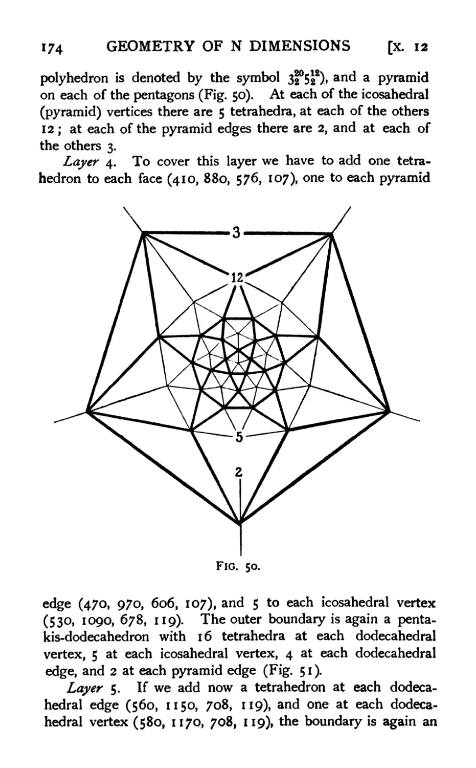
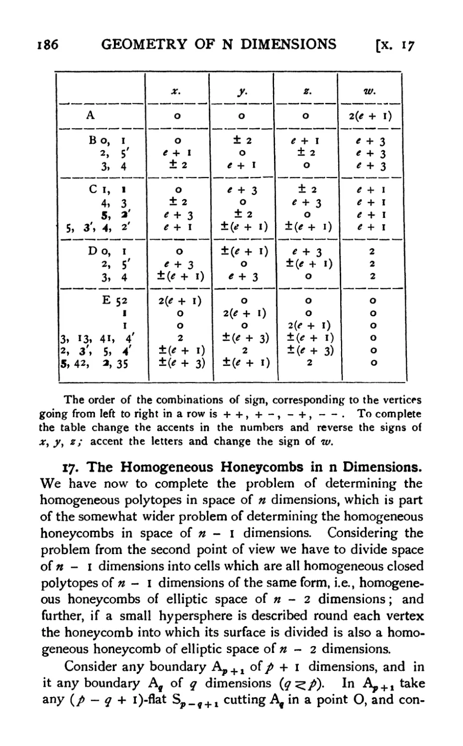
/


Текст
AN INTRODUCTION
TO THE GEOMETRY
OF N DIMENSIONS
BY
D. M. Y. SOMMERVILLE
M.A., D.Sc, F.N.Z.Inst.
PROFHSSOK ΟΓ PDKF. AND АГР1ЛЫ) MATHEMATICS, VICTORIA
I'NIVERSITY COLLEGE, WELLINGTON, N.Z.
WITH SIXTY DIAGRAMS
METHUEN & CO. LTD.
36 ESSEX STREET W.C.
LONDON
CONTENTS
CHAPTER I
Fundamental Ideas
PACE
1. Origins of geometry ι
2. Extension of the dimensional idea I
3. Definitions and axioms of geometry 2
4. The axioms of incidence 3
5. Projective geometry 4
6. Construction of three-dimensional space ..... 4
7. Desargues' theorem. 5
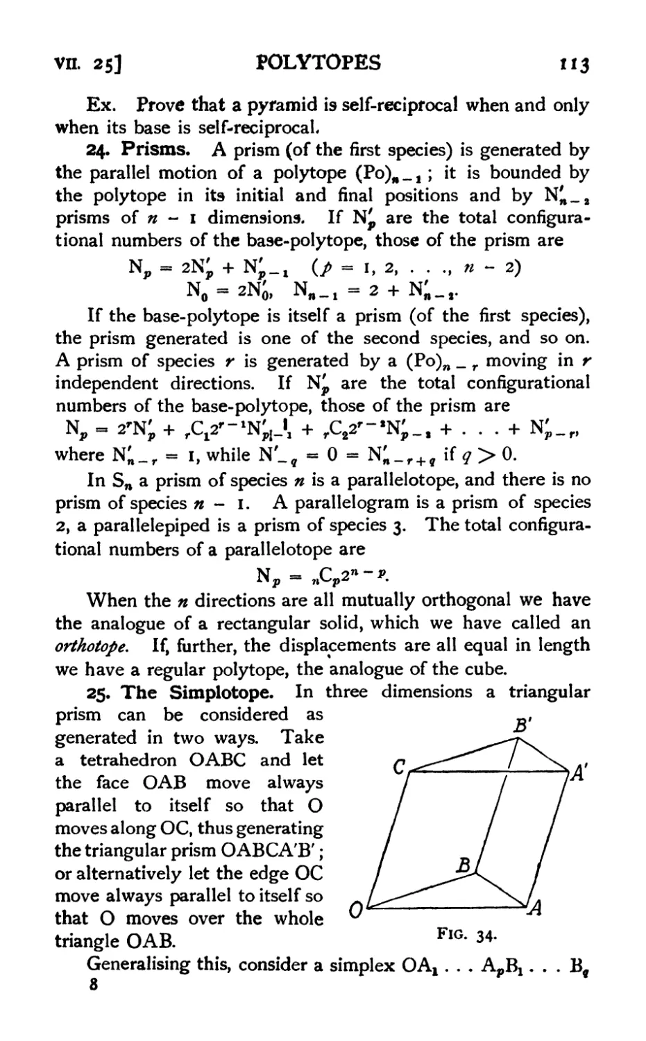
8. Extension to four dimensions 6
9. Degrees of freedom : dimensions 7
10. Extension to η dimensions 8
11. Independent points 8
12. Common flat and containing flat of two linear spaces . . 8
13. Degrees of freedom of linear spaces : constant-number . . 9
14. Degrees of incidence 9
15. Duality 9
16. Number of conditions required for a given degree of incidence . 10
17. Incidence of a linear space with two or more linear spaces:
enumerative geometry 10
18. Principle of specialisation 11
19. Enumerative geometry of linear spaces 11
20. Duality in enumerative geometry 12
21. Number of incident spaces in two and three dimensions . . 12
22. Incident spaces in four dimensions 13
23. Incident spaces in five dimensions 15
24. A general enumerative problem in η dimensions . . .18
25. Motion and congruence . . . . . . . 19
26. Order. Division of Sn by η + ι hyperplanes : the simplex . 20
CHAPTER II
Parallels
1. Parallel lines. Elliptic, hyperbolic, euclidean, and projective
geometries 22
xi
xii
GEOMETRY OF N DIMENSIONS
PACK
2. Transitivity of parallelism 22
3. Euclidean geometry : Parallel lines and planes . . .23
4. Direction and orientation 24
5. Points, lines, and plane at infinity 24
6. Parallelism in space of four dimensions. Half-parallel planes . 25
7. The hyperplane at infinity 26
8. Parallelism in Sn ; Degrees of parallelism 26
9. Degrees of parallelism possible in a given space ... 27
10. Sections of two parallel or intersecting spaces .... 27
11. The parallelotope 28
CHAPTER III
Perpendicularity
1. Line normal to an (n - i)-flat 30
2. System of л mutually orthogonal lines. Complete orthogonality 31
3. Orthogonality in relation to the absolute : absolute poles and
polars 31
4. The absolute in four dimensions 33
5. Half-orthogonal planes in S4 33
6. Orthogonality in Sn 35
7. Degrees of orthogonality 36
8. Degrees of orthogonality possible in a given space ... 36
9. Relation between orthogonality and parallelism 37
10. Degrees of orthogonality of a linear space to linear spaces lying
in another flat 37
CHAPTER IV
Distances and Angles between flat spaces
1. Mutual invariants of two linear spaces 39
2. Angle between an S^ and an SQ which have highest degree of
intersection 39
3. Distance between two completely parallel /-flats ... 40
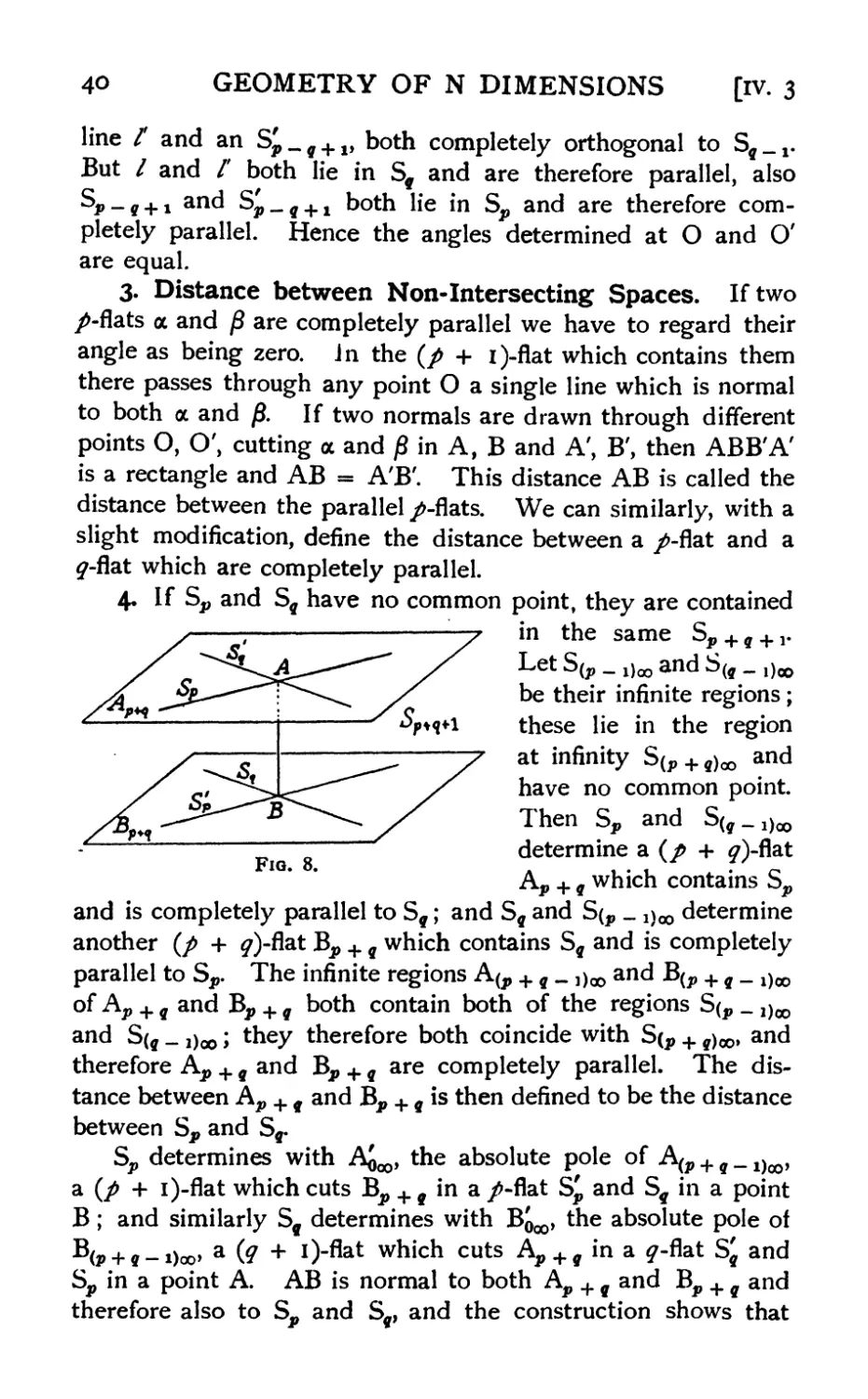
4. Distance between two linear spaces with no common point . 40
5. Distances between two parallel spaces 41
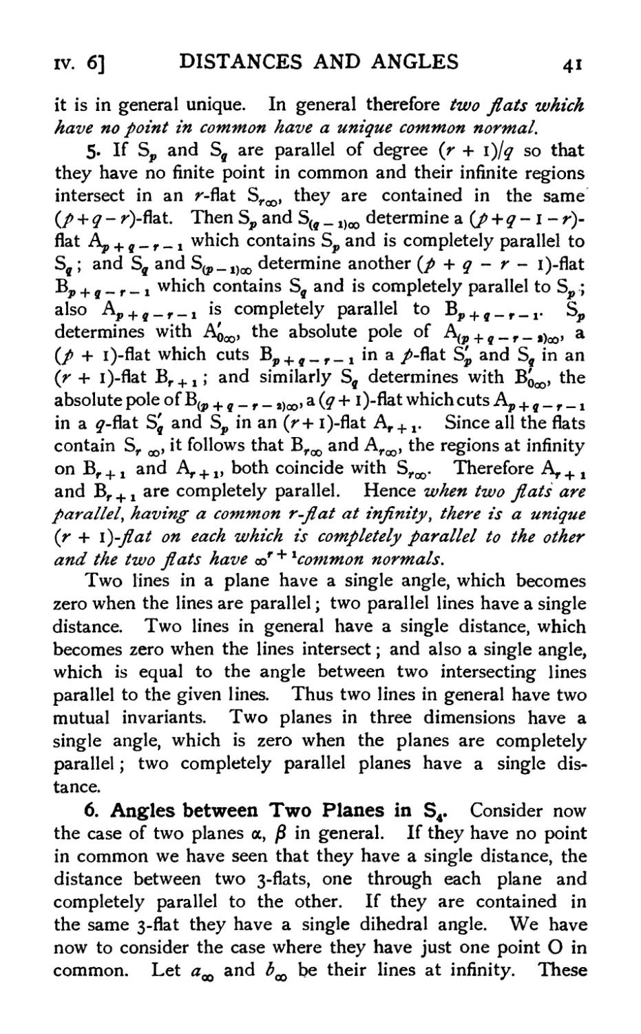
6. Angles between two planes in S4 41
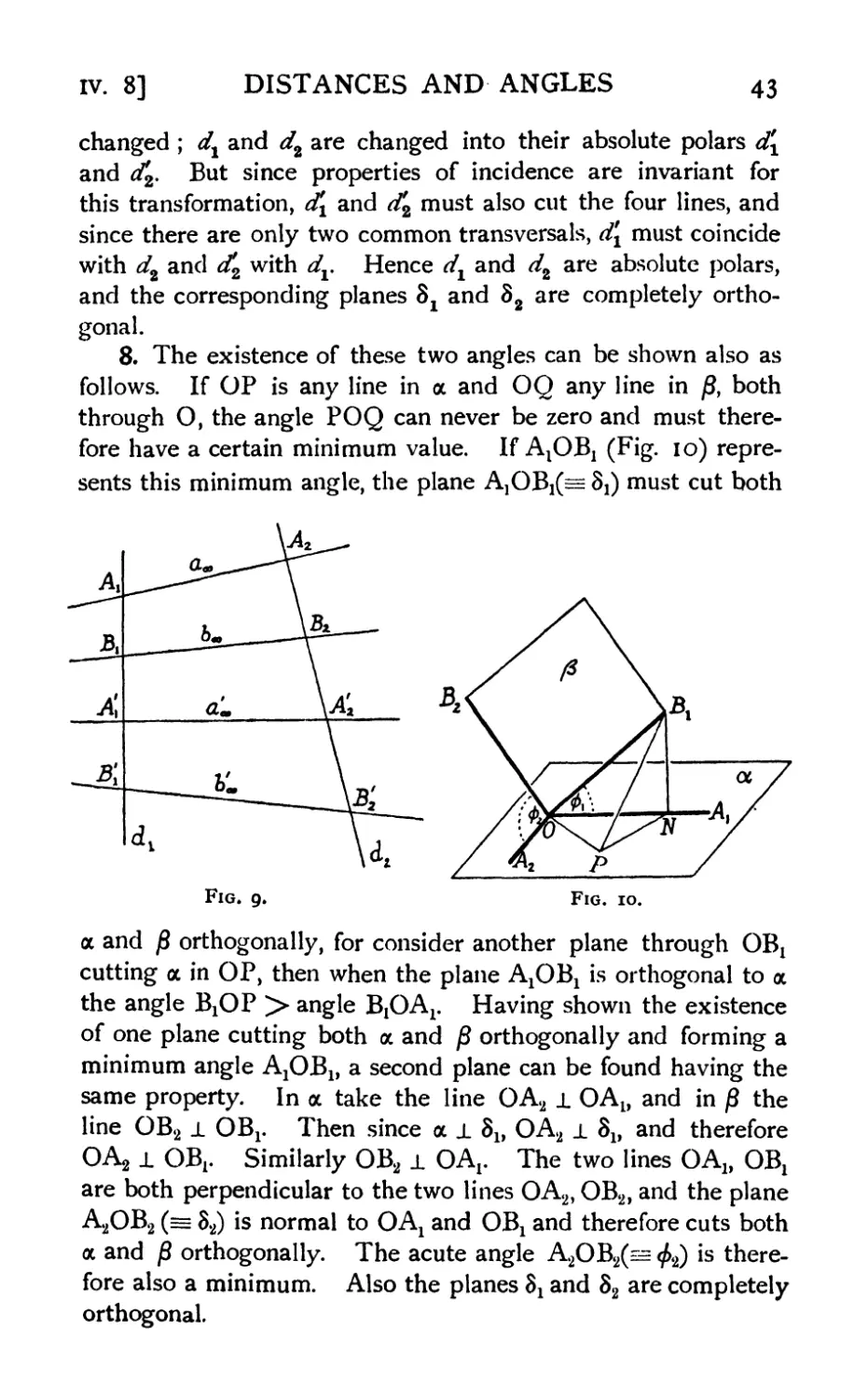
7. The two common orthogonal planes of two given planes . . 42
8. Maximum and minimum angles 43
9. Isocline planes 44
10. Special cases of two planes 44
11. The three mutual invariants of two planes in general . . 45
12. The/angles between two/-flats 45
13. The q angles between an Sp and an Sq with one common point. 45
14. Mutual invariants of Sp and Sq in general .... 46
15. Construction of the q angles between an Sj> and an Sa . . φ
CONTENTS
xiii
PAGE
16. Angles between the normal flats to two given flats ... 47
17. Angles between Sq and the normal flat to Sp . . .47
18. Projections 48
19. Parallel projection 48
20. Orthogonal projection 49
21. Projection of an orthotope into an orthotope .... 49
22. Content of the projection of a /-dimensional region ... 50
CHAPTER V
Analytical Geometry : Projective
1. Representation of a point by a set of numbers . . . 51
2. Parametric equations of a line, plane, . . . , {p- i)-flat . . 51
3. Equation of an (л - i)-flat 52
4. Equations of a (p - i)-flat 52
5. Matrix notation. Rank of a matrix 53
6. Number of conditions implied by the rank of a matrix . 53
7. Condition that/points should be independent . . . 54
8. Condition thatp hyperplanes should be independent . . -55
9. Simplex of reference 55
10. The unit-point. Co-ordinates expressed by cross-ratios . . 55
11. Duality 56
12. Equation of a variety : its order 56
13. Parametric equations. Rational varieties 57
14. Rational normal curves 57
15. Intersection of a variety by a linear space 58
16. Rational normal varieties 58
17. Quadric varieties 59
18. Conjugate points, polar, tangent 59
19. Correlations 60
20. Polar system, null system 61
21. Canonical equation of quadric 62
22. Real linear spaces lying on a quadric 62
23. Sylvester's Law of Inertia 63
24. Specialised quadrics. Double elements. Hypercones . 64
25. Hypercones in general 65
26. Polar spaces 66
27. Tangent spaces 67
28. Conditions for a hypercone 67
29. Degenerate quadrics 67
30. Linear spaces on a quadric : cases where η is odd or even . 68
31. Multiplicity of the linear spaces 69
32. Further distinction for η odd or even 70
33. The two systems of/-flats on a V* _ x : distinction for/ odd or
even 71
GEOMETRY OF N DIMENSIONS
CHAPTER VI
Analytical Geometry : Metrical
PAGE
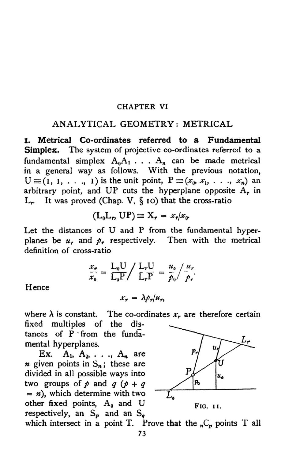
1. Metrical co-ordinates referred to a fundamental simplex . . 73
2. Identity connecting the point-co-ordinates 74
3. The hyperplane at infinity 74
4. Special co-ordinate systems analogous to trilinears and areals . 74
5. Cartesian co-ordinates 75
6. Radius-vector ; distance between two points . . . -75
7. Direction-angles ; angle between two lines .... 76
8. Equation of a hyperplane ; distance from a point to a hyperplane у у
д. Equations of a straight line ; Joachimsthal's formulae . . - УУ
10. The hypersphere yS
11. The hypersphere at infinity ; Absolute 79
12. General cartesian co-ordinates ; the distance-function . . 80
13. D irecti on-ratios ; angle between two lines . . . .81
14. The hyperplane ; direction and length of the perpendicular from
the origin 82
15. Angle between two hyperplanes ; tangential equation of the
Absolute 82
16. Plucker co-ordinates of a plane through the origin in S4 . 83
17. Condition that two planes through the origin should have a line
in common 84
18. Representation of the lines of Ss or the planes through a point in
S4 by points on a quadric in S5 85
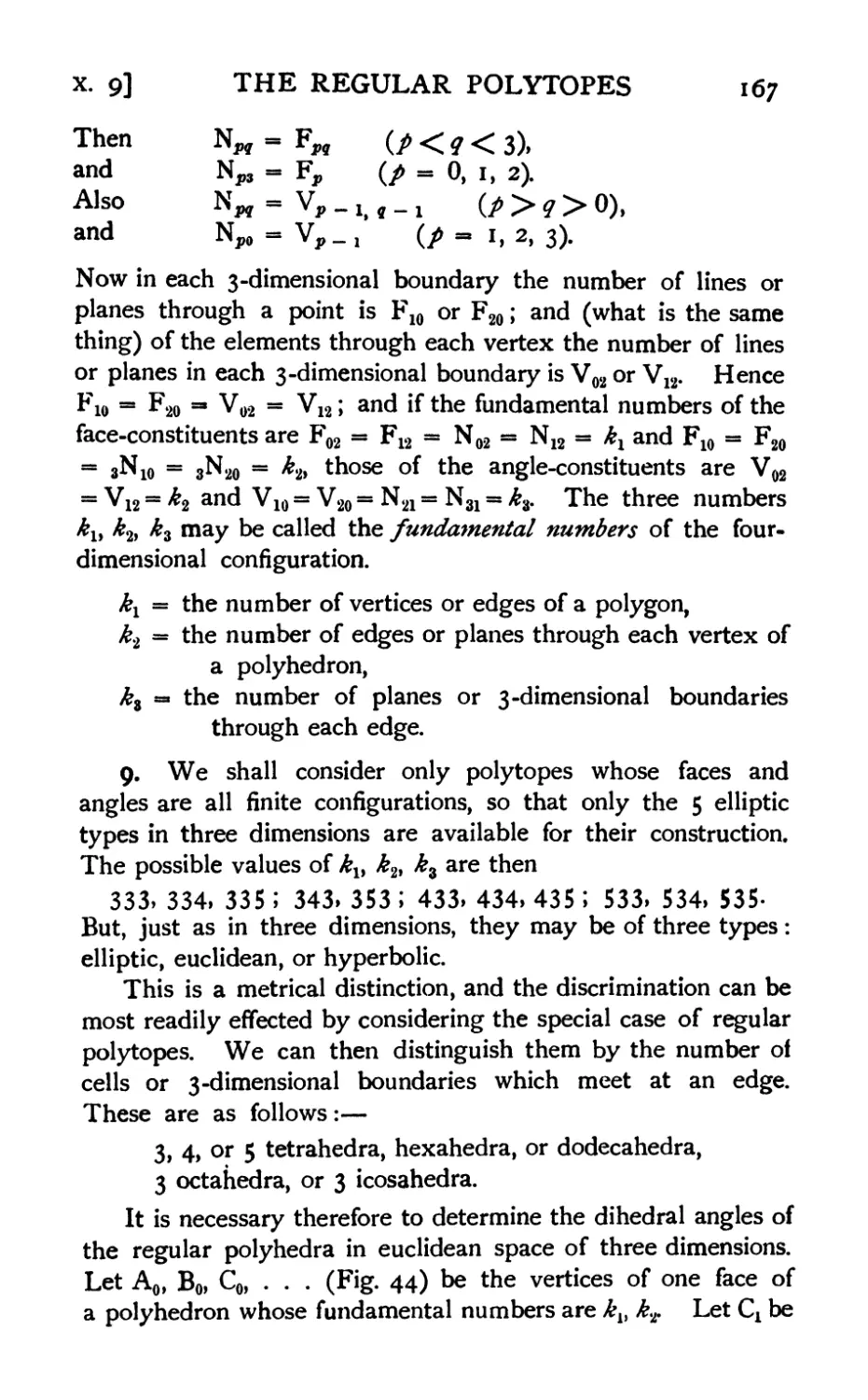
19. Linear complex, linear congruence,'and regulus ... 86
20. The special linear congruence 87
21. Metrical relations between planes through a point in S4 ; the
absolute polar of a plane 87
22. Condition that two planes should have a line in common . . 88
23. Condition that two planes should be completely parallel . . SS
24. Condition that two planes should be half-parallel ... 89
25. Condition that two planes should be completely orthogonal . 89
26. Condition that two planes should be half-orthogonal ... 89
27. The two common orthogonal planes to two planes through the
origin 89
28. Numerical example 90
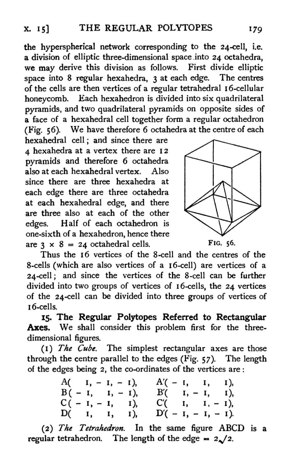
29. Co-ordinates of a {k - i)-flat in Sn 91
30. Identities connecting the co-ordinates 93
31. Condition of intersection of a /-flat and a ^-flat in Sp + q + г . 94
32. Variety representing the assemblage of £-flats in S^ . . .94
CHAPTER VII
Polytopes
1. Definition; boundaries 96
2. Boundaries of the simplex об
CONTENTS
xv
PAGE
3. Configurations 97
4. Relations connecting the configurational numbers ... 97
5. Application of configurational numbers to a polytope ... 98
6. Simple and complex polytopes ....... 98
7. Convex polytopes 99
8. Face- and vertex-constituents 99
9. Isomorphism 100
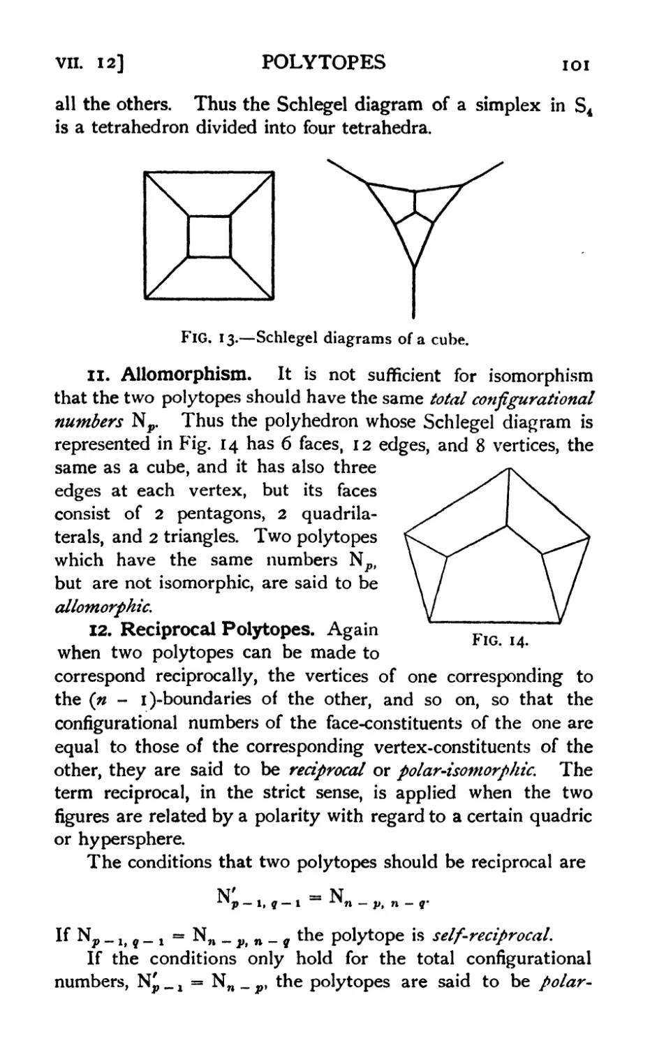
10. Schlegel diagrams 100
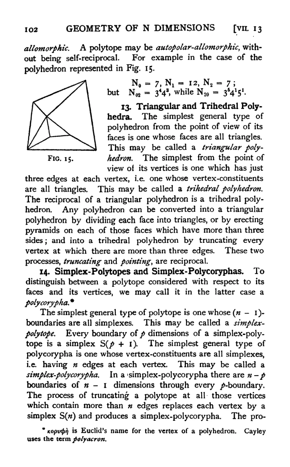
11. Allomorphism 101
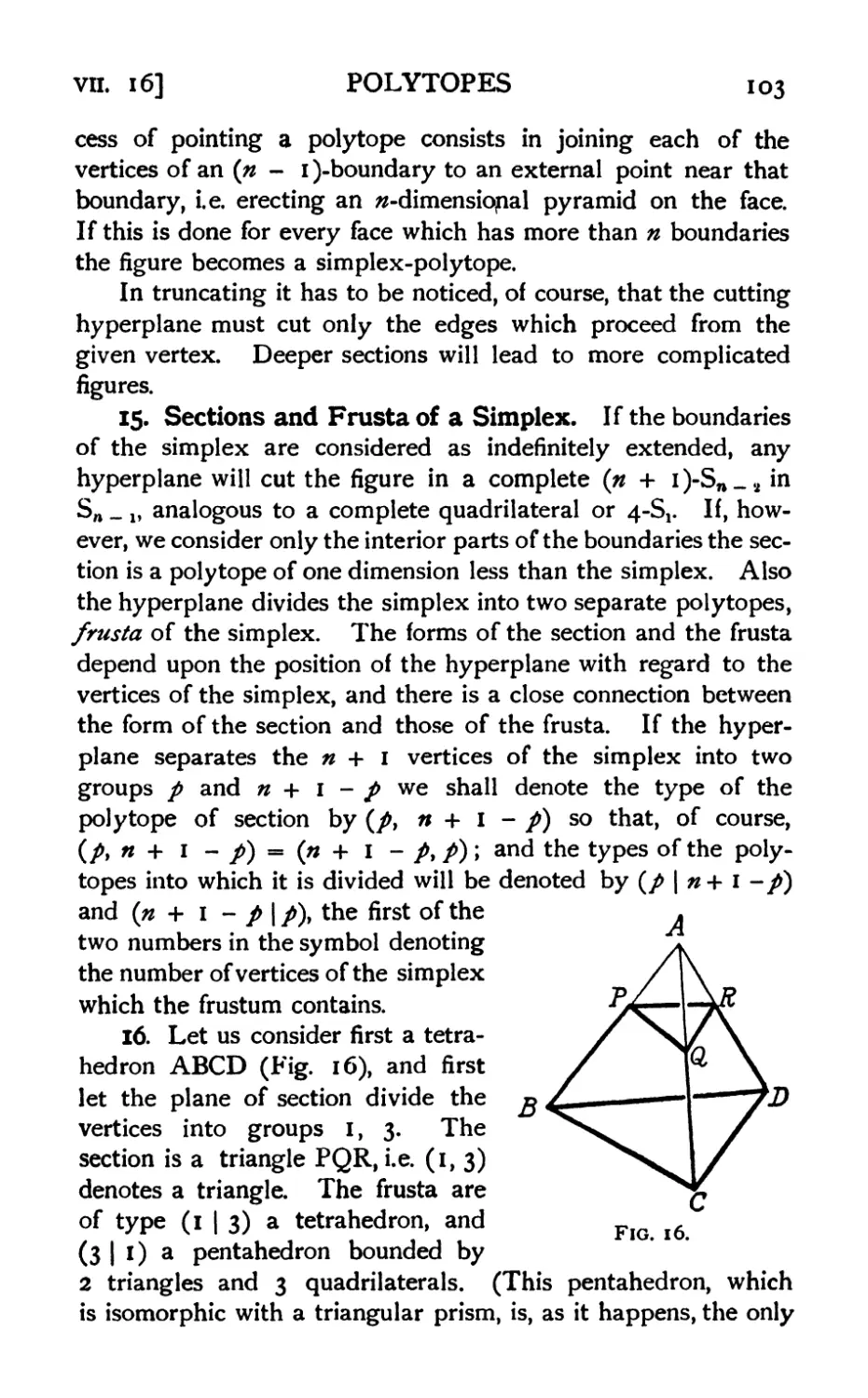
12. Polar-isomorphism, reciprocal polytopes 101
13. Triangular and trithedral polyhedra. Truncating and pointing . 102
14. Simplex-polytopes and simplex-polycoryphas . . . .102
15. Sections and frusta of a simplex 103
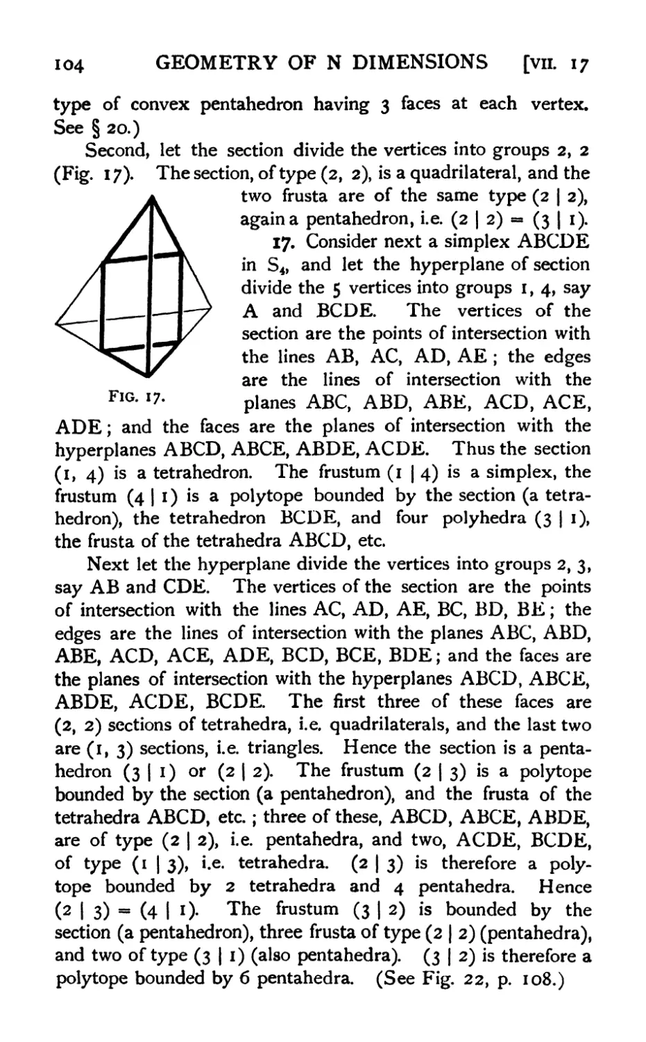
16. Sections and frusta of a tetrahedron . . . . . .103
17. Sections and frusta of a simplex in S4 104
18. Sections and frusta of a simplex in Sn 105
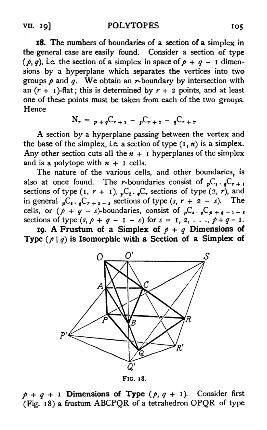
19. Isomorphism between sections and frusta of simplexes . .105
20. Number of simplex-poly topes in Sn with η + 2 cells . . . 106
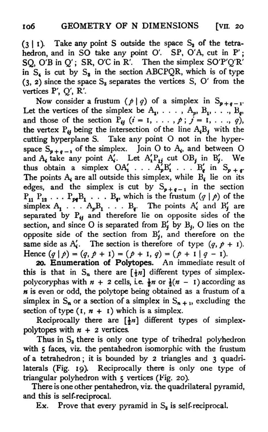
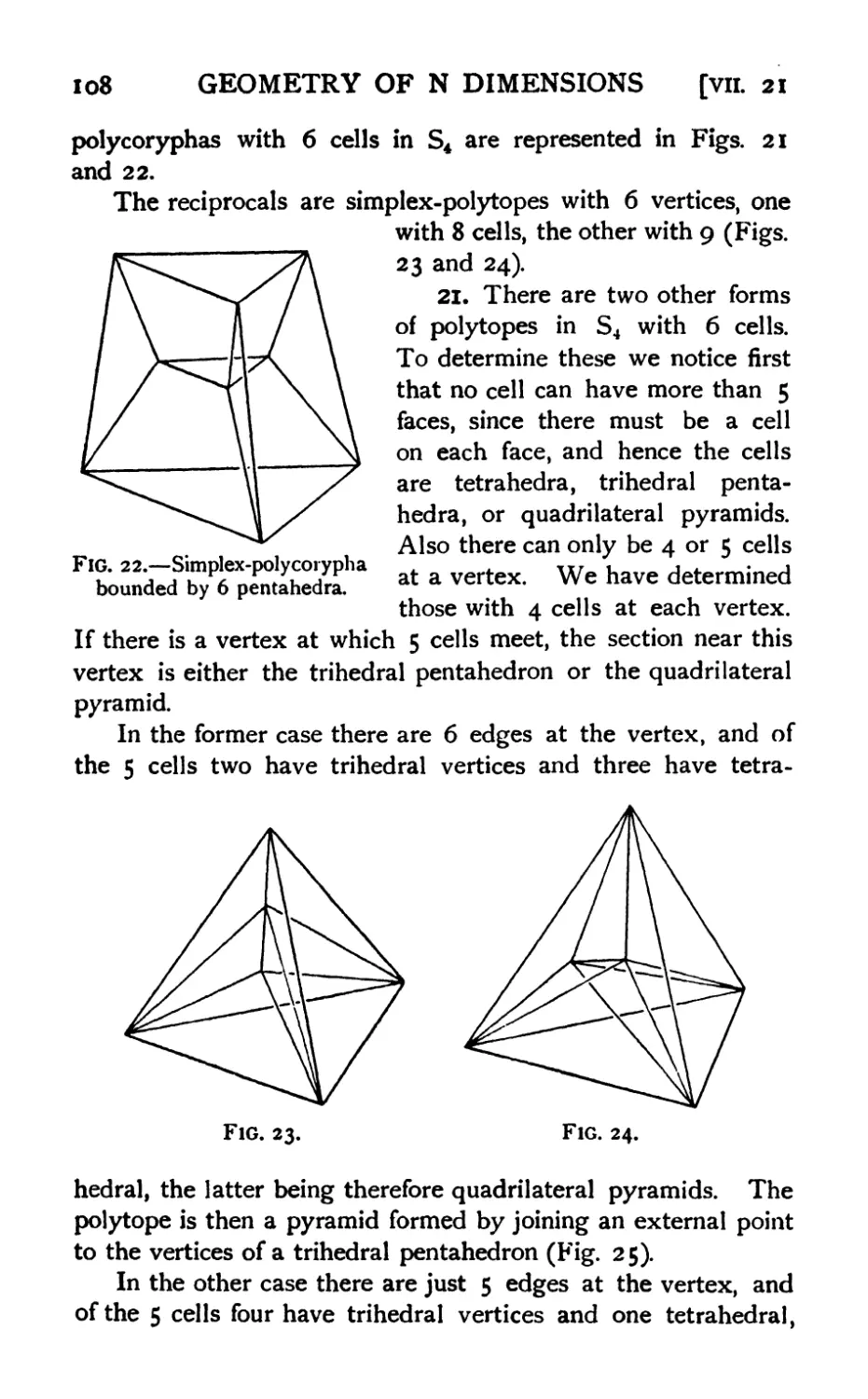
21. Other 6-cells in S4 108
22. Enumeration of polyhedra in S3; the complete enumeration of
hexahedra 109
23. Pyramids 111
24. Prisms; parallelotope, orthotope 113
25. The simplotope 113
26. The pyramidoid 115
27. Prismoids 115
CHAPTER VIII
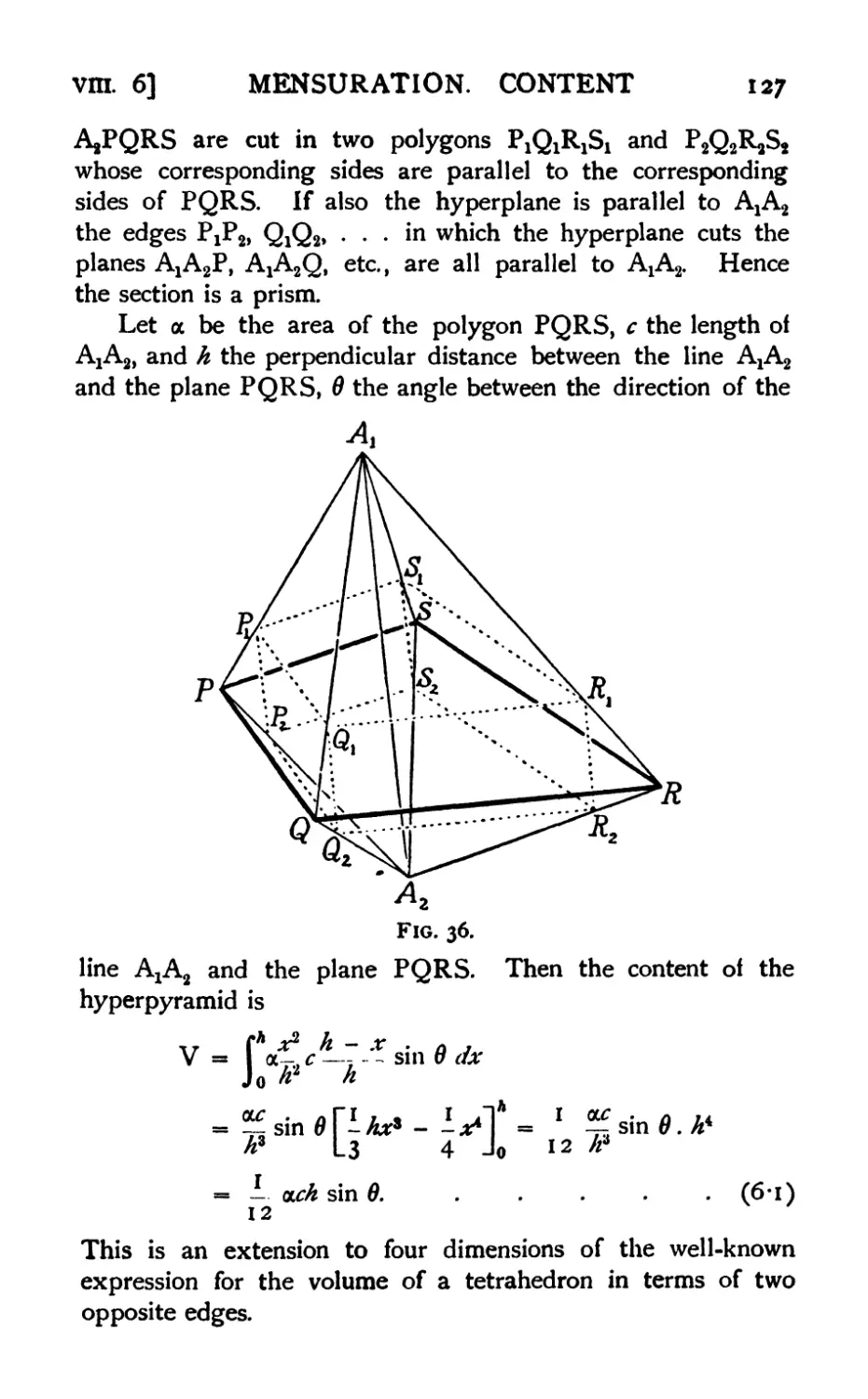
Mensuration : Content
1. General considerations. The orthotope 118
2. The prism 118
3. The parallelotope 119
4. The pyramid 123
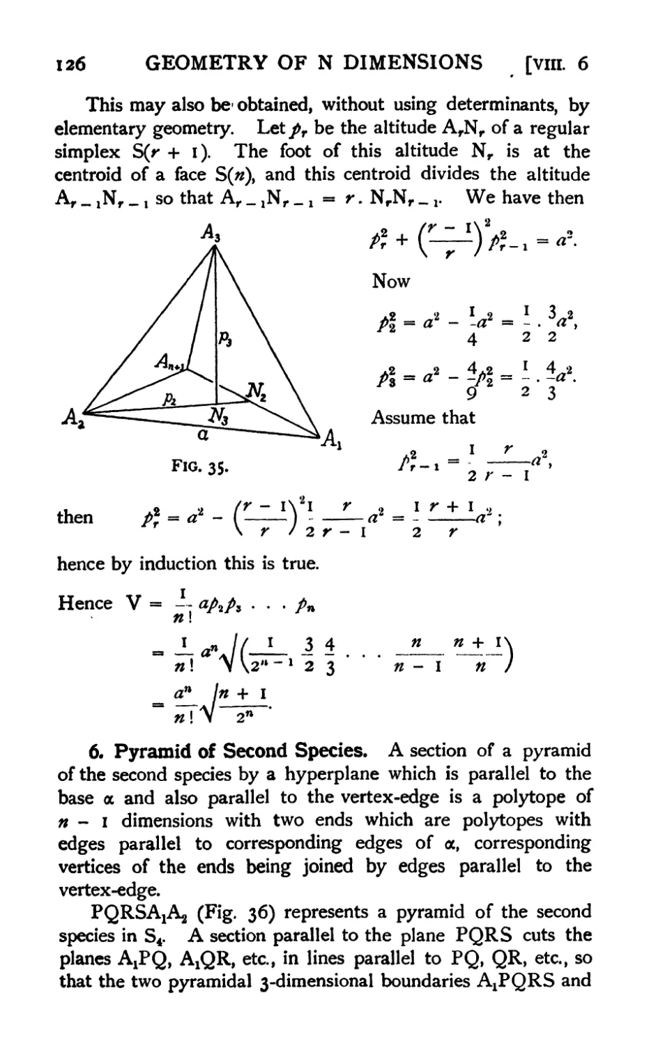
5. The simplex, in terms of its edges 124
6. The pyramid of second species, in terms of base and opposite
edge 126
7. The pyramid of species r 128
8. The simplotope *3°
9. Prismoidal formulae I31
10. The content of the prismoidal figure of species r expressed by
means of pairs of parallel sections 131
11. Determination of the coefficients 132
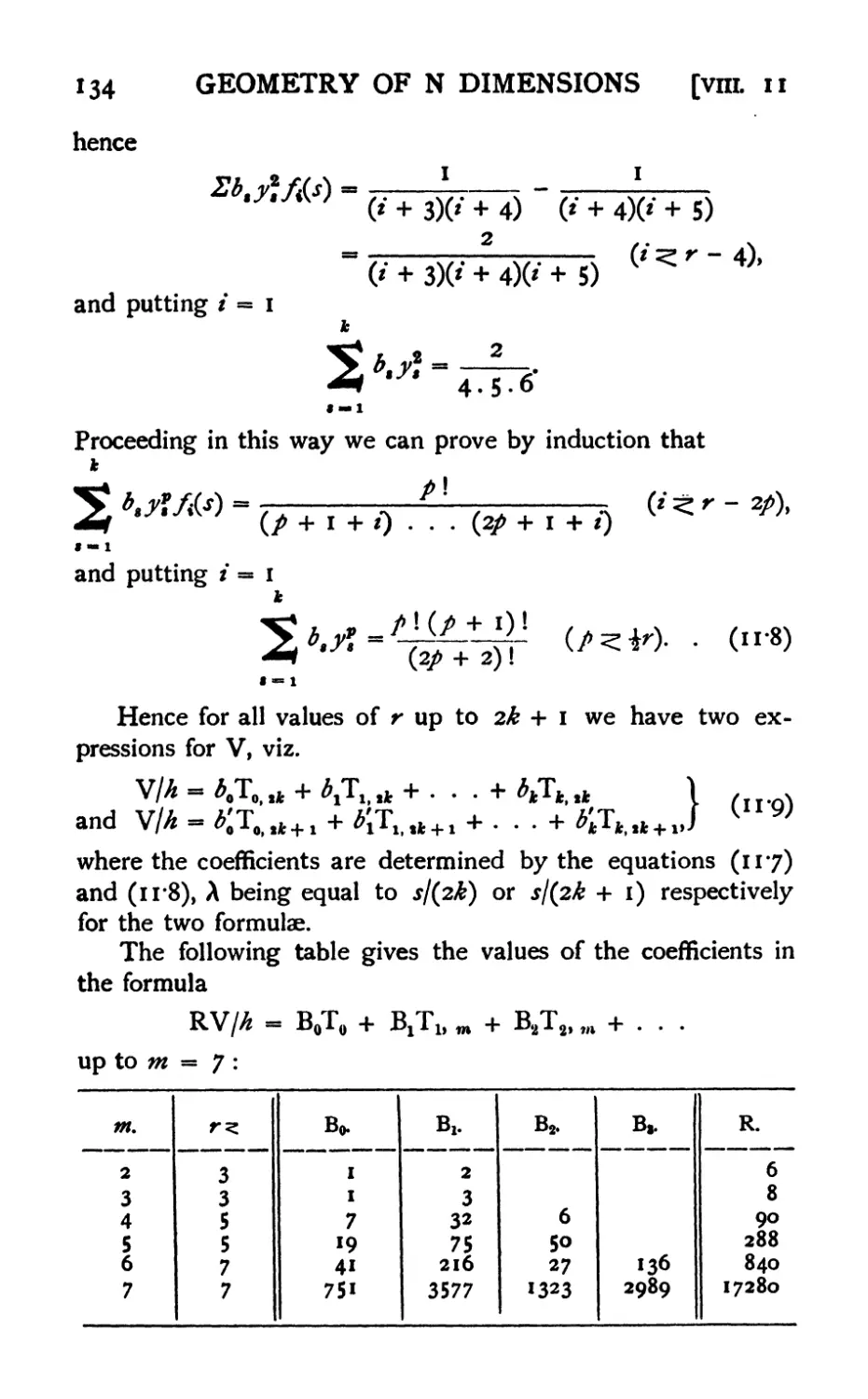
12. Content of the general prismoid 135
13. The hypersphere : volume-content 135
b
GEOMETRY OF N DIMENSIONS
PAGE
14. The hypersphere: surface-content 136
15. Varieties of revolution 137
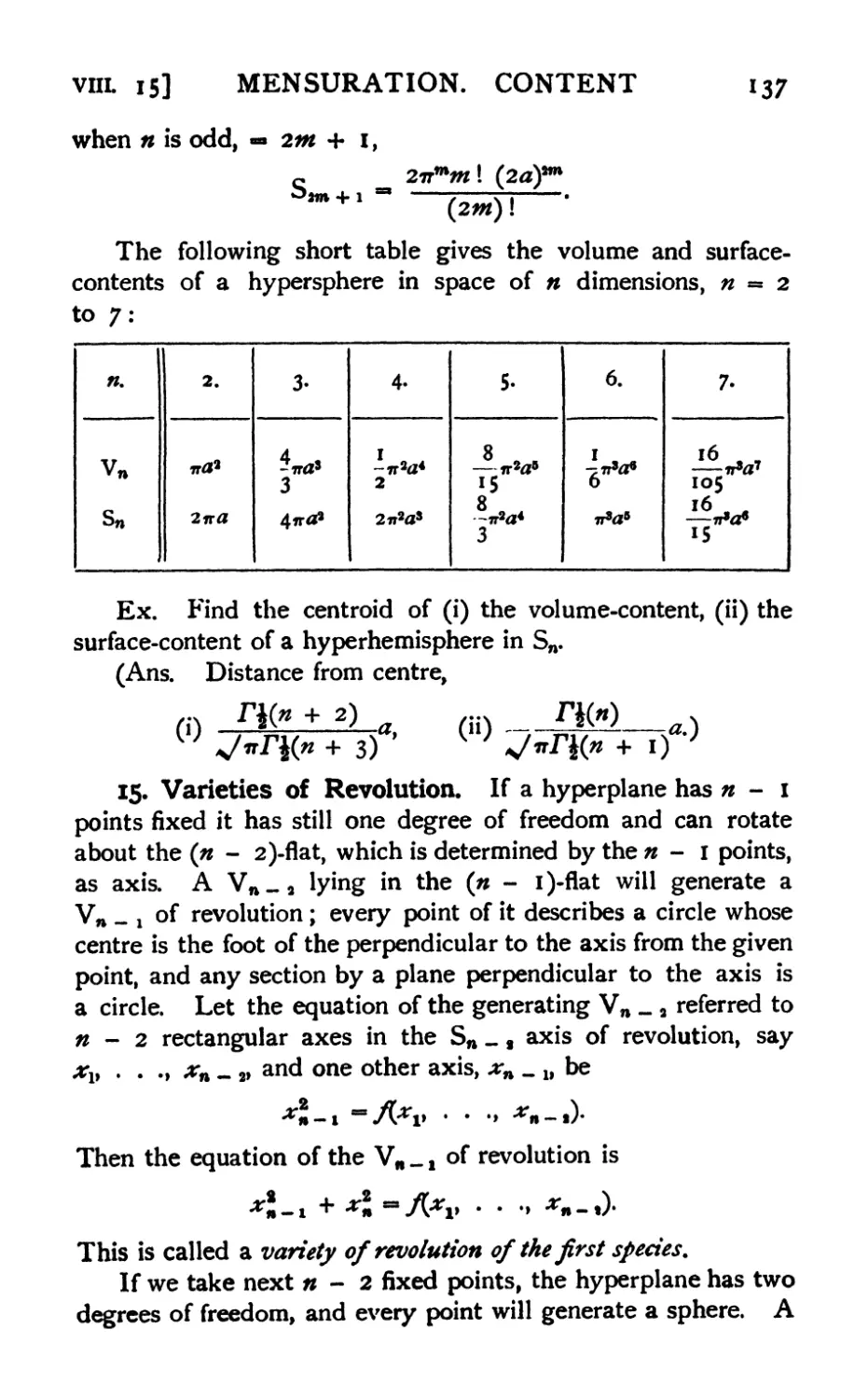
16. Content of a variety of revolution of any species . . . .138
17. Extensions of Pappus' Theorem 139
CHAPTER IX
Euler's Theorem
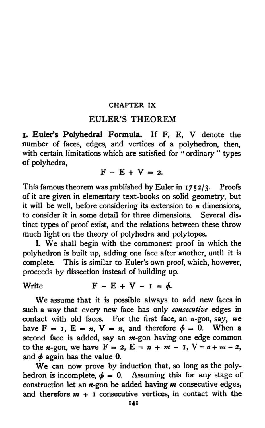
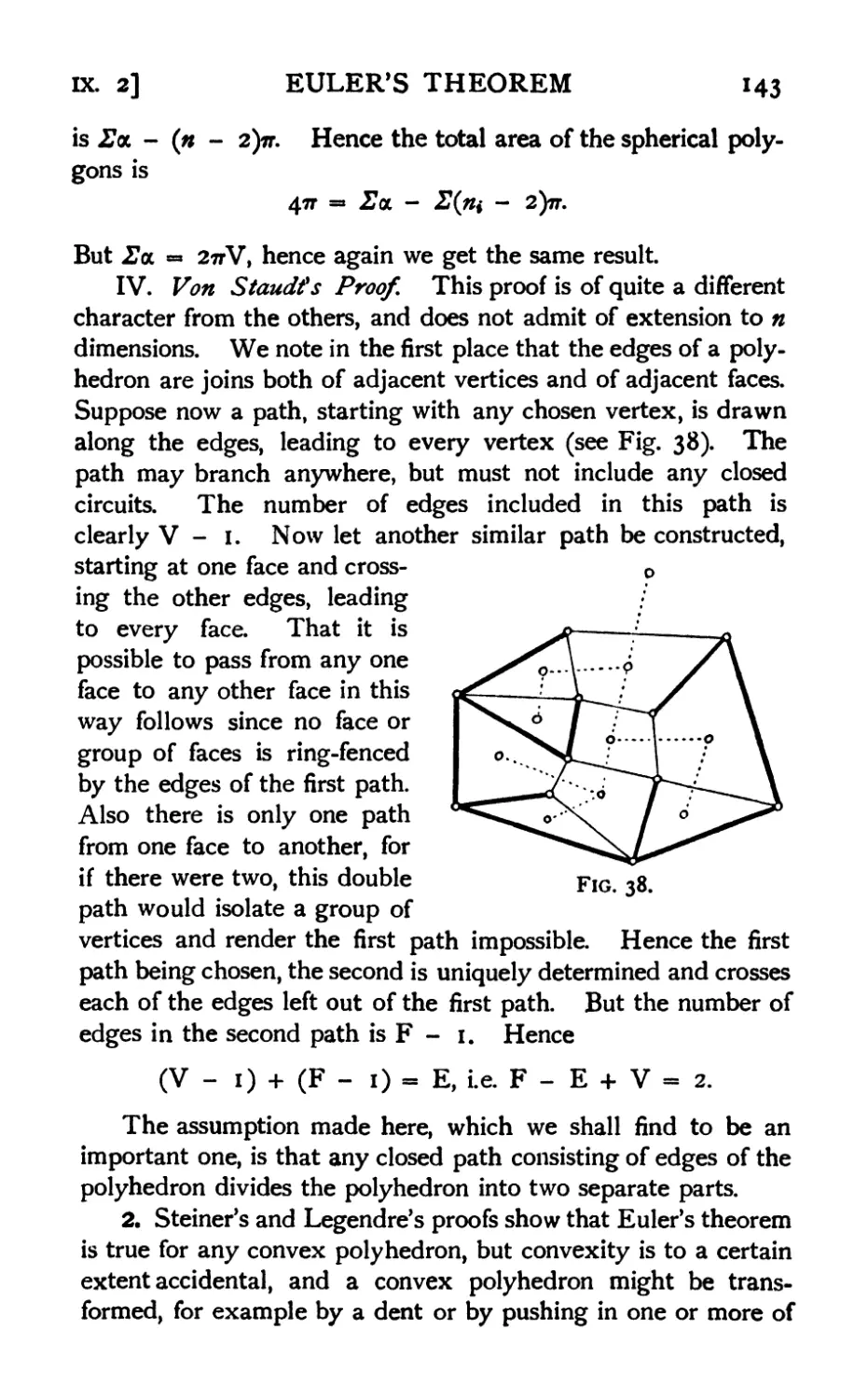
1. Euler's polyhedral formula : various proofs . . . .141
2. Conditions of validity 143
3. Connectivity of polygons 144
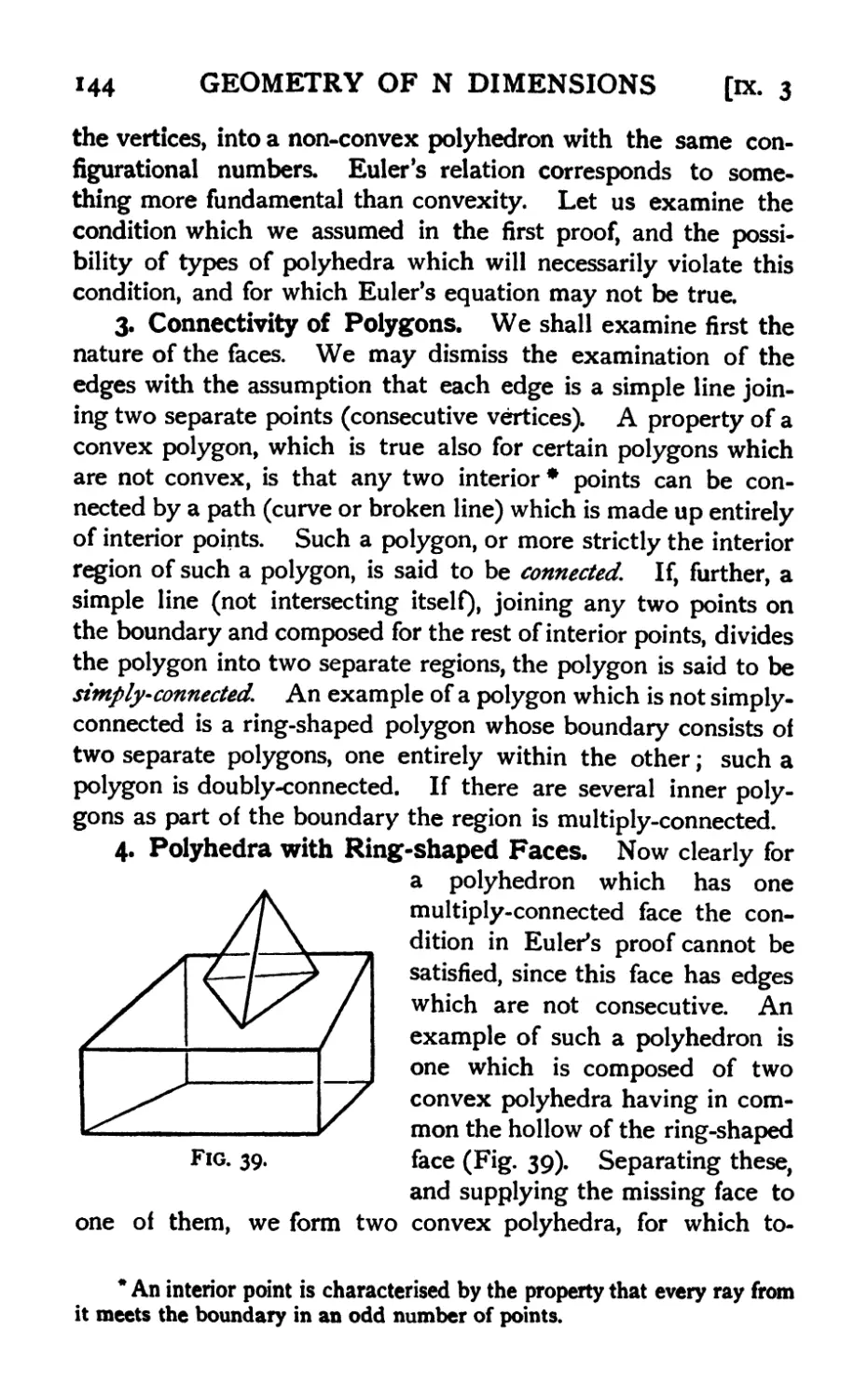
4. Polyhedra with ring-shaped faces 144
5. Connectivity of polyhedra 145
6. Ring-shaped polyhedra 145
7. Polyhedra with cavities 146
8. Eulerian polyhedra 146
9. Incomplete polyhedra and polytopes 146
10. Euler's theorem for simply-connected polytopes . . . .147
11. Other relations connecting the number of boundaries of a
polyhedron 147
12. Configurational relations in higher space 149
13. General theorems on simplex-polytopes and polycoryphas . .149
14. Proofs of Euler's theorem in four dimensions by consideration of
angles 150
15. Measurement of л-dimensional angles 152
16. Relation connecting the area and angle-sum of a triangle in
spherical geometry 154
17. Angular regions of a simplex 154
18. The angle-sums 155
19. Relations connecting the angle-sums of a simplex . . .156
20. Extension to an Eulerian polytope in spherical hyperspace . . 157
21. The angular relation corresponding to Euler's equation in
euclidean or non-euclidean geometry 159
CHAPTER X
The Regular Polytopes
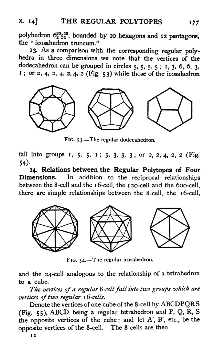
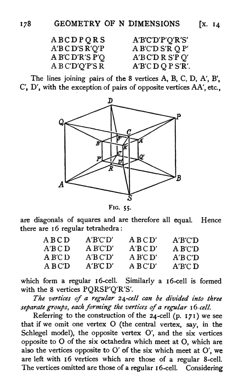
1. Conditions determining a regular or a homogeneous polyhedron . 161
2. A polyhedron as a configuration 161
3. Three types of configurations : elliptic, euclidean, and hyperbolic 162
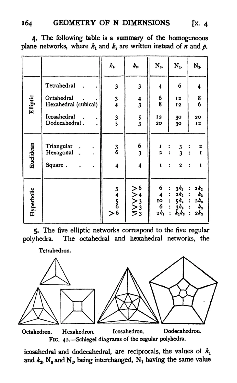
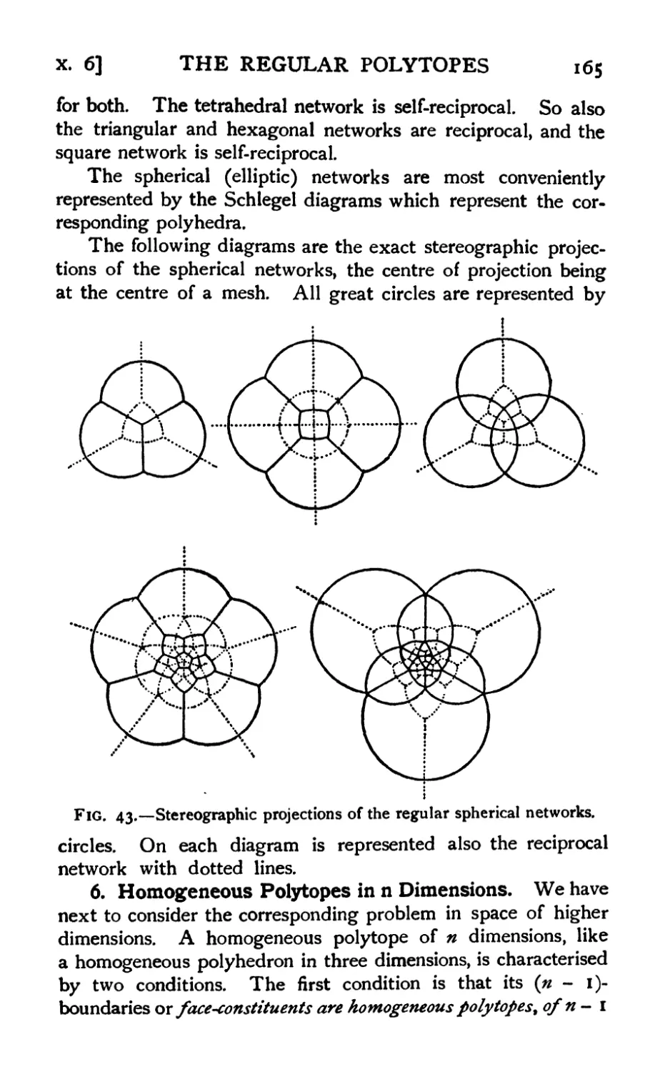
4. Table of the homogeneous plane networks 164
5. The five elliptic networks or regular polyhedra . . . .164
6. Conditions determining a regular or homogeneous polytope in
ft dimensions 165
7. Eleven possible homogeneous honeycombs in three dimensions . 166
CONTENTS
xvii
8. Configurational numbers of a four-dimensional polytope
9. Discrimination of elliptic honeycombs by dihedral angles .
10. The six regular poly topes in four dimensions
11. Ratios of the configurational numbers ....
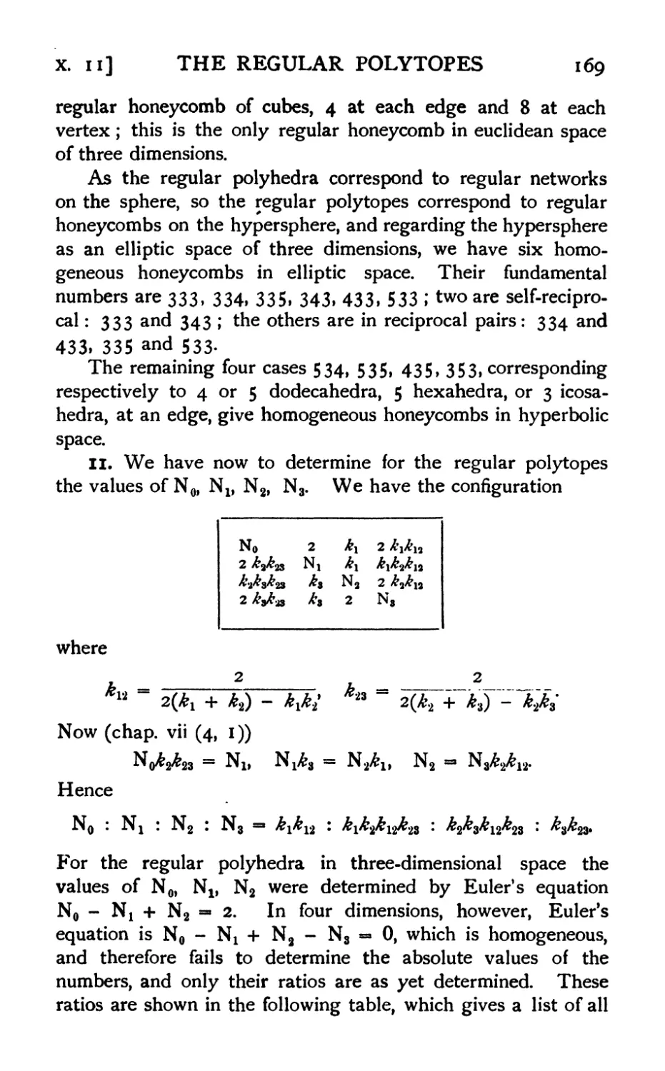
12. The construction of the six regular poly topes
13. Comparison with the three-dimensional polyhedra
14. Relations between the regular poly topes in four dimensions
15. The regular polyhedra referred to rectangular axes
16. The regular polytopes referred to rectangular axes
17. The problem in η dimensions
18. Eleven possible homogeneous honeycombs in four dimensions
19. Method of discrimination
20. Three regular polytopes in five dimensions....
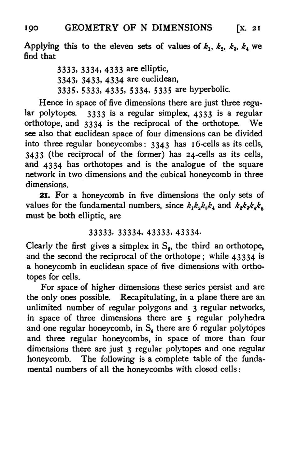
21. Table of homogeneous honeycombs in η dimensions .
Index
193
GEOMETRY OF N DIMENSIONS
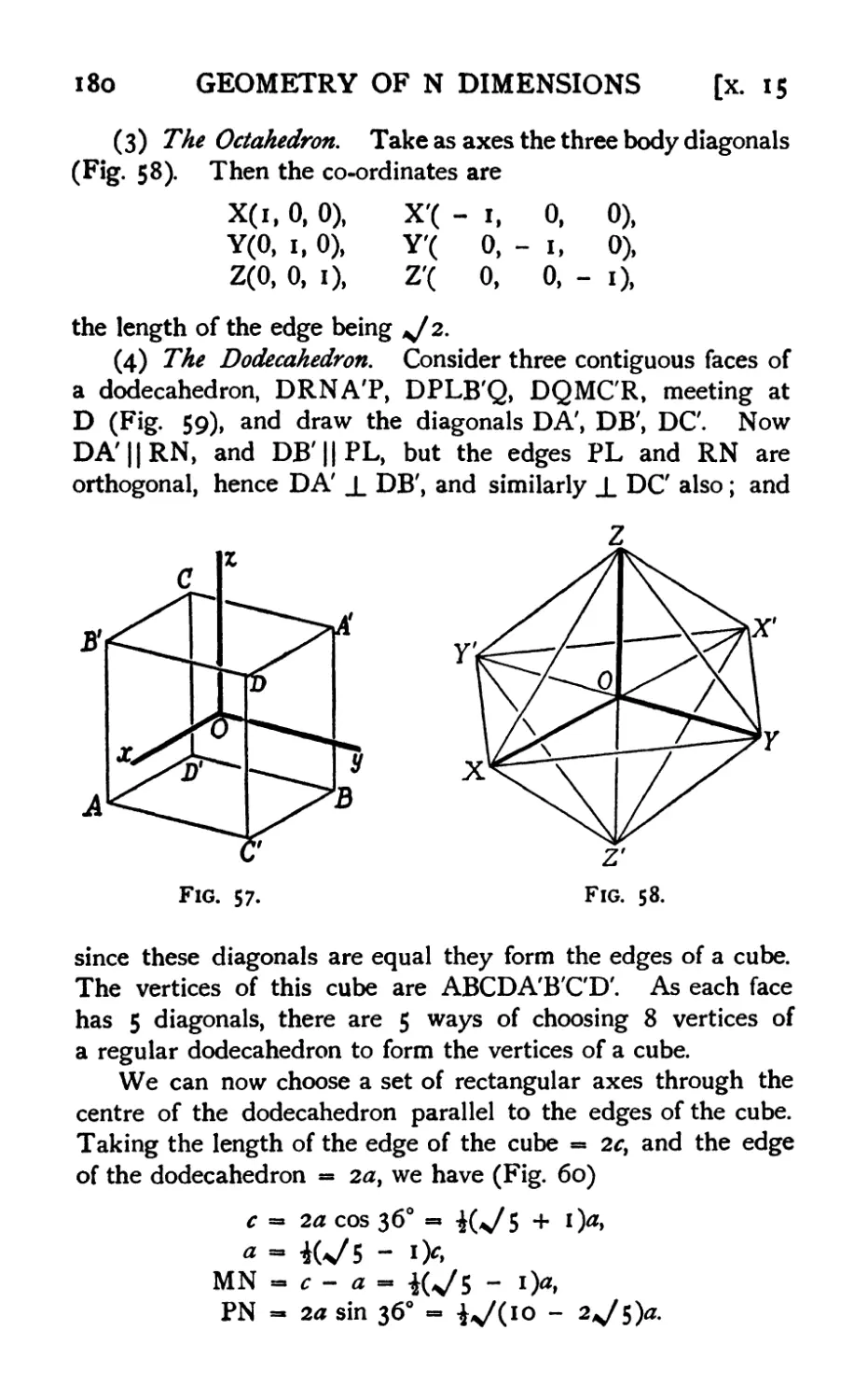
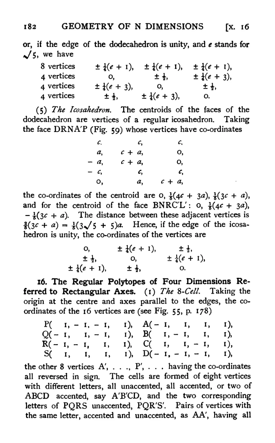
CHAPTER I
FUNDAMENTAL IDEAS
I. Origins of Geometry. Geometry for the individual begins
intuitionally and develops by a co-ordination of the senses of
sight and touch. Its history followed a similar course. The
crude ideas of shape, bulk, superficial extent, and length
became analysed, refined, and made abstract, and led to the
conception of geometrical figures. The development started
with the solid; surface and line, without solidity, were later
abstractions. Witness the inability of most animals and some
primitive races of men to recognise a picture. Having no
depth, except such as is imitated by the skilfulness of the drawing
or shading, it conveys to the undeveloped intelligence only an
impression of flat regions of contrasted colouring. When the
power of abstraction had proceeded to the extent of conceiving
surfaces apart from solids, plane geometry arose. The idea of
dimensionality was then formed, when a region of two
dimensions was recognised within the three-dimensional universe.
This stage had been reached when Greek geometry started.
It was many centuries, however, before the human mind began
to conceive of an upward extension to the idea of dimensionality,
and even now this conception is confined to the comparatively
very small class of mathematicians and philosophers.
2. Extension of the Dimensional Idea. There are two
main ways in which we may arrive at an idea of higher
dimensions: one geometrical, by extending in the upward
direction the series of geometrical elements, point, line, surface,
solid; the other by invoking algebra and giving extended
geometrical interpretations to algebraic relationships. In
whatever way we may proceed we are led to the invention of new
ι
2
GEOMETRY OF N DIMENSIONS
[I· 3
elements which have to be defined strictly and logically if exact
deductions are to be made. A great deal is suggested by
analogy, but while analogy is often a useful guide and stimulus,
it provides no proofs, and may often lead one astray if not
supplemented by logical reasoning. If we follow the geometrical
method the only safe course is that which was systematically
laid down for the first time by Euclid, that is to lay down a
basis of axioms or assumptions. When we leave the field of
sensuous perception and can no longer depend upon intuition
as a guide, our axioms will no longer be " self-evident truths,"
but simply statements, assumed without proof, as a basis for
future deductions.
3. Definitions and Axioms. In geometry there are objects
which have to be defined, and relationships between these
objects which have to be deduced either from the definitions
or from other simpler relationships. In defining an object we
must make reference to some simpler object, hence there must
be some objects which have to be left undefined, the inde-
finables. Similarly, in deducing relations from simpler ones
we must arrive back at certain statements which cannot be
deduced from anything simpler; these are the axioms or
unproved propositions. The whole science of geometry can
thus be made to rest upon a set of definitions and axioms.
The actual choice of fundamental definitions and axioms is
to a certain extent arbitrary, but there are certain principles
which have to be considered in making a choice of axioms.
These are:—
(1) Self-consistency. The set of axioms must be logically
self-consistent. No axiom must be in conflict with deductions
from any of the other axioms.
(2) Non-redundance or Independence, This condition is not
a necessary one, but in a logical scheme it is desirable. Peda-
gogically the condition is frequently ignored.
(3) Categoncalness. This means not only that the set of
axioms should be complete and sufficient for the development
of the science, but that it should be possible to construct only
a unique set of entities for which the axioms are valid. It is
doubtful whether any set of axioms can be strictly categorical.
If any set of entities is constructed so as to satisfy the axioms,
14]
FUNDAMENTAL IDEAS
3
it is nearly always, if not always, possible to change the ideas
and construct another set of entities also satisfying the axioms.
Thus with the ordinary ideas of point and straight line in plane
geometry the axioms can still be applied when instead of a point
we substitute a pair of numbers (ж, y\ and instead of straight
line an equation of the first degree in χ and у; corresponding
to the incidence of a point with a straight line we have the fact
that the values oix and у satisfy the equation. It is desirable,
in fact, that the set of axioms should not be categorical, for
thereby they are given a wider field of validity, and propositions
proved for the one set of entities can be transferred at once to
another set, perhaps in a different branch of mathematics.
4. The Axioms of Incidence. As indefinables we shall
choose first the point, straight line> and plane. With regard to
these we shall proceed to make certain statements, the axioms.
If these should appear to be very obvious, and as if they might
be taken for granted, it will be a good corrective for the reader
to replace the words point and straight line, which he must
remember are not yet defined, by the names of other objects to
which the axioms may be made to apply, such as " committee
member" and "committee." Following Hubert we divide the
axioms into groups.
THE AXIOMS
Group I
AXIOMS OF INCIDENCE OR CONNECTION
I. I. Any two distinct points uniquely determine a straight
line.
We imagine a collection of individuals who have a craze for
organisation and form themselves into committees. The committees are so
arranged that every person is on a committee along with each of the
others, but no two individuals are to be found together on more than one
committee.
I. 2. If A, B are distinct points there is at least one point not
on the straight line AB.
This is an " existence-postulate."
I. 3. Any three non-collinear points determine a plane.
4
GEOMETRY OF N DIMENSIONS [I. 5
I. 4. If two distinct points А, В both belong to a plane a,
every point of the straight line AB belongs to a.
From I. 1 it follows that two distinct straight lines have
either one or no point in common. From I. 4 it follows that
a straight line and a plane have either no point or one point in
common, or else the straight line lies entirely in the plane; from
I. 3 and 4 two distinct planes have either no point, one point,
or a whole straight line in common.
I. 5. If A, By С are non-collinear points there is at least one
point not on the plane ABC.
I. 2 and 5 are existence-postulates; 2 implies two-dimensional
geometry, and 5 three-dimensional.
The next of Hubert's axioms is that if two planes have one
point A in common they have a second point В in common, and
therefore by I. 4 they have the whole straight line AB in
common. If this is assumed it limits space to three dimensions.
5· Projective Geometry· There is a difficulty in
determining all the elements of space by means of the existence
postulates and other axioms, for while Axiom I. 1 postulates
that any two points determine a line, there is no axiom which
secures that any two lines in a plane will determine a point.
In fact, in euclidean geometry this is not true since parallel lines
have no point in common. For the present therefore we shall
confine ourselves to a simpler and more symmetrical type of
geometry, projective geometry, for which we add the following
axiom:
I. 1'. Any two distinct straight lines in a plane uniquely
determine a point.
6. Construction of Three-dimensional Space. We may
proceed now to obtain all the elements, points, lines, etc., of
space with the help of the existence postulates and other axioms.
Starting with two points А, В we determine the line AB, and
on this we shall suppose all the points determined. Taking
a third point C, not on AB, a plane ABC is determined. In
this plane there are determined : first, the three points А, В, С,
then the three lines ВС, СА, AB and all their points; then all
lines determined by two points one on each of two of these
lines, and since every line in the plane meets these three lines
all the lines of the plane are thus determined ; finally any point
ι. 7] FUNDAMENTAL IDEAS
5
of the plane is determined by the intersection of two lines
which have already been determined, e.g. if Ρ is any point of
the plane, the line PA cuts ВС in a point L and PB cuts CA
in a point Μ ; there are therefore two points, L on ВС and Μ
on CA, such that LA and MB determine P.
We next take a point D not in the plane ABC, and
determine planes, lines and points as follows: first, the planes DBC,
DCA, DAB and all the lines and points in these planes; then
the lines determined by joining D to the points of ABC, and all
the points on these lines, and all the lines and planes determined
by any two or any three of the points thus determined. .If now
Ρ is any point we cannot be sure that it is one of the points thus
determined unless the line DP meets the plane ABC. For this
we could assume as an axiom: " every line meets every plane
in a point," which is true for projective geometry of three
dimensions; but a weaker axiom, which is true also in euclidean
geometry, is sufficient, viz. Hubert's axiom :
I. 6. If two planes have a point A in common, they have a
second point В in common.
Then if Ρ is any point, the planes PAD and ABC, which
have the point A common, have another point, say Q, common,
and the lines AQ and DP which lie in the same plane determine
a point R which lies in the line DP and also in the plane ABC.
Hence DP meets the plane ABC, and therefore all points are
obtained by this process.
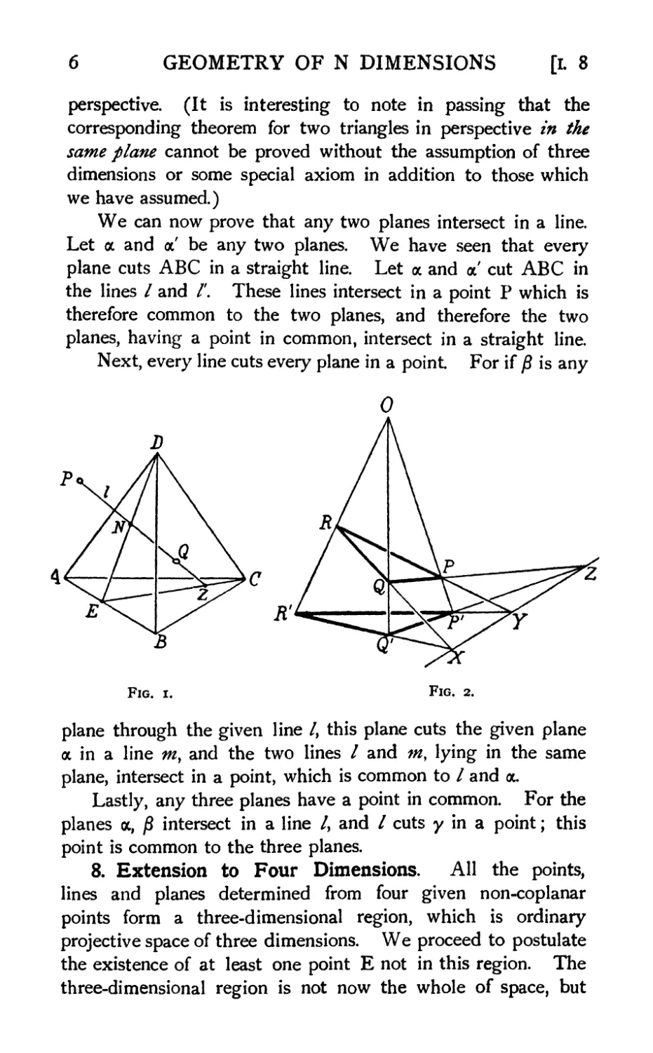
If/ is any line (Fig. i), determined by the two points P, Q,
the planes PQD and ABD, having D in common, intersect in a
line which cuts PQ in N, say, and AB in Ε; then PQ and CE
lie in the same plane and therefore meet in a point Z. Hence
every line cuts the plane ABC.
7. If α is any plane (Fig. 2), determined by the three points
P, Q, R, and О is a point not in this plane, the lines OP, OQ,
OR cut ABC in P', Q', R'. QR and Q'R', being in the same
plane, intersect in a point X. Similarly RP and R'P' intersect
in Y, and PQ and P'Q' in Z. Hence every plane cuts the
plane ABC.
The points Χ, Υ, Ζ all lie in both of the planes PQR and
P'Q'R' and are therefore collinear. This theorem is known as
Desargues* Theorem^ PQR and P'Q'R' being two triangles in
6 GEOMETRY OF N DIMENSIONS [ι. 8
perspective. (It is interesting to note in passing that the
corresponding theorem for two triangles in perspective in the
same plane cannot be proved without the assumption of three
dimensions or some special axiom in addition to those which
we have assumed.)
We can now prove that any two planes intersect in a line.
Let α and a' be any two planes. We have seen that every
plane cuts ABC in a straight line. Let α and a' cut ABC in
the lines / and /'. These lines intersect in a point Ρ which is
therefore common to the two planes, and therefore the two
planes, having a point in common, intersect in a straight line.
Next, every line cuts every plane in a point For if β is any
Fig. i. Fig. 2.
plane through the given line /, this plane cuts the given plane
α in a line mf and the two lines / and m, lying in the same
plane, intersect in a point, which is common to / and a.
Lastly, any three planes have a point in common. For the
planes α, β intersect in a line /, and / cuts у in a point; this
point is common to the three planes.
8. Extension to Four Dimensions. All the points,
lines and planes determined from four given non-coplanar
points form a three-dimensional region, which is ordinary
projective space of three dimensions. We proceed to postulate
the existence of at least one point Ε not in this region. The
three-dimensional region is not now the whole of space, but
I. 9] FUNDAMENTAL IDEAS
7
will be called a hyperplane lying in hyperspace. A hyperplane
is thus determined by four points. We may determine
similarly the hyperplanes ABCE, ABDE, etc., and the planes,
lines and points in them, and further the hyperplanes, planes,
and lines determined by four, three, or two points not all lying
in one of these hyperplanes. The hyperplanes ABCE and
ABDE have the three points Α, Β, Ε in common and therefore
the plane ABE. We may show that any two hyperplanes in
this region have a plane in common. For example, if α and a'
are two hyperplanes determined by four points P, Q, R, S and
P', Q', R', S' lying on EA, EB, EC, ED respectively, PQ
and P'Q', being in the plane EAB, cut in a point Z, similarly
QR and Q'R' cut in a point X, and RP and R'P' in a point Υ;
PS and P'S' cut in U, QS and Q'S' in V, RS and R'S' in W.
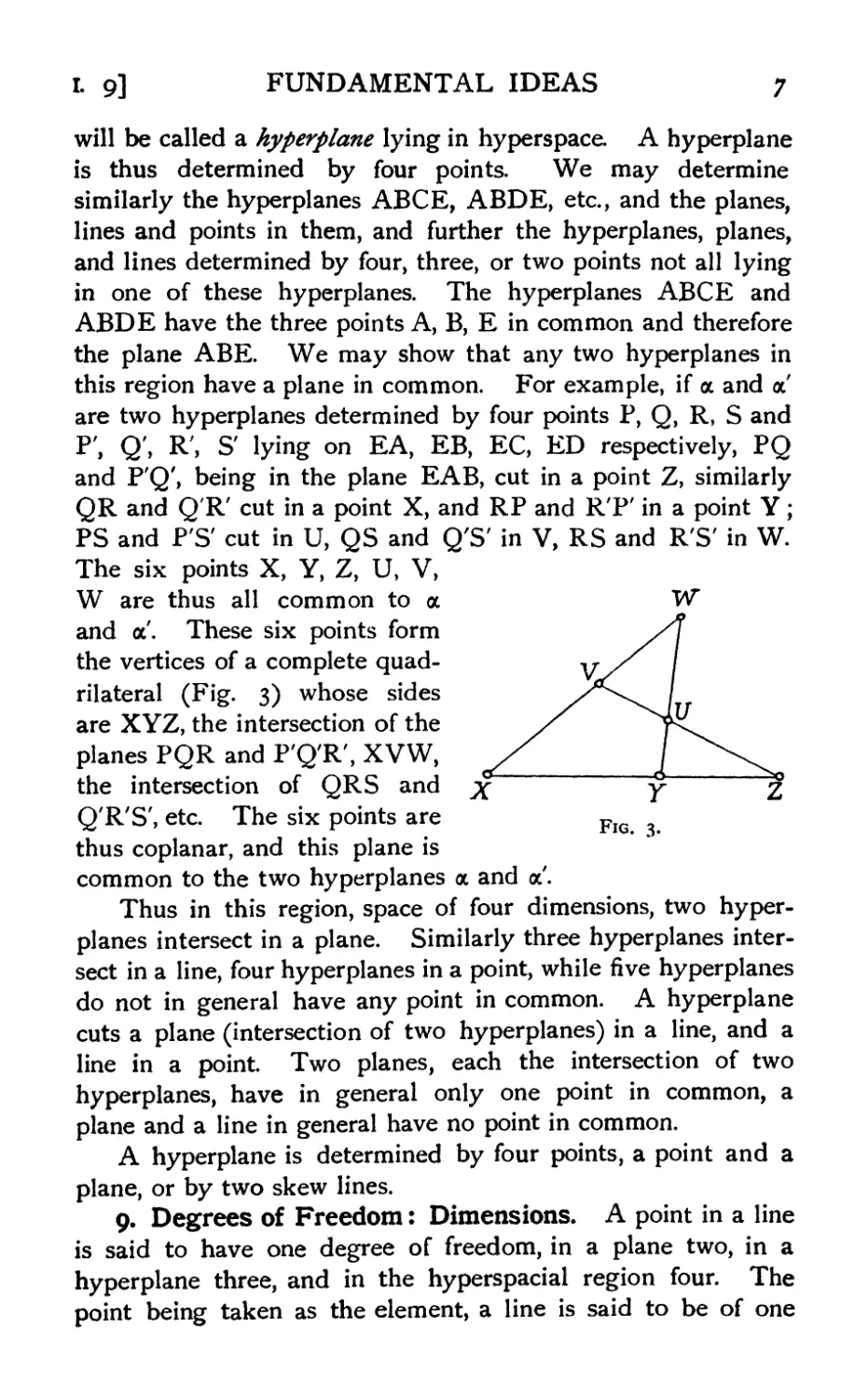
The six points X, Y, Z, U, V,
W are thus all common to α W
and a'. These six points form S\
the vertices of a complete quad- V / I
rilateral (Fig. 3) whose sides /**^\ /
are XYZ, the intersection of the / 1^^
planes PQR and P'Q'R', XVW, / i_"\,
the intersection of QRS and χ γ j?
Q'R'S', etc. The six points are FlG
thus coplanar, and this plane is
common to the two hyperplanes α and a'.
Thus in this region, space of four dimensions, two
hyperplanes intersect in a plane. Similarly three hyperplanes
intersect in a line, four hyperplanes in a point, while five hyperplanes
do not in general have any point in common. A hyperplane
cuts a plane (intersection of two hyperplanes) in a line, and a
line in a point. Two planes, each the intersection of two
hyperplanes, have in general only one point in common, a
plane and a line in general have no point in common.
A hyperplane is determined by four points, a point and a
plane, or by two skew lines.
9. Degrees of Freedom: Dimensions. A point in a line
is said to have one degree of freedom, in a plane two, in a
hyperplane three, and in the hyperspacial region four. The
point being taken as the element, a line is said to be of one
8 GEOMETRY OF N DIMENSIONS [i. 10
dimension, a plane two, a hyper plane three, and the hyper-
spacial region four. For a point to be in a given hyperplane
one condition is required, or one degree of constraint, thus
reducing the number of degrees of freedom from four to three.
For a point to lie in a plane two conditions are required; if
it is to lie simultaneously in two planes four conditions are
required and it is completely determined.
io. Extension to η Dimensions. We may now extend
these ideas straightaway to η dimensions, and at the same time
acquire both greater generality and greater succinctness in ex-
pressioa The series point, line, plane, hyperplane (or as it
is more explicitly termed three-flat), . . ., «-flat are regions
determined by one, two, three, four, ...,# + ι points, and
having zero, one, two, three, . . ., η dimensions, i.e. an r-flat
is determined by r + I points, and every/-flat (/ < f) which
is determined by/ + I of these points lies entirely in the r-flat.
We shall suppose that the «-flat, or space of η dimensions,
contains all the points. A/-flat, or hyperplane of/ dimensions
will be denoted by SF A flat space is also called a linear space.
11. Independent Points. \ip + ι points uniquely
determine a/-flat they must not be contained in the same (/ - i)-
flat Also no r of them (r ^ /) must be contained in the same
(r - 2)-flat, for this (r - 2)-flat, which is determined by r - ι
points, together with the remaining / + ι - r points, would
determine a (/ - i)-flat We shall call a system of / + ι
points, no r of which lie in the same (r - 2)-flat, a system of
linearly independent points. Any / + ι points of a /-flat, if
they are linearly independent, can be chosen to determine the
/-flat.
12. Consider a /-flat and a <?-flat, which are determined
respectively by / + ι and q + ι points. If they have no
point in common we have / + q + 2 independent points which
determine a (/ + q + i)-flat. Hence ap-flatanda q-flat taken
arbitrarily lie in the same (/ + q + I yflat
Η p + q + ι is greater than η the two flats will have a
region in common. Let this region be of dimensions r. In
this region we may take r + I independent points; to
determine the /-flat we require / - r additional points, and to
determine the ^-flat q - r additional points, i.e. altogether
t 15] FUNDAMENTAL IDEAS
9
(r + i) + (/-r) + (y-r)e/ + 0-r+ 1, and these
determine a (/ + q - r)-flat. Hence
Λί /з/йя/ дек/ α ^-/fo/ which have in common an r-fiat are both
contained in a (/ + q - r)-flat; if they have no point in common
they are both contained in a (/ + q + IУ flat,
Л p-flat and a q-flat, which are both contained in an n-flat,
have in common a (p + q - n)-flaty provided p + q> η - I.
Up + q< η they have no point in common. When two flats
do not intersect we may say that they intersect in a ( - i)-flat.
13. Degrees of Freedom of Linear Spaces. A /-flat
requires p + ι points to determine it, and each point requires
η conditions to determine it in space of η dimensions. But we
have in the choice of each point / degrees of freedom. Hence
the number of conditions required to determine the /-flat in
space of η dimensions is (p + i)(n -/), i.e. the number of degrees
of freedom of a p-flat in an η-flat is (p + i)(n - p). This is
called the constant-number of the/-flat.
This result may be proved otherwise, thus. Take any
p + 1 fixed {n - /)-flats. The /-flat cuts each of these in a
point, and these/ + I points determine the/-flat. Each point
has η - / degrees of freedom in its (n - /)-flat. Hence the
total number of degrees of freedom of the/-flat is (/ + I ){n -p).
If the /-flat has r points fixed, / + 1 - r points are still
required to determine it, hence the number of degrees of freedom
of the ^-flat is (n - p\p - r + 1); hence also the number of
degrees of freedom of a p-flat lying in a given η-flat and passing
through a given r-flat is (n - /)(/ - r).
14. The degree of incidence of a /-flat and a ^-flat can be
represented by a fraction. Let / > q. Complete incidence,
when the/-flat contains the ^-flat, can be represented by 1 ;
skewness, when they have no point in common, by o. If they
have in common an r-flat, the degree of incidence can be
represented by the fraction (r + 1) / (q + 1).
15. Duality or Reciprocity. A/-flat and an {n - / - 1)-
flat in Sn have the same constant-number (p + \){n - /). A
(1, 1) correspondence between points and (n - i)-flats can be
established in various ways, so that to the line joining two points
P, Q corresponds the (n - 2)-flat of intersection of the two
corresponding (n - i)-flats. If three points are collinear their
ΙΟ
GEOMETRY OF N DIMENSIONS
[ι. ι б
corresponding (n - i)-flats pass through the same (n - 2)-flat.
To a (p - i)-flat, which is determined by ρ given points,
corresponds the {n - /)-flat common to the {n - i)-flats which
correspond to the / points.
16. Number of Conditions Required for a given Degree
of Incidence. In Sn a /-flat has (n - p){p + i) degrees of
freedom, but if it passes through a given r-flat it has only
(n - p)(p - r) degrees of freedom. Hence the number of
conditions that a p-flat in Sn should pass through a given r-flal
(n >p > r) is (n - p)(r + i).
If the r-flat is free to move in a given ^-flat, it has
(r + \){q - r) degrees of freedom. Hence the number of
conditions that a p-flat and a q-flat in Sn should intersect
in an r-flat is (r + i)(n ~ p - q + r). This implies that
p + q <; η + r. lfp+q>n + r they intersect in a region
of dimensions p + q - ny which is greater than r.
17. Incidence of a Linear Space with two or more
Linear Spaces. Enumerative Geometry. In S3 a line
has 4 degrees of freedom (constant-number 4), and the number
of conditions that it should intersect another line is 1. Hence
a line which cuts a fixed line has 3 degrees of freedom, and the
whole system of lines all cutting a fixed line forms a
three-dimensional assemblage which is a particular case of a congruence ; the
system of lines cutting two fixed lines forms a two-dimensional
assemblage, a particular case of a complex; and the system of
lines cutting three fixed lines forms a one-dimensional assemblage,
a line-series. A line which is required to cut four given lines is
deprived of all freedom. The line is not, however, uniquely
determined. An important problem, which belongs to a branch
of mathematics called enumerative geometry, is to determine the
number of linear spaces which satisfy given conditions, in
number equal tp the constant-number of the linear space.
This problem can sometimes be solved directly by simple
geometrical considerations. As an example let us find the
number of lines in S5 (constant-number 8) which pass through
a given point О (4 conditions) and cut two given planes a, b
(2 conditions for each intersection). The required line must
lie in each of the 3-flats (Oa) and (0#), hence it is uniquely
determined as the intersection of these two 3-flats.
L 19]
FUNDAMENTAL IDEAS
II
18. Principle of Specialisation. The determination of
the number of lines which cut four lines in S3 is not so simple,
and we apply a very useful principle, called by Schubert the
" conservation of number" (Erhaltung der Anzahl), or "
principle of specialisation." The principle is that the number of
elements determined will be the same if the determining figures
are specialised, provided the number does not thereby become
infinite. In simple cases it is equivalent to the statement in
algebra that the number of roots of an algebraic equation is not
altered if the coefficients are specialised in any way, unless,
indeed, the equation becomes an identity.
As an example of the application of this principle let us
complete the problem to determine how many lines in S8 cut
four given lines. Let the four lines intersect in pairs: α and b
in P, с and ί/ in Q. A line which cuts both α and b must
either pass through Ρ or lie in the plane (ab); and as Ρ must
not lie in the plane (cd), nor Q in the plane (ab), for in either of
these cases there would be an unlimited number of lines cutting
all four lines, the required line must either pass through both Ρ
and Q, or lie in both of the planes (ab) and (cd). Hence there
are two lines satisfying the given conditions.
19. The general enumerative problem relating to linear
spaces is: to find the number of/-flats which have incidence of
specified degrees with a given set of linear spaces, the number
of assigned conditions being equal to the constant-number of
the /-flat
Let (n : /, q : r) represent the condition that a /-flat and
a ^-flat in Sn should intersect in an r-flat If Ρ and Q
represent any conditions, the product PQ is taken to mean that
both conditions must be simultaneously satisfied; the sum
Ρ + Q that one or other of the conditions is satisfied. Thus
(3 : 2, о : о)(з : 2, ι : 1) means the condition that a plane in S8
should contain a given point and a given line; (3 : 1, 1 : o)4
means the condition that a line in S3 should cut four given lines.
The number of simple conditions involved in (n:/, q: r)
may be denoted by C(n : /, q : r)y and we have proved that
C(n : /, q : r) = (r + \)(n - / - q + r).
The constant-number of a /-flat in Sn is equal to
C(n :/,/:/) - (p + l)(n -/>
12 GEOMETRY OF N DIMENSIONS [i. 20
We may also represent the number of elements determined by
a given condition by prefixing N to the symbol of the condition.
Thus N(3 : 1, 1 :o)4 = 2.
20. Duality in Enumerative Geometry. The duality
between the /-flat and the (n - ρ - i)-flat extends to
enumerative problems. Not only are the constant-numbers equal, viz.
(p + \)(n - p)> but we have also, as is easily verified,
C(n:/>, q : r) « C(n \ η - ρ - Ι, η - q- I : η-ρ- q+r- i);
and the number of/-flats determined by (/ + \){n - /) simple
conditions is equal to the number of {n - /> - i)-flats
determined by the corresponding reciprocal conditions. Thus in S4
there are two lines which lie in a given 3-flat and cut four given
planes, for the planes cut the 3-flat in lines. The reciprocal
statement is: there are two planes which pass through a given
point and cut four given lines; i.e.
N(4 : 1, 3 : i)(4 : 1, 2 : o)4 = N(4 : 2, о : o)(4 : 2, 1 : o)4.
21. In two dimensions the only conditions are
C(2 :0, 0 : O) = 2 = C(2 : 1, 1 : i),
C(2 : O, I : 0) = I = C(2 : I, О : о),
i.e. a point coincident with a given point, a line coincident with
a given line; and a point incident with a given line, a line
incident with a given point. The constant-number К of a point
or a line is 2, and we have only two enumerative results with
their duals, viz.:—
N(2 : о, о : o) = 1, i.e. one point is coincident with a given point,
N(2 : o, 1 : o)2 = 1, i.e. one point is incident with two given lines,
N(2 : 1, 1 : 1) = 1, i.e. one line is coincident with a given line,
N(2 : Ι, ο : о)2 - ι, i.e. one line is incident with'twogiven points.
The results may be exhibited more compactly in tabular
form. For a specified linear space let qr denote that it cuts a
given y-flat in an ^-flat. Then for S8 all the results are
represented in the following table. Point and plane, being
reciprocals, are grouped together.
I 22]
FUNDAMENTAL IDEAS
13
Point
Plane
С
Oo
22
3
1
•
•
Io
II
2
#
I
•
20
Oo
I
#
I
3
к =
N
I
I
I
3
Line
С
Oo
2
2
I
I
•
•
•
•
Io
I
•
2
•
4
2
•
•
Ii
4
1
•
2i
2
#
•
I
•
I
•
2
k-4
N
1
I
0
2
I
I
I
С is the number of simple conditions, N is the number of
elements determined. In each row the sum of the numbers,
each multiplied by the corresponding value of C, is equal to the
constant-number of the element K.
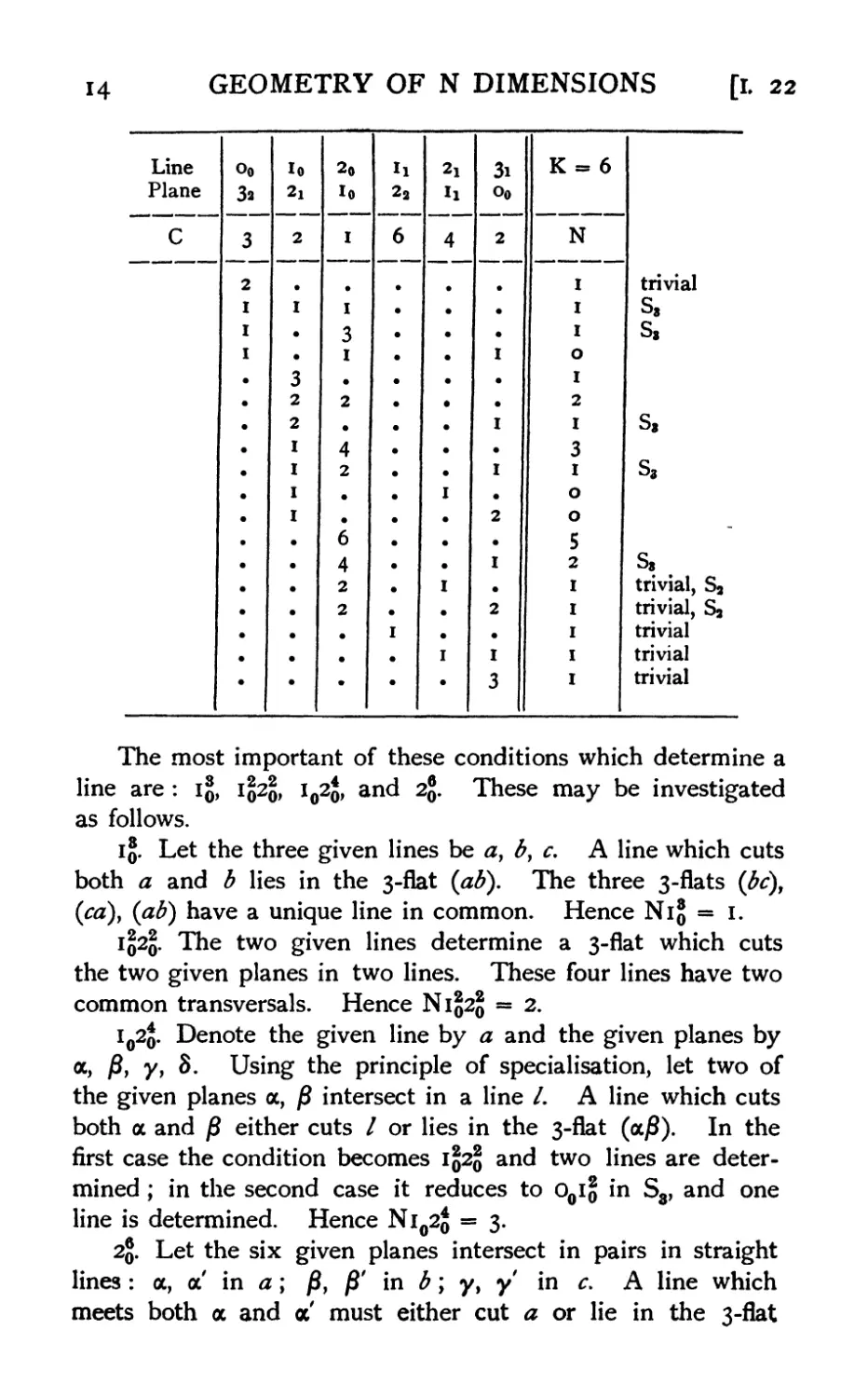
22. Incident Spaces in Four Dimensions. In general
many of the combinations are either trivial, or belong to a space
of lower dimensions, e.g. in S4 the statement, that one line
passes through a given point and intersects three given lines, is
the reciprocal of the statement that one plane lies in a given
3-flat and cuts three given lines (the plane is in fact determined
by the three points in which the given lines cut the 3-flat).
The following is the complete table of results for S4, most
of which the reader will have no difficulty in verifying. Results
marked "trivial" are the fundamental determinations of an
element or its reciprocal, e.g. a plane determined by three
points. " S3" indicates that the result belongs to space of three
dimensions.
Point
3-flat
С
o0
3s
4
1
•
•
•
•
io
23
3
2o
II
2
#
•
2
I
•
30
Oo
I
#
I
•
2
4
K-4
N
all trivial
Η
GEOMETRY OF N DIMENSIONS
[Г. 22
Line с
Plane 2
с
{_
>o lo
\2 2i
3 2
2
I I
I
3
2
2
I
I
I
I
1 *
1 *
•
1 *
1 *
1 *
•
20
ι0 Ι :
I
•
I
3
I
• ι
2
• 1
4
2
• ,
* *
6
4
2
2
• Ι ι
• 1 ·
1
II '
22
5
_l·
h
II
4
3i
o0
2
2
I
3
1
K = 6
N
I
I
I
о
I
2
I
3
I
о
О :
5
2
trivial
s,
s,
s,
s,
s,
trivial, Sj
trivial, Sj
trivial
trivial
trivial
The most important of these conditions which determine a
line are : ij,
as follows.
T2?2
i02q, and 2®. These may be investigated
Iq. Let the three given lines be a, b} c, A line which cuts
both a and b lies in the 3-flat (ab). The three 3-flats (be),
(ca), (ab) have a unique line in common. Hence Nijj = 1.
Iq2q. The two given lines determine a 3-flat which cuts
the two given planes in two lines. These four lines have two
common transversals. Hence Niq2q = 2.
i02q. Denote the given line by a and the given planes by
α, β у γ у 8. Using the principle of specialisation, let two of
the given planes α, β intersect in a line /. A line which cuts
both a and β either cuts / or lies in the 3-flat (aj8). In the
first case the condition becomes Iq2q and two lines are
determined ; in the second case it reduces to o0Iq in S8, and one
line is determined. Hence Ni02q = 3.
2q. Let the six given planes intersect in pairs in straight
lines: a, a' in a; )3, β' in b; y, γ in с A line which
meets both a and a' must either cut a or lie in the 3-flat
I. 23] FUNDAMENTAL IDEAS
15
(αα'). Hence the required line either (1) cuts three given
lines, (2) cuts two given lines and lies in a given 3-flat (three
different ways), (3) cuts a given line and lies in two given 3-flats
(also three different ways), or (4) lies in three given 3-flats.
Under the first category one line is determined; under the
second, three; no line exists under the third category, since
the given line does not in general cut the plane common to
the two 3-flats, and if it did, an infinity of lines would be
possible; lastly, under the fourth category one line is
determined. Hence N2q = 5.
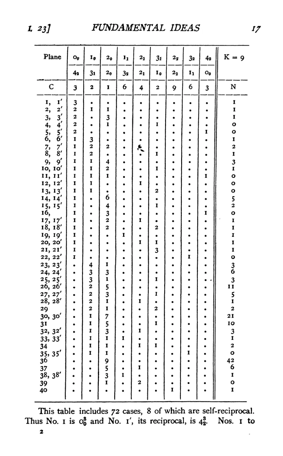
23. Incident Spaces in Five Dimensions. In five
dimensions we have the reciprocal pairs : point and 4-flat,
line and 3-flat, plane (self-reciprocal). Omitting the cases
of point and 4-flat, which are trivial, the following are the
complete results (see p. 16).
With the exception of Nos. 16, 20, 21, 23, 27 and 34
these can all be proved directly or deduced from previous
results in S4 or S3. 20 and 23 can be solved by letting two of
the planes intersect in a point; 16, 21, 27 and 34 by letting
two of the 3-flats intersect in a plane.
ι б GEOMETRY OF N DIMENSIONS [i. 23
Line
3-flat
С
Oo
3»
8
3i
4i
Oo
К = 8
N
I 23] FUNDAMENTAL IDEAS 17
о»
20
3l
32
42
K = 9
42
3i
З2
l0
II
Oo
I
4
3
3
2
2
2
2
1
3
1
5
3
1
1
7
5
3
1
I
I
9
5
3
1
•
N
This table includes 72 cases, 8 of which are self-reciprocal.
Thus No. 1 is 0$ and No. i', its reciprocal, is 4|. Nos. 1 to
18 GEOMETRY OF N DIMENSIONS [l 24
22> 33» 35» 38 and 40, can be proved directly or deduced
from results in S^ or S4. For the others we may use the
principle of conservation of number. If the condition involves
the factor 2% let the two planes at, β cut in a line /. Then
the required plane either cuts /, or cuts the 3-flat (ocj8) in a
line. Hence
2$ - i0 + 3r
This leads to a number of equations, such as
N(i*20) + Ν(φο3ι),
N(i$28) + N(i02$3l)
Ν(φ») + 2Ν(φ&) + N(Io2$3?)
Ν(φ0) + 3Ν(φο3ι) + 3Ν(φο3?) + Ν(ι02ο3?),
and so on. Next, if the condition involves the factor 2%$v
let the two planes я, b meet the 3-flat α in lines /, tn. Then
(act.) and (bo.) are 4-flats. The required plane then either
lies in (aa) and cuts bt or lies in (bo.) and cuts a, or cuts both
/ and m. Hence
2o3i - 2(2^) + i§.
The equations derived from this, together with the previous
ones, will be found to determine all but Nos. 28, 32 and 37,
which involve the factor 2r If we assume the relation
h2o = *(°o) + X2o) + *(2o3i) + «<4i),
where x, у, ζ, w are certain unknown numbers, we have, by
applying this to OqI020, o0i02q31 and φ0, the relations
1 = χ + y, 1 = 2y + z, and 3 = χ + 6y + $z + wf giving
у = ι - x> ζ = 2x - 1, w = - x. Then applying it to
\$p,x we find N(2q2x) = 2N(i02§21) ; and applying it to
φ02χ and i0202131 we find Ν(φβ2χ) = 1 and N(1^2^ = 3.
The χ here plays the part of a catalytic agent.
24. We shall conclude this section with a few general
results.
In Sn the constant-number of a line is 2{n - 1), and one
condition is required in order that a line should cut a given
(n - 2)-flat, hence a finite number of lines in Sn cut 2(n - 1) linear
spaces of η - 2 dimensions. It was proved by W. F. Meyer that
N(i?2S)
I. 25] FUNDAMENTAL IDEAS
19
the number of lines is an _ 2Cn = -^-? ^-,. A more
n- 1 л ! (»- 1) !
general result, which includes this as a particular case, was
proved by Schubert, viz. the number of p-flats in Sn which cut
n - pgiven (n - 2p - i)-flats is
ι Ι2Ι3Ι · · · ·/»{(/+ iX» -/)}!
» ! (« - 1) 1 (л - 2) ! . . ..(«-/)!"
Zi? jfe^ /Й£ number of lines in S2k _ 2 доЛ/бб cut 4 linear
spaces of {k- 1) dimensions. The constant-number of a line in
S2jb- 1 is 4(£ - 0> anc* t^e number of conditions that it should
cut a (k - i)-flat is X? - 1. Hence there is a finite number.
Let the (k - 1 )-flats intersect in pairs in points: α, β in P, and
y, δ in Q. A line which cuts α and β either passes through Ρ
or lies in the (2k - 2)-flat (aj8). We have then (1) one line
through Ρ and Q, (2) lines through Ρ and lying in the
(2k - 2)-flat [none], (3) lines in the {2k - 3)-flat common to
(aj8) and (y8), and cutting the four {k - 2)-flats in which α, β
are cut by (γ&), and y, δ by (a)3). Hence if/(£) is the number
of lines which cut four (k - i)-flats in S.^ _ v
/№=/(*- 0 + 1.
But, for k = 2, we have 2 lines in S3 cutting 4 lines, i.e. /(2) = 2.
Hence f(k) - £.
Ex. (1) Prove that there is one 3-flat in S2? cutting three
^-flats in lines.
(2) One plane in S2q cutting three ^-flats in lines.
(3) One plane in S^ + 2 cutting four ^-flats in points.
(4) One plane in S8? + 2 cutting four (5^ + i)-flats in lines.
25. Motion and Congruence. Strictly speaking the idea
of motion is foreign to geometry. When we speak of a point
moving along a line we really mean that we are focussing our
attention successively on a series of points in the line. When
we speak of a figure being displaced in space we are really
transferring our attention from one figure to another (congruent)
figure; or we are considering a transformation in which certain
relations, distances and angles, are invariant. The idea of
motion thus involves sequence or order, and congruence. For
these there are two corresponding groups of axioms. As these
20 GEOMETRY OF N DIMENSIONS [i. 26
axioms deal almost exclusively with plane geometry, and the
new ideas involving congruence in higher space can be dealt
with' by definitions, we may simply refer for a discussion of the
axioms to Hubert's "Foundations of Geometry" or to the
more recent c< Foundations of Euclidean Geometry," by Forder.
26. Order. As regards order in euclidean geometry, a
point divides a line into two parts, but does not of course divide
a plane; a line divides a plane, but does not divide space ;
a plane divides space, but does not divide a 4-flat, for in S4 the
line joining two points does not in general intersect a given
plane: and so on.
If A! and A2 are given points on a line they determine
a segment which consists of all points Ρ such that A^Ag are in
this order. Ax and A2 divide the line into three parts, for which
we have respectively the orders PA^, А^Аз, А^Р.
If Av A2, A3 are three non-collinear points in a plane, they
determine three lines which form a triangle. The segments
A2A3, etc., are the sides or edges, and if A23 denotes any point
on the segment A2A3 the interior of the triangle consists of all
points Ρ such that A^A^ are in this order. The three lines
divide the plane into seven regions, consisting of points
characterised by the following orders:
(1) the interior of the triangle: A^A^ or A2PA31 or A3PA12,
(2, 3, 4) three regions on the faces: A^gP, AjjA^P,
A3A12P,
(5> 6, 7) three regions on the vertices: PA^A^, PA2A31,
PA3A12,
Similarly four non-coplanar points Av A2, A3, A4 determine
four planes and six lines forming a tetrahedron. Its faces are
the interiors of the triangles A2A3A4, etc. The four planes
divide space into 15 regions which consist of points Ρ
characterised by the following orders, where A234 denotes any
point on the face A2A8A4, and A12 any point on the edge AXA2:
the interior of the tetrahedron : A^A^, etc.,
four regions on the faces: AjA^P, etc.,
four regions on the vertices: A^AjP, etc.,
six regions on the edges: A^A^P, etc.
L 26] FUNDAMENTAL IDEAS 21
(In explanation of the last statement we note that the plane
PAl2 cuts the line A8A4 in a point, and if Ρ is in the region
specified this point lies in the segment АзА4.)
In space of four dimensions we have similarly five points
determining 5 hyperplanes, 10 planes, and 10 edges, forming
a four-dimensional stmplex% and dividing S4 into 31 regions:
the interior of the simplex: ΑχΡΑ,^β, etc.,
5 regions on the 3-dimensional boundaries: AJLA2345P, etc->
10 regions on the 2-dimensional boundaries: Α12Α34δΡ, etc.,
10 regions on the edges: АША45Р, etc.,
5 regions on the vertices: АШ4АбР, etc.
The extension to η dimensions is now obvious. The figure
formed by η + ι independent points and the lines, planes, etc.,
directly determined by them is called a simplex of η dimensions
and will be denoted by S(n + 1). The lines, planes, etc., are
called its boundaries of one, two, etc., dimensions; the points
are its vertices. An S(# + 1) has n + iCr + 1 boundaries of
r dimensions.
REFERENCES
CAYLEY, A. A memoir on abstract geometry. Phil. Trans. 160 (1870),
51-63 ; Math. Papers, vl No. 413.
Forder, H. G. The foundations of euclidean geometry. Cambridge:
Univ. Press, 1927.
Hilbert, D. The foundations of geometry. Authorised trans, by E. J.
Townsend. Chicago : Open Court, 1902. (Original German edition :
Grundlagen der Geometrie, Leipzig, 1899. 6. Aufl. 1923).
Manning, H. P. Geometry of four dimensions. New York: Macmillan,
1914. (Synthetic method. The introduction contains an interesting
short history of the subject.)
Meyer, W. F. Apolaritat und rationale Curven. Eine systematische
Voruntersuchung zu einer allgemeinen Theorie der linearen Raumen.
Tubingen, 1882.
SCHUBERT, H. Die n-dimensionalen Verallgemeinerungen des dreidimen-
sionalen Satzes, dass es zwei Strahlen giebt, welche vier gegebene
Strahlen schneiden. Hamburg, Mitt. Math. Ges., No. 4, 1884.
— Kalkiil der abzahlenden Geometrie. Leipzig, 1879.
SEGRE, С Mehrdimensionale Raume. Encykl. Math. Wiss. iii. с 7.
1921.
1921.
CHAPTER II
PARALLELS
I. Parallel Lines. In projective geometry two straight lines
in a plane always intersect This is not true in euclidean or
hyperbolic geometry.
Let / be a given line (Fig. 4) and О a given point not on /;
A any fixed point on /, and Ρ a variable point on /. Let Ρ move
always in one direction along /, i.e. we consider a series of points
Px, P2, . . . in the order APjPy ... As Ρ moves along / it
may return to its initial position. This occurs in projective
geometry, and also in elliptic geometry, in which two lines in a
plane always intersect. Other-
___—~-____ r wise as the segment AP in-
■"" " ~~ " creases without limit, the line
OP will tend to a definite
limiting position OL. The
pi ~л ъ line OL, which separates the
rays through О which inter-
IG* 4* sect AP from those which do
not, is said to be parallel to AP. If Ρ moves in the opposite
sense we get another limiting position OL', and OL' is parallel
to AP'.
In euclidean geometry the two rays О L, OL' form one and
the same line, but in hyperbolic geometry they belong to
distinct lines, and we have to distinguish the two directions of
parallelism to a given straight line. In projective geometry the
foregoing considerations are irrelevant, since projective geometry
does not involve the idea of distance.
2. A fundamental theorem is the following:
If A A II CC\ and BB' \\ CC\ then A A' II BB.
(1) Let the three lines be coplanar, and (i) let CC lie
between A A' and BB' (Fig. 5). We may assume that А, С, В
22
п. 3]
PARALLELS
23
are collinear. Within the angle BAA' draw any line AP.
Since AA'IICC, AP cuts CC in a point R. Then since
RC || BB', PR produced must cut BB'. Also AA does not
cut BB', therefore AA' || BB'.
(ii) In the same figure let AA' || BB', and CC || BB'. AA'
cannot cut CC, for it would then cut BB', but any other line
within the angle BAA' cuts CC, therefore AA' || CC.
(2) Let the three lines be not all in the same plane, and let
AA' || BB' and CC II BB' (Fig. 6). Take any point Ρ on BB'.
Then as Ρ moves along BB', AP -> AA', and CP -► CC, while
P, А, С are always coplanar, therefore AA' and CC are
coplanar. Again, if CP is fixed while the plane РАС moves,
PA -> PB', and the plane CPA -> СРВ'. СА, the line of
intersection of CPA and CCAA', therefore -» CC, and CC || AA'.
в с
Fig. 5. Fig. 6.
3. Parallel Lines and Planes. We shall confine our
attention now for the present to euclidean geometry. In a plane
two straight lines either intersect in one point or are parallel.
In three dimensions two planes which have a point in common
intersect in a straight line. If they have no point in common
they are said to be parallel. Two parallel planes are cut by a
third plane in two straight lines which have no point in common
and are therefore parallel. A straight line either cuts a given
plane in one point or has no point in common with the plane;
in the latter case the straight line is said to be parallel to the
plane.
Consider a plane α and a point О not in oc Let β be any
plane through О cutting α in a line b. Then through О and
in j3 there is one line parallel to b and therefore parallel to a.
24 GEOMETRY OF N DIMENSIONS [il 4
By taking different planes β we get a system of lines through О
all parallel to a. Let /, m, η be three such lines. The planes
(Im) and (In) are both parallel to a, and must coincide, for let
у be a plane through О cutting α in cy (Int) in gt and (In) in h.
Then g and h are both parallel to с and therefore (in euclidean
geometry) coincide. Hence all the lines through О parallel to
α lie in one plane which is parallel to a.
4. Direction and Orientation. By an extension of the
meanings of the words point and line we can greatly simplify
the statements of the relations between parallel lines and planes.
A system of concurrent lines in a plane, called a pencil of lines,
determine a unique element, their common point, and this is
determined by any two lines of the system; just as a system
or range of collinear points determine a unique element, their
common line, which is determined by any two points of the
system. Pencil of lines is said to be reciprocal or dual to range
of points. In three dimensions a system of concurrent lines, or
bundle of lines, is of two dimensions, and is reciprocal to the
plane field of points. A system of straight lines all parallel to
the same straight line also determine a unique element, a
direction^ which is uniquely determined by any two of the lines.
A direction together with a point uniquely determine a straight
line. A direction together with two points uniquely determine
a plane, for one of the points together with the given direction
determine a line, and this with the other point determine a
plane. Similarly two directions together with a point uniquely
determine a plane. Thus a direction may take the place of a
point in determining lines or planes.
Two directions by themselves do not determine a plane,
but only the orientation of a plane; and we may then say an
orientation together with a point uniquely determine a plane.
Also if two planes have their orientations given, their line of
intersection has a fixed direction, thus two orientations uniquely
determine a direction. An orientation may thus take the place
of a line in determining planes and points. As, however, two
lines only determine a point when they are coplanar, while two
orientations (in space of three dimensions) always determine a
direction, orientations appear to correspond to coplanar lines.
5. Points at Infinity. To bring out more explicitly the
II. б]
PARALLELS
25
connection between direction and point, orientation and line,
we give them the names "point at infinity" and "line at
infinity " respectively, and we shall be justified in extending to
them the language used for points and lines. We speak of the
" point at infinity on a line" for the direction of a line, the " line
at infinity on a plane " for the orientation of a plane. A " point
at infinity on a plane" is the direction of some line in that
plane. The orientation determined by two directions is said
to contain the two directions; thus a line at infinity is
determined by two points at infinity; and, since the directions of any
two lines of a given plane determine the orientation of the plane,
it follows that any two points at infinity on a plane determine
or lie on the same line at infinity.
We may now draw correct logical conclusions by picturing
a line at infinity as a line whose elements are points at infinity.
Parallel lines can then be pictured as lines which meet in a point
at infinity. In a given plane we picture the line at infinity as
a special line /^ in the plane, and the condition for parallelism
of two lines a, b in the plane is expressed by the concurrency
of a, b and l^. Since (in three dimensions) two lines at
infinity always determine a point at infinity, we have to
picture the assemblage of all lines at infinity as lines in one
common plane. The assemblage of all orientations in space of
three dimensions is called the plane at infinity in this space.
We may denote this by 7^. The point at infinity on any line,
and the line at infinity on any plane, is its intersection with the
plane at infinity. Two lines are parallel when they intersect
on the plane at infinity; a line is parallel to a plane when the
point at infinity on the line lies on the line at infinity in the
plane; two planes are parallel when their lines at infinity
coincide. Two arbitrary planes, α, β have in common one point
at infinity, the common point of the three planes а, Д 77^, or the
common point of their lines at infinity. In ordinary language,
if α is not parallel to j8, it is always possible to get two series of
parallel lines, one in α and one in j8, viz., the lines which are
parallel to the line of intersection of α and β.
6. Parallel and Half-parallel Planes. We shall consider
now parallelism in euclidean space of four dimensions. Two
hyperplanes which have a point in common intersect in a plane.
2б GEOMETRY OF N DIMENSIONS [п. 7
If they have no point in common they are said to be parallel.
Two parallel hyperplanes are cut by a third hyperplane in two
planes which have no point in common and are therefore parallel
in the ordinary sense. Two planes in general intersect in just
one point. We have defined parallel planes when they lie in
space of three dimensions and meet in a line at infinity. But
in space of four dimensions two planes may have another sort of
parallelism when they do not lie in the same hyperplane and
have no point in common. The term " half-parallel " or " semi-
parallel " has been used to describe this.
7. The Hyperplane at Infinity. Two hyperplanes each
parallel to a third are parallel to one another. We shall say
that two parallel hyperplanes determine a stratification^ just as
two planes in three dimensions determine an orientation. Two
stratifications determine an orientation; three stratifications
determine a direction. All the orientations in a given
hyperplane belong to the stratification of that hyperplane, so that the
stratification of a hyperplane is identified with the plane at
infinity in that hyperplane. Since two planes at infinity always
determine a line at infinity we have to picture the assemblage
of all planes at infinity as planes in one common hyperplane, so
we call the assemblage of all planes at infinity the hyperplane at
infinity in space of four dimensions.
We can now perceive the distinction between parallel and
semi-parallel planes. Parallel planes have in common a straight
line at infinity, semi-parallel planes have in common only a point
at infinity. In ordinary language, parallel planes have the
same orientation and an infinity of common directions; to every
line in the one plane there is a system of lines parallel to it in
the other. Semi-parallel planes have only one common
direction; there is only one system of parallel lines in the one
plane which are parallel to lines in the other.
8. Degrees of Parallelism. We can now extend the idea
of parallelism to space of η dimensions. In euclidean space of
η dimensions there is a unique (n - i)-flat at infinity. Two
(n - i)-flats are parallel when their common (n - 2)-flat is an
{n - 2)-flat at infinity, i.e. an element of the (n - i)-flat at
infinity. Two planes, in addition to the possibility of being
parallel or semi-parallel, mav have no ooint at all in common
и. ίο]
PARALLELS
27
and have no common containing hyperplane; they are then
skew. Two 3-flats which have no point in common (i), if they
lie in the same 4-flat, have a plane at infinity in common; (ii),
if they lie only in the same 5-flat, they have a line at infinity in
common; (iii), if they lie only in the same 6-flat, they have a
point at infinity in common ; and (iv), if they do not lie in the
same 6-flat, they are skew. In the three cases (i), (ii), (iii) the
two 3-flats are said to be (i) completely parallel, (ii) two-thirds
parallel, (iii) one-third parallel.
In general, a /-flat and a ^-flat (/ ;> q\ which are both
contained in the same (/ + q - r)-flat, and would therefore in
general intersect in an r-flat, but have no point in common, are
said to be {r + \)\q parallel, and have in common an r-flat at
infinity. It is to be noted that if a /-flat and a ^-flat are
contained in the same (p + q - r)-flat, they have at least a common
(r - i)-flat at infinity, for, if they intersect, their common
r - flat contains a unique (r - i)-flat at infinity. Thus, in
order that two flats should be parallel it is not sufficient that
they should have a certain dimensionality of common points at
infinity ; they must also have no finite point in common.*
9. Complete parallelism may occur in space of any number
of dimensions. Partial parallelism requires a certain minimum
dimension. Thus half-parallelism only appears for the first
time in S4 when two planes are half-parallel. One-third
parallelism does not appear in space of lower dimensions than
six. In general parallelism of order {r + i)/q> where r + 1 is
prime to q, requires space of at least 2q - r dimensions, as it
implies the existence of a /-flat and a #-flat contained in the
same (p + q - r)-flat, and p *> q.
10. Sections of two Parallel or Intersecting Spaces by
a Third Space. If Sp and SQ (ρ ^ q) are completely parallel,
so that the region at infinity S(J) _ ^«, on Sp contains S(q _ ^,
S« and S„ 1 ie in the same (/ + 1 )-flat Sp + » which is
determined by S(p _ ^oo and two finite points, one on Sp and one on
* Schoute leaves out the condition of having no finite point in common,
and defines a /-flat and a $r-flat (p ;> q) as (r + i)/g parallel when they
have in common an r-flat at infinity. According to this, two intersecting
planes in three dimensions would be half-parallel since they have in common
a point at infinity, viz. the point at infinity on their line of intersection.
28 GEOMETRY OF N DIMENSIONS [π. 11
Sq. An r-flat {r >p - q + i) in Sj, +, cuts S^ in an [r - i)-
flat Sr _ ! and S? in a (q + r - / - i)-flat Sq + r __ ^ _ „ and
it cuts their common region at infinity in a (q + r - p - 2)-flat
which is the whole of the region at infinity on Sq + r _ p _ l#
Hence the two sections are completely parallel.
If Sj, and SQ are parallel of degree {r + \)jq so that they
have in common an r-flat at infinity, they lie in the same
(p + q _ ;-)-flat, which is determined by r + ι common points
at infinity, ρ - r finite points on Spt and q - r finite points on
Sq. An .г-flat in this Sp + q _ r cuts Sp in an (s+ r- y)-flat
and S<, in an (j + r - /0-flat, and their common region at
infinity in an (s + 2r - / - ^)-flat. The sections are therefore
in general parallel of degree (s + 2r - ρ - q + \)j(s + r - p).
This fraction = I if r = q - I.
If Sp and Sq intersect in an Sr and therefore lie in the same
Sj, + 7 _ r they have in common an S<r _ ,)^. Let an .r-rlat Ss
parallel to Sr of degree (m + i)jr (s ^ r - i) cut Sp and S?
in Ss + r _ ? and S, + r _ p. These two sections have then an
S/noo in common and are parallel of degree (m+ i)/(s + r - /).
II. The Parallelotope. In η dimensions the analogue of
the parallelogram and the parallelepiped is a figure bounded by
pairs of parallel {n - i)-flats. Consider a simplex with a
vertex О and η edges through О : ОАА, ОА2, . . . , OAn, no
r of which lie in the same (r - i)-flat The η - ι edges
OA^, . . ., OAn determine an {n - i)-flat, and through A1
there is just one (n - i)-flat parallel to this. Constructing the
{n - i)-flats, one through each of the η vertices Av . . ., AM
parallel to the opposite face of the simplex, we form a figure
bounded by 2n (n - i)-flats, which is called a parallelotope*
Each {n - ι )-flat is cut by each of the {n - ι )-flats except the
one which is parallel to it in an {n - 2)-flat, and these
гп - 2 (n - 2)-flats are parallel in pairs and form a parallelotope
of η - ι dimensions. Each of these again is bounded by
parallelotopes of η - 2 dimensions, and so on.
The parallelotope may be generated also by successive
motions in one, two, three, . . . dimensions. Thus a point
* The suffix tope which occurs in several of the terms used in
«-dimensional geometry—polytope, simplotope, orthotope, etc.—is from the Greek
И. II]
PARALLELS
29
moving in a straight line through a distance αλ generates a line-
segment. This segment moving parallel to itself, so that all its
points generate parallel line-segments of length a2, generates
a parallelogram with two edges of length ax and two edges of
length a.2. The parallelogram by parallel motion similarly
generates a parallelepiped, and so on.
Let Nr denote the number of ^-dimensional boundaries of
a parallelotope of η dimensions, N'r the corresponding number
for a parallelotope of η - ι dimensions ; and consider the
expression
N0 + Ntx + N^ + . . . + Ν,.,**-1 + N„*»
Nn being equal to 1 since the parallelotope itself is the only
л-dimensional boundary. The Nr boundaries of r dimensions
of the «-dimensional parallelotope are produced by the N^ _ г
boundaries of r- 1 dimensions of the(« - i)-dimensional
parallelotope together with its N'r boundaries of r dimensions in their
initial and final positions. Hence Nr = N^_j + 2NJ. We
have therefore
N0 + Nxx + . . . + Ν7ϊχη = (N; + Nj* + . . . + Кхп)(2+х),
and hence by induction
N0 + N^ + . . . + Nn;rw = (2 + x)n,
i.e. Nr-mCr.2«-'.
The number of r-dimensional boundaries which pass
through one vertex is nCr, and all the r-dimensional
boundaries fall into nCr groups, each containing 2n~r
completely parallel r-flats.
REFERENCE
SCHOUTE, P. H. Mehrdimensionale Geometric 1. Teil: Die linearen
Raume. Leipzig : Goschen, 1902.
CHAPTER III
PERPENDICULARITY
I. Line Normal to an (n - i)-flat In three dimensions if
a line PN is perpendicular to two intersecting lines ΝΑ, ΝΒ at
their point of intersection N, it is perpendicular to every line
through N in the plane determined by NA and NB, and is said
to be perpendicular to the plane ANB ; and conversely, all lines
through N perpendicular to NP lie in one plane which is
perpendicular to NP.
We shall consider first all lines, planes, etc., passing through
a fixed point O. The number of degrees of freedom of a /-flat
which has to pass through О isp(n - p). One condition is
required in order that two given lines through О should be
perpendicular. Let one line a be fixed, then a line / through О
perpendicular to a has η - 2 degrees of freedom and may
therefore move in a region of η - ι dimensions. Let 4 and /2 be
any two lines through О perpendicular to ay then all lines of the
plane (44) which pass through О are perpendicular to a. In
this plane we have then just a single infinity of lines through О
perpendicular to a. Let /3 be a third line through О
perpendicular to a and not lying in the plane (//2). 4» 4» 4 determine
a three-flat; let b be any other line of this three-flat passing
through O. The planes (44) and (lzb) intersect in a line с which
lies in (//g) and is therefore ± a. Then since с and /8 are both
± ay and b lies in the plane (r/3), b ± a. Hence a is
perpendicular to every line through О in the three-flat (44/3).
Proceeding in this way we obtain η - ι independent lines
4> 4> · · ·> 4-1> no three lying in one plane, and all j. a; and
every line through О in the {n - i)-flat determined by these
lines is χ a. Hence through any point О of a straight line a
there is a unique (n - i)-flat which is normal to a; and at any
30
Ш. з] PERPENDICULARITY 31
point 0 in a given (n - i)-flat there is a unique line a which is
Jl every line of the (n - i)-flat which passes through O. The
normal (n - i)-flat to the line a at О contains every/-flat which
is normal to a at O.
2. System of η Mutually Orthogonal Lines. Complete
Orthogonality. Through any point О we can find η lines all
mutually perpendicular. Starting with a line llf all lines through
О ± lx lie in the normal (n - i)-flat to Ιλ at O. Let /2 be one
of these lines. Then all lines j_ both lx and /2 at О lie in the
(n - 2)-flat which is the intersection of the normal (n - 1)-
flats to Ιλ and /2. Let /8 be one of these lines. Proceeding in
this way we shall arrive at a system of η lines llf /2, . . , /n, all
mutually perpendicular, p of the lines lv /2, . . . lp determine
a/-flat Spt and the remaining η - p lines determine an (n - p)-
flat Sn _ p. These two flats, which intersect only at O, have the
property that every line of Sp through О is perpendicular to
every line of Sn _ p through O. The two flats are said to be
completely orthogonal.
In two dimensions two lines at right angles, and in three
dimensions a plane and a normal line, are completely orthogonal,
but two planes cannot be completely orthogonal. In the case of
two orthogonal planes in three dimensions only one line in each
plane is orthogonal to every line in the other.
In four dimensions the assemblage of all lines through a
point О of a plane α perpendicular to α is another plane a' which
is completely orthogonal to a. If a is any line of a, and a any
line of a', through O, the plane (ad) is perpendicular to both α
and a' in the ordinary three-dimensional sense.
When two lines in space do not intersect we can still say
that they are orthogonal when two lines, parallel to them,
intersect at right angles. Similarly two planes in Sn (n > 4), which
have no point in common, may still be said to be completely
orthogonal when two planes, completely parallel to them
respectively, and having a common point, are completely orthogonal.
3. Orthogonality in Three Dimensions in Relation to
the Absolute; Absolute Poles and Polars. The
orthogonality of lines and planes in three dimensions may be explained
with reference to their points and lines at infinity. Consider
first two lines af ά and use ordinary rectangular co-ordinates.
32 GEOMETRY OF N DIMENSIONS [in. 3
Let the two lines pass through the origin and have direction-
cosines (/, m, n) and (/', m\ ri). Writing xjt, y\t, and z\t instead
of x, yy and z> so that xy y, z, t are now the homogeneous
cartesian co-ordinates, the equation of the plane at infinity is / = 0.
The co-ordinates of the points at infinity on the two lines are
(/, m, n, 0) and (/*, m\ ri> 0). The condition that the two lines
should be orthogonal is //' 4- tntri + nri = 0. But this is the
condition that the two points (/, my ny 0) and (/', m> n\ 0)
should be conjugate with regard to the virtual conic or circle
x1 + y2 + zl = 0, / = 0. Similarly two planes in S3 are
orthogonal when their lines at infinity are conjugate with regard to
the virtual circle at infinity; and a line and a plane are
orthogonal when the point at infinity on the line is the pole of the
line at infinity on the plane. This conic, or rather the
degenerate quadric surface of which this conic forms the envelope and
the plane at infinity taken double forms the locus, is called the
absolute. In two dimensions it reduces to just two imaginary
points called the " circular points at infinity," together with the
line at infinity taken twice. In non-euclidean geometry the
absolute is a non-degenerate conic, real for hyperbolic geometry
and virtual for elliptic geometry.
By viewing the absolute as a degenerate quadric surface, and
not simply as a conic in the plane at infinity, we may obtain the
absolute polars of finite elements. The polar of any finite point
with regard to the absolute, which as a locus consists of just the
plane at infinity taken double, is the plane at infinity itself; the
polar of a point at infinity P^ is any plane passing through the
polar line (at infinity) of P^ with regard to the circle at infinity.
Hence the absolute pole of an ordinary plane α is the point at
infinity which is the pole of the line at infinity in α with regard
to the circle at infinity. The absolute polar of a line is the line
at infinity polar with regard to the circle at infinity of the point
at infinity on the line. The absolute pole of an ordinary plane
is the point at infinity on any of its normals, and the absolute
polar of an ordinary line is the line at infinity on any of its
normal planes. When we speak of the absolute polar of a finite
element we shall mean the polar with regard to the degenerate
quadric, but when we speak of the polar of an element at infinity
we shall mean the polar with regard to the virtual quadric at
infinity.
ш. 5] PERPENDICULARITY 33
We may then state the relations as follows. A line is
perpendicular to a plane when it passes through the absolute polar
of the plane, and reciprocally the plane contains the absolute
polar of the line. Two lines are orthogonal when each cuts the
absolute polar of the other. Two planes in S3 are orthogonal
when each contains the absolute pole of the other.
4. The Absolute in Four Dimensions. In euclidean space
of four dimensions the absolute is a degenerate quadric consisting
as a locus of the hyperplane at infinity taken twice and as an
envelope of a virtual quadric in the hyperplane at infinity. In
S4 two lines are orthogonal when their points at infinity are
conjugate with regard to the absolute; a line and a hyperplane,
when the point at infinity on the line is the pole of the plane at
infinity on the hyperplane; two hyperplanes when their planes
at infinity are conjugate, i.e. when the normal to one hyperplane
lies in the other.
Two arbitrary planes α, β in S4 cut the hyperplane at infinity
in two arbitrary lines α^, β^. In general these lines do not
intersect, and the two planes have one finite point in common and
no common points at infinity. If the two lines at infinity
intersect, either this common point at infinity is the only common
point of the two planes, and they are half-parallel; or they have
also a finite common point and therefore a line in common and
are then situated in the same three-flat. If the two lines at
infinity coincide the two planes are completely parallel.
5. If the two lines at infinity are mutual polars, the polar
planes of all points on one line pass through the other, and
every point on the one line is conjugate to every point on the
other. In this case the two planes are completely orthogonal ;
all the normals to the one plane at their common point lie in the
other plane, and every line in the one plane is orthogonal to
every line in the other plane.
In general the polar plane of a point on the one line cuts the
other line, so that to every point on the one line there corre-
ponds just one point on the other which is conjugate to it.
Thus in the case of two arbitrary planes through O, to every
line through О in the one plane there corresponds just one line
through О in the other plane such that the two lines are
orthogonal.
3
34
GEOMETRY OF N DIMENSIONS [in. 5
If, however, there should happen to exist a point a^ in
oc^ such that its polar plane passes through jS^, then every
point in β^ is conjugate to a^ and there corresponds in α a
line a which is orthogonal to every line in β. Let a^ and
β'^ be the polars of a^ and β^. Then since a^ lies in the
polar plane of every point of a^, and therefore in the polar
plane of a^, which contains β^ the lines a^ and β^ lie in
the same plane and intersect in a point b^ ; then the polar
plane of b^ passes through ада, and β'^ cuts ада in a^.
Hence the two planes α, β are reciprocally related: in а
there is a line a which is orthogonal to every line in j8, and
in β there is a line b which is orthogonal to every line in a.
The two planes are then said to be half-orthogonal. The
condition for this therefore is that the line at infinity on each
should intersect the polar of the line at infinity on the other,
or that each plane should be half-parallel to the plane which
is completely orthogonal to the other. Two planes which
are orthogonal in the ordinary sense in space of three
dimensions evidently satisfy this condition and are half-orthogonal,
but we may have half-orthogonal planes in space of higher
dimensions which meet in just one point, or which have no
point in common.
The lines at infinity a^ and β'^ are the absolute polars of
α and β. We may then state the conditions for orthogonality
of two planes in the form : two planes in S4 are completely
orthogonal when each contains the absolute polar of the other ;
they are half-orthogonal when each cuts the absolute polar of
the other.
Every plane through a normal line to a given plane is
half-orthogonal to the given plane; hence if α and β are
completely orthogonal at O, so that a^ coincides with β^
and β'φ with ада, every plane through О which cuts α in a
straight line is half-orthogonal to β, and every plane which
cuts both α and β in straight lines is orthogonal to both а
and β in the ordinary three-dimensional sense. If α and β
are half-parallel, so that αα cuts β^ in a point C^, the polar
plane of C^ passes through both a^ and jS^ and therefore
these two lines also intersect, in a point C^, say; hence if a'
and β' are the planes through О which are completely ortho-
ш. 6] PERPENDICULARITY
35
gonal to α and j8, a' and β' are also half-parallel. If the four
lines a^, /J^, a^, β'^ intersect in this order, forming a skew
quadrilateral (Fig. 7), the two planes α and β are both half-
parallel and half-orthogonal provided they have no finite point
in common ; if they have a finite point in common they
intersect in a line and are orthogonal in the ordinary sense in
three dimensions. (If α is a real plane it is not possible for
a^ to intersect a^ for then we should have a line in α
orthogonal to itself.)
6. Orthogonality in Sn. We can now extend these
ideas to space of η dimensions. Consider a /-flat α and a
^-flat β {q <^/) having not more than a point in common, so
that η *> ρ + q. Their regions at infinity are a (/ - i)-flat oc^
and a (q - i)-flat β^ while the absolute is a virtual hyperquadric
in the («-i)-flat at infinity. The
absolute polar of any point P^ in a^
is an {n - 2)-flat, and if/
independent points are chosen on a^
their absolute polars intersect in an
{n-p- I)-flat oc^, the absolute polar
of a^. Similarly the absolute polar
of β^ is an (n - q - i)-flat jB^. If α
is real, a^ and a^ can have no
common point. Also a^ has in
general no region in common with β^ (since η - ρ - ι + q-
1 < η - ι), but β'^ has in common with a^ а (ρ - q - 1)-
flat at least.
If j8^ contains a^, then a^ contains β^ ; α and β are
then completely orthogonal, and every flat in α is completely
orthogonal to every flat in β.
In the general case there is in α at least a (/ - ^)-flat which
is completely orthogonal to j8, and every flat which lies in this
(/ "* ?)-flat or is completely parallel to it is completely
orthogonal to β. The absolute polar [n - 2)-flat of any point P^ in
0^ cuts β^ in a (^-2)-flat. Hence to every line in α there
corresponds a series of parallel (q- i)-flats in β normal to it, to
every r-flat in α (r < q) there corresponds a series of parallel
(q - r)-flats in β completely orthogonal to it. Similarly to
every r-flat in β there corresponds a series of parallel (p - r)^
flats in α completely orthogonal to it.
Fm. 7.
Зб GEOMETRY OF N DIMENSIONS [ш. 7
7. Degrees of Orthogonality. If a^ and β^ have a
common r-flat b^, the polar (n - 2)-flat of every point on a^
contains b^. β'^, the polar (n-q- i)-flat of jS^, is determined
by the intersection of the polar (n - 2)-flats of any q independent
points on β^ ; r + ι of these can be taken in b^> and the
polar (n - 2)-flats of these all contain a^ ; the polar (n - 2)-flats
of the remaining q-r-ι points intersect in an (n - q + r)-flat
which cuts a^ in а (ft - q + r)-flat a^ i.e. β'^ cuts ада in a
(ft - q + r)-flat яда. Every point in a^ is conjugate to every
point in /?да, and every point in b^ is conjugate to every
point in a^. Hence in this case α contains a series of
parallel (ft - q + r + i)-flats which are completely orthogonal
to βy and β contains a series of parallel (r + i)-flats
completely orthogonal to a. When r + I = qy a and β are
completely orthogonal. When r + ι = 0 they are in general
position ; there is then no line in β orthogonal to every line
of a, although there is always a (ft - ^)-flat in α which is
completely orthogonal to β if / > q. Thus in three
dimensions, with a line and a plane in general position, there is
just one direction in the plane which is orthogonal to the
given line. The degree of orthogonality of a /-flat α and a
^-flat β (ft ^q) may be represented by the fraction (r + i)/qt
where r is the dimension of the region common to a^ and /Зда,
i.e. the denominator represents the dimensions of the lower-
dimensioned space j8, and the numerator is the highest
dimension of a flat lying in β and completely orthogonal to a.
8. Consider now the case in which α and β have an
тя-flat μ in common. Their regions at infinity a^ and β^
then intersect in an (m - i)-flat μ^. The absolute polars a^
and β'^ have in common μ'^, the absolute polar (n - ra)-flat
of μ да. If аад cuts β^ in an r-flat, this r-flat cuts μ^ in an
(m + r - ^)-flat, but since μ^ and μ'^ can have no common
point, ада cannot cut /i^, hence r<^q - m. The highest
degree of orthogonality is therefore (q - m)jqy which occurs
when r = q - m - i. Then ада and β^ have a common
(q - m - i)-flat, and a^ and j8TO have a common (ft-m-i)~
flat. In this case α contains a series of parallel (/ - /#)-flats
completely orthogonal to j8, and β contains a series of parallel
(q - m)-flats completely orthogonal to a.
ш. ίο] PERPENDICULARITY
37
Conversely, in order that a /-flat and a ^-flat (q <; ρ)
should have orthogonality of degree rjq they must not have
in common a space of higher dimensions than q - r ; the
space which contains them both must be of dimensions not
lower than ρ + r. For complete orthogonality they must not
have more than a point in common, and must not be
contained in a space of dimensions lower than/ + q.
In three dimensions a line and a plane may be completely
orthogonal, but two planes can only be half-orthogonal.
9. A line perpendicular to an Sw _ x in Sn passes through
the absolute pole of Sn_1. Hence all lines in Sn which are
orthogonal to the same Sn_x are parallel. Similarly an Sp
which is completely orthogonal to an S^ in Sp + q passes
through the absolute polar (/ - i)-flat at infinity of Sq.
Hence all ρ-flats which are completely orthogonal to the same
q-flat and lie in a given (ρ + q)~flat arc completely parallel.
10. If two linear spaces are completely orthogonal, every
linear space contained in one is completely orthogonal to
every linear space contained in the other.
Consider a />-flat α and a ^-flat β (ρ ^> q) orthogonal of
degree (r + i)fq> and having not more than a point in common,
so that oc^ and β^ have a common r-flat b^ and ада and j8^
have a common (J> - q + r)-flat a^.
Let у be any j-flat lying in β. Its region at infinity уда
lies in β^ and cuts b^ and therefore a^ in a £-flat. (i) Let
s > r and also s ^> q - r. Then s + r-q^k^r. Hence
γ is orthogonal to α of degree between (s + r - q + i)/s and
(r + i)/s inclusive, (ii) Let q - r> j > ry so that r <i\q.
The lower limit of orthogonality is then zero, (iii) Let
r !> s ^ Я "~ r> so tnat r "> \4- Then s + r-q^&^s,
and the limits of orthogonality are (s + r - q + i)/s and 1.
(iv) Let s <; r and also s <iq - r. Then all degrees of
orthogonality are possible.
Next consider an j-flat у lying in a, and (i) let s ;> q.
The (n - s - i)-flat y^ contains oc^ and therefore has in
common with β^ an r-flat at least. Hence γ is orthogonal
to β of degree (r + i)/q at least, and may be completely
orthogonal to β. (ii) Let q - r < s < q and also
s - 1 >/ - q + r.
38 GEOMETRY OF N DIMENSIONS [ж ю
γ^ lies in α^ and cuts a^ and therefore β'^ in a /fc-flat where
s-g + r-^k^p-q + r. Then γ is orthogonal to β of
degree between (s - q + r + \)\s and (/ - q + r + i)/s. (iii)
If ^ - r <s <q and j - ι </ - q + r, the upper limit of
orthogonality becomes i. (iv) \{ s^q-r and j - ι >/ - ^ + r
the lower limit of orthogonality becomes zero, and (v) if s ^ q - r
and s - I </ - ^ + rail degrees of orthogonality are possible.
Other cases in which α and β intersect can be worked out
in a similar way.
As a further example, suppose α and β are completely
orthogonal, so that oc^ contains β^ and β'^ contains ада ;
and consider an j--flat γ which contains β. γ^ contains β^
and therefore cuts a^ in a {q - i)-flat at least. Hence if
s ^ Л У is orthogonal to α of degree at least q/s. It is
completely orthogonal only if γ^ lies in a^ ; this requires that
n ~ Ρ _ ! !> ·** ~ 1> i-e- n !> ·** + Л as °f course у and α must
have no more than a point in common. If s>p> we note
that γ^ lies in jS^ and cuts ада in at least a (/ + ^ - s - i)-
flat, and the orthogonality is of degree (/> + #- j)// at least.
Consider now γ containing а. уда contains a^ and therefore
cuts β'^ in a (/ - i)-flat at least. Then у is orthogonal to β
of degree ρ/s at least.
REFERENCE
Sommerville, D. Μ. Υ. The elements of non-euclidean geometry.
London: Bell, 1914.
CHAPTER IV
DISTANCES AND ANGLES BETWEEN FLAT SPACES
I. Two linear spaces which have their highest degree of
intersection determine an angle, and this angle determines completely
the shape of the figure consisting of the two spaces. For
example, two straight lines in a plane determine a plane angle;
two planes in 3-space determine a dihedral angle, which can be
measured by means of a plane angle. If the figure is moved
about rigidly this angle remains fixed; or, to put it more
geometrically, if the figure is referred to a system of rectangular
co-ordinates and we transform to any other system of rectangular
co-ordinates there is an analytical expression corresponding to
the angle which remains invariant.
2. Angle between two Completely Intersecting Spaces.
We have then to show first that two flat spaces Sp and Stf
(p ;> q) which intersect in an Sq^1 and therefore lie in the
same Sp + г have a single mutual invariant.
If S^-! is not simply a point there is a unique Sp_i + a
through any point О of Sq _ j which is completely orthogonal to
Sq _ r This cuts Sq in a line and S^, in an Sp _ q + ,.
Conversely, if the line and the Sp _ q + г are given, intersecting in
O, they determine a unique Sp _ q + 2 containing them both ; at
O, and in an arbitrary Sp +! containing Sp _ q + 2, there is a
unique Sq _ x completely orthogonal to Sp _ q + 2, and a unique
S,, containing Sq _ 2 and Sp _q + 1. We have therefore reduced
the problem to determining the angle between a line S! and an
Sr which cut in a point. In Sr there is a unique Sr _ г
orthogonal to Sj, and a unique line / orthogonal to Sr _ г. The two
lines Sj and / then determine the unique angle.
If now a similar construction is made with another point
O' on Sy^j, then we have at О a line / and a (p - q + i)-flat
S^ - q +1, both completely orthogonal to Stf _ x, and also at О' а
39
4θ GEOMETRY OF N DIMENSIONS [iv. 3
line /' and an S,_f+ 1, both completely orthogonal to Sq_v
But / and /' both lie in S^ and are therefore parallel, also
%-f + i anc* Sp_i + 1 both lie in Sp and are therefore
completely parallel. Hence the angles determined at О and O'
are equal.
3. Distance between Non-Intersecting Spaces. If two
/-flats α and β are completely parallel we have to regard their
angle as being zero. J η the (/ + i)-flat which contains them
there passes through any point О a single line which is normal
to both α and β. If two normals are drawn through different
points O, O', cutting α and β in А, В and A', B', then ABB'A'
is a rectangle and AB = A'B'. This distance AB is called the
distance between the parallel /-flats. We can similarly, with a
slight modification, define the distance between a /-flat and a
#-flat which are completely parallel.
4. If Sp and Sq have no common point, they are contained
in the same Sp + q +,.
Let Sip _ l)oo and S(f _ l)oo
be their infinite regions;
these lie in the region
at infinity S(p + i)oo and
have no common point.
Then Sp and S(g_l)oo
determine a (p + ^)-flat
Ap + q which contains Sp
and is completely parallel to Sq; and Sq and S(p _ l)oo determine
another (p + ^)-flat Bp + q which contains Sq and is completely
parallel to Sp. The infinite regions A(p + q _ ])oo and B(p + q _ l)oo
of Ap + q and Bp + q both contain both of the regions S(p _ 1)οο
and S{q _ ,)^; they therefore both coincide with S(p + ^«,, and
therefore Ар + ff and Bp + i are completely parallel. The
distance between Ap + q and Bp + q is then defined to be the distance
between Sp and Sq.
Sp determines with A^, the absolute pole of A(p + q _ 1)oo,
a (/ + i)-flat which cuts Bp + q in a /-flat Sp and S^ in a point
В; and similarly Sq determines with Bq^, the absolute pole of
B(i> + я - i)oo> a (? + 0-flat which c"ts Ap + g in a y-flat S^ and
Sp in a point А Атл * ..«..* * ^
therefore also to Sp and
AB is normal to both Ap + q and
Bp + q and
Sqf and the construction shows that
ιν. 6] DISTANCES AND ANGLES
it is in general unique. In general therefore two flats which
have no point in common have a unique common normal.
5. If Sp and Sq are parallel of degree (r + \)\q so that
they have no finite point in common and their infinite regions
intersect in an r-flat S/00, they are contained in the same
(p + q- O-flat. Then Sp and S(i _ 1)oo determine a (p + q - 1 - r)-
flat \ + q _ r _ j which contains S^ and is completely parallel to
Sg; and Sq and S^^^ determine another (p + q - r - i)-flat
Bp + q _ r_j which contains Sg and is completely parallel to Sp ;
also hp+q^r^x is completely parallel to Bj + f_f_r Sp
determines with A^, the absolute pole of A(p + q_r_t)oo, a
(/ + i)-flat which cuts Bp + i_f-1 in a /-flat S^ and Stf in an
(r + i)-flat Br + 1; and similarly Sq determines with Bq^, the
absolute pole of Bip + q _ r _ 2)00, a (^ + i)-flat whichcuts Ap + g _ f _ t
in a #-flat Sq and Sp in an (r + i)-flat Ar + r Since all the flats
contain Sr ^, it follows that Broo and Aroo, the regions at infinity
on Br + j and Ar + li both coincide with Syoo. Therefore A,. + г
and Br + 1 are completely parallel. Hence when two flats are
parallel^ having a common r-flat at infinity, there is a unique
(r + i)-flat on each which is completely parallel to the other
and the two flats have oor + x common normals.
Two lines in a plane have a single angle, which becomes
zero when the lines are parallel; two parallel lines have a single
distance. Two lines in general have a single distance, which
becomes zero when the lines intersect; and also a single angle,
which is equal to the angle between two intersecting lines
parallel to the given lines. Thus two lines in general have two
mutual invariants. Two planes in three dimensions have a
single angle, which is zero when the planes are completely
parallel; two completely parallel planes have a single
distance.
6. Angles between Two Planes in S4. Consider now
the case of two planes a, j8 in general. If they have no point
in common we have seen that they have a single distance, the
distance between two 3-flats, one through each plane and
completely parallel to the other. If they are contained in
the same 3-flat they have a single dihedral angle. We have
now to consider the case where they have just one point О in
common. Let a^ and b^ be their lines at infinity. These
42 GEOMETRY OF N DIMENSIONS [iv. 6
do not in general intersect. If they intersect, α and β
intersect in a line ; if they coincide, α and β are completely
parallel. The absolute polars of a^ and b^ are two lines a^
and b'^. If α and β are real, a^ and a^ cannot intersect.
If a^ cuts b'^y reciprocally a^ cuts b^> and the two planes are
half-orthogonal. If a^ coincides with b'^ and reciprocally a^
coincides with b^, the two planes are completely orthogonal.
In the general case a^y b^ a^ b'^ are four skew lines. Take
any other plane γ through O, and let c^ be its line at infinity
and c^ the absolute polar of this line. If c^ cuts a^ γ cuts
α in a line; if c^ cuts a^ γ and α are half-orthogonal.
Hence if c^ cuts both a^ and a^ γ and α are orthogonal in
three dimensions. Through any point B^ on b^ there passes
just one line which cuts both a^ and a^ viz. the line of
intersection of the planes B^a^ and B^a^. Hence through
any line m of j8, through O, there passes just one plane which
cuts α orthogonally in a straight line, / say; this plane is not
in general orthogonal to β. If, however, it is possible to find
a common transversal A^B^A^B^ of all four lines a^ b^y
a'<x>> ^oo we obtain a plane through О which cuts both α and j8
orthogonally in straight lines / and m. Now this is in general
possible in two ways. The assemblage of all transversals of
three skew lines a^ £да, а^ is a regulusy or system of lines on
a ruled surface of the second degree (hyperboloid cr paraboloid).
On this surface there is a second set of lines all mutually skew,
and every line of the one system cuts every line of the other
system. The fourth line b' cuts the surface in two points B^
and Bg, and through each of these there passes a line of the
second system and these therefore cut the first three lines in
points Aj, Bv A'x and \y B2 A'2 (Fig. 9). Hence we have two
lines dx and d2 cutting all four lines.
We have therefore through О two planes, 8X and δ2 say,
each cutting α and β orthogonally in straight lines, say lx and
/2 on a, and mx and m2 on β. The two planes therefore
determine two angles, φχ = tv (Jim\) anc* Φ2 = ^v (4;;z2)> *^е
angles which they cut out on the two common orthogonal
planes 8χ and 8r
7· If we transform the figure by taking the absolute polar
of every point and line, a^ and a^ Ьф and Ь'ф are inter-
iv. 8] DISTANCES AND ANGLES 43
changed ; dx and d2 are changed into their absolute polars d[
and сСг. But since properties of incidence are invariant for
this transformation, d[ and d*2 must also cut the four lines, and
since there are only two common transversals, d[ must coincide
with d2 and ct2 with dv Hence dx and d2 are absolute polars,
and the corresponding planes 8г and δ2 are completely
orthogonal.
8. The existence of these two angles can be shown also as
follows. If OP is any line in α and OQ any line in j8, both
through O, the angle POQ can never be zero and must
therefore have a certain minimum value. If A^Bj (Fig. 10)
represents this minimum angle, the plane Α,ΟΒ^ξξ Sj) must cut both
Fig. 10.
α and β orthogonally, for consider another plane through OBx
cutting α in OP, then when the plane A^Bi is orthogonal to α
the angle BxOP > angle BjOA^ Having shown the existence
of one plane cutting both α and β orthogonally and forming a
minimum angle AjOB^ a second plane can be found having the
same property. In α take the line OA2 1 OAL, and in β the
line OB2 jl OBr Then since α jl 8lf OA2 jl 8lf and therefore
OA21 OBi. Similarly OB2 χ OAr The two lines OA2, OB!
are both perpendicular to the two lines OA2, OB2, and the plane
A2OB2 (ξξ 82) is normal to OAx and OBx and therefore cuts both
α and β orthogonally. The acute angle A2OB2(~ <£2) is
therefore also a minimum. Also the planes 8X and S2 are completely
orthogonal.
Fig. 9.
44 GEOMETRY OF N DIMENSIONS [iv. 9
If OPj is any line of α there is one plane through OPj which!
cuts β orthogonally in OQv say. Then there is one plane
through Οζ>! which cuts α orthogonally in OP2, say, and so on.
Now since the plane OQ^ χ ΟΡχΡ* the angle QfiF^ < the
angle PiOQj. Hence we have a sequence of lines ΟΡυ ΟΡ2,
... on α and a sequence of lines Οζ)υ OQ2, . . . on β such
that
Z.PiOQ1>Q1OP,>P>OQl>. . .
The sequence P1OQ1, P2OQ2, . . . therefore tends to a finite
limit, which is A^Bj. Similarly the sequence in the ascending
order tends to a finite limit which is A2OB2. Thus while each
of the two angles φλ and <f>2 is a minimum value of the angle
POQ, where OP and OQ are any lines in α and β respectively,
φ1 is a minimum and ф± a maximum in the series of angles
P1OQ1 for which the plane ΡχΟζ^ is always χ a.
9. We see also that if φλ = φ2, all the intermediate angles
P1OQ1, etc., are equal, and each of the planes ΡχΟζ^ cuts both
α and β orthogonally. In this case the two planes are said to
be isocline. The lines at infinity a^ and b^ and their absolute
polars a ^ and b'<*> all belong to the same regulus, and are cut by
all the generators of the other system.
The theory of isocline planes through a point is the same as
the theory of equidistant straight lines in elliptic geometry of
three dimensions, usually called Clifford's parallels or paratactic
lines.*
Thus it may be proved that if the planes α and β are isocline,
so also are any two planes which cut them both orthogonally.
Through any line OA which cuts a given plane α in О there
pass two planes isocline to a. Let the plane through OAloc
cut α in ON, and let /.NOA « Θ. denote the plane NOA
by 8, and let δ' be the plane through О completely orthogonal
to δ. δ' cuts α in the line ON' χ ON. In δ' construct the two
lines OBL and OB2, each making with ON' the angle Θ. Then
the planes AOBj and AOB2 are each isocline to a.
10. Returning now to the general case, two planes α and β
through a point О have two minimum angles AjOBj = φλ and
*See Sommerville, "The Elements of Non-euclidean Geometry,"
chap. iii.
ιν. 13]
DISTANCES AND ANGLES
45
A2OB2 - <f>2- If Φι - 0 the lines OAx and OBj coincide and
the planes have the line 0Aa in common; the other angle is
the ordinary dihedral angle between the two planes. If also
<f>2 = 0 the planes coincide. If ф2 =· до° the planes are
half-orthogonal, and if also φχ = 900 they are completely
orthogonal.
11. If the two planes α, β have no point in common and
have only a common containing 5-flat, they have a minimum
distance d, and also two minimum angles φχ and φ2 which may
be defined as being equal to those belonging to two planes
through a point О which are completely parallel to the given
planes. If φλ = Ο, α and β are half-parallel; if also φ2 = 0
they are completely parallel; and they coincide only if d, φλ and
ф.г all vanish. Thus two planes in S5 have three mutual
invariants, one distance and two angles.
12. Angles between two Linear Spaces. Two 3-flats
which lie in S6, and therefore have a point in common, cut the
hyperplane at infinity in two planes having no point in common.
These two planes have three mutual invariants, all distances,
and these measure three angles which form the mutual invariants
of the two 3-flats.
It can be proved by induction that two/-flats in S2pi and
therefore having a point in common, have p mutual invariants,
all angles. For assuming this for/, two /-flats in S.2p + lt having
no point in common, have / + 1 mutual invariants, / angles
and one distance. Then two (p + i)-flats in S2J> + 2, having
just one point in common, cut the hyperplane at infinity in two
/-flats which have no point in common and have therefore />+ ι
mutual invariants ; these determine the / + 1 mutual invariants
of the two (/ + i)-flats.
13. Consider now an Sp and an Sq (/ > q) having just one
point in common, and lying in an Sp + q. From every point
of Sq there can be drawn one and only one line cutting Sp at
right angles. The assemblage of the feet of the perpendiculars
is an S'q which is the projection of the given Sq on the Sp.
The assemblage of all the perpendiculars forms an S^
containing Sq and S'q. The assemblage of all the perpendiculars
to Sj^ in the Sp + q at points of S^ is the Sp. Thus the Sp is
determined when the Sq and S^ are given, and the mutual
φ GEOMETRY OF N DIMENSIONS [IV. 14
invariants of the Sp and Sq are the same as those of the S^
and Sq, q in number.
14. Consider lastly an Sp and an S, having in common an
Sr and all lying in an Sp + q _ r (p > q > r). As before this
may be reduced to the Sq and its projection Sq on Sp, so that
we have only to consider two Sg's having in common an Sr
and lying in an S^ _ ,. At any point of S, there is a unique
S^ _ sr in the Stq _ r absolutely orthogonal to Sr, and this cuts
the Sf's in Sq _ r's. We have then two Sq _ /s in S^ _ lr and
having one point in common, and these determine the original
Sp and Sq. Hence we have in this case q - r mutual invariant
angles. An Sp and an Sq (p ^ q) both lying in an Sn (n ^ p + q)
have η - p mutual invariant angles ; if η ^p + q + 1, they
have q angles and one distance.
15. The actual construction of the q angles between an Sp
and an Sq(p ^ q) which have one point О in common can be
obtained as follows. If OP is any line in Sp and OQ any line
in Sq the angle POQ has a certain minimum value since it
cannot be zero, Sp and Sq having no common line. Let
PxOQj = 0! be this minimum angle. Then the plane PiOQ! is
half-orthogonal to both Sp and S^, and θλ is one of the angles
between these two flats.
Now at О there is in Sp a unique Sp _ 1 normal to ОР1э
and in Sq a unique Sf _ г normal to OQp and if OP is any line
in Sp _! and OQ any line in Sfl _ г the angle POQ has again
a minimum value, say P2OQ2 — 02> and the plane P2OQ2 is half-
orthogonal to both Sp_r and Sq _ v Since PxOQi is half-
orthogonal to Sp which contains the plane ΡχΟΡ2, it is
half-orthogonal to ΡχΟΡ2; and since OPjjxOPj it follows
that OP2 ± PxOQx. Similarly OQ2 ± PxOQx. Hence P2OQ2
and PxOQ! are completely orthogonal. In the plane P2OQ2 let
OP'±OP2 and OQ'±OQ2. Then OF ±S,-X and also
JL OPx, hence OP' j. Sp, and similarly OQ' ± Sr Therefore
P2OQ2 is half-orthogonal to both Sp and Sg, and the angle 02
is a second angle between these two flats.
Take next in Sp the Sp _ 9 which is absolutely orthogonal
to the plane PxOP2, and in Sq the S^ _a orthogonal to QxOQ*
Then we obtain again a minimum angle between lines of Sp _ a
and S,_ a, viz. P,OQa - 03, and it is proved as before that
IV. 17] DISTANCES AND ANGLES 47
P,OQs is half-orthogonal to Sp _ a and Sg _ a and hence to Sp
and Sg. Also the three planes PxOQX) P2OQ2, P,OQ8 are
mutually completely orthogonal
This process can be continued until we have obtained q - 1
angles. The next step gives an Sp _ q + г orthogonal to the
(q - i)-flat OPiPj . . . PJel and a line / normal to the
(q - i)-flat OQiQa . . . Qq-V There is then one line in
Sp _ q + ! which makes a minimum angle with the line /, and
we then obtain q angles.
A clearer picture of this is obtained when we consider
projections (see § 18).
If Sp and Sq have an Sr common and are therefore contained
in an Sp + q _ r, at any point О of Sr there is a unique Sp + q _ ir
completely orthogor.al to S^ This cuts Sp in an Sp _ r and Sg
in an Sq _ r, and these two spaces have q - r angles which are
the angles between Sp and Sg. The other r angles which
should exist are now zero.
16. If Sp and Sq (p ^ q) have just one common point O,
and Sn_p and Sn_g are the spaces through О completely
orthogonal to them, these two spaces intersect in an Sn _ p _ q
and have therefore (n - p) - (n - p - q) =* q angles; these
are respectively equal to the q angles between Sp and Sg. If
Sp and Sg have an Sr in common and still lie in Sn, so that they
have q - r angles, the normal spaces Sn _ p and Sn _ q both lie
in the Sn_r which is normal to Sr and have therefore a
common Sn « p _ q + r; they have therefore also (я - /) -
(n-p-q+r) = q-r angles, which are equal to the
corresponding angles between Sp and Sq.
17. If Sp and Sg {p ^ q) have just one point О in common
and 'lie in an Sn, so that η >/ + q, and Sn - P is the (n - p)-
flat normal to Sp at Ο, η - p ^ q, therefore Sn _ p and Sq have
q angles; these are the complements of the angles between Sp
and Sg. Similarly if Sp and Sg hav^an Sr in common and lie
in an Sp + g-.r Then the Sn-p> i-e. Sg_r, normal to Sp,
makes q - r angles with Sg which are the complements of the
angles between Sp and Sr But if/ + q > η >/ + q - r, so
that ^>»-/>^-r, the normal Sn._ p, which cannot meet
Sg in more than a point, has η - ρ angles with Sg, exceeding
therefore the number q - r. In this case the Sft _ r normal to
48 GEOMETRY OF N DIMENSIONS [iv. 18
Sr contains Sn _ p and cuts Sq in an Sq _ r The q - r angles
between Sq and this Sg_r are the complements of those
between Sp and Sq.
18. Projections. In the general conception of projection
there is a fixed point O, the centre of projection^ and a fixed
(n _ i).flat π, the hyperplane of projection^ not passing through
O, and the projection of a point Ρ on to it is the point P' in
which the line OP cuts π. The projection of a line / is the line
of intersection of the plane O/ with π, and in general the
projection of a /-flat α is the /-flat a' in which the (/ + I )-flat θα
cuts я·. The projection of a /-flat α may be a (/ - i)-flat, in
the case where α passes through Ο ; α' is then just the
intersection of α with π.
In this conception of projection every element has.a unique
projection, but any/-flat a' in η is the projection of any /-flat
which lies in the (/ + i)-flat θα'. A more specialised and
fruitful conception of projection, which, however, is not now
being considered, confines the elements, which are being
projected, to an (n - i)-flat not passing through O: this is the
basis of projective geometry.
To project on to an (n - 2)-flat, as hyperplane of projection
π, the centre of projection is replaced by a straight line /, the
axis of projection, which does not cut π. The projection of a
point Ρ is then the point P' in which the plane /P cuts w. The
projection of a /-flat α is the/-flat at! in which the (/ + i)-flat
/a cuts 7Γ.
Similarly to project on to an j-flat π, we take as axis of
projection an (n - s - i)-flat S, which does not cut π, and the
projection of a point Ρ is the point P' in which the (n - ^)-flat
SP cuts тт. The projection of a /-flat α (/ < s) is the /-flat a'
in which the (n - s + /)-flat Sa cuts π. The projection of а
/-flat will be a (/ - ^-flat if the/-flat cuts S in an (r - i)-flat;
a point if it cuts S in a (/ - i)-flat.
19. Parallel Projection. In parallel projection the axis of
projection is an (n - s - i)-flat at infinity S^, the hyperplane
of projection being an j-flat π, whose region at infinity does not
cut Sqq. The (n - j)-flats which project points are all
completely parallel to one another. Since S^ lies in the
hyperplane at infinity, the projection of any element at infinity is
IV. 2i] DISTANCES AND ANGLES
itself an element at infinity. If a/-flat and a ^-flat (s >/ 5 q)
are parallel of degree (r + i)/qy so that they intersect in an r-flat
at infinity, and have no finite point in common, their projections
are also parallel of degree (r + i)/q. In particular the
projection of a parallelotope is a parallelotope.
20. Orthogonal Projection. In orthogonal projection,
which is a particular case of parallel projection, the axis of
projection is the absolute polar тг^ of the j-flat of projection
тт. The (n - j)-flats which project points on to π are
completely orthogonal to π and are all completely parallel to one
another. The projection of a /-flat α (/ < s) is always a
/-flat, provided α has no degree of orthogonality with π. As
in parallel projection in general, the projection of a
parallelotope is always a parallelotope.
If Sq is the projection of Sq on Sp the angles between Sp
and S^ are the same as those between S^ and Sq. In each of
these flats we have, by the construction of § 15, a set of q
rectangular axes ΟΡΓ OP2, . . ., O?q and OQv OQ,, . . .,
OQj, and these are so related that OPr 1 OQ, if r φ sy but
the angle between corresponding axes OPr and OQr = 0r.
21. Projection of an Orthotope into an Orthotope.
A rectangular parallelotope, i.e. one whose concurrent edges
are all mutually at right angles, will be called an orthotope.
Consider an orthotope of/ dimensions (/ < s) with edges av
<*%* · . ., ap concurrent at O, and suppose first that its/-flat α
does not cut π, or only cuts π in one point. Let O' be the
projection of O, and let a' be the /-flat through СУ completely
parallel to a. Then in a' there are / mutually perpendicular
axes O'Pj, O'Pg, . . ., O'Pp, and in π thereare also / mutually
perpendicular axes 0'QV 0'Qy . . ., 0'Qp, the projections of
the former, such that the angles P<OQ^ (/ + j) are all right
angles, while P<OQ< = 0<. The angles θν . . ., θρ are then
the / angles between a' and π or between α and π. If then
the edges of the orthotope in α are parallel to the
corresponding axes in a', the orthotope is projected into an
orthotope with edges a[ =» ax cos θν аг = a% cos 0a, . . .,
ap - ap cos θρ.
If α cuts π in an r-flat, r of the angles θρ _ r + M . . ., θρ are
zero, and we can take r of the edges of the orthotope parallel to
4
50
GEOMETRY OF N DIMENSIONS [iv. 22
r rectangular axes in the r-flat, the remaining/ - r being
determined as above.
22· Content of the Projection of a/-Dimensional Region.
The content of an orthotope with edges ab . . ., ap in a/-flat
α is V = afy . . . dp. When its projection on π is also an
orthotope and α meets it in no more than one point, the content
of the projection is
V - V cos 9X cos 0a . . . cos θρ ;
and if α cuts π in an r-flat
V = V cos θχ cos θ2 . . . cos θρ _ r,
where θν 0„ . . . are the angles between α and π.
As any/-dimensional region can be divided into small ortho-
topes whose total content is in the limit equal to that of the
given region, these relations hold also generally.
REFERENCE
Jordan, C. Essai sur la geometrie b. η dimensions. Paris, Bull. Soc. Math.,
3 (1875), 103-174; 4 (1877), 92. (Abstract in C.-R. Acad. Sc, 75,
16144617.)
CHAPTER V
ANALYTICAL GEOMETRY: PROJECTIVE
I. The axioms of plane projective geometry are verified when
a point is represented by a set of three numbers (x, yy z\ real
or complex but not all zero, taken in a given order, with the
understanding that if k is any factor, not zero, the set of
numbers (kx, ky, kz) represents always the same point; and a line
is the assemblage of points represented by numbers {xy y, z)
which satisfy a fixed homogeneous equation of the first degree
Ix + my + nz « 0.
In projective geometry of η dimensions a point χ is
represented by the ratios of η + I numbers or co-ordinates xoy xlt
. . ., xni and has thus η degrees of freedom.
2. Parametric Equations. A line is a series of points,
having one degree of freedom and therefore depending on a
single parameter, which is completely determined by two points.
We may therefore define a line as the assemblage of points
represented by the equations
pxr - xf + λχ'τ' (r - 0, i, . . ., n) . (21)
where x'f and x" are fixed, ρ is a factor of proportionality,
and λ is a variable parameter, or by
pXr - tx'f + UX" (Г = 0, I, . . ., П) . (2-2)
where the ratio t\u is the variable parameter, χ and x" are
two fixed points on the line, and correspond respectively to
the values и — 0 and / — 0 of the homogeneous parameters.
Similarly
pxr - txr + их" + vx"' (r = 0, I, . . ., n) . (2-3)
represents a plane through the three pointsx\x"}x"y provided
they are not collinear. All points on the line through these
points lie in the plane.
5i
52
GEOMETRY OF N DIMENSIONS [v. 3
And generally
pxt - tx3^ + . . . + Vr» (r
0, i,
«) (24)
represents a (p - i)-flat through the points *(1), . . ., лДО.
3· Equation of a Hyperplane. When / = я we can
eliminate the (я + ι) quantities p, tv ...,/„ between these
homogeneous equations, and we obtain a single equation
0 (31)
Xb X\ · · · Xn
χψ χψ . . . *ff»
4л> 4
(η)
Λη)
which is homogeneous and of the first degree in xr. An
(n - l)-flat or hyperplane is thus represented also by a single
equation of the form
2^
(3-2)
f-0
4. / distinct points in general determine a (/ - i)-flat.
The equation (3-1) is the condition that the η + ι points χ, χ$),
. . .,;г(л> should be in the same (n - i)-flat. Similarly the
condition that the p + 1 points лг, *(*), . . ., x&) should lie in
the same (/ - l)-flat is found by eliminating the {ρ + ι)
quantities pt tl9 . ., tp between the η + ι equations (24). This
is represented by
= 0 . . (4·ι)
4« ж?)
и(1)
*?>
which implies the vanishing of every determinant obtained by
striking out any η - / columns of this array or matrix. As a
point in Sft has η degrees of freedom, and in Sp _ χ has/ - 1
degrees of freedom, a point constrained to lie in the Sp^.x
determined by f given points has η - ρ + ι degrees of con-
straint. The equation (4*1) which involves the vanishing of
η + iCj> + χ determinants, is equivalent to only η - / + ι
conditions.
v. 6] ANALYTICAL GEOMETRY: PROJECTIVE 53
5. Matrix Notation. As we shall frequently have to use
this notation it is necessary to state some definitions and
theorems regarding matrices.
A matrix is a rectangular arrangement of mn elements amn
in m rows and η columns, which may be denoted by [amn]. If
we choose any r rows and the same number of columns, an
r-rowed determinant is formed which is called a determinant of
the matrix. If every (r + i)-rowed determinant of a matrix
vanishes, but there is at least one r-rowed determinant which
does not vanish, the matrix is said to be of rank r.
6. The vanishing of all the f-rowed determinants of the
matrix [tfwn] will be denoted by the equation
II amn || , - 0,
or, more accurately, by the statement that the matrix is of rank
7-1.
The number of r-rowed determinants in this matrix is
mCr. nCr, but they are not all independent, and if a certain
number of them, suitably chosen, are equated to zero, the rest
will vanish identically. For example take the matrix
pi *ι ΊΊ
\βι h ^2J.
If αφ2 - a2bx « 0 and axc2 - a2cx » 0, then, provided ax and
a2 do not both vanish, we have
ύ2 &2 C2
and therefore bfa - 62cx = 0.
THEOREM. The number of independent conditions involved
in the equation
II amn || r - 0
is in general (m - r + i)(n - r + 1).
Consider first the array
II <*m II r,
and let all the determinants (n - r + 1 in number) vanish
which have the same r - 1 columns, only differing, s? in
the last column; expanding each in terms of the со
54
GEOMETRY OF N DIMENSIONS [v. 7
A^ - Αμ„* - Αμ, say, of the elements of the last column, we
have
2 αμνΑμ m 0 (ν =* r, r + 1, . . ., «).
We assume that the A's are not all zero. Now take any other
determinant of the array
alVl alV2 . . . aXVf
&τνχ <*rv2 · · · <*rvr
Multiply the rows respectively by Ab A^, . . ., Ar, and add to
the first row. In the/th column we have then as element of the
first row
<*μνρ Αμ
If
У» я I, 2,
u-1
or r - ι this is a determinant which has
two columns the same and therefore vanishes identically, and if
vp — rf r + 1, . . . or я, it is one of the determinants which
already vanish. Hence all the elements of the first row
vanish, and the whole determinant vanishes identically.
Taking now the array || amn \\ rt if we equate to zero all the
r-rowed determinants which differ only in the elements of the
last column or the last row (the number of these being
(tn - r + i)(n - r + 1)), the previous proof shows that all
the determinants vanish which have their first r - ι rows
chosen from the elements of the first r - 1 rows of the array,
and then applying the same result to columns instead of rows
we deduce the vanishing of all the other determinants of the
array as well.
7. Linearly Independent Points. If/ points do not all
lie in the same (p - 2)-flat it follows that no set of r of them
lie in the same (r - 2)-flat, for r - 2, 3, . . ., p. The/ points
are then said to be linearly independent The condition for this
can be expressed by saying that the matrix
diuon
w · · · *sn
Li?).'.. J?A
ν. ίο] ANALYTICAL GEOMETRY: PROJECTIVE 55
is of rank /. If the matrix is of rank ρ - I, the/ points all lie
in the same (p - i)-flat, but not in a (/ - 2)-flat. Similarly
it can be shown that the necessary and sufficient condition that
the ρ points should all lie in the same ^-flat, but not in the same
(q - i)-flat is that the matrix is of rank q.
8. p hyperplanes (p ^n) in general have in common an
(n - /)-flat, and η + ι hyperplanes have in general no point
in common. If no set of r of the p hyperplanes have in
common an (n - r + i)-flat {r - 3, 4, . . ., p) they are said
to be linearly independent. If their equations are Σξ^χτ =* 0
(s = 1, . . ., p) the condition for this is that the matrix
tf> · ■ · ЙП
#> ·'.. eJ
is of rank p. If the matrix is of rank q ( </), the/
hyperplanes all contain the same (n - ^)-flat. This holds also if
P>n.
Clearly not more than η + ι points or hyperplanes can be
independent since the matrix has only η + ι columns and
cannot be of higher rank than η + I.
9. Simplex of Reference. The η + ι points A0==(i,
o, . . ., o), ^ = (0, 1, o, . . ., o), . . .Λξ(ο,ο,..., ο, ι)
are independent and are called the points of reference or
fundamental points of the co-ordinate-system. They form a
simplex called the simplex of reference or fundamental simplex.
The equations of its (я- i)-dimensional boundaries or
fundamental hyperplanes are x0 = 0, xx — 0, . . ., xn = 0.
10. Unit-point; Cross-ratios. To fix the co-ordinate-
system it is not sufficient to fix the points of reference. We are
still free to give any values to the co-ordinates of a particular
point; and we shall choose a certain point, not on any of the
fundamental hyperplanes, and give its co-ordinates all the value
unity. We call this the unit-point, U = (i, I, . . ., 1).
It can now be shown that the co-ordinates t>f any other
point are determined, in terms of certain cross-ratios. Let
Ρ = (x'0) . . ., x'n)y join UP and let it cut the hyperplane
opposite Ar in Lr Let the cross-ratio (L0L„ UP) - Xr.
The co-ordinates of any point on UP are given by
5б GEOMETRY OF N DIMENSIONS [v. и
where /, и are homogeneous parameters. By a fundamental
theorem (which we assume) since there is a (i, i)
correspondence between the points of the line and the ratios of the
homogeneous parameters tju (= λ), the cross-ratio of four
points on the line is equal to the cross-ratio of the parameters,
this cross-ratio being defined to be
(λΛ, λ3λ4) ш ji—^ /ξΖΓ%
The parameters of the four points L0, Lr, U, Ρ are given by
0 - x'ifx + uv 0 - xrt% + uv t% - 0, uA = 0, and the cross-ratio
9
(\K λ3λ4) = —4.
- χο
Hence 4 - Xr-
xQ
XX. Duality. A point and an (л - i)-flat in Sn have the
same number of degrees of freedom and can be put into(i, i)
correspondence. The assemblage of all (n - i)-flats in Sn is an
«-dimensional manifold or space of η dimensions which we may
denote by 27n. The (n - i)-flat is here regarded as the element
and can be fixed by co-ordinates like a point. The simplest
correspondence between Sn and Ση is established by defining the
homogeneous co-ordinates of the (n - ι )-flat whose
point-equation is Σξ+τ - 0 to be (£0, £, . . ., ξη).
There is an exact duality between points and (n - i)-flats,
lines and (n - 2)-flats, and so on. To an (n - i)-flat
considered as an assemblage of points corresponds an assemblage
of (» - ι )-flats through a point. The equations
pur - β + λ# (г = 0, ι, . . ., η)
represent an assemblage of {n - i)-flats all passing through
the (n - 2)-flat in which ξ and ξ" intersect.
12. Order of a Variety. A homogeneous equation of
degree r in the point-co-ordinates xv represents an (n - i)-
dimensional assemblage of points or a variety of order r,
characterised by the property that it is cut by an arbitrary
line in r points, real, coincident, or imaginary. It is denoted
v. i4] ANALYTICAL GEOMETRY: PROJECTIVE 57
by У η - r A system of/ homogeneous equations in x¥
represents a variety οι η - ρ dimensions V£ _ pi the intersection of
^ varieties of η - I dimensions. Ijts order r is equal to the
number of points in which it is cut by an arbitrary /-flat.
13. A system of equations of the form
P*r = Φ»(λ) (* = 0, I, . . ., я),
where φν denote functions of the single parameter λ, represents
a curve. If the <f>'s are rational, integral, algebraic functions,
the curve is said to be rational. If the functions are each of
degree r the order of the curve is r, for it is cut by an arbitrary
(n - i)-flat ΣΙ»*» = 0 in r points corresponding to the r roots
of the equation ΣΙνφν = 0.
A system of equations of the form
pxv = φΑβ» tv . . ., tp) (? - 0, 1, . . ., n\
where φν denote rational, integral, algebraic functions,
homogeneous in the/ + 1 parameters /, each of degree r, represents
a rational Vp.
Generally, a V£ is a variety of/ dimensions of order r> i.e.
such that an arbitrary {n - /)-flat in the Sn which contains it
cuts it in r points.
14. Rational Normal Curves. A curve of order r lies
entirely in a flat space of dimensions r or lessf for if r + I
arbitrary points are taken on the curve they determine an Sr
which would cut the curve in r + 1 points, and must therefore
contain the whole curve.*
A curve of order η in Sn is always rational^ for if we take
η - ι fixed points on the curve there is a one-dimensional pencil
of (n - i)-flats through these fixed points, and each cuts the curve
in one other point. There is thus a (1, I) correspondence
between the points of the curve and the values of the parameter
which determines hyperplanes of the pencil. A curve of oider
* Or a portion of the curve. In the latter case the curve is not a
proper curve of order r, but decomposes. Thus a proper cubic curve
must be contained in a space of three dimensions ; but a conic together
with a line which does not meet the plane of the conic form a composite
cubic which is not contained in a space of fewer than four dimensions.
Three mutually skew lines form a composite cubic which may be contained
in a space of not fewer than five dimensions.
58 GEOMETRY OF N DIMENSIONS [v. 15
r which is not contained in any flat space of fewer than r
dimensions is called a rational normal curve; e.g. a conic, a twisted
cubic, a curve of the fourth order in S4, and so on.
15. A normal curve of order r cannot be cut by any line in
more than two points, for suppose a certain line cuts the curve in
three points, then the line together with r - 2 other points on
the curve determines an (r - i)-flat which cuts the curve in
r + 1 points; and, generally, a curve of order r which is
contained in aflat space of η dimensions (η ^ r) cannot be cut by a
p-flat (p < n) in more than p + r - η + I points, for suppose
it to be cut in p + r - η + 2 points; then through the /-flat,
which is determined by ρ + ι points, and η - p - 1 other
points on the curve there passes an [n - l)-flat which cuts the
curve in(^ + r-»+2)+(»-/- 1) — r + 1 points.
A surface of order r, i.e. a VJ, in Sn, but not lying in an
Sn -1 is cut by an arbitrary S„ _ t in r points. The Sn _ a is
determined by η - ι points. Hence η - I ^ r> i.e. a V£ is
always contained in aflat space of r + 1 dimensions or less.
A Vp in Sn, but not lying in an S„ _ „ is cut by an arbitrary
Sw - ρ in r points. The Sn _ p is determined by η - p + 1
points. Hence η - / + I ^ r> i.e. л V£ is always contained
in a flat space ofr+p- 1 dimensions or less. In particular
a Vp, or quadric variety, is always contained in a flat space of
ρ + l dimensions.
A VJ which is contained in a flat space of η dimensions
(n^ r + q - 1) cannot be cut by an Sp (ρ <? η - q) in more
than p + r - η + q points.
16. Rational Normal Varieties. A Vw_f+1 which is
contained in a space of dimensions η but not fewer is said to
be normal, and is rational. For if we take r - 1 fixed points
on the variety there is an (n - r + i)-dimensional linear
system of (r - i)-flats through these r - 1 points, and each
cuts the variety in one other point. Thus the co-ordinates of
this variable point can be expressed rationally in terms of
η - r + 1 variable parameters; or the points of the variety
can be put into (1,1) correspondence with the points of a flat
space of η - r + 1 dimensions. A quadric variety of any
dimensions is rational. A quadric in space of three
dimensions can be represented rationally on a plane; the process,
ν. 18] ANALYTICAL GEOMETRY: PROJECTIVE 59
already indicated in the general proof, is by projecting the
surface on to the plane from a centre of projection lying on
the surface, i.e. stereographic projection.
In a plane the only rational normal variety is the conic.
In three dimensions the only rational normal varieties are the
cubic curve, and the quadric surface. In four dimensions we
have the quartic curve, the cubic surface, and the 3-dimensional
quadric. In Sn the only rational normal varieties are the V*,
V5""1, . . ., Vj_r There are of course other rational varieties,
e.g. rational plane cubic curves, rational cubic surfaces in S3,
etc., but for such varieties special conditions have to be
satisfied.
Quadric Varieties
17. We shall consider now in more detail the quadric variety,
represented by a homogeneous equation in xf of the second degree
η η
>► *S?arSrX, - 0 . . (171)
When s = r we have a " square " term arrx*; when s Φ r we
have " product " terms, and the coefficient of xrxt is att + atr ;
this can be written as a single coefficient, say гс!пл which is
equivalent to assuming afi = atr This assumption therefore
does not lead to any loss of generality.
18. Conjugate Points, Polar, Tangent. Let α and β be
any two points, then any point on their join is represented by
pxv =* λα, + μβ¥ (γ - 0, ι, . . ., η) . (ι8·ι)
If x lies on the quadric we have
ΣΣα„(λατ + /ttj8r)(Aa# + μβ,) - 0,
i.e. λ2ΣΣατί/χτ<χ.9 + 2λμΣΣα„*τβ9 + μ2ΣΣα„βτβ, = 0 (18 2)
This quadratic equation in λ : μ determines the two points in
which the line joining α and β cuts the quadric. If these points
are harmonic conjugates with regard to α and β the two values
of λ : ft must be equal but opposite in sign, and therefore
ΣΣαΫ&τβ, - 0 . (ι8·3)
The two points α, β are then said to be conjugate with regard to
бо GEOMETRY OF N DIMENSIONS [v. 19
the quadric. If α is fixed, the locus of harmonic conjugates, or
the polar of α is
ΣΣαηα^χ% = 0 . . . (ι8·4)
If α and β are conjugate points, and α lies on the quadric,
equation (18-2) becomes
μ?ΣΣα„βτβ, - 0 . . (ι8·5)
If /χ Φ 0 then ΣΣαηβφ8 = 0; in this case β lies on the quadric,
the value of λ : μ is indeterminate, and all points of the line aj8
lie on the quadric ; we shall return to this case later. If β does
not lie on the quadric, μ — 0, and the point of intersection χ
coincides with a. In this case the line ccj8 cuts the quadric in
two coincident points at α and is said to be a tangent to the
quadric; if α is fixed and β variable the locus of β consists of
all points on all the tangents through a, this is the tangent
hyperplane at α; if β is fixed and α variable the locus of α
consists of all the points of contact of tangents through β. In the
former case, when α and β are conjugate and both lie on the
quadric, every point on the line aj3 also lies on the quadric.
19. Correlations. The correspondence between a point and
its polar hyperplane with regard to a quadric variety is a special
case of the general (1, 1) correspondence or correlation between
points and hyperplanes; such a correlation is possible since the
point and the hyperplane have the same number of degrees of
freedom. The assemblage of all points, and the assemblage of
all hyperplanes, are manifolds of the same dimensions. If the
(1,1) correspondence is determined by the equations
η
ir - 2j Vi (' - 0, 1, . . ., n) . (191)
#-0
where x% are the homogeneous co-ordinates of the point, and
£'f the coefficients in the equation of the hyperplane, or the
homogeneous co-ordinates of the hyperplane (we do not
assume here that art = atr)> the assemblage of points which
lie on the corresponding hyperplane is represented by the
equation Σχ£'Ψ « 0, i.e.
272?α„*Λ-0, . . (ΐ9·3)
a quadric-locus F.
V. 20] ANALYTICAL GEOMETRY: PROJECTIVE 61
If the equations (i) are solved for χ we get
xr - ΣΚ%£\ (r - 0, i, . . ., n) . (19-3)
where Ar, is the cofactor of art in the determinant | ann \ = D.
It is assumed that this determinant does not vanish, so that
П П
агшАг8 β D, and ^K ar8Att = 0 for r φ A
5-0 $-0
If D = 0 the hyperplanes 27лгл = 0 have at least one point
common to all, and every hyperplane in the S-space which
corresponds to a point in the S'-space passes through this fixed
point The correlation is then said to be singular. We
exclude this case for the present.
From equation (19*3) we obtain similarly the assemblage of
hyperplanes which pass through the corresponding point, viz.
ΣΣΚ£& = 0, . . (194)
a quadric-envelope Ф. F and Φ are in general different figures.
If ж is a point of F the corresponding hyperplane is £', which is
a tangent hyperplane to Ф, but not in general to F. To the
point χ in the space S' corresponds a hyperplane. The point
χ is represented in the space S' by the equation
ΣχΧ = 0,
i.e. ΣΣα,,χ',χ, - 0. . . . (i9'5)
But this is the hyperplane whose co-ordinates are
ξ.=ΣαΤ8χ'ψ or ζψ-Σα„χ\ . . (i9'6)
20. Polar System, Null System. If the points χ and x'
which correspond to the same hyperplane (in S' and S
respectively) are the same, we see from (19*1) and (19*6) that
the equations
Σατ%χ% = 0 and Σα%χχ% = 0
must be identical, therefore
art = ρα„.
Interchanging r and j, we have
alT =» part.
2
62 GEOMETRY OF N DIMENSIONS [v. 21
Hence
p2 - ι and ρ - ± 1.
If ρ — + I we have then the conditions
The correlation is symmetrical and is a polar system with
respect to the quadric
ΣΣατ^γχ% « 0.
In this case the quadrics F and Φ are the same figure, as locus
and envelope respectively.
If ρ == - ι we have
af% = - am arr = 0.
In this case the quadrics F and Φ do not exist, since their
coefficients all vanish identically. This is called a null system.
Every point lies on its corresponding hyperplane and vice versa.
A non-singular null system cannot, however, exist in space of
even dimensions, for in that case the determinant D, being a
skew symmetric determinant of odd order, vanishes identically.
2Σ. Canonical Equation of a Quadric. In the polar
system, if the simplex of reference is chosen so that each vertex
is the pole of the opposite hyperplane, the equations of the
polarity (19 Ί) become
ξ'τ = a,xf
and the equation of the quadric (19*2) is
Σα,ζ* - 0.
This is called its canonical equation, referred to a self-conjugate
simplex.
22. The Real Lines, Planes, etc., which lie on a Quadric.
If the two distinct points α and j3 are conjugate with regard to
the quadric and if both of them lie on the quadric we have seen
that every point on their join also lies on the quadric. We
have then a line oj8 lying entirely on the quadric. If у is a
third point also lying on the quadric, conjugate to both α and
/3, but not lying on the line сф, it follows that every point ot
the plane οφγ will lie entirely on the quadric, and so on.
v. 23] ANALYTICAL GEOMETRY: PROJECTIVE 63
Consider the quadric whose equation is
VJ + . . . + <*ъ-х*1-х - ***ϊ - · · · - arA - 0,
where the a's are all positive, i.e. there are k positive terms
and η - k + 1 negative terms. We assume that k ^ \n; if
this is not so we may change the signs all through and then
<*k> ···»** become the positive coefficients. The edge А^Д.
of the fundamental simplex, which has the equations
xx » 0, . . ., xk_t - 0, xi + l - 0, . . ., xn - 0
cuts the quadric in two real points P0, Q0 say, determined by
Vo - **** - 0. Similarly ^A4 + 1>A^Ai + 1, . . ., A»_ A*-i
cut the quadric in the pairs of points
Pi> Qi; P2>Q2'» · · ·; Р*-1» Q»-r
Now P0 and Q0 are conjugate to all points lying on the hyper-
plane AjAj . . . ΑΑ_χΑ4 + ι . . . A„, and therefore to all the
other points Pf, Qr, and similarly any two of the 2k points,
with different suffixes, are conjugate. Further, any к of them
whose suffixes are all different are independent, i.e. do not lie
in the same (k - 2)-flat; the {k - 2)-flat determined by
*o» ν * * ·> * * — *
e.g. does not cut the edge Ai^1A2k^v Hence the k points
P0, Pr . . ., P*_! are independent and conjugate in pairs,
and hence the (k - i)-flat determined by them lies entirely in
the quadric. Now no real flat of higher dimensions can lie
entirely in the quadric, for it would cut in at least one point
every (n - £)-flat, e.g. the flat AftAi + 1 . . . Att; but the
section of the quadric by this flat is
a&\ + . . . + a^x* = 0
which contains no real points.
Hence if the canonical equation of the quadric contains k
terms of one sign and k' terms of opposite sign (k + k' being »
η + i), and ifk^k', the quadric contains real fiats of dimension
k - 1 and no higher dimension.
23· If the equation EEattxrxt =» 0 is transformed by any
linear equations with real coefficients into ΣΣα'^εΨχ'Λ = 0, and it
the canonical forms of the equations are
Zarf - 0, Σα\γ? - 0
64 GEOMETRY OF N DIMENSIONS [v. 24
then the two expressions on the left-hand sides have the same
number of positive coefficients. This is known as Sylvester's
Law of Inertia.
24. Specialised Quadrics. When the equation of the
quadric is reduced to its canonical form
Σα,χΙ = 0
the nature of the quadric projectively, i.e. apart from metrical
properties, depends only on the signs of the coefficients ar If
the coefficients are all of the same sign the quadric contains no
real points and is said to be virtual. We have so far
disregarded the cases in which one or more of the coefficients are
zero, and excluded the case in which the determinant D
vanishes. But when the equation is in the canonical form the
determinant D reduces to the product α0αλα2 . . . an, so that
when D -» 0, one or more of the coefficients vanish. When r
of the coefficients vanish the quadric is said to be specialised
r times. The condition for this is that the matrix or
determinant D is of rank η - r + 1.
If one of the coefficients, a0f vanishes, the polar hyperplane
of the point у is
axyxxi + аьу& + . . . + any^n = 0
and this always passes through the point A0==(i, 0, . . ., 0);
and the polar hyperplane of A0 is quite indeterminate. Any
line through A0,
px0 - txQ + 1,
pxr = txr, (r = I, . . ., n)
cuts the quadric where
я
2j ?α,χ'τ = 0.
r — 1
This equation is satisfied for all values of / if χ lies on the
quadric, but gives equal roots t2 = 0 for other lines. Hence A0
is a double-point on the quadric. The quadric is a hypercone
with vertex A0 and can be generated by a line which passes
always through A0. Similarly if two coefficients vanish, a0 and
αϊ, the polar hyperplanes of all points contain the line A^
v. 25] ANALYTICAL GEOMETRY: PROJECTIVE 65
while the polars of points on this line are indeterminate. A0AX
is a double-line> and the quadric can be generated by planes
which pass through A0AX. In this case the quadric is said to
be specialised twice and is called a hypercone of the second
species; A0AX is called the vertex-edge. And in general when
r coefficients vanish the quadric is specialised r times and is a
hypercone of species r with an (r - i)-flat as vertex-edge.
25. Hypercones. A hypercone can be defined more
generally as follows. If V is a variety of * - 2 dimensions,
and О a point not lying in its hyperplane, the ruled hyper-
surface generated by straight lines joining О to the points of V
is a hypercone of η - ι dimensions. V is the base and О the
vertex. Any section of the hypercone by a hyperplane not
passing through О is a variety of the same order as V and may
equally serve as base. We may call it more properly director.
A section by a hyperplane passing through О is a hypercone of
η - 2 dimensions.
To find the equation of a hypercone with vertex at
A0==(i, 0, . . ., 0) and base a variety
Vo + uixo~x + U^V% + . . . » 0, а0ж0 4- 04 - 0,
where ur and ar denote homogeneous polynomials of degree r
in*!, . . ., xn.
Let у be any point on the base. Then the freedom-
e'juations of a line joining A0 to^ are
Ρ** β У* (ν β 1э · · -ι η)
ρχ{) = t.
Then /j30 + βι = 0,
trvQ + tr - λυχ + Г ~ Ч + . . . = 0,
where β0ί βν v0i vu . . . are the same functions of у as
αο» <*υ Щ> иъ · · · a**e of x. Eliminating / we get
β\ν0- β'Γ1*^* β'Γ*σ*ν2-. . .=0.
This equation is homogeneous in (xXi . . ., xn).
If the base V is itself a hypercone of η - 2 dimensions with
iyertex A0 the hypercone generated by taking a vertex Ax is
called a hypercone of the second species. Every section of this
5
66 GEOMETRY OF N DIMENSIONS [v. 26
cone by a hyperplane not passing through both A0 and Аг is a
hypercone and could equally well be taken as base, and then
any point on the line A,^ as vertex. The vertices A0 and Ax
are therefore not specialised in any way, but are any two points
on a certain fixed line, the vertex-edge. If V is an (n - 3)-
dimensional section of the base V, not passing through the
vertex, the hypercone with edge Α0ΑΧ can be generated by the
planes which pass through the line A0A! and points of V. A
hypercone of the second species is thus determined by a straight
line as vertex-edge and a variety of η - з dimensions as
director. Any section not containing the vertex-edge cuts the
hypercone of the second species in a hypercone of the first
species, and any section containing the vertex-edge cuts it in a
hypercone of the second species.
Generally, a hypercone of η - ι dimensions and of species
k is generated by the £-flats which pass through a given
(k - i)-flat, the vertex-edge, and points of a given variety
Vn _ к -1· Any section by a hyperplane which cuts the vertex-
edge in a/-flat is a hypercone of species/ + I.
For a hypercone of species k in Snt with vertex-edge a
(k - i)-flatwhose equations arex0 = 0, xx « 0, . . ., жя_*=0,
and director a variety Vn _ * _ x whose equations are ux = 0,
»2 = 0,. . ., uh + ! « 0, eliminating the k co-ordinatesxn _ к + v
. . ., xn between the k + 1 equations u¥ = 0 we get the
equation of the hypercone, which is homogeneous тх^х19 . . .,
26. Polar Spaces. Since the relation between conjugate
points is symmetrical it follows that if the polar hyperplane of
a point Ρ passes through Q, then the polar hyperplane of Q
will pass through P. The polars of Ρ and Q intersect in an
Sn-.t) and the polar of any point on Sn_t passes through both
Ρ and Q and therefore contains the line PQeeSj, and the
polars of all points on S2 contain Sn _ a; S4 and Sn _ a are called
polars with regard to the quadric. More generally, the polars
of all points on an Sp pass through an Sn-.p-l and vice versa;
Sp and Snmmp_t are called polars with regard to the quadric.
Every point of Sp is conjugate to every point of its polar
Sn„P_v Sp cuts the quadric in a V|el, and the tangent
hyperplanes to Vyel at the points of section all pass through
the polar Sn_p_r
v. 29] ANALYTICAL GEOMETRY: PROJECTIVE 67
27. Tangent Spaces. An Sp and its polar Su_p_l in
general have no point in common. If they intersect and have
in common an Sr, the points of Sr are all self-conjugate and
therefore Sr lies entirely in the quadric ; these points are also
conjugate to all points of Sp and Бп_р_г and therefore the
section V£_! of the quadric by Sp (or Vj.,., by Sn-.p_1)
is a hypercone having Sr as vertex-edge. In particular the
tangent hyperplane at any point P, which is the polar of the
point P, cuts the quadric in a hypercone of the first species
with Ρ as vertex (it may of course be virtual with Ρ as its
only real point). When Sp and its polar Sfl_1)_1 have an St
in common, Sp is said to be a tangent to the quadric in Sr
or in any linear space which is contained in Sr. This includes
the case of a point being tangent to a quadric when it lies on
the quadric. An Sn_x can only touch in a point (unless the
quadric is specialised as a hypercone), an Sn _ t can touch in a
point or a line, and so on.
If Sp lies entirely in the quadric, each of its points is
conjugate to aJl the points of any linear space which touches the
quadric in Sp or in a linear space containing Sp. Hence the
polar Sn _ p _! of Sp contains not only Sp but also every linear
space containing Sp and lying in the quadric.
28. Conditions for a Hypercone. If the quadric
ΣΣατ^γΧ$ = 0 . . . (29· i)
is specialised k times, so that it is a hypercone of species k%
with a double {k - 1 )-flat S* _ x as vertex, the polar hyperplane
of every point contains S* _ v Taking the polars of A0, Ab . . .,
An, it follows that the η + ι hyperplanes
Earfpcr = 0 (i - 0, 1 я) . (29-2)
all pass through the same S* _ v The condition for this is that
the matrix || ann \\ should be of rank η - k + 1. Then any
η - k + I of the equations (29*2) determine the vertex-edge.
29. Degenerate Quadrics. In a plane S2 there are no
proper cones. Considering cones of the second order only, a
cone of the first species in S2 degenerates to two lines through
a point. In S3 a cone of the second species degenerates to two
planes through a line. In Sn a hypercone of species η - ι
68 GEOMETRY OF N DIMENSIONS [v. 30
degenerates to two {n - i)-flats through an (n - 2)-flat; a
hypercone of species η would have an (n - i)-flat as vertex or
double-space, and must therefore be considered as degenerating
to this (n - i)-flat counted twice.
In Sart if an «-flat Sn cuts its polar Sn _ t with regard to a
given Vn-г in an Sn_t, Sn touches V^^j at the Sn_, and
meets thequadric in a hypercone Vjel of species η - ι which
therefore consists of two (n - i)-flats; if Sw contains its polar
S„_1, it touches the quadric in this Sw_1 and meets the quadric
in this Sn^.l twice.
In Stn + 1 if an Sn + 1 contains its polar Se_t with regard to
a given V,n it touches the quadric in this S„ _ 2, and the section
consists of two «-flats; if an Sn cuts its polar Sn in an Sn^t it
touches the quadric in this Sn-1 and the section is this SnSt
counted twice ; if an Sn coincides with its polar Sn it lies
entirely in the quadric.
30. Linear Spaces on a Quadric. We shall consider now
in more detail, and apart from the question of reality, the lines,
planes, etc., lying on a quadric. Take any point C0 on the
quadric, and let SjpL 1 be its polar ; this therefore cuts the
quadric in a hypercone V£_a having C0 as a double-point.
On this hypercone take a point Cx distinct from C0, then the
line С0Сл lies on the quadric ; and the polar {n - 2)-flat of
С0СХ is a hypercone V£_a of the second species having C0C,
as vertex-edge. On this hypercone take a third point C2, not
on C0C1, then the plane С^С^ lies on the quadric, and is the
vertex-edge for the hypercone V£_4 of the third species in
which the polar (n - 3)-flat of С0СхСа cuts the quadric, and so
on.
We have now to distinguish according as η is odd or even.
If η is even, = 2/, when we have obtained in this way/
points C0, Q, . . ., Cp _ v the (/ - i)-flat determined by them
lies in the quadric, and its polar /-flat cuts the quadric in a
hypercone having this (p - 1 )-flat as vertex-edge; this к а
degenerate hypercone consisting of the (fi - i)-flat counted
twice. This terminates the process. At any stage of course
the hypercone may have no real elements except its vertex edge,
and as regards real elements the process may thus terminate
earlier.
v. 3i] ANALYTICAL GEOMETRY: PROJECTIVE 69
If η is odd, ■* 2/ + I, when we have obtained/ points C0,
Q, . . ., Cp-1> we again have a (/ - i)-flat on the quadric,
and its polar is a (/ + l)-flat which cuts the quadric in a hyper-
cone having the (/ - i)-flat as vertex-edge; this hypercone
therefore degenerates to two /-flats through the vertex-edge, and
the process then terminates.
Hence a V„ __ x in Sn contains linear spaces of one, two, . . .
up to \n - 1 or \{n - 1) dimensions·, according as η is even or
odd; or we may say, since the quadric is of η - ι dimensions,
the dimensions of a linear space contained in a quadric are
equal to or less than half the dimensions of the quadric.
31· To find the number of degrees of freedom of a /-flat in
a Vj _ r The first point C0 has η ~ I degrees of freedom ; the
second Cx has η - 2 ; the third η - 3, and so on. Hence the
/ + 1 points C0, Cv . . ., Cp have
2J (* - Г) - П(р + I) - 4(/ + l)(/ + 2).
But each point has / degrees of freedom in the /-flat, hence
the /-flat has
n(p+i) - 4(/+i)(/ + 2) -/(/+1) = *(/+i)(2*-#-2)
degrees of freedom in the V£ _ r
To find the number of degrees of freedom of a /-flat passing
through a ^-flat in the V£_ v The first q + 1 points C0, Cv . . ., Cq
are fixed, and the remaining points have
jH-i
2 (* - 0 - *0> - ?) - K/ - ?)(/ + ? + 3)
r~q+*
degrees of freedom, but each of the last / - q points has /
degrees of freedom in the /-flat, hence the /-flat has
<р-я)-Ъ(р-я)(р+я+ъ)-р(р-я) = Ъ(р-я)(?п-гр-°-ъ)
decrees of freedom.
If η = 2/, the number of degrees of freedom of a (/ - 1)-
flatt the space of highest dimensions, is J/(/ + 1) =* \n(n + 2),
and there is a single infinity of (/ - i)-flats through every
(/ - 2)-flat.
if η = 2/ + ι, the number of degrees of freedom of a/-flat,
the pace of highest dimensions, is again J/(/ + 1) = J(^2~ 0»
and there are two/-flats through every (/ - i)-flat.
70
GEOMETRY OF N DIMENSIONS [v. 32
32. In S3 there are two singly infinite systems of lines on a
quadric, two through every point, and every line of the one
system cuts every line of the other system, but no two lines of
the same system intersect.
In S4 a quadric contains a triple infinity of lines, and through
every point Ρ a single infinity of lines forming a cone with vertex
Ρ in the tangent hyperplane at P. The lines through any point
therefore form one continuous series and are not separated into
two groups. Any other line of the quadric cuts the tangent
hyperplane at Ρ in a point Q which also lies on the quadric
and therefore cuts one of the lines which pass through P.
Every point of a line on the quadric is the vertex of a cone
and therefore every line cuts 00 2 other lines.
The study of the lines, etc., on a quadric is assisted by the
process of stereographic projection. If a quadric in S3 is
projected from any point О on the surface on to a plane π not
passing through O, the two generators through О are projected
into points A, B, and the whole tangent plane at Ρ into the line
AB. Any plane section of the quadric is projected into a conic
passing through A and B, and any generating line is projected
into a line which passes through either A or B. Thus the
separation of the generating lines into two systems is made clear.
Taking a V* _ г and projecting it from a point О on the
quadric on to a hyperplane π, the tangent hyperplane τ at О
is projected into the S„_2 in which it cuts π, and all the lines
through O, which form a hypercone V„_a, are projected into
a quadric V£_, in S„_t; the lines, planes, 3-flats, . . . through
О are projected into points, lines, planes, . . . of V„_8. If
Sp is a /-flat of Vj.j, not passing through O, it cuts τ in an
Sp-г which also lies in V£_r Sp is projected into S^ in τ,
and S^j into Sp_t which lies in V£_8; also S^ passes through
Sp_r Hence the /-flats in π which correspond to /-flats of
Vn-i pass through (/ - i)-flats of V*_8.
The V* _ 8 can tnen be stereographically projected, and its
planes, 3-flats, etc., become the lines, planes, etc., of a V„ 5.
and so on. If η is odd, =* 2/ + 1, we get finally in this way
a Vq, i.e. a pair of points, and from this we conclude that the
lines of the Vf form two separate systems, then the planes of
Vf and so on up to the /-flats of V\r If η is even, = 2/, ^vc
v. 33] ANALYTICAL GEOMETRY: PROJECTIVE 71
get finally a Vf or conic in which the points form one
continuous series, and hence the (p - i)-flats of V^_r
Hence in Stp + г the spaces of maximum dimensions p on a
quadric form two separate systems\ in Stp the spaces of
maximum dimensions p - 1 form a single continuous system.
33. A distinction has further to be made in the case where
η is odd, « гр + I, according as/ is odd or even.
In S3 a V| has two separate systems of lines, and every
line of the one system cuts every line of the other system, but
no two lines of the same system intersect.
Consider a Vf in S5 and let О be any point on the quadric.
Project from О on to a hyperplane π. The tangent hyper-
plane τ at О cuts π in a 3-flat and meets the quadric in a
hypercone Vf with vertex O. The lines and planes of V§
which pass through О cut π in the points and lines of a V\.
As the lines of V| form two separate systems so also do the
planes of Vf through О ; two planes of the same system have
only the point О in common ; two planes of different systems,
through intersecting lines of V|, intersect in a line of Vf.
Let α be any plane of Vf, not passing through Ο. α cuts
τ in a line / which is projected into a line /' of Vf, and α is
projected into a plane a' in π, which passes through /'. Hence
the planes of π which correspond to planes of Vf are those
which pass through lines of Vf.
Let α, β be two planes of Vf of the same system. If they
have one point in common we can take this point as O, and
then we have proved that О is their only common point.
Suppose, if possible, that they have no point in common.
The corresponding planes α', /J' in π cut V| in
non-intersecting lines /, m\ and have in general just one point С in
common. As С is not on V| it corresponds to just one point
С on Vf and this point is common to α and j8. Hence a, j8,
two planes of Vf of the same system, have one and only one
point in common.
Second, let α, β be two planes of Vf of different systems.
If they have one point in common, taking this as О we have
seen that they have a line in common. We suppose then that
a and β have no point in common so that / and m do not
intersect. The corresponding planes α', β' in π cut V| in
72 GEOMETRY OF N DIMENSIONS [v. 33
intersecting lines and have therefore the point of intersection
С in common. Since / and m do not intersect, the line ОС,
which is a line of V4, cuts / and m in different points, and
therefore С does not correspond to a point of intersection of
α and /}, and therefore α, β have no point in common.
Hence two planes of V4 of the same system either intersect
in a line or have no point in common.
We may proceed by induction from V|fp to W\p + 2> assuming
the results for V\p which is the quadric in which the lines of
W\v +, through a given point О cut the hyperplane π, and the
general result may be stated as follows:
A Vjfp in S2p + i has two different systems of ρ-flats. If p
is even, two p-flats of the same system can intersect only in a
space of odd dimensions ( - 1 equivalent to no common point,
I equivalent to a line in common, and so on), and two p-flats
of different systems can intersect only in a space of even
dimensions (point, plane, etc.). If p is odd, the reverse is
the case.
REFERENCES
Bertini, E. Introduzione alia geometria proiettiva degli iperspazi, con
appendice sulle curve algebriche e lore» singolarita. Pisa, 1907.
(2. ed., 1923. German trans, by Duschek. Wien, 1924.)
Caylev, A. Chapters in the analytical geometry of («) dimensions.
Cambridge Math. J., 4 (1843), 119-127 ; Math. Papers, i., No. 11.
— On the superlines of a quadric surface in 5-dimensional space. Q.J.
Math., 12 (1873), 176-180; Math. Papers, ix., No. 570.
CLIFFORD, W. K. On the classification of loci. Phil. Trans., 169 (1878),
663-681 ; Math. Papers, No. 33.
CULLIS, С. Е. Matrices and determinoids. Cambridge : Univ. Press.
Vol. i. (1913), ii. (1918), iii. (part i.) (1925). (Especially vol. ii.,
P· 78, § 139» and chap, xviii.)
Sylvester, J. J. A demonstration of the theorem that every
homogeneous quadratic polynomial is reducible by real orthogonal
substitutions to the form of a sum of positive and negative squares. Phil.
Mag., 4 (1852), pp. 138-142 ; Math. Papers, i., No. 47. (This paper,
which contains the famous Law of Inertia, has no explicit reference
to hyperspace; but in certain other of his papers, notably No. 30 of
this volume : On certain general properties of homogeneous functions,
Camb. and Dublin Math. J., 6 (1851), he makes use of geometrical
language; for example he introduces here the term homaloid for a
flat space. Nos. 25 and 36 and vol. iv., No. 39, also have explicit
reference to higher space.)
CHAPTER VI
ANALYTICAL GEOMETRY: METRICAL
I. Metrical Co-ordinates referred to a Fundamental
Simplex. The system of projective co-ordinates referred to a
fundamental simplex A0Ai . . . An can be made metrical
in a general way as follows. With the previous notation,
U==(i, i, . . ., i) is the unit point, P=(.% xb . . ., xn) an
arbitrary point, and UP cuts the hyperplane opposite Ar in
L,. It was proved (Chap. V, § 10) that the cross-ratio
(L0Lr, UP) =Xr = *,/*<,
Let the distances of U and Ρ from the fundamental hyper-
planes be ur and pr respectively. Then with the metrical
definition of cross-ratio
Hence
V _ L0U I L^U __ u0 I ur
70 " LjF/ up ~ ρ J p;
xr = \pf\ufy
where λ is constant. The co-ordinates xr are therefore certain
fixed multiples of the
distances of Ρ from the
fundamental hyperplanes.
Ex. Ai, A,, . . ., An are
η given points in Sn; these are
divided in all possible ways into
two groups of ρ and q (p + q
= n), which determine with two
other fixed points, A0 and U
respectively, an Sp and an S^
which intersect in a point T. Prove that the nCp points Τ all
73
Fig. ii.
74 GEOMETRY OF N DIMENSIONS [vi. 2
lie in one hyperplane τ; and that if the hyperplanes (Alf A2
. . . Ал) and τ cut the line A0U in points N and Μ respectively
the cross-ratio (A0U, MN) = - pjq. (S. Kantor, "Torino
Atti Ace," 36 (1901), p. 916.)
[Taking A0, Alf . . ., An as fundamental simplex and
U as the unit-point the equation of the hyperplane τ is
Р*ь ~ x\ - *2 ~ · · · - *n - 0.]
2· The distances pt are not independent If Ρ is joined to
the vertices Af the whole simplex С is divided into η + I
simplexes S(# + 1). If Cr is the content of the simplex S(n)
in the fundamental hyperplane opposite Ar, the content of the
simplex S(n + 1) with base Cr and vertex Ρ is Crpr
(see Chap. VIII, § 4). Hence
Σ<Ζγργ - (« - i)C,
and LQjUfXr « X(n - i)C.
3· The equation
ECrUrXr — 0,
being homogeneous and linear, represents a certain hyperplane.
But this hyperplane does not contain any finite point The
equation is satisfied by oon ~x sets of finite values of x„ but
these do not correspond to finite values of pr since λ must here
be zero. It therefore represents the hyperplane at infinity.
4. Special systems of co-ordinates corresponding to trilinear
or areal co-ordinates can be defined, corresponding to a special
choice of the point U : viz. for the system corresponding to
trilinear co-ordinates we take U equidistant from the
fundamental hyperplanes, so that ur is constant and xr « \pr; the
co-ordinates of a point are proportional to its distances from
the fundamental hyperplanes, and the equation of the
hyperplane at infinity is ZCfXr = 0. For the system corresponding
to areal co-ordinates we take U such that the lines joining U
to the vertices divide the fundamental simplex into simplexes
of equal content; then CfUr is constant and xr = XCrpr; the
co-ordinates of a point are proportional to the contents of the
simplexes into which the fundamental simplex is divided, and
the equation of the hyperplane at infinity is Σχτ = 0. The
latter is the simplest symmetrical system of metrical со-
νι. 6] ANALYTICAL GEOMETRY: METRICAL 75
ordinates, and would be useful in investigating analytically the
properties of a simplex.
5. Cartesian Co-ordinates. For metrical geometry,
however, the simplest system of metrical co-ordinates is defined by
taking the hyperplane at infinity as one of the fundamental
hyperplanes, say x0 — 0. We shall then denote the opposite
vertex by О and call it the origin. The fundamental lines
through O, OAr, are called the co-ordinate-axes, and the
fundamental hyperplanes through О the co-ordinate
hyperplanes; in each hyperplane there are η - ι axes. As unit
point we take a point whose distance from each co-ordinate
hyperplane measured along a line parallel to the opposite axis
is unity. The co-ordinates (xlt x2t . . . }xn) of any point are
then proportional to its distances from each hyperplane
measured along a line parallel to the opposite axis, or, what
comes to the same thing, the distance cut off on each axis by
a hyperplane parallel to the opposite co-ordinate hyperplane.
Then, since the ratio p0/uQ becomes equal to unity, the factor
of proportionality, λ, becomes simply ж0. The co-ordinates
χφ xx% . . . yXn are then the general homogeneous cartesian
co-ordinates, with x0 = 0 as hyperplane at infinity. It is usual
to deal with non-homogeneous cartesian co-ordinates; these are
defined as the ratios xr/xQ, and are therefore equal to the
distances cut off on the axes by hyperplanes parallel to the
co-ordinate hyperplanes. When the axes OAr are all mutually
orthogonal we have a rectangular cartesian system.
We shall consider first the elementary formulae in non-
homogeneous rectangular co-ordinates, which are immediate
extensions of those in ordinary geometry.
6. Length of the Radius-vector OP. Let FN be the
perpendicular from Ρ on the (n - i)-flat О A! . . . Ал_1#
The co-ordinates of N are {x^xb . . ., χΛ- ι, 0). Assuming
the formula
ΟΝ2=λγ? + xi + . . . +**β1
to be true for η - ι dimensions, we have, by the theorem of
Pythagoras,
p2 β OP2 - ON2 + NP2 = x\ + . . . + x\_y + x* (61)
Hence by induction this formula is true generally.
76
GEOMETRY OF N DIMENSIONS
[vi. 7
The distance, d, between two points Ρ = (χ) and Q = (y)
is given similarly by
<P-E(xr-yTf . . . (6-2)
7. Angles. The angles ArOP, = 0r, are called the
direction-angles of OP, and their cosines are called direction-cosines.
If OP = p, we have
xr = ρ cos 0r,
and ρ* = Σχ* - ρ2Σ cos2 вг
Hence Σ cos2 0r = ι . . . (7*ι)
Since the projection of OP on any line is equal to the sum
of the projections of OAx, OA2, . . ., we get, projecting on OP,
ρ = ΣχΨ cos θ,-
Let OP' be any other line and F ξπ (χ) ; let the direction-
angles of OF be #;, and the angle POF = <£. Then, pro-
jecting OP' on OP, we get
OP' cos φ = Σχτ cos 0,
= ΣΟΡ' cos 0; cos 0r.
Hence cos φ = Σ cos 0r cos 0^ . . (7*2)
If /r, 4 ar^ the direction-cosines of the two lines,
cos φ - Σ1/τ, Σ% - ι - 27/;2.
Since
/,/,
II /i /2 ·
we have
27/* 2744
2:// 27/;2
1 - (2ЭД2
sin"
к ■
i'
= Σ{ΐΑ - //,)*·
Two lines / and /' are orthogonal when
ΣΙΑ = 0,
and parallel when
It -4 (r - 1, 2, . . ., я). '
If /r . . ., /л are numbers proportional to the direction-
cosines, the actual values of the direction-cosines are found
by dividing these by (27/?)*, and we have
cos φ =
(Σ/* . Σζ*)*
(7-3)
νι. 9] ANALYTICAL GEOMETRY: METRICAL 77
The orientation of an {n - l)-flat is determined by the
direction of a normal, and the direction-angles of the {n - 1)-
flat are those of the normal. The above formulae then give
also the angle between two (n - i)-flats.
8. Equation of an (n - i)-flat Any equation of the
first degree represents an (n - i)-flat. We shall obtain the
equation in the canonical form. Through О there is a unique
normal ON to the {n - i)-flat, and if Ρ is any point in the
(n - l)-flat, NPjlON. Let ON - /, and the direction-
cosines of ON be (/). Let Ρ == (x). Then projecting on CM*
Zlrxr - ρ . . . . (8·ι)
To find the perpendicular distance from a point χ to the
hyperplane take x' as origin, writing χ = χ + у, then the
equation of the hyperplane becomes
Σ1£χτ +yr)=P or Elryr -ρ- ΣΙΧ.
The perpendicular from the new origin is the distance p' which
we require, hence
ρ'-ρ-ΣΐΛ . · . (8-2)
9. A straight line is determined by η - ι (n - i)-flats and
is represented by η - ι linear equations. It is more
conveniently represented, however, by parametric equations. Let
с be a fixed point on the line, and let / be its direction-cosines.
Then χ being an arbitrary point on the line and ρ the distance
between the two points, we have
xr=Cr + pit (r = 1, 2, . . ., ή) . . (9·ι)
Using homogeneous co-ordinates the equations
xr = a,u + brv (r = 0, 1, . . ., n) . (9-2)
are homogeneous parametric equations of the line through the
points (a) and (b).
The point at infinity P^ on the line is determined by
x0 = 0 « a0u + bQv.
The values of the parameter vju for the four points a, b, x, P^
are 0, oo, vju, - a0/£g. Hence if aQ — 1 = b0) so that ar and br
78 GEOMETRY OF N DIMENSIONS [vi. 10
are equal to the non-homogeneous co-ordinates of the points a
and b, then the cross-ratio
(αί,χΡω) = Щ - (0. · ; v\u, - l) = - l
Hence v/u is equal to the ratio (ax)l(xb)f in which χ divides the
segment ab. The non-homogeneous co-ordinates of the point
χ are then
xt a^u + brv
Xa
• (9'3)
These are Joachimsthal's formulae for the co-ordinates of a
point dividing the join of two points a, b in the ratio vju.
The equations xr = cr + plr written in homogeneous
coordinates with homogeneous parameters u, ν such that vju = p,
and with c0 = i, become
J.*V = ГуИ + /гг/ (г = I, 2, . . ., я)
"Wo - «.
For ν = 0 we get the point *:, for « = 0 we get the point at
infinity on the line with homogeneous co-ordinates (0, /1э /2,
. . ., 4>
10. The Hypersphere. The locus of a point in Sn which
is at a constant distance ρ from a fixed point С is called a
hypersphere ofn-ι dimensions. If the centre С = (cl9 c2i . . ., cn)
the equation of the hypersphere is
Σ(χτ - crf = p2 . . . (ιοί)
This is an equation of the second degree in which the coefficients
of the square terms x\ are all unity, and the coefficients of the
product terms x^^ all zero. Conversely, the equation
αΣχ\ + 2Earxr + с « 0 (io*2)
can be written in the form
Σ(χτ + ajdf - Σα*/α* - c/af
and represents a hypersphere with centre (- aja) and radius
(Σα*/α2 - с\а}. The homogeneous co-ordinates of the centre
are (-л, av av . . ., an) so that if a = 0 the centre is a
point at infinity, and the radius is infinite. In this case,
writing the equation (102) in terms of homogeneous co-ordinates
αΣχ* + 2Earxrx^ + Cxl = °
νι. ιι] ANALYTICAL GEOMETRY: METRICAL 79
it reduces to
and represents a finite hyperplane 2Earxr + cx0 = 0 and the
hyperplane at infinity x0 = 0.
When α φ 0 we may without loss of generality give it the
value unity. Then ρ2 = Σα* - с. If this is positive the
radius is real; if it is negative the radius is imaginary and the
hypersphere is said to be virtual; if it is zero the hypersphere
is called a point-hyper sphere. In the last case the equation is
homogeneous in (xf + ar) and represents a hypercone of the
first species with vertex ( - ar).
A /-flat in Sn cuts a hypersphere of η - I dimensions in a
hypersphere of p - ι dimensions with real, imaginary, or zero
radius.
II· Every hypersphere of η - ι dimensions cuts the hyper-
plane at infinity in the same virtual hypersphere of η - 2
dimensions. The equation of the hypersphere in homogeneous
co-ordinates being
η η
Χ* + 2 2 arxrxQ + cxl = °»
the equations of the section by the hyperplane at infinity x0 = 0
are
η
Г —1
This is the extension to η dimensions of the circular points at
infinity in a plane, and the circle at infinity in space, and is
called the hypersphere at infinity. A plane cuts the
hypersphere at infinity in two points, which are the circular points
in that plane; and a space of three dimensions cuts it in a
circle, which is the circle at infinity for that space. All angular
relations can be expressed as projective relations when referred
to the hypersphere at infinity. The two lines with direction-
cosines lr and l'r are orthogonal when LlTl'r = 0, but this is
the condition that the points at infinity (0, lv . . ., /л),
(0, l'v . . ., l'n) on the lines should be conjugate with regard
to the hypersphere at infinity. The hypersphere at infinity,
2
8o GEOMETRY OF N DIMENSIONS [νι. ϊ2
together with the hyperplane at infinity counted twice, form
a degenerate quadric considered as an envelope and a locus
respectively, and is called the Absolute.
12. General Cartesian Co-ordinates. In the general
system of cartesian co-ordinates the axes may make any angles
with one another. Let θη be the angle between the axes xT
and x$y and write cos θ„ = crr
The fundamental formula is the distance-function. In two
dimensions we have for the square of the radius vector
p2 = OP2 = x\ + x\ + 2сХ2хгхг.
By induction we can show that in η dimensions
p2=x\ + . . . + x\ + 2c12xxx2 + . . . + 2cn_1>nxn_xxn (in)
If the line through Ρ parallel to OxT cuts the opposite
co-ordinate hyperplane in Nr, the co-ordinates of Nr are
(xv . . .,*>_!, Otxf + 1% . . ., xn). Assuming the formula
for p2 to be true for η - ι dimensions we have
ON*-*?*. . .+4-1 + 2^^ + . . . + 2<я_2>я_л_2*я_1.
Now
OP2 =* ON* + x\ + 2xn x (projection of ΟΝΛ on the axis of xn)
Λ — 1
and the projection of ONn = ^f crnxr.
r — ι
Hence
η
0p2 - 2J·*? + 2^Л^2 + · · · + 2ί;-·,·-Λ-Λ-ι
1
+ *Ίιτ*Γ*η + . . . + 2Cn_ltnXn_1Xn.
Hence the formula is true also for η dimensions.
We can write
η η
P! = JJW»· · (12-2)
since cn =» ι when r =* j, and £r, ■» rer.
Similarly the square of the distance between two points (x)9
p2 - <££<:„(.*, - jvX*. - л) · · (I2*3)
VI. 13] ANALYTICAL GEOMETRY: METRICAL 81
When ρ and yr are constant, and^r variable, these equations
represent a hypersphere of radius ρ and centre the origin and
the point (y) respectively.
The equations of the absolute, or hypersphere at infinity, are
x0 =* 0, EEctsx:rx8 =* 0.
13· The direction of the line OP is determined by the
ratios of the co-ordinates xlf . . ., -xn. Denote xrjp by lr;
then lr are called the direction-ratios of OP, so that
χ* - ph · · · · (13-1)
The direction-ratios are connected by the identical relation
EEcJJ, =i . . . (ι 3-2)
If φ is the angle between the two lines OP, OF with
direction-ratios /r, /'rt then
PP'2 = EEcTt(xr - x'f)(x, - xt)
= OP2 + OP'2 - 2OP. OP' cos φ.
But xf = plr and x'f = pl'fy
hence
p2EEcrtlr/t + p,<lEEcJrl\ - 2ppEEcJ/8 - p2 + /o'2 - 2/0/0' cos ^ ;
therefore
са&ф-ЕЕсМ . . . (13*3)
The condition that the two lines be orthogonal is
EEcJX .= 0,
which is the condition that the two points at infinity /r, l't
should be conjugate with regard to the absolute.
As only the ratios of /r are required, an expression for
cos φ in terms of these ratios is preferable. This is
If фг is the angle which the line (/) makes with the axis
of xfi we have from (134)1 putting l\ = 0, except when s = r,
cos фг - EcJJiEEcijlA)* . . (13-5)
6
82 GEOMETRY OF N DIMENSIONS [vi. 14
14. Equation of a Hyperplane. Let ON (« p) be the
normal from О to the hyperplane, and let the direction-ratios
of ON be /r, and let Р = (лг) be any point on the hyperplane.
Projecting the co-ordinates of Ρ on to ON we get
ρ - Exr cos фг - EEcJ^^EEc^J^, . (14*1)
an equation of the first degree. If the equation of the
hyperplane is
ΣξτχΨ = k, . . . (14-2)
the direction-ratios lr of its normal and the length of the
perpendicular p from the origin are given by the equations
л « -j~ - ^ [r = i, 2, . . ., и;
Denote the determinant | cnn | by C, and the co-factor of crt by
C,r Then
η
λ]gQrf, - CA. . . . (143)
which determines the direction-ratios 4
Then
с22Гг/л=а2/г6~А222
η η η η
and c 2 2 ^"λ2 2 2CiiU>i-
Г = 1 * - 1 t = 1 j = 1
Hence 'ш(аяш> ■ ■ ■ (I4'4)
15. The angle ^ between two hyperplanes ξ, ξ is equal to
the angle between their normals, hence
9 {ΣΣ^,ξ,ξ,.ΣΣΖ,,ξ',ξ',Ϋ
i.e. the expression for the angle between two hyperplanes is the
same as that for two lines with Crg instead of cri; and the
condition that the two hyperplanes should be orthogonal is
ςς€„μ: - о.
Vty&«>
νι. 16] ANALYTICAL GEOMETRY: METRICAL 83
This is the condition that they should be conjugate with regard
to the quadric whose tangential equation is
ΣΣΟ.Χ = 0.
Now this is just the tangential equation of the absolute, or the
condition that the hyperplane ΣξγΧτ = 0 should touch the cone
EEcr9XfXf = 0.
16. Pliicker Co-ordinates. We shall consider now in
greater detail the analytical metrical geometry in space of four
dimensions.
A plane through the origin is represented by two equations
/л + /л + 4л + /л = ол (1б*
тххх + т^2 + т^сг + т#к = 0.J
These involve six constants, but a plane through a point has
just four degrees of freedom. The same plane is determined if
we take instead of lb /2, lv /4 the numbers ίλ + Xmlt /2 + \m2i
etc., where λ is any parameter. A symmetrical set of
coordinates for the plane is got by taking the six expressions
litHj - IjtHi = ρ^ (*,/ - I, 2, 3, 4) . (l6'2)
where /»j — - pp. The ratios of these six quantities are the
same whatever pair of hyperplanes we take to fix the same
plane, for
(/»· + \mi)(lj + μΐη$) - (lj + λ^·)(/$· + μηίί) « (μ - A)(/l;;/y - /,·#*»).
Eliminating xl} x.l% x% and xK in succession between the two
equations (i6*i) we get
АЛ + ΑΛ + AA - °Л
ΑΛ + ΑΛ + AA - 0,1
ΛΛ + ΑΛ + ΑΛ - 0, f · · ^lD Ъ)
АЛ + to + АЛ «O.J
These represent four hyperplanes all passing through the same
plane. Eliminating x\ and x2 from the first three equations of
(i6#3) by multiplying them respectively by p2Zi p3h pl2 and
adding, x% also disappears, and we obtain the relation
PnPu + PnPu + /12/34 = 0 . . (16*4)
Hence by this identity the six quantities / are equivalent to
only four independent co-ordinates. Further, any set of six
84 GEOMETRY OF N DIMENSIONS [vi. 17
quantities connected by the identical relation (1б\ф) uniquely
determine a plane, for this is represented by any two of the
equations (16*3).
The plane can also be represented by parametric equations
Xi - иа{ + vbi (i » I, 2, 3, 4). . (16-5)
where a and b are two points which, with the origin, determine
the plane. For a and b can be substituted any point on the
lines Oa and Ob respectively, so that only the ratios of the
coordinates of the two points are required, hence we have again
six constants. Again for a we may substitute any point on the
line ab> i.e. for аъ a2t a3, aK we may substitute ax + \bu etc.,
where λ is any parameter. A symmetrical set of co-ordinates
for the plane is got by taking the six expressions
αφ§ - ajbi = Wij (t\j - I, 2, 3, 4) . (ι6·6)
and the ratios of these six quantities are the same whatever
pair of points we take to fix the same plane through O.
Since each of the two points lies in each of the two hyper-
planes we have
El&r =» 0, Σ1φτ = 0, Emrar « 0, Σηιφτ - 0.
Eliminating /4 from the first two, and m± from the last two, we get
/ltu14 + 4^24 + 4^*34 в О,
and ЩЩа + ^2^24 + ^ЗШ34 = 0 J
hence the ratios of mw ш24, mu are determined, viz.:—
ши : ш24 : Шз4 - Аз ". Αι ' Pw
Similarly we can prove that
Ш14 : tar24 : G*34 : Я72з : t&3i · Щг β Аз ' Αι : Аг : Α4 : Α4 : Ρ и·
The two sets of co-ordinates are therefore equivalent
17. Condition that two Planes A p' through the Origin
should have a Line in Common. The condition is that the
four hyperplanes /, m, Г, mf should have a line in common, i.e.
= 0.
ΙΊ
14,
'■ '.
и ι
/4!
When this is expanded it gives
РиРг* + At/ii +/34/12 + As/u +P*iPu + РъРи - °·
νι. 18] ANALYTICAL GEOMETRY: METRICAL 85
18. Representation by Points on a Quadric in Five
Dimensions. By making the two planes coincide, we obtain
again the identity
Φ =Р\\Ргг + A4 Αι + РмРп — 0·
The co-ordinates p or w are precisely the same as Plucker's
co-ordinates of a line in S3. In fact the geometry of planes
through a point in S4 is projectively the same as that of lines
in S3. If we take pij as the homogeneous co-ordinates of a
point in S6, the identical relation φ, which is of the second
degree, represents a quadric. Thus lines in S3, and planes
through a point in S4, can be represented by points on a certain
quadric in S6. If we make the real transformation
Pu = Ух + У* Рчк = Уч + Л> A* = У* + Л»
Аз = Ух ~ У* Αι - Уч - Уь> Рхч = Уъ - Je,
0 becomes
у\ + yl + у\ - у\ - у\ ~ у\ = ъ>
and therefore the quadric ^ in S5 contains two systems of real
planes. (Chap, v, § 22.)
The condition that two planes in S4 should intersect in a
line is that their corresponding points on <f> should be conjugate,
and hence their join lies entirely in φ. Hence a line in φ
represents a singly infinite system of planes in S4 all passing
through the same line, i.e. a pencil of planes; hence also it
represents a plane pencil of lines in S3. A plane in φ similarly
represents a doubly infinite system of lines in S3 of which every
two intersect, i.e. either a system of lines all passing through
the same point (bundle of lines), or a system of lines all in one
plane (plane field of lines); and similarly it represents in S4
either a sheaf of planes all passing through the same line, or a
system of planes all lying in the same 3-flat and of course
passing through О, ке. a bundle of planes in space of three
dimensions. These two different systems, in S3 or in S4,
correspond to the two separate systems of planes in φ.
Two bundles of lines in S3 have just one line in common,
that which joins the vertices; two plane fields of lines in S8
have also just one line in common, the line of intersection of
their planes; in S4 two sheaves of planes through intersect-
86 GEOMETRY OF N DIMENSIONS [vi. 19
ing lines have just one plane in common, that determined by
their axes; and two 3-dimensional bundles of planes in S4
through a common point have just one plane in common, the
plane common to the two 3-flats:—these properties
correspond to the fact that two planes of φ of the same system have
one and only one point in common.
Again, a bundle of lines, and a plane field of lines, in S3,
have either a plane pencil of lines in common when the vertex
of the bundle lies in the plane of the field, or have no line in
common; a sheaf of planes through a line in S4, and a bundle
of planes in a 3-flat of S4, whose vertex lies in the axis of
the sheaf, have either a pencil of planes in common when the
axis of the sheaf lies in the 3-flat of the bundle, or have no
plane in common: these properties correspond to the fact that
two planes of φ of different systems have either no point in
common or intersect in a line.
19. All the planes in S4 through О which cut a given plane
through О in straight lines form a 3-dimensional assemblage
represented by the section of φ by a tangent hyperplane; this
is a hypercone of the first species whose vertex (the point of
contact) corresponds to the fixed plane. In S3 the
corresponding system is the system of lines all cutting a given line.
In S3 a system of lines corresponding to a single
homogeneous equation in рф and therefore depending on three
parameters, is called a complex of lines ; two equations in p^
represent a congruence; and three equations a line-series.
When the equations are linear we have the linear complex,
linear congruence, and regulus. A linear complex is
represented by a hyperplane section of φ, i.e. by a V| on φ. When
the hyperplane is tangent to φ the complex is called a special
linear complex. A linear congruence is represented by a Vf
on фу and a linear series by a conic. Since φ is of the second
class as well as second degree, through any 3-flat there pass
two tangent 4-flats. Hence the 3-flat of any V| on φ is the
intersection of two tangent 4-flats, and therefore a linear
congruence is in general compounded of two special linear
complexes, i.e. it consists of lines which intersect two fixed lines ;
these are called its directrices, and they correspond to the
points of contact of the two 4-flats. Similarly a linear series
νι. 21] ANALYTICAL GEOMETRY: METRICAL 87
consists of lines which intersect three fixed lines, and is
therefore a regulus or system of rectilinear generators of a quadric
surface. 1
20. A special type of linear congruence corresponds to
sections of φ by tangent 3-flats. If the 3-flat is tangent in a
line it meets the quadric in a hypercone having this line double,
i.e. two planes through the line. The directrices of the
congruence are represented by any two points on the line, and as
this line lies in φ the two points are conjugate and therefore the
directrices intersect. The congruence thus consists of all lines
which cut two intersecting lines; if A is the point and α the
plane common to the two directrices, the two planes of φ which
represent the congruence correspond to the bundle of lines
through A and the plane field of lines in a.
If the 3-flat is tangent in a point it meets φ in a cone. In
the congruence the two directrices coincide and form one line a%
which corresponds to the vertex of the cone, and cuts every
other line of the congruence; the other lines form a system of
plane pencils, a being a line of each pencil, and therefore the
planes of the pencils all pass through a. This congruence is
called the special linear congruence.
21. Metrical Relations between Planes through a
Point in S4. Metrical relations are relations referred to the
absolute. Taking rectangular cartesian co-ordinates, the point-
equations of the absolute are
x\ + x\ + x\ + x\ = 0, x\ - 0.
\{ a and b are two points on a plane through O, the absolute
polars of a and b are
αχχγ + α.μτ2 + ед + a^ = 0,
Ьххх + b^2 + Ь&ъ + b^rA = 0,
and the intersection of these two hyperplanes is the absolute
polar of the given plane. The Plucker co-ordinates of the
absolute polar of the plane/ are therefore
i.e. the absolute polar of the plane
(Аз» Рги Р\ъ Р\ь Рм> Ргд
is (А* р2» Ри> Лз> An A2)·
88 GEOMETRY OF N DIMENSIONS [vi. 22
22. Condition that two Planes should have a Line in
Common. Let the planes be determined by the pairs of
hyperplanes (summations being from 0 to 4)
ΣΙ^τ - 0,) <£/>, - 0,)
EtnrXr - 0,/ Em\
Then it must be possible to determine λ and λ' so that
Σ1,χψ + ΧΣμ^ = 0,
and Σζχτ + AT«>f - 0
should coincide. Therefore
/0 + А т0 /4 + A w4
i.e. /f + A;;*r - К - £λΧ =0 (г = 0, . .
Eliminating A, £, £λ' we have
4)·
"О
"1
Ό *Ί
тл
пи
'4
т.
= 0,
his is equivalent to 2 conditions.
x0 /уц
i.e. this matrix is of rank 3.
23. Conditions for Parallelism. Two planes are com-
pletely parallel when they intersect the hyperplane at infinity in
the same line, hence the 5 hyperplanes
Σΐ,Χτ = 0> Σμ^ = 0,
have a line in common. The condition for this is that the
matrix
Σζχτ = 0, Σηΐψχγ = 0, x0 = 0
П
о
"ι
4 4
т'0
0
0
should be of rank 3, and therefore the matrix
Г/,
1
m9
"3
tit*
"4
should be of rank 2.
l\ 4 I % Γι
jn\ tn'2 пг'ь triA
This is equivalent to 4 conditions.
νι. 27] ANALYTICAL GEOMETRY: METRICAL 89
24· Two planes are half-parallel when they intersect in one
point at infinity and have no finite point in common. The
condition for this is that
Ί
mx
4
t
к
m*
e%
т'г
'·
тл
t%
m'z
U
tnA
r\
m\
0,
i.e. that the matrix should be of rank 3 (one condition).
In terms of the Pliicker co-ordinates this is equivalent to
/23/14 + /31/24 + Л2/34 + /14/23 + /24/31 + Л4/12 = 0,
which expresses that the lines at infinity on the two planes
intersect. If the planes both pass through О this is the
condition that the planes should intersect in a line.
25. Conditions for Orthogonality. Two planes are com-
pletely orthogonal when the line at infinity on each coincides
with the absolute polar of the line at infinity on the other. In
terms of the Pliicker co-ordinates this is expressed by the
equations
b& β φ _ Лг β Λ_4 _ Pu = Рц
Pu /24 /34 /23 /31 Pit
This is equivalent to 4 conditions, for if five of these ratios are
equated the equality of the sixth follows from the identical
relation between the co-ordinates.
26. Two planes are half-orthogonal when the line at infinity
on each intersects the absolute polar of the line at infinity on
the other. The condition for this is
/23/23 + Л1/31 + /12/Ί2 + /14/14 + /24/24 + /34/34 = 0
(one condition).
Ex. Show that the two planes
x3 « 0,) and xQ + tnxxx + mjc% = О,)
are both half-parallel and half-orthogonal.
27. Consider two planes p and p' through O, and let q and
q be their absolute polars. Then there are two planes through
90
GEOMETRY OF N DIMENSIONS
[vi. 28
О which cut these four planes in straight lines. If these planes
are u> ν we have, to determine и or vf the equations
АЛ* + АЛ· + Риим + АЛз + ΑΛι + ΑΛ2 - 0,
Аз"14 + . . . =0,
ΑΛι + АЛ* + АЛ· + АЛ» +ΑΑι + ΑΛι я °»
and also
These five equations, of which four are linear and one quadratic,
determine two sets of values of the ratios u^
If the two planes are isocline, they have an infinity of
common perpendicular planes. The condition for this is that
the matrix
ГАз Αι Aa Aa Pu A*]
I/23 Al Ρ12 Pu Pu PzA
\Pu At Pu Аз Αι Α2
IP'u Pu /34 /23 Pn ΡνΛ
should be of rank 3. This is equivalent to two single conditions.
Ex. Show that the plane (a, b,c\a% b% c') is isocline to the
plane xz = 0 = xAt and prove that if φ is the angle between
them, tan2 φ = - с/с.
28. When the Plucker co-ordinates p^ are given, the
coefficients in the equations of the two hyperplanes which
determine the plane still admit of a variety of values. If pu φ 0 we
may take ^==0, /2 = i, ^=1, m2 = 0t then /3=/3b /4= -pw
Щ=Ря> Ma=Pu·
The problem to calculate the angles between two planes can
be illustrated with a numerical example.
Let the given planes be
Ax\ + 7*2 + *з = 0, .Лхх + x2 = 0,
P\ *< = <>, Ρ \хг + χ, = 0,
and let q> q* be their absolute polars.
Then the Plucker co-ordinates are
23 3» 13
^000
p' I - I О
q I 7 I
q' I 10
14
I
I
0
I
24
7
I
0
- I
34
I
0
0
0
νι. 29] ANALYTICAL GEOMETRY: METRICAL 91
Let uij be the co-ordinates of a plane cutting these four planes in lines.
Then
«14 + 7*24 + W34 = 0
*<23 " U*l + W" + ^34 * 0
uM + 7**1 + it» - 0
«a» + "si + Wu - W34 = 0
Hence uu = - им, «34 « trS|, «34 = Was - 7**si> *ia = - fr„ - 7*81.
Substituting in the equation
in terms of u^ and w81, we have
- **, + <ι - *« + 49**ίι - 0,
i.e. u\3 = 25^, and Wj» - ± 5^βι·
Hence the two common orthogonal planes are
23 31 n 4 24 34
u$ 1-12 -5 1 -2
v-5 1 -2 5 1-12
We can express these as
U( 12*3 + *3 + 5*4 = О, Т/Г 2Лз + *S - 5ЛГ4 я 0,
l^i - 5*2 - 2*4 = 0, U'i + 5-r2 " 12л'< =* 0.
We have next to find the direction-cosines of the lines of intersection of
P and p' with both и and v. For the line of intersection of p and и we
take any three of the four equations in xh xb x3i xA whose coefficients are
Hence we find
Similarly
1, 7,
0, 0,
0, 12,
i> -5,
W«> = < 5,
(P'u) = ( i,
W = (-5,
(*'*) = ( 3,
1, 0,
0, 1,
1, 5,
0, - 2.
I, -12, O).
- i> - 3, 3),
I, - 2, O),
-3, 1» -О-
The two angles θ and φ between the planes are the angles between (pu)
and (p'u), (pv) and {p'v\ Hence
40 4 - 20 2
COS 0 = -77 ч я —,—» COS φ =* - = -
л/(170 χ 20) л/34 ^ л/(3° х 2°) V°
Ex. Show that the two planes xx + *a + *3 = 0>\ and *i + ;ra = Ο,ϊ
*4 - 0,J XZ + *4 - 0,J
intersect in a line, and find their dihedral angle. ί Ans. cos-1 —j-\
29. Co-ordinates of a (k - i)-flat A (£ - i)-flat in Sn
can be determined by co-ordinates analogous to Plucker's
coordinates of a straight line in S3. These were first introduced
92 GEOMETRY OF N DIMENSIONS [vi. 29
by Grassmann, and will be called Grassmann's co-ordinates.
The (k - i)-flat is determined by k points with co-ordinates
0*oo, <%, · · ·, aon\
and we may take as co-ordinates of the (£- i)-flat the £-rowed
determinants of this matrix, the number of which is л + tC*.
Denote the determinant obtained by choosing the columns
numbered a, j8, y, . . . (i.e. having these numbers as the second
suffix) by Аэу—, the suffixes a, j3, y, . . . being arranged in
ascending order of magnitude.
The(£ - i)-flat is also determined by η - k + 1 equations
^00^0 ■** Α>Λ + . . . + %г*п = ^»
and we may take as co-ordinates of the (A - i)-flat the
(я - k 4· i)-rowed determinants of the matrix of these
equations, the number of which is also n + гСь Denote the
determinant obtained by choosing the columns numbered a, j8, y, . . .
by Φα0γ...
We can show that these two sets of co-ordinates are
proportional. Since each of the k points lies on each of the
η - k + 1 hyperplanes we have
чмЛо + *οιΛοι + . . . + lmam — 0,
/η-*,ο#οο + 4-*,i#oi + · · · + 4-*,τΛη = 0.
Multiply these equations respectively by the co-factors of
*o> ^1» · · ·» ^n - * *n the determinant
^0 A>,*h-i · · · A>n
I On-lc *n-kJk+\ · · · 4-Jfc,n I
and add. The last η - k terms vanish and we get
#00Am + «oiAtt + · · · + *·*/** β 0>
where и stands for the succession of suffixes k + 1, . . ., n.
VI. зо] ANALYTICAL GEOMETRY: METRICAL 93
Similarly
*ιοΑ« + anPiu + . . . + alkpku = 0,
ak-xtopwi + *k-i$}?i% + . . . + <*к_1крки a 0.
These yfc equations determine the ratios of /0tt, . . ., ркю and
we have
A,fc+i,.. .,n = Anylf2f..., kt etc.
and generally
Pabe . . . = λδΤβ/5γ
where #fo . . . αβγ ... is an even permutation of the
numbers 0, 1, 2, . . ., n; i.e. each co-ordinate of the one set
is proportional to the co-ordinate of the other set with the
complementary suffixes.
30. A £-flat in Sn has {k + i)(n - k) degrees of freedom.
We have л + гСк + 1 homogeneous co-ordinates. These are
connected by n + iQ + i - 1 - (k + ι)(λ - k) independent
identities.
Consider the matrix
I #00 #01 · · · #o,n—fc-H #o,n—к · · · #on "I
L ak0 aki . . . akn_k_! #лг|П-* · · · akn J
and denote by Ar the co-factor of ar in the determinant
ao #otn—Jfc+i · · · #on
I ak aktn-k+i · · · akn I
Then iiu denotes the succession of suffixes η - к + ι,. . ., ny
Рои = #00 A0 + #ю Aj + . . . + # fc0 Afc>
-At·— #01 A0 + #11 A! + . . . + яЛ1 Afc>
( ~ )Λ *А»-*« = #o,n-jk A> + я1П_* A! + . . . + akn_k Akt
0 = #0fn-fc+i A> + #i,n-fc+i Aj + . . . + ΛΛ>Λ_*+1 Afc
0 = am К + aln Аг + . . . + л*л Afc
If we take the last k equations with any two of the others and
eliminate the A's we get a relation which is satisfied identically,
94 GEOMETRY OF N DIMENSIONS [vi. 31
e.g. taking the first two equations with the last k and
eliminating we get merely p^piu - A«A« - °- But if we take three
of the first set with k - 1 of the last, e.g. the first three with
the last k - 1, we get a three-termed relation
Α, л — * + ι . ... η A, a. η-λ+2 η — Α, η-*+ι η A, 2, n-fc-И η,
~" Α, η — * + ι λ Α, ι, η — * + a η β "·
These relations are all of the type
Padi ...} Pbd . . . i + Ad» . . . i Aai . . . i + Adi . . . i Pabi . . . ) β 0>
where ζ . . . у denotes a permutation of £ - 1 of the numbers
0, 1, . . ., η and a, 6, c, d are four of the remaining ones.
31. A /-flat and a ^-flat in Sp + q + x in general do not
intersect, but require one condition for intersection in a point.
The /-flat is represented by q + 1 equations
dta^o + ΛοΛ + · · · + aot ρ + q + \xp +? + i == Q>
ΛϊΛ + aqiFi + · · · + Λ9, ρ + } + **\p + ί + l = ^>
and the ^-flat by / + 1 equations
UwjXq + Vi + ... + #0, ρ + g + 1 xp + ? + 1 β ^>
Eliminating дг0, . . ., xp + q + l between these / + q + 2
equations we get the result in the form of a determinant
which when expanded gives the condition
Zpiju . . . qimn . . . - 0,
where ijk · . . Itnn ... is an even permutation of the suffixes
0, I, ...,/ + £+ 1, the first set containing q + 1 numbers
and the other set/ + 1, and the summation extends to all the
different partitions of the / + q + 2 numbers into two such
sets. The condition for intersection is thus linear and
homogeneous in the co-ordinates of the/-flat and the ^-flat
32. In Sn a £-flat has Λ + ιΟ> + 1 homogeneous co-ordinates,
and if these are taken as point-co-ordinates in a space of
N«JI + lQ + l-i dimensions the assemblage of £-flats is
represented by points on a variety VM of Μ =» {k + i)(n - k)
VI. 32] ANALYTICAL GEOMETRY: METRICAL 95
dimensions in this SN. VM is cut by an SN _ M in points, the
number R of such points being the order of the variety. Now
an SN _ M is represented by Μ linear equations in the
co-ordinates, and each such equation represents the condition that the
£-flat in Sn should intersect an {n - k - i)-flat. Hence the
order R of Vm is equal to the number of £-flats in Sn which
cut (k + \){n - k) arbitrary {n - k - i)-flats.
It has been proved by Schubert (see Chap. I, § 24) that
the number
R=s 1 1 2! 3I ... k\{(k+ i)(n-k))\
n\ (я - ι)! (n - 2)! . . . \n - k)\
REFERENCES
Baker, H. F. Principles of geometry. Cambridge: Univ. Press.
Vol. i. Foundations (1922); Vol. ii. Plane geometry, conies, circles,
non-euclidean geometry (1922); Vol. iii. Solid geometry, quadrics,
cubic curves in space, cubic surfaces (1923); Vol. iv. Higher
geometry, being illustrations of the utility of the consideration of
higher space, especially of four and five dimensions (1925).
Grassmann, H. Die lineale Ausdehnungslehre. Leipzig, 1844. 2. ed.
1878. Werke, Band i., Teil 1.
— Die Ausdehnungslehre. Berlin, 1862. Werke, Band i., Teil 2.
JESSOP, CM. A treatise on the line complex. Cambridge; Univ.
Press, 1903.
Klein, F. Uber Liniengeometrie und metrische Geometrie. Math. Ann.,
5 (1872), 257-277. Ges. Math. Abh., i, p. 106.
MULLER, E. Die verschiedenen Koordinatensysteme. Encykl. math.
Wiss., Ill, it (Ill, AB 7). 1910.
PLUCKER, J. Neue Geometrie des Raumes. Leipzig, 1868, 1869.
— Gesammelte wiss. Abh., I. Bd., Math. Abh. Leipzig, 1895.
CHAPTER VII
POLYTOPES
I. A polytope, the analogue of a polygon in two dimensions
and a polyhedron in three dimensions, is a figure bounded by
hyperplanes and specified more particularly in ways which we
shall describe. Adjacent hyperplanes meet in boundaries of
η - 2 dimensions, and in the usual types of polytopes two and
only two hyperplanes meet in each boundary of я - 2
dimensions. Three or more adjacent (n - i)-flats meet in boundaries
of η ~ 3 dimensions; p or more meet in boundaries of η - /
dimensions, η or more meet in points, the vertices. For
shortness we may call a boundary of r dimensions an r-boundary.
2. The Simplex. The simplest polytope in Sn is the
simplex S(# +1), which is bounded by η + ι hyperplanes.
It is the analogue of a triangle and a tetrahedron. Every
hyperplane cuts every other hyperplane in an {n - 2)-flat, and
there are therefore « + 1C2 = \n(n +1) boundaries of η - 2
dimensions, each an S(«). The boundaries of η - з
dimensions are formed by the intersections of sets of three
hyperplanes, and so on. The vertices, η + ι in number, are the
intersections of all but one of the hyperplanes. Let Nr be the
number of r-boundaries, and N^ the number of /-boundaries
which lie in (if/ < q) or pass through (p > q) each ^-boundary.
Then
N - С (n±j)\
r*r — n + iW + 1 — 7—r тч ■ /м—
(r +" 1)! («"- r)V
and NM = i + 1Cp + 1 (/<?),
Nr is the co-efficient of xT +x or xn ~r in the expansion of
(1 + x)n + \ Puttings = - 1 we have
1 - N0 + Nx - . . . + (-yN,., + (- i)* + l - 0.
96
νιι. 4]
POLYTOPES
97
This formula, which will be established later for a general class
of polytopes, is the «-dimensional extension of Eulers
Polyhedral Formula in three dimensions, viz. N0 - Nx + N2 = 2.
For two dimensions it reduces to N0 - Nx = 0 (the number of
edges of a polygon is equal to the number of vertices), for four
dimensions N0 - N1 + N2 - N3 = 0. It will be noticed that
when η is even the formula is homogeneous in the Nr, but
when η is odd there is a term independent of the N's; we shall
deduce an important consequence of this later.
3. Configurations. The simplex is a particular example of
a configuration. A configuration is a system of points, lines,
planes, etc., such that through every point there pass the same
number of lines, the same number of planes, etc. ; on every line
there are the same number of points, through every line the
same number of planes, etc. A configuration can be
represented by a square array or matrix of symbols Npq denoting the
number of/-flats which are incident with each #-flat, i.e. when
p > qt N^ denotes the number of/-flats passing through each
^-flat, and when p < ^, the number of /-flats lying in each
^-flat. Nyp, which may be written also Np, denotes the total
number of /-flats in the configuration. The dimensions of the
containing space being ny we have
iN« ~ IN pp ~ ΐΝρΛ . . · ^3 *■)
4· These numbers are not independent. If we reckon up
the number of /-flats by counting Npq at each of the Nq ^-flats
(/ > q) we obtain Nq . Npi. But each /-flat is counted once
for every ^-flat which lies in it. Hence
Ν,.Ν,,-Ν,.Ν,, . . . (4·ι)
This relation is symmetrical in /, q and therefore holds whether
/ > or < q.
We may also use the 3-index symbol rNpq (^ >/>>?),
which denotes the number of /-flats passing through a given
^-flat and lying in a given r-flat. If r = η we have
nNpq - Npq. . . . (4*2)
Ur>q>p
г^ря - Njt · · · (4*3)
Also rNpp « rNpr - Npr (/->/> · . (44)
7
98 GEOMETRY OF N DIMENSIONS [та 5
Writing the equation (44) in the form
Ν Ν
Ν Ν
and changing η into r, we have (for r >/ > q)
Nfr.rNw - Npr. Nqp . . . (4-5)
Hence the 3-index symbols are all expressible in terms of the
2-index symbols.
5. A polytope is not in general a configuration. We may
still use the symbols Np with the same meaning, but N^ will
in general have different values for the different ^-dimensional
boundaries. The equations (4*1) can still be applied in a
modified form. If there are Ν£} boundaries of p dimensions which
contain Njj? ^-boundaries, N^2) containing NJJ, etc., and Nj1*
boundaries of q dimensions through which pass NjJ}
/-boundaries, etc., then we have
N<X> + N<2>N«> + .
= NWNg» + NfN&> +
and also
NO> + N<*> + .
n<x> + К + ·
· = ΝΛ.
Fig. 12.
As an example consider the
polyhedron (Fig. 12) in which
N3 - 9, N, - 14, N0 = 7.
N01 = Nal = 2 for each of the 14
edges, Nw has the value 3 for 8
faces, and 4 for one. We can
represent Noa by the symbol 3 V.
Then2N2Noa = (8 χ 3) + 4 = 28.
Also Nao is of type 3V51 and ΣΝοΝ.» - 3 + (5 χ 4) + 5 = 28. N10 is of
type 3l4*S\ the same as Nao» and 2NoNw = 28 = N^.
6. Simple Polytopes. A polytope may be simple or
complex. In a simple polytope two and only two (n - 1)-
boundaries meet at each (n - 2)-boundary, and the same is
true for the boundaries of any dimensions, viz. in any /-boundary
two and only two (/ - ι)-boundaries meet at each (/ - 2)-
boundary, i.e.
pNp _ 1§ p _ 2 - 2 (/ - 2, 3, . . ., ft).
Also N01 =» 2 ; this may be included in the general statement if
we understand qNp _2 to mean the number of/-boundaries,
νπ. 8]
POLYTOPES
99
without restriction, which lie in a ^-boundary, i.e. Npi(/ < q\
so that, for/ - i, pNp _ lf p _ 2 . 1Ne§ _ α - Nor
An example of a complex polygon is the complete
quadrilateral, which has four edges and six vertices. We shall
confine our attention generally to simple polytopes.
Ex. Show that for any simple polyhedron
27N0. N10 - 27N0. N20 = ΣΝ2. NM - 27Na. Nia - 2N,.
7. Convex Polytopes. A polytope is convex when it lies
entirely to one side of each of its (n - 1)-boundaries. If a
polytope is convex so also are each of its boundaries of any
dimensions. For suppose a polytope to have a /-boundary
which is not convex, but is such that the (/ - i)-flat Sp„x
containing one of its (/ - ι )-boundaries divides the /-boundary,
then an (n - 1 )-flat containing S^ _ x but not containing the
/-flat divides the /-boundary in the same way; it therefore
divides the polytope, and the polytope is not convex.
Conversely, however, a polytope whose boundaries are all convex
may not itself be convex.
8. Face and Vertex Constituents. We shall confine our
attention generally to simple convex polytopes, and we shall
denote, with Schoute, a simple convex polytope of η dimensions
by (Po)n.
Each (n - i)-boundary of a (Po)n is а (Ро)л-1. We may
call these the face-constituents. The configurational numbers
rYn of a particular face-constituent are
г? pq =s г-^до»
and in particular
Γ ρ ~ ™p, η — i>
where of course only one (n - i)-boundary and only those
r-boundaries which are contained in it are involved.
Consider any vertex O, and construct a small hypersphere
with centre O. Each edge through О cuts the hypersphere in
a point, the plane of each two-dimensional boundary cuts the
hypersphere in a line (arc of great circle), and so on, and we
have on the hypersphere a hyperspherical polytope of η - ι
ioo GEOMETRY OF N DIMENSIONS [να 9
dimensions. We shall call this a vertex-constituent The con-
figurational numbers rVrq of a particular vertex-constituent are
V — N
*" v РЯ ~" r + l Ρ + 1, tf + *»
and in particular
Vp == Np + lf 0.
9. Isomorphism. Polytopes may be investigated
fundamentally from the point of view of morphology, without respect
to measurement, lengths of edges, or magnitudes of angles.
This is part of the subject-matter of analysis situs. It is more
general even than projective geometry, for we are not concerned,
for example, whether the edges are straight or curved, or the
faces flat; we are only concerned with the arrangement of the
parts, i.e. the configurational numbers. When two polytopes
are such that the vertices, edges, etc., can be made to correspond
each to each, the edge joining a pair of vertices of the one
corresponding to the edge joining the corresponding vertices of
the other, and similarly for all their boundaries, they are said to
be isomorphic. They have then the same set of numbers rNw.
Thus all simplexes of η dimensions are isomorphic. Any two
simple quadrilaterals are isomorphic. The cube is isomorphic
with any hexahedron whose faces are all quadrilaterals.
10. Schlegel Diagrams. A very useful method of
representing.a convex polyhedron is by a plane projection. If it is
projected from any external point, since each ray cuts it twice,
it will be represented by a polygonal area divided twice over
into polygons. It is always possible by suitable choice of the
centre of projection to make the projection of one face
completely contain the projections of all the other faces. This is
called a Schlegel diagram of the polyhedron. The Schlegel
diagram completely represents the morphology of the
polyhedron. It is sometimes convenient to project the polyhedron
from a vertex; this vertex is projected to infinity and does not
appear in the diagram, the edges through it are represented by
lines drawn outwards. Thus a cube is represented by either of
the figures in Fig. 13.
In four dimensions the Schlegel diagram or model of a
polytope is a three-dimensional projection or representation in
which the projection of one of its boundary polyhedra contains
VII. 12]
POLYTOPES
ΙΟΙ
all the others. Thus the Schlegel diagram of a simplex in S4
is a tetrahedron divided into four tetrahedra.
FlG. 13.—Schlegel diagrams of a cube.
11. Allomorphism. It is not sufficient for isomorphism
that the two polytopes should have the same total configurational
numbers Np. Thus the polyhedron whose Schlegel diagram is
represented in Fig. 14 has б faces, 12 edges, and 8 vertices, the
same as a cube, and it has also three
edges at each vertex, but its faces
consist of 2 pentagons, 2
quadrilaterals, and 2 triangles. Two polytopes
which have the same numbers Nj,,
but are not isomorphic, are said to be
allomorphic.
12. Reciprocal Polytopes. Again
when two polytopes can be made to
correspond reciprocally, the vertices of one corresponding to
the (n - i)-boundaries of the other, and so on, so that the
configurational numbers of the face-constituents of the one are
equal to those of the corresponding vertex-constituents of the
other, they are said to be reciprocal or polar-isomorphic. The
term reciprocal, in the strict sense, is applied when the two
figures are related by a polarity with regard to a certain quadric
or hypersphere.
The conditions that two polytopes should be reciprocal are
Fig. 14.
n:
j>-i, я-1
N„
Ρ, η - q-
If N^ _ lf q _ j « NM _ Pt n _ q the polytope is self-reciprocal.
If the conditions only hold for the total configurational
numbers, N' x = Nn _-, the polytopes are said to be polar-
102
GEOMETRY OF N DIMENSIONS [να 13
allomorphic. A polytope may be autopolar-allomorphic,
without being self-reciprocal. For example in the case of the
polyhedron represented in Fig. 15.
N0 - 7. Ni - 12, N2 - 7;
but N02 - 344*> while N20 - 3У 51·
13. Triangular and Trihedral Poly-
hedra. The simplest general type of
polyhedron from the point of view of its
faces is one whose faces are all triangles.
This may be called a triangular poly-
Fig. 15. kedron. The simplest from the point of
view of its vertices is one which has just
three edges at each vertex, i.e. one whose vertex-constituents
are all triangles. This may be called a trihedral polyhedron.
The reciprocal of a triangular polyhedron is a trihedral
polyhedron. Any polyhedron can be converted into a triangular
polyhedron by dividing each face into triangles, or by erecting
pyramids on each of those faces which have more than three
sides; and into a trihedral polyhedron by truncating every
vertex at which there are more than three edges. These two
processes, truncating and pointing, are reciprocal.
14. Simplex-Polytopes and Simplex-Polycoryphas. To
distinguish between a polytope considered with respect to its
faces and its vertices, we may call it in the latter case a
polycorypha*
The simplest general type of polytope is one whose (n - 1 )-
boundaries are all simplexes. This may be called a simplex-
polytope. Every boundary of/ dimensions of a simplex-poly-
tope is a simplex S(^ + i). The simplest general type of
polycorypha is one whose vertex-constituents are all simplexes,
i.e. having η edges at each vertex. This may be called a
simplex-polycorypha. In a > simplex-polycorypha there are η -p
boundaries of η - ι dimensions through every ^-boundary.
The process of truncating a polytope at all those vertices
which contain more than η edges replaces each vertex by a
simplex S(n) and produces a simplex-polycorypha. The pro-
* κορυφή is Euclid's name for the vertex of a polyhedron. Cayley
uses the term polyacron.
й
VII. I б]
POLYTOPES
103
cess of pointing a polytope consists in joining each of the
vertices of an (n - i)-boundary to an external point near that
boundary, i.e. erecting an ^-dimensional pyramid on the face.
If this is done for every face which has more than η boundaries
the figure becomes a simplex-polytope.
In truncating it has to be noticed, of course, that the cutting
hyperplane must cut only the edges which proceed from the
given vertex. Deeper sections will lead to more complicated
figures.
15. Sections and Frusta of a Simplex. If the boundaries
of the simplex are considered as indefinitely extended, any
hyperplane will cut the figure in a complete (n + i)-Sn_4i in
Sn _ !, analogous to a complete quadrilateral or 4-Sj. If,
however, we consider only the interior parts of the boundaries the
section is a polytope of one dimension less than the simplex. Also
the hyperplane divides the simplex into two separate polytopes,
frusta of the simplex. The forms of the section and the frusta
depend upon the position of the hyperplane with regard to the
vertices of the simplex, and there is a close connection between
the form of the section and those of the frusta. If the
hyperplane separates the η + I vertices of the simplex into two
groups p and η + ι - p we shall denote the type of the
polytope of section by (p, η + I - p) so that, of course,
(pt η + ι -/) = («+ 1 - p, p)\ and the types of the
polytopes into which it is divided will be denoted by (p \ n+ I -/)
and (n + I ~ p\P), the first of the .
two numbers in the symbol denoting ж
the number of vertices of the simplex / l\
which the frustum contains. ν'χΓΐ /^
16. Let us consider first a tetra- / ^sy \
hedron ABCD (Fig. 16), and first / Ίτ \
let the plane of section divide the β / \~~/ ^
vertices into groups I, 3. The ^ч^ 1 /
section is a triangle PQR, i.e. (1,3) ^v. \/
denotes a triangle. The frusta are ^c
of type (1 I 3) a tetrahedron, and p 6
(3(1) a pentahedron bounded by
2 triangles and 3 quadrilaterals. (This pentahedron, which
is isomorphic with a triangular prism, is, as it happens, the only
104 GEOMETRY OF N DIMENSIONS [та ιγ
type of convex pentahedron having 3 faces at each vertex.
See § 20.)
Second, let the section divide the vertices into groups 2, 2
(Fig. 17). The section, of type (2, 2), is a quadrilateral, and the
4 two frusta are of the same type (2 | 2),
again a pentahedron, i.e. (2 | 2) = (3 | 1).
17. Consider next a simplex ABCDE
in S4, and let the hyperplane of section
divide the 5 vertices into groups 1, 4, say
A and BCDE. The vertices of the
section are the points of intersection with
the lines AB, AC, AD, AE ; the edges
are the lines of intersection with the
FlG· f7- planes ABC, ABD, ABE, ACD, ACE,
ADE; and the faces are the planes of intersection with the
hyperplanes ABCD, ABCE, ABDE, ACDE. Thus the section
(1, 4) is a tetrahedron. The frustum (1 | 4) is a simplex, the
frustum (4 I 1) is a polytope bounded by the section (a
tetrahedron), the tetrahedron BCDE, and four polyhedra (3 | 1),
the frusta of the tetrahedra ABCD, etc.
Next let the hyperplane divide the vertices into groups 2, 3,
say AB and CDE. The vertices of the section are the points
of intersection with the lines AC, AD, AE, ВС, BD, BE; the
edges are the lines of intersection with the planes ABC, ABD,
ABE, ACD, ACE, ADE, BCD, ВСЕ, BDE; and the faces are
the planes of intersection with the hyperplanes ABCD, ABCE,
ABDE, ACDE, BCDE. The first three of these faces are
(2, 2) sections of tetrahedra, i.e. quadrilaterals, and the last two
are (1, 3) sections, i.e. triangles. Hence the section is a
pentahedron (3 I 1) or (2 I 2). The frustum (2 | 3) is a polytope
bounded by the section (a pentahedron), and the frusta of the
tetrahedra ABCD, etc.; three of these, ABCD, ABCE, ABDE,
are of type (2 | 2), i.e. pentahedra, and two, ACDE, BCDE,
of type (1 I 3), i.e. tetrahedra. (2 | 3) is therefore a
polytope bounded by 2 tetrahedra and 4 pentahedra. Hence
(2 I 3) - (4 I 1). The frustum (3 | 2) is bounded by the
section (a pentahedron), three frusta of type (2 | 2) (pentahedra),
and two of type (3 | 1) (also pentahedra). (3 | 2) is therefore a
polytope bounded by б pentahedra. (See Fig. 22, p. 108.)
νπ. 19]
POLYTOPES
105
18. The numbers of boundaries of a section of a simplex in
the general case are easily found. Consider a section of type
(A ?)» i-e- the section of a simplex in space of/ + q - 1
dimensions by a hyperplane which separates the vertices into two
groups p and q. We obtain an r-boundary by intersection with
an {r + 1 )-flat; this is determined by r + 2 points, and at least
one of these points must be taken from each of the two groups.
Hence
N — С - Г - С
A section by a hyperplane passing between the vertex and
the base of the simplex, i.e. a section of type (i, n) is a simplex.
Any other section cuts all the η + I hyperplanes of the simplex
and is a poly tope with η + ι cells.
The nature of the various cells, and other boundaries, is
also at once found. The r-boundaries consist of PC,. gCr + Y
sections of type (1, r + 1). pC2. ^Сг sections of type (2, r), and
in general pCt. qCr + 2 _ t sections of type (st r + 2 - s). The
cells, or (/ + q - ^-boundaries, consist of pC$. qCp + я _ ! _ 8
sections of type (syp + q - 1 - j) for j = I, 2, . . ., p + q- I.
19. A Frustum of a Simplex of p + q Dimensions of
Type (/ I q) is Isomorphic with a Section of a Simplex of
Fig. 18.
p + q + ι Dimensions of Type (Д q + 1). Consider first
(Fig. 18) a frustum ABCPQR of a tetrahedron OPQR of type
юб GEOMETRY OF N DIMENSIONS [νπ. 20
(3 Ι ι). Take any point S outside the space S8 of the
tetrahedron, and in SO take any point O'. SP, O'A, cut in P';
SQ, O'B in Q'; SR, O'C in R'. Then the simplex SO'P'Q'R'
in S4 is cut by Ss in the section ABCPQR, which is of type
(3, 2) since the space S3 separates the vertices S, O' from the
vertices P', Q', R'.
Now consider a frustum (p \q) of a simplex in Sp + ff_r
Let the vertices of the simplex be \y . . . , Ap, B1, . . ., Bff,
and those of the section Pg (/ = I, . . . , p; j = I, . . ., q)y
the vertex P^ being the intersection of the line AJ&} with the
cutting hyperplane S. Take any point О not in the hyper-
space Sp + q_t of the simplex. Join О to A<, and between О
and A< take any point AJ·. Let AiPD. cut OBi in BJ. We
thus obtain a simplex OA^ . . . A^B^ . . . Bq in Sp + q.
The points A< are all outside this simplex, while B< lie on its
edges, and the simplex is cut by Sp + q_1 in the section
Pn P12 . . . FpqBx . . . Bf, which is the frustum (q \ p) of the
simplex Aj . . . ApBx . . . Bq. The points A^ and BJ are
separated by P^ and therefore lie on opposite sides of the
section, and since О is separated from Bj by Bj, О lies on the
opposite side of the section from Bj, and therefore on the
same side as Aj. The section is therefore of type (^, p + i).
Hence {q \p) - (9>ρ + i) - (p + I, q) = {p + I | q - i).
20. Enumeration of Polytopes. An immediate result of
this is that in Sn there are [\ri\ different types of simplex-
polycoryphas with η + 2 cells, Le. \n or \(n - i) according as
η is even or odd, the polytope being obtained as a frustum of a
simplex in Sn or a section of a simplex in Sn + „ excluding the
section of type (ι, η + ι) which is a simplex.
Reciprocally there are [\n\ different types of simplex-
polytopes with η + 2 vertices.
Thus in S3 there is only one type of trihedral polyhedron
with 5 faces, viz. the pentahedron isomorphic with the frustum
of a tetrahedron; it is bounded by 2 triangles and 3
quadrilaterals (Fig. 19). Reciprocally there is only one type of
triangular polyhedron with 5 vertices (Fig. 20).
There is one other pentahedron, viz. the quadrilateral pyramid,
and this is self-reciprocal.
Ex. Prove that every pyramid in S3 is self-reciprocal.
VII. 20]
POLYTOPES
107
In S4 there are two types of simplex-polycoryphas with
6 cells, viz. the sections of type (2, 4) and (3, 3) of a simplex
in S6.
FlG. 19.—The trihedral pentahedron. Fig. 20.—The triangular
polyhedron with 5 vertices.
Denoting the vertices of the simplex in S5 by Ab AL,, B1% B2,
B3, B4, the cells of the four-dimensional section are sections of
the following simplexes:
2 A's and 3 B's: type (2, 3), a pentahedron,
1 A and 4 B's: type (1, 4), a tetrahedron.
The section of type (2, 4) is therefore bounded by 2 tetrahedra
and 4 pentahedra.
For type (3, 3), denoting the vertices of the simplex in S5
by Ab A2, A3, Bb B2, B3, the cells are sections of the following
simplexes:
3 A's and 2 B's: type (3, 2), a pentahedron,
2 A's and 3 B's: type (2, 3), a pentahedron.
The section of type (3, 3) is therefore bounded by б pentahedra.
or
Fig. 21.—Simplex polycorypha bounded by 2 tetrahedra
and 4 pentahedra.
The Schlegel diagrams of these two types of simplex-
io8 GEOMETRY OF N DIMENSIONS [vn. 21
polycoryphas with 6 cells in S4 are represented in Figs. 21
and 22.
The reciprocals are simplex-polytopes with 6 vertices, one
with 8 cells, the other with 9 (Figs.
23 and 24).
21. There are two other forms
of polytopes in S4 with 6 cells.
To determine these we notice first
that no cell can have more than 5
faces, since there must be a cell
on each face, and hence the cells
are tetrahedra, trihedral penta-
hedra, or quadrilateral pyramids.
Also there can only be 4 or 5 cells
at a vertex. We have determined
those with 4 cells at each vertex.
If there is a vertex at which 5 cells meet, the section near this
vertex is either the trihedral pentahedron or the quadrilateral
pyramid.
In the former case there are 6 edges at the vertex, and of
the 5 cells two have trihedral vertices and three have tetra-
FlG. 22.—Simplex-polycorypha
bounded by 6 pentahedra.
Fig. 23.
Fig. 24.
hedral, the latter being therefore quadrilateral pyramids. The
polytope is then a pyramid formed by joining an external point
to the vertices of a trihedral pentahedron (Fig. 25).
In the other case there are just 5 edges at the vertex, and
of the 5 cells four have trihedral vertices and one tetrahedral,
νιι. 22] POLYTOPES 109
the latter being a quadrilateral pyramid. The polytope is then
a pyramid with a quadrilateral pyramid as base (Fig. 26).
Fig. 25. Fig. 26.
22. All the different types of trihedral polyhedra with a
given number N of faces can be obtained by taking a
tetrahedron along with N - 4 other planes, observing the condition
that not more than three planes pass through one point.
A single additional plane gives a pentahedron, of which we
have seen there is only one form.
Fig. 27.
Two additional planes give rise to several cases, first
according as the line of intersection of the two planes does or does not
cut the tetrahedron, and second according to the disposition of
the vertices of the tetrahedron in the spaces into which the
planes divide the tetrahedron.
no GEOMETRY OF N DIMENSIONS [να 22
Thus if the line of intersection lies entirely outside the
tetrahedron we have (retaining of course only the cases in which
each plane separates the vertices of the tetrahedron) the cases
in which the vertices have the dispositions 3, o, 1 ; 2, 1, I ;
2, o, 2 ; 1, 2, 1. The first case gives just a pentahedron. The
third gives the type 4е (Figs. 28 and 29) (6 quadrilateral faces),
Fig. 28.—(2, o, 2) 4*. Fig. 29.—46.
isomorphic with a cube. The second and fourth lead to the
same type 3V5* (2 triangles, 2 quadrilaterals, and 2 pentagons),
as is seen by considering the tetrahedron ABCD with the
sections B'EFC and PQR, and the tetrahedron A'B'C'D with
the sections ECF and PQR (Figs. 27 and 30). For both poly-
hedra N2 = 6, Nl = 12, N0 « 8 ; i.e. they are allomorphic.
Fig. 30.—3V52.
When the line of intersection of the two cutting planes cuts
the tetrahedron we get again various cases, but it is found that
only the two foregoing types of polyhedra are produced.
The reciprocals of these form two types of triangular
polyhedra with six vertices, one of which is isomorphic with the
regular octahedron (Figs. 31 and 32).
VIL 23]
POLYTOPES
III
In addition to the two trihedral hexahedra there are 5 other
hexahedra (Fig. 33).
In a similar way the different types of simplex-polycoryphas
Fig. 31.
Fig. 32.
having η + 3 cells of η - ι dimensions could be investigated
by cutting a simplex with two hyperplanes. The problem of
determining the different types of polytopes with a given
Fig. 33.
number N of boundaries becomes of great complexity as η and
N increase, and we shall not pursue it further. The following
short table gives the number of convex polyhedra in S3 with
N faces, from N = 4 to N « 8.
N.
Trihedral polyhedra .
Total number of polyhedra
4
1
I
5
1
2
6
2
7
7
5
34
8
14
257
Polytopes of Special Form
23. Pyramids. A pyramid (of the first species) is
constructed by joining all the points on the boundary of a convex
polytope of η - ι dimensions (the base) to a fixed point О (the
Ii2 GEOMETRY OF N DIMENSIONS [vn. 23
vertex), not in the hyperplane of the base. If N^ are the total
configurational numbers of the base, those of the pyramid are
nj, = n; + n;_1, o> = 1,2, ...,«- 2)
n„_x = 1 + n;_„ n0 = κ + ι·
It is bounded by the base and N„_t pyramids of η - ι
dimensions.
If the base itself is a pyramid (of first species) with vertex
A2) the pyramid in Sn with vertex Ax is said to be of the second
species, and may be considered as a pyramid in two different
ways. If α is the base of the (n - I )-dimensional pyramid, the
pyramid of the second species is constructed by forming first
either the pyramid Αχα or the pyramid A2oc, and then using
this as base and the remaining point A2 or Ax as vertex. In
addition to the boundaries of the base-polytope a, the pyramid
of second species has as boundaries the vertices Alt A2; the
edges AXA2 and those joining Ax and A2 to the vertices of α ;
the triangles formed by Av A2 and a vertex of a, and Аг or A2
with an edge of α; and so on. If N'p are the total
configurational numbers of a, those of the pyramid of the second species
are
n, = n; + 2n;_, + n;_, ψ = ο, ι, . . ., %r о
with the understanding that
nl.-i, n'_, = o, n;_, = i, n;_1 = o.
In general a pyramid of species r is formed by joining the
r vertices A19 . . ., Ar of a simplex S(^) to the boundary
points of a polytope (Ро)л _ f. If N^ are the total
configurational numbers of the base-polytope, those of the pyramid are
n, = n; + ич;_, + ,с^;_, +. . . + n;_„
it being understood that N'_, = 1 = NJ, _ f, while
N'_i-0 = N;_f+J_1if?>I.
In Sn a pyramid of species η + ι is a simplex, and there
is no pyramid of species η or η - ι. A triangle is a pyramid
of species 3; a tetrahedron is a pyramid of species 4, any
other pyramid in S8 is of species 1.
ΥΠ. 25]
POLYTOPES
ИЗ
Ex. Prove that a pyramid is self-reciprocal when and only
when its base is self-reciprocaL
24. Prisms. A prism (of the first species) is generated by
the parallel motion of a polytope (Po)n_t; it is bounded by
the polytope in its initial and final positions and by N^_2
prisms of я - 1 dimensions. If N^ are the total configura-
tional numbers of the base-polytope, those of the prism are
np = 2n; + ν;_, (/ - 1,2, . . ., η - 2)
n0 = 2n;, n^ = 2 + n;_2.
If the base-polytope is itself a prism (of the first species),
the prism generated is one of the second species, and so on.
A prism of species r is generated by a (Po)n _ r moving in r
independent directions. If N'p are the total configurational
numbers of the base-polytope, those of the prism are
n, - 2'n; + A2'"1^-1! + Α2'-'ν;_, + . . . + ν;_γ,
where N^r = 1, while N'_f - 0 = N^r + f if q > 0.
In Sn a prism of species η is a parallelotope, and there is no
prism of species η - ι. A parallelogram is a prism of species
2, a parallelepiped is a prism of species 3. The total
configurational numbers of a parallelotope are
Np- nCp2»-*.
When the η directions are all mutually orthogonal we have
the analogue of a rectangular solid, which we have called an
orthotope. If, further, the displacements are all equal in length
we have a regular polytope, the analogue of the cube.
25. The Simplotope. In three dimensions a triangular
prism can be considered as
generated in two ways. Take
a tetrahedron OABC and let
the face OAB move always
parallel to itself so that О
moves along ОС, thus generating
the triangular prism OABCA'B';
or alternatively let the edge ОС
move always parallel to itself so
that О moves over the whole
triangle OAB.
Generalising this, consider a simplex OAt
8
И4 GEOMETRY OF N DIMENSIONS [vn. 25
in Sp + r Then a new polytope is generated by moving the
simplex oip dimensions Р = (ОА! . . . Ap) always parallel to
itself so that О moves over the whole boundary of the simplex
Q = (OBt . . . Bt), and the same polytope is generated when
the roles of the two simplexes are interchanged. This
polytope is called a simplotope of type (/, q).
Number of Boundaries of a Simplotope (p, q) in Sp + r
When the point О of the generating simplex Ρ is at a vertex
of Q we obtain p + I vertices of the figure, hence
N0 = (p + i)(q + 1). Each vertex of Ρ generates an edge
when О moves along an edge of Q, and in each of its various
positions when О is at a vertex of Q it furnishes p + гСа edges,
therefore Nx = p + jC,. q + гС2 + p + гС2. q + гСг Similarly each
edge of Ρ generates a parallelogram when О moves along an
edge of Q, each vertex of Ρ generates a triangle when О moves
over a triangular boundary of Q, and in each position of Ρ
when О is at a vertex of Q it furnishes p + ХСЪ triangles. Hence
■^2 = ρ + i^2 · q + 1^2 + ρ + Λί · q + Л'З + ρ + 1^з · q + Λί
of which p + &. q + XC2 are parallelograms and the rest triangles.
In general
^*r ~ p+iW+i · f+r~i + ρ+Λτ · 5+1^2 + . . . + p+1^1 · g+iW+»
JNp +0 — 1 = ρ + iCp + ! . q + fig + p + fip . q + fiq + x
= {q + I) + 0> + I) = p + q + 2.
The boundaries of all dimensions are simplotopes. Of the
r-boundanes p + jCf + 1. q + xCr _, + x + p + jCr _ , + j. ^ + £, + x
are simplotopes of type (s, r - .r).
Nr is equal to the coefficient of xr +2 in the expansion of
(1 + xY + \\ + дг)« + 1, i.e. (1 + *у + я + \ omitting the two
terms p + xCr + a and g + £, + a> hence
Nr =* p + ? + ,Cr + 2 - ρ + jCy + 2 - 0 + ,Cr + 2.
Comparing this with the result for a section of a simplex (p. 105)
we find that the simplotope of type (pt q) is isomorphic with
the section of type (p + 1, q + 1) of a simplex in S^ + q + ,.
IfN the vertices of a simplex in Sp + q +! are divided into
two groups / + I and q + I, these form two simplexes in
VII. 27]
POLYTOPES
"δ
flat spaces α and β ofp and q dimensions respectively. These
may be called complementary boundaries of the simplex. The
spaces at infinity a^ and jS^,, of dimensions / - 1 and q - 1,
determine a (p + q - i)-flat at infinity. Hence there is a
single infinity of (p + ^)-flats completely parallel to both
α and β. A simplotope is a section of a simplex by a hyper-
plane parallel to two complementary boundaries.
26. Pyramidoids. A pyramid of species r can be
generalised further by replacing the simplex S(r) by a polytope
(Ро)г_г Let (Po)p and (Po)^ be two polytopes in Sp + q + li so
that their hyperplanes do not intersect. Then a polytope is
formed by joining all the boundaries of the one polytope to
all the boundaries of the other. We may call this a Pyramid-
oid of type {(Ро)р, (Po)f}. Its other boundaries are also
pyramidoids which may simplify to pyramids or simplexes.
If (Po)p and (Po)q are both simplex-polytopes all the other
boundaries of the pyramidoid are simplexes. Let Nj. and N"
be the total configurational numbers of the two polytopes, and
Nr those of the pyramidoid, then
n, = n; + K-iK + νγ-*ν;' +. . . + n;n;^ + n;',
with the understanding that
while nl, = o = n;+_1, n'i.-u-n;^.., (*>o.
In particular Np + q = N^_ x + N^el,
N0 = Ni + NJ'.
Ex. Show that the section of a pyramidoid with base
polytopes (Po)n _ r and (Po)r _ x is isomorphic with the polytope
generated by moving the polytope (Po)f _ x always parallel to
itself so that one of its vertices moves over the whole boundary
of the polytope (Po)n . r
27. Prismoids. This process may be extended still further
by removing the restriction that the hyperplanes α and β of the
two base-poly topes (Po)p and (Po)^ are skew. We shall only
assume that they have no finite point in common, i.e. they are
either skew or parallel, and may lie in a space Sw {n^p + q + 1).
If the condition of parallelism also is removed isomorphic
polytopes of more general form result.
ii6 GEOMETRY OF N DIMENSIONS [та 27
This class of polytopes, called Prismoids, may be
represented generally by those constructed on a basis of two
polytopes P', P", each of η - ι dimensions, lying in parallel
hyperplanes. One or both of these may degenerate to a
polytope of lower dimensions. Assuming that P' and P" are
both convex, a definite procedure for obtaining a convex pris-
moid is then as follows. Choose any (n - 2)-boundary of
P', then through this there are just two (n - i)-flats which
meet P" in just a vertex ; * one of these separates points of P'
and P", the other lies entirely to one side of both. Choose
the latter and form the pyramid with this boundary of F as
base and the vertex of P" as vertex. In this way we obtain
N«-i pyramids as boundaries of the prismoid, and similarly
we get Ν^_, pyramids with (n - 2)-boundaries of P" as base
and a vertex of P' as vertex. Then taking an (n - 3)-boun-
dary of F, if the pyramids on the two (n - 2)-boundaries
which pass through this (n - 3)-boundary do not have a
common boundary of η - 2 dimensions, we form one or more
pyramids of the second species with this {n - 3)-boundary as
base and two vertices of P" as vertices; and in general a
pyramidoid as boundary is obtained with its bases a (/ - 1)-
boundary of F and an {n - /)-boundary of P". If F and P"
are both simplex-polytopes, all the other boundaries of the
prismoid are simplexes.
Ex. 1. Show that a prismoid in S4 whose bases are two
tetrahedra is a polytope bounded by 16 tetrahedra (the tetra-
hedral 16-cell), and that a section parallel to the base is a
polyhedron bounded by б quadrilaterals and 8 triangles.
Ex. 2. The prismoid whose bases are a cube and an
octahedron has for its remaining boundaries б quadrilateral
pyramids and 20 tetrahedra. A section parallel to the base is
a polyhedron bounded by 18 quadrilaterals and 8 triangles.
Ex. 3. If one base is a cube and the other a tetrahedron
with each edge parallel to a corresponding face-diagonal of the
* It may happen that an (л - i)-flat which is made to pass through a
vertex of P" contains as well an edge or higher boundary through this
vertex; in this case some of the boundaries which would in general be
separate lie in one flat and form a more complex single boundary.
VII. 27]
POLYTOPES
117
cube, the remaining boundaries of the prismoid are 4 tetra-
hedra, and б prismoids with base a square and top a single edge.
Ex. 4. A prismoid whose bases are a cube and a
tetrahedron in general position has for its remaining boundaries
б quadrilateral pyramids and 16 tetrahedra. A section parallel
to the base is a polyhedron bounded by 18 quadrilaterals and
4 triangles; 42 edges and 22 vertices.
REFERENCES
BRUCKNER, M. Vielecke und Vielflache. Theorie und Geschichte.
Leipzig, 1900.
— Die Elemente der vierdimensionalen Geometrie mit besonderer Beriick-
sichtigung der Polytope. Zwickau, Jahresber. Ver. Natk., 1893, pp. 61.
Eberhard, V. Zur Morphologie der Polyeder. Leipzig, 1891.
Schlegel, V. Theorie der homogenen zusammengesetzten Raumgebilde.
Halle, Nova Acta Leop., 44 (1883), 343-459.
Schoute, P. H. Mehrdimensionale Geometrie. 2. Teil: Die Polytope.
Leipzig, 1905.
Steinitz, E. Polyeder und Raumeinteilungen. Encykl. math. Wis&
III, AB 12, 1916.
CHAPTER VIII
MENSURATION. CONTENT
X. The simplest enclosed regions in space of any number of
dimensions are comprised in the series: line-segment, square,
cube, . . ., regular orthotope. The measure of length is a
unit line-segment, the length of a straight line being measured
by the number of times it contains the unit The area or
content of a rectangle is measured similarly by the number of
times it contains the unit square, and so on. We need not
enter in detail into the question of measuring a rectangular
region when the unit is not contained an exact number of times.
We assume that fractional parts of the unit can be measured,
and the same principle applies without modification in η
dimensions. In Sn the unit of content is an orthotope whose
edges are each of unit length. The content of an orthotope
with edges alt . . ., an is represented by the product axa2 . . . an.
A region whose boundaries are not rectangular cannot be
divided into orthotopes without an unlimited division of the
unit, and the process of integration has to be applied.
2. The Prism. Consider first a prism of the first species
whose base is a polytope (Po)n _ x of content С If h is its
height, the content of the prism is
V - Ck (2·ι)
If the axis makes an angle θ with the normal to the base, and
a is the length of the axis, the height h « a cos 0, and
V « Ca cos ft . . . (2-2)
A prism of the second species is generated by a base-
polytope (Po)n _ 2 of content С moving first through a distance
ax in a direction making an angle вг with the normal to С which
lies in the (n - i)-flat (Саг\ thus generating a prism of the
u8
via з] MENSURATION. CONTENT
first species with content Cax cos вг; then this prism, moving
through a distance a2 in a direction making an angle 02 with the
normal to (Саг). The content of the prism is then
V = С axa2 cos θλ cos 02. . . (2*3)
Generally, the content of a prism of species r with base a poly-
tope (Po)n _ r of content Cn _ r and axes alt . . ., ar is
V(Cn_n alt . . ., яг) = C^^ . . . tfrcos0!. . . cos 0r, . . . (24)
where θ9 is the angle which the axis at makes with the normal
to the (n - r + s - i)-flat (Qn-r<*\ · · · Д«-0 which lies in
the (# - r + j)-flat (Cn _ ^ . . . at).
If the angles 0, are all right angles, each axis is normal to
Cn _ r, and the r-flat determined by the r axes drawn through
a point О of Cn _ r is completely orthogonal to Cn _ ^
Moreover in this case the axes themselves are mutually orthogonal,
and determine an orthotope of content ax . . . aT. The
content of the right prism of species r is then
Cn_rax . . . aTi . . . (2-5)
i.e. the product of the base and the content of the orthotope
formed by the axes.
In the general case the axes form an oblique parallelotope.
at cos θ9 is the projection of ag on the r-flat Sr which is
completely orthogonal to Cn_r. The lines a8 cos 08(s = I, . . ., r)
form a parallelotope, which is the projection on Sr of the
parallelotope formed by the axes. Hence the content of a prism
of any species is the product of the content of the base-poly tope
(Po)n __ r and that of the projection 0/ the axes-parallelotope on the
normal Sr.
Hence if фъ фъ . . ., фг are the angles which the r-flat
containing the axes makes with the r-flat normal to the base,
and Ar is the content of the parallelotope formed by the axes,
Cn _ r that of the base,
V(Cn_r, *!,..., ar) « СЯ_ГАГ cos φι cos φ2. . . cos фг (2 6)
This includes of course the parallelotope.
3. The Parallelotope. We shall obtain an expression for
the content of a parallelotope in terms of the lengths of the
edges ar and the angles θ„ between them. Let the content
be denoted by VC^, . . ., an). Take a system of rectangular
i2o GEOMETRY OF N DIMENSIONS [vra. 3
co-ordinates with the origin at a vertex, and let the direction-
cosines of the edge ar be <£.* Let 0r be the angle between the
edge ar and the normal to the (r - i)-flat (av . . ., afmml)
which lies in the r-flat (av . . ., aT). Then
V(av . . ., af) = V(av . . ., ar_x)ar cos 0r.
Let /„ be the direction-cosines of the normal. Then since it
lies in (av . . ., ar)
?K - j^ u£ (v = I, . . ., n)
where uv . . ., ur are r homogeneous parameters. Also since
it is perpendicular to each of the axes av . . ., ar_lt
ν — l
η r
22*^ = °
i' — 1 i» 1
r η
• — 1 Vm\
η
2 ^ " COS 0<i = '«'
η
ν — 1
r
>, «t· cos 0# = 0
(У=1.·
U = ι. ·
say,
C/'-i...
...r-i),
• ·, r-i),
-,r-i).
i.e.
i.e.
But
and
Hence
These r - 1 equations determine the ratios of uv . . ., ur. Let
Qj be the co-factor of ci} in the determinant | crr |.
Then ui = Qr.
* Throughout this and the next two paragraphs with a few obvious
exceptions upper indices are used not for powers but as diacritical marks,
as in the tensor-calculus.
»—ι κ—ι
viil з] MENSURATION. CONTENT
л η r
Now ρ cos 0, = ρ ^ 4< - 2 « 2 "^
ι—Ι ι» — 1 {— 1
П Г Г П
= 22 °*#'=2 <с* 2 ^
μ«- 1 »— 1
г
- 2С{Лг =' ^
ί «= 1
г
and ρ/, - ^ d/i ;
i-1
г г л
hence ,«=2 2(с*с* 2гЛ)=2 2 С,,с,,г«
1 = 1 j «= 1 μ «» 1
Г Г
= 2 ^с<г Σс^*
121
i-ij~i
j = l
But
г
^V Cj/ij = 0 if ζ Φ r, and = | rrr | if / = r.
i-i
Hence
We have then
The determinant
p2 =
c„
cos2 0r -
k„l-
I
«M
<V.
1 '„ I-
rl2 . .
I . .
cn . .
• Лг
• <"ir
. I
is a function of the angles ву between the pairs of axes av
. . ., ar. For two axes av a% it reduces to I - ^f2 ~ s'n2 ®w
Its positive square root is therefore called the sine of the r-
dimensional angle whose edges are av . . ., ary and is denoted
by sin (av . . ., ar). Crr is the determinant of the same form
for r - 1.
Hence
cos θ~ =* -4
sin (alt . . ., ar)
sin^, . . ., аг-.хУ
122 GEOMETRY OF N DIMENSIONS [vm. 3
Now
V(av a2) = αλα,ζ sin θ12 = axa% sin (av a2),
V(<*i> a* a*) - V(eIt a2>3 cos 03 - axa>pz sin fo, л,) sin ^ ^
- α λ/ϊ, sin (al% a2t a3),
and generally
V(tf!, л, лп) = α,α, . . . an sin (*„ я2, . . ., an).
(3-0
We have sin2 (av . . ., tfrt) =
ι сл
12 '
с ^«, . . . 1
ад ад ... адм
27Л1 27Л2 . . . Σ<?<?
.1 -1 „Ι
1 ^2
. С
(3-2)
Κ 4 - · · 4l
Hence
V(*lf tf2, . . ., ап) - <ζ,<*2 . . . ля | £
Let ^ be the co-ordinates of the end of the edge ar through.
O, then xrv = afSvy and
V(*r . . .,aj-\x\ x\ . . . *i|. . (3-3)
We have similarly for a prism of species r, referred to
rectangular axes, with the axes xr+v ■ ■ ·, xn in the base Cn _ ,,
V(CB _ r) av . . ., ar) - C„ _ ,ax . . . aTy/\ if |
= Q _,.<*, . . . ar\<fr\, . (34)
where
<*"
= 2^'
and V(C„ _ „ av . . ., ar) = C„ _ r
A
xl!.
• χ.
(3-5)
νπι. 4] MENSURATION. CONTENT
The determinant | xTr | is therefore equal to the projection on
the r-flat of (xv . . ., xr) of the parallelotope whose edges
are the lines joining the origin to the r points with
co-ordinates (χζ).
4. The Pyramid. Consider first a pyramid of the first
species whose base is a polytope (Po)n _ , and vertex O. By a
series of hyperplanes parallel to the base it is divided into slabs
or thin prisms of thickness dx. The content of the section at
a distance χ from the vertex is proportional to the (n - i)th
power of the distance. Hence if С is the content of the base
and h the altitude, the content of the pyramid is
V-£^C*-ic*. · · (4-0
i.e. equal to one-»th of the content of a prism of first species
with the same base and altitude.
Consider now a pyramid of species r whose base is a
polytope (Po)n_r of content Cn_n and vertices Alf . . ., A,.
Let kx be the distance of Ax from the base Cn _ ry h2 the
distance of A2 from the (n - r + i)-flat (Ся _ ГАД and so on.
Then
v Сп_Д/га . . . kr
" (n - r + \)(n - r + 2) . . . η
Let О be any vertex of the base, OA, = at and Θ, the angle
which О A, makes with the normal to (Cn _ ,Αι . . . A, _,)
which lies in (Cn . rAx . . . A,). Then
V = _...J^^L^-'-fr cos 9X cos 0a . . . cos 0r.
n{n - i) ...(«- r + i)
(4-2)
If rectangular axes are taken with origin О and the axes
*V + i» · · ·> xn tyfog ^n the base, and if (x\) are the co-ordinates
of the vertex A,
v-Of-^Jc
η — r
П \
xx . . . xr
*\
(4-3)
124
GEOMETRY OF N DIMENSIONS [vra. 5
Hence also the content of a simplex with one vertex at
the origin and η vertices A, with rectangular co-ordinates (x*v) is
v=^
(44)
If the co-ordinates of the vertices \ A»+i referred
to any system of rectangular axes are (rj), and those referred
t° Ац+ι are (X)> w»th /? + 1 = 0, we have
/ |( """* **■ μ · ·*Ί
.«+1
and *! V-|,:i- I**+*- + »!-
1 x\
1 лг?
ι x\
+ 1
„n + i
(4'5)
Again, taking the origin at the vertex An + 1 let the
direction-cosines of the edges Ая + xAr through Ая +, be (?„. Then
n\V = ai . . . αη\<ϊ\.
Squaring the determinant and denoting by cri the cosine of
the angle between the edges afi аш we have
I 4 I" -
1 'и · · · 'in
= sin2 (av . . ., an)
hence
n\V = αχ . . . an sin (*r . . ., αη). . (4*6)
5. Content of a Simplex in Terms of the Lengths of
the Edges. We may write the equation
n\ V-
*i
«♦1
. · «**«
• *"n + l I
in the form
(- i)n2n«! V =
1
2x\
- 2*i
Гжг+1дг;+1 - 2*ϊ+· ... - zr;+i ι
νιιΐ. 5] MENSURATION. CONTENT
(- i)tn + ln\ V =
125
or
о о
ι Α
ι *ΐ + ι
Σχ\χ\
. λ" + 1 Σχ» + ι *· + »
Multiply these together by rows. The elements of the first
row and column in the product are all units except the first
which is zero. Take any element of the diagonal
Σχτχ - 2Σχτχ + Σχ'Χ = 0.
The element in the (r + i)th row and (s + i)th column is
Extt - 2ExrX + Σχ'Χ - Σ(χΙ - x'„f = a%,
where ar, is the length of the edge Α,Α,.
Hence
(-ι)· + ι2"(*!),ν1-
0 I
I 0
ι a\x
I
о
. . . ι
. . . a\n
. . . d\n
I
2
ai,n + i
dl
I «5 + 1.1 rt5 + i,S · · · «5 + ι,η°
(5-0
For a regular simplex ari = constant = a, and the determinant
becomes, on subtracting the last column from each of the
others except the first,
0 о о
ι -л* о
1 о - d
я
I О О
ι а1 а1
о
о
о
-Л2
о
О -а»
о
о
-д2
а2
ι
I
I
п+ ι
- I
О - I
о
о
о
о
о
о
- I
о
:(- ι)η + ](η+ ι)α*η.
Hence the content of a regular simplex of edge a is
ν = a\ \"-±l
(52)
126 GEOMETRY OF N DIMENSIONS [via 6
This may also be» obtained, without using determinants, by
elementary geometry. Let/r be the altitude ArNr of a regular
simplex S(r + ι). The foot of this altitude Nr is at the
centroid of a face S(#), and this centroid divides the altitude
Ar _ гЦг _ , so that Ar_lNrmml « r. NrNr _ x. We have then
Now
p\ _. *« - _*« = 1 . 3^
422
9 23
Assume that
/?-i-- -<**>
2 r - 1
__ .2 2 lr - Л*1 r 2 1 r + 1 v
then /? = al - ( ) a2 = л2;
\ r / 2 r - ι 2 r
hence by induction this is true.
η η + ι\
я - Ι η )
6. Pyramid of Second Species. A section of a pyramid
of the second species by a hyperplane which is parallel to the
base α and also parallel to the vertex-edge is a polytope of
η ~ ι dimensions with two ends which are polytopes with
edges parallel to corresponding edges of a, corresponding
vertices of the ends being joined by edges parallel to the
vertex-edge.
PQRSA^ (Fig. 36) represents a pyramid of the second
species in S4. A section parallel to the plane PQRS cuts the
planes AXPQ, AiQR, etc., in lines parallel to PQ, QR, etc., so
that the two pyramidal 3-dimensional boundaries AXPQRS and
Hence V = -- д/2А · · · Pn
η \
n\ 1W-1 2 3
= o*_ In + 1
vm. 6] MENSURATION. CONTENT 127
AjPQRS are cut in two polygons PiQiRiSi and PsQ2RsS*
whose corresponding sides are parallel to the corresponding
sides of PQRS. If also the hyperplane is parallel to AXA2
the edges PiP2, Q1Q2» ... in which the hyperplane cuts the
planes A^P, AxA2Qt etc., are all parallel to A^. Hence
the section is a prism.
Let α be the area of the polygon PQRS, с the length of
A^, and h the perpendicular distance between the line AXA2
and the plane PQRS, θ the angle between the direction of the
Fig. 36.
line AXA2 and the plane PQRS. Then the content of the
hyperpyramid is
V - [\^с~;.Хвтв</х
Jo hl h
-" sin e\lhx* - lA = ' if sin β.#
A3 L3 4 Jo 12 ¥
- - tick sm θ (6·ι)
12
This is an extension to four dimensions of the well-known
expression for the volume of a tetrahedron in terms of two
opposite edges.
128 GEOMETRY OF N DIMENSIONS [vm. 7
For a pyramid of second species in Sn we have similarly
V - ?<£llch-ZJL sin θ dx
Jo A"-s h
= r?L.sin^_I_ - i>
» *CH Sin g . . . (6'2)
*(* - I) V *
7. Consider now a pyramid of the third species in S5, with
a base-polygon of area a, and three vertices Αυ Α2, A3.
Let the base-polygon be α == PQR . . . and have N sides.
The pyramid is bounded by three pyramids of second
species oAgAj, аА3Аь ocA^, and N simplexes PQAiAjA*
QRAJA2A3, . . .
Divide the pyramid by 4-flats parallel to the two
planes α and A^Aj. The section by a 4-flat is a figure
bounded by three N-gonal prisms P2Q2R2 · · · P3Q3R3 · · ·>
P3Q3R3 · · · P1Q1R1 · · .. PiQA - - - P2Q2R2 · ■ ·, and N
triangular prisms Р^РзСЬСШз. Q1Q2Q3R1R2R3» ... Let
h be the distance between the planes α and A^Ag, and
χ the distance of the 4-flat from the plane A^gA* Then
P1Q1 β P2Q2 =* P3Q3 = 7 ^Q» and these three lines are parallel
h
to PQ ; similarly for QiBLv etc. Also
h - χ
^A β Q1Q2 = . . . = —τ—A^Ag,
and these N lines are all parallel to АгА2; similarly for P2P8,
etc. Hence the three polygons P^Rj . . ., P2Q2R2 · ., P3Q3R3
... are congruent, with corresponding sides parallel.
We have first to find the content of the 4-dimensional
section. Dividing it by 3-flats parallel to that of the prism
P2Q2R2 · · · *V23R3 · · ·>
the section is a prism P2Q2R2 · · · PsQiRa- ... It ^ is the
distance between the 3-flat of the prism P2Q2 . . . P3Q3 . . .
and the plane PjQj . . ., and у the distance of the 3-flat of
νπι. 7] MENSURATION. CONTENT 129
section from the plane Ρ,Ο^ . . ., we have
pip; = ой;=· · ·=|ρλ
The section is therefore a prism whose base
and axis
P&;r; . . . - P^R, . . . = fj«,
p'p' _ ^p ρ _ У h ~ xa δ
ВД - fft - -k —pA^r
Let θ be the angle which A^ makes with the normal to α
which lies in the 3-flat parallel to α and A^. Then the
volume of the prism
рда; · · · ШК - (P2QA · · · ЖК cos θ,
and the content of the 4-dimensional section is
jVtQtRi · · О |(Р2Рз) cos θ dy
- *(P*QiRs · · ·)*(№) cos Л
Now k = PXP2 cos ^, where φ is the angle which ΡΧΡ2 makes
with the line which is normal to both α and P2P3 and which
lies in the 4-flat parallel to а, P2P3, and РХР2. Hence the con-
tent of the 4-dimensional section
- 5 ^(^'(Μ,ΧΑΑ) cos θ cos φ.
Hence finally the content of the 5-dimensional pyramid
- I " (AAXAjA,) cos θ cos ф["г\& - xfdx
2 h Jo
«. JLaiA^XAaAs)^ cos θ cos φ.
Now ^(A^XAjAj) cos θ cos φ is the projection of the area of
the triangle A^A, on the plane which is completely
orthogonal to a. Hence if the area of this projection is denoted by
A' we have
V - — αΑΆ . (7-1)
ΐ3θ GEOMETRY OF N DIMENSIONS [vin. 8
Let us extend this now for a pyramid of third species in S»,
whose base is a polytope (Po)„ _, of content α and vertices Ax,
Aj, A,. We have
V = ΚΑιΑ2)(Α2Α8) cos θ cos φ J (I) (—j^j dx.
■ ■ (72)
and hence
V _ 2adKA
n(n - i)(n - 2)'
and in general the content of a pyramid of species r in Sn is
(r-i)IaA'* Jf-OKn-QlaA'i f .
n{n- i) . . . (я-r+i) я! ' u *'
where a is the content of the base-polytope (Po)n _ r, A' the
projection of the content of the simplex AjA^ . . . Ar on an
(r - i)-flat completely orthogonal to the base, and h the
distance between the base and the (r - i)-flat AXA2 . . . A^.
If A is the content of the simplex formed by the vertices,
and фъ фь . . . the (r - i) or {n - r) angles (whichever
number is the less) which its (r - i)-flat makes with the
base-(« - r)-flat,
V = —-^ sin 0! sin 02 (74)
r. nK^r
8. The Simplotope. The simplotope of type (ρ, η - p)
is generated by moving a simplex S(/ + i) so that one
vertex traverses every point of a simplex S(n - ρ + ι). Let
the latter simplex be divided into elementary parallelotopes.
Then when one vertex of the simplex S(^ + i) traverses this
(n - /)-dimensional parallelotope it generates a prism of species
η - p whose base is S(^ + i) and axes the edges of the
parallelotope. Hence if φν . . ., φη~ρ are the angles which
the {n - /)-flat of S(n - / + i) makes with the normal
(я - /)-flat to S(/ + ι), and Cp> Cn _ p denote the contents of
the two simplexes, we have by summing the contents of the
prisms, according to the result of § 2, for the content of the
simplotope
V - CpCn^p cos^ . . . cos^^p, . (8ч)
vm. io] MENSURATION. CONTENT 131
or if Cn_v is the projection of the simplex $(n - p + 1) on
the normal (n - ^)-flat to S(/ + 1),
V-C,Cl.r . . . (8-2)
9. Prismoidal Formulae. It is well known that Simpson's
formula V = JA(A + В + 4M) for the content of a figure
bounded by two parallel ends, A and В being the contents
of the two ends, Μ that of the parallel mid-section, and
h the distance between the two ends, holds for figures in
both two and three dimensions for which the content of
any section parallel to the ends is a cubic function of the
distance from one end. Simpson's rule was applied only at
first in the case of a quadratic function, and this is the case
for a prismoid in three dimensions. For a prismoid in four
dimensions it can be shown that the section is a cubic
polynomial, and that Simpson's rule still holds. In higher
dimensions polynomials of higher degree occur and the rule has to be
extended.
10. Consider the general case of a figure bounded by two
parallel ends, distant h apart, and such that the content of the
parallel section at a distance XA from one end is a polynomial
in λ of degree r. We shall call this a prismoidal figure of
species r. Except for the two flat ends the boundaries need
not necessarily be flat, but might be curved, e.g. a quadric
surface bounded by two planes parallel to principal planes.
The content of the section may be expressed in the form
Μ(λ) = *0(ι -A)r + ^(i -A)r-1A+ . . .+ar^(i - λ)λ'-1 + ^
Then the whole content is
v - Смщт.
Jo
Now
Hence
!+iv-* + £+«!-+...+!*=_> + *
ft r\^i r^"i Г^-Ί
- (*o + *r) + (*i + <*r - ι)/Α + . . . ,
132 GEOMETRY OF tf DIMENSIONS [vra. u
the last term being
{а^г _ 1} + aw + ,,}/^ -,) if r is odd
and a^r/rC^r if ^ is even.
Now take two sections equidistant from the two ends. We
have
Μ(λ) + M(i - λ) = (α0 + *Γ){λ' + (ι - λ)'}
+ (*ε + *-ι)*(ι -λ){λ'- + (ΐ-λ)'-}+ . . .,
the last term being
{aw _ 0 + *i(, + 0}{λ(ι - A)!«f - J> if r is odd
and 2^|r{A(i - λ)}*' if r is even.
V is thus expressed in terms of the [\r\ + I quantities
(ap + ar _ p); and these can be expressed linearly in terms of
the same number of quantities Μ(λ) + M(i - λ). Whether
r = 2k or 2k + ι the number of pairs of parallel sections
required is the same, viz. k + I. Thus if
Tw - M@ + *(« - J).
V can be expressed in terms of the k + ι quantities T„ a* + x
or Т„а* {s - ο, ι, . . ., £). When the denominator is 2/fe,
T*, 2b = 2M(£), i.e. double the mid-section. It is clear that
any formula of this type which holds for a particular value of r
will hold for any smaller value of r, since a polynomial of degree
r - ι can be regarded as a polynomial of degree r in which the
highest coefficient is zero.
II. We shall find it more convenient now to express Μ(λ)
in the form
Μ(λ) - c0 + cxX + c2X* + . . . + crXr, . (ii-i)
Then
Уjk - ( M(X)dX - cQ + \cx + \c, + . . . + _J—cr, (II-2)
Jo r + *
and
Μ(λ) + M( ι - λ) - 2r0 + сг + φ* + (ι - λ)2}
+ ... +*{λ' + (ι-λ)'}. (ιι·3)
Write
λ' + (ι -λ/-Λ . . . (ιι·4)
and Λ(ι - λ) -^. . . . (ι ι 5)
vm. ii] MENSURATION. CONTENT 133
If we require to express the value of λ in/, and у we shall use
the notation f/s) and y8 for fr and у when λ = s\(2k) or
s\{2k + i).
Then we have
/,-j/,-i-{* + 0 -W -λ(ι -λ){λ*-* + (ι -λ)»-»}
-λ* + * + (ι -λ)* + *-/, + 1. . (116)
Now let
V/A - *0T0 + b{lx + . . . + bkTh%
where Тд. is written for either T*, 2* + l or T*, „*.
Substituting from (11*3), viz.:
T, - cJls) + cjx(s) + . . . + Crfjs)
we have
V/k - c0Zb<f0(s) + cxEbJx{s) + . . . + crEbJAs),
summations being from jaotojai, Comparing this with
(11-2), which is true for all values of r up to 2k + 1, we have
* τ I
Since/(.r) — I this gives
Again by (11 -6)
ΣΚ/i + ls) - Ebji + ls) - Eb9yJ%{s)>
hence
Eb.yJ/s) - —ί —— « - (f ^ r - 2)
ιΛ/* ; 1 + 2 1+3 (' + 2X1 + 3)
and putting / = 1
ft
Ц Ъ.У. - £.
• -1
since ^β β 0.
Again
134 GEOMETRY OF N DIMENSIONS [vm. u
hence
"(.- + 3X/ + 4X/+5) (^Г-4)'
and putting i = ι
Proceeding in this way we can prove by induction that
к
2 «^ - (, + , + ο ·"■(» + .+ o (''*r -2Л
»-» 1
and putting i = ι
2'·*-'-&?$ ('^· ■ ("·8)
• -=1
Hence for all values of r up to 2k + ι we have two
expressions for V, viz.
and V/A - K\*k + i + ^iTlftfc + 1 + . . . + *;т*§14 + 11/
where the coefficients are determined by the equations (117)
and (ιγ8), λ being equal to sj(2k) or s\{2k + 1) respectively
for the two formulae.
The following table gives the values of the coefficients in
the formula
RV/h = B0T0 + В^ь m + B2T2,m + . . .
up to m = 7 :
m.
2
3
4
5
6
7
ГК
3
3
5
5
7
7
Bo.
1
I
7
19
41
751
Bl
2
3
32
75
216
3577
B2.
6
50
27
1323
B,.
136
2989
R.
6
8
90
288
840
17280
viii. 13] MENSURATION. CONTENT
T0 is the sum of the two ends, Tb 2 - T2) 4 « T3, β = double
the middle section.
12. We shall now show that aprismoid in Sn is a prismoidal
figure of species η - ι. In addition to the flat ends A, B, poly-
topes of η - I dimensions, the boundaries are pyramidoids of
η - I dimensions. The prismoid may be divided into simpler
figures in the following way. Joining a vertex of A to all the
vertices of В we obtain a pyramid of the first species. The
remaining figure can be divided into prismoids which have as
bases a boundary of В and either A or a boundary of A. These
may be divided further into prismoids having as bases boundaries
of A and В of lower dimensions, giving ultimately pyramidoids
of η dimensions, each with a (p - i)-boundary of A and an
(n - /)-boundary of В as bases.
Now consider a section of the prismoid parallel to the ends
and at a distance XA from A; and in particular the section of
the pyramidoid which has as bases the (p - i)-boundary a of
A and the (n - /)-boundary b of B. This section is a polytope
generated by moving a polytope a always parallel to itself so
that one of its vertices moves over the whole boundary of a
polytope V; a being a polytope similar to a but of content
(i - λ)*"""1**, and V a polytope similar to b but of content
λη - *b. The content of this section is thus proportional to the
product (i - Xy ~ !λΛ " pab. Hence the content of the section
of each region of the prismoid is represented by a polynomial
of degree η - ι.
13. The Hypersphere. The content of a hypersphere of
η dimensions, of radius a> is proportional to an} and we can
write
where Kn is some numerical function of η which is to be
determined. Dividing the hypersphere into thin slabs by a
series of parallel hyperplanes, since each section is a
hypersphere of η - ι dimensions, we have
Vn = Knan « 2\aKn_l(di - x>y~*~dx.
Jo
13б GEOMETRY OF N DIMENSIONS [νια 14
Put χ = a cos Θ, dx = - a sin θ<№. Then
sin» 0d0
jr-rJ)'·®
2Kn_,-
2Г
(i-)
U К, - K.„ 3^-iv"'·
Also Va ■» πα2, therefore Ka » π. Hence we find
к,- ·'
and therefore
Υλ "" Щп + ι)'
When # is even, = 2tny
v 7rwa2W.
and when η is odd, = 2w + ι,
v _ тгт*я! (2a)m+1
(2m + 1)!
14. Surface-content of a Hypersphere. If the interior of
a hypersphere is divided into concentric shells we have another
method of finding the volume-content by integration. Let
Sn — Cnan ~ 1 be the surface-content of a hypersphere of η
dimensions. Then
Vn = Kna» - Γ 0/>-tfr = lcna»
Jo n
Hence Cn » яКп, and the surface-content is
2π*ηαη ~1
When η is even, = 2^,
(/« - ι) ι
viii. is] MENSURATION. CONTENT
when η is odd, « 2tn + I,
Ъ*т + ι
137
2nmm\ (2a)*
(2m)!
The following short table gives the volume and surface-
contents of a hypersphere in space of η dimensions, η « 2
to 7:
n.
v»
П
2.
тгЛ*
2πα
3.
3
4tro*
4-
-π2α4
2
2w2as
s.
8
— irV
15
3
6.
о
τΑι»
Ю5
IS
Ex. Find the centroid of (i) the volume-content, (ii) the
surface-content of a hyperhemisphere in Sn.
(Ans. Distance from centre,
(0 r*(* + 2) (ii) Γ^ή
-«.)
15. Varieties of Revolution. If a hyperplane has η - ι
points fixed it has still one degree of freedom and can rotate
about the (n - 2)-flat, which is determined by the η - ι points,
as axis. A Vn«2 lying in the (n - i)-flat will generate a
Vn _ ! of revolution; every point of it describes a circle whose
centre is the foot of the perpendicular to the axis from the given
point, and any section by a plane perpendicular to the axis is
a circle. Let the equation of the generating Vn _ 2 referred to
η - 2 rectangular axes in the Sn „, axis of revolution, say
χν . · ·» xn - 2» anc* one other axis, xn _ u be
xn-\ ** f\xV * ' ** Xn-%)*
Then the equation of the Vn-t of revolution is
χ\-χ + *\=Axv · · ·» *·-ύ·
This is called a variety of revolution of the first species.
If we take next л - 2 fixed points, the hyperplane has two
degrees of freedom, and every point will generate a sphere. A
138 GEOMETRY OF N DIMENSIONS [νιπ. 16
Vn _ , lying in the hyperplane will generate a Vn _ г of
revolution of the second species, whose equation will be of the form
4-i + 4-i + 4 - K*v · · ·>**»-,).
Generally, a Vn.,of revolution of species p is generated
by a Vn « ρ _ , rotating about an (n - ρ - i)-flat lying in its
{n - /)-flat; every point generates a hypersphere of / + ι
dimensions. The equation of the variety of revolution is of the
form
η
n-p
A hypersphere of η dimensions is a variety of revolution of
species η - ι. If the generating variety is an {n - / - i)-flat
the variety of revolution of species ρ is a quadric hypercone of
species η - ρ - ι. A quadric hypercone (of revolution) of
species r is a variety of revolution of species η - r - ι.
l6. Content of a variety of revolution of species η ~ 2,
generated by a curve
4-1 e/C*n)
rotating about the axis of xw
Dividing the content by hyperplanes perpendicular to the
axis, each section is a hypersphere and the total content is
The surface is similarly
(я - i>«"-l> W> u ,
Γ
— J!1
2
For a variety of revolution of species p - ι we have multiple
integrals:
ν°^"ϊχίτΤ)ί···^···Λ·-'·
Surface = /WT7)И::i+lύSn-1,,
where dSn _ ^ is the element of surface of the generating variety.
νπι. i7] MENSURATION. CONTENT i39
17. Extensions of Pappus' Theorem. Consider first a
variety of revolution of the first species.
V = ttJ . . . J^-Ax · · .^n-2.
Let xn _ j be the distance of the centroid of the generating
figure from the axis of rotation, then
*«-iJ \dx\ · ^n-i - J \*n-xdxx · Лгц-г
Let A be the content of the generating figure, then
Axn_x = J . . yn-xdxx. . . Жг^-ij . . . γΙ-χάχλ. .. dxn_v
Hence 2пхп^гА = V.
Again, let S be the surface-content ot the generating figure,
xn _ ! the distance of the centroid of the surface from the axis
of rotation, then
SiL , - \xu-.4dS.
1 " \Xn-ia
Hence 27rPn _ XS = 2π \xn _ xdS
= the surface-content of the
figure of revolution,
i.e. the volume-content of a variety of revolution of the first species
is equal to the product of the volume-content of the generating
figure and the length of the path described by the centroid of this
volume^ and
The surface-content of a variety of revolution of the first species
is equal to the product of the surface-content of the generating
figure and the length of the path described by the centroid of this
surface.
These results can be extended to varieties of revolution of
any species/ - 1. Let
140 GEOMETRY OF N DIMENSIONS [vra. 17
^ v-nffbi···^···*-
/π
ρ
m~TT)\ · · · \хГЧх> ■ ■ ■ dx«->dx*
where An^p^.1 is the volume-content of the generating figure.
Hence the volume-content of a variety of revolution of species
ρ - / is equal to the product of the volume-content of the
generating figure and the surface-content of the hyper sphere traced by the
(J> - i)th centroid of the generating figure.
Again if
Uzlp + 1dSn.
^n-/> + i
then
ь д^+1)р-'+4^-*-2^)дг"-* + л-'·
i.e. the surf асе-content of a variety of revolution of species p - ι w
equal to the product of the surface-content of the generating figure
and the surface-content of the hypersphere traced by the (p - i)th
centroid of this surface.
REFERENCES
Cotes, Roger. Harmonia mensurarum sive Analysis et synthesis per
rationum et angulorum mensuras promotae. Cambridge, 1722.
Schlafli, L. Theorie der vielfachen Kontinuitat.
N. Denkschr. Schweiz. Ges. Natw., 38(1901). (Published
posthumously, written in 1850-2. Part transl. by Cayley, Q.J. Math., 2
(1858), 269-301; 3 (i860), 54-68, 97.108.)
Simpson, Thomas. Of the areas of curves, etc., by approximation.
Math. Dissertations, pp. 109-119. 1743.
CHAPTER IX
EULER'S THEOREM
i. Euler's Polyhedral Formula. If F, E, V denote the
number of faces, edges, and vertices of a polyhedron, then,
with certain limitations which are satisfied for " ordinary " types
of polyhedra,
F - Ε + V - 2.
This famous theorem was published by Euler m 1752/3. Proofs
of it are given in elementary text-books on solid geometry, but
it will be well, before considering its extension to η dimensions,
to consider it in some detail for three dimensions. Several
distinct types of proof exist, and the relations between these throw
much light on the theory of polyhedra and polytopes.
I. We shall begin with the commonest proof in which the
polyhedron is built up, adding one face after another, until it is
complete. This is similar to Euler's own proof, which, however,
proceeds by dissection instead of building up.
Write F-E + V-1-4.
We assume that it is possible always to add new faces in
such a way that every new face has only consecutive edges in
contact with old faces. For the first face, an я-gon, say, we
have F = ι, Ε -> *, V >■ », and therefore φ — 0. When a
second face is added, say an m-gon having one edge common
to the я-gon, we have F =* 2, Ε = # + ;/* - ι, V = я + /я ~ 2,
and φ again has the value 0.
We can now prove by induction that, so long as the
polyhedron is incomplete, φ =» 0. Assuming this for any stage of
construction let an #-gon be added having m consecutive edges,
and therefore m + 1 consecutive vertices, in contact with the
141
142
GEOMETRY OF N DIMENSIONS [ιχ. ι
old ones. Then, unaccented letters referring to the one stage
and accented letters to the next, we have F' = F + I,
E' - Ε + (η - m)% V - V + {η - m - ι), and therefore
f-F-E' + V'-i-F-E+V-i-^-O.
When the last face is added, however, no new edges or
vertices are added; F'=F+ i, E'=*E, V' = V, and φ' = φ+ ι = ι.
Before examining this further we give three other
alternative proofs, of which the first two are valid only for convex
polyhedra.
II. Lhuilier and Sterner s Proof. Project the polyhedron
orthogonally and we obtain a
polygon covered twice over
with a network of polygons
(Fig. 37). This is always the
case for a convex polyhedron
since no line can meet its
boundary in more than two
points; it may be possible to
project a non-convex
polyhedron in this way by suitable
choice of the plane of
projection.
Let S be the sum of the angles of these polygons, and let
the numbers of sides of the F faces be nh n2f . . ., #F. Then
S = Е(щ - 2) - (2E - 2F)tt,
since Ещ = 2E. But if the boundary polygon has η vertices,
there are V - η interior vertices, and we have also
S - 2(n - 2)π + (V - η)2π - (2V - 4)π.
Hence 2E - 2F » 2V - 4, i.e. F - Ε + V - 2.
III. Legendre's Proof. Project the polyhedron from an
interior point on to the surface of a sphere of unit radius with this
point as centre. Since for a convex polyhedron every ray from
an interior point cuts the boundary once only, the sphere will be
covered completely, once over, by a network of spherical
polygons. The area of a spherical triangle with angles a, j5, γ is
(a + β + γ - π), and that of a spherical polygon of η sides
ix. 2] EULER'S THEOREM 143
is Σα. - (я - 2)π. Hence the total area of the spherical
polygons is
47Г = Ecu - Е{щ - 2)77·.
But 27oc » 2wV, hence again we get the same result.
IV. Von Staudfs Proof. This proof is of quite a different
character from the others, and does not admit of extension to η
dimensions. We note in the first place that the edges of a
polyhedron are joins both of adjacent vertices and of adjacent faces.
Suppose now a path, starting with any chosen vertex, is drawn
along the edges, leading to every vertex (see Fig. 38). The
path may branch anywhere, but must not include any closed
circuits. The number of edges included in this path is
clearly V - 1. Now let another similar path be constructed,
starting at one face and
crossing the other edges, leading
to every face. That it is
possible to pass from any one
face to any other face in this
way follows since no face or
group of faces is ring-fenced
by the edges of the first path.
Also there is only one path
from one face to another, for
if there were two, this double Fig. 38.
path would isolate a group of
vertices and render the first path impossible. Hence the first
path being chosen, the second is uniquely determined and crosses
each of the edges left out of the first path. But the number of
edges in the second path is F - 1. Hence
(V - 1) + (F - 1) - E, i.e. F - Ε + V - 2.
The assumption made here, which we shall find to be an
important one, is that any closed path consisting of edges of the
polyhedron divides the polyhedron into two separate parts.
2. Steiner's and Legendre's proofs show that Euler's theorem
is true for any convex polyhedron, but convexity is to a certain
extent accidental, and a convex polyhedron might be
transformed, for example by a dent or by pushing in one or more of
144 GEOMETRY OF N DIMENSIONS [ix. 3
the vertices, into a non-convex polyhedron with the same con-
figurational numbers. Euler's relation corresponds to some-
thing more fundamental than convexity. Let us examine the
condition which we assumed in the first proof, and the
possibility of types of polyhedra which will necessarily violate this
condition, and for which Euler's equation may not be true.
3. Connectivity of Polygons. We shall examine first the
nature of the faces. We may dismiss the examination of the
edges with the assumption that each edge is a simple line
joining two separate points (consecutive vertices). A property of a
convex polygon, which is true also for certain polygons which
are not convex, is that any two interior * points can be
connected by a path (curve or broken line) which is made up entirely
of interior points. Such a polygon, or more strictly the interior
region of such a polygon, is said to be connected. If, further, a
simple line (not intersecting itself), joining any two points on
the boundary and composed for the rest of interior points, divides
the polygon into two separate regions, the polygon is said to be
simply-connected. An example of a polygon which is not simply-
connected is a ring-shaped polygon whose boundary consists of
two separate polygons, one entirely within the other; such a
polygon is doubly-connected. If there are several inner
polygons as part of the boundary the region is multiply-connected.
4. Polyhedra with Ring-shaped Faces. Now clearly for
a polyhedron which has one
multiply-connected face the
condition in Euler's proof cannot be
7\ satisfied, since this face has edges
/ which are not consecutive. An
/ example of such a polyhedron is
J one which is composed of two
у convex polyhedra having in com-
k mon the hollow of the ring-shaped
Fig. 39. face (Fig. 39). Separating these,
and supplying the missing face to
one of them, we form two convex polyhedra, for which to-
* An interior point is characterised by the property that every ray from
it meets the boundary in an odd number of points.
/Ф
IX. б]
EULER'S THEOREM
145
gether F - Ε + V = 4. Hence for the original polyhedron
F-E + V-3.
If the face has m holes in it, each connected with a separate
convex polyhedron, we have F - Ε + V = 2{m + i)-m=*2 + ni.
5. Connectivity of Polyhedra. A region in general, of any
number of dimensions, is said to be connected when any two
points of the region can be connected by a path which consists
entirely of points belonging to the region. A region of three
dimensions is said to be simply-connected when it is divided into
separate regions by every partition, consisting of a
simply-connected region of two dimensions, whose boundary is a simple
closed curve lying entirely in the boundary of the
three-dimensional region. The interior of an anchor-ring is an example of
a three-dimensional region which is not simply-connected.
6. Ring-shaped Polyhedra. An example of a ring-shaped
polyhedron is a picture-frame bevelled on both sides (Fig. 40).
Fig. 40.
If this is divided by a partition such as ABCD, and two faces,
with edges and vertices complete, are supplied to each side of
the cut, it becomes simply-connected. Now, accents referring
to the transformed polyhedron, we have
F - F + 2, E' - Ε + 2я, V - V + 2*.
Hence F - Ε + V - F' - Ε' + V - 2 - О,
and φ — - ι. If there are q such rings φ = ι - 2q.
10
i46 GEOMETRY OF N DIMENSIONS [ix. 7
7. Polyhedra with Cavities. The boundary of an ordinary
polyhedron is a simply-connected region of two dimensions;
that of a ring-shaped polyhedron is connected, but not simply
connected. We may further have a polyhedron whose
boundary is not even connected, but consists of distinct parts.
An example of this is a polyhedron with a cavity inside, having
an outer and an inner boundary. It is therefore equivalent to
two separate polyhedra, for each of which F - Ε + V has the
value 2. Hence for the whole polyhedron F - Ε + V « 4,
and φ =s 3. If there are r separate cavities,
F - Ε + V - 2(r + 1).
8. Eulerian Polyhedra. The three cases just considered
can be summed up in one statement. For a polyhedron with
ρ ring-shaped faces, q rings, and r cavities
F - Ε + V = 2 + p - 2q + 2r.
A simply-connected polyhedron whose boundary is
simply-connected is called an Eulerian polyhedron, sometimes a spheroidal
(kugelartig) polyhedron, and for such polyhedra the relation
F - Ε + V = 2 is verified. The converse is not true, for a
polyhedron may have a combination of singularities for which
p - 2q + 2r = 0; for example, a ring-shaped polyhedron with
two ring-shaped faces, a polyhedron with a ring-shaped cavity,
and so on.
9. Incomplete Polyhedra and Polytopes. We have now
to extend Euler's theorem to η dimensions, and we shall adapt
the first form of proof, where we consider the polytope in process
of construction. We have therefore to consider it both when
complete and when in an incomplete state. When a
simply-connected polyhedron is cut in two along a simply-connected polygon
(in general skew) the two parts are incomplete polyhedra, each
with one free rim. We may suppose that one of the parts takes
with it the edges and vertices of the dividing polygon; we shall
call this an incomplete bounded polyhedroa The other part
with no bounding edge will be called an incomplete marginless
polyhedron, or a polyhedron with one null rim. For each of
these the value of N2 - Nx + N0 is 1, the value of Nx - N0 for
the dividing polygon being zero. Similarly when a simply-
IX. II]
EULER'S THEOREM
47
connected polytope (Po)n is severed along a simply-connected
polytope (Po)n _ j (not in general lying in an Sn _ Д the two
parts are incomplete polytopes, one bounded, the other
marginless.
io. Euler's Theorem for Simply-connected Polytopes.
We shall now prove by induction thatyZ?r an Eulerian
polytope (Po)n
Φη= Nn_, - N„_,+ ... + (- )»-»N0+ ( - i)n» i,
and for an incomplete bounded polytope with one free rim φη has
the value 0.
Let us assume that these results are true up to η - ι.
Then for a single polytope (Po)M-1 we have Nn-1 = ι while
Nw_2 - . . . + (-)n-*N0+ (-i)—* = i, and therefore ^n = 0.
Let polytopes (Po)n_1 be built on, one at a time, so as to
produce at any stage an incomplete bounded polytope (Po)n
whose margin is a simply-connected skew polytope (Po)n_r
When one more polytope (Po)n_1 is applied, we have then
added an incomplete marginless polytope (Po)n_!; the value
of N;_3 - N;_4 + . . . + (-)"-·Ν£ for the margin is by
our assumption equal to ι - (- i)n~\ hence the value of
Νή-2 ~ N^_3 + . . . + (~)n~2NO for the marginless polytope
added is ( - ι)Λ + ι - ( - i)n"" * = I. We have therefore added
I to Nn_j and also ι to Nn_a - Nn_3 + . . ., and therefore
the value of φη remains unaltered and equal to i. The theorem
is therefore proved. We have proved also that for an
incomplete marginless polytope with one null run
Ν·-ι- N,_l+ ...+(- y-'No- i.
Ex. Prove that for an incomplete polytope with / free
rims, φη = ι - p; and for an incomplete polytope with q null
rims, φη - ι + ( - )*q.
ii. Other Relations Connecting the number of
Boundaries. Euler's equation connects the total configura-
tional numbers of a polytope, without reference to the nature
of the boundaries, triangular, quadrilateral, or otherwise. In
addition there are relations connecting the numbers of boundaries
of different forms.
Let us confine our attention first to three dimensions. Let
Fn be the number of faces having η sides. The maximum
148 GEOMETRY OF N DIMENSIONS [ix. u
number of sides of a face is V - I, which occurs in the case of
a pyramid only, and the minimum is 3. Hence
Fs + F4 + . . . + FV_1 = F. . . (in)
Let Vp be the number of vertices at which p edges meet The
maximum value of/ is F - 1, which occurs also only in the case
of a pyramid, and the minimum value is 3. Hence
V3 + V4 + . . . + Vp., = V. . . (π·2)
Also, since each edge adjoins two faces, we have
3F3 + 4F4 + . . . + (V - OFv., = 2E; . (II-3)
and since each edge joins two vertices,
3V3 + 4Vf + . . . + (F - OVp., = 2K . (114)
We have also Euler's equation
F - Ε + V = 2. . . . (irs)
Multiplying (11 *i) and (11*2) each by 4 and subtracting the
sum of (11 -3) and (114) we get
(F3 + V3)-(F6 + V6)-2(Fe+Ve)- . . . =4(F + V-E)~8.
Hence F3 + V3 ^ 8.
The tetrahedron, octahedron, and cube are examples of poly-
hedra for which F3 + V3 - 8.
Multiply (in) by 3 and subtract from (11*3), and (11*2)
by 3 and subtract from (11*4), and we get
pF - F4 + 2F6 + 3F€ + . . . + (V - 4)РУ-, - 2E - 3F,
pv - V4 + 2V5 + 3Ve + . . . + (F - 4)Vp.1 = 2E - 3V,
whence
pF + pv - 4E - 3(F + V) = Ε - 6.
For a triangular polyhedron pF = 0 and pv = Ε - 6; for a
trihedral polyhedron pv = 0 and pF = Ε - 6.
For a trihedral polyhedron we have
3V - 2E and 2F - 4 + 2E - 2V = 4 + V;
also, multiplying (ill) by 6 and subtracting from (113),
3F8 + 2F4+F5-F7-2F8 - ... - (V-7)Fv.1-6F-2E-i2.
Putting F3, F4, F7, F8, etc., = Owe deduce that if a trihedral
polyhedron has only pentagonal and hexagonal faces the number
of pentagonal faces is 12.
ix. 13] EULER'S THEOREM 149
Also for any polyhedron, subtracting (11-3) from 6 times
(h-i),
3F3 + 2F4 + F6-F7-2F8- ... - (V-7)FV-1=4E-6V+125:12,
since 2 Ε ^ 3V. Hence there is no convex polyhedron whose
faces are all hexagons or polygons with more than 6 sides.
Ex. 1. If a trihedral polyhedron has only quadrilateral and
hexagonal faces show that the number of quadrilateral faces is 6.
Ex. 2. If a trihedral polyhedron has only triangular and
hexagonal faces show that the number of triangular faces is 4.
12. In space of four and more dimensions the relations
between the partial configurational numbers of polytopes become
of great complexity owing to the great variety of polytopes
of lower dimensions of which their boundaries are composed.
There is also a new condition introduced on passing from three
to four dimensions due to the necessity that two adjacent poly-
hedra should have in common a face with the same number of
sides; a tetrahedron cannot be adjacent to a cube, for example.
The corresponding condition in three dimensions involves only
the equality of edges, which is a metrical condition and
therefore irrelevant from the point of view of analysis situs. A
distinction between odd and even values of η must be emphasised
here also. When the dimensional number η is odd Euler's
relation is not homogeneous in the total configurational numbers,
but when η is even the equation is homogeneous and gives
only a relation between the ratios of the numbers. As the
configurational relations are also homogeneous it would be
impossible, in space of four dimensions, for example, to derive
from these relations alone results relating to the actual numbers
of boundaries of given type such as we found for polyhedra in
three dimensions.
13. We conclude this section with some general theorems
relating to simplex-polytopes and simplex-polycoryphas.
In a simplex-poly tope the boundaries of all dimensions are
simplexes; in particular the two-dimensional boundaries are
triangles; the three-dimensional boundaries are tetrahedra. In
a simplex-polycorypha the angle-constituents of all dimensions
are simplexes, i.e. through every (n - /)-dimensional boundary
there are / boundaries of η - ι dimensions, pCr boundaries of
ISO GEOMETRY OF N DIMENSIONS [ix. 14
η - r dimensions; at every vertex there are η edges, no r of
which lie in an (r - i)-flat Hence an ^-boundary cannot have
more than r edges at a vertex and must therefore be a simplex-
polycorypha. Thus in a simplex-polycorypha the boundaries of
all dimensions are simp lex-poly coryphas. Similarly in a simplex-
polytope the angle-constituents of all dimensions are simplex-
polytopes.
A simplex-polytope which is also a simplex-polycorypha is
necessarily a simplex. But, further, a simplex-polycorypha
whose boundaries of η - 2 dimensions are simplexes is also
necessarily a simplex, for its {n - i)-dimensional boundaries are
simplex-polycoryphas whose boundaries are simplexes, and are
therefore simplexes; the figure is therefore also a simplex-
polytope, and therefore a simplex. By induction we can prove
finally that a simplex-polycorypha whose two-dimensional
boundaries are all triangles is necessarily a simplex; and
reciprocally, a simplex-polytope which has just three {n - 1)-
dimensional boundaries through each boundary of η - 3
dimensions is necessarily a simplex.
14. Proofs of EulePs Theorem in Four Dimensions by
Consideration of Angles. Let us return now to examine
whether Steiner's and Legendre's methods of proof of Euler's
theorem can be extended to higher dimensions.
In space of four dimensions, projecting a convex polytope
orthogonally we obtain a polyhedron filled twice over with a
honeycomb of polyhedra. Let Ng, Ν'χ, Νό be the numbers of
faces, edges, and vertices of the outer polyhedron, N3, N2, Np
N0 the numbers of cells, faces, edges, and vertices of the
polytope, and N^ the number of faces of the various cells (j = 1,
2, . . ., N3). Instead of plane angles we have to consider
dihedral angles and polyhedral angles (solid angles at a vertex).
A solid angle is measured by the area which it cuts out on the
surface of a unit sphere whose centre is at the vertex, and the
measure of the total solid angle at a vertex is taken to be 47т.
Similarly a dihedral angle may be measured by the area which
it cuts out on the surface of a unit sphere whose centre lies on
the edge, and we shall take the measure of the total dihedral
angle at an edge also 47г. Let now S^ denote the sum of the
dihedral angles of a polyhedron, S^ the sum of the polyhedral
IX. 14] EULER'S THEOREM
151
angles, and let SJ, S'0 denote the same for the outer polyhedron.
We have then, summing for all the polyhedra into which the
outer polyhedron is divided,
Σ3? = 2S; + 4w(Nt - N'O, . . (141)
27SJP = 2S; + 4^(N0 - Ю- ■ ■ (14-2)
We have next to get a relation between Sx and S0 for any convex
polyhedron. Construct a small sphere round any vertex A ; let
a0 be the measure of the solid angle, and olv β^ . . . those of the
dihedral angles at the edges through A. We have then on the
surface of the sphere a spherical polygon of area a0, and angles
<*ι> βι· · · ·> the measure of the angles being such that the total
angte round a point on the surface of the sphere is \ττ (not 2π).
If η is the number of sides of this spherical polygon we have
a0 = \Eclx - (η - 2)π.
Summing for all the vertices we have
Si? » Sf - Σ{η - 2)π.
But Ση = 2Ν(1*), hence
S£> - S|? = 2πΝ(1*) - 2πΝ(1ί) - 2π(Ν^ - 2). . (Н'З)
Subtracting equation (14*2) from (14*1) and applying (14*3)
to both accented and non-accented symbols, we have
rsp - Σ$ρ=£(Ν<2·> - 2)2π=(ν; - 2)47г+4τγ(ν1 - n0 - ν;+ν;).
But ΣΝ$} = 2Ν2, hence, dividing by 47т wc have
n2 - n3 = n; - 2 + n, - n0 - n; + n;,
therefore
n3 - n2 + Nt - n0 - 2 - ν^ + n; - n:, »0,
by Euler's theorem in three dimensions.
Legendre's proof is still more easily extended. Projecting
a convex polytope from an interior point О on to a unit hyper-
sphere with centre O, the hypersphere is divided into a
honeycomb of spherical polyhedra. The relation between the angle-
sums of a spherical polyhedron is the same as for a euclidean
polyhedron, viz. :
Si - S0 = 2тг(я2 - 2),
where щ is the number of two-dimensional faces
152 GEOMETRY OF N DIMENSIONS [ix. 15
Summing for all the cells of the honeycomb we have
4πΝχ - 4τγΝ0 - 2πΣ(ηψ - 2)
= 4τγΝ2 - 4τγΝ3.
hence N3 - N2 + Nx - N0 = 0.
This connection between Euler's equation and angle-sums
can be extended to η dimensions. Euler's equation for (Po)n is
definitely connected with a relation connecting the angle-sums
of a (Po)n _! in spherical space.
15. Measurement of «-Dimensional Angles. We have
first to explain the different species of angles and their measure,
and it is necessary to consider non-euclidean as well as euclidean
geometry. In a plane there is just one species of angle, the
plane angle. With the radian as unit, the complete angle at
a point is 2тг, and the measure of a right angle is £тг. This is
true both in euclidean and in non-euclidean geometry, although
in the latter case the unit angle cannot be defined as the angle
subtended by an arc equal to the radius, for in non-euclidean
geometry the ratio of the circumference to the radius is not
constant. However, for any given angle it is true, both in
euclidean and in non-euclidean geometry, that the ratio of the
arc to the whole circumference, or the ratio of the sector to the
area of the whole circle, is independent of the radius. This
ratio therefore affords a measure for a plane angle in non-
euclidean as well as in euclidean geometry, and 2π times this
measure is the " radian " measure.
In three dimensions there are, in addition to the plane
angle, two species of " solid " angles: dihedral angles, or angles
at an edge; and polyhedral angles, or angles at a vertex. To
measure a solid angle, let О be the vertex, or, in the case of a
dihedral angle, any point on the edge; and construct a sphere
with centre O. The plane boundaries of the angle cut out a
certain area on the surface of the sphere, and, both in euclidean
and in non-euclidean geometry, the ratio of this area to the
whole surface of the sphere is independent of the length of the
radius. The unit of solid angle is chosen so that, in the case
of euclidean geometry, the measure of the angle is equal to the
ratio of the area cut out on the surface of the sphere to the
square of the radius; the measure of the complete solid angle,
ix. 15] EULER'S THEOREM 153
at a vertex or at an edge, is then 47г. We may therefore
define the " radian " measure of a solid angle, in euclidean or
non-euclidean geometry, as 4η times the ratio of the area cut
out on the surface of the sphere to the whole area of the sphere,
or 4π times the ratio of the volume of the sector to the whole
volume of the sphere.
In spherical or elliptic geometry, where the whole of space
is finite, there is another way of defining the radian measure.
Consider first spherical geometry of two dimensions which is the
same as the geometry on a sphere, great circles taking the place
of straight lines. The angle at a point, the angle between two
great circles, can be measured by the ratio of the area (lune)
enclosed between the two great semi-circles to the whole surface
of the sphere. If k is the radius of the sphere, or the " space-
constant " of the spherical space, the whole area of the two-
dimensional space is 4nkl. In radian measure the whole angle
at a point is 2π, hence in spherical geometry of two dimensions
the angle between two rays is equal to the ratio of the area
enclosed between the two rays to 2k2.
Elliptic geometry differs from spherical geometry in the
circumstance that antipodal points always coincide. The whole
area of the elliptic " plane" is 2nk2. Two rays which proceed
from a point О do not meet until they return to O. The angular
region enclosed between two opposite rays comprises the whole
of the elliptic plane, and the radian measure of this angle is π.
Hence, as in spherical geometry, the radian measure of a plane
angle in elliptic geometry is equal to the ratio of the area
enclosed between the two rays to 2k2.
In η dimensions there are η - ι species of angles : angles
at a point, a line, a plane, . . ., an {n - 2)-flat, or, enumerating
them in the reverse order, angles bounded by 2, ...,«- 2,
n- 1, or more than η- ι hyperplanes. In euclidean geometry
we define the radian measure of an «-dimensional angle as the
ratio of the surface-content cut out of a hypersphere whose centre
is on the axis (vertex, edge, etc.) to the (n - i)th power of the
radius. The surface-content of a hypersphere of radius k in
η dimensions is kn ~ 12п*п/Г(£п). Hence the radian measure of
the complete angle at a point, or an edge, etc., is гет^/Д^я).
Hence, in both euclidean and non-euclidean geometry, the radian
154 GEOMETRY OF N DIMENSIONS [ix. 16
measure of an «-dimensional angle is 2π*η/Τ( £я) times the ratio
of the surface-content cut out of a hypersphere whose centre is
on the axis to the surface-content of the whole hypersphere;
or the corresponding ratio of volume-contents. In spherical
geometry, taking the hypersphere in the extreme case when it
occupies the whole of space, whose volume-content, which is the
surface-content of a hypersphere of radius k of η + ι
dimensions, is 2π*(Λ + 1№/Γ{$(η + ι)}, the radian measure of an angle
is 2π*η/Γ(^η) times the ratio of the volume-content enclosed by
the bounding hyperplanes to 2π^η + 1)&п/Г{Ь(п + ι)}, i.e. equal
to the ratio of this volume-content to kn*Jn. Γ{£(/*+ ι)}/Γ(ί«).
This holds also for elliptic geometry. The radian measure of
the complete angle is 2n^njr(^n)y and the total volume of
spherical space is 2пНп + 1)Ьп/Г{%(п + ι)}.
16. Relation Between the Area and Angle-Sum of a
Spherical Triangle. We proceed now to investigate the
relations connecting the angle-sums of a simplex in spherical
geometry with space-constant k.
For two dimensions we have the familiar relation connecting
the sum of the angles and the area of a spherical triangle. Let
V be the area, and a, j3, у the radian measures of the angles, the
complete angle at a point being 2π. We have (Fig. 41)
_ area of lune ABA'C
whole area of spherical surface*
Now the six lunes ABA'C, AB'A'C, etc., cover the whole sphere
once with the exception of the interior of the triangle ABC and
the antipodal triangle A'B'C which are covered three times.
Hence the sum of the areas of the six lunes
= 47T/t2 + 4V
= 2k1. 2Σ<χ.
Hence
V - k2 (Σα - π).
17. Angular Regions of a Simplex. The same method
can be applied to a simplex in spherical space of η dimensions.
The η + ι hyperplanes which form the faces of the simplex
divide the whole spherical space into 2n +x regions, which occur
in pairs of antipodal regions. Each of these regions is the in-
ιχ. 18] EULER'S THEOREM 155
terior of a simplex. Denote the vertices of the chosen simplex
by o, i, . . ., n> and those of the antipodal simplex by
o\ i', . . ., n. Then the vertices of each of the 2n+l sim-
plexes are represented by the я+ ι digits o, I, . . ., n> with or
without accents. It is convenient to represent the interior of
Fig. 41.
each region by the unaccented figures alone. Thus the
antipodal regions (0Ί2 . . . //) and (01'2' . . . n) will be
represented by (12 ... n) and (o) respectively ; this indicates their
relationship to the given simplex as standing on an {n - 1)-
dimensional boundary and a vertex respectively. (01 . . . n)
is the interior of the chosen simplex, and ( ) that of the
antipodal simplex.
The number of regions of the type (o 1 . . . r\ standing on
an ^-dimensional boundary, is n + ,Cr + ,, and there are the same
number of regions of the type (r + 1, . . ., //). When η is
even, antipodal regions are always of different type, but when η
is odd the antipodal regions {01... \{n - 1)} and {J(« + 1). .. «}
are of the same type, both standing on boundaries of \{n - 1)
dimensions. Any region of type (01 ... r) will be denoted
by [r + 1].
18. We have now to consider the angular regions. A
single hyperplane 123 ... η divides space into two regions ;
that which contains the interior of the simplex will be taken
156 GEOMETRY OF N DIMENSIONS [ix. 19
as the positive side or interior and denoted by alt # n, the
other region, which is antipodal to this, will be called the co-
interior and denoted by <x.[t # n. Two hyperplanes 123 ... η
and 023 . . . η determine an angular region whose interior is
that which contains the interior of the simplex and will be
denoted by a2S _ # n ; the co-interior, which contains the
antipodal simplex, will be denoted by оц, t _ n ; and so on. Thus
0Lpqr # # # represents an angular region whose axis is the boundary
of the simplex determined by the points ft, qy ry . . . a01t n
can be taken to mean the whole of space = S ; alt n = -£S.
a will be taken to mean the volume V of the simplex, a' that
of the antipodal simplex.
The angular region ocr + 1(..., n contains all the regions
[k] whose symbols include all the digits o, 1, . . ., r which
ar +1,..., η does not contain; i.e. it contains the following
regions:—
the simplex (01 ... я),
n-rQ regions on (η - ι )-dimensional boundaries, whose
symbols are formed with η of the digits 0,1, . . ., η
always including o, 1, . . ., r\
n _ rC2 regions on (n - 2)-dimensional boundaries, and so
on, up to the region (01 ... r) on the ^-dimensional
boundary.
The number of angular regions of the type <xr + lt.. ,t n is
С - С
We have next to consider the sums of the angular regions
of the same type. Let Σ\τ] be denoted by Ar, so that An + 1
denotes the volume of the simplex V, and A0 the (equal)
volume of the antipodal simplex. Let A^ denote the sum of
the regions antipodal to those which compose Ar. Then
K + i = An-r> both in total content and in separate parts,
and Ay + 1 = Ал _ r in content.
Let Ϊ7α01 r, the summation extending to all angular
regions with r + 1 suffixes, be denoted by 27r, and Σα!91 . . . r
by Σ'τ. 27a( = a) may be denoted by Σ_ly so that Σ„x =* V.
Σα^χ я = α01 η *= Ση « the whole content of space S.
27a12;;; я = jf.iv- κ» + φ - *c» + №.
19. Now a given region [s] (s ;> η - r) is contained in each
IX. 2θ]
EULER'S THEOREM
157
of the angular regions of type a01,,, r whose suffixes contain all
the η + I - s digits which are not included in the symbol of
\s\ and the number of these angular regions is 8Cn _ r; hence
in the sum Σα^... r each region [s] occurs ,Cn _ r times' Hence
&r =s η + v^n — г**л 4- 1 "^" rr^n — r**-n + · · · "b η — r^n — rAn — r
= 71 + 1*-T + 1V + wV'rA1 + · . · + η - r^ffl-r + 1·
Thus, putting r = o, 1, . . ., я, we have the following я + ι
equations in Aly . . ., An:
Д> = n + iQV + Alt
Σχ =» n + iC2V + ЛС1А1 + Aa,
Ln _ ι =* n + iCnV + »4Cn — jAj + η - ι^η - 2A2 + . . . + An,
Ση - V + At + A2 + . . . + Aw + V.
Also the relations
Ar + 1 - An_r (r-o, 1 ■!*- 1 or *(*- 1))
supply ^» or £(# + 1) further equations, according as η is even
or odd. Hence by eliminating the A's we get, connecting the
volume V and the sums of the angular regions 27r, \n + 1 or
i(n +1) relations, i.e. [£/z] + 1, where [«£»] denotes the
integral part of \n.
20. Relation between the Volume and Angle-sums of a
Polytope. One of these relations is
ΣΛ - 27. _, + . . . +(-)пД> = V + (-)»V,
as is easily verified since the coefficient of An_r is (1 - i)r+1 = 0.
The other relations will not be required.
We shall now prove that this relation holds not only for
simplexes, but for any polytope which can be divided into
simplexes. Consider first a simplex-polytope and divide it
centrally ; i.e. take any point in its interior and join it to all
the vertices. We assume that the joining rays lie entirely
within the polytope, and the polytope is thus divided into
simplexes. Let Σ, denote the sum of the angular regions at
the ^--boundaries for the polytope and Σ'τ the corresponding
sum for a constituent simplex; V the whole volume and V'
that of a constituent simplex. Then
158 GEOMETRY OF N DIMENSIONS [ix. го
ΣΚ = Νη_Α,
ΣΣη _ г = Ση _ г + Nw _ t2/n,
272^ _ a - 27n _ 2 + ΝΛ _ 327n,
ΣΣ'Χ = 27, + Ν^,
ΣΣ'0 = Σ0 + Ση,
ΣΥ = V.
For each constituent simplex
Σ'η-Σ'η_1 + . . . + (-)»re-V' + (-)»V.
Hence
^ν' + ί-^^Ν,^-Ν,., +. . .+(-)"" ^. + (-0"}^«
-{ΣΛ.Χ-Σ„_% + . . .-(-)*^0}.
But by Euler's theorem the coefficient of Ση = ι, hence
Ση-Ση_ι + . . . + (-)»£,-V + (-)"V.
Next consider any Eulerian polytope; take any r-bound-
ary and divide it centrally. Let a, be the volume of the
angular region at that ^-boundary as edge; ΣΛ the sum of the
angular regions at an ^-boundary for the given polytope and
Σ\ that for the transformed polytope. Then
Σ\ = Σν (s = ny η - ι, . . ., r + i)
2rr-27r + (Nr_lir- iK,
Σ\ = ΣΜ + N8_1>rar, (x-f-i,r-2 i)
Σ0 = Σ0 + ar,
V- V.
Hence 2£-2£_1 + . . . + (-)»Г0
-27.-Я.... + . . . + (-)»- '27,+ . . .+ (-)n270
+ (-)w~r{Nr_1>r - Nr_2,r +. . . + (-)-*N0,r + (- ι)' - ι}α,
But the given ^-boundary being assumed to be an Eulerian
polytope,
Nr_l>r-Nr_,,r + . . .+ (-)'-'N,r + (-!)'- i.
Hence the expression 27n - 27n _, + ...+(- )ηΣ0 is not
altered by this transformation. If now all the boundaries of the
polytope, of all dimensions, are divided centrally, the polytope
К. 21] EULERS THEOREM
159
is transformed into a simplex-polytope. Hence the relation
Γ„ - £„_, + . . . + (-)»£, = >i + (- i)»}V (2o-i)
is true for any Eulerian polytope in spherical hyperspaca
21. Now let S, denote the sum of all the angles at r-dimen-
sional edges expressed in radian measure, so that
Σ - S kn rO)ffl (r - ο ι я - 2Ϊ
2^η-ι — ^η-ι ^*«·
Then equation (20*1) becomes
^{sn_2 - S„ _,+ .... + (-)»S0 + ~r(^2 ~ NnTi)}
This relation is true for any Eulerian polytope in spherical or
elliptic space of η dimensions. In euclidean space k -> » and
the equation reduces to
S„-,-Sn_3+ ... +(-),1йвЦ1//)(-Ч-1-2). (2Р2)
In hyperbolic space X; is purely imaginary. Replacing к by *#
when η is even we have
- *n{sw_2 - Srt_3 + . . . + (-)»S. + ~~(2 - Νη_θ}
When я is odd the right-hand side vanishes; hence in this case
equation (21*2) is true in both euclidean and non-euclidean
geometry.
Ex. 1. If a0 is the solid angle at a vertex and αλ the
dihedral angle at an edge, show that for the regular tetrahedron,
cube, and dodecahedron 3a! - 2a0 = 2π, for the octahedron
2ax - α0 = 2π, and for the icosahedron 50^ - 2α0 = 6π.
Ex. 2. For the regular polytopes in S4 prove that
N3i(oc2 - π2) - 2(ax - π2).
i6o GEOMETRY OF N DIMENSIONS [ix. 21
REFERENCES
CAUCHY, A. L. Recherches sur les polyedres. J. l£c. Polyt., 9, cah. xvi.
(1813), pp. 68-86-98 ; Oeuvres (2), i.
Dehn, M. Die Eulersche Formel im Zusammenhang mit dem Inhalt in
der nichteuklidischen Geometrie. Math. Ann., 61 (1905), 561-586.
— M., and Heegaard, P. Analysis situs. Encykl. math. Wiss., III.,
ii(HI.,AB2), 1907.
Euler, L. Elementa doctrinae solidorum.—Demonstratio nonnullarum
insignium proprietatum, quibus solida hedris planis inclusa sunt
praedita. Novi comment acad. sc. imp. Petropol., 4 (1752-3),
109-140-160.
Legendre, A. M. Elements de geometric Paris, 1794. (Liv. vii.,
Prop. xxv. and Note viii.)
LHUILIER, S. A. J. Memoire sur la polyedrometrie, contenant une
demonstration directe du theoreme d'Euler sur les polyedres, et un
examen de diverses exceptions auxquelles ce theoreme est assujetti.
Gergonne Ann. Math., 3 (1812), p. 169.
Listing, J. B. Der Census raumlicher Complexe oder Verallgemeinerung
des Euler'schen Satzes von den Polyedern. Gottingen, 1862. (Gott.
Ab. Ges. Wiss., 10.)
POINCARE, H. Analysis situs. J. Йс. Polyt. (2) 1 (1895). Continued in
Palermo Rend., 13 (1899); Proc. London Math. Soc, 37 (1900);
Bull. Soc. Math., 30 (1902); Liouville J. Math. (5) 8 (1902); and
Palermo Rend., 18 (1904).
Sommerville, D. Μ. Υ. The relations connecting the angle-sums and
volume of a polytope in space of η dimensions. Proc. R. Soc,
London, A, xi5 (1927), 103-119.
v. Staudt, G. К. С Geometrie der Lage. Nurnberg, 1847. (§4, p. 20.)
Steiner, J. Leichter Beweis eines stereometrischen Satzes von Euler.
Crelle J. Math., χ (1826), 364-367. Werke, i., p. 97.
CHAPTER X
THE REGULAR POLYTOPES
I. THE regular polyhedra have been famous from the time of
the Greek geometers, and it will be well, before considering the
corresponding figures in higher space, to examine these more
familiar figures in some detail. Each is characterised by two
conditions: (i) its faces are regular polygons with the same
number of sides, the lengths of the sides being therefore all
equal; and (2) there are the same number of faces and edges
at each vertex. It can be proved that the vertices are then
also necessarily regular, i.e. not only the face-angles but also
the dihedral angles are all equal. Notice that condition (1) by
itself is not sufficient; e.g. two equal regular tetrahedra placed
base to base form a polyhedron whose faces are all equilateral
triangles, but it is nevertheless not a regular polyhedron. From
the point of view of morphology, or analysis situs, the regular
polyhedra are special forms of a more general class, the
homogeneous polyhedra, with which they are isomorphic. Thus the
regular tetrahedron is isomorphic with the general tetrahedron,
the fact that the faces are all equilateral triangles being an
unnecessary accident. To determine the homogeneous
polyhedra we leave out the condition that the faces are regular
polygons and define them by the two conditions : (1) each face
has the same number, η say, of edges or vertices, and (2) each
vertex has the same number,/ say, of edges or faces.
2. Polyhedral Configurations. A homogeneous
polyhedron is therefore a particular type of configuration which is
characterised by a matrix of the type
N.
Ρ
Ρ
2
Ν,
2
η
η
Na
11 161
1б2 GEOMETRY OF N DIMENSIONS [χ. з
The two numbers N^ = N12 = η (the number of sides or vertices
of the polygons), and N10 — N20 = / (the number of edges or
faces at a vertex), are called its fundamental numbers.
We have then the relations
/Nd - 2NX - «N*
and Euler's formula
N2 - Nl + N0= 2;
N0 = гп\ Nj = np\ N2 = 2p\
2
whence
where
λ =
г{п + ρ) - np
3. Elliptic, Euclidean, and Hyperbolic Types. There are
now three cases.
(i) If the polyhedron is finite, λ must be finite and positive,
hence
P<
2n
n~^~2'
The smallest value of η is 3, and then ρ < б ; for η = 4, p < 4 ;
for η = 5,/ < 4 ; for « ^ б, / < з, but з is the least value of
p. Hence we have just the five cases
I n
Ρ
3
3
3
4
3
5
4
3
5
3
(ii) If 2{n + p) - np =s ο, λ becomes infinite, and we have
an " open " polyhedron. The only cases here are
ι η
Ρ
3
6
4
4
6
3
(iii) If 2{n + /) - np < o, no configuration appears at first
sight to be possible. We shall examine this presently.
In the first case the polyhedron may be represented iso-
morphically by a configuration of N0 points on the surface of a
sphere, and if the edges are replaced by arcs of great circles we
have a network on the sphere having N2 meshes, N0 nodes, and
χ. з] THE REGULAR POLYTOPES 163
Nx edges. If S denotes the sum of the angles of a spherical
я-gon, its area « {S - (n - 2)77·}^, where r is the radius of the
sphere.
Now £S « 2πΝ0,
and /N0 = 2NX = ηΝγ
Hence the total area of the meshes is
{2N0 - (n - 2)Ν2}π^ - 2(» + A " ^Ν0π*
If 2(я + /) - nft = Of either r, or N0 (and therefore Nj and
N2), or both r and N0, must become infinite. If r is infinite the
sphere becomes a plane. If r is finite the meshes become
indefinitely small, and euclidean geometry applies to them since now
S = {n - 2)π. In either case then the configuration can be
represented by a network on the euclidean plane.
If 2{n 4* p) - »/<owe would have to postulate a sphere
of imaginary radius, since r2 must be negative. Now the
formulae of spherical trigonometry, when the radius becomes
purely imaginary, are still real ; e.g. the radius being ikf the
formulae
cos A = tan — cot — are equivalent to cos A = tanh - coth -1
ik ik\ k k\
cos A = sin В cos — I cos A = sin В cosh - I
tk) k )
and similarly for the others, and the latter are the
trigonometrical formulae which hold in the non-euclidean geometry of
Lobachevsky, or hyperbolic geometry; the former, for a real
radius (replacing ik by k) being the trigonometrical formulae
for spherical or elliptic geometry.
Case (iii) can then be represented by a network on the
hyperbolic plane, case (ii) by a network on the euclidean plane,
and case (i) by a network on the elliptic plane.*
* In hyperbolic geometry there are three types of spheres : spheres of
real radius, like ordinary spheres; spheres of infinite radius, which are not
planes but the so-called " limit-surfaces,n which correspond conformally to
euclidean planes; and spheres of unreal radius, surfaces equidistant from
a plane, "equidistant-surfaces," which include the plane as a particular
case. Thus in hyperbolic geometry all three types of networks can be.
represented.
1б4 GEOMETRY OF N DIMENSIONS [χ. 4
4· The following table is a summary of the homogeneous
plane networks, where kx and k% are written instead of» and/.
Elliptic
Euclidean
Hyperbolic
Tetrahedral .
Octahedral
Hexahedral (cubical)
Icosahedral
Dodecahedral.
Triangular .
Hexagonal .
Square .
j kx.
3
3
4
3
5
3
6
4
3
4
5
6
>6
К
3
4
3
5
3
6
3
4
>6
>4
>3
>3
1 ^3
N0.
4
6
8
' 12
20
Νχ.
6
12
12 '
30
30
Na.
4
8
6
20
12
1:3:2
2:3:1
ι : 2 : 1 1
6 : 3^2
4 : 2k2
10 : 5^2
6 : 3/ir2
ik\ : k\k%
: 2^2
: k2
: 2k2
: k2
: 2^2
5. The five elliptic networks correspond to the five regular
polyhedra. The octahedral and hexahedral networks, the
Tetrahedron.
Octahedron. Hexahedron. Icosahedron. Dodecahedron.
Fig. 42.—Schlegel diagrams of the regular polyhedra.
icosahedral and dodecahedral, are reciprocals, the values of kx
and k2f N0 and N3, being interchanged, Nj having the same value
Χ. 6] THE REGULAR POLYTOPES
for both. The tetrahedral network is self-reciprocal. So also
the triangular and hexagonal networks are reciprocal, and the
square network is self-reciprocal.
The spherical (elliptic) networks are most conveniently
represented by the Schiegel diagrams which represent the cor-
responding polyhedra.
The following diagrams are the exact stereographic
projections of the spherical networks, the centre of projection being
at the centre of a mesh. All great circles are represented by
Fig. 43.—Stereographic projections of the regular spherical networks.
circles. On each diagram is represented also the reciprocal
network with dotted lines.
6. Homogeneous Polytopes in η Dimensions. We have
next to consider the corresponding problem in space of higher
dimensions. A homogeneous polytope of η dimensions, like
a homogeneous polyhedron in three dimensions, is characterised
by two conditions. The first condition is that its (n - 1)-
boundaries or face-constituents are homogeneous polytopes, ofn-i
1бб GEOMETRY OF N DIMENSIONS [χ. 7
dimensions, all of the same form. The second condition
corresponds to the fact that a homogeneous polyhedron has the
same number of edges at each vertex, but the condition is not
quite so simple. If the elements which pass through a given
vertex О are cut by a hyperplane not passing through the
vertex, the section is a polytope of η - ι dimensions in which
any boundary of r - I dimensions is the section of an /'-boundary
through О of the given polytope. This is a vertex- or angle-
constituent. The second condition is then that all the angle-
constituents are homogeneous poly topes of the same form.
To form a homogeneous polytope of η dimensions we have
therefore to choose for the face, and angle-constituents two
homogeneous polytopes of η - ι dimensions. But we shall
see that these two polytopes cannot be chosen independently.
7. The Eleven Homogeneous Honeycombs in Three
Dimensions. Let us confine ourselves for the present to four
dimensions. We have at our choice five homogeneous polyhedra
of three dimensions: tetrahedron, hexahedron, dodecahedron,
with 3 edges at a vertex; octahedron with 4; and icosahedron
with 5. If the face-constituent is a tetrahedron, hexahedron, or
dodecahedron, the angle-constituent must have triangular faces,
and must therefore be either a tetrahedron, an octahedron, or an
icosahedron. If the face-constituent is an octahedron, the
angle-constituent must have quadrilateral faces, and can only
be a hexahedron. If the face-constituent is an icosahedron, the
angle-constituent must have pentagons for faces, and can only
be a dodecahedron. There are thus not more than eleven
possible cases. These correspond to homogeneous honeycombs
in space of three dimensions. We shall express these conditions
in a more convenient form.
8. Configurational Numbers. A homogeneous polytope
of four dimensions is a configuration, and we shall employ the
usual notation for its configurational numbers: N^ = the number ot
/-boundaries incident with a given ^-boundary, Npp or N^ = the
total number of/-boundaries, rNpq = the number of/-boundaries
passing through a ^-boundary and lying in an ^-boundary.
Denote the configurational numbers of the face-constituents by
Fpi and those of the vertex-constituents by Vpr
Χ. 9] THE REGULAR POLYTOPES 167
Then
and
Also
and
N^-F,, 0><?<3),
nj» - Fp (/ - 0. 1, 2).
N« = V,-i,f-i (J>9>0),
N„, - Vp_, (/ - i,2, 3).
Now in each 3-dimensional boundary the number of lines or
planes through a point is F10 or F20; and (what is the same
thing) of the elements through each vertex the number of lines
or planes in each 3-dimensional boundary is V02 or V12. Hence
F10 = F20 » V02 = V12; and if the fundamental numbers of the
face-constituents are F02 = F12 = N02 « N12 = kx and F10 = F20
= 3N10 = 3N20 = kb those of the angle-constituents are V02
= V12 = k2 and V10 = V20 = N21 = N31 = kx The three numbers
^1» ^2> *з таУ be called the fundamental numbers of the four-
dimensional configuration.
kx = the number of vertices or edges of a polygon,
k2 = the number of edges or planes through each vertex of
a polyhedron,
kz ·» the number of planes or 3-dimensional boundaries
through each edge.
9. We shall consider only polytopes whose faces and
angles are all finite configurations, so that only the 5 elliptic
types in three dimensions are available for their construction.
The possible values of klt kb kz are then
333, 334, 335 ; 343» 353 i 433, 434, 435 , 533, 534, 535-
But, just as in three dimensions, they may be of three types:
elliptic, euclidean, or hyperbolic.
This is a metrical distinction, and the discrimination can be
most readily effected by considering the special case of regular
polytopes. We can then distinguish them by the number of
cells or 3-dimensional boundaries which meet at an edge.
These are as follows:—
3, 4, or 5 tetrahedra, hexahedra, or dodecahedra,
3 octahedra, or 3 icosahedra.
It is necessary therefore to determine the dihedral angles of
the regular polyhedra in euclidean space of three dimensions.
Let A0, B0, C0, · · · (Fig- 44) be the vertices of one face of
a polyhedron whose fundamental numbers are kl% k2. Let Q be
i68 GEOMETRY OF N DIMENSIONS [χ. ίο
the mid-point of an edge through C0, C2 the centre of a face
through С0СР and C8 the centre of the polyhedron. The
angle CoQA « nfkx; let /.QCoQ = θν ZAQCj - 0* Draw
a unit sphere round C0; the edges and faces through C0 cut this
in a regular spherical polygon of k2 sides; θγ is half the length
of its edge, and 02 half the magnitude of its angle, while n/k2
Fig. 44. Fig. 45.
is half the angle which an edge subtends at the centre. Hence
by spherical trigonometry (Fig. 45)
cos n/k2 = sin 02 cos θι = sin θ2 sin ir/ku
which determines the dihedral angle 202 of the polyhedron.
By calculation we find the following table:
Tetrahedron
Octahedron .
Hexahedron .
Icosahedron .
Dodecahedron
К
3
3
4
3
5
к
3
4
3
5
3
COS 202.
J
-*
0
Vs
3
VS
5
202.
70·$°
109-5
90
138*2
1166
Possible
Values
of*,.
3, 4, or 5
3, (4)
—
3
10. The Six Regular Polytopes in Four Dimensions.
Hence closed polytopes are possible only with 3, 4, or 5 tetra-
hedra at an edge, or 3 octahedra, 3 hexahedra, or 3 dodeca-
hedra. 4 hexahedra at an edge completely fill up the space,
like 4 squares in a plane; this produces in euclidean space a
χ. ιι] THE REGULAR POLYTOPES 169
regular honeycomb of cubes, 4 at each edge and 8 at each
vertex; this is the only regular honeycomb in euclidean space
of three dimensions.
As the regular polyhedra correspond to regular networks
on the sphere, so the regular polytopes correspond to regular
honeycombs on the hypersphere, and regarding the hypersphere
as an elliptic space of three dimensions, we have six
homogeneous honeycombs in elliptic space. Their fundamental
numbers are 333, 334, 335, 343, 433, 533 ; two are
self-reciprocal: 333 and 343 ; the others are in reciprocal pairs: 334 and
433, 335 and 533.
The remaining four cases 534, 535, 435, 353, corresponding
respectively to 4 or 5 dodecahedra, 5 hexahedra, or 3 icosa-
hedra, at an edge, give homogeneous honeycombs in hyperbolic
space.
II. We have now to determine for the regular polytopes
the values of N0, Nlt N2, N3. We have the configuration
N„
2 kjt<x
^Ά^23
2 kjtv
2
N1
k%
кг
k\ 2 ^1^12
k\ k\k^k\2
N2 2 ^2^12
2 Nf
where
*« = 20t7TT2) - kxki
Now (chap, vii (4, 1))
Hence
JNq I JNj ! JN2 '· JN3 = k 1^12 · ^1^2^12^23 · ^2^3^12^23 · ^3^23·
For the regular polyhedra in three-dimensional space the
values of N0, Nx, N2 were determined by Euler's equation
N0 - Nj + N2 — 2. In four dimensions, however, Euler's
equation is N0 - Nx + N2 - N8 = 0, which is homogeneous,
and therefore fails to determine the absolute values of the
numbers, and only their ratios are as yet determined. These
ratios are shown in the following table, which gives a list of all
k* ~ 2{kt + *,) - k$i
= N2£i, N2 - N3£2£12.
170 GEOMETRY OF N DIMENSIONS [x. 12
the homogeneous honeycombs in space of three dimensions,
elliptic, euclidean, and hyperbolic.
Elliptic
Euc.
Hyperbolic
ki.
3
3
4
3
5
3
4
4
5
5
3
k%.
3
3
3
3
3
4
3
3
3
3
5
1
К
3
4
3
5
3
3
4
5
4
5
13
*№
1
t
I
f
2
I
I
I
2
2
1 ·
4»
1
i
2
*
I
I
1 2
I
2
1*
No : N, : N2 : N8
1 2 2 1 1
1 3 42
2 4 31
1 6 10 5
5 I0 6 1 1
1 4 41
1 1
1 3 31
1 2 12 15 5 1
ς 15 12 2 1
i 6 6 1 I
I 10 10 I
1 1
To determine the absolute values of N0, Nlf N2, N3 for the
regular polytopes in S4 we shall actually build up the figures.
Each polytope can be identified by its fundamental numbers
12. (333). The cells are tetrahedra, 3 at each edge, 4 at
each vertex.
Starting with a central tetrahedron, place a tetrahedron on
each face. This covers also the edges and the vertices, since
there are now 3 at each edge and 4 at each vertex. We have
now 5 tetrahedra, 10 triangles, 10 edges, and 4 vertices, and all
the triangles and edges are covered. The 4 new edges must
therefore meet in one remaining vertex and the figure is
completed (5, 10, 10, 5). It is therefore a simplex or 5-cell.
(433). The cells are cubes, 3 at each edge, 4 at each vertex.
Starting with a central cube we add a cube on each face,
thus covering the edges and the vertices. Each new cube has
one old face, four common to two new cubes, and one face free;
four old edges, four common to three, and four common to two ;
four old vertices and four common to three. Hence we have
added 6 cubes, (2 + 1)6 = 18 faces, (£ + 2)6 - 20 edges,
χ. 12] THE REGULAR POLYTOPES
and | χ 6 я 8 vertices; and we have now 7 cubes, 24 faces,
32 edges, and 16 vertices, i.e. (7, 24, 32, 16). The outer
boundary of the figure is again a cube, with 2 at each edge and
3 at each vertex, and one more cube, without any new faces,
edges, or vertices, completes the figure (8, 24, 32, 16). (See
Fig· 55) P· !78.) This is called the hexahedral 8-cell, or
simply the 8-cell, as it is the most important figure with 8 cells
in space of four dimensions. Other special isomorphic forms
are the parallelotope, the analogue of the parallelepiped, and
more specially the rectangular parallelotope or orthotope.
(334). This is the reciprocal of the 8-cell and can be obtained
from it by taking as vertices the centres of the eight cells. The
centres of the four cells at a vertex are the vertices of a
tetrahedron ; the centres of the 3 cells at an edge form a triangle;
and the centres of two cells with common face are the ends of
an edge. Hence to each vertex of the 8-cell corresponds a
cell; to each edge, a face; to each face, an edge; and to each
cell, a vertex. The figure is therefore a 16-cell (16, 32, 24, 8).
This is the analogue of the octahedron.
(343)· The cells are octahedra, 3 at each edge, 6 at each
vertex.
Let us start with 6 octahedra at a vertex. The outer
boundary is then of the form of a
cube with a pyramid on each face,
represented by the Schlegel diagram
(Fig. 46). At each of the cubical
edges (thick lines) there are two
octahedra, and at each of the cubical
vertices three; at each of the
octahedral edges and vertices there is just
one. Each octahedron has four free
faces, and four common to two
octahedra ; four free edges, four common to two octahedra, and
four common to three octahedra ; one free vertex, four common
to three octahedra, and one common to six. Hence we have
so far 6, octahedra 6(4 + 2) = 36 faces, 6(4 + 2 + |) = 44 edges,
and 6(1 + £ + £)= *5 vertices, i.e. (6, 36, 44, 15).
At each of the cubical edges we have to add one octahedron.
We have then 6 at each cubical vertex, 5 at each octahedral
172 GEOMETRY OF N DIMENSIONS [x. 12
vertex, and 3 at the octahedral edges, so that only the
octahedral vertices remain uncovered, while new vertices, with three
octahedra at each, appear in place
of the old cubical vertices. The
outer boundary is of the same form
as before, but at cubical edges there
is now just one octahedron, at
octahedral edges 2, at cubical vertices 3,
and at octahedral vertices 5 (Fig.
47). Each new octahedron has 2
old faces, 2 free faces, and 4 common
to two octahedra; 5 old edges, 1
free edge, 4 common to two octahedra, and 2 common to three;
4 old vertices, and 2 common to three octahedra. We
have therefore added 12 octahedra, 12(2 + 2) =* 48 faces,
12(1 + 2 + |) = 44 edges, and 12 χ -§- -> 8 vertices, and we
now have (18, 84, 88, 23).
The figure is now completed by adding one octahedron at
each octahedral vertex. Each new octahedron has 4 old faces,
and 4 common to two octahedra; 8 old edges, and 4 common
to three octahedra; 5 old vertices, and 1 common to six
octahedra. Hence we have added 6 octahedra, 12 faces, 8 edges,
and 1 vertex, giving (24, 96, 96, 24). This figure, the 24-cell,
is self-reciprocal.
(335). The cells are tetrahedra, 5 at each edge, and 20 at
each vertex.
Layer 1. Start with 20 tetrahedra at a vertex. The outer
boundary is then an icosahedron;
each edge has two tetrahedra, and
each vertex 5, (20, 50, 42, 13).
(Fig. 48).
Layer 2. Adding one
tetrahedron to each face, each icosa-
hedral edge has now 4 tetrahedra,
and each icosahedral vertex 10,
(40, no, 102, 33). In order to
cover the edges and vertices of
the first layer we require to add further one tetrahedron to
each edge (70, 170, 132, 33), and 5 to each vertex (130, 290,
χ. 12] THE REGULAR POLYTOPES
204, 45). To the vertices of the first layer there now
correspond vertices in similar positions, and also a vertex
corresponding to each of the faces of the first layer, i.e. we have both
icosahedral and dodecahedral vertices. The icosahedral edges
have disappeared and are replaced by dodecahedral edges.
The outer boundary is now a dodecahedron with pentagonal
pyramids on the faces, a " pentakis-dodecahedron" (Fig. 49).
At each of the dodecahedral vertices there are 10 tetrahedra,
and at each of the icosahedral vertices 5 ; at each of the
Fig. 49.
dodecahedral edges (thick lines) there are 3, and at each of the
others 2.
Layer 3. To cover this layer we require now to add one
tetrahedron to each face (190, 440, 324, 75), one to each of the
pyramid edges (250, 560, 384, 75), one to each of the
dodecahedral vertices (270, 580, 384, 75), and 5 to each of the
icosahedral vertices (330, 700, 456, 87). The icosahedral
vertices are now replaced by others in similar positions, while
the dodecahedral vertices are replaced by triangles. The outer
boundary is now a polyhedron bounded by 12 pentagons and
20 triangles, two of each at each vertex (this semi-regular
174 GEOMETRY OF N DIMENSIONS [χ. 12
polyhedron is denoted by the symbol з|°522)» and a pyramid
on each of the pentagons (Fig. 50). At each of the icosahedral
(pyramid) vertices there are 5 tetrahedra, at each of the others
12; at each of the pyramid edges there are 2, and at each of
the others 3.
Layer 4. To cover this layer we have to add one
tetrahedron to each face (410, 880, 576, 107), one to each pyramid
Fig. 50.
edge (470, 970, боб, 107), and 5 to each icosahedral vertex
(530, 1090, 678, 119). The outer boundary is again a penta-
kis-dodecahedron with 16 tetrahedra at each dodecahedral
vertex, 5 at each icosahedral vertex, 4 at each dodecahedral
edge, and 2 at each pyramid edge (Fig. 51).
Layer 5. If we add now a tetrahedron at each
dodecahedral edge (560, 1150, 708, 119), and one at each
dodecahedral vertex (580, 1170, 708, 119), the boundary is again an
χ. ΐ2] THE REGULAR POLYTOPES 175
icosahedron, with 3 tetrahedra at each edge and 15 at each
vertex (Fig. 52).
The addition of one tetrahedron to each face adds 2 to each
Fig. 51.
edge and 5 to each vertex, and thus completes the figure (600,
1200, 720, 120), which is thus a 600-cell.
The 120 vertices of the боо-cell have thus been divided into
groups as follows:
1, 12, 20, 12, 30, 12, 20, 12, 1.
In the three-dimensional Schlegel
model, with a vertex at the centre,
groups of 12 vertices form regular
icosahedra, groups of 20 form
regular dodecahedra, and the central
group forms the icosidodecahedron
з!°522. A representation of the
600-cell, with a description of a
model, based on this dissection of the figure, will be found in
Proc. R. Soc. Edinburgh, vol. 34 (1914).
The 120 vertices of the 600-cell are most conveniently
176 GEOMETRY OF N DIMENSIONS [x. 12
denoted according to the zones in which they lie. The zones
are denoted by letters A, B, C, D, E, D', С, В', A'. A and A'
are single vertices. The vertices in other zones are numbered,
opposite vertices of a zone being distinguished by accents.
В and D consist of 12 vertices, numbered o; J, 2, 3, 4, 5 ; 1',
2Ί З') 4> 5'; °'· С consists of 20 vertices numbered 1, 2, 3, 4,
5 ; I, 2,3,4,5; I', 2', 3', 4', 5'; 1', 2', 3', 4', 5'. In zone E, the
mesial zone, the 30 vertices are numbered 1, 2, 3, 4, 5 ; I, 2, 3,
4» 5; !3> 24, 35, 41, 52 ; 13' or 31, etc.; the 10 vertices of the
equator of this zone being represented by the pairs of numbers
which represent the vertices to which they are connected.
The edges are shown as follows:
A joined to each B.
Bo
I
Ci
I
Do
I
El
I
13
)>
>»
>>
»>
Μ
>>
»
»
ί>
)>
>>
>»
>>
Μ
»
ft
>>
>»
Α; Β ι, 2, з, 4, 5; С ι, 2, з,4, 5; Do.
А; В 0, 2, 3', 4', 5 ; С ι', 3. 4» 3. 4; D ι.
В о, 3, 4; С I, 2, 5 ; D о, 3, 4; Ε I, з, ф
Β ι', 3,4; С ι,3', 4'; Di'. 3.4; Ει, 13, Ι4·
В о; С ι, 2, 3, 4, 5; Ε ι, 2, 3, 4. 5; D' ο.
Β ι; С ι', 3,4,3. 4! Ε 1,31,41.3,4; D' ΐ·
С 3,4; Do, ι; Ε 2, 5.3.4; DO, ι; С з, 4·
С ι, ι; D 3,4; Ε 3,4, 13. Η; D'3,4; Ci, ι.
С ι, 3'; D ι', з; Ε ι, 3', 53. 14; D' 1', 3 ; С' 1,3'.
(To complete this table: (i) perform a cyclic permutation of
the numbers 12345 in each row, keeping о unaltered; (2)
interchange accents. E' is the same as E.)
(533)· This is the reciprocal of the 600-cell, and has
therefore the numbers (120, 720, 1200, 600). It is called the 120-
cell, being bounded by 120 dodecahedra. In the Schlegel
model with a dodecahedron at the centre we have successive
zones of dodecahedra
1, 12, 20, 12, 30, 12, 20, 12, 1.
The 600 vertices are then arranged in zones
20, 20, 30, 60, 60, 60, 20, 60, 20, 60, 60, 60, 30, 20, 20.
Groups of 20 form the vertices of regular dodecahedra, groups
of 30 form the vertices of the semi-regular icosidodecahedron,
and groups of 60 form the vertices of another semi-regular
x. 4] THE REGULAR POLYTOPES 177
polyhedron б£°5}2, bounded by 20 hexagons and 12 pentagons,
the " icosahedron truncum."
13. As a comparison with the corresponding regular poly-
hedra in three dimensions we note that the vertices of the
dodecahedron can be grouped in circles 5, 5, 5, 5 ; 1,3, б, 6, 3,
I; or 2. 4, 2, 4, 2,4, 2 (Fig. 53) while those of the icosahedron
Fig. 53.—The regular dodecahedron.
fall into groups 1, 5, 5, 1 ; 3, 3, 3, 3 ; or 2, 2, 4, 2, 2 (Fig.
54).
14. Relations between the Regular Polytopes of Four
Dimensions. In addition to the reciprocal relationships
between the 8-cell and the 16-cell, the 120-cell and the 600-cell,
there are simple relationships between the 8-cell, the 16-cell,
Fig. 54.—The regular icosahedron.
and the 24-cell analogous to the relationship of a tetrahedron
to a cube.
The vertices of a regular Ъ-cell fall into two groups which are
vertices of two regular \6-cells.
Denote the vertices of one cube of the 8-cell by ABCDPQRS
(Fig. 55), ABCD being a regular tetrahedron and P, Q, R, S
the opposite vertices of the cube; and let A', B', etc., be the
opposite vertices of the 8-cell. The 8 cells are then
12
178 GEOMETRY OF N DIMENSIONS [x. 14
ABCDPQRS A'B'C'DT'Q'R'S'
A'B С D'S R'Q'P A B'CD S'R Q P'
A B'C D'R'S P'Q A'B CD R ST Q'
А В CD'Q'P'S R A'B'C D Q Ρ S'R'.
The lines joining pairs of the 8 vertices A, B, C, D, A', B',
C'f D', with the exception of pairs of opposite vertices AA', etc.,
are diagonals of squares and are therefore all equal. Hence
there are 16 regular tetrahedra:
ABCD A'B'C'D' A B CD' A'B'C'D
A'BCD ABCD' ABCD' AB'C'D
ABCD ABCD' AB'CD' ABCD
А В CD A'B'C D' А В CD' A'B'C D
which form a regular 16-cell. Similarly a 16-cell is formed
with the 8 vertices PQRSP'Q'R'S'.
The vertices of a regular г^-cell can be divided into three
separate groups, each forming the vertices of a regular 16 cell.
Referring to the construction of the 24-cell (p. 171) we see
that if we omit one vertex О (the central vertex, say, in the
Schlegel model), the opposite vertex O', and the six vertices
opposite to О of the six octahedra which meet at O, which are
also the vertices opposite to O' of the six which meet at 0\ we
are left with 16 vertices which are those of a regular 8-cell.
The vertices omitted are those of a regular 16-cell. Considering
χ. is] THE REGULAR POLYTOPES 179
the hyperspherical network corresponding to the 24-cell, i.e.
a division of elliptic three-dimensional space into 24 octahedra,
we may derive this division as follows. First divide elliptic
space into 8 regular hexahedra, 3 at each edge. The centres
of the cells are then vertices of a regular tetrahedral 16-cellular
honeycomb. Each hexahedron is divided into six quadrilateral
pyramids, and two quadrilateral pyramids on opposite sides of
a face of a hexahedral cell together form a regular octahedron
(Fig. 56). We have therefore 6 octahedra at the centre of each
hexahedral cell; and since there are
4 hexahedra at a vertex there are 12
pyramids and therefore 6 octahedra
also at each hexahedral vertex. Also
since there are three hexahedra at
each edge there are three octahedra
at each hexahedral edge, and there
are three also at each of the other
edges. Half of each octahedron is
one-sixth of a hexahedron, hence there
are 3 χ 8 = 24 octahedral cells. FlG· 56·
Thus the 16 vertices of the 8-cell and the centres of the
8-cells (which are also vertices of a 16-cell) are vertices of a
24-cell; and since the vertices of the 8-cell can be further
divided into two groups of vertices of 16-cells, the 24 vertices
of the 24-cell can be divided into three groups of vertices of
16-cells.
15. The Regular Polytopes Referred to Rectangular
Axes. We shall consider this problem first for the three-
dimensional figures.
(1) The Cube. The simplest rectangular axes are those
through the centre parallel to the edges (Fig. 57). The length
of the edges being 2, the co-ordinates of the vertices are :
A( 1, - 1, - 1), A'( - 1, 1, 1),
B( - 1, 1, - 1), B'( 1, - 1, 1),
C( - 1, - i, 1), C'( ι, ι, - 1),
D( 1, 1, 1), D'( - i, - if - 1).
(2) The Tetrahedron. In the same figure ABCD is a
regular tetrahedron. The length of the edge « 2^2.
18o GEOMETRY OF N DIMENSIONS [x. 15
(3) The Octahedron. Take as axes the three body diagonals
(Fig. 58). Then the co-ordinates are
Χ(ι,Ο,Ο), X'( - i, 0, 0),
Y(0, i, 0), Y'( 0,-i, 0),
Z(0, 0, 1), Z'( 0, 0,-i),
the length of the edge being ^2.
(4) The Dodecahedron. Consider three contiguous faces of
a dodecahedron, DRNA'P, DPLB'Q, DQMC'R, meeting at
D (Fig- 59)» and draw the diagonals DA', DB', DC Now
DA'||RN, and DB'||PL, but the edges PL and RN are
orthogonal, hence DA' JL DB', and similarly JL DC also; and
Fig. 57.
since these diagonals are equal they form the edges of a cube.
The vertices of this cube are ABCDA'B'CD'. As each face
has 5 diagonals, there are 5 ways of choosing 8 vertices of
a regular dodecahedron to form the vertices of a cube.
We can now choose a set of rectangular axes through the
centre of the dodecahedron parallel to the edges of the cube.
Taking the length of the edge of the cube - 2*r, and the edge
of the dodecahedron = 2я, we have (Fig. 60)
с - 2a cos 360 - £(^/5 + i)ay
MN - с - a - |(^/5 - i)a,
PN - 2a sin 360 - i^/C10 ~ 2s/S)a-
x. 15]
THE REGULAR POLYTOPES
181
Hence PM2-PN2-MN2 = 4(io-2^/5 - 6 +24/5K = «s.
i.e. PM - a = \{y/$ - 1У-
Fig. 6o.
The co-ordinates of the vertices of the dodecahedron are
then
A, B, C, D, A, B', C, D' ± с, ±с, ± с,
P, L, F, L' о, ± a, ±(c + a),
Q, M, Q', Μ' ± (с + а) о, ± a,
R, N, R', Ν' ± α, ± (с + а), о;
182 GEOMETRY OF N DIMENSIONS [x. 16
or, if the edge of the dodecahedron is unity, and e stands for
y/ζ, we have
8 vertices
4 vertices
4 vertices
4 vertices
± i(* + I),
o,
± iO + 3),
±h
± \(e + i),
±i,
o,
± № + 3),
± № + 0.
± K« + 3),
±4,
o.
(5) The Icosahedron, The centroids of the faces of the
dodecahedron are vertices of a regular icosahedron. Taking
the face DRNAT (Fig. 59) whose vertices have co-ordinates
c.
<*>
- <*>
- c,
0,
c,
с + a,
с + a,
£>
<*>
cy
0,
0,
c,
с + a,
the co-ordinates of the centroid are o, \(<\c + 3a), £(3*: + a),
and for the centroid of the face BNRC'L': o, \(<\c + 3a),
- i(3^ + a). The distance between these adjacent vertices is
f(3^ + a) =» £(3^/5 + S)a- Hence, if the edge of the
icosahedron is unity, the co-ordinates of the vertices are
o, ± \{e + 1), ± i,
± h о, ± \(e + 1),
± i(* + 0» ± h o.
16. The Regular Polytopes of Four Dimensions
Referred to Rectangular Axes. (1) The i-CelL Taking the
origin at the centre and axes parallel to the edges, the
coordinates of the 16 vertices are (see Fig. 55, p. 178)
P( 1, - i, - 1, 1), A(- 1, 1, 1, 1),
Q(- 1, 1, - 1, 0, B( 1, - 1, 1, 1),
R(- 1, - i, 1, 1), C( 1, 1, - 1, 1),
S( 1, 1, 1, 1), D(- 1, - 1, - 1, 1),
the other 8 vertices A', . . ., P', . . . having the co-ordinates
all reversed in sign. The cells are formed of eight vertices
with different letters, all unaccented, all accented, or two of
ABCD accented, say A'B'CD, and the two corresponding
letters of PQRS unaccented, PQR'S'. Pairs of vertices with
the same letter, accented and unaccented, as AA', having all
χ. 16] THE REGULAR POLYTOPES 183
the co-ordinates different, form 8 body diagonals. Pairs of
ABCD or PQRS, each with or without accent, having two
coordinates different, form 48 diagonals of squares. Pairs such
as AP, AQ', AR', AS', (not AP'), having three co-ordinates
different, form 32 diagonals of cubes. Pairs such as AP', AQ,
AR, AS, having one co-ordinate different, form the 32 edges.
The length of the edge » 2.
(2) The 16-Cell. Taking for axes the four body-diagonals,
the co-ordinates of the vertices are
(±1, o, o, o),
( o, ± 1, o, o),
( o, o, ± 1, o),
( o, o, o, ± 1),
the length of the edge being ^/2.
The vertices of the 16-cell may also be taken as half the
vertices of the 8-cell, say ABCDA'B'C'D' or PQRSP'Q'R'S'.
Its edges are diagonals of squares, of length 2^/2.
(3) The S-Ce//. Another set of axes for the 8-cell may be
obtained from this last representation by taking the centroids
of the cells of the 16-cell. The centroids are: for ABCD,
(o, 0,0, 1); for ABCD', (·£, £, ■£, £). Hence we obtain a$
vertices of the 8-cell
P( 1, -1, -i,i),P'(-i, 1, i,-i),F,F(±2, o, o, o),
Q(-i, 1,-i,O.Q'( 1,-1, 1, - i),G,G'( o, ±2, o. o),
R(-i,-i. i,i),R'( 1, 1, - 1, - 1), H,H'( o, o, ±2, o),
S( 1, 1, i,i).S'(-i. -ι, -ι, -ι),Κ,Κ'( ο, ο, 0, ±2),
the length of the edge being 2. The vertices PP'QQ'RR'SS'
form one! 16-cell, and the vertices FF'GG'HH'KK' another 16-
cell. The 32 edges are FP, FQ', FR', FS, KP, KS ; the others
being obtained from these by cyclic permutations (PQR)(FGH)
and interchanging accents.
(4) The 24-О//. The vertices of a 24-cell are the vertices
and cell-centres of an 8-cell. Hence we can represent them by
ABCDA'B'C'D', PQRSP'Q'R'S', FGHKF'G'H'K', with
coordinates (±1, ± I, ± I, ± I), (± 2, О, О, О), (О, ± 2, О, О),
(o, o, ± 2, o), (o, o, o, ±2). The edges are FA', FB, FC,
FD'; FP, FQ', FR', FS; PA', PB, PC, PD ; К A, KB, КС,
184 GEOMETRY OF N DIMENSIONS [x. 16
KD; KP, KQ, KR, KS; SA, SB, SC, SD\ and others ob-
tained by the simultaneous cyclic permutations (ABC) (PQR)
(FGH) and interchange of accents. The length of the edge =* 2.
(5) The ζ-Cett. Take one of the tetrahedra as (xyz)-co-
ordinate-flat, the co-ordinates of its four vertices being
(- 1, I, 1,0), (i,1- 1, 1,0), (I, 1, - 1,0), (- I, - 1, - 1,0).
The line joining the centroid С of this tetrahedron to the
opposite vertex of the 5-cell is the axis of wt and the co-ordinates
of the 5th vertex are (о, о, о, с). The edges are all equal if
8 = 3 + <?, hence с = ^/5 = e. The co-ordinates of the
centroid of the 5-cell are now (о, о, 0, \e\ so that transforming to
parallel axes through the centroid we obtain the vertices
(- I, 1, 1,- \e), (1, - I, 1, - \e\ (1, 1, - 1, - \e\
(- I, - 1, - 1, - \e\ (o, 0,0, \e).
The length of the edge = 2^/2.
(6) The 600-CV//. The vertices of the 600-cell have been
grouped in zones of 1, 12, 20, 12, 30, 12, 20, 12, 1. The
central zone consists of the semi-regular icosidodecahedron whose
vertices are the mid-points of the edges of a regular
dodecahedron. Referring this to rectangular axes we find the
coordinates of its 30 vertices:
± \{e + 1), o, o,
o, ± \{e + 1), o,
о, о, ± i(e + 1),
± i(* + 3)> ±h ± \{* + 0,
± ±0 + 0> ± iO + 3). ± h
±h ± i(* + 0. ± i(* + 3),
the length of each edge being unity, and the radius of the
circumscribed sphere $(e + 1). For each of these vertices the
fourth co-ordinate w =* 0, and the co-ordinates of the two
vertices at each end of the series of zones are {о, о, о, ± \{e + 1)}.
If we interchange the axes of χ and у and at the same time
those of ζ and w we get further vertices, and thus obtain the
104 vertices:
χ. ιό] THE REGULAR POLYTOPES 185
0,
0,
0,
0,
0,
o,
±h
±1
± \(e +
0,
0.
3),
3),
0.
3).
0.
o,
±i(< + 0.
0,
0,
± K« + 0.
± K* + 3),
o,
o,
0.
± K< + 3),
±i(« + 0.
±1.
± έ(« + 3),
±K'+ О.
0,
0,
±K« + 0.
0,
± i(< + 3),
± K* + 3),
0.
0,
0,
± l(e + I),
±i
± к* + 3),
0,
0,
0,
± K* + 3).
± i(« + 0.
± i(< + 3),
±έ(« + Ο;
± \(e + I),
±h
± i(* + 3);
0,
0,
0.
We have now obtained zones of vertices at distances
h(e + Οι lb* + 3)» έ(* + 0» it anc* 0, from the central zone,
and the numbers in these zones are I, 12, 12, 12, 30. Hence
there are 8 more vertices with w = \{e + 1). As from
symmetry there must also be 8 more with χ = \{e + 1), etc., the
additional 1 б vertices can only be
± \{e + I), ± l(e + I), ± |0 + »), ± \{e + i).
We verify that these vertices also are at a distance i(e + 1)
from the centre.
The following table identifies the co-ordinates with the
vertices according to the notation of § 12. The edge is taken
equal to 4 :
186 GEOMETRY OF N DIMENSIONS [x. 17
A
Bo,
2,
3,
С 1,
4,
5,
5, 3', 4,
D 0,
2Э
3>
£
3» 13» 4i,
2, 3', 5,
5, 42, a,
I
5'
4 1
1
3
2'
2'
1
5'
4
52
1
I
4'
4'
35
"*·
0
0
e + 1
±2 1
0
±2
' + 3
e + 1
0
' + 3
±(' + 0
2{e + 1)
0
0
2
±C + 0
±(' + 3)
У%
0
± 2
0
e + 1
* + 3
0
±2
±(* + 0
±e + 0
0
*+ 3
0
2(* + I)
0
±(' + 3)
2
±(' + О
z.
0
e + 1
± 2 1
0
± 2
* + з
0
±(* + 0
e + 3
1 ±(* + 1)
0
0
0
2{e + 1)
±e + 0
±e + 3)
2
or.
2(* + I)
* + 3
* + 3
' + 3
* + 1
e + 1
* + 1
* + 1
2
| 2
2
О
О
О
О
О
О
The order of the combinations of sign, corresponding to the vertices
going from left to right in a row is + +,+-,-+, . To complete
the table change the accents in the numbers and reverse the signs of
x, yy ζ ; accent the letters and change the sign of w.
17. The Homogeneous Honeycombs in η Dimensions.
We have now to complete the problem of determining the
homogeneous polytopes in space of η dimensions, which is part
of the somewhat wider problem of determining the homogeneous
honeycombs in space of η - ι dimensions. Considering the
problem from the second point of view we have to divide space
of η - ι dimensions into cells which are all homogeneous closed
polytopes of η - ι dimensions of the same form, i.e.,
homogeneous honeycombs of elliptic space of η - 2 dimensions; and
further, if a small hypersphere is described round each vertex
the honeycomb into which its surface is divided is also a
homogeneous honeycomb of elliptic space of η - 2 dimensions.
Consider any boundary Ap + 1 oi p + ι dimensions, and in
it any boundary A^ of q dimensions (q^P). In A^ + 1 take
any (/ - q + i)-flat S^_i + l cutting Aq in a point O, and con-
χ. 18] THE REGULAR POLYTOPES 187
struct a small hypersphere with centre O. Boundaries of
q + r dimensions through A^ are cut by Sp_i + 1 in r-flats
through O, and these cut the hypersphere in {r —
^-dimensional regions; in particular the (q + i)-boundaries through
A^ cut the hypersphere in points, the (q + 2)-boundaries in
arcs of great circles, and so on. Thus the figure formed on
the hypersphere is a homogeneous elliptic honeycomb of/ — q
dimensions, and if aN^ are its configurational numbers
N' — N
al^be ~~ a + qL^b + q, с + q-
In particular for q = p — 1 we have an elliptic honeycomb of
1 dimension, i.e. a polygon, and
Ρ + Ι^Ρ, Ρ - 1 "~ 21110 ~" ζ у
for q = /> - 2 we have a 2-dimensional honeycomb, and
p-f il^p,p -a — 3^20 ~ 3 10 — p + ι^ρ-ι,ρ - r
The numbers
Ρ+ιΝΡ.ρ-·βρ+ιΝ*-ι.*-· β kv (/ - I. 2, . . ., * - I)
are called tint fundamental numbers of the honeycomb. The
notation is extended to hold for/ = 1, with the understanding
that rNp# __ j means the total number of />-boundaries in an
^-boundary, = Npr.
Now let p¥qr be the configurational numbers of the face-
constituents or cells of the complete honeycomb of η - ι
dimensions, then
Hence the fundamental numbers of the face-constituents are
Let pWqr be the configurational numbers of the vertex-
constituents or assemblage of elements through a vertex, then
ρ + \Vp, ρ - 2 ~ p + !»Np + ,, ρ _ , = A'j, + 1э
Hence the fundamental numbers for the vertex-constituents are
18. The Eleven Homogeneous Honeycombs in Four
188 GEOMETRY OF N DIMENSIONS [x. 19
Dimensions. For a finite polytope in η dimensions with
closed cells both the face-constituents and the vertex-constituents
must be elliptic honeycombs or closed polytopes. For finite
homogeneous polytopes in four dimensions or elliptic
honeycombs in three dimensions we have seen that the only sets of
fundamental numbers are
333, 334, 335, 343, 433, 533-
Hence for homogeneous polytopes in five dimensions or
honeycombs in four dimensions with closed cells the only sets of
fundamental numbers possible are
3333, 3334, 3335, 3343, 3433, 4333,
4334.4335, 5333, 5334, 5335-
19. We have now to discriminate as before whether these
are elliptic, euclidean, or hyperbolic, and as the same problem
will recur successively in passing from one dimension to the next
we shall investigate a general criterion depending on the
dihedral angles.
Consider a regular honeycomb in space of η dimensions
(elliptic, euclidean, or hyperbolic), with the fundamental
numbers kv k2t. . ., kn. Let C0 be any vertex (Fig. 44, p. 168),
Q the mid-point of an edge through C0> C2 the centre of a two-
dimensional boundary (polygon) through С0СХ, and in general
Cr the centre of an r-boundary through С0СХ . . . Cr _ v
CpCqCr (p < q < r) is always a right-angled triangle with right
angle at Cq.
The angle CJZjZx is half the angle at the centre of a plane
face subtended by an edge and is equal to Tt\kv The angle
QC0C2 is half the angle between two adjacent edges, = θν say;
C2QC3 is half the dihedral angle between two adjacent plane
faces, = 02, say; in general let C^C,, _ XCP + ь half the dihedral
angle between two adjacent /-boundaries, be denoted by θρ.
Since there are kn boundaries of η - ι dimensions at each
(n - 2)-boundary the angle Сл _ £>n - гСп = θη _ λ = n/kn.
In the 3-dimensional boundary CoQCgC, draw a small
sphere with centre C0. This is cut by the lines and planes
through C0 in a regular spherical polygon with sides 2θχ and
Χ. 20] THE REGULAR P0LYT0PES 189
angles 202> and the angle subtended at the centre of the polygon
by half the side =» n/k2. Hence by spherical trigonometry
cos 7г/£2 =* sin 02 cos 0X.
In the 4-boundary C0 . . . C4 take a hyperplane α
perpendicular to C0C1 at Q, and in this hyperplane draw a small
sphere with centre Q. This is cut by the lines and planes in
which α cuts the planes and hyperplanes through С0СХ in a
regular spherical polygon with sides 202 and angles 203, and the
angle subtended at the centre of the polygon by half the side
= Trjkz, Hence
cos irjkz = sin 03 cos 02.
Proceeding in this way we have the recurring formula
cos n/kr = sin 0r cos 0r _ ! (r= 2, 3, ...,«- 1)
and as 0n _ г = n/kn this formula determines in succession
0n - 2» 0n - 3» · · ·» "1·
As the formulae of spherical trigonometry are the same for
elliptic, euclidean, or hyperbolic geometry, the geometry at an
angle being always elliptic, the foregoing investigation holds
whether space is elliptic, euclidean, or hyperbolic. To
discriminate this we take now the angles in a plane face, and
consider the right-angled triangle QQCg. In euclidean
IT IT
geometry 0X + π/^ = π/2, in elliptic geometry 0X > - - j-, and
in hyperbolic geometry it is less.
20. The Three Regular Polytopes in Five or more
Dimensions. Now for a honeycomb in 4 dimensions
cos TTJkb = sin 03 cos 02 = sin тт\кк cos 02,
and cos π/Α2 — sin 02 cos θν
Hence COS; *f » + Ч^^Ь - i,
sin2 irjk^ cos2 0X
and the honeycomb will be elliptic, euclidean, or hyperbolic,
according as
cos2 π/L· cos2 π/Α. . ^
~T"1T + --γ~7Χ < , - , or > 1.
sw π/#4 sin2 тт\кх
190 GEOMETRY OF N DIMENSIONS [x. 21
Applying this to the eleven sets of values of klf k2* &з> &* we
find that
3333, 3334, 4333 are elliptic,
3343, 3433, 4334 are euclidean,
3335, 5333, 4335, 5334, 5335 are hyperbolic
Hence in space of five dimensions there are just three
regular polytopes. 3333 is a regular simplex, 4333 is a regular
orthotope, and 3334 is the reciprocal of the orthotope. We
see also that euclidean space of four dimensions can be divided
into three regular honeycombs: 3343 has 16-cells as its cells,
3433 (the reciprocal of the former) has 24-cells as its cells,
and 4334 has orthotopes and is the analogue of the square
network in two dimensions and the cubical honeycomb in three
dimensions.
21. For a honeycomb in five dimensions the only sets of
values for the fundamental numbers, since k^k^k^ and к2к^Акь
must be both elliptic, are
33333, 33334, 43333,43334.
Clearly the first gives a simplex in Se, the third an orthotope,
and the second the reciprocal of the orthotope; while 43334 is
a honeycomb in euclidean space of five dimensions with
orthotopes for cells.
For space of higher dimensions these series persist and are
the only ones possible. Recapitulating, in a plane there are an
unlimited number of regular polygons and 3 regular networks,
in space of three dimensions there are 5 regular polyhedra
and one regular honeycomb, in S4 there are 6 regular polytopes
and three regular honeycombs, in space of more than four
dimensions there are just 3 regular polytopes and one regular
honeycomb. The following is a complete table of the
fundamental numbers of all the honeycombs with closed cells:
χ. 2ΐ] THE REGULAR POLYTOPES 191
Dimensions.
Elliptic
Euclidean .
Hyperbolic.
2. !
33
34
43
35
53
44
36
63
3.
333
334
433
335
533
343
434
435
I 534
535
353
4·
3333
3334
4333
4334
3433
3343
4335
5334
1 5335
3335
5333
*>4·
33 ... 33
33 ... 34
43 ... 33
43 ... 34
REFERENCES
Schlafli, L. (see chap. viii.). (The second part of this paper, published
in i860, gives the first enumeration of the regular polytopes in space
of л dimensions, though priority is often ascribed to Stringham.)
Schoute, P. H. Regelmassige Schnitte und Projectionen des Achtzelles,
Sechzehnzelles und Vierundzwanzigzelles im vierdimensionalen Raume.
Amsterdam, Verh. K. Akad. Wet., II., No. 2 (1893).
— ... des 120-zelles und 600-zelles. . . . Ibid. No. 7, and IX., No. 4
(1907).
Sommerville, D. M. Y. The regular divisions of space of η dimensions
and their metrical constants. Palermo, Rend. Circ. mat., 48 (1924),
9-22.
— Description of a projection-model of the 600-cell in space of four
dimensions. Proc. R. Soc. Edinburgh, 34 (1914), 253-258 (1 plate).
Stringham, W. I. Regular figures in л-dimensional space. Amer. J.
Math., 3(1880), 1-14.
(A set of projection-models of the regular four-dimensional figures,
prepared by V. Schlegel, was exhibited at the Nurnberg meeting of the
Deutsche Math. Vereinigung, 1892, and were afterwards on sale by M.
Schilling. A set of these models, from Professor Steggall's collection in
Dundee, was shown at the exhibition in connection with the Napier
Tercentenary at Edinburgh, 1914. These are described in the following.)
Dyck, W. Katalog mathematischer Modelle. Munchen, 1892. Deutsche
Math. Ver. Niirnberger Ausstellung, p. 253.
Schilling, M. Catalog math. Modelle. Leipzig, 7. Aufl., 1911.
STEGGALL, J. E. A. Napier Tercentenary Celebration Handbook, ed.
E. M. Horsburgh. R. Soc. Edinburgh, or London: Bell, 1914.
p. 319·
INDEX
{The references are to the pages)
Absolute, the, 32-33 ; point-equations,
79-81, 87 ; tangential equation, 83.
Allomorphic polytopes, 101.
Analysis situs, 100, chap, ix., 161.
Angle between two hyperplanes, 39 ;
in rectangular co-ordinates, 77 ;
oblique co-ordinates, 82.
— between two lines, rectangular
coordinates, 76; oblique
co-ordinates, 81.
— я-dimensional, 152-154.
— solid and dihedral, 150.
Angle-constituents of a polytope, 100,
166.
Angle-sum of a spherical polygon,
142, 154.
— of a polytope, 150-152, 157-159.
Angles between two planes, 41-45 ;
analytical, 90-91.
— between two linear spaces, 45-48.
Angular regions of a simplex, 154-
157.
Axioms, 2-4, 5, 19.
Baker, H. F., 95.
Bertini, E., vii, 72.
Bruckner, M., 117.
Canonical equation of quadric, 62.
of {n - i)-flat, 77y 82.
Categoricalness of a set of axioms, 2.
Cauchy, A. L., 160.
Cayley, Α., ν, 2i, 72, юг.
Clifford, W. K., v, vi, 72.
Complementary boundaries of a
simplex, 115.
Completely orthogonal, 31 ; analytical
conditions, 89.
— parallel, 27; analytical conditions,
88.
Complex of lines, 10, 86.
13 1
Complex polytopes, 98.
Configurations, 97-98; polyhedral,
161, 166.
Congruence, 19.
— of lines, 10, 86.
Conjugate points, 59.
Connectivity, 144-146.
Conservation of number, 11.
Consistency of axioms, 2.
Constant-number, def., 9.
Content, chap. viii.
— of orthogonal projections, 50.
Convex polytope, 99, 143.
Co-ordinates, rectangular, 75; general
cartesian, 80 ; Grassmann, 92 ;
homogeneous, 51,75; metrical,
73 ; Plucker, 83, projective, 51.
— of a hyperplane, 56.
— of a plane, 83.
Correlations, 60.
Correspondence, 56.
— dualistic, 56, 60.
Cotes, R., 140.
Cross-ratio co-ordinates, 55, 7^.
Cullis, С Ε., 72.
Degenerate quadrics, 67.
Degrees of freedom, 7, 9.
— of incidence, 9.
— of orthogonality, 36.
— of parallelism, 26.
Dehn, M., 160.
Desargues' Theorem, 5.
Direction, 24.
Direction-angles and cosines, 76;
ratios, 81.
Directrices of a congruence, 86.
Distance between parallel flats, 40 ;
non - intersecting flats, 40 ; two
points, 76, 80; from a point to a
hyperplane, 77y 82.
194
GEOMETRY OF N DIMENSIONS
Duality, 9, 56; in enumerative
geometry, 12.
Dyck, W., 191.
Eberhard, V., 117.
Elliptic geometry, the absolute in,
32 ; measurement of angle, 152-
154; angle-sums, 159 ;
trigonometry, 163 ; networks, 163-165 ;
honeycombs, 166, 186-191.
Enumerative geometry, 10-19.
Equations of a /-flat, 52, 82; of a
quadric, 59 ; parametric, 51, 56-57.
Euclidean geometry, parallel lines, 4 ;
incidence of planes, 5; the absolute,
32 ; measurement of angle, 152;
angle-sums, 159.
Euler, L., 160.
Eulerian polyhedra, 146.
Euler's polyhedral formula, 97, chap,
ix.
Existence-postulates, 3.
Face-constituents of a polytope, 99,
165.
Flat space, 8.
Forder, H. G., 20, 21.
Freedom, degrees of, 7, 9 ; of a p-
flat in a V5_lf 69.
Frustum of a simplex, 103-106.
Fundamental numbers of a
homogeneous polyhedron, 162 ;
polytope, 167, 187.
— points of co-ordinate system, 55.
Grassmann, H., v., 95.
— co-ordinates, 92.
Half-orthogonal, 34 ; analytical
condition, 89.
Half-parallel, 25 ; analytical
condition, 89.
Heegaard, P., 160.
Hilbert, D., 3, 20, 21.
Homaloid, 72.
Homogeneous co-ordinates, 51, 75.
— parameters, 51.
— polyhedra, 161.
— poly topes, 165.
Honeycombs, 166.
Hyperbolic geometry, parallel lines,
22 ; the absolute in, 32 ;
trigonometry, 163 ,· angle-sums, 159;
networks, 163-164; honeycombs in
three dimensions, 166;
honeycombs in four dimensions, 187-191.
Hypercones, 64-66.
Hyperplane, def., 7 ; equation of, 52 ;
co-ordinates of, 56 ; at infinity, 26.
Hypersphere, equation of, 78;
content, 135-137.
— at infinity, 79.
Incidence, axioms of, 3 ; degrees of,
9.
— of linear spaces, 10-19.
Incomplete polytopes, 146-147.
Indefinables, 2.
Independence of axioms, 2.
Independent points, 8, 54.
— hyperplanes, 55.
Inertia, Law of, 64.
Infinity, hyperplane at, 26, 74.
— hypersphere at, 79.
— points, lines and planes at, 24-25,
31.
Interior points of a simplex, 20-21 ;
of a polytope, 144.
Isocline planes, 44; analytical
condition, 90.
Isomorphic polytopes, 100.
Jessop, C. M., 95.
JoachimsthaTs formulae, 78.
Jordan, C, 50.
Klein, F., 95.
Legendre, A. M., 160; proof of
Eulerb Theorem, 142.
Lhuilier, S. A. J., 160; proof of
Euler*s Theorem, 142.
Linear space, def.y 8.
Linearly independent points, 8, 54 ;
hyperplanes, 55.
Listing, J. В., i6o.
Manning, H. P., 21.
Matrix, 52-54.
Mensuration, chap. viii.
Meyer, W. F., 18, 21.
Motion, 19.
Muller, E., 95.
Networks, 162-165. I
Normal curves, 57 ; varieties, 58.
— to a hyperplane, 30; common
to two non-intersecting flats,
41.
Null system, 61.
Order of a curve, 57; of a variety,
56.
— or sequence, 19, 20.
Orientation, 24.
Orthogonality, chap. Hi., analytical
conditions, 76, 81, 82, 89.
Orthotope, def.y 49 ; projection, 59 ;
configurational numbers, 113;
content, 118; regular, 171, 177,
182, 190.
Pappus* Theorem, 139.
Parallel, half or semi, 26.
Parallelism, degrees of, 26.
Parallelotope, 28-29 ; projection, 49 ;
content, 119-123.
Parametric equations, 51, 56, 57.
Pentahedron, 103.
Perpendicularity, see Orthogonality.
PLUCKER, J., 95.
РШскегЪ co-ordinates, 83, 91.
Poincaru, H., 160.
Pointing, 102.
Polar isomorphism, 101;
allomorphism, 101.
— system, 61.
— with regard to a quadric, 59,
66; absolute, 32.
Polyacron, 102.
Polycorypha, 102, 150.
Polytope, de/.f 96.
Prism, 113; content, 118.
Prismoid, 115-117; content, 135.
Prismoidal figure, 131, 135.
— formulae, 131-135.
Projection, 48 ; orthogonal, 49-50 ;
parallel, 48.
Projective geometry, 4, 22;
analytical, 51.
Pyramid, 106, 111 -113 ; content,
123-124 ; of second and higher
species, 126-130.
Pyramidoid, 115.
Quadric varieties, 59-72.
EX 195
Radian angular measure, 152-154.
Radius vector, 75, 80.
Rank of a matrix, 53.
Rational curve, 57 ; variety, 58.
Reciprocal poly topes, 101.
Reciprocity or duality, 9.
Regular polyhedra, 161, 177, 179.
182.
— polytopes, chap. x.
— simplex, content of, 125.
Regulus, 86.
Ring-shaped polygons, 144;
polyhedra, 145.
Schilling, M., 191.
Schlafli, L., v, 140, 191.
SCHLEGEL, V., V, 117.
Schlegel diagram, 100.
Schoute, P. H., vii, 27, 29, 117,
191.
Schubert, H., ii, 19, 21, 95.
Sections of parallel spaces, 27 ; of a
simplex, 103-106, 114.
Segment, 20.
Segre, C, 21.
Self-reciprocal polytopes, 101.
Simple polytope, 98.
Simplex of reference, 55.
— regions, 21, 154-157;
configurational numbers, 96;
complementary boundaries, 115;
content, 124-126 ; sections and
frusta, 103-106.
Simplex-polycorypha, 102, 150.
Simplex-polytope, 102, 149-150, 157.
Simplotope, n 3-115; content, 130.
Simply-connected regions, 144-145.
Simpson, Т., 140.
Sine of ^-dimensional angle, 121.
Singular correlation, 61.
Sommerville, D. Μ. Υ., vii, 38,
44, 160, 191.
Specialisation, principle of, 11.
Spherical geometry, 153 (see also
Elliptic).
STAUDT, G. С. К. von, 160; proof
of Euler's Theorem, 143.
Steggall, J. Ε. Α., 191.
Steiner, J., 160; proof of Euler's
Theorem, 142.
Steinitz, E., ii7.
ip6 GEOMETRY OF
Stereographic projection of rational
varieties, 59, 70 ; of spherical
networks, 165.
Stratification, 26.
Stringham, W. I., 191.
Surface-content of hypersphere, 136.
Sylvester, J. J., v, 64, 72.
Tangent to quadric, 59, 67.
Total configurational numbers, 101.
N DIMENSIONS
ι Triangular polyhedron, 102, 148.
Trihedral polyhedron, 102, 148.
Truncating, 102.
Unit-point of co-ordinate system, 55.
Varieties, 56; of revolution, 137-138.
Vertex-constituent of polytope, 99,
166.
I Virtual hypersphere 79 ; quadric, 64.
PRINTED IN GREAT BRITAIN AT THR UNIVERSITY PRESS, ABERDEEN