Programming Language Theory

PROGRAMMING LANGUAGE
THEORY

Alvin Albuero De Luna

ARCLER

P

r

e

s

s

www.arclerpress.com

Programming Language Theory
Alvin Albuero De Luna

Arcler Press
224 Shoreacres Road
Burlington, ON L7L 2H2
Canada
www.arclerpress.com
Email: orders@arclereducation.com

e-book Edition 2023
ISBN: 978-1-77469-652-1 (e-book)

This book contains information obtained from highly regarded resources. Reprinted material
sources are indicated and copyright remains with the original owners. Copyright for images and
other graphics remains with the original owners as indicated. A Wide variety of references are
listed. Reasonable efforts have been made to publish reliable data. Authors or Editors or Publishers are not responsible for the accuracy of the information in the published chapters or consequences of their use. The publisher assumes no responsibility for any damage or grievance to the
persons or property arising out of the use of any materials, instructions, methods or thoughts in
the book. The authors or editors and the publisher have attempted to trace the copyright holders
of all material reproduced in this publication and apologize to copyright holders if permission has
not been obtained. If any copyright holder has not been acknowledged, please write to us so we
may rectify.

Notice: Registered trademark of products or corporate names are used only for explanation and
identification without intent of infringement.

© 2023 Arcler Press
ISBN: 978-1-77469-437-4 (Hardcover)

Arcler Press publishes wide variety of books and eBooks. For more information about
Arcler Press and its products, visit our website at www.arclerpress.com

ABOUT THE AUTHOR

Alvin Albuero De Luna is an IT educator at the Laguna State Polytechnic University
under the College of Computer Studies, which is located in the Province of Laguna,
in Philippines. He earned his Bachelor of Science in Information Technology from
STI College and his Master of Science in Information Technology from Laguna State
Polytechnic University. He was also a holder of two (2) National Certifications from
TESDA (Technical Education and Skills Development Authority), namely NC II Computer Systems Servicing, and NC III - Graphics Design. And he is also a Passer of
Career Service Professional Eligibility given by the Civil Service Commission of the
Philippines.

TABLE OF CONTENTS

List of Figures.........................................................................................................xi
List of Tables........................................................................................................xiii
List of Abbreviations.............................................................................................xv
Preface........................................................................................................... ....xvii
Chapter 1

Introduction to the Theory of Programming Language............................... 1
1.1. Introduction......................................................................................... 2
1.2. Inductive Definitions........................................................................... 5
1.3. Languages............................................................................................ 7
1.4. Three Ways to Define the Semantics of a Language............................ 10
1.5. Non-Termination............................................................................... 12
1.6. Programming Domains...................................................................... 12
1.7. Language Evaluation Criteria............................................................. 14
References................................................................................................ 25

Chapter 2

Evaluation of Major Programming Languages.......................................... 35
2.1. Introduction....................................................................................... 36
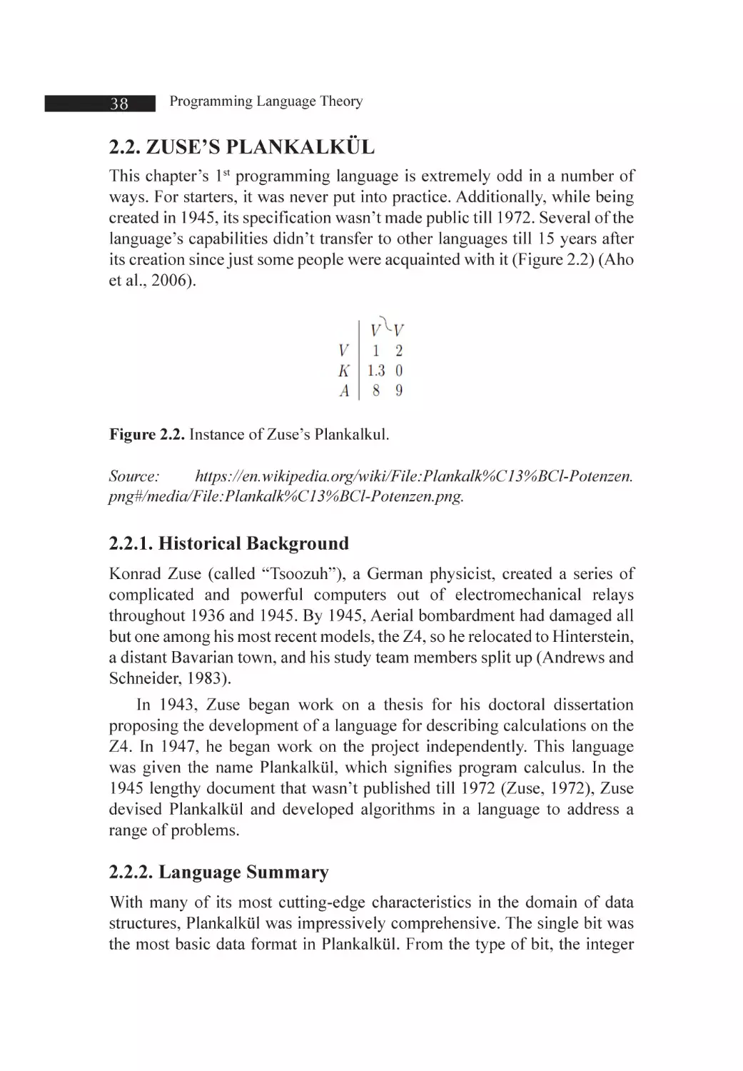
2.2. Zuse’s Plankalkül............................................................................... 38
2.3. Pseudocodes...................................................................................... 40
2.4. IBM 704 and Fortran.......................................................................... 44
2.5. Functional Programming: LISP........................................................... 47
2.6. Computerizing Business Records....................................................... 53
2.7. The Early Stages of Timesharing.......................................................... 56
2.8. Two Initial Dynamic Languages: Snobol and APL............................... 58
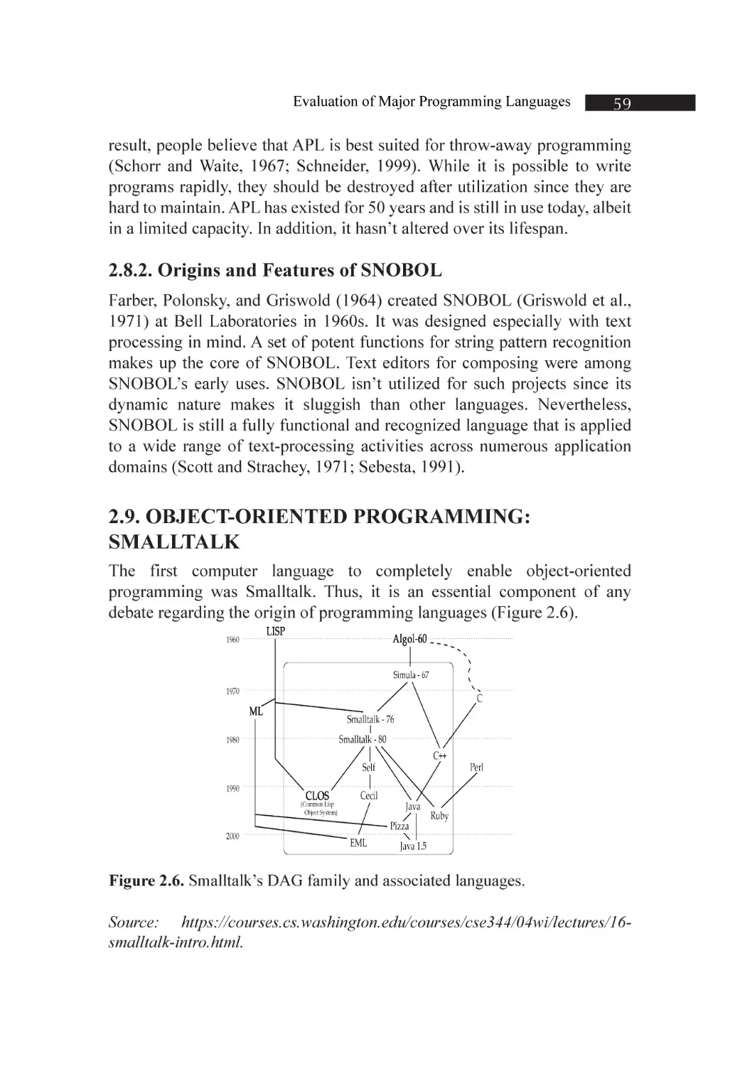
2.9. Object-Oriented Programming: Smalltalk.......................................... 59
2.10. Merging Imperative and Object-Oriented Characteristics................. 60
2.11. An Imperative-Centered Object-Oriented Language: Java................ 63
2.12. Markup-Programming Hybrid Languages......................................... 67

2.13. Scripting Languages......................................................................... 69
References................................................................................................ 73
Chapter 3

The Language PCF.................................................................................... 87
3.1. Introduction....................................................................................... 88
3.2. A Functional Language: PCF.............................................................. 88
3.3. Small-Step Operational Semantics for PCF......................................... 90
3.4. Reduction Strategies.......................................................................... 93
3.5. Big-Step Operational Semantics for PCF............................................ 96
3.6. Evaluation of PCF Programs............................................................... 96
References................................................................................................ 97

Chapter 4

Describing Syntax and Semantics........................................................... 101
4.1. Introduction..................................................................................... 102
4.2. The General Problem of Describing Syntax...................................... 103
4.3. Formal Methods of Describing Syntax.............................................. 105
4.4. Attribute Grammars......................................................................... 118
4.5. Describing the Meanings of Programs.............................................. 124
References.............................................................................................. 130

Chapter 5

Lexical and Syntax Analysis.................................................................... 141
5.1. Introduction..................................................................................... 142
5.2. Lexical Analysis............................................................................... 144
5.3. The Parsing Problem........................................................................ 148
5.4. Recursive-Descent Parsing............................................................... 153
5.5. Bottom-Up Parsing........................................................................... 156
5.6. Summary......................................................................................... 159
References.............................................................................................. 162

Chapter 6

Names, Bindings, and Scopes................................................................. 171
6.1. Introduction..................................................................................... 172
6.2. Names............................................................................................. 174
6.3. Variables.......................................................................................... 175
6.4. The Concept of Binding................................................................... 178
6.5. Scope.............................................................................................. 180
References.............................................................................................. 183

viii

Chapter 7

Data Types............................................................................................. 187
7.1. Introduction..................................................................................... 188
7.2. Primitive Data Types........................................................................ 191
7.3. Character String Types...................................................................... 195
References.............................................................................................. 199

Chapter 8

Support for Object-Oriented Programming........................................... 205
8.1. Introduction..................................................................................... 206
8.2. Object-Oriented Programming........................................................ 207
8.3. Design Issues for Object-Oriented Languages.................................. 209
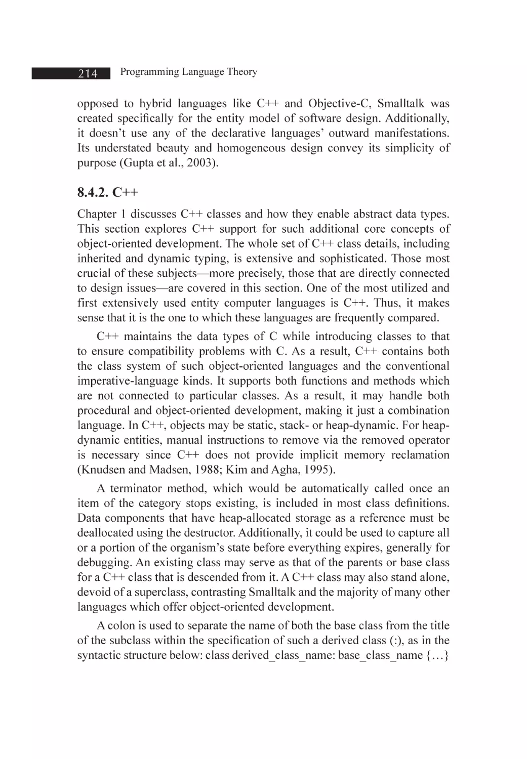
8.4. Support for Object-Oriented Programming in Specific Languages.... 213
References.............................................................................................. 217
Index...................................................................................................... 223

ix

LIST OF FIGURES
Figure 1.1. Division of a program
Figure 1.2. The fixed-point principle
Figure 1.3. A group of symbolism
Figure 1.4. Examples of variables
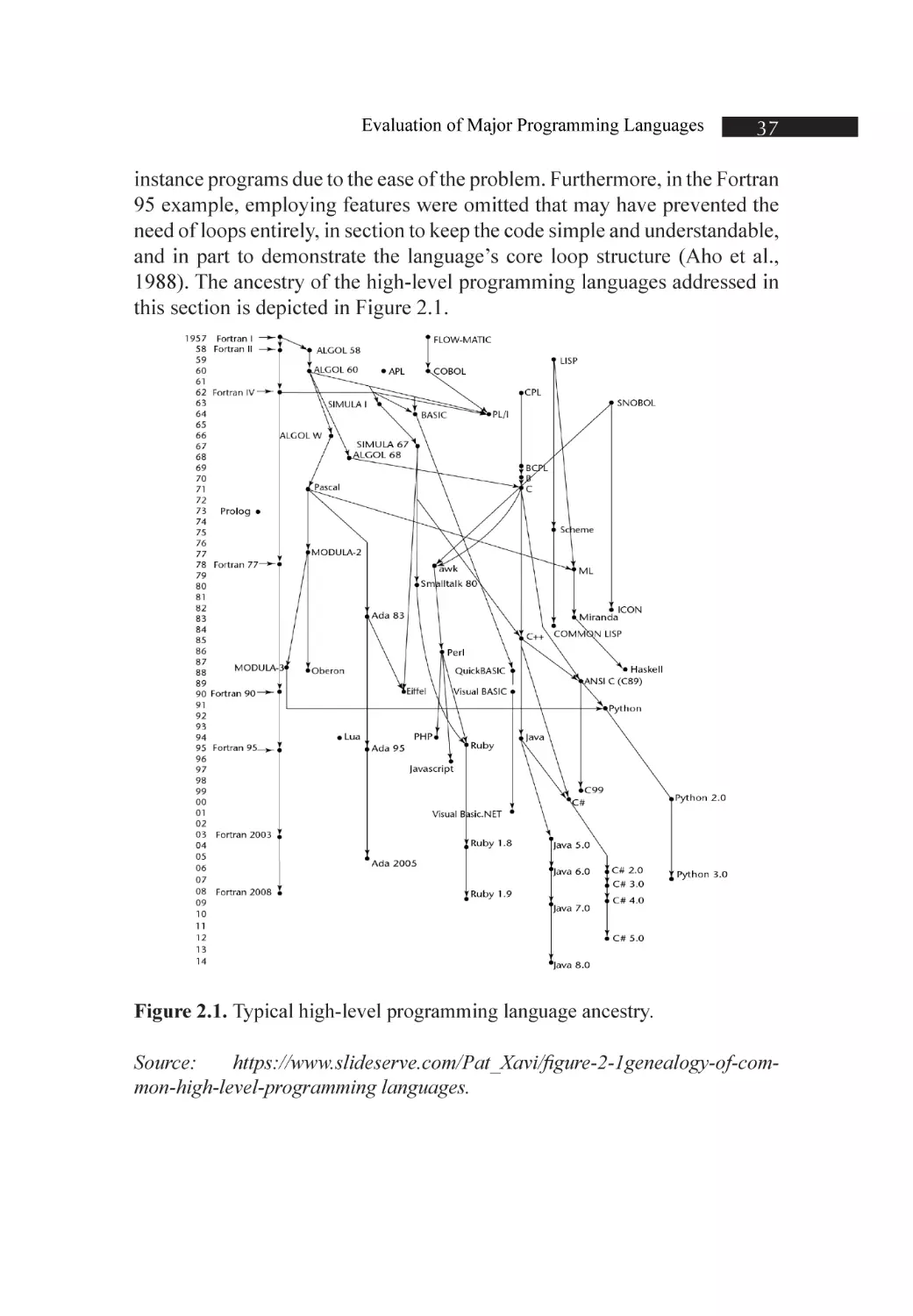
Figure 2.1. Typical high-level programming language ancestry
Figure 2.2. Instance of Zuse’s Plankalkul
Figure 2.3. Instance of pseudocode
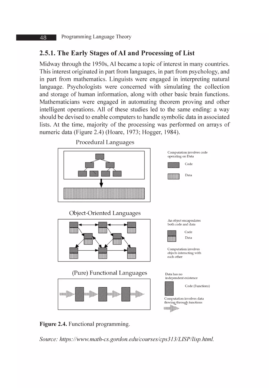
Figure 2.4. Functional programming
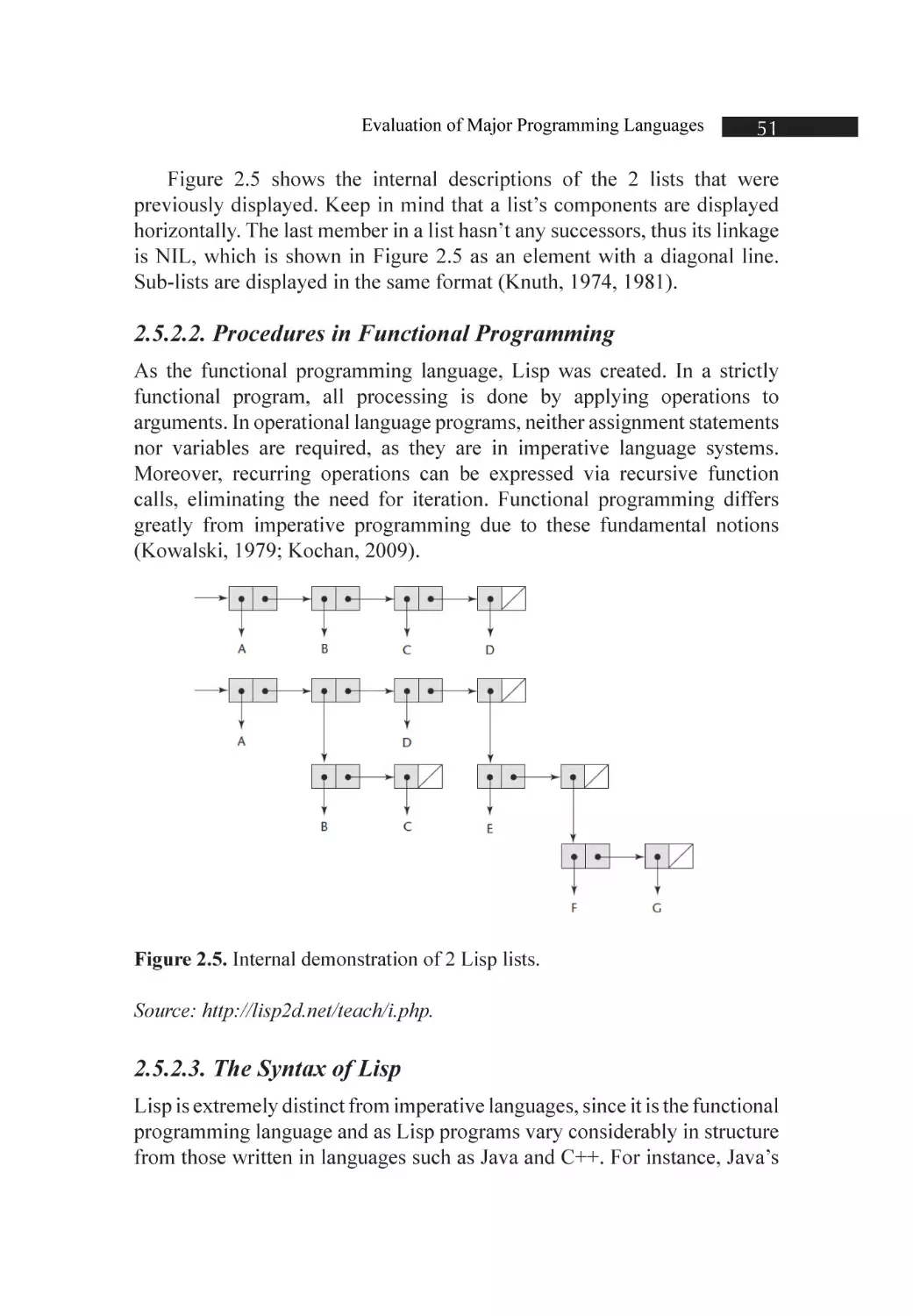
Figure 2.5. Internal demonstration of 2 Lisp lists
Figure 2.6. Smalltalk’s DAG family and associated languages
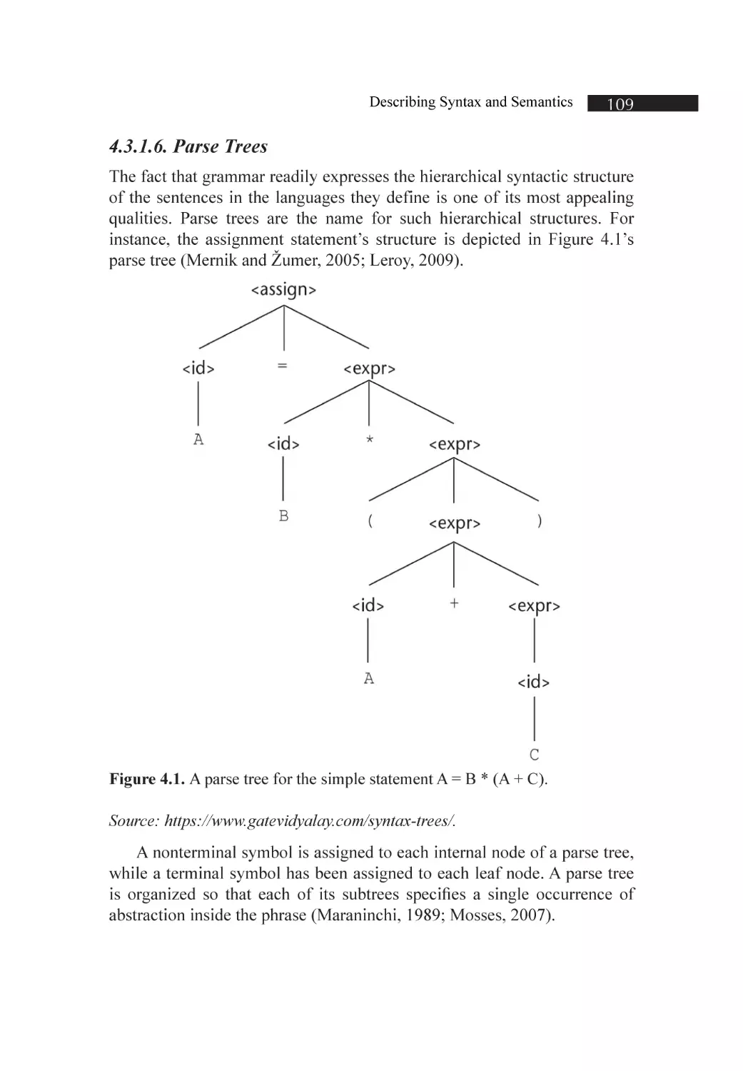
Figure 4.1. A parse tree for the simple statement A = B * (A + C)
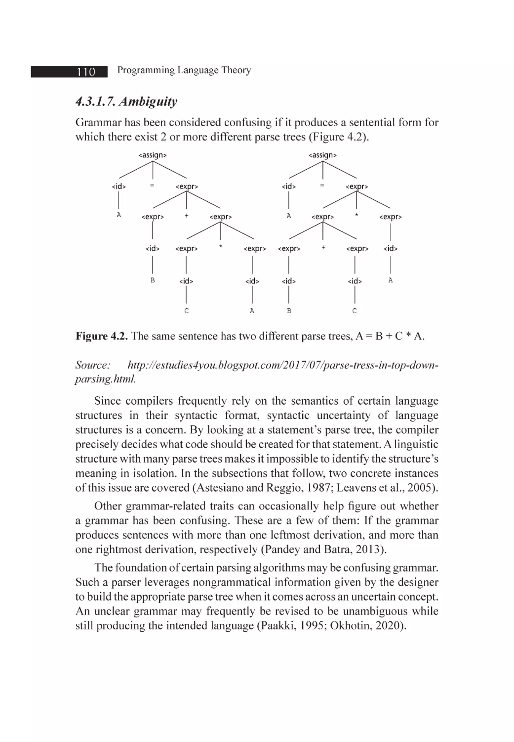
Figure 4.2. The same sentence has two different parse trees, A = B + C * A
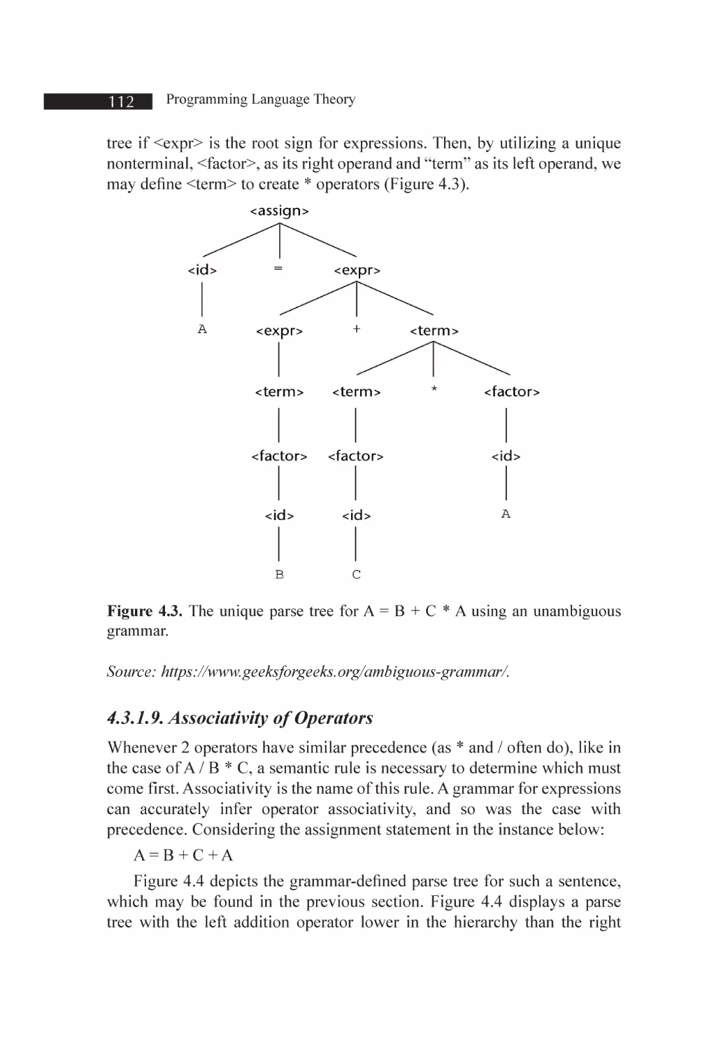
Figure 4.3. The unique parse tree for A = B + C * A using an unambiguous grammar
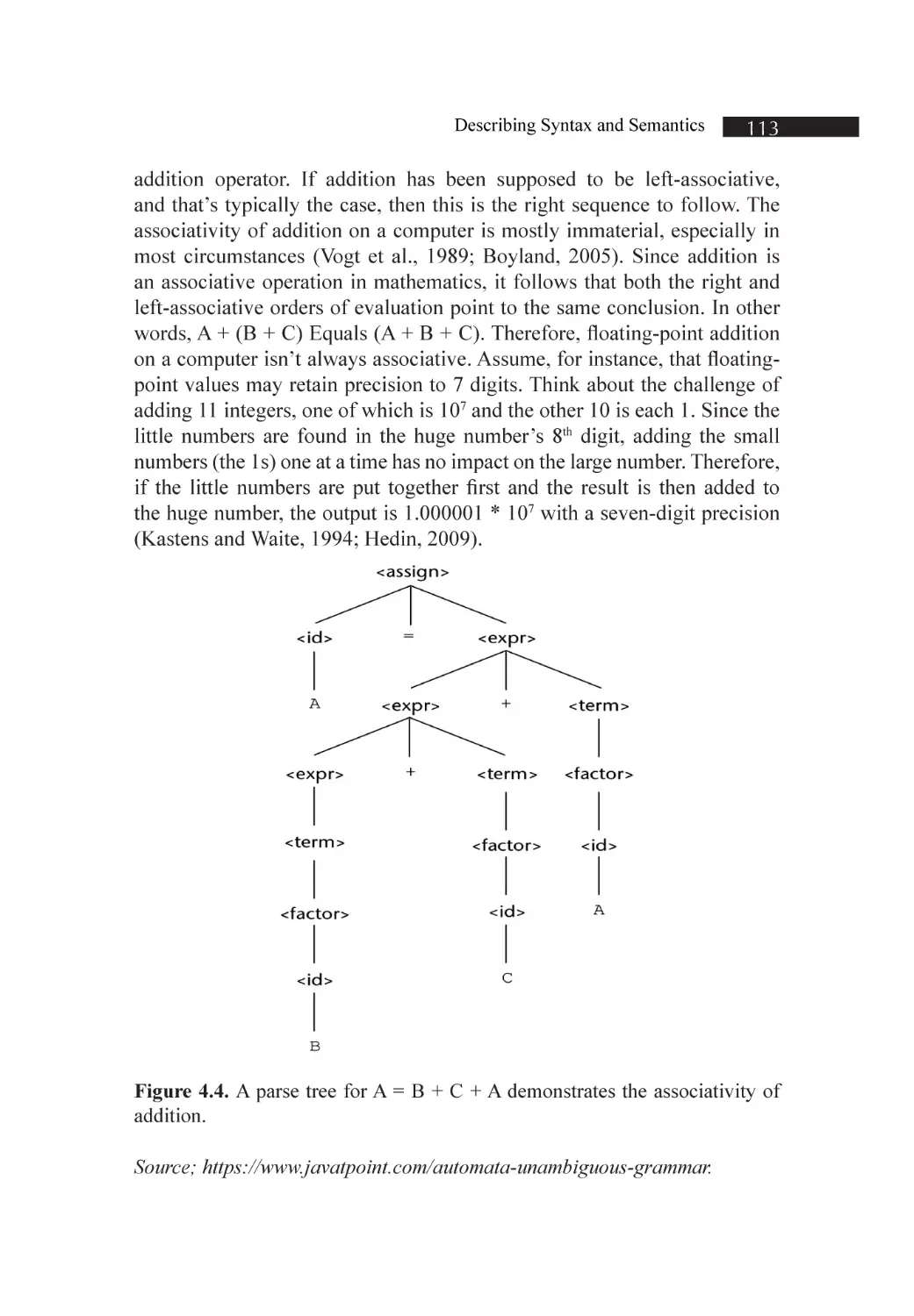
Figure 4.4. A parse tree for A = B + C + A demonstrates the associativity of addition
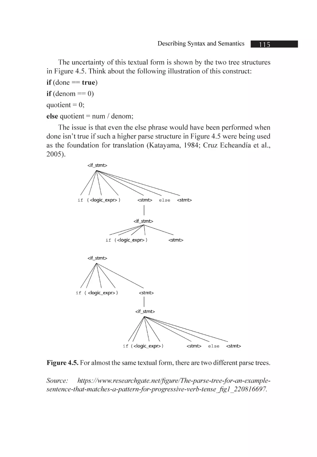
Figure 4.5. For almost the same textual form, there are two different parse trees
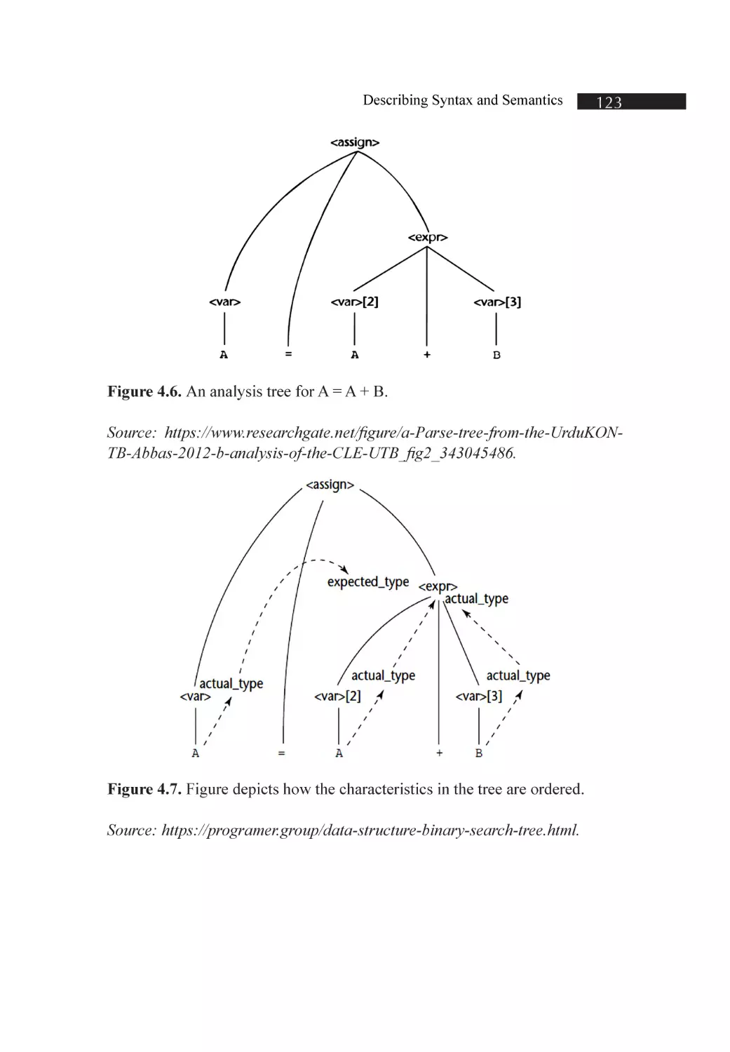
Figure 4.6. An analysis tree for A = A + B
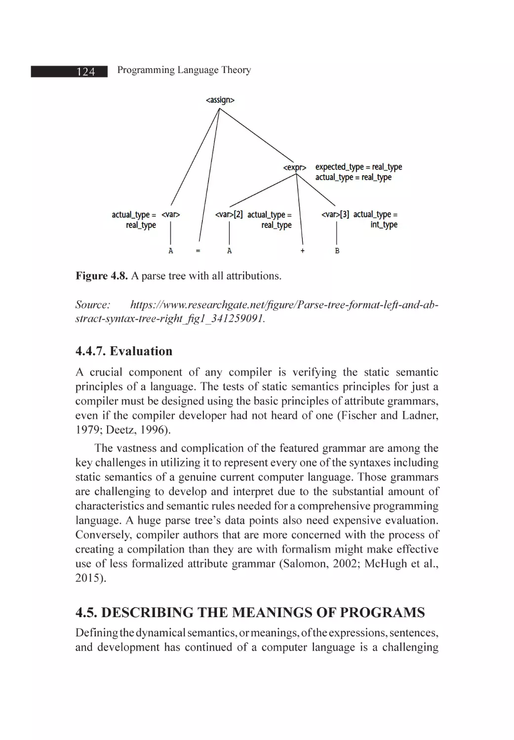
Figure 4.7. Figure depicts how the characteristics in the tree are ordered
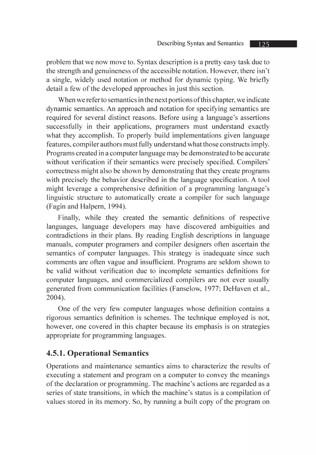
Figure 4.8. A parse tree with all attributions
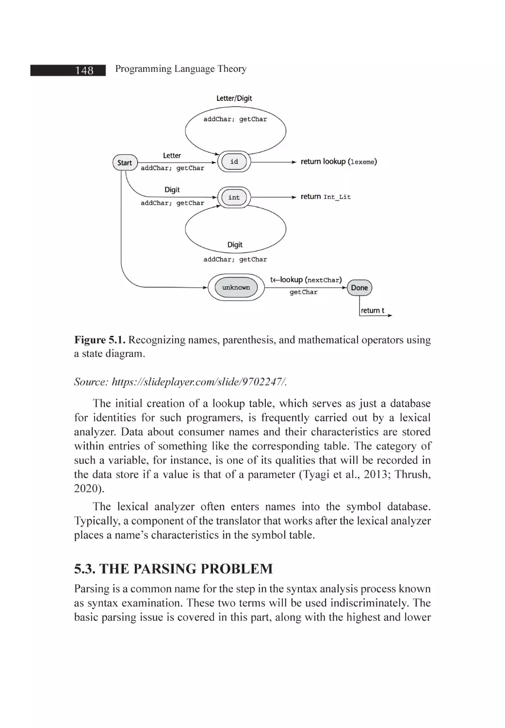
Figure 5.1. Recognizing names, parenthesis, and mathematical operators using a state
diagram
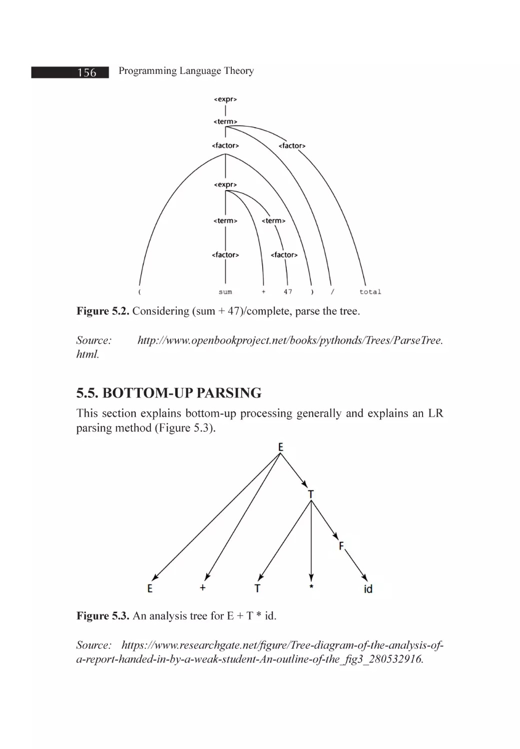
Figure 5.2. Considering (sum + 47)/complete, parse the tree
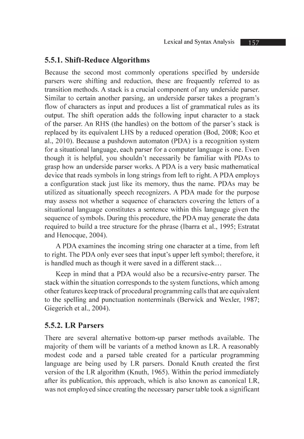
Figure 5.3. An analysis tree for E + T * id
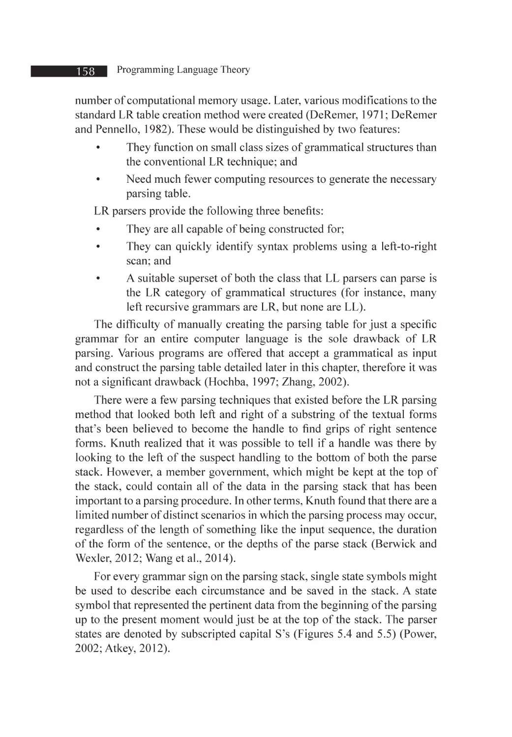
Figure 5.4. The structure of an LR parser
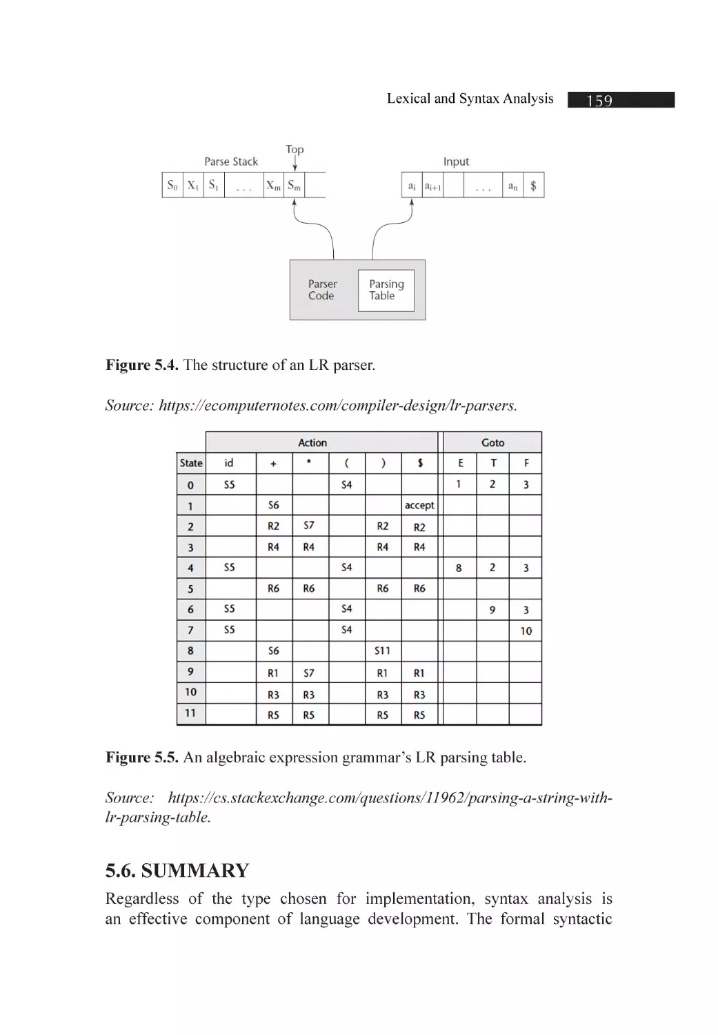
Figure 5.5. An algebraic expression grammar’s LR parsing table
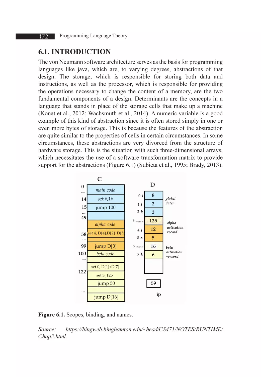
Figure 6.1. Scopes, binding, and names
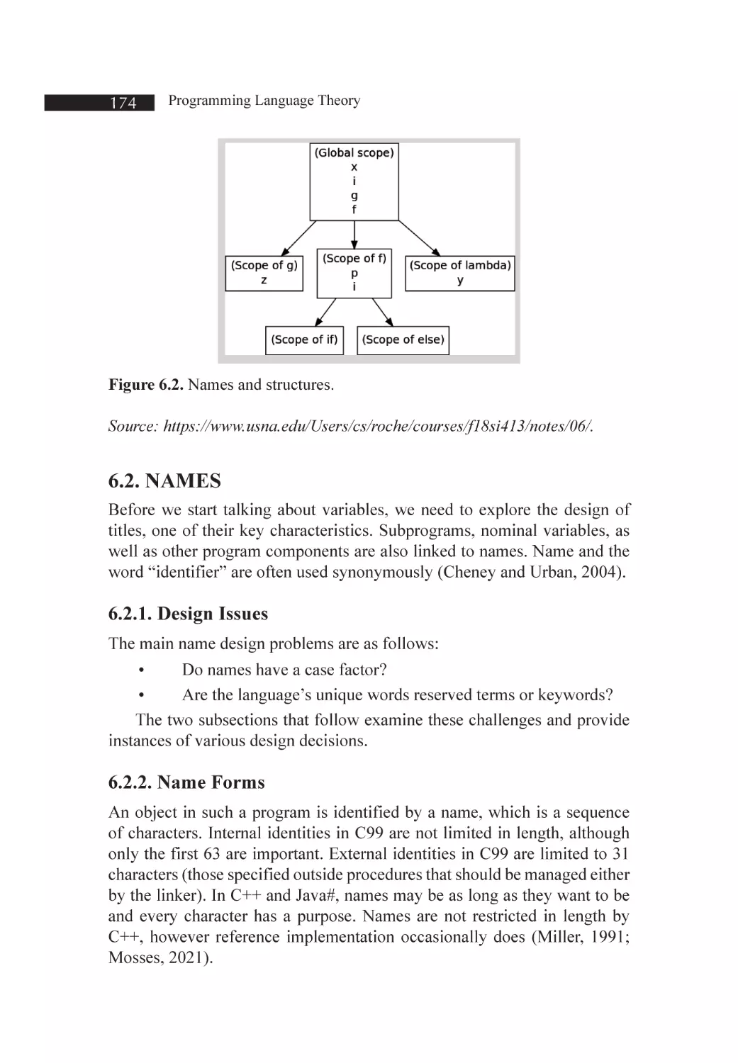
Figure 6.2. Names and structures
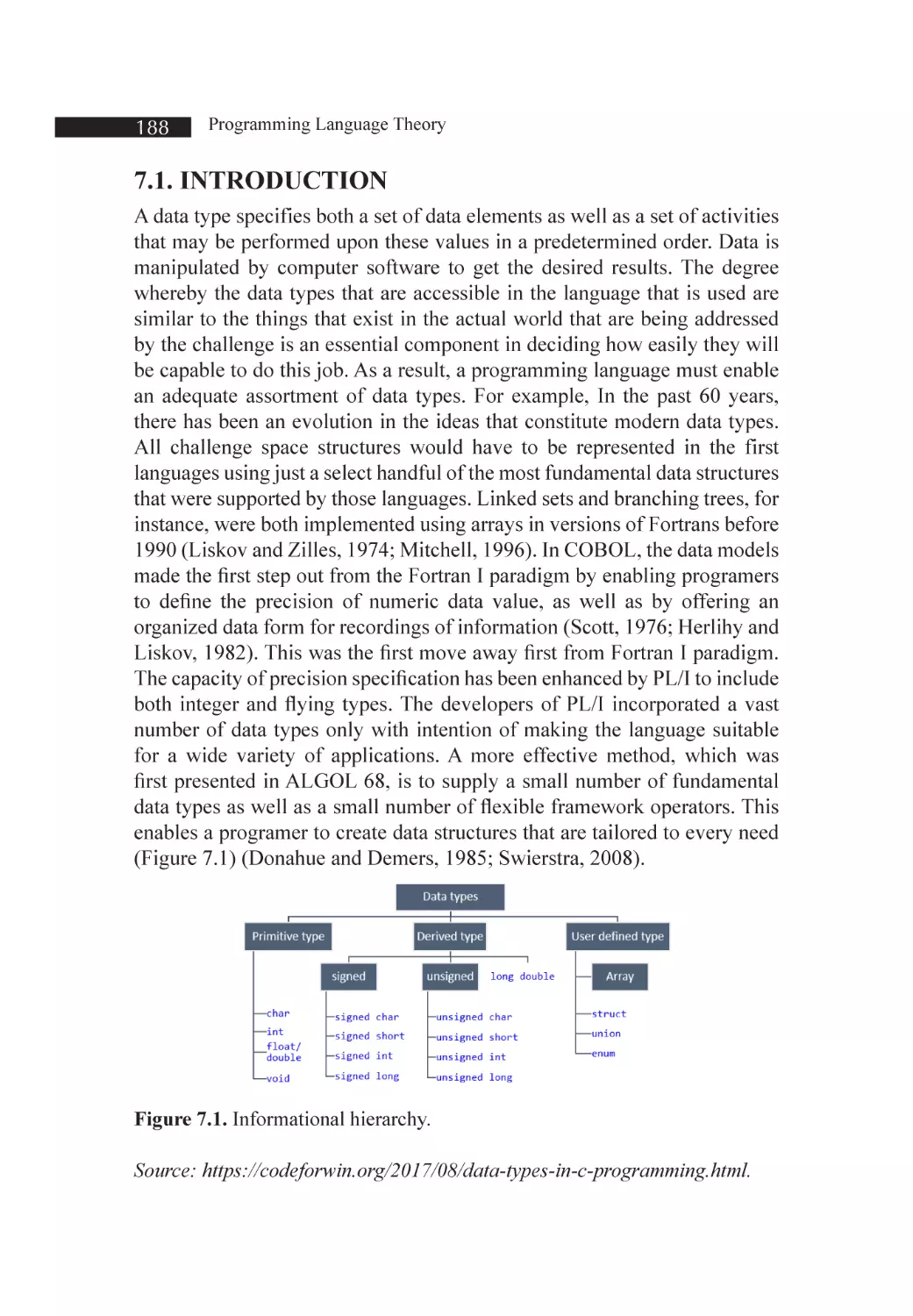
Figure 7.1. Informational hierarchy
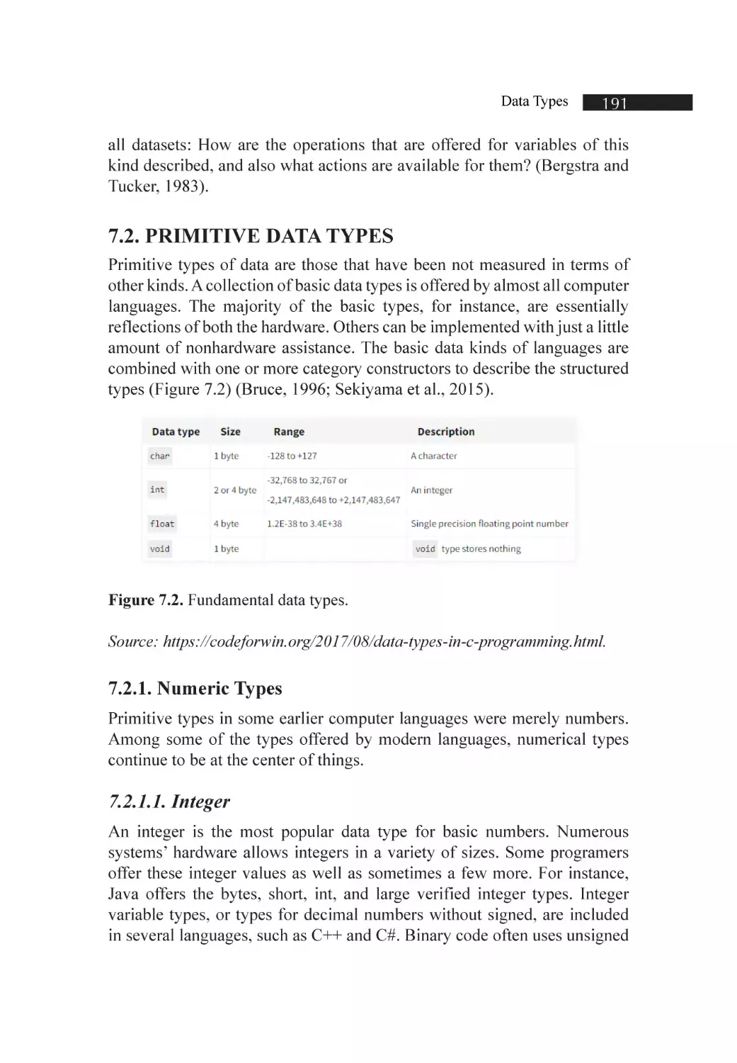
Figure 7.2. Fundamental data types
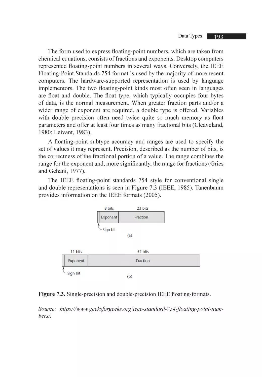
Figure 7.3. Single-precision and double-precision IEEE floating-formats

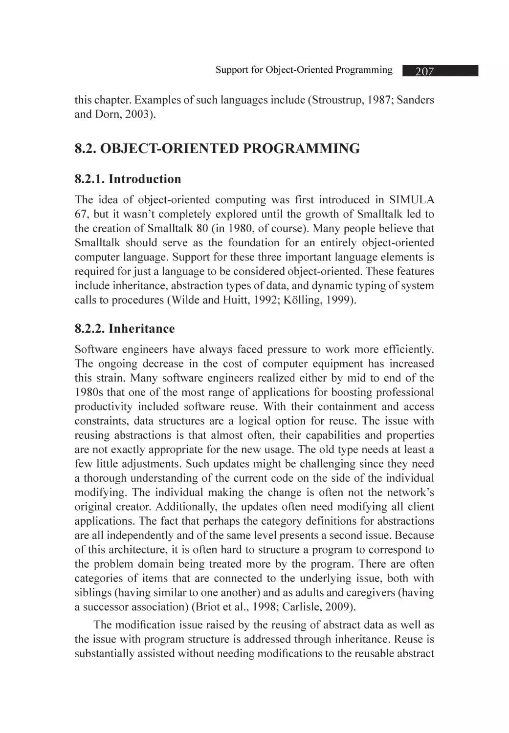
Figure 8.1. An easy case of inheritance
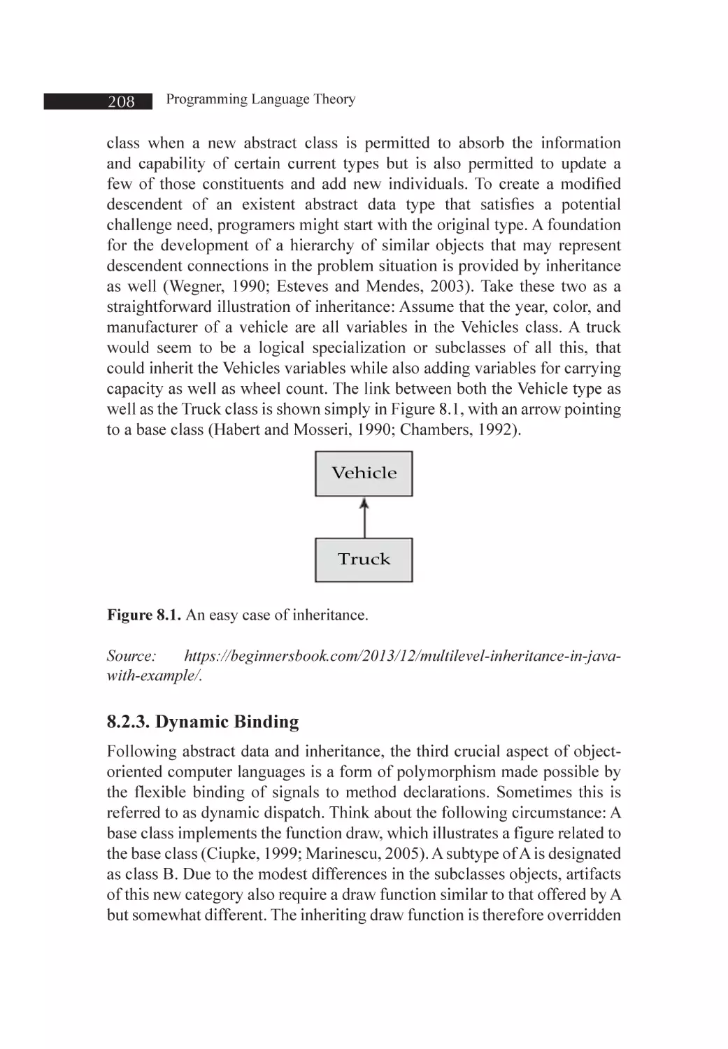
Figure 8.2. Dynamically bound
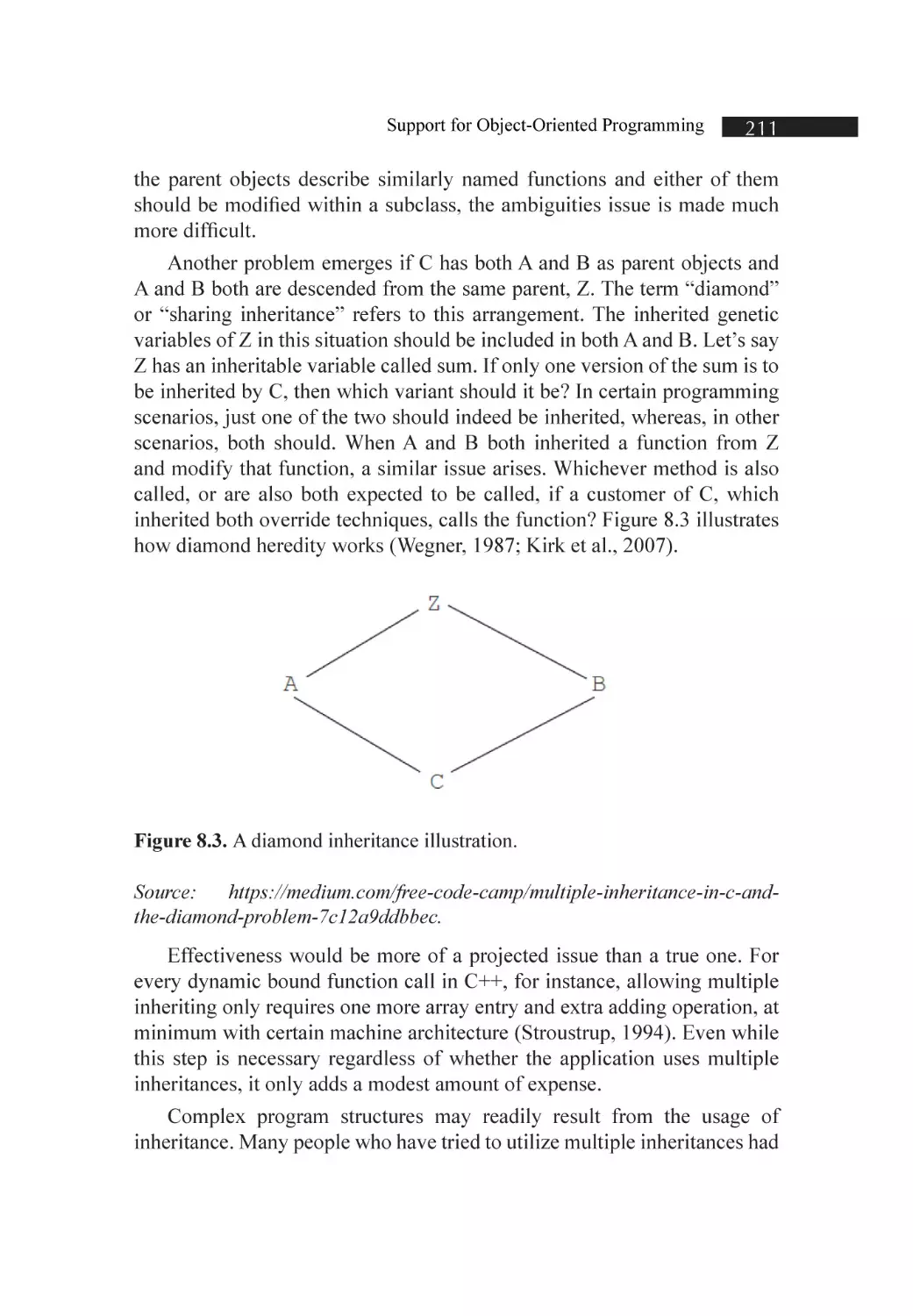
Figure 8.3. A diamond inheritance illustration
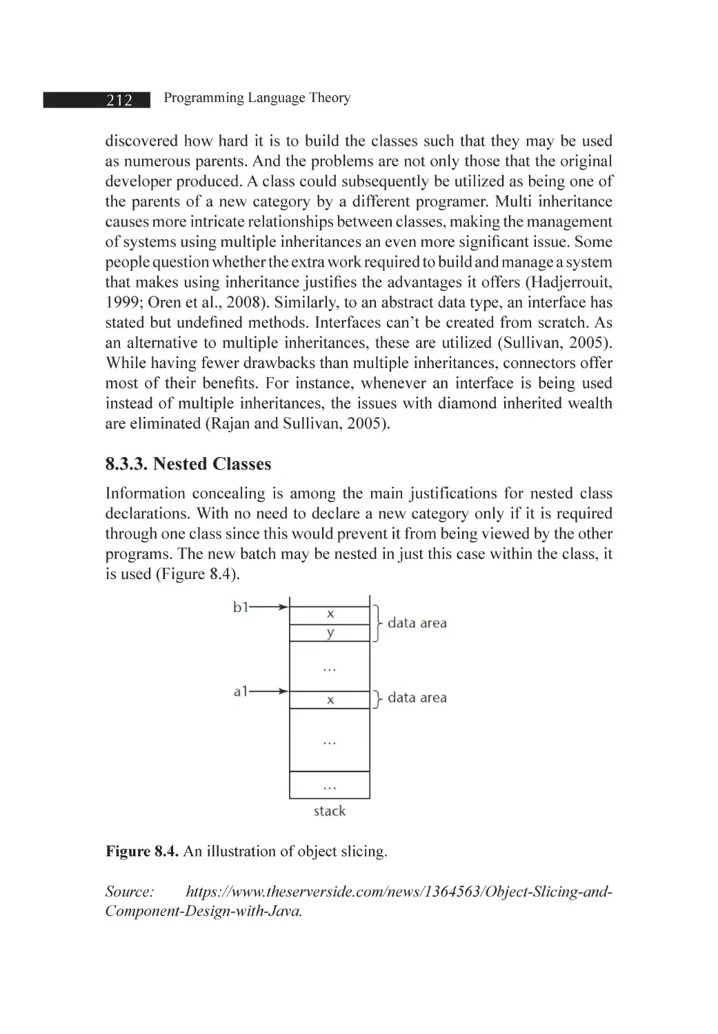
Figure 8.4. An illustration of object slicing
Figure 8.5. Several inheritances
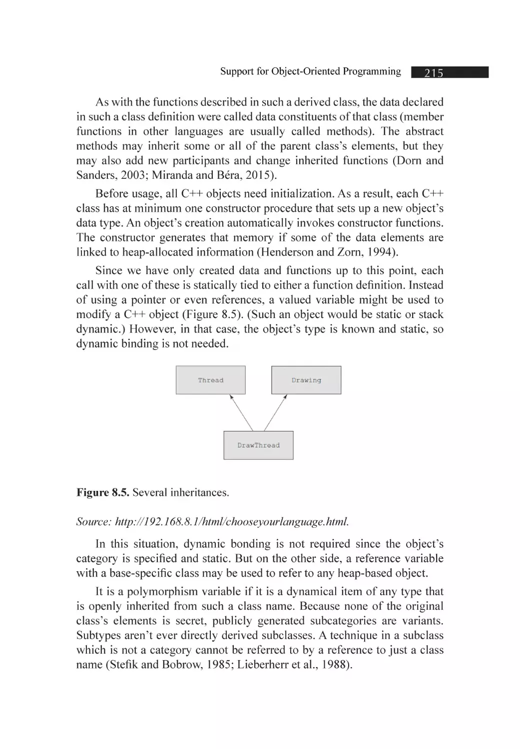
Figure 8.6. Dynamically bound

xii

LIST OF TABLES

Table 1.1. Criteria for evaluating languages and the factors that influence them

LIST OF ABBREVIATIONS
AI

artificial intelligence

CGI

common gateway interface

GUI

graphical user interfaces

IPL-1

information processing language I

ISO

International Standards Organization

JIT

just-in-time

LHS

left-hand side

PDA

pushdown automaton

PLT

programming language theory

RHS

right-hand side

VB

visual basic

VDL

Vienna definition language

WWW

world wide web

XML

extensible markup language

XSLT

eXtensible stylesheet language

PREFACE
PLT, which is an abbreviation that stands for “programming language theory (PLT),”
is a subfield of computer science that investigates the design, implementation,
analysis, characterization, and classification of formal languages that are referred to
as programming languages as well as the components that make up those languages
on their own. PLT also looks at how formal languages are characterized and classified.
PLT is a branch of computer science that draws from and impacts a wide range of other
academic fields, including mathematics, software engineering, languages, and even
cognitive science. It is also regarded to be its academic subject. PLT has developed into
a well-known area of study within the field of computer science and an active area of
investigation. The findings of this research are published in a large number of journals
that are specifically dedicated to PLT, in addition to publications that are generally
dedicated to computer science and engineering.
The primary body of the writing is partitioned into a total of eight separate chapters.
In Chapter 1 of the book, the reader is presented with an introduction to the theory
that supports programming languages. In Chapter 2, a great amount of time and effort
is focused on presenting an in-depth overview of the development of several distinct
programming languages. This chapter covers the history of the development of a wide
range of programming languages. Chapter 3 delves further into the PCF programming
language and provides extensive coverage of it.
The readers are given an introduction to the syntax and semantics in Chapter 4 of the
book, which is titled “Describing Syntax and Semantics.” This chapter is located in the
middle of the book. In Chapter 5, a significant amount of emphasis is focused, not only
on the syntactical analyzes but also on the lexical analyzes. This is because both of these
aspects are equally important. In Chapter 6, a list and presentation of the names and
bindings are provided. A rundown of the names is also provided in this chapter for your
perusal. In addition, an explanation of the different data types may be found in Chapter
7 of this book. Chapter 8 is titled “Support for Object-Oriented Programming,” and it
is in this chapter that the information that is relevant to the topic of support for objectoriented programming is covered.
This book does an excellent job of presenting an overview of the myriad of various
issues that are addressed in the theory that drives programming languages. If a person
reads this handbook, they should have no trouble understanding the fundamental ideas
that form the basis for the philosophy of programming languages. This is because the
content is structured and presented in such a way that even an inexperienced reader
should have no trouble doing so. After all, it is organized and presented in such a way
that even an experienced reader should have no trouble doing so.
—Author

1

CHAPTER

INTRODUCTION TO THE THEORY OF
PROGRAMMING LANGUAGE

CONTENTS
1.1. Introduction......................................................................................... 2
1.2. Inductive Definitions........................................................................... 5
1.3. Languages............................................................................................ 7
1.4. Three Ways to Define the Semantics of a Language............................ 10
1.5. Non-Termination............................................................................... 12
1.6. Programming Domains...................................................................... 12
1.7. Language Evaluation Criteria............................................................. 14
References................................................................................................ 25

2

Programming Language Theory

1.1. INTRODUCTION
The ultimate and most definite program code has still not been developed,
and this is not even close to being the case. There is almost always a new
language being developed, and established languages are continually having
additional capabilities added to them. Computer language advancements
help reduce the amount of time spent developing software, cut down on
the amount of time spent maintaining software, and make the software
more dependable overall. To meet new demands, including the creation of
parallel, dispersed, or mobile applications, modifications are also required
(Bird, 1987; Bauer et al., 2002).
When it comes to creating a computer language, the very first thing that
has to be described is indeed the syntax of the language. Would we write
x:= 1 or just write “x” equal to 1? Should brackets be placed after an if, or
will they be left out? In a broader sense, what are some examples of possible
sequences of signs that may be utilized in a program? There is indeed a tool
that may be used for this purpose, and that is the concept of a grammatical
structure. By utilizing grammar, we can provide an accurate description of a
syntactic of a language. As a result, it is now feasible to construct programs
that validate the syntactic and semantic accuracy of other programs (Asperti
and Longo, 1991; Hoare and Jifeng, 1998). However, this is not necessary to
know what such a grammatically valid program is in need to know exactly
what is going to occur whenever we run the system to know exactly what is
going to occur when we execute the system. When establishing a computer
language, it is also required to specify the language’s semantics, which
refers to the behavior that is anticipated from the programs when it is run.
It’s possible for two languages and has the same grammar but completely
distinct meanings (Tennent, 1976; Hagino, 2020).
Below is an illustration of what has been indicated by the term “semantic
information” in a more casual context. The following is a common
explanation for how functional evaluation is done. The following is how you
may acquire the outcome V of both the assessment of an equation of a form f
e1, …, en, in which the sign f would be a rational function either by equation
f x1, …, xn = e’. “The outcome V of an assessment of the equation of a form
f e1, …, en is as follows: Once that, the values e1, …, en are returned after
the inputs e1, …, en have been processed. After that, all values are assigned
to variables x1, …, xn, but then the equation e’ is ultimately evaluated. The
outcome of this assessment is represented by the value V (Norell, 2007).

Introduction to the Theory of Programming Language

3

This description of the semantics of a language, written in a basic
language (English), enables us to comprehend what takes place whenever a
program is run; nonetheless, the question remains as to whether or not it is
accurate. Take, for instance, the show that is now airing (Reynolds, 1997;
Nipkow et al., 2000):
fxy=x
g z = (n = n + z; n)
n = 0; print(f (g 2) (g 7))
The preceding explanation may be understood in several different ways,
and based on which one we choose, we can infer that now the program
would produce either the number 2 or even the number 9. This is because the
reasoning offered in basic language doesn’t specify whether we are required
to assess 7 pre- or post-evaluating 2, and the sequence wherein we assess
these statements is crucial in this particular scenario. Instead, the following
could have been included in the elaboration: “the influences e1, …, en are
assessed initially from e1” or different “opening after en.”

If two separate programers study the same description that is confusing,
they may come to different conclusions about what it means. To make matters
much worse, the developers of the translator again for language can decide
to use various norms. The very same program would thus provide varying
outputs depending on the particular compiler that was used (Strachey, 1997;
Papaspyrou, 1998).
It is commonly recognized since language varieties are also too
inaccurate to convey the syntactic of a computer language, a specific term
should only be used. Likewise, usual languages are too inaccurate to convey
the semantics of a computer language, but we need to utilize a proper
language (Mitchell, 1996; Glen et al., 2001).
What exactly is meant by the term “programming semantics”? Take, for
example, a program denoted by the letter p that prompts the user for just
an integer, calculates that number’s square, and then shows the outcome of
this action. It is necessary to specify crucial Links between both the value
that is entered and the output that is produced by this program to adequately
explain its operation (Figure 1.1) (Wadler, 2018).

4

Programming Language Theory

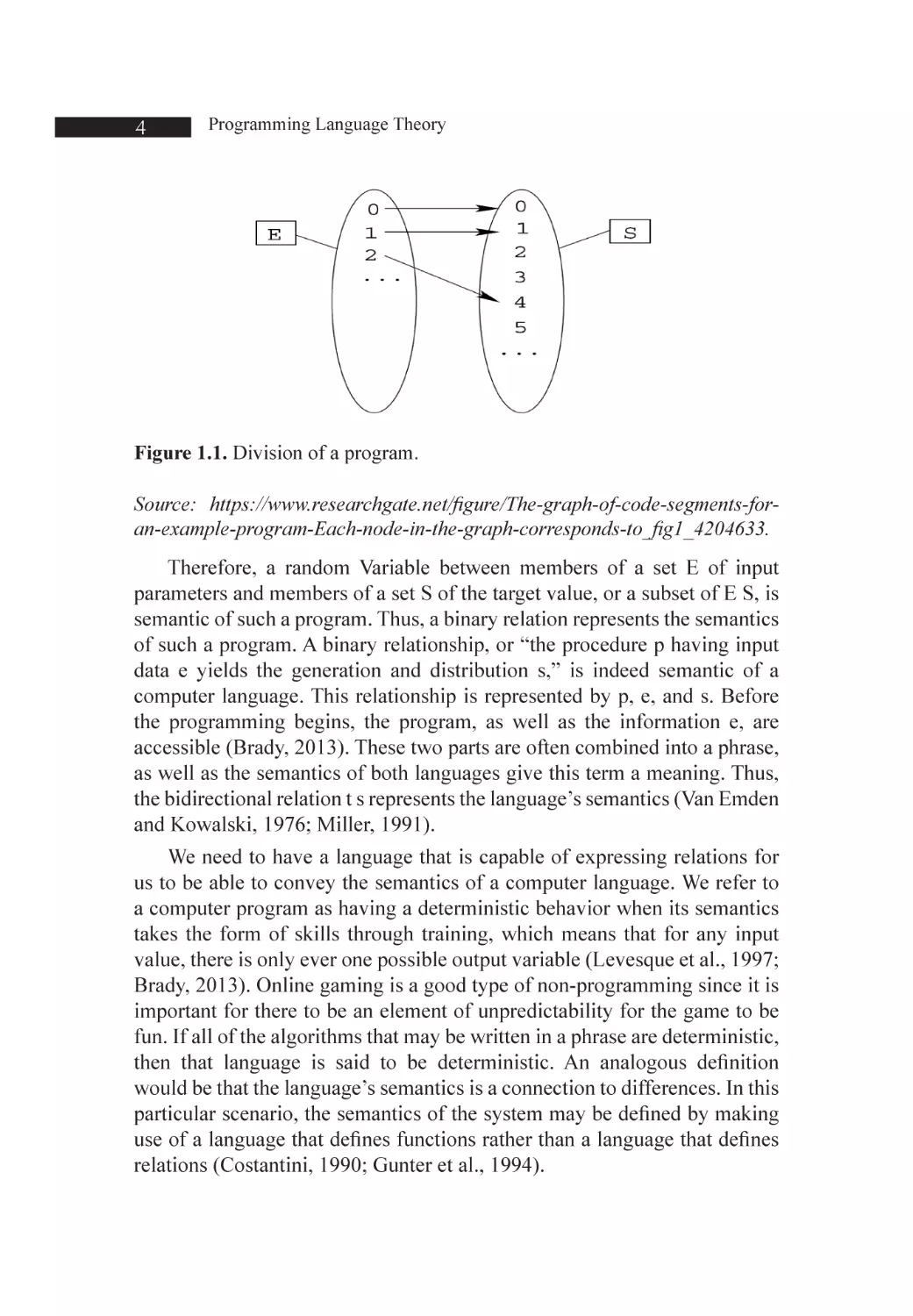
Figure 1.1. Division of a program.
Source: https://www.researchgate.net/figure/The-graph-of-code-segments-foran-example-program-Each-node-in-the-graph-corresponds-to_fig1_4204633.

Therefore, a random Variable between members of a set E of input
parameters and members of a set S of the target value, or a subset of E S, is
semantic of such a program. Thus, a binary relation represents the semantics
of such a program. A binary relationship, or “the procedure p having input
data e yields the generation and distribution s,” is indeed semantic of a
computer language. This relationship is represented by p, e, and s. Before
the programming begins, the program, as well as the information e, are
accessible (Brady, 2013). These two parts are often combined into a phrase,
as well as the semantics of both languages give this term a meaning. Thus,
the bidirectional relation t s represents the language’s semantics (Van Emden
and Kowalski, 1976; Miller, 1991).
We need to have a language that is capable of expressing relations for
us to be able to convey the semantics of a computer language. We refer to
a computer program as having a deterministic behavior when its semantics
takes the form of skills through training, which means that for any input
value, there is only ever one possible output variable (Levesque et al., 1997;
Brady, 2013). Online gaming is a good type of non-programming since it is
important for there to be an element of unpredictability for the game to be
fun. If all of the algorithms that may be written in a phrase are deterministic,
then that language is said to be deterministic. An analogous definition
would be that the language’s semantics is a connection to differences. In this
particular scenario, the semantics of the system may be defined by making
use of a language that defines functions rather than a language that defines
relations (Costantini, 1990; Gunter et al., 1994).

Introduction to the Theory of Programming Language

5

1.2. INDUCTIVE DEFINITIONS
We will begin by providing basic tools to construct collections and relations
because the semantics of a computer language is just a connection.
The idea of a precise definition has been the most fundamental instrument.
For instance, we may construct a method that doubles its input directly 2: x
→ 2 * x, {n ∈ N | ∃p ∈ N n = 2 * p}, or the connection of divisibility: {(n,m)
∈ N2 | ∃p ∈ N n = m * p}. These precise definitions, unfortunately, do not
specify all entities we want. The idea of an induction explanation is just a
second tool for defining collections and relations. This idea is supported by
the convergence point theorem, a straightforward theorem (Nordvall and
Setzer, 2010; Dagand and McBride, 2012).

1.2.1. The Fixed-Point Theorem
Let be an ordered relation more than a set E, which is bidirectional, the
system can be categorized, and bidirectional relation. u0, u1, u2, … Let be an
ordered relation more than a set E, which is bidirectional, the system can be
categorized, and bidirectional relation. ≤ u1 ≤ u2 ≤ … The element l of E is
called the limit of the sequence u0, u1, u2, … if it is the set’s least upper bound
{u0, u1, u2, …}, that is, if – for all i, ui ≤ l – if, for all i, ui ≤ l,’ then l ≤ l.’
The element l of E is called limit of the sequence u0, u1, u2, ... if it is a
least upper bound of the set {u0, u1, u2, ...}, that is, if – for all i, ui ≤ l – if,
for all i, ui ≤ l’, then l ≤ l’.
If all of the growing sequences have an upper bound, the sorting relation
is also said to be minimally complete.
A weakly completed ordering is shown by the common ordered
relationship so over actual figures [0, 1]. This connection also has a
minimum element of 0. The rising sequence 0, 1, 2, 3, … don’t even have
a limit, hence the conventional ordering connection over R+ isn’t weak or
incomplete (Paulson and Smith, 1989; Dybjer, 1994).
Let A represent a random set. An instance of a weakly completed ordering
is the inclusiveness relationship and overset (A) of all the subgroups of
A. The maximum in a rising series U0, U1, U2, … is the set Ui∈NUi. . This
relationship also has the lowest element.
A symbol connecting E to E, letting f be. If, some functional form is
growing x ≤ y ⇒ f x ≤ f y. If, in particular, for every growing sequence limi,
it’s indeed ongoing. (f ui) = f (limi ui).

6

Programming Language Theory

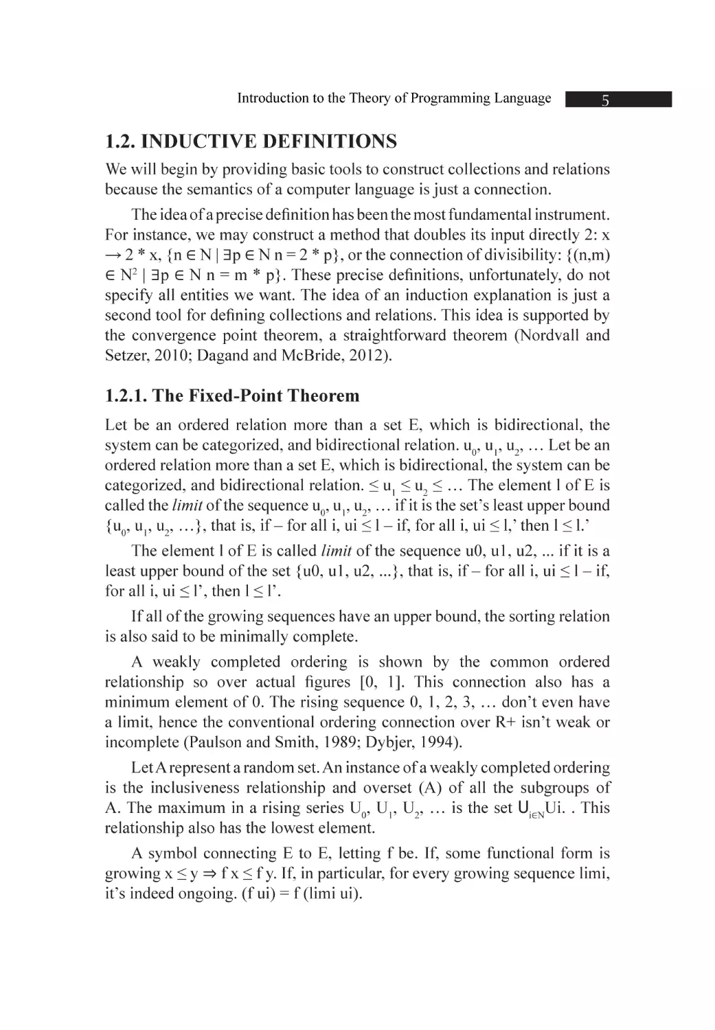
Let f be a purpose from E to E. If f is incessant then p = limi (fi m) is the
smallest secure fact of f (Figure 1.2).

Figure 1.2. The fixed-point principle.
Source: https://people.scs.carleton.ca/~maheshwa/MAW/MAW/node3.html.

Proof Initial, meanwhile m is the minimum component in E, m ≤ f m.
The purpose f is cumulative, so fi m ≤ fi+1 m. The series has a limitation since
it is rising. The order fi+1 m similarly has p as border, thus, p = limi (f (fi m))
= f (limi (fi m)) = f p. Furthermore, p remains the smallest secure point, since
if q is an additional fixed opinion, then m ≤ q and fi m ≤ fi q = q (since f is
cumulative). Hence = limi (fi m) ≤ q.
The second new equilibrium theorem asserts that growing functions
may have fixed points even though they’re not continuous, so long as when
the ordering fulfills a more stringent requirement. When every subgroup A
of set E does have the lowest upper limit sup A, then an arrangement over set
E is firmly complete (Paulson and Smith, 1989; Denecker, 2000).
Extremely comprehensive ordering relations include the common order
relation across the range. The fact that the set R+ itself has had no upper
limit prevents the conventional order over R+ from being firmly complete
(Hagiya and Sakurai, 1984; Muggleton and De Raedt, 1994).

Introduction to the Theory of Programming Language

7

1.2.2. Structural Induction
The writing of proofs is suggested by deductive definitions. When a feature
is inheritable, that is, if it consistently holds for y1, …, yni as well as for fi y1,
…, yni, we may infer that it consistently applies for all the components of E.
The second focus requires a theorem that may be used to demonstrate
this, and it can be shown that E is included in the subset P of A that contains
the values that meet the property because it is closed underneath the
functions fi. Another way is to use the first fixed point theorem and to show
by induction on k that all the elements in Fk ∅ satisfy the property.
(Muggleton, 1992; Coquand and Dybjer, 1994).

1.3. LANGUAGES
1.3.1. Languages without Variables
Nowadays induction definitions have been discussed, we will use this
method to define the concept of a language. It makes no difference whether
we write 3 + 4, +(3,4), or 3 4 + since these superficial grammatical rules
are not taken into consideration when defining the concept of language. A
tree will serve as an abstract representation of this phrase (Coquand and
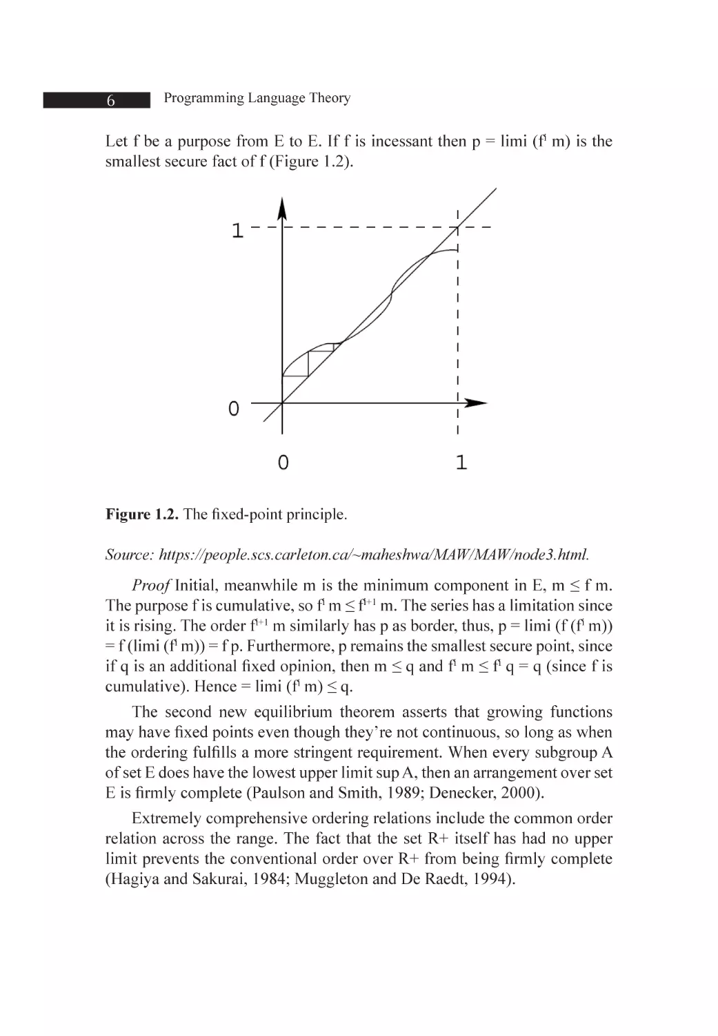
Paulin, 1988; Nielson and Nielson, 1992). The tree’s nodes will each be
identified by a symbol (Figure 1.3). A network node label determines how
many children it has—2 kids if the description is:
+, 0 if it is 3 or 4,…

Figure 1.3. A group of symbolism.
Source: https://www.ncl.ucar.edu/Applications/eqn.shtml.

8

Programming Language Theory

A language is thus a set of symbols, each with an associated number
called arity, or simply a number of arguments, of the symbol. The symbols
without arguments are called constants (Zieliński, 1992; Schmidt, 1996).
The collection of forests inductive reasoning defined by – if f is symbolic
with n parameters seems to be the set of words in the language and t1, …, tn
are rapports formerly f(t1, …, tn)—that is, the tree that has a root labeled by
f and subtrees t1, …, tn—is a term.

1.3.2. Variables
Imagine that we wish to create functionalities in a language that we plan to
project. Using variables would’ve been one option. sin, cos, … besides a
sign with two arguments ◦. We might, for instance, build the terms in ◦ (cos
◦ sin) in this verbal.
However, we are aware that using a concept developed by F makes it
simpler to describe functions. The idea of the variable was developed by
Viète (1540–1603). Thus, sin (cos (sin x)) may be used to represent the
function mentioned above (Berry and Cosserat, 1984; Strachey, 2000).
We have been writing this method since the 1930s. x → sin (cos (sin
x)) or λx sin (cos (sin x)), Using the sign → or λ the variables to be bound
x. We may differentiate between the stored procedure inputs and possible
parameters by specifying specifically which parameters are constrained.
By doing so, we also determine the parameters’ order (Berry and Cosserat,
1984).
The sign #→ looks to be N’s introduction. Bourbaki about 1930, and
the sign λ by A. Church about a similar period. The representation λ is a
condensed form of an earlier notation. ˆx sin (cos (sin x)) used by A. N.
Whitehead and B. Russell since the 1900s.
The definitions = x → sin (cos (sin x)) is occasionally written x = sin (cos
(sin x)). The benefit of writing f = x #→ sin (cos (sin x)) is that by doing so,
we may differentiate between two separate procedures.: the structure of the
purpose x → sin (cos (sin x)) and the explanation the situation, it identifies a
previously created object. In computer programming, it is frequently crucial
to have footnotes that let us construct things without obviously giving them
names (Smith, 1984).
Throughout this book, the word “fun” is used. x → sin (cos (sin x)
describing this procedure. The period amusing x → sin (cos (sin x) has a
function specified. Though it includes a free variable whose meaning we

Introduction to the Theory of Programming Language

9

need not understand, the subterm sin x doesn’t describe anything when it’s
neither a true figure nor a function (Plotkin, 1977; Ritchie et al., 1978).
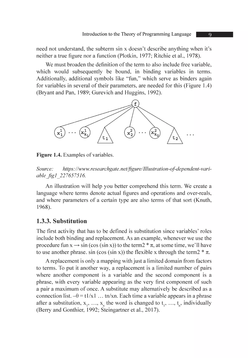
We must broaden the definition of the term to also include free variable,
which would subsequently be bound, in binding variables in terms.
Additionally, additional symbols like “fun,” which serve as binders again
for variables in several of their parameters, are needed for this (Figure 1.4)
(Bryant and Pan, 1989; Gurevich and Huggins, 1992).

Figure 1.4. Examples of variables.
Source:
https://www.researchgate.net/figure/Illustration-of-dependent-variable_fig1_227657516.

An illustration will help you better comprehend this term. We create a
language where terms denote actual figures and operations and over-reals,
and where parameters of a certain type are also terms of that sort (Knuth,
1968).

1.3.3. Substitution
The first activity that has to be defined is substitution since variables’ roles
include both binding and replacement. As an example, whenever we use the
procedure fun x → sin (cos (sin x)) to the term2 * π, at some time, we’ll have
to use another phrase. sin (cos (sin x)) the flexible x through the term2 * π.
A replacement is only a mapping with just a limited domain from factors
to terms. To put it another way, a replacement is a limited number of pairs
where another component is a variable and the second component is a
phrase, with every variable appearing as the very first component of such
a pair a maximum of once. A substitute may alternatively be described as a
connection list. –θ = t1/x1 … tn/xn. Each time a variable appears in a phrase
after a substitution, x1, …, xn the word is changed to t1, …, tn, individually
(Berry and Gonthier, 1992; Steingartner et al., 2017).

10

Programming Language Theory

Just the independent variables are impacted by this substitution. For
instance, we should get the phrase 2 + 3 if we replace the variable x with the
word 2 in phrase x + 3. Therefore, we will get the phrase fun x → x and just
not fun x → 2 if we replace the variable x with the word 2 within the phrase
fun x → x, which denotes identity mapping.
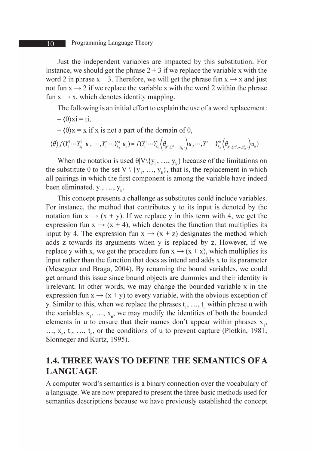
The following is an initial effort to explain the use of a word replacement:
– ⟨θ⟩xi = ti,

– ⟨θ⟩x = x if x is not a part of the domain of θ,

− θ f (Y11 Yk11 u1 ,  , Y1n Yknn un ) =
f (Y11 Yk11 θ|V \{Y 1 ,,Y 1 } u1 , , Y1n Yknn θ|V \{Y n ,,Y n } un )
1

k1

1

kn

When the notation is used θ|V\{y1, …, yk} because of the limitations on
the substitute θ to the set V \ {y1, …, yk}, that is, the replacement in which
all pairings in which the first component is among the variable have indeed
been eliminated. y1, …, yk.

This concept presents a challenge as substitutes could include variables.
For instance, the method that contributes y to its input is denoted by the
notation fun x → (x + y). If we replace y in this term with 4, we get the
expression fun x → (x + 4), which denotes the function that multiplies its
input by 4. The expression fun x → (x + z) designates the method which
adds z towards its arguments when y is replaced by z. However, if we
replace y with x, we get the procedure fun x → (x + x), which multiplies its
input rather than the function that does as intend and adds x to its parameter
(Meseguer and Braga, 2004). By renaming the bound variables, we could
get around this issue since bound objects are dummies and their identity is
irrelevant. In other words, we may change the bounded variable x in the
expression fun x → (x + y) to every variable, with the obvious exception of
y. Similar to this, when we replace the phrases t1, …, tn within phrase u with
the variables x1, …, xn, we may modify the identities of both the bounded
elements in u to ensure that their names don’t appear within phrases x1,
…, xn, t1, …, tn, or the conditions of u to prevent capture (Plotkin, 1981;
Slonneger and Kurtz, 1995).

1.4. THREE WAYS TO DEFINE THE SEMANTICS OF A
LANGUAGE
A computer word’s semantics is a binary connection over the vocabulary of
a language. We are now prepared to present the three basic methods used for
semantics descriptions because we have previously established the concept

Introduction to the Theory of Programming Language

11

of languages and provided tools for defining relations. As a functional, an
induction specification, or the reactionary closing of such an explicitly stated
relation, the semantics of languages is often provided. Multiple meanings
semantically, big-step functional semantics and lower operating semantics,
and syntactic are the three terms used to describe them (Van Hentenryck and
Dincbas, 1986; Cortesi et al., 1994).

1.4.1. Denotational Semantics
Deterministic programming benefits from multiple meanings semantics. In
this instance, the input-output relationship specified by such a program is
just a function, denoted by [p], for every program p.
The relation →is then defined by:
p,e → s if and individual if [p]e = s
Naturally, this just makes the issue worse since it forces us to describe
the procedure [p]. Explicit descriptions of functions as well as the constant
value theorem will be our two important tools for this, but we’ll save that for
later (Dijkstra and Dijkstra, 1968; Henderson and Notkin, 1987).

1.4.2. Big-Step Operational Semantics
Naturally, semantics and structural operational semantics (S.O.S.) are
other names for big-step functional semantics. It defines the relationship
inductively. →.

1.4.3. Small-Step Operational Semantics
Reducing semantics is another name for lower operating semantics. It
establishes the relationship by way of another relationship that outlines
the fundamental procedures required to convert the starting word t into the
ending term s (Tsakonas et al., 2004; Odiete et al., 2017).
For instance, we get the output 20 when we execute the method fun x →
(x * x) + x with both the inputs 4. However, the phrase (fun x → (x * x) + x)
4 first becomes (4 * 4) + 4, next 16 + 4, and eventually 20. Doesn’t become
20 all at once.
The relationship between the terms (fun x → (x * x) + x) 4 and 20 wasn’t
the most significant one; rather, it is the relationship between the terms (fun
x → (x * x) + x) 4 and (4 * 4) + 4, 16 + 4, plus 20.

12

Programming Language Theory

When the relation ‣ is assumed, → can be resulting after the reflexivetransitive conclusion ‣∗ of the relation ‣ t →s if then only if t ‣∗ s and s is
complicated.
It follows that nothing further to calculate in s since the phrase s is
indivisible. For instance, the word 20 cannot be reduced, whereas the term
16 + 4 may. If there isn’t a phrase s’ so that s s’, then a phrase s is reductive
(Lewis and Shah, 2012; Rouly et al., 2014).

1.5. NON-TERMINATION
A system’s implementation may conclude in success, a failure, or it may
never end. Errors may be thought of as certain types of outcomes. There are
numerous different approaches to defining a semantic with non-terminating
algorithms. Considering the first option, which states that there is no pair
(t,s) in connection if the phrase t doesn’t finish. →.
Another option is to include a certain component. ⊥ declaring that now
the connection applies to the collection of target value →comprises the
couple (t,⊥) while the phrase t remains unfinished. The distinction could
seem negligible: Getting rid of all of the other form pairings is simple (t,⊥),
If there isn’t a pairing of both types (t,s) within relations, you may add one.
Visitors who already are knowledgeable about computational complexity
issues will note, therefore, that if we combine the pairs (t,⊥), the relation →
is not sequentially enumerable anymore (Wan et al., 2001; Strawhacker and
Bers, 2019).

1.6. PROGRAMMING DOMAINS
From operating nuclear power plants to offering digital mobile games
phones, computers were used in a wide variety of applications. Scripting
languages with widely varied objectives have been created as a result of the
enormous variety in computer usage. In this part, we’ll talk a little bit about
a few separate computer application fields as well as the languages that go
along with them (Filippenko and Morris, 1992; Mantsivoda et al., 2006).

1.6.1. Scientific Applications
Within the 1940s and 1950s, the very first digital processors were developed
and utilized for scientific purposes. The state of knowledge of the era typically
used very basic data formats but required a significant amount of floatingpoint mathematical operations. The most popular control architectures were

Introduction to the Theory of Programming Language

13

measuring loops and select, whereas the most popular data formats were
arrays as well as matrices. High-level coding languages from the beginning
(Howatt, 1995; Samimi et al., 2014).
developed for scientific purposes were created to meet those
requirements. Performance was the main consideration since machine
language remained their main rival. Fortran was the first language used for
applications in science. Except they were created that can be used in other
relevant fields as well, ALGOL 60 and the majority of its offspring were
also meant to be employed in this field. No succeeding language is much
superior to Fortran for certain application areas where performance is the
key issue, including those that were popular in the 1950s early 1960s, which
explains how Fortran is still being used today (Kiper et al., 1997; Samimi
et al., 2016).

1.6.2. Business Applications
Within the 1950s, the first commercial uses of computers appeared. For this
reason, special systems and unique languages were created. The first highlyregarded language of business was COBOL, which initially debuted in 1960
(ISO/IEC, 2002). It is still most likely the language used for such apps.
The capacity to express decimal mathematical operations, accurate means of
representing and storing numeric values, and the capacity to make complex
reports are characteristics of commercial languages (Suganthan et al., 2005;
Kurtev et al., 2016).
Aside from the growth and development of COBOL, there haven’t been
many advancements in software product languages. As a result, this book
just briefly discusses COBOL’s structural elements.

1.6.3. Artificial Intelligence (AI)
A large category of software applications known as artificial intelligence
(AI) is distinguished through the use of symbols rather than numerical
calculations. The manipulation of symbols—which are made up of names
instead of numbers—is referred to as symbolic computing (Liang et al.,
2013).
Additionally, directories of data are more practical for symbolic
computing than arrays. Often, compared to other programming disciplines,
this form of programming calls for greater flexibility. For instance, the
ability to write and run code parts as they are being executed is useful in
certain AI applications. The effective language Lisp, which originally

14

Programming Language Theory

debuted in 1959, was the very first popular programming language created
for Ai technologies (McCarthy et al., 1965). Before 1990, the majority of Ai
technologies were created in Lisp with one of its close cousins. But in the
early 1970s, logic computing that used the Logic language (Clocksin and
Mellish, 2013) emerged as a substitute strategy for any of these systems.
Several Ai systems have lately been created using programming languages
like C, Scheme (Dybvig, 2009), a Lisp dialect, and Prolog.

1.6.4. Web Software
A diverse range of languages, including display languages like HTML,
which are not scripting languages, to broad sense programming languages
such as Java, enable the Internet. Due to the widespread demand for
changeable Web information, content display technology often includes
some computing capabilities. Coding may be used in any HTML document to
give this capability. These programs often take the form of scripts written in
languages like JavaScript or PHP (Tatroe, 2013). There are various markuplike languages that have been enhanced to incorporate documentation
features.

1.7. LANGUAGE EVALUATION CRITERIA
As was already said, the objective of this book would be to thoroughly
investigate the fundamental ideas behind the numerous constructions and
abilities of computer languages. We will assess these attributes as well,
paying particular attention to how they affect the assessment criteria. Even
two software engineers can’t agree just on the relative importance of any
two linguistic characteristics, therefore a listing of such criteria is always
contentious. Despite these variations, the majority would concur that the
factors covered in subsequent sections are crucial (Parker et al., 2006; Kim
and Lee, 2010).
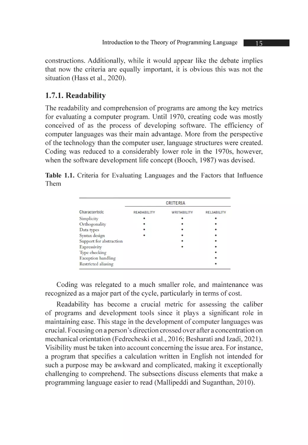
Table 1.1 lists a few of the traits that affect three of the four particularly
crucial such criteria, and the requirements themselves are covered in
subsections. In keeping with the discussions in the next subcategories, those
most crucial traits are included in the table. It’s possible to argue that, if one
took into account less significant factors, “bullets” may be present at almost
all table places.
Be aware that most of these qualities—like writability—are general and
imprecise while others—like exception handling—are specialized language

Introduction to the Theory of Programming Language

15

constructions. Additionally, while it would appear like the debate implies
that now the criteria are equally important, it is obvious this was not the
situation (Hass et al., 2020).

1.7.1. Readability
The readability and comprehension of programs are among the key metrics
for evaluating a computer program. Until 1970, creating code was mostly
conceived of as the process of developing software. The efficiency of
computer languages was their main advantage. More from the perspective
of the technology than the computer user, language structures were created.
Coding was reduced to a considerably lower role in the 1970s, however,
when the software development life concept (Booch, 1987) was devised.
Table 1.1. Criteria for Evaluating Languages and the Factors that Influence
Them

Coding was relegated to a much smaller role, and maintenance was
recognized as a major part of the cycle, particularly in terms of cost.
Readability has become a crucial metric for assessing the caliber
of programs and development tools since it plays a significant role in
maintaining ease. This stage in the development of computer languages was
crucial. Focusing on a person’s direction crossed over after a concentration on
mechanical orientation (Fedrecheski et al., 2016; Besharati and Izadi, 2021).
Visibility must be taken into account concerning the issue area. For instance,
a program that specifies a calculation written in English not intended for
such a purpose may be awkward and complicated, making it exceptionally
challenging to comprehend. The subsections discuss elements that make a
programming language easier to read (Mallipeddi and Suganthan, 2010).

16

Programming Language Theory

1.7.1.1. Overall Simplicity
The accessibility of a computer language is significantly influenced by how
simple it is overall. It is much more challenging to master a language with
many fundamental concepts than with fewer. When using a huge language,
developers often only learn a small portion of it and pay little attention to
the rest. The high number of language structures is sometimes justified by
reference to this training pattern, although such justification is unsound.
Every time the program’s creator has studied a distinct subset than the
fraction the reader is used to, readability issues arise (Das and Suganthan,
2010; Karvounidis et al., 2017).
A computer language’s features plurality, or having several ways to
complete an action, is a secondary complicating factor. For instance, a client
in Java has four options for increasing a basic integer value:
count = count + 1
count += 1
count++
++count
The latter two sentences have somewhat distinct meanings from one
another and unlike others in specific circumstances, but if used as hold
phrases, they always have the same sense.
Operators overloaded, where one operator’s sign has many meanings,
is a third possible issue. Though that is often helpful, if users are permitted
to construct their own overloaded and will not do so intelligently, it might
result in poorer readability. For instance, it is legal to overload + and then
use it for either addition of integers or the addition of floating points. In
actuality, by lowering the number of available operators, this overloaded
makes a language simpler. Consider a scenario where the developer-defined
+ as the summation of all items in both single-dimensional array arithmetic
operations. This unique interpretation of vector addition may be confusing
to both the writer as well as the project’s readers since the typical meaning
is far distinct from this. A client defining + across two-dimensional operands
as the differential between each operand’s initial element is an even more
severe case of software misunderstanding. (Parker et al., 2006; Abdou and
Pointon, 2011).
Even fact, minimalism in languages may go far. As you’ve seen
whenever you look at the declarations in further section, the structure and
how it works of the majority of assembler expressions are examples of

Introduction to the Theory of Programming Language

17

simplicity. However, because of this simplicity, assembler language courses
are harder to interpret. The framework is less visible since there are less
sophisticated control statements, and because the declarations are simpler,
there are considerably, even more, them needed than in comparable programs
with high-level language languages. The less severe scenario of elevated
languages with insufficient management and data-structuring features is
also addressed by many considerations (Liang et al., 2006; Wu et al., 2017).

1.7.1.2. Orthogonality
A software program is said to have been orthogonal if the data and control
components of a language can be built from a relatively limited set of
fundamental constructs in a comparatively small variety of ways. Every
feasible pairing of primitives is also valid and significant. Think about data
types as an example. Let’s say a language contains two category operators
and the following four basic types of data: integers, floating, doubles, and
characters (array and pointer). Numerous data structures may be built if
indeed the two operators are used to the four basic data types as well as
themselves (Meador and Mezger, 1984).
An omnidirectional language concept’s meaning is unaffected by
the context in which it appears in a program. The mathematical idea of
perpendicular vectors, that are independent of one another, is where the name
“orthogonal” originates. From the symmetry of the relationships between
the primitives, orthogonality results. There are exemptions to the language’s
rules where there is a shortage of directionality (Jaffar and Lassez, 1987;
Magka et al., 2012).
For instance, it should be feasible to construct a link in a software
program that allows pointers to refer to any particular type specified within
a language. However, several potentially valuable consumer data objects
cannot be constructed if references are not permitted to refer to arrays.

1.7.1.3. Data Types
Another important factor that contributes to accessibility is the availability
of suitable resources for designing data types and information structures
inside a language. Assume, for instance, that a numerical form is utilized for
an indication flag since the language lacks a Boolean type. We may be given
a task in a very language similar to the following:
timeOut = 1

Programming Language Theory

18

The meaning of this statement is unclear, whereas in a language that
includes
We would take the appropriate Boolean types:
timeOut = true
This statement’s meaning is quite apparent.

1.7.1.4. Syntax Design
The accessibility of programs is greatly influenced by the syntax, or formal
structure, of language’s constituent parts. Instances of grammatical design
decisions that have an impact on readability include the following:
•

Special Words: The shapes of such a language’s special words
have a significant impact on program presentation and, therefore,
program readability (for example, though, session, and aimed
at). The process for creating compounded phrases, or assertion
groups, is very crucial, particularly in control constructions. In
certain languages, groupings may be formed by combining pairs
of specific words or symbols. Braces are used to denote compound
sentences in C and their derivatives (Levine and Humphreys,
2003; Drescher and Thielscher, 2011).
Since assertion groups have always been concluded in the very same
manner in each of these languages, it’s indeed difficult to identify which
grouping is being stopped whenever an end or perhaps a right brace occurs.
This is made clearer by Fortran 95 and Ada (ISO/IEC, 2014), which use
different closing syntaxes for various kinds of statement groups. Ada, for
instance, employs the end if statement to finish a selection construction and
the end loop statement to stop a loop construction. This is an illustration of the
tension between readability, which may be improved using more restricted
words, and efficiency, which can be achieved by using less protected words,
just like in Java (Mayer, 1985).
The question of whether special terms in a language may be used
as identifiers for program variables is also another crucial one. If so, the
programs that arise might be exceedingly perplexing. For instance, in Fortran
95, special words like Do as well as End are acceptable variable names,
therefore their use in a program may not even imply special meaning.
•

Form and Meaning: Improving readability may be achieved by
designing assertions such that their look at least somewhat reveals
their intent. Syntax, or structure, should come before semantic,

Introduction to the Theory of Programming Language

19

or content. Two linguistic constructions that seem to be similar
or identical but still have distinct meanings depending may
sometimes break this rule. The reserved term static, for instance,
has a different meaning in C depending on where it appears.
When used for a variable defined within a function, it indicates
that the variable was generated at compilation time. When used
to a variable declaration being outside of all functions, it indicates
that now the variable also isn’t exported first from a file in which
this is defined and is only accessible there (Resnick et al., 2009).
The fact that now the UNIX shell procedures’ look doesn’t necessarily
indicate their purpose is one of their main criticisms of them (Robbins, 2005).
For instance, understanding the significance of the UNIX command grep
requires previous knowledge, or possibly cunning and acquaintance with
both the UNIX editor, ed. For UNIX newbies, the existence of grep means
nothing. (The /regular expression/ command in ed looks for a subsequence
that corresponds to the target sequence. This becomes a global command
when prefixed with g, indicating that the entire file being modified is the
search’s scope. P indicates that lines containing the matched sequence need
to be printed after the command. Consequently, grep, which is a command
that displays all lines in such a file that include subsequences that match a
mathematical equation, outputs all words in a document that includes the
mathematical equation.)

1.7.2. Writability
A language’s Writability rating indicates how simple it is to write programs in
that language for a certain problem area. Most linguistic traits that influence
reading also influence writability. This directly results from the need for the
developer to often look over the portions of a program that have previously
been created throughout the process of writing.
Writability should be taken into account in the framework of the intended
specific problem of such a language, much as accessibility. Comparing the
writability of a second language within the context of one program when
one was created for just that application while the other wasn’t is just unfair.
For instance, visual basic (VB) (Halvorson, 2013) and C have quite different
writing capabilities when it comes to designing programs with graphical
user interfaces (GUI), which VB is best suited for. For creating systems
programs, including an operating system, about which C was developed,

20

Programming Language Theory

their writing capabilities are also very different. The key factors affecting
a language’s code readability are described in subsections (Maxim, 1993).

1.7.2.1. Simplicity and Orthogonality
Many programers may not be acquainted with almost all of a language’s
many constructs when it has a vast number of them. Due to this circumstance,
certain features might well be utilized inappropriately while others—which
could be more elegant, effective, or both—may be neglected. As stated
by Hoare (1973), it could even be feasible to mistakenly apply unknown
characteristics, leading to strange outcomes. Therefore, orthogonality is far
preferable to merely having a big number of basic constructs than a fewer
group of primitive constructions and a consistent system of regulations
for mixing them. A developer just has to master a few basic primitive
constructions to create a resolution to a complicated issue.
On either side, excessive orthogonality may damage the code readability
of a system. When practically any arrangement of primitives is acceptable,
programming errors may go undiscovered. This may result in code oddities
that the compiler is unable to detect (Savić et al., 2016).

1.7.2.2. Expressivity
Inside a language, expressive power may refer to several distinct traits. It
indicates that there are extremely powerful operators in such a language
as APL (Gilman and Rose, 1983), which enables a lot of calculations to be
done with a little program. More often, it indicates that a language includes
simple methods for defining calculations as opposed to complex ones. For
instance, count++ is more practical and concise than count = count + 1 in the
C language. Additionally, describing short-circuit processing of the Boolean
statement in Ada is easy to do using the and afterward Boolean operators.
Java’s use of a for comment makes developing counting loops simpler than
it would be with the usage of the alternative, while. These all improve a
language’s code readability.

1.7.3. Reliability
If a program consistently complies with its requirements, it is considered
to be dependable. The many linguistic characteristics that significantly
affect a language’s capacity to produce reliable programs are presented in
subsections.

Introduction to the Theory of Programming Language

21

1.7.3.1. Type Checking
Simply said, category checking involves verifying effects. In addition
to category errors, whether by the compilers or during the execution of
a program. The dependability of language is strongly affected by type
checking. Compile-time type of testing is preferred since run-time validation
is more costly. Furthermore, it is less costly to perform the necessary fixes
the sooner problems in programs are found. The class of practically all
parameters and expressions must be verified at build time due to Java’s
architecture. This essentially removes type mistakes in Java applications
at run time. There includes an extensive discussion of categories and type
verification (McCracken et al., 2001).
The usage of subprogram variables inside the initial C language is
one instance of how an inability to types verify, either at compilation time
or operating speed, has resulted in many program faults (Kernighan and
Ritchie, 1978). This language did not verify whether the kind of such an
actual argument in a method call matches the type of the equivalent actual
parameter within the function. Both the compilers and the operating systems
would not catch the inconsistency if an int kind variable is being used as an
actual argument in a request to a method that required a floating kind as an
actual parameter. For instance, if such a number 23 is passed to a method
that expects a floating-point argument, all usage of the variable within the
function would result in gibberish since the binary string that defines the
number 23 is unconnected to the binary string that reflects a floating-point
23. Furthermore, it might be challenging to detect these issues (McCracken
et al., 2001). The latest version of C has solved this issue by mandating type
checking for all arguments. There includes a discussion of subprograms and
parametric methods (Urban et al., 1982).

1.7.3.2. Exception Handling
Reliability is aided by such a program’s capacity to identify run-time faults
(and other odd circumstances detected either by the program), take remedial
action, and then proceed. This feature of the language is known as exception
handling. Substantial exception management features are available in Ada,
C++, Java, and C#, although they are almost nonexistent in certain popular
programming languages, including C.

22

Programming Language Theory

1.7.3.3. Aliasing
A loose definition of aliasing is possessing two or more different names
that can both access the very same cell state inside a program. Aliasing is
now well acknowledged to be a risky aspect of programming languages.
The majority of computer languages support some form of aliasing, such as
when two points (or references) are set up to reference the very same object.
The developer must constantly keep in mind that, in a program like
this, altering the value referred to by a few of the two also affects the value
referred to by another. The structure of such a language may prohibit certain
types of aliasing.
Several languages employ aliasing to make up for shortcomings in their
data annotation capabilities. To improve their dependability, some languages
severely prohibit aliasing (Jadhav and Sonar, 2009).

1.7.3.4. Readability and Writability
Reliability is influenced by both readability and accessibility. A program
developed in a language that does not allow for the natural expression of
the necessary algorithms will inevitably employ unnatural techniques.
Unnatural methods are much less likely to be effective in every scenario. A
program is much more likely to be accurate if it is simpler to create. Both the
authoring and management stages of the product lifecycle have an impact
on readability. Programs that are challenging to read are often challenging
to create and change (Zheng, 2011).

1.7.4. Cost
Numerous attributes of a computer language affect its overall cost. The
cost of programming language classes is the very first consideration, and it
depends on the expertise of the programers as well as the language’s clarity
and isotropy. Even though they often are, more complex languages are not
always harder to master.
The expense of creating programs within language comes in second.
This is a result of something like the language’s writability, which would be
related to how well it matches the aim of the specific application. To reduce
the price of developing software, elevated languages were first developed
and put into use (Tsai and Chen, 2011). In a strong programming ecosystem,
both the expense of teaching developers as well as the cost of building
programs in such a language may be greatly decreased.

Introduction to the Theory of Programming Language

23

The price of generating programs within language comes in third. The
unacceptably high cost of operating the very first Ada compiler was a key
barrier to initial Ada use. The emergence of enhanced Ada compilers helped
to mitigate this issue.
Fourth, the architecture of a language has a significant impact on how
much it costs to execute software written within this language. No matter
how good the compiler is, a language that requires a lot of run-time category
checks will make it impossible to execute code quickly. Even though it
was the main consideration when designing early systems, implementation
efficiency is today seen to be less significant (Dietterich and Michalski,
1981).
There is a straightforward trade-off that may be performed between
compiling cost and converted code execution performance. The term
“optimization” refers to a group of methods that compilers might use to
reduce the size and/or speed up the execution of both the software they
generate. Compilation may happen significantly more quickly if little to no
optimization is done than when a lot of work is put into creating efficient
code. The ecosystem where the compilers will be utilized affects the decision
between both two options. Minimal to no optimization should indeed be
performed in a lab setting for beginner coding students, who frequently
recompile their programs several times throughout development but utilize
little code throughout execution (since their applications are brief and only
need to run successfully once). It is preferable to spend the additional money
to optimize the code while working in a production setting where built
applications are run repeatedly after construction (Orndorff, 1984).
The price of a language implementing system makes up the fifth
component of such a language’s expense. One of the reasons for Java’s quick
adoption is the availability of free compiled code systems not long after the
concept was made public. A language’s likelihood of gaining widespread
adoption will be significantly reduced if its implementing system is costly
or can only operate on expensive gear. For instance, first-generation Ada
translators’ exorbitant prices contributed to the language’s early lack of
popularity.
The expense of inadequate dependability is the sixth factor. The cost
might be quite expensive if the software malfunctions in a crucial system, like
a nuclear power plant or a hospital X-ray equipment. Non-critical network
failure may also be highly extremely costly of missed future revenue or legal
action resulting from software system defects.

24

Programming Language Theory

The cost of sustaining programs, which includes both fixes and updates
to incorporate new capability, is the last factor to be taken into account.
The expense of maintainability is influenced by a variety of linguistic traits,
readability being among them. Poor readability may make the process very
difficult since maintenance is often performed by someone other than the
computer’s original inventor.
It is impossible to exaggerate the value of software maintenance.
According to estimates, the cost of maintenance for big software systems
with reasonably lengthy lifespans might be up to 2 to 4 times more than
those for development (Sommerville, 2010).
The three most significant factors that affect language expenses
are program construction, maintenance, and dependability. These are
characteristics of writability and readability, and hence, these two assessment
criteria are by far the most crucial.
Of course, a variety of other factors might be taken into consideration
when rating computer languages. The simplicity in which programs may
be transferred from one implementation to the next is another instance
of portability. The level of linguistic uniformity has the most impact on
mobility. Many languages have no standards whatsoever, which makes
porting programs written in them from one implementation to another quite
challenging. The fact that certain languages’ implementations now have a
specific source helps to solve this issue in some circumstances. The process
of standardization takes a lot of time and effort. In 1989, a group started
working on creating a standard edition of C++. In 1998, it was authorized.

Introduction to the Theory of Programming Language

25

REFERENCES
1.

Abdou, H. A., & Pointon, J., (2011). Credit scoring, statistical techniques
and evaluation criteria: A review of the literature. Intelligent Systems in
Accounting, Finance and Management, 18(2, 3), 59–88.
2. Asperti, A., & Longo, G., (1991). Categories, Types, and Structures: An
Introduction to Category Theory for the Working Computer Scientist
(Vol. 1, pp. 3–10). MIT press.
3. Bauer, C., Frink, A., & Kreckel, R., (2002). Introduction to the GiNaC
framework for symbolic computation within the C++ programming
language. Journal of Symbolic Computation, 33(1), 1–12.
4. Berry, G., & Cosserat, L., (1984). The ESTEREL synchronous
programming language and its mathematical semantics. In:
International Conference on Concurrency (pp. 389–448). Springer,
Berlin, Heidelberg.
5. Berry, G., & Gonthier, G., (1992). The esterel synchronous programming
language: Design, semantics, implementation. Science of Computer
Programming, 19(2), 87–152.
6. Besharati, M. R., & Izadi, M., (2021). Langar: An Approach to Evaluate
Reo Programming Language. arXiv preprint arXiv:2103.04648.
7. Bird, R. S., (1987). An introduction to the theory of lists. In: Logic
of Programming and Calculi of Discrete Design (pp. 5–42). Springer,
Berlin, Heidelberg.
8. Brady, E., (2013). Idris, a general-purpose dependently typed
programming language: Design and implementation. Journal of
Functional Programming, 23(5), 552–593.
9. Bryant, B. R., & Pan, A., (1989). Rapid prototyping of programming
language semantics using prolog. In: [1989] Proceedings of the
Thirteenth Annual International Computer Software & Applications
Conference (pp. 439–446). IEEE.
10. Chen, H., & Hsiang, J., (1991). Logic programming with recurrence
domains. In: International Colloquium on Automata, Languages, and
Programming (pp. 20–34). Springer, Berlin, Heidelberg.
11. Coquand, T., & Dybjer, P., (1994). Inductive definitions and type theory
an introduction (preliminary version). In: International Conference
on Foundations of Software Technology and Theoretical Computer
Science (pp. 60–76). Springer, Berlin, Heidelberg.

26

Programming Language Theory

12. Coquand, T., & Paulin, C., (1988). Inductively defined types. In:
International Conference on Computer Logic (pp. 50–66). Springer,
Berlin, Heidelberg.
13. Cortesi, A., Le Charlier, B., & Van, H. P., (1994). Combinations of
abstract domains for logic programming. In: Proceedings of the 21st
ACM SIGPLAN-SIGACT Symposium on Principles of Programming
Languages (pp. 227–239).
14. Costantini, S., (1990). Semantics of a metalogic programming
language. International Journal of Foundations of Computer Science,
1(03), 233–247.
15. Dagand, P. E., & McBride, C., (2012). Elaborating Inductive
Definitions. arXiv preprint arXiv:1210.6390.
16. Das, S., & Suganthan, P. N., (2010). Problem Definitions and
Evaluation Criteria for CEC 2011 Competition on Testing Evolutionary
Algorithms on Real World Optimization Problems (pp. 341–359).
Jadavpur University, Nanyang Technological University, Kolkata.
17. Denecker, M., & Vennekens, J., (2007). Well-founded semantics
and the algebraic theory of non-monotone inductive definitions. In:
International Conference on Logic Programming and Nonmonotonic
Reasoning (pp. 84–96). Springer, Berlin, Heidelberg.
18. Denecker, M., (2000). Extending classical logic with inductive
definitions. In: International Conference on Computational Logic (pp.
703–717). Springer, Berlin, Heidelberg.
19. Dietterich, T. G., & Michalski, R. S., (1981). Inductive learning of
structural descriptions: Evaluation criteria and comparative review of
selected methods. Artificial Intelligence, 16(3), 257–294.
20. Dijkstra, E. W., & Dijkstra, E. W., (1968). Programming languages.
In: Co-operating Sequential Processes (pp. 43–112). Academic Press.
21. Drescher, C., & Thielscher, M., (2011). ALPprolog–A new logic
programming method for dynamic domains. Theory and Practice of
Logic Programming, 11(4, 5), 451–468.
22. Dybjer, P., (1994). Inductive families. Formal Aspects of Computing,
6(4), 440–465.
23. Fedrecheski, G., Costa, L. C., & Zuffo, M. K., (2016). Elixir
programming language evaluation for IoT. In: 2016 IEEE International
Symposium on Consumer Electronics (ISCE) (pp. 105–106). IEEE.

Introduction to the Theory of Programming Language

27

24. Fetanat, A., & Khorasaninejad, E., (2015). Size optimization for hybrid
photovoltaic–wind energy system using ant colony optimization
for continuous domains based integer programming. Applied Soft
Computing, 31, 196–209.
25. Filippenko, I., & Morris, F. L., (1992). Domains for logic programming.
Theoretical Computer Science, 94(1), 63–99.
26. Glen, A. G., Evans, D. L., & Leemis, L. M., (2001). APPL: A probability
programming language. The American Statistician, 55(2), 156–166.
27. Gunter, C. A., Mitchell, J. C., & Mitchell, J. C., (1994). Theoretical
Aspects of Object-Oriented Programming: Types, Semantics, and
Language Design. MIT press.
28. Gurevich, Y., & Huggins, J. K., (1992). The semantics of the C
programming language. In: International Workshop on Computer
Science Logic (pp. 274–308). Springer, Berlin, Heidelberg.
29. Hagino, T., (2020). A Categorical Programming Language. arXiv
preprint arXiv:2010.05167.
30. Hagiya, M., & Sakurai, T., (1984). Foundation of logic programming
based on inductive definition. New Generation Computing, 2(1), 59–
77.
31. Hass, B., Yuan, C., & Li, Z., (2020). On the evaluation criteria for the
automatic assessment of programming performance. In: Developments
of Artificial Intelligence Technologies in Computation and Robotics:
Proceedings of the 14th International FLINS Conference (FLINS 2020)
(pp. 1448–1455).
32. Henderson, P. B., & Notkin, D., (1987). Guest editors’ introduction:
Integrated design and programming environments. Computer, 20(11),
12–16.
33. Hoare, C. A. R., & Jifeng, H., (1998). Unifying Theories of Programming
(Vol. 14, pp. 184–203). Englewood Cliffs: Prentice Hall.
34. Howatt, J., (1995). A project-based approach to programming language
evaluation. ACM SIGPLAN Notices, 30(7), 37–40.
35. Jadhav, A. S., & Sonar, R. M., (2009). Evaluating and selecting
software packages: A review. Information and Software Technology,
51(3), 555–563.
36. Jaffar, J., & Lassez, J. L., (1987). Constraint logic programming.
In: Proceedings of the 14th ACM SIGACT-SIGPLAN Symposium on
Principles of Programming Languages (pp. 111–119).

28

Programming Language Theory

37. Karvounidis, T., Argyriou, I., Ladias, A., & Douligeris, C., (2017). A
design and evaluation framework for visual programming codes. In:
2017 IEEE Global Engineering Education Conference (EDUCON)
(pp. 999–1007). IEEE.
38. Kim, Y. D., & Lee, J. Y., (2010). Development of an evaluation
criterion for educational programming language contents. The KIPS
Transactions: Part A, 17(6), 289–296.
39. Kiper, J. D., Howard, E., & Ames, C., (1997). Criteria for evaluation
of visual programming languages. Journal of Visual Languages &
Computing, 8(2), 175–192.
40. Knuth, D. E., (1968). Semantics of context-free languages.
Mathematical Systems Theory, 2(2), 127–145.
41. Kurtev, S., Christensen, T. A., & Thomsen, B., (2016). Discount method
for programming language evaluation. In: Proceedings of the 7th
International Workshop on Evaluation and Usability of Programming
Languages and Tools (pp. 1–8).
42. Levesque, H. J., Reiter, R., Lespérance, Y., Lin, F., & Scherl, R. B.,
(1997). GOLOG: A logic programming language for dynamic domains.
The Journal of Logic Programming, 31(1–3), 59–83.
43. Levine, J., & Humphreys, D., (2003). Learning action strategies for
planning domains using genetic programming. In: Workshops on
Applications of Evolutionary Computation (pp. 684–695). Springer,
Berlin, Heidelberg.
44. Lewis, C. M., & Shah, N., (2012). Building upon and enriching
grade four mathematics standards with programming curriculum.
In: Proceedings of the 43rd ACM technical symposium on Computer
Science Education (pp. 57–62).
45. Liang, J. J., Qu, B. Y., & Suganthan, P. N., (2013). Problem
Definitions and Evaluation Criteria for the CEC 2014 Special Session
and Competition on Single Objective Real-Parameter Numerical
Optimization (Vol. 635, p. 490). Computational Intelligence
Laboratory, Zhengzhou University, Zhengzhou China and Technical
Report, Nanyang Technological University, Singapore.
46. Liang, J. J., Qu, B. Y., Suganthan, P. N., & Chen, Q., (2014). Problem
Definitions and Evaluation Criteria for the CEC 2015 Competition
on Learning-Based Real-Parameter Single Objective Optimization
(Vol. 29, pp. 625–640). Technical Report 201411A, Computational

Introduction to the Theory of Programming Language

47.

48.

49.

50.

51.

52.

53.
54.

55.

29

Intelligence Laboratory, Zhengzhou University, Zhengzhou China and
Technical Report, Nanyang Technological University, Singapore.
Liang, J. J., Qu, B. Y., Suganthan, P. N., & Hernández-Díaz, A. G.,
(2013). Problem Definitions and Evaluation Criteria for the CEC 2013
Special Session on Real-Parameter Optimization (Vol. 201212, No.
34, pp. 281–295). Computational Intelligence Laboratory, Zhengzhou
University, Zhengzhou, China and Nanyang Technological University,
Singapore, Technical Report.
Liang, J. J., Runarsson, T. P., Mezura-Montes, E., Clerc, M., Suganthan,
P. N., Coello, C. C., & Deb, K., (2006). Problem definitions and
evaluation criteria for the CEC 2006 special session on constrained
real-parameter optimization. Journal of Applied Mechanics, 41(8),
8–31.
Lustig, I. J., & Puget, J. F., (2001). Program does not equal program:
Constraint programming and its relationship to mathematical
programming. Interfaces, 31(6), 29–53.
Magka, D., Motik, B., & Horrocks, I., (2012). Modelling structured
domains using description graphs and logic programming. In: Extended
Semantic Web Conference (pp. 330–344). Springer, Berlin, Heidelberg.
Mallipeddi, R., & Suganthan, P. N., (2010). Problem Definitions and
Evaluation Criteria for the CEC 2010 Competition on Constrained
Real-Parameter Optimization (Vol. 24). Nanyang Technological
University, Singapore.
Mantsivoda, A., Lipovchenko, V., & Malykh, A., (2006). Logic
programming in knowledge domains. In: International Conference on
Logic Programming (pp. 451, 452). Springer, Berlin, Heidelberg.
Maxim, B. R., (1993). Programming languages—Comparatively
speaking. ACM SIGCSE Bulletin, 25(1), 25–29.
Mayer, R. E., (1985). Learning in complex domains: A cognitive
analysis of computer programming. In: Psychology of Learning and
Motivation (Vol. 19, pp. 89–130). Academic Press.
McCracken, M., Almstrum, V., Diaz, D., Guzdial, M., Hagan, D.,
Kolikant, Y. B. D., & Wilusz, T., (2001). A multi-national, multiinstitutional study of assessment of programming skills of first-year
CS students. In: Working Group Reports from ITiCSE on Innovation
and Technology in Computer Science Education (pp. 125–180).

30

Programming Language Theory

56. Meador, C. L., & Mezger, R. A., (1984). Selecting an end user
programming language for DSS development. MIS Quarterly, 267–
281.
57. Meseguer, J., & Braga, C., (2004). Modular rewriting semantics of
programming languages. In: International Conference on Algebraic
Methodology and Software Technology (pp. 364–378). Springer,
Berlin, Heidelberg.
58. Miller, D., (1991). A logic programming language with lambdaabstraction, function variables, and simple unification. Journal of
Logic and Computation, 1(4), 497–536.
59. Mitchell, J. C., (1996). Foundations for Programming Languages (Vol.
1, pp. 1, 2). Cambridge: MIT press.
60. Muggleton, S., & De Raedt, L., (1994). Inductive logic programming:
Theory and methods. The Journal of Logic Programming, 19, 629–679.
61. Muggleton, S., 1992). Inductive Logic Programming (No. 38). Morgan
Kaufmann.
62. Nielson, H. R., & Nielson, F., (1992). Semantics with Applications
(Vol. 104). Chichester: Wiley.
63. Nipkow, T., Von, O. D., & Pusch, C., (2000). uJava: Embedding a
programming language. Foundations of Secure Computation, 175, 117.
64. Nordvall, F. F., & Setzer, A., (2010). Inductive-inductive definitions.
In: International Workshop on Computer Science Logic (pp. 454–468).
Springer, Berlin, Heidelberg.
65. Norell, U., (2007). Towards a Practical Programming Language
Based on Dependent Type Theory (Vol. 32). Chalmers University of
Technology.
66. Odiete, O., Jain, T., Adaji, I., Vassileva, J., & Deters, R., (2017).
Recommending programming languages by identifying skill gaps
using analysis of experts. A study of stack overflow. In: Adjunct
Publication of the 25th Conference on User Modeling, Adaptation and
Personalization (pp. 159–164).
67. Orndorff, M. S., (1984). Evaluation of Automated Configuration
Management Tools in Ada Programming Support Environments. Air
Force Inst of Tech Wright-Patterson AFB Oh School of Engineering.
68. Papaspyrou, N. S., (1998). A Formal Semantics for the C Programming
Language (p. 15). Doctoral Dissertation, National Technical University
of Athens. Athens (Greece).

Introduction to the Theory of Programming Language

31

69. Parker, K. R., Chao, J. T., Ottaway, T. A., & Chang, J., (2006). A formal
language selection process for introductory programming courses.
Journal of Information Technology Education: Research, 5(1), 133–
151.
70. Parker, K. R., Ottaway, T. A., & Chao, J. T., (2006). Criteria for
the selection of a programming language for introductory courses.
International Journal of Knowledge and Learning, 2(1, 2), 119–139.
71. Parker, K., Chao, J., Ottaway, T., & Chang, J.(2006) A formal process
for programming language evaluation for introductory courses. In: In
SITE 2006: Informing Science+ IT Education Conference (Vol. 6).
72. Paulson, L. C., & Smith, A. W., (1989). Logic programming, functional
programming, and inductive definitions. In: International Workshop
on Extensions of Logic Programming (pp. 283–309). Springer, Berlin,
Heidelberg.
73. Plamauer, S., & Langer, M., (2017). Evaluation of micropython as
application layer programming language on CubeSats. In: ARCS 2017;
30th International Conference on Architecture of Computing Systems
(pp. 1–9). VDE.
74. Plotkin, G. D., (1977). LCF considered as a programming language.
Theoretical Computer Science, 5(3), 223–255.
75. Plotkin, G. D., (1981). A Structural Approach to Operational Semantics
(p. 14). Aarhus university.
76. Resnick, M., Flanagan, M., Kelleher, C., MacLaurin, M., Ohshima,
Y., Perlin, K., & Torres, R., (2009). Growing up programming:
Democratizing the creation of dynamic, interactive media. In: CHI’09
Extended Abstracts on Human Factors in Computing Systems (pp.
3293–3296).
77. Reynolds, J. C., (1997). Design of the programming language Forsythe.
In: ALGOL-Like Languages (pp. 173–233). Birkhäuser Boston.
78. Ritchie, D. M., Johnson, S. C., Lesk, M. E., & Kernighan, B. W., (1978).
The C programming language. Bell Sys. Tech. J., 57(6), 1991–2019.
79. Rouly, J. M., Orbeck, J. D., & Syriani, E., (2014). Usability and
suitability survey of features in visual ides for non-programmers.
In: Proceedings of the 5th Workshop on Evaluation and Usability of
Programming Languages and Tools (pp. 31–42).
80. Samimi-Dehkordi, L., Khalilian, A., & Zamani, B., (2014).
Programming language criteria for model transformation evaluation.

32

81.

82.

83.
84.
85.

86.

87.
88.
89.

90.

91.

Programming Language Theory

In: 2014 4th International Conference on Computer and Knowledge
Engineering (ICCKE) (pp. 370–375). IEEE.
Samimi-Dehkordi, L., Khalilian, A., & Zamani, B., (2016). Applying
programming language evaluation criteria for model transformation
languages. International Journal of Software & Informatics, 10(4).
Savić, M., Ivanović, M., Radovanović, M., & Budimac, Z., (2016).
Modula-2 versus java as the first programming language: Evaluation
of students’ performance. In: Proceedings of the 17th International
Conference on Computer Systems and Technologies 2016 (pp. 415–
422).
Schmidt, D. A., (1996). Programming language semantics. ACM
Computing Surveys (CSUR), 28(1), 265–267.
Slonneger, K., & Kurtz, B. L., (1995). Formal Syntax and Semantics of
Programming Languages (Vol. 340). Reading: Addison-Wesley.
Smith, B. C., (1984). Reflection and semantics in lisp. In: Proceedings
of the 11th ACM SIGACT-SIGPLAN Symposium on Principles of
Programming Languages (pp. 23–35).
Steingartner, W., Eldojali, M. A. M., Radaković, D., & Dostál, J.,
(2017). Software support for course in semantics of programming
languages. In: 2017 IEEE 14th International Scientific Conference on
Informatics (pp. 359–364). IEEE.
Strachey, C., (1997). The varieties of programming language. In:
Algol-Like Languages (pp. 51–64). Birkhäuser Boston.
Strachey, C., (2000). Fundamental concepts in programming languages.
Higher-Order and Symbolic Computation, 13(1), 11–49.
Strawhacker, A., & Bers, M. U., (2019). What they learn when they learn
coding: Investigating cognitive domains and computer programming
knowledge in young children. Educational Technology Research and
Development, 67(3), 541–575.
Suganthan, P. N., Hansen, N., Liang, J. J., Deb, K., Chen, Y. P., Auger,
A., & Tiwari, S., (2005). Problem definitions and evaluation criteria
for the CEC 2005 special session on real-parameter optimization.
KANGAL Report, 2005005(2005), 2005.
Tennent, R. D., (1976). The denotational semantics of programming
languages. Communications of the ACM, 19(8), 437–453.

Introduction to the Theory of Programming Language

33

92. Tsai, W. H., & Chen, L. S., (2011). A study on adaptive learning of
scratch programming language. In: Proceedings of the International
Conference on e-Learning, e-Business, Enterprise Information
Systems, and e-Government (EEE) (p. 1). The Steering Committee of
The World Congress in Computer Science, Computer Engineering and
Applied Computing (WorldComp).
93. Tsakonas, A., Dounias, G., Jantzen, J., Axer, H., Bjerregaard, B., & Von,
K. D. G., (2004). Evolving rule-based systems in two medical domains
using genetic programming. Artificial Intelligence in Medicine, 32(3),
195–216.
94. Urban, J., Edmonds, L., Holland, D., King, B., Moghis, M., & Valencia,
H., (1982). An analysis of programming environments. In: Proceedings
of the 20th Annual Southeast Regional Conference (pp. 182–188).
95. Van, E. M. H., & Kowalski, R. A., (1976). The semantics of predicate
logic as a programming language. Journal of the ACM (JACM), 23(4),
733–742.
96. Van, H. P., & Dincbas, M., (1986). Domains in logic programming. In:
AAAI (pp. 759–765).
97. Wadler, P., (2018). Programming language foundations in Agda. In:
Brazilian Symposium on Formal Methods (pp. 56–73). Springer, Cham.
98. Wan, Z., Taha, W., & Hudak, P., (2001). Real-time FRP. In: Proceedings
of the Sixth ACM SIGPLAN International Conference on Functional
Programming (pp. 146–156).
99. Wu, G., Mallipeddi, R., & Suganthan, P. N., (2017). Problem
Definitions and Evaluation Criteria for the CEC 2017 Competition
on Constrained Real-Parameter Optimization. National University
of Defense Technology, Changsha, Hunan, PR China and Kyungpook
National University, Daegu, South Korea and Nanyang Technological
University, Singapore, Technical Report.
100. Zheng, Y., (2011). The unitary optimization and practice in assembly
language programming course. In: Education and Educational
Technology (pp. 535–541). Springer, Berlin, Heidelberg.
101. Zieliński, C., (1992). Description of semantics of robot programming
languages. Mechatronics, 2(2), 171–198.

2

CHAPTER

EVALUATION OF MAJOR
PROGRAMMING LANGUAGES

CONTENTS
2.1. Introduction....................................................................................... 36
2.2. Zuse’s Plankalkül............................................................................... 38
2.3. Pseudocodes...................................................................................... 40
2.4. IBM 704 and Fortran.......................................................................... 44
2.5. Functional Programming: LISP........................................................... 47
2.6. Computerizing Business Records....................................................... 53
2.7. The Early Stages of Timesharing.......................................................... 56
2.8. Two Initial Dynamic Languages: Snobol and APL............................... 58
2.9. Object-Oriented Programming: Smalltalk.......................................... 59
2.10. Merging Imperative and Object-Oriented Characteristics................. 60
2.11. An Imperative-Centered Object-Oriented Language: Java................ 63
2.12. Markup-Programming Hybrid Languages......................................... 67
2.13. Scripting Languages......................................................................... 69
References................................................................................................ 73

36

Programming Language Theory

2.1. INTRODUCTION
This chapter explains how a group of programming languages evolved.
It emphasizes on the capabilities of the language and the reasons for its
evolution while also examining the environments in which it was created.
The novel aspects that each language introduces are simply addressed,
not the entire descriptions of the languages. The characteristics that most
affected later languages or the discipline of computer science are of key
significance (Backus, 1954; Arnold et al., 2006).
This chapter doesn’t go into detail on any language characteristic or
idea; that is reserved for later chapters. For the journey through the evolution
of these languages, brief, informal descriptions of traits will serve. This
chapter covers a wide range of language ideas and languages that many
readers will be unfamiliar with. These subjects are only covered in depth in
later chapters. Those who consider this disturbing might wish to postpone
studying this chapter till they have finished the entire book.
The selection of the languages to be discussed in this chapter was
selective, and some of the readers will be disappointed that some or all of
their favorites were omitted. To preserve this historical scope to a fair extent,
though, it was essential to exclude some languages that are widely praised
by some. The selections were determined by estimation of the significance
of every language to linguistic evolution and the computing industry itself.
The chapter is structured as follows: Language’s founding iterations are
typically framed chronologically. Languages’ following iterations, though,
appear alongside their first iteration instead of in later parts. For instance,
the part with Fortran I discusses Fortran 2003 (1956). Additionally, in some
circumstances, auxiliary languages that are associated with a language that
possesses its own part are included in that section. There are 14 complete
example programs listed in this chapter, all in a distinct language. Various
programs serve as examples of how programs in such languages appear;
they aren’t explained here. Except for the portions written in Lisp, Smalltalk,
and COBOL, much of the code in such programs must be readable and
understandable to readers who are acquainted with either of the popular
programming languages (ACM, 1979, 1993).
Fortran, PL/I, Basic, ALGOL 60, Pascal, C, Java, Ada, JavaScript, and
C# applications all tackle the same issue. Although most of the modern
languages in the list above offer dynamic arrays, they weren’t use in the

Evaluation of Major Programming Languages

37

instance programs due to the ease of the problem. Furthermore, in the Fortran
95 example, employing features were omitted that may have prevented the
need of loops entirely, in section to keep the code simple and understandable,
and in part to demonstrate the language’s core loop structure (Aho et al.,
1988). The ancestry of the high-level programming languages addressed in
this section is depicted in Figure 2.1.

Figure 2.1. Typical high-level programming language ancestry.
Source:
https://www.slideserve.com/Pat_Xavi/figure-2-1genealogy-of-common-high-level-programming languages.

38

Programming Language Theory

2.2. ZUSE’S PLANKALKÜL
This chapter’s 1st programming language is extremely odd in a number of
ways. For starters, it was never put into practice. Additionally, while being
created in 1945, its specification wasn’t made public till 1972. Several of the
language’s capabilities didn’t transfer to other languages till 15 years after
its creation since just some people were acquainted with it (Figure 2.2) (Aho
et al., 2006).

Figure 2.2. Instance of Zuse’s Plankalkul.
Source:
https://en.wikipedia.org/wiki/File:Plankalk%C13%BCl-Potenzen.
png#/media/File:Plankalk%C13%BCl-Potenzen.png.

2.2.1. Historical Background
Konrad Zuse (called “Tsoozuh”), a German physicist, created a series of
complicated and powerful computers out of electromechanical relays
throughout 1936 and 1945. By 1945, Aerial bombardment had damaged all
but one among his most recent models, the Z4, so he relocated to Hinterstein,
a distant Bavarian town, and his study team members split up (Andrews and
Schneider, 1983).
In 1943, Zuse began work on a thesis for his doctoral dissertation
proposing the development of a language for describing calculations on the
Z4. In 1947, he began work on the project independently. This language
was given the name Plankalkül, which signifies program calculus. In the
1945 lengthy document that wasn’t published till 1972 (Zuse, 1972), Zuse
devised Plankalkül and developed algorithms in a language to address a
range of problems.

2.2.2. Language Summary
With many of its most cutting-edge characteristics in the domain of data
structures, Plankalkül was impressively comprehensive. The single bit was
the most basic data format in Plankalkül. From the type of bit, the integer

Evaluation of Major Programming Languages

39

and floating-point numeric kinds were developed. The most important bit of
the standardized fraction portion of the floating-point number wasn’t stored
since the two’s-complement notation and hidden bit technique were utilized
instead. Plankalkül supported records and arrays further to the typical scalar
kinds (known as structs in languages based on C). Nested records may be
present in the records (Arden et al., 1961; ANSI, 1966).
Even though there was no clear goto, the language did contain a repetitive
expression comparable to the Ada for. It also included the instruction Fin
with a superscript indicating an escape from a set number of iterative loop
nesting or the start of a novel iteration process. Plankalkül added a choice
statement, but an else clause wasn’t permitted.
The incorporation of mathematical equations depicting the existing
connections amongst program variables was among the most intriguing
aspects of Zuse’s programming. These expressions indicated what might be
valid during processing at the locations where they occurred in the code. These
are nearly identical to axiomatic semantics and Java assertions statements.
The programs in Zuse’s paper were significantly more complicated than
those developed before 1945. In it were programs for sorting arrays of data,
testing the interconnection of a graph, performing integer and floating-point
functions, incorporating square root, and performing syntax evaluation on
logic formulas with 6° of priority for parentheses and operators. His 49
pages of codes for chess, a game in which he wasn’t an adept, were by far
his most astounding accomplishment (Backus, 1954, 1959).
Zuse’s explanation of Plankalkül might have been difficult to execute
as stated if it had been discovered by a computer engineer in the 1950s.
That one component of the language was the notation. 2 or 3 lines of code
made up every statement. The declarations of modern languages were most
reminiscent of the 1st sentence. The subscripts of array references in the 1st
line were on the 2nd line, which was discretionary. In the mid-19th century,
Charles Babbage wrote algorithms for the Analytical Engine using the same
technique for signaling subscripts. The class names for the parameters stated
in the 1st line were included in the last line of every Plankalkül statement.
When first viewed, this notation might be rather frightening (Backus, 1978).
This syntax is demonstrated by the assignment statement in the instance
below that allocates the value of the term A[4]+1 to A[5]. Subscripts are
listed in the V-labeled row, while data types are listed in the S-labeled row.
1.n in this case denotes an integer with n bits:

40

Programming Language Theory

| A + 1 => A
V|45
S | 1.n 1.n
If Zuse’s approach had been universally recognized in 1945 or indeed
1950, one can only hypothesize about the path programming language
creation would have followed. It is also intriguing to think how his work
may have differed if he had conducted it in a calm setting accompanied by
other scientists, as opposed to in Germany in absolute solitude (Backus et
al., 1963; Bodwin et al., 1982).

2.3. PSEUDOCODES
First, keep in mind that this context uses the word pseudocode differently
than that nowadays. The languages covered in this section are referred to as
pseudocodes since that is the term given to them when they were created and
used. Therefore, it is obvious that these aren’t pseudocodes in the modern
sense (Bohm and Jacopini, 1966).
Computers of the 1940s and 1950s were significantly less useful than all
of those accessible today. The machines of the time were computationally
intensive due to the absence of supporting software, additional to being
slow, inaccurate, costly, and having incredibly limited memories. Because
there weren’t any high-level languages or indeed assembly languages,
programming had to be executed in machine code, which is time-consuming
and error-prone. One of its flaws is the usage of numeric codes to convey
instructions. An ADD command, for instance, could be represented by the
code 14 instead of a connotative textual term, even if just by a single letter.
This makes reading programs extremely tough. Exact addressing is a much
more critical issue that makes program updating time-consuming and errorprone. Assume there is a machine language program preserved in memory
(Figure 2.3) (Brinch Hansen, 1975, 1977).

Evaluation of Major Programming Languages

41

Figure 2.3. Instance of pseudocode.
Source: https://www.journaldev.com/55777/pseudocode.

Several of these instructions relate to other areas inside the program,
typically to refer data or to specify the destinations of branch instructions.
Since these addresses should be raised to accommodate the new command,
the accuracy of any commands that relate to addresses outside the insertion
point is compromised when an instruction is inserted anywhere besides at
the end of the program. To correctly perform the addition, it is necessary
to locate and modify all instructions that relate to locations following the
addition. A similar issue happens when an instruction is deleted. In this
instance, machine languages typically offer a no-operation command that
can substitute removed instructions, so averting the issue (Brinch Hansen,
1978).
These issues plague all machine languages uniformly, and they served
as the main driving forces behind the creation of assemblers and assembly
languages. The majority of programming issues at the time were numerical,
necessitating the usage of floating-point arithmetic and some form of
indexing in order to conveniently employ arrays. Nevertheless, neither
of these features was built into the structure of the computers that were
available in the 1940s and 1950s. The emergence of languages that are a
little more advanced was a logical result of these shortcomings (Chomsky,
1956; Chambers, and Ungar, 1991).

2.3.1. Short Code
John Mauchly created the 1st of these novel languages, dubbed Short Code,
in the year 1949 for BINAC computer, the 1st practical stored-program

42

Programming Language Theory

electronic computer. Ultimately, Short Code was ported to a UNIVAC I
computer (the 1st electronic computer marketed in the US) and served as
among the principal programming languages for such machines for a
number of years. A programming guide for UNIVAC I version of the initial
Short Code survived, even though its comprehensive explanation wasn’t
ever published (Remington-Rand, 1952). It is reasonable to presume that the
2 versions were essentially identical (Chomsky, 1959; Clarke et al., 1980).
In the UNIVAC’s own words I had 72 bits of memory, which were
organized into 12 six-bit chunks. Short Code was made up of coded copies
of mathematical equations to be assessed. The programs were byte-pair
numbers, and a word might include several equations. The function codes
listed below were included:
01 – 06 abs value 1n (n+2)nd power
02) 07 + 2n (n+2)nd root
03 = 08 pause 4n if <= n
04 / 09 (58 print and tab
Constants and variables were designated with byte-pair codes. A0 and
B0 might be variables, for instance. The assertion would be represented as
00 A0 03 20 06 B0 in a word.
A0 = SQRT(ABS(B0))
The term was padded with the number 00 to make it longer. It’s worth
noting that there wasn’t any multiplication code; rather, multiplication was
easily signaled by aligning the 2 operands, like in algebra.
Short Code was executed with a pure operator instead of being
transformed into machine code. This was known as automated programming
at the time. The programming procedure was clearly reduced, but at the cost
of processing time. Short code translation was roughly 50 times slower as
compared to machine code translation (Cohen, 1981; Converse and Park,
2000).

2.3.2. Speedcoding
Other locations were developing interpretative systems that broadened
machine languages to incorporate floating-point computations. John
Backus’s Speedcoding system for IBM 701 is an instance of such system
(Backus, 1954). The Speedcoding interpreter transformed the 701 into a
3-address virtual floating-point calculator. The system provided pseudo

Evaluation of Major Programming Languages

43

commands for the 4 floating-point arithmetic functions, along with square
root, arc tangent, sine, logarithm, and exponent (Conway, 1963; Conway
and Constable, 1976).
The virtual design also included input/output transformations, and
unconditional and conditional branches. Observe that after loading the
translator, there were only 700 words left in accessible memory and that
the add command took around 4.3 milliseconds to complete. This gives
you a sense of the restrictions of such systems. However, Speedcoding also
had a cutting-edge feature that automatically increased address registers. It
wasn’t till the UNIVAC 1107 computers in the year 1962 that this feature
was implemented in hardware. These characteristics allowed matrix
multiplication to be completed in 12 Speedcoding commands. Backus
asserted that utilizing Speedcoding, issues that may take 2 weeks to design
in machine code might be programed in matter of hours (Deliyanni and
Kowalski, 1979; Correa, 1992).

2.3.3. The UNIVAC Compiling System
During 1951 and 1953, a group headed by Grace Hopper at UNIVAC created
the A-2, A-1, and A-0 compiling systems, which extended the pseudocode
into machine code modules in almost the same manner that macros are
extended into assembly language. Even though the pseudocode source for
these compilers was still relatively basic, it was a significant advance over
machine code since it made source programs considerably shorter. Wilkes
(1952) proposed a similar approach separately.

2.3.4. Associated Work
Around the same time, other ways to make programming easier were
being created. The difficulty of actual addressing was partially solved at
Cambridge University in the year 1950 thanks to a technique devised by
David J. Wheeler. Later, Maurice V. Wilkes expanded on the notion to create
an assembly program that might integrate certain subroutines and assign
storage (Wilkes et al., 1951, 1957). Certainly, this was a significant and
essential advancement (DeRemer, 1971).
It is also worth noting that assembly languages, that are very distinct
from the pseudocodes presented, emerged in the early 1950s. They had
very little influence, however, on the architecture of high-level languages
(Deutsch and Bobrow, 1976; DeRemer and Pennello, 1982).

44

Programming Language Theory

2.4. IBM 704 AND FORTRAN
The release of IBM 704 in the year 1954 marked one of the most significant
developments in computing, in large part since its characteristics encouraged
the invention of Fortran. One might claim that if IBM hadn’t introduced
the 704 and Fortran, another company with a comparable machine
and corresponding high-level language might have quickly followed.
Nevertheless, IBM was the 1st company with the insight and resources to
implement these innovations (Dijkstra, 1968).

2.4.1. Historical Background
The absence of floating-point architecture in the accessible computers from
the 1940s to mid-1950s was among the main factors contributing to the
acceptance of interpretive systems’ speed. It took a long time to mimic
every floating-point function in software. The cost of translation and the
modeling of indexing were comparatively small due to the substantial
amount of processor time that was dedicated to software floating-point
computation. The interpretation was a reasonable cost as long as floatingpoint computation need to be done by software. Several more programers at
the time, though, avoided using interpretative systems in favor of manually
written machine (or assembly) language, which they felt was more effective.
The conclusion of the interpretative period, at least for scientific processing,
was announced with the introduction of the IBM 704 system, which included
indexing and floating-point commands in hardware. The hiding spot for
the expense of translation was eliminated by the addition of floating-point
hardware (Dijkstra, 1972, 1975).
Even though Fortran is frequently credited as the 1st created high-level
language, the subject of who gets credit for designing the 1st such language is
rather debatable. Alick E. Glennie’s Autocode translator for the Manchester
Mark I computer is credited to Pardo and Knuth (1977). Glennie created
the translator at Royal Armaments Research Establishment at Fort Halstead,
England. By September 1952, the translator was fully working. Conversely,
Glennie’s Autocode, as per John Backus (Wexelblat, 1981), was very lowlevel and machine-focused that it must not be regarded a built system.
Laning and Zierler of the MIT (Massachusetts Institute of Technology) are
credited by Backus.
The Zierler and Laning system were the 1st algebraic interpretation
system to be developed. By algebraic, it is meant that it interpreted arithmetic
statements, employed subprograms to perform transcendental operations

Evaluation of Major Programming Languages

45

(such as logarithm and sine), and contained arrays. In 1952, an exploratory
prototype version of the system was built on the MIT Whirlwind computer,
and by May 1953, a more practical version had been developed. The
translator created a subroutine call for every program formula or expression.
Just one actual machine commands contained were for branching, which
made the source language simple to comprehend. Even though this workinitiated Fortran development, it never left MIT.
Despite these earlier efforts, Fortran was the 1st extensively used
compiled high-level language. The following parts provide a history of this
significant advancement (Dijkstra, 1976; Dybvig, 2009).

2.4.2. Design Process
Fortran development began well before the 704 platform was unveiled in
May 1954. In November 1954, IBM’s John Backus and his team completed
the study “The IBM Mathematical Formula Translating System: FORTRAN”
(IBM, 1954). This document describes the initial version of Fortran, known
as Fortran 0, before it was implemented. It also declared confidently that
Fortran will deliver the effectiveness of hand-coded systems as well as the
simplicity of programming of interpretive pseudocode systems. Another
rush of confidence was expressed in the text, which claimed that Fortran
might remove coding errors and the troubleshooting procedure. The earliest
Fortran translator had limited syntax error checking centered on this notion
(Ellis and Stroustrup, 1990).
The following factors influenced the development of Fortran: (a)
computers had limited memory, were slow, and were generally unreliable;
(b) scientists used computers primarily for computational modeling; (c)
there were no current efficient and productive ways to code computers; and
(d) since computers were more expensive than programers, the 1st Fortran
compilers focused primarily on the speed of the created object code. This
setting directly influences the features of the 1st Fortran versions (Farber et
al., 1964).

2.4.3. Fortran I Overview
Throughout the execution period, which started in January 1955 and lasted
until the compiler’s launch in April 1957, Fortran 0 was updated. The
developed language, which is referred to as Fortran I, is documented in
October 1956 edition of the original Fortran Programer’s Reference Manual
(IBM, 1956). Fortran I supported input/output structuring, variable names

46

Programming Language Theory

with up to 6 characters, and user-defined subroutines, despite the absence of
the statement (Farrow, 1982; Fischer et al., 1984).
The 704 instructions served as the foundation for all Fortran I control
commands. It is unclear if the creators of Fortran I recommended these
commands to the designers of 704 or even whether the Fortran I designers
mandated the architecture of control statement. The Fortran I language
doesn’t contain any statements for data-typing. All parameters were assumed
to be of the floating-point type except those whose names started with I, J,
K, L, M, or N. The letters chosen for this standard were centered on the point
that engineers and scient at the period typically employed the letters I j, and
k as variable subscripts. The 3 extra letters were included by the inventors
of Fortran as a kind gesture (Flanagan, 2011). The boldest assertion made
by the Fortran design team during the creation of language would be that
the machine code generated by the translator would be approximately half
as effective as code generated by hand. This, above all, made potential
customers skeptical and prohibited a significant amount of attention in
Fortran prior to its debut. To practically everyone’s amazement, the Fortran
design team came close to achieving its efficiency objective (Frege, 1892;
Floyd, 1967). The 18 worker-years utilized to build the 1st compiler were
mostly devoted to optimization, and the outcomes were very successful. The
outcomes of a poll taken in April 1958 demonstrate the achievements of
Fortran. Despite the pessimism of the majority of the software industry just
a year earlier, at a certain time, nearly half of the program being created for
704s was being developed in Fortran (Friedl, 2006).

2.4.4. Fortran II
In 1958, the Fortran II translator was released. It corrected numerous flaws
in the Fortran I translation system and included some important language
characteristics, the most significant of which was the autonomous translation
of subroutines. Without autonomous compilation, any modification to
a program necessitated recompilation of the complete program. Fortran
I’s absence of independent-compilation ability, along with the 704’s low
stability, limited program length to around 3 to 400 lines (Wexelblat, 1981).
Longer programs have a lower likelihood of being entirely generated before
the failure of machines. The capability to include pre-compiled machine
language variants of subprograms significantly simplified the compilation
procedure and enabled the development of much large software systems
(Fuchi, 1981; Goldberg and Robson, 1983).

Evaluation of Major Programming Languages

47

2.4.5. Evaluation
The initial Fortran engineering team saw language development as merely
a needed preamble to the essential task of translating. Moreover, it never
appeared to the team that Fortran might be utilized on machines other than
IBM’s. Furthermore, since the replacement to 704, 709, was revealed before
the 704 Fortran translator was released, they were compelled to investigate
developing Fortran translators for other IBM machines. In view of the basic
intentions of its founders, the impact of Fortran on computer usage, as well
as the fact that all succeeding programming languages feel indebted to
Fortran, is quite astonishing (Gordon, 1979; Goos and Hartmanis, 1983).
The fact that the kinds and memory for all of the variables are set
before program execution was a characteristic of Fortran I including its
predecessors prior to version 90 that allowed highly efficient compilers.
Implementation couldn’t assign any additional variables or room. Versatility
was given up in favor of clarity and effectiveness. It made it impossible
to build data structures that expand or change shape continuously, and it
precluded the notion of recursive subprograms. As compared to more
contemporary software projects, the programs which were being developed
at the time the first Fortran versions were developed were predominantly of a
numerical character. Consequently, the sacrifice wasn’t a big one (Griswold
et al., 1971; Halstead, 1985). It’s difficult to overestimate Fortran’s overall
effectiveness. It fundamentally altered how computers are utilized today. In
fact, a major factor in this is the fact that it was the first extensively utilized
high-level language. Early iterations of Fortran fail in a number of ways
when compared to ideas and languages created later, as is to be anticipated.
Even so, it would be unfair to contrast the efficiency and service quality of
the 2015 Ford Mustang with those of the 1910 Model T Ford. Nevertheless,
despite Fortran’s shortcomings, it has been in use for close to 60 years due,
among other things, to the massive investment made in Fortran software
(Hammond, 1983; Harbison et al., 2002).

2.5. FUNCTIONAL PROGRAMMING: LISP
The 1st functional programming language was created to give language
characteristics for list computation, which arose from the earliest applications
in the field of AI (artificial intelligence).

48

Programming Language Theory

2.5.1. The Early Stages of AI and Processing of List
Midway through the 1950s, AI became a topic of interest in many countries.
This interest originated in part from languages, in part from psychology, and
in part from mathematics. Linguists were engaged in interpreting natural
language. Psychologists were concerned with simulating the collection
and storage of human information, along with other basic brain functions.
Mathematicians were engaged in automating theorem proving and other
intelligent operations. All of these studies led to the same ending: a way
should be devised to enable computers to handle symbolic data in associated
lists. At the time, majority of the processing was performed on arrays of
numeric data (Figure 2.4) (Hoare, 1973; Hogger, 1984).

Figure 2.4. Functional programming.
Source: https://www.math-cs.gordon.edu/courses/cps313/LISP/lisp.html.

Evaluation of Major Programming Languages

49

At RAND Corporation, J. C. Shaw, Herbert Simon, and Allen Newell
created the idea of list processing. The Logic Theorist, including some of
the earliest AI systems, and the language in which it might be executed were
first described in a famous work (Simon and Newell, 1956). Information
processing language I (IPL-1) was the name of the language, however it was
never used. The following iteration, IPL-II, was put into practice using the
RAND Johnniac computer. IPL was still being developed in the year 1960,
the year that the IPL-V description was released (Tonge and Newell, 1960).
The IPL languages weren’t widely used because of their low-level. The
execution of these languages on the mysterious Johnniac machine prevented
them from becoming widely used; they were basically assembly languages
for the theoretical computer, executed with an interpreter (Horn, 1951).
The IPL languages made significant contributions to list structure and
demonstrating that list computation was viable and beneficial. In the 1950s,
IBM got interested in AI and chose theorem demonstrating as a showcase area.
The Fortran project was in progress at the time. The expensive expenditure
of the Fortran I compiler persuaded IBM that their list computation must be
included into Fortran instead of as a separate language. As a result, FLPL
(Fortran list processing language) was devised and executed as the Fortran
extension. FLPL was utilized to build the theorem prover for plane geometry,
that was previously thought to be the easiest subject for mechanical theorem
proving (Huskey et al., 1963; Hughes, 1989).

2.5.2. Lisp Design Procedure
In the year 1958, John McCarthy of MIT accepted an internship with the IBM
Information Research Department. His objective for the internship was to
research symbolic calculations and construct a set of criteria for performing
such computations. He selected differentiation of algebraic expressions as
a pilot instance problem domain. This research generated a set of language
needs. Among these were mathematical operation control flow approaches,
such as recursion and conditional formulations. Fortran I, the only accessible
high-level language at the time, lacked both of these features (IEEE, 1985).
The necessity for constantly created linked lists and some sort of implied
deallocation of discarded lists emerged from the symbolic-differentiation
analysis as additional requirements. McCarthy might simply not permit
his sophisticated differentiation algorithm to become overburdened with
specific deallocation declarations (Jensen and Wirth, 1974; Johnson, 1975).

50

Programming Language Theory

McCarthy realized that a novel language was required because FLPL
didn’t enable recursion, dynamic storage management, conditional
expressions, or implicit deallocation. Marvin Minsky and McCarthy created
the MIT AI Project with money from Research Laboratory of Electronics
upon McCarthy’s arrival to MIT in 1958. The project’s initial significant
endeavor was to develop the software system for processing of list. It was
generally to be utilized primarily to execute the McCarthy-proposed Advice
Taker scheme (Knuth, 1965). This application inspired the creation of the
language for processing of list, Lisp. It is frequently referred to as pure Lisp
since it is a strictly functional language. Following is a description of the
evolution of pure Lisp (Knuth, 1965; Kernighan and Ritchie, 1978).

2.5.2.1. Data Structures
Atoms and lists are the only 2 types of data structures available in pure Lisp.
Atoms can be literal numbers or symbols that take the shape of identifiers.
IPL-II made utilization of the logical idea of storing symbolic data in
associated lists. Such structures permit entries and removals at any time,
which were previously believed to be essential elements of list processing.
Conversely, it was later discovered that these procedures are infrequently
needed by Lisp applications.
Parentheses are used to separate the elements of lists. Simple lists with
only atoms as elements have the following structure:
(A B C D)
Parentheses are also used to specify nested list structures. Consider the
following list:
(A (B C) D (E (F G)))
is made up of four elements. The 1st is atom A; the 2nd is sublist:
(B C); the 3rd is atom D; the 4th is sublist (E (F G)), which possesses as
its 2nd element the sublist (F G).
Fundamentally, lists are maintained as single-linked list architectures,
for each node representing a list element and containing 2 pointers. The
initial pointer of a node comprising an atom point to a description of the
atom, including its symbol or numerical value, or a link to the sublist. The
initial pointer of node for the sublist element points to the 1st node of the
sublist. In both instances, the 2nd pointer of the node points to following list
item. The initial element of a list is referred via a pointer.

Evaluation of Major Programming Languages

51

Figure 2.5 shows the internal descriptions of the 2 lists that were
previously displayed. Keep in mind that a list’s components are displayed
horizontally. The last member in a list hasn’t any successors, thus its linkage
is NIL, which is shown in Figure 2.5 as an element with a diagonal line.
Sub-lists are displayed in the same format (Knuth, 1974, 1981).

2.5.2.2. Procedures in Functional Programming
As the functional programming language, Lisp was created. In a strictly
functional program, all processing is done by applying operations to
arguments. In operational language programs, neither assignment statements
nor variables are required, as they are in imperative language systems.
Moreover, recurring operations can be expressed via recursive function
calls, eliminating the need for iteration. Functional programming differs
greatly from imperative programming due to these fundamental notions
(Kowalski, 1979; Kochan, 2009).

Figure 2.5. Internal demonstration of 2 Lisp lists.
Source: http://lisp2d.net/teach/i.php.

2.5.2.3. The Syntax of Lisp
Lisp is extremely distinct from imperative languages, since it is the functional
programming language and as Lisp programs vary considerably in structure
from those written in languages such as Java and C++. For instance, Java’s

52

Programming Language Theory

syntax is a complex combination of algebra and English, but Lisp’s syntax
is a paradigm of clarity. The format of program code and data is identical:
parenthesized lists. Consider once more the list:
(A B C D)
It appears as the list of 4 elements when taken as data. When considered
as code, it is the 3 parameters B, C, and D being applied to the function A.

2.5.2.4. Evaluation
Lisp has ruled AI applications over the past few decades. Much of what
gave Lisp its image for inefficiency has been eradicated. Many modern
executions are generated, and the implementing algorithms is far faster
than interpreting the source code. Additional to its achievements in AI,
Lisp was a leader in functional programming, a field of programming
language research that has demonstrated to be vibrant. Many academics in
programming languages consider that functional programming is a superior
method for developing software as compared to procedural programming
with the help of imperative languages.

2.5.3. Two Successors of Lisp
Scheme and Standard Lisp are two of the most widespread dialects of Lisp
today. These are explained briefly in the subheadings that follow.

2.5.3.1. Scheme
MIT developed the Scheme programming language in the 1970s. It is
compact in size, using static framing exclusively, and treats procedures as
first-class objects. Scheme operations, as first-class objects, can be allocated
to variables, supplied as parameters, and retrieved as the results of function
applications. They can also serve as list components. The initial version
of Lisp lacked all of these features and didn’t employ static scoping. The
Scheme, a tiny language with simple linguistic structure, is well-suited
for instructional applications, like functional programming programs and
general programming presentations (Laning and Zierler, 1954; Ledgard and
Marcotty, 1975).

2.5.3.2. Common Lisp
Many distinct dialects of Lisp were created and utilized throughout the 1970s
and early 1980s. As a result, the issue of portability across programs written

Evaluation of Major Programming Languages

53

in different dialects emerged, which is a well-known issue. Graham (1996)
proposed Standard Lisp as a solution to this problem. The characteristics
of numerous Lisp dialects created in early 1980s, notably Scheme, were
combined to create Common Lisp. Standard Lisp is a fairly vast and
sophisticated language due to its amalgamation. Conversely, because it is
based entirely on Lisp, its syntax, basic operations, and core structure are all
inspired by that language (Liskov et al., 1981; Lischner, 2000).

2.6. COMPUTERIZING BUSINESS RECORDS
In a way, the history of COBOL is the antithesis of that of ALGOL 60. COBOL
has little influence on the architecture of later programming languages, with
the exception of PL/I. It might still be the most extensively used language
(Lutz, 2013), but it is hard to say with certainty. As of COBOL’s debut, some
have tried to build a modern language for business applications. This is
perhaps the most significant reason for COBOL’s lack of impact. This is due
in large part to the suitability of COBOL’s abilities to its application domain.
Small firms have experienced a considerable deal of development in business
computers during the past three decades. Such little software advancement
has occurred in these companies. Rather, the majority of software is bought
off the shelf for a variety of typical commercial applications (Lomet, 1975;
Lutz, 2013).

2.6.1. Historical Background
The origins of COBOL are kind of comparable to those of ALGOL 60 in
that the syntax was created by a group of individuals who met for very
brief intervals of time. When Fortran was just being developed, in 1959, the
condition of business computing was comparable to the level of scientific
computing at the time. FLOW-MATIC, a built language for commercial
applications, had been introduced in the year 1957, but it was exclusive to
UNIVAC and was created for their machines. The United States Air Force
also employed AIMACO, but it was really a slight variant of FLOW-MATIC.
IBM had created COMTRAN, a language for commercial applications, but
it hadn’t yet been put into use. Other language structure initiatives were also
in the works (MacLaren, 1977).

54

Programming Language Theory

2.6.2. FLOW-MATIC
FLOW-MATIC was the main ancestor of COBOL, therefore its roots are at
least deserving of a brief examination. In December 1953, Grace Hopper
of Remington-Rand UNIVAC authored a truly prescient suggestion. It
proposed that mathematical programs must be expressed in mathematical
notation and data processing algorithms must be written using English
language (Wexelblat, 1981). However, it was hard in 1953 to persuade nonprogramers that the computer might be programed to comprehend English
language. It wasn’t till 1955 that a comparable idea had a chance of being
financed by UNIVAC administration, and anyway, a prototype system was
required to make the final case.
A step in this selling procedure entailed developing and running a simple
software that used English, German, and French keywords in that order. The
UNIVAC administration thought this presentation was outstanding, which
was a key factor in them approving Hopper’s suggestion (McCarthy, 1960;
Marcotty et al., 1976).

2.6.3. COBOL Design Procedure
On May 28–29, 1959, the Pentagon hosted the 1st formal meeting on the
topic of a universal language for commercial applications, which was
funded by the Department of Defense. The committee reached a conclusion
that the language, dubbed Common Business Language CBL at the time,
must possess the following basic features: The majority agreed that as
much English as feasible must be used, while a few pushed for a much
more mathematical language. To increase the number of people who can
program computers, the language should be simple to use, even if that
means being less effective. Additional to making the language easier to use,
it was anticipated that managers might be able to read programs written in
English. Finally, the architecture shouldn’t be excessively constrained by
execution issues.
One of the committee’s main interests was that actions to build this global
lang4uage be taken promptly, as much work was being done to build other
commercial languages. Sylvania and RCA were developing their respective
commercial application languages additional to the existing ones. It was
obvious that the more it took to create a global language, the harder it should
be to spread the language. On this logic, it was agreed that current languages
must be studied quickly. The Short-Range Committee was constituted for
this purpose (McCracken, 1961, 1970).

Evaluation of Major Programming Languages

55

Initial decisions were made to divide the language’s statements into two
groups-data description and computational operations—and to place the
statements from each category in discrete sections of programs. The ShortRange Committee debated whether or not to include subscripts. Subscripts,
according to numerous committee members, were too complicated for
those working in processing of data, who were regarded to be uneasy with
mathematical notation. Comparable debates surrounded the inclusion of
mathematical expressions. The language that would ultimately be known as
COBOL 60 was detailed in the Short-Range Committee’s final report, which
was finished in December 1959 (Meyer, 1990; Metcalf et al., 2004).
The language description for COBOL 60 was classified as initial when it
was issued by the Government Printing Office in April 1960. The publication
of modified versions occurred in 1961 and 1962. ANSI (American National
Standards Institute) formalized the terminology in 1968. ANSI certified the
subsequent three iterations in 1974, 1985, and 2002. Today, the language
keeps evolving (Milos et al., 1984).

2.6.4. Evaluation
Numerous innovative concepts were created by the COBOL language,
most of which later emerged in other languages. For instance, the 1st highlevel language structure for macros was the DEFINE verb from COBOL
60. More significantly, COBOL was the first programming language to
execute hierarchical data structures, which were introduced in Plankalkül.
The majority of the languages created since then have them included. Due to
its support for extended names and word-connector characters, COBOL was
also the first programming language to permit names to have true figurative
meanings (hyphens) (Naur, 1960; Mitchell et al., 1979).
Generally, the data partition of COBOL’s architecture is powerful, but
the process division is somewhat weak. The data partition defines each
variable in detail, such as the amount of decimal digits and the placement of
the assumed decimal point. This degree of information is also used to define
file records, as well as lines to be sent to a printer, making COBOL excellent
for producing accounting reports. The absence of functions was the most
significant flaw of the initial procedure division. Editions of COBOL before
the 1974 version also didn’t support parameterized subprograms (Nilsson,
1971; Ousterhout, 1994).
The last point on COBOL: It was the 1st programming language for which
the Department of Defense ordered its use (DoD). COBOL wasn’t built

Programming Language Theory

56

expressly for the Department of Defense, therefore this necessity occurred
after its inception. Without this requirement, COBOL undoubtedly wouldn’t
have survived despite its advantages. Poor performance of initial compilers
rendered the language prohibitively expensive. Gradually, compilers grew
more effective, and computers become significantly faster, inexpensive,
and had higher memory capacities. Together, these elements contributed to
COBOL’s success within and beyond the DoD. Its introduction led to the
digital mechanization of accounting, a significant advance by any standard
(Pagan, 1981; Paepcke, 1993).

2.7. THE EARLY STAGES OF TIMESHARING
One more programming language that has seen extensive utilization but
little recognition is basic (Waite and Mather, 1971). It has been generally
disregarded by computer scientists, much like COBOL. Such as COBOL, it
was also clunky and had a small number of control expressions in its early
iterations.
In 1970s and 1980s, Basic was widely used on microcomputers. This was
a direct result of 2 of the primary features of initial versions of Basic. It was
simple to learn for novices, particularly those who weren’t science-oriented,
and its smaller languages might be executed on computers with very little
memory (Mather, 1971). As the capability of microcomputers increased and
alternative programming languages were created, Basic’s usage declined. In
the early 1990s, visual basic (VB) (Microsoft, 1991) sparked a comeback in
the popularity of the Basic programming language.

2.7.1. Design Procedure
Two mathematicians, Thomas Kurtz, and John Kemeny, created the first
version of Basic at Dartmouth College in New Hampshire in 1960s. At
the time, they were working on compilers for a number of ALGOL 60 and
Fortran dialects. The majority of their students had no issue picking up or
utilizing such languages during their courses. Dartmouth, conversely, was
predominantly a liberal arts college with just around 25% of the student
body being scientific and engineering majors. In 1963, it was determined to
create a brand-new language specifically for liberal arts students. Terminals
might be the means of computer access for this novel language. The system
had the following objectives:
•
•

It should be simple for non-science students to study and use;
It should be amusing and friendly;

Evaluation of Major Programming Languages

57

•
•
•

It should offer rapid improvement for homework;
It should permit free and remote access;
It should contemplate user time more significant as compared to
computer time.
The final objective was a radical idea. It was founded at least in part
on the assumption that computers might become much less expensive over
time, which was indeed the case. Combining the 2nd, 3rd, and 4th objectives
resulted in the timesharing feature of Basic. In 1960s, these objectives might
be attained with unique access via terminals by a large number of concurrent
users. Utilizing remote access to the GE 225 computer, Kemeny started
work on the translator for the original version of Basic in 1963. In the winter
of 1963, the architecture and programming of the operating system for
Basic commenced. At 4 in the morning, on May 1, 1964, the 1st time-shared
Basic program was entered and executed. The amount of terminals on the
system increased to 11 in June and 20 by the fall (Perlis and Samelson,
1958; Peyton, 1987).

2.7.2. Language Overview
The first variant of Basic was incredibly compact and weirdly non-interactive:
There wasn’t any method for a program that was running to receive input
from the user. Programs were entered by hand, compiled, and then executed
in the batch-oriented fashion. Only 14 distinct statement kinds and one data
type—floating-point—were accessible in the 1st version of Basic. The type
was designated as numbers since it was thought that some of the potential
consumers might understand the distinction amongst integer and floatingpoint types. It was a fairly restricted language altogether, but it was also very
simple to learn (Pratt, 1984).

2.7.3. Evaluation
The most significant characteristic of the initial Basic was that it was
generally the 1st extensively utilized language that could be accessed via
terminals linked to remote computers. At the time, terminals had just become
accessible. Before that though, the majority of computer programs were
submitted using paper tape or punched cards. The syntax of ALGOL 60 had
a little impact on the architecture of Basic, which was largely influenced by
Fortran. Later, it expanded in a number of ways, with no standardization
effort. ANSI published the Minimal Basic standard (ANSI, 1978b); however,
this reflected the minimal amount of linguistic characteristics. In fact, the

58

Programming Language Theory

first version of Basic closely resembled minimal basic (Richards, 1969;
Robbins, 2005). Even though it might come as a surprise, Digital Equipment
Corporation wrote a big section of its biggest operational system for PDP11 minicomputers, RSTS, in 1970s using a pretty complex variant of Basic
called Basic-PLUS. Basic has been chastised for, among many other things,
the poor architecture of software written in it. According to the grading
criteria, notably accessibility and consistency, the language performs very
poorly. Obviously, the initial stages of the language weren’t intended for,
and shouldn’t have been utilized for, large-scale systems. Newer versions
are far more suitable for such jobs (Roussel, 1975; Rubin, 1987).

2.8. TWO INITIAL DYNAMIC LANGUAGES: SNOBOL
AND APL
This section’s structure differs from those of the other segments since the
languages described here are rather distinct. Both APL and SNOBOL had no
significant impact on subsequent popular languages.
SNOBOL and APL are very distinct from one another in both appearance
and intent. However, they have two things in common: dynamic typing and
dynamic storage assignment. Both languages have fundamentally untyped
variables. A variable takes on the kind of the value it is given when it is
given a value, at which point it gets a type. A variable only receives storage
when a value is given to it since there isn’t any way to predict how much
storage will be required in advance (Rutishauser, 1967; Sammet, 1969).

2.8.1. Origins and Features of APL
Kenneth E. Iverson created APL (Brown et al., 1988) at IBM about 1960.
It was initially supposed as a language for defining computer design, not as
the programming language for implementation. APL was 1st defined in the
book A Programming Language, from whence it derives its name (Iverson,
1962). IBM created the initial execution of APL in 1960s.
It was difficult for implementors to use APL since it includes so many
strong operators that are stated with so many symbols. APL was originally
used with IBM terminals of printing. These terminals included unique
additional print balls that offered the peculiar character set the language
demanded. APL offers a lot of unit functions on arrays, which is one cause
why it has so many operators. For instance, any matrix can be transposed
using just one operator. Although the huge operator library offers extremely
high expressivity, it also renders APL programs challenging to read. As a

Evaluation of Major Programming Languages

59

result, people believe that APL is best suited for throw-away programming
(Schorr and Waite, 1967; Schneider, 1999). While it is possible to write
programs rapidly, they should be destroyed after utilization since they are
hard to maintain. APL has existed for 50 years and is still in use today, albeit
in a limited capacity. In addition, it hasn’t altered over its lifespan.

2.8.2. Origins and Features of SNOBOL
Farber, Polonsky, and Griswold (1964) created SNOBOL (Griswold et al.,
1971) at Bell Laboratories in 1960s. It was designed especially with text
processing in mind. A set of potent functions for string pattern recognition
makes up the core of SNOBOL. Text editors for composing were among
SNOBOL’s early uses. SNOBOL isn’t utilized for such projects since its
dynamic nature makes it sluggish than other languages. Nevertheless,
SNOBOL is still a fully functional and recognized language that is applied
to a wide range of text-processing activities across numerous application
domains (Scott and Strachey, 1971; Sebesta, 1991).

2.9. OBJECT-ORIENTED PROGRAMMING:
SMALLTALK
The first computer language to completely enable object-oriented
programming was Smalltalk. Thus, it is an essential component of any
debate regarding the origin of programming languages (Figure 2.6).

Figure 2.6. Smalltalk’s DAG family and associated languages.
Source: https://courses.cs.washington.edu/courses/cse344/04wi/lectures/16smalltalk-intro.html.

60

Programming Language Theory

2.9.1. Design Procedure
Alan Kay’s PhD thesis at the University of Utah in 1960s laid the groundwork
for the foundation of the Smalltalk programming language (Kay, 1969). Kay
possessed exceptional foresight to foresee the emergence of sophisticated
desktop computers in the future. Remember that the 1st microcomputer
systems didn’t become commercially available till the 1970s, and they
were just distantly similar to the machines envisaged by Kay, which were
expected to implement a million or more commands per second and had
numerous MB megabytes of memory. In 1980s, these machines, in the shape
of workstations, became commonly accessible (Shaw, 1963; Sommerville,
2010). Kay anticipated that non-programers will utilize desktop computers,
necessitating the necessity for extremely potent human-interface capabilities.
Computers in 1960s were batch-oriented and only utilized by scientists and
experienced programers. Kay reasoned that a computer might need to be
extremely interactive and have complex visuals in its user interface in order
for nonprogramers to utilize it. Some of the graphical ideas were inspired by
Seymour Papert’s LOGO expertise, which used visuals to help kids utilize
computers (Papert, 1980).
Initially, Kay conceived a system he termed Dynabook, which was
intended to be a general-purpose information processor. It was partially
centered on the Flex programming language, which he had assisted develop.
Flex was mostly centered on SIMULA 67. Dynabook utilized the standard
desk model, which consists of a number of barely obscured pages. The
emphasis is frequently on the top sheet, with the others briefly out of sight.
Utilizing screen windows to signify the numerous pieces of paper on desktop,
Dynabook’s display might mimic this image. The interaction between the
user and such a display evolved from Smalltalk. Object-oriented software
development approaches and programming languages are by far the most
influential today. Even though some of the concepts of object-oriented
languages originated in SIMULA 67, they matured in Smalltalk. It is evident
that Smalltalk’s influence on the computing industry is vast and will last for
a long time (Stoy, 1977; Steele, 1990).

2.10. MERGING IMPERATIVE AND
OBJECT-ORIENTED CHARACTERISTICS
Bjarne Stroustrup at Bell Laboratories made the initial transition from C to
C++ in the year 1980. The early changes to C indulged the inclusion of type

Evaluation of Major Programming Languages

61

verification and conversion for function argument values as well as, more
importantly, classes that are comparable to those in Smalltalk and SIMULA
67. Also included were buddy classes, destructor, and constructor procedures,
private/public access management of inherit modules, and derived classes.
Inline functions, basic parameters, and the assignment operator overloading
were all implemented in the year 1981. The final language, known as C with
Classes, is detailed in Stroustrup (1983).
It is worthwhile to examine some C with Classes objectives. The
fundamental objective was to create the language in which codes could
be structured similarly to SIMULA 67, with classes and heredity. The 2nd
significant objective was to have minimal or no performance disadvantage
compared to C. For instance, array index range verification wasn’t explored
since it would outcome in a considerable performance loss compared to C. 3rd
objective of C with Classes was that it might be used for all applications for
which C might be used, therefore essentially neither of C’s characteristics,
including those deemed hazardous, would be deleted (Suzuki, 1982; Syme
et al., 2010).
Virtual techniques, which offer dynamic linking of approach calls to
particular method descriptions, name of method and operator overloading,
and types of reference, were added to this language in the year 1984. The
name of this language variant was C++. In Stroustrup, it is mentioned
(1984). The first accessible execution, known as Cfront, which converted
C++ code into C programs, debuted in the year 1985. Release 1.0 refers
to both the variant of Cfront and C++ that it executed. In Stroustrup, it is
mentioned (1986).
Throughout 1985 and 1989, C++ underwent further development,
particularly in response to user feedback on the initial distributed execution.
Release 2.0 is the name of the ensuing version. In June 1989, the Cfront
execution of it was released. Functionality for several inheritance and
abstract classes, as well as the few additional improvements, were the two
most significant innovations included to C++ Release 2.0.
C++ Version 3.0 emerged throughout 1989 and 1990. Templates that
offer parameterized kinds and exception management were introduced.
ISO describes the existing variant of C++, which was specified in 1998.
Microsoft announced its .NET computing system in the year 2002, which
contained the latest edition of C++ known as Managed C++ or MC++. MC++
enhances C++ to enable access to the .NET Platform’s features. Capabilities,

62

Programming Language Theory

delegates, interfaces, and the reference type for garbage-gathered objects
are among the additions (Teitelman, 1975; Tenenbaum et al., 1990).

2.10.1. Language Summary
Since C++ enables algorithmic and object-oriented programming, it has
both methods and functions. In C++, operators may be saturated, allowing
the user to add new operators to replace those that already appear on userdefined types. Additionally, C++ methods can be “overloaded,” which
allows the user to declare many methods with about the same name as long
as their argument types or numbers change.
Virtual methods in C++ offer dynamic binding. These techniques offer
type-dependent operations inside a set of classes that are associated via
inheritance by employing overloaded methods. A pointer to an object of
class A could also point to objects of classes that share an ancestor with
class A. When this pointer is pointed to an overridden virtual technique, the
method of the existing type is dynamically selected.
Classes and methods can be designed, allowing them to be parameterized.
For instance, a method can be built as a functionalized method in order to
support several parameter types. Classes have the same level of flexibility.
C++ allows for various inheritance.

2.10.2. Evaluation
The popularity of C++ has continued to grow. The accessibility of good and
affordable translators is one of the reasons for its growth. The point that it
is almost entirely fully compatible with C (which means that C algorithms
can be converted into C++ programs with little modification) and that C++
code can typically be linked with C code makes it reasonably simple for
numerous C programers to learn C++. Last but not least, C++ was the only
language that was accessible at the time it initially arose and when objectoriented programming started to get considerable interest.
On the downside, since C++ is such a vast and difficult language, it
obviously has limitations comparable to PL/I. It absorbed most of C’s flaws,
making it less secure than languages like Ada and Java (Thompson, 1999;
Thomas et al., 2013).

Evaluation of Major Programming Languages

63

2.10.3. An Associated Language: Objective-C
Objective-C is a mixed language with object-oriented and imperative
elements (Kochan, 2009). Tom Love and Brad Cox created Objective-C in
1980s. Originally, it was composed of C and Smalltalk’s classes and message
forwarding. Objective-C seems to be the only computer language built
by providing features for object-oriented programming to the imperative
language using the Smalltalk syntax for this assistance.
The NeXT computer software was created using Objective-C, which
Steve Jobs acquired when he left Apple and started NeXT. Together with
the NeXTstep programming environment and a collection of tools, NeXT
also launched its Objective-C translator. Following the failure of the NeXT
project, Apple purchased NeXT and utilized Objective-C to create MAC
OS X. All iPhone software is written in Objective-C, which illustrates why
it gained prominence so quickly after the iPhone debuted (Turner, 1986;
Ullman, 1998).
The flexible binding of messages to objects is an attribute that
Objective-C borrowed from Smalltalk. This means that messages aren’t
checked statically. If the message is delivered to an object and object is
incapable of responding, it isn’t known till runtime, when an anomaly is
thrown. Apple introduced Objective-C 2.0 in the year 2006, which provided
a garbage gathering method and a novel syntax for specifying properties.
Consequently, the iPhone runtime doesn’t support trash collection.
Objective-C is a tight superset of C, so most of that language’s vulnerabilities
are available in Objective-C as well (van Wijngaarden et al., 1969).

2.11. AN IMPERATIVE-CENTERED
OBJECT-ORIENTED LANGUAGE: JAVA
Java’s developers began with C++, then eliminated some constructs, altered
others, and introduced a few more. The resultant language has much of
C++’s strength and versatility, but it is smaller, easier, and safer. Java has
evolved significantly since that first design.

2.11.1. Design Procedure
Along with many other programming languages, Java was created for a
specific purpose for which there didn’t seem to be a suitable prevailing

64

Programming Language Theory

language. Sun Microsystems decided in the year 1990 that a programming
language was required for embedded consumer electronics, including
toasters, microwaves, and interactive TV systems. One of the main objectives
with such a language was dependability. It might not appear like a crucial
aspect of the software for a gas oven might be dependability. If software in an
oven malfunctioned, it’s unlikely that it would endanger anyone seriously or
result in expensive lawsuits. Unfortunately, it might be expensive to recall a
specific model if it turned out to have flawed software after a million copies
had been produced and sold. As a result, software reliability is a key feature
of consumer electronics goods (Wadler, 1998).
After evaluating C and C++, it was determined that none were suitable
for software development for consumer electronic products. Even though
C was a compact programming language, it lacked assistance for objectoriented programming, which they thought essential. C++ enabled objectoriented programming, and it was deemed too vast and difficult since it
allowed procedural programming. Also, it was assumed that C or C++ nor
Java had been developed. It was created with the core objective of delivering
greater clarity and dependability than C++ was thought to provide.
User electronics were the primary inspiration for Java, so even though
neither of the early items that utilized it were ever commercialized. Java
was discovered to be a helpful tool for Web programming beginning in the
year 1993, when the WWW (world wide web) started to become extensively
utilized, partly due of the novel graphical browsers (Warren et al., 1979).
Particularly, Java applets swiftly grew in popularity in the mid to
late 1990s. Java applets are comparatively short Java algorithms that are
processed in Web browsers but whose results can be indulged in visible
Web documents. The Web was Java’s most widely used application during
its early years of prominence. James Gosling, who also created the UNIX
emacs operator and the NeWS window-based system, led the Java design
department.

2.11.2. Language Outline
As already said, Java is centered on C++, but was meant to be smaller,
cheaper, and more dependable. Java, like C++, contains classes and primitive
kinds. Java arrays are examples of an already defined class, while C++ arrays
aren’t; however, several C++ users create wrapper classes for arrays to add
functionality such as index range verification, which is explicit in Java.

Evaluation of Major Programming Languages

65

Although Java lacks pointers, its reference types nonetheless offer
some of the features of pointers. These identifiers are employed to identify
instances of classes. The heap is used to generate all items. When appropriate,
references are still effectively dereferenced. They therefore act more like
common scalar variables. Java features a built-in primitive Boolean type
called Boolean that is mostly utilized for control expressions in control
statements (like while and if). Arithmetic expressions can’t be utilized as
control expressions, contrasting C and C++ (Wegner, 1972; Watt, 1979).
Java, unlike several of its contemporaries that enable object-oriented
programming, such as C++, doesn’t permit the creation of independent
subprograms. Most Java subprograms are expressed as methods within
classes. Additionally, methods can only be accessed via a class or object. As
a result, C++ allows object-oriented and procedural programming, whereas
Java solely facilitates object-oriented programming.
The fact that C++ permits several inheritances explicitly in its class
definitions is another significant distinction among C++ and Java. Java
primarily allows for a single class’s inheritance, but its interface structure
allows for some of the advantages of multiple inheritance. Structures and
unions are two C++ constructs that weren’t translated into Java. Through
the synchronized modifier, that can be present on methods and blocks,
Java supports a rather basic type of concurrency control. It results in a lock
being connected in either situation. The lock makes guarantee that access or
implementation are strictly exclusive. Concurrent processes, often known
as threads in Java, are rather simple to construct (Weissman, 1967; Wegner,
1972).
Java objects utilize implicit memory deallocation, commonly known
as garbage collection. This eliminates the necessity for the programer to
remove objects manually when they aren’t any longer required. Programs
built in languages that lack garbage gathering frequently suffer from memory
leakage, which occurs when storage is generated but never removed. This
will inevitably result in the exhaustion of all accessible storage space.
Java only supports assignment kind coercions (automatic type
conversions) if they are expanding (moving from smaller type to the bigger
type), in contrast to C and C++. Therefore, coercions from int to float are
performed throughout the assignment operator, and not from float to int.

66

Programming Language Theory

2.11.3. Evaluation
The developers of Java did an excellent job of removing unnecessary or
hazardous C++ functionality. For instance, the deletion of 50% of C++’s
assignment coercions were unquestionably a step toward higher certainty.
Index range verification for array accesses also increases the safety of the
language. The introduction of multitasking and the class libraries for GUIs,
database access, and networking expand the range of programs that may be
created in the language.
The adaptability of Java, particularly in intermediate step, has sometimes
been ascribed to the language’s architecture, but this isn’t the case. Every
language can be transformed to an intermediate step and run on any system
that offers that intermediate form’s virtual machine. The cost of adaptability
is the price of translation, which has generally been several orders of
magnitude higher as compared to the cost of machine code implementation.
The original Java interpreter, known as JVM (Java Virtual Machine),
was really at least 10 times slower as compared to equivalent compiled C
programs. Conversely, utilizing JIT (just-in-time) compilers, several Java
programs are transformed to machine program before being run. This
puts Java programs on par with programs written in traditional compiled
languages like C++, particularly when array index range verification is
ignored (Wheeler, 1950; Weissman, 1967).
Java’s popularity grows rapidly as compared to every other programming
language. This was first owing to its usefulness in programming dynamic
Web content. One of several reasons for Java’s rapid ascent to popularity is
that programers enjoy its structure. Some programers believed that C++ was
too vast and complicated to be useful and secure. Java provided them with
a powerful alternative to C++, but in a cheaper, safer language. A further
argument is that the compiler system for Java is available for free and may
be downloaded from the Internet. Java is currently utilized in a range of
application domains.
Year 2014 saw the release of Java SE8, the latest version of Java. The
language has gained important characteristics since the original iteration. A
novel iteration construct, generics, lambda expressions, enumeration class,
and various class libraries are among them (Wheeler, 1950).

Evaluation of Major Programming Languages

67

2.12. MARKUP-PROGRAMMING HYBRID
LANGUAGES
In this language some elements, like control flow and calculation, can
express programming activities. Following are descriptions of two hybrid
languages: XSLT and JSP:
•

XSLT: The meta-markup language is XML (extensible markup
language). The definition of markup languages is done using
this language. The markup languages that describe XML data
documents are derived from XML. Even though XML documents
can be read by humans, machines process them. Occasionally, this
processing consists just of conversions into different forms that
could be successfully shown or printed. These modifications are
frequently made to HTML, which the web browser may display.
In other instances, the document’s data is processed in the same
way as other types of data files are (Wirth, 1971, 1973).
One more markup language, XSLT (eXtensible stylesheet language)
transforms, is used to convert XML files to HTML files. XSLT allows you
to express programming-like actions. As a result, XSLT is a hybrid markupprogramming language. W3C (World Wide Web Consortium) developed
XSLT in 1990s.
A program that accepts input an XML data file and XSLT file is an XSLT
processor. Using the alterations indicated in the XSLT file, the XML data
file is changed into another XML file, 21 during this procedure. The XSLT
file provides transformations by specifying templates, which seem to be
data patterns the XSLT processor might find in XML input document. Every
template in the XSLT file is accompanied by its translation commands,
which explain how the matching data should be converted prior to being
included in an output file. The templates so function as subprograms that are
“run” when the XSLT processor detects a pattern fit in the XML file’s data
(Wirth, 1988; Wilson, 2005).
Lower-level programming constructs are also present in XSLT. A
looping component, for instance, enables the selection of repeated sections
of the XML file. A sorting procedure is also present. These more basic
constructions are described by XSLT elements like <for-each>.
•

JSP: The main portion of JSTL (Java Server Pages Standard Tag
Library) is one more markup-programming hybrid language,
albeit with a different shape and function than XSLT. It is

68

Programming Language Theory

required to teach servlets and JSP (Java Server Pages) prior to
discussing JSTL. A servlet is the Java class example that sits on
and is implemented by a Web server.
A markup document that is being shown by the web browser requests
the implementation of a servlet. The HTML document representing the
servlet’s output is delivered to requesting browser. A servlet container is
a software that runs within the Web server procedure and manages the
implementation of servlets. Form computation and database access are
prominent applications of Servlets.
A group of technologies known as JSP was created to assist dynamic
Web content and meet additional processing requirements. When the
browser requests a JSP file, which frequently combines Java and HTML,
the JSP processor algorithm, which is installed on the Web server system,
turns the content to a servlet. The servlet receives a copy of the embedded
Java code from the document. In Java print commands, the plain HTML is
captured and output in its original form. The processing of the JSTL markup
found in the JSP file is covered in the paragraph that follows.
The servlet container runs the servlet generated by the JSP processor. The
JSTL describes a set of XML action components that govern the processing
of JSP documents on a Web server. These items have the same structure as
other XML and HTML elements. The JSTL control step element if, which
defines a Boolean expression as such an attribute, is among the most often
used. The body of the if element is HTML program that will only be used
for the output document if a Boolean expression examines to true. The if
element corresponds to the #if preprocessor command in C/C++. Similar
to whether the C/C++ preprocessor computes C and C++ code, the JSP
container handles the JSTL portions of JSP documents. The preprocessor
instructions are commands that tell the preprocessor how to build the output
file from the input document. Likewise, JSTL control action items are
directives that guide the JSP processor on how to construct the XML output
document from the XML input document (Wirth and Hoare, 1966).
The if element is frequently used to validate form data that users of
browsers have contributed. The JSP processor has accessibility to form data,
which may be evaluated to see if it is logical data using the if element. If not,
the output file’s if element may include an error code for the user.
JSTL includes choose, when, and else elements for various selection
controls. JSTL also offers a forEach element that iterates across collections,

Evaluation of Major Programming Languages

69

which are often client-provided form values. Begin, end, and step properties
can be used with the forEach element to govern its repetitions.

2.13. SCRIPTING LANGUAGES
Over the last 35 years, scripting languages have progressed. These languages
were first employed by placing a collection of commands, known as a
script, in a document to be translated. The earliest of these languages, sh
(for shell), started as a tiny set of instructions that were translated as calls
to system subprograms that executed utility duties like file handling and
simple filtering of file.
With the addition of variables, functions, control flow statements, and
several other capabilities, a comprehensive programming language was
created. David Korn created among the most effective and well-known of
these languages, ksh (Korn and Bolsky, 1995), which is among the most
generally recognized. One other scripting language is awk, which was created
at Bell Laboratories by Al Aho, Peter Weinberger, and Brian Kernighan
(Aho et al., 1988). Initially, awk was a report-generation language, but it has
now evolved into a more common language.

2.13.1. Origins and Features of Perl
The first form of the Perl language, which Larry Wall created, was an
amalgam of sh and awk. Since its inception, Perl has developed substantially
and is now a potent, albeit somewhat archaic, programming language. Even
though it is usually compiled, at minimum into an interpreted form, before
it is run, despite the fact that it is still frequently referred to as the scripting
language, it is essentially more comparable to a standard imperative
language. Additionally, it provides all the building blocks necessary to be
applicable to a broad range of processing problem domains.
Perl contains numerous fascinating characteristics, of which only a
handful are covered here. Perl variables are labeled and declared implicitly.
The initial character of variable names indicates one of three separate
namespaces. All scalar names of variable start with dollar signs ($), all
names of array start with at signs (@), and all of the hash names of variable
start with percent signs (%). This approach makes names of variable in
programming languages more understandable as compared to any other
language (Wulf et al., 1971).

70

Programming Language Theory

Implicit variables are plentiful in Perl. Many of them are utilized to save
Perl parameters, like the specific execution’s newline character or newline
characters. Default operands for various operators and standard parameters
for designed functions are frequently used with implicit variables. The
names of the implicit variables, like $! and @_, are unique but obscure. The
names of the implicit variables employ the 3 namespaces, just as the names
of user-defined variables, therefore $! is scalar.
Two traits distinguish Perl’s arrays from the arrays of most imperative
programming languages. First, their length is dynamic, implying it can
expand and contract as required during implementation. Second, arrays may
be sparse, indicating that there may be empty spaces amongst elements.
These gaps don’t utilize memory space, and the array looping instruction
for every iterates across the missing elements.
Hash-like associative arrays are included in Perl. These hash tables are
implicitly managed data structures with string indexes. The hash operation
is provided by the Perl system, which can also expand the structure’s size
as needed. Perl is a strong language, but it may also be risky. Numbers and
strings, that are typically kept in double-precision floating-point version, are
saved in its scalar form. It is possible to force numbers to become strings
and conversely depending on the situation. When the string is utilized in the
numeric context but can’t be transformed to the number, 0 is used instead
and the user receives no error or warning. This may result in errors that
the translator or run-time system is unable to find. Since no array has a
predefined subscript limit, array indexing can’t be verified. In a numeric
framework, under, which is returned by links to non-prevailing elements,
is taken to mean 0. As a result, access to an array element doesn’t include
detection of error.

2.13.2. Origins and Features of JavaScript
After the 1st graphical browsers arrived in 1990s, Web usage skyrocketed. The
necessity for computation connected with HTML texts, which are perfectly
static in and of themselves, suddenly became crucial. The CGI (common
gateway interface) enabled server-side processing by allowing HTML pages
to demand the implementation of programs on server, with the outcomes of
such calculations delivered to the browser in the shape of HTML files. With
the introduction of Java applets, browser-based processing became possible.
T Both of these systems have mostly been supplanted by novel technology,
particularly scripting languages.

Evaluation of Major Programming Languages

71

Brendan Eich of Netscape was the originator of JavaScript. It was
originally called Mocha. Eventually, it was rebranded LiveScript. In 1995,
Live-Script was transformed into a partnership between Sun Microsystems
and Netscape and renamed JavaScript. The progression of JavaScript from
variant 1.0 to 1.5 involved the addition of numerous new characteristics and
capabilities.
The ECMA (European Computer Manufacturers Association), which
was founded in 1990s, created ECMA-262 as the language reference
for JavaScript. The ISO (International Standards Organization) has also
given this reference the designation ISO-16262. JScript.NET is the title of
JavaScript’s implementation by Microsoft.
Even though the JavaScript interpreter might be integrated in a variety of
applications, Web browsers are its most typical host. The browser interprets
JavaScript code inserted in HTML files when the files are shown. JavaScript
is primarily utilized in Web programming to verify form input information
and generate dynamic HTML output.
Despite the nomenclature, the only similarity between JavaScript and
Java is in syntax. Java is statically typed but JavaScript is tightly typed.
Character arrays and strings in JavaScript have variable lengths. As a result,
array indices aren’t validated, even though Java requires this. Objectoriented programming is completely supported by Java, conversely neither
inheritance nor dynamic binding of function calls to methods are supported
by JavaScript. JavaScript is a powerful tool for dynamically producing
and changing HTML content. JavaScript provides an object chain that
corresponds to the File Object Model’s definition of the hierarchical structure
of an HTML file. These objects serve as the gateway for motion control of
the components of documents and allow access to HTML file elements.

2.13.3. Origins and Features of PHP
Rasmus Lerdorf, a participant of Apache Group, designed PHP in 1994
(Tatroe et al., 2013). His first objective was to offer the tracking tool for
his personal website visits. In 1995, he created Personal Home Page Tools,
which has become the 1st version of PHP to be disseminated publicly. PHP
was essentially an acronym for Personal Home Page. Eventually, its user
community adopted the recursive term PHP: Hypertext Preprocessor, so
obscuring the original designation. Currently, PHP is produced, disseminated,
and maintained as a fully accessible product. PHP processors exist on the
majority of Web servers.

72

Programming Language Theory

PHP is the server-side programming language with HTML integration
that was created primarily for web services. When a browser requests an
HTML file containing PHP code, the PHP program is interpreted on the
Web server. Typically, HTML code is output from PHP code, replacing
PHP program in the HTML text. PHP code is thus never visible to the web
browser. In terms of syntax, the dynamic behavior of its arrays and strings,
and the usage of dynamic type, PHP is comparable to JavaScript. Perl hashes
and JavaScript arrays are combined to create PHP’s arrays.

Evaluation of Major Programming Languages

73

REFERENCES
1.

2.
3.
4.

5.

6.
7.
8.
9.
10.

11.

12.

13.

ACM, (1979). “Part a: Preliminary ADA reference manual” and “part
B: Rationale for the design of the ADA programming language.”
SIGPLAN Notices, 14(6).
ACM, (1993a). History of programming language conference
proceedings. ACM SIGPLAN Notices, 28(3).
ACM, (1993b). High performance Fortran language specification part
1. FORTRAN Forum, 12(4).
Aho, A. V., Kernighan, B. W., & Weinberger, P. J., (1988). The AWK
Programming Language (Vol. 14, pp. 6–9). Addison- Wesley, Reading,
MA.
Aho, A. V., Lam, M. S., Sethi, R., & Ullman, J. D., (2006). Compilers:
Principles, Techniques, and Tools (2ndedn., Vol. 18, pp. 15–18).
Addison- Wesley, Reading, MA.
Andrews, G. R., & Schneider, F. B., (1983). Concepts and notations
for concurrent programming. ACM Computing Surveys, 15(1), 3–43.
ANSI, (1966). American National Standard Programming Language
Fortran (pp. 5–16). American National Standards Institute, New York.
Arden, B. W., Galler, B. A., & Graham, R. M., (1961). MAD at
Michigan (Vol. 7, No. 12, pp. 27, 28). Datamation.
Backus, J., (1954). The IBM 701 speedcoding system. J. ACM, 1, 4–6.
Backus, J., (1959). The syntax and semantics of the proposed
international algebraic language of the Zurich ACM-GAMM
conference. Proceedings International Conference on Information
Processing (pp. 125–132). UNESCO, Paris.
Backus, J., (1978). Can programming be liberated from the von
Neumann style? A functional style and its algebra of programs.
Commun. ACM, 21(8), 613–641.
Backus, J., Bauer, F. L., Green, J., Katz, C., McCarthy, J., Naur, P.,
Perlis, A. J., et al., (1963). Revised report on the algorithmic language
ALGOL 60. Commun. ACM, 6(1), 1–17.
Bodwin, J. M., Bradley, L., Kanda, K., Litle, D., & Pleban, U. F.,
(1982). Experience with an experimental compiler generator based on
denotational semantics. ACM SIGPLAN Notices, 17(6), 216–229.

74

Programming Language Theory

14. Bohm, C., & Jacopini, G., (1966). Flow diagrams, Turing machines,
and languages with only two formation rules. Commun. ACM, 9(5),
366–371.
15. Brinch, H. P., (1975). The programming language concurrent- pascal.
IEEE Transactions on Software Engineering, 1(2), 199–207.
16. Brinch, H. P., (1977). The Architecture of Concurrent Programs.
Prentice- Hall, Englewood Cliffs, NJ.
17. Brinch, H. P., (1978). Distributed processes: A concurrent programming
concept. Commun. ACM, 21(11), 934–941.
18. Chambers, C., & Ungar, D., (1991). Making pure object- oriented
languages practical. SIGPLAN Notices, 26(1), 1–15.
19. Chomsky, N., (1956). Three models for the description of language.
IRE Transactions on Information Theory, 2(3), 113–124.
20. Chomsky, N., (1959). On certain formal properties of grammars.
Information and Control, 2(2), 137–167.
21. Clarke, L. A., Wileden, J. C., & Wolf, A. L., (1980). Nesting in Ada is
for the birds. ACM SIGPLAN Notices, 15(1)1, 139–145.
22. Cohen, J., (1981). Garbage collection of linked data structures. ACM
Computing Surveys, 13(3), 341–368.
23. Converse, T., & Park, J., (2000). PHP 4 Bible (pp. 12–15). IDG Books,
New York.
24. Conway, M. E., (1963). Design of a separable transition- diagram
compiler. Commun. ACM, 6(7), 396–408.
25. Conway, R., & Constable, R., (1976). PL/CS – A Disciplined Subset
of PL/I (Vol. 1, pp. 7, 8). Technical Report TR76/293. Department of
Computer Science, Cornell University, Ithaca, NY.
26. Correa, N., (1992). Empty categories, chain binding, and parsing. In:
Berwick, R. C., Abney, S. P., & Tenny, C., (eds.), Principle- Based
Parsing (pp. 83–121). Kluwer Academic Publishers, Boston.
27. Deliyanni, A., & Kowalski, R. A., (1979). Logic and semantic networks.
Commun. ACM, 22(3), 184–192.
28. DeRemer, F., & Pennello, T., (1982). Efficient computation of LALR
(1) look- ahead sets. ACM TOPLAS, 4(4), 615–649.
29. DeRemer, F., (1971). Simple LR(k) grammars. Commun. ACM, 14(7),
453–460.

Evaluation of Major Programming Languages

75

30. Deutsch, L. P., & Bobrow, D. G., (1976). An efficient incremental
automatic garbage collector. Commun. ACM, 11(3), 522–526.
31. Dijkstra, E. W., (1968a). Goto statement considered harmful. Commun.
ACM, 11(3), 147–149.
32. Dijkstra, E. W., (1968b). Cooperating sequential processes. In: Genuys,
F., (ed.), Programming Languages (pp. 43–112). Academic Press, New
York.
33. Dijkstra, E. W., (1972). The humble programmer. Commun. ACM,
15(10), 859–866.
34. Dijkstra, E. W., (1975). Guarded commands, nondeterminacy, and
formal derivation of programs. Commun. ACM, 18(8), 453–457.
35. Dijkstra, E. W., (1976). A Discipline of Programming (Vol. 3, No. 5,
pp. 7–12.). Prentice- Hall, Englewood Cliffs, NJ.
36. Dybvig, R. K., (2009). The Scheme Programming Language (4thedn.,
Vol. 1, No. 2, pp. 10–13). MIT Press, Boston.
37. Ellis, M. A., & Stroustrup, B., (1990). The Annotated C++ Reference
Manual (Vol. 1, pp. 10–15). Addison-Wesley, Reading, MA.
38. Farber, D. J., Griswold, R. E., & Polonsky, I. P., (1964). SNOBOL, a
string manipulation language. J. ACM, 11(1), 21–30.
39. Farrow, R., (1982). LINGUIST 86: Yet another translator writing
system based on attribute grammars. ACM SIGPLAN Notices, 17(6),
160–171.
40. Fischer, C. N., & LeBlanc, R. J., (1977). UW- Pascal Reference
Manual (Vol. 3, No. 1, pp. 11–16). Madison Academic Computing
Center, Madison, WI.
41. Fischer, C. N., & LeBlanc, R. J., (1980). Implementation of runtime
diagnostics in pascal. IEEE Transactions on Software Engineering, SE,
6(4), 313–319.
42. Fischer, C. N., & LeBlanc, R. J., (1991). Crafting a Compiler in C
(Vol. 1, No. 5, pp. 1–5). Benjamin/Cummings, Menlo Park, CA.
43. Fischer, C. N., Johnson, G. F., Mauney, J., Pal, A., & Stock, D. L.,
(1984). The Poe language- based editor project. ACM SIGPLAN
Notices, 19(5), 21–29.
44. Flanagan, D., (2011). JavaScript: The Definitive Guide (6thdn., Vol. 1,
No. 1, pp. 5–8). O’Reilly Media, Sebastopol, CA.

76

Programming Language Theory

45. Floyd, R. W., (1967). Assigning meanings to programs. In: Schwartz, J.
T., (ed.), Proceedings Symposium Applied Mathematics. Mathematical
Aspects of Computer Science, American Mathematical Society,
Providence, RI.
46. Frege, G., (1892). Über sinn und bedeutung. Zeitschrift für Philosophie
und Philosophisches Kritik, 100, 25–50.
47. Friedl, J. E. F., (2006). Mastering Regular Expressions (3rdedn.).
O’Reilly Media, Sebastopol, CA.
48. Friedman, D. P., & Wise, D. S., (1979). Reference counting’s ability to
collect cycles is not insurmountable. Information Processing Letters,
8(1), 41–45.
49. Fuchi, K., (1981). Aiming for knowledge information processing
systems. Proceedings of the International Conference on Fifth
Generation Computing Systems. Japan Information Processing
Development Center, Tokyo. Republished (1982) by North-Holland
Publishing, Amsterdam.
50. Gehani, N., (1983). Ada: An Advanced Introduction. Prentice- Hall,
Englewood Cliffs, NJ.
51. Gilman, L., & Rose, A. J., (1983). APL: An Interactive Approach
(3rdedn.). John Wiley, New York.
52. Goldberg, A., & Robson, D., (1983). Smalltalk- 80: The Language and
Its Implementation. Addison-Wesley, Reading, MA.
53. Goldberg, A., & Robson, D., (1989). Smalltalk- 80: The Language.
Addison- Wesley, Reading, MA.
54. Goodenough, J. B., (1975). Exception handling: Issues and proposed
notation. Commun. ACM, 18(12), 683–696.
55. Goos, G., & Hartmanis, J., (1983). The Programming Language Ada
Reference Manual. American National Standards Institute. ANSI/
MIL- STD- 1815A– 1983. Lecture Notes in Computer Science 155.
Springer- Verlag, New York.
56. Gordon, M., (1979). The Denotational Description of Programming
Languages, An Introduction. Springer-Verlag, New York.
57. Graham, P., (1996). ANSI Common LISP. Prentice-Hall, Englewood
Cliffs, NJ.
58. Gries, D., (1981). The Science of Programming. Springer-Verlag, New
York.

Evaluation of Major Programming Languages

77

59. Griswold, R. E., & Griswold, M. T., (1983). The ICON Programming
Language. Prentice-Hall, Englewood Cliffs, NJ.
60. Griswold, R. E., Poage, F., & Polonsky, I. P., (1971). The SNOBOL
4 Programming Language (2ndedn.). Prentice-Hall, Englewood Cliffs,
NJ.
61. Halstead, R. H. Jr., (1985). Multilisp: A language for concurrent
symbolic computation. ACM Transactions on Programming Language
and Systems, 7(4), 501–538.
62. Halvorson, M., (2013). Microsoft Visual Basic 2013 Step by Step.
Microsoft Press, Redmond, WA.
63. Hammond, P., (1983). APES: A User Manual. Department of Computing
Report 82/9. Imperial College of Science and Technology, London.
64. Harbison, S. P. III., & Steele, G. L. Jr., (2002). A. C. Reference Manual
(5thedn.). Prentice- Hall, Upper Saddle River, NJ.
65. Henderson, P., (1980). Functional Programming: Application and
Implementation. Prentice-Hall, Englewood Cliffs, NJ.
66. Hoare, C. A. R., & Wirth, N., (1973). An axiomatic definition of the
programming language pascal. Acta Informatica, 2, 335–355.
67. Hoare, C. A. R., (1969). An axiomatic basis of computer programming.
Commun. ACM, 12(10), 576–580.
68. Hoare, C. A. R., (1972). Proof of correctness of data representations.
Acta Informatica, 1, 271–281.
69. Hoare, C. A. R., (1973). Hints on programming language design.
Proceedings ACM SIGACT/SIGPLAN Conference on Principles of
Programming Languages. Also published as Technical Report STANCS- 73- 403, Stanford University Computer Science Department.
70. Hoare, C. A. R., (1974). Monitors: An operating system structuring
concept. Commun. ACM, 17(10), 549–557.
71. Hoare, C. A. R., (1978). Communicating sequential processes.
Commun. ACM, 21(8), 666–677.
72. Hoare, C. A. R., (1981). The emperor’s old clothes. Commun. ACM,
24(2), 75–83.
73. Hogger, C. J., (1984). Introduction to Logic Programming. Academic
Press, London.
74. Hogger, C. J., (1991). Essentials of Logic Programming. Oxford
Science Publications, Oxford, England.

78

Programming Language Theory

75. Holt, R. C., Graham, G. S., Lazowska, E. D., & Scott, M. A., (1978).
Structured Concurrent Programming with Operating Systems
Applications. Addison- Wesley, Reading, MA.
76. Horn, A., (1951). On sentences which are true of direct unions of
algebras. J. Symbolic Logic, 16, 14–21.
77. Hudak, P., & Fasel, J., (1992). A gentle introduction to Haskell. ACM
SIGPLAN Notices, 27(5), T1–T53.
78. Hughes, J., (1989). Why functional programming matters. The
Computer Journal, 32(2), 98–107.
79. Huskey, H. K., Love, R., & Wirth, N., (1963). A syntactic description
of BC NELIAC. Commun. ACM, 6(7), 367–375.
80. IBM, (1954). Preliminary Report, Specifications for the IBM
Mathematical Formula Translating System, FORTRAN. IBM
Corporation, New York.
81. IBM, (1956). Programmer’s Reference Manual, The Fortran Automatic
Coding System for the IBM 704 EDPM. IBM Corporation, New York.
82. IBM, (1964). The New Programming Language. IBM UK Laboratories,
Hursley, England.
83. Ichbiah, J. D., Heliard, J. C., Roubine, O., Barnes, J. G. P., KriegBrueckner, B., & Wichmann, B. A., (1979). Part B: Rationale for the
design of the Ada programming language. ACM SIGPLAN Notices,
14(6).
84. IEEE, (1985). Binary Floating-Point Arithmetic (Vol. 754). IEEE
Standard, IEEE, New York.
85. Ierusalimschy, R., (2006). Programming in Lua (2nd edn.). Lua.org,
Rio de Janeiro, Brazil.
86. INCITS/ISO/IEC, (1997). 1539-1-1997, Information Technology
– Programming Languages – FORTRAN, Part 1: Base Language.
American National Standards Institute, New York.
87. Ingerman, P. Z., (1967). Panini- Backus form suggested. Commun.
ACM, 10(3), 137.
88. ISO, (1982). ISO7185:1982, Specification for Programming Language
Pascal. International Organization for Standardization, Geneva,
Switzerland.
89. ISO, (1998). ISO14882-1, ISO/IEC Standard – Information Technology
– Programming Language – C++. International Organization for
Standardization, Geneva, Switzerland.

Evaluation of Major Programming Languages

79

90. ISO, (1999). ISO/IEC 9899:1999, Programming Language C.
American National Standards Institute, New York.
91. ISO/IEC, (1996). 14977:1996, Information Technology— Syntactic
Metalanguage— Extended BNF. International Organization for
Standardization, Geneva, Switzerland.
92. ISO/IEC, (2002). 1989:2002, Information Technology— Programming
Languages—COBOL. American National Standards Institute, New
York.
93. ISO/IEC, (2010). 1539-1, Information Technology— Programming
Languages— Fortran. American National Standards Institute, New
York.
94. ISO/IEC, (2014). 8652/2012(E), Ada 2012 Reference Manual.
Springer-Verlag, New York.
95. Iverson, K. E., (1962). A Programming Language. John Wiley, New
York.
96. Jensen, K., & Wirth, N., (1974). Pascal Users Manual and Report.
Springer-Verlag, Berlin.
97. Johnson, S. C., (1975). YACC: Yet Another Compiler Compiler.
Computing Science Report 32. AT&T Bell Laboratories, Murray Hill,
NJ.
98. Jones, N. D., (1980). Semantic- Directed Compiler Generation: Lecture
Notes in Computer Science, 94. Springer- Verlag, Heidelberg, FRG.
99. Kay, A., (1969). The Reactive Engine. PhD Thesis. University of Utah,
September.
100. Kernighan, B. W., & Ritchie, D. M., (1978). The C Programming
Language. Prentice-Hall, Englewood Cliffs, NJ.
101. Knuth, D. E., & Pardo, L. T., (1977). Early development of programming
languages. In: Holzman, G., & Kent, A., (eds.), Encyclopedia of
Computer Science and Technology (Vol. 7, pp. 419–493). Dekker, New
York.
102. Knuth, D. E., (1965). On the translation of languages from left to right.
Information & Control, 8(6), 607–639.
103. Knuth, D. E., (1967). The remaining trouble spots in ALGOL 60.
Commun. ACM, 10(10), 611–618.
104. Knuth, D. E., (1968a). Semantics of context- free languages.
Mathematical Systems Theory, 2(2), 127–146.

80

Programming Language Theory

105. Knuth, D. E., (1968b). The Art of Computer Programming (Vol. I, 2nd
edn.). Addison- Wesley, Reading, MA.
106. Knuth, D. E., (1974). Structured programming with goto statements.
ACM Computing Surveys, 6(4), 261–301.
107. Knuth, D. E., (1981). The Art of Computer Programming (Vol. II, 2nd
edn.). Addison-Wesley, Reading, MA.
108. Kochan, S. G., (2009). Programming in Objective- C 2.0. AddisonWesley, Upper Saddle River, NJ.
109. Kowalski, R. A., (1979). Logic for problem solving. Artificial
Intelligence Series, 7. Elsevier- North Holland, New York.
110. Laning, J. H. Jr., & Zierler, N., (1954). A Program for Translation of
Mathematical Equations for Whirlwind I. Engineering memorandum
E-364. Instrumentation Laboratory, Massachusetts Institute of
Technology, Cambridge, MA.
111. Ledgard, H. F., & Marcotty, M., (1975). A genealogy of control
structures. Commun. ACM, 18(11), 629–639.
112. Ledgard, H., (1984). The American Pascal Standard. Springer- Verlag,
New York.
113. Lischner, R., (2000). Delphi in a Nutshell. O’Reilly Media, Sebastopol,
CA.
114. Liskov, B., & Snyder, A., (1979). Exception Handling in CLU. IEEE
Transactions on Software Engineering, SE, 5(6), 546–558.
115. Liskov, B., Atkinson, R. L., Bloom, T., Moss, J. E. B., Scheffert, C.,
Scheifler, R., & Snyder, A., (1981). CLU Reference Manual. Springer,
New York.
116. Lomet, D., (1975). Scheme for Invalidating References to Freed
Storage. IBM Journal of Research and Development, 19, 26–35.
117. Lutz, M., (2013). Learning Python (5th edn.). O’Reilly Media,
Sebastopol, CA.
118. MacLaren, M. D., (1977). Exception handling in PL/I. ACM SIGPLAN
Notices, 12(3), 101–104.
119. Marcotty, M., Ledgard, H. F., & Bochmann, G. V., (1976). A sampler
of formal definitions. ACM Computing Surveys, 8(2), 191–276.
120. Mather, D. G., & Waite, S. V., (1971). Basic (6th edn.). University Press
of New England, Hanover, NH.

Evaluation of Major Programming Languages

81

121. McCarthy, J., (1960). Recursive functions of symbolic expressions and
their computation by machine, part I. Commun. ACM, 3(4), 184–195.
122. McCarthy, J., Abrahams, P. W., Edwards, D. J., Hart, T. P., & Levin,
M., (1965). LISP 1.5 Programmer’s Manual (2nd edn.). MIT Press,
Cambridge, MA.
123. McCracken, D., (1961). Guide to FORTRAN Programming. John
Wiley & Sons, Inc., New York.
124. McCracken, D., (1970). Whither APL (pp. 53–57). Datamation.
125. Metcalf, M., Reid, J., & Cohen, M., (2004). Fortran 95/2003 Explained
(3rd edn.). Oxford University Press, Oxford, England.
126. Meyer, B., (1990). Introduction to the Theory of Programming
Languages. Prentice- Hall, Englewood Cliffs, NJ.
127. Meyer, B., (1992). Eiffel: The Language. Prentice- Hall, Englewood
Cliffs, NJ.
128. Milner, R., Harper, R., & Tofle, M., (1997). The Definition of Standard
ML-Revised. MIT Press, Cambridge, MA.
129. Milos, D., Pleban, U., & Loegel, G., (1984). Direct implementation
of compiler specifications. POPL ‘84 Proceedings of the 11th ACM
SIGACT- SIGPLAN Symposium on Programming Languages, 196–
202.
130. Mitchell, J. G., Maybury, W., & Sweet, R., (1979). Mesa Language
Manual, Version 5.0, CSL- 79- 3. Xerox Research Center, Palo Alto,
CA.
131. Moss, C., (1994). Prolog++: The Power of Object-Oriented and Logic
Programming. Addison- Wesley, Reading, MA.
132. Moto-Oka, T., (1981). Challenge for knowledge information
processing systems. Proceedings of the International Conference on
Fifth Generation Computing Systems. Japan Information Processing
Development Center, Tokyo. Republished (1982) by North- Holland
Publishing, Amsterdam.
133. Naur, P., (1960). Report on the algorithmic language ALGOL 60.
Commun. ACM, 3(5), 299–314.
134. Newell, A., & Simon, H. A., (1956). The logic theory machine—
A complex information processing system. IRE Transactions on
Information Theory (IT), 2(3), 61–79.

82

Programming Language Theory

135. Newell, A., & Tonge, F. M., (1960). An introduction to information
processing language V. Commun. ACM, 3(4), 205–211.
136. Nilsson, N. J., (1971). Problem Solving Methods in Artificial
Intelligence. McGraw- Hill, New York.
137. Ousterhout, J. K., (1994). Tcl and the Tk Toolkit. Addison- Wesley,
Reading, MA.
138. Paepcke, E., (1993). Object- Oriented Programming: The CLOS
Perspective. MIT Press, Cambridge, MA.
139. Pagan, F. G., (1981). Formal Specifications of Programming
Languages. Prentice- Hall, Englewood Cliffs, NJ.
140. Papert, S., (1980). MindStorms: Children, Computers and Powerful
Ideas. Basic Books, New York.
141. Perlis, A., & Samelson, K., (1958). Preliminary report— International
algebraic language. Commun. ACM, 1(12), 8–22.
142. Peyton, J. S. L., (1987). The Implementation of Functional Programming
Languages. Prentice-Hall, Englewood Cliffs, NJ.
143. Pratt, T. W., & Zelkowitz, M. V., (2001). Programming Languages:
Design and Implementation (4th edn.). Prentice- Hall, Englewood
Cliffs, NJ.
144. Pratt, T. W., (1984). Programming Languages: Design and
Implementation (2nd edn.). Prentice- Hall, Englewood Cliffs, NJ.
145. Schmitt, W. F. (1988). The Univac Short Code. Annals of the History
of Computing, 10(1), 7-18.
146. Reppy, J. H., (1999). Concurrent Programming in ML. Cambridge
University Press, New York.
147. Richards, M., (1969). BCPL: A tool for compiler writing and systems
programming. Proc. AFIPS SJCC, 34, 557–566.
148. Robbins, A., (2005). Unix in a Nutshell (4th edn.). O’Reilly Media,
Sebastopol, CA.
149. Robinson, J. A., (1965). A machine- oriented logic based on the
resolution principle. Journal of the ACM, 12, 23–41.
150. Roussel, P., (1975). PROLOG: Manual de Reference et d’utilization.
Research Report. Artificial Intelligence Group, University of AixMarseille, Luming, France.
151. Rubin, F., (1987). ‘Goto statement considered harmful’ considered
harmful (letter to editor). Commun. ACM, 30(3), 195–196.

Evaluation of Major Programming Languages

83

152. Rutishauser, H., (1967). Description of ALGOL 60. Springer- Verlag,
New York.
153. Sammet, J. E., (1969). Programming Languages: History and
Fundamentals. Prentice-Hall, Englewood Cliffs, NJ.
154. Sammet, J. E., (1976). Roster of programming languages for 1974–75.
Commun. ACM, 19(12), 655–669.
155. Schneider, D. I., (1999). An Introduction to Programming Using Visual
BASIC 6.0. Prentice-Hall, Englewood Cliffs, NJ.
156. Schorr, H., & Waite, W., (1967). An efficient machine independent
procedure for garbage collection in various list structures. Commun.
ACM, 10(8), 501–506.
157. Scott, D. S., & Strachey, C., (1971). Towards a mathematical semantics
for computer language. In: Fox, J., (ed.), Proceedings, Symposium
on Computers and Automation (pp. 19–46). Polytechnic Institute of
Brooklyn Press, New York.
158. Scott, M., (2009). Programming Language Pragmatics (3rd edn.).
Morgan Kaufman, San Francisco, CA.
159. Sebesta, R. W., (1991). VAX Structured Assembly Language
Programming (2nd edn.). Benjamin/ Cummings, Redwood City, CA.
160. Sergot, M. J., (1983). A query- the- user facility for logic programming.
In: Degano, P., & Sandewall, E., (eds.), Integrated Interactive Computer
Systems. North- Holland Publishing, Amsterdam.
161. Shaw, C. J., (1963). A Specification of JOVIAL. Commun. ACM, 6(12),
721–736.
162. Smith, J. B., (2006). Practical OCaml. Apress, Springer- Verlag, New
York.
163. Sommerville, I., (2010). Software Engineering (9th edn.). AddisonWesley, Reading, MA.
164. Steele, G. L. Jr., (1990). Common LISP The Language (2nd edn.).
Digital Press, Burlington, MA.
165. Stoy, J. E., (1977). Denotational Semantics: The Scott–Strachey
Approach to Programming Language Semantics. MIT Press,
Cambridge, MA.
166. Stroustrup, B., (1983). Adding classes to C: An exercise in language
evolution. Software—Practice and Experience, 13, 139–161.

84

Programming Language Theory

167. Stroustrup, B., (1984). Data abstraction in C. AT&T Bell Laboratories
Technical Journal, 63(8), 1701–1732.
168. Stroustrup, B., (1986). The C++ Programming Language. AddisonWesley, Reading, MA.
169. Stroustrup, B., (1988). What is object- oriented programming? IEEE
Software, 10–20.
170. Stroustrup, B., (1991). The C++ Programming Language (2nd edn.).
Addison- Wesley, Reading, MA.
171. Stroustrup, B., (1994). The Design and Evolution of C++. AddisonWesley, Reading, MA.
172. Stroustrup, B., (1997). The C++ Programming Language (3rd edn.).
Addison- Wesley, Reading, MA.
173. Sussman, G. J., & Steele, G. L. Jr., (1975). Scheme: An Interpreter for
Extended Lambda Calculus. MIT AI Memo No. 349.
174. Suzuki, N., (1982). Analysis of pointer ‘rotation’. Commun. ACM,
25(5), 330–335.
175. Syme, D., Granicz, A., & Cisternino, A., (2010). Expert F# 2.0. Apress,
Springer- Verlag, New York.
176. Tanenbaum, A. S., (2005). Structured Computer Organization (5th
edn.). Prentice- Hall, Englewood Cliffs, NJ.
177. Tatroe, K., MacIntyre, P., & Lerdorf, R., (2013). Programming PHP
(3rd edn.). O’Reilly Media, Sebastopol, CA.
178. Teitelbaum, T., & Reps, T., (1981). The Cornell program synthesizer:
A syntax- directed programming environment. Commun. ACM, 24(9),
563–573.
179. Teitelman, W., (1975). INTERLISP Reference Manual. Xerox Palo
Alto Research Center, Palo Alto, CA.
180. Tenenbaum, A. M., Langsam, Y., & Augenstein, M. J., (1990). Data
Structures Using C. Prentice- Hall, Englewood Cliffs, NJ.
181. Thomas, D., Hunt, A., & Fowler, C., (2013). Programming Ruby 1.9
& 2.0: The Pragmatic Programmers Guide (The Facets of Ruby). The
Pragmatic Bookshelf, Raleigh, NC.
182. Thompson, S., (1999). Haskell: The Craft of Functional Programming
(2nd edn.). Addison- Wesley, Reading, MA.
183. Turner, D., (1986). An overview of Miranda. ACM SIGPLAN Notices,
21(12), 158–166.

Evaluation of Major Programming Languages

85

184. Ullman, J. D., (1998). Elements of ML Programming (ML97 edn.).
Prentice- Hall, Englewood Cliffs, NJ.
185. Van, E. M. H., (1980). McDermott on prolog: A rejoinder. SIGART
Newsletter, (72), 19–20.
186. Van, W. A., Mailloux, B. J., Peck, J. E. L., & Koster, C. H. A.,
(1969). Report on the algorithmic language ALGOL 68. Numerische
Mathematik, 14(2), 79–218.
187. Wadler, P., (1998). Why no one uses functional languages. ACM
SIGPLAN Notices, 33(2), 25–30.
188. Warren, D. H. D., Pereira, L. M., & Pereira, F. C. N., (1979). User’s
Guide to DEC System- 10 Prolog. Occasional Paper 15. Department of
Artificial Intelligence, University of Edinburgh, Scotland.
189. Watt, D. A., (1979). An extended attribute grammar for pascal. ACM
SIGPLAN Notices, 14(2), 60–74.
190. Wegner, P., (1972). The Vienna definition language. ACM Computing
Surveys, 4(1), 5–63.
191. Weissman, C., (1967). LISP 1.5 Primer. Dickenson Press, Belmont,
CA.
192. Wexelblat, R. L., (1981). History of Programming Languages.
Academic Press, New York.
193. Wheeler, D. J., (1950). Program organization and initial orders for the
EDSAC. Proc. R. Soc. London, Ser. A, 202, 573–589.
194. Wilkes, M. V., (1952). Pure and applied programming. In: Proceedings
of the ACM National Conference (Vol. 2, pp. 121–124). Toronto.
195. Wilkes, M. V., Wheeler, D. J., & Gill, S., (1951). The Preparation of
Programs for an Electronic Digital Computer, with Special Reference
to the EDSAC and the Use of a Library of Subroutines. AddisonWesley, Reading, MA.
196. Wilkes, M. V., Wheeler, D. J., & Gill, S., (1957). The Preparation of
Programs for an Electronic Digital Computer (2nd edn.). AddisonWesley, Reading, MA.
197. Wilson, P. R., (2005). Uniprocessor Garbage Collection Techniques.
Available at: http://www.cse.iitm.ac.in/~krishna/courses/2012/oddcs6013/gcsurvey.ps (accessed on 10 August 2022).
198. Wirth, N., & Hoare, C. A. R., (1966). A contribution to the development
of ALGOL. Commun. ACM, 9(6), 413–431.

86

Programming Language Theory

199. Wirth, N., (1971). The programming language pascal. Acta Informatica,
1(1), 35–63.
200. Wirth, N., (1973). Systematic Programming: An Introduction. PrenticeHall, Englewood Cliffs, NJ.
201. Wirth, N., (1975). On the design of programming languages.
Information Processing 74 (Proceedings of IFIP Congress 74) (pp.
386–393). North Holland, Amsterdam.
202. Wirth, N., (1977). Modula: A language for modular multi-programming.
Software—Practice and Experience, 7, 3–35.
203. Wirth, N., (1985). Programming in Modula (2nd, 3rd edn.). SpringerVerlag, New York.
204. Wirth, N., (1988). The programming language Oberon. Software—
Practice and Experience, 18(7), 671–690.
205. Wulf, W. A., Russell, D. B., & Habermann, A. N., (1971). BLISS: A
language for systems programming. Commun. ACM, 14(1)2, 780–790.
206. Zuse, K., (1972). Der Plankalkül (pp. 42–244). Manuscript prepared
in 1945, published in Berichte der Gesellschaft für Mathematik und
Datenverarbeitung No. 63) (Bonn, 1972); Part 3, 285 pp. English
translation of all but pp. 176–196 in No. 106 (Bonn, 1976).

3

CHAPTER

THE LANGUAGE PCF

CONTENTS
3.1. Introduction....................................................................................... 88
3.2. A Functional Language: PCF.............................................................. 88
3.3. Small-Step Operational Semantics for PCF......................................... 90
3.4. Reduction Strategies.......................................................................... 93
3.5. Big-Step Operational Semantics for PCF............................................ 96
3.6. Evaluation of PCF Programs............................................................... 96
References................................................................................................ 97

88

Programming Language Theory

3.1. INTRODUCTION
Multiple meanings semantics is based on the discovery that a function may
be computed by a deterministic computer; these concepts were developed
from this insight. This observation also serves as the foundation for a
category of computer languages known as functional languages. These
languages, which include Caml, Haskell, and Lisp, are the ones that are
often used to start the studies of computer languages. In such languages,
the concept of a mathematical equation and the concept of a program are
brought closer together to reduce the gap between the two. To put it another
way, the objective is to increase the degree to which programs reflect their
representations semantics (Escardó, 1996; Mazza and Pagani, 2021).
The explicit creation of a function and textual fun are the primary
building blocks of the PCF programming language. x → t, as well as the use
of a function in conjunction with a parameter, written u. PCF involves not
only the natural numbers but also a constant for each of them, the operations
+, –, *, /, as well as a test to identify the value of zero if z t then u else v.
Using the conventions that have been established, the operations of addition,
multiplying, and subtracting may be described for any natural numbers. – m
= 0ifn < m. The traditional method of division in Euclidean mathematics is
division; nevertheless, division by 0 results in an error (Stoughton, 1991;
Hyland and Ong, 2000).

3.2. A FUNCTIONAL LANGUAGE: PCF
3.2.1. Functions Are First-Class Objects
This is possible to describe a purpose that accepts or returns another purpose
in many computer languages, but frequently this necessitates using a syntax
that’s also distinct from the syntax for a usual argument, like an absolute
value or a string. No matter whether they accept numbers or other functions
as assertions, features in functional languages is similarly defined (Hyland
and Ong, 1995; Abramsky et al., 2000).
For instance, fun defines the combination of a functional with itself:
f → fun x → f (f x).
We are using the phrase “functions were all first lesson objectives” to
emphasize the idea that they have been not treated differently from other
objects and may thus be used in the parameters or given as outcomes for
those other functions (Abramsky and McCusker, 1997; Paolini, 2006).

The Language PCF

89

3.2.2. Functions with Several Arguments
There really is no sign in PCF to construct a function with multiple
parameters. These procedures are constructed via invariance as singleargument functions. (A × B) → C = A → (B → C). As an illustration, consider
the function that links the numbers x and y. x * x + y * y is described as
a function that relates a function to x, which would in turn connects the
number x to y. * x + y * y, that is, fun x → fun y → x * x + y * y.
As a result, to apply the linear function to figures 3 and 4, we must first
implement it to 3, resulting in the phrase f 3, which denotes the purpose that
links 3 * 3 + y * y to y, and then to 4, resulting within the term (f 3) 4. Since
implementation associates with the left by conference, we will abbreviate
this phrase as as f 3 4 (Dowek and Lévy, 2011; Ehrhard et al., 2018).

3.2.3. No Assignments
The primary characteristic of PCF, in comparison to languages like Caml
or Java, is the complete absence of assignments. The shape has not been
constructed. x:= t or x = t to allocate a cost toward a “variable” (Mitchell,
1996; Goubault-Larrecq, 2015).

3.2.4. Recursive Definitions
Some mathematical functions can’t have a clear definition. For instance, the
definition of a power series in a secondary school textbook is frequently:

x, n  
x
×
×
x


n times

or by an inductive definition.
Versions and iterative definitions are similar concepts found in languages.
A unique construct is included in PCF to describe iterative functions. When
a function is utilized with its description, it is frequently argued that now
the procedure is recursive. This is nonsensical since circular concepts are
useless everywhere, even in computer languages. We cannot use fun to
“describe” the functionality of a fact. n → if z n then 1 else n * (fact (n – 1)).
Generally speaking, we cannot construct a function f by such a term as G
that includes an instance of f (Sieber, 1992; Ong, 1995). However, the focus
required the functional fun may be used to describe the function f. f → G.
For instance, the focus requires an equation fun may be used to construct the
function fact. f → fun n → ifz n then 1 else n * (f (n – 1)).

90

Programming Language Theory

Has this formula a fixed point, or not? if so, is this stationary point
singular if it does? If not, to what fixed position are we alluding? Let’s
put these concerns on hold for the time being and just say that a recursion
function can be defined as just a fixed location (Mackie, 1995; Laird, 1997).
In PCF, the phrase fix f G designates the fixed position of the procedure
fun, and the sign fix fixes variables in its argument. f → G. After that, the
functional fact may be described as fix f fun n → if z n then 1 else n * (f
(n – 1)).
Again, take note that we could construct the factorial expression that
uses the symbol fix without obviously giving it just a name (Danos and
Ehrhard, 2011; Castellan et al., 2015).

3.2.5. Definitions
Theoretically, we could eliminate definitions and just replace all defined
symbols with their meanings. However, using definitions makes programs
easier and more understandable.
Then, we include a final PCF construct that is written let x = t in u.
While those in t aren’t bound, instances of the x variables in u are. Through
its second parameter, the binary operation let binds a variable (Edalat and
Escardó, 2000; Kreuter et al., 2013).

3.3. SMALL-STEP OPERATIONAL SEMANTICS FOR
PCF
3.3.1. Rules
Applying the software will be entertaining x → 2 * x to the fixed number
3. To get the phrase (fun x → 2 * x)3. Let’s attempt to assess this word
step-by-step using the lower operating semantics rules to come up with the
following conclusion: 6 If everything is correct, the nominal argument x
is replaced with the real argument (Kreuter et al., 2013). The original term
changes to the term2 * 3. after a first tiny conversion (Sabry, 1998; Ehrhard
and Danos, 2011). The second stage evaluates the expression 2 * 3, which
yields the number 6. Every time we have such a phrase of the form, we
may conduct the first simple step, argument passing. (fun x → t) u place a
pleasant event occurs x → t is used in a debate. As a result, we identify the
two rules, referred to as a β-reduction rule (fun x → t) u −→ (u/x)t

The Language PCF

91

The relative t −→ u would be read “t decreases—or revisions—to u.”
The additional stage stated above can be generalized as surveys
p ⊗ q −→ n (if p ⊗ q = n)

where; ⊗ is PCF compatible with any of the four algebraic expressions.
Similar guidelines are included for conditionals.
If z 0 then t else u −→ t

if z n then t else u −→ u (if n is an amount dissimilar from 0)
a law for secure opinions
fix x t −→ (fix x t/x)t
and law to let
let x = t in u −→ (t/x)u
A phrase that could be reduced is called a redex. To put it another way, a
phrase t is a redex if a phrase u occurs through which t −→ u.

3.3.2. Numbers
One may argue, very reasonably, that the principle p ⊗ q −→ n (if p ⊗
q = n), of which 2 * 3 −→ 6 is an example, although it just swaps out the
multiplying in PCF with that in arithmetic, not explaining the semantic of
algebraic expressions (Milner, 1977; Cartwright et al., 1994).
This decision, however, is predicated on the fact that our objective is to
draw attention to the semantics of all other language constructs and that we are
not particularly concerned with the semantics of algebraic expressions. We
must take into consideration a version of PCF without numerical constants,
in which we introduce only one variable again for the number 0, as well
as a sign S – “successor” – with one parameter, to establish the semantic
of the algebraic expressions in PCF without reference to the mathematics
operators. S(S(S(0))) is used to show the number 3, for example. Next, we
introduce gradual rules (Cartwright and Felleisen, 1992; Brookes and Geva,
1993).
0 + u −→ u
S(t) + u −→ S(t + u)
0 – u −→ 0
t – 0 −→ t
S(t) – S(u) −→ t – u

92

Programming Language Theory

0 * u −→ 0
S(t) * u −→ t * u + u
t / S(u) −→ ifz t – u then 0 else S((t – S(u)) / S(u))
Be aware that we need add a condition for dividing by 0 to be more
accurate, which should result in an exception called error (Dal Lago and
Petit, 2013; Shah et al., 2020).

3.3.3. Confluence
Are several outcomes from closed capabilities offered? Can a word, in
general, reduce to several distinct irreducible terms? These inquiries had a
negative response. Every PCF software is deterministic in reality, although
it was not a simple characteristic to have. See why will we?
The period (3 + 4) + (5 + 6) has two redexes for its subterms. Therefore,
we may begin by lowering 3 + 4 to 7 or 5 + 6 to 11. Certainly, the term (3 +
4) + (5 + 6) decreases to both 7 + (5 + 6) and (3 + 4) + 11.
Fortunately, none of these variables is irreducible, so if we go on with the
calculation, we arrive just at term 18 in both situations. We must demonstrate
that if multiple computations starting from the same term generate various
terminology, now they will finally reach the same reductive term to
demonstrate that each term could be simplified to at most one reductive term
(Mejía et al., 2020; Buccini et al., 2021).
This property follows from another relational property. ◃: confluence.
A relative R is merging if apiece period we have a R∗ b1 and a R∗ b2, there
happens some c such that b1 R∗ c and b2 R∗ c.

Conflation assumes that every term does have at the most one indefinable
result, and this is an easy concept to demonstrate. If the word t can be
simplified to the variables u1 and u2, which are indestructible, then we get t.
◃∗ u1 and t ◃∗ u2. Since ◃ is merging, there occurs a term v such that u1 ◃∗
v and u2 ◃∗ v. Since u1 is complex, the solitary term v such that u1 ◃∗ v is u1
itself. Consequently, u1 = v and likewise u2 = v. We arrange that u1 = u2. In
additional words, t decreases to a maximum of one complex period (Rajani
et al., 2021).
We won’t include the relation’s convergence proof here. The notion is
that we can locate the residuals of r2 in t1 and decrease them whenever a
term t includes two redexes, r1 and r2, and t1 and t2 are derived by decreasing
r1 and r2, respectively. The identical term may be obtained by reducing the

The Language PCF

93

residuals of r1 in t2. For example, by reducing 5 + 6 in 7 + (5 + 6) and
reducing 3 + 4 in (3 + 4) + 11, we get the similar period: 7 + 11.

3.4. REDUCTION STRATEGIES
3.4.1. The Notion of a Strategy
It doesn’t matter how we decrease the redexes in such a term—if we achieve
an indivisible word, it will still be the same since in PCF every term can
only have one outcome (according to the unicity condition noted above).
But such reductions sequence may arrive at such an irreducible phrase while
another one doesn’t. For instance, make C the word fun. x → 0 and let b1 be
the time (fix f (fun x → (f x))) 0. The term b1 decreases to b2 = (fun x → (fix
f (fun x → (f x)) x)) 0 and then again to b1 (Dal Lago and Gaboardi, 2011;
Visser et al., 2014).
The term C b1 may be decreased to 0 as well as to C b2, which in turn
could be decreased to 0 and C b1 since it includes numerous redexes (amongst
other terms). To create an infinite reducing series C, we must always reduce
the innermost redex. b1 ◃ C b2 ◃ C b1 ◃···, while decreasing the outer redex
yields the value 0.
This example would seem an example since procedure C doesn’t utilize
its argument; however, notice that the if z construction is identical, but in the
numerical function instance, we will see the same behavior when calculating
the factorial of 3, for example.: The period if z 0 then 1 else 0 * ((fix f
fun n → if z n then 1 else n * (f (n – 1))) (0 – 1)) has numerous redexes.
Farthest reduction products the outcome 1 (the other redexes vanish), while
plummeting the redex fix f fun n → if z n then 1 else n * (f (n – 1)) we get an
immeasurable discount order. In additional words, the term fact 3 canisters
are summary to 6, but it can also produce discounts that go on incessantly
(Pfeiffer and Gail, 2011; Mok et al., 2019).
Not that all reducing sequences arrive at a result, although C b1 and fact 3
both provide a singular result. An evaluation, or software that accepts a PCF
term as an argument and outputs its value, must return 0 when computing b1
because the term C b1 does have the value 0 following the PCF semantics.
Try evaluating this word utilizing some of the most recent compilers. The
program is written in Cam l:
let rec f x = f x in let g x = 0 in g (f 0)

94

Programming Language Theory

doesn’t come to an end. We had a similar issue with the software in Java.
class Omega {
static int f (int x) {return f(x);}
static int g (int x) {return 0;}
static public void main (String [] args) {
System.out.println(g(f(0)));}}
Only a few compilers, like Haskell, Sluggish-ML, or Gaml, construct a
finishing program for this term when they use call via name or lazy execution.
This is so that the tiny semantics of PCF can’t be compared to those of Java
or Caml. In actuality, it is overly generic and leaves open which reduce
should be decreased first when a phrase includes many redexes. It mandates
the termination of any program that is capable of producing a response by
default. This semantic description is incomplete because it lacks the idea of
a strategy, which determines the order in which redexes are reduced (Dybjer
and Filinski, 2000).
A technique is a complete function that links many of its redex instances
with each phrase through its domain. Specified a plan s, in place of the
relation, we might specify alternative semantics. ◃ by a new relative ◃s
such that t ◃s u if s t by lowering the redex, is specified, and u is achieved.
s t in t. Formerly, we describe the relative ◃∗s as the reflexive-transitive
end of ◃s, and the relative →s as beforehand. An option for formulating a
plan would be to reduce the reduction criteria, particularly the congruence
requirements, since only a limited number of reductions may be carried out
(Escardo, 1999; Avanzini et al., 2015).

3.4.2. Weak Reduction
Let’s use another example to demonstrate the too broad nature of the functional
semantics given previously and to justify the development of strategies or
lesser reduction criteria again for term C b1. Applying the software will be
entertaining. x → x + (4 + 5) to the constant 3. We obtain the term (fun x →
x + (4 + 5)) 3 that comprises two redexes. We can then reduce it to 3 + (4 +
5) or to (fun x → x + 9) 3. The system’s execution includes the first decrease
but not the second. Typically, when we run a function without first passing
it any arguments, we refer to this as optimizing or specializing the program
(Horton and Murray, 2015).

The Language PCF

95

3.4.3. Call by Name
Let’s review the phrase C b1 reductions that are offered. We must choose
whether to assess the parameters for method C before passing them to a
procedure or whether to provide the parameters directly to the function.
The weak contact by person approach always decreases the upper left
redex isn’t under a fun before the call by person strategy, which always
decreases the leftmost redex. The term C b1, therefore, decreases to 0. The
call via name strategy finishes if a phrase can be converted to an indivisible
term, which is a characteristic of this method known as standardization.
Alternatively put, →n = →. Additionally, when assessing the term (fun x
→ 0) (fact 10) We don’t have to calculate the factorial of 10 when utilizing
a call by name technique. However, while assessing the phrase (fun x → x
+ x) (fact 10), we will calculate it twice that used a call by named approach
since this term decreases to (fact 10) + (fact 10).
To prevent this repetition of computation, the majority of call-by-name
analyzers employ sharing; in this instance, we refer to this as lazy assessment
(Clairambault and Dybjer, 2015).

3.4.4. Call by Value
Contrarily, when calling a function through value, the parameters are always
evaluated before being passed on to the function. Its foundation is indeed
the following custom: We are limited to reducing a phrase of the kind (fun
x → t) u if u is a worth. Therefore, once we assess the term (fun x → x + x)
(fact 10), We begin by simplifying the argument in order to (fun x → x + x)
3628800, the leftmost redex is then reduced.
This simply requires us to calculate the factor of 10 once. This class
includes all tactics that assess arguments before accepting them. For example,
the technique that always minimizes the redex on the left of the authorized.
As a result, call by values is a family of tactics rather than a single tactic.
This convention can also be defined by weakening the β-reduction rule: the
period (fun x → t) Only when the phrase u has a quantity is u a redex. When
a weak approach lowers a term of a form, which is said to perform call by
value. (fun x → t) u only if u is an actual value and it’s not fun (Shah et al.,
2017).

96

Programming Language Theory

3.4.5. A Bit of Laziness Is Needed
A conditioned expression if z should be assessed using call by name even
when using a call with the business world: like in form of an if z word. t then
u else v, the three reasons should never be put to the test. Instead, we need
to examine t first, then, based on the outcome, either u or v. It is clear that
the assessment of the word fact 3 doesn’t come to an end if we analyze the
three parameters of an if z.

3.5. BIG-STEP OPERATIONAL SEMANTICS FOR PCF
We may regulate the sequence wherein the redexes are decreased by
specifying a big-step functional semantics as opposed to creating a strategy
or lowering the reducing criteria of a lower operating semantics. A computer
language’s big-step functional semantics offers an inductive characterization
of the relation →, without first defining −→ and ◃.

3.6. EVALUATION OF PCF PROGRAMS
A closed PCF term is inputted into a PCF evaluator, which then outputs the
value of the term. The big-step semantic principles can be viewed as the
core of such an evaluator when viewed from the bottom up: One begins by
analyzing themselves before reviewing an application and t, … programming
this in languages like Caml is simple.
let rec eval p = match p with
| App(t,u) → let w = eval u
in let v = eval t
in…
|…
The big-step semantic rules provide us with the choice to analyze u first
or last in the instance of an application. t first— Call by Value is a set of
methods rather than a single tactic. —, but the period (W/x)t’ Since it is
constructed from the outcomes of the prior two evaluations, it must have
been the third to just be assessed (Paul et al., 2008; Flores and Nooruddin,
2009).

The Language PCF

97

REFERENCES
1.

Abramsky, S., & McCusker, G., (1997). Call-by-value games. In:
International Workshop on Computer Science Logic (pp. 1–17).
Springer, Berlin, Heidelberg.
2. Abramsky, S., Jagadeesan, R., & Malacaria, P., (2000). Full abstraction
for PCF. Information and Computation, 163(2), 409–470.
3. Avanzini, M., Dal, L. U., & Moser, G., (2015). Analyzing the
complexity of functional programs: Higher-order meets first-order. In:
Proceedings of the 20th ACM SIGPLAN International Conference on
Functional Programming (pp. 152–164).
4. Blok, L., Creswell, J., Stevens, R., Brouwer, M., Ramis, O., Weil, O., &
Bakker, M. I., (2014). A pragmatic approach to measuring, monitoring
and evaluating interventions for improved tuberculosis case detection.
International Health, 6(3), 181–188.
5. Brookes, S., & Geva, S., (1993). Sequential functions on indexed
domains and full abstraction for a sub-language of PCF. In: International
Conference on Mathematical Foundations of Programming Semantics
(pp. 320–332). Springer, Berlin, Heidelberg.
6. Buccini, G., Venancio, S. I., & Pérez‐Escamilla, R., (2021). Scaling up
of Brazil’s Criança Feliz early childhood development program: An
implementation science analysis. Annals of the New York Academy of
Sciences, 1497(1), 57–73.
7. Cartwright, R., & Felleisen, M., (1992). Observable sequentiality and
full abstraction. In: Proceedings of the 19th ACM SIGPLAN-SIGACT
symposium on Principles of Programming Languages (pp. 328–342).
8. Cartwright, R., Curien, P. L., & Felleisen, M., (1994). Fully abstract
semantics for observably sequential languages. Information and
Computation, 111(2), 297–401.
9. Castellan, S., Clairambault, P., & Winskel, G., (2015). The parallel
intensionally fully abstract games model of PCF. In: 2015 30th Annual
ACM/IEEE Symposium on Logic in Computer Science (pp. 232–243).
IEEE.
10. Clairambault, P., & Dybjer, P., (2015). Game semantics and
normalization by evaluation. In: International Conference on
Foundations of Software Science and Computation Structures (pp.
56–70). Springer, Berlin, Heidelberg.

98

Programming Language Theory

11. Dal, L. U., & Gaboardi, M., (2011). Linear dependent types and
relative completeness. In: 2011 IEEE 26th Annual Symposium on Logic
in Computer Science (pp. 133–142). IEEE.
12. Dal, L. U., & Petit, B., (2013). The geometry of types. ACM SIGPLAN
Notices, 48(1), 167–178.
13. Dal, L. U., & Petit, B., (2014). Linear dependent types in a call-byvalue scenario. Science of Computer Programming, 84, 77–100.
14. Danos, V., & Ehrhard, T., (2011). Probabilistic coherence spaces as
a model of higher-order probabilistic computation. Information and
Computation, 209(6), 966–991.
15. Dowek, G., & Lévy, J. J., (2011). The language PCF. In: Introduction to
the Theory of Programming Languages (pp. 15–31). Springer, London.
16. Dybjer, P., & Filinski, A., (2000). Normalization and partial evaluation.
In: International Summer School on Applied Semantics (pp. 137–192).
Springer, Berlin, Heidelberg.
17. Edalat, A., & Escardó, M. H., (2000). Integration in real PCF.
Information and Computation, 160(1, 2), 128–166.
18. Ehrhard, T., & Danos, V., (2011). Probabilistic coherence spaces as
a model of higher-order probabilistic computation. Information and
Computation, 152(1), 111–137.
19. Ehrhard, T., Pagani, M., & Tasson, C., (2018). Full abstraction for
probabilistic PCF. Journal of the ACM (JACM), 65(4), 1–44.
20. Escardó, M. H., (1996). PCF extended with real numbers. Theoretical
Computer Science, 162(1), 79–115.
21. Escardo, M., (1999). A metric model of PCF. In: Workshop on
Realizability Semantics and Applications (Vol. 417, p. 418).
22. Flores, T. E., & Nooruddin, I., (2009). Financing the peace: Evaluating
world bank post-conflict assistance programs. The Review of
International Organizations, 4(1), 1–27.
23. Goubault-Larrecq, J., (2015). Full abstraction for non-deterministic
and probabilistic extensions of PCF I: The angelic cases. Journal of
Logical and Algebraic Methods in Programming, 84(1), 155–184.
24. Horton, E., & Murray, C., (2015). A quantitative exploratory evaluation
of the circle of security‐parenting program with mothers in residential
substance‐abuse treatment. Infant Mental Health Journal, 36(3), 320–
336.

The Language PCF

99

25. Hyland, J. M. E., & Ong, C. H., (1995). Pi-calculus, dialogue games
and full abstraction PCF. In: Proceedings of the Seventh International
Conference on Functional Programming Languages and Computer
Architecture (pp. 96–107).
26. Hyland, J. M. E., & Ong, C. H., (2000). On full abstraction for PCF: I,
II, and III. Information and Computation, 163(2), 285–408.
27. Kreuter, B., Shelat, A., Mood, B., & Butler, K., (2013). {PCF}: A
portable circuit format for scalable {two-party} secure computation.
In: 22nd USENIX Security Symposium (USENIX Security 13) (pp. 321–
336).
28. Laird, J., (1997). Full abstraction for functional languages with
control. In: Proceedings of Twelfth Annual IEEE Symposium on Logic
in Computer Science (pp. 58–67). IEEE.
29. Mackie, I., (1995). The geometry of interaction machine. In:
Proceedings of the 22nd ACM SIGPLAN-SIGACT Symposium on
Principles of Programming Languages (pp. 198–208).
30. Mazza, D., & Pagani, M., (2021). Automatic differentiation in PCF.
Proceedings of the ACM on Programming Languages, 5(POPL), 1–27.
31. Mejía, A., Bertello, L., Gil, J., Griffith, J., López, A. I., Moreno, M.,
& Calam, R., (2020). Evaluation of family skills training programs
to prevent alcohol and drug use: A critical review of the field in Latin
America. International Journal of Mental Health and Addiction, 18(2),
482–499.
32. Milner, R., (1977). Fully abstract models of typed λ-calculi. Theoretical
Computer Science, 4(1), 1–22.
33. Mitchell, J. C., (1996). Foundations for Programming Languages (Vol.
1, pp. 1–2). Cambridge: MIT Press.
34. Mok, J. K., Sheha, E. D., Samuel, A. M., McAnany, S. J., Vaishnav,
A. S., Albert, T. J., & Qureshi, S., (2019). Evaluation of current trends
in treatment of single-level cervical radiculopathy. Clinical Spine
Surgery, 32(5), E241–E245.
35. Ong, C. H. L., (1995). Correspondence between operational and
denotational semantics: The full abstraction problem for PCF.
Handbook of Logic in Computer Science, 4, 269–356.
36. Paolini, L., (2006). A stable programming language. Information and
Computation, 204(3), 339–375.

100

Programming Language Theory

37. Paul, K. H., Dickin, K. L., Ali, N. S., Monterrosa, E. C., & Stoltzfus, R.
J., (2008). Soy-and rice-based processed complementary food increases
nutrient intakes in infants and is equally acceptable with or without
added milk powder. The Journal of Nutrition, 138(10), 1963–1968.
38. Pfeiffer, R. M., & Gail, M. H., (2011). Two criteria for evaluating risk
prediction models. Biometrics, 67(3), 1057–1065.
39. Rajani, V., Gaboardi, M., Garg, D., & Hoffmann, J., (2021). A unifying
type-theory for higher-order (amortized) cost analysis. Proceedings of
the ACM on Programming Languages, 5(POPL), 1–28.
40. Sabry, A., (1998). What is a purely functional language?. Journal of
Functional Programming, 8(1), 1–22.
41. Sekandi, J. N., Dobbin, K., Oloya, J., Okwera, A., Whalen, C. C., &
Corso, P. S., (2015). Cost-effectiveness analysis of community active
case finding and household contact investigation for tuberculosis case
detection in urban Africa. PloS One, 10(2), e0117009.
42. Shah, L., Peña, M. R., Mori, O., Zamudio, C., Kaufman, J. S., Otero,
L., & Brewer, T. F., (2020). A pragmatic stepped-wedge cluster
randomized trial to evaluate the effectiveness and cost-effectiveness of
active case finding for household contacts within a routine tuberculosis
program, San Juan de Lurigancho, Lima, Peru. International Journal
of Infectious Diseases, 100, 95–103.
43. Shah, L., Rojas, M., Mori, O., Zamudio, C., Kaufman, J. S., Otero,
L., & Brewer, T. F., (2017). Cost-effectiveness of active case-finding
of household contacts of pulmonary tuberculosis patients in a low
HIV, tuberculosis-endemic urban area of Lima, Peru. Epidemiology &
Infection, 145(6), 1107–1117.
44. Sieber, K., (1992). Reasoning about sequential functions via logical
relations. Applications of Categories in Computer Science, 177, 258–
269.
45. Stoughton, A., (1991). Interde nability of parallel operations in PCF.
Theoretical Computer Science, 79, 357–8.
46. Visser, E., Wachsmuth, G., Tolmach, A., Neron, P., Vergu, V., Passalaqua,
A., & Konat, G., (2014). A language designer’s workbench: A onestop-shop for implementation and verification of language designs.
In: Proceedings of the 2014 ACM International Symposium on New
Ideas, New Paradigms, and Reflections on Programming & Software
(pp. 95–111).

4

CHAPTER

DESCRIBING SYNTAX AND
SEMANTICS

CONTENTS
4.1. Introduction..................................................................................... 102
4.2. The General Problem of Describing Syntax...................................... 103
4.3. Formal Methods of Describing Syntax.............................................. 105
4.4. Attribute Grammars......................................................................... 118
4.5. Describing the Meanings of Programs.............................................. 124
References.............................................................................................. 130

102

Programming Language Theory

4.1. INTRODUCTION
The success of a programming language depends on its ability to be concisely
explained in a manner that is easy to comprehend. Both ALGOL 68 and
ALGOL 60 had been initially introduced utilizing brief formal descriptions;
however, in both situations, the descriptions were difficult to comprehend
in part because each employed a different notation. Consequently, both
languages’ levels of acceptability plummeted. On the other hand, several
languages have experienced the issue of having numerous marginally
distinct dialects as a consequence of a straightforward but loosely defined
concept (Johnstone and Scott, 1998; Okhotin, 2007).
One of the challenges in defining a language is the variety of individuals
who should comprehend it. Initial evaluators, implementors, and consumers
have been included. Before their designs are finalized, the majority of new
programming languages undergo a period of review by future consumers,
who are frequently members of the organization that employs the language’s
creator. These are the first reviewers. The effectiveness of this feedback
cycle is strongly dependent on the precision of the description (Murching et
al., 1990; Redziejowski, 2007).
Programming language implementors certainly need to be capable of
understanding how a language’s statements, expressions, and program units
have been put together, as well as what they are supposed to accomplish
when they have been run. The accuracy and thoroughness of the language
definition affect how tough the implementors’ task will be in part (Hanson,
1985).
Ultimately, a language reference handbook should be accessible to
language consumers so they may learn how to encrypt software solutions.
Although courses and textbooks are included in this procedure, language
manuals are typically the sole reliable written source of knowledge on a
language (Koskimies, 1990).
The study of natural languages and the study of programming languages
may be broken down into analyzes of semantics and syntax. The structure
of a computer language’s statements, expressions, and program modules has
been referred to as its syntax. The meaning of such phrases, statements,
and program modules is their semantics. The syntax for a while statement
in Java, for instance, is while (boolean_expr) statement. The embedded
statement is performed when the Boolean expression’s current value is true,
according to the semantics of this statement form. Control implicitly shifts
back to the Boolean expression to act once more. The statement after the

Describing Syntax and Semantics

103

whilst construct takes control if the Boolean expression returns false (Wöß
et al., 2003; Barash, 2013).
Semantics and syntax are tightly connected concepts, although they
are frequently discussed separately. Semantics should naturally flow from
syntax in a well-designed programming language, which means that a
statement’s look must make it abundantly clear what it is intended to do.
Since there is a succinct and widely used notation for expressing syntax,
but none for defining semantics has yet been created, explaining syntax is
simpler than expressing semantics (Slonneger and Kurtz, 1995; Becket and
Somogyi, 2008).

4.2. THE GENERAL PROBLEM OF DESCRIBING
SYNTAX
A language is a collection of character strings taken from an alphabet,
whether it be a natural language like English or an artificial language like
Java. Statements and sentences have been the names given to linguistic
strings. Which groups of characters from the language’s alphabet have
been used in a language are determined by its syntactic rules. For instance,
the rules governing the syntax of sentences in English are numerous and
intricate. Only the most advanced and complicated programming languages
are quite basic syntactically in contrast (Polanyi and Scha, 1983; Jin et al.,
2004).
For simplicity, the lowest-level syntactic units are frequently left out
of formal definitions of computer language syntax. Lexemes are the name
for these little objects. A lexical specification, that is often distinct from
the language’s syntactic specification, may provide information on lexemes.
A computer language’s lexemes contain things like its operators, special
words, and literals for numbers. Instead of being made up of characters,
programs may be thought of as strings of lexemes (Harel and Rumpe, 2004).
The names of classes, methods, variables, and other terms form a category
in programming languages known as identifiers. Lexemes are divided into
groups. A name, or token, is used to identify every lexeme group. A group
of a language’s lexemes would thus be considered its token. An identifier,
for instance, is a token which has lexemes, or examples, like total and sum.
A token could only have one potential lexeme in particular circumstances.
For instance, there is just one potential lexeme for the token representing the
arithmetic operator sign +. Take into account the following Java sentence:
index = 2 * count + 17;

104

Programming Language Theory

The statement’s tokens and lexemes are:
Lexemes Tokens
index identifier
= equal_sign
2 int_literal
* mult_op
count identifier
+ plus_op
17 int_literal
; semicolon
In this chapter, there are several simple examples of language
specifications, many of which contain lexeme descriptions (Bar-Hillel,
1954; Jin et al., 2002).

4.2.1. Language Recognizers
Generally speaking, there are 2 different approaches to officially describing
languages: the way of recognition and generation (Nevertheless, neither
offers a definition that can be used by anybody attempting to learn or utilize
a programming language on its own). Let’s say we have a language L with an
alphabet Σ of characters. We will need to build a mechanism R, sometimes
known as a recognition device, that is able of reading strings of letters from
the alphabet Σ to define L officially utilizing the recognition approach. R will
let you know if a particular input string was in L or not. R will essentially
reject or accept the supplied string. These tools act as filters, distinguishing
properly constructed sentences from ones that are not. Whether any string
of characters over Σ is supplied to R, and R only takes it if it is in L, then R
is a specification of L. This may seem like a time-consuming and ineffective
approach since the majority of usable languages are, including all intents
and purposes, endless. Thus, recognition tools serve a different function
than just listing all the phrases in a language. A compiler’s syntax analysis
section serves as a language translator and recognizer. In this capacity, the
recognizer isn’t required to examine every conceivable string of characters
from a set to see if each is a member of the language. Instead, it just needs to
ascertain if certain programs have been written in the language. In essence,
the syntax analyzer establishes the correctness of the provided programs’
syntax (Harel and Rumpe, 2000; Meyer, 2013).

Describing Syntax and Semantics

105

4.2.2. Language Generators
A tool that may reproduce sentences in a language has been known as a
language generator. When a button is pressed on the generator, a sentence
from the language is produced each time. A generator appears to be a tool
of limited value as a language descriptor since the specific phrase that it
will create whenever its button is pressed seems unexpected (Shapiro, 1997;
Horridge et al., 2006).
Furthermore, since they are simpler to read and comprehend, some types
of generators are preferred by users than recognizers. In contrast, since it
is being utilized in a trial-and-error manner, the syntax-checking element
of a compiler (a language recognizer) is not as helpful to a programer as a
language detail. For instance, a programer may only provide a speculative
version of a statement and observe if the compiler accepts it to establish the
statement’s proper syntax. On either side, by comparing a statement’s syntax
to the structure of the generator, that is frequently feasible to ascertain if that
is accurate or not (Marks, 1990; Horridge et al., 2012).
Formal recognition and generation devices for similar languages
have a very close relationship with one another. It was among the most
important discoveries in the history of computer science, and it paved the
way for a significant portion of what has been currently understood about
formal languages and the theory behind compiler design. In the following
paragraph, we will discuss the connection that exists between generators
and recognizers (Karttunen, 1977; Crane, 1990).

4.3. FORMAL METHODS OF DESCRIBING SYNTAX
This section addresses the formal language-generation processes, frequently
referred to as grammars, that have been typically employed to specify the
syntax of programming languages (Carlson, 1987).

4.3.1. Backus-Naur Form and Context-Free Grammars
The same syntax specification formalism was created in the middle to
late 1950s by 2 individuals, John Backus, and Noam Chomsky, as part of
independent research projects. It later rose to become the most popular
approach for programming language syntax (Hoare and Lauer, 1974).

106

Programming Language Theory

4.3.1.1. Context-Free Grammars
Noam Chomsky, a well-known linguist (amongst many other things),
defined four classes of generative tools or grammar which describe 4 classes
of languages in the middle of the 1950s (Chomsky, 1956, 1959). Contextfree and regular were 2 such grammar classes that ended up helping explain
programming language syntax. Regular grammar may be used to explain
the shapes of the tokens used in programming languages. With just a few
small exceptions, context-free grammar may adequately explain the syntax
of whole computer languages (Floyd, 1964; Wing, 1990).
Being a linguist, Chomsky’s main interest was in the theoretical
underpinnings of natural languages. The artificial languages utilized to
connect with computers at the time had little appeal to him. Thus, his work
wasn’t applied to programming languages until much later (Mosses, 2006;
Parnas, 2010).

4.3.1.2. Origins of Backus-Naur Form
Chomsky’s work on language classes was completed just before the ACMGAMM group started developing ALGOL 58. John Backus, a well-known
member of the ACM-GAMM group, delivered a seminal work on ALGOL
58 at an international conference in 1959 (Backus, 1959). In this study, a
new formal notation for describing computer language syntax was created.
Later, Peter Naur made a little modification to the novel notation for the
specification of ALGOL 60 (Naur, 1960). Backus-Naur Form, or just BNF,
is the abbreviation for this updated syntax description technique (Scott and
Strachey, 1971; Shan and Zhu, 2008).
An organic notation for expressing syntax is BNF. In reality, Panini,
several 100 years before Christ, employed terminology like BNF to
characterize the grammar of Sanskrit (Ingerman, 1967). Although computer
users did not initially embrace the usage of BNF in the ALGOL 60 report,
it quickly became and is now the most prevalent approach to succinctly
defining programming language syntax. It is amazing how closely BNF
resembles context-free grammar, Chomsky’s generating tools for contextfree languages. We simply refer to context-free grammars as grammars
throughout the remaining sections of the chapter. Additionally, the grammar
and BNF of the word are utilized synonymously (Tennent, 1976; Kitchin et
al., 2009).

Describing Syntax and Semantics

107

4.3.1.3. Fundamentals
A language that describes another language has been known as a
metalanguage. Programming language metalanguages include BNF. For
syntactic structures, BNF employs abstractions. The abstraction <assign>,
for instance, may express a straightforward Java assignment expression (To
separate the names of abstractions, pointed brackets have been frequently
utilized). The precise meaning of <assign> may be found in:
<assign> → <var> = <expression>
The abstraction being described has been described in the text on the lefthand side (LHS), which is appropriately designated as that side of the arrow.
The description of the LHS is in the paragraph to the right of the arrow.
The right-hand side (RHS) is made up of a combination of lexemes, tokens,
and allusions to other abstractions. (Tokens are essentially abstractions
as well.) The definition is referred to as a rule, or output, as a whole. The
abstractions <expression> and <var> in the aforementioned instance rule
should be specified for the <assign> expression to be functional (Kneuper,
1997; Papaspyrou, 1998).
According to this specific rule, the abstraction <assign> has been
described as an example of <var>, the lexeme =, an example of <expression>,
and finally an example of <var>. The rule’s description of the syntactic
structure of one sample sentence is:
total = subtotal1 + subtotal2
The tokens and lexemes of the rules have been referred to as terminal
symbols, or merely terminals, while the abstractions in a BNF detail, or
grammar, are frequently referred to as nonterminal symbols, or just
nonterminals. A grammar or BNF description is a set of rules. Nonterminal
symbols may express 2 or many potential syntactic types in the language
by having two or many distinct definitions. The symbol|, which stands for
logical OR, may be used to split various definitions within a single rule to
represent multiple definitions. For instance, the rules may be used to define
a Java if statement.
<if_stmt> → if (<logic_expr>) <stmt>
<if_stmt> → if (<logic_expr>) <stmt> else <stmt>
or with the rule:
<if_stmt> → if (<logic_expr>) <stmt>

108

Programming Language Theory

| if (<logic_expr>) <stmt> else <stmt>
The term <stmt> in such rules might refer to a simple or complex
statement.
Despite being straightforward, BNF is strong enough to cover almost
any programming language syntax. More specifically, this may entail
operator precedence and operator associativity and specify lists of related
constructions, the order where certain constructs should occur, nested
structures of arbitrary depth, and other properties (Papaspyrou, 1998;
Steingartner, 2020).

4.3.1.4. Describing Lists
In mathematics, variable-length lists have been frequently expressed with
an ellipsis (…); 1, 2, … is one instance. An alternate approach is needed to
describe arrays of syntactic components in programming languages as the
BNF doesn’t include ellipsis (a data description statement can contain, for
instance, a list of Identifiers that occur there). Recursion is an option for
BNF. If a rule’s LHS occurs in its RHS, this is recursive. Recursion has been
utilized to express lists, as shown by the following rules:
<ident_list> → identifier
| identifier, <ident_list>
A single token (identifier) or an identifier preceded by a comma and
another example of <ident_list> are both considered to be <ident_list>
according to this definition. In a number of the instance grammars in the
remaining sections of this chapter, recursion has been utilized to express
lists (Wu et al., 2009; Steingartner et al., 2019).

4.3.1.5. Grammars and Derivations
An instrument for describing languages seems to be grammar. The rules
are applied in a certain order, starting with the start symbol, a particular
nonterminal of the grammar, to produce the language’s sentences. A
derivation is a term used to describe this set of rule implementations. The
start symbol, which sometimes goes by the term <program>, in grammar for
a full programming language, indicates a finished program (Neuhold, 1971;
Hanford and Jones, 1973).

Describing Syntax and Semantics

109

4.3.1.6. Parse Trees
The fact that grammar readily expresses the hierarchical syntactic structure
of the sentences in the languages they define is one of its most appealing
qualities. Parse trees are the name for such hierarchical structures. For
instance, the assignment statement’s structure is depicted in Figure 4.1’s
parse tree (Mernik and Žumer, 2005; Leroy, 2009).

Figure 4.1. A parse tree for the simple statement A = B * (A + C).
Source: https://www.gatevidyalay.com/syntax-trees/.

A nonterminal symbol is assigned to each internal node of a parse tree,
while a terminal symbol has been assigned to each leaf node. A parse tree
is organized so that each of its subtrees specifies a single occurrence of
abstraction inside the phrase (Maraninchi, 1989; Mosses, 2007).

110

Programming Language Theory

4.3.1.7. Ambiguity
Grammar has been considered confusing if it produces a sentential form for
which there exist 2 or more different parse trees (Figure 4.2).

Figure 4.2. The same sentence has two different parse trees, A = B + C * A.
Source: http://estudies4you.blogspot.com/2017/07/parse-tress-in-top-downparsing.html.

Since compilers frequently rely on the semantics of certain language
structures in their syntactic format, syntactic uncertainty of language
structures is a concern. By looking at a statement’s parse tree, the compiler
precisely decides what code should be created for that statement. A linguistic
structure with many parse trees makes it impossible to identify the structure’s
meaning in isolation. In the subsections that follow, two concrete instances
of this issue are covered (Astesiano and Reggio, 1987; Leavens et al., 2005).
Other grammar-related traits can occasionally help figure out whether
a grammar has been confusing. These are a few of them: If the grammar
produces sentences with more than one leftmost derivation, and more than
one rightmost derivation, respectively (Pandey and Batra, 2013).
The foundation of certain parsing algorithms may be confusing grammar.
Such a parser leverages nongrammatical information given by the designer
to build the appropriate parse tree when it comes across an uncertain concept.
An unclear grammar may frequently be revised to be unambiguous while
still producing the intended language (Paakki, 1995; Okhotin, 2020).

Describing Syntax and Semantics

111

4.3.1.8. Operator Precedence
One apparent semantic problem that arises whenever an equation has 2
distinct operators, such as x + y * z, is the sequence in which the 2 operators
are evaluated (for instance, in this expression, is it add first, then multiply,
or the opposite)? Varying operators may be given various precedence levels
to address this semantic query (Knuth, 1990; Johnsson, 1987).
For instance, irrespective of the order in which the two operators occur
in the equation, multiplication would be performed first if * has been given
a greater priority than + (by the language designer).
As was earlier said, grammar may define a specific syntactic structure
such that the parse tree may be used to infer some of the structure’s meaning.
For instance, it may be said that one operator in an arithmetic expression
has precedence over another operator created further up in the tree if it is
formed lower in the parse tree (and so has to be assessed first). For instance,
the multiplication operator is created later in the first parse tree of Figure
4.2, which may mean that it takes priority over the addition operator in the
phrase. Meanwhile, the second parse tree shows the exact opposite. Thus,
it indicates that the 2 parse trees provide contradicting precedence data (De
Moor et al., 2000; Wyk et al., 2002).
The precedence sequence of the operators is not the normal one, even
though the grammar is clear. This grammar places the rightmost operator in
the expression at the lowest position in the parse tree, with the subsequent
operators in the tree increasing progressively higher as one proceeds to the
left in the expression, independent of the specific operators implicated. For
instance, the lowest node in the formula is A + B * C, *, which denotes that
it should be completed first. The lowest sign (+) in the phrase A * B + C,
although, denotes that it should be completed first (Demers et al., 1981).
No matter what order the + and * operators exist in an expression, a
grammar may be created that has been clear and establishes uniform
precedence for the basic expressions we have been considering. When
representing the operands of operators with varying precedence, distinct
nonterminal symbols are used to provide the correct sequencing. This
necessitates new rules and more nonterminals. We may utilize 3 nonterminals
to indicate operands rather than utilizing <expr> for the operands of both +
and *. This would enable the language to force various operators to multiple
stages in the parse tree. When utilizing the new nonterminal, <term>,
as the right operand of +, it is possible to force + to the top of the parse

112

Programming Language Theory

tree if <expr> is the root sign for expressions. Then, by utilizing a unique
nonterminal, <factor>, as its right operand and “term” as its left operand, we
may define <term> to create * operators (Figure 4.3).

Figure 4.3. The unique parse tree for A = B + C * A using an unambiguous
grammar.
Source: https://www.geeksforgeeks.org/ambiguous-grammar/.

4.3.1.9. Associativity of Operators
Whenever 2 operators have similar precedence (as * and / often do), like in
the case of A / B * C, a semantic rule is necessary to determine which must
come first. Associativity is the name of this rule. A grammar for expressions
can accurately infer operator associativity, and so was the case with
precedence. Considering the assignment statement in the instance below:
A=B+C+A
Figure 4.4 depicts the grammar-defined parse tree for such a sentence,
which may be found in the previous section. Figure 4.4 displays a parse
tree with the left addition operator lower in the hierarchy than the right

Describing Syntax and Semantics

113

addition operator. If addition has been supposed to be left-associative,
and that’s typically the case, then this is the right sequence to follow. The
associativity of addition on a computer is mostly immaterial, especially in
most circumstances (Vogt et al., 1989; Boyland, 2005). Since addition is
an associative operation in mathematics, it follows that both the right and
left-associative orders of evaluation point to the same conclusion. In other
words, A + (B + C) Equals (A + B + C). Therefore, floating-point addition
on a computer isn’t always associative. Assume, for instance, that floatingpoint values may retain precision to 7 digits. Think about the challenge of
adding 11 integers, one of which is 107 and the other 10 is each 1. Since the
little numbers are found in the huge number’s 8th digit, adding the small
numbers (the 1s) one at a time has no impact on the large number. Therefore,
if the little numbers are put together first and the result is then added to
the huge number, the output is 1.000001 * 107 with a seven-digit precision
(Kastens and Waite, 1994; Hedin, 2009).

Figure 4.4. A parse tree for A = B + C + A demonstrates the associativity of
addition.
Source; https://www.javatpoint.com/automata-unambiguous-grammar.

114

Programming Language Theory

Whether it’s in mathematics or even on a computer, division and
subtraction aren’t associative. Thus, given an expression including any of
these, proper associativity can be necessary (Swierstra and Vogt, 1991;
Hedin, 1994).
A grammar rule has been considered to be left recursive if its LHS also
appears at the start of its RHS. Left associativity has been specified by this
left recursion. As an illustration, the left recursion of the grammar’s rules
makes multiplication and addition both left-associative (Deransart et al.,
1988).
However, certain crucial syntax analysis methods cannot be used
because of left recursion. The language should be changed to eliminate the
left recursion whenever one of such algorithms is to be utilized. As a result,
the language is unable to define specifically which operators have been
left-associative. Fortunately, although the grammar doesn’t require it, left
associativity may be ensured by the compiler (Dueck and Cormack, 1990;
Sloane et al., 2010).
The exponentiation operator is right-associative in the vast majority of
languages that support it. Right recursion is a sign of right associativity.
If the LHS originates at the right end of the RHS, a grammar rule is right
recursive. Rules like:
<factor> → <exp> ** <factor>
|<exp>
<exp> → (<expr>)
|id
might be utilized to elaborate exponentiation as a right-associative operator.

4.3.1.10. An Unambiguous Grammar for If–Else
The following are the BNF guidelines for a Java if-else statement:
<if_stmt> → if (<logic_expr>) <stmt>
if (<logic_expr>) <stmt> else <stmt>
Suppose that we additionally <stmt> → <if_stmt>, The grammar here
is unclear. The most straightforward sentence structure to demonstrate this
issue is:
if (<logic_expr>) if (<logic_expr>) <stmt> else <stmt>

Describing Syntax and Semantics

115

The uncertainty of this textual form is shown by the two tree structures
in Figure 4.5. Think about the following illustration of this construct:
if (done == true)
if (denom == 0)
quotient = 0;
else quotient = num / denom;
The issue is that even the else phrase would have been performed when
done isn’t true if such a higher parse structure in Figure 4.5 were being used
as the foundation for translation (Katayama, 1984; Cruz Echeandía et al.,
2005).

Figure 4.5. For almost the same textual form, there are two different parse trees.
Source: https://www.researchgate.net/figure/The-parse-tree-for-an-examplesentence-that-matches-a-pattern-for-progressive-verb-tense_fig1_220816697.

116

Programming Language Theory

That isn’t what the construct’s creator had in mind. We’ll create a clear
syntax that explains this even if the statement is next. The default behavior
for if statements in very many languages are to match an otherwise phrase
with the closest previously unmatched else phrase. As a result, between a
then phrase and it’s corresponding otherwise, there could be an if expression
without it. In this case, it is necessary to differentiate among statements
which are matching those that are not, whereby mismatched statements were
those that were not matched (Van Wyk et al., 2010; Sloane et al., 2013).
All those other declarations are matched with ifs. The issue with the
previous grammatical is that it considers every assertion as though it were
matched and also that it has equal syntactic value (Jones, 1990; Farrow et
al., 1992).
It is necessary to utilize several abstractions, or nonterminals, to
represent the many sorts of assertions. Based on these concepts, the clear
grammar is as follows:
<stmt> → <matched> | <unmatched>
<matched> → if (<logic_expr>) <matched> else <matched>
|any non-if statement
<unmatched> → if (<logic_expr>) <stmt>
|if (<logic_expr>) <matched> else <unmatched>
Using this language, there is only one viable parse tree for the given textual
form:
if (<logic_expr>) if (<logic_expr>) <stmt> else <stmt>

4.3.2. Extended BNF
BNF has been expanded in several ways due to a few minor drawbacks.
Even though they’re not all precisely the same, expanded versions are often
referred to as Extended BNF or even EBNF. The additions simply improve
the readability as well as writability of BNF; certainly, do not improve its
expressive capacity (Alblas, 1991; Parigot et al., 1996).
The different EBNF versions often have three modifications. The first
of them designates a bracketed optional portion of an RHS. A C if-else
expression, for instance, may be explained as:
<if_stmt> → if (<expression>) <statement> [else <statement>]
The following two principles would be necessary to describe the
syntactic structure of this sentence without the usage of the parentheses:

Describing Syntax and Semantics

117

<if_stmt> → if (<expression>) <statement>
|if (<expression>) <statement> else <statement>
The use of brackets in an RHS to denote that the contained section may
be repeated endlessly or omitted entirely is the second expansion. Rather than
recurrence and two principles, this modification enables the construction of
lists with only one rule. For instance, comma-separated lists of IDs may be
specified (Kennedy and Warren, 1976; Koskimies, 1991).
By the subsequent law:
<ident_list> → <identifier> {, <identifier>}
The component wrapped in brackets may be iterated as many times as
necessary, replacing the recursive with an implicit iteration.
Multiple-choice choices are the subject of the third basic extension. The OR
operator is used to divide the possibilities when just one component from
such a group should be selected. For example:
<term> → <term> (* | / | %) <factor>
In BNF, a description of this <term> would need the subsequent three
directions:
<term> → <term> * <factor>
| <term> / <factor>
| <term> % <factor>
In the EBNF modifications, the brackets, brace, and parentheses are meta
symbols, which indicates that they are mathematical notation aids rather
than terminal signs in the grammatical structures they aid in describing.
The situations when these meta symbols also serve as terminal signs in the
languages being described may be italicized or quoted (Wyk et al., 2007;
Bürger et al., 2010).

4.3.3. Grammars and Recognizers
We made a suggestion earlier in just this section that there is still a strong
connection between such a language’s creation and recognition tools.
In reality, an algorithms recognition for the language produced either by
grammar may be built given situational grammar. Many computer programs
have been created that can carry out this building. Such methods are very
significant because they make it possible to quickly create the syntax
analysis section of a translator for a different language. Yacc (yet again
another coder compiler) seems to be the name of one of the earliest of these

118

Programming Language Theory

syntax analyzers compilers (Johnson, 1975). These technologies are now
widely accessible (Jazayeri et al., 1975; Kats et al., 2009).

4.4. ATTRIBUTE GRAMMARS
A tool called attribution grammar is being used to define more of a computer
language’s architecture than a situationally grammatical can. An addition
to just a context-free vocabulary is attributes grammar. Several language
principles, including type compliance, may be readily defined thanks to the
extensions. We first need to establish the notion of dynamic semantics until
we can explicitly specify the structure of feature grammars (Deransart and
Jourdan, 1990; Saraiva, 2002).

4.4.1. Static Semantics
Some features of computer languages are impossible to describe using
BNF, while others are challenging to do so. Examine type compliance
requirements as an instance of a syntactic rule that is difficult to describe
using BNF. In Java, for instance, it is illegal to allocate a floating-point
integer to an unsigned integer object, while it is acceptable to do the converse.
Even though BNF allows for the specification of this constraint, more nonterminal characters and regulations are needed. Because the grammatical
size affects the size of a syntactic analyzer, if some of Java’s type rules were
stated in BNF, the grammatical would grow too huge to be usable (Attali,
1988; Kastens, 1991).
Imagine the conventional rule that almost all elements should be stated
before they can be referred to as an illustration of a syntactic rule which
can be defined in BNF. The inability of this rule to be defined in BNF was
shown.
These issues serve as examples of the types of linguistic regulations
known as static semantic principles. The interpretation of programs when
they are executed is only tangentially connected to a language’s fixed
semantics; instead, that has to do with actual legal structures of programs
(syntax rather than semantics). A language’s category restrictions are stated
in several static semantics rules. Because the research necessary to verify
these requirements may be performed at build time, statically semantic is
just so termed. The difficulties of defining static semantics using BNF have
led to the development of several more potent techniques. Knuth (1968a)
created feature grammatical rules as however one tool to explain both the

Describing Syntax and Semantics

119

syntactic as well as the fixed semantics of programs (Ganapathi and Fischer,
1982; Åkesson et al., 2010).
A formal method for specifying and verifying the accuracy of a system’s
static semantic principles is to use attributes grammars. The fundamental
ideas of characteristic grammars are all at least implicitly employed across
every compiler, albeit not necessarily in a formal manner (Aho et al., 1986).

4.4.2. Basic Concepts
Attributes, computations, and predicated operations are all parts of contextfree grammatical structures known as attribute grammars. In that they could
have values given to them, characteristics, which are connected to terminal
and nonterminal grammatical signs, are analogous to variables. Grammar
rules are connected to attribute computing functions, also known as semantics
functions. They are being used to define the methodology for calculating
attribute values. Grammatical rules are connected to predicated functions,
that express the language’s static semantics rules. After we properly define
attribute grammatical structures and give an instance, these ideas will be
more evident (Saraiva and Swierstra, 1999; Viera et al., 2009).

4.4.3. Attribute Grammars Defined
A language with attribute characteristics includes the following extras:
•

•

Each grammatical symbol X has a set of characteristics A attached
to it (X). The pairs S(X) and I(X), which are referred to as synthesis
and hereditary characteristics, respectively, make up the set A(X).
In contrast to hereditary attributes, which carry semantic features
downwards from across a tree, synthesizing characteristics are
used to convey semantic data up a tree structure.
Associated with each grammar rule is a set of semantic functions
and a possibly empty set of predicate functions over the attributes
of the symbols in the grammar rule. For a rule X0 SX1 c Xn,
the synthesized attributes of X0 are computed with semantic
functions of the form S(X0) = f(A(X1), c , A(Xn)). So the value
of a synthesized attribute on a parse tree node depends only on the
values of the attributes on that node’s children nodes. Inherited
attributes of symbols Xj, 1 … j … n (in the rule above), are
computed with a semantic function of the form I(Xj) = f(A(X0),
c , A(Xn)). So the value of an inherited attribute on a parse tree
node depends on the attribute values of that node’s parent node

Programming Language Theory

120

•

and those of its sibling nodes. Note that, to avoid circularity,
inherited attributes are often restricted to functions of the form
I(Xj) = f(A(X0), c, A(X( j-1))). This form prevents an inherited
attribute from depending on itself or on attributes to the right in
the parse tree
(Ridjanovic and Brodie, 1982; Martins et al.,
2013).
The federation of the characteristic set 5A(X0), c, A(Xn)6, as well
as a set of figurative feature values takes the form of the quantifier
function, which is a Boolean expression. An attribute sentence
construction only permits derivations whereby each predicate
connected to each nonterminal seems to be true. A language rule
that violates syntax or stationary semantics is indicated by a false
quantifier function value. An attribution grammar’s logical data
model is the same as the tree structure based on its base BNF
grammar, with every node optionally having an empty set of
feature importance attributed. The term “fully pertaining” refers
to a parse tree that has all of its feature values computed. Though
it is not usually the case, in reality, it is useful to think of feature
values as being calculated after the compiler has created the
whole unsourced parse tree (Hedin, 1989).

4.4.4. Intrinsic Attributes
Synthesized characteristics of the tree structure, the basis of results have
values that are generated beyond the parse tree. For example, the symbols
table, which is then used to record variables and their types, might provide
the kind of an example of a constant in a program. Based on preceding
declaration expressions, the symbols table’s values are established. Only
one attributes having values at first, presuming that an unsourced parse tree
has already been built and that parameters are required, are the intrinsic
properties of leaf nodes. The semantics methods can be used to calculate the
remainder attribute values on such a parse tree provided the fundamental
attribute values (Swierstra and Azero, 1998; Kaminski and Wyk, 2011).

4.4.5. Examples of Attribute Grammars
Consider a portion of an attribution grammar, which explains the requirement
that now the title after an Ada method matches the procedure’s identity, as
a really basic illustration of just how attribution grammars could be used
to specify static semantics. (This restriction is not allowed in BNF.) Proc

Describing Syntax and Semantics

121

name’s strings attribute, represented by proc name>. string, refers to the
actual sequence of characters which the compiler discovered just after the
protected word procedure. The nonterminals are usually subscripted using
brackets to help you recognize them when they appear more than once in
syntax rule in an attributes grammar. The language presented here does not
include the superscripts or the brackets.
Syntax rule: <proc_def> → procedure <proc_name>[1] <proc_body>
end <proc_name>[2];
Verb phrase: <proc_name>[1]string == <proc_name>[2] string. The
predicated rule in just this example specifies that the name string property
of the <proc_name> The name string property of the word or phrase in the
procedural programming header should match the <proc_name> nonterminal
once the program has finished.
We next take a look at a more extensive attributes grammar instance. The
instance in this instance shows how such an attribute language could be used
to verify the category requirements of a simple reassignment statement. This
assignment’s comment’s syntax, as well as static semantics, are just as tries
to follow: A, B, and C are the sole names for the variables. A constant or an
expression that looks like variables attached to that other variables could be
on the RHS of an assignment. Reality or int are the two possible types for the
parameters. There is no need that the two or more variables on the RHS of
such an assignment to be in the same category. The operands’ types are the
same as the type of the expression. There must be a category match between
the assignment’s left and right sides. As just a result, there might be a mixing
of argument types just on the RHS, however, the assignments are only legal
if the destination, as well as the value obtained by assessing the RHS, are of
that type. Those static semantics rules are specified by the attribute grammar
(Deransart and Małuszynski, 1985; Jones and Simon, 1986).
The part of our instance attribute grammatical structure that deals with
syntax is:
<assign> → <var> = <expr>
<expr> → <var> + <var>
| <var>
<var> → A | B | C
The following sentences provide descriptions of the properties for the
nonterminals in the sample attribution grammar:

Programming Language Theory

122

•

•

actual_type: A synthetic property connected to the nonterminal<
var> and <expr>. It’s being used to contain the true form of a
parameter or expression, such as int as well as real. A variable’s
real type is intrinsic in this case. When it comes to an expression,
the real kinds of a child node or kids access points of the expr>
nonterminal are used to make this determination.
expected_type: A characteristic inherited from the nonterminal
expr>. It is used to hold the intended kind again for expression,
being either int or real depending on what type of the variables
are on the assignment comment’s the left side (Van Wyk et al.,
2008; Kaminski and Wyk, 2012).

4.4.6. Computing Attribute Values
Now think about the procedure for calculating a parsing tree’s attribute
values, often known as designing the parse tree. The process might go from
the roots to leaves entirely highest if all characteristics were transmitted. If
all the qualities were synthesized, it may also progress entirely bottom-up,
from the leaves to the root. Our grammatical contains both synthesis and
inherited characteristics, thus there can be no one way to evaluate it. The
qualities are evaluated in the following list, in the order that they may be
calculated:
•
•
•

<var>.actual_type ← lookup(A) (Rule 4)
<expr>.expected_type ← <var>.actual_type (Rule 1)
<var>[2].actual_type ← lookup(A) (Rule 4) <var>[3].actual_
type ← look-up(B) (Rule 4)
•
<expr>.actual_type ← either int or real (Rule 2)
•
<expr>.expected_type == <expr>.actual_type is either TRUE or
FALSE (Rule 2)
The stream of feature values within instance Figure 4.6 is shown by
the structure in Figure 4.7. Dashed lines depict attributes flow in the tree,
whereas solid lines depict the parse tree. The finalized attribute just on nodes
is shown in the tree in Figure 4.8. In this illustration, A and B are each
specified as real and int, respectively. The average case of such an attribute
grammar’s results allowing order determination is a challenging issue
that necessitates the creation of a graph model that displays all attribute
relationships (Degano and Priami, 2001).

Describing Syntax and Semantics

123

Figure 4.6. An analysis tree for A = A + B.
Source: https://www.researchgate.net/figure/a-Parse-tree-from-the-UrduKONTB-Abbas-2012-b-analysis-of-the-CLE-UTB_fig2_343045486.

Figure 4.7. Figure depicts how the characteristics in the tree are ordered.
Source: https://programer.group/data-structure-binary-search-tree.html.

124

Programming Language Theory

Figure 4.8. A parse tree with all attributions.
Source:
https://www.researchgate.net/figure/Parse-tree-format-left-and-abstract-syntax-tree-right_fig1_341259091.

4.4.7. Evaluation
A crucial component of any compiler is verifying the static semantic
principles of a language. The tests of static semantics principles for just a
compiler must be designed using the basic principles of attribute grammars,
even if the compiler developer had not heard of one (Fischer and Ladner,
1979; Deetz, 1996).
The vastness and complication of the featured grammar are among the
key challenges in utilizing it to represent every one of the syntaxes including
static semantics of a genuine current computer language. Those grammars
are challenging to develop and interpret due to the substantial amount of
characteristics and semantic rules needed for a comprehensive programming
language. A huge parse tree’s data points also need expensive evaluation.
Conversely, compiler authors that are more concerned with the process of
creating a compilation than they are with formalism might make effective
use of less formalized attribute grammar (Salomon, 2002; McHugh et al.,
2015).

4.5. DESCRIBING THE MEANINGS OF PROGRAMS
Defining the dynamical semantics, or meanings, of the expressions, sentences,
and development has continued of a computer language is a challenging

Describing Syntax and Semantics

125

problem that we now move to. Syntax description is a pretty easy task due to
the strength and genuineness of the accessible notation. However, there isn’t
a single, widely used notation or method for dynamic typing. We briefly
detail a few of the developed approaches in just this section.
When we refer to semantics in the next portions of this chapter, we indicate
dynamic semantics. An approach and notation for specifying semantics are
required for several distinct reasons. Before using a language’s assertions
successfully in their applications, programers must understand exactly
what they accomplish. To properly build implementations given language
features, compiler authors must fully understand what those constructs imply.
Programs created in a computer language may be demonstrated to be accurate
without verification if their semantics were precisely specified. Compilers’
correctness might also be shown by demonstrating that they create programs
with precisely the behavior described in the language specification. A tool
might leverage a comprehensive definition of a programming language’s
linguistic structure to automatically create a compiler for such language
(Fagin and Halpern, 1994).
Finally, while they created the semantic definitions of respective
languages, language developers may have discovered ambiguities and
contradictions in their plans. By reading English descriptions in language
manuals, computer programers and compiler designers often ascertain the
semantics of computer languages. This strategy is inadequate since such
comments are often vague and insufficient. Programs are seldom shown to
be valid without verification due to incomplete semantics definitions for
computer languages, and commercialized compilers are not ever usually
generated from communication facilities (Fanselow, 1977; DeHaven et al.,
2004).
One of the very few computer languages whose definition contains a
rigorous semantics definition is schemes. The technique employed is not,
however, one covered in this chapter because its emphasis is on strategies
appropriate for programming languages.

4.5.1. Operational Semantics
Operations and maintenance semantics aims to characterize the results of
executing a statement and program on a computer to convey the meanings
of the declaration or programming. The machine’s actions are regarded as a
series of state transitions, in which the machine’s status is a compilation of
values stored in its memory. So, by running a built copy of the program on

126

Programming Language Theory

such a computer, a clear operational semantic analysis is given. The majority
of developers have, at least once, created a little test program to ascertain
the definition of a particular programming languages construct, frequently
while still learning the language. In essence, a programer like this increases
the efficiency of semantics to ascertain the construct’s semantics (Van Dijk,
1997).
Using this method for comprehensive formal semantic descriptions has
several issues. First off, there are too many and too many little modifications
to the vehicle’s state as a consequence of each computer language step.
Secondly, a genuine computer’s memory is too complicated and enormous
(Ahlgren et al., 2016).
There are often many tiers of storage devices and also internet connectivity
to an infinite number of additional computers and storage systems. As a
result, concrete operational semantics does not involve computer languages
or actual computers. Instead, special interpreters and transitional languages
are created for such a process for hypothetical machines.
Functional semantics may be used at several levels. At the most
fundamental level, the outcome of the performance of a whole program is
what is most important. This is referred to as natural functional semantics
occasionally. Functional semantics may be used to analyze the whole series
of condition changes that take place while a program is run to pinpoint
the actual meaning of such a program. Structured functional semantics is
another name for this application (Guskin et al., 1986).

4.5.1.1. The Basic Process
Designing a suitable intermediary language, with clarity as its main
desirable attribute, is the first stage in constructing an operative semantics
specification of a language. The meaning of each intermediary language
construction must be unambiguous. Although programming language is just
too limited to be readily understood and also another greater language is
manifestly inappropriate, this language is now at the intermediate stage. It
is necessary to create a virtual server (an interpretation) for the interpreted
language if the semantic specification is to be utilized for actual operating
semantics.
The virtual machine may run individual statements, blocks of code, or
even whole programs. If indeed the meaning of only one statement is needed,
the semantics specification may be utilized without the need for a virtual
environment. It is possible to visually analyze the source representation in

Describing Syntax and Semantics

127

this usage, which would be structurally functional semantics. Functional
semantics’ fundamental procedure is not exceptional. In reality, the idea
is commonly utilized in programming courses and reference materials for
programming languages. For instance, shorter statements may be used to
express the meaning of a C for construct as in:
C Statement Meaning:
for (expr1; expr2; expr3) {expr1;
… loop: if expr2 == 0 goto out
}…
expr3;
goto loop
out:…
It is expected that the person reader of just such a representation, who
serves as the virtualized environment, can properly “run” the definition’s
commands and discern the results of such “execution.”
For concrete operational semantic explanations, the intermediary
language, as well as the virtual machine that goes with it, are frequently
very abstract. Instead of being handy for human readers, the intermediary
language is designed to be used for the virtual computer. A more humanfocused intermediary language, however, may be utilized for our objectives.
As an example, think about the set of statements that follows, which are
suitable for outlining the semantics of straightforward control structures in a
common programming language:
ident = var
ident = ident + 1
ident = ident – 1
goto label
if var relop var goto label
Reap is among the associated with the overall first from a set in these
sentences. {=, <>, >, <, >=, <=}, Var may be either an identification or
a constant, whereas ident is an identification. All of these claims are
straightforward, making them simple to comprehend and put into practice.
These three assignment instructions may be somewhat modified to reflect
more generic mathematical statements including assignment instructions.
The updated claims are:

128

Programming Language Theory

ident = var bin_op var
ident = un_op var
where; bin_op stands a second mathematics operative and un_op stands a
unary operative.
This generalization is complicated by the existence of many mathematical
types of data and automated type conversions. It would be possible to
represent the metaphysics of arrays, documents, pointers, and program code
with only a few extra, comparatively simple operations (Downe‐Wamboldt,
1992).

4.5.1.2. Evaluation
The definition of PL/semantics I’s was the earliest and most important use
of concrete operational semantics (Wegner, 1972). Together, the specific
abstract machinery and the PL/I translation rules were given the moniker
Vienna definition language (VDL), which was chosen to honor the Austrian
capital where IBM developed it. As long as even the representations are
maintained informal and straightforward, operational semantics offers a
useful method of explaining meanings for linguistics and implementors.
Unfortunately, the VDL description of PL/I is so complicated that it is
useless.
Operations semantics is dependent on lower-level programming
languages, not mathematics. From the perspective of statements from a
lower-level computer language, one computer language’s statements are
explained.
Circular definitions of ideas in respect of themselves might result from
using this strategy. To the extent that they have been based on mathematical
logic rather than computer languages, the approaches described in the next
two sections are far more formal.

4.5.2. Denotational Semantics
The most exacting and well-known formal approach for expressing the
meanings of programming is multiple meanings semantics. It is firmly
founded on the notion of recursive functions. It would take a lengthy and
intricate explanation to go through the usage of multiple meanings semantics
to define computer language semantics. With a few straightforward examples
which are pertinent to computer language requirements, we want to draw
attention to the key ideas of denotational semantics.

Describing Syntax and Semantics

129

It is necessary to describe a mathematics object as well as a procedure
that maps examples of every language item onto examples of the statistical
model when creating denotational semantic specifications for a computer
language. The objects represent the precise meaning of their related things
since they are well specified. The concept is based on the observation
that whereas computer language components may be rigorously handled,
technical aspects cannot. The creation of the entities and the platform is
where this solution suffers. Because of technical aspect indicate the meanings
of the associated syntactic elements, the approach is called denotational.
Like any mathematical functions, the mappings functions of multiple
meanings semantics computer language definition have such a subject and
a range. The range is the collection of similar arguments mapped, while the
domains are the system of principles that are allowed to be used as parameters
for the method. Because it is grammatical structures which are mapped, the
subject in multiple meanings semantics is known as the syntactic domain.
The semantic range is the term for the range.

130

Programming Language Theory

REFERENCES
1.

Ahlgren, C., Fjellman-Wiklund, A., Hamberg, K., Johansson, E. E.,
& Stålnacke, B. M., (2016). The meanings given to gender in studies
on multimodal rehabilitation for patients with chronic musculoskeletal
pain–a literature review. Disability and Rehabilitation, 38(23), 2255–
2270.
2. Åkesson, J., Ekman, T., & Hedin, G., (2010). Implementation of a
modelica compiler using JastAdd attribute grammars. Science of
Computer Programming, 75(1, 2), 21–38.
3. Alblas, H., (1991). Introduction to attribute grammars. In: International
Summer School on Attribute Grammars, Applications, and Systems
(pp. 1–15). Springer, Berlin, Heidelberg.
4. Astesiano, E., & Reggio, G., (1987). The SMoLCS approach to the
formal semantics of programming languages. System Development
and Ada, 81–116.
5. Attali, I., (1988). Compiling TYPOL with attribute grammars. In:
International Workshop on Programming Language Implementation
and Logic Programming (pp. 252–272). Springer, Berlin, Heidelberg.
6. Barash, M., (2013). Recursive descent parsing for grammars with
contexts. In: SOFSEM 2013 Student Research Forum Špindleruv Mlýn,
Czech Republic (pp. 10–21).
7. Bar-Hillel, Y., (1954). Logical syntax and semantics. Language, 30(2),
230–237.
8. Becket, R., & Somogyi, Z., (2008). DCGs+ memoing= Packrat parsing
but is it worth it?. In: International Symposium on Practical Aspects of
Declarative Languages (pp. 182–196). Springer, Berlin, Heidelberg.
9. Bowen, J. P., (2000). Combining operational semantics, logic
programming and literate programming in the specification and
animation of the Verilog hardware description language. In:
International Conference on Integrated Formal Methods (pp. 277–
296). Springer, Berlin, Heidelberg.
10. Boyland, J. T., (1996). Conditional attribute grammars. ACM
Transactions on Programming Languages and Systems (TOPLAS),
18(1), 73–108.
11. Boyland, J. T., (2005). Remote attribute grammars. Journal of the ACM
(JACM), 52(4), 627–687.

Describing Syntax and Semantics

131

12. Bürger, C., Karol, S., Wende, C., & Aßmann, U., (2010). Reference
attribute grammars for metamodel semantics. In: International
Conference on Software Language Engineering (pp. 22–41). Springer,
Berlin, Heidelberg.
13. Carlson, G. N., (1987). Same and different: Some consequences for
syntax and semantics. Linguistics and Philosophy, 531–565.
14. Crane, T., (1990). The language of thought: No syntax without
semantics. Mind and Language, 5(3).
15. Cruz, E. M. D. L., Puente, A. O. D. L., & Alfonseca, M., (2005).
Attribute grammar evolution. In: International Work-Conference on
the Interplay Between Natural and Artificial Computation (pp. 182–
191). Springer, Berlin, Heidelberg.
16. De Moor, O., Backhouse, K., & Swierstra, S. D., (2000). First-class
attribute grammars. Informatica (Slovenia), 24(3), 329–341.
17. Deetz, S., (1996). Crossroads—Describing differences in approaches
to organization science: Rethinking Burrell and Morgan and their
legacy. Organization Science, 7(2), 191–207.
18. Degano, P., & Priami, C., (2001). Enhanced operational semantics: A
tool for describing and analyzing concurrent systems. ACM Computing
Surveys (CSUR), 33(2), 135–176.
19. DeHaven, M. J., Hunter, I. B., Wilder, L., Walton, J. W., & Berry,
J., (2004). Health programs in faith-based organizations: Are they
effective?. American Journal of Public Health, 94(6), 1030–1036.
20. Demers, A., Reps, T., & Teitelbaum, T., (1981). Incremental evaluation
for attribute grammars with application to syntax-directed editors.
In: Proceedings of the 8th ACM SIGPLAN-SIGACT Symposium on
Principles of Programming Languages (pp. 105–116).
21. Deransart, P., & Jourdan, M., (1990). Attribute grammars and their
applications. Lecture Notes in Computer Science, 461.
22. Deransart, P., & Małuszynski, J., (1985). Relating logic programs and
attribute grammars. The Journal of Logic Programming, 2(2), 119–
155.
23. Deransart, P., Jourdan, M., & Lorho, B., (1988). Attribute Grammars:
Definitions, Systems and Bibliography (Vol. 323). Springer Science &
Business Media.
24. Downe‐Wamboldt, B., (1992). Content analysis: Method, applications,
and issues. Health Care for Women International, 13(3), 313–321.

132

Programming Language Theory

25. Dueck, G. D., & Cormack, G. V., (1990). Modular attribute grammars.
The Computer Journal, 33(2), 164–172.
26. Fagin, R., & Halpern, J. Y., (1994). Reasoning about knowledge and
probability. Journal of the ACM (JACM), 41(2), 340–367.
27. Fanselow, J. F., (1977). Beyond Rashomon: Conceptualizing and
describing the teaching act. TESOL Quarterly, 17–39.
28. Farrow, R., Marlowe, T. J., & Yellin, D. M., (1992). Composable
attribute grammars: Support for modularity in translator design and
implementation. In: Proceedings of the 19th ACM SIGPLAN-SIGACT
Symposium on Principles of Programming Languages (pp. 223–234).
29. Fischer, M. J., & Ladner, R. E., (1979). Propositional dynamic logic
of regular programs. Journal of Computer and System Sciences, 18(2),
194–211.
30. Floyd, R. W., (1964). The syntax of programming languages-a survey.
IEEE Transactions on Electronic Computers, (4), 346–353.
31. Ganapathi, M., & Fischer, C. N., (1982). Description-driven code
generation using attribute grammars. In: Proceedings of the 9th
ACM SIGPLAN-SIGACT Symposium on Principles of Programming
Languages (pp. 108–119).
32. Guskin, S. L., Okolo, C., Zimmerman, E., & Peng, C. Y. J., (1986).
Being labeled gifted or talented: Meanings and effects perceived by
students in special programs. Gifted Child Quarterly, 30(2), 61–65.
33. Hanford, K. V., & Jones, C. B., (1973). Dynamic syntax: A concept for
the definition of the syntax of programming languages. Annual Review
in Automatic Programming, 7, 115–142.
34. Hanson, D. R., (1985). Compact recursive‐descent parsing of
expressions. Software: Practice and Experience, 15(12), 1205–1212.
35. Harel, D., & Rumpe, B., (2000). Modeling Languages: Syntax,
Semantics and all that Stuff (pp. 1–28). N/A n/a.
36. Harel, D., & Rumpe, B., (2004). Meaningful modeling: What’s the
semantics of “semantics”?. Computer, 37(10), 64–72.
37. Hedin, G., (1989). An object-oriented notation for attribute grammars.
In: ECOOP (Vol. 89, pp. 329–345).
38. Hedin, G., (1994). An overview of door attribute grammars. In:
International Conference on Compiler Construction (pp. 31–51).
Springer, Berlin, Heidelberg.

Describing Syntax and Semantics

133

39. Hedin, G., (2009). An introductory tutorial on JastAdd attribute
grammars. In: International Summer School on Generative and
Transformational Techniques in Software Engineering (pp. 166–200).
Springer, Berlin, Heidelberg.
40. Hoare, C. A. R., & Lauer, P. E., (1974). Consistent and complementary
formal theories of the semantics of programming languages. Acta
Informatica, 3(2), 135–153.
41. Horridge, M., Drummond, N., Goodwin, J., Rector, A. L., Stevens, R.,
& Wang, H., (2006). The Manchester OWL syntax. In: OWLed (Vol.
216).
42. Jazayeri, M., Ogden, W. F., & Rounds, W. C., (1975). The intrinsically
exponential complexity of the circularity problem for attribute
grammars. Communications of the ACM, 18(12), 697–706.
43. Jin, Y., Esser, R., & Janneck, J. W., (2002). Describing the syntax
and semantics of UML statecharts in a heterogeneous modeling
environment. In: International Conference on Theory and Application
of Diagrams (pp. 320–334). Springer, Berlin, Heidelberg.
44. Jin, Y., Esser, R., & Janneck, J. W., (2004). A method for describing
the syntax and semantics of UML statecharts. Software & Systems
Modeling, 3(2), 150–163.
45. Johnsson, T., (1987). Attribute grammars as a functional programming
paradigm. In: Conference on Functional Programming Languages and
Computer Architecture (pp. 154–173). Springer, Berlin, Heidelberg.
46. Johnstone, A., & Scott, E., (1998). Generalized recursive descent
parsing and follow-determinism. In: International Conference on
Compiler Construction (pp. 16–30). Springer, Berlin, Heidelberg.
47. Jones, L. G., & Simon, J., (1986). Hierarchical VLSI design systems
based on attribute grammars. In: Proceedings of the 13th ACM SIGACTSIGPLAN symposium on Principles of Programming Languages (pp.
58–69).
48. Jones, L. G., (1990). Efficient evaluation of circular attribute grammars.
ACM Transactions on Programming Languages and Systems
(TOPLAS), 12(3), 429–462.
49. Kaminski, T., & Wyk, E. V., (2011). Integrating attribute grammar
and functional programming language features. In: International
Conference on Software Language Engineering (pp. 263–282).
Springer, Berlin, Heidelberg.

134

Programming Language Theory

50. Kaminski, T., & Wyk, E. V., (2012). Modular well-definedness analysis
for attribute grammars. In: International Conference on Software
Language Engineering (pp. 352–371). Springer, Berlin, Heidelberg.
51. Karttunen, L., (1977). Syntax and semantics of questions. Linguistics
and Philosophy, 1(1), 3–44.
52. Kastens, U., & Waite, W. M., (1994). Modularity and reusability in
attribute grammars. Acta Informatica, 31(7), 601–627.
53. Kastens, U., (1991). Attribute grammars as a specification method. In:
International Summer School on Attribute Grammars, Applications,
and Systems (pp. 16–47). Springer, Berlin, Heidelberg.
54. Katayama, T., (1984). Translation of attribute grammars into
procedures. ACM Transactions on Programming Languages and
Systems (TOPLAS), 6(3), 345–369.
55. Kats, L. C., Sloane, A. M., & Visser, E., (2009). Decorated attribute
grammars: Attribute evaluation meets strategic programming. In:
International Conference on Compiler Construction (pp. 142–157).
Springer, Berlin, Heidelberg.
56. Kennedy, K., & Warren, S. K., (1976). Automatic generation of
efficient evaluators for attribute grammars. In: Proceedings of the 3rd
ACM SIGACT-SIGPLAN Symposium on Principles on Programming
Languages (pp. 32–49).
57. Kitchin, D., Quark, A., Cook, W., & Misra, J., (2009). The orc
programming language. In: Formal Techniques for Distributed Systems
(pp. 1–25). Springer, Berlin, Heidelberg.
58. Kneuper, R., (1997). Limits of formal methods. Formal Aspects of
Computing, 9(4), 379–394.
59. Knuth, D. E., (1990). The genesis of attribute grammars. In: Attribute
Grammars and Their Applications (pp. 1–12). Springer, Berlin,
Heidelberg.
60. Koskimies, K., (1990). Lazy recursive descent parsing for modular
language implementation. Software: Practice and Experience, 20(8),
749–772.
61. Koskimies, K., (1991). Object-orientation in attribute grammars. In:
International Summer School on Attribute Grammars, Applications,
and Systems (pp. 297–329). Springer, Berlin, Heidelberg.
62. Leavens, G. T., Cheon, Y., Clifton, C., Ruby, C., & Cok, D. R., (2005).
How the design of JML accommodates both runtime assertion checking

Describing Syntax and Semantics

63.
64.

65.

66.

67.

68.

69.
70.
71.

72.

73.

135

and formal verification. Science of Computer Programming, 55(1–3),
185–208.
Leroy, X., (2009). Formal verification of a realistic compiler.
Communications of the ACM, 52(7), 107–115.
Maraninchi, F., (1989). Argonaute: Graphical description, semantics
and verification of reactive systems by using a process algebra. In:
International Conference on Computer Aided Verification (pp. 38–53).
Springer, Berlin, Heidelberg.
Marks, J., (1990). A syntax and semantics for network diagrams. In:
Proceedings of the 1990 IEEE Workshop on Visual Languages (pp.
104–110). IEEE.
Martins, P., Fernandes, J. P., & Saraiva, J., (2013). Zipper-based
attribute grammars and their extensions. In: Brazilian Symposium on
Programming Languages (pp. 135–149). Springer, Berlin, Heidelberg.
McHugh, T. L. F., Coppola, A. M., Holt, N. L., & Andersen, C., (2015).
“Sport is community:” An exploration of urban aboriginal peoples’
meanings of community within the context of sport. Psychology of
Sport and Exercise, 18, 75–84.
Mernik, M., & Žumer, V., (2005). Incremental programming language
development. Computer Languages, Systems & Structures, 31(1),
1–16.
Mernik, M., Korbar, N., & Žumer, V., (1995). LISA: A tool for automatic
language implementation. ACM SIGPLAN Notices, 30(4), 71–79.
Meyer, B., (2013). Describing syntax. In: Touch of Class (pp. 295–
320). Springer, Berlin, Heidelberg.
Mosses, P. D., (2001). The varieties of programming language semantics
and their uses. In: International Andrei Ershov Memorial Conference
on Perspectives of System Informatics (pp. 165–190). Springer, Berlin,
Heidelberg.
Mosses, P. D., (2002). Fundamental Concepts and Formal Semantics
of Programming Languages (Vol. 22, p. 39). Lecture notes.
Version 0.2, Available from: https://citeseerx.ist.psu.edu/viewdoc/
summary?doi=10.1.1.200.443 (accessed on 10 August 2022).
Mosses, P. D., (2006). Formal semantics of programming languages:—
An overview. Electronic Notes in Theoretical Computer Science,
148(1), 41–73.

136

Programming Language Theory

74. Mosses, P. D., (2006). Teaching semantics of programming languages
with Modular SOS. Teaching Formal Methods: Practice and
Experience, 1–6.
75. Mosses, P. D., (2007). VDM semantics of programming languages:
Combinators and monads. In: Formal Methods and Hybrid Real-Time
Systems (pp. 483–503). Springer, Berlin, Heidelberg.
76. Murching, A. M., Prasad, Y. V., & Srikant, Y. N., (1990). Incremental
recursive descent parsing. Computer Languages, 15(4), 193–204.
77. Neuhold, E. J., (1971). The formal description of programming
languages. IBM Systems Journal, 10(2), 86–112.
78. Okhotin, A., (2007). Recursive descent parsing for Boolean grammars.
Acta Informatica, 44(3), 167–189.
79. Okhotin, A., (2020). Describing the Syntax of Programming
Languages Using Conjunctive and Boolean Grammars. arXiv preprint
arXiv:2012.03538.
80. Paakki, J., (1995). Attribute grammar paradigms—A high-level
methodology in language implementation. ACM Computing Surveys
(CSUR), 27(2), 196–255.
81. Pandey, S. K., & Batra, M., (2013). Formal methods in requirements
phase of SDLC. International Journal of Computer Applications,
70(13), 7–14.
82. Papaspyrou, N. S., (1998). A Formal Semantics for the C Programming
Language (p. 15). Doctoral Disseration. National Technical University
of Athens. Athens (Greece).
83. Parigot, D., Roussel, G., Jourdan, M., & Duris, E., (1996). Dynamic
attribute grammars. In: International Symposium on Programming
Language Implementation and Logic Programming (pp. 122–136).
Springer, Berlin, Heidelberg.
84. Parnas, D. L., (2010). Really rethinking ‘formal methods’. Computer,
43(1), 28–34.
85. Polanyi, L., & Scha, R. J., (1983). The syntax of discourse. TextInterdisciplinary Journal for the Study of Discourse, 3(3), 261–270.
86. Redziejowski, R. R., (2007). Parsing expression grammar as a primitive
recursive-descent parser with backtracking. Fundamenta Informaticae,
79(3, 4), 513–524.

Describing Syntax and Semantics

137

87. Ridjanovic, D., & Brodie, M. L., (1982). Defining database dynamics
with attribute grammars. Information Processing Letters, 14(3), 132–
138.
88. Salomon, G., (2002). The nature of peace education: Not all programs
are created equal. Peace Education: The Concept, Principles, and
Practices Around the World, pp. 3–13.
89. Saraiva, J., & Swierstra, D., (1999). Generic attribute grammars. In:
Second Workshop on Attribute Grammars and their Applications,
WAGA (Vol. 99, pp. 185–204).
90. Saraiva, J., (2002). Component-based programming for higher-order
attribute grammars. In: International Conference on Generative
Programming and Component Engineering (pp. 268–282). Springer,
Berlin, Heidelberg.
91. Scott, D. S., & Strachey, C., (1971). Toward a Mathematical Semantics
for Computer Languages (Vol. 1). Oxford: Oxford University
Computing Laboratory, Programming Research Group.
92. Shan, L., & Zhu, H., (2008). A formal descriptive semantics of UML.
In: International Conference on Formal Engineering Methods (pp.
375–396). Springer, Berlin, Heidelberg.
93. Shapiro, L. P., (1997). Tutorial: An introduction to syntax. Journal of
Speech, Language, and Hearing Research, 40(2), 254–272.
94. Sloane, A. M., Kats, L. C., & Visser, E., (2010). A pure object-oriented
embedding of attribute grammars. Electronic Notes in Theoretical
Computer Science, 253(7), 205–219.
95. Sloane, A. M., Kats, L. C., & Visser, E., (2013). A pure embedding
of attribute grammars. Science of Computer Programming, 78(10),
1752–1769.
96. Slonneger, K., & Kurtz, B. L., (1995). Formal Syntax and Semantics of
Programming Languages (Vol. 340). Reading: Addison-Wesley.
97. Steingartner, W., (2020). Support for online teaching of the semantics
of programming languages course using interactive software tools.
In: 2020 18th International Conference on Emerging eLearning
Technologies and Applications (ICETA) (pp. 665–671). IEEE.
98. Steingartner, W., Perháč, J., & Biliňski, A., (2019). A visualizing tool
for graduate course: Semantics of programming languages. IPSI BgD
Transactions on Internet Research, 15(2), 52–58.

138

Programming Language Theory

99. Swierstra, D., & Vogt, H., (1991). Higher order attribute grammars. In:
International Summer School on Attribute Grammars, Applications,
and Systems (pp. 256–296). Springer, Berlin, Heidelberg.
100. Swierstra, S. D., & Azero, P. R., (1998). Attribute grammars in the
functional style. In: Systems Implementation 2000 (pp. 180–193).
Springer, Boston, MA.
101. Tennent, R. D., (1976). The denotational semantics of programming
languages. Communications of the ACM, 19(8), 437–453.
102. Van, D. T. A., (1997). Political discourse and racism: Describing others
in Western parliaments. The language and politics of exclusion: Others
in Discourse, 2, 31–64.
103. Van, W. E., Bodin, D., Gao, J., & Krishnan, L., (2008). Silver: An
extensible attribute grammar system. Electronic Notes in Theoretical
Computer Science, 203(2), 103–116.
104. Van, W. E., Bodin, D., Gao, J., & Krishnan, L., (2010). Silver:
An extensible attribute grammar system. Science of Computer
Programming, 75(1, 2), 39–54.
105. Viera, M., Swierstra, S. D., & Swierstra, W., (2009). Attribute
grammars fly first-class: How to do aspect oriented programming in
Haskell. ACM SIGPLAN Notices, 44(9), 245–256.
106. Vogt, H. H., Swierstra, S. D., & Kuiper, M. F., (1989). Higher order
attribute grammars. ACM SIGPLAN Notices, 24(7), 131–145.
107. Von, D. M., Heinzemann, C., Platenius, M. C., Rieke, J., Travkin, D.,
& Hildebrandt, S., (2012). Story Diagrams: Syntax and Semantics.
Software Engineering Group, Heinz Nixdorf Institute, University of
Paderborn, Tech. Rep. tr-ri-12-324.
108. Watt, D. A., & Madsen, O. L., (1983). Extended attribute grammars.
The Computer Journal, 26(2), 142–153.
109. Wing, J. M., (1990). A specifier’s introduction to formal methods.
Computer, 23(9), 8–22.
110. Wöß, A., Löberbauer, M., & Mössenböck, H., (2003). LL (1) conflict
resolution in a recursive descent compiler generator. In: Joint Modular
Languages Conference (pp. 192–201). Springer, Berlin, Heidelberg.
111. Wu, X., Mernik, M., Bryant, B. R., & Gray, J., (2009). Implementation
of programming languages syntax and semantics. In: Encyclopedia of
Information Science and Technology, Second Edition (pp. 1863–1869).
IGI Global.

Describing Syntax and Semantics

139

112. Wyk, E. V., Krishnan, L., Bodin, D., & Schwerdfeger, A., (2007).
Attribute grammar-based language extensions for Java. In: European
Conference on Object-Oriented Programming (pp. 575–599). Springer,
Berlin, Heidelberg.
113. Wyk, E. V., Moor, O. D., Backhouse, K., & Kwiatkowski, P., (2002).
Forwarding in attribute grammars for modular language design. In:
International Conference on Compiler Construction (pp. 128–142).
Springer, Berlin, Heidelberg.

5

CHAPTER

LEXICAL AND SYNTAX ANALYSIS

CONTENTS
5.1. Introduction..................................................................................... 142
5.2. Lexical Analysis............................................................................... 144
5.3. The Parsing Problem........................................................................ 148
5.4. Recursive-Descent Parsing............................................................... 153
5.5. Bottom-Up Parsing........................................................................... 156
5.6. Summary......................................................................................... 159
References.............................................................................................. 162

142

Programming Language Theory

5.1. INTRODUCTION
For a serious exploration of compiler design, at minimum, one semester
of focused study is required. This study must include the formulation and
construction of a translator for a programming language that is relatively
simple but realistic. The lexical and syntactical analyzes are covered in
the first section of a course like this one (Anwar et al., 2009; Ren et al.,
2022). Because the activities of the syntax analyzer drive the actions of
numerous other critical components of a compiler, such as the semantics
analyzer and the intermediary code generation, the syntax analyzer might
be considered the heart of a compiler. In a textbook on computer languages,
certain readers could be confused as to why there is a chapter on one or more
components of a compiler. There’s at mainly two ways why a conversation
on lexical and syntactic analysis should be included in the book: To begin,
syntax analyzers are derived directly from the grammar that was covered
in Chapter 4, therefore it is only reasonable to talk about them in that
context of an application of grammatical structures. Secondly, lexical and
syntactic analyzers are essential in a wide variety of contexts outside of
the construction of compilers. Lexical and syntactic analysis is required in
a wide variety of applications, including program descriptions for matters,
programs that calculate the difficulty of programs, and applications which
must examine and respond to the information of a config file. Because of
this, lexical and syntactic analyzes are subjects that should be covered by
software engineers, even if those developers will never need to construct
a compiler. In addition, there are certain computer science schools that do
not enable learners to take courses in impact productivity. This means that
students in these programs do not get any training in lexical or syntactic
analysis. In situations like these, the computer language class may choose
to cover the material in this chapter. This chapter is optional for degree
programs that require coursework in compiler design and may be ignored if
desired (Bordelois, 1988; Jacquemin and Tzoukermann, 1999).
In Chapter 1, we explore three distinct methods for putting computer
languages into action: compiling, pure interpretations, and mixed
implementation. The compiling method involves writing computer programs
in such a high-level computer language and then translating those programs
into machine instructions using a piece of software known as a compiler. The
compilation is generally employed to create computer languages that are
utilized for the creation of big programs. These applications are frequently
developed in languages like C++ and COBOL (Calvo et al., 2011; Singleton
and Leśniewska, 2021). Systems that rely only on interpretation do not carry

Lexical and Syntax Analysis

143

out any type of translation; instead, a software translator reads computer
programs in the manner in which they were written. Integrated scripts in
HTML pages that are created in languages like JavaScript are an example
of a typical application for pure interpretations, which is often reserved for
less complex systems in which the execution performance of the program
is not a primary concern. The programs that are developed in high-level
languages are translated into varieties by hybrid implementing systems.
These intermediary forms are then interpreted (Marantz, 1997; Yang et al.,
2014).
The execution of programs on such systems is much slower compared
to that on compiler systems, which has contributed significantly to the
widespread use of these systems in recent years. However, during the last
several years, the usage of just-in-time (JIT) compilers has grown more
common, notably for applications Java-based and also for the Microsoft
.NET framework. At the point in time when a method is being called
for the very first time, a JIT compiler, which converts intermediate code
into machine code, is utilized. The use of a JIT compiler has the effect of
converting a hybrid system into one that uses a delay compiler. Lexical and
syntactic analyzers are used at each step of each of the three implementation
strategies that were just reviewed (Pustejovsky, 1991; Ramchand and
Svenonius, 2002).
Nearly invariably, syntax analyzers, also known as parsers, are founded
on a detailed definition of the syntax of the programs they are analyzing. It
is discussed in Chapter 4 that context-free grammars, often known as BNF,
are the formalism that is used for describing syntax most frequently. Using
BNF, especially as opposed to creating use of any other informal form of
syntax description, provides at least three significant benefits that are quite
convincing. To begin, the specifications of the syntax of programs that are
provided by BNF are understandable and unambiguous, not just for humans
but also for the software systems that make using them. Secondly, the BNF
description may serve as the direct foundation again for the syntax analyzer
if that option is selected. Third, the flexibility of the program designed on
BNF makes it straightforward to do maintenance on them (Boas, 1999; ElFarahaty, 2010).
The work of evaluating syntax is split up into two independent pieces,
lexical research, and syntax research, by almost all compilers, even though
the nomenclature for these portions is unclear. The lexical analyzer is
responsible for handling more specific aspects of language, including such
titles and literal numbers. Phrases, statements, and other development has

Programming Language Theory

144

continued are some of the large-scale constructions that the syntax analyzer
is responsible for the processing (Von Stechow, 1995).
There have been three main factors that contribute to the separation of
lexical analysis and syntactic analyzes:
•

•

•

Simplicity: The lexical analysis procedure may be made easier
if it is handled separately since lexical analysis methods are
less complicated than any of those needed for syntax analysis.
Additionally, the syntax analyzer becomes both shorter and less
complicated when the limited lexical analysis features are taken
out of it.
Efficiency: Although it makes sense to improve the lexical
analyzer since it consumes a significant amount of the overall
compilation time, optimizing the syntax analysis is ineffective.
This targeted optimization is made easier by separation.
Portability: The lexical analyzer is rather a platform dependent
since it reads input software applications and often buffers that
data. The syntax analyzer, however, may be extremely flexible.
Isolating machine-dependent components of every software
application is often a good idea.

5.2. LEXICAL ANALYSIS
In essence, a computer program is a patterns matcher. A pattern matcher
seeks for a substring of the supplied character string that adheres to a
predetermined character pattern. A classic aspect of computers is pattern
matching. One of the very first was included in an earlier UNIX release.
Since then, several computer languages, like Perl and JavaScript, have
included pattern recognition. Additionally, it is accessible via the built-in
libraries and tools of C++, Java, and C# (Fukushima, 2005; Church et al.,
2021).
A front endpoint of such a syntax analysis is a lexical analyzer. Lexical
research technically falls within the category of syntax analysis. At the most
fundamental level of programming language, syntax analysis is carried out
by a lexical analyzer. A compiler sees an incoming program as just a single
sequence of characters. The lexical analyzer groups character logically and
then gives inner codes to the groups based on the structure of the groups.
These conceptual groupings are referred to as lexemes in Chapter 4 and their
internal coding for subcategories are referred to as tokens. By comparing
the technique string to character sequence patterns, lexemes are identified.

Lexical and Syntax Analysis

145

Tokens are typically written as decimal numbers, but to make lexical as
well as syntax analyzer easier to interpret, they are frequently referred to by
named variables (Brame, 1981; Hovav et al., 2010).
Examine the assignments expression in the example below:
result = oldsum – value / 100;
The comment’s tokens, as well as lexemes, are as follows:

A particular input text is sent to a lexical analyzer, which extracts the
lexemes and generates the appropriate tokens. Lexical analyzers would often
analyze a complete source program file in the initial periods of compilers,
creating a file of tokens and lexemes within the process. Usually, however,
the majority of lexical analyzers are evaluating and identify that find the
following lexeme in the input, identify its corresponding token codes,
and return these to the calling syntax analyzer. Thus, each time the lexical
analyzer is called, a singular lexeme, as well as its symbol, is returned.
The result of a lexical analyzer, each token at such a moment, is the sole
perspective of the way of setting that the syntax analysis tool sees.
Since they are irrelevant to the program’s meaning, remarks, and white
space from outside lexical items are skipped throughout the lexical analytical
process. Additionally, the lexical analyzer adds consumer names’ lexical
items to a symbol table, which would be needed either by the compiler’s
following stages. The user is informed when lexical analyzers find syntactic
mistakes in tokens, including such improperly constructed floating-point
regular expressions (Booij, 2004; Watson, 2017).
Three methods exist for creating lexical analyzers:
•

Use regular expression-related descriptive words to provide a
detailed explanation of the language’s token sequences (Booij,
2004). These descriptions are fed into a piece of software to create
an automated lexical analyzer. These tools are widely accessible

146

Programming Language Theory

for this. The earliest of them, known as lex, are often present in
UNIX systems.
•
Create software that executes the sequence diagram and defines
the token structures of the language.
•
Create a table-driven version of a state diagram manually and
design a sequence diagram that explains the token structures of
the languages.
A sequence diagram is a transition probability diagram, or simply a state
diagram. State identifiers are written on a state diagram’s nodes. The output
characters that trigger the transitions between the stages are marked just on
arcs. An arc could also specify the steps the parser must take to complete
the transition. Class diagrams of the kind utilized by lexical analyzers are
models of a category of mathematical devices known as finite automata.
Irregular languages belong to a class of all languages that may be recognized
by machine language. For standard language, normal grammars serve as a
generative tool.
A lexical analyzer is just an infinite automaton, as well as the symbols
of a computer language, are sentences in such a regular language. We
would now use a diagram and the corresponding code to demonstrate how
a lexical analyzer is built. Each token pattern’s stages and transitions might
be included in the state diagram. But since every node in the case diagram
would require a transition for each letter in the sequence of characters of
the languages being studied, that technique leads to an extremely huge and
complicated diagram. So, we think of methods to make it simpler (Emonds,
1991; Najeeb et al., 2015).
Let’s say we want a lexical analyzer that exclusively understands
mathematical expressions, containing operands like variable names and
regular expressions for integers. Suppose that now the variable’s names are
made up of strings that include capitalization, lowercase, and numerals, but
they must all start with such a letter. There is no maximum length for names.
The very first thing to notice is that while there are 52 possible characters
(any capital or lowercase) that might start a name, therefore starting from
the diagram’s original conditions would need 52 transfers. However, the
syntax is not interested in whatever particular name it occurs to be; instead,
it is simply concerned with detecting it as a name. For all 52 letters, we

Lexical and Syntax Analysis

147

construct a character class called LETTER, and we only apply one transition
to the initial letter of every name. With the help of the integer actual tokens,
the changeover diagram may also be made simpler. A literal integer may
start with any one of 10 distinct characters. Around 10 transitions would be
necessary starting from the phase diagram’s initial state. Because individual
digits are unimportant to a lexical symbol class DIGIT, which is named
for numbers and use one transition on every character in this symbol class
to reach an arithmetic literal collection state (Delmonte, 1995; Alexiadou,
2010).
The transitioning from of the nodes during the first characters of such a
name may utilize a single movement on LETTER or DIGIT to continue to
collect the elements of a name since our names might include digits.
We subsequently create a few useful subprograms again for the lexical
analyzer’s typical duties. Firstly, we require a subprogram with many
functions, which we may call getChar. When invoked, the global property
nextChar receives the following character from data from the standard
addition. The symbol class of both the features that will help must also be
ascertained by getChar and stored inside the data source charClass. The
spell checker will create a lexeme, which might be represented by a string of
characters or arrays, and will be known as a lexeme (Cowan, 1974; Hoque
et al., 2007).
A subprogram called addChar is used to take the right steps of inserting
the characters in nextChar into the strings array lexeme. Programs sometimes
include letters that do not need to get into lexemes, such as the character
types separating lexemes, therefore this subprogram has to be expressly
called. Furthermore, comments wouldn’t be included in a lexeme in a more
accurate lexical analyzer.
It is helpful if another letter of inputs is the very first letter of the
following lexeme whenever the lexical analyzer is invoked. Because of this,
each moment the analyzer is run, white space is skipped using a method
called getNonBlank. Finally, to determine the tokens coding for only one
token, a subprogram called lookup is required. These are parenthesis as well
as the mathematical operations in our instance. The programer writer gave
tokens arbitrary token codes, which are integers (Figure 5.1) (Bornat, 1979;
Manimaran and Velmurugan, 2017).

148

Programming Language Theory

Figure 5.1. Recognizing names, parenthesis, and mathematical operators using
a state diagram.
Source: https://slideplayer.com/slide/9702247/.

The initial creation of a lookup table, which serves as just a database
for identities for such programers, is frequently carried out by a lexical
analyzer. Data about consumer names and their characteristics are stored
within entries of something like the corresponding table. The category of
such a variable, for instance, is one of its qualities that will be recorded in
the data store if a value is that of a parameter (Tyagi et al., 2013; Thrush,
2020).
The lexical analyzer often enters names into the symbol database.
Typically, a component of the translator that works after the lexical analyzer
places a name’s characteristics in the symbol table.

5.3. THE PARSING PROBLEM
Parsing is a common name for the step in the syntax analysis process known
as syntax examination. These two terms will be used indiscriminately. The
basic parsing issue is covered in this part, along with the highest and lower

Lexical and Syntax Analysis

149

side processing algorithm types and their respective levels of complexity
(Phillips, 2001; Nytrebych and Serdyuk, 2015).

5.3.1. Introduction to Parsing
For specific applications, parsers for computer languages build parse trees.
In other circumstances, the parsing tree is merely implicitly built, resulting
in the generation of potentially only a traverse of both the tree. However, in
every situation, the data necessary to construct the tree structure is generated
during the parse. Derivations and parsing trees typically contain all the
syntactic data required by a language processor (DeRemer, 1976; Zhang et
al., 2003).
The two main objectives of syntax analysis include the following:
The input software must first be examined by the syntax analyzer to see
if that is syntactically sound. The analyzer should generate a diagnosis
report and restart after discovering an error. Recovering in this situation
entails returning to either a normal condition and continuing to analyze
the incoming program. This phase is necessary to ensure that the compiler
analyzes the input software as thoroughly as possible and detects as many
faults as it can. Error recovery might result in additional problems, or at the
very least, more error codes, if that is not done properly. The creation of a
full parse tree given syntactically sound input, or at the very least the tracing
of its structure, is the second objective of syntax analysis. The foundation for
translation seems to be the parsing tree (or its trace) (Rosen, 1989; Savoy,
2010; Houix et al., 2012).
The way that parsers construct their parse trees is used to classify them.
The two main categories of parsing are the highest and lowest part. Topdown parsers build their trees again from roots to the leaves whereas lowest
part parsers build their trees first from leaves towards the roots (Nair and
Rost, 2002).
To keep the following discussion less crowded, we employ a limited set
of basic notational standards for grammatical signs and strings. They are
about as follows in regards to formal languages:
•
•

(Terminals and/or Nonterminals): Small letter Grecian letters
(a, b, d, g).
Terminal indicators Terminal Symbols: Beginning with
lowercase letters, the alphabet (a, b, …).

Programming Language Theory

150

•

Nonterminal Symbols: Starting with capital letters in the
alphabet (A, B, …).
•
Terminals or Nonterminals: Uppercase letters at the end of the
alphabet (W, X, Y, Z).
•
Strings of Terminals: The alphabet’s last set of lowercase letters
(w, x, y, z).
Mixed Strings for computer languages are the little syntactic building
blocks of a language, often known as lexemes. Angle brackets are often used
to enclose figurative names or abbreviations as non-terminal characters in
computer languages, such as:
example, <while_
statement>, <expr>, and <function_def>. Strings of terminals make up a
language’s phrases (or, in the case of a computer language, its programs).
Right-hand describes combined strings.
Grammar rules’ right-hand sides (RHSs) are employed in parser
algorithms (Ballmer and Brennstuhl, 2013; Ezhilarasu and Krishnaraj,
2015).

5.3.2. Top-Down Parsers
An upper parser preferably generates or tracks a tree structure. The roots of
a tree structure are the first node in a sequential traversal. Before following
a node’s branching, every node is examined. A given node’s branching is
tracked going left to right (Mamun et al., 2016; Hewitt et al., 2021).
This is the derivation that is farthest to the left. An upper parser may be
explained in terms of a deduction as follows.
The parser’s job is to locate the following textual form within the upper
left derivative providing a sentence form which is a component of such a
derivation. A left sentence’s form’s general structure is represented either
by mathematical notation conventions xAa, where A is just a nonterminal, a
seems to be a composite string, and x is a sequence of characters of terminals
characters. A must be enlarged to get the following sentence forms in an
upper left derivation since x only includes terminals, making it the upper left
nonterminal within sentences form.
The next textual form is determined by selecting the appropriate
grammatical rule with A as its LHS. An upper parser should choose one of
these three principles, for instance, if somehow the present textual form is

Lexical and Syntax Analysis

151

xAa and also the A-regulations are ASbB, AScBb, and ASa, to determine
the following textual form, that may be xbBa, xcBba, or xaa. The top-down
parser’s parser choice difficulty is this (Lehrer, 2014; Lomas, 2018).
The information that various top-down parser algorithms employ to
generate parsing choices varies. The most popular top-down parsers compare
the following token of inputs with the very first signs that may be produced
by the RHSs of all those principles to determine the proper RHS for the
upper left word or phrase in the present textual form. The proper RHS is
whichever contains that character just at the left end of a string it creates. To
decide whether A-rule must be applied and get the next textual form in the
sentences form xAa, the parser should utilize whichever token will be the
first created by A. The three RHSs of the A-criteria in the aforementioned
example all start with various terminal signs. Depending on the next piece
of inputs, which in this case must be one of the letters a, b, or c, the parser
may quickly determine the right RHS. When some of the RHSs of an upper
left word or phrase in the present sentential format may start with a word
or phrase, selecting the proper RHS is often not as simple (Harris, 1989;
Farrell, 1990).
The most used top-down parser algorithms have many similarities. A
syntax analysis based only on the BNF model of language syntax is known as
just a recursive-descending parser. The most popular alternative for recurrent
descent is to express the BNF principles using a parsed table instead of code.
These two so-called LL techniques are also both equally effective since they
operate along the same collection of context-free grammatical structures. A
left-to-right scanning of input is specified by the first L in LL, and a leftmost
derivative is formed by the second L (Thomas et al., 2005; Minor et al.,
2015).

5.3.3. Bottom-Up Parsers
A bottom-up parsing builds a tree structure from the leaves up, working its
way towards the root. The opposite of a right-hand derivation is represented
by this parsing order. In other words, the derivation’s textual forms are
formed from last to first. A bottom-up parser may be explained in terms of
logic as follows: The parser must figure out what component of the right
textual form is the RHS of a grammatical rule that should be decreased to its
LHS to construct the preceding sentence forms in the right-hand derivative.
To acquire the second last sentence type within derivation, the very first

152

Programming Language Theory

stage in such a bottom-up parsing, for instance, is to identify which subset of
the first provided phrase is the RHS to also be lowered to its matching LHS
(Silberztein, 1997; Monachesi, 1998).
The reality that a right given sentence form may contain over one RHS
from the grammatical structure being parsed makes it difficult to identify
the proper RHS to decrease. The handle is used to describe the proper RHS.
Sentential forms that exist in the right-hand derivation are referred to as
right sentence forms (Waite, 1986; Fu et al., 2019).
Think about the grammar and origin of the following:
S →aAc
A→ aA | b
S => aAc => aaAc => aabc
This paragraph’s underside parser, aabc, begins with both the phrase and
looks for the handle there. This example makes it simple because there is
only one RHS within a string, which is b. The second-to-last sentence type
within the formulation is obtained by replacing b including its LHS, A, by
the parser, which results in aaAc. Determining the handles is significantly
more challenging in the general situation, as previously said, since a textual
type may have several RHSs (Sproat, 2000; Jiao et al., 2018).
By looking at the signs with one maybe both edges of potential handling,
the lowest part parser may determine the grip of such a right given textual
form. Characters within inputs which have not yet been evaluated are often
represented by symbols towards the right of the potential handle.
The LR category, in which the L defines a moved scan of inputs and
also the R indicates that a right-hand derivation is formed, contains the most
widely used underside parsing techniques (Mateescu et al., 1996; Zimitat,
2006).

5.3.4. The Complexity of Parsing
It is difficult and ineffective to create parsing methods that apply to every
clear grammar. In actuality, the time required by these methods is already
on the order of a cube of both the size of the text to also be parsed since
their difficulty is O(n3). These methods often need to back up as well as
reparse a portion of the phrase being studied, which results in the need
for this comparatively long length of time. Whenever the parser makes a
mistake during the parsing procedure, repairing is necessary (Calude et
al., 1999; Yamaguchi et al., 2012). A portion of the tree structure which

Lexical and Syntax Analysis

153

is being formed (or its trace) should be taken apart and reconstructed to
refute the parser. Due to their extreme slowness, O(n3) strategies are often
not suitable for real-world applications, including such syntax evaluation
for compilers. Software engineers often look for less generic, but quicker,
algorithms in cases like these. Efficiency is exchanged for universality.
Faster parser techniques have been developed; however, they only support
a portion of all conceivable grammatical structures. As soon as even the
subset contains grammar that defines computer languages, such methods are
allowed (Abrahams, 1997; Sippu and Soisalon-Soininen, 2012).
All algorithms employed in professional compilers’ syntactic analysts
have such complexity of O(n), meaning that the time it takes to interpret a
string is inversely proportional to its length. This is a big improvement above
O(n3) methods in efficiency (Chisholm, 1987; Costagliola et al., 1997).

5.4. RECURSIVE-DESCENT PARSING
The recursive-descending top-down parsing construction technique is
introduced in the following subsections.

5.4.1. The Recursive-Descent Parsing Process
A recursive-descent parser is so named because it consists of a collection of
subprograms, many of which are recursive, and it produces a parse tree in
top-down order. This recursion is a reflection of the nature of programming
languages, which include several different kinds of nested structures. For
example, statements are often nested in other statements. Also, parentheses
in expressions must be properly nested. Recursive grammatical rules provide
a natural way to characterize the syntactic of these systems. For recursiveentry parsers, EBNF works well. Remember from the fourth chapter that
such two main EBNF expansions are parentheses and brackets. Braces
indicate that what they surround may occur almost once times, whereas
brackets indicate that they can only appear once (Might et al., 2011; Langiu,
2013).
Note that the enclosing symbols are acceptable in both situations. Think
about the following instances:
<if_statement> → if <logic_expr> <statement> [else <statement>]
<ident_list> → ident {, ident}

154

Programming Language Theory

And if comment’s else phrase is not required under the first rule. In
the second, an identification is followed by nought or more instances of a
comma as well as an identifier in such a list formatted as ident list>.
Every nonterminal in the related grammar of a recursive-descending
parser does have a corresponding subprogram. The following are the
responsibilities of a subprogram connected to a certain nonterminal:
Whenever an incoming string is provided, it locates the tree structure whose
roots may be at that word or phrase and whose leaves correspond to the input
text (Amengual and Vidal, 1998; Collins, 2004). A recursive-descent parsed
subprogram effectively functions as a parser again for language (collection
of strings) produced by the linked nonterminal. Take a look at the EBNF
explanation of basic mathematical expressions:
<expr> → <term> {(+ | –) <term>}
<term> → <factor> {(* | /) <factor>}
<factor> → id | int_constant | (<expr>)
Remember from Chapter 4 that this would be an example of an
EBNF language for mathematical expressions which does not impose any
associativity rules. Therefore, care must be taken to guarantee that the coding
procedure, which is often controlled by syntax evaluation, generates code
that complies with the language’s attributes requirements when utilizing
such a grammatical as the foundation for a compiler. Whenever recursivereduction parsing is utilized, this is simple to perform (Tarjan and Valdes,
1980; Tang and Mooney, 2001).
The lexical analysis function is represented in Section 5.2 and is used in
the subsequent lower than previously function, expr. The reference variable
nextToken receives the following lexeme and stores its tokens code there.
As stated in Section 5.2, the symbol codes are described as called constants.
For just a rule with such a single RHS, a recursive-entry subprogram is
quite straightforward. The termination symbol inside the RHS is matched to
nextToken for each terminating symbol. It is a syntactic mistake if they do
not agree. The lexical analyst is contacted to get the subsequent input token
if they coincide. The parsing correcting for that word or phrase is called
for every nonterminal (Govindarajan et al., 1995; Mavromatis and Brown,
2004).

Lexical and Syntax Analysis

155

In the preceding example grammatical, the first law’s recursive-descent
correcting is written in C.
/* expr
Parses strings into the language that the rule has produced:
<expr> → <term> {(+ | –) <term>}
*/
void expr() {
printf(“Enter <expr>\n”);
/* Parse the first term */
term();
/* As long as the next token is + or –, get
the next token and parse the next term */
while (nextToken == ADD_OP || nextToken == SUB_OP) {
lex();
term();
}
printf(“Exit <expr>\n”);
} /* End of function expr */
To create the sample output seen later in this chapter, the expr function
adds tracing outputs instructions. The convention used while writing
recursive-descending parsing software components is to have everyone leave
this next token of inputs in nextToken. As a result, even when a processing
function starts, it thinks that nextToken contains the codes for the input’s
upper left token that hasn’t been utilized in the processing procedure yet
(Tang and Mooney, 2001; Leermakers, 2012).
The expr function extracts one or even more words that are delimited by
giving or taking expressions from the language. That’s the language that the
non-terminal expr> produces. The function that decodes terms is thus called
first (term). Then it keeps using that function since its related regulation has
only had one RHS and its lower than previously algorithm is smaller than
many of them. Since there are no apparent faults related to the grammatical
rule, it also lacks any code for syntactic fault detection or repair (Figure 5.2)
(Blythe et al., 1994; Cordy, 2004).

156

Programming Language Theory

Figure 5.2. Considering (sum + 47)/complete, parse the tree.
Source:
html.

http://www.openbookproject.net/books/pythonds/Trees/ParseTree.

5.5. BOTTOM-UP PARSING
This section explains bottom-up processing generally and explains an LR
parsing method (Figure 5.3).

Figure 5.3. An analysis tree for E + T * id.
Source: https://www.researchgate.net/figure/Tree-diagram-of-the-analysis-ofa-report-handed-in-by-a-weak-student-An-outline-of-the_fig3_280532916.

Lexical and Syntax Analysis

157

5.5.1. Shift-Reduce Algorithms
Because the second most commonly operations specified by underside
parsers were shifting and reduction, these are frequently referred to as
transition methods. A stack is a crucial component of any underside parser.
Similar to certain another parsing, an underside parser takes a program’s
flow of characters as input and produces a list of grammatical rules as its
output. The shift operation adds the following input character to a stack
of the parser. An RHS (the handles) on the bottom of the parser’s stack is
replaced by its equivalent LHS by a reduced operation (Bod, 2008; Koo et
al., 2010). Because a pushdown automaton (PDA) is a recognition system
for a situational language, each parser for a computer language is one. Even
though it is helpful, you shouldn’t necessarily be familiar with PDAs to
grasp how an underside parser works. A PDA is a very basic mathematical
device that reads symbols in long strings from left to right. A PDA employs
a configuration stack just like its memory, thus the name. PDAs may be
utilized as situationally speech recognizers. A PDA made for the purpose
may assess not whether a sequence of characters covering the letters of a
situational language constitutes a sentence within this language given the
sequence of symbols. During this procedure, the PDA may generate the data
required to build a tree structure for the phrase (Ibarra et al., 1995; Estratat
and Henocque, 2004).
A PDA examines the incoming string one character at a time, from left
to right. The PDA only ever sees that input’s upper left symbol; therefore, it
is handled much as though it were saved in a different stack…
Keep in mind that a PDA would also be a recursive-entry parser. The
stack within the situation corresponds to the system functions, which among
other features keep track of procedural programming calls that are equivalent
to the spelling and punctuation nonterminals (Berwick and Wexler, 1987;
Giegerich et al., 2004).

5.5.2. LR Parsers
There are several alternative bottom-up parser methods available. The
majority of them will be variants of a method known as LR. A reasonably
modest code and a parsed table created for a particular programming
language are being used by LR parsers. Donald Knuth created the first
version of the LR algorithm (Knuth, 1965). Within the period immediately
after its publication, this approach, which is also known as canonical LR,
was not employed since creating the necessary parser table took a significant

Programming Language Theory

158

number of computational memory usage. Later, various modifications to the
standard LR table creation method were created (DeRemer, 1971; DeRemer
and Pennello, 1982). These would be distinguished by two features:
•

They function on small class sizes of grammatical structures than
the conventional LR technique; and
•
Need much fewer computing resources to generate the necessary
parsing table.
LR parsers provide the following three benefits:
•
•

They are all capable of being constructed for;
They can quickly identify syntax problems using a left-to-right
scan; and
•
A suitable superset of both the class that LL parsers can parse is
the LR category of grammatical structures (for instance, many
left recursive grammars are LR, but none are LL).
The difficulty of manually creating the parsing table for just a specific
grammar for an entire computer language is the sole drawback of LR
parsing. Various programs are offered that accept a grammatical as input
and construct the parsing table detailed later in this chapter, therefore it was
not a significant drawback (Hochba, 1997; Zhang, 2002).
There were a few parsing techniques that existed before the LR parsing
method that looked both left and right of a substring of the textual forms
that’s been believed to become the handle to find grips of right sentence
forms. Knuth realized that it was possible to tell if a handle was there by
looking to the left of the suspect handling to the bottom of both the parse
stack. However, a member government, which might be kept at the top of
the stack, could contain all of the data in the parsing stack that has been
important to a parsing procedure. In other terms, Knuth found that there are a
limited number of distinct scenarios in which the parsing process may occur,
regardless of the length of something like the input sequence, the duration
of the form of the sentence, or the depths of the parse stack (Berwick and
Wexler, 2012; Wang et al., 2014).
For every grammar sign on the parsing stack, single state symbols might
be used to describe each circumstance and be saved in the stack. A state
symbol that represented the pertinent data from the beginning of the parsing
up to the present moment would just be at the top of the stack. The parser
states are denoted by subscripted capital S’s (Figures 5.4 and 5.5) (Power,
2002; Atkey, 2012).

Lexical and Syntax Analysis

159

Figure 5.4. The structure of an LR parser.
Source: https://ecomputernotes.com/compiler-design/lr-parsers.

Figure 5.5. An algebraic expression grammar’s LR parsing table.
Source: https://cs.stackexchange.com/questions/11962/parsing-a-string-withlr-parsing-table.

5.6. SUMMARY
Regardless of the type chosen for implementation, syntax analysis is
an effective component of language development. The formal syntactic

160

Programming Language Theory

specification of the languages being developed serves as the foundation for
syntax analysis. The most popular method for defining syntax is just contextfree grammar, often known as BNF. Lexical research with syntax research
makes up the two aspects of the work of syntax evaluation. Lexical analyzes
should be separated for several reasons, including scalability, performance,
and simplicity (Giegerich, 2000; Zaytsev, 2014).
A lexical analyzer is just a patterns matcher that separates the little,
or lexical, components of a program. Lexemes may be found in several
categories, including titles and numeric literals. Tokens are the names for
these groups. The lexical analyzer generates the lexeme and the numerical
code given to each token. There are three different methods for generating
lexical analyzers: manually creating a table for just a table-driven analyzer,
utilizing a software tool to create such a table, and creating code to create
state diagrams descriptions of the characters of the languages being
represented. If character classes are utilized for transitioning instead of
having transformations for every conceivable character from each state
node, the state diagram for characters may be kept to a manageable size.
Additionally, by identifying reserved terms to use in a table search, the state
diagram may be made simpler (Parkinson et al., 1977; Zhao and Huang,
2014).
The two objectives of syntax analyzers are to find syntax mistakes in a
given system and to generate a parse tree for that program, or maybe just the
data needed to create one. The two types of syntax analyzers are the highest,
which builds upper left derivations as well as a parse tree in the middle order,
and the lowest part, which builds the opposite of a right-hand derivation
and a parsing tree in underside order. Most unambiguous grammar rules are
covered by parsers of difficulty O(n3). Though they operate on subcategories
of unambiguous grammar rules and have efficiency O, parsers are sometimes
used to create syntax analyzers for computer languages performed on
ambiguous grammatical structures (n) (Hesselink, 1992; Hodas and Miller,
1994).
A LL parser which is built by creating code straight from the parent
language’s grammar is known as a recursive-descent parser. As such
foundation for recursive-descent parsers, EBNF is suitable. Every
nonterminal within grammar does have a corresponding procedure intended
in such a recursive-descent parser. If a grammatical rule just has one RHS, the
coding for that rule is straightforward. Left to a right inspection of the RHS.
The code invokes the corresponding subprogram for every nonterminal, that

Lexical and Syntax Analysis

161

parses any output the nonterminal produces. The program compares every
terminal with the following input token for every terminal. The code just
calls the lexical analysis to obtain the subsequent token if both matches. If
they don’t, a syntax error is reported by the code segment. The programer
must first decide which RHS it really should parse when a rule contains
more than one RHS. Just on the foundation of the upcoming input token,
that must be feasible to determine this (Walker et al., 1997; Ford, 2004).
The development of recursive-Descent parser language characteristics
is hindered by two separate features of the grammar. The left recurrence
is among them. Directly left recursion may be removed from a language
in a very straightforward manner. There is an approach to eliminate both
directly and indirectly left recursion from such a language, albeit we do
not describe it. The pairwise disjointness analysis, which examines whether
such a parsing subprogram can identify whichever RHS is being processed
based on the subsequent token of input, may identify the second issue.
Left factoring may be used to change certain grammatical structures
that frequently failed the pairwise disjointness testing to pass it. Finding
the substring of a present sentence form which must be decreased to its
corresponding LHS to obtain the following (prior) sentences form within
right-hand derivation seems to be the parsing challenge for bottom-up
parsing. The sentence form’s handle is just the name of this substring.
An obvious foundation for handling recognition may be found in such a
parse tree. An underside parser is just a shift-reduce algorithm because it
typically either decreases the handling just at top of the stack or moves
the next incoming lexeme onto the parsing stack (Kay, 1985; Jacquet and
Szpankowski, 1995).
The most popular underside parsing strategy for computer languages
is the LR group of shift-reduce parsing because these parsers offer several
benefits over rivals. An LR parser employs parse stacking to keep track of
the current of the parser. This stack comprises grammatical signals and state
symbols. A state sign that reflects all the data in the parsing stacks that is
essential to a parsing procedure will always be at the top of the parsing
stack. Two parsing databases are used by LR parsers: ACTION and GOTO.
Given the current state symbols just at top of the parser stack and the
following input token, the ACTION portion describes whatever the parser
would perform. Just after reductions have been performed, the GOTO table
is utilized to decide which state sign must be added to the parsing stack
(Berwick and Weinberg, 1982).

162

Programming Language Theory

REFERENCES
1.

Abrahams, J., (1997). Code and parse trees for lossless source encoding.
Proceedings. Compression and Complexity of SEQUENCES 1997
(Cat. No. 97TB100171), 145–171.
2. Alexiadou, A., (2010). Nominalizations: A probe into the architecture
of grammar part II: The aspectual properties of nominalizations, and
the lexicon vs. syntax debate. Language and Linguistics Compass,
4(7), 512–523.
3. Amengual, J. C., & Vidal, E., (1998). Efficient error-correcting
Viterbi parsing. IEEE Transactions on Pattern Analysis and Machine
Intelligence, 20(10), 1109–1116.
4. Anwar, M. M., Anwar, M. Z., & Bhuiyan, M. A. A., (2009). Syntax
analysis and machine translation of Bangla sentences. International
Journal of Computer Science and Network Security, 9(8), 317–326.
5. Atkey, R., (2012). The semantics of parsing with semantic actions. In:
2012 27th Annual IEEE Symposium on Logic in Computer Science (pp.
75–84). IEEE.
6. Ballmer, T., & Brennstuhl, W., (2013). Speech act Classification: A
Study in the Lexical Analysis of English speech Activity Verbs (Vol. 8).
Springer Science & Business Media.
7. Berwick, R. C., & Weinberg, A. S., (1982). Parsing efficiency,
computational complexity, and the evaluation of grammatical theories.
Linguistic Inquiry, 165–191.
8. Berwick, R. C., & Wexler, K., (1987). Parsing efficiency, binding,
c-command and learnability. In: Studies in the Acquisition of Anaphora
(pp. 45–60). Springer, Dordrecht.
9. BERWICK, R. C., & WEXLER, K., (2012). Parsing efficiency, binding,
C-command. Studies in the Acquisition of Anaphora: Applying the
Constraints, 6, 45.
10. Blythe, S. A., James, M. C., & Rodger, S. H., (1994). LLparse and
LRparse: Visual and interactive tools for parsing. ACM SIGCSE
Bulletin, 26(1), 208–212.
11. Boas, H. C., (1999). Resultatives at the crossroads between the lexicon
and syntax. In: Proceedings of the Western Conference on Linguistics
(Vol. 11, pp. 38–52).

Lexical and Syntax Analysis

163

12. Bod, R., (2008). The data-oriented parsing approach: Theory and
application. In: Computational Intelligence: A Compendium (pp. 307–
348). Springer, Berlin, Heidelberg.
13. Booij, G., (2004). Constructions and the interface between lexicon and
syntax. Words in Their Place: Festchrift for JL Mackenzie (pp. 275–
282). Amsterdam: Vrije Universiteit.
14. Bordelois, I., (1988). Causatives: From lexicon to syntax. Natural
Language & Linguistic Theory, 6(1), 57–93.
15. Bornat, R., (1979). Lexical analysis and loading. In: Understanding
and Writing Compilers (pp. 56–72). Palgrave, London.
16. Brame, M., (1981). Trace theory with filters vs. lexically based syntax
without. Linguistic Inquiry, 275–293.
17. Calude, C. S., Salomaa, K., & Yu, S., (1999). Metric lexical analysis.
In: International Workshop on Implementing Automata (pp. 48–59).
Springer, Berlin, Heidelberg.
18. Calvo, H., Gambino, O. J., Gelbukh, A., & Inui, K., (2011). Dependency
syntax analysis using grammar induction and a lexical categories
precedence system. In: International Conference on Intelligent Text
Processing and Computational Linguistics (pp. 109–120). Springer,
Berlin, Heidelberg.
19. Chisholm, P., (1987). Derivation of a parsing algorithm in MartinLöf’s theory of types. Science of Computer Programming, 8(1), 1–42.
20. Church, K., Gale, W., Hanks, P., & Hindle, D., (2021). Using statistics in
lexical analysis. In: Lexical Acquisition: Exploiting on-Line Resources
to Build a Lexicon (pp. 115–164). Psychology Press.
21. Collins, M., (2004). Parameter estimation for statistical parsing
models: Theory and practice of distribution-free methods. In: New
Developments in Parsing Technology (pp. 19–55). Springer, Dordrecht.
22. Cordy, J. R., (2004). TXL-a language for programming language tools
and applications. Electronic Notes in Theoretical Computer Science,
110, 3–31.
23. Costagliola, G., De Lucia, A., Orefice, S., & Tortora, G., (1997). A
parsing methodology for the implementation of visual systems. IEEE
Transactions on Software Engineering, 23(12), 777–799.
24. Cowan, J. R., (1974). Lexical and syntactic research for the design of
EFL reading materials. TESOL Quarterly, 389–399.

164

Programming Language Theory

25. Delmonte, R., (1995). Lexical representations: Syntax-semantics
interface and world knowledge. Rivista dell’AI (pp. 11–16). IA
(Associazione Italiana di Intelligenza Artificiale), Roma.
26. DeRemer, F. L., (1976). Lexical analysis. In: Compiler Construction
(pp. 109–120). Springer, Berlin, Heidelberg.
27. El-Farahaty, H., (2010). Lexical and syntax features of English
and Arabic legal discourse: A comparative study. Comparative
Legilinguistics, 4, 61–80.
28. Emonds, J., (1991). The autonomy of the (syntactic) lexicon and syntax:
Insertion conditions for derivational and inflectional morphemes. In:
Interdisciplinary Approaches to Language (pp. 119–148). Springer,
Dordrecht.
29. Estratat, M., & Henocque, L., (2004). Parsing languages with a
configurator. In: ECAI (Vol. 16, p. 591).
30. Ezhilarasu, P., & Krishnaraj, N., (2015). Applications of finite automata
in lexical analysis and as a ticket vending machine: A review. Int. J.
Comput. Sci. Eng. Technol., 6(05), 267–270.
31. Farrell, P., (1990). Vocabulary in ESP: A Lexical Analysis of the
English of Electronics and a Study of Semi-Technical Vocabulary.
CLCS Occasional Paper No. 25.
32. Ford, B., (2004). Parsing expression grammars: A recognition-based
syntactic foundation. In: Proceedings of the 31st ACM SIGPLANSIGACT symposium on Principles of Programming Languages (pp.
111–122).
33. Fu, Y., Zhou, H., Chen, J., & Li, L., (2019). Rethinking Text Attribute
Transfer: A Lexical Analysis. arXiv preprint arXiv:1909.12335.
34. Fukushima, K., (2005). Lexical VV compounds in Japanese: Lexicon
vs. syntax. Language, 568–612.
35. Giegerich, R., (2000). A systematic approach to dynamic programming
in bioinformatics. Bioinformatics, 16(8), 665–677.
36. Giegerich, R., Meyer, C., & Steffen, P., (2004). A discipline of dynamic
programming over sequence data. Science of Computer Programming,
51(3), 215–263.
37. Govindarajan, K., Jayaraman, B., & Mantha, S., (1995). Preference
logic programming. In: ICLP (pp. 731–745).
38. Harris, J., (1989). Towards a lexical analysis of sound change in
progress. Journal of Linguistics, 25(1), 35–56.

Lexical and Syntax Analysis

165

39. Hesselink, W. H., (1992). LR-parsing derived. Science of Computer
Programming, 19(2), 171–196.
40. Hewitt, L., Dahlen, H. G., Hartz, D. L., & Dadich, A., (2021).
Leadership and management in midwifery-led continuity of care
models: A thematic and lexical analysis of a scoping review. Midwifery,
98, 102986.
41. Hochba, D. S., (1997). Approximation algorithms for NP-hard
problems. ACM SIGACT News, 28(2), 40–52.
42. Hodas, J. S., & Miller, D., (1994). Logic programming in a fragment
of intuitionistic linear logic. Information and Computation, 110(2),
327–365.
43. Hoque, M. M., Rahman, M. J., & KumarDhar, P., (2007). Lexical
semantics: A new approach to analyze the Bangla sentence with
semantic features. In: 2007 International Conference on Information
and Communication Technology (pp. 87–91). IEEE.
44. Houix, O., Lemaitre, G., Misdariis, N., Susini, P., & Urdapilleta, I.,
(2012). A lexical analysis of environmental sound categories. Journal
of Experimental Psychology: Applied, 18(1), 52.
45. Hovav, M. R., Doron, E., & Sichel, I., (2010). Lexical Semantics,
Syntax, and Event Structure (No. 27). Oxford University Press.
46. Ibarra, O. H., Pong, T. C., & Sohn, S. M., (1995). A note on parsing
pattern languages. Pattern Recognition Letters, 16(2), 179–182.
47. Jacquemin, C., & Tzoukermann, E., (1999). NLP for term variant
extraction: Synergy between morphology, lexicon, and syntax. In:
Natural Language Information Retrieval (pp. 25–74). Springer,
Dordrecht.
48. Jacquet, P., & Szpankowski, W., (1995). Asymptotic behavior of
the Lempel-Ziv parsing scheme and digital search trees. Theoretical
Computer Science, 144(1, 2), 161–197.
49. Jiao, Z., Sun, S., & Sun, K., (2018). Chinese Lexical Analysis with
Deep Bi-GRU-CRF Network. arXiv preprint arXiv:1807.01882.
50. Kay, M., (1985). Parsing in functional unification grammar. Natural
Language Parsing, 251–278.
51. Koo, T., Rush, A. M., Collins, M., Jaakkola, T., & Sontag, D., (2010).
Dual Decomposition for Parsing with Non-Projective Head Automata.
Association for Computational Linguistics.

166

Programming Language Theory

52. Langiu, A., (2013). On parsing optimality for dictionary-based text
compression—The zip case. Journal of Discrete Algorithms, 20, 65–
70.
53. Leermakers, R., (2012). The Functional Treatment of Parsing (Vol.
242). Springer Science & Business Media.
54. Lehrer, A., (2014). Prototype theory and its implications for lexical
analysis. In: Meanings and Prototypes (RLE Linguistics B: Grammar)
(pp. 378–391). Routledge.
55. Lomas, T., (2018). The flavors of love: A cross‐cultural lexical analysis.
Journal for the Theory of Social Behavior, 48(1), 134–152.
56. Mamun, M. S. I., Rathore, M. A., Lashkari, A. H., Stakhanova, N.,
& Ghorbani, A. A., (2016). Detecting malicious URLs using lexical
analysis. In: International Conference on Network and System Security
(pp. 467–482). Springer, Cham.
57. Manimaran, J., & Velmurugan, T., (2017). Evaluation of lexicon-and
syntax-based negation detection algorithms using clinical text data.
Bio-Algorithms and Med-Systems, 13(4), 201–213.
58. Marantz, A., (1997). No escape from syntax: Don’t try morphological
analysis in the privacy of your own lexicon. University of Pennsylvania
Working Papers in Linguistics, 4(2), 14.
59. Mateescu, A., Salomaa, A., Salomaa, K., & Yu, S., (1996). Lexical
analysis with a simple finite-fuzzy-automaton model. In: J. UCS The
Journal of Universal Computer Science (pp. 292–311). Springer,
Berlin, Heidelberg.
60. Mavromatis, P., & Brown, M., (2004). Parsing context-free grammars
for music: A computational model of schenkerian analysis. In:
Proceedings of the 8th International Conference on Music Perception
& Cognition (pp. 414, 415).
61. Might, M., Darais, D., & Spiewak, D., (2011). Parsing with derivatives:
A functional pearl. ACM SIGPLAN Notices, 46(9), 189–195.
62. Minor, K. S., Bonfils, K. A., Luther, L., Firmin, R. L., Kukla, M., MacLain,
V. R., & Salyers, M. P., (2015). Lexical analysis in schizophrenia: How
emotion and social word use informs our understanding of clinical
presentation. Journal of Psychiatric Research, 64, 74–78.
63. Monachesi, P., (1998). Italian restructuring verbs: A lexical analysis.
In: Complex Predicates in Nonderivational Syntax (pp. 313–368). Brill.

Lexical and Syntax Analysis

167

64. Nair, R., & Rost, B., (2002). Inferring sub-cellular localization through
automated lexical analysis. Bioinformatics, 18(suppl_1), S78–S86.
65. Najeeb, M., Abdelkader, A., Al-Zghoul, M., & Osman, A., (2015). A
lexicon for hadith science based on a corpus. International Journal
of Computer Science and Information Technologies, 6(2), 1336–1340.
66. Nytrebych, O., & Serdyuk, P., (2015). Development of software usage
model for domain-oriented testing based on syntax and lexical analysis
of program source. Electrotechnic and Computer Systems, 19(95),
248–251.
67. Parkinson, R. C., Colby, K. M., & Faught, W. S., (1977). Conversational
language comprehension using integrated pattern-matching and
parsing. Artificial Intelligence, 9(2), 111–134.
68. Phillips, B. S., (2001). Lexical diffusion, lexical frequency, and lexical
analysis. Typological studies in Language, 45, 123–136.
69. Power, J., (2002). Notes on Formal Language Theory and parsing (p.
47). National University of Ireland, Maynooth, Kildare.
70. Pustejovsky, J., (1991). The syntax of event structure. Cognition,
41(1–3), 47–81.
71. Ramchand, G., & Svenonius, P., (2002). The lexical syntax and lexical
semantics of the verb-particle construction. In: Proceedings of WCCFL
(Vol. 21, pp. 387–400).
72. Ren, L., Xu, B., Lin, H., Zhang, J., & Yang, L., (2022). An attention
network via pronunciation, lexicon and syntax for humor recognition.
Applied Intelligence, 52(3), 2690–2702.
73. Rosen, S. T., (1989). Two types of noun incorporation: A lexical
analysis. Language, 294–317.
74. Savoy, J., (2010). Lexical analysis of US political speeches. Journal of
Quantitative Linguistics, 17(2), 123–141.
75. Silberztein, M., (1997). The lexical analysis of natural languages.
Finite-state Language Processing, 175–203.
76. Singleton, D., & Leśniewska, J., (2021). Phraseology: Where lexicon
and syntax conjoin. Research in Language and Education: An
International Journal [RILE], 1(1), 46–58.
77. Sippu, S., & Soisalon-Soininen, E., (2012). Parsing Theory: Volume I
Languages and Parsing (Vol. 15). Springer Science & Business Media.

168

Programming Language Theory

78. Sproat, R., (2000). In: Dale, R., et al., (eds.), Lexical Analysis, 37–58.
79. Tang, L. R., & Mooney, R. J., (2001). Using multiple clause constructors
in inductive logic programming for semantic parsing. In: European
Conference on Machine Learning (pp. 466–477). Springer, Berlin,
Heidelberg.
80. Tarjan, R. E., & Valdes, J., (1980). Prime subprogram parsing of
a program. In: Proceedings of the 7th ACM SIGPLAN-SIGACT
Symposium on Principles of Programming Languages (pp. 95–105).
81. Thomas, C., Keselj, V., Cercone, N., Rockwood, K., & Asp, E.,
(2005). Automatic detection and rating of dementia of Alzheimer type
through lexical analysis of spontaneous speech. In: IEEE International
Conference Mechatronics and Automation, 2005 (Vol. 3, pp. 1569–
1574). IEEE.
82. Thrush, T., (2020). Compositional Neural Machine Translation by
Removing the Lexicon from Syntax. arXiv preprint arXiv:2002.08899.
83. Tyagi, T., Saxena, A., Nishad, S., & Tiwari, B., (2013). Lexical and
parser tool for CBOOP program. IOSR J. Comput. Eng, 10(6), 30–34.
84. Von, S. A., (1995). Lexical decomposition in syntax. Amsterdam
Studies in the Theory and History of Linguistic Science Series, 4, 81.
85. Waite, W. M., (1986). The cost of lexical analysis. Software: Practice
and Experience, 16(5), 473–488.
86. Walker, N., Philbin, D., Worden, A., & Smelcer, J. B., (1997). A
program for parsing mouse movements into component submovements.
Behavior Research Methods, Instruments, & Computers, 29(3), 456–
460.
87. Wang, W. Y., Kong, L., Mazaitis, K., & Cohen, W., (2014). Dependency
parsing for Weibo: An efficient probabilistic logic programming
approach. In: Proceedings of the 2014 Conference on Empirical
Methods in Natural Language Processing (EMNLP) (pp. 1152–1158).
88. Watson, D., (2017). Lexical analysis. In: A Practical Approach to
Compiler Construction (pp. 37–73). Springer, Cham.
89. Yamaguchi, K., Kiapour, M. H., Ortiz, L. E., & Berg, T. L., (2012).
Parsing clothing in fashion photographs. In: 2012 IEEE Conference
on Computer Vision and Pattern Recognition (pp. 3570–3577). IEEE.
90. Yang, S., Su, X., Wang, T., & Peijun, M. A., (2014). Design and
implementation of lexical and syntax analysis tool CParser for C
language. Intell. Comput. Appl., 5, 21.

Lexical and Syntax Analysis

169

91. Zaytsev, V., (2014). Formal foundations for semi-parsing. In: 2014
Software Evolution Week-IEEE Conference on Software Maintenance,
Reengineering, and Reverse Engineering (CSMR-WCRE) (pp. 313–
317). IEEE.
92. Zhang, H. P., Liu, Q., Cheng, X., Zhang, H., & Yu, H. K., (2003).
Chinese lexical analysis using hierarchical hidden Markov model. In:
Proceedings of the second SIGHAN Workshop on Chinese Language
Processing (pp. 63–70).
93. Zhang, L., (2002). Knowledge Graph Theory and Structural Parsing
(p. 216). Enschede: Twente University Press.
94. Zhao, K., & Huang, L., (2014). Type-Driven Incremental Semantic
Parsing with Polymorphism. arXiv preprint arXiv:1411.5379.
95. Zimitat, C., (2006). A lexical analysis of 1995, 2000 and 2005
ascilite conference papers. In: Proceedings of the 23rd Annual Ascilite
Conference: Who’s Learning (pp. 947–951).

6

CHAPTER

NAMES, BINDINGS, AND SCOPES

CONTENTS
6.1. Introduction..................................................................................... 172
6.2. Names............................................................................................. 174
6.3. Variables.......................................................................................... 175
6.4. The Concept of Binding................................................................... 178
6.5. Scope.............................................................................................. 180
References.............................................................................................. 183

172

Programming Language Theory

6.1. INTRODUCTION
The von Neumann software architecture serves as the basis for programming
languages like java, which are, to varying degrees, abstractions of that
design. The storage, which is responsible for storing both data and
instructions, as well as the processor, which is responsible for providing
the operations necessary to change the content of a memory, are the two
fundamental components of a design. Determinants are the concepts in a
language that stands in place of the storage cells that make up a machine
(Konat et al., 2012; Wachsmuth et al., 2014). A numeric variable is a good
example of this kind of abstraction since it is often stored simply in one or
even more bytes of storage. This is because the features of the abstraction
are quite similar to the properties of cells in certain circumstances. In some
circumstances, these abstractions are very divorced from the structure of
hardware storage. This is the situation with such three-dimensional arrays,
which necessitates the use of a software transformation matrix to provide
support for the abstractions (Figure 6.1) (Subieta et al., 1995; Brady, 2013).

Figure 6.1. Scopes, binding, and names.
Source:
https://bingweb.binghamton.edu/~head/CS471/NOTES/RUNTIME/
Chap3.html.

Names, Bindings, and Scopes

173

A variable may be described by such a collection of traits or
characteristics, the most significant of these is its type, which would be a
basic idea in computer languages. A variable could be described by such a
set of characteristics or attributes. When developing basic types of data of a
language, it is necessary to take into consideration a wide range of concerns.
The extent of their applicability and the length of their existence are two of
the most significant of these problems. Expressions may be given names
in languages that use the functional programming paradigm. These called
phrases give the impression of being assigned to the variable names used
in imperative programming languages; nonetheless, these are significantly
different since they cannot be modified. Therefore, they function similarly
to the called constants that are used in programming languages. The
variables found in programming languages aren’t present in pure functional
programming since such languages should not use them (Pierce and Turner,
2000; Néron et al., 2015).
Moreover, similar variables may be found in a wide variety of functional
programming. In the next sections of the book, a variety of language
categories will frequently be discussed and referenced as though they were
individual languages. For instance, if you say “Fortran,” you’re referring to
all of its several variants. This is true in the case of Ada as well. Similarly,
if you make a mention to C, you are referring to the very first edition of C,
and also C89 or C99. The reason why a particular variety of such a language
is called out by name is that it is distinct from another member of its family
that is relevant to the subject under consideration. If a title of an edition
of a language is appended with such a plus sign (+), we understand that
we are referring to all versions of a language starting with the one that is
mentioned. For instance, every version of Fortran starting with Fortran 95
and beyond is referred to as Fortran 95+. C, Objective-C, C++, Java, and C#
are going to be referred to together as C-syntaxes from this point on (Figure
6.2) (Waddell and Dybvig, 1999; Pierce and Turner, 2000).

174

Programming Language Theory

Figure 6.2. Names and structures.
Source: https://www.usna.edu/Users/cs/roche/courses/f18si413/notes/06/.

6.2. NAMES
Before we start talking about variables, we need to explore the design of
titles, one of their key characteristics. Subprograms, nominal variables, as
well as other program components are also linked to names. Name and the
word “identifier” are often used synonymously (Cheney and Urban, 2004).

6.2.1. Design Issues
The main name design problems are as follows:
•
Do names have a case factor?
•
Are the language’s unique words reserved terms or keywords?
The two subsections that follow examine these challenges and provide
instances of various design decisions.

6.2.2. Name Forms
An object in such a program is identified by a name, which is a sequence
of characters. Internal identities in C99 are not limited in length, although
only the first 63 are important. External identities in C99 are limited to 31
characters (those specified outside procedures that should be managed either
by the linker). In C++ and Java#, names may be as long as they want to be
and every character has a purpose. Names are not restricted in length by
C++, however reference implementation occasionally does (Miller, 1991;
Mosses, 2021).

Names, Bindings, and Scopes

175

A letter is usually followed by several letters, numerals, and underscores
characters (_) in the majority of computer languages. Although using
underscores to create names was quite common in the late 1970s and early
1980s, it is now much less common. It has mostly been supplanted in
C-based programs by so camel notation, which capitalizes each word in
such a name that consists of more than one word, except the first one, as in
my stack. Remember that coding style, not language architecture, is at play
when names include underscores and are written in mixed cases (Dearle er
al., 1990).
PHP requires that every variable name starts with such a dollar sign.
With Perl, a variable’s value is indicated by the special character $, @, or
percent at the start of its name (although in a different sense than in other
languages). The special letters @ or @@ at the start of a global variable in
Ruby signify that value is either an instances variable or a subclass variable,
accordingly. Titles are generally case sensitive in several languages, most
especially the C-based languages, which distinguish between upper- and
lower-case characters (Cardelli, 1995; Pfeffer, 2001).
For instance, the three terms rose, ROSE, and Rose are different in C++.
Some individuals find it to be a severe reading problem since names that
seem to be extremely similar but refer to distinct things. In this way, casesensitivity goes against the design idea that words with similar appearances
should have comparable meanings. But even though Rose and rose seem
to be similar, there is no relationship among them in languages where
qualitative variables are a specific instance. Not everyone believes that case
sensitivity is detrimental to names. Because qualitative variables in C do
not contain capital characters, case sensitivity issues were avoided (Lee and
Friedman, 1993). However, since most of the preset titles in C++ and Java#
contain both capital and lowercase characters, the issue cannot be avoided.
For instance, the Java method parseInt does not accept the spellings parseInt
or parseint when converting a text to that of an integer number. That’s more
of a writability issue than just a readability one since it is harder to develop
effective interventions when you have to remember precise case use. It is
a form of compiler-enforced intolerance just on part of the communication
creator (Sperber et al., 2009; Westbrook et al., 2011).

6.3. VARIABLES
An abstract of such a computer memory module or range of cells seems to be
a programming variable. Variables are considerably more than mere names

176

Programming Language Theory

of main memory, despite the common misconception among programers.
To make programs much more legible and hence simpler to develop and
maintain, exact numerical memory locations for data were mostly replaced
with identities in the transition from programming language to machine
code. Because the translator who changed the names into real addresses also
selected those addresses, assembler languages thus offered a solution to the
issue of manually exact addressing (Subieta, 1996; Chen, 2021).
A variable can be characterized as a sextuple of attributes: (name,
address, value, type, lifetime, and scope). Although this may seem too
complicated for such an apparently simple concept, it provides the clearest
way to explain the various aspects of variables.nOur discussion of variable
attributes will lead to examinations of the important related concepts of
aliases, binding, binding times, declarations, scoping rules, and referencing
environments. The name, address, type, and value attributes of variables are
discussed in the following subsections. (Doh and Mosses, 2003; Pombrio et
al., 2017).

6.3.1. Address
A variable’s location is the location in the computer’s memory where it
is located. This relationship is more complicated than it first seems. The
very same variables may be linked to multiple locations at various points
throughout a program’s operation in several languages. Whenever a
subprogram has been called, variables declared might well be generated
from the operating stack, and further calls may cause the variable to have a
different location. In a way, they are many instances with the same variables
(Appel and MacQueen, 1987; Flatt et al., 2012).
Since the location is what is needed whenever a variable’s title
occurs within the left side of such assignments, it is frequently referred
to as a variable’s “l-value.” Various variables with the same address are
conceivable. The parameters are referred to be aliases when several variable
names may reach the very same memory address. Because aliasing enables
a variable to get its value modified by such an assignment to just a separate
variable, it hinders readability. For instance, if indeed the sum and total of
the parameters are aliases, any changes towards the values of every variable
would also affect the other. The reader of the program must constantly keep
in mind that the words total and sum refer to the very same memory block.
It may be exceedingly challenging in reality since a program might have

Names, Bindings, and Scopes

177

any number of aliases. Program verification is likewise made difficult by
aliasing (Jagannathan, 1994).
Programs may generate aliases in several different methods. Union
types are typical methods in C and C++. Whenever two pointer values
refer to the same part of memory, they are considered aliases. References
variables operate similarly. Simply said, this type of aliasing results from the
waypoints and links work. Whenever a called variable is pointed to by a C++
pointer, the variable’s value and also the pointer become aliases whenever
the pointer is dereferenced (Clark, 1994; Palmkvist and Broman, 2019).
By using procedural programming parameters, aliasing may be produced
in a variety of languages. Comprehension programming languages require a
thorough understanding of a point at which a variable starts to be connected
with just an address (Gentleman and Ihaka, 2000).

6.3.2. Type
The value range a variable may hold as well as the set of activities that
are specified for variables of the category are both determined by the type
of a variable. For instance, the int category in Java provides the adding,
subtracting, multiplying, dividing, modulus mathematical operation, and
even a value ranging from −2147483648 to 2147483647 (Gentleman and
Ihaka, 2000).

6.3.3. Value
The information stored in the main memory or cells that are linked to a
variable is its value. Instead of using physical cells to represent the computer’s
resources, it is more convenient to use abstract cells. Most modern computer
memories include physical cells that are byte-sized or independently
accessible units. A byte has eight bits. For the majority of program variables,
that size is inadequate. The size of an abstracted memory cell depends on
the parameter it is linked to. For instance, even though moveable values
might take four basic bytes in such a specific language implementation, they
are conceptualized as occupying just a single abstract cell state. Each basic
nonstructured subtype value is regarded as occupying a dependent upon the
type cell. The phrase “memory cell” shall hereafter refer to an abstraction
memory cell (Horowitz, 1983; Ahmed et al., 2011).
Because it must be present whenever the local variable occurs on the
right-hand side (RHS) of such an assignments expression, every value of

Programming Language Theory

178

one variable is frequently referred to as its r-value. The l-value must always
be established before the r- the value may be accessed. These decisions are
often not easy to make.

6.4. THE CONCEPT OF BINDING
Binding is just a connection between two entities, such as the kind or value
of a variable, or the relationship between being an action as well as a sign.
Binding time refers to the moment when binding occurs. Significant topics
within the semantics of computer languages include binding-related binding
times. Bindings might happen at the moment of language development,
language implementation, build, loading, linking, or execution. For instance,
when languages are designed, the multiplication action is often associated
with the asterisk symbol (*).
A database subtype range of potential values is fixed at the time of
effective date, for example, int in C. A variable inside a Java program is
associated with a specific type of data at compilation time. During the
memory loading process of the program, a variable might be tied to a storage
cell. In other instances, such as with variables defined in Java functions, the
very same binding doesn’t take place till run time. At linking time, every
code of a library’s code segment is connected to a call (Hamana, 2001).
Take a look at the assignment statement in C++:
count = count + 5;
The following are among the sections of such an assignment document’s
bindings with their respective binding times:
•
•

At the time of compilation, the count type is bound;
At the time of compiler design, the range of feasible counts is
constrained;
•
Whenever the kinds of its arithmetic operations have been
established at compile-time, the interpretation of an operator
symbol + is bound;
•
At processor design time, a limit is placed on the input image of
the numeric 5;
•
This phrase limits the amount of count during execution.
Grasp the semantics of such a computer language requires a thorough
understanding of binding times again for properties of program entities. For
instance, one must comprehend how the formal variables inside a definition’s

Names, Bindings, and Scopes

179

concept are tied to the real parameters in such a call to comprehend what
a subprogram accomplishes. It could be expected to know whenever a
constant was linked to memory and which phrase or statements to ascertain
the variable’s present value (Tennent, 1976; Dearle et al., 1990).

6.4.1. Binding of Attributes to Variables
A binding is considered stable whether it appears for the first-time during run
time as well as stays the same during program execution. Dynamic binding
may alter while a program is running or that first appears during run time.
So, because the page or area of the addresses wherein the cell is located
may well be moved into or out of storage repeatedly while a program is
being executed, the actual connection of variables to just a storage cell in
a memory management environment is complicated. Such parameters are
kind of repeatedly linked and freed. However, those binding are kept up to
date by computer equipment, and any changes are not apparent to the user
or the application. We aren’t concerned with all these hardware bindings as
they are not relevant to the debate. Differentiating between static as well as
dynamic bindings is crucial (Herrmann, 2007; Allais et al., 2018).

6.4.2. Type Bindings
A variable has to be tied to either type of data before it could be used in a
program. How well the type is defined and then when the binding occurs are
the two crucial components of this binding. Types may be defined statically
via an explicitly or implicitly statement of some kind (Citrin et al., 1995).

6.4.3. Storage Bindings and Lifetime
The architecture of a memory binding for just a computer language’s
variables greatly influences the core nature of that language. Hence, it is
crucial to comprehend these connections completely. A storage pool of
accessible memory should be used to choose the memory cell that which a
variable is somehow tied. The name of this procedure is allocation. Restoring
a memory cell to the pool of accessible memory after it has been detached
from a variable is known as deallocation.
A variable’s lifespan is the period that it is attached to a particular
memory region. Therefore, a variable’s lifespan starts when it is tied to a
particular cell and terminates when that is released from such a cell. Scalar
(unstructured) variables may be conveniently divided into four groups based

180

Programming Language Theory

on their lives to study the storage constraints of variables. Dynamic, stackdynamic, explicit heap-dynamic, and implied massive pile are the names
of these classes. The descriptions of all these four classifications, as well as
their goals, benefits, and drawbacks, are covered in the sections that follow
(Gantenbein, 1991; Subieta, 1996).

6.5. SCOPE
The concept of scope is crucial to comprehending variables. The number of
statements where a statistic is accessible is referred to as its scope. When
a variable may be referred to or given in a statement, it is considered to be
accessible within this statement. According to a language’s range criteria, a
name’s relationship to a variable or, with an instance of the a based on the
descriptive, an operation depends on its specific occurrence. Validity rules,
specifically, govern how links to variables defined outside of the section
of code or block that is presently running are connected to their statements
and, therefore, to their characteristics. Therefore, being able to develop or
understand programs inside a language requires a thorough comprehension
of its rules. In a software unit and block, a variable is considered local if
it is defined there. The parameters that really are visible inside a software
unit or block and are not defined there are considered nonlocal parameters
(Morrison et al., 1988; Siek and Lumsdaine, 2000).

6.5.1. Static Scope
Dynamic scoping, a technique for tying identifiers to nonlinear variables
that were first developed in ALGOL 60, has since been adopted by a large
number of urgent and nonimperative systems. Since a variable’s scope may
be defined dynamically, or before the operation, dynamic scoping gets its
name. As a result, a human programming reader (as well as a compiler) can
tell the type of each variable in such a system by looking at its code base.
There are two types of static-scoped language families: those that allow
subprogram nesting, which results in nested dynamic scopes, from those
that do not. Dynamic scopes are likewise formed by program code in the
latter type, but still, only nested class declarations and blocks may build
nested scopes.
Nested subprograms are permitted in Ada, JavaScript, Common Lisp,
Scheme, Fortran 2003+, F#, and Python but not in C-based languages.

Names, Bindings, and Scopes

181

This segment’s description of dynamic scoping concentrates on
programming languages that provide nested blocks of code. All scopes were
initially thought to be connected to software units, as well as all reference
nonlinear variables are thought to be defined in those other program units
(Muchnick, 1979). The assumption made in this chapter it seems the only
way to access nonlocal parameters in the systems under consideration is via
scopes. The same cannot be said for all languages. Even while it is not valid
for any programs that employ static scope, the presumption helps to make
this explanation more straightforward (Bal et al., 1989; Albano et al., 1991).

6.5.2. Global Scope
Variable declarations may exist from outside procedures in several languages,
such as C, C++, PHP, JavaScript, and Python, allowing a software structure
made up of a series of method definitions. Worldwide variables are created
by descriptions outside of procedures in a file and may be accessible to all
those methods. Global data are defined and declared in both C and C++.
Categories and other properties are specified in declarations, although
storage is not allocated as a result.
Definitions define properties and direct the distribution of storage. A-C
program may have any amount of valid assertions for a given global variable,
and only one definition. A variable can be defined in a distinct file when it
is declared outside of method definitions. In C, a variable is automatically
accessible throughout all procedures that come after it, except for those that
also declare a variable name by the very same name. Defining a reference
variable to just be external makes it accessible within the function even if it
was declared just after the function, like in the example below.
Global variable declarations often have beginning values in C99. Global
variable definitions never have input values. The extern declaration also isn’t
required if indeed the statement is made outside of function declarations.
The concept of declaration and descriptions is carried over to C and C++
procedures, where prototypes disclose term description and interface but just
don’t give the stored procedure code. But at the other side, comprehensive
function descriptions are available. The scope operator in C++ may be used
to access a parameter that is concealed by a variable name of the same name
(::). The global might be accessed as::x, for instance, if x is a globally that is
disguised in a method by such a local called x (Jones and Muchnick, 1979;
Stehr and Talcott, 2004).

182

Programming Language Theory

Functions definitions may be inserted between PHP instructions.
Whenever variables exist in expressions in PHP, variables are automatically
defined. Any explicitly stated variable even in a procedure is just a type of
variable; implicitly stated variables inside of procedures are data objects.
Variables declared have a scope that lasts from the time they are declared
until the program’s completion, but it does not include any later function
definitions. Variables declared is therefore not a dynamic array implied
visibility. There are two ways to make global variables noticeable within
functions: (1) if indeed the function contains a variable name with much the
same title as just a worldwide, the global could be made accessible through
to the $GLOBALS array while using the identity of both the global as just
a stemmed literal substring and (2) if indeed the function does not contain
a variable name with about the same title as just a worldwide, the global
could be made transparent while including this in a worldwide declaration
statement (Mosses, 1981; Phillips and Cardelli, 2009).

Names, Bindings, and Scopes

183

REFERENCES
1.

Ahmed, A., Findler, R. B., Siek, J. G., & Wadler, P., (2011). Blame
for all. In: Proceedings of the 38th Annual ACM SIGPLAN-SIGACT
Symposium on Principles of Programming Languages (pp. 201–214).
2. Albano, A., Ghelli, G., & Orsini, R., (1991). A relationship mechanism
for a strongly typed object-oriented database programming language.
In: VLDB (Vol. 91, pp. 565–575).
3. Allais, G., Atkey, R., Chapman, J., McBride, C., & McKinna, J.,
(2018). A type and scope safe universe of syntaxes with binding:
Their semantics and proofs. Proceedings of the ACM on Programming
Languages, 2(ICFP), 1–30.
4. Appel, A. W., & MacQueen, D. B., (1987). A standard ML compiler.
In: Conference on Functional Programming Languages and Computer
Architecture (pp. 301–324). Springer, Berlin, Heidelberg.
5. Bajaj, D., Erwig, M., Fedorin, D., & Gay, K., (2021). Adaptable traces
for program explanations. In: Asian Symposium on Programming
Languages and Systems (pp. 202–221). Springer, Cham.
6. Bal, H. E., Steiner, J. G., & Tanenbaum, A. S., (1989). Programming
languages for distributed computing systems. ACM Computing Surveys
(CSUR), 21(3), 261–322.
7. Brady, E., (2013). Idris, a general-purpose dependently typed
programming language: Design and implementation. Journal of
Functional Programming, 23(5), 552–593.
8. Cardelli, L., (1995). A language with distributed scope. In: Proceedings
of the 22nd ACM SIGPLAN-SIGACT symposium on Principles of
Programming Languages (pp. 286–297).
9. Chen, X., (2021). Redesigning an undergraduate course: Principles
of programming languages. In: 2021 International Conference on
Computational Science and Computational Intelligence (CSCI) (pp.
895–899). IEEE.
10. Cheney, J., & Urban, C., (2004). αProlog: A logic programming
language with names, binding and α-equivalence. In: International
Conference on Logic Programming (pp. 269–283). Springer, Berlin,
Heidelberg.
11. Citrin, W., Hall, R., & Zorn, B., (1995). Programming with visual
expressions. In: Proceedings of Symposium on Visual Languages (pp.
294–301). IEEE.

184

Programming Language Theory

12. Clark, A. N., (1994). A layered object-oriented programming language.
GEC Journal of Research, 11, 173.
13. Dearle, A., Connor, R. C., Brown, A. L., & Morrison, R., (1990).
Napier88-a database programming language?. In: Proceedings Second
International Workshop on Database Programming Languages (pp.
179–195).
14. Doh, K. G., & Mosses, P. D., (2003). Composing programming
languages by combining action-semantics modules. Science of
Computer Programming, 47(1), 3–36.
15. Flatt, M., Culpepper, R., Darais, D., & Findler, R. B., (2012). Macros
that work together: Compile-time bindings, partial expansion, and
definition contexts. Journal of Functional Programming, 22(2), 181–
216.
16. Gantenbein, R. E., (1991). Dynamic binding in strongly typed
programming languages. Journal of Systems and Software, 14(1), 31–
38.
17. Gentleman, R., & Ihaka, R., (2000). Lexical scope and statistical
computing. Journal of Computational and Graphical Statistics, 9(3),
491–508.
18. Hamana, M., (2001). A logic programming language based on binding
algebras. In: International Symposium on Theoretical Aspects of
Computer Software (pp. 243–262). Springer, Berlin, Heidelberg.
19. Harper, R., & Lillibridge, M., (1994). A type-theoretic approach
to higher-order modules with sharing. In: Proceedings of the 21st
ACM SIGPLAN-SIGACT Symposium on Principles of Programming
Languages (pp. 123–137).
20. Herrmann, S., (2007). A precise model for contextual roles: The
programming language ObjectTeams/Java. Applied Ontology, 2(2),
181–207.
21. Horowitz, E., (1983). Scope and extent. In: Fundamentals of
Programming Languages (pp. 169–201). Springer, Berlin, Heidelberg.
22. Jagannathan, S., (1994). Dynamic modules in higher-order languages.
In: Proceedings of 1994 IEEE International Conference on Computer
Languages (ICCL’94) (pp. 74–87). IEEE.

Names, Bindings, and Scopes

185

23. Jagannathan, S., (1994). Metalevel building blocks for modular
systems. ACM Transactions on Programming Languages and Systems
(TOPLAS), 16(3), 456–492.
24. Jones, N. D., & Muchnick, S. S., (1979). Flow analysis and optimization
of LISP-like structures. In: Proceedings of the 6th ACM SIGACTSIGPLAN Symposium on Principles of Programming Languages (pp.
244–256).
25. Konat, G., Kats, L., Wachsmuth, G., & Visser, E., (2012). Declarative
name binding and scope rules. In: International Conference on Software
Language Engineering (pp. 311–331). Springer, Berlin, Heidelberg.
26. Lee, S. D., & Friedman, D. P., (1993). Quasi-static scoping: Sharing
variable bindings across multiple lexical scopes. In: Proceedings
of the 20th ACM SIGPLAN-SIGACT Symposium on Principles of
Programming Languages (pp. 479–492).
27. Miller, D., (1991). A logic programming language with lambdaabstraction, function variables, and simple unification. Journal of
Logic and Computation, 1(4), 497–536.
28. Morrison, R., Atkinson, M. P., Brown, A. L., & Dearle, A., (1988).
Bindings persistent programming languages. ACM SIGPLAN Notices,
23(4), 27–34.
29. Mosses, P. D., (2021). Fundamental constructs in programming
languages. In: International Symposium on Leveraging Applications of
Formal Methods (pp. 296–321). Springer, Cham.
30. Mosses, P., (1981). A semantic algebra for binding constructs. In:
International Colloquium on the Formalization of Programming
Concepts (pp. 408–418). Springer, Berlin, Heidelberg.
31. Néron, P., Tolmach, A., Visser, E., & Wachsmuth, G., (2015). A
theory of name resolution. In: European Symposium on Programming
Languages and Systems (pp. 205–231). Springer, Berlin, Heidelberg.
32. Palmkvist, V., & Broman, D., (2019). Creating domain-specific
languages by composing syntactical constructs. In: International
Symposium on Practical Aspects of Declarative Languages (pp. 187–
203). Springer, Cham.
33. Pfeffer, A., (2001). IBAL: A probabilistic rational programming
language. In: IJCAI (pp. 733–740).

186

Programming Language Theory

34. Phillips, A., & Cardelli, L., (2009). A programming language for
composable DNA circuits. Journal of the Royal Society Interface,
6(suppl_4), S419–S436.
35. Pierce, B. C., & Turner, D. N., (2000). Pict: A programming language
based on the Pi-calculus. In: Proof, Language, and Interaction (pp.
455–494).
36. Pombrio, J., Krishnamurthi, S., & Wand, M., (2017). Inferring scope
through syntactic sugar. Proceedings of the ACM on Programming
Languages, 1(ICFP), 1–28.
37. Siek, J., & Lumsdaine, A., (2000). Concept checking: Binding
parametric polymorphism in C++. In: First Workshop on C++ Template
Programming (p. 56).
38. Sperber, M., Dybvig, R. K., Flatt, M., Van, S. A., Findler, R., &
Matthews, J., (2009). Revised [6] report on the algorithmic language
scheme. Journal of Functional Programming, 19(S1), 1–301.
39. Stehr, M. O., & Talcott, C. L., (2004). Plan in Maude specifying an
active network programming language. Electronic Notes in Theoretical
Computer Science, 71, 240–260.
40. Subieta, K., (1996). Object-oriented standards: Can ODMG OQL be
extented to a programming language? In: CODAS (pp. 459–468).
41. Subieta, K., Beeri, C., Matthes, F., & Schmidt, J. W., (1995). A stackbased approach to query languages. In: East/West Database Workshop
(pp. 159–180). Springer, London.
42. Tennent, R. D., (1976). The denotational semantics of programming
languages. Communications of the ACM, 19(8), 437–453.
43. Wachsmuth, G. H., Konat, G. D., & Visser, E., (2014). Language design
with the spoofax language workbench. IEEE Software, 31(5), 35–43.
44. Waddell, O., & Dybvig, R. K., (1999). Extending the scope of syntactic
abstraction. In: Proceedings of the 26th ACM SIGPLAN-SIGACT
Symposium on Principles of Programming Languages (pp. 203–215).
45. Westbrook, E., Frisby, N., & Brauner, P., (2011). Hobbits for Haskell:
A library for higher-order encodings in functional programming
languages. ACM SIGPLAN Notices, 46(12), 35–46.

7

CHAPTER

DATA TYPES

CONTENTS
7.1. Introduction..................................................................................... 188
7.2. Primitive Data Types........................................................................ 191
7.3. Character String Types...................................................................... 195
References.............................................................................................. 199

188

Programming Language Theory

7.1. INTRODUCTION
A data type specifies both a set of data elements as well as a set of activities
that may be performed upon these values in a predetermined order. Data is
manipulated by computer software to get the desired results. The degree
whereby the data types that are accessible in the language that is used are
similar to the things that exist in the actual world that are being addressed
by the challenge is an essential component in deciding how easily they will
be capable to do this job. As a result, a programming language must enable
an adequate assortment of data types. For example, In the past 60 years,
there has been an evolution in the ideas that constitute modern data types.
All challenge space structures would have to be represented in the first
languages using just a select handful of the most fundamental data structures
that were supported by those languages. Linked sets and branching trees, for
instance, were both implemented using arrays in versions of Fortrans before
1990 (Liskov and Zilles, 1974; Mitchell, 1996). In COBOL, the data models
made the first step out from the Fortran I paradigm by enabling programers
to define the precision of numeric data value, as well as by offering an
organized data form for recordings of information (Scott, 1976; Herlihy and
Liskov, 1982). This was the first move away first from Fortran I paradigm.
The capacity of precision specification has been enhanced by PL/I to include
both integer and flying types. The developers of PL/I incorporated a vast
number of data types only with intention of making the language suitable
for a wide variety of applications. A more effective method, which was
first presented in ALGOL 68, is to supply a small number of fundamental
data types as well as a small number of flexible framework operators. This
enables a programer to create data structures that are tailored to every need
(Figure 7.1) (Donahue and Demers, 1985; Swierstra, 2008).

Figure 7.1. Informational hierarchy.
Source: https://codeforwin.org/2017/08/data-types-in-c-programming.html.

Data Types

189

Without a doubt, this was among the most significant advancements
made in the process of data design style throughout time. Increased
readability is another benefit of using user-defined types, which is achieved
by giving each type a better explanation (Appleby and VandeKopple, 1991;
Läufer and Odersky, 1994). They make it feasible to do types checking
on the parameters of a certain category of usage, which would not have
been possible in any other context. Another benefit of user-defined types
is their contribution to the modifiability of such a program. For example, a
programer may alter the kind of categories of variables used in a software
system by simply modifying a type specification statement. When we take
the idea of a user-defined type one step further, we arrived at the notion
of abstract data. Abstraction types of data are being supported by the vast
majority of computer languages produced since the middle of the 1980s
(Myers, 1984; Morris and McKinna, 2019).
The core concept behind an abstract class would be that the interfaces of
a category, which are visible to users, are isolated from the representations
of the subtype values and also the set of activities that may be performed on
those values. The user does not have access to this information. Abstractions
are every one of the kinds that are made available by an elevated computer
language. A computer language’s category system may be used for a variety
of purposes in various contexts. Error detection is the one that is most
applicable in everyday life (Fegaras and Sheard, 1996; Almeida, 1997). The
action of verifying types, as well as the benefits derived from doing so, are
governed by the system based on the languages. The second way in which a
system might be useful is in the way that it can facilitate the customization of
a program. This is a consequence of the cross-module category verification
that, among other things, guarantees that now the interfaces between modules
are consistent (Garland and Guttag, 1988; Singh and Gulwani, 2016).
Manuals are also another other use for a system based. The type
definitions in a program are used to record information about just the
program’s data, which then in turn reveals insight into the behavior of the
program. A computer language’s system is what determines how well a type
is connected for each statement in that language. It also provides a set of
rules for just how types may be equivalent to one another and how they can
be compatible with one another. Knowing a computer language’s data types
is, without a doubt, among the most crucial steps involved in becoming
familiar with the semantics of that language (Guttag, 1977; Kamin, 1983).
Clusters and records are indeed the two main prevalent structural
(nonscalar) data types in programming languages; nevertheless, the use

190

Programming Language Theory

of associating arrays has substantially grown during the last several years.
Since the introduction of the very first language of this kind in 1959, lists
were an essential component of programming languages (Lisp). Since the
beginning of this decade, programming has been more popular, which has
resulted in lists being introduced to mostly imperative languages, including
Python and C# (Cave and Pientka, 2012).
Category operators, also known as constructors, are what are used to
build type statements, and they are what are being used to define all organized
data types. For instance, arrays and pointers may be specified in C by using
parenthesis and asterisks respectively as category operators. Thinking about
factors in terms of adjectives is a useful mental shortcut that is helpful on
both a logical and a practical level. The assortment of properties that make up
a variable is referred to as its descriptor. A descriptor is a section of memory
that is used in an application to keep information on the characteristics of a
variable. If all of the properties are static, then the descriptor is only needed
during the compilation process. The compiler generates these descriptors,
which are then used throughout the compilation process. They are often
included as a component of the symbol table. However, to make use of
dynamic characteristics, either a portion or the whole of the descriptor has
to be kept throughout execution. In this particular instance, the run-time
system makes use of the descriptor. In every circumstance, descriptors are
utilized to carry out the correct method and the construction of code for
allocations and deallocation procedures (Demers and Donahue, 1980).
When utilizing the word “variable,” one has to exercise caution. Those
who are solely familiar with classic imperative languages could believe
identifiers to be variables; nevertheless, this line of thinking might cause
difficulty when thinking about data types. In certain computer languages,
names will not have types of data associated with them. It is important to
keep in mind that names are only one of the many qualities that may be
associated with a variable. The values of one variable and the amount of
space that an item takes up are often connected with the term “object.”
However, we will only use the term “object” when referring to instances of
consumer and vernacular abstract data all through this book. We will not use
the term “object” when referring to the values of any predefined program
variables (Mallgren, 1982; Atkinson and Buneman, 1987).
Many other forms of commonly used data will be covered in the sections
that follow. For even the most part, design considerations that are unique to
the type are mentioned. For each, a description is provided along with one
or more examples of possible designs. One design problem is intrinsic to

Data Types

191

all datasets: How are the operations that are offered for variables of this
kind described, and also what actions are available for them? (Bergstra and
Tucker, 1983).

7.2. PRIMITIVE DATA TYPES
Primitive types of data are those that have been not measured in terms of
other kinds. A collection of basic data types is offered by almost all computer
languages. The majority of the basic types, for instance, are essentially
reflections of both the hardware. Others can be implemented with just a little
amount of nonhardware assistance. The basic data kinds of languages are
combined with one or more category constructors to describe the structured
types (Figure 7.2) (Bruce, 1996; Sekiyama et al., 2015).

Figure 7.2. Fundamental data types.
Source: https://codeforwin.org/2017/08/data-types-in-c-programming.html.

7.2.1. Numeric Types
Primitive types in some earlier computer languages were merely numbers.
Among some of the types offered by modern languages, numerical types
continue to be at the center of things.

7.2.1.1. Integer
An integer is the most popular data type for basic numbers. Numerous
systems’ hardware allows integers in a variety of sizes. Some programers
offer these integer values as well as sometimes a few more. For instance,
Java offers the bytes, short, int, and large verified integer types. Integer
variable types, or types for decimal numbers without signed, are included
in several languages, such as C++ and C#. Binary code often uses unsigned

192

Programming Language Theory

types. Computers store signed integer values as strings of bits, including one
bit (usually the leftmost) serving as that of the sign. The hardware natively
supports the majority of integer types (Bobrow and Raphael, 1974; Ernst and
Ogden, 1980). The Python large integer type (F# also offers such integers)
is one illustration of such an integer data type which is not funded either by
hardware. This kind of value’s length is unbounded. Large integer numbers
may be given as literals, like in the example below:
243725839182756281923L
When doing integer multiplication in Python, numbers that are too big to
be stored as int form values are instead stored as long integer value variables.
Sign-intensity notation, wherein the sign bit is changed to signify negative
and the remaining bits of a binary string denote the actual value of both
numbers, may be used to store negative integers. But computer mathematics
does not work well with the sign-magnitude language. Nowadays, the
majority of systems store negative numbers using the twos complements
notation since it makes additive inverse easier (Bobrow and Raphael,
1974). In addition to the rational complements of the positives version of
the numbers in two-digit notation, a negatives integer is represented. Some
systems still utilize the individual’s notation. The logical complements of
an integer’s exact amount are used to represent its negatives in the onescomplement format. The drawback of individual notation would be that it
contains two interpretations of zero. For information on integer formats, see
any textbook on assembler programming languages (Selinger, 2004; Liu et
al., 2020).

7.2.1.2. Floating-Point
Actual figures are modeled by flying data types; however, the representations
are simply an approximation of so many true values. For instance, the basic
numbers p and e, which serve as the foundation for natural log, cannot be
accurately expressed in floating-point format. No limited amount of memory
storage can accurately represent any one of these values. The issue is made
worse by the fact that floating-point values are often stored as binary on most
systems. A limited amount of binary digits cannot, for instance, represent
the numerical number 0.1 (Blanchette et al., 2015). Accuracy loss during
arithmetic is a further issue with floating-point types. Consult any textbook
on numerical methods for further details on the issues with floating-point
language (Guttag et al., 1978; Blanchette et al., 2015).

Data Types

193

The form used to express floating-point numbers, which are taken from
chemical equations, consists of fractions and exponents. Desktop computers
represented floating-point numbers in several ways. Conversely, the IEEE
Floating-Point Standards 754 format is used by the majority of more recent
computers. The hardware-supported representation is used by language
implementors. The two floating-point kinds most often seen in languages
are float and double. The float type, which typically occupies four bytes
of data, is the normal measurement. When greater fraction parts and/or a
wider range of exponent are required, a double type is offered. Variables
with double precision often need twice quite so much memory as float
parameters and offer at least four times as many fractional bits (Cleaveland,
1980; Leivant, 1983).
A floating-point subtype accuracy and ranges are used to specify the
set of values it may represent. Precision, described as the number of bits, is
the correctness of the fractional portion of a value. The range combines the
range for the exponent and, more significantly, the range for fractions (Gries
and Gehani, 1977).
The IEEE floating-point standards 754 style for conventional single
and double representations is seen in Figure 7.3 (IEEE, 1985). Tanenbaum
provides information on the IEEE formats (2005).

Figure 7.3. Single-precision and double-precision IEEE floating-formats.
Source: https://www.geeksforgeeks.org/ieee-standard-754-floating-point-numbers/.

194

Programming Language Theory

7.2.2. Boolean Types
Perhaps the most straightforward types are Boolean kinds. They only have
two items in their value range: one is true and another false. Since their
introduction in ALGOL 60, variables have been present in the majority
of broad-sense languages created since that time. C89 is a well-known
example of an exception when numerical expressions are utilized as
conditional expressions. In these formulations, zero is regarded as false and
all processing elements with nonzero numbers as true. Despite having a
Boolean class, C99 and C++ also permit the usage of numerical expressions
in the same manner as Booleans. In contrast, Java and C# are the next two
languages (Demers et al., 1978; Hayward, 1986).
Programs frequently express switching or flags using Boolean types.
The usage of Boolean types is much more understandable than using other
kinds, including such integers, which could be used for these reasons. A
Boolean meaning might well be represented bit, but since many computers
could read a single bit of storage effectively, they are frequently kept inside
the shortest cell of storage that can be addressed efficiently, generally a byte
(Beeri and Ta-Shma, 1994).

7.2.3. Character Types
Computers save textual data as numerical coding. The 8-bit ASCII (American
Standard Code for Information Interchange) code, which employs the
numbers 0 to 127 to represent 128 distinct characters, was historically the
most widely used encoding. Another 8-bit character code is ISO 8859-1,
although this one supports 256 distinct characters. The ASCII character
set was no longer sufficient for globalization of the commerce and the
requirement for computers to interact with one another globally. In 1991,
the Unicode Consortium released the UCS-2 standard, a 16-bit character
set, as a reaction. This character set is sometimes known as Unicode. The
majority of natural languages spoken in the world have symbols in Unicode.
For instance, the Thai numerals and the Serbian Cyrillic alphabet are both
included in Unicode. ASCII and Unicode have the same first 128 characters.
The very first language to utilize the Unicode coding system was Java. Since
then, it has migrated into Perl, JavaScript, and Python (Deschamp, 1982;
Jansson and Jeuring, 1997).
C#, and F#.
After 1991, the Unicode Consortium created a 4-byte symbol code
known as UCS-4, or UTF-32, in collaboration with the International

Data Types

195

Standards Organization (ISO). This code is detailed in the ISO/IEC 10646
Standard, which was released in 2000 (Jorrand, 1971).

7.3. CHARACTER STRING TYPES
A character’s string category is one whose values are collections of individual
characters. All types of data are frequently entered and produced in form of
strings, and characters and strings variables are used to name the output.
Naturally, character strings are also a crucial type for any applications that
work with characters (Ambler and Hoch, 1977; Kaki et al., 2019).

7.3.1. Design Issues
The following are the two most significant design considerations that are
particular to characters string types:
•
•

Should string be treated as a basic type or a specific class of
character arrays? and
Should string lengths be static or dynamic?

7.3.2. Strings and Their Operations
Assignments, catenation, substring referencing, comparing, and pattern
recognition are the most used string actions. A connection to just a substring
of the given text is known as a segment reference. In the broader context of
an array, in which the string references are referred to as sliced, substring
references are explored. In general, the availability of string arithmetic
operations with variable lengths makes assignments and comparison
procedures on special characters more challenging. What occurs, for
instance, whenever a longer string gets allocated to a smaller string or the
other way around? Even though these decisions are often straightforward
and reasonable, programers frequently have problems remembering these
(Weihl, 1989; Egi and Nishiwaki, 2018).
Pattern matching is just a function that certain languages natively
provide. In others, a method or class library offers it. String data is often
kept in an array of individual characters and referred to as being in the
language if strings aren’t declared as basic types. This is the method used
by C and C++ for storing strings in character arrays. These languages’
native libraries include several programming constructs. The tradition that
character strings be ended with such a special character, null, which would

196

Programming Language Theory

be represented by zero, is used by many consumers of strings and also many
utility functions (Lewis and Rosen, 1973). This is an option for keeping track
of string variable lengths. The library functions just continue till the string
being worked on contains the null character. Frequently, library methods
that generate strings provide the null character. The compiler additionally
includes the null characters within-characters string regular expressions that
are created. Think about the statement that follows, for instance:
char str[] = “apples”;
In this case, apples0, wherein 0 is the null symbol, is a member of
the char array str. The most popular library features for character strings
throughout C and C++ include strcpy, which also moves strings, a line
indicating, which catenates person provided string onto the other, strcmp,
which also lexicographically relates two given strings (by the sequence of
their personality codes), and strlen, which gives the total set of characters
inside the text sequence, excluding null characters. Many string processing
functions use char references that refer to char arrays as their arguments and
results of the tests. String literals are another kind of parameter (Musser,
1980; Jones et al., 2019).
The conduction mechanism library’s string manipulating routines, which
are also accessible in C++, are intrinsically unsafe and also have caused a lot
of programming mistakes. The issue would be that this library’s methods for
moving data types do not prevent the destination from overflowing. Think
about the strcpy call strcpy(dest, source); for instance.
Strcpy would write from over 30 bytes after dest if dest is 20 bytes
long and src is 50 bytes long. The issue is that because strcpy is unable to
find the size of the dest, it cannot guarantee that the storage after it won’t
be overwritten. Several additional functions in the C string package are
susceptible to the same issue. C++ provides strings in addition to C-style
strings via its regular economy library, which is comparable to Java’s. C++
developers should utilize the string classes from the standard library instead
of char arrays as well as the C string library due to the weaknesses of a C
string library (Morris, 1973; LaLonde, 1989).
The String type in Java, which contents are fixed characters, and the
StringBuffer class, which values are variable and much more like arrays
containing individual characters, both support strings. The StringBuffer
group’s methods are used to provide these values. String types in C# and
Ruby are comparable to those who are in Java. Python offers operations
like substring referencing, catenation, and indexes to access different

Data Types

197

personalities, as well as techniques for finding and replacements. Strings
are also included as a basic type. A feature association procedure is also
available for strings. Thus, even though Python’s strings are basic types, they
behave just like character arrays for characters as well as substring accesses.
But unlike Java’s String class objects, Python strings are permanent. Strings
are a class in F#. Access to and not a modification of single Unicode UTF-16
characters is possible (MacLennan, 1982; Broy et al., 1987).
The + operator may be used to join strings together. A string is a
basic unchanging type in ML. It has methods for accessing substrings
and determining a string’s size, so it employs the catenation operator.
Pattern-matching procedures are built into Perl, JavaScript, Ruby, and PHP
(Dahlhaus and Makowsky, 1986; Yakushev et al., 2009).
The pattern-matching phrases in such languages are partially based
on prepared statements in mathematics. In reality, regular expressions are
a common name for them. To become a component of the UNIX shell
languages, they developed from the first UNIX line editing, ed. They
eventually developed into their present-day sophisticated form. At least one
comprehensive book is available on these pattern-matching phrases (Friedl,
2006). Through two rather straightforward examples, we provide a quick
overview of the structure of these phrases in just this section. Think about
the following pattern:
/[A-Za-z][A-Za-z\d]+/
This pattern resembles (or describes) the traditional programming
language naming form. Character classes are enclosed in brackets. All letters
are provided in the first symbol class, as well as all letters and numerals
are defined in the second (a digit is specified with the abbreviation \d). We
would be unable to stop a name from starting with a number if just the
second characters type was present. The second category’s addition operator
indicates that there should be either one of the items in the group. The entire
pattern, therefore, matches sequences that start with a letter and then include
one or more additional letters or numbers (Gruver et al., 1984; Weihl and
Liskov, 1985).
Now have a look at the next pattern expression:
/\d+\.?\d*|\.\d+/
This pattern corresponds to literal numbers. The \. specifies a literal
decimal point. The question mark quantifies what it follows to have zero or
one appearance. Two options in the entire pattern are separated by a vertical

198

Programming Language Theory

bar (|). The second choice matches strings that start with such a decimal
place, following through one or even more digits. The very first alternative
matching strings that include one or even more digits, perhaps followed
by such a decimal place, followed by zero or even more digits. Regular
expressions have been used to match patterns in the libraries and tools of
C++, Java, Python, C#, and F# (Pratt et al., 1984; Mehlhorn and Näher,
1989).

Data Types

199

REFERENCES
1.

Almeida, P. S., (1997). Balloon types: Controlling sharing of state in
data types. In: European Conference on Object-Oriented Programming
(pp. 32–59). Springer, Berlin, Heidelberg.
2. Ambler, A. L., & Hoch, C. G., (1977). A study of protection in
programming languages. ACM SIGOPS Operating Systems Review,
11(2), 25–40.
3. Appleby, D., & VandeKopple, J. J., (1991). Programming Languages
(Vol. 3). Tata McGraw-Hill.
4. Atkinson, M. P., & Buneman, O. P., (1987). Types and persistence in
database programming languages. ACM Computing Surveys (CSUR),
19(2), 105–170.
5. Beeri, C., & Ta-Shma, P., (1994). Bulk data types, a theoretical
approach. In: Database Programming Languages (DBPL-4) (pp. 80–
96). Springer, London.
6. Bergstra, J. A., & Tucker, J. V., (1983). Hoare’s logic for programming
languages with two data types. Theoretical Computer Science, 28(1,
2), 215–221.
7. Blanchette, J. C., Popescu, A., & Traytel, D., (2015). Witnessing (co)
datatypes. In: European Symposium on Programming Languages and
Systems (pp. 359–382). Springer, Berlin, Heidelberg.
8. Bobrow, D. G., & Raphael, B., (1974). New programming languages
for artificial intelligence research. ACM Computing Surveys (CSUR),
6(3), 153–174.
9. Broy, M., Wirsing, M., & Pepper, P., (1987). On the algebraic definition
of programming languages. ACM Transactions on Programming
Languages and Systems (TOPLAS), 9(1), 54–99.
10. Bruce, K. B., (1996). Progress in programming languages. ACM
Computing Surveys (CSUR), 28(1), 245–247.
11. Cave, A., & Pientka, B., (2012). Programming with binders and indexed
data-types. In: Proceedings of the 39th Annual ACM SIGPLAN-SIGACT
Symposium on Principles of Programming Languages (pp. 413–424).
12. Cleaveland, J. C., (1980). Programming languages considered
as abstract data types. In: Proceedings of the ACM 1980 Annual
Conference (pp. 236–245).

200

Programming Language Theory

13. Dahlhaus, E., & Makowsky, J. A., (1986). The choice of programming
primitives for SETL-like programming languages. In: European
Symposium on Programming (pp. 160–172). Springer, Berlin,
Heidelberg.
14. Demers, A. J., & Donahue, J. E., (1980). Data types, parameters and
type checking. In: Proceedings of the 7th ACM SIGPLAN-SIGACT
Symposium on Principles of Programming Languages (pp. 12–23).
15. Demers, A., Donahue, J., & Skinner, G., (1978). Data types as values:
Polymorphism, type-checking, encapsulation. In: Proceedings of the
5th ACM SIGACT-SIGPLAN Symposium on Principles of Programming
Languages (pp. 23–30).
16. Deschamp, P., (1982). Perluette: A compilers producing system using
abstract data types. In: International Symposium on Programming (pp.
63–77). Springer, Berlin, Heidelberg.
17. Donahue, J., & Demers, A., (1985). Data types are values. ACM
Transactions on Programming Languages and Systems (TOPLAS),
7(3), 426–445.
18. Egi, S., & Nishiwaki, Y., (2018). Non-linear pattern matching with
backtracking for non-free data types. In: Asian Symposium on
Programming Languages and Systems (pp. 3–23). Springer, Cham.
19. Ernst, G. W., & Ogden, W. F., (1980). Specification of abstract data
types in Modula. ACM Transactions on Programming Languages and
Systems (TOPLAS), 2(4), 522–543.
20. Fegaras, L., & Sheard, T., (1996). Revisiting catamorphisms over
datatypes with embedded functions (or, programs from outer space).
In: Proceedings of the 23rd ACM SIGPLAN-SIGACT symposium on
Principles of Programming Languages (pp. 284–294).
21. Garland, S. J., & Guttag, J. V., (1988). Inductive methods for reasoning
about abstract data types. In: Proceedings of the 15th ACM SIGPLANSIGACT Symposium on Principles of Programming Languages (pp.
219–228).
22. Gries, D., & Gehani, N., (1977). Some ideas on data types in high-level
languages. Communications of the ACM, 20(6), 414–420.
23. Gruver, W. A., Soroka, B. I., Craig, J. J., & Turner, T. L., (1984).
Industrial robot programming languages: A comparative evaluation.
IEEE Transactions on Systems, Man, and Cybernetics, (4), 565–570.

Data Types

201

24. Guttag, J. V., Horowitz, E., & Musser, D. R., (1978). Abstract data
types and software validation. Communications of the ACM, 21(12),
1048–1064.
25. Guttag, J., (1977). Abstract data types and the development of data
structures. Communications of the ACM, 20(6), 396–404.
26. Hayward, V., (1986). Compared anatomy of the programming
languages pascal and C. ACM SIGPLAN Notices, 21(5), 50–60.
27. Herlihy, M. P., & Liskov, B., (1982). A value transmission method for
abstract data types. ACM Transactions on Programming Languages
and Systems (TOPLAS), 4(4), 527–551.
28. Jansson, P., & Jeuring, J., (1997). PolyP—A polytypic programming
language extension. In: Proceedings of the 24th ACM SIGPLANSIGACT symposium on Principles of Programming Languages (pp.
470–482).
29. Jones, M. P., Morris, J. G., & Eisenberg, R. A., (2019). Partial type
constructors: Or, making ad hoc datatypes less ad hoc. Proceedings of
the ACM on Programming Languages, 4(POPL), 1–28.
30. Jorrand, P., (1971). Data types and extensible languages. ACM
SIGPLAN Notices, 6(12), 75–83.
31. Kaki, G., Priya, S., Sivaramakrishnan, K. C., & Jagannathan, S.,
(2019). Mergeable replicated data types. Proceedings of the ACM on
Programming Languages, 3(OOPSLA), 1–29.
32. Kamin, S., (1983). Final data types and their specification. ACM
Transactions on Programming Languages and Systems (TOPLAS),
5(1), 97–121.
33. LaLonde, W. R., (1989). Designing families of data types using
exemplars. ACM Transactions on Programming Languages and
Systems (TOPLAS), 11(2), 212–248.
34. Läufer, K., & Odersky, M., (1994). Polymorphic type inference and
abstract data types. ACM Transactions on Programming Languages
and Systems (TOPLAS), 16(5), 1411–1430.
35. Leivant, D., (1983). Structural semantics for polymorphic data types
(preliminary report). In: Proceedings of the 10th ACM SIGACTSIGPLAN Symposium on Principles of Programming Languages (pp.
155–166).

202

Programming Language Theory

36. Lewis, C. H., & Rosen, B. K., (1973). Recursively defined data types:
Part 1. In: Proceedings of the 1st Annual ACM SIGACT-SIGPLAN
Symposium on Principles of Programming Languages (pp. 125–138).
37. Liskov, B., & Zilles, S., (1974). Programming with abstract data types.
ACM SIGPLAN Notices, 9(4), 50–59.
38. Liu, Y., Parker, J., Redmond, P., Kuper, L., Hicks, M., & Vazou, N.,
(2020). Verifying replicated data types with type class refinements in
liquid Haskell. Proceedings of the ACM on Programming Languages,
4(OOPSLA), 1–30.
39. MacLennan, B. J., (1982). Values and objects in programming
languages. ACM SIGPLAN Notices, 17(12), 70–79.
40. Mallgren, W. R., (1982). Formal specification of graphic data
types. ACM Transactions on Programming Languages and Systems
(TOPLAS), 4(4), 687–710.
41. Mehlhorn, K., & Näher, S., (1989). LEDA a library of efficient data
types and algorithms. In: International Symposium on Mathematical
Foundations of Computer Science (pp. 88–106). Springer, Berlin,
Heidelberg.
42. Mitchell, J. C., (1996). Foundations for Programming Languages (Vol.
1, pp. 1-2). Cambridge: MIT Press.
43. Morris, J. G., & McKinna, J., (2019). Abstracting extensible data types:
Or, rows by any other name. Proceedings of the ACM on Programming
Languages, 3(POPL), 1–28.
44. Morris, Jr. J. H., (1973). Protection in programming languages.
Communications of the ACM, 16(1), 15–21.
45. Musser, D. R., (1980). On proving inductive properties of abstract data
types. In: Proceedings of the 7th ACM SIGPLAN-SIGACT symposium
on Principles of Programming Languages (pp. 154–162).
46. Myers, E. W., (1984). Efficient applicative data types. In: Proceedings
of the 11th ACM SIGACT-SIGPLAN Symposium on Principles of
Programming Languages (pp. 66–75).
47. Pratt, T. W., Zelkowitz, M. V., & Gopal, T. V., (1984). Programming
Languages: Design and Implementation (No. 04, QA76. 7, P8 1984).
Englewood Cliffs, NJ: Prentice-Hall.
48. Scott, D., (1976). Data types as lattices. SIAM Journal on Computing,
5(3), 522–587.

Data Types

203

49. Sekiyama, T., Nishida, Y., & Igarashi, A., (2015). Manifest contracts
for datatypes. In: Proceedings of the 42nd Annual ACM SIGPLANSIGACT Symposium on Principles of Programming Languages (pp.
195–207).
50. Selinger, P., (2004). A brief survey of quantum programming languages.
In: International Symposium on Functional and Logic Programming
(pp. 1–6). Springer, Berlin, Heidelberg.
51. Singh, R., & Gulwani, S., (2016). Transforming spreadsheet data types
using examples. In: Proceedings of the 43rd Annual ACM SIGPLANSIGACT Symposium on Principles of Programming Languages (pp.
343–356).
52. Swierstra, W., (2008). Data types à la carte. Journal of Functional
Programming, 18(4), 423–436.
53. Weihl, W. E., (1989). Local atomicity properties: Modular concurrency
control for abstract data types. ACM Transactions on Programming
Languages and Systems (TOPLAS), 11(2), 249–282.
54. Weihl, W., & Liskov, B., (1985). Implementation of resilient, atomic
data types. ACM Transactions on Programming Languages and
Systems (TOPLAS), 7(2), 244–269.
55. Yakushev, A. R., Holdermans, S., Löh, A., & Jeuring, J., (2009). Generic
programming with fixed points for mutually recursive datatypes. ACM
SIGPLAN Notices, 44(9), 233–244.

8

CHAPTER

SUPPORT FOR OBJECT-ORIENTED
PROGRAMMING

CONTENTS
8.1. Introduction..................................................................................... 206
8.2. Object-Oriented Programming........................................................ 207
8.3. Design Issues for Object-Oriented Languages.................................. 209
8.4. Support for Object-Oriented Programming in Specific Languages.... 213
References.............................................................................................. 217

206

Programming Language Theory

8.1. INTRODUCTION
These days, object-oriented application programs are entrenched in
popularity. Languages that allow this kind of programming are already
widely used. There are now variants of practically every language, including
COBOL to LISP, that allow entity programming. These languages include
virtually every language somewhere between. In addition to object-oriented
programming, both C++ and Objective-C enable the procedural and dataprogramming language paradigms respectively. Additionally able to handle
programming languages is CLOS, which is an object-oriented variant of
LISP (Paepeke, 1993). A few of the more recent computer languages were
developed specifically to support object-oriented software. These languages
need not endorse both these programming languages, but they do continue
to use some of the fundamental crucial constructions and then have the looks
of elderly programming languages. Java and C# are two of these languages.
Ruby defies easy classification since it is both a true object-oriented
language in the notion that all information is an object and a hybrid language
within the notion that it could be used for both program code and objectoriented computing. Smalltalk is just a completely object-oriented language,
even though it is a little bit unorthodox. The computer language Smalltalk
was the first one to provide complete backing for object-oriented design
and development. The specifics of how languages allow object-oriented
computing may vary quite a bit from one another, and comparing those
differences is the major main focus (Florijn et al., 1997; Stroustrup, 1988).
This connection is a reflection of the fact that object-oriented computing
is, at its core, an implementation of the concept of abstractions to data
structures. Abstract types of information are represented by abstractions (Ford
et al., 1988). To be more specific, in object-oriented coding, the aspects of a
group of analogous abstract data types that have commonality are extracted
and incorporated into a brand-new type. These shared characteristics are
passed on to the individuals of a collection by the newly introduced type.
Inheritance is at the core of both object-oriented computing as well as the
languages which enable it since it allows for the expansion of functionality
(Rentsch, 1982; Kölling, 1999).
This chapter also devotes a lot of attention to discussing the second
characteristic aspect of object-oriented development, which is the dynamic
coupling of function calls to their corresponding methods. Although several
structured programming languages such as CLOS, OCaml, and F# enable
object-oriented computing, we will not be covering such languages in just

Support for Object-Oriented Programming

207

this chapter. Examples of such languages include (Stroustrup, 1987; Sanders
and Dorn, 2003).

8.2. OBJECT-ORIENTED PROGRAMMING
8.2.1. Introduction
The idea of object-oriented computing was first introduced in SIMULA
67, but it wasn’t completely explored until the growth of Smalltalk led to
the creation of Smalltalk 80 (in 1980, of course). Many people believe that
Smalltalk should serve as the foundation for an entirely object-oriented
computer language. Support for these three important language elements is
required for just a language to be considered object-oriented. These features
include inheritance, abstraction types of data, and dynamic typing of system
calls to procedures (Wilde and Huitt, 1992; Kölling, 1999).

8.2.2. Inheritance
Software engineers have always faced pressure to work more efficiently.
The ongoing decrease in the cost of computer equipment has increased
this strain. Many software engineers realized either by mid to end of the
1980s that one of the most range of applications for boosting professional
productivity included software reuse. With their containment and access
constraints, data structures are a logical option for reuse. The issue with
reusing abstractions is that almost often, their capabilities and properties
are not exactly appropriate for the new usage. The old type needs at least a
few little adjustments. Such updates might be challenging since they need
a thorough understanding of the current code on the side of the individual
modifying. The individual making the change is often not the network’s
original creator. Additionally, the updates often need modifying all client
applications. The fact that perhaps the category definitions for abstractions
are all independently and of the same level presents a second issue. Because
of this architecture, it is often hard to structure a program to correspond to
the problem domain being treated more by the program. There are often
categories of items that are connected to the underlying issue, both with
siblings (having similar to one another) and as adults and caregivers (having
a successor association) (Briot et al., 1998; Carlisle, 2009).
The modification issue raised by the reusing of abstract data as well as
the issue with program structure is addressed through inheritance. Reuse is
substantially assisted without needing modifications to the reusable abstract

208

Programming Language Theory

class when a new abstract class is permitted to absorb the information
and capability of certain current types but is also permitted to update a
few of those constituents and add new individuals. To create a modified
descendent of an existent abstract data type that satisfies a potential
challenge need, programers might start with the original type. A foundation
for the development of a hierarchy of similar objects that may represent
descendent connections in the problem situation is provided by inheritance
as well (Wegner, 1990; Esteves and Mendes, 2003). Take these two as a
straightforward illustration of inheritance: Assume that the year, color, and
manufacturer of a vehicle are all variables in the Vehicles class. A truck
would seem to be a logical specialization or subclasses of all this, that
could inherit the Vehicles variables while also adding variables for carrying
capacity as well as wheel count. The link between both the Vehicle type as
well as the Truck class is shown simply in Figure 8.1, with an arrow pointing
to a base class (Habert and Mosseri, 1990; Chambers, 1992).

Figure 8.1. An easy case of inheritance.
Source:
https://beginnersbook.com/2013/12/multilevel-inheritance-in-javawith-example/.

8.2.3. Dynamic Binding
Following abstract data and inheritance, the third crucial aspect of objectoriented computer languages is a form of polymorphism made possible by
the flexible binding of signals to method declarations. Sometimes this is
referred to as dynamic dispatch. Think about the following circumstance: A
base class implements the function draw, which illustrates a figure related to
the base class (Ciupke, 1999; Marinescu, 2005). A subtype of A is designated
as class B. Due to the modest differences in the subclasses objects, artifacts
of this new category also require a draw function similar to that offered by A
but somewhat different. The inheriting draw function is therefore overridden

Support for Object-Oriented Programming

209

by the subclass. It is a polymorphism connection if a customer of classes A
and B does have a variable which points to class A’s objects but might also
refer to category B’s objects. If such polymorphic references are used to call
the function draw, which would be present for both classes, the run program
must decide whether to invoke procedure A or procedure B throughout the
performance (by decisive which type of thing is currently referenced by the
reference). Figure 8.2 depicts this circumstance.
Any dynamically-typed object-oriented languages will naturally have
polymorphism. In certain ways, polymorphism transforms strongly typed
languages into one that is somewhat constantly typed. This happens when
method calls are bound to exact techniques. A polymorphism variable’s
category is dynamic (America, 1989; Bruce, 2003).

Figure 8.2. Dynamically bound.
Source:
https://www.researchgate.net/figure/Dynamically-and-staticallybound-links_fig2_2815700.

8.3. DESIGN ISSUES FOR OBJECT-ORIENTED
LANGUAGES
When creating the computer language characteristics that permit inherited
and dynamically binding, a variety of concerns must be taken into account.
This section goes through the ones we believe are most significant
(Papathomas, 1989; Rumbaugh et al., 1991).

8.3.1. The Exclusivity of Objects
An object framework that incorporates all additional type notions is created
by a language developer who is wholly dedicated to the object-oriented

210

Programming Language Theory

paradigm of computing. In just this mentality, everything that a simple
scalar number to an entire software application is an object. The beauty and
strict homogeneity of a language as well as its application are advantages of
this decision. The main drawback is that since simple operations had to go
through a message-passing mechanism, they often are slower than equivalent
actions in such a declarative paradigm, in which such simple processes
are implemented by single machine code. All categories are subclasses in
this most basic paradigm of object-oriented computing. Between defined
and consumer classes, there is no differentiation. In actuality, all types are
handled equally, and message forwarding is used for every computation
(Korson and McGregor, 1990; Chiba, 1998).
With the addition of capability for object-oriented computing, one
alternative to procedural languages’ typical exclusive usage of objects is
indeed the following: Add an object programming model while keeping the
whole set of categories from the basic imperative language. This method
creates a language that is more complex and whose model material may be
unclear to language novices. Another option for exclusive usage of things
is to construct all structured kinds as objects while maintaining a crucial
style building for the basic scalar types. With this option, operations upon
primitive variables may be performed as quickly as would be anticipated
under the imperative paradigm (Marinescu, 2001; Fähndrich and Leino,
2003).

8.3.2. Single and Multiple Inheritance
Would the language provide classes and objects (in addition to single
heredity), which is another straightforward design consideration with
object-oriented language families? Perhaps it’s not quite that easy. Multiple
inheriting enables a new category to derive across two or more different
classes. Should a language designer exclude multiple inheritances, given
that it may sometimes be quite useful? The causes may be divided into two
groups: complication and effectiveness. Several issues serve as illustrations
of the added complexity (Zhao and Coplien, 2003).
First, it should be noted there is no issue when a category has two
separate parent categories and none specifies a term that is specified by the
other. However, let’s say that class B and class A both describe an inherited
genetic method called the show, and class C derives from both of them.
How may both variants of the display be referred to in C? When some of

Support for Object-Oriented Programming

211

the parent objects describe similarly named functions and either of them
should be modified within a subclass, the ambiguities issue is made much
more difficult.
Another problem emerges if C has both A and B as parent objects and
A and B both are descended from the same parent, Z. The term “diamond”
or “sharing inheritance” refers to this arrangement. The inherited genetic
variables of Z in this situation should be included in both A and B. Let’s say
Z has an inheritable variable called sum. If only one version of the sum is to
be inherited by C, then which variant should it be? In certain programming
scenarios, just one of the two should indeed be inherited, whereas, in other
scenarios, both should. When A and B both inherited a function from Z
and modify that function, a similar issue arises. Whichever method is also
called, or are also both expected to be called, if a customer of C, which
inherited both override techniques, calls the function? Figure 8.3 illustrates
how diamond heredity works (Wegner, 1987; Kirk et al., 2007).

Figure 8.3. A diamond inheritance illustration.
Source:
https://medium.com/free-code-camp/multiple-inheritance-in-c-andthe-diamond-problem-7c12a9ddbbec.

Effectiveness would be more of a projected issue than a true one. For
every dynamic bound function call in C++, for instance, allowing multiple
inheriting only requires one more array entry and extra adding operation, at
minimum with certain machine architecture (Stroustrup, 1994). Even while
this step is necessary regardless of whether the application uses multiple
inheritances, it only adds a modest amount of expense.
Complex program structures may readily result from the usage of
inheritance. Many people who have tried to utilize multiple inheritances had

212

Programming Language Theory

discovered how hard it is to build the classes such that they may be used
as numerous parents. And the problems are not only those that the original
developer produced. A class could subsequently be utilized as being one of
the parents of a new category by a different programer. Multi inheritance
causes more intricate relationships between classes, making the management
of systems using multiple inheritances an even more significant issue. Some
people question whether the extra work required to build and manage a system
that makes using inheritance justifies the advantages it offers (Hadjerrouit,
1999; Oren et al., 2008). Similarly, to an abstract data type, an interface has
stated but undefined methods. Interfaces can’t be created from scratch. As
an alternative to multiple inheritances, these are utilized (Sullivan, 2005).
While having fewer drawbacks than multiple inheritances, connectors offer
most of their benefits. For instance, whenever an interface is being used
instead of multiple inheritances, the issues with diamond inherited wealth
are eliminated (Rajan and Sullivan, 2005).

8.3.3. Nested Classes
Information concealing is among the main justifications for nested class
declarations. With no need to declare a new category only if it is required
through one class since this would prevent it from being viewed by the other
programs. The new batch may be nested in just this case within the class, it
is used (Figure 8.4).

Figure 8.4. An illustration of object slicing.
Source:
https://www.theserverside.com/news/1364563/Object-Slicing-andComponent-Design-with-Java.

Support for Object-Oriented Programming

213

Sometimes the new category isn’t immediately in that other class but
nested within a subprogram. The nesting category seems to be the class inside
wherein the new category is nested. Visibility-related design challenges are
the ones that class nesting raises the most visibly. What components of a
nesting category are accessible within the nested category is such a specific
problem. Which one of the nested class’s components is available in the
parent class is another significant question (Bobrow et al., 1986; Danforth
and Tomlinson, 1988).

8.4. SUPPORT FOR OBJECT-ORIENTED
PROGRAMMING IN SPECIFIC LANGUAGES
8.4.1. General Characteristics
Smalltalk is often regarded as the only true object-oriented computer
language. The complete backing for just that concept was introduced within
this language. So, it seems sensible to start an examination of object-oriented
coding language provision with Smalltalk.
The idea of the object is ubiquitous in Smalltalk. Almost it is an item,
from basic things like the numeric constant 2 to intricate file management
systems. They get the same treatment as objects. All of them have local
storage, innate processing power, the capacity to interact with some other
objects, as well as the potential to inherit forebears’ methods and example
variables. In Smalltalk, classes could be nested (Adams and Rees, 1988).
Even a basic arithmetic operation uses messages to carry out the
calculation. As an example, sending the + message to x (to activate the +
method) and delivering 7 as the argument implements the equation x + 7.
The outcome of the addition is returned in a brand-new numeric object by
this operation. Responses to messages take the form of items that are used
to either verify that now the required function has been provided, provide
calculated data, or provide the information requested (Martinez et al., 2018).
Using reference values that are automatically dereferenced, all
Smalltalk entities are generated from the heap. There is no tendency for a
stronger statement or action that is explicit. The use of a garbage collection
procedure for memory reclamation makes all instructed to remove implicit.
Constructors should be directly called when creating objects in Smalltalk.
A class may have many constructors, but each one has to be given a distinct
name. Classes in Smalltalk could be nested inside of other classes. As

214

Programming Language Theory

opposed to hybrid languages like C++ and Objective-C, Smalltalk was
created specifically for the entity model of software design. Additionally,
it doesn’t use any of the declarative languages’ outward manifestations.
Its understated beauty and homogeneous design convey its simplicity of
purpose (Gupta et al., 2003).

8.4.2. C++
Chapter 1 discusses C++ classes and how they enable abstract data types.
This section explores C++ support for such additional core concepts of
object-oriented development. The whole set of C++ class details, including
inherited and dynamic typing, is extensive and sophisticated. Those most
crucial of these subjects—more precisely, those that are directly connected
to design issues—are covered in this section. One of the most utilized and
first extensively used entity computer languages is C++. Thus, it makes
sense that it is the one to which these languages are frequently compared.
C++ maintains the data types of C while introducing classes to that
to ensure compatibility problems with C. As a result, C++ contains both
the class system of such object-oriented languages and the conventional
imperative-language kinds. It supports both functions and methods which
are not connected to particular classes. As a result, it may handle both
procedural and object-oriented development, making it just a combination
language. In C++, objects may be static, stack- or heap-dynamic. For heapdynamic entities, manual instructions to remove via the removed operator
is necessary since C++ does not provide implicit memory reclamation
(Knudsen and Madsen, 1988; Kim and Agha, 1995).
A terminator method, which would be automatically called once an
item of the category stops existing, is included in most class definitions.
Data components that have heap-allocated storage as a reference must be
deallocated using the destructor. Additionally, it could be used to capture all
or a portion of the organism’s state before everything expires, generally for
debugging. An existing class may serve as that of the parents or base class
for a C++ class that is descended from it. A C++ class may also stand alone,
devoid of a superclass, contrasting Smalltalk and the majority of many other
languages which offer object-oriented development.
A colon is used to separate the name of both the base class from the title
of the subclass within the specification of such a derived class (:), as in the
syntactic structure below: class derived_class_name: base_class_name {…}

Support for Object-Oriented Programming

215

As with the functions described in such a derived class, the data declared
in such a class definition were called data constituents of that class (member
functions in other languages are usually called methods). The abstract
methods may inherit some or all of the parent class’s elements, but they
may also add new participants and change inherited functions (Dorn and
Sanders, 2003; Miranda and Béra, 2015).
Before usage, all C++ objects need initialization. As a result, each C++
class has at minimum one constructor procedure that sets up a new object’s
data type. An object’s creation automatically invokes constructor functions.
The constructor generates that memory if some of the data elements are
linked to heap-allocated information (Henderson and Zorn, 1994).
Since we have only created data and functions up to this point, each
call with one of these is statically tied to either a function definition. Instead
of using a pointer or even references, a valued variable might be used to
modify a C++ object (Figure 8.5). (Such an object would be static or stack
dynamic.) However, in that case, the object’s type is known and static, so
dynamic binding is not needed.

Figure 8.5. Several inheritances.
Source: http://192.168.8.1/html/chooseyourlanguage.html.

In this situation, dynamic bonding is not required since the object’s
category is specified and static. But on the other side, a reference variable
with a base-specific class may be used to refer to any heap-based object.
It is a polymorphism variable if it is a dynamical item of any type that
is openly inherited from such a class name. Because none of the original
class’s elements is secret, publicly generated subcategories are variants.
Subtypes aren’t ever directly derived subclasses. A technique in a subclass
which is not a category cannot be referred to by a reference to just a class
name (Stefik and Bobrow, 1985; Lieberherr et al., 1988).

216

Programming Language Theory

Contrary to links or references, C++ doesn’t permit polymorphism
in values variables. The right implement strategic description should be
dynamically associated with the call whenever a polymorphic variable is
used to invoke a member function that is modified from one of the multiple
inheritances. The reserved term virtual, which may only be used in a subclass
body, must come before the header of any member variables that need to be
flexibly bound (Madsen and Møller-Pedersen, 1988; Bruce, 1994).
Think of a scenario where there is a base class called Shapes as well
as several multiple inheritances for various shapes, including circular,
rectangular, etc. If these forms must be shown, then each descendent or
type of shape’s display function defined must be different. It is necessary
to characterize these draw variations as virtual (Figure 8.6) (Jobling et al.,
1994; Chambers, 2014).

Figure 8.6. Dynamically bound.
Source: https://www.researchgate.net/figure/Dynamic-Partner-Example-thedynamically-bound-port-The-expression-Partner_fig9_47553872.

Support for Object-Oriented Programming

217

REFERENCES
1.

Adams, N., & Rees, J., (1988). Object-oriented programming in
scheme. In: Proceedings of the 1988 ACM Conference on LISP and
Functional Programming (pp. 277–288).
2. America, P., (1989). Issues in the design of a parallel object-oriented
language. Formal Aspects of Computing, 1(1), 366–411.
3. Bobrow, D. G., Kahn, K., Kiczales, G., Masinter, L., Stefik, M., &
Zdybel, F., (1986). CommonLoops: Merging Lisp and object-oriented
programming. ACM SIGPLAN Notices, 21(11), 17–29.
4. Briot, J. P., Guerraoui, R., & Lohr, K. P., (1998). Concurrency and
distribution in object-oriented programming. ACM Computing Surveys
(CSUR), 30(3), 291–329.
5. Bruce, K. B., (1994). A paradigmatic object-oriented programming
language: Design, static typing and semantics. Journal of Functional
Programming, 4(2), 127–206.
6. Bruce, K. B., (2003). Some challenging typing issues in object-oriented
languages. Electronic Notes in Theoretical Computer Science, 82(8),
1–29.
7. Carlisle, M. C., (2009). Raptor: A visual programming environment for
teaching object-oriented programming. Journal of Computing Sciences
in Colleges, 24(4), 275–281.
8. Chambers, C., (1992). Object-oriented multi-methods in Cecil. In:
European Conference on Object-Oriented Programming (pp. 33–56).
Springer, Berlin, Heidelberg.
9. Chambers, J. M., (2014). Object-oriented programming, functional
programming and R. Statistical Science, 29(2), 167–180.
10. Chiba, S., (1998). Macro processing in object-oriented languages. In:
Proceedings Technology of Object-Oriented Languages; TOOLS 28
(Cat. No. 98TB100271) (pp. 113–126). IEEE.
11. Ciupke, O., (1999). Automatic detection of design problems in objectoriented reengineering. In: Proceedings of Technology of ObjectOriented Languages and Systems-TOOLS 30 (Cat. No. PR00278) (pp.
18–32). IEEE.
12. Danforth, S., & Tomlinson, C., (1988). Type theories and objectoriented programming. ACM Computing Surveys (CSUR), 20(1), 29–
72.

218

Programming Language Theory

13. Dorn, B., & Sanders, D., (2003). Using jeroo to introduce objectoriented programming. In: 33rd Annual Frontiers in Education, 2003;
FIE 2003. (Vol. 1, pp. T4C-22). IEEE.
14. Esteves, M., & Mendes, A. J., (2003). OOP-Anim, a system to
support learning of basic object oriented programming concepts. In:
CompSysTech (pp. 573–579).
15. Fähndrich, M., & Leino, K. R. M., (2003). Declaring and checking nonnull types in an object-oriented language. In: Proceedings of the 18th
Annual ACM SIGPLAN Conference on Object-Oriented Programing,
Systems, Languages, and Applications (pp. 302–312).
16. Findler, R. B., & Flatt, M., (1998). Modular object-oriented
programming with units and mixins. ACM SIGPLAN Notices, 34(1),
94–104.
17. Florijn, G., Meijers, M., & Winsen, P. V., (1997). Tool support for
object-oriented patterns. In: European Conference on Object-Oriented
Programming (pp. 472–495). Springer, Berlin, Heidelberg.
18. Ford, S., Joseph, J., Langworthy, D. E., Lively, D. F., Pathak, G., Perez,
E. R., & Agarwala, S., (1988). Zeitgeist: Database support for objectoriented programming. In: International Workshop on Object-Oriented
Database Systems (pp. 23–42). Springer, Berlin, Heidelberg.
19. Gupta, A., Chempath, S., Sanborn, M. J., Clark, L. A., & Snurr, R.
Q., (2003). Object-oriented programming paradigms for molecular
modeling. Molecular Simulation, 29(1), 29–46.
20. Habert, S., & Mosseri, L., (1990). COOL: Kernel support for objectoriented environments. In: Proceedings of the European Conference
on Object-Oriented Programming on Object-Oriented Programming
Systems, Languages, and Applications (pp. 269–275).
21. Hadjerrouit, S., (1999). A constructivist approach to object-oriented
design and programming. ACM SIGCSE Bulletin, 31(3), 171–174.
22. Henderson, R., & Zorn, B., (1994). A comparison of object‐oriented
programming in four modern languages. Software: Practice and
Experience, 24(11), 1077–1095.
23. Jobling, C. P., Grant, P. W., Barker, H. A., & Townsend, P., (1994).
Object-oriented programming in control system design: A survey.
Automatica, 30(8), 1221–1261.

Support for Object-Oriented Programming

219

24. Kim, W. Y., & Agha, G., (1995). Efficient support of location
transparency in concurrent object-oriented programming languages. In:
Supercomputing’95: Proceedings of the 1995 ACM/IEEE Conference
on Supercomputing (pp. 39). IEEE.
25. Kirk, D., Roper, M., & Wood, M., (2007). Identifying and addressing
problems in object-oriented framework reuse. Empirical Software
Engineering, 12(3), 243–274.
26. Knudsen, J. L., & Madsen, O. L., (1988). Teaching object-oriented
programming is more than teaching object-oriented programming
languages. In: European Conference on Object-Oriented Programming
(pp. 21–40). Springer, Berlin, Heidelberg.
27. Kölling, M., (1999). The problem of teaching object-oriented
programming, part 1: Languages. Journal of Object-Oriented
Programming, 11(8), 8–15.
28. Kölling, M., (1999). The problem of teaching object-oriented
programming, part 2: Environments. Journal of Object-Oriented
Programming, 11(9), 6–12.
29. Korson, T., & McGregor, J. D., (1990). Understanding object-oriented:
A unifying paradigm. Communications of the ACM, 33(9), 40–60.
30. Lieberherr, K., Holland, I., & Riel, A., (1988). Object-oriented
programming: An objective sense of style. ACM SIGPLAN Notices,
23(11), 323–334.
31. Madsen, O. L., & Møller-Pedersen, B., (1988). What object-oriented
programming may be-and what it does not have to be. In: European
Conference on Object-Oriented Programming (pp. 1–20). Springer,
Berlin, Heidelberg.
32. Marinescu, R., (2001). Detecting design flaws via metrics in objectoriented systems. In: Proceedings 39th International Conference and
Exhibition on Technology of Object-Oriented Languages and Systems.
TOOLS 39 (pp. 173–182). IEEE.
33. Marinescu, R., (2005). Measurement and quality in object-oriented
design. In: 21st IEEE International Conference on Software Maintenance
(ICSM’05) (pp. 701–704). IEEE.
34. Martinez, L. G., Marrufo, S., Licea, G., Reyes-Juárez, J., & Aguilar,
L., (2018). Using a mobile platform for teaching and learning object
oriented programming. IEEE Latin America Transactions, 16(6),
1825–1830.

220

Programming Language Theory

35. Miranda, E., & Béra, C., (2015). A partial read barrier for efficient
support of live object-oriented programming. In: Proceedings of the
2015 International Symposium on Memory Management (pp. 93–104).
36. Oren, E., Heitmann, B., & Decker, S., (2008). ActiveRDF: Embedding
Semantic Web data into object-oriented languages. Journal of Web
Semantics, 6(3), 191–202.
37. Papathomas, M., (1989). Concurrency issues in object-oriented
programming
languages.
Object
Oriented
Development=
Développement Orienté Objet, 207–245.
38. Rajan, H., & Sullivan, K. J., (2005). Classpects: Unifying aspect-and
object-oriented language design. In: Proceedings. 27th International
Conference on Software Engineering, 2005; ICSE 2005 (pp. 59–68).
IEEE.
39. Rentsch, T., (1982). Object oriented programming. ACM SIGPLAN
Notices, 17(9), 51–57.
40. Rumbaugh, J., Blaha, M., Premerlani, W., Eddy, F., & Lorensen, W.
E., (1991). Object-Oriented Modeling and Design (Vol. 199, No. 1).
Englewood Cliffs, NJ: Prentice-hall.
41. Sanders, D., & Dorn, B., (2003). Jeroo: A tool for introducing objectoriented programming. In: Proceedings of the 34th SIGCSE technical
symposium on Computer Science Education (pp. 201–204).
42. Snyder, A., (1986). Encapsulation and inheritance in object-oriented
programming languages. In: Conference Proceedings on ObjectOriented Programming Systems, Languages and Applications (pp.
38–45).
43. Stefik, M., & Bobrow, D. G., (1985). Object-oriented programming:
Themes and variations. AI Magazine, 6(4), 40–40.
44. Stroustrup, B., (1987). What is “object-oriented programming”?. In:
European Conference on Object-Oriented Programming (pp. 51–70).
Springer, Berlin, Heidelberg.
45. Stroustrup, B., (1988). What is object-oriented programming?. IEEE
Software, 5(3), 10–20.
46. Wegner, P., (1987). Dimensions of object-based language design. ACM
SIGPLAN Notices, 22(12), 168–182.
47. Wegner, P., (1990). Concepts and paradigms of object-oriented
programming. ACM SIGPLAN Oops Messenger, 1(1), 7–87.

Support for Object-Oriented Programming

221

48. Wilde, N., & Huitt, R., (1992). Maintenance support for object-oriented
programs. IEEE Transactions on Software Engineering, 18(12), 1038.
49. Zhao, L., & Coplien, J., (2003). Understanding symmetry in objectoriented languages. Journal of Object Technology, 2(5), 123–134.

INDEX

A
Absolute value 88
abstraction 172, 177, 185, 186
Ada 36, 39, 62, 74, 76, 78, 79
Aerial bombardment 38
algebraic expressions 91
algorithms 4, 12, 22
alphabet 103, 104
arity 8
artificial intelligence (AI) 13
artificial languages 106
B
Basic 36, 56, 57, 58, 77, 80, 82
big-step functional semantics 11
Binding 178, 179, 186
Boolean expression 102, 120
Boolean types 194
C
C 36, 39, 49, 50, 51, 52, 60, 61, 62,
63, 64, 65, 66, 68, 73, 74, 75,
77, 78, 79, 80, 81, 83, 84, 85
C# 36
C++ 142, 144
call by values 95

Caml 88, 89, 94, 96
character set 194
character strings 103, 195, 196
Character Types 194
COBOL 36, 53, 54, 55, 56, 79
commercial languages 13
compiler 142, 143, 144, 145, 149,
154, 159
compiler design 142
computation 95, 98, 99
computer language 2, 3, 4, 5, 16, 22
computer program 4, 15
computer science 36
computer software 188
constants 8
context-free grammar 106
context-free languages 106
convergence point theorem 5
D
Data 187, 188, 200, 201, 202, 203
data structures 38, 47, 50, 55, 70, 74
data types 188, 189, 190, 191, 192,
196, 199, 200, 201, 202, 203
deallocation 179
decimal numbers 145
descriptor 190

224

Programming Language Theory

Determinants 172
Deterministic programming 11
diamond 211, 212
digital processors 12
Dynamic binding 179, 184
E
embedded statement 102
Error detection 189
Euclidean mathematics 88
Exact addressing 40
F
file management systems 213
finite automata 146, 164
floating-point 192, 193
floating-point mathematical operations 12
formal language-generation processes 105
formal languages 105
Fortran 36, 44, 45, 46, 47, 49, 53,
56, 57, 73, 78, 79, 81
functional languages 88, 99
G
getNonBlank 147
global variable 175, 181
grammars 105, 106, 108, 118, 119,
120, 124, 130, 131, 132, 133,
134, 135, 136, 137, 138, 139
H
hardware 191, 193
hardware storage 172
High-level coding languages 13
high-level programming languages
37

I
Information concealing 212
integer 188, 191, 192
Integrated scripts 143
International Standards Organization (ISO) 195
Irregular languages 146
J
Java 36, 39, 51, 62, 63, 64, 65, 66,
67, 68, 70, 71
JavaScript 36, 70, 71, 72, 75, 143,
144
just-in-time (JIT) compilers 143
L
language generator 105
left-hand side (LHS) 107
lexemes 103, 104, 107
lexical analysis 144, 154, 161, 163,
164, 165, 166, 167, 168, 169
linguistic strings 103
Lisp 36, 49, 50, 51, 52
literal numbers 143
lower operating semantics 11
M
machine language 40, 46
mathematical equation 88
mathematical functions 89
memory 172, 175, 176, 177, 178,
179
memory cell 177, 179
memory management environment
179
message-passing mechanism 210
metalanguage 107
Microsoft .NET framework 143

Index

Multiple meanings semantics 88
N
natural numbers 88
Nested subprograms 180
Neumann software architecture 172
nonhardware assistance 191
nonterminal symbol 109
numerical types 191
numeric data value 188
numeric variable 172
O
object-oriented application programs 206
object-oriented computing
206,
207, 210
object-oriented language 206, 210,
217, 218, 220
object-oriented paradigm 210
object-oriented software 206
P
paragraph 105, 107
parsers 143, 149, 151, 153, 157,
158, 159, 160, 161
Pascal 36, 75, 78, 79, 80
Perl 144
Phrases 143
PL/I 36, 53, 62, 74, 80
polymorphism 208, 209, 215, 216
Primitive types 191
processor 172, 178
programming language syntax 105,
106
programming semantics 3
Program verification 177

225

pseudocodes 40, 43
pushdown automaton (PDA) 157
Python 180, 181
R
recognition device 104
Recursion 108
redex 91, 93, 94, 95
right-hand side (RHS) 107
Ruby 175
S
Scheme 180
semantic information 2
semantics 2, 3, 4, 5, 10, 11, 25, 26,
27, 30, 32, 33
sentences 103, 104, 105, 108, 109,
110, 121, 124, 127
sequence diagram 146
Serbian Cyrillic alphabet 194
Sign-intensity notation 192
singular lexeme 145
Smalltalk 36, 59, 60, 61, 63, 76,
206, 207, 213, 214
software applications 13
software systems 143
software transformation matrix 172
State identifiers 146
Statements 103
straightforward theorem 5
string 88
String data 195
structural operational semantics
(S.O.S.) 11
symbol 145, 147, 148, 154, 157, 158
syntactic 2, 3, 11
syntactic analysis 142

226

Programming Language Theory

syntax 88, 102, 103, 104, 105, 106,
108, 109, 114, 116, 117, 118,
120, 121, 124, 130, 131, 132,
133, 135, 136, 137, 138
syntax examination 148
T
terminal symbol 109
three-dimensional arrays 172
titles 143, 160

U
Unicode 194, 197
Unicode coding system 194
UNIX 144, 146
user-defined types 189
V
vocabulary 10