The Theory
of the
Design of
Experiments
D.R. COX
Honorary Fellow
Nuffield College
Oxford, UK
AND

N. REID
Professor of Statistics
University of Toronto, Canada

CHAPMAN & HALL/CRC
Boca Raton London New York Washington, D.C.

Library of Congress Cataloging-in-Publication Data
Cox, D. R. (David Roxbee)
The theory of the design of experiments / D. R. Cox, N. Reid.
p. cm. — (Monographs on statistics and applied probability ; 86)
Includes bibliographical references and index.
ISBN 1-58488-195-X (alk. paper)
1. Experimental design. I. Reid, N. II.Title. III. Series.
QA279 .C73 2000
001.4 '34—dc21
00-029529
CIP
This book contains information obtained from authentic and highly regarded sources.
Reprinted material is quoted with permission, and sources are indicated. A wide variety
of references are listed. Reasonable efforts have been made to publish reliable data and
information, but the author and the publisher cannot assume responsibility for the validity
of all materials or for the consequences of their use.
Neither this book nor any part may be reproduced or transmitted in any form or by any
means, electronic or mechanical, including photocopying, microfilming, and recording,
or by any information storage or retrieval system, without prior permission in writing from
the publisher.
The consent of CRC Press LLC does not extend to copying for general distribution, for
promotion, for creating new works, or for resale. Specific permission must be obtained in
writing from CRC Press LLC for such copying.
Direct all inquiries to CRC Press LLC, 2000 N.W. Corporate Blvd., Boca Raton, Florida
33431.
Trademark Notice: Product or corporate names may be trademarks or registered trademarks, and are used only for identification and explanation, without intent to infringe.

Visit the CRC Press Web site at www.crcpress.com
© 2000 by Chapman & Hall/CRC
No claim to original U.S. Government works
International Standard Book Number 1-58488-195-X
Library of Congress Card Number 00-029529
Printed in the United States of America
2 3 4 5 6 7 8 9 0
Printed on acid-free paper

Contents
Preface
1 Some general concepts
1.1 Types of investigation
1.2 Observational studies
1.3 Some key terms
1.4 Requirements in design
1.5 Interplay between design and analysis
1.6 Key steps in design
1.7 A simplified model
1.8 A broader view
1.9 Bibliographic notes
1.10 Further results and exercises
2 Avoidance of bias
2.1 General remarks
2.2 Randomization
2.3 Retrospective adjustment for bias
2.4 Some more on randomization
2.5 More on causality
2.6 Bibliographic notes
2.7 Further results and exercises
3 Control of haphazard variation
3.1 General remarks
3.2 Precision improvement by blocking
3.3 Matched pairs
3.4 Randomized block design
3.5 Partitioning sums of squares
3.6 Retrospective adjustment for improving precision
3.7 Special models of error variation

© 2000 by Chapman & Hall/CRC

3.8 Bibliographic notes
3.9 Further results and exercises
4 Specialized blocking techniques
4.1 Latin squares
4.2 Incomplete block designs
4.3 Cross-over designs
4.4 Bibliographic notes
4.5 Further results and exercises
5 Factorial designs: basic ideas
5.1 General remarks
5.2 Example
5.3 Main effects and interactions
5.4 Example: continued
5.5 Two level factorial systems
5.6 Fractional factorials
5.7 Example
5.8 Bibliographic notes
5.9 Further results and exercises
6 Factorial designs: further topics
6.1 General remarks
6.2 Confounding in 2k designs
6.3 Other factorial systems
6.4 Split plot designs
6.5 Nonspecific factors
6.6 Designs for quantitative factors
6.7 Taguchi methods
6.8 Conclusion
6.9 Bibliographic notes
6.10 Further results and exercises
7 Optimal design
7.1 General remarks
7.2 Some simple examples
7.3 Some general theory
7.4 Other optimality criteria
7.5 Algorithms for design construction
7.6 Nonlinear design

© 2000 by Chapman & Hall/CRC

7.7
7.8
7.9
7.10
7.11

Space-filling designs
Bayesian design
Optimality of traditional designs
Bibliographic notes
Further results and exercises

8 Some additional topics
8.1 Scale of effort
8.2 Adaptive designs
8.3 Sequential regression design
8.4 Designs for one-dimensional error structure
8.5 Spatial designs
8.6 Bibliographic notes
8.7 Further results and exercises
A Statistical analysis
A.1 Introduction
A.2 Linear model
A.3 Analysis of variance
A.4 More general models; maximum likelihood
A.5 Bibliographic notes
A.6 Further results and exercises
B Some algebra
B.1 Introduction
B.2 Group theory
B.3 Galois fields
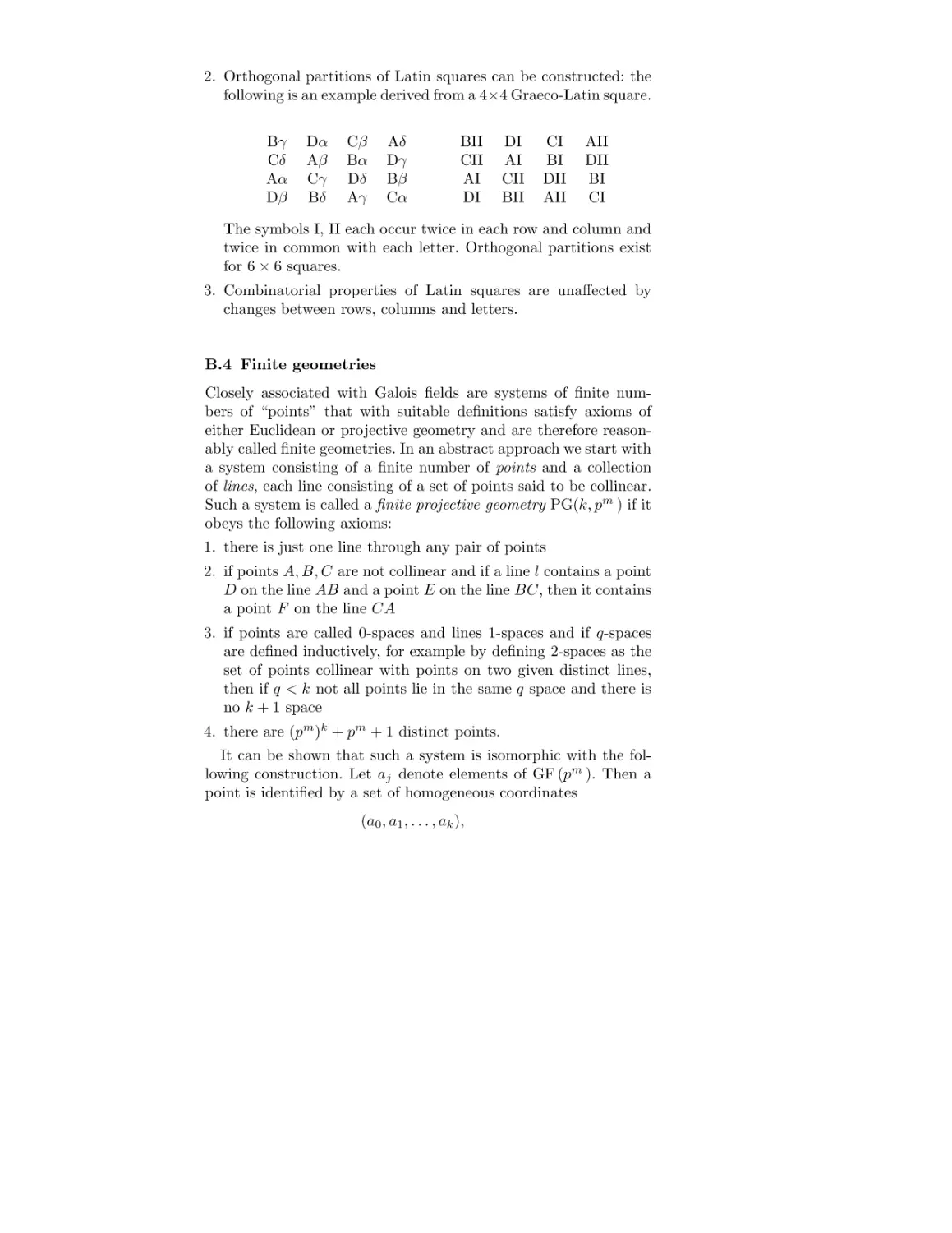
B.4 Finite geometries
B.5 Difference sets
B.6 Hadamard matrices
B.7 Orthogonal arrays
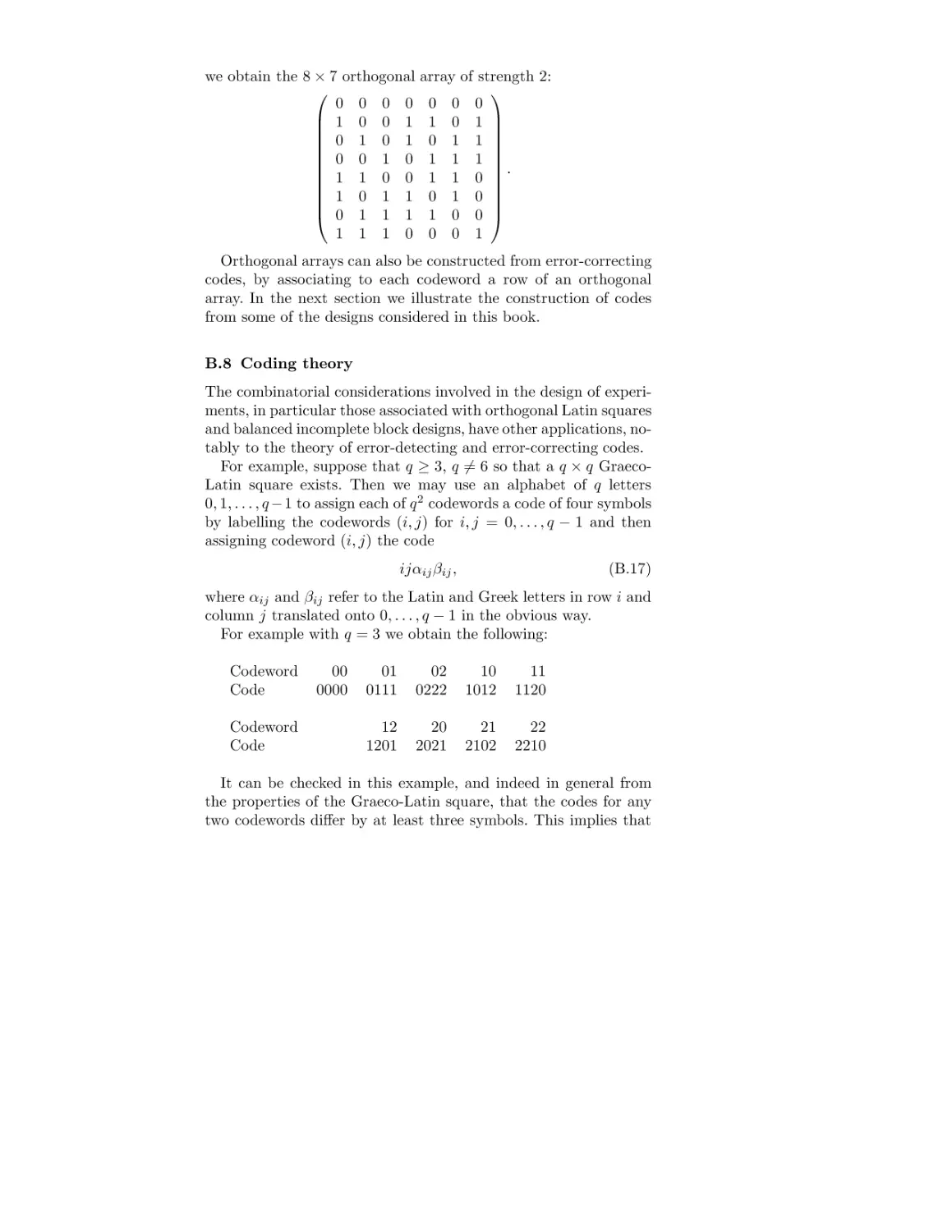
B.8 Coding theory
B.9 Bibliographic notes
B.10 Further results and exercises
C Computational issues
C.1 Introduction
C.2 Overview
C.3 Randomized block experiment from Chapter 3
C.4 Analysis of block designs in Chapter 4

© 2000 by Chapman & Hall/CRC

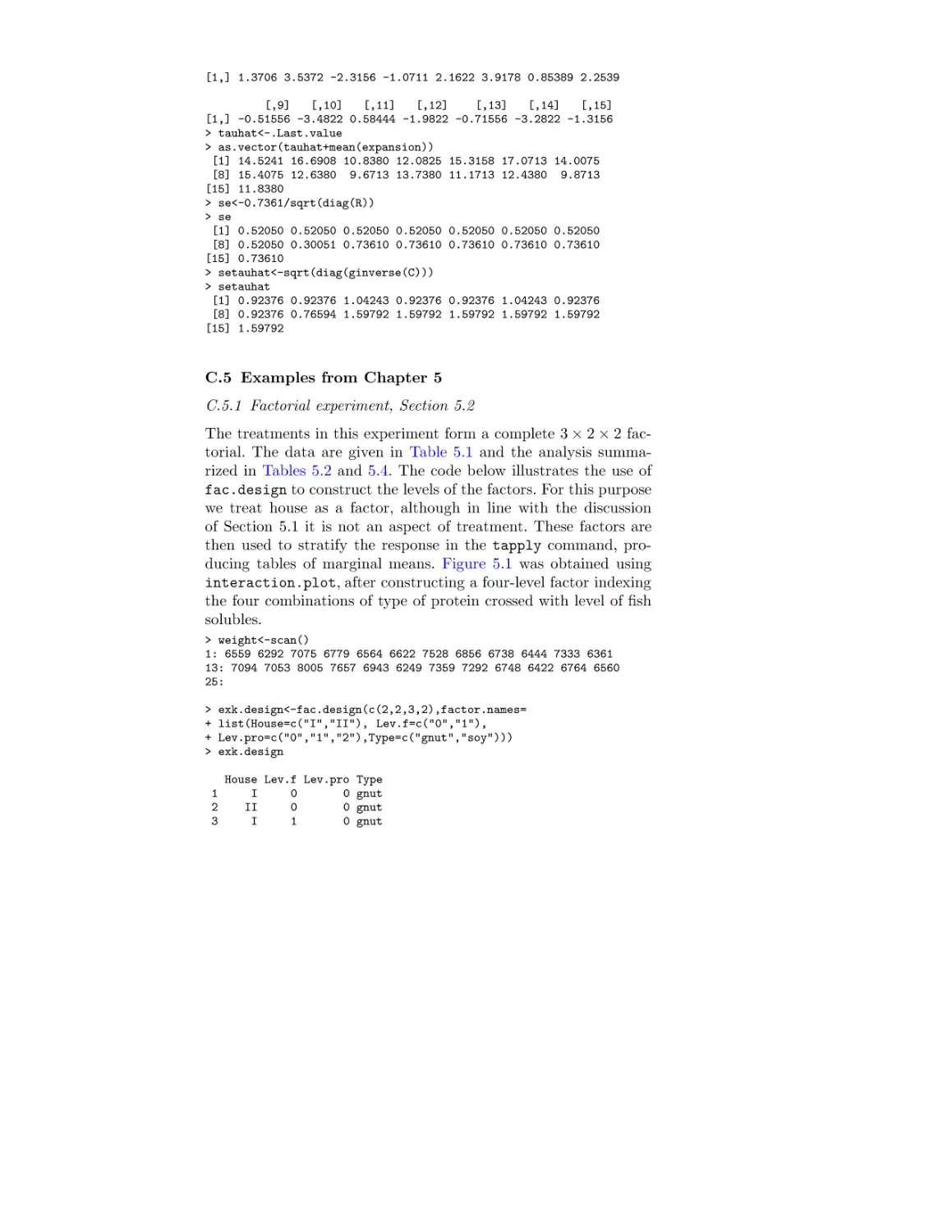
C.5 Examples from Chapter 5
C.6 Examples from Chapter 6
C.7 Bibliographic notes
References
List of tables

© 2000 by Chapman & Hall/CRC

Preface
This book is an account of the major topics in the design of
experiments, with particular emphasis on the key concepts involved
and on the statistical structure associated with these concepts.
While design of experiments is in many ways a very well developed
area of statistics, it often receives less emphasis than methods of
analysis in a programme of study in statistics.
We have written for a general audience concerned with statistics
in experimental fields and with some knowledge of and interest in
theoretical issues. The mathematical level is mostly elementary;
occasional passages using more advanced ideas can be skipped or
omitted without inhibiting understanding of later passages. Some
specialized parts of the subject have extensive and specialized literatures, a few examples being incomplete block designs, mixture
designs, designs for large variety trials, designs based on spatial
stochastic models and designs constructed from explicit optimality
requirements. We have aimed to give relatively brief introductions
to these subjects eschewing technical detail.
To motivate the discussion we give outline Illustrations taken
from a range of areas of application. In addition we give a limited
number of Examples, mostly taken from the literature, used for the
different purpose of showing detailed methods of analysis without
much emphasis on specific subject-matter interpretation.
We have written a book about design not about analysis, although, as has often been pointed out, the two phases are inexorably interrelated. Therefore it is, in particular, not a book on
the linear statistical model or that related but distinct art form
the analysis of variance table. Nevertheless these topics enter and
there is a dilemma in presentation. What do we assume the reader
knows about these matters? We have solved this problem uneasily
by somewhat downplaying analysis in the text, by assuming whatever is necessary for the section in question and by giving a review
as an Appendix. Anyone using the book as a basis for a course of
lectures will need to consider carefully what the prospective students are likely to understand about the linear model and to supplement the text appropriately. While the arrangement of chapters

© 2000 by Chapman & Hall/CRC

represents a logical progression of ideas, if interest is focused on a
particular field of application it will be reasonable to omit certain
parts or to take the material in a different order.
If defence of a book on the theory of the subject is needed it is
this. Successful application of these ideas hinges on adapting general principles to the special constraints of individual applications.
Thus experience suggests that while it is useful to know about special designs, balanced incomplete block designs for instance, it is
rather rare that they can be used directly. More commonly they
need some adaptation to accommodate special circumstances and
to do this effectively demands a solid theoretical base.
This book has been developed from lectures given at Cambridge,
Birkbeck College London, Vancouver, Toronto and Oxford. We are
grateful to Amy Berrington, Mario Cortina Borja, Christl Donnelly, Peter Kupchak, Rahul Mukerjee, John Nelder, Rob Tibshirani and especially Grace Yun Yi for helpful comments on a preliminary version.

D.R. Cox and N. Reid
Oxford and Toronto
January 2000

© 2000 by Chapman & Hall/CRC

List of tables

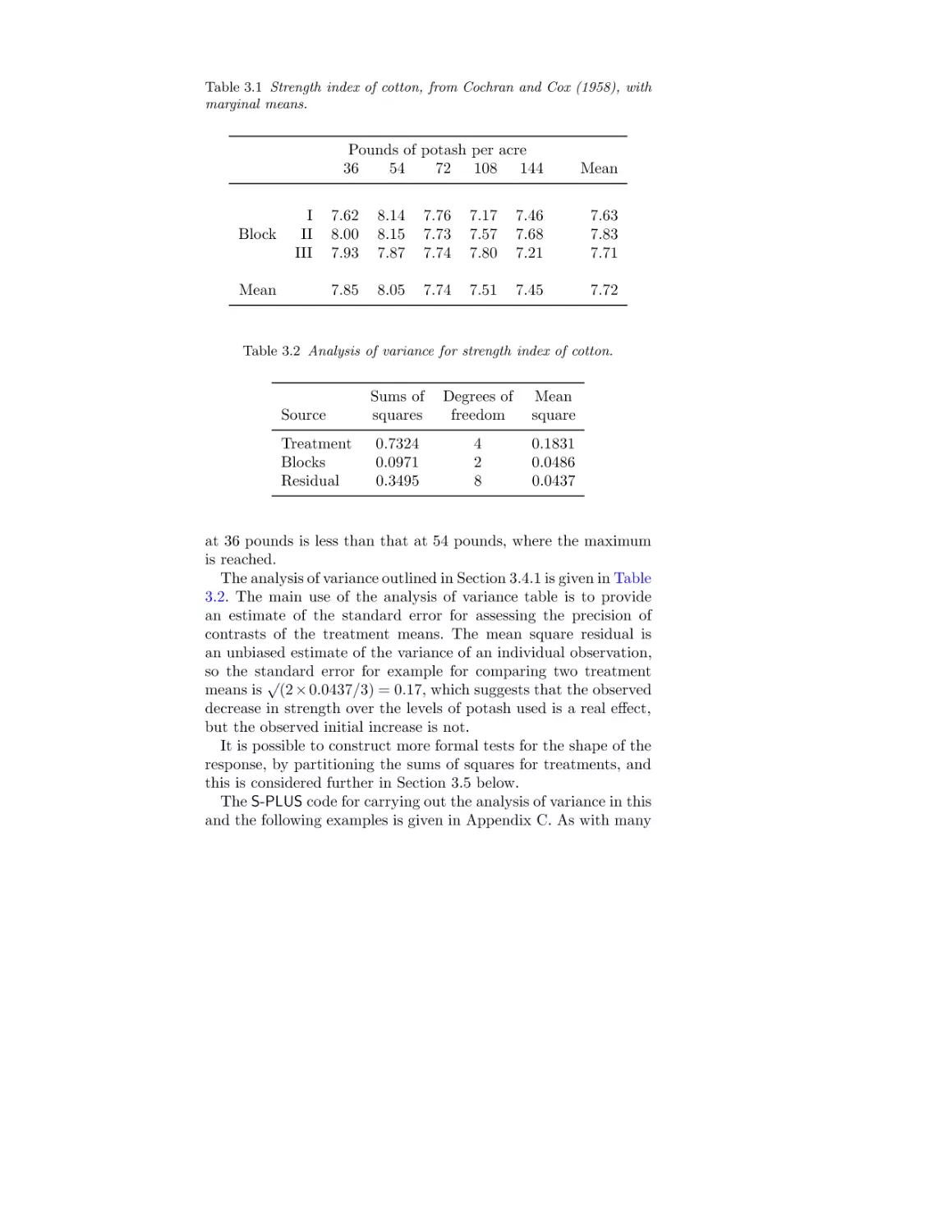
3.1
3.2

Strength index of cotton
Analysis of variance for strength index

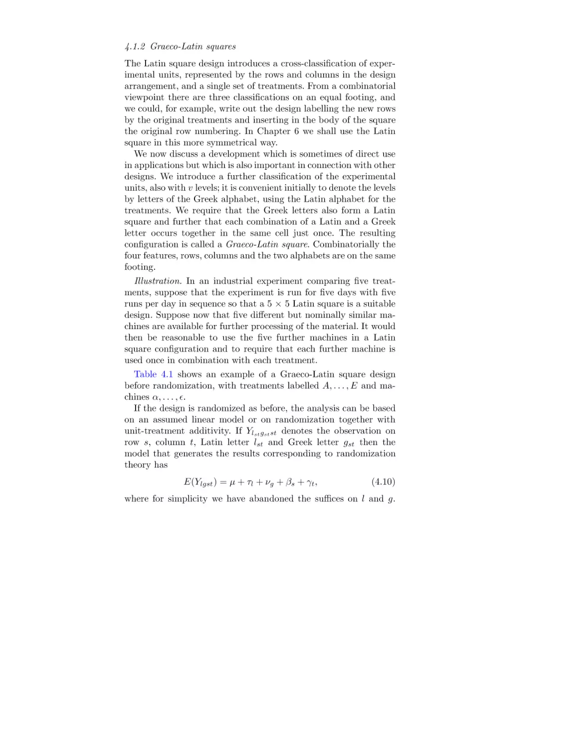
4.1
4.2
4.3
4.4
4.5
4.6
4.7
4.8
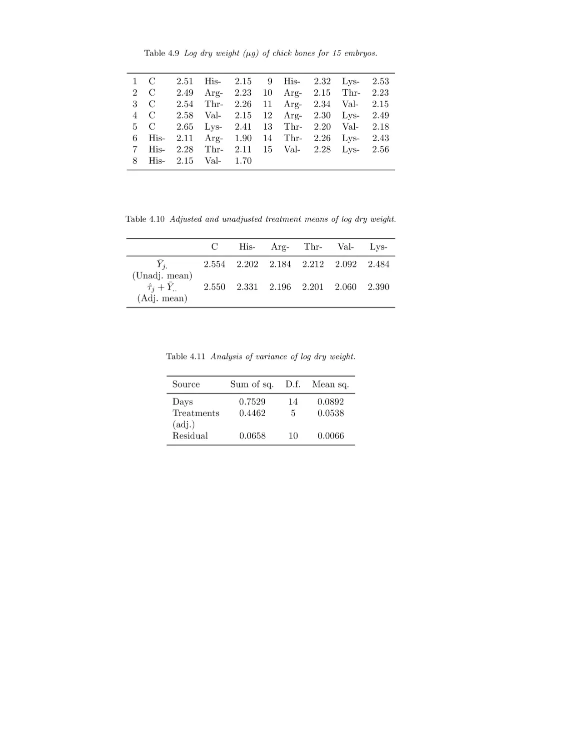
4.9
4.10
4.11
4.12
4.13
4.14
4.15

5 × 5 Graeco-Latin square
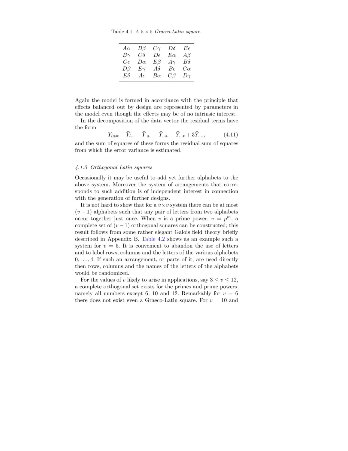
Complete orthogonal set of 5 × 5 Latin squares
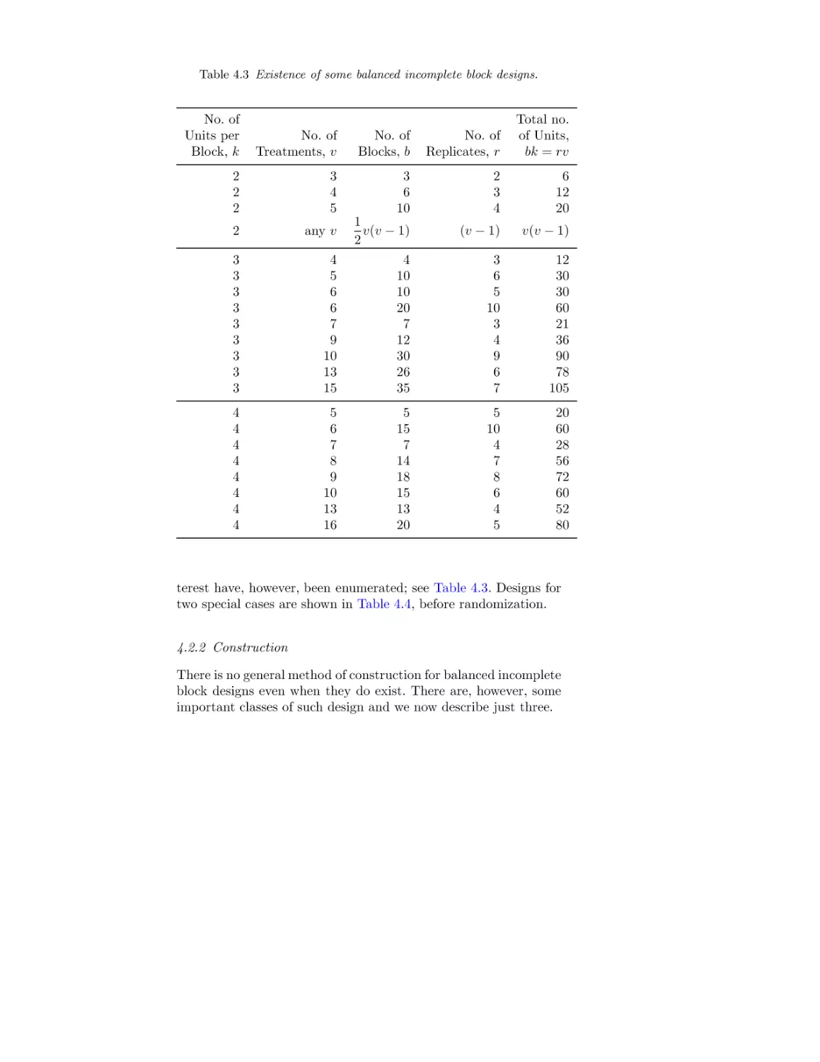
Balanced incomplete block designs
Two special incomplete block designs
Youden square
Intrablock analysis of variance
Interblock analysis of variance
Analysis of variance, general incomplete block
design
Log dry weight of chick bones
Treatment means, log dry weight
Analysis of variance, log dry weight
Estimates of treatment effects
Expansion index of pastry dough
Unadjusted and adjusted treatment means
Example of intrablock analysis

5.1
5.2
5.3
5.4
5.5
5.6
5.7
5.8
5.9
5.10
5.11
5.12

Weights of chicks
Mean weights of chicks
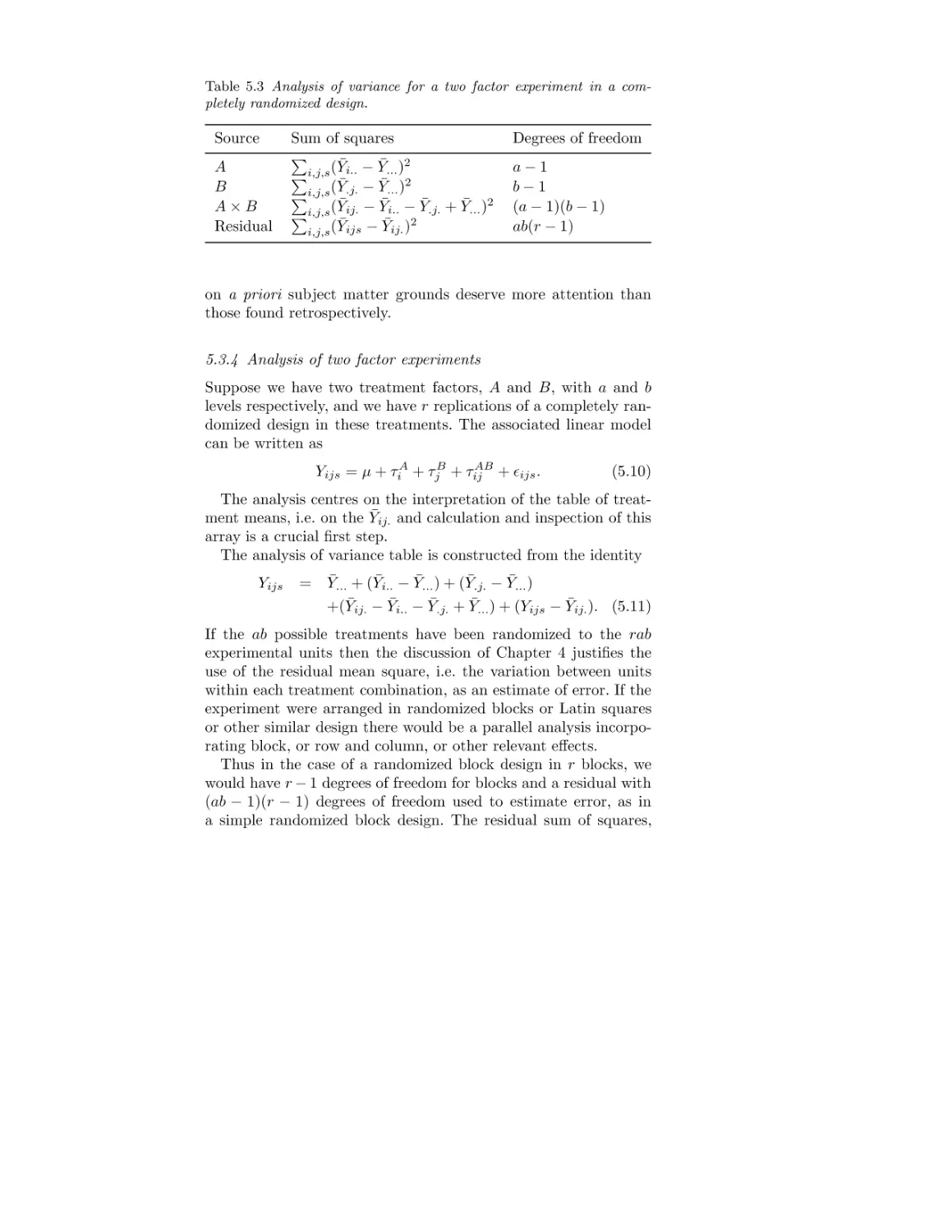
Two factor analysis of variance
Analysis of variance, weights of chicks
Decomposition of treatment sum of squares
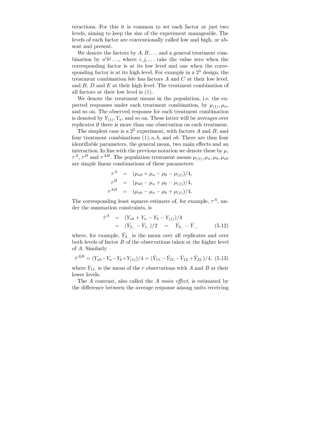
Analysis of variance, 22 factorial
Analysis of variance, 2k factorial
Treatment factors, nutrition and cancer
Data, nutrition and cancer
Estimated effects, nutrition and cancer
Data, Exercise 5.6
Contrasts, Exercise 5.6

© 2000 by Chapman & Hall/CRC

6.1
6.2
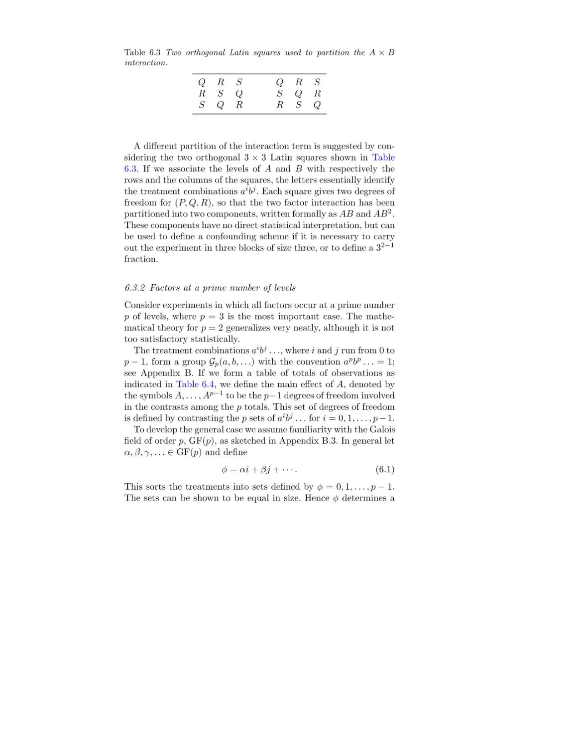
6.3
6.4
6.5
6.6
6.7
6.8
6.9
6.10
6.11
6.12
6.13
6.14
6.15
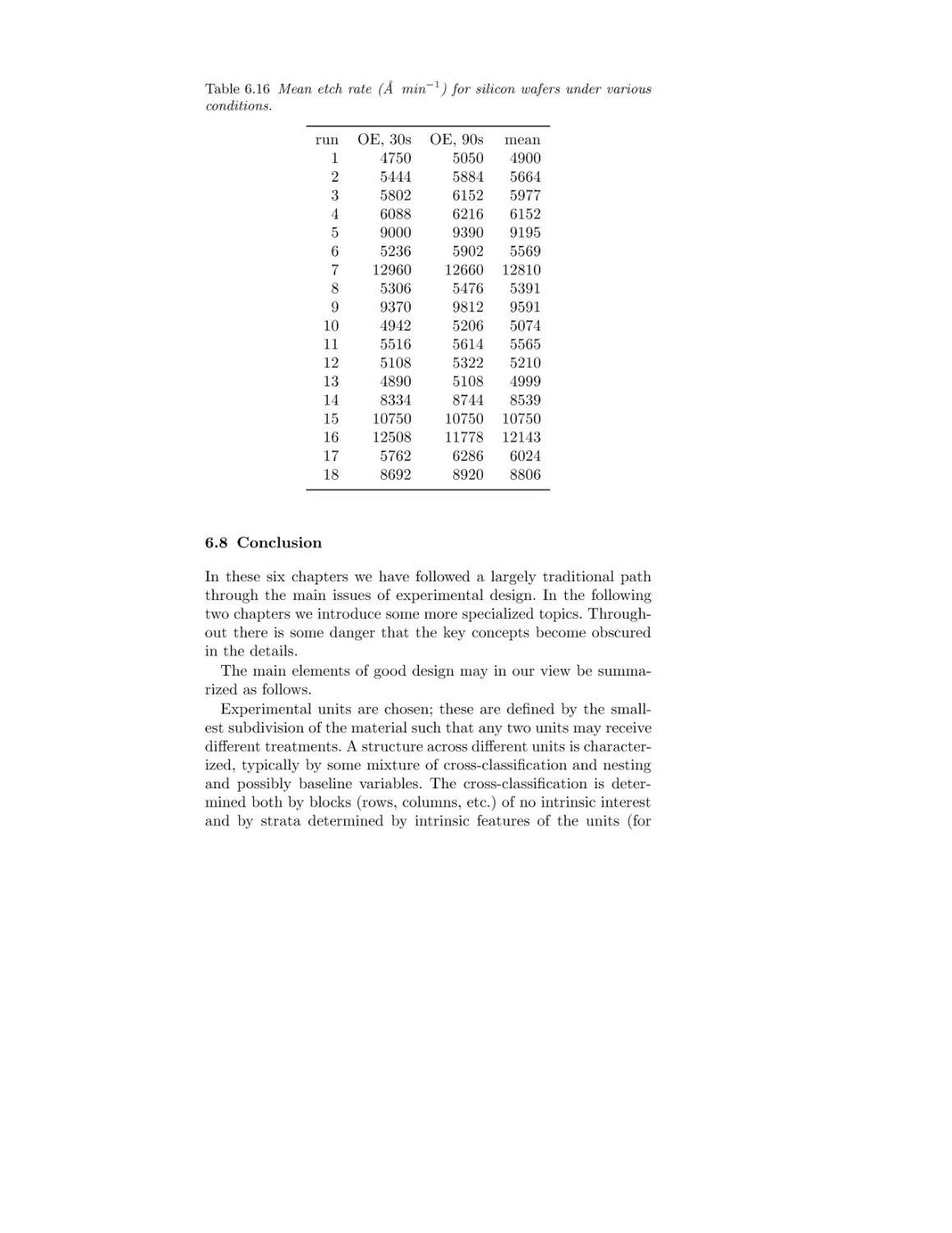
6.16
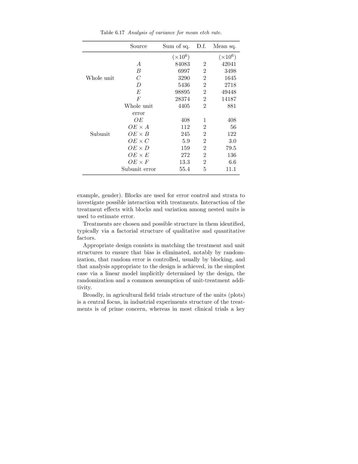
6.17
6.18

Example, double confounding
Degrees of freedom, double confounding
Two orthogonal Latin squares
Estimation of the main effect
1/3 fraction, degrees of freedom
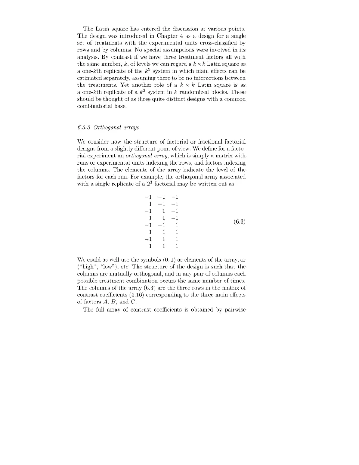
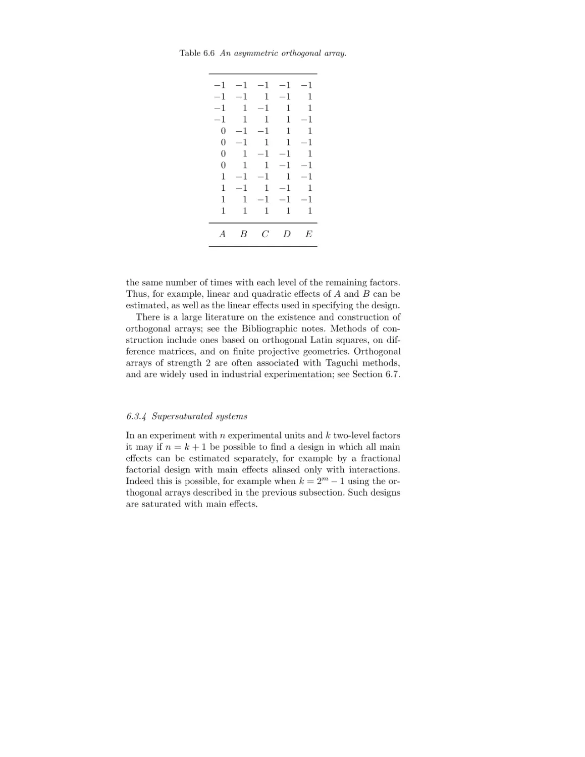
Asymmetric orthogonal array
Supersaturated design
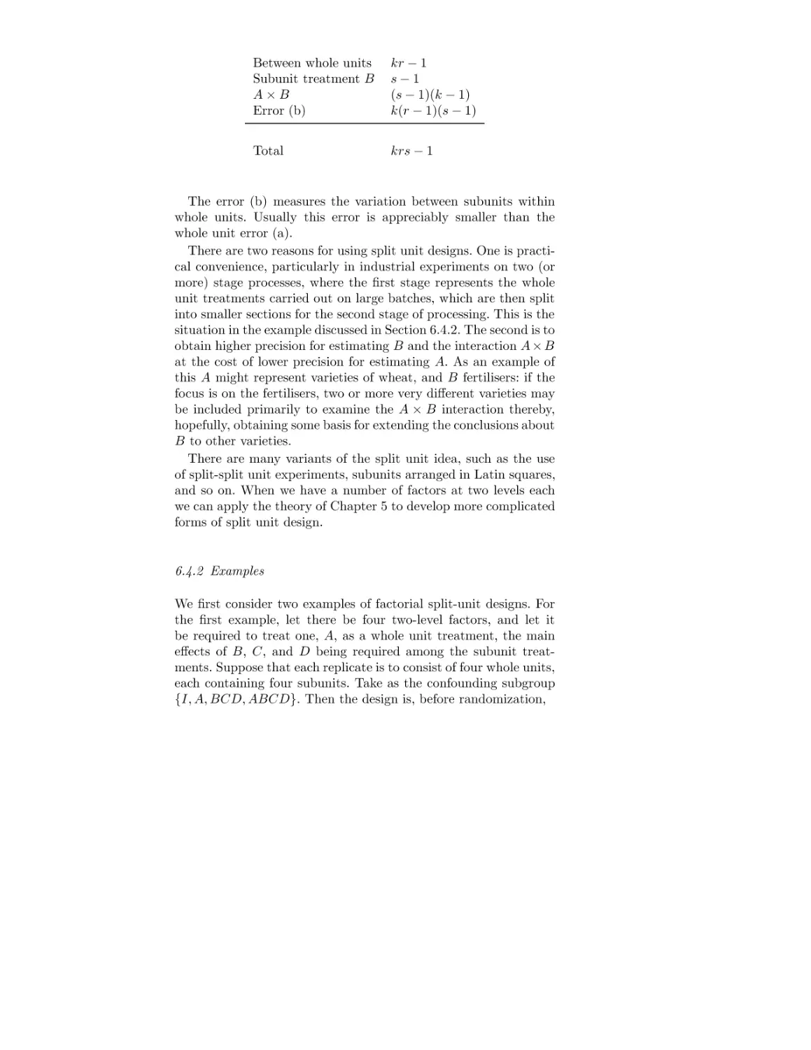
Example, split-plot analysis
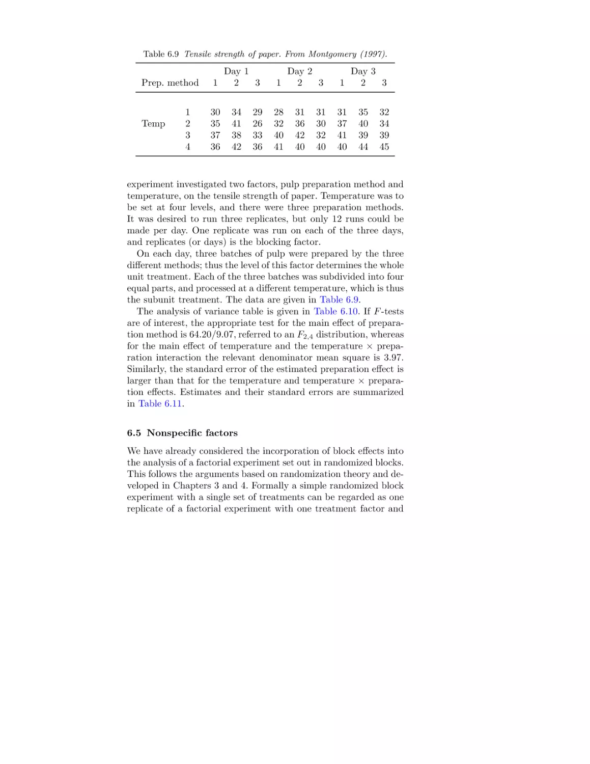
Data, tensile strength of paper
Analysis, tensile strength of paper
Table of means, tensile strength of paper
Analysis of variance for a replicated factorial
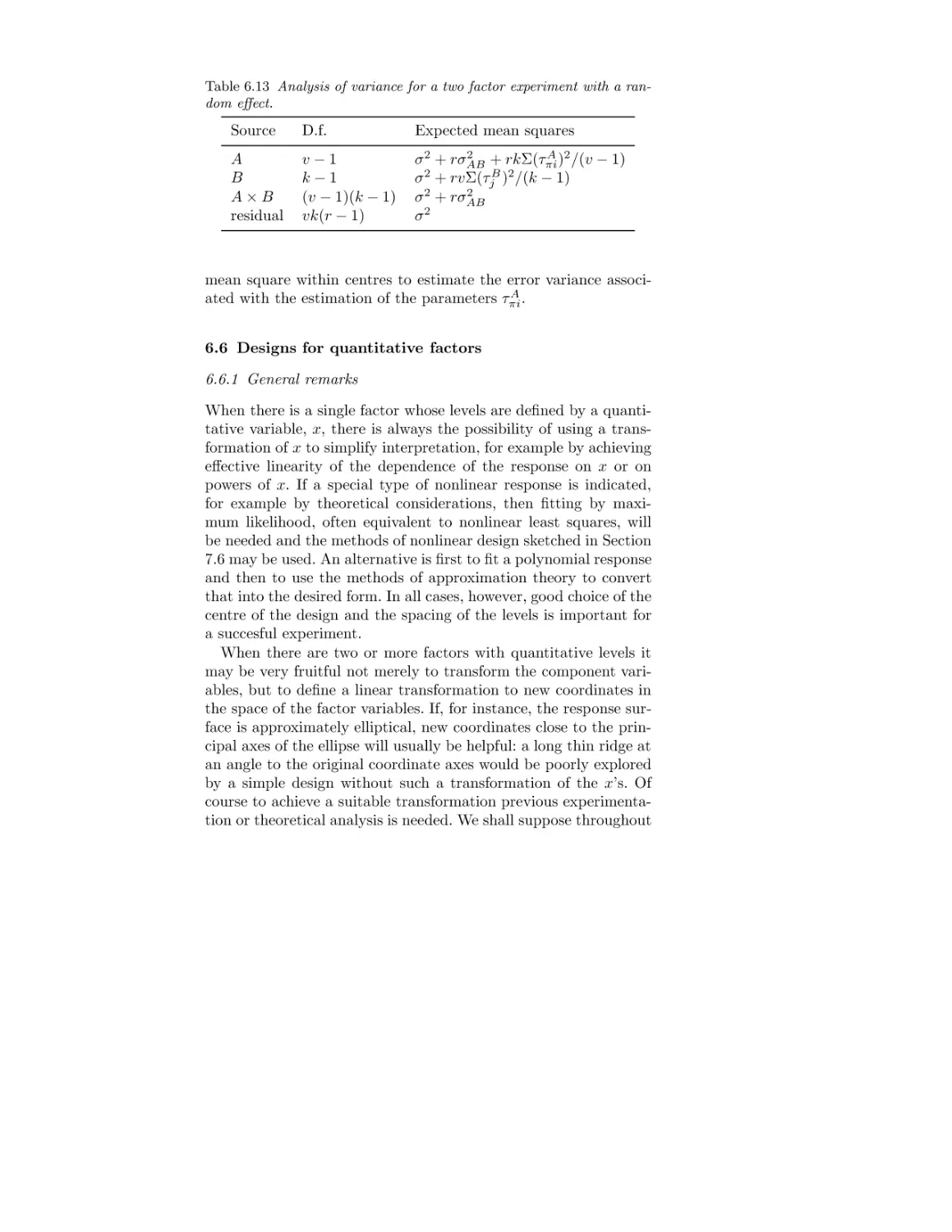
Analysis of variance with a random effect
Analysis of variance, quality/quantity interaction
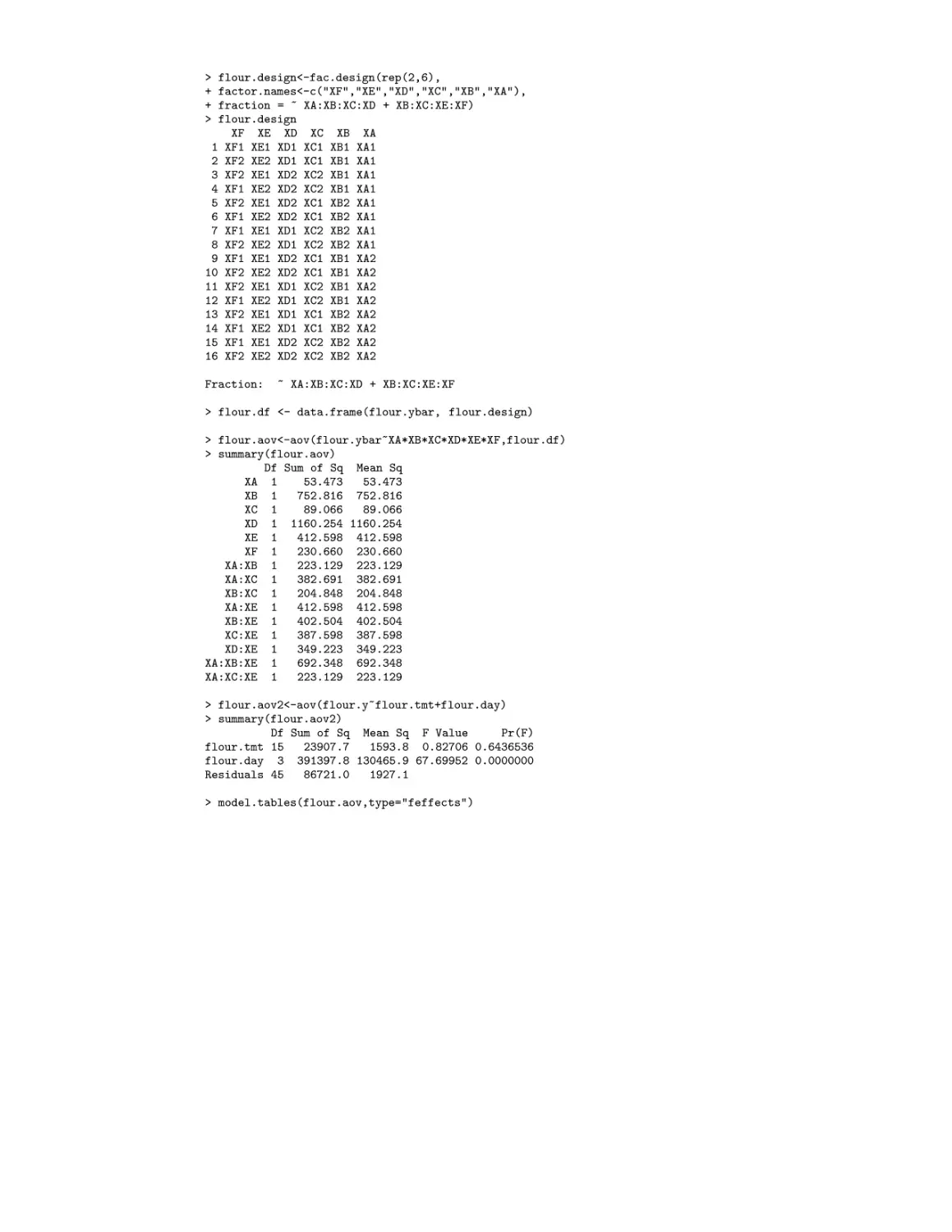
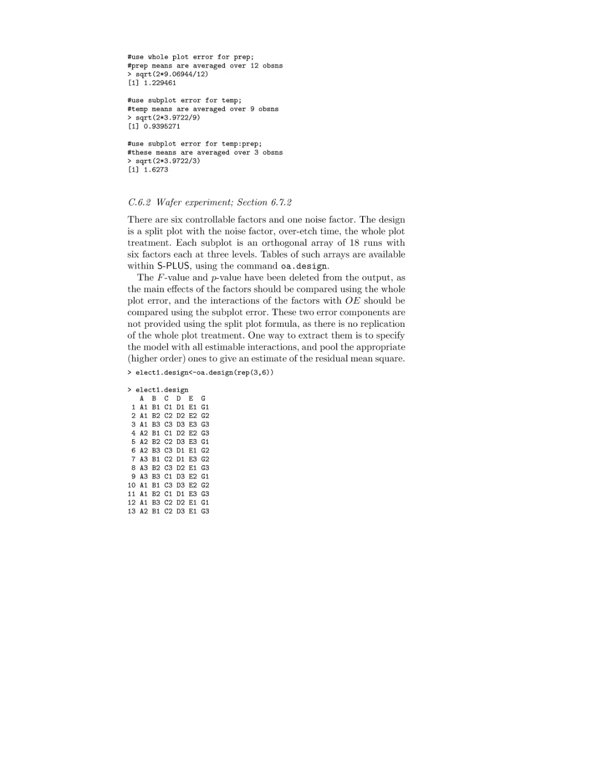
Design, electronics example
Data, electronics example
Analysis of variance, electronics example
Example, factorial treatment structure for incomplete block design

8.1
8.2
8.3

Treatment allocation: biased coin design
3 × 3 lattice squares for nine treatments
4 × 4 Latin square

A.1
A.2
A.3
A.4

Stagewise analysis of variance table
Analysis of variance, nested and crossed
Analysis of variance for Yabc;j
Analysis of variance for Y(a;j)bc

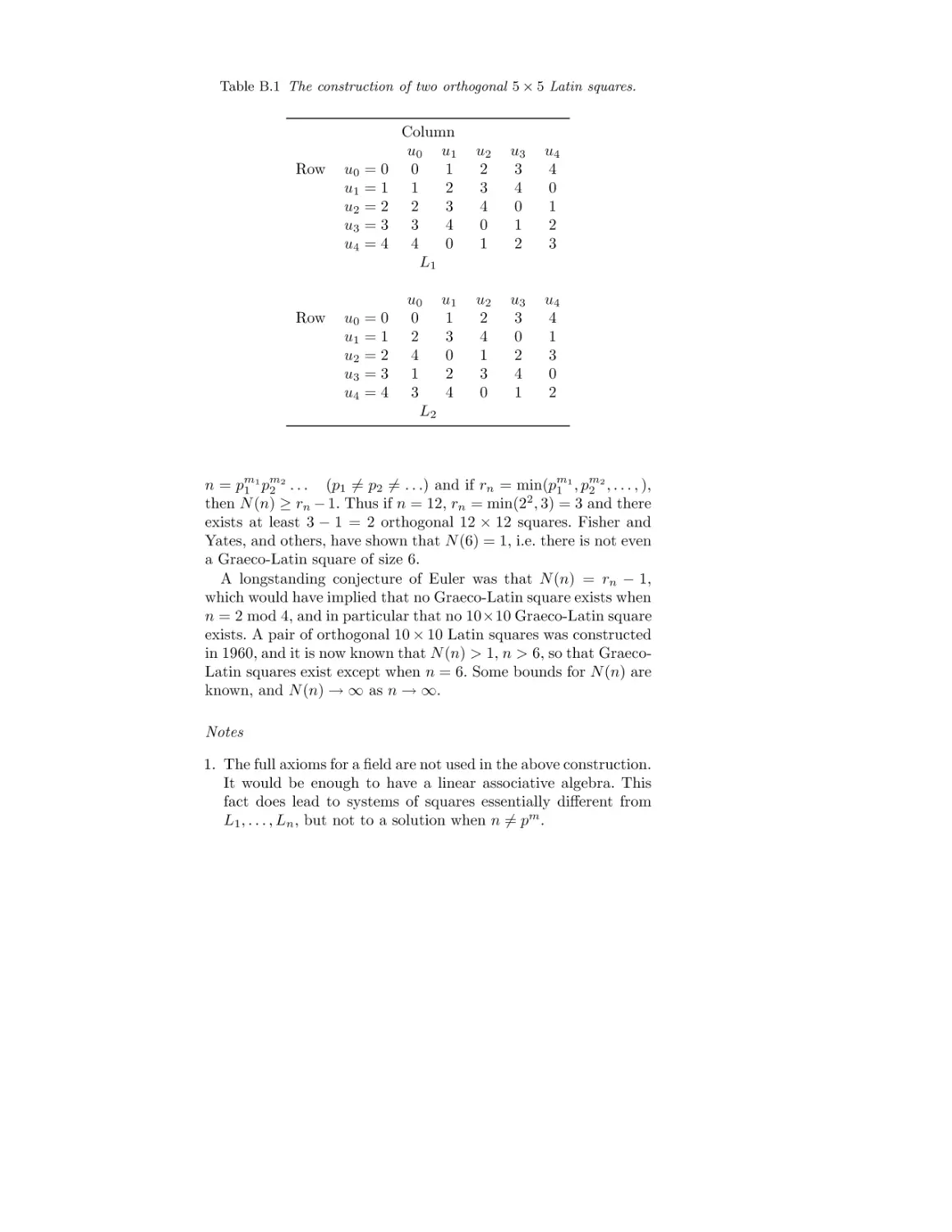
B.1 Construction of two orthogonal 5 × 5 Latin squares

© 2000 by Chapman & Hall/CRC

CHAPTER 1

Some general concepts
1.1 Types of investigation
This book is about the design of experiments. The word experiment
is used in a quite precise sense to mean an investigation where the
system under study is under the control of the investigator. This
means that the individuals or material investigated, the nature of
the treatments or manipulations under study and the measurement
procedures used are all settled, in their important features at least,
by the investigator.
By contrast in an observational study some of these features,
and in particular the allocation of individuals to treatment groups,
are outside the investigator’s control.
Illustration. In a randomized clinical trial patients meeting clearly
defined eligibility criteria and giving informed consent are assigned
by the investigator by an impersonal method to one of two or more
treatment arms, in the simplest case either to a new treatment, T ,
or to a standard treatment or control, C, which might be the best
current therapy or possibly a placebo treatment. The patients are
followed for a specified period and one or more measures of response recorded.
In a comparable observational study, data on the response variables might be recorded on two groups of patients, some of whom
had received T and some C; the data might, for example, be extracted from a database set up during the normal running of a
hospital clinic. In such a study, however, it would be unknown why
each particular patient had received the treatment he or she had.
The form of data might be similar or even almost identical in
the two contexts; the distinction lies in the firmness of the interpretation that can be given to the apparent differences in response
between the two groups of patients.
Illustration. In an agricultural field trial, an experimental field is
divided into plots of a size and shape determined by the investiga-

© 2000 by Chapman & Hall/CRC

tor, subject to technological constraints. To each plot is assigned
one of a number of fertiliser treatments, often combinations of various amounts of the basic constituents, and yield of product is
measured.
In a comparable observational study of fertiliser practice a survey
of farms or fields would give data on quantities of fertiliser used and
yield, but the issue of why each particular fertiliser combination
had been used in each case would be unclear and certainly not
under the investigator’s control.
A common feature of these and other similar studies is that
the objective is a comparison, of two medical treatments in the
first example, and of various fertiliser combinations in the second.
Many investigations in science and technology have this form. In
very broad terms, in technological experiments the treatments under comparison have a very direct interest, whereas in scientific
experiments the treatments serve to elucidate the nature of some
phenomenon of interest or to test some research hypothesis. We do
not, however, wish to emphasize distinctions between science and
technology.
We translate the objective into that of comparing the responses
among the different treatments. An experiment and an observational study may have identical objectives; the distinction between
them lies in the confidence to be put in the interpretation.
Investigations done wholly or primarily in the laboratory are
usually experimental. Studies of social science issues in the context in which they occur in the real world are usually inevitably
observational, although sometimes elements of an experimental approach may be possible. Industrial studies at pilot plant level will
typically be experimental whereas at a production level, while experimental approaches are of proved fruitfulness especially in the
process industries, practical constraints may force some deviation
from what is ideal for clarity of interpretation.
Illustration. In a survey of social attitudes a panel of individuals
might be interviewed say every year. This would be an observational study designed to study and if possible explain changes of
attitude over time. In such studies panel attrition, i.e. loss of respondents for one reason or another, is a major concern. One way
of reducing attrition may be to offer small monetary payments a
few days before the interview is due. An experiment on the effectiveness of this could take the form of randomizing individuals

© 2000 by Chapman & Hall/CRC

between one of two treatments, a monetary payment or no monetary payment. The response would be the successful completion or
not of an interview.
1.2 Observational studies
While in principle the distinction between experiments and observational studies is clear cut and we wish strongly to emphasize its
importance, nevertheless in practice the distinction can sometimes
become blurred. Therefore we comment briefly on various forms of
observational study and on their closeness to experiments.
It is helpful to distinguish between a prospective longitudinal
study (cohort study), a retrospective longitudinal study, a crosssectional study, and the secondary analysis of data collected for
some other, for example, administrative purpose.
In a prospective study observations are made on individuals at
entry into the study, the individuals are followed forward in time,
and possible response variables recorded for each individual. In a
retrospective study the response is recorded at entry and an attempt is made to look backwards in time for possible explanatory
features. In a cross-sectional study each individual is observed at
just one time point. In all these studies the investigator may have
substantial control not only over which individuals are included
but also over the measuring processes used. In a secondary analysis the investigator has control only over the inclusion or exclusion
of the individuals for analysis.
In a general way the four possibilities are in decreasing order of
effectiveness, the prospective study being closest to an experiment;
they are also in decreasing order of cost.
Thus retrospective studies are subject to biases of recall but may
often yield results much more quickly than corresponding prospective studies. In principle at least, observations taken at just one
time point are likely to be less enlightening than those taken over
time. Finally secondary analysis, especially of some of the large
databases now becoming so common, may appear attractive. The
quality of such data may, however, be low and there may be major
difficulties in disentangling effects of different explanatory features,
so that often such analyses are best regarded primarily as ways of
generating ideas for more detailed study later.
In epidemiological applications, a retrospective study is often
designed as a case-control study, whereby groups of patients with

© 2000 by Chapman & Hall/CRC

a disease or condition (cases), are compared to a hopefully similar
group of disease-free patients on their exposure to one or more risk
factors.
1.3 Some key terms
We shall return later to a more detailed description of the types
of experiment to be considered but for the moment it is enough to
consider three important elements to an experiment, namely the
experimental units, the treatments and the response. A schematic
version of an experiment is that there are a number of different
treatments under study, the investigator assigns one treatment to
each experimental unit and observes the resulting response.
Experimental units are essentially the patients, plots, animals,
raw material, etc. of the investigation. More formally they correspond to the smallest subdivision of the experimental material
such that any two different experimental units might receive different treatments.
Illustration. In some experiments in opthalmology it might be
sensible to apply different treatments to the left and to the right
eye of each patient. Then an experimental unit would be an eye,
that is each patient would contribute two experimental units.
The treatments are clearly defined procedures one of which is to
be applied to each experimental unit. In some cases the treatments
are an unstructured set of two or more qualitatively different procedures. In others, including many investigations in the physical
sciences, the treatments are defined by the levels of one or more
quantitative variables, such as the amounts per square metre of the
constituents nitrogen, potash and potassium, in the illustration in
Section 1.1.
The response measurement specifies the criterion in terms of
which the comparison of treatments is to be effected. In many
applications there will be several such measures.
This simple formulation can be amplified in various ways. The
same physical material can be used as an experimental unit more
than once. If the treatment structure is complicated the experimental unit may be different for different components of treatment.
The response measured may be supplemented by measurements on
other properties, called baseline variables, made before allocation

© 2000 by Chapman & Hall/CRC

to treatment, and on intermediate variables between the baseline
variables and the ultimate response.
Illustrations. In clinical trials there will typically be available numerous baseline variables such as age at entry, gender, and specific
properties relevant to the disease, such as blood pressure, etc., all
to be measured before assignment to treatment. If the key response
is time to death, or more generally time to some critical event in the
progression of the disease, intermediate variables might be properties measured during the study which monitor or explain the
progression to the final response.
In an agricultural field trial possible baseline variables are chemical analyses of the soil in each plot and the yield on the plot in
the previous growing season, although, so far as we are aware, the
effectiveness of such variables as an aid to experimentation is limited. Possible intermediate variables are plant density, the number
of plants per square metre, and assessments of growth at various
intermediate points in the growing season. These would be included
to attempt explanation of the reasons for the effect of fertiliser on
yield of final product.
1.4 Requirements in design
The objective in the type of experiment studied here is the comparison of the effect of treatments on response. This will typically
be assessed by estimates and confidence limits for the magnitude
of treatment differences. Requirements on such estimates are essentially as follows. First systematic errors, or biases, are to be
avoided. Next the effect of random errors should so far as feasible be minimized. Further it should be possible to make reasonable assessment of the magnitude of random errors, typically via
confidence limits for the comparisons of interest. The scale of the
investigation should be such as to achieve a useful but not unnecessarily high level of precision. Finally advantage should be taken
of any special structure in the treatments, for example when these
are specified by combinations of factors.
The relative importance of these aspects is different in different fields of study. For example in large clinical trials to assess
relatively small differences in treatment efficacy, avoidance of systematic error is a primary issue. In agricultural field trials, and
probably more generally in studies that do not involve human sub-

© 2000 by Chapman & Hall/CRC

jects, avoidance of bias, while still important, is not usually the
aspect of main concern.
These objectives have to be secured subject to the practical constraints of the situation under study. The designs and considerations developed in this book have often to be adapted or modified
to meet such constraints.
1.5 Interplay between design and analysis
There is a close connection between design and analysis in that an
objective of design is to make both analysis and interpretation as
simple and clear as possible. Equally, while some defects in design
may be corrected by more elaborate analysis, there is nearly always
some loss of security in the interpretation, i.e. in the underlying
subject-matter meaning of the outcomes.
The choice of detailed model for analysis and interpretation will
often involve subject-matter considerations that cannot readily be
discussed in a general book such as this. Partly but not entirely
for this reason we concentrate here on the analysis of continuously
distributed responses via models that are usually linear, leading to
analyses quite closely connected with the least-squares analysis of
the normal theory linear model. One intention is to show that such
default analyses follow from a single set of assumptions common to
the majority of the designs we shall consider. In this rather special
sense, the model for analysis is determined by the design employed.
Of course we do not preclude the incorporation of special subjectmatter knowledge and models where appropriate and indeed this
may be essential for interpretation.
There is a wider issue involved especially when a number of different response variables are measured and underlying interpretation is the objective rather than the direct estimation of treatment
differences. It is sensible to try to imagine the main patterns of
response that are likely to arise and to consider whether the information will have been collected to allow the interpretation of these.
This is a broader issue than that of reviewing the main scheme of
analysis to be used. Such consideration must always be desirable;
it is, however, considerably less than a prior commitment to a very
detailed approach to analysis.
Two terms quite widely used in discussions of the design of experiments are balance and orthogonality. Their definition depends a
bit on context but broadly balance refers to some strong symmetry

© 2000 by Chapman & Hall/CRC

in the combinatorial structure of the design, whereas orthogonality refers to special simplifications of analysis and achievement of
efficiency consequent on such balance.
For example, in Chapter 3 we deal with designs for a number of
treatments in which the experimental units are arranged in blocks.
The design is balanced if each treatment occurs in each block the
same number of times, typically once. If a treatment occurs once
in some blocks and twice or not at all in others the design is considered unbalanced. On the other hand, in the context of balanced
incomplete block designs studied in Section 4.2 the word balance
refers to an extended form of symmetry.
In analyses involving a linear model, and most of our discussion
centres on these, two types of effect are orthogonal if the relevant
columns of the matrix defining the linear model are orthogonal in
the usual algebraic sense. One consequence is that the least squares
estimates of one of the effects are unchanged if the other type of
effect is omitted from the model. For orthogonality some kinds of
balance are sufficient but not necessary. In general statistical theory
there is an extended notion of orthogonality based on the Fisher
information matrix and this is relevant when maximum likelihood
analysis of more complicated models is considered.
1.6 Key steps in design
1.6.1 General remarks
Clearly the single most important aspect of design is a purely substantive, i.e. subject-matter, one. The issues addressed should be
interesting and fruitful. Usually this means examining one or more
well formulated questions or research hypotheses, for example a
speculation about the process underlying some phenomenon, or
the clarification and explanation of earlier findings. Some investigations may have a less focused objective. For example, the initial
phases of a study of an industrial process under production conditions may have the objective of identifying which few of a large
number of potential influences are most important. The methods
of Section 5.6 are aimed at such situations, although they are probably atypical and in most cases the more specific the research question the better.
In principle therefore the general objectives lead to the following
more specific issues. First the experimental units must be defined

© 2000 by Chapman & Hall/CRC

and chosen. Then the treatments must be clearly defined. The variables to be measured on each unit must be specified and finally the
size of the experiment, in particular the number of experimental
units, has to be decided.
1.6.2 Experimental units
Issues concerning experimental units are to some extent very specific to each field of application. Some points that arise fairly generally and which influence the discussion in this book include the
following.
Sometimes, especially in experiments with a technological focus,
it is useful to consider the population of ultimate interest and the
population of accessible individuals and to aim at conclusions that
will bridge the inevitable gap between these. This is linked to the
question of whether units should be chosen to be as uniform as
possible or to span a range of circumstances. Where the latter is
sensible it will be important to impose a clear structure on the
experimental units; this is connected with the issue of the choice
of baseline measurements.
Illustration. In agricultural experimentation with an immediate
objective of making recommendations to farmers it will be important to experiment in a range of soil and weather conditions; a
very precise conclusion in one set of conditions may be of limited
value. Interpretation will be much simplified if the same basic design is used at each site. There are somewhat similar considerations
in some clinical trials, pointing to the desirability of multi-centre
trials even if a trial in one centre would in principle be possible.
By contrast in experiments aimed at elucidating the nature of
certain processes or mechanisms it will usually be best to choose
units likely to show the effect in question in as striking a form as
possible and to aim for a high degree of uniformity across units.
In some contexts the same individual animal, person or material
may be used several times as an experimental unit; for example
in a psychological experiment it would be common to expose the
same subject to various conditions (treatments) in one session.
It is important in much of the following discussion and in applications to distinguish between experimental units and observations. The key notion is that different experimental units must in
principle be capable of receiving different treatments.

© 2000 by Chapman & Hall/CRC

Illustration. In an industrial experiment on a batch process each
separate batch of material might form an experimental unit to be
processed in a uniform way, separate batches being processed possibly differently. On the product of each batch many samples may
be taken to measure, say purity of the product. The number of
observations of purity would then be many times the number of
experimental units. Variation between repeat observations within
a batch measures sampling variability and internal variability of
the process. Precision of the comparison of treatments is, however, largely determined by, and must be estimated from, variation
between batches receiving the same treatment. In our theoretical
treatment that follows the number of batches is thus the relevant
total “sample” size.

1.6.3 Treatments
The simplest form of experiment compares a new treatment or
manipulation, T , with a control, C. Even here care is needed in
applications. In principle T has to be specified with considerable
precision, including many details of its mode of implementation.
The choice of control, C, may also be critical. In some contexts
several different control treatments may be desirable. Ideally the
control should be such as to isolate precisely that aspect of T which
it is the objective to examine.
Illustration. In a clinical trial to assess a new drug, the choice of
control may depend heavily on the context. Possible choices of control might be no treatment, a placebo treatment, i.e. a substance
superficially indistinguishable from T but known to be pharmacologically inactive, or the best currently available therapy. The
choice between placebo and best available treatment may in some
clinical trials involve difficult ethical decisions.
In more complex situations there may be a collection of qualitatively different treatments T1 , . . . , Tv . More commonly the treatments may have factorial structure, i.e. be formed from combinations of levels of subtreatments, called factors. We defer detailed
study of the different kinds of factor and the design of factorial
experiments until Chapter 5, noting that sensible use of the principle of examining several factors together in one study is one of
the most powerful ideas in this subject.

© 2000 by Chapman & Hall/CRC

1.6.4 Measurements
The choice of appropriate variables for measurement is a key aspect
of design in the broad sense. The nature of measurement processes
and their associated potentiality for error, and the different kinds
of variable that can be measured and their purposes are central issues. Nevertheless these issues fall outside the scope of the present
book and we merely note three broad types of variable, namely
baseline variables describing the experimental units before application of treatments, intermediate variables and response variables,
in a medical context often called end-points.
Intermediate variables may serve different roles. Usually the more
important is to provide some provisional explanation of the process
that leads from treatment to response. Other roles are to check on
the absence of untoward interventions and, sometimes, to serve as
surrogate response variables when the primary response takes a
long time to obtain.
Sometimes the response on an experimental unit is in effect a
time trace, for example of the concentrations of one or more substances as transient functions of time after some intervention. For
our purposes we suppose such responses replaced by one or more
summary measures, such as the peak response or the area under
the response-time curve.
Clear decisions about the variables to be measured, especially
the response variables, are crucial.
1.6.5 Size of experiment
Some consideration virtually always has to be given to the number of experimental units to be used and, where subsampling of
units is employed, to the number of repeat observations per unit.
A balance has to be struck between the marginal cost per experimental unit and the increase in precision achieved per additional
unit. Except in rare instances where these costs can both be quantified, a decision on the size of experiment is bound be largely a
matter of judgement and some of the more formal approaches to
determining the size of the experiment have spurious precision. It
is, however, very desirable to make an advance approximate calculation of the precision likely to be achieved. This gives some
protection against wasting resources on unnecessary precision or,
more commonly, against undertaking investigations which will be

© 2000 by Chapman & Hall/CRC

of such low precision that useful conclusions are very unlikely. The
same calculations are advisable when, as is quite common in some
fields, the maximum size of the experiment is set by constraints
outside the control of the investigator. The issue is then most commonly to decide whether the resources are sufficient to yield enough
precision to justify proceeding at all.
1.7 A simplified model
The formulation of experimental design that will largely be used
in this book is as follows. There are given n experimental units,
U1 , . . . , Un and v treatments, T1 , . . . , Tv ; one treatment is applied
to each unit as specified by the investigator, and one response
Y measured on each unit. The objective is to specify procedures
for allocating treatments to units and for the estimation of the
differences between treatments in their effect on response.
This is a very limited version of the broader view of design
sketched above. The justification for it is that many of the valuable
specific designs are accommodated in this framework, whereas the
wider considerations sketched above are often so subject-specific
that it is difficult to give a general theoretical discussion.
It is, however, very important to recall throughout that the path
between the choice of a unit and the measurement of final response
may be a long one in time and in other respects and that random
and systematic error may arise at many points. Controlling for
random error and aiming to eliminate systematic error is thus not
a single step matter as might appear in our idealized model.
1.8 A broader view
The discussion above and in the remainder of the book concentrates
on the integrity of individual experiments. Yet investigations are
rarely if ever conducted in isolation; one investigation almost inevitably suggests further issues for study and there is commonly
the need to establish links with work related to the current problems, even if only rather distantly. These are important matters but
again are difficult to incorporate into formal theoretical discussion.
If a given collection of investigations estimate formally the same
contrasts, the statistical techniques for examining mutual consistency of the different estimates and, subject to such consistency,
of combining the information are straightforward. Difficulties come

© 2000 by Chapman & Hall/CRC

more from the choice of investigations for inclusion, issues of genuine comparability and of the resolution of apparent inconsistencies.
While we take the usual objective of the investigation to be the
comparison of responses from different treatments, sometimes there
is a more specific objective which has an impact on the design to
be employed.
Illustrations. In some kinds of investigation in the chemical process industries, the treatments correspond to differing concentrations of various reactants and to variables such as pressure, temperature, etc. For some purposes it may be fruitful to regard the objective as the determination of conditions that will optimize some
criterion such as yield of product or yield of product per unit cost.
Such an explicitly formulated purpose, if adopted as the sole objective, will change the approach to design.
In selection programmes for, say, varieties of wheat, the investigation may start with a very large number of varieties, possibly
several hundred, for comparison. A certain fraction of these are chosen for further study and in a third phase a small number of varieties are subject to intensive study. The initial stage has inevitably
very low precision for individual comparisons and analysis of the
design strategy to be followed best concentrates on such issues as
the proportion of varieties to be chosen at each phase, the relative
effort to be devoted to each phase and in general on the properties
of the whole process and the properties of the varieties ultimately
selected rather than on the estimation of individual differences.
In the pharmaceutical industry clinical trials are commonly defined as Phase I, II or III, each of which has quite well-defined
objectives. Phase I trials aim to establish relevant dose levels and
toxicities, Phase II trials focus on a narrowly selected group of patients expected to show the most dramatic response, and Phase III
trials are a full investigation of the treatment effects on patients
broadly representative of the clinical population.
In investigations with some technological relevance, even if there
is not an immediate focus on a decision to be made, questions will
arise as to the practical implications of the conclusions. Is a difference established big enough to be of public health relevance in an
epidemiological context, of relevance to farmers in an agricultural
context or of engineering relevance in an industrial context? Do the
conditions of the investigation justify extrapolation to the work-

© 2000 by Chapman & Hall/CRC

ing context? To some extent such questions can be anticipated by
appropriate design.
In both scientific and technological studies estimation of effects
is likely to lead on to the further crucial question: what is the underlying process explaining what has been observed? Sometimes
this is expressed via a search for causality. So far as possible these
questions should be anticipated in design, especially in the definition of treatments and observations, but it is relatively rare for such
explanations to be other than tentative and indeed they typically
raise fresh issues for investigation.
It is sometimes argued that quite firm conclusions about causality are justified from experiments in which treatment allocation is
made by objective randomization but not otherwise, it being particularly hazardous to draw causal conclusions from observational
studies.
These issues are somewhat outside the scope of the present book
but will be touched on in Section 2.5 after the discussion of the
role of randomization. In the meantime some of the potential implications for design can be seen from the following Illustration.
Illustration. In an agricultural field trial a number of treatments
are randomly assigned to plots, the response variable being the
yield of product. One treatment, S, say, produces a spectacular
growth of product, much higher than that from other treatments.
The growth attracts birds from many kilometres around, the birds
eat most of the product and as a result the final yield for S is very
low. Has S caused a depression in yield?
The point of this illustration, which can be paralleled from other
areas of application, is that the yield on the plots receiving S is indeed lower than the yield would have been on those plots had they
been allocated to other treatments. In that sense, which meets one
of the standard definitions of causality, allocation to S has thus
caused a lowered yield. Yet in terms of understanding, and indeed
practical application, that conclusion on its own is quite misleading. To understand the process leading to the final responses it is
essential to observe and take account of the unanticipated intervention, the birds, which was supplementary to and dependent on the
primary treatments. Preferably also intermediate variables should
be recorded, for example, number of plants per square metre and
measures of growth at various time points in the growing cycle.
These will enable at least a tentative account to be developed of

© 2000 by Chapman & Hall/CRC

the process leading to the treatment differences in final yield which
are the ultimate objective of study. In this way not only are treatment differences estimated but some partial understanding is built
of the interpretation of such differences. This is a potentially causal
explanation at a deeper level.
Such considerations may arise especially in situations in which
a fairly long process intervenes between treatment allocation and
the measurement of response.
These issues are quite pressing in some kinds of clinical trial,
especially those in which patients are to be followed for an appreciable time. In the simplest case of randomization between two
treatments, T and C, there is the possibility that some patients,
called noncompliers, do not follow the regime to which they have
been allocated. Even those who do comply may take supplementary
medication and the tendency to do this may well be different in
the two treatment groups. One approach to analysis, the so-called
intention-to-treat principle, can be summarized in the slogan “ever
randomized always analysed”: one simply compares outcomes in
the two treatment arms regardless of compliance or noncompliance. The argument, parallel to the argument in the agricultural
example, is that if, say, patients receiving T do well, even if few of
them comply with the treatment regimen, then the consequences of
allocation to T are indeed beneficial, even if not necessarily because
of the direct consequences of the treatment regimen.
Unless noncompliance is severe, the intention-to-treat analysis
will be one important analysis but a further analysis taking account
of any appreciable noncompliance seems very desirable. Such an
analysis will, however, have some of the features of an observational
study and the relatively clearcut conclusions of the analysis of a
fully compliant study will be lost to some extent at least.
1.9 Bibliographic notes
While many of the ideas of experimental design have a long history,
the first major systematic discussion was by R. A. Fisher (1926)
in the context of agricultural field trials, subsequently developed
into his magisterial book (Fisher, 1935 and subsequent editions).
Yates in a series of major papers developed the subject much further; see especially Yates (1935, 1936, 1937). Applications were
initially largely in agriculture and the biological sciences and then
subsequently in industry. The paper by Box and Wilson (1951) was

© 2000 by Chapman & Hall/CRC

particularly influential in an industrial context. Recent industrial
applications have been particularly associated with the name of
the Japanese engineer, G. Taguchi. General books on scientific research that include some discussion of experimental design include
Wilson (1952) and Beveridge (1952).
Of books on the subject, Cox (1958) emphasizes general principles in a qualitative discussion, Box, Hunter and Hunter (1978)
emphasize industrial experiments and Hinkelman and Kempthorne
(1994), a development of Kempthorne (1952), is closer to the originating agricultural applications. Piantadosi (1997) gives a thorough account of the design and analysis of clinical trials.
Vajda (1967a, 1967b) and Street and Street (1987) emphasize
the combinatorial problems of design construction. Many general
books on statistical methods have some discussion of design but
tend to put their main emphasis on analysis; see especially Montgomery (1997). For very careful and systematic expositions with
some emphasis respectively on industrial and biometric applications, see Dean and Voss (1999) and Clarke and Kempson (1997).
An annotated bibliography of papers up to the late 1960’s is
given by Herzberg and Cox (1969).
The notion of causality has a very long history although traditionally from a nonprobabilistic viewpoint. For accounts with
a statistical focus, see Rubin (1974), Holland (1986), Cox (1992)
and Cox and Wermuth (1996; section 8.7). Rather different views
of causality are given by Dawid (2000), Lauritzen (2000) and Pearl
(2000). For a discussion of compliance in clinical trials, see the
papers edited by Goetghebeur and van Houwelingen (1998).
New mathematical developments in the design of experiments
may be found in the main theoretical journals. More applied papers
may also contain ideas of broad interest. For work with a primarily
industrial focus, see Technometrics, for general biometric material,
see Biometrics, for agricultural issues see the Journal of Agricultural Science and for specialized discussion connected with clinical
trials see Controlled Clinical Trials, Biostatistics and Statistics in
Medicine. Applied Statistics contains papers with a wide range of
applications.
1.10 Further results and exercises
1. A study of the association between car telephone usage and
accidents was reported by Redelmeier and Tibshirani (1997a)

© 2000 by Chapman & Hall/CRC

and a further careful account discussed in detail the study design (Redelmeier and Tibshirani, 1997b). A randomized trial
was infeasible on ethical grounds, and the investigators decided
to conduct a case-control study. The cases were those individuals who had been in an automobile collision involving property
damage (but not personal injury), who owned car phones, and
who consented to having their car phone usage records reviewed.
(a) What considerations would be involved in finding a suitable
control for each case?
(b) The investigators decided to use each case as his own control,
in a specialized version of a case-control study called a casecrossover study. A “case driving period” was defined to be
the ten minutes immediately preceding the collision. What
considerations would be involved in determining the control
period?
(c) An earlier study compared the accident rates of a group of
drivers who owned cellular telephones to a group of drivers
who did not, and found lower accident rates in the first group.
What potential biases could affect this comparison?
2. A prospective case-crossover experiment to investigate the effect
of alcohol on blood œstradiol levels was reported by Ginsberg et
al. (1996). Two groups of twelve healthy postmenopausal women
were investigated. One group was regularly taking œstrogen replacement therapy and the second was not. On the first day half
the women in each group drank an alcoholic cocktail, and the
remaining women had a similar juice drink without alcohol. On
the second day the women who first had alcohol were given the
plain juice drink and vice versa. In this manner it was intended
that each woman serve as her own control.
(a) What precautions might well have been advisable in such a
context to avoid bias?
(b) What features of an observational study does this study have?
(c) What features of an experiment does this study have?
3. Find out details of one or more medical studies the conclusions
from which have been reported in the press recently. Were they
experiments or observational studies? Is the design (or analysis)
open to serious criticism?

© 2000 by Chapman & Hall/CRC

4. In an experiment to compare a number of alternative ways of
treating back pain, pain levels are to be assessed before and after
a period of intensive treatment. Think of a number of ways in
which pain levels might be measured and discuss their relative
merits. What measurements other than pain levels might be
advisable?
5. As part of a study of the accuracy and precision of laboratory
chemical assays, laboratories are provided with a number of
nominally identical specimens for analysis. They are asked to
divide each specimen into two parts and to report the separate analyses. Would this provide an adequate measure of reproducibility? If not recommend a better procedure.
6. Some years ago there was intense interest in the possibility
that cloud-seeding by aircraft depositing silver iodide crystals
on suitable cloud would induce rain. Discuss some of the issues
likely to arise in studying the effect of cloud-seeding.
7. Preece et al. (1999) simulated the effect of mobile phone signals
on cognitive function as follows. Subjects wore a headset and
were subject to (i) no signal, (ii) a 915 MHz sine wave analogue
signal, (iii) a 915 MHz sine wave modulated by a 217 Hz square
wave. There were 18 subjects, and each of the six possible orders
of the three conditions were used three times. After two practice
sessions the three experimental conditions were used for each
subject with 48 hours between tests. During each session a variety of computerized tests of mental efficiency were administered.
The main result was that a particular reaction time was shorter
under the condition (iii) than under (i) and (ii) but that for
14 other types of measurement there were no clear differences.
Discuss the appropriateness of the control treatments and the
extent to which stability of treatment differences across sessions
might be examined.
8. Consider the circumstances under which the use of two different
control groups might be valuable. For discussion of this for observational studies, where the idea is more commonly used, see
Rosenbaum (1987).

© 2000 by Chapman & Hall/CRC

CHAPTER 2

Avoidance of bias
2.1 General remarks
In Section 1.4 we stated a primary objective in the design of experiments to be the avoidance of bias, or systematic error. There are
essentially two ways to reduce the possibility of bias. One is the
use of randomization and the other the use in analysis of retrospective adjustments for perceived sources of bias. In this chapter we
discuss randomization and retrospective adjustment in detail, concentrating to begin with on a simple experiment to compare two
treatments T and C. Although bias removal is a primary objective of randomization, we discuss also its important role in giving
estimates of errors of estimation.

2.2 Randomization
2.2.1 Allocation of treatments
Given n = 2r experimental units we have to determine which are
to receive T and which C. In most contexts it will be reasonable to
require that the same numbers of units receive each treatment, so
that the issue is how to allocate r units to T . Initially we suppose
that there is no further information available about the units. Empirical evidence suggests that methods of allocation that involve
ill-specified personal choices by the investigator are often subject
to bias. This and, in particular, the need to establish publically
independence from such biases suggest that a wholly impersonal
method of allocation is desirable. Randomization is a very important way to achieve this: we choose r units at random out of the
2r. It is of the essence that randomization means the use of an objective physical device; it does not mean that allocation is vaguely
haphazard or even that it is done in a way that looks effectively
random to the investigator.

© 2000 by Chapman & Hall/CRC

Illustrations. One aspect of randomization is its use to conceal
the treatment status of individuals. Thus in an examination of the
reliability of laboratory measurements specimens could be sent for
analysis of which some are from different individuals and others duplicate specimens from the same individual. Realistic assessment of
precision would demand concealment of which were the duplicates
and hidden randomization would achieve this.
The terminology “double-blind” is often used in published accounts of clinical trials. This usually means that the treatment
status of each patient is concealed both from the patient and from
the treating physician. In a triple-blind trial it would be aimed to
conceal the treatment status as well from the individual assessing
the end-point response.
There are a number of ways that randomization can be achieved
in a simple experiment with just two treatments. Suppose initially that the units available are numbered U1 , . . . , Un . Then all
(2r)!/(r!r!) possible samples of size r may in principle be listed
and one chosen to receive T , giving each such sample equal chance
of selection. Another possibility is that one unit may be chosen at
random out of U1 , . . . , Un to receive T , then a second out of the
remainder and so on until r have been chosen, the remainder receiving C. Finally, the units may be numbered 1, . . . , n, a random
permutation applied, and the first r units allocated say to T .
It is not hard to show that these three procedures are equivalent. Usually randomization is subject to certain balance constraints aimed for example to improve precision or interpretability,
but the essential features are those illustrated here. This discussion
assumes that the randomization is done in one step. If units are
accrued into the experiment in sequence over time different procedures will be needed to achieve the same objective; see Section
2.4.

2.2.2 The assumption of unit-treatment additivity
We base our initial discussion on the following assumption that can
be regarded as underlying also many of the more complex designs
and analyses developed later. We state the assumption for a general
problem with v treatments, T1 , . . . , Tv , using the simpler notation
T, C for the special case v = 2.

© 2000 by Chapman & Hall/CRC

Assumption of unit-treatment additivity. There exist constants,
ξs for s = 1, . . . , n, one for each unit, and constants τj , j = 1, . . . , v,
one for each treatment, such that if Tj is allocated to Us the resulting response is
(2.1)
ξs + τj ,
regardless of the allocation of treatments to other units.
The assumption is based on a full specification of responses corresponding to any possible treatment allocated to any unit, i.e.
for each unit v possible responses are postulated. Now only one
of these can be observed, namely that for the treatment actually
implemented on that unit. The other v − 1 responses are counterfactuals. Thus the assumption can be tested at most indirectly by
examining some of its observable consequences.
An apparently serious limitation of the assumption is its deterministic character. That is, it asserts that the difference between
the responses for any two treatments is exactly the same for all
units. In fact all the consequences that we shall use follow from
the more plausible extended version in which some variation in
treatment effect is allowed.
Extended assumption of unit-treatment additivity. With otherwise the same notation and assumptions as before, we assume that
the response if Tj is applied to Us is
ξs + τj + ηjs ,

(2.2)

where the ηjs are independent and identically distributed random
variables which may, without loss of generality, be taken to have
zero mean.
Thus the treatment difference between any two treatments on
any particular unit s is modified by addition of a random term
which is the difference of the two random terms in the original
specification.
The random terms ηjs represent two sources of variation. The
first is technical error and represents an error of measurement or
sampling. To this extent its variance can be estimated if independent duplicate measurements or samples are taken. The second is
real variation in treatment effect from unit to unit, or what will
later be called treatment by unit interaction, and this cannot be
estimated separately from variation among the units, i.e. the variation of the ξs .
For simplicity all the subsequent calculations using the assump-

© 2000 by Chapman & Hall/CRC

tion of unit-treatment additivity will be based on the simple version of the assumption, but it can be shown that the conclusions
all hold under the extended form.
The assumption of unit-treatment additivity is not directly testable, as only one outcome can be observed on each experimental
unit. However, it can be indirectly tested by examining some of its
consequences. For example, it may be possible to group units according to some property, using supplementary information about
the units. Then if the treatment effect is estimated separately for
different groups the results should differ only by random errors of
estimation.
The assumption of unit-treatment additivity depends on the particular form of response used, and is not invariant under nonlinear
transformations of the response. For example the effect of treatments on a necessarily positive response might plausibly be multiplicative, suggesting, for some purposes, a log transformation.
Unit-treatment additivity implies also that the variance of response
is the same for all treatments, thus allowing some test of the assumption without further information about the units and, in some
cases at least, allowing a suitable scale for response to be estimated
from the data on the basis of achieving constant variance.
Under the assumption of unit-treatment additivity it is sometimes reasonable to call the difference between τj1 and τj2 the
causal effect of Tj1 compared with Tj2 . It measures the difference,
under the general conditions of the experiment, between the response under Tj1 and the response that would have been obtained
under Tj2 .
In general, the formulation as ξs + τj is overparameterized and
a constraint such as Στj = 0 can be imposed without loss of generality. For two treatments it is more symmetrical to write the
responses under T and C as respectively
ξs + δ,

ξs − δ,

(2.3)

so that the treatment difference of interest is ∆ = 2δ.
The assumption that the response on one unit is unaffected by
which treatment is applied to another unit needs especial consideration when physically the same material is used as an experimental
unit more than once. We return to further discussion of this point
in Section 4.3.

© 2000 by Chapman & Hall/CRC

2.2.3 Equivalent linear model
The simplest model for the comparison of two treatments, T and
C, in which all variation other than the difference between treatments is regarded as totally random, is a linear model of the following form. Represent the observations on T and on C by random
variables
YC1 , . . . , YCr
(2.4)
YT 1 , . . . , YT r ;
and suppose that
E(YT j ) = µ + δ,

E(YCj ) = µ − δ.

(2.5)

This is merely a convenient reparameterization of a model assigning
the two groups arbitrary expected values. Equivalently we write
YT j = µ + δ + T j ,

YCj = µ − δ + Cj ,

(2.6)

where the random variables  have by definition zero expectation.
To complete the specification more has to be set out about the
distribution of the . We identify two possibilities.
Second moment assumption. The j are mutually uncorrelated and
all have the same variance, σ 2 .
Normal theory assumption. The j are independently normally distributed with constant variance.
The least squares estimate of ∆, the difference of the two means,
is
ˆ = ȲT. − ȲC. ,
(2.7)
∆
where ȲT. is the mean response on the units receiving T , and ȲC. is
the mean response on the units receiving C. Here and throughout
we denote summation over a subscript by a full stop. The residual
mean square is
s2 = Σ{(YT j − ȲT. )2 + (YCj − ȲC. )2 }/(2r − 2).

(2.8)

ˆ by
Defining the estimated variance of ∆
ˆ = 2s2 /r,
evar(∆)

(2.9)

we have under (2.6) and the second moment assumptions that
ˆ
E(∆)
= ∆,
ˆ
ˆ
E{evar(∆)} = var(∆).

(2.10)
(2.11)

ˆ unThe optimality properties of the estimates of ∆ and var(∆)
der both the second moment assumption and the normal theory

© 2000 by Chapman & Hall/CRC

assumption follow from the same results in the general linear model
and are detailed in Appendix A. For example, under the second
ˆ is the minimum variance unbiased estimate
moment assumption ∆
that is linear in the observations, and under normality is the minimum variance estimate among all unbiased estimates. Of course,
such optimality considerations, while reassuring, take no account
of special concerns such as the presence of individual defective observations.
2.2.4 Randomization-based analysis
We now develop a conceptually different approach to the analysis
assuming unit-treatment additivity and regarding probability as
entering only via the randomization used in allocating treatments
to the experimental units.
We again write random variables representing the observations
on T and C respectively
YT 1 , . . . , YT r ,
YC1 , . . . , YCr ,

(2.12)
(2.13)

where the order is that obtained by, say, the second scheme of randomization specified in Section 2.2.1. Thus YT 1 , for example, is
equally likely to arise from any of the n = 2r experimental units.
With PR denoting the probability measure induced over the experimental units by the randomization, we have that, for example,
PR (YT j ∈ Us ) =
PR (YT j ∈ Us , YCk ∈ Ut , s 6= t) =

(2r)−1 ,
{2r(2r − 1)}−1 , (2.14)

where unit Us is the jth to receive T .
Suppose now that we estimate both ∆ = 2δ and its standard
error by the linear model formulae for the comparison of two independent samples, given in equations (2.7) and (2.9). The properties
of these estimates under the probability distribution induced by the
randomization can be obtained, and the central results are that in
parallel to (2.10) and (2.11),
ˆ
=
ER (∆)
ˆ
=
ER {evar(∆)}

∆,
ˆ
varR (∆),

(2.15)
(2.16)

where ER and varR denote expectation and variance calculated
under the randomization distribution.

© 2000 by Chapman & Hall/CRC

We may call these second moment properties of the randomization distribution. They are best understood by examining a simple
special case, for instance n = 2r = 4, when the 4! = 24 distinct permutations lead to six effectively different treatment arrangements.
The simplest proof of (2.15) and (2.16) is obtained by introducing indicator random variables with, for the sth unit, Is taking
values 1 or 0 according as T or C is allocated to that unit.
The contribution of the sth unit to the sample total for YT. is
thus
(2.17)
Is (ξs + δ),
whereas the contribution for C is
(1 − Is )(ξs − δ).

(2.18)

ˆ = Σ{Is (ξs + δ) − (1 − Is )(ξs − δ)}/r
∆

(2.19)

Thus
and the probability properties follow from those of Is .
A more elegant and general argument is in outline as follows:
ȲT. − ȲC. = ∆ + L(ξ),

(2.20)

where L(ξ) is a linear combination of the ξ’s depending on the
particular allocation. Now ER (L) is a symmetric linear function,
i.e. is invariant under permutation of the units. Therefore
ER (L) = aΣξs ,

(2.21)

say. But if ξs = ξ is constant for all s, then L = 0 which implies
a = 0.
ˆ ER {evar(∆)}
ˆ do not depend on ∆ and
Similarly both varR (∆),
are symmetric second degree functions of ξ1 , . . . , ξ2r vanishing if
all ξs are equal. Hence
ˆ = b1 Σ(ξs − ξ¯. )2 ,
varR (∆)
ˆ = b2 Σ(ξs − ξ¯. )2 ,
ER {evar(∆)}
where b1 , b2 are constants depending only on n. To find the b’s
we may choose any special ξ’s, such as ξ1 = 1, ξs = 0, (s 6= 1) or
suppose that ξ1 , . . . , ξn are independent and identically distributed
random variables with mean zero and variance ψ 2 . This is a technical mathematical trick, not a physical assumption about the variability.
Let E denote expectation with respect to that distribution and
apply E to both sides of last two equations. The expectations on

© 2000 by Chapman & Hall/CRC

the left are known and
EΣ(ξs − ξ¯. )2 = (2r − 1)ψ 2 ;

(2.22)

b1 = b2 = 2/{r(2r − 1)}.

(2.23)

it follows that
Thus standard two-sample analysis based on an assumption of
independent and identically distributed errors has a second moment justification under randomization theory via unit-treatment
additivity. The same holds very generally for designs considered in
later chapters.
The second moment optimality of these procedures follows under randomization theory in essentially the same way as under a
physical model. There is no obvious stronger optimality property
solely in a randomization-based framework.
2.2.5 Randomization test and confidence limits
ˆ and evar(∆)
ˆ is the pivotal statistic
Of more direct interest than ∆
√
ˆ − ∆)/ evar(∆)
ˆ
(∆
(2.24)
that would generate confidence limits for ∆ but more complicated
arguments are needed for direct analytical examination of its randomization distribution.
Although we do not in this book put much emphasis on tests
of significance we note briefly that randomization generates a formally exact test of significance and confidence limits for ∆. To see
whether ∆0 is in the confidence region at a given level we subtract
∆0 from all values in T and test ∆ = 0.
This null hypothesis asserts that the observations are totally
unaffected by treatment allocation. We may thus write down the
observations that would have been obtained under all possible allocations of treatments to units. Each such arrangement has equal
probability under the null hypothesis. The distribution of any test
statistic then follows. Using the constraints of the randomization
formulation, simplification of the test statistic is often possible.
We illustrate these points briefly on the comparison of two treatments T and C, with equal numbers of units for each treatment
and randomization by one of the methods of Section 2.2.2. Suppose
that the observations are
P = {yT 1 , . . . , yT r ; yC1 , . . . , yCr },

© 2000 by Chapman & Hall/CRC

(2.25)

which can be regarded as forming a finite population P. Write
mP , wP for the mean and effective variance of this finite population
defined as
=

mP

=

wP

Σyu /(2r),

(2.26)
2

Σ(yu − mP ) /(2r − 1),

(2.27)

where the sum is over all members of the finite population. To
test the null hypothesis a test statistic has to be chosen that is
defined for every possible treatment allocation. One natural choice
is the two-sample Student t statistic. It is easily shown that this is
a function of the constants mP , wP and of ȲT. , the mean response
of the units receiving T . Only ȲT. is a random variable over the
various treatment allocations and therefore we can treat it as the
test statistic.
It is possible to find the exact distribution of ȲT. under the
null hypothesis by enumerating all distinct samples of size r from
P under sampling without replacement. Then the probability of
a value as or more extreme than the observed value ȳT. can be
found. Alternatively we may use the theory of sampling without
replacement from a finite population to show that
ER (ȲT. ) = mP ,
varR (ȲT. ) = wP /(2r).

(2.28)
(2.29)

Higher moments are available but in many contexts a strong
central limit effect operates and a test based on a normal approximation for the null distribution of ȲT. will be adequate.
A totally artificial illustration of these formulae is as follows.
Suppose that r = 2 and that the observations on T and C are
respectively 3, 1 and −1, −3. Under the null hypothesis the possible
values of observations on T corresponding to the six choices of units
to be allocated to T are
(−1, −3); (−1, 1); (−1, 3); (−3, 1); (−3, 3); (1, 3)

(2.30)

so that the induced randomization distribution of ȲT. has mass 1/6
at −2, −1, 1, 2 and mass 1/3 at 0. The one-sided level of significance
of the data is 1/6. The mean and variance of the distribution are
respectively 0 and 5/3; note
√ that
√ the normal approximation to the
significance level is Φ(−2 3/ 5) ' 0.06, which, considering the
extreme discreteness of the permutation distribution, is not too
far from the exact value.

© 2000 by Chapman & Hall/CRC

2.2.6 More than two treatments
The previous discussion has concentrated for simplicity on the comparison of two treatments T and C. Suppose now that there are v
treatments T1 , . . . , Tv . In many ways the previous discussion carries
through with little change.
The first new point of design concerns whether the same number of units should be assigned to each treatment. If there is no
obvious structure to the treatments, so that for instance all comparisons of pairs of treatments are of equal interest, then equal
replication will be natural and optimal, for example in the sense
of minimizing the average variance over all comparisons of pairs of
treatments. Unequal interest in different comparisons may suggest
unequal replication.
For example, suppose that there is a special treatment T0 , possibly a control, and v ordinary treatments and that particular interest focuses on the comparisons of the ordinary treatments with
T0 . Suppose that each ordinary treatment is replicated r times and
that T0 occurs cr times. Then the variance of a difference of interest
is proportional to
1/r + 1/(cr)
(2.31)
and we aim to minimize this subject to a given total number of
observations n = r(v + c). We eliminate r and obtain a simple approximation
√ by regarding c as a continuous variable; the minimum
is at c = v. With three or four ordinary treatments there is an
appreciable gain in efficiency, by this criterion, by replicating T0
up to twice as often as the other treatments.
The assumption of unit-treatment additivity is as given at (2.1).
The equivalent linear model is
Yjs = µ + τj + js

(2.32)

with j = 1, . . . , v and s = 1, . . . , r. An important aspect of having more than two treatments is that we may be interested in
more complicated comparisons than simple differences. We shall
call Σlj τj , where Σlj = 0, a treatment contrast. The special case
of a difference τj1 − τj2 is called a simple contrast and examples of
more general contrasts are
(τ1 + τ2 + τ3 )/3 − τ5 ,

(τ1 + τ2 + τ3 )/3 − (τ4 + τ6 )/2. (2.33)

We defer more detailed discussion of contrasts to Section 3.5.2
but in the meantime note that the general contrast Σlj τj is es-

© 2000 by Chapman & Hall/CRC

timated by Σlj Ȳj. with, in the simple case of equal replication,
variance
(2.34)
Σlj2 σ 2 /r,
estimated by replacing σ 2 by the mean square within treatment
groups. Under complete randomization and the assumption of unittreatment additivity the correspondence between the properties
found under the physical model and under randomization theory
discussed in Section 2.2.4 carries through.
2.3 Retrospective adjustment for bias
Even with carefully designed experiments there may be a need in
the analysis to make some adjustment for bias. In some situations
where randomization has been used, there may be some suggestion
from the data that either by accident effective balance of important
features has not been achieved or that possibly the implementation
of the randomization has been ineffective. Alternatively it may not
be practicable to use randomization to eliminate systematic error.
Sometimes, especially with well-standardized physical measurements, such corrections are done on an a priori basis.
Illustration. It may not be feasible precisely to control the temperature at which the measurement on each unit is made but the
temperature dependence of the property in question, for example
electrical resistance, may be known with sufficient precision for an
a priori correction to be made.
For the remainder of the discussion, we assume that any bias
correction has to be estimated internally from the data.
In general we suppose that on the sth experimental unit there is
available a q × 1 vector zs of baseline explanatory variables, measured in principle before randomization. For simplicity we discuss
mostly q = 1 and two treatment groups.
If the relevance of z is recognized at the design stage then the
completely random assignment of treatments to units discussed in
this chapter is inappropriate unless there are practical constraints
that prevent the randomization scheme being modified to take account of z. We discuss such randomization schemes in Chapters
3 and 4. If, however, the relevance of z is only recognized retrospectively, it will be important to check that it is indeed properly
regarded as a baseline variable and, if there is a serious lack of balance between the treatment groups with respect to z, to consider

© 2000 by Chapman & Hall/CRC

whether there is a reasonable explanation as to why this difference occurred in a context where randomization should, with high
probability, have removed any substantial bias.
Suppose, however, that an apparent bias does exist. Figure 2.1
shows three of the various possibilities that can arise. In Fig. 2.1a
the clear lack of parallelism means that a single estimate of treatment difference is at best incomplete and will depend on the particular value of z used for comparison. Alternatively a transformation of the response scale inducing parallelism may be found. In
Fig. 2.1b the crossing over in the range of the data accentuates the
dangers of a single comparison; the qualitative consequences may
well be stronger than those in the situation of Fig. 2.1a. Finally
in Fig. 2.1c the effective parallelism of the two relations suggests
a correction for bias equivalent to using the vertical difference between the two lines as an estimated treatment difference preferable
to a direct comparison of unadjusted means which in the particular
instance shown underestimates the difference between T and C.
A formulation based on a linear model is to write
E(YT j ) = µ + δ + β(zT j − z̄.. ),
E(YCj ) = µ − δ + β(zCj − z̄.. ),

(2.35)
(2.36)

where zT j and zCj are the values of z on the jth units to receive
T and C, respectively, and z̄.. the overall average z. The inclusion
of z̄.. is not essential but preserves an interpretation for µ as the
expected value of Ȳ.. .
We make the normal theory or second moment assumptions
about the error terms as in Section 2.2.3. Note that ∆ = 2δ measures the difference between T and C in the expected response at
any fixed value of z. Provided that z is a genuine baseline variable,
and the assumption of parallelism is satisfied, ∆ remains a measure
of the effect of changing the treatment from C to T .
If z is a q × 1 vector the only change is to replace βz by β T z, β
becoming a q × 1 vector of parameters; see also Section 3.6.
A least squares analysis of the model gives for scalar z,



µ̂
2r
0
0
 0
2r
r(z̄T. − z̄C. )   δ̂ 
Szz
0 r(z̄T. − z̄C. )
β̂


r(ȲT. + ȲC. )
,

r(ȲT. − ȲC. )
(2.37)
=
Σ{YT j (zT j − z.. ) + YCj (zCj − z.. )}

© 2000 by Chapman & Hall/CRC

Response

Response

Z

Z

(a)

(b)

Response

Z

(c)

Figure 2.1 Two treatments: ×, T and ◦, C. Response variable, Y ; Baseline variable, z measured before randomization and therefore unaffected
by treatments. In (a) nonparallelism means that unadjusted estimate of
treatment effect is biased, and adjustment depends on particular values
of z. In (b) crossing over of relations means that even qualitative interpretation of treatment effect is different at different values of z. In (c)
essential parallelism means that treatment effect can be estimated from
vertical displacement of lines.

where
Szz = Σ{(zT j − z̄.. )2 + (zCj − z̄..2 )}.

(2.38)

The least squares equations yield in particular
ˆ = 2δ̂ = ȲT. − ȲC. − β̂(z̄T. − z̄C. ),
∆

(2.39)

where β̂ is the least squares estimated slope, agreeing precisely
with the informal geometric argument given above. It follows also
either by a direct calculation or by inverting the matrix of the least
squares equations that
ˆ = σ 2 {2/r + (z̄T. − z̄C. )2 /Rzz },
var(∆)

(2.40)

Rzz = Σ{(zT j − z̄T. )2 + (zCj − z̄C. )2 }.

(2.41)

where

© 2000 by Chapman & Hall/CRC

For a given value of σ 2 the variance is inflated as compared with
that for the difference between two means because of sampling
error in β̂.
This procedure is known in the older literature as analysis of covariance. If a standard least squares regression package is used to
do the calculations it may be simpler to use more direct parameterizations than that used here although the advantages of choosing
parameters which have a direct interpretation should not be overlooked. In extreme cases the subtraction of a suitable constant, not
necessarily the overall mean, from z, and possibly rescaling by a
power of 10, may be needed to avoid numerical instability and also
to aid interpretability.
We have presented the bias correction via an assumed linear
model. The relation with randomization theory does, however, need
discussion: have we totally abandoned a randomization viewpoint?
First, as we have stressed, if the relevance of the bias inducing variable z had been clear from the start then normally this bias would
have been avoided by using a different form of randomization, for
example a randomized block design; see Chapter 3. When complete
randomization has, however, been used and the role of z is considered retrospectively then the quantity z̄T. − z̄C. , which is a random
variable under randomization, becomes an ancillary statistic. That
is, to be relevant to the inference under discussion the ensemble of
hypothetical repetitions should hold z̄T. − z̄C. fixed, either exactly
or approximately. It is possible to hold this ancillary exactly fixed
only in special cases, notably when z corresponds to qualitative
groupings of the units. Otherwise it can be shown that an appropriate notion of approximate conditioning induces the appropriate
randomization properties for the analysis of covariance estimate
of ∆, and in that sense there is no conflict between randomization
theory and that based on an assumed linear model. Put differently,
randomization approximately justifies the assumed linear model.

2.4 Some more on randomization
In theory randomization is a powerful notion with a number of
important features.
First it removes bias.
Secondly it allows what can fairly reasonably be called causal
inference in that if a clear difference between two treatment groups

© 2000 by Chapman & Hall/CRC

arises it can only be either an accident of the randomization or a
consequence of the treatment.
Thirdly it allows the calculation of an estimated variance for a
treatment contrast in the above and many other situations based
only on a single assumption of unit-treatment additivity and without the need to supply an ad hoc model for each new design.
Finally it allows the calculation of confidence limits for treatment
differences, in principle based on unit-treatment additivity alone.
In practice the role of randomization ranges from being crucial in
some contexts to being of relatively minor importance in others; we
do stress, however, the general desirability of impersonal allocation
schemes.
There are, moreover, some conceptual difficulties when we consider more realistic situations. The discussion so far, except for Section 2.3, has supposed both that there is no baseline information
available on the experimental units and that the randomization is
in effect done in one operation rather than sequentially in time.
The absence of baseline information means that all arrangements of treatments can be regarded on an equal footing in the
randomization-induced probability calculations. In practice potentially relevant information on the units is nearly always available.
The broad strategy of the subsequent chapters is that such information, when judged important, is taken account of in the design,
in particular to improve precision, and randomization used to safeguard against other sources of variation. In the last analysis some
set of designs is regarded as on an equal footing to provide a relevant reference set for inference. Additional features can in principle
be covered by the adjustments of the type discussed in Section 2.3,
but some frugality in the use of this idea is needed, especially where
there are many baseline variables.
A need to perform the randomization one unit at a time, such
as in clinical trials in which patients are accrued in sequence over
an appreciable time, raises different issues unless decisions about
different patients are quite separate, for example by virtually always being in different centres. For example, if a single group of
2r patients is to be allocated equally to two treatments and this
is done sequentially, a point will almost always be reached where
all individuals must be allocated to a particular treatment in order
to force the necessary balance and the advantages of concealment
associated with the randomization are lost. On the other hand if
all patients were independently randomized, there would be some

© 2000 by Chapman & Hall/CRC

chance, even if only a fairly small one, of extreme imbalance in
numbers. The most reasonable compromise is to group the patients into successive blocks and to randomize ensuring balance
of numbers within each block. A suitable number of patients per
block is often between 6 and 12 thus in the first case ensuring that
each block has three occurrences of each of two treatments. In
line with the discussion in the next chapter it would often be reasonable to stratify by one or two important features; for example
there might be separate blocks of men and women. Randomization
schemes that adapt to the information available in earlier stages of
the experiment are discussed in Section 8.2.
2.5 More on causality
We return to the issue of causality introduced in Section 1.8. For
ease of exposition we again suppose there to be just two treatments,
T and C, possibly a new treatment and a control. The counterfactual definition of causality introduced in Section 1.8, the notion
that an individual receiving, say, T gives a response systematically
different from the response that would have resulted had the individual received C, other things being equal, is encapsulated in the
assumption of unit-treatment additivity in either its simple or in
its extended form. Indeed the general notion may be regarded as
an extension of unit-treatment additivity to possibly observational
contexts.
In the above sense, causality can be inferred from a randomized
experiment with uncertainty expressed via a significance test, for
example via the randomization-based test of Section 2.2.5. The argument is direct. Suppose a set of experimental units is randomized
between T and C, a response is observed, and a significance test
shows very strong evidence against the null hypothesis of treatment identity and evidence, say, that the parameter ∆ is positive.
Then either an extreme chance fluctuation has occurred, to which
the significance level of the test refers, or units receiving T have a
higher response than they would have yielded had they received C
and this is precisely the definition of causality under discussion.
The situation is represented graphically in Fig. 2.2. Randomization breaks the possible edge between the unobserved confounder
U and treatment.
In a comparable observational study the possibility of an unobserved confounder affecting both treatment and response in a

© 2000 by Chapman & Hall/CRC

Y

T,C

U

(a)

Y

T,C

U

(rand)

(b)

Figure 2.2 Unobserved confounder, U ; treatment, T, C; response, Y . No
treatment difference, no edge between T, C and Y . In an observational
study, (a), there are edges between U and other nodes. Marginalization
over U can be shown to induce dependency between T, C and Y . In
a randomized experiment, (b), randomization of T, C ensures there is
no edge to it from U . Marginalization over U does not induce an edge
between T, C and Y .

systematic way would be an additional source of uncertainty, sometimes a very serious one, that would make any causal interpretation
much more tentative.
This conclusion highlighting the advantage of randomized experiments over observational studies is very important. Nevertheless
there are some qualifications to it.
First we have assumed the issues of noncompliance discussed in
Section 1.8 are unimportant: the treatments as implemented are
assumed to be genuinely those that it is required to study. An
implication for design concerns the importance of measuring any
features arising throughout the implementation of the experiment
that might have an unanticipated distortion of the treatments from
those that were originally specified.
Next it is assumed that randomization has addressed all sources

© 2000 by Chapman & Hall/CRC

of potential systematic error including any associated directly with
the measurement of response.
The most important assumption, however, is that the treatment
effect, ∆, is essentially constant and in particular does not have
systematic sign reversals between different units. That is, in the
terminology to be introduced later there is no major interaction
between the treatment effect and intrinsic features of the experimental units.
In an extension of model (2.3) in which each experimental unit
has its own treatment parameter, the difference estimated in a randomized experiment is the average treatment effect over the full set
of units used in the experiment. If, moreover, these were a random
sample from a population of units then the average treatment effect
over that population is estimated. Such conclusions have much less
force whenever the units used in the experiment are unrepresentative of some target population or if substantial and interpretable
interactions occur with features of the experimental units.
There is a connection of these matters with the apparently antithetical notions of generalizability and specificity. Suppose for
example that a randomized experiment shows a clear superiority
in some sense of T over C. Under what circumstances may we reasonably expect the superiority to be reproduced over a new somewhat different set of units perhaps in different external conditions?
This a matter of generalizability. On the other hand the question
of whether T will give an improved response for a particular new
experimental unit is one of specificity. Key aids in both aspects are
understanding of underlying process and of the nature of any interactions of the treatment effect with features of the experimental
units. Both these, and especially the latter, may help clarify the
conditions under which the superiority of T may not be achieved.
The main implication in the context of the present book concerns
the importance of factorial experiments, to be discussed in Chapters 5 and 6, and in particular factorial experiments in which one
or more of the factors correspond to properties of the experimental
units.
2.6 Bibliographic notes
Formal randomization was introduced into the design of experiments by R. A. Fisher. The developments for agricultural experiments especially by Yates, as for example in Yates (1937), put cen-

© 2000 by Chapman & Hall/CRC

tral importance on achieving meaningful estimates of error via the
randomization rather than via physical assumptions about the error structure. In some countries, however, this view has not gained
wide acceptance. Yates (1951a,b) discussed randomization more
systematically. For a general mathematical discussion of the basis of randomization theory, see Bailey and Rowley (1987). For a
combinatorial nonprobabilistic formulation of the notion of randomization, see Singer and Pincus (1998).
Models based on unit-treatment additivity stem from Neyman
(1923).
The relation between tests based on randomization and those
stemming from normal theory assumptions was discussed in detail
in early work by Welch (1937) and Pitman (1937). See Hinkelman
and Kempthorne (1994) and Kempthorne (1952) for an account regarding the randomization analysis as primary. Manly (1997) emphasizes the direct role of randomization analyses in applications.
For a discussion of the Central Limit Theorem, and Edgeworth and
saddle-point expansions connected with sampling without replacement from a finite population, see Thompson (1997).
A priori corrections for bias are widely used, for example in the
physical sciences for adjustments to standard temperature, etc.
Corrections based explicitly on least squares analysis were the motivation for the development of analysis of covariance. For a review
of analysis of covariance, see Cox and McCullagh (1982). Similar
adjustments are central to the careful analysis of observational data
to attempt to adjust for unwanted lack of comparability of groups.
See, for example, Rosenbaum (1999) and references therein.
For references on causality, see the Bibliographic notes to Chapter 1.

2.7 Further results and exercises
1. Suppose that in the comparison of two treatments with r units
for each treatment the observations are completely separated,
for example that all the observations on T exceed all those on
C. Show that the one-sided significance level under the randomization distribution is (r!)2 /(2r)!. Comment on the reasonableness or otherwise of the property that it does not depend on the
numerical values and in particular on the distance apart of the
two sets of observations.

© 2000 by Chapman & Hall/CRC

2. In the comparison of v equally replicated treatments in a completely randomized design show that under a null hypothesis of
no treatment effects the randomization expectation of the mean
squares between and within treatments, defined in the standard
way, are the same. What further calculations would be desirable to examine the distribution under randomization of the
standard F statistic?
3. Suppose that on each unit a property, for example blood pressure, is measured before randomization and then the same property measured as a response after treatment. Discuss the relative
merits of taking as response on each individual the difference between the values after and before randomization versus taking
as response the measure after randomization and adjusting for
regression on the value before. See Cox (1957, 1958, Chapter 4)
and Cox and Snell (1981, Example D).
4. Develop the analysis first for two treatments and then for v
treatments for testing the parallelism of the regression lines
involved in a regression adjustment. Sketch some possible approaches to interpretation if nonparallelism is found.
5. Show that in the randomization analysis of the comparison of
two treatments with a binary response, the randomization test
of a null hypothesis of no effect is the exact most powerful conditional test of the equality of binomial parameters, usually called
Fisher’s exact test (Pearson, 1947; Cox and Hinkley, 1974, Chapter 5). If the responses are individually binomial, corresponding
to the numbers of successes in, say, t trials show that a randomization test is essentially the standard Mantel-Haenszel test
with a sandwich estimate of variance (McCullagh and Nelder,
1989, Chapter 14).
6. Discuss a randomization formulation of the situation of Exercise
5 in the nonnull case. See Copas (1973).
7. Suppose that in an experiment to compare two treatments, T
and C, the response Y of interest is very expensive to measure.
It is, however, relatively inexpensive to measure a surrogate response variable, X, thought to be quite highly correlated with
Y . It is therefore proposed to measure X on all units and both
X and Y on a subsample. Discuss some of the issues of design
and analysis that this raises.

© 2000 by Chapman & Hall/CRC

8. Individual potential experimental units are grouped into clusters each of k individuals. A number of treatments are then
randomized to clusters, i.e. all individuals in the same cluster
receive the same treatment. What would be the likely consequences of analysing such an experiment as if the treatments
had been randomized to individuals? Cornfield (1978) in the
context of clinical trials called such an analysis “an exercise in
self-deception”. Was he justified?
9. Show that in a large completely randomized experiment under
the model of unit-treatment additivity the sample cumulative
distribution functions of response to the different treatments
differ only by translations. How could such a hypothesis be
tested nonparametrically? Discuss why in practice examination
of homogeneity of variance would often be preferable. First for
two treatments and then for more than two treatments suggest
parametric and nonparametric methods for finding a monotone
transformation inducing translation structure and for testing
whether such a transformation exists. Nonparametric analysis
of completely randomized and randomized block designs is discussed in Lehmann (1975).
10. Studies in various medical fields, for example psychiatry (Johnson, 1998), have shown that where the same treatment contrasts
have been estimated both via randomized clinical trials and via
observational studies, the former tend to show smaller advantages of new procedures than the latter. Why might this be?
11. When the sequential blocked randomization scheme of Section
2.4 is used in clinical trials it is relatively common to disregard
the blocking in the statistical analysis. How might some justification be given of the disregard of the principle that constraints
used in design should be reflected in the statistical model?

© 2000 by Chapman & Hall/CRC

CHAPTER 3

Control of haphazard variation
3.1 General remarks
In the previous chapter the primary emphasis was on the elimination of systematic error. We now turn to the control of haphazard
error, which may enter at any of the phases of an investigation.
Sources of haphazard error include intrinsic variation in the experimental units, variation introduced in the intermediate phases of
an investigation and measurement or sampling error in recording
response.
It is important that measures to control the effect of such variation cover all the main sources of variation and some knowledge,
even if rather qualitative, of the relative importance of the different
sources is needed.
The ways in which the effect of haphazard variability can be
reduced include the following approaches.
1. It may be possible to use more uniform material, improved measuring techniques and more internal replication, i.e. repeat observations on each unit.
2. It may be possible to use more experimental units.
3. The technique of blocking, discussed in detail below, is a widely
applicable technique for improving precision.
4. Adjustment for baseline features by the techniques for bias removal discussed in Section 2.3 can be used.
5. Special models of error structure may be constructed, for example based on a time series or spatial model.
On the first two points we make here only incidental comments.
There will usually be limits to the increase in precision achievable by use of more uniform material and in technological experiments the wide applicability of the conclusions may be prejudiced
if artificial uniformity is forced.

© 2000 by Chapman & Hall/CRC

Illustration. In some contexts it may be possible to use pairs
of homozygotic twins as experimental units in the way set out in
detail in Section 3.3. There may, however, be some doubt as to
whether conclusions apply to a wider population of individuals.
More broadly, in a study to elucidate some new phenomenon or
suspected effect it will usually be best to begin with the circumstances under which that effect occurs in its most clear-cut form.
In a study in which practical application is of fairly direct concern
the representativeness of the experimental conditions merits more
emphasis, especially if it is suspected that the treatment effects
have different signs in different individuals.
In principle precision can always be improved by increasing the
number of experimental units. The standard error of treatment
comparisons is inversely proportional to the square root of the
number of units, provided the residual standard deviation remains
constant. In practice the investigator’s control may be weaker in
large investigations than in small so that the theoretical increase
in the number of units needed to shorten the resulting confidence
limits for treatment effects is often an underestimate.
3.2 Precision improvement by blocking
The central idea behind blocking is an entirely commonsense one of
aiming to compare like with like. Using whatever prior knowledge
is available about which baseline features of the units and other
aspects of the experimental set-up are strongly associated with
potential response, we group the units into blocks such that all
the units in any one block are likely to give similar responses in
the absence of treatment differences. Then, in the simplest case,
by allocating one unit in each block to each treatment, treatments
are compared on units within the same block.
The formation of blocks is usually, however, quite constrained
in addition by the way in which the experiment is conducted. For
example, in a laboratory experiment a block might correspond to
the work that can be done in a day. In our initial discussion we
regard the different blocks as merely convenient groupings without
individual interpretation. Thus it makes no sense to try to interpret
differences between blocks, except possibly as a guide for future experimentation to see whether the blocking has been effective in error control. Sometimes, however, some aspects of blocking do have
a clear interpretation, and then the issues of Chapter 5 concerned

© 2000 by Chapman & Hall/CRC

with factorial experiments apply. In such cases it is preferable to
use the term stratification rather than blocking.
Illustrations. Typical ways of forming blocks are to group together neighbouring plots of ground, responses from one subject
in one session of a psychological experiment under different conditions, batches of material produced on one machine, where several similar machines are producing nominally the same product,
groups of genetically similar animals of the same gender and initial
body weight, pairs of homozygotic twins, the two eyes of the same
subject in an opthalmological experiment, and so on. Note, however, that if gender were a defining variable for blocks, i.e. strata,
we would likely want not only to compare treatments but also to
examine whether treatment differences are the same for males and
females and this brings in aspects that we ignore in the present
chapter.
3.3 Matched pairs
3.3.1 Model and analysis
Suppose that we have just two treatments, T and C, for comparison
and that we can group the experimental units into pairs, so that
in the absence of treatment differences similar responses are to be
expected in the two units within the same pair or block.
It is now reasonable from many viewpoints to assign one member of the pair to T and one to C and, moreover, in the absence
of additional structure, to randomize the allocation within each
pair independently from pair to pair. This yields what we call the
matched pair design.
Thus if we label the units
U11 , U21 ;

U12 , U22 ;

...;

U1r , U2r

(3.1)

a possible design would be
T, C;

C, T ;

...;

T, C.

(3.2)

As in Chapter 2, a linear model that directly corresponds with
randomization theory can be constructed. The broad principle in
setting up such a physical linear model is that randomization constraints forced by the design are represented by parameters in the
linear model. Writing YT s , YCs for the observations on treatment

© 2000 by Chapman & Hall/CRC

and control for the sth pair, we have the model
YT s = µ + βs + δ + T s ,

YCs = µ + βs − δ + Cs ,

(3.3)

where the  are random variables of mean zero. As in Section 2.2,
either the normal theory or the second moment assumption about
the errors may be made; the normal theory assumption leads to
distributional results and strong optimality properties.
Model (3.3) is overparameterized, but this is often convenient
to achieve a symmetrical formulation. The redundancy could be
avoided here by, for example, setting µ to any arbitrary known
value, such as zero.
A least squares analysis of this model can be done in several
ways. The simplest, for this very special case, is to transform the
YT s , YCs to sums, Bs and differences, Ds . Because this is proportional to an orthogonal transformation, the transformed observations are also uncorrelated and have constant variance. Further in
the linear model for the new variables we have
E(Bs ) = 2(µ + βs ),

E(Ds ) = 2δ = ∆.

(3.4)

It follows that, so long as the βs are regarded as unknown parameters unconnected with ∆, the least squares estimate of ∆ depends
only on the differences Ds and is in fact the mean of the differences,
ˆ = D̄. = ȲT. − ȲC. ,
∆

(3.5)

ˆ = var(Ds )/r = 2σ 2 /r,
var(∆)

(3.6)

with
2

2

where σ is the variance of . Finally σ is estimated as
s2 = Σ(Ds − D̄. )2 /{2(r − 1)},

(3.7)

ˆ = 2s2 /r.
evar(∆)

(3.8)

so that

In line with the discussion in Section 2.2.4 we now show that the
properties just established under the linear model and the second
moment assumption also follow from the randomization used in
allocating treatments to units, under the unit-treatment additivity
assumption. This assumption specifies the response on the sth pair
to be (ξ1s + δ, ξ2s − δ) if the first unit in that pair is randomized to
treatment and (ξ1s − δ, ξ2s + δ) if it is randomized to control. We

© 2000 by Chapman & Hall/CRC

then have
ˆ = ∆,
ER (∆)

ˆ = varR (∆).
ˆ
ER {evar(∆)}

(3.9)

To prove the second result we note that both sides of the equation do not depend on ∆ and are quadratic functions of the ξjs .
They are invariant under permutations of the numbering of the
pairs 1, . . . , r, and under permutations of the two units in any pair.
Both sides are zero if ξ1s = ξ2s , s = 1, . . . , r. It follows that both
sides of the equation are constant multiples of
Σ(ξ1s − ξ2s )2

(3.10)

and consistency with the least squares analysis requires that the
constants of proportionality are equal. In fact, for example,
ER (s2 ) = Σ(ξ1s − ξ2s )2 /(2r).

(3.11)

Although not necessary for the discussion of the matched pair
design, it is helpful for later discussion to set out the relation with
analysis of variance. In terms of the original responses Y the estimation of µ, βs is orthogonal to the estimation of ∆ and the
analysis of variance arises from the following decompositions.
First there is a representation of the originating random observations in the form
YT s
YCs

=
=

Ȳ.. + (ȲT. − Ȳ.. ) + (Ȳ.s − Ȳ.. )
+(ȲT s − ȲT. − Ȳ.s + Ȳ.. ),

(3.12)

Ȳ.. + (ȲC. − Ȳ.. ) + (Ȳ.s − Ȳ.. )
+(ȲCs − ȲC. − Ȳ.s + Ȳ.. ).

(3.13)

Regarded as a decomposition of the full vector of observations, this
has orthogonal components.
Secondly because of that orthogonality the squared norms of the
components add to give
2
= ΣȲ..2 +Σ(Ȳj. − Ȳ.. )2 +Σ(Ȳ.s − Ȳ.. )2 +Σ(Yjs − Ȳj. − Ȳ.s + Ȳ.. )2 :
ΣYjs
(3.14)
note that Σ represents a sum over all observations so that, for
example, ΣȲ..2 = 2rȲ..2 . In this particular case the sums of squares
can be expressed in simpler forms. For example the last term is
Σ(Ds − D̄. )2 /2. The squared norms on the right-hand side are
conventionally called respectively sums of squares for general mean,
for treatments, for pairs and for residual or error.

© 2000 by Chapman & Hall/CRC

Thirdly the dimensions of the spaces spanned by the component vectors, as the vector of observations lies in the full space of
dimension 2r, also are additive:
2r = 1 + 1 + (r − 1) + (r − 1).

(3.15)

These are conventionally called degrees of freedom and mean squares
are defined for each term as the sum of squares divided by the degrees of freedom. Finally, under the physical linear model (3.3) the
residual mean square has expectation σ 2 .
3.3.2 A modified matched pair design
In some matched pairs experiments we might wish to include some
pairs of units both of which receive the same treatment. Cost considerations might sometimes suggest this as a preferable design,
although in that case redefinition of an experimental unit as a pair
of original units would be called for and the use of a mixture of
designs would not be entirely natural. If, however, there is some
suspicion that the two units in a pair do not react independently,
i.e. there is doubt about one of the fundamental assumptions of
unit-treatment additivity, then a mixture of matched pairs and
pairs both treated the same might be appropriate.
Illustration. An opthalmological use of matched pairs might involve using left and right eyes as distinct units, assigning different
treatments to the two eyes. This would not be a good design unless
there were firm a priori grounds for considering that the treatment
applied to one eye had negligible influence on the response in the
other eye. Nevertheless as a check it might be decided for some
patients to assign the same treatment to both eyes, in effect to see
whether the treatment difference is the same in both environments.
Such checks are, however, often of low sensitivity.
Consider a design in which the r matched pairs are augmented
by m pairs in which both units receive the same treatment, mT
pairs receiving T and mC receiving C, with mT +mC = m. So long
as the parameters βs in the matched pairs model describing interpair differences are arbitrary the additional observations give no
information about the treatment effect. In particular a comparison
of the means of the mT and the mC complete pairs estimates ∆
plus a contrast of totally unknown β’s.
Suppose, however, that the pairs are randomized between com-

© 2000 by Chapman & Hall/CRC

plete and incomplete assignments. Then under randomization analysis the β’s can be regarded in effect as random variables. In terms
of a corresponding physical model we write for each observation
Yjs = µ ± δ + βs + js ,

(3.16)

where the sign of δ depends on the treatment involved, the βs are
2
and the js are,
now zero mean random variables of variance σB
as before, zero mean random variables of variance now denoted
2
. All random variables are mutually uncorrelated or, in the
by σW
normal theory version, independently normally distributed.
It is again convenient to replace the individual observations by
sums and differences. An outline of the analysis is as follows. Let
∆MP and ∆UM denote treatment effects in the matched pairs and
the unmatched data respectively. These are estimated by the previ2
/r
ous estimate, now denoted by ȲMPT − ȲMPC , with variance 2σW
and by ȲUMT − ȲUMC with variance
2
2
+ σW
/2)(1/mT + 1/mC ).
(σB

(3.17)

2
is large compared with
If, as might quite often be the case, σB
the between block comparison may be of such low precision
as to be virtually useless.
If the variance components are known we can thus test the hypothesis that the treatment effect is, as anticipated a priori, the
same in the two parts of the experiment and subject to homogeneity find a weighted mean as an estimate of the common ∆.
Estimation of the two variance components is based on the sum
of squares within pairs adjusting for treatment differences in the
matched pair portion and on the sum of squares between pair totals
adjusting for treatment differences in the unmatched pair portion.
Under normal theory assumptions a preferable analysis for a
common ∆ is summarized in Exercise 3.3. There are five sufficient
statistics, two sums of squares and three means, and four unknown
parameters. The log likelihood of these statistics can be found and
a profile log likelihood for ∆ calculated.
The procedure of combining information from within and between pair comparisons can be regarded as the simplest special
case of the recovery of between-block information. More general
cases are discussed in Section 4.2.

2
,
σW

© 2000 by Chapman & Hall/CRC

3.4 Randomized block design
3.4.1 Model and analysis
Suppose now that we have more than two treatments and that they
are regarded as unstructured and on an equal footing and therefore
to be equally replicated. The discussion extends in a fairly direct
way when some treatments receive additional replication. With v
treatments, or varieties in the plant breeding context, we aim to
produce blocks of v units. As with matched pairs we try, subject
to administrative constraints on the experiment, to arrange that in
the absence of treatment effects, very similar responses are to be
anticipated on the units within any one block. We allocate treatments independently from block to block and at random within
each block, subject to the constraint that each treatment occurs
once in each block.
Illustration. Typical ways of forming blocks include compact arrangements of plots in a field chosen in the light of any knowledge
about fertility gradients, batches of material that can be produced
in one day or production period, and animals grouped on the basis
of gender and initial body weight.
Let Yjs denote the observation on treatment Tj in block s. Note
that because of the randomization this observation may be on any
one of the units in block s in their original listing. In accordance
with the general principle that constraints on the randomization
are represented by parameters in the associated linear model, we
represent Yjs in the form
Yjs = µ + τj + βs + js ,

(3.18)

where j = 1, . . . , v; s = 1, . . . , r and js are zero mean random
variables satisfying the second moment or normal theory assumptions. The least squares estimates of the parameters are determined
by the row and column means and in particular under the summation constraints Στj = 0, Σβs = 0, we have τ̂j = Ȳj. − Ȳ.. and
β̂s = Ȳ.s −Ȳ.. . The contrast Lτ = Σlj τj is estimated by L̂τ = Σlj Ȳj. .
The decomposition of the observations, the sums of squares and
the degrees of freedom are as follows:
1. For the observations we write
Yjs

=

© 2000 by Chapman & Hall/CRC

Ȳ.. + (Ȳj. − Ȳ.. ) + (Ȳ.s − Ȳ.. )
+(Yjs − Ȳj. − Ȳ.s + Ȳ.. ),

(3.19)

a decomposition into orthogonal components.
2. For the sums of squares we therefore have
2
ΣYjs

=

ΣȲ..2 + Σ(Ȳj. − Ȳ.. )2 + Σ(Ȳ.s − Ȳ.. )2
+ Σ(Yjs − Ȳj. − Ȳ.s + Ȳ.. )2 , (3.20)

where the summation is always over both suffices.
3. For the degrees of freedom we have
rv = 1 + (v − 1) + (r − 1) + (r − 1)(v − 1).

(3.21)

The residual mean square provides an unbiased estimate of the
variance. Let
s2 = Σ(Yjs − Ȳj. − Ȳ.s + Ȳ.. )2 /{(r − 1)(v − 1)}.
2

(3.22)
2

We now indicate how to establish the result E(s ) = σ under the
second moment assumptions. In the linear model the residual sum
of squares depends only on {js }, and not on the fixed parameters
µ, {τj } and {βs }. Thus for the purpose of computing the expected
value of (3.22) we can set these parameters to zero. All sums of
squares in (3.20) other than the residual have simple expectations:
for example
E{Σj,s (Ȳj. − Ȳ.. )2 }

= rE{Σj (¯
j. − ¯.. )2 }
(3.23)
2
= r(v − 1)var(¯
j. ) = (v − 1)σ . (3.24)

Similarly E{Σj,s (Ȳ.s − Ȳ.. )2 } = (r − 1)σ 2 , E(Σj,s Ȳ..2 ) = σ 2 , and
that for the residual sum of squares follows by subtraction. Thus
the unbiased estimate of the variance of L̂τ is
evar(L̂τ ) = Σj lj2 s2 /r.

(3.25)

The partition of the sums of squares given by (3.20) is often
set out in an analysis of variance table, as for example Table 3.2
below. This table has one line for each component of the sum of
squares, with the usual convention that the sums of squares due
to the overall mean, nȲ..2 , is not displayed, and the total sum of
squares is thus a corrected total Σ(Yjs − Ȳ.. )2 .
The simple decomposition of the data vector and sum of squares
depend crucially on the balance of the design. If, for example, some
treatments were missing in some blocks not merely would the orthogonality of the component vectors be lost but the contrasts of
treatment means would not be independent of differences between
blocks and vice versa. To extend the discussion to such cases more

© 2000 by Chapman & Hall/CRC

elaborate methods based on a least squares analysis are needed.
It becomes crucial to distinguish, for example, between the sum
of squares for treatments ignoring blocks and the sum of squares
for treatments adjusting for blocks, the latter measuring the effect of introducing treatment effects after first allowing for block
differences.
The randomization model for the randomized block design uses
the assumption of unit-treatment additivity, as in the matched
pairs design. We label the units
U11 , . . . , Uv1 ;

U12 , . . . , Uv2 ;

...;

U1r , . . . , Uvr .

(3.26)

The response on the unit in the sth block that is randomized to
treatment Tj is
(3.27)
ξTj s + τj
where ξTj s is the response of that unit in block s in the absence of
treatment.
Under randomization theory properties such as
ER {evar(L̂τ )} = varR (L̂τ )

(3.28)

are established by first showing that both sides are multiples of
Σ(ξjs − ξ̄.s )2 .

(3.29)

3.4.2 Example
This example is taken from Cochran and Cox (1958, Chapter 3),
and is based on an agricultural field trial. In such trials blocks are
naturally formed from large sections of field, sometimes roughly
square; the shape of individual plots and their arrangement into
plots is usually settled by a mixture of technological convenience,
for example ease of harvesting, and special knowledge of the particular area.
This experiment tested the effects of five levels of application of
potash on the strength of cotton fibres. A single sample of cotton
was taken from each plot, and four measurements of strength were
made on each sample. The data in Table 3.1 are the means of these
four measurements.
The marginal means are given in Table 3.1, and seem to indicate decreasing strength with increasing amount of potash, with
perhaps some curvature in the response, since the mean strength

© 2000 by Chapman & Hall/CRC

Table 3.1 Strength index of cotton, from Cochran and Cox (1958), with
marginal means.

Pounds of potash per acre
36
54
72 108 144

Block

I
II
III

Mean

Mean

7.62
8.00
7.93

8.14
8.15
7.87

7.76
7.73
7.74

7.17
7.57
7.80

7.46
7.68
7.21

7.63
7.83
7.71

7.85

8.05

7.74

7.51

7.45

7.72

Table 3.2 Analysis of variance for strength index of cotton.

Source
Treatment
Blocks
Residual

Sums of
squares

Degrees of
freedom

Mean
square

0.7324
0.0971
0.3495

4
2
8

0.1831
0.0486
0.0437

at 36 pounds is less than that at 54 pounds, where the maximum
is reached.
The analysis of variance outlined in Section 3.4.1 is given in Table
3.2. The main use of the analysis of variance table is to provide
an estimate of the standard error for assessing the precision of
contrasts of the treatment means. The mean square residual is
an unbiased estimate of the variance of an individual observation,
so the standard
error for example for comparing two treatment
√
means is (2 × 0.0437/3) = 0.17, which suggests that the observed
decrease in strength over the levels of potash used is a real effect,
but the observed initial increase is not.
It is possible to construct more formal tests for the shape of the
response, by partitioning the sums of squares for treatments, and
this is considered further in Section 3.5 below.
The S-PLUS code for carrying out the analysis of variance in this
and the following examples is given in Appendix C. As with many

© 2000 by Chapman & Hall/CRC

other statistical packages, the emphasis in the basic commands is
on the analysis of variance table and the associated F -tests, which
in nearly all cases are not the most useful summary information.
3.4.3 Efficiency of blocking
As noted above the differences between blocks are regarded as of
no intrinsic interest, so long as no relevant baseline information is
available about them. Sometimes, however, it may be useful to ask
how much gain in efficiency there has been as compared with complete randomization. The randomization model provides a means
of assessing how effective the blocking has been in improving precision. In terms of randomization theory the variance of the difference between two treatment means in a completely randomized
experiment is determined by
2
Σ(ξjs − ξ¯.. )2 /(vr − 1),
r
whereas in the randomized block experiment it is

(3.30)

2
Σ(ξjs − ξ̄.s )2 /{r(v − 1)}.
(3.31)
r
Also in the randomization model the mean square between blocks
is constant with value
vΣ(ξ¯.s − ξ¯.. )2 /(r − 1).

(3.32)

As a result the relative efficiency for comparing two treatment
means in the two designs is estimated by
2 SSB + r(v − 1)MSR
.
r
(vr − 1)MSR

(3.33)

Here SSB and MSR are respectively the sum of squares for blocks
and the residual mean square in the original randomized block
analysis.
To produce from the original analysis of variance table for the
randomized block design an estimate of the effective residual variance for the completely randomized design we may therefore produce a new formal analysis of variance table as follows. Replace the
treatment mean square by the residual mean square, add the sums
of squares for modified treatments, blocks and residual and divide
by the degrees of freedom, namely vr − 1. The ratio of the two
residual mean squares, the one in the analysis of the randomized

© 2000 by Chapman & Hall/CRC

block experiment to the notional one just reconstructed, measures
the reduction in effective variance induced by blocking.
There is a further aspect, however; if confidence limits for ∆ are
found from normal theory using the Student t distribution, the
degrees of freedom are (v − 1)(r − 1) and v(r − 1) respectively in
the randomized block and completely randomized designs, showing
some advantage to the latter if the error variances remain the same.
Except in very small experiments, however, this aspect is relatively
minor.
3.5 Partitioning sums of squares
3.5.1 General remarks
We have in this chapter emphasized that the objective of the analysis is the estimation of comparisons between the treatments. In
the context of analysis of variance the sum of squares for treatments is a summary measure of the variation between treatments
and could be the basis of a test of the overall null hypothesis that
all treatments have identical effect, i.e. that the response obtained
on any unit is unaffected by the particular treatment assigned to
it. Such a null hypothesis is, however, very rarely of concern and
therefore the sum of squares for treatments is of importance primarily in connection with the computation of the residual sum of
squares, the basis for estimating the error variance.
It is, however, important to note that the treatment sum of
squares can be decomposed into components corresponding to comparisons of the individual effects and this we now develop.
3.5.2 Contrasts
Recall from Section 2.2.6 that if the treatment parameters are denoted by τ1 , . . . , τv a linear combination Lτ = Σlj τj is called a
treatment contrast if Σlj = 0. The contrast Lτ is estimated in the
randomized block design by
L̂τ = Σj lj Ȳj. ,

(3.34)

where Ȳj. is the mean response on the jth treatment, averaged over
blocks. Equivalently we can write
L̂τ = Σj,s lj Yjs /r,

© 2000 by Chapman & Hall/CRC

(3.35)

where the sum is over individual observations and r is the number
of replications of each treatment.
Under the linear model (3.18) and the second moment assumption,
E(L̂τ ) = Lτ ,

var(L̂τ ) = σ 2 Σj lj2 /r.

(3.36)

We now define the sum of squares with one degree of freedom
associated with Lτ to be
SSL = rL̂2τ /Σlj2 .

(3.37)

This definition is in some ways most easily recalled by noting
that L̂τ is a linear combination of responses, and hence SSL is
the squared length of the orthogonal projection of the observation
vector onto the vector whose components are determined by l.
The following properties are derived directly from the definitions:
1. E(L̂τ ) = Lτ and is zero if and only if the population contrast is
zero.
2. E(SSL ) = σ 2 + rL2τ /Σlj2 .
3. Under the normal theory assumption SSL is proportional to
a noncentral chi-squared random variable with one degree of
freedom reducing to the central chi-squared form if and only if
Lτ = 0.
4. The square of the Student t statistic for testing the null hypothesis Lτ = 0 is the analysis of variance F statistic for comparing
SSL with the residual mean square.
In applications the Student t form is to be preferred to its square,
partly because it preserves the information in the sign and more
importantly because it leads to the determination of confidence
limits.
3.5.3 Mutually orthogonal contrasts
(1)

(2)

Several contrasts Lτ , Lτ , . . . are called mutually orthogonal if for
all p 6= q
(p) (q)
(3.38)
Σlj lj = 0.
Note that under the normal theory assumption the estimates of
orthogonal contrasts are independent. The corresponding Student t
statistics are not quite independent because of the use of a common
estimate of σ 2 , although this is a minor effect unless the residual
degrees of freedom are very small.

© 2000 by Chapman & Hall/CRC

Now suppose that there is a complete set of v − 1 mutually orthogonal contrasts. Then
√ by forming
√ an orthogonal transformation
of Ȳ1. , . . . , Ȳv. from (1/ v, . . . , 1/ v) and the normalized contrast
vectors, it follows that
rΣjs (Ȳj. − Ȳ.. )2 = SSL(1) + . . . + SSL(v) ,
τ

τ

(3.39)

that is the treatment sum of squares has been decomposed into
single degrees of freedom.
Further if there is a smaller set of v1 < v −1 mutually orthogonal
contrasts, then the treatment sum of squares can be decomposed
into
Selected individual contrasts
Remainder
Total for treatments

v1
v − 1 − v1
v−1

In this analysis comparison of the mean square for the remainder
term with the residual mean square tests the hypothesis that all
treatment effects are accounted for within the space of the v1 identified contrasts. Thus with six treatments and the single degree of
freedom contrasts identified by
L(1)
τ
L(2)
τ

= (τ1 + τ2 )/2 − τ3 ,
= (τ1 + τ2 + τ3 )/3 − (τ4 + τ5 + τ6 )/3,

(3.40)
(3.41)

we have the partition
(1)

Lτ
(2)
Lτ
Remainder
Total for treatments

1
1
3
5

The remainder term could be divided further, perhaps most naturally initially into a contrast of τ1 with τ2 and a comparison with
two degrees of freedom among the last three treatments.
The orthogonality of the contrasts is required for the simple
decomposition of the sum of squares. Subject-matter relevance of
the comparisons of course overrides mathematical simplicity and
it may be unavoidable to look at nonorthogonal comparisons.
We have in this section used notation appropriate to partitioning the treatment sums of squares in a randomized block design,

© 2000 by Chapman & Hall/CRC

but the same ideas apply directly to more general settings, with
Ȳj. above replaced by the average of all observations on the jth
treatment, and r replaced by the number of replications of each
treatment. When in Chapter 5 we consider more complex treatments defined by factors exactly the same analysis can be applied
to interactions.
3.5.4 Equally spaced treatment levels
A particularly important special case arises when treatments are
defined by levels of a quantitative variable, often indeed by equally
spaced values of that variable. For example a dose might be set at
four levels defined by log dose = 0, 1, 2, 3 on some suitable scale, or
a temperature might have three levels defined by temperatures of
30, 40, 50 degrees Celsius, and so on.
We now discuss the partitioning of the sums of squares for such
a quantitative treatment in orthogonal components, corresponding to regression on that variable. It is usual, and sensible, with
quantitative factors at equally spaced levels, to use contrasts representing linear, quadratic, cubic, ... dependence of the response
on the underlying variable determining the factor levels. Tables of
these contrasts are widely available and are easily constructed from
first principles via orthogonal polynomials, i.e. via Gram-Schmidt
orthogonalization of {1, x, x2 , . . .}. For a factor with three equally
spaced levels, the linear and quadratic contrasts are
−1
1

0
−2

1
1

and for one with four equally spaced levels, the linear, quadratic
and cubic contrasts are
−3
1
−1

−1
−1
3

1
−1
3

3
1
1

The sums of squares associated with these can be compared with
the appropriate residual sum of squares. In this way some notion
of the shape of the dependence of the response on the variable
defining the factor can be obtained.

© 2000 by Chapman & Hall/CRC

3.5.5 Example 3.4 continued
In this example the treatments were defined by increasing levels of
potash, in pounds per acre. The levels used were 36, 54, 72, 108
and 144. Of interest is the shape of the dependence of strength on
level of potash; there is some indication in Table 3.1 of a levelling
off or decrease of response at the highest level of potash.
These levels are not equally spaced, so the orthogonal polynomials of the previous subsection are not exactly correct for extracting
linear, quadratic, and other components. The most accurate way of
partitioning the sums of squares for treatments is to use regression
methods or equivalently to construct the appropriate orthogonal
polynomials from first principles. We will illustrate here the use of
the usual contrasts, as the results are much the same.
The coefficients for the linear contrast with five treatment levels
are (−2, −1, 0, 1, 2), and the sum of squares associated with this
contrast is SSlin = 3(−1.34)2/10 = 0.5387. The nonlinear contribution to the treatment sum of squares is thus just 0.1938 on three
degrees of freedom, which indicates that the suggestion of nonlinearity in the response is not significant. The quadratic component,
defined by the contrast (2, −1, −2, −1, 2) has an associated sum of
squares of 0.0440.
If we use the contrast exactly appropriate for a linear regression,
which has entries proportional to
(−2, −1.23, −0.46, 1.08, 2.61),
we obtain the same conclusion.
With more extensive similar data, or with various sets of similar
data, it would probably be best to fit a nonlinear model consistent
with general subject-matter knowledge, for example an exponential
model rising to an asymptote. Fitting such a model across various
sets of data should be helpful for the comparison and synthesis of
different studies.
3.6 Retrospective adjustment for improving precision
In Section 3.1 we reviewed various ways of improving precision and
in Sections 3.2 and 3.3 developed the theme of comparing like with
like via blocking the experimental units into relatively homogeneous sets, using baseline information. We now turn to a second
use of baseline information. Suppose that on each experimental

© 2000 by Chapman & Hall/CRC

unit there is a vector z of variables, either quantitative or indicators of qualitative groupings and that this information has either
not been used in forming blocks or at least has been only partly
used.
There are three rather different situations. The importance of
z may have been realized only retrospectively, for example by an
investigator different from the one involved in design. It may have
been more important to block on features other than z; this is especially relevant when a large number of baseline features is available.
Thirdly, any use of z to form blocks is qualitative and it may be
that quantitative use of z instead of, or as well as, its use to form
blocks may add sensitivity.
Illustrations. In many clinical trials there will be a large number of baseline features available at the start of a trial and the
practicalities of randomization may restrict blocking to one or two
key features such as gender and age or gender and initial severity.
In an animal experiment comparing diets, blocks could be formed
from animals of the same gender and roughly the same initial body
weight but, especially in small experiments, appreciable variation
in initial body weight might remain within blocks.
Values of z can be used to test aspects of unit-treatment additivity, in effect via tests of parallelism, but here we concentrate
on precision improvement. The formal statistical procedures of introducing regression on z into a model have appeared in slightly
different guise in Section 2.3 as techniques for retrospective bias
removal and will not be repeated. In fact what from a design perspective is random error can become bias at the stage of analysis,
when conditioning on relevant baseline features is appropriate. It
is therefore not surprising that the same statistical technique reappears.
Illustration. A group of animals with roughly equal numbers of
males and females is randomized between two treatments T and C
regardless of gender. It is then realized that there are substantially
more males than females in T . From an initial design perspective
this is a random fluctuation: it would not persist in a similar large
study. On the other hand once the imbalance is observed, unless
it can be dismissed as irrelevant or unimportant it is a potential
source of bias and is to be removed by rerandomizing or, if it is too
late for that, by appropriate analysis. This aspect is connected with

© 2000 by Chapman & Hall/CRC

some difficult conceptual issues about randomization; see Section
2.4.
This discussion raises at least two theoretical issues. The first
concerns the possible gains from using a single quantitative baseline
variable both as a basis for blocking and after that also as a basis
for an adjustment. It can be shown that only when the correlation
between baseline feature and response is very high is this double use
of it likely to lead to a substantial improvement in final precision.
Suppose now that there are baseline features that cannot be reasonably controlled by blocking and that they are controlled by a
regression adjustment. Is there any penalty associated with adjusting unnecessarily?
To study this consider first an experiment to compare two treatments, with r replicates of each. After adjustment for the q × 1
vector of baseline variables, z, the variance of the estimated difference between the treatments is
−1
(z̄T. − z̄C. )},
var(τ̂T − τ̂C ) = σ 2 {2/r + (z̄T. − z̄C. )T Rzz

(3.42)

where σ 2 is the variance per observation residual to regression on z
and to any blocking system used, z̄T. , z̄C. are the treatment mean
vectors and Rzz is the matrix of sums of squares and cross-products
of z within treatments again eliminating any block effects.
Now if treatment assignment is randomized
ER (Rzz /dw ) = Ωzz ,

(3.43)

where dw is the degrees of freedom of the residual sum of squares
in the analysis of variance table, and Ωzz is a finite population
covariance matrix of the unit constants within blocks. With v = 2
we have
ER (z̄T − z̄C ) = 0,

ER {(z̄T − z̄C )(z̄T − z̄C )T } = 2Ωzz /r. (3.44)

Now
1
1
2
r(z̄T − z̄C )T Ω−1
(3.45)
zz (z̄T − z̄C ) = rkz̄T − z̄C kΩzz ,
2
2
say, has expectation q and approximately a chi-squared distribution
with q degrees of freedom.
That is, approximately
2σ 2
(1 + Wq /dw ),
(3.46)
r
where Wq denotes a random variable depending on the outcome of
var(τ̂T − τ̂C ) =

© 2000 by Chapman & Hall/CRC

the randomization and having approximately a chi-squared distribution with q degrees of freedom.
More generally if there are v treatments each replicated r times
−1
)],
avej6=l var(τ̂j − τ̂l ) = σ 2 [2/r + 2/{r(v − 1)}tr(Bzz Rzz

(3.47)

where Bzz is the matrix of sums of squares and products between
treatments and tr(A) denotes the trace of the matrix A, i.e. the
sum of the diagonal elements.
The simplest interpretation of this is obtained by replacing Wq
by its expectation, and by supposing that the number of units n is
large compared with the number of treatments and blocks, so that
dw ∼ n. Then the variance of an estimated treatment difference is
approximately
q
2σ 2
(1 + ).
(3.48)
r
n
The inflation factor relative to the randomized block design is approximately n/(n − q) leading to the conclusion that every unnecessary parameter fitted, i.e. adjustment made without reduction in
the effective error variance per unit, σ 2 , is equivalent to the loss of
one experimental unit.
This conclusion is in some ways oversimplified, however, not only
because of the various approximations in its derivation. First, in a
situation such as a clinical trial with a potentially large value of
q, adjustments would be made selectively in a way depending on
the apparent reduction of error variance achieved. This makes assessment more difficult but the inflation would probably be rather
more than that based on q0 , the dimension of the z actually used,
this being potentially much less than q, the number of baseline
features available.
The second point is that the variance inflation, which arises because of the nonorthogonality of treatments and regression analyses in the least squares formulation, is a random variable depending on the degree of imbalance in the configuration actually used.
Now if this imbalance can be controlled by design, for example by
rerandomizing until the value of Wq is appreciably smaller than its
expectation, the consequences for variance inflation are reduced
and possibly but not necessarily the need to adjust obviated. If,
however, such control at the design stage is not possible, the average inflation may be a poor guide. It is unlikely though that the

© 2000 by Chapman & Hall/CRC

inflation will be more for small  than
(1 + Wq, /n),

(3.49)

where Wq, is the upper  point of the randomization distribution
of Wq , approximately a chi-squared distribution with q degrees of
freedom.
For example, with  = 0.01 and q = 10 it will be unlikely that
there is more than a 10 per cent inflation if n > 230 as compared
with n > 100 suggested by the analysis based on properties averaged over the randomization distribution. Note that when the
unadjusted and adjusted effects differ immaterially simplicity of
presentation may favour the former.
A final point concerns the possible justification of the adjusted
analysis based on randomization and the assumption of unit treatment additivity. Such a justification is usually only approximate
but can be based on an approximate conditional distribution regarding, in the simplest case of just two treatments, z̄T − z̄C as
fixed.
3.7 Special models of error variation
In this chapter we have emphasized methods of error control by
blocking which, combined with randomization, aim to increase the
precision of estimated treatment contrasts without strong special
assumptions about error structure. That is, while the effectiveness
of the methods in improving precision depends on the way in which
the blocks are formed, and hence on prior knowledge, the validity
of the designs and the associated standard errors does not do so.
Sometimes, however, especially in relatively small experiments in
which the experimental units are ordered in time or systematically
arrayed in space a special stochastic model may reasonably be used
to represent the error variation. Then there is the possibility of
using a design that exploits that model structure. However, usually
the associated method of analysis based on that model will not
have a randomization justification and we will have to rely more
strongly on the assumed model than for the designs discussed in
this chapter.
When the experimental units are arranged in time the two main
types of variation are a trend in time supplemented by totally
random variation and a stationary time series representation. The
latter is most simply formulated via a low order autoregression.

© 2000 by Chapman & Hall/CRC

For spatial problems there are similar rather more complex representations. Because the methods of design and analysis associated
with these models are more specialized we defer their discussion to
Chapter 8.
3.8 Bibliographic notes
The central notions of blocking and of adjustment for baseline variables are part of the pioneering contributions of Fisher (1935), although the qualitative ideas especially of the former have a long
history. The relation between the adjustment process and randomization theory was discussed by Cox (1982). See also the Bibliographic notes to Chapter 2. For the relative advantages of blocking
and adjustment via a baseline variable, see Cox (1957).
The example in Section 3.4 is from Cochran and Cox (1958,
Chapter 3), and the partitioning of the treatment sum of squares
follows closely their discussion. The analysis of matched pairs and
randomized blocks from the linear model is given in most books on
design and analysis; see, for example, Montgomery (1997, Chapters
2 and 5) and Dean and Voss (1999, Chapter 10). The randomization
analysis is given in detail in Hinkelmann and Kempthorne (1994,
Chapter 9), as is the estimation of the efficiency of the randomized
block design, following an argument attributed to Yates (1937).
3.9 Further results and exercises
1. Under what circumstances would it be reasonable to have a
randomized block experiment in which each treatment occurred
more than once, say, for example, twice, in each block, i.e. in
which the number of units per block is twice the number of
treatments? Set out the analysis of variance table for such a
design and discuss what information is available that cannot be
examined in a standard randomized block design.
2. Suppose in a matched pair design the responses are binary. Construct the randomization test for the null hypothesis of no treatment difference. Compare this with the test based on that for
the binomial model, where ∆ is the log odds-ratio. Carry out a
similar comparison for responses which are counts of numbers
of occurrences of point events modelled by the Poisson distribution.

© 2000 by Chapman & Hall/CRC

3. Consider the likelihood analysis under the normal theory assumptions of the modified matched pair design of Section 3.3.2.
There are r matched pairs, mT pairs in which both units receive T and mC pairs in which both units receive C; we assume
a common treatment difference applies throughout. We transform the original pairs of responses to sums and differences as
in Section 3.3.1.
(a) Show that r of the differences have mean ∆, and that mT +
mC of them have mean zero, all differences being independently normally distributed with variance τD , say.
(b) Show that independently of the differences the sums are independently normally distributed with variance τS , say, with
r having mean ν, say, mT having mean ν + δ and mC having
mean ν − δ, where ∆ = 2δ.
(c) Hence show that minimal sufficient statistics are (i) the least
squares estimate of ν from the sums; (ii) the least squares
ˆ S of ∆ from the unmatched pairs, i.e. the difference
estimate ∆
ˆD
of the means of mT and mC pairs; (iii) the estimate ∆
from the matched pairs; (iv) a mean square MSD with dD =
r − 1 + mT + mC degrees of freedom estimating τD and (v)
a mean square MSS with dS = r − 2 + mT + mC degrees of
freedom estimating τS . This shows that the system is a (5, 4)
curved exponential family.
(d) Without developing a formal connection with randomization
theory note that complete randomization of pairs to the three
groups would give some justification to the strong homogeneity assumptions involved in the above. How would such homogeneity be examined from the data?
(e) Show that a log likelihood function obtained by ignoring (i)
and using the known densities of the four remaining statistics
is
1
ˆ S − ∆)2 /(2τS )
log τS − m̃(∆
−
2
1
ˆ D − ∆)2 /(2τD )
log τD − r(∆
−
2
1
1
dD log τD − dD MSD /τD
−
2
2
1
1
dS log τS − dS MSS /τS ,
−
2
2

© 2000 by Chapman & Hall/CRC

where 1/m̃ = 1/mD + 1/mS .
(f) Hence show, possibly via some simulated data, that only in
quite small samples will the profile likelihood for ∆ differ appreciably from that corresponding to a weighted combination
of the two estimates of ∆ replacing the variances and theoretically optimal weights by sample estimates and calculating
confidence limits via the Student t distribution with effective
degrees of freedom
d˜ = (rMSS + m̃MSD )2 (r2 MS2S /dD + m̃2 MS2D /dS )−1 .
For somewhat related calculations, see Cox (1984b).
4. Suppose that n experimental units are arranged in sequence in
time and that there is prior evidence that the errors are likely to
be independent and identically distributed initially with mean
zero except that at some as yet unknown point there is likely to
be a shift in mean error. What design would be appropriate for
the comparison of v treatments? After the experiment is completed and the responses obtained it is found that the discontinuity has indeed occurred. Under the usual linear assumptions
what analysis would be suitable if
(a) the position of the discontinuity can be determined without
error from supplementary information
(b) the position of the discontinuity is regarded as an unknown
parameter.

© 2000 by Chapman & Hall/CRC

CHAPTER 4

Specialized blocking techniques
4.1 Latin squares
4.1.1 Main ideas
In some fields of application it is quite common to have two different qualitative criteria for grouping units into blocks, the two
criteria being cross-classified. That is, instead of the units being
conceptually grouped into sets or blocks, arbitrarily numbered in
each block, it may be reasonable to regard the units as arrayed in
a two-dimensional way.
Illustrations. Plots in an agricultural trial may be arranged in a
square or rectangular array in the field with both rows and columns
likely to represent systematic sources of variation. The shapes of
individual plots will be determined by technological considerations
such as ease of harvesting.
In experimental psychology it is common to expose each subject
to a number of different conditions (treatments) in sequence in each
experimental session. Thus with v conditions used per subject per
session, we may group the subjects into sets of v. For each set of v
subjects the experimental units, i.e. subject-period combinations,
form a v × v array, with potentially important sources of variation
both between subjects and between periods. In such experiments
where the same individual is used as a unit more than once, the
assumption that the response on one unit depends only on the
treatment applied to that unit may need close examination.
In an industrial process with similar machines in parallel it may
be sensible to regard machines and periods as the defining features
of a two-way classification of the units.
The simplest situation arises with v treatments, and two blocking
criteria each with v levels. The experimental units are arranged in
one or more v × v squares. Then the principles of comparing like
with like and of randomization suggest using a design with each
treatment once in each row and once in each column and choosing

© 2000 by Chapman & Hall/CRC

a design at random subject to those two constraints. Such a design
is called a v × v Latin square.
An example of a 4 × 4 Latin square after randomization is
T4
T2
T1
T3

T2
T4
T3
T1

T3
T1
T4
T2

T1
T3
T2
T4 .

(4.1)

In an application in experimental psychology the rows might correspond to subjects and the columns to periods within an experimental session. The arrangement ensures that constant differences
between subjects or between periods affect all treatments equally
and thus do not induce error in estimated treatment contrasts.
Randomization is most simply achieved by starting with a square
in some standardized form, for example corresponding to cyclic
permutation:
A
B
C
D

B
C
D
A

C
D
A
B

D
A
B
C

(4.2)

and then permuting the rows at random, permuting the columns at
random, and finally assigning the letters A, . . . , D to treatments at
random. The last step is unnecessary to achieve agreement between
the randomization model and the standard linear model, although
it probably ensures a better match between normal theory and
randomization-based confidence limits; we do not, however, know
of specific results on this issue. It would, for the smaller squares at
least, be feasible to choose at random from all Latin squares of the
given size, yielding an even richer randomization set.
On the basis again that constraints on the design are to be reflected by parameters in the physical linear model, the default
model for the analysis of a Latin square is as follows. In row s
and column t let the treatment be Tjst . Then
Yjst st = µ + τj + βs + γt + jst ,

(4.3)

where on the right-hand side we have abbreviated jst to j and
where the assumptions about jst are as usual either second moment assumptions or normal theory assumptions. Note especially
that on the right-hand side of (4.3) the suffices j, s, t do not range

© 2000 by Chapman & Hall/CRC

freely. The least-squares estimate of the contrast Σlj τj is
Σlj Ȳj.. ,

(4.4)

where Ȳj.. is the mean of the responses on Tj . Further
evar(Σlj Ȳj.. ) = Σlj2 s2 /v,

(4.5)

where
s2 = Σ(Yjst − Ȳj.. − Ȳ.s. − Ȳ..t + 2Ȳ... )2 /{(v − 1)(v − 2)}. (4.6)
The justification can be seen most simply from the following
decompositions:
1. For the observations
Yjst = Ȳ... + (Ȳj.. − Ȳ... ) + (Ȳ.s. − Ȳ... ) + (Ȳ..t − Ȳ... )
+ (Yjst − Ȳj.. − Ȳ.s. − Ȳ..t + 2Ȳ... ).

(4.7)

2. For the sums of squares
2
= ΣȲ...2 + Σ(Ȳj.. − Ȳ... )2 + Σ(Ȳ.s. − Ȳ... )2
ΣYjst

+ Σ(Ȳ..t − Ȳ... )2 + Σ(Yjst − Ȳj.. − Ȳ.s. − Ȳ..t + 2Ȳ... )2 .

(4.8)

3. For the degrees of freedom
v 2 = 1 + (v − 1) + (v − 1) + (v − 1) + (v − 1)(v − 2).

(4.9)

The second moment properties under the randomization distribution are established as before. From this point of view the
assumption underlying the Latin square design, namely that of
unit-treatment additivity, is identical with that for completely randomized and randomized block designs. In Chapter 6 we shall see
other interpretations of a Latin square as a fractional factorial experiment and there strong additional assumptions will be involved.
Depending on the precision to be achieved it may be necessary to
form the design from several Latin squares. Typically they would be
independently randomized and the separate squares kept separate
in doing the experiment, the simplest illustration of what is called
a resolvable design. This allows the elimination of row and column
effects separately within each square and also permits the analysis
of each square separately, as well as an analysis of the full set of
squares together. Another advantage is that if there is a defect in
the execution of the experiment within one square, that square can
be omitted from the analysis.

© 2000 by Chapman & Hall/CRC

4.1.2 Graeco-Latin squares
The Latin square design introduces a cross-classification of experimental units, represented by the rows and columns in the design
arrangement, and a single set of treatments. From a combinatorial
viewpoint there are three classifications on an equal footing, and
we could, for example, write out the design labelling the new rows
by the original treatments and inserting in the body of the square
the original row numbering. In Chapter 6 we shall use the Latin
square in this more symmetrical way.
We now discuss a development which is sometimes of direct use
in applications but which is also important in connection with other
designs. We introduce a further classification of the experimental
units, also with v levels; it is convenient initially to denote the levels
by letters of the Greek alphabet, using the Latin alphabet for the
treatments. We require that the Greek letters also form a Latin
square and further that each combination of a Latin and a Greek
letter occurs together in the same cell just once. The resulting
configuration is called a Graeco-Latin square. Combinatorially the
four features, rows, columns and the two alphabets are on the same
footing.
Illustration. In an industrial experiment comparing five treatments, suppose that the experiment is run for five days with five
runs per day in sequence so that a 5 × 5 Latin square is a suitable
design. Suppose now that five different but nominally similar machines are available for further processing of the material. It would
then be reasonable to use the five further machines in a Latin
square configuration and to require that each further machine is
used once in combination with each treatment.
Table 4.1 shows an example of a Graeco-Latin square design
before randomization, with treatments labelled A, . . . , E and machines α, . . . , .
If the design is randomized as before, the analysis can be based
on an assumed linear model or on randomization together with
unit-treatment additivity. If Ylst gst st denotes the observation on
row s, column t, Latin letter lst and Greek letter gst then the
model that generates the results corresponding to randomization
theory has
E(Ylgst ) = µ + τl + νg + βs + γt ,

(4.10)

where for simplicity we have abandoned the suffices on l and g.

© 2000 by Chapman & Hall/CRC

Table 4.1 A 5 × 5 Graeco-Latin square.

Aα
Bγ
C
Dβ
Eδ

Bβ
Cδ
Dα
Eγ
A

Cγ
D
Eβ
Aδ
Bα

Dδ
Eα
Aγ
B
Cβ

E
Aβ
Bδ
Cα
Dγ

Again the model is formed in accordance with the principle that
effects balanced out by design are represented by parameters in
the model even though the effects may be of no intrinsic interest.
In the decomposition of the data vector the residual terms have
the form
(4.11)
Ylgst − Ȳl... − Ȳ.g.. − Ȳ..s. − Ȳ...t + 3Ȳ.... ,
and the sum of squares of these forms the residual sum of squares
from which the error variance is estimated.
4.1.3 Orthogonal Latin squares
Occasionally it may be useful to add yet further alphabets to the
above system. Moreover the system of arrangements that corresponds to such addition is of independent interest in connection
with the generation of further designs.
It is not hard to show that for a v×v system there can be at most
(v − 1) alphabets such that any pair of letters from two alphabets
occur together just once. When v is a prime power, v = pm , a
complete set of (v − 1) orthogonal squares can be constructed; this
result follows from some rather elegant Galois field theory briefly
described in Appendix B. Table 4.2 shows as an example such a
system for v = 5. It is convenient to abandon the use of letters
and to label rows, columns and the letters of the various alphabets
0, . . . , 4. If such an arrangement, or parts of it, are used directly
then rows, columns and the names of the letters of the alphabets
would be randomized.
For the values of v likely to arise in applications, say 3 ≤ v ≤ 12,
a complete orthogonal set exists for the primes and prime powers,
namely all numbers except 6, 10 and 12. Remarkably for v = 6
there does not exist even a Graeco-Latin square. For v = 10 and

© 2000 by Chapman & Hall/CRC

Table 4.2 Complete orthogonal set of 5 × 5 Latin squares.

0000
1111
2222
3333
4444

1234
2340
3401
4012
0123

2413
3024
4130
0241
1302

3142
4203
0314
1420
2031

4321
0432
1043
2104
3210

12 such squares do exist: a pair of 10 × 10 orthogonal Latin squares
was first constructed by Bose, Shrikhande and Parker (1960). At
the time of writing it is not known whether a 10×10 square exists
with more than two alphabets.
4.2 Incomplete block designs
4.2.1 General remarks
In the discussion so far the number of units per block has been
assumed equal to the number of treatments, with an obvious extension if some treatments, for example a control, are to receive
additional replication. Occasionally there may be some advantage
in having the number of units per block equal to, say, twice the
number of treatments, so that each treatment occurs twice in each
block. A more common possibility, however, is that the number v
of distinct treatments exceeds the most suitable choice for k, the
number of units per block. This may happen because there is a
firm constraint on the number of units per block, for example to
k = 2 in a study involving twins. If blocks are formed on the basis
of one day’s work there will be some flexibility over the value of k,
although ultimately an upper bound. In other cases there may be
no firm restriction on k but the larger k the more heterogeneous
the blocks and hence the greater the effective value of the error
variance σ 2 .
We therefore consider how a blocking system can be implemented when the number of units per block is less than v, the
number of treatments. For simplicity we suppose that all treatments are replicated the same number r of times. The total number of experimental units is thus n = rv and because this is also

© 2000 by Chapman & Hall/CRC

bk, where b is the number of blocks, we have
rv = bk.

(4.12)

For given r, v, k it is necessary that b defined by this equation is
an integer in order for a design to exist.
In this discussion we ignore any structure in the treatments,
considering in particular all pairwise contrasts between T1 , . . . , Tv
to be of equal interest.
One possible design would be to randomize the allocation subject
only to equal replication, and to adjust for the resulting imbalance
between blocks by fitting a linear model including block effects.
This has, however, the danger of being quite inefficient, especially if
subsets of treatments are particularly clustered together in blocks.
A better procedure is to arrange the treatments in as close to
a balanced configuration as is achievable and it turns out that in
a reasonable sense highest precision is achieved by arranging that
each pair of treatments occurs together in the same block the same
number, λ, say, of times. Since the number of units appearing in
the same block as a given treatment, say T1 , can be calculated in
two ways we have the identity
λ(v − 1) = r(k − 1).

(4.13)

Another necessary condition for the existence of a design is thus
that this equation have an integer solution for λ. A design satisfying
these conditions with k < v is called a balanced incomplete block
design.
A further general relation between the defining features is the
inequality
b ≥ v.
(4.14)
To see this, let N denote the v × b incidence matrix, which has
entries njs equal to 1 if the jth treatment appears in the sth block,
and zero otherwise. Then
N N T = (r − λ)I + λ11T ,

(4.15)

where I is the identity matrix and 1 is a vector of unit elements, and
it follows that N N T and hence also N have rank v, but rank N ≤
min(b, v), thus establishing (4.14).
Given values of r, v, b, k and λ satisfying the above conditions
there is no general theorem to determine whether a corresponding
balanced incomplete block design exists. The cases of practical in-

© 2000 by Chapman & Hall/CRC

Table 4.3 Existence of some balanced incomplete block designs.

No. of
Units per
Block, k

No. of
Treatments, v

No. of
Blocks, b

No. of
Replicates, r

Total no.
of Units,
bk = rv

2
2
2

3
4
5

3
6
10

2
3
4

6
12
20

2

any v

(v − 1)

v(v − 1)

3
3
3
3
3
3
3
3
3

4
5
6
6
7
9
10
13
15

1
v(v − 1)
2
4
10
10
20
7
12
30
26
35

3
6
5
10
3
4
9
6
7

12
30
30
60
21
36
90
78
105

4
4
4
4
4
4
4
4

5
6
7
8
9
10
13
16

5
15
7
14
18
15
13
20

5
10
4
7
8
6
4
5

20
60
28
56
72
60
52
80

terest have, however, been enumerated; see Table 4.3. Designs for
two special cases are shown in Table 4.4, before randomization.
4.2.2 Construction
There is no general method of construction for balanced incomplete
block designs even when they do exist. There are, however, some
important classes of such design and we now describe just three.

© 2000 by Chapman & Hall/CRC

Table 4.4 Two special incomplete block designs. The first is resolvable
into replicates I through VII.

k=3
v = 15
b = 35
r=7

I
II
III
IV
V
VI
VII

1
1
1
1
1
1
1

2
4
6
8
10
12
14

3
5
7
9
11
13
15

k = 4, v = 9,
b = 18, r = 8

1
1
2
2
3

2
4
3
5
6

4
2
2
2
2
2
2

8
8
9
13
12
5
4

12
10
11
15
14
7
6

3
6
8
6
7

4
8
9
8
8

1
1
2
3
4

2
3
4
5
5

5
3
3
3
3
3
3

5
6
5
8
7

10 15
13 14
12 15
4 7
5 6
9 10
8 11

6
9
9
9
8

1
1
2
4

2
4
6
6

7
8
7
7

6
6
4
5
4
4
5

11 13
9 15
10 14
11 4
9 13
11 15
9 12

8
9
9
9

1
1
2
3

3
5
3
4

7
7
5
6
7
6
7

5
7
4
5

9
11
8
10
8
8
10

14
12
13
12
15
14
13

7
9
7
6

The first are the so-called unreduced designs consisting of all
combinations of the v treatments taken k at a time. The whole
design can be replicated if necessary. The design has




v
v−1
b=
, r=
.
(4.16)
k
k−1
Its usefulness is restricted to fairly small values of k, v such as in
the paired design k = 2, v = 5 in Table 4.3.
A second family of designs is formed when the number of treatments is a perfect square, v = k 2 , where k is the number of units
per block, and a complete set of orthogonal k × k Latin squares is
available, i.e. k is a prime power. We use the 5 × 5 squares set out
in Table 4.2 as an illustration. We suppose that the treatments are
set out in a key pattern in the form of a 5 × 5 square, namely
1
6

2
7

3
8
..
.

4
9

5
10

We now form blocks of size 5 by the following rules

© 2000 by Chapman & Hall/CRC

1. produce 5 blocks each of size 5 via the rows of the key design
2. produce 5 more blocks each of size 5 via the columns of the key
design
3. produce four more sets each of 5 blocks of size 5 via the four
alphabets of the associated complete set of orthogonal Latin
squares.
In general this construction produces the design with
v = k 2 , r = k + 1, b = k(k + 1), λ = 1, n = k 2 (k + 1).

(4.17)

It has the special feature of resolvability, not possessed in general
by balanced incomplete block designs: the blocks fall naturally into
sets, each set containing each treatment just once. This feature is
helpful if it is convenient to run each replicate separately, possibly
even in different centres. Further it is possible, with minor extra
complications, to analyze the design replicate by replicate, or omitting certain replicates. This can be a useful feature in protecting
against mishaps occurring in some portions of the experiment, for
example.
The third special class of balanced incomplete block designs are
the symmetric designs in which
b = v, r = k.

(4.18)

Many of these can be constructed by numbering the treatments
0, . . . , v − 1, finding a suitable initial block and generating the subsequent blocks by addition of 1 mod v. Thus with v = 7, k = 3 we
may start with (0, 1, 3) and generate subsequent blocks as (1, 2, 4),
(2, 3, 5), (3, 4, 6), (4, 5, 0), (5, 6, 1), (6, 0, 2), a design with λ = 1;
see also Appendix B. Before use the design is to be randomized.
4.2.3 Youden squares
We introduced the v × v Latin square as a design for v treatments
accommodating a cross-classification of experimental units so that
variation is eliminated from error in two directions simultaneously.
If now the number v of treatments exceeds the natural block sizes
there are two types of incomplete analogue of the Latin square. In
one it is possible that the full number v of rows is available, but
there are only k < v columns. It is then sensible to look for a design
in which each treatment occurs just once in each column but the
rows form a balanced incomplete block design. Such designs are

© 2000 by Chapman & Hall/CRC

Table 4.5 Youden square before randomization.

0
1
3

1
2
4

2
3
5

3
4
6

4
5
0

5
6
1

6
0
2

called Youden squares; note though that as laid out the design is
essentially rectangular not square.
Illustrations. Youden squares were introduced originally in connection with experiments in which an experimental unit is a leaf of
a plant and there is systematic variation between different plants
and between the position of the leaf on the plant. Thus with 7 treatments and 3 leaves per plant, taken at different positions down the
plant, a design with each treatment occurring once in each position
and every pair of treatments occurring together on the same plant
the same number of times would be sensible. Another application
is to experiments in which 7 objects are presented for scoring by
ranking, it being practicable to look at 3 objects at each session,
order of presentation within the session being relevant.
The incomplete block design formed by the rows has b = v, i.e.
is symmetric and the construction at the end of the last subsection in fact in general yields a Youden square; see Table 4.5. In
randomizing Table 4.5 as a Youden square the rows are permuted
at random, then the columns are permuted at random holding the
columns intact and finally the treatments are assigned at random
to (0, . . . , v − 1). If the design is randomized as a balanced incomplete block design the blocks are independently randomized, i.e. the
column structure of the original construction is destroyed and the
enforced balance which is the objective of the design disappears.
The second type of two-way incomplete structure is of less common practical interest and has fewer than v rows and columns.
The most important of these arrangements are the lattice squares
which have v = k 2 treatments laid out in k × k squares. For some
details see Section 8.5.

© 2000 by Chapman & Hall/CRC

4.2.4 Analysis of balanced incomplete block designs
We now consider the analysis of responses from a balanced incomplete block design; the extension to a Youden square is quite
direct.
First it would be possible, and in a certain narrow sense valid,
to ignore the balanced incomplete structure and to analyse the
experiment as a completely randomized design or, in the case of
a resolvable design, as a complete randomized block design regarding replicates as blocks. This follows from the assumption of
unit-treatment additivity.
Nevertheless in nearly all contexts this would be a poor analysis,
all the advantages of the blocking having been sacrificed and the
effective error now including a component from variation between
blocks. The exception might be if there were reasons after the experiment had been completed for thinking that the grouping into
blocks had in fact been quite ineffective.
To exploit the special structure of the design which is intended to
allow elimination from the treatment contrasts of systematic variation between blocks, we follow the general principle that effects
eliminated by design are to be represented by parameters in the
associated linear model. We suppose therefore that if treatment Tj
occurs in block s the response is Yjs , where
E(Yjs ) = µ + τj + βs ,

(4.19)

and if it is necessary to resolve nonuniqueness of the parameterization we require by convention that
Στj = Σβs = 0.

(4.20)

Further we suppose that the Yjs are uncorrelated random variables
of variance σk2 , using a notation to emphasize that the variance
depends on the number k of units per block.
Because of the incomplete character of the design only those
combinations of (j, s) specified by the v × b incidence matrix N
of the design are observed. A discussion of the least squares estimation of the τj for general incomplete block designs is given in
the next section; we outline here an argument from first principles.
An alternative approach uses the method of fitting parameters in
stages; see Appendix A2.6.
The right-hand side of the least squares equations consists of the

© 2000 by Chapman & Hall/CRC

total of all observations, Y.. , and the treatment and block totals
Sj = Σbs=1 Yjs njs ,

Bs = Σvj=1 Yjs njs .

(4.21)

In a randomized block design the τj can be estimated directly from
the Sj but this is not so for an incomplete block design. We look for
a linear combination of the (Sj , Bs ) that is an unbiased estimate
of, say, τj ; this must be the least squares estimate required. The
qualitative idea is that we have to “correct” Sj for the special
features of the blocks in which Tj happens to occur.
Consider therefore the adjusted treatment total
Qj = Sj − k −1 Σs njs Bs ;

(4.22)

note that the use of the incidence matrix ensures that the sum is
over all blocks containing treatment Tj . A direct calculation shows
that
E(Qj )

= rτj + (r − λ)k −1 Σl6=j τl
rv(k − 1)
τj ,
=
k(v − 1)

(4.23)
(4.24)

where we have used the constraint Στj = 0 and the identity defining λ. The least squares estimate of τj is therefore
τ̂j =

k(v − 1)
k
Qj =
Qj .
rv(k − 1)
λv

(4.25)

As usual we obtain an unbiased estimate of σk2 from the analysis
of variance table. Some care is needed in calculating this, because
the treatment and block effects are not orthogonal. In the so-called
intrablock or within block analysis, the sum of squares for treatments is adjusted for blocks, as in the computation of the least
squares estimates above.
The sum of squares for treatments adjusted for blocks can most
easily be computed by comparing the residual sum of squares after
fitting the full model with that for the restricted model fitting only
blocks. We can verify that the sum of squares due to treatment is
Σj τ̂j2 (λv)/k = Σj Q2j k/(λv), giving the analysis of variance of Table
4.6.
For inference on a treatment contrast Σlj τj , we use the estimate
Σlj τ̂j , which has variance
var (Σlj τ̂j ) =

© 2000 by Chapman & Hall/CRC

kσk2 2
Σl ,
λv j

(4.26)

Table 4.6 Intrablock analysis of variance for balanced incomplete block
design.

Source

Sum of squares

Degrees of freedom

Blocks (ignoring
treatments)
Treatments
(adj. for blocks)
Residual
Total

Σj,s (Ȳ.s − Ȳ.. )2

b−1

kΣj Q2j /(λv)

v−1
bk − v − b + 1
bk − 1

which is obtained by noting that var(Qj ) = r(k − 1)σk2 /k and that,
for j 6= j 0 , cov(Qj , Qj 0 ) = −λσk2 /k. For example, if l1 = 1, l2 = −1,
and lj = 0, so that we are comparing treatments 1 and 2, we have
var(τ̂1 − τ̂2 ) = 2kσk2 /(λv). In the randomized block design with
the same value of error variance, σk2 , and with r observations per
treatment, we have var(τ̂1 − τ̂2 ) = 2σk2 /r. The ratio of these
E=

v(k − 1)
,
(v − 1)k

(4.27)

is called the efficiency factor of the design. Note that E < 1. It
essentially represents the loss of information incurred by having to
unscramble the nonorthogonality of treatments and blocks.
To assess properly the efficiency of the design we must take account of the fact that the error variance in an ordinary randomized
block design with blocks of v units is likely to be unequal to σk2 ;
instead the variance of the contrast comparing two treatments is
2σv2 /r

(4.28)

σv2

is the error variance when there are v units per block.
where
The efficiency of the balanced incomplete block design is thus
Eσv2 /σk2 .

(4.29)

The smallest efficiency factor is obtained when k = 2 and v is
large, in which case E = 1/2. To justify the use of an incomplete
block design we would therefore need σk2 ≤ σv2 /2.
The above analysis is based on regarding the block effects as arbitrary unknown parameters. The resulting intrablock least squares

© 2000 by Chapman & Hall/CRC

analysis eliminates any effect of such block differences. The most
unfavourable situation likely to arise in such an analysis is that
in fact the blocking is ineffective, σk2 = σv2 , and there is a loss of
information represented by an inflation of variance by a factor 1/E.
Now while it would be unwise to use a balanced incomplete block
design of low efficiency factor unless a substantial reduction in error
variance is expected, the question arises as to whether one can
recover the loss of information that would result in cases where the
hoped-for reduction in error variance is in fact not achieved. Note
in particular that if it could be recognized with confidence that the
blocking was ineffective, the direct analysis ignoring the incomplete
block structure would restore the variance of an estimated simple
contrast to 2σv2 /r.
A key to the recovery of information in general lies in the randomization applied to the ordering in blocks. This means that it
is reasonable, in the absence of further information or structure in
the blocks, to treat the block parameters βs in the linear model
as uncorrelated random variables of mean zero and variance, say
2
. The resulting formulae can be justified by further appeal to
σB
randomization theory and unit-treatment additivity.
For a model-based approach we suppose that
Yjs = µ + τj + βs + js

(4.30)

as before, but in addition to assuming js to be independently
normally distributed with zero mean and variance σk2 , we add the
assumption that βs are likewise independently normal with zero
2
. This can be justified by the randomization
mean and variance σB
of the blocks within the whole experiment, or within replicates in
the case of a resolvable design.
This model implies
Bs = Y.s = kµ + Σj njs τj + (kβs + Σj njs js ),

(4.31)

where we might represent the error term in parentheses as ηs which
2
+ σk2 ). The least squares equahas mean zero and variance k(kσB
tions based on this model for the totals Bs give
µ̃ = B̄. = Ȳ.. ,
Σs njs Y.s − rk µ̃
τ̃j =
r−λ

© 2000 by Chapman & Hall/CRC

(4.32)
(4.33)

Table 4.7 Interblock analysis of variance corresponding to Table 4.6.

Source
Treatment
(ignoring blocks)
Blocks
(adj. for treatment)
Residual

Sum of squares

Degrees of freedom

Σj (Ȳj. − Ȳ.. )2

v−1

by subtraction

b−1

as in intrablock
analysis

bk − b − v + 1

and it is easily verified that
var(τ̃j ) =

k(v − 1)
2
(kσB
+ σk2 ).
v(r − λ)

(4.34)

The expected value of the mean square due to blocks (adjusted
2
/(b − 1) and unbiased estimates
for treatments) is σk2 + v(r − 1)σB
of the components of variance are available from the analysis of
variance given in Table 4.7.
We have two sets of estimates of the treatment effects, τ̂j from
the within block analysis and τ̃j from the between block analysis.
These two sets of estimates are by construction uncorrelated, so an
estimate with smaller variance can be constructed as a weighted
average of the two estimates, wτ̂j + (1 − w)τ̃j , where
w = {var(τ̂j )}−1 /[{var(τ̂j )}−1 + {var(τ̃j )}−1 ]

(4.35)

2
. This approach
will be estimated using the estimates of σk2 and σB
is almost equivalent to the use of a modified profile likelihood function for the contrasts under a normal theory formulation.
2
is large relative to σk2 , then the weight on τ̂j will be close
If σB
to one, and there will be little gain in information over that from
the intrablock analysis.
If the incomplete block design is resolvable, then we can remove
a sum of squares due to replicates from the sum of squares due to
2
is now a component of variance between blocks
blocks, so that σB
within replicates.

© 2000 by Chapman & Hall/CRC

4.2.5 More general incomplete block designs
There is a very extensive literature on incomplete block arrangements more general than balanced incomplete block designs. Some
are simple modifications of the designs studied so far. We might,
for example, wish to replicate some treatments more heavily than
others, or, in a more extreme case, have one or more units in every
block devoted to a control treatment. These and similar adaptations of the balanced incomplete block form are easily set up and
analysed. In this sense balanced incomplete block designs are as
or more important for constructing designs adapted to the special
needs of particular situations as they are as designs in their own
right.
Another type of application arises when no balanced incomplete
block design or ad hoc modification is available and minor changes
in the defining constants, v, r, b, k, are unsatisfactory. Then various
types of partially balanced designs are possible. Next in importance
to the balanced incomplete block designs are the group divisible
designs. In these the v treatments are divided into a number of
equal-sized disjoint sets. Each treatment is replicated the same
number of times and appears usually either once or not at all in
each block. Slightly more generally there is the possibility that each
treatment occurs either [v/k] or [v/k+1] times in each block, where
there are k units per block. The association between treatments is
determined by two numbers λ1 and λ2 . Any two treatments in
the same set occur together in the same block λ1 times whereas
any two treatments in different sets occur together λ2 times. We
discuss the role of balance a little more in Chapter 7 but in essence
balance forces good properties on the eigenvalues of the matrix C,
defined at (4.39) below, and hence on the covariance matrix of the
estimated contrasts.
Sometimes, for example in plant breeding trials, there is a strong
practical argument for considering only resolvable designs. It is
therefore useful to have a general flexible family of such designs
capable of adjusting to a range of requirements. Such a family is
defined by the so-called α designs; the family is sufficiently rich
that computer search within it is often needed to determine an
optimum or close-to-optimum design. See Exercise 4.6.
While quite general incomplete block designs can be readily analysed as a linear regression model of the type discussed in Appendix
A, the form of the intrablock estimates and analysis of variance is

© 2000 by Chapman & Hall/CRC

Table 4.8 Analysis of variance for a general incomplete block design.

Source
Blocks (ignoring
treatments
Trt
(adj. for blocks)
Residual
Total

Sum of squares

Degrees of freedom

B T K −1 B − Y...2 /n

b−1

QT τ̂

v−1

by subtraction
2
2
− Y...
/n
ΣYjsm

n−b−v+1
n−1

still relatively simple and we briefly outline it now. We suppose
that treatment j is replicated rj times, that block s has ks experimental units, and that the jth treatment appears in the sth block
njs times. The model for the mth observation of treatment j in
block s is
(4.36)
Yjsm = µ + τj + βs + jsm .
The adjusted treatment totals are
Qj = Sj − Σs njs Bs /ks ,

(4.37)

where, as before, Sj is the total response on the jth treatment and
Bs is the total for the sth block. We have again
E(Qj ) = rj τj − Σl (Σs njs nls /ks )τl

(4.38)

or, defining Q = diag(Q1 , . . . , Qv ), R = diag(r1 , . . . , rv ), K =
diag(k1 , . . . , kb ) and N = ((njs )),
E(Q) = (R − N K −1 N T )τ = Cτ,

(4.39)

Q = C τ̂ .

(4.40)

say, and hence
The v × v matrix C is not of full rank, but if every pair of contrasts
τj − τl is to be estimable, the matrix must have rank v − 1. Such a
design is called connected. We may impose the constraint Στj = 0
or Σrj τj = 0, leading to different least squares estimates of τ but
the same estimates of contrasts and the same analysis of variance
table. The analysis of variance is outlined in Table 4.8, in which
we write B for the vector of block totals.
The general results for the linear model outlined in Appendix A

© 2000 by Chapman & Hall/CRC

can be used to show that the covariance matrix for the adjusted
treatment totals is given by
cov(Q) = (R − N K −1 N T )σ 2 ,

(4.41)

where σ 2 is the variance of a single response. This leads directly to
an estimate of the variance of any linear contrast Σli τ̂i as lT C − l,
where a specific form for the generalized inverse, C − , can be obtained by invoking either of the constraints 1T τ = Στj = 0 or
1T Rτ = Σrj τj = 0.
These formulae can be used not only in the direct analysis of
data but also to assess the properties of nonstandard designs constructed from ad hoc considerations. For example if no balanced
incomplete block design exists but another design can be shown to
have variance properties close to those that a balanced incomplete
block design would have had then the new design is likely to be
close to optimal. Further the relative efficiencies can be compared
using the appropriate C − for each design.
4.2.6 Examples
We first discuss a simple balanced incomplete block design.
Example I of Cox and Snell (1981) is based on an experiment
reported by Biggers and Heyner (1961) on the growth of bones from
chick embryos after cultivation over a nutrient medium. There were
two bones available from each embryo, and each embryo formed a
block. There were six treatments, representing a complete medium
and five other media obtained by omitting a single amino acid. The
design and data are given in Table 4.9. The treatment assignment
was randomized, but the data are reported in systematic order. In
the notation of the previous subsection, k = 2, λ = 1, v = 6 and
r = 5.
The raw treatment means, and the means adjusted for blocks,
are given in Table 4.10, and these form the basis for the intrablock
analysis. The intrablock analysis of variance table is given in Table
4.11, from which an estimate of σ is 0.0811.
The treatment effect estimates τ̂j , under the constraint Στj =
0, are given by 2Qj /6,√and the standard error for the difference
between any two τ̂j is (4/6) × 0.0811 = 0.066.
These estimates can be combined with the interblock estimates,
which are obtained by fitting a regression model to the block totals. The intrablock and interblock effect estimates are shown in

© 2000 by Chapman & Hall/CRC

Table 4.9 Log dry weight (µg) of chick bones for 15 embryos.

1
2
3
4
5
6
7
8

C
C
C
C
C
HisHisHis-

2.51
2.49
2.54
2.58
2.65
2.11
2.28
2.15

HisArgThrValLysArgThrVal-

2.15
2.23
2.26
2.15
2.41
1.90
2.11
1.70

9
10
11
12
13
14
15

HisArgArgArgThrThrVal-

2.32
2.15
2.34
2.30
2.20
2.26
2.28

LysThrValLysValLysLys-

2.53
2.23
2.15
2.49
2.18
2.43
2.56

Table 4.10 Adjusted and unadjusted treatment means of log dry weight.

Ȳj.
(Unadj. mean)
τ̂j + Ȳ..
(Adj. mean)

C

His-

Arg-

Thr-

Val-

Lys-

2.554

2.202

2.184

2.212

2.092

2.484

2.550

2.331

2.196

2.201

2.060

2.390

Table 4.11 Analysis of variance of log dry weight.

Source
Days
Treatments
(adj.)
Residual

© 2000 by Chapman & Hall/CRC

Sum of sq.

D.f.

Mean sq.

0.7529
0.4462

14
5

0.0892
0.0538

0.0658

10

0.0066

Table 4.12 Within and between block estimates of treatment effects.

τ̂j
τ̃j
τj∗

C

His-

Arg-

Thr-

Val-

Lys-

0.262
0.272
0.264

0.043
−0.280
−0.017

−0.092
−0.122
−0.097

−0.087
−0.060
−0.082

−0.228
−0.148
−0.213

0.102
0.338
0.146

Table 4.12, along with the pooled estimate τj∗ , which is a linear
combination weighted by the inverse variances. Because there is
relatively large variation between blocks, the pooled estimates are
not very different from the within block estimates. The standard
error for the difference between two τj∗ ’s is 0.059.
As a second example we take an incomplete block design that
was used in a study of the effects of process variables on the properties of pastry dough. There were 15 different treatments, and the
experiment took seven days. It was possible to do just four runs
on each day. The data are given in Table 4.13. The response given
here is the cross-sectional expansion index for the pastry dough,
in cm per g. The treatments have a factorial structure, which is
ignored in the present analysis. The treatment means and adjusted
treatment means are given in Table 4.14.
Note that all the treatments used on Day 6, the day with the
highest block mean, were also used on other days, whereas three
of the treatments used on Day 5 were not replicated. Thus there
is considerable intermixing of block effects with treatment effects.
The analysis of variance, with treatments adjusted for blocks, is
given in Table 4.15. It is mainly useful for providing an estimate of
variance for comparing adjusted treatment means. As the detailed
treatment structure has been ignored in this analysis, we defer the
comparison of treatment means to Exercise 6.9.
4.3 Cross-over designs
4.3.1 General remarks
One of the key assumptions underlying all the previous discussion
is that the response on any unit depends on the treatment applied
to that unit independently of the allocation of treatments to the

© 2000 by Chapman & Hall/CRC

Table 4.13 An unbalanced incomplete block design. From Gilmour and
Ringrose (1999). 15 treatments; response is expansion index of pastry
dough (cm per g).

Mean
Day 1
Day 2
Day 3
Day 4
Day 5
Day 6
Day 7

1
15.0
9
12.2
2
15.9
12
12.7
11
13.0
1
14.6
2
15.0

8
14.8
5
14.1
3
10.8
6
18.6
15
11.1
6
17.8
9
10.7

9
13.0
4
11.2
8
15.8
14
11.4
3
10.1
4
12.8
7
10.9

9
11.7
9
11.6
5
15.6
10
11.2
13
11.7
7
15.4
9
9.6

13.625
12.275
14.525
13.475
11.475
15.1
11.55

Table 4.14 Treatment means of expansion index: unadjusted and adjusted for days.

Trt
Ȳj.
τ̂j + Ȳ..
Trt
Ȳj.
τ̂j + Ȳ..

1

2

3

4

5

6

7

8

14.8
14.5

15.4
16.7

10.4
10.8

12.0
12.1

14.9
15.3

18.2
17.1

13.1
14.0

15.3
15.4

9

10

11

12

13

14

15

11.5
12.6

11.2
9.7

13.0
13.7

12.7
11.2

11.7
12.4

11.4
9.9

11.1
11.8

© 2000 by Chapman & Hall/CRC

Table 4.15 Within-block analysis of variance for pastry example.

Source
Days (ign. trt)
Treatment
(adj. for days)
Residuals

Sum of sq.

D. f.

Mean sq.

49.41
96.22

6
14

8.235
6.873

5.15

7

0.736

other units. When the experimental units are physically different
entities this assumption will, with suitable precautions, be entirely
reasonable.
Illustration. In an agricultural fertiliser trial in which the experimental units are distinct plots of ground the provision of suitable
guard rows between the plots will be adequate security against
diffusion of fertiliser from one plot to another affecting the results.
When, however, the same physical object or individual is used
as an experimental unit several times the assumption needs more
critical attention and may indeed be violated.
Illustrations. In a typical investigation in experimental psychology, subjects are exposed to a series of conditions (treatments) and
appropriate responses to each observed; a Latin square design may
be very suitable. It is possible, however, in some contexts that the
response in one period is influenced not only by the condition in
that period but by that in the previous period and perhaps even
on the whole sequence of conditions encountered up to that point.
This possibility would distort and possibly totally vitiate an interpretation based on the standard Latin square analysis. We shall
see that if the effect of previous conditions is confined to a simple effect one period back, then suitable designs are available. If,
however, there is the possibility of more complex forms of dependence on previous conditions, it will be preferable to reconsider the
whole basis of the design, perhaps exposing each subject to only
one experimental condition or perhaps regarding a whole sequence
of conditions as defining a treatment.
An illustration of a rather different kind is to so-called community intervention trials. Here a whole village, community or school
is an experimental unit, for example to compare the effects of

© 2000 by Chapman & Hall/CRC

health education campaigns. Each school, say, is randomized to
one of a number of campaigns. Here there can be interference between units in two different senses. First, unless the schools are far
apart, it may be difficult to prevent children in one school learning
what is happening in other schools. Secondly there may be migration of children from one school to another in the middle of the
programme under study. To which regime should such children be
assigned? If the latter problem happens only on a small scale it
can be dealt with in analysis, for example by omitting the children
in question. Thirdly there is the delicate issue of what information
can be learned from the variation between children within schools.
In experiments on the effect of diet on the milk yield of cows a
commonly used design is again a Latin square in which over the
period of lactation each cow receives each of a number of diets.
Similar remarks about carry-over of treatment effects apply as in
the psychological application.
In an experiment on processing in the wool textile industries
one set of treatments may correspond to different amounts of oil
applied to the raw material. It is possible that some of the oil is
retained on the machinery and that a batch processed following
a batch with a high oil allocation in effect receives an additional
supplement of oil.
Finally a quite common application is in clinical trials of drugs.
In its simplest form there are two treatments, say T and C; some
patients receive the drug T in the first period and C in the second
period, whereas other patients have the order C, T . This, the twotreatment, two-period design can be generalized in various obvious
ways by extending the number of treatments or the number of
periods or both; see Exercise 1.2.
We call any effect on one experimental unit arising from treatments applied to another unit a carry-over or residual effect. It is
unlikely although not impossible that the carry-over of a treatment
effect from one period to another is of intrinsic interest. For the
remainder of the discussion we shall, however, take the more usual
view that any such effects are an encumbrance.
Two important general points are that even in the absence of
carry-over effects it is possible that treatment effects estimated in
an environment of change are not the same as those in a more
stable context. For example, cows subject to frequently changing
diets might react differently to a specific diet from how they would

© 2000 by Chapman & Hall/CRC

under a stable environment. If that seems a serious possibility the
use of physically the same material as a unit several times is suspect
and alternative designs should be explored.
The second point is that it will often be possible to eliminate or
at least substantially reduce carry-over effects by wash-out periods
restoring the material so far as feasible to its initial state. For
example, in the textile experiment mentioned above the processing
of each experimental batch could be preceded by a standard batch
with a fixed level of oil returning the machinery to a standard state.
Similar possibilities are available for the dairy and pharmaceutical
illustrations.
Such wash-out periods are important, their duration being determined from subject-matter knowledge, although unless they can
be made to yield further useful information the effort attached to
them may detract from the appeal of this type of design.
In some agricultural and ecological applications, interference originates from spatial rather than temporal contiguity. The design
principles remain the same although the details are different. The
simplest possibility is that the response on one unit depends not
only on the treatment applied to that unit but also on the treatment applied to spatially adjacent units; sometimes the dependence
is directly on the responses from the other units. These suggest the
use of designs in which each treatment is a neighbour of each other
treatment approximately the same number of times. A second possibility arises when, for example, tall growing crops shield nearby
plots from sunlight; in such a case the treatments might be varieties growing to different heights. To some extent this can be dealt
with by sorting the varieties into a small number of height groups
on the basis of a priori information and aiming by design to keep
varieties in the same group nearby as far as feasible.
In summary, repeated use of the same material as an experimental unit is probably wise only when there are solid subject-matter
arguments for supposing that any carry-over effects are either absent or if present are small and of simple form. Then it is often a
powerful technique.
4.3.2 Two-treatment two-period design
We begin with a fairly thorough discussion of the simplest design
with two treatments and two periods, in effect an extension of the
discussion of the matched pair design in Section 3.3. We regard the

© 2000 by Chapman & Hall/CRC

two periods asymmetrically, supposing that all individuals start
the first period in the same state whereas that is manifestly not
true for the second period. In the first period let the treatment
parameter be ±δ depending on whether T or C is used and in the
second period let the corresponding parameter be ±(δ + γ), where
γ measures a treatment by period interaction. Next suppose that
in the second period there is added to the treatment effect a carryover or residual effect of ±ρ following T or C, respectively, in the
first period. Finally let π denote a systematic difference between
observations in the second period as compared with the first.
If an individual additive parameter is inserted for each pair of
units, i.e. for each patient in the clinical trial context, an analysis
free of these parameters must be based on differences of the observation in the second period minus that in the first. If, however, as
would typically be the case, individuals have been randomly allocated to a treatment order a second analysis is possible based on
the pair totals. The error for this will include a contribution from
the variation between individuals and so the analysis of the totals
will have a precision lower than and possibly very much lower than
that of the analysis of differences. This is analogous to the situation arising in interblock and intrablock analyses of the balanced
incomplete block design.
For individuals receiving treatments in the order C, T the expected value of the first and second observations are, omitting individual unit effects,
µ − δ,

µ + δ + γ − ρ + π,

(4.42)

whereas for the complementary sequence the values are
µ + δ,

µ − δ − γ + ρ + π.

(4.43)

Thus the mean of the differences within individuals estimates respectively
2δ + π + γ − ρ,

−2δ + π − γ + ρ.

(4.44)

and the difference of these estimates leads to the estimation of
2∆ + 2(γ − ρ),

(4.45)

where ∆ = 2δ. On the other hand a similar comparison based on
the sums of pairs of observations leads to the estimation, typically
with low precision, of 2(γ − ρ).
From this we can see that treatment by period interaction and

© 2000 by Chapman & Hall/CRC

residual effect are indistinguishable. In addition, assuming that the
first period treatment effect ∆ is a suitable target parameter, it
can be estimated from the first period observations alone, but only
with low precision because the error includes a between individual
component. If this component of variance were small there would
be little advantage to the cross-over design anyway.
This analysis confirms the general conclusion that the design is
suitable only when there are strong subject-matter arguments for
supposing that any carry-over effect or treatment by period interaction are small and that there are substantial systematic variations
between subjects.
To a limited extent the situation can be clarified by including
some individuals receiving the same treatment in both periods, i.e.
T, T or C, C. Comparison of the differences then estimates (γ + ρ),
allowing the separation of treatment by period interaction from
residual effect. Comparison of sums of pairs leads to the estimation
of 2∆+(γ +ρ), typically with low precision. Note that this assumes
the absence of a direct effect by carry-over effect interaction, i.e.
that the carry-over effect when there is no treatment change is
the same as when there is a change. The reasonableness of this
assumption depends entirely on the context.
Another possibility even with just two treatments is to have a
third period, randomizing individuals between the six sequences
T, T, C; T, C, T ; T, C, C; C, C, T ; C, T, C; C, T, T.

(4.46)

It might often be reasonable to assume the absence of a treatment
by period interaction and to assume that the carry-over parameter
from period 1 to period 2 is the same as, say, between period 2 and
period 3.
4.3.3 Special Latin squares
With a modest number of treatments the Latin square design with
rows representing individuals and columns representing periods is a
natural starting point and indeed many of the illustrations of the
Latin square mentioned in Chapter 4 are of this form, ignoring,
however, carry-over effects and treatment by period interactions.
The general comments made above about the importance of
wash-out periods and the desirability of restricting use of the designs to situations where any carry-over effects are of simple form
and small continue to hold. If, however, the possibility of treat-

© 2000 by Chapman & Hall/CRC

ment by period interaction is ignored and any carry-over effect is
assumed to be an additive effect extending one period only, it is
appealing to look for special Latin square designs in which each
treatment follows each other treatment the same number of times,
either over each square, or, if this is not possible over the set of
Latin squares forming the whole design.
We first show how to construct such special squares. For a v × v
square it is convenient to label the treatments 0, . . . , v − 1 without any implication that the treatments correspond to levels of a
quantitative variable.
If v is even the key to design construction is that the sequence
0, 1, v − 1, 2, v − 2 . . .

(4.47)

has all possible differences mod v occurring just once. Thus if we
generate a Latin square from the above first row by successive addition of 1 followed by reduction mod v it will have the required
properties. For example, with v = 6 we get the following design in
which each treatment follows each other treatment just once:
0
1
2
3
4
5

1
2
3
4
5
0

5
0
1
2
3
4

2
3
4
5
0
1

4
5
0
1
2
3

3
4
5
0
1
2

The whole design might consist of several such squares independently randomized by rows and by naming the treatments but not,
of course, randomized by columns.
If v is odd the corresponding construction requires pairs of squares
generated by the first row as above and by that row reversed.
Note that in these squares no treatment follows itself so that in
the presence of simple carry-over effects the standard Latin square
analysis ignoring carry-over effects yields biased estimates of the
direct treatment effects. This could be obviated if every row is
preceded by a period with no observation but in which the same
treatment is used as in the first period of the standard square. It
is unlikely that this will often be a very practicable possibility.
For continuous observations the analysis of such a design would
usually be via an assumed linear model in which if Ysuij is the
observation in row s, column or period u receiving treatment i and

© 2000 by Chapman & Hall/CRC

previous treatment j then
E(Ysuij ) = µ + αs + βu + τi + ρj ,

(4.48)

with the usual assumptions about error and conventions to define
the parameters in the overparameterized model, such as
Σαs = Σβu = Στi = Σρj = 0.

(4.49)

Note also that any carry-over effect associated with the state of
the individual before the first treatment period can be absorbed
into β0 , the first period effect.
In practice data from such a design are usually most simply
analysed via some general purpose procedure for linear models.
Nevertheless it is helpful to sketch an approach from first principles,
partly to show what is essentially involved, and partly to show how
to tackle similar problems in order to assess the precision likely to
be achieved.
To obtain the least squares estimates, say from a single square
with an even value of v, we argue as follows. By convention number the rows so that row s ends with treatment s. Then the least
squares equations associated with general mean, row, column, direct and carry-over treatment effects are respectively
v 2 µ̂ = Y.... ,

(4.50)

v µ̂ + v α̂s − ρ̂s = Ys... ,

(4.51)

v µ̂ + v β̂u = Y.u.. ,

(4.52)

v µ̂ + vτ̂i − ρ̂i = Y..i. ,

(4.53)

(v − 1)µ̂ − τˆj + (v − 1)ρ̂j − β̂1 = Y...j .

(4.54)

It follows that
(v 2 − v − 1)τ̂i = {(v − 1)Y..i. + Y...i },

(4.55)

although to satisfy the standard constraint Στi = 0 a constant
−Y.... + Y.1.. /v has to be added to the right-hand side, not affecting
contrasts.
A direct calculation now shows that the variance of a simple
contrast is
var(τ̂1 − τ̂2 ) = 2σ 2 (v − 1)/(v 2 − v − 1)
2

(4.56)

showing that as compared with the variance 2σ /v for a simple
comparison of means the loss of efficiency from nonorthogonality
is small.

© 2000 by Chapman & Hall/CRC

This analysis assumes that the parameters of primary interest
are contrasts of the direct treatment effects, i.e. contrasts of the
τi . If, however, it is reasonable to assume that the carry-over effect
of a treatment following itself is the same as following any other
treatment then the total treatment effect τi + ρi would be the focus
of attention.
In some contexts also a more sensitive analysis would be obtained
if it were reasonable to make the working assumption that ρi =
κτi for some unknown constant of proportionality κ, leading to
a nonlinear least squares analysis. There are many extensions of
these ideas that are theoretically possible.
4.3.4 Single sequence
In the above discussion it has been assumed that there are a number of individuals on each of which observation continues for a
relatively modest number of periods. Occasionally, however, there
is a single individual under study and then the requirement is for a
single sequence possibly quite long, in which each treatment occurs
the same number of times and, preferably in which some balance
of carry-over effects is achieved.
Illustration. Most clinical trials involve quite large and sometimes very large numbers of patients and are looking for relatively
small effects in a context in which treatment by patient interaction is likely to be small, i.e. any treatment effect is provisionally
assumed uniform across patients. By contrast it may happen that
the search is for the treatment appropriate for a particular patient
in a situation in which it is possible to try several treatments until, hopefully, a satisfactory solution is achieved. Such designs are
called in the literature n of one designs. If the trial is over an extended period we may need special sequences of the type mentioned
above.
The need for longish sequences of a small number of letters in
which each letter occurs the same number of times and the same
number of times either following all other letters or all letters, i.e.
including itself, will be discussed in the context of serially correlated errors in Section 8.4. In the context of n of one trials it may
be that the objective is best formulated not as estimating treatment contrasts but rather in decision-theoretic terms as that of
maintaining the patient in a satisfactory condition for as high a

© 2000 by Chapman & Hall/CRC

proportion of time as possible. In that case quite different strategies may be appropriate, broadly of the play-the-winner kind, in
which successful treatments are continued until failure when they
are replaced either from a pool of as-yet-untried treatments or by
the apparently best of the previously used and temporarily abandoned treatments.
4.4 Bibliographic notes
Latin squares, studied by Euler for their combinatorial interest,
were occasionally used in experimentation in the 19th century.
Their systematic study and the introduction of randomization is
due to R. A. Fisher. For a very detailed study of Latin squares,
including an account of the chequered history of the 6 × 6 GraecoLatin square, see Denés and Keedwell (1974). For an account of
special forms of Latin squares and of various extensions, such as
to Latin cubes, see Preece (1983, 1988).
Balanced incomplete block designs were introduced by Yates
(1936). The extremely extensive literature on their properties and
extensions is best approached via P. W. M. John (1971); see also
J. A. John and E. R. Williams (1995) and Raghavarao (1971).
Hartley and Smith (1948) showed by direct arguments that every
symmetric balanced incomplete block design, i.e. one having b = v,
can be converted into a Youden square by suitable reordering. For
a careful discussion of efficiency in incomplete block designs, see
Pearce (1970) and related papers.
Cross-over designs are discussed in books by Jones and Kenward
(1989) and Senn (1993), the latter largely in a clinical trial context.
The special Latin squares balanced for residual effects were introduced by E. J. Williams (1949, 1950). For some generalizations of
Williams’s squares using just three squares in all, see Newcombe
(1996). An analysis similar to that in Section 4.3.3 can be found in
Cochran and Cox (1958, Section 4.6a). For some of the problems
encountered with missing data in cross-over trials, see Chao and
Shao (1997).
For n of one designs, see Guyatt et al. (1986).
4.5 Further results and exercises
1. Show that randomizing a Latin square by (a) permuting rows
and columns at random, (b) permuting rows, columns and treat-

© 2000 by Chapman & Hall/CRC

ment names at random, (c) choosing at random from the set of
all possible Latin squares of the appropriate size all generate
first and second moment randomization distributions with the
usual properties. What considerations might be used to choose
between (a), (b) and (c)? Explore a low order case numerically.
2. Set out an orthogonal partition of 6 × 6 Latin squares in which
a second alphabet is superimposed on the first with two letters
each occurring three times in each row and column and three
times coincident with each letter of the Latin square. Find also
an arrangement with three letters each occurring twice in each
row, etc. Give the form of the analysis of variance in each case.
These partitions in the 6 × 6 case were given by Finney (1945a)
as in one sense the nearest one could get to a 6 × 6 Graeco-Latin
square.
3. In 1850 the Reverend T.P. Kirkman posed the following problem. A schoolmistress has a class of 15 girls and wishes to take
them on a walk each weekday for a week. The girls should walk
in threes with no two girls together in a triplet more than once
in the week. Show that this is equivalent to finding a balanced
incomplete block design and give an explicit solution.
4. An alternative to a balanced incomplete block design is to use
a control treatment within each block and to base the analysis
on differences from the control. Let there be v treatments to
be compared in b blocks each of k units, of which c units receive the control C. Suppose for simplicity that v = b(k − c),
and that the design consists of r replicates each of b blocks in
each of which every treatment occurs once and the control bc
times. Discuss the advantages of basing the analysis on (a) the
difference between each treated observation and the mean of
the corresponding controls and (b) on an analysis of covariance,
treating the mean of the control observations as an explanatory
variable. For (a) and for (b) calculate the efficiency of such a
design relative to a balanced incomplete block design without
recovery of interblock information and using no observations on
control and with respect to a completely randomized design ignoring block structure. How would the conclusions be affected
if C were of intrinsic interest and not merely a device for improving precision? The approach was discussed by Yates (1936)
who considered it inefficient. His conclusions were confirmed by

© 2000 by Chapman & Hall/CRC

Atiqullah and Cox (1962) whose paper has detailed theoretical
calculations.
5. Develop the intra-block analysis of an incomplete block design
for v ordinary treatments, and one extra treatment, a control,
in which the ordinary treatments are to be set out in a balanced
incomplete block design and the control is to occur on kc extra
units in each block. Find the efficiency factors for the comparison of two ordinary treatments and for the comparison of an
ordinary treatment with control. Show how to choose kc to optimize the comparison of the v ordinary treatments individually
with the control.
6. The family of resolvable designs called α(h1 , . . . , hq ) designs for
v = wk treatments, r replicates of each treatment, k units per
block and with b blocks in each replicate are generated as follows.
There are r resolution classes of w blocks each. Any pair of
treatments occurs together in h1 or . . . or in hq blocks. In many
ways the most important cases are the α(0, 1) designs followed
by the α(0, 1, 2) designs; that is, in the former case each pair of
treatments occurs together in a block at most once.
The method of generation starts with an initial block within
each resolution class, and generates the blocks in that resolution
class by cyclic permutation.
These designs were introduced by Patterson and Williams (1976)
and have been extensively used in plant breeding trials in which
large numbers of varieties may be involved with a fairly small
number of replicates of each variety and in which resolvability is important on practical grounds. See John and Williams
(1995) for a careful discussion within a much larger setting and
Street and Street (1987) for an account with more emphasis on
the purely combinatorial aspects. For resolvable designs with
unequal block sizes, see John et al. (1999).
7. Raghavarao and Zhou (1997, 1998) have studied incomplete
block designs in which each triple of treatments occur together
in a block the same number of times. One application is to marketing studies in which v versions of a commodity are to be
compared and each shop is to hold only k < v versions. The design ensures that each version is seen in comparison with each
pair of other possibilities the same number of times. Give such
a design for v = 6, k = 4 and suggest how the responses might
be analysed.

© 2000 by Chapman & Hall/CRC

CHAPTER 5

Factorial designs: basic ideas
5.1 General remarks
In previous chapters we have emphasized experiments with a single
unstructured set of treatments. It is very often required to investigate the effect of several different sets of treatments, or more
generally several different explanatory factors, on a response of interest. Examples include studying the effect of temperature, concentration, and pressure on the hardness of a manufactured product, or the effects of three different types of fertiliser, say nitrogen,
potassium and potash, on the yield of a crop. The different aspects
defining treatments are conventionally called factors, and there are
typically a specified, usually small, number of levels for each factor.
An individual treatment is a particular combination of levels of the
factors.
A complete factorial experiment consists of an equal number of
replicates of all possible combinations of the levels of the factors.
For example, if there are three levels of temperature, and two each
of concentration and pressure, then there are 3 × 2 × 2 = 12 treatments, so that we will need at least 12 experimental units in order
to study each treatment only once, and at least 24 in order to get
an independent estimate of error from a complete replicate of the
experiment.
There are several reasons for designing complete factorial experiments, rather than, for example, using a series of experiments
investigating one factor at a time. The first is that factorial experiments are much more efficient for estimating main effects, which
are the averaged effects of a single factor over all units. The second, and very important, reason is that interaction among factors
can be assessed in a factorial experiment but not from series of
one-at-a-time experiments.
Interaction effects are important in determining how the conclusions of the experiment might apply more generally. For example, knowing that nitrogen only improves yield in the presence

© 2000 by Chapman & Hall/CRC

of potash would be crucial information for general recommendations on fertiliser usage. A main basis for empirical extrapolation
of conclusions is demonstration of the absence of important interactions. In other contexts interaction may give insight into how
the treatments “work”. In many medical contexts, such as recently
developed treatments for AIDS, combinations of drugs are effective
when treatment with individual drugs is not.
Complete factorial systems are often large, especially if an appreciable number of factors is to be tested. Often an initial experiment will set each factor at just two levels, so that important main
effects and interactions can be quickly identified and explored further. More generally a balanced portion or fraction of the complete
factorial can often be used to get information on the main effects
and interactions of most interest.
The choice of factors and the choice of levels for each factor are
crucial aspects of the design of any factorial experiment, and will
be dictated by subject matter knowledge and constraints of time
or cost on the experiment.
The levels of factors can be qualitative or quantitative. Quantitative factors are usually constructed from underlying continuous variables, such as temperature, concentration, or dose, and
there may well be interest in the shape of the response curve or
response surface. Factorial experiments are an important ingredient in response surface methods discussed further in Section 6.5.
Qualitative factors typically have no numerical ordering, although
occasionally factors will have a notion of rank that is not strictly
quantitative.
Factors are initially thought of as aspects of treatments: the
assignment of a factor level to a particular experimental unit is
under the investigator’s control and in principle any unit might
receive any of the various factor combinations under consideration.
For some purposes of design and analysis, although certainly
not for final interpretation, it is helpful to extend the definition
of a factor to include characteristics of the experimental units.
These may be either important intrinsic features, such as sex or
initial body mass, or nonspecific aspects, such as sets of apparatus,
centres in a clinical trial, etc. stratifying the experimental units.
Illustrations. In a laboratory experiment using mice it might
often be reasonable to treat sex as a formal factor and to ensure
that each treatment factor occurs equally often with males and

© 2000 by Chapman & Hall/CRC

females. In an agricultural field trial it will often be important to
replicate the experiment, preferably in virtually identical form, in
a number of farms. This gives sex in the first case and farms in
the second some of the features of a factor. The objective is not to
compare male and female mice or to compare farms but rather to
see whether the conclusions about treatments differ for male and
for female mice or whether the conclusions have a broad range of
validity across different farms.
As noted in Section 3.2 for analysis and interpretation it is often desirable to distinguish between specific characteristics of the
experimental units and nonspecific groupings of the units, for example defining blocks in a randomized block experiment.
For most of the subsequent discussion we take the factors as
defining treatments. Regarding each factor combination as a treatment, the discussion of Chapters 3 and 4 on control of haphazard
error applies, and we may, for example, choose a completely randomized experiment, a randomized block design, a Latin square,
and so on. Sometimes replication of the experiment will be associated with a blocking factor such as days, laboratories, etc.
5.2 Example
This example is adapted from Example K of Cox and Snell (1981),
taken in turn from John and Quenouille (1977). Table 5.1 shows
the total weights of 24 six-week-old chicks. The treatments, twelve
different methods of feeding, consisted of all combinations of three
factors: level of protein at three levels, type of protein at two levels,
and level of fish solubles, at two levels. The resulting 3 × 2 × 2
factorial experiment was independently replicated in two different
houses, which we treat as blocks in a randomized block experiment.
Table 5.2 shows mean responses cross-classified by factors. Tables of means are important both for a preliminary assessment of
the data, and for summarizing the results. The average response
on groundnut is 6763 g, and on soybean is 7012 g, which suggests
that soybean is the more effective diet. However, the two-way table
of type of protein by level is indicative of what will be called an
interaction: the superiority of soybean appears to be reversed at
the higher level of protein.
A plot for detecting interactions is often a helpful visual summary of the tables of means; see Figure 5.1, which is derived from
Figure K.1 of Cox and Snell (1981). The interaction of type of

© 2000 by Chapman & Hall/CRC

Table 5.1 Total weights (g) of six-week-old chicks.

Protein

Level of
protein

Groundnut

0
1
2

Soybean

0
1
2

Level of
fish
solubles
0
1
0
1
0
1

House

Mean

I
6559
7075
6564
7528
6738
7333

II
6292
6779
6622
6856
6444
6361

6425.5
6927.0
6593.0
7192.0
6591.0
6847.0

0
1
0
1
0
1

7094
8005
6943
7359
6748
6764

7053
7657
6249
7292
6422
6560

7073.5
7831.0
6596.0
7325.5
6585.0
6662.0

protein with level of protein noted above shows in the lack of parallelism of the two lines corresponding to each type of protein. It is
now necessary to check the strength of evidence for the effects just
summarized. We develop definitions and methods for doing this in
the next section.
5.3 Main effects and interactions
5.3.1 Assessing interaction
Consider two factors A and B at a, b levels, each combination
replicated r times. Denote the response in the sth replicate at level
i of A and j of B by Yijs . There are ab treatments, so the sum of
squares for treatment has ab − 1 degrees of freedom and can be
computed from the two-way table of means Ȳij. , averaging over s.
The first and primary analysis of the data consists of forming the
two-way table of Ȳij. and the associated one-way marginal means
Ȳi.. , Ȳ.j. , as we did in the example above. It is then important to
determine if all the essential information is contained in comparison of the one-way marginal means, and if so, how the precision of

© 2000 by Chapman & Hall/CRC

Table 5.2 Two-way tables of mean weights (g).

Level of
protein

0
1
2

Mean

Level of
fish
Mean

0
1

Groundnut
6676
6893
6719
6763

G-nut

Soy

6537
6989
6763

6752
7273
7012

Soybean
7452
6961
6624
7012

Mean
7064
7927
6671
6887

Level of protein
0
1
2
6750 6595 6588
7379 7259 6755
7064 6927 6671

Mean
6644
7131
6887

associated contrasts is to be assessed. Alternatively, if more than
one-way marginal means are important then appropriate more detailed interpretation will be needed.
We start the more formal analysis by assuming a linear model
for Yijs that includes block effects whenever dictated by the design, and we define τij to be the treatment effect for the treatment
combination i, j. Using a dot here to indicate averaging over a
subscript, we can write
τij = τ.. + (τi. − τ.. ) + (τ.j − τ.. ) + (τij − τi. − τ.j + τ.. ),

(5.1)

and in slightly different notation
τij = τ.. + τiA + τjB + τijAB .

(5.2)

If the last term is zero for all i, j, then in the model the following
statements are equivalent.
1. There is defined to be no interaction between A and B.
2. The effects of A and B are additive.
3. The difference between any two levels of A is the same at all
levels of B.
4. The difference between any two levels of B is the same at all
levels of A.
Of course, in the data there will virtually always be nonzero
estimates of the above quantities. We define the sum of squares for

© 2000 by Chapman & Hall/CRC

7800
7600

mean weight

7400
7200
7000
6800
6600
6400
0

1
Level of protein

2

Figure 5.1 Plot of mean weights (g) to show possible interaction.
Soybean, Lev.f = 0 (———); Soybean, Lev.f = 1 (– – –); G-nut,
Lev.f = 0 (· · · · · ·); G-nut, Lev.f = 1 (— — —)

interaction via the marginal means corresponding to the last term
in (5.1):
X
(Ȳij. − Ȳi.. − Ȳ.j. + Ȳ... )2 .
(5.3)
i,j,s

Note that this is r times the corresponding sum over only i, j. One
problem is to assess the significance of this, usually using an error
term derived via the variation of effects between replicates, as in
any randomized block experiment. If there were to be just one
unit receiving each treatment combination, r = 1, then some other
approach to estimating the variance is required.
An important issue of interpretation that arises repeatedly also
in more complicated situations concerns the role of main effects in
the presence of interaction.
Consider the interpretation of, say, τ2A − τ1A . When interaction
is present the difference between levels 2 and 1 of A at level j of
factor B, namely
(5.4)
τ2j − τ1j

© 2000 by Chapman & Hall/CRC

in the notation of (5.1), depends on j. If these individual differences
have different signs then we say there is qualitative interaction. In
the absence of qualitative interaction, the main effect of A, which is
the average of the individual differences over j, retains some weak
interpretation as indicating the general direction of the effect of
A at all levels of B used in the experiment. However, generally in
the presence of interaction, and especially qualitative interaction,
the main effects do not provide a useful summary of the data and
interpretation is primarily via the detailed pattern of individual
effects.
In the definitions of main effects and interactions used above the
parameters automatically satisfy the constraints
Σi τiA = Σj τjB = Σi τijAB = Σj τijAB = 0.

(5.5)

The parameters are of three kinds and it is formally possible to
produce submodels in which all the parameters of one, or even two,
types are zero. The model with all τijAB zero, the model of main
effects, has a clear interpretation and comparison with it is the
basis of the test for interaction. The model with, say, all τjB zero,
i.e. with main effect of A and interaction terms in the model is,
however, artificial and in almost all contexts totally implausible as
a basis for interpretation. It would allow effects of B at individual
levels of A but these effects would average exactly to zero over
the levels of A that happened to be used in the experiment under
analysis. Therefore, with rare exceptions, a hierarchical principle
should be followed in which if an interaction term is included in a
model so too should both the associated main effects. The principle
extends when there are more than two factors.
A rare exception is when the averaging over the particular levels
say of factor B used in the study has a direct physical significance.
Illustration. In an animal feeding trial suppose that A represents
the diets under study and that B is not a treatment but an intrinsic
factor, sex. Then interaction means that the difference between diets is not the same for males and females and qualitative interaction
means that there are some reversals of effect, for example that diet
2 is better than diet 1 for males and inferior for females. Inspection
only of the main effect of diets would conceal this. Suppose, however, that on the basis of the experiment a recommendation is to
be made as to the choice of diet and this choice must for practical
reasons be the same for male as for female animals. Suppose also
that the target population has an equal mix of males and females.

© 2000 by Chapman & Hall/CRC

Then regardless of interaction the main effect of diets should be
the basis of choice. We stress that such a justification will rarely
be available.
5.3.2 Higher order interaction
When there are more than two factors the above argument extends
by induction. As an example, if there are three factors we could
assess the three-way interaction A × B × C by examining the twoway tables of A × B means at each level of C. If there is no threefactor interaction, then
τijk − τi.k − τ.jk + τ..k

(5.6)

is independent of k for all i, j, k and therefore is equivalent to
τij. − τi.. − τ.j. + τ... .

(5.7)

We can use this argument to conclude that the three-way interaction, which is symmetric in i, j and k, should be defined in the
model by
ABC
= τijk − τij. − τi.k − τ.jk + τi.. + τ.j. + τ..k − τ...
τijk

(5.8)

and the corresponding sum of squares of the observations can be
used to assess the significance of an interaction in data.
Note that these formal definitions apply also when one or more
of the factors refer to properties of experimental units rather than
to treatments. Testing the significance of interactions, especially
higher order interactions, can be an important part of analysis,
whereas for the main effects of treatment factors estimation is likely
to be the primary focus of analysis.
5.3.3 Interpretation of interaction
Clearly lack of interaction greatly simplifies the conclusions, and
in particular means that reporting the average response for each
factor level is meaningful.
If there is clear evidence of interaction, then the following points
will be relevant to the interpretation of the analysis. First, summary tables of means for factor A, say, averaged over factor B,
or for A × B averaged over C will not be generally useful in the
presence of interaction. As emphasized in the previous subsection

© 2000 by Chapman & Hall/CRC

the significance (or otherwise) of main effects is virtually always
irrelevant in the presence of appreciable interaction.
Secondly, some particular types of interaction can be removed
by transformation of the response. This indicates that a scale inappropriate for the interpretation of response may have been used.
Note, however, that if the response variable analysed is physically
additive, i.e. is extensive, transformation back to the original scale
is likely to be needed for subject matter interpretation.
Thirdly, if there are many interactions involving a particular
factor, separate analyses at the different levels of that factor may
lead to the most incisive interpretation. This may especially be the
case if the factor concerns intrinsic properties of the experimental
units: it may be scientifically more relevant to do separate analyses
for men and for women, for example.
Fourthly, if there are many interactions of very high order, there
may be individual factor combinations showing anomalous response,
in which case a factorial formulation may well not be appropriate.
Finally, if the levels of some or all of the factors are defined by
quantitative variables we may postulate an underlying relationship
E{Y (x1 , x2 )} = η(x1 , x2 ), in which a lack of interaction indicates
η(x1 , x2 ) = η1 (x1 ) + η2 (x2 ), and appreciable interaction suggests a
model such as
η(x1 , x2 ) = η1 (x1 ) + η2 (x2 ) + η12 (x1 , x2 ),

(5.9)

where η12 (x1 , x2 ) is not additive in its arguments, for example depending on x1 x2 . An important special case is where η(x1 , x2 ) is a
quadratic function of its arguments. Response surface methods for
problems of this sort will be considered separately in Section 6.6.
Our attitude to interaction depends considerably on context and
indeed is often rather ambivalent. Interaction between two treatment factors, especially if it is not removable by a meaningful nonlinear transformation of response, is in one sense rather a nuisance
in that it complicates simple description of effects and may lead to
serious errors of interpretation in some of the more complex fractionated designs to be considered later. On the other hand such interactions may have important implications pointing to underlying
mechanisms. Interactions between treatments and specific features
of the experimental units, the latter in this context sometimes being called effect modifiers, may be central to interpretation and, in
more applied contexts, to action. Of course interactions expected

© 2000 by Chapman & Hall/CRC

Table 5.3 Analysis of variance for a two factor experiment in a completely randomized design.

Source
A
B
A×B
Residual

Sum of squares
P
(Ȳ − Ȳ... )2
Pi,j,s i..
(Ȳ − Ȳ... )2
Pi,j,s .j.
(Ȳ − Ȳi.. − Ȳ.j. + Ȳ... )2
Pi,j,s ij.
2
i,j,s (Ȳijs − Ȳij. )

Degrees of freedom
a−1
b−1
(a − 1)(b − 1)
ab(r − 1)

on a priori subject matter grounds deserve more attention than
those found retrospectively.
5.3.4 Analysis of two factor experiments
Suppose we have two treatment factors, A and B, with a and b
levels respectively, and we have r replications of a completely randomized design in these treatments. The associated linear model
can be written as
Yijs = µ + τiA + τjB + τijAB + ijs .

(5.10)

The analysis centres on the interpretation of the table of treatment means, i.e. on the Ȳij. and calculation and inspection of this
array is a crucial first step.
The analysis of variance table is constructed from the identity
Yijs

= Ȳ... + (Ȳi.. − Ȳ... ) + (Ȳ.j. − Ȳ... )
+(Ȳij. − Ȳi.. − Ȳ.j. + Ȳ... ) + (Yijs − Ȳij. ). (5.11)

If the ab possible treatments have been randomized to the rab
experimental units then the discussion of Chapter 4 justifies the
use of the residual mean square, i.e. the variation between units
within each treatment combination, as an estimate of error. If the
experiment were arranged in randomized blocks or Latin squares
or other similar design there would be a parallel analysis incorporating block, or row and column, or other relevant effects.
Thus in the case of a randomized block design in r blocks, we
would have r − 1 degrees of freedom for blocks and a residual with
(ab − 1)(r − 1) degrees of freedom used to estimate error, as in
a simple randomized block design. The residual sum of squares,

© 2000 by Chapman & Hall/CRC

Table 5.4 Analysis of variance for factorial experiment on the effect of
diets on weights of chicks.

Source
House
p-type
p-level
f-level
p-type× p-level
p-type× f-level
p-level× f-level
p-type× p-level× f-level
Residual

Sum of sq.

D.f.

Mean sq.

708297
373751
636283
1421553
858158
7176
308888
50128
492640

1
1
2
1
2
1
2
2
11

708297
373751
318141
1421553
429079
7176
154444
25064
44785

which is formally an interaction between treatments and blocks,
can be partitioned into A × blocks, B × blocks and A × B × blocks,
giving separate error terms for the three components of the treatment effect. This would normally only be done if there were expected to be some departure from unit-treatment additivity likely
to induce heterogeneity in the random variability. Alternatively
the homogeneity of these three sums of squares provides a test of
unit-treatment additivity, albeit one of low sensitivity.
In Section 6.5 we consider the interpretation when one or more of
the factors represent nonspecific classification of the experimental
units, for example referring to replication of an experiment over
time, space, etc.
5.4 Example: continued
In constructing the analysis of variance table we treat House as a
blocking factor, and assess the size of treatment effects relative to
the interaction of treatments with House, the latter providing an
appropriate estimate of variance for comparing treatment means,
as discussed in Section 5.3. Table 5.4 shows the analysis of variance.
As noted in Section 5.3 the residual sum of squares can be partitioned into components to check that no one effect is unusually
large.
Since level of protein is a factor with three levels, it is possible

© 2000 by Chapman & Hall/CRC

Table 5.5 Decomposition of treatment sum of squares into linear and
quadratic contrasts.

Source
House
p-type
p-level
linear
quadratic
f-level
p-type× p-level
linear
quadratic
p-type× f-level
p-level× f-level
linear
quadratic
p-type× p-level× f-level
linear
quadratic
Residual

Sum of sq.

D.f.

708297
373751

1
1

617796
18487
1421553

1
1
1

759510
98640
7176

1
1
1

214370
94520

1
1

47310
2820
492640

1
1
11

to partition the two degrees of freedom associated with its main
effects and its interactions into components corresponding to linear
and quadratic contrasts, as outlined in Section 3.5. Table 5.5 shows
this partition. From the three-way table of means included in Table
5.1 we see that the best treatment combination is a soybean diet
at its lowest level, combined with the high level of fish solubles: the
average weight gain on this diet is 7831 g, and the next best diet
leads to an average weight gain of 7326 g. The estimated variance
of the difference between two treatment means is 2(σ̃2 /2 + σ̃ 2 /2) =
211.62 where σ̃ 2 is the residual mean square in Table 5.4.
5.5 Two level factorial systems
5.5.1 General remarks
Experiments with large numbers of factors are often used as a
screening device to assess quickly important main effects and in-

© 2000 by Chapman & Hall/CRC

teractions. For this it is common to set each factor at just two
levels, aiming to keep the size of the experiment manageable. The
levels of each factor are conventionally called low and high, or absent and present.
We denote the factors by A, B, . . . and a general treatment combination by ai bj . . ., where i, j, . . . take the value zero when the
corresponding factor is at its low level and one when the corresponding factor is at its high level. For example in a 25 design, the
treatment combination bde has factors A and C at their low level,
and B, D and E at their high level. The treatment combination of
all factors at their low level is (1).
We denote the treatment means in the population, i.e. the expected responses under each treatment combination, by µ(1) , µa ,
and so on. The observed response for each treatment combination
is denoted by Y(1) , Ya , and so on. These latter will be averages over
replicates if there is more than one observation on each treatment.
The simplest case is a 22 experiment, with factors A and B, and
four treatment combinations (1), a, b, and ab. There are thus four
identifiable parameters, the general mean, two main effects and an
interaction. In line with the previous notation we denote these by µ,
τ A , τ B and τ AB . The population treatment means µ(1) , µa , µb , µab
are simple linear combinations of these parameters:
τA

=

(µab + µa − µb − µ(1) )/4,

B

=

(µab − µa + µb − µ(1) )/4,

AB

=

(µab − µa − µb + µ(1) )/4.

τ
τ

The corresponding least squares estimate of, for example, τ A , under the summation constraints, is
τ̂ A

= (Yab + Ya − Yb − Y(1) )/4
= (Ȳ2.. − Ȳ1.. )/2 = Ȳ2.. − Ȳ...

(5.12)

where, for example, Ȳ2.. is the mean over all replicates and over
both levels of factor B of the observations taken at the higher level
of A. Similarly
τ̂ AB = (Yab −Ya −Yb +Y(1) )/4 = (Ȳ11. − Ȳ21. − Ȳ12. + Ȳ22. )/4, (5.13)
where Ȳ11. is the mean of the r observations with A and B at their
lower levels.
The A contrast, also called the A main effect, is estimated by
the difference between the average response among units receiving

© 2000 by Chapman & Hall/CRC

high A and the average response among units receiving low A,
and is equal to 2τ̂ A as defined above. In the notation of (5.2)
τ̂ A = τ̂2A = −τ̂1A , and the estimated A effect is defined to be
τ̂2A − τ̂1A . The interaction is estimated via the difference between
Yab − Yb and Ya − Y(1) , i.e. the difference between the effect of A
at the high level of B and the effect of A at the low level of B.
Thus the estimates of the effects are specified by three orthogonal
linear contrasts in the response totals. This leads directly to an
analysis of variance table of the form shown in Table 5.6.
By defining
I = (1/4)(µ(1) + µa + µb + µab )
we can write


I
 A 


 B =
AB


(1/4)
1
1
1
(1/2) 
−1
1
−1

(1/2)  −1 −1
1
(1/2)
1 −1 −1

(5.14)


1
µ(1)
 µa
1 

1   µb
µab
1

and this pattern is readily generalized to
example
 

1 1 1 1 1 1 1
8I
  −1 1 −1 1 −1 1 −1
 4A
 

  −1 −1 1 1 −1 −1 1
 4B
 

 4AB   1 −1 −1 1 1 −1 −1
=

  −1 −1 −1 −1 1 1 1
 4C
 

 4AC   1 −1 1 −1 −1 1 −1
 

 4BC   1 1 −1 −1 −1 −1 1
−1 1 1 −1 1 −1 −1
4ABC






(5.15)

k greater than 2; for
1
1
1
1
1
1
1
1














µ(1)
µa
µb
µab
µc
µac
µbc
µabc







 . (5.16)






Note that the effect of AB, say, is the contrast of ai bj ck for which
i + j = 0 mod 2, with those for which i + j = 1 mod 2. Also the
product of the coefficients for C and ABC gives the coefficients for
AB, etc. All the contrasts are orthogonal.
The matrix in (5.16) is constructed row by row, the first row
consisting of all 1’s. The rows for A and B have entries −1, +1
in the order determined by that in the set of population treatment means: in (5.16) they are written in standard order to make
construction of the matrix straightforward. The row for AB is the
product of those for A and B, and so on. Matrices for up to a 26
design can be quickly tabulated in a table of signs.

© 2000 by Chapman & Hall/CRC

Table 5.6 Analysis of variance for r replicates of a 22 factorial.

Source

Sum sq.

Factor A
Factor B
Interaction
Residual
Total

SSA
SSB
SSAB

D.f.
1
1
1
4(r − 1)
4r − 1

5.5.2 General definitions
The matrix approach outlined above becomes increasingly cumbersome as the number of factors increases. It is convenient for
describing the general 2k factorial to use some group theory: Appendix B provides the basic definitions. The treatment combinations in a 2k factorial form a prime power commutative group; see
Section B.2.2. The set of contrasts also forms a group, dual to the
treatment group.
In the 23 factorial the treatment group is
{(1), a, b, ab, c, ac, bc, abc}
and the contrast group is
{I, A, B, AB, C, AC, BC, ABC}.
As in (5.16) above, each contrast is the difference of the population
means for two sets of treatments, and the two sets of treatments
are determined by an element of the contrast group. For example
the element A partitions the treatments into the sets {(1), b, c, bc}
and {a, ab, ac, abc}, and the A effect is thus defined to be (µa +
µab + µac + µabc − µ(1) − µb − µc − µbc )/4.
In a 2k factorial we define a contrast group {I, A, B, AB, . . .}
consisting of symbols Aα B β C γ · · ·, where α, β, γ, . . . take values 0
and 1. An arbitrary nonidentity element Aα B β · · · of the contrast
group divides the treatments into two sets, with ai bj ck · · · in one
set or the other according as
αi + βj + γk + · · · =
αi + βj + γk + · · · =

© 2000 by Chapman & Hall/CRC

0 mod 2,
1 mod 2.

(5.17)
(5.18)

Then
1
{sum of µ0 s in set containing aα bβ cγ · · ·
2k−1
(5.19)
− sum of µ0 s in other set},
1
{sum of all µ0 s}.
(5.20)
I =
2k
The two sets of treatments defined by any contrast form a subgroup
and its coset; see Section B.2.2.
More generally, we can divide the treatments into 2l subsets
using a contrast subgroup of order 2l . Let SC be a subgroup of
order 2l of the contrast group defined by l generators
Aα B β C γ · · · =

G1 =
G2 =
..
.
Gl

=

Aα1 B β1 · · ·
Aα2 B β2 · · ·
(5.21)
αl

A B

βl

···.

Divide the treatments group into 2l subsets containing
(i) all symbols with (even, even, ... , even) number of letters in
common with G1 , . . . , Gl ;
(ii) all symbols with (odd, even, ... , even) number of letters in
common with G1 , . . . , Gl
..
.
l
(2 ) all symbols with (odd, odd, ... , odd) number of letters in
common with G1 , . . . , Gl .
Then (i) is a subgroup of order 2k−l of the treatments group, and
all sets (ii) ... (2l ) contain 2k−l elements and are cosets of (i). In
particular, therefore, there are the same number of treatments in
each of these sets.
For example, in a 24 design, the contrasts ABC, BCD (or the
contrast subgroup {I, ABC, BCD, AD}) divide the treatments
into the four sets
(i) {(1), bc, abd, acd }
(ii) {a, abc, bd, cd }
(iii) {d, bcd, ab, ac }
(iv) {ad, abcd, b, c }.
The treatment subgroup in (i) is dual to the contrast subgroup.

© 2000 by Chapman & Hall/CRC

Any two contrasts are orthogonal, in the sense that the defining
contrasts divide the treatments into four equally sized sets, a subgroup and three cosets.
5.5.3 Estimation of contrasts
In a departure from our usual practice, we use the same notation
for the population contrast and for its estimate. Consider a design
in which each of the 2k treatments occurs r times, the design being
arranged in completely randomized form, or in randomized blocks
with 2k units per block, or in 2k × 2k Latin squares. The least
squares estimates of the population contrasts are simply obtained
by replacing population means by sample means: for example,
1
{sum of y 0 s in set containing aα bβ cγ · · ·
2k−1 r
(5.22)
− sum of y 0 s in other set},
1
{sum of all y 0 s}.
(5.23)
I =
2k r
Each contrast is estimated by the difference of two means each
of r2k−1 = (1/2)n observations, which has variance 2σ 2 /(r2k−1 ) =
4σ 2 /n. The analysis of variance table, for example for the randomized blocks design, is given in Table 5.7. The single degree of
freedom sums of squares are equal to r2k−2 times the square of the
corresponding estimated effect, a special case of the formula for a
linear contrast given in Section 3.5. If meaningful, the residual sum
of squares can be partitioned into sets of r − 1 degrees of freedom.
A table of estimated effects and their standard errors will usually
be a more useful summary than the analysis of variance table.
Typically for moderately large values of k the experiment will
not be replicated, so there is no residual sum of squares to provide a
direct estimate of the variance. A common technique is to pool the
estimated effects of the higher order interactions, the assumption
being that these interactions are likely to be negligible, in which
case each of their contrasts has mean zero and variance 4σ 2 /n. If
we pool l such estimated effects, we have l degrees of freedom to
estimate σ 2 . For example, in a 25 experiment there are five main
effects and 10 two factor interactions, leaving 16 residual degrees
of freedom if all the third and higher order interactions are pooled.
A useful graphical aid is a normal probability plot of the estimated effects. The estimated effects are ordered from smallest
Aα B β C γ · · · =

© 2000 by Chapman & Hall/CRC

Table 5.7 Analysis of variance for a 2k design.

Source

Degrees of freedom

Blocks

r−1 


2k − 1



Treatments

Residual

1
..
.
1

(r − 1)(2k − 1)

to largest, and the ith effect in this list of size 2k − 1 is plotted
against the expected value of the ith largest of 2k − 1 order statistics from the standard normal distribution. Such plots typically
have a number of nearly zero effect estimates falling on a straight
line, and a small number of highly significant effects which readily stand out. Since all effects have the same estimated variance,
this is an easy way to identify important main effects and interactions, and to suggest which effects to pool for the estimation of
σ 2 . Sometimes further plots may be made in which either all main
effects are omitted or all manifestly significant contrasts omitted.
The expected value of the ith of n order statistics from the standard normal can be approximated by Φ−1 {i/(n + 1)}, where Φ(·)
is the cumulative distribution function of the standard normal distribution. A variation on this graphical aid is the half normal plot,
which ranks the estimated effects according to their absolute values, which are plotted against the corresponding expected value of
the absolute value of a standard normal variate. The full normal
plot is to be preferred if, for example, the factor levels are defined in
such a way that the signs of the estimated main effects have a reasonably coherent interpretation, for example that positive effects
are a priori more likely than negative effects.
5.6 Fractional factorials
In some situations quite sharply focused research questions are formulated involving a small number of key factors. Other factors may
be involved either for technical reasons, or to explore interactions,

© 2000 by Chapman & Hall/CRC

but the contrasts of main concern are clear. In other applications of
a more exploratory nature, there may be a large number of factors
of potential interest and the working assumption is often that only
main effects and a small number of low order interactions are important. Other possibilities are that only a small group of factors
and their interactions influence response or that response may be
the same except when all factors are simultaneously at their high
levels.
Illustration. Modern techniques allow the modification of single
genes to find the gene or genes determining a particular feature
in experimental animals. For some features it is likely that only a
small number of genes are involved.
We turn now to methods particularly suited for the second situation mentioned above, namely when main effects and low order
interactions are of primary concern.
A complete factorial experiment with a large number of factors
requires a very large number of observations, and it is of interest to investigate what can be estimated from only part of the
full factorial experiment. For example, a 27 factorial requires 128
experimental units, and from these responses there are to be estimated 7 main effects and 21 two factor interactions, leaving 99
degrees of freedom to estimate error and/or higher order interactions. It seems feasible that quite good estimates of main effects
and two factor interactions could often be obtained from a much
smaller experiment.
As a simple example, suppose in a 23 experiment we obtain observations only from treatments (1), ab, ac and bc. The linear combination (yab + yac − ybc − y(1) )/2 provides an estimate of the A
contrast, as it compares all observations at the high level of A with
those at the low level. However, this linear combination is also the
estimate that would be obtained for the interaction BC, using the
argument outlined in the previous section. The main effect of A is
said to be aliased with that of BC. Similarly the main effect of B
is aliased with AC and that of C aliased with AB. The experiment
that consists in obtaining observations only on the four treatments
(1), ab, ac and bc is called a half-fraction or half-replicate of a 23
factorial.
The general discussion in Section 5.5 is directly useful for defining a 2−l fraction of a 2k factorial. These designs are called 2k−l
fractional factorials. Consider first a 2k−1 fractional factorial. As

© 2000 by Chapman & Hall/CRC

we saw in Section 5.5.2, any element of the contrast group partitions the treatments into two sets. A half-fraction of the 2k factorial
consists of the experiment taking observations on one of these two
sets. The contrast that is used to define the sets cannot be estimated from the experiment, but every other contrast can be, as
all the constrasts are orthogonal. For example, in a 25 factorial we
might use the contrast ABCDE to define the two sets. The set of
treatments ai bj ck dl em for which i + j + k + l + m = 0 mod 2 forms
the first half fraction.
More generally, any subgroup of order 2l of the contrast group,
defined by l generators, divides the treatments into a subgroup and
its cosets. A 2k−l fractional factorial design takes observations on
just one of these sets of treatments, say the subgroup, set (i). Now
consider the estimation of an arbitrary contrast Aα B β . . .. This
compares treatments for which
αi + βj + . . . = 0 mod 2

(5.24)

αi + βj + . . . = 1 mod 2.

(5.25)

with those for which

However, by construction of the treatment subgroup all treatments
satisfy αr i + βr j + . . . = 0 mod 2 for r = 1, . . . 2l − 1, see (5.21), so
that we are equally comparing
(α + αr )i + (β + βr )j + . . . = 0

(5.26)

(α + αr )i + (β + βr )j + . . . = 1.

(5.27)

with
Thus any estimated contrast has 2 − 1 alternative interpretations,
i.e. aliases, obtained by multiplying the contrast into the elements
of the alias subgroup. The general theory is best understood by
working through an example in detail: see Exercise 5.2.
In general we aim to choose the alias subgroup so that so far as
possible main effects and two factor interactions are aliased with
three factor and higher order interactions. Such a design is called
a design of Resolution V; designs in which two factor interactions
are aliased with each other are Resolution IV, and designs in which
two factor interactions are aliased with main effects are Resolution
III. The resolution of a fractional factorial is equal to the length of
the shortest member of the alias subgroup.
For example, suppose that we wanted a 1/4 replicate of a 26
l

© 2000 by Chapman & Hall/CRC

factorial, i.e. a 26−2 design investigating six factors in 16 observations. At first sight it might be tempting to take five factor interactions to define the aliasing subgroup, for example taking ABCDE,
BCDEF as generators leading to the contrast subgroup
{I, ABCDE, BCDEF, AF },

(5.28)

clearly a poor choice for nearly all purposes because the main effects of A and F are aliased. A better choice is the Resolution IV
design with contrast subgroup
{I, ABCD, CDEF, ABEF }

(5.29)

leaving each main effect aliased with two three-factor interactions.
Some two factor interactions are aliased in triples, e.g. AB, CD and
EF , and others in pairs, e.g. AC and BD, and occasionally some
use could be made of this distinction in naming the treatments. To
find the 16 treatment combinations forming the design we have to
find four independent generators of the appropriate subgroup and
form the full set of treatments by repeated multiplication. The
choice of particular generators is arbitrary but might be ab, cd ,
ef , ace yielding
(1) ab
ace bce

cd
ade

abcd
bde

ef
acf

abef
bcf

cdef
adf

abcdef
bdf

(5.30)

A coset of these could be used instead.
Note that if, after completing this 1/4 replicate, it were decided
that another 1/4 replicate is needed, replication of the same set of
treatments would not usually be the most suitable procedure. If,
for example it were of special interest to clarify the status of the
interaction AB, it would be sensible in effect to reduce the aliasing
subgroup to
{I, CDEF }

(5.31)

by forming a coset by multiplication by, for example, acd, which
is not in the above subgroup but which is even with respect to
CDEF .
There are in general rich possibilities for the formation of series
of experiments, clarifying at each stage ambiguities in the earlier
results and perhaps removing uninteresting-seeming factors and
adding new ones.

© 2000 by Chapman & Hall/CRC

5.7 Example
Blot et al. (1993) report a large nutritional intervention trial in
Linxian county in China. The goal was to investigate the role of
dietary supplementation with specific vitamins and minerals on the
incidence of and mortality from esophageal and stomach cancers,
a leading cause of mortality in Linxian county. There were nine
specific nutrients of interest, but a 29 factorial experiment was not
considered feasible. The supplements were instead administered in
combination, and each of four factors was identified by a particular
set of nutrients, as displayed in Table 5.8.
The trial recruited nearly 30 000 residents, who were randomly
assigned to receive one of eight vitamin/mineral supplement combinations within blocks defined by commune, sex and age. The treatment set formed a one-half fraction of the full 24 design with the
contrast ABCD defining the fraction. Table 5.9 shows the data,
the number of cancer deaths and person-years of observation in
each of the eight treatment groups. Estimates of the main effects
and the two factor interactions are presented in Table 5.10. The
two factor interactions are all aliased in pairs.
Table 5.8 Treatment factors: combinations of micronutrients. From Blot
et al. (1993).

Factor

Micronutrients

Dose per day

A

Retinol
Zinc
Riboflavin
Niacin
Vitamin C
Molybdenum
Beta carotene
Selenium
Vitamin E

5000 IU
22.5 mg
3.2 mg
40 mg
120 mg
30 µg
15 mg
50 µg
30 mg

B
C
D

We estimate the treatment effects using a log-linear model for the
rates of cancer deaths in the eight groups. If we regard the counts
as being approximately Poisson distributed, the variance of the log
of a single response is approximately 1/µ, where µ is the Poisson

© 2000 by Chapman & Hall/CRC

Table 5.9 Cancer mortality in the Linxian study. From Blot et al.
(1993).

Treatment

Person-years of
observation, nc

Number of
cancer deaths, dc

Deaths from
all causes

(1)
ab
ac
bc
ad
bd
cd
abcd

18626
18736
13701
18686
18745
18729
18758
18792

107
94
121
101
81
103
90
95

280
265
296
268
250
263
249
256

Table 5.10 Estimated effects based on analysis of log(dc /nc ).

A
−0.036

B
−0.005

AC, BD
0.152

AD, BC
−0.058

C
0.053

D
−0.140

AB, CD
−0.043

mean (Exercise 8.3), so the average of these across the eight groups
is estimated by 18 (1/107 + . . . + 1/95) = 0.010. Since each contrast
is the difference between averages of four totals, the standard error
of the estimated effects is approximately 0.072. From this we see
that the main effect of D is substantial, although the interpretation
of this is somewhat confounded by the large increase in mortality
rate associated with the interaction AC = BD. This is consistent
with the conclusion reached in the analysis of Blot et al. (1993),
that dietary supplementation with beta carotene, selenium and
vitamin E is potentially effective in reducing the mortality from
stomach cancers. There is a similar effect on total mortality, which
is analysed in Appendix C.
To some extent this analysis sets aside one of the general principles of Chapters 2 and 3. By treating the random variation as
having a Poisson distribution we are in effect treating individual
subjects as the experimental units rather than the groups of sub-

© 2000 by Chapman & Hall/CRC

jects which are the basis of the randomization. It is thus assumed
that so far as the contrasts of treatments are concerned the blocking has essentially accounted for all the overdispersion relative to
the Poisson distribution that is likely to be present. The more
careful analysis of Blot et al. (1993), which used the more detailed
data in which the randomization group is the basis of the analysis,
essentially confirms that.

5.8 Bibliographic notes
The importance of a factorial approach to the design of experiments was a key element in Fisher’s (1926, 1935) systematic approach to the subject. Many of the crucial details were developed
by Yates (1935, 1937). A review of the statistical aspects of interaction is given in Cox (1984a); see also Cox and Snell (1981; Section
4.13). For discussion of qualitative interaction, see Azzalini and
Cox (1984), Gail and Simon (1985) and Ciminera et al. (1993).
Factorial experiments are quite widely used in many fields. For
a review of the fairly limited number of clinical trials that are factorial, see Piantadosi (1997, Chapter 15). The systematic exploration of factorial designs in an industrial context is described by
Box, Hunter and Hunter (1978); see also the Bibliographic notes for
Chapter 6. Daniel (1959) introduced the graphical method of the
half-normal plot; see Olguin and Fearn (1997) for the calculation
of guard rails as an aid to interpretation.
Fractional replication was first discussed by Finney (1945b) and,
independently, for designs primarily concerned with main effects,
by Plackett and Burman (1945). For an introductory account of
the mathematical connection between fractional replication and
coding theory, see Hill (1986) and also the Bibliographic notes for
Appendix B.
A formal mathematical definition of the term factor is provided
in McCullagh (2000) in relation to category theory. This provides a
mathematical interpretation to the notion that main effects are not
normally meaningful in the presence of interaction. McCullagh also
uses the formal definition of a factor to emphasize that associated
models should preserve their form under extension and contraction
of the set of levels. This is particularly relevant when some of the
factors are homologous, i.e. have levels with identical meanings.

© 2000 by Chapman & Hall/CRC

5.9 Further results and exercises
1. For a single replicate of the 22 system, write the observations
as a column vector in the standard order 1, a, b, ab. Form a new
4 × 1 vector by adding successive pairs and then subtracting
successive pairs, i.e. to give Y1 + Ya , Yb + Yab , Ya − Y1 , Yab − Yb .
Repeat this operation on the new vector and check that there
results, except for constant multipliers, estimates in standard
order of the contrast group.
Show by induction that for the 2k system k repetitions of the
above procedure yield the set of estimated contrasts.
Observe that the central operation is repeated multiplication by
the 2 × 2 matrix


1
1
M=
(5.32)
1 −1
and that the kth Kronecker product of this matrix with itself
generates the matrix defining the full set of contrasts.
Show further that by working with a matrix proportional to
M −1 we may generate the original observations starting from
the set of contrasts and suggest how this could be used to smooth
a set of observations in the light of an assumption that certain
contrasts are null.
The algorithm was given by Yates (1937) after whom it is commonly named. An extension covering three level factors is due
to Box and reported in the book edited by Davies (1956). The
elegant connection to Kronecker products and the fast Fourier
transform was discussed by Good (1958).
2. Construct a 1/4 fraction of a 25 factorial using the generators
G1 = ABCD and G2 = CDE. Write out the sets of aliased
effects.
3. Using the construction outlined in Section 5.5.2 in a 24 factorial,
verify that any contrast does define two sets of treatments, with
23 treatments in each set, and that any pair of contrasts divides
the treatments into four sets each of 22 treatments.
4. In the notation of Section 5.5.2, verify that the 2l subsets of the
treatment group constructed there are equally determined by
the conditions:
(i)

α1 i + β1 j + . . . = 0,

© 2000 by Chapman & Hall/CRC

α2 i + β2 j + . . . = 0,

...,

αl i + βl j + . . . = 0,
(ii)

α1 i + β1 j + . . . = 1,
αl i + βl j + . . . = 0,
..
.

α2 i + β2 j + . . . = 0,

...,

(2l )

α1 i + β1 j + . . . = 1,

α2 i + β2 j + . . . = 1,

...,

αl i + βl j + . . . = 1.
5. Table 5.11 shows the design and responses for four replicates
of a 1/4 fraction of a 26 factorial design. The generators used
to determine the set of treatments were ABCD and BCEF .
Describe the alias structure of the design and discuss its advantages and disadvantages. The factors represent the amounts of
various minor ingredients added to flour during milling, and the
response variable is the average volume in ml/g of three loaves
of bread baked from dough using the various flours (Tuck, Lewis
and Cottrell, 1993). Table 5.12 gives the estimates of the main
effects and estimable two factor interactions. The standard error of the estimates can be obtained by pooling small effects or
via the treatment-block interaction, treating day as a blocking
factor. The details are outlined in Appendix C.
6. Factorial experiments are normally preferable to those in which
successive treatment combinations are defined by changing only
one factor at a time, as they permit estimation of interactions as
well as of main effects. However, there may be cases, for example
when it is very difficult to vary factor levels, where one-factor-ata-time designs are needed. Show that for a 23 factorial, the design which has the sequence of treatments (1), a, ab, abc, bc, c, (1)
permits estimation of the three main effects and of the three
interaction sums AB + AC, −AB + BC and AC + BC. This
design also has the property that the main effects are not confounded by any linear drift in the process over the sequence of
the seven observations. Extend the discussion to the 24 experiment (Daniel, 1994).
7. In a fractional factorial with a largish number of factors, there
may be several designs of the same resolution. One means of
choosing between them rests on the combinatorial concept of
minimum aberration (Fries and Hunter, 1980). For example a
fractional factorial of resolution three has no two factor interactions aliased with main effects, but they may be aliased with

© 2000 by Chapman & Hall/CRC

Table 5.11 Exercise 5.6: Volumes of bread (ml/g) from Tuck, Lewis and
Cottrell (1993).

Factor levels; factors are coded
ingredient amounts
A
B
C
D
E
F
−1 −1 −1 −1 −1 −1
−1 −1 −1 −1
1
1
−1 −1
1
1 −1
1
−1 −1
1
1 −1 −1
−1
1 −1
1 −1
1
−1
1 −1
1
1 −1
−1
1
1 −1 −1 −1
−1
1
1 −1
1
1
1 −1 −1
1 −1 −1
1 −1 −1
1
1
1
1 −1
1 −1 −1
1
1 −1
1 −1
1 −1
1
1 −1 −1 −1
1
1
1 −1 −1
1 −1
1
1
1
1 −1 −1
1
1
1
1
1
1

Average specific volume
for the following days:
1
2
3
4
519 446 337
415
503 468 343
418
567 471 355
424
552 489 361
425
534 466 356
431
549 461 354
427
560 480 345
437
535 477 363
418
558 483 376
418
551 472 349
426
576 487 358
434
569 494 357
444
562 474 358
404
569 494 348
400
568 478 367
463
551 500 373
462

Table 5.12 Estimates of contrasts for data in Table 5.11.

A
13.66
AC
0.22

B
3.72
BC
−2.84

C
14.72
AE
−0.1

D
7.03
BE
0.03

E
−0.16
CE
0.16

F
−2.41
DE
−0.66

AB
−2.53
ABE
3.16

ACE
2.53

each other. In this setting the design of minimum aberration
equalizes as far as possible the number of two factor interactions in each alias set. See Dey and Mukerjee (1999, Chapter 8)
and Cheng and Mukerjee (1998) for a more detailed discussion.
Another method for choosing among fractional factorial designs
is to minimize (or conceivably maximize) the number of level
changes required during the execution of the experiment. See

© 2000 by Chapman & Hall/CRC

Cheng, Martin and Tang (1998) for a mathematical discussion.
Mesenbrink et al. (1994) present an interesting case study in
which it was very expensive to change factor levels.

© 2000 by Chapman & Hall/CRC

CHAPTER 6

Factorial designs: further topics
6.1 General remarks
In the previous chapter we discussed the key ideas involved in factorial experiments and in particular the notions of interaction and
of the possibility of extracting useful information from fractions
of the full factorial system. We begin the present more specialized
chapter with a discussion of confounding, mathematically closely
connected with fractional replication but conceptually quite different. We continue with various more specialized topics related to
factorial designs, including factors at more than two levels, orthogonal arrays, split unit designs, and response surface methods.
6.2 Confounding in 2k designs
6.2.1 Simple confounding
Factorial and fractional factorial experiments may require a large
number of experimental units, and it may thus be advisable to
use one or more of the methods described in Chapters 3 and 4
for controlling haphazard variation. For example, it may be feasible to try only eight treatment combinations in a given day, or
four treatment combinations on a given batch of raw material.
The treatment sets defined in Section 5.5.2 may then be used to
arrange the 2k experimental units in blocks of size 2k−p in such
a way that block differences can be eliminated without losing information about specified contrasts, usually main effects and low
order interactions.
For example, in a 23 experiment to be run in two blocks, we can
use the ABC effect to define the blocks, by simply putting into one
block the treatment subgroup obtained by the contrast subgroup
{I, ABC}, and into the second block its coset:
Block 1:
Block 2:

© 2000 by Chapman & Hall/CRC

(1)
a

ab
b

ac
c

bc
abc

Note that the second block can be obtained by multiplication mod
2 of any one element of that block with those in the first block. The
ABC effect is now confounded with blocks, i.e. it is not possible
to estimate it separately from the block effect. The analysis of
variance table has one degree of freedom for blocks, and six degrees
of freedom for the remaining effects A, B, C, AB, AC, BC. The
whole experiment could be replicated r times.
Experiments with larger numbers of factors can be divided into
a larger number of blocks by identifying the subgroup and cosets of
the treatment group associated with particular contrast subgroups.
For example, in a 25 experiment the two contrasts ABC , CDE form
the contrast subgroup {I, ABC , CDE , ABDE }, and this divides
the treatment group into the following sets:
Block
Block
Block
Block

1:
2:
3:
4:

(1)
a
c
ac

ab
b
abc
bc

acd
cd
ad
d

bcd
abcd
bd
abd

ace
ce
ae
e

bce
abce
be
abe

de
ade
cde
acde

abde
bde
abcde
bcde

following the discussion of Section 5.5.2. The defining contrasts
ABC , CDE , and their product mod 2, namely ABDE , are confounded with blocks. If there were prior information to indicate
that particular interactions are of less interest than others, they
would, of course, be chosen as the ones to be confounded.
With larger experiments and larger blocks the general discussion
of Section 5.5.2 applies directly. The block that receives treatment
(1) is called the principal block. In the analysis of a 2k experiment
run in 2p blocks, we have 2p − 1 degrees of freedom for blocks,
and 2k − 2p estimated effects that are not confounded with blocks.
Each of the unconfounded effects is estimated in the usual way,
as a difference between two equal sized sets of treatments, divided
by r2k−1 if there are r replicates, and estimated with variance
σ 2 /(r2k−2 ). A summary is given in a table of estimated effects
and their standard errors, or for some purposes in an analysis of
variance table. If, as would often be the case, there is just one
replicate of the experiment (r = 1), the error can be estimated
by pooling higher order unconfounded interactions, as discussed in
Section 5.5.3.
If there are several replicates of the blocked experiment, and the
same contrasts are confounded in all replicates, they are said to be

© 2000 by Chapman & Hall/CRC

totally confounded. Using the formulae from Section 5.5.3, the un√
confounded contrasts are estimated with standard error 2σm / n
2
is the variance among
where n is the total number of units and σm
responses in a single block of m units, where here m = 2k−p . If
the experiment were
√ not blocked, the corresponding standard error would be 2σn / n, where σn2 is the variance among all n units,
2
.
and would often be appreciably larger than σm
6.2.2 Partial confounding
If we can replicate the experiment, then it may be fruitful to
confound different contrasts with blocks in different replicates, in
which case we can recover an estimate of the confounded interactions, although with reduced precision. For example, if we have
four replicates of a 23 design run in two blocks of size 4, we could
confound ABC in the first replicate, AB in the second, AC in the
third, and BC in the fourth, giving:
Replicate I:
Replicate II:
Replicate III:
Replicate IV:

Block
Block
Block
Block
Block
Block
Block
Block

1:
2:
1:
2:
1:
2:
1:
2:

(1)
a
(1)
a
(1)
a
(1)
b

ab
b
ab
b
b
c
a
c

ac
c
c
bc
ac
bc
bc
ab

bc
abc
abc
ac
abc
ab
abc
ac

Estimates of a contrast and its standard error are formed from
the replicates in which that contrast is not confounded. In the
above example we have three replicates from which to estimate
each of the four interactions, and four replicates from which to
2
denotes the error variance
estimate the main effects. Thus if σm
corresponding to blocks of size m, all contrasts are estimated with
higher precision after confounding provided σ42 /σ82 < 3/4.
A further fairly direct development is to combine fractional replication with confounding. This is illustrated in Section 6.3 below.

6.2.3 Double confounding
In special cases it may be possible to construct orthogonal confounding patterns using different sets of contrasts, and then to

© 2000 by Chapman & Hall/CRC

Table 6.1 An example of a doubly confounded design.

(1)
abd
abce
cde
bcf
acdf
aef
bdef

abcd
c
de
abe
adf
bf
bcdef
acef

bce
acde
a
bd
ef
abd
abcf
cdf

ade
be
bcd
ac
abcdef
cef
df
abf

acf
bcdf
bef
adef
ab
d
ce
abcde

bdf
af
acdef
bcef
cd
abc
abde
e

abef
def
cf
abcdf
ace
bcde
b
ad

cdef
abcef
abdf
f
bde
ae
acd
bc

associate the sets of treatments so defined with two (or more) different blocking factors, for example the rows and columns of a
Latin square style design. The following example illustrates the
main ideas.
In a 26 experiment suppose we choose to confound ACE , ADF ,
and BDE with blocks. This divides the treatments into blocks of
size 8, and the interactions CDEF , ABCD , ABEF and BCF are
also confounded with blocks. The alternative choice ABF , ADE ,
and BCD also determines blocks of size 8, with a distinct set of
confounded interactions (BDE , ACDF , ABCE and CEF ). Thus
we can use both sets of generators to set out the treatments in a
23 × 23 square. The design before randomization is shown in Table
6.1. The principal block for the first confounding pattern gives the
first row, the principal block for the second confounding pattern
gives the first column, and the remaining treatment combinations
are determined by multiplication (mod 2) of these two sets of treatments, achieving coset structure both by rows and by columns.
The form of the analysis is summarized in Table 6.2, where the
last three rows would usually be pooled to give an estimate of error
with 22 degrees of freedom.
Fractional factorial designs may also be laid out in blocks, in
which case the effects defining the blocks and all their aliases are
confounded with blocks.

© 2000 by Chapman & Hall/CRC

Table 6.2 Degrees of freedom for the doubly confounded Latin square
design in Table 6.1.

Rows
Columns
Main effects
2-factor interactions
3-factor interactions
4-factor interactions
5-factor interactions
6-factor interaction

7
7
6
15
20 − 8=12
15 − 6 = 9
6
1

6.3 Other factorial systems
6.3.1 General remarks
It is often necessary to consider factorial designs with factors at
more than two levels. Setting a factor at three levels allows, when
the levels are quantitative, estimation of slope and curvature, and
thus, in particular, a check of linearity of response. A factor with
four levels can formally be regarded as the product of two factors
at two levels each, and the design and analysis outlined in Chapter
5 can be adapted fairly directly.
For example, a 32 design has factors A and B at each of three
levels, say 0, 1 and 2. The nine treatment combinations are (1),
a, a2 , b, b2 , ab, a2 b, ab2 and a2 b2 . The main effect for A has two
degrees of freedom and is estimated from two contrasts, preferably
but not necessarily orthogonal, between the total response at the
three levels of A. If the factor is quantitative it is natural to use
the linear and quadratic contrasts with coefficients (−1, 0, 1) and
(1, −2, 1) respectively (cf. Section 3.5). The A × B interaction has
four degrees of freedom, which might be decomposed into single
degrees of freedom using the direct product of the same pair of
contrast coefficients. The four components of interaction are denoted AL BL , AL BQ , AQ BL , AQ BQ , in an obvious notation. If the
levels of the two factors were indexed by x1 and x2 respectively,
then these four effects are coefficients of the products x1 x2 , x1 x22 ,
x21 x2 , and (x21 − 1)(x22 − 1). The first effect is essentially the interaction component of the quadratic term in the response, to which
the cubic and quartic effects are to be compared.

© 2000 by Chapman & Hall/CRC

Table 6.3 Two orthogonal Latin squares used to partition the A × B
interaction.

Q
R
S

R
S
Q

S
Q
R

Q
S
R

R
Q
S

S
R
Q

A different partition of the interaction term is suggested by considering the two orthogonal 3 × 3 Latin squares shown in Table
6.3. If we associate the levels of A and B with respectively the
rows and the columns of the squares, the letters essentially identify
the treatment combinations ai bj . Each square gives two degrees of
freedom for (P, Q, R), so that the two factor interaction has been
partitioned into two components, written formally as AB and AB 2 .
These components have no direct statistical interpretation, but can
be used to define a confounding scheme if it is necessary to carry
out the experiment in three blocks of size three, or to define a 32−1
fraction.
6.3.2 Factors at a prime number of levels
Consider experiments in which all factors occur at a prime number
p of levels, where p = 3 is the most important case. The mathematical theory for p = 2 generalizes very neatly, although it is not
too satisfactory statistically.
The treatment combinations ai bj . . ., where i and j run from 0 to
p − 1, form a group Gp (a, b, . . .) with the convention ap bp . . . = 1;
see Appendix B. If we form a table of totals of observations as
indicated in Table 6.4, we define the main effect of A, denoted by
the symbols A, . . . , Ap−1 to be the p−1 degrees of freedom involved
in the contrasts among the p totals. This set of degrees of freedom
is defined by contrasting the p sets of ai bj . . . for i = 0, 1, . . . , p − 1.
To develop the general case we assume familiarity with the Galois
field of order p, GF(p), as sketched in Appendix B.3. In general let
α, β, γ, . . . ∈ GF(p) and define
φ = αi + βj + · · · .

(6.1)

This sorts the treatments into sets defined by φ = 0, 1, . . . , p − 1.
The sets can be shown to be equal in size. Hence φ determines a

© 2000 by Chapman & Hall/CRC

Table 6.4 Estimation of the main effect of A.

a0
Y0...

(Sum over b, c, ...)
a1
ap−1
Y1...

Yp−1···

contrast with p − 1 degrees of freedom. Clearly cφ determines the
same contrast. We denote it by Aα B β · · · or equally Acα B cβ · · ·,
where c = 1, . . . , p−1. By convention we arrange that the first nonzero coefficient is a one. For example, with p = 5, B 3 C 2 , BC 4 , B 4 C
and B 2 C 3 all represent the same contrast. The conventional form
is BC 4 .
We now suppose in (6.1) that α 6= 0. Consider another contrast
defined by φ0 = α0 i + β 0 j + . . ., and suppose α0 6= 0. Among all
treatments satisfying φ = c, and for fixed j, k, . . ., we have i =
(c − βj − γk − . . .)/α and then eliminating i from φ0 gives
α0
α0
c + (β 0 − β)j + . . .
(6.2)
α
α
with not all the coefficients zero. As j, k, . . . run through all values,
with φ fixed, so does φ0 . Hence the contrasts defined by φ0 are
orthogonal to those defined by φ.
We have the following special cases
φ0 =

1. For the main effect of A, φ = i.
2. In the table of AB totals there are p2 −1 degrees of freedom. The
main effects account for 2(p−1). The remaining (p−1)2 form the
interaction A × B. They are the contrasts AB, AB 2 , . . . , AB p−1
each with p − 1 degrees of freedom.
3. Similarly ABC, ABC 2 , . . . , AB p−1 C p−1 are (p − 1)2 sets of (p −
1) degrees of freedom each, forming the A × B × C interaction
with (p − 1)3 degrees of freedom.
The limitation of this approach is that the subdivision of, say,
the A × B interaction into separate sets of degrees of freedom usually has no statistical interpretation. For example, if the factor
levels were determined by equal spacing of a quantitative factor,
this subdivision would not correspond to a partition by orthogonal
polynomials, which is more natural.

© 2000 by Chapman & Hall/CRC

In the 32 experiment discussed above, the main effect A compares ai bj for i = 0, 1, 2 mod 3, the interaction AB compares ai bj
for i + j = 0, 1, 2 mod (3), and the interaction AB 2 compares ai bj
for i + 2j = 0, 1, 2 mod (3). We can set this out in two orthogonal
3 × 3 Latin squares as was done above in Table 6.3.
In a 33 experiment the two factor interactions such as B × C are
split into pairs of degrees of freedom as above. Now consider the
A × B × C interaction. This is split into:
ABC
ABC

2

2

AB C
AB 2 C 2

: i + j + k = 0, 1, 2 mod 3
: i + j + 2k = 0, 1, 2 mod 3
: i + 2j + k = 0, 1, 2 mod 3
: i + 2j + 2k = 0, 1, 2 mod 3

We may consider the ABC term for example, as determined from
a Latin cube, laid out as follows:
Q
R
S

R
S
Q

S
Q
R

R
S
Q

S
Q
R

Q
R
S

S
Q
R

Q
R
S

R
S
Q

where in the first layer Q corresponds to the treatment combination
with i + j + k = 0, R with i + j + k = 1, and S with i + j + k = 2.
There are three further Latin cubes, orthogonal to the above cube,
corresponding to the three remaining components of interaction
ABC 2 , AB 2 C, and AB 2 C 2 . In general with r letters we have (p −
1)r−1 r-dimensional orthogonal p × p Latin hypercubes.
Each contrast divides the treatments into three equal sets and
can therefore be a basis for confounding. Thus ABC divides the 33
experiment into three blocks of nine, and with four replicates we
can confound in turn ABC 2 , AB 2 C, and AB 2 C 2 . Similarly taking
{I, ABC} as defining an alias subgroup, the nine treatments Q
above form a 13 replicate with
I

=

A =
B =
C
AB 2

=
=

© 2000 by Chapman & Hall/CRC

ABC = A2 B 2 C 2
A2 BC = B 2 C 2 (= BC)
AB 2 C = A2 C 2 (= AC)
ABC 2 = A2 B 2 (= AB)
A2 C(= AC 2 ) = BC 2 , etc.

Factors at pm levels can be regarded as the product of m factors
at p levels or dealt with directly by GF(pm ); see Appendix B. The
case of four levels is sketched in Exercise 6.4.
For example, the 35 experiment has a 13 replicate such that
aliases of all main effects and two factor interactions are higher
order interactions; for example we can take as the alias subgroup
{I, ABCDE, A2 B 2 C 2 D2 E 2 }. This can be confounded into three
blocks of 27 units each using ABC 2 as the effect to be confounded
with blocks, giving
ABC 2 = A2 B 2 DE = CD2 E 2 ,
A2 B 2 C = C 2 DE = ABD2 E 2 .
The contents of the first block must satisfy i + j + k + l + m =
0 mod (3) and i + j + 2k = 0 mod (3), which gives three generators.
The treatments in this block are
(1) de2 d2e ab2 a2 b

ab2de2 ab2d2e

a2 bde2 a2 bd2e

acd acd2e2 acd2e bcd b2cd a2b2cd2e2 a2b2ce bcd2e2
bce a2c2d2 a2c2e2 a2c2de abc2d2 b2c2d2 b2c2e2 b2c2de
abc2e2 abc2de
The second and third blocks are found by multiplying by treatments that satisfy i + j + k + l + m = 0, but not i + j + 2k = 0.
Thus ad2 and a2 d2 will achieve this. The analysis of variance is set
out in Table 6.5.

Table 6.5 Degrees of freedom for the estimable effects in a confounded
1/3 replicate of a 35 design.

Source

D.f.

Blocks
Main effects
Two factor interactions
= three factor interactions
Two factor interactions
= four factor interactions
Three factor interactions
(6= two factor interactions)
Total

2
10

© 2000 by Chapman & Hall/CRC

( 5×4
1×2 ) × 2 = 20
20
5×4×3
1×2×3

80

×3×2×

1
2

− 2 = 28

The Latin square has entered the discussion at various points.
The design was introduced in Chapter 4 as a design for a single
set of treatments with the experimental units cross-classified by
rows and by columns. No special assumptions were involved in its
analysis. By contrast if we have three treatment factors all with
the same number, k, of levels we can regard a k × k Latin square as
a one-kth replicate of the k 3 system in which main effects can be
estimated separately, assuming there to be no interactions between
the treatments. Yet another role of a k × k Latin square is as
a one-kth replicate of a k 2 system in k randomized blocks. These
should be thought of as three quite distinct designs with a common
combinatorial base.

6.3.3 Orthogonal arrays
We consider now the structure of factorial or fractional factorial
designs from a slightly different point of view. We define for a factorial experiment an orthogonal array, which is simply a matrix with
runs or experimental units indexing the rows, and factors indexing
the columns. The elements of the array indicate the level of the
factors for each run. For example, the orthogonal array associated
with a single replicate of a 23 factorial may be written out as
−1
1
−1
1
−1
1
−1
1

−1
−1
1
1
−1
−1
1
1

−1
−1
−1
−1
1
1
1
1

(6.3)

We could as well use the symbols (0, 1) as elements of the array, or
(“high”, “low”), etc. The structure of the design is such that the
columns are mutually orthogonal, and in any pair of columns each
possible treatment combination occurs the same number of times.
The columns of the array (6.3) are the three rows in the matrix of
contrast coefficients (5.16) corresponding to the three main effects
of factors A, B, and C.
The full array of contrast coefficients is obtained by pairwise

© 2000 by Chapman & Hall/CRC

multiplication of columns of (6.3):
1
1
1
1
1
1
1
1

−1
1
−1
1
−1
1
−1
1

−1
−1
1
1
−1
−1
1
1

1
−1
−1
1
1
−1
−1
1

−1
−1
−1
−1
1
1
1
1

1
−1
1
−1
−1
1
−1
1

1
1
−1
−1
−1
−1
1
1

−1
1
1
−1
1
−1
−1
1

A

B

C

D

E

F

G

(6.4)

As indicated by the letters across the bottom, we can associate
a main effect with each column except the first, in which case (6.4)
defines a 27−4 factorial with, for example, C = AB = EF , etc.
Array (6.4) is an 8 × 8 Hadamard matrix; see Appendix B. Each
row indexes one run or one experimental unit. For example, the first
run has factors A, B, D, G at their low level and the others at their
high level. The main effects of factors A up to G are independently
estimable by the indicated contrasts in the eight observations: for
example the main effect of E is estimated by (Y1 − Y2 + Y3 − Y4 −
Y5 +Y6 +Y7 −Y8 )/4. This design is called saturated for main effects;
once the main effects have been estimated there are no degrees of
freedom remaining to estimate interactions or error.
An orthogonal array of size n×n−1 with two symbols in each column specifies a design saturated for main effects. The designs with
symbols ±1 are called Plackett-Burman designs and Hadamard
matrices defining them have been shown to exist for all multiples
of four up to 424; see Appendix B.
More generally, an n×k array with mi symbols in the ith column
is an orthogonal array of strength r if all possible combinations
of symbols appear equally often in any r columns. The symbols
correspond to levels of a factor. The array in (6.3) has 2 levels in
each column, and has strength 2, as each of (−1, −1), (−1, +1),
(+1, −1), (+1, +1) appears the same number of times in every set
of two columns. An orthogonal array with all mi equal is called
symmetric. The strength of the array is a generalization of the
notion of resolution of a fractional factorial, and determines the
number of independent estimable effects.
Table 6.6 gives an asymmetric orthogonal array of strength 2
with m1 = 3, m2 = m3 = m4 = 2. Each level of each factor occurs

© 2000 by Chapman & Hall/CRC

Table 6.6 An asymmetric orthogonal array.

−1
−1
−1
−1
0
0
0
0
1
1
1
1

−1
−1
1
1
−1
−1
1
1
−1
−1
1
1

−1
1
−1
1
−1
1
−1
1
−1
1
−1
1

−1
−1
1
1
1
1
−1
−1
1
−1
−1
1

−1
1
1
−1
1
−1
1
−1
−1
1
−1
1

A

B

C

D

E

the same number of times with each level of the remaining factors.
Thus, for example, linear and quadratic effects of A and B can be
estimated, as well as the linear effects used in specifying the design.
There is a large literature on the existence and construction of
orthogonal arrays; see the Bibliographic notes. Methods of construction include ones based on orthogonal Latin squares, on difference matrices, and on finite projective geometries. Orthogonal
arrays of strength 2 are often associated with Taguchi methods,
and are widely used in industrial experimentation; see Section 6.7.

6.3.4 Supersaturated systems
In an experiment with n experimental units and k two-level factors
it may if n = k + 1 be possible to find a design in which all main
effects can be estimated separately, for example by a fractional
factorial design with main effects aliased only with interactions.
Indeed this is possible, for example when k = 2m − 1 using the orthogonal arrays described in the previous subsection. Such designs
are saturated with main effects.

© 2000 by Chapman & Hall/CRC

Table 6.7 Supersaturated design for 16 factors in 12 trials.

+
+
−
+
+
+
−
−
−
+
−
−

+
−
+
+
+
−
−
−
+
−
−
+

+
+
+
+
−
−
−
+
−
−
+
−

+
+
+
−
−
−
+
−
−
+
−
+

+
+
−
−
−
+
−
−
+
−
+
+

+
−
−
−
+
−
−
+
−
+
+
+

+
−
−
+
−
−
+
−
+
+
+
−

+
−
+
−
−
+
−
+
+
+
−
−

+
+
−
−
+
−
+
+
+
−
−
−

+
−
−
+
−
+
+
+
−
−
−
+

+
−
+
−
+
+
+
−
−
−
+
−

−
−
+
−
+
+
+
+
+
−
−
−

−
−
+
+
+
+
−
−
+
+
−
−

−
−
−
+
−
+
+
+
+
+
−
−

−
−
+
+
+
−
+
−
+
−
+
−

−
−
+
+
−
+
+
+
−
−
+
−

Suppose now that n < k + 1, i.e. that there are fewer experimental units than parameters in a main effects model. A design
for such situations is called supersaturated. For example we might
want to study 16 factors in 12 units. Clearly all main effects cannot
be separately estimated in such situations. If, however, to take an
extreme case, it could plausibly be supposed that at most one factor has a nonzero effect, it will be possible with suitable design to
isolate that factor. If we specify the design by a n × k matrix of 1’s
and −1’s it is reasonable to make the columns as nearly mutually
orthogonal as possible. Such designs may be found by computer
search or by building on the theory of fractional replication.
These designs are not merely sensitive to the presence of interactions aliased with main effects but more seriously still if more
than a rather small number of effects are present very misleading
conclusions may be drawn.
Table 6.7 shows a design for 16 factors in 12 trials. It was formed
by adding to a main effect design for 11 factors five additional
columns obtained by computer search. First the maximum scalar
product of two columns was minimized. Then, within all designs
with the same minimum, the number of pairs of columns with that
value was minimized.

© 2000 by Chapman & Hall/CRC

While especially in preliminary industrial investigations it is entirely possible that the number of factors of potential interest is
more than the number of experimental units available for an initial experiment, it is questionable whether the use of supersaturated designs is ever the most sensible approach. Two alternatives
are abstinence, cutting down the number of factors in the initial
study, and the use of judicious factor amalgamation. For the latter suppose that two factors A and B are such that their upper
and lower levels can be defined in such a way that if either has
an effect it is likely to be that the main effect is positive. We can
then define a new two-level quasi-factor (AB) with levels (1), (ab)
in the usual notation. If a positive effect is found for (AB) then it
is established that at least one of A and B has an effect. In this way
the main effects of factors of particular interest and which are not
amalgamated are estimated free of main effect aliasing, whereas
other main effects have a clear aliasing structure. Without the assumption about the direction of any effect there is the possibility
of effect cancellation. Thus in examining 16 factors in 12 trials we
would aim to amalgamate 10 factors in pairs and to investigate
the remaining 6 factors singly in a design for 11 new factors in 12
trials.
6.4 Split plot designs
6.4.1 General remarks
Formally a split plot, or split unit, experiment is a factorial experiment in which a main effect is confounded with blocks. There is,
however, a difference of emphasis from the previous discussion of
confounding. Instead of regarding the confounded main effects as
lost, we now suppose there is sufficient replication for them to be
estimated, although with lower, and maybe much lower, precision.
In this setting blocks are called whole units, and what were previously called units are now called subunits. The replicates of the
design applied to the whole units and subunits typically correspond
to our usual notion of blocks, such as days, operators, and so on.
As an example suppose in a factorial experiment with two factors
A and B, where A has four levels and B has three, we assign the
following treatments to each of four blocks:
(1) b b2

a b ab2

© 2000 by Chapman & Hall/CRC

a2 a2 b a2 b 2

a3 a3 b a3 b 2

in an obvious notation. The main effect of A is clearly confounded
with blocks. Equivalently, we may assign the level of A at random
to blocks or whole units, each of which consists of three subunits.
The levels of B are assigned at random to the units in each block.
Now consider an experiment with, say kr whole units arranged
in r blocks of size k. Let each whole unit be divided into s equal
subunits. Let there be two sets of treatments (the simplest case
being when there are two factors) and suppose that:
1. whole-unit treatments, A1 , . . . , Ak , say, are applied at random
in randomized block form to the whole units;
2. subunit treatments, B1 , . . . , Bs , are applied at random to the
subunits, each subunit treatment occurring once in each whole
unit.
An example of one block with k = 4 and s = 5 is:
A1
B4
B3
B5
B1
B2

A2
B2
B1
B5
B3
B4

A3
B1
B2
B3
B4
B5

A4
B5
B4
B3
B2
B1

All the units in the same column receive the same level of A. There
will be a similar arrangement, independently randomized, in each
of the r blocks.
We can first do an analysis of the whole unit treatments represented schematically by:
Source

D.f.

Blocks
Whole unit treatment A
Error (a)

r−1
k−1
(k − 1)(r − 1)

Between whole units

kr − 1

The error is determined by the variation between whole units
within blocks and the analysis is that of a randomized block design.
We can now analyse the subunit observations as:

© 2000 by Chapman & Hall/CRC

Between whole units
Subunit treatment B
A×B
Error (b)

kr − 1
s−1
(s − 1)(k − 1)
k(r − 1)(s − 1)

Total

krs − 1

The error (b) measures the variation between subunits within
whole units. Usually this error is appreciably smaller than the
whole unit error (a).
There are two reasons for using split unit designs. One is practical convenience, particularly in industrial experiments on two (or
more) stage processes, where the first stage represents the whole
unit treatments carried out on large batches, which are then split
into smaller sections for the second stage of processing. This is the
situation in the example discussed in Section 6.4.2. The second is to
obtain higher precision for estimating B and the interaction A × B
at the cost of lower precision for estimating A. As an example of
this A might represent varieties of wheat, and B fertilisers: if the
focus is on the fertilisers, two or more very different varieties may
be included primarily to examine the A × B interaction thereby,
hopefully, obtaining some basis for extending the conclusions about
B to other varieties.
There are many variants of the split unit idea, such as the use
of split-split unit experiments, subunits arranged in Latin squares,
and so on. When we have a number of factors at two levels each
we can apply the theory of Chapter 5 to develop more complicated
forms of split unit design.

6.4.2 Examples
We first consider two examples of factorial split-unit designs. For
the first example, let there be four two-level factors, and let it
be required to treat one, A, as a whole unit treatment, the main
effects of B, C, and D being required among the subunit treatments. Suppose that each replicate is to consist of four whole units,
each containing four subunits. Take as the confounding subgroup
{I, A, BCD, ABCD}. Then the design is, before randomization,

© 2000 by Chapman & Hall/CRC

(1)

bc

cd

bd

a

abc

acd

abd

ab

ac

abcd

ad

b

c

bcd

d

As a second example, suppose we have five factors and that it
is required to have 12 replicates consisting of four whole units each
of four subunits, with factor A having its main effect in the whole
unit part. In the language of 2k factorials we want a 12 replicate
of a 25 in 22 blocks of 22 units each with A confounded. The alias
subgroup is {I, ABCDE} with confounding subgroups
A = BCDE, BC = ADE, ABC = DE.

(6.5)

This leaves two two factor interactions in the whole unit part
and we choose them to be those of least potential interest. The
design is
(1)

bc

de

bcde

ab

ac

abde

acde

cd

bd

ce

be

ae

abce

ad

abcd

The analysis of variance table has the form outlined in Table 6.8.
A prior estimate of variance will be necessary for this design.
Table 6.8 Analysis of variance for the 5 factor example.

Source
Between whole plots

Main effects
Two factor interactions

A
BC
DE
B,C,D,E

D.f.
1
1
1
4
8 (= 10 − 2)
15

Our third example illustrates the analysis of a split unit experiment, and is adapted from Montgomery (1997, Section 12.4). The

© 2000 by Chapman & Hall/CRC

Table 6.9 Tensile strength of paper. From Montgomery (1997).

Prep. method

Temp

1
2
3
4

1
30
35
37
36

Day 1
2
3
34
41
38
42

29
26
33
36

1
28
32
40
41

Day 2
2
3
31
36
42
40

31
30
32
40

1
31
37
41
40

Day 3
2
3
35
40
39
44

32
34
39
45

experiment investigated two factors, pulp preparation method and
temperature, on the tensile strength of paper. Temperature was to
be set at four levels, and there were three preparation methods.
It was desired to run three replicates, but only 12 runs could be
made per day. One replicate was run on each of the three days,
and replicates (or days) is the blocking factor.
On each day, three batches of pulp were prepared by the three
different methods; thus the level of this factor determines the whole
unit treatment. Each of the three batches was subdivided into four
equal parts, and processed at a different temperature, which is thus
the subunit treatment. The data are given in Table 6.9.
The analysis of variance table is given in Table 6.10. If F -tests
are of interest, the appropriate test for the main effect of preparation method is 64.20/9.07, referred to an F2,4 distribution, whereas
for the main effect of temperature and the temperature × preparation interaction the relevant denominator mean square is 3.97.
Similarly, the standard error of the estimated preparation effect is
larger than that for the temperature and temperature × preparation effects. Estimates and their standard errors are summarized
in Table 6.11.
6.5 Nonspecific factors
We have already considered the incorporation of block effects into
the analysis of a factorial experiment set out in randomized blocks.
This follows the arguments based on randomization theory and developed in Chapters 3 and 4. Formally a simple randomized block
experiment with a single set of treatments can be regarded as one
replicate of a factorial experiment with one treatment factor and

© 2000 by Chapman & Hall/CRC

Table 6.10 Analysis of variance table for split unit example.

Source

Sum of sq.

D.f.

Mean sq.

Blocks
Prep. method
Blk × Prep.(error (a))

77.55
128.39
36.28

2
2
4

38.78
64.20
9.07

Temp
Prep× Temp
Error (b)

434.08
75.17
71.49

3
6
18

144.69
12.53
3.97

Table 6.11 Means and estimated standard errors for split unit experiment.

Temp

Mean

1
2
3
4

1
29.67
34.67
39.33
39.00

Prep
2
33.33
39.00
39.67
42.00

3
30.67
30.00
34.67
40.33

Mean
31.22
34.56
37.89
40.44

Standard error
for difference 0.94

35.67 38.50 33.92 36.03
Standard error for difference 1.23

one factor, namely blocks, referring to the experimental units. We
call such a factor nonspecific because it will in general not be determined by a single aspect, such as sex, of the experimental units.
In view of the assumption of unit-treatment additivity we may use
the formal interaction, previously called residual, as a base for estimating the effective error variance. From another point of view
we are imposing a linear model with an assumed zero interaction
between treatments and blocks and using the associated residual
mean square to estimate variance. In the absence of an external
estimate of variance there is little effective alternative, unless some
especially meaningful components of interaction can be identified
and removed from the error estimate. But so long as the initial
assumption of unit-treatment additivity is reasonable we need no
special further assumption.

© 2000 by Chapman & Hall/CRC

Now suppose that an experiment, possibly a factorial experiment, is repeated in a number of centres, for example a number
of laboratories or farms or over a number of time points some appreciable way apart. The assumption of unit-treatment additivity
across a wide range of conditions is now less appealing and considerable care in interpretation is needed.
Illustrations. Some agricultural field trials are intended as a basis
for practical recommendations to a broad target population. There
is then a strong case for replication over a number of farms and
over time. The latter gives a spread of meteorological conditions
and the former aims to cover soil types, farm management practices
and so on. Clinical trials, especially of relatively rare conditions,
often need replication across centres, possibly in different countries,
both to achieve some broad representation of conditions, but also in
order to accrue the number of patients needed to achieve reasonable
precision.
To see the issues involved in fairly simple form suppose that we
start with an experiment with just one factor A with r replicates of
each treatment, i.e. in fact a simple nonfactorial experiment. Now
suppose that this design is repeated independently at k centres;
these may be different places, laboratories or times, for example.
Formally this is now a two factor experiment with replication. We
assume the effect of factors A and B on the expected response are
of the form
(6.6)
τij = τiA + τjB + τijAB ,
using the notation of Section 5.3, and we compute the analysis of
variance table by the obvious extension to the decomposition of the
observations for the randomized block design Yijs used in Section
3.4:
Yijs

=

Ȳ... + (Ȳi.. − Ȳ... ) − (Ȳ.j. − Ȳ... )
+(Ȳij. − Ȳi.. − Ȳ.j. + Ȳ... ) + (Yijs − Ȳij. ). (6.7)

We can compute the expected mean squares from first principles
under the summation restrictions ΣτiA = 0, ΣτjB = 0, Σi τijAB = 0,
and Σj τijAB = 0. Then, for example, E(MSAB ) is equal to
E{rΣij (Ȳij. − Ȳi.. − Ȳ.j. + Ȳ... )2 }/{(v − 1)(k − 1)}
ij. − ¯i.. − ¯.j. + ¯... )}2 /{(v − 1)(k − 1)}
= rEΣij {τijAB + (¯
ij. − ¯i.. − ¯.j. + ¯... )2 }/{(v − 1)(k − 1)}.
= rΣij (τijAB )2 + {rΣij E(¯

© 2000 by Chapman & Hall/CRC

The last expectation is that of a quadratic form in ¯ij. of rank
(v − 1)(k − 1) and hence equal to σ 2 (v − 1)(k − 1)/r.
The analysis of variance table associated with this system has
the form outlined in Table 6.12. From this we see that the design
permits testing of A × B against the residual within centres. If
unit-treatment additivity held across the entire investigation the
interaction mean square and the residual mean square would both
be estimates of error and would be of similar size; indeed if such
unit-treatment additivity were specified the two terms would be
pooled. In many contexts, however, it would be expected a priori
and found empirically that the interaction mean square is greater
than the mean square within centres, establishing that the treatment effects are not identical in the different centres.
If such an interaction is found, it should be given a rational
interpretation if possible, either qualitatively or, for example, by
finding an explicit property of the centres whose introduction into
a formal model would account for the variation in treatment effect.
In the absence of such an explanation there is little quantitative
alternative to regarding the interaction as a haphazard effect represented by a random variable in an assumed linear model. Note
that we would not do this if centres represented a specific property
of the experimental material, and certainly not if centres had been
a treatment factor.
A modification to the usual main effect and interaction model is

Table 6.12 Analysis of variance for a replicated two factor experiment.

Source

D.f.

Expected Mean squares

A, Trtms
B, centres

v−1
k−1

σ 2 + rkΣ(τiA )2 /(v − 1)
σ 2 + rvΣ(τjB )2 /(k − 1)

A×B

(v − 1)(k − 1)

σ 2 + rΣ(τijAB )2 /{(v − 1)(k − 1)}

Within
centres

vk(r − 1)

σ2

© 2000 by Chapman & Hall/CRC

now essential. We write instead of (6.6)
A
AB
+ τjB + ηij
,
τij = τπi

(6.8)

AB
are assumed to be random variables with zero mean, unwhere ηij
2
, representing the hapcorrelated and with constant variance σAB
hazard variation in treatment effect from centre to centre. Note the
crucial point that it would hardly ever make sense to force these
haphazard effects to sum to zero over the particular centres used.
There are, moreover, strong homogeneity assumptions embedded
in this specification: in addition to assuming constant variance we
are also excluding the possibility that there may be some contrasts
that are null across all centres, and at the same time some large
treatment effects that are quite different in different centres. If that
were the case, the null effects would in fact be estimated with much
higher precision than the non-null treatment effects and the treatment times centres interaction effect would need to be subdivided.
A
A
− τπ1
specifies the contrast of two levels averaged
In (6.8) τπ2
out not only over the differences between the experimental units
AB
, i.e. over a
employed but also over the distribution of the ηij
hypothetical ensemble π of repetitions of the centres.
A commonly employed, but in some contexts rather unfortunate,
terminology is to call centres a random factor and to add the usually irrelevant assumption that the τjB also are random variables.
The objection to that terminology is that farms, laboratories, hospitals, etc. are rarely a random sample in any meaningful sense
and, more particularly, if this factor represents time it is not often meaningful to regard time variation as totally random and
free of trends, serial correlations, etc. On the other hand the approximation that the way treatment effects vary across centres is
represented by uncorrelated random variables is weaker and more
plausible.
The table of expected mean squares for model (6.8) is given
in Table 6.13. The central result is that when interest focuses on
treatment effects averaged over the additional random variation the
appropriate error term is the mean square for interaction of treatments with centres. The arguments against study of the treatment
main effect averaged over the particular centres in the study have
already been rehearsed; if that was required we would, however,
revert to the original specification and use the typically smaller

© 2000 by Chapman & Hall/CRC

Table 6.13 Analysis of variance for a two factor experiment with a random effect.

Source

D.f.

Expected mean squares

A
B
A×B
residual

v−1
k−1
(v − 1)(k − 1)
vk(r − 1)

2
A 2
σ 2 + rσAB
+ rkΣ(τπi
) /(v − 1)
2
B 2
σ + rvΣ(τj ) /(k − 1)
2
σ 2 + rσAB
2
σ

mean square within centres to estimate the error variance associA
.
ated with the estimation of the parameters τπi
6.6 Designs for quantitative factors
6.6.1 General remarks
When there is a single factor whose levels are defined by a quantitative variable, x, there is always the possibility of using a transformation of x to simplify interpretation, for example by achieving
effective linearity of the dependence of the response on x or on
powers of x. If a special type of nonlinear response is indicated,
for example by theoretical considerations, then fitting by maximum likelihood, often equivalent to nonlinear least squares, will
be needed and the methods of nonlinear design sketched in Section
7.6 may be used. An alternative is first to fit a polynomial response
and then to use the methods of approximation theory to convert
that into the desired form. In all cases, however, good choice of the
centre of the design and the spacing of the levels is important for
a succesful experiment.
When there are two or more factors with quantitative levels it
may be very fruitful not merely to transform the component variables, but to define a linear transformation to new coordinates in
the space of the factor variables. If, for instance, the response surface is approximately elliptical, new coordinates close to the principal axes of the ellipse will usually be helpful: a long thin ridge at
an angle to the original coordinate axes would be poorly explored
by a simple design without such a transformation of the x’s. Of
course to achieve a suitable transformation previous experimentation or theoretical analysis is needed. We shall suppose throughout

© 2000 by Chapman & Hall/CRC

the following discussion that any such transformation has already
been used.
In many applications of factorial experiments the levels of the
factors are defined by quantitative variables. In the discussion of
Chapter 5 this information was not explicitly used, although the
possibility was mentioned in Section 5.3.3.
We now suppose that all the factors of interest are quantitative,
although it is straightforward to accommodate qualitative factors
as well. In many cases, in the absence of a subject-matter basis
for a specific nonlinear model, it would be reasonable to expect
the response y to vary smoothly with the variables defining the
factors; for example with two such factors we might assume
= η(x1 , x2 ) = β00 + β10 x1 + β01 x2
1
+ (β20 x21 + 2β11 x1 x2 + β02 x22 )
(6.9)
2
with block and other effects added as appropriate. One interpretation of (6.9) is as two terms of a Taylor series expansion of η(x1 , x2 )
about some convenient origin.
In general, with k factors, the quadratic model for a response is
E(Y )

E(Y ) = η(x1 , . . . , xk ) = β00... + β10... x1 + . . . + β0...1 xk
1
+ (β20... x21 + 2β11... x1 x2 + . . . + β0...2 x2k ). (6.10)
2
A 2k design has each treatment factor set at two levels, xi = ±1,
say. In Section 5.5 we used the values 0 and 1, but it is more convenient in the present discussion if the treatment levels are centred on
zero. This design does not permit estimation of all the parameters
in (6.10), as x2i ≡ 1, so the coefficients of pure quadratic terms are
confounded with the main effect. Indeed from observations at two
levels it can hardly be possible to assess nonlinearity! However, the
parameters β10... , β01... and so on are readily identified with what
in Section 5.5 were called main effects, i.e.
2β̂10...

=

average response at high level of factor 1
− average response at low level of factor 1,

for example. Further, the cross-product parameters are identified
with the interaction effects, β11... , for example, measuring the rate
of change with x2 of the linear regression of y on x1 .
In a fractional replicate of the full 2k design, we can estimate
linear terms β10... , β01... and so on, as long as main effects are not

© 2000 by Chapman & Hall/CRC

x2
x2

x1

x1

x3

x3
(a)

(b)

Figure 6.1 (a). Design space for three factor experiment. Full 23 indicated by vertices of cube. Closed and open circles, points of one-half
replicates with alias I = ABC. (b) Axial points added to form central
composite design.

aliased with each other. Similarly we can estimate cross-product
parameters β11... , etc., if two factor interactions are not aliased
with any main effects.
To estimate the pure quadratic terms in the response, it is necessary to add design points at more levels of xi . One possibility is to
add the centre point (0, . . . , 0); this permits estimation of the sum
of all the pure quadratic terms and may be useful when the goal
is to determine the point of maximum or minimum response or to
check whether a linear approximation is adequate against strongly
convex or strongly concave alternatives.
Figure 6.1a displays the design space for the case of three factors;
the points on the vertices of the cube are those used in a full 23
factorial. Two half fractions of the factorial are indicated by the
use of closed or open circles. Either of these half fractions permits
estimation of the main effects, β100 , β010 and β001 . Addition of one
or more points at (0, 0, 0) permits estimation of β200 + β020 + β002 ;
replicate centre points can provide an internal estimate of error,
which should be compared to any error estimates available from
external sources.
In order to estimate the pure quadratic terms separately, we

© 2000 by Chapman & Hall/CRC

must include points for at least three levels of xi . One possibility is
to use a complete or fractional 3k factorial design. An alternative
design quite widely used in industrial applications is the central
composite design, in which a 2k design or fraction thereof is augmented by one or more central points and by design points along
the coordinate axes at (α, 0, . . . , 0), (−α, 0, . . . , 0) and so on. These
axial points are added to the 23 design in Fig. 6.1b. One approach
to choosing the coded value for α is to require that the estimated
variance of the predicted response depends only on the distance
from the centre point of the design space. Such designs are called
rotatable. The criterion is, however, dependent on the scaling of
the levels of the different factors; see Exercise 6.8.

6.6.2 Search for optima
Response surface designs are used, as their name implies, to investigate the shape of the dependence of the response on quantitative
factors, and sometimes to determine the estimated position of maximum or minimum response, or more realistically a region in which
close to optimal response is achieved. As at (6.10), this shape is
often approximated by a quadratic, and once the coefficients are
estimated the point of stationarity is readily identified. However if
the response surface appears to be essentially linear in the range of
x considered, and indeed whenever the formal stationary point lies
well outside the region of investigation, further work will be needed
to identify a stationary point at all satisfactorily. Extrapolation is
not reliable as it is very sensitive to the quadratic or other model
used.
In typical applications a sequence of experiments is used, first to
identify important factors and then to find the region of maximum
response. The method of steepest ascents can be used to suggest
regions of the design space to be next explored, although scale
dependence of the procedure is a major limitation. Typically the
first experiment will not cover the region of optimality and a linear
model will provide an adequate fit. The steepest ascent direction
can be estimated from this linear model as the vector orthogonal
to the fitted plane, although as noted above this depends on the
relative units in which the x’s are measured and this will usually
be rather arbitrary.

© 2000 by Chapman & Hall/CRC

6.6.3 Quality and quantity interaction
In most contexts the simple additive model provides a natural basis for the assessment of interaction. In special circumstances, however, there may be other possibilities, especially if one of the factors
has quantitative levels. Suppose, for instance, that in a two factor
experiment a level, i, of the first factor is labelled by a quantitative
variable xi , corresponding to the dose or quantity of some treatment, measured on the same scale for all levels j of the second
factor which is regarded as qualitative.
One possible simple structure would arise if the difference in
effect between two levels of j is proportional to the known level xi ,
so that if Yij is the response in combination (i, j), then
E(Yij ) = αj + βj xi ,

(6.11)

with the usual assumption about errors; that is, we have separate
linear regressions on xi for each level of the qualitative factor.
A special case, sometimes referred to as the interaction of quality
and quantity, arises when at xi = 0 we have that all factorial
combinations are equivalent. Then αj = α and the model becomes
E(Yij ) = α + βj xi .

(6.12)

Illustration. The application of a particular active agent, for example nitrogenous fertiliser, may be possible in various forms: the
amount of fertiliser is the quantitative factor, and the variant of
application the qualitative factor. If the amount is zero then the
treatment is no additional fertiliser whatever the variant, so that
all factorial combinations with xi = 0 are identical.
In such situations it might be questioned whether the full factorial design, leading to multiple applications of the same treatment,
is appropriate, although it is natural if a main effect of dose averaged over variants is required. With three levels of xi , say 0, 1
and 2, and k levels of the second factor arranged in r blocks with
3k units per block the analysis of variance table will have the form
outlined in Table 6.14.
Here there are two error lines, the usual one for a randomized
block experiment and an additional one, shown last, from the variation within blocks between units receiving the identical zero treatment.
To interpret the treatment effect it would often be helpful to fit
by least squares some or all of the following models:

© 2000 by Chapman & Hall/CRC

E(Yij ) =

α,

E(Yij ) =
E(Yij ) =

α + βxi ,
α + βj xi ,

E(Yij ) =
E(Yij ) =

α + βxi + γx2i ,
α + βj xi + γx2i ,

E(Yij ) =

α + βj xi + γj x2i .

The last is a saturated model accounting for the full sum of squares
for treatments. The others have fairly clear interpretations. Note
that the conventional main effects model is not included in this
list.
6.6.4 Mixture experiments
A special kind of experiment with quantitative levels arises when
the factor levels xj , j = 1, . . . , k represent the proportions of k
components in a mixture. For all points in the design space
Σxj = 1,

(6.13)

so that the design region is all or part of the unit simplex. A number
of different situations can arise and we outline here only a few key
ideas, concentrating for ease of exposition on small values of k.
First, one or more components may represent amounts of trace
elements. For example, with k = 3, only very small values of x1
may be of interest. Then (6.13) implies that x2 + x3 is effectively
constant and in this particular case we could take x1 and the proportion x2 /(x2 + x3 ) as independent coordinates specifying treat-

Table 6.14 Analysis of variance for a blocked design with treatment effects as in (6.11).

Source

D.f.

Treatments
Blocks
Treatments× Blocks
Error within Blocks

2k
r−1
2k(r − 1)
r(k − 1)

© 2000 by Chapman & Hall/CRC

ments. More generally the dimension of the design space affected
by the constraint (6.13) is k−1 minus the number of trace elements.
Next it will often happen that only treatments with all components present are of interest and indeed there may be quite strong
restrictions on the combinations of components that are of concern.
This means that the effective design space may be quite complicated; the algorithms of optimal design theory sketched in Section
7.4 may then be very valuable, especially in finding an initial design
for more detailed study.
It is usually convenient to use simplex coordinates. In the case
k = 3 these are triangular coordinates: the possible mixtures are
represented by points in an equilateral triangle with the vertices
corresponding to the pure mixtures (1, 0, 0), (0, 1, 0) and (0, 0, 1).
For a general point (x1 , x2 , x3 ), the coordinate x1 , say, is the area
of the triangle formed by the point and the complementary vertices
(0, 1, 0) and (0, 0, 1). The following discussion applies when the
design space is the full triangle or, with minor modification, if it is
a triangle contained within the full space.
At a relatively descriptive level there are two basic designs that
in a sense are analogues of standard factorial designs. In the simplex centroid design, there are 2k − 1 distinct points, the k pure
components such as (1, 0, . . . , 0), the k(k − 1)/2 simple mixtures
such as (1/2, 1/2, 0, . . . , 0) and so on up to the complete mixture
(1/k, . . . , 1/k). Note that all components present are present in
equal proportions. This may be contrasted with the simplex lattice
designs of order (k, d) which are intended to support the fitting
of a polynomial of degree d. Here the possible values of each xj
are 0, 1/d, 2/d, . . . , 1 and the design consists of all combinations of
these values that satisfy the constraint Σxj = 1.
As already noted if the object is to study the behaviour of mixtures when one or more of the components are at very low proportions, or if singular behaviour is expected as one component
becomes absent, these designs are not directly suitable, although
they may be useful as the basis of a design for the other components of the mixture. Fitting of a polynomial response surface is
unlikely to be adequate.
If polynomial fitting is likely to be sensible, there are two broad
approaches to model parameterization, affecting analysis rather
than design. In the first there is no attempt to give individual
parameters specific interpretation, the polynomial being regarded
as essentially a smoothing device for describing the whole surface.

© 2000 by Chapman & Hall/CRC

The defining constraint Σxj = 1 can be used in various slightly
different ways to define a unique parameterization of the model.
One is to produce homogeneous forms. For example to produce a
homogeneous expression of degree two we start with an ordinary
second degree representation, multiply the constant by (Σxj )2 and
the linear terms by Σxj leading to the general form
Σi≤j δij xi xj ,

(6.14)

with k(k+1)/2 independent parameters to be fitted by least squares
in the usual way. Interpretation of single parameters on their own
is not possible.
Other parameterizations are possible which do allow interpretation in terms of responses to pure mixtures, for example vertices
of the simplex, simple binary mixtures, and so on.
A further possibility, which is essentially just a reparameterization of the first, is to aim for interpretable parameters in terms of
contrasts and for this additional information must be inserted. One
possibility is to consider a reference or standard mixture (s1 , . . . , sk ).
The general idea is that to isolate the effect of, say, the first component we imagine x1 increased to x1 + ∆. The other components must change and we suppose that they do so in accordance
with the standard mixture, i.e. for j 6= 1, the change in xj is to
xj − ∆sj /(1 − s1 ). Thus if we start from the usual linear model
β0 + Σβj xj imposition of the constraint
Σβj sj = 0
will lead to a form in which a change ∆ in x1 changes the expected
response by β1 ∆/(1 − s1 ). This leads finally to writing the linear
response model in the form
β0 + Σβj xj /(1 − sj )

(6.15)

with the constraint noted above. A similar argument applies to
higher degree polynomials. The general issue is that of defining
component-wise directional derivatives on a surface for which the
simplex coordinate system is mathematically the most natural, but
for reasons of physical interpretation not appropriate.

© 2000 by Chapman & Hall/CRC

6.7 Taguchi methods
6.7.1 General remarks
Many of the ideas discussed in this book were first formulated in
connection with agricultural field trials and were then applied in
other areas of what may be broadly called biometry. Industrial
applications soon followed and by the late 1930’s factorial experiments, randomized blocks and Latin squares were quite widely
used, in particular in the textile industries where control of product
variability is of central importance. A further major development
came in the 1950’s in particular by the work of Box and associates
on design with quantitative factors and with the search for optimum operating conditions in the process industries. Although first
developed partly in a biometric context, fractional replication was
first widely used in this industrial setting. The next major development came in the late 1970’s with the introduction via Japan
of what have been called Taguchi methods. Indeed in some discussions the term Taguchi design is misleadingly used as being
virtually synonymous with industrial factorial experimentation.
There are several somewhat separate aspects to the so-called
Taguchi method, which can broadly be divided into philosophical,
design, and analysis. The philosophical aspects relate to the creation of working conditions conducive to the continuous emphasis
on ensuring quality in production, and are related to the similarly
motivated but more broad ranging ideas of Deming and to the
notion of evolutionary operation.
We discuss here briefly the novel design aspects of Taguchi’s
contributions. One is the emphasis on the study and control of
product variability, especially in contexts where achievement of
a target mean value of some feature is relatively easy and where
high quality hinges on low variability. Factors which cannot be controlled in a production environment but which can be controlled
in a research setting are deliberately varied as so-called noise factors, often in split-unit designs. Another is the systematic use of
orthogonal arrays to investigate main effects and sometimes two
factor interactions.
The designs most closely associated with the Taguchi method
are orthogonal arrays as described in Section 6.3, often PlackettBurman two and three level arrays. There tends to be an emphasis
in Taguchi’s writing on designs for the estimation only of main
effects; it is argued that in each experiment the factor levels can or

© 2000 by Chapman & Hall/CRC

should be chosen to eliminate or minimize the size of interactions
among the controllable factors.
We shall not discuss some special methods of analysis introduced
by Taguchi which are less widely accepted. Where product variability is of concern the analysis of log sample variances will often be
effective.
The popularization of the use of fractional factorials and related
designs and the emphasis on designing for reduction in variability
and explicit accommodation of uncontrollable variability, although
all having a long history, have given Taguchi’s approach considerable appeal.
6.7.2 Example
This example is a case study from the electronics industry, as described by Logothetis (1990). The purpose of the experiment was
to investigate the effect of six factors on the etch rate (in Å/min) of
the aluminium-silicon layer placed on the surface of an integrated
circuit. The six factors, labelled here A to F , control various conditions of manufacture, and three levels of each factor were chosen
for the experiment. A seventh factor of interest, the over-etch time,
was controllable under experimental conditions but not under manufacturing conditions. In this experiment it was set at two levels.
Finally, the etch rate was measured at five fixed locations on each
experimental unit, called a wafer: four corners and a centre point.
The design used for the six controllable factors is given in Table
6.15: it is an orthogonal array which in compilations of orthogonal
array designs is denoted by L18 (36 ) to indicate eighteen runs, and
six factors with three levels each.
Table 6.16 shows the mean etch rate across the five locations on
each wafer. The individual observations are given by Logothetis
(1990). The two mean values for each factor combination correspond to the two levels of the “uncontrollable” factor, the over-etch
rate. This factor has been combined with the orthogonal array in
a split-unit design. The factor settings A up to F are assigned to
whole units, and the two wafers assigned to different values of OE
are the sub-units.
The design permits estimation of the linear and quadratic main
effects of the six factors, and five further effects. All these effects
are of course highly aliased with interactions. These five further

© 2000 by Chapman & Hall/CRC

Table 6.15 Design for the electronics example.

A
−1
−1
−1
0
0
0
1
1
1
−1
−1
−1
0
0
0
1
1
1

B
−1
0
1
−1
0
1
−1
0
1
−1
0
1
−1
0
1
−1
0
1

C
−1
0
1
−1
0
1
0
1
−1
1
−1
0
0
1
−1
1
−1
0

D
−1
0
1
0
1
−1
−1
0
1
1
−1
0
1
−1
0
0
1
−1

E
−1
0
1
0
1
−1
1
−1
0
0
1
−1
−1
0
1
1
−1
0

F
−1
0
1
1
−1
0
0
1
−1
0
1
−1
1
−1
0
−1
0
1

effects are pooled to form an estimate of error for the main effects,
and the analysis of variance table is as indicated in Table 6.17.
From this we see that the main effects of factors A, E and F
are important, and partitioning of the main effects into linear
and quadratic components shows that the linear effects of these
factors predominate. This partitioning also indicates a suggestive
quadratic effect of B. The AE linear by linear interaction is aliased
with the linear effect of F and the quadratic effect of B, so the interpretation of the results is not completely straightforward. The
simplest explanation is that the linear effects of A, E and AE are
the most important influences on the etch rate.
The analysis of the subunits shows that the over-etch time does
have a significant effect on the response, and there are suggestive
interactions of this with A, B, D, and E. These interaction effects
are much smaller than the main effects of the controllable factors.
Note from Table 6.17 that the subunit variation between wafers is
much smaller than the whole unit variation, as is often the case.

© 2000 by Chapman & Hall/CRC

Table 6.16 Mean etch rate (Å min−1 ) for silicon wafers under various
conditions.

run
1
2
3
4
5
6
7
8
9
10
11
12
13
14
15
16
17
18

OE, 30s
4750
5444
5802
6088
9000
5236
12960
5306
9370
4942
5516
5108
4890
8334
10750
12508
5762
8692

OE, 90s
5050
5884
6152
6216
9390
5902
12660
5476
9812
5206
5614
5322
5108
8744
10750
11778
6286
8920

mean
4900
5664
5977
6152
9195
5569
12810
5391
9591
5074
5565
5210
4999
8539
10750
12143
6024
8806

6.8 Conclusion
In these six chapters we have followed a largely traditional path
through the main issues of experimental design. In the following
two chapters we introduce some more specialized topics. Throughout there is some danger that the key concepts become obscured
in the details.
The main elements of good design may in our view be summarized as follows.
Experimental units are chosen; these are defined by the smallest subdivision of the material such that any two units may receive
different treatments. A structure across different units is characterized, typically by some mixture of cross-classification and nesting
and possibly baseline variables. The cross-classification is determined both by blocks (rows, columns, etc.) of no intrinsic interest
and by strata determined by intrinsic features of the units (for

© 2000 by Chapman & Hall/CRC

Table 6.17 Analysis of variance for mean etch rate.

Source

Whole unit

Subunit

A
B
C
D
E
F
Whole unit
error
OE
OE × A
OE × B
OE × C
OE × D
OE × E
OE × F
Subunit error

Sum of sq.

D.f.

Mean sq.

(×106 )
84083
6997
3290
5436
98895
28374
4405

2
2
2
2
2
2
2

(×106 )
42041
3498
1645
2718
49448
14187
881

408
112
245
5.9
159
272
13.3
55.4

1
2
2
2
2
2
2
5

408
56
122
3.0
79.5
136
6.6
11.1

example, gender). Blocks are used for error control and strata to
investigate possible interaction with treatments. Interaction of the
treatment effects with blocks and variation among nested units is
used to estimate error.
Treatments are chosen and possible structure in them identified,
typically via a factorial structure of qualitative and quantitative
factors.
Appropriate design consists in matching the treatment and unit
structures to ensure that bias is eliminated, notably by randomization, that random error is controlled, usually by blocking, and
that analysis appropriate to the design is achieved, in the simplest
case via a linear model implicitly determined by the design, the
randomization and a common assumption of unit-treatment additivity.
Broadly, in agricultural field trials structure of the units (plots)
is a central focus, in industrial experiments structure of the treatments is of prime concern, whereas in most clinical trials a key

© 2000 by Chapman & Hall/CRC

issue is the avoidance of bias and the accrual of sufficient units
(patients) to achieve adequate estimation of the relatively modest
treatment differences commonly encountered. More generally each
new field of application has its own special features; nevertheless
common principles apply.
6.9 Bibliographic notes
The material in Sections 6.2, 6.3 and 6.4 stems largely from Yates
(1935, 1937). It is described, for example, by Kempthorne (1952)
and by Cochran and Cox (1958). Some of the more mathematical
considerations are developed from Bose (1938).
Orthogonal arrays of strength 2, defined via Hadamard matrices, were introduced by Plackett and Burman (1945); the definition used in Section 6.3 is due to Rao (1947). Bose and Bush
(1952) derived a number of upper bounds for the maximum possible number of columns for orthogonal arrays of strength 2 and
3, and introduced several methods of construction of orthogonal
arrays that have since been generalized. Dey and Mukerjee (1999)
survey the current known bounds and illustrate the various methods of construction, with an emphasis on orthogonal arrays relevant to fractional factorial designs. Hedayat, Sloane and Stufken
(1999) provide an encyclopedic survey of the existence and construction of orthogonal arrays, their connections to Galois fields,
error-correcting codes, difference schemes and Hadamard matrices, and their uses in statistics. The array illustrated in Table 6.6
is constructed in Wang and Wu (1991).
Supersaturated designs with the factor levels randomized, socalled random balance designs, were popular in industrial experimentation for a period in the 1950’s but following critical discussion of the first paper on the subject (Satterthwaite, 1958) their
use declined. Booth and Cox (1962) constructed systematic designs by computer enumeration. See Hurrion and Birgil (1999) for
an empirical study.
Box and Wilson (1951) introduced designs for finding optimum
operating conditions and the subsequent body of work by Box
and his associates is described by Box, Hunter and Hunter (1978).
Chapter 15 in particular provides a detailed example of sequential
experimentation towards the region of the maximum, followed by
the fitting of a central composite design in the region of the maximum. The general idea is that only main effects and perhaps a few

© 2000 by Chapman & Hall/CRC

two factor interactions are likely to be important. The detailed
study of follow-up designs by Meyer, Steinberg and Box (1996)
hinges rather on the notion that only a small number of factors,
main effects and their interactions, are likely to play a major role.
The first systematic study of mixture designs and associated
polynomial representations was done by Scheffé (1958), at the suggestion of Cuthbert Daniel, motivated by industrial applications.
Earlier suggestions of designs by Quenouille (1953) and Claringbold (1955) were biologically motivated. A thorough account of the
topic is in the book by Cornell (1981). The representation via a
reference mixture is discussed in more detail by Cox (1971).
The statistical aspects of Taguchi’s methods are best approached
via the wide-ranging panel discussion edited by Nair (1992) and the
book of Logothetis and Wynn (1989). For evolutionary operation,
see Box and Draper (1969).
The example in Section 6.7 is discussed by Logothetis (1990),
Fearn (1992) and Tsai et al. (1996). Fearn (1992) pointed out that
the aliasing structure complicates interpretation of the results. The
split plot analysis follows Tsai et al. (1996). The three papers are
give many more details and a variety of approaches to the problem.
There are also some informative interaction plots presented in the
two latter papers. For an extended form of Taguchi-type designs
for studying noise factors, see Rosenbaum (1999a).
Nelder (1965a, b) gives a systematic account of an approach to
design and analysis that emphasizes treatment and unit structures
as basic principles. For a recent elaboration, see Brien and Payne
(1999).
6.10 Further results and exercises
1. A 24 experiment is to be run in 4 blocks with 4 units per block.
Take as the generators ABC and BCD, thus confounding also
the two factor interaction AD with blocks and display the treatments to be applied in each block. Now show that if it is possible
to replicate the experiment 6 times, it is possible to confound
each two factor interaction exactly once. Then show that 5/6
of the units give information about, say AB, and that if the
ratio σc /σ is small enough, it is possible to estimate the two
factor interactions more precisely after confounding, where σc2
is the variance of responses within the same block and σ 2 is the
variance of all responses.

© 2000 by Chapman & Hall/CRC

2. Show that the 2k experiment can be confounded in 2k−1 blocks
of two units per block allowing the estimation of main effects
from within block comparisons. Suggest a scheme of partial confounding appropriate if two factor interactions are also required.
3. Double confounding in 2k : Let u, v, . . . and x, y, . . . be r + c = k
independent elements of the treatments group. Write out the
2r × 2c array
1
x
y
xy
u ux uy uxy
v vx . . .
uv
w
..
.

z
uz

...

The first column is a subgroup and the other columns are cosets,
i.e. there is a subgroup of contrasts confounded with columns,
defined by generators X, Y, . . .. Likewise there are generators
U, V, . . . defining the contrasts confounded with rows. Show that
X, Y, . . . ; U, V, . . . are a complete set of generators of the contrasts group.
4. We can formally regard a factor at four levels, 1, a, a2 , a3 as the
product of two factors at two levels, by writing, for example 1,
X, Y , and XY for the four levels. The three contrasts X, Y , and
XY are three degrees of freedom representing the main effect of
A. Often XY is of equal importance with X and Y and would
be preserved in a system of confounding.
(a) Show how to arrange a 4 × 22 in blocks of eight with three
replicates in a balanced design, partially confounding XBC,
Y BC and therefore also XY BC.
(b) If the four levels of the factor are equally spaced, express the
linear, quadratic and cubic components of regression in terms
of X, Y , and XY . Show that the Y equals the quadratic component and that if XY is confounded and the cubic regression
is negligible, then X gives the linear component.
Yates (1937) showed how to confound the 3 × 22 in blocks of
six, and the 4 × 2n in blocks of 4 × 2n−1 and 4 × 2n−2 . He also

© 2000 by Chapman & Hall/CRC

constructed the 3n × 2 in blocks of 3n−1 × 2 and 3n−2 × 2. These
designs are reproduced in many textbooks.
5. Discuss the connection between supersaturated designs and the
solution of the following problem. Given 2m coins all but one
of equal mass and one with larger mass and a balance with two
pans thus capable of discriminating larger from smaller total
masses, how many weighings are needed to find the anomalous
coin.
By simulation or theoretical analysis examine the consequences
in analysing data from the design of Table 6.7 of the presence
of one, two, three or more main effects.
6. Explore the possibilities, including the form of the analysis of
variance table, for designs of Latin square form in which in addition to the treatments constituting the Latin square further
treatments are applied to whole rows and/or whole columns of
the square. These will typically give contrasts for these further
treatments of low precision; note that the experiment is essentially of split plot form with two sets of whole unit treatments,
one for rows and one for columns. The designs are variously
called plaid designs or criss-cross designs. See Yates (1937) and
for a discussion of somewhat related designs applied to an experiment on medical training for pain assessment, Farewell and
Herzberg (2000).
7. Suppose that in a split unit experiment it is required to compare two treatments with different levels of both whole unit and
subunit treatments. Show how to estimate the standard error
of the difference via a combination of the two residual mean
squares. How would approximate confidence limits for the difference be found either by use of the Student t distribution with
an approximate number of degrees of freedom or by a likelihoodbased method?
8. In a response surface design with levels determined by variables
x1 , . . . , xk the variance of the estimated response at position
x under a given model, for example a polynomial of degree d,
can be regarded as a function of x. If the contours of constant
variance are spherical centred on the origin the design is called
rotatable; see Section 6.6.1. Note that the definition depends
not merely on the choice of origin for x but more critically on
the relative units in which the different x’s are measured. For a

© 2000 by Chapman & Hall/CRC

quadratic model the condition for rotatability, taking the centroid of the design points as the origin, requires all variables to
have the same second and fourth moments and Σx4iu = 3Σx2iu x2ju
for all i 6= j.
Show that for a quadratic model with 2k factorial design points
(±1, . . . , ±1) and 2k axial points (±a, √
0, . . .), . . . , (0, . . . , ±a),
the design is rotatable if and only if a = ( 2)k . For comparative
purposes it is more interesting to examine differences between
estimated responses at two points x0 , x00 , say. It can be shown
that in important special cases rotatability implies that the variance depends only on the distances of the points from the origin
and the angle between the corresponding vectors. Rotatability
was introduced by Box and Hunter (1957) and the discussion of
differences is due to Herzberg (1967).
9. The treatment structure for the example discussed in Section
4.2.6 was factorial, with three controllable factors expected to
affect the properties of the response. These three factors were
quantitative, and set at three equally spaced levels, here shown
in coded values, following a central composite design. Each of the
eight factorial points (±1, ±1, ±1) were used twice, the centre
point (0, 0, 0) was replicated six times, and the six axial points
(±1, 0, 0), (0, ±1, 0), and (0, 0, ±1) were used once. The data
and treatment assignment to blocks are shown in Table 4.13;
Table 6.18 shows the factorial points corresponding to each of
the treatments.
A quadratic model in xA , xB , and xC has nine parameters in addition to the overall mean. Fit this model, adjusted for blocks,
and discuss how the linear and quadratic effects of the three
factors may be estimated. What additional effects may be estimated from the five remaining treatment degrees of freedom?
Discuss how the replication of the centre point in three different blocks may be used as an adjunct to the estimate of error
obtained from Table 4.15.
Gilmour and Ringrose (1999) discuss the data in the light of
fitting response surface models. Blocking of central composite
designs is discussed in Box and Hunter (1957); see also Dean
and Voss (1999, Chapter 16).
10. What would be the interpretation in the quality-quantity example of Section 6.6.3 if the upper of the two error mean squares

© 2000 by Chapman & Hall/CRC

Table 6.18 Factorial treatment structure for the incomplete block design
of Gilmour and Ringrose (1999); data and preliminary analysis are given
in Table 4.13.

Trtm
xA
xB
xC
Day

1
−1
−1
−1
1, 6

2
−1
−1
1
3, 7

3
−1
1
−1
3, 5

4
−1
1
1
2, 6

5
1
−1
−1
2, 3

6
1
−1
1
4, 6

7
1
1
−1
6, 7

Trtm
xA
xB
xC
Day

9
0
0
0
1, 2, 7

10
−1
0
0
4

11
0
−1
0
5

12
0
0
−1
4

13
1
0
0
5

14
0
1
0
4

15
0
0
1
5

8
1
1
1
1, 3

were to be much larger (or smaller) than the lower? Compare
the discussion in the text with that of Fisher (1935, Chapter 8).
11. Show that for a second degree polynomial for a mixture experiment a canonical form different from the one in the text results
if we eliminate the constant term by multiplying by Σxj and
eliminate the squared terms such as x2j by writing them in the
form xj (1 − Σk6=j xk ). Examine the extension of this and other
forms to higher degree polynomials.
12. In one form of analysis of Taguchi-type designs a variance is
calculated for each combination of fixed factors as between the
observations at different levels of the noise factors. Under what
exceptional special conditions would these variances have a direct interpretation as variances to be empirically realized in applications? Note that the distribution of these variances under
normal-theory assumptions has a noncentral chi-squared form.
A standard method of analyzing sets of normal-theory estimates
of variance with d degrees of freedom uses the theoretical variance of approximately 2/d for the log variances and a multiplicative systematic structure for the variances. Show that this
would tend to underestimate the precision of the conclusions.
13. Pistone and Wynn (1996) suggested a systematic approach to
the fitting of polynomial and some other models to essentially

© 2000 by Chapman & Hall/CRC

arbitrary designs. A key aspect is that a design is specified via
polynomials that vanish at the design points. For example, the
22 design with observations at (±1, ±1) is specified by the simultaneous equations x21 − 1 = 0, x22 − 1 = 0. A general polynomial
in (x1 , x2 ) can then be written as
k1 (x1 , x2 )(x21 − 1) + k2 (x1 , x2 )(x22 − 1) + r(x1 , x2 ),
where r(x1 , x2 ) is a linear combination of 1, x1 , x2 , x1 x2 and
these terms specify a saturated model for this design. More generally a design with n distinct points together with an ordering
of the monomial expressions xa1 1 · · · xakk , in the above example,
1 ≺ x1 ≺ x2 ≺ x1 x2 , determines a Gröbner basis, which is a set
of polynomials {g1 , . . . , gm } such that the design points satisfy
the simultaneous equations g1 = 0, . . . , gm = 0. Moreover when
an arbitrary polynomial is written
X
ks (x)gs (x) + r(x),
the remainder r(x) specifies a saturated model for the design respecting the monomial ordering. Computer algorithms for finding Gröbner bases are available. Once constructed the terms in
the saturated model are found via monomials not divisible by
the leading terms of the bases. For a full account, see Pistone,
Riccomagno and Wynn (2000).

© 2000 by Chapman & Hall/CRC

CHAPTER 7

Optimal design
7.1 General remarks
Most of the previous discussion of the choice of designs has been on
a relatively informal basis, emphasizing the desirability of generally
plausible requirements of balance and the closely associated notion
of orthogonality; see Section 1.7. We now consider the extent to
which the design process can be formalized and optimality criteria
used to deduce a design. We give only an outline of what is a quite
extensive theoretical development.
This theory serves two rather different purposes. One is to clarify
the properties of established designs whose good properties have
no doubt always been understood at a less formal level. The other
is to give a basis for suggesting designs in nonstandard situations.
We begin with a very simple situation that will then serve to
illustrate the general discussion and in particular a key result, the
General Equivalence Theorem of Kiefer and Wolfowitz.
7.2 Some simple examples
7.2.1 Straight line through the origin
Suppose that it is possible to make n separate observations on a
response variable Y whose distribution depends on a single explanatory variable x and that for each observation the investigator
may choose a value of x in the closed interval [−1, 1]. We call the
interval the design region D for the problem. Suppose further that
values of Y for different individuals are uncorrelated of constant
variance σ 2 and have
E(Y ) = βx,

(7.1)

where β is an unknown parameter.
We thus have a very explicit formulation both of a model and
a design restriction; the latter is supposed to come either from a

© 2000 by Chapman & Hall/CRC

practical constraint on the region of “safe” or accessible experimentation or from the consideration that the region is the largest
over which the model can plausibly be used.
We specify the design used, i.e. the set of values {x1 , . . . , xn }
employed, by a measure ξ(·) over the design region attaching design
mass 1/n to the relevant x for each observation; note that the same
point in D may be used several times and then receives mass 1/n
from each occurrence.
It is convenient to write
Z
(7.2)
n−1 Σx2i = x2 ξ(dx) = M (ξ),
say. We call M (ξ) the design second moment; in general it is proportional to the Fisher information. If we analyse the responses by
least squares
var(β̂) = (σ 2/n){M (ξ)}−1 .

(7.3)

To estimate the expected value of Y at an arbitrary value of
x ∈ D, say x0 , we take
Ŷ0 = β̂x0 ,

(7.4)

with
var(Ŷ0 ) =

σ2
σ2
{M (ξ)}−1 x20 =
d(x0 , ξ),
n
n

(7.5)

say.
There are two types of optimality requirement that might now
be imposed. One is to minimize var(β̂) and this requires the maximization of M (ξ). Any design which attaches all the design mass
to the points ±1 achieves this. Alternatively we may minimize the
maximum over x0 of var(Ŷ0 ). We have that
¯ = sup
d(x0 , ξ) = {M (ξ)}−1
(7.6)
d(ξ)
x0 ⊂D

and this is minimized as before by maximizing M (ξ). Further when
this is done
¯ = 1.
(7.7)
inf ξ d(ξ)
7.2.2 Straight line with intercept
Now consider the more general straight line model with an intercept,
E(Y ) = β0 + β1 x.

© 2000 by Chapman & Hall/CRC

(7.8)

We generalize the design moment to the design moment matrix


1
x̄
M (ξ) =
,
(7.9)
x̄ n−1 Σx2i
where x̄ = n−1 Σxi , for example, can be written as
Z
x̄ = xξ(dx).

(7.10)

The determinant and inverse of M (ξ) are
det M (ξ) = n−1 Σ(xi − x̄)2 ,
{M (ξ)}−1 = n{Σ(xi − x̄)2 }−1



n−1 Σx2i
−x̄

(7.11)
−x̄
1


.

(7.12)

Now the covariance matrix of the estimated regression coefficients is {M (ξ)}−1 σ 2 /n. It follows that, at least for even values of
n, the determinant of M and the value of var(βˆ1 ) are minimized
by putting design mass of 1/2 at the points ±1, i.e. spacing the
points as far apart as allowable. There is a minor complication if
n is odd.
Also the variance of Ŷ0 = β̂0 + β̂1 x0 , the estimated mean response
at the point x0 , is again d(x0 , ξ)σ 2 /n, where now
d(x, ξ) = (1

x) {M (ξ)}−1 (1 x)T .

It is convenient sometimes to regard this as defining the variance
of prediction although for predicting a single outcome σ 2 would
have to be added to the variance of the estimated mean response.
A direct calculation shows that for the symmetrical two-point
design
¯ = inf sup
inf ξ d(ξ)
x⊂D d(x, ξ) = 2.
ξ

(7.13)

Again in this case, although not in general, different optimality
requirements can be met simultaneously. In summary, any design
with x̄ = 0 minimizes var(βˆ0 ), the design with equal mass 1/2 at
¯
±1 minimizes var(βˆ1 ) and also can be shown to minimize d(ξ).
7.2.3 Critique
These results depend heavily on the precise specification of the
model and of the design region. In many situations it would be
a fatal criticism of the above design that it offers no possibility

© 2000 by Chapman & Hall/CRC

of checking the assumed linearity of the regression function; such
checking does not feature in the optimality criteria used above so
that it is no surprise that it does not feature in the optimal design.
We now investigate informally two approaches to the inclusion
of some check of linearity. One is to use the optimal design for a
proportion (1 − w) of the observations and to take the remaining
proportion w at some third point, most naturally at zero in the
absence of special considerations otherwise; see Section 6.6. The
variance of the estimated slope is increased by a factor (1 − w)−1
and nonlinearity can be studied via the statistic comparing the
sample mean Y at x = 0 with the mean of the remaining observations. That analysis is closely associated with the fitting of the
quadratic model
E(Y ) = β0 + β1 x + β2 x2 .

(7.14)

A direct calculation shows that the optimal design for estimating
β1 has w = 0, the optimal design for estimating β2 has w = 1/2
and that for minimizing both the determinant of the covariance
¯ has w = 1/3,
matrix of β and the prediction based criterion d(ξ)
leading also to
¯ = inf sup
d(x, ξ) = 3.
(7.15)
inf ξ d(ξ)
ξ

x⊂D

If a suitable criterion balancing the relative importance of estimating β1 and testing the adequacy of linearity were to be formulated then and only then could a suitable w be deduced within the
present formulation.
7.2.4 Space-filling designs
There is another more extreme approach to design in this context.
If a primary aspect were the exploration of an unknown function
rather than the estimation of a slope then a reasonable strategy
would be to spread the design points over the design region, for
example approximately uniformly. It is a convenient approximation
to allow the measure ξ(·) to be continuous and in particular to
consider the uniform distribution on (−1, 1). For the simple twoparameter linear model this would lead to the moment matrix
M (ξ) = diag(1, 1/3), {M (ξ)}−1 = diag(1, 3),
representing a three-fold increase in variance of the estimated slope
as compared with the optimal design. Hardly surprisingly, the ob-

© 2000 by Chapman & Hall/CRC

jectives of estimating a parameter in a tightly specified model and
of exploring an essentially unknown function lead to quite different
designs. See Section 7.7 for an introduction to space-filling designs.

7.3 Some general theory
7.3.1 Formulation
We now sketch a more general formulation. The previous section
provides motivation and exemplification of most of the ideas involved.
We consider a design region D, typically a closed region in some
Euclidean space, Rd , and a linear model specifying for a particular
x ⊂ D that
E(Y ) = β T f (x),

(7.16)

where β is a p × 1 vector of unknown parameters and f (x) is
a p × 1 vector of known functions of x, for example the powers
{1, x, x2 , . . . , xp−1 } or orthogonalized versions thereof, or the first
few sinusoidal functions as the start of an empirical Fourier series.
We make the usual second moment error assumptions leading to
the use of least squares estimates. Under some circumstances this
might be justified by randomization.
A design is specified by an initially arbitrary measure ξ(·) assigning unit mass to the design region D. If this is formed from
atoms of size equal to 1/n, where n is the specified number of observations, the design can be exactly realized in n observations, but
otherwise the specification has to be regarded as an approximation
valid in some sense for large n.
We define the moment matrix by
Z
(7.17)
M (ξ) = f (x)f (x)T ξ(dx),
so that the covariance matrix of the least squares estimate of β
from n observations with variance σ 2 is
(σ 2 /n){M (ξ)}−1

(7.18)

and the variance of the estimated mean response at point x is
(σ 2 /n)d(x, ξ), where
d(x, ξ) = f (x)T {M (ξ)}−1 f (x).

© 2000 by Chapman & Hall/CRC

(7.19)

We define a design ξ ∗ to be D–optimal if it maximizes detM (ξ)
or, of course equivalently minimizes det{M (ξ)}−1 , the latter determining the generalized variance of the least squares estimate of
β.
We define a design to be G–optimal if it minimizes
¯ = sup d(x, ξ).
d(ξ)

(7.20)

x⊂D

7.3.2 General equivalence theorem
A central result in the theory of optimal design, the General Equivalence Theorem, asserts that the design ξ ∗ that is D–optimal is also
G–optimal and that
¯ ∗ ) = p,
d(ξ

(7.21)

the number of parameters. The specific example of linear regression
in Section 7.2 illustrates both parts of this.
We shall not give a full proof which requires showing overall
optimality and uses some arguments in convex analysis. We will
outline a proof of local optimality. For this we perturb the measure
ξ to (1 − )ξ + δx, where δx is a unit atom at x. For a scalar, vector
or matrix valued function H(ξ) determined by the measure ξ, we
can define a derivative
der{H(ξ), x} = lim −1 H{(1 − )ξ + δx },
→0+

(7.22)

where the limit is taken as  tends to zero through positive values. This is a generalization of the notion of partial or directional
derivatives and a special case of Gâteaux derivatives, the last having a similar definition with more general perturbing measures. A
necessary condition for ξ ∗ to produce a local stationary point in H
is that der{H(ξ ∗ ), x} = 0 for all x ∈ D.
To apply this to D–optimality we take H to be log detM (ξ). For
any nonsingular matrix A and any matrix B, we have that as 
tends to zero
det(A + B) = det(A)det(I + A−1 B)
= det(A){1 + tr(A−1 B)} + O(2 ), (7.23)
where tr denotes the trace of a square matrix. That is, at  = 0,
we have that
(d/d) log det(A + B) = tr(A−1 B).

© 2000 by Chapman & Hall/CRC

(7.24)

The moment matrix M (ξ) is linear in the measure ξ and if all the
mass is concentrated at x the moment matrix would be f (x)f T (x).
Thus
M {(1 − )ξ + δx } = M (ξ) + {f (x)f (x)T − M (ξ)}.

(7.25)

Therefore
der[log det{M (ξ), x}] = tr{M −1 f (x)f (x)T − I}.

(7.26)

Note that the derivative is meaningful only as a right-hand derivative unless there is an atom at x in the measure ξ in which case the
subtraction of a small atom is possible and negative  allowable.
Now the trace of the first matrix on the right-hand side is equal
to tr{f (x)T M −1 f (x)} and that of the second matrix is p, the dimension of the parameter vector:
der[log det{M (ξ), x}] = d(x, ξ) − p.

(7.27)
∗

Next suppose that we have a design measure ξ such that at all
sets of points in D which have design measure zero, d(x, ξ ∗ ) < p
and at all points with positive measure, including especially points
with atomic design mass, d(x, ξ ∗ ) = p. Then the design is locally
D–optimal. For a perturbation that adds a small design mass where
there was none before decreases the determinant whereas with respect to changes at other points there is a stationary point, in fact
a local maximum. Global D–optimality and the second property
of G–optimality hinge on convexity, G–optimality in particular on
the generalized derivative being nonpositive, so that indeed the
“worst” points for prediction are the points of positive mass where
¯ ∗ ) = p.
d(ξ
The most important point to emerge from the above outline is
the mathematical basis for the connection between the covariance
matrix of the least squares estimates and the variance of estimated
mean response and the origin of the, at first sight mysterious, identity between the maximum variance of prediction and the number
of parameters.
7.3.3 Some special cases
If the D–optimal design has support on p distinct points with design masses δ1 , . . . , δp it follows that the moment matrix has the
form
M (ξ) = Cdiag(δ1 , . . . , δp )C T ,

© 2000 by Chapman & Hall/CRC

(7.28)

where the p × p matrix C depends only on the positions of the
points. It follows that
detM (ξ) = {det(C)}2 Πδi .

(7.29)

The condition for D–optimality thus requires that Πδi is maximized subject to Σδi = 1 and this is easily shown to imply that all
points have equal design mass 1/p. Not all D–optimal designs are
supported on as few as p points, however.
As an example we take the quadratic model of (7.14), and for
convenience reparameterize in orthogonalized form as
E(Yx ) = γ0 + γ1 x + γ2 (3x2 − 2).

(7.30)

With equal design mass 1/3 at {−1, 0, 1} we have that
M (ξ ∗ ) = diag(1, 2/3, 2),
M −1 (ξ ∗ ) = diag(1, 3/2, 1/2),

(7.31)

so that on calculating var(Ŷ0 ), we have that
d(x0 , ξ ∗ ) = 3 − 9(x20 − x40 )/2

(7.32)

and all the properties listed above can be directly verified. That
is, in the design region D the generalized derivative is negative at
all points except the three points with positive support where it is
zero and where the maximum standardized variance of prediction
of 3 is achieved.
7.4 Other optimality criteria
The discussion in the previous section hinges on a link between a
global criterion about the precision of the vector estimate β̂ and
the variance of prediction. A number of criteria other than D–
optimality may be more appropriate. One important possibility
is based on partitioning β into two components β1 and β2 and
focusing on β1 as the component of interest; in a special case β1
consists of a single parameter.
If the information matrix of the full parameter vector is partitioned conformally as


M11 M12
M (ξ) =
(7.33)
M21 M22
the covariance matrix of the estimate of interest is proportional to

© 2000 by Chapman & Hall/CRC

the inverse of the matrix
−1
M21
M11.2 (ξ) = M11 − M12 M22

(7.34)

and we call a design Ds –optimal if the determinant of (7.34) is
maximized.
An essentially equivalent but superficially more general formulation concerns the estimation of the parameter Aβ, where A is a
q × p matrix with q < p; the corresponding notion may be called
DA –optimality.
Other notions that can be appropriate in special contexts include
A–optimality in which the criterion to be minimized is tr(M −1 ),
and E–optimality which aims to minimize the variance of the least
well-determined of a set of contrasts.
7.5 Algorithms for design construction
The use of the theory developed so far in this chapter is partly to
verify that designs suggested from more qualitative considerations
have good properties and partly to aid in the construction of designs for nonstandard situations. For example an unusual model
may be fitted or a nonstandard design region may be involved.
There are two slightly different settings requiring use of optimal
design algorithms. In one some observations may already be available and it is required to supplement these so that the full design is
as effective as possible. In the second situation only a design region
and a model are available. If an informative prior distribution were
available and if this were to be used in the analysis as well as the
choice of a design the two situations are essentially equivalent.
We shall concentrate on D–optimality. There are various algorithms for finding an optimal design; all are variants on the following idea. Start with an initial design, ξ0 , in the first problem
above with that used in the first part of the experiment and in
the second problem often with some initially plausible atomic arrangement with atoms of amount 1/N , where N is large compared
with the number n of points to be used. Cover the design region
with a suitable network, N , of points and compute the function
d(x, ξ0 ) for all x in N . The network N should be rich enough to
contain close approximations to the points likely to have positive
mass in the ultimate design. The idea is to add design mass where
d is large until the D–optimality criterion is reasonably closely
satisfied. Then it will be necessary to look at the design realizable

© 2000 by Chapman & Hall/CRC

with n observations and, especially importantly, to check that the
design has no features undesirable in the light of some aspect not
covered in the formal optimality criterion used.
For the construction of a design without previous observations
one appealing formulation is as follows: at the kth step let the
design measure be ξk . Remove an atom from the point in N with
smallest d(x, ξk ) and attach it to the point with largest d(x, ξk ).
There are many ways of accelerating such an algorithm.
In some ways the simplest algorithm, and one for which convergence can be proved, is at the kth step to find the point xk at
which d(x, ξk ) is maximized and to define
ξk+1 = kξk /(k + 1) + δxk /(k + 1).

(7.35)

If other optimality requirements are used a similar algorithm can
be used based on the relevant directional derivative.
These algorithms give the optimizing ξ. The construction of the
optimum n point design for given n is a combinatorial optimization
problem and in general is much more difficult.
7.6 Nonlinear design
The above discussion concerns designs for problems in which analysis by least squares applied to linear models is appropriate. While
quite strong specification is needed to deduce an optimal design the
solution does not depend on the unknown parameter under study.
When nonlinear models are appropriate for analysis, much of the
previous theory applies replacing least squares estimation by maximum likelihood estimation but the optimal design will typically
depend on the unknown parameter under study.
This means that either one must be content with optimality at
the best prior estimate of the unknown parameter, checking for
sensitivity to errors in this prior estimate, or, preferably, that a
sequential approach is used.
As an illustration we discuss what was historically one of the
first problems of optimal design to be analysed, the dilution series.
Suppose that organisms are distributed at random at a rate µ per
unit volume. If a unit volume is sampled the number of organisms
will have a Poisson distribution of mean µ. If the unit volume is
diluted by a factor k the number will have a Poisson distribution of
mean µ/k. In some contexts it is much easier to check for presence
or absence of the organism than it is to count numbers, leading at

© 2000 by Chapman & Hall/CRC

dilution k to consideration of a binary variable Yk , where
P (Yk = 0; k, µ) = e−µ/k , P (Yk = 1; k, µ) = 1 − e−µ/k ,

(7.36)

corresponding respectively to the occurrence of no organism or one
or more organisms.
A commonly used procedure is to examine r samples at each of a
series of dilutions, for example taking k = 1, 2, 4, . . .. The number of
positive samples at a given k will have a binomial distribution and
hence a log likelihood function can be found and µ estimated by
maximum likelihood. Samples at both large and very small values
of µ/k provide little quantitative information about µ; it is the
samples with a value of k approximately equal to µ that are most
informative. There is one unknown parameter and the design region
is the set of allowable k, essentially all values greater than or equal
to one. The design criterion is to minimize the asymptotic variance
of the maximum likelihood estimate µ̂ or equivalently to maximize
the Fisher information about µ. It is plausible and can be formally
proved that this is done by choosing a single value of k.
The log likelihood for one observation on Yk is
−µk −1 (1 − Yk ) + Yk log(1 − e−µ/k ),

(7.37)

so that the expected information about µ is
ν 2 e−ν (1 − e−ν )−1 µ−2 ,

(7.38)

where ν = µ/k, the function having its maximum for given µ at
ν = 1.594, i.e. at kopt = 0.627µ, the corresponding expected information per observation about µ being 0.648/µ2. If we made
one direct count of the number of organisms at dilution k ∗ yielding a Poisson distributed observation of mean µ/k ∗ the expected
information about µ is 1/(k ∗ µ) and if it so happened that the
above optimal dilution had been chosen, so that k ∗ = kopt , the
information about µ would then be 1.594/µ2. Some of the loss of
information involved in the simple dilution series method could be
recovered if it were possible to record the response variable in the
extended form 0, 1, more than 1. Then, of course, the optimality
calculation would need revision. If particular interest was focused
on whether µ is larger or smaller than some special value µ0 it
would be reasonable to use the design locally optimal at µ0 .
The key point is that the optimal choice of design depends on
the unknown parameter µ and this is typical of nonlinear problems
in general. To examine sensitivity to the choice of the dilution

© 2000 by Chapman & Hall/CRC

constant we write k = ckopt , so that c is the ratio of the dilution
used to its optimal value. The ratio of the resulting information
to its optimal value can be found from (7.38). The dependence on
errors in assessing k is asymmetric, the ratio being 0.804 at c = 2
and 0.675 at c = 1/2 and being 0.622 at c = 3 and 0.298 at c = 1/3.
It would thus be better to dilute by too much than by too little if
a single dilution strategy were to be adopted.
In normal theory regression problems there would be a similar
dependence if the error variance depended on the unknown parameter controlling the expected value.
If the dependence of intrinsic precision on the unknown parameter is slight then designs virtually independent of the unknown
parameter are achieved. For example, suppose that a reasonable
model for the observed responses is of the generalized linear regression form in which Y1 , . . . , Yn are independently distributed in
the exponential family distribution with the density of Yj being
exp{φj yj + a(yj ) − k(φj )},
where φj is the canonical parameter, a(yj ) a normalizing function
and k(φj ) the cumulant function. Suppose also that for some known
function h(·) the vector h(φ) with components h(φj ) obeys the
linear model
h(φ) = β T f (x),

(7.39)

where β and f (x) have the same interpretation as in the linear
model (7.16). The natural analogue to the moment matrix is the
information matrix for β,
Σm{β T f (xj )}f (xj )f (xj )T ,

(7.40)

where the function m(·) depends on the functions h(·) and k(·). If
the dependence of the response on the covariates is weak, that is if
we can work locally near β = 0, Taylor expansion shows that the
information matrix is proportional to the moment matrix M (ξ),
so that, for example, the D–optimal design is the same as in the
linear least squares case. This conclusion is qualitatively obvious
when h(φ) = φ on remarking that the canonical statistics are the
same as in the normal-theory case and the dependence of their
asymptotic distribution on β is by assumption weak. For example,
locally at least near a full null hypothesis, optimal designs for linear
logistic regression are the same as in the least squares case.

© 2000 by Chapman & Hall/CRC

7.7 Space-filling designs
The optimal designs described in Sections 7.2–7.4 typically sample at the extreme points of the design space, as they are in effect targetted at minimizing the variance of prediction for a given
model. In problems where the model is not well specified a preferable strategy is to take observations throughout the range of the
design space, at least until more information about the shape of the
response surface is obtained. Such designs are called space-filling
designs.
In Section 6.6 we discussed two and three level factorial systems
for exploration of response surfaces that were well approximated
by quadratic polynomials. If the dependence of Y on x1 , . . . , xk is
highly nonlinear, either because the system is very complex, or the
range of values of X is relatively large, then this approximation may
be quite poor. A space-filling design is then useful for exploring the
nature of the response surface.
Illustrations. In an engineering context, an experiment may involve running a large simulation of a complex deterministic system
with given values for a number of tuning parameters. For example,
in a fluid dynamics experiment, the system may be determined
via the solution of a number of partial differential equations. As
the system is deterministic, random error is unimportant. Of interest is the choice of tuning parameters needed to ensure that the
simulator reproduces observations consistent with data from the
physical system. Since each run of the simulator may be very expensive, efficient choice of the test values of the tuning parameters
is important.
In modelling a stochastic epidemic there may be a number of
parameters introduced to describe rates of infectivity, transmission
under various mechanisms, and so on. At least in the early stages
of the epidemic there will not be enough data to permit estimation
of these parameters. Some progress can be made by simulating the
model over the full range of parameter values, and accepting as
plausible those parameter combinations which give results consistent with the available data. A space-filling design may be used to
choose the parameter values for simulation of the model.
A commonly used space-filling design, called a Latin hypercube,
is constructed as follows. The range for each of m design variables
(tuning parameters in the illustrations above) is divided into n
subintervals, equally spaced on the appropriate scale for each vari-

© 2000 by Chapman & Hall/CRC

able. An array of n rows and m columns is constructed by assigning
to each column a random permutation of {1, . . . , n}, independently
of the other columns. Each row of the resulting array defines a design point for the n-run experiment, either at a fixed point in each
subinterval, such as the endpoint or midpoint, or randomly sampled within the subinterval. These designs are generalizations of
the lattice square, which is constructed from sets of orthogonal
Latin squares in Section 8.5.
For example, with n = 10 and m = 3, we might obtain the array

T
10 8 9 7 6 5 3 1 4 2
 9 2 3 8 5 1 4 10 6 7  .
(7.41)
5 2 1 7 6 10 9 8 4 3
Thus if each of the three design variables take values equally spaced
on (0, 1), and we sample midpoints, the design points on (0, 1)3 are
(0.45, 0.85, 0.95), (0.15, 0.15, 0.75), and so on. With n = 9 we could
use the design given in Table 8.2.
Latin hypercube designs are balanced on any individual factor,
but are not balanced across pairs or larger sets of factors. An improvement of balance may be obtained by using as the basic design
an orthogonal array of strength two, Latin hypercubes being orthogonal arrays of strength 1; see Section 6.3.
In addition to exploring the shape of an unknown and possibly
highly nonlinear response surface, y = f (x1 , . . . , xk ), space-filling
designs can be used to evaluate the integral
Z
f (x)dx
(7.42)
where f (·) may represent a density for a k-dimensional variable x
or may be the expected value of a given function f (X) with respect
to the uniform density. The resultant approximation to (7.42) often
has smaller variance than that obtained by Monte Carlo sampling.

7.8 Bayesian design
We have in the main part of the book deliberately emphasized the
essentially qualitative good properties of designs. While the methods of analysis have been predominantly based on an appropriate
linear model estimated by the method of least squares, or implicitly by an analogous generalized linear model, were some other

© 2000 by Chapman & Hall/CRC

type of analysis to be used or a special ad hoc model developed,
the designs would in most cases retain considerable appeal. In the
present chapter more formal optimum properties, largely based on
least squares analyses, have been given more emphasis. In many aspects of design as yet unknown features of the system under study
are relevant. If the uncertainty about these features can be captured in a prior probability distribution, Bayesian considerations
can be invoked.
In fact there are several rather different ways in which a Bayesian
view of design might be formulated and there is indeed a quite
extensive literature. We outline several possibilities.
First choosing a design is clearly a decision. In an inferential
process we may conclude that there are several equally successful
interpretations. In a terminal decision process even if there are
several essentially equally appealing possibilities just one has to be
chosen. This raises the possibility of a decision-analytic formulation
of design choice as optimizing an expected utility. In particular
a full Bayesian analysis would require a utility function for the
various designs as a function of unknown features of the system
and a prior probability distribution for those features.
Secondly there is the possibility that the whole of the objective
of the study, not just the choice of design, can be formulated as a
decision problem. While of course the objectives of a study and the
possible consequences of various possible outcomes have always to
be considered, in most of the applications we have in mind in this
book a full decision analysis is not likely to be feasible and we shall
not address this aspect.
Thirdly there may be prior information about the uncontrolled
variation. Use of this at a qualitative level has been the primary
theme of Chapters 3 and 4. The special spatial and temporal models of uncontrolled variation to be discussed in Sections 8.4 and
8.5 are also of this type although a fully Bayesian interpretation of
them would require a hyperprior over the defining parameters.
Finally there may be prior information about the contrasts of
primary interest, i.e. a prior distribution for the parameter of interest.
We stress that the issue is not whether prior information of these
various kinds should be used, but rather whether it can be used
quantitatively via a prior probability distribution and possibly a
utility function.
If the prior distribution is based on explicit empirical data or

© 2000 by Chapman & Hall/CRC

theoretical calculation it will usually be sensible to use that same
information in the analysis of the data. In the other, and perhaps
more common, situation where the prior is rather more impressionistic and specific to experience of the individuals designing the
study, the analysis may best not use that prior. Indeed one of the
main themes of the earlier chapters is the construction of designs
that will lead to broadly acceptable conclusions. If one insisted on a
Bayesian formulation, which we do not, then the conclusions should
be convincing to individuals with a broad range of priors not only
about the parameters of interest but also about the structure of
the uncontrolled variation.
Consider an experiment to be analysed via a parametric model
defined by unknown parameters θ. Denote a possible design by ξ
and the resulting vector of responses by Y . Let the prior density of
θ to be used in designing the experiment be p0d (θ) and the prior
density to be used in analysis be p0a (θ). One multipurpose utility
function that might be used is the Shannon information in the
posterior distribution. A more specifically statistical version would
be some measure of the size of the posterior covariance matrix of
θ.
Now for linear models the posterior covariance matrix under
normality of both model and prior is proportional to
{nM (ξ) + P0 }−1 ,

(7.43)

where P0 is a contribution proportional to the prior concentration
matrix of θ. Because the prior distribution in this formulation does
not depend on either the responses Y or the value of θ all the nonBayesian criteria can be used with relatively minor modification.
Thus maximization of
log det{M (ξ) + P0 /n}
gives Bayesian D–optimality. Unless the prior information is strong
the Bayesian formulation does not make a radical difference. Note
that P0 would typically be given by the prior to be used for analysis,
should that be known. That is to say, even if hypothetically the
individuals designing the experiment knew the correct value of θ
but were not allowed to use that information in analysis the choice
of design would be unaffected.
The situation is quite different in nonlinear problems where the
optimal design typically depends on θ. Here at least in principle the
preposterior expected utility is the basis for design choice. Thus

© 2000 by Chapman & Hall/CRC

with a scalar unknown parameter and squared error loss as the
criterion the objective would be to minimize the expectation, taken
over the prior distribution p0d (θ) and over Y , of the posterior mean
of θ evaluated under p0a (θ). In the extreme case where p0d (θ) is
highly concentrated around θ0 but the prior p0a (θ) is very dispersed
this amounts to using the design locally optimum at θ0 with the
non-Bayesian analysis. This design would also be suitable if interest
is focused on the sign of θ − θ0 . In the notionally complementary
case where the prior for analysis is highly concentrated but not to
be used in design it may be a waste of resources to do an experiment
at all!
It can be shown theoretically and is clear on qualitative grounds
that, especially if the design prior is quite dispersed, a design with
many points of support will be required.
Implementation of the above procedure to deduce an optimal design will often require extensive computation even in simple problems. One much simpler approach is to find the Fisher information,
I(θ, ξ) for a given design, i.e. the expected information averaged
over the responses at a fixed θ, and to maximize that averaged
over the prior distribution p0d (θ) of θ or slightly more generally to
maximize
Z
(7.44)
φ{I(θ, ξ)}p0d (θ)dθ;
for some suitable φ. This would not preclude the use of p0a (θ) in
analysis, it being assumed that this would have only a second-order
effect on the choice of design.
Thus in the dilution series a single observation at dilution k
contributes Fisher information
I(µ, k) = k −2 e−µ/k (1 − e−µ/k )−1
so that the objective is to maximize
Z
I(µ, k)p0d (µ)dµξ(dk)

(7.45)

with respect to the design measure ξ. Note that the prior density
p0d must be proper. For an improper prior, evaluated as a limit of
a uniform distribution of µ over (0, A) as A tends to infinity, the
average information at any k is zero.
This optimization problem must be done numerically, for example by computing (7.45) for discrete designs ξ with m design points
and weight wi assigned to dilution ki , i = 1, . . . m. Given a prior

© 2000 by Chapman & Hall/CRC

range for µ = (µL , µU ), say, we will have ki ∈ (1.594/µU , 1.594/µL)
as in Section 7.6. Numerical calculation based on a uniform prior
for log µ indicates that for a sufficiently narrow prior the optimal
design has just one support point, but a more diffuse prior permits
a larger number of support points; see the Bibliographic notes.
7.9 Optimality of traditional designs
In the simpler highly balanced designs strong optimality properties
can be deduced from the following considerations.
Suppose first that interest is focused on a particular treatment
contrast, not necessarily a main effect. Now if it could be assumed
that all other effects are absent, the problem is essentially that
of comparing two or more groups. Provided that the error variance is constant and the errors uncorrelated this is most effectively
achieved by equal replication. In the case of comparison of two
treatment groups this means that the variance of the comparison
is that of the difference between two means of independent samples
of equal size.
Next note that this variance is achieved in the standard factorial or fractional factorial systems, provided in the latter case the
contrast can be estimated free of damaging aliasing.
Finally the inclusion of additional terms into a linear model cannot decrease the variance of the estimates of the parameters initially present. Indeed it will increase the variance unless orthogonality holds; see Appendix A.2.
Proof of the optimality of more complex designs, such as balanced incomplete block designs, is in most cases more difficult; see
the Bibliographic notes.
7.10 Bibliographic notes
Optimal design for fitting polynomials was considered in great detail by Smith (1918). The discussion of nonlinear design for the dilution series is due to Fisher (1935). While there are other isolated
investigations the first general discussions are due to Elfving (1952,
1959), Chernoff (1953) and Box and Lucas (1959). An explosion of
the subject followed the discovery of the General Equivalence Theorem by Kiefer and Wolfowitz (1959). Key papers are by Kiefer
(1958, 1959, 1975); see also his collected works (Kiefer, 1985).
Fedorov’s book (Fedorov, 1972) emphasizes algorithms for design

© 2000 by Chapman & Hall/CRC

construction, whereas the books by Silvey (1980) and Pukelsheim
(1993) stress respectively briefly and in detail the underlying general theory in the linear case. Atkinson and Donev (1992) in their
less mathematical discussion give many examples of optimal designs for specific situations. Important results on the convergence
of algorithms like the simple one of Section 7.5 are due to Wynn
(1970); see also Fedorov and Hackl (1997). There is a large literature on the use of so-called “alphabet” optimality criteria for
a number of more specialized applications appearing in the theoretical statistical journals. Flournoy, Rosenberger and Wong (1998)
presents recent work on nonlinear optimal design and designs achieving multiple objectives.
A lucid account of exact optimality is given by Shah and Sinha
(1989). A key technique is that many of the optimality criteria
are expressed in terms of the eigenvalues of the matrix C of Section 4.2. It can then be shown that unnecessary lack of balance
in the design leads to sub-optimal designs by all these criteria. In
that way the optimality of balanced incomplete designs and group
divisible designs can be established. For the optimality of orthogonal arrays and fractional factorial designs, see Dey and Mukerjee
(1999, Chapter 2).
A systematic review of Bayesian work on design of experiments
is given by Chaloner and Verdinelli (1995). For the use of previous data, see Covey-Crump and Silvey (1970). A general treatment
in terms of Shannon information is due to Lindley (1956). Atkinson and Donev (1992, Chapter 19) give some interesting examples.
Dawid and Sebastiani (1999) have given a general discussion treating design as part of a fully formulated decision problem.
Bayesian design for the dilution series is discussed in Mehrabi
and Matthews (1998), where in particular they illustrate the use
of diffuse priors to obtain a four-point design and more concentrated priors to obtain a one-point design. General results on the
relation of the prior to the number of support points are described
in Chaloner (1993).
Box and Draper (1959) emphasized the importance of spacefilling designs when the goal is prediction of response at a new
design point, and when random variability is of much less importance than systematic variability. Latin hypercube designs were
proposed in McKay, Beckman and Conover (1979). Sacks, Welch,
Mitchell and Wynn (1989) survey the use of optimal design theory for computer experiments; i.e. simulation experiments in which

© 2000 by Chapman & Hall/CRC

runs are expensive and the output is deterministic. Aslett et al.
(1998) give a detailed case study of a sequential approach to the
design of a circuit simulator, where a Latin hypercube design is
used in the initial stages. For applications to models of BSE and
vCJD, see Donnelly and Ferguson (1999, Chapters 9, 10). Owen
(1993) proves a central limit theorem for Latin hypercube sampling, and indicates how these samples may be used to explore the
shape of the response function, for example in finding the maximum of f over the design space. He considers the more general
case of evaluating the expected value of f with respect to a known
density g.
Another approach to space-filling design using methods from
number theory is briefly described in Exercise 7.7. This approach
is reviewed by Fang, Wang and Bentler (1994) and its application in design of experiments discussed in Chapter 5 of Fang and
Wang (1993). In the computer science literature the method is often called quasi-Monte Carlo sampling; see Neiderreiter (1992).
7.11 Further results and exercises
1. Suppose that an optimal design for a model with p parameters
has support on more than p(p + 1)/2 distinct points. Then because an arbitrary information matrix can be formed from a
convex combination of those for p(p + 1)/2 points there must be
an optimal design with only that number of points of support.
Often fewer points, indeed often only p points, are needed.
2. Show that a number of types of optimality criterion can be encapsulated into a single form via the eigenvalues γ1 , . . . , γp of
the matrix M (ξ) on noting that the eigenvalues of M −1 (ξ) are
the reciprocals of the γs and defining
Πk (ξ) = (p−1 Σγs−k )1/k .
Examine the special cases k = ∞, 1, 0. See Kiefer (1975).
3. Optimal designs for estimating logistic regression allowing for
robustness to parameter choice and considering sequential possibilities were studied by Abdelbasit and Plackett (1983). Heise
and Myers (1996) introduced a bivariate logistic model, i.e. with
two responses, for instance efficacy and toxicity. They defined Q
optimality to be the minimization of an average over the design
region of a variance of prediction and developed designs for estimating the probability of efficacy without toxicity. See several

© 2000 by Chapman & Hall/CRC

papers in the conference volume edited by Flournoy et al. (1998)
for further extensions.
4. Physical angular correlation studies involve placing pairs of detectors to record the simultaneous emission of pairs of particles
whose paths subtend an angle θ at a source. There are theoretical grounds for expecting the rate of emission to be given by a
few terms of an expansion in Legendre polynomials, namely to
be of the form
β0 + β2 P2 (cos θ) + β4 P4 (cos θ) =
β0 + β2 (3 cos2 θ − 1)/2 + β4 (35 cos4 θ − 30 cos2 θ + 3)/8.
Show, assuming that the estimated counting rate at each angle is
approximately normal with constant variance, that the optimal
design is to choose three equally spaced values of cos2 θ, namely
values of θ of 90, 135 and 180 degrees. If the resulting counts
have Poisson distributions, with largish means, what are the
implications for the observational times at the three angles?
5. In an experiment on the properties of materials cast from high
purity metals it was possible to cast four 2 kg ingots from a 8 kg
melt. After the first ingot from a melt had been cast it was possible to change the composition of the remaining molten metal
but only by the addition of one of the alloying metals, no technique being available for selectively reducing the concentration
of an alloying metal. Thus within any one melt and with one alloying metal at two levels (1, a) there are five possible sequences
namely
(1, 1, 1, 1); (1, 1, 1, a); (1, 1, a, a); (1, a, a, a); (a, a, a, a),
with corresponding restrictions on each factor separately if a
factorial experiment is considered. This is rather an extreme
example of practical constraints on the sequence of experimentation.
By symmetry an optimal design is likely to have
n1 , n2 , n3 , n2 , n1
melts of the five types. Show that under the usual model allowing for melt (block) and period effects the information about
the treatment effect is proportional to
12n1 n2 + 8n1 n3 + 6n2 n3 + 4n22 .

© 2000 by Chapman & Hall/CRC

By maximizing this subject to the constraint that the total number of melts 2n1 +2n2 +n3 is fixed show that the simplest realizable optimal design has 8 melts with n1 = 1, n2 = n3 = 2. Show
that this is an advantageous design as compared with holding
the treatment fixed within a melt, i.e. taking a whole melt as
an experimental unit if and only if there is a substantial component of variance between melts. For more details including the
factorial case, see Cox (1954).
6. In Latin hypercube sampling, if we sample randomly for each
subinterval, we can represent the resulting sample (X1 , . . . , Xn ),
or in component form (X11 , . . . , X1m ; . . . ; Xn1 , . . . , Xnm ), by
Xij = (πij − Uij )/n,

i = 1, . . . n, j = 1, . . . , m,

(7.46)

where π1j , . . . , πnj is a random permutation of {1, . . . , n} and
Uij is a random variable distributed uniformly on (0, 1). Suppose
our goal is to evaluate Y = f (X), X ∈ Rm and Y ∈ R where f
is a known function but very expensive to compute. Show that
var(Y ) under the sampling scheme (7.46) is
n−1 var{f (X)} − n−1

m
X

var{fj (Xj )} + o(n−1 ),

(7.47)

j=1

where fj (Xj ) = E{f (X)|Xj } − E{f (X)} is the “main effect” of
f (X) for the jth component of X. For details see Stein (1987)
and Owen (1992). Tang (1993) shows how to reduce the variance
further by orthogonal array based sampling.
7. Another type of space-filling design specifies points in the design
space using methods from number theory. The resulting design is
called a uniform, or uniformly scattered design. In one dimension
a uniformly scattered design of n points is simply
{(2i − 1)/(2n), i = 1, . . . , n}.

(7.48)

This design has the property that it minimizes, among all npoint designs, the Kolmogorov-Smirnov distance between the
design measure and the uniform measure on (0, 1):
(7.49)
Dn (ξ) = supx∈(0,1) |Fn (x) − x|
P
where Fn (x) = n−1 1{ξi ≤ x} is the empirical distribution
function for the design ξ = (ξ1 , . . . ξn ).
In k ≥ 2 dimensions the determination of a uniformly scattered
design, i.e. a design that minimizes the Kolmogorov-Smirnov

© 2000 by Chapman & Hall/CRC

distance between the design measure and the uniform measure
on [0, 1]k is rather difficult and is often simplified by seeking designs that achieve this property asymptotically. Detailed results
and a variety of applications are given in Fang and Wang, (1993,
Chapters 1, 5).

© 2000 by Chapman & Hall/CRC

CHAPTER 8

Some additional topics
8.1 Scale of effort
8.1.1 General remarks
An important part of the design of any investigation involves the
scale of effort appropriate. In the terminology used in this book
the total number of experimental units must be chosen. Also, commonly, a decision must be made about the number of repeat observations to be made on important variables within each unit,
especially when sampling of material within each unit is needed.
Illustration. In measuring yield of product per plot in an agricultural field trial the whole plot might be harvested and the total yield measured; in some contexts sample areas within the plot
would be used. In measuring other aspects concerned with the
quality of product, sampling within each plot would be essential.
Similar remarks apply to the product of, for example, chemical
reactions, when chemical analyses would be carried out on small
subsamples.
It is, of course, crucial to distinguish between the number of
experimental units and the total number of observations, which
will be much greater if there is intensive sampling within units.
Precision of treatment contrasts is usually determined primarily
by the number of units and only secondarily by the number of
repeat observations per unit.
Often the investigator has appreciable control over the amount
of sampling per unit. As regards the number of units, there are two
broad situations.
In the first the number of units is largely outside the investigator’s control. The question at issue is then usually whether the
resources are adequate to produce an answer of sufficient precision
to be useful and hence to justify proceeding with the investigation.
Just occasionally it may be that the resources are unnecessarily
great and that it may be sensible to begin with a smaller investi-

© 2000 by Chapman & Hall/CRC

gation. The second possibility is that there is a substantial degree
of control over the number of units to use and in that case some
calculation of the number needed to achieve reasonable precision is
required. In both cases some initial consideration of the number of
units is very desirable although, as we shall see, there is substantial
arbitrariness involved and elaborate calculations of high apparent
precision are very rarely if ever justified.
If the investigation is of a new or especially complex kind it
will be important to do a pilot study of as many aspects of the
procedure as feasible. The resources devoted to this will, however,
typically be small compared with the total available and this aspect
will not be considered further.
A further general aspect concerns the time scale of the investigation. If results are obtained quickly it may be sensible to proceed
in relatively small steps, calculating confidence limits from time to
time and stopping when adequate precision has been achieved. To
avoid possible biases it will, however, be desirable to set a target
precision in advance.
A decision-theoretic formulation is outlined in a later subsection, but we deal first with some rather informal procedures that
are commonly used. The importance of these arguments in fields
such as clinical trials, where they are widely applied, is probably
in ensuring some uniformity of procedure. If experience indicates
that a certain level of precision produces effective results the calculations provide some check that in each new situation broadly
appropriate procedures are being followed and this, of course, is
by no means the same as using the same number of experimental
units in all contexts.
We deal first with the number of experimental units and subsequently with the issue of sampling within units. In much of the
discussion we consider an experiment to compare two treatments,
T and C, the extension to more than two treatments and to simple
factorial systems being immediate.
8.1.2 Precision and power
We have in the main discussion in this book emphasized the objective of estimating treatment contrasts, in the simplest case differences between pairs of treatments and in more complex cases
factorial contrasts. In the simplest
√ cases these are estimated with
a standard error of the form σ (2/m), where m is related to the

© 2000 by Chapman & Hall/CRC

total number n of experimental units. For example, if comparison
of pairs of treatments is involved, m = n/v, when v equally replicated treatments are used. The standard deviation σ is residual
to any blocking system used. Approximate confidence limits are
directly calculated from the standard error.
A very direct and appealing formulation is to aim that the standard error of contrasts of interest is near to some target level, d,
say. This could also be formulated in terms of the width of confidence intervals at some chosen confidence levels. Direct use of the
standard error leads to the choice
m = 2σ 2/d2

(8.1)

and hence to an appropriate n. If the formulation is in terms of a
standard error required to be a given fraction of an overall mean,
for example 0.05 times the overall mean, σ is to be interpreted as a
coefficient of variation. If the comparison is of the means of Poisson
variables or of the probabilities of binary events essentially minor
changes are needed.
Now while we have put some emphasis in the book on the estimation of precision internally from the experiment itself, usually
via an appropriate residual sum of squares, it will be rare that
there is not some rough idea from previous experience about the
value of σ 2. Indeed if there is no such value it will probably be
particularly unwise to proceed much further without a pilot study
which, in particular, will give an approximate value for σ 2. Primarily, therefore, we regard the above simple formula as the one to use
in discussions of appropriate sample size. Note that to produce substantial improvements in precision via increased replication large
changes in m and n are needed, a four-fold increase to halve the
standard error. We return to this point below.
A conceptually more complicated but essentially equivalent procedure is based on the power of a test of the null hypothesis that a
treatment contrast, for example a simple difference, is zero. If ∆0
represents a difference which we wish to be reasonably confident
of detecting if present we may require power (1 − β) in a test at
significance level α to be achieved at ∆ = ∆0 . If we consider a
one-sided test for simplicity this leads under normality to
√
(8.2)
∆0 = (kα + kβ )σ (2/m),
where Φ(−kα ) = α.

© 2000 by Chapman & Hall/CRC

This is equivalent to requiring the standard error to be ∆0 /(kα +
kβ ).
Quite apart from the general undesirability of focusing the objectives of experimentation on hypothesis testing, note that the
interpretation in terms of power requires the specification of three
somewhat arbitrary quantities many of them leading to the same
choice of m. For that reason a formulation directly in terms of a
target standard error is to be preferred. A further general comment concerns the dependence of standard error on m or n. The
inverse square-root dependence holds so long as the effective standard deviation, σ, does not depend on n. In practice, for a variety
of reasons, if n varies over a very wide range it is quite likely that
σ increases slowly with n, for example because it is more difficult
to maintain control over large studies than over small studies. For
that reason the gains in precision achieved by massive increases in
n are likely to be less than those predicted above.
Finally, if observations can be obtained and analysed quickly
it may be feasible simply to continue an investigation until the
required standard error, d, has been achieved rather than having
a prior commitment to a particular n.
8.1.3 Sampling within units
We now suppose that on each of n experimental units r repeat
observations are taken, typically representing a random sample of
material forming the unit. Ignoring the possibility that the sampled
material is an appreciable proportion of the whole, so that a finite
population correction is unnecessary, the effective variance per unit
is
2
/r,
σb2 + σw

σb2

(8.3)

2
σw

and
are respectively components of variance between
where
and within units: see Appendix A.3. The precision of treatment
comparisons is determined by
2
/r)/n
(σb2 + σw

(8.4)

and we assume that the cost of experimentation is proportional to
κn + rn,

(8.5)

where κ is the ratio of the cost of a unit to the cost of a sampled
observation within a unit.

© 2000 by Chapman & Hall/CRC

We may now either minimize the variance for a given cost or
minimize the cost for a given variance, which essentially leads to
minimizing the objective function
2
/r)(κ + r).
(σb2 + σw

(8.6)

The optimum value of r for the estimation of treatment contrasts
is κ1/2 σw /σb . Also, because the third derivative of the objective
function is negative, the function falls relatively steeply to and rises
relatively slowly from its minimum so that it will often be best to
take the integer larger than the in general non-integer value given
by the formula. The arguments for this are accentuated if either
estimation of the components of variance is of intrinsic interest or
if it is required to take special precautions against occasional bad
values.
There will usually be strong arguments for taking the same value
of r for all units. A possible exception is when the formal optimum
given above is only slightly greater than one when a balanced subsample of units should be selected, preferably with an element of
randomization, to be sampled twice.
A final general point is that observations on repeat samples
within the same unit should be measured blind to their identity.
Otherwise substantial underestimation of error may arise and at
least some of the advantages of internal replication lost.

8.1.4 Quasi-economic analysis
In principle the choice of number of units involves a balance between the cost of experimental units and the losses arising from
imprecision in the conclusions. If these can be expressed in common units, for example of time or money, an optimum can be
determined. This is a decision-oriented formulation and involves
formalizing the objective of the investigation in decision-theoretic
terms.
While, even then, it may be rather rare to be able to attach
meaningful numbers to the costs involved it is instructive to examine the resulting formulae. There are two rather different cases
depending on whether an essentially continuous choice or a discrete
one is involved in the experiment.
As probably the simplest example of the first situation suppose

© 2000 by Chapman & Hall/CRC

that a regression relation of the form
E(Y ; x) = β0 + β1 x + β2 x2 = m(x),

(8.7)

is investigated, for x ∈ [−1, 1], with a design putting n/3 observations at each of x = −1, 0, 1. Assume that β2 > 0 so that the
minimum response is at θ = −β1 /(2β2 ) and that this is estimated
via the least squares estimates of β1 , β2 leading to θ̂ = −β̂1 /(2β̂2 ).
Now suppose that Y represents the cost per unit yield, and the
objective is to achieve minimum response in future applications.
The loss compared with complete knowledge of the parameters
can thus be measured via
m(θ̂) − m(θ) = β1 (θ̂ − θ) + β2 (θ̂2 − θ2 ),

(8.8)

with expected value
β2 E(θ̂2 ) + β1 E(θ̂) +

β12
.
4β2

(8.9)

Now make the optimistic assumption that via preliminary investigation the design has been correctly centred so that, while β1 has
still to be estimated its true value is small and that curvature is
the predominant effect in the regression. Then approximately
var(θ̂) = var(β̂1 )/(4β22 )
= 3σ

2

/(8nβ22 )

(8.10)
(8.11)

under the usual assumptions on error.
If now the conclusions are applied to a target population equivalent to N experimental units and if cy is the cost of unit increase
in Y per amount of material equivalent to one experimental unit,
then the expected loss arising from errors in estimating θ is
3N cy σ 2
,
8nβ2

(8.12)

whereas the cost of experimentation, ignoring set up cost and assuming the cost cn per unit is constant, is ncn leading to an optimum value of the number of units of
1/2

3N cy σ 2
.
(8.13)
8cn β2
This has the general dependence on the defining parameters that
might have been anticipated; note, however, that the approxima-

© 2000 by Chapman & Hall/CRC

tions involved preclude the use of the formula in the “flat” case
when both β1 , β2 are very small.
Now suppose that a choice between just two treatments T, C is
involved. We continue to suppose that the response variable Y is
such that its value is to be minimized and assume that for application to a target population equivalent to N units the difference
in costs is N cy times the difference of expected values under the
two treatments, i.e. is N cy ∆, say. On the basis of an experiment
ˆ with variance
involving n experimental units we estimate ∆ by ∆
2
4σ /n. For simplicity suppose that there is no a priori cost difference between the treatments so that the treatment with smaller
mean is chosen. Then the loss arising from errors of estimation is
ˆ have the same sign and is N cy |∆| otherwise. For
zero if ∆ and ∆
given ∆ the expected loss is thus
ˆ < 0; ∆) = N cy |∆|Φ{−|∆|√n /(2σ)}.
(8.14)
N cy |∆|P (∆∆
The total expected cost is this plus the cost of experimentation,
taken to be cn n.
The most satisfactory approach is now to explore the total cost as
a function of n for a range of plausible values of ∆, the dependence
on N cy /cn being straightforward. A formally more appealing, although often ultimately less insightful, approach is to average over
a prior distribution of ∆. For simplicity we take the prior to be
normal of zero mean and variance τ 2 : except for a constant independent of n the expected cost becomes
√
4
N cy τ n
(8.15)
(n + 2 )−1/2 + ncn ,
− √
κ
(2π)
where κ = τ /σ. The optimum n can now be found numerically as a
function of κ and of N cy τ /cn . If κ is very large, a situation in which
a large value of n will be required, the optimum n is approximately
N cy τ
√
.
(2π)cn

(8.16)

The dependence on target population size and cost ratio is more
sensitive than in the optimization problem discussed above presumably because of the relatively greater sensitivity to small errors of
estimation.
When the response is essentially binary, for example satisfactory and unsatisfactory, an explicit assignment of cost ratios may
sometimes be evaded by supposing that the whole target popula-

© 2000 by Chapman & Hall/CRC

tion is available for experimentation, that after an initial phase in
which n units are randomized between T and C the apparently
superior treatment is chosen and applied to the remaining (N − n)
units. The objective is to maximize the number of individuals giving satisfactory response, or, equivalently, to maximize the number
of individuals receiving the superior treatment. Note that n/2 individuals receive the inferior treatment in the experimental phase.
The discussion assumes absence of a qualitative treatment by individual interaction.
We argue very approximately as follows. Suppose that the proportions satisfactory are between, say 0.2 and 0.8, for both treatments. Then the difference ∆ between the proportions satisfactory
√
is estimated with a standard error of approximately 0.9/ n; this
is because the binomial variance ranges from 0.25 to 0.16 over the
proportions in question and 0.2 is a reasonable approximation for
exploratory
√ purposes. The probability of a wrong choice is thus
Φ(−|∆| n /0.9) and the expected number of wrongly treated individuals is
√
n/2 + (N − n)Φ(− | ∆| n /0.9).
(8.17)
Again we may either explore this as a function of (n, ∆) or average over a prior distribution of ∆. With a normal prior of zero
mean and variance τ 2 we obtain an expected number of wrongly
treated individuals of
0.9
n N −n
+
tan−1 ( √ ).
(8.18)
2
π
τ n
For fixed N and τ the value of n minimizing (8.18), nopt , say, is
readily computed. The optimum proportion, nopt /N is shown as a
function of N and τ in Figure 8.1. This proportion depends more
strongly on τ than on N , especially for τ between about 0.5 and
3. As τ approaches 0 the proportion wrongly treated becomes 0.5,
and as τ approaches ∞ the number wrongly treated is n/2.
While the kinds of calculation outlined in this section throw
some light on the considerations entering choice of scale of effort
their immediate use in applications is limited by two rather different considerations. First the explicit formulation of the objective of
experimentation in a decision-making framework may be inapplicable. Thus, even though the formulation of maximizing the number of correctly treated individuals is motivated by clinical trial
applications, it is nearly always a considerable oversimplification

© 2000 by Chapman & Hall/CRC

0.30

optimum proportion

0.25

0.20

0.15

0.10

0.05

0

1

2

3

4

5

tau

Figure 8.1 Optimum proportion to be entered into experiment, nopt /N ,
as a function of target population, N , and prior variance τ of the difference of proportions: N = 100 (———), 200 (– – –), 50(· · · · · ·).

to suppose that strategies for treating whole groups of patients
are determined by the outcome of one study. Secondly, even if the
decision-theoretic formulation of objectives is reasonably appropriate, it may be extremely hard to attach meaningful numbers to the
quantities determining n.
For that reason the procedures commonly used in considerations
of appropriate n are the more informal ones outlined in the earlier
subsections.
8.2 Adaptive designs
8.2.1 General remarks
In the previous discussion it has been assumed implicitly that each
experiment is designed and implemented in one step or at least in

© 2000 by Chapman & Hall/CRC

substantial sections dealt with in turn. If, however, experimental
units are used in sequence and the response on each unit is obtained quite quickly, much greater flexibility in design is possible.
We consider mostly an extreme case in which the response of each
unit becomes available before the next unit has to be randomized
to its treatment. Similar considerations apply in the less extreme
case where experimental units are dealt with in smallish groups at
a time or there is a delay before each response is obtained, during
which a modest number of further experimental units can be entered. The greater flexibility can be used in various ways. First, we
could choose the size of the experiment in the light of the observations obtained, using so-called sequential stopping rules. Secondly,
we might modify the choice of experimental units, treatments and
response variables in the light of experience. Finally, we could allocate a treatment to the next experimental unit in the light of the
responses so far obtained.
Illustrations. An agricultural field trial will typically take a growing season to produce responses, a rotation experiment much longer
and an experiment on pruning fruit trees many years. Adaptive
treatment allocation is thus of little or no relevance. By contrast
industrial experiments, especially on batch processes, and some
laboratory experiments may generate responses very quickly once
the necessary techniques are well established. Clinical trials on
long-term conditions such as hypertension may involve follow-up of
patients for several years; on the other hand where the immediate
relief of symptoms of, for instance, asthma is involved, adaptive
allocation may become appropriate.
We concentrate here largely on adaptive treatment allocation,
with first some brief comments on modifications of the primary
features of the experiment.
8.2.2 Modifications of primary features
Considered on a sufficiently long time-scale the great majority of
experimentation is intrinsically sequential; the analysis and interpretation of one experiment virtually always raises further questions for investigation and in the meantime other relevant work
may well have appeared. Thus the possibility of frequent or nearly
continuous updating of design and objectives is, at first sight, very
appealing, but there are dangers. Especially in fields where new

© 2000 by Chapman & Hall/CRC

ideas arise at quite high speed, there can be drawbacks to changing
especially the focus of investigations until reasonably unambiguous
results have been achieved.
The broad principles underlying possible changes in key aspects
of the design in the course of an experiment are that it should be
possible to check for a possible systematic shift in response after
the change and that a unified analysis of the whole experiment
should be available. For example, changes in the definition of an
experimental unit may be considered.
Illustration. Suppose that in a clinical trial patients are, in particular, required to be in the age range 55–65 years, but that after
some time it is found that patient accrual is much slower than expected. Then it may be reasonable to relax the trial protocol to
allow a wider age range.
In general it may be proposed to change the acceptable values
of one or more baseline variables, z. Analysis of the likely effects
of this change is, of course, important before a decision is reached.
One possibility is that the treatment effects under study interact
with z. This might take the form of a linear interaction with z, or,
perhaps more realistically in the illustration sketched above, the
approximation that a treatment difference ∆ under the original
protocol becomes a treatment difference κ∆ for individuals who
pass the new, but not the old, entry requirements; here κ is an
unknown constant, with probably 0 < κ < 1, especially if the
original protocol was formulated to include only individuals likely
to show a treatment effect in the most sensitive form. Another
possibility is that while the treatment effect ∆ is the same for the
new individual the variance is increased.
A rather crude analysis of this situation is as follows. Suppose
that an analysis is considered in which, if the protocol is extended
the null hypothesis ∆ = 0 is tested via the mean difference over all
individuals. Let there be m units on each treatment a proportion
p of which meet the original protocol. The sensitivity of a test
using only the individuals meeting the original protocol will be
determined by the quantity
√
∆ (pm)/σ,
(8.19)
where σ is the standard deviation of an individual difference. For
the mean difference over all individuals the corresponding measure

© 2000 by Chapman & Hall/CRC

is

√
√
{p∆ + (1 − p)κ∆} m/[σ {p + γ(1 − p)}],

(8.20)

where γ ≥ 1 is the ratio of the variance of the individuals in the
extended protocol to those in the original.
There is thus a formal gain from including the new individuals
if and only if
p + (1 − p)κ > {p2 + p(1 − p)γ}1/2 .

(8.21)

The formal advantages of extending the protocol would be greater
if a weighted analysis were used to account for differences of variance possibly together with an ordered alternative test to account
for the possible deflation of the treatment effect.
Note that amending the requirements for entry into an experiment is not the same as so-called enrichment entry. In this all units
are first tested on one of the proposed treatments and only those
giving appropriate responses are randomized into the main experiment. There are various possible biases inherent in this procedure.
Modification of the treatments used in the light of intermediate
results is most likely by:
1. omitting treatments that appear to give uninteresting results;
2. introducing new and omitting current factors in fractional factorial experiments (see Section 5.6);
3. changing the range of levels used for factors with quantitative
levels; see Section 8.3 below.
If the nature of the response variable is changed, it will be important to ensure that the change does not bias treatment contrasts
but also, unless the change is very minor, to aim to collect both new
and old response variable on a nontrivial number of experimental
units; see Exercise 8.1.
8.2.3 Modification of treatment allocation: two treatments
We now consider for simplicity the comparison of two treatments
T, C; the arguments extend fairly directly to the comparison of
any small number of treatments. If the primary objective is the
estimation of the treatment difference, then there will be no case
for abandoning equal replication unless either the variance of the
response or the cost of implementation is different for the two treatments. For example, if T involves extensive modifications or novel

© 2000 by Chapman & Hall/CRC

substances it may be appreciably more expensive than C and this
may only become apparent as the work progresses. If, however,
an objective is, as in Section 8.1, to treat as many individuals as
possible successfully, there are theoretically many possible ways
of implementing adaptive allocation, either to achieve economy or
to address ethical considerations. We consider in more detail the
situation of Section 8.1 with binary responses.
The formulation used earlier involved a target population of N
individuals, randomized with equal representation of T and C, until some point after which all individuals received the same treatment. Clearly there are many possibilities for a smoother transition
between the two regimes which, under some circumstances may
be preferable. The question of which is in some sense optimum
depends rather delicately on the balance between the somewhat
decision-like formulation of treating individuals optimally and the
objective of estimating a treatment difference and may also involve
ethical considerations.
The play-the-winner rule in its simplest form specifies that if and
only if the treatment applied to the rth unit yields a success the
same treatment is used for the (r + 1)st unit. Then if this continues
for a long time the proportion of individuals allocated to T tends to
θC /(θT + θC ), where θT and θC are respectively the probabilities of
failure under T and C. Unless the ratio of these probabilities is appreciable the concentration of resources on the superior treatment
is thus relatively modest. Also, in some contexts, the property that
the treatment to be assigned to a new unit is known as soon as
the response on the previous unit is available would be a source
of serious potential bias. There are various modifications of the
procedure incorporating some randomization that would overcome
this to some extent.
A further point is that if after n units have been used the numbers of units and numbers of successes are respectively nT , nC and
rT , rC under T and C, then these are sufficient statistics for the
defining parameters provided these parameters are stable in time.
A concept of what might be called design sufficiency suggests that
if a data-dependent allocation rule is to be used it should be via
the sufficient statistics. The play-the-winner rule is a local one and
is not in accord with this. This suggests that it can be improved
unless the success probabilities vary in time, in which case a more
local rule might indeed be appealing.
There are many possibilities for an allocation rule in which the

© 2000 by Chapman & Hall/CRC

probability that the (r + 1)st unit is allocated to T depends on
the current sufficient statistic. The simplest is the biased coin randomization scheme in which the probability of allocation to T is
1/2 + c if the majority of past results favour T , 1/2 − c if the
majority favour C and 1/2 if there is balance; in some versions
the probability of 1/2 is maintained for the first n0 trials. Here
c is a positive constant, equal say to 1/6, so that the allocation
probabilities are 2/3, 1/3 and 1/2, respectively.
Much more generally, in any experiment in which units enter and
are allocated to treatments in order, biased coin randomization can
be used to steer the design in any desired direction, for example
towards balance with respect to a set of baseline variables, while
retaining a strong element of randomization which might be lost if
exact balance were enforced.
The simplest illustration of this idea is to move towards equal
replication. Define an indicator variable

1 if rth unit receives T
(8.22)
∆r =
−1 if rth unit receives C
and write Sr = ∆1 + . . . + ∆r . Then biased coin randomization can
be used to move towards balance by making the probability that
∆r+1 = 1 equal to 1/2 − c, 1/2, 1/2 + c according as Sr >, =, < 0.
While it is by no means essential to base the analysis of such a
design on randomization theory some broad correspondence with
that theory is a good thing. In particular the design forces fairly
close balance in the treatment allocation over medium-sized time
periods. Thus if there were a long term trend in the properties
of the experimental units that trend would largely be eliminated
and thus an analysis treating the data as two independent samples
would overestimate error, possibly seriously.
Some of the further arguments involved can be seen from a simple special case. This is illustrated in Table 8.1, the second line of
which, for example, has probability
1/2 × 1/3 × 1/3 × 2/3.

(8.23)

To test the null hypothesis of treatment equivalence, i.e. the null
hypothesis that the observation on any unit is unaffected by treatment allocation, a direct approach is first to choose a suitable test
statistic, for example the difference in mean responses between the
two treatments. Then under the null hypothesis the value of the
statistic can be computed for all possible treatment configurations,

© 2000 by Chapman & Hall/CRC

the probability of each evaluated and hence the null hypothesis distribution of the test statistic found. Unfortunately this argument is
inadequate. For example, in two of the arrangements of Table 8.1,
all units receive the same treatment and hence provide no information about the hypothesis. More generally the more balanced the
arrangement the more informative the data. This suggests that the
randomization should be conditioned on a measure of the balance
of the design, for example on the terminal value of Sr . If a time
trend in response is suspected the randomization could be conditioned also on further properties concerned with any time trend
in treatment balance; of course this requires a trial of sufficient
length.
This makes the randomization analysis less simple than it might
appear.
To study the consequences analytically we amend the randomization scheme to one in which for some suitable small positive
value of  we arrange that
E(∆r+1 | Sr = s) = −s.

(8.24)

For small  the Sr form a first order autoregressive process. If we
define the test statistic Tn to be the difference Σyr ∆r , where yr
is the response on the rth unit, it can be shown that asymptotically (Tn , Sn ) has a bivariate normal distribution of zero mean and

Table 8.1 Treatment allocation for four units; biased coin design with
probabilities 1/3, 1/2, 2/3. There are 8 symmetrical arrangements starting with −1.

Treat alloc
1
1
1
1
1
1
1
1

1
1
1
−1
1
−1
−1
−1

© 2000 by Chapman & Hall/CRC

1
1
−1
1
−1
1
−1
−1

1
−1
1
1
−1
−1
1
−1

S4

Prob

4
2
2
2
0
0
0
−2

1/54
2/54
2/54
3/54
4/54
6/54
6/54
3/54

covariance matrix specified by
var(Tn ) = nc0 − nΣcr (1 − )r ,
cov(Sn , Tn ) = −Σr6=s yr (1 − )|r−s| /2,
var(Sn ) = (2)−1 ,
where

ck = n−1 ΣYr Yr+k

(8.25)
(8.26)
(8.27)
(8.28)

and the sum in the first formula is from r = 1, . . . , n − 1.
This suggests that for a formal asymptotic theory one should
take  to be proportional to 1/n.
An approximate test can now be constructed from the asymptotically normal conditional distribution of Tn given Sn = s which
is easily calculated from the covariance matrix. More detailed calculation shows that if there is long- or medium-term variation in
the yr then the variance of the test statistic is much less than that
corresponding to random sampling.
In this way some protection against bias and sometimes a substantial improvement over total randomization are obtained. The
main simpler competitor is a design in which exact balance is enforced within each block of 2k units for some suitable fairly small
k. The disadvantage of this is that after some point within each
block the allocation of the next unit may be predetermined with a
consequent possibility of selection bias.
8.3 Sequential regression design
We now consider briefly some of the possibilities of sequential treatment allocation when each treatment corresponds to the values of
one or more quantitative variables. Optimal design for various criteria within a linear model setting typically leads to unique designs,
there being no special advantage in sequential development unless
the model to be fitted or the design region change. Interesting possibilities for sequential design arise either with nonlinear models,
when a formally optimal design depends on the unknown true parameter value, or with unusual objectives.
As an example of the second, we consider a simple regression
problem in which the response Y depends on a single explanatory
variable x, so that E(Y ; x) = ψ(x), where ψ(x) may either be an
unknown but typically monotonic function or in some cases may
be parameterized. Suppose that we wish to estimate the value of

© 2000 by Chapman & Hall/CRC

xp , say, assumed unique, such that
ψ(xp ) = p.

(8.29)

A special case concerns binary responses when xp is the factor
level at which a proportion p of successful responses is achieved. If
p = 1/2 this is the so-called ED50 point when the factor level is
dose of a drug.
There are two broad classes of procedure which can now be used
for sequential allocation. In one there is a preset collection of levels of x, often equally spaced, and a rule is specified for moving
between them. In the more elaborate versions the set of levels of x
varies, typically shrinking as the target value is neared.
Note that if the function ψ(x) is parameterized, optimal design
for the appropriate parametric function can be used and this will
typically require dispersed values of x. The methods outlined here
are primarily suitable when ψ(x) is to be regarded nonparametrically.
For a fixed set of levels, in the so-called up and down or staircase
method a rule is specified for moving to the next higher or next
lower level depending usually only on the current observation. Note
that this will conflict with design sufficiency. The rule is chosen
so that the levels of x used cluster around the target; estimation
is typically based on an average of the levels used eliminating a
transient effect arising from the initial conditions. Thus with a
continuous response the simplest rule, when ψ(x) is increasing, is
to move up if the response is less than p, down if it is greater than
p. If the rule depends only on the last response observed the system
forms a Markov chain.
The most widely studied version in which the levels of x vary as
the experiment proceeds is the Robbins-Monro procedure in which
xr+1 = xr + ar−1 (xr − p),

(8.30)

where a > 0 is a constant to be chosen. This is in effect an up
and down method in which the step length decreases at a rate
proportional to 1/n; see Exercise 8.2.
8.4 Designs for one-dimensional error structure
We now turn to some designs based on quite strong assumptions
about the form of the uncontrolled variation; for some preliminary

© 2000 by Chapman & Hall/CRC

remarks see Section 3.7. We deal with experimental units arranged
in sequence in time or along a line in space.
Suppose then that the experimental units are arranged at equally
spaced intervals in one dimension. The uncontrolled variation thus
in effect defines a time series and two broad possibilities are first
that there is a trend, or possibly systematic seasonal variation with
known wavelength, and secondly that the uncontrolled variation
shows serial correlation corresponding to a stationary time series.
In both cases, especially with fairly small numbers of treatments,
grouping of adjacent units into blocks followed by use of a randomized block design or possibly a balanced incomplete block design
will often supply effective error control without undue assumptions
about the nature of the error process. Occasionally, however, especially in a very small experiment, it may be preferable to base
the design and analysis on an assumed stochastic model for the
uncontrolled variation. This is particularly likely to be useful if
there is some intrinsic interest in the structure of the uncontrolled
variation.
Illustration. In a textile experiment nine batches of material were
to be processed in sequence comparing three treatments, T1 , T2 , T3
equally replicated. The batches were formed by thoroughly mixing
a large consignment of raw material and dividing it at random
into nine equal sections, numbered at random 1, ..., 9 and to be
processed in that order. The whole experiment took appreciable
time and there was some possibility that the oil on the material
would slowly oxidize and induce a time trend in the responses on
top of random variation; there was some intrinsic interest in such
a trend. It is thus plausible to assume that in addition to any
treatment effect there is a time trend plus random variation.
Motivated by such situations suppose that the response on the
sth unit has the form
Ys = µ + τ[s] + β1 φ1 (s) + . . . + βp φp (s) + s ,

(8.31)

where τ[s] is the treatment effect for the treatment applied to unit
s and φq (s) is the value at point s of the orthogonal polynomial of
degree q defined on the design points and the ’s are uncorrelated
errors of zero mean and variance σ 2 . Quite often one would take
p = 1 or 2 corresponding to a linear or quadratic trend.
For example with n = 8 the values of φ1 (s), φ2 (s) are respectively

© 2000 by Chapman & Hall/CRC

−7

−5

−3

−1

+1

+3

+5

+7

+7

+1

−3

−5

−5

−3

−1

−7

and for n = 9
−4
+28

−3
+7

−2
−8

−1
−17

0
−20

+1
−17

+2
−8

+3
+7

+4
+28.

Now for v = 3, n = 9 division into three blocks followed by randomization and the fitting of (8.31) would have treatment assignments some of which are quite inefficient; moreover no convincing
randomization justification would be available. The same would
apply a fortiori to v = 4, n = 8 and with rather less force to v = 2,
n = 8. This suggests that, subject to reasonableness in the specific
context, it is sensible in such situations to base both design and
analysis directly on the model (8.31).
Then a design such that the least squares analysis of (8.31) is
associated with a diagonal matrix, i.e. such that the coefficient
vectors associated with treatments are orthogonal to the vector of
orthogonal polynomials, will generate estimates of minimum variance.
This suggests that we consider the v×p matrix W ∗ with elements
∗
= ΣTi φ∗q (s),
wiq

(8.32)

where the sum is over all units s assigned to Ti and the asterisks
refer to orthogonal polynomials normalized to have unit sum of
squares over the data points. The objective is to make W ∗ = 0
and where that is not combinatorially possible to make W ∗ small
in some sense. Some optimality requirements that can be used to
guide that choice are described in Chapter 7. In some contexts
some particular treatment contrasts merit special emphasis. Often,
∗
small and
however, there results a design with all the elements wiq
the choice of specific optimality criterion is not critical.
The form of the optimal solution can be seen by examining first
the special case of two treatments each replicated r times, n = 2r.
We take the associated linear model in the slightly modified form
E(Ys ) = µ ± δ + β1 φ∗1 (s) + . . . + βp φ∗p (s),

(8.33)

where the treatment effect is 2δ and the normalized form of the
orthogonal polynomials is used. The matrix determining the least

© 2000 by Chapman & Hall/CRC

squares estimates and their precision is

n 0 0 0 ...
 0 n d∗1 d∗2 . . .

 0 d∗1 1 0 . . .

 .
.
.
.
.
0 d∗p 0 0 . . .

0
d∗p
0




,



(8.34)

1

where
d∗q = ΣT2 φ∗q (i) − ΣT1 φ∗q (i).

(8.35)

The inverse of the bordered matrix is easily calculated and from it
the variance of 2δ̂, the estimated treatment effect, is
Σd∗2
2σ 2
t
(1 −
)−1 .
(8.36)
r
2r
Some of the problems with the approach are illustrated by the
case n = 8. For p = 2 the design
T2 T1 T1 T2 T1 T2 T2 T1
achieves exact orthogonality, d∗1 = d∗2 = 0 so that quadratic trend
elimination and estimation is achieved without loss of efficiency.
On the other hand the design is sensitive to cubic trends and if
a cubic trend is inserted into the model by introducing φ3 (s) the
variance of the estimated treatment effect is almost doubled, i.e.
the design is only 50% efficient. A design specifically chosen to
minimize variance for p = 3 has about 95% efficiency.
For general values of the number, v, of treatments similar arguments hold. The technically optimal design depends on the specific
criterion and for example on whether some treatment contrasts are
of more concern than others, but usually the choice for given p is
not critical.
Suppose next that the error structure forms a stationary time
series. We deal only with a first-order autoregressive form in which
the Gaussian log likelihood is
− log σ − (n − 1) log ω − (y1 − µ − τ[1] )2 /(2σ 2 )
−Σ{ys − µ − τ[s] − ρ(ys−1 − µ − τ[s−1] )}2 /(2ω)2 ,

(8.37)

where τ[s] is the treatment effect for the treatment applied to unit s,
where ρ is the correlation parameter of the autoregressive process
and where σ 2 and ω 2 are respectively marginal and innovation
variances of the process so that σ 2 = ω 2 /(1 − ρ2 ). The formally

© 2000 by Chapman & Hall/CRC

anomalous role of the first error component arises because it is
assumed to have the stationary distribution of the process.
Maximum likelihood can now be applied to estimate the parameters. It is plausible, and can be confirmed by detailed calculation,
that at least for ρ ≥ 0, the most common case, a suitable design
strategy is to aim for neighbourhood balance. That is, every pair
of different treatments should occur next to one another the same
number of times. Note, however, that for ρ < 0 allocating the same
treatment to some pairs of adjacent units enhances precision.
It is instructive and of intrinsic interest to consider the limiting
case ρ = 1 corresponding to a random walk error structure. In this
the error component for the sth experimental unit is
ζ1 + . . . + ζs ,
where the {ζs } are uncorrelated random variables of zero mean
and variance σζ2 , say. Suppose that Tu is adjacent to Ts λsu times,
for s < u. We may replace the full set of responses by the first
response and the set of differences between adjacent responses.
Under the proposed error structure the resulting errors are uncorrelated. Moreover the initial response is the only one to have an
expectation depending on the overall mean µ and hence is uninformative about treatment contrasts. Thus the design is equivalent to
an incomplete block design with two units per block and with no
possibility of recovery of interblock information. When the treatments are regarded symmetrically it is known that a balanced incomplete block design is optimal, i.e. that neighbourhood balance
is the appropriate design criterion.
Suppose that this condition is exactly or nearly satisfied, so that
there are λ occurrences of each pair of treatments. Then with v
treatments there are n = λv(v − 1)/2 units in the effective incomplete block design and thus r = λ(v − 1)/2 replicates of each
treatment. Note, however, that in the notional balanced incomplete design associated with the system each treatment is replicated 2r times, because each unit contributes to two differences.
The efficiency factor for the balanced incomplete block design is
v/{2(v − 1)} so that the variance of the difference between two
treatments is, from Section 4.2.4,
σζ2 (v − 1)/(vr).

(8.38)

Suppose now that the system is investigated by a standard randomized block design with its associated randomization analysis.

© 2000 by Chapman & Hall/CRC

Within one block the unit terms are of the form
ζ1 , ζ1 + ζ2 , . . . , ζ1 + . . . + ζv

(8.39)

and the effective error variance for the randomized block analysis
is the expected mean square within this set, namely
σζ2 (v + 1)/6.

(8.40)

Thus the variance of the estimated difference between two treatments is
σζ2 (v + 1)/(3r)
so that the asymptotic efficiency of the standard randomized block
design and analysis is
3(v − 1)/{v(v + 1)}.

(8.41)

Thus at v = 2 the efficiency is 1/2, as is clear from the consideration that half the information contained in a unit is lost in
interblock contrasts. The efficiency is the same at v = 3 and thereafter decreases slowly with v. The increase in effective variance and
decrease in efficiency factor as v increases are partially offset by the
decreasing loss from interblock comparisons.
A possible compromise for larger v, should it be desired to use
a standard analysis with a clear randomization justification, is to
employ a balanced incomplete block design with the number of
units per block two or three, i.e. chosen to optimize efficiency if
the error structure is indeed of the random walk type. Another
possibility in a very large experiment is to divide the experiment
into a number of independent sections with a systematic neighbour
balance design within each section and to randomize the names of
the treatments separately in the different sections.
Finally we need to give sequences that have neighbour balance.
See Appendix B for some of the underlying algebra. For two, three
and four treatments suitable designs iterate the initial sequences
T1 , T2
T1 , T2 , T3 ; T2 , T1 , T3 ;
T1 , T2 , T3 , T4 ; T2 , T3 , T1 , T4 ; T3 , T1 , T4 , T2 .
There is an anomaly arising from end effects which prevent the
balance condition being exactly satisfied unless the designs are regarded as circular, i.e. with the last unit adjacent to the first, but

© 2000 by Chapman & Hall/CRC

this is almost always not meaningful. In a large design with many
repetitions of the above the end effect is negligible.
8.5 Spatial designs
We now turn briefly to situations in which an important feature
is the arrangement of experimental units in space. In so far as
special models are concerned the discussion largely parallels that
of the previous section on designs with a one-dimensional array
of units. A further extension, unexplored so far as we are aware,
would be to spatial-temporal arrangements of experimental units.
There are two rather different situations. In the first one or more
compact areas of ground are available and the issue is to divide
them into subareas whose size and shape are determined by the
investigator, usually constrained by technological considerations of
ease of processing and often also by the need for guard areas to isolate the distinct units. Except for the guard areas the whole of the
available area or areas is used for the experiment. The other possibility is that a very large area is available within which relatively
small subareas are chosen to form the experimental units.
Illustration. In an agricultural field trial one or more areas of
land are divided into plots, the area and size of these being determined in part by ease of sowing and harvesting. By contrast in
an ecological experiment a large area of, say, forest is available.
Within selected areas different treatments for controlling disease
are to be compared. With k treatments for comparison, a version
of a randomized block design will require the definition of a number
of sets of k areas. The areas within a set should be close together
to achieve homogeneity, although sufficiently separated to ensure
no leakage of treatment from one area to another and no direct
transmission of infection from one area to another.
For example with k = 3 the areas might be taken as circles of
radius r centred at the corners of an equilateral triangle of side
d, d > 2r. The orientation of the triangle might not be critical; the
centroids of different triangles would be chosen to sample a range
of terrains and perhaps to ensure good representation of regions of
potentially high infection, in order to study treatment differences
in a context where most sensitive estimation of effects is possible.
In a recent experiment on the possible role of badgers in bovine
tuberculosis the experimental areas were clusters of three approximately circular areas of radius about 10 km with separation zones.

© 2000 by Chapman & Hall/CRC

The treatments were proactive culling of badgers, reactive culling
following a breakdown, and no culling. The regions were chosen
initially as having high expected breakdown rates on the basis of
past data. Before randomization the regions were modified to avoid
major rivers, motorways, etc., except as boundaries. The whole investigation consists of ten such triplets, thus forming a randomized
block design of ten blocks with three units per block.
When the units are formed from a set of essentially contiguous
plots a key traditional design is the Latin square or some generalization thereof. It is assumed that the plots are oriented so that any
predominant patterns of variability lie along the rows and columns
and not diagonally across the square.
There are many variants of the design when the number of treatments is too large to fit into the simple Latin square form or, possibly, that even one full Latin square would involve too much replication of each treatment. Youden squares provide one extension
in which the rows, say, form a balanced incomplete block design
and each treatment continues to fall once in each column. We shall
describe only one further possibility, the lattice square designs.
In these designs the whole design consists of a set of q×q squares,
where the number of treatments is q 2 . The design is such that each
treatment occurs once in each square and each pair of treatments
occurs together in the same row or column of a square the same
number of times. Such designs exist when q is a prime power, pm ,
say. The construction is based on the existence of a complete set
of (q − 1) mutually orthogonal Latin squares.
We first set out the treatments in a q × q square called a key
pattern. Each treatment in effect has attached to it (q + 1) aspects,
row number, column number and the (q − 1) symbols in the Galois
field GF(pm ) in the various mutually orthogonal Latin squares.
Notionally we may use the Galois field symbols to label also the
rows and columns. We then form squares by taking the labelling
characteristics in pairs, choosing each equally often. Thus if q is
even, we need to take each twice and if q is odd, so that the number
of labelling characteristics is even, then each can be used once.
Table 8.2 shows the design for nine treatments in two 3 × 3
squares. The first part of the table gives the key pattern and two
orthogonal 3 × 3 Latin squares. Imagine the rows and columns
labelled (0, 1, 2). The design itself, before randomization, is formed
by taking (rows, columns) and (first alphabet, second alphabet) as

© 2000 by Chapman & Hall/CRC

Table 8.2 3 × 3 lattice squares for 9 treatments: (a) key pattern and
orthogonal Latin squares; (b) the design.

(a)
1
4
7

2
5
8

3
6
9

1
4
7

2
5
8

3
6
9

00
12
21

11
20
02

22
01
10

1
9
5

6
2
7

8
4
3

(b)

determining via the key pattern the treatments to be assigned to
any particular cell. For instance, the entry in row 1 and column 0 of
the second square is the element in the key pattern corresponding
to (1, 0) in the two orthogonal squares. The way that the design is
constructed ensures that each pair of treatments occurs together
in either a row or a column just once. The design is resolvable.
For 16 treatments the rows and columns of the key pattern and
the three alphabets of the orthogonal Latin squares give five criteria. In this case it needs five 4 × 4 squares to achieve balance,
for example via (row, column); (column, alphabet 1); (alphabet 1,
alphabet 2); (alphabet 2, alphabet 3); (alphabet 3, row).
The above designs all have what might be called a traditional
justification. That is, for continuous responses approximately normally distributed there is a naturally associated linear model with a
justification via randomization theory. For other kinds of response,
for example binary responses, it will often be reasonable to start
with the corresponding exponential family generalization.
While the Latin square and similar designs retain some validity
whatever the pattern of uncontrolled variability they are sensible
designs when any systematic effects are essentially along the rows
and columns. Occasionally more specific assumptions may be suitable. Thus suppose that we have a spatial coordinate system (η, ζ)
corresponding to the rows and columns and that the uncontrolled
component of variation associated with the unit centred at (η, ζ)
has the generalized additive form
a(η) + b(ζ) + (η, ζ),

© 2000 by Chapman & Hall/CRC

(8.42)

Table 8.3 4×4 Latin square. Formal cross-product values of linear by
linear components of variation and an optimal treatment assignment.

+9, T1
+3, T4
−3, T3
−9, T2

+3, T2
+1, T3
−1, T4
−3, T1

−3, T3
−1, T2
+1, T1
+3, T4

−9, T4
−3, T1
+3, T2
+9, T3

where the ’s are independent and identically distributed and a(η)
and b(ζ) are arbitrary functions. Then clearly under unit-treatment
additivity the precision of estimated treatment contrasts is determined by var().
Now suppose instead that the variation is, except for random
error, a polynomial in (η, ζ). We consider a second degree polynomial. Because of the control over row and column effects, a Latin
square design balances out all terms except the cross-product term
ηζ. Balance of the pure linear and quadratic terms does not require
the strong balance of the Latin square but for simplicity we restrict
ourselves to Latin squares and look for that particular square which
is most nearly balanced with respect to the cross-product term.
The procedure is illustrated in Table 8.3. The rows and columns
are identified by the standardized linear polynomial with equally
spaced levels, for example by −3, −1, 1, 3 for a 4 × 4 square.
With the units of the square are then associated the formal product of the row and column identifiers. By trial and error we find
the Latin square most nearly balanced with respect to the crossproduct term. This is shown for a 4 × 4 square in Table 8.3. Especially if the square is to be replicated, the names of the treatments
should be randomized within each square but additional randomization would destroy the imposed balance.
The subtotals of the cross-product terms for the four treatments
are respectively 4, −4, 4, −4. These would be zero if exact orthogonality between the cross-product spatial term and treatments could
be achieved. In fact the loss of efficiency from the nonorthogonality
is negligible, much less than if a Latin square had been randomized. Note that if the four treatments were those in a 22 factorial

© 2000 by Chapman & Hall/CRC

system it would be possible to concentrate the loss of efficiency on
the interaction term.
If the design were analysed on the basis of the quadratic model
of uncontrolled variation, two degrees of freedom would be removed from each of the between rows and between columns sums
of squares and reallocated to the residual.
Often, for example in agricultural field trials, a much more realistic model of spatial variation can be based on a stochastic model
of neighbourhood dependence. The simplest models of such type
regard the units centred at (η − 1, ζ), (η + 1, ζ), (η, ζ − 1), (η, ζ + 1)
as the neighbours N (η, ζ) of the unit centred at (η, ζ). If ξ(η, ζ) is
the corresponding component of uncontrolled variation one representation of spatially correlated variation has
ξ(η, ζ) − αΣj∈N (η,ζ) ξ(j) = (η, ζ),

(8.43)

where the ’s are independently and identically distributed.
A different assumption is that the ξ’s are generated by a twodimensional Brownian motion, i. e. that
ξ(η, ζ) = Ση0 ≤η,ζ 0 ≤ζ ∗ (η 0 , ζ 0 ),

(8.44)

∗

where again the  ’s are independent and identically distributed.
It is in both cases then very appealing to look for designs in
which every pair of treatments are neighbours of one another the
same number of times.
Sometimes, especially perhaps when a rather inappropriate design has been used, it may, whatever the design, be reasonable to
fit a realistic spatial model, for example with a long-tailed distribution of  or ∗ . This may partly recover the efficiency probably achievable more simply by more appropriate design. Typically
quite extensive calculations, for example by Markov chain Monte
Carlo methods, will be needed. Also the conclusions will often be
relatively sensitive to the assumptions about the uncontrolled variation.
8.6 Bibliographic notes
There is a very extensive literature on the choice of sample size
via considerations of power. A thorough account is given by Desu
and Raghavarao (1990). For an early decision-oriented analysis, see
Yates (1952).
Optimal stopping in a sequential decision-making formulation

© 2000 by Chapman & Hall/CRC

is connected with general sequential decision making; for formulations aimed at clinical trials see, for example, Carlin, Kadane and
Gelfand (1998) and Wang and Leung (1998).
For a critique of enrichment entry, see Leber and Davis (1998).
Most designs in which the treatment is adapted sequentially trial
by trial have little or no element of randomization. For discussion
of a design in which randomization is needed and an application
in psychophysics, see Rosenberger and Grill (1997).
There is a very extensive literature on sequential stopping, stemming originally from industrial inspection (Wald, 1947) and more
recently motivated largely by clinical trials (Armitage, 1975; Whitehead, 1997; Jennison and Turnbull, 2000).
Early work (Neyman, 1923; Hald, 1948) on designs in the presence of polynomial trends presupposed a systematic treatment arrangement with a number of replicates of the same sequence. Cox
(1951) discussed the choice of arrangements with various optimum
properties and gave formulae for the increase in variance consequent on nonorthogonality. Atkinson and Donev (1996) have reviewed subsequent developments and given extensions. Williams
(1952) discussed design in the presence of autocorrelated error
structure and Kiefer (1958) proved the optimality of Williams’s
designs. Similar combinatorial arrangements needed for long sequences on a single subject are mentioned in the notes for Chapter
4.
Methods for using local spatial structure to improve precision in
field trials stem from Papadakis (1937); see also Bartlett (1938).
Subsequent more recent work, for example Bartlett (1978), makes
some explicit use of spatial stochastic models leading to some notion of neighbourhood balance as a design criterion. At the time
of writing the extensive literature on the possible advantages of
neighbourhood balanced spatial designs over randomized blocks
and similar techniques is best approached via the paper of Azaïs,
Monod and Bailey (1998) showing how a careful assessment of relative advantage is to be made and the theoretical treatment of
randomization theory under a special method of analysis (Monod,
Aza+ïs and Bailey, 1996). Besag and Higdon (1999) describe a
very detailed analysis of some spatial designs based on a Markov
chain Monte Carlo technique using long-tailed distributions and a
specific spatial model. For a general review of the applications to
agricultural field trials, see Gilmour, Cullis and Verbyla (1997).

© 2000 by Chapman & Hall/CRC

8.7 Further results and exercises
1. Suppose that in comparing two treatments T and C, a variable
Y1 is measured on r1 units for each treatment with an error variance after allowing for blocking of σ12 . It is then decided that a
different response variable Y2 is to be preferred in terms of which
the final comparison of treatments is to be made. Therefore a
further r12 units are assigned to each treatment on which both
Y1 and Y2 are to be measured followed by a further r2 units for
each treatment on which only Y2 is measured.
Under normal theory assumptions in which the regression of Y2
on Y1 is the same for both treatments, obtain a likelihood based
method for estimating the required treatment effect. What considerations would guide the choice of r12 and r2 ?
2. The Robbins-Monro procedure is an adaptive treatment assignment rule in effect of the up-and-down type with shrinking step
sizes. If we observe a response variable Y with expectation depending in a monotone increasing way on a treatment (dose)
variable x via E(Y ; x) = η(x), where η(·) is unknown, the objective is assumed to be the estimation for given p of x(p) , where
η(x(p) ) = p.
Thus for a binary response and p = 1/2, estimation is required
of the 50% point of the response, the ED50. The procedure is
to define treatment levels recursively depending on whether the
current response is above or below the target via
xt+1 = xt − at (xt − p),
where the preassigned sequence at defines the procedure. If the
procedure is stopped after n steps the estimate of x(p) is either
xn or xn+1 .
Give informal motivation for the formal conditions for convergence of the procedure that Σat is divergent and Σa2t convergent
leading to the common choice an = a/n, for some constant a.
Note, however, that the limiting behaviour as t increases is relevant only as a guide to behaviour in that the procedure will
always have to be combined with a stopping rule.
Assume that the procedure has reached a locally linear region
near x(p) in which the response function has slope η 0(p) and the
variance of Y is constant, σ 2 , say. Show by rewriting the defining

© 2000 by Chapman & Hall/CRC

equation in terms of the response Yt at xt and assuming appropriate dependence on sample size that the asymptotic variance
is
a2 σ 2 /(2aη 0(p) − 1).
How might this be used to choose a?
The formal properties were given in generality by Robbins and
Monro (1951); for a more informal discussion see Wetherill and
Glazebrook (1986, Chapters 9 and 10).
3. If point events occur in a Poisson process of rate ρ, the number
Nt of points in an interval of length t0 has a Poisson distribution
with mean and variance equal to ρt0 . Show that for large t0 ,
log Nt0 − log t0 is asymptotically normal with mean log ρ and
variance 1/(ρt0 ) estimated by 1/Nt0 .
Show that if, on the other hand, sampling proceeds until a preassigned number n0 of points have been observed then the corresponding time period T0 is such that 2ρT0 has a chi-squared
distribution with 2n0 degrees of freedom and that the asymptotic variance of the estimate of ρ is again the reciprocal of the
number of points counted.
Suppose now that two treatments are to be compared with corresponding Poisson rates ρ1 , ρ2 . Show that the variance of the
estimate of log ρ2 − log ρ1 is approximately 1/N2 + 1/N1 which if
the numbers are not very different is approximately 4/N.; here
N1 and N2 are the numbers of points counted in the two groups
and N. = N1 + N2 . Hence show that to achieve a certain preassigned fractional standard error, d, in estimating the ratio sampling should proceed until about 4/d2 points have been counted
in total, distributing the sampling between the two groups to
achieve about the same number of points from each.
What would be the corresponding conclusion if both processes
had to be corrected for a background noise process of known
rate ρ0 ? What would be the consequences of overdispersion in
the Poisson processes?
4. In a randomized trial to compare two treatments, T and C, with
equal replication over 2r experimental units, suppose that treatments are allocated to the units in sequence and that at each
stage the outcomes of the previous allocations are known and
moreover that the strategy of allocation is known. Some aspects

© 2000 by Chapman & Hall/CRC

of the avoidance of selection bias can be represented via a twoperson zero-sum game in which player I chooses the treatment to
be assigned to each individual and player II “guesses” the outcome of the choice. Player II receives from or pays out to player
I one unit depending on whether the guess is correct or false.
Blackwell and Hodges (1957) show that the design in which the
treatments are allocated independently with equal probabilities
until one treatment has been allocated r times is the optimal
strategy for player I with the obvious associated rule for player
II and that the expected number of correct guesses by player II
exceeds r by


√
2r
r
/22r ∼ (r/π),
r
whereas if all treatment allocations are equally likely and player
II acts appropriately the corresponding excess is


√
2r
∼ (πr/4).
22r−1 /
r
Note that the number of excess correct guesses could be reduced
to zero by independently randomizing each unit but this would
carry a penalty in terms of possibly serious imbalance in the two
treatment arms.
5. The following adaptive randomization scheme has been used in
clinical trials to compare two treatments T and C when a binary
response, success or failure, can be observed on each experimental unit before the next experimental unit is to be randomized.
The initial randomization is represented by an urn containing
two balls marked T and C respectively. Each time a success is
observed, a ball marked by the successful treatment is added to
the urn.
In a trial on newborn infants with respiratory failure, the new
treatment T was highly invasive: extracorporeal membrane oxygenation (ECMO), and C was conventional medical management. The first patient was randomized to T and survived, the
second was randomized to C and died, and the next ten patients
were randomized to T , all surviving, at which time the trial was
terminated. (Wei, 1988; Bartlett et al., 1985).
Compare the efficiency of the adaptive urn scheme to that of
balanced allocation to T and C, for an experiment with a total sample of size 12, first under the assumption that p1 , the

© 2000 by Chapman & Hall/CRC

probability of success under T is 0.80, and p2 , the probability
of success under C is 0.20, and then under the assumption that
p1 = p2 . See Begg (1990) for a discussion of inference under the
adaptive randomization scheme.
The results of this study were considered sufficiently inconclusive that another trial was conducted in Boston in 1986, using
a sequential allocation scheme in which patients were randomized equally to T and C in blocks of size four, until four deaths
occurred on either T or C. The rationale for this design and
the choice of stopping rule is given in Ware (1989); analysis of
the resulting data (9 units randomized to T with no failures,
10 units randomized to C with 4 failures) indicates substantial
but not overwhelming evidence in favour of ECMO. The discussion of Ware (1989) highlights several interesting ethical and
statistical issues.
Subsequent studies have not completely clarified the issue, although the UK Collaborative ECMO Trial (1996) estimated the
risk of death for ECMO relative to conventional therapy to be
0.55.

© 2000 by Chapman & Hall/CRC

APPENDIX A

Statistical analysis

A.1 Introduction

Design and statistical analysis are inextricably linked but in the
main part of the book we have aimed primarily to discuss design
with relatively minimal discussion of analysis. Use of results connected with the linear model and analysis of variance is, however,
unavoidable and we have assumed some familiarity with these. In
this Appendix we describe the essential results required in a compact, but so far as feasible, self-contained way.
To the extent that we concern ourselves with analysis, we represent the response recorded on a particular unit as the value of a
random variable and the objective to be inference about aspects of
the underlying probability distributions, in particular parameters
describing differences between treatments. Such models are an essential part of the more formal part of statistical analysis, i.e. that
part that goes beyond graphical and tabular display, important
though these latter are.
One of the themes of the earlier chapters of this book is an interplay between two different kinds of probabilistic model. One is the
usual one in discussions of statistical inference where such models
are idealized representations of physical random variability as it
arises when repeat observations are made under nominally similar
conditions. The second model is one in which the randomness enters only via the randomization procedure used by the investigator
in allocating treatments to experimental units. This leads to the
notion that a standard set of assumptions plus consideration of
the design used implies a particular form of default analysis without special assumptions about the physical form of the random
variability encountered. These considerations are intended to remove some of the arbitrariness that may seem to be involved in
constructing models and analyses for special designs.

© 2000 by Chapman & Hall/CRC

A.2 Linear model
A.2.1 Formulation and assumptions
We write the linear model in the equivalent forms
E(Y ) = Xθ,

Y = Xθ + ,

(A.1)

where by definition E() = 0. Here Y is a n × 1 vector of random
variables representing responses to be observed, one per experimental unit, θ is a q × 1 vector of unknown parameters representing
variously treatment contrasts, including main effects and interactions, block and similar effects, effects of baseline variables, etc.
and X is a n × q matrix of constants determined by the design and
other structure of the system. Typically some components of θ are
parameters of interest and others are nuisance parameters.
It is frequently helpful to write q = p+1 and to take the first column of X to consist of ones, concentrating then on the estimation
of the last p components of θ. Initially we suppose that X is of full
rank q < n. That is there are fewer parameters than observations,
so that the model is not saturated with parameters, and moreover
there is not a redundant parameterization.
For the primary discussion we alternate between two possible
assumptions about the error vector : it is always clear from context
which is being used.
Second moment assumption. The components of  are uncorrelated and of constant variance σ 2 , i.e.
E(T ) = σ 2 I,

(A.2)

where I is the n × n identity matrix.
Normal theory assumption. The components of  are independently normally distributed with zero mean and variance σ 2 .
Unless explicitly stated otherwise we regard σ 2 as unknown. The
normal theory assumption implies the second moment assumption.
The reasonableness of the assumptions needs consideration in each
applied context.
A.2.2 Key results
The strongest theoretical motivation of the following definitions is
provided under the normal theory assumption by examining the
likelihood function, checking that it is the likelihood for an exponential family with q + 1 parameters and a q + 1 dimensional

© 2000 by Chapman & Hall/CRC

canonical statistic and that hence analysis under the model is to
be based on the statistics now to be introduced. We discuss optimality further in Section A2.4 but for the moment simply consider
the following statistics.
We define the least squares estimate of θ by the equation
X T X θ̂ = X T Y,

(A.3)

the residual vector to be
Yres = Y − X θ̂

(A.4)

and the residual sum of squares and mean square as
T
Yres ,
SSres = Yres

MSres = SSres /(n − q).

(A.5)

Occasionally we use the extended notation Yres.X , or even Y.X ,
to show the vector and model involved in the definition of the
residual.
Because X has full rank so too does X T X enabling us to write
θ̂ = (X T X)−1 X T Y.

(A.6)

Under the second moment assumption θ̂ is an unbiased estimate
of θ with covariance matrix (X T X)−1 σ 2 and MSres is an unbiased
estimate of σ 2 . Thus the covariance matrix of θ̂ can be estimated
and approximate confidence limits found for any parametric function of θ. One strong justification of the least squares estimates is
that they are functions of the sufficient statistics under the normal
theory assumption. Another is that among unbiased estimators linear in Y , θ̂ has the “smallest” covariance matrix, i.e. for any matrix
C for which E(CY ) = θ, cov(θ̂)−cov(CY ) is positive semi-definite.
Stronger results are available under the normal theory assumption;
for example θ̂ has smallest covariance among all unbiased estimators of θ.
Under the second moment assumption on substituting Y = Xθ+
 into (A.6) we have
θ̂

=

(X T X)−1 X T Xθ + (X T X)−1 X T 

=

θ + (X T X)−1 X T .

(A.7)

The unbiasedness follows immediately and the covariance matrix
of θ̂ is
E{(θ̂ − θ)(θ̂ − θ)T } =
=

© 2000 by Chapman & Hall/CRC

(X T X)−1 X T E(T )X(X T X)−1
(X T X)−1 σ 2 .
(A.8)

Further
Yres = {I − X(X T X)−1 X T }.
T
Yres ,
Yres

Now the residual sum of squares is
value of the residual sum of squares is

(A.9)

so that the expected

σ 2 tr({I − X(X T X)−1 X T }T {I − X(X T X)−1 X T }).
Direct multiplication shows that
{I − X(X T X)−1 X T }T {I − X(X T X)−1 X T }
= {I − X(X T X)−1 X T }
and its trace is
tr{(In − X T X(X T X)−1 )} = tr(In ) − tr(Iq ) = n − q,

(A.10)

where temporarily we show explicitly the dimensions of the identity
matrices involved.
A.2.3 Some properties
There is a large literature associated with the results just sketched
and their generalizations. Here we give only a few points.
First under the normal theory assumption the log likelihood is,
except for a constant
−n log σ − (Y − Xθ)T (Y − Xθ)/(2σ 2 ).

(A.11)

The identity
(Y − Xθ)T (Y − Xθ)
= {(Y − X θ̂) + X(θ̂ − θ)}T {(Y − X θ̂) + X(θ̂ − θ)}
= SSres + (θ̂ − θ)T (X T X)(θ̂ − θ),

(A.12)

the cross-product term vanishing, justifies the statement about sufficiency at the beginning of Section A2.2.
Next we define the vector of fitted values
Ŷ = X θ̂,

(A.13)

the values that would have arisen had the data exactly fitted the
model with the estimated parameter value. Then we have the analysis of variance, or more literally the analysis of sum of squares,
Y TY

= (Y − X θ̂ + X θ̂)T (Y − X θ̂ + X θ̂)

© 2000 by Chapman & Hall/CRC

= SSres + Ŷ T Ŷ .

(A.14)

We call the second term the sum of squares for fitting X and
sometimes denote it by SSX . It follows on direct substitution that
E(SSX ) = (Xθ)T (Xθ) + qσ 2 .

(A.15)

A property that is often useful in analysing simple designs is that
because X T X is of full rank, a component θ̂s of the least squares
estimate is the unique linear combination of X T Y , the right-hand
side of the least squares equations, that is unbiased for θs . For such
a linear combination lsT X T Y to be unbiased we need
E(lsT X T Y ) = lsT X T Xθ = eTs θ,

(A.16)

where es is a vector with one in row s and zero elsewhere. This
implies that ls is the sth column of (X T X)−1 .
Finally, and most importantly, consider confidence limits for a
component parameter. Write C = X T X and denote the elements
of C −1 by crs . Then
var(θ̂s ) = css σ 2
is estimated by
css MSres
suggesting the use of the pivot
√
(A.17)
(θ̂s − θ)/ (css MSres )
to calculate confidence limits for and test hypotheses about θs .
Under the normal theory assumption the pivot has a Student t
distribution with n − q degrees of freedom. Under the second moment assumption it will have for large n asymptotically a standard
normal distribution under the extra assumptions that
1. n − q also is large which can be shown to imply that MSres
converges in probability to σ 2
2. the matrix X and error structure are such that the central limit
theorem applies to θ̂s .
Over the second point note that if we assumed the errors independent, and not merely uncorrelated, it is a question of verifying
say the Lindeberg conditions. A simple sufficient but not necessary
condition for asymptotic normality of the least squares estimates
is then that in a notional series of problems in which the number
of parameters is fixed and the number of observations tends to infinity the squared norms of all columns of (X T X)−1 X T tend to
zero.

© 2000 by Chapman & Hall/CRC

A.2.4 Geometry of least squares
For the study of special problems that are not entirely balanced
we need implicitly or explicitly either algebraic manipulation and
simplification of the above matrix equations or, perhaps more commonly, their numerical evaluation and solution. For some aspects of
the general theory, however, it is helpful to adopt a more abstract
approach and this we now sketch.
We shall regard the vector Y and the columns of X as elements
of a linear vector space V. That is, we can add vectors and multiply
them by scalars and there is a zero vector in V.
We equip the space with a norm and a scalar product and for
most purposes use the Euclidean norm, i.e. we define for a vector
Z ∈ V, specified momentarily in coordinate form,
kZk2 = Z T Z = ΣZi2 ,

(A.18)

and the scalar product by
(Z1 , Z2 ) = Z1T Z2 = (Z2 , Z1 ).

(A.19)

Two vectors are orthogonal if their scalar product is zero.
Given a set of vectors the collection of all linear combinations of
them defines a subspace, S, say. Its dimension dS is the maximal
number of linearly independent components in S, i.e. the maximal number such that no linear combination is identically zero. In
particular the q columns of the n × q matrix X define a subspace
CX called the column space of X. If and only if X is of full rank
q = dCX .
In the following discussion we abandon the requirement that X
is of full rank.
Given a subspace S of dimension dS
1. the set of all vectors orthogonal to all vectors in S forms another
vector space S ⊥ called the orthogonal complement of S
2. S ⊥ has dimension n − dS
3. an arbitrary vector Z in V is uniquely resolved into two components, its projection in S and its projection in the orthogonal
complement
Z = ZS + ZS ⊥

(A.20)

4. the components are by construction orthogonal and
kZk2 = kZS k2 + kZS ⊥ k2 .

© 2000 by Chapman & Hall/CRC

(A.21)

We now regard the linear model as specifying that E(Y ) lies in
the column space of X, CX . Resolve Y into a component in CX and
a component in its orthogonal complement. The first component,
in matrix notation X θ̃, say, is such that the second component
Y − X θ̃ is orthogonal to every column of X, i.e.
X T (Y − X θ̃) = 0

(A.22)

and these are the least squares equations (A.3) so that θ̃ = θ̂. Further, the components are the vectors of fitted values and residuals
and the analysis of variance in (A.14) is the Pythagorean identity
for their squared norms.
From this representation we have the following results.
In a redundant parameterization, the vector of fitted values and
the residual vector are uniquely defined by the column space of X
even though some at least of the estimates of individual components of θ are not uniquely defined.
The estimate of a component of θ based on a linear combination
of the components of Y is a scalar product (l, Y ) of an estimating vector l with Y . We can resolve l into components lCX , lC⊥X in
and orthogonal to CX . Every scalar product (l⊥ , Y ), in a slightly
condensed notation, has zero mean and, because of orthogonality, var{(l, Y )} is the sum of the variances of the components. It
follows that for a given expectation the variance is minimized by
taking only estimating vectors in CX , i.e. by linear combinations
of X T Y , justifying under the second moment assumption the use
of least squares estimates. This property may be called the linear
sufficiency of X T Y .
We now sketch the distribution theory underlying confidence limits and tests under the normal theory assumption. It is helpful,
although not essential, to set up in CX and its orthogonal complement a set of orthogonal unit vectors as a basis for each space
in terms of which any vector may be expressed. By an orthogonal
transformation the scalar product of Y with any of these vectors
is normally distributed with variance σ 2 and scalar products with
different basis vectors are independent. It follows that
1. the residual sum of squares SSres has the distribution of σ 2 times
a chi-squared variable with degrees of freedom n − dCX
2. the residual sum of squares is independent of the least squares
estimates, and therefore of any function of them

© 2000 by Chapman & Hall/CRC

3. the least squares estimates, when uniquely defined, are normally
distributed
4. the sum of squares of fitted values SSX has the form of σ 2 times
a noncentral chi-squared variable with dCX degrees of freedom,
reducing to central chi-squared if and only if θ = 0, i.e. the true
parameter value is at the origin of the vector space.
These cover the distribution theory for standard so-called exact
tests and confidence intervals.
In the next subsection we give a further development using the
coordinate-free vector space approach.
A.2.5 Stage by stage fitting
In virtually all the applications we consider in this book the parameters and therefore the columns of the matrix X are divided
into sections corresponding to parameters of different types; in particular the first parameter is usually associated with a column of
one’s, i.e. is a constant for all observations.
Suppose then that
E(Y ) = X0 θ0.1 + X1 θ1.0 ;

(A.23)

no essentially new ideas are involved with more than two sections.
We suppose that the column spaces of X1 and of X0 do not coincide
and that in general each new set of parameters genuinely constrains
the previous model.
It is then sometimes helpful to argue as follows.
Set θ1.0 = 0. Estimate θ0 , the coefficient of X0 in the model ignoring X1 , by least squares. Note that the notation specifies what
parameters are included in the model. We call the resulting estimate θ̂0 the least squares estimate of θ0 ignoring X1 and the associated sum of squares of fitted values, SSX0 , the sum of squares
for X0 ignoring X1 .
Now project the whole problem into the orthogonal complement
of CX0 , the column space of X0 . That is, we replace Y by what we
now denote by Y.0 , the residual vector with respect to X0 and we
replace X1 by X1.0 and the linear model formally by
E(Y.0 ) = X1.0 θ1.0 ,

(A.24)

a linear model in a space of dimension n − d0 , where d0 is the
dimension of CX0 .

© 2000 by Chapman & Hall/CRC

We again obtain a least squares estimate θ̂1.0 by orthogonal projection. We obtain also a residual vector Y.01 and a sum of squares
of fitted values which we call the sum of squares adjusted for X0 ,
SSX1 .0 .
We continue this process for as many terms as there are in the
original model.
For example if there were three sections of the matrix X; X0 ,
X1 , X2 , the successive sums of squares generated would be for
fitting first X0 ignoring (X1 , X2 ), then X1 ignoring X2 adjusting
for X0 and finally X2 adjusting for (X0 , X1 ), leaving a sum of
squares residual to the whole model. These four sums of squares,
being squared norms in orthogonal subspaces, are under the normal theory assumption independently distributed in chi-squared
distributions, central for the residual sum of squares and in general noncentral for the others. Although it is an aspect we have not
emphasized in the book, if a test is required of consistency with
θ2.01 = 0 in the presence of arbitrary θ0 , θ1 this can be achieved
via the ratio of the mean square for X2 adjusting for (X0 , X1 )
to the residual mean square. The null distribution, corresponding
to the appropriately scaled ratio of independent chi-squared variables, is the standard variance ratio or F distribution with degrees
of freedom the dimensions of the corresponding spaces.
The simplest special case of this procedure is the fitting of the
linear regression
E(Yi ) = θ0.1 + θ1.0 zi ,

(A.25)

so that X0 , X1 are both n × 1. We estimate θ0 ignoring X1 by the
sample mean Ȳ. and projection orthogonal to the unit vector X0
leads to the formal model
E(Yi − Ȳ. ) = θ1.0 (zi − z̄. )

(A.26)

from which familiar formulae for a least squares slope, and associated sum of squares, follow immediately.
In balanced situations, such as a randomized block design, in
which the three sections correspond to terms representing general
mean, block and treatment effects, the spaces X1.0 , X2.0 are orthogonal and X2.0 is the same as X2.01 . Then and only then the
distinction between, say, a sum of squares for blocks ignoring treatments and a sum of squares for blocks adjusting for treatments can
be ignored.
Because of the insight provided by fitting parameters in stages

© 2000 by Chapman & Hall/CRC

and of its connection with the procedure known in the older literature as analysis of covariance, we now sketch an algebraic discussion, taking for simplicity a model in two stages and assuming
formulations of full rank.
That is we start again from
E(Y ) = X0 θ0.1 + X1 θ1.0 ,

(A.27)

where Xj is n × dj and θj.k is dj × 1. The matrix
R0 = I − X0 (X0T X0 )−1 X0T
R0T R0

(A.28)
R02

=
= R0 and for any
is symmetric and idempotent, i.e.
vector u of length n, R0 u is the vector of residuals after regressing
u on X0 . The associated residual sum of squares is (R0 u)T (R0 u) =
uT R0 u and the associated residual sum of products for two vectors
u and v is uT R0 v. Further for any vector u, we have X0T R0 u = 0.
In the notation of (A.24) R0 Y = Y.0 and R0 X1 = X1.0 .
We can rewrite model (A.27) in the form
E(Y ) = X0 θ0 + R0 X1 θ1.0

(A.29)

θ0 = θ0.1 + (X0T X0 )−1 X0T X1 θ1.0 .

(A.30)

where

The least squares equations for the model (A.29) have the form


 
 T
θ̂0
0
X0T Y
X0 X0
(A.31)
=
0
X1T R0 X1
X1T R0 Y
θ̂1.0
from which the following results can be deduced.
First the parameters θ0 and θ1.0 are orthogonal with respect to
the expected Fisher information in the model, and the associated
vectors X0 and X1.0 are orthogonal in the usual sense.
Secondly θ1.0 is estimated from a set of least squares equations
formed from the matrix of sums and squares of products of the
columns of X1 residual to their regression on X0 and the covariance
matrix of θ̂1.0 is similarly determined.
Thirdly the least squares estimate θ̂1.0 is obtained by adding to
θ̂0 a function uncorrelated with it.
Continuing with the analysis of (A.29) we see that the residual
sum of squares from the full model is obtained by reducing the
residual sum of squares from the model ignoring θ1 , i.e. Y T R0 Y ,
by the sum of squares of fitted values in the regression of R0 Y on

© 2000 by Chapman & Hall/CRC

R0 X1 :
(Y − X0 θ̂0 − R0 X1 θ̂1.0 )T (Y − X0 θ̂0 − R0 X1 θ̂1.0 )
T
X1T R0 X1 θ̂1.0 .
= Y T R0 Y − θ̂1.0

(A.32)

Under the normal theory assumption, an F test of the hypothesis
that θ1.0 = 0 is obtained via the calculation of residual sums of
squares from the full model and from one in which the term in θ1.0
is omitted.
It is sometimes convenient to display the results from stage by
stage fitting in an analysis of variance table; an example with just
two stages is outlined in Table A.1. In the models used in this
book, the first section of the design matrix is always a column of
1’s corresponding to fitting an overall mean. This is so rarely of
interest it is usually omitted from the analysis of variance table,
so that the total sum of squares is (Y − Ȳ 1)T (Y − Ȳ 1) instead of
Y TY .
A.2.6 Redundant parameters
In the main text we often use formulations with redundant parameters, such as for the completely randomized and randomized block

Table A.1 Analysis of variance table emphasizing the fitting of model
(A.27) in two stages.

Source

D.f.

Sums of
squares

Expected
mean square

Regr.
on X0

rank X0
=q

θ̂0T X0T X0 θ̂0

σ2 +
θ0T X0T X0 θ0 /q

Regr. on
X1 , adj.
for X0

p−q

T
T
X1.0
X1.0 θ̂1.0
θ̂1.0

Residual
Total

n−p−q
n

(Y − Ŷ )T (Y − Ŷ )
Y TY

© 2000 by Chapman & Hall/CRC

σ2 +
T
T
θ1.0
X1.0
X1.0 θ1.0 /(p − q)
σ2

designs
E(Yjs ) =
E(Yjs ) =

µ + τj ,
µ + τj + βs .

(A.33)
(A.34)

With v treatments and b blocks these models have respectively v+1
and v + b + 1 parameters although the corresponding X matrices
in the standard formulation have ranks v and v + b − 1.
The least squares equations are algebraically consistent but do
not have a unique solution. The geometry of least squares shows,
however, that the vector of fitted values and the sum of squares
for residual and for fitting X are unique. In fact any parameter of
the form aT Xθ has a unique least squares estimate.
From a theoretical viewpoint the most satisfactory approach is
via the use of generalized inverses and the avoidance of explicit
specification of constraints. The issue can, however, always be bypassed by redefining the model so that the column space of X
remains the same but the number of parameters is reduced to
eliminate the redundancy, i.e. to restore X to full rank. When
the parameters involved are parameters of interest this is indeed
desirable in that the primary objective of the analysis is the estimation of, for example, treatment contrasts, so that formulation
in terms of them has appeal despite a commonly occurring loss of
symmetry.
While, as noted above, many aspects of the estimation problem
do not depend on the particular reparameterization chosen some
care is needed. First and most importantly the constraint must
not introduce an additional rank reduction in X; thus in (A.33)
the constraint
µ + Στs = a

(A.35)

for a given constant a would not serve for resolution of parameter
redundancy.
In general suppose that the n × q matrix X is of rank q − r and
impose constraints Aθ = 0, where A is r × q chosen so that the
equations
Xθ = k,

Aθ = 0

uniquely determine θ for all constant vectors k. This requires that
(X T , AT ) is of full rank. The least squares projection equations

© 2000 by Chapman & Hall/CRC

supplemented by the constraints give


XT X
A

AT
0



θ̂
λ




=

XT Y
0


,

(A.36)

where λ is a vector of Lagrange multipliers used to introduce the
constraint.
The matrix on the left-hand side is singular but is converted into
a nonsingular matrix by changing X T X to X T X +AT A which does
not change the solution. Equations for the constrained estimates
and their covariance matrix follow.
In many of the applications discussed in the book some components of the parameter vector correspond to qualitative levels of a
factor, i.e. each level has a distinct component. As discussed above
constraints are needed if a model of full rank is to be achieved. Denote the unconstrained set of relevant components by {ψ1 , . . . , ψk };
typical constraints are ψ1 = 0 and Σψj = 0, although others are
possible. The objective is typically the estimation with standard
errors of a set C of contrasts Σcj ψj with Σcj = 0. If C is the set
of simple contrasts with baseline, i.e. the estimation of ψj − ψ1
for j = 2, . . . , k, the resulting estimates of the constrained parameters and their standard errors are all that is needed. In general,
however, the full covariance matrix of the constrained estimates
will be required; for example if the constrained parameters are denoted by φ2 , . . . , φk , estimation of ψ3 − ψ2 via φ̂3 − φ̂2 is direct
but the standard error requires cov(φ̂3 , φ̂2 ) as well as the separate
variances.
In the presentation of conclusions and especially for moderately
large k the recording of a full covariance matrix may be inconvenient. This may often be avoided by the following device. We attach pseudo-variances ω1 , . . . , ωk to estimates of so-called floating
parameters a + ψ1 , . . . , a + ψk , where a is an unspecified constant,
in such a way that exactly or approximately
var(Σcj ψ̂j ) = var{Σcj (a + ψ̂j )} = Σωj c2j

(A.37)

for all contrasts in the set C. We then treat the floating parameters as if independently estimated. In simple cases this reduces to
specifying marginal means rather than contrasts.

© 2000 by Chapman & Hall/CRC

A.2.7 Residual analysis and model adequacy
There is an extensive literature on the direct use of the residual
vector, Yres.X , for assessing model adequacy and detecting possible
data anomalies. The simplest versions of these methods hinge on
the notion that if the model is reasonably adequate the residual
vector is approximately a set of independent and identically distributed random variables, so that structure detected in them is
evidence of model inadequacy. This is broadly reasonable when the
number of parameters fitted is small compared with the number
of independent observations. In fact the covariance matrix of the
residual vector is
σ 2 {I − X(X T X)−1 X T }

(A.38)

from which more refined calculations can be made.
For many of the designs considered in this book, however, q is
not small compared with n and naive use of the residuals will be
potentially misleading.
Possible departures from the models can be classified roughly as
systematic changes in structure, on the whole best detected and
analysed by fitting extended models, and data anomalies, such as
defective observations, best studied via direct inspection of the
data, where these are not too extensive, and by appropriate functions of residuals. See the Bibliographic notes and Further results
and exercises.
A.3 Analysis of variance
A.3.1 Preliminaries
In the previous section analysis of variance was introduced in the
context of the linear model as a schematic way first of calculating
the residual sum of squares as a basis for estimating residual variance and then as a device for testing a null hypothesis constraining
the parameter vector of the linear model to a subspace. There are,
however, other ways of thinking about analysis of variance.
The first corresponds in a sense to the most literal meaning of
analysis. Suppose that an observed random variable is in fact the
sum of two unobserved (latent) variables, so that in the simplest
case in which systematic effects are absent we can write
Y = µ + ξ + η,

© 2000 by Chapman & Hall/CRC

(A.39)

where µ is the unknown mean and ξ and η are uncorrelated random
variables of zero mean and variances respectively σξ2 , ση2 ; these are
called components of variance. Then
var(Y ) = σξ2 + ση2 ,

(A.40)

with obvious generalization to more than two components of variability.
If now we observe a number of different random variables with
this general structure it may be possible to estimate the components of variance σξ2 , ση2 separately and in this sense to have
achieved a splitting up, i.e. analysis, of variance. The two simplest
cases are where we have repeat observations on a number of groups
of observations Yaj , say, with
Yaj = µ + ξa + ηaj

(A.41)

for a = 1, . . . , A; j = 1, . . . , J, where it is convenient to depart
briefly from our general convention of restricting upper case letters
to random variables.
The formulation presupposes that the variation between groups,
as well as that within groups, is regarded as best represented by
random variables; it would thus not be appropriate if the groups
represented different treatments.
A second possibility is that the observations are cross-classified
by rows and columns in a rectangular array and where the observations Yab can be written
Yab = µ + ξa + ηb + ab ,

(A.42)

where the component random variables are now interpreted as random row and column effects and as error, respectively.
It can be shown that in these and similar situations with appropriate definitions the components of variance can be estimated
via a suitable analysis of variance table. Moreover we can then, via
the complementary technique of synthesis of variance, estimate the
properties of systems in which either the variance components have
been modified in some way, or in which the structure of the data
is different, the variance components having remained the same.
For example under model (A.41) the variance of the overall mean
of the data, considered as an estimate of µ is easily seen to be
σξ2 /A + ση2 /(AJ).
We can thus estimate the effect on the precision of the estimate of

© 2000 by Chapman & Hall/CRC

µ of, say, increasing or decreasing J or of improvements in measurement technique leading to a reduction in ση2 .
A.3.2 Cross-classification and nesting
We now give some general remarks on the formal role of analysis of
variance to describe relatively complicated structures of data. For
this we consider data classified in general in a multi-dimensional
array. Later it will be crucial to distinguish classification based on a
treatment applied to the units from that arising from the intrinsic
structure of the units but for the moment we do not make that
distinction.
A fundamental distinction is between cross-classification and
nesting. Thus in the simplest case we may have an array of observations, which we shall now denote by Ya;j , in which the labelling
of the repeat observations for each a is essentially arbitrary, i.e.
j = 1 at a = 1 has no meaningful connection with j = 1 at a = 2.
We say that the second suffix is nested within the first. By contrast
we may have an arrangement Yab , which can be thought of as a
row by column A × B array in which, say, the column labelling
retains the same meaning for each row a and vice versa. We say
that rows are crossed with columns.
Corresponding to these structures we may decompose the data
vector into components. First, for the nested arrangement, we have
that
Ya;j = Ȳ.. + (Ȳa. − Ȳ.. ) + (Ya;j − Ȳa. ).

(A.43)

This is to be contrasted with, for the cross-classification, the decomposition
Yab = Ȳ.. + (Ȳa. − Ȳ.. ) + (Ȳ.b − Ȳ.. ) + (Yab − Ȳa. − Ȳ.b + Ȳ.. ). (A.44)
As usual averaging over a suffix is denoted by a full-stop.
Now in these decompositions the terms on the right-hand sides,
considered as defining vectors, are mutually orthogonal, leading to
familiar decompositions of the sums of squares. Moreover there is
a corresponding decomposition of the dimensionalities, or degrees
of freedom, of the spaces in which these vectors lie, namely for the
nested case
AJ = 1 + (A − 1) + A(J − 1)

© 2000 by Chapman & Hall/CRC

and in the cross-classified case
AB = 1 + (A − 1) + (B − 1) + (A − 1)(B − 1).
Note that if we were mistakenly to treat the suffix j as if it were a
meaningful basis for cross-classification we would be decomposing
the third term in the analysis of the data vector, the sum of squares
and the degrees of freedom into the third and fourth components of
the crossed analysis. In general if a nested suffix is converted into a
crossed suffix, variation within nested levels is typically converted
into a main effect and one or more interaction terms.
The skeleton analysis of variance tables corresponding to these
structures, with degrees of freedom, but without sums of squares,
are given in Table A.2.
There are many possibilities for extension, still keeping to balanced arrangements. For example Yabc;j denotes an arrangement in
which observations, perhaps corresponding to replicate determinations, are nested within each cell of an A×B×C cross-classification,
whereas observations Y(a;j)bc have within each level of the first classification a number of sublevels which are all then crossed with the
levels of the other classifications. The skeleton analysis of variance
tables for these two settings are given in Tables A.3 and A.4. Note
that in the second analysis the final residual could be further decomposed.
These decompositions may initially be regarded as concise descriptions of the data structure. Note that no probabilistic considerations have been explicitly involved. In thinking about relatively

Table A.2 Skeleton analysis of variance table for nested and crossed
structures.

Nested

Crossed
D.f.

Source

D.f.

Source

Mean
A-class (groups)
Within groups

1
A−1
A(J − 1)

Mean
A-class (rows)
B-class (cols)
A×B

1
A−1
B−1
(A − 1)(B − 1)

Total

AJ
Total

AB

© 2000 by Chapman & Hall/CRC

Table A.3 Skeleton analysis of variance for Yabc;j .

Source

D.f.

Mean
A
B
C
B×C
C ×A
A×B
A×B×C
Within cells
Total

1
A−1
B−1
C −1
(B − 1)(C − 1)
(C − 1)(A − 1)
(A − 1)(B − 1)
(A − 1)(B − 1)(C − 1)
ABC(J − 1)
ABCJ

Table A.4 Skeleton analysis of variance for Y(a;j)bc .

Source

D.f.

Mean
A
Within A
B
C
B×C
C ×A
A×B
A×B×C
Residual
Total

1
A−1
A(J − 1)
B−1
C−1
(B − 1)(C − 1)
(C − 1)(A − 1)
(A − 1)(B − 1)
(A − 1)(B − 1)(C − 1)
A(BC − 1)(J − 1)
ABCJ

complex arrangements it is often essential to establish which features are to be regarded as crossed and which as nested.
In terms of modelling it may then be useful to convert the data
decomposition into a model in which the parameters associated
with nested suffixes correspond to random effects, differing levels
of nesting corresponding to different variance components. Also

© 2000 by Chapman & Hall/CRC

it will sometimes be necessary to regard the highest order interactions as corresponding to random variables, in particular when
one of the interacting factors represents grouping of the units made
without specific subject-matter interpretation. Further all or most
purely cross-classified suffixes correspond to parameters describing the systematic structure, either parameters of direct interest
or characterizations of block and similar effects. For example, the
model corresponding to the skeleton analysis of variance in Table
A.4 is
BC
AB
AC
ABC
+ τab
+ τac
+ τabc
+ j(abc) .
Y(a;j)bc = τaA + ηj(a) + τbB + τcC + τbc

For normal theory linear models with balanced data and a single
level of nesting the resulting model is a standard linear model and
the decomposition of the data and the sums of squares have a
direct use in terms of standard least squares estimation and testing.
With balanced data and several levels of nesting hierarchical error
structures are involved.
Although we have restricted attention to balanced arrangements
and normal error, the procedure outlined here suggests a systematic approach in more complex problems. We may have data unbalanced because of missing combinations or unequal replication.
Further the simplest appropriate model may not be a normal theory linear model but, for example a linear logistic or linear probit
model for binary response data. The following procedure may nevertheless be helpful.
First write down the formal analysis of variance table for the
nearest balanced structure.
Next consider the corresponding normal theory linear model. If
it has a single error term the corresponding linear model for unbalanced data can be analysed by least squares and the corresponding
generalized linear model, for example for binary data, analysed by
the method of maximum likelihood. Of course even in the normal
theory case the lack of balance will mean that the sums of squares
in the analysis of variance decomposition must be interpreted in
light of the other terms in the model. If the model has multiple error
terms the usual normal theory analysis uses the so-called residual
maximum likelihood, or REML, for inference on the variance components. This involves constructing the marginal likelihood for the
residuals after estimating the parameters in the mean. The corresponding analysis for generalized linear models will involve some
special approximations.

© 2000 by Chapman & Hall/CRC

The importance of these remarks lies in the need to have a systematic approach to developing models for complex data and for
techniques of analysis when normal theory linear models are largely
inapplicable.
A.4 More general models; maximum likelihood
We have, partly for simplicity of exposition and partly because of
their immediate practical relevance, emphasized analyses for continuous responses based directly or indirectly on the normal theory
linear model. Other types of response, in particular binary, ordinal or nominal, arise in many fields. Broadly speaking the use of
standard designs, for example of the factorial type, will usually be
sensible for such situations although formal optimality considerations will depend on the particular model appropriate for analysis,
except perhaps locally near a null hypothesis; see Section 7.6.
For models other than the normal theory linear model, formal
methods of analysis based on the log likelihood function or some
modification thereof provide analyses serving essentially the same
role as those available in the simpler situation. Thus confidence
intervals based on the profile likelihood or one of its modifications
are the preferred analogue of intervals based on the Student t distribution and likelihood ratio tests the analogue of tests for sets
of parameters using the F distribution. We shall not review these
further here.
A.5 Bibliographic notes
The method of least squares as applied to a linear model has a
long history and an enormous literature. For the history, see Stigler
(1986) and Hald (1998). Nearly but not quite all books on design
of experiments and virtually all those on regression and analysis of
variance and most books on general statistical theory have discussions of least squares and the associated distribution theory, the
mathematical level and style of treatment varying substantially
between books. The geometrical treatment of the distribution theory is perhaps implicit in comments of R. A. Fisher, and is certainly a natural development from his treatment of distributional
problems. It was explicitly formulated by Bartlett (1933) and by
Kruskal (1961) and in some detail in University of North Carolina
lecture notes, unpublished so far as we know, by R. C. Bose.

© 2000 by Chapman & Hall/CRC

Analysis of variance, first introduced, in fact in the context of
a nonlinear model, by Fisher and Mackenzie (1923), is often presented as an outgrowth of linear model analysis and in particular
either essentially as an algorithm for computing residual sums of
squares or as a way of testing (usually uninteresting) null hypotheses. This is only one aspect of analysis of variance. An older and
in our view more important role is in clarifying the structure of
sets of data, especially relatively complicated mixtures of crossed
and nested data. This indicates what contrasts can be estimated
and the relevant basis for estimating error. From this viewpoint
the analysis of variance table comes first, then the linear model
not vice versa. See Nelder (1965a, b) for a systematic formulation
and from a very much more mathematical viewpoint Speed (1987).
Brien and Payne (1999) describe some further developments. The
main systematic treatment of the theory of analysis of variance
remains the book of Scheffé (1959).
The method of fitting in stages is implicit in Gauss’s treatment;
the discussion in Draper and Smith (1998, Chapter 2) is helpful. The connection with analysis of covariance goes back to the
introduction of that technique; for a broad review of analysis of
covariance, see Cox and McCullagh (1982). The relation between
least squares theory and asymptotic theory is discussed by van der
Vaart (1998).
The approach to fitting models of complex structure to generalized linear models is discussed in detail in McCullagh and Nelder
(1989).
For techniques for assessing the adequacy of linear models, see
Atkinson (1985) and Cook and Weisberg (1982).
For discussion of floating parameters and pseudo-variances, see
Ridout (1989), Easton et al. (1991), Reeves (1991) and Firth and
Menezes (2000).
A.6 Further results and exercises
1. Show that the matrices X(X T X)−1 X T and I − X(X T X)−1 X T
are idempotent, i.e. equal to their own squares and give the
geometrical interpretation. The first is sometimes called the hat
matrix because of its role in forming the vector of fitted values
Ŷ .
2. If the covariance matrix of Y is V σ 2 , where V is a known positive definite matrix, show that the geometrical interpretation

© 2000 by Chapman & Hall/CRC

of Section A.2.3 is preserved when norm and scalar product are
defined by
kY k2 = Y T V −1 Y,

(Y1 , Y2 ) = Y1T V −1 Y2 .

Show that this leads to the generalized least squares estimating
equation
X T V −1 (Y − X θ̂) = 0.
Explain why these are appropriate definitions statistically and
geometrically.
3. Verify by direct calculation that in the least squares analysis of
a completely randomized design essentially equivalent answers
are obtained whatever admissible constraint is imposed on the
treatment parameters.
4. Denote the jth diagonal element of X(X T X)−1 X T by hj , called
the leverage of the corresponding response value. Show that 0 <
hj < 1 and that Σhj = q, where q is the rank of X T X. Show
that the variance of the corresponding component of the residual
vector, Yres,j is σ 2 (1 − hj ), leading to the
√ definition of the jth
standardized residual as rj = Yres,j /{s (1 − hj )}, where s2 is
the residual mean square. Show that the difference between Yj
and the predicted mean for Yj after omitting the jth value from
the analysis, xTj β̂(j) , divided by the estimated standard error of
the difference (again omitting Yj from the analysis) is
rj (n − q − 1)1/2 /(n − q − rj2 )1/2
and may be helpful for examining for possible outliers. For some
purposes it is more relevant to consider the influence of specific
observations on particular parameters of interest. See Atkinson
(1985) and Cook and Weisberg (1982, Ch. 2).
5. Suggest a procedure for detecting a single defective observation
in a single Latin square design. Test the procedure by simulation
on a 4 × 4 and a 8 × 8 square.
6. Develop the intra-block analysis of a balanced incomplete block
design via the method of fitting parameters in stages.
7. Consider a v × v Latin square design with a single baseline variable z. It is required to fit the standard Latin square model
augmented by linear regression on z. Show by the method of fitting parameters in stages that this is achieved by the following

© 2000 by Chapman & Hall/CRC

construction. Write down the standard Latin square analysis of
variance table for the response Y and the analogous forms for
the sum of products of Y with z and the sum of squares of z.
Let RY Y , RzY , Rzz and TY Y , TzY , Tzz denote respectively the
residual and treatment lines for these three analysis of variance
tables. Then
(a) the estimated regression coefficient of Y on z is RzY /Rzz ;
(b) the residual mean square of Y in the full analysis is (RY Y −
2
/Rzz )/(v 2 − 3v + 1);
RzY
(c) the treatment effects are estimated by applying an adjustment proportional to RzY /Rzz to the simple treatment effects estimated from Y in an analysis ignoring z;
(d) the adjustment is uncorrelated with the simple unadjusted
effects so that the standard error of an adjusted estimate is
easily calculated;
(e) an F test for the nullity of all treatment effects is obtained
by comparing with the above residual mean square the sum
of squares with v − 1 degrees of freedom
TY Y + RY Y − (TzY + RzY )2 /(Tzz + Rzz ).
How would treatment by z interaction be tested?
8. Recall the definition of a sum of squares with one degree of
freedom associated with a contrast lT Y = Σlj Yj , with Σlj = 0,
as (lT Y )2 /(lT l). Show that in the context of the linear model
E(Y ) = Xθ, the contrast is a function only of the residual vector
if and only if lT X = 0. In this case show that under the normal
theory assumption l can be taken to be any function of the
fitted values Ŷ and the distribution of the contrast will remain
σ 2 times chi-squared with one degree of freedom.
For a randomized block design the contrast Σljs Yjs = Σljs (Yjs −
Ŷjs ) with ljs = (Ȳj. − Ȳ.. )(Ȳ.s − Ȳ.. ) was suggested by Tukey
(1949) as a means of checking deviations from additivity of the
form
E(Yjs ) = µ + τj + βs + γ(τj βs ).

© 2000 by Chapman & Hall/CRC

APPENDIX B

Some algebra
B.1 Introduction
Some specialized aspects of the design of experiments, especially
the construction of arrangements with special properties, have links
with problems of general combinatorial interest. This is not a topic
we have emphasized in the book, but in this Appendix we review in
outline some of the algebra involved. The discussion is in a number
of sections which can be read largely independently. One objective
of this Appendix is to introduce some key algebraic ideas needed
to approach some of the more specialized literature.
B.2 Group theory
B.2.1 Definition
A group is a set G of elements {a, b, . . .} and a rule of combination
such that
G1 for each ordered pair a, b ∈ G, there is defined a unique element
ab ∈ G;
G2 (ab)c = a(bc);
G3 there exists e ∈ G, such that ea = a, for all a ∈ G;
G4 for each a ∈ G, there exists a−1 ∈ G such that a−1 a = e.
Many properties follow directly from G1–G4. Thus ae = ea,
aa−1 = a−1 a = e, and e, a−1 are unique. Also ax = ay implies
x = y.
If ab = ba for all a, b ∈ G, then G is called commutative (or
Abelian). If it has a finite number n of elements we call it a finite
group of order n. All the groups considered in the present context
are finite.
A subset of elements of G forming a group under the law of
combination of G is called a subgroup of G.
Starting with a subgroup S of order r we can generate the group
G by multiplying the elements of S, say on the left, by new elements

© 2000 by Chapman & Hall/CRC

to form what are called the cosets of S. This construction is used
repeatedly in the theory of fractional replication and confounding.
We could equally denote the law of combination by +, but by
convention we restrict + to commutative groups and then denote
the identity by 0.
Examples
1. all integers under addition (infinite group)
2. the cyclic group of order n: Cn (a). This is the set
{1, a, a2, . . . , an−1 }

(B.1)

with the rule ar as = at where t = (r + s) mod n. Alternatively this can be written as the additive group of least posi+
tive residues mod n, G+
n , Gn = {0, 1, . . . , n − 1}, with the rule
r + s = t, where t = (r + s) mod n. Clearly Cn and G+
n are
essentially the same group. They are said to be isomorphic; the
elements of the two groups can be placed in 1-1 correspondence
in a way preserving the group operation.
B.2.2 Prime power commutative groups
Let p be prime. Build up groups from Cp (a), Cp (b) as follows:
1
b
..
.

a
ab
..
.

bp−1

abp−1

a2
a2 b
a2 bp−1

...
...

ap−1
ap−1 b
..
.

(B.2)

. . . ap−1 bp−1

This set of p2 symbols forms a commutative group if we define
(a b )(ak bl ) = ai+k bj+l , reducing mod p where necessary. We call
this group Cp (a, b). Similarly, with the symbols a, b, . . . , d we define
Cp (a, b, . . . , d) to be the set of all powers ai bj . . . dk , with indices
between 0, . . . , p − 1. The group is called a prime power commutative group of order pm and a, b, . . . , d are called the generators.
i j

Properties
1. A group is generated equally by any set of m independent elements.
2. Any subgroup is of order p, p2 , . . . and is generated by a suitable
set of elements.

© 2000 by Chapman & Hall/CRC

In the group Cp (a, b) enumerated above, the first line is a subgroup. The remaining lines are obtained by repeated multiplication
by fixed elements and are thus the cosets of the subgroup.
B.2.3 Permutation groups
We now consider a different kind of finite group. Let each element
of the group denote a permutation of the positions
{1, 2, . . . , n}.
For example, with n = 4 the elements a and b might produce
a : 2, 4, 3, 1;
b : 4, 3, 2, 1.
We define ab by composition, i.e. by applying first b then a to give
in the above example
1, 3, 4, 2;
note that ba here gives
3, 1, 2, 4
showing that in general composition of permutations is not commutative. A group of permutations is a set of permutations such
that if a and b are in the set so too is ab; the unit element leaves all
positions unchanged and we require also the inclusion with every
a, its inverse a−1 defined by aa−1 = e, i.e. by restoring the original
positions.
The simplest such group is the set of all possible permutations,
called the symmetric group of order n, denoted by Sn ; it has n!
elements.
A group of transformations is called transitive if it contains at
least one permutation sending position i into position j for all i, j.
It is called doubly transitive if it contains a permutation sending any
ordered pair i, j; i 6= j into any other ordered pair k, l; k 6= l. It can
be shown that if i 6= j 6= k 6= l then the number of permutations
with the required property is the same for all i, j, k, l.
An important construction of a group of permutations is as follows. Divide the positions into b blocks each of k positions. Consider
a group formed as follows. Take a permutation from the symmetric
group Sb to permute the blocks. Then take permutations from b
separate symmetric groups Sk to permute positions within blocks.
The group formed by composing these permutations is called a
wreath product.

© 2000 by Chapman & Hall/CRC

B.2.4 Application to randomization theory
The most direct way of thinking about the randomization of a design is to consider the experimental units as given, labelled 1, . . . , n,
say and then a particular pattern of treatment allocation to be
chosen at random out of some suitable set of arrangements. In
this sense the units are fixed and the treatments randomized to
the units. It is equivalent, however, to suppose that a treatment
pattern is fixed and then the units allocated at random to that
pattern.
For example consider an experiment with two treatments, T and
C and six units 1, . . . , 6, a completely randomized design with equal
replication being used. We may start with the design
T, T, T, C, C, C.
Next apply the symmetric group S6 of 6! permutations to the initial
order 1, 2, 3, 4, 5, 6 of the six experimental units. This generates the
set
1, 2, 3, 4, 5, 6
1, 2, 3, 4, 6, 5
..
.
6, 5, 4, 3, 2, 1
Then we choose one permutation at random out of that set as the
specification of the design. In some respects this is a clumsy construction but it has the advantage of making it clear that because
the set of possible designs is invariant under any permutation in S6
so too must be the properties of the randomization distribution.
If instead we had used the matched pair design based on the
pairs (1, 2), (3, 4), (5, 6) the initial design would have been
T, C, T, C, T, C.
The permutations would either have interchanged units within a
pair or interchanged units within a pair and pairs as a whole.
The first possibility gives
1, 2, 3, 4, 5, 6
1, 2, 3, 4, 6, 5
1, 2, 4, 3, 5, 6
1, 2, 4, 3, 6, 5

© 2000 by Chapman & Hall/CRC

2, 1, 3, 4, 5, 6
2, 1, 3, 4, 6, 5
2, 1, 4, 3, 5, 6
2, 1, 4, 3, 6, 5
The second possibility, which would become especially relevant if a
second set of treatments was to be imposed at the pair level, would
involve also interchanging pairs to give, for example
3, 4, 1, 2, 5, 6
3, 4, 2, 1, 5, 6
etc. In the first case, the set of designs is invariant under the permutation group consisting of all possible transpositions of pairs. In
the second a larger group is involved, in fact the wreath product
as defined above. Again it follows that the randomization distributions involved are invariant under the appropriate group.
When the second moment theory of randomization is considered
we are concerned only with the properties of linear and quadratic
functions of the data. The arguments used in Sections 3.3 and 3.4
use invariance to simplify the randomization expectations involved.
If in the present formulation the set of designs is invariant under a
group G of permutations so too are all expectations involving the
unit constants ξ in the notation of Chapters 2 and 3.
There are essentially two uses of this formulation. One is in connection with complex designs where randomization has been used
but it is not clear to what extent a randomization-based analysis is
valid. Then clarification of the group of permutations that leaves
the design invariant can resolve the issue.
Secondly, even in simple designs where second moment properties are considered, the maximal group of permutations may not
be required; the key property is some version of double transitivity
because the focus of interest is the randomization expectation of
quadratic forms. This leads to the notion of restricted randomization; it may be possible to label certain arrangements generated
by the “full” group as objectionable and to find a restricted group
of permutations having the right double transitivity properties to
justify the standard analysis but excluding the objectionable arrangements. The explicit use of permutation groups is unnecessary
for the relatively simple designs considered in this book but is essential for more complex possibilities.

© 2000 by Chapman & Hall/CRC

B.3 Galois fields
B.3.1 Definition
The most important algebraic systems involving two operations, by
convention represented as addition and multiplication, are known
as fields and we give a brief introduction to their properties.
A field is a set F of elements {a, b, . . .} such that for any pair
a, b ∈ F, there are defined unique a + b, a · b ∈ F such that
F1 Under +, F is an additive group with identity 0;
F2 Under ·, all elements of F except 0 form a commutative group;
F3 a · (b + c) = a · b + a · c.
Various properties follow from the axioms. In particular we have
cancellation laws: a + b = a + c implies b = c; a · b = a · c and a 6= 0,
imply b = c. F2 implies the existence of a unit element.
If F contains a finite number n of elements it is called a Galois
field of order n.
The key facts about Galois fields are:
1. Galois fields exist if and only if n is a prime power pm ;
2. any two fields of order n are isomorphic, so that there exists
essentially only one Galois field of order pm , which we denote
GF(pm ).
Fields of prime order, GF(p), may be defined as consisting of
{0, 1, . . . , p − 1}, defining addition and multiplication mod p. This
construction satisfies F1 for all p, but F2 only for prime p.
We use GF(p) to construct finite fields of prime power order,
GF(pm ). These consist of all polynomials
a0 + a1 x + . . . + am−1 xm−1 ,
with ai ∈ GF(p). Obviously there are pm such expressions. Addition is defined as ordinary addition with reduction of the coefficients mod p. To define multiplication, we use an irreducible
polynomial P (x) of degree m, and with coefficients in GF(p). That
is we take
P (x) = α0 + α1 x + . . . + αm xm

(αm 6= 0),

(B.3)

where P (x) is not a product, reducing mod p, of polynomials of
lower degree. Such a P (x) always exists. The product of two elements in GF(pm ) is the remainder of their ordinary product after
division by P (x) and reduction of the coefficients mod p. It can be
shown that this defines a field.

© 2000 by Chapman & Hall/CRC

Example. For GF(22 ) the elements are {0, 1, x, x + 1}. An irreducible polynomial is P (x) = x2 + x + 1; note that P (x) is not x2
or x · (x + 1) or (x + 1)2 = x2 + 1. Then for example x · x is
x2 = (x2 + x + 1) − (x + 1) = −(x + 1) = x + 1,

(B.4)

after division by P (x) and because −1 = 1.
The field GF(pm ) can alternatively be constructed using a power
m
cycle from a primitive element in which the powers x1 , . . . , xp −1
are identified with each nonzero element of the field. In the Examm
ple above x1 = x, x2 = x + 1, x3 = 1. The powers x1 , . . . , xp −1
contain each nonzero element of the field just once. The power
cycle can be used to work back to the multiplication table; e.g.
x · (x + 1) = xx2 = 1.
We define a nonzero member a of the field to be a quadratic
residue if it is the square of another member of the field. It can be
seen that quadratic residues are even powers of a primitive element
of the field and that therefore the number of nonzero nonquadratic
residues is the same as the number of quadratic residues. That is,
if we define

 1 a is a quadratic residue
−1 a 6= 0 and is not a quadratic residue
χ(a) =
(B.5)

0 a = 0,
then
Σχ(a) = 0,

χ(a)χ(b) = χ(ab),

(B.6)

Σj χ(j − i1 )χ(j − i2 ) = −1,

(B.7)

the last, a quasi-orthogonality relation, being useful in connection
with the construction of Hadamard matrices.
B.3.2 Orthogonal sets of Latin squares
We now sketch the application of Galois fields to orthogonal Latin
squares, adopting a rather more formal approach than that sketched
in Section 4.1.3.
A set of n × n Latin squares such that any pair are orthogonal is
called an orthogonal set and an orthogonal set of n − 1 n × n Latin
squares is called a complete orthogonal set.
The central result is that whenever n is a prime power pm ,
a complete orthogonal set exists. To see this, number the rows,
columns and letters by the elements of GF(pm ); u0 = 0, u1 =

© 2000 by Chapman & Hall/CRC

1, u2 , . . . , un−1 . For each λ = 1, . . . , n − 1 define a Latin square Lλ
by the rule: in row ux , column uy , put letter uλ ux + uy . Symbolically
(B.8)
Lλ : {ux , uy : uλ ux + uy }.
Then these are a complete orthogonal set. For
1. Lλ is a Latin square;
2. if λ 6= λ0 , Lλ and Lλ0 are orthogonal.
To prove 1., note that if the same letter occurs in row ux and
columns uy and uy0 , then
uλ ux + uy = uλ ux + uy 0 .

(B.9)

This implies that uy = uy0 , because of the cancellation law in the
additive group GF(pm ).
Similarly if the same letter occurs in rows ux , ux0 , and in column
uy , then
uλ ux + uy
uλ ux
ux

= u λ u x0 + u y ,
= u λ u x0 ,
= u x0

using both addition and multiplication cancellation laws.
To prove 2., suppose that row ux , column uy contain the same
pair of letters as row ux0 and column uy0 . Then
uλ ux + uy
uλ0 ux + uy

=
=

u λ u x0 + u y 0 ,
uλ0 ux0 + uy0 .

Therefore (uλ − uλ0 )ux = (uλ − uλ0 )ux0 . Thus ux = ux0 , since
uλ − uλ0 6= 0. Similarly uy = uy0 .
From this it follows that any square of the set can be derived
from any other, in particular from L1 , by a permutation of rows.
For if and only if uλ ux = uλ0 ux0 , then the ux row of Lλ is identical
with the ux0 row of Lλ0 . Further the last equation has a unique
solution for ux0 , so that each row of Lλ occurs just once in Lλ0 .
(This result is not true for all complete orthogonal sets.)
A second consequence is that L1 is the addition table of GF(pm ).
For it is given by the rule {ux , uy ; ux + uy }. An example of two
orthogonal 5 × 5 Latin squares is given in Table B.1.
Let N (n) be the maximum possible number of squares in an
orthogonal set of n × n squares. We have shown above that if
n = pm , N (n) = n − 1. This can be extended to show that if

© 2000 by Chapman & Hall/CRC

Table B.1 The construction of two orthogonal 5 × 5 Latin squares.

Row

u0
u1
u2
u3
u4

=0
=1
=2
=3
=4

Row

u0
u1
u2
u3
u4

=0
=1
=2
=3
=4

Column
u0 u1
0
1
1
2
2
3
3
4
4
0
L1
u0
0
2
4
1
3
L2

u1
1
3
0
2
4

u2
2
3
4
0
1

u3
3
4
0
1
2

u4
4
0
1
2
3

u2
2
4
1
3
0

u3
3
0
2
4
1

u4
4
1
3
0
2

m2
1 m2
1
n = pm
(p1 6= p2 6= . . .) and if rn = min(pm
1 p2 . . .
1 , p2 , . . . , ),
2
then N (n) ≥ rn − 1. Thus if n = 12, rn = min(2 , 3) = 3 and there
exists at least 3 − 1 = 2 orthogonal 12 × 12 squares. Fisher and
Yates, and others, have shown that N (6) = 1, i.e. there is not even
a Graeco-Latin square of size 6.
A longstanding conjecture of Euler was that N (n) = rn − 1,
which would have implied that no Graeco-Latin square exists when
n = 2 mod 4, and in particular that no 10×10 Graeco-Latin square
exists. A pair of orthogonal 10 × 10 Latin squares was constructed
in 1960, and it is now known that N (n) > 1, n > 6, so that GraecoLatin squares exist except when n = 6. Some bounds for N (n) are
known, and N (n) → ∞ as n → ∞.

Notes
1. The full axioms for a field are not used in the above construction.
It would be enough to have a linear associative algebra. This
fact does lead to systems of squares essentially different from
L1 , . . . , Ln , but not to a solution when n 6= pm .

© 2000 by Chapman & Hall/CRC

2. Orthogonal partitions of Latin squares can be constructed: the
following is an example derived from a 4×4 Graeco-Latin square.
Bγ
Cδ
Aα
Dβ

Dα
Aβ
Cγ
Bδ

Cβ
Bα
Dδ
Aγ

Aδ
Dγ
Bβ
Cα

BII
CII
AI
DI

DI
AI
CII
BII

CI
BI
DII
AII

AII
DII
BI
CI

The symbols I, II each occur twice in each row and column and
twice in common with each letter. Orthogonal partitions exist
for 6 × 6 squares.
3. Combinatorial properties of Latin squares are unaffected by
changes between rows, columns and letters.

B.4 Finite geometries
Closely associated with Galois fields are systems of finite numbers of “points” that with suitable definitions satisfy axioms of
either Euclidean or projective geometry and are therefore reasonably called finite geometries. In an abstract approach we start with
a system consisting of a finite number of points and a collection
of lines, each line consisting of a set of points said to be collinear.
Such a system is called a finite projective geometry PG(k, pm ) if it
obeys the following axioms:
1. there is just one line through any pair of points
2. if points A, B, C are not collinear and if a line l contains a point
D on the line AB and a point E on the line BC, then it contains
a point F on the line CA
3. if points are called 0-spaces and lines 1-spaces and if q-spaces
are defined inductively, for example by defining 2-spaces as the
set of points collinear with points on two given distinct lines,
then if q < k not all points lie in the same q space and there is
no k + 1 space
4. there are (pm )k + pm + 1 distinct points.
It can be shown that such a system is isomorphic with the following construction. Let aj denote elements of GF (pm ). Then a
point is identified by a set of homogeneous coordinates
(a0 , a1 , . . . , ak ),

© 2000 by Chapman & Hall/CRC

not all zero. By the term homogeneous coordinates is meant that
all sets of coordinates (aa0 , aa1 , . . . , aak ) for a any nonzero element
of the field denote the same point. The line joining two points
(a0 , a1 , . . . , ak ),

(b0 , b1 , . . . , bk )

contains all points with coordinates
(λa0 + µb0 , λa1 + µb1 , . . . , λak + µbk ),

(B.10)

where λ, µ are elements of the field.
The axioms defining a field can be used to show that the requirements of a finite projective geometry are satisfied.
Now in “ordinary” geometry, Euclidean geometry is obtained
from a corresponding projective geometry by deleting points at infinity. A similar construction is possible here. Take all those points
with a0 6= 0; without loss of generality we can then set a0 to the
unit element of the field and take the remaining points as defined
by a unique set of k coordinates, a1 , . . . , ak , say. This system is
called a finite Euclidean geometry, EG(k, pm ). In effect the set of
points with a0 = 0 plays the role of a point at infinity.
Many of the features of “ordinary” geometry, for example a duality principle in which k − 1 subspaces correspond to points and
k − 2 subspaces to lines can be mimicked in these systems.
In particular if m1 < m and we define a subfield GF(pm1 ) contained in GF(pm ) we can derive a proper subgeometry PG(k, pm1 )
within PG(k, pm ) by using only elements of the subfield.
As an example we consider PG(2, 2) contained within PG(2, 22 ).
We start with the elements of the Galois field labelled {0, 1, x, x+1}
as above. The full system has 21 points with homogeneous coordinates as follows:
A
0, 0, 1
F
1, 0, 0
K
1, 1, 1
P
1, x, x
U
1, x + 1, x + 1

B
C
D
E
0, 1, 0
0, 1, 1
0, 1, x
0, 1, x + 1
G
H
I
J
1, 0, 1
1, 0, x
1, 0, x + 1
1, 1, 0
L
M
N
O
1, 1, x
1, 1, x + 1
1, x, 0
1, x, 1
Q
R
S
T
1, x, x + 1 1, x + 1, 0 1, x + 1, 1 1, x + 1, x

© 2000 by Chapman & Hall/CRC

The lines are formed from linear combinations of coordinates. Thus
on the line AB are also the points 0, µA + λB for all choices of λ,
µ from the nonzero elements of GF(22 ). This leads to the line
containing just the points A, B, C, D, E.
The subgeometry PG(2, 2) is formed from the points with coordinates 00, 01, 10, 11 formed from the elements 0, 1 of GF(2).
These are the points A, B, C, F, G, J, K in the above specification
and when these are arranged in a rectangle with associated lines
as columns we obtain the balanced incomplete block design with
seven points (treatments) arranged in seven lines (blocks), with
three points on each line, each pair of treatments occurring in the
same line just once:
A
B
C

B
F
J

F
C
K

C
J
G

J
K
A

K
G
B

G
A
F

(B.11)

A Euclidean geometry is formed from points F, . . . , U specifying
each point by the second and third coordinate, for example M as
(1, x + 1).
B.5 Difference sets
A very convenient way of generating block, and more generally
row by column, designs is by development from an initial block
by repeated addition of 1. That is, if there are v treatments labelled 0, 1, . . . , v − 1 we define an initial block and then produce
more blocks by successive addition of 1 and reduction mod v. For
example, if v = 7 and we start with the initial block 1, 2, 4 then
with the successive blocks, namely 2, 3, 5; 3, 4, 6; 4, 5, 0; 5, 6, 1;
6, 0, 2; 0, 1, 3, we have a balanced incomplete block design with
v = b = 7, r = k = 3, λ = 1, different from that in (B.11).
The key to this construction is that in the initial block the differences between pairs of entries are 3 − 2 = 1, 2 − 3 = −1 = 6,
5 − 2 = 3, 2 − 5 = 4, 5 − 3 = 2, 3 − 5 = 5, so that each possible
difference occurs just once. This implies that in the whole design
each pair of treatments occurs together just once.
There are connections between difference sets and Abelian groups
and also with Galois fields. Thus it can be shown that for v = pm =
4q + 1 there are two starting blocks with the desired properties,
namely the set of nonzero quadratic residues of GF(pm ) and the

© 2000 by Chapman & Hall/CRC

set of nonzero nonquadratic residues. If v = pm = 4q − 1 we take
the nonzero quadratic residues.

B.6 Hadamard matrices
An n × n square matrix L is orthogonal by definition if
LT L = I,

(B.12)

where I is the n × n identity matrix. The matrix L may be called
orthogonal in the extended sense if
LT L = D,

(B.13)

where D is a diagonal matrix with strictly positive elements. Such
a matrix is formed from mutually orthogonal columns which are,
however, not in general scaled to have unit norm. The columns of
such a matrix can always be rescaled to produce an orthogonal
matrix.
An n×n matrix H is called a Hadamard matrix if its first column
consists only of elements +1, if its remaining elements are +1 or
−1 and if it is orthogonal in the extended sense.
For such a matrix to exist n must be a multiple of 4. It has been
shown that such matrices indeed exist for all multiples of 4 up to
and including 424.
If for a prime p, 4t = p + 1 we may define a matrix by
hi0 = h0j = 1, hii = −1, hij = χ(j − i)

(B.14)

and the required orthogonality property follows from those of the
quadratic residue. If pm = 4t − 1 we proceed similarly labelling
the rows and columns by the elements of GF(pm ). The size of a
Hadamard matrix, H, can always be doubled by the construction


H
H

H
−H


.

The following is a 8 × 8 Hadamard matrix:

© 2000 by Chapman & Hall/CRC

(B.15)














1
1
1
1
1
1
1
1

1
1
1
1
−1
−1
−1
−1

1
1
−1
−1
1
1
−1
−1

1
1
−1
−1
−1
−1
1
1

1
−1
1
−1
1
−1
1
−1

1
−1
1
−1
−1
1
−1
1

1
−1
−1
1
1
−1
−1
1

1
−1
−1
1
−1
1
1
−1







.






(B.16)

This is used to define the treatment contrasts in a 23 factorial
in Section 5.5 and a saturated main effect plan for a 27 factorial in
Section 6.3.

B.7 Orthogonal arrays
In Section 6.3 we briefly described orthogonal arrays, which from
one point of view are generalizations of fractional factorial designs.
The construction of orthogonal arrays is based on the algebra of
finite fields. Orthogonal arrays can be constructed from Hadamard
matrices, as illustrated in Section 6.3, and can also be constructed
from Galois fields, from difference schemes, and from sets of orthogonal Latin squares.
A symmetric orthogonal array of size n with k columns has s
symbols in each column, and has strength r if every n × r subarray contains each r-tuple of symbols the same number of times.
Suppose s = pm is a prime power. Then an orthogonal array with
n = sl rows and (sl − 1)/(s − 1) columns that has strength 2
can be constructed as follows: form an l × (sl − 1)/(s − 1) matrix
whose columns are all nonzero l-tuples from GF(s) in which the
first nonzero element is 1. All linear combinations of the rows of
this generator matrix form an orthogonal array of the required size.
This is known as the Rao-Hamming construction.
For example, with s = 2 and l = 3 and generator matrix


1
 0
0

© 2000 by Chapman & Hall/CRC

0 0
1 0
0 1

1 1
1 0
0 1


0 1
1 1 
1 1

we obtain the 8 × 7 orthogonal array of strength 2:


0 0 0 0 0 0 0
 1 0 0 1 1 0 1 


 0 1 0 1 0 1 1 


 0 0 1 0 1 1 1 


 1 1 0 0 1 1 0 .


 1 0 1 1 0 1 0 


 0 1 1 1 1 0 0 
1 1 1 0 0 0 1
Orthogonal arrays can also be constructed from error-correcting
codes, by associating to each codeword a row of an orthogonal
array. In the next section we illustrate the construction of codes
from some of the designs considered in this book.
B.8 Coding theory
The combinatorial considerations involved in the design of experiments, in particular those associated with orthogonal Latin squares
and balanced incomplete block designs, have other applications, notably to the theory of error-detecting and error-correcting codes.
For example, suppose that q ≥ 3, q 6= 6 so that a q × q GraecoLatin square exists. Then we may use an alphabet of q letters
0, 1, . . . , q − 1 to assign each of q 2 codewords a code of four symbols
by labelling the codewords (i, j) for i, j = 0, . . . , q − 1 and then
assigning codeword (i, j) the code
ijαij βij ,

(B.17)

where αij and βij refer to the Latin and Greek letters in row i and
column j translated onto 0, . . . , q − 1 in the obvious way.
For example with q = 3 we obtain the following:
Codeword
Code

00
0000

Codeword
Code

01
0111

02
0222

10
1012

11
1120

12
1201

20
2021

21
2102

22
2210

It can be checked in this example, and indeed in general from
the properties of the Graeco-Latin square, that the codes for any
two codewords differ by at least three symbols. This implies that

© 2000 by Chapman & Hall/CRC

two errors in coding can be detected and one error corrected, the
last by moving to the codeword nearest to the transmitted word.
In the same way if q = pm , we can by labelling the codewords via
the elements of GF(pm ) and using the complete set of mutually
orthogonal q×q Latin squares obtain a coding of q 2 codewords with
q + 1 symbols per codeword and with very strong error detecting
and error correcting properties.
Symmetrical balanced incomplete block designs with b = v can
be used to derive binary codes in a rather different way. Add to
the incidence matrix of the design a row of 0’s and below this the
matrix with 0’s and 1’s interchanged, thus producing a 2v + 2 by
v matrix coding 2v + 2 codewords with v symbols per codeword.
Thus with b = v = 7, r = k = 3, λ = 1, sixteen codewords are each
assigned seven binary symbols. Again any two codewords differ by
at least three symbols and the error-detecting and error-correcting
properties are as before.
B.9 Bibliographic notes
Restricted randomization was introduced by Yates (1951a, b) to
deal with a particular practical problem arising with a quasi-Latin
square, i.e. a factorial experiment with double confounding in square
form. The group theory justification is due to Grundy and Healy
(1950). The method was rediscovered in a much simpler context by
Youden (1956). See the general discussion by Bailey and Rowley
(1987).
Galois fields were introduced into the study of sets of Latin
squares by Bose (1938).
A beautiful account of finite groups and fields is by Carmichael
(1937). Street and Street (1981) give a wide-ranging account of
combinatorial problems connected with experimental design.
John and Williams (1995) give an extensive discussion of designs
formed by cyclic generation.
For the first account of a 10 × 10 Graeco-Latin square, see Bose,
Shrikhande and Parker (1960). For orthogonal partitions of Latin
squares, see Finney (1945a).
For an introduction to coding theory establishing connections
with experimental design, see Hill (1986). The existence and construction of orthogonal arrays with a view to their statistical applications is given by Hedayat, Sloane and Stufken (1999). The use of
error-correcting codes to construct orthogonal arrays is the subject

© 2000 by Chapman & Hall/CRC

of their Chapter 5, and the Rao-Hamming construction outlined
in Section A.8 is given in Chapter 3.
There is an extensive specialized literature on all the topics in
this Appendix.
B.10 Further results and exercises
1. For the group C2 (a, b, c) = {1, a, b, ab, c, ac, bc, abc} write out
the multiplication table and verify that the group is equally
generated by (ab, c, bc). Enumerate all subgroups of C2 (a, b, c).
2. Write out the multiplication table for GF(2 2 ).
3. Construct the addition and multiplication table for GF(32 ) taking x2 + x + 2 as the irreducible polynomial. (Verify that it is
irreducible.) Verify the power cycle
x = x,

x2 = 2x + 1,

x5 = 2x,

x3 = 2x + 2,

x6 = x + 2,

x4 = 2,

x7 = x + 1

and conversely use the power cycle to derive the multiplication
table.
4. Use the addition and multiplication tables for GF(32 ) to write
down L1 , L2 for the 9 × 9 set. Check that L2 can be obtained
by permuting the rows of L1 .
5. Construct a theory of orthogonal Latin cubes.
6. Count the number of lines and points in finite Euclidean and
projective geometries.

© 2000 by Chapman & Hall/CRC

APPENDIX C

Computational issues
C.1 Introduction
There is a wide selection of statistical computing packages, and
most of these provide the facility for analysis of variance and estimation of treatment contrasts in one form or another. With small
data sets it is often straightforward, and very informative, to compute the contrasts of interest by hand. In 2k factorial designs this
is easily done using Yates’s algorithm (Exercise 5.1).
The package GENSTAT is particularly well suited to analysis of
complex balanced designs arising in agricultural application. SAS
is widely used in North America, partly for its capabilities in handling large databases. GLIM is very well suited to empirical model
building by the successive addition or deletion of terms, and for
analysis of non-normal models of exponential family form.
Because S-PLUS is probably the most flexible and powerful of
the packages we give here a very brief overview of the analysis
of the more standard designs using S-PLUS, by providing code
sufficient for the analysis of the main examples in the text. The
reader needing an introduction to S-PLUS or wishing to exploit its
full capabilities will need to consult one of the several specialized
books on the topic. As with many packaged programs, the output
from S-PLUS is typically not in a form suitable for the presentation
of conclusions, an important aspect of analysis that we do not
discuss.
We assume the reader is familiar with running S-PLUS on the
system being used and with the basic structure of S-PLUS, including the use of .Data and CHAPTER directories (the latter introduced
in S-PLUS 5.1 for Unix), and the use of objects and methods for objects. A dataset, a fitted regression model, and a residual plot are
all examples of objects. Example of methods for these objects are
summary, plot and residuals. Many objects have several specific
methods for them as well. The illustrations below use a command
line version of S-PLUS such as is often used in a Unix environment.

© 2000 by Chapman & Hall/CRC

Most PC based installations of S-PLUS also offer a menu-driven
version.

C.2 Overview
C.2.1 Data entry
The typical data from the types of experiments we describe in this
book takes a single response or dependent variable at a time, several classification variables such as blocks, treatments, factors and
so on, and possibly one or more continuous explanatory variables,
such as baseline measurements. The dependent and explanatory
variables will typically be entered from a terminal or file, using a
version of the scan or read.table command. It will rarely be the
case that the data set will contain fields corresponding to the various classification factors. These can usually be constructed using
the rep command. All classification or factor variables must be
explicitly declared to be so using the factor command.
Classification variables for several standard designs can be created by the fac.design command. It is usually convenient to collect these classification variables in a design object, which essentially contains all the information needed to construct the matrix
for the associated linear model.
The collection of explanatory, baseline, and classification variables can be referred to in a variety of ways. The simplest, though
in the long run most cumbersome, is to note that variables are
automatically saved in the current working directory by the names
they are assigned as they are read or created. In this case the data
variables relevant to a particular analysis will nearly always be vectors with length equal to the number of responses. Alternatively,
when the data file has a spreadsheet format with one row per case
and one column per variable, it is often easy to store the dependent
and explanatory variables as a matrix. The most flexible and ultimately powerful way to store the data is as a data.frame, which is
essentially a matrix with rows corresponding to observations and
columns corresponding to variables, and a provision for assigning
names to the individual columns and rows.
In the first example below we illustrate these three methods of
defining and referring to variables: as vectors, as a matrix, and
as a data frame. In subsequent examples we always combine the

© 2000 by Chapman & Hall/CRC

variables in a data frame, usually using a design object for the
explanatory variables.
As will be clear from the first example, one disadvantage of a
data frame is that individual columns must be accessed by the
slightly cumbersome form data.frame.name$variable.name. By
using the command attach(data.frame,1), the data frame takes
the place of the working directory on the search path, and any
use of variable.name refers to that variable in the attached data
frame. More details on the search path for variables is provided by
Spector (1994).

C.2.2 Treatment means

The first step in an analysis is usually the construction of a table of treatment means. These can be obtained using the tapply
command, illustrated in Section C.3 below. To obtain the mean response of y at each of several levels of x use tapply(y, x, mean).
In most of our applications x will be a factor variable, but in any
case the elements of x are used to define categories for the calculation of the mean. If x is a list then cross-classified means are
computed; we use this in Section C.5. In Section C.3 we illustrate
the use of tapply on a variable, on a matrix, and on a data frame.
A data frame that contains a design object or a number of factor
variables has several specialized plotting methods, the most useful
of which is interaction.plot. Curiously, a summary of means
of a design object does not seem to be available, although these
means are used by the plotting methods for design objects.
An analysis of variance will normally be used to provide estimated standard errors for the treatment means, using the aov
command described in the next subsection. If the design is completely balanced, the model.tables command can be used on the
result of an aov command to construct a table of means after an
analysis of variance, and this, while in principle not a good idea,
will sometimes be more convenient than constructing the table of
means before fitting the analysis of variance. For unbalanced or
incomplete designs, model.tables will give estimated effects, but
they are not always properly adjusted for lack of orthogonality.

© 2000 by Chapman & Hall/CRC

C.2.3 Analysis of variance
Analysis of variance is carried out using the aov command, which
is a specialization of the lm command used to fit a linear model.
The summary and plot methods for aov are designed to provide
the information most often needed when analysing these kinds of
data.
The input to the aov command is a response variable and a
model formula. S-PLUS has a powerful and flexible modelling language which we will not discuss in any detail. The model formulae
for most analyses of variance for balanced designs are relatively
straightforward. The model formula takes the form y ~ model,
where y is the response or dependent variable. Covariates enter
model by their names only and an overall mean term (denoted 1)
is always assumed to be present unless explicitly deleted from the
model formula. If A and B are factors A + B represents an additive
model with the main effects of A and B, A:B represents their interaction, and A*B is shorthand for A + B + A:B. Thus the linear
model
AB
E(Yjs ) = µ + βxjs + τjA + τsB + τjs
can be written
y~x+A*B
while
AB
E(Yjs ) = µ + βj xjs + τjA + τsB + τjs

can be written
y~x+x:A+A*B.
There is also a facility for specifying nested effects; for example
the model E(Ya;j ) = µ + τa + ηaj is specified as y ~ A+B/A.
Model formulae are discussed in detail by Chambers and Hastie
(1992, Chapter 2).
The analysis of variance table is printed by the summary function, which takes as its argument the name of the aov object. This
will show sums of squares corresponding to individual terms in the
model. The summary command does not show whether or not the
sums of squares are adjusted for other terms in the model. In balanced cases the sums of squares are not affected by other terms
in the model but in unbalanced cases or in more general models
where the effects are not orthogonal, the interpretation of individual sums of squares depends crucially on the other terms in the
model.

© 2000 by Chapman & Hall/CRC

S-PLUS computes the sums of squares much in the manner of
stagewise fitting described in Appendix A, and it is also possible to
update a fitted model using special notation described in Chambers
and Hastie (1992, Chapter 2). The convention is that terms are
entered into the model in the order in which they appear on the
right hand side of the model statement, so that terms are adjusted
for those appearing above it in the summary of the aov object. For
example,
unbalanced.aov <- aov(y ~ x1 + x2 + x3)
summary(unbalanced.aov)

will fit the models
y

= µ + β1 x1

y
y

= µ + β1 x1 + β2 x2
= µ + β1 x1 + β2 x2 + β3 x3

and in the partitioning of the regression sum of squares the sum
of squares attributed to x1 will be unadjusted, that for x2 will be
adjusted for x1 , and that for x3 adjusted for x1 and x2 . Be warned
that this is not flagged in the output except by the order of the
terms:
> summary(unbalanced.aov)
Df Sum of Sq Mean Sq
x1
(unadj.)
x2
(adj. for x1)
x3
(adj. for x1, x2)
residuals

F Value

Pr(F)

C.2.4 Contrasts and partitioning sums of squares
As outlined in Section 3.5, it is often of interest to partition the
sums of squares due to treatments using linear contrasts. In SPLUS each factor variable has an associated set of linear contrasts,
which are used as parameterization constraints in the fitting of
the model specified in the aov command. These linear contrasts
determine the estimated values of the unknown parameters. They
can also be used to partition the associated sum of squares in the
analysis of variance table using the split option to summary(aov).
This dual use of contrasts for factor variables is very powerful, although somewhat confusing. We will first indicate the use of

© 2000 by Chapman & Hall/CRC

contrasts in estimation, before using them to partition the sums of
squares.
The default contrasts for an unordered factor, which is created
by factor(x), are Helmert contrasts, which compare the second
level with the first, the third level with the average of the first two,
and so on. The default contrasts for an ordered factor are those
determined by the appropriate orthogonal polynomials. The contrasts used in fitting can be changed before an analysis of variance
is constructed, using the options
P command. The summation constraint for an unordered factor
τj = 0 is imposed by specifying
contr.sum, and the constraint τ1 = 0 is imposed by specifying
contr.treatment:
> options(contrasts=c("contr.sum", "contr.poly"))
> options(contrasts=c("contr.treatment", "contr.poly"))

It is possible to specify a different set of contrasts for ordered
factors from polynomial contrasts, but this will rarely be needed. In
Section C.3.3 below we estimate the treatment parameters under
each of the three constraints: Helmert, summation and τ1 = 0. If
individual estimates of the τj are to be used for any purpose, and
this should be avoided as far as feasible, it is essential to note the
constraints under which these estimates were obtained.
The contrasts used in fitting the model can also be used to partition the sums of squares. The summation contrasts will rarely
be of interest in this context, but the orthogonal polynomial contrasts will be useful for quantitative factors. Prespecified contrasts
may also be specified, using the function contrasts or C. Use of
the contrast matrix C is outlined in detail by Venables and Ripley
(1999, Chapter 6.2).
C.2.5 Plotting
There are some associated plotting methods that are often useful. The function interaction.plot plots the mean response by
levels of two cross-classified factors, and is illustrated in Section
C.5 below. An optional argument allows some other function of
the response, such as the median or standard error, to be plotted
instead.
The function qqnorm, when applied to an analysis of variance
object created by the aov command, constructs a half-normal plot
of the estimated effects (see Section 5.5). Two optional arguments
are very useful: qqnorm(aov.example, label=6) will label the six

© 2000 by Chapman & Hall/CRC

largest effects on the plot, and qqnorm(aov.example, full=T)
will construct a full normal plot of the estimated effects.
C.2.6 Specialized commands for standard designs
There are a number of commands for constructing designs, including fac.design, oa.design, and expand.grid. Fractional factorials can be constructed with an optional argument to fac.design.
Details on the use of these functions are given by Chambers and
Hastie (1992, Chapter 5.2); see also Venables and Ripley (1999,
Chapter 6.7).
C.2.7 Missing values
Missing values are generally assigned the special value NA. S-PLUS
functions differ in their handling of missing values. Many of the
plotting functions, for example, will plot missing values as zeroes;
the documentation for, for example, interaction.plot includes
under the description of the response variable the information
“Missing values (NA) are allowed”. On the other hand, aov handles
missing values in the same way lm does, through the optional argument na.action. The default value for na.action is na.fail,
which halts further computation. Two alternatives are na.omit,
which will omit any rows of the data frame that have missing values, and na.include, which will treat NA as a valid factor level
among all factor variables; see Spector (1994, Ch. 10).
In some design and analysis textbooks there are formulae for
computing (by hand) treatment contrasts, standard errors, and
analysis of variance tables in the presence of a small number of
missing responses in randomized block designs; Cochran and Cox
(1958) provide details for a number of other more complex designs.
In general, procedures for arbitrarily unbalanced data may have to
be used.
C.3 Randomized block experiment from Chapter 3
C.3.1 Data entry
This is the randomized block experiment taken from Cochran and
Cox (1958), to compare five quantities of potash fertiliser on the
strength of cotton fiber. The data and analysis of variance are given

© 2000 by Chapman & Hall/CRC

in Tables 3.1 and 3.2. The dependent variable is strength, and there
are two classification variables, treatment (amount of potash), and
block. The simplest way to enter the data is within S-PLUS:
> potash.strength<-scan()
1: 762 814 776 717 746 800 815 773 757 768 793 787 774 780 721
16:
> potash.strength<-potash.strength/100
> potash.tmt<-factor(rep(1:5,3))
> potash.blk<-factor(rep(1:3,rep(5,3)))
> potash.tmt
[1] 1 2 3 4 5 1 2 3 4 5 1 2 3 4 5
> potash.blk
[1] 1 1 1 1 1 2 2 2 2 2 3 3 3 3 3
> is.factor(potash.tmt)
[1] T

We could also construct a 15 × 3 matrix to hold the response
variable and the explanatory variables, although the columns of
this matrix are all considered numeric, even if the variable entered
is a factor.
> potash.matrix<-matrix(c(potash.strength, potash.tmt,
+ potash.blk),15,3)
> potash.matrix
[,1] [,2] [,3]
[1,] 7.62
1
1
[2,] 8.14
2
1
[3,] 7.76
3
1
[4,] 7.17
4
1
.
.
.
>is.factor(potash.tmt)
[1] T
>is.factor(potash.matrix[,2])
[1] F

Finally we can construct the factor levels using fac.design,
store them in the design object potash.design, and combine this
with the dependent variable in a data frame potash.df. In the
illustration below we add ‘names’ for the factor levels, an option
that is available (but not required) in the fac.design command.
>
+
>
>

fnames<-list(tmt=c("36", "54", "72", "108", "144"),
blk=c("I","II","III"))
potash.design<-fac.design(c(5,3),fnames)
potash.design
tmt blk
1 36
I
2 54
I
3 72
I
4 108
I

© 2000 by Chapman & Hall/CRC

.
.
.
> strength<-potash.strength # this is simply to use a shorter
# name in what follows
> rm(strength, fnames, potash.design) # remove un-needed objects
> potash.df<-data.frame(strength,potash.design)
> potash.df
potash.df
strength tmt blk
1
7.62 36
I
2
8.14 54
I
3
7.76 72
I
4
7.17 108
I
.
.
.

C.3.2 Table of treatment and block means
The simplest way to compute the treatment means is using the
tapply command. When used with an optional factor argument as
tapply(y,factor,mean) the calculation of the mean is stratified
by the level of the factor. This can be used on any of the data
structures outlined in the previous subsection:

> tapply(potash.strength,potash.tmt,mean)
1
2
3
4
5
7.85 8.0533 7.7433 7.5133 7.45
> tapply(potash.matrix[,1],potash.matrix[,2],mean)
1
2
3
4
5
7.85 8.0533 7.7433 7.5133 7.45
> tapply(potash.df$strength, potash.df$tmt, mean)
36
54
72
108 144
7.85 8.0533 7.7433 7.5133 7.45

As is apparent above, the tapply command is not terribly convenient when used on a data matrix or a data frame. There are
special plotting methods for data frames with factors that allow
easy plotting of the treatment means, but curiously there does not
seem to be a ready way to print the treatment means without first
constructing an analysis of variance.

© 2000 by Chapman & Hall/CRC

C.3.3 Analysis of variance
We first form a two way analysis of variance using aov. Note that
the summary method for the analysis of variance object gives more
useful output than printing the object itself.
In this example we illustrate the estimates τ̂j in the model yjs =
by the Helmert
µ+τj +βs +js under the default constraint specified
P
contrasts, under the summation constraint
τj = 0, and under
the constraint often used in generalized linear models τ1 = 0. If
individual estimates of the τj are to be used for any purpose, it is
essential to note the constraints under which these estimates were
obtained. The analysis of variance table and estimated residual sum
of squares are of course invariant to the choice of parametrization
constraint.
> potash.aov<-aov(strength~tmt+blk,potash.df)
> potash.aov
Call:
aov(formula = strength ~ tmt + blk, data = potash.df)
Terms:
tmt
blk Residuals
Sum of Squares 0.73244 0.09712
0.34948
Deg. of Freedom
4
2
8
Residual standard error: 0.20901
Estimated effects are balanced
> summary(potash.aov)
Df Sum of Sq Mean Sq F Value
Pr(F)
tmt 4
0.73244 0.18311 4.1916 0.04037
blk 2
0.09712 0.04856 1.1116 0.37499
Residuals 8
0.34948 0.04369
> coef(potash.aov)
(Intercept)
tmt1
tmt2
tmt3
tmt4 blk1
blk2
7.722 0.10167 -0.069444 -0.092222 -0.068 0.098 -0.006
> options(contrasts=c("contr.sum","contr.poly"))
> potash.aov<-aov(strength~tmt+blk,potash.df)
> coef(potash.aov)
(Intercept) tmt1
tmt2
tmt3
tmt4
blk1 blk2
7.722 0.128 0.33133 0.021333 -0.20867 -0.092 0.104
> options(contrasts=c("contr.treatment","contr.poly"))
> potash.aov<-aov(strength~tmt+blk,potash.df)
> coef(potash.aov)
(Intercept)
tmt54
tmt72
tmt108 tmt144 blkII blkIII
7.758 0.20333 -0.10667 -0.33667
-0.4 0.196
0.08

The estimated treatment effects under the summation constraint
can also be obtained using model.tables or dummy.coef, so it

© 2000 by Chapman & Hall/CRC

is not necessary to change the default fitting constraint with the
options command, although it is probably advisable. Below we
illustrate this, assuming that the default (Helmert) contrasts were
used in the aov command. We also illustrate how model.tables
can be used to obtain treatment means and their standard errors.
> options("contrasts")
$contrasts:
[1] "contr.helmert" "contr.poly"
> dummy.coef(potash.aov)
$"(Intercept)":
[1] 7.722
$tmt:
36
54
72
108
144
0.128 0.33133 0.021333 -0.20867 -0.272
$blk:
I
II
III
-0.092 0.104 -0.012
> model.tables(potash.aov)
Tables of effects
tmt
36
0.12800

54
0.33133

72
108
144
0.02133 -0.20867 -0.27200

blk
I
II
III
-0.092 0.104 -0.012
Warning messages:
Model was refitted to allow projection in: model.tables(potash.aov)
> model.tables(potash.aov,type="means",se=T)
Tables of means
Grand mean
7.722
tmt
36
54
72
108
144
7.8500 8.0533 7.7433 7.5133 7.4500
blk
I
II
III
7.630 7.826 7.710
Standard errors for differences of means
tmt
blk

© 2000 by Chapman & Hall/CRC

0.17066 0.13219
replic. 3.00000 5.00000

C.3.4 Partitioning sums of squares
For the potash experiment, the treatment was a quantitative factor,
and in Section 3.5.5 we discussed partitioning the treatment sums
of squares using the linear and quadratic polynomial contrasts for a
factor with five levels using (−2, −1, 0, 1, 2) and (2, −1, −2, −1, 2).
Since orthogonal polynomials are the default for an ordered factor,
the simplest way to partition the sums of squares in S-PLUS is to
define tmt as an ordered factor.
> otmt<-ordered(potash.df$tmt)
> is.ordered(otmt)
[1] T
> is.factor(otmt)
[1] T
> contrasts(otmt)
.L
.Q
.C
^ 4
36 -6.3246e-01 0.53452 -3.1623e-01 0.11952
54 -3.1623e-01 -0.26726 6.3246e-01 -0.47809
72 -6.9389e-18 -0.53452 4.9960e-16 0.71714
108 3.1623e-01 -0.26726 -6.3246e-01 -0.47809
144 6.3246e-01 0.53452 3.1623e-01 0.11952
> potash.df<-data.frame(potash.df,otmt)
> rm(otmt)
> potash.aov<-aov(strength~otmt+blk,potash.df)
> summary(potash.aov)
Df Sum of Sq Mean Sq F Value
Pr(F)
otmt 4
0.73244 0.18311 4.1916 0.04037
blk 2
0.09712 0.04856 1.1116 0.37499
Residuals 8
0.34948 0.04369
> summary(potash.aov,split=list(otmt=list(L=1,Q=2)))
Df Sum of Sq Mean Sq F Value
Pr(F)
otmt 4
0.73244 0.18311
4.192 0.04037
otmt: L 1
0.53868 0.53868 12.331 0.00794
otmt: Q 1
0.04404 0.04404
1.008 0.34476
blk 2
0.09712 0.04856
1.112 0.37499
Residuals 8
0.34948 0.04369
> summary(potash.aov,split=list(otmt=list(L=1,Q=2,C=3,QQ=4)))
Df Sum of Sq Mean Sq F Value
Pr(F)
otmt 4
0.73244 0.18311
4.192 0.04037
otmt: L 1
0.53868 0.53868 12.331 0.00794
otmt: Q 1
0.04404 0.04404
1.008 0.34476
otmt: C 1
0.13872 0.13872
3.175 0.11261
otmt: QQ 1
0.01100 0.01100
0.252 0.62930
blk 2
0.09712 0.04856
1.112 0.37499
Residuals 8
0.34948 0.04369

It is possible to specify just one contrast of interest, and a set of

© 2000 by Chapman & Hall/CRC

contrasts orthogonal to the first will be constructed automatically.
This set will not necessarily correspond to orthogonal polynomials
however.

> contrasts(tmt)<-c(-2,-1,0,1,2)
> contrasts(tmt)
#these contrasts are orthogonal
#but not the usual polynomial contrasts
[,1]
[,2]
[,3]
[,4]
36
-2 -0.41491 -0.3626 -0.3104
54
-1 0.06722 0.3996 0.7320
72
0 0.83771 -0.2013 -0.2403
108
1 -0.21744 0.6543 -0.4739
144
2 -0.27258 -0.4900 0.2925
> potash.aov<-aov(strength~tmt+blk,potash.df)
> summary(potash.aov,split=list(tmt=list(1)))
Df Sum of Sq Mean Sq F Value Pr(F)
tmt 4
0.7324 0.1831
4.19 0.0404
tmt: Ctst 1 1
0.5387 0.5387
12.33 0.0079
blk 2
0.0971 0.0486
1.11 0.3750
Residuals 8
0.3495 0.0437

Finally, in this example recall that the treatment levels are not
in fact equally spaced, so that the exact linear contrast is as given
in Section 3.5: (−2, −1.23, −0.46, 1.08, 2.6). This can be specified
using contrasts, as illustrated here.

> contrasts(potash.tmt)<-c(-2,-1.23,-0.46,1.08,2.6)
> contrasts(potash.tmt)
[,1]
[,2]
[,3]
[,4]
1 -2.00 -0.44375 -0.4103 -0.3773
2 -1.23 -0.09398 0.3332 0.7548
3 -0.46 0.86128 -0.1438 -0.1488
4 1.08 -0.15416 0.6917 -0.4605
5 2.60 -0.16939 -0.4707 0.2318
> potash.aov<-aov(potash.strength~potash.tmt+potash.blk)
> summary(potash.aov,split=list(potash.tmt=list(1,2,3,4)))
Df Sum of Sq Mean Sq F Value Pr(F)
potash.tmt 4
0.7324 0.1831
4.19 0.0404
potash.tmt: Ctst 1 1
0.5668 0.5668
12.97 0.0070
potash.tmt: Ctst 2 1
0.0002 0.0002
0.01 0.9444
potash.tmt: Ctst 3 1
0.0045 0.0045
0.10 0.7577
potash.tmt: Ctst 4 1
0.1610 0.1610
3.69 0.0912
potash.blk 2
0.0971 0.0486
1.11 0.3750
Residuals 8
0.3495 0.0437

© 2000 by Chapman & Hall/CRC

C.4 Analysis of block designs in Chapter 4
C.4.1 Balanced incomplete block design
The first example in Section 4.2.6 is a balanced incomplete block
design with two treatments per block in each of 15 blocks. The
data are entered as follows:
> weight<-scan()
1: 251 215 249 223 254 226 258 215 265 241
11: 211 190 228 211 215 170 232 253 215 223
21: 234 215 230 249 220 218 226 243 228 256
31:
> weight<-weight/100
> blk<-factor(rep(1:15,rep(2,15)))
> blk
[1] 1 1 2 2 3 3 4 4 ...
> tmt <- 0
> for (i in 1:5) for (j in (i+1):6) tmt <- c(tmt,i,j)
> tmt <- tmt[-1]
> tmt <- factor(tmt)
> tmt
[1] 1 2 1 3 1 4 1 5 1 6 2 3 2 4 2 5 2 6 3 4 3 5 3 6 4 5 4 6 5 6
> fnames<-list(tmt=c("C","His-","Arg-","Thr-","Val-","Lys-"),
+ blk=c(1:15))
> chick.design<-design(tmt,blk,factor.names=fnames)
> chick.design
tmt blk
1
C
1
2 His1
3
C
2
4 Arg2
.
.
.
> chick.df<-data.frame(weight,chick.design)
> rm(chick.design, fnames, blk)
> chick.df
weight tmt blk
1
2.51
C
1
2
2.15 His1
3
2.49
C
2
4
2.23 Arg2
5
2.54
C
3
6
2.26 Thr3
.
.
.

We now compute treatment means, both adjusted and unadjusted, and the analysis of variance table for their comparison. This
is our first example of an unbalanced design, in which for example
the sums of squares for treatments ignoring blocks is different from

© 2000 by Chapman & Hall/CRC

the sums of squares adjusted for blocks. The convention in S-PLUS
is that terms are added to the model in the order they are listed in
the model statement. Thus to construct the intrablock analysis of
variance, in which treatments are adjusted for blocks, we use the
model statement y ~ block + treatment.
We used tapply to obtain the unadjusted treatment means, and
obtained the adjusted means by adding τ̂j to the overall mean
Ȳ.. . The τ̂j were obtained under the summation constraint. It is
possible to derive both Qj and the adjusted treatment means using model.tables, although this returns an incorrect estimate of
the standard error and is not recommended. The least squares estimates of τj under the summation constraint are also returned
by dummy.coef, even if the summation constraint option was not
specified in fitting the model.
> tapply(weight,tmt,mean)
1
2
3
4
5
6
2.554 2.202 2.184 2.212 2.092 2.484
> options(contrasts=c("contr.sum","contr.poly"))
> chick.aov<-aov(weight~blk+tmt,chick.df)
> summary(chick.aov)
Df Sum of Sq Mean Sq F Value
Pr(F)
blk 14
0.75288 0.053777
8.173 0.0010245
tmt 5
0.44620 0.089240 13.562 0.0003470
Residuals 10
0.06580 0.006580
> coef(chick.aov)
(Intercept)
blk1
blk2
blk3
blk4
blk5
blk6
2.288 -0.1105 -0.013 0.0245 0.060333 0.060333 -0.25883
blk7
blk8
blk9
blk10 blk11 blk12 blk13 blk14
-0.071333 -0.2705 0.0645 -0.0088333 0.117 0.102 0.0595 0.0495
tmt1
tmt2
tmt3
tmt4
tmt5
0.26167 0.043333 -0.091667 -0.086667 -0.22833
> dummy.coef(chick.aov)
$"(Intercept)":
[1] 2.288
...
$tmt:
C
HisArgThrValLys0.26167 0.043333 -0.091667 -0.086667 -0.22833 0.10167
> tauhat<-.Last.value$tmt
> tauhat+mean(weight)
C
HisArgThrValLys2.5497 2.3313 2.1963 2.2013 2.0597 2.3897
> model.tables(chick.aov,type="adj.means")

© 2000 by Chapman & Hall/CRC

Tables of adjusted means
Grand mean
2.28800
se 0.01481
...
tmt
C
HisArgThrValLys2.5497 2.3313 2.1963 2.2013 2.0597 2.3897
se 0.0452 0.0452 0.0452 0.0452 0.0452 0.0452

We will now compute the interblock analysis of variance using regression on the block totals. The most straightforward approach is
to compute the estimates directly from equations (4.32) and (4.33);
the estimated variance is obtained from the analysis of variance table with blocks adjusted for treatments. To obtain this analysis of
variance table we specify treatment first in the right hand side of
the model statement that is the argument of the aov command.
>
>
>
>
>
>
>
>

N <- matrix(0, nrow=6, ncol=15)
ind <- 0
for (i in 1:5) for (j in (i+1):6) ind <- c(ind,i,j)
ind<- ind[-1]
ind <- matrix(ind, ncol=2,byrow=T)
for (i in 1:15) N[ind[i,1],i] <- N[ind[i,2],i] <-1
B<-tapply(weight,blk,sum)
B
1
2
3
4
5
6
7
8
9
10
11
12
4.66 4.72 4.8 4.73 5.06 4.01 4.39 3.85 4.85 4.38 4.49 4.79
13
14
15
4.38 4.69 4.84

> tau<-(N%*%B-5*2*mean(weight))/4
> tau<-as.vector(tau)
> tau
[1] 0.2725 -0.2800 -0.1225 -0.0600 -0.1475
>
> summary(aov(weight~tmt+blk,chick.df))
Df Sum of Sq Mean Sq F Value
Pr(F)
tmt 5
0.85788 0.17158 26.075 0.000020
blk 14
0.34120 0.02437
3.704 0.021648
Residuals 10
0.06580 0.00658
> sigmasq<-0.00658
> sigmaBsq<-((0.34120/14-0.00658)*14)/(6*4)
> sigmaBsq
[1] 0.010378
> vartau1<-sigmasq*2*5/(6*6)
> vartau2<-(2*5*(sigmasq+2*sigmaBsq))/(6*4)
> (1/vartau1)+(1/vartau2)

© 2000 by Chapman & Hall/CRC

0.3375

[1] 634.91
> (1/vartau1)/.Last.value
[1] 0.86172
> dummy.coef(chick.aov)$tmt
C
HisArgThrValLys0.26167 0.043333 -0.091667 -0.086667 -0.22833 0.10167
> tauhat<-.Last.value
> taustar<-.86172*tauhat+(1-.86172)*tau
> taustar
C
HisArgThrValLys0.26316 -0.0013772 -0.09593 -0.082979 -0.21716 0.13428
> sqrt(1/( (1/vartau1)+(1/vartau2)))
[1] 0.039687
> setaustar<-.Last.value
> sqrt(2)*setaustar
[1] 0.056125

C.4.2 Unbalanced incomplete block experiment
The second example from Section 4.2.6 has all treatment effects
highly aliased with blocks. The data is given in Table 4.13 and
the analysis summarized in Tables 4.14 and 4.15. The within block
analysis is computed using the aov command, with blocks (days)
entered into the model before treatments. The adjusted treatment
means are computed by adding Ȳ.. to the estimated coefficients. We
also indicate the computation of the least squares estimates under
the summation constraint using the matrix formulae of Section 4.2.
The contrasts between pairs of treatment means do not have equal
precision; the estimated standard error is computed for each mean
using var(Ȳj. ) = σ 2 /rj , although for comparing pairs of means it
may be more useful to use the result that cov(τ̂ ) = C − .
> day<-rep(1:7,rep(4,7))
> tmt<-scan()
1: 1 8 9 9 9 5 4 9 2 3 8 5 ...
29:
> expansion<-scan()
1: 150 148 130 117 122 141 112 ...
29:
> day<-factor(day)
> tmt<-factor(tmt)
> expansion<-expansion/10
> dough.design<-design(tmt,day)
> dough.df<-data.frame(expansion,dough.design)
> dough.df
expansion tmt day
1
15.0
1
1
2
14.8
8
1
3
13.0
9
1

© 2000 by Chapman & Hall/CRC

4
5
6

11.7
12.2
14.1
.
.
.

9
9
5

1
2
2

> tapply(expansion,day,mean)
1
2
3
4
5
6
7
13.625 12.275 14.525 13.475 11.475 15.15 11.55
> tapply(expansion,tmt,mean)
1
2
3 4
5
6
7
8
9
10 11
14.8 15.45 10.45 12 14.85 18.2 13.15 15.3 11.46667 11.2 13
12
13
14
15
12.7 11.7 11.4 11.1
> dough.aov<-aov(expansion~day+tmt,dough.df)
> summary(dough.aov)
Df Sum of Sq Mean Sq F Value
Pr(F)
day 6
49.41
8.235 11.188 0.00275
tmt 14
96.22
6.873
9.337 0.00315
Residuals 7
5.15
0.736
> dummy.coef(.Last.value)$tmt
1
2
3
4
5
6
7
8
1.3706 3.5372 -2.3156 -1.0711 2.1622 3.9178 0.85389 2.2539
9
10
11
12
13
14
15
-0.51556 -3.4822 0.58444 -1.9822 -0.71556 -3.2822 -1.3156
> replications(dough.design)
$tmt:
1 2 3 4 5 6 7 8 9 10 11 12 13 14 15
2 2 1 2 2 1 1 6 1 1 2 2 1 2 2
$day:
[1] 4
> R<-matrix(0,nrow=15,ncol=15)
> diag(R)<-replications(dough.design)$tmt
> K<-matrix(0,nrow=7,ncol=7)
> diag(K)<-rep(4,7)
> N<-matrix(0,nrow=15,ncol=7)
> N[,1]<-c(1,0,0,0,0,0,0,1,2,0,0,0,0,0,0)
> N[,2]<-c(0,0,0,1,1,0,0,0,2,0,0,0,0,0,0)
> N[,3]<-c(0,1,1,0,1,0,0,1,0,0,0,0,0,0,0)
> N[,4]<-c(0,0,0,0,0,1,0,0,0,1,0,1,0,1,0)
> N[,5]<-c(0,0,1,0,0,0,0,0,0,0,1,0,1,0,1)
> N[,6]<-c(1,0,0,1,0,1,1,0,0,0,0,0,0,0,0)
> N[,7]<-c(0,1,0,0,0,0,1,0,2,0,0,0,0,0,0)
> Q<-S-N%*%solve(K)%*%B
> C<-R-N%*%solve(K)%*%t(N)
> Q%*%ginverse(C)
[,1]
[,2]
[,3]
[,4]
[,5]

© 2000 by Chapman & Hall/CRC

[,6]

[,7]

[,8]

[1,] 1.3706 3.5372 -2.3156 -1.0711 2.1622 3.9178 0.85389 2.2539
[,9]
[,10]
[,11]
[,12]
[,13]
[,14]
[,15]
[1,] -0.51556 -3.4822 0.58444 -1.9822 -0.71556 -3.2822 -1.3156
> tauhat<-.Last.value
> as.vector(tauhat+mean(expansion))
[1] 14.5241 16.6908 10.8380 12.0825 15.3158 17.0713 14.0075
[8] 15.4075 12.6380 9.6713 13.7380 11.1713 12.4380 9.8713
[15] 11.8380
> se<-0.7361/sqrt(diag(R))
> se
[1] 0.52050 0.52050 0.52050 0.52050 0.52050 0.52050 0.52050
[8] 0.52050 0.30051 0.73610 0.73610 0.73610 0.73610 0.73610
[15] 0.73610
> setauhat<-sqrt(diag(ginverse(C)))
> setauhat
[1] 0.92376 0.92376 1.04243 0.92376 0.92376 1.04243 0.92376
[8] 0.92376 0.76594 1.59792 1.59792 1.59792 1.59792 1.59792
[15] 1.59792

C.5 Examples from Chapter 5
C.5.1 Factorial experiment, Section 5.2
The treatments in this experiment form a complete 3 × 2 × 2 factorial. The data are given in Table 5.1 and the analysis summarized in Tables 5.2 and 5.4. The code below illustrates the use of
fac.design to construct the levels of the factors. For this purpose
we treat house as a factor, although in line with the discussion
of Section 5.1 it is not an aspect of treatment. These factors are
then used to stratify the response in the tapply command, producing tables of marginal means. Figure 5.1 was obtained using
interaction.plot, after constructing a four-level factor indexing
the four combinations of type of protein crossed with level of fish
solubles.
> weight<-scan()
1: 6559 6292 7075 6779 6564 6622 7528 6856 6738 6444 7333 6361
13: 7094 7053 8005 7657 6943 6249 7359 7292 6748 6422 6764 6560
25:
>
+
+
>

1
2
3

exk.design<-fac.design(c(2,2,3,2),factor.names=
list(House=c("I","II"), Lev.f=c("0","1"),
Lev.pro=c("0","1","2"),Type=c("gnut","soy")))
exk.design
House Lev.f Lev.pro Type
I
0
0 gnut
II
0
0 gnut
I
1
0 gnut

© 2000 by Chapman & Hall/CRC

4
5
...

II
I

1
0

0 gnut
1 gnut

> exk.df<-data.frame(weight,exk.design)
> rm(exk.design)
> tapply(weight,list(exk.df$Lev.pro,exk.df$Type),mean)
gnut
soy
0 6676.2 7452.2
1 6892.5 6960.8
2 6719.0 6623.5
> tapply(weight,list(exk.df$Lev.f,exk.df$Type),mean)
gnut
soy
0 6536.5 6751.5
1 6988.7 7272.8
> tapply(weight,list(exk.df$Lev.f,exk.df$Lev.pro),mean)
0
1
2
0 6749.5 6594.5 6588.0
1 7379.0 7258.7 6754.5
> tapply(weight, list(exk.df$Lev.pro,exk.df$Lev.f,exk.df$Type),
+ mean)
, , gnut
0
1
0 6425.5 6927
1 6593.0 7192
2 6591.0 6847
, , soy
0
1
0 7073.5 7831.0
1 6596.0 7325.5
2 6585.0 6662.0
>
+
>
>
+
>

Type.Lev.f<-factor(c(1,1,2,2,1,1,2,2,1,1,2,2,
3,3,4,4,3,3,4,4,3,3,4,4))
postscript(file="Fig5.1.ps",horizontal=F)
interaction.plot(exk.df$Lev.pro,Type.Lev.f,weight,
xlab="Level of protein")
dev.off()

Table 5.3 shows the analysis of variance, using interactions with
houses as the estimate of error variance. As usual, the summary
table for the analysis of variance includes calculation of F statistics and associated p-values, whether or not these make sense in
light of the design. For example, the F statistic for the main effect
of houses does not have a justification under the randomization,
which was limited to the assignment of chicks to treatments. Indi-

© 2000 by Chapman & Hall/CRC

vidual assessment of main effects and interactions via F -tests is also
usually not relevant; the main interest is in comparing treatment
means. As the design is fully balanced, model.tables provides a
set of cross-classified means, as well as the standard errors for their
comparison. The linear and quadratic contrasts for the three-level
factor level of protein are obtained first by defining protein as an
ordered factor, and then by using the split option to the analysis
of variance summary.
> exk.aov<-aov(weight~Lev.f*Lev.pro*Type+House,exk.df)
> summary(exk.aov)
Df Sum of Sq Mean Sq F Value
Pr(F)
Lev.f 1
1421553 1421553 31.741 0.00015
Lev.pro 2
636283 318141
7.104 0.01045
Type 1
373751 373751
8.345 0.01474
House 1
708297 708297 15.815 0.00217
Lev.f:Lev.pro 2
308888 154444
3.449 0.06876
Lev.f:Type 1
7176
7176
0.160 0.69661
Lev.pro:Type 2
858158 429079
9.581 0.00390
Lev.f:Lev.pro:Type 2
50128
25064
0.560 0.58686
Residuals 11
492640
44785
> model.tables(exk.aov,type="mean",se=T)
Tables of means
Grand mean
6887.4
Lev.f
0
1
6644 7130.8
...
Standard errors for differences of means
Lev.f Lev.pro
Type House Lev.f:Lev.pro Lev.f:Type
86.396 105.81 86.396 86.396
149.64
122.18
replic. 12.000
8.00 12.000 12.000
4.00
6.00
Lev.pro:Type Lev.f:Lev.pro:Type
149.64
211.63
replic.
4.00
2.00
Warning messages:
Model was refit to allow projection in: model.tables(exk.aov,
type = "means", se = T)
> options(contrasts=c("contr.poly","contr.poly"))
> exk.aov2<-aov(weight~Lev.f*Lev.pro*Type + House, data=exk.df)
> summary(exk.aov2,split=list(Lev.pro=list(1,2)))
Df Sum of Sq Mean Sq

© 2000 by Chapman & Hall/CRC

F Value

Pr(F)

Lev.f 1
Lev.pro 2
Lev.pro: Ctst 1 1
Lev.pro: Ctst 2 1
Type 1
House 1
Lev.f:Lev.pro 2
Lev.f:Lev.pro: Ctst 1 1
Lev.f:Lev.pro: Ctst 2 1
Lev.f:Type 1
Lev.pro:Type 2
Lev.pro:Type: Ctst 1 1
Lev.pro:Type: Ctst 2 1
Lev.f:Lev.pro:Type 2
Lev.f:Lev.pro:Type: Ctst 1 1
Lev.f:Lev.pro:Type: Ctst 2 1
Residuals 11

1421553 1421553 31.74
636283 318141 7.10
617796 617796 13.79
18487
18487 0.41
373751 373751 8.34
708297 708297 15.81
308888 154444 3.45
214369 214369 4.79
94519
94519 2.11
7176
7176 0.16
858158 429079 9.58
759512 759512 16.96
98645
98645 2.20
50128
25064 0.56
47306
47306 1.06
2821
2821 0.06
492640
44785

0.0001
0.0104
0.0034
0.5337
0.0147
0.0022
0.0689
0.0512
0.1742
0.6966
0.0039
0.0017
0.1658
0.5869
0.3261
0.8064

C.5.2 24−1 fractional factorial; Section 5.7
The data for the nutrition trial of Blot et al. (1993) is given in Table 5.9. Below we illustrate the analysis of the log of the death rate
from cancer, and the numbers of cancer deaths. The second analysis is a reasonable approximation to the first; as the numbers at
risk are nearly equal across treatment groups. Both these analyses
ignore the blocking information on sex, age and commune. Blot et
al. (1993) report the results in terms of the relative risk, adjusting
for the blocking factors; the conclusions are broadly similar. The
fraction option to fac.design defaults to the highest order interaction for defining the fraction. In the model formula the shorthand
.^ 2 denotes all main effects and two-factor interactions. We illustrate the use of qqnorm for constructing a half-normal plot of the
estimated effects from an aov object. The command qqnorm.aov is
identical to qqnorm. The command qqnorm(aov.object, full=T)
will produce a full-normal plot of the estimated effects, and effects
other than the grand mean can be omitted from the plot with the
option omit=. Here we omitted the plotting of the aliased effects,
otherwise they are plotted as 0.
> lohi<-c("0","1")
> cancer.design<- fac.design(levels=c(2,2,2,2),
+ factor=list(A=lohi,B=lohi,C=lohi,D=lohi),fraction=1/2)
> death.c<-scan()
1: 107 94 121 101 81 103 90 95
9:
> years<-scan()
1: 18626 18736 18701 18686 18745 18729 18758 18792

© 2000 by Chapman & Hall/CRC

9:
> log.rates<-log(death.c/years)
# Below we analyse number of deaths from cancer and
# the log death rate; the latter is discussed in Section 5.7.
> logcancer.df<-data.frame(log.rates,cancer.design)
> cancer.df<-data.frame(death.c,cancer.design)
> rm(lohi,death.c,log.rates)
> logcancer.aov<-aov(log.rates~.^2,logcancer.df)
> model.tables(logcancer.aov,type="feffects")
Table of factorial effects
A
B
C
D
A:B
A:C
-0.036108 -0.005475 0.053475 -0.13972 -0.043246 0.15217
A:D
-0.058331
> cancer.aov<-aov(death.c~.^2,cancer.df)
> model.tables(cancer.aov,type="feffects")
Table of factorial effects
A
B
C
D A:B A:C A:D
-2.5 -1.5 5.5 -13.5 -5 15 -6
> postscript(file="FigC.1.ps",horizontal=F)
> qqnorm(logcancer.aov,omit=c(8,9,10),label=7)
> dev.off()
> mean(1/death.c)
[1] 0.0102

C.5.3 Exercise 5.6: flour milling
This example is adapted from Tuck, Lewis and Cottrell (1993);
that article provides a detailed case study of the use of response
surface methods in a quality improvement study in the flour milling
industry. A subset of the full data from the article’s experiment I is
given in Table 5.8. There are six factors of interest, all quantitative,
labelled XA through XF and coded −1 and 1. (The variable name
“F” is reserved in S-PLUS for “False”.) The experiment forms a
one-quarter fraction of a 26 factorial. The complete data included
a further 13 runs taken at coded values for the factors arranged in
what is called in response surface methodology a central composite
design. Below we construct the fractional factorial by specifying the
defining relations as an optional argument to fac.design. As the
S-PLUS default is to vary the first factor most quickly, which is the

© 2000 by Chapman & Hall/CRC

A:C •

0.20

D •

0.15

Effects
0.10
C •
A:B •
A •

0.05

0.0

• B
• C:D
0.5

1.0

1.5

Half-normal Quantiles

Figure C.1 Half normal plots of estimated effects: cancer mortality in
Linxiang nutrition trial.

opposite of the design given in Table 5.8, we name the factors in
reverse order.
> flour.y <- scan()
1: 519 446 337 415 503 468 343 418 ...
61: 551 500 373 462
65:
> flour.tmt <- rep(1:16,rep(4,16))
> flour.tmt
[1] 1 1 1 1 2 2 2 2 3 3

3

3

...

> flour.tmt <- factor(flour.tmt)
> flour.day <- rep(1:4,16)
> tapply(flour.y,flour.tmt,mean)
1
2
3
4
5
6
7
8
9
429.25 433 454.25 456.75 446.75 447.75 455.5 448.25 458.75
10
11 12
13
14 15
16
449.5 463.75 386 449.5 452.75 469 471.5
> flour.ybar<-.Last.value

© 2000 by Chapman & Hall/CRC

>
+
+
>

flour.design<-fac.design(rep(2,6),
factor.names<-c("XF","XE","XD","XC","XB","XA"),
fraction = ~ XA:XB:XC:XD + XB:XC:XE:XF)
flour.design
XF XE XD XC XB XA
1 XF1 XE1 XD1 XC1 XB1 XA1
2 XF2 XE2 XD1 XC1 XB1 XA1
3 XF2 XE1 XD2 XC2 XB1 XA1
4 XF1 XE2 XD2 XC2 XB1 XA1
5 XF2 XE1 XD2 XC1 XB2 XA1
6 XF1 XE2 XD2 XC1 XB2 XA1
7 XF1 XE1 XD1 XC2 XB2 XA1
8 XF2 XE2 XD1 XC2 XB2 XA1
9 XF1 XE1 XD2 XC1 XB1 XA2
10 XF2 XE2 XD2 XC1 XB1 XA2
11 XF2 XE1 XD1 XC2 XB1 XA2
12 XF1 XE2 XD1 XC2 XB1 XA2
13 XF2 XE1 XD1 XC1 XB2 XA2
14 XF1 XE2 XD1 XC1 XB2 XA2
15 XF1 XE1 XD2 XC2 XB2 XA2
16 XF2 XE2 XD2 XC2 XB2 XA2
Fraction:

~ XA:XB:XC:XD + XB:XC:XE:XF

> flour.df <- data.frame(flour.ybar, flour.design)
> flour.aov<-aov(flour.ybar~XA*XB*XC*XD*XE*XF,flour.df)
> summary(flour.aov)
Df Sum of Sq Mean Sq
XA 1
53.473
53.473
XB 1
752.816 752.816
XC 1
89.066
89.066
XD 1 1160.254 1160.254
XE 1
412.598 412.598
XF 1
230.660 230.660
XA:XB 1
223.129 223.129
XA:XC 1
382.691 382.691
XB:XC 1
204.848 204.848
XA:XE 1
412.598 412.598
XB:XE 1
402.504 402.504
XC:XE 1
387.598 387.598
XD:XE 1
349.223 349.223
XA:XB:XE 1
692.348 692.348
XA:XC:XE 1
223.129 223.129
> flour.aov2<-aov(flour.y~flour.tmt+flour.day)
> summary(flour.aov2)
Df Sum of Sq Mean Sq F Value
Pr(F)
flour.tmt 15
23907.7
1593.8 0.82706 0.6436536
flour.day 3 391397.8 130465.9 67.69952 0.0000000
Residuals 45
86721.0
1927.1
> model.tables(flour.aov,type="feffects")

© 2000 by Chapman & Hall/CRC

Table of factorial effects
XA
XB
XC
XD
XE
XF XA:XB
XA:XC
5.1707 19.401 6.6733 24.086 -14.363 10.739 14.937 -19.563
XB:XC XD:XE XA:XB:XE XA:XC:XE XB:XC:XE XA:XE:XF XB:XE:XF
14.312 18.687
26.313 -14.937
0
0
0

C.6 Examples from Chapter 6
C.6.1 Split unit
The data for a split unit experiment are given in Table 6.8. The
structure of this example is identical to the split unit example
involving varieties of oats, originally given by Yates (1935), used
as an illustration by Venables and Ripley (1999, Chapter 6.11)
Their discussion of split unit experiments emphasizes their formal
similarity to designs with more than one component of variance,
such as discussed briefly in Section 6.5. From this point of view the
subunits are nested within the whole units, and there is a special
modelling operator A/B to represent factor B nested within factor
A. Thus the result of
aov(y ~ temp * prep + Error(reps/prep))
is a list of aov objects, one of which is the whole unit analysis of
variance and another is the subunit analysis of variance. The subunit analysis is implied by the model formula because the finest
level analysis, in our case “within reps”, is automatically computed. As with unbalanced data, model.tables cannot be used
to obtain estimated standard errors, although it will work if the
model statement is changed to omit the interaction term between
preparation and temperature. Venables and Ripley (1999, Chapter 6.11) discuss the calculation of residuals and fitted values in
models with more than one source of variation.
> y<-scan()
1: 30 34 29 35 41 26 37 38 33 36 42 36
13: 28 31 31 32 36 30 40 42 32 41 40 40
25: 31 35 32 37 40 34 41 39 39 40 44 45
37:
> prep<-factor(rep(1:3,12))
> temp<-factor(rep(rep(1:4,rep(3,4)),3))
> days<-factor(rep(1:3,rep(12,3)))
> split.design<-design(days,temp,prep)
> split.df<-data.frame(split.design,y)
> rm(y, prep, temp, days, split.design)
> split.df
days temp prep y
1
1
1
1 30

© 2000 by Chapman & Hall/CRC

2
3
4

1
1
1
...

1
1
2

2 34
3 29
1 35

> split.aov<-aov(y~temp*prep+Error(days/prep),split.df)
> summary(split.aov)
Error: days
Df Sum of Sq Mean Sq F Value Pr(F)
Residuals 2
77.556 38.778
Error: prep %in% days
Df Sum of Sq Mean Sq F Value
Pr(F)
prep 2
128.39 64.194 7.0781 0.048537
Residuals 4
36.28
9.069
Error: Within
Df Sum of Sq Mean Sq F Value
Pr(F)
temp 3
434.08 144.69 36.427 0.000000
temp:prep 6
75.17
12.53
3.154 0.027109
Residuals 18
71.50
3.97
> model.tables(split.aov,type="mean")
Refitting model to allow projection
Tables of means
Grand mean
36.028
temp
[,1]
1 31.222
2 34.556
3 37.889
4 40.444
prep
[,1]
1 35.667
2 38.500
3 33.917
temp:prep
Dim 1 : temp
Dim 2 : prep
1
2
1 29.667 33.333
2 34.667 39.000
3 39.333 39.667
4 39.000 42.000

3
30.667
30.000
34.667
40.333

#calculate errors by hand

© 2000 by Chapman & Hall/CRC

#use whole plot error for prep;
#prep means are averaged over 12 obsns
> sqrt(2*9.06944/12)
[1] 1.229461
#use subplot error for temp;
#temp means are averaged over 9 obsns
> sqrt(2*3.9722/9)
[1] 0.9395271
#use subplot error for temp:prep;
#these means are averaged over 3 obsns
> sqrt(2*3.9722/3)
[1] 1.6273

C.6.2 Wafer experiment; Section 6.7.2
There are six controllable factors and one noise factor. The design
is a split plot with the noise factor, over-etch time, the whole plot
treatment. Each subplot is an orthogonal array of 18 runs with
six factors each at three levels. Tables of such arrays are available
within S-PLUS, using the command oa.design.
The F -value and p-value have been deleted from the output, as
the main effects of the factors should be compared using the whole
plot error, and the interactions of the factors with OE should be
compared using the subplot error. These two error components are
not provided using the split plot formula, as there is no replication
of the whole plot treatment. One way to extract them is to specify
the model with all estimable interactions, and pool the appropriate
(higher order) ones to give an estimate of the residual mean square.
> elect1.design<-oa.design(rep(3,6))
> elect1.design
A B C D E
1 A1 B1 C1 D1 E1
2 A1 B2 C2 D2 E2
3 A1 B3 C3 D3 E3
4 A2 B1 C1 D2 E2
5 A2 B2 C2 D3 E3
6 A2 B3 C3 D1 E1
7 A3 B1 C2 D1 E3
8 A3 B2 C3 D2 E1
9 A3 B3 C1 D3 E2
10 A1 B1 C3 D3 E2
11 A1 B2 C1 D1 E3
12 A1 B3 C2 D2 E1
13 A2 B1 C2 D3 E1

G
G1
G2
G3
G3
G1
G2
G2
G3
G1
G2
G3
G1
G3

© 2000 by Chapman & Hall/CRC

14
15
16
17
18

A2
A2
A3
A3
A3

B2
B3
B1
B2
B3

C3
C1
C3
C1
C2

D1
D2
D2
D3
D1

E2
E3
E3
E1
E2

G1
G2
G1
G2
G3

Orthogonal array design with 5 residual df.
Using columns 2, 3, 4, 5, 6, 7 from design oa.18.2p1x3p7
> OE<-factor(c(rep(1,18),rep(2,18)))
> elect.design<-design(elect1.design,OE)
Warning messages:
1: argument(s) 1 have 18 rows, will be replicated to 36 rows to
match other arguments in: data.frame(elect1.design, OE)
2: Row names were wrong length, using default names in: data.f\
rame(elect1.design, OE)
> elect.design
A B C D
1 A1 B1 C1 D1
2 A1 B2 C2 D2
3 A1 B3 C3 D3
4 A2 B1 C1 D2
...
33 A2 B3 C1 D2
34 A3 B1 C3 D2
35 A3 B2 C1 D3
36 A3 B3 C2 D1

E
E1
E2
E3
E2

G OE
G1 1
G2 1
G3 1
G3 1

E3
E3
E1
E2

G2
G1
G2
G3

2
2
2
2

> y<-scan()
1: 4750 5444 5802 6088 9000 5236 12960 5306 9370 4942
11: 5516 5084 4890 8334 10750 12508 5762 8692 5050 5884
21: 6152 6216 9390 5902 12660 5476 9812 5206 5614 5322
31: 5108 8744 10750 11778 6286 8920
37:
>
>
>
>

elect.df<-data.frame(y,elect.design)
rm(y, elect.design)
elect.aov<-aov(y~(A+B+C+D+E+G)+OE+OE*(A+B+C+D+E+G),elect.df)
summary(elect.aov)
Df Sum of Sq Mean Sq
A 2 84082743 42041371
B 2
6996828 3498414
C 2
3289867 1644933
D 2
5435943 2717971
E 2 98895324 49447662
G 2 28374240 14187120
OE 1
408747
408747
OE:A 2
112170
56085
OE:B 2
245020
122510
OE:C 2
5983
2991
OE:D 2
159042
79521
OE:E 2
272092
136046

© 2000 by Chapman & Hall/CRC

OE:G 2
Residuals 10

13270
4461690

6635
446169

> summary(elect.aov,split=list(A=list(1,2),B=list(1,2),
+
C=list(1,2),D=list(1,2),
+
E=list(1,2),G=list(1,2)))
Df Sum of Sq Mean Sq
A 2 84082743 42041371
A: Ctst 1 1 27396340 27396340
A: Ctst 2 1 56686403 56686403
B 2
6996828 3498414
B: Ctst 1 1
5415000 5415000
B: Ctst 2 1
1581828 1581828
C 2
3289867 1644933
C: Ctst 1 1
2275504 2275504
C: Ctst 2 1
1014363 1014363
D 2
5435943 2717971
D: Ctst 1 1
130833
130833
D: Ctst 2 1
5305110 5305110
E 2 98895324 49447662
E: Ctst 1 1 22971267 22971267
E: Ctst 2 1 75924057 75924057
G 2 28374240 14187120
G: Ctst 1 1
2257067 2257067
G: Ctst 2 1 26117174 26117174
OE 1
408747
408747
OE:A 2
112170
56085
OE:A: Ctst 1 1
620
620
OE:A: Ctst 2 1
111549
111549
OE:B 2
245020
122510
OE:B: Ctst 1 1
192963
192963
OE:B: Ctst 2 1
52057
52057
OE:C 2
5983
2991
OE:C: Ctst 1 1
3220
3220
OE:C: Ctst 2 1
2763
2763
OE:D 2
159042
79521
OE:D: Ctst 1 1
55681
55681
OE:D: Ctst 2 1
103361
103361
OE:E 2
272092
136046
OE:E: Ctst 1 1
1734
1734
OE:E: Ctst 2 1
270358
270358
OE:G 2
13270
6635
OE:G: Ctst 1 1
12331
12331
OE:G: Ctst 2 1
939
939
Residuals 10
4461690
446169
> summary(aov(y~A*B*C*D*E*G*OE,elect.df))
Df Sum of Sq Mean Sq
A 2 84082743 42041371
B 2
6996828 3498414
C 2
3289867 1644933
D 2
5435943 2717971
E 2 98895324 49447662
G 2 28374240 14187120

© 2000 by Chapman & Hall/CRC

OE
A:B
B:C
B:E
A:OE
B:OE
C:OE
D:OE
E:OE
G:OE
A:B:OE
B:C:OE
B:E:OE

1
2
2
1
2
2
2
2
2
2
2
2
1

408747
229714
3001526
1175056
112170
245020
5983
159042
272092
13270
2616
49258
3520

408747
114857
1500763
1175056
56085
122510
2991
79521
136046
6635
1308
24629
3520

> (229714+3001526+1175056)/5
[1] 881259.2
> (2616+49258+3520)/5
[1] 11078.8

C.7 Bibliographic notes
The definitive guide to statistical analysis with S-PLUS is Venables
and Ripley (1999), now in its third edition. A detailed discussion
of contrasts for fitting and partitioning sums of squares is given
in Chapter 6.2, and analysis of structured designs is outlined in
Chapter 6.7 and 6.8. Models with several components of variation
are discussed in Chapter 6.11 and the latest release of S-PLUS
includes a quite powerful method for fitting mixed effects models,
lme. The software and sets of data for Venables and Ripley (1999)
are available on the World Wide Web; a current list of sites is
maintained at
{\tt http://www.stats.ox.ac.uk/pub/MASS3/sites.html}.
Chambers and Hastie (1992) is a useful reference for detailed understanding of the structure of data and models in S and has many
examples of analysis of structured designs in Chapter 5. Their book
refers to the S language, which is included in S-PLUS. Spector
(1994) gives a readable introduction to both languages, with a
number of useful programming tips. The manuals distributed with
S-PLUS are useful for problems with the same structure as one of
their examples: designed experiments are discussed in Chapters 13
through 15 of the S-PLUS 2000 Guide to Statistics, Vol I.
There are a number of S and S-PLUS functions available through
the statlib site at Carnegie-Mellon University:
{\tt http://www.stat.cmu.edu}.

© 2000 by Chapman & Hall/CRC

Of particular interest is the Designs archive at that site, which
includes several programs for computing optimal designs, and the
library of functions provided by F. Harrell (Harrell/hmisc in the
S archive).

© 2000 by Chapman & Hall/CRC

References
Abdelbasit, K.M. and Plackett, R.L. (1983). Experimental design for
binary data. J. Amer. Statist. Assoc., 78, 90–98.
Armitage, P. (1975). Sequential medical trials. Oxford: Blackwell.
Aslett, R., Buck, R.J., Duvall, S.G., Sacks, J. and Welch, W.J. (1998).
Circuit optimization via sequential computer experiments: design of
an output buffer. Appl. Statist., 47, 31–48.
Atiqullah, M. and Cox, D.R. (1962). The use of control observations as
an alternative to incomplete block designs. J. R. Statist. Soc. B, 24,
464–471.
Atkinson, A.C. (1985). Plots, transformation and regression. Oxford
University Press.
Atkinson, A.C. and Donev, A.N. (1992). Optimal experimental designs.
Oxford University Press.
Atkinson, A.C. and Donev, A.N. (1996). Experimental designs optimally
balanced against trend. Technometrics, 38, 333–341.
Azaïs, J.-M., Monod, H. and Bailey, R.A. (1998). The influence of design
on validity and efficiency of neighbour methods. Biometrics, 54, 1374–
1387.
Azzalini, A. and Cox, D.R. (1984). Two new tests associated with analysis of variance. J. R. Statist. Soc. B, 46, 335–343.
Bailey, R.A. and Rowley, C.A. (1987). Valid randomization. Proc. Roy.
Soc. London, A, 410, 105–124.
Bartlett, M.S. (1933). The vector representation of a sample. Proc.
Camb. Phil. Soc., 30, 327–340.
Bartlett, M.S. (1938). The approximate recovery of information from
field experiments with large blocks. J. Agric. Sci., 28, 418–427.
Bartlett, M.S. (1978). Nearest neighbour models in the analysis of field
experiments (with discussion). J. R. Statist. Soc. B, 40, 147–170.
Bartlett, R.H., Roloff, D.W., Cornell, R.G., Andrews, A.F., Dillon, P.W.
and Zwischenberger, J.B. (1985). Extracorporeal circulation in neonatal respiratory failure: A prospective randomized study. Pediatrics,
76, 479–487.
Begg, C.B. (1990). On inferences from Wei’s biased coin design for clinical trials (with discussion). Biometrika, 77, 467–485
Besag, J. and Higdon, D. (1999). Bayesian analysis of agricultural field

© 2000 by Chapman & Hall/CRC

experiments (with discussion). J. R. Statist. Soc. B, 61, 691–746.
Beveridge, W.V.I. (1952). The art of scientific investigation. London:
Heinemann.
Biggers, J.D. and Heyner, R.R. (1961). Studies on the amino acid requirements of cartilaginous long bone rudiments in vitro. J. Experimental Zoology, 147, 95–112.
Blackwell, D. and Hodges, J.L. (1957). Design for the control of selection
bias. Ann. Math. Statist., 28, 449–460.
Blot, W.J. and 17 others (1993). Nutritional intervention trials in Linxian, China: supplementation with specific vitamin-mineral combinations, cancer incidence, and disease-specific mortality in the general
population. J. Nat. Cancer Inst., 85, 1483–1492.
Booth, K.H.V. and Cox, D.R. (1962). Some systematic supersaturated
designs. Technometrics, 4, 489–495.
Bose, R.C. (1938). On the application of Galois fields to the problem of
the construction of Hyper-Graeco Latin squares. Sankhyā, 3, 323–338.
Bose, R.C. and Bush, K.A. (1952). Orthogonal arrays of strength two
and three. Ann. Math. Statist., 23, 508–524.
Bose, R.C., Shrikhande, S.S. and Parker, E.T. (1960). Further results on
the construction of mutually orthogonal Latin squares and the falsity
of Euler’s conjecture. Canad. J. Math, 12, 189-203.
Box, G.E.P. and Draper, N.R. (1959). A basis for the selection of a
response surface design. J. Amer. Statist. Assoc., 54, 622–654.
Box, G.E.P. and Draper, N.R. (1969). Evolutionary operation. New
York: Wiley.
Box, G.E.P. and Hunter, J.S. (1957). Multi-factor experimental designs
for exploring response surfaces. Ann. Math. Statist., 28, 195–241.
Box, G.E.P. and Lucas, H.L. (1959). Design of experiments in nonlinear
situations. Biometrika, 46, 77–90.
Box, G.E.P. and Wilson, K.B. (1951). On the experimental attainment
of optimum conditions (with discussion). J. R. Statist. Soc., B, 13,
1–45.
Box, G.E.P., Hunter, W.G. and Hunter, J.S. (1978). Statistics for experimenters. New York: Wiley.
Brien, C.J. and Payne, R.W. (1999). Tiers, structure formulae and the
analysis of complicated experiments. J. R. Statist. Soc. D, 48, 41–52.
Carlin, B.P., Kadane, J. and Gelfand, A.E. (1998). Approaches for optimal sequential decision analysis in clinical trials. Biometrics, 54,
964–975.
Carmichael, R.D. (1937). Introduction to the theory of groups of finite
order. New York: Dover, 1956 reprint.
Chaloner, K. (1993). A note on optimal Bayesian design for nonlinear
problems. J. Statist. Plann. Inf., 37, 229–235.
Chaloner, K. and Verdinelli, I. (1995). Bayesian experimental design: a

© 2000 by Chapman & Hall/CRC

review. Statist. Sci., 10, 273–304.
Chambers, J.M. and Hastie, T.J. (editors) (1992). Statistical models in
S. Pacific Grove: Wadsworth & Brooks/Cole.
Chao, S.-C. and Shao, J. (1997). Statistical methods for two-sequence
three-period cross-over trials with incomplete data. Statistics in
Medicine, 16, 1071–1039.
Cheng, C.-S., Martin, R.J. and Tang, B. (1998). Two-level factorial designs with extreme numbers of level changes. Ann. Statist., 26, 1522–
1539.
Cheng, C.-S. and Mukerjee, R. (1998). Regular fractional factorial designs with minimum aberration and maximum estimation capacity.
Ann. Statist., 26, 2289–2300.
Chernoff, H. (1953). Locally optimal designs for estimating parameters.
Ann. Math. Statist., 24, 586–602.
Ciminera, J.L., Heyse, J.F., Nguyen, H. and Tukey, J.W. (1993). Tests
for qualitative treatment by center interaction using a push-back procedure. Statistics in Medicine, 12, 1033–1045.
Claringbold, P.J. (1955). Use of the simplex design in the study of the
joint reaction of related hormones. Biometrics, 11, 174–185.
Clarke, G.M. and Kempson, R.E. (1997). Introduction to the design and
analysis of experiments. London: Arnold.
Cochran, W.G. and Cox, G.M. (1958). Experimental designs. Second
edition. New York: Wiley.
Cook, R.D. and Weisberg, S. (1982). Residuals and inference in regression. London: Chapman & Hall.
Copas, J.B. (1973). Randomization models for the matched and unmatched 2 × 2 tables. Biometrika, 60, 467–476.
Cornell, J.A. (1981). Experiments with mixtures. New York: Wiley.
Cornfield, J. (1978). Randomization by group: a formal analysis. American J. Epidemiology, 108, 100–102.
Covey–Crump, P.A.K. and Silvey, S.D. (1970). Optimal regression designs with previous observations. Biometrika, 57, 551–566.
Cox, D.R. (1951). Some systematic experimental designs. Biometrika,
38, 310–315.
Cox, D.R. (1954). The design of an experiment in which certain treatment arrangements are inadmissible. Biometrika, 41, 287–295.
Cox, D.R. (1957). The use of a concomitant variable in selecting an
experimental design. Biometrika, 44, 150–158.
Cox, D.R. (1958). Planning of experiments. New York: Wiley.
Cox, D.R. (1971). A note on polynomial response functions for mixtures.
Biometrika, 58, 155–159.
Cox, D.R. (1982). Randomization and concomitant variables in the design of experiments. In Statistics and Probability: Essays in honor of
C.R. Rao. Editors G. Kallianpur, P.R. Krishnaiah and J.K. Ghosh.

© 2000 by Chapman & Hall/CRC

Amsterdam: North Holland, pp. 197–202.
Cox, D.R. (1984a). Interaction (with discussion). Int. Statist. Rev., 52,
1–31.
Cox, D.R. (1984b). Effective degrees of freedom and the likelihood ratio
test. Biometrika, 71, 487–493.
Cox, D.R. (1992). Causality: some statistical aspects. J. R. Statist. Soc.,
A, 155, 291–301.
Cox, D.R. and Hinkley, D.V. (1974). Theoretical statistics. London:
Chapman & Hall.
Cox, D.R. and McCullagh, P. (1982). Some aspects of analysis of covariance (with discussion). Biometrics, 38, 541–561.
Cox, D.R. and Snell, E.J. (1981). Applied statistics. London: Chapman
& Hall.
Cox, D.R. and Wermuth, N. (1996). Multivariate dependencies. London:
Chapman & Hall.
Daniel, C. (1959). Use of half normal plot in interpreting factorial twolevel experiments. Technometrics, 1, 311–341.
Daniel, C. (1994). Factorial one-factor-at-a-time experiments. American
Statistician, 48, 132–135.
Davies, O.L. (editor) (1956). Design and analysis of industrial experiments. 2nd ed. Edinburgh: Oliver & Boyd.
Dawid, A.P. (2000). Causality without counterfactuals (with discussion).
J. Amer. Statist. Assoc., 95, to appear.
Dawid, A.P. and Sebastiani, P. (1999). Coherent dispersion criteria for
optimal experimental design. Ann. Statist., 27, 65–81.
Dean, A. and Voss, D. (1999). Design and analysis of experiments. New
York: Springer.
Denés, J. and Keedwell, A.D. (1974). Latin squares and their applications. London: English Universities Press.
Desu, M.M. and Raghavarao, D. (1990). Sample size methodology. New
York: Academic Press.
Dey, A. and Mukerjee, R. (1999). Fractional factorial plans. New York:
Wiley.
Donnelly, C.A. and Ferguson, N.M. (1999). Statistical aspects of BSE
and vCJD. London: Chapman & Hall.
Draper, N. and Smith, H. (1998). Applied regression analysis. 3rd edition. New York: Wiley.
Easton, D.F., Peto, J. and Babiker, A.G. (1991). Floating absolute risk:
alternative to relative risk in survival and case-control analysis avoiding and arbitrary reference group. Statistics in Medicine, 10, 1025–
1035.
Elfving, G. (1952). Optimum allocation in linear regression theory. Ann.
Math. Statist., 23, 255–262.
Elfving, G. (1959). Design of linear experiments. In Cramër Festschrift

© 2000 by Chapman & Hall/CRC

volume, ed. U. Grenander, pp.58–74. New York: Wiley.
Fang, K.-T. and Wang, Y. (1993). Number-theoretic methods in statistics. London: Chapman & Hall.
Fang, K.-T., Wang, Y. and Bentler, P.M. (1994). Some applications of
number-theoretic methods in statistics. Statist. Sci., 9, 416–428.
Farewell, V.T. and Herzberg, A.M. (2000). Plaid designs for the evaluation of training for medical practitioners. To appear.
Fearn, T. (1992). Box-Cox transformations and the Taguchi method:
an alternative analysis of a Taguchi case study. Appl. Statist., 41,
553–559.
Fedorov, V.V. (1972). Theory of optimal experiments. (English translation from earlier Russian edition). New York: Academic Press.
Fedorov, V.V. and Hackl, P. (1997). Model oriented design of experiments. New York: Springer.
Finney, D.J. (1945a). Some orthogonal properties of the 4 × 2 and 6 × 6
Latin squares. Ann. Eugenics, 12, 213–217.
Finney, D.J. (1945b). The fractional replication of factorial arrangements. Ann. Eugenics, 12, 283–290.
Firth, D. and Menezes, R. (2000). Quasi-variances for comparing groups:
control relative not absolute error. To appear.
Fisher, R.A. (1926). The arrangement of field experiments. J. Ministry
of Agric., 33, 503–513.
Fisher, R.A. (1935). Design of experiments. Edinburgh: Oliver & Boyd.
Fisher, R.A. and Mackenzie, W.A. (1923). Studies in crop variation II.
The manurial response of different potato varieties. J. Agric. Sci., 13,
311–320.
Flournoy, N., Rosenberger, W.F. and Wong, W.K. (1998) (eds). New
developments and applications in experimental design. Hayward: Institute of Mathematical Statistics.
Fries, A. and Hunter, W.G. (1980). Minimum aberration in 2k−p designs.
Technometrics, 222, 601–608.
Gail, M. and Simon, R. (1985). Testing for qualitative interaction between treatment effects and patient subsets. Biometrics, 41, 361–372.
Gilmour, A.R., Cullis, B.R. and Verbyla, A.P. (1997). Accounting for
natural and extraneous variation in the analysis of field experiments.
J. Agric. Bio. Environ. Statist., 2, 269–273.
Gilmour, S.G. and Ringrose, T.J. (1999). Controlling processes in food
technology by simplifying the canonical form of fitted response surfaces. Appl. Statist., 48, 91–102.
Ginsberg, E.S., Mello, N.K., Mendelson, J.H., Barbieri, R.L., Teoh, S.K.,
Rothman, M., Goa, X. and Sholar, J.W. (1996). Effects of alcohol
ingestion on œstrogens in postmenopausal women. J. Amer. Med.
Assoc. 276, 1747–1751.
Goetghebeur, E. and Houwelingen, H.C. van (1998)(eds). Special issue

© 2000 by Chapman & Hall/CRC

on noncompliance in clinical trials. Statistics in Medicine, 17, 247–
390.
Good, I.J. (1958). The interaction algorithm and practical Fourier analysis. J. R. Statist. Soc., B, 20, 361–372.
Grundy, P.M. and Healy, M.J.R. (1950). Restricted randomization and
quasi-Latin squares. J. R. Statist. Soc., B, 12, 286–291.
Guyatt, G., Sackett, D., Taylor, D.W., Chong, J., Roberts, R. and Pugsley, S. (1986). Determining optimal therapy-randomized trials in individual patients. New England J. Medicine, 314, 889–892.
Hald, A. (1948). The decomposition of a series of observations. Copenhagen: Gads Forlag.
Hald, A. (1998). A history of mathematical statistics. New York: Wiley.
Hartley, H.O. and Smith, C.A.B. (1948). The construction of Youden
squares. J. R. Statist. Soc., B, 10, 262–263.
Hedayat, A.S., Sloane, N.J.A. and Stufken, J. (1999). Orthogonal arrays:
theory and applications. New York: Springer.
Heise, M.A. and Myers, R.H. (1996). Optimal designs for bivariate logistic regression. Biometrics, 52, 613–624.
Herzberg, A.M. (1967). The behaviour of the variance function of the
difference between two estimated responses. J. R. Statist. Soc., B, 29,
174–179.
Herzberg, A.M. and Cox, D.R. (1969). Recent work on the design of
experiments: a bibliography and a review. J. R. Statist. Soc., A, 132,
29–67.
Hill, R. (1986). A first course in coding theory. Oxford University Press.
Hinkelman, K. and Kempthorne, O. (1994). Design and analysis of experiments. New York: Wiley.
Holland, P.W. (1986). Statistics and causal inference (with discussion).
J. Amer. Statist. Assoc., 81, 945–970.
Huang, Y.-C. and Wong, W.-K. (1998). Sequential considerations of
multiple-objective optimal designs. Biometrics, 54, 1388–1397.
Hurrion, R.D. and Birgil, S. (1999). A comparison of factorial and random experimental design methods for the development of regression
and neural simulation metamodels. J. Operat. Res. Soc., 50, 1018–
1033.
Jennison, C. and Turnbull, B.W. (2000). Group sequential methods with
applications to clinical trials. London: Chapman & Hall.
John, J.A. and Quenouille, M.H. (1977). Experiments: design and analysis. London: Griffin.
John, J.A., Russell, K.G., Williams, E.R. and Whitaker, D. (1999). Resolvable designs with unequal block sizes. Austr. and NZ J. Statist.,
41, 111–116.
John, J.A. and Williams, E.R. (1995). Cyclic and computer generated
designs. 2nd edition. London: Chapman & Hall.

© 2000 by Chapman & Hall/CRC

John, P.W.M. (1971). Statistical design and analysis of experiments.
New York: Macmillan.
Johnson, T. (1998). Clinical trials in psychiatry: background and statistical perspective. Statist. Methods in Medical Res., 7, 209–234.
Jones, B. and Kenward, M.G. (1989). Design and analysis of crossover
trials. London: Chapman & Hall.
Kempthorne, O. (1952). Design of experiments. New York: Wiley.
Kiefer, J. (1958). On the nonrandomized optimality and randomized
nonoptimality of symmetrical designs. Ann. Math. Statist., 29, 675–
699.
Kiefer, J. (1959). Optimum experimental design (with discussion). J. R.
Statist. Soc., B, 21, 272–319.
Kiefer, J. (1975). Optimal design: variation in structure and performance
under change of criterion. Biometrika, 62, 277–288.
Kiefer, J. (1985). Collected papers. eds. L. Brown, I. Olkin, J. Sacks and
H.P. Wynn. New York: Springer.
Kiefer, J. and Wolfowitz, J. (1959). Optimal designs in regression problems. Ann. Math. Statist., 30, 271–294.
Kruskal, W.H. (1961). The coordinate-free approach to Gauss-Markov
estimation, and its application to missing and extra observations.
Proc. 4th Berkeley Symposium, 1, 435–451.
Lauritzen, S.L. (2000). Causal inference from graphical models. In Complex stochastic systems. C. Klüppelberg, O.E. Barndorff-Nielsen and
D.R. Cox, editors. London: Chapman & Hall/CRC.
Leber, P.D. and Davis, C.S. (1998). Threats to the validity of clinical
trials employing enrichment strategies for sample selection. Controlled
Clinical Trials, 19, 178–187.
Lehmann, E.L. (1975). Nonparametrics: statistical methods based on
ranks. San Francisco: Holden-Day.
Lindley, D.V. (1956). On the measure of information provided by an
experiment. Ann. Math. Statist., 27, 986–1005.
Logothetis, N. (1990). Box-Cox transformations and the Taguchi
method. Appl. Statist., 39, 31–48.
Logothetis, N. and Wynn, H.P. (1989). Quality through design. Oxford
University Press.
McCullagh, P. (2000). Invariance and factorial models (with discussion).
J. R. Statist. Soc., B, 62, 209–256.
McCullagh, P. and Nelder, J.A. (1989). Generalized linear models. 2nd
edition. London: Chapman & Hall.
McKay, M.D., Beckman, R.J. and Conover, W.J. (1979). A comparison
of three methods for selecting values of input variables in the analysis
of output from a computer code. Technometrics, 21, 239–245.
Manly, B.J.F. (1997). Randomization, bootstrap and Monte Carlo methods in biology. London: Chapman & Hall.

© 2000 by Chapman & Hall/CRC

Mehrabi, Y. and Matthews, J.N.S. (1998). Implementable Bayesian designs for limiting dilution assays. Biometrics, 54, 1398–1406.
Mesenbrink, P., Lu, J-C., McKenzie, R. and Taheri, J. (1994). Characterization and optimization of a wave-soldering process. J. Amer.
Statist. Assoc., 89, 1209–1217.
Meyer, R.D., Steinberg, D.M. and Box, G.E.P. (1996). Follow up designs
to resolve confounding in multifactorial experiments. Technometrics,
38, 303–318.
Monod, H., Azaïs, J.-M. and Bailey, R.A. (1996). Valid randomization
for the first difference analysis. Austr. J. Statist., 38, 91–106.
Montgomery, D.C. (1997). Design and analysis of experiments. 4th edition. New York: Wiley.
Montgomery, D.C. (1999). Experimental design for product and process
design and development (with comments). J. R. Statist. Soc., D, 48,
159–177.
Nair, V.J. (editor) (1992). Taguchi’s parameter design: a panel discussion. Technometrics, 34, 127–161.
Neiderreiter, H. (1992). Random number generation and quasi-Monte
Carlo methods. Philiadelphia: SIAM.
Nelder, J.A. (1965a). The analysis of experiments with orthogonal block
structure. I Block structure and the null analysis of variance. Proc.
Roy. Soc. London, A, 283, 147–162.
Nelder, J.A. (1965b). The analysis of experiments with orthogonal block
structure. II Treatment structure and the general analysis of variance.
Proc. Roy. Soc. London, A, 283, 163–178.
Newcombe, R.G. (1996). Sequentially balanced three-squares cross-over
designs. Statistics in Medicine, 15, 2143–2147.
Neyman, J. (1923). On the application of probability theory to agricultural experiments. Essay on principles. Roczniki Nauk Rolniczych, 10,
1–51 (in Polish). English translation of Section 9 by D.M. Dabrowska
and T.P. Speed (1990), Statist. Sci., 9, 465–480.
Olguin, J. and Fearn, T. (1997). A new look at half-normal plots for
assessing the significance of contrasts for unreplicated factorials. Appl.
Statist., 46, 449–462.
Owen, A. (1992). Orthogonal arrays for computer experiments, integration, and visualization. Statist. Sinica, 2, 459–452.
Owen, A. (1993). A central limit theorem for Latin hypercube sampling.
J. R. Statist. Soc., B, 54, 541–551.
Papadakis, J.S. (1937). Méthods statistique poure des expériences sur
champ. Bull. Inst. Amér. Plantes à Salonique, No. 23.
Patterson, H.D. and Williams, E.R. (1976). A new class of resolvable
incomplete block designs. Biometrika, 63, 83–92.
Pearce, S.C. (1970). The efficiency of block designs in general.
Biometrika 57, 339–346.

© 2000 by Chapman & Hall/CRC

Pearl, J. (2000). Causality: models, reasoning and inference. Cambridge:
Cambridge University Press.
Pearson, E.S. (1947). The choice of statistical tests illustrated on the
interpretation of data classed in a 2 × 2 table. Biometrika, 34, 139–
167.
Piantadosi, S. (1997). Clinical trials. New York: Wiley.
Pistone, G. and Wynn, H.P. (1996). Generalised confounding with
Gröbner bases. Biometrika, 83, 653–666.
Pistone, G., Riccomagno, E. and Wynn, H.P. (2000). Algebraic statistics.
London: Chapman & Hall/CRC.
Pitman, E.J.G. (1937). Significance tests which may be applied to
samples from any populations: III The analysis of variance test.
Biometrika, 29, 322–335.
Plackett, R.L. and Burman, J.P. (1945). The design of optimum multifactorial experiments. Biometrika, 33, 305–325.
Preece, A.W., Iwi, G., Davies-Smith, A., Wesnes, K., Butler, S., Lim,
E. and Varney, A. (1999). Effect of 915-MHz simulated mobile phone
signal on cognitive function in man. Int. J. Radiation Biology, 75,
447–456.
Preece, D.A. (1983). Latin squares, Latin cubes, Latin rectangles, etc. In
Encyclopedia of statistical sciences, Vol.4. S. Kotz and N.L. Johnson,
eds, 504–510.
Preece, D.A. (1988). Semi-Latin squares. In Encyclopedia of statistical
sciences, Vol.8. S. Kotz and N.L. Johnson, eds, 359–361.
Pukelsheim, F. (1993). Optimal design of experiments. New York: Wiley.
Quenouille, M.H. (1953). The design and analysis of experiments. London: Griffin.
Raghavarao, D. (1971). Construction and combinatorial problems in design of experiments. New York: Wiley.
Raghavarao, D. and Zhou, B. (1997). A method of constructing 3designs. Utilitas Mathematica, 52, 91–96.
Raghavarao, D. and Zhou, B. (1998). Universal optimality of UE 3designs for a competing effects model. Comm. Statist.–Theory Meth.,
27, 153–164.
Rao, C. R. (1947). Factorial experiments derivable from combinatorial
arrangements of arrays. Suppl. J. R. Statist. Soc., 9, 128–139.
Redelmeier, D. and Tibshirani, R. (1997a). Association between cellular
phones and car collisions. N. England J. Med., 336, 453–458.
Redelmeier, D. and Tibshirani, R.J. (1997b). Is using a cell phone like
driving drunk? Chance, 10, 5–9.
Reeves, G.K. (1991). Estimation of contrast variances in linear models.
Biometrika, 78, 7–14.
Ridout, M.S. (1989). Summarizing the results of fitting generalized linear
models from designed experiments. In Statistical modelling: Proceed-

© 2000 by Chapman & Hall/CRC

ings of GLIM89. A. Decarli et al. editors, pp. 262–269. New York:
Springer.
Robbins, H. and Monro, S. (1951). A stochastic approximation method.
Ann. Math. Statist., 22, 400–407.
Rosenbaum, P.R. (1987). The role of a second control group in an observational study (with discussion). Statist. Sci., 2, 292–316.
Rosenbaum, P.R. (1999). Blocking in compound dispersion experiments.
Technometrics, 41, 125–134.
Rosenberger, W.F. and Grill, S.E. (1997). A sequential design for psychophysical experiments: an application to estimating timing of sensory events. Statistics in Medicine, 16, 2245–2260.
Rubin, D.B. (1974). Estimating causal effects of treatments in randomized and nonrandomized studies. J. Educ. Psychol., 66, 688–701.
Sacks, J., Welch, W.J., Mitchell, T.J. and Wynn, H.P. (1989). Design
and analysis of computer experiments (with discussion). Statist. Sci.,
4, 409–436.
Sattherthwaite, F. (1958). Random balanced experimentation. Technometrics, 1, 111–137.
Scheffé, H. (1958). Experiments with mixtures (with discussion). J.R.
Statist. Soc., B, 20, 344–360.
Scheffé, H. (1959). Analysis of variance. New York: Wiley.
Senn, S.J. (1993). Cross-over trials in clinical research. Chichester: Wiley.
Shah, K.R. and Sinha, B.K. (1989). Theory of optimal designs. Berlin:
Springer.
Silvey, S.D. (1980). Optimal design. London: Chapman & Hall.
Singer, B.H. and Pincus, S. (1998). Irregular arrays and randomization.
Proc. Nat. Acad. Sci. USA, 95, 1363–1368.
Smith, K. (1918). On the standard deviation of adjusted and interpolated values of an observed polynomial function and its constants, and
the guidance they give towards a proper choice of the distribution of
observations. Biometrika, 12, 1–85.
Spector, P. (1994). An introduction to S and S-Plus. Belmont: Duxbury.
Speed, T.P. (1987). What is an analysis of variance? (with discussion).
Ann. Statist., 15, 885–941.
Stein, M. (1987). Large sample properties of simulations using Latin
hypercube sampling. Technometrics, 29, 143–151.
Stigler, S.M. (1986). The history of statistics. Cambridge, Mass: Harvard
University Press.
Street, A.P. and Street, D.J. (1987). Combinatorics of experimental design. Oxford University Press.
Tang, B. (1993). Orthogonal array-based Latin hypercubes. J. Amer.
Statist. Assoc., 88, 1392–1397.
Thompson, M. E. (1997). Theory of sample surveys. London: Chapman

© 2000 by Chapman & Hall/CRC

& Hall.
Tsai, P.W., Gilmour, S.G., and Mead, R. (1996). An alternative analysis of Logothetis’s plasma etching data. Letter to the editor. Appl.
Statist., 45, 498–503.
Tuck, M.G., Lewis, S.M. and Cottrell, J.I.L. (1993). Response surface
methodology and Taguchi: a quality improvement study from the
milling industry. Appl. Statist., 42, 671–681.
Tukey, J.W. (1949). One degree of freedom for non-additivity. Biometrics, 5, 232–242.
UK Collaborative ECMO Trial Group. (1986). UK collaborative randomised trial of neonatal extracorporeal membrane oxygenation.
Lancet, 249, 1213–1217.
Vaart, A.W. van der (1998). Asymptotic statistics. Cambridge: Cambridge University Press.
Vajda, S. (1967a). Patterns and configurations in finite spaces. London:
Griffin.
Vajda, S. (1967b). The mathematics of experimental design; incomplete
block designs and Latin squares. London: Griffin.
Venables, W.M. and Ripley, B.D. (1999). Modern applied statistics with
S-PLUS. 3rd ed. Berlin: Springer.
Wald, A. (1947). Sequential analysis. New York: Wiley.
Wang, J.C. and Wu, C.F.J. (1991). An approach to the construction of
asymmetric orthogonal arrays. J. Amer. Statist. Assoc., 86, 450–456.
Wang, Y.-G. and Leung, D. H.-Y. (1998). An optimal design for screening trials. Biometrics, 54, 243–250.
Ware, J.H. (1989). Investigating therapies of potentially great benefit:
ECMO (with discussion). Statist. Sci., 4, 298–340.
Wei, L.J. (1988). Exact two-sample permutation tests based on the randomized play-the-winner rule. Biometrika, 75, 603–606.
Welch, B.L. (1937). On the z test in randomized blocks and Latin
squares. Biometrika, 29, 21–52.
Wetherill, G.B. and Glazebrook, K.D. (1986). Sequential methods in
statistics. 3rd edition. London: Chapman & Hall.
Whitehead, J. (1997). The design and analysis of sequential medical trials. 2nd edition. Chichester: Wiley.
Williams, E.J. (1949). Experimental designs balanced for the estimation
of residual effects of treatments. Australian J. Sci. Res., A, 2, 149–
168.
Williams, E.J. (1950). Experimental designs balanced for pairs of residual effects. Australian J. Sci. Res., A, 3, 351–363.
Williams, R.M. (1952). Experimental designs for serially correlated observations. Biometrika, 39, 151–167.
Wilson, E.B. (1952). Introduction to scientific research. New York: McGraw Hill.

© 2000 by Chapman & Hall/CRC

Wynn, H.P. (1970). The sequential generation of D-optimum experimental designs. Ann. Statist., 5, 1655–1664.
Yates, F. (1935). Complex experiments (with discussion). Suppl. J. R.
Statist. Soc., 2, 181–247.
Yates, F. (1936). A new method of arranging variety trials involving a
large number of varieties. J. Agric. Sci., 26, 424–455.
Yates, F. (1937). The design and analysis of factorial experiments. Technical communication 35. Harpenden: Imperial Bureau of Soil Science.
Yates, F. (1951a). Bases logiques de la planification des expériences.
Ann. Inst. H. Poincaré, 12, 97–112.
Yates, F. (1951b). Quelques développements modernes dans la planification des expériences. Ann. Inst. H. Poincaré, 12, 113–130.
Yates, F. (1952). Principles governing the amount of experimentation in
developmental work. Nature, 170, 138–140.
Youden, W.J. (1956). Randomization and experimentation (abstract).
Ann. Math. Statist., 27, 1185–1186.

© 2000 by Chapman & Hall/CRC