Euclidean Design Theory - Sawa Masanori, Hirao Masatake, Kageyama Sanpei

1 Kernel Functions
1.1 Kernels and Polynomials
2.1 Cubature Formula and Elementary Construction Methods
2.3 Euclidean Design and Spherical Symmetry
3 Optimal Euclidean Design
3.1 Regression and Optimality
3.2 Optimal Euclidean Design and Characterization Theorems
3.3 Realization of the Kiefer Characterization Theorem
4 Constructions of Optimal Euclidean Design
4.2 Invariant Polynomial and the Sobolev Theorem
Автор: Sawa Masanori Hirao Masatake Kageyama Sanpei
Теги: математика статистика комбинаторика
ISBN: 2191-544X
Год: 2019
Похожие
The Theory of the Design of Experiments
Harmonic Analysis and the Theory of Probability
Handbook of Mathematics
Fractional Integrals and Derivatives: Theory and Applications
Текст
                    SPRINGER BRIEFS IN STATISTICS
JSS RESEARCH SERIES IN STATISTICS

Masanori Sawa
Masatake Hirao
Sanpei Kageyama

Euclidean Design
Theory

123

SpringerBriefs in Statistics
JSS Research Series in Statistics

Editors-in-Chief
Naoto Kunitomo, Graduate School of Economics, Meiji University, Bunkyo-ku,
Tokyo, Japan
Akimichi Takemura, The Center for Data Science Education and Research,
Shiga University, Bunkyo-ku, Tokyo, Japan
Series Editors
Genshiro Kitagawa, Meiji Institute for Advanced Study of Mathematical Sciences,
Nakano-ku, Tokyo, Japan
Tomoyuki Higuchi, The Institute of Statistical Mathematics, Tachikawa, Tokyo,
Japan
Toshimitsu Hamasaki, Ofﬁce of Biostatistics and Data Management, National
Cerebral and Cardiovascular Center, Suita, Osaka, Japan
Shigeyuki Matsui, Graduate School of Medicine, Nagoya University, Nagoya,
Aichi, Japan
Manabu Iwasaki, School of Data Science, Yokohama City University, Yokohama,
Tokyo, Japan
Yasuhiro Omori, Graduate School of Economics, The University of Tokyo,
Bunkyo-ku, Tokyo, Japan
Masafumi Akahira, Institute of Mathematics, University of Tsukuba, Tsukuba,
Ibaraki, Japan
Takahiro Hoshino, Department of Economics, Keio University, Tokyo, Japan
Masanobu Taniguchi, Department of Mathematical Sciences/School,
Waseda University/Science & Engineering, Shinjuku-ku, Japan

The current research of statistics in Japan has expanded in several directions in line
with recent trends in academic activities in the area of statistics and statistical
sciences over the globe. The core of these research activities in statistics in Japan
has been the Japan Statistical Society (JSS). This society, the oldest and largest
academic organization for statistics in Japan, was founded in 1931 by a handful of
pioneer statisticians and economists and now has a history of about 80 years. Many
distinguished scholars have been members, including the influential statistician
Hirotugu Akaike, who was a past president of JSS, and the notable mathematician
Kiyosi Itô, who was an earlier member of the Institute of Statistical Mathematics
(ISM), which has been a closely related organization since the establishment of
ISM. The society has two academic journals: the Journal of the Japan Statistical
Society (English Series) and the Journal of the Japan Statistical Society (Japanese
Series). The membership of JSS consists of researchers, teachers, and professional
statisticians in many different ﬁelds including mathematics, statistics, engineering,
medical sciences, government statistics, economics, business, psychology, education, and many other natural, biological, and social sciences. The JSS Series of
Statistics aims to publish recent results of current research activities in the areas of
statistics and statistical sciences in Japan that otherwise would not be available in
English; they are complementary to the two JSS academic journals, both English
and Japanese. Because the scope of a research paper in academic journals inevitably
has become narrowly focused and condensed in recent years, this series is intended
to ﬁll the gap between academic research activities and the form of a single
academic paper. The series will be of great interest to a wide audience of
researchers, teachers, professional statisticians, and graduate students in many
countries who are interested in statistics and statistical sciences, in statistical theory,
and in various areas of statistical applications.

More information about this series at http://www.springer.com/series/13497

Masanori Sawa Masatake Hirao
Sanpei Kageyama
•

•

Euclidean Design Theory

123

Masanori Sawa
Graduate School of System Informatics
Kobe University
Kobe, Hyogo, Japan

Masatake Hirao
School of Information and Science
Technology
Aichi Prefectural University
Nagakute, Aichi, Japan

Sanpei Kageyama
Research Center for Mathematics
and Science Education
Tokyo University of Science
Tokyo, Japan
Hiroshima University
Hiroshima, Japan

ISSN 2191-544X
ISSN 2191-5458 (electronic)
SpringerBriefs in Statistics
ISSN 2364-0057
ISSN 2364-0065 (electronic)
JSS Research Series in Statistics
ISBN 978-981-13-8074-7
ISBN 978-981-13-8075-4 (eBook)
https://doi.org/10.1007/978-981-13-8075-4
© The Author(s), under exclusive license to Springer Nature Singapore Pte Ltd. 2019
This work is subject to copyright. All rights are solely and exclusively licensed by the Publisher, whether
the whole or part of the material is concerned, speciﬁcally the rights of translation, reprinting, reuse of
illustrations, recitation, broadcasting, reproduction on microﬁlms or in any other physical way, and
transmission or information storage and retrieval, electronic adaptation, computer software, or by similar
or dissimilar methodology now known or hereafter developed.
The use of general descriptive names, registered names, trademarks, service marks, etc. in this
publication does not imply, even in the absence of a speciﬁc statement, that such names are exempt from
the relevant protective laws and regulations and therefore free for general use.
The publisher, the authors and the editors are safe to assume that the advice and information in this
book are believed to be true and accurate at the date of publication. Neither the publisher nor the
authors or the editors give a warranty, expressed or implied, with respect to the material contained
herein or for any errors or omissions that may have been made. The publisher remains neutral with regard
to jurisdictional claims in published maps and institutional afﬁliations.
This Springer imprint is published by the registered company Springer Nature Singapore Pte Ltd.
The registered company address is: 152 Beach Road, #21-01/04 Gateway East, Singapore 189721,
Singapore

Preface

Research in the area of discrete optimal designs has been steadily and rapidly
growing, especially during past several decades. The number of publications available in this area is in several hundreds. The optimality problems have been formulated
in various models arising in the experimental designs and substantial progress has
been made toward solving these problems. In the meantime, the theory of mainly
continuous optimal designs has been reviewed and reorganized in a comprehensive
survey by Pukelsheim’s book Optimal Design of Experiments (1993; John Wiley) of
over 400 pages, which also tries to give a uniﬁed optimality theory of embracing a
wide variety of design problems. Further developments can be found in a book Topics
in Optimal Design (2002; Springer) by Liski, Mandal, Shah, and Sinha who cover a
wide range of topics in both discrete and continuous optimal designs.
We want to deal with the construction of optimal experimental designs
pure-mathematically and systematically under a new framework. The aim of the
present book is to show the modern ﬁrst treatment of experimental designs for
giving a comprehensive introduction to the interrelationship of the theory of optimal designs with the theory of cubature formulas in numerical analysis. It also
provides the reader with original new ideas for constructing optimal designs,
though this is not a full-length treatment of the subject.
The book opens with the basics on reproducing kernel Hilbert space, and builds
up to more advanced topics including, bounds for the number of cubature formula
points, equivalence theorems for statistical optimalities, and the Sobolev theorem
for the cubature formula. It ends with a generalization for the abovementioned
classical results in a functional analytic manner.
Since papers on optimal designs are published in a variety of journals, and
because of the extensive role of these designs in design of experiments and other
areas we believe it is imperative to gather these results and present them in varied
form to suit diverse interests. This book is an instance of such an attempt.
As the Contents show, the material is covered in ﬁve chapters. Chapter 1 provides
a brief summary of basic ideas and facts concerning kernel functions which are
closely related to the theories of cubature formula in numerical analysis as well as of
Euclidean design which is a special point conﬁguration in the Euclidean space.
v

vi

Preface

Chapter 2 is to show that cubature formulas can be used for ﬁnding optimal designs of
experiment as a statistical application. In this sense, the relationship between cubature
formulas and Euclidean designs is discussed. Chapter 3 is devoted to organically
combining optimal experimental designs and Euclidean designs in algebraic combinatorics. Chapter 4 discusses and describes two advanced methods of constructing
optimal Euclidean designs, one based on orbits of reflection groups and another based
on combinatorial or statistical subjects such as combinatorial t-designs and orthogonal arrays. The climax of this book, Chap. 5, introduces the concept of generalized
cubature formula and lays the foundation of Euclidean Design Theory, which not
only produces a novel framework for understanding optimal designs, based on the
theory of cubature formulas in analysis and spherical or Euclidean designs in combinatorics, but also ﬁnds some applications to design of experiments.
This book is especially intended for readers who are interested in recent advances
in the construction theory of cubature formulas, Euclidean designs, and optimal
experimental designs. Moreover, it is recommended to research workers who seek
rich interactions between optimal experimental designs and various mathematical
subjects including spherical design theory in combinatorics, embedding theory of
Banach spaces in functional analysis, and cubature theory in numerical analysis.
A novel communicating platform is ﬁnally provided for “design theorists” in a wide
variety of research ﬁelds. Of course, since we are also aiming at an audience with a
wide range of backgrounds, including postgraduate students in statistics or combinatorics or both, we have assumed a reasonable knowledge of linear algebra, analysis, ﬁnite ﬁeld theory, but very little else. Number theory and some essential
statistical or analytical concepts are developed as needed. If you would glance at titles
in the references, you might conceive how to deal with topics on these problems.
It is hoped that the book will also be useful as a secondary and primary reference
for statisticians and mathematicians doing research on the design of experiments,
and also for the experimenters in diverse ﬁelds of applications.
Acknowledgments Masanori Sawa sincerely appreciates his wife Ikumi and three children,
Kojiro, Kenji, and Shiori, who have been patiently watching him indulging in writing the present
book during holidays or even vacations. He would also like to thank his mother Kazuko, his late
father Seiji, and the family of uncle, Koji, Sumiko, Takuji for their warm supports so far. Masatake
Hirao is eagerly thankful to his family for their support and encouragement, especially his wife
Tomoko and wonderful child Rintaro. Finally, we would like to thank Prof. M. Iwasaki,
Yokohama City University, who is one of Series editors, JSS Research Series in Statistics, for his
warm encouragements of preparing our draft for the Series.

Kobe, Japan
Nagakute, Japan
Hiroshima, Japan
May 2019

Masanori Sawa
Masatake Hirao
Sanpei Kageyama

Contents

.
.
.
.
.
.

.
.
.
.
.
.

.
.
.
.
.
.

.
.
.
.
.
.

.
.
.
.
.
.

.
.
.
.
.
.

.
.
.
.
.
.

.
.
.
.
.
.

1
1
6
11
14
17

2 Cubature Formula . . . . . . . . . . . . . . . . . . . . . . . . . . . . . . .
2.1 Cubature Formula and Elementary Construction Methods
2.2 Existence Theorems and Lower Bounds . . . . . . . . . . . . .
2.3 Euclidean Design and Spherical Symmetry . . . . . . . . . .
2.4 Further Remarks and Open Questions . . . . . . . . . . . . . .
References . . . . . . . . . . . . . . . . . . . . . . . . . . . . . . . . . . . . . .

.
.
.
.
.
.

.
.
.
.
.
.

.
.
.
.
.
.

.
.
.
.
.
.

.
.
.
.
.
.

.
.
.
.
.
.

.
.
.
.
.
.

19
20
23
31
38
42

3 Optimal Euclidean Design . . . . . . . . . . . . . . . . . . . . . . . . . . .
3.1 Regression and Optimality . . . . . . . . . . . . . . . . . . . . . . .
3.2 Optimal Euclidean Design and Characterization Theorems
3.3 Realization of the Kiefer Characterization Theorem . . . . .
3.4 Further Remarks and Open Questions . . . . . . . . . . . . . . .
References . . . . . . . . . . . . . . . . . . . . . . . . . . . . . . . . . . . . . . .

.
.
.
.
.
.

.
.
.
.
.
.

.
.
.
.
.
.

.
.
.
.
.
.

.
.
.
.
.
.

.
.
.
.
.
.

45
45
51
55
58
60

4 Constructions of Optimal Euclidean Design . . . . .
4.1 Finite Reﬂection Groups . . . . . . . . . . . . . . . . .
4.1.1 Group Ad . . . . . . . . . . . . . . . . . . . . . .
4.1.2 Group Bd . . . . . . . . . . . . . . . . . . . . . .
4.1.3 Group Dd . . . . . . . . . . . . . . . . . . . . . .
4.2 Invariant Polynomial and the Sobolev Theorem
4.2.1 Group Ad . . . . . . . . . . . . . . . . . . . . . .
4.2.2 Group Bd . . . . . . . . . . . . . . . . . . . . . .
4.2.3 Group Dd . . . . . . . . . . . . . . . . . . . . . .

.
.
.
.
.
.
.
.
.

.
.
.
.
.
.
.
.
.

.
.
.
.
.
.
.
.
.

.
.
.
.
.
.
.
.
.

.
.
.
.
.
.
.
.
.

.
.
.
.
.
.
.
.
.

63
64
65
68
71
73
76
79
80

1 Kernel Functions . . . . . . . . . . . . . . .
1.1 Kernels and Polynomials . . . . . .
1.2 Kernels and Compact Formulas .
1.3 Kernels and Dimension . . . . . . .
1.4 Further Remarks . . . . . . . . . . . .
References . . . . . . . . . . . . . . . . . . . .

.
.
.
.
.
.

.
.
.
.
.
.

.
.
.
.
.
.

.
.
.
.
.
.

.
.
.
.
.
.

.
.
.
.
.
.

.
.
.
.
.
.

.
.
.
.
.
.

.
.
.
.
.
.

.
.
.
.
.
.

.
.
.
.
.
.

.
.
.
.
.
.

.
.
.
.
.
.
.
.
.

.
.
.
.
.
.

.
.
.
.
.
.
.
.
.

.
.
.
.
.
.

.
.
.
.
.
.
.
.
.

.
.
.
.
.
.

.
.
.
.
.
.
.
.
.

.
.
.
.
.
.

.
.
.
.
.
.
.
.
.

.
.
.
.
.
.

.
.
.
.
.
.
.
.
.

.
.
.
.
.
.
.
.
.

.
.
.
.
.
.
.
.
.

vii

viii

Contents

4.3 Corner Vector Methods . . . . . . . . . . .
4.3.1 Group Ad . . . . . . . . . . . . . . .
4.3.2 Group Bd . . . . . . . . . . . . . . .
4.3.3 Group Dd . . . . . . . . . . . . . . .
4.4 Combinatorial Thinning Methods . . .
4.5 Further Remarks and Open Questions
References . . . . . . . . . . . . . . . . . . . . . . . .
5 Euclidean Design Theory . . . . . . . . . . .
5.1 Generalized Cubature Formula . . . .
5.2 Generalized Tchakaloff Theorem . . .
5.3 Generalized Fisher Inequality . . . . .
5.4 Generalized LP Bound . . . . . . . . . .
5.5 Generalized Sobolev Theorem . . . . .
5.6 Conclusion and Further Implications
References . . . . . . . . . . . . . . . . . . . . . . .

.
.
.
.
.
.
.
.

.
.
.
.
.
.
.

.
.
.
.
.
.
.

.
.
.
.
.
.
.

.
.
.
.
.
.
.

.
.
.
.
.
.
.

.
.
.
.
.
.
.

.
.
.
.
.
.
.

.
.
.
.
.
.
.

.
.
.
.
.
.
.

.
.
.
.
.
.
.

.
.
.
.
.
.
.

.
.
.
.
.
.
.

.
.
.
.
.
.
.

.
.
.
.
.
.
.

.
.
.
.
.
.
.

.
.
.
.
.
.
.

.
.
.
.
.
.
.

.
.
.
.
.
.
.

.
.
.
.
.
.
.

.
.
.
.
.
.
.

.
83
.
85
.
87
.
91
.
94
.
98
. 100

.
.
.
.
.
.
.
.

.
.
.
.
.
.
.
.

.
.
.
.
.
.
.
.

.
.
.
.
.
.
.
.

.
.
.
.
.
.
.
.

.
.
.
.
.
.
.
.

.
.
.
.
.
.
.
.

.
.
.
.
.
.
.
.

.
.
.
.
.
.
.
.

.
.
.
.
.
.
.
.

.
.
.
.
.
.
.
.

.
.
.
.
.
.
.
.

.
.
.
.
.
.
.
.

.
.
.
.
.
.
.
.

.
.
.
.
.
.
.
.

.
.
.
.
.
.
.
.

.
.
.
.
.
.
.
.

.
.
.
.
.
.
.
.

.
.
.
.
.
.
.
.

.
.
.
.
.
.
.
.

.
.
.
.
.
.
.
.

103
104
108
112
116
119
121
128

Index . . . . . . . . . . . . . . . . . . . . . . . . . . . . . . . . . . . . . . . . . . . . . . . . . . . . . . 131

Chapter 1

Kernel Functions

The present chapter provides a brief summary of basic ideas and facts concerning
kernel functions, which are closely related to the theories of cubature formula being
a certain class of integration formulas in numerical analysis, as well as of Euclidean
design, which is a special point configuration in the Euclidean space.
The first three sections review some general elementary facts such as the Aronszajn
theorem and the Riesz representation theorem, after which the emphasis gradually
shifts to technical details, including explicit computations of kernel functions and
dimensions of finite-dimensional normed vector spaces. The final section covers
related topics such as the Seidel’nikov inequality in discrete geometry [14] and a
novel connection between kernel machines and cubature formulas [5].
The aim of this chapter is to match the breadth of theory of kernel functions and
that of cubature formulas. Each section includes results about cubature formulas
without detailed explanations on terminologies; such details will be explained in
the subsequent chapters. The prerequisite for reading this chapter is a knowledge
of functional analysis at the standard undergraduate level, but the reader who has
not learned it can still read this chapter by accepting some advanced materials in
spherical harmonics and orthogonal polynomials.
Most of the materials concerning kernel functions, which appear in this chapter without proofs, can be found in [13]. For an extensive treatment of spherical
harmonics and orthogonal polynomials, we refer the reader to [16, 17].

1.1 Kernels and Polynomials
At first, the definition of kernel function is described. Throughout let Ω be a set,
usually, of real vectors, or more generally a topological space.
Definition 1.1 (Kernel function) A function K : Ω × Ω → R is called a kernel
(function) on Ω if
© The Author(s), under exclusive license to Springer Nature Singapore Pte Ltd. 2019
M. Sawa et al., Euclidean Design Theory, JSS Research Series in Statistics,
https://doi.org/10.1007/978-981-13-8075-4_1

1

2

1 Kernel Functions

(i) K is positive semi-definite, namely
n


ci c j K (ωi , ω j ) ≥ 0

for all n ≥ 1, ci ∈ R and ωi ∈ Ω,

(1.1)

i, j=1

(ii) K is symmetric, namely
K (ω, ω ) = K (ω , ω) for all ω, ω ∈ Ω.
The following fact is fundamental in the theory of kernel functions.
Theorem 1.1 (Aronszajn theorem, [2]) Let K be a kernel function on a set Ω. Then
there exists a unique Hilbert space (say, H K ) with inner product (·, ·)H K such that
f ω := K (·, ω) ∈ H K for every ω ∈ Ω,
f (ω) = ( f (ω ), K (ω , ω))H for every ω ∈ Ω and f ∈ H K .

(1.2)

The latter condition of (1.2) is called the reproducing property. Some authors,
thus, use the term “reproducing kernels” for kernel functions K and accordingly
“reproducing kernel Hilbert spaces (RKHS)” for the corresponding spaces H K .
Remark 1.1 Throughout the present book, we are mainly concerned with finitedimensional normed vector spaces of functions, which are always Hilbert spaces.
Most of the results given in this chapter are described over the field of real numbers,
some of which will also be discussed over the field of complex numbers in Chap. 5.1
It is also assumed that functional spaces considered in the present book always have
a basis.
n
Let { f i }i=1
be a basis of an n-dimensional real vector space H of R-functions
on a set Ω with
 inner product (·, ·)H . Then any vector f ∈ H is expressed in the
form of f = i ci f i . It follows that

 f H :=



(c1 , . . . , cn )A(c1 , . . . , cn )T

can define a norm of space H , when A = (ai j ), ai j = ( f i , f j )H , is a positivedefinite matrix, where (c1 , . . . , cn )T is the transpose of (c1 , . . . , cn ). The space H
equipped with norm  · H has a unique kernel
K (ω, ω ) =

n


bi j f i (ω) f j (ω ),

i, j=1

1 Some

results described in this chapter can also be proved for separable Hilbert spaces.

(1.3)

1.1 Kernels and Polynomials

3

n
where B = (bi j ) is the inverse of A. In particular when { f i }i=1
is orthonormal,2 the
right-hand side of (1.3) is expressed as follows:
n


n


bi j f i (ω) f j (ω ) =

i, j=1

aii−1 f i (ω) f i (ω ) =

i=1

n

i=1

1
f i (ω) f i (ω )
 f i 2H

as will be seen in Example 1.1.
Remark 1.2 With the above notation, A is the so-called Gram matrix. The information matrix, as will be available in Chap. 3, is a class of Gram matrices. Note
that
n

bi j f i (ω) f j (ω ) = ( f 1 (ω), . . . , f n (ω))B( f 1 (ω ), . . . , f n (ω ))T .
i, j=1


Hence for ( f i , f j )H := Ω f i (ω) f j (ω)μ(dω) for probability measures μ on Ω,
(1.3) is related to the famous G-optimality in the theory of optimal designs [8]. It is
quite likely that most of the previously published works concerning optimal designs
have been written without being aware of this viewpoint.
Example 1.1 (Kernel polynomial) Denote by P(R) the space of all polynomials
defined on the real line Ω := R, with inner product given by
( f, g)P (R)

:= 
R

1
exp(−u 2 )du


R

f (u)g(u) exp(−u 2 ) du.

Let H := Pt (R) be the subspace of P(R) that consists of all polynomials of degree
t+1
be an orthonormal basis. Then the function
at most t and let { f i }i=1
K (u, u  ) :=

t+1

i=1

1
f i (u) f i (u  ), u, u  ∈ R
 f i 2P (R)
1/2

(1.4)

is a kernel function on R, where  f P (R) := ( f i , f i )P (R) . It is obvious that the
function K is symmetric. Condition (1.1) also holds since
n

i, j=1

2 The

ci c j K (u i , u j ) =

n

i, j=1

ci c j

t+1

k=1

1
f k (u i ) f k (u j )
 f k 2P (R)

definition of orthonormal basis will be given in the next section.

4

1 Kernel Functions

=

t+1

k=1

=

n

1
ci c j f k (u i ) f k (u j )
 f k 2P (R) i, j=1

t+1 

k=1

2
n

1
ci f k (u i )
 f k P (R) i=1

≥ 0.
Kernel (1.4) is closely tied with the theory of quadrature formulas, as will be seen
in Theorem 1.3. The notion of kernel polynomials can also be considered for multivariate polynomial spaces, as will be seen in Theorem 2.4 in Sect. 2.2.
Now some elementary properties about kernel functions are reviewed for further
arguments below.
Proposition 1.1 Let a1 , a2 be nonnegative real numbers and K (1) , K (2) be kernel
functions on a set Ω. Then the following hold:
(i) a1 K (1) + a2 K (2) is a kernel on Ω;
(ii) K (1) K (2) is a kernel on Ω.
Proof Statement (i) is straightforward.
(1)
To see (ii), first let K () (ωi , ω j ) := K i()
j for  = 1, 2. Then the matrix (K i j )i, j is
positive semi-definite and so by the singular value decomposition there exist mutually
orthogonal row vectors v1 , . . . , vd ∈ Rd and nonnegative reals λ1 , . . . , λd such that
(K i(1)
j )i, j =

d


λk vkT vk .

k=1

Hence


(2)
ci c j K i(1)
j Ki j =

i, j


i, j

=


k

ci c j


k

λk vki vk j



K i(2)
j

i, j


λk
(ci vki )(c j vk j )K i(2)
j
i, j

≥ 0.
Here, the positive semi-definiteness of K (2) is used in the last inequality and also vki
is the kth coordinate of vi .

Example 1.2 (Polynomial kernel) For column vectors ω, ω ∈ Rd , ordinary
Euclidean inner product

1.1 Kernels and Polynomials

5

ω, ω  := ω T ω :=

d


ω j ωj

j=1

is a kernel function on Rd , which is often used in linear discriminant analysis (see,
e.g., [4]). More generally, the -th power ω, ω  for all  is a kernel function on Rd
by Proposition 1.1 (ii).
The next result characterizes Hilbert spaces that correspond to the sum and product
of given kernels.
Theorem 1.2 (e.g., [13]) Let H ,  = 1, 2, be the Hilbert space corresponding to
a kernel function K () on a set Ω, together with inner product (·, ·)H  . Then the
following hold:
(i) The sum K := K (1) + K (2) corresponds to the Hilbert space
H K := { f 1 + f 2 | f 1 ∈ H1 , f 2 ∈ H2 }
with norm
 f 2H = min{ f (1) 2H +  f (2) 2H | f = f (1) + f (2) , f (1) ∈ H1 , f (2) ∈ H2 }.
1

K

2

(ii) The product K (1) K (2) corresponds to the Hilbert space
H K :=

⎧
⎨
⎩

(1) (2)
(1)
(2)
f j f j | f j ∈ H1 , f j ∈ H2 ,

j


j

⎫
⎬

(1)
(2)
 f j 2H  f j 2H < ∞
1
2
⎭

with norm
 f 2H

K

= min


j

(1)

(2)

 f j 2H  f j 2H | f =
1
2


 (1) (2)
(1)
(2)
f j f j , f j ∈ H1 , f j ∈ H2 .
j

∗
∗
Example 1.3 (Modified kernel) Let H1 := P2e−1
(R) (resp. H2 := P2e
(R)) be the
space of polynomials of odd degree ≤ 2e − 1 (resp., of polynomials of even degree
e+1
e
(resp. F2 := { f i(2) }i=1
) be an orthonormal basis of H1
≤ 2e). Let F1 := { f i(1) }i=1
(resp. H2 ) with respect to (·, ·)P (R) . An argument similar to the calculation done in
Example 1.1 shows that the function

K () (u, u  ) :=



1

i

 f i() 2P (R)

f i() (u) f i() (u  ), u, u  ∈ R

is a kernel for H , respectively. Some authors call them modified (polynomial) kernels [6]. By Theorem 1.2 (i), the sum

6

1 Kernel Functions

K (u, u  ) = K (1) (u, u  ) + K (2) (u, u  ) =


f ∈F 1 ∪F 2

1
f (u) f (u  )
 f 2P (R)

∗
∗
(R) ⊕ P2e
(R).
produces a kernel for direct sum P2e (R) = P2e−1

The following fact reveals a close connection between kernel functions and cubature formulas:
Theorem 1.3 (Hermite–Gauss quadrature, [6]) Let He be the Hermite polynomial
of degree e, which is orthogonal with respect to inner product (·, ·)P (R) as in Example 1.1, and let x1 , . . . , xe be the simple roots of He . Further, let K be the kernel
function corresponding to P2e−1 (R). Then

R

1
exp(−u 2 ) du


R

f (u) exp(−u 2 ) du =

e

=1

1
f (x ) for all f ∈ P2e−1 (R).
K (x , x )

The weights 1/K (x , x ) are often called Christoffel numbers. The Christoffel
numbers have various elegant expressions in terms of He and He+1 . For example,
√
2e+1 e! π
1
=−
,
K (x , x )
He+1 (x )He (x )

(1.5)

where He denotes the derivative of He . This directly follows from the so-called
Christoffel–Darboux formula of K , as will become clear in the next section (see
Example 1.4).
Mysovskikh [11] proves higher dimensional analogues of Theorem 1.3, which
are fundamental in the theory of cubature formulas; for example, see Chap. 2. In
Chap. 5, we will generalize the Mysovskikh result to hold for all finite-dimensional
Hilbert spaces.

1.2 Kernels and Compact Formulas
Let H be a real vector space with inner product (·, ·)H . A subset { f i }i of H is
called an orthonormal system (ONS) if ( f i , f j )H = δi j . An orthogonal system { f i }i
of H is called an orthonormal basis (ONB) if
( f, f i )H = 0 for all i ≥ 1

=⇒

f = 0.

For any Hilbert space, there exists an orthonormal basis consisting of at most countably many vectors. For a basis of H , an orthonormal basis can be constructed by
using the Gram–Schmidt orthonormalization. The following fact is standard.
Proposition 1.2 Let { f i }i be a subset of a real Hilbert space H with inner product
(·, ·)H . Then the following are equivalent:

1.2 Kernels and Compact Formulas

(i)
(ii)
(iii)
(iv)

7

{ f i }i is an orthonormal basis.
{ f i }i is dense in H .
SpanR
f = i ( f,
f i )H f i for all f ∈ H (Fourier expansion).
 f 2H = i |( f, f i )H |2 for all f ∈ H (Parseval identity).

Let H be a real Hilbert space of R-functions on a set Ω, with inner product
(·, ·)H . For each ω ∈ Ω, the linear functional L ω is defined as
L ω : H −→ R,

f −→ f (ω).

(1.6)

Moreover, assume that for each ω, L ω is bounded.3 This is equivalent to say that for
each ω ∈ Ω, L ω is continuous. This condition is automatically satisfied when H
has finite dimension.
Remark 1.3 For a special type of integrals, called centrally symmetric integrals (see
Sect. 2.3), Möller [9] shows a lower bound for the number of points in a given cubature
formula of odd degree and characterizes cubature formulas which are minimal with
respect to his bound. Note that the functional L 0 plays a key role in his results; see
Theorem 2.3 of Chap. 2. The Möller work has not been recognized in the theory
of Euclidean designs in the design of experiments and algebraic combinatorics, and
Bannai et al. [3] first bring the idea of Möller into the theory of Euclidean design and
thereby improves a classical lower bound for Euclidean designs. More details will
be explained in Sect. 2.2.
The following fact is standard in functional analysis.
Theorem 1.4 (Riesz representation theorem) With the above L ω , there exists a
unique function f ω ∈ H such that
L ω ( f ) = ( f, f ω )H for every f ∈ H .
Moreover it holds that
inf{M ≥ 0 | |L ω ( f )| ≤ M f H for all f ∈ H } =  f ω H .
The following fact mentions an approach for explicitly realizing kernel functions.
Proposition 1.3 With Ω, f ω , H as in Theorem 1.4, take an orthonormal basis { f i }i
of H . Let K be the kernel function corresponding to H . Then
K (ω, ω ) =



f j (ω) f j (ω ) for all ω, ω ∈ Ω.

j

real normed vector spaces, H and H  , an R-linear map L : H → H  is said to be bounded
if there exists some M > 0 such that L( f )H  ≤ M f H for all f ∈ H .

3 For

8

1 Kernel Functions

Proof Let ω, ω ∈ Ω. Then it follows from Proposition 1.2 (iii) and Theorem 1.4
that
K (ω, ω ) = ( f ω , f ω )H



=
( f ω , f j )H f j ,
( f ω  , f j )H f j
j

j

H


=
( f ω , f i )H ( f ω  , f i )H
i

=



f i (ω) f i (ω )

i



which completes the proof.

It is realized, in (1.5), that Christoffel numbers of the Hermite–Gauss quadrature
have an elegant expression in terms of Hermite polynomials. To understand it, the
following fact, Example 1.4, is needed (e.g., [6]).
Example 1.4 (Christoffel–Darboux
formula) LetH = Pt (R), and consider Gaus
sian integration I [ f ] := R f (u) exp(−u 2 ) du/ R exp(−u 2 ) du. The Hermite polynomial of degree , say H (x), is an orthogonal polynomial with respect to I . By
(1.4), the kernel K for polynomial space H is then given by
K (u, v) =

e

=0

1
H (u)H (v).
H 2H

This has the following “compact form”, called Christoffel–Darboux formulas:
kt
Ht (u  )Ht+1 (u) − Ht (u)Ht+1 (u  )
·
, u, u  ∈ R,
h t kt+1
u − u
kt
(H  (u)Ht (u) − Ht (u)Ht+1 (u)), u ∈ R
K (u, u) =
h t kt+1 t+1

K (u, u  ) =

(1.7)

where H has the leading coefficient k and squared norm h  .
To see√
(1.5), the formula (1.7) is used. Using the fact (e.g., [17]) that kt = 2t and
t
h t = 2 t! π , it follows that
√
1
h t kt+1
2t+1 t! π
=
=
−
.
K (x , x )
kt Ht+1 (x )Ht (x )
Ht (x )Ht+1 (x )
In general, the kernel function admits the Christoffel–Darboux formula for any
sequence of orthogonal polynomials defined on a subset of R. However, in higher
dimensions, the situation is quite different, with some special exceptions creating
beautiful connections with the theory of cubature formulas. The details on these
connections will be explained throughout this book.

1.2 Kernels and Compact Formulas

9

Compact formulas are here described for kernels of several linear spaces of polyd−1
= {ω ∈ Rd | ω = 1}
nomials defined
√ on (d − 1)-dimensional unit sphere S
with ω = ω, ω.
The Gegenbauer polynomial of degree  with parameter α > −1/2, say C(α) is
defined by the generating function
∞

 (α)
1
=
C (u)x  .
2
α
(1 + 2ux + x )
=0

(1.8)

Polynomials C(α) (u) are orthogonal with respect to measure (1 − u 2 )α−1/2 du
defined on interval [−1, 1]; for example, see Erdélyi et al. [7, pp. 174–178]. For
further arguments, the case where α = (d − 2)/2 is only considered.
Let Hom (Rd ) be the space of all homogeneous polynomials of degree exactly
 in d variables ω1 , . . . , ωd . Also denote by Harm (Rd ) the subspace of harmonic
polynomials, namely

Harm (Rd ) =

f ∈ Hom (Rd ) |


d

∂2
f
=
0
.
∂ωi2
i=1

It is well known (cf. [7, 16]) that


h d

:= dim Harm (R ) = dim Harm (S
d

d−1

 

d +−1
d +−3
)=
−
.

−2
(1.9)

The notation Harm (Sd−1 ) is used for the space of all polynomials in Harm (Rd )
restricted to sphere Sd−1 , and similarly for other polynomial spaces and regions Ω.
((d−2)/2)

Example 1.5 Here are small examples of C
((d−2)/2)

C0

((d−2)/2)

(u) ≡ 1, C1

:

(u) = (d − 2)u,

(d − 2)(du − 1)
d(d − 2)u{(d + 2)u 2 − 3}
((d−2)/2)
, C3
,
(u) =
2
3!
(d − 2)d{(d + 2)(d + 4)u 4 − 6(d + 2)u 2 + 3}
((d−2)/2)
C4
(u) =
.
4!
((d−2)/2)

C2

(u) =

2

By (1.9), it is checked that
h d0 = 1, h d1 = d, h d2 =

1
1
(d − 1)(d + 2), h d3 = (d − 1)d(d + 4).
2
6

The following fact, called the addition formula in spherical harmonics (e.g.,
Erdélyi et al. [7, pp. 242–243]), plays a crucial role in the study of cubature formulas for spherical integration.

10

1 Kernel Functions

Theorem 1.5 (Addition formula) Let {φ,i | 1 ≤ i ≤ h d } be an orthonormal basis
of Harm (Sd−1 ) with respect to inner product
( f, g)Sd−1 =

1
|Sd−1 |


Sd−1

f (ω)g(ω) ρ(dω)

where |Sd−1 | is the surface area and ρ is the surface measure on Sd−1 . Then, with
h d defined in (1.9),
d

h


φ,i (ω)φ,i (ω ) =

i=1


d + 2 − 2 ((d−2)/2) 
C
ω, ω  , ω, ω ∈ Sd−1 .
d −2

Remark 1.4 In combinatorics and related areas, the notation Q  or Q d is more widely
used to mean the scaled Gegenbauer polynomial of degree , namely
Q  (u) = Q d (u) =

d + 2 − 2 ((d−2)/2)
C
(u), u ∈ R.
d −2

The following is another famous example of compact formulas [18].
Theorem 1.6 Denote by Bd the unit ball centered at the origin, namely, Bd := {ω ∈
Rd | ω ≤ 1}. Let K t(α) be the kernel for polynomial space Pt (Bd ) with respect to
multivariate Jacobi integral Bd ·(1 − ω2 )α−1/2 dω/ Bd (1 − ω2 )α−1/2 dω, where
α ≥ 0. Then
K t(α) (ω, ω )


 π


(α+ d+1
2 )
Ct
ω, ω  + 1 − ω2 1 − ω 2 cos ψ
=
0




(α+ d+1
)
+Ct−1 2 ω, ω  + 1 − ω2 1 − ω 2 cos ψ
 π
2α−1
dψ
(sin ψ)2α−1 dψ
×(sin ψ)
0
d+2
)Γ (t +
2

2Γ (α +
2α + d)
Γ (2α + d + 1)Γ (t + α + d/2)


 π


(α+d/2,α+d/2−1)
ω, ω  + 1 − ω2 1 − ω 2 cos ψ
Pt
×
0
 π
(sin ψ)2α−1 dψ, ω, ω ∈ Bd
×(sin ψ)2α−1 dψ
=

0

and, for α = 0,

1.2 Kernels and Compact Formulas

11

(0)

K t (ω, ω )
 d+1 







(
)
( d+1 )
1
Ct 2
ω, ω  + 1 − ω2 1 − ω 2 + Ct−12
ω, ω  + 1 − ω2 1 − ω 2
=
2
 d+1 







(
)
( d+1 )
1
ω, ω  − 1 − ω2 1 − ω 2 + Ct−12
ω, ω  − 1 − ω2 1 − ω 2
+ Cm 2
2





Γ ( d+2
(d/2,d/2−1)
2 )Γ (t + d)
Pt
ω, ω  + 1 − ω2 1 − ω 2
=
Γ (d + 1)Γ (t + d/2)




(d/2,d/2−1)
ω, ω  − 1 − ω2 1 − ω 2 , ω, ω ∈ Bd
+Pt
(β,β  )

where Γ is the Gamma function and Pt
with parameters β, β  > −1.

is the Jacobi polynomial of degree t

Xu [19] uses the above formulas to derive a lower bound for the number of points in
a given cubature on the unit ball. His bound belongs to a class of linear programming
(LP) bounds, which, as will be discussed in Sect. 2.4 (see also Sect. 1.3), can be the
best known bound in some special situations, where compact formulas given in
Theorem 1.6 play a crucial role; for details see the original paper by Xu [19].

1.3 Kernels and Dimension
Let μ be a positive measure on a set Ω. Further
let L 2 (Ω, μ) be the space of all

square-integrable R-functions for Ω ·dμ/ Ω dμ, namely, L 2 (Ω, μ) consists of all
R-functions f such that


Ω

1
μ(dω)

1/2


| f (ω)| μ(dω)
2

Ω

< ∞.

(1.10)

Consider a subset of L 2 (Ω, μ) defined by
Z = { f ∈ L 2 (Ω, μ) | f = 0 at almost everywhere with respect to μ}.
Clearly, Z is a subspace of L 2 (Ω, μ).
Let H be a subspace of L 2 (Ω, μ) which is embedded in the quotient space
2
L (Ω, μ) = L 2 (Ω, μ)/Z . Let (·, ·)H be the inner product corresponding to (1.10).
When F ⊂ H is an orthonormal basis of H , the cardinality of F is called the
dimension of H and denoted by dim H .
Proposition 1.4 With the above notation Ω, μ, H , let K be the kernel corresponding to
 H . Moreover, assume that μ is finite, H is closed with respect to (·, ·)H ,
and Ω×Ω |K (ω, ω )|2 μ(dω)μ(dω ) < ∞. Then H has finite dimension and

12

1 Kernel Functions

dim H = 
Ω

1
μ(dω)


Ω

K (ω, ω) μ(dω).


Proof Since Ω×Ω |K (ω, ω )|2 μ(dω)μ(dω ) < ∞, K is a Hilbert–Schmidt kernel
that corresponds to the Hilbert–Schmidt integral operator
f (·) −→ 

FK : L 2 (Ω, μ) −→ L 2 (Ω, μ),

Ω

1
μ(dω)


Ω

K (·, ω ) f (·) μ(dω );

see, e.g., [1]. Since K has the reproducing property, FK is the identity map which is
not a Hilbert–Schmidt operator in the infinite case. Therefore, the dimension of H
dim H
be an orthonormal basis of H . Then it follows from
is finite. Finally, let { f i }i=1
Proposition 1.3 that
dim H =

dim
H

i=1



1
Ω μ(dω)


Ω

f i2 (ω) μ(dω) = 

1
=
Ω μ(dω)


Ω

1
Ω μ(dω)

 
Ω

f i2 (ω) μ(dω)

i

K (ω, ω) μ(dω).



Example 1.6 Let K be the kernel function that corresponds to the space, Harm
(Sd−1 ), of all harmonic homogeneous polynomials of degree exactly  on unit sphere
Sd−1 . Then, by the addition formula (Theorem 1.5) and Remark 1.4, the dimension
of Harm (Sd−1 ) is expressed in terms of Gegenbauer polynomial Q  as follows:
((d−2)/2)

K (ω, ω ) = Q 



ω, ω  , ω, ω ∈ Sd−1 .

For each ω ∈ Sd−1 , consider the function f ω : Sd−1 → R given by
f ω (ω ) = Q  (ω , ω).
By the Riesz representation theorem (Theorem 1.4), it is seen that
K (ω, ω ) = ( f ω , f ω )Sd−1 = f ω (ω) = Q  (ω, ω ).

Here recall the notation ( f, g)Sd−1 := Sd−1 f g dρ/|Sd−1 |.
By use of Theorem 1.7, it is concluded that h d = Q  (1), since

(1.11)

1.3 Kernels and Dimension

13



1

dim Harm (Sd−1 ) =

K (ω, ω) ρ(dω)
|Sd−1 | Sd−1

1
Q  (ω, ω) ρ(dω)
= d−1
|S | Sd−1

1
= d−1
Q  (1) ρ(dω)
|S | Sd−1
= Q  (1).

In general, there are various expressions to find the values of classical orthogonal
polynomials Φ(u) at u = 1. For instance, Szegő [17, p.80] covers the desired information for Jacobi polynomials. Among various expressions for Q  (1), it seems
that

 

d +−1
d +−3
−
(1.12)
Q  (1) =

−2
is preferred in combinatorics and harmonic analysis.
Example 1.7 (Example 1.6, continued) The famous Fischer decomposition states
(e.g., [16]) that

Hom (Sd−1 ) =
Harmi (Sd−1 ),
0≤i≤
i≡ (mod 2)

P (S

d−1



)=

(1.13)
Harmi (S

d−1

).

0≤i≤

By combining (1.11) with Theorem 1.2, kernel functions for spaces Hom (Sd−1 ) and
P (Sd−1 ), say K Hom and K P respectively, are given by
K Hom (ω, ω ) =



Q i (ω, ω ),

0≤i≤
i≡ (mod 2)

K P (ω, ω ) =



(1.14)
Q i (ω, ω ).

0≤i≤

Some standard arguments in calculus (e.g., [17]) show that polynomials
P (u) :=


0≤i≤,
i≡ (mod 2)

Q i (u),

R (u) :=



Q i (u),

≥0

(1.15)

0≤i≤

are orthogonal with respect to measures (1 − u)d/2 (1 + u)(d−2)/2 du and (1 − u 2 )d du
on interval [−1, 1], respectively. It thus follows from Theorem 1.7 and (1.12) that

14

1 Kernel Functions

dim Hom (Sd−1 ) = P (1)

=

Q i (1)

0≤i≤
i≡ (mod 2)



=



0≤i≤
i≡ (mod 2)

 

d +i −1
d +i −3
−
i
i −2



d +−1
=
.


(1.16)

Similar arguments also show that
dim P (S

d−1


 

d +−1
d +−2
)=
+
,

−1

(1.17)

which is used to derive a certain class of bounds for cubature formulas including the
following result.
Theorem 1.7 Assume that there exist points x1 , . . . , xn ∈ Sd−1 and positive real
numbers w1 , . . . , wn such that


1
|Sd−1 |

Sd−1

f (ω) ρ(dω) =

n


wi f (xi ) for all f ∈ Pt (Sd−1 ).

i=1

Then the number of points is bounded below as
⎧
 

d +e−1
d +e−2
⎪
⎪
+
⎪
⎪
⎨
e
e−1
n≥


⎪
⎪
d +e−1
⎪
⎪
2
⎩
e

if t = 2e,
if t = 2e + 1.

This bound is a kind of Fisher-type bounds, which is substantially different from
LP bounds that have been briefly stated at the last part of Sect. 1.2.

1.4 Further Remarks
The quadratic forms (the left-hand side of (1.1)) appearing in the definition of kernel
functions in Sect. 1.1 are of interest in its own, providing interdisciplinary topics in
fields as diverse as combinatorics, geometry, coding theory, electrostatic, etc., where
the term “potential energy” is frequently used for those quadratic forms. For example,
the following fact, Theorem 1.8 of [14], is well known.

1.4 Further Remarks

15

Theorem 1.8 (Seidel’nikov inequality) Let X be a finite subset of unit sphere Sd−1 .
Then for each positive integer 

≥

⎧
⎨
⎩

1 
x, y
|X |2 x,y∈X



1
|Sd−1 |2

Sd−1 ×Sd−1

ω, ω  ρ(dω)ρ(dω )
0

if  ≡ 0

(mod 2),

if  ≡ 1

(mod 2).

Moreover, the equality holds for all 1 ≤  ≤ t if and only if X is a spherical t-design
on Sd−1 .
Roughly speaking, a spherical design in Theorem 1.8 coincides with an equiweighted cubature formula for spherical integration Sd−1 · dρ/|Sd−1 |. The precise
definition will be given in Chap. 2, together with that of Euclidean designs.
It is interesting to discuss Seidel’nikov-type inequalities for other kernel functions.
For example, consider K (ω, ω ) := Q  (ω, ω ) as in Example 1.6. Let x1 , . . . , xn ∈
Sd−1 with positive weights w1 , . . . , wn . Then it follows that
n


wi w j Q  (xi , x j ) ≥ 0.

(1.18)

i, j=1

Recall that Q  (ω, ω ) is a kernel function corresponding to Harm (Sd−1 ). To find
conditions for equality, a key observation is that
n


n


wi w j Q  (xi , x j ) =

i, j=1

d

wi w j

i, j=1
h  n


k=1

φk (xi )φk (x j )

k=1

2

d

=

h


wi φk (xi )

i=1

hd


where {φk }k=1
is an orthonormal basis of Harmi (Sd−1 ). Therefore, the equality holds
in (1.18) if and only if

n


wk f (xk ) = 0 for all f ∈ Harm (Sd−1 ).

k=1

Hence, the Fischer decomposition (1.13) yields the following result.
Theorem 1.9 Let x1 , . . . , xn ∈ Sd−1 with positive weights w1 , . . . , wn . Then the following are equivalent:
n
(i)
i, j=1 wi w j Q  (x i , x j ) = 0 for all 1 ≤  ≤ t.

16

1 Kernel Functions

(ii) xi and wi , 1 ≤ i ≤ n, form a cubature formula
n of degree t for spherical integrawi f (xi ) for all f ∈ Pt (Sd−1 ).
tion, namely, Sd−1 f (ω) ρ(dω)/|Sd−1 | = i=1
Now, Proposition 1.3 in Sect. 1.2 gives a construction of kernel functions K by
utilizing orthonormal basis of the corresponding Hilbert spaces. We shall look at a
different construction, which is related to kernel methods in machine learning; for
example, see [5, 10].
A kernel function K : Rd × Rd → R is said to be shift invariant, if there exists a
univariate function φ such that
K (ω, ω ) = φ(ω − ω )

for all ω, ω ∈ Rd .

For example, the Gaussian kernel exp(−ω − ω 2 /2σ 2 ) is in a class of shiftinvariant kernels.
Theorem 1.10 (Bochner theorem (e.g., [12])) Let φ be a continuous function on Rd
such that φ(0) = 1. Then the following are equivalent:
(i) φ is positive semi-definite, namely
n


ci c j φ(ωi − ω j ) ≥ 0 for all c1 , . . . , cn ∈ R and all ω1 , . . . , ωn ∈ Rd .

i, j=1

(ii) There exists a nonnegative probability measure μ on Rd such that

φ(ω) =

Rd

√
exp( −1ω̃ T ω)μ(d ω̃).

In particular, any continuous shift-invariant kernel K is the Fourier transform of
some probability measure μ, namely


K (ω, ω ) =


Rd

√
exp( −1z T (ω − ω )) μ(dz).

(1.19)

The random Fourier features, which approximate integral (1.19) by using randomly chosen n samples, present a common approach for finding a feature map from
Rd to Cn . Dao et al. [5] propose a different deterministic approach by considering
the feature map
√
√
√
√
f (ω) = ( w1 exp( −1ω1 T ω), . . . , wn exp( −1ωn T ω)),
where ω1 , . . . , ωn are fixed points in Rd with fixed weights w1 , . . . , wn > 0. Our
objective is then to evaluate the approximation error


ε := sup 
ω≤M

Rd

√

exp( −1z ω)μ(dz) −
T

n

i=1



√
T
wi exp( −1ωi ω)

1.4 Further Remarks

17

where M is the supremum of the usual Euclidean norm ω − ω  among all possible
points ω, ω in a given region M . Dao et al. [5] investigate the error for many classes
of cubature formulas such as Smolyak method [15] and product rule (which they
also call “polynomially-exact rules”); for more details, see Sect. 2.1. They also show
good performance of their methods compared to the random Fourier features in some
situations. For the details, we refer the reader to [5] and references therein.

References
1. Akhiezer, N.I., Glazman, I.M.: Theory of Linear Operators in Hilbert Space. Dover Publications, Inc., New York (1993). Translated from the Russian and with a preface by Merlynd
Nestell. Reprint of the 1961 and 1963 translations. Two volumes bound as one
2. Aronszajn, N.: Theory of reproducing kernels. Trans. Am. Math. Soc. 68, 337–404 (1950)
3. Bannai, E., Bannai, E., Hirao, M., Sawa, M.: Cubature formulas in numerical analysis and
Euclidean tight designs. Eur. J. Comb. 31(2), 423–441 (2010)
4. Bishop, C.M.: Pattern Recognition and Machine Learning. Springer, New York (2006)
5. Dao, T., De Sa, C., Ré, C.: Gaussian quadrature for kernel features. Adv. Neural. Inf. Process.
Syst. 30, 6109–6119 (2017)
6. Dunkl, C.F., Xu, Y.: Orthogonal Polynomials of Several Variables, Encyclopedia of Mathematics and its Applications, vol. 155, second edn. Cambridge University Press (2014)
7. Erdélyi, A., Magnus, W., Oberhettinger, F., Tricomi, F.: Higher Transcendental Functions, II.
MacGraw-Hill (1953)
8. Kiefer, J., Wolfowitz, J.: The equivalence of two extremum problems. Can. J. Math. 12, 363–366
(1960)
9. Möller, H.M.: Lower bounds for the number of nodes in cubature formulae. In: Numerische
integration (Tagung, Math. Forschungsinst., Oberwolfach, 1978), Internat. Ser. Numer. Math.,
vol. 45, pp. 221–230. Birkhäuser, Basel-Boston, Mass. (1979)
10. Munkhoeva, M., Kapushev, Y., Oseledets, E.B.I.: Quadrature-based features for kernel approximation. Adv. Neural. Inf. Process. Syst. 31, 9147–9156 (2018)
11. Mysovskih, I.P.: On the construction of cubature formulas with the smallest number of nodes
(in Russian). Dokl. Akad. Nauk SSSR 178, 1252–1254 (1968)
12. Rudin, W.: Fourier Analysis on Groups. Wiley (1990)
13. Saitoh, S.: Theory of Reproducing Kernels and its Applications. Pitman Research Notes in
Mathemtical Series, 189. Longman Scientific and Technical, UK (1988)
14. Seidel’nikov, V.M.: New estimates for the closest packing of spheres in n-dimensional Euclidean space (in Russian). Mat. Sb. (N.S.) 95, 148–158 (1974)
15. Smolyak, S.A.: Quadrature and interpolation formulas for tensor products of certain classes of
functions (in Russian). Dokl. Akad. Nauk SSSR 148(5), 1042–1053 (1963)
16. Stein, E.M., Weiss, G.: Introduction to Fourier Analysis on Euclidean Spaces. Princeton University Press (1971)
17. Szegő, G.: Orthogonal Polynomials. Colloquium Publications, Vol. XXIII. American Mathematical Society, Providence, R.I. (1975)
18. Xu, Y.: Summability of fourier orthogonal series for Jacobi weight on a ball in R d . Trans. Am.
Math. Soc. 351(6), 2439–2458 (1999)
19. Xu, Y.: Lower bound for the number of nodes of cubature formulae on the unit ball. J. Complexity 19(3), 392–402 (2003)

Chapter 2

Cubature Formula

A cubature formula reveals a numerical integration rule that approximates a multiple
integral by a positive linear combination of function values at finitely many specified
points on the integral domain. A central objective is to investigate the existence as
well as the construction of cubature formulas in high dimensions. A great deal of work
has been done on this subject from a viewpoint of numerical analysis, and several
celebrated books, which the reader will find valuable introductions and references,
are available; for example, see [13, 20, 21, 29, 57, 58, 61].
On the other hand, combinatorial and geometric configurations often appear in
many examples of cubature formulas for the so-called spherically symmetric integrals, which are thus of great importance from a viewpoint of algebraic combinatorics
and discrete geometry. In those areas of mathematics, the term Euclidean design is
often used; e.g., see [2–4, 40]. The existence problem of Euclidean designs are
closely related to topics as diverse as linear programming problems, quasi-Monte
Carlo integrations, isometric embeddings of Banach spaces, and Hilbert identities.
The present chapter reviews basic results on the existence and construction of
cubature formula, with particular emphasis on the relationship among cubature formulas and reproducing kernels introduced in Chap. 1, some of which involve further
arguments in subsequent Chap. 3 through Chap. 5.
Section 2.1 first presents the precise definition of cubature formula and then discusses elementary construction methods. Section 2.2 outlines some basic results
on the existence of cubature formulas including, a general existence theorem by
Tchakaloff (Theorem 2.1), the Fisher-type bound which is a classical lower bound
for the number of points in a cubature formula (Theorem 2.2), and the Möller bound
(Theorem 2.3) which is an improvement of the Fisher-type bound. Section 2.3 gives
the definition of Euclidean designs and some related results, for example, a remarkable theorem by Bondarenko et al. (Theorem 2.7), with which people in combinatorics and geometry have their familiarity. Finally, Sect. 2.4 is closed with advanced
topics as such stated in the previous paragraph.

© The Author(s), under exclusive license to Springer Nature Singapore Pte Ltd. 2019
M. Sawa et al., Euclidean Design Theory, JSS Research Series in Statistics,
https://doi.org/10.1007/978-981-13-8075-4_2

19

20

2 Cubature Formula

2.1 Cubature Formula and Elementary Construction
Methods
Let Rd be the d-dimensional Euclidean space with ordinary inner product ·, · and
norm  · . Throughout this chapter, let μ be a finite positive measure on a subset Ω
of Rd unless otherwise noted. Given a function f on Ω, define the integral
I[f] = 
Ω

1
μ(dω)


f (ω)μ(dω).

Ω

One of the central objectives in numerical analysis is to find a numerical integration
formula that approximates I [ f ] by a weighted summation rule as
Q[ f ] =



w(x) f (x)

x∈X

where X is a fixed finite subset of Ω and w is a positive weight function on X .
The definition of cubature formula is as follows.
Definition 2.1 (Cubature formula) Given a nonnegative integer t, a cubature formula of degree t for I is defined by a finite weighted pair (X, w) such that
I [ f ] = Q[ f ] for all f ∈ Pt (Rd ).
In particular, the term quadrature formula is often used for 1-dimensional cubature
formula.
The Simpson rule, for which there are many variations, is often used for numerical
integrations. The following is the simplest one.
Example 2.1 (Simpson rule) Let μ(du) = du be the Lebesgue measure on closed
interval [a, b]. Then




1
b−a
2
b−a
, b , w(a) = w(b) = , w
=
X = a,
2
6
2
3
form a quadrature formula of degree 3 for


1
b−a

b

f (u) du =

a

2
1
f (a) + f
6
3



b
a

· du/(b − a):

a+b
2


+

1
f (b) for all f ∈ P3 (R).
6

Actually, it can be checked that
1
b−a


a

b

u  du =

a
2
b+1 − a +1
=
+
( + 1)(b − a)
6
3



a+b
2



+

b
,  = 0, 1, 2, 3.
6

2.1 Cubature Formula and Elementary Construction Methods

21

Fig. 2.1 Simpson rule for f (u) = −u + 1 (left) and g(u) = (u − 1/2)2 (right)

1
Figure 2.1 illustrates the Simpson rule for definite integral −1 ·du/2.
Theorem 1.3 deals with a typical example of quadrature called Hermite–Gauss
quadrature. For other Gaussian quadratures such as Jacobi–Gauss quadrature and
Laguerre–Gauss quadrature, see e.g., Dunkl and Xu [20], Krylov [29] and Szegő [59].
Note that quadratures are utilized to characterize optimal experimental designs in
Sects. 3.2 and 3.4.
Then what about the higher dimensional cases? It is not hard to construct cubature formulas for product measures on Rd , e.g., for Gaussian measure μ(dω) =
d
d
ωi2 ) dω1 · · · dωd = i=1
exp(−ωi2 ) dωi , as the following example
exp(− i=1
shows.
Example 2.2 (Product rule for Gaussian integration) Hermite–Gauss quadratures
introduced in Theorem 1.3 are focused on again. For all integers a j with 0 ≤ a j ≤
2e − 1 and j = 1, . . . , d,
⎛
⎞

d

1
ωa1 · · · ωdad exp ⎝−
ω2j ⎠ dω1 · · · dωd
π d/2 Rd 1
j=1


d 



1
a
ω j j exp −ω2j dω j
√
π R
j=1
⎛
⎞
d
e


⎝
=
w j xa ⎠

=

j

j=1

=

e

1 =1

 j =1

···

e

d =1

⎛
⎝

d

j=1

⎞
w j ⎠ xa11 . . . xadd

22

2 Cubature Formula

Fig. 2.2 Degree-five 32 -points product rule for bivariate Gaussian integration (left), Degree-five
33 -points product rule for trivariate Gaussian integration (right)

where K is the kernel polynomial corresponding to Pe (R) and w j = 1/K (x j , x j ).
This is a cubature formula of degree 2e − 1 for multivariate Gaussian integration
I [·] = Rd · exp(− d=1 ω2 ) dω1 . . . dωd /π d/2 . Namely, it holds that for all f ∈
P2e−1 (Rd ),
⎛
⎞

d

1
f (ω1 , . . . , ωd ) exp ⎝−
ω2j ⎠ dω1 . . . dωd
π d/2 Rd
j=1
⎛
⎞
e
e
d

 
⎝ w j ⎠ f (x1 , . . . , xd ).
=
···
1 =1

d =1

j=1

See Fig. 2.2, where two point sets of product rules of degree 5 for Gaussian integration
are illustrated in two and three dimensions, respectively.
Another typical method of constructing high-dimensional cubature formulas
employs a particular type of group orbits, which works even for non-product measures.
Example 2.3 (cf. [62]) Let Sd−1 = {ω ∈ Rd | ω = 1} be the (d − 1)-dimensional
unit sphere with d = 3k
X be a set of all permutations and all sign
√ − 2.√Further let √
changes of vector (1/√ k, 1/ k, · · · , 1/ k, 0, · · · , 0) such that the first k coordinates are equal to 1/ k and the remaining 2k − 2 coordinates are equal to 0. Then
it holds that


1
1
f (ω) ρ(dω) = 3k−2
f (x) for all f ∈ P5 (Rd ),
d−1
k
|S | Sd−1
2 k x∈X
where |Sd−1 | is the surface area and ρ is the surface measure on Sd−1 .

2.1 Cubature Formula and Elementary Construction Methods

23

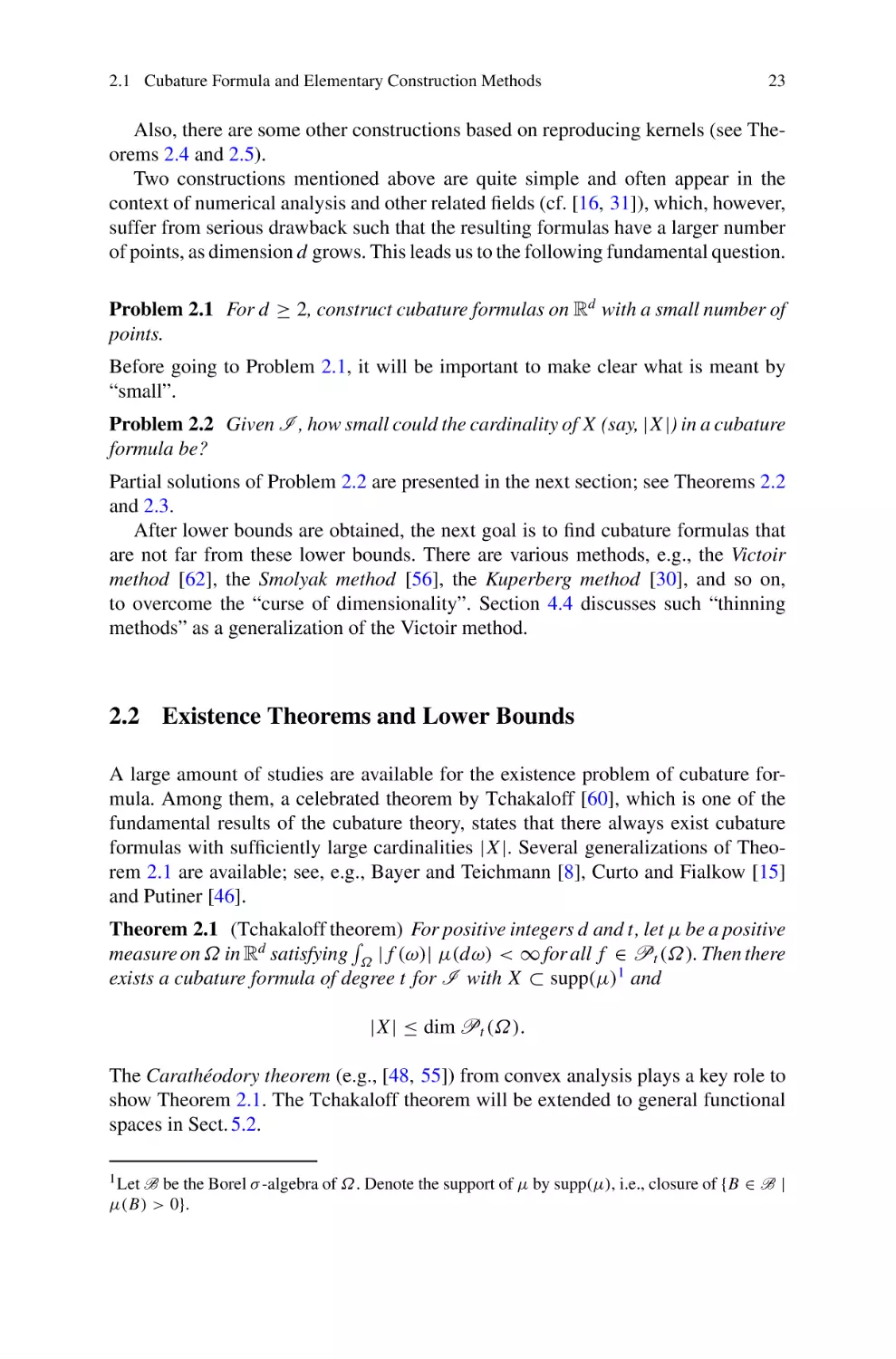
Also, there are some other constructions based on reproducing kernels (see Theorems 2.4 and 2.5).
Two constructions mentioned above are quite simple and often appear in the
context of numerical analysis and other related fields (cf. [16, 31]), which, however,
suffer from serious drawback such that the resulting formulas have a larger number
of points, as dimension d grows. This leads us to the following fundamental question.
Problem 2.1 For d ≥ 2, construct cubature formulas on Rd with a small number of
points.
Before going to Problem 2.1, it will be important to make clear what is meant by
“small”.
Problem 2.2 Given I , how small could the cardinality of X (say, |X |) in a cubature
formula be?
Partial solutions of Problem 2.2 are presented in the next section; see Theorems 2.2
and 2.3.
After lower bounds are obtained, the next goal is to find cubature formulas that
are not far from these lower bounds. There are various methods, e.g., the Victoir
method [62], the Smolyak method [56], the Kuperberg method [30], and so on,
to overcome the “curse of dimensionality”. Section 4.4 discusses such “thinning
methods” as a generalization of the Victoir method.

2.2 Existence Theorems and Lower Bounds
A large amount of studies are available for the existence problem of cubature formula. Among them, a celebrated theorem by Tchakaloff [60], which is one of the
fundamental results of the cubature theory, states that there always exist cubature
formulas with sufficiently large cardinalities |X |. Several generalizations of Theorem 2.1 are available; see, e.g., Bayer and Teichmann [8], Curto and Fialkow [15]
and Putiner [46].
Theorem 2.1 (Tchakaloff theorem)
For positive integers d and t, let μ be a positive

measure on Ω in Rd satisfying Ω | f (ω)| μ(dω) < ∞ for all f ∈ Pt (Ω). Then there
exists a cubature formula of degree t for I with X ⊂ supp(μ)1 and
|X | ≤ dim Pt (Ω).
The Carathéodory theorem (e.g., [48, 55]) from convex analysis plays a key role to
show Theorem 2.1. The Tchakaloff theorem will be extended to general functional
spaces in Sect. 5.2.
be the Borel σ -algebra of Ω. Denote the support of μ by supp(μ), i.e., closure of {B ∈ B |
μ(B) > 0}.

1 Let B

24

2 Cubature Formula

Next let us look at two types of lower bounds for the number of points in a cubature
formula. The lower bound in Theorem 2.2 is well known as the Fisher-type bound
in combinatorics and related areas or the Stroud bound in analysis; see, e.g., Cools
et al. [14], Delsarte and Seidel [18] and Stroud [58].
Theorem 2.2 (Fisher-type bound) Let X be the set of points of a cubature formula
of degree t for I . Then the following holds:
|X | ≥ dim P

t/2

(Ω).

(2.1)

A sketch of proof of this theorem (along the lines given in Stroud [58]) goes as
follows.
Sketch of proof. A cubature formula of degree 4 for a bivariate Gaussian integral is
focused for simplicity. A key point of the proof is to use the non-singularity of the
moment matrix.
Assume that there exists an n-point cubature formula of the form
1
π



f (ω1 , ω2 )e−(ω1 +ω2 ) dω1 dω2 =
2

R2

2

n


w f (x , y ) for all f ∈ P4 (R2 ).

=1

Then by letting f (ω1 , ω2 ) = (1, ω1 , ω2 , ω12 , ω1 ω2 , ω22 )T , it holds that
( f (x1 , y1 )T , . . . , f (xn , yn )T )T diag(w1 , . . . , wn )( f (x1 , y1 ), . . . , f (xn , yn ))
⎞
⎛
1 0 0 1/2 0 1/2
⎜ 0 1/2 0 0 0 0 ⎟
⎟
⎜
⎜ 0 0 1/2 0 0 0 ⎟
⎟
=⎜
⎜1/2 0 0 3/4 0 1/4⎟
⎟
⎜
⎝ 0 0 0 0 1/4 0 ⎠
1/2 0 0 1/4 0 1/2
where diag(w1 , . . . , wn ) is the diagonal matrix with elements w1 , . . . , wn . If n <
dim P2 (R2 ) = 6 then this matrix has rank < 6. But the matrix on the right-hand
side is the so-called moment matrix, which is always non-singular and then has rank
6. Therefore, the above equality cannot be valid if n < 6.

A generalization of Theorem 2.2 is presented in Chap. 5.
Before giving the next lower bound, a certain class of integrals called centrally
symmetric integrals is introduced.
Definition 2.2 (Centrally symmetric integral) An integral I is said to be centrally
symmetric if I [ f ] = 0 for all odd polynomials f .2
Example 2.4 Multivariate Gaussian integrals have been discussed in Example 2.2,
i.e.,
2 An

odd polynomial f is a polynomial satisfying f (−ω) = − f (ω) for all ω ∈ Ω.

2.2 Existence Theorems and Lower Bounds

I[f] =
=



1
π d/2
1
π d/2

R

25

f (ω)e−ω dω
2

d

Rd

f (ω1 , . . . , ωd )e−(ω1 +···+ωd ) dω1 . . . dωd .
2

2

This is a typical example of centrally symmetric integrals, which also belongs to a
certain class of spherically symmetric integrals. Roughly speaking, I is called a
spherically symmetric integral if region Ω has rotational invariance and the density
function depends on the radial component of ω. The precise definition is given in the
next section.
Theorem 2.2 is improved for odd-degree cubature formula for a centrally symmetric integral I . The following lower bound is known as the Möller bound; see
Möller [34, 35] and Mysovskikh [37].
Theorem 2.3 (Möller bound) Let X be the set of points in a cubature formula of
degree 2e + 1 for a centrally symmetric integral I . Then the following holds:

|X | ≥

2 dim Pe∗ (Ω) − 1 if e ≡ 0 (mod 2) and 0 ∈ X,
otherwise.
2 dim Pe∗ (Ω)

(2.2)

A sketch of proof of this theorem (along the lines given in Möller [34] or
Stroud [58]) goes as follows.
Sketch of proof. Let X = {x1 , . . . , xn } be an n-point subset of Ω with 0 ∈ X , and let
e be an even integer for simplicity. A key point of this proof is to consider functionals
L x : P2e+1 (Ω) → R defined by
L x ( f ) = f (x) for every x ∈ X
as in (1.6).
First, it is known (e.g., [5, pp. 429–430]) that
dim SpanR {L xi |P e∗ (Ω) | i = 1, . . . , n} = dim Pe∗ (Ω).
Then, let m = dim Pe∗ (Ω) − 1 and L 1 , . . . , L m be functionals among {L x1 ,
. . . , L xn } \ {L 0 } such that L 1 |P e∗ (Ω) , . . . , L m |P e∗ (Ω) is a basis of SpanR {L xi |P e∗ (Ω) |
i = 1, . . . , n}.
Since an odd polynomial g ∈ Hom1 (Ω) with
L 0 (g) = 0,

L  (g) = 0,  = 1, . . . , m,

is obtainable, it can be checked that L 1 |g·P e∗ (Ω) , . . . , L m |g·P e∗ (Ω) are linear inde∗
∗
(Ω), L 1 |P e+1
pendent. Moreover, since g · Pe∗ (Ω) is a subset of Pe+1
(Ω) , . . . ,
∗
are
also
linear
independent.
This
implies
that
L m |P e+1
(Ω)
∗
dim SpanR {L xi |P e∗ (Ω) | i = 1, . . . , n} − 1 = dim SpanR {L xi |P e+1
(Ω) | i = 1, . . . , n}.

26

2 Cubature Formula

Thus, it holds that
|X | ≥ dim SpanR {L xi |Pe+1 (Ω) | i = 1, . . . , n}
= dim SpanR {L xi |P ∗ (Ω) | i = 1, . . . , n} + dim SpanR {L xi |Pe∗ (Ω) | i = 1, . . . , n}
e+1
= 2 dim SpanR {L xi |Pe∗ (Ω) | i = 1, . . . , n} − 1,



which complete the proof.

The following lemma is employed to explicitly calculate lower bound (2.1) or (2.2)
for Ω, a set S p of p concentric spheres centered at the origin; see also Example 2.5.
Lemma 2.1 (cf. [1]) Let S p be a set of p concentric spheres centered at the origin
and ε S p ∈ {0, 1} by
/ Sp.
ε S p = 1 if 0 ∈ S p , ε S p = 0 if 0 ∈
Then the following hold:
(i) When p ≤

t+ε S p
2
2( p−ε S p )−1 



dim Pt (S p ) = ε S p +

=0

(ii) When p ≥

t+ε S p
2

 

d +t −−1
d +t
<
= dim Pt (Rd ).
t −
t

+1

dim Pt (S p ) =

 

t 

d +t −−1
d +t
=
.
t −
t
=0

(iii) When p ≥ t/2 + 1
dim Pt∗ (S p )

=

dim Pt∗ (Rd )


t/2 

d + t − 2 − 1
.
=
t − 2
=0

(iv) When p ≤ t/2 and t is odd or t is even and 0 ∈
/ Sp
dim Pt∗ (S p )


p−1 

d + t − 2 − 1
< dim Pt∗ (Rd ).
=
t
−
2
=0

(v) When p ≤ t/2 with even t and 0 ∈ S p
dim Pt∗ (S p )


p−2 

d + t − 2 − 1
< dim Pt∗ (Rd ).
=1+
t
−
2
=0

2.2 Existence Theorems and Lower Bounds

27

Fig. 2.3 Minimal cubature formulas of degree 4 of types (i) (left) and (ii) (right)

The definition of minimality of a cubature formula is now introduced.
Definition 2.3 (Minimal cubature formula) A cubature formula of degree t for I
is said to be minimal if it attains (2.1) or (2.2), according as t is even or not.
Example 2.5 By using Lemma 2.1, bounds (2.1) and (2.2) are explicitly computed
for cubature formulas of degrees 4 and 5 for the bivariate Gaussian integral as follows:


2+2
= 6,
|X | ≥ dim P2 (R2 ) =
2
   
3
1
+
− 1 = 7.
|X | ≥ 2 dim P2∗ (R2 ) − 1 = 2
2
0
Bannai et al. [6] shows that minimal cubature formulas of degree 4 are classified as
the following two types (i) and (ii) (see also Fig. 2.3):
(i)
Q[ f ] =



4
√
1 
1
2π √
2π
f (0, 0) +
, 2 sin
for all f ∈ P4 (R2 ).
f
2 cos
2
10
5
5
=0

(ii)
√ 3


5+2 5 
2π
2π
Q[ f ] =
f r1 cos
, r1 sin
30
3
3
√

+

5−2 5
30

=0

3

=0

f



(2 + 1)π
(2 + 1)π
, r2 sin
for all f ∈ P4 (R2 )
r2 cos
3
3

√
√
√
√
with r1 = ( 10 − 2)/2 and r2 = ( 10 + 2)/2.
Two illustrations in Fig. 2.3 may be thought of as a “discretization” of bivariate
Gaussian distribution. For example, focusing on the left illustration, the weight at
the origin (colored orange) indicates the peak of the density function and the other

28

2 Cubature Formula

Fig. 2.4 Minimal cubature
formula of degree 5 of type
(iii)

weights are identical and smaller than the peak at the remaining five points equidistant
from the origin (colored blue). Similarly for the right illustration, points on the
interlayer (colored orange) have identical weights which are larger than those on the
outer layer (colored blue).
Hirao and Sawa [28] also show that minimal cubature formulas of degree 5 are
classified as the following type (iii) (see also Fig. 2.4):


5
√
1 
1
π √
π
, 2 sin
for all f ∈ P5 (R2 ).
f
2 cos
(iii) Q[ f ] = f (0, 0) +
2
12
3
3
=0

In the remaining part of this section, a relationship between cubature formulas
and the (modified) kernel polynomials is discussed; see Sect. 1.1 for the definition
of (modified) kernel polynomials. The method of constructing cubature formulas
through reproducing kernels has been first considered by Mysovskikh [38, 39] and
later studied by Möller [33]; see also [14, 63] and references therein.
Given a positive integer e, let K e be the (multivariate) kernel of Pe (Ω) with
inner product ( f, g)P e (Ω) . In order to construct a cubature formula of degree 2e
for I , this method needs to choose a d-point set {a1 , . . . , ad } of Rd such that the
hypersurfaces H1 , . . . , Hd intersect at ed points, where H = {ω ∈ Rd | K e (ω, a ) =
0},  = 1, . . . , e. The following procedure explains how to choose {a1 , . . . , ad } (see,
e.g., [14, 63]):
(i) Pick any point a1 in Ω which is not a common zero of { f  } , where { f  } is an
orthonormal basis of Home (Ω).
(ii) Pick a point a2 from the hypersurface H1 which is not a common zero of { f  } .
(iii) When the points a1 , . . . , ak are selected, pick a point ak+1 from the intersection
of hypersurfaces H1 ∩ . . . ∩ Hk which is not a common zero of { f  } .
(iv) Iterate (iii) until a1 through ad are selected.
Theorem 2.4 (cf. [39]) If H1 , . . . , Hd defined by a1 , . . . , ad intersect at ed distinct
points, say b1 , . . . , bed , then there exists a cubature formula of degree 2e for I which
is of the form

2.2 Existence Theorems and Lower Bounds

Q[ f ] =

d

=1

29


1
f (a ) +
w f (b ) for all f ∈ P2e (Rd ),
K e (a , a )
=1
ed

(2.3)

where w are solutions of a certain system of linear equations determined by linear
functional I [ f ] −  f (a )/K e (a , a ).
Moreover, when I has central symmetry, the following type of cubature formulas
of degree 2e + 1 may be constructed: Given a positive integer e, let K̃ e be the modified
kernel corresponding to Pe∗ (Ω) with inner product (·, ·)P e∗ (Ω) . Further let a d-point
set {a1 , . . . , ad } of Rd such that the hypersurfaces H̃1 , . . . , H̃d intersect at ed points,
where H̃ = {ω ∈ Rd | K̃ e (ω, a ) = 0},  = 1, . . . , e, and points ai are chosen in
the above-mentioned procedure with H replaced by H̃ .
Theorem 2.5 (cf. [39]) Assume that I is a centrally symmetric integral. If
H̃1 , . . . , H̃d defined by a1 , . . . , ad intersect at ed points, say b1 , . . . , bed , then there
exists a cubature formula of degree 2e + 1 for I which is of the form
Q[ f ] =

d


d

1

2 K̃ e (a , a )
=1

{ f (a ) + f (−a )} +

e

=1

w f (b ) for all f ∈ P2e+1 (Rd ),

(2.4)
where w are solutions of a certain system of linear equations determined by linear
functional I [ f ] − d=1 ( f (a ) + f (−a ))/2 K̃ e (a , a ).3


Example 2.6 ([63]) A cubature formula of degree 5 for B2 ·dω/ B2 dω is con(1/2)
structed as follows. Set a1 = (0, 0). Since K̃ 2 (ω, ω ) := K̃ 2 (ω, ω ) = 12ω, ω 2 +
6ω2 ω 2 − 6(ω2 + ω 2 ) + 4 from Theorem 1.6, it holds that
H̃1 = {ω ∈ R2 | K̃ 2 (ω, a1 ) = 0} = {ω ∈ R2 | ω2 = 2/3}.
√
Let a2 = (2/ 6, 0). Since
H̃2 = {ω ∈ R2 | K̃ 2 (ω, a2 ) = 0} = {(ω1 , ω2 ) ∈ R2 | 6ω12 − 2ω22 = 0},
√
√
it is easy to check that {b1 , . . . , b4 } = {(±1/ 6, ±1/ 2)} ∈ H1 ∩ H2 . Thus, it follows from Theorem 2.5 that

 




1
2
1
1
2
1
1
f √ , 0 + f −√ , 0
f ±√ , ±√
Q[ f ] = f (0, 0) +
+
4
8
8
6
6
6
2
√

√
5
1
1
π
π
6
6
= f (0, 0) +
cos
,
sin
f
for all f ∈ P5 (R2 ),
4
8 =0
3
3 3
3
which forms a minimal cubature formula of degree 5; see also Example 2.5.
3 See

[39, Theorems 12.1,12.2] for details of the proofs of Theorems 2.4 and 2.5.

30

2 Cubature Formula

The method of Theorem 2.4 (respectively, Theorem 2.5) is based on reproducing
kernels K e (respectively, K̃ e ), which is of theoretical interest from a viewpoint of
functional analysis. We refer the reader to Xu [63] who explains some merits of
Theorems 2.4 and 2.5 are explained. In some special cases, K e and K̃ e have a quite
elegant form that represents (2.3) and (2.4) in a more explicit manner. For example,
Xu [63] uses a compact formula of K e and K̃ e for multivariate Jacobi integral (see
Theorem 1.6 in Sect. 1.2) and thereby produces many examples of cubature formulas.
An important application of reproducing kernels to the cubature theory is to characterize minimal cubature formulas, which can be regarded as a high-dimensional
generalization of Gaussian quadrature formula.
Theorem 2.6 ([36, 39])
(1) Assume that there exists a cubature formula of degree 2e for an integral I . This
formula is minimal if and only if
(i) K e (x, x  ) = 0 for all x, x  ∈ X with x = x  ,
(ii) w(x) = 1/K e (x, x) for all x ∈ X .
(2) Assume that there exists a cubature formula of degree 4k + 1 for a centrally
symmetric integral I of the form
Q[ f ] = w(0) f (0) +



w(x){ f (x) + f (−x)}.

x∈ X̃ \{0}

This formula is minimal if and only if
(i) K̃ 2k (x, x  ) = 0 for all x, x  ∈ X with x = ±x  ,
(ii) w(0) = 1/ K̃ 2k (0, 0), w(x) = 1/(2 K̃ 2k (x, x)) for all x ∈ X \ {0}.
(3) Assume that there exists a cubature formula of degree 4k + 3 for a centrally
symmetric integral I of the form
Q[ f ] =



w(x){ f (x) + f (−x)}.

x∈ X̃

This formula is minimal if and only if
(i) K̃ 2k+1 (x, x  ) = 0 for all x, x  ∈ X with x = ±x  ,
(ii) w(x) = 1/(2 K̃ 2k+1 (x, x)) for all x ∈ X .
Example 2.7 By using Theorem 2.6 (2), Noskov and
 Schmid
 [43] give a classification of minimal cubature formulas of degree 5 for Bd ·dω/ Bd dω. As a by-product,
they show that

2.2 Existence Theorems and Lower Bounds

31

X = {(0, 0, 0, 0, 0, 0, 0),

√3 (±1, ±1, 0, ±1, 0, 0, 0),
11
√3 (0, ±1, ±1, 0, ±1, 0, 0), √3 (0, 0, ±1, ±1, 0, ±1, 0),
11
11
√3 (0, 0, 0, ±1, ±1, 0, ±1), √3 (±1, 0, 0, 0, ±1, ±1, 0),
11
11
√3 (0, ±1, 0, 0, 0, ±1, ±1), √3 (±1, 0, ±1, 0, 0, 0, ±1)}
11
11



forms a 57-point minimal cubature formula of degree 5 for Bd · dω/ Bd dω, which is
the same structure as the 57-point minimal cubature for Rd · exp(−ω2 ) dω/π d/2
found by Victoir [62]. Note that X \ {(0, . . . , 0)} has the same arrangement as Box–
Behnken design No. 5 in [11, Table 4]; see also Example 4.8 in Sect. 4.4. Moreover,
X \ {(0, . . . , 0)} is essentially the same as the characteristic functions (vectors) of
blocks of a 2-(7, 3, 1)-design, which is the smallest nontrivial example of combinatorial 2-designs, i.e., balanced incomplete block (BIB) designs. See Sect. 4.4 for the
definition of combinatorial designs.
Hirao and Sawa [27] extend the Noskov–Schmid formula to minimal cubature
formulas for spherically symmetric integrals in general; see Definition 2.7 for the
definition of spherical symmetry.
The next section discusses the relationship between cubature formulas and
Euclidean designs, which will be used for subsequent Chaps. 3 and 4.

2.3 Euclidean Design and Spherical Symmetry
The present section first gives the concept of spherical design defined by Delsarte
et al. [17], which is one of main research objects in algebraic combinatorics.
Definition 2.4 (Spherical design) Given a nonnegative integer t, a finite subset X
of Sd−1 is called a spherical t-design if
1
|Sd−1 |


Sd−1

f (ω) ρ(dω) =

1 
f (x) for all f ∈ Pt (Rd ).
|X | x∈X

(2.5)

As immediately seen by Definition 2.4, a spherical t-design of Sd−1 is just a
cubature formula of degree t for spherical integration. In analysis language, this
is just an equal-weighted cubature formula, called a Chebyshev-type cubature formula (e.g., [57]). The Chebyshev-type cubature shows an extension of the famous
Chebyshev–Gauss quadrature as


1
−1

1
f (u) √
=
f
e =1
π 1 − u2
du

e



2 − 1
π
for all f ∈ P2e−1 (R),
cos
2e

32

2 Cubature Formula

where cos ((2 − 1)π/2e) are the zeros of the first kind Chebyshev polynomial of
degree e. This is minimal with
√ respect to (2.3) among all quadrature formulas of
1
degree 2e − 1 for −1 ·1/(π 1 − u 2 ) du.
Remark 2.1 Neumaier and Seidel [41] show the equivalence between optimal experimental designs of degree e on the unit sphere and spherical 2e-designs where X may
be a multi-set. This relationship will be explained in detail in Sect. 3.2. Moreover, a
spherical design with rational weights and rational points is closely connected with
isometric embeddings of classical finite-dimensional Banach spaces or a certain class
of polynomial identities called Hilbert identities; for details see Sects. 2.4 and 5.6.
Remark 2.2 Polar coordinate systems are used when calculating a spherical integration. Polar coordinates r, θ1 , . . . , θd−1 are converted to ω1 , . . . , ωd by using trigonometric functions as
ω1 = r sin θd−1 sin θd−2 · · · sin θ2 sin θ1
ω2 = r sin θd−1 sin θd−2 · · · sin θ2 cos θ1
..
.
ωi = r sin θd−1 sin θd−2 · · · sin θi cos θi−1
..
.
ωd−1 = r sin θd−1 cos θd−2
ωd = r cos θd−1 ,
where 0 ≤ r , 0 ≤ θ1 < 2π and 0 ≤ θi ≤ π for i = 2, . . . , d − 1. Moreover, the cor−1
θ dθd−1 dθd−2 · · · dθ1 . By
responding volume element is given by r d−1 d−1
=2 sin
d−1
is calculated as follows:
using this system, the surface area of S

d−1
|S | =
ρ(dω)
Sd−1

 2π  π
 π d−1

−1
=
···
sin θ dθd−1 · · · dθ1
0


=
0

0
2π 
0

0
π


···
0



π

= |Sd−2 | ·
= |Sd−2 | ·


sin

−1



θ dθd−2 · · · dθ1 ·

=2

π

sind−2 θd−1 dθd−1

0

sind−2 θd−1 dθd−1

0
1/2

π

=2


π d−2


Γ ((d − 1)/2)
,
Γ (d/2)

where Γ is the Gamma function. By using the abovementioned procedure repeatedly,
it holds that |Sd−1 | = 2π d/2 /Γ (d/2).

2.3 Euclidean Design and Spherical Symmetry

33

Moreover, with the multi-index notation ωa = ω1a1 · · · ωdad for a = (a1 , . . . , ad ) ∈
it is known (e.g., [22]) that

Zd≥0 ,



1

|Sd−1 | Sd−1

ωa ρ(dω) =

⎧
⎪
⎪
⎨

Γ (d/2)
2a1 Γ (a1 /2 + d/2)

⎪
⎪
⎩0,

·

d (a )!
j=1 j
, if a j are even for all j;
d (a /2)!
j=1 j

otherwise

(2.6)
with a1 = a1 + · · · + ad , which will be used in the proof of Theorem 5.1.
Now, a fundamental question concerns the existence of spherical t-designs.
Seymour and Zaslavsky [53] show that there exists a spherical t-design for sufficiently large number of points (see also Corollary 5.2). A recent work by Bondarenko
et al. [9] is an improvement of Seymour–Zaslavsky theorem ( [53]).
Theorem 2.7 (Bondarenko–Radchenko–Viazovska theorem, [9]) Given d ≥ 2,
there exists a spherical t-design on Sd−1 with |X | points for all |X | ≥ cd t d−1 where
the constant cd does only depend on d.
Note that this lower bound has the same asymptotic behavior as the Fisher-type bound
(2.1) for fixed d. Moreover, Bondarenko et al. [10] show a similar existence result for
“well-separated” spherical designs X , i.e., X satisfies |xi − x j | ≥ cd n −1/(d−1) , i =
j, where the constant cd does only depend on d.
Next, the tightness of spherical designs is defined. In algebraic combinatorics, tight
designs are of particular interest for the mathematical richness of its own structure.
Definition 2.5 (Tight spherical design) A spherical t-design is said to be tight if the
equality in (2.1) or (2.2) is attained for Ω = Sd−1 , according as t is even or not.
Remark 2.3 In numerical analysis, minimal is often used for tight; recall Definition 2.3.
Example 2.8 (Tight spherical designs of S1 ) Given a positive integer t, the vertices of
a regular (t + 1)-gon inscribed in S1 form a tight spherical t-design; see, e.g., [2, 3].
For example, the vertices of a regular pentagon inscribed in S1 form a tight spherical
4-design, i.e., it holds that
1
2π



2π
0

1
f (cos θ, sin θ ) dθ =
f
5 =0
4



2π
2π
, sin
cos
5
5


for all f ∈ P4 (R2 ).

While tight spherical designs always exist on S1 , the situation becomes quite
different in higher dimensional cases, i.e., tight designs only sporadically exist in
higher dimensions. The known results on the classification on tight spherical tdesigns of Sd−1 (d ≥ 3) are summarized as follows ([2, 3]):
(i) X is a tight spherical 1-design of Sd−1 if and only if X = {x, −x} is an antipodal
set with x ∈ Sd−1 .
(ii) X is a tight spherical 2-design of Sd−1 if and only if X is a regular simplex.

34

2 Cubature Formula

(iii) X is a tight spherical 3-design of Sd−1 if and only if X is isomorphic to a cross
polytope {±e | 1 ≤  ≤ d}, where e1 , . . . , ed is the standard basis of Rd .
(iv) There does not exist a tight spherical t-design of Sd−1 with possible exceptions
that t ≤ 5 and t ∈ {7, 11}.
(v) The classifications of tight spherical 4-, 5-, 7-designs are not complete yet; see
also Bannai et al. [7]. As of today, the only known examples are as follows:
a. t = 4: a 27-point set on S5 related to the E 6 root system, a 275-point set on
S21 related to the McLaughlin graph.
b. t = 5: a set of 12 vertices of the icosahedron on S2 , a set of 126 vectors of
the E 7 root system on S6 , a 552-point set on S22 related to 276 equiangular
lines.
c. t = 7: a set of 240 vectors of the E 8 root system on S7 , a 4600-point set on
S23 related to an iterated kissing configuration.
(vi) X is a tight spherical 11-design of S23 if and only if X is isomorphic to a set of
196560 minimal vectors in the Leech lattice in R24 .
Neumaier and Seidel [40] give the concept of Euclidean designs as a generalization
of spherical designs; see also Delsarte and Seidel [18].
Let X be a finite subset of Rd and w be a positive weight function on X . Denote
by R the radius set of X , i.e.,
R = {x | x ∈ X } = {r1 , . . . , r p } with r1 > r2 > · · · > r p ≥ 0.
= {ω ∈ Rd | ω = ri } be the (d − 1)-dimensional sphere with radius ri
Let Srd−1
i
p
and S p = ∪i=1 Srd−1
be a set of p concentric spheres centered at the origin. Furi
ther, let X i = X ∩ Srd−1
and Wi = x∈X i w(x). Let ρri be the surface measure and
i
|
be
the
surface
area
of Srd−1
. For notational convenience, when r p = 0, we
|Srd−1
i
i
d−1
let Srd−1 f (ω) ρr p (dω)/|Sr p | = f (0). Then, consider a cubature formula for the
p
integral I  defined as
I ( f ) =

p

Wi
i=1

|Srd−1
|
i


Srd−1
i

f (ω) ρri (dω).

Under this setting, the following definition is introduced.
Definition 2.6 (Euclidean design) Given a nonnegative integer t, a finite weighted
pair (X, w) is called a Euclidean t-design supported by a set S p of p concentric
spheres if
(2.7)
I  [ f ] = Q[ f ] for all f ∈ Pt (Rd ).
Remark 2.4 (i) If p = 1, r1 = 1 and w ≡ 1 on X , then X is a spherical t-design of
Sd−1 (see Definition 2.4).
(ii) If 0 ∈ X , then X \ {0} is also a Euclidean t-design.

2.3 Euclidean Design and Spherical Symmetry

35

The following theorem is known as the Neumaier–Seidel equivalence theorem.
Theorem 2.8 (Neumaier–Seidel equivalence theorem, [40]) Let (X, w) be a finite
weighted pair. Then the following are equivalent:
(i) A
pair (X, w) is a Euclidean t-design.

w(x)x2 j φ(x) = 0 for every φ ∈ Harm (Rd ), with 1 ≤  ≤ t, 0 ≤ j ≤
(ii)
x∈X
t−
2

.

Proof It is known (e.g., [40]) that the polynomial space Pt (Rd ) is decomposed as
a finite sum of products of ω2 j and harmonic homogeneous polynomial spaces
Harm (Rd ) with 0 ≤ 2 j +  ≤ t, i.e.,
Pt (Rd ) =



ω2 j Harm (Rd ).

0≤2 j+≤t

This is the Rd -version of the Fischer decomposition (1.13). This implies the desired
result.

An algebraic generalization of this result will be available in Sect. 4.2.
Let us look at the relationship between Euclidean designs and cubature formulas
for spherically symmetric integrals.
Example 2.9 A multivariate Gaussian integral, which has appeared several times in
this chapter, i.e.,
I[f] =
=

1
π d/2
1
π d/2



f (ω)e−ω dω
2

R

d

Rd

f (ω1 , . . . , ωd )e−(ω1 +···+ωd ) dω1 . . . dωd
2

2

is a typical example of spherically symmetric integrals. Roughly speaking, if the
region Ω has “rotational invariance” and the density function depends on the radial
component of ω, then I is a spherically symmetric integral. Particularly, in the
2-dimensional case, the term circularly symmetric integral or radially symmetric
integral is often used.
Let Ω = {ω = (ω1 , . . . , ωd ) ∈ Rd | α ≤ ω ≤ β} be a connected annulus region
with nonnegative real values α, β with α < β, and W be a radial weight function, i.e.,
a density function of ω for all ω ∈ Ω. Under this setting, the following definition
is introduced.
Definition 2.7 (Spherically symmetric integral) With the above setting, integral I
is said to be spherically symmetric if it is of the form

36

2 Cubature Formula

I[f] = 

1
Ω W (ω) dω

= β
α



1
W (r )r d−1 dr

f (ω)W (ω) dω

Ω



β



|Sd−1 |

α





1

Sd−1

f (r ω) ρ(dω) r d−1 W (r ) dr.

The Neumaier–Seidel equivalence theorem (Theorem 2.8) gives the close relationship between Euclidean designs and cubature formulas for spherically symmetric
integrals I .
Corollary 2.1 A cubature formula of degree t for a spherically symmetric integral
I forms a Euclidean t-design.
Proof For  ≥ 1 and φ ∈ Harm (Rd ),


w(x)x2 j φ(x) = 

1
W
(ω)
dω
Ω

=

1
W
(ω)
dω
Ω

x∈X




Ω

ω2 j φ(ω)W (ω) dω

β
α

r +2 j+d−1 W (r ) dr


Sd−1

φ(ω) ρ(dω)

= 0.


Thus, the desired result is obtained from Theorem 2.8.

Definition 2.8 (Tight Euclidean design) A Euclidean t-design is said to be tight if
the equality in (2.1) or (2.2) is attained for Ω = S p , according as t is even or not.
Example 2.10 By Corollary 2.1, the examples given in Example 2.5 are tight
Euclidean designs. There exist some classification results of tight t-designs for small
values of t. For example, Bannai [1] gives a classification of tight Euclidean 5-designs
in low dimensions and presents some new examples of tight 5-designs, namely, let
X = X 1 ∪ X 2 be a finite subset of R6 , where

X 1 = {±ei | i = 1, . . . , 6},

X2 =

r
√ | εi ∈ {1, −1}, |{i | εi = 1}| ≡ 0
6


(mod 2)}

and w is a positive weight function such that w(x) = 1 for x ∈ X 1 and w(x) =
9/(8r 4 ) for x ∈ X 2 . Then a pair (X, w) forms a tight Euclidean 5-design on two
concentric spheres. Note that this tight design is invariant under reflection group D6 ;
for details on reflection groups, see Chap. 4.
A technique for constructing Euclidean designs is presented. The idea is almost
trivial. However, it is of great important from a viewpoint of design of experiments
in connection with optimal design theory; see, e.g., Theorem 4.10.
Proposition 2.1 Let (Yi , wi ), i = 1, . . . , p, be Euclidean t-designs on the unit
p
sphere. Let Λ1 , . . . , Λ p and r1 , . . . , r p be positive real numbers. Then (∪i=1 ri Yi , w)
p
is a Euclidean t-design on S p = ∪i=1 Srd−1
, where w(ω) = Λi wi (ri−1 ω) if ri−1 ω ∈ Yi .
i

2.3 Euclidean Design and Spherical Symmetry

37

Proof The polynomial space Pt (Rd ) is decomposed as a finite sum of homogeneous
polynomial spaces Hom (Rd ) with 0 ≤  ≤ t; see, e.g., Neumaier and Seidel [41].
Given positive real numbers Λ1 , . . . , Λ p , it holds that for all f ∈ Hom (Rn ) with
0 ≤  ≤ t,
p

Λi
i=1

|Srd−1
|
i


Srd−1
i

f (ω) ρri (dω) =
=


p

ri Λi
f (ω) ρ(dω)
|Sd−1 | Sd−1
i=1
p


ri Λi

i=1

=



wi (x) f (x)

x∈Yi

p



(Λi wi (x)) f (ri x),

i=1 x∈Yi



which implies the desired result.

Moreover, the following is a simple but not entirely trivial construction of cubature
formulas for spherically symmetric integrals.
Proposition 2.2 (cf. [26]) Assume that there exist a Euclidean t-design (Y, w) on
the unit sphere and a quadrature formula ({ri2 }i , {Λi }i ) of degree t/2 for integral
J [ f ] =  β2
α2

1


√

u d/2−1 W ( u) du

β2
α2

√
f (u)u d/2−1 W ( u) du.

Then a finite weighted pair ({ri Y }i , {Λi w}i ) forms a cubature formula of degree t
for a spherically symmetric integral I .
Proof By recalling the argument used in the proof of Theorem 2.8, polynomial space
Pt (Rd ) is decomposed as
Pt (Rd ) =



ω2 j Harm (Rd ).

0≤2 j+≤t

For all f ∈ ω2 j Harml (Rd ) with 1 ≤  ≤ t and 0 ≤ j ≤ (t − )/2 , it holds that
p



(Λi w(x)) f (ri x) =

i=1 x∈Y

p

i=1
p

=


i=1
p

=

+2 j

ri


x∈Y

+2 j
ri

 Λi
i=1

Λi

Λi
|Sd−1 |


|Srd−1
|
i

Srd−1
i

w(x) f (x)

Sd−1

f (ω) ρ(dω)

f (ω) ρri (dω) = 0.

(2.8)

38

2 Cubature Formula

Moreover, for all f = ω2 j with j = 0, 1, . . . , t/2 , it holds that
p


1

2j

Λi ri =  β 2
α2

i=1


√

u d/2−1 W ( u) du

β2
α2

√
u j · u d/2−1 W ( u) du.

(2.9)


Combining (2.8) and (2.9) gives the desired result.

The existence of Gaussian quadrature (e.g, [58]) always implies the existence of
a quadrature formula of degree t for J with t/2 points. Therefore, if a spherical
design can be explicitly constructed, then so is a cubature formula of degree t for a
spherically symmetric integral I .
Note that these observations will be used in Proposition 3.1.

2.4 Further Remarks and Open Questions
In Sect. 2.2, two classical lower bounds, the Fisher-type bound (Theorem 2.2) and
the Möller bound (Theorem 2.3), have been derived by using standard techniques
in linear algebra and functional analysis. Delsarte et al. [17] show the same lower
bounds for spherical designs in a unified approach based on the linear programming
(LP) techniques. A sketch of their idea is as follows: Given positive integers d and
t, let Fd,t be a collection of continuous functions f on interval [−1, 1] such that
(i) f (u) ≥ 0 for all u ∈ [−1, 1] and f (1) > 0,
(ii) f  ≥ 0 for all  ≥ t + 1, where
1
f  = −1
1

((d−2)/2)

f (u)C

(u)(1 − u 2 )(d−3)/2 du

((d−2)/2)
(u)}2 (1
−1 {C 

− u 2 )(d−3)/2 du

.

((d−2)/2)

Here Cl
denotes the Gegenbauer polynomial defined by (1.8) in Sect. 1.2.
Then the number of points in a spherical t-design X is bounded from below as
|X | ≥ sup

f ∈F d,t

f (1)
.
f0

To derive the Fisher-type bound (Theorem 2.2) and the Möller bound (Theorem 2.3), Delsarte et al. [17] choose f as follows:
⎧
2
e
⎪

⎪
⎪
⎪
Q  (u) , if t = 2e,
⎪
⎨
=0
f (u) =
 e/2
2
⎪

⎪
⎪
⎪
Q e−2 (u) , if t = 2e + 1.
⎪(u + 1)
⎩
=0

(2.10)

2.4 Further Remarks and Open Questions

39

With the symbols Q  (in Remark 1.4) and P and R (in Example 1.7), (2.10) is simplified as (Re (u))2 and (u + 1)(Pe (u))2 . Direct calculations show that f 0 = Re (1) if t =
2e, and f 0 = Pe (1) if t = 2e + 1. It thus remains to calculate Re (1) and Pe (1). For
example, when t = 2e + 1, recall (1.16), i.e., the computation of dim Home (Sd−1 ),
which is just the computation of Pe (1). As implied by (1.17), the computation of
Re (1) is substantially the same as that of dim Pe (Sd−1 ). In summary, bounds (2.1)
and (2.2) are obtained in a unified fashion. For an improvement of the Delsarte LP
bound, we refer the reader to Yudin [65].
As mentioned in Sect. 1.2, Xu [64] finds an analogue of the Delsarte LP bound for
multivariate Jacobi integral over unit ball Bd by combining the above techniques with
“compact” expression of reproducing kernels (Theorem 1.6). A challenging problem
is to find such compact expressions of the kernel function corresponding to Gaussian
integration by using classical orthogonal polynomials like Xu’s compact formula
(Theorem 1.6). Gaussian integration may be of particular interest from a viewpoint
of the cubature theory and statistical applications (e.g., [16, 31]). Not only is the
LP bound improved for Gaussian integration as mentioned in the unit ball case, but
also many new cubature formulas can be generated by the Mysovskikh theorems
(Theorems 2.4 and 2.5).
In the context of space-filling design (e.g., [45]), a numerical integration method
called the quasi-Monte Carlo (QMC) method on unit cube Ω = [0, 1]d is often used.
The aim of QMC method on a RKHS H is to construct sequences {X n }n , where
each X n is an n-point configuration on Ω, which gives a certain optimal convergence
rate, faster than the Monte Carlo rate of O(n −1/2 ), for the worst-case error defined as


n


1


(2.11)
wce(H ; X n ) :=
sup
f (ω) dω −
f (x ) .


n
f ∈H , f H ≤1  Ω
=1

The reproducing kernel theory discussed in Chap. 1 plays a key role in investigating a
convergent rate of (2.11) for given sequences of point configurations. Then a number
of “good” sequences, such as the Sobol sequence, lattice rules, digital nets, and so
on, have been proposed; see Dick and Pillichshammer [19], Niederreiter [42] and
references therein.
On the other hand, works on spherical cases Ω = Sd−1 have been increasing in
recent years. Brauchart et al. [12] introduce the concept of QMC design sequences
for some RKHS. For example, they show that an increasing sequence of n-point
spherical t-designs X n on Sd−1 with n = O(t d−1 ) forms a QMC design sequence.
Comparison of numerical accuracy of quasi-Monte Carlo approaches and cubature
approaches is discussed by several authors. Schürer [51, 52] performs numerical
experiments with Genz functions [23] by choosing classical QMC points such as
Sobol sequences, Niederreiter sequences (cf. [19]) and some classes of classical
cubatures, as exemplified by Stroud formula (see [58]), in dimension up to 100.
What Schürer’s works make clear is that cubature approaches give more accurate
numerical integrations than QMC approaches when the integrand is continuous. It
will be interesting to perform similar experiments as in [51, 52] using higher degree
cubatures as such by Victoir [62] and Kuperberg [30].

40

2 Cubature Formula

Moreover, Brauchart et al. [12] discuss numerical integration errors for a certain
continuous function and worst-case error for Sobolev space, by choosing several point
configurations and spherical designs on S2 , and further clarify that spherical design
approaches show the best performance numerically among all other approaches under
consideration. An interesting problem is to perform similar experiments as in [12]
by constructing higher dimensional spherical designs.
Brauchart et al. [12] and Hirao [25] propose probabilistic generating methods
of QMC design sequences using some point processes called determinantal point
processes in probability theory. It is desirable to develop a method that is more computationally efficient than the method using jittered samplings proposed by Brauchart
et al. [12]. To discuss QMC design sequences on integral domains (especially, “asymmetric” domain) other than cubes and spheres is still of great interest.
Isometric embeddings of Banach spaces are closely tied with the theory of cubature formula. Let p be a positive integer, consider the p-norm  ·  p : Rd → R
defined by
 d
1/ p

p
|ω |
, ω = (ω1 , . . . , ωd ) ∈ Rd .
ω p =
=1

The Euclidean space Rd endowed with norm  ·  p is a classical finite-dimensional
Banach space, usually denoted by dp .
One of the important problems in the Banach space theory is to clarify the existence
of an R-linear map ι : d2 → n2e satisfying
ι(ω)2e = ω2 for all ω ∈ d2 .
Such a map ι is called an isometric embedding d2 → n2e ; see, e.g., [50].
A famous result in the theory of Euclidean design is the equivalence between
an isometric embedding d2 → n2e and a Euclidean design of index 2e for spherical
integration, i.e.,
1
|Sd−1 |


Sd−1

f (ω) ρ(dω) =



w(x) f (x) for all f ∈ Hom2e (Rd );

x∈X

see also [32, 54] and references therein.
Example 2.11 (isometric embedding 32 → 42 ) Here is a simple example of constructing an isometric embedding from a Euclidean design on unit sphere S2 .
Let

X = {x1 , x2 , x3 , x4 } =

1
1
1
1
√ (1, 1, 1), √ (−1, 1, 1), √ (1, −1, 1), √ (1, −1, 1)
3
3
3
3



be the vertices of a regular tetrahedron on unit sphere S2 . Then X is not only a tight
spherical 3-design of S2 but also a Euclidean design of index 2 on S2 , i.e., it holds that

2.4 Further Remarks and Open Questions

1
|S2 |



41

1
f (x ) for all f ∈ Hom2 (R3 ).
4 =1
4

S2

f (ω) ρ(dω) =

Then the linear map defined as
√
3
ι(ω) =
(ω, x1 , ω, x2 , ω, x3 , ω, x4 ) for all ω ∈ R3
2
is an isometric embedding 32 → 42 , since for f (ω ) = ω, ω 2 ∈ Hom2 (R3 ),
4


1
w ω, x  = 2
|S |
=1

√

√
3
3
2
ω, ω  ρ(dω ) =
ω, ω =
ω22 .
2
2
S2



2

 2



(2.12)

In particular, Shatalov [54] puts a vast amount of data of isometric embeddings together as several tables, which are called “Shatalov tables” by some authors
[44, 50].
Identities of type (2.12) are called the Hilbert identities in the theory of quadratic
and higher degree forms.
Proposition 2.3 (cf. [24, 47]) For each i = 1, . . . , n, let xi = (xi1 , . . . , xid ) ∈ Sd−1
and wi be positive reals. Let Cd,e be a constant given by
Cd,e =

1



|Sd−1 |

Sd−1

ω12e ρ(dω) =

e

d + 2e − 2 j
j=1

2e + 1 − 2 j

with ω = (ω1 , . . . , ωd ). Then the following are equivalent:
(i) There exists an n-point Euclidean design of index 2e on unit sphere Sd−1 .
(ii) There exists a Hilbert identity as
Cd,e (ω12 + · · · + ωn2 )e =

n


λi (yi1 ω1 + · · · + yid ωd )2e .

(2.13)

i=1

A particularly interesting class of Hilbert identities is that of rational identities,
i.e., polynomial identities of type (2.13) with all λi and yi j rational. For example,
6(x12 + x22 + x32 + x42 )2 =


1≤i< j≤4

(xi + x j )4 +



(xi − x j )4

(2.14)

1≤i< j≤4

is a rational identity in four indeterminates x1 , x2 , x3 , x4 . This identity is used to
prove the following type of statements in number theory (the Waring problem for
quartic numbers): every positive integer n is expressed as a sum of at most 53 quartics.
In fact, let n = 6s + r , 0 ≤ r ≤ 5, and use the Lagrange four-square theorem. Then
there exist integers yi j such that

42

2 Cubature Formula

⎛
⎞2
4
4


⎝
n = 6s + r = 6
yi2j ⎠ + r.
i=1

j=1

2

4
2
is replaced by at most 12 quartics and so n
By (2.14), each form 6
j=1 yi j
is a sum of at most 53 quartics. In general, if a rational identity of type (2.14) is
explicitly constructed, then a constructive solution of the Waring problem is obtained.
The Waring problem is solved by Hilbert [24] in general, but his solution relies on
complicated arguments from analysis and is not constructive (see also [47, 49]).

References
1. Bannai, E.: On antipodal euclidean tight (2e + 1)-designs. J. Algebr. Comb. 24(4), 391–414
(2006)
2. Bannai, E., Bannai, E.: Spherical designs and Euclidean designs. In: Recent Developments
in Algebra and Related Areas (Beijing, 2007). Advance Lectures in Mathematics, vol. 8, pp.
1–37. Higher Education Press, Beijing; International Press (2009)
3. Bannai, E., Bannai, E.: A survey on spherical designs and algebraic combinatorics on spheres.
Eur. J. Comb. 30(6), 1392–1425 (2009)
4. Bannai, E., Bannai, E.: Euclidean designs and coherent configurations. In: Combinatorics and
graphs. Contemporary Mathematics, vol. 531, pp. 59–93. AMS, Providence, RI (2010)
5. Bannai, E., Bannai, E., Hirao, M., Sawa, M.: Cubature formulas in numerical analysis and
Euclidean tight designs. Eur. J. Comb. 31(2), 423–441 (2010)
6. Bannai, E., Bannai, E., Hirao, M., Sawa, M.: On the existence of minimum cubature formulas
for Gaussian measure on R2 of degree t supported by [ 4t ] + 1 circles. J. Algebr. Comb. 35(1),
109–119 (2012)
7. Bannai, E., Munemasa, A., Venkov, B.: The nonexistence of certain tight spherical designs.
Algebra i Analiz 16(4), 1–23 (2004)
8. Bayer, C., Teichmann, J.: The proof of Tchakaloff’s theorem. Proc. Am. Math. Soc. 134(10),
3035–3040 (2006)
9. Bondarenko, A., Radchenko, D., Viazovska, M.: Optimal asymptotic bounds for spherical
designs. Ann. Math. 178, 443–452 (2013)
10. Bondarenko, A., Radchenko, D., Viazovska, M.: Well-separated spherical designs. Constr.
Approx. 41(1), 93–112 (2015)
11. Box, G.E.P., Behnken, D.: Some new three level designs for the study of quantitative variables.
Technometrics 2(4), 455–475 (1960)
12. Brauchart, J.S., Saff, E.B., Sloan, I.H., Womersley, R.S.: QMC designs: optimal order quasiMonte Carlo integration schemes on the sphere. Math. Comput. 83(290), 2821–2851 (2014)
13. Cools, R.: An encyclopaedia of cubature formulas. J. Complexity 19(3), 445–453 (2003)
14. Cools, R., Mysovskikh, I.P., Schmid, H.J.: Cubature formulae and orthogonal polynomials. J.
Comput. Appl. Math. 127, 121–152 (2001)
15. Curto, R.E., Fialkow, L.A.: A duality proof of Tchakaloff’s theorem. J. Math. Anal. Appl.
269(2), 519–532 (2002)
16. Dao, T., De Sa, C., Ré, C.: Gaussian quadrature for kernel features. Adv. Neural. Inf. Process.
Syst. 30, 6109–6119 (2017)
17. Delsarte, P., Goethals, J.M., Seidel, J.J.: Spherical codes and designs. Geom. Dedicata 6(3),
363–388 (1977)
18. Delsarte, P., Seidel, J.J.: Fisher type inequalities for Euclidean t-designs. Lin. Algebra Appl.
114–115, 213–230 (1989)

References

43

19. Dick, J., Pillichshammer, F.: Digital Nets and Sequences: Discrepancy Theory and Quasi-monte
Carlo Integration. Cambridge University Press, Cambridge (2010)
20. Dunkl, C.F., Xu, Y.: Orthogonal Polynomials of Several Variables. Encyclopedia of Mathematics and its Applications, vol. 155, second edn. Cambridge University Press, Cambridge
(2014)
21. Engels, H.: Numerical Quadrature and Cubature. Computational Mathematics and Applications. Academic Press, Inc. [Harcourt Brace Jovanovich, Publishers], London, New York (1980)
22. Folland, G.: How to integrate a polynomial over a sphere. Amer. Math. Monthly 108, 446–448
(2001)
23. Genz, A.: Testing multidimensional integration routines. In: Proceedings of International Conference on Tools. Methods and Languages for Scientific and Engineering Computation, pp.
81–94. North-Holland Inc, New York, NY, USA (1984)
24. Hilbert, D.: Beweis für die Darstellbarkeit der ganzen Zahlen durch eine feste Anzahl n ter
Potenzen (Waringsches Problem). Math. Ann. 67(3), 281–300 (1909)
25. Hirao, M.: QMC designs and determinantal point processes. In: Monte Carlo and Quasi-monte
Carlo Methods 2016, pp. 331–343. Springer, Cham (2018)
26. Hirao, M., Sawa, M.: On almost tight Euclidean designs for rotationally symmetric integrals.
Jpn. J. Stat. Data Sci (To appear)
27. Hirao, M., Sawa, M.: On minimal cubature formulae of small degree for spherically symmetric
integrals. SIAM J. Numer. Anal. 47(4), 3195–3211 (2009)
28. Hirao, M., Sawa, M.: On minimal cubature formulae of odd degrees for circularly symmetric
integrals. Adv. Geom. 12(3), 483–500 (2012)
29. Krylov, V.I.: Approximate Calculation of Integrals. Dover Publications (1962)
30. Kuperberg, G.: Numerical cubature using error-correcting codes. SIAM J. Numer. Anal. 44(3),
897–907 (2006)
31. Lyons, T., Victoir, N.: Cubature on Wiener spaces. Proc. R. Soc. Lond. A Math. Phys. Sci. 460,
169–198 (2004)
32. Lyubich, Y.I., Vaserstein, L.N.: Isometric embeddings between classical Banach spaces, cubature formulas, and spherical designs. Geom. Dedicata 47(3), 327–362 (1993)
33. Möller, H.M.: Polynomideale und kubaturformeln. Ph.D. thesis, University of Dortmund (1973)
34. Möller, H.M.: Kubaturformeln mit minimaler knotenzahl. Numer. Math. 35(2), 185–200 (1976)
35. Möller, H.M.: Lower bounds for the number of nodes in cubature formulae. In: Numerische Integration (Tagung, Math. Forschungsinst., Oberwolfach, 1978). International Series of Numerical
Mathematics, vol. 45, pp. 221–230. Birkhäuser, Basel-Boston, Mass (1979)
36. Mysovskih, I.P.: On the construction of cubature formulas with the smallest number of nodes
(in Russian). Dokl. Akad. Nauk SSSR 178, 1252–1254 (1968)
37. Mysovskih, I.P.: Construction of cubature formulae (in Russian). Vopr. Vychisl. i Prikl. Mat.
Tashkent 32, 85–98 (1975)
38. Mysovskih, I.P.: The approximation of multiple integrals by using interpolatory cubature formulae. In: DeVore, R.A., Scherer, K. (eds.) Quantitative Approximation. Academic Press, New
York (1980)
39. Mysovskikh, I.P.: Interpolatory Cubature Formulas. Nauka, Moscow (1981). (in Russian)
40. Neumaier, A., Seidel, J.J.: Discrete measures for spherical designs, eutactic stars and lattices.
Nederl. Akad. Wetensch. Indag. Math. 50(3), 321–334 (1988)
41. Neumaier, A., Seidel, J.J.: Measures of strength 2e and optimal designs of degree e. Sankhyā
Ser. A 54, 299–309 (1992)
42. Niederreiter, H.: Random Number Generation and Quasi-Monte Carlo Methods, CBMS-NSF
Regional Conference Series in Applied Mathematics, vol. 63. Society for Industrial and Applied
Mathematics (SIAM), Philadelphia, PA (1992)
43. Noskov, M.V., Schmid, H.J.: On the number of nodes in n-dimensional cubature formulae of
degree 5 for integrals over the ball. J. Comput. Appl. Math. 169(2), 247–254 (2004)
44. Nozaki, H., Sawa, M.: Remarks on Hilbert identities, isometric embeddings, and invariant
cubature. Algebra i Analiz 25(4), 139–181 (2013)

44

2 Cubature Formula

45. Pronzato, L., Müller, W.: Design of computer experiments: space filling and beyond. Stat.
Comput. 22(3), 681–701 (2012)
46. Putinar, M.: A note on Tchakaloff’s theorem. Proc. Am. Math. Soc. 125(8), 2409–2414 (1997)
47. Reznick, B.: Sums of even powers of real linear forms. Mem. Am. Math. Soc. 96(463) (1992)
48. Rockafellar, R.T.: Convex Analysis. Princeton University Press, Princeton (1970)
49. Sawa, M., Uchida, Y.: Discriminants of classical quasi-orthogonal polynomials with application
to diophantine equations. J. Math. Soc. Jpn. (To appear)
50. Sawa, M., Xu, Y.: On positive cubature rules on the simplex and isometric embeddings. Math.
Comp. 83(287), 1251–1277 (2014)
51. Schürer, R.: Parallel high-dimensional integration: Quasi-monte carlo versus adaptive cubature
rules. In: 2001 Proceedings of International Conference on Computational Science – ICCS
2001, San Francisco, CA, USA, May 28–30, Part I, pp. 1262–1271. Springer, Berlin (2001)
52. Schürer, R.: A comparison between (quasi-)monte carlo and cubature rule based methods
for solving high-dimensional integration problems. Math. Comput. Simul. 62(3–6), 509–517
(2003)
53. Seymour, P.D., Zaslavsky, T.: Averaging sets: a generalization of mean values and spherical
designs. Adv. Math. 52(3), 213–240 (1984)
54. Shatalov, O.: Isometric embeddings l2m → l np and cubature formulas over classical fields. Ph.D.
thesis, Technion-Israel Institute of Technology, Haifa, Israel (2001)
55. Silvey, S.D.: Optimal Design Monographs on Applied Probability and Statistics. Chapman &
Hall, London-New York (1980)
56. Smolyak, S.A.: Quadrature and interpolation formulas for tensor products of certain classes of
functions (in Russian). Dokl. Akad. Nauk SSSR 148(5), 1042–1053 (1963)
57. Sobolev, S.L., Vaskevich, V.L.: The Theory of Cubature Formulas, Mathematics and its Applications, vol. 415. Kluwer Academic Publishers Group, Dordrecht (1997)
58. Stroud, A.H.: Approximate Calculation of Multiple Integrals. Prentice-Hall Series in Automatic
Computation. Prentice-Hall Inc, Englewood Cliffs, N.J. (1971)
59. Szegő, G.: Orthogonal Polynomials. Colloquium Publications, Vol. XXIII. American Mathematical Society, Providence, R.I. (1975)
60. Tchakaloff, V.: Formules de cubatures mécaniques à coefficients non négatifs. Bull. Sci. Math.
2(81), 123–134 (1957)
61. Verlinden, P., Cools, R.: On cubature formulae of degree 4k + 1 attaining Möller’s lower bound
for integrals with circular symmetry. Numer. Math. 61(3), 395–407 (1992)
62. Victoir, N.: Asymmetric cubature formulae with few points in high dimension for symmetric
measures. SIAM J. Numer. Anal. 42(1), 209–227 (2004)
63. Xu, Y.: Constructing cubature formulae by the method of reproducing kernel. Numer. Math.
85(1), 155–173 (2000)
64. Xu, Y.: Lower bound for the number of nodes of cubature formulae on the unit ball. J. Complexity 19(3), 392–402 (2003)
65. Yudin, V.A.: Lower bounds for spherical designs. Izv. Ross. Akad. Nauk Ser. Mat. 61(3),
213–223 (1997)

Chapter 3

Optimal Euclidean Design

The main problem in optimal design theory is to find a finite set of observation points
(design) where unknown parameters of a regression model are “well-estimated” with
some statistical criterion. D-optimality is a popular criterion that seeks for designs
minimizing the determinant of the covariance matrix. Here and hereafter, we are
mainly concerned with D-optimal designs on the unit ball.
Section 3.1 starts with a quick review of polynomial regression and optimality criteria and then outlines the Kiefer–Wolfowitz equivalence theorem [18] that makes a
beautiful connection between D- and G-optimality criteria. In Sect. 3.2, a D-optimal
design on the unit ball is characterized as a weighted sum of uniform measures supported by finitely many concentric spheres (Theorem 3.3), which results in defining
a certain concept called D-optimal Euclidean design. Section 3.3 describes ways of
determining a weight set as well as a radius set of concentric spheres corresponding
to D-optimal Euclidean designs. Finally, Sect. 3.4 is closed with further remarks
concerning optimality criteria other than D-optimality.
While, in standard textbooks (e.g., [21]), optimal design theory is often discussed
in the framework of convex analysis, the present chapter and subsequent Chap. 4
strongly emphasize connections to the theories of reproducing kernel and cubature
formula.

3.1 Regression and Optimality
At first, a review of polynomial regression in statistics is given. Among many other
comprehensive monographs, the interested reader may refer to, e.g., [1, 3, 6, 21].
Let Ω be a subset of Rd as an experimental region. Given a positive integer t,
let k = dim Pt (Ω). Let f 1 , . . . , f k be a basis of the polynomial space Pt (Ω) as
regression functions and F = ( f 1 , . . . , f k )T be the k-dimensional column vector of
these functions. With unknown real parameters θ1 , . . . , θk , let θ = (θ1 , . . . , θk )T be
the k-dimensional column vector of these parameters. Further, let Y be the response
© The Author(s), under exclusive license to Springer Nature Singapore Pte Ltd. 2019
M. Sawa et al., Euclidean Design Theory, JSS Research Series in Statistics,
https://doi.org/10.1007/978-981-13-8075-4_3

45

46

3 Optimal Euclidean Design

at a point ω ∈ Ω. Consider the polynomial regression model as follows:
Y (ω) = F(ω)T θ + εω

(3.1)

where εω is a random variable with mean 0 and variance σ 2 > 0. Moreover, different
observations are assumed to be independent, that is, E[εω εω ] = σ 2 δω,ω for all ω, ω .
For a set of n observations X = {x1 , . . . , xn } ⊂ Ω, model (3.1) is represented as
Y (xi ) = F(xi )T θ + εi , i = 1, . . . , n
where εi = εxi for i = 1, . . . , n. These equations are also represented in matrix
form as
Y = Xθ + ε
where
⎞
f 1 (x1 ) · · · f k (x1 )
⎜
.. ⎟ , Y = (Y (x ), · · · , Y (x ))T
X = (F(x1 )T , · · · , F(xn )T )T = ⎝ ...
n
1
. ⎠
f 1 (xn ) · · · f k (xn )
⎛

and ε = (ε1 , . . . , εn )T with
E[ε] = (0, . . . , 0)T , Cov[ε] = σ 2 E n .
Here, E n is the identity matrix of order n.
Particularly, X is called a design matrix for model (3.1). It is well known (e.g., [21])
that, if XT X is non-singular, the least squares estimator of θ in model (3.1) is given by
θ̂ = (XT X)−1 XT Y,
which is the best linear unbiased estimator of θ by the well-known Gauss–Markov
theorem. The expected value of θ̂ and the covariance matrix of θ̂ are obtained as
E[θ̂ ] = θ, Cov[θ̂] = σ 2 (XT X)−1 .

(3.2)

The matrix XT X is called the information matrix of θ for model (3.1). Note that
covariance matrix Cov[θ̂] depends only on information matrix XT X, i.e., depending
only on the choice of X .
Example 3.1 (Simple linear regression) A simple linear regression is the most useful approach to predict response Y based on one variable u, i.e., model (3.1) is
represented as
Y (u) = θ1 + θ2 u + εu .

3.1 Regression and Optimality

47

Given a set of n observations X = {x1 , . . . , xn }, let

X=

1 ··· 1
x1 · · · xn

T

, Y = (Y (x1 ), · · · , Y (xn ))T .


Since the information matrix is calculated by XT X =

n
i

i

xi

i

xi
, the least
xi2

square estimator θ̂ of θ is calculated by
θ̂ = (θˆ1 , θˆ2 )T = (XT X)−1 XT Y
=

n

i

1
2
xi −

i (2x i


)2

−

i

xi2 − i xi
−n
i xi



Y (xi )
.
xi Y (xi )

i
i

Thus
θˆ1 =

i

xi2
n

Yi − i xi i xi Yi
n i xi Yi − i xi i Yi
, θˆ2 =
.
2
2
n i xi2 − ( i xi )2
i xi − ( i xi )

i

Now, a design ξ is a probability measure on Ω. Given a design ξ , a semi-definite
inner product on the measure space (Pt (Ω), ξ ) is always defined as
( f, g)ξ =

Ω

f (ω)g(ω) ξ(dω) for all f, g ∈ Pt (Ω).

(3.3)

A design ξ is of degree t if a bilinear form1 (·, ·)ξ on Pt (Ω) is positive definite, i.e.,
(·, ·)ξ forms an inner product on Pt (Ω). As mentioned in Sect. 1.1, the information
matrix of θ using a design ξ for model (3.1), which is a generalization of information
matrix XT X, becomes a Gram matrix of F = ( f 1 , . . . , f k )T .
Definition 3.1 (Information matrix) Given a design ξ on Ω, the k × k-matrix
M(ξ ) =

Ω

F(ω)F(ω)T ξ(dω) = ( f i , f j )ξ

i, j=1,...,k

is the information matrix of θ using ξ for model (3.1).
Note that, for a design ξ of degree t, the information matrix M(ξ ) is non-singular,
i.e., the inverse of M(ξ ) is obtainable.
Example 3.2 Let X be the vertices of a regular 5-gon on Ω = S1 . By recalling
Example 2.8, X is a spherical 4-design of S1 . Further, let ξ X = x∈X δx /5 be the
design corresponding to X , where δx is the Dirac measure at point x. Then, it is easy
to check that ξ X is a design of degree 2.
1 Symbols

( f, g)ξ is used for ( f, g)P t (Ω) in the context of optimal design theory.

48

3 Optimal Euclidean Design

Set F = (φ0,1 , φ1,1 , φ1,2 , φ2,1 , φ2,2 )T , where φ ,i is an orthonormal basis of
Harm (R2 ) defined in Theorem 1.5. It is easy to check that the information matrix
M(ξ X ) of θ for model (3.1) is reduced to the identity matrix E 5 . Thus M(ξ X ) is
non-singular.
n
Remark 3.1 For n distinct points x1 , . . . , xn in Ω, let ξn = i=1
pi δxi be a convex
combination of Dirac measures δxi . This ξn is called a continuous or an approximate
design, as introduced by Kiefer [14]. Then, the covariance matrix of θ̂ and the variance
of F(ω)T θ̂ at point ω ∈ Ω for model (3.1) are calculated as follows:

σ 2 −1
M (ξn ),
n
σ2
d(ω, ξn ),
Var[F(ω)T θ̂ ] =
n
Cov[θ̂ ] =

(3.4)

where d(·, ξ ) is the corresponding normalized variance function defined by
d(ω, ξ ) = F(ω)T M−1 (ξ )F(ω), ω ∈ Ω.

(3.5)

To explain the relationship between experimental designs and Euclidean designs
given in Sect. 2.4, the two important concepts, rotatability and invariance, are introduced. Let O(d) be the orthogonal group of Rd . Further let ξ Q −1 be the induced
measure with respect to Q ∈ O(d), i.e., ξ Q −1 (A) = ξ(Q A) for all measurable set A
of Ω.
Definition 3.2 (Rotatable design)
(i) A design ξ is said to be rotatable if (·, ·)ξ = (·, ·)ξ Q−1 for all Q ∈ O(d).
(ii) A design ξ is said to be O(d)-invariant (or invariant for simplicity) if ξ = ξ Q −1
for all Q ∈ O(d).
Given a design ξ , there exists an invariant design ξ̄ as
ξ̄ =

Q∈O (d)

ξ Q −1 dμ

where μ is the normalized Haar measure on O(d). Note that invariant designs are
also rotatable designs.
Remark 3.2 Rotatability is often defined in terms of d(·, ξ ), namely, a design ξ is
said to be rotatable if
d(·, ξ ) = d(Q·, ξ ) for all Q ∈ O(d).
Example 3.3 Recall Example 3.2. By using polar coordinates (ω1 , ω2 ) = (cos θ,
sin θ ) in S1 , an orthonormal basis {φ ,i } of Harm (R2 ) is explicitly given by

3.1 Regression and Optimality
φ0,1 ≡ 1, φ ,1 (ω) = φl,1 (θ ) =

49
√
√
2 cos( θ ), φ ,2 (ω) = φl,2 (θ ) = 2 cos( θ ),

= 1, 2, . . . .

It is easy to check that
d(ω, ξ X ) = F(θ )T F(θ )
√
√
√
√
= 1 + ( 2 cos θ )2 + ( 2 sin θ )2 + ( 2 cos(2θ ))2 + ( 2 sin(2θ ))2
= 5 for all ω ∈ Sd−1 ,
which implies that ξ X is a rotatable design (of degree 2). In general, a Euclidean 2edesign is a rotatable design of degree e, and vice versa; see [19] and Proposition 3.1
in Sect. 3.2.
The present goal on optimal designs is to find a design ξ for model (3.1), which
decreases covariance matrix Cov[θ̂ ] in some optimality criteria.
Many optimality criteria for design, which are explicitly or implicitly written
in terms of eigenvalues of the information matrix, have been proposed; see e.g.,
Atkinson et al. [1], Kiefer [17], Pukelsheim [21] and Silvey [25]. The following are
typical examples:
• The D-optimality criterion seeks for a design ξ such that
ξ minimizes det M−1 (ξ ) (or maximizes det M(ξ )).
For D-optimal designs, the least square estimator θ̂ of θ in model (3.1) has the
smallest determinant of the covariance matrix. This is equivalent to minimizing
the volume of confidence ellipsoids for the estimator θ̂ .
• The A-optimality criterion seeks for a design ξ such that
ξ minimizes tr M−1 (ξ ).
For A-optimal designs, the sum or average of variance of the least square estimator
θ̂ of θ in model (3.1) is as small as possible.
• The G-optimality criterion seeks for a design ξ such that
ξ minimizes max d(ω, ξ );
ω

see also (3.5). For G-optimal designs, the largest prediction variance overall points
in Ω is as small as possible.
• The E-optimality criterion seeks for a design ξ such that
ξ minimizes max λi−1 (ξ )
i

where λ1 (ξ ), . . . , λk (ξ ) are the eigenvalues of M(ξ ). This criterion is known
(e.g., [1, 25]) as a special case of G-optimality criterion. For E-optimal designs,
the largest variance of ω T θ̂ over all ω in Sk−1 is as small as possible.

50

3 Optimal Euclidean Design

Among these criteria, the next section particularly focuses on the most popular
D-optimality criterion.
In the remaining part of this section, a relationship between D- and G-optimality
criteria is discussed. Kiefer and Wolfowitz [18] (see also Karlin and Studden [13])
show the equivalence of D- and G-optimality criteria, which plays a key role to
classify D-optimal designs on Bd as in Theorem 3.3.
Theorem 3.1 (Kiefer–Wolfowitz equivalence theorem) Let M(ξ ) be the information
matrix of θ using ξ for model (3.1), and let d(·, ξ ) be the corresponding normalized
variance function for M(ξ ). Then, the following three statements are equivalent:
(i) ξ maximizes det M(ξ ).
(ii) ξ minimizes maxω d(ω, ξ ).
(iii) ξ satisfies that
max d(ω, ξ ) = dim Pt (Ω).
ω

Moreover, the set Ξ of all ξ satisfying these conditions is convex, and M(ξ ) does not
depend on the choice of ξ in Ξ .
Corollary 3.1 Given a positive integer t, let ξ be a D-optimal design of degree t.
Then, it holds that
d(ω, ξ ) = dim Pt (Ω) for all ω ∈ supp(ξ ).
Proof Let K be the kernel function (reproducing kernel) of space Pt (Ω) equipped
with inner product Ω · dξ . Then, by (1.3), function d(ω, ξ ) can be expressed in
terms of kernel K as follows:
d(ω, ξ ) = K (ω, ω) for all ω ∈ Ω.
It follows from Proposition 1.4 that

Ω

d(ω, ξ ) ξ(dω) =

Ω

K (ω, ω) ξ(dω) = dim Pt (Ω).

Therefore,
max d(ω, ξ ) ≥ dim Pt (Ω).
ω

The result then follows from Theorem 3.1.



Note that other criteria and the Kiefer general equivalence theorem [16] are also
discussed in Sect. 3.4.

3.2 Optimal Euclidean Design and Characterization Theorems

51

3.2 Optimal Euclidean Design and Characterization
Theorems
Throughout this section, let us consider d-dimensional unit ball Bd = {ω ∈ Rd |
ω ≤ 1} as an O(d)-invariant experimental region. As usual, the standard eth
degree polynomial regression model is considered. Namely, functions f 1 , . . . , f k
in mode (3.1) is a basis of Pe (Bd ) with k = dim Pe (Bd ).
The following is well known in the theory of optimal experimental design.
Theorem 3.2 (cf. [15, 19]) Assume that there exists a D-optimal design (for model
(3.1)) of degree e on Bd . Then, the following (i) and (ii) hold:
(i) All D-optimal designs of degree e have the same inner product on Pe (Bd ), i.e.,
have the same information matrix M(ξ ).
(ii) The set of all D-optimal designs of degree e is a closed convex set consisting of
rotatable designs, and containing an invariant design.
Since any invariant design ξ on Bd can be separated as
1

ξ(B) =
0

ρ(r −1 (B ∩ Srd−1 )) τ (dr )

(3.6)

where τ is a probability measure on interval [0, 1] and B is any measurable set of
Srd−1 .
The following proposition implies that any invariant design on the unit ball can be
represented as a probability measure supported by finitely many concentric spheres
centered at the origin.
Proposition 3.1 Let ξ be an invariant design of degree e on Bd . Assume that there
exists a finite weighted pair ({ri }i , {Wi }i ) satisfying

Bd

f (ω) ξ(dω) =

p

Wi
i=1

|Srd−1
|
i

Srd−1
i

f (ω) ρri (dω) for all f ∈ P2e (Rd ).

Then it holds that p ≥ e/2 + 1.
Sketch of proof. A key point of this proof is to consider quadratures corresponding
to the radial components of ξ .
By recalling the argument used in the proof of Theorem 2.8 and (3.6), it suffices
to find a pair ({ri }i , {Wi }i ) satisfying
1
0

r 2 τ (dr ) =

p


Wi ri2 ,

= 0, 1, . . . , e.

i=1

Namely, ({ri2 }i , {Wi }i ) forms a quadrature formula of degree e. The required result
follows from (2.1) or (2.2).


52

3 Optimal Euclidean Design

The following forms a key result for further arguments developed in Chap. 4.
Theorem 3.3 (Kiefer characterization theorem, [15]) Let ξ be a D-optimal invarie/2 +1
ant design of degree e on Bd . Then there uniquely exist R = {ri }i=1
and
e/2 +1
e/2 +1
W = {Wi }i=1 , such that i=1
Wi = 1 and
e/2 +1
Bd

f (ω) ξ(dω) =

with r1 = 1 > r2 > · · · r



Wi

i=1

|Srd−1
|
i

e/2 +1

Srd−1
i

≥ 0, and r

f (ω) ρri (dω) for all f ∈ P2e (Rd )
e/2 +1

= 0 when e is even.

Sketch of proof. The proof below is based on Proposition 3.1 and Corollary 3.1, which
is a blended version of two proofs, one by Farrell et al. [9], and one by Neumaier
and Seidel [19].2
Assume that e = 3 and F is an orthonormal basis of P3 (Bd ) for simplicity. By
Theorem 3.1 and Corollary 3.1, it is seen that a design ξ ∗ is D-optimal if and only if
d(ω, ξ ∗ ) = F(ω)T M−1 (ξ ∗ )F(ω) ≤ k =


d +3
3

for all ω ∈ Bd

with the equality for points on the supports of ξ ∗ . Since F(ω) gives an orthonormal
basis, for any Q ∈ O(d) there exists an orthogonal matrix U Q such that F(Qω) =
F(ω)U Q . Then it holds that
d(Qω, ξ ∗ ) = F(Qω)M−1 (ξ ∗ )F(Qω)T
= F(ω)U Q M−1 (ξ ∗ )U Q F(ω)T
= F(ω)M−1 (ξ Q∗ −1 )F(ω)T
= F(ω)M−1 (ξ ∗ )F(ω)T
= d(ω, ξ ∗ ).
It thus turns out (cf. [7, 9]) that
d(ω, ξ ∗ ) = α + βω2 + γ ω4 + δω6

(3.7)

where α, β, γ , δ do not depend on the choice of ω. Since M(ξ ∗ ) is non-singular,
δ must be positive and d(ω, ξ ∗ ) is a cubic polynomial of ω2 . There are at most
two maximum points on 0 ≤ ω ≤ 1, and hence by Proposition 3.1, the number of
spheres must be two. Finally, it is easy to see that one of the spheres has radius one
by (3.7).


2A

different proof can be found in Karlin and Studden [13] where techniques concerning Hankel
matrices and convexity are employed.

3.2 Optimal Euclidean Design and Characterization Theorems

53

e/2 +1

Remark 3.3 Replacing an invariant design of type i=1
Wi ρri /|Srd−1
|, D-optimal
i
or not, by a weighted point set is just the concept of Euclidean design. In Draper
e/2 +1
Wi ρri /|Srd−1
| is called a
and Pukelsheim [8], a weighted uniform measure i=1
i
“boundary nucleus design”.
By recalling Corollary 2.1, a cubature formula for an integral with respect to a
D-optimal invariant measure ξ ∗ is a Euclidean design. Let us now define the Doptimality for Euclidean 2e-designs, first introduced by Bannai and Bannai [2].
Definition 3.3 (D-optimal Euclidean design) A pair (X, w) is called a D-optimal
Euclidean 2e-design on Bd , if it is a Euclidean 2e-design supported by e/2 + 1
concentric spheres and there exists a D-optimal invariant design ξ ∗ of degree e on
Bd such that
e/2 +1

∗

Bd

f (ω) ξ (dω) =



Wi

i=1

|Srd−1
|
i

Srd−1
i

f (ω) ρri (dω) for all f ∈ P2e (Rd ).

Example 3.4 Two concrete examples of D-optimal Euclidean 4- and 6-designs on
B2 are, respectively, given as
Q[ f ] =


4
1
2 π
1
2 π
f cos
f (0, 0) +
, sin
6
6
5
5
=0

Q[ f ] =


4
1 − W2 
2 π
2 π
f cos
, sin
5
5
5
=0

+

,

(3.8)


4
W2 
(2 + 1)π
(2 + 1)π
f r2 cos
, r2 sin
5
5
5
=0

where W2 and r2 are some optimal values; see Fig. 3.1. Details on how to calculate
these optimal weight W2 and radius r2 are described in Sect. 2.3. Here, a D-optimal
Euclidean 4-design is focused. Since a set {1, ω2 , φ1,1 , φ1,2 , φ2,1 , φ2,2 } forms an
orthonormal basis of P2 (B2 ) (see Theorem 1.5 for notation φ ,i ), we can let F =
(1, ω2 , φ1,1 , φ1,2 , φ2,1 , φ2,2 )T ; see also (3.11) for more details. Further, let ξ X be
the corresponding measure of the D-optimal Euclidean 4-design defined in (3.8).
Then, it is easy to check that the information matrix using ξ X is calculated as
⎞
⎛
1 5/6 0 0 0 0
⎜5/6 5/6 0 0 0 0 ⎟
⎟
⎜
⎜ 0 0 5/6 0 0 0 ⎟
⎟
M(ξ X ) = ⎜
⎜ 0 0 0 5/6 0 0 ⎟ .
⎟
⎜
⎝ 0 0 0 0 5/6 0 ⎠
0 0 0 0 0 5/6
Thus, the normalized variance function d(·, ξ X ) is represented as
d(ω, ξ X ) = 6 −

48
48
ω2 + ω4 ≤ 6,
5
5

where the equality holds if ω ∈ {(0, 0)} ∪ S1 ; see also Fig. 3.2.

54

3 Optimal Euclidean Design

Fig. 3.1 D-optimal Euclidean 4-design (left) and 6-design (right) of B2
Fig. 3.2 Normalized
variance function d(ω, ξ X )
with respect to D-optimal
Euclidean 4-design

In Chap. 4, D-optimal Euclidean designs are constructed by using corner vector
methods.
In the remaining part of this section, bounds for D-optimal Euclidean 2e-designs
are briefly reviewed.
Proposition 3.2 (cf. [9]) Given positive integers d and e, let


Nd,e := min |X | | X is the point set of a D-optimal Euclidean 2e-design on Bd .
Then



d +e
d + 2e
≤ Nd,e ≤
.
e
2e

(3.9)

By Theorem 2.1, there exists a D-optimal Euclidean 2e-design (X, w) on Bd
supported by e/2 + 1 concentric spheres such that

3.2 Optimal Euclidean Design and Characterization Theorems


|X | ≤

d + 2e
(= dim P2e (Bd ))
2e

55

(3.10)

which implies the right-hand side of (3.9). On the other hand, the Fisher-type bound
(2.1) tells us

d +e
|X | ≥
(= dim Pe (Bd ))
e
showing the left-hand side
 This can be interpreted in a statistical manner:
 of (3.9).
d+e
unknown parameters θ , in order to estimate these
Since model (3.1) has N = e
parameters, we need at least N observation locations.
These results are classical both in numerical analysis and design of experiments,
e.g., in optimal design theory, which seem not to have been fully recognized in
combinatorics, until relatively recently.

3.3 Realization of the Kiefer Characterization Theorem
As seen in the previous section, the Kiefer theorem (Theorem 3.3) characterizes a
D-optimal invariant design by a weighted summation of uniform measures supported
by some concentric spheres. As a realization of this fact, the present section discusses
how to calculate radii and weights of D-optimal invariant designs. These information
will be employed when developing construction methods of D-optimal Euclidean
designs on unit ball Bd in the next chapter.
The following proposition plays a key role to classify D-optimal designs.
Proposition 3.3 A D-optimal design for the eth degree polynomial regression model
(3.1) on Bd does not depend on the choice of a basis of Pe (Bd ).
Proof Let F and G be two k-dimensional column vectors of bases of Pe (Bd )
with k = dim Pe (Bd ), respectively. Further, let A be a matrix of the transformation defined by F = AG. Then the information matrix of θ using ξ for model (3.1) is
M(ξ ) =

Bd

F(ω)F(ω)T ξ(dω) = A

Bd

 )A T
G(ω)G(ω)T ξ(dω)A T = AM(ξ


 ) = d G(ω)G(ω)T ξ(dω). Thus it holds that det M(ξ ) = (det A)2
where M(ξ
B
 ). If a design ξ maximizes det M(ξ ), then ξ also maximizes M(ξ
 ) since
det M(ξ
det F is independent of ξ . Thus, a D-optimum design is determined regardless of

the choice of bases of Pe (Bd ).
Following Bannai and Bannai [2] and Neumaier and Seidel [19], a multivariate “Zernike-type” polynomial basis of Pe (Bd ) is adopted hereinafter to specify
D-optimal designs. By recalling φ ,i and h d defined in Sect. 1.2, a Zernike-type
polynomial basis of Pe (Bd ) is given as

56

3 Optimal Euclidean Design


Qe (Bd ) = ω2 j φ

,i

|0≤

≤ e, 0 ≤ j ≤

e − 
2


, 1 ≤ i ≤ hd .

(3.11)

As will be described along the lines given in Bannai and Bannai [2] (see also Sawa and
Hirao [24]), an advantage of this basis is the simplicity for calculating information
matrices.
From Theorem 3.3, it is seen that there exists a D-optimal invariant design ξ ∗ of
degree e supported by e/2 + 1 concentric spheres S e/2 +1 , which has the form

Bd

f (ω) ξ ∗ (dω) =

e/2 +1


i=1

Wi
|Sd−1 |

f (ri ω) ρ(dω)

Sd−1

(3.12)

where i Wi ≡ 1, r1 = 1 and r e/2 +1 = 0 when e is even.
The entries of information matrix M(ξ ∗ ) are given as follows.
(i) If 0 ∈ S e/2

+1 ,

then for ω2 j1 φ

1 ,k1

, ω2 j2 φ

2 ,k2

∈ Qe (Bd )

(ω2 j1 φ 1 ,k1 , ω2 j2 φ 2 ,k2 )ξ ∗

1
if j1 = j2 =
=
p
2( j + j + )
δk1 ,k2 δ 1 , 2 i=1 ri 1 2 1 Wi if j1 + j2 +
(ii) If 0 ∈
/ S e/2

+1 ,

then for ω2 j1 φ

1 ,k1

, ω2 j2 φ

2 ,k2

, ω2 j2 φ 2 ,k2 )ξ ∗
1 ,k1

= δk1 ,k2 δ



1,

= 0,
≥ 1.

2
2

∈ Qe (Bd )
e/2 +1

(ω2 j1 φ

=
+
1
1

2

2( j1 + j2 + 1 )

ri

Wi .

i=1

Let M ,k (ξ ∗ ) be the matrix with ( j1 , j2 )-entry defined by
(ω2 j1 φ ,k , ω2 j2 φ ,k )ξ ∗
for ω2 j1 φ ,k , ω2 j2 φ
M

,k1 (ξ

,k
∗

∈ Qe (Bd ). Since it holds that for each

)=M

,k2 (ξ

∗

) for every 1 ≤ k1 , k2 ≤ h d ,

each M ,k (ξ ∗ ) is denoted by M (ξ ∗ ). Then it can be easily checked that the determinant of M(ξ ∗ ) is represented by products of determinants of M (ξ ∗ ).
Lemma 3.1 Let ξ ∗ be a D-optimal invariant design defined in (3.12). Then it holds
that
e

hd
det M (ξ ∗ ) .
(3.13)
det M(ξ ∗ ) =
i=0

Example 3.5 (cf. [2, 24]) Let us first compute the optimal weights Wi of a D-optimal
invariant design of degree 2. It holds that

3.3 Realization of the Kiefer Characterization Theorem

M0 (ξ ∗ ) =



57

1 W1
, M1 (ξ ∗ ) = M2 (ξ ∗ ) = (W1 ).
W1 W1

Equation (3.13) implies that
det M(ξ ∗ ) = (1 − W1 )W1

d(d+3)/2

.

Thus it follows that
W1 =

d(d + 3)
2
, W2 =
.
(d + 1)(d + 2)
(d + 1)(d + 2)

(3.14)

Next, let us compute the optimal values of Wi and ri of a D-optimal invariant
design of degree 3. Since 0 ∈
/ S2 , it holds that

1
W1 + r22 W2
W1 + r22 W2 W1 + r24 W2
∗
, M1 (ξ ) =
,
M0 (ξ ) =
W1 + r22 W2 W1 + r24 W2
W1 + r24 W2 W1 + r26 W2
∗



M2 (ξ ∗ ) = (W1 + r24 W2 ), M3 (ξ ∗ ) = (W1 + r26 W2 ).
Equation (3.13) implies that
det M(ξ ∗ ) =

3


(det M (ξ ∗ ))h .
d

=0

Note that W1 = 1 − W2 . In order to obtain the optimal values of W2 and r2 , it suffices
to solve the following equations:
⎧
d
2(d + 1)
2h d2 W2 r22
3h d3 W2 r24
⎪
⎪
−
+
+
= 0,
⎪
⎪
⎨ r22
1 − r22
1 − W2 + W2 r24
1 − W2 + W2 r26
⎪
⎪
h d2 (1 − r24 )
(d + 1)(1 − 2W2 )
h d3 (1 − r26 )
⎪
⎪
⎩
−
−
= 0;
W2 (1 − W2 )
1 − W2 + W2 r24
1 − W2 + W2 r26

(3.15)

see also [11, 19]. Solving them numerically generates optimal values of W2 and r22 .
Now we list up in Table 3.1 all optimal values of W2 and r22 for D-optimal
Euclidean 6-designs in low dimensions by use of computer software Mathematica. Of course, depending on practical situations, the desired estimation accuracy
of these values will vary. However, all values of W2 and r22 listed up in Table 3.1
are rounded to no more than six significant figures. Note that throughout this book,
optimal values are rounded to no more than six significant figures for convenience.
Chapter 4 will present several examples of D-optimal Euclidean 6-designs by
taking these optimal values of W2 and r22 ; see subsequent Sects. 4.3.2, 4.3.3 and 4.5.

58

3 Optimal Euclidean Design

Table 3.1 Characteristics of
D-optimal Euclidean
6-designs

d

W2

r22

3
4
5
6
7
8
9
10
..
.
50

0.208007
0.149692
0.112748
0.087914
0.070438
0.0576841
0.0480964
0.040710
..
.
0.002297

0.296255
0.313408
0.324217
0.331571
0.336856
0.340816
0.343882
0.346316
..
.
0.362628

Remark 3.4 In calculating the optimum values, a “Zernike-type” polynomial regression model is considered here. The original Zernike polynomial regression model is
defined as follows: With unknown real parameters {θi, j, }, define the model
t−

Y (ω) =

d

h
t 
2



θi, j, R , j (ω2 )φ ,i (ω) + εω , ω ∈ Bd ,

=0 j=0 i=1

where R

,j

is a polynomial of ω2 of total degree 2 j such that
1
0

1

1
r d−1 dr

R , j (r 2 )R

, j  (r

2

)r 2

+d−1

dr = δ j, j  .

0

Optimal designs for a multivariate Zernike polynomial regression model are discussed in, e.g., Dette et al. [7] and Hirao et al. [11]. This model is useful in several
areas, including optics, circular or spherical data analysis, and so on; see also RamosLópez et al. [22].

3.4 Further Remarks and Open Questions
While in the present chapter the D-optimality criterion is mainly discussed, there
are many other criteria to be considered. Among them, it is theoretically important
to consider the Kiefer φ-optimality criteria (cf. [16, 17]): Let Ξ be a class of probability measures on Ω. Further let M = {M(ξ ) | η ∈ Ξ } and φ be a real-valued
concave function on M . A design ξ maximizing φ(M(ξ )) among all ξ is called a
φ-optimal design.

3.4 Further Remarks and Open Questions

59

For example, let φ = φq be a real function on M defined by

φq (M(ξ )) = k

−1

tr(M

−q

(ξ ))

1/q

= k

−1

k


1/q
−q
λi (ξ )

, q = 0, −1 ≤ q < ∞

i=1

and
φ0 (M(ξ )) = lim φq (M(ξ )) = det M−1 (ξ )
q→+0

1/k

=

 k


−1/k
λk (ξ )

,

i=1

φ∞ (M(ξ )) = lim φq (M(ξ )) = max λi−1 (ξ )
q→+∞

i

where λ1 (ξ ), . . . , λk (ξ ) are eigenvalues of M(ξ ). The φ0 -, φ1 -, and φ∞ -optimality
criteria are familiar with D-, A- and E-optimality criteria; see also Sect. 3.1.
Kiefer [16] shows the following general equivalence theorem as a full generalization of Theorem 3.1 (see also Silvey [25]): Given M1 , M2 ∈ M , the Fréchet
derivative (e.g., [23]) is defined as
Fφ (M1 , M2 ) = lim

ε→+0

1
(φ ((1 − ε)M1 + εM2 ) − φ(M1 )) .
ε

Theorem 3.4 (cf. [16, 25]) Assume that φ is concave on M . Then ξ ∗ is φ-optimal
if and only if
Fφ (M(ξ ∗ ), M(ξ )) ≤ 0 for all ξ ∈ Ξ.
Moreover, when φ is concave on M and differentiable at M(ξ  ),
Fφ (M(ξ ∗ ), F(ω)F(ω)T ) ≤ 0 for all ω ∈ Ω.
Example 3.6 ([25]) Let M be a set of information matrices of θ for model (3.1)
and φ(M) = log det M be a real function on M ∈ M . By using determinant approximations, it is easy to check that the Gâteaux derivative of log det M at M1 in the
direction of M2 (e.g., [23]) is
Gφ (M1 , M2 ) = lim

ε→+0

log det(M1 + εM2 ) − log det M1
= tr M2 M1−1 .
ε

Thus it holds that
Fφ (M1 , M2 ) = Gφ (M1 , M2 − M1 ) = tr M2 M1−1 − k.
Thus, by using Theorem 3.4, ξ is D-optimal if and only if
Fφ (M(ξ ), F(ω)F(ω)T ) = F(ω)T M−1 (ξ )F(ω) − k = d(ω, ξ ) − k ≤ 0

60

3 Optimal Euclidean Design

for all ω ∈ Ω (see Theorem 3.1 and Corollary 3.1 again).
Furthermore, various optimality criteria which are not explicitly defined in
terms of information matrices are proposed in the context of space-filling designs
(e.g., [20]). For example, Johnson et al. [12] introduce optimality criteria related
to the distance of observation points on hypercube, and discusses the relationship
between D- or G-optimality criteria and the following two distance criteria.
• The maximin-distance criterion seeks for an n-point set X such that
X maximizes min xi − x j .
i= j

• The minimax-distance criterion seeks for an n-point set X such that
X minimizes max min x − xi .
x

xi

In addition, there are several optimality criteria in terms of potential energies. A
most comprehensive criteria is the Cohn–Kumar universal optimality criterion [5] for
spherical configurations. Let f : (0, 4] → [0, ∞) be any decreasing and continuous
function.
• The Cohn–Kumar universal optimality criterion seeks for an n-point set X such
that

f (xi − x j 2 )
X minimizes the f - potential energy
i= j

for each completely monotonic potential function f .
In particular, when f (u) = u −α for α > 0, f -potential energy is known as the discrete Riesz potential energy. There are a number of works which examine “goodness”
of spherical point configurations based on Riesz potential energy (e.g., [4, 10]). A
somewhat challenging problem is to clarify the relationship between Riesz potential energy and some classical optimality criteria in statistics. For example, it may be
interesting to find out whether Riesz potential minimization problem can be regarded
as a dual problem of finding D-optimal designs, i.e., as a determinant maximization
problem of information matrices.

References
1. Atkinson, A.C., Donev, A.N., Tobias, R.D.: Optimum Experimental Designs, With SAS, Oxford
Statistical Science Series, vol. 34. Oxford University Press, Oxford (2007)
2. Bannai, E., Bannai, E.: On optimal tight 4-designs on 2 concentric spheres. Eur. J. Comb. 27(2),
179–192 (2006)
3. Box, G.E.P., Draper, N.R.: Response Surfaces, Mixtures, and Ridge Analyses, 2nd edn. Wiley
Series in Probability and Statistics. Wiley-Interscience, Wiley, Hoboken, NJ (2007)

References

61

4. Brauchart, J.S.: Optimal discrete Riesz energy and discrepancy. Unif. Distrib. Theory 6(2),
207–220 (2011)
5. Cohn, H., Kumer, A.: Universally optimal distribution of points on spheres. J. Am. Math. Soc.
20(1), 99–148 (2007)
6. Dean, A., Voss, D.: Design and Analysis of Experiments. Springer Texts in Statistics, 2nd edn.
Springer, Cham (1999)
7. Dette, H., Melas, V.B., Pepelyshev, A.: Optimal designs for statistical analysis with Zernike
polynomials. Statistics 41(6), 453–470 (2007)
8. Draper, N., Pukelsheim, F.: On third order rotatability. Metrika 41(1–2), 137–162 (1994)
9. Farrell, R.H., Kiefer, J., Walbran, A.: Optimum multivariate designs. In: Proceedings Fifth
Berkeley Symposium, vol. 1, pp. 113–138. University California Press, Berkeley, Calif (1967)
10. Hardin, D.P., Michaels, T.J., Saff, E.: Asymptotic linear programming lower bounds for the
energy of minimizing Riesz and Gauss configurations. Mathematika 65(1), 157–180 (2019)
11. Hirao, M., Sawa, M., Jimbo, M.: Constructions of Φ p -optimal rotatable designs on the ball.
Sankhyā Ser A 77(1), 211–236 (2015)
12. Johnson, M., Moore, L., Ylvisaker, D.: Minimax and maximin distance designs. J. Stat. Plan.
Inference 26, 131–148 (1990)
13. Karlin, S., Studden, W.J.: Tchebycheff Systems. Pure and Applied Mathematics, Vol. XV.
Interscience Publishers, Wiley, New York-London-Sydney (1966)
14. Kiefer, J.: Optimum experimental designs. J. Roy. Stat. Soc. Ser. B 21, 273–319 (1959)
15. Kiefer, J.: Optimum experimental designs V, with applications to systematic and rotatable
designs. In: Proceedings 4th Berkeley Symposium, vol. 1, pp. 381–405. University California
Press, Berkeley, Calif (1960)
16. Kiefer, J.: General equivalence theory for optimum designs (approximate theory). Ann. Stat.
2, 849–879 (1974)
17. Kiefer, J.: Optimal design: variation in structure and performance under change of criterion.
Biometrika 62, 277–288 (1975)
18. Kiefer, J., Wolfowitz, J.: The equivalence of two extremum problems. Can. J. Math. 12, 363–366
(1960)
19. Neumaier, A., Seidel, J.J.: Measures of strength 2e and optimal designs of degree e. Sankhyā
Ser. A 54, 299–309 (1992)
20. Pronzato, L., Müller, W.: Design of computer experiments: space filling and beyond. Stat.
Comput. 22(3), 681–701 (2012)
21. Pukelsheim, F.: Optimal Design of Experiments, Classics in Applied Mathematic, vol. 50.
Society for Industrial and Applied Mathematics (SIAM), Philadelphia, PA (2006). Reprint of
the 1993 original
22. Ramos-López, D., Sánchez-Granero, M.A., Fernandez-Martinez, M.: Optimal sampling patterns for zernike polynomials. Appl. Math. Comput. 274, 247–257 (2016)
23. Rockafellar, R.T.: Convex Analysis. Princeton University Press, N.J. (1970)
24. Sawa, M., Hirao, M.: Characterizing D-optimal rotatable designs with finite reflection groups.
Sankhyā Ser. A 79(1), 101–132 (2017)
25. Silvey, S.D.: Optimal Design. Monographs on Applied Probability and Statistics. Chapman &
Hall, London, New York (1980)

Chapter 4

Constructions of Optimal Euclidean
Design

The most straightforward way of replacing an optimal invariant design ξ ∗ of degree
e on unit ball Bd by a Euclidean 2e-design (X, w) is to solve the moment equations

∗
x∈X w(x) f (x) = Bd f (ω) ξ (dω) for all monomials of degree up to 2e. But a
serious concern for this approach is that the number of equations rapidly grows with
the number of unknown parameters θi even in the quadratic or cubic regression (3.1)
in Sect. 3.1.
A commonly used approach is to restrict a weighted pair (X, w) to a class of
invariant weighted pairs under a finite subgroup G of orthogonal group O(d) (cf. [27,
35]). It is often the case in design of experiments that G is taken to be hyperoctahedral group Bd . A great advantage of such situations is the drastic reduction of
the optimum design problem to an optimization problem with small steps involving only five or six moments (e.g., [12]). A series of previous works, among many
others, are due to Gaffke and Heiligers [11–13] (see also [14]) who propose a good
algorithm for numerically exploring optimal Euclidean designs (X, w) and thereby
produce many examples. Their algorithm is based on techniques on convex analysis
for square matrices; for a detailed account of those techniques, we refer the reader
to Pukelsheim’s book Optimal Design of Experiments [36].
The main purpose of the present chapter is to provide a method of explicitly
constructing optimal Euclidean designs, called corner vector method. Intuitively,
corner vectors are vertices, the midpoints of edges, the barycenter of faces, etc. of
a regular polytope in Rd . For example, when G = Bd , corner vectors are points of
type (1, . . . , 1, 0, . . . , 0) that have been traditionally employed in the construction
theory of optimal Euclidean designs. The corner vector method provides a full generalization of this traditional construction of Euclidean designs, as well as various
classical fractional factorial designs such as Scheffé {d + 1, 2}-lattice design [40],
central composite designs [6], Box–Hunter polygonal designs [5], and so on. On
the other hand, this chapter includes a different type of construction methods called
thinning method. The idea is to first prepare a G-invariant Euclidean design and then
reduce the number of observation points through various statistical and combinatorial
arrangements such as orthogonal arrays, combinatorial t-designs, and so on.
© The Author(s), under exclusive license to Springer Nature Singapore Pte Ltd. 2019
M. Sawa et al., Euclidean Design Theory, JSS Research Series in Statistics,
https://doi.org/10.1007/978-981-13-8075-4_4

63

64

4 Constructions of Optimal Euclidean Design

While Victoir [42] appears to be the first who formulates such methods in the
context of the cubature theory, similar ideas can be found in some previous works
in design of experiments; for example, see [4]. The thinning method described in
the present chapter shows a full generalization of those previous works in numerical
analysis and design of experiments.
Section 4.1 gives preliminaries, where definitions and basic properties on finite
reflection groups are reviewed. Section 4.2 outlines the theory for invariant Euclidean
designs, with particular emphasis on the Sobolev theorem [41] that is a key for
further arguments. Section 4.3 discusses the corner vector method, especially, for
three classical reflection groups Ad , Bd , Dd , and provides many examples with
infinite families of D-optimal Euclidean designs. Section 4.4 first outlines the ideas
of thinning method for group Bd and afterward, presents some important examples
of families of D-optimal Euclidean designs by combining the corner vector method
with the thinning method. Finally, Sect. 4.5 describes the conclusion including further
remarks and open questions related.

4.1 Finite Reflection Groups
In this section, definitions and properties concerning finite reflection groups are
reviewed. Most of the materials appearing in this section can be found in Broubaki [3],
Coxeter [7], Humphreys [23], and references therein.
Given a nonzero vector α ∈ Rd , let Hα = {ω ∈ Rd | ω, α = 0} be the hyperplane orthogonal to α. An orthogonal linear transformation rα : Rd → Rd is called
a reflection with respect to Hα if
rα (ω) = ω −

2ω, α
α for all ω ∈ Rd .
α, α

A finite group generated by reflections is called a finite reflection group. Note that a
finite reflection group is a subgroup of orthogonal group O(d) of Rd since
rα (ω), rα (ω ) = ω, ω  for all ω, ω ∈ Rd .
A root system Φ in Rd is a finite subset of Rd \ {0} satisfying the following two
conditions:
(i) Φ ∩ SpanR {α} = {α, −α} for all α ∈ Φ.
(ii) rα (Φ) = Φ for all α ∈ Φ where rα (Φ) = {rα (ω) | ω ∈ Φ}.
Moreover, a subset Π of root system Φ in Rd is called a fundamental system if
(i) Π is linearly independent,

(ii) when x ∈ Φ, x = y∈Π c y y, where all c y ≥ 0 or c y ≤ 0.
It is well-known (e.g., [23, Chap. 2.4]) that fundamental systems are conjugate.

4.1 Finite Reflection Groups

65

Given a root system Φ in Rd , let G be the finite reflection group generated by
all rα , α ∈ Φ. Further, let Π = {α1 , . . . , αd } be a fundamental system of Φ. Then
w = rα1 · · · rαd is called the Coxeter element of G. The exponents of G are defined
to be the integers m of 0 < m ≤ h such that ξ m is an eigenvalue
of the Coxeter
√
element of G in its representation on Rd , where ξ = exp(−2π −1/ h) and h is the
order of w.
The following concept plays a key role in the description of our method of constructing D-optimal Euclidean designs in Sect. 4.3.
Definition 4.1 (Corner vector) Let α1 , . . . , αd ∈ Rd be the fundamental roots of
a finite reflection group. The corner vectors v1 , . . . , vd ∈ Rd are to satisfy that for
every i = 1, . . . , d, vi ⊥ α j if and only if i = j.
Given a fundamental system Π of root system Φ, the Coxeter graph is a graph
with vertices Π , where two vertices α and β are joined by an edge if and only if the
order of reflections rα rβ is greater than or equal to 3. A finite reflection group G is
said to be irreducible if and only if its Coxeter graph is connected. It is well-known
that finite irreducible reflection groups are completely classified, as the following
shows.
Theorem 4.1 (cf. [3, 7, 23]) A finite irreducible reflection group G is classified by
groups Ad (d ≥ 1), Bd (d ≥ 2), Dd (d ≥ 4) and exceptional groups H3 , H4 , F4 , E 6 ,
E 7 , E 8 and I2 (n).
In the subsequent part of this section, the certain information about finite irreducible reflection groups Ad , Bd and Dd such as fundamental roots, corner vectors,
and exponents are briefly presented one by one, which will be used to construct
D-optimal Euclidean designs in Sects. 4.2 and 4.3. See [3, 23] for the definition and
some elementary facts about exceptional groups. Group I2 (n) is the Dihedral group
of order 2n acting on a regular n-gon in R2 , which often appear in the present book.

4.1.1 Group Ad
Throughout this subsection, let G = Ad , d ≥ 1. This group can be realized as the
symmetry group of a regular simplex in Rd which is isomorphic to symmetric
group Sd+1 defined over a set of d + 1 symbols. Traditionally, a regular simplex
is defined as
T d+1 = {ω ∈ Rd+1 | ω1 = ω1 + · · · + ωd+1 = 1 and ωi ≥ 0 for every i}
in the usual context of the cubature theory; see e.g., Sawa and Xu [39]. But in this
subsection and subsequent sections, deviating from such traditional manners, T d+1
is transformed to a certain solid regular simplex T d embedded in Rd by combining
projections with affine transformations (see Fig. 4.1). These two expressions of a

66

4 Constructions of Optimal Euclidean Design

Fig. 4.1 Projection of T 3 onto the x y-plane and affine transformation of the right-angled triangle
to a solid regular simplex T 2

Fig. 4.2 Orbits v1A2 (left) and v2A2 (right)

simplex convey the same geometric meanings. However, the associated technicalities
fairly differ, namely, the latter is inscribed in unit sphere Sd−1 so as to be naturally
handled in the setting of Theorem 3.3 for D-optimal invariant designs; see also
Fig. 4.2. Most of the materials given below can be found in Nozaki and Sawa [33,
pp. 8–12].1
Fundamental roots
αi = ei − ei+1 , 1 ≤ i ≤ d − 1,
αd = (a, a, . . . , a, b)
with a = (−1 +

1 Note

√
√
d + 1)/d and b = (d − 1 + d + 1)/d.

that Broubaki [3] and Sali [37, pp. 163–164] deal with materials such as fundamental roots,
reflections, corner vectors, and orbits, defined for regular simplex T d+1 but not for solid regular
simplex T d .

4.1 Finite Reflection Groups

67

Reflections
The reflections rαi are regarded as elements of general linear group G L d (R) like
T
T
T
, ei+1
, eiT , ei+2
, . . . , edT ), 1 ≤ i ≤ d − 1,
rαi = (e1T , . . . , ei−1


T
T
ιd−1 ) −abιd−1
E d−1 − a 2 (ιd−1
rαd =
−abιd−1
1 − b2 ,

where E d is the identity matrix of order d, and ιd is the all-one d-dimensional row
vector.
Corner vectors
vk = ck

k

i=1

ei + dk

d


ei ,

i=k+1

where
√
d +1
−k
ck = 
, dk = 
.
√
√
k(d + 1 − k)(d + 2 + 2 d + 1)
k(d + 1 − k)(d + 2 + 2 d + 1)
d +1−k+

Orbits2
Let U1 ⊂ Rd be the set of all vectors with exactly k coordinates being ck and the other
d − k coordinates dk . Similarly, let U2 ⊂ Rd be the set of all vectors with exactly
k − 1 coordinates being c̃k and the other coordinates d̃k , where
√
d +1−k
−k − d + 1
˜

,
d
.
c̃k = 
=
k
√
√
k(d + 1 − k)(d + 2 + 2 d + 1)
k(d + 1 − k)(d + 2 + 2 d + 1)

Then it follows that


vkAd

= U1 ∪ U2 ,

vkAd

=

Ad
−vd+1−k
,

|vkAd |


d +1
=
.
k

For each k, the orbit vkAd corresponds to the set of barycenters of all k-dimensional
faces of a regular simplex inscribed in Sd−1 .
Exponents
1, 2, . . . , d.



Example 4.1 The group A2 is generated by reflections of root system Φ =
√
e2 , ±e2 , ± −1+2 3 e1

±

√
1+ 3
e2
2

± e1 ∓

in R2 . It is easy to check that

G be a finite reflection group and v be a point on Sd−1 . Denote by v G the orbit of v under G,
i.e., v G = {v g | g ∈ G}.

2 Let

68

4 Constructions of Optimal Euclidean Design

−1 +
Π = α1 = e1 − e2 , α2 =
2

√
3

√
1+ 3
e1 +
e2
2

is a fundamental system of Φ. Then reflections rα1 , rα2 are regarded as elements of
G L 2 (R) like
√


3
− 21
0 −1
, rα2 = 2
rα1 =
.
√
1 0
− 21 − 23
The Coxeter element rα1 rα2 of A2 is represented as

 √3
− 21
0 −1
2
√
1 0
− 21 − 23

=

1
2
√
3
2

√

3
2

− 21

being of order 2. Since rα1 rα2 has the eigenvalues
√
√
−1 = exp(−π −1), 1 = exp(−2π −1),
the exponents of A2 are 1, 2.
Remark 4.1 The orbits v1A2 ∪ v2A2 form vertices of√a regular
in S1 ;
√ 6-gon
√ inscribed
√
A2
the orbit v1 can be obtained by taking the point (( 2 + 6)/4, ( 2 − 6)/4) and
by rotating it by 2π/3 and√4π/3 radians.
Similarly, v2A2 can be obtained by taking the
√
normalized midpoint (1/ 2, 1/ 2) and by rotating it by 2π/3 and 4π/3 radians;
see Fig. 4.2. These six points have the same structure as the Hexagon design, which
is one of the polygonal designs introduced by Box and Hunter [5].
In the general dimension case, the orbit v1Ad ∪ vdAd is essentially the same as the
Scheffé {d + 1, 2}-lattice design on a regular simplex in the first orthant [40], whose
D-optimality is discussed in [28]; see also Fig. 4.3.

4.1.2 Group Bd
In this subsection, let G = Bd , d ≥ 2. This is the semi-direct product of Sd and
(Z/2Z)d , where Sd consists of all reflections permuting ei in Rd and (Z/2Z)d
consists of all coordinate-wise sign changes of ei , which can be realized as the
symmetry group of a hyperoctahedron or its dual hypercube in Rd . It is then obvious
that Bd has order 2d d!. Most of the materials given here can be found in Broubaki [3],
Nozaki and Sawa [33, pp. 12–13], Sali [37, pp. 164–165], and references therein.
Fundamental roots
αi = ei − ei+1 , 1 ≤ i ≤ d − 1, αd =

√
2ed .

4.1 Finite Reflection Groups

69

Fig. 4.3 The Scheffé
{3, 2}-lattice design

Corner vectors

i
1 
ek , 1 ≤ i ≤ d,
vi = √
i k=1

where each of vi has exactly i nonzero coordinates.
Reflections
The reflections rαi are regarded as elements of general linear group G L d (R) like
T
T
T
, ei+1
, eiT , ei+2
, . . . , edT ), 1 ≤ i ≤ d − 1,
rαi = (e1T , . . . , ei−1
T
rαd = (e1T , . . . , ed−1
, −edT ).

Orbits

√
The orbit vkBd is the set of vectors with exactly k nonzero coordinates equal to ±1/ k,
and the size of vkBd (or the cardinality of vkBd ) is given by
|vkBd | = 2k

 
d
, 1 ≤ k ≤ d.
k

Exponents
1, 3, . . . , 2d − 1.
Example 4.2 The
B2 is generated by reflections of root system Φ = {±e1 ±
√ group √
e2 , ±e1 ∓ e2 , ± 2e1 , ± 2e2 } in R2 . It is easy to check that
Π = {α1 = e1 − e2 , α2 =

√

2e2 }

70

4 Constructions of Optimal Euclidean Design

is a fundamental system of Φ. Then reflections rα1 , rα2 are regarded as elements of
G L 2 (R) like
 


01
1 0
rα1 =
, rα2 =
.
10
0 −1
The Coxeter element rα1 rα2 is represented as


1 0
0 −1

  
 

01
0 1
cos(−π/2) − sin(−π/2)
=
=
10
−1 0
sin(−π/2) cos(−π/2)

being of order 4. Since rα1 rα2 has the eigenvalues
√
√
√
√
π −1
3π −1
−1 = exp −
− −1 = exp −
,
,
2
2
the exponents are 1, 3.
Remark 4.2 It is noted that v1Bd ∪ vdBd to which origin 0 is added has the same structure
as a central composite design, which is an important class of second-order response
surface designs consisting of 2d full factorials (±1, . . . , ±1), star points ±ei and
central run 0. Also, totally, eight points in v1B2 ∪ v2B2 form a regular 8-gon inscribed
in unit circle S1 as illustrated in Fig. 4.4, again belonging to an important class of
polygonal designs (e.g., Box and Hunter [5]).

Fig. 4.4 Orbits v1B2 (left) and v2B2 (right)

4.1 Finite Reflection Groups

71

4.1.3 Group Dd
Let G be group Dd for d ≥ 3. This group is a two-index subgroup of group Bd , which
is the symmetry group of a demihypercube in Rd , i.e., semi-direct product of Sd and
(Z/2Z)d−1 of order 2d−1 d!. It is well-known (cf. Broubaki [3], Humphreys [23]) that
group D3 is isomorphic to group A3 . Most of the materials given here can be found
in Broubaki [3], Nozaki and Sawa [33, pp. 14–16], Sali [37, p. 165], and references
therein.
Fundamental roots
αi = ei − ei+1 , 1 ≤ i ≤ d − 1, αd = ed−1 + ed .
Reflections
The reflections rαi are regarded as elements of general linear group G L d (R) like
T
T
T
, ei+1
, eiT , ei+2
, . . . , edT ), 1 ≤ i ≤ d − 1,
rαi = (e1T , . . . , ei−1
T
T
rαd = (e1T , . . . , ed−2
, −edT , −ed−1
).

Corner vectors
i
d−1
d
ek
ek − ed
k=1 ek
vi = k=1
, 1 ≤ i ≤ d − 2, vd−1 = k=1√
, vd = √
.
√
i
d
d
Orbits
Dd
(respectively, vdDd ) consists of the vectors in
vkDd = vkBd for 1 ≤ k ≤ d − 2, and vd−1
√ n
{±1/ d} with an odd (respectively, even) number of coordinates of negative signs.
Dd
Dd
∪ vdDd partitions vdBd . This means that if both vd−1
and vdDd are employed,
Hence, vd−1
then the corner vector method for Dd can be regarded as a refinement of the corner
vector method for Bd . The size of the Dd -orbit of vi is given by

|viDd |

 
d
Dd
Dd
, 1 ≤ i ≤ d − 2, |vd−1
=2
| = |vd−1
| = 2d−1 .
i
i

Exponents
1, 3, . . . , 2d − 3, d − 1.
Example 4.3 The group D3 is generated by root system Φ = {±e1 ± e2 , ±e1 ∓ e2 ±
e2 ± e3 , ±e2 ∓ e3 , ±e1 ± e3 , ±e1 ∓ e3 } in R6 . It is easy to check that
Π = {α1 = e1 − e2 , α2 = e2 − e3 , α3 = e2 + e3 }

72

4 Constructions of Optimal Euclidean Design

is a fundamental system of Φ. Then reflections rα1 , rα2 , rα3 are regarded as elements
of G L 3 (R) like
rα1

⎛
⎞
⎛
⎞
⎛
⎞
010
100
10 0
= ⎝1 0 0⎠ , rα2 = ⎝0 0 1⎠ , rα3 = ⎝0 0 −1⎠ .
001
010
01 0

The Coxeter element rα1 rα2 rα3 of D3 is represented as
⎞⎛
⎛
010
10
⎝1 0 0⎠ ⎝0 0
001
01

⎞⎛
⎞ ⎛
⎞
01 0
0
10 0
1⎠ ⎝0 0 −1⎠ = ⎝1 0 0 ⎠
0
01 0
0 0 −1

being of order 2. Since rα1 rα2 rα3 has the eigenvalues
 √ 


√ 
√ 
−1 = exp −π −1 , 1 = exp −2π −1 , −1 = exp −3π −1 ,
the exponents are 1, 2, 3.
Remark 4.3 The orbits v1D3 , v2D3 , and v3D3 are given as follows:


v1D3
v2D3
v3D3

1
1
1
√ (±1, 0, 0), √ (0, ±1, 0), √ (0, 0, ±1) ,
3
3
3

1
1
1
1
= √ (1, 1, −1), √ (1, −1, 1), √ (−1, 1, 1), √ (−1, −1, −1) ,
3
3
3
3

1
1
1
1
= √ (1, −1, −1), √ (−1, −1, 1), √ (−1, 1, −1), √ (1, 1, 1) .
3
3
3
3
=

Namely, orbit v1D3 forms six vertices of a regular octahedron, and orbits v2D3 and v3D3
form two partitions of barycentres of eight faces of the octahedron; see Fig. 4.5.
In statistics language, vectors v1D3 ∪ v2D3 ∪ v3D3 together with origin 0 have the
same structure as a three-factor central composite design.

Fig. 4.5 Orbits v1D3 (left), v2D3 (middle), and v3D3 (right)

4.2 Invariant Polynomial and the Sobolev Theorem

73

4.2 Invariant Polynomial and the Sobolev Theorem
The purpose of this section is to give a detailed explanation of the Sobolev theorem [41], which plays a key role in the development of corner vector methods as will
be described in the next section.
At first, the definition of invariant polynomials is given.
Let G ⊂ O(d) be a finite reflection group. The action of g ∈ G on f ∈ P(Rd )
is defined by
−1
f g (ω) = f (ω g ),
ω ∈ Rd .
A polynomial f is said to be G-invariant if f g = f for every g ∈ G. Denote by
Pt (Rd )G and Harmt (Rd )G , the set of G-invariant polynomials in Pt (Rd ) and
Harmt (Rd ), respectively.
Definition 4.2 (Invariant weighted pair) A finite weighted pair (X, w) is said to be
G-invariant if
(i) X is a union of G-orbits,
(ii) for each x ∈ X , w(y) = w(y  ) for every y, y  ∈ x G .
The following fact is known as the Sobolev theorem.
Theorem 4.2 (Sobolev theorem, [41]) Let (X, w) be a G-invariant finite weighted
pair. Then the following are equivalent:
(i) A pair (X, w) is a Euclidean t-design supported by unit sphere Sd−1 , i.e., it holds
that


1
f (ω) ρ(dω) =
w(x) f (x) for all f ∈ Pt (Rd ).
d−1
|S | Sd−1
x∈X
(ii) It holds that


1
|Sd−1 |

Sd−1

f (ω) ρ(dω) =



w(x) f (x) for all f ∈ Pt (Rd )G .

x∈X

Example 4.4 Let us apply Theorem 4.2 to show that
1
|S1 |



S1

f (ω) ρ(dω) =

1
4



f (x) for all f ∈ P3 (S1 ).

x∈{(±1,±1)}

 

1 0
0 −1
,
, which occasionally coincides with group B2 and so
0 −1
1 0
has exponents 1 and 3, as already seen in Example 4.2. As will be seen in Theorem 4.4,

Take G =

74

4 Constructions of Optimal Euclidean Design

P3 (S1 )G is spanned by the constant function f ≡ 1. The fact that vertices of a regular
4-gon form a spherical (tight) 3-design has already been introduced in Example 2.8.
Next, note that G is isomorphic to Dihedral group I2 (4) of order 8. It then
follows from standard calculations that any G-invariant bivariate polynomial on
S1 is expressed by a polynomial of cos 4θ in polar coordinate system (x, y) =
(cos θ, sin θ ). Since cos 4θ corresponds to homogeneous polynomial g(x, y) =
x 4 − 6x 2 y 2 + y 4 by trigonometric addition formulas, there do not exist nontrivial
G-invariant polynomials of degrees 2 and 3. In summary, P4 (S1 )G is spanned by the
constant function f ≡ 1 and the above g. Thus, by checking the definition property
(2.5) only for the above f and g, it is easily seen that the vertices of a regular 5-gon
form a (tight) spherical 4-design.
Nozaki and Sawa [33] generalize the Sobolev theorem for Euclidean designs
supported by a single sphere to multiple concentric spheres; see also Theorem 2.8 in
Sect. 2.3.
Theorem 4.3 (Sobolev theorem forEuclidean design, [33]) Let (X, w) be a Ginvariant weighted pair with X = k (rk xk )G , where xk ∈ Sd−1 and rk > 0. The
following are equivalent:
(i) A
pair (X, w) is2 aj G-invariant Euclidean t-design.d G
(ii)
x∈X w(x)x φ(x) = 0 for every φ ∈ Harm (R ) with 1 ≤
 t−2 .

≤ t, 0 ≤ j ≤

A proof is here provided to make the present book more self-contained. For the proof,
the following lemma is first needed.
Lemma 4.1 Let G be a subgroup of O(d). Further let f be a G-invariant polynomial
and x G be a G-orbit. Then it holds that f (y) = f (x) for all y ∈ x G .
Proof The definition of a G-invariant polynomial shows that for given g ∈ G
−1

f (y) = f (x g ) = f g (x) = f (x).



Proof of Theorem 4.3. For f ∈ Harm (Rd ), it is seen that the polynomial
φ(ξ ) =

1 
f (ξ g )
|G| g∈G

is an element of Harm (Rd )G ; this is so-called Reynolds operator (see Sect. 5.5). Let
w(x) = wk for every x ∈ (rk xk )G . Then it follows from Lemma 4.1 that for every
f ∈ Harm (Rd )

4.2 Invariant Polynomial and the Sobolev Theorem



w(x)||x||2 j f (x) =



x∈X

75
2j

wk rk

k



f (rk x)

x∈xkG

 wk r 2 j+ |x G | 
g
k
k
f (xk )
|G|
k
g∈G

2 j+
G
=
wk rk |xk |φ(xk )

=

k

=


k

=



2j

wk rk



φ(rk x)

x∈xkG

w(x)||x||2 j φ(x).

x∈X

The required result thus follows from Theorem 2.8.



On account of Theorem 4.3, Corollary 4.1 can be obtained.
Corollary 4.1 Let (X, w) be a G-invariant finite weighted pair. A pair (X, w) is a
G-invariant
Euclidean t-design supported by unit sphere Sd−1 if and only if it holds

that x∈X w(x)x2 j φ(x) = 0 for every φ ∈ Harm (Rd )G with 1 ≤ ≤ t, 0 ≤ j ≤
 t−2 .
Since the space of G-invariant harmonic polynomials has very small dimension,
Theorems 4.2 and 4.3 drastically reduce the computational cost of solving a system
of algebraic equations involving the defining property (2.7) of Euclidean designs.
Let qi = dim Harmi (Rd )G . Then qi is explicitly calculated by use of the harmonic
Molien-Poincaré series.
Theorem 4.4 ([15]) Let G ⊂ O(d) be a finite (irreducible) reflection group. Then
∞


qi u i =

i=0

d

i=2

1
1 − u 1+ni

where 1 = n 1 ≤ n 2 ≤ · · · ≤ n d are the exponents of G (see Sect. 4.1 for the definition
of exponent).
In the subsequent part of this section, harmonic Molien-Poincaré series, dimension
of invariant harmonic polynomial space and some related materials are computed
for groups Ad (d ≥ 2), Bd (d ≥ 2), Dd (d ≥ 4). It is convenient to use the notation
sym( f ) for a symmetric polynomial as defined by
sym( f ) :=


1
f (x g )
|(Sd ) f |
g∈S d

76

4 Constructions of Optimal Euclidean Design

with (Sd ) f := {g ∈ Sd | f (x g ) = f (x) for all x ∈ Rd }. For example, when f (x) =
x12 ∈ P2 (R3 ), it holds that
sym(x12 ) =

1
(2x12 + 2x22 + 2x32 ) = x12 + x22 + x32
2

since |(S3 )x12 | = |{e, (2, 3)}| = 2.

4.2.1 Group Ad
Harmonic Molien-Poincaré series
With the exponents of Ad described in Sect. 4.1.1, the harmonic Molien-Poincaré
series is given by
⎧
⎨ 1 + u 3 + u 6 + O(u 9 ),
1
= 1 + u 3 + u 4 + u 6 + O(u 7 ),
(1 − u 3 )(1 − u 4 ) · · · (1 − u d+1 ) ⎩ 1 + u 3 + u 4 + u 5 + O(u 6 ),

if d = 2,
if d = 3,
if d ≥ 4.

Dimensions of G-invariant harmonic polynomial spaces
By combining the above harmonic Molien-Poincaré series and Theorem 4.4, dimensions of Ad -invariant harmonic polynomial spaces are given by
dim Harm1 (Rd ) Ad = dim Harm2 (Rd ) Ad = 0, d ≥ 2,
dim Harm3 (Rd ) Ad = 1, d ≥ 2,

0, d = 2,
dim Harm4 (Rd ) Ad =
1, d ≥ 3,

0, d = 2, 3,
dim Harm5 (Rd ) Dd =
1, d ≥ 4.
Basis of G-invariant harmonic polynomial spaces
By direct calculations, it is easy to find a basis of Ad -invariant harmonic polynomial
spaces.
• The space Harm3 (Rd ) Ad is spanned by the following f 3 as
⎧
⎪
x13 − 3x12 x2 − 3x1 x22 + x23 ,
d = 2,
⎪
⎪
⎪
⎨
3
3
3
2
x3 ),
d = 3,
f 3 = sym(x1 ) − 2 sym(x1 x2 ) − 4 sym(x1 x2√
⎪
⎪
3
6(2 − d + 1)
⎪
⎪
⎩sym(x13 ) −
sym(x1 x22 ) +
sym(x1 x2 x3 ), d ≥ 4.
d −1
(d − 1)(d − 3)
• The space Harm4 (Rd ) Ad is spanned by the following f 4 as

4.2 Invariant Polynomial and the Sobolev Theorem

⎧
⎨

20
h 4,3 ,
d = 3,
f4 =
13
⎩h + c h + c f , d ≥ 4,
4,1
4,2 4,2
4,3 4,3
h 4,1 −

where
6
sym(x12 x22 ),
d −2
= sym(x1 x2 x3 x4 ),
6
sym(x1 x2 x32 )
= sym(x1 x23 ) −
d −2

h 4,1 = sym(x14 ) −
h 4,2
h 4,3
and
c4,2
c4,3

√
24(d + 2)(d 2 − 5d − 12 + 4 d + 1)
,
=
(d − 1)(d − 2)(d 3 − 2d 2 − 15d − 16)
√
4(d + 2)(d 2 − 2d − 7 − (d − 1) d + 1)
=−
.
(d − 1)(d 3 − 2d 2 − 15d − 16)

• The space Harm5 (Rd ) Ad is spanned by the following f 5 as
√
√
17 − 20 5
10(18 + 5)
h 5,2 +
h 5,3 , d = 4,
h 5,1 +
f5 =
58
87
⎩
h 5,1 + c5,2 h 5,2 + c5,3 f 5,3 + c5,4 h 5,4 ,
d ≥ 4,
⎧
⎨

where
10
30
sym(x12 x23 ) +
sym(x1 x22 x32 ),
d −1
(d − 1)(d − 2)
10
5
sym(x12 x23 ) +
sym(x1 x24 ),
= sym(x15 ) −
d −1
d −1
9
sym(x1 x2 x3 x42 ),
= sym(x1 x2 x33 ) −
d −3
= sym(x1 x2 x3 x4 x5 )

h 5,1 = sym(x15 ) −
h 5,2
h 5,3
h 5,4
and

√
2d 3 + 5d 2 − 21d − 90 − d(d + 6) d + 1
,
4d 3 + 3d 2 − 60d − 180
√
20(2d 3 + 6d 2 − 32d − 168 + (d 2 − 8d + 12) d + 1
,
=
(d − 1)(d − 2)(4d 3 + 3d 2 − 60d − 180)
√
120(d + 6)(d 2 − 11d − 78 + (2d 2 − 2d + 12) d + 1)
=−
.
(d − 1)(d − 2)(d − 3)(4d 3 + 3d 2 − 60d − 180)

c5,2 = −
c5,3
c5,4

77

78

4 Constructions of Optimal Euclidean Design

Substituting vk for G-invariant harmonic polynomials
1. Degree 3.
(i) For d ≥ 2, d = 3
k − d+1
2
f 3 (vk ) = − √
φ3 (d),
k(d + 1 − k)
where
√
2(d 3 + 3d 2 − 12d − 16 + (3d 2 − 4d − 16) d + 1)
φ3 (d) =
.
√
(d − 1)(d − 3)(d + 2 + 2 d + 1)3/2
(ii) For d = 3
√
3 3
f 3 (v1 ) =
,
4
2. Degree 4.
For d ≥ 3
f 4 (vk ) =

f 3 (v2 ) = 0,

√
3 3
.
f 3 (v3 ) = −
4

(k − α)(k − β)
φ4 (d)
k(d + 1 − k)

with
√
6(d + 1)(d 5 + 7d 4 − 24d 3 − 160d 2 − 256d − 128 + 4(d 4 − 20d 2 − 28d − 32) d + 1)
,
√
(d − 1)(d − 2)(d 3 − 2d 2 − 15d − 16)(d + 2 + 2 d + 1)2

φ4 (d) =

d +1
−
α=
2



d +1
3(d 2 − 1)
, β=
+
6
2

3. Degree 5.
For d ≥ 4
f 5 (vk ) = −


3(d 2 − 1)
.
6

(k − d+1
)(k − α  )(k − β  )
2
φ5 (d)
{k(d + 1 − k)}3/2

with
24(d + 1)(2d 6 + 31d 5 + 50d 4 − 448d 3 − 2144d 2 − 3200d − 1536)
√
(d − 1)(d − 2)(d − 3)(4d 3 + 3d 2 − 60d − 180)(d + 2 + 2 d + 1)3/2
√
24(d + 1)(11d 5 + 50d 4 − 96d 3 − 1120d 2 − 2432d − 1536) d + 1
+
,
√
(d − 1)(d − 2)(d − 3)(4d 3 + 3d 2 − 60d − 180)(d + 2 + 2 d + 1)3/2

φ5 (d) =

d +1
−
α =
2


√

3(d + 1)(2d − 3)
d +1
, β =
+
6
2

√

3(d + 1)(2d − 3)
.
6

4.2 Invariant Polynomial and the Sobolev Theorem

79

4.2.2 Group Bd
Harmonic Molien-Poincaré series
With the exponents of Bd described in Sect. 4.1.2, the harmonic Molien-Poincaré
series is given by
⎧
⎨ 1 + u 4 + u 8 + O(u 12 ),
1
= 1 + u 4 + u 6 + u 8 + O(u 10 ),
(1 − u 4 )(1 − u 6 ) · · · (1 − u 2d ) ⎩ 1 + u 4 + u 6 + 2u 8 + O(u 10 ),

if d = 2,
if d = 3,
if d ≥ 4.

Dimensions of G-invariant harmonic polynomial spaces
By combining the above harmonic Molien-Poincaré series and Theorem 4.4, dimensions of Bd -invariant harmonic polynomial spaces are given by
dim Harm1 (Rd ) Bd = dim Harm2 (Rd ) Bd = dim Harm3 (Rd ) Bd = 0, d ≥ 2,
dim Harm4 (Rd ) Bd = 1, d ≥ 2,

0, d = 2,
dim Harm6 (Rd ) Bd =
1, d ≥ 3.

1, d = 2, 3,
dim Harm8 (Rd ) Bd =
2, d = 4.
Basis of G-invariant harmonic polynomial spaces
By direct calculations, it is easy to find a basis of Bd -invariant harmonic polynomial
spaces.
• The space Harm4 (Rd ) Bd is spanned by the following polynomials f 4 as
f 4 = sym(x14 ) −

6
sym(x12 x22 ), d ≥ 2.
d −1

• The space Harm6 (Rd ) Bd is spanned by the following polynomials f 6 as
f 6 = sym(x16 ) −

15
180
sym(x12 x24 ) +
sym(x12 x22 x32 ), d ≥ 3.
d −1
(d − 1)(d − 2)

• The space Harm8 (Rd ) Bd is spanned by the following polynomials f 8,1 and f 8,2 ,
respectively, as
28
70
sym(x12 x26 ) +
sym(x14 x24 ), d ≥ 2,
d −1
d −1
6
= sym(x14 x24 ) −
sym(x12 x22 x34 )
d −2
108
+
sym(x12 x22 x32 x42 ), d ≥ 4.
(d − 2)(d − 3)

f 8,1 = sym(x18 ) −
f 8,2

80

4 Constructions of Optimal Euclidean Design

Substituting vk for G-invariant harmonic polynomials
1. Degree 4.
For d ≥ 2



k−1
1
1−3
.
f 4 (vk ) =
k
d −1

2. Degree 6.
For d ≥ 3
f 6 (vk ) =

1
k2



k−1
(k − 1)(k − 2)
1 − 15
+ 30
.
d −1
(d − 1)(d − 2)

3. Degree 8.
(i) For d ≥ 2
f 8,1 (vk ) =

1
k3



k−1
1+7
.
d −1

(ii) For d ≥ 4


k−2
k−1
(k − 2)(k − 3)
1−6
.
f 8,2 (vk ) =
+9
2k 3
d −2
(d − 2)(d − 3)

4.2.3 Group Dd
Harmonic Molien-Poincaré series
With the exponents of Dd described in Sect. 4.1.3, the harmonic Molien-Poincaré
series is given by
⎧
1 + 2u 4 + u 6 + 3u 8 + O (u 10 ),
⎪
⎪
⎪
⎪
1 + u 4 + u 5 + u 6 + 2u 8 + O (u 9 ),
⎨
1
= 1 + u 4 + 2u 6 + 2u 8 + O (u 10 ),
(1 − u 4 )(1 − u 6 ) · · · (1 − u 2d−2 )(1 − u d ) ⎪
⎪
1 + u 4 + u 6 + u 7 + 2u 8 + O (u 10 ),
⎪
⎪
⎩
1 + u 4 + u 6 + 2u 8 + O (u 10 ),

if
if
if
if
if

d
d
d
d
d

= 4,
= 5,
= 6,
= 7,
≥ 8.

Dimensions of G-invariant harmonic polynomial spaces
By combining the above harmonic Molien-Poincaré series and Theorem 4.4, dimensions of Dd -invariant harmonic polynomial spaces are given by
dim Harm1 (Rd ) Dd = dim Harm2 (Rd ) Dd = dim Harm3 (Rd ) Dd = 0, d ≥ 4,

2, d = 4,
d Dd
dim Harm4 (R ) =
1, d ≥ 5,

4.2 Invariant Polynomial and the Sobolev Theorem


dim Harm5 (Rd ) Dd =

dim Harm6 (Rd ) Dd =

dim Harm7 (Rd ) Dd =

dim Harm8 (Rd ) Dd =

81

0, d = 4, d ≥ 6,
1, d = 5,
1, d = 4, 5, d ≥ 7,
2, d = 6,
0, d = 4, 5, 6, d ≥ 8,
1, d = 7,
3, d = 4,
2, d ≥ 5.

Basis of G-invariant harmonic polynomial spaces
By direct calculations, it is easy to find a basis of Dd -invariant harmonic polynomial
spaces.
• The space Harm4 (Rd ) Dd is spanned by the following polynomials f 4,1 and f 4,2 as
6
sym(x12 x22 ), d ≥ 5,
d −1
f 4,2 (x) = x1 x2 x3 x4 , d = 4.
f 4,1 (x) = sym(x14 ) −

• The space Harm5 (R5 ) D5 is spanned by the following f 5 as
f 5 = x1 x2 x3 x4 x5 .
• Harm6 (Rd ) Dd is spanned by the following polynomials f 6,1 and f 6,2 as
15
180
sym(x12 x24 ) +
sym(x12 x22 x32 ), d ≥ 4, d = 6,
d −1
(d − 1)(d − 2)
= x1 x2 x3 x4 x5 x6 , d = 6.

f 6,1 = sym(x16 ) −
f 6,2

• Harm7 (R7 ) D7 is spanned by
f 7 = x1 x2 x3 x4 x5 x6 x7 .
• The space Harm8 (Rd ) Bd is spanned by the following polynomials f 8,1 , f 8,2 , f 8,3 ,
respectively, as
28
70
sym(x12 x26 ) +
sym(x14 x24 ), d ≥ 4,
d −1
d −1
6
sym(x12 x22 x34 )
= sym(x14 x24 ) −
d −2
108
+
sym(x12 x22 x32 x42 ), d ≥ 4,
(d − 2)(d − 3)
10
= sym(x15 x2 x3 x4 ) − sym(x13 x23 x3 x4 ), d = 4.
9

f 8,1 = sym(x18 ) −
f 8,2

f 8,3

82

4 Constructions of Optimal Euclidean Design

Substituting vk for G-invariant harmonic polynomials
1. Degree 4.
(i) For d ≥ 5

⎧ 
1
k−1
⎪
⎨
1−3
, 1 ≤ k ≤ d − 2,
d −1
f 4,1 (vk ) = k
⎪
⎩− 2 ,
k = d − 1, d.
d
(ii) For d = 4
f 4,2 (v1 ) = f 4,2 (v2 ) = 0,

1
,
16

f 4,2 (v4 ) =

1
√ ,
25 5

f 5 (v5 ) =

f 4,2 (v3 ) = −

1
.
16

2. Degree 5.
For d = 5
f 5 (v1 ) = f 5 (v2 ) = f 5 (v3 ) = 0,

f 5 (v4 ) = −

1
√ .
25 5

3. Degree 6.
(i) For d ≥ 4, d = 6

⎧ 
1
k−1
(k − 1)(k − 2)
⎪
⎨
1
−
15
+
30
, 1 ≤ k ≤ d − 2,
2
d −1
(d − 1)(d − 2)
f 6,1 (vk ) = k
⎪
⎩ 16 , k = d − 1, d.
d2
(ii) For d = 6
f 6,2 (v1 ) = · · · = f 6,2 (v4 ) = 0,

f 6,2 (v5 ) = −

1
,
216

f 6,2 (v6 ) =

1
.
216

4. Degree 7.
For d = 7
f 7 (v1 ) = · · · = f 7 (v5 ) = 0,

f 7 (v6 ) = −

1
√ ,
343 7

f (v7 ) =

5. Degree 8.
(i) For d ≥ 4

⎧ 
1
k−1
⎪
⎨
, 1 ≤ k ≤ d − 2,
1
+
7
3
d −1
f 8,1 (vk ) = k
⎪
⎩ 8 , k = d − 1, d.
d3

1
√ .
343 7

4.2 Invariant Polynomial and the Sobolev Theorem

83

(ii) For d ≥ 4


⎧
k−1
k−2
(k − 2)(k − 3)
⎪
⎨
1
−
6
+
9
, 1 ≤ k ≤ d − 2,
2k 3
d −2
(d − 2)(d − 3)
f 8,2 (vk ) =
⎪
⎩ 2(d − 1) , k = d − 1, d.
d3
(iii) For d = 4
f 8,3 (v1 ) = f 8,3 (v2 ) = 0,

f 8,3 (v3 ) =

1
,
96

f 8,3 (v4 ) = −

1
.
96

4.3 Corner Vector Methods
As already seen several times in the previous sections, corner vectors associated with
a regular simplex or a hyperoctahedron in Rd provide a geometric understanding of
various classes of experimental designs such as Scheffé lattice design [40], Box–
Behnken design [4], Box–Hunter polygonal design [5], and so on. Then a natural
direction of research is toward the application of corner vectors to the construction
of optimal Euclidean designs. In this section a powerful method for constructing
optimal Euclidean designs, called corner vector method, is provided together with a
number of infinite families and individual examples of optimal designs. Among many
other optimality criteria, our attention is restricted to D-optimality for simplicity of
description. It is also assumed that experimental domains under consideration are
unit ball Bd , but there are no technical differences to obtain similar results for other
experimental domains such as hypercubes, the entire space Rd , and so on.
Let G be a finite reflection group that can be realized as the symmetry group of a
regular polytope in Rd , namely, G is taken to be one of the groups classified in The, . . . , Srd−1
.
orem 4.1. Let R be the radius set of e/2 + 1 concentric spheres Srd−1
1
e/2+1
It is assumed without loss of generality that r1 > · · · > re/2+1 ≥ 0; for convenience
let re/2+1 = 0 if e is an even integer. Further, let J = {J1 , . . . , Je/2+1 } be a subset of power set 2{1,2,...,d} . For convenience, when re/2+1 = 0, we set Je/2+1 = ∅.
A conclusion emerging from Definition 3.3, Theorems 4.2 and 4.3 is the following
method of constructing optimal designs.
Theorem 4.5 (Corner vector construction) Let
e/2+1

X (G, R, J ) =

 
i=1

(ri vk )G

k∈Ji

be a G-invariant set on e/2 + 1 concentric spheres. Especially, when Je/2+1 = ∅,

G

i.e., e is even, we set k∈Je/2+1 re/2+1 vk = {0}. Further, let w be a G-invariant
weight function on X (G, R, J ) satisfying

84

4 Constructions of Optimal Euclidean Design

w(x) ≡ wk(i) (constant) for every x ∈ (ri vk )G .
solution of the optimization
Assume that a pair (R, {Wi }i=1,...,e/2+1 ) is the unique
problem to maximize (3.13) in Sect. 3.3, where Wi = x∈k∈J (ri vk )G w(x) on Srd−1
i
i
for each i. Then the following are equivalent:
(i) (X (G, R, J ), w) is a D-optimal Euclidean 2e-design supported by e/2 + 1
concentric spheres.
(ii) There exists a solution of a system of equations given by


w(x)x2 j φ(x) = 0

x∈X (G,R ,J )

for every φ ∈ Harm (Rd )G with 1 ≤

≤ 2e, 0 ≤ j ≤  2e−
.
2

Remark 4.4 As mentioned at the first part of this chapter, the simplest way of finding
a D-optimal Euclidean
 2e-design (X, w) is to solve the nonlinear moment equations

w(x)
f
(x)
=
f (ω)ξ(dω) for all monomials f of degree up to 2e. Such
x∈X
approaches have been traditionally used in design of experiments [4, 21]. However,
they often suffer the serious disadvantage of heavy computational cost even for
small values of t. For example, see Box–Behnken [4, Appendix A] and [32]. A
great advantage of our approach is that the existence of a D-optimal Euclidean
2e-design can be reduced to finding a solution of a certain system of only a few
nonlinear equations for any e. This will be explained in detail only for e = 2 and 3
in subsequent Sects. 4.3.1, 4.3.2, and 4.3.3, but is always true even for larger values
of e. A concrete example for e = 4 is given in Yamamoto et al. [43, Theorem 2.5
and Remark 2.6]; see also Sawa and Hirao [38] for higher cases of e.
The following theorems (Theorems 4.6 and 4.7) mention the maximum degree 2e
for which a G-invariant Euclidean design possibly exists.
Theorem 4.6 ([33]) Let G be one of finite reflection groups Ad , Bd , and Dd . Further
let
(i) e ≥ 3 if G = Ad ,

(ii) e ≥ 4 if G = Bd ,

(iii) e ≥ 4 if G = Dd .

Then there is no choice of R, J and w for which (X (G, R, J ), w) is a Euclidean
2e-design supported by finitely many concentric spheres in Rd .
The evaluation of e described in Theorem 4.6 is “best”, as the following Theorem 4.7 shows.
Theorem 4.7 ([33]) Let G be one of finite reflection groups Ad , Bd , and Dd . Further
let
(i) e = 2 if G = Ad ,

(ii) e = 3 if G = Bd ,

(iii) e = 3 if G = Dd .

4.3 Corner Vector Methods

85

Then there exists a choice of R, J and w for which (X (Dd , R, J ), w) is a
Euclidean 2e-design supported by finitely many concentric spheres in Rd .
The following corollary follows immediately from Theorem 4.7.
Corollary 4.2 ([33]) Let G be one of finite reflection groups Ad , Bd , and Dd . Further
let
(i) e ≥ 3 if G = Ad ,

(ii) e ≥ 4 if G = Bd ,

(iii) e ≥ 4 if G = Dd .

Then there exists no choice of R, J and w for which (X (G, R, J ), w) is a Doptimal Euclidean 2e-design supported by finitely many concentric spheres in Rd .
In the next subsection, it will be shown that the evaluations of values of e in
Corollary 4.2 are best for G = Ad , Bd , Dd .
Note that most of the results given in the next subsection can be also found in
Hirao et al. [20] and Sawa and Hirao [38].

4.3.1 Group Ad
By Corollary 4.2 (i), there does not exist a D-optimal Euclidean 6-design of type
(X (Ad , R, J ), w). Here, a D-optimal Euclidean 4-design of type (X (Ad , R, J ),
w) supported by Sd−1 ∪ {0} is presented, since it is sufficient to construct a Doptimal Euclidean 4-design when we consider the second-order regression model.
Hereinafter, recalling (3.14), let R = {1, 0}, J = {J1 , ∅} with a non-empty subset
J1 of {1, . . . , d}, and let
W1 =

 

w(x) =

k∈J1 x∈v Ad
k

d(d + 3)
2
, W2 = w(0) =
.
(d + 1)(d + 2)
(d + 1)(d + 2)

The following is the main result in this section.
Theorem 4.8 ([38], Theorem 9) Let d ≥ 4 and J1 be a non-empty subset of
{1, . . . , d}. A pair (X (Ad , {1, 0}, {J1 , ∅}), w) is a D-optimal Euclidean 4-design
supported by Sd−1 ∪ {0} if and only if there is a solution of a system of equations
given by
 
 wk(1) d+1 (k − d+1 )
2
= 0,
√ k
k(d
+
1
−
k)
k∈J1
 
 wk(1) d+1 (k − α)(k − β)
k
= 0,
k(d
+ 1 − k)
k∈J1
 (1) d + 1
d(d + 3)
=
,
wk
k
(d
+
1)(d + 2)
k∈J
1

(4.1)

(4.2)
(4.3)

86

4 Constructions of Optimal Euclidean Design

where
d +1
α=
−
2



3(d 2 − 1)
d +1
, β=
+
6
2



3(d 2 − 1)
.
6

Proof Let d ≥ 4. By recalling Sect. 4.2.1,
dim Harm1 (Rd ) Ad = dim Harm2 (Rd ) Ad = 0.
Moreover, Harm3 (Rd ) Ad and Harm4 (Rd ) Ad are spanned by f 3 and f 4 , respectively.
By substituting each corner vector vk into f 3 and f 4 , it holds that
f 3 (vk ) = − √

k−

d+1
2

k(d + 1 − k)

φ3 (d),

f 4 (vk ) =

(k − α)(k − β)
φ4 (d).
k(d + 1 − k)

By applying Theorem 4.5, a pair (X (Ad , {1, 0}, {J1 , ∅}), w) is a Euclidean 4-design
supported by Sd−1 ∪ {0} if and only if for i = 3, 4
0=



w(x) f i (x) =

x∈X (Ad ,{1,0})

 

wk(1) f i (x)

k∈J1 x∈v Ad
k

=


k∈J1

wk(1)



d +1
f i (vk ),
k

 
where the last equality follows from Lemma 4.1 and the fact that |vkAd | = d+1
; see
k
Sect. 4.1.1. These equations are equivalent to (4.1) and (4.2) since φ3 (d), φ4 (d) = 0
for d ≥ 4. Finally, (4.3) just follows from the definition of W1 , which completes the
proof.

Theorem 4.8 yields many families of D-optimal Euclidean 4-designs.
Proposition 4.1 ([38], Proposition 2)
(i) Let d ≥ 5 be an odd integer and k be a positive integer such that
1+d
1≤k≤
−
2

√
√
−1 + d 2
−1 + d 2
1+d
+
or
≤ k ≤ d.
√
√
2
2 3
2 3

, d − k + 1}. Then (X (Ad , {1, 0}, {J1 , ∅}), w) with
Let J1 = {k, d+1
2
1 k(d + 1 − k)(d − 1)d(d + 3)
(1)
= d+1
,
wk(1) = wd−k+1
(d + 1)(d + 2)2 (1 − 2k + d)2
k
w(1)
d+1 = 
2

1

d+1
(d+1)/2



d(d + 3)(2 − 6k + 6k 2 + 3d − 6kd + d 2 )
(d + 2)2 (1 − 2k + d)2

forms a D-optimal Euclidean 4-design.

4.3 Corner Vector Methods

87

(ii) Let d, k be positive integers such that d ≥ 4 and
3 + 3d −



1+d −
3(−1 + d 2 )
≤k≤
6
2

1+d +

d(1+d)
4+d

2

≤k≤

3 + 3d +

d(1+d)
4+d

or



3(−1 + d 2 )
.
6

Let J1 = {k, d − k + 1, d}. Then (X (Ad , {1, 0}, {J1 , ∅}), w) with
1
(1)
= d+1
wk(1) = wd−k+1
k

wd(1)

d(d + 3)g(d, k)
,
2(−1 + k)(k − d)(−1 + 2k − d)(d + 1)2 (d + 2)2

d 2 (d + 3)(2 − 6k + 6k 2 + 3d − 6kd + d 2 )
=
(−1 + k)(k − d)(d + 1)3 (d + 2)2

forms a Euclidean 4-design, where
!
g(d, k) = (d − 1) k(k − d − 1)(2k − d − 1)(d − 2)

"
− (2 − 6k + 6k 2 + 3d − 6kd + d 2 ) dk(1 − k + d) .
Remark 4.5 Among conditions (4.1) through (4.3) in Theorem 4.8, the first two
are substantial and the remaining one is just a side condition because it can be
automatically achieved from the other two. Theorem 4.8 states that the existence
of a D-optimal Euclidean 4-design is equivalent to the existence of a solution
of a certain system of only two nonlinear equations, which drastically reduces
computational
cost in comparison with

 the approach of directly solving equations

d−1
W
f
(ω)ρ
(dω)/|S
|
=
d−1
i
r
i
ri
i
x∈X w(x) f (x) for all monomials f of degree
Sri
up to 2e. This is also true for groups Bd and Dd . For example, when G = Bd , it is
shown in Theorem 4.9 that the existence of a D-optimal Euclidean 6-design is equivalent to the existence of a solution of a certain system of two nonlinear equations.

4.3.2 Group Bd
By Corollary 4.2 (ii), there does not exist a D-optimal Euclidean 8-design of type
(X (Bd , R, J ), w). Here, a D-optimal Euclidean 6-design of type (X (Bd , R, J ),
w) supported by Sd−1 ∪ Srd−1 is presented. Hereinafter, let R = {1, r }, J = {J1 , J2 }
with non-empty subsets J1 , J2 of {1, . . . , d}, and let
W1 =

 
k∈J1 x∈v Bd
k

w(x) = 1 − W, W2 =





w(x) = W,

k∈J2 x ∈(r vk ) Bd

where a pair (r, W ) is a solution of a system of equations (3.15).
The following is the main result in this subsection.

88

4 Constructions of Optimal Euclidean Design

Theorem 4.9 ([20], Proposition 1) Let d ≥ 3 and J1 , J2 be non-empty subsets
of {1, . . . , d}. A pair (X (Bd , R, {J1 , J2 }), w) is a D-optimal Euclidean 6-design
supported by Sd−1 ∪ Srd−1 if and only if there exists a solution of a system of equations
given by
0=



(1) 2

wk

k∈J1

k+1 d

k2

−1
k−1


1−3

k−1
d −1


=



(2) 2

wk

k∈J2

k+1 d

k2

−1
k−1


1−3


2k+1 d



−1
k−1
(k − 1)(k − 2)
(1)
1
−
15
+
30
0=
3wk
k3 k − 1
d −1
(d − 1)(d − 2)
k∈J1




 (2) 2k+1 d − 1
k−1
(k − 1)(k − 2)
1 − 15
+ 30
,
+
3wk r 6 3
k−1
k
d −1
(d − 1)(d − 2)
k∈J2
 (1) d   (2) d 
=
.
W =1−
wk 2 k
wk 2 k
k
k


k∈J1


k−1
,
d −1

(4.4)

(4.5)
(4.6)

k∈J2

Proof Let d ≥ 3. By recalling Sect. 4.2.2, it is seen that
dim Harmi (Rd ) Bd = 0, i = 1, 2, 3, 5.
Moreover, Harm4 (Rd ) Bd and Harm6 (Rd ) Bd are spanned by f 4 and f 6 , respectively.
By substituting each corner vector vk into f 4 and f 6 , it holds that


k−1
1
1−3
,
f 4 (vk ) =
k
d −1


k−1
(k − 1)(k − 2)
1
+ 30
.
f 6 (vk ) = 2 1 − 15
k
d −1
(d − 1)(d − 2)
By applying Theorem 4.5, a pair (X (Bd , {1, r }, {J1 , J2 }), w) is a Euclidean 6-design
supported by Sd−1 ∪ Srd−1 if and only if


0=

w(x)x2 j f i (x)

x∈X (Bd ,{1,r })

=

 

k∈J1 x∈v Bd
k

wk(1) f i (x) +

 

wk(2)r 2 j f i (x)

k∈J2 x∈(r vk ) Bd

 d  (2)
 d  (1)
k
wk f i (vk ) +
wk r i+2 j f i (vk )
2
2k
=
k
k
k∈J
k∈J
1

(4.7)

2

for (i, j) = (4, 0), (4, 1),
 (6, 0), where the last equality follows from Lemma 4.1 and
the fact that |vkBd | = 2k dk ; see Sect. 4.1.2. Since 0 < r < 1, the above Eq. (4.7) for
(i, j) = (4, 0), (4, 1) are equivalent to (4.4). The above Eq. (4.7) for (i, j) = (6, 0)
is equivalent to (4.5). Finally, (4.6) just follows from the definition of W , which
completes the proof.


4.3 Corner Vector Methods

89

The following proposition characterizes D-optimal Euclidean 6-designs with
|J1 | = 3 and |J2 | = 2. For all positive integers k1 , k2 , let
G(k1 , k2 ) := (d + 2 − 3k1 )(d + 2 − 3k2 ) + 6(k1 − 1)(k2 − 1) + 2(d − 1).
Proposition 4.2 ([20], Proposition 5) Let J1 = {i 1 , i 2 , i 3 } and J2 = { j1 , j2 } such
< i 3 and j1 < d+2
< j2 . Assume that
that i 1 < i 2 < i 3 with i 1 < d+2
3
3
j1 j2 G(i 2 , i 3 )(1 − W ) + i 2 i 3 G( j1 , j2 )r 6 W > 0,
j1 j2 G(i 1 , i 3 )(1 − W ) + i 1 i 3 G( j1 , j2 )r 6 W < 0,
j1 j2 G(i 1 , i 2 )(1 − W ) + i 1 i 2 G( j1 , j2 )r 6 W > 0.
Then (X (Bd , {1, r }, {J1 , J2 }), w) with
wi(1)
1
wi(1)
2
wi(1)
3
w(2)
j1

!
"
i 12 j1 j2 G(i 2 , i 3 )(1 − W ) + i 2 i 3 G( j1 , j2 )r 6 W i 1 !(d − i 1 )!
,
=
2i1 (i 2 − i 1 )(i 3 − i 1 ) j1 j2 (d + 2)(d + 4)d!
"
!
i 22 j1 j2 G(i 1 , i 3 )(1 − W ) + i 1 i 3 G( j1 , j2 )r 6 W i 2 !(d − i 2 )!
,
=−
2i2 (i 2 − i 1 )(i 3 − i 2 ) j1 j2 (d + 2)(d + 4)d!
"
!
i 2 j1 j2 G(i 1 , i 2 )(1 − W ) + i 1 i 2 G( j1 , j2 )r 6 W i 3 !(d − i 3 )!
,
= 3
2i3 (i 3 − i 1 )(i 3 − i 2 ) j1 j2 (d + 2)(d + 4)d!
j1 (d + 2 − 3 j2 )W j1 !(d − j1 )!
j2 (d + 2 − 3 j1 )W j2 !(d − j2 )!
, w(2)
=
j2 =
2 j1 ( j1 − j2 )(d + 2)d!
2 j2 ( j2 − j1 )(d + 2)d!

forms a D-optimal Euclidean 6-design.
Proof The result follows from (4.4), (4.5), and (4.6).



Example 4.5 Many examples of D-optimal Euclidean 6-designs with |J1 | = 3
and |J2 | = 2 are provided by Proposition 4.2. For the case (d, i 1 , i 2 , i 3 , j1 , j2 ) =
(4, 1, 2, 4, 1, 3), by combining Proposition 4.2 and Table 3.1 in Sect. 3.3, (X (B4 , {1,
0.537239}, {{1, 2, 4}, {1, 3}}), w) with
w1(1) = 0.0177159, w2(1) = 0.0177655, w4(1) = 0.0177159,
w1(2) = 0.00463894, w3(2) = 0.0034792
forms a D-optimal Euclidean 6-design. Moreover, for the case (d, i 1 , i 2 , i 3 , j1 , j2 ) =
(7, 1, 3, 7, 1, 6), by combining Proposition 4.2 and Table 3.1 in Sect. 3.3, (X (B7 , {1,
0.548728}, {{1, 3, 7}, {1, 6}}), w) with
w1(1) = 0.00468281, w2(1) = 0.00226964, w4(1) = 0.00179264,
w1(2) = 0.000992644, w3(2) = 0.00012408
forms a D-optimal Euclidean 6-design. Note that these optimal values are rounded
to no more than six significant figures for convenience.

90

4 Constructions of Optimal Euclidean Design

Next, by use of Corollary 4.1, Euclidean 6-designs supported by Sd−1 of type
(X (Bd , {1}, {J1 }), w̃) are presented. Namely


1
|Sd−1 |

Sd−1

f (ω) ρ(dω) =



w̃(x) f (x) for all f ∈ P6 (Rd ).

x∈X (Bd ,{1},{J1 })

Similarly to the argument used in Proposition 4.2, the following lemma is obtained.
Lemma 4.2 ([20], Lemma 1) Let J1 = {k, l} such that k <
(d+2−3k)(d+4)
. Then (X (Bd , {1}, {J1 }), w̃) with
3(d+4−5k)
w̃k(1) =

d+2
3

< l with l =

k(3l − d − 2)k!(d − k)!
l(d + 2 − 3k)l!(d − l)!
, w̃l(1) =
2k (l − k)(d + 2)d!
2l (l − k)(d + 2)d!

forms a Euclidean 6-design supported by unit sphere Sd−1 .
Example 4.6 Let (d, k) = (3m + 2, 1) with m ≥ 1. By Lemma 4.2 (i), (X (B3m+2 ,
{1}, {1, m + 2}), w̃) with
w̃1(1) =

(1 + 3m)!
(2 + m)(1 + 3m)(2m)!(2 + m)!
, w̃1(m+2) = 2+m
(1 + m)(4 + 3m)(2 + 3m)!
2
(1 + m)(4 + 3m)(2 + 3m)!

forms a Euclidean 6-design supported by unit sphere S3m+1 .
By combining these four Euclidean 6-designs supported by Sd and Proposition 2.1
in Sect. 2.3, many examples of Euclidean 6-designs supported by Sd−1 ∪ Srd−1 of type
(X (Bd , {1, r }, {J1 , J2 }), w) are produced. Moreover, some infinite families of Doptimal Euclidean 6-designs are obtained.
Theorem 4.10 ([20], Theorem 11) Let d = 3m + 2 with m ≥ 1. Further, let J1 =
{1, m + 2} and J2 = {1, m + 2}. Then there exists a D-optimal Euclidean 6-design
of type (X (Bd , {1, r }, {J1 , J2 }), w) supported by Sd−1 ∪ Srd−1 .
Proof Take two copies of a Euclidean 6-design of types (X (Bd , {1}, {1, m + 2}), w)
on unit sphere S3m+1 . Applying Proposition 2.1 to the optimal radius and weight
(solutions of (3.15) in Sect. 3.3) provides a sequence of D-optimal Euclidean 6designs of type (X (Bd , {1, r }, {J1 , J2 }), w) with
⎧
(1 − W )(1 + 3m)!
(1)
⎪
⎪
,
⎪(1 − W )w̃1 =
⎪
(1 + m)(4 + 3m)(2 + 3m)!
⎪
⎪
⎪
(1 − W )(2 + m)(1 + 3m)(2m)!(2 + m)!
⎪
(1)
⎪
⎨(1 − W )w̃m+2
,
=
22+m (1 + m)(4 + 3m)(2 + 3m)!
w(x) =
W
(1
+
3m)!
⎪
⎪W w̃(1) =
,
⎪
1
⎪
⎪
(1 + m)(4 + 3m)(2 + 3m)!
⎪
⎪
W (2 + m)(1 + 3m)(2m)!(2 + m)!
⎪
(1)
⎪
⎩W w̃m+2
= 2+m
,
2
(1 + m)(4 + 3m)(2 + 3m)!

B

x ∈ v1 3m+2 ,
B

3m+2
x ∈ vm+2
,

B

x ∈ r v1 3m+2 ,
B

3m+2
.
x ∈ r vm+2



4.3 Corner Vector Methods

91

4.3.3 Group Dd
By Corollary 4.2 (iii), there does not exist a D-optimal Euclidean 8-design of type
(X (Dd , R, J ), w). Here, a D-optimal Euclidean 6-design of type (X (Dd , R,
J ), w) supported by Sd−1 ∪ Srd−1 is presented. Hereinafter, let R = {1, r }, J =
{J1 , J2 } with non-empty subsets J1 , J2 of {1, . . . , d}, and let
W1 =

 

w(x) = 1 − W, W2 =





w(x) = W

k∈J2 x ∈(r vk ) Bd

k∈J1 x∈v Bd
k

where a pair (r, W ) is a solution of a system of equations (3.15).
The following is the main theorem in this subsection.
Theorem 4.11 ([38], Theorem 8) Let d ≥ 7 and J1 , J2 be non-empty subsets of
{1, . . . , d}. A pair (X (Dd , {1, r }, {J1 , J2 }), w) is a D-optimal Euclidean 6-design
supported by Sd−1 ∪ Srd−1 if and only if there exists a solution of a system of equations
given by
0=

wk(i) 2k



d  

k−1
1 − 3 d−1
k
k

k∈Ji \{d−1,d}

0=

2






ri6

i=1 k∈Ji \{d−1,d}

−

(i)
δd−1,Ji 2d wd−1
δd,Ji 2d wd(i)
−
, i = 1, 2,
d
d

 
k d 

wk(i) 2
k2

k

1 − 15

(4.8)
k−1
(k − 1)(k − 2)
+ 30
d −1
(d − 1)(d − 2)



(i)
2d+3 wd−1
2d+3 wd(i)
,
+
δ
d,J
i
d2
n2



d
(1)
W1 =
wk(1) 2k
+ δd,J1 2d−1 wd(1) ,
+ δd−1,J1 2d−1 wd−1
k
k∈J1 \{d−1,d}
 

(2) k d
(2)
+ δd−1,J2 2d−1 wd−1
W2 =
wk 2
+ δd,J2 2d−1 wd(2) .
k
k∈J \{d−1,d}

+ δd−1,Ji

(4.9)
(4.10)
(4.11)

2

Proof An argument similar to the proof of Theorem 4.9 shows the desired result. Let
d ≥ 7. In this case, by recalling Sect. 4.2.3, dim Harmi (Rd ) Dd = 0 for i = 1, 2, 3, 5.
Moreover, Harm4 (Rd ) Dd and Harm6 (Rd ) Dd are spanned by f 4 and f 6 , respectively.
By substituting each corner vector vk into f 4 and f 6 , it holds that

1
k−1
1 − 3 d−1
, if 1 ≤ k ≤ d − 2,
k
f 4 (vk ) =
2
−d ,
if k = d − 1, d,
f 6 (vk ) =

1
k2



(k−1)(k−2)
k−1
1 − 15 d−1
, if 1 ≤ k ≤ d − 2,
+ 30 (d−1)(d−2)
16
,
d2

if k = d − 1, d.

92

4 Constructions of Optimal Euclidean Design

By Theorem 4.5, a pair (X (Dd , {1, r }, {J1 , J2 }), w) is a Euclidean 6-design supported by Sd−1 ∪ Srd−1 if and only if


0=

w(x)x2 j f i (x)

x∈X (Dd ,{1,r })

=

 

(1)

wk f i (x) +





(2)

wk r 2 j f i (x)

k∈J2 x∈(r vk ) Dd

k∈J1 x∈v Dd
k

 

(1)
(1)
(1)
k d
=
2
w f i (vk ) + δd−1,J1 2d−1 wd−1 f i (vd−1 ) + δd,J1 2d−1 wd f i (vd )
k k
k∈J1 \{d−1,d}
 

(2)
(2)
k d
w r i+2 j f i (vk ) + δd−1,J2 2d−1 wd−1 r i+2 j f i (vd−1 )
2
+
k k
k∈J2 \{d−1,d}

(2)

+ δd,J2 2d−1 r i+2 j wd f i (vd )

for (i, j) = (4, 0), (4, 1), (6, 0), where the last equality follows from Lemma 4.1 and
Dd
| = |vdDd | = 2k ; see Sect. 4.2.3.
the fact that |vkDd | = 2k dk , k = 1, . . . , d − 2 and |vd−1
Since 0 < r < 1, the above equations for (i, j) = (4, 0), (4, 1) are equivalent to
(4.8). The above equation for (i, j) = (6, 0) is equivalent to (4.9). Finally, (4.10)

and (4.11) just follow from the definition of Wi , which completes the proof.
By Theorem 4.11, many families of D-optimal Euclidean 6-designs are provided.
For positive integers k1 , k2 , let
G(k1 , k2 ) := (d + 2 − 3k1 )(d + 2 − 3k2 ) + 6(k1 − 1)(k2 − 1) + 2(d − 1).
Proposition 4.3 ([38], Proposition 1) Let d ≥ 8.
(i) Let J1 = {k, , d} and J2 = {m, d} with k <
that

≤ d − 2 and m <

d+2
.
3

Assume

m(−4 + 6 − d)(1 − W ) + (−4 + 6m − d)r 6 W > 0,
m(−4 + 6k − d)(1 − W ) + k(−4 + 6m − d)r 6 W < 0,
2k (−4 + 6m − d)(−1 + d)r 6 W + md(1 − W )G(k, ) > 0.
Then (X (Dd , {1, r }, {J1 , J2 }), w) with
(1)
wk

w

(1)

!
"
k 2 (d − 1) m(−4 + 6 − d)(1 − W ) + (−4 + 6m − d)r 6 W k!(d − k)!
=
,
2k−1 (k − )m(k − d)(d + 2)(d + 4)d!
2 (d − 1){m(−4 + 6k − d)(1 − W ) + k(−4 + 6m − d)r 6 W } !(d − )!
=
,
2 −1 ( − k)m( − d)(d + 2)(d + 4)d!

4.3 Corner Vector Methods
(1)
wd
(2)
wm

93

"
!
d 2k (−4 + 6m − d)(−1 + d)r 6 W + md(1 − W )G(k, )
,
=
2d− m(d + 2)(d + 4)(d − k)(d − )
m(d − 1)W m!(d − m)!
(2 − 3m + d)dW
(2)
= m−1
, wd = d−1
2
(d − m)(d + 2)d!
2 (d − m)(d + 2)

forms a D-optimal Euclidean 6-design.
(ii) Let J1 = {k, , d} and J2 = { j, m} such that k <
with j < d+2
and m > d+2
. Assume that
3
3

≤ d − 2 and j < m ≤ d − 2

2 jm(−4 + 6 − d)(−1 + d)(1 − W ) + dr 6 W G( j, m) > 0,
2 jm(−4 + 6k − d)(−1 + d)(1 − W ) + kdr 6 W G( j, m) < 0,
jmG(k, )(1 − W ) + k r 6 W G( j, m) > 0.
Then (X (Dd , {1, r }, {J1 , J2 }), w) with
(1)
wk

=

(1)

=

w

(1)

wd =
(2)
=
wm

!
"
k 2 k!(d − k)! 2 jm(−4 + 6 − d)(−1 + d)(1 − W ) + dr 6 W G( j, m)
,
2k j (k − )m(k − d)(d + 2)(d + 4)d!
!
"
2 !(d − l)! 2 jm(−4 + 6k − d)(−1 + d)(1 − W ) + kdr 6 W G( j, m)
,
2 j ( − k)m( − d)(d + 2)(d + 4)d!
!
"
n 2 jmG(k, )(1 − W ) + k r 6 W G( j, m)
,
2d−1 jm(d + 2)(d + 4)(d − k)(d − )
m(−2 + 3 j − d)W m!(−m + d)!
j (−2 + 3m − d)W j!(d − j)!
(2)
, wj =
2m ( j − m)(d + 2)d!
2 j (m − j)(d + 2)d!

forms a D-optimal Euclidean 6-design.
Proof The result follows from (4.8), (4.9), (4.10), and (4.11).



Example 4.7 Many D-optimal Euclidean 6-designs are produced by Proposition 4.3.
For the case (d, k, , m) = (10, 1, 4, 2), combining Proposition 4.3 (i) and Table 3.1
in Sect. 3.3 yields that (X (D10 , {1, 0.55259}, {{1, 4, 10}, {2, 10}}), w) with
(1)
= 0.000371822,
w1(1) = 0.00190373, w4(1) = 0.000217705, w10
(2)
= 0.0000489075
w2(2) = 0.0000834688, w10

forms a D-optimal Euclidean 6-design. Moreover, for the case (d, k, , m, j) =
(10, 1, 4, 2, 6), by combining Proposition 4.3 (ii) and Table 3.1 in Sect. 3.3, (X (D10 ,
{1, 0.55259}, {{1, 4, 10}, {2, 6}}), w) with
(1)
= 0.000371925,
w1(1) = 0.00190426, w4(1) = 0.000217686, w10
(2)
= 2.31858 × 10−6
w2(2) = 0.0000741945, w10

forms a D-optimal Euclidean 6-design. Note that these optimal values are rounded
to no more than six significant figures for convenience.

94

4 Constructions of Optimal Euclidean Design

Dd
Remark 4.6 In statistics language, vd−1
or vdDd is the half fraction of a 2d full factorial
d
design. It can be also shown by Theorem 4.11 that X = {0} ∪ v1Dd ∪ viD (i = d −
1, d) cannot be of third-order rotatable; see also Theorem 5.1. Another statistical
application of viDd can be found in some recent work by Aoki et al. [1] in the area
of computational algebraic statistics. In their work, the design matrix of a certain
log-linear model for Box–Behnken {0} ∪ v2Dd designs is characterized in terms of
centrally symmetric configuration associated with group Dd .

4.4 Combinatorial Thinning Methods
Victoir [42] proposes a thinning method for constructing cubature formulas with
small number of points. The basic idea is to first prepare a Bd -invariant cubature
formula in Rd and then reduce the number of points through combinatorial t-designs
and orthogonal arrays (OAs). Hirao et al. [20] apply this thinning method to construct (optimal) Euclidean designs. While the corner vector method is powerful and
produces a number of D-optimal Euclidean designs, designs obtained from that
method have more experimental points than the Tchakaloff bound (3.10). The thinning method described in this section overcomes this inconvenience with combinatorial designs and OAs.
Let λ, t, d be positive integers with t ≤ d, and let K be a set of distinct positive
integers k1 , . . . , k ≤ d. A pair of a d-element set X and a collection B of subsets
of X with sizes ki in K is called a t-wise balanced design, say t-(d, K , λ), if
 
X
|{B ∈ B | T ⊂ B}| = λ for every T ∈
.
t
In particular when K = {k}, this is usually called a (combinatorial) t-design and
denoted by t-(d, k, λ). Elements of X and B are called points and blocks, respectively. In statistics, 2- and 3-designs are called balanced incomplete block (BIB)
designs and doubly BIB designs, respectively [21]. For a comprehensive treatment
of combinatorial designs, we refer the reader to [24].
The number of blocks of a t-(d, k, λ) is given by
d 
λ kt  .
t

Moreover, it is known (e.g., [24]) that for every 0 ≤ t  ≤ t, a t-design is also a t  design, namely, that the number of blocks containing a t  -element subset T  is given by
d−t  


t−t
λ k−t
 = λ
t−t 

(d − t  )(d − t  − 1) · · · (d − t + 1)
.
(k − t  )(k − t  − 1) · · · (k − t + 1)

4.4 Combinatorial Thinning Methods

95

In general, t-wise balanced designs do not have this property. A t-wise balanced
design (X, B) is said to be regular if for every 0 ≤ t  ≤ t, the number of blocks
containing a t  -element subset T  does not depend on the choice of T  [25]. When
t = 2, some authors use the term “equireplicate” instead of “regular” [16].
Let s, , L , κ be nonnegative integers. An orthogonal array (OA) of strength s,
constraint and index κ is an L × matrix such that in every s columns, each of
the 2s ordered s-tuples of elements ±1 appears exactly κ times among L rows; for
example, see [17]. This is often denoted by O A(L , , 2, s). Parameter κ is not put
in the notation because κ = L/(2s) by the definition of orthogonal array.
In the following result (Theorem 4.12), G (respectively, H ) stands for a subgroup
of Bd consisting of all permutations of the axes of Rd (respectively, all sign changes of
the coordinates of a vector) which is isomorphic to symmetric group Sd (respectively,
elementary abelian group (Z/2Z)d ). Also, let τ (ω) denote the nonzero components
of ω ∈ Rd , and let
k
d


(α,β)
=α
ei + β
ei .
vk
i=1

i=k+1

The following Theorem 4.12 will directly follow from Propositions 5.1 and 5.2 (see
Sect. 5.1).
Theorem
(i) Let K be a subset of {1, 2, . . . , d}. Let X (α,β) be a subset of
 4.12
(α,β) G
) such that X (1,0) is the set of characteristic functions (vectors)
k∈K (vk
of a regular t-wise balanced design. Moreover, assume that there exists a Ginvariant Euclidean 2e-design of Rd of the form

(α,β)
|X (α,β) ∩ (vk )G |
Q[ f ] = c
 
|X (α,β) | dk
k∈K





f (x) +

(α,β) G
)

x∈(vk


 G
x∈
v

w f (x)

with a positive integer c. Then
Q[ f ] =



c
|X (α,β) |

f (x) +

x∈X (α,β)


 G
x∈
v

w f (x)

yields a Euclidean 2e-design of Rd .
(ii) For each i = 1, . . . , k, let Yi be the set of row vectors of O A(|Yi |, τ (xi ), 2, 2e)
corresponding to the runs. Assume that there exists an H -invariant Euclidean
2e-design of Rd of the form
Q[ f ] =


k
x∈ i=1
xiH

wi f (x).

96

4 Constructions of Optimal Euclidean Design

Then
Q[ f ] =


k
x∈ i=1
xiH

2τ (xi )wi
f (x)
|Yi |

yields a Euclidean 2e-design of Rd .
Remark 4.7 As far as the authors know, Theorem 4.12 (i) has been first formulated
by Victoir [42, Theorem 3.3] only for combinatorial t-designs, and then extended by
Nozaki and Sawa [34, Proposition 3.1] for regular t-wise balanced designs in general.
See [30, 34] for the existence of regular t-wise balanced designs. The idea used in
Theorem 4.12 (ii) goes back to a paper by Kôno [29] who utilizes particular types
of orthogonal arrays to construct D-optimal Euclidean 4-designs on the hypercube.
In [10], similar ideas are used to construct D-optimal designs of degree 3 on the
hypercube; see also [35].
The following theorem is simple but theoretically very useful.
Theorem 4.13 ([20], Theorem 13) Assume that there exists a Bd -invariant Doptimal Euclidean 2e-design. Then any design obtained by Theorem 4.12 preserves
the D-optimality. Moreover, if there exists a Bd -invariant D-optimal Euclidean 2edesign with rational weights, then any design obtained by Theorem 4.12 also preserves the rationality of weights.
Proof Note that the radii ri and the total weights Wi of a D-optimal Euclidean design
are not changed by Theorem 4.12.

Example 4.8 (i) According to Theorem 3.1, when d = 7, there exists a D-optimal
invariant design ξ ∗ on B7 of degree 2 of type

B7

f (ω) ξ ∗ (dω) =

35
36|S6 |


S6

f (ω) ρ(dω) +

1
f (0) for all f ∈ P4 (R7 ).
36

Then the following sum gives a B7 -invariant D-optimal Euclidean 4-design:
1
36


x∈(v1(1,0) ) B7

f (x) +

1
f (0).
36

Applying Theorem 4.12(i) to the 2-(7, 3, 1) design produces a D-optimal Euclidean
4-design of the form
1
36


x∈(v1(1,0) ) B7

f (x) +

5 
1
1
f (0) =
f (0)
f (x) +
36
36 x∈X
36

4.4 Combinatorial Thinning Methods

97

where X is a 56-point configuration induced by the 2-(7, 3, 1) design as
X = { √13 (±1, ±1, 0, ±1, 0, 0, 0),
√1 (0, 0, ±1, ±1, 0, ±1, 0),
3
√1 (±1, 0, 0, 0, ±1, ±1, 0),
3
√1 (±1, 0, ±1, 0, 0, 0, ±1)};
3

√1 (0, ±1, ±1, 0, ±1, 0, 0),
3
√1 (0, 0, 0, ±1, ±1, 0, ±1),
3
√1 (0, ±1, 0, 0, 0, ±1, ±1),
3

see also Example 2.7. In analysis language, X ∪ {(0, . . . , 0)} has the same structure
as the nodes of the Victoir minimal cubature formula for Gaussian integral [42,
Sect. 5.1.1]. For a full generalization of the Victoir formula, see Hirao-Sawa [19,
Corollary 4.5]. In design-theoretic language, this is the same arrangement as the
Box–Behnken design No. 5 in [4, Table 4].
(ii) Applying Theorem 4.10 to the case where d = 8 with J1 = J2 = {2, 8}, a 736point D-optimal Euclidean 6-design
  is obtained. Namely, this design improves the
= 3003 points to 736 points; see also PropoTchakaloff bound (3.10) from 14
6
sition 3.2. This can be further reduced to a 480-point 6-design by use of an
O A(27 , 8, 2, 6); see [17] for the existence of such OA.
Theorem 4.12 can be utilized to construct D-optimal Euclidean 6-designs with
smaller number of points. As far as the authors know, the following Theorem 4.14
seems to be the first infinite family of D-optimal Euclidean 6-designs of Rd with
O(d 5 ) points.
Theorem 4.14 ([20], Theorem 14) Let q = 3m + 1 be an odd prime power with
m∈
/ {1, 2, 4}. Then there exists a D-optimal Euclidean 6-design supported by B3m+2
with O(m 5 ) points.
Proof It is known [22] that if (k − 1) | (q − 1), k  q and k ∈
/ {3, 5}, then there
exists a 3-(q + 1, k + 1, k(k + 1)/2); see also [26, p. 82]. Let l be an integer with
22 −2 ≤ m + 1 < 22 , ≥ 3. Take an O A(26 −1 , 22 , 2, 7) with ≥ 3 which is the
dual of Delsarte–Goethals code. The required result then follows from Theorems 4.10
and 4.12. The order of the number of points is computed as follows:
26

+11

·

3(3m + 1)(3m + 2)
= 210 m 2 (3m)(3m + 1)(3m + 2) = O(m 5 ) (m → ∞).
2



Remark 4.8 (i) The idea of thinning method (Theorem 4.12) can be found in some
classical works in design of experiments, for example; see Box–Behnken designs [4].
Several subsequent works have been devoted to similar but more general constructions. For example, Das and Narasimham [9] discuss a generalization of Box–
Behnken designs through combinatorial 3-designs (doubly BIB designs in their
paper); see also Huda [21, Chap. 4] and Pesotchinsky [35]. The idea of Box–Behnken
designs is to first prepare a BIB design and then extend it to an incomplete three-level

98

4 Constructions of Optimal Euclidean Design

factorial design. Whereas, our idea in Theorem 4.12 (i) is a reverse thinking. Namely,
a Bd -orbit of corner vectors is first prepared so that an invariant theory is applicable
to the construction of Euclidean designs and drastically reduce computational cost.
The idea of Theorem 4.12 (ii) at least goes back to Farrell et al. [10, pp. 136–137]
(see also Kôno [29]), where a class of strength-four OA is employed to construct
D-optimal Euclidean 4-designs with O(d 3 ) observation points. Afterward, a large
number of strength-four OA with fewer runs are found such as the Delsarte–Goethals
OA; see e.g., [17, p. 103]. Note that these OA produce D-optimal Euclidean 4-designs
with O(d 2 ) observation points, which improves the result by Farrell et al. [10].
(ii) Theorem 4.14 uses an orthogonal array which is the dual of the Delsarte–Goethals
code. The Delsarte–Goethals code belongs to a class of nonlinear codes and its construction is a bit complicated. Among many classical linear codes, a remarkably
simple one is the BCH code; for example, see Hedayat et al. [17]. Cubature formulas reduced with the BCH code has somewhat larger sizes than cubature formulas
reduced from the Delsarte–Goethals code, however, the former have a fairly simple structure and their constructions are quite simple. For more details about this,
see Kuperberg [31].

4.5 Further Remarks and Open Questions
Euclidean designs of higher degree are not only of theoretical interest, as discussed
in the previous section, but also useful in practice. In recent years, the construction theory for Euclidean designs of higher degree has gradually received attractive
attention in the study of deterministic construction of (approximate) feature maps
on machine learning (e.g., Dao et al. [8], Hirao and Sawa [18, Sect. 4]). However, as
seen by Theorem 4.6, Euclidean designs of degree higher than or equal to 8 cannot
be constructed just by use of our corner vector method for finite reflection groups
Ad , Bd and Dd . In order to overcome this problem, Yamamoto et al. [43] propose
the use of internally dividing points v A,s of corner vectors of group Bd as
v A,s = √

1



A+s

√

Ae1 +

s+1 

ei ,

A > 0, A = 1, 1 ≤ s ≤ d − 1.

i=2

By substituting v A,s into f 4 , f 6 , f 8,1 , f 8,2 defined in Sect. 4.2.2, it holds that
• for d ≥ 2
f 4 (v A,s ) =

1
(A + s)2


A2 + s −



s(s − 1)
6
sA +
,
d −1
2

4.5 Further Remarks and Open Questions

99

• for d ≥ 3
f 6 (v A,s ) =


1
15
(As + A2 s + s(s − 1))
A3 + s −
(A + s)3
d −1


s(s − 1) s(s − 1)(s − 2)
180
a2
,
+
+
(d − 1)(d − 2)
2
3!

• for d ≥ 2

1
28
f 8,1 (v A,s ) =
(As + A3 s + s(s − 1))
A4 + s −
4
(A + s)
d −1


s(s − 1)
70
2
A s+
,
+
d −1
2
• for d ≥ 4
f 8,2 (v A,s ) =



A(s − 1)s
1
(s − 1)s
6
2
A(s − 1)s +
A
s
+
−
4
(A + s)
2
d −2
2

(s − 2)(s − 1)s
9s(−3 + 4 A + s)(s − 2)(s − 1)
+
+
.
2
2(d − 3)(d − 2)

Combining these equations and the Sobolev theorem for Euclidean designs (Theorem 4.3) provides Bd -invariant Euclidean 8-designs supported by three concentric
spheres including the origin. For example, a B6 -invariant D-optimal Euclidean 8design is given as follows:
Q[ f ] = 0.000408226



f (x) + 0.00409238

B6
x∈v5.98153,3

+ 0.00116098



B
x∈v4 6

+ 0.00119499

f (x) + 0.00050098


f (x)

B
x∈v2 6

f (x)

B
x∈v5 6



f (x) + 0.000672181

x∈(0.713334v1 ) B6

+ 0.000336092







f (x)

x∈(0.713334v3 ) B6

f (x) + 0.0287936 f (0).

x∈(0.713334v6 ) B6

Note that these optimal values are rounded to no more than six significant figures
for convenience.
Another approach for pushing up maximum degree is to relax the choice of (reflection) groups. For example, Sawa and Hirao [38] determine the maximum degree of
the D-optimal Euclidean design constructed by corner vectors of exceptional groups
H3 , H4 , F4 , E 6 , E 7 , and E 8 . A statement in [38], without proof, is quoted here.

100

4 Constructions of Optimal Euclidean Design

Theorem 4.15 Let G be one of exceptional groups H3 , H4 , F4 , E 6 , E 7 and E 8 .
Further let
(i) e ≥ 6 if G = H3 , (ii) e ≥ 12 if G = H4 , (iii) e ≥ 6 if G = F4 ,
(iv) e ≥ 5 if G = E 6 , (v) e ≥ 6 if G = E 7 ,

(vi) e ≥ 8 if G = E 8 .

Then there is no choice of R, J , and w for which (X (G, R, J ), w) is a D-optimal
Euclidean 2e-design, independent of the number of supporting concentric spheres.
Sawa and Hirao [38] discover D-optimal Euclidean 10- and 12-designs for groups
E 8 and H4 , respectively, and classifies maximum degree designs for groups H3 , H4 ,
and F4 acting on the 3- and 4-dimensional Euclidean spaces.
An inspiring approach is to examine an appropriate finite subgroup of orthogonal
group O(d) to find Euclidean designs of high degree. For example, it is interesting to find proper subgroups, e.g., cyclic subgroups (see Bose and Carter [2]), of
groups Ad , Bd and Dd for which the maximum degree of invariant Euclidean designs
becomes 8 or larger.

References
1. Aoki, S., Hibi, T., Ohsugi, H.: Markov-chain monte carlo methods for the box-behnken designs
and centrally symmetric configurations. J. Stat. Theory Pract. 10(1), 59–72 (2016)
2. Bose, R.C., Carter, R.L.: Complex representation in the construction of rotatable designs. Ann.
Math. Stat. 30, 771–780 (1959)
3. Bourbaki, N.: Lie Groups and Lie Algebras. Elements of Mathematics. Springer, Berlin (2002).
Translated from the 1968 French original by Andrew Pressley
4. Box, G.E.P., Behnken, D.: Some new three level designs for the study of quantitative variables.
Technometrics 2(4), 455–475 (1960)
5. Box, G.E.P., Hunter, J.S.: Multi-factor experimental designs for exploring response surfaces.
Ann. Math. Stat. 28(1), 195–241 (1957)
6. Box, G.E.P., Hunter, J.S., Hunter, W.G.: Statistics for experimenters. In: Wiley Series in Probability and Statistics, 2nd edn. Wiley-Interscience, Wiley, Hoboken, NJ (2005)
7. Coxeter, H.S.M.: Introduction to Geometry. John Wiley & Sons Inc, New York-London-Sydney
(1969)
8. Dao, T., De Sa, C., Ré, C.: Gaussian quadrature for kernel features. Adv. Neural. Inf. Process.
Syst. 30, 6109–6119 (2017)
9. Das, M.N., Narasimham, V.L.: Construction of rotatable designs through balanced incomplete
block designs. Ann. Math. Stat. 33(4), 1421–1439 (1962)
10. Farrell, R.H., Kiefer, J., Walbran, A.: Optimum multivariate designs. In: Proceedings of the
Fifth Berkeley Symposium, vol. 1, pp. 113–138. University of California Press, Berkeley,
California (1967)
11. Gaffke, N., Heiligers, B.: Algorithms for optimal design with application to multiple polynomial
regression. Metrika 42(3–4), 173–190 (1995)
12. Gaffke, N., Heiligers, B.: Computing optimal approximate invariant designs for cubic regression on multidimensional balls and cubes. J. Stat. Plan. Inference 47(3), 347–376 (1995)
13. Gaffke, N., Heiligers, B.: Optimal and robust invariant designs for cubic multiple regression.
Metrika 42(1), 29–48 (1995)

References

101

14. Gaffke, N., Heiligers, B.: Minimum support invariant designs for multiple cubic regression. J.
Stat. Plan. Inference 72(1–2), 229–245 (1998)
15. Goethals, J.M., Seidel., J.J.: Cubature formulae, polytopes, and spherical designs. In: The
Geometric Vein, pp. 203–218. Springer, Berlin (1981)
16. Gupta, S., Jones, B.: Equireplicate balanced block designs with unequal block sizes. Biometrika
70(2), 433–440 (1983)
17. Hedayat, A.S., Sloane, N.J.A., Stufken, J.: Orthogonal Array. Springer Series in Statistics.
Springer, Berlin (1999)
18. Hirao, M., Sawa, M.: On almost tight euclidean designs for rotationally symmetric integrals.
Jpn. J. Stat. Data Sci. (to appear)
19. Hirao, M., Sawa, M.: On minimal cubature formulae of small degree for spherically symmetric
integrals. SIAM J. Numer. Anal. 47(4), 3195–3211 (2009)
20. Hirao, M., Sawa, M., Jimbo, M.: Constructions of Φ p -optimal rotatable designs on the ball.
Sankhya Ser. A 77(1), 211–236 (2015)
21. Huda, S.: Rotatable designs: constructions and considerations in the robust design of experiments. Ph.D. thesis, Imperial College, University of London (1981)
22. Hughes, D.R.: On t-designs and groups. Am. J. Math. 87, 761–778 (1965)
23. Humphreys, J.E.: Reflection Groups and Coxeter Groups. Cambridge University Press (1990)
24. Ionin, Y.J., van Trung, T.: Symmetric designs. In: Handbook of Combinatorial Designs, 2nd
edn, pp. 110–124. CRC Press, Boca Raton, USA (2007)
25. Kageyama, S.: A property of t-wise balanced designs. Ars Combinatoria 31, 237–238 (1991)
26. Khosrovshahi, G.B., Laue, R.: t-Designs with t ≥ 3. In: Handbook of Combinatorial Designs,
2nd edn, pp. 79–101. CRC Press, Boca Raton, USA (2007)
27. Kiefer, J.: Optimum experimental designs V, with applications to systematic and rotatable
designs. In: Proceedings of the 4th Berkeley Symposium, vol. 1, pp. 381–405. University
California Press, Berkeley, California (1960)
28. Kiefer, J.: Optimum designs in regression problem II. Ann. Stat. 32, 298–325 (1961)
29. Kôno, K.: Optimum design for quadratic regression on k-cube. Mem. Fac. Sci. Kyushu Univ.
Ser. A 16, 114–122 (1962)
30. Kramer, E., Kreher, D.: t-wise balanced designs. In: Handbook of Combinatorial Designs, 2nd
edn, pp. 657–663. CRC Press, Boca Raton, USA (2007)
31. Kuperberg, G.: Numerical cubature using error-correcting codes. SIAM J. Numer. Anal. 44(3),
897–907 (2006)
32. Njui, F., Patel, M.: Fifth order rotatability. Commun. Stat. Theory Methods 17, 833–848 (1988)
33. Nozaki, H., Sawa, M.: Note on cubature formulae and designs obtained from group orbits. Can.
J. Math. 64(6), 1359–1377 (2012)
34. Nozaki, H., Sawa, M.: Remarks on Hilbert identities, isometric embeddings, and invariant
cubature. Algebra i Analiz 25(4), 139–181 (2013)
35. Pesotchinsky, L.: Φ p -optimal second order designs for symmetric regions. J. Stat. Plan. Inference 2(2), 173–188 (1978)
36. Pukelsheim, F.: Optimal design of experiments. In: Classics in Applied Mathematic, vol. 50.
Society for Industrial and Applied Mathematics (SIAM), Philadelphia, PA (2006). Reprint of
the 1993 original
37. Sali, A.: On the rigidity of spherical t-designs that are orbits of finite reflection groups. Des.
Codes Cryptogr. 4, 157–170 (1994)
38. Sawa, M., Hirao, M.: Characterizing D-optimal rotatable designs with finite reflection groups.
Sankhya Ser. A 79(1), 101–132 (2017)
39. Sawa, M., Xu, Y.: On positive cubature rules on the simplex and isometric embeddings. Math.
Comp. 83(287), 1251–1277 (2014)
40. Scheffé, H.: Experiments with mixtures. J. R. Stat. Soc. Ser. B 20, 344–360 (1958)
41. Sobolev, S.L.: Cubature formulas on the sphere which are invariant under transformations of
finite rotation groups (in Russian). Dokl. Akad. Nauk SSSR 146, 310–313 (1962)
42. Victoir, N.: Asymmetric cubature formulae with few points in high dimension for symmetric
measures. SIAM J. Numer. Anal. 42(1), 209–227 (2004)
43. Yamamoto, H., Hirao, M., Sawa, M.: A construction of the fourth order rotatable designs
invariant under the hyperoctahedral group. J. Stat. Plan. Inference 200, 63–73 (2019)

Chapter 5

Euclidean Design Theory

The design of experiments, which has rapidly grown in connection with a wide
range of fields such as engineering, psychology, etc., and which in particular has led
to the development of the statistical quality control, is one of the most important
areas in applied statistics. On the other hand, the theory of experimental design has
been pursued mainly by quality engineers and statisticians, which is, however, still
in its early stages from a viewpoint of mathematical description and elucidation.
For example, in most standard textbooks on fractional factorial designs, the use
of regular designs of two or three levels is emphasized and there are only a few
descriptions concerning non-regular designs, with some exceptions such as Box–
Behnken designs and Plackett–Burman designs. As far as the authors know, the only
mathematical description dealing generally with multi-level multi-factorial designs
is based on algebraic methods that can be used to express confounding relationship
between factor effects.
In the present chapter, as a general mathematical description of experimental
designs, we introduce the concept of generalized cubature formula and lay the foundation of Euclidean Design Theory. In the classical framework, a factorial design is
an array with some alias relation, whereas in our new framework, a design is just a
finite set of points in a given normed vector space. The present theory starts from
such a simple geometric interpretation and then can be extended by incorporating
some basic facts about kernel functions (reproducing kernels) introduced in Chap. 1.
Section 5.1 first gives the precise definition of generalized cubature formulas and
translates binary orthogonal arrays and t-wise balanced designs in terms of cubature formulas. In Sect. 5.2 through 5.5, some fundamental results are selected in the
classical cubature theory, as already seen in the previous chapters, and they are discussed what a natural generalization should be for them. Finally, Sect. 5.6 provides
various further implications of some basic results in numerical analysis, algebraic
combinatorics, and design of experiments that have already appeared in the previous
chapters.
Some of the results given in this chapter can be also found in Sawa [29], where
the description will be also updated below.
© The Author(s), under exclusive license to Springer Nature Singapore Pte Ltd. 2019
M. Sawa et al., Euclidean Design Theory, JSS Research Series in Statistics,
https://doi.org/10.1007/978-981-13-8075-4_5

103

104

5 Euclidean Design Theory

5.1 Generalized Cubature Formula
Let μ be a (possibly infinite) positive measure on a set Ω. With the notation L 2 (Ω, μ)
as in Sect. 1.3, let H be a subspace of L 2 (Ω, μ) embedded in L 2 (Ω, μ), the L 2 space on Ω. For convenience, let us call elements of H “L 2 -integrable functions”,
and similarly for “L 1 -integrable functions”.
Definition 5.1 (Generalized cubature formula) Let A be a subset of Ω where a
measure μ is concentrated, namely, μ(Ω \ A) = 0. A generalized cubature formula
(GCF) for H is defined by points x1 , . . . , xn ∈ A and weights w1 , . . . , wn > 0 such
that

n

f (ω) μ(dω) =
wi f (xi ) for all f ∈ H .
Ω

i=1

In particular this is said to be of Chebyshev-type if wi is independent of the choice
of index i.
Example 5.1 A GCF for Pt (Ω) is a cubature formula of degree t on a region
Ω ⊂ Rd . In particular when Ω = Sd−1 , a Chebyshev-type GCF for Pt (Sd−1 ) or a
GCF for Homt (Sd−1 ) with respect to uniform measure ρ/|Sd−1 | on unit sphere Sd−1
is a spherical t-design or a Euclidean design of index t on Sd−1 , respectively. For the
definition of index-type Euclidean design, see Sect. 2.4.
The following Proposition 5.1 gives an analytic definition of (regular) t-wise
balanced designs in the context of cubature formulas, where a design is identified with
the characteristic vectors of blocks; see Sect. 4.4 for the definition of t-wise balanced
designs. It is emphasized that Proposition 5.1 and subsequent Proposition 5.2 play a
crucial role in the construction of D-optimal Euclidean designs, as already seen in
Theorems 4.3 and 4.14. For the significance of this point, the proof is given below.
Proposition 5.1 ([22]) Let X be the characteristic functions (vectors) of the blocks
of a given
 t-wise balanced design with a set V of d points and a family of blocks
B = i=1
Bi of sizes k1 , . . . , k , where each Bi consists of blocks of size ki . Let
Ω :=




d−1
d−1
S√
, S√
:= {ω ∈ {0, 1}d | ω22 := ω12 + · · · + ωd2 = ki }
k
k
i

i

i=1

and
μ :=



|Bi | 
δω .
 
|B| kdi
d−1
i=1
√
ω∈S

Then it holds that

Ω

f (ω) μ(dω) =

ki

1 
f (x) for all f ∈ Pt (Ω).
|B| x∈X

(5.1)

5.1 Generalized Cubature Formula

105

Proof Clearly, for any f ∈ P
t (Ω) and a1 , . . . , ad ∈ N, it is seen that f (ω1 , . . . , ωd )

d−1
S√
. One may think of Ω as “binary spheres”
= f (ω1a1 , . . . , ωdad ) on Ω = i=1
ki
and of μ as “uniformmeasure” on Ω. Hence, it suffices to show that (5.1) holds for
j
monomials f (ω) = i=1 ωi , 1 ≤ j ≤ t.
Let 0 ≤ t  ≤ t. By the regularity, the number of blocks containing a t  -subset of
V is a constant, say λ . It turns out that



ki
t

|Bi |

i=1

= λ

d
.
t

(5.2)

 
To prove this, the size of the set A := {(T  , B) ∈ Vt × B | T  ⊂ B} is computed by
double-counting technique. By using the characteristic function, say χ , it holds that


i=1

|Bi |

ki
t

=

  

i=1

= |A | =

B∈B
|B|=ki



χ (T  , B) =

T  ⊂B
V
T  ∈(t  )

 
B∈B



χ (T  , B)

T  ⊂B
V
T  ∈(t  )

χ (T  , B) = λ


T  ∈(tV ) T ⊂B∈B

d
.
t

t 
Now let f (ω) = i=1
ωi . Then it follows from (5.2) and elementary calculations
on binomial coefficients that
1 
1 
λ
f (y) =
|B| x∈X
|B|

ki 

1 

=
|Bi | td 
|B| i=1
t
ki  d 

 |Bi | 1
t k
·  d  · d  i
=
|B|
k
t
i=1
i



|Bi |
d − t
=
d  ·
ki − t 
|B| ki
i=1

=



|Bi | 
f (ω)
 
|B| kdi
d−1
i=1
√


=

Ω

ω∈S

f (ω) μ(dω).

ki



Another example will be looked at. As already defined in Sect. 4.4, a k × d array
with entries ±1, say A := (ai j ), is an orthogonal array (OA) of k runs, d constraints
and strength t, if the number of columns containing a t-tuple T of ±1 is independent
of the choice of T . Our aim is again to regard array A as a GCF.

106

5 Euclidean Design Theory

Proposition 5.2 ([33]) Let X be the set of rows of a binary k × d orthogonal array
with k runs, d constraints and strength t. Also let
Ω := {±1}d ,
Then it holds that

Ω

f (ω) μ± (dω) =

μ± :=

1 
δω .
2d ω∈Ω

1 
f (x) for all f ∈ Pt (Ω).
|X | x∈X

(5.3)

Proof As in the proof
 jof Proposition 5.1, it suffices to show that (5.3) holds for
monomials f (ω) = i=1 ωi on Ω, where 0 ≤ j ≤ t with the convention f ≡ 1 if
j = 0. One may think of Ω as “binary hypercube” and of μ as “uniform measure”
on Ω. By the defining property of OA, it is easy to see that for 1 ≤ j ≤ t, the both
sides of (5.3) are zero.

Figure 5.1 may be helpful for readers to imagine a geometric realization of combinatorial t-designs and orthogonal arrays through Propositions 5.1 and 5.2. In this
example, a BIB design with 3 treatments and 3 blocks of size 2 is first expressed
as 3-dimensional points (1, 1, 0), (1, 0, 1), (0, 1, 1), i.e., the midpoints of 3 edges
of a regular simplex embedded in R3 . An O A(4, 2, 2, 2) is then regarded as four

Fig. 5.1 What’s “embedding”?

5.1 Generalized Cubature Formula

107

points (1, 1), (1, −1), (−1, 1), (−1, −1) of a square embedded in R2 . Combining
Propositions 5.1 and 5.2 then produces 3 × 4 = 12 points
(1, 1, 0), (1, −1, 0), (−1, 1, 0), (−1, −1, 0),
(1, 0, 1), (1, 0, −1), (−1, 0, 1), (−1, 0, −1),
(0, 1, 1), (0, 1, −1), (0, −1, 1), (0, −1, −1)
which forms a set of the midpoints (corner vectors) of 12 edges of a regular
octahedron in R3 . The first four points (1, 1, 0), (1, −1, 0), (−1, 1, 0), (−1, −1, 0)
(colored red), which originally form a square in R2 , are now embedded in the
slicing plane perpendicular to the z-axis, and similarly for the remaining classes
{(1, 0, 1), (1, 0, −1), (−1, 0, 1), (−1, 0, −1)} (colored green) and {(0, 1, 1),
(0, 1, −1), (0, −1, 1), (0, −1, −1)} (colored blue).
The thinning method [15] for D-optimal Euclidean designs (Theorem 4.10) is
based on Propositions 5.1 and 5.2, which produces an infinite series of optimal
Euclidean 6-designs of Rd with O(d 5 ) points (Theorem 4.14) that improves the upper
bound by Farrell et al., [11] (see Proposition 3.2). This is an important application
of Euclidean design theory to the optimal design theory.
Another important application of Euclidean design theory is able to evaluate the
maximum order of classical rotatable designs. For example, let us take a look at Box–
Behnken designs with n runs, based on a BIB design with d treatments and blocks of
size k [4]. Such designs are just 2-dimensional d × n arrays in the classical framework
of design of experiments, whereas they are, in our new framework, regarded as a finite
set of points, say X = {x1 , . . . , xn }, in the Euclidean space Rd . Now, with the multiindex notation ωa = ω1a1 · · · ωdad for a = (a1 , . . . , ad ) ∈ Zd≥0 , consider the standard
monomial regression of degree t as
Y (ω) =



αa ωa + εω

(5.4)

a∈Zd≥0
a1 ≤t

where E[εω ] = 0, Var[εω ] = σ 2 for all ω ∈ Ω and a1 = a1 + · · · + ad . The usual
least square theory then shows (cf. [17, Eq. (4.1.3)]) that the normalized variance
function of estimated response Ŷ (ω) at ω ∈ Ω is given as
d(ω,

n


T
δxi ) = (ωa )a
(
1 ≤t

i=1

n


xia xib )a1 ,b1 ≤t (ωa )a1 ≤t ,

(5.5)

i=1

where (ωa )a1 ≤t is the vector with all monomials ωa as coordinates as in (3.5). Box
and Hunter [5] prove that the following statements are equivalent:
(i) X is of eth order rotatable.1
1X

is of eth order rotatable if (5.5) is a function of ω; see also Remark 3.2.

108

5 Euclidean Design Theory

(ii) For any integer 0 ≤  ≤ 2e there exists some cd, > 0 such that for any a ∈ Zd≥0
with a1 = ,
n
1 a
x =
n i=1 i

cd,
0,

d
j=1

a j !/(2/2

d

j=1 (a j /2)!),

if a j are even for all j;
otherwise.
(5.6)

The following result evaluates the maximum value e for which Box–Behnken designs
are of eth-order rotatable.
Theorem 5.1 Let xi be the set of blocks (characteristic vectors) of a BIB design with
d treatments and blocks of size k. Then the following hold:

(i) Box–Behnken design {0} ∪ i xiBd cannot be of third-order rotatable.

(ii) Box–Behnken design {0} ∪ i xiBd is of second-order rotatable only if
d = 3k − 2.
Here Bd denotes the hyperoctahedral group defined in Sect. 4.1.
Proof As already seen in (2.6), conditions (5.6) are fulfilled for all moments up to
degree 2e with respect to spherical integration Sd−1 · dρ/|Sd−1 |. After appropriate
scaling of points, X can be regarded as a Euclidean 2e-design on Sd−1 . Statement (i)
then immediately follows from Corollary 4.2 (i) in Sect. 4.3. Also, it is not difficult
to prove (ii) by slightly modifying the argument concerning f 4 (vi ) in the proof of
(4.4) in Theorem 4.9, i.e., by conventionally identifying inner sphere Srd−1 with unit

sphere Sd−1 (and index set J1 with J2 ).
To regard Box–Behnken designs as Bd -invariant Euclidean designs is the key point
of Theorem 5.1. Similar results may be also obtained for other classes of classical
fractional factorial designs such as Plackett–Burman designs and central composite
designs (e.g., [6]), which is, however, left for future work.
The subsequent sections discuss what a natural generalization should be for some
fundamental results concerning classical polynomial-type cubature formulas, including the Tchakaloff theorem and the Sobolev theorem; recall Sects. 2.2 and 4.1. The
Fisher inequality for BIB designs is also generalized in the framework of GCF and
equality conditions are provided in terms of kernel functions (reproducing kernels).

5.2 Generalized Tchakaloff Theorem
The Tchakaloff theorem is a fundamental result in the classical theory of cubature
formulas. In this section, as a starting point of the present theory, this theorem is
generalized in the framework of GCF. It is here assumed that μ is a positive Borel
measure, although most of the results given below can be proved even for positive
measures in general.

5.2 Generalized Tchakaloff Theorem

109

Theorem 5.2 (Generalized Tchakaloff theorem) Let μ be a (possibly infinite) positive Borel measure on a measurable space (Ω, F ) concentrated in A ∈ F . Also let
H be a finite-dimensional vector space of L 1 -functions on Ω. Then there exist a positive integer n ≤ dim H + 1, points x1 , . . . , xn ∈ A, and weights w1 , . . . , wn > 0
such that

n

f (ω) μ(dω) =
wi f (xi ) for all f ∈ H .
Ω

i=1

Moreover if H contains the constant function, then the evaluation of value n can be
improved by one.
To prove this, some basic terminology and lemmas are reviewed.
Let μ be a measure on a measurable space (Ω, F ) and φ : Ω → R N be a Borel
measurable map. Denote by φ∗ μ the push-forward Borel measure on R N , following
the notation of Bayer and Teichmann [3, p. 3036].
Lemma 5.1 ([3, Corollary 2]) Let μ be a (possibly infinite) positive Borel measure
on a measurable space (Ω, F ) concentrated in A ∈ F , and φ : Ω → R N be a Borel
measurable map. Assume that the first moment of φ∗ μ exists, i.e.,

RN

xφ∗ μ(d x) < ∞.

Then there exist an integer 1 ≤ n ≤ N + 1, points x1 , . . . , xn ∈ A, and weights
w1 , . . . , wn > 0 such that

Ω

φ j (ω) μ(dω) =

n


wi φ j (ωi ) for every 1 ≤ j ≤ N + 1

i=1

where φ j denotes the jth component of φ. Moreover, if φ N +1 is a constant, then the
evaluation of the value n can be improved by one.
The following is a standard result in measure theory.
Lemma 5.2 Let (Ω, F ) be a measurable space and φ : Ω → R N be a map. Then
φ is measurable if and only if for any j = 1, . . . , N , the map φ j : Ω → R is measurable, where φ j denotes the jth component of φ.
Proof The “if” part is trivial. Conversely, assume that φ j is measurable for any j.
Then for any open subset I j ⊂ R, the inverse image φ −1
j (I j ) is in F . Since
N

φ −1
j (I j ),

φ −1 (I1 × · · · × I N ) =
j=1

φ is measurable.



110

5 Euclidean Design Theory

Proof of Theorem 5.2. Let N = dim H and f 1 , . . . , f N be a basis of H . Define
φ : Ω → R N , ω → ( f 1 (ω) . . . , f N (ω)),
and consider the standard inner product on R N . Lemma 5.2 shows that the map φ
is Borel measurable. It will be shown that the first moment of φ exists. In fact, note
that
φ(ω) ≤ | f 1 (ω)| + · · · + | f N (ω)|
for any ω ∈ Ω. Since f 1 , . . . , f N are L 1 ,

Ω

φ(ω) μ(dω) ≤

N 

i=1

Ω

| f i (ω)| μ(dω) < ∞.

The proof is thus completed by Lemma 5.1.



As a corollary of Theorem 5.2, a famous theorem due to Bayer and Teichmann [3]
is obtained (Corollary 5.1), which generalizes the Tchakaloff theorem and also its
various extensions and analogues as in [8, 25, 27].
Corollary 5.1 ([3]) Let μ be a finite positive Borel measure on Rd concentrated in
A ∈ F , such that the moments up to degree t exist. Then there exist a positive integer
n ≤ dim Pt (A), points x1 , . . . , xn ∈ A, and weights w1 , . . . , wn > 0 such that

Rd

f (ω) μ(dω) =

n


wi f (xi ) for all f ∈ Pt (A).

i=1

Now, under some topological assumptions, a strengthening of Theorem 5.2 is proved.
Theorem 5.3 Let Ω be a path-connected topological space and μ be a (possibly
infinite) positive Borel measure on Ω with full support.2 Denote by H a finitedimensional vector space of continuous L 1 -integrable functions on Ω. Then there
exists a Chebyshev-type cubature for H .
The proof needs the following lemma which has been first proved by Seymour
and Zaslavsky [30, Sect. 6].
Lemma 5.3 ([30]) Let V be a finite-dimensional Euclidean space and Ω̃ be a pathconnected subset of V . Fix a vector v0 in Conv(Ω̃). Then there exists a finite subset
Y of Ω̃ such that
1 
y = v0 .
|Y | y∈Y
2 Namely,

μ(U ) > 0 for every non-void open set U .

5.2 Generalized Tchakaloff Theorem

111

Lemma 5.3 states that if v0 belongs to Conv(Ω̃), then it can be represented as an
average of points in some finite subset of Ω̃.
Proof of Theorem 5.3. First take a basis f 1 , . . . , f n of H and consider the map
φ : Ω → Rn as in the proof of Theorem 5.2. Since any function in H is continuous,
the map φ is also continuous. Put


v0 :=
f 1 (ω) μ(dω), . . . ,
f n (ω) μ(dω) ∈ Rn .
Ω

Ω

To prove Theorem 5.3, it suffices to find a finite subset Y ⊂ Ω and a positive number
λ such that

φ(y) = v0 .
λ
y∈Y

 By Theorem 5.2, there exists a cubature (X, w) for H on (Ω, μ). Put λ0 :=
x∈X wx > 0. Then


v0 =
f 1 (ω) μ(dω), . . . ,
f n (ω) μ(dω)
Ω

=



wx f 1 (x), . . . ,

x∈X

=





Ω

wx f n (x)

x∈X

wx φ(x)

x∈X

=

 wx
x∈X

λ0

(λ0 φ(x)).

This means that v0 ∈ Conv(λ0 φ(Ω)) with
λ0 φ(Ω) := { λ0 φ(ω) | ω ∈ Ω } ⊂ Rn .
Since map φ is continuous and Ω is path-connected, λ0 φ(Ω) is also path-connected.
Hence, Lemma 5.3 shows the existence of a finite subset Ỹ of λ0 φ(Ω) such that
v0 =

1 
|Ỹ |

ỹ.

ỹ∈Ỹ

For each ỹ ∈ Ỹ , there is y ∈ Ω such that ỹ = λ0 φ(y), which completes the
proof.

The following result has been proved by the Seymour–Zaslavsky theorem [30] as
a generalization of the mean value theorem for a univariate continuous function on
a bounded interval.
Corollary 5.2 ([30]) Let Ω be a path-connected topological space and μ be
a finite positive Borel measure on Ω with full support. Further, let H be a

112

5 Euclidean Design Theory

finite-dimensional vector space of continuous L 1 -integrable functions on Ω. Then
there exists a Chebyshev-type cubature formula for H .
The Seymour–Zaslavsky theorem ensures the existence of Chebyshev-type cubature formulas on connected manifolds Ω, including existence theorems of Chebyshevtype cubature formulas for Grassmannian manifolds [1], compact symmetric spaces
of rank one [2], flag manifolds [20], and the unitary groups [28]. Remark that all of
such connected manifolds are also homogeneous groups of a Lie group. In general,
if Ω is a homogeneous space of a Lie group G with finitely many connected components and μ is a G-invariant Haar measure, then connected components of Ω are
isomorphic each other as measure spaces. In this case, the following Corollary 5.3
can also be proved.
Corollary 5.3 Let Ω be a manifold with finitely many connected components and μ
be a (possibly infinite) positive Borel measure on Ω with full support. Suppose that
the connected components are isomorphic each other as measure spaces. Then for
any finite-dimensional vector space H of continuous L 1 -integrable functions on Ω,
there exists a Chebyshev-type cubature formula for H .
Proof Denote by (Ω1 , μ1 ), . . . , (Ω p , μ p ) the connected components of (Ω, μ). Let
Hi = { f |Ωi | f ∈ H }. Take a topological measure space (Ω0 , μ0 ) isomorphic to
any connected component of (Ω, μ). For each i = 1, . . . , p, an isomorphism ϕi :
Ω0 → Ωi is fixed between topological measure spaces. Denote by H0 the functional
space on Ω0 spanned by ϕ1∗ H1 , . . . , ϕ ∗p H p , where ϕi∗ Hi is the pullback of Hi by
ϕi for each i. Then H0 is also a finite-dimensional vector space of continuous L 1 integrable functions on Ω0 . Since Ω0 is path-connected, by Theorem 5.3 there exists
a Chebyshev-type
cubature X 0 for H0 on (Ω0 , μ0 ). Then, taking the disjoint union
p

X := i=1 ϕi (X 0 ) ⊂ Ω, X is a Chebyshev-type cubature for H on (Ω, μ).
As an important implication of Corollary 5.3, a general existence theorem of
optimal designs is obtained on a possibly disconnected experimental region Ω. The
details will be coming up soon in Sect. 5.6.

5.3 Generalized Fisher Inequality
The previous section is devoted to general existence theorems of GCF with sufficiently large number of points. Now, how small can the number of points be? In this
section, a lower bound is presented for the number of points needed and conditions
for the equality are provided in terms of kernel functions (reproducing kernels).
Let μ be a positive measure on a set Ω. Further let H be a finite-dimensional
Hilbert space over K = R or C that consists of K-valued L 2 -integrable functions on
Ω, with inner product as

( f, g)H =

Ω

f (ω)g(ω) μ(dω),

f, g ∈ H .

5.3 Generalized Fisher Inequality

113

By the Riesz representation theorem (Theorem 1.4), for each ω ∈ Ω, there exists a
function f ω ∈ H such that f (ω) = ( f, f ω )H for any f ∈ H . Consider a kernel
function given by
K (ω1 , ω2 ) := ( f ω1 , f ω2 )H .
It is remarked, by Proposition 1.3, that if f 1 , . . . , f N form an orthonormal basis of
H with N = dimK H , then
K (ω1 , ω2 ) =

N


f j (ω1 ) f j (ω2 ) for all ω1 , ω2 ∈ Ω

j=1

Note that functional space
H · H − := SpanK { f · g | f, g ∈ H }
is a finite-dimensional vector space of L 1 -integrable functions on Ω.
Example 5.2 (Example 1.7, revisited). Let Ω = Sd−1 and ρ be the surface measure
on Sd−1 . By (1.14), kernel polynomial K P (ω, ω ) for H := Pe (Sd−1 ) with respect
to Sd−1 · dρ/|Sd−1 | is expressed by
K P (ω, ω ) =

e


Q i (ω, ω ),

ω, ω ∈ Sd−1

i=0

where Q i is the scaled Gegenbauer polynomial of degree i; see also [10, Definition
1.2]. Note that P2e (Sd−1 ) = Pe (Sd−1 ) · Pe (Sd−1 ).
The following is the main result of this section.
Theorem 5.4 (Generalized Fisher inequality) Let X be a finite subset of Ω and w
be a positive weight function. Then the following hold:
(i) Suppose that (X, w) is a cubature formula for H · H − . Then
|X | ≥ dimK H .

(5.7)

Moreover, the equality |X | = dimK H holds if and only if
√
wx w y K (x, y) = δx y

for every x, y ∈ X.

(5.8)

(ii) Suppose that (5.8) holds. Then |X | ≤ dimK H . Moreover, the equality |X | =
dimK H holds if and only if (X, w) is a cubature formula for H · H − .
To prove this, additional notations and lemmas are necessary.

114

5 Euclidean Design Theory

Let K X be the space of all K-valued functions on X . Define a scalar (inner)
product (·, ·) X on K X by
(f, f ) X :=



f(x)f (x)wx for f, f ∈ K X .

x∈X

Note that dimK K X = |X |. Now consider the restriction map
res : H → K X ,

f → f | X .

Then it is obvious that res : H → K X is a K-linear map.
The following lemma not only plays a key role in the proof of Theorem 5.4 but
also provides a geometric meaning of the definition of GCF.
Lemma 5.4 The following are equivalent:
(i) (X, w) is a cubature formula for H · H − .
(ii) The restriction map res : H → K X is a linear isometry.
Also define the adjoint map of res : H → K X by
res∗ : K X → H .
Namely, for a function f on X , res∗ f is the unique function in H such that
( f, res∗ f)H = (res f, f) X

for all f ∈ H .

For each x ∈ X , let δx (y) = δx y for every y ∈ X . Then {δx | x ∈ X } is a basis of K X .
Note that res∗ δx = wx f x for each x ∈ X , by the definition of res∗ and f x ∈ H .
Lemma 5.5 The following are equivalent:
√
(i) wx w y K (x, y) = δx y for any x, y ∈ X .
(ii) The map res∗ : K X → H is a linear isometry.
Proof Since {δx | x ∈ X } is a basis of K X , condition (ii) means that
(res∗ δx , res∗ δ y )H = (δx , δ y ) X
Note that (δx , δ y ) X =

√

for every x, y ∈ X.

wx w y δx y . Since res∗ δx = wx f x for each x ∈ X , it holds that

(res∗ δx , res∗ δ y )H = wx w y ( f x , f y )H = wx w y K (x, y)
for every x, y ∈ X .
It is now ready to prove Theorem 5.4.



5.3 Generalized Fisher Inequality

115

Proof of Theorem 5.4. (i) By Lemma 5.4 restriction map res : H → K X is a linear
isometry, which is injective and hence
dimK H ≤ dimK K X = |X |.
Note that dimK H = |X | if and only if res : H → K X is an isometric isomorphism,
or equivalently, adjoint map res∗ : K X → H is an isometric isomorphism. The result
thus follows from Lemma 5.5.
(ii) By Lemma 5.5 adjoint map res∗ : K X → H is a linear isometry, which is injective and hence
|X | = dimK K X ≤ dimK H .
The equality dimK H = |X | holds if and only if res∗ : K X → H is an isometric
isomorphism. The required result thus follows from Lemma 5.4.

By use of Theorem 5.4 (i), a famous inequality (Corollary 5.4) is presented for
the number of blocks in a combinatorial 2e-design. The first case to consider is
when e = 1, i.e., the Fisher inequality for BIB designs [12]. The case of e = 2 was
proved by Petrenjuk [23] and then generalized to all 2e-designs by Ray-Chaudhuri
and Wilson [26].
Corollary 5.4 (Wilson–Petrenjuk inequality) Let t = 2e and d ≥ k + e. Assume
that there exists a t-design with d points and b blocks of size k. Then it holds that
b≥

d
.
e

d−1
Proof As in Proposition 5.1, let Ω = S√
and μ be the normalized counting meak
sure. Letting H = Home (Ω), it is remarked that

H · H − = Home (Ω) · Home (Ω) = Homt (Ω).
Theorem 5.4 (i) shows that |X | ≥ dimR Home (Ω).
It remains to prove that
dimR Home (Ω) =

d
.
e

(This is trivial for e = 1, since all Dirac functions δx (x ∈ 
X ) give a basis of
Hom1 (Ω).) This is equivalent to showing that all monomials ej=1 ωi j of degree
e arelinearly
  independent over Ω. For this purpose, introduce a zero-one matrix of
size di × dj , say Mi j , with rows indexed by the i-subsets of points and columns
indexed by the j-subsets of points, and with entry 1 in row I p and column Jq if
I p ⊂ Jq , where 0 ≤ i ≤ j ≤ d. Then the present goal is to show the positive defiT
. In fact, note that the number of k-subsets, each of which contains
niteness of Mek Mek
 d−2e  d−2e
a (2e − i)-subset I  but is disjoint from an i-subset I , is λ k−2e+i
/ k−2e , where λ

116

5 Euclidean Design Theory

is the index of the design. By the definition of Mi j , it is seen that
T
Mek Mek
=

e
e−1


( d−2e ) T
( d−2e ) T
(d−2e
k−e )
Mie Mie =
Mie Mie + λ d−2e
E d
λ k−2e+i
λ k−2e+i
d−2e
d−2e
(k−2e)
(k−2e)
(k−2e) (e )
i=0

i=0



which is clearly positive definite.

Theorem 5.4 (i) moreover generalizes various Fisher-type bounds that have been
discussed separately in [1, 2, 13, 20, 28].
Now, how good is an estimate of lower bound (5.7)? Particularly for the case where
H · H − = P2e (Ω), this has been a central theme in the theory of cubature formula
in analysis, combinatorics and related areas. Several “tight” examples actually exist,
for example, for BIB designs and sporadic examples of combinatorial 4- and 5designs (e.g., [18]). Similar phenomena can be also observed for spherical designs
and index-type Euclidean designs on the unit sphere, as already seen in Sect. 2.4.
Also, Sect. 5.6 will describe one more class of tight GCF with respect to bound (5.7).

5.4 Generalized LP Bound
In this section linear programming (LP) bounds for spherical designs, which are
substantially different from Fisher-type bounds (Theorem 5.4), are generalized in
the framework of GCF. Throughout the present section let K = R or C.
Let (Ω, μ) be a measure space. Also let η be a L 1 - and L 2 -integrable function
such that Ω η(ω) μ(dω) = 0. Define

η2 :=

Ω

1/2

|η(ω)|2 μ(dω)

> 0.

Denote by K η the kernel function (reproducing kernel) corresponding to 1-dimensional
functional space Kη. It is then easy to see that
K η (ω1 , ω2 ) =

1
η(ω1 )η(ω2 )
η22

for all (ω1 , ω2 ) ∈ Ω × Ω.

Let H be the space of all L 1 - and L 2 -integrable functions f such that Ω f (ω)
μ(dω) = 0. Further, let {Hi }i∈I be a family of subspaces of H with kernel functions
K i (·, ·), where I is an index set.
Now, assume that for an arbitrary set Υ there exists a surjection  : Ω × Ω → Υ .
Let
Δ(Υ ) := { (ω, ω) | ω ∈ Ω}.

5.4 Generalized LP Bound

117

Moreover assume that
(i)  −1 (Δ(Υ )) = {(ω, ω) | ω ∈ Ω};
(ii) η(ω) depends only on  (ω, ω), not depending on the choice of (ω, ω);
(iii) K η (ω1 , ω2 ) depends only on  (ω1 , ω2 ), not depending on the choice of
(ω1 , ω2 );
(iv) K i (ω1 , ω2 ) depends only on  (ω1 , ω2 ) for each i ∈ I , not depending on the
choice of (ω1 , ω2 ).
Then the functions
ψ : Δ(Υ ) → K,

ψ( (ω, ω)) := η(ω),

Q̃ η : Υ → K,

Q̃ η ( (ω1 , ω2 )) := K η (ω1 , ω2 ),

Q̃ i : Υ → K,

Q̃ i ( (ω1 , ω2 )) := K i (ω1 , ω2 )

are well defined where ω ∈ Ω, (ω1 , ω2 ) ∈ Ω × Ω.
Consider formal
 K-vector space K[Υ ] with basis Υ . Now use the notation ξ  0
if a vector ξ = α∈Υ ξα α ∈ K[Υ ] satisfies that ξα ≥ 0 for every α ∈ Υ .
Let T be a subset T of an index set I . Consider the convex subset of K[Υ ] given
by
Υη,I,T := {ξ ∈ K[Υ ] | ξ  0, Q̃ η (ξ ) =

| Ω η(ω) μ(dω)|2
, Q̃ t (ξ ) = 0, Q̃ i (ξ ) ≥ 0
η22

for every t ∈ T and i ∈ I \ T },



where Q̃ i is defined by i∈Υ ξi Q(i) for ξ = i∈Υ ξi i (ξi ∈ K) and similarly for
Q̃ η . Define
Hη,T := Kη ⊕ SpanK { f | f ∈ Ht , t ∈ T }.
Then the following bound can be presented.
Theorem 5.5 (Generalized LP bound) Let (X, w) be a cubature formula for Hη,T
and

ξα ψ(α).
ψ(ξ ) :=
α∈Δ(Υ )

Then an inequality
|X | ≥

| Ω η(ω) μ(dω)|2
sup{ψ(ξ ) | ξ ∈ Υη,I,T }

holds. Moreover, the equality holds only if |η(x)|wx is constant on X .
Proof It follows from the Cauchy–Schwarz inequality that
2

2  





0<
η(ω) μ(dω) = 
η(x)wx  ≤ |X |
|η(x)|2 wx2
Ω

x∈X

x∈X

118

5 Euclidean Design Theory

and hence

| Ω η(ω) μ(dω)|2
.
|X | ≥ 
2 2
x∈X |η(x)| wx

It remains to show that


|η(x)|2 wx2 ≤ sup{ψ(ξ ) | ξ ∈ Υη,I,T }.

(5.9)

x∈X

For ξ X,w ∈ K[Υ ], define the αth entry (α ∈ Υ ) of ξ X,w as follows:
(ξ X,w )α :=



wx w y .

(x,y)∈X ×X
 (x,y)=α


Then it holds that x∈X |η(x)|2 wx2 = ψ(ξ X,w ). Since ξ X,w ∈ Υη,I,T , (5.9) follows. It
is clear that a necessary condition for equality is the constancy of |η(x)|wx for all
x ∈ X.

Example 5.3 Let Ω = Sd−1 and μ be the uniform measure on Sd−1 . With the univariate polynomial Re defined in (1.15), let η(ω) = Re (ω, ω). Then η(ω) ≡ Re (1)
and the corresponding kernel K η (ω1 , ω2 ) ≡ 1 on Sd−1 . Taking H = P2e (Sd−1 ) and
2e
Hi as in (1.13).
Hi = Harmi (Sd−1 ) provides the Fischer decomposition H = i=0
By the addition formula (Theorem 1.5), the kernel K i corresponding to Hi is given
as
h id

φi, j (ω1 )φi, j (ω2 ) = Q i (ω1 , ω2 ).
K i (ω1 , ω2 ) =
j=1

Regard  as Euclidean inner product ·, ·. All conditions (i) through (iv) are satisfied for , η, K η , K i given above. Of course, in this case, functions ψ and Q̃ η
are constant functions. Let I = {0, 1, . . . , 2e} and T = I \ {0}. Condition Q̃ η (ξ ) =
| Ω η(ω) μ(dω)|2 /η22 concerning Υη,I,T is automatically satisfied. Condition
Q̃ t (ξ ) = 0 implies that for 1 ≤ t ≤ 2e, a finite weight summation of Q̃ t at ξ is equal
to zero; for example, see Sect. 1.4. Since Kη consists of the constant functions,
Hη,T = Kη ⊕ SpanR { f | f ∈ Ht , t ∈ T }
= Harm0 (Sd−1 ) ⊕

2e

i=1

Harmi (Sd−1 ) =

2e


Harmi (Sd−1 ) = P2e (Sd−1 ).

i=0

Delsarte et al. [10] choose a good candidate for sup{ψ(ξ ) | ξ ∈ Υη,I,T } and thereby
obtains the LP bound for cubature formulas with respect to the uniform measure
on Sd−1 . A detailed explanation on their work can be also found in Sect. 2.4 of the
present book.

5.4 Generalized LP Bound

119

Remark 5.1 To get nontrivial bounds using Theorem 5.5, it is necessary to consider
how to evaluate sup{ψ(ξ ) | ξ ∈ Υη,I,T }. This is a kind of linear programming problems. It is quite likely that Delsarte et al. [10] have first treated LP bounds for spherical
designs which are much better than Fisher-type bounds. Another good LP bound has
been found by Xu [34] for cubature formulas with respect to the multivariate Jacobi
weight function on unit ball Bd .

5.5 Generalized Sobolev Theorem
As already seen in Chap. 4, the classical invariant theory can be naturally absorbed
in the theory of polynomial-type cubature formulas, producing a huge number of
Euclidean designs and cubature formulas. In this section, the Sobolev theorem (Theorem 4.2) is generalized in the framework of GCF.
Let G be a finite subgroup of orthogonal group O(d). For a measure space (Ω, μ)
in Rd , (Ω, μ) is said to be G-invariant if Ω and μ are invariant under G, respectively.
This terminology is also used for weighted pair (X, w), where X is a finite subset of
Ω and w is a positive weight function on X . Given an R-function f on Ω, consider
the action of g ∈ G on f as follows:
−1

f g (ω) = f (ω g ), ω ∈ Ω.
Fix R-functions f 1 , . . . , f  on Ω and define
g

H = SpanR { f i | 1 ≤ i ≤ , g ∈ G}.
A function f is said to be G-invariant if f g = f for every g ∈ G. Denote by H G the
set of G-invariant functions in H . Define Reynolds operator R as follows (e.g., [7]):
R:H →H,

R( f ) =

1  g
f .
|G| g∈G

Lemma 5.6 The following hold:
(i) R is a linear map.
(ii) R( f ) ∈ H G for any f ∈ H . In particular R( f ) = f for any f ∈ H G .
Proof (i) is straightforward. To prove (ii), fix h ∈ G. Since G is invariant under
multiplication by h, it turns out that
R( f )h (ω) =
=

1  h g−1
1 
−1 −1
f (ω ) =
f (ω g h )
|G| g∈G
|G| g∈G

1  hg
1  g
f (ω) =
f (ω) = R( f )(ω)
|G| g∈G
|G| g∈G

120

5 Euclidean Design Theory

which shows R( f ) ∈ H G . Proof of the latter part is left as an exercise.



Theorem 5.6 (Generalized Sobolev theorem) Let (Ω, μ) be a G-invariant measure
space and (X, w) be a G-invariant pair. Then the following are equivalent:
(i) (X, w) is a GCF for H .
(ii) (X, w) is a GCF for H G .
Proof The implication “(i) to (ii)” is trivial. Next assume (ii). Let f ∈ H . Define
φ := R( f )

=

1  g
f
|G| g∈G

which is G-invariant by Lemma 5.6 (ii). By the G-invariance of (Ω, μ), it holds that


1 
f (ω) μ(dω) =
f (ω) μ(dω)
|G| g∈G ω∈Ω
Ω

1 
=
f (ω) μ(dω)
Ω |G| g∈G

1 
−1
−1
=
f (ω g ) μ(dω g )
Ω g |G| g∈G

1  g
=
f (ω) μ(dω)
Ω |G| g∈G

=
φ(ω) μ(dω).
Ω

Similarly from the G-invariance of (X, w), define X =
x ∈ xiG . Then it follows that


f (ω) μ(dω) =
φ(ω) μ(dω)
Ω

Ω

=



wi

i

=


i


i

xiG and wi = w(x) for

 1 
f g (x)
|G|
G
g∈G

x∈xi

wi

1  g
f (x),
|G| g∈G G
x∈xi



1 
wi
f (x),
=
|G| g∈G G
i
x∈xi
 
wi
f (x),
=
i

=


x∈X

x∈xiG

wx f (x),

5.5 Generalized Sobolev Theorem

121



which completes the proof of the theorem.

When Ω = Sd−1 and ρ/|Sd−1 | is the uniform measure on Sd−1 , Theorem 5.6 just
coincides with the Sobolev theorem (Theorem 4.2). The following provides a simple
upper bound for the number of generators of H G .
Proposition 5.3 H G = SpanR {R( f i ) | 1 ≤ i ≤ }. In particular, the number of
generators of H G is bounded above by .
g

Proof Since R( f i ) = R( f i )
Lemma 5.6 (i).

for

any

g ∈ G,

the

result

follows

from


As for the polynomial case (See Sect. 4.2), there is the possibility that the number
of generators of H G could be much smaller than , depending on the choices of G
and f i .
Theorem 5.6 drastically reduces the computational cost of finding cubature formulas for a given functional space. In the next section Theorem 5.6 is utilized
−
to obtain
e a new class 2of cubature formulas for functional space H · H with
H = i=e−1 Homi (R ), which are tight with respect to the generalized Fisher
inequality (5.7).

5.6 Conclusion and Further Implications
In the present chapter, the notion of generalized cubature formula has been introduced
as a unified treatment of various mathematical and/or statistical objects, and such
basic results as the Tchakaloff theorem, the Sobolev theorem, LP bounds and the
Fisher inequality are extended. As mentioned several times in the previous section, a
theoretical impact of the GCF framework will be the “thinning construction” of optimal Euclidean designs with small number of experimental points. It is also emphasized that Euclidean design theory finds meaningful application in the evaluation
of the maximum value t for which classical fractional factorial designs such as
Box–Behnken designs and central composite designs are of tth order rotatable (Theorem 5.1). Nevertheless, the present theory is just in the starting stage and far from
completion. For example, the Möller bound (Theorem 2.3) is, as already checked
in Chap. 2, an important result in the classical theory of cubature formulas, which
has not been discussed here in the framework of GCF. Hopefully, this direction of
research will make further progress with the effect that practical and/or theoretical
applications follow.
The final section is now closed with further implications of the basic results in
connection with some selected topics in analysis, algebra, and design of experiments.
As explained in Sect. 5.3, there have been various examples of tight combinatorial
designs, tight spherical designs, and tight index-type spherical designs. One more
new class of tight GCF with respect to bound (5.7) is here presented.

122

5 Euclidean Design Theory

2
Theorem
(ω) dω. For a positive integer e, let
e 5.7 Let Ω = R and μ(dω) = W
H = i=e−1 Homi (Ω) and αe = Ω ω2e μ(dω). For 0 ≤ i ≤ 2e define


xi :=
Then

αe
·
αe−1

cos

2πi
2πi
, sin
2e + 1
2e + 1


Ω

f (ω) μ(dω) =

2e


, wi :=

αe
1
.
· e−1
2e + 1 αee−1

wi f (xi ) for all f ∈ H · H − .

(5.10)

i=0

Moreover, this configuration is tight with respect to bound (5.7).
Proof Denote by√X the vertex set of the regular (2e + 1)-gon inscribed in the
circle of radius αe /αe−1 . By Theorem 5.6 it suffices to show (5.10) for f ∈
(H · H − ) I2 (2e+1) , where I2 (n) denotes the Dihedral group of order 2n acting on a
regular n-gon in R2 ; see Sect. 4.1. Since
H ·H

−

e


=

i=e−1

Homi (Ω) ·

e

i=e−1

Homi (Ω) =

2e


Homi (Ω),

i=2e−2

and ω2e
the space (H · H − ) I2 (2e+1) is spanned by ω2e−2
2
2 . By the definition of
wi and xi , it holds that
2e


wi xi 2e−2
=
2

i=0
2e

i=0



αe
1
αe 2e−2
· e−1
·
=
α
=
ω2e−2
μ(dω),
e−1
2
2e + 1 αee−1
αe−1
Ω
i=0

2e


wi xi 2e
2 =



αe
1
αe 2e
· e−1
·
=
α
=
ω2e
e
2 μ(dω),
2e + 1 αee−1
αe−1
Ω
i=0

2e


which prove the
assertion. The latter assertion is shown by noting that |X | =
first
e
Homi (Ω).

2e + 1 = dim i=e−1
Remark 5.2 The above examples of tight GCF are closely related to a class of integration formulas called Laplacian-type cubature formulas [14], which are closely
connected to the so-called Hermite interpolation in numerical analysis and Gauss
mean value property in harmonic analysis. For more details, see [14] and [31].
The left-hand side of Fig. 5.2 illustrates a tight cubature formula for
(Hom2 (B2 ) ⊕ Hom1 (B2 ))2 = Hom4 (B2 ) ⊕ Hom3 (B2 ) ⊕ Hom2 (B2 )
where the origin is not crucial as cubature points. The right-hand side of Fig. 5.2 (see
also Sect. 2.2) describes a tight cubature formula for P4 (B2 ), where the origin plays
an important role because any translate of polynomials of degree at most 4 is taken

5.6 Conclusion and Further Implications

123

Fig. 5.2 Tight cubature for (Hom2 (B2 ) ⊕ Hom1 (B2 ))2 (left) and P4 (B2 ) (right)

into consideration. As already seen in the previous two chapters, a natural statistical
model for the left is the standard quadratic regression (5.4), whereas a model for the
right may be proposed by deleting the constant term from (5.4) where only the firstand second-order terms are of interest.
To find other integrals and functional spaces for which the generalized Fisher-type
bound is sharp will be a challenging and interesting problem.
As another implication of the basic results, we give an alternative proof of a
famous theorem by Reznick [27, Theorem 9.5] on Hilbert identities.
Theorem 5.8 ([27]) A binary Hilbert identity with e + 1 2eth powers is uniquely
given by
e+1

(ai x1 + bi x2 )2e .
(x12 + x22 )e =
i=1

Here the 2e + 2 points {±(ai , bi ) | i = 1, . . . , e +
 are the vertices of a regular
 1}
(2e + 2)-gon inscribed in the circle of radius 2−1 ( 2ee /(e + 1))1/2e about the origin.
By Proposition 2.3, this is equivalent to the statement that a GCF for Hom2e (R2 )
with e + 1 points is uniquely determined by

e+1
1
1 
f
(ω)
ρ(dω)
=
f
e+1
|S1 | S1
i=1

cos

iπ
iπ
+ θ , sin
+θ
e+1
e+1

, θ ∈ [0, 2π ).

Lemma 5.7 If points x1 , . . . , xn and weights w1 , . . . , wn form a GCF for Hom2e (R2 )
1 2e+1
dr form
with respect to B2 · dω, then points xi /xi 2 and weights xi 2e
2 wi / 0 r
a GCF for Hom2e (R2 ) with respect to S1 · ρ(dω)/|S1 |. Conversely, if x1 , . . . , xn and

124

5 Euclidean Design Theory

w1 , . . . , wn form a GCF for Hom2e (R2 ) with respect to S1 · ρ(dω)/|S1 |, then points
1
ωi and weights wi 0 r 2e+1 dr form a cubature formula for Hom2e (R2 ) with respect
to B2 · dω.
Proof The result can be easily shown by observing that for all f ∈ Hom2e (R2 )



B2

f (ω) dω =
0

1




S1



1

f (r ω) ρ(dω) r dr =

r

2e+1

dr

0

S1

f (ω) ρ(dω).



Proof of Theorem 5.8. By Lemma 5.7, it suffices to consider a cubature formula for
Hom2e (R2 ) for integral B2 · dω. For further arguments below, it is remarked that
dim Home (R2 ) = e + 1,
Hom2e (R2 ) = Home (R2 ) · Home (R2 ).
To ω = (ω1 , ω2 ) ∈ B 2 \ {0} associate the complexification z ω , that is,
z ω = rω e

√

−1θω

∈C

with rω := |z ω | = ω and θω := Arg z ω . Note that {z i z e−i | i = 0, . . . , e} is a basis
of Home (R2 ). Then the kernel function K for Home (R2 ) is given by

1
i
(e + 1)rωe rωe 
z ωi z ω l−i z l−i
ω z ω
π
i=0
e

K (ω, ω ) =
=

e
l

√
1 
(l + 1)rωl rωl 
exp( −1(2i − l)(θω − θω ))
π l=e−1
i=0

=


1
(e + 1)rωe rωe 
cos(2i − l)(θω − θω ).
π
i=0
l

Then it follows that
⎧
1
⎪
⎪
(e + 1)2 rωe rωe  (−1)ek
if θω − θω = kπ ;
⎪
⎨
π

K (ω, ω ) =
⎪
sin((e + 1)(θω − θω ))
1
⎪
⎪
⎩ (e + 1)rωe rωe 
if θω − θω ∈
/ π Z.
π
sin(θω − θω )

(5.11)

Now, let (X, w) be a cubature formula for Hom2e (R2 ) with e + 1 points. Theorem 5.4
(i) and (5.11) show that

5.6 Conclusion and Further Implications

wx =
θx − θx  ∈

125

π
for every x ∈ X,
(e + 1)2 x2e

(5.12)

π
Z \ π Z for every distinct x, x  ∈ X.
e+1

Hence, there exist nonzero pi ∈ [−1, 1] and θ ∈ [0, π/(e + 1)] such that
{z x | x ∈ X } = { pi e

√

−1(iπ/(e+1))+θ

| i = 0, . . . , e}.

(5.13)

Conversely, if X and w are of the form (5.13) and (5.12), respectively, then by (5.11)
and Theorem 5.4 (ii), it is seen that (X, w) is a cubature formula for Hom2e (R2 ) with
e + 1 points.

Remark 5.3 (i) A function of type, sin((t + 1)u)/ sin u, appearing in (5.11) is widely
known as the Chebyshev polynomial of the second kind and often denoted by
Ut (cos u) [32]. With a change of variables, x = cos u, function Ut (cos u) in variable u is simply converted to a polynomial in √
variable x. Such polynomials are then
orthogonal with respect to density function π 1 − x 2 /2 on closed interval [−1, 1],
which are not only of great importance in the theory of orthogonal polynomials but
also provide various attractive subjects in design of experiments, e.g., in the study of
limiting optimal design measures on [−1, 1] for large-degree polynomial regressions;
for details, see Chap. 2 of Huda [17].
(ii) Reznick’s proof of Theorem 5.8 utilizes various algebraic techniques from the
theory of binary forms; see [27, Chap. 5] for details. Lyubich and Vaserstein [19] have
given an alternative proof of Theorem 5.8 by using some basic facts about spherical
cubature, e.g., Hong’s characterization [16] of tight spherical cubature which is based
on the Newton formula for power sums.
One more implication of the basic results are looked at.
Let H be a space of L 2 -integrable K-valued functions on a set Ω. Let f 1 , . . . , f N
be a basis of H with N = dimK H . Let F = ( f 1 , . . . , f N )T . Start with a linear
regression model
ω∈Ω
(5.14)
Y (ω) = F(ω)T θ + εω ,
where θ = (θ1 , . . . , θ N )T is a vector of unknown parameters θi and εω is a random
error such that E[εω ] = 0 and E[εω εω ] = σ 2 or 0 according as ω = ω or not. Clearly,
this model generalizes the classical polynomial model (3.1).
A positive Borel measure μ on Ω, called a design, defines an inner product

(g, h)H =

Ω

g(ω)h(ω) μ(dω),

g, h ∈ H .

In order that θ be estimable, our attention is restricted to designs μ with positive
definite information matrix M(μ) = (( f i , f j )H )1≤i, j≤N .
As already seen in Chap. 3, a fundamental problem in design of experiments is to
find a finite set of observation locations in Ω, to represent a design μ which is optimal

126

5 Euclidean Design Theory

with respect to some statistical criterion; see, e.g., [21, 24]. In a classical polynomial
regression model,3 this is just reduced to the existence problem on cubature of a given
degree. Similarly for model (5.14), we will approximate a continuous design by a
discrete design. As long as a space H of L 2 -functions is taken into consideration,
Theorem 5.2 ensures that such a discretization is always possible.
Theorem 5.9 ([29]) Let μ be a (possibly infinite) design on a measurable
space (Ω, F ) concentrated in A ∈ F , with information matrix M(μ) on a finitedimensional vector space H of L 2 -functions on Ω. Then there exist a positive integer n ≤ dim H · 
H − + 1, x1 , . . . , xn ∈ A and w1 , . . . , wn > 0 such that
n
wi δxi . In particular if μ is optimal, then so is ξ .
M(μ) = M(ξ ) with ξ = i=1
Moreover, if H contains constant functions, then the evaluation of value n can be
improved by one.
Corollary 5.5 ([21, Theorem 5.4]). Let μ be a probability measure on a subset Ω
of Rd , with information matrix M(μ) on Pe (Ω). Then there exists a design ξ with
M(μ) = M(ξ ) having finite support of size at most dim P2e (Ω). In particular, if μ
is optimal, then so is ξ .
Let us now look at how to estimate θ by making use of a Chebyshev-type cubature.
Let μ be a (possibly infinite) design on a measurable space (Ω, F ) with information
matrix M(μ) on H . With samples x1 , . . . , xn , model (5.14) is reduced to
Y (xi ) = F(xi )T θ
which can be written in the matrix form as
Y = Xθ + ε
where
⎞
⎛
⎞
⎛ ⎞
⎛ ⎞
f 1 (x1 ) · · · f N (x1 )
θ1
ε1
Y (x1 )
⎜ ..
⎟
⎜
⎟
⎜
⎜ .. ⎟
.
.
.. ⎠ , θ = ⎝ .. ⎠ , ε = ⎝ ... ⎟
Y = ⎝ . ⎠, X = ⎝ .
⎠.
θN
εn
Y (xn )
f 1 (xn ) · · · f N (xn )
⎛

As in (3.2), the least square theory shows that θ̂ = (XT X)−1 XT Y and
E[θ̂ ] = θ,

Cov[θ̂ ] = σ 2 (XT X)−1 .

If x1 , . . . , xn are the points of a Chebyshev-type cubature for H (repeated points
allowed), then Cov[θ̂] can be directly connected with information matrix M(μ) as
follows:
σ 2 −1
M (μ).
Cov[θ̂] =
n

3 Namely,

H is a polynomial space. A design is said to have degree e if H = P2e (Ω); see [21].

5.6 Conclusion and Further Implications

127

This fact follows since
σ (X X)
2

T

−1

=σ

n


2

l=1

=

σ
n

2

f i (xl ) f j (xl )

Ω

−1
i, j

n
σ2 1 
=
f i (xl ) f j (xl )
n n l=1

f i (ω) f j (ω) μ(dω)

−1

−1
i, j

.

i, j

This is a full generalization of (3.4) in Remark 3.1.
By Theorem 5.3, the following result can be obtained.
Theorem 5.10 ([29]) Let Ω be a path-connected topological space. Let μ be a
(possibly infinite) design on Ω with full support, and with information matrix M(μ)
on a finite-dimensional vector space H of continuous L 2 -functions. Then there
exists a design ξ with M(μ) = M(ξ ) and finite support X with rational weights. In
particular, if μ is optimal, then so is ξ .
In the course of the proof of Corollary 5.2, Seymour and Zaslavsky [30, Sect. 8]
prove the existence of a cubature with rational weights, along with the evaluation
of the number of points needed. For instance, if Ω is an analytic manifold and
H consists of analytic functions, then the number of points in a rational-weighted
cubature is bounded from above by dim H + 1. Moreover if the connectivity of
Ω is assumed, then the number of points can be reduced by one [9]. Replacing the
Carathéodory theorem by this improvement in the argument of [30, pp. 219–220]
gives the following result (Theorem 5.11).
Theorem 5.11 Let Ω be a connected analytic manifold. Let μ be a (possibly infinite)
measure on Ω, with information matrix M(μ) on a finite-dimensional vector space
H of analytic L 2 -functions. Then there exist a positive integer n ≤ dim H · H − ,
points x1 , . . . , x
n ∈ Ω and positive rational numbers w1 , . . . , wn such that M(μ) =
n
M(ξ ) with ξ = i=1
wi δxi . In particular, if μ is optimal, then so is ξ .
This theorem, together with [21, Theorem 5.1], shows a strengthening of a theorem
of Neumaier and Seidel [21, Corollary 5.5].
Corollary 5.6 For any positive integers d and e, there exists an optimal experimental
design of degree e on unit sphere Sd−1 , with at most dim P2e (Sd−1 ) points.
For statistical applications, the number n of points in Theorem 5.11 will be desirable to be small rather than large and thus our results, Theorems 5.9 and 5.11, may
be of no practical importance. But, we know that, in general regression model (5.14),
any optimal design μ can be represented by a discrete design with rational weights,
if μ is an infinite measure or a finite measure without full-support assumption.
Finally, we want to mention more. The authors do not know whether infinite
designs find actual applications in statistical experiments, but Professor Takafumi
Kanamori mentions the following implication of cubature for infinite measures: In
Bayesian inference the posterior distribution p(ω |ω)q(ω)/ Ω p(ω |ω)q(ω)dω is

128

5 Euclidean Design Theory

used for statistical prediction problems. Here, p(ω |ω) is a statistical model of a
quantity ω with parameter ω ∈ Ω and q(ω) is a prior distribution defined over
parameter space Ω. Although a probability measure is often adopted as the prior
distribution, there are some situations that we need to consider an infinite design
q(ω)dω, i.e., the Bayesian estimator with an improper prior. As far as L 1 -functions
p(ω |ω) (e.g., for finitely many data ω ) are picked up, a cubature for Ω q(ω)dω
can always be obtained by Theorem 5.2, which may have a practical impact for
computation of the posterior defined from the improper prior. Then a challenging
problem will be to present explicit constructions of cubature for general functional
spaces for infinite measures.

References
1. Bachoc, C., Coulangeon, R., Nebe, G.: Designs in Grassmannian spaces and lattices. J. Algebr.
Comb. 16(1), 5–19 (2002)
2. Bannai, E., Hoggar, S.G.: On tight t-designs in compact symmetric spaces of rank one. Proc.
Japan Acad. Ser. A Math. Sci. 61(3), 78–82 (1985)
3. Bayer, C., Teichmann, J.: The proof of Tchakaloff’s theorem. Proc. Am. Math. Soc. 134(10),
3035–3040 (2006)
4. Box, G.E.P., Behnken, D.: Some new three level designs for the study of quantitative variables.
Technometrics 2(4), 455–475 (1960)
5. Box, G.E.P., Hunter, J.S.: Multi-factor experimental designs for exploring response surfaces.
Ann. Math. Stat. 28(1), 195–241 (1957)
6. Box, G.E.P., Hunter, J.S., Hunter, W.G.: Statistics for Experimenters, 2nd edn. Wiley Series in
Probability and Statistics. Wiley-Interscienced, Hoboken, NJ (2005)
7. Cox, D.A., Little, J., O’Shea, D.: Ideals, Varieties, and Algorithms. Undergraduate Texts in
Mathematics, 4th edn. Springer, Cham (2015)
8. Curto, R.E., Fialkow, L.A.: A duality proof of Tchakaloff’s theorem. J. Math. Anal. Appl.
269(2), 519–532 (2002)
9. Danzer, L., Grünbaum, B., Klee Jr., V.L.: Helly’s theorem and its relatives. In: Proceedings of
Symposia Pure Mathematics, vol. 7, pp. 101–180. American Mathematical Society, Providence,
RI (1963)
10. Delsarte, P., Goethals, J.M., Seidel, J.J.: Spherical codes and designs. Geom. Dedicata 6(3),
363–388 (1977)
11. Farrell, R.H., Kiefer, J., Walbran, A.: Optimum multivariate designs. In: Proceedings of Fifth
Berkeley Sympos., vol. 1, pp. 113–138. University of California Press, Berkeley, California
(1967)
12. Fisher, R.A.: An examination of the different possible solutions of a problem in incomplete
blocks. Ann. Eugen. 10, 52–75 (1940)
13. de la Harpe, P., Pache, C.: Cubature formulas, geometrical designs, reproducing kernels, and
Markov operators. In: Infinite Groups: Geometric. Combinatorial and Dynamical Aspects.
Progress in Mathematics, vol. 248, pp. 219–267. Birkhäuser, Basel (2005)
14. Hirao, M., Okuda, T., Sawa, M.: Some remarks on cubature formulas with linear operators. J.
Math. Soc. Jpn. 68(2), 711–735 (2016)
15. Hirao, M., Sawa, M., Jimbo, M.: Constructions of  p -optimal rotatable designs on the ball.
Sankhyā Ser. A 77(1), 211–236 (2015)
16. Hong, Y.: On spherical t-designs in R 2 . Eur. J. Comb. 3(3), 255–258 (1982)
17. Huda, S.: Rotatable designs: constructions and considerations in the robust design of experiments. Ph.D. thesis, Imperial College, University of London (1981)

References

129

18. Ionin, Y.J., van Trung, T.: Symmetric designs. In: Handbook of Combinatorial Designs, Second
edn., pp. 110–124. CRC Press, Boca Raton, USA (2007)
19. Lyubich, Y.I., Vaserstein, L.N.: Isometric embeddings between classical Banach spaces, cubature formulas, and spherical designs. Geom. Dedicata 47(3), 327–362 (1993)
20. Meyer, B.: Extreme lattices and vexillar designs. J. Algebra 322(12), 4368–4381 (2009)
21. Neumaier, A., Seidel, J.J.: Measures of strength 2e and optimal designs of degree e. Sankhyā
Ser. A 54, 299–309 (1992)
22. Nozaki, H., Sawa, M.: Remarks on Hilbert identities, isometric embeddings, and invariant
cubature. Algebra i Analiz 25(4), 139–181 (2013)
23. Petrenjuk, A.Y.: Fisher’s inequality for tactical configurations. Mat. Zametki 4, 417–424 (1968)
24. Pukelsheim, F.: Optimal Design of Experiments. Classics in Applied Mathematic, vol. 50.
Society for Industrial and Applied Mathematics (SIAM), Philadelphia, PA (2006). Reprint of
the 1993 original
25. Putinar, M.: A note on Tchakaloff’s theorem. Proc. Am. Math. Soc. 125(8), 2409–2414 (1997)
26. Ray-Chaudhuri, D.K., Wilson, R.M.: On t-designs. Osaka J. Math. 12(3), 737–744 (1975)
27. Reznick, B.: Sums of even powers of real linear forms. Mem. Am. Math. Soc. 96(463) (1992)
28. Roy, A.: Bounds for codes and designs in complex subspaces. J. Algebr. Comb. 31, 1–32 (2010)
29. Sawa, M.: The theory of cubature formulas (in Japanese). Sugaku 68(1), 24–53 (2016)
30. Seymour, P.D., Zaslavsky, T.: Averaging sets: a generalization of mean values and spherical
designs. Adv. Math. 52(3), 213–240 (1984)
31. Shamsiev, E.A.: Cubature formulas for a disk that are invariant with respect to groups of
transformations of regular polyhedra into themselves. Comput. Math. Math. Phys. 46(7), 1147–
1154 (2006)
32. Szegő, G.: Orthogonal Polynomials. Colloquium Publications, vol. XXIII. American Mathematical Society, Providence, R.I (1975)
33. Victoir, N.: Asymmetric cubature formulae with few points in high dimension for symmetric
measures. SIAM J. Numer. Anal. 42(1), 209–227 (2004)
34. Xu, Y.: Lower bound for the number of nodes of cubature formulae on the unit ball. J. Complexity 19(3), 392–402 (2003)

Index

A
Addition formula, 9, 12, 113
Adjoint, 114
Algebraic Code
BCH code, 98
Delsarte–Goethals code, 98
Approximate design, 48, 126
Aronszajn theorem, 2

B
Banach space, 40
Bayesian inference, 127
Binary hypercube, 106
Binary sphere, 105
Block design
t-wise balanced design, 94, 104
balanced incomplete block (BIB) design,
94, 106, 115
combinatorial t-design, 31, 94, 115
doubly BIB design, 94
Bochner theorem, 16
Bondarenko-Radchenko-Viazovska theorem, 33
Bound
Fisher-type bound, 14, 19, 24, 38, 54
generalized linear programming (LP)
bound, 117
linear programming (LP) bound, 11, 38,
116
Möller bound, 19, 25, 38, 121
Stroud bound, 19, 24, 38, 54
Boundedness of linear operator, 7

C
Carathéodory theorem, 23, 127

Cauchy–Schwarz inequality, 117
Centrally symmetric configuration, 94
Central symmetry of integral, 24
Characteristic function, 31, 95, 104, 105
Christoffel–Darboux formula, 6, 8
Christoffel number, 6
Classical orthogonal polynomial, 13
Chebyshev polynomial of the first kind,
32
Chebyshev polynomial of the second
kind, 125
Gegenbauer polynomial, 9, 38
Hermite polynomial, 6, 8
Jacobi polynomial, 11, 13
scaled Gegenbauer polynomial, 10, 12,
113
Compact formula, 8, 10
Continuous design, 48, 126
Convexity, 23, 110, 117
Corner vector, 63, 65, 67, 71, 83
Corner vector method, 54, 63, 83, 98
Coxeter element, 65
Coxeter graph, 65
Cross polytope, 34
Cubature formula, 19
Chebyshev-type, 31
degree-type, 20, 104
index-type, 104, 116
Laplacian-type, 122
minimal cubature, 27, 33
rational-weighted cubature, 127

D
Degree
of cubature formula, 20
of experimental design, 47, 126

© The Author(s), under exclusive license to Springer Nature Singapore Pte Ltd. 2019
M. Sawa et al., Euclidean Design Theory, JSS Research Series in Statistics,
https://doi.org/10.1007/978-981-13-8075-4

131

132
Demihypercube, 83
Design matrix, 46, 94
Determinantal point process, 40
Dihedral group, 65, 74
Dimension of functional space, 11, 26
Discriminant analysis, 5
Double-counting technique, 105

E
Equiangular line, 34
Euclidean design, 15, 19, 34
degree-type, 34, 73, 84
D-optimality, 45, 53, 55, 84, 99, 107
index-type, 40, 104
tight design, 36, 116
Euclidean design theory, 103
Experimental design, 47, 125
Exponent, 65, 67, 69, 71, 75

F
Feature map, 16, 98
random Fourier feature, 16
Fischer decomposition, 13, 35, 37, 118
Fisher inequality, 108, 115
Fourier expansion, 7
Fractional factorial design, 103
Box–Behnken design, 31, 83, 94, 97, 107
Box–Hunter polygonal design, 68, 70, 83
central composite design, 70, 72, 108
half-fractional factorial design, 94
Plackett–Burman design, 108
Scheffé lattice design, 68, 83
Fréchet derivative, 59
Fundamental root, 66, 68, 71
Fundamental system, 64

G
Gamma function, 11, 32
Gâteaux derivative, 59
Gauss–Markov theorem, 46
Gauss mean-value property, 122
Generalized cubature formula (GCF), 104
Chebyshev-type, 104
tight design, 121
Generalized Fisher inequality, 113
Generalized Sobolev theorem, 74, 84 120
Generalized Tchakaloff theorem, 109
Gram matrix, 3, 47
Gram–Schmidt orthonormalization, 6
Group orbit, 67, 69, 71

Index
H
Harmonic Molien-Poincaré series, 75, 76,
79, 80
Harmonic polynomial, 9
Hermite interpolation, 122
Hilbert identity, 41, 123
rational identity, 41
Hilbert–Schmidt operator, 12
Hilbert space, 2
reproducing kernel Hilbert space
(RKHS), 2, 39
Homogeneous polynomial, 9
Hyperoctahedral group, 108
Hyperoctahedron, 83
I
Icosahedron, 34
Infinite design, 127
Information matrix, 3, 46, 47, 53, 56, 125
Inner product
Euclidean inner product, 4, 20
L 2 -inner product, 3, 47, 112
scalar (inner) product, 114
Invariance of function, 73, 76, 79, 81, 119
Invariance of measure
central symmetry, 7
O(d)-invariance, 48, 51, 56
shift-invariance, 16
Invariance of measure space, 119
Invariance of weighted pair, 36, 73, 84
Irreducibility of reflection group, 65
J
Jittered sampling, 40
K
Kernel function (reproducing kernel), 1, 23,
50, 112, 113, 124
Gaussian kernel, 16
Hilbert–Schmidt kernel, 12
kernel polynomial, 3, 6, 22, 28, 113
modified kernel polynomial, 5, 29
reproducing property, 2
shift-invariant kernel, 16
Kiefer characterization theorem, 52, 56, 66
Kiefer general equivalence theorem, 59
Kiefer–Wolfowitz equivalence theorem, 45,
50
L
Leech lattice, 34

Index
Limiting optimal design, 125
Linear functional, 7, 25
Linear isometry of normed vector spaces, 32,
40, 114, 123
L 1 -integrable function, 104
L 2 -integrable function, 104

M
McLaughlin graph, 34
Measure
Borel measure, 108
counting measure, 115
Dirac measure, 47
full-support measure, 110
product measure, 21
push-forward measure, 109
surface measure, 10, 22, 34, 113
uniform measure on sphere, 104, 121
Missing configuration, 34
Multivariate Jacobi weight function, 10, 30,
39, 119
Mysovskikh theorem, 6, 29, 39

N
Neumaier–Seidel equivalence theorem, 35,
74
Newton formula for power sum, 125

O
Octahedron, 72, 107
Optimal experimental design, 21, 32, 107
Optimality criterion
A-optimality, 49
Cohn–Kumar universal optimality, 60
D-optimality, 45, 49
E-optimality, 49
G-optimality, 3, 49
maximin-distance optimality, 60
minimax-distance optimality, 60
φ-optimality, 58
Orthogonal array (OA), 95, 105
BCH OA, 98
Delsarte–Goethals OA, 98
Orthonormal basis (ONB), 3, 6, 48
Orthonormal system (ONS), 6

P
Parseval identity, 7
Polar coordinate system, 32
Potential energy, 14, 60

133
discrete Riesz potential, 60
f -potential, 60
Product rule, 17, 21

Q
Quadrature formula, 20, 37, 51
Chebyshev–Gauss quadrature, 30, 31
Gaussian quadrature, 30, 38
Hermite–Gauss quadrature, 6, 21, 30
Jacobi–Gauss quadrature, 21, 30
Laguerre–Gauss quadrature, 21, 30
Quasi-Monte Carlo (QMC) method, 39

R
Reflection, 64, 67, 69, 71
Reflection group, 36, 64, 65, 84, 99
Regularity of t-wise balanced design, 95,
104
Regular polygon, 27, 33, 47, 68, 70, 74, 122,
123
Reynolds operator, 74, 119
Riesz representation theorem, 7, 12, 113
Root system, 34, 64
Rotatable design, 48, 51, 107

S
Seidel’nikov inequality, 15
Seymour–Zaslavsky theorem, 33, 111
Simplex, 33, 65, 68, 83, 106
Simpson rule, 20
Singular value decomposition (SVD), 4
Sobolev theorem, 73, 119
Space-filling design, 39
Spherical design, 15, 31, 116
tight design, 33, 47, 74
Spherical symmetry of integral, 25, 35
circularly (radially) symmetric integral,
35
Gaussian integration, 8, 21, 24, 35, 39,
97
spherical integration, 9, 10, 15, 31, 73,
108, 113
Support of measure, 23
Symmetric polynomial, 75
Symmetric region
ball, 51
concentric spheres, 26, 34
sphere, 9, 22, 34
Symmetry group
of demihypercube, 36, 65, 71, 80, 84, 91

134
of hyperoctahedron, 65, 68, 79, 84, 87,
108
of simplex, 65, 76, 84, 85

Index
Volume of confidence ellipsoid, 49

W
Waring problem, 41
Weighted summation rule, 20
Wilson–Petrenjuk inequality, 115

T
Tchakaloff theorem, 23, 54, 108
Thinning method, 63, 95, 107
Kuperberg method, 23
Smolyak method, 17, 23
Victoir method, 23

X
Xu compact formula, 29, 39, 119

V
Variance function, 48, 52, 107

Z
Zernike-type polynomial basis, 55