/


Текст
METHODS
OF
MATHEMATICAL PHYSICS
by
HAROLD JEFFREYS, M.A., D.Sc., F.R.S.
Plumian Professor of Astronomy, University of Cambridge,
and Fellow of St John's College
and
BERTHA SWIRLES JEFFREYS, M.A., Ph.D.
Felloiv and Lecturer of Girton College
SECOND EDITION
CAMBRIDGE
At the University Press
1950
<> PUBLISHED BY
THE SYNDICS OF THE CAMBRIDGE UNIVERSITY PRESS
London Office : Bontley House, N.W. I
American Branch : New York
Agents for Canada, India, and Pakistan : Macmillan
First Edition 1946
Second Edition 1950
Printed in Oreat Britain at the University Press, Cambridge
(Brooke CrutcMey, University Printer)
Preface
This book is intended to provide an account of those parts of pure mathematics that are
most frequently needed in physics. The choice of subject-matter has been rather difficult.
A book containing all methods used in different branches of physios would be impossibly
long. We have generally included a method if it has applications in at least two branches,
though we do not claim to have followed the rule invariably. Abundant applications to
special problems are given as illustrations. We think that many students whose interests
are mainly in applications have difficulty in following abstract arguments, not on account
of incapacity, but because they need to 'see the point' before theit Interest can be
aroused. . v ; :
A knowledge of calculus is assumed. Some explanation of the standard of rigour and
generality aimed at is desirable. We do not accept the common view t&at any argument
is good enough if it is intended to be used by scientists. We hold that it is as necessary
to science as to pure mathematics that the fundamental principles should be clearjy
stated and that the conclusions shall follow from them. But in science it is also necessary
that the principles taken as fundamental should be as closely related to observation as
possible; it matters little to pure mathematics what is taken as fundamental, but it is of
primary importance to science. We maintain therefore that careful analysis is more
important in science than in pure mathematics, not less. We have also found repeatedly
that the easiest way to make a statement reasonably plausible is to give a rigorous proof.
Some of the most important results (e.g. Cauchy's theorem) are so surprising at first
sight that nothing short of a proof can make them credible. On the other hand, a pure
mathematician is usually dissatisfied with a theorem until it has been stated in its most
general form. The scientific applications are often limited to a few special types. We have
therefore often given proofs under what a pure mathematician will consider unneces-
sarily restrictive conditions, but these are satisfied in most applications. Generality is
a good thing, but it can be purchased at too high a price. Sometimes, if the conditions
we adopt are not satisfied in a particular problem, the method of extending the theorem
will be obvious; but it is sometimes very difficult, and we have not thought it worth
while to make elaborate provision against cases that are seldom met. For some exten-
sive subjects, which are important but need long discussion and are well treated in some
standard book, we have thought it sufficient to give references.
We consider it especially important that scientists should have reasonably accessible
statements of conditions for the truth of the theorems that they use. One often sees a
statement that some result has been rigorously proved, unaccompanied by any verifica-
tion that the conditions postulated in the proof are satisfied in the actual problem and
very often they are not. This misuse of mathematics is to be found in most branches of
science. On the other hand, many results are usually proved under conditions that are
sufficient but not necessary, and scientists often hesitate to use them, under the mistaken
belief that they are necessary. We have therefore often given proofs under more general
conditions than are usually taught to scientists, where the usual sufficient conditions
are often not satisfied in practice but less stringent ones are satisfied. Both troubles are
due chiefly to the fact that the theorems are scattered through many bQfik&ftQd papers,
and the scientist does not know what to 'look for or where to
vi Preface
The book can be read consecutively, but some parts are independent of much that
precedes them, and it is possible, and indeed desirable, to study different chapters con-
currently. In some cases we have given special cases of a theorem before the general
form where the latter involves more elaborate treatment, especially where the student
is likely to meet applications to several instances of the special cases before he needs
the general theorem.
We hesitated before including a chapter on the theory of functions of a real variable.
This is far from a complete treatment, but fuller works are mostly longer than the
theoretical physicist has time to read; and unfortunately they sometimes relegate
theorems that are frequently needed to small type or unworked examples, or omit them
altogether. We have aimed at giving accounts of the principal methods of the theory
but not at proving every result in detail; but we think that students will benefit by
filling in some of the details for themselves. If a student has difficulty in achieving the
degree of abstraction needed in most of this chapter, we advise him to read as much as
he can stand and then proceed to a later chapter, referring back when necessary. He
will find that he has covered the whole of it before finishing Chapter 14, and that he
knows both what is there and why it is there. We have not succeeded in avoiding forward
references altogether, but the most serious, the proof in Chapter 12 of the theorem that
an algebraic equation of degree n has n roots, used in Chapter 4, is so time-honoured
that a few smaller transgressions may, we hope, be forgiven.
The notation of special functions has grown up haphazard, and is inconvenient in
several respects. Quantum theorists are making wholesale changes of definition to
ensure normalization, but we consider that this replaces the old complications by new
ones. We have modified the usual definitions of the Legendre functions, with the result
that a more symmetrical treatment becomes possible and the relation to Bessel functions
becomes free from complicated numerical factors. We have returned to Heaviside's
definition of the function K n but denoted it by Kh n . Among other advantages, this
simplifies the relation to Legendre functions of the second type. We have also dropped
the F notation for the factorial function, which seems to have no recommendations
whatever.
The immediate stimulus for the book was the announcement that the second edition
of Operational Methods in Mathematical Physics by one of us was out of print. Most of
this tract has been incorporated and later developments have been added. The chapter
on dispersion was somewhat out of place in the tract, as it was largely independent of
the operational method, but was included because the notion of group velocity had not
previously been discussed in relation to the method of steepest descents. It now finds
a more natural place in a chapter on asymptotic expansions, in which some methods
widely used but hitherto accessible only in scattered papers are also described. Most
of Cartesian Tensors has also been incorporated. The applications of thermodynamics
in it to hydrodynamics and elasticity would be more suitably treated in textbooks of
the latter subjects.
We have not tried to give a detailed account of any branch of physics ; that is a matter
for the special text-books.
We are deeply indebted to many friends for their encouragement during the writing
of this book. Above all we must thank Dr F. Smithies, who placed his great knowledge
freely at our disposal, and generously helped in the proofreading. His suggestions have
Preface vii
been invaluable. It is only fair to him to say that in some places we have persisted in
our ways in spite of his vigorous protests. Dr J. C. P. Miller gave us special help with
Chapters 9 and 23, and Mr H. Bondi with Chapter 24. We have also had valuable
suggestions at various points from Professors M. H. A. Newman, A. C. Offord,
L. Rosenhead and H. W. Turnbull, and from Mr A. S. Besicovitch, Miss M. L. Cartwright
and Mr D. P. Dalzell.
We also thank the Universities of Cambridge, London and Manchester for permission
to use examination questions as examples, and the staff of the Cambridge University
Press for their care in the printing and their readiness to meet the wishes of a rather
exacting pair of authors.
HAROLD JEFFREYS
BERTHA JEFFREYS
1946
The main sections of each chapter are numbered decimally at intervals of 0*01 ;
subsections are indicated by further decimals. When the argument of a section or
subsection continues that of the previous one, the numbering of the equations also
continues.
Notes at the end are numbered according to the subsection referred to; references to
them are indicated by a small index letter in heavy type in the text; for instance, the a
on p. 49, in subsection 1-13, refers to note l13a, which will bo found on p. 691.
Sources of examples are indicated by the following abbreviations:
M. T. Mathematical Tripos, Part II and Schedule A.
M. T., Sched. B. Mathematical Tripos, Part III and Schedule B.
Prelim. Preliminary Examination in Mathematics.
M/c, III. Manchester, Final Honours in Mathematics.
I.C. Imperial College, London.
Preface to the Second Edition
As a second edition of this book has been called for, we have taken the opportunity of
making considerable revisions. Most of the notes at the end have been incorporated in
the text. Otherwise the principal changes are as follows. In Chapter 1, the Heine-Borel
theorem and Goursat's modification have been placed early, and used to derive several
theorems that had been proved by separate applications of methods that could be used
to prove the general theorems. In other respects, notably the theory of the Riemann
integral, the theory has been given more fully. In Chapter 4 an account of block
matrices has been added, and the theorem on characteristic solutions of commuting
matrices has been more fully discussed. Chapter 5 (multiple integrals) has been almost
completely rewritten, and now includes an account of the theory of functions of several
variables, part of which was given in Chapter 11. In Chapter 9 the treatment of re-
laxation methods has been extended, and should now serve as an adequate introduction
to the special works on the subject. Many improvements have been made in Chapters 1 1
and 12, including an important correction to the proof of Cauchy's theorem, a proof of
the Osgood-Vitali theorem, and a complete revision of the theory of inverse functions.
In Chapter 17 the conditions for the truth of Watson's lemma have been somewhat
relaxed, so that they are now wide enough to cover almost all physical applications,
and the method of stationary phase is more fully treated. In Chapter 24 the treatment
of multipole radiation has been extended.
Where possible the proofs have been either replaced by shorter ones or generalized.
Some new examples have been added.
We are indebted to numerous correspondents for pointing out errata. The two most
serious corrections were given by Professor J. E. Little wood and Dr M. L. Cartwright.
We are particularly grateful for comments by Professor Littlewood (Chapters 1, 5, 11 and
12), Mr P. Hall (Chapter 4), Professor A. S. Besicovitch and Dr J. C. Burkill (Chapter 5).
15 November 1948.
HAROLD JEFFREYS
BERTHA JEFFREYS
Contents
Preface
Chapter 1. The Real Variable 1
2. Scalars and Vectopfik- ^
3. Tensors \^^ 86
4." Matrices
5. Multiple Integrals
6. Potential Theory
7. Operational Methods
8. Physical Applications of the Operational Method 244
9. Numerical Methods
10. Calculus of Variations
11. Functions of a Complex Variable ^-^ 333
12. Contour Integration and Bromwich's Integral 376
13. Conformal Representation
14. Fourier's Theorem
15. The Factorial and Related Functions 462
16. Solution of Linear Differential Equations of the Second Ord6r 474
17. Asymptotic Expansions 498
18. The Equations of Potential Waves, and Heat Conduction 529
19. Waves in One Dimension and Waves with Spherical Symmetry 646
20. Conduction of Heat in One and Three Dimensions 663
21. Bessel Functions \^^^ ^^- 674
22. Applications of Bessel Functions \^^ 696
23. The Confluent Hypergeometric Function ^^ 606
24. Legendre Functions and Associated Functions \s"^ 628
25. Elliptic Functions 667
Notes 691
fift7
Appendix on Notation *
Index 701
Chapter 1
THE REAL VARIABLE
'In dem days dey wuz monstus fon* or ininnors.*
JOEL CHANDLER HARRIS, Uncle Remns
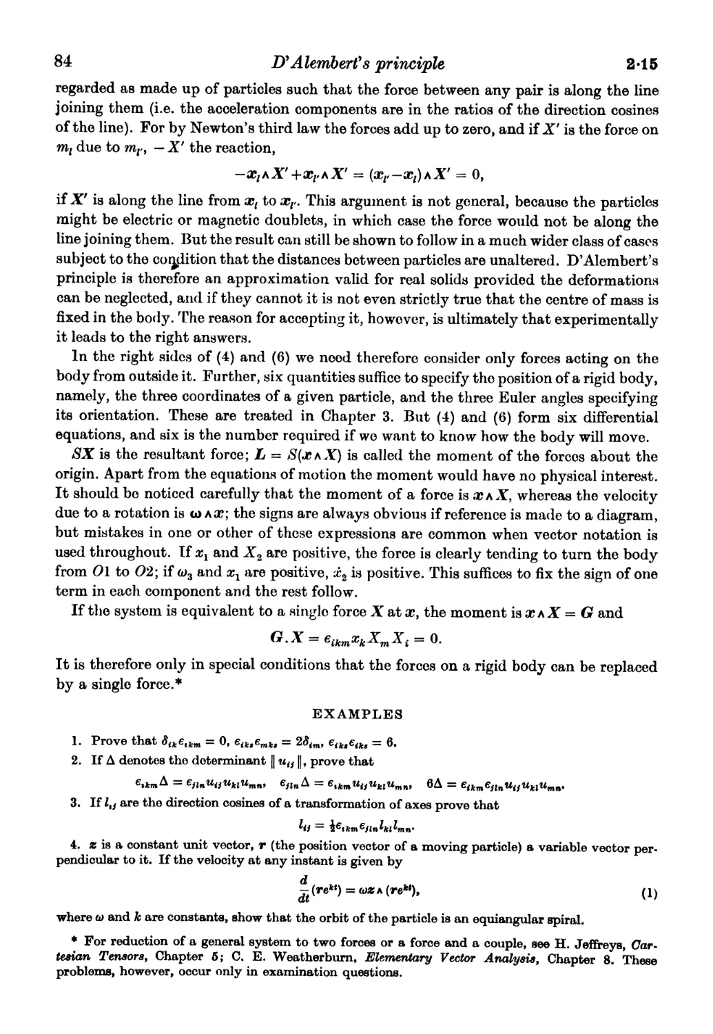
1-01. The relation of mathematics to physics. The simplest mathematical
notion is that of the number of a class. This is the property common to the class and to any
class that can be matched with it by pairing off the members, one from each class, so that
all members of each class are paired off and none left over. Tn terms of the definition we
can give meanings to the fundamental operations of addition and multiplication. Con-
sider two classes with numbers a, b and no common member. The sum of a and b is the
number of the class consisting of all members of the two classes taken together. The
prochict of a and b is the number of all possible pairs taken one from each class. We cannot
always give meanings to subtraction and division, because, for instance, we cannot find
a class whose number is 2-3 or 7/5. But it is found to be a great convenience to extend the
notion of number so as to include negative numbers, ratios of numbers irrespective of
whether they are positive or negative, and even irrational numbers. When this is done
we can define all the four fundamental operations of arithmetic, and the result of carrying
them out will always be a number within the system. We need trouble no more about
whether an operation is possible with a particular set of numbers, since we know that it is,
once we have given sufficient generality to what we mean by a number. 80 long as we
keep to the fundamental operations we can use algebra; that is, we can prove formulae
that will be correct when any numbers whatever are substituted for the symbols in them,
with only one exception, namely, that we must not divide by 0.
Now the formulae may still be correct when we replace the letters in them by something
other than numbers, and it is to this fact that the possi bility of mathematical ph ysics is due .
It is therefore useful to know just what conditions have to be satisfied if we are to take
over the rules of algebra into any subject that does not deal entirely with numbers. We
may then have to find new meanings for the fundamental operations (or have them found
for us) and for the sign = , but can still manipulate the symbols with their new meanings
in the old way. A suitable set of conditions is as follows.* We say that they are to hold
in a field F consisting of all elements of the system considered:
(1) For any a, b of F, a + b and ab are uniquely determined elements of F.
(2) b + a = a + b. (Commutative law of addition.)
(3) (a -f b) -H c = a + (b 4- c). (Associative law of addition.)
(4) ba = ab. (Commutative law of multiplication.)
(5) a(bc) = (ab)c. (Associative law of multiplication.)
(6) a(b -f c) = ab + ac. (Distributive law.)
(7) There are two elements and 1 in F, such that a + = a, al = a.
(8) For any element a of F there is an element x of F such that a H- x = 0.
(9) For every element a of F, other than 0, there is an element y of F such that ay = 1 .
* Stated first by Dedekind for the case where + and x have their ordinary arithmetic meanings;
in general by H. Weber.
JMP i
2 . Mathematics as a language 1-01
It is to be noticed that the first seven rules are true if F consists only of the positive
integers and 0, but the last two are false of that F, since there is no positive or zero
integer x that makes a-f# = 0ifa=l, and there is no positive or zero integer y that
makes ay = 1 if a = 2. The eighth rule introduces negative numbers and hence sub-
traction. The ninth introduces reciprocals and hence division and rational fractions.
The rules are true if F consists of all rational numbers, positive or negative.
The rules mention no ordering relation: that is, they suppose a meaning attached to
equality and therefore to =)= , but do not distinguish between greater and less. We could
agree to arrange the numbers in any order, keeping the same correspondences between
them according to (1), (7), (8), (9), and the rules would still be true. Algebra and pure
geometry can get on to some extent without such a distinction, but higher mathematics
cannot, nor can any kind of physics. A measurement is not a statement of exact equality
but of equality within a certain range of error. We therefore need new rules concerning
inequalities.
(10) For any a, b of F, either a > 6, a = 6, or b > a. (Law of comparability.)
(11) For given a, b of F, only one of a > b, a = 6, b > a can bo true. (Trichotomy.)
(12) If a > ft and 6 > c, then a > c. (Transitive property.)
(13) If a > I), then a + c > b + c for any c. (Adclitivity of ordering.)
(14) If a > b, c> 0, then ac > be. (Multiplicativity of ordering.)
(15) Ifa>b,b<a. (Definition of <.)
The use of mathematics in science is that of a language, in which we can state relations
too complicated to be described, except at inordinate length, in ordinary language. The
rules satisfied by the symbols are the grammar of the language. This point of view has
been developed greatly in recent years, especially by R. Carnap. But for a language to
be suitable it must satisfy two conditions. It must be possible to say in it the things that
we need to say; that is, it must have sufficient generality. It must also be self-consistent;
that is, starting from the rules themselves it must be impossible to deduce something
declared to be false by those rules. It would, for instance, be fatal to the scientific useful-
ness of mathematics if it was possible to prove by it that for some a and 6, a is both greater
and less than b. It was always taken for granted until the later nineteenth century that
mathematics was consistent. But then an unexpected set of difficulties cropped up, and
showed that a complete analysis of the foundations was necessary. The great Principia
Mathematica of Whitehead and Russell showed that all the propositions asserted in
mathematics concerning real numbers (not only ratios of integers, positive or negative)
could be restated as propositions about the elementary notion of comparing classes by
pairing their members, and demonstrable from the axioms of such comparison and others
relating to pure logic. Later workers have modified some of the latter axioms, and the
best choice of axioms is still a matter of discussion. Godel and Carnap, more recently,
have shown that the proposition that a given system of axioms for mathematics is con-
sistent cannot be proved by methods using only the rules of the system. But it is found
impossible to prove certain propositions that could be proved if the system was inconsis-
tent. We have to come back to something like ordinary language after all when we want
to talk about mathematics ! This work on the boundary between logic and what we usually
consider the elements of mathematics has a considerable modern literature, and it is well
for physicists to know of its existence, though its detailed study is a matter for specialists.
1*02 Physical magnitudes 3
1-02. Physical magnitudes. Generality requires that, in any particular field, the
language shall contain symbols for the things that we need to talk about and for the
processes that we carry out. A shepherd would be severely handicapped if ho had to do
his best with a language containing no words for sheep and shearing; in fact he would
make such words, and that is what we habitually do in science. So long as the language
is consistent it is none the worse for containing a lot of words that we do not use. A pure
mathematician, working entirely on the theory of numbers, can use ordinary algebra
freely in spite of the fact that ho may not need to use negative numbers or fractions. For
him rules (8) and (9) are just an unnecessary generality. Now in physics the fundamental
notion of measurement corresponds closely to that of addition, and most physical laws
are statements of proportionality, which corresponds to the notions of multiplication and
division. This is the ultimate reason why mathematics is useful. Thus, for instance, we
can say that if two bars are placed end to end to make one straight bar, the length of the
combined bar is the sum of those of the original ones. This is not a theorem or an experi-
mental fact; it is the definition of addition for lengths. Further, it is irrelevant which is
taken first; thus the commutative law of addition holds. Again, if we unite three bars, the
total length is independent of the order; hence the associative law of addition also holds.
These are experimental facts established by actual comparison with other bars. Those
rules are enough to justify the use of scales of measurement for length, by which any
length is compared with a standard one by moans of a scale, every interval of which lias
been compared with a standard object in the process of manufacture. Quantities measur-
able by some process of physical addition have been called fundamental mof/nititdea by
N. R. Campbell.* The most widely important ones are numbers (of classes), length, time,
and mass, but physical processes of addition can also be stated for area and volume, for
electric charge, potential, and current, and many other quantities.
There is a divergence of practice among physicists at the next stage. A statement that
a distance is 3-7 cm. contains a number and a unit. It is often thought that algebra applies
only to numbers and therefore that in the mathematical treatment the symbol used for
the distance refers only to the 3-7 and not to tho centimetres. The unit matters, otherwise
we should find ourselves saying that 10 mm. expresses a different length from 1 cm. and
that 1 cm. is the same as 1 mile; and this is contrary to physics because tho only justifica-
tion of using measurement at all is in the direct physical comparison by superposition.
We avoid this difficulty if we say that the symbol for the length refers to tho length itself
and not simply to the number contained in its measure. * 1 inch = 2-54 crn.' is a useful
statement; either symbol, '1 inch' or '2-54 cm.', denotes tho same length. In general
theorems this procedure can always be followed. When a particular application to a
measured system is made we naturally give the symbols their actual values in terms of
the measures, which will include a statement of the units; but in the general theory the
unit is irrelevant. The symbols will then be said to stand, not for numbers, but for physical
magnitudes.
The alternative method would be to let the symbols stand for the numbers, but then
confusion can occur, and does, between the relations between measures of the same system
in different units, which are different ways of saying the same thing, and ordifferent
systems in the same units, which say different things. If, however, the numerical values
in terms of special units are used for a and b in ah, their product will be the number in tho
* 'Elementary' might be better.
4 Dimensions 1 02
expression of ab in what is usually called the consistent unit for ab. The word germane,
introduced by E. A. Guggenheim, is better because it is not inconsistent to measure distances
upward in feet, horizontally in yards, and downward in fathoms; it is merely a nuisance.
With adequate care this method can be used correctly, but it has several disadvantages;
in particular it then leads to placing too much emphasis on the units and too little on the
fundamental physical comparisons without which the units would be useless. It also
suggests many comparisons that are physically meaningless, as we shall see in a moment.
If we use the notion of magnitude and retain the processes of algebra the question will
at once arise, what do we mean by a = b and a + b if a is a length and b a time or a mass ?
A meaning could be attached to a + 6, though it would be very artificial, but no physical
process will give one to a = b. But a/6 would have a meaning, being respectively a velocity
or a length per unit mass.
The group of rules (10)-(14) therefore needs modification. Those up to (9) could stand,
though they bring in many additions and subtractions and possibly some multiplications
and divisions that we shall never have occasion to use; but in addition to the three possi-
bilities enumerated in (10) we must admit a fourth, that a and 6 may not be comparable
and therefore belong to different fields, and their product and ratio may belong to other
fields again. This is a further disadvantage of the use of symbols to denote only the
number stated in a measure, since all numbers are comparable, and the language would not
exhibit the fact that it is meaningless to say that a time is greater than a density. We can
then say also that if a and b are not comparable, a + b is not a physical magnitude and
addition does not arise. The whole field of physical magnitudes is thus divided into plots.
Magnitudes in the same plot will be comparable, but their product will belong to a
different plot unless at least one of them is a number.
The language needed for physics is therefore not quite the same as ordinary algebra.
Since the latter is self-consistent and the statement that some magnitudes are not com-
parable cuts out some propositions from it and adds no new ones, the language of magni-
tude is also self-consistent. It will be seen that the modification corresponds to the notion
of dimensions. Quantities of different dimensions are not comparable; also some quantities
of the same dimensions are not. For instance, according to one pair of definitions in use,
electric charge and magnetic pole strength have the same dimensions, and they are both
fundamental magnitudes, but it is meaningless to add them. The field of physical magni-
tudes can be taken to satisfy the laws of algebra, but is classified; comparable quantities
satisfy ( 10) , and are capable of addition at least in calculation ; incomparable ones do not.
It should be noticed that failure of addition by a physical process is not confined to in-
comparable magnitudes. For instance, there is no process of combining two substances
of density 1 g./cm. 3 to give one of density 2 g./cm. 3 Density is not measured directly but
calculated from the additive magnitudes mass and length, and is called a derived magni-
tude. Some quantities can be both additive and derived; thus electric current measured
by its magnetic effect is a fundamental magnitude, but regarded as the charge passing
per unit time it is derived. Many derived magnitudes are ratios of two magnitudes of the
same dimensions; thus we could regard the shape of a triangle as specified by two ratios,
those of two sides to the third. These ratios are pure numbers and the rules of algebra
can be applied to them without change.*
* A similar treatment was advocated by W. Stroud; for discussion and applications to teaching,
of. Sir J. B. Henderson, Engineering, 116, 1923, 409-10.
1-03 Real numbers 5
1*03. Real numbers. Most of the present chapter will be already familiar to those
who have studied a good modern book on calculus, and it is not intended to compete with
standard works on pure mathematics. We think, however, that some discussion here is not
out of place, for several reasons. First, the latter works for the most part do not emphasize
why the refined arguments that they give have any relevance to physics, and physicists
therefore tend to believe that they are irrelevant. Secondly, they are liable to be so long
that a physicist can hardly be blamed if he decides that he has not the time to work
through them. Thirdly, the attention to very peculiar functions has led the subject to
be regarded as the pathology of functions. The reply is that every function, except an
absolute constant, is peculiar somewhere, and that by studying where a function is
peculiar we can arrive at constructive results about it that would be very hard to obtain
otherwise. But we are entitled to regard ourselves as general practitioners and to restrict
ourselves to the kinds of peculiarities that occur in physics; rare diseases may be handed
over for treatment to a specialist, in this case a professional pure mathematician.
The nature of the problem was foreshadowed in a theorem of Euclid that the ratio of
the hypotenuse to one side of an isosceles right-angled triangle is not equal to any
rational fraction. Euclid, it must be remembered, made no use of what we should now
call numerical measures of physical magnitudes. When ho said that two lines were equal
he meant that one could be placed on the other so that the two ends of one coincided with
the two ends of the other; this is the direct physical comparison and does not require any
numerical description of the lengths. When he said that the square on the hypotenuse
was twice that on a side ho meant that it could be cut into pieces and that the pieces could
then be put together so as to make the square on the side twice over. He was working
throughout with the quantities themselves, not with the numbers that we choose to
associate with them in measurement with regard to any special unit. The use of numbers
for this purpose is a choice of a language. What Euclid's theorem showed was that the
language of rational numbers was incapable of describing simultaneously the lengths of
the side and the hypotenuse of a triangle that could easily be drawn by the rules of his
geometry.
Measurement in terms of a unit is too useful a procedure to be lightly abandoned, and
it could be retained, consistently with Euclid's theorem, in any of the following ways:
(1) Since an infinite number of pairs of integers x, y can be found such that # 2 + y* z* t
where z is another integer, and so that x/y is as near 1 as we like, we could suppose that the
sides of a right-angled triangle satisfy z 2 + i/ 2 = z 2 exactly but that x = y is not true
exactly but only within the errors of measurement, and the sides are always exact mul-
tiples of some definite length. (2) We might say that x/y can be exact but x 2 -f y 2 = z 2 is
only approximate. (3) We can say that the language of rational numbers is not enough
for what we need to say, and that we need a fuller language in which x = y and x 2 -f y 2 = z 2
can be both said consistently. The last alternative is the one that has been universally
adopted by the admission to arithmetic of irrational numbers. It does not contradict
Euclid's axioms; the first does, since he assumes that a line can have any length,
and the second contradicts one of their best-known consequences. An experimental
proof that it is right is impossible because either (1) or (2) could be true within the
errors of measurement even if x, y, z were restricted to be integers. But they would
be intolerably complicated, and the adoption of either would require the existence
of an unknown and indeterminable standard of length such that all actual lengths are
6 Nests of intervals 1031
exact multiples of it, besides abandoning the simplicity of Euclid's rules without experi-
mental reason. The universal practice in physics is to adopt alternative (3) and create a
language of sufficient generality. We introduce real numbers and assume that the opera-
tions of addition, subtraction, multiplication and division can be applied to them in such
a way that the same fundamental rules as for rational numbers are satisfied, and that an
ordering relation satisfying rules (10)--(15) can be defined. They differ from the rationals
in possessing a certain property of completeness, which ensures, for instance, that there is
a real number ^2 whose square is 2. It is not obvious that this can be done without incon-
sistency (and it was certainly believed for 2000 years that real numbers were meaningless*),
but the 1 9th century investigations of Dedekind, Cantor, and others have established
their workability for all practical purposes. That is enough justification for our pur-
poses. Bui the Jogical justification involves the consideration of infinite collections.
It is indeed obvious that the evaluation of ^2 by root extraction or by successive
approximation to a continued fraction, if taken to a finite number of steps, can never
yield anything but a rational number; to give any exact meaning to ^/2 in numerical terms
requires an infinite number. Euclid's procedure does lead in a finite number of steps to
a ratio that can be identified with >/2, but does not describe it in a numerical way, and
the proof that his axioms are themselves consistent has so far been completed only by
way of the numerical approach. The notion of ^/2 is accepted at school largely because
we believe that a consistent system of measurement of physical objects is possible and
Euclid's axioms look plausible; but we forget that the Euclidean triangle is not the real
triangle, or, if we remember, we think that the real triangle is an imperfect representation
of the Euclidean one. Physically the Euclidean triangle is an idealized approximation
to the real one, and we cannot take it for granted that the idealization does not introduce
new troubles of its own.
1-031. Nests of intervals: Dedekind section. The fundamental property of real
numbers is that they can be approximated to as closely as we please by rational numbers.
When we say that
V2= 1-414...,
we assert the following set of propositions: (1) 2 is between I 2 and 2 2 ; (2) 2 is between
1-4 2 and 1-5 2 ; (3) 2 is between 1-41 2 and 1-42 2 ; (4) 2 is between 1-414 2 and 1-415 2 ; and so
on to any desired accuracy. At each stage this process can be regarded as separating the
decimals, to a given number of places, into two classes, those whose squares are respec-
tively greater or less than 2. At stage 3, for instance, the squares of 1-414, 1*413, 1-412
are less than 2, those of 1-415, 1-416, 1*417 greater than 2. We say nothing at this stage
about the fractions 1-4141, 1-4142, ..., 1-4149; but at the next stage we say that 2 lies
between the squares of 1-4142 and 1-4143. By taking a sufficient number of decimals
we can make the unconsidered interval as small as we like, since we divide it by 10 at
each step. Thus any decimal with a finite number of places will ultimately be classified
according as its square is less or greater than 2. Now this process determines a unique
infinite decimal, which we can take to be ^2, and it can be regarded as the limit approached
by the successive approximations from either side.
This process, which is capable of great extension, is an example of the definition of a
real number by a nest of intervals. We denote an interval with rational end-points a, b by
* Hence the name 'irrational numbers'.
1*031 Dedekind section 7
(a, 6), and a nest of intervals is a sequence of intervals (a l9 6^, (a a , 6 a ), ..., (a n , 6 n ), ... such
that each interval (a n + v b n+l ) is contained in its predecessor (a n ,6 n ), and the length
6 n a n of the nth interval becomes arbitrarily small as n increases. We can express the
last statement more precisely as follows: if e is any positive rational number, we can find
a number JV such that 6 n a n <e for every n>N. Any nest of intervals defines a real
number, which lies in every interval of the nest and can be regarded as the limiting value
of the approximating sequences a v a 2 , ..., a n , ... and 6 lf 6 2 -, b n , ... of rational numbers.
At each stage of the process we restrict the range and obtain closer and closer approxima-
tions to the real number we are defining.
A nest of intervals may turn out to define a rational number. For instance, if we con-
sider decimals whoso squares are respectively just less and just greater than 2-25, wo get
the nest (1 , 2), (1-4, 1-6), (1-49, 1-51), (1-499, 1-501), .... The only decimal lying in all those
intervals is 1*5, whose square is in fact 2-25. For every rational number we can construct
such a nest, so that the rationals are themselves real numbers.
A single real number can be defined by many different nests of intervals. For instance,
instead of dividing the interval by 10 at each stage wo could divide by 2, in this way
generating a binary fraction or 'decimal to base 2 '. It would take more than three times
as many steps to get as good an approximation, but the process defines the same real
number as before. Two nests (a n , b n ) and (a n , /J n ) define the same real number if and only
if (a n ,b n ) contains (a m ,/? m ) for sufficiently largo m, and (,/?) contains (a m ,b m ) for
sufficiently large m\ in fact only one of these conditions need bo known to hold the other
follows as a consequence.
We now come to the most important property of the real number system. If wo abandon
the condition that tho intervals of a nest shall have rational end-points, and consider
a nest (a n ,6 n ), where the a n and b n may be any real numbers, and b n -a n is ultimately
smaller than every positive real e, it can be proved that there is one and only one real number
lying in every interval of the nest. In other words, if we apply to the real numbers the
process that we have applied to the rationals, we got nothing now, but remain within
the system that we have already defined. This is the property of completeness mentioned
in 1-03.
It can be shown that the real number system is essentially the only one satisfying the
rules (1)-(15) and possessing the completeness property; that is, it is characterized
abstractly by these conditions.
Another important way of defining real numbers is by a Dedekind section or cut. If the
rational numbers are divided into two classes L and R such that every member of L is
less than every member of R, there is only one real number greater than or equal to every
member of L and at the same time loss than or equal to every member of R. If this real
number is rational, then it will be either the greatest member of L or the smallest member
of jR. For instance, L might consist of the negative rationals together with and tho
positive rationals whose squares are less than 2, and R of the positive rationals whose
squares are greater than 2. This cut defines the real number ^2.
Dedekind section arises most naturally when the numbers are classified according
as they possess or do not possess a certain property. For instance, 'x has a square
not greater than 2-25' defines an L class, the largest member of which is 1-5; 'x has
a square less than 2-25* defines an L class with no largest member, and 1-6 is the
smallest member of the R class. ( x is rational and has a square less than 2' defines
8 Indirect proofs 1-032
L and E classes of rationals with no largest and no smallest member respectively.
'x is real and has a square less than 2' defines an L class with no largest member
and an R class with smallest member ^/2.
In terms of the Dedekind section, the completeness property of the real number system
is equivalent to the statement that any cut in the real numbers defines a real number.
Thus many problems that have no answer in the rational number system can be solved
in terms of real numbers. We have so far considered only ^2, but we are also ready for
n and e when they turn up, and shall not need to search for a statement of each problem
in such a form that it can be solved in rational numbers. The use of the real number
system therefore avoids a lot of complications with no relevance to physics.
The methods of nested intervals and of Dedekind section are equivalent. If L and B
classes exist we can form a nest of intervals, taking a v a 2 , ... from L and 6 lf 6 2 , ... from R y
in such a way that the conditions required for a nest of intervals are satisfied. Conversely,
if a nest exists, some rationals r will be exceeded by a m for some ra, others will not be
exceeded by any a m . These inequalities define an L and an R class and the conditions for
a cut are satisfied.
If the nest (a m ,b m ) defines a positive real numbers, (l/6 m , 1/aJ will define I/a;. Then if
nests (a m , b m ) (a' m , b' m ) define x, x', (a m a' m , b m b' m ) will define xx'. ( - 6 m , - aj will define - x,
and whether x, x' are positive or negative, if (a m , b m ) defines x and , b' n ) defines x', then
( a m + a 'm> b m + b 'm) wiu define x + x'. Thus all the operations of addition, subtraction,
multiplication and division are defined for the real numbers and can be shown to satisfy
the fundamental rules. Pull details are given by Knopp.*
Neither method proves the existence of irrational numbers, but both show that they can
be used consistently and that any proposition proved by using them can be interpreted as
a true proposition about rational numbers (usually, of course, much more complicated to
state). In Principia Mathematica tho aim is somewhat more ambitious: a real number is
interpreted as a class of rationals (essentially the Dedekind L class) and meanings are
given to the laws of algebra in terms of certain operations on these classes; and the laws
so stated are proved to be true. In this sense there is an actual proof of the existence of
irrationals satisfying the laws of algebra.
1-032. e; indirect proofs. A peculiarity of the basic theorems about real numbers is
that many of them seem incapable of direct proof. They are proved by the process known
as reductio ad absurdum. We have to state the contradictory of the theorem and show
that this itself leads to a contradiction; and then we argue that the theorem cannot be
false and therefore must be true. But since most of the theorems have conclusions of the
form x = y, their contradictories are inequalities of the form 'x<y or x>y\ Most be-
ginners find it much more difficult to handle inequalities correctly than equalities, and
of all the difficulties found in mathematical physics the greatest found by many students
is in learning to approximate. That is why lower marks are obtained in problems of small
oscillations in dynamics and of potentials of nearly spherical bodies than in any other part
of the Mathematical Tripos. Nature does not consist entirely, or even largely, of problems
designed by a Grand Examiner to come out neatly in finite terms, and whatever subject
we tackle the first need is to overcome timidity about approximating. A difference
between the theory of the real variable and dynamics is that in the former we are willing
* Theory and Application of Infinite Series.
1-083-1-OM Sets g
to consider arbitrarily close approximations carried to any number of stages, whereas in
the latter we only want an approximation close enough for the practical end in view.
But experience in the one will tend to produce confidence in the other.
The simplest type of argument of this form is : if x ^ 0, and x < e, where e is positive but
can be chosen as small as we like, then x = 0. For no value of x greater than can be less
than every positive e. An immediate extension is obtained by considering the modulus
or absolute value of a, denoted by | x \ and read * mod x '. This is equal to x when x is positive
or zero, and to - x if x is negative. It is therefore always ^ 0. Then if | x \ < e for all positive
e, | x | = and therefore x = 0. Note that | | + | y | | s + y |, | #-y | ^ | a? | - | y |.
It is necessary for this argument to use a symbol for the small quantity. If we said
'e = 0-001 ', and proved that | x \ < 0-001 by calculation, an objector might say 'you have'
not proved that x = 0; it might be 0-OOOr. The symbol e, to denote an arbitrarily*
small quantity, prepares us for such an objection, since by proving that | x \ is less
than any e we are ready to disprove any value of x, other than 0, that an objector
might suggest.
The essential point is that we are concerned with processes that in the most general case
could be completed only in an infinite number of steps, e.g. showing that two nests of
intervals determine the same real number. We overcome this and obtain a finite proof by
saying that if a + b, \ a - 6 | has a definite value M , which is not zero. If, then, we can show
that M<e for every positive e, it follows that M = 0, contradicting the hypothesis, so^
that a and b must be equal.
1-033. Sets. A limit-point of a set of numbers is a number x such that for any e>
there is a member of the set, y, different from x, such that < | y - x \ < e. It follows that
there arc infinitely many values of y satisfying this condition For by definition there
is one; call this ^ and take a new e, say e l9 less than \y t -x\. Then there must be
another y of the set, say t/ 2 , such that 0< |y 2 -tf | <e v The process can evidently be
continued indefinitely.*
Clearly no finite set can have a limit-point. But an infinite set also may have none;
consider the set of all integers. No member has another within distance 1 of it, and no
number not an integer can have more than one within distance . In the set of rational
numbers every member is a limit-point since there is a rational number as near as we
like to any other. The same applies to the real numbers. A set may have only one limit-
point; consider for instance the numbers n- 1 , where n can be any integer. There are
infinitely many within any finite distance from 0, which is therefore a limit-point; but
around any other number, rational or not, we can take an interval that contains no
member of the set, other than the number itself if it is a member. A limit-point of a set is
not necessarily itself a member of the set. We can, for instance, make a set of rational
numbers whose limit-point is ^2 by taking the successive approximations to ^2 by
decimals, but ^/2 itself is not a rational number.
1-034. // a set has infinitely many members mthin a finite range a^x^b, then it has at
least one limit-point x such thata^x^b. For if we bisect the range, one half at least must
* It should be noticed that expressions such as 'the process can be continued indefinitely 1 and
'and so on' cover applications of mathematical induction. We shall seldom state such arguments in
full, for reasons of space. The student should, however, complete some of them for himself for
practice.
10 Sequences ! 035-1*04
contain an infinite number of points of the set; bisect that half. One half again contains
an infinite number, and we see that by repeating the process we can find an interval as
small as we like containing an infinite number of points of the set. But this corresponds
to the method of specifying a real number by a nest of intervals and therefore identifies
a real number such that any small interval about it contains an infinite number of points
of the set. It is therefore a limit-point of the set. This is known as the Bolzano-Weierstrass
theorem.
1-035. An infinite set is enumerable if its members can be paired with the positive
integers in such a way that to each member corresponds one and only one positive integer,
and vice versa. Thus the squares I 2 , 2 2 , ...,7i a , ... form an enumerable set, since to each n
corresponds one n 2 and to each n 2 one n. The rational fractions between and 1 form
another, for they can be arranged J, J, f , J, f , , f , f , f , . . ., and the one that occurs in the
nth place can be paired with n. The whole of the positive rationals form another, since
they can be arranged, ^, , f , J, f J, f , f , -}-, .... Here the numbers are arranged in groups,
the sum of the numerator and denominator being the same for all in each group and greater
by 1 than in the previous group, while those in each group are arranged in order of
increasing numerator. In these two cases the comparison with the positive integers
requires complete rearrangement from the natural order.
Not all infinite sets are enumerable. Far the most important exceptions are the set of
all real numbers and the set of all real numbers within a given finite interval. Cantor
proved that however we may try to put them into a one-one correspondence with the
positive integers there will always be some omitted.
1-036. Necessary: sufficient. If two statements denoted by I and II are so related
that if I is true, then II is true, we say that I is a sufficient condition for II and II is a
necessary condition for I; that is, I cannot be true unless II is true. If II is true if and
only if I is true, then I is a necessary and sufficient condition for II, and vice versa. In
this case we may also say that I and II are equivalent.
In general if a necessary and sufficient condition can be stated for the truth of a
given proposition several can. For instance, a necessary and sufficient condition that x,
a real quantity, shall be is | x \ <e for any assignable positive e; but others are x 2 =
and a; 3 = 0. A necessary and sufficient condition that ax 2 2bx + c>0 for all a; is that
a > 0, ac 6 2 > 0; but another is that c> 0, ac 6 2 > 0.
A necessary and sufficient condition may contain superfluous information. For
instance, if ax 2 2bx + c>0 for all x, we must have a>0, c>0, ac 6 2 >0, and con-
versely. Hence a > 0, c> 0, ac> 6 2 is a necessary and sufficient condition. But if ac> 6 a ,
either a > or c> implies the other and one of them is superfluous in the sense that it
follows from the other information given. On the other hand either a > 0, c> 0, or ac> 6 a
by itself would not guarantee that ax 2 2&# + c>0 for all x: none of these conditions
alone is sufficient. A set of necessary and sufficient conditions for the truth of a
proposition is called minimal if the conditions left when any part of them is removed
are not sufficient.
1-04. Sequences.* In considering the properties of a set we are not restricted to
taking the members in any particular order. In the argument of 1-034, for instance, the
* Fuller discussions of sequences than are possible here will be found in K. Knopp's Tlieory and
Application of Infinite Series and in Hardy's Pure Mathematics.
1*041 Convergence 11
points actually in any range are determined by the specification of the set, just as, if we
put some balls into a box, what balls are in the box has nothing to do with their rearrange-
ment by shaking or sorting.
When we come to study properties essentially connected with a particular order we are
dealing with sequences. The numbers 1, 2, 3, ... in ascending order constitute a sequence;
if they were rearranged, but in such a way that we always knew whore to find a particular
one, they would form a different sequence but the same set. If we write s n for the nth in
a given arrangement, the property s n+1 - s n = 1 is true for all n for the original order but
for no other. In general if s n is completely specified when n is given, s n may be described as
a function of the positive integral variable n, and the values s v s 2t ...,s n , ..., for successive
values of n, form a sequence. (Those who have some knowledge of series often suppose at
first that the terms of a sequence are to be summed, but this is not so.) Both
*' 2' 3' '" n' " (1)
and 1, 2, 1, 2, 1, 2, ... (2)
are sequences. In the first the members are the members of an infinite set arranged in a
certain order. In the second they are the members of a finite set repeated over and over
again.
A sequence whose general term is s n can be denoted by {s n }.
1-041. Bounded, unbounded, convergent, oscillatory. Let M be an arbitrary
positive number; it is possible that whatever M we take there is at least one value of s n
such that | s n \ > M. Such a sequence is called unbounded. s n = n is an obvious example,
fo^we need only take n to be any integer greater than M. By an argument similar to that
for limit-points, an unbounded sequence must have an infinite number of terms such that
| s n | is greater than any assigned M.
If we can choose an M such that all | s n \ are less than M , the sequence is called bounded.
Both the sequences given at the end of 1-04 are bounded; the condition holds for both if
M = 3.
If there is a number s such that, given any positive number e, we can choose m ao that
for every n > m
|n-*|<*> U)
the sequence is said to be convergent, and to have limit s. We then write
(n->oo), (2)
or lim s n = s.
n->co
The arrow is read 'tends to'. Wo can write simply
= , (3)
if no ambiguity is possible. Of the above examples 1-04(1) is convergent with limit 0;
we need only take m> 1/e. 1-04(2) is not, because whatever s and m we take, if e< |,
there will be terms with n > m such that | s n a \ ^ > e.
The most important property of a convergent sequence is that if we have a rule for
calculating each term, then we can calculate the limit to any accuracy we like. Some
12 Limit-points 1-042
methods of approximation (cf. Chapters 9, 17) will prove that a quantity lies within a given
range, but this range is not arbitrarily small; the accuracy may be enough for the
application in view but is not capable of being improved indefinitely.
A sequence that is bounded but not convergent is said to oscillate finitely, or simply to
oscillate. An example is 1-04(2); another is
*n = (-l)" + ^. (4)
Unlike 1-04 (2), all s n are different. The sequence is bounded, because | s tl | < 2 for every n\
but it does not converge since for large n the members are alternately near to 1 and - 1,
and (1) cannot be satisfied if e < .
If for any M there is an m such that s n > M for all n > m, we write
(5)
8 n = n and s n = n 2 are examples.
If for any M there is an m such that s n < M for all n > m, we write
*n->-- (6)
s n = n and s n = n 2 are examples.
Other types of unbounded sequences are represented by
) n n, s n = n cos 7771, s n = n(\ -cos?).
These cannot be said to tend to anything particular, not even infinity, and are sometimes
called infinitely oscillating. Unbounded sequences can be called divergent] but different
writers use this term in different senses, some (e.g. Bromwich and Hardy) excluding
infinitely oscillating sequences and some (e.g. Knopp) including finitely oscillating ones.
A useful device is to classify sequences according as they have or have not the properties
(1) for any m, and any positive M, there is an n > m such that s n > M,
(2) for any m, and any positive M, there is an n > m such that s n < M .
Sequences with neither property are bounded. If a sequence possesses (1) but not (2),
it is bounded below, unbounded above, and similarly for the other two cases.
Note that no definite meaning is attached to infinity as such. What we do is to give
meanings to all the expressions that contain the word infinity or the symbol oo. s n -**cc>
is a shorthand statement of the property of {s n } stated in the definition of *^->oo', and
does not imply the existence of any real quantity denoted by oo.
Infinity is excluded from the rules of algebra, not because there is any inconsistency
in the notion of infinite numbers, but because they follow different rules. In fact
the notion of an infinite set is implicit in most of our theory, since there are infinitely
many values of x in any interval of x. A consistent algebra of positive infinite numbers
was set up by Cantor, and has been extended by many later writers. But it is different
from ordinary algebra. If a and b are positive infinite numbers we can define a + b and ab
uniquely; but a 4- 6 need not be greater than a in fact it is in general equal to a or to 6.
It is not possible to define a 6 and a/6 uniquely. Consequently an algebra that includes
both finite and infinite numbers must still distinguish between them in its rules.
1*042. If an infinite set has a limit-point, s, then we can form a sequence from its members
whose limit is s; if it has more thin one limit-point we can farm sequences tending to any of
them.
1*048-1*044 Upper and laiver bounds 13
We have shown (beginning of 1-033) that there is an infinite number of members of
the set within a given distance of a limit-point; if we take specimens in the order indicated
we have a sequence with the property required.
1*043. Any sequence formed of different members of a bounded infinite set with only one
limit-point s will converge to the limit s. It is clear that in forming a sequence from the set
we have a choice at every stage; hence the number of different sequences that can be
formed from the set is infinite. We have to show that they all have the same limit. For
any m, the number of terms s n of a sequence with n > m is infinite. But since the set is
bounded and has only one limit-point, any interval not including the limit-point can
contain only a finite number of members. Hence for any e only a finite number of members
lie outside the range s \e, say s a> Sp, ...,8^. Let m be the greatest of a,/?, ...,/4. Then for
all n greater than m, | s n s \ ^ ie<e, and therefore the sequence converges to s.
The result does not follow if the members of the sequence are not required to bo dif-
ferent and some can recur infinitely often. For instance, if the set is that of the reciprocals
of the integers, its only limit-point is 0; but if repetitions are allowed we can form from
it the sequence 111
1, 2> * 3' lj 4' *' > ,' !
which is oscillatory. If no member recurs more than a fixed number k times, however,
the result still follows by a simple extension of the argument.
1 '044. Upper and lower bounds. A set (or sequence) bounded above has an upper bound ;
and one bounded below has a lower bound. The upper bound of a set is a quantity M such that
110 member of the set exceeds M, but if e is any positive quantity, however small, there is
a member that exceeds M e. The lower bound is a quantity m such that no member is
less than m, but there is always one less than m-f e.
We use the method of Dedekind section. There are quantities a such that a is exceeded
by some member of the set; for we might take an a less than a known member of the set.
Since the set is bounded above, there are quantities b that are not exceeded by any member
of the set. Every 6 is greater than any a, and every quantity of the same dimensions is
either an a or a 6. Hence the quantities a form an L and b an R class, and determine
a cut, say at M . M is a member of the .R class. For if it was a member of the L class it would
be exceeded by some member of the set, say K, and there would be no quantities b between
M and K] hence M would not be the quantity given by the cut. Hence no member of the
set exceeds M . Also M e is in the L class and therefore is exceeded by some member of
the set. The corresponding result for lower bounds follows similarly.
The argument does not suppose the set infinite; but for a finite set the greatest of the set
is the upper bound. For an infinite set all members may be less than the upper bound; for
the set 1-04(1) the upper bound is 1 and is equal to the first term, but the lower bound is
and no actual member is 0.
What we call the upper bound is often called the least upper bound] and any quantity such
that no member of the set exceeds it is then called an upper bound.
Note that if s n < t n for all n, and s n -+ s, t n -+ t, then s ^ t, not 8 < t. Consider s n = 1 - 2 - n ,
t n = 1 - 3~ n . Here s = t. We may regard (s n , t n ) as an interval whose length tends to zero,
but these intervals do not constitute a nest because each is not part of its predecessor,
and, in fact, the whole of each interval is on the same side of the limit.
14 General principle of convergence 1-0441-1-046
1 -0441 . // 8 n > 8 n _i for all n, and the sequence is bounded, then the sequence converges. Let
the upper bound of s n be s. Then for all n, s n < s. But also for any e there is an m such that
s m > s - e; and then for every n > m
and therefore the sequence converges with limit s.
1*0442. Ifs n > s n ^ l9 t n ^ t n _ lt and for every m there is an n such that t n > s rn , and for every m
there is a p such that s p > t m , and {s n } is bounded, then {t n } converges to the same limit as {s n }.
For t n has upper bound s = lim s n , and if s s m < e, there is an n such that s - 1 n < e, and
s-t p <e for ollp>n.
1*045. The general principle of convergence. A necessary and sufficient condition
for convergence of a sequence {s n } is that for any positive quantity e we can choose m so that
for all values of n and p, greater than m,
p
-* n \<e. (1)
First, we show that the condition is necessary. Let s be the limit. Then we have to
show that an m exists such that (1) is true. For any positive o> we can take an m such
that for all values of n and p greater than m
\s n -s\<a), \s p -s[<o), (2)
and therefore
| p - n |<2w. (3)
Take o> = e; then | s p - s n \ < e. (4)
To prove that the condition (1) is sufficient, wo notice first that since s v s 2 , ..., a m+1 are
all finite, and all s p , with p > m, satisfy (1) with n = m+ 1, the sequence is bounded.
Suppose first that there is a quantity s such that s n = s for an infinite number of values
of n. Take m so that (1) is satisfied for all n, p>m. There is an n>m such that s n = s.
Hence | s p s \ < e for all p>m. Hence the sequence converges.
Suppose, on the other hand, that there is no s such that s n = s for infinitely many values
of n. Then for any m there is an n > m such that s n is different from all of s l ... s m . Hence
the values of s n form an infinite bounded set, which must therefore have a limit point.
Denote this by s. Then for any positive (o there are infinitely many values of n such that
| $ n s | < o). Take m so that | s p s n \ <o)fora,l\n,p>m. There is always an n > m such that
j s n s | < a). Hence for all p >m, \ s p s \ < 2 a) and convergence follows, since we can take
6> = Je.
The condition can also be stated: A necessary and sufficient condition for convergence of
( n ) is that for any positive e we can choose m so that for all n ^ m, | s n s m \ < e. This is obviously
implied by the above condition (1). Conversely, if p^m, n^m, then \8 p & m \<e,
I *n "" s m I < J hence | s p s n \ < 2e, which is also arbitrarily small.
The device of introducing a subsidiary arbitrarily small positive quantity, usually
denoted by 6>, <J, or ?/, which is later defined as a fraction of e, will be met frequently in
theorems where the quantity to be proved less than e is expressible as the sum of several
parts.
1-05 Series 15
1*05. Series. If the nth term of an infinite series is u n , the sums
constitute a sequence. If this sequence is convergent we say that the series
where n is now mado indefinitely great, is convergent; and we call the limit of s n the sum
of the series.* If {s n } is not convergent but finitely oscillating we shall speak of the
series as finitely oscillating.
To every theorem about sequences corresponds one about series; for if {s n } is a
n
sequence, and we take u { = s lf u n = s n s n _ 1 for n> 1, v Uf = s n .
The geometric series is x n = 1 + x + # 2 -f . , . .
n0
n-+l
Here, if x =(= 1 ,
and | a; n+1 1 becomes indefinitely large with increasing n if | # | > 1 . If | # | < 1 , x n + l tends to O.|
Hence the series is convergent if | x \ < 1, but not if | x \ > 1 . If x = 1 , the sum of n terras
is n, and the series is not convergent. Ifx = 1 the sum of any odd number of terms is 1 , but
that of any even number of terms is 0. The series therefore oscillates finitely. A necessary
and sufficient condition for the series to converge is therefore | x \ < 1.
00 11
The Riemann series is S n ~ x = * + - + -- + . . . .
n=0 *
First take x> 1. We can take the terms in batches:
and the sums in brackets after the first are respectively less than
2 4 __L 1
2^ 4^"' " ""2*"^' (2*- 1 ) 2 ' "*"
Then, if m = 2 r - 1, and w,
which can be made <e by taking r large enough. Hence the series converges if x> I.
If x = 1, we write
and all the sums in brackets exceed |. Hence the series is not convergent; s n -> oo. All the
terms after the first are increased if < x < 1 ; hence again s n -> oo.
The related series for log 2 is
* As for sequences, different definitions of divergent are in use; some writers restrict the term to
cases whore w ->oo or * n -> oo, others call all non -convergent series divergent.
t Strict proofs of these apparently obvious statements will be found in Hardy's Pure Mathematics,
pp. 134-5.
16 Absolute convergence 1*061-1*052
Here -. =
and the sum in brackets is >0 whether n-p is even or odd. But also
._. _ + (JL_/_i-__L)_(_ 1 __..i ).\
p n " [n+l \n+2 n-f3/ \n + 4 n + 5/ J
and every expression in brackets ( ) is positive. Hence
<l*-*l<iiVI.
and this is less than e for all n,p > m if (ra-f 1) > 1/e. Hence the series is convergent.
The argument can be adapted at once to show that if u n > 0, u tl > u ll+1 for all n, and
, then the series
is convergent.
1*051. Absolute convergence. If the series S | u n \ converges, X u n converges; for the
sum of any batch of terms u n to u p cannot have a modulus greater than the sum of the
corresponding terms | u n \ to | u p |. In this case %u n is said to be absolutely convergent; if
*Lu n is convergent but | u n \ is not, %u tl is said to be conditionally convergent. (The word
semiconvergent is sometimes used, but the prefix is misused, and the same word is also
used for asymptotic series, which are best not regarded as infinite series at all. This word
is therefore best avoided.)
We have seen that the series obtained from that for log 2 by taking all the signs positive
is not convergent. Hence the series for log 2 is conditionally convergent. The geometric
series, if convergent at all, is absolutely convergent.
1 -052 . Rearrangement of series. The sum of an absolutely convergent series is unaltered
by taking the terms in any order. Let I t u n be absolutely convergent, with sum s, and %v n ,
the same series, but with the terms differently arranged. Tt is understood that every term
of either scries appears in the other, but not in general in the same place. Take an arbitrary
positive quantity o) and choose m so that the sum of the moduli of any batch of terms
after the wth formed from the first series is less than d). Take m' so that all the terms u n
up to u m appear in the second series for values of n' less than m'. Write
Then s' m > s m is the sum of a set of terms of the first series after the wth and its modulus
is < (i). Also if we take n',p'> m', s p , s' n , is the sum of another set of terms of the first
series after the mth and therefore its modulus also is < o>. Hence the second series is
convergent. Let its sum be s'. Then
and can therefore be proved less than any arbitrary e by taking <y = Je. Hence the two
series have the same sum.
The theorem is not true of conditionally convergent series. It can be shown that if
S u m is conditionally convergent we can rearrange it so as to make the sum anything we like.
They have a precise meaning when the order of the terms is given, but not otherwise.
1- 053-1-06 Double series 17
They usually converge too slowly to be of much use for computation, but they can be used
in theoretical work.
Tests for convergence based on the use of 'comparison series' are so closely related to
tests for uniform convergence that we shall postpone them till we discuss the latter
property (1-115, 1-117).
1-053. Double series. Similar remarks apply to double series, in which the general
term is u m >n . The condition of convergence is now that we can choose m, n so that for all
p' q' P
P>P' greater than ra and all q, q' greater than n, the sums S u r 8 , 2 S % a differ by a
rl *1 ' r~l s-*l '
quantity with modulus less than e. Absolute and conditional convergence can be defined
similarly, and it is again true that an absolutely convergent double series has the same
sum however the terms are arranged. The proofs differ only in complexity from those for
simple series.
1*06. Limits of functions: Continuity. In the most general sense, when we say
that f(x) is a function of x in some range of values of a; we mean that for every value of a:
in the range one or more values off(x) exist. We can, for instance, speak of a function ofx
that is equal to 1 if # is rational but to if x is irrational. Such a function would be fairly
regarded by a physicist as pathological, and he is interested in a much narrower class of
functions, roughly speaking such as can be represented by graphs.* It will usually also
be required that the function shall be single-valued, but not necessarily. Thus for the circle
we have y = + <J(a 2 x 2 ),
and y is a function of x\ but we get its values over the whole circle only by taking both
signs for the root. A single-valued function of # in a range is one that has precisely one
value for each value of #. We shall in the first place consider single- valued functions only.
If # is a real variable, its values within any assigned interval constitute an infinite set,
and the corresponding values of f(x) in general constitute another. From these sots wo
can form sequences; wo take values
x l> X 29 > %n' >
and the corresponding values of f(x)
If we write x n = x + h n , and the limit of h n is 0, the limit of x n is x. The theory of con-
tinuity concerns the circumstances under which the limit off(x n ) will bef(x). In practical
cases it usually is, but not always. The sequence {f(x n )} may be unbounded or oscillatory;
and even if it is convergent its limit may not be f(x). It may also happen that different
sequences of values h n give limits for/(# n ), but different ones. Physically the latter cases are
exceptional, but it is important to notice that they can occur for quite ordinary functions.
The commonest is where f(x + h), for some value of x, has one definite limit as A->>0
* This function is frequently used as a warning. It can be used for that purpose at once. We might
try to define a pathological function as one that is neither a continuous function nor the limit of one.
But nothing could be more ordinary than the function cos 2n m ! nx, whiVh tends to this function when
m first tends to infinity and then n does.
JMP a
18 Continuity 1-061
through any set of positive values, and a different one as A-> through any set of negative
values. Such a case is called an ordinary or simple discontinuity. For instance, if
the limit of f(h) as h ->0 through any set of positive values is 1, and that as h ->0 through
any set of negative values is 0. This is a very common function in physical applications,
since it represents, for instance, a force that begins to act on a system at a definite instant
and thereafter is constant. It is usually known
as the Heaviside unit-function. The postage on
a letter, considered as a function of weight, has
simple discontinuities. The value at x = usually
does not need to be specified in experimental
applications, because for an object to be visible -''
it must have some size, and therefore if x is a
,. . , v ** Simple discontinuity : the Heaviside
position coordinate we cannot observe a quantity
at an exact value of #, but only a mean value over
a range. Similarly, if x is a time we cannot observe a quantity at a single moment but
only over a non-zero interval. The usual tendency in pure mathematics is to insist that the
function shall be specified for all values of the independent variable, but in physics it is
usually enough that its integral shall be determinate. As the value of the function at a
single point, provided it is finite, does not affect the integral, it is usually irrelevant to
physical applications, and if a special value is assigned it is for the sake of convenience.
The notations, for h > 0,
limf(x + h) = f(x + ), limf(x - h) f(x - ),
fc->0 h-+Q
are often used. Then the case we have been considering is one where
It may happen that /(a + ) = f(a- ) but is not equal to /(a). Such a function is said to
have a removable discontinuity, but as /(a) does not affect the integral such discontinuities
are not of much importance. It is, of course, impossible to illustrate by a graph.
A limit will not exist at all if the function is unbounded in tho neighbourhood of a
value of a;, as for/(#) = l/x near x = 0. For any sequence of values of x tending to 0,/(#)
will be unbounded. Again, if f(x) = 8in(l/#), and x tends to through the values Ijnn,
where n is an integer, the limit is 0. But if it tends to zero through the values l/(n + ) n it
tends to -I- 1 if n is restricted to be even and to 1 if n is restricted to be odd. This kind of
misbehaviour is the most troublesome to detect when the definition of the function is at
all complicated, and also it is the kind that is most easily forgotten.
1-061. Definitions of continuity at a point and in an interval. All types of
discontinuity are excluded if for any e we can choose a positive quantity $ such that,
provided I h \ < S,
F ' !
and if this is satisfied we say that /(a) is continuous at x = a. For if we take any sequence
{A n } tending to 0, there will be an m such that | h n \ <S for all n > m, and then
1-062 Continuity 19
Hence for all such sequences f(a + h n ) tends to /(a). We can also say that a function is
continuous in an interval if it is continuous at every point of the interval. It is necessary
sometimes to distinguish between closed and open intervals. f(x) is continuous in the
open interval a < x < b if it is continuous for every value of x such that a<x<b. Tt is
continuous in the closed interval a ^ x ^ b if this condition is satisfied and also
Note that to say that f(x) is continuous at x = c implies that/(c) is finite; for otherwise
we could attach no meaning to f(c -f h) -/(c) at all. Similarly, if/(.t') is continuous in an
interval it is finite at all points of the interval. We shall prove that in the latter condition
it is bounded in the interval if this is closed, but not necessarily if it is open.
We denote the closed interval a ^ x ^ 6 by (a, 6) and the open interval a <*x < b by \a, />].
When we speak of a closed interval (a, 6) it is understood that a and 6 are finite, that is,
that the interval is bounded. It is possible to speak of half-closed intervals a < x < 6 or
a < x < 6, but we shall use no special notation for them.*
Note that every point x of an open interval is an interior point; that is, there are points
y , z of the interval such that a<y<x<z<b. This is not true for a closed interval si tico x may
then be equal to a or to b. But if a, b are finite they are limit-points of the sot in [a, b].
Another way of expressing the distinction between closed and open intervals is to say that
all limit-points of sets in a closed interval are members of the interval; those of sots in an
open interval may riot be, since those of some sets are the end-points. When we say that x
is within an interval (or in later chapters within a region) we mean that it is an interior
point; if we say that it is o/a closed interval or region it may be an end or boundary point.
Functions that are continuous except at a finite number of points, whore they have
simple discontinuities, are called sectionally continuous.
A function is continuous if it is differentiable; the converse is not true, as we see from the
example of <Jx in ^ x < 1. This is continuous in the interval, including the end-points, but
is not differentiable at O.f Functions have actually been constructed that are continuous
everywhere in an interval but differentiable nowhere. As a rule we shall be concerned with
functions that are differentiable except possibly at isolated points, but such points are
very numerous in crystal physics. There is a theorem of Weierstrass that any continuous
function can be represented as closely as we like by a polynomial throughout any finite
range, or by a sum of sines and cosines with suitable coefficients (cf. 14-08). Consequently,
though a continuous function is not necessarily differentiable, it can be replaced with
as much accuracy as we like by a function that is differentiable.
1 -062. Covering theorems. We see that the property of continuity asserts that every
point x of the interval (a, 6) is in an interval [x 6, x 4- ty] (where 3 and 77 may depend on x)
such that (1) # is an interior point of the interval (except where x = a or 6, when it may be
* Most books, where they use special notations for open and closed intervals, use ( ) and [ ] in
the opposite senses. We have considered altering our notation, but the danger of omissions is so great
that we have not ventured.
t Nomenclature varies between different writers in such a case. However we choose x nt positive
and tending to zero, (<Jx n Q)/x n ultimately exceeds any given positive value. If f(x) = x sin (1 /x) 9
f(x n )/x n can be made to tend to any limit between 1 and 1 by suitable choice of the x n . In the
latter case, /'(a?) is said not to exist at x = 0. For f(x) = Jx,f'(x) would be said by many writers to
be infinite at x = 0. It is a matter of definition whether we say that/ / (a?) does or does not exist when
[f(x + h) -f(x)}/h -> oo; we shall usually say that it doee not.
20 Heine-Borel theorem 1-0621
an end-point), (2) the length of the interval is not zero, (3) for every point of the interval
a certain property holds, in this case
!/()-/(*) I <.
We can show that in such circumstances it is possible to choose a, finite number of intervals
such that every interval satisfies such conditions and every point of (a, b) belongs to at
least one of them. For different purposes we need to make the choice in somewhat different
ways, and two theorems are therefore needed to show that it is possible.
1-0621. The Heine-Borel theorem. // every point of a closed interval (a, b) is within
some interval I of a family F, then there is a finite subfamily of F such that every point of (a, 6)
is within at least one interval of the subfamily. We say that / covers (c, d) if every point of
(c t d) is an interior point of / (i.e. not an end-point).
There may be an interval / belonging to F that covers the whole of (a, 6). If so there is
nothing to prove. If not, bisect (a, b). There may be a pair of intervals I v 7 2 such that
every point of (a, \a, + \b) is interior to I I and every point of (\a + \b, b) to 7 2 . If either half
is not included in an interval /, bisect that half. We say that in a finite number of steps we
shall arrive at a stage where every portion of (a, 6) lies within at least one interval /. For if
not, the successive bisection of intervals will give a sequence of intervals, each part of
tho preceding one, and each half the length of the preceding one, and none of them
included in an /. Such a sequence forms a nest of intervals and identifies a number X Q
common to all its members. But by hypothesis :r is interior to an 7, say 7 , and hence there
is a positive S such that all points of (x - 8 9 x + S) are in 7 . Therefore all intervals of the
nest whose lengths are less than 8 are included in 7 , and we have a contradiction. Hence
the process of bisection leads in a finite number of steps to a set of subdivisions such that
every division of (a, 6) is wholly interior to some /. Taking for each division an / that
includes it we have the theorem.
A slight modification is often made where an end-point, say a, is an end-point of an
interval of the family, say 7 fl , closed at a; I a is still supposed of non-zero length S a . Then
a is interior to the interval J a (a- J # a ,a + a ), and the argument applies to the set of
intervals J, where J is the same as 7 except that I a is replaced by J a \ every point of (a, 6)
is an interior point of at least one J. But then it follows that every point of (a, 6) is an
interior point of some 7 except that a may be an end-point of I a or 6 of I b provided that
I a has a as a member and I b has b.
A trivial application is the axiom of Archimedes. Every point of (0, 1) lies in some
interval of length 1/n, where n may be any positive number. Hence a finite set of intervals
of length 1/Ti will cover the whole of (0, 1) so that every point lies within at least one of these
intervals. A suitable set is
The theorem also gives the Bolzano-Weierstrass theorem (1-034) as a special case.
If possible, let (a, 6) contain no limit-point of the set. Then every point of (a, 6) is in an
interval 7 containing not more than one member of the set. Hence (a, 6) can be covered by
a finite set of such intervals 7 and therefore contains only a finite number of members of
the set of points considered, contrary to hypothesis.
1-0622-1-063 Modified Heine-Borel theorem 21
In the argument as we have stated it the only intervals bisected at each stage are those
not already covered by an 7. We could, however, equaUy well bisect all the intervals. For
if / covers (c,d) it covers both halves of it. Hence (a, 6) in the conditions stated can be
divided into a finite set of equal intervals each covered by an /.
1-0622. The modified Heine-Borel theorem. In the Heine-Borel theorem the
intervals / may be specified by any rule so long as each is of non-zero length and every point
of (a, 6) is an interior point of at least one of them (except that a and b may be end-points).
Sometimes, however, a further restriction is made, according to which each point x of
(a, 6) specifies an 7^., of which x is an interior point. Then the following theorem holds.
Suppose that every point x of (a, 6) is within an interval I x (x -*,, + ^), where S x > 0, //, > 0,
except that I a may be (a, a + y a ) and I b may be (b - d b , 6) ; then (a, 6) may be divided into a fin He
set of intervals such that each interval is part of the I x defined for some, point of that interval.
The proof is by successive bisection as before. Assuming the theorem false, we establish
the existence of a nest of intervals converging to some # , such that none is part of 7 r for
any x within that interval ; but all of them less than a certain length are parts of 7, , and wo
have a contradiction. In this case, however, it does not follow that (a, b) can bo divided
into equal intervals with the required property. If (c, d) in covered by /.,., where x is in
(c,d), x can be interior to only one half of (c, d)\ then the other half is not necessarily
covered by an I y , when y is now restricted to be in that half.
The most important application is to diiforeutiable functions. Let/(#) be differentiate
at all points of (a, 6); this says that for any w, for any x in (a, 6), there is a positive 8 (, x)
such that for | h \ <S
)-f(x)-hf'(x)\<u\h\.
Then (a, 6) can be divided into a finite set of intervals (a- f , a r41 ) such that for all x in (z r , x r+l )
r itself being a point of (x r , av+J.
The first covering theorem seems to have been given by Heine* in proving that a
continuous function is uniformly continuous (1-071). The specific use of overlapping
intervalstis due to Borel; the form of the Heine-Borel theorem given here to W. H. Young. J
The recognition of the effect of the restriction when the sections of (a, 6) are required
each to contain a point x with which the I x covering that section is associated is duo to
Goursat, who made use of the two-dimensional form in an important simplification of
the conditions for Cauchy's theorem.*
1-063. A function continuous in (a, b) is bounded in (a, b). Take an arbitrary positive e.
For every x of (a, 6) there is an interval I x = ( x -d x ,x + y r ) such that for every of this
interval
-/(*) | <e. (1)
Here S a = 0, % = 0, otherwise d,.,i) x >Q. Therefore for every 1( 2 of this interval
|/(Sx) -/(&)!< 28. (2)
* J. reine angew. Math. 74, 1871, 188.
t The 7's necessarily overlap ; for if I x contained no points interior to any other, its end-points would
not be interior to any / at all.
J Proc. Land. Math. Soc. (1) 35, 1903, 384-8.
22 Properties of continuous functions 1*064-1-0641
Then we can divide (a, b) into a finite number, say n, of intervals (x r , x r+l ) such that for all
n> r2 f eac h interval, including the end-points,
2fi. (3)
Hence for any a: of (a, 6)
' |/(*)-/(a)|<2we f (4)
and therefore f(x) is bounded (above and below) in (a, 6).
It follows that/(#) has upper and lower bounds in (a, b). Iff(x) has upper bound M and
lower bound ra in an interval (irrespective of whether f(x) is continuous) we call M m
the leap off(x) in the interval.*
1 -064. A function continuous in a closed interval attains its upper and lower bounds in that
interval. Evidently if M is the upper bound off(x) in (a, 6) it is the upper bound in at least
one of (a, a-f 6), (a-f 6, 6). Bisect this interval; M is again the upper bound in one of
the quarters. We obtain by repetition a nest of intervals converging to a point c in (a, fe),
in each of which M is the upper bound of f(x). Then since f(x) is continuous there is for
any e an interval (c - 6, c + 3) such that \f(x) -/(c) \ < e for all x common to this interval
and (a, 6). But also there are values of x in this interval such that ^ M -f(x) < e. Hence
^ M -f(c) < 2e. Since e is arbitrarily small,/(c) = M . The result for a lower bound follows
similarly or by considering f(x).
Alternatively, it is easy to show that if g(x) is continuous and nowhere zero in a closed
interval, l/g(x) is continuous and therefore bounded. But if f(x) has upper bound M,
l/{M-f(x)} is unbounded; but M-f(x) is continuous. Hence M-f(x) must be zero for
some x.
The need for the restriction to continuous functions is made clearer by considering the
function f(x) = x (0 < x < J), f(x) = ( < x < 1). This has upper bound , but f(x) is never
equal to .
In 1-003 and 1-064 the interval must be closed. Take/(#) = l/x in 0<x< 1; this is
continuous at every point of the interval but is unbounded. If f(x) = x for < x < 1, the
upper bound is 1, since for any y < 1 there is an x < 1 such that f(x) > ?/, but f(x) is not
equal to 1 for any x<l.
1*0641. A further theorem, easier to prove, is that if a continuous function f(x) fias
opposite signs at the beginning and end of an interval it must vanish for some value within
the interval. For if we bisect the interval the function must either vanish at the mid-point
or have opposite signs at the ends of one half; bisect this half and proceed. We ultimately
either find a place where f(x) = or obtain a set of intervals converging to a point
x = such that f(x) changes sign in each. Then if /() * there are values of /(#), for x
arbitrarily close to f, where f(x) has the opposite sign to/() and therefore
But /() is independent of x and therefore this contradicts the hypothesis that f(x) is
continuous. a
Note that this theorem is not true for discontinuous functions.
* The name oscillation is in use. This strikes us 849 unfortunate because it is applied to functions
that do not oscillate; when we describe a sequence as oscillatory there is some resemblance to what a
physicist means by oscillation. SdUua is used by Hobson and leap by Newman.
1 -0642-1 '07 Inverse functions 23
1*0642. An immediate corollary is that in any interval a continuous function takes
every value between its upper and lower bounds at least once.
1-065. Increasing and decreasing functions. A function is called increasing in an
interval a < x < b if for any x^ x 2 such that a < x : < x 2 < bj(x l ) <f(x 2 ). It is called decreasing
if, when a < x l < x 2 < b ) f(x l ) >f(x 2 ). A non-decreasing function is one such that/(a? 1 ) </(;r 2 ) ;
similarly for a non-increasing function. Such functions may be constant for some parts
of the interval; increasing and decreasing functions are nowhere constant. Increasing
and decreasing functions are together called monotonic.*
1*066. If f(x) is continuous and monotonic in an interval its upper and lower bounds
are the values at the ends; and the function takes once, and only once, every value between
them. Hence there is a single-valued inverse function, which also is monotonic. (The con-
dition that f(x) must be monotonic is necessary. Consider for instance sin x for < x ^ n.
The bounds are and 1 , but for any value of sin x between and 1 there are two admissible
values of x in the range, and the inverse function is not single-valued. It is also not
sufficient that f(x) shall be non-increasing or non-decreasing.) The inverse function is
continuous. For just as the continuity of f(x) requires that for any given positive e we
can find a positive S such that
)-f(z)\<e if \h\<i, (1)
the continuity of #, considered as a function of/(a;), requires that for any x and any positive
if we can find a A such that
\h\<i if |/(* + A) -/(*)|< A. (2)
We take A less than the smaller of
A many-valued function can often be regarded as a set of single-valued ones. Thus for
any x > there are two admissible values of <Jx. But if we agree to take always the positive
root or always the negative one we get in either case a single-valued continuous function
of x. The theorems for continuous functions will then apply to either of these separately,
but having decided which to take we must not change our minds.
1-07. Uniformity of continuity. In general if we choose * so that
|/(a + *)-/(s)|<6 if \h\<t, (1)
for some particular value of #, it will be found that for some other values of a? and the same
e the inequality will not be satisfied for the same value of S. For instance, let
f(x) = x* (O^x^l). (2)
If a = 0, (1) will be true if S = Je. But if x = 1
KI-AP-II-IM-WI
which will not be less than e if A is, say, \ ^e and e is small enough. But if we take S = e,
(1) will be true for all a; in the range.
This brings us to the idea of uniformity, which we shall meet again and again. ( 1 ) specifies
an inequality that is satisfied for some S for every e and x, but S for given e may depend on
* In many works what we call an increasing function is called a strictly increasing function, and
what we call a non-decreasing one is called an increasing one. Similarly what we have called a
monotonic function is often called a strictly monotonio one.
24 Orders of magnitude 1-071-1-09
x, and can be written 8(e, x). A proposition (here \f(x + h) f(x) \ < e) is said to hold uni-
formly with regard to a variable (here x) if a condition for its truth can be stated so as
not to depend on x\ thus here | h \ < 8(e), where 8(e) may depend on e but not on x.
1*071. A continuous function is uniformly continuous in any closed interval. In the
argument of 1-063, which applies to any value of e, replace e by a) and let $8 be the length
of the shortest interval (x r , x r+1 ). Then any two points g lf 2 of (a, 6) such that | - 1 1 < *
must belong to the same or adjacent intervals, and therefore
Take w = Je; then there is a 8 such that whenever ^,? 2 are points of (a, 6) satisfying
1-08. Orders of magnitude. If as x tends to a limit (f>(x) tends to or oo, B,ndf(x)/<f>(x)
is bounded, we say that/(#) = 0{<j>(x)}, or that/(z) is of the same order of magnitude as <f>(x).
Iff(x)l<f>(x)->QQ > s<f>(x)-^QwewTiiQf(x) = o{<f>(x)}. lff(x) is bounded we can write/(o;) = 0(1).
This notation must be distinguished from the common usage in physics, where we may say
that the masses of Jupiter and Saturn are of the same order of magnitude, meaning roughly
that they differ by not more than a factor 10 without there being any question of a limit.
In the physical sense the quantities compared must have the same dimensions. This is
not necessary in the mathematical sense, x may, for instance, be a time-interval and/(#)
the distance travelled by a sound wave. Then f(x) == O(x) because f(x)/x is the velocity
of sound and is supposed finite.
Note that 0(x m ) 0(x n ) = 0(x m + n ), o(x m ) 0(x n ) = o(x m + n ).
1*09. Functions of bounded variation. If the function/^) is defined in the closed
interval (a, 6), and there is a number M such that
for every subdivision a x (i <x l <x 2 < ... <x n _ 1 <x n = 6, f(x) is said to be of bounded
variation in the interval (a, 6); and the upper bound of the sums v for all possible selections
of the subdivisions is called the total variation off(x) in the interval.* In particular, if the
interval can be divided into stretches throughout each of which the function is non-
increasing or non-decreasing, the total variation off(x) is the sum of the absolute values
of the changes of the function in the individual stretches. The total variation is of interest
since it is related to the condition for existence of a Stieltjes integral (1*102), and to the
determination of the total length of a curve, and it is useful in the theory of Fourier series
and Fourier integrals.
We assume repeatedly that the sum and product of two continuous functions (and
therefore of any finite number) are continuous, and that those of two functions of bounded
variation are of bounded variation. The proofs are simple: for the last, notice that
and it follows that if M , N are the upper bounds of | f(x) \ , | g(x) \ , and (7, V the total varia-
tions of/(#), g(x) in the interval, the total variation of/ (x) g(x) is not greater than M V + NU.
* Some authors use fluctuation instead of variation.
1* 091-1* 092 Functions of bounded variation 25
Note that it is not satisfactory to define the total variation as the limit of the sum given, for there
may be no limit for some ways of making the subdivision, or different ways may givo diffcnmt limits.
Take for instance
f(x) = 0(0<aj< J); /() = !; f(x) = 0(J<.c^ 1).
But the limit, if it exists, does give the total variation if the function is continuous or mouotonio.
1*091. If a function is continuous it need not have bounded variation, or conversely.
For if f(x) = for x ^ 0, and = 1 for x > 0, the variation of f(x) is 1 in any interval
including x = 0; but f(x) is discontinuous. Conversely, if f(x) = xvosl/x for
and/(0) = 0,
nn
The variation between x = and x = is therefore at least | . and
nn (n+l)n nn (n+l)n
that between x = l/n and x = l/nn
I/, 2 2 2
which tends to infinity with n. Hence f(x) has not bounded variation. But f(x) is seen
to be continuous even at x = 0, since \f(x) \ <#, /(O) = 0.
1*092. Any function of bounded variation is the difference of two bounded non-
decreasing functions. For any subdivision we consider the sums
taken over all the terms f(x r ) /(x,,^) that are positive, and
taken over all negative terms. The upper bound of p over all possible subdivisions is the
positive variation P of /(#), and the upper bound of n is the negative variation N. Now
if we denote the total, positive, and negative variations in an interval (c, d) by V(c, d),
P(c,d), N(c,d) and if we take two adjacent intervals (c,d), (d,e),
F(c, d) + V(d, e) = F(c, e), P(c, d) + P(d, e) = P(c, e), N(c, d) + N(d, e) = N(c, e).
It follows that V(a, x), P(a, x), N(a, x) are all non-decreasing functions ofx. For any fixed
x we now consider v, p, n, V, P and N for the interval (a, x). We have
Hence p = fr + *{/(*) -/(a)}, 11 = ^-
Taking the upper bounds for all possible subdivisions we have
Hence /(*) -/(a) = P - ^ = P() -
so that /(a:) is expressed as the difference of two non-decreasing functions. Both are
bounded in any interval such that V is bounded, since P and N are not negative and their
sum is V.
26 Discontinuities 1-093-1- 10
1 -093. A II discontinuities of a function of bounded variation are simple or removable. The
characteristic feature of a simple discontinuity at x = a is that /(a) and f(a + ) exist
and are different. That of a removable discontinuity is that they exist and are equal,
but not equal to/(a). Suppose if possible that one of them does not exist; that is, there
are two quantities M , m (M > m) such that in any interval, however short, on one side
of a there are points where f(x) > M and points where f(x) < m. Let x be a point where
f(x)>M. Then there is a point between a and 1? say 2 , where f(x)<m\ then there is
a 8 between a and 2 where f(x) > M, and so on. Ft follows that the total variation in the
interval (a,^) is unbounded, and therefore f(x) is not of bounded variation.
Alternatively, let/(x) be of bounded variation in (a, b) and consWer the positive variation
P(x) in (a, x). This is a bounded non-decreasing function of a; and therefore has limits (not
necessarily equal) as x-+c (in (a, b)) through larger or smaller values. The same holds for
the negative variation. Hence by subtraction f(x) has limits as x-+c through larger or
smaller values, and therefore c is either a point of continuity or a simple or removable
discontinuity.
If /(c-f ) exists we may speak of the variation in a half-closed interval (c, d) on
the right of c, meaning the variation of g(x) in (c,d), where g(c) =f(c + ) and otherwise
9( x ) = /(#) Then this variation tends to zero as d->c. Similarly, wo can define a variation
in an interval on the left of c, with the same property.
1-094. Leap at a discontinuity. Let f(x) be discontinuous at a but bounded in an
interval including a as an interior point. Then for some positive 8,f(x) has upper and lower
bounds M , m in (a - 8, a + d). If S' < 5, the upper bound in (a - 5', a + 8') cannot be greater,
or the lower less, than in (a $,a + S). Hence the leap in (a 8, a + 8) has a non-negative
limit as #-> 0. If this limit is zero the function is continuous at a; if positive, we call the
limit the leap of tho function at a.
It can be shown that the discontinuities of a function of bounded variation form at most
an enumerable set.
Iff(x) = ()(x<()),f(x) = 1(*>0), the leap at is 1. If /(a) = 0(aj + 0),/(j;) = 1 (x = 0)
the leap at is again 1 . If f(x) = sin 1/ar, the leap at x = is 2, since values arbitrarily
near 1 and 1 occur in any interval about 0.
1-10. Integration : Riemann, Stieltjes. Two different definitions of an integral will
be used in this book.
Let X},x 2 , ....x n be a set of increasing values of x between a and 6, subject to all
x r+1 -x r <8 (we take when convenient x = a, x n+l = 6). Take in each interval a r , so that
i; and form the sum
(6-*). (1)
This sum will depend both on the values chosen for the x r and on those for r , unless f(x)
is constant; but if we take a sequence of values of 8 tending to zero, taking at every stage
x r and g r in accordance with the inequalities, and form the sum S n for each, these sums may
tend to a limit, and this limit may be independent of the choice of the x r and r at each stage.
If so, this limit is called the Riemann integral and denoted by
f(x)dx. (2)
Integration 27
It is also possible to integrate with respect to a function. If f(x) and g(x) are both
functions of #, we form the sum
the being chosen as in (1). If this sum tends to a unique limit when the intervals of x
all tend to zero, the limit is called a Stieltjes integral* and denoted by
J j
f(*)dg(x).
The method of writing the termini needs attention because g(x) may not be monotonio.
It might return to its original value, but we must not write the range of integration as
g(a) to g(a), which would apparently make the integral zero. It is x, not Q(JC)> that is
required to increase steadily throughout the range.
rb
1-101. The Biemann integral^ J(x) dx exists if and only iff(x) is bounded in (a, b) and,
for any positive values of oj and ?/, (a, 6) can be divided into a finite set of interval* such that
those where the leap off(x) is ^ a> have a total length < rf.
First, it is clearly necessary to the existence of the integral that /(a) shall bo bounded.
For if f(x) is unbounded in (a, 6) there is always at least ono interval (.r r , # rfl ) whore it is
unbounded; and therefore the possible values of S n formed with different choices of r
in that interval are unbounded. Hence, however wo choose the intervals, 8 n oannot tend
to a unique limit irrespective of the choice of r at eacli stage.
Suppose then that the upper and lower bounds off(x) in (a, b) are M,m. Suppose also
that the upper and lower bounds in (a;,, x r+l ) are M ry m r , so that for any choice of r wo have
Form the sums
These will be called the lower and upper sums for the subdivision specified by the points
x r and are the lower and upper bounds of S n for that subdivision.
Now in any interval (x r , x r ^) there will be a value of x where/(#) ^ \M r -f \m r and a value
where f(x) ^ {M r + %m r . Hence ifJ^-m^ajit will be possible to make such choices of
fc. that the corresponding values of /(&) (x^-x,) differ by at least fa(x r+1 -x r ). Then,
since the choices of g r in all intervals are made independently, if the intervals whore
M r - m r ^ (i) have total length 5* ^, where rj is positive, we can make two sets of choices of
the g r in each interval such that the corresponding values of S n differ by at least ^r/.
If then there is a positive a) such that the total length of any finite set of intervals where the
leap of f(x) is > 6> is always at least iy, where t\ is positive, 8 n cannot have a unique limit.
Hence the condition is necessary.
Since m r ^ M , M r ^ m, we have always
Hence the values of h n given by all possible subdivisions have an upper bound, say h\
and the values of H n have a lower bound, say H. We show first that h < H.
* T, J. Stieltjes, Ann. d. Fac. d. Sciences, Toulouse, 8, 1894, J., 68-76; also D V Widder The,
Laplace Transform, 1941, Chapter 1; S. Pollard, Q. J. Math. 49, 1923, 73-138.
28 Integration 1*101
If in any interval (x r , x r+l ) we insert a further point of subdivision, say a? rl , and again
form the lower and upper sums, the upper bound off(x) in either part may be less than
M r but cannot exceed it. Hence insertion of new points of subdivision may decrease the
upper sum but cannot increase it; and similarly may increase the lower sum but cannot
decrease it.
Now consider two different modes of subdivision specified by points x r , x' 8 . Let the
respective sums be H ny h n , H py h' p . Consider the subdivision formed by taking all the points
of both subdivisions together. Let the sums for it be H J, h" q . It may be regarded as a sub-
division of either the x r or the x' 8 set. Hence, by the last paragraph,
H n ^H'^J^h p . (3)
Thus it is impossible for any lower sum to exceed an upper sum, and therefore for all n y
H n ^h and therefore H ^ h.
Again, if we can find a method of subdivision such that ff n h )t < e, it will follow that
H-h<e\ for H n -h n = (H-h) + (H n -H) + (h-h n ), and H n -II>0, h-h n >Q. Now
suppose that the intervals are classified into A intervals, where M r m r < w, and B intervals,
where M r m r ^ o). In the B intervals we still have M r m r ^M m. If a is the total length
of the B intervals, we have
(4)
Assume now that for any o) the total length of the B intervals can be taken arbitrarily
small. Then for any positive e we can take a), oc so that
(5)
It follows that ^ // h < e, and therefore, since H, h are independent of e, that
H = h. (6)
We have still to show that if we take methods of subdivision such that the length of the
longest interval is 8, and we make #->0, then H n ->H, h n -*h = H. Let x r give a set of
points of subdivision satisfying (5), so that H n h n < e. In this subdivision let the shortest
interval be 8, and consider another subdivision by points x' 8 such that the longest interval
is less than 8. Let this give upper and lower sums H p ,h p . Then any consecutive points
x' 8 , x' 8+l either belong to the same interval of the x r set or to two adjacent ones. If the latter
are both A intervals the leap is less than 2 a) ; if both B intervals, or if one is an A and one a
B interval, it cannot exceed M-m. But if a B interval is of length /t ^ 8, the length of the
x' 8 intervals that have common points with it cannot exceed p + 28^ 3/4. Hence the leaps
off(x) in the x 8 intervals are < 2&> except possibly in a set of total length ^ 3S/4 = 3a.
Thus
(7)
Also H' p >H, h' p ^H; hence
e, H-h' p <%e. (8)
Since this is true for all subdivisions such that the longest interval is less than 8, the result
follows.
Finally; since h n ^S n ^ H n , S n also tends to H.
1*103 Differentiation 31
ro /! /u
fdg and /dgr both exist and are zero, but fdg does not exist. The converse
Jx--l Jaj-0 Jx--l
is true with a slightly different definition of the Stieltjes integral given by Pollard.
It follows at once that it is not sufficient for the existence of the Stieltjes integral that
f(x) and g(x) shall both be of bounded variation. It is also not sufficient that they shall
both be continuous. But we shall see in a moment that it is sufficient that either shall be
continuous and the other of bounded variation.
1-103. Differentiation.
r*
(a) If f(x) is continuous and f(u)du = F(x),
J a
then gr^*) =/(*),
and F(x) is a continuous function of x.
(b) If x F(x)=f(x),
and f(x) is integrable, then f(u) du = F(x) - F(a).
J a
Note that it is possible for F(x) to be differentiable and for its derivative not to be
integrable; for example,
Fix) = # 2 sin- 5
x*
for ^ x < 1. The derivative exists even at x = 0, but is unbounded in any neighbourhood
ofO.
rb fx
(c) If f(x) has a Eiemann integral \ f(x)dx } then\ f(u)du exists and is continuous for
J a Jo
all x such that a^x^b; and its derivative is equal tof(x) except possibly at a set of measure
zero, namely, the points of discontinuity off(x).
(a) and (c) are almost obvious. (6) is easily proved as follows.
Since F(x) is differentiable in (a, b), we know from 1-0622 that for any positive (o wo can
divide (a, b) into a finite set of intervals (x r , x r+l ), each containing a point r , such that for
every point of (x rt x r ^
\F(x)-F( r )-(x- r )F'( r )\o\x- r \ t
and therefore | F(x M ) - F(x r ) - (* r+ i - * r ) *"(& \ < <*(X M - x r ).
By addition | F(b) - F(a) - ^(x r ^ - x r )f(g r ) \o(b- a).
C b
Let w->0. Then S(a? r+1 -a? r )/( r )-> f(x)dx, and the result follows.
J a
The exception in (c) is of some importance. If, for instance, f(x) for x ^ 0, and
* 1 forx>0,
r
32 Integration by parts 1-1031
and -v- F(x) does not exist at x = 0. Again, if f(x) = for #=f=0 and = 1 for 3 = 0,
i/
f(u)du = over any interval and has derivative everywhere; but this derivative
is not equal to f(x) when x = 0.
1*1031. Integration by parts needs special attention because most text-books
state it in an unnecessarily restrictive form and thereby reduce its usefulness. We shall
assume that the Stieltjes integral exists, and that f(a +) = /(a),/(6-) = /(6). Then by
definition
(i)
with the conditions of 1-10 on the way of proceeding to the limit, where
gl) -/(go)} ~ - - g(*n) tf(gn) -/(g-l)}. (3)
In the limit the first two terms tend to/(6) g(b) -/(a) g(a). The rest, apart from the sign,
form a sum used to define
lim
(4)
for the r are a set of points of subdivision, which in the limit become indefinitely close,
and are separated by the x r . Hence
f f(x) dg(x) = \f(x) g(x)] b - f g(x) df(x).
J x^a L Ja J x=a
(5)
Therefore, since the left side exists, jg(x)df(x) exists if jf(x)dg(x) does. This result is
usually stated in the form
f /(*) g'(*) dx = \f(x) g(x)] b - \ b g(x)f(x) dx 9 (6)
*/ L Ja Jo
thus apparently requiring both f(x) and g(x) to be differentiable. But the differentiation
is unnecessary and the form (5) is true in much wider conditions. For instance, g(x)
might be x from to 1 and x* from 1 to 2. This is continuous but has no derivative
at x = 1. Incidentally the application of (6) is easiest if g'(x) is first integrated and (6)
rewritten in the form (5).
We have seen that the Stieltjes integral jf(x) dg(x) exists if f(x) is continuous arid g(x)
of bounded variation. It follows from (5) that it also exists if g(x) is continuous and f(x)
of bounded variation.
K /( + )*/(<*) or/(6~)=(=/(6), and we restrict to be >a and <&, (5) will be
replaced by
f * /(*) dg(x) = lim lim ["/(?) g(b) -/() g(a) - f ? g(x) df(x)\
J x-a ->o i-+b L J x= J
) - f ^ g(x) df(x).
Ja-a+
! 1032-1- 104 Change of variable 33
1-1032. Change of variable in an integral. If x = %) = \ g(u)du t and if
J a
/= f f(x)dx, J=( b f(x)g(y)dy
Jl/=a Ja
both exist, then I = J. Since both integrals exist by hypothesis, it is enough to prove that
the Riemann sums tend to the same limit for some way of forming them. Take x r = h(y r ) t
r = % r ),
7 n = S/( r ) (X M - X r ), J n = S/(g r ) g( Vr ) (y M - y r ). ( 1 )
Since 0(i/) is integrable, the intervals of y can be chosen so that those where the leap of
g(y) is greater than a) have total length < 8, where o>, $ are arbitrarily small. Also \ g(y) \
is bounded, say < O\ hence if the greatest interval y r+1 -y r is less than A, the greatest
I x r+i~ x r \ is less than OA. Hence /->/, J n ->J. Now if (7 r , r are the upper and lower
bounds of g(y) for y r
9r(Vr+l - Vr) < *r+l ~ *r < ^r^r-fl ~ 2/r)> (2)
Pr0tor)<0r (3)
and therefore | a: r+1 -^ r -^(^ r ) (y r ^-y r ) \ ^ (O r -g r ) (y r+l -y r ), (4)
| 4 -
Let the leap of g(y) in the whole interval be AT; and let O r -g r be ^ o> except in a set of
intervals of total length S. Then
a-$) t (G)
where F is the upper bound of \f(x) \. This is arbitrarily small; hence
4-4t->0, / = </. (7)
f 6 f ft c^a;
The usual form f(x)dx= f(x)-rdy (8)
J l/=a J a dy
is somewhat less general because it assumes dx/dy to exist everywhere. If this condition is
satisfied the theorem is proved very easily by an application of Roile's theorem (1-13). But
the more general form is needed for transformation of integrals along curves, which may
have corners where there is no definite tangent. (8) can be made valid if at any point c
where dx/dy does not exist, we understand it to be replaced by any value between the
limits, as 8-* 0, of the upper and lower bounds of dx/dy in (c S, c + S).
1-104. Infinite and improper integrals. The proof of the existence of an integral
breaks down if either the interval 6 a is infinite or the function to be integrated is
unbounded in the interval. In the former case, b a is infinite and we cannot make
w> 0, (6 a) (t) < e by any choice of o). In the latter the approximating sum may vary to
any extent according to the point chosen to sample f(x) in the subinterval where f(x) is
unbounded. A special device is needed in either case to give a meaning to the integral.
The method used for integrals with an infinite upper limit is to use first an integral with
a finite upper limit; if the integral tends to a definite limit when the upper^ljucnit tends to
JMP
34 Infinite integrals 1*1041
infinity this limit is taken as the value of the infinite integral. The need for such a device
may be illustrated by the integral
_ rsinoj,
/= dx.
Jo x
According to our rule this must be interpreted as
lim dx.
Jt-voojo X
The integral up to X exists for all X since the integrand is everywhere continuous. If
we take Y > X , m to be the integer next greater than X/TT, n to be the greatest integer
less than F/TT,
C Y smx- ^C mir smx f r sin# n ~ 1 f (r+1)7r sina; .
I d/X == I . (% -j- i d'jfi -|- y ^ i - CLX.
JX % JX X J nn X r-mjrir X
The first of these integrals, since |sin#|^l and mn X^TT, is numerically
Similarly, the second is numerically ^ 1/n. The sum consists of alternately positive and
negative terms, each less in magnitude than the preceding; and we have the theorem that
if u >u l >...>u n >0
Hence the sum is less numerically than its first term, and
r sm# .
dx
X
-
m
,, , . 7
Thus I I dx
IT 1 1 STT
_J j . < -^r.
X n m X
which can be made arbitrarily small for all Y > X by taking X large enough. Hence for
any positive quantity e, however small, we can choose X so that no matter how much we
increase the upper limit beyond X we cannot change the integral by more than e. Thus
the integral up to X has a definite limiting value as X tends to infinity, and the infinite
integral exists in the sense defined.
The tests of 1-0441 and 1-045 are easily adapted to infinite integrals.
1*1041. Now in an integral with finite limits it does not matter in what order we take
the terms in forming the approximating sums. At any stage in the approximation
their number is finite and no rearrangement can make any difference. But no finite
number of finite stretches of x can cover an infinite range, and there is no guarantee that
rearrangement is permissible. In the case just considered, if we took the upper limit as
infinity at the outset and tried to take all the stretches with sin a; positive together and
then all those with sin a; negative, we should get no result. For in every range of x between
consecutive integral multiples of n there is a stretch of length f n where | sin a; | ^ |; then
the contribution from a range mn to (m + 1) 77, with m even, is greater than
But the sum J( 1 + \ + 1 + . . . ) tends to infinity. Hence the sum of the contributions from
the ranges where sin x> is + oo. Similarly, that from the ranges where sin x < is oo.
1*042 Convergence of infinite integrals 35
Proceeding in this way we should therefore arrive at the meaningless result that the
integral is oo - oo. We see hi fact that the integral is intimately related to the conditionally
convergent series
which, though it has a sum when the terms are taken in the order given, cannot be summed
by taking the positive and negative terms separately; and further, if it is rearranged so
that the ratio of the numbers of positive and negative terms taken at any stage tends to
any limit other than 1, the sum will be altered even though every term is ultimately taken
into account. The method of defining an infinite integral is therefore directly connected
with the principle that we must take the terms of a conditionally convergent series in
their proper order.
1-1042. The relation between infinite integrals and series is so close that the same
words are convenient to express the properties:
is unbounded as X -> oo.
[co rx
f(x)dxis convergent i/lim f(x)dx exists.
Ja X-+<x>Ja
[ [X
f(x)dx is unbounded if f(x)dx
J a J a
[<*> [X
f(x)dx = oo if f(x)dx->ao as x-^co.
J a J a
f(x) dx is finitely oscilldtory if there arc positive quantities a), M such that for any X we
can choose l\ > X so that f(x) dx > w, but cannot choose 7 2 so that | *f(x) dx > M.
Examples of convergent integrals are
fete f 00 fsina?, f QO sina: J
^2 *~ x dx, ^~dx, -dx.
Ji x Jo Ji x* Jo x
Unbounded integrals are
f 00 , rdx f 00 . ,
I ax, , xsmxdx.
Ji Ji % Jo
The last of these would usually be called ' infinitely oscillating ' but we have no occasion
to make this distinction.
Finitely oscillatory integrals are
r[ao
voaxdx, sinxdx.
Jo
Unbounded and finitely oscillatory integrals have no definite values.
The integral f(x) dx is called absolutely convergent if | \f(x) | dx is convergent. If
J <* J a
the former integral is convergent but the latter is not, the former is called conditionally
convergent. With an absolutely convergent integral the contributions to the sums can
be taken in any order without affecting the value of the integral, analogously to the
possibility of rearranging the terms of an absolutely convergent series. Of the above
examples of convergent integrals, the first three are absolutely convergent, the last
conditionally convergent.
3"2
36 Analogy between series and integrals 1- 043-1*11
1*1043. If f(x) is positive and non-increasing for x>x , the integral I = f(x)dx
J.TO
00
converges if and only if the series S f(n) converges; where n is the integer next greater
than x . For clearly neither the series nor the integral can converge unless /(#)-> 0;
take an integer m > x and such that f(m) < e. Then
/
-l)*\
J
where n is the integer next greater than X. Hence
I"
J m
- V/W
r=*m
and e is arbitrarily small. Hence if either the integral or the sum tends to a definite limit
the other does.
1-1044. Similarly, if f(x) tends to infinity at some point of the range we can define an
improper integral by first modifying the range so as to cut out an arbitrarily short interval
about the infinity and then making the length of this interval tend to zero. Thus
[ l x-^dx = [2^1 = 2-2e^, lim f x~^dx = 2.
Je L Je fi->0je
f 1
This process is taken as the definition of x~^dx, which is not directly intelligible as
J o
it stands in terms of the definition of an integral as the limit of a sum.
The analogy between infinite and improper integrals in respect of convergence is so
close that the nomenclature can be taken over unchanged.
1 1 045. Change of variable may convert an ordinary integral into an infinite or improper
one, but will not change its value. For instance, if for all y, x = h(y) as in 1-1032,
/Mi/) fv
f(x)dx= f(x)g(y}dy, (1)
J/KO) Jo
when y and h(y) are finite, g(y) ^ 0, then they have the same limit if either y or h(y) or both
fb
tend to infinity. If h(y)->b as ?/->oo, and f(x)dx exists, it is the limit of the left side
Jft(O)
of (1); hence the limit is equal to the Ricmann integral when this exists.
I'll. Functions of two variables. So far we have been considering sequences, which
may be regarded as functions of one variable capable of taking only integral values, and
functions of a continuous variable. In what follows we shall be concerned with what are
essentially functions of two variables, which may be either integral or continuous. This
introduces new complications when limiting processes are used, since it is not always
obvious, or even true, that the same result will be obtained when the order of the limiting
processes is changed. The simplest sufficient condition for the reversibility of limiting
processes is provided by the following theorem on absolute convergence.
1*111 Inversion of limiting processes 37
1-111. Iff(x t y) is a non-decreasing function of both x and y (either or both of which may
take only integral values), and
), lim f(x,y) = h(x), (1)
then lim y(y) = lim h(x), (2)
in the sense that if either of the limite in (2) exists the other exists and the two are equal.
Note first that g(y) is a non-decreasing function of y. For if i/ 2 > y 1
(7(2/ 2 ) - gfai) = l {/(*. 2/ 2 ) -/(*, 2/i)l > 0. (3)
#->-ao
Similarly, if a? 2 > o^, A(:r 2 ) ^ ^(Xi). (4)
Let g(y) have a limit M. For any e there is a 7 such that for all y ^ Y
M>g(y)>M-e. (5)
For all x,y, M^ g(y) >f(x, y). Also X exists such that for all x > X
f(x,Y)>g(Y)-e t (6)
and therefore for all y > Y, x > X
M>f(x,y)*g(Y)-e*M-2e. (7)
Hence, if j/->oo, x>X
>M-2e, (8)
and therefore, since e is arbitrary, h(x) also has limit M as #->oo.
We have three immediate applications. If
f (9)
r-lsl
where tt r 8 is not negative, /(m, r&) is a non-decreasing function of m and n. Hence for
a double series of non-negative terms
OO 00
S S *.,. = X S "r..-
r=ls-l =lr=l
If some of the u ft8 are negative, we can write
and all v r 8 , t^ r a are non-negative. If then US | u ft 8 \ exists for one order of summation we
see easily that v r s and w ttB satisfy the condition for inversion of the order of summation,
and by subtraction u fi8 does so. Hence for any absolutely convergent double series the
order of summation can be inverted. As a corollary, if Sa r and S6 8 are absolutely
convergent, a r %b s = 2 S a A where the terms may be taken in any order in the sum
r 8 r 8
on the right.
If u m (x) is always non-negative, then
S ru m (x)dx=("&u m (x)}dx. (12)
TO-lJO JO
38 Uniform convergence 1-112
co /*oo
If u m (x) is not always of the same sign, but | u m (x) \ dx exists, the two double limits
tw.=l J
in (12) exist and are equal.
If <t>(x,y) is non-negative,
W dx r<j>(x,y)dy = {" dy ( $(x,y)dx,
o Jo Jo Jo
(13)
where we take f(x, y) to be the assumed common value for the two integrals for upper
termini x,y. As before, if <f>(x,y) is not always of the same sign, a sufficient condition for
existence and equality of the double limits is that one of them shall exist for | <f>(x,y) |.
1-112. Uniform convergence of sequences and series. The terms of a sequence
{f n (x)} may be functions of a variable x. Then if the sequence converges for all values of x in
an interval, its limit is a function of #, say f(x). If we choose an arbitrarily small positive e
we shall for any x be able to choose n(x) so that \f p (x) -f(x) \ < e for eJlp ^ n(x) because the
sequence converges. In general the least value of n(x) such that this is true will depend on
x. But it may be possible to choose an n independent of a; such that \f p (x) -f(x) \ < e for
all p > n and for all x in the interval. If this is possible for every e, f n (x) is said to be
uniformly convergent tof(x) in the interval. It can fail to be uniformly convergent if there
is an x, say c, within or at the end of the interval such that if we take a succession of
values of x, tending to c, the corresponding values of n(x) for given e tend to infinity.
As f n (x) may be the sum of the first n terms of a series, all these statements have im-
mediate analogues for series Iu n (x) over an interval ofx. Thus the series Xx n converges
for all x such that < x < 1 , but it is not uniformly convergent for all such x. For if we fix
e and then choose n so as to make
n + l
(1)
J. X
less than e for all p 2 1 we must make
x n <(\-x}e, (2)
and therefore n > , (3)
logo;
which tends to infinity as x tends to 1. This series is therefore uniformly convergent in
a range a^x^b, where a and 6 are fixed quantities between and -t- 1, since we can choose
n greater than the greater of the quantities
log {(1- a) e} log {(1-6)6)
log a ' log 6 '
and the same value of n will then do for any intermediate value of x. It is convergent
for any x such that 1 < x < 1 . But it is not uniformly convergent in the range 1 < x < 1
because, even though the signs < exclude the possibilities that x may be actually - 1 or
+ 1, they permit any intermediate value, however close to 1, and however we choose n
we shall always be able to find values ofx such that (3) is false.
Iff n (x) -+f(x) uniformly in each of a finite set of intervals (a r , b r ) (r = 1 to fc), then it does
so uniformly in the whole set. For each interval, n r exists such that \f p (x)-f(x) \ <e for
p ^ n r and a r < x < 6 r . Take m equal to the greatest of the n r \ then forp > m, \f p (x) -f(x) \ < e
for x in any of the intervals.
1*113 Uniform convergence 39
#/n(*) ->/(*) * (a, 6), andf n (x)->f(x) uniformly in [a, 6], fAen. convergence is uniform
in (a, 6). We need only apply the argument of the last paragraph to the open interval
[a, 6] and the special points a, 6, and take m equal to the largest value of n for the three.
This seems to be the basis of a common statement that a sequence cannot converge
uniformly in an open interval. It can, but then it also converges uniformly in the closed
interval if it converges at the end-points. But if
(f n (x)} is uniformly convergent in the open interval but not in the closed interval.
1-113. Continuity and integrability of uniformly convergent series* The sum of
a series of continuous functions of x, uniformly convergent iti a range, is itself a continuous
function of x in the range.
The integral with regard to x of the sum of a series, uniformly convergent in a finite range
ofx, is the sum of the integrals of its terms, provided that the termini of the integral are in the
range.
To prove the first statement, let S(x) be the sum of the series. Then since the series is
uniformly convergent, if a) is a positive quantity we can choose n independent of x so
that if S n (x) is the sum up to u n (x)
\S(x)-S n (x)\o, \8(y)-S n to)\<*> (1)
for all x, y in the range. But S n (x) is the sum of a finite number of continuous functions
and therefore is continuous. Hence for any x we can choose 8 positive but so small that
\8n(y)-S n (x)\ (2)
for all | y x \ < 8. Therefore for such y
\8(y)-S(x)\<*u 9 (3)
and by taking 0) = e and then choosing 8 in accordance with (2) we can make
\8(z + h)-S(x)\<e (4)
for all h satisfying 0<&J. Hence S(x) is continuous (and therefore integrable).
To prove the second statement, we have, if
S(x) = S n (x) + R n (x), (6)
and j R n (x) | < o> for all x such that a ^ x ^ 6,
fb fb fb
S(x)dx=\ S n (x)dx+\ R n (x)dx (6)
J a J a J a
and i R n (x)dx <w(6-a), (7)
which is arbitrarily small. Hence by taking n large enough we can make
f S n (x)dx= (\ n (x)dx (8)
Jo r-1 J a
fb
as near as we like to S(x) dx. The theorem is often expressed by saying that a uniformly
J a
convergent series of continuous functions can be integrated term by term in any finite range.
40 Discontinuity and non-uniform convergence 1*114
A uniformly convergent series can also be integrated term by term if the terms are
integrable but not necessarily continuous. If 8(x) is integrable the argument from (5)
still holds. Take n so that | R n (x) \ < a). The leap of R n (x) exceeds 2w in no interval.
S n (x) is integrable. Divide (a, 6) into a finite set of intervals so that the total length
of those where the leap of S n (x) exceeds a) is less than 8. Then the total length of those
where the leap of S(x) exceeds 3w is less than 8. oj and 8 are arbitrary; hence S(x) is
integrable.
fx /V
If / n () ->/() uniformly in (0,6), A()d tends uniformly to /()<;. For if
J a J a
\f n (x)-f(x)\<U, I T {/()-
\J a
1-114. Discontinuity associated with non-uniform convergence. The geometric
series does not converge at either # = 1 or # = 1 and therefore does not define a value
of the function at the limits; thus the question of continuity does not arise. But it is
possible for a series to converge at certain values of x and yet not to be uniformly con-
vergent in a range approaching them. The example given by Stokes, who first discussed
this property, was
%u n (x) converges for all x, since
1
Take x >0. Then _
n
n+p
2 "
and we can make this less than e by taking n large enough. If x = 0, the last bracket in
(2) is and the sum is < l/n. The series is therefore convergent for x ^ 0. But it is not
uniformly convergent. For if the quantity on the right of (3) is greater than e the quantity
on the left can be made greater than e by taking p large enough ; and l/n is always positive.
If, then,
2
that is, (n-I)x< 1, (5)
G
the loft of (3) will exceed e for p large enough; and to make the left of (3) less than e for
2/e }
all p we must take n > ~ -- h 1. Hence, if we fix e at the start, the appropriate values
of n increase without limit as x is made smaller, and the series is not uniformly convergent.
Stokes described such series as converging with infinite slowness near x = 0.
Now consider the sum of the series. We have for all x
1*115-1*1151 M test for uniform convergence 41
and the sum of the series, if x is not zero, is 3, since the terms on the right containing n
tend to zero with increasing n. Hence the limit of the sum as x tends to is 3. But if
we put x zero first the terms in the second bracket cancel for all n, and the aum is 1.
This example is artificial, but the functions used are quite simple, and it serves to
illustrate the fact that the results of carrying out two limiting processes may bo quite
different according to which we do first. We have to make x tend to and n to infinity.
If we make x tend to first and then n to infinity wo got 1 ; if we make n tend to infinity
first and then a; to we get 3.
M15. Tests for uniform convergence. M test. If for all x in the range considered
\u n (x) | ^v n , where v n is independent of x, and the series 2v n converges, then Zu n (x) is
uniformly convergent in the range. For we can choose n to make
n+ p
since Sv n converges; and then for any x
n-fp
stc
n+p n +p
; s I *.(*) | < s
This test is known as W eierstrass's M test.
The use of comparison series for testing ordinary convergence rests on the same prin-
ciple, and wo need only state the theorem. // as n->oo, | u n \ ^ v ny and ^v n converges,
then %u n converges.
The M test is very simple to apply and we shall have numerous applications of it.
1-1151. Extension of the M test. A modification of the M test is sometimes
useful even for conditionally convergent series where we cannot find a convergent series
of positive terms v n numerically greater than u n (x). Suppose that as n->oo, u n (x) tends
uniformly to (see below); that the terms ofu n (x) can be taken in batches of m without
deranging tho order, giving a series SC(a?); and that | U v (x) \ < V V9 where S J is convergent.
Then S U v (x) is uniformly convergent by the M test. It remains to show that in the
conditions stated lZu n (x) exists and is equal to U v (x).
Since u n (x) tends uniformly to 0, for any e we can choose n so that | u p (x) \ < e for all
p ^ n and for all x in the range. Then if we take v for given n so that
Take v so that U a (x) < \e, and so that all | u p (x) | < for p > mv. Then
2m
<e
for all x, and all n > mv, and ^u n (x) is uniformly convergent.
This can be applied to the series
42 AbeTs test 1-1152-1-1153
For by taking the terms in pairs we get a series whose terms are < those of Z-~ - ,
and which therefore satisfies the M test. Also the general term is numerically ^ I In for
all x, and therefore tends uniformly to zero. Hence the series is uniformly convergent.
1*1152. Abel's test. Though the M test is the commonest in actual applications,
series may be uniformly convergent and not satisfy it; it is sufficient but not necessary.
This applies to all the tests that we shall consider. A more sensitive test is that of Abel.
// the series Sa n is convergent (not necessarily absolutely) and if for all x in a range v n (x) is
a sequence of positive quantities, bounded with regard to x and non-increasing for given x
as n increases, then %a n v n (x) is uniformly convergent in the range.
Write s p = a n+l + a n + a + . . . + a n+p .
Then a n+l = a lf . . . , a n+p = s p - s p _ ly
For any real positive quantity a) we can choose n so that every sum s p has modulus < M,
since Sa n is convergent. None of the expressions v n ^(x)-v n+2 (x), ... is negative, since
v n (x) is positive and never increases with n, and therefore they are equal to their moduli.
Hence S p has a modulus
Since v n+l (x) is bounded in the range there is a quantity M that it never exceeds; hence
if we take
oxejM
and choose n accordingly, | S p \ will be less than 6 for all x in the range. But n is indepen-
dent of x and therefore Ha n v n (x) is uniformly convergent.*
The most important application of this theorem is to power series ^a n x n . If the series
converges for x = 1, the powers x n , for 0^#< 1, satisfy the conditions imposed on v n (x)\
hence the series Sa n x n converges uniformly up to x = 1 and the limit of its sum is 2a n .
This is Abel's theorem. It saves a great deal of trouble; for we often get a result in the form
of a power series and want to know whether the sum of the series for x < 1 tends in the
limit to the sum for x = 1 when x is made to approach L The theorem gives us a simple
answer: it does so provided the series for x = 1 converges.
The theorem is still true if a n = a n (x) and Za n (x) is uniformly convergent. The proof
needs no change.
1-1 153. Dirichlet -Hardy test. A slightly different test is due to Dirichlet and Hardy, t
a n is now made a function of #, and Za n (x) is not required to converge, but permitted to
oscillate finitely as n increases, within bounds independent of x. v n , on the other hand,
* The case where v n (x) = x w (0<rc^ 1) was proved and used by Abel. The general form of the
theorem is due to Hardy.
t Dirichlet gave a test for convergence of a series of constants, which Hardy converted into a
test for uniform convergence. Hardy proposed to call the tests Abel's and Dirichlet's respectively,
but the application to uniform convergence in the latter case is entirely due to Hardy.
1*116 Dirichlet-Hardy test 43
may or may not depend on x, but is required to be a set of positive non-increasing quantities
tending to zero; if v n is a function of x it must approach zero uniformly with regard to x.
We now have
) J \8 P (X)\<M.
= ( Vrt - Vrt) *l(*) + - + (fntp-1 ~ *Wp) *p
1 #,(*) | < (v n+1 - v n+2 ) Jf + . . . + K+PHL - v n + p ) Jf + v n+p M = v, m Jf.
Hence if we choose n so that v n+l < e/M , | # p (a?) | will be less than e for all p and for all x
in tho range. Hence the series *Lv n a n (x) converges uniformly.
A remarkable feature of this test is that it establishes uniform convergence without
requiring any comparison series to converge. The most important applications are to
series of the forms S v n cos nO , S v n sin nd. Here
J, with ^TT > ^> 0, is the smallest value of | sin \d \ in a range, the modulus of the
cosine sum never exceeds \ cosec \8 -f J, that of the sine sum J cot J5 4- 1 cosoc Jd, whatever
n and may be. If then v^v 2 ^ ... ^ v n ->0, it follows that Sv n cos^/9 and ^v n sinn^
are uniformly convergent in any closed interval a^d^b that contains no zero of sin 0;
that is, excluding = 0, 2n, 4-n, ....
In particular, the series
are uniformly convergent in any range a^O^b that excludes 0, 2n, .... Actually the first
diverges at 6 = 0, the second converges everywhere, but not uniformly in any interval
containing x = 0. We shall see later (ch. 14, ex. 4) that it jumps from \n to \rt as 6
increases through 0, so that non-uniform convergence is associated with a discontinuity
as in 1-114.
1*116. Uniformity of convergence is a sufficient condition for continuity and inte-
grability of the sum, provided the separate terms are continuous and integrable. It is
not a necessary condition for either property; in fact the sum of the last series is
integrable from to 2n. But it is a very useful sufficient condition.
n
It can be shown that if for a ^ x ^ b the sum u r (x) converges and is bounded for all
n and x, and is uniformly convergent in a finite set of intervals of length b a 8 t where S
is arbitrarily small, then the series %u r (x) can be integrated term by term.*
The behaviour of f n (x) and
lim I f n (x)dx, f lim/ n (a:)da:
n-> JO JO n->oo
should be studied for the cases
f n (x) = xer, f n (x) = nxe-, f n (x) = tfxer.
* Titchinarsh, Thevry of Functions, 1932, 41.
44 Comparison series 1-117-1-1S
1*117. Useful comparison series. By far th most important comparison series are
Iix n (0^x< 1), Zn- 9 (s> 1), which we have already studied, and Sw a a n ((Ka< 1). The
convergence of the latter follows at once from the M test if s < 0. If s ^ 0, we have
As n increases this tends to a. Hence, since a < 1, we can take m large enough for this
ratio to be less than 6 for all n > w, where a < b < 1. Then for n > m,
\u n \<u m b n - m ,
and "Lb n ^ rn is a convergent series of positive terms. Hence 2?i 8 a n converges for < a < 1.
Comparison with the series Sn~ 8 can often be simplified. If v n = n~ 8 (l <s),
/ tl \ ( //W _ 1\8\
If u n is positive for all n, and nil -- - I -> > 1,
\ u n-\l
we can take s = ( + 1), and then we can choose m so that for all n > m
/, U n \ L /W-IV)
nil -- M>n l-( ----- ;
\ -!/ I I //
and then w < u m ( I
\n/
and Itu n converges. Similarly, if t exists and is less than 1, u n diverges. If = la more
sensitive test is needed, but we shall find no such case in this book.
To summarize, if u n ^0, Su n converges if either
or if -*-
tt -i
1-12. Uniform convergence of infinite integrals. If the integrand depends on x
and also on another parameter /, the notion of uniform convergence arises as for series.
rx
We shall suppose in all cases that f(x) dx exists however large X may be. This remark is
Jo
needed because no meaning can be attached to the convergence of an integral, that is, to
the proposition that a set of integrals with finite upper termini tend to a limit when the
upper terminus tends to infinity, unless these integrals all exist. It is with the convergence
of the infinite integral, assuming the existence of the finite integrals, that we are concerned
C x C
in what follows. In particular, if f(x) dx exists and \f(x)\dx<e, for all Y>X,
Jo J x
r fx
f(x)dx converges; but the existence of \f(x)\dx does not guarantee that of
J Jo
rx
f(x) dx. If for any e we can choose X so that for all Y greater than X and for all y in
J o
the range 6 to 6 X
f
the integral f(x, y) dx is said to be uniformly convergent in the range b Q ^y* b v This
J o
1*121-1*122 Uniform convergence of infinite integrals 45
property permits the reversal of the order of integration in a repeated integral even when
one of the limits is infinite. By a repeated integral wo mean one of the form
where f(x,y) is to be integrated with regard to x between a and a t and the result with
regard to y from 6 to 6 X . Let us consider the integral, where/(x, y) is supposed continuous
with regard to both x and y,
(i)
Now since all limits are finite
r fe i r x rx ffti
<fy f(*>y)fa=\ dx\ f(x,y)dy. (2)
Jt> J<t J a J b x '
(The proof is simple.*) X is at our disposal; choose it so that for all Y>X
IJ.
F
f(x,y)dx
)x
Then the second part of (1) is numerically less than (^-fco) o)\ and
rx /&!
- (te f(x 9 y)dy
J O J &o
(3)
(4)
But o> is arbitrarily small and we can always choose X so that (3) will be satisfied. Hence
fX [hi /oo /&,
/=lim dxl f(x,y)dy=\ dx\ f(x,y)dy, (5)
X-> co J a J 6, J a J &.
which establishes the theorem.
This theorem can be stated in the form : a uniformly convergent integral can be integrated
under the integral sign. It follows that an infinite integral ] f(x 9 y) dx can be differentiated
J a
under the integral sign with regard to y provided that df/dy exists and that its integral
with regard to x is uniformly convergent in the neighbourhood of the value of y under
consideration. This follows immediately by putting df/dy forf(x,y) in the last theorem.
An extension to uniformly convergent integrals, where f(x 9 y) is not necessarily con-
tinuous, can be made on the lines of the argument at the end of 1-113.
1-121. M test. The commonest test for uniform convergence is the analogue of the
M test for series. If for all y such that b ^y^ b lt
\f(x,y)\<g(x),
/*oo /<
where g(x) dx converges, f(x, y) dx is uniformly and absolutely convergent in
J CL J Ct
1-122. Abel's and Dirichlet's tests can be adapted to integrals. The analogue of Abel's
/CO
test is as follows. // f(x) dx converges (not necessarily absolutely) and if for every value ofy
J a
such that bQ^y^bi the function v(x, y) is positive, bounded for all x, y, and never increasing
/co
with x, then f(x)v(x,y)dx is uniformly convergent in the interval.
J a
* For/(ar,y) continuous; the statement will be seen in Chapter 6 to be true under somewhat wider
conditions.
46 Uniform convergence of infinite integrals 1-123
Choose X so that J f(x) dx < e ( Y > X), (1)
and put f f(x)dx = F(Y). (2)
J x
Take also M so that v(x, y) < M for all x > X, 6 < y ^ b v Then
r fY
f(x)v(x,y)dx = v(x,y)dF(x)
f
J
x
F(x)dv(x,y), (3)
since F(X) = 0, .F(#) is continuous and v(x,y) is of bounded variation with regard to x\
hence
I fF /*F
(4)
f f(x)v(x 9 y)dx <eJtf + f ^(aOdvte
\Jx Jx=x
All changes of v(x y y) as a; increases are negative and their sum is between and M;
hence the modulus on the right will not be decreased if we replace F(x) by | F(x) \ < e,
and therefore is < eM. Hence the expression on the left of (4) is < 2eM , which is
arbitrarily small and independent of y.
/*00 i r\ y
For instance, dx converges; and e~ xy is positive, bounded and not increasing
Jo x
/*oo QITI y
with x for < y < co. Hence e~ xy - dx is uniformly convergent for y^Q.
Jo x
rx
1-123. The analogue of Dirichlet's test is as follows. // f(x, y) dx is bounded for all X
Ja
and all y such that b^^y^b^, and if v(x) is positive and non-increasing, and tends to zero with
increasing x, then I v(x)f(x t y)dx is uniformly convergent in (6 0> 6 X ). Take X so large that
v(x) < e for all x > X, and so that
f F
is numerically < M for all r > X and all y in the range. Then
[Y fY
v(x)f(x,y)dx= \ v(x)dF(x 9 y)
JX Jx^X
= v( Y ) F( Y , y) - f F(x, y) dv(x),
| J^ v(x)f(x, y) dx < v(X) \F(7,y)\ + M{v(X) - v( Y)},
/
and this is less than 2eM for all y. Note that f(x,y)dx is not required to converge.
J a
j. f x 7 1 cosXt/
Jb or instance, sma:i/aa; = -,
Jo y
and if | y \ >S> this is numerically less than 2/5. Also I/a: is positive and tends to zero
C sin xij
with increasing x. Hence I -dx is uniformly convergent in any range such that
Jo a?
| y | >8 > 0. It is not uniformly convergent in any range that includes y = 0, Actually it
is equal to -f JTT for y > 0, \n for y < 0, and for y = 0; so that, as for series, non-uniform
1*124 Special infinite integrals 47
convergence of an integral can be associated with discontinuity of its value. It is not
/*
difficult to show that if f(x y y) dx is uniformly convergent J(x, y) is continuous with regard
J a
to y, and a is either fixed or a continuous function ofy t then the integral is itself a continuous
function of y.
Uniform convergence of an integral of a continuous function is a very useful sufficient
condition for continuity of the integral and for the legitimacy of integration under
the integral sign. We have had one case where non-uniform convergence is associated
with discontinuity of the integral. The following example, given by Courant,* shows
that it can be associated with the impossibility of reversing the order of integration. If
pi poo poo pi
we find dx\ /(#, y) dy = 0, dij\ f(x,y)dx=l.
Jo Jo Jo Jo
rv
We have /(#, u) du = xy*e~ xv .
Jo
|00
For any x 4= this tends to as y -> oo ; and for x 0, f(x, y ) = for all y . Thus f(x, y) dy
Jo
is convergent, but it is not uniformly convergent near x 0, since if rj is the larger value
of y that makes xy 2 e~ xy = e, xy*e~ xy < e for all y > 9/; but i) tends to infinity as x->0.
The extension of the results for integrals with respect to two variables to integrals
with respect to three and more variables involves no new principles.
The following application of Dirichlet's test is sometimes useful. Let
poo
/= cos (f(x)} dx,
J a
where f'(x)>Q for x^a, and /'(#)-><x> as o?->oo. Put f(x) y, f'(x) = l/</(y), f(a) = 6.
Then y is an increasing function of x y and
po
/=
Jb
But g(y) > 0, and is a decreasing function with limit if b is large enough. Hence a sufficient
/oo poo
condition for cos{f(x)}dx, sin {/( x)} dx to converge is that f'(x)->ao. For instance
Jo Jo
poo poo
cosx 2 dx, cos(x* mx)dx (mreal)
Jo Jo
converge,
1*124. Integrals with upper limit tending to infinity. Iff(x,n)-+g(x),B,n
when 7&->oo, we sometimes need a condition that
rA r
f(x,n)dx^\ g(x)dx. (1)
Ja Ja
The question is clearly related to that of uniform convergence; in fact we can define a
function
h(x, n) = f(x, n)(a^x< A n ), h(x, n) = (A n < x) (2)
fA* f
and then f(x,n)dx=\ h(x,n)dx. (3)
Ja Ja
* Differential and Integral Calculus, 2, 1936, 316.
48 Inversion of limiting processes 1-125
Consequently a sufficient condition for (1) is that h(x t n) shall satisfy any of the tests of
1-121, 1-122, and 1-123.
Detailed proofs of the required forms of 1 1 2 1 and 1-122, and of the analogues for series,
are given by Bromwich* under the name of Tannery's theorem.
1-125. Inversion of infinite double series and repeated integrals. The theorem
(due to E. H. Moore) for uniform convergence corresponding to 1-111 is as follows.
If (is */-> oo, /(#,?/)->#(#), and if as x~*ao,f(x,y)-*g(y) uniformly, then
lim h(x), lim g(y) (1)
x->oo y-><x>
both exist and are equal. Take X so that \f(x, y) - g(y) \ < <*) for x ^ X and all y. Then take Y
so that \f(X, y)-h(X) \<wfoTy>Y. Then for x > X and y > Y
f(x,y)-h(X) = {f(x 9 y)-g(y)}-(f(X 9 y)-g(y)} + {/(X t y)^h(X)}}
|/(*,0)-A(X)|<36>, |sr(y)-A(i)|<3w, J
and therefore if y l ,y 2 > Y,
-0(yi)|<6fti. (3)
Since w is arbitrary, g(y) has a limit F.
Hence we can take Y' so that | g(y) - F \ ^ oj for all y > Y'. If Y" is the greater of F, Y r ,
and x>X,y> Y",
I /(*, y) - g(y) \ + \ g(y) -F\*i *<>>. (*)
Let y->oo; then | h(x)-F\ ^2w and h(x)->F.
There are corollaries for sums of double series, sums of infinite integrals, and repeated
integrals, analogous to those of 1-111.
m n
For series, if f(m,n) = 2 2 w ( r > 5 )> (5)
r-i s-l
the conditions are: as n~>oo, f(w,n) converges for any m, and as w->oo,/(w, n) converges
uniformly to g(n) for all n.
m f*jr
If /(m,*)= S ^(g), (6)
r~ljO
the conditions are: the integrals converge as #->oo for any m, and the sum for finite x
converges uniformly for all x greater than some # . Alternatively, taking
f * I
-
JO l
S (
O lr=l
we have the conditions: the series converges over any finite interval of , and the integral
converges uniformly for all m greater than ra .
= r
Jo
(7)
the conditions are: the integral with regard to ij converges in any interval of , and the
second integral converges uniformly for all y greater than some Y.
* Theory of Infinite Series, 1908, 123, 438, 443.
1-13-1-131 Rollers theorem 49
1-13. Mean-value theorems. We have seen that a continuous function vanishes
at least once in any interval where it changes sign. Let f(x) be continuous for a ^x^ b
and have a derivative f'(x) for a < x < 6, and let f(a) =/(&) = 0, but for some inter-
mediate value , /() > 0. Then let x = rj correspond to the upper bound of /(*) in the
interval. ^ is not equal to a or 6, since /(?/) ^/() > 0. Now
A,). Km
fc->o >
If A > 0,/fo + A) </ft) and therefore/'^) ^ 0. If A < 0,/(// + A) </fo), and therefore/'^/) > 0.
These are consistent only if j '(?/) = 0. f'(x) is not required to be continuous.
If f(x) has a lower bound <0 in the interval, we obtain the same result by applying
die argument to -/(#). Hence if f(x) has a derivative in a<x<b, and is continuous in
a^x^b, the derivative vanishes between any two zeros off(x). This result is known as Kolle's
theorem.
If c, d are any two values of x such that f(x) is continuous for c^x^d and has a
derivative for c < x < d, consider the function
This vanishes for x = c and x = d. Its derivative therefore vanishes for some x between
c and d, say ; and then
Thus
where c<y<d. This is the mean-value theorem for derivatives. Geometrically it states
that if we take a chord of a smooth curve, the tangent at some intermediate point is
parallel to the chord.
The most important application is: if f(x) is continuous in (a, 6) and f'(x) = for
a<x<b y thenf(x) is constant in (a, 6). For f(x) -/(a) = (x-a)/'(), where a<,<x\ but
/'() = and therefore f(x) = /(a). Note that it is not sufficient that/'(^) = almost
everywhere. A function is known, continuous in (0, 1), and with a derivative almost
everywhere zero in (0,1), but the function is not constant. But it is sufficient that
f'(x) = except at a finite set of points, where f(x) is continuous. Another consequence is
useful in some cases where a derivative is required at a point x = a but for some special
reason is difficult to evaluate there, owing, for instance, to failure of an integral or series
representing it to converge. If f(x) is continuous and f'(x) exists except possibly at
where < < 1. Now let A tend to zero; then if the left side tends to a limit this limit is
/'(a). But if f'(x) tends to a limit when x tends to a the right side tends to this limit, and
the left side, being equal to the right, also has this limit. Hence iff(x) is continuous and
f'(x) lias a limit as x tends to a, f'(a) exists and is equal to this limit*
1-131. The first mean -value theorem for integrals . If for all x such that a ^ x ^ 6,
rb
\
Ja
50 First mean-value theorem for integrals 1*132-1'133
C b
and therefore f(x)dx = N(b a),
J a
where N is such that m^N ^ M. In particular if f(x) is continuous there is a in the
range such that/() = N 9 and
( b f(x)dx = (b-a)f(g).
J a
1-132. Extension of first mean-value theorem. To obtain Taylor's theorem
we require a special case of an extension of the first mean- value theorem; namely, if
g(x) is ^ for a < x ^ 6, and m ^f(x) < M ,
r& /& r^
0(#)d#^ /(it;) 0(#) dx < Jtf g(x)dx,
J a J a J a
which we can write in the form
/*b /*ft
f(x)g(x)dx = N\ g(x)dx
J a J a
the last being true for some if f(x) is continuous.
1-133. Taylor's theorem. Let f(x) have derivatives up to order n, and denote the
nth derivative by/ (n) (#). Consider the function
-/(o) - */'(o) - V" (o) - ... - / (
On differentiating n 1 times in succession we see that g(x) and all its derivatives up to
the (n l)th vanish at x = 0. Also
Now consider the
fx (% _ ^\n 1
integral h(x) = v - f . ,- / (/l) (^) dw,
Jo (^-1)!
where f (n) (u) is supposed bounded and integrable. (The reason for this choice will appear
when we discuss operational methods.)
By repeated integration by parts
Hence
1*134 Taylor's theorem 51
This is an exact form of Taylor's theorem. It does not require f (n \u) to be continuous.
If m and M are the lower and upper bounds off (n \u) for ^ u < x, the integral is not less
than
m
f x (x-u) n - l j x n
V d u = m
Jo (n-l)l n\
and similarly it is not greater than Mx n /n ! . Hence it is equal to Nx n jn ! , where m < N ^ M .
If further f (n) (u) is continuous there will be a value Ox (0 < 6 < 1) that makes it equal to N,
and the integral can be written
This is Lagrange's form of the remainder. But the form Nx n jn\ only requires the nth
derivative to be bounded.
An alternative form of the remainder, due to Cauchy, is got by noticing that, iff (n \u)
is continuous, there is a such that ^ 6 ^ 1 and such that
fx
I (x u) n ~ 1 f^ n \u) du = x(x 6x) n ~ l f( n \dx)
Jo
by the first mean value theorem for integrals; hence the remainder can be written
It will be seen that these forms of Taylor's theorem do not require the convergence of
an infinite series. But they are much used in proving convergence by showing that the
remainder tends to for large n and in estimating the error possible for a given finite
number of terms.
1-134. The second mean-value theorem for integrals. Let f(x) be integrable
for a ^ x ^ 6 and (f>(x) positive and non-increasing. Put
( X f(t)dt = F(x). (1)
J a
Then F(a) = 0, and f $(x)f(x) dx = 0(6) F(b) - f * F(x) d<j>(x). (2)
Jo, J x=a
Let F(^) and F(gJ be the greatest and least values of F(x) in the range. Then the integral
on the right lies between F(^){(f>(b)-(f>(a)} and F( 2 ){<t>(b)-<f>(a)}\ rearranging, we have
(a) Fftj + W) (F(b) - F&)} ^ ( b ^(x)f(x) dx
J a
+ <j>(b) (F(b) - F(&}. (3)
But 0(a) F() + 0(6) {^(6) - F()} is a continuous function of g. Hence there is a g between
x and 2 , and therefore between a and 6, such that
<j>(x)f(x) dx = 0(a) J J(x) dx + 0(6) ['/(*) dx. (4)
This is du Bois-Beymond's form of the second mean-value theorem.
In (3), F(b) - F&) ^ 0, F(b) - Ffa) > 0; hence, since 0(6) > 0,
0(a) F&) > f "<f>(x)f(x) dx > 0(a
Ja
52 Second mean-value theorem 1*135-1*14
and therefore there is an ij between t and 2 , and therefore again between a and 6, such that
F
J a
This is Bonnet's form of the second mean-value theorem.
By changing <f>(x) to -<f>(x) we can obviously extend (4) to cases where (f>(x) is non-
decreasing. If the leap of <f>(x) in the range is < o) we have
Note that we do not use the condition that/(#) is bounded; it is enough that F(x) shall
exist as an improper integral.
1*135. If (a:) in 1-134 is not non-decreasing but has variation a) in the range it can
be expressed as the difference of two non-decreasing functions i]r(x) and x( x )> neither of
them varying by more than 6>; and , TJ exist such that
t b t(x)f(x)dx-f(a)F/(x)dx
Ja Ja
and therefore
I
[ b <l>(x)f(x)dx-<t>(a)[ b f(x)dx <w J /(z)to + (d\l"f(x)dx
If then f(x)dx
for all between a and 6, the right side of (3) is less than
(1)
(2)
(3)
(4)
rb
Thus we can replace the original integral by 0(a) f(x) dx with a known limit of error.
J a
1*14. Infinite products. If
n j| =(l+a l )(l+o a )...(l+a w ), (1)
the limit of !! when n tends to infinity, if it exists and is not zero, is denoted by
1I(1+J,
(2)
and the infinite product is then said to converge. It is zero if any factor is zero. (In the
latter case it is often said to converge to zero to distinguish it from such a product as
which tends to zero without any factor being zero. Such products are said to diverge
to zero.)
The theory of convergence of infinite products is closely related to that of infinite
series; in fact, if all a n are positive, or all negative, a necessary and sufficient condition
for the convergence of (2) is that Sa n shall converge. We have
(3)
1*15 Infinite products 53
Clearly neither 11(1 + a n ) nor Sa n can converge unless a^O. We need therefore only
consider the case a n ->0. Then
Hence the ratios of corresponding terms of the two series log ( 1 + a n ) and Za^ are bounded
and the series converge or not together. But if S n has a limit 8, U n has a limit e' s , and con-
versely if n n tends to a limit, not oo or 0, S n tends to a limit; which proves the proposition.
If the a n are not all of one sign and S | a n \ is convergent, 11(1 + a n ) is easily shown to
be convergent. If S | a n \ is not convergent but a n -> we can choose m so that for n > m
log (!+) = *
where c< | A n | <d and c, d are fixed; and therefore, if Sa* is convergent and Sa w is con-
ditionally convergent, 11(1 4-aJ is convergent.
The argument fails for such a product as n 1 + ^y ] Here Za n converges but Sa*
does not. This product is easily proved not convergent.
M5. The Lipschitz condition. Tf
!/<)-/(*) I <4 1 6-s|>
for given x and all | g-z | < <J, where A, ft are independent of , and /?> 0, and a is the
upper bound of all the fi such that a finite J. exists, /() is said to satisfy a Lipschitz con-
dition of order a at = x. If/() satisfies a Lipschitz condition it is continuous at = x,
and if it satisfies one for all x in a ^ x ^ 6 it is continuous for a ^ x ^ 6. But even if a = 1
the function need not be differentiable or have bounded variation. For instance, take
/(0) = 0, /(a) a? Bin-.
x
This satisfies a Lipschitz condition of order 1 even at x = 0; but it is not differentiable at
x = 0, and it has unbounded variation in any interval including x = 0. The function I x \
satisfies a Lipschitz condition of order 1 at x = 0, and has bounded variation in any
interval, but is not differentiable at x = 0. For some theorems it is found that the Lip-
schitz condition is sufficient when continuity is not sufficient and differentiability is
sufficient but not necessary.
If a Lipschitz condition of order a > 1 is satisfied at x, clearly f'(x) ** 0. If at every
point of the interval it is satisfied for some a> 1, f'(x) throughout the interval.
Hence f(x) is constant; consequently only the case 0<a^ 1 is of much interest.
An important case is where f(x) satisfies a Lipschitz condition of order 1 uniformly in
(a, b) ; that is, if a constant A exists such that | f(x 2 ) -/(a^) | < A \ x 2 - Xl \ for all x lt x 2 in
(a, 6). Clearly/(a;) must be both continuous and of bounded variation. It is not necessarily
differentiable at all points of (a, 6), as we see from the example/(#) = | x \ in ( - 1, 1). But
it can be proved that/(a) has a derivative almost everywhere and is the Lebesgue integral
of a bounded function. This is a particular case of a rather difficult theorem due to W. H.
and G. C. Young that a function of bounded variation has a derivative almost everywhere;*
but the special case is equivalent to the proposition that a curve of finite length has
* Proc. Lond. Math. Soc. (2) 9, 191 1, 326-35. Incidentally this is not true of all continuous functions.
54 Lipschitz condition; Cauchy's inequality 1*18
a tangent almost everywhere, an elementary proof of which has been given by
A. S. Besicovitch.*
1*16. Cauchy's inequality. If a x ... a n , 6 X ... b n are any numbers
(al + ...+al)(b*+... + bl)-(a l b l +...+a n bJ* = (a l b^
This is an extension of Lagrange's identity. Then
11 1
This is Cauchy's inequality. It follows that if <f>(x), i/s(x) are two functions,
r& rt ( |6 \2
Ja Ja (J a }
This is Schwarz's inequality. In particular if \[r = 1, $(x)
(6 -a) / 2
Ja
Also if n = 2, and 6f + 61 == 1> (o 1 6 1 4-tt 2 6 2 ) 2 <af-|-a2. There are numerous applications
of similar results.
EXAMPLES
1. Which, if any, of the field axioms given in 1-01 are not fulfilled by (1) the set of all positive
integers, (2) the set consisting of zero and all square roots of positive integers?
2. A student (naturally not at Cambridge) was heard to say that he had found a route from his
lodgings to his lectures and back that was downhill both ways. Which of the axioms does his notion
of height fail to satisfy ?
3. If a set of intervals (a m , b m ) are such that every pair have at least one point in common, and
&m tt m -> 0, then there is one and only one point 8 common to all intervals; and if a m < c m < 6 m , for all
m, then c m ->*. Hence prove the general principle of convergence.
2
4. Prove that if OQ = 3, a n+1 = 3 , a n -> 2.
2
Show graphically, using the curves 2/ = 3 ,3/ = a?, that the sequence has limit 2 for all values
of a except a = 1. (Infinite values of a n are allowed.) (I.C. 1938.)
6. If 8 n+l = A /(2s n -|-o), where 8 1 and a are positive and the positive value of the square root is
taken, prove that as n tends to infinity, 8 n tends to the limit 1 + ^(0+1). (M.T. 1940.)
n fs 1\
6. Prove that, if > 1, then 2 I I s log n
v~\ \v v 9 /
tends to a limit as n->oo, 8 remaining fixed; and that, if this limit is 0(), then
0<0(*) + -<*-l. (M.T. 1938.)
8 I
7. Show how to derive a positive root of the equation
by considering the convergence and the limit of the sequence defined by
1
x n+l ~ ~> , *
z.i + 4
Determine this root to four places of decimals. (I.C. 1937.)
* J. Lond. Moth. Soc. 19, 1944, 206-7.
Examples 55
8. Solve the following difference equations
(1) yn+i- lly w + 2/n-i = 0, where y = 0, ^ = 1.
(2) 2/n+i + fyn + 2z n = 0, * n+1 + 2z n + 2y n = 0. (T.C. 1941.)
9. By expressing sinwtf and sinh mu in terms of exponentials, prove the identity
sinw0 sin0
S __ - = 2 - - (u>0, real). (M.T. 1938.)
m _ismhmu naE icosh(2n-l)u-cos0 v '
10. If /(#) is equal to for irrational values of x and to 1 for rational values, prove that xf(x) is
continuous at x = and nowhere else, and that x*f(x) is difforentiablo at x = and nowhere else.
1 _ /2n n-l / rTT \
11. Prove that if a 1 * 1 - - - = O ( 1 - 2a cos -- + a I .
l-a a raal \ n /
/*7T
If a is real, prove that log ( 1 - 2a cos x + a) cfcr =
JO
if | a | < 1, and find its value if | a \ > 1. (M.T. 1939.)
12. Prove that the sum of the series
exists for all real values of a; but has a discontinuity. (M.T, 1938.)
13. For what values of x is each of the following series uniformly convergent?
(i) S-~-, (ii) -l + i + ...+sinna;. (M/c, TIT, 1928.)
14. Prove that Iog3 = 1 + i-f + l + i-
and obtain a similar series for log o, where a is a positive integer. (Hint: use Abel's test for uniform
convergence.) (M/c, III, 1930.)
15. Show that for any positive value of n
limo;( - + - 5- + + -- | =log(l+3). (I.C. 1938.)
n-^o, \n + x n + 2x n + nxj
16. Prove that the binomial series
1+
r-1
converges for | x | < 1 and is unbounded for | x \ > 1. Prove also that (1) if x = 1 the series converges
for n< 0, and is unbounded for n> 0, (2) if x = 1 the series converges for n < 1, is unbounded for
n> 1, and oscillates for n = 1.
17. If for n > m, | u n | 1/n < k < 1, show that S u n converges. Apply this rule to the series given by
Will the rule of 1-117 establish the convergence of this series? If not, what extension of the rule
will do so?
18. Show that the series S
converges or not according as a> } or <f. (M/c, III, 1932.)
19. For the two series S = 2 n- 4 , T = 2 2-",
l 1
find how large n must be to make the error in stopping at the nth term (1) < 0-005, (2) < 0-0000005.
66 Examples
i
20. Prove that
n(logn)"
converges or tends to infinity according as p> 1 or p^ 1.
Hence show that if
u n >0, -^~1, n(l ^-)->l, and lognjn (l--^-) -
M n-l \ W n _j/ I \ t* n-1 /
the series Sw n converges.
21. Discuss the convergence of the series
ax g(g + 2) g(a + 2)(g-
^ b 6(6+1) ^ 6(6+l)(6 + 2) *"'
for positive values of o, 6, x. (I.C. 1944.)
22. Show that lA + ... + * +1 ^
2y
converges if 0<#<1, and if a: = 1 and
23. Prove that the product of two Riemann-integrablo functions has a Riemann integral.
24. Prove the result of 1-104 by integration by parts.
25. If
prove that J + JTT < S < J + ITT.
N N I i\
26. If /()= S o n cosA n OT, g(x)= S o w 0081^ + -ITT,
n-o n-0 \ /
where the a n and A n are real, prove that if f(x) or g(x) has no zero in the interval ~ < x ^ i where
m+1 m*
m is a positive integer, then the other function has at least one zero in the interior of this interval.
(M.T. 1938.)
27. Prove that *=?,* = _ |f *.a. = j. (M . T .
28. Investigate the convergence of the infinite products 11(1 + w n ), where
. 1928.)
29. By considering f(x) = V^cos-, g(x) = V^sin^, show that it is not a sufficient condition for
rl
the existence of f(x)dg(x) that f(x) and g(x) shall both bo continuous.
J x=0
30. If /(a?) has derivatives up to the (n- l)th for -a<a?<a, and if /W(0) exists, prove that
r-l r!
K ( ^f a derivat i ve / / (^) for <*<6. and iff(a)<p<f'(b), then there is a g such that
a < < o and/ () = p. (/'() i s not assumed continuous).
32. /(*) is non-decreasing with respect to x in (a, 6) or (-00, oo) and uniformly bounded
with respect to n; and^m /.(*)=/(*). Prove that convergence is uniform in any interval that
includes no discontinuity of f(x).
Chapter 2
SCALARS AND VECTORS
'The moral of that is, "Take care of the sense and the sounds will take care of themselves 'V
LEWIS CARROLL, Alice in Wonderland
2-01. Cartesian coordinates: summation convention. Any physical measure-
ment is the assignment of a single magnitude. Physics may bo defined as the study of the
relations between magnitudes, so that from one set of measurements other sets, given the
conditions of observation, can be predicted. The most elementary measures, exeept for
simple counting, are those of distance. Now we saw that distances along the same straight
line are found experimentally to be additive in a definable sense, and to satisfy the
associative and commutative laws of addition. But when two distances are not along the
same straight line it is found that they no longer have a unique sum unless another
condition is provided; if P, Q, E are three points, it is not true that the distance PR
depends only on PQ and QJR. There is, however, an experimentally verifiable relation
between distances along any two intersecting lines PQQ' and PRR', namely,
PQ 2 + PR 2 - QR* _ PQ'* + PR' 2 - Q'X'*
2PQ.PR " 2PQ 7 .PR' '
when P is not between Q and Q' nor between R and R'. This ratio (a number) is denoted
by cos 6, and is called the angle between the lines. Cos is never less than 1 or greater
than + 1. Now that measurement has largely replaced
Euclid's methods and the experimental treatment of R
'geometry* is advocated, it is desirable that one of
the first steps in teaching should be the direct verifica-
tion of this law, and that it should be made the basis
of the development of the subject. It is far better
verified than some of the usual axioms. It makes angle p
a derived magnitude, and the additive property of
angles in a plane, taken as a postulate by Euclid, can be deduced from it. This is all
to the good because a plane is a more difficult idea than a straight line. From (1 ) the whole
Euclidean theory can be developed up to the introduction of rectangular coordinates.*
In Euclid's methods the notion of superposition plays a prominent part, and he is
always speaking of the actual things compared. The tendency of modern teaching is to
try to avoid superposition. But it is directly related to physical methods, and Euclid's
language makes it impossible to confuse, say, a length with an area. The language of
physical magnitude can say things easily that have physical meaning and would be
difficult or impossible to express in Euclid's. But the attempt to reduce his system to
pure mathematics removes what, for physics, are its outstanding good points.
Rectangular coordinates have the property that any distance between two points can
be expressed in terms of them symmetrically by a sum of three squares of their differences.
* H. Jeffreys, Scientific Inference, Chapter 7; other considerations concerning physical magni-
tudes will be found in Chapters 4 and 6. It is particularly important to recognize that the
establishment of scientific laws is a matter of successive approximation.
58 Rectangular coordinates 2*01
This property is shared by no other way of specifying position. The common statement
that rectangular coordinates have no special physical significance is nonsense. In pro-
jective geometry the notion of distance is rejected because it is metrical. In physics we
cannot do without it. But when it is introduced we can consider what is the shortest
distance between a point and the points on a given plane (defined as the locus of points
equidistant from two given points), and this leads directly to the notions of perpen-
diculars and rectangular coordinates.
A rectangular coordinate is a distance from a given plane; we agree to associate it with
a positive sign for points on one side of the plane and a negative sign for points on the
other side. Then we can speak of the displacement from P to Q as specified by three
components, namely, the differences of the rectangular coordinates of the two points, and
these differences are equal to the projections of PQ on the three axes used. As each is a
distance along a given line, measured in a given direction, they have the additive pro-
perty, and can be taken in any order. That is, starting from P, we can find a point P'
with the same y and z coordinates as P but the x coordinate of Q\ then a point P" with
the same x and z coordinates as P' and the y coordinate of Q\ and finally we get to Q by
varying the z coordinate. But we could adjust the coordinates in six different orders and
still reach Q in three steps. This would still be true with any kind of coordinates, but with
rectangular coordinates the three displacements have a special property, that each is in
a given direction and has a given magnitude. (This is also true with oblique Cartesian
coordinates, but these are used only in special applications and we shall not treat them
till Chapter 4.) In a sense, then, we can regard parallel displacements of the same amount
as equivalent. This is a particular case of the parallelogram law, but the latter is used in
its general form only for oblique axes and we are not concerned with it at present. We can
regard the equivalence as representing a physical process by supposing the displacements
transferred bodily to their new starting points by means of a T-square and set-square.
The process, however, is not of frequent application.
The really important property of rectangular coordinates is that they express the
properties of distance equally well, and in the same form, whatever directions we take
for the axes, subject only to their being mutually perpendicular. We do often want to
change axes, and we require a way of inferring the coordinates with regard to one set of
axes, given their values with respect to another. Now the components of a displacement
with regard to the new set will be its projections on the new axes, with due attention to
sign. Now if a line RS makes angles a, ft, y with the old axes, and the displacement PQ
has components u, v, w with respect to them, then the projection of PQ on ES is
u cos a + v cos /? + w cos y . (2)
This notation is cumbersome. It is usual to shorten it by denoting the three cosines by
I, m, n and to call them the direction cosines of the line RS; then the projection becomes
lu + mv + nw. A further shortening is achieved if we denote the axes by x l9 x 2 , # 3 ; the com-
ponents will then be denoted by u l9 u 2 , u 3 and the direction cosines by I l9 Z 2 , Z 3 . Then the
projection is
2S<ti< (* = l,2 f 3). (3 )
The advantage of suffix notation is that the most general laws of physics have the same
form for all components. Hence if we have, say, differential equations for the three
coordinates of a particle it is enough to write one equation in suffix notation and let it
2*02-2*021 Transformation of coordinates 59
be understood that the suffix is to take all the values 1, 2, 3 in turn. A further shortening
of writing is obtained by the summation convention. We see that in (3) each term contains
the same suffix twice, and the results are to be added. We make it a rule that in any expres-
sion in suffix notation containing a repeated suffix, that suffix is to be given all possible
values and the results then added. Thus for (3) we write simply l { u { and leave the sum-
mation to be understood from the convention.
2*02, Transformation. Now if we have two sets of rectangular axes 0123, Or2'3'
with a common origin 0, we denote the two sets of coordinates by x it x^ respectively. These
must be regarded as two different ways of saying where P is. We denote the direction
cosines of a particular x'j axis with respect to the x i axes by l if . Then x^ is the projection
of OP on the direction of the #J axis and therefore is equal to l^x^ This is true whether
j = 1,2, or 3; hence
x] = l ijXi . (4)
This summarizes the three equations of the transformation, each of which has three
terms on the right side.
We have not used the condition that the axes x] are mutually perpendicular. The
condition that x[ and x' 2 are perpendicular is
kilt* = > (6)
with two similar relations for the other pairs. Again, since l tl are direction cosines of the
x( axis referred to 0123
with two similar relations. (We do not write l^ l^ here because that would imply summation
with regard to both i and j, which we do not intend.) Hence, though there are nine ly,
they are connected by six relations of the forms (5) and (6), and we should expect that
only three of them can be assigned independently. This is actually true, but this argument
must not be regarded as a proof.
2*021. S ik . These six relations can be written as one. We introduce a set of numbers
S ik > where i and k can each be 1, 2, or 3, such that S ik = 1 if i = k, and 8 ik = if i =(= k,
Then we have
Vii = <V ( 7 )
This set of quantities is called the substitution tensor;* in any expression containing a
suffix k, not repeated, if we multiply by 8 ik and add, the only non-zero term is that with
k = i, and the result is therefore to replace k by i. Note that we must distinguish between
d ik with i = k, which is 1, and 8 it , which implies a summation and is 3. Note also that in
Z t -/ the form of the expression itself indicates that the two Ts cannot possibly mean the
same thing. It is unavoidable with suffix notation that the same letter may be required in
twosenses, since so many letters already have special meanings, but a suffix simply identifies
an axis and can take the values 1, 2, 3, and the same letter on the line stands for a physical
magnitude. If this is borne in mind no confusion will be possible. The suffixes used here
are i, k,m,p, ... for the original axes,j, l,n,q, ... for the transformed ones, o is omitted
* See 3-03. We do not need the definition of tensors in general at present. S ije is a particular case
of the *Kronecker $\
60 Vectors 2-022-2-023
because it might be confused with a figure. Consecutive Greek or italic letters are often
used in each system, but this is liable to lead to overrunning the end of the alphabet in
one system or to require additional accents, which make writing more difficult.
2-022. Reverse transformation. Since the x'j axes are an orthogonal set and the
cosine of the angle between the x i and x'j axes is l^, we have also
x i = l if x r , 9 (8)
and since the x i set are orthogonal
Wu = *<* (9)
This set of relations is deduced algebraically from (7) in 2-073. (This in itself is a warning
against complete trust in the method of counting constants. We now have 12 relations
between 9 quantities.)
2-023. Velocity, acceleration, force. Definition of vector. Unit or direction
vectors. Now in dynamics the equations of motion of a particle take the form
mx i = X i9 (10)
when the axes are inertial.* (Inertial is better than the usual word fixed.) But if we take
another inertial set the l^ are not varying with time, and therefore
*} = /,;* x'j^lfjXt. (11)
Hence the components of velocity and acceleration with respect to the a?J axes are related
to the components with regard to the x i axes as the coordinates are.
Now (10) are supposed to be true for any inertial axes; for different sets the force
components X i9 X'j must have different values, but we must still have
tno-J = X' f , (12)
however the axes are transformed, and quite irrespective of the actual values of X t .
But this can be true only if
X'j = l ti Xt. (13)
Thus besides displacement we find that on change of axes velocity, acceleration and force
all transform according to the rule (4): force on the supposition that the equations of
motion are stated in a form true for all inertial axes. Thus for a particle moving under
gravity, with 03 upwards, we have (x l9 x^ 9 x^) = (0, 0, g). But this is not true for
other axes and the general form is x i gl iy where l i are the direction cosines of the
upward vertical.
Any three quantities A^ that transform on rotation of axes according to the rule
A] = l^Ai (14)
are said to be the components of a vector with regard to those axes. Now if we start from
any set of three equations that are true for every set of axes and work out from them any
consequence, using a particular set of axes 01, 02, 03, we could equally well have derived
from the equations stated in terms of another set of axes 01', 02', 03' a consequence
* It is not our purpose to explain in detail here how, and how far, Newtonian dynamics is based
on experiment. A discussion will be found in Scientific Inference, Chapter 8.
2-023 Transformation of vectors 61
differing formally from the first only in the appending of accents to all the letters. If the
consequence consists of a set of three equations, and the left sides are the components of
a vector, we know that the left sides in the two systems are related according to (14).
But since both sets of equations are true the right sides also must transform according
to ( 14) and be the components of a vector. Conversely if three equations assert the equality
of all components of two vectors with respect to one set of axes, it follows from the fact
that both sides transform according to the same rule that the set can be adapted at once
to any other set of axes by merely inserting accents.
If we take any two lines whose direction cosines with regard to the x i axes are m i9 r/ t >,
the cosine of the angle between them is m^^ If in particular the first line is the axis of
#J, the cosine of the inclination to it of a line with direction cosines n^ is
n] = I u n i9 (15)
so that the direction cosines of a given line transform according to the rule (14) and are
the components of a vector. Such a vector is often called a unit vector: we prefer direction
vector, since the only application is to specify a direction.
We can speak of the component of a vector in any direction. If a line has direction
cosines n t with respect to a set of axes, the component of the vector A i in that direction
is fyAi. Now suppose that we used the a?J system and tried to find the component of the
same vector in the same direction. It would be
- n t A t , (16)
and therefore the component of a vector in any given direction is independent of the
axes used.
This result could also be derived by taking a third set of axes, one of which is in the
direction of the line n i9 and carrying out the transformation of axes first directly and then
by way of the x'j set.
A vector is often defined as an entity requiring three components for its specification,
and with an additive property expressed by the parallelogram law. The latter part of the
definition, however, supposes for its application that the vectors considered are to be
represented by displacements with an arbitrary scale factor, usually dimensional; until
this is done we do not know what we mean by the parallelogram law for that kind of
vector. The introduction of the parallelogram is really an unnecessary complication, and
it is better to proceed directly to the analytical statement of the required property.
Again, the rule requires that we should know what we mean by addition for that kind of
vector. We have natural interpretations for displacement, velocity and acceleration, and
force. But we shall meet more complicated vectors such that it becomes difficult to find
anything but an analytical definition of addition; and it is quite unnecessary that we
should find one, since all that is required for our purposes is that our equations shall be
true; if we can calculate a quantity correctly, it is not necessary for physics that we
should find a separate physical interpretation for every term contained in it. Ac-
cordingly, we shall define a vector by the transformation property of its components
A i9 which includes the statement that the component in a direction with direction
cosines n t is n i ^4 i . A scalar is a single quantity, the same for all
62 Single-letter notation 2*03-2*031
2*03. Single-letter notation. A vector with components A i can be still more shortly
denoted by A in heavy type. It is not really necessary, and is in fact rather difficult, to
define what we mean by a vector apart from its components. In making comparisons with
observation it is the components that we are concerned with, but it is often convenient
to work with the single symbol. We can then define the sum of two vectors A and B to
be the vector whose components are A i -f B i and denote it by A -f B. B is the vector
whose components are -5^; and A-B = A + (-B). We can define the product of a
vector A by any scalar m to be the vector whose components are mA^ It is obvious that
with this definition vectors satisfy the commutative and associative rules of addition;
B-f A is the vector whose components are B i + A i = A i + B i , and these are the com-
ponents of A+ B. Similarly, the associative rule
follows at once from the definition. We cannot significantly add a vector to a scalar,
since the former is altered on change of axes and the scalar is not; but clearly mA and Am
represent the same vector, and the commutative law of multiplication is satisfied.
Similarly if m and n are scalars
)A = mA + nA =
provided m and n have the same dimensions; otherwise addition is meaningless. Also
m(nA) = (mn)A.
The displacement from P to Q, considered as a vector, will be denoted by PQ.
We have seen that a vector is completely specified by three components; but it is easy to see that
this condition can be satisfied without the commutative law of addition being satisfied and therefore
is not by itself a sufficient condition for the vector property.
Consider the rotation of a rigid body through a finite angle
about any axis through a fixed point O of the body. The
natural 'sum' of two successive rotations is a single rotation,
which would bring the body into the same final configuration.
A single rotation is completely specified by the direction of
the axis of rotation, which requires two data to specify it, and
the angle turned through. Let us take a set of rectangular axes
O123, fixed in space, and consider two successive rotations,
first through %n about 01, then through \TJ about 02, both
being right-handed rotations. If we take them in this order a
point P with coordinates (0, 0, 1) goes first to P'(0, -1,0) and / P"
remains there at the second rotation. But if we make the
rotation about 02 first, the point goes to P"(l, 0, 0) and
is undisplaced by the second rotation. The order of the
rotations affects the result. Now if the sum of the two rotations was obtained by the vector law this
could not be so, since the commutative law of addition holds for the latter. The representation of
finite rotations will be considered more fully in the next chapter.
2'031. The geometrical representation of a vector can be shown to be possible from our
definition. For if A is any vector we can multiply its components A i by a constant c
chosen so as to make them lengths. Then if x i = cA it the projection of a? on the direction
/ is
' ' li*i = diAt,
and dividing by c we recover the component of A in the direction 1 4 . The addition of
vectors of the same dimensions is then seen to be completely expressed by representing
2*032 Geometrical representation 63
them by displacements on the same scale, and the parallelogram law is thus recovered
for the general vector. Further properties of vectors can be inferred from those of dis-
placements by this representation. In particular, any vector has a modulus and a direc-
tion; for if r is the length of the displacement representing it on a given scale, we have
r 2 = x\ + x\ + xl = c*(A\ + A\ + Al) = c*A* 9 (1)
where A* = A^^ (2)
and is independent of the choice of axes. Then A (taken positive) can be called the modulus
o{A, and corresponds to the distance in a displacement. Also if A =J= 0, and if we write
xjr = A t l A = m it
the m i are the direction cosines of a definite line, which can be called the direction of A.
It follows further that the projection on a lino in the direction l i of the representative
displacement is cAl i m i = cA cos 6, where 6 is the angle between the directions of l i and
m t \ and the component of A in the direction l i is A cos 0. But the component in any given
direction is independent of the axes of reference and therefore A and 6, for all I i9 are
independent of the axes. Hence A is the same magnitude and m i the same direction,
whatever the axes.
It is convenient in one case to depart from the rule that we take A positive. A straight line can be
represented by the equations
If we keep l { the same, we can get all points on the line by allowing a to range from oo to oo, and this
corresponds to proceeding along the line in a definite direction. If l t is assigned it is therefore convenient
to take for a line through the origin
x i = xl it
thus admitting negative values of the quantity x. The distance from the origin, taken positive, will
always be denoted by r. When we take
Xi = rl t
with r positive we are considering two linos in opposite directions from the origin as different lines, with
equal and opposite values of l t . This is sometimes convenient, but not always.
2*032. Comparison of notations. The importance and use of vector notation is a
matter of debate among mathematical physicists. Anything that can be said by means
of A can be said by means of A i or by writing out the components in full. If, however, the
geometrical representation of a vector by a directed line segment is constantly borne in
mind, to some minds the content of many physical laws is most clearly understood in
vector notation. A little trouble is needed to learn to * think in vectors'. A little is also
required to acquire confidence that the compactness achieved by the summation con-
vention does not lead to mistakes. It must, moreover, be remembered that if a physical
result about a vector is obtained, it will always take three measurements to verify it,
and the three components will have to be unpacked, whether it is expressed in vector or
suffix notation. The unpacking from suffix notation is often easier and never harder than
from vector notation. Some general theorems are more compactly expressed in the one,
some in the other. In special problems judgment is needed to decide on the best moment
for unpacking, and many students defer it too long when the conditions of the problem
indicate one or two special directions. In elasticity and the dynamics of viscous fluids
the suffix notation adapts itself far more naturally, and in the theory of relativity vector
64 Null and direction vectors 2-033-2-04
notation breaks down completely because the parallelogram law fails for velocities. Con-
sequently some mathematical physicists hold that vector notation is pure waste of time
and delays the acquisition of familiarity with the more generally useful method. What
we shall do in the present chapter is to show the two methods, as far as possible, side by
side. Ability to translate from either language to the other, or to the expanded form, is
an absolute necessity in understanding modern physical literature. It is often useful to
visualize a vector as a displacement vector, and while as a matter of definition we make
a clear distinction between a general vector and a displacement vector, we shall frequently
speak of a general vector in geometrical terms: e.g. the angle between two vectors A and
B means strictly 'the angle between the displacement vectors representing A and B
according to some specified scale'; 'two perpendicular vectors A and B y means 'two
vectors A and B such that the displacements representing them are perpendicular'.
The use of this analogy is unnecessary in suffix notation, analytical definitions being
provided.
2*033. Null vector. A null or zero vector is one whose modulus is zero.
2*034. Direction vectors. A vector of modulus 1 (a number) in the direction of a
vector A is called a unit or direction vector in that direction. Its components are evidently
J , the direction cosines of the direction of A with regard to the coordinate axes. In
particular we shall denote direction vectors in the directions of the axes by C( 1) , e< 2 ), e (3 )
respectively; that is,
*<D = (1,0,0), *<2) = (0, 1,0), e (3) - (0,0, 1).
The use of the brackets round the suffix is to emphasize that it does not denote a com-
ponent, but a particular vector. Any vector A may be written as
Some books denote direction vectors parallel to the axes by t, j, fc and write
A^AJ+AJ + AJk.
2-04. Linearly dependent or coplanar vectors. If there is a relation
(1)
between three vectors, where a, y#, y are real numbers (not all zero) , then A, B, C are said
to be linearly dependent. Geometrically this means that A, B, C can be represented by
displacement vectors lying in a plane, since if 74= 0,
(2)
and therefore C is represented by a displacement vector lying in the plane of the dis-
placements representing A and B, supposing these drawn through the same point. The
vectors themselves are then said to be coplanar. We may recall at this point that parallel
vectors of equal magnitude are equivalent in the system we are using. Some writers
distinguish between 'free vectors' and 'localized vectors', a localized vector including,
for instance, the specification both of a force and of its point of application. In our sense
a localized vector is not a vector but two vectors, one to specify the force and the other to
specify the point of application.
2-041-2*06 Resolution along oblique axes 65
If there is no such relation as (1) the three vectors are said to be linearly independent
or non-coplanar.
The corresponding results in suffix notation can be written down at once.
2-041. Expression of any vector In terms of three non-coplanar vectors. If
A, B, C are any three non-coplanar vectors and D is any vector, then D can be expressed
as oiA +/?JB + y<7, where a, /?, y are real quantities. For, let 1PQ represent D. Then lines
through P representing A and B define a plane. Let RQ be a line through Q in the direction
of C and meeting the plane defined by A and B in JR. Then
But RQ represents yC, where y is a scalar; and PR
is a vector coplanar with A and B, and can therefore
be expressed as aA + pB. Hence
Since there is always a relation of this type between P
four vectors it follows that four vectors cannot be
linearly independent. From the construction given it
is clear that for given A, B 9 C (non-coplanar) and any JD, the quantities a, /?, y are
uniquely determined.
When A, B, C are direction vectors, mutually perpendicular to one another, we have
the particular case given by 2-034. If A, B, C aro not mutually perpendicular, ocA , fiB, yC
are the oblique components of D in the directions of A, B, C respectively.
2*05. Multiplication of vectors. We have considered multiplication of a vector
by a scalar, but the meaning, if any, to be assigned to multiplication of two vectors is
not immediately obvious. We can set out the nine products of the components in a
square array, thus:
A^ A^B 2 A^
A 2 B 1 A Z B 2 A 2 B 3
A^B, A..B 2 A^Bs
and we shall find that these products all reappear in Chapter 3. The two products called
the scalar and vector products , which we now proceed to define, are particular combinations
of these nine products, and their choice is dictated by their usefulness in physical applica-
tions.
2-06. Scalar product. This function is directly related to the fundamental and
experimentally verifiable relation 2-01(1) between distances not measured along the
same line. We have
PQ . PRcosd ^ $(PQ* + PR*- QR*), (1)
and this is completely determined by the three distances PQ, PR, QR. Since distance is
the fundamental notion of the whole subject and is the same for every frame of reference,
this expression is a single quantity whose value is independent of the coordinate system:
J MP
66 Scalar product 206
we have called such quantities scalars. Now if we translate into Cartesian coordinates,
if x i denotes PQ, and y i denotes PR, then y i x i denotes QJR t and
^ 1 }], ft)
(3)
This is called the scalar product of the vectors a& and tj, and in general the scalar product
of A and B is defined by
A.B^AiBi + AtBi + AtBt** S AiB^AtBi, (4)
i-1,2.3
using the summation convention. 4. B is equal to A B cos 0, where 6 is the angle between
the directions of the two vectors: We read it as '^IdotjB'. The two expressions in
coordinates in (2), (3) would be written by the summation convention as
(5)
and the left side can be further shortened to
to-**) 1 }. (6)
We recall that # 2 would formerly have been written xx, which is what we mean by #*;
so when we see an expression like x\ we interpret it as x+x^ and apply the summation
convention. In terms of this convention the modulus A of a vector A is given by
A 2 = A\.
This expression is the scalar product of A with itself. The saving of writing by the sum-
mation convention is enormous, so great that on the rare occasions when we do not use
it we say so specially. Without it, suffix notation would have little advantage over writing
everything out fully in Cartesian coordinates; with it, expressions that when fully
developed would contain 9 or 81 terms can be written down and handled as easily as one.
The convention remains useful in the theory of relativity and in general dynamics,
since it is simply a linguistic device and does not depend on the parallelogram law.
The proof that A i B i is independent of the axes of reference, without the use of the
displacement representation, is
^5 *} = M*^<* = *<*4<** = 4<J5, f (7)
just as in deriving 2-023 (16).
Commutative law. It is clear from the definition that the order of A and B in the scalar
product is irrelevant: A. B = B.A.
Associative law. A . B is not a vector, and we cannot go on to form a product A.B.C,
so the associative law has no meaning. (A.B)C means a vector in the direction of C and
of A . B times its magnitude.
Distributive law. We can, however, prove that
2*07 Vector product 67
for this follows at once from the definition. This can be immediately extended so that the
scalar product of two sums of vectors can be expanded into a sum of scalar products.
In particular, since
C (2)- e (3) = e (3)' e (l) = e (D- C (2) = >
e (l)' e (l) = e (2)' e (2) = e (3)' e (3) = 1|
A.B =
We thus recover the definition (4).
Notice that when direction vectors along the axes are introduced the rectangular
coordinates are regarded as scalars.
It should be noticed that if the scalar product of two displacements is zero it implies
PQ 2 + PR 2 = QR 2 ; that is, either one displacement is zero or they are perpendicular.
The vanishing of A .B does not imply that either A or B is a null vector; it implies that
either they are perpendicular or one of them is a null vector. But if A . B v A.B Z , A.B 9
are all zero, where B lt B 2 , B 3 are not coplanar, A cannot be perpendicular to all and must
be null.
The cosine of the angle between two lines is the scalar product of two direction vectors
along the lines; that is, if l iy m i are the direction cosines of the lines
cos = Z^w^.
The component of a vector A along a line with direction cosines 1 4 is l^A i9 which is the
scalar product of A and a direction vector along the line.
2-07. Vector product. The vector product of two vectors is written A*B (read,
A cross B) and is defined as follows by the displacement model. If OP and OQ, representing
A and B respectively, are not parallel they define a plane. Let OR represent a direction
vector n perpendicular to this plane. Then if d is the angle turned through from OP to
OQ, right-handedly about OR,
A^B = ABsindn.
It will be seen that the definition is independent of the choice of the direction of n. If
we took the opposite direction as n the angle turned through right-handedly about it
would be 2n 0, and since sin (2n 0) = - sin the result for the magnitude and direction
of the vector product would be the same.
In the vector product the order of the factors matters. For
(1)
The commutative law is not satisfied by the vector product. We shall soon see that the
associative law is also not satisfied, but we can prove that the distributive law holds,
namely,
4A(B + C) = A*B + A*C. (2)
We consider first two particular cases.
(1) A is perpendicular to B and C. We notice that if A and B are perpendicular, then
A A B is obtained from B by first multiplying B by A and then rotating it about A through
a right angle. Hence the vectors A A (B + C), A A B, A A C are represented by line segments
5-2
68 Properties of vector product 2-07
of lengths equal to A times the sides of the triangle representing B + C, B, C respectively,
and each is turned through a right angle. It follows that the vectors A A (B + C),
A AC are represented by the sides of a triangle similar to that representing B + C,B, C y
and hence equation (2) follows for this case.
(2) A y B, C are coplanar. Then A*(B + C), A*B, A*C are all in a direction per-
pendicular to the plane and the result follows from the addition formula for sines.
In the general case we assume A and B not coincident or perpendicular and write B
as B p +B n , where B p is parallel to A and B n perpendicular to A in the plane of A and B.
Then since B n = J3sin0, it follows that
If, similarly, C = C p + C n , then A A C = A A C n . But
and since B p , C p are parallel to A and B n , C n perpendicular
to it, it follows that B n + C n is the component of B + C per-
pendicular to A, and therefore
(3)
But by Case 1 this is equal to
(4)
The vector product of a vector with itself or with any parallel vector is a null vector.
If the vector product of any two vectors vanishes, it can be inferred that either they are
parallel or one of them is a null vector. Again, it does not follow from the fact that the
vector product is the null vector that one of the factors is null. But if A A B 1 and A A B 2
are null, and B l9 B 2 are not parallel, A must be null.
In particular, for the vectors e (1 ), e (2) , e (3) we have
so that
C (3) A e (3) = >
e (3) A 0(0,
B 2 e (2) + JS 3 e (3) )
(5)
(6)
(7)
A geometrical interpretation is available for the vector product of two displacements.
If P is x i and Q is y i9 the projections on the plane x l = are Pi(Q,x 2 ,x 3 ), Qi(0,y 2 ,j/ 3 ),
and the area of the triangle made by theso two points and the origin is ^(x 2 y^-x 3 y 2 ).
If we rotate OP 1 positively about Ox l the area is positive if OQ l is reached after a rotation
less than TT. It will be found that taking double the three projections in turn we have
2-071 Analytic treatment of vector product 69
But by a theorem of geometry these are equal to twice the magnitude of the area of
the triangle OPQ multiplied by the three direction cosines of the normal to its plane,
taken on the side such that the rotation of OP to OQ is in the positive sense about
the normal and less than TT. They are therefore the components of the vector
product x At/.
Vector area. In the definition of the vector product x At/ the sense taken for n is irrelevant,
but the right-handed rotation about n needed to bring a? into- the direction oft/ may have
any value less than 2n. The statements in the last paragraph would remain true if the
rotations wero all taken about lines in the opposite directions to those stated and a com-
ponent taken positive if the rotation about the negative direction of the corresponding
axis is between n and 2n. But the signs of all components arc reversed if x and y are inter-
changed. There are advantages in being able to speak of the triangle OPQ as having the
same directed area irrespective of the labels attached to its sides; and this can be done by
defining its vector area as
\\xysmd\n = i|a?At/|n,
with a particular choice of the sense of n. It will be equal to the vector product if sin0
is positive, that is, if the rotation from OP to OQ in the positive sense about n is less
than TT; its sign will be reversed if n is reversed.
To make the vector area unambiguous we need a criterion for identifying the sense of n.
This arises most simply in relation to a surface made up of triangles. By addition we can
define a vector area for the whole surface, n being defined so that it does not cut through
the surface when we pass from one face to an adjacent one. In particular, for a closed
polyhedron, we can taken to be always outwards. In this case the faces with positive n v
will have vector areas whose components are the areas of the projections of the faces on
the plane 023 and make up the area contained in the rim of the projection. Those with
negative n t give components whose total is the same area with the sign changed. Hence
the vector area of a closed polyhedron is zero.
2-071. Analytic treatment of vector product: c ikm . In the analytic treatment
we define the vector product directly as a vector with components
(A 2 B.,-Az]3 2 , A^B^A^B^ A^B^A^).
It then requires proof that this set of quantities has the proper transformation properties
and that its components are equal to AB^mOn^ The reason for introducing the vector
product at all is that this set of quantities arises naturally in the discussion of the equa-
tions of dynamics, especially the motion of a rigid body and the motion of a charge under
magnetic force, and in electromagnetic theory.
We consider the set of 27 numbers e ikrn specified by the rules (1) if any two of the i, k, m
are equal, e ikm = 0; (2)if they are all differentand occur in successionin the order!2312 ...
which we call even, e ikm = 1; (3) if they are all different and occur in the order 21321 ...
which we call odd,* e ikm = 1. That is,
6 123 == 231 = 6 312 = 1 /| (1)
6 321 If (2)
* The reason for the terms even and odd is derived from the number of interchanges of suffixes
needed to produce the order 123. Thus 231 can, by interchanging two suffixes once, be turned into
132 and by a second interchange to 123. But 213 is turned into 123 by a si
70 Transformation property of vector product 2-072
while any of e m , e 112 , e 232 and so on are zero. Now consider the sum
f A 7? /o\
tikm^k&m' (o)
Here k and m are both repeated suffixes. For each i it is therefore the sum of nine terms.
But if either k = i , m = i, or k = m, e A:m = 0. The only terms that can differ from are
therefore the two that have k and m different from i and from each other. Thus if, for
instance, i = 1, we must have k = 2 and m = 3 and therefore e tkm = 1, or k = 3, m = 2,
ifcm = -~ ! Hence
*l*4fctf = A 2 B. 3 -A 3 B 29 (4)
and similarly for i = 2 and 3 we find the other two components of the vector product.
Thus (3) gives a compact expression for the components of the vector product. We shall
denote them at present by (A^B) t to facilitate comparison with results already obtained
in vector notation.
Two other important properties of e ikm are as follows. Clearly whatever A i may be,
since all the terms cancel; this formulates analytically the statement that the vector
product of a vector with itself or any parallel vector is null. lfA i9 B it Q are any sets of three
quantities,
ii A A,
the determinant formed by the nine components. If it vanishes there are values a, ft, y
such that
Ci -0 (7)
for all i, so that the vanishing of (6) is the condition for vectors A, B, C to be coplanar.
If the determinant does not vanish, the equations
= A (8)
have a unique solution for any />, and we recover the result that any vector can be expressed
linearly in terms of any three non-coplanar vectors.
We now proceed to prove analytically that e ikm A k B m are the components of a vector;
this proof is quite independent of the argument in 2-07.
2-072. Transformation property of vector product. Take any pair of lines with
direction cosines I l9 m t . The conditions that a line with direction cosines n i shall be per-
pendicular to both are, written in full,
^1 ^1 "t~ ^2 ^"2 ~^" ^3 ^3 == m^n^-{" I7l 2 7l 2 "i"^3^'3 == ^> (1)
i r n>-\ n 9 n
whence , - ^ = ^ = -ii? -
(2)
/ "
But the sum of squares in the denominator is, by Lagrange's identity,
= l-cos 2 = sin 2 0, (3)
2-073 Relations between the ly 71
where 6 is the angle between the lines l iy m t . Also since n^ are direction cosines the numer-
ator in the last expression in (2) is 1 . Hence each of these expressions is equal to cosec 0,
and
n t = cosec e ikm l k m m . ()
The ambiguity of sign corresponds to a choice of direction of travel along the line n^
If we take it so that the direction of rotation from ^ to m i through the angle 6 is right-
handed about ^ we see from consideration of
k = (1,0,0), m i = (cos 0, sin/?, 0), n, = (0,0, 1)
that the positive sign must be taken. Hence
n t = cosec Oe ikm l k m m . (6)
Now if l t and m i are given directions, the perpendicular to them is in a fixed direction
independent of the axes; hence n iy being the direction cosines of a fixed direction, trans-
form according to the vector rule.
For two general vectors A and B we can now define two directions I i9 w i by A i = Al it
B i = Bm it and then ABsinO is a scalar since A, B, and are all independent of the axes.
Hence AB sin 0^ is a vector. But
ABsinfln, = ABe ikm l k m m = e ikm A k B m , (6)
which proves that for two general vectors the components of the vector product transform
according to the vector rule and that their values are equal to those given by the dis-
placement definition.
In suffix notation 2-07 (1) and (2) are obvious, and 2-07 (7) does not arise because we
need never consider direction vectors along the axes.
2-073. Relations between the l tf . We can now proceed to show that the relations
2-02 (9) do follow from 2-02 (7). This is really a consistency theorem. If it was not true
there would be more than six independent relations between the nine direction cosines
involved in a transformation of axes, and not more than two elements of the transformation
could be assigned independently. But apparently we can rotate the axes by an arbitrary
amount about any line, and this line itself needs two parameters to specify its direction,
making three in all; and by the properties of rigid bodies the frame of the axes will remain
rectangular. Hence we really have already all the information -required to justify the
statement that 2-02(9) must be a consequence of 2-02(7). But the metrical relations
assumed in the argument might conceivably be mutually inconsistent, and a direct proof
is desirable as a check. We take the above ^ to be the l n of the transformation, and m i to
be Z i2 . Then since 03' is perpendicular to 01' and 02', and the rotation from 01' to 02' is
taken right-handedly about O3' through a right angle, sin# = 1, and
^3 = G ikm l kJmV (1)
Similarly, l tl = c ikm l k2 l mB ; I i2 = e ikm l k j ml . (2)
Now this is the same as saying that in the determinant
L
(3)
72 Relations between the ly 2-073
every element is equal to its cofactor. For each of the relations (1), (2) asserts this for all
the elements of a column of the determinant. If we expand in terms of the elements of the
first column ( j = 1) we therefore get Zf ls which is 1. Hence L = 1. But if we expand in
terms of elements of the first row (i = 1) we get l\p which must therefore also be 1;
similarly,
l\, = l\, = 1. (4)
On the other hand, if we form l^l^, where i and k are unequal, we get a determinant with
two rows equal and therefore zero. Hence for all i y k
The relations (1), (2) are in the form needed for the proof of the theorem, but are stated
as three separate equations. Their similarity suggests that they can be written as one;
this is
iln l tj = e ikm l kl l mn' ( 6 )
The only suffixes not repeated on either side are i, I, n. (a) If n follows / in the order 1231,
the only value of j that makes e jln different from is the predecessor of I, and then e j[n = 1 .
Hence in this case the left side reduces to l^, where j^l,n, and this is equal to the right
side by (1), (2). (6) If n precedes I in the order 1231, the left side is
where jps are consecutive in the order 12312; and therefore p = n, s = I, and the right
side is
(c) Ifl = n, both sides are unaltered if I and n are interchanged; but this interchange
reverses both sides, which are therefore zero. Hence (6) is true for all values of/, n.
By multiplying (6) by l pl we get
and putting It for p we have e ikm l mn = e^l^. (7)
If a determinant is written as
(8)
A =
^u
^33
the first suffix referring to the row and the second to the column, it is
and hence e ikm A = e jln A^A M A mn . (9)
2-074-2-08 ikmepsm 73
Thus a determinant whose elements are all identified by row and column suffixes can be
written as an expression in one line by means of the e notation. This can be extended to
determinants of any order.*
2-074. The numbers e ikm e psm . One of the most important properties of e ikm is an
identity satisfied by the 81 numbers
ikm psm'
Here we have of course to sum with regard to w, but each of i, A% p y s leads to a separate
expression according as it is taken to be 1, 2, or 3. As each of these four suffixes is capable
of only three values, at least two of them must be the same in each component. Evidently
all components with i k orp = s are zero. If i =J= k, there is only one value of m that makes
e ikm different from zero, and then the only values ofp and s that make e psm different from
zero are i and k, in either order. If the orders are the same, e ikm and e psm are either both 1
or both 1, and the product is 1. If the orders are different the product is 1. Hence
<toW = (' = *)
= (p = 8)
= 1 ( = <p, & = *)
= - 1 (i = s, k = p)
= (i+pois, or kJrpors).
Now consider the set of numbers
*<p*Jfe-*fc**P'
If i = k or p = s the components cancel. If i =4= p or a, or k =J= p or s, one factor of each term
is 0. Hence the only non-zero components are those with i, k equal to p, s> in either order,
and the members of each pair themselves unequal. But if i = p and k = s, the first term
is 1 and the second 0, and if i = s and k = p the first is and the second 1. Hence for every
possible assignment of the four non-repeated suffixes
e ikm e p8m = S ip S ks - S i8 S kp- ( 1 )
We shall meet this identity again and again in different applications.
Since e p8m = e mps = e mp , (2)
for all assignments of the letters, and similarly for e ikm , the values of the expression on
the left of (1) will not be altered by replacing ikm by kmi or mik. We can therefore provide
a general rule for the signs: take i and p to be the suffixes that follow the repeated suffix in
the respective e (if the repeated suffix is the last, take the respective i or p to be the first)
factors; then 3 ip appears with the positive sign, and the rest of the formula can be filled in by
symmetry.
2-08. Division of vectors. This cannot be defined without ambiguity and is avoided.
It is easily seen that, given a non-zero vector A and a scalar M , there is a vector B such that
the scalar product A . B = M . But the division is not unique, because we could add to B
any vector perpendicular to A without affecting the scalar product. In general there is
no vector B such that the vector product A AB = C, where A and C are given vectors.
* Cf. Durell and Robson, Advanced Algebra, 1937, Chapter 16.
74 Triple scalar product 2-09-2-091
For A AB is perpendicular to A, and if C is not perpendicular to A there is no vector B
that satisfies the conditions. If C, on the other hand, is perpendicular to A we could add
to B any vector parallel to A without affecting the vector product, and the quotient would
be ambiguous.
In the field of quaternions, which is an extension of vector algebra, a quotient does
in general exist. Few physicists had used the quaternion method until recently, but it is
now receiving some notice in quantum theory. (Cf. Chapter 4, Ex. 12.)
2-09. Triple products. The scalar product of BA C with another vector 4, A. (BA C)
is called the triple scalar product of A, B and C. We shall show that in such a product the
order of the factors is immaterial so long as the cyclic order is preserved, and the dot and
the cross may be interchanged without altering the value. There are thus six possible
ways of writing it.
We can also form the vector product A A (B A C) of a vector A with the vector product
of B and C.
We first examine some special cases:
(i) B.(BAC). Clearly
B.(BAC) = 0, (1)
since B A C is perpendicular to B.
(ii) BA(BA<7). BA(BA<?) is perpendicular both to B and to BA and hence is in
a direction perpendicular to B in the plane of B and C, obtained by rotating
right-handedly about B through a right angle. Its magni-
tude is B times that of BAG, i.e. it is B 2 CsinO. From
the figure it therefore follows that
B A (B A C) = B*C sin 6 cot - B*C sin cosec 6
J3
= (B.C)B-B*C.
= G 2 B-(B.C)C.
Similarly,
This follows immediately from the definitions.
2-091. The triple scalar product A.(B*C). From the commutative law for the
scalar product we have
A.(B*c) = (BK).A. (6)
Further, we can write any vector A as
(7)
(8)
since B, C, B A C are not coplanar if none of them is null. Then
A.(B*C)
Also
so that
C.(A*B) = y[B*C*-(B.C) z ] = A.(B*C).
(9)
(10)
2-092-2-094 Triple vector product 75
Similarly, B.(C *A) = A.(B*C). (11)
Hence altogether we have six equal products
Brackets are unnecessary, since the order of forming the vector and scalar products is
unambiguous. If the cyclic order is A, C, B, instead of
A,B,C> the sign is changed.
Geometrical meaning. Since the modulus of BAG is
the measure of the area of the parallelogram formed
by line segments representing B and C it follows that
if the angle between A and B A C is acute, then A.B&C A
is the measure of the volume of the parallelepiped
formed by line segments representing A, B and C. If
the angle is obtuse then A.B^C is equal to this
volume.
The triple scalar product A .B A C is sometimes written [A, B, C].
2-092. The triple vector product A A (ZJ A C). As before we write
(13)
Then
Similarly, it may be shown that
).C\B-[(<zB+/JC).B]C
(A.C)B-(A.B)C.
= (A.C)B-(B.C)A.
(14)
(15)
It should be noticed (1) that the associative law does not hold, (2) as an aid to remem-
bering the signs, the term on the right-hand side in which the middle vector of the left-
hand side occurs in the scalar product has the negative sign.
2-093. In suffix notation the equivalence of the various forms of the triple scalar
product is obvious. For
B
C\
and the forms A. (B*C), B.(CA^), C.(^lAB) represent the expansions of this deter-
minant in terms of the elements of different rows. The other three are expressions of the
relation A i B i = B^^
2-094. The expression for the triple vector product depends on the identity 2-074 (1)
satisfied by the e ikm . We notice first that the use of the summation convention requires
that any repeated suffix must occur only twice, otherwise there will be an ambiguity
76 Differentiation of a vector 2-10
about the order of summation. We must therefore write the i component of the triple
vector product A A (B*C) as
and A*(B*C) = (A.C)B-(A.B)C.
Also (A*B)*C = -C*(A*B) = -(C.
Mathematical physicists differ widely with respect to their ability to remember these
formulae; but the formulae can always be recovered in a few lines from the identity
2-074 (1), which is much less difficult for the memory and has other applications.
2-10. Vector functions of a scalar variable. Differentiation. We shall denote a
general scalar variable by t and let A(t) be a general vector function. We define the dif-
ferential coefficient of A(t) with respect to t in the following way. Consider the ratio
SA _ A(t + Jtt)-A(t)
~dt ~ ~ 8t~ *
If St is any non-zero quantity it is clear that dA/St is a vector, and if as 8t-> SA/St tends
to a limit, we define this limit as the vector dA/dt. A formal proof that the limit is itself
a vector depends simply on the theorem that the sum of the limits & two functions is
equal to the limit of their sum.
The components of the vector dA/dt are (dA^dt, dA 2 /dt, dA^dt). It is important to
notice that not only is the modulus ofdA/dt in general different from that of A, but also
its direction. In particular the differential coefficient of a vector of constant modulus,
whose direction varies, is not zero.
Differentiation of products. The rule for differentiating a product of two scalar functions
is easily extended to differentiation of the product of a scalar with a vector function and
to scalar and vector products. We shall simply state the results here; the proof is in every
case straightforward and is left to the reader.
(1) If a is any scalar function of t, then
d . -. doc . dA d , . ^ doc
(2) If A andB are two vector functions of t then
The order in the products is here immaterial.
4 ,v d . dA dB
dA k _ . dB
e ikm - B m + e ikm A k -
2*11 Applications to particle dynamics 77
The order in the products must here be maintained in the vector notation. In suffix
notation rearrangement of the factors is permissible.
Some special results arising from these are important:
(1) If A is a vector of constant modulus then
A n
4.^-0,
which shows that dA/dt is perpendicular to A. Translation into suffix notation is im-
mediate.
This can be seen geometrically. In the figure the lines representing A and A + SA are
of the same length. As Q approaches P the angle between OP
and PQ approaches a right angle.
(2) If any vector function A is written as the product of its
modulus A with the direction vector n, then
dA_dA dn
dt - dt n + A di*
It should be noticed that
dA
is not in general equal to
dA
dt
2-11. Motion of a particle under gravity with resistance varying as the velocity.
Let the origin be at the point of projection. The resistance is assumed to act along the
tangent to the path in the opposite direction to that of motion and is therefore expressed
by a force vector -mKV, where m is the mass of the particle and K is a constant. Let k
be a direction vector in the direction of the upward vertical. Then equating the mass
times acceleration of the particle to the force acting on it we have
or
= - mgk -
X + KX = -gk.
We can integrate this vector equation as it stands. It may be written
( i )
(2)
(3)
so that xe Kt = - <- Kt k + V+ ?k,
K K '
if F is the velocity of projection from at time t = 0. Hence
and
since x = when t = 0.
(5)
(6)
78 Applications to particle dynamics 2*12
It can be seen immediately from this equation that at time t all particles projected with
speed V from lie on a circle whose centre C is at a depth - -^ (1 - er**) below 0, for
K K
i.e.
\CO+x\ =
-:<
(7)
(8)
Hence CP is equal to (1 e~ Kt ) and is independent of the direction
of projection.
Differentiating (2) with respect to the time we have
i.e. if the acceleration is a at time t = 0,
a =
(9)
' (10)
Hence throughout the motion the direction of the acceleration is the same. Also if u is
the horizontal component of the velocity and U Q its initial value we have from (5)
u =
and if d is the distance travelled horizontally in time t, since u = d,
w o
K
Hence
and (10) becomes
P - Ki 1
^ _ _
Kd
(11)
(12)
(13)
(14)
2-12. Motion of a charged particle in electric and magnetic fields at right
angles. If m, c are the mass and electric charge of the particle, c the velocity of light,
JB, II the electric and magnetic fields in Gaussian units, the equation of motion is
that is,
Take
Then
E=(E,0,Q), H=(0,0,H).
! = - E-~xH,
m me
e
me"
(1)
(2)
(3)
(4)
(5)
(6)
2 13 Angular velocity 79
Let the particle start from the origin with zero velocity. Then # 3 = for all time; the
motion is in a plane perpendicular to the magnetic field. Multiply (5) by i and add to (4),
and put x l + ix 2 = z.* Then
eE ieH .
m
me
Z 10)Z = -
eE
"m 9
ma)
= ieEl
ma) \
mw
eE
Put eH/mc = o>; then
since z = at t = 0; and
TTjJ
#! = -- o(l
1 ma) 2
eE
%* = -- -(w
* ma) 2 v
The path is a cycloid with its cusps along the negative direction of the axis of x 2 .
2' 13. Small angular displacement; angular velocity. Let a particle originally
at P(x) receive a displacement due to a small rotation 86 (right-handed) about a line ON
through with direction cosines n t . Let a be the angle
between the axis of rotation and OP. Then to the first
order in SO the displacement of P is perpendicular to the
plane of x and n and has modulus r sin a SO. Hence the
displacement 8x is given by
since | n A x \ = r sin a ; or if we put
(1)
is a vector because 80 is a scalar and n i are the direction cosines of a given line.
It follows that if v is the velocity of P and Sd/St has a limit a) when 8t-+ 0,
v =
8x
where
"" tt
to = wit.
= o>Aa?,
(4)
(5)
Conversely, if the velocity x is given by an expression of the form (4) for all t, with to
constant in magnitude and direction, we can recognize the motion as circular motion
* If the student is not already acquainted with the elements of the theory of the complex variable
he should read the beginning of Chapter 11 at this point.
80 Motion on a curve 2-131
with constant velocity. For A . to == and therefore the motion is in a plane perpendicular
to to. Also x .x = 0; and therefore r 2 is constant and the motion is on a sphere. It is there-
fore in a circle about ON of radius r sin a. Finally,
x.x = (to AX), (to AOP) = (o>r sin a) 2 , (6)
and therefore the velocity is constant and the angular velocity d). The sign can be checked
separately.
The equation (4) can be regarded as a family of three differential equations for the x i9
namely,
*i = G ikmU k X m . ( 7 )
The student should carry through the derivation of (6) for himself for practice in using
e ikm* C*0 can ^ e use( l ^ illustrate a method that is often useful when one axis is specialized.
We take the axis of to as that of # 3 ; then to (0, 0, w) and
#! = <i)x 2 , x 2 = a)X 1 , #3 = 0. (8)
Then x 3 is constant. Multiply the second equation by i and add to the first,* and put
= x i + ix. Then
(9)
with C and ft real, and the real and imaginary parts give *
x l = C cos (oft + 0), x 2 = (7 sin (wt 4- /?). (10)
These equations represent uniform motion in a circle of radius C\ and the solution
contains three adjustable constants as it should, namely, # 3 , (7, and /?.
We can solve equation 2-12 (1) in another way. Integrating once we have
(11)
c
We put E = Ee (l) - #e (2) A <? (3) , H = #e (3) . (12)
Then (11) may be rearranged as
. ell I cEt
which we interpret immediately as follows: the particle is moving with angular velocity
J71
eH/mc about an axis parallel to e (3) which is itself moving with constant velocity e^.
2-131 . In particular if i and j are two mutually perpendicular direction vectors in the
(1, 2) plane and, at time t, i makes an angle and j an angle ^n + with Ol, we have that
* Cf. footnote on p. 79.
2-14 Angular velocity of rigid body 81
If at time t the position vector of a particle moving in a plane isx, then the components
of its velocity dx/dt and acceleration d 2 x/dt 2 resolved along 01, 02 are (x l9 z a ) and (x l9 i ; a )
respectively. If i and j are direction vectors along x and perpendicular to it, we have
x = ri,
dx
~di"
and
d 2 x
d
~
(3)
(4)
(3) and (4) give the components of velocity and acceleration resolved along and per-
pendicular to the radius vector.
n
n
Similarly, if T and n are direction vectors along the tangent and inward normal to the
path of the particle, and if i/r is the angle between T and a fixed direction chosen so that
^ is increasing going along the path in the direction of motion, T, then
di = dt n
.
= -; sn
ds
where s is distance measured along the path from a fixed point and p is the radius of
curvature (here taken essentially positive). Now the velocity vector v may be written
hence the acceleration dv/dt is given by
dv
~
dt
n.
2-14. Angular velocity of a rigid body. Any displacement of a rigid body is
equivalent to a translation, that is, a motion such that every particle receives the same
displacement, followed by a rotation about an axis. By definition a rigid body is such that
in any possible motion the distance between any pair of particles is unaltered. Let a
particle at go to O f in the actual displacement. First consider every particle to receive
82 Angular velocity of rigid body 2-14
a displacement 00'; this alters no distance between particles. Let this displacement take
two particles P, QtoP', Q'. Let the positions taken by P, Q in the actual displacement
be P", Q". The metrical definition of a plane is that it is a locus of points equidistant
from two given points. Then the points equidistant from P'
and P" lie on a plane, and 0' is on this plane because O'P' and
O'P" are both equal to OP. Similarly, points equidistant ^^^^7 Q*
from Q' and Q" lie on a plane through 0'. These two planes
intersect in a line, and every point R r of this line must satisfy
R'P' = R'P", R'Q' = R'Q". Therefore, since it maintains its
distance also from the particle at 0', it is occupied by the
same particle in the P'Q' and P"Q" positions.
Now consider any pair of particles /S, T in their three
positions. Angles between planes of particles are conserved;
hence the angle between the planes O'R'S' and O'R'S" is equal to that between
O'R'T' and O'R'T". Therefore the P'Q' position can be brought into the P'Q"
position by turning every particle about O'R' through the same angle.
Let the position of be a, of 0' a + da. Let O r R' have direction cosines n i9 and let the
rotation about it be through a small angle 86. Then the displacement of P(x) to P' is Sa,
and P 7 T i ^ndd^0 7 P 7 + O(SO)\ (1)
Put as before nSd = #8; then
0'P' = OP = a?-a, (2)
= da + 86 A (x - a) + 0(80)*, (3)
which gives the displacement of a general particle of the body.
The velocity of P is then _
r PP" da .. S9 ,
t>= km ~r = -+lim--A(;r--a)
wA(a?-a), (4)
where u>
and is called the angular velocity of the body. Alternatively, we can write (4) as
*i = d i + ikm>k(Xm - O- ( 6 )
To check the fact that the set of velocities (6) represents a motion of a rigid body, consider
the variation of the distance between two particles with coordinates x it y^ We have
= 0, (7)
which proves the result. Applying the same argument to small rotations we find that
distances between particles are unchanged to the first order by a set of displacements
given by (3); the second-order terms are more complicated. If we neglect them we can
say that small angular displacements can be compounded by the parallelogram rule, in
the sense that the sum of the displacements of a particle due to small rotations about
2-15 Forces on rigid body 83
different lines is the displacement due to the resultant of the rotations according to the
rule. In particular
(WA^-e^W^ (8)
and the components are (# 3 <J0 2 # 2 #0 3 , x l S0 3 ^x 3 SO lt X 2 80 l x l 8d 2 ) which are the sums
of those due to separate rotations (80 l9 80 2 , 80$) about the axes.
2-15. Forces on a rigid body. For a particle we have the usual equations of motion,
which can be written
rade = X, r/u^ = ^L^. (1)
Then for every particle of a rigid body these equations are true. If we simply add them
and use 8 to denote summation over all particles we have
S(m) = SX. (2)
If we now write 8m = M , M will be the whole mass of the body; and if further we write
S(mx) = MX, (3)
x^ will be the coordinates of a point, which we shall call the centre of mass; and
MA = SX, (4)
the resultant of the forces on the particles.
Next, form the vector product of (1) with x\ then
mx A # = x A X, me ikm x k x m = e ikm x k X m . (5)
By addition S(mx*) = 8(x*X), S(me ikm x k x m ) = S(e ikm x k X m ). (6)
The centre of mass of a rigid body is fixed in the body. This is usually taken for granted,
but is not obvious. Let us consider r x the distance of the centre of mass from any given
particle, originally at x lt and let any other particle of mass m l be at o?j. Then
(Snii) (x^-x) = (Sm l )x l - 8(^1^)
Xt), (7)
= SS'm^^x^ -x t ) (x l -x r ), (8)
8 denoting summation with respect to Z, S' with respect to I'. But
(Xt-xjfa-Xr) = itrSr + rSr-ffiO. (9)
with an obvious notation. Hence r\ is expressed entirely in terms of masses of particles
and distances between them, and therefore is unaltered in any rigid-body displacement.
Hence the centre of mass retains its distance from every particle of the body.
It is not enough to consider a particle originally at x, since for a hollow sphere there is
no such particle.
The forces on the particles can be imagined to be separated into external forces and
internal reactions. According to a principle due to d'Alembert, the internal reactions form
a system in equilibrium among themselves, and their contributions to the right sides of (4)
and (6) are zero. This principle is perhaps most completely understood if we regard the
rigid body as the limiting case of an elastic one; but it follows at once if the body is
6-2
84 D'Alemberfs principle 2-15
regarded as made up of particles such that the force between any pair is along the line
joining them (i.e. the acceleration components are in the ratios of the direction cosines
of the line). For by Newton's third law the forces add up to zero, and if X' is the force on
m t due to ra r , X ' the reaction,
-x^X' +x v kX' = (x v -x^KX' = 0,
if X' is along the line from x l to x r . This argument is not general, because the particles
might be electric or magnetic doublets, in which case the force would not be along the
line joining them. But the result can still be shown to follow in a much wider class of cases
subject to the coijjlition that the distances between particles are unaltered. D'Alembert's
principle is therefore an approximation valid for real solids provided the deformations
can be neglected, and if they cannot it is not even strictly true that the centre of mass is
fixed in the body. The reason for accepting it, however, is ultimately that experimentally
it leads to the right answers.
In the right sides of (4) and (6) we need therefore consider only forces acting on the
body from outside it. Further, six quantities suffice to specify the position of a rigid body,
namely, the three coordinates of a given particle, and the three Euler angles specifying
its orientation. These are treated in Chapter 3. But (4) and (6) form six differential
equations, and six is the number required if we want to know how the body will move.
SX is the resultant force; L = 3(x*X) is called the moment of the forces about the
origin. Apart from the equations of motion the moment would have no physical interest.
It should be noticed carefully that the moment of a force is x A X, whereas the velocity
due to a rotation is co A a?; the signs are always obvious if reference is made to a diagram,
but mistakes in one or other of these expressions are common when vector notation is
used throughout. If x 1 and JT 2 are positive, the force is clearly tending to turn the body
from 01 to 02; if o) 3 and x l are positive, x 2 is positive. This suffices to fix the sign of one
term in each component and the rest follow.
If the system is equivalent to a single force X at x, the moment is x A X = G and
G -X = e ikm x k X m X i = 0.
It is therefore only in special conditions that the forces on a rigid body can be replaced
by a single force.*
EXAMPLES
1. Prove that d ik e tkm = 0, e ika e mkg = 28 im , e ik ,e ikg = 6.
2. If A denotes the determinant || u if || , prove that
e.jtmA = e,i n w<,tt fcl tt mn , e iln A = e tkm u if u kl u mn , 6A = ^fi^t*,, !*,..
3. If l ti are the direction cosines of a transformation of axes prove that
l n = fak m eji n l M lm n -
4. * is a constant unit vector, r (the position vector of a moving particle) a variable vector per-
pendicular to it. If the velocity at any instant is given by
d
-(re*) = w*A(re w ), (1)
where 6> and k are constants, show that the orbit of the particle is an equiangular spiral.
* For reduction of a general system to two forces or a force and a couple, see H. Jeffreys, Car-
teaian Tensors, Chapter 5; C. E. Weatherburn, Elementary Vector Analysis, Chapter 8. These
problems, however, occur only in examination questions.
Examples 85
A particle is moving in a plane under the action of a force to a fixed point proportional to the radial
distance and a frictional resistance proportional to its velocity. Obtain the equation of motion of tho
particle, and by seeking solutions of the type (1) or otherwise show that the velocity at any instant
is the vector sum of the velocities of the two particles describing equiangular spirals in opposito
directions with equal angular velocities. (M/c, Part II, 1931.)
5. A,B,C are any three points on a sphere, centre 0, of unit radius. The position vectors of A , B, C
relative to O are u, v, w respectively. Show that the diameter which is perpendicular to the piano
ABC cuts the sphere in the points whose position vectors are d, where
[u,v,w]dsecO = VAW + WAU+UAV
and is tho angle between d and u.
By considering the product u Af , or otherwise, prove that
ct b o
[u, v, w] tan = 4 sin - sin t sin % ,
2> & "2
where a, 6, c are the sides of the spherical triangle ABG. (Prelim. 1941.)
6. If A, B t C, D are any four vectors, prove that
. (A AH). (CAD) = (A.C)(B.D)-(A.D)(B.C),
C4AB)A(CAl>) = [C,D,A]B-[B,C,D]A
= in,A,B]C-[A,B,C]D,
where [A, B, C] denotes the triple scalar product A . (B A C).
Deduce the sine and cosine rules of spherical trigonometry. (Prelim. 1940.)
7. Two particles are projected simultaneously from tho origin with velocities v l9 1? 2 respectively
and move under a constant acceleration a. Prove that if v l . V 2 < 0, thnro is 0110 and only one instant
during the subsequent motion at which the particles subtend a right angle at tho origin.
Show that at this instant tho position vectors r x , r a of the particles satisfy the equation
a *( r i v z r z v i) + ( a r a r i) ( v i + a v *) + 2t? i v *( a - v* a - v i ) = 0.
(Prolim. 1940.)
8. Find an expression for the position vector r, at timo t y of a particle of unit mass which moves
under the action of a constant force (n* + k z )b, together with an attractive force of magnitude
(n* + k z )r towards the origin (whore n=J=0), in a medium which produces a retardation 2k times tho
speed. At time t = the particlo has velocity v and is at r = o.
Deduce that the triple scalar products of r, v, a b and of o, b, v are equal. (Prolim. 1941.)
9. A particle of charge e and mass m moves under the action of a uniform electric field of intensity
(0, E, 0) and a uniform magnetic field of intensity (0, 0, H), Gaussian units being used. Prove that tho
motion can be regarded as the constant velocity (Ec/H 9 0, 0) superposed upon uniform motion in a
circular helix with angular velocity eH/mc about the axis. It is to bo assumed that the variation of
mass with velocity is negligible.
Prove that, if the particlo starts from the origin, then, whatever its initial velocity, it crosses each
of tho straight lines x = 2nnmc*E/eH*, y = 0, where n = 1, 2, 3, .... (M.T. 1943.)
10. A particle of mass m at r is acted upon by a central force pr together with a force e(H Ar)/c,
whore If is a uniform magnetic field. Show that if r and f are initially perpendicular to H the particle
will describe a plane curve.
Show that the particlo can describe a circle about the origin under these forces, with either of two
constant angular velocities. (I.C. 1942.)
1 1 . Determine a vector O C perpendicular to OA = a( 2, 3, 0) , O B = 6( 2, 0, 1 ) such that the rotation
from OA to OB is positive about OC. Calculate the volume of the tetrahedron OABC.
Find the sides and angles of the spherical triangle ABC defined by
Chapter 3
TENSORS
We know that intellectual food is sometimes more easily digested, if not taken in the most
condensed form. It will be asked, To what extent can specialized notations be adopted with
profit ? To this question we reply, only experience can tell.
p. OAJOBI, History of Mathematical Notations, p. 77
3-01. In this chapter we develop the theory of tensors in a simple and restricted
form. In many branches of physics the tensor notation in this form provides a
compact mathematical expression, and familiarity with it is a preparation for the
complete theory, involving the use of oblique axes, curvilinear coordinates and space
of more than three dimensions; it is also an introduction to the ideas of matrix algebra.
General tensor theory is indispensable as the mathematical apparatus of the theory of
relativity, and matrix algebra in quantum mechanics and much of classical physics find
their clearest expression in this notation. In the applications made in this chapter the
physical ideas involved are simple, and practice in using the notation in this way is
extremely valuable before proceeding to the applications of its complete form to theories
where the physical ideas themselves are more difficult to grasp.
3-02. Transformatipji.ot(X)ordinates. Contraction. We have defined a vector^
by the transformation property
A^i^ (i)
which is equivalent to A i = l^A' r (2)
A vector can also be called a tensor of the first order. A scalar is a tensor of zero order.
Now if we consider the set of nine products A i B k we notice that the scalar and vector
products are particular linear combinations of these products. If we form a similar set
for the components referred to new axes
AiBi = WuAtB k , (3)
^i^k lijlklA'j B'l- (4)
In the same way as we use the transformation property to define a vector we now use
these relations to define a tensor of the second order. A set of quantities depending on
two directions and specified by nine components K ik referred to 0123 and K' n referred
to 01'2'3' forms a tensor of the second order if for all changes of axes
or the equivalent relation K ik = 1^1 M K'^ (6)
The two suffixes denoting the component of K refer each to one of the coordinates of the
same system. The direction cosines l^ do not form a tensor since the two suffixes refer to
axes of different sets.
In the square array
/ A ll ^12 ^13 \
(7)
3-03 Isotropic tensors 87
the components K u , 1T 22 , K& are called the diagonal components. Their sum K^ is called
the trace or spur and is a scalar. For
K'ti - hjhi K ik = S ik K ik = ^ (8)
The operation of putting two suffixes equal in a tensor and then summing is called
contraction. The order of the tensor is reduced by 2.
The sum of two tensors K and L is defined by
(K+L) ik =
and is clearly also a tensor.
Tensors of higher orders are defined in a similar way; that is, a tensor of the nth order
transforms like the product A i B k C m ... to n factors. We shall be mainly concerned with
second-order tensors with some use of third and fourth order ones.
3-03. Isotropic tensors. We can show that the set of quantities 8 ik constitute a
tensor. For if we apply the transformation (5) we get a set of quantities Z7J| given by
and therefore the set S ik transforms into A,, on any rotation of axes.
Similarly, we can show that a third-order tensor with components e ikm referred to
0123 has the same set of components referred to 01'2'3'. For on transformation we get
for the jln component h^Jd l mn ikm- Expanding, we have, since i, k, m are all different in
non-zero terms,
hj ^2Z hn + hj *3/ hn + hj hi hn
hjhihn hjhihn "" hjlyhn-
If j = Z all components cancel; similarly, if j = n or I = n. If j, I, n are all different the
expression is
hi
hn
which is equal to 1 if j, I, n are in even order and - 1 if they are in odd order. Hence e ikm
transforms into j ln under the rule for tensors of the third order.
Tensors whose components are unaltered by rotation of the axes are called isotropic.
It can be shown* that there is no isotropic tensor of the first order, and the only ones of
the second and third orders are scalar multiples of S ik and e ikm . There are three independent
ones of the fourth order, namely,
*ifc*mn> 1
(10)
We have met the last as an alternative expression for e ik3 e mp8 . The other two appear in
the derivation of the equations of motion of viscous fluids and elastic solids.
* H. Jeffreys, Cartesian Tensors, Chapter 7. See also note 3 -03 a.
88 Isotropic tensors of order 4 3-031
3*031. Isotropic tensors of order 4. If u ikmj> is an isotropic tensor of order 4 we have
= U ilnq (1)
for all rotations. Having regard to tho fact that at least two suffixes must bo equal in any component
we see that the components fall into four patterns typified by ti llllf tt ma , w 1122 , w 1128 .
First rotate the axes about a line with direction cosines 1/V3, 1/V3, 1/V3 so as to bring axis 1 into
coincidence with tho original axis 2, and so on. Since the result is a cyclic interchange of suffixes it
follows from the isotropic property that
M 1122 =
Next rotate through 90 about 03. Thpn
!=!, J 21 = -l, Z 33 =l (3)
and the rest are zero. Take/ = 3, Z = n = 5 = 1. Then the non-zero terms are for i = 3, k = m = p = 2,
and
aiii = -3iir W
Take also/ = 3, Z = n = g = 2. Then we must take i = 3, A; = w = p = 1, and
^3222 = "3111- (5)
By similar methods it follows that all components with throe suffixes equal and tho other different
are zero.
Similarly, we find, with
j = I = I, n = q - 2; t = k ~ 2, m = p = 1 : w 1122 = f* mi ,1
; = n = 2, ^ = 7 = 3; t = m=l f A;=:p = 3: w 2823 = w lslt , i (6)
j = q = 1, /; = n - 2; i = ^ = 2, fc = m = 1 : w mi = t* an2 J
j = 3, I = n = 2, g = l ; * = 3, & = w = 1, p = 2: w 3221 = -w 8111 ,l
j = 3, i = n = 1, g = 2; t = 3, fc = w = 2, p = 1 : w 8112 = w 3221 . j
(7)
Hence the only non-zero components are those with the suffixes all equal or equal in pairs; and by
cyclic interchange
= W 2222 M 3333 K > (8)
W 2323 M 1313 W 3131 = ^2121 = W 12L2 = ^3238 = J 1 9 (10)
^1221 = W 2112 = W 2332 = 3223 = *SII3 = ^1331 = " (H)
These relations would all be satisfied for cubic symmetry. Wo can now w rite
u tkmj , = A^ fc * IIIJ , + Mifi*Ap + ^p*tm + ( | f-A-/*-p)i; <fcM , f (12)
where v ikmyt = 1 if all four suffixes are equal and otherwise zero. Now if u tkmv is a tensor of order 4,
u ikmp x tyk z m w i> * s a scalar, and conversely (see 3-05). This expression reduces to
^iy^ m w m ^iix % z,y k w k -\-vx^w l y k z k -\-(K---X-^-v)(x l y^z^w^ + ...). (13)
The first three expressions are all products of scalars. But the last, if we take all the vectors the same,
is x{ + rrj + a*J, which is not a scalar. It has cubic symmetry but not spherical symmetry. E.g. if
a?! = a? t = ar, = 1/^/3, a-}-f x$ + x 4 3 = 1/3; but if x[ = 1, a-J = a-J = 0, x? + x? + r? = 1; and this change of
components would be achieved by a rotation of axes. Hence if the tensor is isotropic
xr-A-/*-*> = 0, (14)
and the most general isotropic tensor of order 4 is given by tho first three terms of (12). It can be
rewritten as the sum of three tensors of the forms 3-03 (10).
3-04-3*05 Quotient rule 89
For any solid the elastic constants form a fourth-order tensor, which must bo isotropic if the solid is.
The v ikmt> term expresses an extra generality and permits the expression of the elastic properties of
a cubic crystal: Young's modulus can have different values for strains along a diagonal and parallel
to an edge.
3'04. Dyadic notation. It is sometimes convenient to denote a tensor of the second order by
a single letter, as we do for a vector. If we multiply all components of a tensor K tk by those of a voctor
A m we get a tensor of the third order. But we can form from this product two different vectors by
putting m equal to i or k and summing, namely, K lk A % and K ik A k . In dyadic notation these are written
A . K and K. A respectively, the rule for remembering which is which being that the order taken in the
product is such that summation is always taken over adjacent suffixes; thus
(A.K) k = A t K tk , (K.A)< = K lk A k . (1)
The proof that contracting a tensor of order n gives one of order n 2 is similar to that of 3-02 (8) and
need not be given in full. The use of heavy type can be taken as an indication that one or more suffixes
are suppressed.
Similarly, we can form contracted products of two tensors K and L of the second order, iiamoly,
(K.L) lk = K im L mk , (L.K) lk = L tm K mk . (2)
Again in general the result depends on the order; this typo of multiplication is not commutative.
In this notation the tensor A i B k is written as AB; the absence of the dot distinguishes tho tensor from
both the scalar and the vector products. Dyadic notation has analogies with matrix notation, which
will be developed in the next chapter. The compression introduced by the suppression of (ho suffixes
is compensated by the extra caro that has to be taken to preserve tho order, and by tho fact that wo
sometimes do not want to contract. In particular the elastic constantsof a crystal form a fourth-order
tensor.
3-05. The quotient rule. If we have a set of equations
K ik A k = B t , (1)
where A k and B t are known to be first-order tensors, or if
KA n = S im9 (2)
where T km and S fm are second-order tensors, can we conversely infer that K ik is a second-
order tensor? The answer is that we can, provided that all the components A k or T km can
be varied independently. We take the simplest case, starting from (1 ). We transform the
axes; then we do not know how K ik transforms but it must give a set /ijj with nine com-
ponents specified by 3J3J/9.4J. Then
K' n A\ = Bj = l^Bi = l ij K ik A k
= l it l u K^A\. (3)
Hence (*;, - / * K ik ) A\ = 0. (4)
But if this is true for every j, when each A\ is varied separately,
Kjl = kjlklKik* (5)
and K ik is a second-order tensor.
An important particular case of the general theorem is that if K ikm T ikm is a scalar,
then if T is an arbitrary nth-order tensor K is also an nth-order tensor. In particular, the
coefficients a ik in a quadratic form a^x^^ where a ki = a ik , in the coordinates of a point
form a tensor of the second order.
90 Differentiation with respect to position #06
3*06. Differentiation of scalar and vector functions of position. A scalar, or the
components of a vector or a tensor, may have different values at different places, even if
we consider them only at a single instant of time and do not transform the axes. Thus the
different particles of a body differ in distance from the origin, but the distance of a given
particle does not depend on the directions of the axes. Such a function is called a scalar
function of position. Again, the velocity of a particle of a fluid is a vector, but in general
varies with position, and can be called a vector function of position. The existence of such
functions makes it necessary to consider their differentiation.
If <f> is a scalar function, the set of three derivatives d^jdx i specifies a vector denoted by
grad $ or V0. To show that it is a vector wo rotate the axes; we have
30 _ dx t 80 30
~ i '' (1)
which proves the result. This assumes that is differentiable in three dimensions in the
sense of Stolz and Young : a sufficient condition for this is that the partial derivatives of
are continuous with regard to all the coordinates. Cf. 5-04.
If HI is a vector function,
' . 3?*', 3 3
7/
= V* .
and therefore du k /dx { is a tensor of the second order.
It follows that dut/dxt is a scalar function; it is usually denoted by divti or V.t*. If,
further, there is a function such that u t = 30/9.r ,
dx i
_ 3V _ 3V 3 V 9 2
" " + " "
This combination of second derivatives has an importance in mathematical physics
second only to differentiation with regard to the time. It is denoted by V 2 0.
The quantities
du dw ?v
in Cartesian notation, determine a vector. It is denoted by curlw. (VA u is also used.) It
will be noticed that if u is the gradient of a scalar, curlw = 0:
^ p j
(curlgradtf), = *tkmQ-- d ~ = - (5)
Also if u is any vector function
3 Su m 3 2 M
since all the terms cancel.
3*07 Symmetry properties 91
A useful result is obtained by taking the curl again. We have
/ 1 1 X 9
(curlcurlu), = e ikm -
= (graddivu-V 2 ^. (7)
3*07. Symmetry properties. If K ik is a tensor, we show that K ki , obtained by inter-
ch&nging rows and columns, is another. This means that if K ik transforms into K' ilt
according to the rule z-> 7 7 i^ /*x
A ;7 = t tj l kl K ik , (1)
and we write L ik = K ki , L ik will transform according to the same rule. But
Here i and k are repeated suffixes; it is therefore immaterial which we call i and which
and therefore they can be interchanged, giving
so that the transformed set also differs from K' jt in having rows and columns interchanged.
If K ik K ki , the tensor is said to be symmetrical] if K ik K ki , it is said to be anti-
symmetrical. Again, if K ik is a tensor, two others are K ik -f K ki and K ik K ki . The first of
these is unaltered if i and k are interchanged and is a symmetrical tensor; the second has
the signs of all components reversed and is an antisymmetrical tensor. Since any tensor
K can be written as .
it can be expressed as the sum of a symmetrical and an antisymmetrical tensor.
Since K ik A k and AiK ik are vectors we can form their scalar products B i K ik A k and
A i K ik B k with another vector B. These products are not in general equal. But if K ik is
symmetrical they are equal, for
B.K.A = B i K ik A k = B f K ki A k = A k K ki B { -A.K.B. (5)
On the other hand, if K ik is antisymmetrical the sign is reversed in the third of these
expressions, and R R A = __ AKB (6)
It is important to notice that if K ik is symmetrical and n i a vector, every term in
K ik u i u k with i 4= k occurs twice. Thus for i = 1 , k = 2 we get a term K l2 u l u 29 but there is
another term with i = 2, k = 1 equal to K 21 u 2 u v If K 12 = K 21 these terms are equal.
Thus the expansion of T
^ 1 = J^ uu
is -Siii ^i -f 2K 12 % u 2 -f K 22 u\
dT
and
1/1*1
= 2K lk u k ,
dT
and in general ~ = 2K ik u k .
i
92 Vector and antisymmetrical tensor 3-071-3-072
$07 1. The vector of a tensor, vecK. Consider the triad e ikm K km . This is the twice
contracted product of tensors of the third and second orders and therefore is a vector;
alternatively, by changing axes we have
6 jln,K'ln = jlnhl^nn^km = ikmhj^km' CO
We can therefore write this as 2 vec K, where
(veoJK) <s = ikm K km \ in components, {(^23-^32), i(tf 31 -Jr l3 ), l(K lz -K 21 )}. (8)
3-072. Relations between an antisymmetrical tensor and a vector. The com-
ponents of an antisymmetrical tensor W ik with i = k must vanish, and since for the others
W ik = W ki only three independent quantities need be given to specify an antisymmetrical
tensor, which then takes the form
o w u -
-W u W n . (9)
31 -Ji: J3 o
But W 23 , W 3l , WM are the components of vec W. We shall denote this vector by w, that is,
This property, that the number of components of a vector is equal to that of the in-
dependent components of an antisymmetrical tensor, is peculiar to three dimensions.
In n dimensions an antisymmetrical tensor has %n(n 1) independent components,
while a vector has n components.
It follows that the set of quantities in (9) is the same as the set
(11)
that is, W 12 w 3 , W 2l = - MS, and in general
W ik = (i = k),
= w m (ikm in even order),
~ w m (ikm in odd order),
and therefore
W ik = eikm w m- (12)
It is sometimes convenient to use the vector and sometimes the antisymmetrical tensor
representation; equations (10) and (12) give the relations between them.
In particular, if we take a vector product (w A 4),
i - e lkm w k A m = {e ikm e kp$ W ps A m
(13)
3 ' 08 Principal axes 93
Hence we can replace vector multiplication by the vector w by multiplication by the
antisymmetrical tensor -Hfo. Alternatively, we can derive the result by writing out a
special component, say i = 1.
In physical applications it is sometimes the one and sometimes the other that appears
first most naturally. In deriving the equations of angular momentum, for instance, we
start from x t = X t i multiply the k equation by x m> the m equation by x k , and subtract.
Then we have the nine equations
in which both sides are antisymmetrical tensors. The reason for converting these equations
into the vector form is that this eliminates the three that have the form = and three
others that can be inferred from those retained by a change of sign.
3-08. Symmetrical tensor: principal axes. We have seen that an antisymmetrical
tensor can be related to a vector. A symmetrical tensor can be related to a quadric. If
K ik is a symmetrical tensor with real components the equation
Kik x i x k = constant ( 1 )
represents a central quadric with centre at the origin. Now
x i = x h (2)
represents a line through the origin, and the polar plane of a point on it is
K ik l k Xi = constant. (3)
This plane is perpendicular to the line if
where A is the same for i = 1, 2, 3. The condition for consistency of these equations is
a cubic equation for A, and any root will in general give admissible ratios of the l { .
These will be real if A is real, and then the line will be perpendicular to the polar piano
of any point on it and in particular to the tangent plane at the point where the lino
meets the quadric. Such a line is a principal axis.
We show first that if there are two solutions corresponding to different values of A, say
A! and A 2 , they give values of I i9 say l tl and I i2 satisfying l^l^ = 0. If A x and A 2 are real
this says that the lines are perpendicular. Then
K ik l k2 = A 2 J i2 . (0)
Multiply these respectively by Z i2 , Z rt and contract; then
But since K ik is symmetrical the expressions on the left are equal. Therefore
-O, (9)
and if A x 4= A 2 ,
1*1* = 0. (10)
94
Reduction to diagonal form
3*08
The condition of consistency for (4), with l t =4= 0, is that the determinant J K ik - A<J ifc || = 0;
that is
L 13
K
23
L 31
L 32
= 0.
(11)
This must have one real root; call it A x . Take the resulting l tl as the direction cosines of a
new axis of x[, and take two axes a? 2 , x' z perpendicular to this. Then if accents indicate
direction cosines with regard to the new axes, l' n = 1, 1 21 = l' 3l = 0; and by (4)
0.
(12)
The equation (11) therefore now takes the form
I!-A
Hence
or A 2 (K
Equation (16) has real roots, since
-^33 ~
= 0.
= 0.
(13)
(14)
(15)
) 2 >0. (16)
If this expression is zero the roots are equal, and conversely. If the roots are different
there are three real perpendicular directions satisfying (4), and they are called the prin-
cipal axes and the values of A the principal values of the tensor. When the tensor is referred
to the principal axes x^ it takes the form
(17)
and is said to be reduced to diagonal form. Then with respect to the original axes
&ik = lii Ikl^'il = ^1 lil Ikl + ^2 ^2 ^2 + ^3 ^'3 W ( 1 ^)
and the quadric
(19)
If two roots are equal, take them to be A 2 ; then K' 22 = K' 3 & K' z
becomes
= constant.
It is therefore a surface of revolution and any line in the plane of x' 2 and x' z is a principal
axis.
If all three roots are equal the quadric is a sphere.
In both these special cases it remains true that we can find three perpendicular direc-
tions satisfying (4); but we can now do it in an infinite number of ways, whereas when all
the roots are unequal we can only do it in one way.
3*081
Inertia tensor
95
3*081. Inertia tensor _of_a jigid body. Consider a rigid body moving with angular
velocity co with one point fixed. If a particle P(x i ) has mass m we have
j t Sm(x k x m -x m x k ) = Sm(x k x m -x m x k ) = 8(x h X m -x m X k ), (I)
which is a relation between antisymmetrical tensors, expressible also in vector form
d
d
-j-Sm(XAJb) = SlXkX). (3)
at x '
or
The expression Sm(x A ) is called the angular momentum of the body about and denoted
by h(0). Now since is fixed, if co is the angular velocity,
that i8 >
and
X
= Sme ikm x k e mpa oj p x
pap8
where I ik is the symmetrical tensor
In dyadic notation
7 lA . is called the inertia tensor of the body about 0. Written out in full it ia
Sm(xl 4- x\) - Sm x 1 x 2 - Sm x v x$
- 8m x : x 2 Sm(xl + x\ ) -Smx 2 tr 3
z Sm(x\ + x|)
(6)
(7)
(8)
(9)
The diagonal components are the moments of inertia about the axes, and the non-diagonal
components are the products of inertia multiplied by 1. Since I ik is a symmetrical tensor,
axes can be found such that the products of inertia vanish and the tensor takes the form
400
B . (10)
C
A, B, (7, are the principal moments of inertia at O. It is readily proved that
(1) The moment of inertia about a line with direction cosines n i is
*<*<** - n i l ik n k =n.l.n. (11)
(2) The product of inertia with respect to two perpendicular lines with direction
cosines
s
i = -n./.n'.
(12)
96 Finite rotation 3 '09
(3) If the centre of mass of the body is O with coordinates S< relative to 0, and if I ik (0)
and I ik (0) are the inertia tensors at and O respectively, and Sm = M ,
(13)
(4) The kinetic energy of the body, moving with fixed, is
^(0)^01* = i./(0).w. (14)
(6) The kinetic energy of the body moving in any manner is
.co, (15)
where V is the velfccity of the centre of mass.
Since I ik (o k is a vector, its components about any set of axes can be written down at
once. In particular, if we take as axes the principal axes of inertia the components of
angular momentum about them are (Aa) lt B<o 2 , Cw 3 ), and for a rigid body A, B, C are in-
independent of time. It is this fact that makes the use of moving axes convenient.
3-09. Finite rotation of a rigid body. We have shown* that a finite rotation of a
rigid body about a fixed point cannot be represented by a vector in the direction of the
axis of rotation. We now show how such a rotation can be
represented by a tensor.
We take the origin at the point of the body, and .*
0123 is the frame of reference. Let P(x t ) be a point of
the body. The body is rotated through an angle Q about
a line through with direction cosines n t , and P moves
to Q(Vi)- Let M be the projection of P on the axis of
rotation; then M is n k x k n i = pn i say. The rotation dis-
places P through (l-cosO)PM towards M, and through
PM sin0 at right angles to the plane OPM. If 6 is a
right-handed rotation the latter displacement is in the
direction of the vector product WA#. To get its magni-
tude, let the angle M OP be a; then the modulus of n A x is
OP sin a = PM. Hence the second part of the displacement is sin0(w A.T), and
y t = cos 6x i + (1 - cos 0) n^g* -f- sin Oe ikm n k x m
= {cos08 ik +(I-cosV)<n i n k -amde ikm n m }x k . (I)
The quantity in brackets { } is clearly a tensor of order 2, which we may denote by R ik . It
is neither symmetrical nor anti symmetrical.
If the body undergoes successive rotations represented by tensors
then the final position of P is given by
_ rn-1)
X i -
We have seen in 2-03 that the order of the rotations is important.
* Soo 2-03, p. 62, passage in small typo.
3-091-3-10 Angular velocity as a tensor 97
3-091. When 6 is small, R ik reduces, to the first order, to 8 ik Oe itan n m and
y-x = 6*x, (2)
where 9 = On. (3)
The resultant of two successive small rotations 0, 8' is
A;r, (4)
and in this sense a small rotation is represented by a vector. The same result was obtained
in Chapter 2, but it was not possible there to give explicitly the terms of order 2 neglected
in its derivation.
3-092. Tensor representation of angular velocity. We have shown in Chapter 2
that there is a vector to representing the angular velocity of a rigid body, and that the
velocities v p , V Q of two points are connected by the relation
VQ - *Y + coAP>. (1)
If PQ has components x % and we write the components of v p and V Q as vf , r?, we have
by 3.072 (13) that if
"ifc - e tJtm w m> V^J
t#-if = -Q,^. (3)
The form (3) is in a sense more general than (1). A rotation about 03 is the same thing
as one from 01 towards 02, in three dimensions. Tn any number of dimensions ( ^ 2) we
can speak of a rotation from Ol towards O2; but it is only in three dimensions that such
a rotation can be said to be about any particular axis. We shall consider this further in
the next chapter.
3-10. General motion of a fluid. When the particles of a system are not constrained
to remain at constant distances apart, the motion can no longer be specified by the
velocity of one point and an angular velocity.
Let x i be the position vector of a general particle P of the fluid and let v { be its velocity
at a given time. Then v i is a function both of x t and of t. The velocity v i + Sv i at a neigh-
bouring point Q (x t -f SXj) is
(1)
To the first order in 8x k we have therefore
. 1 idvj, dvA . 1 /dv k d
to* = I5 J? + ^ I***- .15---*- -
1 2\dx i dxj k 2\^ dx k /
= e ik 8x k - ik 8x k , (2)
say. Then e ik is a symmetrical tensor and ik an antisymmetrical one, both of dimensions
1/t. The part of Sv i depending on iA . is the same as the displacement due to a rigid-body
rotation with components ( 23 , 31 , 12 ). We shall see in a moment what the other part
represents. Consider the rate of change of %PQ 2 ; this is
faifot = (e ik 8x k - ik Sx k )Sxi, (3)
and the part depending on ik is zero because ik is antisymmetrical and all the terms
cancel. Changes of distance between neighbouring particles therefore depend entirely on
98 General motion of fluid 3-10
the e ik . Of these, any one can be different from zero and the others zero except of course
the one required not to be zero by the conditions of symmetry if i 4= k. Thus if S^ = efa v
Sv 2 = Svz = we have e u = e and all the rest 0. If 3v t = (eSx 2 , e8x l9 0) we have e 12 = <? 21 = e
and all the rest 0; and similarly for the other components by symmetry. The corre-
sponding changes in the plane of 8x 9 = are illustrated.
The tensor c ljf therefore represents the rates of change in size and shape of rn element of
fluid surrounding P. It is called the rate of strain tensor. It has three principal axes, and
the changes can be reduced to three extensions along them. If the principal values are
equal the rates of extension are the same in all directions, that is, the strain near P is a
symmetrical expansion or compression.
In a certain sense the tk represent a local angular velocity; but 1 his statement requires qualification
because the e ik obviously imply angular velocities, though these are in opposite senses for different
parts of the element, and without further restriction an angular velocity of an element round P has
no definite meaning. We consider a small element of fluid with P as its centre of mass, and suppose a
small rigid body with the same density distribution to have the same angular momentum about P.
Then we shall show that, provided the principal axes of the inertia tensor I ik (P) coincide with those
of e ik , the angular velocity of the rigid body is w< = $e, km km = J(curl v) { .
We have, if h t is the angular momentum of the element considered,
Now since P is the centre of mass of the element, Smdx k = 0. Also
Sm8x k 8r 9 = - /* + 8 k ,Sm ArJ.
(5)
Suppose now that I ik and e ik have the same principal axes; that is, we can take the axes so that
l ik = 0, e ik = unless i = k. Then
since e mp l kp and 6 mp 8 kp vanish unless m k and c ikm = if ra = k. JTcnce the second term on the
right of (4) is
(-/*p + flwtoa fc ,)e, fcw f m , = 0. (7)
If we write
., = <w -f *=le ltm g, w . (cf. 3-072, (10) and (12))
the last term in (4) becomes
which is the angular momentum of a rigid body filling the element with inertia tensor I ik and angular
velocity f k . Hence
I ik o) k = I ik k , (8)
and therefore a) k = f k provided || I ik || 4= 0.
Conversely, if (t) k = f fc , it follows that
Sme (km e m9 8x k 8x, = 0. (9)
3-101-3-102
Elastic strain: stress
99
Refer to principal axes of I ik . Then Smdx k Sx 9 = Qifk^p. Then, for example, if i = 1, the only non-
zero terms in (9) are for k = p = 2, m = 3, and k = p = 3, m = 2; and
Hence either
Similarly, we see that
e 32 Sm 3*1 - c 23 Sw 83% = 0.
e 23 = or J 22 = / 83 .
= or / =
61* = or / tl =
(10)
(ID
(12)
If then the principal axes of the element are determinate (/ n ^ / 2a 4= ^33), we have e |jfc = for = Jfc,
and therefore the principal axes of e i]t and I ik coincide.
3-101. Elastic strain. The analysis of displacement in an elastic solid is almost
identical with that of velocity in a fluid. It is convenient to consider the particle at P(x i )
at time t to have already received a small displacement u it so that its undisturbed position
was at x i u i . Then if u^du^ is the displacement at Q(x i -\-8x i ), wo have in just the
same way
k du t \
.
n
where e ik and ifc are respectively symmetrical and antisymmetrical tensors. They can
be interpreted as giving the changes of size and shape of an element, and its rotation; in
a fluid, since v^ is there taken to be the velocity, the e ik and ik there denned correspond
to the rates of change of those denned here for an elastic solid.
3-102. Stress. In the interior of a substance, whether solid, liquid, or gas, there are
in general reactions between the parts. The general nature of these can be seen by con-
sidering how we can apply forces to the outside of a solid with, say, one face clamped. They
can be applied to any part of the accessible sur-
face; and we can either press or pull normally
on the surface or apply a tangential drag, as by
friction. The notion of a state of stress extends
this notion of a force across a surface to all
elements of surfaces, even in the interior. If dS
is a small element of surface, with its normal in
the direction n i9 we speak of the reactions acting
across dS, and representing the forces between
the particles on opposite sides of it. The com-
ponents of the force depend both on the size
and on the direction of dS and therefore are
written p ni dS. In particular if ^ is in the
direction of x k we denote the force by p ki dR
and call p ki the stress components, which are therefore force* per unit area. The sign is
specified by taking p ki dS to be the reaction on the matter on the side where x k is smaller
and tending to increase its i coordinate. The force on the side where x k is greater, tending
to increase its i coordinate, will be p ki d8.
The stress components have two remarkable properties. They form a symmetrical
tensor; and they have a simple linear relation to the rate of strain tensor in the case of a
fluid, and to the strain tensor in an elastic solid provided the strains are small. We shall
assume them to have continuous derivatives.
100 Properties of stress tensor 3-1 03-3 -1 04
3*103. We first show that they form a tensor. Let a plane of x^ constant make small
intercepts of order a on the x i axes and consider the forces on the small tetrahedron between
this plane and the x i axes. Let dS be the area of the a;J plane forming the base of this
tetrahedron. Then p^dS are the forces acting on the interior
across dS. Now the magnitude of the force acting across the
face of constant x k is p ki times the area of that face, and the
area is lydS, where l kj is the cosine of the angle between x k
and x'j. It acts, however, on the matter on the positive side
of x k = and must therefore be taken with the negative
sign.
The matter inside the tetrahedron will in general be acted
on by external forces such as gravity, which will be of order
a 8 when a is small. These are called body forces. It will also
have an acceleration, which wo suppose always finite. Then
the rate of change of momentum is also of order a 3 , and
the condition that the rate of change of momentum of the element is equal to the
total force gives
2
This relates the forces in the direction of x t . But we can now resolve them in the direction
of x\\ and
= 0(a*).
But lupjidS is the component in the direction of x\ of the force across a plane of x^ constant;
and therefore is the same as p'^dS, where p'^ are the stress components with regard to the
new axes. Also dS is of order a 2 ; hence by making a tend to zero we have
Therefore p ik is a tensor.
3'104. Now take a small parallelepiped with centre at x t and sides Sx it and consider
the moments about a line through the centre parallel to the axis of x 9 . First ignore
variations of the stress components in the
region. Across the face % 2 -\-\Sx 2 there is a force
parallel to x l equal to p^Sx^Sx^ an( ^ ^ n ^ s ^ as
moment p 2 iSx 1 Sx^Sx 2 ). The force across the
face x ^ ^Sx 2 is equal and opposite, but as it is
on the opposite side it has the same moment.
The forces parallel to x 2 across the planes of x l
constant have moment p^dx^x^dx^. Evidently
all forces arising from other stress components over the faces have no moment. Hence
if the stress was uniform the moment would be
A little consideration will show that the change of the moment due to non -uniformity
of stress is of order a 4 with the most extreme possible variability, where a? lf Sx 2 , Sx 3 are of
order a. The body forces give a total force of order a 3 , and will have a moment of order a 4 .
3 ! 05-3 -1 061 Equations of motion 101
Similarly, the total rate of change of angular momentum, BO long as the acceleration is
finite, is of order a 4 at most. Hence
and by taking a sufficiently small region we show that
Piz = #21-
By symmetry it follows that
Pik = Pki>
and therefore p ik is a symmetrical tensor.
3-105. Equations of motion. Consider again a small parallelepiped. Let p be the
density and/ t - the acceleration of the particle of matter momentarily at x t ] and let X+ be
the body force per unit mass. Then {^pf^x^dx^dx^ through the element is equal to the
total force on the element. The body force contributes ^^pX t dx^dx^dx^\ and we have to
consider what contributions arise from non-uniformity of the stress. The face x l + ^Sx l
will contribute p^Sx^Sx^ where p u is to be given its mean value over the face. But the
opposite face contributes p^Sx^Sx^ where p lt is to be given its mean value over that
face. If the stress components are different iable, which will in general be true, the two
faces together contribute
Then all six faces contribute
and by taking a sufficiently small parallelepiped we have the equations of motion
The above argument assumes nothing about the properties of the material except that
action and reaction between neighbouring portions are equal and opposite, that all
accelerations are bounded, and that the stress components are differentiable. It is equally
valid for solids and liquids. Differences between the states of matter arise when we deal
with the relation between stress and strain.
3*106. Stress-strain relations. 3-1061. Elastic solid. It is fairly obvious that
a simple displacement or rotation of an elastic solid to a new position of equilibrium
requires no change of stress; and therefore that the stress components are independent
of the rotation. The fundamental relation is expressed by Hooke's law, which, in its most
general form, states that as long as the strain components are small the stress is linearly
related to them. This is true for the most anisotropic crystals. The usual theory of elasticity
is for isotropic solids; we then assume a much more restrictive relation; one way of stating
this is that the stress tensor and the strain tensor always have the same principal axes.
When a tension is applied along a uniform bar, the bar extends longitudinally and con-
tracts laterally, the changes of length of equal elements in all lateral directions being equal.
This is expressed, if the axis of x^ is taken along the bar, by
Ee n = p n , Ee 22 = Ee^ = -(rp n . (I)
102 Stress-strain relations for solid 3-1061
E is called Young's modulus and <r Poisson's ratio; both are constants of the material.
In the conditions specified all stress components other than p n are zero, and the three
strain components e 23 , e 31 , e 12 are also zero. But then if we consider also stresses ^> 22 , # 33 ,
since the stress-strain relation is linear, we can add the corresponding strains and get the
more general form
*23 = <> ^ 2 3 = 0, (2)
with symmetrical relations. The first of these can be written
Ee n = (l+(r)p n -cr(p u +2>n+pM), (3)
and the whole set are summarized by
This set of equations is valid for the set of axes chosen, which are principal axes of the
stress tensor and of the strain tensor. But if we now transform to any other set of rect-
angular axes, every term transforms according to the rule for second-order tensors and
therefore we shall get
)ih-*pn** (5)
and Pun = Pmm- ()
Hence the form (4) is not confined to principal axes and is true for any rectangular axes
whatever. Its usefulness is due to the fact that in most problems of elasticity the principal
axes of the stress are not in the same direction at all points and we need a form valid for
all directions. It is convenient if the stresses are known and we have to find the strains
from them.
In many problems, on the other hand, the stresses are unknown and the equations of
motion must be regarded as differential equations for the displacements. Then we need
to express the stresses in terms of the displacements, and therefore in terms of the strains.
This can be done as follows. First contract the equations (4); we get
(V)
()
(9)
x (rK E
A =
\ and [i are known as Lame's constants. A has no special name; ft is called the rigidity.
Evidently if a block is clamped along the plane of x 2 = and a tangential stress p 2l is
applied over the opposite face the block will be distorted. Suppose the displacement to
be (r/x 2 , 0, 0). Then ij is a small angle and is a measure of the shear. All the strain com-
ponents are found to be zero except e 12 , which is ?/; and then from (9)
// (11)
so that 11 is the ratio of shear stress to shear, and measures the resistance of the substance
to distortion.
3-1062 Stress-strain relations far fluid 103
Another important constant arises in the case where the strain is spherically sym-
metrical; that is, if e ll = e 22 = e S3 , e 28 = e 31 = e 12 = 0. This means that the matter is
stretched in the same ratio in all directions, and the associated type of stress is called
hydrostatic. Then (9) gives
(12)
where fc = A-ff/j. (13)
k is called the bulk modulus because the relative change of volume is 3e u to the first order,
so that k is the ratio of the symmetrical stress to the change of volume. It is also known as
the incompressibility and l/k as the compressibility.
In terms of A and p
Experimentally E, k, and /* are the easiest of the elastic constants to measure directly.
All have the dimensions of a stress.
An alternative method is to assert directly that if there is a universal linear relation
Pik = <* ikm9 e m9
valid for all axes, c ikmp is a tensor of order 4. If further its components have the same values for all
axes, it is isotropic, and therefore, by 3-031,
whore A, /t, v are scalars. Then
since e {Je is symmetrical.
This method has the advantage that it is possible, by suitable modifications of the method of 3-031,
to find out what fourth -order tensors have the symmetry properties associated with various types of
crystal. Then this method can be extended to obtain the stress -strain relations for cystals.
3*1062. Fluid. In a fluid the mean stress \p mm is nearly always negative and is
denoted by p\ p is called the pressure. (Contrary to what is stated in some text-books,
a liquid carefully freed from dissolved gases can stand an appreciable tension; but it is
true that tension seldom occurs in practice.) In a classical fluid the stress tensor is simply
~P$ik> an d this is a good approximation in many problems relating to real fluids. The
departure of the stress from this value is linearly related to the rate of strain, and if this
is now denoted by e ik it is true for a real fluid, as for an isotropic elastic solid, that the
principal axes of the stress tensor are also those of the tensor e ik . The required relations
can therefore be written
Pik +P*ik = *'<WA + 2/e ifc , (1)
but we must impose the further condition that by the definition of p the tensor on the
left gives zero on contraction. Hence
e mm ~0 (2)
Pik - -** + 2X(<*- Km***)- (3)
fi f is called the viscosity. Its dimensions are those of a stress multiplied by a time. The
function multiplied by 2/i' is the departure of the rate of strain from spherical symmetry.
104 Acceleration 3*1063
The pressure p has important properties. It is nearly independent of the rate of strain,
though it might theoretically contain a small term proportional to e mm . This, however, is
so small that it has no practical importance. The pressure can therefore be treated as a
function of the density and temperature alone, according to the usual laws of thermal
expansion and compressibility for a liquid or gas.
3-1063. The acceleration. We have left the acceleration term in the equations of
motion in the form pf t . We need to express it, for a fluid, in terms of derivatives of the
velocity; for a solid, of derivatives of the displacement. Our derivation of the equations
of motion made use of a parallelepiped fixed in space. We could take an element of volume
moving with the matter instead, but this would not in general remain rectangular, and
the resolution of the forces would be much more difficult. But the acceleration does refer
to a particular particle of the matter.
To make this explicit it is convenient temporarily to use Lagrange's way of specifying
the motion. The particle at x i at time t is supposed to have been at a t at time J ; then the
motion of every particle is described by an equation of the form
x i = g(a 1 ,a 29 a 3l t) J (1)
where, for a given particle, a i is independent of t. Then the velocity and acceleration of
the particle are
where the suffix means that a k is kept constant during the differentiation.
In the usual Eulerian way of specifying the motion, the velocity of a particle is regarded
as a function of its position at time t instead of at time t Q . Hence if in time St the particle
moves from x i to x i -\-8x i , its velocity will be v i evaluated at t + St, x i -i-dx i . Hence its
acceleration is
and Sx k /St, in the limit, is itself the velocity of the particle, v k . Hence
The operator d/dt + v k d/dx k , which gives the time derivative of any quantity associated
with a particular particle (i.e. a i constant in Lagrange's specification) is usually denoted by
D/Dt in English works. It is, however, simply the partial differential operator 9/9$, with
a i kept constant instead of x^ When, as in the Eulerian method, we suppress mention of
a t altogether, there seems to be no adequate reason against regarding the operator as
an ordinary total derivative and denoting it by djdt. The notation D/Dt is really a survival
from the time when dfdt was used to denote partial differentiation.
In a fluid, therefore, the equations of motion have the form
fy
where the stress components are related to the rate of strain and the pressure according
to 3-102(3).
3-11 Electromagnetic stress tensor 105
In a solid the conditions are somewhat different, since the initial position appears in
the specification of the displacements; in fact
o f = a: < -u t . (6)
But in nearly all problems of elasticity the displacements are small, and if we neglect their
squares djdt can be replaced by 9/3*. Squares of the strains are also neglected in taking
the stress-strain relations as linear, so that there is no loss of generality in also neglecting
them in the acceleration.*
3-11. Electromagnetic stress tensor. Take the electric forces first. If K is the
dielectric constant, supposed uniform, E the electric intensity, and p the electric charge
per unit volume, the electric force per unit volume is
X = pE (1)
and 4np = KdivE. (2)
Then
x k
-KWl-KB* (3)
since E is the gradient of a potential ; and
4aX t -K^(E t E k -i&M. (4)
Hence the mechanical force can be regarded as derived from a stress
(5)
Now consider the force due to a magnetic field H on a medium carrying an electric
current of density j. The permeability fi is taken constant. Then
j
X = fi j - A H, curl H = 47rj/c, (6)
c
= /te,. fcm (curlH) fc // m
*"*.
* The fullest discussion of the second-order terms is by F. D. Murnaghan, Am. J. Math. 59, 1037,
236-60.
106 Rotating axes 3-12
But A (/W /4 + tf (8)
Cx m
and dHJdx m = 0. Hence
m m
ft (HtH* - |#|<U, (9)
ox m
and X 7 . can be derived from a stress tensor
p ik ^^(H t H k -\Hl8 ik ). (10)
For the additional terms required when K and fi are not constant, see Abraham-
Becker, Classical Electricity and Magnetism, pp. 104, 146.
3-12. Rate of change of a vector, when the axes are rotating. We have stated
the transformation rule for vectors in a way that depends only on the mutual inclinations
of the axes; so far we have not had occasion to consider what happens if these inclinations
are themselves varying with the time. So long as the transformation from one set of axes to
another is purely algebraic, there is no trouble; all identities depending on finding the
component of a vector in a given direction will remain true even if the direction cosines
themselves are varying, provided that we take all their values at the same instant. But if
we have to differentiate with regard to the time we are considering different instants, and
special attention to the variation of the direction cosines becomes necessary. To take a
very simple case, let a particle be moving with uniform angular velocity in a circle, so that
x l = a cos o)t, # 2 = a sin wt, x z = 0.
The velocity components are ( wasmcot, wacostot, 0), and the acceleration components
( o) 2 x lt fc> 2 # 2 , 0). Now take a set of rotating axes, x' 3 coinciding with # 3 , while x{ is
inclined at o)t to x l and therefore permanently directed towards the particle. Then the
coordinates in tho Ol'2'3' system are permanently (a, 0, 0), and their rates of change are
(0, 0, 0). But the components of the velocity relative to 0123 along these axes are (0, toa, 0)
and those of the acceleration ( w 2 a, 0, 0). Rates of change of the coordinates with respect to
sets ofaxw in relative rotation do not transform according to the vector rule. We can say that
the operations of differentiation with regard to t and resolution in a given direction com-
mute only if the direction is fixed.*
The elementary form of the equations of motion of a particle, mfy = X i9 requires the
axes to be inertial. If we use instead a set of rotating axes x' jy the force X i can be resolved
along them by the rule for a vector, and the equations are equivalent to
ml^x^l^K^X], (1)
but the left side is not equal to mx'j. In dealing with the motion of rigid bodies, especially,
it is usually convenient to state the equations of motion referred to rotating axes,
* We shall meet the non -commutative property of operators repeatedly. The simplest case is
where the operations are multiplication by x and differentiation with regard to x:
d
which is not the same as x .
ax
3 -12 Rotating axes 107
which we can often take to be fixed in the body, and therefore we require to be able to
express l ti x t in terms of x] and its derivatives; similarly, if A i are the components of dis-
placement, velocity or angular momentum with respect to inertial axes, we need expres-
sions for ItjdAJdt in terms of l l} A i and its derivatives. We can continue to denote l l -A i
by Aj. It will still be true that if B t = A i9 then
W = Mi. (2)
even though the axes of x^ are rotating, and conversely. Then
At = MJ, (3)
-
Now if we take a point on the zj axis at a fixed distance c from the origin, its coordinates
with respect to the x i axes are d if and its velocity components are cdl^/dt. But the x,
axes are a rigid frame; hence the velocity of a point rigidly attached to them with
coordinates x i is - & ik x k where Q ik represents their rate of rotation as in 3-092. Hence
the x i velocity of the point just considered is c& ik l k ^ and
^--e,*/^ <)
dA dA
But l a ly dp, and li t l k jQ ik is @ij, defined as the result of transforming ffr to tho axes
x' jt x\ according to the rule for second-order tensors. This gives the components required:
These are the components along x\ of a vector whose components along x i arc dA^Ai\
and it is easy to verify that if we take a third frame of reference the components with regard
to it will be the same whether we transform directly from the i frame or by way of the
j frame. These components therefore satisfy the consistency rule for vectors.
Whether we regard the separate terms dA'jdt and (8 A;!) as vectors is a matter of
definition, and two methods are open to us. According to our original definition the
transformation rule is the sole criterion for a set of three quantities to be the components
of a vector, and this rule has nothing to do with whether the direction cosines occurring
in the transformation are constant. If we retain this definition when the l u are functions
of the time, we have that since
dA, dA i
dt *'~dT'
dA/dt is not a vector if the frames considered are in relative rotation; but dA/dt + (0 A A)
is one, and therefore (8 A A) is not. The fact that for compactness of writing it is written
as a vector product does not make it into a vector. The test is in the transformation rule,
108 Euler's angles 3-13
and before we can say that a set of quantities are the components of a vector we have to
show that this rule is satisfied; and in this case with this transformation rule it is not.
The alternative method is to restrict the scope of the transformation rule to axes that
are not in relative rotation. To simplify matters suppose that A is a displacement from the
origin. Then dA/dt is by definition a velocity, the components of which are relative to a
fixed frame. We can, however, imagine a triply infinite set of fixed frames with the same
origin, and at any moment the moving axes are passing through one of them, which is
thereby identified. We are entitled to resolve with respect to this frame, and the velocity
components with regard to it are l^dAJdt. Those are the components of a vector. 9*A
is the velocity, referred to any of the fixed frames, of a point rigidly connected to the
moving axes. Such a motion is possible, and in this sense 6 A A is a vector. Then l^dA^/dt
are the components, with regard to the x i frame, of a vector; but it is not the same, vector
as dA/dt. It is the velocity of a point moving in the x i frame with the part of the velocity
dA/dt that is not expressed in 6 A A.
With this interpretation the expressions in (8) are to be regarded as components of the
rate of change of A, not along the moving axes, but along the fixed axes that they are
instantaneously passing through.
Either of these interpretations is tenable; the important thing to realize is that they
are not the same thing and they must not both be made at once, otherwise mistakes are
inevitable.*
The angular velocity 0^ is sometimes called the angular velocity of the rotating axes
'with reference to themselves', without any clear explanation of why such an angular
velocity should not be identically zero. On inspection of its derivation we see that it is
the angular velocity of the axes about fixed axes instantaneously coinciding with them. If
the angular velocity about any fixed axes is known, ^ or its vectorial representation is
found by resolving.
3-13. Applications to mechanics. Euler's angles. The position of a rigid body,
of which one point O is fixed, can be specified with regard to a fixed frame of reference
Oxyz in the following way. We take first a marked
line of particles in the body and take this as the axis
03 of a set of rectangular axes fixed in the body. The
polar angles of this line are denoted by 6, A. The
position of the body is now known except for a
possible rotation about 03, so that it is completely
fixed if we know the angle between a marked plane
of the body through O3 and the plane z03. We call
this angle #, and the three angles 0, A, x are Euler's
angles.
We have to express the angular velocity of the
body in terms of the rates of change of these three
angles. We use an intermediate frame of reference
O123, where Ol is in the plane z03 and at right
angles to 03. Then 02 is normal to the plane z03. All frames are taken to be right-
handed. 0123 is not in general fixed either in space or in the body. But if 031' is a fixed
* A similar point arises in what is called 'covariant differentiation* in general relativity Cf
Eddington, Mathematical Theory of Relativity; McConneil, Absolute Differential Calculus.
3*131 Spherical polar coordinates 109
plane in the body making an angle x with 031, we can take a third axis 02' perpendicular
to O31', and this also is fixed in the body.
Evidently the rate of rotation of the body is specified by rates A about Oz, 6 about 02,
and x about O3. These can be resolved about any convenient directions. Their com-
ponents with regard to 0123 are clearly (-sin#A, 6, x + cos0A). Resolving again with
regard to Ol'2'3 we get the components
which are the components of the angular velocity of the body about axes fixed in the
body.
In many actual problems the body has an axis of symmetry, which can be taken as 03.
It is then convenient to use the frame of reference 0123 rather than Ol'2'3 on account of
the simpler relations between the components of angular velocity and Eider's angles.
There is one important difference, since we shall see that it is necessary to consider both
the rotation of the body and that of the frame of reference, when the latter is not fixed
in space. If we denote the angular velocity of the frame of reference by 9(0 19 0^0 9 ) 9
then if the frame is fixed in the body
6 = o).
But if we use the frame 0123 this has not the angular velocity component x> since Ol
always remains in the plane z03. Hence for it
while the components of the angular velocity of the body are then
(ci> 1} <*>, M 3 ) = ( sin#A, 6, 4- cos/9 A).
The relations 6 l = a) v 2 o) 2 evidently mean that the axis 03 has the same angular
velocity as the line of particles occupying it; that is, that O3 is fixed in the body. The fact
that 3 =t=<e> 3 is a reminder that Ol and 02 are not fixed in the body.
3*131. To illustrate the method, let us calculate the acceleration components of a
particle in spherical polar coordinates (r, 6, A). We take the axis O3 towards the particle;
the axes Ol and 02 are taken as in 3-13, and the components of angular velocity of the
axes are ( sin#A,$, cos#A). As the particle is permanently on the axis 03 its velocity
components are (0, 0, r) + (O lt 2 , 3 ) A (0, 0, r)
as may also be seen by inspection. Then the acceleration components are
K, ^2' a a) = - ( r( )> r in0 A, r) 4- (0 lf 2 , 3 ) A (**#, r sin0 A, r),
a x = ~ (r6) + r6-r&mO cos/9 A 2 = r(d - sin cosO A 2 ) 4- 2r0,
dt
c =
Euler's dynamical equations 3-14-3-15
3-14. Euler's dynamical equations. Let Ol'2'3' be taken along the principal
axes of a rigid body moving with fixed. IfA,B,C are the principal moments of inertia
and <o is the angular velocity of the body about inertial axes, the angular momentum
about is h(0) = (Aa) lt Bk) 2 , Co) Q ). The rate of change of angular momentum about is
therefore
dh
_ + A*,
with components (Ao) l (JB C) &> 2 w 3 , etc.) about the instantaneous positions of the
principal axes.
3-141. Motion of a top. The axis of symmetry is taken as 03; using the axes 0123
as in 3-13, the angular velocity of the top is (-Asin0, 6, #-fAcos0) and that of the axes
is ( - A sin 0, 6, A cos 0). The moments of inertia being A,A,C, the components of angular
momentum are { u4Asin0, A&, C^ + Acosfl)}.
If N is the moment of the external forces
dh A _
^4-6Afe = JV. (1)
If the top is moving under gravity and its centre of mass is at (0, 0, h),
N= (0, M gh sin 0,0). (2)
The third component of (1) gives immediately
$ + Acos0 = const. = n, (3)
say. The second component gives
A9 + CnX. sin 6 - ^lA 2 sin cos 6 = M gh sin 9, (4)
so that the condition for a steady precession with = a and A = Q is
AW cos a - CnD, + Mgh = 0.
For the general motion the simplest method is to notice that there are two other first
integrals:
(1) The angular momentum about the vertical is constant, whence
A sin 2 #A 4- On cos = constant.
(2) The total energy is constant, whence
sin 2 6 + 2 ) + C(A cos + #) 2 + 2 M gh cos 9 = constant.
Once the expressions for the kinetic and potential energy have been found, the equa-
tions of motion can be found by using Lagrange's equations (10*07).
3-1 5. Tensors in two dimensions. If the only rotations of the axes permitted do
not displace the axis of z 3 , the possible changes of axes are more restricted than for a
general rotation, and additional sets of functions are found to have the requisite trans-
formation properties under the changes permitted. In fact if u t (i = 1, 2) is a vector in
3-16 Tensors in two dimensions 111
two dimensions its component in a direction a is % cos a 4- u 2 sin a. Now there is a vector
v whose component in direction a is equal to that of u in direction ^n + a. For this is
equivalent to
t^cosa-f v 2 sina = ?/ 1 cos(^-f a)-h ^sinQTr + a)
= M! sin a -f w a cos a, (1)
and therefore if
Vi = */2 V2 = -Wi, (2)
t>! and r a are the components of a vector, which are the components of u referred to axes
rotated through a right angle. In particular (x 2 , %i) are the components of a vector.
But the derivative of a vector is a tensor of the second order. Taking this vector to be
(a? 2 , - %i) we have that
-
is a tensor in two dimensions. Thus S ik is not the only isotropic tensor of order 2 in two
dimensions; and any linear combination
where A and fi are scalars, is another.
Now consider the fourth-order tensor 7^7^,. All components with i = m or k = p
vanish, and
= = ! 1
l I (5)
~ 1 -j
Now 'yitm'lJkpz T is a second-order tensor if <j> is a scalar. But if i = k = 1 the only
cx m vx p
non-zero terms are for m = p 2, and the component is 9 2 0/9a::j. Tf i = 1, k 2, wo must
take m 2, p = 1 and the component is d z (p/dx l dx 2 . Proceeding, we see that
are the components of a second-order tensor in two dimensions. This tensor has applica-
tionsin elasticity, particularly in relation to the bending of thin plates and the distribution
of stress between parallel planes.
3*16. Parallax. Tensor methods are sometimes useful in obtaining the formulae of
spherical astronomy. Consider the parallax of the
moon or a planet. Take the origin at the centre of
the earth, axis 3 towards the pole, axis 2 on the ob-
server's meridian. Let the coordinates of the planet */
be x i rl it those of the observer , = a\ t . The distance
from the observer to the planet is jR, given by
112
Parallax
3-16
to the first order in a/r. Then the direction cosines of the line from the observer to the
planet are {*, where
A), (3)
where P = a/r, the horizontal parallax. Now the direction cosines are given in terms of
the angular coordinates by
Zj, = cos S sin h, 1 2 = cos d cos h, 1 3 = sin ,]
A x = 0, A 2 = cos^, A 3 = sin^i,J
and A fc l k = cos cos d cos A 4- sin (/> sin 5.
For the parallax in declination w 8
(5)
= P{ sin </> -f sin (cos cos 8 cos A -h sin <J> sin #)}
= P(shi(y cos d cos cos A sin ^ cos 2 5),
whence tz70 = P(sin S cos cos h sin cos S).
If A' is the observed hour angle
tan h' = Zi//2, tan h = ZJLj, log tan h = log Z x - log 1 2 ,
cos 5 cos h '
S/ /<- = Pcos^ sinA seC(J,
and tZ7 a , the parallax in right ascension, is (h f h).
(6)
(7)
(8)
(9)
(10)
1. Show
2. Show that cur
3. Show that
EXAMPLES
.l*)A(K.C)= ||/C ||-4,BAC.
= (f> curl ,4 -f grad <}>*A.
{curl(ylA)} < = 4 < divB-B,div^H-B t - f -A k -'.
fc H
4. If K ik is a tensor, prove that
Ha
L aa
and is a scalar. Relate this scalar to an invariant of the roots of the equation || K i1c X8 i1c || = 0.
5. If the stress tensor is 2^^ 8 i1t A* 9 where A { is a vector function of position, A* denotes
4J + -4J + A\ 9 and d ik equals unity if i = k and equals zero otherwise, verify that at any point the
direction of A< is a principal direction of stress, and show that the stress at this point can be repre-
sented as a tension A* along the direction of Ai and a pressure A* normal to this direction.
Examples
6. A body is deformed by internal stress so that the particle which in the strained state is at the
point (x, y, z) referred to a set of fixed rectangular axes has undergone the displacement whoso com-
ponents are
where K is a small constant. Show that there is no rotation of any small portion of tho body in the
neighbourhood of (x,y t z) t that one principal extension is 3/r, and determine the other two principal
extensions. (Prolim. 1941.)
7. For a chain of three uniform mutually perpendicular rods each of mass m and length 2a, show
that the equation of the inertia quadric at the mass centre referred to axes parallel to tho rods may be
written in the form
jma 2 (5a a -f 5y 2 + 3z a - 3yz + 3zx + xy) = K.
Deduce that one principal moment of inertia at the mass centre is ma 2 and find the others.
(Prolim. 1940.)
8. Two equal uniform cones of height h are placed with their bases, of radius a, in contact. Deter-
mine tho inertia tensor at the common centre of the bases, and give tho ratios of the principal moments
of inertia. (1 .C. 1943.)
9. Determine the inertia tensor at the centre of one end of a uniform solid right prism of mass M
and length 2H t whose ends are equilateral triangles of side a. Determine the principal moments of
inertia when (1) a = H, (2) a = IQH. In the second case show that the moment of inertia of the
prism about any of the end edges is ^$-MH*. (l.C. 1940.)
10. Motion relative to the earth. The position vector of a particle relative to a point O at the earth's
surface is r ; the velocity and acceleration of the particle relative to a frame at rost relative to the earth
at O are r and r. If the particle moves under the earth's attraction and a force F per unit mass, prove
that
where to is the earth's angular velocity andg(r) is the acceleration relative to the frame at O of a freely
falling particle instantaneously at rest relative to tho frame at the? point r.
If a particle is projected with velocity Ffrom O at time t = 0, show that to the first order in u> its
position vector r at time t Is given by
r=
where g = g(O).
11. Foucault's pendulum. Small oscillations. The origin is taken at the point of suspension, i is
tho direction vector towards the bob of mass m. Then if T is the tension in tho string, to the first order
in u)
T
nt
Putting g = gz and t = z + p, show that to the first order in p,
p 2d) sin A A p -f '- p = 0,
where A is the latitude of O, and I is the length of the string.
By taking the components of this equation in two perpendicular directions in n plane perpendicular
to Zj use the method of 2- 12 to show that the piano of oscillation rotates about tho downward vertical
with angular velocity cosiiiA.
JMP
Chapter 4
MATRICES
"All that isn't Bolgrave Square is Strand and Piccadilly.*
w. s. GILBERT, Utopia Limited
4-01. Introduction: definitions. In considering tensors of the second order in three
dimensions we have used an abbreviated notation K ik for the set of nine quantities
When they are displayed in this way the first suffix refers to the row and the second to the
column. Such a set forms a tensor if each suffix refers to one of a set of axes, of the same
system of reference, and the coefficients have certain transformation properties when the
axes are rotated. We have so far considered rectangular axes only, but this is a particular
case of a more general tensor algebra. The generalizations take three lines: (a) to tensors
of any order in n (especially four) dimensions, still referred to rectangular axes; (6) to
tensors of any order in curvilinear coordinates; (c) to the study of an algebra of square
arrays of quantities, which has many formal similarities to that of tensors of the second
order, but is not restricted to an interpretation in terms of axes of reference.
When we take the algebraic point of view we speak of an array of quantities
ml ^/2 Kmnl
as a matrix of order* m x n. It has m rows and n columns. We may write it as (K 1k ), the
first suffix referring to the row and the second to the column. A square matrix of order
n x n is a particular case. So is a single-column matrix of m rows (order m x 1 ) and a single-
row matrix of n columns (order 1 x n). These three types of matrix have many applications
in physical theories.
We shall denote a matrix by a single symbol, which stands for the set of m x n quantities
of elements expressed in the matrix. For such an entity what we mean by addition, sub-
traction, multiplication, and division is a matter of definition. The use of heavy type is
an indication that one or more suffixes are suppressed, as in vector and dyadic notation.
Addition. The sum of two matrices a and b is written as a + 6 and stands for the matrix
with elements a ik + b ik .
Subtraction. The matrix -a is defined as the matrix with elements -a ik , and a-b is
defined as the matrix with elements a ik -b ik . For addition and subtraction to be signi-
ficant the matrices must have the same number of rows and the same number of columns.
* A tensor of order 2 as written above would thus have to be spoken of as a matrix of order 3x3.
The word order has quite distinct meanings as applied to tensors and matrices. A tensor of order
greater than 2 cannot be written as a matrix.
Multiplication \ ] 5
It is clear that for addition of matrices the associative law
and the commutative law a+b = 6 + a (2)
both hold.
Multiplication. The law of multiplication is that 06 is the matrix with elements (ab) ik
given by
(ab) ik = a^b jkt (3)
the summation convention being understood. For this to be significant j must range over
the same set of values in both factors, and therefore the number of columns of a must be
equal to the number of rows of 6. The product is then a matrix, witli as many rows as a
and as many columns as 6. In particular, if o is an n x n matrix, 6 must have n rows; but
6 may be a single column, and then the product matrix will also be a single column. If 6 is
also &nnxn matrix, ab will be emnxn matrix. On the other hand, if o is a single column,
6 must be a single row and ab is the matrix whose elements are a>ib k . If o is a single row
(1 x n), b must have n rows. If b is square the product is then a single row; if b has only
one column the product has one row and one column, that is, it is a single quantity. The
important cases for us are therefore, using single suffixes for matrices of one row or column
and double ones for square matrices,
ab
In
Rows Columns Rows Columns Rows Columns suilixea
n n n n n n
n n n I n I a it b t
n I In n n a j b k
1 H n n 1 n
I n n I I I
The third case does not involve the use of the summation convention and is called the
outer product of a and 5. The others are all called inner products.
In works on algebra single-row and single-column matrices aro often called vectors. This differ*
from the physical use of the word vector. In algebra the vector is a set of n elements and has nothing
to do with any particular transformation law. In physics the vector requires both the elements and
the assertion of a particular type of transformation law for its specification. Thus in physics we spoak
of the same vector as having different components in different systems of reference; the algobraistH
would call these representations themselves different vectors. We shall avoid this usage.
The commutative law of multiplication does not necessarily hold even if a and 6 are
square. For ba must be defined as the matrix whose elements are b^a jk , and this will be
equal to a^b^ k only in special cases; in general
ab^ba.
Pairs of matrices that satisfy ab - ba are said to commute, those that satisfy ab = -ba
to anticommute.
The rule of multiplication is that the factors are always arranged so that repeated
suffixes are adjacent. a if b ik = b jk a ijf but this cannot be contracted to ba because the two
j's are not adjacent. Explicit statement of the suffixes cannot lead to contradictions,
but if they are suppressed contradictions will arise unless we have a definite rule about
H 2
116 Unit, null, transposed matrices 4-01
where the repeated suffixes are supposed to be. The rule suffices to distinguish ba from
ab while maintaining the order of the factors in the explicit expression for the product.
The associative law (ab)c = a(bc), (4)
and the distributive law a(6 + c) = afc + ae (5)
hold, provided the order is maintained and the operations are significant. These are easily
verified by writing out the elements explicitly. For the first
{(*) "} = KA*) C M = <y(fy*e w ) = {(bc)} /f . (6)
In consequence these products can be written without brackets as 6c, since the
position of the brackets is irrelevant. It follows that all positive powers of a given matrix
commute; for a 2 a = aa 2 , and a m a n = a n a m follows by induction.
The unit matrix will be denoted by 1 and has components S ik , where
(7)
and we shall write 8 ik for its components. It is clear that
la - al = a. (8)
The unit matrix is often denoted by /, or even by 1 in cases where no ambiguity can
arise.
The null matrix is one all of whose elements are zero.
The product of two matrices may be null without either factor being null. Thus
/I 0\/0 0\ /() 0\
\o OHO i; \o or
The non-zero clement of the first can be multiplied only into elements of the first row of
the second, which are both zero. But if AB whatever B may be, then A = 0; similarly,
if AB = whatever A may be, then B = 0.
The transposed matrix of a matrix a is the matrix formed from a by interchanging its
rows and columns. We shall denote it by d and its elements by a ik . Then
Since (ab) ik = a u b jk = a jL ^ kj = K ki a it = (6*)^,, (10)
it follows that the transposed matrix of the product 06, denoted by a&, is equal to the
product 6a, in this order.
Note that it would be possible to define (ob) ik to mean a^b^; this matrix is in fact often
required, but then we should have
(ab.c)^ = (ab),,c^ = a tf &,,c w , (a.bc)^ = a n (bc) u = a^c^
which are not the same. The device of summing over adjacent suffixes is needed to make the
associative law of multiplication true. We therefore write
tftj, not as o6), but as aB = a&.
Beginners sometimes find multiplication of matrices easier if they first transpose the
second matrix and multiply rows into rows.
*' 01 Symmetry; diagonal, adjugate, reciprocal matrices 117
If a is a single-column matrix, a is a single-row matrix, and conversely. We have, if 6
is a square matrix,
(fta)< = 6,,a, = afi^ = &$ = (6)<, (11)
so that the same rule applies as for square matrices.
The conjugate complex matrix. The elements of a matrix may be real or complex. The
matrix whose elements are the conjugate complexes of those of a is denoted by a* and
its elements are a$ k .
The transposed matrix of the conjugate complex matrix, ci*, is denoted by at and its
elements are
<4 = a*i. (12)
Symmetry properties. A matrix is said to be symmetrical if it is unaltered by inter-
changing rows and columns, that is,
<>>ik = <*>ki (13)
or a = a. (14)
It is antisymmetrical or skew-symmetrical if the sign is changed when rows and columns
are interchanged, that is,
a iic = - a ki> (15)
a = -dL (10)
A complex matrix is said to be kermitian if it is equal to its transposed conjugate
complex, that is,
a = at, (17)
and antihermitian if a = at. n$\
For real matrices (17) and (18) reduce to (14) and (15) respectively. If a is hermitian, ia is
antihermi tian .
A diagonal matrix is one all of whose elements are zero except those in the leading
diagonal, i.e., a n , a 22> ..., a nn . All pairs of diagonal matrices commute.
The adjugate matrix and the reciprocal matrix. If we consider the determinant formed
by the elements of a square matrix a
\\a ik \\ -deto, (19)
each element a ik has a cofactor, which we may denote by A ik9 and
(20)
To preserve the rule about summing over adjacent suffixes we rewrite this by forming the
adjugate matrix adj a,
(21)
If a is symmetrical or hermitian, so is adj a. Further, provided that det a does not vanish,
we have
Tf therefore we define the reciprocal a- 1 of a matrix a by
(a ~ X) * = &> (23)
we have a^ " 1 )* " S u = (~%>*. (24)
or oa~ 1 =o~ 1 o=l.
118 Division; unitary and orthogonal matrices 4*02
The product of a matrix with its reciprocal is the unit matrix in whatever order the
multiplication is carried out; provided the reciprocal exists, the order does not matter.
If, however, deto vanishes, a has no reciprocal and is said to be singular.
Note that we must write (a~%, not ajj 1 ; the latter would mean the reciprocal of the
ij element of a.
Division. Division by a non-singular matrix may now be defined as multiplication by
its reciprocal, but the quotient depends on the order, as for the product. a~ l b is not the
same as ba~ l .
Reciprocal of a product. Since
-to- 1 = ala- 1 = 1, (26)
it follows that b~ l a~ l is the reciprocal of ab, that is, (ob)- 1 . Informing the reciprocal of a
product the order of the factors must be inverted as in forming the transpose of a product.
Written in suffixes (26) takes the form
<*MadJ ft ) w (adj a) lm = a^det b) fy(adj a) lm
-\ m = W (27)
Unitary and orthogonal matrices. A matrix such that
oat = oto = 1 (28)
is called a unitary matrix. For such a matrix we have
a- l atf = a- 1 !, whence at = ar\ (29)
and hence for a unitary matrix the reciprocal is the same as the transposed conjugate
complex. A matrix satisfying
o = a- 1 (30)
is said to be orthogonal. A real unitary matrix is evidently orthogonal, since then a* = A.
If a unitary matrix is also hermitian, then t a and
a = a~\ (31)
from which it follows that aa = a 2 = 1. (32)
4*02. Solution of linear equations. A set of linear equations
,"... 1 !!.. 2 ..........!?.. n . 2 .' " (*)
may be written in the abbreviated form
a u x i =* tin (2)
where i and j run from 1 to n. If we think of x i as a matrix with a single column (2) may
be written as
& = y> (3)
4*02-4*021 Solution of linear equations 119
where y is also a matrix with a single column. We assume at present that o is non-singular,
and denote the oofaotor of a ik by A ik .
Now since ^ik^ij = (deta)# w , (4)
we can multiply the ith equation of (2) by A ik and add, and the sum will be
(det a) ^ = 4^,, (6)
that is, if det a* 0, x k = y< = (a- l ) wy< (6)
or x = a-ty, (7)
which we might have got from (3) directly by multiplying both sides in front by O" 1 .
Any of the sets of equations (5), (6), (7) gives the solution of the equations (1) in a
compact form.*
If the matrix a is unitary (6) and (7) become respectively
x = tfy. (9)
If a is orthogonal x k = a ik y i9 (10)
x = ay. (11)
4*02 1 . Multiplication of determinants. We have assumed that the reader is already
familiar with the rule for multiplying determinants, but the following proof is interesting
because it brings it into direct relation with the existence of solutions of homogeneous
linear equations. Let a^, by be typical elements of two determinants. Then || a^ \\ =
is a necessary and sufficient condition that the equations
ayXj =
have a set of solutions Xj different from 0. Multiply by b ik and add; then the equations
b ik a ij x j =
have a set of solutions different from 0, and therefore if
IK ll = o, K/cM = o.
Similarly, if || by || = 0,
II a tkbu || = 0; and || b 1k a it \\ = || a lk b it ||,
since one of these is the transpose of the other. Hence ||6^ a ^|| contains ||a^||, ||^||
as factors; and by comparing coefficients of ct>nb u a 22 b^...a nn b nn wo see that the other
factor is 1.
In matrix notation
a^b ik = d^b ik = (&b) jk and det (&b) = det & det6 = deta det b.
* In practice the numerical solution ifl not most easily found by this method. We give a
practical method in 9-16.
120 Transformations 4-03-4-031
4'03. Transformations. If we have a set of relations expressed by
/ = #> (1)
where a is a non-singular square matrix, we can infer as in the last section that
x^a^y. (2)
If the x i are variables the matrix a can be said to effect a transformation of variables.
Two specially important cases are those where a is respectively orthogonal and sym-
metrical.
4*031. Orthogonal transformations. For transformations of rectangular axes we
have had the rules
x'j^lyXt (1)
and x i = lijXj. (2)
The latter is already in the form of a matrix product, x i and x'j being matrices of one
column. It can therefore be written
X = lx f . (3)
But then we can suppose these equations to be solved to give the x'j in terms of the x i9
and the solution will be
x' = l~ l x (4)
or sj-d- 1 )**,. (r>)
Comparing this with (1) and noticing that they must be equivalent for all values of the
x i we have
(-% = J*. ()
and therefore I is an orthogonal matrix; for
I- 1 = I (7)
(1) can also be written ' = xl. (8)
We must write df, not a?, because a single-column matrix cannot come first; we must
therefore take the transpose of x to give a single-row matrix. Thus a rotation of axes can
be expressed as an orthogonal transformation. Now
x = XM (9)
and x'jx'f - ill- 1 * = xlx - JF.i' - r.x t . (10)
This verifies that the form x i sc i is invariant under an orthogonal transformation.
Conversely, if x i = i tf a?J (11)
and x&t = x'jx'j (12)
for all values of x' jt we have C^j) (ki x 'i) = *^}^i (13)
and therefore, since lyly is a symmetrical matrix,
Mtf^*^ tfaBl -
Hence I is an orthogonal matrix.
4 '032 Orthogonal matrices \ o l
On the face of it (6) represents n 2 relations between w a unknowns, and we might expect
only a finite number of solutions to exist, and even these might be complex. But what-
ever I might be, I^Z tf is symmetrical in j and Z, and the sufficient condition for ortho-
gonality therefore requires only \n(n+ 1) independent relations. Thus apparently the
components l fj might be made to satisfy \n(n- 1) additional conditions, and this number
is actually correct.
Now suppose that we keep the same axes x i but rotate a rigid body about the origin.
Imagine a set of axes a?J to have originally coincided with the x i ones but to bo fixed in the
body and therefore to be rotated with it. Then the coordinates of any particle of the body
with respect to the x'j axes are unaltered. Wo require its new coordinates y t with respect
to the x i axes. If the direction cosines are denoted by l it as before we have
y. = l.. x '. = l. jXjt *j = lx, (15)
and similarly any vector u on rotation becomes v, where
r = Jn. (10)
4-032. 2x2 orthogonal matrix in terms of one parameter. Now let I denote the
orthogonal matrix
/a /A
(y *) (17)
Then ll = ( a ,
\Y *
Then we can choose A so that
a = cosA, /? = sinA, (19)
and then y/S = fl/a = - tcin A, (20)
which, with y 2 + <S 2 = 1, (21)
gives y = sin A, 8 cos A, (22)
or 7 = sin A, 8 = -cos A. (23)
. i / cos A sin A\
y sin A cos A/
involving one adjustable constant. A = gives 1=1.
, /cos A sin A \
(23) gives I = ( . , J . (25)
v ' & \sm A cos A/ v '
, /I
A = gives In - J
If we regard x lt x 2 as rectangular coordinates in two dimensions and if we substitute (24)
in (15) we obtain a rotation through A. (23), with A = 0, leaves x l unchanged but
reverses the sign of x 2 . In general, (25) represents a reflexion.
122 n x n orthogonal matrices 4'033-4r034
4*033. General orthogonal transformation. In n dimensions, if we take
I
cos a
sin a
...\
, 1-
cos a
-sin a
"A
-sin a
cos a
...
sin a
cos a
...
1
...
1
...
1 ...
1
...
we find at once that 11=1, and I is orthogonal. The transformation can be regarded as
a rotation on the plane of the axes of x l and x 2 , leaving coordinates in the other n 2
dimensions unaltered. We cannot speak of the rotation as being about any axis, as we can
in three dimensions, but we can continue to say that it is parallel to a plane. Such a
rotation, of arbitrary amount, can be made on any plane including two of the axes; hence
\n(n 1) independent rotations are possible in n dimensions.
The independent components of an antisymmetrical matrix have the same number,
and it can actually be shown that the elements of an orthogonal matrix can always be
expressed in terms of those of an antisymmetrical one, but the proof is rather long.*
4*034. General rotation of a rigid body. In three dimensions the matrix expressing a
rotation through an angle a right-handedly about an axis with direction cosines n { is, by 3- 09,
cos a 4- n\ (1 cos a) n l n 2 (l cos a) n% sin a
cos a) -f n 3 sin a cosa-fnf(l cosa)
x ( 1 cos a) 7& 2 sin a w 3 n 2 ( 1 cos a) -f n sin a
Let 0123 be a set of axes and x i the coordinates of a
point of a body referred to them. Let the body be ro-
tated into a position specified by Euler's angles, which
we shall denote by 0, A, X- We require the final position
of the particle that was at x l before rotation. Suppose
the body first rotated right-handedly through 6 about
02; particles originally on the axes move to 1'23'. The
matrix for this rotation is
cos a) + n 2 sin a\
cosa) Wjsi
cos a -f- /if (1 cos a)
1
and a particle at x moves to y = l^x. Now rotate
through A about 03 (not 03'). The particles at 1'23'
move to 1*2*3" and the general particle moves to z, where
(cos A - sin A 0\ /cos A cos 6 sin A cos A sin 0\
sin A cos A 01, I 2 l t = I sinA cos0 cosA sin A sin0 1 .
I/ \ -sin0 cos0 /
* W. L. Ferrar, Algebra, pp. 162-7; or see Ex. 10, p. 169.
4*04 Symmetric matrices 123
This important matrix gives the coordinates of a particle whose position with regard to
the axes 01 "2*3" is known, and may be regarded as the basis of most of the formulae of
spherical astronomy. For a rigid body, however, the positions of all particles are not
specified without a third angle; and A can be chosen to specify one line of particles in
the body, but those originally on 01 need not finish on 01". We must therefore consider
a further rotation x about 03". The working out of the matrix for this, followed by its
multiplication into I 2 l v is not a matter to be undertaken if there is anything else to do.
It can, however, be avoided. The displacement from 0123 to 01*2*3" is a rigid-body
displacement. If the displacements A and were undone, in this order, the plane 3"l w
would return to a position still inclined at x to the plane 31. Hence we can allow for x by
making a rotation about 03 first and then applying the rotation l a l r The matrix for
the former is
cos# -sinx ON
I 3 =
and the complete rotation is given by
(cos A cos 6 cos x sin A sin #, cos A cos sin x sin A cos x> cos A sin 0\
sin A cos 6 cos x + cos A sin %, - sin A cos sin x + cos A cos #, sin A sin I .
sin 6 cos ^ sin sin x, cos /
Thus, for example, a point originally at (a, 0, 0) will finish at
a(cos A cos 6 cos x sin A sin x> sin A cos cos x + cos A sin x, sin cos #).
4-04. Symmetric matrices. We have already seen that a 3 x 3 real symmetric
matrix has three orthogonal principal axes. If we take these as axes of reference x'^ their
direction cosines with respect to the original axes are the ly already found in 3*08, and
i i,j j 9 *** ***' \ /
Then K ik x i x k = l ij l kl K ik x f j ^ l
where 1CJ/ = l^lja^ik = ^ji^ik^ki (3)
K = Em. (4)
But comparing with 3-08 (12) we see that if j and I are different K'^ = 0; and if they are
the same, equal to 1 say,
"tri \ j j ^ ( f\\
Thus /A! 0\
A 2 j, (6)
,0 A 3 /
and the transformation (3) has reduced K to a diagonal form.
124 Bank of a matrix 4-05
This result can be extended. A real symmetrical matrix of any order can be reduced
to diagonal form by an orthogonal transformation of the form (4). A still further extension
is that a hermitian matrix of any order can be reduced to diagonal form by a unitary
transformation of the form K' = VKl.
In considering the general motion of a fluid we have seen that part of the motion in a
small neighbourhood is represented by a symmetrical matrix, and that this part expresses
the changes of distance between particles. Consider then the transformation expressed
by a symmetrical matrix K\ we take
(8)
Then yy = xKKx. (9)
For a symmetrical matrix KK is not in general equal to 1, and
yy^xx.
But if wo refer to principal axes of K we shall have
y = fy', x = lx' t */ = #'?, = #7, (10)
y' = ltj = lKlx' = K'x' 9 (11)
and tfi^A^I, yJ = A a a:;, y = A 3 ;rJ, (12)
since K' is in diagonal form. The displacement therefore changes the lengths of three
perpendicular marked lines in the body but not their directions; all lengths parallel to
each of these lines are altered in the same ratio. Such a deformation is called a pure strain.
We shall carry through the general reduction of an n x n hermitian matrix to the
diagonal form, of which the reduction of a symmetrical matrix is a particular case. This
problem occurs in many branches of mathematical physics. Before considering it, how-
ever, we must consider the solution of a set of homogeneous linear equations and some
properties of determinants.
4-05. Rank of a matrix. Homogeneous linear equations. In general a set of n
linear equations in n unknowns, with n constants on the right, has a unique solution.
But if we take such a pair as
= 1,
there is no solution. This fact is associated with a property of the coefficients; for whereas
the pair
has no solution other than x = y = 0, the pair
has an infinite number of solutions, namely, any pair such that ?/ = x. In the former
case the matrix of the coefficients is non-singular, in the latter it is singular. This is a
general rule: if the constants on the right are all zero, a necessary and sufficient con-
dition for the existence of solutions different from is that the determinant of the coeffi-
cients ia zero, and if the constants are not all zero and the determinant of the coefficients
4-05 Rank of a matrix 125
is zero, then either the equations are inconsistent and have no solution, or they are
consistent and have an infinite number.
It is possible, moreover, for n equations to have a doubly infinite set of solutions, or
indeed a set in which any number less than n of the unknowns can be assigned arbitrarily.
To see how this arises it is convenient to introduce the idea of the rank of a matrix or a
determinant. Consider the set of n equations
ax =
0.
(1)
There is clearly always one solution x k = (k = 1, 2, ..., n).
A determinant obtained from || a ik \ by suppressing in rows and m columns is called
a minor of order n-nr, \\ a ik || itself may be called the minor of order n, and any singlo
element is a minor of order 1. If m rows and columns are suppressed in such a way that
the values of i for the rows are the same as those of k for the columns, the- minor is a
principal minor; a principal minor is symmetrically placed about the leading diagonal.
The principal minor in the top left-hand corner is called a leading minor. Thus in the
determinant of order 4
''12
the minor enclosed by dotted lines is simply a minor of order 2. That enclosed by broken
lines is a principal minor, and that enclosed by continuous lines is the leading minor
of order 2.
Now it may happen that all the minors of order r-f 1 vanish (and therefore all those of
order greater than r-f 1 do) while some of those of order r do not. The matrix and tho
determinant are then said to be of rank r. r is the largest integer for which it can ho said
'not all minors of order r are zero'. In particular, a determinant of order n that vanishes,
while not all its first minors (minors of order n 1) vanish, is of rank nl. If the deter-
minant || a ik || itself does not vanish, tho matrix and the determinant are of rank n*
We can see at once that unless a is of rank less than n the equations (1) have no solution
other than X = 0. For if a is of rank n it lias a reciprocal a~ l , and
implies
a Vrr =
x T-. 0.
(2)
(<*')
Conversely, suppose that a is of rank n 1. This means that || a ik || = 0, but not all the
cofactors A ik are 0. For definiteness suppose that A nn , the leading first minor, is not zero.
This can always be attained by rearranging the equations and renumbering the unknowns.
* It is possible to extend the notion of rank to mxn matrices ; for instance,
are inconHistent for all finite x t y t 2. Wo need riot consider such cases, which have little physical
interest and greatly complicate the analysis.
126 Rank of a matrix 4-05
Then a solution of equations (1) can be obtained by putting x n = 6, an arbitrary
constant. For we can solve the first n - 1 equations for x l , x% , . . ., x n __ l in the usual way,
since the determinant of the coefficients of these unknowns is A nn , which by hypothesis
is not zero. The solution is
We have to verify that this solution also satisfies the nth equation. Substituting, we have
&**= J ~S *'/;'* , t fc==-V- Kfc||, (5)
^nn k ^nn
since the sum is the expansion of || a ik || in terms of elements of the last row. But this
is zero because || a ik \ = 0, 4 nn =|=0. Hence the nth equation is also satisfied. Thus the
ratios of the x i are unique, but the x i can all be multiplied by an arbitrary factor.
If the cofactor A pq obtained by striking out the pth row and gth column is not zero
we could similarly, putting x q = c, obtain the solution
* = A ?~. (6)
A pq
But for (4) and (6) to be consistent, for all k, p, q,
A V kA n(l A nk A m = 0. (7)
The vanishing of this expression when || a ik \\ vanishes is a special case of Jacobi's theorem,
which we shall prove later. It follows further that if a determinant and one first minor are
zero, the minors either of all elements in the same row or of all in the same column are zero.
Suppose now that the matrix a is of rank r. For definiteness suppose the equations
arranged so that the leading minor of order r is not zero. We must suspend the summation
convention for summations that are not from 1 to n. Then the equations can be written
For any set of values of X K (K = r + 1 to n) the first set has a unique solution. If in fact we
denote the determinant of the coefficients on the left of (8) by a, it is non-singular and has
a reciprocal; and we denote the cofactor of a ik in it by a ik . Then for k = I to r, (8) are
satisfied if, and only if,
r oc~ n
Substitute in any of (9). We got for i > r
fc-l
n X ( r r \
- -r(ao<-2 I,a ik ai k a .
<c-r+l \ p-lfc-1 * V J
4*06 Determinantal equations 127
Consider the following minor of order r -f 1, and expand in terms of the last row and
riumn:
column:
o
lr
il
a
(12)
The coefficient of a iK in its expansion is a. That of a ik a ptc is that ofa iK a pk with the sign
reversed, and this is a pfc . Hence the coefficient of xjot, in (11) is a minor of order r-f 1
of the original determinant, which vanishes by hypothesis. Thus if the matrix a is of rank
r less than n, n r of the unknowns can be assigned arbitrarily and the remainder are
homogeneous linear functions of them.
4'06. Determinantal equations. We often have to consider a set of n equations
0)
where A must be determined in such a way that solutions exist with some of the x k
different from 0. This requires that A must be equal to some root of the equation
II Aa /Jt - b ik ||=0. (2)
This will in general have n distinct roots. For each root Ay a set of values of tho r,., say l^
can be found to satisfy (1), and any multiple of this set will bo a solution. For some
common types of matrices, notably symmetrical and unitary ones, the solution has
special properties, which we shall study later.
If a ik =s 8 ik , the left of (1) reduces to Aa* t . Then (1) can be written in matrix form
Ax - for, (3)
and the A are variously called the latent roofs, characteristic values, proper values, and
eigenvalues of the matrix 6.* The equation determining them
K*-M*ll = o, (4)
is called the characteristic equation of the matrix. A set of ar t , say l^, satiftfyinc; (3) for a
particular value of A, say Ay, may be called a characteristic solution or rigensolution.
If we take a general set of numbers X { it may always be possible to find a set ^ so that
*i = k&- (5)
The condition for this is that the matrix 1 U shall be non-singular. This is easily proved to
be satisfied when all the Ay are different. For if l^ was singular we could take non-zero
values of y so that
S'jw^-O (6)
for all jfc.
* Both A and A" 1 sometimes occur in actual problems. Hilbert and Courant (Methoden d. Math.
1, 13) use characteristic value, for A defined by (3) and eigenvalue for I/A.
128 Reduction to diagonal form 4*061
Let r be the smallest number of the t represented in any such set of equations. Then
we can arrange so that j runs from 1 to r. Then for all i
= (&,*- AA**) i: J W y = S (^- A,)^,. (7)
j=*l
But if we take I to be any j represented in (6) the corresponding factor A^ - X l = 0, and we
have a set of relations for all i between at most r 1 of the ^y, since by hypothesis the A^
are all different and the terms in (7) cannot all vanish. Thus the hypothesis that /^ is
singular leads to a contradiction.
1^ is also often non-singular, but not always, when some of the roots are equal. Consider
the matrices ( I, j I. Each has a repeated root 1. For the first, two characteristic
solutions are (1, 0), (0, 1). The only characteristic solution of the second is (1, 0).
Consider the matrix A^ whose diagonal elements are the A ; - and all others zero. Then
we can write (3) as
biklkj lik^W (*0
for all i,j; and, if I is non-singular, multiplying before with l~ l we have
I-W = X. (9)
Thus a transformation of the form (9) reduces b to diagonal form. Applied to the unit
matrix it gives I" 1 II, which is 1. Hence such a transformation leaves the unit matrix
unaltered: it is called a collineatory transformation and two matrices connected by such
a transformation are said to be similar. It is not necessary to specify that I is non-singular;
this is taken as understood from the fact that l~ l appears in the formula- if 1 WHS singular
there would be no such formula.
4-061. Importance of diagonal matrices. All diagonal matrices commute with
one another. If the diagonal elements of a diagonal matrix X are A r , those of X n are A?
and all others zero. If no A r is zero the diagonal elements of X" 1 arc A^ 1 and all others are
zero. If l~ l al = X, then a n = (tXI~ 1 ) n = IX 7 '!' 1 , all intermediate II- 1 cancelling when the
expression is written out in full.
This result is connected directly with the behaviour of dynamical systems satisfying
linear equations of motion. If the coordinates and velocities are given at time 0, those
at time r are linear functions of them. If then we denote their values at times and r
by X i and Y i (i = 1 to 2n, where n is the number of degrees of freedom), then
Now if 4'06 (5) is satisfied by characteristic solutions of the matrix equations ax =
we can write
and r* = ^A^ = ^A^ r-fti-ur.
If now Z i are the values at time 2r they are found from Z = a = a?X = IX 2 !- 1 ^. The
process can be repeated to any multiple of r, and therefore so long as I is not singular the
solution is found. Evidently the A#(j = I) are the time factors exp(yr) in the solution
of the dynamical equations by the usual method.
4*062-4*063 Diagonal matrices 129
Since in general the roots are different I is usually not singular; in some important
special cases I is not singular even if some of the roots are equal, and the same method
can still he used.
4*062. A matrix satisfies its own characteristic equation. If the equation
Ha<-A*ll = (1)
is expanded in powers of A, we get an equation of degree n in A:
J>(A) = a n 4-a n ^A4-a n ^AH-..,4.(~l)'A'' = 0. (2)
The theorem means that if we substitute the matrix a for A in each term and interpret by the rules of
matrix multiplication and addition, we get a matrix D(a) every element of which is 0.
We assume first that the equation (2) has n distinct roots. For each root A, a set of non-zero x if
exista satisfying
croc, = jc,AJ, (4)
since A/ is a number. Then take y t = fl f x ii9 y = fijXf, (6)
where fa are n arbitrary multipliers. Then
. + (-!) A?) fax,
= 0, (6)
since the A, all satisfy (2). But tho matrix of x it is non-singular, and the fa can bo chosen to make y<
anything we like; and therefore
D(a) = 0. (7)
If )(A) = has multiple roots we can suppose the elements altered so as to make the roots distinct,
and then apply (7). Then if the elements are made to approach their original values continuously
each element of D(a) also approaches its original value continuously. But it is always 0; hence the
original value of each element must also bo 0.
Shorter proofs exist; this one is given to illustrate the use of diagonal matrices.
4*063. Block matrices. Suppose that the elements of a matrix are grouped into blocks
(squares and rectangles). These blocks themselves can be regarded as elements of a matrix
of lower order. Thus from the matrix
(^11 -^12\ >
^21 ^*22/
;n #12 %3\ we may derive {A n A 12 \, (1)
a 21 #22
#31 #32
where A n = /a n a 12 \ , A n = /a 18 \ , A 21 = (a 31 , a 32 ), A M = 38 . (2)
W a J vW
We whall speak of the matrix on the right in ( 1 ) as in block form and denote it by A . That on
the left will be said to be in expanded form. Two matrices A> B in block form may be
multiplied to give another matrix AB = C in block form by the usual rule,
,*, (3)
provided that (1) the number of block columns of A is equal to the number of block rows
of B, (2) the number of columns of the matrix A tj is equal to the num
JMP
130 Block matrices 4*064
matrix Bj k . For instance, if A, B are built up as follows, the marginal entries indicating
the numbers of rows and columns, m, n, p of the components,
A / y^ A \ *v U / U >> U \ / M \
A /^*ii ^12\ ^1* ** = /^*11 **12 -"ISV ^1> (*)
\^*21 ^*22/ ^2 \"21 -"22 -"23/ W 2
where ^4 n , ^ 12 , ^4 21 , ^L 22 are respectively m^ x n ly m x n 2 , m 2 x n v m 2 x n 2 and B 1]L , B 12 , . . .,
are n x p l9 ^xp 2) . . . , the product matrix is
Pi P* Pz
* (5)
where C n , C 12 , . . . are m 1 x p v m l xp 29 ....
If o, 6 are simple matrices and 06 = c, then if ^4, B are block forms of a, 6, C is a block
form of c. In other words, if we form C we can derive c by writing out all the elements of
the matrix elements of C in full and removing internal brackets. We prove this for the case
where A n , B n are n x n l9 A 12 , B 12 are n^ x n 2 , A 2l , B 2l are n 2 x n lt and A 22 , B 22 are n 2 x n 2 .
It is convenient in A 12 , A 22 to number the columns n t + 1 to % + n 2 , and in A 2V A 22 to
number the rows n^ -f 1 to n t -f w 2 - Then
< k ^ n^ -f n 2 ),
()
The same rules are applied to 6. Now
/ HI
6-(*)-(S+ S PV (7)
U-l i
For i, k ^ n lt this is
B)* = (C) tt . (8)
The proof is similar for the other parts of the product.
We shall speak of a matrix as in diagonal block form if it is in block form and all the
matrix elements other than the diagonal ones are null. The expanded matrix found by
writing out in full and removing brackets will then have the property that all its non-zero
elements are in non-overlapping squares symmetrical about the leading diagonal. A
diagonal matrix is a special case.
If A, B are in diagonal block form it is clear that the product AB is also in diagonal
block form.
4-064. // A is a diagonal block matrix whose diagonal elements are A r8 (s = r) and its
expanded matrix is a, a necessary and sufficient condition that a shall be redvtibk to diagonal
form by a collineatory transformation is that all the A^ shall be so reducible; and the
characteristic solutions of a are obtained from those of the A rs by including zero components.
4-064 Block matrices
We take the case where A is 2 x 2, since the extension to the case where it is n x n
follows by repetition. The statement that A^ is reducible to diagonal form means that
a non-singular I/ x exists such that L- 1 ^ 11 L 1 = X x , where X t is diagonal. Then if .4 2a is
similarly reducible to X 2 by I/ 2 ,
o \ M U o \ /L X o \ IL^AL o
The expanded matrix formed from Ij L \ is non-singular because I/ 1 , L 2 are non-
singular, and
/Lr 1 OWL, o\ /i o\
U Lf'jlo J'lo ,) < 2 >
Hence the condition is sufficient.
Conversely, let a be reducible to diagonal form by a collineatory transformation. Let
A n , A 22 be 7i x x n^ and n 2 x n a respectively. Then the statement that a is reducible to
diagonal form by a transformation l~^al means that n^ + n 2 linearly independent sots
= 1 to tti + ttjj) exist such that for each sot there ia a \ k satisfying
)> (3)
where the brackets round the suffix mean that we are not summing with regard to k.
The A*, need not all be different, but the statement that l~*al is diagonal implies that even
if some of the \ k are equal corresponding solutions can still be chosen so as to be linearly
independent.
We note first that
det(a-Al) = det(4 n -Al)det(^ 22 -Al). (4)
Therefore every root of a is one of either A^ or 4 22 ; and if A is a p-fold root of A n and a
2-fold one of 4 22 it is a (p + g)-fold one of a.
We have to show that, in the given conditions, A u and A 22 have n^ and 7i 2 linearly
independent characteristic solutions respectively. (Neither, of course, can have more.)
We number the rows and columns in 4 U from 1 to n lt and those in 4 22 from n^ 1 to
If L i(k ^ is a characteristic solution of A u , so that
(5)
then if
(6)
i = A<*)i> (* ^ %), }
r
= 0, K-f l^i^Wi + ^J
we have, for %<n a^^ - (A^L^^ = AL i0fc)1 = \l m (7)
and for i>n <^ (fc)1 = OL^ )1 + (^ 22 ) y = AZ i0fc)1 , (8)
Hence Z i0fc)1 is a characteristic solution of a with the same A. Similarly, if I/ i(fc)2 is a charac-
teristic solution of A 22 , with i^n^+l, there is a characteristic solution l i(k)2 of a, given by
taking
4<A:)2 K+Ki^ + T^). (9)
Further, if the solutions taken for A llt A 22 respectively are linearly independent, the l i(k}
derived from them are also linearly independent.
9-2
132 Reduction of commuting matrices 4*065
Suppose now that there are m l linearly independent characteristic solutions of A n and
m a of A 22 , where
m^n lt ra 2 <n 2 , but m 1 +m a <n 1 -|-n2.
Then we can derive by the method just given fewer than %4-7i 2 characteristic solutions
of a; hence there is at least one other characteristic solution of a, say ^0^+^+1), satisfying,
for some A,
But this is equivalent to the two sets of equations
}
rf m a +D
The It by hypothesis are not all zero; hence the first set give a characteristic solution of
A ll9 or the second one of A 22t or both statements are true. In any case we can write
^(fiH+ma+l) ~ ^(mj+wia+l)! + A(m 1 +m 8 +D2- (12)
But by hypothesis we have already found all the characteristic solutions of A n , A 229
hence the li( mi +mi+i>i can be expressed linearly in terms of the m l known solutions for A n ,
and the Z^+^+Da in terms of the m 2 known solutions for A 22 . But then it follows that
^(mi+mg+i) can be expressed linearly in terms of the solutions already obtained; this
contradicts the fact that it is a new independent solution. Hence m 1 = n lt m 2 = n 2 , and
the theorem is proved. In particular, if A is a jp-fold root of A u and a q-fold root of ^1 22 ,
this process yields p + q independent characteristic solutions of a corresponding to
that A.
If l i(k) is any characteristic solution of a, the method used to get (11) will give a charac-
teristic solution of either A n or 4 22 or both. If the associated A is a root of A n but not of
4 22 , it will yield a solution of A ll9 but a zero solution of ^1 22 .
/L x
We notice also that (
\0 L
and therefore the reduction of a can be carried out in stages by transforming the blocks
to diagonal form in turn.
4-065. // two matrices are both reducible to diagonal form by collineatory transformations,
a necessary and sufficient condition that they shall be reducible by the same transformation is
that they shall commute.
If l~ l al = X, |-!6I = |x,
where X, (A are diagonal and therefore commute,
ab = IXJ- 1 !^-! = IXjxJ * = lixXl- 1 = 60.
Hence the condition is necessary.
Conversely, if f-iol = X, 1^61 = c,
where X is diagonal but c is not assumed to be so, and ab = 6a,
Xc = I-'all-W = l^abl = l^bal = cX.
4*066-4087 Reduction of commuting matrices 133
Now (Xc) ijb Ay C , fc Ac <Jfe ,
where summation is not understood for i; and similarly
where summation is not understood for k. Hence either c ik = OorA = A^. If all diagonal
elements of X are different, it follows that all non-diagonal elements of c are zero and c is
in diagonal form. If some diagonal elements of X are equal, c can be arranged in diagonal
block form, the diagonal of each block corresponding to a set of equal diagonal components
of X. But by hypothesis c is reducible to diagonal form; hence by 4-064 the reduction can
be carried out by reducing each block in turn, and such a transformation does not affect
the corresponding elements of X because they form a multiple of a unit matrix.
The following proof of sufficiency was communicated to us by Mr P. Hall; it does not dopond on the
properties of block matrices. If a, b are both n x n, the statement that they can be reduced to diagonal
form is equivalent to the statement that each has n linearly independent characteristic solutions;
and we have to show that if ob = bo there are n linearly independent solutions characteristic of both
a and 6. Any set of n quantities can be expressed as a linear combination of the characteristic solutions
of a, since these are linearly independent; in particular, any characteristic solution x t of b corresponding
to the root /* can be so expressed, say,
We may assume that a^ k) = A (fc > I (fc) with different A fc , since if two characteristic solutions of a correspond
to the same A, any linear combination of them is also a characteristic solution corresponding to that A.
Then
r
and since ob = ba it follows that E A( fc )Z <(fc ) is also a characteristic solution of b corresponding to the
root /*. Hence so is
r
&-1
By repeating the argument we show that (A t - A T ) (A a - A r ) . . . (A r-1 - A f ) l i(r) is a characteristic solution
of b and therefore l i(r ) is one. We conclude, since the ordering of k is irrelevant, that every l i(k) is a
characteristic solution of b as well as of a. Hence every characteristic solution of b can be expressed
as a linear combination of simultaneous characteristic solutions of a and b, and therefore any set of
n numbers can be so expressed.
4-066. The theorems of 4*064, 4*065 are of importance in quantum theory in the special
case where a is hermitian. It will be shown in 4-083 that if o is hermitian it can always bo
reduced to diagonal form by a collineatory transformation, with I unitary. Then if o is
hermitian and in diagonal block form the diagonal blocks are also hermitian and can be
reduced similarly. Hence we do not need the general theorem of 4*064, but we do need
the property expressed by 4-064(13).
4*067. The following numerical example occurs in determining the eigenvalues of the angular
momenta for a certain configuration of electrons in an atom (cf. Condon and Shortloy, Theory of Atomic
Spectra, C.U.P. (1935), pp. 222-6).
134 Reduction of commuting matrices
Consider the three matrices:
4-087
A = J /3 I
/
\
B
/4 -2
\
/ 3 i
-2 4
74
4
1
2 -2
\ 47
4
2 4 -2
\ I**
V
\
(
3 -2 2 /
c=l
/-
-1
V 2 -V 2
\
-1
o V 2 -<
fl }
1
y2 o
V 2 V 2
\
o -V 2
1
All three matrices are symmetrical and all commute. The roots of A are J (four times), l . Those
of B are 2, 2, 6, 6, 0. As the matrices are symmetrical the reduction can bo performed for each by
an orthogonal transformation (cf. 4-081). We find, starting with B, that the orthogonal matrix
gives
f _ 1 A/3 V 3 \
f = V6
V3 -V 3
o V 3 iV 2
00 -2 V 2
\o -V 3 o i V 2 /
3
0\
I-BI =
2 0\
3000
02000
0300
00600
0030
00060
\o
15^
\0 Oj
-1 V 2
V 2 o
\
-i V 6
V6
A
A
n^
4-07
Jacobi's theorem
135
The first two matrices are in diagonal form, the third in diagonal block form. The separate blocks can
now be transformed to diagonal form without disturbing I-^AI and 1~ 1 BL This further transformation
m, where
m =
gives
/
j |
\
V6 -3 |
:
3 V 6 !
\o
o i
V15/
-'C(lm) = *
/I
o\ .
0-200
0020
000-3
0000
o.
4*07. Minors of adjugate matrices : Jacob i's theorem. Let a be a matrix of the
nth order; denote its determinant by D. If M is a minor of order fc, then the (n - Jfc)-rowed
minor obtained by striking out from D all the rows and columns represented in M is
called the complement of M . In particular, if M is a single element a ik its complementary
minor is the corresponding first minor, but in this case it is often more convenient to use
the signed minor or cofactor A ik . Similarly, it is convenient to define the signed com-
plement of M as follows. If M is an r-rowed minor of D, in which the rows i lf i 2 , . . . , i r are
represented, and the columns k l9 k 2t ...,fc r , the signed complement of M is defined by
Signed complement of M = (- l)^+ < - | --^r+fci+A: a +...+fc r ( coin pi ement o f ^
For a principal minor t x = k v ... 9 i r = k r , and the signed complement is the same as the
complement. The signed complement of the determinant itself is defined to be 1.
We now form the determinant A of the adjugate matrix
n
22
A
n2
(1)
where the A ik are the cofactors of the a ik of the original determinant. Then we can prove
the following theorem about the corresponding minors of D and A. If M and M ' are
corresponding r-rowed minors of D and A, then
M' = D 1 "- 1 (signed complement of M).
In particular, if r n, A D n ~ l .
If r = n 1, then if a ik is the cofactor of A ik in A, we have
a ik = D
(2)
(3)
(4)
136 JacoU's theorem 4*08
If r SB 2, suppose that M and M ' are obtained by striking out all but the i and m rows
and the k and p columns. Then
A ik A i
A^Je A~
D (signed complement of M).
(5)
The case of D = has already appeared in the discussion of a set of n homogeneous
linear equations (4'06(7)).
We prove the general theorem first for the special case where M and M ' are leading
minors. Then we can write
Multiplying by
we have
A
11 ^
In - A rl
...
A
i,
A r2
...
D
A
lr
Ay,,
... <
A 1
rH
A rr+l I
...
1 .
A*.
n
A r , n
...
1
D =
a n a 12 ... a ln
r/
D C
a nl a nn
* ... a 1>m
L
> ...
... . .
D a
... Or>n
.
^H-l
.
a,...,!
a
(7)
(8)
= /X x complement of M in D,
which proves the theorem. It should be noticed that with our definition of the comple-
ment of D itself this proof holds for r = n.
The proof for the general case when M is not a leading minor is done by rearranging
both determinants so as to bring M into the leading position and studying the changes of
sign involved. Details of the proof will be found in M. Bocher, Introduction to Higher
Algebra, p. 32.
4*08. Quadratic and hermitian forms. A function of n quantities x i of the form
a ik x i x k with a ik real is called a quadratic form. If y i are another set of quantities a^x^j.
is called a bilinear form. In matrix notation they may be written ax and 3kay. a ik can be
taken to be a symmetrical matrix in the former case. For if a^x^x^ is one term,
4*08 Quadratic and hermitian farms 137
is another, and their sum is unaltered if we replace both a la and a n by i(a 12 +a ); and
similarly for any pair of values of t and k. M '
By a change of variables a quadratic form can always be reduced to a sum of squares
(not necessarily with positive coefficients). A simple and very useful method is to take
11
as a new variable. Then if we subtract a u f from a ik x t x k all terms containing x l cancel.
Then by introducing a new variable g a we can similarly remove all terms in x 2 ; and in
general we shall reduce the quadratic to the sum of n squares. Then
> (2)
where each r starts with x r . The method fails if the form contains no square torms
originally, for then there is no starting-point; but a simple change of variable will intro-
duce them. Thus if a ik = wheni = k, buta 12 =j=0, put x 2 = x^fa thena^ =. sf + Xjg,,
and we can proceed.
The features to be noticed* are
(1) The product of the coefficients on the right of (2), up to yff r , is the determinant
of the coefficients on the left up to that of af .
(2) The reduction to sums of squares can be done in an infinite number of ways, of
which this is only one; but however it is done the numbers of positive, negative, and zero
coefficients are the same so long as the transformation is non-singular; that is, if the old
variables can be expressed uniquely in terms of the new ones and vice versa.
(3) a ik x i x k is called a positive definite form if it is in general positive and can be zero
only if all the x i are zero; and a set of necessary and sufficient conditions for it to be
positive definite is
a n >0,
n 12
o, a~
(3)
^21 ^22 ^'23
A quadratic form can be essentially positive without being positive definite; for
instance, (x- 2#) 2 = for x = 2, y = 1. For such a form || a ik || = 0.
a ik x i x k is negative definite if a, (k x i x k is positive definite.
(4) If all these determinants of orders > r vanish, but that of order r does not, the form
is reducible to r squares and is said to be of rank r. The matrix a ik is then also of rank r.
If a ik is a hermitian matrix, a^x^ is called a hermitian form. It is real; for if we take
a particular term a ik x,xl 9 another particular term is got by interchanging the values of
i and k and is therefore a ki x k xf. But a ki = a? fc for a hermitian matrix, and therefore
these two terms are conjugate complexes and their sum is real. Similarly a ik x t yl is called
a hermitian bilinear form. The theory of hermitian forms is almost identical with that of
quadratic forms, the only change being that in place of (2) we shall have
j;, (4)
* Proofs will be found in the standard books, e.g. W. L. Ferrar's Algebra, Chapters 10 and 11.
138 Reduction of pair of hermitian forms 4*081
where the coefficients on the right are all real; and the form will be positive definite under
the same conditions as (3). The determinants in (3) are all real; for they are unaltered by
transposing rows and columns; but this replaces i by -i everywhere, and the imaginary
part would be reversed if any determinant was complex.
4-081. Reduction of pair of hermitian forms. Any pair of real quadratic forms
a ik x i x k> b ik x i x k can i n general be reduced simultaneously to sums of squares by trans-
formation of variables; this is always true if one of the forms is positive definite. Any pair
of hermitian forms can similarly be reduced simultaneously to the form (4) under the same
conditions. The analysis for the two cases is practically the same; we shall take the hermi-
tian case since it includes the other, and has applications in quantum theory. The case
where a ik is symmetrical presents itself in almost every branch of physics. The simplest
is the one we have already discussed, the reduction of a second-order symmetrical tensor,
with n = 3, to principal axes, which amounts to taking a ik = S ik . But without this con-
dition we could reduce two forms in three variables to sums of squares simultaneously by
a linear change of variables; geometrically this implies that any two concentric quadrio
surfaces have a set of three mutually conjugate diameters in common. The case of n
variables arises in the theory of small oscillations in dynamics, where it is clear that if we
can reduce the kinetic and potential energies simultaneously to the forms
each variable will satisfy a differential equation
br = ~-
and their variations with time are therefore independent. The condition for stability is
therefore that all the A, shall be positive. Since T is positive definite all the m r are positive,
and therefore V also must be positive definite for stability.
It is convenient to start with the set of n equations
A*ik x k = b ik x k- (I)
Then the general method of solution leads to the equation for A
I|A-M = 0. (2 )
For a general real A, || Xa ik -b ik \ is hermitian and therefore real. Hence all the coeffi-
cients of A in its expansion in powers of A are real. We shall assume that a^g* is positive
definite.
Let A! and A 2 be two roots of (2), and let x w X& be corresponding non-zero values of x t .
Then
(3)
(4)
Multiply (3) by z* a and add; multiply (4) by x*i and add. Then
(5)
(6)
4*081 Reduction of pair of hermitian forms 139
Taking the conjugate of (5) we have
A? a****i3? = &*fc**i* ia . (7)
But <4**i#fa = a ki x i2 x^ = a^x^x^ (8)
by interchange of dummy suffixes. Similarly
*SbsJi*ii = *f***a*?i (0)
and therefore, by comparing (8) and (9) with (6),
(A a - A?) a^M**! = 0. (10)
First let the two solutions compared be the same; then a ik x kl x*i is real. If it was zero
b ik x kl x*i would also be zero by (5). This is impossible if either of these expressions is a
positive definite form. It then follows that A! = A* and therefore A x is real. Hence all the
roots of (2) are real, and for real forms the ratios of the x tl are also real.
Next let A! and A 2 be different. Then since they are real A a 4= A*, and therefore
i**w3?i - 0, 6 a ^ 2 a == 0. (11)
We shall call this property of the solutions orthogonality with respect to a and b and
denote it by "orthogonal a".
At each simple root of (2) the determinant has a non-zero derivative with regard to A.
But this derivative is a linear function of first minors of the determinant, and therefore
not all of these can be zero. It follows that at a simple root of (2) the rank of the matrix
is n - 1 . At an r-fold root the rth derivative is not zero and is a linear function of rth minors,
and therefore the rank of c ik is at least n r. We shall show that it is actually equal to
n r , but this requires the rather intricate argument of the theorem of the separation of
the roots.
We first take the case where all the roots are simple. Then for any root, say A lf the
ratios of the x i are unique and we can write
*<i = Z a gi. (12)
Evidently ^ ik l kl = b ik l kl , (13)
* rea l an d n( >t zero. Also if A x and A 2 are different, by (11)
<*'*i - 0. & tt & -0. (15)
If we denote the various solutions by the suffix j, we can regard l^ as a transforming matrix :
$* = ( |f 'W (16)
It follows from (15) that all non-diagonal components of Val and Vbl are zero; hence this
transformation reduces both matrices to diagonal form. If we denote the diagonal terms
by A n and B jt (l =j), B^A^ is equal to the corresponding value of A, by (14). Again,
140 Reduction by unitary matrix 4*082
which is the product of diagonal components, none of which is zero. Hence I and P are
non-singular matrices, and if we now write in general
it will be possible to solve and find the j for any assigned values of the X t . Then
= Arftff, (19)
b ik X k XS = Brf. (20)
Thus all terms with j + 2 are absent from both forms.
An important special case is where a ik = S ikt so that the original equations reduce to
Aa? < = b ik x k .
In this case a^X^l = | X i | 2 + ... + 1 X* n |,
and is a positive definite form, and
A n = lji$ ik l kl = Ijfa
must be in diagonal form. But for any solution A^ the l^ are arbitrary by a constant factor.
Choose this so that
$fo=l 0' = *).
In any case If fa = (j=f= l)\ hence
A ji = *ifc>
and the transformation does not alter the unit matrix; hence I is unitary. Hence any
hermitian matrix 6 with no repeated root can be reduced to diagonal form by a transforma-
tion Pbl, where I is unitary; and the transformation X = I? will reduce b^XiX* to
IihjXjX*. If b is a real symmetrical matrix I will be a real unitary matrix, that is, an
orthogonal matrix.
4-082. The theorem of the separation of the roots. This resembles Sturm's theorem
in the theory of equations. We still take o, b hormitian n x n, and aJoae positive definite,
and write
*a>ik-bik = <>ik> Aa-b = c. (1)
We denote || c ik \\ by D. We have already seen that when A is any root of D = 0, D cannot
be of higher rank than n 1 , and that if A is an r-fold root D cannot be of lower rank than
n r. We propose to show that the rank is actually equal to n r.
Let the leading minors of D of orders n, n 1, ..., 1, be denoted by
We assume first that D has no repeated root and that no two consecutive D r , D r-1 vanish
for the same value of A. We consider for any value of A the changes of sign as we go along
the finite sequence D n to D .
4*082 Root separation theorem 141
From Jacobi's theorem we have, if C ik is the cofactor of c ik in D,
G/~t
~ V>*.
71, 71 X ttTl
Similarly, if (7* fc denotes the cofactor of c ik in D 8 ,
<^^-2 Ai-i ^2-i s-i ~~ I ^2-i a I 2 * (3)
If A is a root of D 8 _ l9 then since neither D 8 nor D g _ a is zero for that value of A, D 8 D 8 ^ is not
zero, and must be negative. Hence when D 8 _ l = 0, D 8 and D a _ a have opposite signs. Now
since a^z^a* is positive definite we see that as A -> 4- oo the signs of the D 8 are all positive.
When A-> oo they are alternately positive and negative. Hence as A increases from
-oo to 4-00, n changes of sign are lost in the sequence. We can see, however, that the
number of changes of sign is unaffected as A varies, except by changes of sign of D itself.
For if A increases through a zero of D^, D 8 and D 8 _ 2 have opposite signs, and in any case
there is one change of sign in the sequence D 8 , D 8 _ v D ff _ 2 , an( i there is no alteration in the
totalnumberofchangesofsignalongthesequenceD n toZ> . ButD = land never changes
sign; therefore all the n changes of sign lost are lost at the beginning, that is, by A passing
through n real zeros of D.
The figure shows how the roots of the sequence
of equations D n = 0, D w _i = 0, ..., must lie
relative to one another. The graph of Z) lies
parallel to the A axis. That of D t is a straight
line passing to -f oo at A = +00 and to -oo at
A =s oo. D! = has one real root.
Z> 2 -> + oo as A->oo, and when D l = it is
negative. Therefore D 2 = has two real roots,
one less and one greater than the root of D^ = 0.
D 3 -> oo as A->-oo and to +00 as A~>4-oo.
When D 2 = and D l < 0, D 3 must be > 0; when
D 2 = and D 1 >0, jl) 8 <0. Therefore the roots
of D 2 = separate those of i> 3 = 0. Similarly,
those of D 8 = separate those of D 8+l = 0. This proves the theorem of the separation
of the roots when those of D n = are all different.
If D n has an r-fold root, A = A p , by making small changes in the b ik , to b' ik say, we can
alter the equation so that all roots become distinct. If D 8 and D 8 ^ vanish for the same A,
it will be possible to alter D 8 by changing, say, b l8 without altering D 8 _ v Hence if the
conditions postulated are not satisfied we can make small alterations so that they are
satisfied. Consider the group of r roots that coalesce at \ p when b' ik -+b ik . Between them
there are r 1 zeros of D n _ v r~2 of D n _ 2 , ... 1 of 7) n _ r+1 , none of D n _ r .
Since we could arrange the determinant with any diagonal term in the top left corner
by an interchange of two rows followed by one of two columns, without disturbing its
hermitian form, it follows that if A p is an r-fold root of D = 0, all the principal minors of
orders from n down to w-r-t- 1 vanish for A = A p . The principal minors of order n-r
cannot all vanish because then A p would be an (r + l)-fold root of D = 0.
We have seen that if a determinant and a first minor vanish, then the first minors
either of all elements in the same row or of all in the same column vanish. Consider
\
142 Extension of normal property 4-083
then any principal minor of order n r + 2. This and any first principal minor in it vanish
for A = A p , the latter being a principal minor of order n-r+ 1 of D. Let the row and
column omitted be the ith. Then either all the minors of c ik or of c ki vanish. But these
are conjugate complexes, and if one set do the others do. Hence all minors of order
nr+ 1 of D vanish, and when A = A p , c ik is a matrix of rank n r, as was to be proved.
Again, A = A p is at least a simple zero of all minors of order n r + 1 and higher orders.
But the derivative of any minor is a linear function of those of the next lower order.
Hence the minors of order n r + 2 have double zeros and those of order n 1, that is,
the first minors of/), have at least (r l)-fold zeros. We shall meet this result again when
we come to the operational treatment of small oscillations.!
4-083. Extension]of the orthogonal property. We have proved this property for the
ly associated with any pair of different roots of the dcterminaiital equation. If A = Aj is
an r-fold root, then since the matrix c ik is of rank n r for A = Ay we can choose r linearly
independent sets of ratios of the ly. Let two of these be Z il and l {2 . Then
^i a ik^kl = biklkl* ^j a ik^k2 = b ik lkto (1)
and therefore ^<W*2& = 6 tfcW*i- ( 2 )
These expressions may be zero; if so, the solutions are already orthogonal a. If not,
consider
<1 = J<1-0*<1. (3)
where 6 is independent of i. The w i2 are not all zero, since l n and l it are not proportional.
Then for any 6
a ik m k2 tl = a ik M 1 - a ik k\ l> (5)
which can be made zero by a suitable choice of 0; and then it follows from (2) that b ik m kz Zj
is also zero.
If Aj is an r-fold root we can choose one set of ly for it and then make all the others
orthogonal o to that set by subtracting suitable multiples of it. Choosing one of the
modified sets we can make all the others orthogonal a to that one, and proceed until we
have made all the r sets mutually orthogonal a. Thus even if the equation for A has
multiple roots we can still choose n sets of ly with the orthogonality property, and the
reduction of a ik and b ik to diagonal form can still be carried out (in fact in infinitely many
ways). If a ik = S ik , I can be taken unitary as before.
If the normal coordinate corresponding to a particular solution is required we can
proceed as follows. Let x i = l^^ be the solution. Take a general set of x i and determine
%! so as to make a^z* Z*ii) (#*-#ii) stationary for variations of f 1 . Both real and
imaginary parts may be varied, but the derivatives with regard to them can both vanish
if and only if the derivatives with regard to x and f, treated as independent, vanish.
Hence
t First proved by Weierstrass, Monatsber. d. K. Akad. d. Wise. Berlin, 1858; Werke, 1, 233-46.
Several other proofs exist; one is in Lamb's Higher Mechanics, 1920, 222-6; another in Bromwich's
Quadratic Forms, 1906. The last is specially interesting because it proceeds by discovering normal
coordinates directly and reducing the quadratic forms to sums of squares by successive substitution.
We have followed Routh's method because it is the most easily adapted to gyroscopic systems.
4*084 Examples an equal roots 143
the second of which reduces to the first on interchanging i and k and taking the conjugate.
Hence
If x k = ^2^2* say, l*ia ik x k = by the orthogonal property; hence the that is not zero in
any characteristic solution can be found explicitly in terms of the x i without the need to
find all the solutions.
As an example, take a = / 3 -1 1\, b = / 1 3 12 \.
-1 3 1 ] [31-8
1 1 9/ \12 -8 -2>
Scax is positive definite and the roots of det (6 - Aa) = are 2, 2, - 3.
The three equations for A = 2 all reduce to
and we may take solutions to be (1, 1, 0), (0, - 2, 1). These give
Ij^ali = 4, l L al t = -2;
hence a solution normal to the first is m a = 2(l a + 4fi) = (1, -3,2). The solution for A = -3 is
Then we may .write
Also m a am a = 64, I 8 ol 8 = 64,
hence 3kax - 4j+ 64g| + 64J, xbx = 8j+ 128f5- 192gJ.
To illustrate what can happen if neither matrix is that of a positive definite form, we take the forms
\(x\ x\) 9 a^aij. The equations required are
and A 2 = - 1, A = i. We can therefore take
Thus the forms are reduced to sums of squares, but not with real coefficients. Here a^l^V^ = 0.
Since a hermitian matrix can always be reduced to diagonal form by a transformation
I-ktf, where I is unitary, the condition required in 4-065 that the matrices shall be reducible
to diagonal form by a collineatory transformation is always satisfied when the matrices
are hermitian.
The peculiarity in the case of equal roots may be illustrated geometrically by the problem
of finding principal axes of an ellipsoid of revolution. Any diameter in the plane of circular
symmetry is a principal axis. If we arbitrarily choose two directions l lt 1 2 in this plane
they will not in general be perpendicular; but we can use them to form a coplanar direction
I a - Oli perpendicular to l^.
4-084. The stationary property of X : Rayleigh's principle. For any set of x i we
can define a quantity A by
144 Rayleigh's principle 4*09
This always lies between the greatest and least of the \j since all A^ > 0. If all the ^ are
zero except one, the ratio reduces to the corresponding Ay. If the others are small the change
in A is of the second order. Hence the ratio is stationary for all variations of the ^ and
therefore of the x t . This is Rayleigh's principle.
Conversely, the ratio has no other stationary values. For we have
^ikW* = *<***? (2)
and if <JA is of the second order we have to the first order for all changes of the x it both real
and imaginary changes being permitted,
XS(a ik x k x^) = S(b ik x k x%), (3)
whence ^ a ik x k = b ik x k , ha ik x* = b ik x*, (4)
the second of which reduces to the first on interchanging i and k and taking the conjugate
complex.
The principle is often useful in numerical work. Without actually forming and solving
the determinantal equation, we may be able to see roughly what ratios the x i must have
in a particular solution, usually the one with the smallest A. If we substitute rough values
for these ratios in (1) and work out A, it will be correct within a second-order error. This
may be accurate enough or it may serve as a starling point for a closer approximation to
the ratios of the x^ If the A^ all have the same sign, the approximate value taken by A
with any ratios of the x i is numerically greater than the smallest of them. Direct use of
the principle therefore never underestimates the smallest root.f
4-09. Small oscillations. If the changes of the coordinates in a dynamical system
from their values in a position of equilibrium are x i ... x n , the kinetic energy can be written
T = faikXiXk* an d i 8 a positive definite form. The change of the work functionf can be
written as W = ty^x^. Then Lagrange's equations of motion are
a>ikXk = b ik x k . (1)
Assume a solution of the form a^oc e?*, (2)
where y is constant. Then y 2 a ik x k = b ik x k , (3)
and we have a set of equations of the form already studied, y 2 replacing A. It follows that
all the values of y 2 are real. If any of them is positive the system is unstable; the condition
of stability is that they shall all be negative. We wish to see what this implies about T
and W. Referring back to 4-082 we see that the condition is that all the changes of sign
in the sequence of determinants shall be lost as y 2 increases from oo to 0. Therefore
the sequence
" (4)
are all positive; and this is the condition that W is a negative definite form, or alter*
natively that the potential energy V = - W is a positive definite form.
f A full account is given by G. Temple and W. G. Bickley, Rayleigh's Principle, Oxford, 1933.
J In most dynamical problems the work function W is slightly more convenient than the potential
energy V - W. The exceptions are when W is obviously a negative definite form and therefore
V a positive one.
4-091 Small oscillations 145
Evidently if we make a substitution
x i = l^ (5)
that reduces a ik x i x k to a sum of squares of the gj it will also reduce a^x^ to sums of
squares of the ^. Our general argument then shows that T and W can be expressed
simultaneously as sums of squares (the latter with all the coefficients negative in a stable
system) even if the determinantal equation has multiple roots. Then Lagrange's method
gives independent differential equations for the ^ with regard to the time, and they
therefore all vary independently. They are known as the normal coordinates of the system.
In practice this method of obtaining the solution is laborious, and the operational method
to be described later is much easier if anything more than the free periods is required. The
present method, however, explains a feature always found in the operational method
when the period equation has equal roots. At present we need only give an illustration of
what happens to the normal coordinates in that case. Consider a pendulum free to vibrate
in any horizontal direction. If the horizontal rectangular coordinates are x l and x 2 wo
have to the second order, in the usual notation,
Both are already expressed as sums of squares and x l9 x 2 are normal coordinates. But we
COUld PUt *> r r y
x \~ & cos a a sin a, x 2 = 1 sin a + 2 cos a,
and then 2T = m(i\ + gf) , 2 W = - ^ (gf + fl),
so that f lf 2 are also normal coordinates. In fact the coincidence of the periods implies
that wo can choose the normal coordinates in an infinite number of ways.
4-091. Small oscillations about steady motion. In these cases, first studied
systematically by Routh, the equations of motion take the form
0, (1)
where a ik and b ik are symmetrical but g ik is antisymmetrical. All are real, and a ik x i x k is
positive definite. A sufficient condition for stability follows if we multiply by x i and add;
the g ik terms cancel, and
j t (a>ikii*k - b ik x t x k ) = 0. (2)
The first term inside the bracket is positive definite, and it follows that iib ik x i x k is nega-
tive definite it can never exceed numerically a value determined by the initial conditions;
hence in these conditions the system is stable. For oscillations about equilibrium this
condition is also necessary, but for oscillations about steady motion it is not, otherwise,
for instance, a top could not stand up. The method of solution for given systems is straight-
forward, but some general features will be discussed.
If we assume a^oc e?* as before we get the equation of consistency
M =- (3)
If we denote the general element by c ik the matrix c ik is hermitian if y is purely imaginary.
But if y is real the matrix is real and not symmetrical, so that our previous discussion
IMP
146 Oscillations about steady motion 4*092
needs modification. Further, the general element contains terms of three degrees 0, 1, 2
in y, so that the theory of small oscillations about steady motion is in two respects more
complicated than that of what we may now call simple hermitian matrices, where terms
are of degrees and 1 in A.
Changing y to y and then interchanging rows and columns leaves D unaltered; hence
the values of y occur in equal and opposite pairs. But if y is imaginary, the ratios of the
x i are usually complex and the phases of the coordinates differ in any simple oscillation.
No reduction to normal coordinates is possible.
For the stability condition we form the minors Z> n (= D), D n _ lt ...,Z) as before. We
still have
D,D,-* = ^-iCS-M-x-CU.nCU-x- (4)
If y is pure imaginary
and again as y 2 increases from oo to changes of sign can be lost only at the beginning.
But if y 2 is positive CV_i, n and O n n-1 are no longer conjugate complexes and their
product need not be positive. The root-separation theorem therefore still holds so long
as y 2 is negative; if then di k x t x k is a positive definite form, as it must be, and if also
b ik x i x k is negative definite, it follows exactly as before that there must be n negative real
values of y 2 and the system is stable. This is the case that we derived directly from tho
equations of motion. But it does not follow that if b^x^ is not negative definite the system
is unstable. For here, unlike the case of oscillations about equilibrium, a change of sign
can be gained at the beginning of the sequence. This did not arise before because n changes
of sign were lost in any case as y 2 varied from oo to -f oo, and if any had been gained at
any stage they would have had to be compensated by additional losses, so that we should
have had an algebraic equation of the nth degree with more than n roots. But changes of
sign can be gained in a gyroscopic system. Consequently in a gyroscopic system, with
bik x i x k n k negative definite, we cannot assert instability without actually investigating
the period equation in detail.
Again, if the system is unstable, y 2 may not be real. For the root-separation theorem
fails for positive y 2 , and without it changes of sign may be lost when y 2 passes through a
zero of some intermediate member of the series. Thus there may be a loss of an even
number of changes of sign not accounted for by real zeros of D, which must therefore have
complex zeros.
Since the root-separation theorem is true for b ik x i x k negative definite it still follows
that if there is an r-fold zero of D for negative y 2 the matrix c ik is of rank n - r for that value
and all first minors of D have (r- l)-fold zeros. But this is not true if b (k x ( x k is not negative
definite.
4*092. These considerations are illustrated by the upright top if we take the coordinates
x l9 x 2 to be direction cosines of the axis with respect to two perpendicular horizontal axes.
The equations of motion are, in a usual notation,
Axi -Cnx 2 - Mghxi = 0, Ax 2 + Cnx^ - M ghx 2 = 0, ( 1 )
so that b ik XiX k = Mgh(x\ + x\), (2)
and is positive definite.
4-093 Upright top 147
We put x l9 x 2 proportional to &*\ then
f
(A y 2 M gh) x l = CnyXfr (A y 2 M gh) x 2 =
D a = C4y 2 Mgh) 2 + C 2 n 2 y 2 = 0, -4y 2 iCny M gh = 0,
, iCn i /CW 4Mgh\*
*V == 4- * h - I .1 I .
(3)
These values are all purely imaginary if C 2 n 2 > 4AMgh. If C^ 2 < <LAMgh two roots have
positive real parts and the top is unstable; but y 2 is complex, whereas it would be real and
positive for an unstable position of equilibrium. The motion of the end of the axis is an
equiangular spiral, to the first order.
If 2 n 2 = 4A Mgh the roots become equal in pairs. Taking y = -f $iCn/A we find that
the matrix of the coefficients is 2Mgh I . " I , which is of rank 1. Hence there is
only one solution of the form ** with this y, and similarly with the opposite sign for y.
The other solutions are of the form ie?*, which do riot occur at all in oscillations about
equilibrium.
We have D l = ^4y 2 - Mgh, D Q = 1,
and the signs run as follows, failing to reveal any zeros of D 2 for negative y 2 :
y 2 D 2 D, D
-oo + - +
+ - +
00 + + +
If, however, we discuss the top hanging downwards, b ik x i x k is negative definite. We
need only reverse the sign of g. In this case there cannot be equal roots; and the signs in
the last table run:
y 2 D 2 D, D
-oo + ~ +
+ 4- +
CO + + +
so that two changes of sign are lost between oo and 0.
4*093. The imaginary values of y have a stationary property for gyroscopic systems. If
we take y so that
we see that the equations (1) are equivalent to the statement that y is stationary for both
real and imaginary variations of the x^ For any complex x i9 x k , g ik x k x* is purely imaginary.
We take it not zero. Put for any solution of the form x i = l^
a ik x k x * = Pf ffik x k x * = *& b ik x k x * = #
Then 2Py - iQ ( - Q 2 + 4 JRP)*.
148 Unitary and orthogonal matrices 4*10-4-101
If Q 2 < 4JSP both roots are complex, and | y 2 1 = RIP. Thus if the system would be
unstable in the absence of gyroscopic terms, the real part of y is less than it would be for
the same x i if the g ik were all 0. But this, by Rayleigh's principle, is less than for the actual
values of the x t in the mode without gyroscopic terms that gives the largest y . Hence the
gyroscopic effects tend to reduce instability.
If Q 2 > 4.RP both roots are imaginary and the system is stable. If E is a negative definite
form, the system is stable for all Q, and if for oscillations with g ik = there are two
roots icr, the gyroscopic effects will increase the speed of vibration for one and diminish
it for the other.
4*10. Roots of unitary and orthogonal matrices. Let a ik be a unitary matrix of
n rows and columns. Then
<W (1)
Consider the equations a tk x k = ^<- ( 2 )
In general the roots of the detcrminantal equation
K*-AM=O (3)
will be complex. Then the conjugate of (2) gives
*&.* = A**?. (4)
Multiply (2) and (4). Then a ik a^ m x k x^ = AA*^a#. (5)
But on account of (1), (5) reduces to
x k xl = AA%a#, (6)
and therefore A A* = 1. (7)
Hence all the roots of a unitary matrix have modulus 1.
Now let A! and A 2 be two different roots of (3) and x iL , x iz corresponding values of the x^
Then proceeding as before we get
<fc?m*jfciaa = Ma &**> (8)
and also = x k\ x **- (9)
Hence either A X AJ = 1 (10)
or *<!* = 0. (11)
In the former case A x = A 2 , which we have already considered. Hence the solutions have
a property of complex orthogonality similar to that possessed by a set of hermitian
equations.
A unitary matrix o can always be transformed to diagonal form by a transformation
l~ l al, where I is unitary.t This holds in particular for a real unitary matrix; but I in general
remains complex.
4-101. Consider now the most general 2x2 unitary matrix. As in 4-032 we write
-C 3-
j- D. E. Littlowood, The Theory of Group Characters, 1940, 16. See also Ex. 10, p. 169.
4*102
Then
and we can take
with a, ft, y real. Then
2x2 unitary matrices
ac* + 6d*\
cc*+M*)
*\ II 0\
" (o l)
a
a* = cosae
tf, 6 = ~sinac^, ]
f
:-<, &* = -sinae-*\J
149
(3)
V
3 = -^ = tanae^-r>,
(L d
c*
d*
b
a
and these are equivalent. Also
cc
-73- = tan 2 a, dd* = cos 2 a, cc* = sin 2 a,
*
and all the conditions are satisfied if
d = cos a c a f c = si
Take
(5)
x '
(7)
Then / cos a e* e +*> - sin a e^\ = / cos a e^ - sin a e^- tf >
"" \si - e - ~
where
i./ 6 ^ W cosa -sin a We** \
"" 6 6 \ e-^/ \sin a cos a / \ -**/ f
6 = ^ + y - e),
- y + e ).
(9)
Thus whereas the most general real orthogonal 2x2 matrix can be expressed in terms of
one angle, the most general unitary one needs four.
4-102. General rotation In three dimensions in terms of a 2x2 unitary
transformation. Let A - (A lt B 1 ,C' 1 ),4 2 = (A 2 , B 2 ,C 2 ) be two real vectors, equal in
magnitude and perpendicular, that is,
Four of the real quantities A v B ly C l9 A 2 , B 2 , C 2 can evidently be assigned independently.
Under an orthogonal transformation both vectors preserve their magnitudes and remain
perpendicular; and if under a transformation this is true for all pairs of equal perpendicular
real vectors the transformation is orthogonal.
Form the ' complex vector ' (a, 6, c) such that
a = A l + iAfr b = B l + i B 29 c = Q + f<7 a .
Then by (1) a 2 + 6 2 + c 2 = 0,
whence (ib a) (ib 4- a) = c 2 .
We may call (a,6,c) a complex null vector; and x l9 x% exist such that
(2)
(3)
(4)
150 Rotation in three dimensions 4*102
Then x l9 a? 2 are determined except for sign if (a,6,c) are given; and conversely for any
assigned (complex) x l9 x 2 (4) will give (a, 6, c) satisfying (3), and (1) follow on equating real
and imaginary parts. Also
and also = (A* + B\ + C 2 ) + (A\ + B\ + C 2 ). (6)
If x l9 #2 undergo a linear transformation to y l9 y 2 such that
* = 2/i2/* + 2/22/2 , (6)
a', &', c' defined by replacing x l9 x 2 by y l9 y 2 in (4) will be linear in x\ , aj, a^ and therefore
in (a,6,c); and
|a'| + |&' 1 | + |c' 1 |-;i*l + l* 1 l + |c 1 l- (7)
It follows that the vectors -4J, A' 2 derived from a', 6', c' are equal in magnitude to A^ and
B! and mutually perpendicular. But in general A( will depend on both A 1 and A 2 . We
want a real transformation that will represent a general rotation of A into A(, and
A 2 into A' 29 where J.^ is independent of A 2 and JLJ of -^i- T Ws requires a further re-
striction, namely that the real and imaginary parts of a, fr, c transform separately. We
proceed to find in what conditions the transformation given by (6) will have this property.
Now the most general unitary transformation of two variables can be put in the form
e^, (8)
where e is real and aa* + /?/?* = 1. Then if
(9)
we find that
s (a-a+^-^)6-(a^+ a */J*)c,
-aV*)e,
(10)
The coefficients on the right are all real. Hence the condition that the real and imaginary
parts of a, 6, c shall transform separately is that e~ 2i < is real and therefore 1. In either
case the transformation is orthogonal. If a = 1, ft = 0, it is seen at once that the deter-
minant of the coefficients on the right is 1. For any a, fi we can take e = 0, and the trans-
formation, being orthogonal, must give determinant 1 ; and as it is a continuous function
of a and /? it must therefore always be 1 . Hence if e~ 2i * = I the transformation is a rotation.
If c -2i = _ i ^ i 8 a reflexion. (With a lavish expenditure of paper the determinant can be
shown to be identically (oa* + #?*) 3 .) Hence we can represent the most general rotation
by taking e = in (8) and (10).
T x- i i / a P\ /cosi0
In particular, take I ** * I = I . f/>
r \-/ff* a*/ \sini0
4H1 Pauli spin matrices 151
Then A[ = A^osd* C^md, BJ = B 19 C[ = -^sinfl + Cicosfl. (12)
This represents a right-handed rotation through 6 about the y axis.
If a-e-W, /? = 0, (13)
we have A[ = A l cos ^ - ^ sin ^, #i = A l sin ^r + B l cos ^, (7^ = C^, (14)
which represents a right-handed rotation through ^ about the z axis.
If a = cos 0, ft = - i sin J0, (15)
s^, (16)
which represents a right-handed rotation through <f> about the z-axis.
The most general unimodular unitary transformation can be built up from operations
of this type. The transformation given by the matrix
a 0\/e-W OWcos0 - sin 0\ /e-"*
-/?* a
cos c-x - sn
sin 0eW-*> cos
loads to the general rotation in the 3-space given in 4-034.
4*11. The Pauli spin matrices. In the x, y, z space small rotations e about the
axes x, y, z respectively are given by the three matrices
(18)
where powers of e above the first are neglected. The corresponding 2x2 unitary trans-
formations are given by the matrices
/ i -ife\ /i -M yi-ife o \
(-lie 1 )' ^ e 1 ) ( 1 + tfcJ- (19)
If we write <r, = (J J), cr a = (J -*"), cr 3 - (J ^J. (20)
the matrices (19) are 1 \ie<r v 1 - iieer 2 , 1 Jfea-j.
The matrices (20) are the Tauli matrices', which occur in the theory of electron spin
in quantum mechanics.
We can verify that
The matrices cr lf (r 2 , cr 3
152 Eddington and Dirac matrices 4-12
4-12. The Eddington and Dirac 4x4 matrices. Consider the 4 x 4 matrices
E I = \O I it) 9 ^ 2== \o 8 iff) 9 E *~\<r 9 or ~ 4 ~i o
where, for example,
I ^
the elements (r being written out as indicated and the inner enclosing brackets then
removed. By 4-063, multiplication may be carried out on the 2 x 2 matrices of which the
elements are themselves 2x2 matrices, and the results then expanded into 4x4 matrices.
Then
and similarly the squares of E 2 ,
anticommute. If we now write
are 1. Also the four matrices are easily shown to
= (
we have
E\ =
E^ E 2
E E 2
and iEiEz = E 2 E^E^ iE^E^ = E^E^E^E^E^ = E i E l E 2 E^E 4k = E^E^E^.
Thus J5 5 anticommutes with E lt and similarly with E& JE7 8 , and J57 4 .
Thus we have an anticommuting pentad of square roots of 1 . Written in full they
are as follows, in order:
Any matrix E^E^/i + v) has square - 1. Denoting it by E^ we find
_/i<r 2 0\ I -
"-\0 iffj \
ur t \
-icrj
r
4*13
/
\
O -ar
y 35
(iU \
\ o -w)
We thus have fifteen matrix square roots of -1, to which we can add a sixteenth,
EM = il. It can be shown that the first fifteen form six anticommuting pentads, each E
being a member of two pentads.* All are antihermitian and unitary.
The matrices introduced by Dirac in the solution of the relativistic wave equation are
anticommuting square roots of 1 and are connected with a pentad of Eddington's by the
relations ^ = .^ a ^ iE ^ a 3 = -^ 16 , /? = -^ 36 , a^a^ = t# 46 .
4-13. Oblique axes. So far the axes of reference that we have considered have been
rectangular. The position of a point could, however, be expressed either by the orthogonal
projections on the axes of its displacement from the origin, or by displacements in
any three non-coplanar directions that will add up vectorially to the displacement from
the origin to the point. The second method corresponds to the usual resolution into oblique
components; we shall see that the first also has a physical significance. The characteristic
feature of rectangular axes is that the two sets of quantities are then identical. Let us
see what happens with oblique axes. Suppose that we have a set of rectangular axes x i
and take three oblique axes x' t with direction cosines ly with respect to the rectangular
ones. For a reason that we shall see in a moment we denote the oblique coordinates by an
index instead of a suffix, thus, #'*. Then the rectangular coordinates of a point P will be
Iqx'* as before. Since ly for fixed j are the direction cosines of a single line,
1, (1)
but in general for j =)= 1 S ^ ki * 0, (2)
since this is the cosine of the angle between the directions of x'* and x' 1 , which are not
perpendicular. The distance of a point from the origin is r, where
r- a? =(^) (")
- l^l a x'ix", (3)
* Eddiiigton, Relativity Theory of Protons and Electrons, 1936. Eddington does not write the
matrices out in full, but they are implicit in equations 3-61, p. 42. The antisymmetrical ones appear
with reversed sign; this is due to the fact that in an element a ik he takes i to refer to the column and
k to the row, contrary to the usual convention. In Fundamental Theory, 1946, p. 142, he gives the
matrices in detail with the present convention; his E n is - JS 19 .
154 Oblique axes 4*13
which is a quadratic form, and can be written
r a = f&ifW, (4)
where g' n = g' 22 = g'^ 1, but g'^g^g^ are not 0. If the axes tf are rectangular, but
not otherwise, grjj = 5^.
Now consider the orthogonal projection of OP on the direction of x'* and denote it by
x' with a suffix. It is
(5)
and x'jx'i = flJia/V = r 2 . (6)
Thus the form x t x correct for rectangular axes needs to be modified for oblique ones by
raising one of the suffixes. We cannot now write it as x'f.
The position of P can be specified equally well by the values of either x'j or x'i\ but the
actual magnitudes of the three quantities are different. The former are called the covariant
components and the latter the contravariant components of the displacement OP. It is
commonly thought anomalous that the adjectives are not interchanged. But the covariant
component in the direction Oj has the property that for a given position of P it is inde-
pendent of the directions of the other two axes; this is not true of the contravariant
component, and in this respect the covariant components might appear to be the more
fundamental. On the other hand, if we vary one contravariant component without
altering the other two, we know directly how much and in what direction the point is
displaced. This is not obvious for variation of one covariant component. Both systems
therefore have their advantages and we need a means of transforming from either to
the other.
We write 11^11 = 0', (7)
denote the cofactor of g'# in 0' by Q'** 9 and put
jil G'l'IQ' = g'. (8 )
Then g'i* is the reciprocal matrix of g^ h and
This formula with its companion
} = ftV (10)
are known as the formulae for raising or lowering indices. The determinant G' is seen to
be fundamental. If we denote the angle between the x[ and x% axes by a 8 and so on,
cos a s cos a 2
(11)
L - cos 2 a x - cos 2 a 2 - cos 2 a 3 + 2 cos a! cos a a cos a 8 . (12)
cosa a 1
cosa 2 cos ^
But gr' 11 , gr' 22 , gr' 33 are not in general equal to 1 or to one another.
Alternatively 0' = || Z^Z tf || = || l^ \ || l^ || = || l^ || 2 . n$\
But || ly || is the volume of the parallelepiped with edges of unit length along the axes,
or alternatively the continued scalar product of direction vectors along the axes. It could
4-131 Crystal structure 155
therefore be zero only if the axes were coplanar. The element of volume is therefore
If A is a general vector, the resultant of components A' 1 , A'*, A' 3 along the oblique axes,
its rectangular components will be
Ai = lyA't, (14)
and its covariant components will be
** lAi- (15)
Now let <f> be a scalar and consider its derivatives with regard to x'*. We have
d<f> __ dx i d<f> __ d(f>
and d$/dx'1 are therefore the covariant components of grad0. To get the contra variant
components we must multiply by g'1* and contract.
If A and B are two vectors,
A}B'l-l il A t B't-A i B t , (17)
which is their scalar product. Similarly,
which is the divergence of A.
As for rectangular axes we can define tensors of any order, but the transformation rules
will be different according as each index is upper or lower. We can contract with respect
to a repeated index provided that it is upper in one occurrence and lower in the other,
and the result will be a tensor of order lower by 2.
4- 131. Crystal structure: the reciprocal lattice. A simple three-dimensional
lattice is specified if three fundamental displacement vectors are given. Taking any atom
as origin, there will be a similar atom at any point n l a l -{-n 2 a 2 + n z a 39 where a 1 ,a 2 ,a g
are the displacements to three neighbouring atoms not in the same plane as the origin,
and n lt n z , n 3 are integers, positive or negative. The points so specified are called lattice
points. A plane through any three lattice points will include similar atoms in a repeating
pattern. Its direction can be specified by its intercepts on axes through the origin in the
directions of a v o a , a 3 ; lot these, divided by a suitable integer, be Oj/Aj, 2 /A 2 , 3/*8 where
AI, A 2 , h & are integers with no common factor. Then h l9 h 2 , h 3 are called the indices( M iller
indices) of the plane,* and are the same for all parallel planes.
We shall denote the volume a 1 . a 2 A a 8 of a single cell of the lattice by v a .
The set of vectors 6 X , 6 2 , 6 3 reciprocal to the set a l9 a 2 , a 3 is defined as
(1)
They satisfy the relations a t . bj = dy (2)
, , , , b 1 .b 2
and v b = 6! . 6 2 Ab 3 = -* =
* The suggestion for this specification was made by Grassmann and others, but first became
popular through Miller's Lehrbuch der Kristattographie (1863).
156
Crystal structure
4-131
Any vector A can be expressed by
(4)
(5)
If, therefore, we build up a lattice with b lt b 2t b 3 as fundamental vectors, the volume
of a cell is the reciprocal of that in the original lattice.
Since ajh^ a 2 /h 2 , a a /A 8 are points in a lattice plane, the directions of the vectors
are parallel to this plane; but both these directions are perpendicular to hjb^ + h 2 b 2 -f 7& 3 6 3 ,
and this displacement in the reciprocal lattice is normal to the planes of the atomic
lattice with Miller indices h l9 h 2y A 3 . The equation of any of these planes can therefore
be written
* ' - = p 9 (6)
and p is the perpendicular from the origin on to it. Now if a; is a lattice point it is of the
form Tij^H-Wjj o> 2 -\-n^tt^\ then
Now if h v h 2 , HZ have no common factor we can choose n l9 n 2 , n 3 so that the sum on the
right is 1. For, first, if h ly h 2 have a common factor q the process of finding the highest
common factor enables us to determine s v s 2 so that 5 1 A 1 + 5 2 ^ 2 = q. Similarly, if h 2 , A 3
have a common factor r we can find t l9 1 2 so that ^ h 2 + 1 2 h 3 = r. But, by hypothesis, q and r
have no common factor; therefore we can find a linear combination of these expressions,
with integral coefficients, that is equal to 1. This can bo taken as A^-f h 2 n 2 -\-h 3 n B .
Evidently 7& 1 n 1 + 7i 2 n 2 + A 3 ra 3 can be made by taking % = n 2 = w 3 = 0. Then the per-
pendicular distance d h between the planes with the corresponding values of a? is equal to
h/i 3 6 3 1" 1 , and this is the spacing of the crystal pianos with Miller indices
Now consider a parallel beam of X-rays falling on a crystal. Suppose that plane waves
travelling in a direction S fall on the atomic lattice and are scattered by the separate
atoms. We want the condition that those travelling away in a direction s shall reinforce
one another. The difference of path for waves scattered by two atoms separated by a,, is
4-14 Curvilinear coordinates 157
(8-s ).a^, and the condition for reinforcement is that this shall be a multiple of the
wave-length A for all atoms in the region. Hence
(s-8 ).a, = fyA (j=l,2,3), (8)
where the k j are integers. Then from (5)
8 - 8 = X(k l b l + & 2 6 2 + fc 3 6 3 ), (9)
or, supposing k l9 k 2 , & 3 to have a common factor n,
s-s = nA^^-f A 2 6 a + A 3 6 8 ). (10)
Now take an origin at a point O of the reciprocal lattice. The geometrical meaning of
( 10) is that if P is a point such that PO = S /A, then if PQ is s/A, Q must be a point of the
reciprocal lattice, and all such points that lie on a sphere of radius I/A about P will corre-
spond to reflexions of rays of wave-length A. Moreover OQ is parallel to the external
bisector of the angle OPQ, and hence the reflexion can be regarded as taking place at
planes with Miller indices (h l9 h 2 , h$) whose normal is in the direction OQ.
If we write 20 for the angle OPQ, so that is the angle of reflexion, we have
n 12
(11)
or nA = 2<4sin0, (12)
which is Bragg's reflexion condition.
Further, by squaring (11) we have that
(13)
and also from (10) since
s 2 = \nl(h l b l + A 2 6 2 + A 3 & 3 ) + 8 | a (14)
Further developments are given by P. P. Ewald.*
444, Curvilinear coordinates. For many problems it is convenient to specify the
position of a point by three functions of the rectangular coordinates that are not constant
over planes. We may, for instance, use spherical polar coordinates; then the coordinate
r is constant over a sphere with centre at the origin. If we continue to denote rectangular
coordinates by x i and call the curvilinear ones x'l, we shall have
Sufi
so that the summation convention is still applicable. But the partial derivatives are no
longer constant. In (1) x i must of course be regarded as a known function of the three
*'', which are permitted to vary independently; in (2), x'1 is conversely regarded as a
41 Kristalle und Rontgenstrahlen, 1923, particularly Notes 1 and 2.
158 Curvilinear coordinates 4-14
function of the three x^ The relations between the coordinates are no longer linear, but
those between small changes are linear, and so are those between derivatives of a scalar.
Sets of quantities that transform like dx'i are called contra variant and those that trans-
form like 30/3#'* are called covariant, as for oblique rectilinear axes. If ds is the distance
between two neighbouring points we have
ds* - dx\ = g'vdx'idx' 1 , (3)
where jj.'. (4)
Just as for oblique rectilinear coordinates we can form the reciprocal set of quantities
g('# defined by
' 'i - -
9il9 ~ i ' 1 "~^~ '1
Covariant and contravariant tensors of the second order can be defined according as
they transform under further changes of coordinates like g'^ or jr'#. It may be verified,
as an exercise in differential calculus, that if we take a third set of coordinates x" a we get
the same form for g" ab by transforming first from x i to x'* and then to x" a as if we trans-
formed to x" a directly.
All information about magnitudes of displacements for small changes of the curvilinear
coordinates is summarized in the g'^ If we vary x' 1 without varying x' 2 and #' 3 the dis-
placement will be (V((7ii) da' 1 , 0, 0). The three component displacements for separate
changes of the new coordinates will not, however, in general be at right angles. The
inclinations are easily found in terms of the g^ as for oblique coordinates, but are seldom
required. We usually choose our coordinates so that the displacements corresponding
to small changes of the x'* separately will be at right angles; and the condition for this is
ww-
or ^ = (j=M)- (8)
If these conditions are satisfied the new coordinates are said to be orthogonal.
As an example let us take the x'i to be spherical polar coordinates r, 0, A. Then
x l = rsinflcosA, x 2 = rsinflsinA, x 3 = rcos0,
dx l = sin0cosAdr + rcos0cosAe?0 rsintfsinAdA,
dx 2 = sin sin \dr + r cos 6 sin \d6 + r sin 6 cos AdA,
dx$ = cos ddr r sin Od6 9
and (dxj* + (dx 2 )* + (datf = rfr* + rW 2 + r 2 sin 2 0d\*.
Hence g' n = 1, g' n = r 2 , g' n = r 2 sin 2 6.
4*14 Curvilinear coordinates 159
The determinant of the transformation is (0ii0Ja033) Va = r a sin0. The inverse trans-
formation is
dr = sin cos \dx l -f sin 6 sin \dx^ -f cos Odx 3t
The reciprocal matrix to g^ is
We have here a decided difference from any rectilinear coordinates. The non-zero elements
in g'j t and g'V are now not merely unequal but of different dimensions. In fact in spherical
polar coordinates the contravariant components of a displacement are dr, dO, d\. We can
define a set of covariant components by
But neither set are the physical components. The latter would bo taken to be component
displacements with regard to rectangular axes at the point, and would be (dr , rdO, rainOdh).
The physical components are all lengths. In practice we are usually concerned with the
physical components. We denote gr n , 22 , 33 by h\, h\, h$, and small changes of the curvi-
linear coordinates make displacements ds iy ds 2 , <fe 3 ; then wo have for the physical com-
ponents
ds l = h^dx' 1 , ds 2 = h 2 dx' 2 , ds 3 =
The same relations hold for components of velocity. If we have for rectangular axes a
relation between vectors of the form
this transforms directly to any set of orthogonal axes, and, written in physical com-
ponents, will be
Multiplying or dividing by the corresponding h we got the same equations written as
relations between covariant and contravariant components.
The derivative of a vector A i9 in curvilinear coordinates, does not in general transform
like a second-order tensor, on account of the variation of g'j t with position. This is the
greatest complication of the tensor treatment in curvilinear coordinates. It can be
overcome by a suitable modification of the derivative, but this would take us beyond the
scope of this book.*
The rules for transforming coordinates will work equally well even if distances between
neighbouring points cannot be put in the form S^x 16 by any choice of coordinates. On
a sphere, for instance, we can express the position of any point by two variables, but there
is no way of choosing variables x l9 x 2 so that in all neighbourhoods on the sphere
* Full accounts are given by A. J. McConnell, Applications of the Absolute Differential Calculus,
1931; T. Levi-Civita, The Absolute Differential Calculus, 1927.
160 Electromagnetic theory 4-15
The theory of transformations when the quantity corresponding to distance cannot be
put into Euclidean form without introducing new dimensions is the basis of Biemannian
geometry and of the general theory of relativity.
4*15. Electromagnetic theory. The tensor method can be extended to four dimen-
sions, and then forms a convenient way of stating the equations of electromagnetism. If
we consider the quantity
ds* = dx\ + dx\ + dx\ - c W, ( 1 )
where c is the velocity of light, ds taken between two neighbouring events (each specified
by three position coordinates and the time) is the same for all observers even if they are in
uniform relative motion. This statement is equivalent to three physical ones : (a) A particle
moving with uniform velocity relative to one frame is moving with uniform velocity
relative to the other. (6) Both observers attach equal values to distances at right angles
to their direction of relative motion, (c) Both observers find the same value for the velocity
of light, in whatever direction, (a) and (6) are taken over from Newtonian physics, (c) is
an additional rule required by the Michelson-Morley experiment. Now if we write
# 4 = ict, ds 2 reduces to the sum of four squares and can be treated like the square of a
distance in Euclidean geometry, except that we now have to work in four dimensions.
Since it is the same for all frames of reference the transformation from one to another is
an orthogonal transformation in four dimensions.
Let us denote a new frame by accented letters and take the axes of x 2 and x' 2 , also x s
and #3, at right angles to the direction of the relative motion. Then x 2 = x' 2 , x 3 = #3, and
(2)
This is satisfied if
x[ = x l cos a - # 4 sin a, OJ 4 = x sin a + # 4 cos a. (3)
The origin of the second frame has zero velocity in that frame; hence if we take dx[/dx^ = 0,
dx^dx^ will be v/ic, where v is the velocity of the second origin with respect to the first
frame. But this gives
ivS , ivB
- fl ' "to *4 = -f *i - PX* (6)
where /? =
This transformation, due to Larmor and Lorentz, is a complex orthogonal transformation,
not a unitary one; it satisfies ll = 1, not IF = 1. For real x l and t it leaves x[ and t' real.
The ordinary transformations due to rotation of the axes of x ly x 2) # 3 , leaving x 4 unchanged,
can of course be superposed on it. Sets of four quantities, defined for each system of
reference, that are transformed into one another by the Larmor-Lorentz transformation,
can be called components of four-vectors. The fundamental four-vector is x a (a = 1, 2, 3, 4)
itself. But since ds is a scalar, mdxjds is a four- vector, where m is any other scalar. Ifm
is the intrinsic mass of a particle, supposed the same in all frames of reference, and u is
the resultant velocity, it follows that muJ<J(l-u 2 /c 2 ) is a four-vector, where
u = dxjdt = ic.
4-15 Electromagnetic theory
The first three components correspond to those of linear momentum in Newtonian
dynamics, the Newtonian mass being replaced by m/<J(l - w 2 /c a ). Then if we denote the
first three components by italic suffixes when treating them separately from the fourth,
/ mu a _ iwic \
wti-uwvri-NW)/ (7)
is a four- vector.
Again, since the transformation is orthogonal, the four-dimensional volume element
dx t dx 2 dx^dx^ is unaltered. Hence the three-dimensional element dr = dx l dx 2 dx 8 trans-
forms like 1/dxi, that is, like
ds
If we define density as intrinsic mass per unit volume it therefore transforms like
ra(l - u 2 /c 2 )- l h; and a momentum per unit volume like the product of the density and the
velocity. Comparing with (7) we see that if p is the density
(pu a ,icp) (9)
is a four-vector. In the same way, assuming that the electric charge of a particle is the
same in all frames of reference we have that, if p is the electric charge per unit volume and
j a the current density, ( j a , icp) is a four- vector. It follows that
is a scalar and unaltered by transformation. It is actually zero;
^ + divj = (11)
by the equation of continuity.
The pair of Maxwell's equations
dE
ccurlff--- = 47T/, (12)
divJ3=47rp, (13)
now show that |c(curl//) a - -", tcdivJBJ (14)
is a four-vector. Here E and H are the intensities of electric and magnetic field, the former
in e.s.u. The four-dimensional divergence of (14) is obviously 0.
The other pair div H = 0, curljE + - = 0, (15)
show that H is the curl of a three-vector A, and that then
E. ISA AJ.
*$-&**. (16)
where ^ is a scalar. A is arbitrary for given H to the extent of the gradient of any scalar,
the effect of which on E could be compensated by a suitable change in 0. Hence we can
IMP
162 Electromagnetic theory 4-15
impose another condition on A; we suppose that (A^) = A a is a four-vector. The
condition that dAJdx a shall be scalar is satisfied if
with symmetrical relations; and iE a and /f a are six components of an antisymmetrical
tensor. We write
3A f dA a
^-- (20)
and / a>ff , the field tensor, is
Z/, -// 2 -i^A
# // x -t^ I
H Z -H, o -^ 8 r (22)
#! ^ 2 i^ 8 /
If we now write (} a ,icp) = s a , the pair of equations (12), (13) can be written
3/./ 4*r
.'"A _ _ - { nn\
dx f ~ c '' (23)
The pair (15) can be written
If a, )?, y are all different these reduce to (15); if two of a, /?, y are equal they are identities.
The Lorentz force and the generalized stress tensor. If fc is the mechanical force per unit
volume,
fc=pE + -jAir, (26)
c
which may be written as the first three components of
*. = Ifo'r (26)
The fourth component defined by this is
*t-?*J. (27)
so that fc 4 is i/c times the work done by the field on the charge per unit volume per unit
time. Using (23) we now have
4-16 Probabilities in chains 163
If we define a tensor T ay by
/,*/}. (29)
c'7 7
we find after some algebra that k a = x *-. (30)
C/U/y
The tensor T has the form
i$i/c iS%/c *$3/c
where the 3 x 3 set in the top left corner is the Maxwell stress tensor, S is the Poynting
c 1
vector JEA//, and u is the energy density , (J&? 2 + // 2 ).
477" STT
4-16. Probabilities in chains. We consider a system capable of several different
states. At any instant there is a probability x+ that it is in a state denoted by sufVix i.
We consider the probability that it will be in state i at a later instant. Given that it
is in state k at the first instant (i.e., if x k = 1) the probability is a ik . Then since it must
be in some state at the second instant
S*-i. (i)
and the total probability, for any set of values x k , that it will be in state i at the second
instant, is
Card shuffling is the most familiar instance. The x t will bo the probabilities of the; 52!
possible orders of the cards at the start. The conditions of shuffling imply that for any
order before a redistribution several different orders are possible after it; for a known
order k at the first instant these would have probabilities a iky which must add up to 1 .
The total probability of order i after redistribution is then given by (2), by the usual rules
for combining probabilities.
The same principle occurs in statistical mechanics. If the data are that the momenta
and coordinates of a system are within specified finite (not zero) ranges at one instant,
the subsequent motion is not exactly determinate even on classical mechanics, and
motions differing considerably will occur according, say, to what pair of molecules
encounter at the next collision.
Such probabilities can occur in chains, since the processes can be repeated. If a second
rearrangement is made and the probability of state i after it is z iy we shall have
*i = a im2/m> (3)
and so on. The successive probabilities are obtained by multiplication by the same matrix.
This suggests a general treatment. The equations
Mi = *<*** (4)
are consistent if || a ik - \8 ik || =0. (5)
164 Probabilities in chains 4-16
Suppose that (5) has n roots A^, and denote the 6 i in the respective solutions by Oy. Sum-
mations with regard to j must be made explicit. Suppose further that x i can be expressed
in the form a. Then
and the result of p applications of the operation (2) will be ^? a ^0# a s for the class of
dynamical problems described in 4*061. If in (5) we add the elements of each column
we get n sums all equal to 1 A, by (1). Hence A = 1 is always a root.
It follows that for any set a ik there is a possible sot of values of the x i such that y t = x t .
They need not all be equal, since we have not assumed
Z<*=1. (6)
k
But this condition is often simply a matter of our choice of what distributions aro taken
together and what are considered as alternatives. In the card-shuffling problem each a ik
is 1/52!, both i and k have 52! possible values, and the condition is satisfied. But if we
treated all separately, except that we lumped together those where the ace of spades is
later in the order than the ace of hearts, all ^ a ik would still be 1, but all J a ik would not,
* k
since for a given i, a ik would bo systematically greater if i corresponds to one of the com-
bined alternatives than to one of the unaltered ones. Similarly, in the problem of collisions
between molecules of a gas X a ik will be systematically greater if i refers to a region of
k
larger volume than for a smaller one. But this can be remedied by taking all the regions
of equal size. Thus in actual problems (6) will often be satisfied, and if not we can usually
choose the alternatives in such a way that it will become satisfied.
We shall therefore assume (6), which makes a considerable simplification in the analysis.
We return to (2). Let the greatest and least of the x i be M and m. We assume that the x i
are not all equal, so that H>m. We assume also that no a ik = 0. Then, using (6),
Vi-M^^adPt-M). (7)
Terms with x k = M contribute nothing to this sum and no term is positive. Of the others
there- is at least one with x k = m, and therefore if a is the least of the a ik , and therefore
< \ if there are at least two states,
y i -M<a(m-M). (8)
Similarly y i -m>a(M^m). (9)
If then M ' and m' are any two of the y it
- a(M - m), (10)
m), (11)
|Jf'-'|<(Jlf-ffi)(l--2a). (12)
Thus the extreme range of the variables is multiplied at each step by a positive factor
lea^than 1 -2ot, and must therefore tend to zero with a sufficient number of trials, what-
4*16 Probabilities in chains 165
ever the initial probabilities of the possible distributions may be. Thus the probabilities
of all the distributions tend to equality, provided only that none of the a ik is zero. The
theorem can be extended even if some of the a ik are zero. It might be impossible, for
instance, to pass directly from state 1 to state 2, but possible to pass from state 1 to state 3
and back to state 2. The analysis applies equally if we apply it to the result of taking r
steps, a ik now being the probability that the system would reach state in r steps, given
that it was in state k initially. Evidently it will be possible for all a ik to be positive in this
case when some of them are zero for one step. Hence, provided that for some finite number
r of steps, and for any state k, there is a non-zero probability for every i that state i will
be reached, the probabilities of all states will tend to equality whatever the initial
probabilities.
It might happen that | M ' - m' \ in (12) was for all pairs. In that case uniform prob-
ability distribution would be reached in one step.
An alternative proof, using complex variable theory, is due to Fr^chet. For a given A
let the 6^ of largest modulus be such that | Oy \ = R. Then in the Argand diagram* the
kj are a set of points within or on a circle of radius .R about the origin, and whatever the
a ik may be, subject to their not being negative and to their sum being 1, a ik O kj cannot lie
outside this circle. Therefore | A | R < R and all
l^l^ 1 - (13)
Again for each i, (A -a w )0^ = X a a^
IV a l|0</l<^^ = ^(l-a). (U)
K^t
But for one t p \0y\ = R\ hence for this i,
|A,-afl|^l-a w . (15)
If then a H > 0, A^ lies within or on a circle with centre a it touching the unit circle at + 1.
Further such a circle centred on the smallest a u will include all the A,. Hence if all a ik with
i = k are different from it will be impossible for any A other than 1 to have modulus 1 . But
this condition says simply that whatever state the system is in it is not certain to move out
of that state; and the conclusion is that whenp, the number of steps taken, is large enough
A* tends to zero unless A = 1. Hence if none of a n , a 22 , .. ., a nn is zero the probabilities of
the states will all tend to definite limits given by the solutions of (4) with A = 1. It is
possible to have more than one such solution. In fact we could have all the diagonal
elements 1 and then y i = x i for all i and the probabilities never change. A necessary
and sufficient condition that there shall be only one solution with A = 1 is that the
matrix a ik S ik shall be of rank n - 1 .
Up to a point we can consider all possible solutions with | A | = 1 together. In (4) let
0! be the 0+ with the largest modulus R. Then if any O k such that a lk * is such that ) k \ < R
which is a contradiction. The argument can then be extended to i = 2 if 1 0, | = | O l |
and so on. Then if all the a ik are different from the only solution with | A | 1 is
=...*=0 nt A-l,
*Cf. 11-04.
166 Probabilities in chains 416
and therefore we have another proof that the only possible ultimate steady values of the
probabilities are equal. The argument can again be extended to the case where some of
the a ik are zero; it can only stop if after all | O i \ up to | 6 m \ (m < n) it is found that all a ik
vanish for k > m and i < m. But this means that it is impossible for any state with k > m
to pass to one with k ^ w. In this case it is easily seen by using the relations (1) and (6)
again that all a ik will also vanish if k < m and i > m, and the converse process is also
impossible. Then there will be an infinite number of possible limiting states, depending
on the total initial probabilities in the various independent sets. Thus the case of a multiple
root at A = 1 corresponds to the case where the probabilities fall into two or more inde-
pendent sets: and the limiting probability will be the same for each state of the same set.
This shows incidentally that we cannot always make (6) true. For we could certainly
have a set of a ik such that probability could pass from the states with i < m to those with
i > m but not conversely. It is clear that in this case the whole probability tends to become
concentrated in the latter set.
We have already seen that the existence of a solution with | A | = 1 but A 4= 1 requires
that some a ik , with i = k, is zero, and further, in order to make, for | O k \ < | O l \ ,
there must be some k9 say 0%, such that | 2 | = | l |, and all O k such that a lk ^ must be
equal to 2 . Since the a ik are real, a n = (as we know already) and 2 = A6/ P
Now we can take a in place of 6 l and infer that there is a 0% equal to A0 2 , and that for
all k Hiich that O k =t= 3 , a 2fc = 0. But since only n values of k are available the process must
close in a number of steps m, where m ^ n, and it follows, since all the O k found are different,
that in every row of a ik all elements are except one, which must therefore be 1. Thus the
matrix a ik contains a minor of the form, for m = 4,
and the equation II a ik X8 ik || = is satisfied if
1-A = 0, (17)
the roots of which are exp (2/vri/w), where r is any integer from to m 1. The form of
a ik shows directly that if the system starts in any state of these m, it will necessarily pro-
ceed to the others in a definite order and return to the original one in m steps.
If m = 7i, the system must describe the whole set of possible states. For m < n the states
not included in the cycle are independent of those in the cycle and may form other cycles
or have | A | < 1 for all roots not equal to 1.
The problem therefore resolves itself into several cases.
(1) If the a ik are such that, no matter what the initial state, there is a non-zero prob-
ability that any other state will be reached in some given finite number of steps, then
the probabilities of all states tend to become equal when the number of redistributions
is made large. This is the ergodic theorem.
(2) If the a ik are such that the states form sets, each member of any one of which is a
possible successor of any other of that set but not of one of any other set, then the cha-
4*17 Integral equations 167
racteristic equation has 1 as a multiple root and the probabilities within each set tend to
become equal; but their limiting values are not independent of the initial values.
(3) In the above cases the roots of the characteristic equation are all either 1 or have
modulus less than 1. If there is a root with modulus 1 but not equal to 1, some of the states
will form a cycle such that each one has a determinate successor, and the original state
will be reattained after a number of steps not greater than n.
Case 1 is the one that arises in ordinary card shuffling and in the kinetic theory of gases.
(The arguments usually given, due to Boltzinann and Gibbs, are fallacious.) Case 2 could
arise in card shuffling if the pack was divided into two halves and these shuffled separately
and finally placed together. Obviously many orders attainable by shuffling the complete
pack become impossible. But the probability that the aces of spades and hearts will be
together will never become independent of the probability that they were in the same
half of the pack to start with. Case 3, in card shuffling, would describe a case where the
'shuffle* consisted of always removing one card from the top and putting it at the bottom
which will never give more than a cut and never a true shuffle. But it also connects any
deterministic mechanics with chain probabilities, since it shows that a necessary and
sufficient condition that later states shall be exactly specifiable given the state at one
instant is that the time factors in the solutions shall have modulus 1.*
4*17. Integral equations. These are of several types, the common feature being the
occurrence of an unknown function under the integral sign. They have a considerable
literature, but can only be considered briefly in the present book. Throe related types
are as follows:
! a
Jo
r
Jo
(1)
S*K(x, y) <f>(y) dy = f(x), (2)
Jo
(3)
Here the limits are fixed; K(x,y) and f(x) are known functions, and ^ is a function to be
found. These equations can be considered as limiting cases of matrix equations. For if
we take points of subdivision at y/a =* 0, 1/n, 2/n, ..., (n l)/n, we can put
K (*i,yk) - K i (4)
Then the equations are the limits of
X Q K ik Y k = X { , (0)
i .**** -** (7)
* For applications to statistical mechanics and to quantum theory, cf. Proc. Roy. Soc. A, 160,
1937, 337-47; Phil. Mag. (7) 33, 1942, 815-31.
168 Examples 4-17
when n-*co. These are useful for numerical solution. With more accurate integration
formulae they can be solved directly for any number of intervals up to 12 on Mallock's
machine for solving simultaneous equations. But they also show that considerable
similarities are to be expected between these types of integral equation and algebraic
linear equations. In particular, (7) will in general be soluble only for a certain set of
discrete values of A, n in number, and therefore in the limit there will be an infinite number
of solutions. There will be complications in the solutions of (5) and (6) also in cases where
the determinant formed by the coefficients of the Y k vanishes.
The function K (x t y) is called the kernel of the equation. The condition K ik = K ki
for a symmetrical matrix corresponds to
K(y,x) = K(x,y). (8)
If this is true the kernel is said to be symmetrical. We can define a hermitian kernel by
the condition
). (9)
Similarly, we can have an antisymmetrical kernel defined by
K(x,y) = -K(y,x). (10)
Analogues of orthogonal matrices exist. In (1), a solution may be
!
Jo
(11)
which is easily seen to correspond to the solution of a set of simultaneous equations by
multiplication by the reciprocal matrix when afi = 1.
Integral equations can seldom be solved in finite terms; but there are extensive theories
of their solution by successive approximation.*
EXAMPLES
1. By considering the matrices I i, I I, show that two symmetrical matrices do not
necessarily commute.
o A u x -n0\ / i -tanJ0\ / 1 tanJ/V*.
2. Prove that ^ , ) - (^ 1 ) (_ i&n ^ ^ )
3. One of the quadratic forms
3x* + 2y* + 6z* + 2yz-2zx, a; 1 + 2y a + 8t/ + I2zx+I2xy
is positive definite. Determine which, and find a real linear transformation that reduces them to the
forms a + if + , 4g - 2y* - *. (Prelim. 1943.)
* E. Schmidt, Math. Ann. 63, 1907, 433-76; F. Smithies, Proc. Land. Math. Soc. 43, 1937, 256-79-
46, 1940, 409-66; Duke Math. J. 8, 1941, 107-33.
Examples
4. Find a real non-singular linear transformation that will reduce the form
to the standard form 3/i + i/a + ... + 2/J~!/J.fi- ... -
where P = .r? + ...+^> Q = S.r,.
Determine for all real A the rank r = p + g and the signature a = p - g of the forms P + 2A<?.
(M.T. 1935.)
6. Two uniform bars AB, EC are freely pivoted at B t and supported in a straight lino by springs
of stiffness A at A, B and C. The mass of each bar being m, show that the periods of the normal modes
of vibration are given by wy a /A = 3, 3 ^3. (I C 1 1940 )
6. A long chain of rods each of mass 3m and length 2a, pivoted freoly at the joints, lies in a straight
line, and at each joint there is a spring producing a restoring force equal to - tn AJ tinu* the transverse
displacement. One end of the chain is acted on by a force of period 27T/A, and the other is fixed. Show
that if A /V3<A< A all rods will be equally agitated, but that for other values of A the motion is
confined to the neighbourhood of the exciting end. (This is a mechanical analogue of a radio fro* money
filter.)
7. A light string AB of length I has n- 1 particles P lt F 8 , ..., P n _ 1 of mass m/n attached to it, so
that AP l = PiP a = . . . = P n -iB. A and B are fixed, and the whole is under tension P.
Show that in a normal mode of period 27T/y the amplitudes a, of small transverse motions of the
particles are connected by the relation
y _ 1 =
where cos a = 1 y*ml/2n 2 T; find the normal frequencies.
By taking the limit as n -> oo, obtain the normal frequencies of a uniform heavy string with tho ends
fixed.
8. Illustrate Raylaigh's method by considering the vibration of a uniform rod of length / and flexural
rigidity El, clamped at both ends which are free from end-thrust. Show that Kuylcigh's muthod gives
the fundamental frequency v as - V(504J//pZ) if the approximate form of the rod at any instant is
taken to be given by y =/(#), where /(x) is the simplest polynomial satisfying the boundary con-
ditions. (M/c, 111, 1936.)
9. If o, b are hermitian, show that ab + ba and i(ab ba) are hermitian.
10. Prove that if H is a hermitian matrix, the matrix U = (/ + il )-* (// H ) exists and is unitary;
and that if U is a unitary matrix, H = i(U+ 1) (f/~ l)~ l exists and is hormitiaii provided that V has
not a characteristic value 1.
Hence show that any characteristic solution of U is one of H and conversely, and hence that there
is a unitary matrix I such that T 171 is diagonal. Extend the last result to the case where U hag a
characteristic value 1.
11. Show that any 2x2 matrix that anticommutes with Pauli's ^ is of the form a<7 a -f6er 8 .
Hence show that there are 8 linearly independent 4x4 matrices that antiroinrmite with
Eddington's E^.
12. If a quaternion is defined by the rule
u =
where * f = f = * f = -1. = *. fi = -*.
and UoUjti, u z are real numbers, show that for any quaternions u, w there exists a quaternion v such that
UV SB W,
provided that t* , w x , u,, u s are not all zero.
Show that the Eddington matrices E lv E n , E tl satisfy the conditions for i, J, k.
170 Examples
13. A triangular matrix T is defined as one such that T i1t = if k>i, or one such that T ik =
if k<i. Show that a triangular matrix with all its diagonal elements different from zero has an
inverse, and relate this result to the method of solving a set of linear simultaneous equations
a ik x k = 6< by successive elimination.
Show also that if TT f = T f T, then T is diagonal.
14. Show that any transformation of the form B = PAQ, where P, Q are non-singular, makes
the ranks of A, B 9 equal.
16. Show that if H is hermitian VHl is hermitian, and that if A is antihermitian VAl is anti-
hermitian.
16. A is n x n and has n different latent roots, and B commutes with A. Prove that B can be
expressed as a polynomial in A of degree n 1.
17. 1~ 1 AI is diagonal, and all its diagonal elements have modulus 1 ; and I is unitary. Prove
that A is unitary.
Chapter 5
MULTIPLE INTEGRALS
*One by one, or all at once.'
w. s. GILBERT, The Yeomen of the Guard
5*01. Distance; neighbourhoods; curves; regions. In this chapter we shall be
concerned with functions of two or more variables, say #, y , z. These will often be rectangular
coordinates of a point in the ordinary sense, but not always. We shall generally take them
to be two or three in number, but extensions to more will be obvious. Some simple ideas
from Euclidean geometry can be extended usefully to the cases whore the variables are
not rectangular coordinates. One of the chief of those is distance. The distance r between
two points given by rectangular coordinates (x,y,z)(x',y' J z l ) is the non-negative value
that satisfies ^ = (x > _ x)2 + (y , _ y)2 + (2 > _ g)2- ( i )
If the variables are not all of the same dimensions this will be meaningless, but we can
extend the definition by taking
r* = a(x'-x)* + ft(y'-y)*+y(z'-z)*, (2)
where a, ft, y are positive constants chosen to make addition possible; and then by a change
of variables we can reduce this again to the form (1). The distance so defined will not in
general be the Euclidean distance; for instance, x, y, z may be spherical polar coordinates,
and r will then be quite different from the distance expressed in terms of these coordinates.
Often x, y, z will be numbers. The reason for introducing it is that if x'->x, y r ->y, z'->z,
then r->0, and conversely, so that the statement that two sets of values of the variables
are near together can be adequately summarized by the single statement that the distance
is small.
Note that if P, Q, R are three points with coordinates x h y { , z i (i not necessarily running
fr m 1 t0 3) yt-zt = (?,-*,)-(*,-*,), (S)
+QR = r *>Q + r Pn ~ 22 (y, - xj (z i - *,). (4)
But by Cauchy's inequality
{S (y, - *<) (z, - *,)} < S(y, - x t )* X (z, - xtf = r* VQ r\> R . (5)
Hence (r PQ - r^) 2 ^ r* QR ^ (r PQ 4- r PR ) 2 , (G)
I r PQ ~ r PR I < r QR < r PQ + T PR- ( 7 )
This is an extension of a familiar inequality in Euclidean geometry; but it is here to be
understood as a purely analytical theorem. By induction, if P r (x ri ) are a set of points, the
distance from P x to P n is ^ the sum of the distances from P l to P 2 , P 2 to P 3 . . . , P n ^ to P n .
We shall use geometrical language freely; in particular, we shall say that a given set of
values of the variables specifies a point. We need an analogue for more than one variable
of the notion of an interval of one variable. This contemplates (1 ) that the values of the
variable, if necessary after multiplying by a constant dimensional factor, are real numbers,
and uses the facts: (2) between any two real numbers there is another; (3) any limit-
point of a set of real numbers is also a real number. Further (4) if x v # a ft re points of
172 Neighbourhoods 5-011
an interval, any value between x l and x 2 is also a point of the interval intervals have no
gaps in them; and (6) an interval, except that of the whole set of finite real numbers, has
at least one end-point, which may be characterized by the fact that within any distance of
it, however small, there are some real numbers that belong to the interval and some that
do not. An end-point may belong to the interval or not. (2) and (4) require only a notion
of an order; we could conceivably say x 2 > x without saying how much it is greater. But
(3) and (6) do require the idea of a distance, which we express by | x 2 x l |.
The generalization of an interval of one variable will be called a region for two or more.
We are not yet ready to define it, but we have seen that distance for one variable plays an
essential part, and that distance is easily defined for any finite number of variables. It
enables us to give an immediate definition of a limit-point in m dimensions in terms of the
notion of a neighbourhood. A neighbourhood of a point P specified by coordinates (x, y, z) in
three dimensions is the set of points Q(x' y y',z') such that the distance PQ, defined as tlie
non-negative value of r satisfying
is less than some positive quantity $. (If we exclude the point P itself we say so explicitly.)
// R is any set of points, P is a limit point of the set B if for any S there is a point of R, not
identical with P, whose distance from P is less than S\ or more briefly, if every neighbourhood
of P contains at least one point of R other than P, and therefore an infinite number as in one
dimension. A set is closed if all limit points of subsets of it are members of it.
For more than one variable, we might require that, in general, if all but one are kept
fixed, the other should be capable of values over an interval and no others. But this leads
at once to a difficulty. In two dimensions, if y is fixed, it would say that the values of x
must lie in one interval; thus we should not be able to call the interior of a polygon with
a re-entrant angle a region. Thus the extension of (4) to more than one dimension requires
some modification of the obvious procedure of varying only one variable at a time. We
say instead that if P, Q are within a region they can be connected by a curve lying wholly
within the region. This rule, however, makes it necessary also to provide a definition of
a curve.
The notion of end -points is replaced by that of boundary points; that of interior points
presents no difficulty.
Since we shall provide an analytical definition of a curve, we might attempt to provide
one of a region by saying that it is a set of points specified by an inequality, just as an
interval may be specified by a < x < b. In fact, regions are often specified in this way, but
a precaution is needed. Suppose that we took the inequality |#|x|se 2| + |y|<J. This
specifies two patches about (0, 0) and (2, 0), with no point in common. The inequality
| sin x | + | y \ < \ specifies an infinite set of patches about the points x = nn, y = 0, no
two of which have a point in common. A single inequality therefore does not necessarily
provide a satisfactory specification of a region.
5-011. Curves. We have to translate into mathematical language what we mean by
saying that a set of points forms a curve. We shall state the argument for three dimensions,
but it applies for any finite number. The first essential is that the points occur in an order
as we proceed along the curve. The second is that there are no gaps in the curve we can
travel between any two points of the curve without ever leaving the curve. We can express
these conditions by saying that the variables x, y , z, for points on the curve, are continuous
5*01 2-5-013 Length of a curve 173
functions of a parameter t in an interval of t. (If the interval oft is finite and closed, x, y, z
will be bounded.) The order of increasing t specifies the order of points on the curve; and
the condition that x, y, z are continuous functions of t and all values of tin the interval are
admissible ensures the absence of gaps. It may appear that the assumption that x, y, z
are continuous functions of a continuous parameter t is not obviously true for all sets that
we may wish to call curves. But the definition gives more generality than we need, not
less. Curves have been defined satisfying this condition, with t bounded, that pass through
every point of the closed region bounded by a unit square.* The possibility of obtaining
useful results about curves arises from the further restriction, which wo shall come to in
a moment, that they have lengths; and if they have, the length along the curvo from a
fixed point to the point considered will serve as the parameter t.
A curve will have a multiple point if there are unequal values t = c, t d y such that
(x, y, z) t ^ G = (x, y y z) t==d . Curves with no multiple points are called simple.
Ifx, y, z are bounded on the curve and take the samo values for both extreme values of
t t the curve is closed. A simple curve that is not closed is called an arc. (The meaning of
closed as applied to curves is quite unrelated to its meaning as applied to intervals, and as
we shall apply it to regions.) A closed curve in two dimensions is usually called a contour.
5-012. The length of a curve is defined as follows. Take points P r (x r , y rt z r ) on the curvo,
in order of increasing t r , where A is (# , // , z ) and B is
define h r as the positive value satisfying
*? = (3Wl ~ X r) 2 + (Vr+l - !/r
n-1
and let s n =
r-O
As n increases indefinitely, the largest interval of t tending to zero, s n may tend to a limit.
If it does, and if the limit is independent of the way of choosing the t r at each stage, the
limit is called the length of the curve between A and B. An equivalent statement is that
the length is the upper bound (if one exists) of s n for all ways of choosing n and the t r \
and evidently it is unaltered if t is replaced by any parameter t' that is a monotonio
function oft. We denote the length of the curve between A and an arbitrary point P by a.
A given value of s defines a point on the curve, and s y if it exists, can be used as a parameter
in place of t. Curves with lengths are called rectifioble.
5-013. A necessary and sufficient condition for a curve to have a finite length is that x, y t z
all have bounded variation on the curve. First assume that the curve has a finite length.
Wehave
Hence for any choice of the points P r , S | x r ^-x r \ is not greater than the length of the
curve; hence x has bounded variation on the curve. Similarly, y and z have bounded
variation on the curve. Conversely, let V f , V yt V z , the total variations of x, y t z on the
curve, all be less than M. Then for any subdivision
* First by Peano: cf. Hobson, Functions of a Real Variable, Camb. Univ. Proas, 1907, 330.
174 Regions 5-014
and therefore Sft r is bounded above. But adding new points of subdivision cannot reduce
S^ r ; hence for any process of subdivision S h r tends to a limit. Uniqueness of the limit is
proved as for the Riemann integral.
5*0 14. Hence we are led to the following definitions. An interior point of a set of points
in ra dimensions is a point P of the set such that for some 5, every point within distance 8
of P is a member of the set. An exterior point Q is one not of the set such that for some 8,
no point within distance 3 of Q is a member of the set. A boundary point B is a point (either
of the sot or not) such that however we choose 5, within distance S of R there is at least one
point that is a member of the set and at least one that is not. A region is a set such that
every pair of points of the set can be joined by a curve all of whose points, except possibly
the end points, are interior points of the set. A region is dosed if all its boundary points
are members of it, open if all its points are interior points. It is bounded if for all pairs P, Q
of points of it, the distances PQ have an upper bound. This upper bound is called the
diameter. Clearly in a bounded region the values of all coordinates are bounded. As for
intervals, if we refer to a region as closed we imply that it is bounded.
We take the following examples, mostly in two dimensions.
(1) The circle x 2 + y* = 1 is not a region. For if we take any circle about a point of it, it
contains points that are on the circle and points that are not. Hence all points of the set
are boundary points; and if we pass from one point to another along the circle, we never
pass through an interior point at all.
(2) The points where x z + y*< 1 form an open region. The boundary is the circle
About any point within the circle we can draw a circle with sufficiently small radius for
all points within it to satisfy a; 2 + y 2 < I ; hence all points are interior points and the region
is open. The diameter is 2.
(3) The points where a? 2 -f ;y 2 ^ 1 form a bounded closed region.
(4) The points where ^ x < a, < y ^ 6 form a bounded closed region of diameter
(5) The points where O^x^a, 0<y<b form a bounded region, which is neither open
nor closed, since part of the boundary belongs to the region and part does not.
(6) The set of all points in a plane is an unbounded open region.
(7) The set of all points in the plane, excluding points on the line from ( 1 , 0) to ( 1 , 0)
is an unbounded open region. The line is the boundary in this case an internal one.
(S) The set of points such that < x 2 + y 2 < 1 is a bounded open region; the origin and the
circle together constitute the boundary.
(9) The set of all points interior to two circles of radius and centres ( 1,0) and (1,0)
is not a single region, because if we take a pair of points, one within each circle, there is
no curve that connects them without passing outside both circles.
( 1 0) Even the set of all points within and on two circles of radius 1 and centres (1,0)
and (1,0) is not a single region. For though we can pass from any point of it to any other
without leaving the set, we cannot pass from ( 1, 0) to (1, 0) in the set without passing
through (0, 0), which is not an interior point but a boundary point.
(11) The set of points defined by 1 < x 2 + y 2 < 4 is a closed region, but has the peculiarity
that we can pass from any point of it to any other by paths of two distinct sets (clockwise
and counterclockwise) while keeping within the region, and a path of one set cannot be
5*02 Heine-Borel theorem 175
deformed into one of the other without passing outside the region. Such regions are called
multiply connected, andplay aprominentpart inthe theory of functions of a complex variable.
(12) On the other hand, in three dimensions, if we take the region given by
though it has the same property that we may describe as having a hole in it, any path
connecting two points can be continuously deformed into any other. Thus there is a quite
fundamental difference between regions in two and more dimensions.
In two dimensions any simple closed curve divides the plane into two regions, an interior
and an exterior one; this looks obvious, but is in fact difficult to prove,* and we shall
assume it. Conversely, the boundary of a region in two dimensions may be a simple closed
curve, but may consist in part or wholly of arcs or isolated points, as in examples (7), (8).
In ra dimensions, where m> 2, a closed curve does not divide the space into parts; tho
boundary of a region is usually a region of m - 1 dimensions, but may be of any smaller
number. If m = 3 the boundary is usually of two dimensions and is specified by taking
the coordinates as functions of two parameters; such sets are called surfaces.
By definition every point of a region and every boundary point are limit-points of
points of the region, whether the region is open or closed or neither. Conversely, any
limit-point of a set of points of a region is a point of the region or a boundary point (and
therefore a point of the region if the region is closed). For if not, it would be an exterior
point and therefore no point of the region would be within a certain non-zero distance
from it.
5-02. The Heine-Borel theorem in m dimensions. Let D be a bounded closed set of
points; let F be a family of regions I such that every 'point P of D is an interior point of one
of the family, say I P ; then a finite subset of F exists such that the same relations hold for
the I of the subset. The proof is almost the same as in one dimension. We state it as
for three dimensions. Since D is bounded it lies within a cube E of side L, with sides
parallel to the axes. As before, if all points of D are interior to a single / there in nothing to
prove. If not, divide E by planes parallel to all the axes into 8 cubes of side \ L. Any cube
that contains no points of D needs no further consideration. If for each cube that contains
points of D these points are all interior to a single / the result holds; if not, again divide
any cube that is not included in a single / into eight equal cubes. Then if the result is not
established in a finite number of steps we have a nest of cubes, each part of the preceding
one, with half the side, all containing at least one point of Z>, and none included in an /.
This nest determines a limit point P , which must be a point of D since D is closed. But P
is interior to an /, say 7 ; and therefore there is a S such that all points within distance t
ofP Q lie in 7 . But for some n the diameter of the cube of side 2~ n L is less than S and there-
fore this cube is contained in 7 . Thus, contrary to supposition, there is an n such that the
cube of the nest of side 2- n L is wholly interior to an /. Hence the result follows.
Note that the argument does not assume that D is a region. It might be the set of points
(1/n, 0, 0), where n is a positive integer, together with (0, 0, 0), which is the only limit point
of the set.
Note also that, though we have proceeded by dividing only cubes not yet covered by
an /, the theorem follows equally if we divide all cubes at each stage; for if a single /
includes a cube it also includes any of its parts. Thus there is no objection to taking all the
equa . * M. H. A. Newman, Topology of Plane Sets, 1939, 104.
176 Continuity 5*021-5*031
As in one dimension we may relax the conditions slightly. If P is a boundary point of D
it is enough that it should also be a boundary point of a closed I P . For about each boundary
point we may take a sphere and define J P as the region consisting of all points belonging
either to I P or to this sphere (or both); and for other points of D take J P identical with I P .
Then the conditions hold for J P \ and each boundary point is a point of I P , though not
necessarily an interior point.
An immediate consequence, as for one variable, is that an infinite set of points in a bounded
dosed region has a limit-point belonging to the region.
5-021. The modified Heine-Borel theorem. Let D be a bounded dosed region. Let
every point PofDbe interior to a region I P of a family F. Then D can be divided into a finite
set of regions G such that every G P is part of the I P associated with a point P common to G P
and D. The same relaxation for boundary points of D can be made as for the main theorem.
The proof is the same as for the Heine-Borel theorem. But now we cannot necessarily
make all the cubes equal; for if a cube is covered by an I P corresponding to a point P
interior to the cube, and is then divided, only one part can contain this P as an interior
point; and then another part may not be covered by an I Q corresponding to any Q of itself.
5-03. Functions of several variables. As for one variable, a function is defined for all
points of a set. In particular we may consider its behaviour over a region.
5'031. Continuity in more than one dimension. Wea&y th&ta function f(P) = f(x,y),
/(> J/> 2), * is continuous at a point P if for any e there is a neighbourhood of P such that for
all points Q of this neighbourhood \f(Q) f(P) \ <e. Clearly if /is continuous in this sense,
it is a continuous function of any coordinate when the others are kept constant. The
converse is not true. Take
except when x = y = 0, when/(0, 0) = 0. This is a continuous function of a; for any fixed
y, and of y for any fixed x. But if x = r cos#, y = r sin#,
f(x, y) = cos sin 9
which takes all values from \ to \ irrespective of r. Hence in any neighbourhood of (0, 0)
there are points where f(x, y) differs from /(O, 0) by more than J.
A function is continuous in a region if for every P of the region and any e there is a 8(P)
(depending possibly on the position of P) such that for any Q of the region satisfying
r PQ <S(P), \f(Q)-f(P)\<*.
This does not assume that/ is continuous at boundary points; the inequality stated might
not hold if P is a boundary point and Q a point exterior to the region, but we are not
interested in exterior points and therefore insert the words * of the region ' in the second line.
Since a neighbourhood is a region, we can infer at once from the Heine-Borel theorem
that iff(P) is continuous in a bounded closed region, for any e there is a 8 such that if P and Q
are any points of the region satisfying
r PQ <S t then |/(Q)-/(P)| <.
The following theorems may be proved by similar methods to those used for one
variable:
A function continuous in a closed region is bounded in the region, and attains its upper and
lower bounds.
5*032-5*033 Distance from a set 177
Iff(P) is continuous in a region and there are points A, Bin the region where
then for any curve in the region connecting A , B there is a point P on the curve where f( P) = 0.
5*032. We define a distance between a point P and a set of points 8 as the lower bound
of the distances between P and points of the set. We define a distance between two sets
similarly.
The distance of a point Pfrom a set Sis a continuous function of the position of P. Denote
the distance of P from the set by S(P). Then for any o) there is a point Q of 8 such that
Take another point P' and put PP' = r. Then
Similarly there is a Q' such that
and P'Q'^P'Q.
Hence
Similarly
hence | S(P') - S(P) \ ^ 2r + 2a).
Take oj = Jc; then for all r < Je | tf(P') - 8(P) \ < e,
and the result follows.
It follows that if C is a curve all points of which are interior to a region, the distance of C
from the boundary of the region is positive. For the distances of points of C from the boundary
are a set of positive quantities, and their lower bound is positive or zero. But since the
distance is a continuous function of position on C it takes its lower bound; the distance
never being zero the lower bound is not zero.
5*033. Any two interior points A, B of a region can be connected by a finite number of
displacements, in each of which only one coordinate varies. We state the proof as for two
dimensions. By definition of a region A, B can be connected by a curve C wholly interior
to the region, and this curve has a positive distance 8 from the boundary. Also, since (x, y)
on the curve are continuous functions of a parameter t, the distance of a point on the curve
from a fixed point is a continuous function of t, and is therefore bounded. Take a square
with sides parallel to the axes and large enough to include the whole of C, and subdivide
it into squares of diameter less than 8. Of those intersected by the curve none meets the
boundary of the region. The curve may intersect the boundary of a square many times,
even an infinite number. But if t = at A, the values of t such that the point on the curve
specified by t is in the same square as A have an upper bound, which we may say defines
the point f\ where the curve last leaves the square containing A and enters another. Then
for the square entered at P l take P 2 , the last point where the curve enters another, and so
on. The number of squares is finite; hence the number crossed by the curve is finite, so that
it is possible to proceed from A to B by a finite number of steps each within one square.
For each square we can now proceed from P r to P r+l by changing the coordinates in
succession.
We see incidentally that any two interior points of a region can be connected by a rectifiaJble
curve.
IMP Ia
178 ' Differentiability 5-04
A consequence is: If the partial derivatives of a function are zero everywhere in a region,
the function is constant at all interior points. If x alone is varied in a displacement, and
df/dx = from a? = x r to x r+lt withy, z constant, it follows from 1- 13 that/(# r ,y) ^ f(x r+v y) 9
and similarly for variations of y or z alone. Hence we can show in a finite number of steps
that / has the same value, say a, at any two interior points. If in addition f(x t y) is
continuous in a closed region and P is a boundary point, for any e there is an interior point
Q such that | f(Q) -/(P) | < e, and therefore | f(P) - a | < e. Thus f(x, y) is also equal to a
at boundary points if it is continuous in the closed region.
This result is the basis of the extension to several dimensions of the method of finding
an integral as the inverse of a derivative. It would not be true if we had defined a region
in a way that permitted it to consist of several detached pieces.
5*04. Differentiability in more than one dimension. The derivative of a function
f(x) of one variable is ,
/'(*) = Km ,-{/(* + *)-/()}. (1)
This may be written f(x 4- h) = f(x) -h hf'(x) + o(h). (2)
In several dimensions we want an approximation to the values off(P) in a neighbourhood
of /*, with an error again that becomes arbitrarily small compared with the distance when
the distance is small enough. The kind of approximation needed is therefore, for two
variables, /(flj+ ^ y + k) = f( X9 y) + h f. + #, + *(& + )*, (3)
where f x ,f y are independent ofh, k, and A for given #, y is a function of h, k, tending to
when A 2 4- P -> 0. Taking k = 0, h = in turn we have
by definition of partial derivatives. We suppose f(x + h,y + k) continuous in a neighbour-
hood of (x,y). Then for given h* + fe 2 , A is bounded, and we may write the condition as:
f(x, y) is differentiate at (x,y) if, for any e, there is a 8 such that for h* + k 2 < fi*
\f(x + h 9 y + k)-f(x,y)-hf x ~kf y \^(h* + k*)*, (5)
wheref x >f y are independent ofh and k. We shall see in a moment that this condition is more
severe than the mere existence of the partial derivatives, less severe than their continuity.
If for every P(x, y) of a region, a relation of the form (5) is satisfied for given e by the values
off at other points Q(x + A, y + k) of the region satisfying (A 2 -f & 2 )*J, where 8 may now
depend on P,f(x, y) is said to be differentidble in the region.
The modifications for larger numbers of variables are obvious.
This definition of differentiability of a function of several variables is due to Stolz and
W. H. Young.* It is the basis of the theory of functions of a complex variable (of.
Chapter 11) and also has important physical applications, of which we have made use in
Chapter 3, and which follow immediately from the definition. If a function is continuous in
a region, a necessary and sufficient condition for its gradient at a point to be a vector is that the
function shall be differentiable there. A necessary and sufficient condition for the gradient of
a function to be a vector function in a region is that the function shall be differentiable at every
point of the region (for if there is a point where it is not continuous it is not differentiable
there). Similarly, if ^ is a vector function in a region, a necessary and sufficient condition
that Sujdx k shall be a tensor of the second order is that the components u i shall be differentiable.
* Proc. Lond. Math. Soc. (2)7, 1909, 157-80.
6-041-5442 Differentiability 179
Note that the partial derivatives of a function may exist everywhere without the function
being differentiable. This is true, for instance, of the function
Here at (0, 0) we have df/Sx = 9//3y = 0, but for small x, y
which is unbounded in any neighbourhood of (0, 0).
x^u
Even for the function f(x,y) = ~ 2 2 , /(0, 0) 0,
x -\-y
we find J{/(,Jf)-/eO,0)-|(0,0)-^(0,0)j = -
/ 2 2 \
which takes values over an interval I - -j- , j- \ within any neighbourhood of the origi n .
5-041. If the partial derivatives of a function are continuous in a neighbourhood of a point,
the function is differentiable at the point. For
f(x + h,y + k) -f(x, y) = {f(x + h,y+k) -/(a? + A, y)} + {/(or + A, y) -/(a?, y)}
for some 6^, between and 1, since the derivatives exist throughout the interval con-
sidered; and since they are continuous, for any positive <y there is a d such that if
(2)
,,,,
and therefore, since h* + 6 2 k* < d 2 , <f> 2 h 2 <6 2 ,
/ x t y \ v y/ x t y
This is the simplest sufficient condition for differentiability. To show that it is not a
necessary condition, take
f(v lA 4*2 Bin . //A A\ A
J\ x 9y) x sm~, J(v,v) =3 u.
JC
Sf/Sx and ?f/Sy exist everywhere and are zero at (0, 0); and evidently
r x
which tends to with r. Hence the function is differentiable at (0, 0). But for x 4*
= - I < 1
dx~~ S x XBm x*
which is not continuous in a neighbourhood of (0, 0).
5-042. Covering theorem for differentiable function.*. For variety we take the case of three
variables. ///(#, y, z) is differentiable throughout a bounded closed region D t for any e it is
12-2
180 Double integrals 5-05-5-051
possible to superpose a finite set of cvbes G, such that for each G r there is a point P r common to
G r and D such that for any point belonging to G r and to D
|/(*,y,*)-(*-^)^
An inequality of the form 5-04 (6) extended to three variables holds for a neighbourhood of
every point of D. Hence, by the modified Heine-Borel theorem, we can superpose a finite
set of cubes with the required property. The cubes will in general not be equal.
5*05. Double integrals. We define first the double integral of a function f(x, y) over
a rectangle Q^x^A,Q^y^B. We suppose the rectangle divided into rectangles of sides
h r , k 8 all of whose diagonals are < <J; in each of these we take a specimen value of f(x, y),
say /( r , %), and form the sum S/( r , ij 8 ) h r k a . If this sum tends to a unique limit when
(J->0, this limit is the double integral
fA fB
/(*,
Jo Jo
y)dxdy. (1)
A necessary and sufficient condition for the existence of the double integral is that f(x, y)
shall be bounded and that for any o),athe pointe where the leap off(x, y) is ^ o) can be enclosed
in a finite set of rectangles whose total area is < a. The proof is a straightforward extension
of that of the corresponding theorem for the Riemann integral. It is easy to show that
a rectifiable curve can be enclosed in a finite set of rectangles of arbitrarily small area.
Consequently discontinuities along a finite set of rectifiable curves do not affect the
existence of the integral.
A double integral, say I g(x,y)dxdy, over S, the interior of a closed plane curve C,
can then be defined by taking a rectangle D enclosing G and defining f(x, y) = g(x, y) in S
and f(x,y) = outside 8. Then g(x,y)dxdy is defined as f(x,y)dxdy ovor the
interior of D, provided f(x,y) satisfies the condition of integrability over D.
5-051. Repeated integrals. A double integral, if it exists, is usually evaluated by
[B
integrating with respect to the variables in turn. For given x, f(x,y)dy is a single
Jo
integral and is a function of x. If this is then integrated with regard to x the result is the
fA I fB \ [A fB
repeated integral I f(x, y) dy\dx\ this is usually written dx f(x, y) dy, but other
JolJo / Jojo
conventions are in use. Alternatively, we could integrate first with respect to x and then
fB fA
with respect to y, obtaining the repeated integral dy f(x t y) dx.
Jo Jo
fA fB
If f(%>y)dxdy exists, both repeated integrals exist and are equal to the double
Jo Jo
integral. This needs to be understood in a rather extended sense. If for some x, say x = a,
fB
f (a, y) = for irrational y and = 1 for rational y, /(a, y) dy does not exist. But the line
Jo
of integration can be enclosed in a rectangle of arbitrarily small area, and such irregularity
for only one value ofx will not affect the existence of the double integral. However, we saw
in the discussion of the Riemann integral that whether the integral exists or not, so long
as the function is bounded, the upper and lower integrals H, h exist. Then we define
H(x), h(x) as the upper and lower integrals of f(x, y) with respect to y for given x, and form
the sums
5*051 Repeated integrals 181
The existence of the double integral 6-05(1), which we shall denote by /, implies that
for any e a 8 exists such that whenever the subdivision is into rectangles whose diagonals
do not exceed 9. /- e<S 2>,A*.<SS^A*,</+ (2)
r a r s
where x r ^-x r = h r , y 9+l -y 8 = k 8t and J s , m ra are the upper and lower bounds off(x,y)
in the rectangle indicated by the suffixes. Take a line of constant a;(a^<a;^aT r _ H1 ). In any
rectangle the upper and lower bounds of /(#, y) on this line lie in (w ra , M rs ); hence
2 r A < *(*) < H(*) < S MrA (3)
and if the largest k 8 tends to zero
7-e<;&i r * r <Stf r A r </ + (4)
where by n r we mean the lower bound of h(x), by JVJ. the upper bound ofH(x) in each interval
of #. Now let the largest h r tend to zero, and take the upper bound /j of the first sum, the
lower bound J 2 of the second for all such subdivisions. If / x and / a are equal we say that the
repeated integral exists. Now
/-e^/i^/a^I+e. (6)
Mince /!, 7 2 are independent of e, both must be equal to /. Hence h(x), H(x) are both
integrable with respect to x and their integrals are equal to the double integral. The
[A A
repeated integral can therefore be interpreted as either h(x)dx or H(x)dx. The
Jo Jo
argument shows incidentally that if there are points where H(x) h(x) ^o)>0 9 these
points can be enclosed in a finite set of intervals of x of arbitrarily small total length.
The converse is not true; the repeated integrals may both exist and bo equal without the
double integral existing. But in practice such cases are rare and in any ordinary case
direct examination of the function will decide quickly whether the condition for the
existence of the double integral is satisfied.
A double integral I \f(x,y)dxdy over an infinite region R can be defined by taking
a sequence of regions {R n } such that, for any part of R, this part is included in all R n for
n greater than some ra. If the double integral over R n has a unique limit for all such
sequences, this limit can be taken as the definition of the integral over R. Improper
double integrals may be defined similarly. It appears, however, that unless the same process
gives a unique value when \f(x,y) \ is substituted for f(x,y) the value of the limit will
depend on the shapes of the regions R n , and consequently a non-absolutely convergent
double integral has no meaning unless these are specified. For an absolutely convergent
double integral inversions of limiting processes can be justified by the theorem of 1*111*
Analogous statements are true for triple and n-ple integrals. With the definition of the
area of a surface that we shall give, if a surface possesses a finite area it can be enclosed in
a set of parallelepipeds of arbitrarily small total volume (5-07a).
If /(# y) = outside a region other than a rectangle with sides parallel to the axes, the
termini for y in the repeated integral, if x is kept constant, will depend on x. Thus let us
suppose that the region is a quadrant of a circle defined by x ^ 0, y ^ 0, x 2 + y 2 < a 2 . For
given x, these inequalities require
* For further details see Hobson, Theory of /unctions of a real variable, 1907, Ch. 6; 1920, Vol. 1,
182 Change of variables 5*052
and the range of integration for y is therefore to (a 2 a; 2 ) 1 ' 2 . Then x can range from
to a, and the integral over the quadrant is
{ a dx( a X) f(x,y)dy.
Jo Jo
Similarly, it can be written
( a
Jo
f(x, y) dx.
The region of integration always specifies a set of inequalities to be satisfied by the
independent variables. From these the limits for a repeated integral can be found either
by direct transformation, as in the example just considered, or with the aid of a figure.
The latter is often useful, particularly when the boundary consists of several curves
with different equations.
A repeated integral often arises directly, but is sometimes most easily evaluated by
inverting the order of integration. When the limits are not constant, the easiest way of
deciding the limits of the inverted integral is usually to find inequalities as for the double
integral as an intermediate step. Thus consider
= P
Jo
/(</)%
y
The inequalities indicated, if x and y are to be within the
region of integration, are
arid for given y, y ^ x ^ t, while y, if unrestricted by x, can
range from to t. Then
= ('dy [fWdx = fV ?
JO Jy Jo
}y JO v/ ,x
so that one integration has been performed immediately. Geometrically, the integral is
over the triangle whose corners are (0, 0), (t, 0), (t, t)} and if we integrate first with regard
to x it must proceed from y to t to cover the variation possible for given y within the
triangle.
5*052. Change of variables. Take a double integral
which is ordinarily evaluated by successive integration with respect to x and y. Let
and y be two differentiate functions ofx and y. The curves of constant and y constant
will in general mark out the plane of x, y into four-cornered figures, which could be used
as the elements of area in defining the double integral. We have to express the elements
of area in terms of and ?/. x and y will now be regarded as functions of , if.
As we turn to the left in turning from the axis of positive x to that of positive y, we
also take and rj so that we turn to the left in changing from the direction of increasing
to that of increasing i\\ but these directions will not in general be perpendicular. The
simplest approach is to notice that as <J and 6ij tend to zero the element of area specified
approximates to a parallelogram except possibly near special points, such as the centre
of a circle if , y are polar coordinates. To the first order in <J, dr/ 9 if one corner is (x, y) the
two adjacent ones are
6-052 Change of variables
But the area of a parallelogram with three of its vertices at
2/i 1
#2 1
y 3 *
and therefore the area of the parallelogram is
Sx dy
183
, (x*yi),
is
The determinant is called the Jacobian of x, y with respect to f , 9 and denoted by
where f(x,y) must be expressed as a function of and ij, and the range of integration is
such that each element of area within the original region appears once and only once in
the transformed integral.
This is the simplest way of getting the answer, but has several disadvantages. It is diffi-
cult to fix limits to the error in replacing the element bounded by curves of constant f and ij
by a parallelogram, and therefore to show that the total error tends to zero when all the
ranges Sx, Sy do. Also it is difficult to generalize, for though the argument in this form is
easily extended to triple integrals, since we have a convenient form for the volume of a
general parallelepiped, the extension to n-ple integrals is not obvious. We get, in fact,
where
d(x,y,z)
dx dy Sz
9| M M
OX ulf OZ
dy dy dy
dx dy dz
But four variables of integration occur in general relativity, and in more than three
dimensions it becomes difficult to see what we mean by any generalization of the volume
even of a parallelepiped, except by adopting a purely analytic definition by an integral.
Then the known properties of area and volume in Euclidean geometry can no longer be
used to short-circuit the direct transformation of variables. The variables x, y, z may not
be Cartesian coordinates; then it becomes difficult to see what we mean by the area or
volume of a region. For all these reasons it is best to proceed by direct transformation
of variables, one at a time. It is convenient to use a suffix notation and to take the case
of a triple integral to illustrate the method, which can clearly be extended to any order.
We start with
184 Jacobians 6-052
and regard x v x z , x z as functions of a , 2 , 3 , with continuous first partial derivatives, such
that there is a one-one correspondence between points of the x i9 g i regions. Then, by the
mean value theorem,
tei* *?#/! ( 2 )
where each 8^/8^ is to be regarded as evaluated at some point (not necessarily all at the
same point) inside the element bounded by two sets of values of the g t differing by 8j.
We first express x t as a function of g lf # 2 and s 3 . Then, keeping x 2 and a 8 constant, we have
to solve the equations
3 ^/v. 'Ar*
(3)
-??*&.
and the solution is
3*,,
8x3 8*3
(4)
When 8i -> the determinants tend to the Jacobians evaluated at (x i x 2 X B ) ; and therefore
Now express x 2 as a function of 2 , g x and a; 3 ; we find similarly, keeping g lf a; 8 constant,
v C/fct/o R> \jJCn *.p
'36,
Finally, express x 8 as a function of 8 , x and | 2 ; then keeping g t and | 2 constant
and
(7)
(8)
(9)
(10)
The successive changes of variables are justified by M032 provided the integrals exist,
and the result (10) can be identified as the triple integral if the latter exists. In the con-
ditions stated, J is continuous and bounded in any finite region, so that the triple
integral necessarily exists.
There is, however, a difficulty if J changes sign within the region of integration. Even
for change of a single variable, say x to , ifdxjd^ changes sign within the range of integra-
tion, two or more values of will correspond to a given x, and the integral must be written
5*053-5*054 Jacobians ]g5
in the Stieltjes manner if the correct answer is to be reached. In the transformation of
repeated integrals, if the Jacobian vanishes at a point within the region, there is a
neighbourhood of the point where a given set of values ofx l9 a? 2 , # 3 will correspond to more
than one set 1? 2 , 3 . If this occurs, the best procedure is usually to break up tJio region
into subregions in each of which the Jacobian keeps a constant sign and to consider each
separately.
This method shows that the first method, based on treating elements of area or volume
as parallelograms or parallelepipeds, actually gives the right answer, and being justified
to this extent can be used directly in many cases where it is more convenient than working
out the Jacobian explicitly. The transformation is often simplified by use of the theorem
for i
for 3fc
where x i on the left is regarded as a function of the r/ k and on the right as a function of the
y. But the determinant of the expressions on the right of (12) is the product of the two
determinants on the right of ( 1 1 ), by the rule for multiplying determinants. Alternatively,
the theorem is required by consistency; for if it was false we could get a different result
by transforming an integral to variables ij k directly from what we should get by trans-
forming first to j and then to ?/ fc .
There is a theorem that if the Jacobian of x , ..., n with respect to x lt ... 9 x n is zero
everywhere, one of the 's is determined when the others are given, and they are not a
suitable system of coordinates. A proof will be found in most books on calculus.
5*053. Changes of limits. Change of variables naturally implies changes of the limits.
The new limits may be found either analytically, by writing the ranges in terms of
inequalities, or by drawing a figure and finding the limits by examining the ranges of
the new variables required to cover the latter. No general rule of transformation can be
given, but the methods will be illustrated by examples.
There is an apparent inconsistency between the Jacobian transformation and the
simple reversal of order in an integral with regard to two variables, for ----*-' = J .
This is explained as follows: * Y\ * s uttered by any cyclic interchange of x, y, z
^(b>??>b)
or of , ?/, . It is positive if, when the directions of dg, dy, d are turned so that d and dy
lie in the plane of dx and dy, the rotation about dz from d to dy being positive, d makes
an acute angle with positive dz. Thus the positive Jacobian means that d, dy, d form a
right-handed set of directions, and if #, y, z increase throughout their ranges of integration,
> ?/> will also increase; for each integration the lower limit is the smaller. If the Jacobian
is negative d, dy, d form a left-handed set, but an odd number of them will decrease
through the range. If we still make all the lower limits the smaller wo must therefore also
reverse the sign. Hence if the lower limit is made the smaller for every variable, the Jacobian
must be replaced by its modulus. The formula for two variables is right because the limits
are not reversed and therefore we must not use d(x, y)ld(y, x) but its modulus, which is -f 1.
5-054. Polar coordinates. Take
/ = ///(*, y) dxdy (0 < z 2 + y 2 ^ a 2 ),
186 Change of limits 6*055-5'056
and transform to polar coordinates r, 6. Then
cos 6 -rsin0
sin# rcos#
and / :
With the usual conventions we always take r > 0; then we represent every point within
the circle once by taking 6 from to 2zr, and the limits are to a for r, to 2n for 6. It
would be possible to allow negative values of r, so that ( x 9 y) would correspond to
( r,6) with the same 6 as for (x,y)\ but then to represent every point once 6 can only
range from to TT, and the limits become a to a for r, to TT for 0. Either system is equally
valid. The origin is a singular point of the transformation, but gives no trouble.
5*055. Evidently if we change from rectangular coordinates x, y t z to cylindrical
coordinates tzr, A, z we get similarly
d(Xj y, z)
57 ~i \ == ^*
If we now change from cylindrical to spherical polar coordinates (r, A, 6) we must put
3(777, A, Z) _ 3(tZ7, Z) _
and therefore i/ i~if\ = "~ rw ~ "" f2 s * n ^ f ^/ a\\ ~ r * s ^ n &
This can also be obtained directly by taking
x = r sin cos A, y = r sin 6 sin A, 2 = r cos 0.
We represent the whole of the interior of a sphere of radius a by letting r range from
to a, 6 from to TT, and A from to 27T, But either of the following would be equivalent:
We must not take the ranges as, for instance, O^r^a, TT^^^TT, 0<A<2;r, for this
would cover the sphere twice over and give twice the correct result.
5*056. As an illustration of several features in the treatment of double integrals let
us take the method given in many text-books for evaluating the integral
/*00 /*00
It proceeds as follows: /* = e~ x *dx x e~ v *dy (1)
Jo Jo
Jo Jo * '
-nr^*" (3)
-i.fcr; (5)
therefore / = J^;r. (6)
5-057 A definite integral 187
The passage from (1) to (2) requires justification; it is not obvious that the product of
two single integrals can be converted into a double integral. Actually / must bo under-
stood to mean rx [Y
lim e~ x *dx = lim I er**dy % n\
jsr->oojo v '
and we can without loss of generality take X = 7. Then (1) reads
rx [X
I 2 = lim e~* dxx
x->*> Jo Jo
But in
o
x rx
rx r
Jo J
(0)
the limits are finite and the integrand continuous. Honce it can be evaluated as a repeated
integral and is the same as the product of integrals in (8). Honce
/ 2 =lim f f e-<**+v*>dxdy. (10)
Jf-oojo Jo
But this is not obviously transformed to (3) by change
of variables; for the region of integration is a square,
and (3) must be understood to mean
rn /*Va
im
-+<x>JO Jo
lim
R-+
e-'*rdrdO,
(11)
m
/-'/aw
X
(12)
By an obvious transformation we find the result, often wanted later,
and in this the region of integration is a quadrant.
The justification is that the integrand is positive for
all x, y, and the integral over the square must lie
between those over quadrants of radii X and X ^/2. (
That is, f x fk-n f x f x rxv* f \_
I I e~~ r *rdrdO< I I e~* x *+ y *)dxdy< \ I e~**rdrdO.
Jo Jo Jo Jo Jo Jo
When we integrate with regard to and then proceed to the limit, the first and third
expressions tend to the same limit; hence
: fa (13)
(14)
.d* n (1)
is often wanted, where W a<*a;<* (2)
is a positive definite form and the limits are oo to oo for all variables. If W is riot positive definite
the integral does not converge. We know that W can bo reduced to a sum of squares by a transforma-
tion to variables & ... n , such that the Jacobian of the transformation is unity (cf. 4' 08). Then if
/ is the product of n integrals of the form
j!.""-*"- e *-y()- ">
* See Chapter 15 for the definition of the factorial function*
(-)! = (* x- l l
Jo
5-057. A multiple integral. Especially in the theory of probability the integral
188 Integrals along curves 5-06-5*07
But A n A n ...A nn = \\a {k \\. *i (5)
.
Henc I
5*06. Integrals along rectifiable curves. If
f
J
/(*,,*)*, (1)
A
s increases continuously as we pass along the curve, and / is a Biemann integral. Note that
if |/ 1 < M , and the length of the curve from A to B is L, \ I \ < ML.
Ifu, v, w are three functions of x, y, z, bounded and continuous on the curve, let
fi
~
J =*
(wlx + vdy + wdz). (2)
This is regarded as the sum of three Stieltjes integrals, since x, y, z are not necessarily
monotonic functions of 8. x is both continuous as a function of s and of bounded variation.
But even if u is continuous as a function of s it may not be continuous as a function of x,
for part of the curve may be perpendicular to the axis of x, say for x = a, and then u may
change discontinuously as x passes through a because y or z does so. But it follows from
(sufficient) conditions for the existence of the Stieltjos integral that J will exist if the curve
can be divided into a finite number of arcs, on each of which u 9 v, w are either continuous
or of bounded variation.
It can be shown* that a rectifiable curve has a tangent almost everywhere; hence the
derivatives
I = dx/ds, m = dy/ds, n = dz/ds, (3)
exist almost everywhere. By a change of variable we can write
J = (lu + mv + nw)ds = l^ds = l.uds. (4)
Sufficient conditions for this change of variable are that both (2) and (4) shall exist and
that the dxjds are bounded, as they obviously are. In practice u t and l t are usually
continuous except possibly at a finite number of points, and the integrals will be seen to
exist on inspection.
5*07. Surface integrals: area of surfaces. Corresponding to simple closed curves
and arcs are closed surfaces and surfaces with boundaries. A closed surface is one of finite
diameter and with an inside and an outside, so that we can pass from any point of the
surface to any other without leaving the surface, from any internal point to any other
without crossing the surface, and similarly from one external point to another; but we
cannot pass from an internal point to any external point without crossing the surface.
If in addition any simple closed curve on the surface can be shrunk up to a point without
leaving the surface, the surface is called simply connected. These conditions are satisfied
by most ordinary surfaces, in particular by the boundaries of solids, but it is possible
to construct an anomalous surface known as the Klein bottle, which has no inside and
outside, and no bounding curve. It is of finite extent and we can pass from any point of
* Moat simply by A. S. Besioovitch, J. Lond. Math. Soc. 19, 1944, 205-7.
5*07 Surfaces 189
it to any other without leaving it, but any two points not on the surface can be connected
by a path that does not cross it. Such surfaces are excluded from our discussion. Any
straight line that intersects a closed surface at all will intersect it in an even number of
points; we shall not consider surfaces such as, in cylindrical coordinates,
w = sin 2 -,
which is intersected an infinite number of times by any lino A = 0, w = a, where < a < 1 .
An example of a surface that is not simply connected is an anchor ring.
Any simple closed curve on a closed simply connected surface divides it into two portions,
which we shall call caps. The curve will be called the rim of either cap. Either cap separately
has no inside, but usually has the further property that a simple closed curve on it and
not meeting the boundary divides it into two regions separated by the curve, and any such
interior curve can be contracted to a point without leaving the surface. That is, tho cap
must not have a hole in it. We exclude the Mobius strip because it is possible to draw
closed curves on it that do not divide the strip into two mutually inaccessible regions.
A Mobius strip can be made by taking a long rectangle of paper, giving it a half twist,
and pasting the ends together. It clearly has a single boundary, and a complete longi tud inal
cut along it, following the original middle line, does not separate it into two pieces because
the strip is still held together at tho edge. Again, we can make a longitudinal cut one-third
or less of the way across; this will be found to divide the surface into two pieces, tho eclgo
portion giving a strip with two edges and a complete twist in it, while the inner portion
remains as a narrower Mobius strip interlocked with the edge portion. Wo thus seo that
the original edge of the strip can be deformed into a circle by continuous distortion.
Further, had the strip been made of a more extensible material, tho inner portion, instead
of being severed, might have been stretched to maintain its connexion with tho outer;
hence a circle can be filled by a one-sided surface. Therefore any closed curvo capable of
being continuously deformed into a circle is also capable of being filled by a one-Hided sur-
face. But it is obviously also capable of being filled by a two-sided surface. Imagining tho
deformation now reversed so that the circle is deformed into tho edgo of a Mobius strip,
we see that the edge of the latter can also be filled by a two-sided surface.* In what follows
we shall bo entirely concerned with two-sided surfaces.
Such considerations about properties of figures in space that are maintained in any
continuous deformation of the figures belong to the branch of mathematics known as
topology. Such statements as that a plane closed curvo has an inside and an outside scorn
trivial at first sight, but are actually true only when the definition of a closed curve is
made perfectly clear and even then are quite difficult to prove. Again, in the theory of tho
magnetic field of an electric current it is usually taken for granted that the closed circuit
can be filled in by a two-sided surface; but the edge of a Mobius strip would bo quito a
possible form for such a circuit, and how to fill it up with a two-sided surface is far from
obvious, though it can be done.
* For illustrations of a one-sided surface filling a circle, and a two -Hided surface filling tho edge
of a Mdbius strip, see Courant and Bobbins, What is Mathematics? pp. 261, 388. The ono-wided
surface is not simply a mathematical curiosity; one will actually be formed by a soap film stretched
across a boundary of suitable form. Whether the film will be stable as a two-sided or a one-sided
surface is simply a matter of which has the smaller area.
190 Areas of surfaces 5*07
Corresponding to the length of a curve it is natural to try to define the area of a curved
surface by taking a set of points in the surface, connecting them up so as to form triangles,
and defining the area of the surface as the limit of the sum of the areas of the triangles
when these are made indefinitely small. (With plane polygons of more than three vertices,
there is, of course, an extra complication ; four points on a curved surface do not necessarily
lie in one plane.) Unfortunately, without some further restrictions on how we are to
select the points and what pairs are to be joined, this does not lead to a unique definition
of the area, except when the surface is a plane. From the study of the definition of a
multiple integral it is natural to require that all sides of the triangles should tend to zero
and not simply that the areas should; but even this is not sufficient. To take an example
given by H. A. Schwarz,* imagine a circular cylinder of radius 1 with its axis parallel to
the z axis, divided up by plane cross-sections at interval m. Take on each section n points
equally spaced about it; for each section the n points are opposite the points midway
between those chosen in the adjacent sections. Then these points specify a set of isosceles
triangles with their vertices in the surface, and their sides can be made arbitrarily small
by taking m small enough and n large enough. But if A, B are points of a section with their
cylindrical coordinates A differing by 2n/n, the midpoint of A, B is inside the cylinder by
a distance 1 cos TT/W, and the z coordinate (lifters from that of C, the nearest point of the
next section, by m. Hence the plane of the triangle is inclined to the tangent plane at C
at an angle
tan- 1 ! -sin 2 I.
\M In]
This is small only if win* is large; if m tends to zero like n~ l the planes of the triangles
approach the tangent planes, but not if m tends to zero like n ' 2 . Again, the area of a
triangle is
*(
Bin-(
n\
2nf
and that of the triangles covering length 1 of the cylinder is
/ A \ I/,-
2wsin |l + ~ isin 4 - I .
n \ m 2 2nf
If n->oo, this tends to 2n provided that wn 2 ->oo. Thus the condition that the sum of the
areas of the triangles shall approach that of the cylinder is the same as the condition that
their planes shall tend to the tangent planes. If this condition is not satisfied the sum
may tend to any limit greater than 2flr.
Consequently the definition of the area of a curved surface is more difficult than that
of the length of a curve. For a curve, so long as the direction cosines of the tangent vary
continuously with position, the direction of a short chord must tend to that of the tangent,
and the ratio of its length to that of the arc must tend to 1. For a surface, the corre-
sponding approximations for triangles require a further condition, which can be taken to
be that all angles of the triangles are greater than some fixed angle S. But this introduces
the further question: for what sort of surfaces is such a choice possible however short the
* Ges. math. Abhand. 2, 1890, 309-11.
5-07 Areas of surfaces 191
sides ? It has been shown possible* provided that the surface is bounded in all directions,
and has a normal at every point, such that if Q v Q% . . . are points on the surface tending
to P, the normal at Q n tends to that at P. The last condition is often described by saying
that the surface has a continuously turning normal. These conditions are somewhat
unnecessarily strict, being obviously not satisfied by a cube. But since the usual formula
for the area of a surface is an integral of a function of direction cosines the mere existence
of the integral implies that they cannot be greatly relaxed if this formula is to bo correct,
and they may as well be adopted.
If the surface is given in the form
z = F(x,y), (1)
where F has continuous partial derivatives F x , F y with regard to x and y , we can cover the
projection of the surface on the x y y plane by rectangles of sides A, k so that the leaps of
F and F in each rectangle are less than e. Take the points where lines through the corners
of these rectangles parallel to the z axis meet the surface. In each quadrilateral so deter-
mined on the surface join one diagonal. We thus find a set of triangles with all their vertices
in the surface; the projection of each on the x, y plane is \hk. If now the vortices on the
(x,y) plane are (x r ,y r )(x f + h,y r )(x r ,y r + k), ami we label them with suffixes 1, 2, 3, the
projection on the plane of x constant is
r ), (2)
where < < I . Similarly for (x r + A, y r ) (x r , y r + k) (x r + h, y r + k) the projection is
Then the sum of the areas of the triangles is
(3)
where F X9 F v are to be evaluated in each case for two points of the rectangle in the (x, y)
plane. If now we make e tend to zero this sum tends to the integral
(4)
which exists in the conditions stated. But it must be remembered that this result depends
on a particular way of choosing the triangles, though it is a very natural way. If we want
the integral of a function f(x, y, z) over the surface we can take for each triangle the value
off(x,y, F(x,y)) for a point of the triangle in the (x,y) plane, and iff is continuous the
result will be jjf(x t y,z)(l + F x + F*)* dxdy, which may be briefly written jjfdS.
The method assumes z single-valued. If a line parallel to the z axis meets the surface
in two points it will be necessary to treat the two separately; thus the surface of a sphere
must be regarded as two surfaces, one corresponding to the set of the smaller values for
given x, y, the other to the larger values. Also it assumes F xt F y continuous and therefore
bounded, since the integration is over a closed region of a:, y\ but for a sphere they tend
to infinity and the integrals must be interpreted as improper ones by first excluding a zone
O. D. Kellogg, Foundations of Potential Theory, 1929, 100-112.
192 Areas of surfaces 507
about the boundary of the region and then making the width of the zone tend to zero.
If F x , F y are discontinuous along a rectifiable curve or at a finite set of isolated points, the
surface can be subdivided so as to make the discontinuities part of the boundaries of the
pieces, and there is no special difficulty. If part of the surface consists of lines parallel
to the axis of z, we take it in the form x = (y, z) or y = H (z, x).
The integrals are usually improper, and to avoid difficulties connected with infinite
series of improper integrals it is usual to require that the surface shall not be intersected
an infinite number of times by any line parallel to an axis. The restrictions on the types of
surface considered are therefore rather numerous, but fortunately they are satisfied by
most of the surfaces we meet in practice.*
The surface may be given parametrically by x = #(, y) and similar equations, where
x, y, z have continuous derivatives with regard to and ij. If we take A, p so that the leaps
of these derivatives are always less than e when | x 2 1 < A, | ij l r/ 2 \ ^ /*, we can apply
a similar argument to triangles specified by rectangles in the , t\ plane of sides A, fi. It is
found that the sum now tends to
jjJdgdij, (5)
where ,' '
and that the direction cosines of the normal are given by
the sign being positive if the rotation for d to dy is positive about the normal. By
direct transformation of variables it can be shown that this integral is equal to that
given by (4) and reduces to it when = x, ij = y, so that the rule for the area is in-
variant for different parametric representations of the surface. This is specially important
because the method of triangulation adopted is specially chosen for each representation
and it is therefore necessary to verify consistency.
The difficulties of a definition of area for a general surface are considerable. Lebesgue
avoided the difficulty of Schwarz by a process involving the use of lower bounds of the
sum of the areas of triangles approximating to the surface, thus preventing gross over-
estimates of the area, but Besicovitch has shown that it can lead to gross underestimates.
He has invented a set of points with a finite area according to Lebesgue's definition, but
with a positive volume.* The best general definition seems to be by C. Caratheodory.f
All these definitions lead to the same integral formula for the areas of ordinary surfaces.
Necessary and sufficient conditions for the formula to be given by Carath6odory's defini-
tion are given by Besicovitch. J
In suffix notation, in transforming an integral over a surface we can interpret l { dS as
(8)
* Q. J. Math (Oxford series), 16, 1945, 86-102.
t Gott. Nachr. 1914, 404-26.
J Q. J. Math (Oxford series), 20, 1949, 1-7.
5-08 Green's lemma 193
and e ip S ^i d ^ ~~37~r^~\~ d d ' y l9 (9)
subject again to the restriction that d, dy and the normal form a right-handed frame.
If they form a left-handed frame the signs are reversed.
5*08. Green's lemma. This theorem, otherwise known as Gauss's theorem,
Ostrogradsky's theorem,* and the divergence theorem, asserts that if F is a closed region
and 8 its bounding surface
provided that the triple integrals of du/dx, dv/dy, dw/dz through V exist and no straight
line parallel to an axis meets S more than a fixed number of times; /, m, n are the direction
cosines of the outward normal to S. It is to be understood as in 5-05 that the integral of
du/dx through V means the integral through a parallelepiped D enclosing F, bounded by
planes x = X ly X 2l y = T l9 Y 2 ,z = Z v Z 2y of a function p(x,y,z) equal to du/dx in F and
zero outside it, and the statement that the integral through F exists means that the
function p(x, y, z) is integrable through Z>.
By 5-051 the existence of the triple integral implies that the integral can be evaluated
by successive integration. Then
err du r r T Z| f Xt
dx dxdy(lz = dydz
For any pair of values of y y z that are taken by no point of F, p is zero for all x. If a line
parallel to the axis of a; does meet $, label the intersections 1 , 2, 3, . . . , in order of increasing
x, so that odd suffixes will correspond to points of entry and even ones to points of exit.
The number of intersections 2k is bounded with rcapcct to y, z. Then along such a line
rrr AH
HI ^
and dxd y dz = (-WVidydz^W-iyUjdydz (4)
the integrand being taken as for values of y, z corresponding to no point of S.
Now from 5-07(4)
|<H'+(IH)T
and for any portion of S
SJdS = j$dydz/\l\. (6)
But we see by reference to a figure that at a point of exit the outward normal makes an
acute angle with the x axis and therefore has an x direction cosine I = 1 1 \ ; at a point of
entry I = 1 1 1. Hence the integral on the right of (4) is jjludS taken over all points
of intersection. But these points of entry and exit cover the whole of 8 except where a line
parallel to the axis of x lies on S over an interval of x\ and on such a line I = and therefore
any part of S composed of such lines makes no contribution to the integral.
JMP *3
194 Green's lemma 5-08
We obtain similar results for -^-dxdydz and -^-dxdydz by integrating first
with respect to y and z respectively, and by addition we have the theorem (1).
The expression IdS is really to be regarded as an abbreviation for + dy dz, the sign being
chosen according as points of a neighbourhood are points of exit or entry, so that the right
side of (1) is to be regarded as the sum of three ordinary double integrals and does not
involve the special difficulties of the area of a surface. In evaluation of the surface integral,
when the surface is expressed parametrically, the formula 5-07(8) will be used:
l^dl-dr,, (7)
where l t , d^, dy form a right-handed set of directions.
The above proof gives greater generality than is often needed. Sufficient conditions
usually satisfied are (1) 8 is bounded, has a continuously turning normal except possibly
on a finite set of rectifiable curves, and is not intersected more than a fixed number of
times by any straight line (2) the derivatives du/dx, dv/dy t dw/dz exist in V and are
bounded, and are continuous except possibly on a finite set of surfaces of finite area.
There is no objection to V having a hole in it. It may, for instance, be the region bounded
by two concentric spheres. Then S consists of both the outer and the inner boundary, so
that the normal at the inner boundary is taken outwards from V and therefore toward
the centre.
If u, v t w are the components of a vector u t we can write the theorem in the forms
//Jr
*" 1 * -* 48 - <">
u n being the component of u along the outward normal. The method of proof given treats
the terms separately and there would be no special advantage in using vector or tensor
notation in it. The proof that we shall give later (11-053) uses a suffix notation, and is
somewhat more general, but also is more difficult.
A common practice, especially in German books, is to write the integrals with only one
sign of integration. This has the disadvantage that for evaluation the integrals must be
written as double or triple integrals, and some confusion can arise: there are no variables
of integration 8 and r.
If all the components are independent of z and we apply the theorem to the region
between two planes of constant z and a cylinder with its generators parallel to the z axis,
we get the two-dimensional form of the theorem
JJ(
+ dxdy =(lu + mv) *'
For the ends contribute nothing to tbp surface integral, since I = m = there, and the
values of nw at corresponding points of the two ends are equal and opposite; and the
length of the cylinder cancels. This result is also easily proved directly.
Replacing u by v and v by u we have
5-081-5-082 Greeria and Stokes's theorems 195
But if we proceed along the tangent in the positive direction (i.e. keeping the area on the
left), the direction cosines of the tangent are ( - m, I) = (dx/ds, dy/ds). Hence the integral
on the right is J (udx + vdy) taken around the boundary in the positive sense. This is the
two-dimensional form of Stakes' s theorem.
5'081. Green's theorem. In Green's lemma put
where by dV/dn we understand differentiation along the outward normal. Similarly
and therefore f f f (f7V 2 7- VV*U)dr = f tt
provided that UdVldx i and VdU/dx i have first derivatives integrable within the region;
that is, that the second derivatives of U and V exist and are intograble.
5*082. Stokes's theorem. Let C be a simple rectifiable closed curve and S a two-
sided surface with C as its boundary. Let x i be the coordinates, u t three functions of
position with continuous first derivatives. Stokes's theorem is that
t;, <
or in vector notation u . dx = I . curl u . dS, (2)
where l are the direction cosines of the normal to the surface at the element dS. The sense
to be taken for the normal is given by the consideration that if G is continuously deformed
and displaced so that it is described in the positive sense in a plane of z constant, and S lies
in this plane, the normal becomes parallel to the positive direction of the z axis.
We suppose the surface expressed in terms of parameters , rj. Then
by the two-dimensional form of Stokes's theorem. But this is just I u m dx m .
J c
13-2
196 Flux and circulation 5-09
The proof assumes that d 2 x m lddrj and d 2 x m /dijd exist and are equal; this can be
proved on the supposition that they are continuous.*
n . dS is often written as dS, regarded as a vector with magnitude dS directed along n.
5'09. Flux and circulation. If u t is a vector, n t the direction of the normal to a
surface, f f n^^S taken over a surface is called the flux of u t through the surface. In
hydrodynamics, if u t is the velocity of a fluid at any point, the flux is the volume of fluid
passing through the surface per unit time; hence the name. u i dx i taken around a
Jo
circuit is called the circulation around the circuit. Then Green's lemma can be read:
The flux of a vector through a closed surface is equal to the volume integral of its diver-
gence through the interior. Stokes's theorem can be read: The circulation of a vector
around a circuit is equal to the flux of its curl through a cap filling the circuit.
If the u t are differentiable at P and we take any sequence of surfaces of constant form
and orientation surrounding P, the diameter and volume of 8 n being a n , V n , it follows from
5-04 (5) that
where | v f |-> uniformly with a n .
The last term tends to with a n , since jjjrdS n = 0(a* n ) = 0(V n ). Hence
Km 1 f f l iUi dS tl = (*J) .
On >0 y n JJ \VXiI P
(2)
This result is particularly useful when the divergence of a vector has to be expressed in
terms of curvilinear orthogonal coordinates.
Vectors with zero divergence everywhere in a region are called solenoidal in the region.
The flux of a solenoidal vector through any closed surface in the region is zero; and con-
versely, by the last result, if a vector has zero flux through any closed surface in a region,
it is solenoidal in the region. Especially, in the flow of a fluid of density p, where p may
be variable, the rate of transfer of mass through a surface is Jf pl t u t dS. If the mass within
every surface remains constant with time, the vector pu t is therefore solenoidal and
div(/oti) = 0. In particular, if the fluid is homogeneous and incompressible, so that the
mass within a closed surface within it is necessarily constant and dp/dx t = 0, we have
simply divii = 0. In many hydrodynamical problems the latter condition is satisfied.
A sufficient condition for a vector to be solenoidal is evidently that it shall be the curl of
another vector. We shall prove in 6-11 that this condition is necessary.
Vectors with zero circulation about every circuit in a region are called irrotational in
the region. If A(^) and B(x i ) are any two points in the region and we connect them by
two different paths L and U in the region,
(3)
Cf. Gibson, Cakidua, 221-2.
5-09 Irrotational vectors 197
For the path along L from A to B together with the path U from JB to A form a closed
circuit in the region, and if u 4 is irrotational the integral around it will be zero. But in this
circuit the part L' is traversed in the opposite direction; hence the result stated follows.
[B
Thus u i dx i depends only on the termini and not on the intervening path, and can be
J -A
expressed in the form <f> B -$ A , where <j> is a scalar function of position. Now take a point
B' with coordinates (x l + dx v x 2 , x 3 ). To get from A to B' we can go to B and then on to
B', and
whence ft^* = u ( 5 )
36
and by symmetry u t = ; -- .
ox^
Hence an irrotational vector is the gradient of a scalar. Again,
dill d z d> du k
_ * _ _ *_ _ _ . _ ? //\
dx k dx t dx k dx i 9 * '
and therefore an irrotational vector has zero curl. Conversely, if a vector hns zero curl
everywhere in a region we can apply Stokes's theorem to show that its circulation about
any circuit capable of being filled by a cap in the region is zero and therefore it is irrota-
tional, and therefore, by the above argument, it is the gradient of a scalar.
If t^ is both solenoidal and irrotational, <j> exists and then, since du i /dx i = 0,
which is written compactly
= 0. (8)
EXAMPLES
1 . Prove that, if n < a < TT,
exp ( x* 2xy cos a y 8 ) dxdy = - .
2 sin a
2. S, T are the fixed points (0, 0, \R), and P is the variable point (x, y, z) ; the distances PS, PT
are denoted by 8, t respectively. If
8+t 8-t
and <t> is the angle between the plane PST and the plane y = 0, show that
8
Hence prove that III" e ^ 9+f>lRdxd y dz =
the integral being taken over all space. (Prelim. 1942.)
Examples
3. By using the transformation
x+iy = (w+t'v) 1
or otherwise, evaluate
Sf(x*+y*)~*dxdy
taken over the region enclosed by arcs of the confocal parabolas
y*=4a r (x + a f ) (r=l,2,3),
where o 1 >a a >0, a,<0.
4. Prove that the integral
CdS
J P
taken over the surface of an ellipsoid of semi-axes a, 6, c, whore p is the length of the perpendicular
from the centre on to the tangent piano at a point of the ellipsoid, is equal to
Evaluate J . (M .T. 1940.)
5. Determine the new limits in the following integrals, when the orders of integration are reversed :
fi fi /Van rbcoacc&
\ <te\ f(*,y)dy> dO\ f(r,6)dr. (I.e. 1940.)
J o J J ft Jo
6. Express the integral
r r* rv( v *~~v*)
\ dz\ dy\ dx
Jo Jo Jo
in spherical polar coordinates, and show that its value is 7ra 8 /24. (I.e. 1938.)
7. If K n is a homogeneous polynomial of positive integral degree n in the coordinates, satisfying
V a /C n = 0, and S is a sphere of radius a about the origin, prove that
8. Tf A and B are two vector functions of position, prove that
If further A and B are functions of the time and are connected by the relations
dA dB
= curlB, = -curM,
and T is a volume enclosed by a fixed surface S, prove that
SS JJJ ( " 11+l|i)clr = " jj( A * B )' dS - Wo, Part III, 1931.)
9. Prove that
div(0.4) = ^divA-f ^L.grad^.
If div D = 4np, E = - grad ^, D = KJSJ, whore K is independent of J2, show that, if is 0( 1/r) at infinity
the integrals being taken through all space.
Chapter 6
POTENTIAL THEORY
'But all that moveth doth Mutation love.*
SPENSER, The Faerie Queene, Bk. 7
6*01. 1/r as a solution of V 2 = 0. Let x i be the coordinates of a point P and r its
distance from the origin. Then
3 1 d (l\ dr
r*'
Now put Jb = t and apply the summation convention; since
= r 2 , = 3,
a a i
so that 1/r is a solution of Laplace's equation, V 2 <f> = 0, except at the origin.
It follows at once that if < are the coordinates of another point Q, and
H-foc-W 1
(summed), then
-*
?) i ^) i
except at a:^ = ^. Note that = --- = - , a result that will be needed repeatedly.
uX^ T C/g^ 7*
Further, if we take n points Q^...Q n and denote their coordinates by ^, and the
various distances Q 8 P by r g , then
V 2 S ^ = 0, (5)
-i ^
where a a are any constants, except when any of the r e is 0, that is, when P coincides
with any of the points Q 9 . Differentiation is of course understood to be with regard to
n
the coordinates of P. Hence with this restriction any function of the form a g /r f is
0-1
a solution of Laplace's equation.
Now the gravitational potential due to a distribution of particles is of this form. So is
the electrostatic potential due to a set of point charges. Hence both satisfy Laplace's
equation. This equation arises also in the hydrodynamics of an incompressible fluid. For
if tt{ is the velocity at P(x+) the condition that the mass within any closed surface is
constant requires that u 4 is a solenoidal vector ; and for any circuit capable of being filled
200 Potential due to particles 6-01
by a cap occupied wholly by fluid that has never passed near a solid boundary the cir-
culation ^u i dx i round it is practically zero, so that to a good approximation u t is also
an irrotational vector. In classical hydrodynamics we adopt the approximation
where is a scalar function of the coordinates, satisfying Laplace's equation, and called
the velocity potential. The solutions of this equation therefore contain the whole of the
part of hydrodynamics that neglects viscosity and treats the fluid as having a constant
density independent of pressure and of any other complication such as variation of
temperature or composition. These conditions are not satisfied in any real fluid, but in
many actual motions of fluids about solid boundaries they are satisfied within the obser-
vational uncertainty except in parts of the fluid that have passed close to a solid; and the
modern development called boundary layer theory deals with the latter regions, which are
usually thin.
If r is the distance of P from the origin, rJr-> 1 when r->oo. Hence when r is large
enough n n
rtf-rS-^Sa.. (6)
8 = 1 ' 8 8^1
Thus unless 2a s = 0, <f> behaves for large r like 1/r. If Sa, = 0, <f> will decrease more
rapidly than 1/r.
Now consider the flux of the gradient of 1/r through a sphere of radius a about the origin.
The direction cosines of the outward normal are x^r\ hence
But the area of the sphere is 47ra 2 ; hence
-K;"--'-
This can be extended to any closed surface surrounding the origin. For if we take such
a surface 8, and take a sphere 2 large enough to enclose 8 completely, we can apply
Green's lemma to the region S - 8 between 8 and 2. Using d/dv to denote differentiation
along the outward normal from this region, which will be outwards from over 2 and
inwards over 8, we have
-
The left side is zero. The contribution to the right from S is 4n. Hence
JUG)"-*- <>
Since dp is here taken towards the side containing 0, it follows that if we take dn out-
wards from O
which extends (7) to any surface enclosing the origin. (An easy application of Green's
lemma shows that this integral is zero if 8 does not enclose the origin.)
6-02 Continuous distributions 201
In classical hydrodynamics, if the flow is radial and symmetrical about the origin, and
u is the velocity at distance r from the origin, u is a function of r only. The rate of outflow
through a sphere of radius r is then 4nr *u. If the region between two such spheres of
radii r and r a is filled with fluid throughout the motion, it follows that r\ u = r\u^\ thus
where 4-nm is the volume of fluid issuing from the origin per unit time. Then
#7. ()
apart from an irrelevant constant. If m is positive, this is the velocity potential of a source
emitting volume 4nm of fluid per unit time; if m is negative, it is that of a sink. That due
to any set of sources and sinks is obtainable by addition as for gravitation and electro-
statics.
The resemblance between these three branches of mathematical physics, to which the
flow of electric current in a uniform conductor may be added, is so close that the mathe-
matical theory common to all is most conveniently developed in one piece. With a slight
modification much of the theory is also applicable to magnetism. It is known as potential
theory.
It follows at once from (10) that if
#= S -. (13)
(H)
where the summation in S' covers all the a 8 corresponding to the points Q 8 that lie within
$; for if Q 8 lies within 5, a 8 /r 8 contributes 4na 8 to the sum, and if Q 8 lies outside S the
term contributes 0. This is a case of Gauss's theorem.
6-02. Continuous distributions. The application of these results to continuous dis-
tributions meets with two difficulties, one mathematical and one physical. If we identify
our particles with protons and electrons, the gravitational and electrical potentials will
consist of finite sums of the form just discussed. In practice, however, the number of
elements in any piece of matter of ordinary size is so large that the working out of the sum
would be impossible, and also there are additional forces at short distances. But just for
this reason another method becomes possible. An integral is the limit of a finite sum when
the number of intervals becomes very large, their total length remaining the same. Thus
a sum over a large finite number of intervals is a good approximation to the integral;
but, conversely, the integral is a good approximation to the sum. This suggests that
instead of taking the matter or charge as concentrated in separate points we may take it
as distributed continuously through the volume, in such a way as to keep approximately
the same total mass or charge in any given region containing many elements. It is
obviously impossible to make the totals exactly the same for every region. For if so we
could take a closed surface surrounding a single element; the mass within it will tend to
zero when the surface is taken small enough if the distribution is continuous, but to a
finite limit for the actual distribution. The approximation is in fact good only for expres-
202 Density 6-02
sing average properties of regions containing many elements, and will not deal with
individual particles. The former type of properties are usually called molar or macroscopic,
the latter molecular or microscopic. (It need not be inferred from this choice of words that
an actual microscope is capable of observing individual molecules!) If, for instance,
a region not exceptionally long in one dimension in comparison with the others contains
n elements, where n is large, in the actual distribution, and the equivalent mass or
charge of n*Jn in the continuous one, we have the sort of approximation required.
The density at each point can be identified with the ratio of the total mass in such a
region to its volume, and similarly for the charge density, and both will be finite every-
where.
The physical difficulty is that if a solid consisted entirely of stationary particles, under
no forces except inverse square ones, it could not be stable and would collapse to zero
volume. This has been partly met either by supposing additional repulsive forces,
considerable at short distances, but falling off with distance faster than r~ a , or by supposing
the particles to be in rapid orbital motion. In the former case the additional forces must
be studied separately; this method has been adopted especially by Born and Lennard-
Jones in the theories of crystals and gases. In the latter the potential due to a given body,
even apparently at rest, will be a rapidly varying function of the time. The quantum theory
aims at combining both suggestions into a single hypothesis. The various solutions all
make the forces between particles follow the inverse square law so long as the distance is
considerably greater than 10~ 8 cm., and their mean values over intervals of the order of
10~ 17 sec. change little from one such interval to the next. Consequently the mathematical
and physical difficulties can be met in the same way: the predictions of the inverse square
law will be right provided that we apply them only to changes of mean position or
momentum, during intervals of time longer than about 10~ 17 sec., of the matter within
regions greater than about 10~ 8 cm. in linear extent, and when they are right they will
be approximately the same as those for continuous distributions that preserve the same
total mass or charge within such regions.
In our formula for we therefore replace a a by pd^d^d^, so that , specifies a point
of the distribution. We continue to use x i for the point where is being evaluated. Then
we are led to study the function
# - 7 iia. (1)
where now p will be a function of lf f a , 3 , the coordinates of a point Q\ x lt x 2 , x 3 are
coordinates of a point P, and B is the distance QP given by
^=(*<-i) 2 . (2)
y is a constant with different values in different branches of physics. For shortness we
write d^d^d^ = dr, so that dr is an element of volume.
We suppose as before that p = for points at more than a given distance from the
origin. Then again when r is large
r0-*y//J>dr. (3)
If p throughout any region, V 2 = in that region. For if we differentiate (1) under
the integral sign we get
6-03 Uniform spherical shell 203
For values of R sufficiently small, Q will be in the region where p = 0. The integrand is
therefore a continuous function of x v x 2 , a? 8 , wherever It does not vanish, and the ranges
of integration are finite. Differentiation under the integral sign is therefore justified.
Then, by addition, we get as before V 2 = 0.
Important intermediate cases between discrete particles and continuous distributions
are surface and line distributions, in which the mass or charge per unit area or unit length
respectively is finite. It is again obvious that the potential satisfies Laplace's equation
except possibly on the surface or line.
6*03. Uniform spherical shell. Before proceeding further with the general theory
we consider a few important special cases. Take first a uniform surface density or over a
sphere of radius a. <j> is obviously independent of direction and therefore is a function of
r only, and it must satisfy Laplace's equation except actually on the sphere. Now if
accents denote differentiation with respect to r, and is a function of r only
(2)
Hence since V 2 ^ = everywhere except on the sphere
<f> = A + *. (3)
where A and B are constants. But when r is large
r<f>->y fjcrdS = 47rya 2 cr. (4)
Therefore outside the sphere .4 = and B = 4/ryaV; and*
At the centre <f> is obviously finite and equal to 47ryo<r; hence B must be within the
sphere and
(6)
Thus <f> has two distinct analytic forms inside and outside the sphere. Its radial
derivative is
36 47rya 2 cr , v 1
- = -- r > a
(7)
* No stronger evidence for the need for an adequate notation could be required than that pro-
vided by the history of this formula. There is good reason to suppose that Newton delayed for about
twenty years his publication of the comparison between the gravitational acceleration of the moon
with gravity at the earth's surface because he was unable to prove that the attraction of a sphere
at all external points was the same as that of a particle of equal mass at its centre. But the proof
from Laplace's equation is so easy as to be almost trivial. Why did Newton not discover Laplace's
equation? Presumably because his fluxion notation did not allow him to contemplate more than
one independent variable and could not express partial derivatives.
204 Sphere; spherical cap 6 031-6-032
and therefore has a discontinuity - 47ryor as r increases through a. <f> itself, however, is
continuous on crossing the sphere. This is a general result: the potential is continuous
when a surface distribution is crossed, but the normal derivative has a discontinuity of
- 4-Trycr.
6*031. Uniform sphere. Next consider a uniform sphere of density p and radius a.
We can imagine it built up of concentric spherical shells of radius a, thickness #a, and
therefore surface densities pSa. Then at points outside the sphere
Any pa*
= 3 (*><*) ( 8 )
as we should expect. For internal points it is easiest to work with 30/3r, since shells with
a > r make no contribution to this. We have
30
f
At the centre = 47ry/> a doc = 27ry/>a 2 ,
Jo
and therefore = 27ry/>(a 2 r 2 ) (r < a).
Hence both and 30/3r are continuous on crossing the sphere, for
lim
lim ( - 1
r->-a \ *
lim ( -
r--o
But for r < a does not satisfy Laplace's equation; for
^-(~
V 2 ( -
,nx
(9)
(10)
(11)
(12)
(13)
( 1 4)
This is Poisson's equation and expresses a general property of the potential inside matter.
It follows that when the density is discontinuous we can expect the potential and its
first derivatives to be continuous but at least one second derivative to be discontinuous.
6*032. Spherical cap. Consider now the potential on the axis of a segment of a
sphere of radius a and semi-angle a.
, . rro-ds fr
We have 6 = y - = jcr\
JJ X JoJ(
6 and A being spherical polar coordinates of Q. But
for variations of Q\ hence
27ryo-
J 0~
(18)
6*033 Line density 205
and again d<f>/dr has a discontinuity - 47ry<r when r increases through a. R for 6 = must
of course be taken positive, | r a \ , whether r > a or r < a, being simply the distance AP.
If a == TT, so that the segment becomes the whole surface of a sphere, we recover the
formulae (5).
If a becomes large, with r a = x and a sin a = b fixed, we get the case of a circular
disk of radius 6. In this case
(19)
(20)
which tends to + 2nycr or 2ny<r as x-> from negative or positive values respectively.
Formulae (18) (20) are correct, of course, only when P is on the line of symmetry. But
they show how the discontinuity in the normal derivative maintains the same value
even though the values on one side range from zero to 27ry<r as a varies.
6*033. Line density. As an example of a line density consider a distribution A per
unit length along the axis of z, from f = a to -fa. We have
If x* + 1/ 2 ->0 and -a<z<a, both terms tend to -foo logarithmically; but if z < -a or
z > a one tends to 4- oo and the other to oo, and the limit of the sum is finite. If a is
very large and x, y> z not large
== yA J2 log 2a - log ( + y a ) + Q) . (22)
The parts of this that do not tend to zero as a->oo are
, (23)
where w is the distance from the z axis. This is a solution of Laplace's equation; for
+*> - - #
|ilo8<*'+')-0-
Thus log w/2a is a two-dimensional solution of Laplace's equation. Its gradient is inde-
pendent of a, which is needed only because logw is, strictly, meaningless because w is a
length, not a number. This is the simplest possible case of another general result : near a line
density A the potential tends to infinity like - 2yA log m/b, where w is the shortest distance
to the line and 6 is some fixed length, even though the line may be curved.
206 Doublet 6*034-6-035
6*034. A closely related two-dimensional potential function, as we shall see in the
theory of the complex variable, is
<f> = tan- 1 ^. (25)
For here ?- _*
jiornere _
30 _1 1 _ x ay _ 2xy
dy ~ " ~ ~
and V 2 = 0. (26)
The magnitude of grad^ is 1/tu, as for </> = logrzr, but its direction is along the circle
w = constant whereas that due to <f> = log wjb is radial. <f> is not a single-valued function
of x and y, but its derivatives are single-valued.
Volume densities are good approximations to those that arise in problems of gravita-
tion, and surface densities to those of electrostatics. Line densities are more difficult to
realize in the theory of attractions, but the particular potential distribution log (wjb) is
important in two-dimensional hydrodynamics and the flow of electricity in plane sheets.
The form tan ~ l y/x occurs in vortex motion and the magnetic field due to an electric
current.
6*035. Doublet. Another type of potential of theoretical importance is that of a
doublet or dipole. If
where R\ = (x - a) 2 + y* + z 2 , El = (x + a) 2 + y 2 + z 2 9 (28)
and we make a -> 0, A -> oo, in such a way that 2aA ->/t,
< 29 )
This is a solution of Laplace's equation except at r = 0, since
= 0. (30)
$ is called the potential due to a doublet of moment ft at the origin, directed along the
axis of x. For a doublet of moment /JL in a direction Z i at t -
where R 2 = (*, -<)*. (32)
The direction ^ is called that of the axis of the doublet.
The doublet field represents closely that of a small bar magnet, and occurs in many
physical problems. The equipotential surfaces are closed, with the axis of the doublet
as axis of symmetry, and all touch at the doublet.
6-036 Doublet shell 207
6*036. A doublet shell is a distribution of doublets over a surface so that their axes
are all along the outward normal to the surface. Nothing like it exists, but some general
theorems make use of its properties. If ftdS is the moment per element of area dS y and
l i are the direction cosines of the normal,
This is capable of a simple transformation. Take P to be
the point x i9 Q to be t , and lot QP make an angle x with
the normal at Q. Then
(34)
If a cone is drawn from P to the boundary of dS, and
we draw around P a sphere of radius a, the area of the P a
intercept on this sphere is
J2 * W*'/
The ratio do) is called the element of solid angle subtended by dS at P, and the sum of the
a*da) is the intercept on the sphere by a cone joining P to the boundary of S; and
<f> = y))/tdo>, (36)
a remarkably simple form. It is important to attend to the sign of da), which is that of
CO&X- In the figure da) is positive for <f> P , negative for <J> PI and P| . Evidently the potential
at a great distance behaves like r~ 2 instead of f 1 ; and if /* is constant over a closed surface
$ = at all external points and <f> = 4tnyju, at all internal ones. Hence <f> has a dis-
continuity 4nyfi on crossing the surface outwards. For a uniform plane doublet sheqt $
jumps from 2ny/i to 2ny/i on crossing it.
Consider a uniform doublet shell filling the half-plane y = 0, x < 0, with the axes
directed towards positive y. The solid angle subtended at P is 6/27T times that subtended
by a whole sphere about P, and therefore is 20, where 6 is te^r l yfx. Hence
= 2y/*0 = 2y/*tan~ 1 ^. (37)
x
When 0->flr, <fi->2nyfi; when 0-> TT, ^i-> 2;ry/i, and therefore again there is a dis-
continuity knyfi on crossing the shell in the direction of the axes of the doublets. In this
case does not tend to as r->oo, but that is because the sheet does not satisfy the con-
dition that all matter is within some given finite distance from the origin.
To sum up, if we call a surface of simple discontinuity of density a discontinuity of
zero order in the density, we can call a surface density a discontinuity of order 1,
and a doublet shell one of order 2. All can be regarded as limits of continuous
distributions. If p = p tanha;/a, and a ->(), />->p f r >0 and -> /? for x<0. If
<r i x 2 \ C h
p 7--expl g)'/ 9 ""* as a->0 * r an y s+O, but I pdx-+<r however small h may
be. If p = -g-r"/*a:exp| -^|, /)->0 for any x*Q, pdx-+0, I pxdx-+/i. The order
is that of increasing irregularity in the continuous distribution needed to give the
208 Internal potential 6-04
requisite properties in the limit: in the respective cases /> mar = 0(1), 0(a~ l ) and 0(a~ a ),
where a represents the linear scale of the distribution. The corresponding orders of
discontinuity in the potential, measured by the orders of the lowest discontinuous
derivatives, are 2, 1, and 0. The rule can be extended to discontinuities in higher
derivatives; in most practical problems the order of the discontinuity of the potential
is higher by 2 than that of the density.
6-04. Potential inside a continuous distribution. We have now to consider more
general cases. V 2 = always holds when P is outside matter. When P is inside matter
(which would be impossible for particle distributions), p does not vanish at P and the
integrand tends to infinity. It is therefore necessary to define <f> as an improper integral
by first excluding a small region about P from the region of integration and then taking
the limit of the integral when the diameter of the small region tends to zero. In order that
the limit shall exist we shall require that its value shall be the same for every shape of the
excluded region. Take (j to be a small sphere of radius a about P and or' to be any surface
entirely within <r, and consider the contribution to <j> made by replacing cr by cr'. It is
where R, 0, A are spherical polar coordinates with origin at P. Assume that p is bounded
and integrable in the neighbourhood of P; replace it by p m , the upper bound of its modulus
within cr. Then
| JpRdR | ^ \p m (a* - R\) < \p m a\ (2)
where R 1 is the radius of cr' in direction 0, A; and
n a 2 sin OdOdX = . 47rp m a 2 . (3)
fir fin
Jo Jo
Hence if e is an arbitrarily small positive quantity, we have only to choose a so that
2nyp m a 2 < e, and then the contribution of the region between cr' and cr will be less than e,
whatever the shape of cr'. Therefore the improper integral gives a definition of <f> inside
matter independent of the limiting form of the cavity excluded.
We are also concerned with the gradient 30/3^ inside matter, and we wish to know
whether it is equal to the limit of the gradient ^cp ff \^x i inside a small cavity, where c/> is
the value of c/> in the cavity. The physical meaning of the latter is seen on considering how
we could measure the intensity of a field of force inside a solid. Clearly we cannot do it
if the instruments themselves are embedded in the solid, since the solid itself would
prevent them from moving and recording anything. Observations must be made in
cavities, which will usually be made small in comparison with the solid itself. Then
where the suffix indicates that integration is through the part of the solid outside cr.
Now Ixt-Zil^R; proceeding as in the last paragraph we see that the change in this
integral when we take a smaller cavity er' instead of cr is O(a), and therefore the integral
tends to a definite limit.
6-041 Gauss's theorem 209
Again, = 00+01) (6)
where is the contribution from the matter outside er and X that from matter inside.
can be differentiated under the integral sign;
The problem therefore reduces to showing that 30 1 /3# i -> when cr is taken small. But if
we take two points P, P' within cr, where P' has coordinates x+ + h i9
where R and R' are the distances of dr from P and P'; and this is
rJp*$S.
But \R-R'\
hence
pp ,
(9)
and each part of this is O(a). But when PP'->0 the left side becomes the gradient of 0i
in the direction PP'. This proves the result. Then
If is known for the complete body, d<f> Q /dx i in a small cavity is therefore found approxi-
mately by differentiating <j)\ and differentiation under the integral sign is permissible.
Note that this argument assumes only that p is bounded near P, not that it is con-
tinuous. therefore exists and has first derivatives at a finite discontinuity of p, as for
instance at a free surface.
6-041. Gauss's theorem. Let us consider the flux ofd^/dx t through a closed surface
8. The points x i are taken to be on S. pis a, function of the ^ only and does not involve x+\
hence
, (ii)
since inversion of the order of integration is permissible provided p is continuous and 8
has a finite area (actually in somewhat wider conditions). Now in the integration over S
the i are to be treated as constants. If a point Q with coordinates t lies outside S, then
by Green's lemma
taken through the interior of 8. If Q is outside S, V 2 (1/R) = at all points within 8 and
the integral-is zero. If Q is inside S, we have, as in 6-01 (7),
S = -4;r. (13)
j^ *""< \*v
JMP 14
210 Poisson's equation 6-042-6043
Hence ^fo d/Sf = ~ 4 " ypdr ' (U)
where the range of integration for r is through the interior of S. This extends Gauss's
theorem to continuous distributions.
6*042. First treatment of Poisson's equation. Gauss's theorem provides an easy,
though not satisfactory, way of getting Poisson's equation. The last integral in (14) is
unaltered if we now replace f f by x t everywhere, including />; and the first integral is
Thus JlJVtydx^XzdXz = - 47ry JJJpcfejctejcte,. (16)
This must be true for every region, and therefore
V 2 = -47ry/D (17)
almost everywhere. This is Poisson's equation, and gives the appropriate modification
of Laplace's equation inside matter.
6*043. Second treatment of Poisson's equation. This is one way of getting
Poisson's equation, but is not altogether satisfactory for three reasons, (i) The use of
Green's lemma to derive (16) from (14) has been completely justified only if 9^/9^ have
continuous derivatives with regard to all the coordinates; but we have not even proved
that the derivatives 9 2 0/3# i 9a;j k exist, (ii) There is also a complication from points Q
actually on /S, but this is easily treated. For in that case the integral in (13) is easily seen
to be bounded, though not equal to either or 4?r ; and since the total volume of the points
on 8 is it does not affect the right of (14). (iii) For one variable, if for all a; of a range
I f(t)dt= I g(t)dt, it follows only that f(x) = g(x) almost everywhere; they might
Jo Ja
differ at any set of values of a; capable of being enclosed in ranges of arbitrary small total
length. The proof that f(x) g(x) everywhere is easily completed if it is known that f(x)
and g(x) are continuous, but in the present case it has not been proved that V 2 ^ is con-
tinuous even if p is.
The following treatment rests more directly on assumed properties of p. We start
from (10) above. One result found at an intermediate stage has applications in the
theory of magnetism. We must notice that
the first integral being over the surface of the body. This expresses 90/9^ as the sum of
two potential functions, one due to a density l+p per unit area over , the other to
density 9p/9& through the interior. Hence if p has bounded and integrable derivatives
6-048 Poisson's equation 211
Now if P is within S, take a sphere S about P and entirely within fif, and apply Green's
lemma to the region between S and 8. We assume now that the first derivatives of p
are continuous. Then we have
<">
taken through the region between S and 8. l t on S is towards P. Then
where the first volume integral is through the interior of S, and the second through the
region between S and 8. But now on putting k = i and summing, the last integral vanishes.
The second is arbitrarily small when the radius of S is taken small; and the first in similar
conditions tends to knyp evaluated at P. Hence
(23)
This argument assumes no properties of <f> other than those inferred from properties of
p and its derivatives. In using Green's lemma we have assumed the existence and
continuity of '^p^r^ between S and 8. The factor 1/JZ gives no trouble, so that
we have shown that a sufficient condition for Poisson's equation is that p shall have
continuous derivatives in the neighbourhood of the point considered. This is rather a
stringent condition, but not a necessary one. A less stringent one was given by Holder.*
Consider a heterogeneous sphere of radius a, with p a function of r. The potential at
an internal point is
47TY t r C a
- pofdoL + 47rv padot,
r JO Jr
4777/9,
with no restriction on p except that it is continuous at the point considered and
integrable for < r < a.
The fact is that the use we have made of Green's lemma is a three-dimensional general-
ization of integration by parts, the rule for which can be stated either in a form involving
derivatives and therefore assuming the functions differentiable, or in one that, at most,
assumes one of them continuous and the other of bounded variation. The three-
* Cf. O. D. Kellogg, Foundations of Potential Theory, 1929, 162-56. The Holder condition is that
for any point Q, \ p P -p Q \ **AR t where A and a are fixed, 0<a< 1, and R<e. It is an extension
to three independent variables of the Lipschitz condition in one.
14-2
212 Surface density 8-05
dimensional extension is most easily stated in terms of derivatives, but a more general
statement not involving derivatives would be possible, though more complicated, and
it is the latter that would be needed to prove Poisson's equation in the most general case.
6*05. Surf ace distributions. Surface density. Let us suppose that over a surface
S there is a bounded concentration cr per unit area; then the potential at P is
;AS. (1)
If P is on the surface this is to be interpreted as an improper integral by excluding the
interior of a curve C on the surface about P and then making C shrink up to P. Evidently
Laplace's equation is satisfied at all points not on S.
Take a point on S, and the axis of X B so that at every point of S within a certain non-
zero distance from 0, except possibly at itself, there is a normal to 8 making an angle
with the # 3 axis differing from a right angle by more than some fixed amount. If S is a
smooth surface we need only take the axis of x 3 to be the normal at 0. If 8 has a conical
point at (not a cusp) we can take the axis of # 3 within the angle. Then we can take a
curve C about so that <r/Z 3 is bounded within (7, where 1 3 is the third direction cosine
of the normal. Then if P is (0, 0, x 3 ) and we take a closed curve c on S so that c is entirely
within C the contribution to <f> from the part of the surface between c and C is
over the part stated. If we take cylindrical coordinates TZJ, A
and (2) is < yK jjdwd\ ^ ZiryaK, (6)
where a is the greatest value of w on C. This is arbitrarily small, and therefore even for
x z = the improper integral has the same value irrespective of the limiting form of C.
Hence <f> has a definite value even if P is on 8.
Now take C so that bnyaK < \e. Then take x 3 so small that the contributions to <f> at
P and 0, say $ and <f> , from the part of 8 outside C differ by less than \e\ then
Hence <f> approaches continuously when P approaches from either side.
<f> is also continuous on 8. For if P is on S, within (7, and at a distance r from 0, the
largest distance of P from any point on G is ^ a 4- r ^ 2a. Hence the contribution to
1 0o I fr m the interior of C is < GTrya/f, by (5). We take a so that this is < e and then
take r so small that the contributions from parts outside C differ by less than \e. Then
| (ft 1 < e, and we can find a region on 8 about such that | <f> <f> \ < e at all points
of it. Hence <f> is continuous everywhere.
If 8 has an edge passing through 0, or if a finite number of edges meet at 0, the results
follow on applying the argument to each face separately and adding.
The results still follow for a cusp if cr is bounded. These cover the cases possible for
surfaces not intersected an infinite number of times by any straight line.
6-05 Surface density 213
Referring back to 6-043 (20) we see that at a simple discontinuity of a volume density
d$ldx 4 is continuous. For 3j&/3a^ can be expressed as the sum of two potential functions,
one due to a volume density and the other to a surface density. But both these potentials
are continuous, by what we have just proved.
The normal gradient of $S is discontinuous on S. This is seen most easily by again using
Gauss's theorem, though as for the proof of Poisson's equation the argument giving the
amount of the discontinuity is difficult to complete. We suppose that the surface has
bounded curvatures. Take a small curve C on /S, and at each point within and on C take the
normal to 8. On each side of S take points at a small distance h from the surface. These
determine two caps with the interior of C between them. Complete the closed surface E
by taking these two caps and the parts of the normals to S at the rim C between them.
Then by Gauss's theorem
where dv is drawn from the interior of S and the integral on the right is over the part of 8
within C. This equation is independent of A. Now let A tend to 0. The normals to the caps
approach those to S, drawn away from 8 on each side, and the contribution from the rim
tends to zero. If dn is an element of the normal to S measured in the same sense on each
side of /S, dv = dn on the side where dn is receding from 8 (indicated by suffix 0), and
= -dn on the side whore dn is approaching (suffix 1). Then
//.SHM-G9.K
JM- Qh
and since this is true for all caps
.-.--^
The chief objections to the argument are that we have not yet proved that the normal
derivatives have definite limits as P approaches the surface, and that even if this is true
the passage from (9) to (10) might be unjustified at a set of points of measure zero. As for
Poisson's equation it is better to have recourse to direct study of the expression for d<f>/dn.
We notice that the discontinuity found is the same as for the uniform distributions over
segments of a sphere considered in 6-032, and this suggests taking a small piece of the
tangent plane at a point O of the surface as a standard of comparison. We take as origin
and the tangent plane there as # 3 = 0. We assume that the surface has finite curvatures
at and near 0. Take C to be such that all points of it are at distance a from the axis of
# 3 , and consider the contribution to 30/9# 3 at points on the axis of X B from the part of J5
within C. This is
Mfii (11)
for ? -h | < a 2 , where r = cr/l 3 . We have to consider the error introduced by taking 3 0.
For any function whose derivative exists
(12)
214 Surface density
where p = f'(0 z ), < < I . But
1 3(,-a
and
where
- *+*.
and R l lies between R Q and R. Then
ff 3-*3 JO f
7 cr^j^iW--?
JJc M* Ji
oo
f f ""
JoJo
6-05
(13)
(14)
(15)
(16)
(17)
In the second integral on the right, R l > tzr, and since the surface is assumed to have a
finite curvature 3 = 0(w 2 ). The integral is therefore small of order a. For any e we can
therefore choose a so that the second integral is less than e.
Again we have mdw R dR , since a; 3 is taken constant; then
fa (*2ff T
-y r -
JoJo
r is supposed continuous. This is equal to
k.l
) /*2r Tr
9
Jo -#0
(18)
(19)
where TJ lies between the upper and lower bounds of r within (7. Since r is continuous we
can put T = or + ?/, where cr is evaluated at and equal to r there, and 1/ -+ with a. Also
the modulus of the terms in brackets is < 1. Hence if a is small enough (18) differs from
27ry(T I p^r . 2 3 2 1 by less than Je. Next, by taking 3 sufficiently small compared
with a we can make the second term in the brackets as small as we like, say < e, for
all |# 3 |<(J. In all (11) will differ from 2nycrx z /\ x 3 \ by less than fe. It therefore
changes discontinuously by an amount arbitrarily near to 47ry<r when x 3 increases
through 0.
Further, since the contribution to d(f>/dx 3 from the part of S outside C is continuous,
we can choose # 3 so that its values at and P differ by less than Je. Then for values of x 3
such that | # 3 1 < 3, but # 3 has opposite signs, the difference between the values of d<f>/dx z
on the two sides of 8 differs from irryo* by less than e.
Here a has to be chosen first, so as to make the differences arising in (17) and (18) from
the variations of 3 and r within C each < \e\ then x 3 is chosen so that those arising from
the second term in (19) and from r cr are <e, and the contribution from the parts of
8 outside C differs by less than \e from its value at 0; thus we show that d<f>/dx 3 tends to a
limit as a? 3 ->0 from either side, the difference between it and its limiting value on that
side being less than \e\ and finally the difference between the limiting values on the two
sides differs from Anycr by less than e, which is arbitrarily small.
The argument for the tangential derivatives proceeds similarly. We have
(20)
6-06-6-07 Doublet shett 215
The only serious modification of the argument is in the treatment of the integral over
the circle in the tangent plane. The integrand here is an even function of z 3 and the
integral must therefore have the same limit when x 3 -* from either side if it has a limit
at all. Now
-
J
in which both terms are potential-functions. Hence if r is differentiable 30/3^ an
exist at all points of 03 and are continuous.
These various results require conditions of different stringency on the form of the
surface and the distribution of surface density. Continuity of $ is satisfied if cr is bounded
and integrable and 8 meets no given line more than a fixed number of times. The
normal gradient has discontinuity - Inycr if or is continuous and S has finite curvatures.
The tangential derivatives of are continuous if <r has integrable derivatives and S has
finite curvatures. Some of these conditions can be somewhat relaxed, but the cases
where they are not satisfied and the theorems remain true are rare.
6*06. Doublet shell. We have already had
If, as before, we take O on the surface and a small circuit C around it, the contribution
to $ from the part of S outside C is continuous. For the part within C, if/i is continuous,
the contribution can be made as near as we like to y/4 jfdo). But this increases by 4ny/i Q
when the point considered passes through 0.
There is a relation between this result and the discontinuity in d<fi/dn for a surface
density. If we displace the whole surface by dn parallel to 03, the change in <j> will be
to the first order in dn equal to that of a distribution of doublets of moment density <rdn
with axes parallel to the z 3 axis, and for points close to this axis the axes will be nearly
normal to the surface. This relation can be presented formally in various ways so as to
show directly that the discontinuity in tyfin due to surface density <r is the same as that
in due to doublet density -cr, but the partial integrations are tricky.
6*07. Uniqueness theorem for solutions of Laplace's equation. Let <f> and <j>'
be two different functions satisfying Laplace's equation within a closed surface S and
having continuous first and second derivatives. Then their difference <f>* also satisfies it.
But by Green's theorem
<>
Now if either <j> and 0', or d<f>/dn and d<f>'/dn, are equal at all points of /S, this integral
vanishes. But the integral on the left is not less than and can vanish only if
at all points within S. Hence $* is a constant and will be if it is on S. Hence (1) if <f>
is given over S, it is uniquely determined inside /S, (2) if d<p/dn is given over 8, <j> is uniquely
determined inside S except for an additive constant.
216 Uniqueness and minimal theorems 6-071-6-073
6*071* The same result is true if ^ and </>' satisfy Laplace's equation outside a closed
surface 8 9 provided that they decrease sufficiently rapidly at large distances. Take a
sphere of large radius A surrounding S and apply (1) to the region between 8 and this
sphere, dv on 8 will now be towards the interior of 8. Now let <f>, $' be given to tend to
at large distances and 30/3^, d^'fixi to be 0(1 /r 2 ) when r is large. Then <f> and <f>' are
O(l/r). Then the integral over the large sphere is 0(l/A) and decreases indefinitely as
A -> oo. We therefore have
where the integration on the left is through all space outside of 8. Hence the integral on
the left vanishes if <f> = <f>' or d<f>/dn = d<f>'/dn at all points of 8] then d$"ldx t = outside 8.
In this case 0"->0 at infinity and the difference must be zero at all points. Thus if $ or
d<f>/dn is given at all points of 8 and satisfies Laplace's equation outside it, while <f> -> and
d^/dx i 0(1 /r 2 ) when r->oo, <f> is uniquely determined at all points outside 8.
The theorems remain true if is given over part of 8 and d<f>/dn is given over the re-
mainder. For, forming $" as before, the integrals over 8 still vanish.
6*072. Minimal theorems. Let satisfy Laplace's equation within 8 and let <f>' be
a function not satisfying Laplace's equation but such that $' = at all points of 8. Put
'-S=:". Then
s
The solution of Laplace's equation therefore makes I I 1 1 -~ \ dr a minimum subject to
the given boundary conditions. The extension to the region outside 8, subject to the same
restrictions as in the last theorem about the behaviour of <f>, <f>' for large r, is simple.
6*073. A related theorem due to Kelvin is as follows. <f> is taken to satisfy V 2 =
within /S, and u^ is a solenoidal vector such that Z i w i = 9^/3n over 8. Put
0)
Then l iVi - on 5; pi - ^- W = 0,
r
///{<*>-*)*
,ASf = 0,
6-074 Uniqueness theorem in two dimensions 217
and therefore I I u\ dr >\\\ (jp) dr. (4)
Thus JJJttfdr is a minimum, given that 11+ is a solenoidal vector within S and has a given
normal component on S, if t^ is the gradient of a solution of V 2 ^ = 0. '
These theorems prove that subject to the given conditions there cannot be more than
one solution. The proof that one solution exists is difficult.*
6-074. Uniqueness theorem in two dimensions. The above theorems apply
equally well to two-dimensional problems for the interiors of closed curves and
cylinders.
Modification is needed for external problems because in two important cases the
vector u t in two dimensions is 0(l/r), not 0(l/r 2 ), when r' is large. For a cylinder with a
finite charge per unit length the potential at a large distance behaves like logr. For two
plates extending to infinity with asymptotes inclined at X and 2 to the x axis, and with
different limiting values of <f> on them at large distances, the conditions will be satisfied
if, for large r, <f> = A 4- B9, which is a solution of Laplace's equation. B must be zero
for the exterior of a closed curve to make <f> single-valued; but it can be non-zero if the
boundary is such that a complete circuit about the origin is impossible for large r without
crossing the boundary. In both cases u t will be 0(l/r). But then ^u\dS diverges since
dS = rdrdO. It therefore becomes meaningless to say that if we alter u t we shall increase
this integral. The same applies if the boundary, which we shall now call (7, goes to infinity
along two curves with parallel asymptotes, since if <f> tends to different limits on them the
normal gradient tonds to a constant and again the integral diverges. The minimal theorems
therefore do not hold in two dimensions unless there is some further restriction on the
behaviour of t^ at large distances.
If, however, we take the extra conditions in the uniqueness theorem to be, for a closed
curve, that a, 6 exist so that for large r
we have 0" = 0(l/r), = O(l/r 2 ),
r r fifh*
and for a large circle 0* --da = 0(l/r 2 ).
Hence the uniqueness theorem still holds if the behaviour of <f> and 0' at large distances is
suitably restricted.
Evidently, from Green's theorem, f(d<f>/dn)da has the same value for C and any closed
curve enclosing it. This integral can be taken as a datum in many problems, since in
electrostatics it is related directly to the total charge and in hydrodynamics to the total
rate of outflow, and we can restrict ourselves to variations that preserve these. But if
this integral is finite and not zero the radial component must tend to zero like 1/r, and
the potential will behave like logr, with a given coefficient.
* O. D. Kellogg, Foundations of Potential Theory, 236 and 277-328.
218 Rayleigh-Ritz method 6-08-6-09
If C goes to infinity in two directions we can take ^, 0' to behave like aO + b for large r,
a and b being chosen so as to fit the limiting values of on C in the two directions. If
we take
(j>-aO-b = o(l), <t>'-aO-b = o(l),
0-o0-&) = o(l/r) f
then
for a large arc, and the uniqueness theorem holds. This applies equally well to a semi-
infinite plate, for which we can take the limiting values of on the two faces to be and 2n.
If C goes to infinity with two parallel asymptotes, on which has limits, we can take
the external boundary to be a curve normal to both. A sufficient extra condition to ensure
uniqueness is now that d$*ldn-+ on any curve cutting the two asymptotes normally at
a large distance.
6-08. The Rayleigh-Ritz method. Minimal theorems are the basis of a useful
method of numerical solution used by Rayleigh and Ritz and justified by Krylov. The
usual method of solution would be to solve the partial differential equation and then
combine solutions so as to satisfy the boundary conditions. But when the differential
equation is equivalent to the principle that a quadratic form is stationary it is possible to
choose a f unction / that satisfies the boundary conditions and a set of functions / 1 ,/ a , ...
that contribute nothing to the boundary values; then
satisfies the boundary conditions. But if, as here, the correct solution makes I j I f^-l dr
a minimum we can substitute <f>' for <f>, evaluate the various integrals numerically, and
then determine a x , a 2 , ... so as to make the resulting expression a minimum. If the func-
tions/,, are such that any twice differentiable function can be expressed in terms of them
the solution is theoretically complete, and can, with sufficient effort, give accurate
numerical solutions where the formal solution of the differential equation is too com-
plicated. An extension due to Richardson and Southwell does not even require the
functions/,, to be given explicitly. In this method a rectangular network of points is taken
at sufficiently close intervals, and the integral to be minimized is expressed directly in
terms of the values at these points, using centred finite differences. The values of the
function are then solved for directly by successive approximation. The method is
laborious, but, as Southwell remarks, will always work if the computer will. Whether
it is more laborious than tabulating solutions of a partial differential equation depends
on special circumstances.
6-09. Green's equivalent stratum. Let satisfy Laplace's equation within a
closed surface /S, and let B be the distance of the point Q( t ) from P(x { ). If P is within S t
take a small sphere o- about P and apply Green's theorem to the region between cr and S.
If P is not within S, apply the theorem to the interior of S directly. In either case
SB within the region used, and we have for P within S
.
8-09 Green's equivalent stratum 219
where dv is normally outwards from the region towards P, and therefore equal to dR.
For P not within 8 the two integrals over cr do not arise, and we have simply
-*
d$/dn being the derivative approaching S from the inside.
For P within S, and cr of radius a, which is arbitrarily small,
This equation is a three-dimensional analogue of the theorem (11-13) in the theory of
functions of a complex variable
when/(z) is analytic within C and 2 is within C. It suffices to determine at all points
within a surface given and its normal derivative on the surface. The term in l/B is the
potential due to a surface density on S, that in d(l/R)/dn that of a doublet shell on 8.
But these distributions cannot be assigned independently; for we see from (2) that if
P' is a point external to S and R' the distance QP', there is a relation
for every such position of P'. We should expect this since we know that if there is a solu-
tion at all, the values of either <f> or d<f>/dn over the boundary are sufficient to determine it,
and therefore either will determine the other, apart possibly from an additive constant.
The complex variable analogue is that either the real or the imaginary part of a function
/(z) over a closed contour will determine the other, apart from an additive constant,
subject to /(z) being analytic within the contoiir.
With a suitable restriction on $ at a large distance the result can be adapted to deter-
mine outside a surface, given </> and d<f> /dn on the surface. For suppose that satisfies
V 2 ^ = outside S and tends to at a large distance like 1/r, r being the distance from a
fixed point within S. P is outside S] we draw a large sphere 2 enclosing S and P, and a
small sphere <r about P as before, and apply the theorem to the region between $, cr, and S.
where dv is still taken outwards from the region used and therefore, on /S, is from the
outside. On S, <f> and l/R are of order 1/r, and d</>/dv and 3(1/-R) dv of order 1/r 2 . Hence the
integral over S is of order jjd S /r 3 and tends to when r -> oo. Taking dn outwards from 8 9
220 Qreerfs problem far a sphere 6-091
Comparing this with (2) we see that they can be consistent only if either or d<f>/dn is
discontinuous on crossing /S, and by subtraction
suffixes and 1 indicating limits on approaching 8 from the outside and inside respec-
tively. If $ is continuous across /S,
(11)
j J ** i w y< y o \ ui *j if
If 30/9n is continuous,
rr a / 1\
(12)
The field can therefore be represented in terms of a distribution either of charge or of
doublets over S. Consequently all theorems derived from the integral definition of a
potential are true given only that the function satisfies Laplace's equation in the region.
Unfortunately, direct application of these theorems to find the internal or external
field is seldom possible. The integrand in each of the equations, given either <j> or d<f>ldn
over S, involves the other, and to find the latter usually involves the complete solution
of the problem, and the potential at P will be found in the process. It can, however, be
carried out in the important special cases of a sphere, a circle, and a plane. The case of
the circle is treated in Chapter 14.
6*091. Solution for a sphere: external point. Let <j> be given over a sphere of
radius a, P an external point at distance r, and P' its inverse point in the sphere. Let Q
be any point on the surface and take PQ = R, P'Q = R. Then
and 0- fe \-ff]~s> Z W (2)
because P' is an internal point and the value taken
for d<f>/dn at Q is the external value. But on the sphere
~^^mm^^^~~
B' a
-R = r- ( 3 )
Hence we can eliminate (90/9ft)g; we get
Denote the angle POQ by #. Then
= a+r-2arcos , 9^^ = ^^= ^3 , (5)
and similarly (keeping P' fixed in the differentiation)
dnR'~ R'* ' ( 6 )
6*092-6*093 Green's problem for sphere and plane 221
Hence, on substituting and simplifying,
3 (r 2 -aVS. (7)
6-092. Internal point. Similarly, we find for the potential at the internal point P',
where OP' = r' f
dS. (8)
This problem, solved by Green, is sometimes called the first boundary potential pro-
blem for a sphere. The second problem is the determination of the field given the normal
gradient over a sphere. It can be solved by noticing that if </> is a potential function,
rd<f>/dr is another, and the information supplied gives its surface value. The third problem
is the one that occurs in the study of gravity, where the level surfaces are approximately
spherical but d<f>/dn is observed, not on a sphere, but over a surface where <f> is constant.
It is found that, to the first order of small departures from spherical symmetry, this
information is equivalent to the values of ~ + 2- over the sphere of equal volume. But
-g- (r*<j>) is a potential function and the information determines it over the sphere. Its
values outside the sphere are therefore determined and those of <j) are found by an integra-
tion under the integral sign with regard to r. The problem was solved by this method by
Tdelson and Malkin; the original solution was by Stokes, using spherical harmonics. Cf.
24-114.
In (8) we notice that if P f is at 0, r' = 0, R' = a for all Q t and
Thus the mean value of a potential function over a sphere is equal to its value at the centre.
It follows that a function cannot have a maximum or a minimum at any internal point
of a region where it satisfies Laplace's equation. The extreme values must be taken on
the boundary.
6*093. Solution for a plane. If we make the radius of the sphere very large we
approach in the limit the solution of the corresponding problem to Green's for a plane.
If z is the normal distance of P from the plane,
It can be verified that the solutions obtained satisfy V 2 = and tend to the proper value
on the boundary; the method* is similar to that used in 6-091 and 6-092. Also if
the solution has a derivative tending to the proper value on the boundary. The last result
is of course obvious, since the surface density corresponding to a derivative (d<f>/dz) over
* Given in full by Poincar<$, TMorie du Potential Newtonien, 1899, pp. 183-91.
222 Polarized medium 6-10
6*10. Potential and field in a polarized medium. Consider a finite region where
there is no total electric charge, but the polarization at a point Q is P; that is, if dr is a
small element of volume about Q( t ) the dipole moment of the element is Pdr. Consider
first the potential and field at P(x t ) a point outside the region. Then
--
is the same as the potential due to a distribution of charge of density divP through
the region and one of surface density l t P i9 the normal component of P, over the boundary
of the region.
As for a continuous distribution of charge, when we wish to find the potential and field
at a point P inside the region we must first suppose a small cavity made about P and study
the behaviour of the integrals when the size of the cavity tends to zero. But now the
improper integrals in (2) depend on the shape of the cavity. Those in (3) do not. We denote
the outer boundary by S, that of the cavity by 2, the region inside 8 by V and that inside
S by v, and therefore the region between them by V - v. Then the potential is given by
*. ,4,
Provided P < is bounded the second integral tends to zero, and
<>
which is the same as the potential due to a surface distribution l i P i over S and a volume
distribution -divP through V. Then if divP satisfies the conditions imposed on p in
6-04 we know by the considerations there that we may differentiate (6) under the integral
sign; then
-
We denote this by E i and call it the electric intensity; it also is independent of the limiting
shape of the cavity.
Again, E t is the field due to the surface distribution l t P t over 8 and the volume dis-
tribution -divP through F. As we shall see, it is not in general the same as the limit of
the field in the cavity. It follows from Poisson's equation that
div E = - V 2 = - 4?ry div P, (7)
or div (E + 47ryP) = 0. (8)
If in addition to the distribution of dipoles there was a charge density p there would
be additional terms in and E, and (8) would be replaced by
div (E + 47ryP) = liryp. (9)
6*10 Polarized medium 223
This is physically possible. We could make a hole in a block of paraffin wax, create a
charge on its interior by friction, and then fill up the hole again, thus leaving a charge
density in the interior of a solid. The vector E + nyP is called the displacement or in-
duction and denoted by D.
Now consider the field inside v. Since P is an external point of the region V - v the field is
which is equal, if we make the cavity tend to zero, to
dS. (11)
If we take the cavity to be a circular cylinder of length 2a and radius b with its centre
at Q and its axis in the direction of P, then l k P k at A is P and at B is P (the normal
being into the cavity) and is zero over the sides, apart from small effects due to variation
of P in the neighbourhood. Then the field at Q due to the surface distribution over the
walls of the cavity is
~
Hence if as a and b become small, b/a -> this contribution to the
field is zero. If a/6 ->0 the contribution is 47ryP. Hence E as defined
by (5) is the limit of the field in a needle-shaped cavity with its axis
in the direction of P, and D ( = E+lrryP) is the limit of the field in
a coin-shaped cavity with its axis in the direction of P.
For a spherical cavity the surface density on the wall is P cos 6 and hence the field
at the centre due to it is f TryP.
Suppose now that there is a relation
P = /rJB, (13)
so that D = E( 1 + 47ry/c) = KE, (14)
where /r, and similarly K, are continuous scalar functions of position. Then AC is called the
electric susceptibility and K the dielectric constant of the material, which is isotropic.
If the relation between D and E has the form
D, = K ik E kt (15)
where K ik is a tensor that is not a multiple of S ikJ the medium is aniso tropic.
We consider now the behaviour of D and E at the boundary of two uniform media of
different dielectric constants K lt K 2 . The intensity E at any point is that due to a volume
distribution div P and a surface distribution P ln P 2n , where n denotes the component in
the direction of the normal drawn from the medium 1 to the medium 2. Owing to the
surface distribution there h a discontinuity in the normal component of E 9 namely,
Hence the normal component of D has the same value on both sides of the boundary.
The corresponding theory for magnetism is similar. The differences are (1) p is always 0,
(2) K and K (now called the permeability /*) may vary greatly with the magnetic intensity
ff, (3) there are permanent magnets, with fixed intensity of magnetization, so that we
can write B = J5T+ 47ryJ, but there is no relation between / and H.
224 Vector potential 6*11-6-111
6 1 1 . Vector potential. Let u be a solenoidal vector. Then we can show that in general
there is another vector A such that u is its curl. It is convenient first to call the com-
ponents u, v 9 w and A, B, C\ then we have to satisfy
9C SB 3A dC 3jB SA
(2)
Take C^ = 0, A l = f* vdz, B l = - | udz 9
J *. J *.
where z is independent of x, y and z, and the path of integration is parallel to the axis of z.
Then the first two equations are satisfied. But
i dv\ j [*dw -
- /j _ 4 /)/i* it y \ f^t
M/ M/y*/, t^ , <()/ V"*
vW C/V (7WJ
since a~~ + a~~"* " ^- (*)
In general w(a;, y, z ) will not be zero, but it depends on x y y only and can be denoted by w .
Now put
A = A! + A 2 , etc.; (5)
fal r)y J Ttv rl'v ' %f Sit """ 0* \^/
Take B 2 = 0, C 2 = 0, ^4 2 = I iy di/. (7)
Jv.
Then all the equations are satisfied. There is still a considerable arbitrariness in the
solution; for we could add to (A, B, C) the gradient of any scalar whatever without
affecting its curl. Conversely we can impose an additional condition on (A,B, C) to make
its divergence anything we like, in particular zero. For we need only add the gradient of
a scalar <t> such that V 2 * cancels the divergence of the solution we have already found;
and given suitable boundary conditions <& will be determinate. Hence, translating into
tensor notation, if
jr*- = 0, (8)
a vector A i exists satisfying
and A i is unique subject to the same sort of boundary conditions as ensure uniqueness of
solution in a potential problem. A is called the vector potential.
6*111. The above method is very unsymmetrical in the coordinates. A symmetrical
solution can be found in some cases as follows, and is useful when curlti is given every-
where. Let
Su m du,j
and assume u t = e< P ., = 0. (U)
6-111 Vector with given curl 225
Then
___
, a*. 34 " v A
Therefore the conditions are satisfied if
through all space and if A i has zero divergence. But applying Green's theorem to the
region between a small sphere about x i and a large sphere
Oyl 1 I* I* I* O / 1 \
oAj 1 ,. frf / 1 \ _
a m I I I ( '*i :uf I I ^ T
- -^^ f f ^^lim f f f %'dT. (14)
47T JJ . 47T JJjJZa^ V '
The second integral vanishes since ^ is the curl of a vector. The first taken over the inner
sphere tends to if <jj t is bounded near g { = x^ and over the larger sphere also tends to
if ^ tends to suitably at large distances. Hence (13) gives a solution of the problem. It
is still not unique because to A t we could add the gradient of any solution of Laplace's
equation without affecting the relations (11).
This method fails if u^ is irrotational. For then <o i is everywhere and (13) vanishes.
Its chief use is when 0)4 = outside a filament of very small cross-section and is large
inside it. This case arises in vortex motion and in the magnetic field due to an electric
current. In either case the integral
(15)
= f
J
taken around a closed circuit, is zero if the circuit can be filled up by a cap not cutting the
filament or wire, and has the same value for all circuits that can be filled up by caps
that cut through it once. If we consider the contribution to A i from an element between
two planes separated by d it and call the element of surface in a plane parallel to them dS,
we have
dr = dgtdf), (16)
JJw,cW = Jfv% = Q
by Stokes's theorem ; hence
taken along the length of the filament. Also
Q 3 l
where da is an element of length of the filament and Z m a direction cosine of the tangent.
JMP 15
226 Vector potentials of point charge and doublet 6*112
In hydrodynamics Q is the circulation about the filament. In electromagnetism it is
47r//c, where J is the current in electrostatic units, and u^ is the magnetic field.
6*112. Vector potentials of point charge and doublet. Take a doublet along the
axis of 2, so that
u = //grad(z/r 3 ).
Then in 6-1 1 (2) we take the lower limit for z to be - oo; and
* 3zx
and from 6-11 (7) A 2 = 0,
since w tends to when z-> oo. Then a solution is 1^, ^-, Ol , and the divergence
of this is zero. Therefore, if ^ is the gradient of a potential /4, k x k /r 3 , it is also the curl of a
vector potential
A similar treatment applied to the elementary vector grad(l/r) shows that it is the
curl of the vector
The part ( y/tu 2 , z/tz; 2 , 0) is the gradient of the scalar ta,n- l y/x and is irrelevant; so we
can take
yz xz
This is still very unsymmetrical; partial symmetry can be given to it by taking its mean
with the two other vectors obtained by cyclic interchange of the coordinates, but at the
cost of producing lines of singularity along three coordinate axes instead of one. General-
ization by rotation of axes merely increases the complexity.
EXAMPLES
1. If the attraction between two elements of mass m t m' is mm'f(R), where R is the distance
between them, show that the inward acceleration due to a uniform thin spherical shell of mass M and
internal radius a, at an internal point distant x (x < a) from the centre, is F, where
F =
If F is zero for all values of a and x, subject to the condition x < a, show that the only possible form of
f(R)is A[R* t where A is a constant.
2. Assuming that at any point the magnetic potential of a body magnetized to intensity 1 is the
same as that of a volume distribution of magnetic poles of density div/ together with a surface
distribution n 4 I it where n< are the direction cosines of the outward normal, prove that (i) the field
inside a sphere permanently magnetized to intensity J is of uniform intensity -frrl, (ii) the field
vanishes in a spherical cavity (not necessarily concentric) made in this sphere, (iii) if a plane lamina of
Examples 227
uniform thickness and infinite extent is permanently magnetized to uniform intensity I the field in
a spherical hole made in the lamina is of intensity ftf/ 47r(I.ti)n, where n is normal to one of the
plane faces of the lamina. (M.T. 1039.)
3. O is the centre of a uniform cube of mass M , and P is an external point. The distance OP is
large compared with the edge a of the cube, and the direction cosines of OP referred to throe con-
current edges of the cube are l t m, n. Show how to express the gravitation potential at P in a power
series in OP~ l t and evaluate it up to the term in OP~ 6 . (Prelim. 1930.)
4. If 0! and 2 satisfy the conditions ( 1 ) is continuous everywhere, and has continuous second
derivatives except on certain surfaces, (2) Kd<f>/dn has a given discontinuity on crossing such surfaces,
(3) tends to like 1/r, and 00/da;,. like l/r when r is largo; and if further div{7i gnul^-^)} =
except on the surfaces of discontinuity, show that
taken through all space; and hence that, subject to the conditions given, <p is uniquely determined
provided K. is everywhere positive.
6. Prove that if satisfies conditions (1) and (3) above, the conditions that
shall be stationary for all small variations of are that
except on the special surfaces, and thatKd0/0Ai shall bo continuous on crossing such surfaces; and that
if K is everywhere positive the stationary value of V is a minimum. Show also that if Kd(f>/dn has a
prescribed discontinuity in crossing any such surface, F is still stationary provided <f> is not varied on
that surface.
If <f> is the electrostatic potential in a field containing dielectrics, give the physical interpretations
of the postulates and conclusions.
6. Show that if a is a constant vector
r n / r n
and hence or otherwise find an expression for the vector potential inside an infinite straight solenoid.
(M/c, Pail in, 1936.)
7. Vt*! = 0, V 2 w 2 = in a closed region D, and u^ = u 2 in a rogion D p which is part of D. Prove
that u^ = u 2 in the whole of D.
8. Deduce from Stokes's theorem that
J 0cf = (dS A grad
by considering the projection of {$dn on a line of direction n.
Deduce that the mutual potential energy of two uniform magnetic shells of strengths /*, /*' is
15-2
Chapter 7
OPERATIONAL METHODS
Even Cambridge mathematicians deserve justice.
OLIVER HEAVISIDB
7-01. Rules of arithmetic for differential operator. In a certain sense the opera-
tions of differentiation and definite integration satisfy the rules of arithmetic. For if a
and b are constants
^/W + /(*) = <tf(x) + -lf(x) 9 (1)
d
, (4)
and if we define
which is permissible by (1), we have the forms of the distributive law
< + 6)/(aO-|><) + w^ (6)
6
Thus in any algebraic combination witli constants, involving only addition (and therefore
subtraction) and multiplication, the differential operator can be manipulated as if it were
itself a numerical constant. The function f(x) operated on remains on the right and the
operation can be carried out on it at the end.
7-011. Operation of definite integration. The same applies to the operation of
ft
definite integration. If we write Qf(t) for f()d,
Jo
QW + af(t) = af(t) + Qf(t), (1)
and therefore both can be denoted by
(0 + )/(0 = (a + C)/(0; (2)
also (Qf(t) + af(t)} + bf(t) = Qf(t) + (af(t) + &/(*)}, (3)
Q{af(t)} = a{Qf(t)}, (4)
Q{ahf(t)} = (Qa){bf(t)}, (5)
Q{(a + b)f(t)} = Qaf(t) + Qbf(t) t (6)
(7)
7-012-7-02 Properties of Q operator 229
Analogous relations can be found by replacing a or 6 by Q and interpreting
! l
Jo
o
where Qf(r) is the same function ofr as Qf(t) is of t.
7-012. Non-commutative property of differentiation and definite integration.
The above properties of differentiation, in the hands of Boole, became the basis of a well-
known method of obtaining particular integrals of linear differential equations of certain
types. It is also the basis of a method of obtaining the formulae required in numerical
interpolation, differentiation, and integration. The corresponding property of definite
integration was apparently noticed first by J. Caque,* and led to a number of developments
in the theory of the solution of linear differential equations in the hands of Fucha, Peano,
Picard, and H. F. Baker. Heaviside attended particularly to linear differential equations
with constant coefficients, which enable the maximum use to be made of the fact that the
operator of integration can be combined with constants exactly as if it was a number.
Of course it does not commute with variables; Q{tf(t)} is not the same as t{Qf(t)}. But the
reason why his methods worked can really be traced back to the method used by Picard
in proving, for assigned conditions, the existence of solutions of differential equations.
Unfortunately, though Heaviside noticed that the operators of differentiation and in-
tegration combine with constants without restriction, he did not notice that they do not
commute with each other. In fact
which differ by/(0). Heaviside obtained a considerable number of wrong results through
interchanging the order of differentiation and integration, and their explanation in terms
of this non-commutative property was first given by H. Jeffrey s.f Heaviside was also
not particularly interested in questions of convergence, and this fact so disturbed the pure
mathematicians of the time that they omitted to find out in what conditions the methods
could be justified, as in fact they can within their proper scope. For dynamical systems
with a finite number of degrees of freedom the systematic use of the definite integration
operator provides far more concise solutions than any other method gives, and its justi-
fication is complete for such problems without needing any pure mathematics more
advanced than was available in Heaviside's time.
7-02. Interpretation of Q*f(t) as a single integral. If/(/) = 1 we have by successive
integrations 2
For a general function f(t) we have by definition
(2)
. (3)
* J. de Math., (2) 9, 1864, 185-222. f Operational Methods in Mathematical Physics, 1927.
230 Series of operators 7-03-7-031
The integral is over the shaded region in the figure. We change the order of integration
and get
Similarly
and in general, by induction,
The same may be proved as follows. Q n f(t) is the function that vanishes at t =
and has derivative equal to Q n ~ l f(t). The former condition is
satisfied by (6). For the latter we differentiate under the ^
integral sign with regard to t, and the result is
(7)
The integrand vanishes at the upper limit if n > 1 and therefore
differentiation of the limits gives nothing. Hence if the result
is right for Q n ~ l it is right for Q n \ but it is right for n = 1;
hence it is right for all positive integer values of n.
Thus any integral power of Q operating on a function gives a result expressible by a
single integral, provided only that the function is integrable.
7-03. Series of operators. These rules permit us to express as a single integral any
sum of a finite number of terms of the form
n ft (/ TV- 1
S r7r-jTr
r=lJO \l i)-
The extension to infinite series requires special justification.
7-031. Convergence theorem. If the series
o + a l 2f+...+a n * + ... (1)
converges for some value of z different from zero, and f(r) is a function of T, then the series
(a + a l Q 4- . . . -f a n Q n -f . . , ) f(t) (2 )
is uniformly and absolutely convergent for all values of t such that f(r) dr exists, and is
equal to
(_ j)n-l
' 7*i_n! fW dr - ( 3 )
7-032 Composition of operators 231
The two series (2) and (3) are equal term by term and therefore have the same sum if
either of them converges. But since the series (1) converges for, say, z = r, then for any
positive p less than | r \ we can find a quantity M such that for all n
\a n \p<M. (4)
Also since Qf(t) is bounded for < T, say, there is a positive quantity C such that
\Qf(t)\<C (O^T). (5)
Hence | Q*f(t) \ <Cdr < C\ t\, \ Q*f(t)\ < *C\ t\dr<lC\*\ 9 (6)
and in general | Qf(t) \ < TJJ] G \ t n ~ l \ . (7 )
Hence the moduli of the terms of the series after the first are respectively less than the
terms of the series
(8)
But this is an exponential series and is absolutely convergent for all t. Further, the terms
are not greater than those of the series obtained by replacing t by T, and this also is a
convergent series of positive terms independent of t. Hence our series satisfies the M test
for uniform convergence in the range < J < T\ that is, in any range of t such that Qf(t)
is bounded.
Iff(t) is a continuous function, every term of the series is a continuous function; and
since the sum of a uniformly convergent series of continuous functions is continuous, it
follows that the sum of the series is a continuous function of t in the range ^ t^ T. For
the same reason the summation can be carried out under the integral sign: thus
o ft I oo (_ r \n-l\
2 Q n f(t) = o/(0 + f(r) S n v -. '- - dr. (10)
n=0 J \n~l (ft A )i /
The argument is still valid if the terms of (1) are required only to be bounded; also if
f(r)dr exists only as an improper integral owing to/(r) being unbounded.
7*032. Composition of operators. Let
F(z) = a -fa 1 z + a 2 z 2 + ..., (1)
* + ..., (2)
be two series that both converge for some non-zero value of \z\ 9 say r. Then for any
positive quantity p less than r, quantities M 9 N exist such that
\a n \<M/p, \b n \<N/p. (3)
232 First order linear differential equations 7-04
For any z such that | z \ </o the product series
(4)
is absolutely convergent. We shall prove that if F(Q) and G(Q) are the operational series
obtained by replacing z by Q, and if G(Q) operates on a function <f>(t) satisfying the con-
ditions of the last theorem, and if F(Q) then operates on the resulting function, the result
is the same as if we replaced z by Q in the product series (4) and operated on <f>(t) directly.
We have
(5)
By the last theorem the series representing G(Q)<f>(t) is an absolutely and uniformly
convergent series, and can therefore be integrated term by term. Hence
. (6)
and F(Q) G(Q) <f>(t) = S S a m b n Q+*4(t) 9 (7)
where the summation with regard to n is to be carried out first. But if | Q<fi(t) \ < C and
, (8)
and the terms are less than those of a double series of positive terms. All terms of this
series with the same m + n = k are equal and there are k -f 1 of them, n ranging from
to k. Hence their sum is
-
and the sum of this with regard to k is convergent. Hence the series in (7) is absolutely
convergent and can be rearranged in any order without affecting its convergence or its
sum. We can therefore collect all terms in Q m + n \ but we then have
F(Q)0(Q)<f>(t) = (C + c 1 # + o 2 g 2 +...)r y 6(*), (10)
which proves the theorem.
7-04. First order linear differential equations. Now consider the linear differ-
ential equation of the first order
^-o* = ?HO (1)
where a is constant and x is given to be equal to X Q at t = 0. Replace t by r and
integrate both sides with regard to r from to t. We get
(2)
that is, (l-aQ)x = x +Q<f>(t), (3)
and the expression on the right is a continuous function of t if <f>(t) is integrable. Now
operate on both sides of the equation with the series (1 + aQ + <x?Q 2 + ...). By the last
theorem the result of performing the operations 1 aQ and 1 H- aQ + a*Q 2 4- ... successively
7-04 First order linear differential equations 233
on is simply x\ for if we put z for Q in these series we get two series convergent for
| z | < I/a whose product series is 1. Hence
This gives a formal solution, which could be developed in a series of powers of a. But we
know otherwise that the solution of (1) is
ft
XQe^ + e*'} e-* T <[>(T)dT.
Jo
Hence the expressions on the right of (4) and (5) are equal for all values of a* ; therefore
* = e<%, (6)
= e*<Q{e-*'<t>(t)}. (7)
We have so far given no meaning to division by an operator. But just for that reason we
are entitled to do so now, provided that we can ensure consistency. If, for instance, we
give a meaning to - - 7^y(t), ^ must be such that the operator 1 <x,Q acting on it gives
g(t). But we have
(8)
by the rule for the composition of operators, for all g(t) such that the operations are
applicable. Hence we may define
i+... f (9)
and write the above interpretations in the compact form
= I
J
) dr. (106)
Similarly, if F(z) is any function of z expansible in a power series near z = 0, F(0) not
being zero, and G(z) is the reciprocal series, we can interpret l/F(Q) to mean 0(Q). That is,
the fundamental interpretation of any operator is always its expansion in positive powers
of Q as if Q was a constant. Operators such as Q~ n and e hlQ are not expansible in positive
powers of Q in the sense indicated; that is, the functions z~ n and e hfz are not capable of
being expanded in positive powers of z. Consequently we can give them no interpretation
at present; and it turns out that in the important class of physical problems that require
the solution of a finite number of linear differential equations with constant coefficients
such operators do not arise.
We have
. f (11)
which is not an immediately recognizable form; but
1( ? n --) 1 -* + ^ 1 + taV+... + ^jyjl
- to* (12)
234 Simultaneous equations 7-05
We now see that
which is the same as (11). But (1 aQ)~~ n 1 contains more and more terms in its finite
interpretation as n increases; Q*~ l (l -<zQ)~ n 1 does not, for
at n
i L L
i ' / T \ i ' rt I /_. -i \ I ' *
(n-1)! (n-l)l 2!(n-l)I
.^1-e-, (14)
on interpreting the separate terms by 7-02 (1). Similarly, by expansion,
Alternatively we may use (106): we have
oo
J
and so on as in proving 7-02 (6).
7*05. Set of n linear differential equations of the first order. Consider the
equations
where / 1 , y a > > ^n are dependent variables, is the independent variable, S t to 5 n are
known integrable functions of t> in ^ t ^ T, and
d ,
where a rs and 6 ra are constants. We do not assume at present that a r8 = a^, b rs = 6^, but
we do assume that the determinant
^ = KJ (3)
is not zero. If it is, we shall be able to show later that there is a defect in the specification
of the conditions.
7*05 Simultaneous equations 235
Using the summation convention we can write the equations in the form
<*r, d jf + l>r.y, = S r . (4)
Perform the operation Q on both sides of each equation; that is, replace t for a moment by
an auxiliary variable r and integrate with regard to r from to t. We get
(6)
u 8 being the value of y a at t = 0. We rearrange this in the form
frays = (<*rs + & Q) V 8 = d r9 U a + QS r . (6)
These equations take account of both the differential equations and the initial conditions.
Now let D denote the operational determinant
D= \\frsl . (?)
If this determinant is expanded by the rules of algebra we shall obtain a polynomial in Q,
in general of the nth degree. The term not containing Q is A, which by hypothesis does not
vanish. Let F r8 be the cofactor of f rs in this determinant. F T8 also is a polynomial in Q.
Now operate on the first equation of (1) with F lm , the second with F 2m , and so on, and
add. We have
(8)
But F rm f r8 = unless m = s, for it is a determinant with two columns equal. If m = 8,
Frmfr* = D. Therefore
Dy m = F rm (a r8 u 8 +Q8 r ). (9)
The expression on the right is a bounded integrable function of t because the S r are. Also
the function D(z), obtained by replacing Q by a number z, is not zero at z = because
A 4= 0. Hence l/D(z) can, for z less than some positive quantity p y be expressed as a power
series in z. In accordance with the rule of 7-04 we define D" 1 as the power series in Q
obtained by putting Q for z in the series for ljD(z). Then operate on both sides of (9)
with D- 1 . We get
= J>-^ m (a w tt f + QS r ). ( 1 0)
But series of powers of Q can be multiplied together according to the rules of algebra;
hence D~ l Dy m is simply y m , and we have the formal solution
y m ^D^F rm (a ra u a ^Q8 r ). (11)
The fundamental rule of interpretation is that the operators are to be multiplied out and
interpreted term by term, but we shall see that they can all be reduced, at the worst, to
single integrals by means of rules that we have already. The series D~ l operating on an
integrable function always gives a convergent series; hence the result has a meaning, and
must be the solution corresponding to the differential equations and the initial con-
ditions if these have a solution at all. To show that there actually is a solution we must
verify that (11) satisfies the initial conditions and the differential equations.
First, if t tends to all terms containing Q tend to 0; then D~ l tends to A- 1 , F rm to A^
the cofactor of a,^ in D. Hence for t =
y m A^A^a^u.. (12)
236 Introduction of p 7*051
But 4 m a rtf as unless m = s, when it is equal to A. Hence
Vm = ^m
and the solution satisfies the initial conditions.
Secondly, o=/ w -60. ( 13 )
and therefore the solution can be written
y m = D-*F rm (f n u,-b rs u s Q + QS r ). (14)
The iirst term as before reduces to u m on summation. Hence
y m ^u m +D-^F rm Q(S r -b n u,), (15)
and the last term consists of positive powers of Q operating on a known function. But
Hence W + 6 Qf (t) = (a vm + b vm Q)f(t) = f vm f(t), (17)
= b mn u m +/, D-^ rm (<S r -&) (18)
But again f mn F rm = unless r = v, when it is equal to D. Hence the last term reduces to
8 v b v8 u s . The second term cancels the term b vm u m and finally
which shows that the solution obtained satisfies the differential equations and completes
the proof that the problem has a unique solution given by (11).
We now consider the case of A = 0. Multiply the equations (1) by the respective ^L m
and add. Then a rs A rm = even for 8 = m, since the sum is then A . Hence
4rm 6 y a = Arm$r> (20)
for all t, and in particular for t = 0. Thus the values of the y 9 at t = cannot be assigned
independently. If they are assigned so as to satisfy (20) there is a fixed relation between
the y s for all time and one of the variables is redundant; if they do not satisfy (20) the
conditions are self-contradictory. The condition that A =(=0 (i.e. a ra is a matrix of rank n)
therefore expresses the condition that the initial values of the unknowns can be assigned
independently, and will be satisfied in any properly stated problem.
7-05 1. The symbol p. The process of getting the operational solution (11) from (6)
is the same as that of solving a set of algebraic equations in the y a . The above procedure
is the most convenient for establishing the general theorems, but the actual evaluation
of the operational solution is made easier by a change of notation. We replace Q by p- 1 ;
the rule that operators must be expressible in the form
then becomes the rule that they must be expressible in the form
7-052 Elementary operators
where the coefficients are such that the series
237
converges for some value of z different from 0. Rewriting in this notation the interpreta-
tions that we have so far obtained we have
"
T) dr.
X,
(21)
The advantage of this notation is that tlic operators in the last two equations expressible
by a single term have p or 1 in the numerator instead of Q" l or Q n .
We also have immediately by direct expansion
2 1 = cosh n,
-n 2
~
1 = sinh nt.
(23)
'
Returning to (6) we see that as the solution is a purely algebraic process, if wo write
p~ l for Q in each of the equations (6) and then formally multiply by p, and carry through
the solution by algebra we shall arrive at the same solution, provided that we keep to the
fundamental rule that operators are to be expanded in zero and negative powers of p
before interpretation. But with this rule we get in place of (6)
s) V* =
+ S r .
(24)
These equations are called the subsidiary equations. They are formed from the differential
equations as follows, as we see on inspection.
Write p for d/dt on the left of each equation; to the right of each equation add the result of
dropping the b r8 on the left and replacing the y 8 by their initial values. The resulting subsidiary
equations are to be solved by algebra as if p was a number; and the result is to be interpreted
by expanding in decreasing powers of p and interpreting p~ l as the operation of integrating
from to t.
7*052. Partial fraction rule. Since the operational solution (11) is expansible in
powers of Q or p~ l , beginning with a constant term, the operator must be of the form
F(p)/Q(p), where F(p) is a polynomial in p of the same degree as G(p) or lower. If p is
replaced by a number 2, F(z)/G(z) is a rational function of z and can therefore be expressed
in partial fractions. Each such fraction can be expressed in descending powers of z,
possibly beginning with a constant, and the sum of the expansion is the expansion of
238 Partial fraction rule 7-052
F(z)IQ(z). Consequently if we formally break up the operator into partial fractions and
apply each separately to a given function, the sum of the results is the result of applying
the expansion of the operator F(p)/G(p) to the same function.
The resolution is particularly simple when O(z) has only simple zeros of the form z = a
and is not zero at z = 0. We have then the algebraic identity
F(p)
whence
G(p)
pO(p) pG(Q)
* (25)
* l ;
Hence the part of the solution that depends on the initial conditions is expressed directly
in finite terms. A different form is more convenient when the function operated on is not
a constant; we can write
'
The interpretation (25) is often called Heaviside's expansion theorem. But his methods
involve two other expansion theorems, namely, expansion in powers of p" 1 and in powers
of e ~~ ph 9 where h is a constant, and in the present treatment the former is fundamental.
Consequently (25) will be called the partial fraction rule in the present work. It can be
read: Divide by p, put into partial fractions, multiply by p and interpret.
If there are multiple zeros of G(p), or if it contains p as a factor, the expression of
F(p)/pG(p) in partial fractions can still be carried out, but there will be terms of the form
p~* or (p a)~*, and F(p)/G(p) will contain terms of the forms p~te~V or p/(p a) s . These
can be interpreted by means of (21). Consequently, whenever the functions S r are
integrable and the initial values of the unknowns can be assigned independently the
solution can be obtained by operational methods and the result can at worst be expressed
in terms of a finite number of single integrals.
A convenient way of finding the terms in (p a)~ 8 may be illustrated by the following
example. Take
When 2->- i, l/(z + 2) tends to 1; then
p p
By subtraction we can in this way reduce the highest index in the denominator by 1 at
each stage. Each step checks the algebra of the previous one.
7-053-7*06 Superposition 239
7-053. Principle of superposition. It is, however, sometimes inconvenient to have
to use two different resolutions into partial fractions according as the operand is a constant
or not. This can be avoided by the principle of superposition. We have in the p notation, if
say, then at n ~ l
*' /'(O ! + <+. ..+- ( ^ rl y-, + ...,
and from the third line of (21)
F(P)4(t) = o#(0 + t't(T)f'(t-T)dT. (27)
Jo
Integrating by parts we have
*(l)#(0-#(0)/(0+r M-TW(T), (28)
Jr-0
since /(O) = a . Hence if we know F(p) 1, the evaluation of F(p) <f>(t) is reduced to a
single integration. Using this result we can derive 7-052 (26) from (25), and need only
one resolution into partial fractions.
This theorem can be interpreted physically as follows. We can regard a system as
subject to disturbances represented by our S r (t). But if it was in the state of y 8 = up
to time and then the y 8 were suddenly raised to u a , we could represent this as due to a
set of impulsive disturbances, thus virtually absorbing the initial values into QS r at the
r*
cost of making 8 r (r)dr = a r8 u 8 in the limit when 8 is made arbitrarily small. Then the
Jo
term0(0)/() can be regarded as the residual effect at time t of the impulsive disturbances
0(0) at time 0. The later disturbances due to S r or <{>(t) can then be regarded as the resultant
effect of numerous small disturbances S r dr or d(j)(r) in time dr. Each produces its residual
effect at time t, but the interval is now t r instead of t. Consequently their total con-
tribution is the sum of elements of the form f(t r)d<p(r), which gives the form of the
integral. It is not necessary for this purpose that <j)(t) should be differentiate, but if it is
not the integral is not the usual Riemann integral but the extended form due to Stieltjes.
(Of. 1-10, 1-102.)
7-054. A third method is often most convenient when the operand itself can be
expressed in the form O(p) 1 = g(t). Then
9 (29)
and we can proceed direc bly to the interpretation of the rightsideby thepartialfractionrule.
7*06. Equations of higher order. The method is most easily extended to equations
of higher order by breaking them up into equations of the first order. Thus if we have
an equation of the second order such as
d 2 x dx
240 Equations of second order 7-061
with x =s x , dx/dt = x-^ at t = 0, we introduce a new variable y given by
g-^O, (2)
and the original equation can be replaced by
1. (3)
Then (2) and (3) are two equations of the first order, and the subsidiary equations are
px-y = pr , (4)
py + bx + ay =pxt + I. (5)
Eliminating y by algebra we get
which we can interpret by the partial fraction rule on putting
6 - (p-a) (#-/?). (7)
7' 061. If we have n differential equations of the second order, possibly with variable
functions on the right, we proceed in the same way. If a typical equation is
+ Cr^W, (1)
f]fj
we take z s = -'** (2)
ts defining a new set of variables z s \ then (1) can be written
<*rs ~% + I> rs z 8 + c,,?/. - flf r (0, (3)
and instead of n equations of the second order we have now 2n equations of the first order.
The operational method of solution will then work provided that the initial values of all
the y s and z s can be assigned independently. If they are u 8 and v 9 we write the subsidiary
equations
lWt-2. a =lw af (4)
(a rs p + b n ) z s + c n y = S r (t) 4- a r8 pv 8 . (5)
The first step of solving is to eliminate z 8 between these two; then
(* n P + b n )P(y*-u 9 ) + c n 1t 9 = 8 r (t) + a n pv 99 (6)
that is, (<*r*P* + 1> n p + c n )yi = ^)^(^rsP 2 + b ra p)u 8 + a r8 pv a . (7)
These can be solved for the y a as for a set of first order equations and the same rules of
interpretation apply. The allowance for the initial values of y a and dyjdt is made by the
terms in u $ and v t on the right.
7*062 Further operators
The determinant of the coefficients ofdyjdt and dzjdl in (2) and (3) is
241
n
ia
lw
- <*,,
<*
nn
so that solution is possible with arbitrary initial values of all y 8 and dyjflt provided again
that || a ra || 4= 0.
The physical interpretation of the condition A = || a rs \\ 4= is clear in this case. The y s
may be the coordinates of a dynamical system and will satisfy differential equations of
the second order with regard to the time. Then the condition that the initial values of
f/, and dyjdt can be assigned independently amounts to saying that the coordinates
chosen and their rates of change may have any initial values.
7*062. We have already had the rules
v 2 nv
2 - 21 = cos nt, ~ - 2 1 = sin nt. ( 1 )
These can also be verified by the partial fraction rule. Tf we differentiate with respect
to n the series expansions of these operators in powers of p l we get series that con-
verge; hence
p
2n 2 p'
2n 2 p
1 = w/sinw^,
1 =
whence
7~ 2 2\2
7-04 (106) may be written ^ \_ m = 1
~~ ntconnt.
e-' - J /) = {e-f(t)},
e~*'F( p-a)f(t)**F(p) {e-f(t)}.
Hence
In particular
- _?(?-_?)_ i _ P(P + ") ,-at _ P(P + *) __P_ i = P 2
& / \ n /jo ^ ~~" nn ^ . />O . * / O . i
(p cx-Y+ft
and therefore .^"' na . 1 =
1 = cos /ft,
(2)
(3)
(4)
(5)
(6)
(7)
(8)
Also
and therefore
o~ &t-
(p-af+fi*
1 = sin /ft,
242 Limits as t -> oo 7-07-7-08
These are given here as an illustration of 7-04 and 7-064. Alternatively, we can apply
the partial fraction rule directly:
p a ip
and we separate real and imaginary parts.
TCT/ \
7-07. We sometimes want the limits, if any, of ~~r 1 and its integral as t tends to in-
finity. The problem of the induction balance in the next chapter is an instance. These can
be simply found from the partial fraction rule. It is not necessary to consider repeated
factors, since we can separate them by making small changes in the constants. The roots
a must all have negative real parts, otherwise the interpretation would contain ex-
ponentials with positive indices and increase without limit, or else trigonometrical
terms, which will oscillate finitely. Then
F(p) F(Q) F(a)
+
and the limit as t tends to infinity is F(0)/G(0). Also if the integral is to have a finite limit
F(0)/G(0) must be 0; then
r F(OL
Jo aG(
F(a) 1 .. F(\) ....
--^-^ = lim l7 ^r. (11)
a(?'(a)A-a A _ >0 AG'(A)
'-.
provided that the limits on the right exist, and that all zeros of Q( p) have negative real
parts.
7' 08. In dynamical applications 0(p) is often an even function of p with simple zeros
in. We can separate F(p) into even and odd parts, thus
where S(p) and T(p) are even functions; and then
F(P) , _ S(p)+pT(p) _ flf(O) S(in) + inT(in)
G(p) G(p) G(oy inG'(in) ( >
Taking the terms from e int together we have
8(0) _ 28(in) . ~ . 4
77>VTv + s /^ / \ooBirf-S T-^~amnt. (16)
0(0) mG tyn) mG (in) v ;
7*09 Solution in cosines and sines 243
But
0(p) 0(0)
_d# 2 Jp n
Since $ and T are polynomials in p containing only terms of even degrees this expresses
the interpretation directly in real form in terms of trigonometrical functions.
7-09. The Heaviside unit function. This function H(t) is defined by
H(t) = (*<0); U(t) = 1 (t>0). (1)
Evidently p~ n H(t) = p~ n 1 (* > 0) ; p~ n ll(t) = (J < 0). (2)
Hence if JF(p) 1 =/(*),
^(p) W = /() (* > 0), ^(p) H(t) = (* < 0), (3)
and in general F(p) II (t) = f(t) H(t). (4)
We are usually interested only in positive values of t\ and then it is irrelevant
whether F(p) is supposed to operate on 1 or on H(t). Then for either F(p) I or F(p) II (t)
it is customary to write simply F(p) and leave the fact that F(p) is supposed to operate
on 1 or on H(t) to be understood.
EXAMPLES
Solve the following differential equations with the initial conditions stated:
ft x dx
2. -y~ + 6- - + &c = 12; x = 2, a? = 0.
rto
3. \-'3x = e~ 2i ; X Q = 0.
at
4. + 4 - + 4a; = < 2 e~ 2< ; x = 0, ^ = 0.
d^ 2 d<
dti d^y d't/
given that y = 6, -^ = 0, ^ = 4, ^ = when a; = 0, (M/c, 1930.)
6. Solve the equation*: --_- 4- 6a? -f 2y = e^',
ax
given that x = 1, y = when J = 0. (Prelim. 1946.)
7. If F(p)l=f(t)
prove that |^(p) --HP)} l =
Chapter 8
PHYSICAL APPLICATIONS OF THE OPERATIONAL METHOD
Cut the cackle and come to the hosses.
8*01. Charging of a condenser. An electric circuit contains a cell, a condenser and
a coil with self-induction and resistance. Initially the circuit is open. It is suddenly
completed; find how the charge on the plates varies with the time.
Let y be the charge on the condenser, t the time, C the capacity of the condenser,
L the self-induction, R the resistance of the circuit and E the electromotive force of the
cell. The current is y, and the charging of the condenser produces a potential difference
y/C tending to oppose the original e.m.f. Then y satisfies the differential equation
j. (I)
Initially ?/ and ?/, the current, are zero. Hence the subsidiary equation is simply
E, (2)
and the operational solution is
E E
say. The interpretation is, by the partial fraction rule,
E _ Ee~** Er-fi*
~~ L\-~fo
= EC + 7 -~ - (-*-<- \e~A . (4)
L(a,-fi)\a fi J v '
Since a + fi and a/? are both positive, a and ft must be either both real and positive, or
else conjugate complexes with positive real parts. In either case y tends to a limit CE,
as we should expect.
We notice that if the circuit contained no capacity or self-induction the differential
equation would be simply
H * J Ry=E. (5)
Hence if the solution has been found for simple resistances, self-induction and capacity
can be allowed for by writing Lp + E+ l/Cp for R. For this reason this expression is
sometimes called a resistance operator, and the operational method generally the method
of resistance operators. The exponential terms in the solution become negligible after a
short time, though they are important in experiments where we need to know how long
it will take to approach a steady state. They are often called the transient.
8*02. Alternating e.m.f. applied to a coil with self-induction. Let x be the
current produced. The e.m.f. is voosnf, which we can take as the real part of ve in *. Then
we have to solve
Lz+ Rz = ve in * = ^- >
p in
8'03 Mutual induction 245
and if z is initially zero the initial conditions contribute nothing to the subsidiary equation.
Thus the operational solution is
_
(L P + R)(p-in)
v I e ini
L \in+'RIL +
e 6 >'
and the real part of this is
x = yy- 2 p- 2 (R cos nt + Ln sin nt Re, ^ m :t ).
JL/ fl "T~ JK
The first two terms give a harmonic variation, out of phase with the e.m.f. The last term
gives the transient, which becomes negligible after a time of order L/R.
The harmonic part has amplitude v/(L 2 n 2 + jR 2 ) 1/a , and can be written as the real part of
ve
ii\t
Lin
This is the basis of the so-called 'vector diagram*, which has nothing to do with
vectors, but is a special case of the geometrical representation of complex quantities
usually associated with the name of Argand, though he was anticipated by Wallis and
Wessel.
8*03. Discharge of a condenser in one of two mutually influencing circuits.
Suppose that we have two similar circuits, each with self-induction L and containing a
condenser of capacity C, but negligible resistance, and that the condenser in one has a
charge X Q initially and the other none. The coefficient of mutual induction is M . The first
circuit is closed; find the ensuing variations of the charges.
i 3 ut CL = I/a 2 , M = Lfi\ if x, y denote the charges on the condensers in the two
circuits
0, (1)
0. (2)
Initially x = * , x = 0, y = 0, y = 0, (3)
and the subsidiary equations are
p*x , (4)
On solving by algebra
x
/*
thati8 '
246
Then
Determination of self-induction
8*04
2 (l-A)P 2 \.
+ a
cos
a
(8)
yfa 2
(1
l c08 V(n
[ji^o
If we write ,-
V<
the solutions take the forms
a
a
(10)
a; = x cos y cos tit, y x {) sin yt sin &. (11)
If Jlf is small, Sis small, and the disturbance consists of a rapid oscillation in period 27r/y,
with the amplitude varying so that the oscillation is transferred from one circuit to the
other in time n/26. This is the case of beats due to weak coupling. A similar phenomenon
is well known for two pendulums hanging on the same support, the support being not
quite rigid, so that one pendulum influences the other by displacing the support. The
same phenomenon of the transfer of the vibration from one pendulum to the other occurs
at regular intervals.
If the coupling is strong, so that ft is nearly 1, the two periods 2n<](l ft) /a are very
different, and the variation of the charge consists of a rapid oscillation superposed on a
slow one of equal amplitude. The slow component has the same phase in the two circuits,
the rapid one opposite phases.
8-04. Rimington's method of determining self-induction.* In this method the
unknown inductance is placed in the first arm of a Wheatstone bridge; the fourth arm is
shunted, a known capacity being placed in the shunt.
First consider the ordinary Wheatstone bridge, the resistances y7\ x ~"0
of the arms being R^R^R^ O that of the galvanometer, 6 that */ ^\^ /?
of the battery and leads; x is the current in R lt y that in R 2 , g that
through the galvanometer. Then
E,
and on solving (1) and (2) we find
9
x + y
* K C. Kimington, Phil. Mag. (5) 24, 1887, 64-60; Bromwich, Phil. Mag. (6) 37, 1919, 407-19.
8*04 Determination of self-induction 247
If g is small compared with x and y we have nearly
< 6 >
The important feature of the arrangement is that g = if R 2 R 3 = R^, irrespective of
the accuracy of the approximation (5).
According to our first result we can allow for the self-induction L in the
first arm by replacing B l by Lp + R r Let the arrangement in the fourth
arm be as shown. The resistance of the main wire is /? 4 , that of the shunted
portion of it r. The shunt has resistance S. Then the effective resistance of
the whole arm is
.
4 r+8
If the shunt contains a capacity C we allow for it by replacing 8 by S+l/Cp. Hence in
the formula (6) for g we must replace R by Lp + R ly and R^ by
The result expresses the current through the galvanometer when the battery circuit is
suddenly closed.
It can be shown that in actual conditions g cannot vanish for all values of the time.
A sufficient condition for this would be that the modified operator R 2 R 3 R 1 R^ should
be identically zero; then g would vanish whatever the remaining factor might represent.
A little consideration will show that this condition is also necessary. This factor is
modified to
Multiplying up and equating coefficients of powers of p to zero, we find
(9)
Q, (10)
(11)
From the construction of the apparatus r ^ R^, 8^0. Hence (9) can hold only if r = /Z 4
and 8 = 0; the shunt wire must be attached to the ends of 7? 4 and have zero resistance.
(11) is the usual condition for balance; and substituting in (10) we have
L^R^C. (12)
These conditions cannot be completely satisfied. But the changes of current on closing
the battery circuit are so rapid that an ordinary galvanometer will not follow them. If
the current settles down to nothing we have the usual condition for balance; but if there
is a resultant flow through the galvanometer in one direction or the other it will act on the
248 Seismograph 8*05
galvanometer as an impulse, and there will be a ballistic throw. The condition that g
tends to and that there shall be no ballistic throw are
& = 0. (13)
But these are satisfied, by 7-07, if the constant term and the term in p in the operational
form for g vanish; and again, irrespective of the approximation (5), we can use (8). The
formal limit when p -> is
/J^-fl^-O (14)
as before. The coefficient of p is
(15)
and the vanishing of this is the condition for no ballistic throw. Condition (9), which
came from the terms in p 2 , no longer arises. The method is therefore first to set up the
bridge in balance in the usual way, thus satisfying (14); and then to connect the shunt
containing the capacity to different points in the arm R so as to vary r. When the adjust-
ment is such that there is no ballistic throw r is determined, and then (15) gives L.
8-05. The seismograph. In principle most seismographs are Euler pendulums
pendulums with supports rigidly attached to the Earth, so that when the ground moves it
displaces the point of support horizontally and disturbs the pendulum. The seismograph
differs from the Euler pendulum as considered in text-books of dynamics in two ways.
Instead of being free to vibrate in a vertical plane, it is constrained to swing, like a gate,
about an axis nearly, but not quite, vertical, so that the period is much lengthened; and
fluid viscosity or electromagnetic damping is introduced to give a friotional term pro-
portional to the relative velocity. The displacement of the mass with regard to the Earth
then satisfies an equation of the form
A, (1)
where g is the displacement of the ground and K, n, A are constants of the instrument.
Some instruments, such as those of Wiechert and Wood- Anderson, are not on the prin-
ciple of the Euler pendulum, but nevertheless give an equation of this form. Others are
arranged to record vertical displacement of the ground; this requires a heavy mass
elastically supported, and is convenient for ground movements of short period, as in
seismic prospecting. For longer periods it is more difficult to design an instrument such
that x will satisfy a linear differential equation, but the difficulties have been overcome in
several different ways, and the differential equation is again of the form (1).
The first object of the instrument is to record as accurately as possible the time of any
sudden change of the velocity of the ground. The second is that when such a change has
been recorded the instrument shall return as quickly as possible to its original position
so as to be ready to record any later disturbances.
Suppose first that the ground suddenly acquires a finite velocity, say unity. Then
jumps from to 1, and therefore x from to A. The initial conditions are therefore
x = 0, x = A, (2)
and our subsidiary equation is
(p* + %Kp + n*)x = \p (t>0). (3)
Put p 2 + 2/cj? + n 2 = (p + a) (p + ft). (4)
8-05
Then
Seismographs
Ap
(00)
249
(5)
The recorded displacement x therefore begins by increasing at a finite rate A, reaches a
//JAl/(a-A) 1 a
maximum A I ^ I after a time -jlog ^, and then tends asymptotically to zero.
\oc / ot p p
If a and ft are real, and ft< a, the behaviour after a long time depends mainly on e~^\
to confine the effects of a disturbance to as short an interval of time as possible, we should
therefore make /? as largo as possible. But
(7)
and for given n, ft is greatest (given that it is real and therefore K ^ n) when K = n. This is
the condition for what is called aperiodicity. The solution then reduces to
x =
The maximum displacement is now at time l/n and is equal to A/en.
0-5 r
If K<n, we can put
Then (6) becomes
Response of aperiodic and Milne -Shaw seismographs.
n 2 -* 2 = y 2 .
x = -e~ Kt sir\yt,
y
(10)
and the motion dies down more rapidly the larger K is, in the range considered. The
aperiodic state K = n therefore gives the least motion after a long time for given n.
In practice, however, K is usually made rather less than n. In the Milne-Shaw instrument,
for instance, K is about 0*7n. The motion is then oscillatory, but the ratio of the first
swing to the second is e**fr f about 20. But x vanishes after an interval rr/y from the start,
250 Oalitzin seismograph 8*05
or about 4/n, and ever afterwards is a small fraction of its first maximum. The reduced
damping effect after a long time is considered less important than the quick recovery to
zero after the first maximum. The time of the first maximum is 1-1 \n from the start, as
against l/n for the aperiodic instrument and 1-57/n for the undamped one.
The Galitzin seismograph is similarly arranged, but the motion of the pendulum,
instead of being recorded directly, generates by electromagnetic induction a current, which
passes through a galvanometer. If x is the displacement of the pendulum, and y that of
the galvanometer mirror, the differential equations are
A, (11)
M (12)
where the reaction of the induced current on the pendulum is neglected. Again supposing
the ground to start with unit velocity, we have
Til)
(13)
0-3
0-2
0-1
,,l
Response of Galitzin seismograph.
In instruments of the original design K and n were made the same for both the inter-
acting systems, and both were made aperiodic, so that
Then
= K 2 = /&! = n 2 = n.
< <>0 >
(14)
". (15)
The indicator therefore begins to move with a finite acceleration, instead of with a
finite velocity as for the pendulum. The maximum displacement follows after time
(S-^/S)/^ = l'27/7&, the mirror passes through the equilibrium position after time 3/n,
and there is a maximum displacement in the opposite direction after time 4*73/w. The
mirror then returns asymptotically to the position of equilibrium. The ratio of the two
extreme displacements is e 2v ^ 3 /(2-f V 3 ) 2 2 ' 3 - I n comparison with a partically damped
instrument such as the Milne-Shaw, recording directly, the Galitzin machine gives the
8-06-8-07 Resonance 251
first maximum a little later, the first zero a little earlier, and the next extreme displacement
is larger in comparison with the first. It will be seen from the graph that in spite of the
fact that y for small t is proportional to t 2 instead of t , it begins to increase rapidly so soon
that the beginning of the movement can be very accurately read.
Later modifications of the Galitxin instrument have been to abandon the relations (14)
by reducing the damping and by making the galvanometer period shorter than the pen-
dulum period. For harmonic motions of the ground this makes the magnification vary
less with the forced period. It does not seem possible, however, to reduce the overswing
on recovery after an impulsive change in the velocity of the ground. In some modern
designs the reaction of the induced current on the pendulum can no longer be neglected.*
8'06. Resonance. A simple pendulum, originally hanging in equilibrium, is disturbed
for a finite time by a force varying harmonically in a period equal to the free period of the
pendulum. Find the motion after the force is removed.
The differential equation is
f~ 2 (0<t<T),
with x = 0, x = at t 0. Then
*
The motion can therefore be regarded as a harmonic motion of continually increasing
amplitude. Suppose that the disturbance acts for a time T = rn/n, where r is an integer.
At the end of this time ,
The subsequent motion is therefore given by
mf Tnf
x = -(-l) r cos(nt-rn) = -
and is therefore a harmonic motion with amplitude proportional to the duration of the
disturbance.
Linear differential equations in dynamics are usually the result of neglecting the square
and higher powers of the displacement. What the result shows is that the amplitude, if
the forced and free periods agree, will grow until the neglected terms need to be taken
into account.
8-07. Three particles of masses ra, f^w, and m, in order, are attached to a light stretched
string of length 41, dividing it into equal intervals. One of the particles of mass m is struck by
a transverse impulse I. Find the subsequent motion of the middle particle. (Intercollegiate
Examination, 1923.)
If x l9 # 2 # 3 are the displacements of the three particles and P the tension, we find in
the usual way the equations of motion
(1)
* The theory is more fully developed by J. Rybner, Oerlands Beitr. 31, 1931, 269-81; 61, 1937,
376-401; 65, 1939, 303-13.
-Af-*! + 2*2-0:3),
252 Small oscillations 8*08
where A = P/mL Initially, all the displacements are zero, x 2 = x s = 0, x = //m. Then
the subsidiary equations are
(p 2 + 2A) x l - Az 2 = #//
- A*! + (ftp 1 4- 2A) * 2 - A* 3 = 0, (2)
As we are asked only for the variation of x 2 we eliminate x l and # 3 . We have
and then | oV + 2 A- ,, = -, (4)
and on simplifying (7^ 2 + 4A) (3p 2 4- 10A) z 2 = 20Ap//w. (5)
20 I / lp Zp \ , n
Then ^ 2 = 58m\V^~3?TuW l j
10 7 /sin at sin/?
~"
where a 2 = ^A, /? 2 = -^A. (8)
If we want also the motions of the other particles they can be found by using (3) and
applying the partial-fraction rule. They will contain terms with the same periods as those
in (7), but also terms with period 27r/ N /(2A). These correspond to a third normal mode, in
which the middle particle does not move. This illustrates one great advantage of the
operational method. We are asked only for # 2 , and the method gives it directly. In the
usual method we should have to determine the amplitudes of all three normal modes
separately, even though one of them is irrelevant to the question asked.
8-08. Small oscillations in dynamics. Consider a dynamical system with a
Lagrangian function given by
2L = a r8 x r x 8 -c r9 x r x 8 , (1)
so that the equations of motion are
rA + C r^ = ^r ( 2 )
S r being any generalized force component applied to x r and not taken into account in the
potential energy. If the system starts from rest and only one of the S r differs from zero
we can write
em8 = a msP* + c ma , (3)
and the subsidiary equations are
^^ = ^r (w = r). (4)
Writing A for the determinant of the e^ and E ra for the cofactor of e ra in this determinant,
we have the operational solution
*. = ^S r . (6)
Notice that r is a particular suffix and is not summed over. Now the determinant A is
symmetrical, so that E ra = E w . Thus a given force S r applied to the coordinate x r will
8-08 Reciprocity theorems 253
produce exactly the same variation in x 8 as the same force would produce in x r if it was
applied to x 8 . Thus we have a reciprocity theorem applicable to all non-gyroscopic and
frictionless systems.
Itds easy to see that friction does not affect the result if it is expressible by a dissipation
function F = \b r8 x r x 8 . In particular, the result is true for electrical networks.
Now suppose that the force reduces to an impulse J r at i = and suppose that A has no
repeated factor; we can write
A = ^ri(2> 2 + a 2 ), (6)
and replace S r by pJ r . Then
where E n ( - a 2 ) and IT( - a") denote the results of putting - a 2 for p* in E n and
and then
The separate terms have different periods, and the terms of the same period in different
coordinates constitute a normal mode of the system.
An immediate consequence is that if for some s and a, say a t , /?( a 2 ) = for all r,
x 8 contains no term in sino^t whatever impulses are applied; in other words, if x 8 is the
displacement of a particle of the system, that particle is at a node of the mode in question.
But then if we consider an impulse J 8 applied to x 8 we shall have
and again, since E^ = E rs , the term in sin a l t will have zero coefficient in every coordinate.
Hence we have another general reciprocity theorem; no mode can be excited by striking
the system at anynode of that mode. It can be shown similarly that if the initial conditions
specify initial values of the coordinates but the velocities are zero, the subsequent values
contain terms with factors E r9 ( a 2 ) cos at, and the initial displacement at a node of any
mode will not contribute to the terms in that mode in the subsequent motion.
This principle, in a continuous system, provided one of the crucial tests of the existence
of deep-focus earthquakes. Most earthquakes occur at depths not over about 60 km., and
produce, besides the waves that travel right through the earth, two types of surface waves
explained theoretically by Rayleigh and Love. These resemble waves on deep water in
that the displacements die down rapidly with increasing depth and are inappreciable at
depths over about a wave-length, in this case something of the order of 50-100 km. By
the above principle they should not be excited appreciably by disturbances at greater
depths. The late Professor H. H. Turner had inferred from the times of travel of the
bodily waves that a few earthquakes originated at depths up to some 400 km., but the
evidence appeared capable of other interpretations. Examination of the seismograms of
these earthquakes by Stoneley, however, showed that the surface waves were absent, and
this fact was not explicable by any of the other suggestions, but was just what would be
expected from the reciprocity principle if the earthquakes in question originated at great
depths.
254 Equal roots 8*09-8-10
8-09. Case of equal roots. In the discussion of the oscillations of dynamical systems
about equilibrium the ordinary method of seeking for solutions of the form x a = A s e^
meets with a difficulty when the determinantal equation for y 2 has equal roots. In the
ordinary way, if we have a set of simultaneous linear differential equations for n variables,
and we eliminate them in succession in favour of one, we get a differential equation for
that one. If we substitute e?* for it we shall get an equation for 7, and if there is a repeated
root there will be a second solution toy*. If this happened in the theory of small oscillations
it would appear that a repeated value of 7 would lead to terms of the form t cos Kt t t sin Kt
(K = iy), and except for special initial conditions a small oscillation would grow indefinitely.
This was never found to happen, and in fact if it could happen it would contradict the
fundamental principle that if the potential energy is a minimum in the position of equili-
brium, and the initial displacements and velocities are sufficiently small but not zero,
there is a limit that no displacement can ever exceed. Laplace was puzzled, and the
explanation was finally given by Routh* and Heaviside.f If the system is not dissipative
and the roots are unequal, we know from 4-082 and 4*09 that the zeros of the minor of any
element in the leading diagonal separate those of the original determinant, and if the
determinant A has a factor (p* + a 2 ) fc , every first minor contains the factor (p 2 + a 2 )*- 1 .
Hence when we evaluate the contribution from the initial conditions to the operational
solution, namely, from 7-061 (7), _
a factor (p* + a 2 ) 7 "" 1 will cancel and we are left with only a single factor (^) 2 + a 2 ) in the
denominator. The same will happen for every repeated root, and the interpretation will
contain only terms of the forms cos at and sin at. Varying u a and v s will alter the ratios of
the coefficients of these trigonometric factors for different coordinates; it will not intro-
duce terms like t cos at or t sin at.
8-10. Dissipative and gyroscopic systems. Here the root separation theorem may
not hold. Then the operational solution may have a repeated factor in the denominator
and terms like te~ ', t cos at, t sin at may occur in the interpretation. We have had a simple
instance of this for a dissipative system in the aperiodic seismograph. This will not affect
stability if the undamped system is stable and non-gyroscopic, since the solutions are
exponentially decreasing and will still tend to with increasing t. But if a system is kept
stable only by gyroscopic action, coincidence of the roots may ruin the stability. Suppose
that the equations satisfied by two coordinates x l9 x 2 are
= 0, x 2 + bx t + c 2 Xt = 0. (1)
Assume x l = A 1 e^ / , x 2 = A a e^. (2)
We find that 7 must satisfy the determinantal equation
0, (3)
l -67
by 7 2 + c 2
that is, 7* + (c x + c 2 + 6 2 ) 7 2 + c t c 2 0. (4)
A necessary condition for stability is that both values of 7 2 shall be real and < 0. Hence
c x c a > 0, and we have two cases according as c and c a are both positive or both negative.
* Stability of a given State of Motion, 1877. t Electrical Papers, 1, 529.
8*101 Gyroscopic systems 255
Take first the case where they are both positive. Then the system would be stable even
if b was 0. The condition for equal roots is
(5)
is, ( Cl - c 2 ) 2 + 26 2 (c 1 + c 2 ) + ft 4 = 0. (6)
With c 1? c 2 > this can be satisfied only if b = 0, and then c t = c a . Hence if (3) has equal
roots and y 2 is equal to one of them, all elements of the determinant vanish. This is what
we should expect, since cx\ -f c 2 #| is a positive form in this case, and the root separation
theorem still holds in a gyroscopic system when the terms c ra x r x a are a positive form.
If, however, c x and c 2 are both negative (6) can be satisfied, provided that
6 2 = - ( 6l + c 2 ) V{(C! + c,) - ( Cl - c 2 ) 2 }
= -(Ci + c 2 )2V( Cl c 2 ) = W(-Ci) Vf-Oi)} 1 - (7)
Thus the determinantal equation can have equal roots in this case without 6 being zero.
It reduces now to
7 2 =+V( c i<* 2 )- (8)
In this case the separate elements of the determinant (3) do not vanish, though y 2 is still
real and negative. With the lower sign in (7) and (8), y 2 would be positive and the
system obviously unstable. We therefore take the negative sign in (8) and the positive
sign in (7). To see what will happen to a system satisfying these conditions, with
x = u l9 x = 0, # 2 = 0, x 2 = at t = 0, we write
(9)
i -t = a pttj. (10)
The operational solution is
+-*&:%* *- -
(13)
Hence if a system is kept stable only by the gyroscopic terms, and the coefficients of
these are such as to make the periods equal, the stability may be ruined in the sense that
the amplitude of a disturbance will increase linearly with the time. This corresponds to the
top with C 2 n* = 4AMgh.
8-101. Gyroscopic system with slight friction. Here we need not consider a
general initial disturbance, but confine ourselves to the period equation. If the equations
of motion are .. f
X 1 +fx l + c l x 1 -bx 2 = 0, x 2 +fx z + c, l ,x 2 + bx l = 0, (1)
where c x < 0, c a < O,/^ 0, and b is large enough to ensure stability when /is put equal to 0,
we assume solutions proportional to e?* and find that y must satisfy
y 4 + 2/y 8 + y 2 ^ -f c 2 -f 6 2 +/ 2 ) +/y ( Cl 4- c a ) + c x c a = 0. (2)
256 Radioactivity 8-11
Hence Sy = -2/<0, 2- = -/(-+ 1 2*0. (3)
y \GI c 2 /
Let the roots for / = be in lt in 2 , with n l >n 2 \ and for / small and > let them be
in^ <%!, in% a 2 to order /. Then we have to this order
i + a a = : />0,
1 1 1 1 2a t 2a 2 A
I L L ^ -, ~ i . * >> H
T^ . " I- r . T- 2 2 ^ V<
These inequalities are consistent only if a x and a 2 have opposite signs, and in fact, since
n > n a , #i > 0, a 2 < 0. Hence if a system is kept stable by gyroscopic action only, the effect
of small friction is always to produce instability. The quicker free vibration will be
damped, but the slower will increase in amplitude with time.
This feature of gyroscopic motion has considerable theoretical and practical importance.
If we use the usual method to treat small oscillations about steady motion, neglecting
friction, we often find that all the roots y are purely imaginary, and infer that the system
is stable. If the expression c ra x r x s is essentially ^0, and there is a little friction,
a r8 x r s 8 + c r8 x r x 8 will decrease, and the oscillations will be gradually damped down. Such
systems are called secularly stable. But if the quadratic form in question is not essentially
^ and the system is kept stable only by the gyroscopic terms, the slower oscillation about
steady motion will gradually increase in amplitude until it can no longer be treated as
small, and may lead to a complete change in the character of the motion. Such systems
are called ordinarily stable but secularly unstable. The engineer tries to avoid them.
They have possibly had considerable importance in the development of stellar systems,
and of the solar system in particular.
8-11. Radioactive disintegration. The uranium family of elements are such that
an atom of any of them, except the last, is capable of breaking up into an atom of the next
and either an atom of helium (a-particlo) or a free electron (/?-particle). The emitted
particle leaves the atom and has no effect on the later stages. The number of atoms of
any element that break up in a short interval of time is proportion to the time interval
and to the number of atoms of that element present.* If u, x lt x z ,...,x n are the expectations
of the numbers of atoms of the various elements present at time t, they will satisfy the
differential equations
du
*---**
dx l
dx 2
'dt
(1)
<^n
dt n ~ l n ~ 1 '
* Strictly speaking, since radioactivity is a random process, this rule is true of the expectation
of the number of atoms breaking up. The actual number will deviate somewhat from expectation,
but we can neglect the difference if the expectation is large.
8*11 Radioactivity 257
Suppose that at t = only uranium is present; then u = w , and all the other dependent
variables are zero. The subsidiary equations are
/CM,
(2)
n-l/
and the operational solutions are written down immediately:
= _ ".-
) (p + *!)...
These are directly adapted for interpretation by the partial -fraction rule; in fact
u =
i AC
(4)
x,, = - - - ' ; :.l>- e !_.... (5)
(*i-*)-(f.-i-f)
Of all tlio decay constants K is much the smallest. If the time elapsed is long enough for
all the exponential factors except e~ Kl to have become insignificant, the results reduce
approximately to
K K
u = tt e-^ x = - uer Ki , ^ = - u e' Kt t ..., ()
ACj AC 2
^=^,(1-^0. (7)
With the exception of the last, the quantities of the various elements decrease, retaining
constant ratios to one another in the inverse ratios of their decay constants.
On the other hand, if the time elapsed is so short that unity is still a first approximation
to all the exponential functions, we can proceed by expanding the operators in descending
powers of p and interpreting term by term. Hence at first x l will increase in proportion
to t, # 2 to I 2 , and x n to t n .
In experimental work an intermediate condition often occurs. Some of the exponentials
may become insignificant in the time taken by the experiment, while others are still
nearly unity. We have
= *r-l(l- 1 *r-l - * rp-V-1 +-), (8)
and if K r t is small we can neglect the second and later terms in comparison with the first.
Hence in this case
Xr^*r-lP~ l Xr-I. (9)
JMP 17
258 Radioactivity 8-11
If # f -i k of the form $*, we have from (8)
~ _ *r-i*l = ^ii!__JL. = ^il!e-M (10)
r ~
IfK r t is small we can replace the exponential by 1 and confirm (8). But if it is great
- + 0(e~ K r<), (11)
f
JO
O K r
and on continuing the integrations
1 1 t 8
-
(12)
Hence * r * ^ ! - ^ *,-i- ( 13 )
/C r AC r
Classifying elements into long-lived and short-lived according as K r t is small or large for
them, t being the duration of the experiment in question, we find that the quantity of the
first long-lived disintegration product increases in proportion to t t the second to t 2 , and
so on. Short-lived products vary nearly in proportion to the previous long-lived one. All
/?-ray products are short-lived when t has ordinary values.
Radium is the third a-ray disintegration product of uranium. In rock specimens
the time elapsed since formation is usually such that the relations (6) have become
established. As a matter of observation the numbers of atoms of radium and uranium are
found to be in the constant ratio 3-58 x 10 ~ 7 . This determines /c/AC 8 . Also the rate of break-
up of radium is known directly; in fact
1/AC 3 = 2280 years.
Hence I/* = 6-37 x 10 9 years.
This gives the rate of disintegration of uranium itself.*
A number of specimens of uranium compounds were carefully freed from radium by
Soddy, and then kept for ten years. It was found that new radium was formed, increasing
like the square of the time. This would suggest that of the two elements between uranium
and radium in the series one was long-lived (in comparison with ten years) and the other
short-lived. Actually, however, it is known independently that both are long-lived. The
first, however, is chemically inseparable from ordinary uranium, and therefore was
present in the original specimens; initially, instead of x = 0, we have
For the next element, ionium, we have
AC
-
K i
and for radium x 3 = K 2 p~ l x 2 = \KK^U^.
* The numerical data used here have been revised in later experimental determinations, but it
has also been found that the series branch and reunite to some extent, so that to take the more
recent results into account would complicate the analysis without introducing any new principle.
8'11 Radioactivity 259
Soddy* found that 3 kg. of uranium in 10-16 years gave 202 x 20~" g. of radium. Hence,
allowing for the difference of atomic weights,
x 3 /u = 7-1 x 10- 14 ,
and, K being known,
* 2 = 8-64 x 10~ 6 /year, l//c 2 = 1-16 x 10 6 years.
This gives the rate of degeneration of ionium. Soddy gets a slightly lower value of l//c a
from more numerous data.
In another case that sometimes occurs in experiment the specimen has been found in
nature with the various products in approximately the ratios indicated by (6), but the
uranium and possibly some later products are then removed chemically, and the behaviour
of the remainder is studied. A solution for this case has been given by W. F. Sedgwick.f
The operational treatment, the possibility of which was suggested by A. F. Crossley, is
as follows. Let x s at t = be for s < r> and u s for s ^ r, where u 8 = u r except for r = n.
K B
The subsidiary equations are now
r )x r = pu r , (14)
(16)
P*n=^n + *n-l*n-l'
We have for r < 8 < n
(P + K.) X s = (P + O U 8 - K S U 8 + *
that is, if u 8 - x 8 = y 8 , ( 1 8)
(P + O2/ = **-i 2/*-i ( 19 )
With (P + K r )yr = K rU>r> PVn = ~ K n-l^n-l + ^n-l^n-l- ( 20 )
The operational solutions are therefore
K r U r
Therefore y r = u r (l - e~^) t x r = u r er K ^\ (22)
and since K r u r = K 8 u 8 each y 8 except y n tends to u 8 when t tends to infinity, by the partial
fraction rule. Hence each x 8 except x n tends to 0, as would be expected;
e - Kf +
"
K r+l'~ K r t
(23)
and so on.
* Phil. Mag. (6) 38, 1919, 483-88. t Proc. Camb. Phil. Soc. 38, 1942, 283.
17-2
260 Radioactivity 8*11
The interesting case occurs when the duration of the experiment is such that some of
the earlier exponentials have time to become small. The short-lived earlier products then
disappear during the experiment. If the first not to become small is e~**', we have
approximately
BO that this element decays nearly as if the others were not present; and the decay of later
elements in the series will follow the same law so long as there is no intervening element
with K 8 ^K m . For those with longer lives, however, x 8 will contain a term in e~*', which
may be larger.
EXAMPLES*
1. A light string of length 3Z is stretched under tension P botwoen two fixed points. Masses 6m
and 8m are attached at the points of trisection. A small transverse velocity u is given to the particle
of mass 5m. Prove that the displacement of the other particle is
5 u / /20 . / 3 , . oit\
I /--sin / at J2 sin - I,
14a\V 3 A/20 V 2 /
where a 8 = P/mZ. (M.T. 1929.)
2. A Galitzin seismograph is so adjusted that
*** <n' 2 *J 2 9ir2
Aj ft 2 f, 7cj 7I>2 4K. *
Prove that the response to a unit impulsive change of velocity is
- - - (Kt sin Kt sin Kt -f Kt cos Kt) er Kt .
2/c 2
3. Prove that if x is the displacement on the record given by a Galitzin seismograph, due to
an impulsive change of velocity of the ground,
xdt =
o
whatever the constants of the instrument may be.
* Numerous examples are given by G. W. Carter, The Simple Calculation of Electrical Transients,
1944.
Chapter 9
NUMERICAL METHODS
I have no satisfaction in formulas unless I feel their numerical magnitude.
LORD KELVIN, Life by Sytvanus Thompson, p. 827
9-01. Approximation by polynomials. The characteristic feature of most numerical
methods is that values of a function f(x) are given for a set of distinct values of x 9
but not for intermediate values; for purposes of computation these are filled in on
the hypothesis that f(x) can be replaced by a polynomial agreeing with f(x) at the places
where its values are given. The simplest case is that of linear interpolation, in which only
two adjacent values off(x) are taken from a table and intermediate values are calculated
on the supposition that f'(x) is constant in the interval. This procedure is accurate provided
that /'(#) changes little in the interval, but cases often arise that require allowance for
higher derivatives. The use of a polynomial for fitting can never be mathematically exact
unless f(x) is itself a polynomial, but it can, in suitable circumstances, be as accurate as
the tabulated values themselves.
9*011. Lagrange's interpolation formula.* Let f(x) be given for x = x l9 x 2 , ..., x n .
Then the function
tends to f(x^) for x = x l9 to f(x 2 ) for x =* x 2 > and so on. Also it is a polynomial of degree
n 1. It is symmetrical in the sense that it is unaltered by any interchange of the suffixes;
the tabulated values can therefore be taken in any order.
Most interpolation formulae can be derived from this. It is not usually convenient on
account of the fact that in practice g(x) will usually be determined mainly by the adjacent
tabulated values, so that linear interpolation will need only a small correction; but all
the arguments appear symmetrically in (1) and the contributions from all terms will
need to be taken into account. Computations are made easier by using a form that
makes the special dependence on neighbouring values explicit and therefore by aban-
doning the symmetry.
'9-012. Divided differences. The values of x r and/(# r ) are first arranged in a table
#! . . . x n . For any two consecutive arguments x r and x r+l we form the ratio
/ (r y \ Frr r 1
Jl( x r x r+l) ~ L x r x r+ll
*>+!
* Really due to E. Waring, Phil. Trane. 69 (1779), 69-67; Euler rediscovered it in 1783.
Lagrange's publication was in 1796. It must however have been obvious to Newton. For historical
references see Karl Pearson, Tracts for Computers, 2 (1920).
262 Divided differences 9-012
The notations/! and [x r x r ^] are both in frequent use. This ratio is called the first divided
difference. We then form
This is the second divided difference; so we proceed, the divisor at each stage being the
difference of the two values of x each used in only one of the differences subtracted. Now
consider a general x not equal to any of x lt x 2 , ..., x n . The divided differences involving x
exist; and by definition
t whence /(*) M) + [aaj (* - o^), (4)
X\ ~~* X
* ] =^J, whence [wj = foaj + ^ad (*-), (6)
...
ar n x
whence [xx l x 2 ... x n ^] = fo . . . x n ] + [xx l x 2 . . . x n ] (x - x n ). (7)
Substitute for [as&J in the first identity its value giyen by the second; we get a three-term
relation involving [xx^]. Substitute for [xx^x^ its value given by the third identity
and proceed. We have finally
/(*H/(*i) + (*~*i){^ ( 8 )
where R(x) = [xx l x^ . . . x n ] (x - x^ (x - x 2 ) . . . (x - z n ). (9)
Expanding the series we have
f(x) - /(*i) + (*-*i) [*i*J + (*-*i) (*-i) [*iia] +
f-JCi). ..(*-*,!-!) [^^-.afj-f-^*) (10)
(11)
say. This is a pure identity arising out of the definition of divided differences. Its utility
depends on the value of R(x), which is not known from the definitions unless f(x) is; but
if we can fix limits to R(x) otherwise, we thereby get limits to the error involved in omitting
it. Then P(x) will be apolynomiai of degree n 1 representing/^) with assignable accuracy.
Now consider the divided differences of af, where r is an integer. We have
, (12)
which is a polynomial of degree r 1. This can be extended at once to any polynomial
of degree r. Therefore the rth divided difference of a polynomial of degree r is a constant
and all higher ones are zero.
Now/(x) is equal to Lagrange's interpolation function g(x) whenever x = x l9 x 2 , ..., x n .
g(x) therefore has the same divided differences based on those n points as f(x). Con-
sequently if we apply (10) to g(x) we shall obtain
.x n ](x-x 1 )...(x-x n _ l )(x-x n ), (13)
9-012 Error term 263
the divided difference in the last term being the nth divided difference of g(x). But g(x)
is a polynomial of degree n 1 and therefore its nth divided difference is 0. Hence
g(x) = P(x) (14)
for all values of a;. Therefore if we define B(x) as/(#) - P(x), B(x) = for x = x v rr 2 ... # n .
This is not obvious from the occurrence of a zero factor in (9), because the divided difference
is not defined when two entries coincide.
Now suppose that f(x) has derivatives up to the nth in a range (a, 6). Then the same
applies to R(x), since g(x) is a polynomial. Suppose x l9 x 2 , ...,x n arranged in ascending
order. Since g(x) is symmetrical this does not affect B(x). Then by Rolle's theorem, since
R(x) = for x = x l and x = x& R'(x) = for some intermediate x\ similarly R'(x) = for
some x in each of the ranges x 2 to # 3 , ..., x n _ l to x n . Again applying Rollers theorem we
see that R"(x) = for n 2 values of x between x l and x n , and proceeding we have
R (n "^(x) = for one intermediate value, say x = . But by differentiating (8) we have
Xt...xA + -V(x) 9 (16)
and therefore / (n ~ 1} () = (n - 1 ) ! fo x 2 . . . x n ]. (16)
Hence there is at least one value of x between x l and x n such that the (n l)th divided
difference is l/(n 1)! times the (n l)th derivative off(x). This result is true for all n;
hence we can replace n 1 by n and infer that
where rj is within the range whose end-points are the least and greatest of x, x l and x n .
Then returning to (9) we have
If we can fix limits to the nth derivative in any range of n values of the argument, we can
therefore fix a limit to the error introduced by using P(x) instead off(x). The result of
neglecting R(x) in (10) is Newton's interpolation formula.
It is obvious from successive applications of (12) that the nth divided difference of
x n is 1. It also follows from (17). For if f(x) = x n the right of (17) is 1 for all x\ and the
numerators of all higher differences are 0. This fact is convenient in the fitting of power
series to given values of a function. For if the nth divided differences are all found to be
a n , a n is the coefficient of # n . We subtract a n x n from all tabulated values, and again form
divided differences. If the arithmetic has been done correctly the differences of order nl
will be constant, and this value will be the coefficient of x n ~ l , and so on. The process
is self-checking, any arithmetical mistake being detected in the next stage of the
calculation.
From the form (18) it is clear that if f (n) (x) does not vary greatly R(x) will be least if
the tabular values used, x l to x n , are as nearly as possible symmetrically placed about x.
The formula is valid for any set of tabular values, but the error inevitable if f (n \x) is not
zero is much less for interpolation than for extrapolation. Similarly, we shall ordinarily
264 Use of Newton's interpolation formula 9*013
get greater accuracy in interpolating in the middle 6f a table than near the ends. The
table of differences will be set out as follows:
/i /t /.
f/~ \ [*i*!j] r~ ~ ~ -i
5 1*1*2*3*4]
//* \ L ~*~* J T^ j] l>3*4*5*6]
*5 y\*s/ L*4*5*eJ
If we wish to interpolate between x 3 and a; 4 the contributions from/ 3 will be least if we use
the differences [# 3 # 4 ], [x 2 x 3 x^ and [x^x^x^x^ or any other sequence that ends in the
same third difference. It is necessary that the second difference used shall be one of the
two used in forming the third difference, and that the first difference used shall be one of
those used in forming the second difference used. Otherwise it is irrelevant what route
we choose so long as we end with the same third difference; the results will always be values
of the cubic polynomial that agrees with f(x) at x = x 2 , x 3 , # 4 , x 5 . But the arithmetic is
easier if we keep as nearly as possible to a horizontal line of the table.
The form (10) is usually less convenient than (8); the higher divided differences
are usually small and it is troublesome to keep track of the decimal point when they
are multiplied by two or more factors. Using (8) we begin at the end and calculate
(x x n _i) [XiX 2 ... x n ]. We add this to [xx 2 ... a n _J; multiply the result by (x x n _ 2 ), add
to [&X&2 x n-*\ an d so wor k back to the beginning. A better way still is to compute the
first two terms directly; these represent the result of linear interpolation, and can be
built up directly on a multiplying machine. First f(x^ is set up and transferred to the
product register by one turn of the handle. Then [x^x^} is set up and multiplied into
all values of x x^ required up to and including x^ x v The last should give f(x 2 )
and check the calculation of [tf!^]- ^ho multiplier register should be cleared before
multiplication begins so that the successive values of x x^ can be read directly on it.
We then write (8) in the form
The last batch of terms will be a small correction in most cases, and those in the first
brackets have already been built up on the machine. It is desirable to work to one more
figure than is given in the data in order to prevent accumulation of rounding-off errors.
The standard numerical methods all depend on replacing f(x) by the interpolation
polynomial P(x). which is of degree one less than the number of data. In general/(#) =4= P(x)
except at the datum values, but the difference lies within assignable limits. P(x) is the
smoothest function that agrees with f(x) at the required points, since d n P(x)jdx n =
for all x\ this would not be true of any other function.
9*013. As a specimen of the method let us take some irregularly spaced values of sin x
and interpolate to multiples of 5. The data and the divided differences are as follows:
8ina? /I /2 /
O-oooo .>.v5o/io_onmi
M SSS 0.18171?: O-Oieil ^' -<*l*' = -0-000000 8
. 0-1951/13 = 0.01501 os '30- 0-OOOOg -0-000031/41 = -0-0000008
- . " -- -
M 0-S090 0-2072/17 = 0.01219 " oo^rtino I 0-000120 -0-000020/43 = -0-0000006
~ ~
- -
67 0-1115/13 = 0-00858 ~ oo 2 - ~ u - 0-000020/42 = - 0-0000005
?! JSX 0-0011/12 = 0.00509 ~JJSJS:"S.Sool2 -0-000009/36 = -0-0000002
90 10000 0-0184/11=0-00167 -0-00342/23^ -- 0000149
Linear
X
formula
5
0-08655
- 6x 8(
10
0-17310
-lOx 3(
15
0-25804
- 2x 9(
20
0-34064
- 7x 4(
25
0-42171
- Ixl2(
30
0-49676
- 6x 7(
35
0-67181
-llx 2(
40
0-63837
- 3xl4(
45
0-69932
- 8x 9(
50
0-76027
-13x 4(
55
0-81758
- Ixl2(
60
0-86048
- 6x 7(
65
0-90338
-llx 2(
70
0-93577
- 3x 9(
75
0-96122
- 8x 4(
80
0-98327
- 1 x 10(
85
0-99162
- 6x 5(
Correct
sinx
value
40 x 0-000018 = 0-00072
0-08727
0-0872
30 x 0-000022 = 0-00066
0-17376
0-1736
18 x 0-000045 = 0-00081
0-26885
0-2588
28x0-000052 = 0-00137
0-34201
0-3420
12 x 0-000073 = 0-00088
0-42259
0-4226
42 x 0-000077 = 0-00323
0-49999
0-5000
22x0-000081 =0-00178
0-57359
0-6736
42 x 0-000104 = 0-00437
0-64274
0-6428
72x0-000107 = 0-00770
0-70702
0-7071
52x0-000110 = 0-00572
0-76599
0-7660
12 x 0-000129 = 0-00155
0-81913
0-8192
42 x 0-000132 = 0-00554
0-86602
0-8660
22 x 0-000134 = 0-00295
0-90633
0-9063
27x0-000143 = 0-00386
0-93963
0-9397
32x0-000144 = 0-00461
0-96583
0-9659
10x0-000152 = 0-00162
0-98479
0-9H48
30x0000153 = 0-00459
0-99621
0-9962
9*013-9*02 Equal intervals 265
The interpolation runs as follows. The second column gives the part built up by linear
interpolation between the two adjacent datum values, the third the correction for / a
Correction
0-000033 + 19x0-0000008)
0-000033 + 14x0-0000008)
0-000033- 15 x 0-0000008)
0-000033- 20 x 0-0000008)
0-000063 -12x0-0000008)
0-000003- 17 x 0-0000008)
0-000003 -22x0-0000008)
0-000094- 16 x 0-0000006)
0-000094- 21 x 0-0000006)
0-000094- 26 x 0-0000006)
0-000120- 18x0-0000005)
0-0001 20- 23 x 0-0000005)
0-0001 20- 28 x 0-0000005)
0-000140- 16 x 0-0000002)
0-000140- 21 x 0-0000002)
0-000149 -13 x 0-0000002)
0-000149- 18 x 0-0000002)
The results of the interpolation are given in the last column but one, and the values taken
directly from the tables in the last. It will be seen that the difference only once exceeds
a unit in the fourth place, and is fully accounted for by the fact that errors from neglect
of the fifth decimal would run up to half a unit in the fourth place both in the datum
values and in those used for comparison at the end. At 45 the contribution from / 3
amounts to 10 units in the fourth place, and an error of half a unit in the last .figure of/ 3
would contribute 0-7 in the fourth place of the interpolate. It is only for rather wide
intervals such as these that the third difference matters in interpolation to four iigures.
Since the first difference used in each case is based on the two adjacent values, the
coefficient of/ 2 is always negative. From 15 onwards the second difference used is that
given on the same horizontal line as the beginning of the interval, and the extra datum
value used in forming it is the one before the beginning of the interval. Consequently
x-Xz, the new factor multiplying / 3 , is positive. This is not possible in the first interval;
the second difference used is opposite the end of the interval and involves the datum
at 24. Hence the factor multiplying / 3 is negative in this range.
An increase of accuracy is sometimes possible if the derivative of the function is known
for some value in the range. Here, for instance, we know that at 90 the derivative of
sin a; is 0. This can be treated by extending the table one line as follows:
x
67
79
90
90
sin a;
0-9205
0-9816
1-0000
1-0000
/i
0-00509
0-00167
0-00000
/
-0-000149
-0-000152
-0-000003/23 = -0-0000001
l-OOOO 0-00000 ""
Between 79 and 90 we can now use the formula
sina: = l-0000~0-000152(a;-90) 2 --()-0000001(a:-90) 2 (a;-79).
9-02. Interpolation with equal intervals. The formation of divided differences is
rather laborious, but cannot be avoided when the intervals of the argument and the
function are both irregular. If the intervals of the argument are all equal it can be replaced
by simple subtraction. Two classes of formulae are available: the Gregory formula and
266 Gregorys interpolation formula 9-02
what is called the Gregory-backwards formula, on the one hand, and the various central
difference formulae on the other. The Gregory formula corresponds to the method that we
used near the beginning of the range in the above illustration, whereas the central differ-
ence formulae use as far as possible differences near the same horizontal line of the table.
For the same reason as with divided differences the latter will be the better when they
can be used, since the higher differences will be multiplied by smaller factors.
With equal intervals we form the differences as follows:
2 2/r+l + 2/r> etc -
each difference being formed by subtracting the two nearest entries to its left. This
notation is the most convenient when the Gregory formula is being used. With central
differences and backward differences other notations are more convenient, but the actual
entry in each position in the table is the same:
Forward difforoncos Central differences Backward differences
AO &-*
%* ^
V'y.
yi Ay, * y
2/a A 2 </! "" ~" <w d*y 2 ~ *" ra '* a V 2 ^
It is evident from the mode of formation that the first divided differences in corre-
sponding positions would be Ay /A, the second A 2 *//27i 2 , and the nth bPy\n ! h n . Then if we
use differences based on z , # -f A, x Q + 2h, ... we have at once from Newton's formula
y(x +8h) =
' - + ^W^ + ... + ^^+*^ (1)
where J? n ^. T is found from the remainder in 9-012 (18) to be
This is Gregory's formula, discovered by James Gregory in 1670; Newton's more general
formula was published in 1687. We see that it has the form of a binomial series, y being
preceded by the operator ( 1 + A)*. It has in fact an operational interpretation. If we define
D as meaning d/dx, Taylor's theorem may be written
. (2)
If we also write f(x + h) = Ef(x) = ( 1 + A)/(z) = e hD f(x), (3)
we have f(x + Oh) - e? hD f(x) = ( 1 + A)^/(a;). (4)
These operators occurring in interpolation theory are fundamentally different from
those of Heaviside's methods; here the fundamental operator is D, whereas in Heaviside's
methods it is p-\ which is not simply the inverse of D because the two do not commute.
The justification of their use is therefore quite different. Expansion in powers of p~ l is
9-03 Gregory's extrapolation formula 267
justifiable in a much wider class of cases than that in powers of D. The infinite Taylor
series becomes meaningless if the function operated on has no derivative above a certain
finite order at some point of the range, but the p~ l series requires nothing more of the
function than that it should be integrable. The justification here rests on the fact that in
interpolation the function is replaced by a polynomial P(x), with an accuracy fixed by
the lowest difference neglected. The terms of the Taylor series of P(x) containing D n and
higher powers are all zero if only differences to order n 1 are used. The operational process
in powers of D is therefore valid in problems of interpolation because it is carried out only
on the interpolation polynomial, not on the original function, of which the polynomial is
only an approximate representation of known accuracy.
The binomial theorem can be derived from Gregory's formula. Take intervals 1 of
the exponent in (1 +x) n for given x\ the difference table reads:
n f(n) A/(n) A 2 /(n) A'/(n)
1 x
\ |iB s '<'+" *
and the Gregory formula based on /(O) and its differences reads
\ x I '
which is the binomial theorem for a real fractional index.*
9*03. In the Gregory backwards formula the differences ascending diagonally from x
are used. We have
2! -,-+.... (6)
This also can be easily derived operationally. If we write
f( x r) -f( x r-l) = Vf( x r)> (7)
we have ^V = A = E- 1, (8)
whence E = Y^> (9)
f(x+0h) = Ef(x) - (1 - V)-/(x) (10)
.. (11)
* It appears to be established that James Gregory knew and used Taylor's theorem as early as
1670, and therefore had another approach to the binomial theorem at that time. He apparently
did not publish it on account of a mistaken belief that Newton must have found it too. Brook
Taylor's publication of the theorem was in 1712, that of the so-called Maclaurin's theorem in 1742.
It is incredible that between the latter two dates nobody thought of putting a = in Taylor's theorem.
Maclaurin has three better titles to fame, namely his independent discovery of the Euler-Maclaurin
expansion and of the 'Maclaurin ellipsoids' in hydrodynamics, and the introduction into mechanics
of the systematic use of rectangular coordinates. Cf. H. W. Turnbull, James Gregory Tercentenary
Volume (1930) and Mathematical Discoveries of Newton (1945); Bell, Development of Mathematics.
268 Central difference formulae 9-04
This formula is really an extrapolation formula, since it can be used to infer values of the
function beyond the range tabulated; of course with the usual increase of inaccuracy due
to the extra range. The same applies to the Gregory formula for 6 < 0.
9*04. Using the central difference notation and a zigzag set of differences following a
horizontal line as closely as possible we have from Newton's formula
6h(6h-h)(0h + h)(0h-
- - -
3! -- a " ----- 41
-l)
d 1
-
This is the Newton-Gauss formula. An equivalent formula can of course be obtained by
using the differences <$/_i/ a , <J 2 / , # 3 /-i/ a , > but would be less convenient for interpolating
between = and 0=1. The zigzag arrangement of the differences used makes the
formula somewhat awkward to use, but this can be circumvented in three ways. We
introduce a further symbol fi to indicate the mean of two adjacent elements in the same
-vertical column; thus
M/o =
and so on. Then we can rewrite the Newton-Gauss formula as follows:
...--
(2w)! JOT....
This is the Newton- Stirling formula. We see that it involves rewriting the difference table
so that all the entries lie on horizontal lines through the datum values. The even differ-
ences remain where they were, but the odd ones are replaced by means in accordance with
the definition of/*.
Alternatively, if we are interpolating between = and 1, we may keep the odd differ-
ences where they are but use mean even differences centred on \. We have
(2n/0) (16)
whence **/ = J^/.+tt^A-*"-* 1 /*) - /*<J 2 / % - 1^ +1 / % , (16)
9*04 Central difference formulae 269
and the terms in <J 2w , # 2n+1 of the Newton-Gauss formula can be written
The last factor is /*$*"/% + ^- <J 2n+1 /i/ r
*
Hence
This is the Newton-Bessel formula*
A further modification of the Newton-Gauss formula is obtained by using (15) to
eliminate the odd differences. We find
where ^ = 1 0;
also 0(0-l)...(0 + n-l)(0-n) = 0(0- 1)...
This is Everett's formula.
These three formulae all have special advantages. The Newton-Stirling formula,
proceeding in terms of differences centred on # , has the terms in the even differences even
functions of 6, those in the odd differences odd functions of 0. Hence to get values for
equal and opposite values of we can build up the terms in the odd and even differences
separately, and then the values of/(.r Oh) are found by simple addition and subtraction,
that is, by three turns on a multiplying machine. It is also convenient for deriving
expressions for the derivatives of the function at the datum values. The advantage of the
Newton-Bessel formula is that the odd differences after the first are all multiplied by
functions that vanish at = \. In comparison with the Newton-Stirling formula we
notice that the maximum of | 0(0* - 1)| for 0<0< is f, but that of 0(0- 1)(0- \) is
O048. If then we neglect the third difference the Newton-Bessel formula is seven times
as accurate. In other words, if we want the error to be less than half a unit we can neglect
third differences under 60 units. In practice we often need to retain second differences,
* These three formulae are actually all due to Newton. The second name in each case is only
a label. See Karl Pearson's bibliography mentioned on p. 261. Pearson condemns the Newton-
Gauss formula, and it is true that this formula is never used for computation. But its direct re-
lation to Newton's formula makes it the easiest to prove, and the others follow from it without
trouble.
270 Modified differences 9-04
and third differences are sometimes needed. But the need for them is very greatly reduced
if we partly absorb them into the second differences by using a mean second difference
and the Newton-Bessel formula. If we do this it is convenient to arrange the difference
table slightly differently. We notice that
#Li, 3 ), (19)
and therefore is half the difference of the two first differences just after and just before
the interval that we are to interpolate in. Consequently we need not write out the column
of second differences explicitly. We rewrite Bessel's formula, accurate to second differences,
in the form
*/_%), (20)
and the last factor, obtained by subtracting alternate first differences, is written instead
of the second difference. The function of is as follows, for multiples of 0-1 :
0-0, 1-0 0-0000
0-1, 0-9 -0-0225
0-2, 0-8 -0-0400
0-3, 0-7 -0-0525
0-4, 0-6 -0-0600
0-5 -0-0625
A more extended table is given by Milne-Thomson and Comrie.*
Everett's formula, if second differences are kept, also takes complete account of the
third differences, and in this respect is even better than the Newton-Bessel formula. The
coefficients of the second and fourth differences are as follows:
0-0
-0
0-1
-0-0165
0-00329
0-2
-0-0320
0-00634
0-3
-0-0455
0-00890
0-4
-0-0560
0-01075
0-5
-0-0625
0-01172
0-6
-0-0640
0-01165
0-7
-0-0595
0-01044
0-8
-0-0480
0-00806
0-9
-0-0285
0-00455
1-0
Allowing for the fact that adjacent values of <J 4 / will in general be nearly equal we see that
S l f can reach 20 units in a given decimal place without introducing a correction of half a
unit in that place into the interpolate. Second differences exceeding 4 units require
attention. If Bessel's formula is used third differences over 60 units should be retained;
but it then becomes just as easy to use Everett's formula.
Another method, known as the throw-back, is usefully combined with Everett's formula.
The coefficients of each difference in this formula keep the same sign across an interval.
In particular, that of the fourth difference is (4 2 )/20 times that of the second, and this
ratio varies only in a ratio of 3 to 4. Consequently the fourth differences can be largely
taken into account by a suitable modification of the second differences. It is shown by
Comriet that if, instead of using <J 2 as it stands, we use <J a 0* 1 84# 4 , the resulting error in
* Standard Four-Figure Mathematical Tables.
f British Association Mathematical Tables, vol. 1, Introduction.
9*041 Accuracy of interpolation formulae 271
the interpolate will not exceed half a unit if fl 4 itself does not exceed 1000 units. A similar
device is extensively used in the British Association tables for modifying <J 4 to take partial
account of (J 6 and so on. a
Many mathematical tables are now published with differences ready printed.
First differences are given when the function will stand linear interpolation, but
the usual arrangement of a difference table with the odd differences on intermediate
lines gives rise to some trouble in printing if second and higher differences are given.
Everett's formula has the great advantage at this point that it uses only even
differences, so that only these need be printed, and they lie on the same line as
the datum value.
9-041. Discussion of efficiency. The most convenient formulae to use with equal
intervals in various circumstances are as follows, if the lowest difference noirleeted is to
contribute less than half a unit in the last place.
(1) Near the beginning or end of the table, where a centred second difference is not
avciilable at one end of the interval, there is no alternative to the Gregory formula. (2) If
the third differences do not exceed 60 units in the last place and the second differences
exceed 4 units, BessePs formula with mean second differences is far the most convenient.
(3) If the third differences exceed 60 units but the fourth differences do not exceed 1000
units Everett's formula with the throw-back is adequate. (4) Larger fourth differences
need explicit allowance for 3 V and possibly higher differences; a full account is given in
the introduction to the British Association Mathematical Tables, vol. 1.
The conditions contemplated in the third case, and still more so in the fourth, arise
for functions tabulated to a large number of figures. A prohibitive number of entries
would then be needed to permit even Bessel interpolation, with second differences,
and there is no alternative to using intervals so long that higher differences become
necessary. In such cases it is quite possible for interpolation with fourth differences to
give an answer correct to ten figures when linear interpolation will not give one correct
to three.
Mention should be made at this point of the use of Taylor's theorem. As it depends only
on the function and its derivatives at one datum value it can hardly be called inter-
polation; but when the derivatives are known it will achieve a higher accuracy for a given
interval with the same number of terms. In the divided difference formula knowledge of
derivatives up to the nth at one datum value is equivalent to having n + 1 data with their
divided differences at that value, and the corresponding terms in the interpolation formula
are those of Taylor's series. There is no way of taking such information into account with
equal intervals.
In general /^ 2w + 1 / is about / (2n+1) (#o) ^ 2n+1 , and for small its coefficient in the
(n \ ) 2
Newton-Stirling series is about 6- ^. The whole term is therefore about
The corresponding term in Taylor's series is --- -- r /<*+*> (X
. - iv i/i V**'!)/* **v v\**.*. vyuj_jv^i..*v* j *pS **' * - *~j *'' *'*-" *VP* * . _ -
and is much smaller for | 6 \ < 1 even for quite small values of n. Consequently if the
derivatives are known there is no point in using any of the interpolation formulae;
these are required when our only information about the function is derived from the
tabular values themselves.
272 Use of BesaeVs and Everett's formulae 9-042-9-043
9-042. The following example illustrates the use of Bessel's formula. Given a 1/a for
x = 2, 3, 4, 5, 6, infer values between x = 3 and x = 4. The difference table is as follows:
X
2-0
3-0
4-0
5-0
6-0
v*
1-414
1-732
2-000
2-236
2-449
A/
+ 0-318
+ 0-268
4-0-236
+ 0-213
A 2 /
-0-050
-0-032
-0-023
2/*<y
-0-082
-0-055
Inspection of the second differences shows that the third differences are under 20 in the
last place; hence we can use Bessel's formula with second differences. We first interpolate
linearly at intervals of 0-1. We then multiply the double mean second difference 0-082
(= -0-050-0-032 = 0-236-0-318) by the coefficients -0(l-0) from the table above,
and add to tho linear interpolate (note that in all formulae the coefficient of the second
difference is negative):
3-1
3-2
3-3
3-4
3-5
3-6
37
38
3-9
The error never exceeds 1 in the third figure. It is surprising at first sight that such good
agreement should be possible when a constcant second difference is used for interpolation,
seeing that the second differences at the beginning and end of the range are nearly as
3 to 2. But the mean second difference must give agreement at the beginning, middle, and
end of each interval, and the errors never have a chance to accumulate.
9-043. The following harder example illustrates the usa of Everett's formula:
Correct value
1-7588 + 0-001 8 =1-7606 1-761
1-7850 + 0-0033 = 1-7889 1-789
8124 -1-0-0043= 1-8167
817
8392 + 0-0049 =
8441
844
8060 + 0-0051 =
8711
871
8928 + 0-0049 =
8977
897
9196 + 0-0043 =
9239
924
9464 + 00033 =
9497
919
1-9732 f 0-0018 =
9750
975
X
Cot .T
A/
A 2 /
AY
A 4 / I
f-j (modified)
30
1-7321
35
40
45
50
55
1-4281
1 1918
1-0000
0-8391
0-7002
0-3040
2:>3
-0 1918
-0-1009
-0-13S9
0-1228
+ 0-0677
+ 0-0445
+ 0-0309
+ 0-0220
+ 0-0161
0-0232
-0-0136
0-0089
- 0059
+ 0-0096
+ 0-0047
+ 0-0030
+ 0-0427
+ 00300
+ 0-0214
60
0-5774
The third differences forbid the use of Bessel's formula to second differences only, but
the fourth differences can be thrown back on the second for the use of Everett's formula.
Each is multiplied by 0-184 and subtracted from the second difference in the same line
to give the modified second difference. This is then multiplied by the coefficients in
Everett's formula and combined with the linear interpolate:
x cot x Correct value
41 1-15344-0-00205-0-00096 = 1-1604 1-1504
42 M1508-0-00273-0-00168 = M107 1-1106
43 1-07672 -0-00239 -0-00192= 1-0724 1-0724
44 1-03836-0-00137-0-00144= 1-0356 1-0355
45 1-00000 = 1-0000 1-0000
46 0-96782 - 0-00144 - 0-00068 = 0-9657 0-9657
47 0-93564- 0-00192 -0-00120 = 0-9325 0-9325
48 0-90346 -0-00168 -0-00137 = 0-9004 0-9004
49 087128-0-00096-0-00103 = 0-8693 0-8693
There are only two differences of 1 in the last place in spite of the rather large higher
differences. The effect of <J 4 / is well over a unit in places, but is adequately taken into
9-044-9-045 Rounding-off errors 273
account by the throw-back with hardly any additional work. It will be noticed that one
set of corrections is symmetrical about 45. In long interpolations this halves the work
with Everett's formula; there is a corresponding simplification with the Newton-Stirling
formula and also with the Newton-Bessel one.
9-044. When a function is originally given at a number of irregularly and widely
spaced values, as often happens when the determinations are from experiment, and a
detailed table is wanted, the usual procedure would be: first interpolate by divided differ-
ences to equal intervals such that on an average about two values lie between con-
secutive datum values; then interpolate by Bessel's or Everett's formula to intervals
such that linear interpolation is possible. It is a matter of convenience whether we proceed
by stages in this way or do the whole interpolation by divided differences at once. Detailed
tables of the Bessel and Everett coefficients at intervals 0-001 of have been published by
A. J. Thompson,* E. Chappell,f Comrie J and L. J. Briggs and A. N. Lowan.|| The above
specimen values would usually suffice for an interpolation, but if only a few values are
wanted the use of these tables will give them with only one rounding-off error instead of two.
On the other hand, this difficulty can be greatly reduced by carrying out the preliminary
interpolations to an extra figure. It is a customary requirement of mathematical tables
that the last figure given should be correct to half a unit, and in using them it is often well
worth while to keep an extra figure to reduce the accumulation of rounding-off errors if
the work has to be done in several stages. A lot could be said for tolerating errors up to 3
in the last place of published tables; a five-figure table with such errors is more accurate
than a four-figure one with errors up to 0-5 in the last figure, and involves no more trouble
in interpolation. Such a device is virtually used in the tables of Milne-Thomson and
Comrie, which are printed to four decimals, but an upper dot is added at the end if the
correction needed is between + ^ and + in the last figure, and a lower dot if it is between
- and -. Thus if 0-0008' is read as 0-00083, and 0-0008. as 0-00077 the tables can be
used as five-figure ones, and interpolation does not need the retention of more figures than
are needed to prevent rounding-off errors in the last place with the usual four-figure ones.
It is customary to round off to the nearest integer in the last place, not to the next
integer below. This prevents all the rounding-off errors from having the same sign and
accumulating in a sum. When the first figure neglected is 5, one usually takes the nearest
even integer in the place kept.
9-045. Interpolation when a derivative becomes infinite. It should be remem-
bered that the limitation of accuracy in interpolation formulae imposed by the higher
derivatives of the function is not trivial. This is obvious if the function is infinite at a
point of the range, since differences that involve the value at that point are infinite and
the whole method breaks down. But it is also serious if a derivative is infinite, as for, say,
a? 1/a at x = 0. We have the following difference table:
x x 1 ^ A A' A* A^
- 0-444
1
2
3
4
0-000
1-000
1-414
1-732
2-000
+ 1-000
+ 0-414
+ 0-318
+ 0-268
-0-586
-0-096
-0-050
+ 0-490
+ 0-046
* Tracts for Computers, 5, 1921; second edition 1944. f Published privately, 1929.
% * Interpolation and Allied Tables', from NatUical Almanac, 1937.
|| Tables of Lagrangian interpolation coefficients, W.P.A., New York, 1944.
JMP
18
274 Inverse interpolation
We try to interpolate a value for x = 0-5 by Gregory's formula. We get
9*05
2
O
0-5000 + 0-0732 + 0-0306 + 0-0172 -f ... = 0-6210+....
The correct value is 0-7071, but we have not achieved a tolerable approach to it even with
fourth differences. It is necessary to the success of the interpolation process that deri-
vatives up to the order of the last difference retained shall exist throughout the range used
in forming that difference.
This difficulty can often be circumvented by a change of f(x). Thus though cot is
infinite at x = 0, x cot x has a definite limit there equal to 57-30, and its derivatives
are finite. If cot a: is given for a set of values of x we can therefore interpolate a; cot a;
and then divide by x. Again, cosh" 1 (1+ a) behaves like (2#) 1/a near x = 0; but we can
interpolate its square and take the root afterwards.
905. Inverse interpolation: solution of equations. This process is useful when
we have values of a function for equal intervals of the argument and want to know for
what value the function takes a given value.* Consider the equation
f(x)
-3z-7 = 0.
By inspection there is a root between -f 2 and + 3. We can begin by calculating values for
x = 2, 2-1, ..., 3-0 or by calculating for 2, 2-2, ..., 3-0 and then interpolating to the mid-
points, where the third difference is irrelevant. We find
X
2-2
2-3
2-4
2-5
2-6
2-7
/(*)
-2-952
-1-733
-0-376
+ 1-125
+ 2-776
+ 4-583
+ 1-219
+ 1-357
+ 1-501
+ 1-651
+ 1-807
+ 0-138
+ 0-144
+ 0-150
+ 0-166
+ 0-006
+ 0-006
+ 0-006
The constancy of A 8 /(as) checks the arithmetic. The root is clearly about 2-425. We inter-
polate by Everett's formula for the highest accuracy and get
x f(x)
2-40 -0-37600
2-41 -0-2259-0-00410-0-00248 = -0-23248
2-42 - 0-0758 - 0-00691 - 0-00480 = - 0-08761
2-43 +0-0743-0-00857-0-00682 = +0-05891
2-44 +0-2244 -0-00922 -0-00840 = +0-20078
2-45 +0-3745-0-00900-0-00938 = +0-35612
, . u , 52
Jo 14407
J JJ' i ?%
+ ft 147ft7
7Tl4Q<>4
"*"
+0-00145
+ 0-001 45
+ 0' 00145
+0-00147
The third differences are now irrelevant, and the root is near 2-426. We interpolate by
Bessel's formula as follows:
x /(*)
2-425 - 0-01430 - 0-00018 = - 0-01448
2-426 +0-00034-0-00017 = +0-00017
* Comrie, Inverse Interpolation.
9*06 Algebraic equations 275
The contributions from the second difference are nearly constant and we have
x - 2-425 + 0-001 x - 2-4269884,
0-01465
with a possible error in the last figure.
Alternatively, we could interpolate between 2-4 and 2-6 by using a mean second
difference. The neglect of third differences might then make an error of 0-0001 in f(x)
and an error of 0-000007 in x might be expected. For most purposes such accuracy would
be ample.
These methods are not restricted to algebraic equations. They would, for instance,
enable us to construct a table of sin- 1 x given a table of sin x.
The following method is also useful for algebraic equations. In the above equation we put
then -/(a) = 7 + 3(2 + * 1 )-(8+12:r 1 +6a;2 + z?) = 5-9^-6^-^ = 0.
Now put #! =0*4 4-# 2 , and the equation becomes
+ 0-376 -14-28s a - 7-2*1 -a* = 0.
Write this as 14-28a; 2 = + 0-376- 7-2z| -sjj
and put x 2 = + 0-026 on the right, which is now + 0-371 1162, giving a further approxima-
tion x' 2 = + 0-02598846. Try next x 2 = + 0-0269; the right side becomes + 0-3711628,
x% = + 0-025991 09. Linear interpolation gives for
X 2 = 0-02599, x' 2 = 0-02598872,
and direct calculation x' 2 = 0-02598872. This justifies linear interpolation; and finally
interpolating to x 2 = 0-025989 we have x 2 = 0-02598875. Then
x = 2-42598875.
In principle this method* is the same as that usually known as Homer's, but it is closer
to one given by Newton. Horner's contribution seems to have been the introduction of
synthetic division, a useful device in its proper place, but experience of the method does
not encourage the belief that the easiest way to add 3 x 4 is to add 4 in three separate
operations. One great advantage of not multiplying the roots by 10 at each stage is that
the coefficient of the first power of the unknown then varies little in the later stages, and
it is easier to see what higher powers can be neglected consistently with the accuracy
required.*
9-06. Checking by differences. When a function is given at close intervals the higher
differences decrease rapidly. When the values have been found independently the forma-
tion of differences therefore gives an easy check on the arithmetic. They will not in general
be zero, since the tabulated values will usually have errors up to 0-6 in the last place, with
either sign. Consequently the error of A/ may reach a whole unit; while
* Cf. also Jeffreys, Math. Gaz. 27, 1943, 20; L. J. Mordell, Nature, 119, 1927, 42; Jeffreys,
Nature, 119, 1927, 565.
276 Checking 9-06
and may reach 2, 4, and 8 units respectively. Thus we take a set of values from Bot-
tomley's table of natural logarithms:
*
logo;
A/
A'/
A'/
A*/
7-00
1-9459
7-01
7-02
7-03
7-04
7-05
7-06
7-07
7-08
7-09
1-9473
1-9488
1-9602
1-9516
1-9530
1-9544
1-9559
1-9573
1-9587
+ 14
+ 15
+ 14
+ 14
+ 14
+ 14
+ 15
+ 14
+ 14
+ 1
-1
+ 1
-1
-2
+ 1
+ 1
-2
+ 1
+ 3
-1
+ 1
-3
+ 3
-1
7-10
1-9601
+ 14
and the differences call for no comment. In interpolating such a table there is not only
no gain but an appreciable loss of accuracy if any attempt is made to keep diiferences
above the first. The rounding-off error may have the same sign at two consecutive entries,
and nothing can reduce it; but if it has opposite signs at two consecutive entries the errors
of the linear interpolates will be intermediate and on the whole smaller than those of the
tabulated values. To see the effect of this let us round off the values at intervals of 0-02
to the third figure and see what happens if we then try to keep a second difference and
halve the interval.
X
log*
A/
Ay
7-00
1-946
7-02
1-949
+ 3
1
7-04
1-952
T *
-1
7-06
7-08
1-964
1-957
+ 2
+ 3
+1
7-10
7-12
7-14
1-960
1-963
1-966
+ 3
+ 3
+ 3
-1
7-16
7-18
1-968
1-971
+ 2
+ 3
+ 1
7-20
1-974
+ 3
The linear interpolates to four figures, the Bessel corrections, and the correct values are
as follows:
X
logos
Correct
Error
X log 2
Correct
Error
7-01
1-9475
9473
+ 2
7-11
9615
1-9616
7-03
1-9505
+ 1
9502
+ 3
7-13
9645
+ 1
1-9643
+ 2
7-05
1-9530
9530
7-15
9670
1-9671
-1
7-07
1-9555
-1
9559
-4
7-17
9695
-1
1-9699
-4
7-09
1-9585
9587
-2
7-19
9725
1-9727
2
The errors given are those of the last figure in the linear interpolate and never reach 5.
The Bessel corrections are at most 0-6 in this place and trivial in any case; but in all four
cases where they are not zero they increase the magnitude of the error. This is a general
result and applies also to higher differences; the errors of interpolated values are on the
whole a little less than those of the tabular values, but the gain in accuracy on inter-
polation is reduced by taking account of nth differences less than 2 71 " 1 in the last place.*
This statement applies to interpolation between two neighbouring values. Many
books of tables print mean differences over a whole line of the table. If these are used the
tendency of adjacent errors to cancel disappears, and instead each interpolated value has
three nearly independent errors: rounding of the datum values; rounding of the printed
R. A. Fisher and J. Wishart, Proc. Camb. Phil. Soc. 23, 1927, 912-21.
9-07 Differentiation 277
difference; and variation of the difference within a line of the table. Mean differences
save some trouble if last figure errors do not matter, but should not be used if they do.
Differencing will often show up a mistake in arithmetic immediately; thus suppose that
we had miscopied an entry in the table of logo: as follows:
/ A/ A 2 / A 8 / Ay
1-9459
1-9*73 Tj! +1 2
1-9488 JJJ -1 -J + 2
1-9502 + |* -1 " +3
1-9515 +JJ +2 +1 -6
1-9530 tif - 1
1-9644 +1 *
The large fourth difference, though just possible with only rounding-off errors present,
picks out the incorrect value off(x).
9-07. Differentiation. Newton's and Gregory's interpolation formulae can be differ-
entiated at once; we have
H
(1)
< 2 >
The former is not often used because it yields derivatives only at the tabular values of
the argument. If they are wanted for intermediate values it is easier to interpolate the
function to equal intervals by divided differences and apply one of the rules for equal
intervals to the interpolate. The most useful form for equal intervals is got by differ-
entiating the Newton-Stirling formula, for in this all even differences are multiplied by 0*
and give terms in the derivatives that vanish for the tabular values of the argument.
We have ^ ., _, . 2
= tff*-U/&f*+-'- + '^l^Qfrf^%+--~ (3)
, j i \4tii + i ) i
This is, of course, subject to the same limitation as applies to the central difference formulae
for interpolation, that it cannot be used near the beginning and end of the table.
Since the tabular errors in the function will usually be of the same order of magnitude
for all values of x, the accuracy of the right side of this formula is independent of the
interval, but the left contains a factor h. Consequently accuracy can be increased by using
a large interval, even though it may make higher differences important. Thus consider
sin a; at x = 1-0, with x in radians. The table of Milne-Thomson and Comrie is at intervals
of 0-001, and the first differences above and below 1-000 are +0-0006 and +0-0005. All
that we could say from this is that the derivative is likely to be between 0-5 and 0-6. If
we use intervals of 0-01 instead we have
0-0054 0-0000
Then 0-01/' = 0-0054, /' = 0-54. But fiS may be wrong by half a unit in the last place
and we can say only that 0-535 </' < 0-545.
X
einx
A/
A'/
A'/
0-980
0-8305
0-990
1-000
1-010
0-8360
0-8415
0-8468
+ 65
+ 55
+ 53
-2
-2
+ 2
1-020
0-8521
+ 63
278
Now try intervals of 0- 1 :
Integration
9-08
x sin* A/ A*/ A 8 /
0-8 0-7174 R Q
0-9 0-7833 "[?; -77 -
1-0 0-8415 j]^ -86 ~l
M 0-8912 T**' -89
1-2 0-9320
+530-5 -6
O-l/' = 0-05395 + 0-00010, /' = 0-5405 with a possible error of 0-0005. The correct value
is 0-5403.
Second derivatives can be found by differentiating the Newton-Stirling formula twice
and then putting 6 = 0. We have
1
The remarks above on the need for a wide interval of course apply even more forcibly to
this formula.
9-08. Integration. The simplest integration formula and one of the most useful is
the Euler-Madaurin formula. If/() is differentiable we have by integration by parts
t l
Jo
f(x)dx = (*)- (*)<fc - t/(0) + !/(!)- x-M(x)dx. (1)
o LJoJo Jo
The first two terms give the 'trapezoidal' rule for integration; the integral expresses a
correction to it. Now for < x < 1 and r ^ 2 define
P r (0) = 0,
(2)
and choose the b r so that P r (l) also equals for all r > 2.
P r (s) = f*{6 r . 1 +P r _ 1 (g)}dg,
JO
(3)
(4)
Then by successive integrations by parts
P P' t (x)f'(x)dx = [Pi(z)f'(x)\ l - \ l P t (x)f'(x)dx
Jo L Jo Jo
since all P r (x) vanish at both limits.
(6)
9*08 Euler-Maclaurin formula 279
Now consider the series
(7)
r-0
We shall show that the 6 r and P r (t ) defined in this way are identical with those given by
the above definitions (2). Differentiate (7) with regard to t\ then
and also
r-l
Equating coefficients of a r we have for r > 2
P;(*) = Pr-i(*) + W (8)
For r = 0, 1, 2 we expand and get
whence P Q (t) = 0, Pjp) = *. P 2 (0 = i(* a -), (9)
and .PiW-f-i. (10)
Also if < = 0, the function on the left of (7) vanishes; hence all P r (0) = 0. If t = 1 the func-
tion reduces to a; hence P r (l) = except for P^l), which is 1. This proves that for r > 2
the functions defined by (2) and (6) and (7) are identical.
In (6) change a to a; we have
a - ae a - a a
Hence (6) is an even function of a, and all 6 r with r odd are zero. Then (5) simplifies to
-M/ (2r - 1) (l)-/ (2 '- 1) (0)}+ PPirrtW*^)**. (11)
Jo
Integrating the remainder term by parts we have
in which the integrated part vanishes.
If we now apply this result to the intervals to 1 , 1 to 2, . . . , n - 1 to n and add, we have, from
(1) and (11) theEuler-Maclaurin formula (the method is essentially due to W. Wirtinger,*)
(12)
(s) dx = i/(0) +/(!) +/(2) + ... +f(n -
n~l /m4-l
- S
m-0 J m
* Acta Math. 26, 1902, 265-60.
280 Bernoulli's numbers afad polynomials 9*08
In its usual form this formula is stated in terms of the Bernoulli numbers* and
polynomials, B r , <f> r (x) defined by
6 r =5 r /r!, P r (x) = <f> r (x)lrl. (13)
The easiest way of calculating them is by successive applications of the relations (2).
The introduction of the factorials reduces the accumulation of large denominators in
the successive integrations, but slightly complicates the proof of the above theorem.
) = z 3 - -f z 2 + Jx, ^(x) = a; 4 -
- Jar, 6 (s) = x* -
-V .* 5 4- 2a; 3 - &x, <f> 1Q (x) = a; 10 - 5x 9 + ^a; 8 - 7a; 6 + 5a; 4 -
Changing x to x + 0h, we have
fa;.+nfc
/(*)
Jxo
(15)
/*m+l
P ar+1 (d-m)f^+ 1 ^ + eh)dd. (16)
m-0 Jm
Now in (7) put t = ^. We have
Change a to a and subtract; we have
o =
oddr
and therefore A(i) = i An-id) = 0, (2r+l>l).
We shall prove that P^ r+l (t) has no other zeros than 0, , and 1 for < t < 1 ; and P 2r (t)
has none but and 1.
Suppose that P 2r _ 1 (0 has simple zeros at t = 0, and 1, and at no other value. Take it
positive for < t < . Then by (8)
*ir(9 - JWO >
<0
and P 2r (^) = JPir(l) = 0.
Hence P 2r has one maximum at i = ^ and no other stationary value, and in < t < 1 it
has the sign of P 2r _ 1 (e), where by e we mean some number between and J.
Next,
* At least three different definitions of B r are current; this one is that used by Milne-Thomson
except for B 19 and is far the most convenient. His B r (x) is the present <J> r (x) 4- B r .
The formula was first given by Euler and rediscovered independently by Maclaurin a few years
later. Continental authors usually refer to it as the Euler formula, but there are many Euler
formulae and only one Euler-M aclaurin formula.
9'08 Euler-Maclaurin formula 281
But as P r has only one zero inO<$<l,J^. + 6 2r can vanish for at most two values of t,
and /a r+1 (0 can have at most three zeros in ^ <^ 1. Hence t = 0, ^, 1 are the only zeros
of P2r+i(0 Also Pto(\) must be numerically greater than 6 2r> and therefore the zero
of /2r+i(0 at J = J is simple.
Also since P 2r (t) does not change sign between and 1, P 2r (t) has the opposite sign
to 6^, by (4). Since P 2r (0) = 0, Parf i( e ) and therefore P a r+i( ) liave the 8ai ne sign as 6 2r ,
which is the opposite sign to P 2r and therefore the opposite sign to P^-^e). Hence
P ar+1 (e) alternate in sign with r. It follows that the b^ alternate in sign.
The sign of a typical remainder term in (12) is that of
fm+l
-f
Jl
and if /< 2r + 1 >(#) is monotonio in the interval, we have, since P 2r + 1 (#) has opposite signs for
< x < $ and < a: < 1 , that the sign is that of - P 2rK (e) {/ (2r+1) (m) -f*+ l (m + J)}. In an im-
portant class of cases all the odd derivatives have the same sign. Hence, since the P^ + i()
alternate in sign, the errors due to stopping at a given value of r alternate in sign. Hence
the true value of the integral always lies between the sums of r and r+l terms of the series.
The condition will be seen to be satisfied in the examples that follow.
The expansion can be derived operationally as follows. From (1)
x 9 +(m+I)h fl
. (17)
[
J
x 9 +mh
Put A = D. (18)
9*o
Then the last term is - h z f 1 (6 - ) De< m ^ hD f(x Q ) dO, (19)
Jo
in which the operator D is independent of and therefore commutes with all functions
of 0. Hence we can integrate with regard to 6 as if D was a constant. Then we get on
integration by parts
A+(^- J*)^-!)]/^. (20)
n- 1 pnhD _ i
Also emu> = ^___ t (21)
and therefore the sum with regard to m of the last terms in (17) is
r( Xo )}-.... (22)
We thus obtain the Euler-Maclaurin expansion again but without a form for the remainder
after a given number of terms.
The expansion should not be interpreted as an infinite series. The theorem of 9-012
fixes an upper bound to the remainder term in interpolation formulae, and the integral
off(x) is the sum of the integrals of the interpolation polynomial and this remainder term.
If the remainder is small throughout the range the integral of the interpolation poly-
nomial is within specifiable limits an approximation to that of the function. But the
282 Use of Euler-Maclaurin formula 9*081-9*082
derivatives of the polynomial vanish exactly above a certain finite order, and the expan-
sions are properly interpreted as the sum of a finite number of terms. The justification
of the operational method in this problem therefore has nothing to do with convergence
of series. It rests on the facts that (1) the operators are expansible in positive integral
powers of D and therefore the terms after a certain order vanish when the operand is a
polynomial, (2) since negative powers of D do not arise, the non-commutative property
of differentiation and definite integration does not matter, (3) the error is the integral of
the error of the interpolation polynomial, and is fixed for any finite order irrespective of
questions of convergence.
As a matter of fact what usually happens is that the terms of the expansion decrease
rapidly at first but afterwards increase, on account of the tendency of higher derivatives
to increase if the function is not a polynomial. The most accurate value of the integral is
then got by taking the sum up to the smallest term. We shall return to this matter when
we come to asymptotic expansions, of which this is an example.
9*081. Consider the integral
r 20 ^
=
JlO %
We have fc)- t /'(*) = --, /"(*)- -,
and
iog2- -1-+1+1+...+1+- 1 B./JL. ~M-N-- -}-?( l M
8 2.10 1K12 T ^19^2.20 2 \10 2 20 2 / 4 \10* 20 4 / 6 \10~20 6 / ""
We arrange the calculation as follows:
0-0500000000 - i^O-Ol - 0-0025) = - 0-000625
0-0909090909
0-0833333333 + ^(0-0001 - 0-00000625) = + 0-0000008333 - 0-0000000621
0-0769230769
0-0714285714 -^(0-000001) (1 -^) = -0-0000000039
0-0666666667
0-0625000000 + ^(0- 00000001) (l-*f*) = +0-0000000000
0-0588235294
0-0666565566 Total = - 0-0006242227
0-0526315789
0-0250000000 Hence log 2 = + 0-693147 1804
0-6937714031
The correct result is 0-6931471805....
9-082. Consider next Euler's constant y defined by
We have
/*TI //OJ
logn log 10 =
Jio a
1 1 1
a- + 4.
f)A ' 1 1 ' 1 O
*U IX 1^5
and
9-083 Gregory's integration formula 283
Also 1 4- i+.-.+ik- log 10 = 0-626383161
by direct summation. Hence by addition
y a 0-577215665.
This is correct to nine figures. It will be noticed that the extension from three- to nine-
figure accuracy requires the computation of only two extra terms.*
9'083. Gregory's integration formula. The Euler-Maclaurin formula is the
simplest and most accurate formula of numerical integration, but requires that direct
calculation of the derivatives shall be possible. Higher derivatives may be mathematically
complicated and it may be easier to replace them by differences. This can be done either
by a formula due to Gregory or by a central difference formula.
We have seen that the correcting terms in the Euler-Maclaurin expansion can be
expressed as in 9-08 (22). We also have at the beginning and end of the range respectively
V), (1)
h 1 17 h ' h 17 h h
e"-r]D 2 A T log(l+A) * V log(l-V)
Two procedures are possible. We can express D in powers of A and V and substitute in
the Euler-Maclaurin formula; or we can expand the operators in (2) directly without
appealing to previous knowledge of the Bernoulli numbers. Both involve rather heavy
algebra. A direct attack (Gregory again!) seems easier than either method. Developing
the Gregory interpolation function in powers of 6 we have
0(0-1) = 2 -0, 0(0-1) (0-2) = 3 -30 2 + 20,
0(0- 1) (0- 2) (0- 3) = 4 - 60 3 + 110 2 - 60,
0(0- 1)...(0- 5) = 6 ~150 5 + 850 4 -2250 3 + 2740 2 -1200,
0(0-1). ..(0-6) = 7 -210 6 +1760 5 -7350 4 +16240 3 -17640 2 + 7200,
0(0-1). .. (0-7) = 8 - 280 7 + 3220 6 - 1 9600 8 + 67690 4 -1 31 320 3 +130680 2 - 50400,
and the respective integrals from to 1 are
-i +J, -H. +1. -
Hence
1 ft \ i t.lA/tx \ ^ A O/y \. -^ A o // \ A7
)x. ;
lf
fejx,
(3)
* These and other fundamental numerical constants were computed by J. C. Adams to 272
figures (Collected Scientific Papers 1, 459-470).
284 Central difference formula 9-084
The first two terms are ^{/(# ) +/(z + *)} On adding for intervals up to x^ + rih we
have therefore
x.+nh
~A/(a ?0 )}4-^{A 2 /(^ + nA)-.A 2 /M+.... (4)
But we could equally well work in powers of V, and the expansion will be the same as in
terms of A except that the signs of all even powers will be reversed. The point again is
that 9-08 (22) is exact as applied to the interpolation polynomial. The relation between V
and A given in (2) is also exact as applied to this polynomial. Hence we can replace the
terms in A r (a? + n&) by the equivalent expression in V r (# -f nh). The argument does not
assume that f(x) is determinate beyond X Q -f nh, merely that the interpolation polynomial
is, and this is true. Hence
) dx = %f(x ) -f/(# + h) + . . . + f{x + (n - 1 ) h} + \f(x Q + nh)
)}.... (5)
This is the Gregory formula.
9*084. Central difference formula. Similarly we can integrate the Newton-Bcssel
formula. Here all the terms involving odd differences give on integration; the others give
- < 6)
But
Hence
1 rx.+r
*U*0
^/(xo+nh)-^/^)}. (8)
Fewer terms have to be calculated with this formula than with the Gregory one, and the
coefficients of the higher ones are smaller. On the other hand, the formation of the central
differences requires knowledge of the function outside the range of integration, whereas
the Gregory formula does not.
9'085 Comparison of integration formulae
9*085. As an illustration take the integral
rv* dx
/o Vil"^ 2 )*
The square roots to 8 figures were taken from Barlow's tables.
285
f
- Jo
A 2
A 8
A*
A'
A
A 7
0-05
0-10
0-15
0-20
0-25
0-30
0-35
0-40
0-45
0-50
0-56
0-60
0-65
0-70
1-00000000
1-00125235
1-00503781
1-01144347
1-02062072
1-03279556
1-04828484
1-06752103
1-09108945
1-11978502
M 6470054
1-19736869
1-25000000
1-31590339
1-40028009
0-00125235
0-00378546
0-00640566
0-00917725
0-01217484
0-01548928
0-01923619
0-02356842
0-02869557
0-03491552
0-04266815
0-05263131
0-06590339
0-08437670
0-00250470
0-00253311
0-00262020
0-00277159
0-00299759
0-00331444
0-0037-1091
0-00433223
0-00512715
0-00621995
0-00775263
00996316
0-01327208
0-01847331
0-00002841
0-00008709
0-00015139
0-00022600
0-00031685
0-00043247
0-00058532
0-00079492
0-00109280
0-00153268
0-00221053
0-00330892
0-00520123
0-00005682
0-00005868
0-00006430
0-00007461
0-00009085
0-00011562
0-00015285
0-00020960
0-00029788
0-00043988
0-00067785
0-00109839
0-00189231
0-00000186
0-00000562
0-00001031
0-00001624
0-00002477
0-00003723
0-00005675
0-00008828
0-00014200
0-00023797
0-00042054
0-00079392
0-00000372
0-00000376
0-00000469
0-00000593
0-00000853
0-00001246
0-00001952
0-00003153
0-00005372
0-00009597
0-00018257
0-00037338
0-00000260
0-00001201
0-00008660
0-00019081
We have
10-47518052.
Using the central difference formula we see that all odd differences vanish at x 0; and
the odd differences give at 0-50
= 0-07758367, 2//<J 3 = 0-00374321 , 2//<S 5 = 0-00065851, 2/tS 1 = 0-00027741.
Then the correction terms are
> = -0-00323265 + 0-00002859 -0-000001 04 + 0-00000010
= -0-00320500.
Then \n = 0-05(10-47518052-0-00320500) = 0-5235987760,
n = 3-1415926560.
The correct value is
TT = 3-141592654.
Using the Gregory formula we find the following correction terms:
A -0-00280.126
A a -
A 3 -
A* -
A 5 -
A 6 -
A 7 -
36471
2654
679
111
43
9
-0-00320493
and n = 3-141592677. This is inferior in accuracy to the last; the difference of 7 units in
the last figure of the sum might just be due to rounding-off errors but is not likely to be.
We see that the last pair of terms in the central difference formula differ by a factor of
286 Simpson's rule 9-09
about 10; so do the last pair from odd differences in the Gregory formula. We might then
expect that A 9 would contribute about 1 in the last place. But then we should also
expect A 8 to contribute about 4 in this place. It is probable therefore that the difference
arises because the terms in the Gregory formula decrease more slowly than those of the
central difference formula.
This example is rather favourable to the Gregory formula because of the infinity of
the function at x = 1. In finding centred differences we have to use values of the function
up to 0-70, and the higher centred differences are correspondingly larger than those
within the range of integration. If we had used instead the expression
dx
the contrast would have been more striking.*
9'09. Special rules of integration. Let f(x) be given for x = - h, 0, and A; then by
Lagrange's formula the interpolation quadratic is
and ( h g(x)dx = W(- A) + 4/(0) +/(*)}.
J h
This leads to Simpson's rule.^ Divide the range into a number of equal intervals; take the
sum of the end ordinates, add four times the sum of the ordinates at the middles of the intervals
and twice the sum of the ordinates at the junctions of the intervals, and multiply by a sixth of
the interval. It amounts to fitting a quadratic to the three values of /(#) at the beginning,
middle, and end of each interval. No attempt is made to maintain smoothness at the
junctions between the quadratics.
The possible presence of a cubic term does not affect the rule. For the cubic could differ
from the quadratic only by a function that vanishes at &, and A, and such a function
must be of the form Ax(h 2 x 2 ). But the integral of this from htoh is 0.
Next, suppose f(x) is given for x = 3A, A, A, 3A, that is, for four equally spaced
values. These determine an interpolation cubic
* Ste x \ /<-)/* te 9
""" """""""
* This integral is worked out by Whittaker and Robinson, Calculus of Observations, pp. 147-9,
third differences being used in the central difference formula; there is an error of 2 in the seventh
decimal of IT. Ten intervals were used as here and seven decimals in the integrand.
f Simpson's publication was in 1743. It had been given earlier by Cavalieri (1639) and James
Gregory (1668).
9-09 Three-eighths rule 287
and . .
- 3ft) + 3/( - A) + 3/(A) +/(3A)}.
Comparing with Simpson's rule, if we call the length of the range II in both cases, this
rule is
fVs
J
g(x)dx =
r
and is called the three-eighths rule. Simpson's rule for the same range is
g(x) dx = $H{f( $H) -h <
i:
Note that iff(x) is constant both rules give ///(#), as they should; this is a help towards
remembering the numerical coefficients. The three-eighths rule is due to Cotes. Both are
correct up to cubic terms. Let us see how they work for a fourth power. Take H = 2,
f(x) = a; 4 . The correct value is then
f = 0-4.
Simpson's rule gives
t(l + 0+l) = 0-667.
The three-eighths rule gives
Thus both give results in excess of the true value, the three-eighths rule being the better. 11
But both will be inferior to the rules based on interpolation formulae, which take the
fourth and higher powers into account explicitly.
As an example, we apply Simpson's rule to the data of 9*086. They give
\n = 0-523699265,
which is in error by 0-00000049. The <J 8 term in the central difference formula contributed
0-05 x 0-00002859 = 0-00000143, the fl 6 term 0-00000005. Hence the error given by
Simpson's rule is about a third of the 3 term in the central difference formula and about
ten times the # 6 term. A quartic term would be integrated exactly by the central difference
formula including <J 3 , but less accurately by Simpson's rule.
The merits of Simpson's and the three-eighths rules are that they are simple and
easily remembered; but they are less accurate than either difference formula up to <J 3 if
the number of intervals used is the same. They do not need the formation of differences,
but differences should be formed in any case as a check on the calculation of /(#), whether
they are used for calculation or not. If saving of labour is a consideration it is better to
save it by computing just enough values of f(x) to give a good check by differences. The
use of the elementary rules should be restricted to cases where there really are only three
or four determined values of the function and we have to do our best with them.
A number of more complicated rules, the best-known of which is Weddle's, take partial
account of higher differences; but it is not often convenient to divide the range up into
an integral multiple of the number of intervals that they require. For the same reason
they fail if we require the integral up to every tabular value of the argument. Some other
288 Deferred approach to limit 9*091-9-092
rules, one of them due to Gauss, attempt to economize labour by choosing the datum
points so that the integral based on them will be independent of powers higher than the
number of datum points. But the trouble of interpolating the function to the suggested
datum points is far greater than that of using a formula based on equal intervals, even if
they have to be more numerous. These rules are best regarded as museum pieces.
9*091. L. F. Richardson's method. One device for taking approximate account
of second differences is due to L. F. Richardson, and sometimes gives an answer of the
same order of accuracy as Simpson's rule with very little trouble. It is based on the
principle that if a result is of the form A + B/n 2 -f . . . , we can get an approximate value of
A by using two finite values of n and extrapolating to n = oo. For instance,
,.
n = lim
n->oo
and n sin ~ is of the form n -f - = -h = ; + . . ..
n n* n 4
Take n = 4 and 6; then neglecting C,
71 + j = 3 ' 00 '
Solving for n we have n = 3-138,
which is a good return for this amount of work. Or take
With one interval this gives by the trapezoidal rule
4 + JJ= |(l + i) = 0-75.
With another ordinate at x = 1-5, and therefore two intervals,
^ + i = i(l + t+i) = 0-7083;
whence log 2 = A = 0-6944.
This method is useful for estimating limits of many different types, and is not confined
to integration. An extension to take account of terms in n~ 4 is also possible, and would
give integrals equivalent to those containing third differences at the termini without the
need to remember the coefficients in the formulae. The method is called by Richardson
'the deferred approach to the limit.'
9-092. Functions that behave like x J ^ at a terminus. All the usual formulae
for numerical integration fail when the integrand behaves like ar 1 ' 2 at a terminus; yet the
integral converges. They are also unsatisfactory when it behaves like x 1/a . Thus
/;
= 1-8856,
9-092 Functions like x Va cti terminus 289
while Simpson's rule applied to x = 0, 1, 2 gives 1-8047. Similarly,
f3
2^3 = 3-4641,
o
and the three-eighths rule applied to 0, 1, 2, 3 gives 3-3655. These rules will therefore
underestimate the contributions from the intervals near the ends by 3 or 4 per cent. It
is easy, however, to obtain more accurate formulae where the integrand is known to behave
like o;~ 1/a or z 1/a at the end of the range, using values at x = h and 2h or 3& as the data. The
Gregory formula can then be used for the remainder of the range. Writing suffixes to
indicate the arguments used, we find*
f
Jo
i-l-3333y t ) f (1)
te 1/a ) dx = 2hj3 y l + 1/ 3 = 3-4641^ -f 0-0000y 8 , (2)
J,
/:
(3)
, (4)
3/1
(6)
7i(l'484r) 2 / 1 -hO-8398z/ a + 0-46712/3). (6)
As an example let us evaluate
dx
*"-/lv(i
using only two and three intervals. (1) gives with h = J
a; (1-z 2 )- 1 ' 9
i 1-16470 -1 -33332/2- -1-53956
I 1-51186 3-7712^ = 5-701G3
4-16197
Hence n = 3 x J x 4-16197 = 3-1215.
(3) gives with A =
re (l-z 2 )- 1/a
$ 1-1647 x 2-4000 = 4-2-7713
f 1-3416 x - 3-9192 = - 5-2680
| 1-8091 x 4-8497 = -h 8-7736
6-2869
Hence n 3 x $ x 6-2869 = 3-1434.
Thus we have an error of only 0-06 per cent from the use of only three intervals. A much
closer estimate could be obtained by using the Gregory formula at intervals of 0-05 up
* An extension is due to Bickley (Adm. Res. Ctee., Paper 9211, 1946).
JMP
290 Graphical methods 9-09a-9'10
to a; = 0-85 and adding the integral from 0'85 to 1-00 obtained by means of (3). This
method has been extensively used in calculations in seismology, where the integrand is
f a f a
of the form cosh- 1 (1 4- )dx and = ax + 0(x 2 ) for x small, or ~ ll *dx, where has
Jo Jo
the same property.
9*093. Graphical methods are best avoided entirely. A rough sketch is useful to exhibit
the general appearance of a function, but in any attempt at accurate work a numerical
method will always give a more accurate result than a graphical one and with less trouble.
From observations of the disastrous results of graphical methods in seismology it has
appeared that graphical methods are liable to be less accurate than numerical ones that
use only first differences. This seems nearly incredible at first sight, but may be due to a
defect in most commercial squared paper. The spaces between the edges of the lines are
uniform, not those between the centres. Consequently there is a systematic difference
between the small squares adjacent to the thick lines that separate large squares and
those near the middle of largo squares.
9-10. Numerical solution of differential equations. The simplest method, in
principle, and one that has come increasingly into prominence recently, is the direct use
of Taylor's series. For a second order equation,
Jf^/fay*!/)*
given that y = y and y' = y l when x = 0, we can calculate y* for x = directly from the
differential equation. Differentiating the equation, we have
in which we can substitute the value oft/" just found, and so determine y'". Differentiating
again we determine t/ (4) and so on to any order desired. The results are substituted in
Taylor's series for both y and y', as follows:
These are used to calculate y and y' up to such a value of x that the terms neglected do
not affect the last figure retained. Let this be h. Then for x = h we have y and y'\ again
using the relations found by differentiation we determine y"(h), y' ff (h), y< 4) (A), ... and
form new Taylor series in x - h. These are used to find values up to x = 2h. An important
check is obtained by summing the odd and even powers in the series separately. If we
have them for x h = , their sum gives y for x = h + ; but their difference gives y for
x * h , which is among the values already calculated, and the two calculations for
A should agree. If they do they check the whole of the formation of the derivatives
and the Taylor expansion about h. By repetition we can proceed to any desired value ofx.
This process was given by J. R. Airey for the solution of Emden's equation
9-10 Solution by Taylor's series 291
where y 1, y' = at x = 0, and the calculations were done by J. C. P. Miller and
D. H. Sadler.* It is quite straightforward, and on account of the fact that the numerical
coefficients in Taylor's series are much smaller than in any of the finite difference formulae
it enables a given range of argument to be covered in a smaller number of stages. It can
be applied to a differential equation of any order; for a first-order equation, of course,
only a series for y is wanted; for a third-order one, series for y, y' and y".
As a simple example, take the equation
dy
T^-**'
with y = 1 at x = 0, the solution of which is exp( J# 2 ). By successive differentiation
and substitution for y' at each stage we get
y m = ($x
j/< 4 >=(3
2/< 5 >= (-
t/ 6 >= (-
The series expansion for x small is
___
When x = 0-6 the last term is 0-0003, and four terms will give four-figure accuracy in
this range. We find
* y
0-1 0-9950
0-2 0-9802
0-3 0-9560
0-4 0-9231
0-5 0-8825
We now use our general expressions to work out the derivatives at x = 0-5. With their
factorial divisors they are:
y' = - 0-4412, y"/2 ! = - 0-3309, j^/3 ! + 0-2022,
j/W/4 ! = + 0-0675, y< 6 >/6 1 = - 0-0462, ^ fl >/6 ! = - 0-0057.
Now we use = x 0-6 and work out sums of even and odd powers, as follows:
Sum
0-8353
0-7828
0-7262
0-6671
0-6065
The greatest difference from the values previously calculated is 0-0001 at x = 0-1, and
this entry is the sum of six, all with rounding-off errors in the last place. An error of
0-0003 is therefore possible.
* British Association Mathematical Tables, vol. 2, 1932.
19-2
g
Even powers
Odd powers
x
Difference
2
0-1
0-8792
-0-0439
0-4
0-9231
0-6
0-2
0-8694
-0-0866
0-3
0-9560
0-7
0-3
0-8532
-0-1270
0-2
0-9802
0-8
0-4
0-8311
-0-1640
0-1
0-9961
0-9
0-6
0-8033
0-1968
0-0
1-0001
10
I
Even powers
Odd powers
x
Difference
x
0-1
0-6065
-0-0604
0-9
0-6669
1-1
0-2
0-6064
-0-1197
0-8
0-7261
1-2
0-3
0-6061
-0-1766
0-7
0-7827
1-3
0-4
0-6053
-0-2299
0-6
0-8352
1-4
0-5
0-6035
-0-2788
0-5
0-8823
1-6
292 Adams-Bashforth method 9-11
We next take f = x - 1-0 and work out derivatives at x = 1-0.
y ' = - 0-6065, j/"/ 2! = ' 2/"73! = + 0-2022,
yW/4 ! = - 0-0605, j/ (5) /5 ! = - 0-0303, j/ 6 >/6 ! = + 0-0135.
In the next stage we get
Sum
0-5401
0-4867
0-4296
0-3754
0-3247
The greatest discrepancy is 0-0002, at x = 0-5 and 0-9. So we may proceed. There is an
inevitable tendency for rounding-off errors to accumulate. Generally speaking if an entry
is the sum of ra rounded-off values an error of \m in the last figure is possible, but can
occur only if all have such signs as will produce errors in the same direction and all
approach the extreme possible. Ordinarily their distribution is nearly random and each
can be taken as ^ rr (standard error) ; the resultant of m will then be | V( a m )> * n &ccord-
2 y 3
ance with the usual principles of the composition of random errors. Errors up to this
will then be usual, and if m is large errors of <J( \m) or a little more may occur in about
1 entry in 20. If we proceed by series up to sixth powers the basic values for x = 0-6, 1 -0, . . .
are sums of seven terms, and if integration is carried out to 10 stages an error of 5 units
may easily accumulate. This is avoided in practice by carrying out computations to one
or even two places more than are needed in the final answer. Some computers go so far
as to insist that computations should be carried to such a stage that it can be decided
with certainty whether the rounded-off figures are 0-499 or 0-501, and round off three
figures at the end in every entry to avoid the risk that 1 entry in 500 may be rounded off
in the wrong direction. This is hardly worth the extra labour, but the policy of keeping
one extra figure is a good one.
9*11. The Adams-Bashforth method. This starts with the Gregory backwards
extrapolation formula
Expanding the terms and integrating we find
Hence if y' = /(s,t/),
and we know y and/ up to x = a, we can obtain a value for y at x = a -f h from /at a and its
backward differences. For a given interval the terms decrease much more slowly than
with Taylor series. Thus, in our example above, the sixth derivative of y at the origin is
15. For an interval 0-5 the seventh backward difference of xy will be of order 15 x 0*5 6
or about 0-24, and its coefficient is about J. Hence if this method is used with the same
interval there will be serious errors in the second decimal. Shorter intervals therefore
become necessary. We try the same example with interval 0-1,
9*12 Central-difference method 293
With a finite difference method we always need a few values for a start. Here we know
that at x = 0, y = 1, y 1 = 0, y" = - 1. We use the first three terms of the Taylor series
to compute values at 0-1, and form xy and its first two differences. Then for the next
stage we have
lOAy = - 0-0995 - (0-0995)- = -0-1493, Ay = -0-0149.
This gives y for x = 0-2. We form xy, and now have differences up to V 3 . In the next stage
lOAy = -0-1 960 -(0-0965) + ^( 0-0030) + f (0-0030) = -0-2420, Ay = -0-0242.
Hence y is found for x = 0-3, and we proceed. It saves trouble both in writing and
reading to keep only significant figures in the differences.
X
y
-xy V
V
V 8
V
-0-1
0-9950
+ 0-0995
1-0000
o-oooo m
0-1
0-9950
-0-0995 Q
+ 30
+ 30
-3
0-2
0-9801
-0-1900 I
+ 57
27
-0
0-3
0-9559
-0-2808
+ 84
+ -67
-7
0-4
0-9230
-0-3092 *"*
+ 104
+ 20
-3
0-6
0-8824
-0-4412 rqn
+ 121
+ 17
-0
0-0
0-8352
-0-5011 ^
+ 132
+ 11
-0
0-7
0-7820
-0-5178 *!?'
+ 137
+ u:>
-5
0-8
0-7200
-0-5808 *
+ 137
+ 00
0-9
0-0008
-0-0001
1-0
0-0004
-0-0004
The contributions from the second and higher differences are at most in the third
decimal and can be safely worked out on the slide rule. As the total contribution cal-
culated from xy and its differences is divided by 10 there is virtually only one rounding-off
error at each stage. But such an error, once made, is carried on through the rest of the
calculation. 3
9*12. Central -difference method. One difficulty of the Adams-Bashforth method
is to know how to start. In the above example values of y were computed for x = 0-1
from the first three terms of Taylor's series, and a second difference centred on x = was
thus obtained. But no higher differences could be found for early values without using
more terms of Taylor's series. In this example this would be practicable; but it often
happens that higher derivatives become excessively complicated in form, and their
calculation is a serious undertaking. This may make the whole method of Taylor's series
impracticable; for instance, though it is extensively used in the calculation of mathe-
matical tables, astronomers prefer a quite different method for the computation of
cometary perturbations. Usually, however, a few terms of Taylor's series are found and
used to compute four or five values of the solution, and the rest of the work is done by
finite differences.
The other difficulty is in the large coefficients of the higher differences. In the above
calculation the fourth differences gave effects at each step well within the rounding-off
error, but as they keep the same sign over several intervals they cannot be safely neglected.
It was absolutely necessary to keep third differences. Still higher differences would be
needed if greater accuracy was being attempted. But we know that the coefficients of
higher differences are much less with central differences formulae than with the Gregory
formulae, and it is possible to modify the calculation so as to make use of this fact. We
have simply calculated, for instance, y for x = 0-3 by using y at x = 0-2 and the differences
294 Central-difference method 9*12
of ~xy running backwards from 0-2; xy for x = 0-3 is then calculated from the corre-
sponding value of y. We have made no direct use of the fact that the increment of y from
x 02 to x = 0-3 must be the integral of -xy over the range right up to 0*3. If some
higher difference that we have neglected actually made an error in the estimated y, we
should be able to check it by computing an integral from our estimates of -xy; the two
should agree, but they will not if some high-order differences have been illegitimately
neglected. When the table is complete such an integral can be found by a central-difference
formula; but it can also be found as we proceed. We have
l!** h f(x)dx - i/(a) + if(a + A)- T V^
In this the terms in p,8 2 and /iS* will be a small correction. But we cannot use it directly
to compute the integral because we do not know M 2 /a+Vaft until /a+2^ is known, and we do
not know//<J 4 / a+ i/ 2 ft until f a ^ h is known. We can, however, proceed by successive approxi-
mation. These terms are small in any case, much smaller than those of the same orders
in the Adams-Bashforth method. We can therefore extrapolate the last difference retained
one stage, add the result to the previous difference, thus extrapolating that one, and so
work up to an extrapolated value off(a + h). Also by extrapolating two stages we get
an extrapolated value of S 2 f a ^ h . The fourth difference is small and has a very small coeffi-
cient, so that it can usually be neglected; if it cannot we may have to extrapolate three
stages to determine it. In this way we get trial values of all the quantities needed to
compute the integral, and in forming it we introduce the further small factor h. Hence
the value found for y at x = a+A will be very nearly right. We now use it to calculate
f(a 4- A) and form corrected differences. With these we recalculate the integral and get a
much closer approximation. If we have chosen the interval suitably the change will not
be more than a few units in the last place.
Returning to the same example, we write our first few values as follows:
x y xy A A 1
-0-1 0-9950 + 0-0995 _ QO -
o i-oooo o-oooo : o
4-0-1 0-9960. -0-0996
At this stage we have no means of predicting the variation of A 2 and so our first step is
to take <J 2 / 0>1 as zero. We then have */ . 16 = - 0-0996, / . 2 = - 0-0995 - 0-0996 = - 0-1990.
rtTL _
lOAj/ = (- 0-0996 -0-1 990) = -0-1492, At/ = -0-0149.
We therefore enter y . a as 0-9801; this makes -xy = -0-1960 instead of -0-1990, and
*/o-i5 = -0-0966, 52/0.! = +0-0030, <J 3 / . 06 = + 0-0030. These suggest a revised value
# 2 /o.2 - + 0-0060, and/*<J 2 /o-i5 = -f 0-0046. The table, with the necessary corrections, is now
x y xy A A* A*
-0-1 0-9950 -f 0-0995 _ fifi5
0-0 1-0000 _
+ 0-1 0-9950 -0-0995 + 30 /1 2m
+ 0-2 -0-1960 ~ 965 ( + 60) < + 30 >
where extrapolated values are shown in brackets. With the corrected values
lOAy (- 0-0996 -0-1 960) -^(0-0046) -0-1481, Aj/ = -0-0148,
and hence y . 2 =* 0-9802. We thus make only a last-figure change in y at the second approxi-
9-12 Central-difference method 295
mation, even though we had no information at all for our first extrapolation of A 3 .
There is no further change in -xy to this accuracy. We now have
* y *y A A 1 A 8
o i-oooo o OOIC o
0-1 0-9960 -0-0995 ~ +30 +3
0-2 0-9802 -0-1960 * ( + 60)
Then ' 3 (-0-2865) I yUO > ( + 90)
lOAy = i(-0-1960-0-2865)-^(0-0076) = -0-2418, Ay = -0-0242, y . z = 0-9560.
This gives - xy = - 0-2868 and we correct the differences accordingly. lOAy is changed to
(- 0-1960 -0-2868) -0-0006 = -0-2420,
and we need no further change in y. So we proceed; the final table, after the readjustments
have been made, is
X
y
-xy
A
A
A
-0-1
0-9950
+ 0-0996
o
1-0000
o
yyo
0-1
0-2
0-9950
0-9802
-0-0995
-0-1960
-995
-965
+ 30
+ 57
+ 30
+ 27
0-3
0-4
0-5
0-6
0-7
0-9560
09231
0-8825
0-8353
0-7827
-0-2868
-0-3692
-0-4412
-0-5012
-0-5479
908
-824
-720
-600
-467
OOA
+ 84
+ 104
+ 120
+ 133
+ 137
+ 27
+ 20
+ 16
+ 13
+ 4
0-8
0-7261
-0-6809
330
+ 137
0-9
0-6669
-0-6002
+ 130
7
1-0
0-6065
-0-6065
03
This method has several advantages over the Adams-Bashforth one. The third differences
do not appear at all except in so far as they are taken into account in the extrapolated A 2 .
The coefficient of the second difference is only one-fifth as large. Consequently we can have
greater confidence that inaccuracy has not crept in through neglect of higher differences.
There is also a difference at the start. There is a difficulty in all methods about starting the
integration if derivatives are troublesome to calculate. In both methods we started
assuming only the first two derivatives at x = 0. In the Adams-Bashforth method this
gave us a second difference at but at no earlier value; but a third backward difference
from this was needed to infer y at x = 0-2. This was not available and we had to proceed
to 0-2, effectively, with the same quadratic formula as was used up to 0-1. If then there
are terms in x 3 and a; 4 that are appreciable at x = 0-2 but not at x 0-1, the method will
give an error there. This could be corrected by working backwards to x - 0-2 as well,
but this sacrifices the direct progress, which is the outstanding good point of the method.
In the central-difference method, on the other hand, we get a first approximation at
x as 0-2, which is the same as the Adams-Bashforth value, but also have the means of
correcting it, and actually introduce a last-figure change in y.
Actually with the central-difference method we do not even need a second difference
at the start. Suppose that we simply start with the information that at x = 0, y =* 1,
y' = 0. Then since y' = we can take as our trial values at 0-1 the same value ofy as
at x =s 0. Then the table at this stage reads
y xy A A 1
-0-1 1-0000 +0-1000 ft1AAft
0-0 1-0000 0-0000 ~T frJJ
0-1 1-0000 -0-1000 - V * 1UUU
Then using the formula up to z = Ol we have
"" ^0-0) - i(0-0000 - 0- 1000), y^ - y^o - - 0-0050,
296 Equations of higher order 9*121
giving a corrected value y 0>1 = 0-9950. Similarly, we get a value at x = 0-1, and with-
out ever differentiating the differential equation we have the datum values needed for
a start.
The correct values, taken from the British Association Tables, are as follows. The last-
figure errors of the solutions by the various methods are given for comparison:
Taylor Adams- Central
x y series Bashforth differences
0-0 1-0000 000
0-1 0-9950 000
0-2 0-9802 -1
0-3 0-9560 -1
0-4 0-9231 -1
0-5 0-8825 -I
0-6 0-8353 -1
0-7 0-7827 +1 -1
0-8 0-7261 4-1 -1
0-9 0-6670 +1 -2 -1
1-0 0-6065 -1
As far as this example goes there is little to choose between the Taylor series* and the
central differences method. The error at x = 0-2 in the Adams-Bashforth method,
which could not be corrected in that method without either working backwards a
stage or finding another term of the series, is carried on throughout the work. An india-
rubber is indispensable for the central-difference method.
9-121. Equations of higher order. All these methods can be directly adapted to
equations of higher orders. If our equation is
with at x = y = y , y' = y lt
we need only take z = y' as a new variable and write two first-order equations
which we can then proceed to solve as before, the initial values of y and z being given. We
naturally advance by alternate stages in the solution of the two equations, and y and z
will be found with comparable accuracy. Take, for instance, the equation satisfied by
the Airy integral
dy dz
We treat this as two, dx^ Zj dx = xy *
and investigate the solution that makes y = 1, z = when x = 0. Without using Taylor's
series we start with the values not bracketed in the following:
x z a*/ A A a y s A A 1
-0-1 (0-0060) -0-1000 , lnrtft ( + 0-0050) , rm
0-0 0-0000 0-0000 " 1-0000 7^ (+100)
0-1 ( + 0-0050) 0-1000 + 100 ( + 0-0050) < + 60 ) '
For the first step we have /iS 2 (xy) = 0, and
lO^o-o--^^) = - ^(O- 1000 + 0) = -0-0500, 2 0<1 = +0-0050,
10(2 .! - 2 . ) = ^(0 + 0- 1000) = + 0-0500, 20.! = -h 0-0050.
* Which proceeded five steps at a time in comparison with the others' one.
9-13 Solution by extrapolation of S*y
Proceeding to the right part of the table we have
1%0-o-y-o-i) - 1(0-0060 + 0) -0-0008 = 0-0017,
1%0-i-yo-o) - $(0-0050 + 0)- 0-0008 = 0-0017,
Filling in these values we have
297
0-9998,
1-0002.
x
-0-1
0-0
0-1
0-2
z
0-0050
0-0000
0-0050
(0-0200)
-0-1000
0-0000
+ 0-1000
( + 0-2000)
+ 0-
+ 0-
( + 0-
A
1000
1000
1000)
A 1
(0)
y
z
A
A
0-9998
0-0050
60
1-0000
0-0000
+ 100
1-0002
0-0050
+ 50
( + 100)
(1-0014)
(0-0200)
IT )
can be extrapolated and gives xy = + 0*2000 at x = 0-2. Then
lO^-Zo^) = (0-3000), z -a = 0-0050 + 0-0150 = 0-0200.
We enter this on the right and form differences. Extrapolating A a z we have
10(^0-2 -S/o-i) = |(0-0250) -0-0008 = 0-0117, Ay = 0-0012, t^a = 1-0014.
Multiplying this by 0-2 and returning to the left we have xy = 0-2003 instead of 0*2000,
so we revise the differences. The change is too small to make any appreciable change in z.
So we proceed, advancing a stage in each table alternately. The solution up to x = 2*0
is as follows:
x
e
xy
A
A 8
A 3
y
z
A
A"
A 8
0-1
0-0050
-0-1000
1 C\C\(\
C
)-9998
0-0050
0-0
0-0000
0-0000
-IUUU
100ft
]
L-0000
0-0000
50
100
0-1
0-0050
0-1000
1UVHJ
1 fkfiQ
3
0002
0-0050
i Krt
100
0-2
0-0200
0-2003
lUUo
8
0014
0-0200
1OU
101
0-3
0-0451
0-3014
1011
18
16
0046
0-0451
251
353
102
0-4
0-0804
0-4043
1 AftO
33
1 A
0108
0-0804
4.K7
104
0-6
0-1261
0-6106
1UOZ
1110
51
lo
24.
0210
0-1261
to t
566
109
0-6
0-1827
0-6218
M. i. AO
1 1 Qfi
75
fit
nn
0364
0-1827
Aftl
115
0-7
0-2508
0-7406
1 loo
102
27
0580
0-2508
UOl
123
0-8
0-3312
0-8696
1290
1426
136
4.1
0870
0-3312
804
940
136
17
0-9
1-0
1-1
1-2
1-3
1-4
1-5
1-6
1-7
1-8
1-9
2-0
0-4252
0-6345
0-6607
0-8065
0-9761
1-1704
1-3972
1-6614
1-9701
2-3321
2-7580
3-2609
1-0122
1-1726
1-3553
1-5664
1-8126
2-1017
2-4440
2-8510
3-3373
3-9199
4-6200
6-4636
1603
1828
2111
2461
2892
3423
4070
4863
5826
7001
8436
177
225
283
350
431
531
647
793
963
1175
1435
(1745)
48
58
67
81
100
116
146
170
212
260
(310) '
1247
1725
2321
3053
3942
5012
6293
7819
9631
2-1777
2-4316
2-7318
0-4252
0-5345
0-6607
0-8065
0-9751
1-1704
1-3972
1-6614
1-9701
2-3321
2-7580
3-2609
1093
1262
1458
1686
1953
2268
2642
3087
3620
4259
5029
153
169
196
228
267
315
374
445
533
639
770
(930)
16
27
32
39
48
59
71
88
106
131
(160)
9*1 3. For a second-order equation with no term in y' other methods are available. If
we have S*y = (e Dh - 2 + er Dh ) y = h 2 D 2 y + {(2 sinh \KD) 2 - )
Also since
thi8i8
(2 si
6*.
(3)
298 Extrapolation, of S*y 9-13
To expand the operator we have
., (6)
/ y
\8inh-M;
..., (6)
whence h~*8*y = /+A* l /- I i 8 ay+d&B* 6 /--... (7)
The coefficient of the fourth difference in this formula is very small. Consequently it
practically permits a definitive calculation of S*y given / and d 2 f. Then having, say,
y(ah) and y(a), we have Vt/(a), and adding 8*y we have Ay(a) = y(a + h)y(a). Then
y(a + h) is found by addition. The complication here is that f(a + h) will have to be
calculated from y(a + h), and until we know it we do not know S 2 f(a). But this is easily
circumvented. If, for instance, h = 0-1, ^ S h 2 $ 2 fia about T^W/** an( ^ ^^ no * a ff ec ^ ^ e
fourth place of decimals iff is less than 0-0600. Further, if we can infer /* within 0-0600
from entries further up the table, we can use this approximate value in (7) and still get 8*y
right within the rounding-off error. We then proceed by addition to infer y(a + h)\ from
this we calculate f(a + h), and form the differences of the latter accurately. If necessary
we can correct the approximate value taken for f and repeat the calculation. In most
cases, if the interval is suitably chosen, it will rarely be found that further revision
changes &*y by more than a unit in the last place.
It is slightly more convenient to extrapolate ^ 2 /than S 2 f, since it is going to be multi-
plied by the small quantity h 2 in any case. But if we proceed directly to y in this way we
must pay special attention to the initial conditions. If in the above example we worked
to the fourth decimal, the values of y at x = and 0-1 would only determine y' there
within 0-0005, and to this extent the solution would be uncertain by 0-0005 times the
solution that makes y = 0, y' = 1 at x = 0. In this case the solution in question reaches
3-6 at y = 2-0, so that for this reason alone an error of 18 in the fourth place might accu-
mulate. This is avoided by the method already used, since this attends to y 1 explicitly
and takes its value at x = as a starting point. But if we use the present method we can
save the situation only by keeping an extra figure in the calculation.
To treat the example of 9-121 in this way we notice that the first two terms of the
Taylor series are y = 1 + fc 8 + . . . .
We write down a few values of y from this formula:
x y A A xy A A &8*
-0-2 0-99866 -0-19973
-0-1 0-99983 T/}' -100 -0-09998 + ;? +23
o-o i-ooooo + ;' o o-ooooo t.iri* + 4
0-1 1-00017 + " ( + 100) +0-10002 + ( + 23) 2
0-2 (1-00134) { ( + 200) (0-20027) (83) 7
0-3 (1-00451) (317) (0-30135) (10108)
We can ignore ^S 2 (xy) in proceeding to the next stage. We have
lOO^o-i = * 10002 + > ^o-i = 0-00100.
We enter this in its place in the differences of y, add to ^A^o-os to give +0-00117, and add
this in turn to y^ to give y . a 1-00134. We then work out xy with this value, 0-20027,
and form its differences. We now see that ifo8*(xy) should be 2 in the fifth decimal, but this
will affect nothing in the calculation yet made, which can therefore be taken as confirmed.
9*13 Example of method 299
At the next stage we provisionally try &8 2 (zy)<n - 0*00004; then
lOO^a = 0-20027 + 0-00004, 8*y M = 0-00200,
and we enter this and work up to y^. Calculate xy as before and form its differences. We
now find ^^\xy)^^ = 0-00007. Again the change does not affect the last figure of y.
We proceed with the calculation; ^ 2 (xy) increases until it does begin to affect the
extrapolation of y, and then to a stage when a supplementary table of its differences
becomes worth while to assist its extrapolation. Thus at a later stage we have
a
1-4
1-5
1-6
1-7
1-8
y
1-50089
1-62894
1-78148
1-96259
(2-17714)
A
12805
15254
18111
(21455)
A
2106
2449
2857
(3344)
xy
2-10125
2-44341
2-85037
3-33640
(3-91885)
A
34216
40696
48603
(58245)
5298
6480
7907
(9642)
442
640
659
(804)
A
98
119
A 1
16
21
From the differences of &$ 2 (xy) we infer that its next second difference is likely to be
about 26, the next first difference therefore 145, so in the next stage we try
6694-145 = 804.
Then 100* Vi-7 =* 3-33640 + 804 = 3-34444;
and we enter 3344 as the second difference of y. The next steps, in order, are
A yi . 7 = 0-21455, y 1>8 - 2-17714, (xy)^ - 3-91885,
A(sy)i. 7 0-58245, S^xy)^ = 9642, ^ 2 - 804.
This agrees with the trial value and no change is needed. The complete table is as
follows:
x
y
A
A
-0-2 (
)-99866
117
-0-1 (
)-99983
17
-100
0-0
00000
0-1
00017
117
4-100
0-2
00134
200
0-3
00461
A1Q
302
0-4
01070
Ol If
1024
405
0-5
0-6
02094
03629
1635
2167
511
622
0-7
0-8
0-9
1-0
05786
08684
12453
17236
2898
3769
4783
5957
741
871
1014
1174
1-1
1-2
1-3
1-4 ]
1-5
1-6 1
1-7 ]
1-8 2
1-9 J
2-0 2
23193
-30507
39390
1-50089
I -62894
1-78148
1-96259
M7714
2-43098
2-73113
7314
8883
10699
12805
15254
18111
21455
25384
30015
1367
1569
1816
2106
2449
2857
3344
3929
4631
(6477)
xy
A
A
A* 1
A
A 1
0-19973
0-09998
9998
23
2
0-00000
0-10002
10002
4
23
2
10025
0-20027
10108
83
7
0-30135
10293
185
15
0-40428
0-61047
0-62177
10619
11130
326
511
743
27
43
62
0-74060
0-86947
1-01208
1-17236
1-35512
1-56608
1-81207
2-10125
2-44341
2-86037
3-33640
3-91885
4-61886
6-46226
11873
12897
14261
16028
18276
21096
24599
28918
34216
40696
48603
58245
70001
84340
1024
1364
1767
2248
2820
3503
4319
6298
6480
7907
9642
11766
14339
86
114
147
187
235
292
360
442
540
659
804
980
1195
(1457)
29
33
40
48
67
68
82
98
119
145
176
215
262
11
14
16
21
26
31
39
47
The solution differs at x = 2-0 by 0-0007 from the previous one. This is about the difference
that might be expected from the accumulation of rounding-off errors. The correct solution
found from power series is 1-17230 for x = 1-0, 2-73088 for x = 2-0.
With regard to the neglected term in 8*(xy), this also may accumulate. But if we sum
(7) we see that the total contribution of S*(xy) will be about A 2 /240 times the change of
300
Qauas- Jackson method
914
3*(xy), and by inspection of the table this change is about 3000 in the fifth decimal. Hence
the total effect of the <J 4 term in the range is about 1 in the sixth decimal and is correctly
neglected.
9*14. The Gauss- Jackson method. The last method was used by Cowell and Crom-
melin in their work on the motion of Halley's comet between 1759 and 1910, and has been
extensively used in the solution of Schrodinger's equation, particularly by D. R. Hartree.*
Cowell, however, recommended a slightly different method in an appondix.f This is
discussed further by J. Jackson, J who remarks that the matter had been left in a prac-
tically perfect state by Gauss. The procedure is to introduce a function whose second differ-
ences aref. If we have such a function we can denote it by <J~ 2 /; and then (7) can be written
and the two functions
h-*y, s-y+hf-AsPf+rffaW-... (9)
have the same second differences. But a differential equation of the second order needs
two adjustable constants to specify its solution; and any function of the form A + Bx
will give zero second difference. Consequently we are at liberty to add A + Bx to S ~ 2 /and
choose A and B so that the expressions (9) will be equal for two values of #. Then since the
second differences are equal the functions are equal for all tabulated values of #, and
h~* = s -
The advantage of this procedure is that the summation to get <J- 2 , once we have started,
can be done exactly, and each rounding-off error in the correcting terms of (10) arises only
once, and, with h = 0-1, is divided by 100 before it is passed on to the next stage of the
calculation.
To make a start with the solution of the same equation as before we fit the values
already found at x = and 0-1. We have
100-000
whence
100(1-000167) =
-i = 100-0083.
The calculation is now straightforward. We enter the table as follows:
X
*-v
*-y
/
lOOy
X
*-/
a-V
/
lOOy
0-0
0-1
100-0000
100-0083
0-0083
0-10832
0-00000
0-10002
100-000
100-017
1-0
1-1
117-13221
123-07291
5-94070
7.9QK7R
1-17230
1-35505
117-230
123-186
0-2
100-11662
0-30859
0-20027
100-133
1-2
130-36866
' i\3<J IO
8.8ftl 1A.
1-56599
130*499
0-3
0-4
0-5
0-6
0-7
0-8
0-9
I'O
100-42521
101-03515
102-04937
103-57405
105-72051
108-60744
112-36381
117-13221
0-60994
1-01422
1-52468
2-14646
2-88693
3-75637
4-76840
0-30135
0-40428
0-51046
0-62178
0-74047
0-86944
1-01203
1-17230
100-450
101-069
102-092
103-626
106-782
108-680
112-448
117-230
1-3
1-4
1-5
1-6
1-7
1-8
1-9
2-0
139-23040
149-90409
162-67889
177-89692
195-96509
217-36939
242-69222
272-63351
OOi ft
10-67369
12-77480
15-21803
18-06817
21-40430
26-32283
29-94129
1-81195
2-10111
2-44323
2-85014
3-33613
3-91853
4-61846
5-46178
139-381
150-079
162-882
178-134
196-243
217-696
243-077
273-089
* Manchester Lit. and Phil. Mem. and Proc. 77, 1933, 91-107; D. R. Hartreo and W. Hartree,
Proc. Roy. Soc. A, 160, 1935, 9-33; 164, 1936, 688-607; 166, 1936, 45-62; 166, 1938, 450-64.
t Greenwich Observations, 1909. % Mon. Not. R. Astr. Soc. 84, 1924, 602-6.
With no extra trouble we could find an extra figure in &~*J W and this would improve the
accuracy. This has not been done, however, so as to have a fairer comparison with the other
methods.
9-14 Advantages of Qauss- Jackson method 301
To start with, we difference the first two values of *~ 2 / to get *"Vo-o5- / is known at 0-1,
and we add it to S' 1 ^ to get (J-Vo-is- This is then added to &-*f<n to give <J- 2 /o-2- Then
k given by the equation
100?/=
By extrapolation we try /^ = 0-200, and the correcting term is + 0-01 67, making
lOOy = 100-133. Multiplying this by 0-2 we have/ . a = 0-20027, and the change makes
no change in the third decimal of lOOy. If there was a change at any stage we should
continue the approximation till there is none. It is convenient to extrapolate ^/at each
stage, and not to fill in /till the second approximation to save rewriting.
The fourth decimal in S~*f and the third in S~ 2 f have little direct importance, but it is
as easy to write them in as not, and they enable the rounding-off errors to be absorbed
harmlessly in a place where they will be divided by 100 before y is calculated. The result
for x = 2-0 is y = 2-73089, which is 1 unit of the fifth place from the correct value; and
the amount of subsidiary calculation is less than with either of the other methods. It is
not even necessary to write in the differences of/ and y, since neither affect the calcula-
tion. The approximation for y, however, is of a kind such that a mistake is likely to be
repeated at the next approximation, and differences should be used as a check. Occasional
inspection of the second differences of /is also desirable in case their contributions should
become appreciable; but they must reach 120&~ 2 in the last place retained for them to
matter, and if they do it is less trouble to use a shorter interval. Special attention should
bo given to the calculation of the first two values of <J~ 2 /, because an error in their differ-
ence produces an error that may increase steadily throughout the calculation. As soon as
four or five values of y have been found they should be differenced to check this stage of
the calculation.
The possibility of using this method depends on the absence of a term in dyfdx from the
differential equation.* The convenience of the method is such that when such a term is
present in a linear equation it is best to begin by transforming the equation so as to remove
it. Astronomers, in computing perturbations, therefore largely prefer to use rectangular
coordinates, even though this involves sacrificing the use of the elliptic orbit as a first
approximation. The component accelerations due to the sun are included in the numerical
computation at each stage and treated just like the planetary terms. This inconvenience
is far more than compensated by having to deal with differential equations of the form
instead of, for example, in polar coordinates,
^ (sin 2 0A) = g(x v x 2 , . . . , x n ).
If/(#,y) varies considerably within the range of integration it may be convenient to
increase or reduce the interval. To change from interval 0-1 to 0-2 at x = 2-0, we should
use the values already found for y VB and y 2 . to find corresponding values of (J_ a / an d
start afresh. To change from 0-1 to 0-05 would require first the interpolation of a value
for y lt95 , and then the calculation of <J~ 2 /i. 95 , #~ 2 /a-o- The latter will not be the same as for
the original interval.
302 Eigenvalues 9-15
9*15. Estimation of an eigenvalue. This method of solution is conveniently
combined with Rayleigh's principle to give a rapidly converging series of approximations
to, for instance, the period of a dynamical system. Consider for instance the oscillations
of water in a narrow lake of elliptical plan. If is the elevation of the water surface, u the
velocity, h the depth, g gravity, and 6 the breadth, the equations for a small oscillation of
period 27r/y are a ar a a
On OL O .. . , , x
8i --'S' a^--^* 61 * (1)
Put hbu = F; (2)
then on elimination in favour of V we have
where /c 2 = y 2 /gh. (4)
The boundary conditions are that F = at the ends. We can remove the term in dV/dx
by the substitution
J V = b l '*U; (6)
then r '
With 6oc(l-a: 2 ) 1 / a , (7)
this is -^-^ = l/c 2 JLJ^L- 1 rr m (Q\
^2 1* 9/1^2X21^' V/
It can be shown* that the two solutions near x = 1 make Z7 behave like (1 a: 2 )" 1 ' 4 or
(1 -& 2 ) 5 /. The former would make V different from zero at x = 1, and must therefore
be excluded. The problem is to find the values of /c 2 that make it possible to avoid this
solution at both ends. By symmetry U must be either an even or an odd function of x.
The mean kinetic energy over a period is given by
4T - jbhu*dx = I* ^dx, (9)
and the mean potential energy by
Using the principle that the mean kinetic and potential energies in a period are equal
we get
-S-Ji'-//"-/^'*// *-
Rayleigh's principle is that any form of F satisfying the boundary conditions, but not
the differential equation, will give a second-order error in * 2 when substituted in (11),
It is fairly clear that the lowest value of K will be such that dV/dx is, on the whole, as
small as possible for given mean F 2 ; and therefore that F keeps the same sign for all x.
The next lowest value will make F change sign once, and so on.
* Cf. Chapter 16,
9*15 Estimation of an eigenvalue 303
For each trial value of K* we first make a table of the coefficient of U in (8). We take
U - 1-00000, dU/fa = at x 0, and have for small x
-, (12)
which gives U for x 0-1 and hence <J~ 2 /, where / is the right side of (8).
The solution is then developed. An incorrect value of /c 2 will be shown by the solution
tending to oo at x = 1. Specimen solutions are as follows:
x tf(* = 3) E7(* a = 4) x U(t* = 3)
0-0 1-0000 1-0000 0-5 0-7129 0-6024
0-1 0-9876 0-9826 0-6 0-6028 0-4615
0-2 0-9606 0-9310 0-7 0-4862 0-2912
0-3 0-8908 0-8478 0-8 0-3718 0-1288
0-4 0-8104 0-7365 0-9 0-2781 -0-0292
With the information that the solutions near x = 1 should be of the form
we can find A and B roughly from the last two entries in each table. We find
/c 2 = 3, A = + 15-5, B = + 10-7,
A: 2 = 4, A = +17-2, B = - 7-1.
Hence the former solution will make U tend to + oo, the second to -oo, as #->!. By
interpolation B should vanish with /c 2 about 3-6. A pair of trials for 3-4 and 3-6 suggested
3-56; but at this point it seemed that intervals of 0-05 instead of 0-1 would be safer in
testing the behaviour near x = 1. The solution with this interval is as follows:
** = 3-56
x U x U x U
1-0000 0-36 0-8210 0-70 0-3754
0-05 0-9962 0-40 0-7693 0-76 0-3036
0-1 0-9850 0-46 0-7127 0-80 0-2327
0-15 0-9662 0-60 0-6610 0-85 0-1643
0-20 0-9401 0-65 0-5857 0-90 0-1000
0-26 0-9069 0-60 0-6175 0-95 0-0428
0-30 0-8671 0-65 0-4471
If the solution was correct the ratio of the last two entries should be nearly 2 B '< = 2-378.
It is actually 2-338, so that we are very close. To get a better approximation we use
Rayleigh's principle. We multiply U by (1 -a; 2 ) 1 '* to get V, differentiate numerically, work
out (1 -X 2 )- 1 '* (dV/dx) 2 , and integrate. As the integrand behaves like (1 - 2 ) 1/a near x = 1
it is best to use the formulae of 9-092 from 0-90 to 1-00, and the Gregory formula up to
0-90. This gives
The integration of U 2 is simple except again for values beyond 0-9. For these we
assume that
"-<" "
fl-0
whence J . U * d * - - 004
and f U*dx = 0-4596.
304 Solution of simultaneous linear equations 9*16
Previous solutions had given AC = 1-886 by totally different methods.*
The solutions for K Z = 3 and *c 2 = 4 were not really necessary to the method, but are
given to show how we can detect with a wrong value that the solution is not tending to
zero in the way it should. Rayleigh's solution will usually give an accuracy within a few
per cent with an assumed form that is even roughly near the truth, and it would have been
possible to apply it at the start with U = (1 # 2 ) B/4 . This gives /c 2 = 3-6 immediately. As
the error is squared at each stage it should be possible to get four-figure accuracy with at
most three solutions.
Alternatively, we could assume a solution (1 # 2 ) 5/4 (l-f Ax* + Bx*) and determine
A 9 B to make K 2 , as found from (11), stationary for small variations of A, B. A similar
method in principle was used by Ritz to determine the normal modes of vibration of a
square plate.
To treat the second mode it is desirable to begin by subtracting from the trial solution
such a multiple of the solution for the lowest mode as will make the remainder exactly
orthogonal with tho latter solution (cf. 6-08). f
9*16* Numerical solution of simultaneous linear equations. The methods
usually given are unnecessarily laborious. We shall illustrate the solution by an example.
Take the three equations
6-3*- 3-2y -h 1-Oz = 4- 7-8, (1)
- 3-2a + S-4y - 2-6z = - 2-3, (2)
4- 1-Oz- 2-61/4- 5-72 = +8-6. (3)
The coefficients here form a symmetrical matrix: this is not necessary to the method, but
in practice the condition is so often satisfied that we may as well take an instance of it.
Divide the first equation by the coefficient of x, and then multiply the resulting equation
by the coefficients of x in the other two. By addition or subtraction we then eliminate x
and proceed. The complete solution is arranged as follows:
6-3#-3-22/4-l-02 = 4-7-8
- 3-2Z4- 8-4y- 2-6z = - 2-3
= 4-8-6
-2-092/4- 5-54z = 4- 7-36
4-892 = 4-7-87
a; -0-5082/4- 0-1 59z = + 1-238
3-2z-l-63i/ 4-0-Slz =4-3-96
a-0-512/ 4-0-162 =+1-24
y- 0-309z = 4- 0-245
2-09t/- 0-65z =4-0-51
2 = 4- 1-609
y = 4-0-2454-0-497 = 4-0-742
x = 1-2384-0-377-0-256 = 4-1-359
* Jeffreys, Proc. Land. Math. Soc. (2) 23, 1924, 463. Goldstein, Proc. Lond. Math. Soo. (2) 28,
1928, 95.
t For further discussion of the Kitz method see Temple and Bickley, Rayleigh's principle,
pp. 160-2.
9*18 SeideVs method 305
Check by substitution:
8-66 -2-37 + 1-61 = +7-80,
- 4-35 -f 6-23 - 4-18 = - 2-30,
+ 1-36- 1-93 + 9-17 = +8-60.
The check shows that the solution is right to about 0-001.
When there are more than three or four equations a mistake will usually be made,
and it is desirable to be able to detect it before reaching the final check by substitution.
This can be done in two ways. (1) If the unknowns are x l9 x 2 , . . . , x n we can first eliminate
x l and then x 2 by the above method. Then transpose the first two equations and eliminate
first # 2 and then x : . The whole of the coefficients in the simplified equations for x Bt x^ 9 ...
should be the same for both methods, and the place where any inconsistency occurs
indicates at once a small set of steps where a mistake can have occurred. (2) If all the
coefficients are calculated to the same number of decimals, we can take their sum and
perform the same operations on the sums. It does not matter whether we reverse the
sign of the term on the right so long as we always do the same. Thus
6-3-3-2+ 1-0 + 7-8 = +11-9, 11-9/6-3 = +1-889,
1-000-0-508 + 0-159+ 1-238 = + 1-889,
which checks the first division. Next,
- 3-2 + 8-4 - 2-6 - 2-3 = + 0-3, 1-889 x 3-2 = 6-04,
0-3 + 6-04 = 6-34, 6-77 - 2-09 + 1-66 = 6-34,
which checks the elimination of y. In this method the check sum is written in an extra
column to the right of its equation, and any mistake can be detected by adding coefficients.
An alternative method due to von Seidel can be used when the matrix of the coefficients
on the left is that of a positive definite quadratic form. To illustrate it on the above set
of equations we write them in the form
x = +1-238 + 0-508*/- 0-1592, (4)
y = - 0-274 + 0-381# + 0-310z, . (5)
z = + l-509-0-175# + 0-456y, (6)
and solve by successive approximation. The method requires for its rapid convergence
that the coefficients of x, y> z on the right shall be fairly small; in these equations they are
a little too large to show the method at its best. We first neglect y and z in (4) and take
the first approximation x = +1-238. Substitute this on the right of (5). This gives
y = +0-198. Substitute both these values in the right of (6); we get z = + 1-382.
Now return to (4) and substitute y = +0-198, z + 1-382; we have now x = + 1-119.
Proceeding, we get approximations in turn as follows:
x +1-238 1-110 1-282 1-340 1-351
y +0-198 0-580 0-703 0-735 0-740
z +1-382 1-677 1-606 1-610 1-608
The change from the third approximation to the fourth is small. Apart from the formation
of (4), (5), (6) the method is iterative and checks itself. It is seen at its best when the
number of equations is large and the non-diagonal coefficients are all small and many
of them zero.
JMP
306 Jury problems 9*17
The point of the method is that the solution is the set of values that make the function
a = 3-15z 2 -3-2;rt/-f l
-3t/-8-6z
a minimum. The minimum exists because the quadratic terms are positive definite.
Let it be S, and let the corresponding values of x, y, z be # , y , z . When we adjust any
unknown we find the value that makes S a minimum given that the ojbher unknowns
have the values taken in the previous approximation. Hence the values of S, say S n ,
corresponding to successive approximations form a non-increasing sequence. Also, unless
all the equations are satisfied, adjustment of at least one of x, y, z will reduce S n \ hence if
S n > Ii, S n + 3 < S. Put S n - S n + 3 = T n \ then, if we consider all values of x, y, z that give the
same value of S n , T n is continuous and takes its lower bound, which therefore cannot be
zero. Also, if we put x = X Q + x', y = j/ + y', z = z + z', S = S + S', T n is a positive definite
quadratic in x' n , y' n , z' n . Let the lower bound of T n when x', y', z' vary, S n being constant,
be otS' n . Then 1 ^ a > 0. If x' n , y' n , z' n are all multiplied by the same constant factor fc,
&' n and T' n are both multiplied by & 2 . Thus for any set of values x' n , y' n , z' n , the approximations
after three more steps will give
Since {S' n } is non-increasing, it follows that /S^-> 0. Also the successive inequalities S' < S' n
specify a set of regions of #, j/, z each contained in the preceding, with diameters tending
to zero. Hence the values of #, y, z given by the process converge to values corresponding
to /S' = 0, that is, to the correct solution.
9-17. Jury problems: ordinary differential equations. For an ordinary differ-
ential equation of the second order we may either have given values of y and dy/dx at
one terminus, or a value of one of them at each of two termini. In the former case we form
the numerical solution by proceeding one step at a time; this has therefore been called a
marching problem by L. F. Richardson. The latter type of problems are called jury pro-
blems. For jury problems, when the equation is linear, we can make the solution depend
on those of two marching problems from one terminus, which are then combined linearly
so as to satisfy the condition at the other. This method fails for non-linear equations. It
is possible to obtain a first approximation that satisfies the terminal conditions, and
then the differential equation can be converted into a finite difference equation and used
to obtain better approximation to the intermediate values. As a simple case, take the
equation
with y = at x = 0, and y = 1 at x = 1. We know that the solution is
_
sin (1 radian)* ' '
But suppose that we did not know this. Try to interpolate a value of y at x = 0-6. We have
using second differences at interval 0*5,
-
9*18 Relaxation methods 307
whence ly^ = 4y & + 4y = 4, (4)
: 0-57. (5)
Now interpolate to intervals 0-2 by second differences. This gives the first approxima-
tion i/, :
X
y\
ft
ft
ft
Correct y
0-2
0-245
0-239
0-238
0-237
0-236
0-4
0-467
0-468
0-466
0-464
0-463
0-6
0-667
0-672
0-674
0-673
0-671
0-8
0-845
0-851
0-853
0-854
0-853
1-0
1-000
1-000
1-000
1-000
1-000
With intervals 0-2, (3) is replaced by
25(y~ h - 2t/ + y h ) = - 1/ , (6)
that is y = <M5102(y_ fc + y h ). (7)
With the values of y 1 at x = 0-6 and 1-0 this gives a second approximation for y at 0*8,
namely, 0-851. This, with y^ at 0-4, gives y 2 at 0-6 equal to 0-672. We thus get the column
y 2 ; further similar approximations give y 9 and / 4 . The correct values are given in the last
column. Fourth differences can be taken into account if required, but it is then necessary
to continue the solution one place beyond the ends of the table.
9-18. Relaxation Methods. Partial differential equations with given boundary
conditions can be treated by an extension of the method. As an example we take Laplace's
equation. Suppose that a solution is expressed in the form
= a + a 1 rcos0 + & 1 rsin0 + a 2 r 2 cos20 + & 2 r 2 sin20-f ...+6 4 r 4 sin40. (1)
Suppose further that we are given the values of at the points ( 1 , 0) (0, 1 ) ( 1 , 0) (0, 1 ).
Denote these by <f>v<t><&<l>v<f>i> Then we take the coefficients up to 6 2 as unknowns and try
to adjust them so as to make the sum agree with these values as closely as possible, judged
by the sum of squares: that is, we make
&i-i- ^ 2 ) 2 + K - i + a, - 3 ) 2 + K - &i - a, - 4 ) a (2)
a minimum. The condition for a minimum, with regard to a , is
(3)
Now consider the set shown in the next diagram and retain
terms to 6 4 . (The point marked 5 is (2, 0) and so on.) Forming
a sum of squares similarly we find that the conditions for a mini-
mum, so far as they contain a , are
34a + 514a 4 =
whence a = fafa + 0, + S + 4 ) - ^(0 6 + 6 + 7 + fa
308 Laplace's equation near a corner 918
For the set in the next figure, we can again retain terms to 6 4 ; but it is obvious that
the estimate of a depends only on the sums
(6)
and we shall get the same value for a by taking mean values
01 = 02 = 03 = 04 = i ><? l 05 = 06 = 07 = 08 = i^2
This makes a t = 6 X = a 3 = 6 8 = 0,
Hence, irrespective of a 4 ,
(7)
If <f> satisfies Laplace's equation in a region, and we want its value at a point of the region
given those at surrounding points of a rectangular network, (3) will give an approximation,
which is simply the mean of the values at the four adjacent points. It takes account only
of terms in r 2 ; the formulae (4) and (7), which are accurate to r 4 , will be substantially more
accurate.
The procedure will then be to take a trial set of values over a rectangular network so as
to satisfy the boundary conditions, and to adjust them in turn.
Special attention is desirable at corners, where the appropriate expansion of (j> will not
be of the form (1). In the problem we shall consider in a moment we ^
have the distribution shown. Take <f> to be over the boundary and 4
to have given trial values at the points marked 2, 3, 4, 5, 6, where the
values for 2 and 6, and for 3 and 5, are equal. Then the appropriate form 5
of (f> near the corner is
(8) 6
(9)
and the correct values will be
Point
4 A . 2'/3 sin \n - 2B = 1-260.4 - 2J?/
3.5 A sin \n =0-8664,
2.6 A. 2^3 sin \n + 2B = 0-6304 + 2B..
It will in general be impossible to find A and B so as to fit three datum values for 0, but
we can adjust them by least squares to give the best fit as a whole and then use the solution
as a smoothing function. If the trial values are 4 , 3 , a we get the minimum sum of squares
of residuals at the five points by taking
A =
If the adjusted values are 4 , ^3, 0J,
fa = 0-7420 4 + 0-562^3 -
03= 0-2810 4 + 0-38603 + 0-2810 2 ,
(11)
9*18 Block adjustment 309
These can be checked by taking 2 , S , 4 satisfying (9) exactly and verifying that 0J , $3, fa
are equal to them respectively. The adjustment does not assume that the term in
r 10/3 sin *6 is zero, but that it is small, and distributes the errors arising from its presence
among 0,0s,0i; but close to the corner the smallness of this term will permit a good
adjustment.
We can use (8) to halve the interval. If we take points 7, 8, 9 bisecting the lines joining
the origin to 2, 3, 4, we have
(12)
7 = 0-39684 + $B = 0-295502 + 0-1 77 10 3 + 0-04550 4 ;
8 = 0-5456.4 = 0-177102 + 0-243503 + 0-177104,
9 = 0-7937,4- \B = 0-091002 + 0-354203 + 0-341004.,
Even if higher terms are not negligible at 2, 3, 4, they will be much reduced at 7, 8, 9.
The process gives a rapid smoothing of departures from the true solution so far as
they produce differences between the values of at adjacent points of t^e net. For
departures that have the same sign at a block of neighbouring points the adjustment is
much slower, and the process may appear to have converged sufficiently when in fact
considerable errors survive. (This was true in the example given in the first edition of this
book.) This is treated by Southwell by a method known as block adjustment. If we consider
the sum
(13)
it is made a minimum for variations of 8 by taking
04-40 ). (14)
Hence + S is the value of a Q given by (3). In general the process of adjustment by (3) is
equivalent to minimizing S(0 r 5 ) 2 , where r and 8 indicate adjacent points of the net.
Now suppose that we have a block of trial values and we wish to apply a uniform
correction S to all values within it, leaving the values outside it unaltered. Then the
only terms in the sum that contain S are those where r indicates an edge point of the
block and s an outside point adjacent to it on the net, and these may be written
taken over all such pairs of points, say N in number; and the condition for this to be
a minimum is
* = ^>J(0 a -0 r ). (15)
This correction is applied to the whole of the block.
In addition to the improvement made by block adjustment, we now discuss a method
by which the convergence can often be made more rapid than that obtained by a naive
use of (3). If at a point of the net differs by 8 from its mean value at neighbouring
points, and we simply apply a correction 8, then at the next approximation at the neigh-
bouring points will be increased by |<J. Thus the difference is not removed, but only
divided by 4, and further corrections will be needed. We can anticipate these by making
the correction in the first place f instead of 8. (See also Note 9-16a.)
310 A potential problem 9*181
For a wholly internal block (i.e. one entirely surrounded by adjustable values) the
effect may be more serious. If we simply apply the correction 8 given by (15) and adjust
values at points adjacent to the block twice, the corrections at these may approach \S.
Hence for such a block it is usually worth while to multiply by a factor greater than
| before applying them; $ is generally found satisfactory.
The normal procedure would be to tabulate the suggested values of S at each stage,
using either (3), (4), or (7); The larger values would be multiplied by and applied.
This process will be varied in two ways. If it is noticed that a circuit of values at
internal points need corrections nearly all of the same sign, a block correction will
be evaluated for points within and on this circuit. If the problem indicates a singu-
larity such that the solution near it is not of the form (1), it will be best to examine
specially what the form will be, and to devise a method of approximation near the
singularity that will be adapted to this form, as for (8).
A block may contain an internal block and it may be convenient to adjust both together.
If the whole block needs a correction 8, and the treatment of the inner block indicates one
of 8', the latter is really relative to the outer parts of the main block, and the whole correction
needed by the inner block is 8+8'.
9*181. As an example we consider a condenser consisting of two concentric long square
prisms of sides 2 and 4, similarly situated. The inner is at potential 1 , the outer at potential
0. Find the distribution of potential between them. Evidently the region consists of eight
similar pieces and we need consider only one of them. As a first approximation we take
the values at c, d by direct interpolation according to 9' 18 (3), giving c = d = O50. For b
we have (using points at 45 to the axes)
and for a from (7)
0a ~ t-i( 2 0& + ) + i-i( 1 + ) = 0-13-f 0-05 = 0-18.
A second approximation to <f> b is now, from (7),
x^O 1
whence $ b = 0-41. Then C and d are corrected to 0-48 and 0-49.
At this point it becomes worth while to retain an extra
figure. We continue to use (7) and get
<f> a = 0-214, 6 = 0-409, = 0-480, <f> d = 0-492.
This is as close as we need attempt without reducing the size of the meshes, since the values
of a and (f> b may be affected by the proximity of the corner. We therefore halve the size
of the meshes; we interpolate to the centres of the coarse meshes by (3) for diagonal
elements, and then fill up by (3) for adjacent elements. But for the three values nearest
to the inner corner we also use (12); the results by this method are 0-706, 0-643, 0-475, as
against 0-722, 0-660 and 0-508 by linear interpolation. The former are the better because
9*181 A potential problem 311
they have taken the peculiar behaviour of the function in this region into account. The
values are shown in the diagram.
/
/ \
197
156
106 /
54 1
1
I
409
%
214
106 '
1
iooo
643/
475 J
1
322
156 |
643 1
. J.
409
197 |
1000
f~"
"i
j
1000
706
458
222 |
1
1
1000
736
480
2361
1
743
490
243.
1000
744
492
244
/
190
149
99 /
47
402
y
207
99
/
470
315
H9
621
402
190
703
453
217
731
475
231
738
485
238
739 487 239
We take blocks as indicated by dotted lines. For the upper block the correction indicated
is given by
-165 = 2(197 +156 + 106 + 54) -2(25 + 49 + 234 + 153)
<J = -5-8;
but we allow partially for correlation with values at adjacent points by multiplying by
l^ and therefore take S = 7.
Apply this correction and work out S for the lower block; it is 4-1, which we similarly
change to -5. The revised distribution, after the values near the corner have been
readjusted, is as in the second diagram above.
We now work out corrections by (7) for all elements; the largest indicated are the ad-
jacent ones where the present values are 0'402 and 0-315, reaching 9 and 8 in the third
figure. We apply corrections - 14 and - 12 and readjust all entries in turn. The result is
shown in the next diagram.
/
/\
188
149
10\S
50 J
1
388
303/
206
101
617/
465
303
149
r
617
388
188,
700
446
216
729
475
232
738
484
239
741 486 241
/
/
50
199 /
200
99
/
461
299
147
615
385
187
698
442
214
727
470
231
737
482
237
740 484 239
312 A potential probkm 9*181
A block correction gives 8 = 2 for the upper block. For the lower we use a double
block for the sake of symmetry (it would have been better to do this at the previous block
adjustment) and get 8 = -3. These corrections are applied; in the next adjustment the
largest correction needed is - 0-004, and the solution is as in the last diagram. It should
be right to about 0-002.
To get the capacity, apply Gauss's theorem to the square with the same centre and side
1-6. Using centred first differences we have the following values of
y -J30/3x A
1-6 0-200 ,
1-25 0-314
1-0 0-428
0-75 0-484
0-50 0-496
0-25 0-500 ' 004
0-00 0-501 ' 001
By numerical integration
and the charge on the inner prism, per unit length, is
x 8x2x0-645 = 0-821,
47T '
which is the capacity per unit length.
An analytical solution of the problem has been given by F. Bowman.* His result is
0-8144. D. C. Gilles, by a relaxation method, has got 0-832.f For comparison, the capacity
per unit length of a condenser formed of two circular cylinders of radii 1 and 2 is
1/2 log 2 = 0-721.
This adaptation of the method of finite differences to the solution of partial differential
equations is due to L. F. Richardson, and successive approximation is always valid if the
solution corresponds to making an integral a minimum. Extensions to many other types
of differential equations, especially
V 2 <f> = w(x, y) y V 4 = w(x, y)
have been given by Richardson J and by R. V. South well and his collaborators. A
valuable introduction is given by L. Fox. || A method of adjusting the values near a corner,
somewhat similar to that used in the above example, is due to H. Motz.^f The method used
above combines features of the methods of Richardson, Southwell and Motz. In a recent
paper Bickley** gives approximations to V 2 <f> and V 4 taking account of higher differences.
One triumph of Southwell's methods is the calculation of the form of a waterfall.
* Proc. Lond. Math. Soc. (2)39, 1935, 211-215; 41, 1936, 271-7.
t Proc. Roy. Soc. A, 193, 1948, 428.
j Phil. Trans. A, 210, 1910, 307-357; 226, 1927, 299-361 (with J. A. Gaunt).
Relaxation Methods in Engineering Science, 1940; Relaxation Methods in Theoretical Physics
1946. '
|| Quart. J. Mech. Appl. Math. 1, 1948, 253-280.
If Quart. Appl. Math. 4, 1937, 371-7.
** Quart. J. Mech. Appl. Math. 1, 1948, 35-42.
Examples 313
EXAMPLES
Practice in numerical work is the only way of learning it. The student should begin by taking
selected entries from standard tables of mathematical functions and applying the methods described
in this chapter.
1. If g(x) is a polynomial of degree n 1 equal to f(x) at x lt x v ..., x nt show that
g(x) 1 x ... x n ~ l = <
/(*.) i x n ...
and that Lagrange's and Newton's interpolation formulae arise from two different ways of expanding
this determinant.
2. Find the general solution of the difference equation
U>y n = A*j, n + 12A2/ B . (1.0. 1940.)
3. Show that when u n is a polynomial of degree JV in n
A n
*
00
if the series is absolutely convergent. Hence evaluate 2 -~ -. (I.C. 1937.)
! 3"
4. Find the real roots of the equation
(a-3)(a-l) = l
to three significant figures. (I.C. 1943.)
fn
6. Using logxdx = nlogn-n+1,
Jl
apply the Euler-Maclaurin formula and show that for integral n
logn! =
1.2n 3.4n '
50 i
6. Estimate X .
7. Prove that
/n+%
I f(x) OX = / -I-/! + -f fn + "i(Qfn+*h ~~ ^f-^) "" ^?Fff(^ 8 /n+ 1 A "" ^ 3 /-%) +
J-V3
//
and check the formula by integrating x*dx.
J-'/a
a R 2n+l
8. Taking logarithms of 2n+l = -i-3 o""!!
and using Richardson's method for n = 2 and 3, derive a value for Euler's constant. (0-5780.)
dy
9. A solution of the equation -- = 3x 2 + y*
dx
passes through (0, 0). Tabulate its values, correct to three decimal places, at intervals 0-1, over the
range 0<g<l. (I-C. 1936.)
10. Illustrate the method of relaxation by finding the values of x lt x g , x t that make the following
function a minimum:
F= 10x1+15x1 + 20x1+ a? 1 rr 2 -|-2a; 1 a? 8 x l 2-Sa;, a? 8 . (I.C. 1939.)
Chapter 10
CALCULUS OF VARIATIONS
When change itself can give no more
'Tie easy to be true.
SIB CHARLES 8EDLBY, Reasons for Constancy
10-01. Condition for an integral to be stationary. Suppose that we have an
integral of the form
*-'(*)* <>
where /is a given function; x is to be a function of t, but we have not yet specified what
function. The problem of the calculus of variations is to decide what function x must be
in order that S may be stationary for small variations of x. In its simplest form we can
consider the determination of the shortest distance between two points. Using Cartesian
coordinates and assuming that y is a differentiate function of x, with an integrable
derivative, the distance along an arbitrary path is
*
If the ends are specified, so that y(x l ) = y v y(x$) = y , two given quantities, we know
that s is made a minimum by taking
This makes the path the straight line connecting (x ,y ) and (x^y^). If we make y any
other function of x we are choosing a different path, and its length will necessarily be
greater than that of the straight line if the termini are kept the same. The characteristic
feature of the calculus of variations, in contrast to ordinary problems of maxima and
minima, is the occurrence of the unknown function or its derivative under the integral
sign. To evaluate the integral (1) we must have the value of x for every value of t in the
range; to make it stationary we have therefore, effectively, to determine an infinite
number of values of x.
Let UR consider two slightly different functions x and x', and write x' x = 8x, which
we call the variation ofx. The corresponding variation ofdx/dt is
^dx dx f dx d
*3i-*--S
The, M -{/(, *)-/(.. ..)}*. (5,
We can write dx/dt = p and regard/ as a function of the three variables p 9 x, t\ then to
the first order
(!*+ !*)* <>
10*01 Calculus of variations 315
No term in St is needed; for fa is defined as a variation of x for given f , and the integral
can be regarded as the limit of a sum over the same ranges of t whether we are considering
x or x'. Thus we are varying x andjp without varying t. Now
Here <Jp no longer appears, and we have to say what conditions are implied by the require-
ment that SS = to the first order for all admissible forms of dx.
If Sx was completely arbitrary it would follow at once that Sf/Sp = at both limits
and that
at all intermediate values. For if df/dp + at t = t we could take Sx + at t = e n and zero
everywhere else, and then SS would not vanish to the first order. If there is any inter-
mediate range of values of t such that is positive at all points within it we could take
dx = outside this range and positive within it, and again SS would not vanish to the
first order. This argument is to be found in some text-books, but is not quite complete,
for Sx is not completely arbitrary. The existence of dp throughout the range implies that
fa is differentiable, and consequently we cannot take it different from zero at J and zero
everywhere else. But if, for instance, df/dp^Q at t = t Q we could take
(10)
where r may be as small as we like. Then Sx is differentiable, and by taking T sufficiently
small, keeping a constant, we can ensure that SS has the same sign as the integrated part.
Again, if there is any range, say from t = a to t = fc, where is positive, we could take
Sx = a(t-a) 2 (b-t) 2
and Sx is differentiable; and with this form of Sx, SS would not vanish to the first order.
Hence if SS is to vanish to the first order for all variations Sx that are differentiable with
respect to t, 3f/Sp must vanish at both limits and <j> = at all intermediate values. Sf/dp
will in general involve p\ hence (f> = is ordinarily a differential equation of the second
order for x.
This argument is applicable to a wide range of problems, but is not quite general. In
writing (6) we have assumed that/has partial derivatives with regard to x smdp throughout
the range, and in deriving (7) we have assumed that -=- ~- exists. These conditions may not
316 Terminal conditions: a first integral 10'011-10'013
be satisfied, and if they are not, totally different and much more difficult methods become
necessary.* Fortunately in practice they usually are satisfied. The conditions of the
problem may also include the condition that 6x = at the termini. This happens in the
simple problem of finding the shortest path between two given points. For if in (2) we
are given j/ and y our data forbid us to vary y at the termini, and the admissible forms of
Sy are all such that 8y$ = 3y l = 0; but then it does not follow that df/dp vanishes at the
ends, and the two terminal conditions to be satisfied by the solution are no longer df/dp =
but that y has to take the assigned values. It will be noticed that in both cases we get
two terminal conditions, the normal number that can be satisfied by the solution of an
equation of the second order.
10*011. A very important case is where/ does not contain t explicitly. In that case
we multiply the differential equation by p:
dfdx ddf ^
-
*/ a/\ V*P.dM\
dt - dx ~dt Sp ~dt ' di \ p dp) ~ dp di + P 'fit (dp) '
since df/dt = 0. Therefore
and a first integral of the differential equation is
constant. ( 1 5)
p ~~ / =
~~
10*012. This case is exemplified by (2); writing
we have j>|-/= _-(p. + l)V a . --
Hence p is constant along the path, which is therefore a straight line.
10*013. A slightly more complicated problem is that of the brachistochrone, first
propounded by John Bernoulli. Let A and B be two points connected by a smooth wire,
A being higher than B. A bead free to slide on the wire is released from A ; what must be the
form of the wire in order that the bead may take the shortest possible time to reach JS?
Take A as origin and the axis oft/ downwards. Then the velocity of the bead when at
depth y is <J(2gy) and the time taken for x to reach a given value X is, with dy/dx = p,
r (_*-,
J *J(2gy)
For this to be stationary for variations of the path, with the ends fixed, we have the
first integral
V* (p*+l)* 1 ^ .
- = constant,
* For illustrations of the failure of the present method, see Courant and Bobbins, What is Mathe-
matics f
10-014-10*015 Variation of the limits 317
and therefore I -~ I + 1 = - .
\dxj y
This is integrated by the substitution y = asin 2 (so that = when the bead is at .4),
and gives
6 x = 0+a(6-$am2d).
Since x is taken at A, ft = 0. The path is therefore a oycloidal arc with A as a cusp. If
the values of a; and y at B are given we have only to choose a so that the path goes through
B and we have the solution.
This answers the question if B is given. But suppose that we are given only that x has
a given value at J3, not the value of y there. Then we need the further condition at B
denoted above by df/Sp = 0, which gives that p = at B. Thus if we are told only that
the lower terminus is in a given vertical line, the cycloid required is the one that cuts
that line horizontally.
10-014. Sufficiency of conditions; maxima and minima. We have obtained
necessary conditions for the integral to be stationary; in the cases just considered it is
clear that they are also sufficient. To decide whether the choice makes the integral a
minimum or a maximum, or merely stationary without being a maximum or a minimum
for all possible variations, requires that account should be taken of the squares of the
variations. In the problem of the shortest distance between two points this is simple.
We can take the line joining the points as the axis of #; then
and the length of the path chosen is a minimum.
10-015. Variation of the limits. In obtaining (8) we have taken the limits , 2 t as
given. If they also are subject to variations A , A^, S will be increased by [f&t]^ at
the upper limit and decreased by (f&t) tmt ^ at the lower. The effect of allowing variation
of the limits is therefore to change the integrated part to
In this expression, however, Sx is the variation of x for given t t and therefore we must
not replace t , by ^ + A^ in calculating Sx v If the varied x at ^ + A^ is x l + Aa^ we have
Aa; 1 = <Ja: 1 -f^ 1 Af 1 , (17)
and the integrated part can be written
i-fH;-
Take, for example, the problem of finding the shortest distance from a given point
(a, 6) to a given line x cos a + y sin a = 1 . As before, the path must be a straight line. But
at the intersection the possible variations of y entail corresponding variations of x, since
?!. Then (18) is
and vanishes if p = tana.
318 Several dependent variables 10-02-10-04
Notice that since Sy l is the variation of y l with x l kept constant we could conveniently
write it as (Syi) Xl , in accordance with a convention used in thermodynamics; and then
Ay x could be written (<Jj/i) a ? 1 oo8+v 1 Bina- I* curious that in spite of the obvious need
in partial differentiation for precise statement of what is being kept constant, such
statement is not embodied in the customary notation of pure mathematics; though it is
provided in thermodynamics, the theory of partial correlation in statistics, and in
probability theory.*
10*02. Several dependent variables. The extension to the case where there are
several dependent variables is quite straightforward. If the independent variables are
?! ?2> > ?n an( l we denote their derivatives with regard to t by q r , the variation of
f V(?i.. .?,</!" ?
<
for small variations of the functions of t chosen for the q'a is
f
J <
where, if A^ * 0, (Ag r ) x = (q r + Sq r ) ii+ ^ - fo,)^, (3)
and similarly if A =t= 0. It follows that if the variations Sq r can be chosen independently
of one another the conditions for S to be stationary are
the latter condition holding at each limit. If /does not involve t explicitly there will be a
first integral as in 10'OH
*\t
/- ? r 5^- = constant. (6)
r 0(7r
If A* = A^ = 0, 8q f df/dq r = (7)
at the limits.
10*03. Most physical applications of the calculus of variations fall under three types.
(1) Determination of conditions of equilibrium from the condition that the potential
energy must be stationary. (2) Format's principle in wave transmission, that the path is
such that the time of transmission is stationary for small variations of the path. (3) Hamil-
ton's principle in dynamics.
10*04. Fermat's principle. The examples that we have already considered can be
used to illustrate Format's principle. If the velocity of a wave is the same at all points of
the medium, the time of travel is proportional to the distance along the ray, and there-
fore is stationary if the ray is straight. If the velocity is proportional to z 1/a , where z is the
distance from some fixed plane, the time of travel is proportional to jds/Jz, and making
* Cf. Yule, J. Roy. Statist. Soc. 99, 1936, 770-1.
10-041-10*05 , Per mat's principle 319
this stationary involves precisely the same analysis as the brachistochrone problem;
the rays will therefore be cycloids with their cusps on z = 0. This example looks artificial,
but actually seems to fit the propagation of explosion waves in clay.
10*041. Another interesting case is that of wave propagation when the velocity is
proportional to the distance from a fixed plane. This arises in the seismic survey of the
earth's outer layers; an explosion is made near the surface, and the times of arrival of the
waves are recorded over a range of distance.
The velocity is c(z -f z), where c and z are constant; then the time of transmission from
(0,0) to (x^zj is
f*(l+
Jo c(
with p = dzjdx taken along the ray. x does not occur in the integrand; hence a first
integral is
that is, (1 +p*) l h (z + z ) = constant.
Let the ray begin at an angle e to the surface, so that at z = 0, p = tan e, and
Then
A II ~'Z ~~ -.'A. ~ / i _\ V I !/. I l"U -" VII "I I
Jo
= z tan e - Vfcg sec 2 e - (z + ^x) 2 },
and the ray is part of the circle
(x - z tan e) 2 + (z + z ) 2 = zg sec 2 e.
The deepest point of the ray isjat x = z tane, z = z (sece- 1). The time of travel to this
point is
fs.tane ^ se ce p.tane Z ReC6
-,dx= -r-- 7 da;
p
Jo
_ _ _
o c(z + z) 2 J c{zgsec 2 e~(a:-z tane) 2 }
x i !- x , t .
= - tanh- 1 - 9 - = - tanh- 1 sin e.
z sece J c
The ray is refracted symmetrically up to the surface again; if X, T are the horizontal
distance traversed and the time taken when it again reaches the surface
2
X = 2z tan e, T = - tanh- 1 sin e.
c
This gives in terms of the parameter e the relation between distance and time of trans-
mission between points on the surface.
10*05. Restricted variation : catenary. The admissible variations may be connected
by some condition that makes them not independent. Consider, for instance, a uniform
chain hanging from two fixed points; the position is one of minimum potential energy
under gravity, and therefore if y is the height at any point {yds is stationary. But the
320 Hamilton's principle 10-06
length of the chain is fixed; hence we can vary y only in such ways that 8 Jcfc - 0. Then
if A is any constant the variations will satisfy
$J(t/-A)d* = *J(y-A)(l + y'*)*dx = 0,
and conversely if we can find a A such that this is satisfied for all variations of y, then
fyds is stationary for all variations that do not alter Jefo. The condition required has the
first integral
L . -
that is, (1-H/ 5 ) 15 = C '
y = A + ccosh :
We are given the values of y for two fixed values of x, and also the length of the chain.
These three data suffice to determine the three constants A, c, a.
10*06. Hamilton'8 principle. Consider a system of n particles, a typical particle
having mass m r and coordinates x n . The components of force acting on it are X H . Then the
equations of motion are, for each r,
m r x H = X ri (r= l,2,...,n;t = 1,2,3). (1)
Multiply these by a set of small vectorial displacements &c ri , which are arbitrary functions
of the time, and add; then we have (summation with respect to r being explicit)
^m r x ri Sx ri =^X ri Sx ri (2)
r
This equation is completely equivalent to the equations of motion; for the Sx H are com-
pletely arbitrary and we may therefore equate all their coefficients and recover the
original equations. Now integrate between two given times; we have
rt f'
^m r x H 8x ri dt = ^X H Sx ri dt. (3)
Jt, r J<o
f e * r "V i f e * d
Now I m r x H dx H dt = jjn^tert^ - J^ *Mr<^&Vi<fc
= I m r x ri dx r J l - I *m r x ri fa r i dt > (4)
L J' J to
and therefore (3) is the same as
*)* = ri>Xfaridt. (5)
Jt 9 r
t 9 Jt. r
If then the 8x H are zero at the limits,
0- (6)
10-07 Lagrange's equations 321
This is the most general form of Hamilton's principle in classical dynamics. The function
^ Sm r a^ is the kinetic energy, T. If there is a work function W, a function of the X H ,
and possibly of t, but not of X H , such that
S X ri 8x rv = <JIK, the variation of W when the coordinates are varied by Sx H \ and (6)
r
becomes ^
dS = <J t (r+TT)* = 0. (b)
J t
This is the form taken by the principle if the system is conservative.
The expressions in (6) and (8) are scalars, so that the device of introducing the variations
has enabled us, for n particles, to summarize 3n equations of motion in one scalar equation.
10-07. Generalized coordinates and Lagrange's equations. Now consider 3w
functions q 8 of the coordinates, such that, if they are known, all the coordinates are
determinate. We can then write
x ri ^x ri (q l ...q zn ) 9 (9)
and call the q 8 generalized coordinates. Then, if we use the summation convention with
regard to s,
2T =
S X H Sx rl = S X rt dq. = Q H 8q tf (12)
and SS can be put into the form
AS- r(ST + Q,Sq a )dt, (13)
J t
where T and Q 8 are now given functions of the q 8 and q 8 . Then
d
*
c& f (14)
and the condition that SS = to the first order for all differentiable tq 9 gives, on equating
coefficients,
These are Logrange 9 s equations. They are usually obtained in text-books on dynamics
by direct transformation of (2); but the derivation from Hamilton's principle explains
also why the left side has the characteristic form of the calculus of variations.
Now it may happen that in the actual motion certain relations between the X H , and
therefore between the q SJ are specified. The most important case is where many particles
belong to the same rigid body, and the coordinates can vary only in such ways that dis-
tances between particles of the same body remain unaltered. Another is when some
JMP 21
322 D'Alembert's principle 10-071
coordinate is constrained by external force to vary in some prescribed way with time, as
when a part of the system is made to move with given linear or angular velocity. Such
constraints do not prevent us from considering variations Sq a such that the constraints
are violated, and we can therefore still treat all the Sq 8 as independent and equate their
respective coefficients. Then (15) remain true. But their physical interpretation is altered.
Whereas in a system of free particles they are differential equations for the separate
coordinates, in a system with constraints some of the q s in the actual motion will be deter-
minate functions of the others and of the time, and the corresponding Q 8 will be the
reactions needed to keep the constraints satisfied. It then becomes convenient to use one
set of q 8 just sufficient in number for them all to be varied without violating the con-
straints; and then Lagrange's equations will hold for this set, and the other q a need not
be considered unless we want to know the corresponding reactions explicitly. But some
of the latter set may be given functions of the time, and in that case the x ri will depend
on the time as well as on the unconstrained q Qt and the time may appear explicitly in the
kinetic energy. This does not affect the form of (15), but it will affect the first integrals.
For a rigid body we need six coordinates to say exactly where all its particles are.
D'Alembert's principle follows at once if the body is regarded as made up of particles such
that the force between any pair is along the line joining them. For the two forces of any
pair add up to and so do their moments about any axis. Also if x i9 y i are the coordinates
of two particles r apart and X \ the force on the first due to the second, with resultant R' 9
then the contribution from their reactions to *LX H Sx H is
X'^ - X' t d yi = R 1 ^^ 8x1 + R ^^ S yi
- 7 to -
which equals if the variations are such that the distance between the particles is un-
altered. Even if the reactions between a pair of particles are not along the line joining
them, so long as the internal reactions have a work function depending only on the mutual
distances of the particles, without necessarily being separable into terms each depending
only on the distance between two of them, it will follow that they contribute nothing to
JX H 8x ri whenever the Sx ri are such that they do not alter the mutual distances. The
r
generalization of such a sum for an elastic solid would be minus the change of elastic strain
energy, which vanishes if the distances between particles are unaltered. Without some
equivalent supposition there seems to be no reason why d'Alembert's principle should
be true, but in any case it is really an approximation since all real solids have some
elasticity.
10*071. Non-holonomic systems. It sometimes happens that some linear relation connects
the velocities but is not intcgrable, so that it is impossible* to use it to eliminate one coordinate in
favour of the others and leave the variations independent. This happens particularly in problems of
rolling spheres and disks in three dimensions. Such systems are called non-holonomic. The method
can still be adapted to their treatment by the use of undetermined multipliers. For simplicity let
us suppose that there is only one such constraint, of the form
o.i = 0, (1)
where the a $ will involve the q 9 . We consider variations such that
a.dg. = 0. (2)
10-072 Non-holonomic systems 323
/d dT dT \
We still have (- - - _-Q.) *,. = 0. (3)
provided the g, are such that the reactions do no work. This implies, in cases of rolling, that the tq
are such that they involve no slipping; if there was slipping the tangential force would do work equal
to its amount times the amount of slip. Hence the condition that (3) may be true, with unaltered Q,,
is simply (2). We do not assume that the varied path itself satisfies the constraints, and in general it
does not; but we do assume that the Sq t do. Then for any A
-*
Choose a particular q,< say q l9 where a^ =J= 0, and suppose A choson so that the coefficient of 8q l in (4)
vanishes; that is,
d dT 'dT
T f ~.-. .--Ci-Aci 1=5 0. (5)
at dq^ &q^
Then we can assign all the other 8q s arbitrarily, since with any choice of their values Sq l is determined
by (3), and contributes nothing to (4) on account of (5). Then since (4) is true for all Sq, (a = 2, 3, ...)
we can equate coefficients and get
d dT dT
If there are m coordinates q, these equations with (5) give m differential equations involving the
coordinates and also the unknown A; but we have also (1), and the equations are in general soluble.
In spite of the apparent simplicity and generality of the method of undetermined multipliers it is
hardly ever used for concrete problems of non-holonomic systems. Wo see that tho sum Xa B 8q 9 is added
to Qstiq,* and therefore is the work done by tho reactions in an arbitrary displacement not satisfying
(2). If the multiplier is chosen so that a s q a is the velocity of slip, a,dq g is the amount of slip in an
arbitrary displacement, and A is therefore the reaction resisting slipping. The method therefore does
riot avoid the explicit introduction of the reactions, but merely gives another way of determining
them. It docs require tho explicit statement of all the coordinates, which the moving axes method
often avoids. For a rolling sphere, for instance, tho method of moving axes need not concern itself at
all with the absolute position of any axis fixed in tho sphere; it states tho equations of motion directly
in terms of angular velocities with respect to axes conveniently chosen with respect to the surface
that the sphere is rolling on. The method of undetermined multipliers requires tho introduction of
three Eulerian angles and their subsequent elimination, since their actual behaviour is usually of
negligible interest. In the most complicated problem of rolling known to us, Whipplo's treatment of
the stability of a bicycle,* AppelFs equations were used in preference to either method usually taught.
10-072. First integrals. For a conservative system, there is a work function W
depending only on the q 8 such that SW/dq a = Q s , and if T and W do not involve the time
explicitly, we have the usual first integral 10-02 (6), namely,
dT
q a ^ - T - W = constant. ( 1 )
v ( la
This is the energy integral T W = constant if T is quadratic in the q 8 . But a similar
integral can exist even if work has to be done from outside to maintain the constraints,
provided that the other forces have a work function, which we shall still denote by W,
In this case some of the coordinates are given functions of the time, and T may not be a
homogeneous quadratic in the unknown q s , since x ri depends partly on the prescribed
velocities. But if T and W do not involve t explicitly the integral (1) will still exist. If
(2)
Q. J. Pure and Appl. Math. 30, 1899, 312-48.
324 Modified energy integral 10*073
where T 2 , T 19 T Q are homogeneous of degrees 2, 1 , in the unconstrained q a> but may involve
q but not t, we have
4.^ = 21; + 21, (3)
and therefore the energy integral is replaced by
y 2 - y o _ w = constant. (4)
This integral is often useful. Consider a circular wire made to rotate with given angular
velocity o> about a vertical diameter. A bead is free to slide on the wire. Then the kinetic
energy is
T = %ma*(0* + sin 2 Oa> 2 ) + i/eo 2 , (5)
and the work function is mga cos 0. If then a) is constant T does not involve the time
explicitly and we can write down at once the first integral
2 sin 2 fty 2 ) - Ufu 2 - mga cos 6 = constant. (6)
The term \IuP is itself constant and therefore irrelevant. The function on the left is not
the energy, which is T W and is not constant, but varies on account of the work that
has to be done by the constraint to keep o) constant while 6 varies. In fact if N is the couple
needed we have for the rate of performance of work by it
No) = j-AT- JF) = f $ma*(fc + sin* Ou*) + %!)* -mga cos 0}
at cltt
= ~ (ma V sin 2 + 7u 2 ) by (6)
dt
= 2ma 2 w 2 sin cos 06. (7)
Hence N = ma 2 -=- (sin 2 da)), (8)
dt
which is the couple needed to maintain the angular velocity of the particle, since the
angular momentum of the particle about the vertical is ma 2 sin 2 Ow and therefore varies
with when a) is kept constant.
10-073. Lagrange's equations for the top. We have
2T = ^(6
W = -.
whence, since A and x occur only through their derivatives, we write down at once two
first integrals
dT
= C(v+ Acos0) = Cn = constant,
X
dT
- = A sin 2 0A -f Cn cos = constant.
3A
The 6 equation is
A (0 - sin cos 0A 2 ) -f Cn sin 0A = Jbf gr& sin 0.
It is convenient to use the last equation rather than the energy equation in treating small
oscillations about steady motion because is of the first order in the amplitude.
10*08 Hamilton- Jacobi equation 325
If the axis is nearly vertical the angles A, x are measured about nearly the same axis.
Hence in treating small oscillations about the vertical it is convenient to take
as a new coordinate instead of Xt 8O that
2T
If I, m, v are direction cosines of the axis with regard to fixed axes, that of z being vertical,
A(l - cos 0) = 2A sin 2 \d = \K sin 2 6 + 0(0*) = \(lm - ml) + 0(0*),
6* + sin 2 0A 2 = / 2 + m 2 + J> 2 = / 2 + m 2 + 0(0*).
Hence, exactly, \jr - A( 1 cos 0) = n,
and to order 2 2T = A (/ 2 + m 2 ) + C{^ - (Zw - m/)} 2 ,
whence, taking I and m as Lagrangian coordinates
Jf-f Cum = Aff/W, Am-Cnt =-
which we have discussed in 4*092.
The device of taking the sum of two rotations about nearly coincident axes as a co-
ordinate is used in this way in the theory of the motions of the planets; it makes the
maximum use of the simplification introduced by the fact that tho mutual inclinations
of the orbits are small.
10-08. The Hamilton- Jacobi equation. Suppose that a work function W exists
and that the system is holonomic, and put T + W = L, the Lagrangian function. We have
f
\
Jt
(1)
v '
if the limits f , t l are unaltered. But if t , t t are also varied by AJ , A^ and Ag 8 is the variation
of q 8 to the new limits, the integrated part will become
since Ag g = dq t +q a &t.
We put q, ?t .-L = H, (3)
SL
%-*- (4)
Then T is called the Hamiltonian function and p 8 a generalized momentum; and
Now if we suppose the q a given at times f , ^, the corresponding p 8 will in general be
determinate, since only one set of momenta at time J will give the same set of displace-
ments up to time t v Hence if 8 is taken along a dynamical path it will be a definite func-
tion of , t l9 (q 8 ) Q , and (q 8 ) v It is called Hamilton's principal function. It is a function of
326 Hamilton's equations 10-09
the q t at the actual t , t T however they are varied, and therefore we can replace t x by /;
then at time t, since the last integral in (5) is zero by Lagrange's equations,
but at time t = (#),, (~ = -(*.),.. (7)
Now (4) can be used to eliminate q, from H , and then H is a function of q a , p e and possibly t.
Then
- -*<fo P., --*,,-.. (8)
This is the Hamilton-Jacobi equation. It is a partial differential equation of the first
order in the n -f 1 variables, not involving 8 explicitly, and its complete integral will
therefore contain n + 1 adjustable constants. From our first point of view S was a function
of t only, containing 2n+ 1 adjustable constants, namely, and the initial coordinates
and momenta; but if the initial and final coordinates and t t Q are given the initial
momenta are determinate and therefore are not adjustable; n-}- 1 is therefore the right
number when 8 is expressed as a function of t and the q s .
If L does not contain the time explicitly, // = constant is the energy integral; if we
denote this constant by h we have
and therefore 8 = - h(t- t Q ) +f(q 8 , 7^). (10)
Again, dS/dq^ is simply p sQ , which is independent off; and thus we have n equations
expressing that the SS/Sq M9 which are functions of the q a , </ a0 , and possibly t, are constant
throughout the motion and equal to p M . Hence, given 8, we have n equations to deter-
mine the q s in terms of t and the initial conditions; the whole solution of the problem is
therefore reduced to manipulation if we can determine 8. This result is due to Hamilton.
The difficulty in using it as it stands is that, while it is often fairly easy to obtain a com-
plete integral of (8) involving n+ 1 constants, it is not often easy to express these con-
stants in terms of # d0 ; they are usually functions of both the q 8Q and the p 8Q . The theorem
was completed by Jacobi, who showed that any complete integral of (8) can be used in
exactly the same way. Before proving this, however, we need Hamilton's form of the
equations of motion.
10-09. Hamilton's equations. L is a function of q 8 , q 8 , and possibly <; H is a function
> Pa> an( * possibly t. Then for arbitrary variations of q g and q 8 , without varying t,
OT or
SH = S(q aPe -L) = &p.+j.A?.-~ Afc-g^A?.. (H)
But by definition p a dLjSq s ; and therefore
xrj rfjt- 3i jt, m m *L
M-t.'p.-ft'b. *. = - a -, ^- = - / (12)
But by Lagrange's equations
10-10 Livens } s theorem 327
,^ f a// . s#
and therefore <p a = - ~ , ? f = ^ (14)
^? 0JP*
These are Hamilton's equations. They are to be regarded as a set of 2n differential equations
of the first order, Lagrange's being n of the second order.
Hamilton's equations can be directly related to a variational principle as follows. Take*
= r{Ps<ls-H(q 8 ,p 8 )}dt. (15)
J t 9
Then SB
The conditions that B shall be stationary when Sq a = at < and t lt for all variations
Sq t , Sp t at intermediate times, q s and # g being supposed to vary independently, are
which are Hamilton's equations. If they are satisfied and the limits also are varied,
. Ag.-//A/T, (18)
Jt.
which is precisely the same as SS.
The last argument does not prove Hamilton's equations. For if we were to define p 9 as
3Lldq 8 in the usual way there are relations between p 8 and q s , and the variations dq s , Sp t
are not independent. Hence we cannot equate their coefficients to zero . On the other hand,
if we do not use a preliminary definition of p 8 there is no particular reason why the integral
should be stationary for variations of p 8 irrespective of q a . But we have seen that, given
p 8 = dL/dq s , q 8 = dH/dp a is merely a matter of differential calculus. The dynamics is
contained in the other set of equations. Then in (16) the coefficients of the Sp a do vanish
identically, and therefore those of Sq 8 can be equated to zero, leading to the other set of
Hamilton's equations. The remarkable point is that, though in fact the p 8 are originally
defined in terms of the velocities, nevertheless if we choose to regard them as subject
to independent variations, B is stationary subject to Hamilton's 2n equations. The
variations are not independent, but B is stationary whether they are or not.
10*10. Jacob! 's theorem. Let
be a complete integral of the Hamilton-Jacobi equation. In the original form the con-
stants a x ... a n are the coordinates at time t ; but Jacobi gives up this restriction and in
place of dSldq* = -p 80 takes
| -A. (to)
| -P., d)
* G. H. Livens, Proc. R. S. Edinb. 39, 1919, 113-19.
328 Jacobi'8 theorem 1(M1
where fi r is another constant. The theorem is that if we still take these as equations to
determine q t and p B , the resulting q 8 , p a will satisfy Hamilton's equations and therefore
give a dynamical motion of the system. For, from (20),
~ dtda r
m . dp 6
--r- + ?-^- ( 22 )
da r **9a r x '
But a r enters into H only through the fact that the p 8 determined by (21) will contain a,..
Hence
(23)
This is true for r = 0, 1 ... n; hence either
(24)
^ = 0. (25)
8(04... aj v '
In the latter case there would be a functional relation between the p a and the initial
momenta could not be varied independently; hence (25) does not hold and therefore
(24) do.
Again, from (21),
m
But
Hence g tf and p 8 found from (20) and (21) satisfy Hamilton's equations.
10-11. Transformation theory. Any transformation of the q 8 to a new set of n
coordinates q' r with no functional relation connecting them will give a new way of stating
the dynamical problem; La grange's equations will hold for the gj,, and can be transformed
to Hamilton's form in exactly the same way. Such a transformation is called a point-
transformation. There is, however, a more general type called a contact-transformation
such that the q' r are defined as functions of both q s and p s , and nevertheless we can still
define a set of p' r so that q' r and p' r satisfy equations of Hamilton's form. Hamilton's
equations in q p B are equivalent to
SB - *{p.q.-H(q. 9 p v t)}dt = p.Sq B (29)
We require also that there shall be a function H ' such that
SB' - S &-H'(, p' r , t)}dt = y;. (30)
10-11 Transformation theory 329
Now suppose that for dynamical paths
t). (31)
Then we can take simultaneously St = 0, Sq 8 = 0, Sq' r = at the limits, and SB and SB'
can vanish simultaneously. If this is true for all t we have
p' r q' r -H'(q' r , p' r , t) - p t q s -H(q,, p t , t)-^. (32)
Let us suppose that this holds identically, that is, for all q s , p t , t whatever. Then
dJ _ sj . a J ., a./
dt~ dt +9t tq a + qr dq i r ' (33)
and since (32) is identically true we can equate coefficients of q, t q' r , getting
and then H'(q'r>Pr> = H(q 81 p 89 1) + . (35)
Now with any J the equations (34) determine q' r and p' r as functions of q s , p bt t\ and then
8B' = 8B-8J, (36)
irrespective of the path; and
SB' = -^-' = jW,*. (37)
/
Hence (30) is true, and q' r = ----,-, $ = -3-7-1 (3S)
^r ' (7r
and the transformation (34) leads to the Hamiltonian form again. Any function J will
do so long as the equations (34) are soluble.
An important case is where
* H = K + K 19 (39)
where K is a Hamiltonian function such that the solution of the Hamilton-Jacobi equation
is known, and K l is small. Let S(q gt a r , t) be the solution for Hamiltonian K . Then we can
take this 8 as J, and take the Jacobi constants a r , /? r as new variables, a r corresponding
to q' r and ft r to p' r . They are constant, of course, only for K = 0; but introducing K^ we
can now use (34) to determine them in terms of the q a , p a at any instant. In celestial
mechanics this is the device of the instantaneous orbit. A planet at any instant has a
definite set of coordinates and velocities; the instantaneous orbit is the one that it would
describe if it started with those coordinates and velocities at the actual time, and pro-
ceeded to revolve about the sun under the attraction of the sun alone. On account of the
attractions of the planets the instantaneous orbit will vary slowly, but if we can find out
how it varies it will give the position at any instant by a simple reversal of the trans-
formation. Now dJ/dt = K(q t , p 9 , t), and if we transform to a r , /? f we have H' = K v
Hen e
'- d/l r ' r ~ da,'
where K l must now be expressed in terms of a r , ft r and t.
330 Least action 10-12-10-13
Hamilton's equations are not much used in ordinary dynamics, because the first step
in solving them would usually be to eliminate half the variables by differentiation and
obtain equations of the second order. Their usefulness is in difficult problems. The
transformation theory just outlined is the basis of the theory of perturbations in celestial
mechanics on account of its adaptability to successive approximation. The Hamiltonian
equations are also fundamental in statistical mechanics and the function H itself plays
an important but still imperfectly understood part in quantum mechanics.
10-12. The principle of least action. We have from Hamilton's equations if H
does not involve t explicitly,
Hence in any conservative holonomic system the Hamiltonian function does not vary
with the time in any dynamical motion of the system. This follows also from 10-072 (1),
f fl
since by definition H is the function there shown to be constant. Now we have S = Ldt,
Jt.
and if the times at the limits are varied
A* = - A + - W. (42)
L fy, Jt. Jt.\2q, dtdqj *' v '
Now take A = 8 + //(^ - 1 ) ; (43)
"-*-
Now in deriving Lagrange's equations from Hamilton's principle we took fixed limits
$ , t v but allowed the q 8 to vary quite arbitrarily. Thus the variations admitted permitted
H to vary. But if we restrict ourselves to varied paths such that H is constant and equal
to its value in the actual path, A// ~ 0, and if also A<7, = and Lagrange's equations are
satisfied, &A = 0. Since L = T+ W, II = T- W,
r<
=
Jt
= 2Tdt.
The function A is called the action, and the rule just given, that in the conditions specified
&A = 0, is the principle of least action.* A is also called the characteristic function and can
be made the basis of the transformation theory instead of the principal function. The
principle of least action is equivalent to Hamilton's principle, but is less convenient to use.
When it is spoken about, Hamilton's principle is usually intended.
10-13. Routh's modified Lagrangian function. In many dynamical problems
some of the coordinates do not occur explicitly in L, only their rates of change occurring.
Such coordinates are called ignorable, the others palpable. By a simple transformation it
is possible to eliminate any or all of the former from the equations of motion. Let us keep
the notation q a for the coordinates that we propose to keep, but <f> ff for the ignorable ones
that we propose to eliminate. Let
dlfifa = i/,. (1)
* It can be shown that A is a minimum for a dynamical path if t^ 1 is not too large; if ^^ t
is large A may be stationary for small variations but neither a true minimum nor a maximum.
10*14 Routh's transformation 331
Then by Lagrange's equations ^ is constant throughout the motion. Now form the
function p T ,
R = L-farj,, (2)
and eliminate <fi ff in favour of r/^ not varying ij ff . We have
and the last terms cancel. Hence when R is expressed in terms of q 8 , q s and //^ and L in
term 8 of ffi , & and ^, ^ ^ 8
Wr'W W,~W/
Therefore, by Lagrange's equations,
Routh's transformation, apart from a sign, is similar to Hamilton's, but is applied only
to the ignorable coordinates (and not necessarily to all of them) instead of to all. Its
applications are totally different, being mostly to small oscillations about steady motion.
A steady motion may be defined as one such that the palpable coordinates are constant.
It follows that in a steady motion dR/dq 8 = 0, and we can expand R to the second order
in departures of the q s from their values in the steady motion and form linear differential
equations for them exactly as for small oscillations about equilibrium. There is, however,
one important difference. The elimination of </> in favour of rj ff usually brings in terms
of the forwf(q r )q 8 , and when we approximate there will be terms in It of the form (/ rtt q r q t .
Now for particular values of r, 8,
/I ( %
dt \Pf fofr
and these terms introduce terms in the velocities into the equations of motion. These
are called gyroscopic terms.
10*14. Variations of multiple integrals. The fundamental equations of many
subjects are equivalent to statements that an integral is stationary for small variations
of some function in it. The equations of static elasticity, for instance, can be expressed
by a principle of stationary energy, the energy being a volume integral of a quadratic
function of the strain components. In some problems the use of this principle is the
nearest approach to a reliable way of getting the signs right.
We take as an illustration the derivation of Schrodinyer's wave equation for a single
particle from a variation principle. The Hamiltonian function is (apart from certain
constant factors)
<)-iP?+F. (1)
and we replace p i by i- : V is the potential energy, supposed to be a given function
vX^
ofx 4 . Consider the integrals
332 Variation of a multiple integral 10-14
through all space, subject to the conditions that ^ tends to zero at infinity at least aa
rapidly as 1/r, and that J is given. Then the condition for / to be stationary for small
variations of ft is
= 5/JJ{f ( - JV Y + W - ^ 2 } *r (3)
= ///{ ~ W v ) + 2F^ ~ 2AjW^r} dr. (4)
But ///*( W^r) dr = JJ/WV 8 ^ + ^V 2 (<Jj5r)} dr (5)
and
by Green's theorem; and tends to in the conditions stated. Hence
= 2 JJJtyr( - JV V + F^ - A^r) dr f (7)
and if this is true for all small variations Stjr
(8)
everywhere.
Further, we can take Sty proportional to v^> an d when ^ satisfies this differential
equation A/J/fdr - ///(- W+lWdr, (9)
which determines A. It is a common practice to choose the constant factor in ijr so that
the integral J is equal to 1.
EXAMPLES
1. If J = I ( ) -f 1} <& between specified limits for x is stationary subject to J = ydx having
a given value, prove that the graph of y against x is an arc of a circle.
If the terminal conditions are x = a, y = 0, what happens if the given value of J is greater than
ra
Ami 2 and J is interpreted as (1) an improper Riemann integral, (2) an integral (dx* + dy*)* 1 * with
J X"-0
an appropriate generalization of the definition of a Stioltjes integral?
2. Find the curves in the (x,y) plane such that J> N /(2JS7 n 2 2/ a )dfi is stationary, where E and n are
constants and the integral is taken between fixed end -points.
Verify that these curves are the tracks of a particle of unit mass moving with energy E under the
force (0, n 2 2/), taking the potential energy to bo zero on the line y = 0. (M.T. 1944.)
3. If the velocity of waves in a sphere is c = a/?/' 2 , where a and ft are constants, prove that
the paths of stationary time are circles; and if a path enters the sphere at an angle e to the surface,
find the polar coordinates of the deepest point of the path and the time taken to reach it.
(Wiechert.)
4. If Jtfo is stationary for variations of a path with fixed termini, where
ds* = gndxidx* (i, k = 1, 2, 3, 4),
d dx k
P rove that ds
three of these equations being independent. (Riemann.)
5. If in Example 4,
find three first integrals of the equations of motion; and if a particle moves nearly in a circle in
the plane ^ TT, find the apsidal angle. (Einstein.)
Chapter 11
FUNCTIONS OF A COMPLEX VARIABLE
Of fowls after their kind, and of cattle after their kind, of every creeping thing of
the earth after his kind, two of every sort shall como unto thee, to keep them alive.
Gtmosis vi, 20
1 1*01 . Meaning and algebra of complex numbers. There are three chief reasons
why complex functions, involving a symbol i such that i.i = 1, are of importance
in physics, which involves only real quantities directly. The first is that many physical
quantities are functions 0, ijr of two variables x and y y where <f> and i/r are connected by
the relations ~ . ~ , ~ , ~ .
c<f> oyr dp c\lr
Sx 3y ' dy dx "
Such pairs of functions occur, for instance, in two-dimensional problems of electrostatics,
where <f> is the potential and ^ the charge function; in two-dimensional hydrodynamics
of an incompressible fluid, where <f> is the velocity potential and i/r the stream function;
and in the closely analogous problem of flow of electric current in a uniform sheet. Then
<f> and ijf are the real and imaginary parts of what is called an analytic function w of the
complex variable z = x + iy. The second is that the solutions of the differential equations
of physics, for certain ranges of a real variable, are usually obtained as power series; but
the same power series will equally well specify the values of a function of a complex
variable, and the study of the complex values is often a great help towards obtaining
more compact expressions for the real ones and relating expressions by power series valid
in different ranges. The third is that many integrals given in real form are most easily
evaluated by relating them to complex integrals and using the powerful method of
contour integration based on Cauchy's theorem.
The important property of complex numbers is that they can be defined in such a way
that they satisfy the fundamental rules of algebra 1-01 (1) to (9). We first consider the
consequences of applying these rules to the real numbers together with a symbol i with
the property i 2 = 1. Since there is no real number with this property it is customary to
speak of i as imaginary. If a and 6 are real numbers, c = a -f ib is called a complex number,
a its real part, and 6 (not ib) its imaginary part. We also use the notations SR(c) = a,
3(c) = 6 to denote the real and imaginary parts of c.
First, if i 2 = 1 and a, 6 are real, and a = ib, it follows that if the rules of algebra are
obeyed by i, = . 2
and therefore a = 6 = 0. If a real quantity is equal to an imaginary one, both are zero.
Next, if c = a-hi&, c' = a' + ib', where a, a', 6, 6' are real, the rules of algebra give
-c = -a-i&, (1)
(2)
6 / ), (3)
ce' = aa' - bV -f i(ab' + a'6), (4)
ic .a _ b + ia. (5)
334 Algebra of complex numbers 11-01
By (3) if c c' 0, a a' and 6 = 6'. If two complex numbers are equal, their real parts
are equal and their imaginary parts are equal. Hence by (2) and (4) the real and imaginary
parts of the sum and product of two complex numbers are uniquely determined in terms
of those of the two original numbers.
We can, however, formulate these rules without tho use of the symbol i, as ah algebra
of pairs of real numbers.* We think now of a pair (a, b) as corresponding to a + ib, and to
show the comparison of the notations we put
y = (a, 6); c == a + ib.
Then a real number a corresponds to the pair (a, 0), and an imaginary number ib to the
pair (0, 6), and in particular i to (0, 1). If we now define -y, y y', yy' by the rules
, (2')
y-y' = (a-a',6-//), (3')
yy ' = (aa 1 - bb' t ab' + a'b), (4')
we havo i 2 = (0, 1) (0, !) = (-!, 0), (6)
ty = (<U )(,&) = (-&, a), (7)
t.iy = (-a, -6) = -y; iy.i = -y. (8)
Thus the definitions of the components of y, yy', yy' and iy are identical with the
rules for the real and imaginary parts of c, c c', cc', t'c, and i 2 corresponds to 1. We
can henceforth use c instead of y, leaving it to be understood from tho context whether
we are speaking of the complex number or the pair of real numbers.
These rules are consistent with the ordinary rules of algebra for addition and multi-
plication of real quantities, which havo been stated in Chapter 1. We havo the com-
mutative law of addition
c + c' = c' + c,
the associative law of addition
= ( c -fc') + c",
the commutative law of multiplication
cc' = c'c,
the associative law of multiplication
c(c'c") = (cc')c',
and the distributive law
c(c' + c") = cc'-f cc".
* A similar idea of number pairs occurs in the theory of rational fractions. What we write as o = a/6
can be written as a number pair c = (a, 6), the rule for addition being taken to be
and the rule for multiplication (a, 6) (a', 6') = (aa', 66').
l/(a, 6) is defined as (6, a), and (a, a) = (1, 1). It may be verified that with these definitions the
laws still hold.
11 '01 Algebra of complex numbers 335
The truth of the first three and the fifth of those, when addition and multiplication are
carried out according to the rules, is obvious. For the fourth we have
c(cV) = (a,6)(aV-6'6*,a7/ + a' r 6')
= (aa'a" - ab'b" - a'bb" - a"bb', ba'a" - bb'b' + aa'b" + aa'V),
(cc')c' = (aa'-&&',a&'+a'&)(a",&' r )
= (aa'a" - a"W - ab'b' - a'bb", aa"b' + a'a'ft + aa'b' - bb'b" ),
and the explicit interpretations are identical. Hence complex numbers can be handled
by algebraic methods just like real numbers.
We see at once that (c c') + c' = c, so that subtraction is the inverse of addition, as
in ordinary algebra. Division is a little more complicated; we write
1 _ a fc'6 _/ a b \
c = a-'+fc* = \a? + P ' ~~ a 2 + & V '
We easily verify that with this definition c(l/c) = 1, so that we have defined the reciprocal
of a complex number except for the case of a = b = 0, which we write 1/c = oo. Then we
take for the ratio of two complex numbers c and c'
c
c' = C W
l\ (a' + bb' a'b-ab'\
'/ ""\a /2 + fr' a " f a'* + l>'*/ 9
and we see that this, written in the i notation, is
aa' + bb' ^(a'b^aU) _ (a + ib) (a' - ib f )
~ '"
a+ b'* a' a
We can verify that with this definition
Also ( 6, a) ( 6', a') = (a, b) (a', 6'), which we can write (ic) (ic f ) cc'. (These should
be proved by means of the five laws of algebra stated above.)
We have now verified that all the fundamental processes of algebra can be carried out
with our number pairs, and the result will always be a number pair. All the rules can be
stated in terms of real numbers, and therefore the consistency of the real number system
implies that of the system of pairs of real numbers subject to these rules; and as each
number pair (a, 6) corresponds to a complex number c = a + ib we have a consistent
algebra for the complex number system.
If a, 6 are physical magnitudes they must have the same dimensions; the relation of
complex magnitudes to complex numbers is similar to that of real magnitudes to real
numbers.
We have meanings at once for SR(c) > 9i(c') and 3(c)>3(c'); there is no meaning for
c> c'. An important related quantity is the modulus or absolute value, which we write as
|c|, and define by
336 Modulus of a complex number 11*02
the positive root being taken. If | a + ib \ < M, where M is some positive real number,
then | a \ and | b \ separately are less than M . If | a + ib \ > M , either a 2 > M 2 or 6 2 > \ M 2 ,
The vanishing of | c | is a necessary and sufficient condition for the vanishing of a
and 6.
On account of this result the modulus thus defined plays the same part in the theory
of the complex variable as in that of the real variable. We have always
Also if | c | < e, whatever positive value e may have, then c = and a = b = 0.
There are some differences in inequalities between complex and real numbers. If a
and b are two real numbers we always have
But for complex numbers we have not necessarily
For c may be 1 and c' = i. Then c 2 = 1, c /2 = - 1, and the left side is and the right 1.
We have, however,
'
for 0, c, c-fc' are three points in the plane and the inequality is a case of 5-01(7).
Also
n n
S | C r | ^ 2 <
r-1 r-l
Also if A, ii are real
(Aa + /*6) 2 ^ (A 2 +/4 2 ) (a 2 + 6 2 )
by Cauchy's inequality, and therefore
a -f- ib
The notion of a limit can be extended to complex numbers. If c n = a n + ib n , and
a n -> a, b tl -> 6, we say that c n -> c = a 4- ib.
11-02, Differentiation and integration of a complex function of a real variable x.
Let 0, ty be two functions that depend on a real variable x, and put
If a; receives a small increment Sx and <j> and ^ corresponding increments $<f>, Sft, we have
*L-W.<*t
8x Sx^ Sx 9
Making Sx tend to limit zero we have ultimately
dfi df
dx+ l dx>
which we take as the definition of df/dx. It exists only if both <f> and ^ are differentiate
at the value of x considered.
11*03 Cauchy-Riemann relations 337
Similarly, we can define
fb fb fb
fdx = (f>dx + i\ i/rdx,
J a J a J a
provided that and ^ are integrable in the range a to 6.
H'03. Functions of a complex variable- Let x and y be a pair of real variables,
and express the complex pair (x, y) briefly by
z = x + iy. (1)
Let and \Jr be a pair of real functions of x and y y and put
f=<f> + ifi. (2)
Consider what meaning we can attach to df/dz, if any. Ifx and y receive small increments
8x, 8y,
_
8z~ 8x + i8y'
which we can always interpret by our rules.
The question is whether this always tends to the same value when 8x t 8y both tend to
zero. We get a necessary pair of conditions in the following way. Take 8y = and then let
8x tend to 0; then if the partial derivatives exist
8f fyi .9^
-> -4-4 (d\
8z dx + *dx' (4)
But if we take 8x = and then let 8y tend to we get
8f .d<f> di/r
8z~*~ l dy+fy' < 6 >
and these can be equal only if
These relations are called the Cauchy-Riemann relations. They evidently imply
If they are not satisfied, df/dz can have no unique meaning irrespective of the limiting
value of 8x/8y , for Sf/Sz will tend to different values according as Sx/8y tends to or infinity.
The first requirement, if df/dz is to have a meaning for all values of x, y within a range
such that we can vary x and y independently, is therefore that (6) shall be true for all
these values.
The second requirement for physical applications is that the components in any
direction of the gradients of and ^ shall be derived from those in the x, y directions
by the vector rule ; that is, if
8x = h cos 0, 8y = h sin 6, (8)
and is fixed while fc->0,
- - , (9)
y are independent of
& are differentiate
Chapter 5.
where $ x , <f> y are independent of 6; with a similar relation for \/f t This amounts to saying
that and & are differentiate as functions of two variables in the sense defined in
338 Differentiability in two dimensions 11*03
Taking 6 = 0, 6 = \n we have, by definition of partial derivatives,
. ?6 , t$ , ^f , W nn v
*- *'& *" *'"V (10)
,4 necessary and sufficient condition that (3) *AoS Aave a unique limit when 8x, Sy-*Q is
that 0, ^ sfcatt sa^6/y the Cauchy-Riemann relations and be differentiable in the sense of (9).*
Using (9) we have
f(x + hcos0,y + ft sing) -/(a;, y) = ^.cosg + ^sin g + 1^ cos g -Musing + o(ft)
" "" cosO + ismd h
(11)
by the Cauchy-Riemann relations; and if A->0 we have
which is independent of 6. Hence the condition is sufficient.
To show that it is necessary, let
f(x + h cos (9, y -h h sin 0) -/(rr,
" '
when A~>0, where u and v are real and independent of 0. Multiply by 7i(cos -f i sin 0)
and separate real and imaginary parts; then
n0)-0(#,j/) = A(M cos - v sin 0) + o(A), (14)
^)-^(a:,y)= A(^sin^ + vcos^)-ho(A), (15)
and therefore and ^/ are differentiable; and
so that the Cauchy-Riemann relations are satisfied.
If 0, ^ satisfy the above conditions, and we take axes of #', y' so that
(17)
then x = lx' - mt/', y = mx' + ly', (18)
9^ 7 s0 a0 f a^ a^ a^ /10 .
..r = i + m ^ = l.^- m -^ = -^ t (19)
P.C' a^ a^ ay aa: r#'
3^ 30 /OA\
and similarly ^/ = - g~7 V zu )
Hence the Cauchy-Riemann relations are satisfied for axes in any direction. In
particular if x f is taken along the normal to a curve, and y' along the tangent, so that
dx' dn, dy' = ds, the rotation from dn to cfo being
* S. Pollard, Froc. Lond. Math. Soc. (2) 21, 1923, 157-80.
11.03 Existence of dfjdz 339
Just as a function of a real variable may be defined only for a certain range of the
argument, or be continuous or differentiable in a certain range, a function of a complex
variable is defined for ranges of x and y (the range of a; for given y possibly depending on
the value of y). The set of pairs of values x, y such that the function is defined for them is
called a region. We shall give a geometrical interpretation in a moment. The essential
ideas have already appeared in Chapter 5.
An analytic function f(z) of the complex variable z is a function <f> + ifi defined for all
x, y within a given region, and possessing a unique derivative df/dzfor every pair of values
of x and y within the region. Then $ and ^ must satisfy the Cauehy-Riemann relations
and be differentiable; and if h is now a complex quantity, for any z in the region and
any positive e there are 6" and A(z) such that
'<* (22)
for all complex h such that | h \ <8, and A(z) satisfies the definition of a derivative and
can be denoted by f'(z) and df/dz.
We can also speak of f(z) as analytic in a closed region if there is also a unique limit
when z is a boundary point and z 4- h is restricted to be a point of the region.
We shall find that if (22) is true at all points of a region second derivatives of/(z) exist;
and therefore if it is true the first derivatives are continuous. But this takes a great deal
of proof and we are not yet in a position to assume it.
Note that z* = x iy is a differentiable function of x and y, but is not an analytic func-
tion of z because it does not satisfy the Cauehy-Riemann relations.
At present we shall consider only single-valued functions. This excludes functions
like z 1 ' 2 , which require special attention to their behaviour before we can say that they aro
differentiable. We shall see that this difficulty can be avoided when we come to consider
branch points. An analytic single-valued function in a region is also called regular^
holomorphic or monogenic in the region.
We notice that if $ and i/r have continuous second derivatives,
?)ydx 9
whence
dx f)x dy \ vy) '
*7 \ */ /
that is, ^2 + ^,2 = - (23)
8V/-
Similarly, -^ + = 0, (24)
and (f> and ^ satisfy Laplace's equation in two dimensions.
We verify easily that if fa -f ii/r l9 fa + ift% are two functions of z, their product function
(0i02~V^i^2)~M(^ r i024~^ r 20i) satisfies the relations (0) and therefore is a function of z.
Since z itself is a function of z it follows that z . z is another and so on to all positive integral
f * Regular' is the most usual term in recent mathematical works. We avoid it because w neod
also to speak of regular singularities of a differential equation.
340 Analytic functions 11*03
j 3
powers of z. Also, since -=- (0 -f i^) = =- (0 + i^), the usual formula for differentiation of
a product holds, namely,
d , , dw z dw* /ft _ v
_ (M , lM , 2 ) = ,,_' + ,,_!. (25)
_ l2 = ,_ ,_.
The same applies to sums and quotients; hence we infer that any rational function of z
is an analytic function except possibly at points where the denominator is zero.
d
We verify by induction that ^-z n = nz n ~~ l \ alternatively
z
= (z + h)*- 1 + (z + h) n ~* Z+...+ z*~\ (26)
Z
which gives the result on making h tend to 0.
In general a function of the complex variable is defined originally only in a given
region of a; and y, and special devices are needed to give it a meaning outside that region.
This does not apply to rational functions, which could be calculated for any pair of values
by means of the fundamental rules. We need notice for them only that for certain values
of z the division rule may fail to give a value for the function. Thus if
our rule gives = ^-
both components of which have the form 0/0 when x 1, y = and are indeterminate.
But we have for any other pair of values
I/I
- 1;
hence if |/| tends to as z approaches some special value, | 1//| will ultimately exceed any
specified finite value; we say that it tends to infinity. Such a point is an example of a pole
of the function I//. Wo notice also that if for any reason f(z) is indeterminate at z = z ,
is indeterminate; hence our rule for defining a derivative fails and z does not belong to
any region where the function is analytic.
This result suggests a difficulty in the treatment of such a function as / = 2 at
z 1
z = - 1. Applying the rules we find that <f> and \jr take the form 0/0. But this can be
avoided; we can show that for any z other than 1
z+1 1
which has a definite value at z = - 1. We can take/ =-|atz = -l, and if we do so
/ is found to be differentiate there. Similar considerations apply to such functions as
(1/z) sin z at z = 0; if a function analytic elsewhere tends to a unique limit at a particular
point, the limit may be taken as the value of the function at the point even though the
11-04 The Argand diagram 341
direct application of the rules gives no determinate result. This process is called definition
by continuity.
In consequence of the rules that if 2 or ft* > Jtf 2 , | <f> + i\jr \ > M , and that if | <f> -fi^ | > M
either 2 or ^ 2 > Jf 2 , we can say that if the modulus of a function tends to infinity at a
point, either its real or its imaginary part will be unbounded, and speak of the function
itself as unbounded. Similarly if either the real or the imaginary part is unbounded
the modulus is unbounded. We speak of a function f(z) as bounded in a region if we can
choose a positive quantity M such that at all points of the region |/(z) | < M.
11-04. The Argand diagram.* A geometrical representation of functions of a
complex variable can be obtained by regarding x and y as rectangular coordinates of a
point in a plane; this point is completely identified by the real and imaginary parts of z.
Then the functions <f> and ^ are functions of position in the plane, and satisfy Laplace's
equation in two dimensions. From the point of view of pure mathematics this device is
only an aid to visualization, but in physical applications it is often much more; x and y
may really be coordinates, and <f> and ^ quantities with definite physical meanings, which
it is usually our task to determine as functions of x and y. Further,
where r is the distance of (x, y) from the origin. There will also be an angle sucli that
and therefore x + iy is equivalent to r(cos0 + i sin 5).
Then d is called the argument^ or phase of z and denoted by arg z. But is not single-
valued; we could alter it by any integral multiple of 2n and still got the same values of
cos and sin 0, and hence the same values of x and y for given r. It can bo made single-
valued by the following device. When x > 0, y = 0, we take arg z = 0; for any other z we
take argz to vary continuously, that is, jumps of 2n are not allowed; and wo make it a
rule never to cross the negative real axis. Then for x negative and y small and positive,
argz is nearly TT; for x negative and y small and negative, arg z is nearly TT; and for all
x, y, 77<argz<7r. This makes a change approaching 2n on crossing the negative real
axis, but we avoid this by not crossing it; we take argz = n on the negative real axis and
approaching, but never attaining, n as we approach the negative real axis from the
side of y negative. Then we write 7r<argz<7r. We could equally well, of course, take
?r<;argz<7r. We shall have several other occasions to use this device of cuts to avoid
ambiguities; they are particularly important in the use of conformal representation. The
value of the argument, with this restriction, is called its principal value.
We sometimes write, if z 4=0,
z/| z | = cos + i sin 6 = sgn z,
and more generally, if f(z) =J= 0,
If /(z) = we take sgn/(z) = 0. This expression plays the part of a direction vector.
* Given first by C. Wessel (1797), J. R. Argand (1806). But J. Wallis (1673) ia stated by
E. T. Bell to have missed it by a hairsbreadth, if at all.
t The word argument is also used in the sense that if f(x) is a function of x, x is called the
argument of /(x). It will generally be clear from the context which sense is intended, but it would
be an advantage if pure mathematicians would agree to alter one of the usages. Amplitude is also
used; this can only be considered a disaster.
342 Continuity 11-041-11-043
If/(z) is a function of z, and \Jr can similarly be regarded as coordinates of a point in
another plane; and the function expresses a correspondence between points in the z plane
and in the /(z) plane.
W( z ) = throughout a region, f(z) is constant in the region. For if/(z) = 56 + ity, it follows
that throughout the region
30 _ 90
But then it follows from 5-033 that and ft, and therefore/, are constant.
Note that if is constant in a region, so is ^, by the Cauchy-Riemann relations, and
conversely.
11*041. Continuity. A function /(z) is said to be continuous at z = z if for any positive e
we can choose d so that |/(z + A)-/(z ) | <e for all | h \ <8. It follows immediately from
the definition of an analytic function that if /(z) is analytic at z = z it is also continuous
there.
If /(z) is analytic at all points within a given boundary it is not necessarily analytic or
even continuous at a point on the boundary. For instance, if
JV ' z-1
/(z) is analytic (arid therefore continuous) at every value of z such that | z | < 1. The boun-
dary of the region is the circle | z | = 1 ; but the point z = 1 is on this circle and/(z) is there
discontinuous.
We shall speak of/(z) as continuous in a closed region if, as in 5*031, for any z of the region
and for any positive e there is a 5(z, e) such that for every z x of the region satisfying
\Zt-zl <d(z,e) 9
we have (/(Zj) /(z) | < e.
11-042. Uniformity of continuity, ///(z) is continuous in a closed region, /(z) is
uniformly continuous; that is, for any e we can choose d so that |/(z-h h) /(z) | < e, for all
values of z and z + h of the closed region and satisfying \ h \ <#. <f> and \[r are continuous;
hence by 5-031, for a given e we can choose a d so that, whenever (x lt yj (x z , y 2 ) are points
of the region satisfying
(*r *r '
\*\ ** t
\$( x vyi)-$( x *y*)\'
and therefore
1 1 *043. Goursat 's lemma. Let f'(z) exist at all points of a closed region D ; and let e be
an arbitrary small positive quantity. Then a set of squares O r can be superposed on D 9 each
containing a point z r common to O r and D such that for all other points common to G r and D
|/(*)-/(*r)-(*-Of (*r) | <e\Z-Z,\.
For any Z of D there is a neighbourhood of Z such that if z is in this neighbourhood and
\f(z)-f(Z)-(z-Z)f'(z)\<e\z-Z\.
11*05-11051 Integration 343
This neighbourhood is a region / as in the modified Heine-Borel theorem (5-021), which
therefore applies directly. A z r may be on the boundary of a O r provided it is not exterior
to Z); if it is on a boundary between two G r it may be used for both if the inequality is
satisfied. The G r need not all be equal.
We shall call a O r satisfying this condition an e-neighbourhood of z r . The lemma has
already appeared in a more general form in 6-04, but we state the case of it that we shall
need in 11-052.
1 1 -05. Integration. We attach a meaning to the integral of a function/(z) of a complex
variable along a rectifiable curve L with termini z , Z as in 5-06 (2) ; that is, we take as para-
meter the arc s measured along the curve, and consider the set of points z r for increasing s r .
In each interval (s rt s r+l ) take a point f r of the curve and consider the sum, with z n+1 = Z,
- X r ) - $(Q (</r+l - 2/r)}
We take a positive quantity fl, and since the curve is rectifiable we can take all the intervals
5 r+i-*r<* w ^h n finite. As <5->0, and n correspondingly to infinity, the sums in 8 n
define the two sums of Stieltjes integrals $<f>dx i/rdy, j<f>dy + i/rdx. x y y are of bounded
variation on the curve; if/(z) is analytic on the curve, (f> and ^ are continuous on the curve
with regard to s. Hence the integrals exist and we can write
{
J
f(z)dz. (2)
We sometimes need to consider the integral of a function along a curve that forms part
of the boundary of the region where the function is analytic. Then <f> and \[r may not be
continuous on the curve but the integrals exist subject to the conditions stated for Stieltjes
integrals.
Note that if |/(z) | < M at all points of the curve
z r+l -z r \, (3)
z m - z r I , (4)
and therefore, proceeding to the limit, if K is the length of the curve,
u
f(z)dz
(5)
11 '051. Two special integrals. Clearly
rz
f
J 8
(1)
and therefore if z n+1 = Z
n+l
r-1
344 Cauchy's theorem 11-052
Take points z r at intervals < 0) along the path; then the modulus of the sum on the right
is
, and
(2)
Consider now the integral of/(z) round a contour C in an e-neighbourhood of Z Q . Let the
upper bound of | z-z 1 be a. Then
/(*) = /(*o) + (* ~ ZG)/'(ZO) + (* - *o) , (3)
where \v\ <e\ and
f /() * = f {/(*<>) + ( - z )/(zo)} cfe + f ( - z ) fk. (4)
Jc J c Jc
The first integral on the right is zero by ( 1) and (2) because the termini are identical. Also
(z z Q )vdz < \acds<ea\, (5)
Jo J
where A is the length of the boundary (7. Hence
I/,
f(z)dz
< ea\.
(6)
We are concerned with two types of contour: (1) a square of side 6, so that
A = 46,
(2) a square with part of its boundary replaced by a curve within the square. In the second
case let the length of the curved part be /t. Then in case (1)
II,
f(z)dz
(7)
where A is the area; and in case (2), since A ^ 46 +fi,
f(z)dz <GeA+^2.eb/i. (8)
r~i
A being the whole area of the square.
1 1 *052. Cauchy 's theorem, ///(z) is analytic in the closed region bounded by C, where C
is a contour of finite length, then /(z) dz = 0.
Jo
Denote C and its interior by D. We can surround C by a
square E of side B. By Goursat's lemma, for any positive a)
we can subdivide E into a finite set of squares G n of side 6 n ,
such that for every G n containing points of D there is a point z n
common to G n and D such that for every z common to G n and D
) ~ (2 - *)/'(*) |
Z -
Some of the G n will bo wholly within D. Others will be inter-
sected by C. Consider for each G n the integral J/(z) dz taken
round the boundary of G n if G n is entirely within D; if G n is intersected by C, take the
integral about the part of the boundary of G n that lies in D together with the part of C that
11*053 Cauchy's theorem 345
lies in G n . Then all these are closed contours satisfying the conditions of the last section
of 11-051. If the area of an internal square O n is A nt
I/.
t f(z)dz
If is a square of side b p overlapping C, and the part of C within it has length
I /
f(z)dz
I/.
Take the sum of all the integrals, all circuits being described in the direction of positive
rotation. Then every interior side or part of a side of a O n traversed in forming the
corresponding integral is traversed in the opposite direction in forming that for an
adjacent O n . Hence all contributions from internal sides cancel and the sum is simply
the integral about C. Hence
li,
f(z)dz
p/*p.
Since the G n , O p are non-overlapping parts of E 9
Also b p ^ B; and S/t p = L, the length of C", which is supposed finite. Honce
u,
f(z)dz
o
The left side and the second factor on the right are independent of a). Hence, since 0) is
arbitrarily small,
f(z)dz = 0.
Jo
Cauchy's theorem is the pivotal theorem of the theory of the complex variable. It
often seems surprising at first sight that such a restriction on the boundary values of a
function should be deducible merely from the condition that the function must have a
derivative within and on the boundary. It becomes less surprising, however, when wo see
first that the function should really be regarded as a pair of functions and that the defini-
tion of a derivative that is being used implies two exact relations between the partial
derivatives of these functions at every point where its existence is asserted.
Several mathematicians have contributed to the relaxation of the conditions for the
theorem. The proof subject only to the conditions that f(z) has a derivative and C has
a finite length is due to Goursat.
11-053. Relation to Green's lemma. An alternative approach to Cauchy's
theorem, similar to Riemann's treatment, is to use the two-dimensional form of Green's
lemma. If u and v are two functions of x and y with continuous first derivatives within
and on C,
where the integral on the left is taken through the interior of C, and I and m are the
direction cosines of the outward normal to C with regard to the axes of x and y. The
346 Green's lemma 11-053
conditions are more restrictive than in the proof already given since they assume con-
tinuity of the separate derivatives; this is the most manageable sufficient condition for
the reversal of the order of integration in the proof of Green's theorem. The direction
cosines of the tangent to (7, proceeding in the direction of positive rotation, are ( -m, I),
so that for displacements along C
(2)
d,s
J
ds
and
(lu + mv)ds = \ (udy-vdx).
Jc Jc
(3)
Now take/(z) = <j> -f i^, where 0, ^ satisfy the Cauchy-Riemann relations; then
f f(z)dz = j (<f> + fy)(dx + idy) = \ (<t>dx-frdy) + i\ (
Green's lemma can be proved in three dimensions in somewhat wider conditions than we used
in 6-08, if we use methods similar to those used in Cauchy's theorem. Note first that if
where a t and b ik are constants, the result follows at once. Note also that if the volume integral of
div u exists the interior of S can be divided up into regions of volume $r n such that however we choose
a specimen value of div u in each, at R n , say, we cannot alter the sum L(divw) n <5r n by more than e.
Now if P is x t and Q is x t + x' it where x(* = r 2 , and each u t is differentiate, there is a neighbourhood of
P such that
where | v< | < o) for r < $. Then over a surface G v of volume T P enclosing P
By subdivisions of the regions <Jr B into S'r v and making straightforward modifications of the proof
of Cauchy's theorem we can show that the sum of the values of the last term for all O 9 , added for all
<jT n , is loss in modulus than M <a, where M is fixed. Hence there is at least one P nt within each S'r r
such that
UfdS n^ te/p./ T " <MW> (7)
and, since the volume integral exists
sfe) *.-fff?*
n Wfi. JJJ Sxt
<.
Hence
(8)
()
(10)
and therefore must be zero since e and (0 are both arbitrary. Hence sufficient conditions for Green's
lemma are that u { is difTerentiable on and inside S, that the volume integral of div u exists, and that
S is bounded and has a finite area given as in 5*07.
11-054 Extension of Cauchy's theorem 347
Since differentiability is a necessary and sufficient condition for the derivatives of u t to be a tensor,
these conditions cover all cases where wo should want to use Green's lornma.
Note that the proof must proceed in two stages, the usual rectangular subdivision boiug used in
each. In the first we make the regions tir n small enough for the sum of (divu) M <Jr n to givo a good
approximation to the volume integral; in the second wo subdivide the Sr n into S'T P so that the
properties of differentiable functions can be used to establish the approximation of the sum to tho
surface integral. The former stop does not arise in Cauchy's theorem bocauso the analogue of div u
is zero.
11-054. Extension of Cauchy's theorem. The theorem also holds under the
following conditions :/(z) is analytic within (7, and continuous in the closed region bounded
by C. Following Goursat,* we suppose that C is such that there is at least one internal
point c such that every straight line from c intersects C just once. Then if z' = c -f A(z c),
where < A < 1, and z is on C, z' is within C, and as z travels around C, z' describes a contour
C' arbitrarily near to C. Then /(z') dz' = 0, by what we have proved; that is,
J C 1 '
;s-c)}Ads = 0; (1)
and we can omit the constant non-zero factor A. But by the principle of uniform con-
tinuity, for any 0) we can take S so that |/(z) -/(z 7 ) | < w for all | z- z' \ < S. But
|z-z'| = (l-A)|z-c| (2)
and | z c | is bounded, say < R. Hence the condition is satisfied if
\-X = SIR. (3)
Then f f(z) dz - f f(z') dz = f {/(z) -/(z')} dz
J c J v Jc
(4)
and
Hence
f*
Jc
o)L. (5)
[z)dz
< o)L and therefore is zero.
Tf C is such that its interior can be cut up into a finite number of regions each with a
suitable internal point, the result follows by addition. There are contours C of finite
length that require an infinite number of subdivisions before each region will satisfy
Goursat's condition, and then the theorem remains true, but becomes much more difficult
to prove. t We shall not need to consider such cases.
This extension of Cauchy's theorem appears to bo necessary for some physical applica-
tions, where we wish to determine a function analytic within a contour and taking given
values on the contour, though the derivative of the function at some points on the contour
may not exist in the sense of the theory of functions of a complex variable, or, indeed,
in that of the theory for a real variable. The further extension to cases where /(z)
behaves like l/(z z ) near a point z on the contour is impossible because there is no
unique way of defining the integral through such a point; we shall refer later to the
principal value of such an integral, but this is not equal to the limit of the integral
around C".
* Cours d' Analyse, 2, 1905, 88.
t S. Pollard, Proc. Lond. Math. Soc. (2), 21, 1923, 456-82; M. H. A. Newman, Topology of Plane
Seta of Points, 1939, 154-6.
348 Multiply -connected regions 11*055-11*066
The theorem remains true if /(z) is bounded but has a finite number of discontinuities
on C. We cut out parts of C by drawing circular arcs of radius y about the discontinuities,
and take C* to consist of the parts of these arcs within C and of the rest of C. Then the
theorem applies to show that f(z)dz = 0. For any arc and the part cut out, /(z)dz = 0(?/),
since /(z) is bounded; hence the theorem again follows. But we shall see (cf. 14-05 and
Ex. 17, p. 374) that a simple discontinuity of 3t/(z) implies that %f(z) is unbounded.
11*055. An important corollary follows at once. Suppose that/(z) is analytic between
two contours C and C", of which C encloses C", and continuous as z approaches either
or C'. Draw two lines AB, EF close together, so as to connect
the two contours. Then ABDEFGA, described as shown, is a
closed contour and /(z) is analytic within it and continuous as
z approaches it. Denote it by S. Then
f(z)dz = 0.
S
Now let the lines AB, FE be made to approach indefinitely
close together. The contribution from the part BDE tends to the
integral around C in the positive direction. That from FQA
tends to that round C' in the negative direction and therefore
to minus that round C" in the positive direction. The contributions from AB, EF ap-
proach equal and opposite values since they ultimately become the same path described
in opposite directions. Hence if we agree to take the same sense of description of both
contours,
f /(z)dz = f f(z)dz.
Jc Jc f
Hence: if a function is analytic between two contours, and continuous on approaching them,
its integral with regard to z round each contour has the same value.
If the argument used in proving Cauchy's theorem is applied to the region between
C and C", the result will be seen to follow directly. We need a separate proof in this
case only because in proving Cauchy's theorem we assumed the region to be simply
connected.
An immediate extension is to the case where C encloses several closed paths C", C", ...,
all external to one another. We can show similarly that the integral around C is equal
to the sum of the integrals around C", 0" 9 ..., provided that the function is analytic
at all points that lie within C and outside C", C" 9 ... and continuous in the closed
region.
11*056. Integral oJf^iL^nalyticJu^iction. It follows from Cauchy's theorem that
if L, L' are two paths connecting z and Z, and/(z) is analytic on L t L' and at all points
between them,
f
J
11-06 Power series 349
say, and F(Z) is single-valued. Also if Z + is in the region where/(z) is analytic, and | | is
small enough, we can take L" to coincide with L from z to Z and then to proceed to Z +
in a straight line. Hence
r^+
f(z)dz 9
r
= \
J
where the integral is along a straight line. Let f tend to 0;/(z) will differ from/(2/) by an
arbitrarily small amount, and
Hence F'(z) = /(z), and F(z) is an analytic function of z.
This theorem should be compared with the three-dimensional one of 5*09(3).
It follows that if 0(z) is analytic within a region and G'(z) = /(z), F (z) - G(z) is constant;
for it is an analytic function with zero derivative. This enables us to extend to complex
integrals the method of integration by finding an indefinite integral.
11 -06. Power series. The fundamental rules, if applied a finite number of times,
will define a rational function of z. But other functions can be obtained by considering
sums of infinite series, the most important of which are those in positive integral powers
of z. Consider then the series
(1)
where the a n may be real or complex. Consider also the companion series
9(r) = b a + b l r + b 2 r* + ...+b n r n + ..., (2)
where 6*=KI> r=|z|. (3)
According to the value of r, the terms b n r n may bo bounded or not. That is, we have
Case 1. There is an M such that b n r tl ^M for all n.
Case 2. For any M there is an n such that b n r n > M.
The geometric series 1 -f z + z 2 -f . . . (4)
comes under Case 1 for r< 1, and under Case 2 for r > 1.
2 z n
The exponential series 1 + Z + -- + . .. + +... (6)
comes under Case 1 for all r. For if we take m > 2r and n > m,
iffi rptn *>n m /fin
.
n!""ro!(ro+l)...n ml *
Then if M is the largest of 1, r, r 2 /2! ... r m /m\, it follows that r n /n\^M for all n.
The series 1+ z + 2!z 2 + ...+ ,\z+...
comes under Case 2 for all r > 0; for if we take m > 2/r and n > m
n ! r n = m I r m . (m -f 1) . . . nr n ~ m >m\r m . 2 n ~ 9
which can be made to exceed any M by taking n large enough, and all later terms are
larger still.
350 Radius of convergence 11*061
Thus there are series that fall within Case 1 for every value of r, others that are always
within Case 2 except for r = 0, and others again that are within Case 1 for some values
of r and Case 2 for others.
Every term of g(r) increases with r unless it is for all r. Hence if the series is in
Case 1 f or r = r l and Case 2 for r = r 2 , we must have r x < r 2 . Now suppose that values
of 1^ and r a satisfying these conditions are found. The property 'the terms of g(r) are
bounded for r < rj defines a cut in the positive values of r , say at r = R.
Hence if g(r) belongs to Case 1 for some values of r and to Case 2 for others there is always
a unique quantity It associated with the series such that all values of r < R belong to
Case 1 and all greater than R to Case 2. We call this the radius of convergence and the circle
| z | = R the circle of convergence. If g(r) belongs to Case 1 for all r we can write R = oo.
When r = R, g(r) may be in either Case 1 or Case 2. Thus for (4) and the series
l-fz + z 2 -|-...+-z n 4-...
n
if r = 1, r n and r n /n are < 1 for all n\ and r n and r n jn are unbounded if r > 1. Thus the
radius of convergence is 1 and the terms are bounded on the circle of convergence.
But for the series
the radius of convergence is again 1, but the terms are unbounded on the circle of con-
vergence.
11*061. Absolute convergence. Suppose now that c is any positive quantity less
than R. We know that for r = c the terms of g(r) are bounded, that is, they do not increase
indefinitely; hence there is a quantity M such that
bc n < M
n
for all n. Hence for any r < c b n r n < M(rfc)\
Further, for any m and p(m < p),
( r
1+J+..- +
I C
m + l
n"<*
n-nt+l
.
l-r/c \cj 1-r/c
Hence if we choose an e, however small, we can choose m so that the sum of terms after
the rath for m ^ m Q will never exceed e however many we take. The series Sfe^r 71 therefore
converges. Further
7>
S
S
and therefore the series a n z n converges for | z | = r < c < jR, and therefore for | z | < R.
Within the circle of convergence the sum of the moduli of the terms is a convergent
series. Such convergence is called absolute by analogy with the corresponding property
for real series.*
* It is usual to take tho property "the series is convergent for any z such that | z | <r " as de-
fining R by a cut. in the values of r ; but it appears to us slightly more obvious that boundedness
of the terms defines a cut, and this boundedness is used directly in proving many later theorems.
11*062 Convergence of power series 351
It is obvious that the series never converges if | z \ > R.
Since (1 r/c)~ l is bounded in any circle | z \ < d < c, we have always
1 1 *062. Uniform convergence. The definitions of uniform convergence for sequences
and series of analytic functions are immediate extensions of those for functions of a real
variable. If for all z in a region / w (z)~>/(z), an( i
and if for any positive e we can choose n so that for every z in the region | R n (z) \ < e t
the sequence (f n (z)} is said to be uniformly convergent to/(z) in the region.* If
it follows that with the same choice of n
and therefore {0 n }, {i/r n } are uniformly convergent to ^, ^ respectively. Conversely if
{0n}> {^n} are uniformly convergent to 0, ^", (0 n H- i^} is uniformly convergent to (f> 4- i^A
00
If we choose d<c<R in 11-061, and m so that S b tl d n <e t then for any z such
that | r |
oo oo oo
6 M r n < e.
n wi+1
nw-fl
n
That is, we can choose m once for all, given e and d, and it will do for all values of
r within a range up to and including d. We thus arrive at a case of the M test for uniform
convergence, extended to the complex variable. Formally we may state it as follows:
If for a tt values of z in a region \ u n (z) \ is less than v n , which is independent ofz, and the series
Ev n is convergent, then the aeries %u n (z) is uniformly convergent in the region. This test is
sufficient for uniform convergence, but not necessary. We see that any series satisfying it is
also absolutely convergent in the region, and a series can be uniformly convergent without
being absolutely convergent. We thus have the theorem: A power series in z is uniformly
convergent within and on any circle with centre 2 = and lying wholly within the circle of
convergence. It may not converge uniformly, or even converge at all, on the circle of
convergence itself.
It follows that if a power series has a radius of convergence R different from 0, then
for any z such that | z \ ^ c < R the sum of the series has a definite value; it therefore defines
a pair of functions <p(x, y) and fi(x, y). Each of them is the sum of two uniformly convergent
real series. If g(r) belongs to Case 1 for all values of r, we may take any finite value for
c in 11-061, and the argument proceeds as before. In that case Sa n z n defines such a pair
of functions over the whole plane.
Some examples will now be given to illustrate the possible modes of behaviour of power
series on the circle of convergence. We have considered the behaviour of the separate
terms; we have now to consider the sums.
* We are not assuming at present that/(z) is analytic; but cf. 11*20.
352 Types of power series 11-063-11-07
11*063. Types of power series: integral functions. Consider again the series
/(z) = l+z + z 2 +.... (I)
It does not converge for any value on the circle | z \ = 1 , since all the terms have modulus 1
and the sum of n terms tends to no limit. This series is easily summed for | z \ < 1; as for
the real variable ,
We notice that though /(z) as defined by (1) is meaningless for | z \ ^ 1, the expression (2)
has a definite value for any z except z = 1.
z n
If we take the series /(z) = z -f z 2 +...+ + ..., (3)
n
we find a different behaviour; as for the last, it converges for all | z | < 1 and diverges for
all | z | > 1, but it also converges for all | z | = 1 except for z = 1 itself.* This series does not
represent a rational function; it can be taken as the definition of -log (1 -z).
The scries /(z) = z+ Z - + ...-f 2 + ... (4)
A 71
has the same circle of convergence but converges even at z = 1. Thus wo have three series
with the same circle of convergence but behaving radically differently on the circle itself.
z 2 z n
The series expz= l + z+ -j + . ..+-- + ..., (5)
on the other hand, converges for any z.
Functions definable by the same power series over the whole plane are called integral
functions. Apart from terminating series, the exponential series is the most familiar
example; closely related to it are the functions coshz, sinhz, cosz, sinz.
The series 1 + I!z + 2!z 2 + ...+n!z+... (6)
is not convergent for any z other than 0, however small. Such a series defines no function
except for z = 0, and we may say that its radius of convergence is zero.
11-07. Differentiation of power series. We have still to show that a function
defined by a power series is analytic. If /(z) is defined by ^a n z n we may call the series
a x -|- 2a 2 z + 3a 3 z 2 + . . . + nd n z n ~ l + ...
obtained by differentiating term by term, the first derived series. We can show easily
that if R is the radius of the circle of convergence of the series defining /(z), it is also that
for the derived series. We can construct derived series of higher orders similarly.
A power series can always be integrated term by term within the circle of convergence,
because it is uniformly convergent (1-113). Hence if *
rz
wo have f(z)dz = F(Z)-F(z ),
Je,
where F(z) = a
...
n ~p i.
* Cf. 1-1153.
11'08-11*091 Differentiation and multiplication 353
Sinrilarly, we may start with the derived series and infer, since this has the same circle
of convergence,
I
J
z
...+na n z n ~ l +...}dz = [a^ + a^-}- ...+a n z n -
Differentiating with regard to Z, we have
a 1 + 2a 2 Z+... + na n Z n - l + ... = df(Z)/dZ 9
and therefore the derived series is the derivative of the original series anywhere within
the circle of convergence. This shows further that a function defined by a power series
has a derivative and therefore is an analytic function within the circle of convergence.
The second derived series similarly represents the second derivative of /(z), and since it
converges the first derivative is continuous. Thus functions defined by power series
satisfy the conditions used in 11 '053,
11-08. Multiplication of power series. It can also be proved that if two series
/(z) = a + a 1 z + a 2 z 2 + ..., g(z) = & + 6 1
both converge within any circle, then the product series
where c = a 6 , c l = <,&! + a^ & , c a = a b 2 + a 1 b l + a 2 6 , ...,
obtained by multiplying terms in pairs and collecting coefficients of the same power of z,
converges within the same circle and is equal to/(z)</(z). The proof is similar to that for
absolutely convergent series of real terms.
It can also be proved that if a series is absolutely convergent it will give the same sum
when the terms are taken in any order.
An immediate application of a similar argument gives
expzexpz' = exp(z + z')
for all z, z', as for the case of two real variables. Since if we write e* for exp z, z obeys the
usual rules of indices, we can take this as a definition of e e when z is complex. It should
be noticed that e z , from this point of view, is not to be regarded as the result of a process
of raising e to the power z. Thus if we take z = ^, exp \ is a unique number defined as the
sum of the series
but the result of taking the square root of e. might be either exp \. We take e z to mean
the same as exp z, but other conventions are in use.
I 1-09. Limit -points. The definition of a limit-point in more than one dimension has
been given in 6-01. We recall that any neighbourhood of a limit-point of a set contains
an infinite number of members of the set and that any bounded infinite set has at least
one limit-point (5-02).
II 091. A power aeries cannot have z = as a limit-point of zeros, unless it vanishes
for all z. For suppose that the series
has a zero sum for some non-zero z within any circle about 0. If possible, suppose that
there is at least one term with a non-zero coefficient. Let the first term with a non-zero
JMP 23
354 Taylor's theorem 11-10
oo
coefficient be a m z m . Then g(z) = z-^/fz) = a> n z n ~ k a Pwer series with the same circle
of convergence as/(z). Therefore it is uniformly convergent and therefore continuous in
a neighbourhood of z = 0. But it is zero for some point in any neighbourhood of 0; hence
g(0) = and a m = 0. Hence /(z) = for all z.
In particular, if /(z) = for all points within a circle about 0, however small, or even
for all points on the real axis within some finite range of x,f(z) is for all z. But these
conditions, which are those usually given in practice, are more than sufficient for the
truth of the theorem: it would be enough, for instance, iff(l/n) = for every integral n
greater than 1000.
The most important application is that a function can have only one expansion in
powers of z. For if, for | z | < 72,
/(z) = Sa^z^ = S<z,
we have 2 (a n - a' n ) z n =
for all | z | < R. Hence a n = a' n . This justifies the method of equating coefficients of
powers of z.
11-10. Taylor's theorem. Let
... (1)
with radius of convergence R. Let as before c be less than R and let all | a n c n \ be less
than M . Then
b n =\a n \<M/c\ (2)
Take z such that | z 1 < c and put z = z -hz'. Substitute in the series, and expand each
term by the binomial theorem; we have
/(Zo + z'Hao + ^Zo + z')*^ (3)
Consider the companion scries obtained by taking the modulus of every term; writing
as before | z | = r, \ z 1 = r , | z' | == r 1 ', wo have
co n n \
'
<M
mi(n
n TI f r nm r 'm
__
which converges if r -f r' < c,
that is, within any circle with centre z that does not pass beyond the circle of radius c.
Hence the series (3) is absolutely convergent within such a circle. Its terms can therefore
be taken in any order and will always give a convergent series with the same sum. Take
them in order of ascending powers of z'. The terms independent of z' are
the coefficient of z' is
. =/'(z ), (6)
11*11 Singularities 355
and in general the coefficient of z' m is
where n^ m\ on putting n-m = w', the general term is
(njt!?^, zj'
where n' ^ 0. Then the coefficient of z' m can be written
=
ml '
the bracketed index indicating the mth derivative. Hence
within any circle about z that does not reach the circle of convergence of the series (1).
This is the form taken by Taylor's theorem when the variable is complex. The infinite
series always converges, and there is no need for a remainder term.
11-11. Singularities. We have so far restricted ourselves to functions that are
uniquely defined at each point of a region and differcntiablo and therefore continuous
for all variations of z within the region. We have thus excluded any function if at any
point of the region it is capable of taking two or more values or if it is non-differentiable;
in particular, if it tends to infinity as z approaches some point in the region. We proceed
now to consider what can happen in the latter cases.
A singularity a of a function /(z) is any value of z such that we cannot choose a
positive 8 so that /(z) is analytic and single-valued for | z a \ < d. It follows from the
definition that a limit-point of singularities is a singularity.
(a) Branch points. Consider the function z 1/2 . This is finite for all finite z, but even for
z real and positive there is an ambiguity about which sign shall bo taken. Suppose that
we agree to take the positive root in that case. Now let us proceed in a circle about the
origin in the direction of increasing argument, and let z 1/a vary continuously. Then if
we put
z = re",
we can take z 1/2 =
We are not varying r and therefore need not vary r 1/8 , and must vary continuously. But
when 9 has reached 2n, \6 has reached TT, and e l l* ie is 1. Increasing further we repeat
all the previous values with the opposite sign. Thus we cannot attach a single value to z 1/a
at every point if we allow to vary by more than 2n with r constant. But if we make it
a rule that is never to reach 2n, we can make z 1/a single-valued. For then, though we may
make as near 277 as we like, the only way of getting back to the positive real axis is to
make the circuit of the origin in the opposite direction, and in doing so we undo the previous
356 Singularities 11*11
variation of 6 and arrive back at the original value of z 1 ' 9 . To use this device it will be
necessary to exclude the possibility of a complete circuit for every value of r, and we speak
of a cut along the positive real axis. This amounts to defining
2 v a = r Va exp \id ((K < 2n),
where we always take the positive value of r 1/a . We could equally well take the range of
6 to be - n < 6 ^ n, or -n^O<iT. In general if n is fractional we can define
z n -.
with the same restrictions on 6.
A function may be single-valued and even differentiable atz = without being analytic
there; z* = at z = 0, and z 8/a = and has a zero derivative there, no matter what sign we
take first. The definition of a branch point concerns its neighbourhood, a point z = a is a
branchpoint off(z) if when z moves around a in an arbitrarily small circle, not of zero radius,
the value off(z) being chosen at each value ofzto preserve continuity, f(z) does not return to
its original value.
If /(z) = (* 2 -a 2 ) 1/a ,
where a is real, there are branch points at a. If z makes a complete circuit about any
curve including both of them, f(z) returns to its original value; for the square roots of
z a and z 4- a both change sign and their product has its original sign. But/(z) would be
reversed if we went round any circuit that included either of a and excluded the other.
Here we can make f(z) single-valued by making it a rule that we take the positive sign
on the real axis when x>a, and never cross the real axis between a and -fa.
When we make a cut, we select one value of the function for every point in the
region, and have a single-valued function in the region. But it is discontinuous when z
crosses the cut, which is therefore a line of singularities. Thus if z 1/a is defined by
r 1/a expi0( 7r<6^7T), where we take the positive sign for z real and positive, z 1 / 2 has
a discontinuity 2ir 1/a when z crosses the negative real axis. If we took z 1/a as meaning
r 1/a exp \iO, we should get a different single-valued function, which can be called a
different branch of z 1/a . In what follows we shall assume that all functions are single-
valued or have been made so by means of a cut or cuts.
// f(z) is not single-valued on a contour C, that is, if it does not return to its original
value when z describes the contour, f(z) varying continuously, f(z) has a singularity within or
on the contour. For if f(z) is analytic within and on the contour we can superpose a net of
squares such that/(z) varies continuously when z describes any interior square D or any
fringing portion D' as in 11-052 and returns to its original value. It follows by addition
that the change of /(z) when z describes C is zero.
(6) Poles. A function /(z) may be unbounded in any circle about a, however small,
but be such that when we make a circuit of the point the function returns to its original
value. A pole of /(z) of order m is a point a such that there is a positive integer m such
that for z=f=a,
in a region enclosing a, where A m ^0, and g(z) is analytic at a. The terms containing
negative powers of z a are called the principal part of the function near z = a. Poles of
11- 111-11- 112 Singularities 357
order 1 are also called simple poles. We do not speak of poles of non-integral order, since
a would be a branch point of (z a)~ n if n was not an integer.
If a is a pole of order m, (z a) m f(z) is analytic in a neighbourhood of a, and so is
l/{/(z) c} y where c is any constant.
(c) Essential singularities. An essential singularity is any point a, not a branch point
or a pole, such that/(z) is not analytic in a neighbourhood of a. Exp (1/z) has an essential
singularity at z = 0. If z is real and positive, then whatever m we choose, z m exp (1/z)
tends to infinity as z tends to 0. The behaviour of functions near essential singularities is
more peculiar than near poles. If/(z) has a pole at a, then for all methods of approach to a,
\f(z) | tends to infinity. But if z tends to through negative real values exp (1/z) tends
to 0. We can say, if we like, that/(z) is infinite at a pole, provided that we understand that
we mean by this nothing more than that, for every sequence of points z n tending to the
pole, \f(z n ) | ->oo. We cannot say that it is infinite at an essential singularity because it
may be possible by choosing the method of approach suitably to make the limit of /(z)
finite. Thus if we take the equation
exp (1/z) = 6,
where 6 is not or oo, it is satisfied wherever
n being an integer, and by taking n larger and larger we can make z as near as we like to
while keeping exp (1/z) always equal to 6. It will be seen that when a many- valued
function has been replaced by a single-valued one by means of a cut, every point of
the cut is an essential singularity.
(d) A formally possible type of singularity, as for the real variable, is a removable
discontinuity. If /(z) is analytic in any ring 0J<|z a|<c, where d is arbitrarily
small, and if f(z)->d when z-*a in any manner, but /(a) 4= d, we call a a removable
discontinuity. Such singularities have no practical importance but are mentioned for
completeness. We shall always suppose that if /(z) tends to a unique limit d when z->a
in any manner, then /(a) = d.
11*111. If /(z) = Sa n z n for all z such that | z | < R, there is no singularity of /(z) for
1 z | < B. For Sa n z n is single-valued and has a derivative everywhere within the circle
of convergence.
If /(z) has a line of discontinuity, the circle of convergence may overlap this line.
Then /(z) has no singularity within the part of the circle that includes z = 0. In the
other part the series will converge but not be equal to /(z).
11*112. Singularities at infinity. If z = l/ and
g() may either be analytic at = or have a branch point, a pole of order m, or an essen-
tial singularity there. In these cases we say respectively that/(z) is analytic at z = oo,
or has a branch point, a pole of order m, or an essential singularity at z = oo. This extension
of the definitions saves some writing.
358 Integrals around poles ; log z 11*1 13
li;H3 t Jnt6teft 1a aroi ^*J ft le9 n Thft equation
^-MP- (1)
is extended to cases where m is a negative integer by using the equation
d . . dv du
- r - J - (2)
dz dz v '
with u = 2 m , v = 3~ m . The left side vanishes, and with m a negative integer
whence the result follows. Hence we have (1) for all integral m, positive or negative. Then
by using (1) we have for any integral m other than
r
(4)
The argument fails for w = 0, since the derivative of z is not a multiple of z~ l but zero.
We define provisionally
i P*
logz = J iT . (5)
The integrand is analytic within any region that does not include the origin, and by
Cauchy's theorem the integral has the same value for any two paths such that it is possible
to deform one into the other without passing through the origin. Now put I z \ = r, arg z = 9
and take the path to be from t = 1 along the real axis to t = r, and then along a circle
about the origin to z. On the first part of the path t is real and positive, and
f r dt .
J i7 =logr.
On the second part we put
t = r(cosA-f fsinA),
and then dt = r( - sin A + i cos A) d\ ;
then r*=fMA = f0.
Jr t Jo
Hence log z = log r + id. (5)
In particular, if we make a complete circuit about the origin
z m - l dz = Q (7)
for m 4 s 0, since z m is single-valued; but if m =
since log r is single-valued but d increases by 2n.
11*114-11-12 Relation of exp ztologz 359
Logz is not single-valued without some restriction on the path of integration used in
its definition; in other words, it has a branch point at the origin. In fact, if we maintained
continuity and allowed z to make several circuits about the origin, log 2 would increase
by 2iri for each circuit, and thus would have infinitely many possible values differing by
integral multiples of 2ni. Our first example, z 1/a , had only two. We can, however, make
log 2 single-valued by means of any cut used for z 1 ' 3 . The principal value of log z is that
such that 1 3 (log z) \ < n, when z is not real and negative.
Now apply these rules to integrate the expression in 1 1 1 1 (6) around a circuit including
the pole at z = a and no other singularity. All terms in (z a)~ n , with n different from 1,
give zero. The integral of g(z) is zero by Cauchy's theorem, since g(z) is analytic in the
region. Hence
f/W*-f j^-HiiA* (9)
J c J c z a
The integral of an analytic function about a pole therefore depends wholly on the
coefficient of (z a)" 1 in its principal part. This coefficient is called the residue of
the function at the pole. The characteristic feature of the method of evaluating definite
integrals known as contour integration is to find a contour containing no singularities other
than poles, the integral around which is equal to the definite integral sought, and then to
equate the integral around this contour to 2ni times the sum of the residues at poles within
the contour. There is no simple analogous rule for branch points and essential singularities,
though one can be found for the latter in some cases by means of Laurent's theorem,
which will be proved later.
11-114. Relation of the exponential and logarithmic functions. By direct
multiplication we have
exp (log z) = exp (log r) x exp id
(since both factors are absolutely convergent series and the same argument applies as for
real numbers)
= r(cos04- isin#)
x + iy-z. (10)
We can make use of the exponential and logarithmic functions to define z w for irrational
and even complex indices; we take
z n = exp(nlogz). (11)
This is single-valued and analytic in any region such that log z is. The verification that it
has a derivative equal to nz n ~ l may be left to the student.
If a is real and positive
a* = exp (z log a) = exp (x log a) exp (iy log a),
| a* | = exp (a log a) = a x .
11*12. Isolated and non-isolated essential singularities. An essential singularity
a may be isolated or not. If it is isolated we can take a circle about a, with a radius not zero,
such that a is the only singularity within it. Thus cosec (1/z) has a pole whenever z = l/nn
and n is an integer, and all these singularities are isolated in the sense that we can draw
360 Cauchy's integral 1M3
a circle about each small enough to contain no other. But they have a limit-point at z = 0,
and we see easily that the function is indeterminate and has no derivative at this point,
nor has any function of the form z m cosec (1/z). Hence z = is an essential singularity,
and it is not isolated since there is another singularity within any circle about it, however
small. On the other hand, expcosec (1/z) has isolated essential singularities at all points
z = l/nn and a non-isolated one at z = 0. Functions can be constructed with non-isolated
essential singularities at all points of a curve. The most important cases are those of
single-valued functions that have been derived from many-valued ones by introducing
outs.
If /(z) is analytic and single- valued in a region except for poles or essential singularities,
and the singularities have a limit-point in the region, the limit-point is a non-isolated
essential singularity. For if the limit-point is z = 0, any neighbourhood of z = contains
singularities of /(z), and therefore z = is a singularity; and it is not a pole because, for
any positive integral m, z m /(z) has singularities in any neighbourhood of z = 0.
11*13. jnaiirhy'fl jnt^gral^ Let f(z) be analytic and single-valued within a contour C
and continuous in the closed region. Then if z is within C 9
If f(t) is expressible as a power series in t z this is obvious because by Taylor's theorem
the residue off(t)/(t-z) at t = z is/(z). But we have not yet proved that an analytic
function can be expressed as a power series and this theorem is one step towards proving it.
The only singularity within the contour is the simple pole at t = z. If we take a small
circle C' about z there is no singularity between G and C", and the integrals about C and
C' are equal by the corollary to Cauchy's theorem. On C', since/(J ) is differentiate at t = z,
f(t)=f(*) + (t-*){f'(*) + v(t)}> (2)
where v()->0 with -z. Then
*
The first term gives 2mf(z), the second 0, and the third tends to as the radius of C'
tends to 0. But the left side is independent of the radius of C'; therefore it is equal to
2nif(z), which proves the proposition.
It follows that /'(z) = Jim \ -L f ( 7 ^ y - W] dt
^o2mjc\t-z- t-z)
i r f(t)
= . I ndt (4)
since | tz \ has a positive lower bound on C. We can find similarly
and all these integrals exist. Hence Cauchy's integral can be differentiated under the
integral sign.
11* 14-11- 141 Cauchy's inequality 361
This result is particularly important because in the argument leading up to Cauchy's
theorem we deliberately avoided assuming that and ty had continuous derivatives; we
assumed only that they were differentiable and satisfied the Cauchy-Riemann relations.
But starting from this assumption we have now shown that the first derivatives in these
conditions are differentiable and therefore are continuous after all. We thus reach the
end of a long story.
11*14. Relation of Cauchy's integral to power series. Now
1 __ 1 z z_ z m +*
Hence, if(7ofll*13isa circle, 1 1 \ = c, where | z \ < c and/(J) is bounded on (7,
*), (7)
where R m (z) = ---. .\ -',,-;- \dt. (8)
m\ / f)<TT/t I ^tm+1/4 j*\ * r
Since 2 is within C, \ t z \ has a lower bound / when t lies on C. Hence
^Mc
P
where M is the upper bound of \f(t) \ on C. Hence | R m (z) \ ->0, and
m+l
, (9)
27T " ^ " "
!, (10)
for all z within (7. Hence, in the conditions stated, /(z) fais a convergent expansion in a
power series, whose radius of convergence is not less than c; and comparing with (5) we see
that this series is the Taylor series for /(z) about z = 0. Consequently all results proved for
functions defined by power series are true for analytic functions in general.
11*141. Cauchy's inequality. If we now write
/(z) = Sa n z (11)
then for I z I < c I a n z n \ = -
II I n i
2/7
dt
-^-c" i
27T C n + l
(12)
Hence within and on a circle about z = no term of the power series expansion off(z) has a
modulus greater than the maximum modulus off(z) on C. This is Cauchy's inequality.
If R is the distance of from the nearest singularity or from the nearest point of the
boundary of the region, whichever is smaller, then by 11*14 the series Sa n z n converges
and is equal to f(z) for all z such that | z \ < R. Further, R is the greatest value such
that this is true whenever | z \ < R. For if not, let it be true whenever | z \ < R', where
R' > R. Then either (1) the circle of convergence of Sa n z n contains a singularity of the
function given by the sum of the series, which is impossible by 11-111, (2) for part of
the circle the sum of the series is not/(z), or (3) the circle of convergence extends beyond
the boundary of the region where /(z) is defined.
362 Liouville'8 theorem 11-142-11-15
If f(z) is defined uniquely for all z except possibly for isolated singularities the theorem
takes the simpler form: the circle of convergence of a power series passes through the
singularity of the function nearest to its centre.
Also, by comparison with 11-091 and 11-14, if two functions are analytic for \ z \ < R,
a necessary and sufficient condition that they shall be equal for \z\<R is that they have
the same expansion in powers of z for \z\<c for some c<R; and both functions will then
be equal to the sum of the series for \z\<R.
11*142. Liouville's theorem; integral functions for large \z\. If f(z) is
analytic over the whole plane, we can take C to be a circle of arbitrarily large radius c.
Then if /(z) is bounded over the whole plane, say |/(z) | ^ M ,
which is arbitrarily small for n > 0. Hence
and therefore a function bounded and analytic over the whole plane is a constant. This is
Liouvitte 9 s theorem.
Conversely if a function is analytic over the whole plane (an integral function) it is
unbounded for large | z \ unless it is constant.
11-15. Analytic continuation. We have seen from Taylor's theorem that if a
f unction /(z) is given by a power series in z, it can be represented also as a power series in
z z , where z is any point within the original circle of convergence, and this series will
converge within any circle about z that does not pass beyond the original circle of con-
vergence. It may, however, converge within a circle that does pass beyond the original
circle of convergence. Take the function
and put z = \i. /(z) is already known to be equal to 1/(1 -z) for | z | < 1, and its derived
series express the functions
1! 2! 3!
Hence the Taylor expansion of /(z) in powers of z' = z \i is
1 z' z' 2
"I 1 I / 1 1 *\9 I / i -t v O I
By Taylor's theorem we know that this series must converge and be equal to the original
function if | z' | < , since i is the point of the circle | z | = 1 nearest to \i. But we see by
inspection that it actually converges if | z' | < 1 1 -\i \ = J^/5. This is what we should
expect since by 11-141 the circle of convergence must pass through the singularity
of the function nearest to the origin used. But the series considered might have repre-
sented no function already known; in that case the new Taylor series would define values
of an analytic function over a range of z where no function is defined by the original series.
11*15 Analytic continuation 363
Then we may be able to extend the range of definition further by taking a new Taylor
series about a point in the new region. This process is called analytic continuation, and is
fundamental in Weierstrass's theory of functions, which takes the power series as the
fundamental definition of an analytic function.* Weierstrass's definition has the merit
of being constructive; that is, we can assign any coefficients we like and always get a power
series, the convergence and continuation of which we can proceed to study. Some func-
tions arise naturally as power series, as, for instance, when we solve a differential equation
by series. Some of the proofs, however, are more difficult with Weierstrass's approach
than with Cauchy's. With the latter, however, we achieve little until we actually find
functions satisfying the conditions stated for a function to be analytic; and what we find
is that the most general analytic functions have power-series expansions. Hence the two
theories are completely equivalent: but in practice our initial information about a func-
tion sometimes shows that it satisfies Weierstrass's condition, sometimes Cauchy's, and
therefore, strictly speaking, both developments are necessary to a complete theory. In
practice, however, when continuation is required the direct use of Taylor series is laborious
and seldom used.
In the Weierstrass theory a function is defined at the outset only within the
circle of convergence of the original power series. The function is then defined by
the values given by the series together with all its continuations, which may pas
branch points on opposite sides and thus give more than one value of /(z) for given z.
But if /(z) is a rational function, not with a pole at the origin, the Weierstrass method
would define it initially only within a circle extending to the pole of smallest modulus,
and the process of continuation is needed before we can calculate it anywhere outside
that circle. The method that we have adopted, on the other hand, enables us to
calculate it directly from the fundamental rules for any value of z except the poles.
Similarly, definitions by definite integrals are often directly applicable over larger
regions than power series.
The introduction of artificial barriers to replace many-valued functions by single-
valued ones is an awkward feature of the present method, since the same object would
usually be attained by many different cuts. It is possible either with the Weierstrass
or the Cauchy method to dispense altogether with the use of cuts and to consider the
function as a whole; we can choose one possible value of /(z) at z = z , say, and con-
sider how /(z) behaves if z varies continuously from z to z t , /(z) varying continuously,
or we can use the method of continuation by Taylor series. The value found for /(Zj)
will then depend on the route chosen if /(z) is many-valued, and the route therefore
must be specified. This is done most systematically by the Riemann surface method,
which replaces the z plane by a number of sheets winding into one another at the
branch points. In this theory it is always true that there is a singularity on the circle
of convergence, and the possibility of the series converging but not being equal to the
function in part of the circle does not arise; the sum of the series is always one value
of the function. The general treatment is beyond the scope of this book. We have
however a number of cases, especially in Chapters 21 and 25, where special attention
has to be given to different paths of integration in presence of one or more branch points.
Fortunately in these cases the distinctions between the paths are fairly simple.
* Harkness and Morley, Theory of Functions; Hurwitz and Courant, Attgemeine Funktionen-
theorie.
364 Continuation 11-151
The treatment of functions with branch points is particularly important in the use
of conformal representation in Chapter 13, but there the principle of one-one corres-
pondence between points of the two planes compared makes the introduction of cuts
unavoidable.
11*151. // two functions /^(z), / 2 (z) are analytic in a region D and equal in a region D'
within D, they are equal everywhere in D. Take z to be any point in Z)', and Z any other
point in D. Then/ 1 (z).= / 2 (2) within any circle about z that does not reach a singularity
or the boundary of D'. Now suppose z and Z connected by a curve of finite length in D
not reaching the boundary of D. The distances between points on the curve and the
boundary of D have a positive lower bound 8. Hence we can choose points z 1? z 2 , . . ., z n ^ 9
z n = Z on the curve such that | z r z r _ \ < $, and n is finite. z l lies within the circle of
convergence of the series representing/ 1 (z) and/ 2 (z) in powers of z z ; hence both functions
have the same Taylor series in z z l9 and z 2 is within its circle of convergence. Proceeding
we can show in a finite number of steps that both functions have the same Taylor series in
z z n _ 1 , and its circle of convergence includes Z. Hence fi(Z) = f 2 (Z).
It is not necessary to the argument that the functions should be known to be equal at
every point of a region. It is enough that they should be equal at, for instance, an infinite
number of points within a square, or even along a finite stretch of a straight line. For we
can establish the existence of a limit-point z by the method of successive bisection, and
it is in a region where / x (z) -/ 2 (z) is analytic. Take it as origin and apply the argument
of 11-091, and it follows that h(z) =/ 1 (z)~ / 2 (z) is everywhere zero for | z z 1 <S.
It is astonishing that so much can be inferred from a knowledge of the values of the
function in a limited region, but we must remember, as for Cauchy's theorem, the severe
restrictions on the possible behaviour of the function imposed by the condition that it is
analytic. We shall see under Fourier's theorem that it is sometimes possible to extend the
definition of a function outside the original range in a quite different way by assuming
different properties outside the range.
The condition that the set of points where h(z) = must have a limit-point is essential. If,
for instance, two functions are known to agree whenever z is an integer, their difference
vanishes at an infinite number of points, but these have no limit-point, and the functions
could differ by any multiple of sin 2nz. The condition that h(z) must also be analytic at
the limit-point is also essential; for instance, if h(z) = when z = l/n it could be any
multiple of sinn/z. The additional information that h(z) is analytic at z = removes this
possibility.
We have seen in 11-141 that any function /(z) defined by a power series must have at
least one singularity on the circle of convergence. The process of continuation may lead
to definitions all round a singularity a. If the result at a given z depends on whether we
pass a on the side where arg z < arg a or arg z > arg a, a is a branch point. If it is independent
of the route, a is a pole or an essential singularity.
A type of application that we shall often meet is to the solution of a differential equation
of the form n
* (Si > 6 > b) = 0,
where F is such that if is an analytic function of z in a region D so also is F. We may
find by some special method that = /(z), where /(z) is analytic, satisfies this equation
in a certain region D' of z, included in D. Then F{z,f"(z)J' (z),/(z)} is an analytic function
11*1 52-11* 161 Maximum modulus principle 365
of z, identically zero in D'. It follows by continuation that this function is zero over the
whole region D, and therefore f(z) satisfies the differential equation in D.
1 1*152. It follows from the modified Heine-Borel theorem that if /(z), a function of the
complex variable, has a power series expansion about every point of a closed region, a finite
set of squares can be found, covering the whole region, so that every square, or the part
of it that is not outside the region, lies wholly within the circle of convergence of the
expansion off(z) about some point of the square.
11*16. Two other theorems with some resemblance to Cauchy's inequality may be
proved here. First, the real or the imaginary part of an analytic function has no maximum
or minimum within any open region. For, if it has, let us take the maximum to be at z =
and the contour C of 11-13 to be a circle about 0. Then
where we have put t = ce** on C. Hence /(O) is equal to the mean value of/(z) = <f> + ift
on any circle about and therefore neither nor ft can be greater at than at every point
on the circle; similarly, they cannot be less than at every point of the circle. The extreme
values of <f> and ft in any region must therefore be taken on the boundary. If <j> is constant
on C, then by the uniqueness theorem (6*074) <f> is constant within C\ then by the
Cauchy-Riemann relations ft is constant within C. Hence f(z) is constant within (7, and
by analytic continuation (ll-15)/(z) is constant over the whole region. and ft can have
stationary points, but if they are maxima for some directions of displacement they are
minima for displacements in some other directions, as we can see by considering the
power-series expansions.
The three-dimensional analogue is that if V 2 ^ = within and on a sphere, (f> at the centre
is the mean of the values over the sphere. (Cf. 6-092.)
11*161. Maximum modulus principle. // f(z) is analytic in a region, \f(z)\ has
no maximum within the region; and if \f(z) \ < M at all points of the boundary, \f(z) \ < M
at all points of the interior unless f(z) is constant. Let z be a point within the region,
put z = z -f t, and take a small circle C, t = ce i0 , within the region. Then, if asterisks denote
conjugate complexes,
and the series are absolutely convergent on (7. If m, n are unequal integers,
f2w f27r
t m t* n d0 = c m + n e (m ~ n
Jo Jo
and therefore - (*' ff*M = ^ f * (oX + S <*n
&n J o *R J o \ i
00
S
Hence |/(z ) | 2 is not greater than the mean value of \f(z) | a on C, equality holding only
if /(z) is constant. If /(z) is not constant it follows that for any z not on the boundary
366 Laurenfs theorem 11-162-11-17
there are points z arbitrarily near z such that |/(z) | > |/(z ) |, and the upper bound of
|/(z) | can be taken only on the boundary.
Alternatively, if arg/(z ) = a, take g(z) = e-**f(z). Then %(z ) = |/(z ) |,3fr(z ) - 0.
If we take any circle C about z as centre, and %(z) is not constant, then, by 11-16,
j > |/(*o) I at some P int z i of C - Hence l/fo) I ^ 1 9&) I > l/fa>) I'
By applying the same arguments to l//(z), we see that |/(z) | cannot have a minimum
at an internal point if l//(z) is analytic.
The maximum modulus principle has considerable mathematical and also physical
importance. It can be stated alternatively: if |/(z) | = M on a closed contour, and at
some point within the contour |/(z) | > M, then/(z) has a singularity within the contour.
If at some point within the contour |/(z) | < M, l//(z) has a singularity within the con-
tour and/(z) will have a zero or an essential singularity.
It shows also that in two-dimensional electrostatics the maximum electric intensity,
and in hydrodynamics the maximum velocity, occur on the boundary provided there are
no singularities within it. These statements can be extended to three dimensions.
A curve of constant |/(z) | may have a node z v If so, we have that for two distinct
directions through z v ~ \f(z) | 2 = 0. But |/(z) | 2 is differentiate;* hence ^ |/(z) | 2 = for
any direction through z l ancl/'^) = 0. (The case l/fo) | = can bo excluded. For if
there was a continuous curve with |/(z) | = \f(z) \ = 0, z l would be a limit-point of zeros
of/(z), which would therefore be zero everywhere.) Conversely, if/'fo) = 0, -- \f(z) | 2 =
for every direction through z 1? and a curve of constant |/(z) | through Zj has a node if
/(z) is not constant everywhere.
If the curve |/(z) | = M passes through a node and has a loop within the region, the
loop may be regarded as a closed curve by itself and the maximum modulus principle
applies to it.
11-162. Schwarz's lemma. If /(z) is analytic and | /(z) | < M for | z | < c, and /(O) = 0,
/(z)/z is analytic for | z | ^ c and | /(z)/z | < M/c for | z | = c. Hence, for | z | < c, | /(z)/z | < M/c,
that is, |/(z) | < - 1 z |. This lemma is due to Schwarz.
c
11*1 7_ Laurent*g ^theorem. Let/(z) be analytic and single-valued between and on
twoHcircles C and C 1 r , with centre O, C' being interior to C. Take z between them and
draw a small circle C" around z. Then ~ is a function of t with no singularity in the
t ~ z
region bounded by (7, C" and C" or on the bounding curves. Hence
f
J
c't-z
all contours being taken in the positive sense. But as for Cauchy's
integral the integral on the left is 2nif(z) t To evaluate that round
C, we can expand in powers of z/t since 1 1 \ > \ z \ ; hence it is
* As a function of x and y, in the sense of Stolz and Young.
H-171-11'172 Isolated essential singularity 367
On C f , | z | > 1 1 1 , and we can expand in powers of t\z\ the corresponding integral is
f(t)t~ l dt.
Altogether f(z) = ^[J^JJ^c ^ ^
This shows that in any region between two concentric circles that is free from singularities
a function can be expanded in a power series including negative powers.
1 1-171. Several important consequences follow. First suppose that /(z) has a singular
point at the origin and no other within C. Then the integrals around C" are independent of
the radius of C", by 11-055. If possible let m be an integer such that z w /(z) is bounded
within some circle D within C", except possibly at the origin; that is, a, M exist so that
\z m f(z)\<M (0<|z|<a).
Then if n ^ m + 1 and the radius of D is b < a
which is arbitrarily small since we can take b as small as we like. But since the integral is
independent of b it must be zero. Therefore if z m f(z) is bounded within any given radius
from the origin (except possibly at the origin itaelf ) the Laurent expansion contains no
terms in z~^ with n > m. If m is the lowest integer ( > 0) that makes this true, /(z) has a
pole of order m at the origin. If it is true for m = 0, the whole of the negative powers
disappear and we recover Cauchy's expansion. We can prove nothing about the value
of /(O) by using Laurent's theorem alone, since z = is always excluded from the region.
But if m = and /(z) is continuous at z = 0, /(O) must be equal to the constant term in
the Cauchy expansion and therefore /(z) is analytic at z = 0. We can therefore say that
if m = and /(z) is continuous, /(z) is analytic at the origin. Hence if m is a positive
integer and z m f(z) is bounded in the neighbourhood of the origin, but z m ~ l f(z) is not, f(z) lias
a pole of order m at the origin; and iff(z) is bounded and continuous it is analytic.
Now this is the converse of the definition of a pole of order m. Therefore a necessary
and sufficient condition for an isolated singularity at z = of a single-valued function to
be an essential singularity is that z m f(z) shall be unbounded near the origin for all positive
integral values of m*
1 1*172. Behaviour near an isolated essential singularity. Again, iff(z) has a pole
of order m, l//(z) has a zero of order m, and conversely. The condition that/(z) is not analytic
at z = a, but l//(z) is, is in fact often taken as the definition of a polo. Similarly, /(z) - c has
a pole of order m, where c is any constant, and therefore l/{/(z) c} has a zero of order m.
Conversely, if the last function has a zero of order m,/(z) c and therefore /(z) have a
pole of order m. If l/{/(z) c} is analytic at 0, and not zero,/(z) is analytic. Hence if/(z)
has an essential singularity at 0, l/{/(z) c} also has an essential singularity at 0. For if
the latter function was analytic /(z) could have at worst a pole, and if l/{/(z) c} had a
pole/(z) would be analytic. But if l/{/(z) -c} has an isolated essential singularity at 0, it
is unbounded near 0; hence in any circle about an isolated essential singularity /(z) must
somewhere approach arbitrarily close to any finite value. It has been proved by Picard
368 Rational functions 11-173-1M76
that it actually takes every value an infinite number of times,* except possibly for one
value that it never takes (for example for/(z) = e lls ). We can, of course, in no circum-
stances speak of the value at the singularity itself, since this is undefinable directly and a
definition by any limiting process will depend on the method of approach.
1 1 1 73. When an expansion of Laurent's form exists about an essential singularity, say
/(*) = S *n*+ S
n-0 m*=l
we have
f(z)dz
JD
where D is any contour lying between C and C" and surrounding the origin. Thus the
method of residues is applicable even to functions with essential singularities provided
that the conditions for Laurent's theorem are satisfied.
11-174. It should be noted that, if there are several singularities within C', the expan-
sion will alter for any change of C" that makes it pass over a singularity. Thus exp (l/z)
has a single expansion in negative powers valid everywhere except at z = 0. But cosec (l/z)
and exp (cosec l/z) can bo expanded only in a zone from | z | = l/(n+ l)n to | z | = I Inn,
and will require different expansions for every value of n. No power series, even including
negative powers, can hold in the neighbourhood of an unisolated essential singularity.
1 1-175 . ///(z) has no singularities except a finite number of poles, a lt a 2 , . . . and is bounded
at infinity, f(z) is the sum of the principal parts at the poles together mth a constant. Take
small circles C V C 2 , ... about the poles and a contour C large enough to include all the
poles; then if z is within C and outside C ly C 2 , ....
The first integral is independent of C so long as C contains all the poles off(t)/(t-z).
Hence we can take C arbitrarily largo. Then since f(t) is bounded for large t the integral
is a finite constant. As in the proof of Laurent's theorem the integral about each C r gives
the principal part at the pole a r . This proves the theorem.
It follows that a function with no singularities except poles, and bounded at infinity,
is a rational function. For we have only to bring the principal parts to a common denomin-
ator, and/(z) is the ratio of two polynomials, the numerator being of degree not higher
than the denominator.
11" 176. Fourier's theorem. A form of this theorem can be derived from Laurent's theorem.
Under the conditions for the latter all the/(J) t "- 1 and/(J) *-"- 1 are analytic in the region used, and the
paths C and C' can therefore be replaced by a circle D, 1 1 \ = \z\. Put z = re* 9 , t = re 1 *; then
n f /W i" 1 - 1 ^ = * r
JD Jo
f(z) =
27Tjo
* The proof is surprisingly difficult to complete. Cf. Titchmarsh, Theory of Functions, p. 283;
Landau, DarsUllung . . . Funktiontheorie, 1929, Ch. 7.
11*18 Functions with no continuation 369
This is one of the simplest ways of finding the Fourier expansion; but it assumes that /(f) is analytic
within a zone 1 1 \ < \ t \ < \ t % \ , where | ^ | < | z \ < \ t t \ t and this condition is not usually satisfied in
the cases where we need the expansion. We shall obtain the expansion under more general conditions
in Chapter 14.
11*18. Functions with no continuation. It might be supposed that, since the most
familiar power series can be continued by Taylor's series beyond their original circles of
convergence, this can always be done. This is not so. Consider the series
/(Z) = 1 + 2 + Z* + Z+ ...+Z 7lI +....
This has radius of convergence 1 , and hence there is at least one singularity with modulus 1 .
As we approach z = I from inside, every term tends to 1 and the siim to infinity; and since
a point where /(z) tends to infinity for at least one direction of approach must be a singu-
larity, z = 1 is a singularity of the function.
Now within any arc of the circle, however short, there are points where arg z is a rational
fraction of 2n. Put then
m
z = rexp2ni - (r< 1),
Tfb
where m and n are integers. Then
l)\ = r nl ,
and so on; and the series becomes
As r approaches 1 the first part tends to a finite limit and the rest to infinity. Honce there
is a singularity at z = exp (2nim/n) and therefore in every arc of the circle. No Taylor
expansion about an internal point of the circle can converge beyond the nearest
singularity, and this is at the nearest point on the circle (since a limit-point of singularities
is a singularity). Hence no continuation is possible.
A still more peculiar case is Osgood's series
where a is an integer greater than 1. The circle of convergence is again | z | 1, but not
only does the series converge at all points of the circle, but its first derived series does.
Yet we know from general considerations that there must be at least one singularity on
the circle. We call this z and consider /(z x ) and/(z 2 ), where
z i = z z = r < *>
k being an integer. As for the last series, the terms up to that with n = m I differ in the
two cases, but the later ones are all identical except for the factor (z 2 /z 1 ) 2 . Consequently
if we form the Taylor series about z l and z 2 and consider points on the respective radii
there will be differences in the early terms, but the later ones, which determine the con-
vergence, are in a constant ratio. Hence the Taylor series in z z a is not convergent
if | z-z 2 1 > 1 r. Since m may be taken arbitrarily large we have again the result that
there must be a singularity in every arc of the circle of convergence, in spit$Lp the
JMP
370 Abel's theorem 1M9
apparently good behaviour of the function there. We may compare the fact that
z a logz and its first derivative vanish at z = 0, which is nevertheless a branch point of
the function; but it is surprising that such behaviour should be possible over an entire
circumference. The reason why the function must be considered non-analytic at | z \ = 1
is that it is impossible to say what we mean by its derivative as | z \ approaches 1 from
outside because we cannot say what /(z) is outside.
These cases are artificial, but are given here to show that it is quite possible that an
analytic function may be defined in part of the plane and completely indefinable outside
it. Every point of the circle of convergence is a singularity.
11-19. Abel's theorem. If a power series %a n z n is convergent at a point Z Q on its circle
of convergence) it is uniformly convergent on the radius up to and including z , and its sum
approaches the sum Sa n Zo in the limit. It is not necessary that Sa n Zo should be absolutely
convergent. The theorem follows by applying that of I'll 62 to the real and imaginary
parts of the sum separately. The theorem is important because it often provides a way of
summing conditionally convergent series that would otherwise be unmanageable. Thus
consider the series
which converges on the circle of convergence except at z = 1. Hence by Abel's theorem
we can put z = e i0 directly, and got
and also = log {2 cos
Separating real and imaginary parts we have
- ... = log(2cos
(-7T<0<7r).
sin0~ Jsin20 + Jsin30-
This device of inserting powers of r ( < 1) in the coefficients of a series to make it abso-
lutely convergent is now usually known as Abel summation. It had previously been
used by Euler, and is therefore also called Euler summation', but the latter name is
now usually given to another method also due to Euler.
The method can even be used to suggest a meaning for a series in a region where it does
not converge. For instance, we might obtain the series
as the solution of some problem, but in the conditions of that problem a > I and the series
has no definite meaning as it stands. Nevertheless, we may try the result of taking a < 1,
when the series becomes
3t{log (1 + ae ie )} = log 1 1 + ae i0 \
= i log (1 + 2a cos -f a 2 ).
This suggests a meaning even when a> 1, and a suggested form for the answer is often
a great help towards obtaining a valid proof. In this case the justification would be
completed if we knew that the function required was the real part of an analytic function
11*20 M or era's theorem 371
of the complex variable ae 10 for all a; for then we could sum within the circle of con-
vergence and apply the result outside by analytic continuation.
11*20. Morera's theorem. Suppose that for all paths L within a certain closed
region the integral of a continuous single-valued complex function, not assumed analytic,
between given termini z = (a? , y Q ), Z = (X, Y) has the same value, and therefore depends
only on the termini. We write
f {4(x,y) + if(x,y)}dz = F(X,Y).
J L
Also f {<j>(x, y) + ty(x, y)} dz = I(X + ,Y + 7/),
J L'
where L' is a path connecting z with Z + , where f is small enough for the straight line
connecting Z with Z + to lie wholly within the region. Then L' can be taken to Ho entirely
within the region. Since F(X -f , Y + y) is unaltered by changes of the path L' so long as
the ends remain the same and it continues to lie within the region, we can take L' to
coincide with L from z to Z and then proceed as a straight line to Z + f . Then if arg = 6
we have for variations with argument
lim \{f(X + ,Y + ii)
lCI->-Ob
= lim
and this is independent of arg. Hence F(X, Y) has a derivative in the sense of 11-03
and is an analytic function of the complex variable Z. Henco <f> + ii/r also is an analytic
function.
This theorem is a converse of Cauchy's.
One importance of this theorem is that it shows that the uniqueness of a complex
integral for variations of the path involves the same sort of restrictions on the real and
imaginary parts of the integrand as the uniqueness of the derivative for variations of
direction.
Another is that it provides an easy proof of the proposition that a uniformly convergent
series of analytic single -valued functions is an analytic single- valued function. So far
we have proved this only for power series. Let
S(z) = S u n (z) 9
n~0
where the u n (z) are analytic single-valued functions of z. If the series is uniformly con-
vergent in a region it can be integrated term by term along any path in the region; hence
f S(z)dz~ S f u n (z)dz.
JL n-OJI,
But since the u n (z) are analytic and single-valued in the region their integrals depend
only on the termini. Hence the integral on the left depends only on the termini. Therefore,
by Morera's theorem, S(z) is an analytic single-valued function in the region.
24-2
372 The Osgood-Vitali theorem 11-21
11-21. The Osgood-Vitali theorem. A much more powerful condition for the limit
of a sequence of analytic functions to be itself an analytic function was given by
W. F. Osgood* and extended by G. Vitalif and R. Jentzsch. Let (f n (z)} be a sequence of
functions, each analytic in a region D; kt \f n (z) \^M for every n and every z in D; and let
f n (z) tend to a limit, asn->ao,ata set of points having a limit-point inside D. Then in any
region interior to D, AW tends uniformly to a limit, and the limit is an analytic function ofz.
We take the limit-point to be z = 0. All f n (z) have power series expansions valid for
| z | < c, where c is any quantity less than the distance of from the boundary of D ; that is,
AW = S **.
p-O
If \f n (z) | < M for | z | = c, then \f n (z) \ ^ M , | a n ^ \ < M for | z \ ^ c. Suppose that a w>m
(m ^ 0) does not tend to a limit as n -> oo but that a Ufp does so for all p < m, if any. Consider
On \z\ = c, \g n (z)\^(m+l)Mlc m . Hence g n (z) is uniformly bounded with respect to
n and z, and g n (0) = a n w . Then g n (z) g n (Q) is uniformly bounded ( < (m -f 2) M/c m ), and
is zero for z = 0; hence for | z \ ^ c, by Schwarz's lemma (11-162)
Now if q > n
I n,m - %m I ^ \Vn(*) ~ "n t m I + I W ~ a a
Take r so that (w + 2) Mr/c m + l < a), and z' such that < | z' \ < r and such that f n (z') and
therefore g n (z') has a limit; take n so that for all q>n
Then for aU q > n \ a n>m - a (Lm \<3(*),
and therefore a Utm has a limit, contrary to hypothesis. Hence a n>m tends to a limit a m for
every m. Also since for all n, \ a np \ < M /c p , we have | a p \ ^ Jf/c p , and the series Sa p z*>
converges in any circle | z \ < c and defines an analytic function f(z). Also convergence of
^a n p z p is uniform with respect to both n and z for | z \ ^ d < c. Hence for | z \ < d
and/ n (^) tends uniformly tof(z).
Now take D' to be any region interior to D and including 2 = 0. Let S be the distance of
the boundary of D' from that of D. Then D' can be covered by a finite set of overlapping
circles of radius c < 3, in such a way that no circle meets the boundary of D, and the centre
of every circle lies within at least one other. Let the centre of a circle C l lie within <7 ,
where C has centre 0. Then the conditions hold in the common part of C^ and C^ and
therefore in the whole of C^; and by repetition they hold in every circle of the set.
Hence f n (z) tends to an analytic limit function f(z) in the whole of D', and convergence is
uniform because the set of circles is finite.
* Annals of Mathematics, (2), 3, 1902, 26-34.
t Annali di Matematica, (3), 10, 1904, 65-82.
11-21 The Osgood-VitdU theorem 373
The most difficult part of any application of the last part of 11*20 is to show that the
series (or the sequence) considered is uniformly convergent. The Osgood-Vitali theorem
establishes this in general subject only to the existence of a limit at an infinite set of points
with a limit-point in the region and to the sequence being bounded. In practice the
existence is usually established at all points of some region enclosed in D, which is a more
stringent condition than that assumed by Osgood, and still more than that assumed by
Vitali.
The limit-function is not necessarily analytic on the boundary of D.
EXAMPLES
1. Prove that if we tried to define an algebra of number pairs by 11-01 (I'), (2'), (3') and
the commutative law of multiplication would not be satisfied.
2. If z n is the (n + 16)th root of unity, of least positive argument, and w n is the nth power of z n ,
prove that for n = 1, 2, ... the points w n proceed anticlockwise once round the unit circle. Determine
how many are situated in each of the four quadrants. Also evaluate | w n z n \ as a function of n
and determine for what n its value is largest. (I.C. 1942.)
3. Prove that if a sequence of complex numbers z n tends to a finite limit c( 0), then l/z n -> 1/c.
Prove also that if/(z) is analytic and/(0) =t= 0, then l/f(z) is analytic at z = 0.
4. Show that, if r and A are positive real numbers, and
- = 24,
'n
then the condition A^l is necessary for the convergence of the sequence {r n }; show that it is also
sufficient in the case r > 1, by verifying that r n > 1 for every n, and
.
for a suitable c> 1. (I.C. 1939.)
6. Given that the series Sa n z n has the radius of convergence 2, find the radii of convergence of
Saz, Sa n z*, a n z', S(a* + aJ + ...+ a k n )z,
where k is a fixed positive integer, and in the fourth series the numbers a n are positive. (M.T. 1942.)
6. By considering the function exp (kf(z)} for suitable constants k, or otherwise, show that
(i) if u is bounded for all z then /(z) is constant,
(ii) if u < v for all z then/(z) is constant,
where /(z) = u + iv is an analytic function of z and u and v are real, (Prelim. Exam. 1943.)
7. What are the radii of convergence of the expansions in powers of z of the following functions?
W ^Ti' (ii) lo IT' (Hi) ^Ptt 1 - 2 ')'"}. (M/c III, 1928.)
8. Derive an alternative proof of the maximum modulus principle from the fact that
log |/(z) | = 9tlog/(z) in a suitably defined region.
9. If/(z) = a + a m z m + R(z), where a m is the first non-zero coefficient after a in the expansion,
prove that c exists such that for | z | <c, | R(z) \ < J | a m z w |, and hence prove the maximum modulus
principle.
10. Prove that an analytic function whose only singularity is a pole at infinity is a polynomial.
374 Examples
11. If fl(/c) = P e**f(x)dx,
where x is real and /(a?) is real and >0, exists for every complex value of K (including K = 0), prove
that Q(K) is an integral function.
12. If /(z) is analytic in a region and not constant, prove that the values of z where |/(z) | = M
do not form an arc with an end interior to the region.
13. Comment on the following proof of Cauchy's theorem.
Put 7(A) = f /(Az)dz.
Jc
Then ~ = f z/'(Az)dz = J|d/(Az) = -1 J\flA*)& = -|.
Therefore I = -4 /A, and by making A -> wo have A = 0. Finally put A = 1.
14. If w n (z) is uniformly convergent on a rectifiablo contour (7, and u n (z) is analytic within C
and continuous in the closed region, prove that w n (z) is uniformly convergent in any region interior
toC.
16. Prove that the real and imaginary parts off(z), where f(z) is analytic within (7, have bounded
variation on any rectifiable path within (7.
16. If /(
a)=-^.f ^
2m Jc*-"
where C is the circle | z \ - 1, find /(a), (i) when <f>(z) = 1/z, (ii) when </>(z) = 5R(z). (M.T. 1940.)
17. C is a contour touching the x axis at z = 0; if z is on G and -> through positive x, 3/(z) -> 0,
and if z ->0 on C through negative x, %f(z) ->&. /(z) is analytic in the interior of C and continuous
in the closed region except possibly at z = 0. Prove that
<R/(z)-(&/7r)logr
is bounded near z = and therefore that 9t/(z) is unbounded if 6 ^= 0.
18. Prove that the radius of convergence of Sa n z n is the smallest limit-point of the set | a n |~ 1/n .
Chapter 12
CONTOUR INTEGRATION AND BROMWICH'S INTEGRAL
'Go round about, Peer Gynt ! '
IBSEN, Peer Gynt
12-01. Description of method. This method of evaluating definite integrals is based
directly on Cauchy's theorem. We have had instances of it already in the proofs of
Cauchy's inequality and Laurent's theorem. A simple example is the following. Take
/== f* dO
where a and 6 are real and a > b > 0. The integrand is an even function of 0, and therefore
dO f 2 " eM _
-6(e'+l)' ( '
(3)
/ . 1 f* d . {*"
2 Jo a- b cos 6 J
Put
As 6 increases from to 2n, z moves round the circle | z \ = 1. Then
/= ~
where the path of integration is around the unit circle. But this is a closed contour and
the integral is therefore equal to 2ni times the sum of the residues at any poles within it.
There are two poles, namely, the zeros of the denominator, and their product is 1; write
6a = a - V(a 2 - 6 2 ), 6/a = a + J(a 2 - 6 2 ),
Then a is within the unit circle and I/a outside. Then
(6)
Near a the integrand has the form
- j -- f. terms analytic at z = a I ,
a-l/a\3-a J /
and the residue is therefore (a I/a)- 1 . Hence
2
12-01 1 . Now consider the rather more complicated integral
/ =
under the same conditions.
(a~6cos^) a
376 Examples of contour integration 12*02
With the same transformation
7 _ ?
2 r zdz
~i& 2 Jc(z-a) 2 (z-l/a) a
again around the unit circle. But now z = a is a double pole and we must expand to get
the coefficient of (z a)- 1 . Put
2-a = z', (4)
/, z'Wl A
a 1 + - --a-z'
\ a/\a /
. - 75
(1/a-z) 2
and the coefficient of 2' is
-)-a HH"(H-
This is the coefficient of z'" 1 when the integrand is developed in powers of 2', and therefore
is the residue. Hence
To- 2 / 1 \~ 3 /!
I=2m-^- --a ~
i& 2 \a / \a
6 j
12*02. The case when 6 > a may be used to illustrate the notion of the principal value
of an integral. Referring to 12-01 (6) we see that in this case the poles {a i*J(b*-a 2 )}jb
are complex and have modulus 1 ; the integrand therefore is unbounded on the suggested
contour, just as it is near cos# = a/6 in the original integral. In such cases the integral is
strictly meaningless, but a related integral sometimes occurs in practice, though its use
always needs special justification. For real variables, if f(x) has a simple pole at x = a
we cut out a range on the path from a h to a + h and form the integral over the remainder.
If this has a limit when h tends to we call the limit the principal value of the integral.
The simplest case is that of the logarithm. If a and 6 are real and have the same sign, we
can choose a real path from a to 6 without passing through the origin, and then
*dx . b
= log-.
a X a
But if a is negative and 6 positive the integral diverges at x = 0. But we can still define
ft-o
12*03 Principal value of an integral 377
This integral is called the principal value and is unambiguous. The condition that we must
use the same A on both sides is essential; it will be seen that by taking the first integral
from a to A and the second from k to 6, we could make the limit anything we like by
making A and k tend to zero in a suitable ratio. Principal values are often written as
ordinary integrals, but this practice should be avoided. We see that if the complex variable
was used we could complete the path by a semicircle from A to -f-A about the origin,
either above or below the real axis. The former, being described in the negative direction,
would give a contribution nil the latter, -f ni. According to the path permitted by any
cuts made in the complex plane we should therefore have in this case
b dz b
= log -j j in.
a * |<*|
The principal value is the mean of these alternatives.
Similarly, if a path in the complex plane passes through a simple pole a we can define a
principal value of the integral along the path by cutting out the part of the path within a
small circle of radius A about a and then making A tend to 0. If we change the variable z to ,
and dz/d is finite and not zero at the pole, the same device will define an integral in the
plane, and the two will be equal. For if the circle in the z plane cuts the path at a k and
a + fc', where | k \ = | k' \ = AJ and that in the plane cuts the path at a-/c and a + /c',
then if k and k' tend to so that k/k' -> 1, K and K' will also tend to so that /c//c' -> 1.
In the case of the integral 12-01 (1), if 6 > a,
where we must cut out parts of the path within small circles about the
two poles and then make the radii tend to 0. But we can still complete
the contour by adding small semicircles about the poles and inside the
unit circle. There is no singularity within this contour and the integral
about it is 0. The two arcs tend to semicircles, and as they are described in the negative
sense the integral on each tends to ni times the residue. But the residues are, at a and
I/a respectively,
1 1 1 1
i a- I/a* i I/a-a*
which are equal and opposite. Hence the integrals around the arcs together tend to 0, and
therefore the principal value of the integral around the unit circle is 0.
This device for defining a principal value succeeds only at simple poles.
12-03. If /(z) = g(z)/h(z), where g(z) is analytic and not zero at z = a, while h(z) has a
simple zero there, we can write
where <f>(z) is analytic at a; then the residue is obtained immediately as g(a)/h'(a). For
multiple poles it is usually necessary to carry out the expansion as far as the term in
(z -a)- 1 , and this may be troublesome.
378 Poles and zeros within a contour 12-04r-12-041
12*04. Let f(z) be analytic in a region except for poles, and consider the function
f'(z)lf(z). If a is a pole of order w,
/(*) = ^(*-a){l +#()}, (1)
where <f>(z) is analytic near a and is zero at a; and
f'(z) = -mAiz-a^-iil+Mzfi + Afr-a^piz). (2)
Hence near a j = ~^ + ^)> ( 3 )
where \jr(z) is analytic at a. If 6 is a zero of order n, we can write
}, (4)
and get similarly J jj = ^ +(*>(z). (5)
Hence the function /'(z)//(z) is analytic in the region except for simple poles at the poles
and zeros of /(z) ; and the residue at a pole of order mis -m, and that at a zero of order
n is n. If then we take
i / f/~\
(6)
around any contour (7 in the region not passing through a pole or a zero of /(z), its value is
Sr&- Sm, the excess of the number of zeros of /(z) within C over the number of poles,
multiple poles and zeros being counted multiply. We notice that (6) can also be written
: [log/(z)] c , the brackets indicating the change of log/(z) when z completes the circuit C,
2tff%
or as [arg/(z)] c .
Similarly if h(z) is analytic in the region,
z = S nh(b) - S mh(a). (7)
In particular if h(z) = z the integral is the excess of the sum of the values of z at the zeros
within C over the sum at the poles.
12*041. ///(z) = <7(z) + A(z), where f(z) and g(z) are analytic on C, and if at all points on C
\h(z)\<\g(z)\ 9 then
(1)
Put /(*)-(! + *)0(). (2)
where | k \ < 1 for all z on C. Then
arg/(z)-arg g(z) = arg(l + k). (3)
But 1-h k has a positive real part ; hence \TT < arg ( I + k) < \n.
Now the changes of arg/(z) and arg g(z) on describing C are integral multiples of 2n.
But since | arg /(z) -arg g(z) \ is always less than $n the difference of their changes is less
than n and therefore must be zero. This is Rouchffa theorem.
12*042-12*05 Algebraic equation of degree n 37$)
12*042. This theorem provides a proof of the theorem used in algebra, but incapable
of being proved by purely algebraic methods, that an algebraic equation of degree n has
n roots. Let the equation be
where a =f= 0. We can find positive quantities r v r, 2 , ... so that
I <*0 | fi > | i |, | o I * > I | . I \ r n > | n I-
Take r = r 1 + r a +... + r n .
Then at all points of the circle | z \ = r,
Hence, by 12-041, if we proceed around this circle the changes of argument of /(z) and
a z n are equal. But arg z n increases by 2nn; hence arg/(z) increases by 2nn. But/(z) has no
poles; hence it has n zeros within the circle. It clearly has none outside.
12*043. Beginners sometimes argue that since
,_.*+*_.... _o
is an equation of infinite degree, it must have an infinite number of roots. The result is
correct, but the argument would apply equally to
z 2
expz = l + z + + ... = 0,
which has no roots at all. The reason why the method of 12-042 breaks down for equations
of infinite degree is that there is no term of highest degree to make a starting point, nor
are there any r and n such that the nth term has a greater modulus than all others for all
| z | >r, so that there is no comparison function satisfying the conditions of 12-041. If
we apply 12-04 directly to expz we have
whatever path we choose; and therefore expz has no zeros and no poles.
12*05. Inverse functions. Suppose that we have an equation
=/(*) (1)
giving as an analytic function of z within a certain region of z. Then conversely we may
regard z as a function of , say z = p( ), at a certain set of points, namely the values of
/(z) taken for values of z in the region of z. The question is whether p() is an analytic
function of , and in the first place whether it is single-valued over a region of . If
f( z i) = f( z t)> and we take a path from z x to z a within the region, describes a contour, since
by hypothesis /(z) is analytic and therefore bounded on the path. Then when describes
this contour z does not return to its original value; hence p() has a branch point within
the contour, by 11-11 (a). For instance, /(z) = z 2 takes the same value for z = a and -a.
If z = ae* with a constant and 6 increasing from to n, arg increases by 2n but z does
380 Inverse functions 12*051
not return to its original value. Hence, since a is arbitrarily small, is a branch point
f P() = 1/a - Again, if f(z) = e z , and if y varies from -TT to TT, x remaining equal to a
constant a, | | remains constant at e a and arg increases by 27T, so that describes the
circle | | = e a . Since a may be indefinitely large and negative, every circle about =
contains a branch point of the inverse function log , and therefore log has a branch point
at = 0. Hence if p() is to be single-valued we must be prepared to make such cuts in
the z plane that f(z) never takes the same value twice in any portion. Functions that
take no value more than once in a region are called simple or schlicht in the region.
Even if this is done it is not obvious that the set of values of ^determined by ( 1 ) constitute
a region; this requires a theorem, which we shall proceed to prove, that in certain conditions
every value of over a neighbourhood of is a value of /(z).
12-051 . Iff(z) is analytic atz = Q, and iff(0) = 0, /'(O) =4= 0, there is a region of the plane
about = such that the equation f(z) = has one and only one solution p() that is analytic
in and tends to when tends to 0. ///'(O) = 0, = is a branch point ofp().
Since /(z) is analytic at z = (and therefore in a neighbourhood of z = by definition
(11-11)) there is an R such that
(1)
Take a l =(= 0. a 2 + a 3 z -J- . . . is bounded in any circle | z \ < c < R. Put
/(z) = a 1 z + A(z). (2)
Then , for some M , | h (z) \ < M \ z 2 1 ; take d so that < M d < | a I \ . Then for < \ z \ ^ d
\f(z)-a l z\<M\z*\^\z\Md<$\a l z\. (3)
For given the number of roots of /(z) = within the circle C (\ z \ = d) is
Let | | < || a^d \. Since | h(z) \ < \ \^d \ at all points of C, \ a^z \ > \ h(z) - \ on C, and
the number of roots of/(z) = z within C is the same as those of a x z = 0, that is, 1. If =
the root is z = 0. Hence z is a single- valued function of , determinate for all satisfying
<
tf'it)
C tf'it)
Now consider the integral */;\
J cj(t)
The only pole of the integrand is where/() = , and the residue is the value of t at this point,
that is, z. Hence the integral is 2niz. The integral is an analytic function of ; hence for
| | < | \a^d |, z is .an analytic function of , equal to when = 0.
If Oj = 0, let a n (n> 1) be the first non-zero coefficient in (1). Applying the necessary
modifications to the argument we find that there is a d such that for any satisfying
< | | < tf, there will be n values of z, tending to with , that make/(z) = , and therefore
z is not a single-valued function of in any neighbourhood of = 0. This completes the
proof of the theorem.
12*052 Branch points of inverse functions 381
If/(z) = a for z = z , corresponding results hold, as we see by considering /(z) -a and
*-*<>
12*052. If/'(0) 4= 0, z is expressed as an analytic function p() over a certain neighbour-
hood, in which /{#()} = K #() can be extended by continuation, this relation will
hold over the whole region attainable by continuation, and therefore the continuation
remains the inverse function. It is desirable to say something about the positions of its
singularities, but a complete account is not possible.
We have seen that if f(z Q ) = 0, /(z ) is a branch point of #(), as for /(z) = z 2 near
z = 0.
Also a value not taken by /(z) obviously cannot be part of a region where p() is
analytic. For instance, if/(z) = e z , the excluded value zero is a branch point of log .
In any neighbourhood of a pole or an isolated essential singularity of /(z), |/(z) | is
unbounded. Then we may consider
If /(z) has a simple pole at z , d^'fdz is not zero; hence in a neighbourhood of z , z is an
analytic function of % and therefore of 1/f. Then^() is analytic, tending to z , for values
of outside a sufficiently large circle. But if /(z) has a multiple pole, p() outside any
circle will be many-valued. If /(z) has an isolated essential singularity at z , any value
except possibly one is taken infinitely many times. Hence a function with such a singularity
cannot have a single-valued inverse unless we introduce cuts. If /(z) never takes a
value , then is a branch point of p(). If /(z) takes all values in a neighbourhood of z
there is at least a branch point at = oo, since values of /(z) of arbitrarily large modulus
occur infinitely many times.
General rules for the neighbourhood of unisolated essential singularities would be
extremely difficult to state.
If near a branch point of /(z)
with m a positive integer, we can put z 1/m = Z. Then Z, and therefore z, have not branch
points at = 0. In this case, though we need a cut to make/(z) single-valued, nevertheless
if we ignore the cut and allow z to proceed many times around 0,/(z) cannot repeat a value
until m circuits have been completed, and then repeats the initial value only for the initial
value of z.
If however /(z) = z mln (a Q + a x z -f . . . )
where m, n are positive integers > 1 and prime to each other, then the inverse function
has a branch point at f = 0.
More complicated behaviour of /(z) near a branch point will necessitate special
treatment.
If z tends to infinity, /(z) may or may not tend to a limit, and the limit, if it exists for
different paths, may or may not have the same value for all paths. Then for a corre-
sponding path for , p() tends to infinity, and the limit of/(z) corresponds to a singularity
of p(). The easiest treatment is to put z' = l/z,/(z) = gr(z'), and to consider the inversion
382 Lagrange's expansion 12*053
12*053. Lagrange's expansion. This provides a formal development of the power
series of expansion of the inverse function, and an extension gives one of an analytic
function of the inverse function. In the integral 12-051(5) we can replace the circle C
by a contour D within the region where/(z) is analytic, and D can be taken as large as we
like subject to f(z) not taking the same value twice within or on it. Then in 12-051 (5) put
f(t) = r and take | | less than the smallest value of | r | on D. Then if A is the corresponding
path in the T plane
Here a = 0, and forn ^
(2)
The integrated part vanishes because f(t) is single-valued. Hence a n is 1 Jn times the residue
of {f(t)}~ n at t = 0. This form is originally duo to Jacobi. Specification of the radius of
convergence of the series may be difficult; by 11-141 it is at least equal to the value of
\f(z) | at the singularity of p() of smallest modulus, but this rule needs care, partly on
account of the treatment of cuts. If we take curves C m enclosing 2 = such that
|/(z)|=m>0,
such curves are simple for m small enough; and if w' < m, C m will enclose C m >. If we increase
m, C m may reach a point 2 = 6 where /'(z) = 0. Then C m has a node at 6, and for larger m
will open at 6 and form a bulge, and values of /(z) near/(6) will be taken twice or more.
Then \f(b) | will be the radius of convergence. But this does not exclude the possibility
that |/(2) | may have smaller values at other stationary points. Consider for instance
This is stationary at z = } and 2=1. At the latter point /(z) = 0, but the radius of con-
vergence of the solution of f(z) = that vanishes with is | /( J) | = ?. If we try to continue
this solution to the neighbourhood of 2 = 1 we must cross the closed curve about 2 =
specified by | | = ^-, and the solutions z = 1 1/2 + ... that make small near 2=1
correspond to different branches of the inverse function.
The coefficients can be evaluated by putting
where 0(z) will not be zero within D. Then
12-06 Mittag-Leffler's theorem 383
But from the formulae for Taylor coefficients in 11-13
J_f ^-^"(O)
2mj D < "(T-HjI
whence = , (6)
and
This is Lagrange's expansion. We have taken z = as starting point. If we have
f(z) = a when 2 = a, and
'
we have the more general form
convergent within a circle in the plane such that
dz-a_4(z)-(z-aW(z)
dzfrz) #(*)}*
never vanishes within it.
It is unusual for the general coefficient in the inverted series to be expressible in a con-
venient form.* But if the radius of convergence is known it guarantees the existence of
the expansion within a definite region, and extends to analytic functions the theorem of
inversion of a monotonic function given in 1*066.
If h(z) is another function of z analytic in the region it is a simple extension to find its
expansion in terms of . We have only to put h(t) for t in (1), and
*(*)-%)= S c lt (-a), (11)
c n is 1/Ti times the residue of {/(z) -f(a)}~ n h'(z) at z = a.
12-06. Mittag-Leffler's theorem. Suppose that /(z) has an infinite number of
poles and no other singularities. We wish to know whether it is possible to extend the
result of 11-175 and say that/(z) differs from the sum of the principal parts at the poles
by a constant. We cannot assume the extra condition used in 11-175 that/(z) is bounded
for all | z | > B, where R is fixed, for /(z) is infinite at some points outside any given
contour. But it may be possible to choose a set of contours C^, <7 2 , suc h that on every
* They are given in detail up to the coefficient of z ia in terms of the coefficients in the series expansion
of /(*) by W. E. Bleieck, Phil. Mag. (7) 33, 1942, 637-8; cf. also W. G. Bickley and J. C. P. Miller,
Phil. Mag. (7) 34, 1943,
384 Applications of Mittag-Leffler's theorem 12*061
(7 m , \f(z) | < M , where Jfcf is independent of m and | z \ > jR m , where 72 m ->oo, and such that
< 2?rA, where A is fixed; that is, we choose the contours to pass between the poles
c w z
and ultimately to become indefinitely large. Then if t = z is not a pole off(t) 9 and C m
encloses z,
where P m (z) is the sum of the principal parts at all poles a within C m . But also, if
f(t) is analytic at t = 0,
_
2iriJ 0m t
and the first term on the right is /(O) - P m (0), by (1). Then
t. (3)
As we take C m larger and larger we include more and more poles and add more and more
terms to the sum, and then the integral gives a remainder term. If it tends to zero the
sum will therefore converge as jB m ->oo and be equal to/(z). But this is true; for
*/()
dt
(4)
Then /( 2 )=/(0) + lim{P m ( 2 )-P m (0)}. (5)
// a function analytic at the origin has no singularities other than poles for finite z, and if
we can choose a sequence of contours C m about 2 = tending to infinity, such that \f(z)\
never exceeds a given quantity M on any of these contours and J | dz/z \ is uniformly bounded
vn them, then (5) holds; where P m (z) is the sum of the princij)al parts off(z) at all poles a,
within C m . If there is a pole at z = we can replace /(O) by the negative powers and the
constant term in the Laurent expansion off(z) about z = 0.
It may not be legitimate to write (5) in the form
for (5) may converge without either (P m (0)} or (P m (z)} converging.
12-061. As an example, take f(z) = cosecz- 1/z. (1)
This is analytic at z = 0, since we can define
snz
and then /'(O)
J N '
.
6
12-062 Expressions for trigonometric functions 385
It has simple poles at z = nn for all integral n, and
cosec (nn + z') , = + analytic terms;
nn + z z COSW77- * '
thus the residue at nn is ( - 1)*.
Now sin (x + iy) = sin x cosh y -f i cos x sinh y ,
| sin (# + iy ) | 2 == sin 2 a: cosh 2 y + cos 2 # sinh 2 y
= sinh 2 y-f sin 2 .r.
It is easiest to see that/(z) is bounded on a suitable series of contours by taking squares
C m with their sides x = (ra + ) TT, y = (m + i) TT, where w is an integer. J | efc/z | around
<7 m is Ssinhr 1 1. On the sides parallel to the y axis
|sinz| ^ | sin(m-f I)TT| = 1,
and on those parallel to the x axis
| sing | ^ |sinh(m-h|)7r| ^
Hence /(z) is bounded on C m for all m and the conditions for Mittag-Leffler's theorem are
satisfied. Hence
i /i i \
(2)
the summation being over all positive and negative integers n, not including 0. If wo
combine equal and opposite values of n,
12-062. Again, take /(z) = cotz--. (4)
The sum given by the formula is, since all residues arc 1,
W_!_ + i)__ ..f..,. ,.,
\z-nn nn] n -^in n z^
To justify it we take the same series of squares C m . We have
tan x + i tanh?/
tanz -
|cotz| 2
9 i9
tan 2 a;-htanh 2 ?y
ltanh 4 v
- -
tanh 2 y +
- .
tan 2 a; -f tanh 2 y
When a: = (m + $)n this is equal to tanh 2 y and less than 1. When y is large, tanh a y is
nearly 1, and | cotz | a is nearly 1 for all x. Hence the conditions are satisfied and (5) is true.
386 Expressions for trigonometric functions 12*063
12*063. By transformation or by similar arguments (not necessarily with the same
choice of squares) we can obtain the following:
8602 = 4
cosech z = - + 2z S -(~f^ , (9)
Z W 2 7T 2 + Z 2 V '
These series are all uniformly convergent in any bounded closed region excluding all
poles. Thus if r is the largest value of | z \ in a range and we take n in the cotangent series
greater than r/n, the nth and succeeding terms can be written
1 z 1
and the moduli are less than the terms of the absolutely convergent series
2r (n 4- 1 ) 2 ~n* -
For the series for sec z and sechz, which are not absolutely convergent, we take the terms
in pairs and apply the extension of the M test in 1*1151. Hence we can integrate all these
series term by term. Then
T sinz> f/ . 1\ ,
log ------ = cot z \dz
L * Jo Jo\ /
2z 2z
oo / 2 2 \
and therefore sin z = z n 1 1 - - 2 ^ I (12)
n -,i\ n^v
Similarly [logseczj
COS Z
12-07 Bernoulli numbers and polynomials 387
12-07. The Bernoulli numbers and polynomials. The method of residues gives
a convenient way of connecting these with trigonometrical functions. If we write 9-08 (0) as
and regard a as a complex variable, tho function on the left has simple polos of residue 1
at all the points a = 2nin, excepted, and is bounded on circles of radius (2/i-f 1) n
centred on the origin. It vanishes for a = 0. Hence it is equal to
y' /__!_ _ ! US _.*?...
-- \a-2rt7 2nin! ^ -InW + 2
the accent meaning that n = is excluded from the sum. Comparing with (1) we have
In particular 6 2 = k , 2 I I + 22"^" 12
and therefore, since B r = r\ b r ,
On account of the smallness of tho second term we have, very nearly, for large r,
& 2 r=(~i) r - i 2 4^ and ^=(-i) ri2 2 ( ^ 2 ;-
Now combining 9-08(6), (7) wo can write
11 '" 1 ' (U)
This function is bounded on circles of radius (2n + 1 ) n for < / < 1 and reduces to t at a = 0.
Hence it is equal to ^ , ^ j \
/i y" f 2niritl _ -- 1 --- I
+ n ^-J' \a-2nm tomi)
00 /2acos27rf
n=l rl
oo oo * i / fJ 2 \r
- S S n^^^^dnW ' (12)
85-z
Operational methods 12*08
Comparing with (1 1) we have
(ID
When J = the right of ( 1 3 ) reduces to 6 2r , and P 2r (Q) = as we should expect. In particular
(16)
(17)
As for the numbers b r these reduce with increasing accuracy to the first terms for large r.
12-08. Operational methods and contour integration. Complex integrals can
be used to interpret many operational solutions of problems relating to systems with an
infinite number of degrees of freedom. We shall first show their relation to the simple
operators p~ n of Chapter 7.
Consider the integral
where C is a closed path in the z plane enclosing the origin, n is a positive integer, and t is
independent of z. On expanding the exponential function we see that the coefficient of
z~ l is t n \n\\ hence this is the residue of the integrand at the origin, and there are no other
poles within C. Hence the integral is equal to t n /nl.
It follows that
00
Now let F(z) = a + v a n z~ n (3)
n-l
converge when | z | = R; it will be uniformly convergent for all greater values of | z |.
Then in the integral
where C is now a contour in the region where I z \ > JR, the integrand is a uniformly con-
vergent series and we can integrate term by term. Hence
This may be compared with the rule for interpreting the operational expression
00 a n t n
^ = ( a o+2X:p- n )l, (6)
n-l
12' 081 Elementary operators 389
which was shown to be valid provided that a positive quantity r exists such that the
00
series S a n n converges for | | < r. Changing to 1/z and r to l/R we see that the con-
n oo
dition for the validity of (5) is that R exists such that a n z~ n converges when I z \ ^ jR.
n-O
But this is precisely the condition assumed in deriving (5), and we can now express it by
saying that F(z) is analytic at infinity. Hence if F(p) satisfies this condition
Hence the result of applying any operator so far defined to unity can be immediately
translated into a contour integral.
Several of our other rules can be derived at once. Thus if F(z) and 0(z) are both expres-
sible in power series in 1/z, converging when | z \ ^ R, they converge absolutely on G and
can be multiplied to give another series in 1/z, which is uniformly convergent. Hence
F(p) G(p)l = . F(z) G(z) dz, (8)
since on expansion we see that the two sides are identical.
The partial fraction rule also follows. For if F(z)/G(z) is the ratio of two polynomials,
G(z) being of the same degree as F(z) or higher,
where P(z a) is the principal part of F(z)/zO(z) at the polo z = a; a = being in general
one pole. There is no constant term since both sides tend to zero at z = oo. Then
(10)
. f ~\e tz dz = -i, f {S P(z-a)}e f *dz.
mJ c zG(z) 2m Jo
The pole at z = gives a finite series of powers of t; while the general term in the con-
tribution from z = a, will be
JLf j^^b-^f * an
27riJc(z-a) ** Z ~ 2m* ) c > 2 n ' ( '
where = z a, and the transformed contour C' now encloses = 0, since C encloses
z = a. But this is A m t m ^e ai l(m\)\ y which is the interpretation given by the partial
fraction rule.
1 2-081. The contour integral interpretation, however, will not give directly the
result of applying an operator to any function other than a constant. We can verify
consistency if the operand g(t) is of the form O(p) 1, where G(p) is an operator within the
meaning of the definition; for then our rule of 7-054 gives
F(p)g(t) = F(p)G(p)I 9 (I)
which can be consistently interpreted by the rule for the composition of operators. But
this is not general. For we have seen that if G(p) fulfils the condition that G(z) is expansible
in a power series in 1/z for | z | > R, g(t) is an integral function of t. We cannot therefore
apply (1) directly if, for instance, the force on a dynamical system is of the form A(a -f t)~ l ,
390 exp(ph) 12-082
even if a is positive, much less to any case where g(t) is not an analytic function of t for
real positive values of t. But we can appeal to the principle of superposition
F(p)g(t) - g(0)f(t)+ P/(*-T)r(T), (2)
Jo
which will provide an interpretation if only F(p) satisfies the fundamental rule. So far,
therefore, the contour integral interpretation is less general than the operational one,
which will always give a solution in terms of a single integral when the problem depends
on a finite number of linear differential equations with constant coefficients.
12*082. Limits of operators. Many physical problems are stated in terms of
partial differential equations, which may be regarded as the formal result of having a
large number n of degrees of freedom and making n tend to infinity. In such cases for any
finite n the operator F n (p) will satisfy the conditions; but the limit of F n (z) may not. In
particular it may not be bounded for large 1 2 | , and there is then no suitable contour C.
A simple case capable of being treated purely operationally is the following. Consider the
equations
dx r n n
~dt + h Xr= h Xr - i>
where all x r = (r > 1) at t = 0, and x = g(t). Then for r ^ 1
Take r = n and consider
where t and h are positive. F n (z) has a convergent expansion in powers of 1/2 for all | z \ > n/h.
We can therefore evaluate this as
(ti\ n ft <rn~l
k) J.rt'-^l)-!^* < 2 >
ntlh
When n is large the integrand, apart from the g factor, has a sharp maximum near v = n 1 .
Hence if t is positive and greater than h, and g (t T) is continuous, the integral approximates
as n increases to
Now when n->oo, F n (z) -> exp ( - zh). When an operator F n (p) is such that as w->oo,
F n (z) -> F(z), we shall speak of F(p) as the formal limit ofF n (p). Then we have in this sense
exp(-pA)gr(0 = 0(*-A), (5)
provided t and h are positive and t>h. We therefore obtain an interpretation of
exp( ph), although exp( zh) is not expansible in powers of z~ l and exp( ph) is
therefore not defined in our fundamental rules.
12-082 Consistency rule for exp ( - ph) g(t) 391
If h > t (3) still holds, but the maximum of the factor v n ~ l e~ v is at t; = n - 1, which for
n > (1 t/h)~ l is outside the range of integration. The integral can then be shown easily to
tend to zero.
Hence the result (5) depends essentially on the condition t > h\ if t < h
Thus this example of a formal limit of an operator leads to an intelligible result; but even
if g(t) is an analytic function the result of the operation is not an analytic function, since
its values for t < h are not the analytic continuation of g(t h) for t > h.
It is a common occurrence in mathematics for the limit of an infinite number of opera-
tions to give something fundamentally different from the separate operations. If -^2 is
expressed as a decimal, the digits up to any finite stage express a rational fraction, but
the complete decimal is not rational. In the theory of the complex variable, any finite
number of applications of the fundamental rules can give only rational functions, with no
singularities other than poles; but an infinite series and its continuations can define a
function with essential singularities and branch points. Hence there is no occasion for
surprise at the interpretation of exp (-ph). But wo must verify whether it commutes
with p~ l . We have, writing exp ( ph) formally as e~** h ,
= e-*h r g (r)dr = f g(r)dr, (7)
Jo Jo
= P<7(T -*)* P h g(r)dr 9 (8)
Jo J -h
so that the commutative rule holds if and only if g(t) = for negative values of t\ and if
it is, all our operations on it will give for negative t.
If we take exp (ph) with h > we are not led to the interpretation
(0)
nor to any interpretation whatever. We have in this case
which can be shown* to tend to no limit as n-oo. We shall illustrate this by a special
case later (12-10). Consequently exp (ph) is not an operator admissible in the system.
These results are intelligible physically. We ordinarily regard the state of a physical
system at time t as determined by its state at time and the disturbances that have affected
it between times and t . For systems with a finite number of degrees of freedom the opera-
tional method makes direct use of this principle. But if exp ( -ph) g(t) was equal to g(t - h)
forh>t we should be saying that the state at time t is determined by disturbances before
time and not taken into account in the specification of the state at time 0. If exp ( ph) g(t)
was equal to g(t + h) for h > we should be saying that a system can be influenced by din-
turbances that have not yet happened. Our results are therefore just what we should
expect physically. The problem is to express them in our mathematical language. It is
necessary to do so because when we treat the vibrations of strings and other problems of
* Proc. Camb. Phil. Soc. 36, 1940, 274.
392 Infinite instability 12-09-12-091
sound by the operational method the operator exp ( ph) makes an appearance. But it
will not obey the commutation rule unless we restrict the operand to be for t < 0, and
though this makes no change in the solution for t > it implies that the contour integral
as defined above is not quite what we need. But a modification of the path of integration
gives a result with the required property.
The particular operators investigated above are far from the only ones that have
exp ( ph) as their formal limits. A criterion of consistency is therefore needed if exp ( ph)
is to be satisfactorily defined. The failure to arrive at a satisfactory definition of exp (ph)
can be understood from the form of F n (p) in this case. It would correspond to a family
of n differential equations of the form
dx r n n
-dt~h x ' = -k x '-*
with all the variables zero at t = 0. But the complementary functions of this set of equa-
tions have the form m exp (nt/h) and become meaningless if n tends to infinity. This will
happen for any mode of approach to a limit such that at least one complementary function
has the form exp (a n J), where the real part of a n tends to + oo with n. We may speak of
such sequences of systems as tending to infinite instability. Hence a necessary condition
for a consistent definition of an operator by a limiting process is that the approach shall
be through systems with no complementary function of this type. It is hard to invent
reasonable sequences of physical systems that tend to infinite instability, but the
principle that it is not approached in the limit turns out to play an important part in
the justification of the application of the operational method to the solution of partial
differential equations.
12-09. Bromwich's integral. The device introduced by Bromwich* is to replace the
path C of 1 2'08 by one from c iootoc + ioo, where c is real and positive and the path is so
chosen that all singularities of F(z) are to the left of it. We denote this path by L. It should
be recalled that for the complex variable, as for the real variable, the usual proof of the
existence of an integral fails if the path has an infinite length. The integral is then defined
by first considering termini at a finite distance, for which the existence of the integral
can be proved; if the integral tends to a limit as the termini approach infinity the limit is
taken as the definition of the integral over an infinite range.
Now let F(z) bo a rational function bounded at infinity, and therefore such that its
numerator is of the same or lower degree than the denominator. We shall show that
for t real
-^-. f - Jf(z) tfe = -?-. f - F(z) dz = /(I)
2m J L z ' 2mj c z
(1)
= (<0). (2)
12-091. Jordan's lemma. For this we need a form of the theorem known as Jordan's
lemma. We first replace F(z)/z by <f>(z) and impose on <f>(z) the weaker condition that for
any a) we can choose r so that for any \z\^r and 9d(z) < c (c> 0), \ <p(z) \ *). Then for
t > we first take A B a finite stretch of L as shown and complete the contour by a rectangle
* Proc. Lond. Math. Soc. (2), 16, 1916, 401-448. A similar device was introduced at the some time
by K. W. Wagner, Archiv.f. Electrotechnik, 4, 1916, 169-193.
12-092 Jordan's lemma: unit function 393
ABCD, the corners of which are c iX, c + iX, X + iX, X-iX. We can choose
X, so that | <j)(z) | < a) at all points of BO, CD, and DA.
\JBC
r x
L '
Then
Similarly
Also
Thus the integrals along BO, CD, DA are together less than
J DA
f I- r x t~
JCD JX
(1)
(2)
(3)
D
(4)
If then wo choose an arbitrary e we can choose a) < {tee* *, and
then X so that 2a)Xe~ iX < e; and then the integrals together
are <e. Therefore e tz <f>(z)dz converges and is equal to the
JL
contour integral around all singularities on the negative side
of L.
If <0 and X>0, (3) may not be arbitrarily small, as the
term e~ ix will be large for large X. But we can form a similar
rectangle on the positive side of L, and the appropriate modifications of the argument
show that the integral on L is equal to a contour integral including all singularities to
the positive aide of L, provided now that we can choose r so that for any | z \ ^ r and
5R(z)S*c, \<f>(z) | <o;.
The argument still holds if </>(z) has an infinite number of singularities on the imaginary
axis. For we are not restricted to vary the path conl inuously , and if we can find a sequence
of paths tending to infinity such that | (f>(z) \ -> on them the theorem will still follow, as
in the proof of Mittag-Leffler's theorem.
12-092. Heaviside's unit function. F(z)jz of 12-09 satisfies the conditions imposed
on <fi(z) in the proof of this lemma; hence (1) and (2) follow, and the use of the path L
instead of the closed contour gives the same interpretations for positive t but zero for
negative t, since there are no singularities to the right of L. In particular if we take
F(z) = 1 the integral is 1 for positive t and for negative t. We define as in 7-09
H(t) = 1 (t>0), //() = (J<0), (1)
and call H(t) the Heaviside unit function, since it occurs, written as 1, in many places in
Heaviside's writings. He also wrote pi for a function whose integral is II (t) and called this
the impulse function. It is identical with the Dirac ^-function. We shall not have occasion
to use this function, which requires a special type of integration to give a meaning to its
applications.
The unit function is discontinuous at t = 0. If we take the principal value of the integral
we get |, but there appear to be no occasions when this is used.
If F(z) is analytic and bounded to the right of L, and the integral exists, we define
F(p)U(t) = -i, F(z)- dz = f(t)H(t).
(2)
394 Properties of BromwicWs integral 12-093-12-10
12*093. Integration and differentiation of Bromwich's integral. In
F(p)H(t) -mH(t)^~F(z)ef^ f (1)
let us integrate under the integral sign from to t\ we have
-~. . (2)
But if F(z)/z is analytic and bounded to the right of L we can write
where L' lies entirely within the region where | F(z)/z \ <a), and w is arbitrarily small.
Hence this integral is and
(4)
which is our interpretation of p~ l F(p) H(t). Hence the integral is consistent with the
interpretation of p~ l as meaning definite integration from to t.
If we differentiate (1) under the integral sign we get
= P F(p)H(t), (5)
provided now that F(z), and not merely F(z)/z y satisfies the conditions of Jordan's lemma:
if it does not the integral is meaningless. But if it does, take t = and use the path L' \ then
=0. (6)
f-*0 tjL'
Hence the interpretation ,
^f(t)H(t)= P F(p)H(t) (7)
is valid provided that/(0) = 0, but not otherwise. Our restriction on the identification
of p with differentiation therefore reappears in relation to Bromwich's integral.
12-10. If we interpret e>xp(ph)F(p)H(t) or F(p)exp(-ph)H(t) by Bromwich's rule
e t~h
e dz=f(z-h)H(t-h), (1)
which agrees with the interpretation obtained by treating exp ( ph) as the limit of an
operator. If we apply the rule to exp(pfe) with h positive we get f(t + h)H(t + h),
whereas our limiting process showed that this operator is not uniquely definable. In one
sense this is trivial because this operator never occurs in practice, but it suggests that
further precautions are needed. Our limiting process gives an explanation. We tried
to define exp (ph) as the formal limit of (1 ~ph/n)- n \ but then the F(z) of the Bromwich
integral is (l-zh/n)~ n and has a pole at z = n/h. Hence, however we draw the path L,
there will be values of n such that the integrand has a pole to the right of it; and the limit
of the operation on/() is not to be identified with the Bromwich integral along any path,
since it is essential to the definition that all singularities shall be on the negative side.
These conditions will clearly arise in any case where there is a tendency to infinite in-
stability.
12*10 Inadmissibility of exp ( +ph) 395
To see what happens in this case, we have from 12-082 (10)
For t > the pole at z = contributes 1 ; a contour C about z = nfh contributes
2'-M0Z'/ f/i-1 / /A\\
where z = njh + z'. The residue of ,-atz' = Oi8 _ j A l + 0\-\\. Hence for large t,
L(t) behaves like
Then . _e- p + l (5 )
n L v '
which is < 1 for sufficiently large t. Hence u n (t), and therefore f n (t), oscillate infinitely for
sufficiently large t as n increases.
It will be true that F(p, n) H(t) = ~l F(z, n) e** (6)
for L drawn so that all singularities of F(z, n) are on the negative side; it will also be true
that
i /* *j
lim F(p,n)IJ(t) = lim --, F(z,n)e* , (7)
n->oo n-voo ^Tffc j jr^ 2
provided that these limits exist, L n being chosen for each n in accordance with the above
rule; but if a n is the largest real part of z at any pole of F(z, n) and a w ->oo we cannot,
necessarily invert the order of integration and make ?i->oo. The result would be
7- < s >
but this assumes a fixed path L, and we cannot draw any fixed L so that all poles of F(z, n)
are on its negative side for all n. Further, the limit (8) may exist, but (7) cannot for all
initial conditions, since the function will in general ultimately increase like en', which
cannot tend to any limit as a w -> oo.
On the other hand, if the systems do not tend to infinite instability, inversion
is possible in fairly wide conditions. For then we can choose k greater than the real
part of any pole of any F n (z)' 9 and then we can take the c of the Bromwich integral
greater than &, and use the same path L for all n. A proof has been given by D. P. Dalzell*
(cf. 12-101). Consequently the operational method for continuous systems is now justified.
We regard the differential equation as a formal limit of a set of ordinary differential
equations in a finite number of variables, which can be solved by the operational method;
and the formal limit of the operational solution is the solution for the continuous system
when the number of variables is made infinite, and can be evaluated by means of Brom-
wich's integral. The formal limit of the operational solution can be found directly by
forming the subsidiary equation from the partial differential equation and solving with
the given boundary conditions.
* Proc. Camb. Phil. Soc. 36, 1940, 276-9
396 Continuous systems as limits of discrete systems 12-101
This approach seems more satisfactory than the usual one, which takes as a funda-
mental requirement that the partial differential equation shall be satisfied. In, for instance,
the motion of a stretched string, the equations of motion are rightly applied to a finite
length of the string since this has a finite mass. But if we proceed to the limit and speak
of the acceleration at a given point of the string we are differentiating a function that may
have no derivative. If, for instance, the initial conditions are that the string is drawn aside
a distance y at x = , the string being straight at intervening points, the partial differential
equation is meaningless at x = , which is the only place where the initial acceleration is
not zero. But if we replace the string by a set of particles uniformly spaced and with total
mass equal to that of the string, we get an unambiguous solution, and the limit of this
when the number of particles is made indefinitely large satisfies the equation for any
finite length of the string, which is as much as we have any right to expect. A further
consideration is that the actual string has an atomic structure and is really composed of
a finite number of particles. The physical problem, therefore, is not the motion of a
continuous string. The interest of the latter is simply that of an approximation, which
for many purposes is good enough ; but any question about the validity of a solution should
be directed towards its accuracy for the discrete system and not towards the validity of
the process used for solving the partial differential equation, since this equation is itself
under suspicion as an expression of the physical facts. The process of making 8x tend to
zero continuously is intrinsically meaningless for an actual string, because there are no
particles to give the displacement a meaning within a certain spacing. Similarly in
thermal problems it is meaningless to specify an absolute temperature within, say,
1 part in 1000, unless something of the order of a million molecules are considered,
and the differential equation of heat flow must also bo regarded as a somewhat faulty
idealization.
12*101. Dalzell's theorem. Let F(z,n), an analytic function of z, satisfy the
following conditions :
(i) For each n a finite B n exists such that for \z\>R n
n
(ii) For all 9l(z)>&, F(z,n) has a limit F(z) as n->ao.
(iii) Positive values of M, k exist such that for all n, and for all 3?(z) > k, \ F(z, n)\<M.
(iv) In any finite interval of t, if c> k, possibly excluding a finite set of fixed intervals
of arbitrarily small total length $,
\,
c-HY
F(z,n)e*dz
<N
} c
for any real 7, where N may depend on S but not on n or t. We show that (v)
F(p,n)H(t)->F(p)H(t)
almost everywhere; and (vi)
F(p,n)U(t)-> l ~F(p)H(t)
for all t.
By the Osgood-Vitali theorem (11-21) it follows from conditions (ii) and (iii) that in
any bounded region of the half plane 3t(z) >k, F(z,n)-*F(z) uniformly, and F(z) is an
12-101 DalzeWs theorem 397
analytic function of z in the half plane, possibly with a singularity at infinity. Clearly
also | F(z) | < M everywhere in the half plane.
The function f n (t) = F(p,n)H(t) = l . f F(z,n)e~ 9 (1)
where 9t(z) = c> k on L, exists for all * * by (i), is for t< by (i) or by (iii) and
Jordan's lemma, and is a continuous function of t for t > 0, by (i). Also if z = c + iy,
and 31(1/2) and 3( l/z) for | rj \ >c are mono tonic functions tending to zero as | ^ |
Hence by Dirichlct's test, in any interval where (iv) is satisfied, for any o> we can
choose Y so that
+ ^.n)-^) < (3)
flMJc-ioo Jc\iY Z/\
for all n; further F(z, n) e sst /z-^F(z) e zt jz uniformly in - Y < $(z) < Y. Therefore
(z)e = F(p)II(t) = /(*), (4)
say; and/(), being the limit of a uniformly convergent sequence of continuous functions,
is continuous in any such interval.
Next, p-y n (t) = J f n ( T ) dT = ~j J(z 9 n) ^ (5)
by 12-093, since F(z,n) has no singularities for 9?(^)>A; and
T (2,n)e^-^)
/
if Y > MeF'/not. Also F(z,ri) e*>/z*-+F(z) e d /z 2 uniformly for - Y < %(z) < Y; and therefore
in any interval of t
and the right side is a continuous function of t.
But in any interval where the sequence (f n (t)} is uniformly convergent
(8)
and therefore the right side of (7) has derivative f(t) except possibly at a finite set of
values of t in any interval of t, and it is continuous at these values. It can therefore
be denoted by p~ l f(t).
Of the conditions stated, (i) is implied by the general principle that we proceed
through a sequence of discrete systems, and (ii) is obviously necessary, (iii) expresses
the necessary condition that the sequence of systems does not tend to infinite instability.
A less severe condition could be sufficient, but not much less. None of the functions
z* z 2 nz*
is uniformly bounded in the half plane, as we see by taking z = tn-hc. For the first,
both (v) and (vi) are true; for the second, (v) is false and (vi) true; for the third, both
are false. The exclusion of a set of measure 8 from (iv) allows us to deal with a sequence
398 Relation, of D to p 12-11-12-12
that would tend, say, to seoh ph. Such sequences arise in wave problems, and the dis-
continuities are an essential feature of the solutions.
DalzelTs argument is different but rests on substantially the same physical principles.
It would be tempting to argue that as p~ l F(p)H(t) is the limit of a uniformly con-
vergent series of analytic functions of t, expressible by power series, p~ l F(p) H(t) is an
analytic function of t and therefore has a derivative everywhere. This is not so; for in
general the integral (1) does not exist for complex t, and the limiting process does not
lead to a definition of p~ l f(t) off the real axis.
12*11. Text-books on differential equations describe a method of finding particular
integrals by expansion in powers of D = d/dt. This is valid if the function operated on is
a polynomial, when the series terminates. Its relation to the expansion in powers of p- 1
is as follows. We have
(1)
where we take the principal parts of F(z)/z m+l at all poles and then replace z by p. One
such pole in general is z = 0. If then near z =
F(z) = aQ-ho^z-f ...+a m z m + *0(z m+1 ), (2)
the corresponding terms in F(p) t m are
= a t m + motj t m ~i -f . . . + m ! a m = ^(D) m , (3)
which is the particular integral found by the usual method. The principal parts at the
other poles a give terms with factors exp (a), which in the usual method are part of the
complementary function. In the Heaviside method they have such coefficients that the
function and its derivatives up to the (n l)th vanish at t = when the expansion of
F(p) in negative powers of p begins with a term in p~ n .
(4)
It follows that F(D) t = ~ . f ^-^ e*dz ,
where C is a contour surrounding the origin but not enclosing any other pole of F(z)\
while
(5)
The difference between the two methods can therefore be stated as a difference in the
path of integration for the same function when the operand is a polynomial.
If, however, the operand g(t) = t m is a positive fractional power of t, the interpretation
of F(p)g(t) remains significant for all positive t. That of F(D)g(t) does not; for
and if L a r z r converges like a geometric progression this series never converges.
Most of the non-convergent series obtained by Heaviside were due to the fact that
he never clearly distinguished p from D.
12*12. Special contour integrals. The unit function can be transformed to give
an integral that is fundamental in the theory of Fourier series.
v- $fe can replace If. by a path from i oo to id, and iS to i oo, connecting them by a small
12*121-12-122 Special definite integrals 399
semicircle of radius 8 about 0, on the positive side. The first two paths give the principal
value of a complex integral ;
,
i*
- sir
TTjo
(2)
o y
The small semicircle, in the limit, gives J. Hence
ini = i7r (*>()), (4)
y
= -J* (*<0). (5)
If = the integral is zero, so that we can write it in general as
12*121. Another similar integral is, for real A,
We complete the contour for A > by a large rectangle on the upper sido of the real
axis. The contour contains a pole at z = i; and the residue is e~ A /2i. Thus
/ = i.2;ri e - = im~\ (7)
i
For the integral as stated this is the value if A is taken positive. But (6) would be
equally correct if we took the negative value of A. In that case however we should
have to complete the contour by a large rectangle below the real axis, and it would
now contain the pole at z = i, described in the negative direction. The residue at this
pole is e A /2i ; hence we get
/ = lrre\ (S)
which is the same as (7) since we are now using the negative value of A.
12*122. This integral can also be written
where K is purely imaginary. In this form it appears in probability theory as the
characteristic function of a certain probability law.*
* Cf. Jeffreys, Theory of Probability, p. 76.
400 Other definite integrals 12-123-12-125
12-123. Take again
cosaa; cosfoe , im^f 00 e ia *-e ibs ,
f
J
For 6 > a > we take a large rectangle as in 1 2- 1 2 1 , indented by a small semicircle about ;
there is a simple pole of residue i(a 6) at the origin, and the integral is
6)} = 4ir(a-6). (11)
12-124. For real a we know that
o
But if we take a path going to infinity in any direction such that JTT < arg z < JTT the
integral will be the same; for we can complete the contour by an arc at a large
distance, on which | zexp ( fatz 2 ) \ can be made arbitrarily small. Putting
z = rexpia,
we have P e ~^ ar2e ^ 2ia dr = (~\ V ia , (2)
whence, separating real and imaginary parts,
re- 1 ^ a|1 * c08aa cos(iarsin2a)dr = t^\ 'cosal
A /n\*
e- l lw****sm(lar*sin2a)dr= I ) sina
It can bo shown that at the limit a = JTT the integral still converges and is continuous
for|a|^i77. (Of. 1-123.) Hence
r
-
These integrals are the basis of the methods of steepest descents and stationary phase
for the approximate evaluation of complex integrals, used especially in the theory of
dispersion of waves and the theory of probability, including statistical mechanics.
12-125. The theory of the factorial function makes use of the integral
/-r^*,. a)
JO
where a may be fractional or complex but
l>9i(a)> 1. Then there is a branch point at
z = 0. Take
around the path shown, ze iir being taken real and
positive between ~1 and 0. The large arcs contribute in the limit since {R(a)<l.
The pole at z = 1 contributes ( 2ni) ( a) in the limit, since the residue is a, and
12-128 Interpretation of p m H(t) 401
the paths from and to -co give contributions cancelling in the limit, since - 1 is not
a branch point. The small circle about gives in the limit since 9t(a) > 1. Thus we
are concerned only with the integrals between and + oo. But these are
z a dz
since arg (ze in ) is TT on the upper line and +TT on the lower. Therefore
r z a dz _ na
Jo(r+) i "5S^5-
12*126. Next consider the integral,* possibly for fractional m,
i i*
pH(t) = . J
(3)
(I)
which converges if m < 1. If m > 1 the integral along L does not exist. But if we modify
the path to L' so that L' has asymptotes in the third and second quadrants, not parallel to
the imaginary axis, the integral will converge for t real
and positive without restriction on m. We therefore con-
sider the integral along L'. Now this is equivalent to an
integral along M , which consists of a small circle about
the origin and two lines from and to oo. In the first
place we take m>0; then the integral about the small
circle tends to when the circle is made arbitrarily small.
We take z to be /te i7r and /j,e~ in on CD and A B respectively.
Then on CD
z m ~' L d st dz = e m7ri /i m ~ l e~^d/i (2)
and on AB similarly it is e~ m7r ^ m ~ 1 e~^d/*. Hence
1 f
z
2m J M
1 f If 00
= . e- m i j4, m - l e-< it du + - .
%mj a ^ r ZTTI J
1 f
= -sinwflr I a m ~ l e~f tt du >
* Jo^
sinw7r(ra 1)!
~
But by a known identity (15-02)
and hence
mn
___,
* '
(6)
for 0<m. But both sides of this equation are analytic functions of m; hence it is true
for all m. (The singularity at z = does not affect this statement. It is proved for
0<m when the circle is arbitrarily small; it is therefore true for 0<m for any size
* Chapter 15 should be read before this section. 12-13 and later sections are independent of
Chapter 15.
JMP
26
4Q2 Fractional m 12-126
of the circle; and with a non-zero radius of the circle the question of divergence at does
not arise.) Changing m to n we have therefore for all n, if t > 0,
r*H(t) = ^, (6)
if the left side is determined by an integral on L' or M ; and this is also true for the path
L if n > 1. In particular, since
(-*)!->, (*)'-*>, (t)i-f-l>. (-1)' = -
and in a special sense
If n is a negative integer n\ is infinite and p~ n H(t) = 0.
Operators with n < 1 are not valid in the strict sense that they can be interpreted by
integrals on the Bromwich path. They require modification of the path to L' or M to
give them a meaning. They do not arise directly in the solution of physical problems. It
often happens, however, that operational solution leads to an integral valid on the
Bromwich path, but the easiest way of evaluating it is first to modify the path to L' or M
(subject to there being no singularities between the paths) and then to expand in ascending
powers of z on L 1 or M . The integrals on L corresponding to n > 1 will then be as
stated in (6); but if n < 1 this formula should be regarded simply as an aid to memory,
as a shorthand for
1 r t n
27riJ M e Z ~ n\
If we differentiate this under the integral sign with regard to n we get another uniformly
convergent integral. If n > 1 it converges on L. Then we have
JL f
Zmj
, (8)
nldn & x '
or, in operational form, p . nlospH(t) . ^ni-lI. (9)
In particular, if n = 0, logpffp) = (-y-logO H(t), (10)
where y is Euler's constant (cf. 15- 04).
Specially important operators are p 1/a exp ( op % ) and exp ( - aj> % ), where a is a positive
constant. Interpreted by integrals on L they are significant, since on L the argument of z lf *
is between JTT and the integrand decreases exponentially at the limits. Then
p l l*exV(-ap l t*)H(t) = ^L. f et-^z-^dz, (11)
*7T1> J L
- (12)
12-126 exp(-ap*)H(f) 403
These can be evaluated in two ways, both of which have many other application*
First, we notice that the integrals are unaffected for t > if we use the paths L' or M .
Also exp ( -az 1 **) can be expanded in an absolutely convergent series. Hence we can
reverse the order of integration and summation (1-111) and write
I oo P
5^S(-l) n a n #*
2-o in
2 Va<n-l)
in the sense of (7); then all terms with odd n vanish, and if n = 2m
(14)
Then for
The effect of removing the factor # 1/a is that it is now the terms with even n that
vanish, with the exception of the first ; we have now
oo tfhn oo fl 2m-|-l/-w-Va
( }
If we define erf* = f'e-^rfu, (17)
we have erf a;
and hence exp ( - ap^) H(t) = 1 - erf -^ - . (1 9)
Alternatively, return to (11) and write
* (20)
= i(*-&* :3 + 2T5 x5 ~ ) (18)
With a and > 0, a/2$ is positive and we can take a path for 2^ through it parallel to the
imaginary axis. Put then
then
-;j -<)<*
26-2
404 Superposition 12*13
Also if (12) is differentiated with regard to a we get (11) with the sign changed. Hence
(22)
But if a = (12) is simply H(t). Hence
-l-erf-'L. (23)
12*13. The generalized principle of superposition. The operators just inter-
preted do not satisfy our original rule that F(z) shall be expansible in powers of z* 1 when
| z | is large enough. The question is whether the interpretations will still satisfy the
principle of superposition. Let
Then it can be shown that under suitable restrictions
(2)
Take $t(u) greater than c; F(z) is analytic for 9l(z)>c; and let the integral of F(z)/z 2
around an infinite semicircle to the right of L be zero. Then if we may invert the order
of integration
r f 00 1 fe-ffoo W( z \ 1 /e+ioo W(\ /oo
-"*/(0* = e-V-.dd a-fWfc *, -^<fe
Jo Jo 2m J^-ioo c 27nj c _ <00 z J
+<**(*)
But 9H(w) is greater than c; hence if we deform the path L into an infinite semicircle to the
right of L we pass over the pole at u, and over no other singularity. But by hypothesis
the integral along this semicircle is zero. Hence the last integral is 2ni times the residue
at this pole, and therefore* u I er"*f(t) dt = F(u). The justification of the inversion of the
Jo
order of integration will be carried out later when we come to the Fourier-Mellin theorem,
which is really the converse of this.
Now suppose that we have two operators F(p) and G(p) satisfying the conditions just
imposed on F(p). Then g(t - T) = if r > t, and
f(T)9(t-T)dT = J
But r/(T)e-"ifr = JFW/*; (5)
j"
hence \* f(r)g(t-T)dr = * f e*F(z) G(z)% = ^^^ H(t). (6)
J &TIV j j^ z p
* This argument is due to S. Goldstein, Proc. Land. Math. Soc. (2) 34, 1931, 104.
12-14-12-15 Aid's and Poisson's integral equations 405
If we differentiate we have
F(p) G(p) H(t) = f/(r) g'(t - r) dr +f(t) 0(0), (7)
Jo
which is our previous rule of superposition, extended to a much wider range of conditions.
Thus again the result of the successive application of two operators whose interpretations
are known can be reduced to a single integral.
12-14. Integral equations of Abel's and Poisson's types. If
' 9(x), (1)
J
where/ and g are given functions, and we wish to determine <f> so that (1) will be true for
all x, we introduce the operational expressions indicated by capital letters and apply the
principle of superposition. Then (1) is equivalent to
(2)
(3)
whence <f>(x) is found by substituting in the Bromwich integral and interpreting. This is
Abel's type of integral equation.
(*x
Poisson's type <j)(x) + <j>()f(x - ) d = g(x) (4)
Jo
is treated similarly. We get
1 ^' v ~' * ~' " (5)
whence the solution follows. Examples are given by Goldstein.*
12-15. The staircase, parapet, and saw-tooth functions. Consider the series
.. (1)
If [t/h] denotes the integral part of t/h, all terms with n < t/h are 1, all with n > t/h are 0,
and the number of the former set is [J/A]. Hence the function is equal to [t/h]. It is equal
to for 0<t<h, and rises discontinuously by 1 at t = h, 2h, 3A, .... It behaves like the
date, given as a function of time. Now if we translate this by Bromwich's integral p is
replaced by z, whose real part is the positive quantity c; then the series is a convergent
geometrical series, and
e -zh
e-zh i f -2zh _ _ r _
-
e- z e- ry/v
Jlence - = I -- = __ H(t\
h z l '*
* Journ. Lond. Math. Soc. 6, 1931, 262-8.
406
Similarly the series
Staircase and related functions
( J - e~ h + e~* h - e~* h + . . . ) #(*)
12*16
(3)
is equal to + J if [t/h] is or an even integer, [ ] if [t/h] is an odd integer, and may there-
fore be written as |( - l) tf/w . The series also can be summed like a geometrical progression
and gives _
(f>0). (4)
These two functions are fundamental in the operational treatment of waves.
2 sinh
The average of t/h for
t rn
function T I T I i i 8 1
1
(t)
i-M-i
between nh and raA-hA is
< = 0, increases uniformly to
Then the
at $ = A, drops discon-
tinuously to |, and then repeats itself periodically . Its operational expression is
Now the first stage of the Euler-Maclaurin formula of integration could be written
^ (6)
(7)
- + \hD 1
and the operator
occurred in the operational derivation of the Euler-Maclaurin series. The similarity of
the two expressions suggests an intimate relation, but the operator (5) acts on H(t) and
cannot be developed in ascending powers of p, whereas (7) must be developed in ascending
powers of D. A relation probably exists, but it does not seem likely to be simple enough to
replace the development of the Euler-Maclaurin formula by integration by parts.
12-16. Fru Hani's integrals. Consider
f(x) satisfying certain conditions that will appear as we proceed. Break up the range of
integration into to S and S to oo, where $ is arbitrarily small. Then if the integral /
converges at the lower limit the integral over to S is arbitrarily small. Then
12-16 FruUanVs integrals 407
provided the two integrals converge; and this is
But if(u) tends continuously to a finite limit as M->0 this approaches
Then / =/(0-f)log~.
rdx f dx b
(cos ax - cos bx) = (er ax - e-**) = log - .
x Jo x a
Neither integral can be treated by contour integration. The first integrand is an odd
function and the integral obtained by changing the range to ( - oo, oo) vanishes identically.
The same method can be extended to many integrals of odd functions. Take, for instance,
rsin 3 a;, 1 f 3 sin x -sin 3^,
/ = dx = -\ dx
Jo z a 4J x*
i f dx
e= lim - (3 sin x - sin 3#) ^
$-*o4J$ x
\ f 00 dx r du \ 3i* f 8 * dx
|i. y& I 1L I I J| iC
\ J o J vO i v *
-I log 3.
EXAMPLES
1. Evaluate the integral f ^^. (M.T. 1943.)
Jo 1+* 8
f 00 sin 1 x , f sin x , f 00 sin 1 a?
2. Show that ^-d= d *' a/i.l^ 55
J ^ Jo J ^ 2 (l+ a )
f 00 tana?
3. Find the principal value of I dx.
J x
4. Prove that as X tends to infinity
' ~\ (a > 0, 6 > 0). (M.T. 1938.)
6. If B r are Bernoulli's numbers, prove that
* . + _^_ __ - + = 0.
2)! (r-2)I2! 2(r~l)I rl
(2a;) a
6. Provethat a?cota? = l~J5 a -
7. a and 6 are real and positive and unequal constants. Find
f dx
Jo (a; + a a )( a + fr i ) i0
Is the result valid also when a = 6t (M.T. 1035.)
408 Examples
8. Prove from Liouville's theorem, by considering z n /f(z), that any polynomial /() of positive
degree n has at least one zero. (M.T. 1035.)
0. Show that the roots of the equation
ZJ 5 -12z a +14 =
lie between the circles I z \ = 1 and I z \ = f . How many of the roots lie inside the circle | z \ = 2 1
(M.T. 1939.)
10. If /(z) = (z-Oj) ... (z-a n ), prove that all the zeros of f'(z) lie within any polygon with no
re-entrant angle that includes all the zeros of/(z).
11. If |/(z) | is constant on a closed contour on which /'(z) nowhere vanishes, show that if/(z) is
analytic within the contour it has one more zero than/'(z) within the contour. (Macdonald.)
12. If
where 6 X =t= 0, the root of <f>(z) = nearest the origin is the coefficient of - in the Laurent expansion of
(W. R. Andress, Math. Oaz. 27, 1943, 92.)
f sir
J-. '
10 01 ,.i_ x i sin(. - .
13. Show that dx = sm2a.
x 2 a 2 2a
14. If f(z)/z is uniformly bounded on a set of contours defined as in Mittag-Lefflor's theorem,
tending to infinity aud/(z) has simple poles a r of residue /? f , prove that
15. Evaluate the integral -^-^dx (w>0).
J o *'(*' 4"^")
e*
16. By integrating the function - (0<a< 1) around a rectangle of breadth 27T, prove that
1 -f e*
/-c
J
dx = -
_oo 1-f e
and derive on alternative proof that z \( z) l = nz cosec nz.
17. Prove that for h>Q smKxe~ Kh = tan~ l , .
K h
f 00
s
Jo
18. Prove that f 00 ~ - dt = 2 f * = Vn\ (I.C. 1944.)
Jo ^ a ~l Jo e v ~e- u * v '
19. If for small | z | sees = 1 -h So 2r z 2r
1 1
P rOVethftt i
Chapter 13
CONFORMAL REPRESENTATION
Plus $a change, plus c'est la mdrae chose.
ALPHONSU KARR, LC9 GtrfpCS, 1849
13*01. Conditions for conformal mapping. Let and z be two complex variables
related by
*-/() (!)
where /() is an analytic function. Then if moves along a curve in the plane of g, y, z will
move along a curve in the plane of a;, y. Every value of that /(f) is defined for will identify
a point in the #, y plane, and conversely if the inverse function exists for a value of z a
value of will be identified. Thus (1) can be regarded as a transformation, enabling us to
map at least a part of the , ij plane on the x, y plane and conversely.
The importance of this type of transformation rests on the facts that it is, in general,
continuous and conformal. For, in the first place, take y a small complex number and
consider z + c = /(+ y). We have
where v tends to zero with y. Hence if/'() exists both the real and imaginary parts of c
tend to zero when those of y do. Thus the transformation from to z is continuous. Con-
versely, that from z to is continuous provided that d^fdz = !//'() exists. But in the
neighbourhood of a point where /'() or its reciprocal does not exist the transformation or
its inverse may not be continuous.
Now take two small complex numbers y and y' and consider the behaviour of
c 7(+y)-/() 7
where now v tends to zero with y and v' with y'. Then when y and y' tend to zero, in any
specified ratio, c'/c tends to the same ratio, provided again that/'( ) has a definite value
different from zero. If it were zero, the limit of c'/c would of course depend on the limit
of the ratio ofv'/v, about which we are not yet in a position to say anything. Apart from
these special oases, then, we have
lim - = lim ,
c y
which is the same as the pair of relations
lim
lim
lim (arg c' - arg c) = lim (arg y' - arg y).
That is, if we take a small triangle in the plane its vertices will determine those of a small
triangle in the z plane, and if we take a sequence of triangles of the same shape in the
plane, the size tending to zero, the corresponding triangles in the 2 plane will tend to the same
shape, always providing/'() 4= 0. This is what we mean by saying that the transformation is
conformal. For any two intersecting curves the angle of intersection is unaltered by the
410 Everywhere conformed transformations 13-01
transformation, and to pass from one to the other we must travel around the point of
intersection in the same sense. In particular since the axes of g and y are at right angles, two
curves in the z plane on which and i\ are respectively constant cut at right angles. Corre-
sponding to straight lines parallel to the axis we have a family of curves in the z plane, and
corresponding to straight lines parallel to the r/ axis a family of curves intersecting the first
family at right angles. We shall refer to these as the families respectively of rj constant and
constant ( and 9; respectively of course varying along the same curve).
The transformation is therefore conformal and continuous except possibly at places
where /'() r V/'() does no * ex is^- We have therefore to consider what happens at
singularities and stationary points of /(). First take a branch point. Since /() does not
return to its original value when makes a circuit about the point, more than one point
in the z plane will correspond to a given point in the f plane unless we restrict the region
in the plane in such a way as to prevent such circuits. Similarly for stationary points,
if m is an integer > 1
will not be uniquely determined as a function of z. For a map to be useful it is clearly
necessary that there shall be a one-one correspondence between the place on the ground
and that on the map. Simple poles of /() do no harm in themselves. But if /() has a
multiple pole or an isolated essential singularity anywhere , for given z, will take a
given value more than once in the neighbourhood. This applies equally if the singularity
is at infinity. Apart therefore from unisolated essential singularities, which would be
difficult to treat either in general or in particular, the transformation can be one-one
over the whole plane only if /() is a rational function with at most simple poles and no
stationary points, and behaving at infinity like either , a constant, or l/. This limits
us to functions of the form
r-i -r
A)has n double poles in a large circle C. But
= if
-2 if 6 = 0, Sa r +0.
Hence /'() has 2n zeros if 6*0, 2n-2ifb = Oand Sa r *0. If 6 = OandSa r = 0,/()-a
behaves for large like -*", where m ^ 2, and the transformation from z to is not
single-valued. Hence for to be a single-valued function of z, either
or = ,n=,
These are therefore the only transformations that need no cuts to give a one-one corre-
spondence over the whole planes and do not involve unisolated essential singularities.
The first is trivial, being merely a combination of a displacement and a change of scale.
The second is interesting. We shall consider it in a simplified form.
13-02 Scale factor 411
It will be found that successive application of transformations of these forms yields only
a transformation of the same form with different constants.
In other cases cuts must be made so that zeros of /'() and all singularities of /() lie
on the boundary or outside it. When they are made the departure from conformality at
the exceptional points is found to provide a means of transforming simple boundaries
in the plane into an extraordinary variety in the z plane and thereby arriving at solutions
of apparently very complicated problems.
We shall speak of any point in the z plane or the plane, such that/'() has a limit other
than and oo when the point is approached, as an ordinary point of the transformation; and
any point such that/'()-*> | /'() | ->oo, or/'() has no definite limit on approaching the
point, as a singular point of the transformation. That is, we call a point a singular point of
the transformation irrespective of whether z has a singularity when considered as a function
of , or has one when considered as a function of z, just as in considering multiple integrals
we called a transformation singular if the Jacobian tended to either or oo.
13*02. Transformations: scale factor. If now F() is an analytic function
w is also an analytic function of z. Therefore when (f> and ^ are expressed in terms of x
and y they satisfy Laplace's equation in two dimensions. If one of them is constant over
a curve in the plane, it will be constant over the transformed curve in the z plane.
Therefore if we can find a solution of Laplace's equation in a region of the , y plane,
which is constant over a given boundary in that plane, then the same function expressed
in terms of x, y will be a solution of Laplace's equation in the transformed figure and will
be constant over the transformed boundary. Consequently the method of conformal
representation is capable of solving a great variety of problems; any analytic function
will yield a new set.
If dcr is an element of area in the plane and dS the corresponding one in the z plane,
d(Xj y) j dz 2
~~ 9(, ?/) "~ rf '
by the Cauchy-Riemann relations : \'dz/d \ is called the modulus or scale factor of the
transformation.
If describes a curve, points near the z curve will be on the left or right of the z curve
according as the corresponding points in the plane are to the left or right of the curve,
in consequence of the fact that rotations retain the same sense on transformation. Also
the normal distances are multiplied by | dz/d \.
If w has a logarithmic singularity at an ordinary point of the plane,
where gr() and 0(z) are analytic; hence w in the z plane also has a logarithmic singularity
with the same coefficient. If is a singularity of the transformation the coefficient will
be different, or the singularity of w may not be logarithmic at all. We must however always
arrange for such singularities to be on the boundary or outside the region, and special
attention must be paid to them to make sure that the physical conditions correspond.
412 Use of complex potential 13*03
13*03. Interpretations of complex potential in electrostatics and hydro-
dynamics.
Hydrodynamics.
w
where <f> is the velocity potential and \[r the stream function. Then
dw d6 .d*!r 36 .36
. = JL + i-JL = ..%. = tt-tv,
dz ox ox ox oy
where u, v are the components of velocity, and
*?
the resultant velocity. If we take a curve joining P and Q
dn
so that pH is the flux across the curve, measured per unit length of a cylinder with its
generators perpendicular to the plane of x 9 y. The directions of da and dn must be oriented
as shown.
A line source at z that emits fluid at a rate 27rw per unit length has the complex
potential
mlog(z-z ).
Electrostatics.
w =
where <f> is the electrostatic potential and ^ the charge function. Then
dw , . v dw
E x ,Ej. being the components of electric field intensity. If a closed conductor connects
P, Q and dn is the norma
and the charge on PQ is
P, Q and dn is the normal outward from the conductor, the surface density a* is -j-^-l
4-non
1 f3ifr II -- \Q
-~r \-*r ds = -7- ^
47TJ ds 47TL Jp
per unit length perpendicular to the plane. Moreover, if z = /(^) and if P', Q' and the curve
joining them in the plane correspond to P, Q and PQ y (f> and ^ are the same for both planes
and the charge on P'Q' per unit length perpendicular to the plane is the same as that on PQ,
although the surface densities at corresponding points are different. Hence the capacity of
a conductor in two dimensions is invariant under conformal transformation.
The sign is most conveniently checked by physical considerations.
A line charge at Z Q of density e per unit length has the complex potential
-2elog(z-z ).
Current electricity
We consider steady currents flowing in a sheet of thickness t and specific conductivity
er; if <j> is the electrostatic potential and j the current density, E the field,
j = crE =
13-04 Useofz=A/ 413
The flow of current across an electrode between two points P and Q is
f030, ^[ Q Wj
-ot\ ^-ds=*-<rt\ -~da
J p on J P os
The complex potential corresponding to an electrode of small circular cross-section,
leading in a current J at z , is
If there is a source of fluid or current, or an electric charge at a point where the trans-
formation is conformal, then there is an equal source or charge at the corresponding
point in the transformed plane.
Suppose there is a source on the boundary at a point where it has a corner of angle a.
If we consider the source to be entirely inside the boundary all the flow will go into the
region. If on the other hand it is a point source actually at the corner only a fraction a/2;r
will go into the region. If at this point the transformation is not conformal and the angle
between the corresponding lines is /? we must on this second supposition place a source
a/fl times the original one at the corresponding point in the transformed plane.
We proceed to consider some special transformations.
-, 13-04. z = Afc (A real). This gives
_ A ~^ _ _ Ar Ax A
z ~ A x -'
It therefore resembles an inversion, since |s||| = |,4|,a constant. But unlike an in-
version, it does not make the directions of (x,y) and (,?/) from their respective origins
coincident. If describes a circle about the origin, z also describes one, but in the opposite
sense, the outside of each becoming the inside of the other. But it still follows that,
in general, circles transform into circles, unless they pass through the origin, when they
transform into straight lines.
As an example, consider a circular cylinder of radius a
lying on its side on a plane. We take the axes a shown.
Incompressible fluid is flowing parallel to the axis of x
with velocity U at a great distance. The boundary con-
dition is that the stream function ^ is constant over the
solid boundary and therefore has the same value over the
plane and the circle. For large | z \ the complex potential * x
w must approximate to Uz.
Putting z as A/ 9 we see that the axis of x transforms into the -axis. The circle will
transform into a line parallel to the axis of , which is identified by taking z = 2ia, which
gives iA/2a. It is convenient to take A so that this is equal to \vn> and therefore
Then 2 = ^.
414 Region between two planes 13*05
For z large w approximates to Uz = naU/, which represents a doublet source at the
origin. We must add extra terms to make w purely real on the boundaries y = and
iff = tyir. For 1/ = this is already satisfied, but for TJ = \irr it is not, but can be adjusted
byaddingaterm - 7TaU/(-in). This is analytic when ^ rj ^ TT, and therefore admissible,
but it disturbs the condition over ?/ = and a further term naU/(+in) is needed*
Proceeding in this way, and using 12-06, we have
W TTtt U
/I 1 1 1 1 \
I -z, -f- T; ;~~ T" "Tr* * r ~"~ ~'c~. ~r T; TT: h I
\ -i7T +i7T -2l7T +2l7T /
TraC/coth .
To verify that this satisfies the conditions, notice first that it is real for z = x and approxi-
mates to Uz for | z | large, as it should. On the circle the radius vector is 2asin0, and
f = \TT cosec 6 e~ i& = - \TI (cot d - i),
w = na U coth (\m \TT cot 5)
= na U tanh ( \n cot 0),
and this is real.
We are interested mainly in the velocity q and the pressure. We have
dw
dz
z 2 sinh 2 7ra/z
When z->0 through real values g->0; thus the velocity vanishes on the line of contact.
At the top point z = 2ia, = \in,
q = | J7T 2 C7 cosec 2 \n | = J7T 2 ?7.
The velocity at the top of the cylinder is therefore about 2*6 times that at a large distance.
The pressure at the top is correspondingly lower. This implies that a stream tends to lift
objects lying on the bottom and is connected with the theory of the transportof sediments.*
13 - 05. z = n (wreal, w=M). The transformation is not conformal at the origin.
Since \z\ = || n , arg z = n arg f, lines through the origin in one figure correspond
to lines through the origin in the other, and circles about the origin to circles about the
origin. This transformation is therefore useful for problems relating to plane boundaries
meeting in a line. If the figure is a pair of lines meeting at TT, and therefore including the
upper half of the plane, the lines in the z plane will therefore meet at nn. n cannot be
greater than 2 for this figure because arg z would then exceed 2n for some values of and
the representation would not be unique. The transformation covers planes meeting at
angles ^2n.
* For the resultant force on the cylinder, cf. Proc. Camb. Phil. Soc. 25, 1929, 272-6.
13*06-1 3- 07 Infinite and semi-infinite strips 415
Consider a line source of fluid at z z , between planes meeting at nn. The complex
potential due to the source is
and that in the figure is accordingly -^-log (- ), since z is not a singularity of the
2/n
transformation. The stream function is
We require the complete stream function to be constant when 77 = 0. ^ does not satisfy
this condition, but if we add on the result of changing rj to ?/ it will. Hence
w = ~<
satisfies all the conditions. Therefore
w _ |L log ( 2 l/n
is the solution, where zj = o: fy .
When r& is the reciprocal of an integer this result can be found by the method of images.
Otherwise the latter method fails because it leads to images, and therefore new singu-
larities, within the region of flow.
The conjugate velocity vector is
dw dw Idz
u-w = -T- =
dz
dw[d is analytic at z = 0; but dz/d behaves like f"- 1 = z 1 - 1 /", which tends to if n > I
and to oo if n< 1 . Hence the velocity will tend to or infinity at the corner according as
n< 1 or n, > 1 , that is, according as the angle occupied by the fluid is less or greater than n.
In the latter case the classical theory fails to give a good approximation to the motion of
a real fluid; it breaks down near a projecting corner for reasons connected with viscosity. 8
13*06. z = aet (a real). Since = log (z/a), is a many- valued function of z and z =
is a branch point. We have
x = ae* cos y, y =* ae* sin 7
and therefore every pair of values of x, y except (0, 0) is obtained by letting 77 vary over a
range 2n and from oo to -I- oo. The whole x, y plane is therefore mapped on an infinite
strip between TJ = and ^ = 2/r, or if more convenient for the particular problem,
TT < if ^ TT. Half the plane is mapped on a strip of width n. The circle | z \ = a corre-
sponds to the line = 0, ^ y < 2n\ the interior to the semi-infinite strip to the left of the
y axis and the exterior to the right of the y axis. In the z plane the curves of constant
are circles with the origin as centre, and the curves of constant if are straight lines through
the origin.
z ~~~ Or
1307. Coaxal circles. = clog - . For simplicity we take a and c real. Then
416
Coaxal circles
13-07
Here a *& no ^ unique and to make g, y one-valued we must prevent it from varying
by more than 2n. This can be done either by making cuts along the real axis from oo
to a, and from -f a to + oo, or by making one from a to -fa. We take the former case.
Then X and 2 satisfy
The family of curves ij = constant are a set of coaxal circles through A( + a) and B( - a),
while the family = constant is the orthogonal set of coaxal circles with A and B as the
limit points.
B
For the part of the circle (7 above the real axis
the angle in the segment APB. For the lower part
that is,
l # 2 = n + a -
Thus X 0% changes discontinuously by n when P passes through A or B. For < a <n
it is always equal to the angle APB on the side that faces downwards.
As we take all such circles with a from to TT, TJ goes from to 2cn. Straight linos y = ca
with < a < TT correspond to arcs of circles in the upper half of the z plane, while those with
TT < a < 2nr correspond to arcs in the lower half of the z plane. 17 = en gives the straight line
BA. 9/->0 for points approaching the x axis outside BA from above, y->2cn for points
approaching it from below.
Now take the orthogonal system r i _ ^
For any point P take the circle A PB and draw the tangent to it, cutting the axis of x in K .
The triangles KPA, KBP are similar, and
r, AP PK AK
BP
PK'
Then BK ^
Therefore for given , K is a fixed point. Also
K
and therefore is constant. Hence the points P with given lie on a circle. Ifr^ is small
the circle is a small one enclosing A ; if it is large we get a small circle enclosing B. Thus
the curves of constant are the coaxal circles with limiting points A 9 B orthogonal to the
intersecting circles of constant ?/.
13-071
Analytically,
Coaxal cylinders
417
2ax
-coth-,
c
= 0.
Thus there is a one-one correspondence between the whole of the z plane and the
infinite strip of width 2cn parallel to the g axis on the f plane.
This transformation is extremely useful in solving problems on coaxal cylinders. For
example:
13*071. A long hollow metal cylinder, whose equation is r = a, is divided into two parts
by the plane sin0 = 0. The parts are slightly separated and charged to potentials m V ly V& and
two thin sheets of metal at potential V 3 occupy the regions r > a, = and r > a, = n. By
means of the transformation = log (2 a) log(z-t-a), or otherwise, show that the surface
density at a point on the inner surface of the cylinder is
47T 2 asin0'
and find the surface density on the outside of the cylinder and on both sides of the planes.
By means of the transformation the upper side of ooB and Aoo becomes y = 0, and
the lower sides become y = 2rr. BPA becomes T/ = \TT and BQA becomes ij = f TT.
2ir
ITT
v,
The problem is thus reduced to one of parallel plate condensers. Considering the inner
condenser between ij = \n and f TT, we have the surface densities in the plane as
Hence that at a point on the inner surface of the cylinder in the z plane is
*
47T 2
dz
Bat
1
2a
dz z-a z + a (z a)(z + a) 9
2a 2a I
dz
r x r s 4a 2 sin \Q cos J^ a sin 6 '
JMP
Non-concentric cylinders
418
Hence the surface density is j-| r^ .
Similarly, that on the outside of the cylinder is
Fj-F, F 2 -F 8 .
27T 2 asin0' 27T 2 asin0 f
on the upper side of the planes it is V - V 3 a
13-072
and on the lower side
7T
13-072. Capacity of a condenser formed by two non -concentric circles. Let
two circles of the system, with c = 1 , have radii a and ft(a>ft) and let the distance between
their centres be d. They can be written
and therefore
Thus
If OC 1 - X,
circles
Hence
(x + a coth ) 2 4- y 2 = a 2 cosech 2 g,
a = a cosech g^ /? = a cosech g 2>
d = a(coth g x coth g 2 )
^ sinhfgjj-g!)
27T
then since a is the length of the tangent from to all the
cosh (|, -
13*073-13*08 Confocal conies 419
If now we have a condenser formed by two conducting cylinders in the z plane it
becomes a parallel plate condenser in the plane, the separation being g a g r The capacity
per unit length is ~ ,
and this therefore gives the capacity in the z plane.
13*073. Another form of the transformation is
z d
z + a^ 6 '
that is, - = pr = coth ~- .
The restriction of a and c to be real is unnecessary; a more general form is
Taking c as a pure imaginary is equivalent to turning the axes in the plane through a
right angle.
The transformation is related to some of the most fundamental problems in two dimen-
sions. Thus, in electrostatics, if there are charges A per unit length along two parallel wires
the complex potential is
w = Alog
a
and it follows at once that the equipotentials are coaxal circular cylinders with the wires
as limiting lines, and the lines of force are the orthogonal set of circles. Similarly, in
hydrodynamics, for parallel lines of sources and sinks of equal and opposite strength,
the coaxal cylinders about the lines give the surfaces of equal <f>, the orthogonal surfaces
the stream lines. Analogous relations for the flow due to a pair of line vortices, and the
magnetic field due to a pair of electric currents, will suggest themselves.
13*08. Gonfocal conies, z = c cosh (c real).
x + i y =a c(cosh cos rf -f i sinh sin ?/),
x = ccoshcos9/, y = csinhsin?/.
Then the curves of constant are
c 2 cosh 2 *c 2 sinh 2 = L
These are ellipses with foci at ( c, 0), axes c cosh , c sinh . rj is then the eccentric angle.
If 1) = constant 2 ^a
c 2 cos 2 17 c 2 sin 2 ?/ ~~
These are hyperbolas with the same foci.
It must be noticed, however, that a particular value of ij does not give the whole
hyperbola. If 0<9/<|7r and ranges from -oo to oo, we get the right branch; if
JTT < if ^ TT we get the left. On the other hand + and , where ^ if ^ 2n, give the
same ellipse.
Problems relating to elliptic boundaries are much more frequent than those for hyper-
bolic boundaries. We therefore make the restriction > 0, and then get the whole ellipse
27-2
420 Confocal conies 13-08
by taking < TJ < 2n. But now with positive we do not even get the whole of one branch
of the hyperbola for a particular value of ij ; in fact if ?/ is an acute angle the parts of the
hyperbola in the four quadrants are given by ^, TT-T/, Tr-f ij t 2n-ij t
With the restrictions made, the semi-infinite strip of width 2n in the plane transforms
into the whole of the z plane. The function cosh- 1 (z/c) is many- valued, but we have made
it single-valued by making a cut in the z plane from ( - c, 0) to (oo, 0). The upper half of
the z plane transforms into the semi-infinite strip > 0, ^ r/ ^ TT, and the lower half into
> 0, TT < ri < 2n. With = 0, z travels from (c, 0) to ( - c, 0) and back as ?/ increases from
to 2;r. The transformation is not conformal at z = c, and the angle TT between adjoining
parts of the x axis from these points transforms into an angle \n at the corresponding
points in the plane.
Suppose now that we have to solve V 2 ^ = in a region bounded by an ellipse of the
system. The solution must have period 2n in order that <f> may be single-valued; for if
not we should be in the situation of having a waistcoat whose buttons did not come
opposite to the buttonholes when it was put on. This condition is satisfied by any linear
combination of e n & and e~ nC for integral n. If we are concerned with a region containing
the line of foci a further condition is needed. The cut in this case is not a physical barrier
but a mathematical device, and must introduce no discontinuities in the physical problem.
Not only <f>, therefore, but d<f>/dx and d(f>/dy must be continuous on crossing the line of foci
and thereby changing if into 2/r ?/. But the normal to the line of foci, on either side, is
the direction of increasing , which is that of increasing y on the upper side and decreasing
y on the lower. In fact
30 , .. . d<j>\ . d(f>
d6 d6dx d6dy I
- = - 5- + ^-o^ = c ( -
8?/ dxdy dySri \
ga? -r. bW o V g^ """*'/ 83'
and if 30/3#, 30/3*/ are to have the same values for == on replacing ij by 2n ij
and 30/9^ must either be or reverse their signs. The admissible solutions are therefore
coshtt cos ny, for which 30/3 = at = and d(p/dij reverses its sign, and sinhn sinn?/,
for which 30/3?/ = and 30/3 reverses its sign. The solutions cosh n sin ny and
sinh?i cosnij are not admissible for a complete ellipse. They would enter if the line of
foci was occupied by a barrier, for then 30/3#, 30/3y need not be continuous across it.
For external problems the data will include information about the behaviour of (f>
for large . The disturbance due to the presence of the elliptic boundary must then tend
to zero for large , and the admissible solutions are of the forms e~ n ^(cosn7/, sin 717).
For the scale of the transformation we have
d2 = cg
= c 2 (sinh a cos 2 5 + cosh 2 sin 2 rj)
c 2 (cosh 2 cos 2 9) = ic a (cosh2co82^).
Also | z 2 1 = c 2 (cosh 2 cos 2 7 + sinh 2 sin 2 9)
* C 2 (oosh 2 -sin a 7) = ic a (cosh2-hoo82^).
13*081-13*083 Elliptic cylinders 421
13*081. Conducting elliptic cylinder in a uniform field of force parallel to
the major axis. The potential of the undisturbed field is
Fx = Fc cosh cos ij -f constant.
Suppose the conductor to be given by g = a. Then the extra term due to the presence of
the conductor must be of the form Ae~tcosi] 9 for this tends to as ->oo, and it must
cancel the variation of Fx over the surface = a. Thus
Ae~ a Fc cosh a = 0.
Hence <f> = constant Fc cosh cos ?/ -f Fee*-* cosh a cos ^
=s constant JPce* sinh ( a) cos y.
The corresponding ^ is
\lr = constant -Fee" cosh ( a) sin y.
The charge induced on the part of the cylinder on the positive side of the y axis is
13*082. Elliptic cylinder of dielectric constant K in a uniform field parallel
to the major axis. Let fa be the potential inside the cylinder and that outside. The
only admissible forms are, apart from a constant,
= Fc cosh cos y + Ae~* cos ?/, ^ = B cosh cos 7.
The boundary conditions are = X , #-^ = "JT at S = a, since 3/3n is continuous.
Hence
-4e~ a - Fc cosh a = -B cosh a, - -4e~ a - JPc sinh a = # 5 sinh a.
JT 1 e a
Then A =* Fc r - ^ . u cosh a sinh a e a , JB - jPc r . .
cosh a -f A sinh a cosh a -f A smh a
13*083. Rotating elliptic cylinder filled with fluid. Let u be the angular velocity.
On the boundary the velocity components of the cylinder are ( a)y,<i)x). But if ^ is the
stream function
W dfi
ci = u > "a = ~ v '
dy dx
and therefore on the boundary
ty as f(udy-vdx) = -^|| 2
The first term is an irrelevant constant, and we can take
, t O cosh2
i = -> a -
r-, r- irs~
cosh2a n T 4 cosh2a ' cosh2a
Thus at points in the interior (u, v) = j^~ (y, x).
We have also, since tanh a - ~ , eosh 2a gi _ fca .
422 Joukowsky transformations 13*09-13-091
Thus, as we should expect, there is no motion inside if the cylinder is circular. In case
there is any doubt of the truth of the result, one may take a teacup with a floating leaf in
it on the side next one's mouth. On turning the cup round the leaf is found to be still on
the side next the mouth. The result is of course true only for fluids of small viscosity.
13'09. Generalized Joukowsky transformations. Suppose that we are given the
equation of a closed curve in the z' plane in the form f(x', y') = 0. Then we cannot at
once give an answer to the question: what is the transformation that will transform the
closed curve to a circle | z \ = a and the region outside the curve to the outside of the circle ?
We have rather to examine various transformations and see what curve in the z' plane
corresponds to | z | = a. It has, however, been found that many of the transformations
important in mathematical physics belong to a very general class, and we first consider
this generally before proceeding to special cases. Let
*' = *$, (i)
r-0 Z
where the a r may be complex and a =}=0. In practice we usually take a = 1. Suppose
further that the series converges for \z\^a and that dz'/dz has no zeros outside the circle
C defined by | z \ = a. Then the transformation is conformal for all z outside the circle.
When z travels round the circle C, z' will describe a closed curve C". Ifdz'/dz has a simple
zero on C, the curve C' will have a cusp at the corresponding point. Further, a large
circle in the z piano with centre at the origin corresponds to a large closed curve, approxi-
mately circular, in the z' plane and conversely. If we proceed inwards from a point on
the large circle in the z plane along a straight line to the origin, the curve in the z' plane
corresponding to the part of the line outside C will have a unique tangent at each point.
z is therefore also a single-valued function of z' and will be expressible by a power series
of the form
-
if z' is sufficiently large.
With the further transformation z = aet we have that the part of the z' plane outside C'
is represented on the semi-infinite strip g ^ 0, < y < 2n of the plane. Hence if a closed
curve in the z' plane can be represented parametrically by
00 a
x' + iy' = ae^ -<r ri * (a real, a r complex, a 4=0), (2)
r-0#
we can at once infer that it is the curve corresponding to g = of the family
' = aef S*- rC = *2; ~r- (3)
r-0 r r-0 * r X '
Particular cases
13*091. Ellipse. Take
, lla + b a(a~-b)\
z =o - z + ~ - (4)
2l a z I v '
With z = ae* 1 * (the circle C) we have
z' x' + iy' = $(a + &)e<* + i(a--&)e-<i
a cos 7 + ib sin 7, (5)
13*092-13*093 Joukowsky aerofoils 423
and the curve C' is an ellipse with semi-axes a, 6, and if is the eccentric angle. This
transformation is also often taken in the form
*'-+7. ()
so as not to alter the scale at infinity; then to the circle | z \ = a correspond the two sides
of a line from (2a, 0) to ( - 2a, 0) and back*. This can also be written
z'
13*092. Joukowsky aerofoils. Take
' + 2a_(z + a\*
'-2a~\z-a)'
l<' (8)
Then C' has a cusp at z{; for near it we have
^-0(z)(*-zi). (9)
where g(z) is analytic and not zero at z = z lt and therefore
Hence as z travels along the circle and passes through z v z 9 approaches z( and then
recedes along a curve with the same tangent.
o **' i 2 / 2
2,z 1 = a,z 2 = -a, _=!-, 3' = + -.,
and we recover (6). But if now instead of the circle C we take a slightly larger circle
passing through 4- a but a little beyond a and transform it, we shall get an Indian club-
shaped figure with a cusp at z' = 2a and a rounded end at z' a little less than 2a. If
further we take the centre of this circle a little off the axis of x the z' figure will not be
symmetrical about the x' axis. Thus two terms are enough to give a fair representation
of the form of an actual aeroplane wing. The most serious departure from actuality is
that all Joukowsky aerofoils have a cusp at the trailing edge, whereas the actual angle is
not a cusp. This can be remedied by a further modification due to Glauert, as follows.
13-093. Region bounded by circular arcs. We take now
z'-(2-n)acoa/9
where n and ft are small and positive. This is evidently the
result of applying two transformations of the form 13-07 with
different values of c, but now we are interested in the external
region. We write
arg (z - ae- 4 *) = l arg (z' - (2 - n) a cos fl) = 0J
= 2
where 6 l9 2 , 6' v 0' 2 are defined to be zero when z is on BA produced, and vary con-
tinuously as z travels on a curve outside the circle,
424 Exterior of a polygon 13*094
Then 6[ - = (2 - n) (0^ - 2 ),
for points z outside C. At P, a 2 = \^~~^ If P transforms to P', P' is on a circular
arc through (2 n) a cos/?, with angle (2 n) (%n ft) at the circumference. But if P pro-
ceeds to near B and then travels round a small semicircle about B y 2 increases by n and
therefore 6 ( 0' 2 becomes
nir
This is negative; we add 2n to give a positive angle, which
will be the angle facing downwards as in 13*07. Then the
lower arc gives an arc in the z' plane containing an angle
If this is less than n the lower arc in the z' plane will be con- * -plane.
cave downwards. The z' figure consists of two circular arcs intersecting at an angle nir.
If instead of C we take a circle through A but passing a little beyond B we get a rounded
leading edge. This is Glauert's transformation. When z is large we find the first few terms
of the series development to be
3 z
13-094. Closed polygonal boundary. Consider
dz' TL / z r W*
&- A A l -n) (1)
where A is constant, and | z r | = a for all r. Take
z = aew, z r = ae*ir. (2)
Then -- = jBe^ 1 - 1 ' 2 * ^ fl {sin \ (y - ty r )} ar/jr , (3)
where B is another constant. Therefore if S a r = 2/r, arg (dz'/dy) is constant. Thus as z
describes the arc between z r and z r+1 , z' proceeds along a straight line. On passing halfway
round z r , however, i?-^ r changes sign and arg(dz'/^) changes by a r The curve C"
is therefore a polygon with external angles a r .
'r -1
We take first the external problem. Then z can travel positively about z r , and arg (z - z r )
increases by TT; thus the curves are oriented as shown.
The condition Ea r = 2n is satisfied by the external angles of a closed polygon; If
(1) is developed in powers of 1/2, it is seen to contain a term in 2 a r z f /z, and therefore z 1
will not be single-valued unless we have also S a r z r = 0. Subject therefore to this con-
dition and S a r = 2;r the outside of a circle C is transformed into the outside of a polygon.
13-095-13'096 Interior of a polygon 425
The same transformation will not do for the inside of a polygon. For if we took the inside
of the circle, then we should have to pass round z r in the negative direction, and arg (dz'/dy)
would decrease by a f . Thus we should not get the inside of the same polygon, but the
outside of its mirror image.
On the other hand, (1) determines z' as a function of 3, which could be continued into
the interior of C by paths between any pair z r , z r + v But then we should have to make a
cut along the whole of C except between these two in order to make z' single-valued; then
this cut would have to be traversed internally and we get the same result as in the last
paragraph.
13*095. But consider the transformation
z'-i;& r af. (4)
rl
(There is no loss of generality in dropping a constant 6 on the right.) Suppose that the
series converges for | z \ <a and that all zeros of dz'jdz lie outside or on this circle. As
before, C corresponds to a closed curve C" in the z' plane, but now a small circle about
z = corresponds to a small curve approximating to a circle. Thus the interior of C is
mapped on to the interior of C'. The transformation of this type for a polygon is known
and is of considerable interest. Take
dz'
s-^
where A is constant and | z r \ = a. As before we get
dz'
j- = iae^Ae^M***!-^* n { - 2i sin \(y - i/ r )}-^, (6)
and arg (dz'/drj) is constant for each arc provided S a r = 2n. But now as z describes a
semicircle about z r on the inside arg (z- z r ) decreases by n and arg (dz'/dy) increases by a r .
Thus the a r are again the external angles, but the interior of C corresponds to the interior
of C'.
13-096. These transformations are due to various writers.*
The transformation of the outside of a circle into the outside of a general closed curve
can be seen to be unique. For we can imagine the curve C' to be occupied by a conductor
carrying a given charge per unit length. Then the external field is determinate and with a
* W. G. Bickley, Phil. Trans. A, 228, 1929, 236-74; R. M. Morris, Proc. Camb. Phil. Soc. 33,
1937, 474-84; Math. Ann. 116, 1939, 374-400.
426 Schwarz-Christoffel transformation 13-10
suitable adjustment of the charge we can arrange for the potential to behave like logr'
and the charge function like 6' for large r. Then
<f> + ii/rlogz' (/large).
Now if z' = /(z) transforms a circle C into the curve C' 9 log z is a function of z' whose real
part is constant over C" and therefore must be equal to <f> provided that z' - z -> for | z |
large. Hence
which is uniquely determined. In fact the external transformation is determined if the
potential problem is solved, and conversely. The outstanding advantage of external
transformations of this type is that they turn the outside of a closed curve into the
outside of another, leaving the scale and orientation at infinity unaltered. Hence if the
form of the complex potential is known at large distances it can be adapted to the
transformed problem by simply writing z for z'. In the internal problem if (j> is constant
over a closed curve and V 2 = in the interior, is constant in the interior and tells
us nothing about z. A variable $ can be arranged by taking <f> = logr'-f-^' within C',
where / = | z'-c | and c is within C", V 2 0' = within C", and = on C'. Then if
z = exp (0-f ity), z == z'-c for z' c small, and | z | = 1 when z' is on C'. Hence the
transformation represents C' and its interior on the unit circle and its interior, an
arbitrary point c within C" corresponding to z = 0.
In both problems the existence of a solution of the potential problem is physically
plausible; the analytical proof is difficult.
13-10. Another class of transformations, closely related but somewhat better known,
is due to Schwarz and Christoffel. We take, keeping z' for the transformed figure,
^ = 4II(*-g-r/*, (1)
where the points t r lie along the real axis, which is taken as the path for t . The region taken
is the upper half of the t plane. Then when t travels, necessarily in the negative sense,
around t r , arg (dz'fdt) increases by a r . If a r = 2n we get the interior of a closed polygon;
if it is 27r we do not get the exterior, because when t describes a large semicircle argz'
will increase by 3?r. If S a r = n two sides are parallel and extend to infinity.
To see the relation to 13-095 we put
2a 2 . t + ia ...
= -ta- . (2)
v '
,
t-ia t-
dz' 2a*A 2ia(t-t r )
(3)
. since S a r = 2n. This is of exactly the same form as (1); the only difference is that the t r
are on the real axis and the z r on the circle.
The external transformation 13-094(1) behaves differently. Wefirstputz == a 2 / to trans-
form the outside of the circle into the inside, and then take instead of z in (2) . We thus get
. t-ia ...
(4)
v '
- r~,
t + ia'
*f! - _ ** A TT / afa(-O V
dt ~ (* + ia) 2 \(t-ia)(t r +ia))
13*10 Schwarz-Christoffel transformation 427
With Sa r = 2ff this has double poles at t = ia. Consequently there is a singularity
in the upper half of the t plane and z' will not be single-valued as a function of t unless the
residue vanishes. Thus we again require an extra condition as for the transformation into
the outside of a circle. The presence of a singularity not on the path of integration probably
makes this transformation less useful for external problems than the transformation into
a circle.
To transform the inside or outside of a given polygon into the upper half of the
t plane, we take the a r equal to the external angles, but still have to find the t r to
make the lengths of the sides right. This is always possible, but the proof that it is
possible is difficult, except for a triangle.
In the Schwarz-Christoffel transformation for a given polygon the points t r for three
corners can be chosen arbitrarily. For if we take, with aS- yf) 4 s 0,
dt *9-vfi = (rr) dz'
r
and the factors ys + S cancel, leaving the form unaltered. But a, yff, y, 3 can be chosen to
put three of the s r anywhere we like. It is usually convenient to take them at some of the
values 0, 1, and oo. Evidently the same will be true of the internal transformation into
a circle. If the polygon has more than three vertices the choice of the values of s r for three
of them will fix those for the others.
The external transformation is unique and no similar simplification is possible. The
relation S a f z r = is equivalent to two relations between the ij r) and a factor of modulus 1
in all the z r will be cancelled by another in the factor A.
A theory of the extension to curved boundaries is given by J. G. Leathern.*
EXAMPLES
1 . A straight slit of width 2a and of great length is cut in a large conducting sheet. Show that, when
the sheet is charged, the field in the neighbourhood of the slit, not too near the ends, can be determined
by a complex transformation of the form w = c(z a -a a ) l/9 . Show that the surface density a at a point
distant x from the central line of the slit varies according to the law
and that the equation of the equipotential surface of potential V is
1943 ->
2. Show that the resistance between two circular electrodes of equal radius 6 in an infinite plane
uniform sheet of material of two-dimensional conductivity cr is approximately
TTCT
l
6
when the distance c between the electrodes is largo compared with 6.
The lines OA, OB of unlimited length form the boundary of a conducting sheet, which occupies
the angle between them. At P on OA and Q on OB semicircular electrodes of radius 6 are let into
* Phil. Trans. A, 216, 1916, 439-87.
428 Examples
the sheet, 6 heing small compared with PQ. The angle AOB = a, and OP = OQ = a. Show that the
resistance between the electrodes is approximately
2 2aa
log-. (M.T. 1941.)
7T(T 77O
3. Electric charge is distributed with density e along the line x = y = 0, and the regions defined
by | y | ^a are occupied by conducting matter at zero potential. Verify that in the space between the
conductors the potential <j> is given by
04-^r = 2elogtanh , z = x + iy.
4a
Prove that the charge induced upon unit length of the strip of surface defined by y = a, 0<a?<6 is
--tan-Hanh. (Prelim. 1937.)
4. Show that by means of the formulae
~ = ^(t 2 - 1) - cosh- 1 * + \ni,
the solution can be found for the problem of the flow on one side of a stepped boundary consisting
of y= a for a5<0, y = a for aj>0, and x = for a<y<a.
Show that if the pressure at infinity is zero the force on unit width of the transverse portion is
zero.
6. Sketch the transformed curves of the axes in the z plane and of the trisectors of the angles
between thorn, under the transformation
(LC. 1942.)
v '
6. By considering the transformation w = exp z 2 in the area A defined by 1 < xy ^ 1, #* y* < 1,
x ^ 0, show that
\[ (x a 4"2/ a )e*<'-V)^dt/ = ie. (LC. 1936.)
7. Find a system of curves orthogonal to the curves of the family x 9 - Sxy 2 = c.
Chapter 14
FOURIER'S THEOREM
'I must go in and out.*
BERNARD s HAW, Heartbreak House
14*01. Harmonics fitted to n equally spaced values. Let the values of f(x) be
specified for n equally spaced values of x 9 namely,
x r = = r\ (r0,l f ... f n-l). (1)
n
Denote f(x r ) briefly by / r ; we wish to determine coefficients C 8 so that
fr -"S C.e*' A . (2)
*-0
These are n equations in n unknowns. Multiply the rth equation by exp ( iVmA), whore
m is one of 0, 1, ..., n 1, and add for all values of r. We get
n 2 / r e^ mA = n S ^ 1 <7X r( *~ w)A . (3)
r-O r-Os-0
n 1 ] _ p in(8 m)A
Nowif S*m, *"* A . .Ij-jj = 0, (4)
since n\ = 2n; if 8 m each term is 1 and the sum is n. Hence
*S 1 /,-*" a - 0m- (6)
r-O
To show that these satisfy the original equations, we have, replacing m by 8,
n~-l 1 n-1 n-1
(6)
0-0 ft0_0r-0
and the sum of eW- r >* with regard to 5 is unless r t t when it is n. Hence the sum (6)
is/,, and (5) is the solution.
I n-1
For s = 0, C 8 is simply - /,. If m is a value of a and not zero, n m is another. Hence
tt*-0
apart from.* = we can take the terms of (2) in pairs; and
1 n-1
(7)
r)A, (8)
r ^o r-o
since rin Jn(t r)A * sin(^ r)?r = 0.
If Wr is even, s = n is one possible value and occurs only once; for this
"
430 Harmonic analysis 14*02
Thus ft = <4 + S A 9 cos 8t\ + S B g sin *A, (9)
where the summations include * = 0, 1, ... up to \n or \(n- 1) according as n is even or
odd; and
o n-1 2 n-1
4. = - S/ r cos*rA, 5 S = - / r sin*rA (0<a<4?&), (11)
ttr-o ft?- o
1 n-l 1 n-1
and if n is even A lhm - / r cos wA = - S ( - l) r / r > ( 12 )
" ft r -0 ttr-O
the sine term vanishing since sinrTr ~ 0.
An alternative method is to assume the form (9) directly and evaluate S/ r , S/ r cosraA,
S/ r sinr$A. The summations are, however, slightly more difficult by this method.
In this way we represent the n values exactly as the sums of a constant and n1
trigonometrical terms. The method is known as harmonic analysis and is extensively used
in the study of observational data. In meteorology, for instance, the pressure, tem-
perature, humidity and so on are recorded at intervals of an hour. From the hourly values
a harmonic representation can be found for each day, including terms of periods 24, 12, 8,
6, 24/5, ... hours down to 2 hours. But for the last the data will determine only a cosine
term, since the corresponding sine term vanishes at all the times where there are obser-
vations; to find it we should need a shorter interval between consecutive observations.
If we extend (9) to fractional values of t we can regard it as an interpolation function.
Analyses can be carried out for all days over an interval and the results compared to see
whether the harmonic terms repeat themselves and can therefore be made the basis of
inferences over longer intervals; for instance, the 24-hourly period in temperature is
obvious, but its amplitude and phase are found by harmonic analysis, while diurnal and
semidiurnal periods in the pressure are noteworthy features of the climate in many
regions.
Useful two-figure tables for harmonic analysis have been published by H. H. Turner*
for 9 to 21 intervals. His r is the present r+ 1.
14*02. Fourier series. Now suppose that f(x) is given for all values of a; from to 2n.
We can increase n indefinitely and thereby make our interpolation function agree with
f(x) at more and more points, and the interval is 2n/n t while rA = x. Then if the coefficients
tend to definite limits these will be
A = i [**/(*)**, A, = - r*f(x)GO*sxdx, B 8 = - r n f(x)sinsxdx, (1)
*7Tjo fljO "JO
provided that the integrals exist, since the method of subdivision used is only one of the
ways that must give the same limit if the integrals exist. It is sufficient that f(x) itself
shall be integrable; this will imply the existence of all the other integrals.
Let g n (x) be the interpolation function obtained as in 14*01 for n intervals. We should
expect that, when n increases indefinitely, the interpolation function tends to a limit f(x)
for every value of x. Unfortunately this is difficult to prove directly, and is not even
always true. Clearly if f(x) is one of the peculiar functions that interest pure mathe-
* Tables for facilitating the use of Harmonic Analysis, 1913.
14-03 Statement of Fourier's theorem 431
maticians, such as one that is zero for all rational fractions of 2n and 1 for all irrational
ones, then Since we sample it only at points of the former set the coefficients in g n (x) will
always be and the limiting series will vanish for all x\ it will therefore disagree with /(re)
at every irrational fraction of 2/r. The integrals ( 1 ) then do not exist in the Rieraann sense
in this case, but they do exist in the Lebesguo sense, and then the series represents the
function at irrational values of x/2n and not at rational ones. Even if f(x) is continuous
we cannot infer that g n (x) -*f(x) unless we can also show that the limit exists, and this
is not always true.*
It is easiest to proceed to direct study of the series of sines and cosines
A + S (A n cos nx -f B n sin nx),
where A n and B n are defined by (1). This series is called the Fourier aeries off(x). We
recall that if f(x) is of bounded variation in an interval (a, 6), it need not be continuous,
but f(x ) and f(x + ) exist for every x within the interval, and/(a -f ) and f(b ) also exist.
Then we shall show
(1) Iff(x) ia of bounded variation in (0, 2;r), the Fourier series off(x) converges to
/(*-)+/(*+)}
for every interior point of the interval, and at the end points to {/(0 -f ) -f f(2rr - )}.
(2) A n , B n tend to zero as n increases, at least as fast as l/n.
(3) // f(x) is also continuous at all points of the interval, the sum of the Fourier series is
equal tof(x) at all points of the interval.
(4) Iff(x) is differentiable at all points of the interval and f'(x) has bounded variation,
the coefficients decrease at least as fast as n~ 2 , and similarly for higher derivatives.
When several derivatives have bounded variation the rapid decrease of the early
terms makes the series useful for computation. We have had an example in the case
of the Bernoulli polynomials, for which the expansions given in 12-07 are the Fourier
expansions. For P 4 () the fourth term of the expansion has an amplitude 1/256 of that of
the first, so that a few terms of the series give a good idea of the general appearance of
the function and can even be used for computation if three-figure accuracy is sufficient.
The Fourier series also has important applications in potential theory; these are
00
shared by what is called the allied series^ (A n sinnx B n coanx). Somewhat more
n-l
severe conditions are needed for the convergence of the allied series.
To prove the above statements we need a lemma.
14*03. Riemann's lemma. If<f>(x) is non-decreasing and bounded in the range a to b,
and A is large,
<f>(x)co&Axdx and I ^ (x) sin \x dx
For
are
f 6 r<f>M ~l ft 1 f b
<f>(x) cos Xxdx = ^y-^sinAa; -7 Bi
Ja L ^ Ja AJx-a
* If f(x) satisfies a Lipschitz condition the statements suggested can be proved: cf. D. Jackson,
The Theory of Approximation, 1930, 130: A. C. Offord, Duke Math. J. 6, 1940, 605-10.
f We use here the name introduced by W. H. Young. The term conjugate series is also used.
432 Summation of Fourier series 14*04
the integral on the right being a Stieltjes integral if <f>(x) changes discontinuously at any
value of x. All elements 8$(x) are > 0, and | sin Arr | < 1 ; hence if | <f>(x) \ < A
I/.
Also, similarly, <f>(x)&in.Axdx
-A -
4A
" A*
If we change $(x) to -<f>(x) the result is seen to be true also if <]>(x) is non-increasing in
the interval.
We know that if f(x) is of bounded variation in the range a to 6, it can be expressed
as the sum of a non-increasing and a non-decreasing function, both bounded in the
interval. Hence for any function of bounded variation
I f(x) cos Xxdx = /~V f f(x) sin Xxdx = (^\ .
14*04. Summation of Fourier and allied series. We can write
1 f 2 *
A n cos nx -f B n sin nx = - f(t) cos n(t x)dt, (I)
ft Jo
i r 2n
-4 n sin nx E n cos nx = /() sin n($ a:) eft. (2)
TJjO
We denote the sums of the Fourier series and the allied series, up to the terms in nx, by
S n (x) and T n (x), and take/(#) to be of bounded variation in (0, 2?r). Then
S n (x) + %T H (x) = - f *
TTJO
.
This reduces (#) and r n (a:) separately to single integrals. We have to study their be-
haviour as n tends to infinity. We notice first that the integrands are finite at all points,
even at t = x. For S n (x), first exclude an arbitrarily small range x S<t<x + 8. Then in
the remaining ranges f(t) cosec \(t x) is bounded, and has bounded variation if f(t)
has. Therefore by Riemann's lemma the contribution to S n (x) from these ranges tends
to with increasing n. Also in x~8<t<x + 6, /(OS?^ - v~-r ^ - rl has bounded
(t(t-x) amt(t-x))
variation. Hence
^D'-'^w^--
Since S is arbitrarily small it follows that that if the series converges its sum depends
wholly on the values of /(<) near t = x. Also, on putting
-x) = u, (5)
14*04 Summation of allied series 433
As n -> oo the limits tend to oo. But as t -> x from larger or smaller values, f(t) ->/(# 4- )
or /(a; ). By our choice of d we can make the variation of the values of f(t) on each side
of a; as small as we like, by 1-093. Hence, by du Bois-Reymond's form of the second mean
value theorem (1-134), putting
we can make the integral as near as we like to
)}, (7)
and therefore S n (x) -> \{f(x + ) +f(x - )}. (8)
The series is therefore convergent at any point x such that f(t) tends to definite limits as
t approaches x on each side. If these limits are the same and equal to f(x), the sum is f(x).
If they are different, as when/(J) has a finite jump at x, the sum is the mean of the limits.
If x or 2n, (4) must be modified ; making the appropriate changes we find
S n (0) = S n (2n) -> i{/(0 4- ) +f(2n - )}.
Now consider
TM- 1 f /m ***-*)-
T (S;) - f(t) -
This is convergent, but the convergence is only saved by the term in cos(n-f- J)(J x),
which we wish to treat as a remainder term. We can, however, proceed as follows. First
exclude a range of length 26 about x as before; outside this the part depending on
cos (n 4- J) (t x) tends to 0. Then T n (x) has the same limit as
and the last portion
Now if {f(x 4- v) -f(x - v)} cosec \v is bounded for ^ v ^ S we can again apply Riomann's
lemma and say that the term in cos (n -f |) v tends to 0. But then, if the upper bound of
this expression is M ,
f *
\
JO
(12)
which we could make arbitrarily small at the outset by a suitable choice of S. The con-
dition assumed is true if(t) is differentiate on each side of #; the inference would remain
valid if the derivative was itself discontinuous at x. Then we have the result that if f(t)
is differentiable on each side of x, the allied series is convergent and its sum is
P denoting the principal value.
JMP
434 Complex theory 14-041-14-Q5
14*041. The Lipschitz condition. If for some positive M and a, and |v|<*,
| f( x + v ) -f( x ) | ^ M | v I*, it will still be true that (12) can be made arbitrarily small by
a suitable choice of 8. With this condition the truth of (8) follows immediately from (6)
and the fact that sinuduju converges.
If a function satisfies this condition with a = 1, and some M independent of x, it
also follows immediately that the function is of bounded variation; for the total variation
is the upper bound of
Hence a sufficient condition for the Fourier series to converge to f(x) and the allied series
to (13) in (0, 27r) is that /(a) shall satisfy a Lipschitz condition of order 1 uniformly; this
takes in its stride the condition that the variation shall be bounded.
14*05. Complex theory. We replace x by 6 and t by #, and regard as the argument
of a complex variable 2, of modulus a. We shall show that in suitable conditions the Fourier
series has a simple relation to the solution of a potential problem, where the potential <f>
is given over the circle | z \ = a and is required in the interior. We have seen from Laurent's
theorem that the supposition that -f ii/r is analytic in a zone containing the circle leads
to the Fourier expansion. We shall now see that the condition is not necessary.
The Fourier and allied series of /(#) can be written together
(1)
Put t = ae**, z = re i0 (r < a), (2)
and consider the series
i
oo
When r->a the terms reduce to those of (1). Since the series is uniformly convergent in
any closed interval of r < a,
1 r 2
2^r Jo
where the integral in the last expression is taken around the circle 1 1 1 = a. This function
is defined subject simply to f(x) being integrable, and provides us with a precise starting
point. We wish to study its properties, and in particular to see whether, when j z \
). p u t x~-0 = & and separate the real and imaginary parts. We get
_i r
TTjo a 2 -
As they are the real and imaginary parts of a function of the complex variable z, these
functions are solutions of Laplace's equation in two dimensions everywhere within
14-05 Complex theory 435
the circle, and we shall expect to be the potential and ^ the charge function, given that
takes the values /(#) on the boundary and that there is no charge inside. We therefore
proceed to examine the behaviour of and \fr when r tends to a. Suppose that when x is
near 0, f(x) tends to limits f(0 ) and/(0-f ) as x tends to through smaller and larger
values respectively. Then for any a) we can choose a quantity S so that
<0.
aja* fO /*\ a* r*
+ + hi 5^ - ^-Z
J-* Joja a -2arcos# +
When r -* a the first integral tends to 0. For the third,
Now, if tan|# = u,
which tends to TT as r -> a. Hence as r -> a we can make the second integral in (9) lie between
n (f(0+ ) w )j an ^ by the type of argument already familiar in potential theory <f> has
a limit asr->a equal to
4
We break up the range for i]r similarly. The range S to Zn - d gives
"~~9~ /(0+#)cott#d# t (12)
and the range S to S gives
if,
The first part on the right of (13) is independent of r. The second is less numerically than
1 ftanVM
-J
which tends to with & iff(0) is differentiate at & 0. (Actually a Lipschitz condition
would do; it would be enough that {/(0-f-#)-/(0-#)}w- should be bounded, where a
is any positive number.) Then both parts tend to with <J, and
(15)
which was found for the sum of the allied series on the circle in 14-04. If/ '(#+#) -f(0 -#)
behaves like l/( - log | u \ ) the integral (14) will not tend to and the principal value will
not exist, but such cases do not seem physically important.
28-2
436 Abel summation of Fourier's and allied series 14*05
Thus the procedure of introducing the factors (r/a) n and letting r tend to a gives the
same values for the series as direct summation does. By Abel's theorem this would be
expected, since we know that if a power series converges at a point on the circle of con-
vergence its sum there is the limit of the sum on approaching that point from within.
But the present results are true under somewhat wider conditions, for the argument
merely assumes that f(0) is integrable, not that it has bounded variation. It may
therefore give a meaning to the series on the circle even though the latter may not
converge. Our theorem then takes the form:
is integrable, and
then the Fourier series $ = A -f S (A n cos nO + B n sin nO)
n-l
and the allied series \{r = (A n sin nO B n cos nO)
n-l
if summed by AbeVs method, give
where <J, 97 > 0, at any value of 6 where this limit exists, and
for any value ofdwheref(0) satisfies a Lipschitz condition.
The use of Abel's theorem can be justified immediately in a large class of cases. The
conditions in 1404 are sufficient for convergence on the circle.
Without previous knowledge of the properties of /(0), something can still be said
about the convergence if the coefficients in the series are known. By a theorem of
Tauber the Fourier series converges if the Abel sum exists and nA n and nB n tend to 0;
by an extension due to Littlowood it is sufficient that they should be bounded.
So far as this theorem relates to it bears the name of Fourier.* Study of the allied
series is modern.f The present form of the theorem seems to be the one with the most
direct physical applications. It is known that a Fourier series is always summable, even
if not convergent, by a method of Ctesaro known as (C, 1), which is less drastic than Abel
summation, at all points where f(0 + ) and/(0 ) exist; but in potential problems the
trigonometrical factors are associated with powers of r in such a way as to make Abel
summation arise naturally, and then the functions and ^ are determined at all internal
points by the integrals (5) and (6), given the values of <f> over the surface. It would be
* For no very obvious reason. The problem of the vibrating string, with twice differentiable initial
displacement, was solved by d'Alembert and Euler in 1747. D. Bernoulli got the solution as a sine
series in 1753. If the solution is unique the two forms must be equivalent and the Fourier sine theorem
follows. Fourier, in his Analytical Theory of Heat, 1822, gave an alleged proof, which is a mathematical
nightmare. The book is an excellent work on heat conduction. The first proof of the theorem under
reasonably general conditions was due to Dirichlet in 1829.
t See Hardy and Littlewood, Proc. Lond. Math. Soc. (2) 24, 1925, 211-240.
14*051 Cosine and sine series 437
equally valid, since <f> is the function allied to ^, to take as/(0) the values of ^ over the
surface provided ^ is differentiable; then (5) will give \/r at internal points and (6) will give
-0. If there are local concentrations of charge, ^ will have finite discontinuities and
will not be determinate there, since the principal value of the integral giving it will not
exist there, and will tend to infinity logarithmically as we approach a discontinuity
in ty. If <f> is discontinuous at a point it would correspond in the electrostatic problem to
a doublet with its axis tangential, and the charge locally will be indeterminate. Hence
the special cases that arise in the summations correspond to physical difficulties also.
The introduction of Abel summation is due to Poisson.
We have seen that a function analytic within a contour can be determined entirely in
terms of its values on the contour. The real and imaginary parts, however, satisfy Laplace's
equations separately, and therefore by general potential theory each is determined by its
values on the contour. Further, by Cauchy's theorem the real and imaginary parts are
connected even on the contour. The present result shows what this relation is when the
contour is a circle. An additive constant could be included in either or \]r without up-
setting the Cauchy-Riemann relations. We have arbitrarily taken the constant term in \Jr
as zero. This is physically unimportant because we are not usually much concerned with
the absolute values of and ^, but only with their differences from place to place, so that
the constant is usually irrelevant.
14-051. The cosine and sine series. Suppose that f(x) is such that/(2^-a;) =/(#)
Then
1 f 2 " 2 f*
-4 - ~ f( x ) cos nx & x = ~ f(x)cosnxdx 9 (2)
ft J Q fljO
1 f 2 "
B n = - f(x) sinnxcte = 0. (3)
TTJO
Hence the Fourier series
(4)
will represent f(x) from to TT, and/(27r x) from n to 2n.
On the other hand, if/(27r #) =
^ = 0, ^ n = 0, (5)
2 f n
B n = - /(a) sin no; d#, (0)
it J o
and the series S B n sin nx, with B n determined by (6), will represent /(#) from to TT, and
-f(27r-x) from TT to 2n. We thus have two representations of the same function valid
from to TT\ but they represent different functions from TT to 2n. This property is very
different from that possessed by power series. It can be regarded as a method of con-
tinuation; but if, for instance, f(x) = x from x = to TT, the analytic continuation is x
mTT<x<2TT, the continuation by (4) is 2n - x, and that by (5) is (2n x). All are correct
in their proper places, but the decision between them depends on the particular problem,
which will itself indicate if the function is analytic, or symmetrical or antisymmetrical
438 Cosine and sine series 14*051
about x TT. If /( - x) = f(x) = f(2n - ) and/(7r - a) = -/(), so that the function is even
but is anti-symmetrical about TT,
f
Jo
o
in which the first and second integrals cancel, also the third and fourth,
2 f"
n = - f(x)coQnxdx = for n even,
4 TVaff
~ ~ /
TTJO
(8)
for n odd, (9)
B n = 0. (10)
Hence f(x) = - cos (2m + 1) a; | **f(x) cos (2m + 1) xdx. (11)
m-ofT Jo
Examples. Take/(0) = 1 for < 6 < n\ then the constant term in the cosine series is 1
and the rest are 0, and the function is everywhere 1; as it should be since the function
represented by the cosine satisfies /(27T-0) =/(0) = /(27r-f0). But for the sine series
we have
B n = * \amn6dd = (l-cosn?r) = or , (12)
n J o nn tin
according as n is even or odd. Hence
4
1 = -(sin0 + |sin30+sin60 + ...) (0<0<7r). (13)
TT
To carry out Abel summation on the series we have
2
S = lim {(re ie + r 3 e 3 ^ +...)- (re"** + |r 3 e"" 3 ^ + ...)} (14)
*= lim . {tanh- 1 (re io ) - tanh- 1 (re- i0 )}. (15)
T> i tanh a: tanh v
x>ut tanh (a; y) = - - ^ - : ,
1 tanh x tanh y
2
, v
and /S = lim
r^iTTi 1-r
(17)
tan"" 1 z being many -valued we must take the value that tends to with r, since the series
on the right of (14) do. Then if sin0> the limit is 1, which verifies the result. But if
sin0<0 the limit is 1, as we should expect since the sine series represents a function
antisymmetrical about n.
If 6 = or TT, the series vanishes. This agrees with our result that at a point of dis-
continuity the sum of the series is the mean of the limits, here -f 1 and 1, on opposite
sides of it.
14*051
The allied series is
and
Cosine and sine series
\lr = --(cos0+icos30+..,),
7T
439
r* fl
TT
rcos0
in 2 . x , rsintf .. , rsin^ \
<*<
= 1 -- log cot \d.
We recover the previous value of 0; and
2
^ = --
which is infinite at the points of discontinuity, as expected. Changing the sign of 6 does
2
not alter ^, which is therefore in general log | cot \0 \ .
The points of discontinuity of <f> are seen to correspond to the points z = re i9 = 1,
where <f> + ift has branch points. The behaviour of <f> and fr at such points is connected
with the fact that near 2 = 0, the real part of i log z changes by n as we go half-way round ,
but the imaginary part is logr, which tends to infinity logarithmically.
Next, take
f(ff) = 0(n-6) 0<0<7T.
For the cosine series
~
"'
n = l \* 0(n-
"JO
Notice that since /(^) -> at <? = 0,
a relation that we have found in considering the Bernoulli numbers.
The sine series is
- sin W sin 50
Notice the much more rapid convergence of the sine series. Three terms give an accuracy
of under 0*3 % of the maximum, whereas three of the cosine series give errors reaching
over 4% of the maximum. The opposite feature was found for the function f(0) = 1,
where one term of the cosine series was enough but convergence of the sine series was slow.
440 Integration of Fourier series 14*06
Generally speaking if the function tends to zero at a terminus, oonvergence is faster for
the series all of whose terms vanish there; if its derivative is zero, it is better to use the
series whose terms have zero derivatives there.
Note that if we put Q = \n in the sine series we get
^ - 82 (l-i + ...).
The allied series is I cos0-f ^ + ... I ,
which converges for all values of 6. There are, however, singularities on the unit circle,
otherwise the combined series K
would converge for some values of | z | > 1, and it docs not. From the fact that the sine
series represents 770 -f 2 for ft < 6 < we see that the first derivative with regard to
is continuous, the second discontinuous, and may suspect that <j> -f iijr contains terms of
the form (z- 1) 2 log (z 1), and analogously (z-f I) 2 log (z-f 1).
14'06. Integration of Fourier series. We know that a uniformly convergent series
of continuous functions represents a continuous function and also that it is integrable
term by term. The terms in a Fourier series are continuous functions, but we have seen
that they can add up to a discontinuous function. Hence the series in such cases are not
uniformly convergent. It may therefore be asked whether the other characteristic pro-
perty of uniformly convergent series, that of being integrable term by term, also fails
for such series. The answer is that it does not. A Fourier series can always be integrated
term by term, not even needing to be convergent, and gives- the integral of its defining function.
Let/(#) have the Fourier series in the range to 2;r
a + S (a n cos nx + b n sin nx). ( 1 )
Then F(x) = fV(0* ( 2 )
Jo
exists, becciuse the fact that f(x) has a Fourier scries implies that it is integrable. Also
if f(x) is integrable F(x) is continuous; and if f(x) is bounded F(x) has bounded
variation. Then F(x) a x has a convergent Fourier series, say
F(x) - a Q x = A Q + S (A n cos nx + B n sin nx) (0 ^ x ^ 2n), (3)
and
f 2 * PI ~] 2 * 1 f 2 *
nA n = (F(x) a Q x}Gosnxdx = -{F(x) a^x}^mnx smnx{F'(x) a Q }dx
J o L. n Jo ftj o
1 f 2 * nb
= - - f(x) sin nxdx = -- ^ (n H= 0), (4)
njQ n
/*2w r 1 "]2w i rl-n
nB n = {F(x)-a Q x} sin nxdx = -~{F(x)-a Q x}cosnx -f - coanx{F'(x)-a Q }dx
Jo L n Jo^Jo
+, (5)
14*081 Differentiation of Fourier series 441
and the first term is by the definition of a as | f(x) dx. Hence
*n Jo
F(x) - a Q x = AQ + S I sin nx - -* cos nz ) . (6)
But ^(0) = 0; hence
(7)
which is the result of integrating the Fourier series of f(x) term by term.
Even if f(x) is unbounded, but if f(x) and \f(x)\ have improper Riemann integrals,
the theorem remains true.
14-061. Differentiation of Fourier series. The corresponding proposition for
differentiation is true provided that we understand that the differentiation is to be carried
out within the original circle; this is valid because (f> + ii/r is analytic with regard to z
within the circle; and the argument may be repeated to show that the limit of the deri-
vative as z approaches the circle is the derivative on the circle, and is equal to the derived
series on the circle at any point whore the latter converges. But what usually happens is
that the first or some later derived series converges nowhere on the circle, even though
the derivative itself may exist at almost all points. Thus the function equal to 1 for
< < n and to 1 for 7T<6<2n gives the derived series
4
-(cos0 + cos30 + cos50+...),
IT
which has no obvious meaning, though it is summable by Abel's method; yet the deri-
vative of the function exists and is except at Q = n. In a special sense we may still speak
of the Fourier series of such a derivative, for even if the simple definition of an integral
fails we often define an 'improper' integral as the limit of a sequence of integrals that
exclude the exceptional point. But this process can be applied to such a derivative as the
last; we take ranges that do not include the value n where the derivative does not exist,
and then let a terminus tend to n. In this case all the Fourier coefficients calculated in
this way will be 0, and the Fourier series will be 0, thus agreeing with the derivative at
every point but one. Let us suppose, then, that f(x) has a derivative except at isolated
points, and we want a Fourier series that will represent this derivative at all other points.
We take for < x < n
(l)
and assume that f'(x) satisfies the conditions for having a Fourier expansion except
possibly at and n. Then suppose
f'(x) = I>b n smnx. (2)
2 f * 2 f "1" 2w C
We have b n = - f'(x) sin nx dx = - f(x) sin nx -- \f(x) cos nx dx
tfjo TTL Jo n J
--*4r (3)
Thus, if f'(x) has a Fourier sine expansion for < x < n, it can be found by differentiating
the cosine expansion of f(x) term by term.
442
If f or < x < n
we assume
Then
Stability of fluid heated below
/(a;) = S5 rt sin7W!,
f'(x) = a + S a n cos nx.
14-062
(4)
(5)
2 f* 2F ~]*~~ 2r& f w
0,1 = - /'(&)oosnd = - f(x)cosnx H -- f(x)ainnxdx
TTJO ^L Jo+ ^JO
(7)
Thus the Fourier series of the derivative of a sine series is not to be found by term-by-term
differentiation unless the original function tends to zero at both limits. But if we have the
limits of /(a) as x tends to and to n we can find the correct coefficients. If we put
/(0+ )+/("-)=%
we can write
- J3/7T,
a n = nB n 2 A ITT n odd,
a n = nB n 2B/n n even,
and (5) will be correct except possibly at and n.
14*062. Fluid heated below. This result can somotimoa be used in the numerical solution of
differential equations. When a thin layer of liquid is heated below, it does not become unstable im-
mediately, viscosity and heat conduction together tending to annul any differences of velocity and
temperature. But when the temperature gradient is large enough ascending currents form in some
places and descending ones in others, giving a cellular pattern. The temperature is no longer constant
over horizontal surfaces, being of the form fiz + Z cos Ix cos my in the simplest type of solution, where
z is the height, x and y the horizontal coordinates, and Z a function of z. It is found that when the
instability first arises Z must satisfy a differential equation of the dimonsionless form
= 0,
(1)
where is proportional to z and /* to ft, the undisturbed temperature gradient. The boundary con-
ditions for two perfectly conducting solid boundaries are
3 = 0, Z" = 0, "'-& a Z' = ( = 0,7r). (2)
We want a value of /t such that the differential equation can be satisfied subject to these six boundary
conditions with Z not zero everywhere. Since Z = at the boundaries it is natural to assume a sine
series
(3)
(4)
Then V = nA n cosn
by 14-061 (7); and then by 14-061 (3)
Z* = -S n a 4 n sinn.
But Zi* = at the termini. Hence
Z"' ss -Sn 8 ^ n cosng,
(5)
(6)
(7)
14-062 Fluid heated below 443
There is no restriction on Z (4) at the boundaries. We therefore put
(8)
7T
-{ZW(0)-ZM(n)} = B, (9)
7T
and Z< = - - + S {M - (4 , B)} cos nf , ( 1 0)
7T
,4 or B being taken according as n is odd or even.
Finally,
(11)
This is the Fourier series of the zero function on the left and therefore the coollicioiita of all terms
must vanish; thus
{(n + 6 a ) s - fib 2 } A n = nA n odd ^
f
= nB n evonj
Also we have the third pair of boundary conditions
'"-& a Z'=:0, (14)
whence Z(n* + b*)nA n = 0, (15)
Hence the sums of terms with n odd and even vanish separately; and by substitution
^ = nodd '
s = weven
*
There are thus two distinct types of solution, those depending on odd values of n being symmetrical
about the median plane = JTT, the others antisymmetrical. We wish to find the least value of /
for each type. Computation is convenient for the following reason. The variation of any term due
to a change of/i is by a factor decreasing like n~ fl , and the terms themselves decrease like n- 1 . Hence,
if we can compute the series obtained by putting /i = 0, the correcting series depending on p, will
consist of terms that decrease like n~, and will therefore bo very rapidly convergent at the start.
Taking the odd solution first, we have
ss In | - tanh %nb + i/r sech 1 \nb ) = T(b) say. (20)
Tin's can be computed directly as a function of 6; and by subtraction
4- T(b) = 0. (21)
/ 9 i Z.1V9 (/ 9 i L9M . L.91 \ / w \"**/
444 Fluid heated below
The second term in the series being small we can write this as
14-062
or
ub 2 =
^
(23)
(24)
l '
A*
A
A
A 8
Corrected
17-836
1 QA.
17-652
17-609
17-691
17-891
lo*
- 43
+ 82
+ 200
+ 141
+ 125
+ 118
-16
- 7
17-587
17-537
17-613
We first neglect K t assume a series of trial values of b, and work out fi for each. The results are
6
0-90
0-95
1-00
1-05
1-10
We now work out the first two terms of K for 6 = 0-95 and 1-00, using our approximate values of /*.
They are 0-0014 and 0-0016 respectively, T(b) being 0-5177 and 0-4581. Allowing for them in (22)
and interpolating for the minimum we have p, = 17-636 at 6 = 0-995. The parameters a and A used
in other treatments are nb = 3-14 and TT*H = 1708-2 respectively. Southwell and Pellew, solving
directly in complex exponential functions, get A = 1707-8.
The lowest modo with even n can be found similarly ; starting with
n a , Id 1\
we get T(6) = S ; - = |-TT I + - 1 <
(n a + 6 2 ) a \do o/
and, proceeding as before, we find
= > coth 776 - JTT cosech 8 frb , (26)
where
Solutions neglecting K are
36^6*
(28)
1-5
1-/35
1-6
1-65
186-9
185-1
183-9
183-0
b
1-7
1-75
1-8
1-85
182-8
183-0
183-5
184-4
For 6 = 1-70 the correcting terms K are 0-0040, while T(b) is 0-2213. The corrected p is then 180*8.
The interest of even n t pointed out by Southwell and Pellew, is in the fact that in those solutions
the conditions Z = Z" = are satisfied at = JTT, with the further condition Z<*> b*Z" = 0, which is the
condition for a free surface, replacing Z m b*Z' = 0. Hence this solution is the solution for a liquid with
a perfectly conducting rigid boundary at the bottom, and a depth half that used in the first case. We
get b and /* for a layer with the same depth as in the first case by multiplying by 2 and 16 respectively.
Restoring also the factor TT* we have A = 1100-6. Southwell and Pollew get A = 1100.
The problem has a considerable literature.* The possibility of using the rules for finding the Fourier
series for the derivatives of a function with no singularities within the range was suggested by Dr S . Gold-
stein. It will be seen that the rapid convergence depends on the fact that the terms of the series S n" 8
decrease extremely rapidly at the beginning, and on the possibility of combining the parts not involving
p into a known function of 6. It is quite convenient to use considering that the solution depends on
a sixth order equation with two adjustable parameters.
* Jeffreys, Phil. Mag. (7) 2, 1926, 833-44; Proc. Roy. Soc. A, 118, 1928, 195-208; A. Pellew and
R. V. Southwell, Proc. Roy. Soc. A, 176, 1940, 312-43.
14'07 The Gibbs phenomenon 445
14-07. The Gibbs phenomenon. This is a peculiarity of the sum of a finite number
of terms of a Fourier series when the function has a simple discontinuity. It is sufficient
to consider the function that is equal to 1 for < x < IT and to 1 when ir<x<2n. From
14-04 (3) the sum of the terms up to those in nx is
l r
fc? J
sn
.
5 sin0 Znjx sm^tf
.-L(f x r^afrfr
MJ-* J,- x / sir
We may regard the first integral as representing the effects of the discontinuity at 0, the
second of that at n. For x small the second will be small, since sin \& is about 1 when
is near TT. For the first we write
n + \ = m, mO = ,
This is when # = 0, and increases till mx = TT. The maximum value then is
1 f singdg ^ 2 psing
Trjo msing/2m "^ 7rJ
when m is large. If the upper limit was oo the integral would be \n and thus give the
limit 1, as we should expect. But
and every term after the first is negative. Hence
Itisactuallyaboutl-179.* Hence near the discontinuity at x = the sum of a finite number
of terms of the Fourier series overshoots the mark appreciably. Increasing the number
of terms does not remove this peculiarity; it merely shifts it nearer to the discontinuity.
The explanation is easy. The sum of a finite number of terms of the series is a con-
tinuous function, and the difference between it and/(#) is orthogonal to all the trigonometric
terms up to cos nx and sin nor. But for some distance from 0, S n (x) is less than f(x) because
f(x) jumps to 1 immediately and S n (x) does not. This difference will make a negative
contribution to j{S n (x) f(x)}8mmxdx (m ^ n), which must be compensated by a positive
contribution somewhere else. But it can be compensated approximately for all m not too
large by having S n (x) >f(x) in an adjacent range.
* The numerical value is given wrongly in several books.
446 Approximation to a continuous function 14Q8
This series could hardly be used for computation, and the Gibbs phenomenon is only
another warning that Fourier series are not of much use for direct computation unless the
coefficients decrease at least as fast as w" 3 .
14*08. Weierstrass's theorem on approximations by polynomials. // a func-
tion is continuous in any finite interval, at the ends of which it has the same value, a finite
number of harmonic terms can be found such that their sum differs from the function by less
than e at every point of the interval; and a polynomial can be found with the same property.
The proof of Fourier's theorem given in 14-04 assumed the function to have bounded
variation; in a certain sense we shall see that this assumption is unnecessary. Evidently
by a linear transformation of the independent variable we can make the interval to 2n t
and the function will also be continuous with regard to this variable. Then the conditions
onf(x) are that it is continuous for O^a;^ 2n and/(0) =f(2n). Now, since a continuous
function is uniformly continuous, for a given positive a) we can choose a set of points of
subdivision 0, x l9 x 2 , ..., x m , 2n such that the upper and lower bounds off(x) in every
interval differ by less than a). In each interval x r to x r+l take the linear function that agrees
with/(#) at x r and x r+l . Then this function differs from/(#) by not more than w, since it
always lies between the upper and lower bounds off(x) in the interval. We thus have a
function g(x) defined for each interval, continuous at all points, including the points of
subdivision, and of bounded variation (^(w +!)&>) between and 2n. It therefore
can be expressed as a Fourier series, and it nowhere differs from f(x) by more than o). The
introduction of g(x) cuts out small but rapid fluctuations such as those of a; sin I/a; near
x = 0, which could make f(x) have infinite total variation without being discontinuous.
Now consider the contributions to the Fourier coefficients from the range x r to x r+1 .
We have in this range
g(x) = \ x -\ x M + ( x M- x m x r) = ax + b say;
x r+l ~ x r
J_
2*r.
1 fSr+i 1 F . "I'r+i a [" ""]*'+
I g(%) cosnxdx = (ax-\-b)&in.nx H~~~o ~~| cos?i# I
77 I ~ nTT I Ir n 7T I IT
/* J Xt I JJV IV " I -J*r
1 fix \ fix \
g(x)sinnxdx
I ft x ) fix )
= - {/(*Wl) COS UX r+\ ~f( X r) COS nx r } + ^ \ M L ( sin ^f+l ~ sin UX rY
When contributions for different intervals are added, the terms in the curled brackets
all cancel, those from 2n cancelling those from 0. Hence
r | o ~ (*wi -
+ S S TJ? 1 *^^^
n-l r-0 \ x r+l~ x r) n "
where x = 0, x m+l = 2n. The terms after the constant are all less than some constant
multiple of 1/w 2 . Hence the series is uniformly convergent. It is therefore possible to
14*081 Approximation to integrable function 447
choose n so that for every x the sum of terms up to those in nx differs from g(x) by less
than a) and therefore from/(fc) by less than 2o>.
We thus have a finite set of harmonic terms. But cos nx and sin nx can be expanded in
uniformly convergent power series. We expand each harmonic term up to such a power
of a:, say x* 9 that the total error committed in neglecting terms after & in all terms is less
than w. Then collecting terms in like powers of x we have a polynomial in x of degree a
that nowhere differs from/(z) by as much as 3w.
For a given e, we can take to = e; then the harmonic series up to terms in nx nowhere
differs from f(x) by as much as fe, and the polynomial nowhere by e. This proves the
theorem.
For the polynomial approximation it is unnecessary that/(0) = f(2n). For we can take
in which the first expression is a polynomial and the second satisfies the conditions imposed
in the main theorem.
This theorem is important partly because it makes it possible to replace functions that
are continuous but have not bounded variation by functions of two of the simplest
possible types, with a known limit of error. But it will also replace a continuous function
that is not differentiable by one that has derivatives of all orders, and if this is done many
proofs can be simplified.
The Fourier series for f(x) and g(x) are obviously different, but will agree closely in the
early terms. The polynomial expression will not in general bo identical with the inter-
polation polynomial found from/fO),/^), ...,/(27r) by divided differences, since the neg-
lected terms will not vanish exactly at the values in question, and to obtain the requisite
accuracy it may be necessary to keep more than m+ 1 terms if f(x) fluctuates rapidly.
In the latter case numerical interpolation might fail owing to large higher derivatives.
/Sir
14-081. Extension of Weierstrass's approximation theorem. // f(x)dx exists,
Jo
the upper and lower bounds off(x) differing by M, then for any e, 8 a finite number of harmonic
terms can be found such tJiat their sum differs from f(x) by less than e at every point of the
interval, except possibly within a set of subintervals of total length S, within which the sum
nowhere differs from f(x) by more than M + e; and a polynomial can be found with the same
property.
We use du Bois-Reymond's necessary and sufficient condition ( 1 1 01 1 ) for the existence
of the Riemann integral. For an arbitrary a> we can enclose all diHcontinnities of/(o;) where
the leap is ^ u within a finite number m of subintervals of total length <J, each discontinuity
being at an interior point of the subinterval, unless it is or 2n, when we take the dis-
continuity as an end point. Call these intervals 0. As in 14-08 we divide the remainder of
the interval (0, 2n) into n subintervals in each of which the leap of the function is less than
o>, and construct a continuous function g(x) by linear interpolation. g(x) is of bounded
variation, <n6> + mM. In the m subintervals G, \ g(x)f(x) \ ^M] in the rest,
\g(x)-f(x)\o.
Then we can find a sum of a finite number of harmonic terms, nowhere differing from
(gx) by more than o>, and a polynomial nowhere differing from g(x) by more than 2o>; the
448 ParsevaVs theorem 14*09
sum of harmonic terms therefore differs from/(#) nowhere by more than M+2u, and
except in the subintervals O it nowhere differs from f(x) by as much as 2cj. For the poly-
nomial we need only replace 2o> by 3w. Taking 6> = Je or e (which is independent of S)
we have the required results.
Corollary. Let T be a sum of harmonic terms with the property stated in the above
theorem, and consider the integral
This exists if f(x) has a Riemann integral. Then
If ij is an arbitrary positive quantity, we can choose e so that 2n 2 < %ij, and then S so that
(M -f e) 2 8 < fyi\ then / < ij. Therefore if /(#) has a Riemann integral we can find a sum T
of a finite number of harmonic terms such that the integral / is arbitrarily small.
14-09. Approximation by least squares: Parseval's theorem. Let S' n (x) be any
finite sum of the form
(1)
r-l
n
and let 8 n (x) = A Q -f ( A r cos rx + B r sin rx),
r=l
where A r , B r are the Fourier coefficients off(x). Then if f(x) is integrable
r {M- s' n (x)}*dx = r{/(x)}*dx-2 r/(x)s' n (x)dx+ f**^^^ ^
Jo Jo Jo Jo
Now all products of the form cosra sinsx have zero integrals; so have all of the forms
cos rx cos sx and sin rx sin sx with r =t= s. Hence
I 2
JO
-f B?). (3)
r-l
/27T [2lT [2lT
Also f(x)dx = 27r4 , f(x)coarxdx = 7r^4 r , /(a;)smra:fc = 7r7? r , (4)
Jo Jo Jo
and therefore f V()^(*)*K = 27TA Q A f Q + 7T^(A r A f r + B r B f r ) (5)
Jo r-l
and !*"{f(x)-S' n (x)}*dx = f 8 *{/()} a cfa + 27r(^ 2 -2^ ^[')
Jo Jo
+ 7T% l (A' r *-2A r A' r + B' r *-2B r B' r ). (6)
rl
But A'*-2A r A' r = (A' r -A r )*-A* r , B?-ZB r F r = (ff r -B r )*-B* (1)
and r{f(x)-S' n (x)}*dx= I*" {f(x
JO JO
r 1
r-l
B r )*}. (8)
1*'10 Harmonic analysis : averaging 449
But the terms involving A' T and B' t in the last expression are all ^ and vanish when
A' r = A r , B' r = B r Hence: if we measure the discrepancy between the function f(x) and a
trigonometrical expression of the form (I) by the integral of the square of the difference between
them, the discrepancy is least if the coefficients are taken to be the Fourier coefficients up to
A n > B n - This result may be compared with that of our original method of determining the
coefficients so that the trigonometrical expression would agree exactly with /(a?) at equally
spaced points. Here we do not attempt to give an exact fit at any specified points, but aim
at the best fit with the function as a whole, measuring the discrepancy as a whole by the
integral of its square. We find that the best fit is the Fourier expansion up to any order
we choose. Results of this type are found for all expressions in terms of orthogonal func-
tions, and are not confined to Fourier expansions.
Again, let S' n (x) be a function T defined as in the corollary to 14-081, so that for an
arbitrarily small e
P
J o
(9)
" '
(*) _ s n (x)? dx < e (10)
and therefore r"{f(x)} 2 dx-2nA*-n$,(A*+ B*)
IJo i
<e. (11)
i r 2n
*o {f( x )Ydx. (12)
, ,. _/7jo v '
This is ParsevaVs theorem.
Note that if /(#) has a Riemann integral and is otherwise unrestricted, it may be of
unbounded variation, and its discontinuities may not be simple; then its Fourier series
may not converge or even be summable by Abel's method for some values of x.
lff(x) and (f(x)} 2 are integrable, even by improper integrals, (8) still follows, and
f2 pff n
{f(x)-S n (x)} 2 dx = [f(x)} 2 dx-27TA%-nV(A* + Bt). (13)
JO Jo r-1
/ 2r
The left side is not negative, and by hypothesis {f(x)} z dx is finite. Hence the sum of
n Jo
positive terms 2 (4J + J3J) cannot increase without limit as n increases. Thus: if a function
and its square Jtave improper integrals, the sum of the squares of its Fourier coefficients is
convergent.
As a corollary, if f(x) and {f(x)} 2 are integrable from to 2n, even by improper integrals,
P2w p2ir
f(x) cosnxdx and f(x) ainnxdx tend to zero. This fact is made the basis of some
Jo Jo
modern treatments of Fourier's theorem and the trigonometric interpolation poly-
nomials.*
14-10. Harmonic analysis: correction for averaging. In a modification of the
problem of 14*01 that often occurs in practice the data are not the actual values of f(x)
at x r == rA, but means of f(x) over ranges centred on x r . In studying the diurnal variation
of atmospheric pressure, for instance, it would be natural to read the barometer at hourly
* Dunham Jackson, The Theory of Approximation, 1930; Fourier Series and Orthogonal Poly-
nomials, 1941.
J M P 29
450 Empirical periodicities 14-101
intervals, and we should then have the conditions of 14-01. But in studying wind the data
would be the runs of the anemometer in each hour, and therefore the mean wind for each
hour. The same formulae could be fitted to such data, but would not give the best deter-
mination of the harmonic components of the wind itself. In fact if we take the mean of
e iax over th e range (r ) A to (r + ) A, it is
and harmonic analysis applied to the mean values will underestimate the coefficients by
a factor (2/sA) sin sA. The coefficients found from mean values must therefore be divided
by this quantity to give the harmonic development off(x).
14-101. Empirical periodicities: the periodogram. The method of 14-01 fits a
set of harmonic functions exactly to a finite number of values of a function. If the solution
is to be used outside the original range (e.g. for prediction) it will be periodic, all terms
being periodic in the interval used for analysis. But the function may be a periodic one
with a period that is not a submultiple of the interval used, and we may wish to determine
its amplitude and phase and possibly even the period itself. In the theory of the tides, for
instance, we know from general theory that there must be harmonic components with
periods calculable from the rates of the earth's rotation and revolution and the moon's
orbital period, but the amplitudes and phases cannot be calculated on account of the
complicated form of the ocean. What can be done, however, is to instal a tide gauge in
each harbour where predictions are required. This records the tide height at regular in-
tervals, often hourly. The amplitude and phase associated with each period can then be
determined so as to fit the observations, and once these are known they provide a basis
of prediction. A year's observations suffice to make predictions as far ahead as we like
(unless of course the harbour silts up). This semi-empirical method, the periods being taken
from astronomy and the amplitudes and phases from direct observation, was introduced
by Sir G. H. Darwin and is systematically carried out at the Liverpool Tidal Institute
under Prof. J. Proudman and Dr A. T. Doodson.
If only one period was concerned the calculation would be simple; the coefficients in
an expression of the form a-f A cosyJH- JBsinyJ could be found from only three observa-
tions, though more would be combined by the method of least squares for greater accuracy.
Actually the tide contains 7 lunar and 7 solar components of incommensurable periods,
and a method of successive approximation has to be used. The interval is chosen so as to
be as nearly as possible a multiple of the two periods with the largest amplitudes, and the
coefficients are estimated from the formulae
A S cos 2 yt = S/(0 cos yt, B S sin 2 yt = S/(J) sin yt,
summation being over the times of observation. With this choice of interval the terms in
f(t) arising from one pair of components will produce a negligible effect on the estimates of
those from the other pair. The contributions from the largest terms are then subtracted
from the observed values, and then the residuals are analysed for further terms. Since
these will not in general repeat themselves exactly in the original interval it may be
necessary, after determining all the terms that should be possible theoretically, to return
to the start and determine corrections to the largest terms from the residuals.
14*101 Detection of unknown periods 451
When a period is suspected but not already known, the estimation is much more
difficult. Suppose that in 14-01
/(a;)==<7expi(yz + a),
where C and a are real and y is not an integer. If we work out C m from 14-01 (5) we get
r-0
. te l-exp{27ri(y-w)}
1 - exp {2ni(y - m)/n}
sin7r(y m)
t exp
Evidently | C m \ is largest when m is as near as possible to y . If m is taken to be the integral
part of y, and therefore m + 1 to be the smallest integer greater than y, the corresponding
terms in the harmonic analysis will be revealed by having the largest coefficients, and
their phases at x = will be nearly opposite. Taking the real part and now taking /(a? j to
be C cos (ya; + a) we shall have for the largest terms
n \ n
The ratio of the amplitudes then gives an equation for y, and C is determined. The phase
of either term then determines a.
This kind of analysis is most used for the detection of natural periodicities, of which
perhaps the best-known is the suiispot period. In practice it is complicated by irregular
disturbances, so that the actual variation is not simple harmonic though the greater part
of it may be represented by a few harmonic terms. If there are n observed values y r with
mean A Qt let
But any harmonic coefficient -4 m or B m (m ^ 1) would contribute \A^ or ^B^ to the mean
square, and there are n I of them. (It is easy to verify that all product terms cancel.)
Thus the average of \A^ or \B^ is s 2 /(n I). This would be true even if the y r were a wholly
random set. Consequently a set of harmonic coefficients by itself gives no evidence that
the periods can be used for prediction unless some of the amplitudes have squares much
greater than 4s 2 /(n 1). In the method just described it is best to rely on the largest
coefficients because these are less aSectod proportionally by any irregular variation that
may be present.
The best way of estimating the uncertainty introduced by the irregular variation
depends on the circumstances.* One that often succeeds is to divide the range up into
equal stretches and do a separate analysis for each. If each stretch contains n observations
the phase of a harmonic with period n/y will increase by 2ny from one stretch to the next,
and if we take the terms in cos ma; and sin ma; in the analysis together the phase will
* Cf. Jeffreys, Theory of Probability, pp. 291-5; M.N.R.A.S. 100, 1940, 139-55; Qerlanda Beitr. z.
Oeophyaik, 53, 1938, 111-39.
452 Fourier's integral theorem 14-11
increase by 2n(y ra). Hence the determinations of the phase for several stretches give
a set of linear equations for y and a, which can be solved by the method of least squares,
and the residuals lead to an estimate of uncertainty. Without some such precaution
periodicities found by harmonic analysis and not predicted by previous theoretical con-
siderations should be mistrusted, as many complications are capable of giving spurious
periods ; not more than a tenth of those that have been asserted will bear a proper statistical
examination.
14*11. Fourier's integral theorem: preliminary discussion. In Fourier's
theorem in the form
1 C* 1 f *
f(x) = f(u)du+ S " f(u)cosn(u-x)dx (1)
MJ-n n-l^J-TT
(subject to certain restrictions already stated) put
x = XIT, u=U/T, f(z) = F(X). (2)
1 C nT 1 r* T <n
Then F(X) = ~- rr \ F(U)dU+X^\ f(D)*l(U-X)tlU. (3)
Z7TlJ__ nT n^l^J J -riT *
This extends the theorem to an arbitrary interval. Now take T very large, and put
n/T = K. (4)
Then the values of K for consecutive terms differ by 1/5P, and the first term will tend to
f
zero if F(U)dU converges. Hence we may expect that
J-oo
F(X) = -(*&(* F(U)cosK(U-X)dU (5)
for values of X where F(X) is continuous, and that at simple discontinuities of F(X) the
repeated integral will be equal to \{F(X + ) 4- F(X )}. This is Fourier's integral theorem.
But we may also expect that the occurrence of a repeated infinite integral will introduce
new problems of convergence. The seriousness of these may be seen from the example
(6)
Here the integral with regard to U is infinite for K = a and indeterminate for all other
values of /c, and the repeated integral is meaningless. This breakdown in the simplest
possible case may serve as a warning against the common belief among physicists that
Fourier's integral theorem is easy.
Even if F(X) = ^ sin aX, (7)
although F(X) dX exists, the integral with regard to U is infinite for K = a.
J 00 /*OO
Convergence of F(X) dX is therefore not a sufficient condition for the truth of the
J-oo
theorem.
If, however, | F(X) \ dX exists, the integral with regard to U will converge uniformly
J-oo
for all /c; and as for the series theorem, if the repeated integral is to have a definite value
for all Jf, we shall expect to need a further condition, such as that F(X) has bounded
variation, and therefore that its discontinuities, if any, are simple.
14*111 Potential given over a plane 453
14-111. A related potential problem. We have seen (6-093) that if a potential
function <f> is given over a plane and x is the normal distance of a point P from the plane,
all charges being either on the plane or on the side of it remote from P, and if <j> satisfies
some suitable condition at large distances,
(I)
If Q is (0, 7j 9 ), and P is (x, y, z) and if <J> Q is a function of 77 only, say /(?;),
Also e- cos K (r, -y)d K = x *+-_^ (3)
and therefore (2) is equivalent to
<f>p = ^ /(?/) */ "** cos K(TJ - y) rf/c. (4)
"J > J o
If we reverse the order of integration and then put x = wo get Fourier's integral theorem
again. But we clearly cannot put x before reversing the order of integration. On the
other hand if z>0, 14-111 (2) exists in much wider conditions than 14-11 (5); it exists
if /(^) is integrable over any finite interval and if Y exists such that ^efo/and 1 ---dii
JY T J-co T
converge. In fact/(?/) might be ij cos QUJ or rj sin a)/, so far as we can see at present. If then
(2) tends to a limit /(t/) when x tends to 0, we shall have a much more general theorem.
This approach is of further interest because
(5)
and therefore there will be, in suitable conditions, a function \lr p allied to <f> P so that
is an analytic function of the complex variable x -I- iy, and if <f> P is a potential
is the corresponding charge function. We therefore consider also the function
Clearly <j> p may exist in cases where ifrp does not. The analogue of 14-11 (5) will be the
repeated integral
" f(rf) sin K(TI -y)d?i. (7)
r
J-o
The allied function was introduced by Titchmarsh;* besides its applications in two-
dimensional potential theory, it is needed in the discussion of the linear response of a
recording instrument (14-15).
* Proc. Lond. Math. Soc. (2) 1926, 109-30. But cf. Lamb, Phil. Trans. A, 203, 1904, 26.
454 Fourier and allied integrals 14*112
14*112. Proof of Fourier's integral theorem. Iff(y) is of bounded variation, and
I f(y) I ** integrablefrom oo to oo, then
i P*c f* /( 9 )ooB*to-y)4r - /<*+)+/<*-)}
fljO J-co
In the conditions stated /(7)cos/c(7 y)dij is uniformly convergent by the M test,
J-oo
and therefore for any finite A
PA / p /^L
d *\ f(*i) cos *fo - y) dr i - /to) <fy
JO J-oo J-oo JO
cos * -
The rest of the argument is substantially the same as for the summation of a Fourier
series. We write
J o *
(2)
where 8 is independent of A . Then since -I" is of bounded variation in S ^ < oo the
second integral tends to zero as A-+CQ, by Riemann's lemma; and the first tends to
% n {f(y + ) +/(y "" )}> as ^ n the proof for the series theorem. Hence the theorem follows.
The corresponding theorem for the allied integral is as follows. Iff(y) satisfies the same
conditions as in Fourier's integral theorem, then at any y where a Lipschitz condition is
satisfied
I foo foo 1 /oo J~
-\ dK\ /fo)Bin*fo-y)fy = -P M-^-.
"JO J-oo IT J_oo 71 y
We have similarly
[A fco fco fA
JA = dK \ ftV) sin *(1 - y) *? = fM d V sin K(<q - y) d/c,
JO J -co J -oo Jo
By the Lipschitz condition, for some M and a (possibly depending on y), where < a ^ 1,
Then
The first integral has modulus less than 4Jtf <J a /a; choose S so that this is less than a). This
choice of <J is independent of A. Then as A ~> oo,
^-<W->0, (6)
and therefore by choosing A suitably we can make
2o>. (7 )
14-113 Use of Abel summation 455
Hence i fd/c P /fo)riiucfo-y)<fy - i lim
*rjo J-oo n*-+Q
In particular this is true if f(ij) is differentiable at ij = y.
14*1 13. Extension of Fourier's integral theorem. ///(y) is bounded for all y and
integrable in any finite range ofy, the integral
1 |00 |*00
(s, y) - - dy\ /fo) e- cos *fo - y) d*
"J-oo JO
w a solution of Laplace's equation for x> 0; and wAen a; tends to t he integral tends to
\{f(y + ) +/(y )} / or aw y vaZ^e of y such that the latter expression exists.
The integral is equal to
This is uniformly convergent, by the M test, in any interval of # and y such that x ^ c> 0.
The integrals obtained by differentiating once and twice under the integral sign are also
uniformly convergent, and therefore differentiation under the integral sign is permissible.
Carrying out the differentiation we show that
y) d*A(x,y)
Next, put ^ = y + a; tan 0. (3)
1 fVa*
Then #(, y) = - /(y + a; tan 0) dd. (4)
^ J -Vaw
It follows immediately that if /(y) has upper and lower bounds Jlf and m, then for all
positive x, m ^ <p(x, y) ^ M .
Suppose that /(?/) is continuous on both sides of 17 = y, but not necessarily at y. We
can choose a range d of ij such that for < x tan 6 ^ S
/(y-)| <n f (5)
where o> is arbitrarily small; and
1
(*i y) = - {/(y + *
1 f tor
+ - (/(y + * tan 0) +/(y - x tan 0)} dd.
ft J tan-^/x
(6)
1 /^
The first term is - [{/(y + ) 4- /(y - )} + 2Aw] tan- 1 - , (7)
where | A | ^ 1 ; and when x-+ this tends to
K/(y+)+/(y- (8)
with an error < Ao>, which is arbitrarily small.
456 Abel summation of allied integral 14-113
The second term in (6) tends to if f(y) is bounded, since the lower limit tends to fa.
HenCe Km #(*,!,) - /(y+)+/(y-)}. (9)
*->-o
The corresponding theorem for the allied function is: if f(y) is bounded for all y, and
f/(v) t~ Y f(y)
integrdble over any finite range of y, and if, for some positive Y, - dy and J dy
converge, then for x>Qthe integral
$(*>y) = - I dv \ f(^)e- KX siuK(ri-y)dK
flj-oo JO
is the imaginary part of an analytic function ofx + iy, of which <f>(x, y) is the real part; and
whenx-+Q ,
at any value of y where f(rj) satisfies a Lipschitz condition.
We have for x >
which is convergent in the conditions stated; and
which is an analytic function of x + iy.
Choose a small quantity 3 such that
r \ dd
Jo #
this can be done because f(ij) satisfies a Lipschitz condition. Then
j;
u;
(13)
do
since the conditions of Abel's test for uniform convergence are satisfied for all x <S.
The theorem follows immediately.
The conditions stated for these two theorems can be appreciably relaxed. If
f(y) = y cos ay or y sin ay
it is easy to show by contour integration that the results for 56(0?, y) remain true. But the
most important extensions are probably to the cases where /(t/) tends to finite limits as
y->oo. If f(y) = A, we get <f>(x,y) = A, and the allied function is a constant by the
Cauchy-Riemann relations. Iff(y) = A (y>0),f(y) = -A(y<0),
%A v
#*,*)- tan- 1 ?
2A
and the allied function is -- log (x 2 + j/ 2 ) I/a .
7T
14-12-14-121 Cosine and sine transforms 457
Hence if /(j/)- C(j/->oo), /(y)-D(y- oo), and r f(y \~ C dy, f r M^ dy oon .
J Y y J -co y
verge for some positive 7, we can still find an allied function by applying the method to
and adding (<7 + D) + tan- 1 -to (f>, - log (a; 2 + y 2 ) 1/a to ^.
7T 2/ 7T
14-12. The cosine and sine transforms. If f(y) is given from y = to oo and if
f( y) =f(y), we have, subject to convergence conditions as in 14-112,
2 f f
f(y) = - I d,K\ f(lj)GQBKII CQSKydl). (I)
fljo Jo
Similarly if /(-*,)= -/(T,),
2 /*oo /
f(y) = - dAC /(?/) sin KYJ sin /ci/rfi/. (2)
Tfjo Jo
These rules can be stated as follows. If
//2\ f 00 //2\ f 00
gf(/c) = /(-I /(?/)cos/q/tfy, then /(y) = /III g(K)w&KydK. (3)
If A(ic) = /(-| f /(^)sin/c7/d^, then /(?/)= /(^l h(K)sinKydK. (4)
These results show a complete symmetry between /(?/) and its two transforms g(K) and
h(K). The latter are known as the Fourier cosine and sine transforms; they constitute two
of the earliest solutions of integral equations, and were given as such by Laplace. Fourier's
integral theorem in its general form can similarly be written : if
r l f 00
V(K, y) = f(rj) cos K(T) - y) dy, then f(y) = - V(K, y) d/c, (6)
J-oo ^JO
or, more symmetrically, if _ 1
then
14*121. Parseval's theorem for integrals. By (3),
r/i^/tto)^" /[-}] fi(y) d y\
Jo V V^/Jo Jo
= r^M^)^
Jo
on replacing y by 7 and reversing the order of integration. Similarly
458 Fourier-Mellin theorem 14-13
e have
r ^w <** = r
o Jo Jo
This is the analogue for integrals of Parseval's theorem for series. For a vibrating
dynamical system both theorems have the physical interpretation that the total energy
of the system is the sum of the energies in the normal modes.
14-13. The Fourier-Mellin theorem. If U(t) is the Heaviside unit function the sum
/(r,) [II (t - Tl ) - H(t - r 2 )} +/(r a ) [H(t - r 2 ) - H(t - r s )} + . . . +/(r f ) {H(t - r r ) - H(t -
(1)
where ^ < r 2 < . . . < r r+1 , is equal to /(r^ for r t < t < T 2 , /(r 2 ) for 7 2 < J < 7 3 and so on. Pro-
ceeding to the limit when the values become indefinitely close, if f(t) is continuous, we
get the Stieltjes integral r<30
/(*) = - f(T)dH(t-T). (2)
J r = oo
We can suppose that f(t) = for J < 0. Now substitute for H(t - r) in terms of Bromwich's
integral. ^ , p c +iao j z i fc-Koo,,** />
/(*) = - I /(7)i/,f e*<->- = ^ ^-& zf(T)e-"dr (3)
'^ Jr-O 7 2^J c _ iG o 2 27TJ c -ico 2 J
assuming that we may invert the order of integration and then differentiate under the
integral sign. Then if for some c> 0, and 9i(z) = c,
F(z) 9 (4)
F(p)H(t)=f(t)H(t). (5)
This gives a rule for deriving an operator for any function f(t) such that the integral (4)
exists for $R(z)^c. (4) is called the Laplace transform of /(J); this name is often given
to F(z)/z.
To justify this, put z = c + iy. Then the second integral in (3) is
dy f(r)e-WMy(t-T)dfr (6)
o -ao Jo
and (3) is equivalent to . ^ ^
/(Q c- rf = - dy\ f(r) e-< cos y(t - r)dr. (7)
TTJO JO
But this is Fourier's integral theorem applied to the function that is for t < and equal
to f(t) e~ cl for t > 0. If this function satisfies the conditions for the theorem for some
positive value of c, the operator corresponding tof(t) can therefore be found by (4). The
result (7) is true for all c large enough for the integral (4) to converge absolutely,
that is, for I |/(r) | e~ CT dr to converge. F(z) found by this method will be analytic
J o
for 9J(z) > c, but will not in general satisfy the rule of our fundamental operators that it
shall have an expansion in negative powers of z for all z with sufficiently large modulus.
Consequently it has been held by some recent writers that the operational method should
be abandoned, or indeed that it has been already abandoned, and replaced by the Fourier-
14*14 Harmonic oscillation of finite duration 459
Mellin theorem.* This, however, seems to be a fundamental mistake in method. The
operational method considers the state of a system given at time 0, and obtains a solution
for its state at time t depending at no point on any information except about its state at
time and the disturbances acting between time and t. The equation (4) is meaningless
unless we know the function at all times up to infinity. It is true that the values at times
later than t will often not affect the state at time t. But if f(t) = exp (at 2 ) with a positive
the integral diverges whatever c may be; and we are never in a position in an actual
experiment to verify that this does not happen for t large enough. Even without such
disturbances, it is a common occurrence for second-order terms neglected in the equations
to rise into importance if the time is long enough, and it is not justifiable to adopt a
procedure that assumes the equations to be linear for all time; the whole theory of equi-
partition of energy rests on this fact. The operational method avoids all such complications
by making the procedure depend directly on the data up to time t and on nothing else.
The Fourier-Mellin procedure makes the validity of the solution depend on the superfluous
extra condition that future disturbances are not of such a character as to make the
integral in (4) diverge for every c. It is a valuable method in its proper place, as has par-
ticularly been shown by van der Pol, since when we know that the solution of a differential
equation satisfies the conditions for the applicability of the method it can often be
obtained in a form immediately adapted to contour integration. The use of p as a notation
for a complex variable in this method is however to be deprecated. The method is not a
substitute for the operational method, since each is valid in conditions where the other
is not, and nothing but confusion can arise from mixing the notations. The usual symbol
z for a complex variable is available, and so is Bromwich's A, and there is no occasion to
use the preoccupied p.
The practice of denoting what we have called F(z)/z by F(z) is to be especially depre-
cated. This function differs from f(t) in dimensions, and gives rise to needless trouble in
checking. The point has been made explicitly by McLachlan.
14*14. Harmonic oscillation of finite duration. Let
f(t) = cos yt (-\T<t<%T),
= (*<-*T, t>\T).
We wish to express f(t) as a Fourier integral. We find
TOO /i/ 2 T
f(r) cos K(T t)dr= cos yr cos K(t T) dr
J-oo J-Var
= /s
\
j *, . 1 r^/sinKy-^T sini(y + K)T\
and f(t) = - ( I5/ -! + 1V/ ; I
"Jo \ ?-K 7 + K I
cos Kt
y-K
* From remarks of some enthusiasts one might infer that if asked to solve - - = cos t , they proceed
as follows: first form the Laplace transform of cos t; multiply by 1/z; substitute the result for F(z)/z
in the Bromwioh integral, and evaluate by contour integration.
If f(t) is unbounded near t = 0, but has an improper Riemann integral, the operational method
needs no special justification. The proof of the Fourier-Mellin theorem, on the other hand, meets
with new difficulties when the function is unbounded.
460 Response of recording instrument 14-15
Thus the Fourier representation of a harmonic oscillation of finite duration includes an
infinite range of frequencies. If we take y positive the second term will be small compared
with the first for values of K near y ; the first has a maximum equal to \T for K = y, and
vanishes first for /c-y = 2n/T. There is a pair of minima at y 37T/T, about -0-2 of
the first maximum. Thus the larger amplitudes are concentrated about K = y provided
that y T is large; but for any finite T there will be a finite range of K and y such that the
amplitude is not negligible, and this will be shown, in the optical case, by a broadening of
the spectral line.
14-15. Response of a recording instrument. Instruments have usually to be
tested to find out whether their actual behaviour is in accordance with that intended.
A common method of testing an instrument for recording vibrations, such as a seismograph,
is to apply known harmonic disturbances of different periods. For each period the lag
and the magnification are recorded when they have become steady. The instrument to
be useful must be stable and damped; its response may satisfy a differential equation of
the second order, but need not do so, but if solutions of the form e xi are possible in the
absence of disturbance, all the values of A have negative real parts. If a disturbance is
cosyJ, the response is /jcos (yt e), where fi and e will be functions of y. This may be
written by saying that the response to &v* + er i '* i is ^(e^' 16 + e~^ Ms ) or that for all y,
fte* is a function of y, fi being an even and e an odd function of y . If we take iy = A,
fie~ ie is an analytic function of A when A has a positive real part, and the two functions
/jcose and /^sine are related in the same way as the electrostatic potential and charge
function. Hence by 14-112(8),
1 /*oo n'Yt
-p, sin e = - {(/i cos e) + - (ft cos e) W ,
TTJO V
and since ifw** is another analytic function
^'
1 r ~* 7'
These are relations between observed quantities and can be used either as a check on the
hypothesis of linear response or to use the observed values of /i and e to improve each
other's accuracy. As a rule // -> with y (very long period). For y very large /i may tend to
a finite limit /* as for a damped pendulum, or to as for a Galitzin seismograph. It can
be shown* that if the disturbance is H(t) the response is for t < 0, and for t > it is
If 00 . dy _ 1 f . . . dy
tfjo y njo 'y*
EXAMPLES
i r
ft, cos e = -I {(ft sin e) y+1f (
^ J o
1. Show
sin a;
_ 2 4 /cos 2x cos 4a? cos 6rc
= 7T "~ 7T I 1 3 ~^~ ~3~fiT "*" '~K~~n~ "
....).
What function does the series represent in the range n < x < ? (Prelim. 1936.)
2. Show that the scries S o n cos b n 7rx, where | a \ < 1, represents a continuous function of x, but
that its derivative, if any, has no Fourier expansion in < x < 1 if 6 is an integer and | ab \ > 1. What
* Jeffreys, Phil. Mag. (7) 30, 1940, 16H-7. A term /4 sinyJ has boon omitted from equation (29)
of the paper.
Examples 461
can be inferred about the derivative from this result? (Actually this series, though continuous for
all real x, can be proved by other methods to have no derivative for any value of a; in the conditions
stated. Cf. Hardy, Trans. Amer. Math. Soc. 17, 1916, 301-25.)
3. Find the cosine and sine expansions of cos J.r and sin \x in the range <x<n t and verify that
they satisfy the rules for differentiating Fourier series.
4. Prove that in [0,7r]
sin0 + Jsin20-f ^sin30+... = \n-\0.
5. Iff (n) is given for every positive or negative integral value of n, prove that ( 1 ) subject to suitable
convergence conditions the function
is equal to f(x) for x = n,
(2)
J 00 00
(Whittaker, Proc. R.8. Edin. 35, 1915, 181-94.)
6. If
f(x) = 4 + S4 n cosn& + SB n sinna? (Q<x<2n) 9
f'(x) - a -f S a n cos nx -f 6 n sin nx (0 < x < 2n),
show that a = , a n = + nB n , b n = -nA n .
277 7T
7. If /(#) = ^
g(x) =
prove that f(x) g(x) dx = A (
27T J o
under conditions to be stated.
8. Prove that if g(x) is the function fitted tof(x) as in 14-01, then according as n is odd or even,
nr\\
())
and explain how this could have been inferred from the theory of the complex variable.
9. Find a series of sines and cosines that will represent e a in the range ir<x<n, and draw the
graph of the sum of the series outside this range. Deduce that
(I.C. 1939.)
I AT** ATM /
10. Find a solution of the integral equation
'00
g(x) cos ocxdx =/(a) f
where /(a) = l~4a a (0<a<l)
= (a>l). (I.C. 1943.)
Chapter 15
THE FACTORIAL AND RELATED FUNCTIONS
* There are three hundred and seventy-two competent renderings of a single verse of one of the
more cryptic Odes, and it has been aptly claimed that even the appearance of a giraffe must be
capable of some rational explanation.' ERNEST BRAMAH, The Moon of Much Gladness.
15*01. We define the factorial function* by
o
u s e- u du, (1)
fo
Jo
'
where 5ft(z) > - 1. Convergence is uniform in any region 9t(z) ^ - 1 + $, where S> 0.
It follows immediately by integration by parts that
(2+1)! = (z+l)z!, (2)
and hence for z a positive integer, since
0! = 1, (3)
z! = 1.2.3....Z. (4)
Also z! is an analytic function because it has a derivative
(5)
which converges uniformly in any closed region of z for 3t(z) > 1 .
Now since z ! is analytic we may expect that it will have an analytic continuation into
the region where the integral (1) is not convergent. In fact if Sl(z) < 1 we can choose
an integer n greater than 9l( z), and define
, (z + n)\
z\ = - . (6)
By the relation (2) this is true for SR(z) > - 1 . For SK(z) < - 1 the expression on the right is
the ratio of two analytic functions and therefore is an analytic function for all 9t(z) > n,
except for poles where z is a negative integer. For its meaning to be unique it must be inde-
pendent of the choice of n, subject to $l(n + z) > 1 ; but if m is an integer greater than n,
(z + m)! / (z + n)\ (z + m)!
- 1) ... (z+ 1)1 (z + n) (z + n- 1) ... (z+ 1) (z + n)\ (z + n+T) ...
(7)
* This function is usually denoted by F(z 4- 1) in mathematical writings except when z is a positive
integer. Tho F notation seems to have arisen through some idea that n ! is denned in the first place only
for n a positive integer, and that when we extend the domain of application we need a new notation.
This is contrary to usual mathematical practice. Ordinarily if a definition is applicable only in a
restricted domain, and another is found that is applicable in a wider domain and is equivalent to the
first in the restricted domain, the second is taken as giving a meaning to the old term in the wider
domain. # a is originally defined only for x a positive integer and then extended in turn to rational,
negative, irrational and complex numbers, sin a; is originally defined for real argument and extended
to complex numbers by means of power series. Weiers trass's theory of analytic continuation rests
on the same principle. There is no reason why the factorial function should receive exceptional treat-
ment in this respect. The extra 1 in the definition of F(z) is a minor but continual nuisance. As the
factorial notation has been adopted in the British Association Tables, which are the fullest tables of
the function, there seems to be no reason why the F notation should be perpetuated. Gauss's II(z)
is often usod and is equivalent to z ! ; but it is liable to confusion with the general notation for a product.
15*02 Beta function 463
and therefore the definition (6) is unique. It therefore must be the analytic continuation
of z I and can be taken as completing the definition. It follows at once that z ! has simple
poles at all negative integral values of z, and no other singularities for finite z.
We have already had (5-056)
(-*)' = >! (8)
(*)!=-*>, (*) = !-
whence (*)! = IV*> (f)! = !*>> -, (9)
(-1)1 -^T - -2^, (-)! = f.f >, ....
15-02. The Beta function. For SR(w), 9t(tt) > - 1 put 3t(w) /e, JR(n) p; then
fco /
mitt! = e~ x a; m d^ e~ v y n dy
Jo Jo
/* f
lim
^-+00 Jo J
(1)
We take the triangles (0, 0) (A, 0) (0, A) and (A, 0) (0, ^4) (A, A)
separately. For the former, put x + y = z and eliminate t/; then
z^A 9 and the range of x is from to z, since j/ ^ 0. The integral
over the triangle (0, 0) (A, 0) (0, A) is then
dz e-*x m (z-x) n dx,
Jo Jo
and putting x = Jz we have
I <iz I jg m + fl + l e-*" l (l-0 11 * = f w (l-0 n * ( A
Jo Jo Jo Jo
(4, 0)
(2)
I
Jo
t m (l-t) n dt.
(3)
The integral over the triangle (A, 0) (A, A) (0, ^4) of x m y n has modulus
1 2
and that ofe~ e x m y n has modulus
Hence for 9ft(m) > - 1, JR(n) > - 1
mini
n- w
The integral is usually denoted by B(w-f l,n + l), but it is somewhat easier to mani-
pulate in the present form.
In (5) put U
t =
then
I* 00 u m du
Jo (l + w) m+n4
mini
464 Gauss's definition 15*03
Again, for 1 < 8l(z) < 1, putting m = z, n = z, we have
f 00 w*
MTTxt^-^K-*)^ ( 7 )
Jo
f
But this integral is TrzcosecTrz, by 12' 125; hence
TT9
(8)
SUITTZ
which is extended at once to all z other than positive or negative integers by con-
tinuation. It is more convenient than the corresponding formula in the F notation, and
easier to remember on account of the obvious check at z = 0.
Again, for -K9t(z), ~~ = (l-t)>dt. (9)
Put 2t = 1 + ; the integral is
-2*~i f (1 -s 2 ) s ds = 2- 2s? f \1 -
J -1 Jo
==2 -^- 1 f (l
Jo
whence
that is, z\(z-\)\ = 2- 2 *7r 1 /3(2z)L (SR()> -|) (10)
This is generalized by continuation. If z is a positive integer the proof is simple;
(2s) I = (2z)(2z-2)...2.(2z-l)(2z-3)...l
= 2^!(s--J)!/(-i)!. (11)
15-03. Gauss's definition. In (5) replace m by z and t by tt/n; then
If n -> oo the last integral tends to
foo
= z! (2)
since ( 1 u/n) n < e^ for < u ^ n and the M test is satisfied.
Hence for fixed z and n tending to infinity
!)!
1 '
irrespective of z. Since also (m+z+ l)/n-> 1 we can write this as
This is an equality for all positive n if z = 1 or z = 0.
15*04 Derivatives of log zl 465
Substitute (4) in 15-01 (6); then since we can take n as large an integer as we like
which provides a definition of z 1 independent of the integral, since n \ can be defined
directly by the product 16-01 (4). (5) was taken by Gauss as the definition of the function
and denoted by U(z). We have not yet proved that (5) agrees with 15-01 (6) for 8t(z) < - 1.
But n(^)=lim^(l-h2)l4-...l-f (6)
""
^ , . m+l
But z lo_ ... _
The series for log 11(2) is therefore convergent for all z. Also j- log IT (z) is a uniformly
convergent series of analytic functions in any closed region excluding negative integers,
and therefore 11(2) is analytic in any region that excludes negative integers. It must
therefore be identical with zl according to our extended definition. We can therefore
remove the restriction 9R(z) > - 1 in (6). Gauss's definition has the advantage that it is
immediately intelligible for all z except the obvious poles; but in practice the function
usually arises through the integral.
We verify at once from (5) that
II(z) .. n* z
giving a direct proof of the inductive relation from Gauss's definition. Also
i/ \ i i* nlnl
nz
in agreement with 16-02 (8).
15-04. The digamma (F) and trigamma (F f ) functions. These are
F'(z\ = log z ! = 1 4- 4- - u /9\
dz a 6 r4.n T /*4.2\^"" T /j.\i^"'* ^/
JMP
466 Asymptotic formulae 15-05
If in (1) we put z we have
-y, (3)
where y is Euler's constant, the numerical value of which is 0*577215665.... Hence
These functions, for 0<z<l-0 and z>10-0, are tabulated in the British Association
Tables. A table covering the range 0<z<20-0 is given by E. Pairman.* The digamma
function, also denoted by ty(z+ 1), has important applications in statistics and in the
solution of differential equations. Webster denotes it by Y(z), which avoids the difficulty
of distinguishing F from F in writing; but the latter does not seem to lead to confusion
in practice.
Note that F(z) = F(z + n) --- ...- T . (5)
z-\-n z-\~ l
15-05. Asymptotic formulae. The series for log z !, F(z) and F'(z) can be summed by
the Euler-Maclaurin formula (9-08). Taking (2) we have for z not real and negative
i =
z J
2.3.4 arfi -
'
TT -// x * A JJ 9, JJ A. Li 9r . *n I \"' ' **/ V2r-f-l \*^ " v t J~ /o\
Honce F'(z) = -__ + -J! + -i + ... + -^+ . | ^T^VzF+3 <** ( 2 )
For 2 real and positive all odd derivatives of (z + x)~ 2 have the same sign ; hence the function
then lies between the sums of r and r + 1 terms of the series . The inequality is more difficult
to state if z is complex, and obviously breaks down altogether if z is real and negative.
Similarly
and by integration . , , t v . JB a J5-
J 6 -z + - + s + ..., (4)
again in the sense that the function on the left, for real positive 2, lies between the sums
off and r-f 1 terms of the series. We have to determine the constant C. Take z large and
use 15-02 (10) in the form
logs! + log(z-i)! = -22log2 + log7r + log(2z)L (5)
Substituting from (4) and simplifying we find that the terms that do not tend to zero for
large z give
C7 = ilog2*r (G)
Hence for large z
(7)
Tractojar Computer*, no. 1.
15-06 Stirling's formula 467
This is Stirli?ig 9 8 formula, and is in continual use for approximations to high factorials.
It should not be regarded as an infinite series for any given z; if so regarded the terms
oscillate infinitely. For we have seen (12-07) that for large r
and the general term of (7) is therefore approximately
Thus for any z the terms are unbounded above and below. Nevertheless the decrease of
the early terms is so rapid that the series is of the greatest use for computation. Even
for z = 1 the terms of (7) up to z~~ 6 and z~ 7 lead to
1-83730 < log 2n < 1-83849.
The correct value is 1-83788, which is almost midway between the two approximations,
which themselves differ by only 0-00119; a truly remarkable result to bo obtained on the
hypothesis that 1 is a large number. Legendre computed z\ for small z by using Stirling's
series for large z and working back by successive division. The series was proved divergent
by Bayes.* The first proof of the asymptotic property is due to Cauchy (1843).
Stirling^ actually gave the following series, with = z + \ and z an integer:
1 7 31 127
-^+^^ ( 9 )
The form (7) usually quoted as Stirling's series was found by de Moivro in consequence of
a letter from Stirling. The coefficients in (9) are somewhat smaller but not so easy to
calculate. The ingenuity needed to obtain the series with the mathematical resources
then available, not even the general definition of z\ being known, is astonishing. The
usual form is most accurately described as de Moivre's form of Stirling's series, since all
the principles used in finding it were given by Stirling. His method consisted in expressing
log n as a difference f(n + 1 ) f(n).
If we return to 9-08 we see that the formula can be written
log*! - (a + i)log-* + llog2r-"!i<B, (10)
[f] meaning the integral part of t. The last term is the Bourguet-Stieltjes form of the
remainder J actually entirely due to Stieltjes; Bourguet found the corresponding expres-
sion in a Fourier series, which Stieltjes saw to be that of t [t] - .
15*06. It may be verified that
f
Jo
When m and n are positive integers, we can substitute the explicit formulae for the
factorials and derive the usual elementary formulae for the integrals.
* Phil. Trans. 63, 1763, 269-271. f Methodue Differentiate, 1730, Prop. 28.
t J. dea Moth. (4), 5, 1889, 425-44.
jO-2
468 Wallis's formula for TT 15-07-15-08
15*07. Wallis's formula for TT. We have
f
Jo
o
and therefore for integral ra
(2m -2) (2m- 4).. .2 (2m- l)(2m~3) ... ITT 2ra(2m-2)...2
(2m- 1) (2m- 3) ... 1 2m(2m- 2) ... 2 2 (2m+ 1) (2m- 1) ... 1 '
x , A . 2m(2m - 2) a . . . 2 2 _ (2m) 2 (2m - 2) 2 . . . 2 2
that 1S > 7^ 1 Y2 T^T QT2 T2 > i 77 > ;
(2m-l) 2 (2m-3) 2 ...l 2 * (2m -hi) (2m- I) 2 ... I 2 '
ext:
for large m. Hence
2m
The ratio of the extreme members of this inequality is , and therefore tends to 1
1 J 2m+l
(2w) 2 (2w-2) 2 ...2 2
~ (2m + iy(2r^l) 2 ... I 2 '
This is Wallis's formula, of historical interest as the first expression of \TT as the limit
of an algebraic function. It can be used to obtain the constant in Stirling's formula as
follows, and even to give the first term of the formula. Inserting the factor
(2m) 2 (2m-2) 2 ...2 2
in botli numerator and denominator we get
If m is large
pm+Va M\
log (2m)!- log m! = log(m+l) + ...4-log2m = \ogxdx+0\ \
Jm+Va \ m /
-(2m + i)log(2m+|)-(m + i)log(m + t)-m + oW. (2)
Use this to eliminate log (2m!) from (1) and drop small terms; then
Iogj7r= limJ21ogm!-f-4mlog2
- (4m + 1 ) (log 2m + - j -I- (2m -f 1 ) (log m + ^~\ + 2m - log 2m|
= Um2{logm!-(m + i)logm + m-log2}, (3)
m!
whence JS. V(2^r-^^ = 1 - (4)
This method of course succeeds only when m is a positive integer. In view of the amazing
ingenuity of many mathematical writers of the period, it is surprising that the first term
was not found in this way until Stirling got the complete expansion.
15-08. Dirichlet integrals. Take
I = jjx m y n dxdy (m, n > - 1) (1 )
over the range of integration x ^ 0, y ^ 0, x + y ^ a. Substituting y = z - x we have
j \
Jo J
x m (z-x) n dzdx, (2)
o
15*08 Dirichlet integrals 469
since, if x exceeded z, y would be < 0. Put x = zt\ then
f fi
/ =
Jo Jo
If we vary a while keeping m and n fixed
___
da (ro + n-t-1)!*.
Now take / a = ^^x m y n z f d.rdydz (5)
over the range a; ^ 0, ?/ > 0, z 5s 0, a; + y + z s? o. Then x and y are restricted so that
and integrating with regard tp them we have
by (3). In general if
_ r a (ffl- p , _
2 ~ J o (m + w + 2) ! " 3 Z ~ "(mT+ n + p + 3)f (6)
I = Jl ... Ja-f 1 u-g 1 * . . . a;' da-, d.r.^ . . . dx r , (7 )
where all x, > and 2 a;, < a,
If re take m = w = in (1), and a = 1, we have the area of a triangle whose corners are at
(0,0), (1,0), (0, 1); and the result is \. If we take m = n p in (5), and a = 1, we
have the volume of a tetrahedron whose vertices are at (0, 0, 0), (1,0, 0), (0, 1, 0), (0, 0, 1),
and the result is |.
The integrals are easily generalized to evaluate
J = //... J/(S *.) crM- . . . a^d^efa, . . . dx r , (9)
under the same restrictions. For from (8)
^_
da~
A proof in greater detail is given by L. J. Mordell.*
One of the most important applications of these integrals is in the theory of statistics,
where we often want integrals of the form
x 2 ...dx. (13)
subject to S zj < a 8 . Put x t = *, (14)
Edin. Math. Soc.> Math. Notea 34, 1944, 15-17.
470 Exponential integral 15*09
and take all t > 0. Then
'
This is the integral through a generalized quadrant; if we allow all the variables to have
negative signs we must multiply by 2 r .
In particular take /(a) unity; then we get the volume of a generalized r-dimensional
sphere of radius a
For r =a 1, 2, 3 this has the values 2a, na 2 , $ net 3 , corresponding to the length of a line, the
area of a circle, and the volume of a sphere.
15-09. The exponential and related integrals. These are related to a case of the
incomplete factorial function, which we shall denote by
y*. (1)
The integral also converges if the upper limit is oo exp ia, and is independent of a, so long
as -^Tr^a^JlTr. Now in
the integrand is an integral function; hence by expansion and integration this integral
is equal to
rz e -t rz fa C z I e ~ l
and therefore dt = --- -
Jet Js t J z t
dt
The left side tends to a definite limit as Z->oo; hence the right side does the same. Then
dt
-
-- jr| + 8 - >3r ... f (5)
where C is a constant. To identify it we have
dz\
^ r
whence, if 7 is Euler 's constant,
~ 7 = /(0)= o e-'logf*. (7)
r r n r /it
Now e~<lo s tdt= -e-'log* + e^~
= C-(l-e-)logz+0(z), . (8)
and also = -y- e^ 1 log tdt.
Jo
15-09 Cosine and sine integrals 471
Hence, making z tend to 0, C = - y, (9)
and 0^) = ^-^*+*- + - + .... (10)
If z is real and negative, and we take the principal value,
which is denoted by Ei (x) in published tables.
An asymptotic expansion* for large z follows at once from 17-01, with n = 1.
andalso = _ r
ant*
The asymptotic formulae follow from
i- 2 '. 1-3!
!-
J/ 4
< I i 1 i- 2 '.
-^ -- + -, + .
\ y ^ J/ 3
-(ft. (12)
If z = iy, where y is real and positive,
Hence d - -y-logy + _ + ..., (13)
/I! 3! \ . /I 2! 4! \
whence _ du~ 00.^-^+.. .j-n^-^ + ? -...J. (15)
f^sin^^ /I 2! 4! \ . /I 3! \
- du~co8y\ --- = + n :-f-...H-sm7/ ^- i+-.|.
Jt/ ti ^\t/ t/ 3 y 6 / J \2/ 2 2/ 4 /
The tabulated functions G (y) and Si (y) are
, (17)
If in (1) we put z =
f^ du
we have ei(-log) = -J ol .
which is denoted by li (f ), the principal value being taken if is real and greater than 1.
* This section should be read after the beginning of Chapter 17.
472 A related integral 15-09
The integral /.f "*?*'
Jo n
cannot be evaluated directly by the method used for the corresponding integral in cos art,
since the integrand is an odd function of t. We can, however, write it as
3 r
J
and replace the path by one from to ioo, with a semicircle about t = t. The residue at
this pole is e~ ap /2f , and the semicircle therefore contributes nothing to the imaginary part
of the integral. Then for x >
-i v
x + c, x ei
1 2! 4!
- + -, +----
# a; 3 x &
EXAMPLES
1. Find the positive number a such that the product 1 . 2 2 . 3 8 . . . n" is large or small in comparison
with n a ' w ' according as a' is less or greater than a. (M.T. 1943.)
2. Prove that the residue of z ! at z = n, where n is a positive integer, is ( l) n-1 /(n 1) 1.
3. Prove that if n is a positive integer
(Euler.)
(Show that the ratio of the two sides is unaltered by changing z to z -f 1; and that it is of the form
l4-0(l/z) for z large.)
4. Obtain the same result from Gauss's definition.
6. Prove that for $l(z) > - 1
/ fa e -_ e -(n+l) \
F(z) = lim (logn- 6-- - dt]
n-^oo\ JO 1-6-* /
(Cf. Frullani's integrals.)
6. If p- 1 denotes integration from to x, prove from the Fourier-Mollm theorem that
and hence that ei(x) + log a; -f 7 = x ^~T- + r-r- ....
2.2 ! 3.3!
Examples 473
7. Prove that
_ _ ft(m-l)}!{l(f!-l)> 1
(Au* + )*(++ { J(m + n)} ! 24 l AK.+i>V a <+i) (" > - 1, n > - 1)
8. Prove that
P er-e-Wdcr = ^T-^ (n>l).
Jo 2 . fcwi-ifc
9. Prove that for positive real n
1 . n ^ 1 , n-fl
log - -<o, log - >0,
n n-1 n e n
and hence show directly that the limit defining Euler's constant exists,
where /(O) = 0, </*<!, and f'(x) is continuous, prove that
d
11. Prove that F '( X ) ~ \ g + -
and derive corresponding expressions for p(x) and log a;!. (A. Lodge.)
12. If I f(T)dr exists, a, /?^0, but not necessarily integers, and p- a f(t)H(t) is defined by
p~f(t) H(t) = f /(I - T) d ( T *- H(r)\
JT=O- \a! /
show that p<>f(t) H(t) = /(*) T(0
P~*p-0f(t)H(t) =p~*p-*f(t)H(t) =p-*-Pf(t)H(t)
and that for ft>0 p-*e- ph y(t) = e-**p-*g(t)
where </(^) is any intograble function zero for negative t.
13. Using 15-05(7) and 16-02(11), derive 16-05(9).
14. Using Wallis's formula and 15-03(4), show that Stirling's formula can be extended to com-
plex z for 5R(z) large and positive.
16. If C(x) and S(x) are Fresnol's integrals, defined for real x by
C(x) + iS(x)= P
Jo
prove that for large positive x
C(x) = - f^-
(*) = ^-PBmx*-
2/y 2
u / x '' ^/ x 1-3.5.7
where ~~ -- + "'' Q( * } ~ -
Chapter 16
SOLUTION OF LINEAR DIFFERENTIAL EQUATIONS
OF THE SECOND ORDER
A merry road, a mazy road, and such as we did tread
The night we went to Birmingham by way of Beachy Head.
Q. K. CHESTBJBTON, The Flying Inn
16-01. When the coefficients in a differential equation are variable the chief methods
of solution are as follows:
(1) Direct numerical solution (Chapter 9). This is often laborious, but in many cases
it is the only method.
(2) Solution by power series.
(3) Solution by substitution of definite or contour integrals.
(4) Asymptotic solutions (Chapter 17). These can be obtained by several methods.
Direct transformation of the differential equation will often yield solutions in the form
of asymptotic series; also a solution as a definite or contour integral can be approximated
to by the method of steepest descents.
16*02. Singular points of a differential equation. Any second order linear equation
can be expressed in the form / j \
y
Ify and dy/dx are given at x = # , the differential equation in general determines
at x = XQ. Differentiating the differential equation we can determine d*y/dx* at x = X Q ,
and so on; the terms of a Taylor series for y can thus be found in turn, and if the series has
a non-zero radius of convergence a solution exists. If y and dy/dx can take any pair of
values at x = x without making d 2 y/dx* infinite we call X Q an ordinary point of the equation;
if not, we call it a singular point. For instance, if
and y = y Q , dyjdx = y l at x = o? , there is a solution
y = t/ cos (a; - X Q ) + y l sin (x - X Q )
whatever # , y Qt y l may be; hence all values of x are ordinary points of this differential
equation. But even with the first order equation
*!/
x, J - = y
dx y
we cannot assign y arbitrarily at x = 0; for if we take y anything but at x = 0, dy/dx
will be infinite and we cannot form the Taylor series. Similarly for
16*03 Solutions about ordinary points 475
if y is not at x = either dy/dx or d^y/dx* is infinite and we cannot form the Taylor series.
The value x = is a singular point of these two equations.
An important property of linear equations is that their singular points are fixed. With
such a simple equation as , ,
S'l^y*'
dy/dx is infinite where y = 1, and this is not at the same value of x, irrespective
of the value of y at x = 0. In fact the solution is y y 3 = x -f a, and y = 1 where
# = | a = f y (0) + ^ft/(0)] 3 . It is this variability of the position of the singularities that
leads to most of the additional difficulty of the general theory of non-linear equations.
16*03. Existence of solutions about ordinary points. Consider the equation
where/(#) and g(x) are analytic functions of a; (which we may take to be a complex variable
for extra generality) within a region including x = 0. When x = let y = T/ O , dyjdx = y v
For them to be assignable arbitrarily f(x) and g(x) must be bounded near x = 0. Define
Perform the operation Q on the differential equation, assuming it possible, and integrate
the second term by parts. Then
(3)
which we can write ^| = y 1 + y /(0) - yf(x) 4- Q{h(x) y}. (4)
Integrating again we have
y = yo+yi*+ yM * - Q{yf(*)} + W*) }. (6)
Put y + 2/i^ + o/() = % ( 6 )
(7)
(8)
and take a straight path from to x. Suppose that on the path \ f(x) \ < S, \ h(x) \ < T,
\ % | < G. Now if | <f>(x) | < A \ x \ r on the path
r4-il*r'; ()
also there is a quantity U such that 8 + \T \ x \ < U for all points of the path. Then
r|, (10)
(11)
/ " ;
and in general | u r+l \ < -r CU r \ x \ r . (12)
476 Power series solutions 16-04
The series u l + u 2 + u 3 -\- ..., (13)
is therefore absolutely convergent; and if the inequalities hold for | x \ < B and arg*
within a given range, the series is also uniformly convergent by the M test. The separate
terms u r are analytic functions of x, since u is an analytic function and by definition
each later term is the integral of an analytic function. But a uniformly convergent series
of analytic functions is analytic; hence the series represents an analytic function. The
proof that it satisfies the differential equation and the conditions imposed at x = is
straightforward.
The existence of a solution is therefore proved for straight paths of integration. By
Cauchy's theorem it will be correct for any other path with the same termini provided
that the new path can be deformed into a straight line without passing over any singu-
larity of the functions integrated. But the only possible singularities of the functions u r
are those off(x) and g(x). The solution is therefore analytic over the whole plane except
possibly at the singular points of the equation.
The method is substantially that of Picard, foreshadowed in unpublished work of
Cauchy and in the paper of Caqu6 already mentioned in Chapter 7.*
The process can be extended to give continuations for the solution around the singular
points. Suppose for instance that there is a singularity at x = 1, and no other. Then we
could proceed from x = to x = 2 + i, transform to 2 + i as a new origin, and infer a value
of y for x = 2, which cannot be reached by a straight path from x = 0. But we should riot
necessarily get the same value in this way as if we proceeded by way of x = 2 i. It is
possible, in fact, forf(x) and g(x) to have poles at a point and therefore to be single-valued
near it, but y and its first derivative cannot be assigned arbitrarily and the admissible
solutions will in general have branch points.
16-04. Power series solutions. This argument proves the existence of a solution.
The method is seldom convenient for obtaining it explicitly, though it can sometimes be
usefully combined with numerical integration. It does, however, show that the solution
is expressible by a power series within a circle reaching to the nearest singularity of the
equation. Since f(x) and g(x) are also so expressible we can substitute directly in the
differential equation and equate coefficients. Then the coefficients in the solution can
be found in turn.
Thus if we take the equation satisfied by the Airy integral
we assume y = a + a, x + a a a; 2 + a 3 x 3 + . . ..
Then by substitution
2a a +3.2a 3 a;+4.3a 4 a: 2 +r(r-l)a r af"" i! + --- = a
and a 2 = 0, a, - L. 4 = , ..
Then y = a l 1 + + r - + ...l+a 1 lo;4- - + + ...). (2)
This is obviously an integral function, as would be expected since the differential equation
has no singular point.
* For historical references see Encyd. d. math. Wisa. n, li, 198-200.
16-05 Solution near isolated singularity 477
Take now Legendre's equation
0. (3)
The singular points are at x = 1. Try
y = a +a 1 x+...+a r af+....
The constant terms and linear terms give
2.1a 2 + n(n+l)a = 0, 3.2a 3 +(n + 2)(n-l)a 1 = 0,
and in general (r + l)(r-f 2)a r+a = -(n-r)(n + r+l)a r . (4)
Hence
^ -~ Mfl ,
x ~~ +
4! ~ ~~ 7,!
/
\
"7
/ (n-lHn + 2)^ | (n-3)(n-lHn + 2)(n + 4) :cli \
We see from (4) that the radii of convergence of both series are in general 1. But if n is
an even positive integer the series of even powers terminates and reduces to a poly-
nomial; if it is an odd positive integer the odd series reduces to a polynomial. In either
case the other solution is still an infinite series and must have a singularity for | x \ = 1 ;
but there will not be even one solution analytic at both + 1 and 1 unless n is an integer.
In both these examples there is a two-term recurrence relation between the coefficients.
This is fortunately true of many of the solutions of the differential equations of physics,
and the series solutions are then easy. If the recurrence relation involves three coefficients
the solution is difficult, and if more it is practically impossible to obtain more than a few
terms explicitly.
16-05. Solution near an isolated singularity. Let f(x) and<7(#) have a singularity
at x = but be single-valued in /S, a region about 0, and have no other singularity in S.
Let x = a be an ordinary point in this region. Then the differential equation has two
independent analytic solutions in a region about a, the first terms being 1 and x a
respectively; denote these by Y^x) and Y 2 (x). They have analytic continuations through-
out S except at 0; let continuation be carried out along a closed path about 0, returning
to a. Let the continuations of Y l and Y 2 be Z l9 Z 2 . These will not in general be equal to
Y ly Y 2 for given x, because x = may be a branch point of the solutions. But Z l9 Z 2 will
be solutions of the differential equation and must therefore be linear functions of Y v 7 a ;
thus for all x in 8 v
The matrix a ik is non-singular. For if it were singular, there would be an identically zero
linear form aZ l +fiZ 2 with a, ft not both zero; on reversing the process of continuation
we could then show that aY l +0Y 2 is identically zero, which is impossible. Hence a ik has
non-zero eigenvalues A x , A 2 .
First let these eigenvalues be different. Then we can find two linear combinations of
Y l and 7 2 , say W^ and W 2 , such that their continuations are A X W^ and A a WJ. But the con-
tinuation of x? is #*exp 2ms. Hence if s^ and 8 2 are such that
^ = log A x , 2nis 2 = log Aa, (2)
478 Solutions near a singularity 16-051
the functions x^W l9 x-**W 2 (3)
are single-valued in 8. They have therefore convergent Laurent expansions in S and
therefore within a circle about extending to the nearest singularity of f(x) or g(x).
If the eigenvalues of a ik are equal, it will be possible to reduce a ik to a triangular matrix
but not in general to a diagonal one; then we can find a W such that its continuation is
XW l9 but for any other linear combination W 2 the continuation will be AW^-}-/^. Then
there will be a solution W such that ar'Jfi is single-valued in S.
For the second solution, if
2ms = log A, 2nit = ^ , (4)
W 2 -Wit\ogx will have continuation X(W 2 -W l t\og) 9 and therefore there is in general
a second solution W 2 such that
(5)
has a convergent Laurent expansion with the same region of validity. But W 2 may be
identically equal to W tlogx. We could, for instance, have a differential equation with
solutions x, xlogx. In any case, however, the solutions can be written as one of the pairs
&iz l9 x**z 2 ; x^z^ X 8 (z 2 - z : t log x) ; x*z l , x 8 z l log a:; (6)
where z 1? z 2 are single-valued and analytic in S except possibly at x = 0, and therefore have
convergent Laurent expansions in S valid in a circle about extending to the nearest
singularity off(x) or g(x). The third case may be regarded as a particular case of the second
when z 2 = 0, t = 1.
It may happen that even if the eigenvalues of a ik are equal, it can be reduced to diagonal
form. In this case p = 0, and there are solutions W ly W 2 such that x~ 8 W^ x~ 8 W 2 are single-
valued in the neighbourhood.
The condition that /(#), g(x) are single-valued in S is necessary to this argument. For
if either of them did not return to its original value when x described a circle about 0,
the relations (1) would not be true.
This argument shows that solutions of the types indicated exist near a pole or an
isolated essential singularity off(x) or y(x). It leaves open the possibility that z l and z 2
may themselves have singularities at x = 0, which may be essential singularities even
iff(x) and g(x) have only poles.
1 6*051. Regular singularities. The Laurent expansions of the functions z l9 z 2 in
16'05 may each contain only a finite number of negative powers; if so, each function has
a pole or an ordinary point at x = 0. If this is so the singularity of the differential equation
is said to be regular. Then, since an alteration of s l9 s 2 or s in 16-05 by an integer does not
affect the corresponding A, we can rewrite the solutions in one of the forms
^ = 2*12!, y 2 = x**z 2 (1)
or ft = x*z lt y 2 = x+ c z 2 + ty l logx, (2)
where z l9 z 2 are now required to be analytic and not zero at x = 0. In (2) c must be an
integer. In (1), if s 1 = 8 2 , we can subtract a multiple of ft from y 2 so as to cancel the first
term. The remainder will not vanish identically because y 2 is not proportional to ft, and
will be a solution independent of ft starting with a power different from x . Hence there is
no loss of generality in taking s^s 2 . In (2), similarly, if c = we can subtract a multiple
16*051 Regular singularities 479
of yi to cancel the first term in a?2 a ; thus there is a solution with c a positive integer. In
this case the whole of z a may disappear and we are left with the special case where
y 2 = y^ogx. Thus in (2) we can take c=J= unless z a = 0.
Iff( x ) <* 9( x ) ^ as an isolated singularity, not a branch-point, at x = 0, a necessary and
sufficient condition for it to be a regular singularity ofy" +f(x) y' + g(x) y = is tJuit xf(x) a fid
x*g(x) shall be analytic at x = 0. We show first that the condition is necessary. Since
y = A 1 y l + A 2 y 2 satisfies the differential equation for all constant A l9 A^ we must have
and also, since y is a solution,
</(*)= lh
From (1) we find by direct substitution
/(#) = l 2 1-0(1); g(x) = 1 o 2 + O|-|. (5)
x x* \x/
From (2), if c is positive or if z a = 0,
From (2), if c is negative,
(6)
. (
In all cases f(x) and (/(a) contain no logarithm. Hence the condition stated is necessary.
Conversely, let xf(x) y x 2 g(x) be analytic at x = 0, and have no singularity for
I x K I *o I = V
Make a cut from to oosgn# . Tlien any point x = re ia (r, a real) within the circle
| a; | = r and not on the cut can be reached from X Q by a straight path from X Q to x l = r e te ,
and then another from r c ia to x, and also by a straight path from x to x directly, and the
two approaches, by the argument of 16-03, will give the same result. Now y and dy/dx are
bounded on | x \ = r . (For if arg a-arg X Q > \TT we can proceed from X Q to x^e*** and
then to x, by straight paths, on which r ^ r Q /^j2.) Define
(8)
Since r < r this is negative for positive 0, but Q 2 <fi(r) is then positive. Now if \f(x) \ < A IT,
| g(x) | < B/r 2 for r ^ r , we can apply the method of 1 6-03 to the integration from r to r ; and
the moduli of the successive terms are ^ those of the solution by the same method of
d*z Adz B
j-* + -,---** = (9)
dr 2 r dr r 2 v '
given that at x = x l9 z and dz/dr have the values of y and | dyfir \ . But this equation
has the solution
z = Cr*i + D&, (10)
where t v t 2 are the roots of t(t- l) + At-B = 0. (11)
Since B is positive the roots are real and cannot be equal; hence the solution of (0) always
has the form (10), and if ^ is the smaller root r~* z is bounded* for < r < r . But | z \ ^ | y \ ,
* Of course it is not analytic, being defined only for a special path.
480 Singularities at infinity 16*052
and C f , D are clearly bounded for variations of a (including on the cut, from whichever
side we approach it) . Hence x^y is bounded for | x \ < r . But this implies that the functions
ZP 2 2 ^ (1)> (^) h ave no ^ essential singularities at 0. Hence the differential equation has
a regular singularity at x = 0.
dy
so that both #/(#) and # 2 0(#) are non-analytic at x = 0. If
y =
.-.
dx* xdx x 1
so that #/(#) is analytic but x z g(x) is not.
16-052. Singularities at infinity. If in
ir-o (D
we put a; = 1/g, we get
g0 + {2g-?/(*)}^+i/(x)y = 0. (2)
We call infinity an ordinary point of (1) if the functions
*^ -*-*), ^=*V(*) (3)
are analytic at = 0, that is, at x = oo. We call it a regular singularity if they are respec-
tively O(l/) = 0(x) and 0(l/ 2 ) = O(:r 2 ).
It is impossible for all points, including infinity, to be ordinary points of (1). For then
f(x) and g(x) must be analytic over the whole plane and therefore integral functions, and
for \x\ large
2a -/(*) = 0(1), v*g(x) = 0(1).
These functions are bounded over the whole piano and therefore arc constants, say a
and b. Therefore
and ^ = is not an ordinary point of (1) even if a = 6 = 0.
It is possible for all points except and oo to be ordinary points of (1) , and for and oo
to be regular singularities. In these conditions for I x \ small
and for | a; | large, 2x-x*f(x) = 0(x), x*g(x) = 0(a; 2 ).
Hence xf(x) and x 2 g(x) are bounded over the whole plane, and are constants. Then (1)
reduces to the form
d 2 y ady b
T^ + -/ + ^2/ =
dx* xdx x* J
which can be solved in terms of elementary functions.
16-06 Regular singularities 481
16-06. Solutions near a regular singularity. In 16-051 (1) (2) the functions 2 X , z a are
analytic in a neighbourhood of 0. Hence all the terms of the differential equation can be
expressed by convergent power series, and we can proceed by substituting power series
for y and equating coefficients. We rewrite the differential equation in the form
.)0 = 0. (1)
Put y = x(a Q + a 1 x+...) (a *0) (2)
and equate powers of tf+ r . We find
{(s + r) (s + r - 1 ) +p (s + r) + q } a r = terms in a to a r _ r (3)
For r = 0, we have, since a 4 s 0,
(4)
which is called the indicial equation. Lot its roots be s ly s 2 . For each root, provided the
coefficient in (3) never vanishes for r > 0, we can determine the a r in turn, a Q being arbitrary.
The series will converge within a circle extending to the nearest singularity of the differential
equation other than x = 0*, and a linear combination of the two solutions will give the
general solution. There is an obvious exceptional case if s l = s 2 - There may be another if
they differ by an integer; if they are a and a k(k > 0), a series solution is obtained as usual
for the larger root. But for tho smaller the coefficient of a r in (3) will vanish when r = k,
and with an arbitrary a , a k and higher terms will in general be infinite. The series can then
be rendered finite only by taking a k finite and all earlier coefficients zero. But then tho
series reduces to that given by the root a, and we have still found only one solution.
It may happen, however, that for an arbitrary a the right side of the equation for a k
also vanishes. Then the equation holds for any value of a k , and the solution starting with
#""-* is arbitrary by a multiple of the solution that starts with X". We therefore get two
solutions in power series in this case. This corresponds to the case where a ik of 16*05 is
reducible to diagonal form in spite of having equal eigenvalues.
It remains to examine the nature of the other solution in the cases where only one
series solution exists. Denote this solution by
w(x) = z a (l+a 1 a;+...), (5)
and put y = w(x) z. (6)
The terms in z cancel because w(x) is a solution of the equation, and
z " 2w ' Po
7 = W x
whence logs' = C 2logwp \ogxp l x
A
(8)
[X
= A x~ p ow- 2 <f>(x)dx,
where C and A are arbitrary, and <f>(x) is analytic, and equal to 1 for x = 0. The first term
in the expansion of x~^w~^ is x- p *- 2a . But if the other root of the indicial equation is a k t
2a-fc = -;p +l, (9)
* For a direct proof see Whittaker and Watson, Modern Analysis,
JMP
482 Regular singularities 16*07
and - p - 2a = - k - 1. If k is not a positive integer or zero we therefore get a series of
powers on integration, starting with or*. If k = 0,
f*l
* = A ) *<
= ^4 (log x + r x # + Jr 8 o? a + . . . ) + constant, ( 1 0)
and y = {,4(loga;-f ^#4- /- 2 # 2 + ...) + J3}w(a;) (11)
so that the solution is a case of 16-051 (2) with c> unless all of r v r 2 , ... are zero, when it
is a case of 16-051 (2) with z 2 = 0.
If k is an integer > 0,
z = 2.
J *
The second solution therefore contains a part w(x) \ogx unless r k = 0. The rest is a power
series beginning with a term in x a ~ k y and a k is the other root of the indicial equation.
The solution is then of the form of 16-051 (2) with y = w(x) and c = k with k positive.
The forms of the indicial equation given by 16-051 (5) (6) (7) lead respectively to the
pairs of indices s l9 s 2 ; s, s; s, s + c. Hence the correspondence of the types of solution in the
two methods of approach is as follows.
16-051 (1). Roots of indicial equation different; if they differ by an integer, 16-06 (12)
with r k = 0.
16-051 (2) with c> or with z 2 = 0. Roots of indicial equation equal. One solution
contains a logarithm. z a = corresponds to all r l9 r 29 ..., of 16-06 (11) being zero.
16-051 (2) with c< 0. Roots of indicial equation differ by an integer; 16-06 (12) with
r k 4= 0. One solution contains a logarithm.
The roots of the indicial equation are usually real. For if
s = u + iv
x* = exp {(u -f iv) log x} = x u {cos (v log x) -f i sin (v log x)}
and the complicated behaviour of the last factor near x = is usually forbidden by some
physical consideration.
The importance of the case where the roots differ by an integer and a logarithm does not
arise far exceeds what might be expected from the fact that it apparently implies two
coincidences. The reason is that it is only in the case where s l9 s 2 are both integers and
a logarithm does not arise that both solutions can be free from a branch-point at x = 0.
16-07. The second solution may be found explicitly, once we know its form, by either
of two methods. We can assume
y = w(x) log x + S b, a-*+ r , (13)
r-O
and determine the coefficients by substitution; or we can use the method of Frobenius.
This consists in substituting in the differential equation a series
y = a?(l+ ai x + a 2 a; 2 + ...)> (14)
and equating coefficients as before, except for the lowest power of x. Then for any s, such
that no 3 -h r for integral r^Q satisfies the indicial equation, all the coefficients are deter-
16*07 Method of Frobeniua 483
mined in terms of a and a exactly as before. But y no longer satisfies the differential
equation; in fact
Jty-W-^+PoJ + flfa}* 1 . (15)
Now if the roots are different and do not differ by an integer, and wo make s tend to either
of them, the coefficient tends to and y therefore tends to a solution of the differential
equation. We thus recover the previous solutions.
If the roots are both equal to a, the coefficient is (s - a) 2 . Hence we have when s -> a both
^
Zty->0, ^J9y->0. (16)
But s does not appear explicitly in Z>; hence
uij
and therefore both y and y tend to solutions of the differential equation. Thus we get
two independent solutions.
If the roots are a and a - k, the coefficient is (s a) (a - a + k) ;
Dy = (s-a)(s-a + &)2*. (18)
P>
When a->a, y tends to the previous solution. But g- Dy does not tend to when a tends
to either root. This can be remedied by multiplying by a-ct + k t and we get a second
solution
. (19)
s-a-fc
The factor a a + k cancels the vanishing factor in the denominators when r^k and in
general we get an infinite series.
It appears that in this case we could get a third solution
by the same method. But no denominator in y tends to when a-> a, and this expression
is simply (y) 8 - a again, so that we recover the first solution.
In spite of its apparent simplicity the method of Frobonius is seldom used, for the
following reason. In general we require the solution of a differential equation to satisfy
certain conditions such as being single-valued and continuous in a region, or tending to
zero at infinity. The solution containing a logarithm usually fails to satisfy the former
condition and therefore we often need only the solution with the higher index, which is
a straightforward series. On the other hand even if both solutions are power series,
they usually tend to infinity with x and to get one that tends to zero we must take a
combination of them in a special ratio. The solution given by the method of Frobenius
is not in general this combination, and it can be discovered only by other methods, which
lead to determinations of the coefficients on the way. We shall find instances of such
methods in relation to Bessel and Legendre functions and the confluent hypergeometrio
function.
31-2
484 Legendre's equation 16*07
In Legendre's equation put x = l + z. Then
The indicial equation is 2s(8 1) + 2s = 0,
and both roots are zero. Using the method of Frobenius, put
y c = z?(l+a l z+...+a r z r +...).
The lowest power of z merely repeats the indicial equation. The terms in z r give
2(r+l + c)(r + 2 + c)a r+1 = -{(r + c)(r+I + c)-n(n+l)}a r
= -(r-hc-n)(r + c + n+I)a r
and
[ (c-n)(c + n+l)z (c~n)(c-tt+l)(c + n+l)(c + tt + 2)/g\ 2 |
2/6 \ (c+l)(c + 2) 2 + ( c+ i)( c + 2)2(c + 3) \2/ "T
When c-> we get a solution
which could have been found directly. Its radius of convergence is 2. This solution is
denoted by P n (x). Ifn is an integer the series terminates and is therefore a multiple of the
terminating series found already (16*04).
The second solution can be taken as dy c /dc, when c -> 0. We have
7) o
z c + r = z r ~ {exp (c log z)} -+ z r log z,
and the second solution is
1.2 2 .3
When n is a positive integer the terminating series is also analytic at x = 1, but there
will be a second solution containing log (x+ 1). It can be shown that the second solution
can be taken as
where f n _ ml consists of the positive and zero powers of # in the expansion of- P n (x) log X +
7T X 1
in descending powers of x.
The properties of the second solution indicate at once a way of excluding it from a large
class of physical problems without actually needing to evaluate it. The most important
applications of the equation concern a sphere, x being the sine of the latitude. In such
problems we usually know that the solution or its derivative is finite at the poles. But
when both indices at the poles are zero the second solution obviously does not satisfy
either condition. Hence the only admissible solution is the first, and this must be analytic
at both 1. The equation has no other singularity, and therefore the admissible solution
16*08 A tidal equation 485
must be an integral function. Of the solutions found in 16*04 the one in powers ofx that
terminates is therefore an admissible solution; the infinite series with radius of con-
vergence 1 is not. Consequently we can assert immediately that the terminating solution
is the one required. Even when the differential equation has other singularities we can
often identify the physically important solution by mere inspection of the indicial
equation and the radii of convergence.
16*08. Three -term recurrence relations. The following example from tidal
theory illustrates both this principle and a method of obtaining solutions when the
recurrence relation involves three coefficients. In the free symmetrical oscillations of
water on a rotating globe, , the elevation of the surface, satisfies the equation
where ju, is the sine of the latitude, ft a positive constant depending on the depth, the rate
of rotation, and the radius of the earth, and/is proportional to the speed of the oscillation
i jtf
to be determined. and ^ - - 2 ~ must be finite for all latitudes. The equation has
singularities at fi = 1, fi = /. Suppose that is expanded in powers of 1 /, starting
2n 2
with (1 /i) n . Then the term of lowest degree in (1 /i) is^ \ (1 /O*" 1 * and the indicial
* '
equation is n* = 0. Consequently one solution contains terms in log(l /i) and is in-
admissible, since it would make d/dju, infinite at the north pole. Similarly one solution
would contain terms in log ( 1 + fi) and be inadmissible at the south pole. The determination
of the periods then reduces to finding values off that give solutions finite at both poles.
It is easily shown that if /=t= the roots of the indicial equation at ft, = / are and 2;
if f = they are and 3. On direct examination, however, it is found that the second
solution near fi = /does not involve a logarithm, and both solutions are therefore analytic
at 11 = /. Hence if we obtain a solution in powers of/* it must be analytic at all the sin-
gularities of the differential equation and therefore be an integral function. Hence the
ratio of the coefficients of consecutive terms tends to 0. If it tended to 1 we should know
at once that the solution becomes logarithmically infinite at the polos. It is not even
strictly necessary to examine the singularities at ft = /. For if | / | < 1 and the solution
was not analytic at /the radius of convergence would be | / 1 < 1, and if both solutions
were found to have radii of convergence > 1 it would follow at once that they are analytic
at 11 = /.
The method of solution adopted by Laplace and many later writers is to take
w
whence by integration
(2)
and also j^-f~ f- = - a - a lt i -(a- T ~ r-a) /*" (3)
Hence
= 0. (4)
r-2
486 Mathieu's equation 16-09
Here we can equate coefficients; the terms in fi r+l give for r ^ 2
= 0, (5)
and if ^ - N r , (6)
TV - ! I/ 2 ' , I (7)
v ;
We have a three-term relation between coefficients. Now if r is large and N r _ 2 not small
of order r~ 2 , J% will be nearly 1, ^ r+2 still more nearly 1, and so on. Hence the radius of
convergence of the series (1), and therefore of the series (2), will be 1, which is what we
must avoid. The only escape is that N r _ 2 must be small of order r~ 2 ; but then the solution
is an integral function. Incidentally the possibility of a singularity at/* = /is disposed of.
The question that remains is whether we can choose N r so that all N r determined by succes-
sive applications of (7) will be small of order r~ 2 . Now (7) can be rewritten in the form
P
(r + l)(r + 2)
+ 2) r
and j^._ 2 is of the order required if N r is. We can therefore express ^ r __ 2 as a convergent
continued fraction; the information that f is an integral function is equivalent to the
statement that all N r are small enough for the continued fractions expressing the ratios
of successive coefficients to converge.
The solution is either an odd or an even function of/*. If we take the even solution and
pick out the terms in /* 2 from (4) we have
O, (9)
that is, j^ =!_. (10 )
JL JL A
T> 4. 1 TIT 4 ' 5 6 ' 7 8.9
ButUo *_ ...,
4 " 1 ~" I " 1 "" +
and equating these two expressions we have the required equation for/ 2 . The method of
solution is by successive approximation; a trial value of/ 2 is substituted in (11), the last
denominator retained being such that the term in/ 2 is small, and JVi is worked out from
(11). Then (10) gives a second approximation to/ 2 and we repeat the process. As a check
an extra denominator can be retained, and if the result agrees with the previous one to the
desired accuracy it can be taken as correct.
1 6*09. This method of treating solutions with three-term recurrence relations between
the coefficients is not confined to power series. An important example is Mathieu's
equation
&u
0, (1)
16*09 M athieu's equation 487
where q is real and a is a function of g chosen so that one solution has period 2n. The equa-
tion arose first in the study of the oscillations of an elliptic membrane; it also occurs in the
oscillations of water in an elliptic lake and has generalizations to wave motion in any
periodic structure such as a crystal. Periodic coefficients occur also in Hill's method of
treating the moon's motion and in the motion of a pendulum on a vibrating support, but
the solutions then have not necessarily the same period as the coefficient.
The periodic solutions of Mathieu's equation are all either symmetrical or antisym-
metrical about and \n ; that is, they have the same symmetry properties as cos x, cos 2x 9
sin a;, sin 2x, to which they reduce when q = and 4a = 1 or 4. We assume them to be
expressible by convergent Fourier series. Take for instance
y = 4 -t-S^ 2r cos2r#. (2)
00
Then - 2 (2r)M 2r cos 2rx + 4a4 2r cos 2rx- 8g 4 2r cos (2r- 2)x
- Bq 2 A 2r cos (2r + 2) x = 0, (3)
Equating coefficients we have for r > 2
2gf4 M + (r 2 - a) A 2r + 2qA 2r + 2 = 0, (4)
and if N r = ^ 2f+2 /^ 2r , (5)
2gff r --(H-a)~5L. (6)
1 IV r-l
Hence if N r _i is not approximately 2#/r 2 , N r will be large of order r 2 , and the series will
diverge exponentially. This contradicts the hypothesis. Hence we rewrite (6) as
and proceed as for the tidal equation.
For the constant terms we have
aA Q -2qA 2 = Q, (8)
and for the terms in cos 2x, since cos ( 2x) = cos 2x,
= 0. (9)
Eliminating A Q we have
^ 2 +l-a^ 2 + 2^ 4 = 0, (10)
wheno.
and also, from (7), N, = -'"- (12)
2q 2q 2q
Equating these two expressions we have an equation for a for given q. Analogous methods
can be applied to the functions expressible by odd cosines, odd sines, and even sines.*
* Goldstein, Camb. Phil. Trans. 23, 1927, 303-36.
488 Infinite determinants 16-091-16-092
16-091. A three-term recurrence relation also occurs in the solution of the equations
that arise in the solution of Schrodinger's equation for the hydrogen molecular ion. The
equation is separable in spheroidal coordinates (cf. 18-063) and for a 2-state the equations
are
and
where -4, R and p are constants.
These equations have a considerable literature. The reader is referred to a paper by
W. G. Baber and H. R. Hass6,* where other references are given.
16-092. Infinite determinants. Differential equations, especially with periodic
coefficients, can often be treated by a method introduced in the theory of the moon's
motion by G. W. Hill, and developed by E. W. Brown. We illustrate it by an example.
A light rod of length I stands on a support, and carries a mass m at its upper end. The point
of support is constrained to vibrate vertically, its displacement being a cos nt\ a /I is very
small but an 2 /g is not necessarily small, so that n 2 is large compared with g/l. If is the
inclination of the rod to the upward vertical we easily find the equation of motion, to
the first order in a,
10= (g-an 2 cosnt)0. (1)
This is of Mathieu's type, but we do not assume the motion to be periodic in time 2n/n.
On the contrary, we try
=
(g-an*cosnt)e = e^S^-M^ + ft^)}^', (3)
and (1) will be satisfied if, for all integral m,
{(y + mn)* l+g}b m = fcm 2 (6 OT+1 + 6 m _ 1 ). (4)
The equation for y can then be written
0. (6)
\an 2 (y n) 2 l+g fan 2
fan 2 y 2 l+g fan 2
00 -Ian 2
The convergence of such infinite determinants is a matter for discussion,! but often irrele-
vant because, even if the determinant does not converge, it can usually be made to do so by
multiplying rows and columns by suitable non-zero factors, which will affect neither the
roots nor the method of solution. It is obvious that if 7 is a root, y + rn is another, where
* Proc. Camb. Phil. Soc. 31, 1935, 564-81.
t Cf. Whittaker and Watson, Modern Analysis, 1915, pp. 36, 407-10; Riesz, Equations linfaires
a une infinite d'inconnues, 1913.
16*10 Solution of complex integrals 489
r is any integer; but this also is irrelevant because it simply makes the diagonal element
with the smallest coefficient of I come at w = r, and the solution is unaltered.
A solution can be found by the continued fraction method, taking M m b m lb m ^ for
m > and N m = b m /b m+l for m < 0.
For 7& = we know that y is purely imaginary. Let us see whether it can become real
if an 2 1 g is large; if it can, the system becomes stable. The transition will be at 7 = 0, and
then, taking m = 0, 1, - 1 in turn, we have from (4)
, (6)
_^ = Jan 2 (6 + 6_ 2 ). (7)
Then it is possible to have 6 > 6 X > 6 2 . . . , 6 > b_ l > b_ z ... if I is large compared with a ; and
then, neglecting 6 a and 6_ a , we have
that is, a 2 n 4 - 2gln* - 2</ 2 = 0. (9)
The positive value of n 2 is given by
a 2 w 2 = gl + (g*P + 20r 2 a 2 )* = 2gl, (10)
so that the maximum velocity of the point of support, an, is the velocity due to a fall
through a distance L Then an 2 lg is largo, as expected, and we have, nearly,
z. L la r i i 1,
i = o-i = g 1 6 o> ^2 = 6 ~2 = 8 7 fe i, > (11)
and the coefficients decrease rapidly with increasing | m \ . Hence the inverted pendulum
can be made stable by giving a sufficiently rapid small vertical vibration to the point
of support.
16-10. Solution by complex integrals. This method consists in substituting for
y in the differential equation an integral of the form J Te^di, where T is a function of t,
a complex variable, and the limits are fixed. Integration by parts may then yield a differ-
ential equation for T. Take for instance BessePs equation
d
With the suggested substitution this becomes
/B
T(x*t 2 + xt + x 2 - w 2 ) e*'dt = 0. (3)
The problem is to find a form of T such that this will hold for all values of #, at least within
a certain range. At present we take x real and positive. We integrate by parts twice, using
xe xi dt = d(e xt ) 9 (4)
and get
' + !*
' + (l-n*)T}dt = 0.
490 BesaeVa equation 16-10
This will hold if (1) the integrated part vanishes, which will be true if, for instance, the
function is single-valued and the path closed, or if it is open and the real parts of A and B
are infinite and negative, and the factor involving T behaves like a power of t when 1 1 \
is large, and if (2)
' + T = n*T. (6)
Put T = u/J(l + t*). (7)
and if -- = dv, (9)
Then w = log{*+V( 2 +l)}, (H)
, (12)
and possible forms for y are
* a " ,,.
' ;
where A and 5 lie at infinity in the third and second quadrants respectively. This con-
dition is satisfied by the path M of 12-126.
Solution by series gives, except when n is zero or an integer (taken positive), the two
solutions , +2r Ui
-
These are independent even if n is half an odd integer, though the roots of the indicial
equation then differ by an integer. We compare them with the complex integral solutions
by expanding in descending powers of t. The first integral has for its first term
e xt dt .x n
y
and the second similarly 2ni - - ~ . Both give series in ascending powers of x. Hence
e xt dt
9 ( *
<">
It follows that if n ^ 0, x > 0, J n (x)H(x) has the operational form*
p
but J- n (x) has no operational form if n > I ; for the expansion of the corresponding
operator would start with p n , which we cannot interpret by the fundamental rule, and if
* Originally obtained by the method of 21*01: H. Jeffreys, Operational Methods in Mathematical
Physics, 1927.
16*11 Conversion of series into integrals 491
we apply the Bromwich integral it diverges. The modification of Bromwich's path to
make R(l) tend to oo at the ends is essential to make the integral for J- n (x) converge.
Numerous interesting applications of similar methods have been given by B. van der
Pol, (15) and (16) in particular being found.* But he has assumed from the start that
the function to be found has an image derivable by the equation
which is meaningless unless convergence conditions are satisfied. It is significant if
f(x) = J n ( x )> but not if f(x) = /L n (#) with n > 1 . Yet his process yields the above differential
equation for T, and he gives the two solutions, one of which cannot be evaluated by the
Bromwich integral, which he states as a fundamental rule at the outset. The matter is
further confused by his use of the expression 'operational solution*. The method used is
not operational, his p being defined as a complex variable and not as an operator. The
fact is that the operational method and the method of substituting contour integrals,
though they have a certain formal similarity and though there is a domain where they
are both applicable, can be used in different regions outside that domain, and cannot be
interchanged indiscriminately. To give a meaning to the integral for J- n (x) it is necessary
to modify the Bromwich path by making its ends proceed to infinity in directions between
the imaginary axis and the negative real axis. But such a modification in problems of
small oscillations would give the wrong result in every case where there are infinitely many
real periods tending to zero. In fact van der Pol, in getting an expression for J- n (x), has
used an equipment insufficiently strong to catch his fish; but the fish has jumped on to
dry land beside him.
If x is complex the series solutions are single-valued if we take n < arg x < n. If n is
integral we need no restriction on arg a;, but we shall see in Chapter 21 that /_ n (#)
and J n (x) are not then independent. The complex integrals, however, need to be
modified in such a way that 9t(atf)-> oo at both ends of the path. We can ensure con-
tinuity by making arg at the ends vary continuously with arg or, and the integrals will
then always agree with the series.
The integrands have branch points at t = t. The integral along any loop passing
around one of these and passing to infinity so that 8t(art)-> oo will give a solution of the
equation. Two other solutions can be found in this way, and are the important Hankel
functions. They are of course not independent of the two solutions J n (x) and /_ n (#), which
can for some purposes conveniently be expressed in terms of them (cf. 21-02).
16*11. Conversion of series into integrals. A series can sometimes be converted
into an integral directly by means of the rule
1 f e ex ., _af
r\'
where for x real and positive M is a path with termini at infinity in the third and second
quadrants and cutting the positive real axis. If we apply this to the series for J n (x) we get
z r
Phil. Mag. (7) 8, 1929, 861-98; 13, 1932, 637-77.
492 Linear dependence 16-12
which must be identical with (15); a direct method of summing the series is given in Ex. 9,
p. 406. Alternatively, we may consider, in operational form,
But we have had
whence
(20)
^
dt
In particular
By continuation,
a?) #(*) =
//.,(*) = /| Jsinj;.
(22)
This method fails for /Li/ a (a;), since (ra- 1) ! is then infinite and the expression (21) takes
the form oo x 0. But direct examination of the series for it shows that
16*12. Ifyi,y^..^y n aren functions of x, with (n-l )th derivatives in an open interval
ofx, a necessary and sufficient condition that they shall be connected by a linear relation, with
constant coefficients, is that the determinant
vi
y n
y'n
for all x in the interval.
First suppose that throughout the interval
r-l **' (2)
where the A r are constants, not all zero. Differentiate n - 1 times, obtaining the relations
n
^r^ ) = (S= 1,2,. ..,71-1). (3)
Since the A r are not all zero it follows by elimination that the determinant (1) is zero.
Conversely, suppose that (1) is satisfied. Then for any x a set of A r exist, not all zero,
such that (2) and (3) are satisfied;* let^4 n be one that is not zero. Then, putting A f \A n = B r ,
we have n-1
(4)
(5)
* If any y r , say y lt is identically zero, y l + Oy, + . . . + Oy n = is a linear relation within the meaning
of the proposition.
18-13
The Wronskian
493
We have not shown that the B r are constants. Differentiate each of the first n-1
equations (4), (5) and subtract the next from it; we have
n-l
and therefore
or
1,2,..., n-l),
y'i
2/2
2/3
2/-l
2/n-i
= 0.
(0)
(7)
(8)
If (7) is true the B r are constant. If (8) is true, we repeat the process; then either there is
a linear relation with constant coefficients between fewer than ra of the y r or
If y 2 =|=0 this gives
yi rt
^ 2/i
= 0.
(10)
and y t = Ay z , where .4 is constant. Hence the condition (1) is sufficient that there shall
be a linear relation with constant coefficients between the y r
16- 13. The Wronskian. Let y l and y z be two solutions of
Then
Multiply (2) by y 2 , (3) by y lf and subtract; then
2/i2/2 - 2/22/1 +/(*) (2/It/2 - 2/22/i) - 0-
Put 2/iy 2 - 2/22/1 = W^-
This expression is called the Wronskian of y t , y z . We have
- = ViVi-tttVi,
whence (4) becomes
and
JT-^expf- f*/(*)d"|,
(1)
(2)
(3)
(4)
(6)
(6)
(7)
(8)
where A is constant. If A = 0, it follows that yjy^ is constant as in 16-12 (10). But
with A + it is possible to determine W, except for a constant factor, directly from the
differential equation.
494 Variation of parameters 16-14
16*14. Variation of parameters. Let the differential equation be
and suppose that we have two independent solutions of the equation when S = 0. Denote
these by y l and t/ 2 . Then if y = u4j/ x + J3?/ 2 , where -4 and B are constants, we have the most
general solution with 8 = 0. The method of variation of parameters consists in making
A and B variable functions of x and choosing them so that the equation can be satisfied
for a general S. We take, then,
y^P(x)y l +Q(x)y^ y (2)
then y 9 - P' Vl + Q'y 2 + Py[ + Qy' 2 . (3)
As we have introduced two new functions P and Q we are entitled to assume one relation
between them; we take
'y, = o. (4)
Then yT = Py\ + Qy" 2 + P't/J + Q'y' z , (5)
and substituting in (1) we have
{Pyl +/(') tyi + g(*) Pyi] + (W* +/(*) %i + 0(*) <&*} + P'vi + 'yi = S. (6)
The terms in brackets cancel because y l and y 2 satisfy the equation with S = 0; hence we
have two equations to determine P' and Q f in terms of 8. Then
which are definite if j/ x and 1/55 are linearly independent. Hence
The lower limits are arbitrary and introduce constant multiples of y and y 2 , and we
have the complete solution. In comparison with the method where only one solution
y x is known and we assume y = y^u, the further integrations with this method are usually
much easier.
Take in particular y" + n*y = S,
with y l = GOSHX, ?/ 2 = sinnx. Then
1 f* 7X i r*
y = cos ?i# #() sm n a - sin nx 8() cos n,
w J n J
5
flf(g) sin w( a;) d + A cos wx + B sin ra;,
which is easily shown to satisfy all the conditions.
This method, in an extended form, is the basis of the methods used for the calculation
of planetary orbits. Without the disturbance due to other planets, the motion of any
planet would be an ellipse, specified by six constants determined by the position and
velocity components at one instant. To allow for perturbations these constants are taken
as variables; that is, at any moment we can speak of the instantaneous ellipse as the orbit
16*15 Green's function 495
that the planet would describe if the perturbations were removed and the planet moved
under the solar attraction alone, with the initial position and velocity that it has at that
instant. Perturbations will prevent this from being always the same orbit, but the
changes are slow and determinate, and from them the position of the planet at a future
instant can be inferred.
It is not necessary for the validity of the method that 8 shall be a known function of or.
If S also involves y (8) will still be true, though not immediately informative since we do
not know what values to take for S in the integral without knowing y first. In such a
case (8) becomes an integral equation for y, since the unknown function y occurs under
the sign of integration. Such equations are often conveniently treated by successive
approximation; a trial form of y, say a constant, is substituted under the integral sign
and the integrals are worked out. The result is a new form of y, which can bo taken as a
further approximation, and substituted under the integral sign as before. This method
is particularly useful when the differential equation, except for one term, is easily tract-
able; the awkward term is put into S and then treated by successive approximation.
A simple illustrative example is
y" = a#- (9)
Neglecting the term on the right we have the two solutions y = 1 , y = x. Then the general
solution of
y" = S (10)
J J Jo
and we have the integral equation
(12)
Putting y = A + B in the integral we get ~^y- -f~jT ' w ^ c h are ^ ie noxt tw terms in
the series solutions of (9). Further approximation develops the series solutions, each one
term at a time.
The method still succeeds if y is required to attain given values at two fixed values of x\
for A and B can be redetermined at each stage so that each approximation satisfies the
terminal conditions exactly. Generally speaking it determines the convergent series
solution if there is one, but leaves some liberty of choice of the stage when it is convenient
to turn to arithmetic. It is, however, usually longer than direct numerical solution by
finite differences.
16-15. Green's function. This is a method closely related to the last, but directly ap-
plicable to problems where a solution is required to take definite values at fixed termini.
It can be extended to two and more dimensions, but has too many ramifications to discuss
here. It has much theoretical importance because it enables a differential equation, with
suitable boundary conditions, to be converted into an integral equation. Accounts are
given by Courant-Hilbert,* Websterj and Temple & Bickley.t The problems of 6-091,
6-092, 6-093 and 14-05 are particular cases of it.
* Methoden der Mathematischen Physik, 1, 1924, 273-299.
t Partial Differential Equations of Mathematical Physics, pp. 109-42, 222-38.
j Rayleigh's principle, 1933.
496 Examples
EXAMPLES
1. Find the general series solution of
Show that one solution is a polynomial, and deduce the other solution in finite terms. (I.C. 1942.)
o T r sinn0 .
2. If y = T0, x = sm J0,
prove that (1 a? 2 ) -j-^ 3x- + (4n 2 1) y = 0,
/ 4(l a -n 2 ) , 4 2 (l 2 -n a )(2 a -w 2 ) .
and hence that y = 2nl + ^ - -x* + ~ 'x* + ...
coanO ! 2 -4n 2 a (l a -4n a )(3 2 -4n 2 ) .
and __ == l + ___ a; a + _ .+ ....
Explain why these series have radius of convergence 1 if 2n is not an integer.
3. If (1-sB 8 )- --6x 9 ~-Qxy =
c/o; 2 do;
and if y = 1, y' = when a? = 0, find a series for y. Sum the series and verify that the sum satisfies
the differential equation. (I.C. 1936.)
4. Prove that if x = sin J0, y = cos nd,
n a n a (n a l 2 )
Hence prove that cos nd = 1 - (2 sin J0) a + (2 sin J0) 4 - ...,
< ! 4 I
nfn a l 2 ^
5. What is the least number of steps required in the continuation in 16-05 when the continuation
is carried out (1) by power series, (2) by the method of 16-03, the successive origins being equally
distant from the singularity?
6. If a linear differential equation of the second order has 0, 1, oo as regular singularities, and no
other singularities, show that it is reducible to the form
Show also that if at each of 0, 1 one solution has index 0, the last term reduces to ey.
7. Solve completely the equation
x*(l+x*)y"-2y = 2* 4 . (M.T. 1936.)
8. If
where P and Q Qifx are analytic at x = 0, where ^4=0, prove that one solution of the equation
always involves a logarithm.
x
9 - If y=
and x = l/ , prove by putting x = cosh u that
Hence prove that
Examples 497
10. Show by the method of Frobenius that two solutions of
are v, = x 1 ... -I-
v yi i o ' i 02 o i 02 02
and t/ ft r
1.2 1.2.3 " 1.2 a .3 a ...(w-l)m*"
x (-l) m x m /2 2
*- - . ia li.2 f ... (wi-
ll. Show that two solutions of
--.
. efo? a?
are x and 1 o;log# ... -
2! "" (m-l)m!""
12. If y* + ^() 2/ = 0,
where x( x ) is an integrable function with period 2n, prove that the solution has in general the form
where <j>i(x) and <j>%(x} have period 2n; and that in the exceptional case
2
where fa and fa have period 2;r.
13. If -
where/(), gr(a;) are analytic in a neighbourhood of x , and/(x ) 4= 0, prove that the roots of the indicia!
equation at x always differ by an integer but that the solution never contains a logarithm.
JMH 32
Chapter 17
ASYMPTOTIC EXPANSIONS
Up the airy mountain
Down the rushy glen.
WILLIAM ALLINGHAM
17*01. Nature of asymptotic expansions: incomplete factorial function.
The incomplete factorial function is defined by the integral
(1)
where x and n are positive. Integrate by parts; we have
/ - e~ x x- n -n\ e-*t- n - 1 dt
- l + n(n+l)x- n -*... + (-) r n(n+I)...(n + r-I)x- n -^
(2)
- ( - ) r n(n + 1 ) . . . (TI + r) P e - / r n ~ r - 1 dt.
This is exact. Now the integral in the last term is always positive, but its coefficient
alternates in sign with successive values of r. Consequently the error committed in neg-
lecting it alternates in sign, and therefore / always lies between the sums of r and r + 1
terms of the series. But the ratio of the term in x~ n -+ to the preceding one is (n + r !)/#.
If, then, x is large compared with n, the terms will decrease to a minimum and then in-
crease again. If we stop at the smallest term but one we shall know that the error is less
than the next term, which will be a small fraction of the sum. Thus we can get a good
approximation to the value of the integral. Nevertheless the terms for a general r are
the terms of an infinitely oscillating series. The properties are similar to those we have
already found for several approximations based on the Euler-Maclaurin expansion.
Such a series is called an asymptotic expansion. It is really not correctly regarded as
an infinite series at all, and some confusion has arisen from the expression ' use of divergent
series ' in relation to such expansions. It is to be regarded as the sum of a finite number of
terms, stopping either at the smallest but one or at some earlier one when we have already
achieved as much accuracy as we want. In suitable circumstances the accuracy may be
very high. But unlike a convergent series, which will theoretically always give as much
accuracy as we want if we take enough terms, an asymptotic series is definitely limited
in accuracy; if we take more than a certain number of terms we increase the error again.
The terms of convergent series often decrease from the start, as for the series
For the second of these the error committed in stopping at any term is less in magnitude
than the first term neglected; for the first it is less than the last term retained. But in
the series
17-02-17-021 Poincarffs definition 499
though it is convergent, and accordingly defines a particular number quite precisely,
the terms increase up to the hundredth, and enormous labour would be needed to sum it
by direct computation.* For calculation an important property of a series is rapid
decrease of the early terms, and successive sums can be regarded as successive approxi-
mations. This property may not bo possessed by $ convergent series, and may be pos-
sessed by a divergent one. But successive approximation is a necessary feature of scientific
work, and is used at the stage of most calculations when the results are reduced to quan-
titative answers. We seldom aim at exact answers; what is desirable is to have some idea
of the accuracy of the answers we do get, and this is given in a most convenient form by
such a series as (2).
The Euler-Maclaurin formula is in general asymptotic. If the function operated on is
a polynomial the series terminates and there is no more to be said. But if the function
contains a fractional or negative power of the argument the higher derivatives acquire
a pair of factors of the form (n-2r)(rt-2r-l)/a; 2 at each step; while the coefficients
b 2r decrease only like (27r)~ 2r . Hence, however small the interval used may be, the terms
will ultimately increase indefinitely on account of the accumulation of factorials in the
numerator. Consequently the series, if regarded as an infinite series, is usually divergent.
Yet the high apparent accuracy obtained by using it can be justified by the method of
9-08.
17-02. Poincar6's definition. The usual definition of an asymptotic approximation,
due to Poincare, is that if/(z) is an analytic function, 8 n (z) is the sum of the terms up to
A n z~ n of the series
SM-A 9 +^ + ...+ + ... t (I)
and if B n (z) =f(z)-S n (z), the series is called an asymptotic expansion of f(z) within a
given interval of arg z if for every n
lim z n R n (z) = 0. (2)
|*|->oo
We write f(z) ~ S(z). (3)
A power series in 1/z that converges for | z \ > R satisfies this definition of an asymptotic
expansion. For there is an M such that the remainder after the term in z~ n has a modulus
less than . . j * , for all values of arg z.
17-021. Asymptotic series can be multiplied unconditionally. For if
s n ( Z ) = A,+^+. ..+-? (i)
are asymptotic representations of f(z) 9 g(z), we can choose z so that
are arbitrarily small.
* Actually, of course, we should work out 1001og 10 e and then evaluate by means of a table of
logarithms to the base 10. When a multiplying machine is available two uses remain for logarithms to
base 10; to work out high powers and logarithms to base e of large numbers.
500 General theorems 17*022-17*024
Also S n (z)T n (z) = C + ^ + ... + ^ + o(z~n) = U n (z)+o(z-*) 9 (3)
^ere O m = A B m + ^J^ + .-.+^Bo. (4)
and z n {/(z) 3(2) - J7 n (z)} is the sum of three terms that tend to zero with 1/z for all n.
17-022. An asymptotic expansion can also be integrated unconditionally. If for
a < arg z < ft, \ z \ > R, f(z) is analytic, and
and Zj satisfies the inequalities, take a path from z x to infinity with constant argz. Then
'{/(*) -S n (z)}dz
6> , __ 6^
( [ao /*oo
"M /()*- #n(z)d
V / J&i J i
that is,
/00
so that the term by term integration of 8 n (z) gives an asymptotic expansion of /(z) dz.
Ifz l and z 2 have the same modulus and we take a circular arc about the origin to connect
them, this arc is of length L < 2n \ z l \ , and
* ( i \ a / vi j &L 27TW
[f(*)-S n (*)}dz <,_<_,
and the same result holds. Since /(z) and 8 n (z) have no singularity in the region we can
connect any two points in the region by a path partly of constant argz and partly of
constant | z | without altering the integral, and the result follows.
17-023. Asymptotic expansions are unique. For if we have for all | z | > R, a < arg z ^ fl
lim z n lf(z)-Afi - ... ^1 = 0, lim z n lf(z) B --... -\ = 0, (1)
g-+ao \ Z Z j --oo v Z 2 J
(A B A B \
AQBQ + - + ...+- -} = (2)
z z^ 1 I
and therefore A = B Q , A l = B l9 ..., A n = B n . (3)
It follows that /(z) can Aave an asymptotic expansion of the form 17-02 (1) for all values
of argz only if the series converges. For if 17-02 (2) held for all values of argz we could
choose quantities M , E such that | z n B n (z) | < M for all | z | > jR; and then z n .R n (z) would
have a convergent expansion in powers of 1/z by Cauchy's inequality. Hence /(z) would
have a convergent expansion with the asymptotic property. But then it follows that the
only asymptotic expansion of /(z) is the convergent series.
17-024. The converse is not true; the same expansion in a given region may be an
asymptotic expansion of several functions provided that their differences f(z)g(z)
satisfy for every n ,. ,, . ,
J J hm z n {/(z) - g(z)} = 0.
This could happen, for instance, if the range of argument was JTT to %n and
/(z) g(z) = e~*. Poincar6's definition therefore does not fix limits to the error for a given
z 9 and these are usually found by special methods.
17-03 Watson's lemma 501
17-03. Watson's lemma. Two of the most important methods of obtaining asymptotic
expansions are the method of steepest descents, due to Debye, and that of stationary
phase, due to Kelvin. They are largely, but not completely, equivalent. We need first
a form of a lemma due to G. N. Watson.* Consider the integral along the real axis
rz
e-**z m f(z)dz (1)
where /(z) is analytic on the path and not zero at z = 0; Z is independent of a, and may
be infinite; a is real and positive; and I exists for some a, say a. Hence m> - 1. Then
within the circle of convergence of the series expansion off(z)
f(z) = a + a 1 z+...+a n _ l z-i + R n (z). (2)
where S n (z)/z tends to a finite limit as z~>0. Take a fixed A in [0, Z] within the circle of
convergence; then
7 = [ JT + J^'^/W^- (3)
In (Q,A) the function
() = {f(z)-(<*o + aiZ + :.+a n _ l z n -i)}z- n (4)
is bounded. Let the upper bound of its modulus be M. Then
(
= \
J
[
=
z + . . . + a n _^ z n ~ l ) dz
r
e~ as z m dMz n dz, (5)
where 0<1. Now
fa
J
e- as z m + r dz = 0(A m + r a- m - r - l e- aA ), (6)
}A v
and the first integral on the right of (5) is
r\\ .
(7)
for Xm(A, Z) be N. Then from the
The second has modulus less than M (m + n) !/a w+n+1 .
For a = a let the upper bound of J e~* z z m f(z) dz
proof of Abel's condition for uniform convergence (since e-&-te is a positive decreasing
function of z)
e -*z m f(z)dz
^ 2e-*-) A N, (8)
* Proc. Lond. Math. Soc. (2), 17, 1918, 133; Theory of Bessel Functions, p. 236.
502 Watson's lemma 17-03
_ 1 y 1 (m-fr)!
r-
and therefore
(9)
where K is independent of a. If we multiply by a m+n and make a->oo the right side tends
to 0. Hence
(10)
There is no reason against the upper limit Z being infinite, since the argument from
Abel's test still applies so long as the integral converges for some a. It is also permissible
for/(z) to be unbounded at some point or points so long as the improper integral exists.
Watson took f(z) bounded on the whole of the real axis and Z infinite. These conditions
are often satisfied, but not always, and the slight extension we have made seems worth
while.
The series is ultimately divergent if /(z) has a singularity at a finite distance JB from the
origin. For if R' > R there exists a k such that | a r \ > k/JR' r for an infinite number of values
of r, and the terms in (10), for any given a, are unbounded with respect to r.
The lemma proves the existence of an asymptotic expansion in Poincar6's sense, and
determines the coefficients. It does not provide an estimate of the error for given a in
stopping at a given term, since wo have not assigned a value to M . An idea of the accuracy
of the sum up to the smallest term can be got by a method related to what J. R. Airey
called 'use of convergence factors'.* The principle is illustrated most easily by our first
example. The integral in the remainder term was
r
X
and if n + r = x the next term is numerically equal to the last kept. But if we take the
logarithmic derivative of the integrand we get
and the two terms are nearly equal when t = x. Hence the integral is nearly
r-ir e -2ud u
Jo
and the remainder term is nearly
. . . (n + r)
which is half the next term in the expansion. Thus a very substantial improvement will
be made if the asymptotic series is computed up to the smallest term, and half the next
term is added. Greater accuracy still is obtainable by expanding {t + (n + r+l)log$} to
higher powers of (tx)jx. We shall return to this point in Chapter 23.
* Phil. Mag. (7), 24, 1937, 521-552.
17*04 Method of steepest descents 503
C B
The case we chiefly need is / = e-w w /(*)fe, (11)
j -^
where A, B are positive and independent of 6, and/(z) still has an expansion given by (2)
near 2 = 0. We put z 2 = ,
The odd powers cancel and
(13)
1704. Method of steepest descents. This is due to Debye, and is applied to the
approximate evaluation of integrals of the form
(1)
where t is large, real and positive, and/(z) is analytic. We write
/() = # + Hfr, (2)
separating its real and imaginary parts. and ^ both satisfy Laplace's equation, and the
integrand will be large where <f> is algebraically large. Henco the integral will be largest
if the points A y B are so situated that a path connecting them must pass through regions
where </> is large. Apart from the possible presence of a singularity, which will need special
attention in any case, there will be advantages in choosing the path so that the large values
of <f> are concentrated in the shortest possible interval on it. can never have an absolute
maximum, but it can have stationary points, where
f-f.O, (3)
dx ty
and these will also be stationary points of ^ and zeros of /'(z). These points are usually
called saddle-points, or sometimes cols. Through any saddle-point it will be possible to
draw at least two curves such that <f> is constant along thorn. In sectors between these
curves <}> will be alternately greater and less than at the saddle-point itself. The sectors
where is greater may be called the hills, the others the valleys. If we wish to keep large
values of <f> in as short a stretch of the path as possible wo must avoid the hills and keep as
far as possible to the valleys. If then the complex plane is marked out by the lines of ^
constant through all the saddle-points, and A and B lie in the same valley, our path must
never go outside this valley; but if they are in different valleys the path must go through
a saddle-point. In the latter case the integral will be much greater than in the former,
and therefore most interest attaches to the case where A and B are in different valleys.
The direction of the path at any point, in the method of steepest descents, is chosen
so that 1 80/ds | is as great as possible. If 6 is the inclination of the path to the axis of x,
we have
> t ..
-, W
504 Method of stationary phase 17-04
and if this is to be a numerical maximum for variations of 6
= -sin+cos = -Bino-cose = -. (5)
ox oy oy ox os ^ '
Hence \Jr is constant along the path. Such a path is called a line of steepest descent. There
will be one in each valley. In general A and J3 will not themselves be on lines of steepest
descent, but can be joined to them by lines within the valleys.
Lines of steepest descent terminate only at singular points of f(z) or at infinity.
If z is a saddle-point f(z) near it can be expanded in the form
/(*) -/(o) + l(-b)T(o) + .", (6)
and the direction of the path will be such that (z 2 ) 2 /"(z ) is real and negative. If then
we put
/(2)-/(Zo) = -K 2 , (7)
and change the variable to f , the integral takes the form considered in Watson's lemma
and the existence of an asymptotic expansion in negative powers of J 1/a can be inferred.
In practice, however, the inversion of series is usually troublesome, and if terms after
the first are required they are usually found in some other way. For many purposes,
however, the first term is sufficient, and can be obtained easily. We have
d. (8)
But if we write for values of z on the path, with r real and small
z-z = re<, (9)
(10)
since /"(z ) e * ia * s reft l an d negative. Then
dz
In the range ( 7T,n) there are two possible choices for a, and they differ by TT. In any
application of the method we have at this point to make an inspection of the behaviour
of <f> and \jr over the complex plane in order to decide the sense in which the path goes
through the saddle-point. If we select the value of a that makes r positive at points on
the path after passing through z , we shall have to take the positive sign in (10), as goes
from oo to + oo on the path. Then by Watson's lemma the integral is given asymptotically
by
urwi* * (12)
17-05 Method of stationary phase 505
Since J~ w exp{/(z )} will be large for all n if /(z ) has a positive real part, we should
strictly write (12) as
in order that Poincar6's definition shall be applicable. We shall, however, use the form
(12) for convenience, with the understanding that where exponential factors are present
in the approximation such a transposition is needed before the definition is applied.
To get from A to B it may be necessary to pass through two or more saddle-points,
with possibly traverses in the valleys between lines of steepest descent between them.
Then each saddle-point makes its contribution to the integral.
1 7*05. Paths of constant <f> : method of stationary phase. In the method of steepest
descents integration is as far as possible along paths of constant i/r. In many problems,
however, the solution is given as an integral along a path of constant 0, and two methods
of approximation are available. One is to deform the path into one of steepest descent,
and this is always the better if there is no saddle-point on the original path. The other is
to keep to the original path and use methods similar to those used in the theory of Fourier
integrals. It will be found that both methods lead to the same approximation, but in
general it will be difficult to determine more than the first term. In the class of problems
for which the method of stationary phase is used we have to consider
(1)
(2)
with the path along the real axis, on which = 0. Then
First put \Ir(x) = 0; then 7 = f J^ edd. (3)
The integral is of the form considered in Riemann's lemma; hence the integral over any
interval in which x( x )/ft'( x ) * s f bounded variation is 0(t~~ l ). Hence we are interested
mainly in cases where fr'(x) vanishes at a point or points on the path, and then the greater
part of the integral will come from the neighbourhood of such points. This argument
formalizes that of Stokes and Kelvin, who argued that in a wave problem the contributions
from parts of the range of integration near a point of stationary phase will be nearly in the
same phase and add up, whereas those from other parts will interfere. Since (f> is constant
on the path, the points where fr'(x) = are saddle-points of /(z).
Suppose then that f(x) has a saddle-point at (X Q , 0) within the range of integration and
that #(z) is analytic there. Consider the integral from X Q 8 to X Q + S. ^"(# ) is supposed
not zero. If ^"(# ) > take
iW*) - lW*b) = u* * ilH*o) ( - *o) 2 - (4)
ft , ..
\ 2udu ex P
506 Method of stationary phase 17*05
When x-x is small, 2x( x ) u W( x ) ** analytic; let its value at x = x be a . Then
The function -$ - is of bounded variation (Cf. Ex. 15, p. 374) and the corresponding
\Ir (x) u
part of the integral is 0(1 /t). Also
Hence ', = e a ^X(*o) b>z^ ' ""**+ 0(1/0- (8)
The integral is a Fresnel integral of complex argument, and is equal to e 1/47r< <J(n/t) -f 0(1 ft).
If i/r"(x Q ) < 0, we must write -u 2 in place of u 2 \ the effect on (8) is to replace ^"(XQ) by
| */r"(x ) \ and u 2 by -w 2 ; hence in either case
M (9)
If there are other saddle-points on the path we must add the contributions from the
neighbourhoods of all.
To use the method of steepest descents, we see that if ft"(x Q ) is positive, a of 17-04 is
f JTT; if negative, JTT. Then if we take a fixed pair of points C, D on the path of
steepest descent and on opposite sides of X Q the contribution is
agreeing with (9). We must however consider also the paths from A to C and from D to B.
If A and C can be joined by a path where ^ is less than on the real axis (except of course at
A) put/(z) = Z\ then
= 0(l/t). (11)
The path from D to B can be treated similarly. Hence again the error in general ia of order
I/I.
The approximation is better in some cases, notably if A = oo, B = oo and the steepest
descents path goes to infinity without crossing the real axis again. In this case the integrals
along the two paths, if that along the real axis converges, can differ only if there is a
singularity z l betweeii them; but even then the residue at this singularity contains a
factor (e?*) e - gl , and is less than on the real axis, and therefore the difference is exponentially
small for large t. In this case we can use the method of steepest descents to any term in
the approximation.
One advantage of the method of stationary phase is that it explains immediately why,
if there are two or more saddle-points on the real axis, each makes its contribution to
17*06 Stirling's formula 507
the integral. With the method of steepest descents it is not immediately obvious that the
path must go through them all. But suppose that there are saddle-points at :r , x v with
positive for X Q < 9t(z) < x l9 < y < ?j(x). Then for 91(2) > x l9 $ will be negative on the upper
side of the real axis, and if we take one integral from # -e- v < nt '<5 to a- + e~ l ^*cJ, another
from x l e 1/4ffi 8 to x l + e lf * ni S, we can cut across from X Q 4- e- 1/4Jr ' $ to ^ - c l i* ni S by a path
entirely in a region of negative 0. Thus it is not necessary to investigate the behaviour
of <f> over the whole plane to find the parts of the steepest descents path that make
important contributions to the integral.
17-06. Stirling's formula by steepest descents. The simplest application of
Watson's lemma is to the factorial function
foo
z! = u*e- u du (3l(c)>-l). (1)
Jo
Put u = zv. Then (z* being interpreted as oxp (zlogz) witli | arg z \ < n) 9
/
z I = z z +* exp {z(log v - v)} dv. (2)
Jo
We shall take
z = rc l
with 6 fixed, and attempt an approximation for given 6 with r large. Then (2) will be
written
/
z I = z* +1 exp [r{e**(log v - v)}] dv (3)
J o
so that
Then log t; - v is analytic if we make a cut from to - oc. The only saddle-point is at v - 1 ,
where/(t>) = -e*,f(v) = -e.
If v is real ( > 0), 9t/(v) = cos ^(log v - v), which never exceeds its value at v = 1 provided
cos 6 is positive. Hence the real axis lies in two valleys reaching and oo. $f(v) is not
constant on the real axis except for 6 = 0. The direction of the line of steepest descent
through v = 1 is given by putting v I = w, with f(l)w 2 = e id w 2 real and positive,
so that arg w = \0 or n J0. The sense to be taken is seen as follows. If we take 8 > 0,
^=1 -AH*, a =! + &-*",
a path consisting of straight lines from to v l9 1, v 8 , oo in turn lies wholly in valleys except
at the saddle-point, so that the direction is always from left to right through the saddle-
point. Then for large r
z I - af exp ( - re") It y ) e-* (r>)
= ^/(27r) +* e~* cos > 0, (6)
where the value of z* with a positive real part is to be taken. This is the first term of
Stirling's expansion. Note that if cos0>0, 9t(z)> -1 is satisfied, so that the latter
condition becomes superfluous.
508 The Airy integral
17' 07. The Airy integral. Consider the integrals
/ z \
{ '
-Ue
2m J
(1)
taken along any of the three paths shown in the figure.
They converge exponentially provided that the real part
of P tends to 4- oo at the termini; thus the three termini can
in the first place be conveniently written 4- oo, oo exp (f ni),
oo exp ( f ;ri). We have
dz^
= 0,
(2)
17-07
since exp (tz - \t*) tends to at both limits in each case. Hence these three integrals are
solutions of the differential equation
jv.rr
(3)
Since this equation is of the second order it can have only two linearly independent solu-
tions, and there must be a linear relation between the integrals. But if we take the integral
around any contour in the positive sense around the origin it will vanish since there is no
singularity of the integrand at a finite distance. Hence, with the senses indicated in the
diagram, the sum of the three integrals is 0.
First take the path L^ and define
Ai(z)
J_ f e^-Wdt
2mjL t
(*)
This is the Airy integral, one form of which was studied first by Airy in relation to dif-
fraction near a caustic surface. It may be proved (cf. 1-123) that it still converges if z is
real and L x is reduced to the imaginary axis. If we put t = is it reduces to
Ai (z)
~ P &****> da = - f
67Tj-<x> 7TJ
cos (sz + Js 3 ) ds,
(5)
which, apart from some constant factors, is the form used by Airy.
Alternatively, take the integrals from to oo, ooexp7ri, oo exp ( f ni) and denote
them respectively by 7 lf 7 2 , / 3 .
exp %fft
1
2 "I""
= -. exp ini \
2m F3 J
= exp (f ni) I(z exp f ni),
J 3 (z) = exp ( - f ni) I^z exp ( - f ni)},
(6)
(1)
and
17-07 A second solution 509
The three solutions are thus expressed in terms of the single function /i(z). Now
1 CfhzY
Hence Ai(z) = -~.< " " ~ 0/ " ( }
v ' 2m
This is the sum of two convergent series for all z and is real for real z. Each separately
satisfies the differential equation (3). Denote the numerical coefficients outside the
brackets by a and -/? and write
Ai (z) = ayi(z)-py*(z). (12)
Using the relation z \ ( z) \
SUITTZ
we find a = 3~*/( - J) !, /? = 3-*/( - f ) !.
For another solution of (3), real for real z, take
(13)
510 Asymptotic solutions 17-07
Reducing 7 2 & n d ^a ^ integrals along the imaginary axis we have also for real z
Bi (z) = - P {e**-W + sin (to + #*)} dt. (14)
fiTjo
The series expansions converge too slowly to be convenient for computation if | z \ is
more than about 3. We try the method of steepest descents. Take first z real and positive.
Call the exponent in the integrals f(t). Then
f'(t) = z-t*; (15)
and the saddle-points are at t = z 1/2 . At t = -z\ f"(t) = + 2z\ and therefore the path
cuts the real axis at right angles; /(z) = fz 8/a . But such a path is deformable into L^
without passing over a hill. Hence
Ai( Z ) ~exp(-f Z ''*) = 2 -V<exp(-f^). (16)
At t = z 1/2 ,/"(f) = 2z 1/a . The imaginary part off(t) is zero on the real axis; hence the path
of steepest descent through z 1 ' 2 passes from z 1/a to +00 along the real axis. But z 1/a is
a saddle-point and the paths of steepest descent from it are to oo exp ( f/ri). The paths
therefore are reducible to the two, L 2 and L 3 , which are combined in Bi (z), and the chief
part comes in either case from the passage through -f z 1/a . Hence
(17)
If z is negative, say z = , the saddle-points are on the imaginary axis at if 1 ' 3 . At
t == -f ig 1 !*, f(t) = 2if 1/a and the line of steepest descent is at 37T/4 to the real axis, pro-
ceeding from right to left. Then the path for Ai (z) comes from oo exp ( 7ri), through the
lower saddle-point, to -foo, and back through the upper saddle-point to ooexp(7ri).
The two contributions are
For Bi (z), the same paths are travelled, but the upper one in the opposite direction, and
an extra factor i is to be included. Hence
Bi ( - = Bi (z) ~ -f-% cos (| % + Jw). (19)
The asymptotic formulae give a much more immediate impression of the appearance
of the function than the convergent ones do. As we proceed towards negative z, both
Ai (z) and Bi (z) perform oscillations of slowly diminishing period and amplitude, a quarter
period apart. On the positive side Ai (z) decreases and Bi (z) increases exponentially. The
particular combinations of solutions chosen as the fundamental pair were actually selected
so that one would decrease exponentially (for any linear combination not proportional
17*08 Dispersion 511
to Ai (z) would increase exponentially) and so that the other would have a similar ampli-
tude for - z large but differ by \n in phase.
To get higher terms of the asymptotic expansions the easiest way is to substitute
directly in the differential equations. We find for z >
1.6 11 1.7.5.11 . 1.7.13.5.11.17
3T483 -
(20)
(2,,
and for z<0 Ai(z) - -r 1/4 {^) sin (^ % + i' r )-^) c08 (^+M. (22)
<J7T
Bi( 2 ) = 4- ^P(Qoofl(K* + fcr) + 3(Oain<K*+J>r)}, (23)
V 77 "
r^.L^y?^-.., (24)
The second terms are about a tenth of the first even at | z | = 1.
The asymptotic expansions look as if they had a branch -point at z = 0. But the ascend-
ing power series show that Ai (z) and Bi (z) are both integral functions. In fact we have
again the phenomenon that an asymptotic expansion cannot be valid for all values of
argz. If we start with z real and positive, and increase argz continuously, fz 8/a becomes
purely imaginary when arg z = \n. Thereafter the series that so far has represented Ai (z)
represents a function that increases with | z | , the one that has represented Bi (z) a decreasing
one; the opposite changes occur at argz = \n and TT. If the movement of the saddle-points
is studied it will be found that the paths of steepest descent change discontinuously at
these values of argz, and though each asymptotic series always represents some solution
of the differential equation, it does not always represent the same solution. This pheno-
menon, discovered by Stokes, is called the discontinuity of the arbitrary constants in asymp-
totic solutions. In the case of the Airy integral and the companion function it is fairly
easy to deal with, since we have exact relations connecting values of the functions when
z is multiplied or divided by exp (7ri), and in many other cases the ascending series provide
the required clue to the proper solutions to take, without the need to study the behaviour
of the lines of steepest descent in detail, often a complicated business if z is complex.*
17'08. Dispersion: wave-velocity and group -velocity. In a continuous dynamical
system capable of propagating waves along the x axis, let wave-length 2?r//c be associated
with period 27r/y . If the original disturbance is unity for -h<x<h and otherwise
zero, we can write it as H (x + h) - H(x - A), or in Fourier form
BlUKhcOSKX . (1)
The original rate of change can also be expressed as a Fourier integral; let us take it,
however, to be zero. We then have the problem of waves spreading out from an initially
512 Group velocity 17-08
disturbed region. For instance, the system may be a long canal and the original disturbance
an elevation or depression of the water surface by some solid striking it. The elevation
for a later time will then be
AK
GOSKX cosytf . (2)
2 f
- si
tfjo
We neglect possible complications due to reflexion at the ends, if any; that is, we treat
the problem as determined entirely by the initial disturbance. The integrand in (2) can
be broken up as follows:
1 f 00 die
= I (sin (yt KX + Kh) sin (yt KX Kh) + sin (yt + KX + Kh) sin (yt + KX Kh)} .
2n Jo K
(3)
If y was proportional to K we should have a system that propagates waves of all lengths
with the same velocity, and then the first and second terms would represent waves
travelling towards x positive, the third and fourth towards x negative. Those represented
by the first and fourth terms would appear to have started from x = h, the others from
x = h. We are concerned here with cases where y is not proportional to K; in other words
the wave-velocity depends on the wave-length. We take y to be an odd function of /c, real
for K real. The treatments of the four terms are all similar, and we may confine attention
to the first. We then take
Lpf
m J-o
Here h appears only in the combination # A; we may therefore omit it, as if the waves
started at x = 0, and restore it later if required. We can also temporarily omit the suffix
in x . This integral is in a form suitable for the application of the method of steepest
descents or of stationary phase. (As the exponent is purely imaginary for real K the path
for the latter is the real axis.) The saddle-points are given by
f'(K) = i(y't-x) = (5)
and also /"(AC) = iy'% (6)
accents denoting differentiation with respect to K. It thus appears that a fundamental
part in the method is played by dy/rf/c; this is called the group-velocity. The wave-velocity,
at which all waves would travel if only one wave-length was present, is y//c; but we see
that the Fourier representation of a local disturbance automatically introduces all
possible wave-lengths, and it remains to be seen whether the wave-velocity reappears
explicitly. We shall find that it does. The relation between them can be written, if we put
y//c = c, dy/dK = (7,
_ d . . dc . dc ._.
C = (/cc) = /c T - + c = c-A- 7 r, (7)
dK dK d\
if we introduce the wave-length A = 2n/K instead of /c; but the results are far more easily
stated in terms of K. (5) is an equation determining K as a function of x\t\ denote this
17*08 Wave-velocity and group-velocity 513
value by * . We assume at present that it is real. Since y' is an even function of *, if K O
is one (positive) root /c is another. We also assume that y is not infinite for any real K,
so that the integrand in (4) has no singularities on the real axis except the pole at K = 0,
which is irrelevant because the other three parts of (3) will also have poles at with residues
l,4>nd their effects will all cancel when they are combined, whatever path of integration
we choose.
Then/"(/c ) is purely imaginary, and y" will have opposite signs at AT O and K Q . If y" is
positive at /r , the path of steepest descent at /c will cross the real axis in the direction JTT,
that at KQ in the direction JTT. If y" is negative these relations will be reversed. Then
the first term in the asymptotic expansion of the contribution from the passage through
K Qt in the first case, is
L V(^) exp? (y * - K Q X)
and the passage through K Q gives
__ L V^ 77
4/ri jc {*y"M 1/a '
on attending to the reversals of sign but remembering tin* it is | y*( A: O ) | that appears in
the denominator, the argument being looked after by the last factor. Combining the
two we have
If yo is negative we still take | y' Q | in the denomir -igns of th
exponents \m. Then in both cases
There is therefore a difference of phase of \TT acr
or decreases with K.
Now consider the angle = y () / /
and see how it varies with x and t, rememberin
x/t determined by (5).
W dy Q 9/Cq
dx d,K () dx
But t-j^ x = by (5); hence the terms in 9
varies by 2n in a distance 27r//c ; and theref
point at distance x near time t. Similarly
3 , &
Hence 2n/y is the period of waves passing ,
velocity of waves passing a point at distanc
with this velocity we shall keep in the
JMF
514 Wave-velocity and group-velocity 17-08
trough. Thus the velocity of an individual wave is the wave-velocity appropriate to its
length. But we cannot infer from this that each wave travels with a constant velocity.
For if 7 is not proportional to K, C is not equal to y/ic; therefore if we take a point travelling
outwards with velocity c it will come to a place where the ratio x/t is different from what it
was at the place and time when we started, C will be different and therefore the local values
of 7, /c, and c will also be different. We can think of an individual wave, and it travels with
velocity c appropriate to its length at the moment; but as the wave goes on its period,
length, and velocity will all change. If on the other hand we travel out so as to keep x/t
the same, we always keep to the same value of C, and therefore of /c, 7 and c; but we do
not keep to the same wave because c =f= (7. That is, periods, wave-lengths and wave-velocities
are propagated with the group-velocity, individual waves travel with the local wave-velocity,
but change their periods, lengths, and velocities as they travel.
Energy also is propagated with the group-velocity, in a certain sense. Let us consider
two points starting at x = at time and moving with velocities 6\, C 2 . The energy
corresponding to the displacements between these points at time t can be taken to be
proportional to
J,v
provided that there are several waves between x = Ct and C 2 t. But then we can take a
mean value of sin 2 - -* -L ^ n ) over each wave, since the individual waves are nearly
harmonic; and tin 'on is nearly
1 c dC
functions of C alone; hence the energy between two
: out with constant speeds is inde2>endent of the time;
\ocitics.
subject to the condition that we can safely reduce
- term. This is usually satisfied; we shall sco later
)n approximately simple harmonic in the neigh-
cling in negative powers of t the approximation
ances.
>ints x = Ct and C 2 t remain constant; but the
ives increases in proportion to t. The original
ive, but as it travels it develops into a train,
3s (5) for some values of x\t. In that case the
the real axis. Then the exponent in (4) will
-he time. In a physical system, if this was
increasing energy. Since this is impossible
e. Hence complex roots of (5) correspond
vrhat there is is not approximately simple-
urn real group- velocity ; in the former case
istance of the origin, increasing with the
"tince a minimum or a maximum group-
17-09 Water waves: minimum group velocity 515
velocity implies the vanishing of y", and therefore of the denominator of our approximate
solution, we can infer that near the front or rear of such a train the amplitudes will be
large; but if we are too near it we can no longer use the method in its present form, since
it depends essentially on y^t being large enough to overwhelm later terms of the series.
Further consideration of this point requires attention to the cubic terms in the exponent,
which introduce the Airy integral.
1 7-09. Dispersion of water waves. All the features described in 1 7-07 and 1 7-08 are
exemplified in the theory of water waves when capillarity and gravity are both taken
into account. The wave-velocity is given as a function of A: by
c 2 = ( - + T'K I tanh /c//, ( 1 )
where the surface tension is T'p, p being the density, and H is the depth of the water. If
we choose the solution that reduces to (<7//) 1/a when A: is small, c is a single-valued function
of K. Then
(2)
and y behaves like (gH) ll *K for K small and like (T'/c 3 ) 1 / 2 for K large. The group-velocity C
therefore tends to (gH)^ for A: small and to +00 for K large. Ta' W^tho second approxi-
mation for K small we have
(
l-l
(3)
If then T'fg < // 2 , C will be less than (<jH)^ when
depth is more than about 0-5 cm.; and for snialle
viscosity into account. We shall assume that H i
K increases from 0, C begins by decreasing; but if
has a minimum for an intermediate value of K. T
for water waves is well known, that of a mini
considerable influence on their dispersion. Wf
water near the origin, up to the distance that '
with the minimum group velocity. Further
with a group-velocity, but this will be as
the shorter controlled mainly by capillari
distance (gH) l l*t there will be no gravity
be possible.
If the depth is large we can take tanh K!
7 = to
_
(gK+
516 Gravity waves 17*09
and the minimum group-velocity corresponds to
If we introduce the minimum wave-velocity c given by
c = 2(gT')\ (8)
and the corresponding wave-length given by
g, (9)
we have for minimum group-velocity
K = 0-393/c , C = 0-7G7c , c = l-212c , (10)
On water the least wave-velocity is 23 cm. /sec., and the corresponding wave-length
18 cm. Hence the minimum group-velocity is 18 cm. /sec., the corresponding wave-
velocity 28 cm./sec., and the wave-length 4/6 cm. The approximation tanh/cfl = 1 is
therefore justified for waves with the minimum group-velocity or shorter waves provided
that the depth is more than about 5 cm.
We shall take fir c " " ^ry deep water and waves such that x/t is small compared
with (gH) 1 !* but la *th the minimum group- velocity. Then we can write
)* 9 (12)
fror 7-08)
sn t--
(15)
sar of the train like # 1/a .
irn to 17*08 (3); for the train that we have esti-
irted from x = 0. There will actually be two
h and the other from x = h. If the wave-
re these, and then the full solution will be
found. It will therefore increase towards the
the train therefore depends greatly on the
rick, for instance, will give 2li about 10 cm.
amplitudes towards the rear of the train,
"e will be a wave-length associated with a
r the scale of the initial disturbance. But
ance with a scale comparable with 1 cm.,
sase all the way to the rear of the train.
17-09 Capillary waves; long waves 517
Next, take capillary waves. Wo have now
*, (10)
(17)
*o
where i(2 I V )* = 7. (18)
c
The amplitude therefore is roughly proportional to #~ % at a given time. Thus even without
the effect of viscosity, which is considerable for these short waves, their amplitudes will
fall off rapidly towards the front.
Two exceptional cases arise, namely for group- velocities near (gH) 11 * and those near the
minimum. The standard formula found in the method of steepest descents depends on
f"(z) being large enough for us to be able to replace exp tf(z) by exp //(z ) exp { \tf (z ) (z - z ) 2 }
until it is small compared with its value at the saddle-point. This will be possible for t
large enough if/"(z ) is not zero. Iff"(z Q ) - 0, the behaviour of the integrand will depend
on the terms in/ w (z ) (z z ) 3 , and the method is not applicable in its simplest form . Near
a value of z that gives/"(z) = the approximation will not be good unless t is much larger
than would suffice to give a good approximation elsewhere. We can, however, obtain useful
solutions in terms of the Airy integral.
Take first the longest waves. Since the horizontal extent is then of dominating import-
ance we allow for the rear wave by applying the operator 2h d/dx to 17*08 (4); then from
17-09 (3)
- r
771 J
f cos {(gH)V* Kt( 1 - i/c 2 // 2 ) - KX]
(19)
Put W = a , *-, --. (20)
Then ^ ( h *~ f 00.^ + ^A = A/ * )* Aif^-P. (21)
n(x-at)Jo d \a,tH*\ [ atH* \
At points where x = at, the amplitude decreases with time like t~~ l h instead of t~ l h as at
places where the group-velocity behaves ordinarily. The front of the gravity wave
therefore becomes more and more the most prominent feature of the disturbance. The
Airy integral decreases towards positive argument, and the disturbance at values of x
greater than at falls off rapidly and smoothly. The maximum elevation is a little behind
the place where x = at, and is followed by a train of waves becoming smaller and shorter.
If x/t is near the minimum group- velocity and h much less than the corresponding wave-
length,
-*>dK = - r cos (yt- Kx)dK. (22)
I* JO
With K = K m +K l9 y^m'm + tfmKl+iC'm*!, (23)
518 Dispersion near minimum group velocity 17-10
where the suffix m refers to values corresponding to the minimum group-velocity. Then
(24)
integrals being along paths near K = K m and K = /c m .
In the first of these integrals put K = iX\ then
I
J -
Vs
(25 >
This is real and is therefore unaffected by changing the sign of i; hence
2 \ 1/a (/ 2
r- ^M^-)Ai- (C m *-*). (26)
For large J the last factor varies much more slowly with x than the cosine, on account of
the small factor t~V* in its argument. Hence the variation can be described as a series of
waves of length 2n/K m and period 2n/K m c m , but with the amplitude falling off exponentially
for x < C m t and oscillating slowly for x > C m t. The most conspicuous feature is the ring of
waves with the length corresponding to the minimum group- velocity, surrounding a
circle of smooth water.
17-10. Interrupted harmonic wave train. In the direct measurement of the
velocity of light or sound a continuous train of waves, which can be treated as harmonic,
is interrupted at regular intervals by a toothed wheel or a revolving mirror, giving a series
of flashes. What is observed is the time such that the flash returning after reflexion at a
distance is blocked by the revolving mechanism near the eye or ear. Thus the experiment
does not depend directly on the time of travel of individual waves, but on that of variations
of intensity. The simplest statement of the phenomenon would be to regard the train as
having beats, so that the disturbance can be expressed in the form
^. (i)
The disturbance has period 27r/y but its amplitude vanishes whenever t is an odd multiple
of fc. In the next beat the phase is reversed. Now suppose that the wave-length 27r//c
for period 27r/y is given by /c = y /c and for neighbouring periods by
17-11 Refraction of a pulse 519
Then the disturbance at distance x is
(2)
Since y = /c c , the first factor shows that the phases travel with the wave-velocity. But
the second factor shows that the beats travel with the group-velocity dyjdic = C. Hence
experiments of the type in question determine the group-velocity associated with period
27r/y , not the wave-velocity.
17-11. Refraction of a pulse. Suppose that there is an instantaneous disturbance
at a point within one medium and that it is partly transmitted into a second medium
where the velocity of propagation is different. Both media are dispersive, that is, the
velocity depends on the wave-length. Suppose that the disturbance in the second medium
is observed at a point P; this may be regarded as the resultant of a set of partial disturb-
ances coming by way of various points Q on the interface. Then the time factor in the
disturb an ee at P is
/^-^^), (1)
where s l and s 2 are the distances of Q from and P, and KJ and K 2 correspond to y in the
two media. Let Q be at a distance s measured along the boundary from some fixed point.
Then the chief part of the disturbance at P, since y and s are both variables, will be found
by making this factor stationary with regard to both, t and the position of P being kept
fixed. This gives
Introducing the wave-velocity and the group-velocity for each medium we see that
these are equivalent to
1 ds* 1 ds* _
J. i 4 ._ /\ / A \
l Z _
q + ^ ' (5)
The first of these is simply the usual law of refraction; the effective values of a are around
the value that makes the time from to P stationary for a point travelling with the wave-
velocity. Thus the directions of travel of the waves are determined by the wave-velocity.
The second relation, however, shows that the dominant period is determined by the group-
velocities; for this is the equation corresponding to x/t = C determining the dominant
period in simple dispersion. Thus refraction in dispersive media is rather complicated,
the lines of constant phase being in general inclined to those of constant period.*
* R. Stoneley, Proc. Camb. Phil. Soc. 31, 1935, 360-7.
520 Solutions of Stokes' s type 17-12
17*12. Asymptotic solutions of differential equations. These are of several
types ' If , ,,
(1)
and/(), g(x) are analytic and bounded as x tends to infinity, we can write the equation as
Then if a , 6 are not both zero, and
(3)
u" + (2A +/(*)} u r + {A 2 + A/(*) + g(x)} u = 0. (4)
Choose A so that A 2 + Aa -f 6 = 0. (5)
Then the constant term in the coefficient of u is zero. A further substitution
u = x?v, (6)
where (2A -f a ) cr -f (Ae^ + bj = 0, (7)
removes the term in u/x. Then by multiplying a; by a constant we can transform the
equation to
Suppose that t?->?/ when -^oo. Then
d 2 ?; dv
JP-JS
We can take v = 97 as a first approximation. Substituting on the right of (9) and solving
we get a second approximation, which we can again substitute on the right, and so on.
We thus get an expression in the form of a series of negative powers of and of integrals
/oo
of the form e^t** dt. The series can be proved convergent ; and substituting asymptotic
J
developments for the integrals we obtain an asymptotic solution. The proof is given in
detail by Ince.*
In some cases the series terminates and the solution is then exact.
It has been assumed above that the transformations leading to (8) do not make the
constant term in the coefficient ofdv/d vanish. If it does, and we change the independent
variable to = l/, we get a differential equation with a regular singularity at = 0.
Hence there are two convergent solutions in powers of f , that is, of l/, unless the indices
are equal or differ by an integer, when one solution may contain log.
Hence if /(#), g(x) tend to a and 6 as x tends to infinity, we can substitute for y a series
and determine the coefficients in turn; and the series so obtained will be either convergent
or asymptotic. We shall refer to such solutions, in descending powers of #, as of Stokes's
type.
* Ordinary Differential Equations, 1927, 160-71.
17*121 Stokes's solutions of BesseVs equation 521
17121. Write Bessel's equation in the form
This is in the form required, with A = i. Put
y = e ix u.
Then u" + (zi + - W + ( * - -*) u = 0.
\ x) \x x 2 )
Now put u =
and choose cr so that the term in v/x is zero. We find that o* = \, and
**
Substitute t> = 1+^ + -! + ...;
X X"
we find the recurrence relation
{r(r + 1 ) - (n 2 ~ J)} a r = 2/(r + 1 ) a r+l .
TT , i- 2 (i-w 2 )(-?> 2 ) (J
Hence t? ~ 1 + ?--- + ^ 4 ; \ 4 - 7 -f ^*
2io; (2i) 2 2!u; 2
- w2 - w2 ), (L-^(l-
"
-vf^i a '
(2t) 3 3! 8
(- f )^
2!(2i) 2 "
^-^-^-Hf-L^j^-n 8 )
3!(2.r) 3
= U iV say.
Thus we have found an asymptotic solution
y^ po x- ll *e ix ( U iV) = x~^( U cos # + F sin x) 4- f"# 1/2 ( U sin a: - F cos x).
The real and imaginary parts separately will be asymptotic solutions.
The choice of coefficients to make the solution correspond to J n (x) can bo made by
considering the first term of the asymptotic expansion found from the complex integral
solution. We shall postpone this until we consider the most convenient companion
function to J n (x).
If n is small and x large the terms begin by decreasing rapidly. Thus for n = and
x = 10 the term in x~ 2 is o o
Ie72~7(20)" 2 ^ I26o
of the first. But the terms of the ascending power series do not bogin to decrease till the
fifth, and many more are needed to give an accuracy of 1 in 1000. The asymptotic series
is therefore of great use.
It is not useful unless 2x is considerably greater than n 2 .
If n is half an odd integer both series terminate and the solutions are expressed in
finite terms. In particular ifn, (7=1, p^o, and a pair of solutions is ar 1/a cosa;,
a;- 1 / 2 sin a?.
522 Another form of solution 17-122-17*123
17*122. Sometimes f(x) and g(x) are not conveniently expressed in power series. The
following method is then useful. Put
y = uv, (1)
and determine v so that the coefficient of u' is 0. This gives
-'+/=0, (2)
(3)
the constant factor being irrelevant. Then the equation for u takes the form
"- *(*) ( 4 )
Put u = exp ydx . , (6)
Then ',, !L'.(Y +f ' _,< + ,.,
U ' U \U] ' ' '
and 1? 2 + ?/' = X( x )- (6)
This equation is remarkably simple in appearance, but is non-linear. However, if x( x )
varies slowly we can take, appioximately,
*-**(*); (7)
and in the second approximation y f will be small. Then
_ _ = yl/2 _ _
* k ]-X >
The easiest way of examining the accuracy is to attempt a third approximation; redeter-
mining y' from (8) and substituting in (6) we find
If ^4 is the smallest value of $* in the range considered the integral of the last term will be
of order --? - - I . If therefore ^j'/X varies by a moderate factor in the range an appreciable
error will accumulate unless x ^ everywhere large.*
17-123. This method can frequently be used to suggest the first term in an asymptotic
expansion. If we take the equation for the Airy integral
rx
we have at once x = #> tf k dx = f # 8/2 , and there are asymptotic solutions beginning with
Jo
ar 1 /* exp (fz 8/a ).
The exponent is not a multiple of #, so that the solution is not of the form considered in
17-12; but we could transform to f# % as a new variable and proceed.
* Cf. W. E. Milne, Trans. Amer. Math. Soc. 31, 1929, 907-18; B. 0. Titohmarsh, Journ. Loud.
Math. Soc. 19, 1945, 66-8.
17-13 Solutions of Green's type 523
17-13. A somewhat similar solution can be obtained if x(%) depends both on x and on
an additional parameter A, and
y ' - xW y - ( A 2 ,\' + hxi +x*)y, ( i )
where h is large. For any h the equation will have a pair of solutions, valid in any range
and not only when x is large. We want to know how these solutions behave when h is large.
We therefore want an expansion in descending powers of A. We assume
(2)
where 0, 6>,/!,/ a , ... are functions of a:, to be determined. Substitute in the differential
equation, divide by e* w and equate coefficients of A 2 , A, and A. We get
<o' 2 = Xo> (3)
-. (5)
Then #-'-^p[J^te], (6)
and solutions, omitting the term in I/A, are
'(^ + ^dx^. (7)
This approximation does not involve # 2 ; hence there is nothing to gain by writing the
integrand as tf* except in so far as it may make integration easier. The term in $"/</>
in (5) may be quite as important.
The solution (7) is exact up to terms independent of A, irrespective of how the various
functions vary with x, so long as none of the/ x , / a , ... are infinite. This implies that the
form cannot be used at a zero of % . But if % is small without being actually zero the
approximation can be as good as we like if A is large enough.
As an illustration, take y = expA0, where is a function of #. This satisfies the dif-
ferential equation
y"-(h*0' 2 + h0")y = 0. (8)
Then one approximate solution, by our formula, is
, (9)
which is exactly exp (A0). The other solution is, exactly,
on integration by parts. Our approximate formula gives the first term of this, and
indicates the order of magnitude of the second.
524 Comparison of types of solution 17-131
To point the warning about the use of*Jx> ^ a ^ e ^ = (log^) 2 * We have
fi 11 g a; - 1
1
x
(log*)"
and the integral of the 'correction' term is
Its exponential is aTs2* < lo **- 4 > (i og ^-I/IG^ ( 13 )
which varies by an arbitrarily large factor for a sufficiently large range of x.
Yet the error of the approximation (7) is zero for one solution, and for the other the
second term is d"l2W* of the first, and this ratio is
log x 1
which tends to as a; tends to infinity. This example* shows that it is quite wrong to regard
htfo + Xi/^Xo 1 &s an approximation to J% and capable of being improved by using the
latter instead. It is liable to be considerably better than ^. The test is, of course, a severe
one, since x tends to as # tends to infinity, but it is by application to extreme cases that
we give defects in approximations the best chance to show themselves.
Approximations of this type have a long history. The first with an application to a
general XQ seems to have been given by G. Green, f who used an equivalent process in
showing that for tidal waves in a canal of slowly varying section the energy is transmitted
without loss by reflexion. We shall therefore describe them as of Green's type. The transi-
tion from physical optics, depending on a second-order partial differential equation in
three dimensions, to geometrical optics, depending on a first-order one, really involves
the same principle. A special application to Bessel functions had been given still earlier,
by G. Carlini in 18174 There are numerous applications in wave mechanics, the chief
perhaps being in the proof that classical mechanics is the limiting case of quantum
mechanics when the energy is large. The present form is due to Jeffreys.
!? 131. The method fails near a zero of % , but this difficulty can be overcome. Pairs
of solutions of the form 17- 13 (7) will exist on both sides of the zero. If it is a simple zero
they will be of exponential type on one side and oscillatory on the other. It is a usual
physical requirement that the solution on the exponential side shall be decreasing, and
the problem is to determine the continuation of the same solution on the other side. This
can be done as follows. We take XQ to vanish at x = 0, and ignore Xi and x* for the present.
On the negative side we write x = g, x( x ) = &()- Pairs of solutions are
(1)
(2)
* Suggested originally by Professor G. H. Hardy.
t Camb. Phil. Trans. 6, 1837, 457-62; Papers, p. 225. Cf. Lamb, Hydrodynamics, 1932, p. 274.
j Watson, Theory of Bessel Functions, p. 6.
Proc. Lond. Math. Soc. (2) 23, 1924, 428-36. Other references in Jeffreys, Phil. Mag. (7) 33, 1942,
451-6.
17*131 Behaviour near a zero of ^(x) 525
fx
where M = h$dx 9 (3)
Jo
o
If A is large and x small, the differential equation is approximately
(5)
Put * = {& 2 Xo(0)} 1/8 *, =-. (6)
Then 2 = s y < 7 )
which is the differential equation satisfied by the Airy integral, and the solutions are
. (8)
But we have the asymptotic expressions for these functions, 17-07 (20) to (23),
(*><>), (9)
ITT "
j >,
(>0). (10)
Also for z >
*
and for 2 <0 i = C % , ^o- 1/< *{xi(0)0- v *-* vi ^(0)}-*f-*. (12)
Then a suitable pair of solutions for z < are
ft-* sin (L+ JTT)
(13)
and f o" 1 /* cos (L + Jar) ~ A* w lfa {A'o(0)}~ V<1 y2
s*) (a > 0)
We introduce the sign < > between two expressions to indicate that they are asymptotic
approximations to the same function in different regions. Then the function that decreases
exponentially for x > is
Xo 1 l'exp(-M)^->2fo 1 l'Bm(L + iT), (15)
and the solution that increases exponentially on the positive side, has the same amplitude
on the negative side, but differs in phase by \ir, is
2^ 1/4 expJlf<->2// -^cos(y,+ |77), (16)
the pair of expressions on the left being valid for x > and the pair on the right for x<0.
526 Accuracy of approximation 17-132
This method rests onthefollowingprinciples. First, there are asymptotic representations
of the solutions of the original equation in the forms (1) and (2), valid except near a zero
of # . A solution representable by one of these expressions on one side will be representable
on the other by a linear combination of the two valid on that side. We have to find the
coefficients in this combination. This is done by noticing that if A is large there is a range
of x surrounding the zero, such that the solutions in it are approximately Ai(z) and Bi(z),
the asymptotic expansions of which have first terms agreeing with combinations of the
first terms of (1) and (2) when | x \ is small enough. Thus by using the comparison with
Ai(z) and Bi(z) we can identify the linear combination of solutions on one side that corre-
sponds to either solution on the other. The possibility of this comparison depends on the
existence of ranges on each side of the zero such that the solutions are valid and the
asymptotic expansions of Ai(z) and Bi(z) also valid; for both fail close to the zero, and
sufficiently far from it % is not proportional to x. The condition fot (1) and (2) to be right
is that XofoXo* s ^ ia ^ be small; but in the range considered this is equal to z~%, and the
smallness of this is the condition for the validity of the asymptotic expansions of Ai(z)
and Bi(z). We can write this as | x \ > A-^Xo()~ 1/3 - Hence the conditions for the validity
of the two asymptotic approximations compared in the same region are equivalent. The
other conditions needing attention are (1) that we can find regions such that x"(0) x 2 shall
be small compared with #'(())#, and this will be possible if
(17)
and (2) that in the same regions the contribution from Xi 8na U be small, which gives
Xi(0)**fo(0)}*. (18)
These will be true if h is large enough.
17-132. As an example of the method, take Bessel's equation for large order
and put x = ne~ z . (2)
Then f! = " 2 (l-e-2%, (3)
the oscillatory side being x > n or z < 0. Then for x < n
M = n ("'(I -6- 1 ) 1 fc<fe = n(0-tanh0), (4)
Jo
where x = n sech 0. (5 )
fC
VOTX>U, L = n\ (e^-1) 1 ^^ = w(tanw-w), (6)
Jo
where x = nsecw. Then the correspondence from 17-131 (15) is
2 tan- 1 ^ u sin (n(tan u - u) + JTT} -> tanh^ fl exp { - n(0 - tanh 0)}
-x*) l l*. (7)
17-132 Besad functions of large order 527
When x is small this is approximately
x"(2n)-"e n . (8)
But the first term in the expansion of J n (x) is - - f (k 1 )*, and if we approximate to the
factorial by Stirling's formula we see that our solution is a representation of (27rn)^J n (x).
For the other solution we have
2 tan- 1 '* u cos {n(tan u - u) + ITT} - 2 tanh- 1 /* exp (n(0 - tanh 0)}
f 4 (n + (ri* - z 2 ) 1 /*}* exp { - (n 2 - * 2 )- 1/a }, (9)
which will be a representation of the second solution of Bessel's equation denoted by
(2nn) l l*Y n (x) (21-02).
The errors of these approximations are of order 1/n. They have one great advantage
over those in descending power series, that they can bo used to fix the adjustable con-
stants so that the solution will represent the same function as the ascending power series
(the gap near the zero of # being filled in, if necessary, by direct use of the Airy integral).
The corresponding adjustment for descending series usually requires the indirect method
of complex integral representation, if such a representation exists; and if it does not, we
may be reduced to numerical comparison in some range where both the convergent and
the asymptotic expansions can be computed directly.
Applications of the method to Mathieu functions are given by H. Jeffreys, Proc. Land.
Math. Soc. (2), 23, 1924, 437-76; to the transparency of a potential barrier in wave
mechanics by B. Jeffreys, Proc. Camb. Phil. Soc. 38, 1942, 401-5.
Extensions to cases where x vanishes to higher orders than the first are given by
S. Goldstein.*
EXAMPLES
1. Jf n = x h, where < h< 1, x > 0, prove that
/co foo/ v \-*fft
t- n e-*dt = ar"e- T 1 1 + - 1 e-*dv
and indicate the use of such an expansion in improving the approximation to tho incomplete
factorial function given by the asymptotic expansion of 17-01. (Bickloy and Miller.)
2. A solution of the equation
y* + 266ye 4 =
is zero at x = 0. Determine approximately where its other zeros lie.
If in addition y' = 1 at x = 0, find the position and magnitude of the first maximum for x > 0.
(I.C. 1936.)
3. Show how to approximate to the solution of the equation
- 2?/ - -?--o (D
cte A'*~' ( }
where X 9 a function of a?, is such that X" is small in comparison with l/X 9 . Hence deduce the exact
solution when X" = 0.
* Proc. Lond. Math. Soc. (2) 28, 1928, 81-90.
528 Examples
Compare the solution with that of
(I.C. 1937.)
where n is large and y - as a; -> oo, prove that y is a multiple of a function given asymptotically by
nj \ n 2 /
n
where cos ^ = a?/n.
6. If -
dx dx
where n is large, prove that
.
where v = tan -1 /n.
6. If a; is large and positive, prove that
FM(x)dx - J-.I- a
Jo ^'sP
and if x = , where is large and positive, prove that
f * Ai (a?) ^ ~ - ? + -L g-^4 C os (f g* + JTT).
Jo 3 V^
7. Prove that Ai (z) Bi'(z) - Ai'(z) Bi (z) = -
verifying that the same constant is obtained by taking z small, z large and positive, or z
and positive.
8. If JTT > | arg z | > d > 0, prove that Stirling's formula can be extended to ( - z) 1.
(Use z !( z) ! = TTZ cosec TTZ.)
Chapter 18
THE EQUATIONS OF POTENTIAL, WAVES,
AND HEAT CONDUCTION
Divide et impora.
LOUIS XI.
18*01. The gravitational potential in free space satisfies Laplace's equation
The same equation is satisfied in free space by the electric and magnetic potentials if the
field is steady, and by the velocity potential in incompressible fluid. In a uniform com-
pressible fluid the velocity potential satisfies
where c is the velocity of sound, provided that the velocities are small. For elastic waves
in a uniform solid the same equation is satisfied by the scalar and vector potentials, which
give the longitudinal and transverse displacements respectively, with two different
values of c. The same equation is satisfied by the field components in electromagnetic
waves, c being then the velocity of light. In a uniform material at rest the temperature
satisfies
W-& (3)
where h 2 is the thermometric conductivity, defined as the thermal conductivity divided
by the heat capacity per unit volume. An equation of the same form is satisfied in
diffusion if is the concentration of the diffusing material.
Evidently in a steady state these two equations both reduce to Laplace's equation.
The equations of vibration of water in a lake or channel of uniform depth, arid that of
vibration of a membrane, are the wave equation without the term 9 2 0/9z a .
These three equations are so widely applicable that they are often called c the differential
equations of physics'. They do not include the wave equation of quantum mechanics,
but even for this more complex equation the study of these equations is a necessary
introduction.
The possibility of solving them depends chiefly on the fact that they are separable in
several systems of coordinates; that is, they have solutions that break up into factors,
each factor being a function of one coordinate or t. We try to choose the coordinate system
so that one coordinate is constant over a surface where a given boundary condition has
to be satisfied by 0. Taking, for instance, the wave equation in rectangular coordinates,
we try a form of solution
$ = XYZT. (4)
IMP 34
530 Separation of variables 18*01
where X is a function of x only, and so on. Substitute in (2) and divide by X YZT. Then
ld*Y ld?2d?T
( }
_
Xdx* Y dy* ~Z dz* ~~ c*T dt* '
Each term is a function of only one of the independent variables. Hence if the equation
is to hold for all values of x, y, z, t each term must be constant, and every expression of
the form
A exp {i(lx + my + nz- yt)}, (6)
where A, I, ra, n, y are constants and
y 2 /c a (7)
is a solution; so is any sum of expressions of this form. The complex exponentials can
evidently be replaced by cosines and sines. Now we know from Fourier's theorem that
in a bounded region the values of <J> and d<f>/dt at t = can in general be expressed in a
series of products of sines and cosines of te, my, nz\ and then we derive the complete
solution by associating with each term its proper factor in yt. As an example, consider a
rectangular membrane whose corners are at (0,0), (a,0), (0,6), (a, 6). Since the margin
is supposed to bo fixed we require a solution that vanishes wherever x = or a, or y =
or b. Thus the admissible terms will contain factors sin sinj , where I and m are
a b
now integers; cosines will not vanish on the edges. The solution will then be
" " . Inx .
S S sui sin
J-lm-l
with
Then (assuming the possibility of differentiating the series)
. Inx .
(<\
8<
If we know the initial values of and d(f>/dt, we can expand them in double Fourier sine
series, and comparison of coefficients determines A l% m and B lm . Thus the solution is found.
For the oscillations of water in a shallow rectangular lake of uniform depth we have
the same differential equation to be satisfied by , the vertical displacement of the free
surface. The boundary conditions are different. It is now the velocity normal to the
boundary that must vanish there, and this is proportional to d/dn. Hence at x = and
x = a, 9/9# = 0; at y = and y = 6, d/dy = 0. The appropriate solutions satisfying the
boundary conditions are now products of cosines instead of sines. Hence and d/dt
f or t = must be expanded in double Fourier cosine instead of sine series; the time
factors are applied as before. Evidently if ^4 0t0 is not it means that the variation of
is about a mean different from 0, that is, that the origin of f has not been taken at the
undisturbed level of the free surface. The mean of (90/9J)<-o over tne rectangle must be 0,
for if not it would imply that the total quantity of water was varying; hence J5 ao = 0.
18-011-18*012 Types of partial differential equations 531
The condition that the initial and d$/dt can be expanded in Fourier series (in one,
two or three variables according as the region is one-, two- or three-dimensional) will be
satisfied by most functions that occur in practice.
18-011. Equations of elliptic, parabolic, and hyperbolic types. We notice that
even for wave propagation in one dimension we can get solutions of
dx*
that vanish for all time at x = a, ft and are not identically zero, and such solutions can
also vanish for a<z<6iH = Oor 2(6-a)/c. This property is to be contrasted with that
of solutions of Laplace's equation in two dimensions
Here if = for all y at x = and x = a, and for all x at y = and y = 6, yS must be
for all x, y within the rectangle. The difference can be traced to the fact that, if we take
all terms to the same side of the equation, the signs are the same for Laplace's equation
and opposite for the wave equation. More generally, if the terms in second derivatives in a
differential equation are a ^ + 2h ^ -f 6 , the conditions that the solution can be made
to satisfy at the boundaries are quite different according as ab ~ h* is positive or negative.
In the former case if ^ is given on a closed curve it is determined everywhere within it,
and the equation is said to be of elliptic type. In the latter the equation is Haid to be of
hyperbolic type and no such conclusion follows. We shall not enter into the general theory,
which is given in full by Webster.* a, 6, h need not be constants, but ab-h* may then'
change sign within the region. This condition occurs in the motion of projectiles at
velocities above that of sound and is then connected with the formation of a shock wave.f
18-012. The equation of heat conduction in one dimension is intermediate in character
(06 -A 2 0) and is said to be of parabolic type. But more generally, since it is of the first
order with regard to t, we cannot assign the values of and 3<j>/dt at t = independently.
The extension to more dimensions is straightforward and we shall only illustrate from
the one-dimensional case. If
_
a*
and = at x = and x = a, a solution is
, . mix
Hence if at t = is expanded in a Fourier series we get the solution
* Partial Differential Equations of Mathematical Physics, Chap. 6,
t G. I. Taylor and J. W. Maccoll, Proc. Roy. Soc. A, 139, 1933, 278-311.
34-2
532 Whittaker' a solutions 18*013-18-02
The characteristic feature is that all the exponents are negative; if the temperature is
kept zero at two points it will tend to zero everywhere as the time increases. If the series
converges for t = 0, and all its derivatives of whatever order with regard to both x and
t exist and will be represented by convergent series for t>0, however small t may be.
The universal tendency of heat conduction is to smooth out differences of temperature.
This, of course, is another way of stating the second law of thermodynamics, but the
equation of heat conduction provides a time scale for the smoothing and the second law
does not. When ^ satisfies the wave equation we can say that when t varies the inequalities
of 56 are not reduced but merely transferred to other places.
It is possible to have periodic solutions of the heat equation, but only if there is a
periodic source of heat, either internal or at the boundary.
Another peculiarity of the equation of conduction is that there is a severe restriction
on the distributions of temperature that can be the successors of any previous distribu-
tions. We have seen that Fourier series in practice usually converge like n~*, where s is
a small integer. In a favourable case like the series of 14-05, it converges like (r/a) w ,
with r<a. Now suppose that <j> was expressible, at time ~r(r>0) by a Fourier
series, however slowly convergent. Then the terms at time would decrease like
exp ( h 2 n 2 7T*T/a 2 ) y which is a faster decrease than for any geometric series. If, then, the
Fourier series of <j> at t = does not satisfy this condition for some r > it cannot be the
successor of any previous distribution unless there has been disturbance from outside.
18-013. Whittaker's general solutions. The test of whether we have obtained
the most general solution of a partial differential equation is not a mere matter of counting
adjustable constants, as it is for ordinary differential equations. We shall only quote
types of general solution that have been given by Whittaker. A general solution of
Laplace's equation is
= f( z + te cos u + iy sin u, u) du,
J -n
where /(, u) is an arbitrary function; a general solution of the wave equation is
= f(xmnucosv + yBiauemv + zcosu + ct 9 u 9 v)dudv.
J -nj -it
These solutions are capable of a wide range of transformation; numerous applications
are given by Whittaker and Watson.
18-02. Curvilinear coordinates. For other forms of boundary solutions of the
form 18-01(4) are seldom obvious, though Whittaker's general solutions can often be
adapted to other forms of boundary on transformation of coordinates. We can, alter-
natively, write
<f>=f(x,y,z)T, (1)
and then y-o -- (2)
T dt) y ( ]
according as the equation considered is Laplace's equation, the wave equation, or the
equation of heat conduction. Both sides must be constant, and the equations are all
reduced to the form
vy --*/, (3)
18-02 Curvilinear coordinates 533
to be solved in accordance with the boundary conditions. Now the wave equation in a
continuous medium can be regarded as the limit of the set of equations of motion for a
set of particles forming a stable close lattice. Then if we take T = &* all possible values
of y 2 for normal modes are real and negative. It follows at once that with the same
boundary conditions on f(x, y, z) all values of y for free flow of heat are real and negative.
The determination of the solutions for given initial conditions therefore reduces to finding
an expansion of a general / in terms of the characteristic functions of the equation (3).
The time factor is thus treated separately in any case and we have simply to consider (3),
where /c 2 will be in potential problems. The time factor will in general not be written
explicitly since it can always be restored at the end. This equation is separable in several
other coordinate systems besides Cartesian ones. In general curvilinear orthogonal co-
ordinates x , 2 , s are used, the elements of length ds v ds 2t ds B corresponding to small
changes dg ly d 2 , d 8 being li^d^ A 2 rf 2 ,
Now by Green's lemma jTj V 2 0dr = \\^dS. (4)
Apply this result to a small volume bounded by the surfaces
On a surface of constant 19 if n is in the direction of increasing f lf
and the area of the element given by ranges # 2 , # 3 is h 2 h^S, 2 S^. Then ^ dS over
/% /* 7 1 pS / "~ " J J (Jtl
such an element is ?. |-d 2 d 3 . The two surfaces given by x = 10 \S^ will to-
JJ ">! ot,!
gether contribute
since on the surface with the larger ^ the outward normal is in the direction of increasing
x and on the opposite one it is in the direction of decreasing g v Then the integral on the
right of (4) is the sum of these expressions for the three pairs of opposite faces. The element
of volume is h^ h 2 A 3 8^ 8 2 3 3 + 0(8^ S 2 S 3 ) . Hence
h h h V 2 <i - + ** + (6)
MAV ^^lX~9^ (6)
almost everywhere, and everywhere if both sides are continuous. The latter condition
will usually be obviously satisfied by the solutions we shall obtain, and the equation to
be solved is a
The transformation is particularly simple if the coordinate 3 is z. This choice of 3 is
convenient if the boundary is a cylinder of any form of section. Then A 3 = 1, and v 2
are functions of a, y only. Now if
634 Cylindrical coordinates 18-03
the orthogonality relations are satisfied on account of the Cauchy-Riemann relations, and
*
+'v.
In particular if is independent of and t the equation reduces to Laplace's equation
with regard to x and 2 .
18-03. Cylindrical coordinates. If
vf^tf + y*, A = tan- 1 2//o;, (1)
log w + iA = log (a; + iy), (2)
and we can take
x = log w, 2 = A, a: + iy = efc+'fc, A 2 = | # + i^ | 2 = tzr 2 . (3)
-
If = PAZ, (6)
where P, A, Z are functions of m, A, z respectively,
1 d 1 dP\ ld*A Jld*Z 2 \ _
-^w-j- hjj-y- l+^-j^ + v 2 (^ -rt + ^ 2 = 0. (7)
P dtu \ dw) A cZA 2 \Z dz 2 / v 7
The second term is a function of A only, the others do not involve A; take it as n 2 . Then
1 d / dP 1 d 2 Z
/ dP\
TZJ^- )
\ dw]
(8)
v '
-- --
Z dz 2 w
The second term involves z only, the others are independent of z. Take it to be /i 2 . Then
Finally, put (/c a -/* 2 ) 1/a tz7 = ^; then
which is Bessd's equation.
This transformation has a singularity at the origin; that is, A is not a single-valued
function of x and y if we are permitted to make a complete circuit about the origin. But <f>
must be single-valued, and therefore A must bo. This can be ensured if n is an integer, for
cosnA and sinnA are then single- valued functions of x and y, but not otherwise. If the
solution is to hold within a complete circle n must therefore be an integer, which without
18*04 Parabolic cylinder coordinates J535
loss of generality can be taken positive. But if it is to hold only within a sector a < A < ft
there will in general be two boundary conditions at A = a and A = ft. Suppose for instance
that is to vanish at all points of the boundary. Then we are limited to solutions of the
form
A = sinn(A a),
where n is restricted to satisfy
sinn(/?-a) = 0,
and again only a discrete set of values of n are possible. It is a general feature of trans-
formations with a singularity within the region considered that the single-valuedriess
of the solution introduces what is virtually an extra boundary condition.
Similarly if <j> is required to be finite at the origin we are limited to the solutions J n ()i
for the other solutions Y n (g) of Bessel's equation are infinite at the origin. If further <f> is to
vanish over the circle w = a we must have / n {(tf 2 ^ 2 ) [ ^a} = 0. J n vanishes for an infinite
number of values of the argument, and the boundary conditions determine a set of pos-
sible values of /c 2 -/ 2 . Further, if the solution is to hold within a cylinder of finite length
there will be a restriction on the possible values of /4. If the solution is to hold only between
two circles the other solution of Bessel's equation will also be required if the boundary
conditions are to be satisfied, and the new boundary condition will determine the ratio
of the coefficients.
18-04. Parabolic cylinder coordinates. Take
i+#2 = (*+^) 1/a , * = !-!, y = 2^^ a . (i)
If j is constant, we can eliminate 2 and get
a set of parabolas with a common focus at the origin and proceeding towards negative x.
If 2 is constant we get similarly
a set of confocal parabolas with their axes towards x = -f- oo. Then
(4)
If also = _^, (5)
there will be solutions of the form
<t> = X.X..Z, (0)
" a =
(8)
where a is a constant. The substitution t = ly turns the first equation into the second, so
that solution of problems relating to parabolic boundaries requires the solution of the
same differential equation for purely real and purely imaginary argument. If /c 2 > /* 2
solutions will be oscillating for both ^ and 2 if they are large enough.
636 Elliptic cylinder coordinates 18*05
This equation arises in the theory of tidal oscillations in parabolic bays. It is also
the equation of the harmonic oscillator in wave mechanics. We can provide that x and
2 shall be single- valued by never crossing the axis of the parabolas on one side of the
origin.
18-05. Elliptic cylinder coordinates. Take
x + iy = ccosh( + i?;), x = c cosh g cos ?/, y = csinhgsin?/. (1)
The curves of constant are the ellipses
* i y 2 -i / 2 \
22 ~ ' ( '
_
C 2 cosh 2 c 2 sinh 2
and those of if constant are the confocal hyperbolas
_.
c 2 cos 2 ?? c 2 sin 2 ?/ ' ' '
If we take always ^ we describe a complete confocal ellipse by increasing y from
to 27T. We have also
h* = | c sinh ( + iy) \ 2 = c 2 (sinh 2 cos 2 77 + cosh 2 sin 2 9/)
= c 2 (cosh 2 - cos 2^), (4)
A * 1 9V
and if again _ = -^ (5)
-/* 2 )0 = 0. (6)
The standard solutions can therefore be taken as
where X and Y satisfy F = X YZ > ( 7 )
-^) cosh 2^} Z = o f (8)
We write c 2 (/c 2 -/* 2 ) = 16g. (10)
The second of these is Mathieu's equation. R is a constant, to be determined in such a way
that the solution has period 2n. Evidently if q = 0, R must be the square of an integer.
Since the coefficient of Y is an even function, there will be one even and one odd solution
for any pair of values of R and q. It has been shown by Ince and others that not more
than one of these can be periodic except for q = 0, and the datum that one is periodic
determines a discrete set of values of R. The even solutions are denoted by ce n (if, q), the
odd ones by se n (^,g). Changing to iO in (8) reproduces (9).
Since we always take positive the only way of comparing values on opposite sides of
the line joining the foci is to change y to 27T-9/. d<p/dx and 90/9y are to be continuous
across this line. But on =
d<f> . . r _ r .
(ii)
Tri -g- = -n
= -crin. (12)
18-06-18-061 Spherical and spheroidal coordinates 537
-I /7V
Hence at = 0, - ^-TF an d -2C-4- are unaltered on changing w to 2n-r). If 7 is
d smy dy e e / /
an even function of ij, Y/sinij changes sign, and the conditions require that dX/d = 0.
Therefore X is an even function of . Secondly, if Y is se n (^, q), an odd function, dY/drj
does not change sign and therefore X = 0. Hence .Y is an odd function. The possible
types of solution (in real form) are therefore
XY n. ce n (tf,sf)co n fo,g) f XY - -ae n (t l j)8e n fo f j). (13)
Mathieu's equation has mathematical interest because it is the simplest second-order
equation with a periodic coefficient. The restriction that the solutions also must have
period 2n is required by the physical conditions in problems of membranes and tidal
oscillations. There are, however, many problems of vibration where the restoring force
contains a periodic coefficient, and these can be treated by similar methods to those used
for the solution of Mathieu's equation.*
18-06. Spherical and spheroidal coordinates. The special feature here is that
one coordinate is constant over the surface, respectively, of a sphere or an ellipsoid of
revolution. In either case there is an axis of symmetry (for the sphere, of course, an infinite
number) and one coordinate 3 = A can be taken to be the azimuth about it and the other
two to be orthogonal coordinates in planes of A constant. If we also take cylindrical
coordinates TZT, A, z we can simplify the analysis by making use of the fact that
TZ7*(coHtfA + isin$A) = (x + iy) 8 (1)
gives a pair of solutions of Laplace's equation. In spherical coordinates, then, we know
at once that there is a family of solutions r s sin 8 0(cos aA, sin $A). Now if we denote one of
these solutions by M we are led to look for other solutions containing it as a factor, say
FM, where F is independent of A. Then
V*(FM) = M V 2 F + 2^|^ + FV*M , (2)
OXj OXj
and the last term is 0. Also the second term is unaltered by rotation of the axes; therefore
dFdJM__dFdM
dx i dx i ^5 1 ds l ds 2 ds 2 3,v 3 ds 3 "
But dsz = TudA, and dF/ds. A = 0. Hence
V^JO.JfW + 2(^?^ + ^f). (4)
v . ' ^ ds t 9a a 3a a /
18*061. Spherical polar coordinates.
ds : = dr, ds z = rdO, ds 3 = rsmOd\, (5)
and
r- sm t7 IGT \
1
Since Laplace's equation is homogeneous in r we try
<t> = FM, F = r n ~*, (1)
538 Legendre'8 equation 18-061
where is s function of 6 only. Then
m . . ,
Ako fri + mvw = r 8(n -
Hence in spherical polar coordinates
V*(FM) - Jtfr--*r^^/sin0^ (10)
Q this gives a differential equation satisfied by ; we put cos = /, and it becomes
When * = this is Legendre's equation.
We denote the solutions by Q v 2 . The solutions of Laplace's equation in spherical
polar coordinates are therefore of the form
, sin s\) r n ~ 8 (Q lt 2 ) = r n em 8 0(Q ly 2 ) (cossA, sinsA). (12)
We have not assumed n positive, and we see that (11) is unaltered if we replace n by
n 1; hence there will be another set of solutions with r~ n ~ l instead of r n , the other
factors remaining the same. If we express in a power series in /* there are two solutions,
one an even and the other an odd function of /*. If n and 8 are integers and 71 5 is even,
we shall see that the even series terminates; if n s is odd the odd series terminates. For
the terminating series, with an appropriate constant factor, we write
sin* 0.0^^), (13)
and for the other sin*0. 2
There is an exceptional case when s = 0; for if
the general solution is A = A + J?A. (15)
But if is to return to its original value when A is increased by 2n, B must be 0. Hence
for = the A factor is a constant. (11) can be written
Differentiate this: -- 0. (16)
(l-// 2 )0 w -2(5 + 2)^0"4-(n-5-l)(w4-5 + 2)0' = 0, (17)
which is the same equation with 0' for and s -h 1 for s. This differentiation does not
assume a positive. Hence if satisfies the equation
(18)
obtained by putting s H- 1 = n in (16),
will satisfy (1 6). But (18) gives (?' oc (p* - 1)". (20)
18-062 Spherical polar coordinates 539
TT d n +*
Hence eoc^fc."-!)- (21)
and a famUy of solutions of Laplace's equation in spherical polar coordinates is
d n +*
!)" (22)
Tft |0
that is, r n sin*0(cos0,sm$0)-p^(^ 2 l) w . (23)
We have obtained only one solution of ( 1 6) . The nature of the second may be seen by taking
8 as n\ the solution that we have found will be constant. The other is
'ocf/* 2 -!)-^* 1 ), (21)
and its (n-8+ l)th integral, with s^n, will be infinite of order sin- 2 ^ at p = 1 and
contain a logarithm. Hence this solution is inadmissible for a complete sphere. It has
other applications, however, and will be considered further under Legendre functions.
Postponing the choice of the constant factors for s =j= 0, we denote the solutions by
, r n g(/0(cos*A,sin*A). For a = the constant is chosen so that
We now return to V 2 r/> = /c 2 0, (26)
and put = AS n (0,A), (26)
where r n S n (0, A) is a solution of V 2 ^ = 0. Then
(28)
Then r - * = 0, (29)
and * = AJ n+ i k ( K r) + BY n+ , k (Kr). (30)
The required solutions are therefore
= r-V*{J n _^(Kr), Y n + % (Kr)}{p 8 n (cos0), <f (cos 9)} (COP *A, rinj?A). (31)
The Bessel functions of order half an odd integer are expressible in finite terms.
18*062. Oblate spheroidal coordinates. We replace the coordinates w, z by , 7
according to
w = c cosh f COST;, z = csinh^siniy, (1)
and again seek for solutions of the form
= FM = jF(g, ?/) tZ7*(cos A, sin $A). (2)
Then ds l = hd, ds 2 = A^, ds^ = rzjrfA, (3)
where A 2 = c 2 (cosh a f - cos 2 y). (4)
540 Spheroidal coordinates 18*063
rri T72Ji ! f 3 / d( f>\ 9 / 9 0\ d (Wd6\\
Then w = - +< +-r' (5)
(8)
v
And if J--Z(g)y^), V 2 = -*V, (10)
oo8 9 ), (11)
ft V"
whence - + (2s + l)tanh^~ + (Ar 2 c 2 cosh 2 ^-5).Y = 0, (12)
-( / c2c 2 co S 2 5 ;- J R)7 = 0, (13)
where 1Z is constant.
In the second of these put sin?/ = /*; we get
which, apart from the term in /c 2 , is the equation satisfied by the function for spherical
polar coordinates, with R = (n - 8) (n + s + 1 ). In the first, similarly, put i sinh = *>; then
which is the same equation. Hence for /c 2 =
X cosh 3 = Ap 8 n (i sinh ) + B<f n (i sinh ), (16)
Fcos 8 ?/ = (7p^(sin?7) + Z)^(sin9/). (17)
These give the solutions of Laplace's equation. The presence of the terms in K* con-
siderably increases the complexity of the solutions of the other equations.
18-063. Prolate spheroidal coordinates. Take
w =s c sinh sin?/, z = c cosh cos ?/, (1)
and proceed as before. We get
/JY
* 0, (2)
B - (3)
18-07-18-08 Orthogonality relations 541
In the second of these put cos?/ = fi\ then
O, (4)
and in the first put cosh f = v\ then
In this case, if r a and r 2 are the distances of a point from the foci (0, 0, c)
With E= (n-*)(n + *+l), K = 0, (7)
J sinn- = Ap n (cos\i ) + <&(cosh ), (8)
T sin* ?/ = (7/4(cos 77) + Dgi(cos ?/). (9)
Both here and in 18-062 tho q^ solution is inadmissible within an ellipsoid if = is a
possible value. In both cases h 2 = where = y = 0, and it is found on examination
that the gradient of p 8 n ^ n would tend to infinity for these values.* Hence within an
oblate ellipsoid of revolution the solutions arc p s n (isu\\\)p 8 n (m\7i), and within a prolate
one they are p^(cosh^)p^(GOSij). But in problems relating to the outside of an ellip-
soid may be indefinitely large. If the solution is not to tend to infinity at a large
distance p* n is inadmissible, but (f n becomes admissible because cannot be in the
region considered and <f n (y) can be defined, except for 1 <i>< 1, so that it tends to
for large \v\. The solutions outside will be g*(t"Rinh)pJ(sin j;) and (f n (cosh ,)p* n (cos if)
respectively.
18-07. The equation is also separable in general ellipsoidal coordinates, and leads to
Lam6 functions, which are an extension of Mathieu functions. f
18-08. Orthogonality relations. If <f> and (j> f are any two functions with continuous
second derivatives in a region,
the first integral being through the region and the second over its boundary, dn being in
the direction of the outward normal. If <p and 0' satisfy Laplace's equation in the region,
< 2 >
Take the surface S to be a sphere, and take
^ = r^8 m (6,X) > ^ = rS n (0,A). (3)
* For details see Hobson, Spherical and Ellipsoidal Harmonica t 1931, 422.
| Webster, Partial Differential Equations of Mathematical Physics t pp. 331-42.
542 Orthogonality relations 18*08
Then the equation reduces to
mjfr<+-*S m S n dS - nffr+ n - l S m 8 n dS, (4)
and r is constant over the boundary. Hence if m 4 s n,
jjS m S n BmOddd<f> = 0. (6)
We express this verbally by saying that any two surface harmonics of different degrees are
/2ir
orthogonal. It is the analogue for a sphere of cosm#cos7&0d0 = and its companion
Jo
relations when m 4= n.
If(f> and </>', instead of satisfying Laplace's equation, satisfy
-*'V (6)
and both <f> and $' satisfy a boundary condition on 8 of the form
a^ + ty = 0, (7)
where a and b are constants, the same for both solutions, it is clear that if either a or 6
is both 0^~-d$ and 0'^d$ are 0. If neither of a and 6 is zero
Hence JJJ0V V - V V V) * = 0, (9)
that is, (/c a - /c' 2 ) jjj^dT = 0. (10)
Hence either /c 2 = /c' 2 or jjj<f><f>'dT = 0. (11)
This gives a further set of orthogonality relations. Thus for a circular cylinder typical
solutions are J m (Kw) cosraA, J U (K'W) coswA, where K and K' may be chosen so that on the
boundary w = a
,(*) = 0, J n (*'a) = 0, or J^(/ca) = 0, J' n (*>a) = 0. (12)
/a f 2w
Then if K =j= /c', 4i( /ctz7 ) Jn(*'flO cos mA cos wA wAwAX = 0. (13)
Jo Jo
This is satisfied if m =t= n\ but if m = n we must have
o
m (K'w)dw = 0, (14)
if K and *' are two different roots of J m (ica) = 0, J' m (Ka) = 0, or of any equation of the form
Similarly, by applj/dng the argument to a sphere, for which the typical solution valid
in the interior is r- 1/a / n +i/ a (/cr) P(cos 6) cosaA, we get
rrJm+V*(Kr)J m +i k (K'r)dr - 0, (16)
Jo
18*09 MacCullagfts formula 543
where K and K' are different roots of J m +*h(m) =* 0, J^\^(KO) 0, or of
a 1 /,
The orthogonality relations determine at once the coefficients in an expansion in terms
of the characteristic solution, provided such an expansion exists. For if the solutions are
0o 0i 0n> (* n general a three-dimensional set) and the function /(#, y,z) is assumed
to be
f(x,y,z) = I,a m <f> m , (16)
then on account of the orthogonality relations
(17)
whence a n is determined. The proof of the existence of an expansion of the form (16),
however, is long and rather difficult. Two methods are used, the Sturm-Liouville method
based on direct study of tho differential equation,* and the method of Green's functions,
which uses the theory of integral equations, f It may be said that the conditions required
are similar to those for Fourier's series theorem. The integral equations method is very
beautiful, but unfortunately too long for this work.
18-09. Potential at external points: MacCullagh's formula. Let be an origin
taken at a point of a distribution, P(x i = rl t ) an external point, Q(x' i = r'/J) an internal
point. Put PQ = R. Then the potential at P due to a distribution of density or electric
charge is
Now when r' <r, if 6 is the angle POQ,
1 1 r'cosfl r /
on expansion. We need take only the volume integral as the modifications for the surface
integral are obvious. Since
(3)
Now
the total mass or charge. The coefficient of y^/r 2 is
jjjp^dr = Jf5i, (6)
which we can make zero by taking the origin at the centre of mass or of charge, provided
that M is not zero. (It does not appear to be noticed as a rule that in electrostatics a
charged body has a charge centre in complete analogy with the centre of mass.) The
coefficient of yr~ 3 is
-^8 ik }dr. (7)
* Ince, Ordinary Differential Equations.
f Erhard Schmidt, Math. Ann. 63, 1907, 433-76; A. Kneser, ibid. pp. 477-524; F. Smithies,
Proc. Land. Math. Soc. 43, 1937, 265-79.
544 Examples 1809
Now if I ik is the inertia tensor at
and (7) may be written fj f / fc /, fc + JJJpr'Wr.
But likl^ is the moment of inertia about OP. If we denote this by / and the principal
moments of inertia at by A, B, C
<P = y 1_ y-(A + B + C-3I) + Ol-i\. (9)
This is known as MacCullagh's formula.
With an obvious extension the work function due to two gravitating bodies whose
centres of mass are r apart is
MacCullagh's formula is also correct right down to the surface of a gravitating solid pro-
vided that this surface is an ellipsoid, the squares of whose departures from a sphere can be
neglected. The justification in the latter case, however, is quite different from the one just
given, and requires the theory of expansions in spherical harmonics over a sphere (24-06).
In the case M = it is clear that the first term of (4) is and that no change of origin
can alter the values of the second, since the effect of any change of origin on the coefficient
would be multiplied by the zero factor M . This case arises in magnetism and in some
problems of dielectrics. In spherical polar coordinates the term in 1/r 2 is
if IV'{cos C03 0' + 8in sin ' cos (0 - 0')} dr -
That in 1/r 8 has the same form as before but the moments must of course be taken about
the same point as was used as origin for the term in 1/r 2 .
EXAMPLES
1. If /() is an analytic function of f in a region -R including the origin and a segment of the real
axis, and if 2, tzr, A are cylindrical polar coordinates, prove that the integral
r
f(z + iw cos a) da
is a potential function in the corresponding region of the variables z and w.
By taking/() to be tarr 1 (a/g), or otherwise, verify that the free distribution of electricity over the
conducting circular disk 2 = 0, w^a has a surface density proportional to (a a m 2 )- 1 **; and show that
the capacity of the disk is 2a/7T. (M.T. 1935.)
2. Six equal point charges e are situated on the axes at equal distances a from the origin, forming
the vertices of a regular octahedron. It is required to expand the potential due to them in the neigh-
bourhood of thu origin. Prove:
(i) that the expression for the potential must be invariant for changes of sign and for interchanges
of the coordinates (x, y, z) ;
(ii) that therefore the lowest terms in the expansion can be written A + Br* -f- Cr 4 -f D(x* + y* 4- s 4 ),
where r a = rr a -f- y 8 -4- z*;
(iii) that in order to satisfy Laplace's equation, B = 0, C = -&D.
By calculating the potential at (x, 0, 0), where x<^a, show that D is positive and find its value.
Examples 545
If instead of six equal charges there are eight, situated at the corners of a cube whose edges, each
of length 26, are parallel to the axes, and whose centre is at the origin, obtain the corresponding
expansion of the potential near the origin, showing that in this case D is negative.
(M/c, Part II, 1938.)
3. Show that the mutual potential energy of two small magnets of strengths ji lt p a whose centres
are at the points r lf r, is
4. Obtain the solution of the equation of heat conduction satisfying the conditions
F = (x = 0, x = a),
V = ic a (o 2 -a; 2 ) (0<z<a, t = 0),
in the form F = 2a
n
[( - lyW-J-?- ~) - (-7^ + 4^1 e-Vrt.'^!^?. <LC . 194 4.)
lL \n 3 7r a n 6 7T 5 / \n 3 ^ 8 n 6 7T 5 /J a
5. Obtain a solution of the equation
in the form z =/(#) 0(y), such that 2 = when as = and y = 0, and dz/dx = when x = ;r.
6. A rectangle has its sides of lengths a and 6 maintained at temperatures and 1 respectively.
Find the steady temperature at any point, and show that at the centre of the rectangle its value is
- S * r ^sech(2n+l)^. (I.C. 1944.)
26 '
7. A circular membrane of radius a is fixed at the edge and under uniform tension P. Show that
in a symmetrical normal displacement the potential energy is
2nrdr.
Assuming z =
and suitably adjusting ft, obtain an estimate of the longest period. (I.C. 1940.)
8. A plane area of heat-conducting material is bounded by an ellipse and its major axis. The
curved boundary is maintained at temperature V l and the straight boundary at F a . Find the
steady temperature at any point within the area. (I.C. 1940.)
9. A conducting solid is charged to potential <f> t . Prove that there is a point of the solid such
that if r is the distance from this point the potential at a large distance is
where c is the electrostatic capacity of the solid.
Two conductors of capacities c l9 c 2 , a long distance apart, have charges e lv e t and potentials
0i 0a Prove that the potential energy F is given by
i j \ v iyjL i w a IT*' i
where r is the distance between the charge centres of the conductors.
JMP
Chapter 19
WAVES IN ONE DIMENSION AND WAVES
WITH SPHERICAL SYMMETRY
19*01. Vibrating string: d'Alembert's solution. In a large class of physical
problems we meet with the differential equation
where t is the time, x the distance from a fixed point or a fixed plane, and c is a known
velocity. The general solution of this equation was given by d'Aleinbert. We take as
new variables . . /ft .
(2)
and then by transforming the differential equation we get
It follows that dy/dv is independent of u, and therefore a function of v only; and inte-
grating again we see that y must be of the form
y =/(tO+p(tO -/(*-<*)+?(*+<*). (4)
Further, any functions / and g substituted in this equation will give a solution of (1)
provided that they are twice differentiable.
Consider a uniform string under tension P, with mass p per unit length, and suppose it
displaced transversely so that the displacement y and its gradient dy/dx are small at all
points. Then to the first order of small quantities the transverse component of the tension
is P dy/dx and is communicating transverse momentum to the part of the string to the
left of x at a rate Pdy/dx. Hence
and on differentiating with regard to x, assuming this
permissible. ~ 9 ~ 9
d y T>d*y
^Iti? ~ dx* 9
which is of the form (1), with c 2 = P/p. But (6), which is physically the more fundamental
equation, only assumes that y is differentiable once with regard to both x and t and (ydx
differentiable with regard to t. Now substitute y = f(x ct) in (5), assuming that f(x - ct)
has an integrable derivative. We have
-p*{f'(x-ct)-f '(-*)}
19*01 Vibrating string 547
Hence (5) is satisfied by a once differentiable f unction f(x ct), and similarly by g(x + ct)',
and (4) therefore satisfies the physical conditions without the need to suppose that y is
twice differentiable. The point is of some importance because (4) is habitually taken as
a solution of wave problems where the second derivatives required in (1) do not exist.
The differentiation with regard to x needed to give (1) or (6) is merely a mathematical
device to present the problem in a tractable form, which suggests a solution but cannot
prove that it is right in all the cases where we want to use it. The proof that the suggested
solution satisfies the mechanical conditions when only the first derivatives exist requires
the further argument leading to (7).
It may be noticed that the restriction that the first derivatives must exist at all points
is still a little unnecessarily severe. The derivatives may have finite discontinuities for
some values of x or t. Inspecting the proof of (7) again we see that it still holds pro-
vided that neither ct nor c$ is a point of discontinuity of the derivative off(x ct).
Even at points where the derivative is discontinuous, the value of f(x ct) can be filled in
from the fact that /(a; ct) is continuous. Hence there is a solution of the form (4) if, for
instance, the string is displaced into a number of straight segments. In this case the
second derivatives in (1) are zero except at the points where the slope changes discon-
tinuously, where the second derivative does not exist, so that (4) becomes meaningless;
but the mechanical problem still has a definite solution.
We require forms of the two functions f(x ct) and g(x + ct) that will correspond to
assigned values of y and y when t = 0. Now if initially y = <f>(x) it is clear that
reduces to <f>(x) at t = for all values of #, and its first derivative with regard to t is zero.
Also fi(x + ct)-ft(x-ct) = at t = and
Hence if at t = 0, y = x( x )> an d we
1
^'(*) = -
c
If*
= - X( x ) dx >
c j
(x + ct) ty(x ct)} will contribute nothing to y at t = and will give the correct value
of y; and
) - \{r(x - ct) = -"
The solution that makes y = <f>(x), y = x( x ) at ^ = is therefore
I rx+ct
y = #(*-<*)+#(a+<*)}+2? x (x)dx - < 8 >
^ c J x-ct
This is d'Alembert's solution. It is the most general solution possible, but as it stands it
is applicable for indefinitely large t only to a string of infinite length in both directions
and subject to no external forces. For if the string extends from x = to x = I, our
data can be only the values of y and y for t = and x = to I, and for any positive t,
however small, there will be values of a; between and I such that x-ct is negative and
values between and I such that x + ct > 1. But for a string of finite length there will in
35-2
548 String with fixed ends 19-02
general be forces at the ends, which will, for instance, keep the ends fixed. The situation
is, therefore, that to obtain the position of the string for positive t we need values of the
functions <f> and x outside the range originally given: but we have instead information
for all time about the displacements at the ends. To make the problem precise we take
the case where the ends are fixed; then if we can choose <f> and ft outside the given range so
that y as given by (8) vanishes at x = and I for all t, we satisfy the equation of motion
within the string and also the end conditions, and therefore have a solution of the problem.
Mathematically stated, the two functions <f> and ft are arbitrary outside the range < x ^ /,
and we choose them to make the solution satisfy the conditions at the ends. Physically,
we imagine the finite string replaced by an infinite one, and choose the initial displace-
ments and velocities of the latter so that the ends will not move ; and we expect that within
the range ^ x < I the solution will be the same as that for a finite string constrained by
forces at the ends that prevent the ends from moving. In the one case the forces come
from reactions with the supports, in the other from the tensions in the outlying parts of
the string. The conditions on <f> and x are seen from (8) to be that both must be anti-
symmetrical about both x = and x = l\ that is,
#(-*) = -#(*), #(-*) = -0(*U
f (")
*(-*) = - x(*). xW - ) = - x(*). J
For fixed ends these equations give at once the complete solution. When the ends are not
fixed, however, as when one end carries a massive particle but is not fixed, the extra-
polations are much less obvious and the easiest method of solution is the operational one.
If we take the term f(x ct) by itself, we see that it is unaltered if we increase t by r
and x by CT. Hence the part of the displacement represented by this term can be regarded
as travelling with constant velocity c in the direction of increasing x\ the term can there-
fore be considered as representing a progressive wave. Similarly the term g(x + ct) can be
regarded as representing a progressive wave travelling with velocity c in the direction of
decreasing x.
19-02. Operational solution for string with fixed ends. Let us consider in detail
the case of a string of length Z, originally drawn aside a distance ij at the point x = 6, so
that initially it lies in two straight pieces, and then released. Then if y Q is the initial
displacement,
and the initial velocity is zero. Hence the subsidiary equation is
2
(2)
and we solve as if p was a constant, subject to the condition that y must always vanish
at x = and x = 1. Operations are supposed performed on H (t) unless the contrary is
stated. The solution is
(3)
19-02 String with fixed ends 549
The constant A must be the same in both these expressions in order that y may be con-
tinuous at x = 6. Also a discontinuity in dy/dx at this point would imply an infinite
acceleration, which cannot persist. There may be discontinuities of dy/dx at special
instants, but these will give impulsive changes in velocity. We therefore choose A so that
dyjdx will in general be continuous at x = b\ this gives
v ( cosh ? sinh f (l ~ b) + sinh ? cosh f (l ~
whence A = - - -, /T , x w cosech?- . (5)
pb(l-b) ' c v '
Then v = --^- (L7* a- - c . ainhgs/CBinhptf - b)/c\
y b(l-b)\ I X p smhpl/c /
(6)
\mhp(l-x)lc\ v '
p smhpl/c
This can be interpreted at once by the partial fraction rule. Taking the first expression,
we see that if we replace p by a constant z and then make z tend to the second term just
cancels the first; hence there is no term in the interpretation independent of t. There are
poles at zl/c = nni, where n is any integer, positive or negative, but not zero, and the
partial fraction rule gives for ^ x < 6,
. . nnx . . nn(l b)
z ^ . t sin t sin -'
y = __ T_ V'
nnicl
. -cosh urn
I c
nnx . nnb nnct
The solution for b^x^l leads to exactly the same expression.
Every term of this satisfies the differential equation
The separate terms can therefore be regarded as each representing an oscillation in period
2l/ne, the displacements for all values of x varying proportionately. As for systems with
a finite number of degrees of freedom, the partial fraction rule leads to the analysis of
the motion into normal modes. The motion corresponding to a given harmonic factor in
the time is called a standing wave. We see that any standing wave can be replaced by a
pair of progressive waves; for
. nnx nnct . nn , M . . nn ,
2sm-y-cos-y- = sin-y (a + c*) + Bin- --(x-ct). (9)
Similarly, any progressive wave can be replaced by a pair of standing waves with phases
\n apart; thus
n7T / ^ - nnx nnct nnx . nnct
&m-=-(x + ct) = sm-y cos ~ + cos-y-8in-y-. (10)
The natural way to try to prove that the solution found satisfies the required conditions
would be to differentiate term by term and substitute in (8). But in this case that method
550 Wave expansion 19-02
does not work, because if we differentiate twice we get a series whose terms oscillate
finitely as n increases. But if we differentiate once we get a convergent series which can
be substituted in 19-01 (6), and the verification that 19-01 (5) is satisfied presents no
particular difficulty. Alternatively, we can break up each term as in (9), and notice that
the series is in this way converted into the sum of a function of x-ct and one of x + ct,
each separately being once differentiate, and therefore it satisfies the equation of motion.
It also satisfies the end conditions. For each term vanishes at x = and x = Z, and the
series is uniformly convergent because the modulus of the general term is ^n~ 2 , and
therefore the sum tends to as #-> or /.
The series (7) converges too slowly to be of much use for actual calculation of the
displacement. Another method of evaluation is as follows. We start with Bromwich's
integral:
c sinhpx/CBinhp(l-b)lc Ul ^ c
'
where 8ft(z) = k > on the line L. But then | e'^ \ < I on L and at all points to the right
of it, and we can expand cosech zl/c in a convergent geometric series 2e~* //c 2 e" 2nellc . The
order of integration and summation can be inverted, and we have
-7. S I
9 (12)
which is the result of expanding (11) directly as if p was a constant with a positive real
part. But
and e-rfte H(t) = (ct< A),
P - (14)
= ct h (ct>h).
The first term of y in (3) is yx/b for x ^ b. All terms of (12) are zero until ct = b-x, so that
y = yx/b (0<ct<b~x). (15)
When ct = b-x the first term in ( 12) begins to differ from 0; it is
-le-i*-**ctH(t) = -i(cl-6 + x) 9 (16)
-
In this stage dy/dx is the mean of rjjb and - y/(l - b), the original slopes of the two parts
of the string. It begins when a wave travelling with velocity c from b has had time to
reach x. It will continue until the term in 2px/c or 2p(l-b)/c no longer vanishes. The
former yields the expression
x<ct), (18)
19-03 Wave expansion
and, adding this to the previous contributions, we find
551
(19)
The beginning of this stage corresponds to the time it would take a wave to travel from
6 to and be reflected back to x. The part of the string reached by this reflected wave ia
therefore parallel to the original position of the part where 6 < x < I.
When ct = (b - x) + 2(1 - b) a wave reflected at x = I arrives,
and afterwards
-I
This holds until ct
b);in the next stage
6(1-6)
.(,-*).
yx
b '
(21)
When ct = 21, the whole of the string is back in its original
position; the term in e~ 2pll then begins to affect the motion,
and the whole process repeats itself. We see that at any
instant the string is in three straight pieces. The two end
pieces are parallel to the two portions of the string in its
original position, and are at rest. For the middle portion
the gradient dy/dx is the mean of those for the end portions,
and the transverse velocity is - 7~ - . The middle portion
is always either extending or withdrawing at each end with
velocity c.
The partial fraction rule and the expansion in negative ex-
ponentials are alternative ways of evaluating the Bromwich
integral. The former in general analyses it into normal modes,
the latter into progressive waves. In the problem just con-
sidered the exact periodicity enables the wave expansion
to give a solution in finite terms for any value of the time, and it is therefore decidedly
the more useful form. It is not, however, a general rule that the solution of a problem
in small oscillations is strictly periodic, and the evaluation of the successive waves may
become laborious if the motion is required after a long time.
19-03. Solution for a general Initial disturbance. We take y = <j>(x),
t = 0; then the subsidiary equation is
* ft?'
and we want a solution that vanishes at x
parameters, we assume that the solution is
at
(1)
and I. Using the method of variation of
px px
y as A cosh + B smh ,
c c
(2)
552 General initial disturbance 19*03
where A and B are functions of a; subject to
A' cosh^? + B' sinh^ = 0. (3)
c c
Substituting in (1 ) we find M m <r\
* ' ^I'sinh^ + B'cosh^ = -#(*). (4)
c c c
Hence A' =^0(a;)sinh^, B' = -^0(a;)cosh^. (5)
C C CO
For a; = 0, y = 4(0); hence, since y = at a; = 0,
Also, since y = at x = Z, . ^pZ ^>Z
.B(Z) smh = - A (I) cosh ,
c c
which gives B(i); and then B(x) is determined since we have B' from (5). We have
B(x) = -coth^ f l3 V(g)sinh^<l+ f?
C J Q C C J x C
Substituting for A and B in (2) wo have
y = f *? # ( OB inhiM=^/ c + f^sinh- (6)
Jo<; c smhpZ/c J X C T c smh^Z/c v x
- Z ('-^) mx
- - 7 . (7)
x y
. tT-TT - - - r-Tl-
smhpl/c c j-x smh^Z/c
By the partial fraction rule
l-x rt ~ 1 . nnx nn nrrct
= - .- - 2 S sin-.- cos-r^ cos y- , (8)
I n^inn I I I ' v '
a; _ ?_ 1 . nnx <n-n, mrct , v
= v + 2 sin - cos - f - cos =- . (9)
V '
v - - f - =- .
I n^iUTT III
The first terms are independent of and contribute nothing to the integrals; and
5, 1 . WTra WTTC^ %7r\
j _ sm cos f cos-y^ . (10)
lWTT III]
The series represents a function with finite discontinuities and a Stieltjes integral is
required.
If we invert the order of integration and summation and then differentiate cos nn /I
in the separate terms, we get
2 f*j//-x nnx n<n nnctj. v
y = y S ^(Osin-pBin^ -?COB df. (11)
n=l J fr t- fc
This is Fourier's solution; putting ^ = we get the sine series
2 * f l j/rx ^^^ ^ 7r /,^v
7 S fH^sin-y-sm-^. (12)
19*04 Loaded string 653
To get a wave expansion we have
- coshyg/c
^ _ g) e _ 2 6 _ to|>go
smb. pi I c n ~o
All the exponents are negative multiples of p\ this always happens. Also
which is constant except for jumps of 1 when the arguments of the unit functions pass
through 0. Then the terms arising from n = give
${(f>(x-ct)-<f>(2l-x-ct)-<f>(ct-x)+<f>(ct + x-
ct)} 9 (16)
where only those terms are to be taken such that the values of that make the arguments
of the corresponding unit functions vanish lie within the ranges of the respective integrals.
The first term in the first line is seen to represent the direct wave from points between
and x y the third, which begins at time x/c, the wave reflected at x = 0, and the other two
the reflexions of these at x = 1. Corresponding relations hold for the terms in the second
line except that they give the contributions from waves starting between x and I. It will
be seen that the solution holds up to time 2Z/c, by which time all the terms have disappeared
on account of their arguments passing out of the ranges permitted; but then the terms
from n = 1 in (13) enter and repeat the entire motion. At time 4//c they also have all
disappeared but those from n = 2 enter, and so on indefinitely.
In the foregoing cases the motion repeats itself exactly at regular intervals. In the
following it does not.
19*04. A uniform heavy string of length 21 is fixed at the ends. A particle of mass m is
attached to the middle of the string. Initially the string is straight and under tension P. A
transverse impulse J is given to the particle. Find the subsequent motion of the particle.*
We take x zero at the middle of the string. By symmetry we need consider only the range
of values Q^x^l. Call the displacement of the particle ?/. When t = 0, y and dy/dt are
zero except at x = 0. The subsidiary equation for the string therefore needs no additional
terms for the initial conditions. The conditions that when x = 0, y = ij, and when x = I,
y = 0, give, therefore,
y '
* Cf. Rayleigh, Theory of Sound, 1, 1894, 204.
554 Loaded string 19-04
The equation of motion of the particle, taking account of the equal tensions in the string
on both sides of it. is
(2)
At t = 0, ij = 0, my = J. Hence the subsidiary equation for i) is
+pJ, (3)
c
and therefore ri =
7
If p is the line density of the string, P = pc 2 , and the mass of the string is 2pl. Put
^ - k 2P-
m -b, 2f-
U/mc
To interpret by the partial fraction rule, we recollect that the system is a stable one
without dissipation, and therefore all zeros of the denominator are purely imaginary.
With pile = io) t o) satisfies , . ,,
^ ' w = kcot(t). (7)
There is a root between every two consecutive multiples of TT, positive or negative, and
the roots occur in pairs of equal magnitude. Then
_ _
me ia)c(l -f k cosec 2 o)) (l/c)
21J 1 .
me w( 2S '
the second summation being only over positive values of <o.
If a root of (7) is nn + A, where A < n,
= k, (9)
and A = k/nn approximately. Then the series converges like S n~ 3 . Four or five terms
should therefore be enough to give 1 % accuracy. For higher accuracy the labour would
be great.
For t not too great an exact solution can be found easily by the wave expansion. It is
convenient to change the unit of time to l/c, the time taken for a wave to travel half the
length of the string. We also replace J/m by V. Then
p + k coth# ( p -f k) (p k) e~ 2p
. V
-
p + k \ p + k
19*05 Loaded vertical bar 555
The first term is zero for t < 0, and for t > it is equal to
F
^(l-e- w ) (*>0). (11)
After t = 2 the second term no longer vanishes. We have
_*_=! ? ^^i-ie-H-fe-" (12)
(p + k) 2 k k(p + k) (p + kf k k
and the second term therefore contributes
--_ . (13)
The third term is zero for t < 4; for t > 4 it is easily found to be
-J [!-{!+ i(- 4) + 1(<- 4)*}e-*-]. (14)
The process may be extended to determine the motion up to any time desired. The entry
of a new term into the solution corresponds to the arrival of a new pair of waves reflected
at the ends.
19-05. A uniform heavy bar is hanging vertically from one end, and a mass m is suddenly
attached to the lower end. Find how the tension at the upper end varies with the time.*
For a light bar it is easy to see that the added mass will perform harmonic oscillations
about the position of equilibrium; when it reaches its lowest position the extra tension
is therefore twice the weight. This feature accounts for the danger of suddenly attaching
a load that a system might be well able to support if the load was added gradually.
For a heavy bar, if a; be the distance from the upper end, y the longitudinal displacement,
y satisfies ~ 2 ~ 2
J y i^y V n\
PM-******* (1)
where p is the density, E Young's modulus, and F the external force per unit volume, in
this case pg. Put E/p = c 2 , and let the displacement of a particle under the tension
before the weight is attached be y . Then
-"- w
When x = 0, y = 0; and when x = I, the length of the bar, dy /dx = 0. Hence
After the weight is attached we still have
and when t 0, y = y ot y = 0. Hence the subsidiary equation is
-< 2 g = ^o-c>5, (6)
Love, Elasticity, 283.
556 Loaded vertical bar 19-05
and the solution that vanishes with x is given by
(6)
where A is independent of #.
If w is the cross section of the bar, the equation of motion of the mass m is
the derivatives being evaluated at x = I. The subsidiary equation is
3v
mp*y = mg + mp 2 y Q - Em ^| , (8)
and on substitution for y from (6)
(9)
c me
The tensile stress at the upper end is
EpA , _ Emg
~
_ n .
+ mcp sinhpl/c* ( >
If k is the ratio of the mass of the weight to that of the bar,
k^mjpwl, mc/Em^kljc, (11)
and the stress is
^mTl
w \Jc cosh pl/c + k(pllc) sinh.pl I c J "
We see that gm/wk is the stress due to the weight of the bar alone, and gm/w is the
statical stress due to the added load. To evaluate the actual stress we expand the
operator in powers ofe~ pl/c . We take l/c for the new unit of time; then
kp sinh^p 4- cosh^ (kp -f 1 ) (kp 1 ) e~ 2p
kp + .
The first term vanishes to time unity, and afterwards is equal to
2(1 g-0-i)/*). (14)
This increases steadily up to time 3, when the next term enters. Again,
kp-l 1 t kp + _ 2kp
(15)
and the first two terms of (13), for t > 3, are equal to
2e-- 3 )/*{l + (2/k) (t-3)- e- 2 "*}. (16)
2
This has a maximum when 1 -f e~ 2/ * = - (^ - 3). (17)
K
This has a root less than 5 if 4/i > 1 + e~^*, (18)
19-06 Periodic internal disturbance 557
which is an equality if k = 2-7. Thus if k = 1 or 2 the maximum stress will occur before
t = 5. If k = 1 it is when t = 3-568, and is equal to 3-266grw/ti7, that is, 1-633 times the
statical stress. If k = 2 the corresponding results are t = 4-368, 2-520grw/tz7, and 1-680
times the statical stress.
The third term enters at t = 5, and afterwards is equal to
2[i - e -- 5 )/* - 2{(t - 6)/4} 2 e-V-M*]. (19)
If k = 4, the maximum stress is when t = 6-183, and is equal to 2-29jrm/TZ7. The statical
stress is l'25gm/w, so that the ratio is 1-83.
This solution and that of 19-04 are due to Bromwich.
19*06. Periodic disturbance at an internal point. It is sometimes argued that if
a periodic motion is enforced at an internal point of a system of finite size, it represents a
continual supply of energy, and the disturbance will ultimately exceed any bound,
irrespective of any question of resonance.* It is interesting to examine what will actually
happen in a simple case where these conditions are satisfied. First, consider a string of
length 21, originally at rest, and suppose that for t > the middle point is made to vibrate
harmonically, the displacement being siunt. The operational solution expressing this
displacement at x = and zero displacement at x = I is
np
~~ ( '
4- e- 2 ^ c -f e'^ c + ...)smntH(t)
. f x\ . (2l-x\ . / 2l + x\ . / 4Z -x\
= sinn 1 1 I smn 1 1 -- l-hsinrm --- I sinnltf -- ) + > (2)
where we are to include only those terms whose arguments are positive. At any instant
the motion therefore consists of a number of superposed harmonic waves of the same
period, their number increasing indefinitely with the time. At first sight this suggests
that the disturbance may grow indefinitely; on the other hand it is possible that this may
be prevented by successive waves interfering. This can be tested by evaluating (1) by
the partial fraction rule. The pole at in contributes
cM = ,. c ^ (
in.2in siunl/c * &innl/c ' ^ '
and with that at in gives - J J/_ sinnt. (4)
sin fill c
The pole at pl/c = rin (r an integer) gives
nrinc/l isinrn(l-x)/l _ nc/l
n-rW/P rincoBrn * ~ V
and altogether
smn(l-x)/c . " nc/l . rn(l x) . met
y = - , v v sm^-2 S (-l) r -j A 2/72 sm ^i sin =-. (6)
smni/c r ri nt-rWc 2 /! 2 I I v '
* Cf. H. M. Macdonald, Proc. Roy. Soc. A, 98, 1921, 409-11.
558 Periodic internal disturbance 19*06
The series is absolutely convergent so long as n is not an exact multiple of ncjl y and its
sum for any x and t is less than the result of replacing the sines by 1 and taking the moduli
of all the terms. Hence y does not increase beyond limit. If we take the kinetic or the
potential energy we again get a series that converges like S r~ a , and the energy never
passes a certain value. The rate of supply of energy is in fact proportional to the product
^j I^J evaluated at# = 0, and one factor consists of sines, the other of cosines, of multiples
of the time. The rate of supply of energy is sometimes positive, sometimes negative.
The mean rate of supply of energy over a long time tends to zero.
In the problem just treated the displacement is prescribed to vary finitely at one point,
and it might be thought that it is this condition that prevents indefinite growth at any
point. We therefore consider also the case where the transverse force, not the displacement,
is prescribed to be sinnt for t > 0. Denoting the displacement at x = by y Q , we have now
x)/c
(7)
(8)
coshpl/c
...) (1 -cosnt)
(10)
where again only the terms with positive arguments are to be included. If we evaluate
(9) by the partial fraction rule we get
nc
(11)
The series in this case converges like S r~ 3 and again there is an upper bound to the dis-
placement. The force at x = is now smut and the velocity is a series of cosines, so that
again after a long time as much energy comes to be taken out as is put in.
The system is supposed to be of finite extent. If we make Z tend to infinity we get an
infinitely long string, which is hardly a practical possibility, but the same analysis would
apply fairly well to a gas in a long tube open at both ends. Simply letting I increase we
see that the waves arising from terms with arguments containing I take longer and longer
to return, and the solution for any given x will reduce to the first term so long as 21 x < ct,
and therefore for a longer range of time the larger I is. Proceeding to the limit we see that
the disturbance consists of a wave of fixed amplitude extending for a greater and greater
distance from the origin; the energy therefore does increase indefinitely. It is therefore
possible for a finite force to produce an indefinitely large amount of energy in an infinite
19-07 Spherical symmetry 559
system provided that it is made to act long enough. It will be noticed that in this case the
operational solution reduces to the first term in the wave expansion and could be found
by writing the subsidiary equation as
and taking the solution as Ae~ px/c 9 rejecting the solution Be* x l c on the ground that it
would represent a wave travelling inwards and therefore a source of energy at a large
distance.
It has been supposed in (6) that n is not an exact multiple of m/l, in ( 1 1 ) that n is not of
the form (s + %) nc/l, where s is an integer. In the special cases where this restriction is not
satisfied we have resonance and the disturbance will grow. The modification of the solu-
tion to take account of the double poles is straightforward, but not of any special interest
since indefinite increase of the disturbance in the case of resonance is formally possible
even for a system with one degree of freedom. The main conclusion is that a harmonic
force of limited amount will never impart more than a given amount of energy to a system,
however long it acts, unless either the system is of infinite extent or the period of the force
agrees exactly with a free period of the system. In the latter case the solution will ulti-
mately need modification to take account of neglected higher powers of the displacement.
19-07. Problems of spherical symmetry. The equation of propagation of sound
in three dimensions is
(')
where <j> is the velocity potential; the velocity components are
P\ i
and the pressure is P = -p~. (3)
(Capital P is used because we want p for the Heaviside operator.) Now if is a function
of r and t only, where r is the distance from a fixed point,
-15- Ps 2- -3~ 2
r*dr dr cr* r dr rdr*
and this has the same form as the equation of vibration of a string or transmission of sound
in one dimension, the dependent variable being now r<j). Hence a general solution is
r0=/(r-rf) + flf(r + cO. (6)
The first term will represent a disturbance travelling outwards, the second one travelling
inwards.
660 Spherical explosion 19*08
19*08. Explosion wave. Consider a spherical region of high pressure, surrounded
by an infinitely extended region of uniform pressure. The boundary between them is
solid, and the whole is at rest. Suddenly the boundary is annihilated; find the subsequent
motion. We suppose the motion small enough for squares of the displacements to be
neglected. At all points, for t > 0, 19-07 (1) holds. We take P to be the excess of the pressure
above the undisturbed pressure outside the sphere. As there is initially no motion, (f> is
constant everywhere, and may be taken as zero. The excess pressure is given by
P = -pty/dt. (1)
This is initially a positive constant P when r < a, and when r > a. Then we can take the
subsidiary equations to be
= -> (r<o)
pc
= (r>a).
(2)
The pressure must remain finite at the centre, and the disturbance for r > a cannot include
any wave travelling inwards. Then
P r vr }
r6 = -f- A sinh (r < a),
PP <> (3)
The pressure and the radial velocity must be continuous at r = a; hence $ and d$/dr must
be continuous. These give
PP < 4 >
(5)
pp c c c N
P P P
whence A = *-= (c + ap) e-* a / c , B = ^= (c - ap) e^ c - ~ \ (c + ap) e~^ c . (C)
* 2pp 2 ^ '
Thus outside the original sphere
* = {C " ap} 6 ~ P<r ~ aVe ~ (C + ap} e " P(r4 )/C /y ). (7)
The associated pressure change is
P = - (__ a ) e -;P(r-a)/c_ (_ + a |e-P(r+a)/c //m
2rL\^ / \p ) J VV
=: _ 5 [ e -P(r-a)/c ( C ^ _ a ) _ e -jXr+a)/e ( cf + a )] ^(^)
For given r >a, therefore, the pressure change is zero up to time (r a)/c, when the first
wave from the compressed region arrives, and after (r + a)/c, when the wave from the
most distant point passes. At intermediate times it is equal to P Q (r ct)/2r. This is equal to
19-09 Oscillating sphere 561
P a/2r just after the first wave arrives, - P a/2r when the last passes, and varies linearly
with the time in between. The compression in front of the shock is associated with an
equal rarefaction in the rear.*
Within the sphere the pressure is
r n n i ic \ ~i
- e,~P a ' c I = /* I 1 I h # I (c~#i a ~~ f " c 6~ P(<H-r)/c\ I (9\
This is equal to P up to time (a-r)/c, then drops suddenly to P (l a/2r), decreases
linearly with the time till it reaches P a/2r at time (a-f-r)/c, and then rises suddenly
to zero. The infinity in the pressure at the centre is only instantaneous, for the time the
disturbance lasts at a given place is 2r/c, which vanishes at the centre. It is due to the
simultaneous arrival of elementary waves from all points on the surface; at other points
the waves from different parts arrive at different times, giving a finite disturbance of
pressure over a non-zero interval. If r < \a, the pressure becomes negative immediately
on the arrival of the disturbance. Strictly, the occurrence of an infinity in the solution
means that squares of the disturbances cannot be neglected within a certain range of
r and t\ but this range will be smaller the smaller P is.
The behaviour of the velocity at distant points is similar to that of the pressure. If
u is the radial velocity,
u =
If r is great the first term is simply pP/c, and its behaviour is inferred immediately. It
is proportional to 1/r, the second to 1/r 2 . The first term gives no total outward displacement,
the outward movement during the stage of increased pressure being just cancelled by the
inward movement during the stage of decreased pressure. The second term, however,
gives a small velocity which vanishes at the beginning and end of the shock, and reaches
a positive maximum at time r/c. It produces a total radial displacement of order a/r
times the maximum given by the first term; this represents the fact that the matter
originally compressed expands till it reaches normal pressure, and the surrounding matter
moves outwards to make room for it.
The corresponding problem in one dimension would be that of an excess pressure P
within a length 2a of an infinite tube and suddenly released. Two waves of excess pressure
$PQ would travel in opposite directions; the reduction of pressure in the rear of the dis-
turbance that we have found in three dimensions has no counterpart in one. We shall
see when we deal with applications of Bessel functions that it has a very striking counter-
part in two dimensions.
Disturbances that do not affect a given place until some definite instant are often con-
veniently called pulses. The sound wave from an explosion is an example; so are flashes
of light from a rotating mirror and the elastic waves sent out by an earthquake.
19*09. Diverging waves produced by a sphere oscillating radially, f Suppose
that a sphere of radius a begins at time to oscillate radially in period 2n/n. We require
the motion of the air outside it.
Initially all is at rest; hence
r<f> = Ae-*> r ' c . (1)
* Cf. Stokes, Phil. Mag. 34, 1849, 52.
t Love, Proc. Land. Math. Soc. (2) 2, 1904, 88; Bromwich, ibid. (2) 15, 1916, 431.
JMP
562 Examples
When r = a the outward displacement is, say, - sin nt when t > 0, and the outward velocity
. Hence
f o H na f ct\\
cp{ -(r a)} (cos MM smnt expl 1}
I c v 'l\ c *\ a))
^[cosn(-^)+^sinn(f-^)-exp(-^^)], (3)
whenc$>r-a.
The solution has a periodic part with a period equal to that of the given disturbance,
together with a part dying down with the time at a rate independent of n, but involving
the size of the sphere. As there is no corresponding term in the problem of the explosion
we may regard it as the result of the constraint introduced by the prescription of a definite
motion of the sphere. Its effect on the velocity or the pressure is to that of the second term
in a ratio comparable with (c/wa) 2 .
EXAMPLES
1. A string of length 31 and line density p is under a tension P = pc a and fixed at its ends. Two
particles of mass m are attached to the points of trisection. A transverse impulse J is given to one
particle. Show that the operational solution for the displacement of the other particle is
PJ sinhjoZ/c
c (mp Binhpl/c + 2P/c coshpl/c)* - P/c a '
and find the explicit solution up to time 3J/c.
2. A heavy uniform string of length 3Z and line density p is fixed at the ends, and a particle of mass
m is attached at a distance I from one end. The tension is pc*. A transverse velocity v is given to the
particle. Show that the displacement of the particle is
_ mv sinh pl/c sinh 2pl/c
mp ainhpl/c sinh 2pl/c + pc sinh 3pl/c
and evaluate ^ up to time 4J/c. (M.T. Sched. B, 1927.)
3. A closed pipe of length I contains air whose density is slightly greater than that of the outside
air in the ratio 1 + : 1. Everything being at rest, the disk closing one end of the pipe is suddenly
drawn aside. Show that after a time t the velocity potential is
(-1)' (2r+l)nx . (2r+l)nct
the origin being taken at the permanently closed end and c being the velocity of sound.
(M/c, Part HI, 1932.)
4. Find the motion produced in the conditions of Ex. 3 except that the pipe is a narrow oone
instead of a cylinder*
Chapter 20
CONDUCTION OF HEAT IN ONE AND THREE DIMENSIONS
Then cold, and hot, and moist, and dry,
In order to their stations leap.
JOHN DRYDBK, Song for St Cecilia's day
20*01. Equation of heat conduction. The rate of transmission of heat across a
surface by conduction is equal to kdV/dn per unit area, where V is the temperature,
k a constant of the material called the thermal conductivity, and dn an element of the
normal to the surface. Hence we can show easily that in a uniform material the rate of
flow of heat into an element of volume dxdydz is kV*Vdxdydz. But the quantity of heat
required to produce a rise of temperature dV in unit mass is cdV, where c is the specific
heat, and therefore that needed to produce a rise dV in unit volume is pcdV, where p is
the density.* Hence V satisfies the equation
(1)
If we put k/pc = A 2 , (2)
h 2 is called the thermometric conductivity, and the equation becomes
~ . (3)
In addition there may be some internal source of heat. If this would raise the tem-
perature by P per unit time if it stayed where it was generated, a term P must be added
to the right of (3). Chemical and radioactive changes are the chief producers of heat
at internal points.
In applying the operational method of solution it is usually convenient to write h 2 q 2
for p. The operational solutions are then functions of g; but q must be expressed again in
terms of p before interpreting.
20*02. Rod cooled at one end. Consider first a uniform rod, with its sides thermally
insulated, and initially at temperature 8. At time the end x = is cooled to temperature
zero, and afterwards maintained at that temperature. The end x I is kept at tem-
perature 8. Find the variation of temperature at other points of the rod.
The problem being one-dimensional, the equation of heat conduction is
while at time 0, V = 8. Hence the subsidiary equation is
-^ -- (3)
* Thermodynamic effects require some modification of this statement, since there will be in general
a thermal expansion, and some of the heat is used in doing work against the pressure of the surrounding
material. The correction required is serious for a gas, but not important for a solid or liquid. Cf. Jeffreys,
Cartesian Tensors, Chapter 8, or Proc. Camb. Phil. Soc. 26, 1930, 101-6.
36-2
564 Rod cooled at one end
The end conditions are that F = at # = 0, J>0;7
20*02
Z. Hence
The operator is an even function of q and therefore a single-valued function of p. The
poles are where ql = inn, that is, p = -A 2 w 2 7T 2 /i 2 , where n is any integer. But the
negative values of Q(g) give the same values of p as the positive ones, and therefore when
we apply the partial fraction rule we need consider only the positive and zero values.
The part arising from p = is
The general term is
_ _
(-h*nWll*)(coBhin7T)(P/2Win7r)
and the complete solution is
= s
nn
If we use the Bromwich integral we have
F a
(8)
v
where A 2 f 2 = z. The integrand is a single-valued function of z with poles at and n 2 A 2 7r 2 // 2 .
It is immaterial whether we define f to be real and positive or real and negative when z
is real and positive. We take it positive. The path
can be deformed as shown; and then into a loop
about z = and small circles about all the negative
poles. The residue at is x/L For the negative
poles, f = -I- inn /Z, and
Hence the residues are
\inn(-l) n nn I
The values = inn /I do not arise, since at the negative poles argf = Jargz = \ni
when the path is taken as shown. Hence we recover (7). The path might also be taken in
either of the following two ways:
It is easy to show that either of these leads to the same result.
20-03 Infinite region 565
The series (7) is rapidly convergent if nhfhfl is moderate; if it is 1 the second exponential
in the sum is e~* = 0-018, and the next e~ 9 = 0-0001. At this stage there is clearly consider-
able cooling for half the length of the rod.
If nht l h/l is small the convergence is slow. In this case we can adopt a form of the
expansion method applied to waves.* We write (4) in the form
For if we interpret this as an integral along the path L, the argument of is between \n
at all points of the path, and the series converges uniformly and absolutely. Integration
term by term is therefore justifiable, and we may interpret term by term. Now
qx = xp l l*/h, (10)
and by 12-126(19) e-**H(t) = 1-erf ^- lfi (*>0). (11)
Hence V , e rf -*, i + l-erf -,- orf + .... <>
When w is great, 1 -erf w is small compared with e~ w *. If then x/Zhf 1 * is moderate, but
l/2ht l l* large, this series is rapidly convergent, and can in most cases be reduced to its
first term. This solution is therefore convenient whenever (7) is not.
The separate terms of (9) do appear to depend on which sign we take for when z is real
and positive, whereas the original integral does not. But if we took the negative sign the
series would diverge on L. There would, however, be a convergent expansion on L with
positive signs in the exponents. But since 3t() is now negative on L we are led again to
precisely the same series. The choice of the positive sign for 9t() is convenient, but the
negative sign would lead to the same answers if the work is done correctly.
The temperature gradient at x = is, for largo I,
This equation played an important part in Kelvin's estimate of the age of the Earth.
Neglecting the curvature of the Earth, he treated the cooling problem as one of one-
dimensional flow, S being the melting point; then measures of the temperature gradient
at the surface led by (13) to an estimate of t. Knowledge not available in his time has led
to considerable change in the result.
20*03. One -dimensional flow of heat in a region infinite in both directions.
First suppose that at time the distribution of temperature is given by
V = H(x). (1)
We have seen that the function
(00) (2)
v y
satisfies the differential equation -~ - h*=~ = (3)
ot ex* * '
* Heaviside, Electromagnetic Theory, 2, 69-79, 287-8.
566 Semi-infinite region 20*04
for positive values of x\ and it will also satisfy it for negative x, since both terms in (3)
are odd functions ofx. Also when t tends to zero this function tends to zero for all positive
values of #, and to 2 for all negative values. It follows that the function
(4)
satisfies the differential equation for all values ofx and all positive t ; and when t tends to
zero it tends to for negative x and to 1 for positive x\ and therefore to H(x). Hence this
function gives the solution for positive t if V = H(x) when t = 0.
Suppose now that the initial distribution of temperature is
F =/(*)=("" f()dH(-x). (5)
Jl -- oo
The solution that reduces to Jff(-z) when t = is
Hence, by the principle of superposition, the solution of the more general problem is
Put now = x + 2/^A; (8)
then F = ~ f f(x + 2ht l l*X) e~d\. (9)
This is the general solution obtained by Fourier.
20*04. Imperfect cooling at the free end of a one -dimensional region. With
the initial conditions of 20-02, let us suppose that the end x = I is maintained at tem-
perature 8 as before, but that the end x = is not effectively cooled to temperature 0.
Instead we suppose that it radiates away heat at a rate proportional to its temperature.
At the same time heat is conducted to the end at a rate kdV/dx per unit area. These effects
must balance if the temperature at the surface is to vary continuously, so that instead
of having V = at the end as before we shall have a relation of the form
3F
^-aF = (* = ). (1)
The operational solution is again
F = S{1 - 4 sinh?(Z -*)}#(*), (2)
where A has now to be determined to satisfy (1); then
qA cosh ql - a(l A sinh ql) = 0, (3)
y -
20-04 Semi-infinite region 567
The roots in p are real and negative, and we can proceed to an interpretation in partial
fractions as usual. Or, using the expansion in 'waves', we have
\n
(6)
q + a"
If the length is great enough to make the terms involving e~** 1 inappreciable, we can reduce
this to its first two terms, thus
/ /v*> (1X\
(6)
If a is great, the solution reduces to that of 20-02: this is to be expected, for (1) then
implies that F = when x = 0, which is the boundary condition adopted in 20-02. If a
is small, F reduces to /S; the reason is that this implies that there is no loss of heat from the
end, and therefore the temperature does not change anywhere. For intermediate values
of a we proceed as follows. If
Bromwich's rule gives
ah
Put z = 2 . The path for is a curve from J?e~ 1/4Wi to jRe 1/4Wi , where -R is great, passing the
origin on the positive side. Denote this path by N. Then
v 4. l f l lr*> x \ir l f /, z^x\dz
But ^exp U^-"TM^ = H"^ expltf--^)
JN r \ */ 27TiJi *\ A / 2
(10)
For the second integral in (9) we put f -f ah = /*; and this part of y is
-- ; - exp \IJLH - /* I 2aht + T}\ exp (a 2 A 2 ^ -f ax) dp
(11)
Hence y = l-erf exp(y 2 + aa:){l~erf(-hy)}, (12)
where = x/2ht ll * t y = aA^ 1/2 ; and
F = S[erf+ exp(y 2 -hax){l-erf (g+y)}]. (13)
This is the same as Riemaim's solution.*
The temperature at x = is Sexpy 2 (1 erf y), whence the gradient at the end follows
by (1). For t small this has a convergent expansion in negative powers oft and therefore
* Riemann-Weber, Partielle Dijferentialgleichungen, 2, 1912, 95-8.
568 Ingen-Hausz's experiment 20-05
falls continuously. The temperature fall at x = is not instantaneous, nor the gradient
momentarily infinite, as in 20*02. For great values of t we can use the asymptotic expan-
sion for erf y:
This is equivalent to one found by Heaviside.*
20*05. A long rod is fastened at the end x = 0, the other end x = I being free. Initially
it is at temperature 0, but at time the clamped end is raised to temperature 8 and kept
there. Each part of the rod loses heat by radiation and convection at a rate proportional
to its temperature.f
The differential equation is now
97 327
where a is a constant. Put p + a 2 = AV 2 , (2)
r)217
and write the equation = r iy (3)
dx 2
The solution for a long rod is
T7 a rx S f L (z + ofi^xldz
V = Se~ rx = - exp z*- v ' . (4)
2tft J L r \ h I z x '
Put z + a 2 = f 2 ; then
But if f = a+//, (6)
the term in !/( a) becomes
2ni I "~~ r l r * r ^ -~K~- ri- ^ ; - 2 ~ ri z, M*" 1 *"" 9*7ih~) ( 7 )
as in 20*04 (11). The complete solution is
If a 1/a is small the error functions are practically unity so long as x/2ht llz is large, and F
is very small. F can be comparable with S for small values of the time only ifx/2ht^ is not
large, and then ax/h is small. Then the solution is practically 8(1 -erfx/2ht 11 *), which is
the solution in the absence of radiation from the sides.
If aJ 1/2 is large and x/2hf lz not large, the first error function is nearly - 1, and the second
+ 1, and V=Se~ axlh . This is the solution for a steady state, and will hold so long as
a 1/a - x/2kfl* is large and positive, even ifx/2ht 11 * is itself large. The steady state is therefore
reached approximately, for given x, when both t > a~ 2 , and t > x/2a,h.
* Electromagnetic Theory, 2, 16.
t Ingen-Hausz's experiment: cf. Edser, Heat for Advanced Students, 1908, p. 424.
20-06 Cooling of the Earth 569
If there are several rods of different conductivities but similar surfaces, so that a is
the same for all, the values of a; where F attains a given steady value will be proportional
to A.
20-06. The cooling of the Earth. Cooling in the Earth since it first became solid
has not had time to become appreciable except at depths small compared with the radius.
It is therefore legitimate to neglect the effects of curvature and treat the problem as one-
dimensional. Radiation from the outer surface must have soon reduced the temperature
to that maintained by solar radiation, so that we may suppose the surface temperature
to be constant and adopt it as our zero of temperature. The chief difference from the
problem of 20-02 is that we must allow for the heating effect of radioactivity in the outer
layers. Suppose first that the quantity P defined in 20-01 is equal to a constant A down
to a depth H and zero below that depth. Take the initial temperature to be S + mx (x > 0),
where m is a constant. Then the subsidiary equation is
*) (0<x<H) (1)
(H<x), (2)
and the solutions are
A
F = + S + mx + Be * + Ce x (0<x<H) (3)
q 1 1
= 8 + mx + De~<* x (H < x). (4)
A term in e qx is not required in the solution for great depths, because it would imply that
the temperature dropped suddenly by a finite amount in consequence of a disturbance
at the surface. F must vanish at x = 0, and F and 9F/9z are continuous at x = //. Hence
B+C + S + A/p =0,
(6)
Solving and substituting in (3), (4) we find
F = S( 1 - e-* x ) + mx + - (1 - e~ x - e~<* n sinh qx} (0 < x < //), (0)
F = S(l-e- a: ) + fiw? + ^(coshj//-l)e- aj (H<x). (7)
The solutions and their derivatives with regard to x involve operators of the forms q- l er* x ,
q-^ e -Qx These can be evaluated by using Bromwich's integral and integrating by parts;
or we can start with
(8)
and if Q^u) = P ( 1 - erf v) dv, <D 2 (w) = ]<!>&) dv, (9)
Jw Ju
570 Cooling of the Earth 20-06
The explicit forms of Oj and <I> 2 are
(11)
-* (12)
The functions have been partly tabulated by Jeffreys and Hartree (cf. 23*08). They are,
however, intimately related to the functions Hh x and Hh 2 treated later and tabulated
in the British Association Tables; it would be useful to have the latter tabulated to four
figures at a short enough interval to permit linear interpolation.
In the actual problem a considerable simplification arises from the fact that H is small
compared with 2A^ a . On this account we can expand the solutions in powers of H and
retain only the earlier terms (the path for the Bromwich integral being modified to M ).
Then for the surface temperature gradient we have
P
AH
and for the temperature at depths greater than H
V = 8(1 -e-**) +mx+j
f IAW
_.
The age of the earth is now known to be of the order of 2 x 10 9 years; with this value the
term AH/h 2 in (13) accounts for about f of the observed temperature gradient.
An alternative possibility is that the radioactive generation of heat, instead of being
confined to a uniform surface layer, may decrease exponentially with depth. The sub-
sidiary equation becomes
u V A
__ g 2 7 _ --er"-<f(8+m) (15)
at all depths. We already know the part of the solution contributed by 8 + mx. The
remainder is
But
and
(19)
where = x/2ht l l*, y = oiht^ (20)
20-07 Spherical thermometer bulb 571
Hence, collecting the terms,
^ = P^ [1 ~ erf ^~ e ~^~^ exp ^
(21)
which is the same as the solution obtained by Ingersoll and Zobel.*
The contribution of radioactivity to the temperature gradient at the surface is
I TO = iT2~~{l ~" ex py 2 (l erfy)}. (22)
/ x o / j + flt h CL
When y is great, as it actually is,
__ 1 \
oM**)/"
To reconcile the various data it is necessary that the radioactivity must be practically
confined to the outermost 20 km.
20*07. A spherical thermometer bulb ia initially at a uniform temperature equal to that of
its surroundings. The temperature of the air decreases with height, and the thermometer is
carried upwards in a balloon at such a rate that the temperature at the outside of the glass varies
linearly with the time. Find how the mean temperature of the mercury varies.^
The temperature within the bulb satisfies the equation
and the subsidiary equation is
|l(rF)-8-rF. (2)
The solution finite at the centre is F = (A/r)&mhqr, where A is a function of t. The
temperature at the outer surface of the glass is Qt, where is a constant. But the glass
has only a finite conductivity, and the surface condition at the outside of the mercury
is nearly
V), (3)
K depending on the ratio of the two conductivities and the thickness of the glass. Then
A __ 2KG /p ,,
Kasmhqa + qacoshqa si
where a is the inner radius of the glass.
The mean temperature of the mercury is
3 C a 3A C a
V = - , r*Vdr = S- rsinhgrdr
a 2 Jo a 2 Jo
qa cosh qa sinh qa
apq 2 Ka sinh qa 4- qa cosh qa sinh qa *
* Mathematical Theory of Heat Conduction, Ginn, 1913.
t A. R. McLeod, Phil. Mag. (6) 37, 1919, 134; Bromwich, ibid. (6) 37, 1919, 407-19.
' '
572 Periodic supply of heat 20*08
In applying the partial fraction rule, we notice that near p =
apq* qa(Ka
_ n_/J_o 1 a
~ (p \15h* + 3h*K
Thus there is a systematic lag in the temperature of the mercury in comparison with that
of the air, which must be allowed for in the measurement of upper-air temperatures.
The other zeros of the denominator give exponential contributions, which are evaluated
in Bromwich's paper.
20-08. Periodic supply of heat. Reference was made in 18-012 to the possibility
of periodic solutions of the equation of heat conduction when there is a periodic
source of heat. As an example, we consider a one-dimensional region where the tem-
perature at x = is given to be 8 cosyt. Regard this as the real part of Sexpiyt. Then
9 2 F 37
-&--%
and the solution tending to zero for large x is
V = Se-
where A 2 = iyh\ A = ~<Jy.h = (!+>.
V^
Then F = 8 exp (iyt - ( 1 + i) KX},
and taking the real part F = Se~ KX cos (yt Kx).
The variation is periodic but its amplitude falls oft exponentially with depth, and the
phase is continually retarded. At a depth TT/K the phase is opposite to what it is at the end
and the amplitude is reduced in the ratio 1 to e~ n . The changes are more rapid with depth
the shorter the period.
This is observed to occur for the diurnal and annual variations of temperature in the
ground, the former being inappreciable at depths more than about 1 and the latter about
18 metres. It is important in meteorology, because the ocean is turbulent and heat is
transferred to much greater depths by mixing. This, even more than the difference of
specific heats, accounts for the greater ability of the ocean than the land to store the heat
it receives during the summer, and to warm the air passing over it in the winter.
EXAMPLES
1. A uniform conducting sphere of radius a and thermometric conductivity h* is initially at tem-
perature 0. Heat is supplied uniformly throughout the sphere in such a way that the temperature
would rise at a rate P if there was no conduction. The outside is maintained at temperature 0. Show
that at any subsequent time the temperature at any point is
Examples 573
If t is small show that an approximation to - dV/dr at the outside is
(M.T. Sched. B, 1926.)
2. A uniform sphere, originally at temperature S, cools from the surface. The temperature gradient
at the surface is K times the temperature there. Prove that after a long time the temperature at
the surface is nearly
f-SAT/l 2 /)
Sexp . (M.T. Sched. B. 1928.)
3. A long uniform string is stretched so as to propagate waves with velocity c. There is a resistance
to transverse movement capable of producing a retardation equal to A times the velocity. One end is
suddenly drawn aside a distance y . Prove that (i) there is no motion at distance x from that end
until time x/c, (ii) the slope at the disturbed end is asymptotically
4. A sphere of radius a with initial temperature F is surrounded by an infinite medium of the
same material, and with initial temperature 0. Prove that the temperature at distance r( > a) from
the centre at time t is
where 6 = . c = (I.C. 1942.)
5. Determine the solution z, valid in the range 0<x<n, t>0, of the equation
dz_ 3H
di~ W
such that z = for x = and x = n, and z = x for t -- 0. (I.C. 1941.)
Chapter 21
BESSEL FUNCTIONS
'Mine is a long and a sad tale !' said the Mouse, turning to Alice, and sighing.
'It is a long tail, certainly', said Alice, looking down with wonder at the Mouse's tail; 'but why
do you call it sad?'
LEWIS CABBOLL, Alice's Adventures in Wonderland
21-01. Definitions of J n (x), I n ( x )- Wehave already had (16-10, 18-03) the functions
ID
The corresponding series with all the signs taken positive are
Clearly I n (x) = e-*" J n (a**) = e** J^xe-***) (3)
I_ n (x) = e**" J_Ja**") = e-
The differential equation satisfied by J n and J_ n is
*
and that satisfied by I n and I_ n is
I n and 7_ n are often called Bessel functions of imaginary argument.
21*011. Complex integrals: operational forms. Convenient complex integrals
for these functions can be found by starting with the operator in terms of t real and
positive,
(7)
/t\ l ^ n
(a) *nP<jW}H(t). (8)
Hence for >- 1, <> 0,
If we now modify the path to M , which has termini at 9t(z) = oo and crosses the positive
real axis, the integral is significant for all n and can be used also to express I_ n {2<J(at)}.
Again, we may put
zt = tt. (10)
21-02 Schldfli'a integrals 575
Then (9) becomes J-. f J ^xp^)^ (11)
and A{M fl O} = ^rt) %n Lexp(M + } ; ^ ( 12 )
which is valid without restriction on t and n.
If we now put t = x 2 , a = 1, we have
andwitho.-I,
as is obvious from comparison of the series (1) and (2).
Another interesting form is got by putting
u = 4zA; (15)
then '-<*>- -- (16)
valid if the termini of M are where 8t(#A) = oo. These are Schlftfli's integrals. Now in
(16) put
=2/<; (18)
then A = /* + (/* 2 -l) 1/a , (19)
the positive sign being taken for /i real and > 1. Then
and similarly J.(.) = ^ 1[ -.- f - l ^. (21)
Thus we have the operational forms for I n (x) and J n (x) forn > - 1,
W, (22)
). (23)
21*02. The Hankel functions Hs w (#), Hi n (x) ; Y n (x). Now integrals of the forms (13),
(14) will also satisfy the differential equations if one terminus is taken at u = 0, provided
x 2
that the approach to is in such a direction that > - oo for I n (x) and to 4- oo for J n (x).
576 Other solutions of BesseVs equation 21*02
This may be verified directly by the method of 16- 10. It is convenient again to take 01
real, and to use (16), (17). Then A + I/A is stationary at 1 and A- I/A at t. These
are saddle-points and we may take the paths through them as follows, for I n (x)
and for J n (x)
In either case the sum of the integrals along the two paths, in the directions indicated,
is I n (x) or J n (x) > as the case may be, since the paths are together deformable into M.
In the latter figure we denote the integral along the upper path by ^Hs n (x) and that
along the lower by %Ki n (x).* Then
Since the dominant parts of the integrands near the respective saddle-points are exp ( + ix),
we see that the three functions are related in the same sort of way as cos a;, expi#, and
exp ( ix), and if we also take
Y rl (x) will be analogous to sin a?. Also
(26)
(27)
The way of writing the limits in (26) means that the path goes from to -oo by way
of i. These integrals, being analytic functions of #, will also be solutions of the differential
equation for complex x such that 5R(x) > 0.
The paths are transformed into themselves by the substitution
A = - 1/w.
(28)
* These functions were introduced by Nielsen and denoted by H"(x) t H%(x). Watson denotes them
by H$(x) and H(x). The former notation has the disadvantage that the same n is a suffix in J n (x);
the latter is awkward in printing and writing, and almost impossible on a typewriter. We use Hs n (#)
and Hi n (z), the V and V meaning 'superior' and 'inferior' in accordance with the paths taken for
the Schlafli integrals. Other notations are in use.
21-02 T n (x) 577
But if we are to maintain the rule that arguments are to be taken as (not 2?r) for quan-
tities on the positive real axis we must take respectively,
for (26), A = rf*lu; for (27), A = er^\u (29)
(30)
m n (x) - MfELn(*). (31)
But we have also
(v\ 4- TTi ( v\ pWTrtTIa (~\ j. c niriTTi //\ /QO\
A**'/ ' *" n\ / "~" n-o/iV 1 *'/ T^ 6 m n ^x/, \v&)
1 f~~ / 1\
and then Hs n (z) = ~ er* exp \x ( u - - 1 u n ~ l du = e- nir <Hs_ w (a;),
_ n
and therefore
i sin twr Hs n (s) = J^(x) - e~ nw< J w (s), i sin WTT Hi n (x) = e* J n (x) - 7L n (x). ( 33)
All functions in the last two relations being analytic in both x and w, they can be taken as
definitions of Hs n (s) and Hi^z) except when sinnTT == 0. In all cases they will be equal to
integrals derivable from (26) and (27) by continuous modification of the path in such a
way that 5R(:rA)-> oo at one terminus. Also from (25)
ftW. (34)
v '
When n is a positive integer J^ n (x) reduces to ( 1 ) n J n (x) ; but when n approaches a positive
integer this expression for T n tends to a definite limit, which we can then take as the
definition of Y n (x). We take then*
Y n (x) = Km ^^)_^^+^r^n^)
e _*o sin (n + e) n
7T
The terms in (1) fall into two classes according as there is an infinite factorial in the
denominator or not. The general term of J H (x) is
(36)
(37)
where F is the digamma function. A similar result holds for the terms of J_ n (x) with r^n.
But for J_ n with r < n we have
(38)
* An astonishing variety of notations exists in different accounts of Bessel functions. Watson's
and our Y n is called Jf n by Jahnke and Emde, -Q n by Heaviside, and 2KJn by various other
writers. G n (x) of Gray, Mathews and MacKobert is Jiw Hs w (a;). Q n has also been used in other
senses. For details of notation for this and other Bessel functions see Mathematical Tables and
other Aide to Computation, 1, 1944, 207-308.
JMP 37
578 Integrals on real paths for J n (x) 9 Y n (x) 21-021
Hence F n (x) - - <- ijr flog !-/(. + r
(40)
Put r = w-f s in the second series; it becomes
2
and Y n (x) = -
"r-O f!
for n a positive integer or 0. There is always a singularity of T n at the origin, and it therefore
cannot arise in any solution that holds at the centre of a circle. It can, however, arise in
solutions that hold between two concentric circles.
21-021. Integrals on real paths for J n (x), T n (x). Another integral expression for
Hs n (a;) can be got by specifying the path of (26) definitely as follows.
On the stretch to -I- 1 put A = e~ tt ; then this part is
: exp {\x(e~ u e u )} e nu du = -. exp ( x sinh u + nu) du. (43)
"* J " J
On the semicircle -f 1 to - 1 put A = exp (iff); then we have
1 f *
- exp(i#sin#)exp( niO}dO. (44)
"Jo
From 1 to oo put A = exp (u + in); this part is
If 00 .
7 I exp ( x sinh u) exp ( nu nm)du 9 (45)
and in all
If" If 00
Hs n (#) = - exp (i# sin - ni0) d0 + ~.\ exp ( x sinh M) {exp nit + exp ( - nu - nni)} du.
"Jo "*Jo ^
Since when # is real Hs n and Hi n are conjugate complexes
1 C" 1 f 00
Hi n (#) = - exp ( ix sin 6 4- niO) dO 7 exp ( - x sinh M) {exp nu + exp ( - nu + nni)} du
I f * If 00
and J n (x) = - cos (a sin 6 - w0) d0 exp ( - x sinh u raj) sin TiTrdw, (48)
"Jo "Jo
i c* i r
Y n (x) = - sin(#sin0 nO)dO exp( a;sinh^){exp^u-f exp( nu)Goann}du
21-022 Integrals on real paths for I n (x), Kh n (a;) 579
valid for 9l(a:) > 0; the first is also valid for Jft(a;) = if JR(n) > 0. If n is a positive integer
J n (x) reduces to the first integral, which is known as Bessel's integral. It occurs in the
expression of the radius vector in planetary motion in terms of the eccentric angle.
21*022. Integrals on real paths for I n (x)\ the second solution Kh n (s). We can
get similar expressions for the integrals along the paths for I n (x) by taking x to be com-
plex with a positive real part and choosing the appropriate path; or we can proceed directly
as follows. Using (16) we take the path in the A plane
On the circle put A = e w . (60)
Then its contribution to I n (x) is
1 f n 1 f w
exp (x cos 6 - niO) dO = exp (x cos 0) cos nOdQ. (61 )
27rJ_ w njo
From oo to - 1 and - 1 to oo put
A = exp (u in), A = exp (u -f in). (62)
The contributions are
If 00 .If 00
- . exp ( x cosh u nu) e nin du + 9 . exp ( x cosh u nu) e~ nin du
ainnn f 00 , , /eox
a- I exp ( x cosh u nu) du. (63)
0" Jo
1 f* &ii\.nn f
Hence I n ( x ) = -| ex P ( x c os 0) cos nOdd exp ( x cosh u nu) du. (64)
77jo IT JO
Also /_ n (^) = - exp (x cos 6) cos n0d# + exp ( - x cosh u + nu) du (66)
TrJo * Jo
and I_ n (x) I n (x) = I exp ( x cosh u) cosh rmdw (66)
TT Jo
= sinri7rKh /l (a;) (67)
say.* Then Kh n is significant even when n is an integer, subject to 9t(x) > 0.
Again, take the integral from oo to by itself, with arg A = TT. Then the part from
oo to 1 gives JT-. e ni7T I exp ( x cosh u n u ) du as before. From 1 to put
2m j o
A = exp( u in).
* This function is that used by Heaviside; Watson, following Macdonald, takes K n (x) equal to |TT
times this, though he recognizes explicitly that the factor complicates the relation to Hs n () and
Hi n (a;). It also complicates the relation to the Legendre function <(/t)* Published tables refer to
Macdonald's function; but the occasions for using the relations between K n , Hs w , and Hi n are so numer-
ous that the most convenient procedure would be to divide the published tables by \it. We write Heavi-
side's function as Kh n (#) to distinguish it from Macdonald's.
37-2
580 Forms for Kh n (z) 21-03
This gives ^ . e ni * exp ( x cosh u -f- nw) efo
and the whole integral is
: e nin exp ( x cosh u) cosh nudu = r Kh n (o:). (68)
Kh n (a?) can be transformed back to the Schlafli form; we have
Kh n (#) = - exp ( - x cosh v) cosh nvdv = - exp ( - x cosh v + nv) dv (3l(x) > 0). (59)
TTjO TTj-co
Put e v = A; then j / / / i\\
Kh n (o:) = - exp { \x \ A 4- v I } A n ~ x dA, ($l(x) > 0) ; (60)
njo I \ A/j
and if
Clearly Kh n (a;) = Kh_ n (a;), so that we can always take n ^ 0.
By continuity the same forms will hold if $t(x) = or 9t(# 2 ) = provided that the
integrals converge. In particular (61) is true if 9J(a; 2 ) = and n > 0.
Kh n can be expressed directly in terms of Hs n or Hi n . For, using our original relations
between the / and J functions, we have
(62)
e 1 ^) (63)
= i sin une'l** H^xe 1 ^), (64)
sin nn Kh n (x) = e" 1 ^^ J_ n (xe- l l^) - e l l** J n (xe~ 1 ^) (65)
= - i sin nire- 1 '** Hi n (xe- l ^ iri ). (66)
Hence Kh^z) = ie l i* nni Hs w (a;e 1/a ' ri ) = - ie" l ^ nni Hi^xe- 1 ^*). (67)
In consequence of these relations all the Bessel functions for given n can be expressed
in terms of the single function Kh n (#). When n is a positive integer or we can represent
*) by
<* (68)
2
-
(69)
and in particular Kh (a;) = - - I (x) log (fr) + - S rr ^( r )- (70)
7T 7T r = Q TlTl
21*03. Further complex integrals for J n (x). Other integral representations of the
Bessel functions can be found by putting in the equation for J n (x)
(71)
Then xu"-(2n-l)u' + xu 0. (72)
21-04 Other forms for J n (x) 581
Substitute u = je* x Zdz (73)
along a path to be determined; then
xu*-(2n-l)u' + xu = j{xz*-(2n-l)z + x}Ze*dz
= [(z*+l)Ze]-jc,{(z*+l)Z' + (2n+l)zZ}dz 9 (74)
j -rxi. -x j- ^ i. ^' (2n+l)z ,.
and if the integrand is to vanish = - - -^- (75)
^ z--f- 1
(76)
Then a solution will be - _^ (77)
where 3t(za?)-> oo at the ends of the path. If n > the integral will converge on the
standard Bromwich path, and we have the operational form p/(p 2 + l) n+% . The first term
in the expansion is p~ 2n = x zn /(2n)\. This identifies the solution as a constant multiple
of x n J n (x), and indeed it is - '. x n J n (x), as we can verify by direct expansion of the
(2n) I
denominator in descending powers of z. Then using the multiplication formula for (2n) !
fn rVa
' (78)
This result was found in this way by van der Pol. Apparently, though the equation (72)
is of the second order and must have another solution x n J_ n (x), we have found only one
solution. But the integrand in (77) has branch points at i. If we take a figure of eight
contour surrounding them, or a loop from oo about either, we shall obtain other solutions.
Analogous integrals are used by Watson in Chapter 6 of his book.
If n + % is an integer the integrand is single-valued and the solutions will be expressible
in finite terms, as we have already seen in considering the asymptotic expansions for this
case. The present form has one advantage over that used by Watson: he gets a factor in
the integrand that would be (z 2 + l) n ~ 1/a in the present notation, and if n \ was a positive
integer or zero the integrals would vanish. This complication is avoided by having the
factor (z 2 + 1)-- 1 /*. On the other hand his form is more manageable when the path is
reduced to a loop about a branch point.
21*04. Recurrence formulae. Returning to
*
and differentiating, we have
J'( X ) =
nv '
I fl . f / IsV du
"" IT~-(t*) I ex Pl^""7~~ \\ x ~ ^Za
2?n v2 ' JM \ u)* u n +*
-^n(*)-4+i(*). (2)
582 Recurrence formulae 21-05
Differentiation of /,<) = ^expA-i^ (3)
By subtraction J n -i(x) + J n+ i(*) = -7 <4(*)- (5)
*/
Also from (4) and (6) ^(as) = J^*) - J J B (). (6)
JO
These differentiations have been carried out on the integrals over the path M, which
give J n (x). But they could equally be done on the paths used for Hs w (z) and Hijz),
which therefore satisfy the same recurrence relations; and then by the definition of Y n (x)
this also will satisfy them.
The corresponding relations for I n (x) and Kh n (x) are somewhat different, on account
of the difference of sign of l/u and I/A in the exponent. We find
W = 4(*)+ W*) = -j4(*)+4-i(*) = *4-i(*)+l4 +1 (*), (7)
JLf JU
2n
4-i(*)-4 + i(*)= /(*), (8)
*/
KK(s) =|Kh n ( a; )-Kh n+1 (x) = -^KL^-Kh,.^) = -iKh^^-iKh^^*), (9)
Kh^^x) - Kh, (+1 (*) = -^Kb n (x). (10)
t/
In consequence of these relations it is possible, given any Bessel function for n = and
n = 1, to build up the same function for any integral n.
Particularly important cases are
(11)
(12)
:). (13)
These occur in hydrodynamical problems relating to cylinders, where if the radial velocity
depends on J Q the azimuthal velocity depends on J lt and conversely.
21*05. Asymptotic formulae of Stokes 's type. These are most easily obtained
for Hs n (x), TLi n (x), and Kh n (z), on account of the fact that the natural paths of integration
to use for them pass through only one saddle-point. The forms 21-02 (26) (27) are perhaps
the most convenient for getting the first term, since with them the positions of the saddle-
points of the exponential factor are independent of x. Writing
/(A) = \x (
A ~X ' /*() = -*/'* = -w^ (1)
21*05 Stokes' s expansions 583
the integrand for Hs n (a) at A = i is
exp (ix) exp { - \(n + 1 ) TT*} (2)
and the path of steepest descent, for x real and positive, is at f n to the positive real
axis. Then , , , ,,
TT 1 /27T\ ' a
Hs w ~ w ex P n* - i^ - i^) I ex P (I 7 )
(
2 V/2
(3)
(2 V a
I exp{-i'(a;-wr-j7r)}. (4)
Hence J n (x) ~ ( " cos (x - ^n/r - JTT), (5)
3 n(a;-itt7r-i7r). (6)
These determine the coefficients of the various first terms. The rest of the expansions can
be determined from some of the integrals, but are most easily found from the differential
equation as in 17-121. We have
$nn- ITT) (U-iV), (1)
(8)
{U cos (x - \nn - JTT) + V sin (a; - \nn - i;r)}, (9)
4 {CT sin (x - \n-n - n) - V cos (x - \nir - fr)}, (10)
F >
3! (So:) 3 ""
These are Stokes's expansions. We have taken x as real and positive, but we see that this
condition can be relaxed. For with a complex x we still obtain the correct integrand at
A = i by direct substitution. The direction of the path is rotated by - Jargx, and this is
allowed for by the factor a;- 1/a . Yet there is a limit to the range permitted to arga;. For, let
us suppose it increased continuously by 2n. J n (x) is multiplied by exp (2nin) and returns
to its original value if n is a positive integer. But each term of (9) is multiplied by exp ( in).
We know already that an asymptotic expansion cannot be correct for all values of
arga: unless it converges; we see here that to permit unlimited variation of arga: would
lead to seriously wrong results. To trace the origin of the change we notice that as
arga? increases, if we keep to paths of steepest descent the path near each saddle-point
rotates negatively by half as much as arga; increases, and further argA must decrease
at | A | = oo and increase at | A | small, by the same amount as arg x increases.
584 Stokes 9 s expansions for I n (x) 9 Kh n (o;) 21-051
Let arga; increase from to 277. Then the paths of steepest descent are exactly as at
the start, but the directions of travel through the saddle-points are reversed, and therefore
they are traversed in opposite directions to their original ones if we try to maintain the
continuity of the approximation. But this is clearly wrong. For with n a positive integer
we must get back to the same value of J n (x), and Hs n (#) is always an integral from to
ooexp(i7r targa;), and Hi n (#) one from ooexp( in isiTgx) to 0, the two together
constituting a loop in the positive sense about the origin. The reversal in sign must come
from a failure of the asymptotic expressions to represent Hs n (#) and Hi w (#) over the
range < arg x ^ 277, and the reason is that at some value of arga; continuous deformation
of the steepest descents path near a saddle-point makes it change from one going from
the origin to infinity instead of from infinity to the origin. Thus let arga; = \n. The
path for Hs n (#) is straight along the imaginary axis, and there is no trouble. But
that for Hi n (a;) is as shown, a dotted line indicating the path
for arga; a little less than \TT. If arga; is a little greater than TT,
we could take a path in a suitable direction from infinity to i,
round the circle, and from i to the origin again in a suitable
way, and TSi n (x) would be given correctly. But such a path would
not be the steepest descents path (the other dotted line), which,
if it is going from left to right near - i, would cross the circle from
inside and go from to infinity. We can see that the difference of
the integrals along the two paths is 2Hs n (a;). This is irrelevant
to the definition of the asymptotic expansion; for every term in
Hs^a;) contains an exponentially small factor when < arg x < n,
and the whole series, when | x | is large enough, will be small compared with any given term
of the series for Hi n (a;). The expansions are therefore both valid when ^ arg x < ir\ but at
arga; = n the moduli of the first terms become equal, and the new portion of Hi^ will
become the larger. Hence the asymptotic expansion of Hi n (a;) is not valid when arg x > ir.
That of Hs n (#) will similarly begin to represent a function with a multiple of Hi n (a;)
when arga; = f/r, and the new part will become the larger when arga; = 27T. A little
further consideration shows that the range of validity of the asymptotic expansions is
n<Q l Tgx<2n for Hs w (#), 2;r<arga;<77 for Hi n (a;). The expansions of J n (x) and
T n (x) based on them are therefore valid for n < arg x < n, but of course not at arg x = n.
21 051. Asymptotic formulae for I n (x) and Kh n (a;) can be derived from these by change
of argument, using (3), (4), or directly from the integrals 21-022 (61), (60). The later
terms are found from the differential equation.
It can be shown that for real argument the error in stopping at any term of the series
U and V has the same sign as the first term neglected, and therefore the function lies
between the sums of r and r + 1 terms of the series if the number of terms retained is so
large that consecutive terms alternate in sign.* The same is true of Kh n (a;), but the
corresponding inequality for I n (x) is more complicated.
Watson, Theory of Besael Functions, p. 209.
21-052 Operators containing Bessel functions 585
21*052. Interpretations of Kb^pw/c), pKh Q (pw/c), Kh (gtu). The physical applica-
tions of the functions can be distinguished by the exponential factors in the asymptotic
expansions. Thus where we should write for a wave travelling in the positive direction
of the axis of x, in one dimension,
cos*c(cJ x) = $lexpiK(ct-x),
we should write for a symmetrical wave in two dimensions $te iKCt Li (Kiy) 9 the phase of
which, when KW is large, will travel outwards with velocity c. The function D (x) used in
Lamb's Hydrodynamics is iHi (#). The function Hi n (z) is therefore specially convenient
for treating spreading harmonic waves.
The finiteness of I n (x) at the origin makes it the suitable function to be used for
problems dealing with the interior of a circle; but since I n (x) tends to infinity with x the
proper function of imaginary argument to use outside a circle is Kh n (ff). Kh (#a), where
p is the Heaviside operator, occurs regularly in problems of the spreading of cylindrical
disturbances and plays a part similar to exp ( ph) in one dimension. In its simplest form
we have
jQ
Then
2 f
Kh (a:) = - I exp ( - x cosh u) du. (1)
ftjQ
) = -L 2 _ f f exp^cosh.Ul*
27ri7rJ Jz, \ c / z
2 /* / ^jj \
= - Hit -- CQ8hu\du, (2)
/ W\ 2 fC08h-d/H7 / w \
= t<~); =- du it>-\
\ c/ ^Jo \ c)
and therefore in general = - cosh" 1 -.Hit -- 1. (3)
TT w \ c) \ '
The operator Kh (ptz7/c) therefore gives a disturbance beginning at time w/c and spreading
out with velocity c; its magnitude at a given place will ultimately increase indefinitely
with time. Differentiating, however, we get a more usual operator
(4)
These show at once a characteristic feature of waves in two dimensions; unlike waves in
one or three dimensions, there is no sudden end to a two-dimensional disturbance, but an
indefinitely prolonged trail.
Again, if h > 0, p = A V, (5)
ir p _. ')*;
TTjo \ 4 h^lf U
586 Functions of large order 21*06
Differentiating with respect to t we have for t >
1 e
(7)
N
and also
IT
' l ;
These operators, which occur in problems of diffusion about circular cylinders, are
special cases of some that lead to the confluent hypergeometric function.
21-06. Functions of large order: approximations of Green's type. Asymptotic
approximations for large n have been found (17-132), apart from constant factors, by
direct study of the differential equations. The constant factors can be identified by com-
parison with the Stokes expansions for x much larger than n. The approximations can be,
and originally were, found by Debye by the method of steepest descents. We illustrate this
by means of I n (x) and Kh n (x) for x real and positive. We have from 21-022 (57),
2 f 00
Kh w (x) = - exp ( - x cosh u) cosh nu du
ffjo
== - exp( xcoshu + nu)du = - exp{/(w)}dw (1)
Trjo fljo
since the term in exp ( nu) decreases steadily with increasing u and is easily shown to
be negligible in comparison with that in exp (nu) when n is large. The path of steepest
descent is the real axis. The integrand is a maximum when
f(u) = n-xsinhu = 0; (2)
and then sinh u = n/x, f"(u) = -x cosh u, f(u) = n sinh- 1 - - (x 2 + n*) lf *,
x
-(* + a?)- 1 /^ + (n z + a; 2 ) 1 /*}* exp { - ( a + a; 2 ) 1 /*}. (3)
For I n (x) we can use 21-011 (20),
where /0)=^a;-log{/t + {/t 2 -l) 1 fe}. (5)
There is a saddle-point where ,. . . n
'
; (6)
21-07 Applications of the Wronskian 587
Since f(ft) is positive the path of steepest descent is parallel to the imaginary axis, and
we find
t*{n + (W 2 + 3.t)fc}-n ex p(n 2 + *)%. (8)
The corresponding approximations to J n (x) and Y n (x) are, for x < n,
* {n + (ra 2 - )%}- exp (ra 2 - a 2 ) 1 '*, (9)
2 )~ 1/4 fa + (n* -*)*} exp {- (n 2 -* 2 )} 1 /*, (10)
and for a; > n ^(#) ~ / ( - 1 ( x * - w 2 )~ 1/4 sin {^(tan v-v) + n}, (11)
, (12)
where sec v = x/n.
Later terms in approximations of this type have been obtained and are given by
Bickley* to order n~ u , but the recurrence relation is more complicated than for the
Stokes expansions. The first term for x> n actually gives quite a good approximation
down to the first zero of J n (x).
21-07. Applications of the Wronskian. Write Bessel's equation in the form
Then if the Wronskian of any two solutions y ls y 2 is taken
4 (2)
In particular J' n (x) J.. n (x) - Jl n (x) J n (x) = . (3)
x
The constant can be fixed by considering the first terms.
,
n yi /~l
^____ ______ .
""(n-ljl-n)! (-n-l)In! n!(-n)!"" TT *
It follows at once that for n not an integer J n (x) and 7L n (#) are two independent solutions,
but become proportional when n is an integer. Also
J n (x) Y' n (x) - J' n (x) Y n (x) =^ (5)
n\ ) n\ ) n\ ) n\ ) ^ \ )
The factors in (6), (6) also follow easily by considering the asymptotic approximations for x
large (21*051). (The existence of asymptotic expansions of the derivatives follows at once
from the recurrence relations.)
* Phil. Mag. (7) 34, 1943, 37-49.
588 Functions of order n + J 21*08-21*09
21*08. Functions of order half an odd integer. We have seen from the asymptotic
expansions (17* 121) that these can be expressed in finite terms. This can be done compactly
by means of the recurrence relations. We take in each case the relation that contains the
function of order n + 1, that of order n, and the derivative of the latter. Thus multiplying
the relation for J n+1 (x) (21-04 (2)) by or*
}, (I)
(2)
and by induction J n+m (x) = ( - 1)**+ -V n (*)}. (3)
(2 \ x /2
I sin a;, (4)
TfXJ
and therefore J^,) = g) Vlp*^^)"^. (5 )
Since we know the exponential factors for the Hankel functions, we infer at once
>
Since Ii^(x) consists of the same terms as J%(x) with all signs taken positive we have
immediately
2
and from the recurrence relation (21-04 (7))
x- n ~ l l n+ i(*) - ~ {ar4W}, (10)
<^-(?)
(2 \Va
Tri) e "* >
21*09. The functions ber, bei, kher, khei.* These are defined by
kher n ()ikhei n (a;) =
* A. Russell, Phil. Mag. (6), 17, 1909, 624-552; C. S. Whitehead, Quart. Journ. Math., 42, 1911,
316-42; H. G. Savidge, Phil. Mag. (6), 19, 1910, 49-58.
21*10 1/r expressed in terms of J Q (KW) 589
They occur especially in problems of periodic heat flow and slow periodic motion of
a viscous fluid with cylindrical boundaries. kher n (a?) and khei n (a?) are 2/?r times the
tabulated functions ker n (x), kei n (#). The properties of the functions are easily inferred
from those of I n (x) and Kh n (&) for complex argument.
If | a; | is small, Kh (z) = - j? log (\x),
2
whence kher (a) 4= log \ \ x \ , khei (a;) = - \(x > 0) , == \(x < 0).
K P~ l f(t) denotes P
Jo
21*10. Expansions and definite integrals. It follows immediately from Schl&fli's
integral and Laurent's theorem that if n is an integer, positive or negative, J n (x) is the
coefficient of A n in the expansion of exp \x I A j I in positive and negative powers of A.
This can also be shown directly by multiplication of series. For this reason the Bessel
functions of integral order are often called Bessel coefficients. We therefore have
(1)
without restriction on x and A. Put A = expi0. Then
exp (ix sin 0) = J n (x)e ni . (2)
n oo
Multiply by exp ( ind) and integrate from n to n\ then
exp i(s sin - n0) d0 = 2nJ n (x) 9 (3)
and J n (a;) = - f * cos (x sin - r&0) d0 9 (4)
^Jo
a particular case of the result for general n.
If n = we can replace 5 by TT in (4), and
Now consider
* IT
27
Integrate first with regard to x\ then
T- f* cos (^ cos e ) d0 = 7r\ ex P ( ia
7T J - ff -67T J - n
/ = J e- * J^(bx)dx (a > 0, a, 6 real) (6)
exp (tfca; sin
^
<*0 1 f <PM _ ^1 f dz
2;rJ o6**-i6e 2 *> + i& TriJ 62 a -2az-6 ^ ;
taken round the unit circle. The poles are at
590 Relation to Kh (ara) 21-10
For real a, 6 these are real, and one is inside and the other outside the circle. The integral
is then found to be (a 2 + 6 2 )- 1 / 2 . With a change of notation
r,
JO
(S)
with z > 0, z, w real. We can regard w, z as cylindrical coordinates ; then the right side is
simply r" 1 , and we have expressed the fundamental solution of Laplace's equation in
terms of solutions of the equation in cylindrical coordinates. This is valid for z> 0; for
z < we evidently must take the exponent as + KZ.
Now we should expect that a solution of Laplace's equation in cylindrical coordinates
(m,\ 9 z) can be expressed in another way. For subject to convergence conditions, if we
keep m, A constant, the solution can be expressed in terms of cos az and sin az as a Fourier
integral J/(a, TZJ, A) cosazda-f-J(/(a,t?7, A)sinazda, and the same will apply to V 2 0. But
if V 2 = for all z,/ and g must satisfy
i a / a/\ i fiy ..
---- IT* ' + o^ 2 -a 2 /==0
dm/ w 2 dA* J
and must therefore be of the form {AI n (am) + BKh n (aw)}(cosn\,sinnX). Such an
expression has obvious drawbacks, since I n (aw) tends to oo as TZF->OO, and Kh n (aw) to
infinity as T*->0. But for a distribution with a singularity at w = and tending to at
infinity we may expect the Kh^ solution to be admissible. It can be obtained as follows.
We may think of the problem as a potential one, with a lino density proportional to cos az
along the axis of z. Then the potential on z = due to such a distribution will be
cos
m
with an indentation in the path about f = im. Put = IK and then AC = 777 cosh v. Then
we have, the integral up to K = w being purely imaginary,
from 21-022(59).
Alternatively, the potential close to the axis must be - 2 log w times the line density.
2
But for w small Kh (atz7) behaves like -- log (law), and therefore 7rKh (atz7) cosa will
behave like 2 log w cos a. Then the potential due to a line density cosaz will be
Now take the density to be ^r from z = - & to z = h and otherwise zero. Then we
/co
can express it as a Fourier integral /(a) cos azda, with
Jo
21-101 Fourier-Bessel integral 591
This is therefore the factor to be associated with cos az in the expression of a line density
uniform for - h < z < h, and the limit function is I/TT when h is small and the distribution
reduces to a unit mass or charge. Then we have
Kh (aTZ7)cosazda (w>Q). (12)
?-r
r Jo
The integral converges at both limits except when 137 = 0.
It is instructive to see how the apparently quite different expressions (8) and (12) can
be connected directly. Starting with (8) we write it as
1 1 f 00
- = o I 6-**{Hs (jctzj) 4- Hi (/oi7)} d,K. ( 1 3)
r AJ o
The two parts must be treated separately since Hs (z)->0 at x = -f too, Hi (z)->0 at
x = too. Then
1 1 /*ioo 1 / ioo
== o I 6~~* 5 xsQ(/cTt7) d/c H I 6~~ lc *Hio (KW ) d/c
1
- k> | e ias OJi Q ( - iaru
^Jo
Kh (at*j) cos azda, (14)
by using the relations 21-022 (67) between Kh and the Hankel functions. This type of
transformation is frequently used in the treatment of waves over plane boundaries, and it is
well to have it in its simplest possible application. A modification for spherical boundaries
is the basis of much work on the propagation of electromagnetic waves over a sphere.
21*101. Fourier-Bessel integral. Subject to conditions similar to those for
Fourier's integral theorem a function of position over a plane can be expressed in
terms of Bessel functions. If <j>(p, x) is the potential at Q t whose cylindrical coordinates
are (p, #, 0), and P is (tzr, A, z), where z > 0,
! d ff *,
-j^J J t(p
(1)
where q is the projection of QP on the plane z = 0, and therefore
g2 == p2 4 . T27 2_2/)T?7COS(^--A). ' (2)
We wish to have an expression in terms of er**J n (Km) (cos nA, sin nA), the typical solutions
of Laplace's equation in cylindrical coordinates. The reduction of J Q (Kq) to this form is
unexpectedly difficult and was apparently discovered by Neumann and Heine as a
limiting case of the corresponding result in spherical polar coordinates. The expansion
required is ,
(x - A). (3)
592 Expansions containing Bessel functions 21-101
To verify it, we substitute Schlafli integrals for the Bessel functions and choose the paths
so that the variables of integration have moduli > 1 at all points of the paths. Then
, . cosw(x-A) a 2 /? 2 -!
and
Then the series is
and since the integrand is single-valued we can replace the paths by any closed contours
such that I a I > 1, I ft I > 1. Write
X-A-*, a-cr/A (7)
where | a* | = | aft \ > 1. Then the index of the exponential is
o
P
/ ,v ~
and ^ = -7-2 ( ex P^)-T ^ - 5 T / ( 9
47T 2 JcJc r V 2 - x/
We can now integrate with regard to ft and get
1(9 / x \ *Y h ((p-''l a \ lk o {p-
= $* P 2 -p<* <r + - -ft* 2 - - P-\- ----
M \ 07 I \\p-<r) \p-w
The path can be taken to be any circle of radius > 1 so as to enclose the poles at cr = exp( id).
Now if we put cr = 1 /or', and study the changes in sign, the form is unaltered, but the
new path is a circle c of radius less than 1 traversed in the negative direction. Thus we
have also, taking c now in the positive sense,
* f
27 Jc
and by addition 2S is simply the sum of the residues at the two poles. This is evaluated
immediately and gives
S = J {*(p 2 - 2wp cos # + tZ7 2 ) J /2} = J Q ( K q) (12)
as was to be shown. Hence
>> X) e ~ K * JQ(KW) J (KP) + 2Jn(KW) Jn(Kp) C S H(X ~
The differentiation with regard to z can be done under the integral sign, and we have the
expansion required. The reversal of the order of summation and integration is permissible
in the same sort of conditions as for Fourier's integral theorem (applied, of course, in two
21-102 Expansion between concentric circles 593
dimensions). The proof of convergence for the limiting integral over the surface obtained
by putting z = at the start requires additional conditions, as for Fourier's theorems;
if it does converge, it is equal to $(tu, A, 0). What is called the Pourier-Bessel expansion
theorem is then
#K A) =
*5iw jo Jo Jo ^'
It should be noticed that when p is large, J n (Kp) is of order p- 1 / 3 , and the absolute con-
vergence of the integrals requires that (f>(p, x) -> faster than p~**.
21*102. Expansion between concentric circles. If u and v are functions of a
satisfying
x z u" + xu' + (A 2 * 2 - 1*) u = 0, (1)
x 2 v" + xv' + (ji 2 x 2 -m 2 )v = 0, (2)
we multiply by v/x, u/x respectively and subtract; then
s^v-wO + ^'v-tt^^ = o, (3)
and by integration
ft p_ m 2\
I {(A 2 -/* 2 )* -- j uvdx = -[x(u'v-uv')]. (4)
The boundary conditions are usually such that the terms on the right vanish there. If
then A = /*, J 4= w,
f dx
J uv ~^ = ' (5)
and if A=fc/*, I m,
fxuvdx = 0, ( 6 )
the limits being any values of a; where the terms on the right of (4) vanish. In particular
if the limits for a; are and a, and A and /i are two different quantities such that
/ m (Aa) = J m (fM) = 0, or J' m (\a) = J f m (fia) . 0,
r a
then xJ m (\x)J m (tt,x)dx = 0. ( 7 )
This might have been expected from the general orthogonality relations inferred from
Green's theorem. To determine the coefficients in the expansion of a given function we
need also the integral of a*? 2 , where v is any solution of (2). Multiplying the equation by
v' we have
= x*v'v" + xv' 2 -f (/i*x* - m 2 ) w' = -
and therefore, between any limits,
694
EXAMPLES
i rr *&y **'
1. 11 x* hna?-
and ss o? m , y = ;
where /4'w 1 = { (n - 1 ) a - 6. (Lommel. )
2. If ^ :
md hence show that the Airy integral is a multiple of a^"Khty(faj*). (Nicholson.)
3. Express Bi(x) in terms of Bessel functions of order J. (Miller.)
Chapter 22
APPLICATIONS OF BESSEL FUNCTIONS
22*01. The majority of applications of Bessel functions are to vibrations of systems
with symmetry about an axis; the z coordinate usually either varies little, as in tidal waves
on circular sheets of water, or the dependent variable is independent of z. Even if it
involves z, Bessel functions usually provide the best treatment if the boundaries are
planes of constant z. Bessel functions of order half an odd integer, in combination with
Legendre functions, arise in problems of vibration for spherical boundaries. They also
occur in various one-dimensional problems, notably the oscillations of a light string
loaded with heavy particles at regular intervals, and the transmission of electric waved
in a submarine cable.
22*02. Cylindrical pulse. Consider the explosion problem of 19-08, with the
modification that the original excess pressure P is within a cylinder of radius a instead of
a sphere. With analogous initial conditions the subsidiary equation is
(1)
= (rz7>a).J
The complementary functions are the Bessel functions of order zero, I (pw/c) and
Kh (#tz7/c). The latter is inadmissible within the cylinder because it is infinite when w = 0.
The former cannot occur outside it. For the interpretation is to be an integral through
values of the variable with positive real parts, and when w is great the asymptotic expan-
sion of / (zif7/c) contains exp (ztu/c) as a factor. Hence the solution would give a pulse
travelling inwards. The solution is therefore
(2)
Also d$/dt and d<f>/dw must be continuous at w = a. Hence
(3)
We have the identity
I' (x) Kh (x) - It(x) Khi(a:) = 2/nx, (5)
from 21-07(6). .
Hence for w> .-r.Kh.. (6)
596 Cylindrical pulse 22*02
But I Q (x) - - I** exp (x cos 0) dd, (7)
TTjO
2 f
Kho( a? ) = - ex P ( x cosh v) dv 9 (8)
Trjo
and therefore ~- = --- cos 6 exp I cos 6 cosh v I dddv
PO tfcjojo \c c /
Since J+-cos0--cosht;<$4- , (10)
c c c c
<f> vanishes at any place up to time (w a)/c; and if we integrate first with regard to v,
we can replace the upper limit by cosh- 1 {(ci + acos^)/tzj} and the unit function by 1,
provided ctf+acos0> w. This will be true at least for = OifcJ>tz7 a. Hence
x /11X
-a). (11)
P<t> a f a u T/cJ + aoosflX
^- = -- costfcosh- 1 --
^o ^^^Jo \ tu /
If c^>tz7-fa, (ct + acos0)/m> 1 for all 0, and the upper limit is n. If < u7 a<ct<w + a J the
upper limit is cos" 1 (mct)/a. The disturbance can therefore be divided into three stages,
according as ct<w a, w a<c<TZ7-t-a, and t/7-f a<c. In the first stage <j> = and we
have a cylindrical pulse travelling outwards with velocity c.
We are interested chiefly in the pressure. This is given by
Put for TIT a < ct < m + a,
and suppose 6 small. Then soon after the arrival of the pulse
P . i //<Ar 1 _36_i^-
The increase of pressure on arrival is therefore ^(a/tu) 1 ^, as against \P Q in the corre-
sponding one-dimensional problem and \ P a/w in the three-dimensional one. The decrease
with time is at first proportionately slower than in the three-dimensional problem, and
P is still positive when ct = w. But it tends to ooatc$ = t!74-a and returns to finite
negative values for greater values of t. The approximate value near ct m + ais*
and when ct wis large compared with a is
P I a*ct
PO
P 9 (*M- m 2\*k m ( 16 )
* n
* Jeffreys, Proc. Camb. Phil. Soc. 39, 1943, 48-61.
22-03 Loaded string 597
This infinite disturbance of pressure does not imply infinite energy, since the infinity is
only logarithmic; and it will in any case be modified by the inclusion of second-order
terms in the hydrodynamical equations. The instantaneous release of the whole of the
surface of an infinite cylinder would be difficult to arrange physically, but an approxima-
tion to it would be possible if the interior was filled with an explosive mixture and the
velocity of the wave of combustion in it was several times the velocity of sound in cool
air. The indefinitely prolonged tail of the disturbance is characteristic of two-dimensional
propagation. It occurs also for a point source between two parallel plates and in the forma-
tion of elastic waves in a solid;* surface waves are formed by diffraction at the boundary,
spread out in two dimensions, and give at any place only an asymptotic return to the
original position, in spite of the fact that the original disturbance may be of finite extent
in all three directions.
22-03. Light string with concentrated loads. We have seen that the operational
method is universally valid for the treatment of a properly specified finite set of linear
equations, and does not need the use of Bromwich's integral. We have suggested that
continuous systems are best regarded physically as derived from discrete systems by a
limiting process, and the solutions found for them as the limits of the solutions for the
discrete systems. It is desirable, therefore, to have a concrete example showing how the
kind of operator that arises for continuous systems can also arise as the limit of a sequence
of operators applicable to discrete systems. One such example is provided by the uniform
stretched string under tension P = pc 2 , with mass p per unit length. If we replace this by
a light string under tension P, with particles of mass pi at intervals I, we have a discrete
system with the same average mass per unit length, and we can approach the uniform
string as a limit by taking I indefinitely small. The equation of motion of a particle is
c 2
yr = -p(2yr-yr-i-y r +i)> (i)
which reduces, on putting x = rl and letting 1-+ with x fixed, to
Suppose that the system starts from rest, that the particle with r = m is kept fixed, and
that y is made to vary with the time in a prescribed manner. Then the subsidiary equa-
tions are
(0<r<m). (3)
These can be solved formally by putting
y r - A**\ (4)
^272
then ^- + 2 = e~ A + e A = 2 cosh A (6)
and there ace two equal and opposite real values of A for real p.
* Lamb, Phil. Trans. A, 203, 1904, 1-42.
598 Wave expansion 22*03
Then if sinhiA = (6)
(5) is satisfied; and if we now take the positive root, and take
sinh(ra r)A
all the conditions are satisfied. But sinhsA/sinhA is a polynomial in sinhJA of degree
2(8 I ). The operator is therefore a rational function of p, and its expansion in descending
powers of p starts with (c/lp) 2r . It follows that the further a particle is from the disturbed
end the more gradually it will begin to move. But also wo can expand in exponentials
.). (8)
For if we replace p by z and A by f, with 91(z) > 0, then 9t() > 0, and \ e~t \ < 1. The first
term in y f is then
which again is expansible in negative powers of p and satisfies our fundamental rules.
Further, if Ir = x and l^ 0, it tends formally to e~ px/c , the operator characteristic of waves
in a uniform string. It does not lead to an interpretation of e px l by a limiting process
because if we change the sign of r or p we get an expression that is not expansible in
negative powers of p.
The physical string, however, has a molecular structure, and we are concerned to know
how closely the solution for the continuous string approximates to that for the actual
string. For this purpose we take t/ = H(t)\ we want to see whether w r ->H(t~xlc) when
rl = x is fixed and I is small. Then
and we use the method of steepest descents. Put
ft- (13)
If rl = x, x/ct = , the saddle-points are at z = (2c/l) (g 2 - I) 1 /* and therefore are on the
real or the imaginary axis according as is greater or less than 1.
If>l we find
w.~-
which tends exponentially to for given if I -> 6. If - 1 is small, put =* cosh w, t> = tin* ft
and consider values of such that v is large. We find that if
t; = 6, w r == 0*0021, =
22*03 Accuracy of approximation 599
Hence if ct/l is large w r is negligible if x exceeds ct by an amount that increases only like
f 1 /*, and tends to zero with L If I = 10~ 8 cm., ct * 10 cm., v = 6, we have 1 =* 1-7 x 10~ 6 .
With ordinary magnitudes, therefore, the motion is negligible at distances so little in
advance of the ideal pulse that the continuous system gives as good an approximation
as we should ever need.
If x < ct, the lines of steepest descent through the saddle-points proceed from and to
-oo; obviously they cannot approach +00, since the integrand tends to infinity there.
Hence they are not together equivalent to the path L, since the pole at z = lies in
between. We must therefore include a loop from oo about the origin, and this makes a
contribution 1 to w r . We find then that for x < ct
When Z->0 this tends to 1, as we expected; but the correction term tends to only like
Z 1/a instead of exponentially, its wave-length tending to zero with I. However, with
l/ct = 10~ 9 , l-^5xlO- 5 , the term never exceeds l-7xlO~ a and diminishes with
decreasing . The sharp front followed by a constant displacement is therefore a good
approximation.
The change of phase of the correction term from one particle to the next is small if
is only a little less than 1, but approaches n if is small. We therefore have dispersion.
The disturbance can be regarded as including all possible wave-lengths ^ 2Z; the longest
have group-velocity c, but the shortest group-velocity 0. This can be seen by returning
to (10) and writing the first two factors as expi(yt-Kx), with
z = ty, rl=*x, |- = sin0, K = 20/1. (16)
*V /* S1T1 /?
The wave velocity is then - = - , (17)
K \J
and values of 6 between and \*n are admissible. (Larger values would give the same
displacement where x ranges through exact multiples of I and are therefore irrelevant.)
The wave velocity therefore ranges from c to 2c/n, and the group velocity is
(18)
which ranges from c to 0.
Suppose now that the string extends on both sides of the particle specified by r = 0,
and that instead of the motion of this particle being prescribed it is given an initial dis-
placement u and then released. Its subsidiary equation is
2c 2
(19)
(20)
(21)
and if the time is short enough for waves reflected at the ends not to have arrived
Ipl
from 21-01(23).
600 Irregularities of structure 22-04
A Bessel function takes its maximum value when the argument slightly exceeds the
order, BO that we see at once that the greatest displacement travels out with velocity c,
and from 21-05(5) that when ct is large compared with rl the motion of a particle is
oscillatory, consecutive particles differing in phase by amounts approaching TT. The rapid
variation of the phase of the movement suggests an analogy with heat conduction, but it
is quite systematic, and the essential property of heat conduction is that the variation is
not systematic. Consecutive particles in random motion are as likely to be in the same
phase as in opposite phases. A little further examination shows that the analogy breaks
down in another respect.* If we consider random initial displacements and velocities
given to all particles in a finite length of the string, the energy is found to spread out so
that the length of the string that contains a given fraction of the initial energy increases
in proportion to t. In heat conduction the length in question would increase like 1/a .
There is a considerable change if there is any irregularity in the structure of the system
itself. Let us assume a harmonic wave train coming from negative x, but that the particle
specified by suffix has mass pl(\ +a) instead of pi, where a may be small. There will be
a reflected wave; we therefore take
y = exp i (yt Kx)+A exp i (yt + KX) (xfl ^ 0) , )
r ( 22 )
y = B exp i(yt - KX) (x/l > 0). J
Then l+A = B. (23)
Also the equation of motion for this particle is
= j z (y^+y +l ), (24)
and substituting from (22) and (23) we find, with id = 20,
If is small, corresponding to long waves, B is practically 1 and there is nearly perfect
transmission. But if 6 is nearly \rr, corresponding to the shortest waves possible, there will
be nearly perfect reflexion even if a is small. Thus even a slight irregularity of structure
will practically destroy the tail of a wave train. If there is a disturbance between two such
irregularities much of the energy will be reflected several times before it gets past either,
and a number of minor irregularities will give an irregular motion closely resembling
thermal agitation, with a slow leakage resembling conduction. In an actual solid we have
a three-dimensional form of the same problem, the irregularities arising from random
motions of electrons even in a crystal and from local departures from a regular pattern
in a glass.
22*04. Diffusion as a limit. It is strictly meaningless to speak of the temperature
at a point, since the temperature expresses the mean energy of random motion of a
number of particles; if we speak of the absolute temperature as specified within a factor
of 10~ 8 we must be considering something of the order of 10 6 particles. In the strict mathe-
matical sense, therefore, the space derivatives of the temperature do not exist. But if I
is sufficiently large for the difference of temperature between two places I apart to be
* Jeffreys, Proc. Camb. Phil. Soc. 23, 1927, 775.
22*04 Diffusion as a limit 601
considerably more than its uncertainty we can convert the equation of conduction into
a finite difference equation, the one-dimensional form of which is
^-ji*(yr-i-a,+!rrt.i). U)
We take y = H(t) and solve operationally. The analysis is very similar to that at the
beginning of the last section, p replacing p 2 , and we get as solution for the inward diffusion
corresponding to (9) of 22-03
i
which is expansible in powers of p~ l . If I is made to tend to while rl tends to x, w r tends
formally to e~ plf%xfh t that is, to our e***. Thus we have obtained the latter operator as the
limit of one expressible as a power series in p- 1 . The difference (w l - u> )/I yields a deriva-
tion of j} 1 ' 9 , namely
N * = = h + ^i + <nr *"v- (*)
By Dalzell's theorem (12-101) we can reverse the order of integration and passage to the
limit; then
. x ....
from 12-126.
When I is small but not zero the saddle-point is slightly displaced, but we may take the
path to be the path of steepest descent for the integral in (6). On this path we can expand
in ascending powers of I, for the main contribution comes from the neighbourhood of the
saddle-point, and an expansion exists if I is small. Then
(
l -
xl*
If x/Zhfl* is large both terms are small irrespective of I. The important values of x are of
the order of 2feJ 1/a or less. At these the last term is of the order of / 2 /48A 2 J of the first, so that
it can be neglected if t > Z 2 /48& 2 .
If we take I 10~ 5 cm., h = 0-1 c.g.s. (a value for a bad conductor), the critical value
of t is 2 x 1C" 10 sec. Thus for a short time after the initial disturbance of temperature the
usual solution is invalid because the temperature itself is meaningless; but this time is
very short and would be shorter for better conductors. The approach through the finite
system therefore confirms the results obtained by treating the continuous case directly
and answers the logical objection to that method*
602 Submarine cable 22*05
22*05. The submarine cable. This is a uniform conductor with self-induction,
capacity, resistance, and leakage. At distance x from the end suppose that the charge per
unit length is y, the potential <j>, and the current J. Then the following equations hold:
y = ty, (1)
UJ
/, k and r are the self-induction, capacity and resistance per unit length. The leakage is such
that a potential <f> produces a current s<f> per unit length leaking away through the insula-
tion. Up to t = 0, y, J, and $ are zero; afterwards <f> is raised to <f> 09 which may be a function
of t, at x = 0. Then the subsidiary equations are
flp + r)/--^, (ip+ftf.-g, (4)
whence _r
r) (kp + s) = g a = ft^jp+p) 1 -**}. (6)
Then the operational solution, neglecting reflexion from the far end, is
# - e-^o- (7)
If self-induction and leakage are negligible we have I = 0, a =* 0, g a = fcrp. Then the
solution has the same form as for conduction of heat. This condition occurs in ordinary
telegraph wires. If in this case = H(t),
.
For given x, 0-> 1 for large t, and the approach is quicker if kr is small. For fairly short
lines the time needed is short enough for successive signals to be transmitted without
overlapping. But for long ones, and especially for submarine cables, the time needed to
built up the requisite potential at the receiving end is long enough to interfere seriously
with the practicable speed of signalling. Reduction of kr means thicker conductors and
therefore prohibitive cost. The modification introduced by Heaviside was the deliberate
introduction of self-induction and leakage far above what the simple cable possessed. The
principle of the self-induction can be seen from the rough analogy of a projectile thrown
through air. If it has negligible mass the resistance damps down the motion quickly and
it does not travel far. But a heavier projectile, though it needs more effort to give it the
same velocity, keeps its velocity better and travels further. Self-induction acts in much
the same way as inertia. The effect of leakage is less obvious, but will appear in a moment.
We P ut ii
ft = 1/c 2 . (9)
Since p+<r = r/l and p-<r = s/k are both positive, p is positive. Then < | <r \ <p.
If or = we have simply
{
-
(10)
22*05 Submarine cable 603
Hence the variation of <j> with time at distance x is an exact copy of that at the trans-
mitter except for the delay x\c, and the constant attenuation factor e~* x/c . The velocity c
is very high and the attenuation can be compensated by amplifiers at the receiving end.
This arrangement is the distortionless cable, and is achieved if Is = kr.
If cr is not zero, we take <f> Q = H(t) and the solution is
1
. --. (11)
The current is
,/ = -
First omit the term in p <r from the first factor. What remains is
Put = \cr(u+ l/u)- 9 then
2mic Jzr I w c uc\ u
The part omitted follows by integration; we have
For ^, notice first that
the second exponential being in descending powers of p+pi hence is zero up to time
x/c and then jumps to e-^ x/c , afterwards varying continuously. Secondly, we can take the
termini to have real part oo, and then differentiate with regard to t\ then
604 Line source; line vortex 22*06
But we know <f> just after t = x/c; hence
(t>xic) -
22*06. Line source of heat: line vortex. The equation of heat conduction, for the
case of symmetry about a straight line, is
9V
^
The same equation is satisfied by the vorticity in a viscous liquid when the motion is
in circles about an axis,* A a being replaced by v, the kinematic viscosity. Take first a
concentration of heat K per unit length along the axis at t = 0; the operational solution
will be
V = AKh (qw). (2)
A being a function of t. Ifpc is the heat capacity per unit volume the excess heat within
distance w of the axis, per unit distance parallel to the axis, is,
2n pcVwdw = 277.4 pcwKh (qw) dw
Jo Jo
= - 27r^ / ocg- 2 Uiz7Kh 1 (gTZ7)T . (3)
When J-* this must tend to K for all w > 0; but
lim -^[qwKh^qw)] = Km -^{qwKh^qw)} = (4)
2
and lim qrvKh^qm) = - . (6)
Hence K = 4Apcq~ 2 (6)
K 1C *>-t* f Wf
A "-"oM-- (7)
Similarly if K is the original circulation about the axis and we put p = vq* we get (2)
t w
for instead of F, and the circulation is 2n wdw. Proceeding similarly we findf
The circulation is *(1 e-* 1 *!**) and the velocity is therefore
* Lamb, Hydrodynamics, 1932, p. 591.
f Goldstein, Proc. Lond. Math. Soc. (2) 34, 1932, 62.
605
EXAMPLES
1. An elevation of the form sin/ra? on the surface of a highly viscous fluid can be shown to de-
crease with time like exp ( Agt/vic). Show that if the initial elevation is i according as x ^ 0,
the elevation at any later time is
and that the discontinuity at x = persists.
2. A unit e.m.f. is applied at t = to the sending end of a non-inductive line of resistance R,
capacity O, and leakage Q per unit length. Show that the current / at the sending end at time t
is given by
where A = 0/G. (I.C. 1943.)
3. The curved surface and the base (z = 0) of the cylinder w = a are maintained at zero
temperature. The other plane end z b is maintained at temperature T. Prove that the steady
distribution of temperature is given by
where p l9 /t, ... are the zeros of J<>(pa). (1.0. 1939.)
4. A uniform chain of length I and weight w hangs freely from one end, and makes small
oscillations. Calculate the length of the simple pendulum equivalent to the slowest mode of
vibration. (I.C. 1938.)
Chapter 23
THE CONFLUENT HYPERGEOMETRIC FUNCTION
'All changes trying, he will take the form
Of ev'ry reptile on the earth, will seem
A river now, and now devouring fire ;
But hold him ye, and grasp him still the more.'
HOMJSR, Odyssey (Cowper's translation)
23*01. The hypergeometric function is defined in general by the series
and satisfies the differential equation
z(I-z)- r z + {c--(a + b + l)z}-^--abu = <). (2)
dZ (tz
A second solution is 2 l ~J?(a c+1,6 c-fl; 2-c; z). (3)
It can be shown by direct transformation that any second order differential equation
with three regular singularities (one of which may be at infinity) and no other singularities
can be reduced to this form, and that all the solutions about them can be expressed in
terms of the hypergeometric function. The function has a large literature and several well
known functions can be expressed in terms of it. We notice at once that if b = c it reduces
to the binomial series, and ifa = 6 = l,c=2, it gives the series for ^logtl z). The
series expressing the Legendre functions in terms of argument 1 # is also of this type.
If c is not an integer both series are significant for | z \ < 1. There are several complica-
tions of the types discussed in Chapter 16 if c is an integer, positive, zero, or negative.
If we put
1
x = -
z
the singularities of the transformed equation are at oo, 1, 0; and if we put
X = 1 3
the singularities are at 1, 0, oo. By successive applications of these transformations we
can express the equation in terms of any of the independent variables
*
z,
and in each case it retains its hypergeometric form, and there are two solutions expressible
in terms of hypergeometric functions of the variable used. The equation therefore has
12 solutions of the forms (1), (3), any of which can be expressed in terms of two funda-
mental solutions. All have radius of convergence 1. Twelve more can be obtained, of the
23*02 Confluent hypergeometric function 607
iype^(l-z) c ^^F(c-a 9 c^b]c\z)sindz l ^(l^z) c ^^F(l^a t l^b\2^c\z). Each of these
is equal to one of the original twelve.
23*02. Series and differential equation for the confluent hypergeometric
function. If we put bz = x and then let 6 tend to infinity the function becomes the series
aH.... (1)
In this notation the above hypergeometric series would be ^F l (a y b\c\z) t the first suffix
denoting the number of factorials in the numerator of the general term, the second the
number, apart from n\, in the denominator. The notation can be extended to series
containing any number of factorials in the general term; such series are known as general-
ized hypergeometric functions. The Bessel functions come under the type Q F lt and can
evidently be derived by putting ax = y and then making a tend to infinity.
Evidently ^(a, y, &) is an integral function. It satisfies the differential equation
. du
X dx*+ (y - x] dx
Another solution is found to be
r \ ( 2 - y) . <~ *- i ^ ^ +1 y ^ 3 ^
except possibly when y is an integer. Hence there are two independent series solutions
except possibly if y is an integer (positive, zero, or negative). If 7 = 1, (1) and (3) are
identical.
If 7 is an integer ^ 2 all terms of (3) from r = 7 - 1 onwards have a zero factor in the
denominator, and (3) will not be a valid form of solution unless there is also a zero factor
in the numerator, that is, unless a is an integer such that 1 < a < 7 - 1.
If 7 is zero or a negative integer, and r = 1 7, all terms of (1) from x r onwards have
vanishing denominators, and (1) will not be a valid form of solution unless a is an integer
such that 7 ^ a ^ 0.
Hence for certain special values of a there are two series solutions even if 7 is an integer
different from 1. A terminating series can be found in each case.
If 7 is not an integer, and a is a negative integer or zero, (1) terminates; if a 7 is a
negative integer, (3) terminates.
If 7 > 0, (1) is always significant. We shall see that (1) can also be expressed in terms of
a complex integral, and that all solutions of (2) can be expressed in terms of the integral
used for (1), with suitable changes of the termini, just as all solutions of Bessel's equation
can be expressed by changes of the termini in the complex integrals used for J n (x) 9 where
Since the function depends on three variables it is practically beyond the reach of
tabulation in general. If a function of one variable takes a page to tabulate, one of two
variables will take a book, one of three variables an ordinary sized room of bookshelves,
and one of four variables a large library. Consequently the theory of this function, and
still more of the hypergeometric function, is mainly a matter of general propositions with
detailed application to a few special cases.
608 Complex integral solutions 23-03
23*03. Complex integral solutions. Complex integrals representing the functions
can be obtained at once by operational methods. We write
-j (y+r-l)!
(y-l)l
v >
and similarly
-+-y
(6)
V ;
These are to be understood in the first place as valid for x real and positive; and then we
have by analytic continuation, putting zx = A,
\ (9)
valid for all x. If the factorial factor is omitted, both are intelligible even if y is an
integer. If we put A = K + x in (8) we get
x,y, -x), (10)
and similarly 2 - * 1 -i' 1 JP 1 (l + a-y,2-y,a:) = 1 -re B 1 J' 1 (l-a,2-y, -a;). (11)
(10) is very useful if y a is an integer < 0, since the last factor is then a polynomial.
Similarly (11) is useful if 1 a is an integer < 0. Hence if either y a or a is an integer,
irrespective of sign, one of the series solutions reduces to an elementary function. Many
recurrence relations exist, analogous to those for the Bessel functions.*
y!
1,*), (12)
as is also obvious by differentiation of the series.
If we put oat = y and then let a tend to infinity, the integrals tend to the forms of
Schlafli's for the Bessel functions, apart from some simple factors.
* B.A. Reports (Committee for the Calculation of Mathematical Tables), 1926. Tables also in
1927 Report.
23*04 Asymptotic formulae 609
23-04. Asymptotic formulae of Stokes's type. 23-03 (8) represents an analytic
function for all values of x t real or complex, but cuts will be needed if a and y are
non-integral. If a; has a positive imaginary part we can replace the path M by a pair of
loops about the branch points, and we can show that each loop separately gives a solution
of the differential equation. Take any integral of the form
where the limits are independent of x. Then
In the numerators replace x by A (A - x) and rearrange in powers of A - x\ then
x A 1
a(a+l)x
(A-*)" (A-*)* (A-s)*- 1 '
a a(a-fl)A a(a-fl)
<*>
(3)
("A - )+ " (A - x)+ l ~ ( A - a;)** 1 """ ( A -
+ 7V^Lzi, W
(6)
and the integral cancels the integrals arising from the last three terms of (4). Hence (1)
is a solution of the differential equation provided that the
integrated part of (5) vanishes, and this will be satisfied for
any path such that SR(A) = - oo at the ends. Hence integrals
on the paths M t and M 2 in the figure give separate solutions
of the differential equation.
On MI we must attend specially to the phase of A x. A a is
taken real and positive on the positive real axis, and there-
fore (A xY t when A x is real and positive, is also real and
positive. If x tends to a real positive value, the contours
being deformed so as never to overlap, we can get from A
real and greater than 9fl(#) to a value near the origin only by turning through TT about a;;
hence on M.
1
, .
(A-a;) a
On Jf t we can now expand in descending powers of x\
' - L <
ya^iair
a
riar^f" I (y-oc-l) (a+l)(y-a-l)(y-q-2) .
-a-l)!\ "*" * + 2!^ + "
(6)
JMP
39
610 Asymptotic formulae 23*04
On M 2 we put A = # + /c; then
_ 00 ,o+ \ a;
j^i + (a -2)! x + (a-3 "
If 9R(a;) is large and positive any term of (7) is large compared with I lt and in Poincare's
sense / x can be neglected. With actual values of 9J(a;), however, I may be comparable with
some terms of the / a series and is then worth retaining. Then for %$(x) >
(S)
If S(^) < the same holds provided that Jf 2 still lies above J^; but if we draw M 2 , as would
be more natural, so as to lie below M l the factor e ailf must be replaced by e~ at \ This is
another instance of the discontinuity of constants in asymptotic expansions.
It follows that, again for $(#) > 0,
-
(-a)!
^( 1+ (l+-J)(-) + ...)
and the two series in (8) and (9) are identical, but their coefficients are in different ratios.
If 3l(z) is large, however, the portion arising from M t is negligible in comparison with that
from J/ 2 , and the two solutions are almost proportional. If $t(x) is small, and especially
when x is purely imaginary, we must keep both series.
It follows that for varying x, ^ and J 2 are constant multiples of/! and 7 2 , subject to the
same expansions remaining valid. For all four functions are solutions of the differential
equation, and / x and / a are not proportional. Hence J and J 2 can be linearly expressed in
terms of 7 X and 7 2 . But if J x = AI^ 4- JS/ 2 , and 5=f= 0, ^ will increase like e x as 8i(a;)->oo,
and it does not. Hence B = 0. Similarly by making 9ft(a;)->-oo we show that 7 2 is a
constant multiple of 7 2 .
This result makes it possible to express I l9 / 2 , J l9 J 2 in terms of the series solutions
MI, ^2 when these exist. For if we write
23-04 U(a, y, x) 611
we have % = 8^ + S t , (12)
We make use repeatedly of the identity
7T
( a)! (a y)!sina7r sin(y a)7r
Now if A = fi
and from the latter,
Then the coefficient of iS^ on the left of (14) is
(16)
-1), (17)
>0), (18)
We write f t = e*** r~^ u (^ 7> x ) ' ( 20 )
(y-a- 1)!
then
-iait r p^X tl ~~y
dA from (20), (21)
from ( n ), (13) and (20), (22)
fiOT1 < 17 )' (23)
0) from(19) ' (24)
/__y){ (y_2)!
T -^\ U I + T- i(i w 2 (7 non-integral) from (14) and (16) (25)
(a y)! (a- 1 ) 1 *
^ ) + a ( a + l)(y-a- a l)(y--2) + | fr om ((J) (M)
(26) is a terminating series ifa lora yisa negative integer, and is then an exact solu-
tion. In either of these cases one of the series solutions in (25) is multiplied by zero, and
U reduces to a multiple of the other.
If y a 1 or a is a negative integer, (21) or (22) is defined by continuity.
39-2
612 Bessel operators 23-05
A full discussion of the functions was first given by Barnes, who converted the series
into complex integrals involving z!, where z is a complex variable of integration, the
terms of the series being the residues of a function at the poles of a factorial. We shall
also give another method due to Goldstein.
23*05. Goldstein's operational expression.* We now consider a different treat-
ment, in which the operational form for a confluent hypergeometric function is obtained
in terms of Bessel functions, and the result 23-04 (23) is again derived. In reducing the
series to operational expressions we have introduced such a power of x that the operator
takes an algebraic form, the y factors being removed from the denominators. We could,
however, remove the a factors from the numerators. We first replace x by a 2 /4, and
if p is now the operator corresponding to t we have
f n tn1 tni 7i 1
,n _ J _ un+1 __ ' ____ = _ _ (!)
P "(-)!' p (-n-l)l (-)!' *'
+1
= ( - a) ! (y - 1 ) ! (\a)^yi^- l ^+^I y ^(ap^). (3)
This is exact for all t with a positive real part. For if we interpret / r _i(op 1/a ) by means of
a complex integral on the path M it gives a factor of order exp (az 11 *), which is over-
whelmed by the factor exp (tz) when t has a positive real part and z-> oo. Then using
23-03 (3) and (10), we find
= e a '/ 4 '(a -y) ! (y - 1) ! (|a) 1 ^-y/'y-+ I A' 7^(^/2). (4)
Similarly, using 23-03 (11),
(5)
The constant factors are in the same ratio as in 23-04 (14). Also if a is large / y _i(a2 1/a )
and Ii-y(az l h) are nearly equal, and a suitable solution with a different behaviour at
infinity will be
U = 7re a / 4/ (ia) 1 -nr-pVay-a^/ a Kh 1 _ y (a^). (6)
To investigate this we use the expression
-tt-^-^ (() >0). (7)
* Proo. Land. Math. Soc. (2) 34, 1931, 103-25.
23*05 Bessel operators
If we interpret (6) by using the path L, U converges since
Kh n (z) = 0(z~ l l*e-) 9
and on this path the relation 3t(a 2 z) > is satisfied. Then
613
exp - u -
i p r- f * e-^
Ja'/
But
and
Hence (9) is
= r/(*-
Jo
(8)
(9)
(10)
1
(12)
The integration is over the shaded region in the diagram. Reversing the order we have
for the limits a 2 /4w < r < t t a a /4 < u < oo; and wo have
/iwif u vi r (*-r)-r- 1 , H=
(w)?" 1 1 e~ u u~Ydu\ ~ - } d/r
av
(.^a^" 1 C"
; W ..
(a-y)!jav
(laiy- 1 f*
= ^-r7t-r
(a -7)! Ja-
,
-- dtt
2 -i'
.
T
a-/
,
du
^
Hence
v v"y (v +^
dv (SR(a-y)>-l)
(14)
is the solution required. Also, using the definition of Kh n in terms of /_ and I n , we have
I l l \
7T COS6C yTT { 7 - rr-r- - - r~. U^ - -- - !
Ua-l)Hl-7)! (a-y)I(y-l)! J
Ua-y)!'
The numerical factors can be checked by taking x = 0. This result is identical with
23-04(26).
614 Solution small at -co 23*05
Now Kh_ n (z) - Kh n (z) (17)
and therefore also
by similar methods; then
a; 1 -? {
Jo
a) > 0). (19)
The two forms (15), (19) were found in 23-04 by using the two loop integrals I t and J r
Since 23-04 (21) (22) are analytic functions of a and y for all values, they can be
taken as providing definitions of U for unrestricted a and y; and then (16), being true
for a continuous range of values of a and y, will be true for all a, y, the right side being
defined by continuity when y is integral. They become ambiguous if # is real and negative,
so that a cut along the negative real axis is needed for x, but a similar cut is needed to
define X I ~Y if y is not an integer, so that this involves no loss of generality.
The integrals are inconvenient for finding the convergent series expansions directly;
for if we try to expand a power of u x in ascending powers of x the series will diverge for
| u | < | x | and it is impossible to find a path passing between the singularities such that
the series converges at all points of it.
If we take the loop M 2 for either integral we find without much trouble that it is a
multiple of &U(y a, y, x) ; but there is a complication because x is to be interpreted
as xe~ in for $(x) > and as xe in for $(x) < 0, on account of the cut in the x plane. It is
awkward to have such a distinction, and in particular to have an arbitrariness when x
is real and positive. To some extent this is inevitable because we do have to decide then
whether to make the loop M 2 pass above or below the origin; we can define a new
function as follows:
F(a, y, x) = ~U? e*
2m
-co,0+
(20)
and ^.^foy,*)-!^^ (3(*)>0), (21)
i4-^i*i(l + -y.*-y.*)^ (3()>0) (22)
TT I e aiir
whence F(.y.) = ----^ + --^- < 23 >
If 3(x) < we can replace % by - 1.
23-051 Positive integral values of y 615
The interesting property of F, apart from its simple asymptotic expansion, is that it
tends exponentially to as 9t(z)->-oo. Further, V as determined by either of the in-
tegrals (20) is a solution of the differential equation, independent of U, even when y is an
integer and the two series solutions coalesce.
In practice the ambiguity of V when x is real and positive makes it an inconvenient
function to use; the difficulty corresponds to the ambiguity of Kh n (z) when x is real and
negative. The most convenient pair of solutions are usually U and either iF^a.y.x) or
3.1-7 .F(l + a -7,2-7,3), according as 7 is greater or less than 1. These correspond to
Kh n and I n respectively, n > 0.
We have also seen from 23-03 (10) and (11) that one solution is expressible in finite
terms if either 7 a or 1 a is an integer. In particular
^(a, a, z) = e*, ^(O.y.s) = 1, ^(-1,7,^=1-^/7.
23-051. Convergent expansion of U(a,y,x) when 7 is a positive integer. Put
7 = ra + c, where m is a positive integer, and let c tend to zero.
:) = 1*10*, m + c, x)
When c-> the terms up to x m ~ 2 in the second series give negative powers of x and have
no counterparts in the first series. The corresponding terms in U tend to
_-
"i- (a-1)! ( *'
where G(x) consists of the expansion of 1 -P' 1 (1+ a m, 2 m,x) up to the term in # m ~ 2 .
Next, take the term in otf in the first series with that in y? + m ~ l in the second. With their
proper multipliers they give
-
(a m c)!r!(m + c)... (m + c-hr 1)
(w + c-2)! (l+a-m-c)...(r + a-l-c)
(a-1)! (r + m-l)!(2-m-c)...(r-c)
(-m-c)! (a + r-1)! (m + c-1)!
(a-w-c)! (a-l)!rf (ra + c + r-1)!
(w + c-2)! (r + a-l-c)!(l-ra-c)!
(a-m-c)!(r + m-
/.
3?
t
af-
* (m + r _ ^^i
(from 15-04)
616 Whittaker'aform 23*06
But
m w + 1"" w+r 1
11111 1
. 1 1 ... +-
T 7T 1 1 7 ~ i
12 r a a+1 a + r 1
Hence V 9 = X '
r (yy| _
where
(-1) ... -
8
/I 1 11 111 1 \
I i j ^ ^_ i
\a a-fl"" a + r 1 1 *" r m m+1 "" m + rI/
and [7(a, m, a;) = Z7 X + ?7 2 -
This solution is due to Stoneley.* A function partly tabulated by H. A. Webb and
J. R. Aireyt omits the terms U v
If m= 1, the terms U l do not arise.
If a is a positive integer less than w, U reduces to U v In this case, and also if a is
a negative or zero integer, U is given exactly by 23-04 (26).
If y is or a negative integer, a convergent expression for U may be obtained by
similar methods, but the chief practical case is that discussed directly in 23-07.
23-06. Whittaker's transformation. If in the original differential equation
xu" + (7 x) u' au = (1)
we put u = ve 1/ax (2)
we get v" + i/H- 1 i-h lw = 0, (3)
X \ %X i
and the further substitution v = x~ l l* y w (4)
n i * (iy a) y(2 y)\
gives M> +(-i + - = -^: + J Hr^ K = - ( 5 )
Putting w = x^y (6)
we have the further form
(7) is interesting because if a = \y it reduces to a form of BessePs equation, and solutions
are /i/ a ( y _i)(i^). In particular we find
1, x) - e** JfcO, &(l 3, x) = e* Ji(fcB). (8)
When the term in x is not zero, however, it can produce a profound change in the cha-
racter of the solutions. Evidently Kh 1/a ( y _ 1 )(^x) will be a further solution of (7) if a = %y
and corresponds to the solution U] but if this condition is not satisfied it is possible to
find a and y such that U is a multiple of one of the series solutions. The Bessel analogue
would be that Kh n could be proportional to either J n or /_ n !.
* M.N.R.A.S. Geophya. SuppL 3, 1934, 226-8.
t Phil. Mag. (6), 36, 1918, 129-41.
23-06 Whittaker's form 617
(5) is Whittaker's form, and is written by him as
-O (9)
so that fc = iy-a, m = (l-y). (10)
This notation simplifies the writing of the differential equation slightly. But if we try to
solve (3), (5) or (7) for general 7, a by a series we get a three term relation between the
coefficients, and it appears that in any useful series a and y will enter explicitly into the
solutions. We shall therefore write solutions of (5) as
e-W/'^^y,*); rf-r^l+a-y^-y,*); E7(a,y,*}. (11)
while those of (7) need an extra factor x~-V* and therefore, unless y = 1, one of the series
solutions tends to infinity at the origin.
An alternative form comes by putting x = 2//,z; then
-.) + OL (12)
In many applications fi is 1 or i.
A case of special interest is where a solution of (5) is required to tend to zero at x = -f oo,
and also to be small compared with # 1/a for x small. The former condition requires that the
solution shall be that in U. But U is a linear combination of two solutions of (1), of
which one is bounded and not zero near x = 0, and the other behaves like re 1 -?, except
for y= 1, when the second solution behaves like log x. The corresponding solutions of
(5) will behave like X*Y and x l ~*y or #*log#. Thus if y^l only the solution of (1)
bounded near the origin is admissible, and if y < 1 only the one that behaves like x 1 ^.
In the former case the solution required is ^(a, y, x). But this increases like e x for
large x unless a 1 is a negative integer, when we take the series to end with the term
in x~ a . In the latter case the solution is x l ~? ^(1 + a y, 2 y, x), which increases like e x
unless a y is a negative integer, when we take the series to end with the term in x?-*~ l .
In either case the admissible solution of (5) is a terminating series multiplied by e~K
The function U is therefore of great physical importance. Whittaker's solution takes
+ * e -lte /-co
- t li)|J
m
^e-^ x x^yU(^y,x), (13)
a = J m i, y=l 2m, a y = m fc \. (14)
We shall write W k ,m( x ) = w (<*> 7> *) (15)
when the a, y notation is being used. The differential equation is unaltered if a; and k are
replaced by x and - k\ hence another solution is W_ ktTn ( - x). The asymptotic expansion
ofW km (x)is
'
which terminates if m + k - \ is an integer ^ or if m - k + \ is an integer < 0. Also
<
which terminates if m + k -hi is an integer <Oorw-fc-4 an integer
618 Hydrogen-like atom 23-07
23-07. Schrttdinger's equation for the hydrogen-like atom. The radial wave
function R satisfies a differential equation reducible to the form
dr 2 r dr
whore I is a positive integer, and Z is positive. JR is required to be bounded for < r <co.
If we put
R = P/r (2)
+ 2 -p-0. ,3,
If E is negative (bound electron) we put 2E = J/c 2 , KT = p, and then find
which is in Whittaker's form with
(5)
The solutions have indices I + 1 and - 1 at p = 0. The latter is excluded, and the solution
required is
P = e-Vay+i x ^( i + j _ 2Z//c, 2Z + 2, p). (6)
When p is large this will be large like exp (|/>) unless the series terminates (compare
23-04 (9)), that is, unless 1 -f I 2Z/K is zero or a negative integer. Hence
(7)
where s is an integer ^0. w- is called the principal quantum number. Then
2 ..), (8)
(9)
The polynomials in this case have a compact operational expression. From 23-03 (4),
if y is an integer ^ 1,
* r - 1 i*l(-*,y,*) = (7- 1)! (l - ~)V~ r = (7- 1)' (P- l) 8 P l ~?-. (10)
But F(p-a) 1 = e** F(p)e~** (11)
and therefore
provided aU derivatives vanish at x = 0, which is true if y > 1. The polynomials
) (13)
23-07 Free electrons 619
are called the Laguerre polynomials.* Now
Writing -psD
df> L t (p) = (D-l)>p (15)
and (14) may be written /; , i \ |
denotes the (21 + l)th derivative of the (2J+a+ l)th Laguerre polynomial
iiStJ+i = ^ a+1 (/> - l^+V^+i. (17)
Comparison of coefficients shows that (16) is equal to
If E is positive (free electron) we have to replace K by f/c; but for large r the exponential
factor will now be exp (i/cr) and will not tend to infinity for r large and real. The differential
equation now reads, with E = $/c 2 , t'/cr = p,
d? + (~*~^P~~P r ~) '
The solution can now be written
P = e- l / 2 ^ (/cr) /+i ^14-^,2/4-2, IKT . (20)
Here a is complex and IKT is purely imaginary. Hence in the asymptotic expansion for
large r we must keep both the series in 23-04(8). We have
P~e-V^(*r)'+i{^ (21)
and i/cr must be interpreted as KT exp (\iri). Then
\
2Z \
in which the constant factor is independent of r.f
(20) can be put in another form. It is equivalent to
* Cf. Conrant-Hilbert, Methoden der mathematischen Physik, 1, 1924, 77-9; E. Schrddinger, Ann. d.
Physik, (4), 80, 1926, 437-90.
t Bethe, Handb. d. Phyeik, 24/1, p. 289. His fc is the present J/c.
620 Parabolic cylinder functions 23*08
Now (19) is unaltered by writing -Z- 1 for I. This suggests considering the expression
- ) - ! f
J M
(25)
Expanding the integrand in descending powers of A and integrating, we find that (25)
is equal to
(-^+i\
(26)
so that (20) diifers from (25) by a constant real factor. It should be noted that the solution
(20) is real.
23-08. The parabolic cylinder, Her mite, and Hh functions. Consider the
equation
(1)
where A and B are real. Clearly all solutions are integral functions of x. Put = # 2 ,
y a ^z. Then
which is in the extended Whittaker form 23-06 (12), with
and solutions of (1) are
exp ( - J BV*x*) {^(a, i B 1 /** 2 ) ; x^Q + a, f , J3%*) ; U(a, I B*x*)} (4)
with three others obtained from these by changing the sign of <JB. Naturally not more
than two of the six solutions can be independent, and in particular if we take the positive
sign for JB and put
exp ( - * B l '*x*) ^(a, i JS 1 /^ 2 ) = exp ( J B*&) ^(a', |, - B l '*x*) 9 (6)
(7)
For the expressions in (6) are even solutions, and those in (7) are odd solutions; and the
ratio of the two sides of each equation tends to 1 when x tends to 0. The same follows
from 23-03(10).
Three specially important cases are distinguished according to the signs of A and B.
First, the equations 18-04(7), (8) satisfied by the parabolic cylinder functions are of the
form (1). For their solutions to be oscillatory for large x or large 2 , as defined in 18-04,
we must have /c 2 >/^ a , and therefore B is negative. This case, in tidal theory, would corre-
spond to a prescribed harmonic motion at a long distance from a parabolic cape, or at the
mouth of a long parabolic bay. Hence in this case the parabolic cylinder functions are
expressible in terms of confluent hypergeometric functions of imaginary argument.
23-08 Hh n functions 621
With A real, a will be complex; but the solutions will be real as in the case of the wave
equation for free electrons near a nucleus. The same differential equation arises in wave
mechanics for a linear repulsive field.
B is positive in the case of the harmonic oscillator in wave mechanics, and in tidal theory
or acoustics in the case of a local disturbance due to a parabolic projection. In the latter
type of problem we have as a limiting case diffraction by a semi-infinite screen, which is
one of the few diffraction problems that have been worked out exactly.* If we require a
solution to tend to zero when x tends to infinity in each direction, no linear combination
of the odd and even solutions can satisfy the conditions unless one of the coefficients
vanishes, and then the solution with a non-zero coefficient must reduce to a polynomial
multiplied by an exponential. Hence 2a is an integer ^0. This is the case of the
Schrodinger wave equation of the harmonic oscillator.
One solution also reduces to an elementary function if 2a is a positive integer. For
then, since a-ha' = ^, one of the series on the right of (6), (7) reduces to a polynomial.
But in this case, since it is multiplied by exp(^ J3 1/2 o; 2 ), the elementary solution
will usually be forbidden. We can however still find a solution based on U that tends
to zero as #-> + oo. This will not be an elementary function, but the functions that occur
in problems of heat flow in one and three dimensions, and the Hh n functions for n ^ 0,
which have importance in statistics, are of this type.
These solutions are conveniently derived by using the function U and its operational
expression. Since
(8)
(2V/3
er* from 21-08(13), (9)
7TX/
(2 V/3
-) Pe-^. (10)
o
But
f e -ap*da = p-^e-w 1 '*,
( 1 2)
and therefore if 2m is an integer ^ 0,
(3 \2m 1
a) wf (13)
and if 2m is an integer ^ 0,
-2rn 1
Now U (a, i, ^] = m"*W( $a) l W*-*p*l*-*Kh lk (ap l l*) from 23-05 (6),
= TrVaeo'/^Va^Va-ote-apVt. (15)
* Lamb, Hydrodynamics, 1932, p. 638.
622 Hh n functions 23-081
Put a = m; then, if 2a is an integer < 0,
These solutions are known as the Hermite polynomials; and their products by
e>xp(-%B ll *x 2 ) satisfy (1). For a given a, where 2a is an integer ^0, (17) is the only
solution that tends to zero at either a; = oo or a; = oo;it does so at both. If 2a is not
an integer ^ there is no solution that tends to zero at both x = oo and x = oo.
If 2a is an integer > 0,
(19)
Thus the solutions can be built up by successive integration or differentiation according
to the sign of a. The forms (16), (18) are convenient as they stand in problems of diffusion
(including heat conduction). For other purposes it is probably best to make use of the
tables given in the British Association Tables, vol. 1 ; though a supplementary table of
the commoner functions at closer intervals and to four or five figures would be very useful.
/oo |*QO
A table of the related functions ierf x = (1 -erf w)dw, iierf x = ierf xdw to four
J X J X
figures is given by Hartree* (cf. 20-06(9)).
23*081. For n an integer ^ 0,
*, (1)
and for n a negative integer
Hh n (*) - ( - l)*-i ^""""Y 1 * 1 . (2)
In particular
Hh (z) = e-^du, Hh ( - oo) = <!(**), (3)
x) = e- 1 /***. (4)
Clearly for all n
*) (5)
and it is easy to show that Hh n (x) satisfies the equation
^ + ^--^ = 0. ( 6)
dx* dx y v '
* Mem. Proc. Manchester Lit. Phil. Soo. 80, 1936, 85-102.
23-081 Hh n functions 623
The functions satisfy the recurrence relation
(n + 1) Hh rt+1 (.T) + xHh n (x) - Hh n _ 1 (.r) = 0. (7)
If we put y = e- l l***z 9 (8)
d*z
we find - (n + \ + Ja; 2 ) 2 = (9)
(j/
for all integral n, positive or negative. This is of the form of 23-08(1), which is reduced
to it by taking
/^. (10)
Then the solution of 23-08 (1) that concerns us, in the cases that we have investigated, can
he written compactly as
eWBhM (11)
for any integral n y positive or negative, and
A = -(2tt+ 1)^/5. (12)
The function D n (x) is defined by
Rh t<r\ = *V4X f / _ 1 M
dx
D n (x) = e 1 /^Hh_ n _ 1 (o;) - 6 V^( - 1)6-W (13)
for n positive. It clearly has n real zeros. It also has an orthogonal property, as we should
expect because it arises in the solution of the wave equation. In fact
D m (x)D n (x)dx
If m 4= n, we can take m to be the greater. Then the function differentiated m times is a
polynomial of degree n y and the derivative is zero. Hence the integral is zero unless
m = n. If m = n the term of highest degree is ( I) n x n , and
n!. (15)
The Hh w functions are all positive when n > and there is no question of orthogonality.
In terms of the series solutions of (6)
', n(n-2)x* \
! 4! 7
624 Asymptotic forms 23-082-23-084
23-082. Asymptotic approximation to Hh n (a;) for x large, n > 0. From 23-081 (1 )
P
(1 )
-\
! Jo
A P
/i! J-
summation being over even values of m ^ n. The latter expression is exact but is given with
the asymptotic expansion because it is in descending powers. It is useful in estimating
(-x) for large x, since 13h n (x) is then small.
23-083. Asymptotic approximation to Hh n (a) for n large, >0, x moderate.
Hh n (#) is very small when x is more than about 3, but n may be large. Then if
<p(t) = wlogJ-te-^ 2 , (5)
#'(*)=--*, ()
Then for n large and x moderate, <j)'(t) = gives t = n 1/2 -a? as a first approximation,
0"(j) = - 2. Then
0( n V 2 ) = Jn log n - tt 1/2 # - |n 4- is 2 (8)
e-Vtx*
and Hh n (#) ~ - Jnn l l* n e- l l* n ~ xVn . (9)
71!
Taking x = and applying Stirling's formula we recover the first term of the ascending
series to order 1/n; the approximation is therefore checked.
23*084. Asymptotic approximation to D n (x) for large n. This is most easily
found from the differential equation 23-081 (9) with n 1 in place of n t which is
-0. (1)
Put n+i = m, z = 2. v /m. (2)
23*09 Accuracy of steepest descents approximations 625
J2~
Then ^Jl + 4m 2 (l- 2 )z = 0. (3)
The solutions are of exponential type for > 1 or < 1 and oscillating for a < 1 ; and
m(fr-0-iain20) ( = sin0), (4)
ri
2m V( 2 - rf = m (i sinh 2w - u ) ( - cosh w )- ( 5 )
Then a solution decreasing exponentially as -> -f oo is
( -|Tr^ ex P{- m ^- 1 >*>tf + Vtf'- l)} m ^-* (T ^v,8m{m(i77-<?-i 8 in2<9) + i7r}. (6)
The constant factor is determined from the fact that when x is large D n (x) is asymptotic-
ally x n exp ( J# 2 ) ; it is thus found to be
2-V 2m V a n e -V2m ^ 2- 1 /2 n Van e -V 9 n < (7 )
A check is obtained by taking x = and therefore = 0. Evidently D n (Q) = for odd n;
for even n the right side of (6) is 2. But for even n
d n Hx 2 Y ! * n (i) 1/an n! ,
= = ~ 2 " B /2B
Hence to obtain an approximation to # n (#) with an error 0(1 /n) we must multiply both
sides of (6) by
(9)
23*09. Accuracy of steepest descents approximations. This approximation to
), when n is large, suggests a way of estimating the error in stopping at the smallest
term in an asymptotic expansion found by steepest descents. In the expression
/= T e ^ a ^f(z)dz (1)
J -00
put/(z) -f/( z) = g(z)\ then g(z) is an even function, and
/= r e -Wg(z)d*. (2)
Integrate 2n times by parts; then, since odd tf m \z) vanish at z = 0,
(3)
where R 2n - Hh 2n (a 2 ) ^^(z) dz = Hh 2n+1 (a 2 ) j (z) dz. (4)
Now let the singularity of smallest modulus off(z) be at re ia \ then g(z) has singularities
at re ia , near which we suppose that g(z) behaves like a negative power or a logarithm.
JMP 40
626 Estimate of remainder 23*09
The contributions to g(z) from these will have the forms
or
where m is independent of a and n. We assume that a is large enough for the smallest
term to be at a large value of n; now
1
1 }
z) m +* n )
' (ra-1)! \(re ia -z) m +* n
(2n)\M ,2nz r
^72n,2^ cosh ^ for* small, (6)
in the sense that M can be chosen so that the ratio of tf 2n \z) to an expression of this form
tends to 1 when n is large. Also if u 2n is the general term of (3)
<7< 2>t + 2) (0) Hhj*2(0) I (2n+l)(2n + 2) 1 ^ 2
_
Hh 2 , t (6) ' o 2 r 2 e 2f 2(n +
The smallest term is therefore specified by
2 = [r 2 o 2 ], (8)
. 2n (2+l)(2w + 2)
2) f
- J . Hh
== 2n o(2n) 1 /> e- 2fa f exp ( - ^(271) az - Jo 2 z 2 ) cosh (V(2) aze-*) dz. (9)
If n is large and a not small, the integrand becomes small before the terra in a*z* becomes
important, and J? 2n reduces to*
ia \ e-*coah(xe- ia )dx
\ia
i> (10)
(11)
The simple rule found for the incomplete factorial function that we should take half the
smallest term is therefore true for steepest descents approximations only if a = + JTT,
and this will be shown by successive terms being precisely opposite in phase. R 2n will
exceed u 2n in modulus if | cot a | > ^3.
This discussion is rough, but serves two purposes. Most discussions of the error in
stopping at a given term of an asymptotic approximation treat special functions and take
the general term. But the method has a wide generality and should be capable of a more
general treatment. We see that the fact that the early terms give a rapid decrease in the
error is due to the rapid decrease of the early Hh n (az) with increasing n or az when a is
large; the early derivatives of g(z) can be treated as approximately constant in the range
* Seo Airey, Phil. Mag. (7), 24, 1937, 526.
23*09 Estimate of remainder 627
where the Hh n factor is appreciable. But when we approximate many times by integration
by parts, though the Hh n factor decreases, the & 2n \z) factor varies more and more rapidly
with z until when 2n = r 2 a 2 its variation becomes as important as that of Hh 2ri (az),
and nothing is to be gained by further attempts to approximate on these lines. This
explanation is probably familiar to many pure mathematicians, but possibly they have
not succeeded in stating it with the precision that they like; but a physicist likes to see
even a rough discussion that brings out the point.
The approximate formula (11) makes it possible to allow for the remainder by simple
inspection of the terms near the smallest, a being determined directly by comparison of the
phases. It breaks down if a = 0, that is, if all the terms have the same sign. This might be
expected, since it means that the path of integration passes through a singularity.
Difficulties have been found, for instance, with the estimation of the remainder in I n (x)
with x real; but the path of steepest descent passes twice through the subsidiary saddle-
point at 1 , and the integrand is infinite there. The situation is saved to some extent by the
fact that the improper integral exists, but it is necessary to break the range of integration
up if integration by parts is to be used. Our approximation (9) is extremely crude in this
case, but if we put a = we get
(12)
and the factor ^n is a warning that the size of the smallest term is no safe guide to the
accuracy in such a case.
Similar considerations are applicable to the integral
(13)
The same methods will apply except that, f/(f 2 ) being an odd function, it will be the terms
in even derivatives that vanish. (11) will still hold with 2n 1 for 2n.
EXAMPLES
1. Prove the recurrence relations
x) =
9 y 9 x) = y(a+x) l F 1 (a,y,x)-x(y-a) l F l (a,y+l,x),
(B.A. Report, 1926.)
oo in
2. Prove that exp ( - fcc + xt - JJ") = S >(*).
/oo
Hence prove that e***D n (x)dx = 2>t"Z> n (2*).
J -00
3. Prove that for real a, 6, e the hypergeometric series converges atz=lifc>a-f& and diverges
if c < o -f 6; and that it converges at z = 1 if c -f 1 > a -H 6.
40-2
Chapter 24
LEGENDRE FUNCTIONS AND ASSOCIATED FUNCTIONS
* You boil it in sawdust; you salt it in glue;
You condense it with locusts and tape;
Still keeping one principal object in view,
To preserve its symmetrical shape.'
LEWIS CABROLL, The Hunting of the Snark
24*01. Associated Legendre functions. We have seen that the solutions of the
potential, wave, and sound equations for spherical boundaries depend on the solution
of the equation
where l^/i^l. Potential problems concerning the outside of spheroids depend on
the same differential equation, with /JL > 1 for prolate spheroids and p purely imaginary
for oblate ones; in these problems we require the solution that tends to when /JL
tends to oo. Except when the contrary is stated, we shall take n, s to be integers,
n^s^O. Then one solution has index at fi = 1 and the other index s. The
latter may contain a logarithm, and in any case will be infinite. Since one solution is an
odd and the other an even function of /*, the solution with index at /JL = 1 will also have
index at /* = 1, and will be the solution needed for problems of spherical boundaries.
It can have no other singularities and is therefore an integral function. Series solutions
can be found easily. They are given explicitly for s = in 16-04. An expression in finite
terms for the solutions analytic at fi = 1 is found by the method of 18-061 to be
d n +*
We can build up the solutions with singularities at 1 from those found by taking s = n
in (1). We have
QZ = <). (3)
One solution of this is a constant, and successive integrations will build up polynomial
solutions for smaller values of a; but these are already given by (2) without the need of
special attention to fix the constants of integration. The other solution is given by
d 0n_
d/i n (^2
and if we choose the constants so that the solutions tend to at p = oo they will be
where the path does not cross the real axis between 1 and 1.
24-02-24-03 Potential in a cavity 629
The indicial equation for p large has roots n - s and - n - s - 1 ; the former corresponds
to (2), and the latter shows that we are justified in assuming for all s the existence of a
solution vanishing at infinity. It is easy to verify that (5) satisfies
(6)
and therefore it must be the second solution required. If we take n = s = it becomes
(7)
so that there are logarithmic singularities at /i = 1, and a special convention will be
needed to give a definite value to the function for 1 </a < 1. Except in this case we can
agree to take the value given by (5) for p real and greater than 1 and define the function
by continuation, excluding the real values of p, between - 1 and 4- 1 by a cut. For
1 </i < 1 we shall see that a modified definition is possible, but in any case the second
solution will become infinite at p = 1.
24-02. Solutions of Laplace's equation in spherical polar coordinates will
then be
= (r n , r--i) sin a #. . (cossA, sinsA) (8)
where is given by either (2) or (5), with an appropriate constant factor; for a complete
sphere the single-valuedness of (f> will require that for 5 = the term in A, which replaces
sinsA in this case, will not occur, and the finiteness of $ at = or n will exclude the
solution (5). We shall see that any function satisfying Laplace's equation inside or outside
a sphere can be expressed in terms of spherical harmonics, being taken as in (2).
24*03. Potential in a cavity. Consider a closed surface not surrounding any matter.
Within it a potential function exists satisfying Laplace's equation. We can draw a sphere
about any point in this region and lying wholly in the region; and within such a sphere
the potential is given in terms of its values on the sphere by Green's integral 6-092(8).
Now if we take r < a,
a 2 r 2 a 2 r 2
If we for a moment regard r as a complex variable, this function and any of its derivatives
have singularities only at r = ae^^, and therefore have expansions in power series in r,
uniformly and absolutely convergent with regard to r for | r | < c < a. But the terms in
r n are the sum of terms of the form (r 2 ) m (r cos#) n ~ 2m , and r cos# is a linear function of
x, y, z. Hence for any <f> integrable over r = a, the terms in r n can be expressed as a homo-
geneous polynomial in x,y,z\ and the series is uniformly convergent with regard to & for
| r | < c. Hence <j> within the cavity can be expressed as the sum of a series of homogeneous
polynomials in x, y, z, valid for r < a, and any derivative of <j> of any order with regard
to x, y, z can also be so expressed. Hence sufficiently near the centre we can write as
the sum of a series of homogeneous polynomials in x, y t z
-. (1)
630 Polynomial solutions 24-04
<f> n being of the nth degree. Since V 2 = for all points in the sphere, V 2 n = 0, by equating
terms of equal degree. Thus <f> can be expressed as a series of polynomials each satisfying
Laplace's equation. Obvious solutions are
Now when z = let <f> n = 9(*>y)> -f = A (*' ^'
(f> n can be expressed as a terminating Taylor series in powers of z. But
and hence the derivatives with regard to z at z = can all be found by differentiating
g(x t y) and h(x,y). If we write
32 92
, (5)
and n is completely determined given g(x, y) and A(z,y). But g(x,y) is a polynomial of
degree n and therefore contains n 4- 1 terms; A(z, y) is of degree w - 1 and contains n terms.
If we substitute (5) in V 2 <f> n , with arbitrary coefficients in g(x y y) and h(x, y), we find that
V 2 n = 0. Hence exactly 2n+ 1 coefficients can be assigned independently, and (f> n can
be expressed in terms of 2n -f 1 linearly independent polynomials.
If we take 8 == 0, l,...,nin
Jn+8
. (^2 _ ijn (cos ^, sin A) (6)
we have 2n+ 1 solutions, which are clearly independent since none of cos$A and sinsA
can be linearly expressed in terms of the A factors for other values of s. The solutions are
expressible as polynomials in x, y, z. For r* sin* 0(cos aA, sin *A) are the real and imaginary
Jn+s
parts of (x + iy)* and therefore are polynomials. Also -r-^(/* 2 - l) n is a polynomial in /A
of degree n - 8 of the form S A m /i n -'~ 2m ', and
Hence the solutions (6) are 2n -I- 1 linearly independent polynomials. Any polynomial of
degree n in x, y, z that satisfies V 2 = can therefore be expressed linearly in terms of them.
24*04. Solid and surface harmonics: explicit forms for p 8 n (p)e M . Laplace's
equation can be written
= 0.
If $ r n # n (0>^) ^ e ^ rs ^ te 1 * 8 ^(^+ 1)^> an d the coefficient is unaltered by changing
n into n- 1. Hence if r n S n (6, A) is a solution, r~ n - l S n (d, A) is another, and conversely.
Such solutions are called solid harmonica of degree n or n 1 as the case may be, and
flf w is called a surface harmonic.
24-04 Derivatives of 1/r as solutions 631
This fact leads to another way of developing the standard solutions. For since 1/r is
a solution of Laplace's equation, of degree 1, any derivative ^-7^ -^ - is another, of
degree -l m-n-l. If we multiply it by r 2 '+ 2m + 2n + 1 we shall therefore get another, of
degree I + m + n. Hence the functions
/ 1 \
/ _ I / 1 x
"\r) ( >
r 2I+2m+2n+ 1
constitute a set of solid harmonics of degree I + m + n. Those of given degree are not
independent, since, for instance,
--0. (2)
r v '
It is easy, however, to obtain an independent set in terms of them. We take
M
This is a solid harmonic, being a linear combination of derivatives of 1/r. Suppose that
2 . Then
i = i/
r z\
z ml
Now
\z~x + 1 fy
= g '
o ji
Successive operations ^ - + i x- therefore introduce powers of x -f iy, but further diiBFeren-
tiation of these gives nothing; and
(m-)! (2m)!
Every term contains the factor (a; + iy)' and therefore e 4 **. The lowest non-zero term has
m = , and reduces to
Hence -K^L n _ ^ = ( l) n -^ : ^^ (1 -f 0(sin 2 0)). (10)
Since this id a solid harmonic of degree n 1 proportional to e** A , and of order
d n +*
sin 8 6 for 6 small, r n+1 jfiCl n _ 1 must be a constant multiple of sin* #6^*3 r~(/* 2 l) n
duP *
632 Explicit form for p n (/4) 24-04
Differentiating by Leibniz's theorem and picking out the only term that does not
vanish at /4 = 1 we have
(n-8)\s\
1 \n * ___ \
and
+ 0(sin 2 0), (11)
_-.
This form suggests the most convenient way of assigning the constant factors in the
standard solutions. We shall take
The usual definition is to take the constant factor as l/2 n n ! and call the resulting function
P*(/j). The present form has one considerable advantage in symmetry. With it, let us
see what happens if we replace 8 by s. Since
. a
we can make the interpretation
a . a \- a+ s m /a .a
- - 1 '
- 1 , (15)
where the asterisk denotes that we replace t'A by - iA. Now see whether we get the same
relation by taking for a in (13); we have
where terms with m > n vanish. Hence all terms contain (/t 2 1) as a factor, and the
sum is
and terms with m< vanish; putting m = 8 +u we have
which is the same series as (16), terms with u > n a vanishing. Hence
(19)
24-04 Normalization 633
In our original derivation we were not concerned with negative values of s, but we should
naturally like jp&expt(7f-*A) and ;pn*expt(y* + *A) to represent two waves of equal
amplitude, passing around a sphere in opposite directions. With the present definition
this condition is satisfied, and apart from it there appears to be no reason for considering
negative s at all. With the usual definition, which omits the factor (n-s) \/n\, the ampli-
tudes expressed by the usual solutions are very different. For n = s = 4 the ratio is
8! = 40320. The factor (1)* presents a minor difficulty in securing symmetry, and
could be absorbed by including a factor i 8 , but this would make the functions imaginary
for odd 8 and does not seem worth while. C. G. Darwin* has already introduced the
factor (n s) ! into the definition for the sake of symmetry, but it seems best at the same
time to divide by n! so as to retain the usual standard solutions when s 0.
Hobson associated the factor ( - 1) 8 with P s n ([i), not with PH *(/*) In this respect ho
is followed by Condon and Shortley,f who use normalized functions.
A common modern procedure is to normalize the functions, that is, to introduce a
constant factor so that the integral of the square of the function over the range used is 1 .
This device simplifies the writing of general proofs in, for instance, the theory of integral
equations. But in a simple application it would mean that we must not use cos x and sin a;
we must use (2//r) 1/a cos x and ( 2/7r) 1/2 sin x if the range used is n, and 7r~ 1/a cos x and 7T~ l h sin x
if the range is 277. Presumably separate tables would be wanted in the two cases. For
more complicated functions the normalizing factor introduces square roots everywhere,
and especially it needlessly complicates the recurrence relations. When the range is
infinite the normalizing integral may diverge (e.g. I xJ^(x)dx\ and other devices are
needed. We shall therefore take as the standard functions of the first kind (i.e., behaving
like sin 8 near 5 = and n)
and the corresponding solutions of Laplace's equation are
(r n ,r- n ~ l )p s n (/i) (cossA, sin*A) (21)
related to the solid harmonics of degree n - 1 by
(3 3W3\ W ~ 8 /1\
to + ^)(s) (;) = (-V n n\r--ip n We<. (22)
The functions p* n ([*>) are usually called the Legendre functions or polynomials, or zonal
harmonics', it is usual to suppress the explicit mention of s when it is zero. p 9 n is called an
associated Legendre function, and ^(cossA,sinsA) tesseral harmonics, apparently after a
kind of dice known to the Romans. If 9 = n the tesseral harmonic is called a sectorial
harmonic.
It is important to have a general idea of the appearance of the functions. By the
general principle that the zeros of a derivative of a continuous function separate those of
the function, since (p* l) n has n zeros at -I- 1 and n at 1 , its first derivative has n - 1 at
each of these values and one between, its second two between 1 and -f 1, and p n has n,
* Proc. Roy. Soc. A, 118, 1928, 668.
t The Theory of Atomic Spectra, 1936, 62.
634 Expansion of (r 2 2rh cos + & 2 )~ 1/a 24-05
all real and between + 1 and - 1. Powers of sin never vanish except at fi = 1 in this
range, and for s> 0, if we do not count the zeros at 6 = and TT, p 8 n will have n 8 zeros, all
real. Thus the zonal harmonics keep the same sign each over n+l belts, as between
parallels of latitude, counting each polar cap as a belt; each increase of 8 by 1 reduces the
number of parallels where the harmonic vanishes by 1, but increases by 2 the number of
meridians where it does so. We see easily from
on differentiating by Leibniz's theorem that all terms but one vanish at /t = 1, giving
2>n(l)=l Pn(~l) = (-l) n . (23)
Actually \p n (/i)\ never exceeds 1. For /i near 1 the lowest term in p* n is got by
taking u = n 8 in (18); we get
*
24-05. Expansion of (r 2 -2rAcos5 + A 2 )"^: Green's function for a sphere. The
harmonics with a = are particularly important, since many disturbances are sym-
metrical about an axis. We have
Consider the function
_! = 1 = 1
^ {x 2 + y* +~(z - A) 2 } 1 /* ~ (r 2 - 2rh cos + A 5 )'* f ^
which has a convergent expansion in negative powers of r if h < r. But since B involves
z and h only through z A,
/a\ n i/a\ n i
Ur -p= -^- -, (3)
\d/i/ ^t \ cz) R
and by Taylor's theorem
This expansion is often taken as providing the definition of P n (/i) (= p n (p)). The explicit
form of P n (/i) can be found from it quite easily by Lagrange's expansion.* But there are
few practical cases where this expansion yields explicit expressions for the general term
without great difficulty, and we prefer to regard it as an existence theorem, in spite of this
solitary instance of its use. In practice the associated functions are extremely important,
and it seems best to have a definition that can deal with them from the start.
If 0<a<l,
^
(5)
and the coefficient of a n is a sum of cosines, all with positive coefficients. It is therefore
greatest numerically if they are all 1 ; hence
l. (6)
* Cf. Jeans, Electricity and Magnetism, 1908, 215.
24-06 Green's function for a sphere : External potential 635
A related series of much importance is
= n | o (2+ !)?(/*). (7)
Differentiating (4) and multiplying by h we have
and therefore
1 r 2 -i
(3
2h M
which is the function that arises in the determination of a potential function given its
values on a sphere. If h > r the same expansions hold with the exception that h and r must
be interchanged.
24*06. Potential outside matter. To the theorem about expansibility of a potential
function in a sphere within a cavity corresponds one about expansibility outside a sphere
that contains the whole of the matter whose potential is being considered. Let P(x i ) be
a point outside such a sphere, the origin being the centre, and Q(i) the position of a mass
dm\ then the potential is yfdm/R, where
JP-te-W 1 , />* = (i)
~ n , (2)
which is uniformly convergent on and outside the sphere, and therefore can be multiplied
by dm and integrated term by term. Thus the potential is developed in a series of negative
powers of r, which can be differentiated term by term as often as we like provided that r
is greater than every value of p. Hence V 2 <f> is another convergent series, and is identically
zero, and the terms in of every degree separately must satisfy V 2 = 0. But \fr~ n - l f(0, A)
satisfies Laplace's equation so does r n /(0,A), and therefore /(0, A) is linearly expressible
in terms of our solutions. Hence <j> can be expressed by a series of the form
S K(/0 K,cosaA + 6 n ,sin*A). (3)
The condition that r is greater than every value of p is sufficient for the existence of
this expansion, but not necessary. Consider any distribution of matter within a surface S t
the maximum of p on which is c. Take a further surface S' outside it. The field outside
S' is the same, by the theorem of the equivalent stratum, as that of a suitable distribution
of sources and doublets over /S', which does not need to be a sphere. Let a be the maximum,
b the minimum, of p on 8'. If the condition that r must be greater than every value of p
was necessary to the existence of an expansion of the form (3), the expansion of the
potential due to the distribution on S' would exist only for r > a. But it is the same as the
potential due to the distribution within S, which has an expansion for all r > c. If then
b>c the expansion will exist right down to 8' even though 8' is not a sphere. It is therefore
possible for the potential outside a surface with matter on it to have an expansion in
negative powers of r without the surface being a sphere, so that the expansion is being
636 Orthogonality relations 24-07
applied at some places where r is less than the largest value of p. This feature in potential
theory is the analogue of analytic continuation in the theory of the complex variable; the
expansion will exist if the potential outside S' is the same as that due to some distribution of
matter within a surface inside 8' such that the largest value of p on this surface is less than
the smallest on S'. It is particularly important in problems relating to boundaries that
are not exact spheres, in particular in the theory of the figure of the Earth. The external
potential can then often be continued into the body, but the result will not be the actual
potential in the body, since the continuation of the external potential, if it exists, will
satisfy Laplace's equation and the actual potential within the body will not. There is also
an analogue of singularities. In the case of a charged sphere with a projecting point on
it there will in general be a local concentration of charge on the projection, and the
potential due to this cannot be represented by that due to any internal distribution.
24-07. Orthogonality relations: expansion theorem. Given that an expansion
exists, it can be determined by considering the values of the function over a sphere.
All our standard solutions are mutually orthogonal in the sense that the product of any two
of them, multiplied by the surface element dS, and integrated over a sphere, gives 0. First,
let S m and S n be any two surface harmonics of different degrees. Then <f> m = r m S m and
(f> n = r n S n satisfy Laplace's equation. Therefore if we apply Green's theorem to a sphere
of radius a
//(*-*)*- ( "
But this is the same as
(m - n) a m + n ~ l f$S m 8 n dS, (2)
and the first factor cannot vanish if m =f= n. Hence if m ={= n
JJX.AASf-0. (3)
Also, for harmonics of the same degree, any pair of p 8 n cos sA, p s n sin sA, p* n cos A, p* n sin A
are orthogonal since the integral with regard to A vanishes, except in the case where s = t
and we take either the cosine factor in both cases or the sine factor in both and are there-
fore integrating the square of a harmonic.
Since we can take S m = p 8 m cos sA, S n = p 8 n cos A, it follows that if m 4= n
* n p* n cos 2 sX sin Oddd\=* 0, (4)
fi
and therefore PmPn d P = (**) (5)
J-i
Linear independence between the standard harmonics follows immediately, though we
have already verified it by another method. For if we denote any of our harmonics by
Y n and there was a general relation
Za,Y 9 = 0,
we could multiply by any Y q with a non-zero coefficient and integrate over the sphere, and
the result would be 0. But every term separately gives by the orthogonality relations
except Y q9 which gives a q jfY*dS, and this cannot vanish since by hypothesis a fl 4=0.
Hence the assumption of any linear relation between the harmonics leads to a contra-
diction.
24*07 Expansion theorem 637
It also follows that every zonal harmonic p n is orthogonal to every polynomial in ft of lower
degree. For if f(fi) is a polynomial in fi of degree m < n, the term of highest degree being
a mP m > we c &n subtract such a multiple of p m as will remove this term. We can then subtract
such a multiple of p m ^ as will remove the term in n m ~* in the remainder, and so proceed.
The process ends in m + 1 steps and a sum of multiples of zonal harmonics of degrees < m
is found that is identically equal to /(/A). But each of these harmonics has degree different
from n and therefore is orthogonal to p n . Hence
/0 = o.
Now suppose that a function /(#, A) has an expansion in spherical harmonics, so that
QO n
where we suppose that/(0, A) is known, and require to determine the coefficients a n8 , b nat
assuming that the expansion exists. Multiplying by the respective harmonics and
integrating with respect to amddffd\ we have, by the orthogonality relations,
"J-1 /O* (Pn) * dfidX = J* ! Jo * f( '
fl f2ir fl /-2ir
(K) 2 cos 2 *Ad/trfA= f(0,\)p* n coBs\d/id\, (8)
J -i Jo J -i J o
f ^b^sin^Arf/^dA-f 1 [*" f(0, X)p* n sins\d/id\. (9)
-i Jo J -i Jo
The coefficients are therefore determined in terms of definite integrals. For those on the
left, integration with regard to A gives 277 or TT. Also
J JP.)-*
Integrate by parts n times; the integrated parts all vanish at both limits and we are left
with
= 2(2n)l
" - 2 2 ' l (n!) 2
The corresponding integration for (p^) a can be simplified a little by using p~*. We have
-i -i
l /n+ Jn-*
^-^^^^
n+1 1)n rfH ( . nB ,
t X l
638 Expansion theorem 24-071
Integrate by parts * times; we get
2 (n-a)\(n+8)\
(12)
Hence f* P*(pJ8in0tfctt - ^j, (13)
Jo Jo
I \J^nJ \**'*S'3 U/V, *** W/ vy A&ii " w' vv ^ Oil / l\2
ojo zn+i (ns;
whence the coefficients can be found from (7), (8), (9).
It will be noticed that this expansion has the property, like the Fourier expansion and
all other expansions in orthogonal functions, that if S is the sum of any finite number of
terms of a series of harmonics, with arbitrary coefficients, and we adjust the coefficients
so as to make J J (/(#, A) S) 2 dpdX a minimum, the resulting coefficients are the coefficients
a n9 , b n8 . There is an immediate analogue of Parseval's theorem,
n-Oa-O n-0*-0
expressing that the mean square of /over the sphere is the sum of the mean squares of its
harmonic components.
24*071. The above argument assumes that the expansion exists. We have proved
this only for the potential over a sphere such that matter is either all exterior or all
interior to it. Extensions to more general forms of f(0, A) can be made in various ways,
as for Fourier series. A proof, on the supposition that f(0, A) has continuous second
derivatives, is given by Courant and Hilbert.* If f(d, A) does not satisfy this condition,
but nevertheless can be uniformly approximated to over the sphere, except possibly in
a set of points capable of being enclosed within an arbitrarily small total area, by
functions that do satisfy it, it will follow immediately that a series of the form (6)
exists that will agree with f(0 9 <f>) to any assignable accuracy, except in the region
excluded. Such a set of functions can be assigned in many ways ; one is by an extension
of the argument of 14-08, but perhaps the simplest is to note that if /(#, A) is the
potential on a sphere of radius a, and ///(#, A) sin#d#dA over the sphere exists, we can
take a set of interior concentric spheres of radii a d n , where <J n -> 0, and the potentials
over these spheres have derivatives of all orders. Further, by a similar argument to
that of 14*05, we can show that as S n -> the potentials on these spheres tend uniformly
to f(d, A) in any closed region of 0, A such that f(6, A) is continuous. Consequently a
sufficient condition that /(#, A) can be approximated to by a series of surface harmonics
almost everywhere is that it shall be integrable over the sphere.
As for Fourier series, this type of approximation is possible in some cases where
there is no expansion of the form 24-07 (6). Conditions that 2407 (6), with coefficients
given by (7), (8), (9), may converge to/(0, A) are more difficult to state than for Fourier
series if f(0, A) has discontinuities.
* Methoden der Mathematischen Physik, 1, 1924, 421-22.
24-08-24-10 Explicit forms for p n ({i) 639
24-08. Explicit forms of the functions^, up to n = 4, are as follows. The polynomials
obtained by multiplying by r n (cos sA, sin sA), and the mean square values of the functions,
associated with their factors in A, over a sphere are also given.
Polynomials
1
z
fzx,
Mean
n
a
P'n
square
1
1
1
C080
1
1
sin0
i
2
fcos 2 0-J
1
f cos sin
A
2
fsin 2
J
3
fcos 3 0-fcos0
1
Jsin0(6cos a 0-l)
A
2
f sin 2 cos
" 5 f
3
|sin 8
V
4
i(35 cos 4 0-30 cos + 3)
|
1
| sin 0(7 cos 3 0-3 cos 0)
2
f sin 2 0(7 cos 2 0-1)
X
3
3 S i n 3 CO8 Q
ft
4
^801*0
V
f ,r{4za - 3z(.r 2 + y 2 )},
) -f 3(
In the mean square values, when 5 = 0, the factor obtained by averaging cos 2 sA or 8in a dA
has been taken into account.
24-09. Analogue of Laurent's theorem. The theorems of 24-03 and 24-06,
relating to the expansions of the potential in a spherical cavity or outside a sphere,
can be extended immediately to the case where $ satisfies Laplace's equation in
the region between two spheres, one inside the other. We can apply the theorem of the
equivalent stratum to the region in question: the potential will be the sum of those due to
distributions over both the inner and the outer spheres, and can be represented by a series
of solid harmonics, but these will now include both positive and negative powers of r.
This is the spherical analogue of Laurent's theorem, and has been much used in terrestrial
magnetism. Part of the variable part of the magnetic field at the Earth's surface is due
to electric (ionization) currents in the upper atmosphere, part to currents in the Earth.
The former will give a potential at the surface expressible by a series of solid harmonics
of positive degrees, the latter a series of negative degrees. The variation of the potential
over the surface can be found by integrating the horizontal intensity of magnetic force,
and the vertical intensity can be measured directly. Now if the potential is
the vertical intensity is
The terms in each harmonic for r equal to the radius of the Earth being found from
observation, the coefficients give a pair of equations for A n and B ny from which it can be
determined how much of the field is due to external and how much to internal currents.
24*10. Recurrence formulae. From
(1)
640 Recurrence formulae 24-10
by differentiation with respect to a, we get
Multiply (1) by (/i-a) and (2) by 1 2/&x + a 2 , and compare coefficients of a n . We find
(n+Vpn+i-Vn+V/ipn + np^ = 0, (3)
a recurrence relation connecting three consecutive zonal harmonics.
Differentiating (1) with respect to p we have
and comparison with (2) leads to
If we now differentiate (3) and eliminate ftdpjd/i we get
(7)
/>
and hence (2w, + 1 ) J ^ p n d[i = p n+1 - jp n . lB
These can be generalized by differentiation to give recurrence relations between the sth
derivatives, and hence between the p* n *
m
Direct relations between the p* n are probably less convenient, since it is desirable to keep
the sin a factor outside the differentiation. The following formula, however, is easily
proved from 24-04 (3) and has the peculiarity that s does not appear in the coefficients:
Other recurrence relations, the proofs of which present no difficulty, are as follows:
lff(/i) = for ft < a, and = 1 for /t > a, where | a | < 1,
(>i).
' -i
* Adams, Collected Scientific Papers, 2, 243-96.
24-11-24-111 Potential due to disk 641
and the expansion of /(/*) in Legendre polynomials is
jS^ft
We can now give a few examples of the use of spherical harmonics.*
24*11. Potential due to a uniform circular disk. We have seen (6*032) that the
potential on the axis is
H*!}, (i)
where b is the radius of the disk and x is the distance from the plane of the disk. Replace
x by r and expand in descending powers of r ; this is valid provided r > 6.
We now interpret r as the distance from the centre of the disk and introduce the polar
coordinate 6 measured from the axis of the disk. The above form of <f> is correct only for
0. But we know that the potential for r > 6 is expansible in a series of the form
S A m r~ m ^' L S m , and by symmetry it must depend on r, 6 only. Hence for every value of
r the expression of 8 m in terms of the standard functions can contain only p m . Further,
p m = 1 for = 0, and therefore the only form of that (1) satisfies Laplace's equation,
(2) has symmetry about the axis, (3) reduces to (2) on the axis, is
0)
If r < b a similar expansion in ascending powers of r is possible.
24*111. Potential due to given surface density over a sphere. By the expansion
theorem we can express a" as a series of spherical harmonics
oo n oo n
<r=S <Wn c S6-A + S^nSinsA, (1)
n-Os^O n0-=l
which we can write shortly as Ec^/S^. The potentials inside and outside the sphere are
expressible by series
" n ~ (2)
The potential is continuous on crossing the sphere. Hence when r = a both and fa
must reduce to the potential on the sphere, and A^ = B^ by the expansion theorem.
Again, the discontinuity in d<f>/dn is 4nycr\ that is,
* Integrals of products of throe spherical harmonics cure given by Adams, loc. cit. pp. 343-400;
J. A. Gaunt, Phil. Trans. A, 228, 1929, 192-6.
IMP
642 Potential due to non-uniform sphere 24-112-24'113
Again using the expansion theorem, we can equate coefficients of all the harmonics, and
Thus and 0! are completely determined. The treatment of all harmonics with the same
n is exactly similar; 8^ is therefore usually replaced simply by S n . But if we are given the
values of cr over a sphere it will be necessary in any case to perform the expansion with
regard to 8 as well as n before we have the answer.
24-1 12. Potential due to given density within a sphere. We take
where p^ will now be a function of r', the distance from the centre. Also
(T\ n ld\ n + 1
-j S ns9 <f> Q = B n8 (- r j $
where A M will be a function of r, but B^ will be a constant since (f> must satisfy Laplace's
equation. Two methods are available. We can use the conditions that ^ must satisfy
Poisson's equation and 56 and d<f>/dr must be continuous at r = a. Alternatively, the shell
between r' and r'-fdr' can be regarded as a surface distribution of density pdr'. The
potential due to this, for r < r', is
and for r>r' 9 is
*+\ p ~ s ~''*'$i
Adding up for all shells,
P S 7* /n + 2
24*113. Potential of a nearly spherical conductor. We take the equation of the
conductor to be
r = a(l4j^| o e n .Aa), (1)
where the e M are constants, small enough for their squares to be neglected. We
assume also
- M " + v <s>
0! will of course be a constant since the surface is supposed to be at uniform potential v.
Since (f> would reduce to its first term if all the e^ were zero we can suppose that all the
A na (n > 0) are small of the same order of magnitude as the e^. There is a difficulty here
about the substitution of (1) into (2) directly, because (2) is not necessarily true if r is less
24-114 Figure of the Earth 643
than some value of r on the conductor. But we can take a sphere r = a + A, where h is
positive and just large enough for the sphere to enclose the whole of the conductor.
(2) holds outside this. Outside the conductor is continuous, and so are all its
derivatives. Hence on the conductor
(a + h r) + o(h), (3)
, ra+h
I a \ n+1 a n+1
/ a \n+l
= 2Mn,(-J ^ + o(A), (4)
and we can apply (2) down to the conductor with a negligible error. Hence
(6)
for all 8, \. Therefore A n , - (n+ ^e^A^, A w = v,
(6)
to the first order in the departures from a sphere.
24*114. The figure of the Earth. In the problems just considered the form of
the surface and the values of <j> or d<f>/dr over it are enough to determine <f> at external
points. We now come to a problem where the form of the surface itself is to be found, but
we know a great deal already about both <}> and 30/3r over it. The Earth is not quite a sphere,
the chief departures being the ellipticity and the elevations and depressions of the solid
surface above and below sea level. The distribution of density inside is not known directly,
but a great deal can be found out about the gravitational field outside the earth and about
its external form from observations of gravity at the solid surface. The departures of
the outer surface, gravity, and the gravitation potential from symmetry about the
centre are small enough for their squares to be neglected in a first approximation, the
range of each being of the order of 1/200 or 1/300 of the mean value.
The external gravitational potential can be written
(1)
where/is the constant of gravitation, M the mass of the Earth, and U' satisfies Laplace's
equation and tends to zero like r~ 3 for large r provided that the centre of mass is taken as
origin. The acceleration of a free particle is grad U. But the solid earth is rotating with
angular velocity w, and each particle of it has component accelerations relative to 'non-
rotating axes
( - o)*x, - <o*y, 0) = - grad w 2 (z 2 + 1/ 2 ) = - grad a> 2 /- 2 sin 2 0. (2)
Hence the difference between the accelerations of a free particle and the ground is grad Y,
where T = U + i<oV 2 sin 2 0. (3)
The function Y is called the geopotential. Observed gravity is its gradient, and the
surfaces of constant *F are the level surfaces.
41-2
644 Condition satisfied by potential 24*114
On the ocean surface T is a constant, which we shall denote by C. Take a standard
value of r, which we shall denote by a and define precisely later; at present we need only
say that it is such that r over the Earth's surface differs from it by small quantities of
the first order. Then since *F fM/r is of the first order, it and its derivatives vary only by
quantities of the second order when we change r from a to a-f r', where r' is of the first
order. If
(4)
where h is small, and we choose a, </ so that
fM fM
-^> '-!? (5)
fM
then to the first order - = C g r', (6)
and r' = A + -(|wV 2 sm 2 0+ U f ). (7)
(Jo
We shall show that to the first order h is the measured height above sea level. We shall
denote the second term by h'\ it represents the departure of the level surfaces from
spheres due to rotation and to the higher harmonics in the potential.
In triangulation differences of level dh are measured upwards, normally to a level
surface at the point of observation; therefore along a survey route the change of X F is
fgdh (the negative sign because g is the downward gradient of T). T is a single- valued
function of position, but g varies, and therefore the measured height of a given place
will depend somewhat on the route taken from sea level. The difference, however, is of
the second order in departures from a sphere and will be neglected. Hence on the surface
Y=C-gh, (8)
where g is the local gravity and h the measured height.
Gravity at the outer surface is given by
and the second and third terms are of the second order. Hence to the first order
The relations between g Q and mean gravity, and between a and the mean radius, will
have to be found. Then from (4)
(11)
-OOS0).
and from (10), (11) g = ~^--w*a&i
JM \ r / or
24-114 Determination of figure 645
This determines the left side in terms of g at the outer surface; but as it is small and the
outer surface is itself nearly a sphere we commit only a second order error in supposing
it to hold at r = a. The first order corrections have been taken into account by the terms
in h and 6> 2 . The observed value of gravity appears only in the expression g(l + 2h/a),
which is practically the result of multiplying it by (a + A) 2 /a 2 , and would be the change
required if gravity had been observed at the same height over the ocean surface and then
the value at sea level was calculated from it according to the inverse square law. This rule,
given by Stokes and later by Helmert, is known as the free air reduction.
To solve, we first take the last term. If
---(-co 8 0), (14)
2U'
~ 3
and since $ - cos 2 6 = - |(f cos a - $) = - |p a , ( 1 6)
U{ is a solution of Laplace's equation. Then putting
U' = U{+ Z7J, (17)
/ 2h\
9 ( + a) =
we find by equating coefficients
0o = y + fw 2 a> (20)
, a n+2
nt = 1/f
Thus U' is determined. The elevation of sea level above the standard sphere is h'. If in
the interior of the land we take a point at a depth below the visible surface equal to
the measured height A, this point also will be at a height A' above the standard sphere.
The locus of such points is called the geoid.
Special interest is attached to the main ellipticity term. Returning to (4) we have on
the geoid
2 a 2 (i - cos 2 6) + U' = </ a, (23)
, )a 5a) 2 a 2 aa
-hence ,-, , -^^ ^^e^S^-S^ (2 4,
The constant terms in r give the mean radius, in terms of which our a is therefore deter-
mined. Denoting this by a and ignoring now all terms but p 2 , we can denote the equatorial
and polar radii by (1 + %e) and a (l - f e), and for a general latitude
r = a ( 1 + Je) sin 2 9 + a ( 1 - e) cos 2 6 + 0(e*)
(26)
646 Clairaut's formula 24-12-24'13
e is the dlipticity. Comparing terms in J - cos 2 6 we have
^ To 7o
and gravity, including the main ellipticity term, is to the first order
7o{l -("*-)(*- cos 2 0)}, (27)
where m = fc> 2 /7o * ^ e present order the ratio of the acceleration at the equator due
to the Earth's rotation to gravity. This is Clairaut's formula. Actually the analysis of
gravity leads to a better determination of e than survey does. The extension to higher
harmonics is due to Stokes.
The analysis leads also to a determination of the difference between the Earth's prin-
cipal moments of inertia. In MacCullagh's formula (18-09) we know that the neglected
terms are of order r" 4 and therefore cannot contain any terms in the S&. Hence the term
in cos 2 6 in V has an exact relation to the moments of inertia. If we take A=B
(28)
the term in question is Jf^--~ ( J cos 2 9) = J^^~ ( cos 2 0), (29)
where / = 2 "JTT * ^ 30 )
But by (22) it is (~~^ + -^02o) ($-cos 2 0). (31)
Therefore J = - 2m = e - \m. (32)
7o
Jis about 1/600. From the theory of precession of the equinoxes it is known that (C A)/C
is about 1/300, whence C/Ma? is about ^. This ratio is clear evidence of the increase of
density of the Earth towards the centre.
The neglect of second order terms makes it likely that the quantities calculated by the
first order theory will be inaccurate by about 1 part in 300. Modern observational deter-
minations are capable of giving them with a higher accuracy, and for this purpose it has
become necessary to extend the theory to the second order of small quantities.
24*12. Value of JJ^ n (cos 0) $ n (0, A) dw over a sphere. We know that there is an
expansion n
and therefore JJpJcos 6) S n da> = a n0 JJ(^>J 2 ^ = ~& . (2)
Also since all p* n vanish at 6 = for s^l, 8 n (Q, A) = a w0 for all A; and a n0 is the value of
S n (0, A) on the axis = 0.
24-13. Change of axes of a zonal harmonic. Let & be the angular distance from a
fixed direction OP(0,\). The angular coordinates of a general point on the sphere are
(0', A'), and by a fundamental formula of spherical trigonometry
cos# = cos cos 0' + sin 6 sin 0' cos (A' - A). (1 )
24*131 Change of axes 647
Consider p n (cos#). This is a surface harmonic of degree n, since we could have taken OP
as axis of reference. Hence it can be expressed in terms of the harmonics of degree n in
0', A'. Take
n
Integrating over a unit sphere we have
I p n (cos#)jj n (cos0')<fa> = - ?-, (3)
J J n -f- 1
(a ) (4)
n\n\ * *
But if in the result of the last paragraph we replace S n (0,\) by ^(cos0')cossA', and
6 by #, we have
4?r " ^ % (6)
with analogous relations; whence
except for , for which the factor 2 does not occur; and
* 7> I 71 I
' '
cos g' ) cos s(X' - A).
This result, due to Legendre, is often called the addition theorem for spherical harmonics,
a biaxial harmonic.
24* 131. Derivation from two - dimensional transformation. In the wave mechanics of com-
plex atoms it is necessary to study the transformation properties of pj(cos 0)e' -A under a rotation.
This can be done by applying the method of 4 102, relating a rotation in three dimensions to a unitary
transformation of two variables.
0l+m+n 1
Since - - ---- transforms like a l 6 m c n , whore a, 6, c may bo components of any vector, and
ex oy oz> T
V 2 (l/r) = 0, we may impose on (a, 6, c) the further restriction that it is a complex mill vector. Then we
have the following correspondence of transformation properties for a positive or zoro:
like <o+)'o like *r*r, (1)
:iU = X!*^= (--*- - - lik (a-i6)'o like (-1)-^^- (2)
Therefore for all a irrespective of sign the functions -K1 B _! transform like a;""**}' 1 "'.
Now xfx 1 + x} x t is invariant and so therefore is (af^+zjx,) 8 ", that is,
S - n . )! -xf (**&*. (3)
If we write therefore X. = - * - - -- rr (4)
' -^ l '
648 Relation to Bessel functions 24-14
L,Xf X 9 is invariant under our unitary transformations of x lt a? 2 and the transformation of X, is
also unitary. Therefore
(5)
*
is invariant. But if we rotate the axes so that 0' becomes 0, = & and all the p n (/i') vanish for a =|= 0,
and jp n (/O = 1. Then we have again
j? n (cos#) = 7? n (cs0)p n (cos0') + 2 S - - * *' K^s^Pntcoa^cos^-A). (6)
s== i (n a) l(n 4- 8) !
24*14. Relation to Bessel functions. Consider the neighbourhood of a pole of a
sphere of large radius a. The curvature of the surface is small and we should expect
that the suitable potential functions will approximate to those useful with cylindrical
coordinates, z corresponding to r-a, w to a sin 6, and A to A. The factor in r can be
written approximately, for (r a)fa small
( r \-n-i
I ^e-^/a^e-**, (1)
with n = Ka. Neglecting the difference between and sin we have from 18*06(6) for
the factor
w or +^ s 2 \y = 0, (2)
w J I w x7 F ' I r2 I ^ ' v '
and the solution finite at w = is J 8 (K&). Hence the solutions r~ n - l p s n (cos sA, sin sA)
correspond to the solutions in cylindrical coordinates e~ KZ J 8 (Kw) (cos sA, sin $A). The usual
n of Bessel functions, however, corresponds to the s of Legendre functions. An appreciable
error will accumulate if 6 is large enough for the difference between sin 9 and no longer
to be neglected. The constant factor follows at once from 24-04 (21 ) ; the first term in p s n is
if n is large compared with s, and this is the first term of J 8 (n sin 0) as it stands. Hence
for given n0, as w->oo,
p 8 n (/*)-*J 8 (nsm0). (4)
With the same approximation the factors (n \) 2 /(n - s) ! (n 4- s) ! in the formula for change
of axes tend to 1 , and a sin # tends to AC/?, where R is the distance between two points
in the plane. Hence
which is the addition formula for Bessel functions, originally found by Heine by this
limiting process. We notice also that 24-04(19) becomes
T t ,*~\ i i \s r/,^-f\ /\
Ut\KW) ss \ ~ 1 ) u s \KW)) \\yj
which is the relation already found for Bessel functions when a is an integer.
24*15-24*16 Asymptotic formulae 649
24*15. Asymptotic formulae for n large and 6 not small. In the differential
equation for p* n
we remove the term in y' by the substitution
y ai/z, ^ij
We get -^ + {(n + ) 2 - (s 2 - J) cosec 2 5} z = 0. (2)
When n is large and a not large asymptotic solutions are therefore simply
yrv sin~~^ a (t^-fa^l^* (Q\
> V /
so that the relation to J A {(n + \)0} is much closer than that to J a (nsin0) found by con-
sidering only small values of 0. The constants can be found by noting that we can take
so that nO is large and n0 3 small, and then comparing with Stokes's asymptotic expansion
for J 8 in this range, namely (cf. 21-05 (5))
V/a
\ cos{(n + )0-$7T-i7r}. (4)
Hence pP nW ~ (_*_}* OOB{(^^ (5)
where 6 is not near or n. The full expansion of this type is given by Hobson, of
course with a different coefficient on account of his definition of the function. Un-
fortunately in practice , if not zero, is usually comparable with n, and expansions of
Stokes's type proceed in powers of s 2 /n and consequently are not often useful. In fact
the approximation obviously breaks down completely when s = n, when the function
has no zeros between and TT.
24*16. Definite integral representations. We have
where f(t) is analytic within C and z is within C. Hence
provided G encloses p. Since n has so far been taken as a positive integer there is no sin-
gularity at t as 1, and C can be taken as large as we like. But even if n and s are not
integers it is easy to verify that (2) satisfies the differential equation for #(/*), and also
holds for unrestricted /i y provided the path C is such that the integrand returns to its
original value on describing it.
The integral (2) is due to Sohl&fli, and is related to his integral for the Bessel functions.
If weput J-/J = A,
650 Definite integrals 24-161
and with A = (1 -/
If (1 /i 2 ) 1 '* is small, the contours fixed, and n large, this approximates to
which is Schlafli's integral for J s (n sin 5). A factor e w(1 ~^ has been replaced by 1, so that the
approximation assumes nO moderate and nO 2 small.
With integral n and s but /i complex we can take C in the J-plane to be a circle with
centre /* and radius | (/4 2 1) | 1/a . In general one of t = 1 is inside C and the other out-
side. Then with
* = /i + (/*- 1)^6**, (6)
we have
But {(/i - 1) e-W + (/** - l)Va e W} {(/^ + 1) a ^W 4- (/* 2 - 1)%
and K(/^) - r : ^ + ( ^^
Powers of cos^ up to the (s l)th will give on integration, and if we take (/e f - l) 1/a to
mean i(l ~/^ 2 ) 1/a we must take {-* outside. This is Laplace's integral. It will be noticed that
the integrand always has modulus <1 for -1^/4^1 and therefore | p n (/*,) | < 1. This
integral yields only one solution of the differential equation. If we reverse the sign of i
and then put (f> = n i/r we clearly recover the same integral except possibly for a change
of sign. Similarly in (2), either the path C encloses fi and gives p* n , or does not enclose p
and gives if n and a are integers. It is useless to take a path going to infinity since the
integral diverges. Other solutions can be obtained if n is not a positive integer, but the
specification of the paths to make the integrand single-valued becomes difficult. A full
treatment of this case is given by Hobson. Unlike what has happened in several other
cases, we get no fundamentally new solution by varying the path for positive integral n, s.
24*161. Another method is to begin with
(10)
(11)
fc f (12)
24-161 Definite integrals 651
where C surrounds the origin but neither of the points h = e ie .
To verify that this satisfies the differential equation, put
(15)
where A ia the constant factor, and
(16)
f ((2*+l)(2a + 3)(l-/ t *) 2(s + l)(23 + l)/t ,(n-J)(n + +l)l .
Jcl A--X+* l n -'X i +*b~~ + ~k*-iX"*~l ( '
Now l-/t 2 = Jr-(//-A) 2 , -^=~2(^-A), (18)
and we proceed to eliminate /t by partial integration. We arrange (17) as follows:
Now
_ f A 2 1+ T > (23H-Af 2(g+l) (2s +
Jo\ h^
A*-!-
\ A'*- <l
- [ ] - (25 + 1 ) J ^ ^ j^-,
-
- -- -
(20)
The first integral remaining cancels the last term of (19); the second, taken with the
remaining terms of (19), gives an expression containing the factor
(26-4-1) (25 + 3)- 2(5 -h 1) (2^ + 1) - (25 -f 1) = 0.
Hence
and therefore the integral will satisfy the differential equation provided that the expres-
sion in [ ] returns to its original value on describing the path; and this is true not only for
integral n and s. In particular it is true if is any loop from infinity around one of the
possible singularities at h = and e i& , provided n + 8+ 1 > 0. If n a is an integer (21)
vanishes if C is a closed path about the origin, not including the other singularities, and
the integrand will be single-valued if we break the path and complete it by two lines to
652 Bateman's integral 24*162
infinity, so that the infinite lines of the path will cancel Hence if we take a loop from
infinity, passing about 0, it will afford a definition of p* n when n and 8 are fractional,
(n+ 8+ 1 > 0), reducing when they are integers to the previous definition.
If n and a are integers the integral around a large circle will be zero, and we can replace
C by a path about the points h = exp ( id). It is usual to reduce the path to a circular
arc | h | = 1 about the origin connecting the points h = exp ( id). The result is Mehler'a
integral; but clearly it will diverge if s ^ . On the other hand we could replace 8
by -a, but then the factor outside the integral is proportional to (1 -/j 2 )- 1 /*, which is
not convenient in a function that behaves like (1 -/I 2 ) 1 ** when JJL is near 1. It seems that
integrals of this type can be useful in practice only for s = 0; then it is found that
,,
* < 22 >
2
- ( 23 >
These formulae are due to Mehler.
24*162. Bateman's integral. A different type of definite integral solution is given
by Bateman. We have, with some modifications of his method, if
- - * . ' ( 24 )
and a and 6 are small constants,
die
Ml- (25)
Then
3n -' 2 " ra! --6)}- . ....
* +i ( }
But l/R is a function of z a and is independent of 6. Hence the operation 3/36 gives 0,
and 3/3o is equivalent to 3/32, and if we make o and 6 tend to we have
3 3\/3\~l fr'
But the left side is ( - 1 ) n ra ! ^^- ,
and therefore p* n = - - sin* I
^ J-oo(
f^4-t^ n " ,
i*. (28)
2n /oo
: sin a
7T J^o
This converges for 5 positive if n-f a > and /* is not purely imaginary; even if/i is purely
imaginary the point t = - i/i gives no trouble if n > s - 1. It therefore provides a definition
of the function in all practical circumstances. If we put A = it we get
to,
< 29 >
24-17 r n (fi) 653
rail may st
- f (/*i. 1 ''
~J (I+V
If we use a different path the integral may still satisfy the differential equation; for if
we take
(31)
n s is a factor, and
{(n - 8 - 1 ) ( 1 + 1 2 ) + 2int(/i + ft)} (/t + ft)"-*- 2 _ . d
Hence
F (n4-it] n ~ s l ~l
(l-^)0 ir -2(8+l)/i0' + (n-)(n + +l)0= -fl*-*) /T n ( 32 )
L (l + * a ) n J
and vanishes for any path with infinite ends if n + 5 4- 1 > 0. The path chosen for p 8 n passes
between the two singularities at t = i\ but we shall be able to obtain another solution
by taking a path from t = ipto infinity. The terms obtained from differentiating the
limits vanish if s < n 1. For s = n they vanish, for s = n - 1 they cancel the right side
of (32). Hence (30), with termini i/i and oo, is a solution for w-fs-r- 1 >0, n a + 1 > 0.
24*17. Solutions when p is not real and between -1 and 1. Far the greater number of
applications of Legendre's equation require only the solutions p' n . The other solution may arise, pos-
sibly with non-integral w, in problems relating to a spherical boundary when the poles are excluded,
and also in external problems for spheroids, p is real and greater than 1 for the region outside a prolate
spheroid, purely imaginary outside an oblate spheroid, and its modulus may be arbitrarily large.
Hence it is convenient to replace the factor (1 -/i 2 ) 1/a * by (p 2 - 1) 1/9 ' and to take the first solution as
This will be real and positive for all real /* > 1. By 24- 162 (29) we have also
On fico / i j_ n\n-$
, = 1 (>_!)%, I M^' . dA
which can be extended to all n, a such that n + a + 1 > 0. If we put A = - p - v and then v = -(/**- 1) V H0
we get
2 n f* 00 l-v} n -'dv
-<n+l)
654 <f n (ii) 24-17
Aflin 24-16(6), using 21-01(16), if ft is real and > 1, this tends to /.{nfoi 1 -!)*} when n^-l^is
fixed and n -> oo. The path must always be taken so as to pass between the poles of the integrand;
these tend to and + oo.
The most convenient form for the second solution is, for n 9 4- 1 and n +s + 1 positive,
2 n + 1
where the path does not intersect the real axis between 1. If we take a cut in the fi plane from 1
to + 1 , q' n W will be analytic and single-valued except possibly at points on the cut. If we put ufi = X t
we get
1 f i 1 /tf a -l UHn+l)
AW = -(p- i) v "J o A ~'~Y+ 2 (Sr + A )j dx * (5)
If n(/t f 1) % = a?, and n - oo, /* - 1 + we find
(6)
by a similar argument to that leading to 24-16(5), using 21-022(60). Hence q' n (/i) defined by (4) is
related to Kh,{n^(/t a 1)} in the same way as * to /, and p' n to J r
a
In the expression (4) put u =
\-v
on+l fl / /i_ \\-ii-l
then AW- - (/* a ~l) 1/a * /*-"-'- 1 v-(l-v)+Ml-^ -} dv.
n J [ !*> a J
Expand in powers of /^" a and integrate term by term; we have
-.
This converges for | /t a | > 1.
It is possible to express <f n in finite terms. Take first s = 0; then n (/0 = >(/*). The roots of the
indicial equation at ft = 1 are both 0, and the differential equation has no other singularities. Hence
any solution of Legondro's equation has the form
= At n (/t) log (fi - 1) + Bt n (fi) log (/*+!) + Ct n (/i) -f(p), (8)
where f n (/i) is analytic at /i = 1 and is therefore an integral function. But n (/0 and q n (/i) are single-
valued for | /i | > 1 ; hence A = B. If = q n (fi), = O(/*~ w - 1 ) for | fi \ largo, and t n (/i) is a polynomial
of degree n. Then the first two terms are together of order /* n-1 . Take O zero. Then will tend to zero
as | /* | -> oo if and only if
q n (fi) = B * n (/*) log fnW , (9)
where f n (/*>) must be the expansion of the first term in the brackets { } in descending powers of ft, as
far as the constant term. Evidently it is of degree n 1. (Further the coefficients of powers from /*~ l
to p~ n must evidently bo zero.)
To determine B, return to (7) with s = 0, and notice that if m is large
i !- ,J1 . O
^ ^
ml (2+l + 2w)! w (m m*
and therefore for | /t | > 1 g B (/t) = ^-"-log- + O{1) . (11)
By comparison with (9), since <(!)= 1, B = 1/ir, and finally
(13)
24-171
Formulae for q* n (/t)
655
This expresses gj(/0 in finite terms. It will be noticed that the differentiations will give terms in
(/*- l)-*and(/* + !)-, while theextra variable factor needed is (/*- !)*. Hencenearz* = l.o'C/t) -*oo
like (/*- !)-*.
Another definite integral for q n (fi) can be found as follows. We start with
on summation under the integral sign, which is possible for all real w>/*>lif|A|<l; then
which can be regarded as the generating function of q n (/i).
On the other hand consider the series
T = E & r ^-^ = r 1
-o J-i /*- J-i(l-
With the substitution
1 2vh + h 2 = v a
'
t - h + (l~
Hence by equating coefficients of h", q n (u) =
dv.
(17)
H8)
* '
Note that if n is even, *(/) is an even function, q n (ft) an odd one, and conversely.
The following are specimen values of q n .
24-171. Asymptotic approximation for n large. The series 24-17 (7) is convergent, so that the
need for approximations of Stokes's type for given n, s and large | fi \ does not arise. If we want the
behaviour for given/4 and increasing n t s we can apply the method of steepest descents to 24-17 (4). Put
#'() =
f(*)--T.
The condition for a saddle-point gives
n a 2nu
n-
2n
656 Second solution for 1 < /* < 1 24-18
since we want the root greater than /i for fi real and > 1 ; then
n ++ 1 fr
(20)
(2\ 1 fr /n-
.) ^- !)-(
valid if u /* at the saddle-point is several times | <j>"(u) \~ l h; this is satisfied if
It may be verified easily that if n is large but a is not, the approximation reduces to
1W ' < 22 >
and if we put n(/i 2 - 1 ) 1/a = x, (23)
this is approximately (2/7ra?) 1/a e" fl> , which is tho first term of the asymptotic expansion
For *J(/0 it is found that the relevant saddle -point is where
(n -f ) u = n/i M
and we get ,>_ <,_,,.-_ __. (V _ ._. (24)
(20) and (24) are valid for all arg p if Jf is defined by continuity.
24-18. Second solution when 1 </*< 1. We have from 21-022 (67)
Bi.(nu) = te^^'Kh^nwe 1 ^'), (2)
2Y,(nu) = - e-^^'Kh^nue- 1 *") - e^'KhXrweW)- (3)
We take u to be positive.
We see from 21-02 (42), 21-022 (69) that the coefficients in the expansions of T g (x) and Kh,(o;) are
equal in magnitude; but as x -> through positive values Kh,(a) -> oo, Y t (x) -> oo. It is convenient
therefore to take our solution as corresponding to Y,(nu) instead of Y t (nu). We know that when n
is large tho function <(/*) behaves like Kh,{n(/t 2 l) 1/fl }. If p is moved clockwise about + 1 so as to reach
a point between 1 and 1,
say. If /t moves counter-clockwise to the same point
Hence we can define a second solution, real in ( 1, 1) and corresponding to F,{n(l /**) 1/ *} by taking
2 n
- (-
r (w/*) n ~* 1
(7)
* - Oi). (8)
If n is even, q n (p) is an odd function when /t is not on the cut; it follows from (8) that it is also an odd
function when defined by (6) on the cut. Similarly if n is odd, q n (fi) will be an even function on the cut.
Hence q n (p) on the out is always a constant multiple of the non-terminating series solution found
in 16-04.
24-18 Second solution for 1 < p< \ 657
To identify the constant, notice first that, from 24-17 (12),
.(/* + Oi) = *>(/) log - MTjU/0 -/</,) . (9)
q a (p - Oi) = i |p n (/t) log J t/f + ,>,,(,,) -/</)) , (10)
and therefore 9.0) - p(A)lW-/.w - (>
/(/) being the same polynomial as in 24-17 (9) and ( 12). Now jf n is even the odd dotation 16-04 (6) ia
_ (n-l)(n+2) (n-3)(n-l)(n+2)(n + 4)
e a _^ -^ + ft ...
(12)
If n is odd the even solution, with the sign changed, is found to be
= tanh-^+Ofl), (13)
1 -I-/*
and therefore in general 0, = p n (/01g +O(1). (14)
2
Hence g n (/*) = ^f) a . (15)
The integral 24-17 (18) can also be adapted to givo a form for g n (/t) on the cut. ffp-+/t (ti where /* is
on the cut, we can indent the path from 1 to 1 by a small semicircle below // ; honco
If 1 P M
and similarly ^n(/* 0) = - I ---- dv, (17)
nJ-i.ji+a/J-y
where P denotes the principal value.
We find also, for h small,
(19)
Now if r = V(^ 2 + y 2 H- a ) h = a/r, z = fir, R = <> /{a; a 4-y 2 -f(z-a) 2 } ? (20)
thi8 leads to S ?"g. W = -log*. (21)
(22)
Also by comparison of the terms containing log- , using 24-04 (22)
(24)
658 Other solutions 24-19-24-20
24*19. Asymptotic approximation to p' n (/i) for n and a both large.* By the method of
steepest descents we find, using 24*162 (29), for </* < 1,
1 fc (n + *)
where 3f = V(* f - n 1 sin* 0) > 0.
, put JV = > /(nlsin a ^- 1 )>0, arg (a/A + iN) = a,
then pjfyi) ~ - - - ^ - tf-*sin{(n + i) /?-** + JTT}. (2)
24*20. Other solutions of Laplace's equation in spherical polar coordinates. In the
simplest possible case, n = a = 0, the solution of Legendre's equation is
= 4 + Blog =
The term .4 represents that in p , which is a constant. The second has branch points at /t = 1, and
is a multiple of (/0 We have virtually had another harmonic of degree already, since = A is an
obvious solution of Laplace's equation in spherical polar coordinates, excluded for a complete sphere
by the condition that the solution must be a single-valued function of x, y, z. Another is log w\ and
since any functions of z + ix and z + iy are other solutions of Laplace's equation, further harmonics of
degree are the real and imaginary parts of their logarithms, namely
= logr + log (1- sin 2 sin 2 A), log(z l -f 2/ 2 ) 1/a = Iogr + ilog(l-sin 2 cos a A), (1)
tan- 1 (tan cos A), tan- 1 (tan sin A). (2)
In fact if we assume a function of 6 and A only as a solution of Laplace's equation we get
Which is satisfied by the real and imaginary parts of any function of log tan %0 + i\, i.e. of tanJ0e <A .
This does not include solutions containing logr. The multiplicity of solutions of Laplace's equation
in spherical polar coordinates is therefore endless. Apart from the constant solution, however, the
new solutions all either become infinite like log r at the centre, are infinite for some 0, A, or do not
return to their original values when or A is increased continuously by 2n. By differentiation
With regard to x, y, z and multiplying by appropriate powers of r we can build up harmonica of any
other degree, just as we built up the functions of the first kind from derivatives of 1/r. But none of
these solutions satisfy our fundamental rule, that they must be expansible in a sphere in a triple
Taylor series in x, y, z, and they are therefore excluded by physical principles at the outset from any
solution intended to hold within a complete sphere or outside one. If we make the restriction that the
solutions are to be finite and periodic in A they become limited to the solutions of Legendre's associated
equation. This condition arises in the problems of spheroids. For the prolate spheroid, the condition
that over a surface of constant is finite and continuous ensures that it is expansible in a series in
pKcosty) (cossA,sin*A), the coefficients depending on . But then the condition that the terms must
satisfy Laplace's equation ensures that the factors in must be ^J(coshf) and gj(cosh f). The modi-
fications for an oblate spheroid are obvious. The physical conditions therefore show that the solutions
that we havo obtained are those actually required. In practice cosh will be real and greater than 1
for a prolate spheroid on the surface and at all external points, so that the singularity of q' n is excluded
from the region considered and the q* n solution becomes admissible. For an oblate spheroid the func-
tions that occur are >J(isinh), gi(tsinhg), with real; and *sinh cannot be 1, so that the q' n is
again admissible in external problems. (We have seen that it is inadmissible in internal problems for
a different reason.)
* Other asymptotic approximations are given by Watson, Mesa. Moth. 47, 1917, 151-60; Camb*
Phil. Soc. Mems. 22, 1918, 277-308.
24-21 Expansions of e-**/R 659
24-21. Expansions of e~ iKR IR. In many applications of the wave equation we need
an expansion of this function, analogous to that of l/B in potential theory, where
jR a = (xt x'j) 2 and the expansion is to be in a series of terms in p n (cos#) multiplied by
the product of two functions, one of r and one of r'. The expansion can be determined as
follows. The function satisfies
(1)
and can therefore, if r < r', be expanded in a series
We write cos# = ft,
r' 2 - 2rr'/t.
Then with r and r' kept constant
RdR = -rr'dn, (5)
a
P , w . <
Now if m > n t d m p n (/A)ldp m = 0. If m < n,
(8)
So if we make r tend to zero the sum on the right of (7) reduces to the limit of the term
with n = m, namely
_ ___
(/cr') m 2 w +Va( m + ^) ] 2"^!* ( '
(2m) ! = 2 2 m !(m - J) I/^/TT, (10)
A (<r'\
and hence (9) reduces to ^ ;
Putting r = on the left of (7) we have therefore
Kr'd( K r')
and therefore ^ m (r') = - (m + 1) m r .
V r
Hence for r<r' = -^ ( + ttajp.^*). (12)
** n \' -y^*
For /c - this reduces to 24-05 (4). For r > r' we must interchange r and r'.
42-2
660 Multipole expansions 24*22
24*22. The classification of multipole radiation. A familiar solution of the
equations of propagation of electromagnetic waves corresponds to radiation from an
oscillating dipole. Other solutions are, however, important physically, and we consider
now how they may be classified.
We have seen that the 2n+ 1 quantities -/fl n _i(s = n, n+ 1, ...,n) transform like
the set of quantities x ~*x 2 +* when x l9 x 2 undergo a unitary transformation of determinant
unity. We shall speak of such a set of quantities as transforming according to R n and as
giving a representation of a real rotation of order n. The three quantities ib a = x\,
c = xx 29 ib + a = x\ 9 where a, 6, c are the components of a null vector in three dimensions,
transform according to R v
We denote the electromagnetic vector potential by A(A l9 A 29 A 3 ) and the scalar potential
by (j>. Then we have in free space
' A / 1 \
^2 2/2 ~~ V * V A /
(2)
(3)
It will be convenient to take as components of A, not A l9 A 2 , A^ but (iA 2 A l9 A& i
which transform according to R 1 . We call these A^ (//. = 1, 0, 1). They satisfy
These equations have solutions of the form
- !?
iff I
from 24-04(22); where (Acr) 1/a / rt /(/cr) is a Bessel function of KT of order n' + \. We consider
the case where the Bessel function is the function Hi; then
"?) w
Let c 8 n be a set of quantities that transform according to R n . Then it may be shown* that
if and only if ri has one of the values n,nI, three linear combinations of c* n v%* can be
formed which transform according to R t . We write these as
f= S
= - 1,0,1),
(5)
where the coefficients | n n , J can be determined.
The three components A^ transform like Tff . We have three cases to consider. To
distinguish them we write in turn h, a and 6 for c.
(1) n' = n.
(2) ti' =
- ?(:,*
^ = s
(3) tt' = n-
(6)
(7)
(8)
* B. L. v. d. Waerden, Die Qruppentheoretische Methode in der Quantenmechanik, 18.
24-22 Multipole expansions 661
The h* n solutions differ fundamentally from the others with respect to reflexion of the axes
in the origin. This reverses all coordinates and is a change from a right-handed to a left-
handed set of axes. Some vectors, for instance displacements, have all their components
reversed under such a transformation, and are called polar vectors. Others, including
all vector products of polar vectors, are unchanged and are called axial vectors. We
may speak of any set of c s n as an n-vector, and again we have two types. Those which are
multiplied by ( l) n on reflexion we shall call polar n-vectors, and those multiplied by
( l) n+l we shall call axial n- vectors. Now A /t and u^~ 8 are polar, and hence h* n is an
axial n- vector and a* n and b* n are polar n- vectors.
It is convenient to define (6) as a vector potential for the electromagnetic field of
a magnetic 2 n -pole and either (7) or (8) as a vector potential for the electromagnetic field
of an electric 2 n -pole.
The scalar potential (f> also satisfies
is a true scalar, that is, it does not change sign on reflexion in the origin. It is of the form
where the c 8 n are components of a polar n-vector. It follows that the scalar potential
corresponding to (6) must be zero, since h* n is an axial w- vector, and that the c 8 n for cases
(7) (8) are related to a* , b* n respectively.
1 3 A
From the relations H = curl A, E = grad^ --- w-
C ut
the properties of E and II corresponding to the three cases can be deduced. They are
summarized in the following tables, in which it is understood that linear combinations are
to be formed of the quantities given:
A <f> E H
/<+i
l<f
2" electric pole
2 n magnetic pole h' n u 1 ^
It will be noticed that whichever form is taken for the potentials for the 2 n electric pole
the form of E and H is the same, as it should be. In comparing the fields for magnetic and
electric poles of the same order we see that the roles of E and H are interchanged.
662 Multipole expansions 24-23
We give some simple cases.
Electric dipole. n = 1, n' = 0:
^-M-*^(|)*^-i
say. In the special case d\ = 1, df l = 0,
~ ^ --
r 9z r
For * = this reduces to the scalar potential for a dipole of unit strength with its axis
along the z axis.
Electric quadripole, n = 2, n' = 1 :
Suppose fig = unless 5 = 0. Then we obtain a solution
r
Magnetic dipole. n = 1, n 7 = 1:
Suppose Aj + 0, /if 1 = 0. Then we obtain a solution
For further discussion the reader is referred to IT. C. Brinkman, Diss. Utrecht, 1932, 1-69.
W. Heitler, Proc. Camb. Phil. Soc. 32, 1936, 112-26. H. A. Kramers, Phyaica, 10, 1943, 261-72.
V. Berestetsky, J. Phys. U.S.S.R. 11, 1947, 85-90.
24-23. Multipole expansion of scalar and vector potentials. In the theory of
electromagnetic radiation we sometimes need an expansion that takes together all terms
containing the same power of /cr'. This can be obtained from 24-21 (12), but also directly
in the following manner. Suppose that we have a finite distribution of charge density
p (x'j) and current density j (x^), both containing a time factor exp (iKCt), and satisfying the
equation of continuity
that is, g + i/c/7 = 0. (2)
Then the scalar and vector potentials (<f>,A) at P(x t ) are given by
~ iKR
(3)
24*23 Multipole expansions 663
p and,/ ( being regarded as functions of the position of Q(x' i ). These satisfy the equation
for if /is any function of a^, #J, writing dx[dx' 2 dx' 3 = dr, we have
We can find a bounding surface such that^ = at every point of it; hence the first integral
vanishes by Green's lemma. Now if/ is a function of x i - x^ only,
and if in particular /(^, x\) = - , (7)
.... c .,
that is, cl+a^^ ' < 9 >
In (5) put successively /= l.a;^, a^x^. Then if AC =t= 0,
JJ/pdr = 0, (10)
iKJjjpx' k dT = HIjiSikdT = JJ/jfc^T, (11)
fJJJ>4*m<*T = J!Sjt(af M t ik +a4 c 9 t JdT = J/J(j fc a:' m +j m 4)dT. (12)
Now the Taylor expansion of for r' < r may be written
(13)
We put:
P< = JJJ/MsJir, P^-JJ/pK4-^x>;.)^; P^jjpx^dT. (14)
Then /^ is a vector which can be expressed as a linear combination of three 6J. Also
P w =s and the tensor P ik has five independent components, which can be expressed as
linear combinations of five 6J. P is a scalar. Then
Multipole expansions 24*23
The term in P i gives the scalar potential for an electric dipole, that in P ik for an electric
quadripole and that in P for an electric single pole. The corresponding expansion for A i is
r, (")
T wr \ T /
by (11) and (14). But by (12) the second term is
liK x P 1/^V^-f V (")
~2r k ik dr\ r } 6 r dr\ r /' v '
these two terms give vector potentials for an electric quadripole and electric single pole
respectively, corresponding to those in the scalar potential. The field (E, II) of the electric
single pole vanishes. (In the conditions stated after (5) there cannot be an oscillating
electric single pole.)
In the last term of (17) we write
nr i f f f / ' ' * \ 3 / 1 O\
KM lk = t JJJ (Xi3k- x k3i)<* r * ( iy )
This is an antisymmetrical tensor and can be related to an axial h{. The term containing
it is a vector potential for a magnetic dipole. We have then as far as terms in (*r') 2
A, - r-ji-Krtr.l--l-. (".
From 24-21 (12) we can write A i as
fox; i: ^..^-^(ooB^rttooBtf)^^*, (21)
fffox;
JJJ n=0
where CL are constants. It can be shown that the terms
71., O
(cos 6') e-^'dr, (22)
can be expressed as linear combinations of quantities c*' 1 , c^. Sets of linear combinations
of products of these with the p* n (cos 0) e^ A that give a polar 1 -vector can be formed in the
following ways.
A c^ +1 polar 2 n+1 electric pole
A cj[-.i polar 2 71 " 1 electric pole
Cn axial 2 n magnetic pole.
24*23 Multipole expansions 665
The terms in $ and A i containing
oi-Kr
xixfr... r
give rise in general to mixed multipole radiation, as we have seen from the case of
EXAMPLES
1 . An electric dipole of moment M is at a distance a from the centre of s sphere of dielectric constant
K and radius b (b<a) and the centre of the sphere is on the axis of the dipole. Prove that the force of
attraction between the sphere and the dipole is
f P-
\a/
(M-T. 1939.)
x
2. Obtain the gravitational potential of a thin spherical layer of matter, the surface density of
which has axial symmetry.
A uniform nearly spherical solid of density p has the surface r = a(l + eP t ) as its boundary. It is
surrounded by liquid of volume ^7r(6 8 a 8 ) and uniform density cr. Show that, provided the solid is
completely covered with liquid, tho equation of the free surface is r = 6(1 + ^P 8 ), where
3. A nearly spherical conductor is bounded by the surface
r = a{l + eP n (cos 6)}
< M - T - 1936 ->
where 6 is small. It is insulated and placed in a uniform field F with its axis in the direction of the
field. Find the disturbance in the field due to the presence of the conductor, and show that the surface
density of the induced charge at a point of the conductor is
SF 3F n
_ cos + e{(n - 2) P^cos 6) + (n + 1 ) P n+1 (cos 0)}. (M.T. 1939.)
4. A small magnet is placed at the centre of a spherical shell of iron of radii a and b and permeability
ft. Show that the field outside the shell is reduced by the presence of the iron in the ratio
6. A condenser is formed from two conducting spheres of radii a, 6 (a<6) with centres at A, B,
where A B is of length c and (c/a) 1 may be neglected. Find the capacity of the condenser when the
outer sphere is earthed, and show that if Q is the charge on the inner sphere, the surface density at
a point P of that sphere is _ , ^ . _ . ^ x
* r Q ( 3accosP4Bl
1 (Prelim. 1936.)
x '
6. An electric charge e is distributed uniformly along the segment BC of a straight line OBC.
P is any point such that OP<OB. Writing
OP = r, OB = 6, OC = c, cos BOP = /i,
obtain an expression in terms of r, P , P lt ... for the potential at P due to the charge.
666 Examples
An earthed conducting sphere of radius a ( < 6) is placed with its centre at O. Obtain an expression
for the potential at a point P in the region a < r < 6, and show that the charge induced on the sphere is
log c log b
eo - -~ .
c 6
7. If K H is a solid harmonic of degree n show that
If U is a homogeneous polynomial inx,y,z of degree 2n, show that
integration being over the sphere r = a.
8. Prove from the integral definition that
(n+l)4n+iW-(2n+l)WnW + n<l n -iW = 0.
Evaluate 4 (/*)> 9i(/0 by integration; and hence prove 24*17 (9) and 24-17 (18).
ri p (v)dv
9. Prove directly that I is a solution of Legendre's equation and hence that it is a
J-i l* v
multiple of q n (p).
10. Prove that if /* is not real and between 1 and 1,
11. Prove that if /i is not real and between 1 and 1, and v is in this interval,
- = \v S (2n+ IJp.J^g,,^). (Heine.)
/* ^ n-O
12. Express sin 8 ^ ( 1 + cos 0) sin 3A as a sum of tesseral harmonics.
13. Toroidal coordinates or, # 9 A are related to cylindrical coordinates w, z, A by the equation
z + im = acot
_ . a 2 ( do- 2 + dft* + sinh 1 (TcZA 2 )
Prove that efe 2 = --- / - - --- 7 - ^ f
(cosh <7 cos^/) a
and hence express Laplace's equation in terms of a, ^, A.
Show that there exist simple toroidal harmonics of the type
(cosh cr cos rfr)V* cos n\Jr cos mA/(cosh <r),
and determine /. (I.C. 1937.)
14. Prove that r*" = (i^ (2n + 1)( - i) ~
n-O "
Chapter 25
ELLIPTIC FUNCTIONS
4 Double, double, toil and trouble.'
25-01. Definition: illustrations. The elliptic functions are characterized by the
following properties. (1) They are single-valued analytic functions over the whole plane,
except at isolated points where they have poles. (2) Two numbers o> and a/ exist, whose
ratio is not real, such that for all values of z
J, Macbeth
and therefore f(z -I- nut) + no)') = f(z),
for all positive and negative integral values of m and n.
The name 'elliptic function* arose first from the relation of the functions to the integral
that arises in the determination of the perimeter of an ellipse. They present themselves
in physics in numerous ways. They have an extensive purely mathematical theory,
possibly more extensive than any other family of transcendental functions, and con-
sisting mainly of three-volume works.* Unlike most functions treated in this book they
satisfy no linear differential equation; they satisfy non-linear differential equations of
the first order. While most of the functions of mathematical physics, in one form or
another, arise from the equations of waves and heat conduction, elliptic functions turn
up in all sorts of places, usually unexpectedly.
They occur naturally in potential problems concerning the interior of a rectangle, the
potential being kept zero over the boundary, while there may be charges inside. The
boundary conditions are satisfied if a suitable doubly-infinite series of images is built
up by successive reflexions in the sides, and the total complex potential is easily seen to
have the essential properties of an elliptic function. An important series of problems
relating to lines of equally spaced vortices between rigid barriers has been solved in this
way by Rosenhead,f and have applications to the resistance of solids in wind tunnels.
25*02. Periodicity of solutions of a type of differential equation: pendulum
and central orbits. A common mode of occurrence of periodicities is through a differ-
ential equation of the form
which is to be regarded as a first integral of a second-order equation x = /'(#); where x
is real and not zero at x # , and/(#) has simple zeros at x = a and x = 6, where a < X Q < b.
The solution is
* Standard works are those of Tannery and Molk, Enneper, and Halphen. A recent one (in one
volume) by B. H. Neville achieves greater symmetry in the treatment.
f Phil. Trans. A, 228, 1929, 275-329.
668 Periodicity 25*02
If x is positive at t = f , it remains positive till x reaches 6. A formally possible solution
henceforward would be that x remains equal to 6; for then we should have x = 0,
f(x) =/(&) = 0.* But this solution is excluded by the condition that x = /'(&), which is
not zero because by hypothesis 6 is a simple zero off(x). (An equivalent condition, if
complex values are admitted, is that x is an analytic function of t.) Hence x must reverse
its sign and x decreases steadily to a, where x again reverses. It follows that in the con-
ditions stated a: is a periodic function of t, with a real period
, J = 2 f 6 -^_
JV{/(*)}' ( '
In one of its simplest forms this type of solution occurs in the motion of a simple pen-
dulum given that at t = 0, Q = , 6 = $ . The energy equation is
2 + ( COS Q _ cos o ) = 6) -t- (sin 2 10^ - sin 2 \0).
I I
This is positive at 6 = and at 6 = 0, and has no zero for < Q < . It is negative at
6 = IT provided that
<? 2 < 2 ?(l + cos0 ),
and then has a simple zero between = # and = n. Similarly it has one between
and - 7T. Hence 6 is a function of t with a real period.
Again, consider motion in a central orbit under an acceleration Ar m towards the centre;
the work function per unit mass is
The energy and angular momentum equations are
r 4 /) 2
whence r 2 = F 2 - -^ 4- 2( U - U ) = f(r).
The signs off(r) are seen to run as follows (f(r Q ) = rg > 0)
r->0 r = r
m<-3 +00 + F 2 -2(7
-3<m<-l -oo + F a -2t7
\<m oo + oo
Hence /(r) always has a pair of zeros on opposite sides of r if m > 1, and if 3<m< 1
provided F 2 <2Z7 . They are easily seen to be simple. Hence in motion under a
central acceleration r is periodic unconditionally if m > 1 (including as an important
special case the law of the direct distance), and if 3<m<-l provided F 2 < 2J7 . The
latter covers as a special case the inverse square law m = 2, and the critical case F 2 = 2 U
is that of parabolic motion.
* Professor D. R. Hartroe informs us that this solution is actually often given by mechanical
integrating machines unless special precautions are taken.
25-03 The first elliptic integral; sn 669
25*03. Differential equation satisfied by sn J: inversion of the integral. This
is a powerful type of argument because it enables us to demonstrate exact periodicity in
suitable conditions by mere inspection of the differential equation, without the need to
solve it first. Let us apply it to the differential equation
(-V-
\dt)
(1)
dx/dt = H- 1, and the right side has simple zeros at x = 1. Then -^-r = ---. Hence
at* 2 ax
where k is real and less than 1, and x is assumed always to exist. When x = 0, we take
dx/dt = H- 1, and
there is a period
-
say. Also, if t = when x = 0,
dx
This is known as the first elliptic integral and K as the first complete elliptic integral.
Integrals of these forms were tabulated and much studied by Euler and Legendre, but
the whole theory was revolutionized by a remark of Abel. Clearly if k = 0, t = sin" 1 ^;
and the study of the integrals as such is analogous to studying the properties of sin"" 1 a?
instead of the much more manageable function sin a;. The method initiated by Abel and
developed by Jacobi is to write sn (t\ k) for x in the upper limit of (3) and to regard the
equation as specifying the upper limit as a function of t, which will have period K
analogous to the period 2n of the circular functions. Then sn(; k) is to be regarded as
a generalization of sin t. It is usual to suppress explicit statement of k when the same value
is to be understood through the work.
K can be expressed as a power series in k by putting x = sin ; then
This is a hypergeoinetric series with radius of convergence 1.
Evidently
snO0, sn#=l; (5)
(6)
So far we have considered only real values of x and t. But if sn t possesses an analytic
continuation to complex values of t this can be taken as completing the definition of
snt. Further, since the equalities (6) hold for all real values in certain intervals they will
also hold for all values accessible by continuation. ~ *** ; - * ** -
670 Inversion of the integral 25*031
25*031. We have therefore to consider whether (3) can be inverted when x is complex,
to give x as an analytic function of t, and whether this function will be single-valued.
We still take k real and < k < 1. Other values will be considered later. The differential
equation shows that t, considered as a function of a?, is analytic in a region that does not
enclose a branch-point of X, where
Z*(l -*)(! -*). (1)
AI d * x * d (dx\* IdX*
Also - -'' (2)
so that the extension to complex values introduces just the extra condition that the
differential equation is a first integral of a second order equation of the form x = $f'(x).
The integral for t converges when x tends to infinity, so that we must also consider its
behaviour near the corresponding values of t (which will differ according to the path
chosen), and there will be infinities of x considered as a function of*.
If a is * a, where a is any of 1, I/k, then t(x) t(a) will begin with a linear term and
the series for t can be inverted, giving x as a single-valued analytic function of t within
any circle about t(a) such that no point x = a lies within it and such that x does not tend
to infinity. Near any point x = a, we have
!-*() -(*-a)*#(*) f (3)
where <f>(x) is analytic and not zero at x = a. This is of a form considered in 12-052, and
x is single-valued near t = t(a), while dxjdt = there.
For x large on any path going to infinity
-Jf 1(1 + 30,
where M is finite and \fr, x are analytic and of order l/x. Hence
where g(t) is analytic at t = M . The points t = M are therefore simple poles of x, of
residue k.
Hence a; is a single-valued analytic function of t over the set of values of t taken by the
integral for all modifications of the path, with simple poles as its only singularities.
If -X* was a quintic or some polynomial of higher degree in x, with no triple or higher
zeros, x considered as a function of t would still be analytic at values of t that make JSC*
zero. But for x large the term in l/x in (4) would be replaced by one in ar?, with 7 > 1.
Hence every infinity of a: would also be a branch-point, and x would not be single-valued.
In other words we could take x along a large arc, not closed, and arrive at the same value
of t as we started from.
If X 2 was a cubic we should get a term in x~^ 9 instead of l/x, and x would still be single-
valued as a function of t, but with double poles instead of simple poles. The student may
examine for himself what happens if Jf 2 is linear or quadratic. The result is that inversion
of the integral makes x a single-valued function of t, provided that X* is of degree not
higher than 4.
25*031 Second period ; poles of sn t 67 1
It follows at once that 25*03 (6) can be extended to all accessible t, and that snt has
period 4JST.
Now consider the continuation when 1 <x< 1/4. To give X a definite sign we take x
to pass 1 by a semicircle above it, so that in the new range
(7)
say; and when a:-* 1/4, t-+K + iK f , (8)
The quartic in the denominator is real and positive in the range, with simple zeros
at 1, Ifk. Then a? is a function of v with period 2K'. Therefore by (7) it is a function
of t with period 2iK' 9 and therefore
(10)
for all t. Also sn (2iK f -t) = -snt. (11)
Now take x purely imaginary and the path along the imaginary axis. Then if x = iy,
and take the upper limit as x = i oo. Then
___ . I fe dz
L " 7/7l2~~7wi i*5\\ = ^ (1^)
Hence i^' is a pole of x considered as a function of t. Also for large y
*"-' -- <15)
and the residue of snf at tK' is 4- 1/k. Since 2i7v' is a period there is another pole at -iK '
with residue l/k. Since sn (2K + 1) = - sn t, there are poles at 2K iK' with residue - 1/4.
K' can be put in another form; in (9) put
*-_, **-l-* f (17)
ir> _ *
~
so that f is the same function ofk'aaKiaof k.
672 Extension to all values of t 25*031
Now if we use only paths starting from x = and such that Q(x) ^ for 9t(a;) between
I/A, t will tend to iK' when x tends to infinity in any direction. On the real axis it
increases from to K as x goes from to 1 ; as x increases further to I/A;, the real part of t
remains constant and the imaginary part increases to K'\ as x->ao, the imaginary part
remains constant and the real part decreases to 0. As a; goes from to 1, I/A, oo
(passing 1 and 1/4 on the positive side), t goes to - K, K + iK ', iK'. Thus t is bounded
in the half-plane of #, and both its real and imaginary parts must take their greatest and
least values on the boundary. Hence for all x in the upper half-plane
If we take paths confined to the lower half-plane, we get similar results except for the
reversal of all imaginary parts. For any t satisfying these inequalities it follows that an x
can be found, and is unique since the region contains no branch-point of t. But the integral
provides no definition of t for | $(t) \ > K' unless the path crosses the real axis where
9t(#) > 1 or 8l(a?) < 1 . We can however make the real and imaginary parts of t as large as
we like by including circuits about two branch-points. In the figure the integrals about
C and C", in the directions shown, are K and 2iK' ; and by including a sufficient number of
-I/A
M
circuits of either type before proceeding from to # we can make the real and imaginary
parts of the integral as large as we like, positive or negative, without altering dx/dt. By
modification of the contour we can get a simple proof of the equivalence of our expressions
(9), (14) for K' . For L can be deformed into M without crossing a branch-point so as to pass
to - i oo as shown. The loop around part of the real axis contributes 2iK r as defined in (9),
the two parts between and 1 cancel, and the path from to ioo makes a contribution
equal and opposite to the integral along L. Since the integrals along L and M must be
equal the equivalence of (9) and (12) follows. 3
We can take the path to include a single loop about x = +1 ; this will contribute 2K, but
X is reversed in sign when we get back to 0. By taking the integral to x we therefore get
d
dt*
sn(2K + t) = -
d
= -~ snt.
at
(19)
Taking it to x we get sn (2K - 1) = sn t. (20)
By suitable combinations of paths C and C' in either sense, with or without a loop about
-f 1, we can therefore attach a meaning to sn t by inversion of the integral for any value of*.
Hence sn$ as defined by continuation is a single-valued analytic function over the whole
t plane, with simple poles of residue I/A at all points 4wjBT+ (2n + l)iK', and simple poles
of residue I/A at all points (4m + 2)K + (2n+I)iK' 9 where m and n are positive or
negative integers, and is a doubly periodic function with periods 4K and 2iK'.
25-04-25-05 General theorems 673
25*04. Impossibility of three independent periods. If an analytic function /()
is not constant, and has a set of periods o> 1 , w a , ... there must be one of them with the
smallest modulus. For if not, take any regular point z of the function; then/(z) = f(z +o> f )
for all r. If there is no smallest | a) r \ , there are infinitely many points t = o> r with as a
limit point such that/(z + 1) = /(). Hence f(z 4- *) -/(z) for all t, and therefore /()
is a constant, contrary to hypothesis. Denote the o> r with least modulus by o>. If possible
let Q be a period with the same argument as o> but not an integral multiple of &>. Let
m be an integer such that w|fc>|<|Q|<(w+l)|o>|. Then Cl-ma) is a period with smaller
modulus than o>, and we have a contradiction. Hence all periods with the same argument
as d) are integral multiples of (t). Let (*)' be the period with smallest modulus that is not an
integral multiple of o>. Consider the plane marked out into parallelograms whose corners
are the points mct>-f nti)', m and n being integers. If possible
let (t)" be a third period, not expressible in the form wo> + no/.
Then any expression d)" nuo ruo' is also a period, and we can
choose m and n so as to make it lie within the parallelogram
whose corners are 0, o>, 6/, o>+6/. Denote the result by i, and
draw the diagonal AC connecting the two obtuse angles. Then Q L
if Q lies within the triangle OAC, the length of OQ is less than
the larger of | w \ and | w' | , and therefore < | a/ | , contrary to our hypothesis that 6/ is the
period of smallest modulus that is not a multiple of o>. Similarly if fl lies within A BC t the
length Bfl is less than | a)' \ . Hence an analytic function, not a constant, cannot have
more than two independent periods.
This result is relevant to the inversion of an integral Jdx/X, where X* is of higher degree than 4.
For a contour about any two simple zeros of X* should define a period. For X 1 of degree < 4 it can be
shown that the integrals about such paths are connected by relations of the form eu + e'o/ H- e*<*)* = 0,
where 6, e', e* are or 1, and determine at most two independent periods. For higher degrees there
are more independent periods, which are possible only because the function is no longer single-
valued. Such functions are called Abelian functions.
We shall call the pair of periods o>, a/ defined as in the last proposition the fundamental
periods. Any parallelogram whose corners are at 2 , z -h w, 2 -fa/, z -f o) +a)' will be called
a fundamental parallelogram. In general z will be taken to be such that there is no pole
on any side. The greater part of the theory of elliptic functions rests on two simple
theorems.
25-05. The integral of an elliptic function about a fundamental parallelogram is zero.
For if A BCD is a fundamental parallelogram the integrals along opposite sides AB, DC,
are equal and opposite on account of the property of periodicity and the fact that the
sides are traversed in opposite directions; similarly those along BC, DA cancel.
An elliptic function with no singularities in a fundamental parallelogram is a constant.
For if it is bounded in a fundamental parallelogram it is bounded over the whole plane on
account of the periodicity; and therefore it is a constant by Liouville's theorem.
If/(z) is an elliptic function, f'(z)lf(z) is another. Applying the first theorem to/(), we
see that the sum of the residues at all poles in a fundamental parallelogram is 0. Applying it
to/'(z)//(z), we see that the number of poles off(z) is equal to the number of zeros, multiple
poles and zeros being taken multiply. Applying it to/'(2)/{/(z) - c}, where c is any constant,
the same holds. But the poles of/(z) - c are those off(z) ; hence f(z) c has the same number
of zeros in a fundamental parallelogram asf(z) t whatever c may be.
JMP 43
674 cnt, dnt, act, etc. 25*06
Now take round a fundamental parallelogram
1 fs/'(s)
27Ti) /(Z)
(z)
If the poles of/(s) are a r , the zeros #., the integral is equal to 2$. Sa r , multiple poles
and zeros being taken multiply. But
where p' is an integer, and similarly the integrals along the other two sides give a multiple
of 2nia). Hence the sums of the values of z at the zeros and poles of f(z) in a fundamental
parallelogram differ by an expression of the form pw+p'w', where p and p' are integers
(possibly zero).
25*06. Other Jacobian elliptic functions : en, dn, etc. The function sn z has poles
in every fundamental parallelogram. This is surprising in a generalization of sins, but we
recall that sin z has an essential singularity at infinity. When &->0 the imaginary period
of snz tends to infinity, and the poles merge into an essential singularity at infinity.
There are four poles in a parallelogram of sides 4K, UK'\ hence the function takes
every other value four times in such a parallelogram.
Associated with sni there are functions corresponding to the other trigonometric
functions. The first two are defined by
cn$ = ^/(l-sn 2 ^), cnO = 1,
dnO = 1.
The zeros and poles of 1 sn 2 1, 1 k* sn 2 1 are double when these functions are considered
as functions of t\ hence en t and dnt are single-valued when continued analytically. The
other functions are defined by division:
so t sn t/cn t, cs t = en t/sn t t
sd t =* sn J/dn t , ds t = dn J/sn t,
cd t = en t /dn t, do t = dn J/cn t,
ns t * 1/sn t, nc t = 1/cn t.
nd*= 1/dnJ,
Then the fundamental differential equation can be written
-^ cut dnt. (1)
at
Hence j;cn 2 J = -^sn 2 * = 2sntcndnf,
at at
jrcntf s. snJdn*, (2)
at
and similarly j- dn t - k* sn t en ^. (3)
Since sn K - 1, cn# - 0, dnJK: - *'; (4)
I/ft, on (+') - -ift'/fc, dn(JT + if ) - 0. (5)
25-07-25-08 Differentiation; residues 675
To reach values of t between K and K+iK' 9 x must pass + 1 on the upper side; then
^/(l x 2 ) becomes - ij(x 2 1) and en* is negative imaginary in this range. When k 0,
en* reduces to cos t, dn* to 1, set to tan*, and so on. The functions are also reducible to
elementary functions in the other extreme case k = 1, when
sn* = tanh*, en* = dn* = sech*.
25-07. Differentiation. By direct transformation we find the following differential
equations satisfied by the functions:
The roots are to be taken positive for
We notice that the functions ns t, cs t, ds $ have poles of residue 1 at the origin and that
the signs of the constants in the roots are respectively both negative, both positive, and
different. E. H. Neville finds it convenient to take these as the fundamental functions.
25-08. Residues at poles. We have seen that all poles of sn t are simple poles of
residue 1/t ; hence all those of en t are simple with residue t/Jfe, and of dn t with residue
t. Whena = sn*-> + 00, passing -f 1 and + 1 /ion the positive side, t ->i#', en t behaves
like -isn$, dn* like -ifcsn*. But the residue of sn* at iK' is 1/fc; therefore those of on*
and dn* are i/k and i. Since en* and dn* are even functions their residues at iK'
are i/k and i; for
_A ___ A 2A/3
which is an even function of *.
Apart from a sign, cd * and sn * satisfy the same differential equation. But if K < t < 2K,
sn* is a decreasing function. Since the equation is of the first order and does not contain
* explicitly, it follows that
r J
where y is some constant. With y = K this holds for * = 0, and therefore universally.
Hence
= cn*/dn*. (1)
By transformation, attending to the signs of the functions between K and 2K , we get
*, dn(* + .) - jfe'/dn*. (2)
It follows that
-en*, dn(* + 2JT) - dn*. (3)
43-3
676 Expressions in partial fractions 25*09
Hence sn t and en t have period 4J5C; but dn t has period 2K. This permits us to say that the
residues of en t at 2K + iK' and 2K iJT are + i/k and - i/k; those of dn are i and -f t .
We therefore have the following set of residues.
iK' -iK' 2K + iK f 2K-iK'
sn* I Ik l/k -l/k -I Ik
en* i/k +i/k + ifk i/k
dn* i +i i + i
If we put nst = kz 9 z also satisfies the differential equation for sn* except for a sign.
Hence there is a 7 such that
1
To make the poles correspond we take y = iK 1 , and taking t small we fix the sign as positive
since the residue of snl is -f l/k at t = iK'. Hence
sn (t + iK') = j , sn (t + 2iK') = sn t. (4)
A/ sn
Further, fixing the constants suitably, we get
(6)
and therefore en (f 4- 2i.') = - en t, dn (* + 2*^') = - dn t. (7)
Also
-*'-. (8)
sn (* + 2JT + 2iJST ') = - sn t, en (* + 2J + 2 JT') = en t, dn (I -f 2K + 2i^') = - dn J. (9)
Each of the functions is therefore periodic in a parallelogram whose area is half that of the
parallelogram of sides 4J5C and 4iK'. All are periodic in the latter parallelogram. It is
usually convenient to use the parallelogram of sides 4A" and iK' for this reason.
25*09. Partial fraction and trigonometric expansions. One of the most prolific
sources of formulae in elliptic functions is the comparison of the principal parts at poles.
The method is illustrated most simply by the functions ns t, cs t, ds t. These are all odd
functions with residue 1 at t = 0. The effects of adding 2K, 2iK', 2K + 2iK' to t are shown
in the following table of signs.
2K
sn -
en
dn +
ns -
cs +
ds -
25*09 Trigonometric expansions 677
Hence by Mittag-Leffler's theorem (the functions being bounded on a suitably chosen
set of parallelograms tending to infinity)
S / 1 1
us J =
22
n~- oo \t - 4mA - 4mA 7 t - (4m + 2) A - 4mA 7
, ! 1 \
' J-4mA-(4w+2);A'
1 1
^~(4m-f2)A~(4n-h2)iA / ; >
1 \
t- 4mA -4mA' ' J-(4m + 2) A-4/u'A'
1
J-4wA-(4n + 2)iA'
1 1
1- (4wi + 2) A- (4n + 2) %K'] '
5 - 4mA - 4wi A' i - (4m + 2) A -
*)
ds* =
The integrals 25-03(2), 26-031 (9) or (14) would define K and K' if Jfc was complex
(K haying singularities at k = 1 and K ' at k = 0), and the series just given will still con-
verge and be analytic functions both of t and of k. Hence they lead to definitions of the
elliptic functions, satisfying the same differential equations, even if k is complex, and
we can now remove the restriction that k is real.
Now
and therefore
TT
TT
TTV
*2K
nv 1
^ = -
1
118 ' = K [ cosec 5 + ? ( cosec !K (< " 2n * Jf ' J + cosec S ^ + 2niK 'n]
IT
7T
2A
00860
nt
nt
nitK' *
i ,
cosh
2nnK'
*A
sm-
,
008h -
r
-j? cosh
A
K
4amrrr? cosh
2^ + ?<- 1 )"
cosh
TTt
- S K)
The series are rapidly convergent if K'/K is not very small. A physical illustration is
given by a lattice of charged wires arranged regularly in planes, in such a way that every
set of four taken at the corners of a cell contains two positively and two negatively charged
wires. In such conditions the potential at a point is determined mainly by the charges in
the neighbouring planes, the contributions from more distant charges nearly cancelling.
678 Addition formulae 25*10
25-10. The addition formulae. If v is constant, sn (u+v) is an elliptic function
ofu, with the same periods as snw. For k = and k = 1 it can be expressed in terms of
functions ofu and v y as follows:
sin (u + v) = BIUU cost?4-oostt sinv,
tanhw-t-tanhv
There is no obvious similarity between these formulae to suggest an analogous expression
for general k. But for small v and any k
v) =
= snu cnv
by symmetry. For k = the error term vanishes. For k = 1 the right side is
tanh u sech 2 v + tanh v sech 2 u + 0(u 2 v 2 )
= (tanh w + tanh ;)(!- tanh u tanh v) -h 0(w V)
= ( 1 - tanh 2 u tanh 2 v) tanh (u + v) + 0(u*v*).
Thus both extreme cases are included in the formula
snu
where /(O) = 0,/(1) = 1; and the formula is right to 0(uW) for any k.
Now sn (u 4- v), considered as a function of u, has a pole at iK ' v. But the numerator
is finite unless u or v itself is of the form iK ' -h 2mK -f 2niK'\ hence the pole can arise only
from the vanishing of the denominator. But
and therefore this condition is satisfied for all v if, and only if,
, , , , x - t .
and then sn (u + v) = - - r^ - r - . (1)
222 l '
If there is any formula expressing sn (u+ v) in terms of elliptic functions of u and v, it
must therefore be (1). It remains to show that (1) is true.
The easiest method is by comparison of residues. The left side has poles of residue l/k
a,tu = -viK', and of residue - l/k at u = - v + 2K + iK'. Adding 2K to u reverses both
sides of ( 1 ), and both sides have period 2iK f . We need therefore consider only u = v + iK'.
At any pole of snu the right side is analytic. Hence poles of the right side can arise
only from the vanishing of the denominator, and will be simple. The denominator vanishes
jfu * viK', but also if u = viK'. We must therefore also considers = v + iK'. But
sn (v + iK 9 ) en v dn v + sn v en (v + iK') dn (v + iK')
i , / tdntA/ .cnA
j cnvdnv + snvl - T 1 1 = 0,
KBJIV \ Asnt>/\ snt>/ '
25*11 Infinite products 679
and therefore v + %K* is not a pole of the right side. Hence the left and right sides have the
same poles. Again, if t*+ v-iK' is small, say 0,
and the right of (1) is
e Ic snv / snv
Hence both functions have the same poles and the same residues, and can therefore differ
only by a constant, which we identify as by taking u = 0.
Alternatively, knowing that both sides of (1) have the same poles and zeros we infer
that their ratio is a constant; and we show that this constant is 1 by taking u small.
The corresponding formulae for en (u + v) and dn (u + v) are
cnwcnt; snt^snvdn^dnv
(3)
v '
These are easily verified by direct transformation.
We have thought it interesting to show how these formulae might have been discovered
by study of extreme cases. They were actually found in a totally different way. Euler
found a complicated identity connecting elliptic integrals, which became (1) when trans-
lated into Jacobi's notation.
Another method of verification, quite straightforward but best suited for a long spell
in a railway waiting room, is to differentiate the right sides and show that the derivatives
of each with regard to u and v are equal. They are therefore functions of u + v, and are
identified by taking u = 0.
25-11. Infinite products for sn t, en t, dn t. The function d (log sn *)/* has simple
poles of residue + 1 at all zeros of snJ, and of residue - 1 at all poles of srU. Mittag-Leffler's
theorem therefore shows that
i
t-(2n+l)iK'-2mK
m = 0, = being excluded from the first two terms. If we take equal numbers of
positive and negative values of m and n the constant terms will cancel. Hence
d. . it ( . irt , .ir(t-2niK') -, . 7r{t-(2n+l)iK'}\
^logsn* = ^(cot^+S'cot 2K '-Scot t ^ ').
Bnt^Aam^g-
.
cosh
/ ,(2n-\)TtK' irt
n(coshi jJ cos^
680 Theta functions 25-111
Put iK' **Kr;q = c <<rr = -*'/*. We assume 9l(K'/K) > 0. Then | q \ < 1, and
snt = .4' sin
A
the constant being adjusted to give the correct derivative at t = 0. The products are all
absolutely convergent since | q \ < 1. Similarly
d oo / i i \
dt g Cn ' = JS H \t-(2m+l)K-2niK' ~ t-(2n+l)iK' -2mKJ
ZK -- - ZK
(l
whence cnt cos
2K\ L TTt
^ l (l+ja)(l--2g*- 1 cos^
Also dn<
A
25*111. # functions. These formulae express the elliptic functions as ratios of four
integral functions all possessing the period 4X. These functions can also be expressed as
series. It is convenient to put .
Z = 2K> M
so that the period becomes 2;r. Then any of the four integral functions, for z with constant
imaginary part, can be expressed as a Fourier series, which can be extended to other values
of the imaginary part by continuation (if it remains convergent). Take first q = e nir ,
f(z) = n (1 - 2g 2n ~ 1 cos 2z + q* n ~*)
* II (1 - ff 271 ' 1 c to ) (1 - 9 2n ' 1 e~ 2iz ).
i
Then f(z + TTT) = fl ( 1 - ff 2 ^ 1 <?**) ( 1 - q* n -*e- 2ie )
i
= f*^) - - fT'e- 2 *^). (2)
Also if $(z) = A + 2A t cos 2z + 2A t cos 4z + . . .
and also = -g-i e - 2 %4 + 4 2 (e 2te + e- 2te )+ ...}.
25-111 Theta functions 681
On equating coefficients we find
<f>(z) = ^ {1 + 2 ( - 1) 4* cos 2nz}, (3)
which we define as A Q & Q (z). (4)
Then by substituting in turn the values z + \n y z -f \ITT , z + JTT + ^TTT for 2 we find
cos 2z + ? 4 *- 2 ), (5)
i
> sin 2 n ( 1 - 2? 2n cos 2z + g 4 *), (6)
oo
~ te cos z H (1 + 2# 2n cos 2z -f- q* n ), (7)
Three functions ^(2), # 2 ( 2 )> ^a( 2 ) are defined in terms of # (z) and expressed in series
as follows: ^
1") = ^a() #a(z) - 1 -f 2 S g n cos 2/i2. (8)
i
2 (-l) w g< w -*- 1 /2)* s in(2n+l)z, (9)
n-O
), & 2 (z) - 2 ^ n+1/a)i cos (2n + l)z, (10)
n-O
The four functions # , $1, "& 2 , ^ 8 are Jacobi's theta-functions.* They are seen to be directly
related to the four infinite products that we have found in the expression of sn, en, dn.
In fact if we put l/A Q = G,
! = 2GgV4 sin z n ( 1 - 2q* n cos 2z -f g 4 "), ( 1 2)
i
2 = 2<?gV4 cos z [ ( 1 4- 2gr 2w cos 2z 4- g 471 ), ( 1 3)
i
cos 2z -f g 4w " 2 ), ( 1 4)
andthen en~ n. (15)
77 7T S ^(Z) (l- 2 ) 2 V '
7T
, - _ .
TT *o() (i+a*- 1 ) 1 *s(o)*.(*)' ( }
It is readily verified that all the # functions satisfy the equation of heat conduction in
* Fundamenta Nova, 1829. Whittaker and Watson denote by # 4 the function here called ^ .
Their * f (ff) is our *,(*).
682 Theta functions 25-111
Since cnO = dnO = 1,
*(0)
When z = $w, dn2Kz/n = &'; hence
Also when z = \n + \-m, cn2Kz/n = ik'/k', then
. ._.
and 8n ^r=vifc)' (22)
by choosing the constant factor so that sn 2Kz/n = l/k when z = \n + JTTT. Hence also
(23)
it \ (z it
Now we can write (22) as ^(z) = V*#o( 2 ) 8n ~ ( 24 )
whence ((z) = V*() 8n+* () cn jr dn r < 25 )
{ftTT /2IT\3
^*0)-(^)
But by the partial differential equation (18) this is equivalent to
and #1(0)
where c is independent of r and z. Taking the lowest powers of q in each series we find that
c-1,
whence #i(0) =#(<>) #i()#s(0
2K
l '
o
whence from (13), (14) and (15)
^(0) n (!-<?)
25*111 Imaginary transformation 683
The infinite product in the denominator is equal to 1 ; for
H (1 +g) (1 + 2 -i) (1 - 2 *-i) n (1 + g*) (1
(l- g ")(l
1. (31)
Hence G=n(l-g 2n ). (32)
i
Also from (22) " " > (W) = *>' (33)
and iK' = r# = i7rr#(0). (34)
The $ functions have one period equal to n or 2;r, which is an advantage in problems
relating to fixed boundaries. The series are extremely rapidly convergent. If K'\K = 1,
q = e~* 9 and g* is practically always negligible. (We can always arrange that K'IK>\\
for we see from the differential equations that if we put t = iu the differential equation
for so t is converted into that for sn t with modulus k'. This is known as Jacobi's imaginary
transformation.) On the other hand k is often among the data, and both periods are to
be found. The sn, en, dn notation is then more convenient.
The transformation for the & functions is closely related to an identity that we have
had in relation to heat conduction. From 20-02 (7), (12)
for all positive t and < x < I. By continuation it can be extended to all x. Differentiate
with regard to x and multiply by I. Then
T3 . nx irhH . K'
Put - r = 2z, -.---,
00 / 2rz\
then 1 + 2 S cos 2nz exp ( - TraV) = cr^e-** 1 1 + 2 e-"' 1 '* cosh I ,
-i \ r-i r /
Hence # 3 (z : cr) cr-^e"^^*. f- :
\cr
The transformation is usually stated in terms of r, but is more convenient in terms of <r,
which is real in most applications. The notation adopted makes the use of <r explicit.
If cr is small the terms on the left diminish slowly at first, those on the right rapidly BO
long as 81(2) <n. The form of the expression on the right does not make the periodicity
in $R(z) explicit, but for larger values of 81(2) the values of the function can be inferred
from the periodicity.
684 Elliptic function in terms of b functions 25*112- L 25113
By using the relations (8), (9), (10), we derive the corresponding transformations of
the other # functions.
25-1 12. Change of argument. When the argument of a # function is increased by
JTT, TTT, or %n + %nr the result is another # function multiplied by a simple factor; the
following table gives the results, several of which have already been used. We write
M = j-^e-fc, M f =
z 2 + JTT 2 -f \irr z -\-\TT-\- JTTT z + n Z + TTT
# &*
^ t Jf^ 8 iM& Q ^, ^f'-^g Jlf^
25*1 13. Expression of elliptic function with given periods in terms of & func-
tions. Since
Hence the function ^i(2)/^!(2) has period TT. It has simple poles of residue 1 at z = 0, TTT,
TT + TTT, ... and its derivative has also the period TTT.
This property can be used to express any elliptic function (j>(u) of periods a) and a)'
in terms of #i/# r Put
where w', to are taken so that %(<*>' I w) > 0.
Then/(z) has the periods TT, TTT. Let the poles off(z) in a fundamental parallelogram be
simple poles at a lf a 2 , ... of residues 4 lf A 2 , .... Then
differs from/(2) by at most an integral function. Further,
I'(Z),
- *(*),
since S 4< is the sum of the residues of /(z) in a fundamental parallelogram and therefore
is zero. Hence
f(z)-F(z) = constant.
25*12 Elliptic integrals : standard forms 685
It follows that //() dz = S A i log&^z - a<) 4- ta,
so that any elliptic function with only simple poles can be integrated in terms of # x .
This can be extended at once to multiple poles by making use of the derivatives of ^i/^.
Again, if f(z) has n poles a<, and n zeros fa we can take
multiple poles and zeros being repeated in the products. Then
G(z + n) - <?(*),
since the numbers of poles and zeros are equal; and
But S fa S a is of the form jp?r + qnr, where # and q are integers; and this can be made
zero by a suitable choice of the fa and a it if necessary going outside the original parallelo-
gram. Thenf(z)/0(z) is a constant.
25*12. Reduction of elliptic integrals to the standard form. Let R(x) be a
quartic with real coefficients and no repeated factor. If we make a bilinear transformation
B(x) takes the form Ri(t)l(yt + d)* 9 R^t) being another quartic, and dx/dt is proportional
to (yt + <J)~ 2 . Hence jdx/<JR(x) is transformed into the form fdt/JR^t). We want to choose
the transformation so that R (t) will be an even function. Let the roots of R(x) be a, 6, c, d,
those of Btf) be - A, - g t g,h.Try
= *~^. (2)
x-c t-g v '
Then 6 corresponds to g and c to +g. For the other roots to correspond we must have
h-g d--b _
' d-c~ h-j'
u d-ba-c
whence I - =- = ^ --- r , (4)
\g-hj d ca-b v '
the cross ratio of the roots d, a with respect to 6, c; also
a-6gr + A
Z = - 1 - . (5)
a-chg
Then if gr is taken arbitrarily (4) determines A and then (5) determines L
Case 1. Let all the roots be real and a < b < c < d. Then if g is real so is h. Take g = 1.
Then taking the positive root ,
h=i >l > h>l > (6)
C(t*~ 1) (t*-W) - C'(l -^) (1 - W), (7)
-iA'/^i-.'-.^ .
and the transformation leads tot =* ABIIU with k = I/A < 1.
686 Second and third elliptic integrals 25*12
Case 2. Let b and c be real, a and d conjugate complexes. Take 0=1. Then
1. W
f-ft
and h is purely imaginary = ij. Then
and integration can be carried out by putting t = cnu, sdu, or dsu.
Case 3. Let a and d be conjugate complexes, 6 and c also. Take g = i. h will be purely
imaginary since (4) is again real; and
(10)
Integration can be carried out by putting t = sou or osu.
Integrals of the form fdt/^J^t) are called elliptic integrals of the first kind, and can be
evaluated in terms of the functions sn, en, dn. More complicated integrals involving the
square root of a quartic can be reduced to the form
I Vuv
where f t and / 2 are rational functions. Then this can be broken up by partial fractions
into terms of the types
dt
* ;
The first form gives an elementary function. For definiteness we take the case when
Si(t) = (1 ^(l k 2 P). In the second, if we put t = sn u, we have
But -j-
au
u p
where a, yff, y are constants. Hence by successive reduction u p can be reduced to u and
jsn 2 udu. The usual standard form is
/i* /anil //I _Jfc2,,,2\
u) - dn*udu . /(i_!L.| c fa |
Jo Jo V \ i-s /
_
E(u) - dn*udu . (_.| c fa | (13)
and is called the second elliptic integral.
The second complete elliptic integral is
E - .#(#) ^dtfudu. (14)
Jo
(u) is not periodic; but the function
Z(u) = E(u)~u (15)
has period IK. It is called the elliptic Zeta function, not to be confused with the Riemann
function
= n-.
n-l
25*13-25*14 Complete elliptic integrals 687
The third form in ( 1 2) is called the third elliptic integral. It can be evaluated in terms of &
functions at the cost of a good deal of algebra; direct recourse to arithmetic is probably
usually the best method.
Integration of elliptic functions can always be carried out in terms of # functions.
For the necessary transformations the special treatises should be consulted.
25*13. Complete elliptic integrals. The complete elliptic integrals often arise by
themselves as definite integrals. They are fully tabulated, but care should be taken in
using the tables; k is sometimes denoted by sin a, sometimes by sin a, the latter being a
survival from the time when the pendulum was the only application of K. x is often
denoted by sin0, ^/(l - JfcV) by A0. Approximations to K' and E' when k is small are of
interest. We have
**S!L where A' = (l-fc' a si
[to //l-jfc' 8 i
Ho VliTF
to /l-
= log2.
/ 2 is integrable exactly;
' fe'^cos^) r ... . .I**
-o V(* a + *' a oofl#) ~ L 8 X ^ VV y;/ Jo
and K' = log
f'/nir /*%r
Similarly if k is small E' = A'(0)<ty == cos$5<ty = 1,
Jo Jo
fVn
while ^= A($5)(^ = i7r+O(ifc 2 ).
Jo
25-14. Reduction of integrals containing a cubic. If
% X* = (x-a)(b-x)(c-x),
V*
we can put x a %*, and then
which is in one or other of the standard forms according to the signs of b a and c-a.
These forma are more generally useful than the Weierstrass one, which takes the standard
function as
'
Landen's transformation 25-15
This satisfies p' a () = 4p3() - jr a fp(u) - g z ,
where S and g 9 are known functions of w, '. This function has the property that for u small
Had Abel been alive he would probably have remarked that this property corresponds to
taking the fundamental trigonometric function as cosec 2 a; \.
The square of any of sn, en, dn and their reciprocals and ratios is a function with only
double poles, and having the periods 2K and 2iK'. These functions can therefore be used
in the same way as @(u) in Weierstrass's method.
25-15. Change of modulus: Landen's transformation. This important trans-
formation is most symmetrically expressed if we take the integral
du
f *
Jofa'
where a^6>0. We put u = - ^-\ (2)
A. ~ JLJ V
J o
o [{(4 - Bv*) 2 + v 2 } {a*(A - JSt; 2 ) 2 + 6V}] 1 /' ' (3)
With a suitable choice of A and B we can arrange that the second square root is pro-
portional to the numerator; this is seen to impose only one condition, and we can add the
further condition that the first factor in the denominator is to vanish when v 2 = 1.
The result will be a new integral of the same form as that in u. The conditions are
*la*, (4)
and A and B can be taken as J ^(1 - 6 2 /a 2 ). Then
dv
o
f
~ J o
and a 2 = (A + J5) 2 a 2 , b 2 = A Ba* ;
dv 1 f du
US
.,,
with
or
..,
with
r ^ rf^ i r^
I _ i- _ as I
Jo {a 2 cos 2 i 5r-hy? 2 sin 2 ^} 1 / a 2j {iCa
If ^ = \ir, $ = ;r, and we have a simple relation between the complete elliptic integrals.
If we denote the integrals by t we have
(10)
with (9) holding between the corresponding so functions.
25*15 Landerfs transformation 689
In (8) the constants a, ft are replaced by their arithmetic and geometric means. Thus
if a = 0-9, ft = 0-1, the arithmetic and geometric means are 0-6 and 0-3; repeating the
transformation we get 0*40 and 0-387. By successive applications of the transformation
we can therefore reduce the elliptic integral as closely as we like to a linear function of
the new argument.
The complete integrals of the form (8) are symmetrical in a and ft; but
/:
o (aooBV+ i ni 1 o a-(a-)sin a
in which the symmetry is no longer obvious. But it is also equal to
in which the symmetry is obvious since K is an even function of k<
The second elliptic integral can be treated similarly. We take
= f {i(a+/?) a cos
Jo
by the same transformation. We have
jrf __ cos \fr sin ^
(a 2 cos 2 ^ + >ff 2 sin 2 y^) 8/l f
and
(a cos 2 \lr + /? sin 2 ^) 2 = - ^ (a 2 cos 4 ^ - y? 2 sin 4 ^)
(a2c082 ^+^^
The easiest way to find the coefficients is to insert a factor cos 2 ^+ sin* ^ in the second
term on the right and then equate coefficients. Then
J = _ i/ _ a*\ f 8 ^ 8in ^ T
5 v ^ ; L( 2 cos a ^ + fP sin ^r)* J,
+ ^jT^eo^^rfB^ + jr^ ^ + A"tfy>^. (14)
which can be written
r(a 8 cos 2 ^+/? 2 sin 2 ^) 1 Ai^ . r{J(a+/ff) a co
Jo
1 /? f ^^ i/ a /w\ c
~ * a/ ^J o ft(a + yff) 2 cos V + a/ysinV} 1 * * ( * "^(a'cos
JMP
690 Landen's transformation - 25*15
Equivalent relations were found by Landen in 1775 in determining the length of an arc of
a hyperbola.
For the complete integrals we hare
f "VooeV+^BmY)*^ = 2 f
Jo Jo
{*(
These relations were used by Legendre in his numerical calculation of the elliptic integrals.
EXAMPLES
1. Prove that X
and find what values of z make snz equal to the four expressions obtained by reversing the signs of
the roots. (Use en K = 0.)
2. Prove that sn &K' = t
and find what values of* make snz = !/</&.
3 If "*
express x as a single-valued function of u.
4. Solve the pendulum equation
^
in terms of elliptic functions.
6. Prove that
m n /
i i \
I
riK')*+K'* (t+(ty+2)K+iriK')*+K'*l*
m n I W 2K' \
^ mv ^ n \(t+tyK+toiK'Y+K'^
and express the double series as series of trigonometric functions of 2Kt/n and of hyperbolic functions
6. Prove that k snudu = log ^ I (t* -*#')} + log-^ (^ :(u+ iK')\
I _ I4A. I v \*j\. I
y "i\ / i \ j
dnu-fccnti
: 11 og ^ ; + constant.
NOTES
1 -0622 a. The recognition that the bisection method used by Goursat* leads to a proof of
the Heine-Borel theorem and its modification in their general forms was the basis of a note
by H. F. Baker,f reported in title only. Goursat's paper does not mention Borel.
1-0641 a. The similarity of the theorems 1-064 and 1-0641 suggests that they could be
proved simultaneously by means of the Heine-Borel theorem. Such a proof is as follows.
Let c be any value not taken by f(x) in (a, 6). Then for any x of (a, 6) there is an interval
I x = (x 8 a , x -h d x ) such that for all g common to (a, 6) and I x we have
I/(Q -/(*)!<*!-/(*) I
since f(x) is continuous and | c-f(x) \ positive. Hence at points common to (a, 6) and I X9
| /() - c | has a lower bound > J | f(x) c \ different from zero, and/() c at all these points
has the sign off(x) c. Therefore (a, 6) can be covered by a finite set of overlapping intervals
I x with the same properties. Therefore (1) the lower bound of |/() - c | in (a, 6) is the least
of the lower bounds in this finite set and therefore is not zero, and therefore c is not the
upper or the lower bound off(x) in (a, 6) ; and (2)/() - c preserves the same sign throughout
(a, 6) and therefore c is not between the upper and lower bounds of f(x) in (a, 6). Hence
both theorems follow.
M30. Differentiability on the right or left. If i {f(a + h) -/(a)} has a limit as
h-+Q through positive values, this limit may be called the derivative of f(x) on the right at
a and denoted by /'(# + ) The argument of 1-13 applies equally to show that if f(x) is
continuous on the right at a and f(a + h) has a limit as h ->0 through positive values,
/'(a + ) exists and is equal to this limit. Similar properties hold for derivatives on the left.
The statement that /'(a) exists is equivalent to the statement that/'(a -f ) and /'(a ) exist
and are equal.
3*03 a. The statement that the only isotropic tensors of orders 2 and 3 are scalar
multiples of S ik and e ikm respectively is easily proved by the method of 3-031.
5'07<*. A surface satisfying the conditions of 5-07 can be enclosed in an arbitrarily small
volume. Since I 2 + m 2 + n 2 = 1, at every point of the surface at least one of I 2 , m 2 , n 2 ^ 1/3.
Take the points where n 2 ^ 1/3; these give a region or regions of #, y since n is continuous,
and
Then JF*<2,j*<2.
Hence | F(x + A, y) - F(x 9 y)\^h<]2, \ F(x, y -h fc) - Ffa y)\^k ./2.
Take k ^ h. Then a parallelepiped of sides 2h, 2k, 2h J2 centred at (a?, t/, z) will include all
points of 8 where |-#|<A, \y-y\<h y and overlap similar parallelepipeds centred at
points of $ corresponding to adjacent points of the lattice; and such a set of parallelepipeds
* Trans. Amer. Math. Soc. 1, 1900, 16.
t Proc. Lond. Math. Soc. (1) 36, 1903, 469.
44-2
692 Notes
about points corresponding to all points of an (&, k) lattice in (x, y) will therefore include the
whole of S. Let the extents of x, y be H, K. Then the number of lattice points is
and the total volume of the parallelepipeds is
which tends to with h since & ^ h.
Apply a similar argument to the points where P or m 2 ^ 1/3 and the result follows by
addition.
5-08 a. Green derived the theorem known by his name* by separating the terms and
integrating by parts. M. V. Ostrogradsky f gave the divergence theorem explicitly, but of
course all principles used in it are included in Green's argument.
9*04 a. The throw-back can also be used with Bessel's formula, as has been pointed out
by Comrie. The coefficient of the fourth difference in this formula is -fa(0+l)(0 2)
times that of the second, and this ratio varies from -^ to ^; the variation is even less
than that of the corresponding ratio in Everett's formula. The ratio of the coefficient of
the fifth difference to that of the third is ^(0 + 1) (6 - 2). Consequently it is advantageous,
if fourth and fifth differences cannot be neglected, to take
9*05 a. This method of transforming the equation is given by Newton in De
Analyst, 1669, and illustrated by the equation o^ 2# 5 = 0. Synthetic division is
not used in Homer's original paper ;J he used another method of transformation.
Synthetic division was introduced and applied to this problem by Horner in a further
series of papers. He did not multiply the roots by 10 at each stage. He emphasizes the
importance of proceeding one figure at a time in the early stages of the work, and this is
perhaps his most important contribution. As it happened, the real root of the equation
used by Newton for illustration is very close to + 2-10. Consequently it is impossible to
say from this example alone whether Newton habitually tried to obtain several figures
at a time or not. He does so in the later stages of the work, when higher powers are
becoming negligible, but so does Horner.
It appears from Homer's papers that Newton's method had been completely forgotten.
When he speaks of 'Newton's method' he means the iterative method stated in geo-
metrical form in the Principia (Lib. 1, Prop. 23) for solving <f> e sin = N(e, N given),
and still usually known as Newton's method. It seems to have been first applied to
algebraic equations by Raphson. It contains no provision for making the determination
* Collected papers, p. 23; Essay on the application of mathematical analysis to electricity and
magnetism, Nottingham, 1828.
f Mem. Acad. Imp. Sci. St Petersburg (6) 1, 1831, 130.
% Phil. Trans. 109, 1819, 306-35.
Leybourne's Mathematical Repository, 5, 1820.
Notes 693
of early figures facilitate that of later ones. For non-algebraic equations such provision
is best made in the method of inverse interpolation.
9*09 a. The comparison of the Simpson and three-eighths rules takes the total range
the same for both, so that Simpson's rule uses one intermediate value and the three-eighths
rule two. If the lengths of the intervals are the same for both the advantage is the other
way. Thus |- . _ =
i
Using unit intervals we have
s -3 -2 -1 1 2 3
a* 81 16 101 16 81
Simpson's rule gives J{162 + 4 x 32 + 2 x 2} = | x 294 = 98-0.
The three-eighths rule gives
f(81 + 3x16 + 3x1 + 0) + 1(0 -h 3 x 1 4- 3 x 16 + 81) f x 132 x 2 = 99-0.
The possibility of this comparison arises only when the number of intervals is a multiple
of 6.
9-10 a. With any method of numerical solution of differential equations, rounding-off
errors tend to accumulate, and as each is carried on to the next step they cannot be
detected by differencing. This is particularly serious for a differential equation of the form
where /(a;) is positive. One solution, y ls increases with x, another, y 2 , decreases. Then the
first two values of a solution y can be represented exactly by a function of the form
Ay i + By 2 . If we start from and try to compute y 2 , the first two values actually chosen
will have rounding-off errors, which can be represented by a term in y l9 and the latter
will increase steadily throughout the work, while y 2 itself diminishes. Thus the pro-
portional error will increase for both reasons. Consequently it is desirable, in solution of
equations of this type, to work in the direction of increasing # if we want y lf but in that of
decreasing # if we want y 2 .
9'llfl. Since
f(a + h) - /(a) + V/(a + A), V*/(a) = ( V" - V n + l )f(a + h)
we can write the Adams-Bashforth formula as
1 t a+h -
^
In this formula the coefficients of the second and higher differences are much smaller than
in the original one, and it is correspondingly more accurate. As for the central-difference
formulae, the procedure is first to extrapolate a value of f(a + h) and then improve it by
successive approximation.
9*140. The Gauss-Jackson method can be adapted to the solution of
if we have a means of calculating dy/dx at the tabular values of x. We have
694
Substituting y from (10) we find
Notes
The coefficients are the same as in 9-084(8). The extra trouble of forming
and taking the mean is not prohibitive.
9*160. Southwell's method depends on the same principles as SeideFs. Its distinctive
features are : (1) at each stage a record is made of the outstanding residuals of all equa-
tions; (2) the next step is to reduce (liquidate, in Southwell's language) the largest
residual; (3) no attempt is made to obtain more than one figure at a time in the next
approximation. Thus, with the same equations as before, the largest term on the right
is in the third equation. Take x = y = 0, z = + 2 as the first approximation. The left
sides are + 2-0, - 5-2, + 11-4. Subtract these from the right sides, leaving the residuals
-I- 6-8, + 2*9, - 2-8. The largest is the first; take x = 4- 1 and proceed. The values given
in later approximations are, of course, corrections to the approximations already found:
6-3s-3-2y+l-Oz=+7-8
-3-2a; + 8-4t/- 2-6z =-2-3
+ l-Oa?-2-6y+ 5-7z= + 8-6
6-3*-3-2y+ 1-08= -0-15
-3-2* + 8-4y-2-6 =-1-48
f l-Oa;-2-63/+5-72 = +0-01
6-3z-3-2y+ 1-02 =+0-03
-32a: + 8-4y-2-62 = -0-09
+ 1-03-2-6J/+ 5-72 =+0-07
The solution is
3 = + 1-0 + 0-5-0-1 -0-04 = + 1*36,
y = + l-O - 0-2 - 0-05 - 0-01 + 0-002 = + 0-742,
z = +2-0-0-3-0-1 +0-01-0-001 = + 1-609.
It is, in general, worth while to overcorrect at each stage in this method (and in
SeidePs). If, for instance, we increase x in one approximation to remove the residual
in the first equation exactly, then it will increase the residual of the second. This will
be compensated by an increase in y. But this will again increase the residual of the
first equation, and x will need a further increase. For this reason, especially if the non-
diagonal coefficients are not small, convergence can be made more rapid by over-
correcting.
If, for instance, the correction to x needed to remove the residual in the x equation
at some stage is 9 X , and we actually increase x by anything between S x and 28 X , it is
easy to see that we shall always decrease 8. In the relaxation method applied to
differential equations it is often worth while to take the correction as $d x or even f .
2=+2
3= + l
y= + l
z=+0-5
= -0-3
+ 2-0 +5-8
+ 6-3 -0-5
-3-2 +2-7
+ 3-15 -0-45
-0-30 -0-15
-5-2 +2-9
-3-2 +6-1
+ 8-4 -2-3
-1-6 -0-7
+ 0-78 -148
+ 11-4 -2-8
+ 1-0 -3-8
-2-6 -1-2
+ 0-5 -1-7
-1-71 +0-01
y=-0-2
a;=-0-l
2= -0-1
t/=-0-05
x =-0-04
+ 0-64 -0-79
-0-63 -0-16
-0-10 -0-06
+ 0-16 -0-22
-0-25 +0-03
-1-68 +0-20
+ 0-32 -0-12
+ 0-26 -0-38
-0-42 +0-04
+ 0-13 -0-09
+ 0-52 -0-51
-0-10 -0-41
-0-67 +0-16
+ 0-13 +0-03
-0-04 +0-07
2/=-0*01
2= +0-01
</=+ 0-002
2 =-0-001
+ 0-03 0-00
+ 0-01 -0-01
-0-01 0-00
-0-00 0*00
-0-08 -0-01
-0-03 +0-02
+ 0-02 +0-00
+ 0-00 0-00
+ 0-03 +0-04
+ 0-06 -0-02
-0-01 -0-01
-0-01 0-00
Notes 695
ll'171a. Another way of stating the theorem form = is: If f(z) is bounded and analytic
in a neighbourhood of z = 0, except possibly at z = 0, then a function g(z) exists that is
equal to f(z) except possibly at z = and is analytic also at z = 0. For the Laurent
expansion of f(z) has the property required.
13-050. The statement that the failure of a moving liquid to turn a sharp corner
smoothly is due to the formation of a negative pressure is still to be found in text-
books of hydrodynamics. As Rayleigh pointed out many years ago, the same pheno-
menon occurs in a gas, in which there is no question of negative pressure.*
13-091 a. If in Osgood's function (11-18) we put z' = z+ 1/z we get a function of z'
bounded over the whole z' plane, but not constant. This does not contradict Liouville's
theorem because there is a line of singularities from - 2 to 2.
14*08a. Lebesguef has given a direct proof of the theorem for polynomial approxi-
mations, not depending on the use of integration. Other proofs independent of the use of
Fourier series exist. One due to Weierstrass, applicable to any number of dimensions, is
to take, for instance,
JIT
g(x,y,z) = J
where /is continuous in D. k can be taken large enough for | gf\ to be uniformly < w,
in any D' interior to D\ and then by expanding the exponentials in D we get the required
approximation. See also Courant and Hilbert, 1, 69-72.
17*07 a. Ai(x) and Bi(or) are tabulated in the British Association Mathematical Tables.
For information about existing tables of numerical values of functions the Index of
Mathematical Tables by A. Fletcher, J. C. P. Miller and L. Rosenhead (1946) should be
consulted.
18*02 a. The gradient of a scalar function $ in general orthogonal co-ordinates has
components, in the directions of x , 2 , 3 increasing,
3^5 3^5 o<f>
The divergence of a general vector function u is found by considering the flux out of an
element d^d^ 2 d^ as in 18*02; it is
The curl of a general vector is found by considering the integral of its normal component
over a surface of constant g lf with 2 constant over one pair of edges and 3 constant over
the other pair; the values of 2 > 3 over opposite edges differ by (J 2 , <K- 3 . Then by Stokes's
theorem this integral is ju i dx i around the element. Expressing this in terms of the
components and taking 5 2 , 3 small we find
(curltt) >
* See also H. Jeffreys, Proc. Roy. Soc. A, 128, 1930, 376-393.
f Bull, dee Sci. Math. 22, part 1, 1898, 278-87.
696 Notes
Cylindrical co-ordinates (tzr,A,z):
3$\
' Tz)>
3
= -~ -,
w d\ dz
. du w du z
(curlu) A = g*-^j t
1 O \
(curl w), = =-
v '"
Spherical polar co-ordinates (r,0,\):
divM = ^*
Components of strain in these co-ordinates are given in Love's Elasticity, 1905, p. 56;
but his h t are the present Ijh^ and his components e 23 , e sl , e la are twice those adopted here.
18*05 a. There are many papers on Mathieu's and related equations, especially by
E. L. Ince and S. Goldstein, who first produced adequate general methods for computa-
tion. References are given by W. G. Bickley.* The fullest account is by N. W. McLachlan.f
25*031 a. When x goes from - 1 to 1 by any path in the upper half-plane, $t(t) goes
from K to K ; hence every value of 9t(J) in this interval specifies a curve going from
a point between 1 and 1 on the real axis to infinity. But on this curve $(t) goes from
to K'. Hence for any t satisfying -K<$l(t)< i K, 0^$(t)<K' 9 there is a value of x
specified by a path from in the upper half plane. Similarly if
there is a suitable path in the lower half plane. Hence, by including suitable numbers of
circuits about the paths C and <?', we can make t take any assigned finite value. This is
the important property of 'ubiquity: that the integral can take any value of t and hence
that its inversion defines x over the whole t plane.
* Phil. Mag. (7), 30, 1940, 310-22.
t Theory and Application of Mathieu Functions, Oxford, 1947.
APPENDIX ON NOTATION
The difficulty of learning mathematical physics is much increased by confusion
of notation, especially the overworking of certain letters and the introduction of
awkward sign conventions. The only criterion usually recognized is conformity with
'standard practice*. Unfortunately standard practice is not unique and students are
put to much unnecessary trouble by having to accustom themselves to work with
different conventions in rapid succession. Research workers in border-line subjects
are also inconvenienced by finding the usual symbols in one subject pre-empted for
different meanings in another.
The following principles are important in choosing conventions:
(1) Complications should be reduced to a minimum. Negative signs should not be
introduced without good reason.
(2) Genuine physical differences should be recognized as such and not disguised as
conventions; attempts to disguise them always lead to later difficulties that should have
been forestalled.
(3) Where a mathematical theory has applications in several subjects the notation
should be such that it can be carried over into those subjects unchanged; so far as possible
it should not use symbols already used with other meanings in those subjects.
The outstanding difficulty of notation at present is the ambiguous use of V and 0.
V is used for potential energy, which is a property of a complete system, but also for the
various potential functions, which are functions of position within the system. It is also
used for Hamilton's characteristic function, and, in hydrodynamics, for a component of
the velocity at a great distance. There is a tendency at present for potential functions to
be denoted by 0, a usage long established in hydrodynamics. This would remove most of
the difficulty. The characteristic function, which has a rather special field of application,
could be denoted by A, and the velocity component by U 2 if tensor notation is adopted.
It would therefore be easy to remove the ambiguity of F. The trouble is now that <j> is
also used for one spherical polar coordinate, corresponding to the longitude, and there are
many potential problems that require this coordinate. One alternative would be to use
capital O for potential in such problems, but this is difficult to write. The other is to find
a new symbol for longitude and, with it, Euler's second angle. Lamb here uses a) in pro-
blems where a velocity potential exists and <f> where none does. The disadvantage of a)
as a regular notation for this purpose is obvious. <j> has the disadvantage that in geodesy,
which also depends greatly on the theory of the gravitational potential, (j> is used for the
latitude, and the longitude is denoted by A. The same notation is used in meteorology.
Again, in classical hydrodynamics we often require to use the velocity potential and the
gravitational potential in the same problem, and it is therefore impossible to use </> for
both. If we maintain its original use for the velocity potential, therefore, we must for this
reason alone find another symbol for the gravitational potential. A universal rule that
potential functions are to be denoted by $ is out of the question. The exceptional treatment
of the gravitational potential would remove the difficulty in geodesy and dynamical
meteorology, where velocity potentials do not occur, but not that of electrical and hydro-
dynamical systems with axial symmetry, where we need another symbol for the azimuthal
698 Notation
coordinate anyhow. The geodetic practice suggests A as a suitable one. Something could
be said for ^; its use as the allied function to in two-dimensional theory would lead to
no confusion because the corresponding angle is there usually denoted by 0, and ^ was
used in the works of Routh for the second Eulerian angle (x would be available for the
third). The replacement of ^by was made only in recent works. Lamb's Higher Mechanics
uses 6, \lr, #. Either change would lead to changes in the notation of spherical polar co-
ordinates, but there seems to be no escape, and in fact the notation given in mathematical
textbooks is not used in a large fraction, perhaps the majority, of problems where position
on a sphere has to be specified.
In dynamics it is generally convenient to use the work function, the work done on a
system in transporting it from some standard state to its state at time t. This avoids a
negative sign in the formation of generalized force-components. The potential energy,
which is the work function with its sign changed, is convenient in the general theory of
smaU oscillations about equilibrium, since it is then a positive quadratic form. This is a
case where a little extra complication in notation is justified. The interest of potential
energy in its own right really arises in relation to stable systems and becomes dominant
in electricity and thermodynamics. In the treatment of large motions it is a nuisance.
There is therefore a definite advantage in having both the work function and the potential
energy as part of our equipment. In electrical problems potential energy is often denoted
by W when V has been preoccupied by the potential function; but if we denote the latter
by (f> we can use V for the potential energy and release W. The position therefore is that
we need symbols for work-function and gravitational potential, and U and W are available.
U is at present widely used for both. It is suggested that W should be used for the work-
function and U for the gravitational potential.
With regard to the choice of signs, the following usages have become common, for the
sake of formal similarity:
dV
Generalized force : Q, = - - , ( 1 )
dq r '
Electric intensity: X i = -~- , (2)
GXi
Velocity in fluid: u { = -^- , (3)
vX<i
r)O
Gravitational acceleration: & = . (4)
cx i ^ '
The first arises if we use potential energy; the sign is reversed if we use the work function,
which is, for instance, the easier in all problems of orbits. The second usage has definite
recommendations. In electrostatics the potential energy is a minimum and is convenient
to write down, since that of two charges is ee'/r in electrostatic units. We must either have
the negative sign in the function to be differentiated or insert it after the differentiation.
The usual potential is the change of potential energy per unit change of charge at the point
considered. If we used the work function per unit charge instead we should have to put a
negative sign into the definition of <j>, which would mean reversing the signs of all recorded
potential differences. Accordingly (2) must be kept. (4) was introduced by Lamb to make
it analogous with (2). But this is a false analogy. There is a fundamental physical differ-
Notation 699
ence between gravitation and electrostatics: two masses attract, two like charges repel,
and a difference of sign somewhere is inevitable. What Lamb's convention does is to make
the gravitational potential always negative and reverse the sign in Poisson's equation,
a heavy price to pay for a thin analogy. The obvious course here is to call the work
function per unit mass E7, and replace (4) by the form in use before Lamb's convention
The negative sign in (3) was also introduced by Lamb. It has never been used outside
Britain; but several other British writers have copied it on the basis either of Lamb's
authority or of a belief that the usage was general in this country. The latter belief is
mistaken; the chief users of the velocity potential in this country are the workers on
aerofoil theory, who have continued to use the positive sign as in Glauert's book. Further,
Lamb's book is as generally recognized as the chief authority abroad as here, but his
convention is not adopted; and Love's Elasticity, an equally authoritative work, uses the
positive sign when irrotational displacements occur. The negative sign in (3) can therefore
be regarded only as an annoying and useless complication. Accordingly all considerations
of convenient expression indicate that the best relations to take are:
Q r = g (general case) - - g (small oscillations), (!')
dU
The difference of sign in (2') and (3') is of little importance because electrostatic and
hydrodynamical aspects seldom occur in the same problem. Gravitation is often important
in hydrodynamics and it is convenient to have the same sign in (3') and (4').
A few words are also desirable about the constant y . This has different values in different
subjects and special symbols may be introduced. It is desirable not to suppress it in
electrostatics and magnetism even though its numerical measure has been made 1 by
a choice of units. The choice of a unit does not make it into a number, and inadequate
analysis of the nature of physical measurement has led to the assertion, which still appears
in textbooks intended for mathematical students, that the ratio of the electrostatic and
electromagnetic units is the velocity of light. Further, the theoretical absolute electro-
magnetic units are never used, and with the practical units these constants are far from
having numerical measure 1. They are not even exact powers of 10; for the practical
coulomb is defined in terms of a specified amount of deposition of silver, and the practical
ohm by a standard column of mercury, and the condition that the absorption of energy
must be PR joules per second is not exactly satisfied by the practical units. The omission
of the constants is possible only if the teaching of electromagnetic theory is completely
separated from application to concrete systems.
700 Notation
In Tisserand's Mtcanique Ctteate, and in many other works on the subject where the
law of gravitation is most used, the constant is denoted by/ (roman or italic), /appears to
be quite free from objection. It has been suggested that it might be mistaken for a
function, but one of us has been using it since 1914 without finding a case where some
letter other than/ was not indicated for any function considered. The alternative G seems
to lead to more difficulty in avoiding ambiguity.
The choice of units recommended by Lorentz and Heaviside, so as to absorb the 4?r
of Poisson's equation into y, seems to have about as much to be said for it as against it.
The theorem of Green's equivalent stratum asserts nothing but relations between values
of 0, and contains the 4/r, and there is no way of removing it from one place without
putting it in in another.
Several different notations are used to indicate that two quantities are not very different :
0, no, =*, and = are all used. The first two have precisely defined mathematical senses. But
in physics we often want to say, without detailed calculation, that two quantities are
unlikely to differ by more than a factor of 10, or by more than, say, 10 per cent. We suggest
that the former statement, usually read as ' a and 6 are of the same order of magnitude ',
should be expressed by ' a ^= 6 ' ; and that the second, which can be read ' a is a rough estimate
of b ' or 'a is approximately equal to b ' can be denoted by 'a == b ', meaning something more
precise than a^=6 and something less precise than a statement of extreme possible values
of the difference. The degree of approximation that is interesting naturally depends on the
problem. A statistical estimate a = 6 or has a meaning defined in works on probability
theory and needs no change.
The expression 'very approximately* literally means 'very closely'; its use to mean
'very roughly' is to be condemned.
Index
Abel, N. H., 405, 473, 669, 688
Abelian functions, 673
Abel's test (integrals) 45, (series), 42, 370
Abel summation, 370, 436, 456
Abraham, M. and Beoker, R., 106
Absolute convergence, see Convergence
Adams, J. C., 284, 293, 640, 641
Adams-Bashforth formula, see Differential equa-
tions
Airey, J. R., 291, 602, 616, 626
Airy integral, 476, 508, 518, 525, 695
Ai (), 476, 695
Algebra, complex numbers, 333
infinity, 12
matrices, 114
operators, 228
rules of, 1
Algebraic equations, linear, 118
numerical solution, 304
higher degrees, 274, 378, 692
Allied Fourier integral, 453, 456
series, 431
Almost everywhere, 30
Amplitude (complex number), see Argument
Analytic continuation, 362
Analytic function, 333, 337
integral of, 343, 348
Andress, W. R., 408
Angular velocity, 79, 81, 97
Appell, P., 323
Area of surface, 188, 691
Argand diagram, 245, 341
Argument of complex number, 341
Arithmetic, rules of, 1
Associative law, 1, 66, 116, 116, 334
Astronomy, 111
Asymptotic expansions, 498, 624
formulae, 282, 466, 649
solutions of differential equations, 520
Stokes's type, 520, 682, 609
Green's type, 523, 686
Baber, W. G., 488
Baker, H. F., 228, 691
Barnes, E. W., 612
Bashforth, F., 293
Bateman, H., 652
Bayes, T., 467
Bell, E. T., 341
Berestetsky, V., 662
Bernoulli, Daniel, 436
Bernoulli, James, numbers and polynomials, 280,
387, 431, 439
Bernoulli, John, 317
Besicovitch, A. 3., 54, 192
Bessel functions, 574
applications, 597
ber, bei, ker, kei, 588
complex integrals, 491, 574, 580
definite integrals containing, 589
expansions containing, 591, 593
Hankel functions, 575, 691, 660
J n , Kh,. 579
J n+i , 539, 689, 659
large order, 586
operational forms, 574
of operators, 685, 612
recurrence formulae, 581
Y nt 576
Bessel's equation, 489, 521, 526, 536
Bessel's interpolation formula, see Interpolation
Beta function, 463
Bethe, H. A., 619
Biaxial harmonics, 647
Bickley, W. G., 135, 383, 425, 495, 527, 696
Bicycle, 323
Bi (x) t 695
Bleieck, W. E., 383
Block matrices, 129
Bdcher, M., 136
Bolzano, N., 10, 20, 172
Bonnet, O., 62
Boole, G., 229
Born, M., 202
Bounded, 11
Bounded variation, 24
Bounds, 13, 21
Bourguet, L., 467
Brachistochrone, 317
Branch points, 355
Briggs, L. J., 273
Brinkman, H. C., 662
Bromwich, T. J. FA., 48, 142, 247, 392, 491, 557, 561,
671
Bromwich integral, 392, 394
Brown, E. W., 488
Cable, submarine, 602
Calculus of variations, 314
restricted variation, 319
variation of limits, 317
Campbell, N. R., 3
Cantor, G., 6, 12
Capacity, 310, 418
Caque, J., 229, 476
Carath6odory, C., 192
Carlini, G., 524
Caraap, R., 2
Carter, G. W., 260
Cartesian coordinates, 57
Cauchy, A. L., 362, 476
Cauohy's inequality, 54, 336
inequality (power series), 361
integral, 360
theorem, 344, 347
Cauohy-Riemann relations, 333, 337, 338, 346,
361
Cavalieri, B., 286
Centre of mass, 83, 643
Cesaro, E., 436
Change of variable in single integral, 33
in multiple integral, 182
702
Index
Chappell, E., 273
Characteristic values, 127
Charge function, 412
Checking, 276
Circle of convergence, 350
Circulation, 195
Ci(x) t ci(*),471
Clairaut's formula, 646
Closed interval, 19
region, 174
Coaxal circles, 415
Collineatory transformation, 128
Commutative laws, 1, 62, 66, 106, 115, 334
Commuting matrices, 1 15
Comparability, 2
Comparison series, 43
Complex numbers, 333
Complex potential, 412
Comrie, L. J., 271, 273, 274, 692
Condenser, charging of, 244
discharge of, 245
Condon, B. J., and Shortloy, G. H., 133, 633
Conduction of heat, 529, 663, 600
Confluent hypergeometric function, 607
integrals for, 608
Whittaker's form, 616
Confocal conies, 419; see also Mathieu's equation
Conforms! mapping, 409
Consistent units, 4
Contact transformation, 328
Continuation, analytic, 362
Continuity, 17, 176, 342
sectional, 19
uniform, 23, 342
Continuous distributions (mass or charge), 202
Contour, 172, 344
integration, 375
Contraction of tensor, 87
Contravariant components, 158
Convergence, 11, 53
absolute, 16, 37, 185
conditional, 16
of integrals, 33
radius of, 350
uniform, 38, 44, 48, 351, 371
Convergence factors, 502
Cooling of bars, 563
Cooling of Earth, 569
thermometer bulb, 67 1
Cosine transform, 457
Co^fant, B*,*?fe Hilbert, D., 127, 495, 619, 638,
' ' 694 /'
Courant, H., aWBobbins, H., 189, 316
Co variant c&mponen,ts, 168
Covering 'theorems, 19, 175
Co^well, P. H., 300
drbajmelin, A. C. D., 300
Crd'ssley, A. F., 259
Cry stale, J 55
Curl, 90;>*4
''length of, 173
Curvilinear coordinates, 157, 632, 694
Cuts (complex), 341, 355
Cylinder, lift on, 414
Cylindrical coordinates, 534, 695
pulse, 595
<*, 59
jD n (as), 623
D'Alembert, J. le R., 436, 547
D'Alembert's principle, 83, 322
Dalzell, D. P., 395, 396
Darwin, C. G., 633
Darwin, G. H., 450
Debye, P., 601, 503
Decreasing functions, 23
Dedekind, R., 1
Dedekind section, 6, 13
Definite integration, as linear operator, 229
Derived magnitudes, 4
Determinants, infinite, 488
multiplication of, 119
Determinantal equations, 127
root-separation theorem, 140, 146, 254
Diagonal block matrices, 130
Diagonal matrices, 94, 117, 128
Diameter of region, 175
Differentiability, 665
of function of several variables, 178, 180, 337
on one side, 691
Differential equations
asymptotic solutions, 520
existence of solution, 474
iiidicial equation, 478
numerical solution, 290
Adams-Bashforth, 292, 693
central differences, 293
Gauss-Jackson, 300, 694
jury problems, 306
Taylor's series, 290
operational method, first order, 232
higher orders, 239
regular singularities, 478
singular points, 474, 477
singularities at infinity, 480
solution by complex integrals, 489
three-term recurrence relations, 485
Differentiation, as linear operator, 229, 398
non-commutative property, 230
numerical, 277
of integral, 31
of power series, 352
under integral sign, 45
Diffraction, 621
Diffusion, 600
Digamma function, 465
Dimensions, 4
Dipole, 206
Dirac, P. A. M., 153
Direction vector, 64
Dirichlet, P. G. L., 436
Dirichlet integrals, 468
Dirichlet-Hardy test (series), 42
integrals, 46
Discontinuity, 18, 26
and non-uniform convergence, 40, 43, 47, 49
of arbitrary constants, 511
removable, 26, 357
simple, 18, 26
Dispersion, 511, 600
of water waves, 515
DLssipative systems, 254
Distance, 57, 171
from set, 177
Index
703
Distributive law, 1, 66, 116, 334
Divergence (sequences), 12
Divergence of vector, 90
theorem, 193, 345
Divided differences, 262
Division of vectors, 73
Doodson, A. T., 450
Double integrals, 180
Doublet, 207
shell, 207, 215
Doubly-periodic functions, see Elliptic functions
Durell, C. V., and Robson, A., 73
Dyadics, 89
c, 8
<*m 6 9 73, 75
Earth, cooling of, 569
figure of, 222, 643
Earthquakes, 253
Eddington, A. S., 108, 161, 153
Edser, E., 568
ef(aj), 470; Ei (a;), 471
Eigenvalues, 127
Einstein, A., 352
Elasticity, 99
Electromagnetic stress tensor, 105
radiation, 660
theory, 160
Ellipsoidal coordinates, 541
Elliptic coordinates, 419, 536
Elliptic equations, 531
Elliptic functions, 667
addition formulae, 67|
infinite products, 679
residues, 675 v
trigonometric expansions, (7ty
ubiquity, 696
Elliptic integral, comple^o, 687
first, 669
second, 686
third, 687
standard form, 685
Empirical periodicities, 450
Enneper, A., 667
Enumerable sets, 10
erf a;, 403, 570
Ergodio theorem, 167
Essential singularity, 357, 367
isolated, 359, 367
Euclid, 5, 57
Euler, L., 261, 370, 436, 472, 669, 679
Euler pendulum, 248
Euler's angles, 108
Euler's constant, 282, 402, 470
Euler's equations, 110
Euler-Maclaurin formula, 279, 280, 406, 466,
499
Everett's formula, 269
Ewald, P. P., 167
Explosion wave, cylindrical, 695
spherical, 560
Factorial function, 185, 401, 462
Format's principle, 318
Ferrar, W. L., 122, 138
Figure of Earth, 643
Fletcher, A., 695
Fluctuation, 24
Fluid, heated below, 442
motion of, 97, 695
Flux, 195
Fourier, J., 436, 566
Fourier series, 368, 430
cosine series, 437
differentiation of, 441
integration of, 440
sine series, 437
Fourier-Bessel expansion, 691
Fourier-Mellin theorem, 458
Fourier's integral theorem, 452
Fresnel integrals, 473, 506
Frobenius, method of, 482
Frullani integrals, 406
Fuchs, L., 229
Functions of complex variable, 337
real variable, 17
several variables, 176
two variables, 36
Fundamental magnitudes, 3
Galitzin seismograph, 250
Gamma function, see Factorial function
Gaunt, J. A., 312, 641
Gauss, C. F., 464, 472
Gauss- Jackson, (J.), method, 300, 693
Gauss's 77 function, see Factorial function
Gauss's theorem, 201, 209
coordinates, 881
Germane units, 4
Gibbs (Willard) phenomenon, 445
Gibson, G. A., 196
Glauert, H., 423, 699
Godel, K., 2
^Goldstein, S., 304, 404, 405, 444, 487, 527, 604, 612,
696
Goursat, E., 21, 342, 346, 347, 691
Graphical methods, 290
Grassmann, H. G., 155
Gray, A., Matthews, G. B., andMacRobert,T.M., 577
Green, G., 524
Green's equivalent stratum, 218
Green's function, 220, 221, 495, 543, 634
Green's lemma, 193, 345
Green's theorem, 196, 692
Gregory, James, 266, 284, 286
Group velocity, 512
Guggenheim, E. A., 4
Gyroscopic systems, 145, 254, 331
Hall, P., 133
Halphen, G. H., 667
Hamilton-Jacob! equation, 325
Hamilton's equations, 326
Hamilton's principle, 318, 320
Hardy, G. H., 15, 42, 436, 461, 524
Harkness, J., and Morley, F., 362
Harmonic analysis, 429, 449
Harmonic oscillation of finite duration, 459
Harmonic wave train, interrupted, 518
Hartree, D. R., 300, 670, 622, 668
Hasse, H. R., 488
Heat conduction, 529, 563, 600
Heat, line source of, 604
periodic supply of, 572
704
Index
Heaviflide, O., 18, 230, 238, 254, 266, 563, 568, 577,
579, 602, 700
Heaviside's unit function, 18, 244, 393
Heine, E., 21, 648, 656
Heine-Borel theorem, 20, 175, 364, 691
Helmert, F. R., 646
Henderson, J. B., 4
Hermite functions, 620
Hermitian forms, 136
matrices, 117, 133, 137
Hh n (*) t 622
Hi n (a;), 575
Hill, G. W., 487, 488
Hobson, E. W., 22, 173, 541, 650
Holder, O., 211
Homer, W. G., 275, 692
H8 n (ar),575
Hurwitz, A., and Courant, B., 362
Hydrodynamics, sources and sinks, 201
complex potential, 412
Hydrogen-like atom, 618
Hydrogen molecular ion, 488
Hyperbolic equations, 531
Hypergeometric function, 606
!<*), 674
Idelaon, N., 222
Imaginary numbers, see Complex numbers
Improper integrals, 33
Inoe, E. L., 520, 543, 696
Incomplete factorial function, 498
Increasing functions, 23
Indicial equation, 478
Indirect proof, 8
Induction, mathematical, 9
Inertia tensor, 95
Infinite determinants, 488
Infinite instability, 392
Infinite integrals, 33
Infinite products, 53
Infinity, 12
Ingen-Hausz's experiment, 568
Ingersoll, L. R., 671
Inner product, 116
Instrument, response of, 460
Integral equations, 167, 405, 457, 473, 496
Integral function, 362, 362
Integrals, double, 180
change of variable, 33, 182
principal value, 376
repeated, 180
Integration, 26
by parts, 32
change of variable, 33, 182
complex, 343, 348
Integration, numerical, 278
central difference, 284
Euler-Maclaurin, 279
Gauss, 288
Gregory, 283
of */(*),*-*/(*), 289
Simpson, 286
three-eighths rule, 287
Weddle, 287
Interpolation, 261
Everett, 269, 272
Gregory* 266
inverse, 274
Lagrange, 261
Newton, 263
Newton-Bessel,*269, 272, 692
Newton-Gauss, 268
Newton-Stirling, 268
Intervals, closed, 19
nests of, 6
open, 19
Inverse functions, 23, 379
Irrotational vector, 196
J n (x) 9 674
Jackson, D., 431, 459
Jackson, J., 300
Jacobi, 0. G. J., 382, 681
Jacobian elliptic functions, 669
Jacobians, 182
Jacobi's imaginary transformation, 683
Jacobi's theorem (determinants), 135
(dynamics), 327
Jahnke, E., and Emde, F., 577
Jeans, J. H., 634
Jeffreys, B., 527
Jeffreys, H., 57, 84, 87, 229, 275, 304, 399, 444,
451, 460, 490, 524, 527, 663, 668, 600,
695
Jentzsch, R., 372
Jordan's lemma, 392
Joukowsky aerofoils, 423
transformation, 422
Kellogg, O. D., 191
Kelvin, 501, 606 * r '
Kh n (a), 679
Khei w (ar), Kher n (s), #
Kinetic theory of g<***, 167, 202
Klein bottle, 188 *'
Kneser, A., 543 * /
Knopp, K., 10, 12 /
Kramers, H. A., 662
Kronecker 8, 59
Lagrange's equations, 321, 324
Lagrange's expansion, 382
Lagrange's interpolation formula, 261
Laguerre polynomials, 619
Lamb, H., 142, 453, 524, 597, 604, 621, 697
Lam6 functions, 541
Lame's constants, 102
Landau, E., 368
Landen's transformation, 688
Language, mathematics as a, 2
Laplace, P. S., 254, 457, 485, 650
Laplace transform, 458
Laplace's equation, 198, 202, $39, 437, 528, 658
uniqueness theorems, 215, 216, 217
Lannor, J., 161
Latent roots, 127
Laurent's theorem, 366, 694
three-dimensional analogue of, 639
Leap, 22, 26
Least action, 330
Leathern, J. G., 427
Lebesgue, H., 192, 695
Lebesgue integral, 29
Legondre, A. M., 467, 628, 633, 647, 668, 691