OPEEATIONAL METHODS

IN MATHEMATICAL PHYSICS

BY
HAROLD JEFFREYS, M.A., D.So., F.R.8.



CAMBRIDGE
AT THE UNIVERSITY PRESS

1927




" Even Cambridge mathematicians deserve justice."
OLIVER HEAVISIDE
FEINTED ax GKBAT RBIXAIX

PREFACE
ris now over thirty years since Heaviside's operational methods of
solving the differential equations of physics were first published, but
hitherto they have received very little attention from mathematical
physicists in general. The chief reason for this lies, I think, in the lack
of a connected account of the methods* Heaviside's own work is not
systematically arranged, and in places its meaning is not very clear.
Bromwich's discussion of his method by means of the theory of functions
of a complex variable established its validity; and as a matter of practical
convenience there can be little doubt that the operational method is far
the best for dealing with the class of problems concerned. It is often said
that it will solve no problem that cannot be solved otherwise. Whether
this is true would be difficult to say ; but it is certain that in a very
large class of cases the operational method will give the answer in a
page when ordinary methods take five pages, and also that it gives the
correct answer when the ordinary methods, through human fallibility,
are liable to give a wrong one. In particular, when we discuss the small
oscillations of a dynamical system with n degrees of freedom by the
method of normal coordinates, we obtain a determinantal equation of
the nth degree to give the speeds of the normal modes. To find the ratios
of the amplitudes we must then complete the solution for each mode. If
we want the actual motion due to a given initial disturbance we must
solve a further family of 2ra simultaneous equations, unless special
simplifying circumstances are present. In the operational method a
formal operational solution is obtained with the same amount of trouble
as is needed to give the period equation in the ordinary method, and
from this the complete solution is obtainable at once by a general rule
of interpretation. For continuous systems the advantage of the opera-
tional method is even greater, for it gives both periods and amplitudes
easily in problems where the amplitudes cannot be found by the ordinary
method without a knowledge of some theorem of expansion in normal
functions analogous to Fourier's theorem. Heat conduction is also
especially conveniently treated by operational methods.
Since Bromwich's discussion it has often been said that the operational
method is only a shorthand way of writing contour integrals. It may be ;

Vi PREFACE
but at least one may reply that a shorthand that avoids the necessity
i r c + i
of writing I d* in every line of the work is worth while. Connected
ZTTIJ c too
with the saving of writing, and perhaps largely because of it, is the fact
that the operational mode of attack seems much the more natural when
one has any familiarity with it. After all, the use of contour integrals
in this connexion was introduced by Bromwich, who has repeatedly de-
clared that the direct operational method of solution is the better of
the two.
My own reason for writing the present work is mainly that I have
found Heaviside's methods useful in papers already published, and shall
probably do so again soon, and think that an accessible account of them
may be equally useful to others. In one respect I must offer an apology
to the reader. Heaviside developed his methods mostly in relation to the
theory of electromagnetic waves. Having myself no qualification to write
about electromagnetic waves I have refrained from doing so ; but as the
operators occurring in the theory of these waves are mostly of types
treated here I think the loss will not be serious. It can in any case be
remedied by reading Heaviside's works or some of the papers in the list
at the end of this tract.
A chapter on dispersion has been included. The operational solution
can be translated instantly into a complex integral adapted for evalua-
tion by the method of steepest descents ; a short account of the latter
method has also been given, because it is not at present very accessible,
and is often incorrectly believed to be more difficult than the method of
stationary phase. Two cases where the Kelvin first approximation to the
wave form breaks down are also discussed.
My indebtedness to the writings of Dr Bromwich is evident from the
references in the text. In addition, the problems of 4.4 arid 4.5 are taken
directly from his lecture notes, and several others are included largely
as a result of conversations with him.
My thanks are also due to the staff of the Cambridge University
Press for their care and consideration during publication.
HAROLD JEFFREYS
ST JOHN'S COLLEGE,
CAMBRIDGE.
1927 July 19.

CONTENTS
Preface page v
Contents vii
Chap. I. Fundamental Notions 1
II. Complex Theory 19
III. Physical Applications : One Independent Variable . 27
IV. Wave Motion in One Dimension .... 40
V. Conduction of Heat in One Dimension ... 54
VI. Problems with Spherical or Cylindrical Symmetry . 66
VII. Dispersion 75
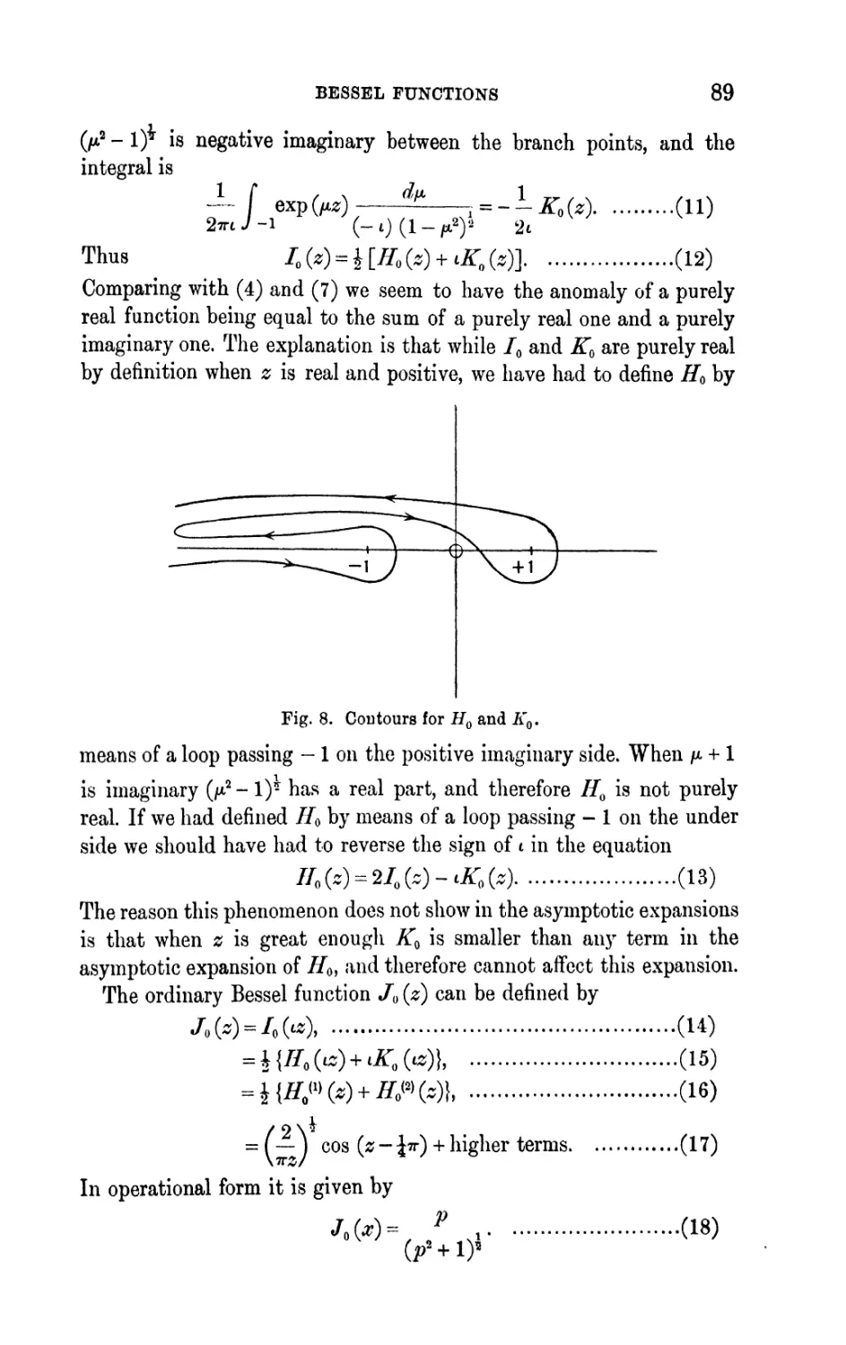
VIII. Bessel Functions 86
Note: On the Notation for the Error Function or Pro-
bability Integral 94
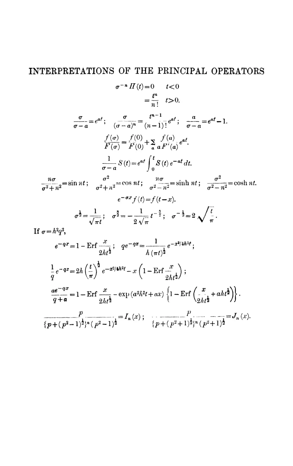
Interpretations of the Principal Operators .... 96
Bibliography 97
Index to Authors 100
Subject Index 101

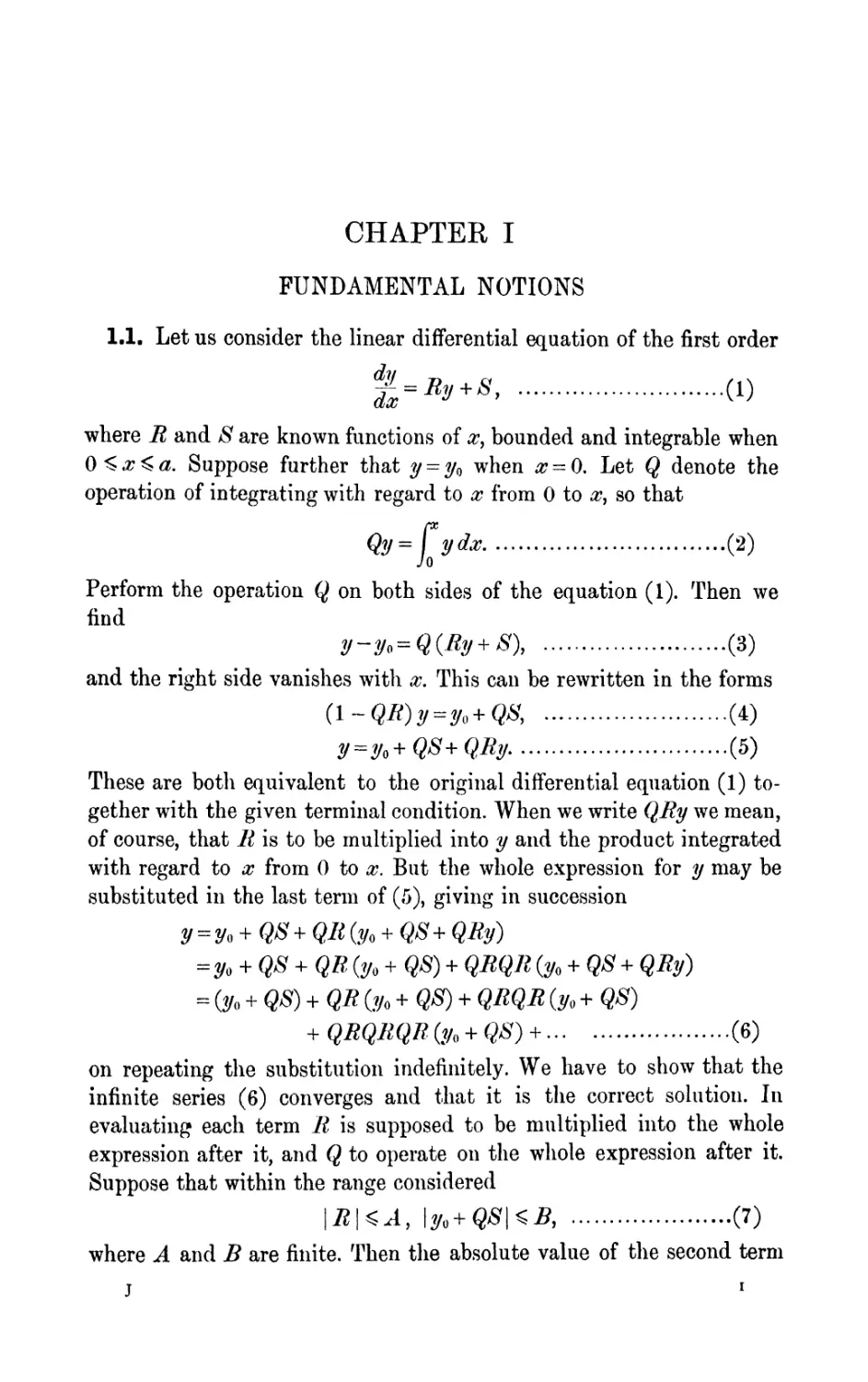
CHAPTER I
FUNDAMENTAL NOTIONS
1.1. Let us consider the linear differential equation of the first order
where R and S are known functions of #, bounded and integrable when
O^x^a. Suppose further that y-y^ when & = (). Let Q denote the
operation of integrating with regard to x from to x, so that
dx (2)
Jo~
Perform the operation Q on both sides of the equation (1). Then we
find
and the right side vanishes with x. This can be rewritten in the forms
y=y*+Q8+QRy (5)
These are both equivalent to the original differential equation (1) to-
gether with the given terminal condition. When we write QRy we mean,
of course, that R is to be multiplied into y and the product integrated
with regard to x from to x. But the whole expression for y may be
substituted in the last term of (5), giving in succession
= y + QS + Q,R(y + QS+ QRy}
= y + QS + QR (y, + QS) + QRQR (y, + QS + QRy)
= (#o + QS) + QR (T/O + QS) + QRQR (y, + QS)
+ QRQRQR O/o + QS) + (6)
on repeating the substitution indefinitely. We have to show that the
infinite series (6) converges and that it is the correct solution. In
evaluating each term R is supposed to be multiplied into the whole
expression after it, and Q to operate on the whole expression after it.
Suppose that within the range considered
where A and B are finite. Then the absolute value of the second term

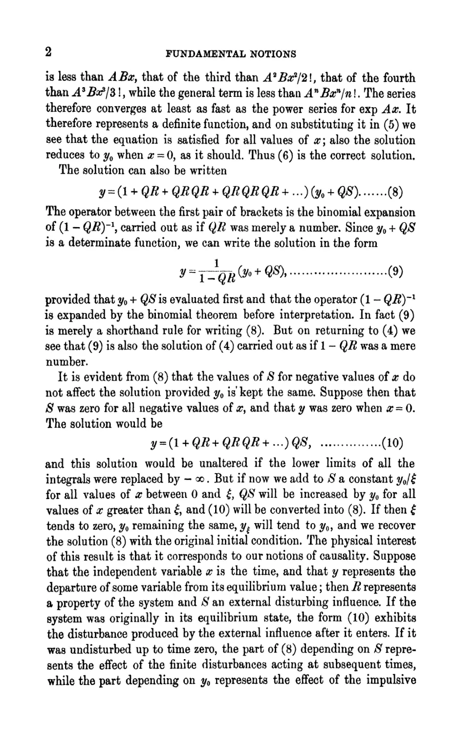
2 FUNDAMENTAL NOTIONS
is less than ABx, that of the third than A 2 Bx?/2l, that of the fourth
than A*x?/3 \ , while the general term is less than A n Bx n jn \ . The series
therefore converges at least as fast as the power series for exp Ax. It
therefore represents a definite function, and on substituting it in (5) we
see that the equation is satisfied for all values of x\ also the solution
reduces to y Q when x = 0, as it should. Thus (6) is the correct solution.
The solution can also be written
} ....... (8)
The operator between the first pair of brackets is the binomial expansion
of (1 - QR)~ l , carried out as if QR was merely a number. Since y -f QS
is a determinate function, we can write the solution in the form
provided that y Q + QS is evaluated first and that the operator (1 -
is expanded by the binomial theorem before interpretation. In fact (9)
is merely a shorthand rule for writing (8). But on returning to (4) we
see that (9) is also the solution of (4) carried out as if 1 - QR was a mere
number.
It is evident from (8) that the values of 8 for negative values of x do
not affect the solution provided y Q is' kept the same. Suppose then that
8 was zero for all negative values of x, and that y was zero when x = 0.
The solution would be
y = (l + QR+QRQR+...)QS, ............... (10)
and this solution would be unaltered if the lower limits of all the
integrals were replaced by - <x> . But if now we add to S a constant y Q /
for all values of x between and , QS will be increased by y for all
values of x greater than f, and (10) will be converted into (8). If then
tends to zero, y Q remaining the same, y^ will tend to y > and we recover
the solution (8) with the original initial condition. The physical interest
of this result is that it corresponds to our notions of causality. Suppose
that the independent variable x is the time, and that y represents the
departure of some variable from its equilibrium value ; then R represents
a property of the system and S an external disturbing influence. If the
system was originally in its equilibrium state, the form (10) exhibits
the disturbance produced by the external influence after it enters. If it
was undisturbed up to time zero, the part of (8) depending on S repre-
sents the effect of the finite disturbances acting at subsequent times,
while the part depending on y<> represents the effect of the impulsive

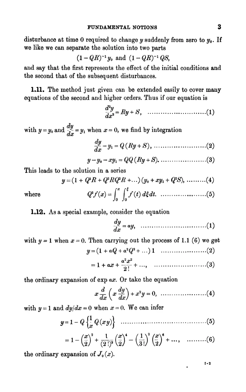
FUNDAMENTAL NOTIONS
disturbance at time required to change y suddenly from zero to y . If
we like we can separate the solution into two parts
and say that the first represents the effect of the initial conditions and
the second that of the subsequent disturbances.
1.11. The method just given can be extended easily to cover many
equations of the second and higher orders. Thus if our equation is
with y = 7/0 and -,- = y when x = 0, we find by integration
GvX
, ........................ (2)
8) ...................... (3)
This leads to the solution in a series
y (1 -f- Q*Jt + QPRtyR +...)(y + #^i + Q 3 $) (4)
where Q 2 /O) - f* ( f()d(dt (5)
Jo Jo
1.12. As a special example, consider the equation
g = ay, (1)
with y = 1 when # = 0. Then carrying out the process of 1.1 (6) we get
- i^*^_i_ /''.^
IT OJu T _ . T . . . , \O)
the ordinary expansion of exp ax. Or take the equation
4(4) + ^=-
with y = 1 and dyjdx = when x = 0. We can infer
(5)
the ordinary expansion of J (a?).

4 FUNDAMENTAL NOTIONS
1.2. The foregoing method is due originally to J. Caqu6*; it is a
valuable practical method of obtaining numerical solutions of linear
differential equations. Its extension to equations of any order, or to
families of simultaneous equations of the first order, is more difficult
unless special simplifications enter. But if the equations have constant
coefficients, which is an extremely common case in physical applications,
a considerable development is possible. This arises from the fact that
the operator Q obeys the fundamental laws of algebra. Thus if a is a
constant and u and v known functions of #,
(1)
, .............................. (2)
Q m+n u.' ..................... (3)
Consequently Q behaves in algebraic transformations just like a number.
If for instance we have two operators/(Q) and g(Q) both expressible
as sums of integral powers of Q, thus
'(Q) = a + a 1 Q + a a Q s + a 3 Q 8 + ......... ' ......... (4)
9(Q) = bo + b l Q + b&+b 9 (f + .................. (5)
where the a's and ft's are constants, let us for a moment replace Q by a
number z small enough to make the series converge absolutely. Form
the product series
f(z) g (z) = (0 + #! z + # 2 z 2 + ) (bo + bi z -f b 2 z 2 +. . .)
= c + CiZ + CiZ*+ .................................... (6)
say. Consider first the case where the series are both polynomials. Then
if S is an integrable function of x
f(Q}ff(Q~)S=(c, + c l Q + c^+...}S, ............ (7)
For the left side means
(a, + a,Q
+ a, (ft.Q'/S +...)+ .............................. (8)
* Liouville's Journal, (2), 9 (1864), 185-222. Further developments are given by
Fuchs, Ann. d. Matem., (2), 4 (1870), 36-49; Peano, Math. Ann., 32 (1888), 450-456;
H. F. Baker, Proc. Lond. Math. Soc. t (1), 34 (1902), 347-360; (1), 35 (1902), 333-
378; (2), 2 (1905), 293-296; Phil. Trans., A, 216 (1916), 129-186. Caqu considers
only a single differential equation, but notices that the operator in the result is
in the form of a binomial expansion. For other operational methods based on these
principles, but applicable to equations of order higher than the first, or to families
of equations of the first order, the above papers of Prof. Baker may be consulted.
Physical applications are given by W. L. Cowley and H. Levy, Phil. Mag., 41
(1921), 584-607; Jeffreys, Proc. Lond. Math. Soc., (2), 23 (1924), 454 and 465;.
M.N.R.A.S., Geoph. Suppl. 1 (1926), 380-383.

FUNDAMENTAL NOTIONS 5
using (1) and (2); and then using (3) we can collect the terms involving
the same power of Q and obtain
a b Q S+ (oo&i + &i 6 ) QS + (flo&a + a i *i + ^2 60) (?8 + - (9)
which is by definition the same as
(co + dQ + *tf+-)& ..................... (10)
When the series are infinite, their convergence may be established
easily. If the series for/(s) converges absolutely when | z\ ^r, then a
number M must exist such that a n r n ^ M for all positive integral values
of n. Thus
and also if for all values of at, \S\^C, where C is a constant,
0"S^C-, ............................ (12)
!
Henceif /(#)#= 2 a^S, ..................... (13)
n =
each term is less than the corresponding term of the series
co /r\ n fl
*M(?) ~, ........................ (u)
n-o \rj n\ J ^ J
which converges for all values of x however large. So long as f(z) is
expansible about the origin in a convergent power series, however
small its radius of convergence may be, the expression f(Q) S will be
the sum of an absolutely convergent series however great x may be. If
f(z) and g(z) are both expansible within some circle, their product
series will also converge within this circle and the expression/(Q)# (Q) S
will be an absolutely convergent series however great x may be.
Provided with this result we can now easily extend the result (7) to the
case where f(z) and g(z) are infinite series, by methods analogous to
those used to justify the multiplication of two absolutely convergent
power series.
1.3. We can now extend these methods to the solution of a family of
n simultaneous differential equations of the first order with constant
coefficients. Suppose the equations are

6 FUNDAMENTAL NOTIONS
where the y's are dependent variables, x the independent variable, e ra
denotes a r8 -r + b r8 , where a rs and b rs are constants, and the S's are
known functions of x. We do not assume that
but we do assume that the determinant formed by the a's is not zero.
When x = 0, y^ - u ly and so on, where the u's are known constants.
First perform the operation Q on both sides of each equation. We have
= /ry.-r, ........................... (2)
where f rs denotes the operator a rs + b rs Q. Then the equations and the
initial conditions are together equivalent to the equations
(3)
/nl yi +/na y a + +/nn #n = t?
where v r = a r iU 1 +a r2 u z + ... + a rn u n ................... (4)
The general equation can be written compactly
S./r.y. = *V+Q& ......................... (5)
Now let D denote the operational determinant formed by the /'s,
namely,
J\l Jvi Jin
J"2\ JW Jin
J nl y n2 y n
If this determinant is expanded by the ordinary rules of algebra and
equal powers of Q collected, we shall obtain a polynomial in Q. The
term independent of Q is simply the determinant formed by the a's,
which by hypothesis does not vanish. Now let F r8 denote the minor of
/ in this determinant, taken with its proper sign. F n also is a poly-
nomial in Q.
Now operate on the first of (3) with F la , on the second with F&, and
so on, and add. Then in the sum the operator acting on y m , say, is
*rFr.fr ............................... (7)
If m = s, this sum is the determinant D ; if m 4= *, it is a determinant with
two columns equal and therefore is zero. The resulting equation is
therefore
(8)

FUNDAMENTAL NOTIONS 7
Now if all the $'s are bounded and integrable within the range of values
of x contemplated, the expression on the right of (8) is also a bounded
integrable function of x> Also since the function D (2), obtained by
replacing Q in D by a number z, is regular and not zero at 2 = 0, the
function l/D (z) is expressible as a power series in z with a finite radius
of convergence. Define D~ l as the power series in Q obtained by putting Q
for z in the series for l/D (z). Then operate on both sides of (8) with D" 1 .
We have
- l Dy 8 = D-^ r F r8 (v r + QSr) ................... (9)
But, since series of positive integral powers of Q can be multiplied
according to the rules of algebra, D~ 1 D gives simply unity, and we
have the solution
y a = D- l 2 r Frs(Vr+QS r ) ...................... (10)
This gives a complete formal solution of the problem. Its form is often
convenient for actual computation, especially for small values of x\ but
it can also be expressed in finite terms. D is, as we have seen, a poly-
nomial in Q of degree n at most, while F rt is a polynomial in Q of
degree n - 1 at most. Our solution is therefore of the form
D(Q)
where < and i/r are polynomials whose degree is ordinarily one less than
that of D. Since the determinant formed by the a's is not zero we may
denote it by A, and then D will be the product of n linear factors,
thus
o^).. .(!-,$), ............ (12)
where the a's will ordinarily be all different. Then <f>(Q)/D(() can be
expressed as the sum of a number of partial fractions of the form
But by 1.12 (3) this is the same as Le* x . The part of the solution arising
from the -y's can therefore be expressed as a linear combination of
exponentials.
The justification of the decomposition of <t>(Q)/D(Q) into partial
fractions is that this decomposition is a purely algebraic process. Hence
if the partial fractions and the original operator are all expanded in
positive powers of Q, and like powers of Q are collected, the coefficients
of a given power of Q will be the same in both expressions, and the
equivalence is complete.

8 FUNDAMENTAL NOTIONS
Exceptional cases will occur if D contains no term in Q n , or if two
or more of the a's are equal. If the term in Q n is absent the expansion
of the operator in partial fractions will usually contain a constant term.
If the term in Q n ~ l is also absent we must divide out, and the expan-
sion in partial fractions will contain a term in Q; this will give a term
in x on interpretation.
If several of the a's are equal, the expression in partial fractions
will involve terms of the form M(l ~a^)~ r . These can be interpreted
by direct expansion ; but another method is more convenient. Starting
with
(l-Q)- l = ^ ......................... (14)
let us differentiate r - 1 times with regard to a. We find
(r- IV O r ~ l
sothat
A rather different form of resolution into partial fractions from the
ordinary one is therefore necessary if each fraction is to give a single
term in the solution. Instead of having constants in all the numerators
we must have powers of Q, the power of Q needed in any fraction being
one less than the degree of the denominator. But if we write p~ l for Q
the fraction in (16) is algebraically equivalent top/(p - a) r . In this form
the power of p in the numerator is independent of the degree of the
denominator, and it is easier to resolve into partial fractions of this form
than into those involving Q directly.
The above remarks apply to the interpretation of the effect of the
initial conditions; that is, of the first term on the right of (11). To find
the effect of the terms in the $'s we may expand the operators simi-
larly. To interpret (1 -aQ)" 1 QS in finite terms, we note that it is the
solution of -T- -ay = 8 that vanishes with x. This is easily found by the
dec
ordinary method to be
y = f*Q(Se-*\ ........................ (17)
which is the interpretation required.
To sum up, we can solve a family of equations of the type (1) by
first integrating each equation once from to x with regard to x, allow-
ing for the initial conditions. This gives a set of equations of the type
(3). The subsequent process for deducing the operational solution (10)
is exactly the same as if the operators f ra were numbers, and the

FUNDAMENTAL NOTIONS 9
ordinary rules of algebra were applied. The solution can be evaluated
by expanding the operators in ascending powers of Q and evaluating
term by term; this in general gives an infinite series. Alternatively it
can be obtained by resolving into partial fractions and interpreting each
fraction separately; this gives an explicit solution in finite terms.
1.4. Heaviside's method is equivalent to that just given; it differs
in using another notation, which is not quite so convenient in a formal
proof of the theorem, but is rather more convenient for actual applica-
tion. In Heaviside's notation the operator above called Q is denoted by
p~~ l . At present we need not specify the meaning of positive powers of
p ; negative integral powers are defined by induction, so that p~ n denotes
Q n . We have noticed that the passage from 1.3 (3) to 1.3 (10) is a
purely algebraic process. Consequently if all the equations (3) were
multiplied by constants before the algebraic solution the same answer
would be obtained. Suppose then that we write the general equation
1.3 (5) in the form
2 8 (a r8 + b rs p- } )y 9 ='% 8 a r8 u 8 + p- l S 1 (1)
Multiply throughout by p as if this were a constant. We get
^(anp + brJys^S.artpUs + Sr ...(2)
On solving the n equations of this form we shall obtain a solution
identical with 1.3 (10) except that p~ l will appear for Q, and both
numerator and denominator will be multiplied by the same power of p.
If the operators in the solution are expanded in negative powers of p,
and p~ l is then interpreted as Q, the result will be identical with that
already given. Comparing (2) with the original equations 1.3 (1) we see
that the new form of our rule is as follows :
Write p for djdx on the left of each equation ; to the right of each
equation add the result of dropping the 6's on the left and replacing
the y's by their initial values; solve the resulting equations (2) by
algebra as if p was a number ; and evaluate the result by expanding
in negative powers of p and interpreting p~ l as the operation of
integrating from to x.
This is Heaviside's rule. In what follows the equations (2) will usually
be called the subsidiary equations.
To obtain the solution explicitly, we put e rs for a ra p + b r6 , denote our
determinant

10 FUNDAMENTAL NOTIONS
by A, and denote the minor of e ra in this determinant, taken with its
proper sign, by E r8 . Then the solution is
r + 8 r ) ................... (3)
Since the determinant formed by the a's is not zero, A is of degree n in
jt?, while E r8 is at most of degree n-1. The operators can therefore be
expanded in negative powers of jt?, as we should expect; positive powers
do not occur. All terms after the first vanish with x\ the first is
........................... (4)
where A rs is the minor of a rs in A, But
2 r A r8 a rin = A O = s)\ ( .
= On**))' ..................... (5)
and (4) reduces to u^ as we should expect. This verifies that the solu-
tion satisfies the initial conditions.
1.5. To interpret the operational solution 1.4 (3) in finite terms we
require rules for interpreting rational functions ofp operating on unity
and on other functions. We have already had the rules
p- l = Qip-* = tf; and so on, .................. (1)
p-i\ = Ql = x\ p~*l = $2? = k jj; and in general p' n 1 - ~j . ...(2)
If unity is replaced by Heaviside's ' unit function/ here denoted by
H(x\ which is zero for all negative values of x and 1 for all positive
values, we shall still have
p-H(*) = , ........................... (3)
when x is positive, but it will vanish when x is negative. We can also
replace the lower limit of the integrations by - oo without altering this
interpretation.
Again, we shall have when x is positive
JL. - . l - * A\
a
(6)
p -a p - a
where the function operated on may be either unity or H(x). In the
latter case all the operators will give zero for negative values of x.

FUNDAMENTAL NOTIONS 11
The operators in 1.4 (3) are of the form/(/?)/jFQp), where/Q0) and
F(p) are polynomials in p, and f(p) is of the same or lower degree
than F(p}. If F(p) is of degree n it can be resolved into n linear
factors of the form p - a. Then provided that the a's are all different
and none of them zero we have the algebraic identity
r- .......... ; .....
If this operates on unity or H(x) we have therefore for positive values
/(lO^/CO)^ /(a) ^ (9)
*\P) -*XO) *aF'(a) ................ W
To justify this we notice as before that (8) is a purely algebraic iden-
tity, and therefore if both sides are expanded in negative powers of p,
beginning with constant terms, the expansions of the two sides will be
identical, and on interpretation in terms of integrations will give the
same result.
The formula (9) is usually known as Heaviside's expansion theorem;
but as Heaviside's methods involve two other expansion theorems* it
will be called the ' partial-fraction rule ' in the present work.
If some of the a's are equal or zero, the expression (7) considered as
a function of p will have a multiple pole, and its expression in partial
fractions will contain terms of the form (;> - a)" 8 , where s is an integer
greater than unity, and a may be zero. Then f(p)IF(p) will contain
terms of the forms p~(*~~v or pf(p - a) s , which can be interpreted by
means of (2) or (5).
By means of these rules we can evaluate all the expressions for the
part of y g in 1.4 (3) that depends on the initial values of the /s. If the
S's are constants for positive values of ,r, as they often are, the same
rules will apply to the part of the solution depending on them. If they
are exponential functions such as #>**, the easiest plan is usually to
rewrite this as /*/(/?-/*) an( ^ reinterpret. Thus
* Namely, expansion in powers of Q or p~ l and interpretation term by term;
and expansion in powers of e~ ph , where h is a constant, as in 4.2.

12 FUNDAMENTAL NOTIONS
If S is expressed as a linear combination of exponentials we can apply
this rule to each separately. This is applicable to practically all func-
tions known to physics.
Alternatively we can resolve the operator acting on 8 into partial
fractions and interpret p~ n S by integration and other fractions by the
rule of 1.3 (17)
JS = e ax {*Se- ax dx (12)
p-a Jo
This completes our rules for solving a set of linear equations of the
first order with constant coefficients. In comparison with the ordinary
method, we notice that the rules are direct and lead immediately to a
solution involving operators, which can then be evaluated completely
by known rules. If it happens that we only require the variation of one
unknown explicitly, we need not interpret the solutions for the others.
In the ordinary method we have to find a complementary function and
a particular integral separately. To find the former we assume a solu-
tion of the form y a ~^e ax and on substituting in the differential equa-
tions with the S's omitted we find an equation of consistency to
determine the n possible values of a, and the ratios of the A/s corre-
sponding to each. The particular integral is then found by some method,
but it does not as a rule vanish with x. The actual values of the A/s
are still undetermined, and the value associated with each a must be
found by substituting in the initial conditions and again solving a set
of n simultaneous equations. The labour of finding the equation for the
a's and the ratios of the X's corresponding to one of them is about the
same as that of finding the operational solution in Heaviside's method ;
the rest of the work is avoided by the operational method. Further, if
some of the a's are equal or zero considerable complications are intro-
duced into the ordinary method, but not into the operational one.
1.6. The above work is applicable to all cases where A, the deter-
minant formed by the #'s, is not zero. We can show that if A is zero
there is some defect in the specification of the system. A system is
adequately specified if when we know the values of the dependent
variables and the external disturbances the rates of change of the
dependent variables are all determinate, and if the initial values of the
variables are independent of one another. Now if A is zero, let us
multiply the r'th equation by A r8 , the minor of a r8 in A, and add up
for all values of r. The coefficient of dy 9 \dx in the sum is A, which is
zero ; that of any other derivative is a determinant with two columns

FUNDAMENTAL NOTIONS 13
equal, and is also zero. Thus the derivatives disappear entirely from
the sum, and we are left with a relation between the y'a and the $'s.
If the coefficients of the y's also vanish, there must be a permanent
relation between the S's, and one of the equations we started with is a
mere logical consequence of the others; then we have not enough
equations to determine the derivatives. If the coefficients of the y's do
not vanish, we can put x = and obtain a relation between the initial
values, which are therefore not independent.
1.7. The method is most easily extended to equations of higher
order by breaking them up into equations of the first order. Thus if we
have an equation of the second order such as
we introduce a new variable z given by
-*- ............................... oo
and the original equation can be replaced by
( 3 )
We have now two equations of the first order in y and z. If initially
y =yo and dyjdx = y l9 the subsidiary equations are
py-z=pyo, .............................. (4)
(p + a)z+by=pyi + & ..................... (5)
Solving by algebra we find
To interpret, put
p* + ap + b = (p-ti)(p-ft}, (7)
and apply the partial-fraction rule. We find
" ao *'*
, ...(8)
which is easily shown to satisfy all the conditions and therefore to be
the solution required.

14 FUNDAMENTAL NOTIONS
1.71. A few illustrative examples may be given, (p is written for
d\dx from the start.)
We consider the subsidiary equation
(jp 8 + 4jt> + 3 ) y = 1 - 2p + 3 (/ +
3p 2 + 10;? + 1
~"~
= TJ-+ 30 ~ i#~ >
on interpreting by the partial-fraction rule.
2. (p* + 5p + 6)y=12; y -2; y I =
Consider (p a 5p + 6) y = 12 + 2 (/ + 5p).
Cancelling the common factor,
3. (^
2?
This can be written (jP + 3) y = - ~ ;
4. (p 3 +w 2 )y = 0.
sin
5. (p+ $fy = a*e-**\ y = 0; ^ = 0.
The expression on the right is equivalent to the operator 2p/(p + 2) 8 .
Hence
2p ^2^ 1
y ~(F+2) 6 ~4l' -12^* '
We notice the advantage of Heaviside's method in avoiding the use
of simultaneous equations todetermine the so-called * arbitrary ' constants
of the ordinary method. In particular in the second example the data
have a property leading to a simple solution. Heaviside's method seizes
upon this immediately and gives the solution in one line; with the
ordinary method the simultaneous equations for the constants would
have to be solved as usual.

FUNDAMENTAL NOTIONS 15
In general we may say that the more specific the problem the greater
will be the convenience of the operational method.
1.72. The method just given can be extended easily to a family of
equations of the second order. If the typical equation is again written
%e rg y^S r , ........................... (1)
d
,
where now a x
we can introduce n new variables z l9 z 2 , z n given by
-*- ............................ w
thus treating the first derivatives of the #'s as a set of new variables.
Then the equations (1) are equivalent to
dz
2,a r ,^ + X(k*a + c r ,y,) = fl r , ............... (4)
and (3) and (4) constitute a set of 2n equations of the first order. Suppose
also that when x = 0, y 8 = u s , z t = v t . According to our rule of 1.5 we
must replace d\dx by p and add pu r to the right of (3), and 2* a r8 pv 8
to the right of (4). We have now to solve by algebra, and may begin by
writing the revised form of (3)
*r=p(yr-U r ) ............................ (5)
When we substitute in the modified form of (4) we get
2, a rg p* (y* - w,) + 2 8 b n p (y 8 - u,} + 2* c r8 y 8 = S r + S, a r8 p 8 , (6)
or, on rearranging,
2, (a r8 p* + b r8 p + c rs } y s = 2* (a rg p* + b r8 p) u s + 2 a a rg pv s + S r . . . . (7)
We have thus n equations for the y's to solve by algebra, and the
solution can be interpreted by the rules.
In Bromwich's paper 'Normal Coordinates in Dynamical Systems' a
method equivalent to the operational one is applied directly to a set of
second order equations. First order equations, however, arise in some
problems of physical interest, and merit a direct discussion. This, as we
have seen, is easily generalized to equations of the second order.
1.73. In the discussion of the oscillations of stable dynamical systems
by the ordinary method of normal coordinates there is a difficulty when
the determinantal equation for the periods has equal roots. This does
not arise in the present method. If the system is not dissipative,
and the determinant formed by the e's as defined in (2) has a multiple
factor (p* + a a ) r , we know from the theory of determinants that every
first minor has a factor Q0 2 + a 2 )*"" 1 . On evaluating the operational solution

16 FUNDAMENTAL NOTIONS
of (7) we can therefore cancel the factor (p* + a 2 ) 1 "- 1 from the numerator
and the denominator, and we are left with a single factor (p 2 + a 2 ) in the
denominator. Thus the part of the solution depending on the initial
conditions is of the trigonometric form as usual; terms of the forms
t cos at and t sin at do not arise.
1.8. In all the problems considered so far the operators that occur in
the solutions are expansible in positive powers of Q, or in negative powers
of p } and we have seen that so long as the series obtained by replacing
Q by a number have a finite radius of convergence, however small, the
operational solution is intelligible in terms of the definitions we have
had. But we have not defined p as such, because we have only needed
to define its negative powers, and p cannot be expanded in terms of its
own negative powers. Then has p any meaning of its own? Since it
replaces djdx when we form the subsidiary equation we may naturally
suppose that p means dfdx, and this is the meaning sometimes actually
attributed to it ; but care is needed. We recall that when the subsidiary
equation is formed a term like py Q appears on the right ; but dy^dx is
zero, so that if we pushed this interpretation too far we should be faced
with the alarming result that the solutions of the equations do not
depend on their initial values. The fact is that though the operators
d\dx and Q both satisfy the laws of algebra and are freely commutative
with constants, they are not as a rule commutative with each other.
Thus
(0
(2)
Thus the operators p and Q are commutative if, and only if, the function
operated on vanishes with x. It appears from (1) that djdx undoes the
operation Q if djdx acts after Q. With this convention we can identify
p, the inverse of Q, with dfdx. When p and Q both occur in an operator,
the Q operations must be carried out before the differentiations*.
This result explains why some of our interpretations differ from those
given in text-books of differential equations for the determination of
particular integrals. For instance, we have interpreted !/(/> a) as
- (e** - 1). In the ordinary method, due to Boole, we expand this operator
in ascending powers of p, and get
V -I
(3)
p - a \a a" / a
* Cf. Heaviside, Electromagnetic Theory, 2, 298.

FUNDAMENTAL NOTIONS 17
This assumes that the sum of all the terms of the series after the first
is zero. But
. ,
p- a a/ a(p-a)
If the operator on the right is written -. ~ ./>!, it is clearly zero.
But if it is written - . p . - . 1, it gives by our rules - <f x . The differ-
ence arises from the fact that the operators p and (p - a)" 1 are non-
commutative.
We may notice, incidentally, that whereas the series in powers of Q
give convergent series on interpretation, the same is not true of the
corresponding series in powers of p. For instance, if S = (x l) r , where r
is fractional, the series for - . S in ascending powers of p diverges
like 2 (# l)~ n nl. Apart from the greater internal consistency of
Heaviside's methods, then, they are capable of much wider application.
We have also
=/(* + *), .............. > ..................... (5)
by Taylor's theorem. The operator e hp increases the argument of a
function by h.
This operator is useful in enabling us to find a theorem that plays
in Heaviside's method a part closely analogous to that played by Fourier's
integral theorem in the ordinary method. Instead of trigonometric
functions, Heaviside treats as fundamental the function here called
//(#), which is zero for negative, and unity for positive, values of x*.
This function being discontinuous, we cannot at once apply Taylor's
theorem to it; but continuous functions can be found as near to it as
we liket, and the results obtained by applying (5) may be regarded as
the limits of results proved for these. Then we shall write
eP h H(z) = 1 when x>- h
(
= when #<-/
* Proc. Roy. Soc., A, 62, 513.
f E.g. J(Erf>u;-f 1) where \ may be made indefinitely great.

18 FUNDAMENTAL NOTIONS
*.
A fuller justification of this step will be given in the next chapter. Then
if Aj <h% y
(e~i - *-*) tf O) = 1 if A! < x < h, ]
-Oif^<^ [ ............. (7)
and = if x > k 2 j
If further A, < A 2 < A 3 < ... < fi n ,
{(e-P^ -0-P*0/(*0 + (e-v h -<-e-P h *}f(h^ + . . . X^*"" 1 -*"**") /(*n)} H(x)
= for x<h lt f(h^) for h l <x<h^ and so on .......... (8)
If then the subdivisions of the interval hi to A n become indefinitely
numerous, we can approximate as closely as we like to a function f(x)
by a sum 2/(A) (e~P hr ~ l - e~i >hr ) H (*). Now with a further proviso about
replacing H(x) by a continuous function and later proceeding to a
limit, we can replace this sum by an integral. Then
- f
J h
v) dk. (9)
If the integration with regard to h is carried out, we obtain a function
of p operating on H(x). In this way a given function of x can be
expressed in the operational form*.
We notice that if h is positive
_ A 1 jry A _;,, / wllCll X <
p \x when x >
' when x<k
[x-h when x > A,
and - er^ II (x) = - 1 // (#-*) = J*# (a? - A) cfe
= when x < h,
-x-h when x > A.
Thus the operators arid e~v fl can be commuted provided A is positive.
r> x & ^ r/- / \ f when x<-h
But 0^ - // (a?) = \ j , ,
jt> I ^ + A when x>h,
j h rrf \
and ~eP h II(x)=\ .
/; x l^r when .r > 0.
Fortunately symbolic solutions seldom contain operators of the form
e ph f where h is positive, so that the fact that this operator is not com-
mutative with - gives little trouble in practice.
* Heaviside, Electromagnetic Theory, 3, 327.

COMPLEX THEORY ^ v 19
CHAPTER II
COMPLEX THEORY
2.1. All the interpretations found so far for the results of operations
on unity or on // (#) are special cases of two closely related general
rules, as follows. If </> is an analytic function,
^C(K)C?K, (1)
*(/o//(*)=^j L v*w <fa (2)
In the former definition the integration extends around a large circle
in the complex plane. In the latter the integration is along a curve
from c-iootoc + icc, where c is positive and finite, such that all
singularities of the integrand are on the left side of the path (that is,
the side including x). These rules are both due to Bromwich*.
Considering first (1), we have
P = ^
and the only pole of the integrand is at the origin, where the residue
is x n \n !. Hence when n is a positive integer
r n
Also we see that
/>" = 0, ................................. (5)
since the integrand has no singularity in the finite part of the plane ;
and
The interpretation 1.5(5) of p/(p~ a } n also follows immediately from
(i).
The partial-fraction rule can also be proved easily. For by (1), with
the notation of 1.5,
on evaluating the residues at the poles 0, a,, a 3) ...a,,.
* 'Normal Coordinates in Dynamical Systems,' Proc. Land. Math. Soc., 15 (1916),
401-448.

20 COMPLEX THEORY
We can also prove that 1.4 (3), when interpreted by the rule (1), is
the correct solution of equations 1.3 (1). If we denote by #,.,(*), A (AC)
and E r8 (K) the results of replacing p by K in e rsy A, and E rit the part
of 1.4 (3) not involving the S*s is equivalent to
>r>s v / y QKX (J K fc)}
* ( K ) ' r
Substituting in the differential equations 1.3 (1) we find that the left
side of the mth equation is
But S 8 E n (<) e ms (K) = A (K) if r = m
= 0it>*, (11)
and the expression (10) is then equal to
dK^O (12)
Thus the differential equations are satisfied.
Now considering the initial conditions, we put x - 0, and find
Also v r = 2 m {e nn (K)-b rm }u M , .................. (14)
and jr. = - 2 r 2 m " * { () - i m } di
jr. = -^ f 2 r
-" 7rt JC
ie
Now A (K) is a polynomial of the w'tli degree in K, and E r (K) one
of the (n - l)th degree. When | K | is great enough the second term in the
integrand is of order *c~ 2 . It therefore gives zero on integration, and we
have
y.= M, .............................. (16)
so that the initial conditions are satisfied.
Next, suppose that instead of the >S"s being zero they are exponential
terms of the form Per*. Since the solutions are additive it is enough
to suppose that the initial values of the T/'S are all zero, and to consider
the effect of an exponential term in the first equation alone. Then the
equations are
ii y\ + M y* + - - - + *m y w = P&* = ^^
(17)

COMPLEX THEORY 21
The operational solution is
This is to be interpreted as
! f H (u\ P
(19)
Substituting in the differential equations we find that the left sides
of all vanish except the first, in consequence of the integrand con-
taining as a factor a determinant with two rows identical; the first
gives
P c P X
f- -L_fe = pM* ...................... (20)
27TI Jfj K - JJL ^ '
The differential equations are therefore satisfied,
When x - and | K \ is large, the integrands in (19) are all (*~ 2 ) and
the integrals are therefore zero. Thus all the y$ vanish with x.
Since all functions that occur in physics can be expressed by Fourier's
theorems as linear combinations of exponentials, the proof that the
solution can be carried out by operational methods is complete. We
shall see later, however, that Fourier's theorems are not so convenient
to use as the formula 1.8 (9) based on the function II (x).
2.2. Now let us consider the integrals 2. 1 (2), taken along the path L.
If we suppose the contour completed by a large semicircle from c -f too
to c-ioo by way of x , all the singularities of the integrand are within
the contour, and therefore the integral around it is the same as the
integral (1) around a large circle. Now if x is positive, and <f> (*)/* tends
to zero uniformly with regard to arg K as K tends to <x> , the integral
around a large semicircle tends to zero as the radius becomes indefin-
itely large, by Jordan's lemma*. Hence the integral along L is equivalent
to the integral around a large circle. Thus if x is positive and
when K is great and n is positive, < (p)H(x) is the same as <#>(j?) 1.
But if x is negative, the integral around the large semicircle on the
negative side of the imaginary axis is no longer an instance of Jordan's
lemma, and this result no longer holds. The integral around a large
semicircle on the positive side of the imaginary axis is, however, re-
ducible to the integral along Z, since by construction there is no
singularity between these two paths. If then <(*)/* = (*~ n ) when K is
* Whittaker and Watson, Modern Analysis, 1915, 115.

22 COMPLEX THEORY
great, the limit of the integral around this large semicircle is zero by
Jordan's lemma, and therefore < (p) //(#) is zero.
Thus if <#> (p) is expansible in descending powers of p, beginning with
a constant or a negative power of p, we shall have
= < (p) I when x >
The integrals 2.1 (2) for p n H(a^ where n is a positive integer, are
divergent, but these derivatives can be found by differentiation. Evi-
dently they are zero except when x = 0, when they do not exist.
Again, ^H(x)--~ \ d* = H(x + K) (2)
JTTI J L K
This proves the result obtained by less satisfactory means in 1.8.
We can also translate into the form of a double integral the opera-
tional expression for a general function. From 1.8 (9)
K (3)
where the integration* gives a function of p operating on //(#). Inter-
preting by Bromwich's rule
*) = -^- f (f(K)<H*- h >dhdK, (4)
ZTTI J oo J L
where the integration with regard to h is to be carried out first.
If the function of p that arises when (3) is integrated has no singu-
larity on the imaginary axis or on the positive side of it, and if further it
contains p as a factor, we can replace the integration with regard to K
in (4) by one along the imaginary axis. Then we can put
K-iA, (5)
and we have
/(#) = - C rf(K)*m\(x-A)dtd\ (6)
7T 7-co JO
This is Fourier's integral theorem.
2.3. In practice the form 2.1 (2) is generally used in preference to
2.1 (1). In problems involving a finite number of ordinary differential
equations of the first order the forms are equivalent for all positive
values of the independent variable ; and since the independent variable
is usually the time, and we require to know how a system will behave if
it is in a given state at time and is afterwards acted upon by known
* The integral is of the type introduced by Stieltjes.

COMPLEX THEORY 23
disturbances, it is as a rule only positive values of the time that con-
cern us. But when we come to deal with continuous systems it usually
happens that when the operational solution <j> (p) is interpreted as an
integral, the integrand has an infinite number of poles, and that no
circle however large can include all of them. Hence the contour integral
2.1 (1) cannot be formed. But the line integral 2.1 (2) usually still
exists. Again, it may happen that < (K) has a branch-point at the origin
or on the negative side of the imaginary axis. Here again the contour
integral does not exist, but the line integral does.
Consequently in most of the writings of Heaviside and Bromwich,
when a function of an operator <j> (/?) occurs without the operand being
stated explicitly, it is to be understood that the operand is H(x), and
that the interpretation 2.1 (2) is to be adopted. This rule will be
followed in this work when we come to treat continuous systems; and
if it is also supposed to be adopted in the problems of the next chapter
no harm will be done.
Considerable latitude is admissible in choosing the path L. Since by
construction the integrand is regular at all points to the right of Z, we
may replace L by any other path on its positive side provided it ends
at c i QO . Again, the systems we are to discuss are usually stable
systems ; that is, the poles of <f> (*) are all on the imaginary axis or to
the left of it. Then L can be taken as near as we like to the imaginary
axis. L must not cross the imaginary axis if there are poles on the
latter; but it can be taken to be a line parallel to the imaginary axis
and distant c from it. This is the device most often used by Bromwich;
the only advantage of the present definition of L is that the solution
is then adaptable to unstable systems as well as stable ones. In all cases
the actual value of c does not affect the results, so long as it is
positive.
2.4. The principal operators involving branch-points are fractional
powers of p. We require then an interpretation of p n H(.r\ where n is
fractional*. By our rule
.................. (1)
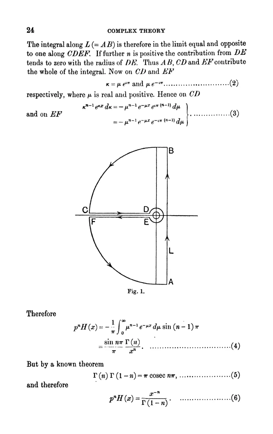
and the integral converges if n < 1. A contour including L as part of
itself, and such that the integrand is regular within it, is as shown.
Evidently if x is positive the large quadrants make no contribution.
* Of. Bromwich, Proc. Camb. Phil. Soc., 20 (1921), 411-427.

24
COMPLEX THEORY
The integral along L(=AB} is therefore in the limit equal and opposite
to one along CDEF. If further n is positive the contribution from DE
tends to zero with the radius of DE. Thus A B, CD and /^contribute
the whole of the integral. Now on CD and EF
K^/U.^ and/Ae-" 1 - ........................... (2)
respectively, where /x is real and positive. Hence on CD
(3)
B
Fig. 1.
Therefore
If 00
p n H(x)~ I p n ~ l e~* x dfji8in (n- l)?r
T J
sin wr T f )
x n
But by a known theorem
r (n) r (1 - n) = TT cosec mr,
and therefore
.(5)
.(6)

COMPLEX THEORY 25
This result has been obtained for <n< 1. If we change n into -TW,
where - 1 < m < 0, we have
* S ...................... (7)
v
Powers of /? outside this range can be found now by integration or
differentiation. We have
which shows that (7) still holds when m l is written for m. (To justify
this, the path AS must be replaced by FEDC.}
Similarly
By induction we may therefore generalize (7) to any value of m. Hence
Since when m is a positive integer T(m + l) = ?n !, and when m is a
negative integer T (m + 1) is infinite, the interpretations already adopted
for integral powers of/? are special cases of these.
In particular, since
r(i) = ^ ............................ (n)
we have
1 1 a 1 _3 ft 1 3 1 _6
"
and so on. Also
^ = 2^ ............................ (13)
A related function that arises in problems of heat conduction is
where a is a constant, and q denotes p^. By Bromwich's rule
r 4 >*x - /iici
-fa ................ (U)
I./X K X '
On L the argument of *i is between j?r. Hence if a is positive the
integral is convergent.
Immediate expansion of e~ aK ~ in a power series and integration term
by term would not be legitimate, because all the resulting integrals
after the first two would diverge. But (14) is equivalent to an integral

26 COMPLEX THEORY
along a path such as FEDC in Fig. 1, and on this path we can proceed
in this way. Thus
All the positive integral powers of K give zero on integration. The other
terras are equivalent to
3 ! 5 ! X/TT \2 N/# 3 \2 *Jx' 2 ! 5 \2 V^/ /
V> (16)
where, by definition,
2
X
^ (IT)
By differentiation with regard to a we find
(18)
We shall sometimes need an asymptotic approximation to Erf w when
w is great. We have
1 - Erf w = -.=, I e-* dt = -, - f e~ n u~* da
VTT^M* \'TTJ^
= --.-_ ^~ w2 ?/^ ! 1 - - ?r~ 2 + - L '"- ^~ 4 - " iv~ Q 4- ...
VTT L 2 2.2 2.2.2 J
NrJ(2re+1) ,
VTT 2. 2. 2. ..2
on successive integrations by parts. But the last integral
2 "-' ) , ............ (20)
so that its contribution to the function is less than the previous term.
We have therefore the asymptotic approximation
- - __..
At a 2.2 2.2.2
-7 + 1
J

ONE INDEPENDENT VARIABLE 27
CHAPTER III
PHYSICAL APPLICATIONS: ONE INDEPENDENT VARIABLE
3.1. An electric circuit contains a cell, a condenser, and a coil with
self-induction and resistance. Initially the circuit is open. It is suddenly
completed ; find how the charge on the plates varies with the time.
Let y be the charge on the plates, t the time, K the capacity of the
condenser, L the self-induction, and R the resistance of the circuit;
and let E be the electromotive force of the cell. Write o- for d/dt.
The current in the circuit is 3?, and the charging of the plates of the
condenser produces a potential difference yjK tending to oppose the
original TG.M.F. Then y satisfies the differential equation
E-Ly + Ry ......................... (1)
Initially y and y, the current, are zero. Hence the subsidiary equation
is simply
(L** + tt* + -^)y = E, ..................... (2)
and the solution is
Zo- 2 + 7iV -t- -i
A
If now the denominator is expressed in the form L (o- + a) (<r + /}), the
interpretation is, by 1.5 (9)
Since a + /J and a/3 are both positive, a and /J must either be both real
and positive, or conjugate imaginaries witli positive real parts. In either
case y tends to KE as a limit, as we should expect.
We notice incidentally that if the circuit contained no capacity or
self-induction the differential equation would be simply
R<ry = E. ................................. (5)
Hence if a problem has been solved for simple resistances, self-induction
and capacity can be allowed for by writing L& + R + -^- for R. For this
reason this expression is sometimes called a 'resistance operator/ and
the method generally the * method of resistance operators/

28
PHYSICAL APPLICATIONS
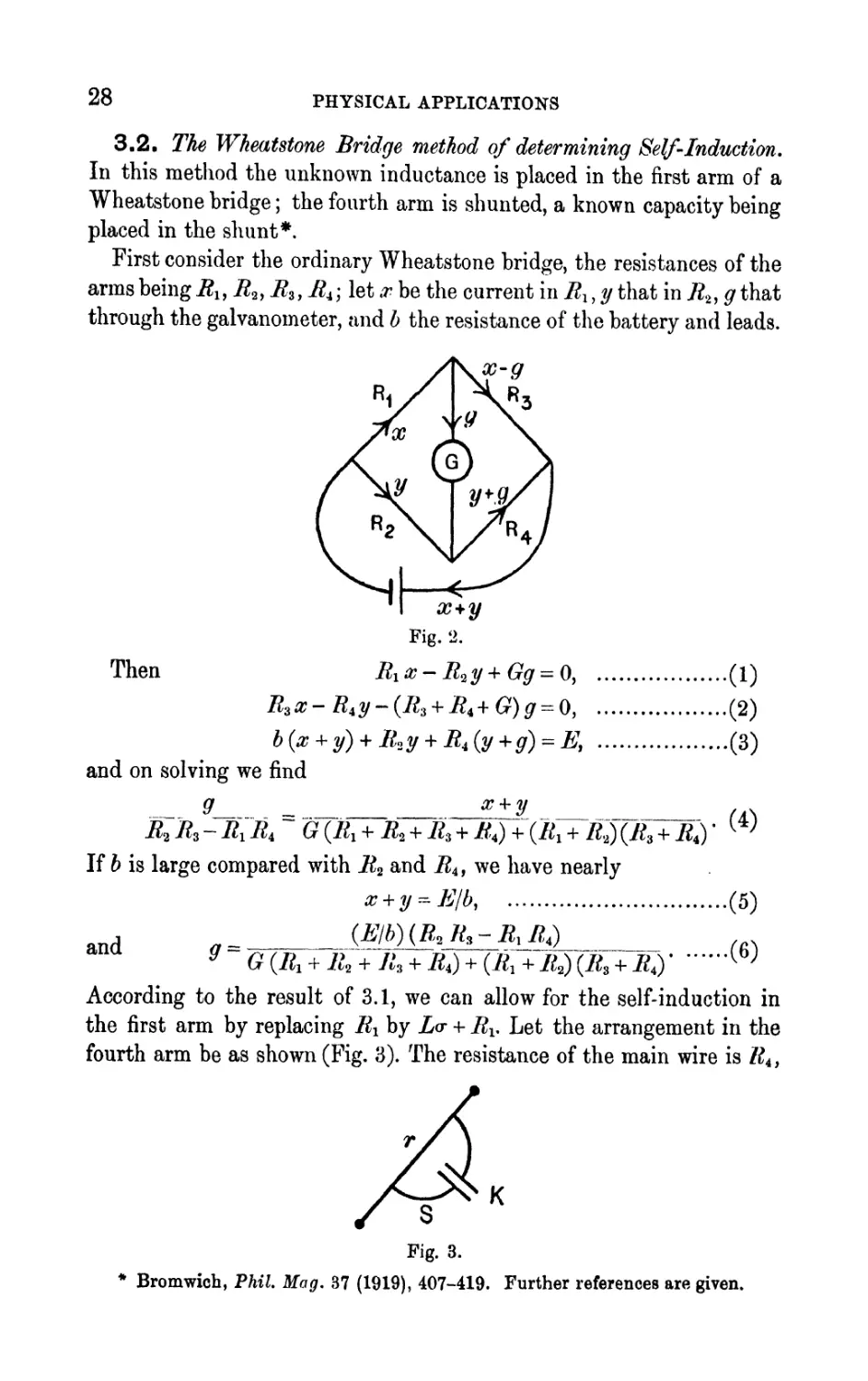
3.2. The Wheatstone Bridge method of determining Self-induction.
In this method the unknown inductance is placed in the first arm of a
Wheatstone bridge ; the fourth arm is shunted, a known capacity being
placed in the shunt*.
First consider the ordinary Wheatstone bridge, the resistances of the
arms being R^R^R^R^ let x be the current in R l , y that in j? 2 , g that
through the galvanometer, and b the resistance of the battery and leads.
Then
b (% + y) + -# 2 y + ^4 (y +0) - JB;
and on solving we find
_
7? Z?
3 111 tf*
.(2)
.(3)
j (Jt 3
r (4)
If 6 is large compared with R 2 and j? 4 , we have nearly
x + y^-Elb,
(5)
and
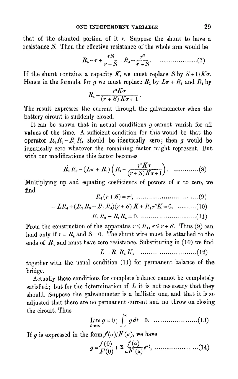
According to the result of 3.1, we can allow for the self-induction in
the first arm by replacing R l by Lv + R^ Let the arrangement in the
fourth arm be as shown (Fig. 3). The resistance of the main wire is H 4 ,
S
Fig. 3.
* Bromwich, Phil. Mag. 37 (1919), 407-419. Further references are given.

ONE INDEPENDENT VARIABLE 29
that of the shunted portion of it r. Suppose the shunt to have a
resistance 8. Then the effective resistance of the whole arm would be
- = 4 --
r+S r+S
(7)
^ '
If the shunt contains a capacity K, we must replace Shy 8+1/Ka-.
Hence in the formula for g we must replace RI by io- + R l and JR 4 by
R _**& _
4 '
The result expresses the current through the galvanometer when the
battery circuit is suddenly closed.
It can be shown that in actual conditions cj cannot vanish for all
values of the time. A sufficient condition for this would be that the
operator B^B^-BiB* should be identically zero; then g would be
identically zero whatever the remaining factor might represent. But
with our modifications this factor becomes
Multiplying up and equating coefficients of powers of a- to zero, we
find
B 4 (r + 8) = r*, ............................. (9)
-LR, + (R,R.-R l R,}(r + S)K+R l rK--^ ......... (10)
/4/4-^i^4-0 ............................ (11)
From the construction of the apparatus r ^ R^ r^r + 8. Thus (9) can
hold only if r = R and 8 = 0. The shunt wire must be attached to the
ends of R and must have zero resistance. Substituting in (10) we find
L = R l JltK, ........................... (12)
together with the usual condition (11) for permanent balance of the
bridge.
Actually these conditions for complete balance cannot be completely
satisfied ; but for the determination of L it is not necessary that they
should. Suppose the galvanometer is a ballistic one, and that it is so
adjusted that there are no permanent current and no throw on closing
the circuit. Thus
Lim</ = 0; f gdt = Q ...................... (13)
If g is expressed in the form/(<r)/jF(<r), we have

30 PHYSICAL APPLICATIONS
where all the a's, in the conditions of the problem, will have negative
real parts. Then the condition that g shall tend to zero gives
/(0)=0 (15)
Also
Equation (15) shows that the operational form of g contains a- as a
factor. Also we can write
a a- - a
so that (16) is the limit of (- #/<r) when o- tends to zero. The vanishing
/oo
of Lim g and I gdt imply therefore that the operational form of g
Jo
contains o- 2 as a factor. Hence the modified form of / 2 // 3 - RiR^ must
contain o- 2 as a factor. Then (10) and (11) still hold; (9) no longer
holds. We now have
RJlt-Rtf^Q, ........................ (18)
LR^H^K, ........................... (19)
which gives the required rule for finding L.
3.3. The Seismograph. In principle most seismographs are Euler
pendulums pendulums with supports rigidly attached to the earth, so
that when the earth's surface moves it displaces the point of support
horizontally and disturbs the pendulum. The seismograph differs from
the Euler pendulum as considered in text-books of dynamics in two
ways : instead of being free to vibrate in a vertical plane, it is con-
strained to swing, like a gate, about an axis nearly, but not quite,
vertical, so that the period is much lengthened ; and fluid viscosity or
electromagnetic damping is introduced to give a frictional term pro-
portional to the velocity. The displacement of the mass with regard to
the earth then satisfies an equation of the form
x+ 2*ff + tt 2 aj = A, ........................ (1)
where is the displacement of the ground, and *, n, and A are constants
of the instrument*. Suppose first that the ground suddenly acquires
a finite velocity, say unity. Then
t = H .............................. (2)
* Some instruments, such as that of Wiechert, are not on the principle of the
Euler pendulum, but nevertheless give an equation of this form.

ONE INDEPENDENT VARIABLE 31
and our subsidiary equation is
((7 2 +2Ko- + ra 2 )#=\o-//() ...................... (3)
Put o" 2 + 2*cr-f ri 2 = (a- + a)(a + (3) ................... (4)
= 0when t<0 ................................. (6)
and = O- pt -<r*) when J>0 ............. (7)
The recorded displacement x therefore begins by increasing at a finite
i
rate A, reaches a maximum \( -- j after a time 3-^ log ^, and
then tends asymptotically to zero.
If a and /? are real, and ft less than a, we see that the behaviour after
a long time depends mainly on e~&\ now as the experimental ideal is
to confine the effects of a disturbance to as short an interval afterwards
as possible, we see that we should make ft as large as possible. But
/? = -( 2 -^- - v (8)
ic+(jc 2 -w 2 )*
and for a given n, ft is greatest when K = n. This is the condition for
what is called aperiodicity ; the roots of the period equation are equal,
real, and negative. Many seismographs are arranged so as to satisfy this
condition. The solution is then
ff=~~ a //(0 (9)
(or -f ??) 2 W V J
= when t<0 (10)
= \te~ nt when t>0 (11)
The maximum displacement is now at time l/n after the start, and is
equal to \/en.
If K<n, we can put
n* -*? = -? (12)
Then the solution is
,r = -$-< sin ytf, (13)
y

32 PHYSICAL APPLICATIONS
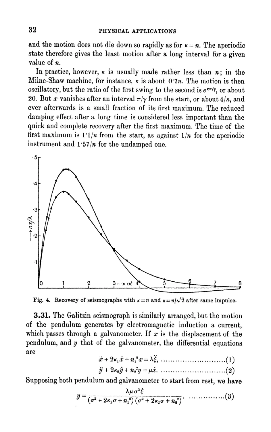
and the motion does not die down so rapidly as for * = n. The aperiodic
state therefore gives the least motion after a long interval for a given
value of n.
In practice, however, K is usually made rather less than n\ in the
Milne-Shaw machine, for instance, K is about (Yin. The motion is then
oscillatory, but the ratio of the first swing to the second is e n /y, or about
20. But x vanishes after an interval ?r/y from the start, or about 4/#, and
ever afterwards is a small fraction of its first maximum. The reduced
damping effect after a long time is considered less important than the
quick and complete recovery after the first maximum. The time of the
first maximum is 1'1/n from the start, as against \jn for the aperiodic
instrument and l*57/ft for the undamped one.
Fig. 4. Recovery of seismographs with /c=n and jc = 7i/\/2 after same impulse.
3.31. The Galitzin seismograph is similarly arranged, but the motion
of the pendulum generates by electromagnetic induction a current,
which passes through a galvanometer. If x is the displacement of the
pendulum, and y that of the galvanometer, the differential equations
are
x + 2*^ + n?x = A, (1)
if + 2K 9 y + nfy = px (2)
Supposing both pendulum and galvanometer to start from rest, we have

ONE INDEPENDENT VARIABLE
33
As a rule the two interacting systems are so arranged that and are
the same for both, and both are aperiodic, so that K = n. Then
y=
(*)
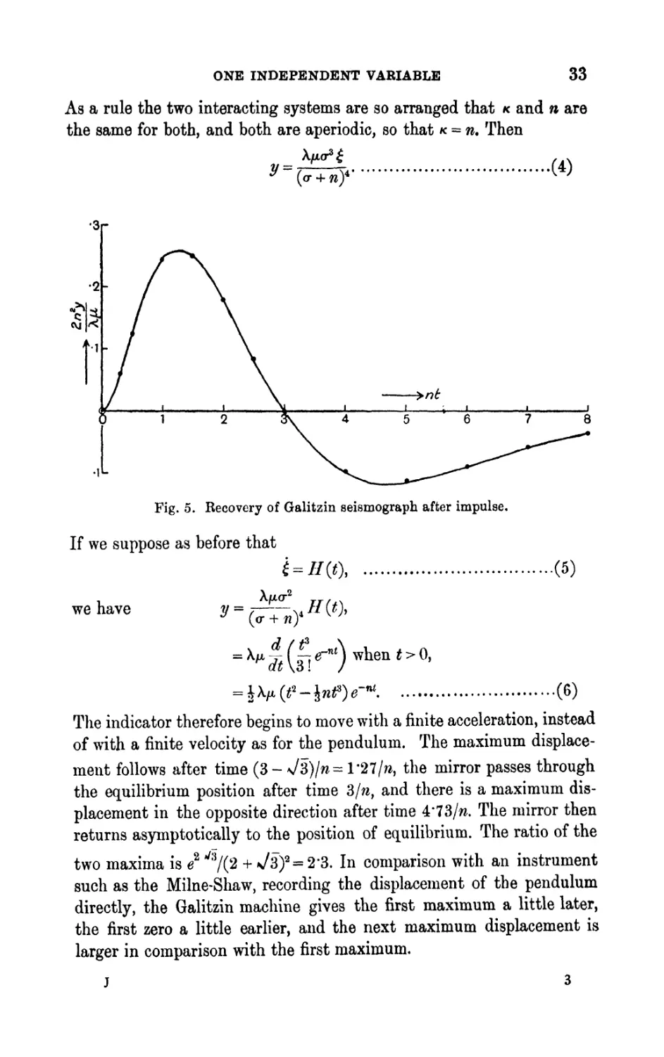
Fig. 5. Recovery of Galitzin seismograph after impulse.
If we suppose as before that
,.(5)
we have
The indicator therefore begins to move with a finite acceleration, instead
of with a finite velocity as for the pendulum. The maximum displace-
ment follows after time (3 - \/3)/= l'27/, the mirror passes through
the equilibrium position after time 3/, and there is a maximum dis-
placement in the opposite direction after time 4'73/ra. The mirror then
returns asymptotically to the position of equilibrium. The ratio of the
two maxima is e 2 J */(2 + N/3) 2 = 2'3. In comparison with an instrument
such as the Milne-Shaw, recording the displacement of the pendulum
directly, the Galitzin machine gives the first maximum a little later,
the first zero a little earlier, and the next maximum displacement is
larger in comparison with the first maximum.

34: PHYSICAL APPLICATIONS
In an actual earthquake the velocity of the ground is annulled by
other waves arriving later ; the complete motion of the seismograph is
a combination of those given by the separate displacements of the ground.
3.4. Resonance. A simple pendulum, originally hanging in equilibrium,
is disturbed for a finite time by a force varying harmonically in a period
equal to the free period of the pendulum. Find the motion after the
force is removed.
The differential equation is
^/sin nt, (1)
n
??O"
The solution is then #=//-5 ^>> (3)
(cr + n )
nothing having to be added on account of the initial conditions.
To evaluate this, we notice that
= - sin nt (4)
CT J + n n
Differentiating with regard to n, we have
1 , . 1
(5)
\v -r-i* j n ri* '
and x - ^ 2 (sin nt - nt cos nt) (6)
JLn
Suppose the disturbance acts for time nrjn^ where r is an integer. At
the end of this time
,__ __/_ rir f iy. ^ = Q (7)
The subsequent motion is therefore given by
(~l) r r7r/ .
x== - * 2 ^ cos { n t _
(8)
3.5. Three particles of masses m y ^m t and m, in order, are attached
to a light stretched string, the ends of the string being fixed. One of the
particles of mass m is struck by a transverse impulse /. Find the sub-
sequent motion of themiddleparticle. (Intercollegiate Examination, 1923.)
If #1, #2, #3 are the displacements of the three particles, P the tension,
and I the distance between consecutive particles, we find in the usual
way the three equations of motion

ONE INDEPENDENT VARIABLE 35
(1)
8 ), ..................... (2)
........................ (3)
p
where A^ - - ...................... (4)
w/ "' v '
Initially all the displacements are zero, 2 = x^ = 0, d^ = I/m. Hence the
subsidiary equations are
(<r 2 + 2X) 1 -Aa? 2 = cr//w, ............... (5)
-toi + (fX + 2X> 2 -Xff 3 = 0, ..................... (6)
-A^ 2 + (or 2 4-2\)^ 3 = ...................... (7)
, /21 . 2X 2 \ Xcr / ...
and (<^+ 2X - v- ^ )ff 2 =-3 TTT" ................ (9)
\20 OT- + 2A/ or 2 + 2Am v ^
Multiplying by or 2 + 2A we find
............ (10)
and
2QAor
_20/| _ 7o^ ___ 3(r
~ 58 m IT^TIX ~ 3o^ +
\
10AJ
10 I (sin dt sin ftt}
29 7)i \ a /3 )
where - z = r x > fP=* ( 12 )
We notice that the mode of speed *J(2ty is excited, but does not need
to be evaluated because it does not affect the middle particle.
3.6. Radioactive Disintegration of Uranium. The uranium family of
elements are such that an atom of any one of them, except the last, is
capable of breaking up into an atom of the next and an atom of helium*.
The helium atom undergoes no further change. The number of atoms
of any element in a given specimen that break up in a short interval of
time is proportional to the time interval and to the number of atoms of
that element present. If then u, #1, # 2 , $n are the numbers of atoms of
the various elements present at time t, they will satisfy the differential
equations
* We neglect 0-ray products, for reasons that will appear later.

36
PHYSICAL APPLICATIONS
du
dt
~dt
dt
K n _j X n _i
(1)
Suppose that initially only uranium is present. Thus when = 0, u = U Q>
and all the other dependent variables are zero. Then the subsidiary
equations are
(cr -f KJ) Xi =
(er 4- *_!) ^
_! = K n _ 2
.(2)
The operational solutions are
cr+K'
K) (<r -f K X
(o- 4- K) + KI ) (or 4- K 2 ) '
(3)
(<r + K)(or+K 1 )...(or+K n _ 1 )'
These are directly adapted for interpretation by -the partial-fraction
rule. In fact
i - K ic 2 -
> ...(4)

ONE INDEPENDENT VARIABLE 37
Of all the decay constants * is much the smallest. If the time elapsed is
long enough for all the exponential functions except er** to have become
insignificant, these results reduce approximately to
M=Wo0-*; a?i =--*; 3? a =-T*; ... x n = w (l-<r"0 ....... (5)
Kj K 2
With the exception of the last, the quantities of the various elements
decrease, retaining constant ratios to one another.
On the other hand, if the time elapsed is so short that unity is still
a first approximation to all the exponential functions, we can proceed
by expanding the operators in descending powers of a- and interpreting
term by term. Hence we see that at first Xi will increase in proportion to
t, # 2 to 2 , and x n to t n .
In experimental work an intermediate condition often occurs. Some
of the exponentials may become insignificant in the time occupied by
an experiment, while others are still nearly unity. We have
K IT
%r^ T -^^ = *r-\\?~*X r _.i-K t <T-*X T -.i + ] ......... (6)
and if K r t is small we can neglect the second and later terms in com-
parison with the first. Thus in this case
a? r = K r . 1 o- 1 ir r _ 1 ......................... (7)
If x r -i is of the form t 9 , we can put
If K r t is small, we can replace the exponential by unity and confirm
(7). If it is great,
rt i
<r- l e-* rt =l e~*r t dt = - +0(0-"r')
JO K r
and on continuing the integrations
.
K r K r S\
Thus x^tL-Jf^a. ...................... (9)
* r *r
Classifying elements into long-lived and short-lived according as K r t is
small or large for them, we find that the quantity of the first long-lived
element after uranium is proportional to , the next to t\ and so on.
All /?-ray products are short-lived when t has ordinary values.
Radium is the third degeneration product of uranium. In rock
specimens the time elapsed since formation is usually such that the

38 PHYSICAL APPLICATIONS
relations (5) have become established. As a matter of observation the
numbers of atoms of radium and uranium are found to be in the con-
stant ratio 3*58 x 10~ 7 . This determines */*,. Also the rate of break-up
of radium is known directly : in fact
!/*,= 2280 years.
Hence 1 /* = 6*37 x 10 9 years.
This gives the rate of disintegration of uranium itself.
A number of specimens of uranium compounds were carefully freed
from radium by Soddy, and then kept for ten years. It was found that
new radium was formed ; the amount found varied as the square of the
time. This would suggest that of the two elements between uranium
and radium in the series one was long-lived and the other short-lived.
Actually, however, it is known independently that both are long-lived.
The first, however, is chemically inseparable from ordinary uranium,
and therefore was present in the original specimens ; initially, instead
of %i = 0, we have
For the next element, ionium, we have
ff a = K 1 or" 1 iT 1 = KM #,
the variation of x l being inappreciable in the time involved. Also
#3 = K^CT~ 1 X^ ^KK^M t 2 .
Soddy* found that 3 kilograms of uranium in 1015 years gave
202 x 10~ 12 gm. of radium. Hence, allowing for the difference of atomic
weights,
and K 2 = 8*64 x 10~ 6 /year; i/ K2 = 116 x 10 5 years.
This gives the rate of degeneration of ionium. Soddy gets a slightly
lower value for l/* 2 from more numerous data.
3.7. Some dynamical applications. Suppose we have a dynamical
system specified by equations such as those in 1.72, save that & is
replaced by t, and that the system is at first at rest and then disturbed
by a force S r applied to the coordinate y r . The subsidiary equations
are
^ 9 e ma y t ^S r (i = r) ....... (1)
Phil. Mag. (6) 38, 1919, 483-488.

ONE INDEPENDENT VARIABLE 39
Writing A for the determinant formed by the e'&, and E n for the minor
of e rB in this determinant, we have the operational solution
* = %8r ............................... (2)
If the determinant A is symmetrical, so that
E n =E ar .............................. (3)
we see that a given force S r applied to the coordinate y r will produce
precisely the same variation in y a as the same force would produce in
y r if it was applied to y. Thus we have a reciprocity theorem applic-
able to all non-gyroscopic systems ; linear damping does not invalidate
the argument if the terms introduced by friction contribute only to
the leading diagonal of A.
If the forces reduce to an impulse, so that S r can be replaced by o-/ r ,
the solution becomes
y. = f"* ............................... (4)
We can evaluate the initial velocities by expanding in descending
powers of <r. The first term is
*=T;'. ............................... (5)
where A is the determinant formed by the a's, and A rs the minor of
a ra in it. Hence the initial velocities, found by operating on this with
<r, are
vy. = 4j!Jr ............................... (6)
Now the constants a rs are merely twice the coefficients in the kinetic
energy, which is a quadratic form. Hence the determinant A is sym-
metrical whether the system is gyroscopic or not, and the reciprocity
theorem for impulses and the velocities produced by them is proved.
The subsequent motion can be investigated by interpreting according
to the partial-fraction rule. But let us consider the simple case where
the system is non-gyroscopic and frictionless. Then
A = 411(0* + a 2 ), ........................ (7)
where the a's are the speeds of the normal modes. Then
where E r *(-<J) denotes the result of putting -a 2 for a 3 in E rg . The

40 WAVE MOTION IN ONE DIMENSION
contribution of the a mode to the initial rate of change of y s is therefore
An immediate consequence of the presence of the factor E T9 (- a 2 ) in
the numerator is that if an impulse is applied at a node of any normal
mode, that mode will be absent from the motion generated.
Another illustration is provided by Lamb's discussion* of the waves
generated in a semi-infinite homogeneous elastic solid by an internal
disturbance. The normal modes of such a system include a type of
waves known as Rayleigh waves. These may be of any length, and
involve both compressional and distortional movement ; if the depth is
2, the amplitude of the compressional movement in a given wave is
proportional to e~ az , and that of the distortional movement to e"^ 9
where a and /J depend only on the wave-length. Lamb found that if
the original disturbance was an expansive one at a depth/, the ampli-
tude of the motion at the surface contained a factor 0~ a/ ; but if the
original disturbance was purely distortional, the corresponding ampli-
tude contained a factor e~&. These factors are the same as would occur
in the compression and distortion respectively at depth /in a Rayleigh
wave with given amplitude at the surface.
CHAPTER IV
WAVE MOTION IN ONE DIMENSION
4.1. In a large class of physical problems we meet with the differen-
tial equation
where t is the time, x the distance from a fixed point or a fixed plane,
y the independent variable, and c a known velocity. Let us consider the
solution of this equation first with regard to the transverse vibrations
of a stretched string. In this case we know that
c* = P/m, (2)
where P is the tension and m the mass per unit length. Write <r for
, and p for d/dx. Suppose that at time zero
y=/00; 1=^00, (3)
* Phil. Tram. A, 203, 1-42, 1904.

WAVE MOTION IN ONE DIMENSION 41
where / and F are known functions of x ; that is, we are given the
initial displacement and velocity of the string at all points of its length.
Then we are led by our previous rules to consider the subsidiary
equation
+ *F(p) (4)
o
or ?/ = ~- f(r\ + 7fYr"> f Vl
vl V ft > 2 y V 1 *'./ 2 2 o V^y V^y
O" 4 C p o" 6 c p"
But
o- 2 - c 2 p' 2 ^ \<r ~ C/>
~ 2 (^ "*" ^ / \"J
O- 1 / or
cr- - c 2 p 2 2cp \cr-cp a +
"
In (7) the I//? has been put last in consequence of our rule that opera-
tions involving negative powers of p must be carried out before those
involving positive powers. Hence
+ f( x _ c ^)l (g)
2 JT ^^*/ = - ^r \Q> C j I lj \*E) ^^
^C Jo
and therefore
fX
' J X
This is D'Alembert's well-known solution.
This cannot, however, be the complete solution. Equation (1) has
been assumed to hold at all points of the string ; but if any external
forces act these must be included on the right of the equation of motion.
In such problems the ends of the string are usually fixed, and reactions
at the ends are required to maintain this state ; in the complete equa-
tions of motion these reactions should appear. They are unknown
functions of t, and therefore necessitate a change in the mode of
solution.

42 WAVE MOTION IN ONE DIMENSION
But D'Alembert's solution can be adapted so as to fulfil all the con-
ditions. We notice that the solution consists of two waves travelling in
opposite directions with velocity c. If the initial disturbance is confined
to a region within the string separated by finite intervals from both
ends, it will take a finite time before D'Alembert's solution gives a
displacement at either end ; hence no force is required to maintain the
boundary conditions, and the solution will hold accurately until one of
the waves reaches one end.
Again, the initial disturbance is specified only for points within the
length of the string, that is, for values of x between and /, say ; and
by the last paragraph D'Alembert's solution would be complete if the
length were infinite. If then we consider an infinite string stretching
from - QO to + co , and disturbed initially so that/(,r) and F(x) are both
antisymmetrical about both # = and %~l,y will vanish ever after at
these points, so that no force is required to keep them fixed, and
D'Alembert's solution for such an infinite string will therefore be
equivalent to that for the actual string from x = to x - /. Thus we have
a formal rule for finding the position of the string at any subsequent
time : consider an infinite string with the actual values of the initial
velocity and displacement between x = and x = /, but with the dis-
placement and velocity outside this stretch so specified as to be
antisymmetrical with regard to both x = and x = /; then D'Alembert's
solution for the infinite string will be correct for the actual string for
the same values of x.
4.2. We may approach the problem in another way. Taking the same
subsidiary equation
9 2 cr 2 tr 2
except that the effects of the initial velocity will not be considered at
present, let us solve with regard to x as if cr were a constant. The
justification of this procedure is given later in 4.6. The boundary con-
ditions are that y = when x = and when x - 1. Using the method of
variation of parameters, we assume that the solution is
y - A cosh + 5sinh , .................. (2)
c c
where A and B are functions of x subject to
(3)
c c

WAVE MOTION IN ONE DIMENSION 43
Substituting in the equation (1) we find
aX T>f L <TX " f( \ f t\
+ B cosh y =--/(*) (4)
Hence
^1' = -/(#)sinh ; jB' = / (a?) cosh (5)
Now y must vanish for all time when x - ; hence A (0) = 0. Thus
r
c c
Also # must vanish when x = /. Hence
7
jB(/) sinh = - A (1) cosh (7)
and J5(/) = -coth~ / -/()sinh- rf, (8)
c JQ c c
giving 5 (a-) = - coth - f '- / (f ) sinh - ^
C JQ C C
In all we find
y = / -/ (f) sinh (cosh - coth sinh ) d
y c v/ c \ c c c /
' f / 1 f.
(j" f cry f trt i &v t ^"t
~ f () sinh ( cosh coth sinh
c ' c \ c c c
o C c SHlcrC
C ^ ...................... (10)
Before carrying out the integration with regard to f , we can interpret
the integrand by the partial-fraction rule. Each integral vanishes when
<r = 0, and therefore no constant term appears in the solution. But
sinh arl/c vanishes when
^=rr .................................. (11)
c
where r is any integer, positive or negative. Hence
rur . , nirt; . , l X
c c
2 2 . nrg . nr^c /1rt x
- 2 ysm-y^sin-y-cos T .......... (12)
r= i* li

WAVE MOTION IN ONE DIMENSION
By symmetry the corresponding factor in the second integral has the
same value. Hence
? ^ f l /./^ . rir ,. . TTTX met , _ v
y= s // / () sm - T <# . sin 7 cos-;- ....... (13)
>=i fr ./o * ll
This is the solution given by the method of normal coordinates. Putting
t zero, we obtain the Fourier sine series
/(*)-?///) "in ^rin^E* ................ (14)
The effect of an initial velocity can be obtained by a similar
process.
But in practice the solution by trigonometrical series is not often the
most convenient form. It usually converges slowly; but what is more
serious is that its form suggests little about the nature of the actual
motion beyond the fact that it is periodic in time 2//c. To find the
actual form of the string at any instant it is necessary to find some way
of summing the series, which may be rather difficult. A more convenient
method is often the following*. We have seen that the interpretation of
any operator valid for positive values of the argument is equivalent to
an integral in the complex plane, the path of integration being on the
positive side of the imaginary axis. Then a factor cosech <rl/c in the
operator can be written
. j, ~- - * + e -* l/c + . . .) . . .(15)
smh <rl/c 1 - e~ 2(Tl/c ^ J ^ '
and when interpreted by Bromwich's rule this will give rise to a series
in powers of e'^ c in the integrand. But since the real part of K is
everywhere positive on the path, the series is absolutely convergent,
and integration term by term is justified. Hence it is legitimate to ex-
pand the operator in this way and to interpret term by term. Then for
*<*,
srnW/c sinh er(f - x)/c __ , (x _ ( .-2,^
vSS^IJc * ( ;
(l-^-2<rtf-ar)/c)( 1+ ^2a//c + ^-4crVc4. ...). ...(16)
and for > #,
=
8mho7/c A \
(1 _ 6 -2a(l-fl/c) (! 4. ... (>>
On multiplying out either expression we obtain a series of negative
exponentials of the forms e~* (-/*, with a > , or a-'tt-o)/^ with ^ > a.
* Heaviside, Electromagnetic Theory, 2, 108-114.

WAVE MOTION IN ONE DIMENSION 45
Then j*' ^f (ft e-* (*-&!' dt= (/($)&- (-*)/' ....... (18)
But according to our rule e~* (~*)/ c is zero when t - (a - )/c is negative
and unity when this quantity is positive. Hence the integral (18) is
zero unless a - ct lies between d and 2 > and then it is equal to/(a - ci).
Similarly ('-/(O*"^""^^- ff(t)deti-M ......... (19)
Ji C J
and 0-* (*-a)/c = o if > <tf + a
= 1 if < ct + a,
so that (19) is zero unless ct + a lies between & and 2 , and then is
equal to/(c + a).
It follows that at any instant the effect of the initial displacement
/() at the point is zero except at a special set of points where one
or other of the quantities a ct is equal to Since a does not involve
, we see that this way of expressing the solution reduces it to a set of
waves moving in each direction with velocity c. The first three factors
in (16) give
...... (20)
for values of x greater than The first term gives \f($) at time
(a?-f)/c, the second -/() at time (x + fyc, the third -/() at
time \x - + 2 (l-x)}/c and the fourth /() at time {.r + + 2 (/-#)}/&
The first term represents the direct wave from to *r, the second the
wave reflected at x = 0, the third that reflected at x - /, and the fourth
one reflected first at x = and then again at x^l. The term e-*"Uc in
the last factor of (16) will give four further and similar pulses, each
later by 2l/c than the corresponding pulse just found. These are pulses
that have travelled twice more along the string, having been reflected
once more at each end. Similarly we can proceed to the interpretation
of later terms as pulses that have undergone still more reflexions.
The part of the solution arising from values of greater than x may
be treated similarly. The interpretation in terms of waves is exactly
the same.
4.3. As a particular case let us consider a string of length /, origin-
ally drawn aside a distance >? at the point x ~ b y so that initially it lies
in two straight pieces, and then released. Then

46 WAVE MOTION IN ONE DIMENSION
and the subsidiary equation is
d 2 y cr 2 __ o- 2
a^~? y ~~? y (2 '
The solution that vanishes at the ends is
X A -L " ' 1 * /I 1\ r. 7
y - rj j + A smh smh -(l-b) <x<b
^ x " ab C ^ , (3)
y = 77 - .- + A sinh sinh -(I- x) b <x<l
J ' l~b c c ^ '
where the constants have been chosen so as to make y continuous at
# = b. Also a discontinuity in By /dan at this point would imply an infinite
acceleration, which cannot persist. Hence we add the condition that
dy/da shall be continuous, which gives
*? I r + T~- L ) + - 1 cos ^ ~~ s i n h - (/ - 6) + sinh cosh - (/- b) \ =-
\6 l-b) c I c c ^ ' c c ^ 'J
(4)
and on simplifying
I i o-/
(5)
Thus
- b c sinh <r%/c sinh <r (/ b)/c\
I cr sinh(r//c J
^_ >;/ (6 /, v c sinh o-^/c sinh <r(lai)/c'
y ~ b (I - 6) U o- sinh o7/c
Interpreting by the partial-fraction rule, we notice that the contribu-
tion from o- = just cancels the term independent of o-, while the rest
gives*
1 rirb . nrx rvct . 7 /rTN
^2 "2 sm ~T sm ~T~ cos ~T" < ^ < /. (7)
^7T 2 III ^ '
Alternatively, we can interpret the solution for < x < b in exponentials,
for
sinh /csmh<r(l-b}/c^ h _ x]} l _ c _ (2ffxlc]
sinhcr^/c 2
and - = ^ #>0 ............................... (9)
cr
Then e-*( b -*V G - = ct-(b-x\ ..................... (10)
* Kayleigh, Theory of Sound, 1, 1894, 185.

WAVE MOTION IN ONE DIMENSION
47
when this is positive, and otherwise is zero. Thus y retains its initial
value i\x\l unaltered until time (b #)/c, when the wave from the part
where x > b begins to arrive. After that we shall Have
......... (ii)
This solution remains correct until ct = b + x, when the wave reflected
at x - begins to arrive. Thenceforward
}-
<r
Hence
'l-b
[ = 2*. ...(12)
(13)
Fig. 6.

48 WAVE MOTION IN ONE DIMENSION
The part of the string reached by the first reflected wave is therefore
parallel to the original position of the part where b<x<L
When ct - (b - x) + 2 (/ - ), a wave reflected at x = / arrives, and
This holds until ct = (b + #) + 2 (/ - 6) ; in the next phase
When ct = 2/, the whole of the string is back in its original position ;
the term in e~ 2ffl l c then begins to affect the motion, and the whole
process repeats itself. We see that at any instant the string is in three
straight pieces. The two end pieces are parallel to the two portions of
the string in its initial position, and are at rest. For the middle portion
the gradient tyfox is the mean of those for the end portions, and the
transverse velocity is nT7ir~h\ - ^ Q middle portion is always either
extending or withdrawing at each end with velocity c. [Fig. 6.]
4.4. A uniform heavy string of length 2/ is fixed at the ends. A
particle of mass m is attached to the middle of the string. Initially the
string is straight. An impulse J is given to the particle. Find the sub-
sequent motion of the particle. (Rayleigh, Theory of Sound, 1, 1894,
204.)
The differential equation of the motion of the string is
Take x zero at the middle of the string. By symmetry we need consider
only the range of values < x < /. Suppose that the displacement of the
particle is 17. When = 0, y and dy/dt are zero except at x-Q. The
subsidiary equation therefore needs no additional terms. The solution
is therefore
v-v
y ~^ sinhcr//c ......................... W
If now P be the tension in the string, the equation of motion of the
particle is
m ^ = 2P (^) ......................... , 8 )
df \fa/ M '
If p be the mass of the string per unit length,
(4)

WAVE MOTION IN ONE DIMENSION 49
On account of the initial conditions the subsidiary equation tor the
particle is
-coth- + Jcr ...................... (5)
c c ^ '
Hence ^
pi _ 7 mass of half the string f ,
A; ..... --- JTTT - T^~T ................... (7)
w mass ot the particle v
Then 2P = /cmc*/l .............................. (8)
i _ _ lJ] mc (a\
aU * " Wc) + k COtF(~cr7/c) ...................... W
To interpret this solution by the partial-fraction rule, we recollect that
the system is a stable one without dissipation, and therefore all the
zeros of the denominator are purely imaginary. Putting
or//C-td) .............................. (10)
we see that the zeros are the roots of
(O^/JCOt 0> ............................... (11)
There is a root between every two consecutive multiples of TT, positive
or negative; and the roots occur in pairs, each pair being numerically
equal but opposite in sign. Then
77 = 2 _ _______ _gi<rf/f ............ (12)
me twc (1 -f k cosec 2 o>) (l/c) '
the summation extending over all positive and negative values of w,
9/7 i
(13)
v x
7 - s-^,
+ A cosec- o>) ' y
the summation being now over positive values of <o.
If a root of (11) is mr + X, where n is great and X < TT, we have
(wir + A)tanX = ........................ (14)
and X^ ^/WTT ................................. (15)
approximately. The series (13) converges like 2 -sin 2 to, or 2 -3. It
therefore converges fairly rapidly at the beginning, but more slowly
later. Also the w's are incommensurable, and therefore the motion does
not repeat itself after a finite time ; thus the labour of computation
would be great.
J 4

50 WAVE MOTION IN ONE DIMENSION
To express the solution in terms of waves, it is convenient to change
the unit of time to //c, the time a wave takes to traverse half the length
of the string. Also J/m may be replaced by V. Then
= F _ = V(l-e-^}
^ ~ a- + k coth <T ~ (a- + k)- (a- - /t) e' 2 "
* -*_
'
The first term is zero for negative values of the time; for positive
values it is equal to
After time 2 the second term no longer vanishes. We have
and the second term is equivalent to
-^f {I- e-*-*> -k(t- 2) e-*^} fort >2 (19)
K
The third term is zero for t < 4; for greater values it is easily found to
be
^[1 - {1 + k (t - 4) + If (t-^f] <r*<'- 4 >] (20)
The process may be extended to determine the motion up to any in-
stant desired. The entry of a new term into the solution corresponds
to the arrival of a new wave reflected at the ends.
4.5. A uniform heavy bar is hanging vertically from one end, and a
mass m is suddenly attached at the lower end. Find how the tension at
the upper end varies with the time. (Love, Elasticity, 283.)
If x be the distance from the upper end, and y the longitudinal dis-
placement, y satisfies the differential equation

WAVE MOTION IN ONE DIMENSION 51
where p is the density, E Young's modulus, and jPthe external force
per unit volume, in this case pg. Put E/p = c 2 , and let the displacement
of a particle before the weight is attached be y . Then
When x = 0, y Q = ; and if the bar be of length /, dyjfa = when x = I.
Hence 2/o = ^(l-|f) ......................... (3)
After the weight is attached, we still have
while when t = 0, y - y 9 and dy/dt = 0. Hence the subsidiary equation is
and the solution that vanishes with ^r is given by
y-y Q = A sinh OT^/C, ........................ (6)
where A is independent of x.
If TO- be the cross section of the bar, the equation of motion of the
mass m is
the derivatives being evaluated at x = I. The subsidiary equation is
fy
wo- 2 y = 772^ + ^(r 5 ?/ - E *-, .................. (8)
which gives on substituting for y from (6)
(a 2 sinh + - cosh } A =g ................ (9)
V c me cj y ^ '
The tension at the upper end is
gpl + Eo-A/c = gpl + - ------ .- - f , , ^ k . yy . . (10)
47 ' AW cosh (CT//C) + wco- smh (o7/c)
If A be the ratio of the mass of the weight to that of the bar,
4'*

52 WAVE MOTION IN ONE DIMENSION
and the tension is
\_k
We see that gmjwk is the tension due to the weight of the bar alone,
and gm/rff is the statical tension due to the added load alone. To evaluate
the actual tension, we expand the operator in (5) in powers of e~* lfc .
Taking lie for the new unit of time, we have
_ _ __
k<r sinh o- + cosh cr ~~ (fca- + 1) -(kv - l)e~' 1(T
...... (13)
The first term vanishes up to time unity, and afterwards is equal to
2 (1-0- (*-i)/*) ............................ (14)
This increases steadily up to time 3, when the next term enters. Again,
k<r
= M +-'/* + 2 (*/*)-</* ............... (15)
and the first two terms, when t > 3, are equivalent to
2(1- *-<*-D/*) - 2 [1 - r<-3V* - 2 {(t - 3)1 1] e^-^]
= 2e--Vl k [l + (2/k)(t-Z)-e-v k ] ................... (16)
This has a maximum when
l + 0-2/* = 2(;_ 3 ) ........................ (17)
Equation (17) has a root less than 5 if
4/>l + <r 2 /*, ........................... (18)
which is an equality if k = 2*7. Thus for k ^ 1 or 2 the maximum tension
will occur before t = 5. If k = 1 the maximum tension is when t = 3 '568,
and is equal to 3'266 gm/& 1*633 times the statical tension. If k = 2
the corresponding results are t = 4*368, 2*520 gm/w, and 1*680 times the
statical tension.
The third term enters at time 5, and afterwards is equal to
2 [1 - -< - *)/* - 2 {(* - 5)/} 2 0-C- 5 )/*].
If k = 4, the maximum stress is when t = 6*183, and is equal to 2*29 gin/m.
The statical tension is 1*25 grm/ar, so that the ratio is 1*83.
Love proceeds by a method of continuation, but the present method
is much more direct, and probably less troublesome in application.

WAVE MOTION IN ONE DIMENSION 53
4.6. A general proof that the results given by the operational method,
when applied to the vibrations of continuous systems, are actually
correct, has not yet been constructed. It would be necessary to show
that the solution actually satisfies the differential equation and that it
gives the correct initial values of the displacement and the velocity at
all points. The proof that it satisfies the initial conditions would be
difficult in the most general case. We have seen that in one of the
simplest problems, that of the uniform string with the ends fixed, the
verification that the solution is valid for the most general initial dis-
placement is equivalent to Fourier's theorem. But for more specific
problems the operational solution is equivalent to a single integral, and
the direct verification that it satisfies the initial conditions is usually
fairly easy. To show that it satisfies the differential equation, it would
be natural to differentiate under the integral sign and substitute in the
equation. But in practice it is usually found that the integrand, near
the ends of the imaginary axis, is only small like some low power of
I/K (the second in the problems of 4.3, 4.4, and 4.5), and consequently
the integrals found by differentiating twice under the integral sign do
not converge. But we can proceed as follows. If a part of our solution is
and this integral is intelligible for all values of x and t within a certain
range, we have
A*
e* h - 2 + e~* h <
If / ^
= Lim ~ I /(K) exp K It + -
- 2
The two integrals are identical before we proceed to the limit, and
therefore their limiting values are the same. Hence
and the differential equation is satisfied. This argument does not
assume that the derivatives of y are expressible as convergent integrals,
but only that they exist.

54 CONDUCTION OF HEAT IN ONE DIMENSION
The argument breaks down at points where the second derivatives do
not exist; as for instance in 4.3 at the points where the slope of the
curve formed by the string suddenly changes. At these points there is
a discontinuity in the transverse component of the tension, so that the
point has momentarily an infinite acceleration. This is why the velocity
changes discontinuously when a wave arrives. The momentum of a
given stretch of the string, however, varies continuously; the difficulty
is the fault of the representation by a differential equation, not of the
method of solution.
CHAPTER V
CONDUCTION OF HEAT IN ONE DIMENSION
5.1. The rate of transmission of heat across a surface by conduction
is equal to -kd V/dn per unit area, where V is the temperature, k a con-
stant of the material called the thermal conductivity, and dn an element
of the normal to the surface. Hence we can show easily that in a uniform
solid the rate of flow of heat into an element of volume dxdydz is
kW.dxdydz.
But the quantity of heat required to produce a rise of temperature dV
in unit mass is cdV, where c is the specific heat, and therefore that
required to produce a rise dV in unit volume is pcdV, where p is the
density. Hence the equation of heat conduction is
*V7. ........................... (1)
If we put
h\ .............................. (2)
is called the thermometric conductivity, and the equation becomes
In addition, there may be some other source of heat. If this would
suffice to raise the temperature by P degrees per second if it stayed
where it was generated, a term P must be added to the right of (3).
It is usually convenient to write o- for d/dt, and
cr = *y .................................. (4)
The operational solutions are then functions of q ; butg must be expressed
again in terms of <r before interpreting.

CONDUCTION OF HEAT IN ONE DIMENSION 55
5.2. Consider first a uniform rod, with its sides thermally insulated,
and initially at temperature 8. At time zero the end x = is cooled to
temperature zero, and afterwards maintained at that temperature. The
end x - / is kept at temperature 8. Find the variation of temperature at
other points of the rod.
The problem being one-dimensional, the equation of heat conduction
while at time 0, V is equal to 8. Hence the subsidiary equation is
"8, (2)
or -&-fr = -y>8. ........................... (3)
The end conditions are that
= when # = 0,1
= Swhenff = /. J ........................ ( }
The integrand is an even function of q, and therefore a single-valued
function of o-. It has poles where
gJ = + iWir; that is, or = - AWir 8 // 2 , ............... (6)
where n is any integer. But the negative values of q give the same
values of a- as the positive values, and therefore when we apply the
partial-fraction rule we need consider only the positive values. The part
arising from o- = is
The general term is
-S~mi~-e-*l? y ...... (8)
and the complete solution is
(9)
V
If irhfi/l is moderate, this series converges rapidly, and no more con-
venient solution could be desired. It evidently tends in the limit to the
steady value 8x11.

56 CONDUCTION OF HEAT IN ONE DIMENSION
But if irkt*/l is small the convergence will be slow. In this case we
may adopt a form of the expansion method applied to waves*. We can
write (5) in the form
For if we interpret this as an integral along the path L, the argument
of q is between \ir at all points of the path, and the series converges
uniformly. Integration term by term is therefore justifiable, and we may
interpret term by term. Now
qx = x<r*lh, (11)
and by 2.4(16) <r x =l-Erf-^ (12)
Hence
- Erf - .-(13)
When w is great, 1 -Erf w is small compared with e~ H *. If then xl"2
is moderate, but l/2hi* large, this series is rapidly convergent, and can
in most cases be reduced to its first term. This solution is therefore
convenient in those cases where (9) is not.
5.3. One-dimensional flmv of heat in a region infinite in both direc-
tions. First suppose that at time the distribution of temperature is
given by
F=//Gr) ............................... (1)
We have just seen that the function expressed in operational form by
*-*=! -Erf-., ........................... (2)
satisfies the differential equation
dt far 4 ' v '
for positive values of x\ and by symmetry it will also satisfy it for
negative values of x, since the function and its derivatives with regard
to x are continuous when x = 0. Also when t tends to zero this function
tends to zero for all positive values of #, and to 2 for all negative
values. It follows from these facts that the function
W
satisfies the differential equation for all values of x and all positive
values of t\ and when t tends to zero the function tends to zero for
* Heaviside, Electromagnetic Theory, 2, 69-79, 287-8.

CONDUCTION OF HEAT IN ONE DIMENSION 57
negative values of #, and to unity for positive values, Hence this function
is the solution required.
Suppose now that the initial distribution of temperature is
Vf(v\ (**\
Y -/ W> W
where /(a?) is any known function. Then this is equivalent to
r\\ (ti\
x )} W
But the solution for positive values of the time that reduces to
when t = is
Hence by the principle of the superposibility of solutions the solution
of the more general problem is
...................... (8)
kt-
Putnow = x + 1kfi\ ............................... (9)
Then V =~r /0 + 2/^\)e-*'<A ................ (10)
VTT.'-oo
This is the general solution obtained by Fourier.
5.4. If the temperature is kept constant at # = 0, but the initial
temperature is/(,r) for positive values of #, we may proceed as follows.
If we consider instead a system infinite in both directions, but with the
initial temperature specified for negative values of .r so that
/(-*)=-/Cr), ........................... (1)
we see that the temperature at ,r = will be zero at all later instants and
the solution of this problem will fit the actual one. Hence
.L r
.'O
(3)

58 CONDUCTION OF HEAT IN ONE DIMENSION
If in particular the initial temperature is everywhere $, /() = $, and
V = S
(4)
Thus the solution of 5.2 is regenerated. In Kelvin's solution of the
problem of the cooling of the earth, 5.3 (10) was adapted to a semi-
infinite region in this way.
The value of 3 Vfix at the end x = is obtainable by differentiating
the solution valid for a semi-infinite region. In Kelvin's problem
F=
and = ty=--- ......................... (5)
The same result is found by differentiating (4).
We notice the curious fact that although the original exact solution
for a finite region in 5.2 (5) is a single-valued function of o-, a square root
of t appears in the approximate solution for a greatly extended region.
The reason can be seen by differentiating the exact solution. It gives
(6)
which is a single-valued function of o-. But when we use Bromwich's
interpretation we find that
............ (7)
^
which is again single valued; but if ** is specified to be real and positive
when K is real and positive, it has a positive real part at all points on
L, and therefore if / is great coth K*l/h is practically unity. The integral
is therefore equivalent to
(8)
which is our interpretation of <r*$/A, and is equal to tilh^KTrt), We could
have started by specifying the sign of K* to be negative when K is positive,
but then *c* and coth **//A would both have been simply reversed in sign,
and the same answer would have been obtained,
5.5. Imperfect cooling at t/ie free end of a one-dimensional region
With the initial conditions of 5,2, let us suppose that the end x = I is
maintained at temperature S as before, but that the end x = is not

CONDUCTION OF HEAT IN ONE DIMENSION 59

effectively cooled to temperature zero. Instead we suppose that it radiates
away heat at a rate proportional to its temperature. At the same time
heat is conducted to the end at a rate kd Vfix per unit area. These
effects must balance if the temperature at the surface is to vary con-
tinuously, so that instead of having V= at the end as before we shall
have a relation of the form

dV

^--aF=Oat# = ......................... (1)

The equation 5.2 (3) is unaltered, and the operational solution is

r=tf{l-4sinh0(J-tf)} ..................... (2)

where A is to be determined to satisfy (1). Hence

qA cosh#/-a(l -A sinh#/) = .................. (3)



and ---" ;

q coshql + a sinhql)

The roots in a- are real and negative, and we can proceed to an inter-
pretation by the partial-fraction rule as usual. Or, using the expansion
in " waves/' we have



\i ... (

/J



If the length is great enough to make the terms involving e~ 2ql inap-
preciable, we can reduce this to its first two terms, thus :



q +

If a is great, the solutions reduce to those of 5.2 ; this is to be expected,
for (1) then implies that F= when #^0, which is the boundary con-
dition adopted in 5.2. If a is small, V reduces to /S; the reason is that
this implies that there is no loss of heat from the end, and therefore the
temperature does not change anywhere. For intermediate values we may
proceed as follows. If

<*<*"** Sn\

# = - .................................... (7)

J q + a.

Brorawich's rule gives

I f ak I . K*X\dK , .

y = , expUf--T-) ................ (8)

y *JiK* + ah ^ k ' K

Put K-V ..................................... (9)




60 CONDUCTION OF HEAT IN ONE DIMENSION
The path of integration for X is a curve going from e~* m to
where R is great, passing on the way within a finite distance of the
origin on the positive side. Denote this path by M. Then
If ak /.. A#\ ,, ,,- N
y = ~ r -- exp (\~t- ,- )d\, ............... (10)
TI JM (\ + a/i)\ r \ h) ^ '
n x
But
If 1 A?. ^\ ^x If I * Ka\d*
- v exp A 2 t--j )rfA = I exp Ktf-- r
Tt M A, \ A / 27TI J L V A / K
(12)
The second part of (11) can be written as an integral with regard to /x,
where
/*-/\ + ak .............................. (13)
along a path obtained by displacing M through a distance aA; but the
integrand is regular between these paths and the route M may still be
used. The second part is therefore
1 ( 1 ( I x\\
--- I - exp \u?t - /A ( 2akt + T ) r ex P (^Wt + a,r) da
JMH ( \ hi] '
= -exp(a 2 A 2 ^a^)(l--Erf^ + 2 f 2# l ............ (14)
I 2ht* J
and y = 1 - Erf - exp (y 2 + cur) {1 - Erf ( + y)j ......... (15)
where = #/2^ 4 ; y = aA^ ......................... (16)
Hence F = fl [Erf* + exp (/+<*?) {1 -Erf (+y)}] ....... (17)
This is the same as Riemann's solution*.
The temperature at the end is
V x = = Szxpf{l-ETfy} ..................... (18)
whence the temperature gradient at the end follows by (1). For small
values of the time the temperature at the free end falls continuously ;
the temperature gradient there is not instantaneously infinite as in
5.4 (5). For great values of the time we can use the approximation 2.4
(21), giving
* Kiemann-Weber, Partielle Differentialgleichungen, 2, 95-98, 1912.

CONDUCTION OF HEAT IN ONE DIMENSION 61
This is equivalent to one found by Heaviside*. Heaviside gives also an
expansion in a convergent series, suitable for small values of t, but it
is probably less convenient than the equivalent expression (18) in finite
terms. We see from (19) that the longer the time taken the better is
the approximation to (9F/9r)a;=o given by the simple theory of 5.2.
5.6. A long rod is fastened at the end x = 0, the other end not being in
contact with a conductor. Initially it is at temperature 0, but at time
the clamped end is raised to temperature 8 and kept there. Each part of
the rod loses heat by radiation at a rate proportional to its temperature.
The differential equation is now
*l^-*v ........................... (i)
a# a^ 2 ^ '
where a is a constant. Let us put
<r + a a =AV .............................. (2)
and write the equation
w-*^ ............................ w
At x = / there is no conduction out of the rod, and therefore d Vfix
vanishes. Also V = 8 when x - 0. The solution is
_ ^
cosh?'/ ' v '
This can be expanded in powers of e~ 2rl . The first term, which is the
only one we require, is
V = Se~ rx ................................................ (5)
8
Put * + a 2 = X 2 ............................... (7)
mi ir S [ f M 2 ox, M Xd\
Then F= -I exp { (X 2 - a") t - -j~ \ --
TTI JM ( h ) A- - a-
....... (8)
v/
But if X = a + fi .............................. (9)
the term in 1/(X -a) becomes
I
Electromagnetic Theory, 2, 15.

62 CONDUCTION OF HEAT IN ONE DIMENSION
as in 5.5 (12). The complete solution is
/n\
....... (11)
When a = this reduces to
(12)
so that the disturbance of temperature spreads along the rod, the time
needed to produce a given rise of temperature at distance x from the
end being proportional to x f \ If t is small enough to make a$ small, the
error functions will be practically unity except where x is not great
compared with 2k$. For such values of x the exponentials are nearly
unity. Thus at first the heating proceeds almost as in the absence of
radiation from the sides of the rod.
But if a$ is great and x\1ht^ small or moderate, the first error func-
tion in (11) is practically - 1, and the second + 1. Thus in these con-
ditions
V = Se-*/>> (13)
This is seen by a return to the original equation to be the solution
corresponding to a steady state. This will hold so long as a$ - xj2ht^
is large and positive, even if x^lit 1 is itself large. The region where the
approximation (13) is valid therefore spreads along the rod with velocity
2aA; if atfi has once become^large, each point on the rod reaches a nearly
steady temperature at a time rather greater than #/2aA.
If a$ is large and xj2ht still greater, the solution is nearly
} (14)
If further the argument of the error function is large, we can write
FJ. /->/ /r I V X ~~ t&flv ) I
_ ___ __ ,v o -~axin OYT~I J - v
. - .__o0 exp ^ A L2+ r
(15)
^ '

CONDUCTION OF HEAT IN ONE DIMENSION 63
In the regions that have not reached their steady state, the temperature
resembles that for the problem without radiation, except that the small
v
factor \ e~ a ** ---- 7- must be introduced.
* x-
5.7. The cooling of the earth. Cooling in the earth since it first became
solid has probably not had time to become appreciable except within a
layer whose thickness is small compared with the radius. It is therefore
legitimate to neglect the effects of curvature and treat the problem as
one-dimensional. Radiation from the outer surface must have soon
reduced the temperature there to that maintained by solar radiation, so
that we may suppose the surface temperature to be constant and adopt
it for our zero of temperature. The chief difference from the problem of
5.2 is that we must allow for the heating effect of radioactivity in the
outer layers. Suppose first that the quantity P defined in 5. 1 is equal
to a constant A down to a depth H, and zero below that depth. Take
the initial temperature to be S + mx, where m is a constant. Then the
subsidiary equation is
and = - (f (S + mx) H < x> J
and the solutions are
,.
and ^S + mz+De-t x H<x.
A term in e qx is not required in the solution for great depths, because
it would imply that the temperature there suddenly dropped a finite
amount at all depths, however great, in consequence of a disturbance
near the surface. The conditions to determine B, G y and D are that V
vanishes at x = 0, and that V and 9 Vfix are continuous at x = H.
Hence
#-f C-f/S+yi/o-^O, .............................. (3)
* = De- H , .................. (4)
-9 H ......................... (5)
Solving and substituting in (2), we find
A *\
V=S(l-e *) + *#+ -{l-e-<* x -e- H $mhqx} 0<#</?
A I (6)
+ mx+-~ (cosh qH- 1) *-* x>H.

64: CONDUCTION OF HEAT IN ONE DIMENSION
These solutions involve terms of the form - e~i a , where a is positive. Tc
interpret, we write
1 ~na 1 ( f ** a \ d"
_ erv = / exp f Kf _\
<r 27Ti JL \ h ) K 2
AaWA
$--T-
h
on integrating by parts. But
1 [ p(W- ) = .- .................. (8)
v* ,/jvr \ fl / A.
and a further integration by parts gives
1 /" /\ 2 * M^ A ! /" ^ ^^ A 2 .
ss L exp ( x ' - T) i^ Si L ( 2 ' - AX) ex P ( xt ~ T
~e^. ...(9)
1 ^ = ^ + -^ f 1 - Erf) - f J -<*-*!***. ...(10)
cr V 2AV \ / n V TT ^ '
In aU
Thus we can obtain a solution in finite terms, which is easily seen to
be identical with that previously obtained by a more laborious method*.
The temperature gradient at the surface is found most easily from
(6) ; we have
Bufc .-,* e*prf- ..................... (12)
q 2-n-LjL L \ h / K ^ '
h ( ( \H\d\
= / exp ( X 2 1 -- r- ) T7,
JM \ h J A-
-ETt ...... (13)
and therefore
_ //Erf -
.........(14)
This is identical with the result given in earlier works of mine except
that in these the factor 2 was omitted from the last term.
* Jeffreys, Phil. Mag. 32, 575-591, 1916; The Earth, 84.

CONDUCTION OF HEAT IN ONE DIMENSION 65
In the actual problem a considerable simplification arises from the
fact that H is small compared with 2h$. On this account we can
expand the solutions in powers of H, and retain only the earlier terms.
Thus for the surface temperature gradient we have
^ -r ill/ -T- 7 a 2 . ^
= -*-+*^n(i-.n-\ (15)
A(^)* & V 2h(irtF'
and for the temperature at depths greater than //
V J ^2^2 2 i
, * ^l// 2
5.71. An alternative possibility is that the radioactive generation of
heat, instead of being confined entirely to a uniform surface layer, may
decrease exponentially with depth. In this case the subsidiary equation is
(1)
at all depths. We already know the part of the solution contributed
by 8+ mx. The remainder is
But jrr-ix= = 1 e'^(t^ t -l) ............ (3)
Jr(<f a 2 ) <T h~af Ivor ^ J ^ '
, a 2 e~ (l * . I a a \ ^
and - - - - o = M ----- ) e~ qx
(jr a" " \q + a q- a/
= i [e-v* _ exp (y 2 + a,z-) {1 - Erf (X + y)}]
(4)
where \ = .r/2A^; y = aht^ ......................... (5)
A
Hence W= 75-5 {exp (y 2 - cur) - exp (- our)}
-fiexp(y 2 -cu;){l-Erf(y-X)}](6)
which is the same as the solution obtained by Ingersoll and Zobel*.
* Mathematical Theory of Heat Conduction, Ginn, 1913.
J 5

66 PROBLEMS WITH SPHERICAL OR CYLINDRICAL SYMMETRY
The contribution of radioactivity to the temperature gradient at the
surface is
(8)
When y is great, as it actually is, we have
BW\ ^A /I \ ^A_l
to / If a V y J^J #a V 1 aA
5.8. The justification of the method is easier in problems of heat
conduction than in those of the last chapter, because the integrands
/ K #\
always contain a factor exp ( -- ^-J . This tends to zero when K tends
to ci oo in such a way that the integrals obtained by differentiating
under the integral sign always converge, and can therefore be sub-
stituted in the differential equation directly. But the integrals for the
temperature are of the form
and when we substitute in the equation
df dzr^
the integrand vanishes identically.
CHAPTER VI
PROBLEMS WITH SPHERICAL OR CYLINDRICAL
SYMMETRY
6.1. So far we have treated only problems of wave transmission or
conduction of heat in one dimension. If our system has spherical
symmetry, the equation of transmission of sound takes the form
........................... (1)
where < is the velocity potential, and
i*dr\ dr dr* r dr

PROBLEMS WITH SPHERICAL OR CYLINDRICAL SYMMETRY 67
The differential equation is therefore equivalent to
This is of the same form as the equation of transmission of sound in
one dimension, r$ taking the place of & ; but differences of treatment
arise from differences in the boundary conditions. A similar transforma-
tion can of course be applied to the equation of heat conduction.
If the symmetry is cylindrical, we take Cartesian coordinates #, y, z,
and put
x*- + if - -or 2 , y = #tan<, ..................... (4)
and if 3> is independent of z and <f> we have
i a /
= - (
w cm \
x.x
rar , ........................ (5)
which is capable of no simple transformation analogous to that just
given for the case of spherical symmetry. This fact gives rise to striking
differences between the phenomena of wave motion in two and three
dimensions.
6.2. Consider first a spherical region of high pressure, surrounded
by an infinitely extended region of uniform pressure; the boundary
between them is solid, and the whole is at rest. Suddenly the boundary
is annihilated. Find the subsequent motion. The problem is that of an
explosion wave. We suppose the motion small enough to permit the
neglect of squares of the displacements. At all points
Initially there is no motion, so that <f> is constant, and may be taken
as zero. The pressure P is - pd<b/dt, where p is the density; this is a
positive constant when r < a, but zero when r > a. Then we can take
the subsidiary equations to be
/a 2 oA
( n -- 2
\dr* cv
or }
~ "2 T T<a Sc*\
c 2 V .................. (2)
= r>a]
The pressure must remain finite at the centre. Hence
- + A sinh r<a .................. (3)
<r c ^ /
= B exp (- or/6') r>a ................... (4)
There can be no term in exp (or/<?) in (4) since it would correspond to
a wave travelling inwards. Now the pressure and the radial velocity

68 PROBLEMS WITH SPHERICAL OR CYLINDRICAL SYMMETRY
must be continuous at r = a; hence & and 9$/9r must be continuous.
These give
a A . , <ra ^ / cra\ /PN
- - + A smh =/jexp ( -- 1, .................. (5;
O" C \ (/ /
whence
. ,
- ~ + -A cosh = --,Z?exp(-
ore C C *
x,, N
(6)
e~
Thus outside the original sphere
r& = - ( c - acr) ^- a ^~
^(T
The associated pressure change is
But
Hence
and
Similarly
and
- --- (c -H acr) g-
"
a = when t is negative |
= ct-a when t is positive, j
f j e -<r(r-a}/c = Q w hen ct<r-a
...(8)
...(9)
, .
( - -f a ) 0-<
^ct~(r- a)-a
= ct-r when ct> r-a
= Q w hen c < r + a
= ct~* r when ct>r + a
(11)
(12)
Hence the pressure disturbance is zero up to time (r - a)/c, when the
first wave from the compressed region arrives, ?ind after (r + a)/c, when
the last wave passes. At intermediate times it is equal to - (r - ct).
Thus it is equal to pa/2?' when the first wave comes, - pa/2r when the
last leaves, and varies linearly with the time in between. The compres-
sion in front of the shock is associated with an equal rarefaction in the
rear
Within the sphere the pressure is
* Of. Stokes, Phil. Mag. 34, 1849, 52.

PROBLEMS WITH SPHERICAL OR CYLINDRICAL SYMMETRY 69
This is equal to p up to time (a-r)jc, then drops suddenly to
p(l~/2r), decreases linearly with the time till it reaches -pa/2r at
time (a + r)/c, and then rises suddenly to zero. The infinity in the
pressure at the centre is only instantaneous, for the time the disturbance
lasts at a given place is 2r/c, which vanishes at the centre. It is due to
the simultaneous arrival of the waves from all points on the surface of
the sphere; at other points the waves from different parts of the surface
arrive at different times, giving a finite disturbance of pressure over a
finite interval. If r < \a, the pressure becomes negative immediately on
the arrival of the disturbance.
The behaviour of the velocity at distant points is similar to that of
the pressure. If u is the radial velocity,
u = d$/dr
= -(r$>-$>/r (14)
If r is great the first term is proportional to 1/r, the second to 1/r 2 .
The first is therefore the more important. But the first term is simply
a multiple of the pressure. Hence there is no motion at a point until
time (r-a)/c, when the matter suddenly begins to move out with
velocity a/2r. This velocity decreases linearly until time (r + a)/c, when
it is - a/2r, and then suddenly ceases. The total outward displacement
contributed is zero. The second term, however, gives a small velocity
which vanishes at the beginning and end of the shock, and reaches a
positive maximum at time r/c. It produces a residual displacement, of
order a/r times the greatest given by the first term; this represents
the fact that the matter originally compressed expands till it reaches
normal pressure, and the surrounding matter moves outwards to make
room for it.
6.21. Consider next the analogous problem with cylindrical sym-
metry. With analogous initial conditions, the subsidiary equation is
1 a / d$\ a* o- ^
*a5raW~?* = ? w<a \ (i)
= &r>a.)
The solutions are Bessel functions of imaginary argument and order
zero, / (<nzr/c) and K Q (<T^IC). The latter is inadmissible within the
cylinder, because it is infinite when m = 0. The former cannot occur
outside it, for the following reason. The interpretation is to be an
integral along a route through values of the variable with positive real
parts, and when vs is great the asymptotic expansion of / (KBT/C) con-
tains exp (KBT/C) as a factor. Hence the solution would involve exp (W/<?)

70 PROBLEMS WITH SPHERICAL OR CYLINDRICAL SYMMETRY
and therefore a disturbance travelling inwards. The solutions are therefore
-*.(-) a<*. I
\ C / J
Also <&/<% and <&/$-& must be continuous at w = a. Hence
Also we have the identity
/ Q ^)^,GO-
Hence we find for points outside
<
But* /<>(*) = - f exp(cosfl)d, .................. (7)
^ Jo
reo
Q (z)= I exp (- cosh v) rf, ............... (8)
Jo
whence
^ = ~IT~T" I I I -expK(^ + -cos fl-- cosh i?) cos Od^dOdv.
^ICJLJQ Jo * * \ C C )
...... (9)
Performing first the integration with regard to K, we obtain a function
of the form //(*-&). Thus
0> = -~ ( w TcosOdOdv .................. (10)
vcJo Jo
where the range of integration is restricted by the condition that
ct + a cos - w cosh i;>0 ...................... (11)
It follows at once that there is no movement at a place until time
(or - a)/c. Integrating next with regard to v 9 we see that the admissible
values range from to cosh' 1 {(c + # cos 0)/or}, provided the quantity
in the parentheses is greater than unity. Hence
*. a [ A i ,/'ct + acosO\ jn , *
<E>= -- fcos^coslr 1 ---- )dO .......... (12)
*cj \ w /
* The notation is that of Watson's Bessel Functions.

PROBLEMS WITH SPHERICAL OR CYLINDRICAL SYMMETRY 71
So long as ct>w-a^ there will be a finite range of integration with
regard to 0; the lower limit is then always zero. If ct>vr + a, the
inequality is satisfied for all values of up to TT, and therefore TT is the
upper limit. If ct <& + a, the inequality is not satisfied when = TT, and
the upper limit is cos" 1 (& - c)/a. The disturbance at any point may
therefore be divided into three stages, the first until ct-tv-a, the
second from then till ct = w + a, and the third later.
We are concerned chiefly with the pressure. This remains constant
until ct = w a ; in the next stage it is equal to
>_p a f c<
7T Jo
and in the last to a similar integral with the upper limit replaced by TT.
By applying the transformation
c + a--nr=26; ct + a cos0 - sr= 2frcos 2 ^ (14)
and integrating on the supposition that & is small, we find that soon
after the arrival of the wave
<>
When the wave arrives the pressure therefore jumps to Jp(a/w)^, and
then falls by f c/a of itself per unit time. The corresponding fraction in
the spherical problem is c/a. At time -zzr/c the pressure is still positive ;
but when ct = w + a or more and is greater than ^?r, the integrand in
(13) is numerically greater than for the supplementary value of 0, and
thus P is negative. The passage of the wave of rarefaction is therefore
indefinitely protracted. To find out how it dies down with the time let
us suppose that ct is greater than w, and that a is small compared with
either. Then
approximately. The residual disturbance falls off like t~*.
6.22. If the motion was one-dimensional, as for instance if the original
excess of pressure was confined to a length 2a of a tube, the resulting
disturbance of pressure would consist of two waves, each with an excess
of pressure equal to Jp, travelling out in opposite directions with
velocity c. Comparing the results for the three cases, we see that the
first disturbance at a given point outside the region originally dis-
turbed, in each case at the same distance from the nearest point of it,

72 PROBLEMS WITH SPHERICAL OR CYLINDRICAL SYMMETRY
occurs in each case at the same moment. The increase of pressure in
the one-dimensional problem is i/>, in the two-dimensional one Jp(a/*0 ,
and in the three-dimensional one %p(a/r). In the first case the pressure
remains constant for time 2a/c, and then drops to zero and remains
there. In the cylindrical problem it begins to fall instantly, and becomes
negative in an interval less than 2a/c ; it then reaches a negative maxi-
mum, and dies down again asymptotically to zero. In the spherical one it
decreases linearly with the time and reaches a negative value equal to
the original positive one at time 2a/c ; then it suddenly becomes zero
again.
6.3. Diverging waves produced by a sphere oscillating radially*.
Suppose that a sphere of radius a begins at time to oscillate radially
in period 2ir/n. We require the motion of the air outside it.
The velocity potential < satisfies the equation
o ...................... (i)
Initially all is at rest; the solution is therefore
rQ = Ae-< rr * c ............................... (2)
When r = a the outward displacement is, say, - sin nt when t> 0, and the
n
outward velocity cos nt. Hence
j ^
and r<p =
<?(?
= -. - 5-0 exp
* 22 F
LMr
o- 2 a 2
1 7
(v /H
w
(V + j
I 2 )(l+<ra/c
)C xp(
c v ;j
'-~ c (r
- a} [ 1 cos ?
, 72^ .
i* H SI
C
n /& - exp i
(-3)
( r
- a} na
r
r-al
* \
c } c
' m i
c }
OYTl
( ct ~ r
+ an
T4")
( a
JJ
k^y
when ct>r~a.
The solution has a periodic part with a period equal to that of the
given disturbance, together with a part dying down with the time at a
rate independent of n, but involving the size of the sphere. As there
is no corresponding term in the problem of 6.2 we may regard it as
Love, Proc. Lond. Math. Soc, (2) 2 1904, 88; Bromwioh, ib. (2) 15, 1916, 431.

PROBLEMS WITH SPHERICAL OR CYLINDRICAL SYMMETRY 73
a result of the constraint introduced by the presence of the rigid sphere.
Its effect on the velocity or the pressure is to that of the second term
in a ratio comparable with (c/rca) 2 .
6.4. Aspherical thermometer bulb is initially at a uniform temperature
equal to that of its surroundings. The temperature of the air decreases
with height, and the thermometer is carried upwards at such a rate that
the temperature at the outside of the glass varies linearly with the time.
Find how the mean temperature of the mercury varies*.
The temperature within the bulb satisfies the equation
Q, ........................ (1)
where <r = *y ................. , ................ (2)
That at the outer surface of the glass is Gt y where G is a constant.
But the glass has only a finite conductivity, so that the surface condition
at the outside of the mercury is
, ........................... (3)
K being another constant. The solution of (1) is
A
V- sinh qr .............................. (4)
^ ,\ 4 a
and (3) gives j4.= 7> .-, ~ --, -- , ............ (5)
v ' Ka sum qa + qa cosh qa sinii qa
where a is the inner radius of the glass.
The mean temperature within the bulb is
V^-J'r'Vdr
a 3 Jo
Q I
= -~ (qa cosh qa - sinh qa)
_ 3J5"C? qa cosh qa - sinh qa ( .
~ avq' 2 Ka sinh qa + qa cosh qa sinh qa .......... ^
In applying the partial-fraction rule, we notice that near <r =
v -
~
_
qa (Ka + K<f<f
! /I a 2 1 a
\Uff + 3A*
* Bromwiob, Phil. Mag. 37, 1919, 407-410; A. R. MoLeod, Phil. Mag. 37, 1919, 134.

74 PROBLEMS WITH SPHERICAL OR CYLINDRICAL SYMMETRY
so that there is a constant lag in the temperature of the mercury in
comparison with that of the air.
The other zeros of the denominator give exponential contributions,
which are evaluated in Brornwich's paper.
6.5. A cylinder of internal radius a can rotate freely about its axis,
It is filled with viscous liquid, and the whole is rotating as if solid with
angular velocity a> , The cylinder is instantaneously brought to rest at
time t = 0, and immediately released. Find the angular velocity later.
(Math. Trip. Schedule B, 1926.)
The motion is two-dimensional, and there is a stream-function $
satisfying the equation
where v is the kinematic viscosity. Since the motion is symmetrical
about an axis the right side is identically zero. Put
* = * V- 1 -?..(*,?-) ............. (2)
tit tzrdtaV da:/ v '
Initially ^=crX; V a ^ = 2w ........................ (3)
and the subsidiary equation is
(V 2 -r 2 )VV = -2r 2 cu ......................... (4)
The solution is
t=AIo (rvj) + ]3K Q (nar) + Clog w + D + tzr 9 o) ....... (5)
The velocity must be finite on the axis ; hence B and C are zero. Also
D is independent of or and therefore cannot affect the motion.
If /be the moment of inertia of the cylinder per unit length and o>
its angular velocity, the equation of motion of the cylinder is
/ ^ = -27ra#,, ........................... (6)
where p s is the shearing stress in the fluid. Now
a /i\ /PTN
(7)
^ '
cm \wo-us /
evaluated on the outer boundary at the point (a, 0). Hence
(8)

DISPEBSION 75
Since the cylinder starts from rest,
7<ro> = Sirvp AT [ra 7 (ra) 27 ' (ra)] (9)
Also aw must be equal to the velocity of the fluid. Hence
aw - Arlo (ra) + ao> (10)
Eliminating A we have
<*> [(Kcr - 2) 7 ; (ra) + ra 7 (ra)] - o> [ra 7 (ra) - 27 ' (ra)]. . .(1 1)
where 2*vpaK=L (12)
The operational solution is therefore
ra 7 (ra) - 27 ' (ra) ,. ^
W = W T^P :rr-r;-r x -T~7 T V liJ J
But
7 (ra) - 1 + 1/-V + ^*a 4 + ... ; 7 ' (ra) = ira + ^a 3 + ... . (14)
The contribution from o- ^0 is found to be
.(15)
say. This is the ultimate angular velocity. The other terms arise from
the zeros of the denominator. If we write ik for r, and substitute for K
in terms of c^, we find that these satisfy
, (Aa) - * J (to) = 0.
The solution is then of the form ^ + 2,A k e- k * vt . The coefficients A k are
determinate by the usual method.
CHAPTER VII
DISPERSION
In the propagation of sound waves in air and of waves on strings the
velocity of travel of waves is independent of the period. In many problems
this is not the case ; waves on water afford an important example.
7.1. Consider a layer of incompressible fluid of density p and depth
77. Take the origin in the undisturbed position of the free surface, the
axis of z upwards, and those of x and y in the horizontal plane. Put
a a a a 2 a 2

76 DISPERSION
The velocity potential 4> satisfies the equation
+ r* = ............................... ( 2 )
At the bottom the vertical velocity vanishes. At the free surface, so
long as the motion is only slightly disturbed from rest, we have
where is the elevation of the free surface. Then we must have
r
The pressure just under the free surface is -Tpr*, where Tp is the
surface tension.
But by Bernoulli's equation it is also equal to - p<rQ - gpt + F (t),
and F(f) does not affect the motion and can therefore be omitted. We
have therefore the further surface condition
(5)
Combining this with (4) we have the differential equation for
{cr 2 -(#-7y)rtanr//K=0 ................... (6)
If the fluid starts from rest with equal to 0| a known function of x and
y, the subsidiary equation will have a term o- 2 on the right, and the
operational solution will be
................... (8)
In the corresponding problem of a uniform string in 4.1 the coefficient
of t was simply pc.
Suppose first that the original disturbance consists of an infinite
elevation along the axis of y, with no disturbance of the surface
anywhere else. Then ^ can be replaced by />, and (8) is equivalent
to the integral
= _L f e ** cosh *{(gr-7V)ic tan *#}*& .......... (9)
ZK^JL
The integrand has an essential singularity wherever K! is an odd
multiple of |TT ; L cannot therefore cross the real axis within a finite
distance of the origin, but becomes two branches extending to + x above
and below the axis.

DISPERSION 77
7.2. The method of steepest descents. The elevation of the surface is
thus expressed in terms of integrals of the type
8 = f* tap* {/(*)}**, ........................ (1)
J A.
where./(^) is an analytic function, and t is real, positive, and independent
of z. Put, following Debye,
f(z)=M + iI, .............................. (2)
thus expressing it in real and imaginary parts. If the integral is taken
along an arbitrary path, the integrand will be the product of a variable
positive factor with one whose absolute value is unity, but which varies
in argument more and more rapidly the greater t is. There will evidently
be advantages in choosing the path in such a way that the large values
of R are concentrated in the shortest possible interval on it. Now if
................................. (3)
i,nk A
we shall have -5-v + -5-5 = ; a
It follows that R can never be an absolute maximum. But it can have
stationary points, where
fa dy ' ..............................
and we know that these points will also be stationary points of /and
zeros of/' (z). These points are usually called the 'saddle points/ or
sometimes 'cols.' Through any saddle point it will in general be possible
to draw two (sometimes more) curves such that R is constant along
them. In sectors between these curves R will be alternately greater and
less than at the saddle point itself. The sectors where R is greater may
be called the 'hills,' those where it is less the * valleys.' If our path of
integration is to be chosen so as to avoid large values of 7?, it must
avoid the hills, and keep as far as possible to the valleys. If then the
complex plane is marked out by the lines of R constant through all the
saddle points, and A and B lie within the same valley, our path must
never go outside this valley; but if A and B lie in different valleys,
the passage from one valley to another must take place through a saddle
point. In the latter case the value of the integral will be much greater
than in the former, and therefore interest attaches chiefly to the case
where the limits of the integral lie in different valleys,
The paths actually chosen are specified rather more narrowly; the
direction of the path at any point is chosen so that | dM/ds is as great

78 DISPERSION
as possible. If ^ is the inclination of the tangent to the path to the axis
of #, we have
3R .*R - ,*R /^
-^cos^+sm^-, ..................... (6)
and if this is to be a numerical maximum for variations in \l/
where dn is an element of length normal to the path, drawn so that
when ds is in the direction of r increasing, dn is in the direction of y
increasing. Hence / is constant along the path. Such a path is called
a 'line of steepest descent.' There will be one in each valley. In general
the limits of the integral will not themselves lie on lines of steepest
descent, but can be joined to them by paths within the valleys.
In general lines of R constant through different saddle points will
not intersect; and there will be only one saddle point on each line of
steepest descent. For the former event would imply that R lias the same
value at two saddle points, the latter that / has, and either of these
events will be exceptional. It follows that as we proceed along a line of
steepest descent R will rarely reach a minimum and then proceed to
increase again. For if R had a minimum dlffis would be zero; but dl/ds
is zero by construction, and therefore the point would be another saddle
point. Lines of steepest descent usually terminate only at singularities
off(z) or at infinity.
The path of integration once chosen, the greater t is the more closely
the higher values of the integrand will be concentrated about the saddle
points. Thus we can obtain an approximation, which will be better the
larger t is, by considering only the parts of the path in these regions.
In these conditions we can take
/(*)=/(*,) +H*- *)'/"(.), .................. W
where is a saddle point. Put
|/" (*.)! = 4; \z-z t \ = r ...................... (9)
Then on a line of steepest descent
/(*) =/0) ~\Ar* t ........................ (10)
and we can put
aig (*-*) = ............................ (11)

DISPERSION 79
on the side after passing through z<>. Then
8= 2 f exp {tf(z Q }\ exp (- \Atr>} d (r exp ca)
Jo
To get from A to 5 it may be necessary to pass through two or more
saddle points, with probably traverses in the valleys between the lines
of steepest descent. Then each saddle point will make its contribution
to the integral.
The error involved in this approximation arises from the terms of the
third and higher orders omitted from (8). Its accuracy therefore depends
on expf^-i^r 2 ) having become small before exp (-*tr*\f" (ZQ)\) has
begun to differ appreciably from unity. Hence
6
must be large. In most cases the approximation is asymptotic, and does
not represent the first term of a convergent series.
7.3. In problems of wave motion we often have to evaluate integrals
of the form
(i)
where <(K) and y are known functions of *. As a rule <#>(*) is an even
function, and y an odd one. When K is purely imaginary y is also purely
imaginary. We require the motion for large values of t, and possibly
also of x.
The function < (K) usually introduces no difficulty. It does not involve
x or t y and therefore when these are large enough it can be treated as
constant throughout the range where the integrand is appreciable.
It is usually convenient to replace K by tK and y by ty, and to consider
the equivalent integral of the form
(2)
The saddle points are given by
*-y'^o (3)
so that a given ratio xjt specifies a set of predominant values of * . But
y' is an even function of *, and therefore if is a saddle point, - KO will

80 DISPERSION
be another, and if the adopted path passes through either it will pass
through the other. We may take * real and positive. Also
Thus if y " is positive * - *c has argument - -rr on the line of steepest
descent, and the contribution from * is
The contribution from - * (where y" is negative) is similarly
and the two together give
Similarly if y " is negative the two saddle points give
(2 \
-,"* ) ^( K o)cOs(K ^-y ^ + -|7r) ................ (g)
TT | y r /
7.31. These formulae, due to Kelvin, are the fundamental ones of the
theory of dispersion. Consider first the cosine factor, and suppose x in-
creased by 8a? and t by &t. Then K #-y is increased by
/c S#-y 8 + (# - yo'O 8*0 >
the term in 8* appearing because K O is defined as a function of x and t
by (3). But the coefficient of 8K is zero by (3). If then t is kept constant,
will vary with x with period 27r/* ; and if x is kept constant, will
vary with t with period 27r/y . Hence 27r/K is the wave-length, and
27r/y the period, of the waves passing a given place. A phase occurring
at a given place and time is reproduced after an interval U at a place
such that 8# = y 8tf/K . Hence y /K is the velocity of travel of individual
waves. It may be denoted by c, and called the wave-velocity.
But *c has been defined by the equation
#-y '*-0
so that a given wave-length and period always occur when xjt has a
particular value; they seem to travel out with velocity y ', which is
called the group-velocity. It may also be denoted by C. In general the
wave-velocity and the group-velocity are unequal, so that a given wave
changes in period and length as it progresses. They are evidently con-
nected by the relation

DISPBESION 81
7.4. Returning now to 7.1 (9) we can separate the hyperbolic function
into two exponentials, which will represent wave-systems travelling out
in opposite directions. One of them is equivalent to
(1)
where y 2 = (g + TV) * tanh * H. ..................... (2)
When K is small,
(3)
(4)
When K is great,
c = (7V)*; 0=1(710* ......................... (5)
In all ordinary cases T/g is insignificant in comparison with /?*. Hence
for some intermediate value of K the group- velocity is a minimum; it
tends to infinity for very short waves, and to a finite limit for very long
ones. Three cases therefore arise. If x\t is less than the minimum group-
velocity, there will be no saddle-point on the real axis, and the disturb-
ance will be small*. If it lies between this minimum and (gH*fi, two
(positive) values of K will give saddle-points, and each will contribute
to the motion. If it is greater than (#//), the only saddle-point will
correspond to a short wave. The disturbance at a given point will there-
fore be in three stages. In the first, leading up to time xl(gtTft, only
very short capillary waves will occur. Then long gravity waves will
arrive, the wave-lengths of those reaching the point diminishing as time
goes on. Superposed on them are further capillary waves, their length
increasing with the time. At a certain moment the wave-lengths of the
two sets become equal. This corresponds to the arrival of the waves
with the minimum group-velocity. From then on the water is smooth.
7.41. Two typical cases therefore arise according as the wave-length is
large or small compared with the one that gives the minimum group-
velocity. Take first gravity waves, such that x\t is small compared with
* It can be shown that the saddle-points are so placed that the relevant one
contributes an exponential with a negative index to the solution. This is almost
obvious from considerations of energy.
r 6

82 DISPERSION
but large compared with the minimum group-velocity. In these
conditions we can write simply
f = g K ; c=(<7/K) 4 ; tf=K<7/") 4 ; <*<?/* = - i (0/* 1 )* ....... (1)
The solution is then
where
and the amplitude increases towards the rear of the wave train like
,-*.
7.42. Take next the capillary waves, short enough for gravity to be
neglected. Then
/-TV; C = (7 T K) i ; = 4 (TV)*; dC/dK = (T/K^ (1)
At a given instant the amplitude is therefore proportional to * , or to
.#*. The front of the disturbance is therefore composed of a series of
capillary waves whose amplitude tends to infinity, and the time taken
for them to arrive is infinitesimal
This impossible result arises from the form assumed for the original
displacement. In taking f -/> we assumed that unit volume of liquid
was originally released on unit length of the actual line x = in the
surface. The mean height of this mass of liquid was therefore infinite,
and its potential energy also infinite. The system being frictionless, this
energy must be present somewhere in the waves existing at any instant,
and infinite amplitudes are therefore a natural consequence of the initial
conditions. If instead we suppose that the same volume of fluid was
originally raised, but that it was distributed uniformly between x = l,
its elevation was 1/2/ in this range. Expressed in operational form this
gives
^[U(x + l)-H(x-l)}^~(^~e-^ (2)
The appropriate solution can be found from 7.4 (1) by introducing a
1 sin K/
factor jry- (^-g-**') or j- into the integrand. If the solution already
2 UK K(>
found makes K Q l small, this additional factor will be practically unity,
and the same solution will hold. Waves whose length is large compared
with the extent of the original disturbance will therefore not be much
affected by its finiteness.

DISPERSION 83
But if K Q l is large we must consider separately the contributions from
the terms in e 1 * 1 and e-" 1 . The factor I/*/ will give an extra !/*</ in all
the solutions. The result will be that at a given instant the amplitude
of a gravity wave will vary like K O ~ * and that of a capillary wave like
K " *. Waves whose length is short compared with that of the original
disturbance are therefore heavily reduced in amplitude.
On deep water the minimum group- velocity is 18 cm. /sec., corresponding
to a wave-length of 4'6 cm. and a wave-velocity of 28 cm./sec. If the
original disturbance has a horizontal extent of 1 cm. or so, only waves
with lengths under 1 cm. or so will be affected, and the amplitudes of
both gravity and capillary waves will increase steadily with diminishing
group- velocity. A wave of large amplitude will therefore bring up the
rear, and will leave smooth water behind it. This is observable in the
waves caused by raindrops and other very concentrated disturbances.
But if the extent of the original disturbance exceeds a few centimetres
the capillary waves produced will be very small, and the largest
amplitude will be associated with a wave whose length is comparable
with the width of the disturbed region. The largest wave produced by
the splash of a brick, for instance, has a length of the order of a
foot.
7.5. Two exceptional cases may arise in the treatment of dispersion,
which are both illustrated in the present problem. The validity of the
approximation 7.2 (12) depends on exp {/(;:)} being proportional to
exp(~| Atr*) on a line of steepest descent. If f"(z) has varied by a
considerable fraction of A before this exponential has become small the
approximation will not be good. This may happen if A is itself small,
or if there are two saddle-points close together. Instances occur when
there is a maximum or minimum group-velocity, or if the group-velocity
tends to a finite limit when * becomes very small. In the former case a
value of x\t a little greater than the minimum group-velocity will give
two slightly different finite values of * . In the latter * nmy be small
enough for the proximity of - K O to affect the contributions of both.
7.51. Since y is an odd function of *, we may suppose that when K is
small
y = c K-c 3 K 3 -f 0(* 5 ) ........................ (I)
and then 7.3 (2) is equivalent to
1 / tfl
= I ^(K)expi(Ktf-c K + c 2 K 8 f) d* .......... (2)
JTTJ-OO
6-2

84
DISPERSION
There are saddle-points where
.(3)
If, as in 7.4, ^ (K) is constant or tends to a limit different from zero when
K tends to zero, this integral is nearly
1 /*
= -
IT JQ
* f
Jo
(4)
where m = (c t- x)l(c*i) 5 ............................ (5)
The integral involved here is called an Airy integral*. It is finite and
positive, but not stationary, when m-0; it has a maximum when
m = 1*28, and oscillates for greater values of m with steadily decreasing
amplitude. For negative values of m it tends asymptotically to zero.
* Airy tabulates
Fig. 7. Graph of the Airy integral.
cos \ TT (v* - mv) dv in Camb. Phil. Trans. 8, 1849, 598. The
graph given here is adapted from Airy's table. The integral can also be expressed in
terms of Bessel functions of order . See Watson, 188-190.

DISPERSION 85
Consequently the disturbance we are considering produces an immediate
rise of the level of the water at all distances greater than c Q t } though
this rise is very small at great distances. The maximum rise of level is
where x is rather less than c , so that it has not travelled out from the
origin so far as a wave with the limiting velocity would. The maximum
is followed by a series of waves of gradually diminishing length and
amplitude, merging ultimately into gravity waves of the deep-water type.
7.52. In the case where there is a minimum group-velocity for a finite
wave-length, let us, with a somewhat different notation from that used
so far, denote the minimum group-velocity by y ' and the corresponding
values of K and y by * and y . Put
K-KO = *I ................................. (1)
y=y + yo'Ki + o + yo"'*i 3 + ...................... (2)
Then
1 /"
= *T- /
Z7r J -
with an analogous contribution from the negative values of *; hence
with the same type of approximation as before we shall have
2 f 00
=- I ^ (K O ) COS (K #-y O cos ( K i#-yuX*-Fyo'W 0^"i
I*" JO
i /*>
(v*-mv)dv ...(4)
i /*
/
.'o
where m= -- -^-r ............................... (5)
The solution is therefore the product of a cosine and an Airy integral,
the interval between consecutive zeros being much greater for the
former than for the latter. In the neighbourhood of a point that has
travelled out with the minimum group-velocity the waves have the
corresponding period and wave-length, but their amplitude falls off
rapidly towards the rear. In front of this point the amplitude increases
for a while and then oscillates.
In both these exceptional cases we notice that the amplitude associated
with the critical velocity falls off only like the inverse cube root of the
time, whereas in the typical case it falls off like the inverse square
root. Hence the further the disturbance progresses the more will the
waves with the critical group- velocities predominate in relation to the
others. In waves on water, however, these phenomena are often modified
by the greater damping effect of viscosity on short waves.

86 BESSEL FUNCTIONS
CHAPTER VIII
BESSEL FUNCTIONS
8.1. The Bessel functions of imaginary argument are defined by the
expansions
where (n + r) ! is to be interpreted asr( + r + l)ifn is not an integer.
Put
(i*) 2 -* .................................. 00
Then *
r=0 r
= #-* n d p~ n exp^~ 1 , ..................... (3)
where jt> denotes rf/rfa;. Hence
;;- n exp/?- l -^ w / n (2^) ...................... (4)
Differentiating and substituting for x we obtain the familiar recurrence
relation
The expression on the left of (4) is equivalent to the integral
\\ d*
if n is positive ; and if the path L is replaced by a loop 37, passing
around the origin and extending to -x , the result holds without restric-
tion on n. Hence
which is equivalent to Schlafli's form *. Putting also
i = X, ................................. (8)
we have ^>^f,^^(^^ ............... ^
* Watson, Bessel Functions, 175-6.

BESSEL FUNCTIONS 87
provided the real part of z is positive. If
*=/* + 0* 2 -i)*, ........................... (ii)
the sign of the root being determined by the fact that X and p must
approach + oo together, we find
z) - r-* ---- , , ...... (12)
giving, in operational form,
/(*)= **,--- (13)
\P "*" (/^ ~~ I) 5 }" (X "" I) 2
This can easily be verified for n = by expanding in negative powers
of/?.
8.2- The integrand in 8.1 (12) has branch points at 1, but no
other singularities in the finite part of the plane. The path can therefore
be modified to two loops from - cc , each passing around one of these
branch points. Consider first / (z). The loop around + 1 gives a con-
tribution denoted, in Heaviside's notation*, by l// (z). We have
, *--,, a)
and if z is great the exponential is appreciable only when R (fx) is near
unity. Then we can put
and write
dv
} vz
wliere, if the loop be supposed indefinitely narrow, we must take (- 2
positive imaginary on the upper side of the path, and negative imaginary
on the lower. Hence
* Electromagnetic Theory, 2, 453.

88 BESSEL FUNCTIONS
Similarly we may consider a loop around - 1 and define
- T , ............... (5)
the positive sign being taken for the root when - 1 </*< + 1. Then we
put
M l-", .............................. (6)
and obtain
ir Jo (2,,)*
By substituting the loop integrals for H Q and K Q in the differential
equation for 7 , namely,
we find easily that they both satisfy it and therefore constitute a pair
of independent solutions. The expansions (4) and (7) are asymptotic,
but a fuller discussion is needed before a limit can be assigned to the
error involved in stopping the expansions at a given term. Their physical
interest is that if the variable z is o-sr/0, where -& has its usual meaning
as a cylindrical coordinate and <r denotes 9/9, K Q contains 0-! as a
factor, and its interpretation by Bromwich's rule will have exp K (t - wfc)
as a factor in the integrand, where the real part of K is positive. It
therefore represents a diverging wave. Similarly HO represents a pure
converging wave. They are also intimately connected with the two
Hankel functions H Q W and H^. If arg z increases till z - iy, where y is
real and positive, the loops must be swung round till they pass to + 1 oo
instead of - oo . Then
8iy
(9)
(10)
To express / in terms of H Q and JT , we suppose that the loop
around + 1 passes to - QO on the upper side of - 1. The integral around
this loop is %H Q by definition. Taking the other loop next, we see that

BESSEL FUNCTIONS
89
(/x 2 - 1)* is negative imaginary between the branch points, and the
integral is
-Lf exp(^) - * - ; = ~IjT (*) .......... (11)
27rJ-l
Thus /
(-0(1 -/
2i
Comparing with (4) and (7) we seem to have the anomaly of a purely
real function being equal to the sum of a purely real one and a purely
imaginary one. The explanation is that while / and jBT are purely real
by definition when z is real and positive, we have had to define H Q by
Fig. 8. Contours for H and A" .
means of a loop passing 1 on the positive imaginary side. When /x + 1
is imaginary (/x 2 - 1)- has a real part, and therefore 7/ is not purely
real. If we had defined H Q by means of a loop passing - 1 on the under
side we should have had to reverse the sign of t in the equation
ff (z) = 2/ 00-^ (*) (is)
The reason this phenomenon does not show in the asymptotic expansions
is that when z is great enough K Q is smaller than any term in the
asymptotic expansion of H , and therefore cannot affect this expansion.
The ordinary Bessel function / (z) can be defined by
Jo 00= /(*),
(2 \
J cos (S-TT) + higher terms (17)
In operational form it is given by
(18)
P
!)**

90 BESSEL FUNCTIONS
8.3. In the case of functions of other orders, the extra factor in
8.1 (12) is {/u, + (/A* - l)*}~ n , which is unity for i*. = 1 and e~ niri for p = - 1.
Hence we can define an ff n and a K n , the latter in real form, and the
former with a real asymptotic expansion. If this is done the first terms
of the expansions will be independent of n, a known result. But when
we proceed to the ordinary Bessel function the complex factors affect
the argument of the cosine; we have indeed Stokes's approximation
Os(s-Jwir-Jir) ................... (1)
8.4. Heaviside's procedure is to define II (.r) by the operator
^ . , and A'o(.r) by . ,
(p-i) J (I-/)*
in the present notation *. The unsatisfactory feature of these definitions
is that whether the fundamental interpretation of an operator is an
expansion in powers of l/p or a complex integral, the former operator
means 2/ (,r) and the latter 2i/ (V). But Heaviside applies a process
equivalent to changing the variable from p. to v as above, and then
expanding in ascending powers of this new variable. The resulting
operators are equivalent to N.2 (4) and (7) above; the method really
amounts to evaluating the portions of the integrals that arise from the
neighbourhoods of the branch points, and therefore gives 7/ and A"
correctly. But the operators introduced at the start do not represent the
functions Heaviside finishes with.
8.5. The present expansions can be applied to the solution of the
problem of 6.21. The operational solution was
* K Q (x), as here defined, in accordance with Heaviside'a practice, differs from the
definition in 6.21, which is that adopted by Watson, following Macdonald; Watson's
KQ is JT times Heaviside's. Watson comments on the fact that the extra factor
obscures the relation between K Q and the Hankcl functions, but hesitates to remove
it because the function is already tabulated. But perhaps tables are of less import.
ance than analytical convenience; when Bessel functions occur in problems they
more often than not seem to disappear from the final answer.

BESSEL FUNCTIONS 91
and the pressure is
which is zero till time (tzr - a)/c, then jumps to \p (a/w) , and proceeds
to fall by f c/a of itself per unit time.
8.6. In much of Heaviside's work use is made of what he calls the
generalized exponential function, defined by the series
where n is a proper fraction. The series formally satisfies the differential
equation
and reduces to the ordinary exponential series when n is an integer.
Its mathematical peculiarity is that the part of the series corresponding
to negative values of n is always divergent. As usual ( + ;)! is to be
interpreted as T(n + r + 1). This series was recently found by Mr A. E.
Ingham and myself to possess an asymptotic property. Suppose we start
with a given term, say r = - 01, where m is a positive integer, and con-
sider the series
if j& is so chosen that i * > 1 at all points of it. Then the integrand has
a pole at * = 1 , which makes a contribution ^ to the integral. The
remainder is equal to
taken around a loop surrounding the origin and passing to oc at both
ends. This is equivalent to
-I* ( ^ / -MX ^ 7 (?\

92 BESSEL FUNCTIONS
and the integral is less than
^ e^ x p,-" dp. = x~ (m ~ n + l] r (01 - 11 + 1)
Jo
F (w w) sill (ft - w)ir '
Hence | fif - ** | < ^^i^yf
so that the error caused by starting at a definite term is less than
the preceding term, and decreases indefinitely when x becomes great.
8.7. As has been indicated, Heaviside's work is largely concerned
with the use of asymptotic series, which he justified mainly by appeal
to actual computation. Less defence of such series is now necessary;
pure mathematicians have proved their validity in many cases, and
even used them themselves. Some of Heaviside's series, however, are in
their actual application convergent. Thus, if we consider the asymptotic
expansion of K^(x\ namely
, . B 1 3 .3 S ...(2H-1) 3
" + (-^--^fe- +
this is formally divergent as it stands ; but in its application to prob-
lems of cylindrical waves the argument is O-BT/C, and the general term
(allowing for the factor x ~ *) is
u = f_iv. I'-a'-C 2 *- 1 ) 2 =r _ n n i 2 .3 2 ...(2/>-i) 2 ^
* ^ ' n+ + V J
, jvn 'll' "
VTT ! (2 + 1) 2" \2w/
The general term in the interpretation of K (} (<r&/c) is therefore
, >/2 ^^^n-J. fct -
^ ^ TT wT(2w+l)2 tt \ 2tsr
and the series converges like a binomial expansion provided
Though a divergent series is used in the course of the work, it leads to
a convergent answer.
8.8. But the operational method raises numerous points concerning
the relation between Pure Mathematics and Mathematical Physics in
general. Chapter I of this work suffices to show that the operational

BESSBL FUNCTIONS 93
method gives the correct results when the system considered has a finite
number of degrees of freedom; but as soon as we begin to consider con-
tinuous systems we find that the solution involves operators not
definable in terms of definite integrations, and the method of Chapter I
is no longer available for a justification. Bromwich's introduction of
complex integration serves three important purposes: it enables us to
prove in large classes of cases that the answers obtained to problems of
continuous systems are correct ; it provides a formal rule for interpreting
operators in general; and it gives the answer, in cases where it involves
new operators, in a form convenient for direct evaluation by contour
integration. It seems curious that physics, dealing entirely with real
variables, should find it necessary to use the complex variable to solve
its problems in the most convenient way. The use of conformal repre-
sentation in two-dimensional electrostatics and hydrodynamics is of
course exceptional, and arises from the fact that the general real solution
of Laplace's equation in two dimensions is the real part of a function of
x + uj] for other equations there is no such explanation. The real reason
is that the solutions of the linear differential equations of physics are
expressible as linear combinations of analytic functions. In the method
introduced by Bromwich himself, for instance, * is written for c/ct before
solution, and then for the general value of * the solution is found that
satisfies the differential equation and the terminal conditions. Such a
combination of these solutions as will satisfy the conditions when =
is then constructed in the form of an integral with regard to K; this
integral is the same as would have been obtained by solving operation-
ally and interpreting according to Bromwich's rule. The utility of the
complex variable then rests on the fact that analytic functions of it
satisfy Cauchy's theorem. I do not think, however, that the complex
integral should be regarded as the definition of the operator. In 2.1 (2)
the </>(/>) is the fundamental notion, and the integral merely expresses
a convenient rule for evaluating it. The rules of Chapter I in my opinion
come nearer to the ultimate meaning of the operators, but their exten-
sion to the operators that arise in the discussion of continuous systems
awaits further investigation.

NOTE
ON THE NOTATION FOR THE ERROR FUNCTION
OR PROBABILITY INTEGRAL
The notation given on p. 26 is one that I adopted in 1916 under the
impression that it was in general use, and I have since used it in several pub-
lications *. My definition was recently queried by a correspondent, and I have
not succeeded in tracing its origin. I have, on the other hand, discovered a
surprising confusion of other notations. The earliest, due to Gauss t, is
No name is given to the function by Gauss, arid there is no sign that he meant
the notation to be permanent. Of modern writers, Carslaw, Brunt, and Coolidge
use this notation. Fourier gives
= - r (^ c'- r ' 2 dr,
VTT J K
but has, so far as I have traced, no modern followers. Jahnke and Emde, in
their tables, use
2 f x 2
*(#)= .-- I e~ x dx,
Y 7T J
and call this the Fehlerintegral. The same notation is widely used by other
German writers. Whittaker and Robinson also use it and call the function
the Error Function. The notation
= /
J x
was introduced by J. W. L. Glaisher||, who also used IF
f x 2
Erfc#=| e~ x efo =4^/71-- Erf #.
J o
The latter function is also called erf x by R. Pendlebury**.
* Phil. Mag. 32, 1916, 579-585; 35, 1918, 273; 38, 1919, 718. M.N.R.A.S. 77,
1916, 95-97. Proc. Roy. Soc. A, 100, 1921, 125-6. The Earth, 1924.
t Werke, 4, 9. First published 1821.
J Thtorie Analytique de la Chaleur, 1822, 458.
Calculus of Observations, 1924, 179.
|| Phil. Mag. (4), 42, 1871, 294-302.
IF Loc. cit. 421-436.
** Loc. cit. 437-440.

NOTE 95
Whittaker and Watson * use Glaisher's notation with the meanings of Erf
2
and Erfc interchanged, while Jeans'st erf# is j=. times Glaisher's Erf.
Numerous other writers use the integrals, but omit to give any special symbol
or use only the non-committal "I."
It can hardly be denied, in view of the wide application of the error function
to thermal conduction, the theory of errors, statistics, and the dynamical theory
of gases, that it merits a distinctive notation. It is equally clear that none of
those yet used has obtained general acceptance. Of them, it seems that those
involving only the single letters 0, 4>, are wholly undesirable. In dynamical
problems these letters are in continual use for couples, while <f> is often wanted
for a velocity potential and ^ or ^ for a stream function ; ^ is of course also
often needed for an angle. Further, has an established meaning already in
the theory of elliptic functions, namely, the Theta Function of Jacobi, while
* has another meaning in the theory of numbers. To avoid confusion in some
of the applications of the function it seems necessary to use a combination of
letters, and the only one in frequent use is Erf.
As to what function should be denoted by this symbol, the most convenient
is indicated by the practice of the compilers of tables, such as Jahrike and
2 fx
Emde and Dale, who tabulate -= \ e~ u "du. This is an odd function and
becomes unity when # = cc , two properties that make for analytical convenience
and are connected with the fact that this form, including the factor STT ~~ t,
usually occurs as such in the solutions of the relevant problems. Accordingly
I think that, of the various notations proposed,
= -fU f
V 7T J
-
V 7
is the most convenient, and is worthy of wider adoption, though I seem myself
to have adopted it under a misapprehension originally.
* Modern Analysis, 1915, 335.
f Dynamical Theory of Gases, 1921, 34.

INTERPRETATIONS OF THE PRINCIPAL OPERATORS
t n
. t>0.
n\
--- - ~ -~
a- a ' (cr-a) n (n 1)! ' <7~a
/() t
1~^(0 = ^ ( i
-a Jo
no- o- ?fa- . ,
eosn/; .- 8 -sinhnr;
-
2\/in
-'= 1 - Erf -r ;
I -*< = 2A f- e-^ 8 '- ^ f 1 - Erf-* A ;
9 \"J \ 2hW
~ == 1 - Erf - exp faVA + ia-) jl - Erf (- X - + aht*}\ .
^ + 2A;4 ' I \2^^4 /J

BIBLIOGRAPHY
The following list refers only to papers where operational methods are used ;
references to other papers where problems similar to those of the present work
are treated by non-operational methods will be found in the text.
Oliver Heaviside, On Operators in Physical Mathematics, Proc. Roy. Soc.
A, 52, 1893, 504-529; 54, 1894, 105-143. Fundamental notions and general
theory: applications to the exponential function, Taylor's theorem, and
Bessel functions. The arguments used are in many cases suggestive rather
than demonstrative, and much in the papers would repay reinvestigation.
Electromagnetic Theory, 1, 466 pp., 1893 ; 2, 542 pp., 1899 ; 3, 519 pp., 1912.
Published by "The Electrician," reprinted by Benn, 1922. The original
edition is the better printed. The applications are mainly to electromag-
netic waves, but heat conduction is also discussed, and much in the work
can be extended to waves in general.
Electrical Papers, 1, 560 pp., 1892; 2, 587 pp., 1892.
T. J. I'A. Bromwich, Normal Coordinates in Dynamical Systems, Proc. Lond.
Math. Soc. (2) 15, 1916, 401-448. Gives the first general justification of the
operational method for systems with a finite number of degrees of freedom,
and develops a formally equivalent method applicable to continuous systems.
A rediscussion of the oscillations of dynamical systems is carried out, and
presents several advantages over the ordinary method of normal coordinates.
Several problems in wave propagation are solved.
Examples of Operational Methods in Mathematical Physics, Phil. Mag.
(6) 37, 1919, 407-419. Finds the temperatures recorded by thermometers
with spherical and cylindrical bulbs when the temperature outside is
varying, and solves the problem of the induction balance.
Symbolical Methods in the Theory of Conduction of Heat, Proc. Camb. Phil.
Soc. 20, 1921, 411-427. The principal operators that arise in problems of
heat conduction are interpreted, and the problem of a sphere cooling by
radiation from the surface is solved.
A certain Series of Bessel Functions, Proc. Lond. Math. Soc. (2) 25, 103-
114, 1926. Discusses the vibration of a circular membrane with given initial
conditions.
Be van B. Baker, An Extension of Heaviside } s Operational Method of Solving
Differential Equations, Proc. Edin. Math. Soc. 42, 1924, 95-103. The
partial-fraction rule is extended to cases where the operand is not H (t).
See also note on the above paper by T. Kaucky, loc. cit. 43, 1925, 115-116,
which considers operators in greater generality.
J 7

98 BIBLIOGRAPHY
E. J. Berg, Heavisidtfs Operators in Engineering and Physics, J. Frank. Inst.
198, 1924, 647-702.
V. Bush, Note on Operational Calculus, J. Math, and Phys. 3, 1924, 95-107.
Notices the non -commutative character oip and /?~ ! ,and discusses its effects
on some interpretations.
J. Carson, Heamside Operational Calculus, Bell Sys. Tech. J. 1, 1922, 43-55.
A General Expansion Theorem for the Transient Oscillations of a Con-
nected System, Phys. Rev. 10, 1917, 217-225.
Electric Circuit Theory and the Operational Calculus, Bell Sys. Tech. J.
4, 1925, 685-761 ; 5, 1926, 50-95, 336-384. A general discussion ab initio.
The operational solution
is interpreted as the solution of the integral equation
T-T= I A (x) e~*x dx.
KZ(K) JO
This equation is then solved by known rules. Numerous electrical applica-
tions are given.
Louis Cohen, Electrical Oscillations in Lines, J. Frank. Inst. 195, 1923, 45-
58. Alternating Current Cable Telegraphy, loc. cit. 165-182. Applications
of Heamside's Expansion Theorem, loc. cit. 319-326. Contents sufficiently
indicated by titles.
Harold Jeffreys, On Compressional Waves in Two Superposed Layers, Proc.
Camb. Phil. Soc. 23, 1926, 472-481. Discusses diffraction of an explosion
wave at a plane boundary, with a seismological application.
J. J. Smith, The solution of Differential Equations by a method similar to
Heaviside's, J. Frank. Inst. 195, 1923, 815-850. General theory, with appli-
cations to electricity and heat conduction.
An analogy between Pure Mathematics and the Operational methods of
Heaviside by means of the theory of II -Functions, J. Frank. Inst. 200, 1925,
519-536, 635-672, 775-814. Mainly theoretical, bearing, I think, more on
the relation of the theory of functions of a real variable to mathematical
physics in general than to Heaviside's methods in particular. The ideas are
interesting and useful, though I arn not in complete agreement with them.
The last paper contains several physical applications.
Norbert Wiener, The Operational Calculus, Math. Ann. 95, 1925, 557-584.
A critical discussion, beginning with a generalized Fourier integral. In
some cases the interpretations of the operators differ from those of other
workers.
Most of the above investigators give Bromwich's interpretation only a
passing mention, or none at all, but it seems to rne at least as general and as
demonstrative as any other, and more convenient in application.

BIBLIOGRAPHY 99
The following appeared while this tract was in the press :
H. W. March, The Heaviside Operational Calculus, Bull. Am. Math. Soc. 33,
1927, 311-318. Proves that Bromwich's integral is the solution of Carson's
integral equation, and derives several rules for interpretation from it. The
author refers to a paper by K. W. Wagner, Archiv fur Elektrotechnik, 4,
1916, 159-193, who seems to have obtained some of Bromwich's results
independently. I have not seen the latter paper.
The following are in the press (July 1927) :
Harold Jeffreys, Wave Propagation in Strings with Continuous and Concen-
trated Loads, Proc. Camb. Phil. Soc. Some of the results for continuous
strings are obtained as the limits of those for light strings loaded regularly
with heavy particles. It is found that the operator e~^ c arises as
when I tends to zero through such values as make x\l integral. This gives
the rule 1.8 (5) in terms of definite integration.
The Earth's Thermal History, Gerlands Beitrage z. Geophysik. The
problem of the cooling of the earth is rediscussed, with allowance for
variation of conductivity with depth.

INDEX TO AUTHORS



Baker, H. F., 4

Bromwich, T. J. FA., 15, 19, 23, 28, 58,
72, 73, 93

Caque", J., 4
Cowley, W. L., 4

Debye, P., 77
Euler, L., 30

Fourier, 57
Fucbs, 4

Heaviside, 0., 9, 11, 16, 18, 23, 44, 56,
61, 87, 90, 91

Ingersoll, 65
Ingham, A. E., 91

Jeffreys, H., 4, 64
Jordan, 21

Kelvin, 58, 80



Lamb, H., 40

Levy, H., 4

Love, A. E. H.,50, 72

Macdonald, H. M., 90
MoLeod, A. li., 73
Milne, J., 32, 33

Peano, 4

Kayleigh, 40, 46, 48
Biemann, 60

Shaw, J. J., 32, 33
Soddy, F., 38
Stokes, 68, 90

Watson, G. N., 21, 70, 84, 86, 90
Weber, H., 60
Whittaker, E. T., 21
Wiechert, E., 30

Zobel, 65




SUBJECT INDEX



Airy integral, 84, 85

Asymptotic approximations, 79, 91, 92

Bars, 50

Bessel functions, 3, 70, 84, 86

Bromwich's rules, 19

Complex integrals, 19, 93
Conduction of heat, 54, 73
Convergence, 4, 44, 53, 92
Cylindrical symmetry, 67, 74, 90

D'Alembert's solution, 41

Definite integration as fundamental con-
cept, 1 ; not commutative with differ-
entiation, 16, 18

Dispersion, 75, 79, 80

Earth, cooling of, 63
Elastic waves, 40, 50
Electrical applications, 27, 28
Error function, 26, 56, 95
Examples, 14

Expansions in waves, 44, 56, 59
Explosion, 67,90
Exponential, generalized, 91

First-order equations, 1, 5, 9, 20
Fourier's theorem (integral), 22; (series)

44, 53
Fundamental theorem, 5

Galitzin seismograph, 32
Group-velocity, 80; minimum, 81, 83

Heat-conduction, 54, 73

Heaviside's unit function, 17, 21, 57, 82



Induction balance, 28
Integration, n on -commutative with dif-
ferentiation, 16, 18

Operational solution of finite number of

equations, 9, 20
Oscillations in dynamics, 15, 34, 38

Partial-fraction rule, 11, 19
Powers of p (or <r): integral, 10, 19; frac-
tional, 23, 56

Radioactivity, 35, 63
Raindrops, 83
Resistance operators, 27
Resonance, 34

Saddle-points, 77

Second-order equations, 13, 15

Seismograph, 30

Sound, 66

Sphere oscillating symmetrically, 72

Spherical symmetry, 66, 72, 73

Spherical thermometer bulb, 73

Splash, 83

Steepest descents, method of, 77

Stieltjes integrals, 18, 22, 57

Taylor's theorem, 17, 98; relation to in-
tegration, 18

Viscosity, 74, 85

Wave-expansion, 44, 56, 59

Waves in strings, 40 ; on water, 75, 81

Wave-velocity, 80

Wheatstone bridge, 28