/


Автор: Hull J.C.
Теги: finance economics financial capital stock market
ISBN: 0- 13-009056-5
Год: 2002


Текст
г
Options, Futures,
AND
Other Derivatives
FIFTH EDITION
JOHN C. Hull’s Options, Futures, and Other Derivatives is unique in that it is both
a best-selling college textbook and the “bible” in trading rooms throughout the world.
The Fifth Edition continues to offer the most current topics in the field with the addition
of seven NEW chapters:
Chapter 4 “Hedging Strategies Using Futures,” a new chapter on the use of futures for hedging.
Chapter 20 “More on Models and Numerical Procedures.”
Chapter 25 “Swaps Revisited,” gives the reader insight into the range of nonstandard swap products.
Chapter 27 “Credit Derivatives,” explains how these products work and how they should be valued.
Chapter 28 “Real Options,” provides realistic examples showing how the real options approach can be used in capital investment appraisal.
Chapter 29 “Insurance, Weather, and Energy Derivatives,” explains non-traditional derivatives and their role in risk management.
Chapter 30 “Derivatives? Mishaps, and What We Can Learn From Them.”
A new version of DerivaGem Software (Version 1.50) comes with every copy of the text. It includes a
new Applications Builder module. Updates to the software can be downloaded from
www.prenhall.com/lnill.
Pearson
Education
Prentice Hall
Upper Saddle River, New Jersey 07458
www.prenhall.coin
PRENTICE HALL FINANCE SERIES
Personal Finance
Keown, Personal Finance: Turning Money into Wealth, Second Edition
Trivoli, Personal Portfolio Management: Fundamentals d Strategies
Winger/Frasca, Personal Finance: An Integrated Planning Approach. Sixth Edition
Undergraduate Investments/Portfolio Management
Alexander/Sharpe/Bailey. Fundamentals of Investments, Third Edition
Fabozzi. Investment Management, Second Edition
Haugen, Modern Investment Theory, Fifth Edition
Haugen. The Neu- Finance, Second Edition
Haugen. The Beast on Wall Street
Haugen. The Inefficient Stock Market. Second Edition
Holden, Spreadsheet Modeling: A Book and CD-ROM Series
(Available in Graduate and Undergraduate Versions)
Nofsinger. The Psychology of Investing
Taggart, Quantitative Analysis for Investment Management
Winger/Frasca, Investments, Third Edition
Graduate Investments/Portfolio Management
Fischer/Jordan. Security Analysis and Portfolio Management, Sixth Edition
Francis/Ibbotson. Investments: A Global Perspective
Haugen. The Inefficient Stock Market, Second Edition
Holden, Spreadsheet Modeling: A Book and CD-ROM Series
(Available in Graduate and Undergraduate Versions)
Nofsinger, The Psychology of Investing
Sharpe,Alexander/Bailey. Investments, Sixth Edition
Options/Futures/Derivatives
Hull, Fundamentals of Futures and Options Markets. Fourth Edition
Hull, Options, Futures, and Other Derivatives, Fifth Edition
Risk Management/Financial Engineering
Mason/Merton,Perold/Tufano, Cases in Financial Engineering
Fixed Income Securities
Handa, FinCoach: Fixed Income (software)
Bond Markets
Fabozzi, Bond Markets, Analysis and Strategics, Fourth Edition
Undergraduate Corporate Finance
Bodie/Merton, Finance
Emery/Finnerty Stowe. Principles of Financial Management
Emery/Finnerty. Corporate Financial Management
Gallagher/Andrew. Financial Management: Principles and Practices, Third Edition
Handa, FinCoach 2.0
Holden, Spreadsheet Modeling: A Book and CD-ROM Series
(Available in Graduate and Undergraduate Versions)
Keown/Martin/Petty'Scott. Financial Management, Ninth Edition
Keown/Martin/Petty/Scott, Financial Management, 9/e activebook™
Keown/Martin/Petty/Scott. Foundations of Finance: The Logic and Practice of Financial Management, Third Edition
Keown;Martin,'Petty/Scott, Foundations of Finance, activebook™
Mathis, Corporate Finance Live: A Web-based Math Tutorial
Shapiro'Balbirer, Modern Corporate Finance: A Multidisciplinary Approach to Value Creation
Van Horne/Wachowicz, Fundamentals of Financial Management, Eleventh Edition
Mastering Finance CD-ROM
Fifth Edition
OPTIONS, FUTURES,
& OTHER DERIVATIVES
John C. Hull
Maple Financial Group Professor of Derivatives and Risk Management
Director, Bonham Center for Finance
Joseph L. Rotman School of Management
University of Toronto
Prentice
Hall
PRENTICE HALL, UPPER SADDLE RIVER, NEW JERSEY 07458
CONTENTS
Preface....................................................................................xix
1. Introduction..............................................................................1
1.1 Exchange-traded markets.......................................................1
1.2 Over-the-counter markets......................................................2
1.3 Forward contracts.............................................................2
1.4 Futures contracts.............................................................5
1.5 Options.......................................................................6
1.6 Types of traders.............................................................10
1.7 Other derivatives............................................................14
Summary......................................................................15
Questions and problems.......................................................16
Assignment questions.........................................................17
2. Mechanics of futures markets.............................................................19
2.1 Trading futures contracts....................................................19
2.2 Specification of the futures contract........................................20
2.3 Convergence of futures price to spot price...................................23
2.4 Operation of margins.........................................................24
2.5 Newspaper quotes.............................................................27
2.6 Keynes and Hicks.............................................................31
2.7 Delivery.....................................................................31
2.8 Types of traders.............................................................32
2.9 Regulation...................................................................33
2.10 Accounting and tax...........................................................35
2.11 Forward contracts vs. futures contracts......................................36
Summary......................................................................37
Suggestions for further reading..............................................38
Questions and problems.......................................................38
Assignment questions.........................................................40
3. Determination of forward and futures prices.............................................41
3.1 Investment assets vs. consumption assets.....................................41
3.2 Short selling................................................................41
3.3 Measuring interest rates.....................................................42
3.4 Assumptions and notation.....................................................44
3.5 Forward price for an investment asset........................................45
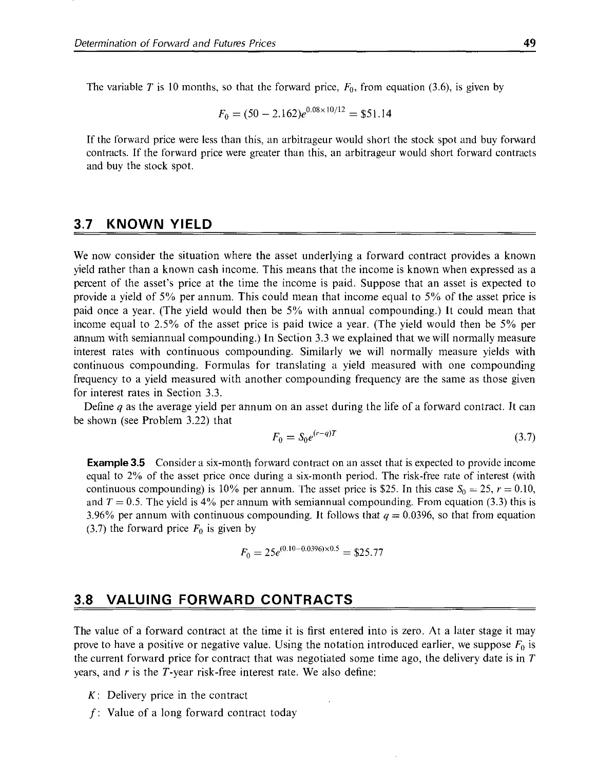
3.6 Known income.................................................................47
3.7 Known yield..................................................................49
3.8 Valuing forward contracts....................................................49
3.9 Are forward prices and futures prices equal?.................................51
3.10 Stock index futures..........................................................52
3.11 Forward and futures contracts on currencies..................................55
3.12 Futures on commodities.......................................................58
ix
X
Contents
3.13 Cost of carry..............................................................60
3.14 Delivery options...........................................................60
3.15 Futures prices and the expected future spot price..........................61
Summary....................................................................63
Suggestions for further reading............................................64
Questions and problems.....................................................65
Assignment questions.......................................................67
Appendix ЗА: Proof that forward and futures prices are equal when interest
rates are constant..........................................................68
4. Hedging strategies using futures.......................................................70
4.1 Basic principles...........................................................70
4.2 Arguments for and against hedging..........................................72
4.3 Basis risk.................................................................75
4.4 Minimum variance hedge ratio...............................................78
4.5 Stock index futures........................................................82
4.6 Rolling the hedge forward..................................................86
Summary....................................................................87
Suggestions for further reading............................................88
Questions and problems.....................................................88
Assignment questions.......................................................90
Appendix 4A: Proof of the minimum variance hedge ratio formula.............92
5. Interest rate markets.............................................................93
5.1 Types of rates.............................................................93
5.2 Zero rates.................................................................94
5.3 Bond pricing...............................................................94
5.4 Determining zero rates.....................................................96
5.5 Forward rates..............................................................98
5.6 Forward rate agreements...................................................100
5.7 Theories of the term structure............................................102
5.8 Day count conventions.....................................................102
5.9 Quotations................................................................103
5.10 Treasury bond futures......................................................104
5.11 Eurodollar futures.........................................................110
5.12 The LIBOR zero curve.......................................................Ill
5.13 Duration...................................................................112
5.14 Duration-based hedging strategies..........................................116
Summary...................................................................118
Suggestions for further reading...........................................119
Questions and problems....................................................120
Assignment questions......................................................123
6. Swaps.................................................................................125
6.1 Mechanics of interest rate swaps..........................................125
6.2 The comparative-advantage argument........................................131
6.3 Swap quotes and LIBOR zero rates..........................................134
6.4 Valuation of interest rate swaps..........................................136
6.5 Currency swaps............................................................140
6.6 Valuation of currency swaps...............................................143
6.7 Credit risk...............................................................145
Summary...................................................................146
Suggestions for further reading...........................................147
Questions and problems....................................................147
Assignment questions......................................................149
Contents
xi
7. Mechanics of options markets...........................................................151
7.1 Underlying assets...........................................................151
7.2 Specification of stock options..............................................152
7.3 Newspaper quotes............................................................155
7.4 Trading.....................................................................157
7.5 Commissions.................................................................157
7.6 Margins.....................................................................158
7.7 The options clearing corporation............................................160
7.8 Regulation..................................................................161
7.9 Taxation....................................................................161
7.10 Warrants, executive stock options, and convertibles.........................162
7.11 Over-the-counter markets....................................................163
Summary....................................................................163
Suggestions for further reading............................................164
Questions and problems.....................................................164
Assignment questions.......................................................165
8. Properties of stock options............................................................167
8.1 Factors affecting option prices.............................................167
8.2 Assumptions and notation....................................................170
8.3 Upper and lower bounds for option prices....................................171
8.4 Put-call parity.............................................................174
8.5 Early exercise: calls on a non-dividend-paying stock........................175
8.6 Early exercise: puts on a non-dividend-paying stock.........................177
8.7 Effect of dividends.........................................................178
8.8 Empirical research..........................................................179
Summary....................................................................180
Suggestions for further reading............................................181
Questions and problems.....................................................182
Assignment questions.......................................................183
9. Trading strategies involving options...................................................185
9.1 Strategies-involving a single option and a stock............................185
9.2 Spreads.....................................................................187
9.3 Combinations................................................................194
9.4 Other payoffs...............................................................197
Summary....................................................................197
Suggestions for further reading............................................198
Questions and problems.....................................................198
Assignment questions.......................................................199
10. Introduction to binomial trees........................................................200
10.1 A one-step binomial model...................................................200
10.2 Risk-neutral valuation......................................................203
10.3 Two-step binomial trees.....................................................205
10.4 A put example...............................................................208
10.5 American options............................................................209
10.6 Delta.......................................................................210
10.7 Matching volatility with и and d............................................211
10.8 Binomial trees in practice..................................................212
Summary....................................................................213
Suggestions for further reading............................................214
Questions and problems.....................................................214
Assignment questions.......................................................215
xii
Contents
11. A model of the behavior of stock prices.................................................216
11.1 The Markov property..........................................................216
11.2 Continuous-time stochastic processes.........................................217
11.3 The process for stock prices.................................................222
11.4 Review of the model..........................................................223
11.5 The parameters...............................................................225
11.6 Ito’s lemma..................................................................226
11.7 The lognormal property.......................................................227
Summary......................................................................228
Suggestions for further reading..............................................229
Questions and problems.......................................................229
Assignment questions.........................................................230
Appendix HA: Derivation of Ito’s lemma.......................................232
12. The Black-Scholes model.................................................................234
12.1 Lognormal property of stock prices...........................................234
12.2 The distribution of the rate of return.......................................236
12.3 The expected return..........................................................237
12.4 Volatility...................................................................238
12.5 Concepts underlying the Black-Scholes-Merton differential equation...........241
12.6 Derivation of the Black-Scholes-Merton differential equation.................242
12.7 Risk-neutral valuation.......................................................244
12.8 Black-Scholes pricing formulas...............................................246
12.9 Cumulative normal distribution function......................................248
12.10 Warrants issued by a company on its own stock.................................249
12.11 Implied volatilities.........................................................250
12.12 The causes of volatility.....................................................251
12.13 Dividends....................................................................252
Summary......................................................................256
Suggestions for further reading..............................................257
Questions and problems.......................................................258
Assignment questions.........................................................261
Appendix 12A: Proof of Black-Scholes-Merton formula.........................262
Appendix 12B: Exact procedure for calculating the values of American calls on
dividend-paying stocks......................................................265
Appendix 12C: Calculation of cumulative probability in bivariate normal
distribution................................................................266
13. Options on stock indices, currencies, and futures.......................................267
13.1 Results for a stock paying a known dividend yield............................267
13.2 Option pricing formulas......................................................268
13.3 Options on stock indices.....................................................270
13.4 Currency options.............................................................276
13.5 Futures options..............................................................278
13.6 Valuation of futures options using binomial trees ...........................284
13.7 Futures price analogy........................................................286
13.8 Black’s model for valuing futures options....................................287
13.9 Futures options vs. spot options.............................................288
Summary......................................................................289
Suggestions for further reading..............................................290
Questions and problems.......................................................291
Assignment questions.........................................................294
Appendix 13A: Derivation of differential equation satisfied by a derivative
dependent on a stock providing a dividend yield....................295
Contents
xiii
Appendix 13B: Derivation of differential equation satisfied by a derivative
dependent on a futures price.......................................297
14. The Greek letters........................................................................299
14.1 Illustration..................................................................299
14.2 Naked and covered positions...................................................300
14.3 A stop-loss strategy..........................................................300
14.4 Delta hedging.................................................................302
14.5 Theta.........................................................................309
14.6 Gamma.........................................................................312
14.7 Relationship between delta, theta, and gamma..................................315
14.8 Vega..........................................................................316
14.9 Rho...........................................................................318
14.10 Hedging in practice...........................................................319
14.11 Scenario analysis.............................................................319
14.12 Portfolio insurance...........................................................320
14.13 Stock market volatility.......................................................323
Summary.......................................................................323
Suggestions for further reading...............................................324
Questions and problems............"...........................................326
Assignment questions..........................................................327
Appendix 14A: Taylor series expansions and hedge parameters...................329
15. Volatility smiles........................................................................330
15.1 Put-call parity revisited.....................................................330
15.2 Foreign currency options......................................................331
15.3 Equity options................................................................334
15.4 The volatility term structure and volatility surfaces.........................336
15.5 Greek letters.................................................................337
15.6 When a single large jump is anticipated...............................338
15.7 Empirical research............................................................339
Summary.......................................................................341
Suggestions for further reading...............................................341
Questions and problems........................................................343
Assignment questions..........................................................344
Appendix 15A: Determining implied risk-neutral distributions from volatility
smiles........................................................................345
16. Value at risk............................................................................346
16.1 The VaR measure...............................................................346
16.2 Historical simulation.........................................................348
16.3 Model-building approach.......................................................350
16.4 Linear model..................................................................352
16.5 Quadratic model...............................................................356
16.6 Monte Carlo simulation........................................................359
16.7 Comparison of approaches......................................................359
16.8 Stress testing and back testing...............................................360
16.9 Principal components analysis.................................................360
Summary.......................................................................364
Suggestions for further reading...............................................364
Questions and problems........................................................365
Assignment questions..........................................................366
Appendix 16A: Cash-flow mapping...............................................368
Appendix 16B: Use of the Cornish-Fisher expansion to estimate VaR.............370
xiv
Contents
17. Estimating volatilities and correlations...............................................372
17.1 Estimating volatility........................................................372
17.2 The exponentially weighted moving average model..............................374
17.3 The GARCH(1,1) model.........................................................376
17.4 Choosing between the models..................................................377
17.5 Maximum likelihood methods...................................................378
17.6 Using GARCH(1, 1) to forecast future volatility..............................382
17.7 Correlations.................................................................385
Summary.....................................................................388
Suggestions for further reading.............................................388
Questions and problems......................................................389
Assignment questions........................................................391
18. Numerical procedures...................................................................392
18.1 Binomial trees...............................................................392
18.2 Using the binomial tree for options on indices, currencies, and futures
contracts..........................................................................399
18.3 Binomial model for a dividend-paying stock...................................402
18.4 Extensions to the basic tree approach........................................405
18.5 Alternative procedures for constructing trees................................406
18.6 Monte Carlo simulation.......................................................410
18.7 Variance reduction procedures................................................414
18.8 Finite difference methods....................................................418
18.9 Analytic approximation to American option prices.............................427
Summary.....................................................................427
Suggestions for further reading.............................................428
Questions and problems......................................................430
Assignment questions........................................................432
Appendix 18A: Analytic approximation to American option prices of
MacMillan and of Barone-Adesi and Whaley.....................................433
19. Exotic options.........................................................................435
19.1 Packages.....................................................................435
19.2 Nonstandard American options.................................................436
19.3 Forward start options........................................................437
19.4 Compound options.............................................................437
19.5 Chooser options..............................................................438
19.6 Barrier options..............................................................439
19.7 Binary options...............................................................441
19.8 Lookback options.............................................................441
19.9 Shout options................................................................443
19.10 Asian options................................................................443
19.11 Options to exchange one asset for another....................................445
19.12 Basket options...............................................................446
19.13 Hedging issues...............................................................447
19.14 Static options replication...................................................447
Summary.....................................................................449
Suggestions for further reading.............................................449
Questions and problems......................................................451
Assignment questions........................................................452
Appendix 19A: Calculation of the first two moments of arithmetic averages
and baskets.................................................................454
20. More on models and numerical procedures................................................456
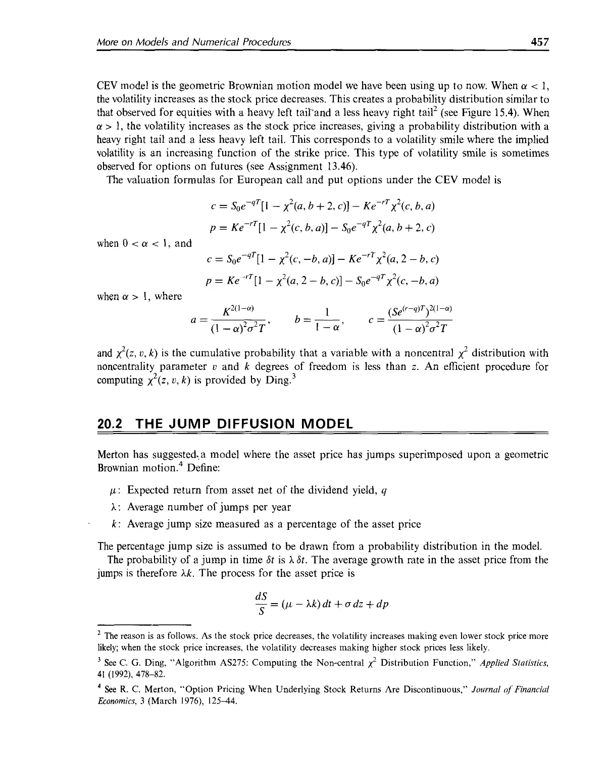
20.1 The CEV model................................................................456
20.2 The jump diffusion model.....................................................457
Contents
XV
20.3 Stochastic volatility models.................................................458
20.4 The IVF model................................................................460
20.5 Path-dependent derivatives...................................................461
20.6 Lookback options.............................................................465
20.7 Barrier options..............................................................467
20.8 Options on two correlated assets.............................................472
20.9 Monte Carlo simulation and American options..................................474
Summary.....................................................................478
Suggestions for further reading.............................................479
Questions and problems......................................................480
Assignment questions........................................................481
21. Martingales and measures...............................................................483
21.1 The market price of risk.....................................................484
21.2 Several state variables...................-..................................487
21.3 Martingales..................................................................488
21.4 Alternative choices for the numeraire........................................489
21.5 Extension to multiple independent factors....................................492
21.6 Applications.................................................................493
21.7 Change of numeraire..........................................................495
21.8 Quantos......................................................................497
21.9 Siegel’s paradox.............................................................499
Summary.....................................................................500
Suggestions for further reading.............................................500
Questions and problems......................................................501
Assignment questions........................................................502
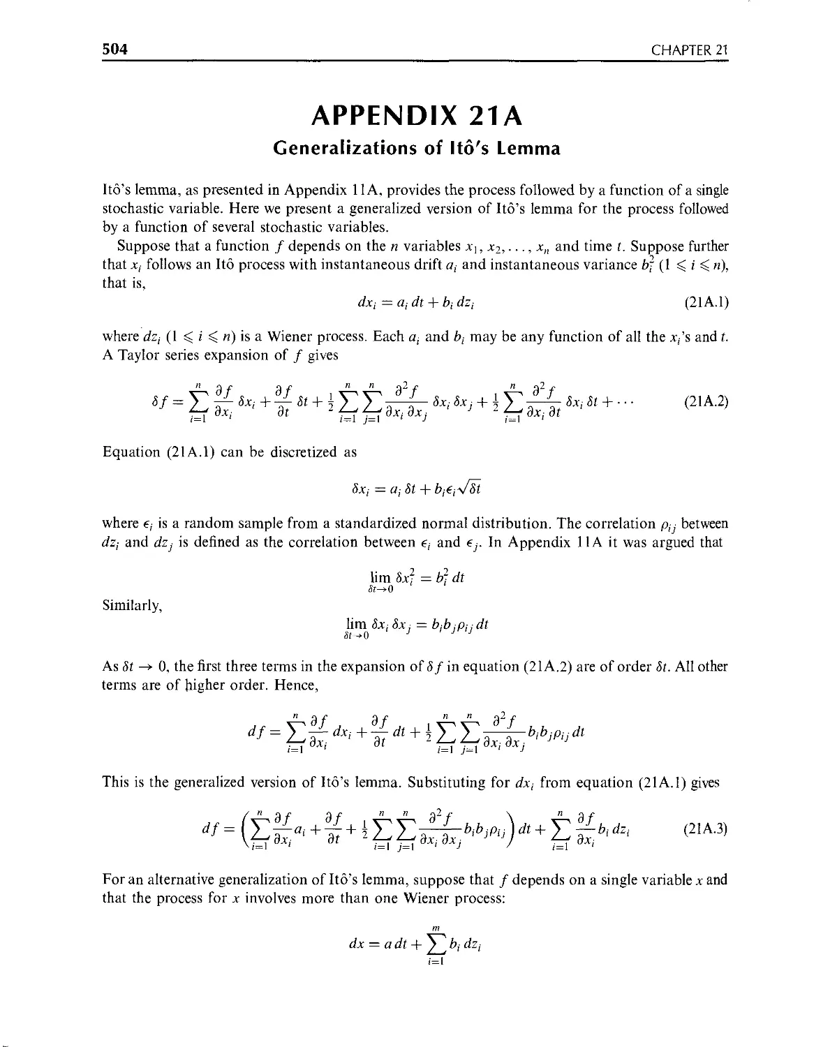
Appendix 21 A: Generalizations of Ito’s lemma...............................504
Appendix 2IB: Expected excess return when there are multiple sources of
uncertainty.................................................................506
22. Interest rate derivatives: the standard market models..................................508
22.1 Black’s model................................................................508
22.2 Bond options.................................................................511
22.3 Interest rate caps...........................................................515
22.4 European swap options........................................................520
22.5 Generalizations..............................................................524
22.6 Convexity adjustments........................................................524
22.7 Timing adjustments...........................................................527
22.8 Natural time lags............................................................529
22.9 Hedging interest rate derivatives............................................530
Summary.....................................................................531
Suggestions for further reading.............................................531
Questions and problems......................................................532
Assignment questions........................................................534
Appendix 22A: Proof of the convexity adjustment formula.....................536
23. Interest rate derivatives: models of the short rate....................................537
23.1 Equilibrium models...........................................................537
23.2 One-factor equilibrium models................................................538
23.3 The Rendleman and Bartter model..............................................538
23.4 The Vasicek model............................................................539
23.5 The Cox, Ingersoll, and Ross model...........................................542
23.6 Two-factor equilibrium models................................................543
23.7 No-arbitrage models..........................................................543
23.8 The Ho and Lee model.........................................................544
23.9 The Hull and White model.....................................................546
xvi Contents
23.10 Options on coupon-bearing bonds..............................................549
23.11 Interest rate trees..........................................................550
23.12 A general tree-building procedure............................................552
23.13 Nonstationary models.........................................................563
23.14 Calibration..................................................................564
23.15 Hedging using a one-factor model.............................................565
23.16 Forward rates and futures rates..............................................566
Summary.....................................................................566
Suggestions for further reading.............................................567
Questions and problems......................................................568
Assignment questions........................................................570
24. Interest rate derivatives: more advanced models........................................571
24.1 Two-factor models of the short rate..........................................571
24.2 The Heath, Jarrow, and Morton model..........................................574
24.3 The LIBOR market model.......................................................577
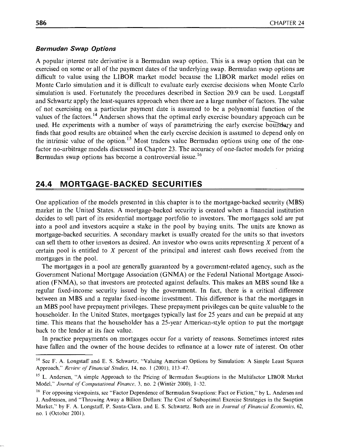
24.4 Mortgage-backed securities................................................. 586
Summary.....................................................................588
Suggestions for further reading.............................................589
Questions and problems......................................................590
Assignment questions........................................................591
Appendix 24A: The A(t, T), nP, and 0(t) functions in the two-factor Hull-White
model........................................................................593
25. Swaps revisited.........................................................................594
25.1 Variations on the vanilla deal...............................................594
25.2 Compounding swaps............................................................595
25.3 Currency swaps...............................................................598
25.4 More complex swaps...........................................................598
25.5 Equity swaps.................................................................601
25.6 Swaps with embedded options..................................................602
25.7 Other swaps..................................................................605
25.8 Bizarre deals................................................................605
Summary.....................................................................606
Suggestions for further reading.............................................606
Questions and problems......................................................607
Assignment questions........................................................607
Appendix 25A: Valuation of an equity swap between payment dates.............609
26. Credit risk.............................................................................610
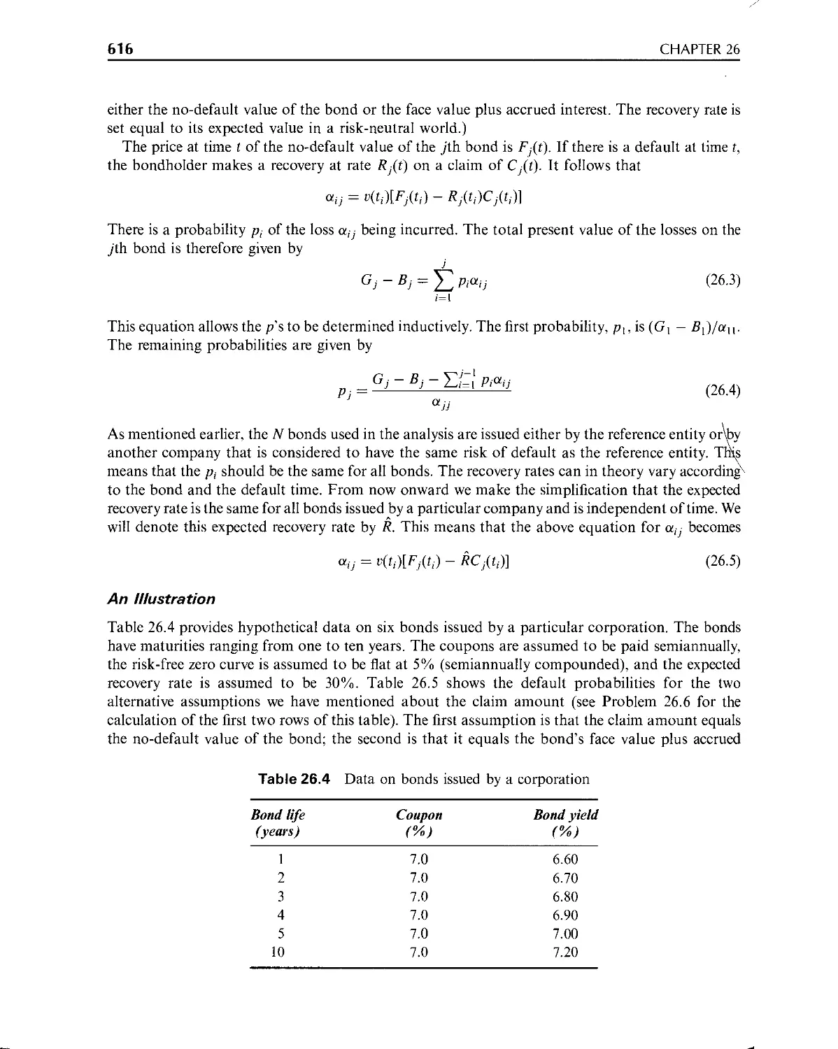
23.1 Bond prices and the probability of default...................................610
26.2 Historical data..............................................................619
26.3 Bond prices vs. historical default experience................................619
26.4 Risk-neutral vs. real-world estimates........................................620
26.5 Using equity prices to estimate default probabilities........................621
26.6 The loss given default.......................................................623
26.7 Credit ratings migration.....................................................626
26.8 Default correlations.........................................................627
26.9 Credit value at risk.........................................................630
Summary.....................................................................633
Suggestions for further reading.............................................633
Questions and problems......................................................634
Assignment questions........................................................635
Appendix 26A: Manipulation of the matrices of credit rating changes.........636
Contents
xvii
27. Credit derivatives.......................................................................637
27.1 Credit default swaps..........................................................637
27.2 Total return swaps............................................................644
27.3 Credit spread options.........................................................645
27.4 Collateralized debt obligations...............................................646
27.5 Adjusting derivative prices for default risk..................................647
27.6 Convertible bonds.............................................................652
Summary.......................................................................655
Suggestions for further reading...............................................655
Questions and problems........................................................656
Assignment questions..........................................................658
28. Real options.............................................................................660
28.1 Capital investment appraisal..................................................660
28.2 Extension of the risk-neutral valuation framework.............................661
28.3 Estimating the market price of risk...........................................665
28.4 Application to the valuation of a new business................................666
28.5 Commodity prices..............................................................667
28.6 Evaluating options in an investment opportunity...............................670
Summary.......................................................................675
Suggestions for further reading...............................................676
Questions and problems........................................................676
Assignment questions......................................................... 677
29. Insurance, weather, and energy derivatives...............................................678
29.1 Review of pricing issues......................................................678
29.2 Weather derivatives...........................................................679
29.3 Energy derivatives............................................................680
29.4 Insurance derivatives.........................................................682
Summary.......................................................................683
Suggestions for further reading...............................................684
Questions and problems........................................................684
Assignment questions..........................................................685
30. Derivatives mishaps and what we can learn from them......................................686
30.1 Lessons for all users of derivatives..........................................686
30.2 Lessons for financial institutions............................................690
30.3 Lessons for nonfinancial corporations.........................................693
Summary.......................................................................694
Suggestions for further reading...............................................695
Glossary of notation..........................................................................697
Glossary of terms.............................................................................700
DerivaGem software..............................................................:.............715
Major exchanges trading futures and options...................................................720
Table for N(x) when x C 0.....................................................................722
Table for N(x) when x 0.......................................................................723
Author index..................................................................................725
Subject index.................................................................................729
PREFACE
It is sometimes hard for me to believe that the first edition of this book was only 330 pages and
13 chapters long! There have been many developments in derivatives markets over the last 15 years
and the book has grown to keep up with them. The fifth edition has seven new chapters that cover
new derivatives instruments and recent research advances.
Like earlier editions, the book serves several markets. It is appropriate for graduate courses in
business, economics, and financial engineering. It can be used on advanced undergraduate courses
when students have good quantitative skills. Also, many practitioners who want to acquire a
working knowledge of how derivatives can be analyzed find the book useful.
One of the key decisions that must be made by an author who is writing in the area of derivatives
concerns the use of mathematics. If the level of mathematical sophistication is too high, the
material is likely to be inaccessible to many students and practitioners. If it is too low, some
important issues will inevitably be treated in a rather superficial way. I have tried to be particularly
careful about the way I use both mathematics and notation in the book. Nonessential mathema-
tical material has been either eliminated or included in end-of-chapter appendices. Concepts that
are likely to be new to many readers have been explained carefully, and many numerical examples
have been included.
The book covers both derivatives markets and risk management. It assumes that the reader has
taken an introductory course in finance and an introductory course in probability and statistics.
No prior knowledge of options, futures contracts, swaps, and so on is assumed. It is not therefore
necessary for students to take an elective course in investments prior to taking a course based on
this book. There are many different ways the book can be used in the classroom. Instructors
teaching a first course in derivatives may wish to spend most time on the first half of the book.
Instructors teaching a more advanced course will find that many different combinations of the
chapters in the second half of the book can be used. I find that the material in Chapters 29 and 30
works well at the end of either an introductory or an advanced course.
What's New?
Material has been updated and improved throughout the book. The changes in this edition
include:
1. A new chapter on the use of futures for hedging (Chapter 4). Part of this material was
previously in Chapters 2 and 3. The change results in the first three chapters being less
intense and allows hedging to be covered in more depth.
2. A new chapter on models and numerical procedures (Chapter 20). Much of this material is
new, but some has been transferred from the chapter on exotic options in the fourth edition.
xix
XX
Preface
3. A new chapter on swaps (Chapter 25). This gives the reader an appreciation of the range of
nonstandard swap products that are traded in the over-the-counter market and discusses how
they can be valued.
4. There is an extra chapter on credit risk. Chapter 26 discusses the measurement of credit risk
and credit value at risk while Chapter 27 covers credit derivatives.
5. There is a new chapter on real options (Chapter 28).
6. There is a new chapter on insurance, weather, and energy derivatives (Chapter 29).
7. There is a new chapter on derivatives mishaps and what we can learn from them (Chapter 30).
8. The chapter on martingales and measures has been improved so that the material flows
better (Chapter 21).
9. The chapter on value at risk has been rewritten so that it provides a better balance between
the historical simulation approach and the model-building approach (Chapter 16).
10. The chapter on volatility smiles has been improved and appears earlier in the book.
(Chapter 15).
11. The coverage of the LIBOR market model has been expanded (Chapter 24).
12. One or two changes have been made to the notation. The most significant is that the strike
price is now denoted by К rather than X.
13. Many new end-of-chapter problems have been added.
Software
A new version of DerivaGem (Version 1.50) is released with this book. This consists of two Excel
applications: the Options Calculator and the Applications Builder. The Options Calculator consists
of the software in the previous release (with minor improvements). The Applications Builder
consists of a number of Excel functions from which users can build their own applications. It
includes a number of sample applications and enables students to explore the properties of options
and numerical procedures more easily. It also allows more interesting assignments to be designed.
The software is described more fully at the end of the book. Updates to the software can be
downloaded from my website:
www.rotman.utoronto.ca/~hull
Slides
Several hundred PowerPoint slides can be downloaded from my website. Instructors who adopt the
text are welcome to adapt the slides to meet their own needs.
Answers to Questions
As in the fourth edition, end-of-chapter problems are divided into two groups: “Questions and
Problems” and “Assignment Questions”. Solutions to the Questions and Problems are in Options,
Futures, and Other Derivatives: Solutions Manual, which is published by Prentice Hall and can be
purchased by students. Solutions to Assignment Questions are available only in the Instructors
Manual.
Preface
xxi
A ckno wledgmen ts
Many people have played a part in the production of this book. Academics, students, and
practitioners who have made excellent and useful suggestions include Farhang Aslani, Jas Badyal,
Emilio Barone, Giovanni Barone-Adesi, Alex Bergier, George Blazenko, Laurence Booth, Phelim
Boyle, Peter Carr, Don Chance, J.-P. Chateau, Ren-Raw Chen, George Constantinides, Michel
Crouhy, Emanuel Derman, Brian Donaldson, Dieter Dorp, Scott Drabin, Jerome Duncan, Steinar
Ekern, David Fowler, Louis Gagnon, Dajiang Guo, Jrgen Hallbeck, Ian Hawkins, Michael
Hemler, Steve Heston, Bernie Hildebrandt, Michelle Hull, Kiyoshi Kato, Kevin Kneafsy, Tibor
Kucs, Iain MacDonald, Bill Margrabe, Izzy Nelkin, Neil Pearson, Paul Potvin, Shailendra Pandit,
Eric Reiner, Richard Rendleman, Gordon Roberts, Chris Robinson, Cheryl Rosen, John Rumsey,
Ani Sanyal, Klaus Schurger, Eduardo Schwartz, Michael Selby, Piet Sercu, Duane Stock, Edward
Thorpe, Yisong Tian, P. V. Viswanath, George Wang, Jason Wei, Bob Whaley, Alan White,
Hailiang Yang, Victor Zak, and Jozef Zemek. Huafen (Florence) Wu and Matthew Merkley
provided excellent research assistance.
I am particularly grateful to Eduardo Schwartz, who read the original manuscript for the first
edition and made many comments that led to significant improvements, and to Richard Rendle-
man and George Constantinides, who made specific suggestions that led to improvements in more
recent editions.
The first four editions of this book were very popular with practitioners and their comments and
suggestions have led to many improvements in the book. The students in my elective courses on
derivatives at the University of Toronto have also influenced the evolution of the book.
Alan White, a colleague at the University of Toronto, deserves a special acknowledgment. Alan
and I have been carrying out joint research in the area of derivatives for the last 18 years. During
that time we have spent countless hours discussing different issues concerning derivatives. Many of
the new ideas in this book, and many of the new ways used to explain old ideas, are as much Alan’s
as mine. Alan read the original version of this book very carefully and made many excellent
suggestions for improvement. Alan has also done most of the development work on the Deriva-
Gem software.
Special thanks are due to many people at Prentice Hall for their enthusiasm, advice, and
encouragement. I would particularly like to thank Mickey Cox (my editor), P. J. Boardman (the
editor-in-chief) and Kerri Limpert (the production editor). I am also grateful to Scott Barr, Leah
Jewell, Paul Donnelly, and Maureen Riopelle, who at different times have played key roles in the
development of the book.
I welcome comments on the book from readers. My email address is:
hull@rotman.utoronto.ca
John C. Hull
University of Toronto
CHAPTER 1
INTRODUCTION
In the last 20 years derivatives have become increasingly important in the world of finance. Futures
and options are now traded actively on many exchanges throughout the world. Forward contracts,
swaps, and many different types of options are regularly traded outside exchanges by financial
institutions, fund managers, and corporate treasurers in what is termed the over-the-counter
market. Derivatives are also sometimes added to a bond or stock issue.
A derivative can be defined as a financial instrument whose value depends on (or derives from)
the values of other, more basic underlying variables. Very often the variables underlying deriva-
tives are the prices of traded assets. A stock option, for example, is a derivative whose value is
dependent on the price of a stock. However, derivatives can be dependent on almost any variable,
from the price of hogs to the amount of snow falling at a certain ski resort.
Since the first edition of this book was published in 1988, there have been many developments in
derivatives markets. There is now active trading in credit derivatives, electricity derivatives, weather
derivatives, and insurance derivatives. Many new types of interest rate, foreign exchange, and
equity derivative products have been created. There have been many new ideas in risk management
and risk measurement. Analysts have also become more aware of the need to analyze what are
known as real options. (These are the options acquired by a company when it invests in real assets
such as real estate, plant, and equipment.) This edition of the book reflects all these developments.
In this opening chapter we take a first look at forward, futures, and options markets and provide
an overview of how they are used by hedgers, speculators, and arbitrageurs. Later chapters will give
more details and elaborate on many of the points made here.
1.1 EXCHANGE-TRADED MARKETS
A derivatives exchange is a market where individuals trade standardized contracts that have been
defined by the exchange. Derivatives exchanges have existed for a long time. The Chicago Board of
Trade (CBOT, www.cbot.com) was established in 1848 to bring farmers and merchants together.
Initially its main task was to standardize the quantities and qualities of the grains that were traded.
Within a few years the first futures-type contract was developed. It was known as a to-arrive
contract. Speculators soon became interested in the contract and found trading the contract to be
an attractive alternative to trading the grain itself. A rival futures exchange, the Chicago
Mercantile Exchange (CME, www.cme.com), was established in 1919. Now futures exchanges
exist all over the world.
The Chicago Board Options Exchange (СВОЕ, www.cboe.com) started trading call option
1
2
CHAPTER 1
contracts on 16 stocks in 1973. Options had traded prior to 1973 but the СВОЕ succeeded in
creating an orderly market with well-defined contracts. Put option contracts started trading on the
exchange in 1977. The СВОЕ now trades options on over 1200 stocks and many different stock
indices. Like futures, options have proved to be very popular contracts. Many other exchanges
throughout the world now trade options. The underlying assets include foreign currencies and
futures contracts as well as stocks and stock indices.
Traditionally derivatives traders have met on the floor of an exchange and used shouting and a
complicated set of hand signals to indicate the trades they would like to carry out. This is known as
the open outcry system. In recent years exchanges have increasingly moved from the open outcry
system to electronic trading. The latter involves traders entering their desired trades at a keyboard
and a computer being used to match buyers and sellers. There seems little doubt that eventually all
exchanges will use electronic trading.
1.2 OVER-THE-COUNTER MARKETS
Not all trading is done on exchanges. The over-the-counter market is an important alternative to
exchanges and, measured in terms of the total volume of trading, has become much larger than the
exchange-traded market. It is a telephone- and computer-linked network of dealers, who do not
physically meet. Trades are done over the phone and are usually between two financial institutions
or between a financial institution and one of its corporate clients. Financial institutions often act as
market makers for the more commonly traded instruments. This means that they are always
prepared to quote both a bid price (a price at which they are prepared to buy) and an offer price
(a price at which they are prepared to sell).
Telephone conversations in the over-the-counter market are usually taped. If there is a dispute
about what was agreed, the tapes are replayed to resolve the issue. Trades in the over-the-counter
market are typically much larger than trades in the exchange-traded market. A key advantage of
the over-the-counter market is that the terms of a contract do not have to be those specified by an
exchange. Market participants are free to negotiate any mutually attractive deal. A disadvantage is
that there is usually some credit risk in an over-the-counter trade (i.e., there is a small risk that the
contract will not be honored). As mentioned earlier, exchanges have organized themselves to
eliminate virtually all credit risk.
1.3 FORWARD CONTRACTS
A forward contract is a particularly simple derivative. It is an agreement to buy or sell an asset at a
certain future time for a certain price. It can be contrasted with a spot contract, which is an
agreement to buy or sell an asset today. A forward contract is traded in the over-the-counter
market—usually between two financial institutions or between a financial institution and one of its
clients.
One of the parties to a forward contract assumes a long position and agrees to buy the underlying
asset on a certain specified future date for a certain specified price. The other party assumes a short
position and agrees to sell the asset on the same date for the same price.
Forward contracts on foreign exchange are very popular. Most large banks have a “forward
desk” within their foreign exchange trading room that is devoted to the trading of forward
Introduction
3
Table 1.1 Spot and forward quotes for the USD-GBP exchange
rate, August 16, 2001 (GBP = British pound; USD = U.S. dollar)
Bid Offer
Spot 1.4452 1.4456
1-month forward 1.4435 1.4440
3-month forward 1.4402 1.4407
6-month forward 1.4353 1.4359
1-year forward 1.4262 1.4268
contracts. Table 1.1 provides the quotes on the exchange rate between the British pound (GBP) and
the U.S. dollar (USD) that might be made by a large international bank on August 16, 2001. The
quote is for the number of USD per GBP. The first quote indicates that the bank is prepared to buy
GBP (i.e., sterling) in the spot market (i.e., for virtually immediate delivery) at the rate of $1.4452
per GBP and sell sterling in the spot market at $ 1.4456 per GBP. The second quote indicates that
the bank is prepared to buy sterling in one month at $1.4435 per GBP and sell sterling in one month
at $1.4440 per GBP; the third quote indicates that it is prepared to buy sterling in three months at
$1.4402 per GBP and sell sterling in three months at $1.4407 per GBP; and so on. These quotes are
for very large transactions. (As anyone who has traveled abroad knows, retail customers face much
larger spreads between bid and offer quotes than those in given Table 1.1.)
Forward contracts can be used to hedge foreign currency risk. Suppose that on August 16, 2001,
the treasurer of a U.S. corporation knows that the corporation will pay £1 million in six months (on
February 16, 2002) and wants to hedge against exchange rate moves. Using the quotes in Table 1.1,
the treasurer can agree to buy £1 million six months forward at an exchange rate of 1.4359. The
corporation then has a long forward contract on GBP. It has agreed that on February 16, 2002, it
will buy £1 million from the bank for $1.4359 million. The bank has a short forward contract on
GBP. It has agreed that on February 16, 2002, it will sell £1 million for $1.4359 million. Both sides
have made a binding commitment.
Payoffs from Forward Contracts
Consider the position of the corporation in the trade we have just described. What are the possible
outcomes? The forward contract obligates the corporation to buy £1 million for $1,435,900. If the
spot exchange rate rose to, say, 1.5000, at the end of the six months the forward contract would be
worth $64,100 (= $1,500,000 — $1,435,900) to the corporation. It would enable £1 million to be
purchased at 1.4359 rather than 1.5000. Similarly, if the spot exchange rate fell to 1.4000 at the end of
the six months, the forward contract would have a negative value to the corporation of $35,900
because it would lead to the corporation paying $35,900 more than the market price for the sterling.
In general, the payoff from a long position in a forward contract on one unit of an asset is
ST - К
where К is the delivery price and ST is the spot price of the asset at maturity of the contract. This is
because the holder of the contract is obligated to buy an asset worth ST for K. Similarly, the payoff
from a short position in a forward contract on one unit of an asset is
K— ST
4
CHAPTER 1
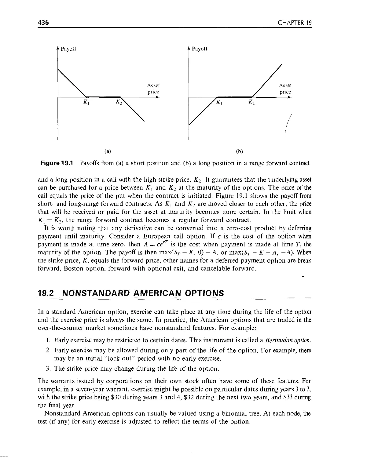
Figure 1.1 Payoffs from forward contracts: (a) long position, (b) short position.
Delivery price = K\ price of asset at maturity = St
These payoffs can be positive or negative. They are illustrated in Figure 1.1. Because it costs
nothing to enter into a forward contract, the payoff from the contract is also the trader’s total gain
or loss from the contract.
Forward Price and Delivery Price
It is important to distinguish between the forward price and delivery price. The forward price is the
market price that would be agreed to today for delivery of the asset at a specified maturity date.
The forward price is usually different from the spot price and varies with the maturity date
(see Table 1.1).
In the example we considered earlier, the forward price on August 16, 2001, is 1.4359 for a
contract maturing on February 16, 2002. The corporation enters into a contract and 1.4359
becomes the delivery price for the contract. As we move through time the delivery price for the
corporation’s contract does not change, but the forward price for a contract maturing on February
16, 2002, is likely to do so. For example, if GBP strengthens relative to USD in the second half of
August the forward price could rise to 1.4500 by September 1, 2001.
Forward Prices and Spot Prices
We will be discussing in some detail the relationship between spot and forward prices in Chapter 3.
In this section we illustrate the reason why the two are related by considering forward contracts on
gold. We assume that there are no storage costs associated with gold and that gold earns no income.1
Suppose that the spot price of gold is $300 per ounce and the risk-free interest rate for
investments lasting one year is 5% per annum. What is a reasonable value for the one-year
forward price of gold?
1 This is not totally realistic. In practice, storage costs are close to zero, but an income of 1 to 2% per annum can be
earned by lending gold.
Introduction
5
Suppose first that the one-year forward price is $340 per ounce. A trader can immediately take
the following actions:
1. Borrow $300 at 5% for one year.
2. Buy one ounce of gold.
3. Enter into a short forward contract to sell the gold for $340 in one year.
The interest on the $300 that is borrowed (assuming annual compounding) is $15. The trader can,
therefore, use $315 of the $340 that is obtained for the gold in one year to repay the loan. The
remaining $25 is profit. Any one-year forward price greater than $315 will lead to this arbitrage
trading strategy being profitable.
Suppose next that the forward price is $300. An investor who has a portfolio that includes gold can
1. Sell the gold for $300 per ounce.
2. Invest the proceeds at 5%.
3. Enter into a long forward contract to repurchase the gold in one year for $300 per ounce.
When this strategy is compared with the alternative strategy of keeping the gold in the portfolio for
one year, we see that the investor is better off by $15 per ounce. In any situation where the forward
price is less than $315, investors holding gold have an incentive to sell the gold and enter into a
long forward contract in the way that has been described.
The first strategy is profitable when the one-year forward price of gold is greater than $315. As
more traders attempt to take advantage of this strategy, the demand for short forward contracts
will increase and the one-year forward price of gold will fall. The second strategy is profitable for
all investors who hold gold in their portfolios when the one-year forward price of gold is less than
$315. As these investors attempt to take advantage of this strategy, the demand for long forward
contracts will increase and the one-year forward price of gold will rise. Assuming that individuals
are always willing to take advantage of arbitrage opportunities when they arise, we can conclude
that the activities of traders should cause the one-year forward price of gold to be exactly $315.
Any other price leads to an arbitrage opportunity.2
1.4 FUTURES CONTRACTS
Like a forward contract, a futures contract is an agreement between two parties to buy or sell an
asset at a certain time in the future for a certain price. Unlike forward contracts, futures contracts
are normally traded on an exchange. To make trading possible, the exchange specifies certain
standardized features of the contract. As the two parties to the contract do not necessarily know
each other, the exchange also provides a mechanism that gives the two parties a guarantee that the
contract will be honored.
The largest exchanges on which futures contracts are traded are the Chicago Board of Trade
(CBOT) and the Chicago Mercantile Exchange (CME). On these and other exchanges throughout
the world, a very wide range of commodities and financial assets form the underlying assets in the
various contracts. The commodities include pork bellies, live cattle, sugar, wool, lumber, copper,
aluminum, gold, and tin. The financial assets include stock indices, currencies, and Treasury bonds.
2 Our arguments make the simplifying assumption that the rate of interest on borrowed funds is the same as the rate
of interest on invested funds.
6
CHAPTER 1
One way in which a futures contract is different from a forward contract is that an exact delivery
date is usually not specified. The contract is referred to by its delivery month, and the exchange
specifies the period during the month when delivery must be made. For commodities, the delivery
period is often the entire month. The holder of the short position has the right to choose the time
during the delivery period when it will make delivery. Usually, contracts with several different
delivery months are traded at any one time. The exchange specifies the amount of the asset to be
delivered for one contract and how the futures price is to be quoted. In the case of a commodity,
the exchange also specifies the product quality and the delivery location. Consider, for example, the
wheat futures contract currently traded on the Chicago Board of Trade. The size of the contract is
5,000 bushels. Contracts for five delivery months (March, May, July, September, and December)
are available for up to 18 months into the future. The exchange specifies the grades of wheat that
can be delivered and the places where delivery can be made.
Futures prices are regularly reported in the financial press. Suppose that on September 1, the
December futures price of gold is quoted as $300. This is the price, exclusive of commissions, at
which traders can agree to buy or sell gold for December delivery. It is determined on the floor of the
exchange in the same way as other prices (i.e., by the laws of supply and demand). If more traders
want to go long than to go short, the price goes up; if the reverse is true, the price goes down.3
Further details on issues such as margin requirements, daily settlement procedures, delivery
procedures, bid-offer spreads, and the role of the exchange clearinghouse are given in Chapter 2.
1.5 OPTIONS
Options are traded both on exchanges and in the over-the-counter market. There are two basic
types of options. A call option gives the holder the right to buy the underlying asset by a certain date
for a certain price. A put option gives the holder the right to sell the underlying asset by a certain
date for a certain price. The price in the contract is known as the exercise price or strike price-, the
date in the contract is known as the expiration date or maturity. American options can be exercised at
any time up to the expiration date. European options can be exercised only on the expiration date
itself.4 Most of the options that are traded on exchanges are American. In the exchange-traded
equity options market, one contract is usually an agreement to buy or sell 100 shares. European
options are generally easier to analyze than American options, and some of the properties of an
American option are frequently deduced from those of its European counterpart.
It should be emphasized that an option gives the holder the right to do something. The holder
does not have to exercise this right. This is what distinguishes options from forwards and futures,
where the holder is obligated to buy or sell the underlying asset. Note that whereas it costs nothing
to enter into a forward or futures contract, there is a cost to acquiring an option.
Call Options
Consider the situation of an investor who buys a European call option with a strike price of $60 to
purchase 100 Microsoft shares. Suppose that the current stock price is $58, the expiration date of
3 In Chapter 3 we discuss the relationship between a futures price and the spot price of the underlying asset (gold, in
this case).
4 Note that the terms American and European do not refer to the location of the option or the exchange. Some
options trading on North American exchanges are European.
Introduction
7
Figure 1.2 Profit from buying a European call option on one Microsoft share.
Option price = $5; strike price = $60
the option is in four months, and the price of an option to purchase one share is $5. The initial
investment is $500. Because the option is European, the investor can exercise only on the expiration
date. If the stock price on this date is less than $60, the investor will clearly choose not to exercise.
(There is no point in buying, for $60, a share that has a market value of less than $60.) In these
circumstances, the investor loses the whole of the initial investment of $500. If the stock price is
above $60 on the expiration date, the option will be exercised. Suppose, for example, that the stock
price is $75. By exercising the option, the investor is able to buy 100 shares for $60 per share. If the
shares are sold immediately, the investor makes a gain of $15 per share, or $1,500, ignoring
transactions costs. When the initial cost of the option is taken into account, the net profit to the
investor is $1,000.
Figure 1.2 shows how the investor’s net profit or loss on an option to purchase one share varies
with the final stock price in the example. (We ignore the time value of money in calculating the
profit.) It is important to realize that an investor sometimes exercises an option and makes a loss
overall. Suppose that in the example Microsoft’s stock price is $62 at the expiration of the option.
The investor would exercise the option for a gain of 100 x ($62 — $60) = $200 and realize a loss
overall of $300 when the initial cost of the option is taken into account. It is tempting to argue that
the investor should not exercise the option in these circumstances. However, not exercising would
lead to an overall loss of $500, which is worse than the $300 loss when the investor exercises. In
general, call options should always be exercised at the expiration date if the stock price is above the
strike price.
Put Options
Whereas the purchaser of a call option is hoping that the stock price will increase, the purchaser of a
put option is hoping that it will decrease. Consider an investor who buys a European put option to
sell 100 shares in IBM with a strike price of $90. Suppose that the current stock price is $85, the
expiration date of the option is in three months, and the price of an option to sell one share is $7. The
initial investment is $700. Because the option is European, it will be exercised only if the stock price
is below $90 at the expiration date. Suppose that the stock price is $75 on this date. The investor can
8
CHAPTER 1
Figure 1.3 Profit from buying a European put option on one IBM share.
Option price = $7; strike price = $90
buy 100 shares for $75 per share and, under the terms of the put option, sell the same shares for $90
to realize a gain of $15 per share, or $1,500 (again transactions costs are ignored). When the $700
initial cost of the option is taken into account, the investor’s net profit is $800. There is no guarantee
that the investor will make a gain. If the final stock price is above $90, the put option expires
worthless, and the investor loses $700. Figure 1.3 shows the way in which the investor’s profit or loss
on an option to sell one share varies with the terminal stock price in this example.
Early Exercise
As already mentioned, exchange-traded stock options are usually American rather than European.
That is, the investor in the foregoing examples would not have to wait until the expiration date before
exercising the option. We will see in later chapters that there are some circumstances under which it is
optimal to exercise American options prior to maturity.
Option Positions
There are two sides to every option contract. On one side is the investor who has taken the long
position (i.e., has bought the option). On the other side is the investor who has taken a short
position (i.e., has sold or written the option). The writer of an option receives cash up front, but
has potential liabilities later. The writer’s profit or loss is the reverse of that for the purchaser of the
option. Figures 1.4 and 1.5 show the variation of the profit or loss with the final stock price for
writers of the options considered in Figures 1.2 and 1.3.
There are four types of option positions:
1. A long position in a call option.
2. A long position in a put option.
3. A short position in a call option.
4. A short position in a put option.
Introduction
9
Figure 1.4 Profit from writing a European call option on one Microsoft share.
Option price = $5; strike price = $60
It is often useful to characterize European option positions in terms of the terminal value or payoff
to the investor at maturity. The initial cost of the option is then not included in the calculation. If
К is the strike price and ST is the final price of the underlying asset, the payoff from a long position
in a European call option is
max(S7 — K, 0)
This reflects the fact that the option will be exercised if ST > К and will not be exercised if ST < K.
The payoff to the holder of a short position in the European call option is
— max(5r — K, 0) = min(X — ST, 0)
Figure 1.5 Profit from writing a European put option on one IBM share.
Option price = $7; strike price = $90
10
CHAPTER 1
Figure 1.6 Payoffs from positions in European options: (a) long call, (b) short call, (c) long put,
(d) short put. Strike price = K: price of asset at maturity = ST
The payoff to the holder of a long position in a European put option is
max(A' — Sj-, 0)
and the payoff from a short position in a European put option is
— max(Ai — ST, 0) = min(Sr — K, 0)
Figure 1.6 shows these payoffs.
1.6 TYPES OF TRADERS
Derivatives markets have been outstandingly successful. The main reason is that they have
attracted many different types of traders and have a great deal of liquidity. When an investor
wants to take one side of a contract, there is usually no problem in finding someone that is
prepared to take the other side.
Three broad categories of traders can be identified: hedgers, speculators, and arbitrageurs.
Hedgers use futures, forwards, and options to reduce the risk that they face from potential future
movements in a market variable. Speculators use them to bet on the future direction of a market
variable. Arbitrageurs take offsetting positions in two or more instruments to lock in a profit. In
the next few sections, we consider the activities of each type of trader in more detail.
Introduction
11
Hedgers
We now illustrate how hedgers can reduce their risks with forward contracts and options.
Suppose that it is August 16, 2001, and ImportCo, a company based in the United States, knows
that it will pay £ 10 million on November 16,2001, for goods it has purchased from a British supplier.
The USD-GBP exchange rate quotes made by a financial institution are given in Table 1.1.
ImportCo could hedge its foreign exchange risk by buying pounds (GBP) from the financial
institution in the three-month forward market at 1.4407. This would have the effect of fixing the
price to be paid to the British exporter at $14,407,000.
Consider next another U.S. company, which we will refer to as ExportCo, that is exporting
goods to the United Kingdom and on August 16, 2001, knows that it will receive £30 million three
months later. ExportCo can hedge its foreign exchange risk by selling £30 million in the three-
month forward market at an exchange rate of 1.4402. This would have the effect of locking in the
U.S. dollars to be realized for the sterling at $43,206,000.
Note that if the companies choose not to hedge they might do better than if they do hedge.
Alternatively, they might do worse. Consider ImportCo. If the exchange rate is 1.4000 on November
16 and the company has not hedged, the £10 million that it has to pay will cost $14,000,000, which is
less than $14,407,000. On the other hand, if the exchange rate is 1.5000, the £10 million will cost
$15,000,000—and the company will wish it had hedged! The position of ExportCo if it does not
hedge is the reverse. If the exchange rate in September proves to be less than 1.4402, the company will
wish it had hedged; if the rate is greater than 1.4402, it will be pleased it had not done so.
This example illustrates a key aspect of hedging. The cost of, or price received for, the underlying
asset is ensured. However, there is no assurance that the outcome with hedging will be better than
the outcome without hedging.
Options can also be used for hedging. Consider an investor who in May 2000 owns 1,000
Microsoft shares. The current share price is $73 per share. The investor is concerned that the
developments in Microsoft’s antitrust case may cause the share price to decline sharply in the next
two months and wants protection. The investor could buy 10 July put option contracts with a strike
price of $65 on the Chicago Board Options Exchange. This would give the investor the right to sell
1,000 shares for $65 per share. If the quoted option price is $2.50, each option contract would cost
100 x $2.50 = $250, and the total cost of the hedging strategy would be 10 x $250 = $2,500.
The strategy costs $2,500 but guarantees that the shares can be sold for at least $65 per share
during the life of the option. If the market price of Microsoft falls below $65, the options can be
exercised so that $65,000 is realized for the entire holding. When the cost of the options is taken
into account, the amount realized is $62,500. If the market price stays above $65, the options are
not exercised and expire worthless. However, in this case the value of the holding is always above
$65,000 (or above $62,500 when the cost of the options is taken into account).
There is a fundamental difference between the use of forward contracts and options for hedging.
Forward contracts are designed to neutralize risk by fixing the price that the hedger will pay or
receive for the underlying asset. Option contracts, by contrast, provide insurance. They offer a way
for investors to protect themselves against adverse price movements in the future while still
allowing them to benefit from favorable price movements. Unlike forwards, options involve the
payment of an up-front fee.
Speculators
We now move on to consider how futures and options markets can be used by speculators.
Whereas hedgers want to avoid an exposure to adverse movements in the price of an asset,
12
CHAPTER 1
speculators wish to take a position in the market. Either they are betting that the price will go up
or they are betting that it will go down.
Consider a U.S. speculator who in February thinks that the British pound will strengthen
relative to the U.S. dollar over the next two months and is prepared to back that hunch to the
tune of £250,000. One thing the speculator can do is simply purchase £250,000 in the hope that
the sterling can be sold later at a profit. The sterling once purchased would be kept in an
interest-bearing account. Another possibility is to take a long position in four CME April
futures contracts on sterling. (Each futures contract is for the purchase of £62,500.) Suppose
that the current exchange rate is 1.6470 and the April futures price is 1.6410. If the exchange
rate turns out to be 1.7000 in April, the futures contract alternative enables the speculator to
realize a profit of (1.7000 — 1.6410) x 250,000 = $14,750. The cash market alternative leads to
an asset being purchased for 1.6470 in February and sold for 1.7000 in April, so that a profit
of (1.7000 — 1.6470) x 250,000 = $13,250 is made. If the exchange rate falls to 1.6000, the
futures contract gives rise to a (1.6410 — 1.6000) x 250,000 = $10,250 loss, whereas the cash
market alternative gives rise to a loss of (1.6470 — 1.6000) x 250,000 = $11,750. The alternatives
appear to give rise to slightly different profits and losses. But these calculations do not reflect
the interest that is earned or paid. It will be shown in Chapter 3 that when the interest earned
in sterling and the interest paid in dollars are taken into account, the profit or loss from the
two alternatives is the same.
What then is the difference between the two alternatives? The first alternative of buying sterling
requires an up-front investment of $411,750. As we will see in Chapter 2, the second alternative
requires only a small amount of cash—perhaps $25,000—to be deposited by the speculator in
what is termed a margin account. The futures market allows the speculator to obtain leverage.
With a relatively small initial outlay, the investor is able to take a large speculative position.
We consider next an example of how a speculator could use options. Suppose that it is October
and a speculator considers that Cisco is likely to increase in value over the next two months. The
stock price is currently $20, and a two-month call option with a $25 strike price is currently selling
for $1. Table 1.2 illustrates two possible alternatives assuming that the speculator is willing to
invest $4,000. The first alternative involves the purchase of 200 shares. The second involves the
purchase of 4,000 call options (i.e., 20 call option contracts).
Suppose that the speculator’s hunch is correct and the price of Cisco’s shares rises to $35 by
December. The first alternative of buying the stock yields a profit of
200 x ($35 - $20) = $3,000 '
However, the second alternative is far more profitable. A call option on Cisco with a strike price
Table 1.2 Comparison of profits (losses) from two alternative
strategies for using $4,000 to speculate on Cisco stock in October
December stock price
Investor’s strategy $15 $35
Buy shares ($1,000) $3,000
Buy call options ($4,000) $36,000
Introduction
13
of $25 gives a payoff of $10, because it enables something worth $35 to be bought for $25. The
total payoff from the 4,000 options that are purchased under the second alternative is
4,000 x $10 = $40,000
Subtracting the original cost of the options yields a net profit of
$40,000 - $4,000 = $36,000
The options strategy is, therefore, 12 times as profitable as the strategy of buying the stock.
Options also give rise to a greater potential loss. Suppose the stock price falls to $15 by
December. The first alternative of buying stock yields a loss of
200 x ($20-$15) = $1,000
Because the call options expire without being exercised, the options strategy would lead to a loss of
$4,000—the original amount paid for the options.
It is clear from Table 1.2 that options like futures provide a form of leverage. For a given
investment, the use of options magnifies the financial consequences. Good outcomes become very
good, while bad outcomes become very bad!
Futures and options are similar instruments for speculators in that they both provide a way in
which a type of leverage can be obtained. However, there is an important difference between the two.
With futures the speculator’s potential loss as well as the potential gain is very large. With options no
matter how bad things get, the speculator’s loss is limited to the amount paid for the options.
Arbitrageurs
Arbitrageurs are a third important group of participants in futures, forward, and options markets.
Arbitrage involves locking in a riskless profit by simultaneously entering into transactions in two
or more markets. In later chapters we will see how arbitrage is sometimes possible when the futures
price of an asset gets out of line with its cash price. We will also examine how arbitrage can be used
in options markets. This section illustrates the concept of arbitrage with a very simple example.
Consider a stock that is traded on both the New York Stock Exchange (www.nyse.com) and the
London Stock Exchange (www.stockex.co.uk). Suppose that the stock price is $152 in New York
and £100 in London at a time when the exchange rate is $1.5500 per pound. An arbitrageur could
simultaneously buy 100 shares of the stock in New York and sell them in London to obtain a risk-
free profit of
100 x [($1.55 x 100)-$152]
or $300 in the absence of transactions costs. Transactions costs would probably eliminate the profit
for a small investor. However, a large investment house faces very low transactions costs in both
the stock market and the foreign exchange market. It would find the arbitrage opportunity very
attractive and would try to take as much advantage of it as possible.
Arbitrage opportunities such as the one just described cannot last for long. As arbitrageurs buy
the stock in New York, the forces of supply and demand will cause the dollar price to rise.
Similarly, as they sell the stock in London, the sterling price will be driven down. Very quickly the
two prices will become equivalent at the current exchange rate. Indeed, the existence of profit-
hungry arbitrageurs makes it unlikely that a major disparity between the sterling price and the
dollar price could ever exist in the first place. Generalizing from this example, we can say that the
14
CHAPTER 1
very existence of arbitrageurs means that in practice only very small arbitrage opportunities are
observed in the prices that are quoted in most financial markets. In this book most of the
arguments concerning futures prices, forward prices, and the values of option contracts will be
based on the assumption that there are no arbitrage opportunities.
1.7 OTHER DERIVATIVES
The call and put options we have considered so far are sometimes termed “plain vanilla” or
“standard” derivatives. Since the early 1980s, banks and other financial institutions have been very
imaginative in designing nonstandard derivatives to meet the needs of clients. Sometimes these are
sold by financial institutions to their corporate clients in the over-the-counter market. On other
occasions, they are added to bond or stock issues to make these issues more attractive to investors.
Some nonstandard derivatives are simply portfolios of two or more “plain vanilla” call and put
options. Others are far more complex. The possibilities for designing new interesting nonstandard
derivatives seem to be almost limitless. Nonstandard derivatives are sometimes termed exotic
options or just exotics. In Chapter 19 we discuss different types of exotics and consider how they
can be valued.
We now give examples of three derivatives that, although they appear to be complex, can be
decomposed into portfolios of plain vanilla call and put options.5
Example 1.1: Standard Oil's Bond Issue A bond issue by Standard Oil worked as follows. The
holder received no interest. At the bond’s maturity the company promised to pay $1,000 plus an
additional amount based on the price of oil at that time. The additional amount was equal to the
product of 170 and the excess (if any) of the price of a barrel of oil at maturity over $25. The
maximum additional amount paid was $2,550 (which corresponds to a price of $40 per barrel). These
bonds provided holders with a stake in a commodity that was critically important to the fortunes of
the company. If the price of the commodity went up, the company was in a good position to provide
the bondholder with the additional payment.
Example 1.2: ICON In the 1980s, Bankers Trust developed index currency option notes (ICONs).
These are bonds in which the amount received by the holder at maturity varies with a foreign
exchange rate. Two exchange rates, K, and K2, are specified with K, > K2. If the exchange rate at the
bond’s maturity is above Kx, the bondholder receives the full face value. If it is less than K2. the
bondholder receives nothing. Between K2 and Kt, a portion of the full face value is received. Bankers
Trust’s first issue of an ICON was for the Long Term Credit Bank of Japan. The ICON specified that
if the yen-USD exchange rate, ST, is greater than 169 yen per dollar at maturity (in 1995), the holder
of the bond receives $1,000. If it is less than 169 yen per dollar, the amount received by the holder of
the bond is
Г /169
1,000-max 0, 1,000 ( —- 1
When the exchange rate is below 84.5, nothing is received by the holder at maturity.
Example 1.3: Range Forward Contract Range forward contracts (also known as flexible for-
wards) are popular in foreign exchange markets. Suppose that on August 16, 2001, a U.S. company
finds that it will require sterling in three months and faces the exchange rates given in Table 1.1. It
5
See Problems 1.24, 1.25, and 1.30 at the end of this chapter for how the decomposition is accomplished.
Introduction
15
could enter into a three-month forward contract to buy at 1.4407. A range forward contract is an
alternative. Under this contract an exchange rate band straddling 1.4407 is set. Suppose that the
chosen band runs from 1.4200 to 1.4600. The range forward contract is then designed to ensure that
if the spot rate in three months is less than 1.4200, the company pays 1.4200; if it is between 1.4200
and 1.4600, the company pays the spot rate; if it is greater than 1.4600, the company pays 1.4600.
Other, More Complex Examples
As mentioned earlier, there is virtually no limit to the innovations that are possible in the
derivatives area. Some of the options traded in the over-the-counter market have payoffs dependent
on maximum value attained by a variable during a period of time; some have payoffs dependent on
the average value of a variable during a period of time; some have exercise prices that are functions
of time; some have features where exercising one option automatically gives the holder another
option; some have payoffs dependent on the square of a future interest rate; and so on.
Traditionally, the variables underlying options and other derivatives have been stock prices, stock
indices, interest rates, exchange rates, and commodity prices. However, other underlying variables
are becoming increasingly common. For example, the payoffs from credit derivatives, which are
discussed in Chapter 27, depend on the creditworthiness of one or more companies; weather
derivatives have payoffs dependent on the average temperature at particular locations; insurance
derivatives have payoffs dependent on the dollar amount of insurance claims of a specified type made
during a specified period; electricity derivatives have payoffs dependent on the spot price of
electricity; and so on. Chapter 29 discusses weather, insurance, and energy derivatives.
SUMMARY
One of the exciting developments in finance over the last 25 years has been the growth of
derivatives markets. In many situations, both hedgers and speculators find it more attractive to
trade a derivative on an asset than to trade the asset itself. Some derivatives are traded on
exchanges. Others are traded by financial institutions, fund managers, and corporations in the
over-the-counter market, or added to new issues of debt and equity securities. Much of this book is
concerned with the valuation of derivatives. The aim is to present a unifying framework within
which all derivatives—not just options or futures—can be valued.
In this chapter we have taken a first look at forward, futures, and options contracts. A forward
or futures contract involves an obligation to buy or sell an asset at a certain time in the future for a
certain price. There are two types of options: calls and puts. A call option gives the holder the right
to buy an asset by a certain date for a certain price. A put option gives the holder the right to sell
an asset by a certain date for a certain price. Forwards, futures, and options trade on a wide range
of different underlying assets.
Derivatives have been very successful innovations in capital markets. Three main types of traders
can be identified: hedgers, speculators, and arbitrageurs. Hedgers are in the position where they
face risk associated with the price of an asset. They use derivatives to reduce or eliminate this risk.
Speculators wish to bet on future movements in the price of an asset. They use derivatives to get
extra leverage. Arbitrageurs are in business to take advantage of a discrepancy between prices in
two different markets. If, for example, they see the futures price of an asset getting out of line with
the cash price, they will take offsetting positions in the two markets to lock in a profit.
16
CHAPTER 1
QUESTIONS AND PROBLEMS
(ANSWERS IN SOLUTIONS MANUAL)
1.1. What is the difference between a long forward position and a short forward position?
1.2. Explain carefully the difference between hedging, speculation, and arbitrage.
'J 1.3. What is the difference between entering into a long forward contract when the forward price is $50
and taking a long position in a call option with a strike price of $50?
1.4. Explain carefully the difference between writing a call option and buying a put option.
1.5. A trader enters into a short forward contract on 100 million yen. The forward exchange rate is
$0.0080 per yen. How much does the trader gain or lose if the exchange rate at the end of the
contract is (a) $0.0074 per yen; (b) $0.0091 per yen?
1.6. A trader enters int^Vshort cotton futures contract when the futures price is 50 cents per pound.
The contract is for the delivery of 50,000 pounds. How much does the trader gain or lose if the
cotton price at the end of the contract is (a) 48.20 cents per pound; (b) 51.30 cents per pound?
' J'' . > -л Г ', ) >
1.7. Suppose that you write a put contract on AOL Time Warner with a strike price of $40 and an
expiration date in three months. The current stock price of AOL Time Warner is $41 and the
contract is on 100 shares. What have you committed yourself to? How much could you gain or lose?
1.8. You would like to speculate on a rise in the price of a certain stock. The current stock price is $29,
and a three-month call with a strike of $30 costs $2.90. You have $5,800 to invest. Identify two
alternative strategies, one involving an investment in the stock and the other involving investment
in the option. What are the potential gains and losses from each?
1.9. Suppose that you own 5,000 shares worth $25 each. How can put options be used to provide you
with insurance against a decline in the value of your holding over the next four months?
1.10. A trader buys a European put on a share for $3. The stock price is $42 and the strike price is $40.
Under what circumstances does the trader make a profit? Under what circumstances will the
option be exercised? Draw a diagram showing the variation of the trader’s profit with the stock
price at the maturity of the option.
1.11. A trader sells a European call on a share for $4. The stock price is $47 and the strike price is $50.
Under what circumstances does the trader make a profit? Under what circumstances will the
option be exercised? Draw a diagram showing the variation of the trader’s profit with the stock
price at the maturity of the option.
1.12. A trader buys a call option with a strike price of $45 and a put option with a strike price of $40.
Both options have the same maturity. The call costs $3 and the put costs $4. Draw a diagram
showing the variation of the trader’s profit with the asset price.
1.13. When first issued, a stock provides funds for a company. Is the same true of a stock option? Discuss.
1.14. Explain why a forward contract can be used for either speculation or hedging.
1.15. Suppose that a March call option to buy a share for $50 costs $2.50 and is held until March.
Under what circumstances will the holder of the option make a profit? Under what circumstances
will the option be exercised? Draw a diagram illustrating how the profit from a long position in
the option depends on the stock price at maturity of the option.
1.16. Suppose that a June put option to sell a share for $60 costs $4 and is held until June. Under what
circumstances will the seller of the option (i.e., the party with the short position) make a profit?
Under what circumstances will the option be exercised? Draw a diagram illustrating how the
profit from a short position in the option depends on the stock price at maturity of the option.
Introduction
17
1.17. A trader writes a September call option with a strike price of $20. It is now May, the stock price is
$18, and the option price is $2. Describe the trader’s cash flows if the option is held until
September and the stock price is $25 at that time.
1.18. A trader writes a December put option with a strike price of $30. The price of the option is $4.
Under what circumstances does the trader make a gain?
1.19. A company knows that it is due to receive a certain amount of a foreign currency in four months.
What type of option contract is appropriate for hedging?
1.20. A United States company expects to have to pay 1 million Canadian dollars in six months.
Explain how the exchange rate risk can be hedged using (a) a forward contract; (b) an option.
1.21. The Chicago Board of Trade offers a futures contract on long-term Treasury bonds. Characterize
the traders likely to use this contract.
1.22. “Options and futures are zero-sum games.” What do you think is meant by this statement?
1.23. Describe the profit from the following portfolio: a long forward contract on an asset and a long
European put option on the asset with the same maturity as the forward contract and a strike
price that is equal to the forward price of the asset at the time the portfolio is set up.
1.24. Show that an ICON such as the one described in Section 1.7 is a combination of a regular bond
and two options.
1.25. Show that a range forward contract such as the one described in Section 1.7 is a combination of
two options. How can a range forward contract be constructed so that it has zero value?
1.26. On July 1, 2002, a company enters into a forward contract to buy 10 million Japanese yen on
January 1, 2003. On September 1, 2002, it enters into a forward contract to sell 10 million
Japanese yen on January 1, 2003. Describe the payoff from this strategy.
1.27. Suppose that sterling-USD spot and forward exchange rates are as follows:
Spot 1.6080
90-day forward 1.6056
180-day forward 1.6018
What opportunities are open to an arbitrageur in the following situations?
a. A 180-day European call option to buy £1 for $1.57 costs 2 cents.
b. A 90-day European put option to sell £1 for $1.64 costs 2 cents.
ASSIGNMENT QUESTIONS
1.28. The price of gold is currently $500 per ounce. The forward price for delivery in one year is $700.
An arbitrageur can borrow money at 10% per annum. What should the arbitrageur do? Assume
that the cost of storing gold is zero and that gold provides no income.
1.29. The current price of a stock is $94, and three-month call options with a strike price of $95
currently sell for $4.70. An investor who feels that the price of the stock will increase is trying to
decide between buying 100 shares and buying 2,000 call options (= 20 contracts). Both strategies
involve an investment of $9,400. What advice would you give? How high does the stock price have
to rise for the option strategy to be more profitable?
1.30. Show that the Standard Oil bond described in Section 1.7 is a combination of a regular bond, a
long position in call options on oil with a strike price of $25, and a short position in call options
on oil with a strike price of $40.
18
CHAPTER 1
1.31. Use the DerivaGem software to calculate the value of the range forward contract considered in
Section 1.7 on the assumption that the exchange rate volatility is 15% per annum. Adjust the
upper end of the band so that the contract has zero value initially. Assume that the dollar and
sterling risk-free rates are 5.0% and 6.4% per annum, respectively.
1.32. A trader owns gold as part of a long-term investment portfolio. The trader can buy gold for $250
per ounce and sell gold for $249 per ounce. The trader can borrow funds at 6% per year and
invest funds at 5.5% per year. (Both interest rates are expressed with annual compounding.) For
what range of one-year forward prices of gold does the trader have no arbitrage opportunities?
Assume there is no bid-offer spread for forward prices.
1.33. Describe how foreign currency options can be used for hedging in the situation considered in
Section 1.6 so that (a) ImportCo is guaranteed that its exchange rate will be less than 1.4600, and
(b) ExportCo is guaranteed that its exchange rate will be at least 1.4200. Use DerivaGem to
calculate the cost of setting up the hedge in each case assuming that the exchange rate volatility is
12%, interest rates in the United States are 3% and interest rates in Britain are 4.4%. Assume that
the current exchange rate is the average of the bid and offer in Table 1.1.
1.34. A trader buys a European call option and sells a European put option. The options have the same
underlying asset, strike price and maturity. Describe the trader’s position. Under what
circumstances does the price of the call equal the price of the put?
и
MECHANICS OF FUTURES
MARKETS
In Chapter 1 we explained that both futures and forward contracts are agreements to buy or sell an
asset at a future time for a certain price. Futures contracts are traded on an organized exchange,
and the contract terms are standardized by that exchange. By contrast, forward contracts are
private agreements between two financial institutions or between a financial institution and one of
its corporate clients.
This chapter covers the details of how futures markets work. We examine issues such as the
specification of contracts, the operation of margin accounts, the organization of exchanges, the
regulation of markets, the way in which quotes are made, and the treatment of futures transactions
for accounting and tax purposes. We also examine forward contracts and explain the difference
between the pattern of payoffs realized from futures and forward contracts.
2.1 TRADING FUTURES CONTRACTS
As mentioned in Chapter 1, futures contracts are now traded very actively all over the world. The
two largest futures exchanges in the United States are the Chicago Board of Trade (CBOT,
www.cbot.com) and the Chicago Mercantile Exchange (CME, www.cme.com). The two largest
exchanges in Europe are the London International Financial Futures and Options Exchange
(www.liffe.com) and Eurex (www.eurexchange.com). Other large exchanges include Bolsa de
Mercadorias у Futures (www.bmf.com.br) in Sao Paulo, the Tokyo International Financial Futures
Exchange (www.tiffe.or.jp), the Singapore International Monetary Exchange (www.simex.com.sg),
and the Sydney Futures Exchange (www.sfe.com.au). For a more complete list, see the table at the
end of this book.
We examine how a futures contract comes into existence by considering the corn futures
contract traded on the Chicago Board of Trade (CBOT). On March 5, an investor in New York
might call a broker with instructions to buy 5,000 bushels of corn for delivery in July of the same
year. The broker would immediately pass these instructions on to a trader on the floor of the
CBOT. The broker would request a long position in one contract because each corn contract on
the CBOT is for the delivery of exactly 5,000 bushels. At about the same time, another investor
in Kansas might instruct a broker to sell 5,000 bushels of corn for July delivery. This broker
would then pass instructions to short one contract to a trader on the floor of the CBOT. The two
19
20
CHAPTER 2
floor traders would meet, agree on a price to be paid for the corn in July, and the deal would be
done.
The investor in New York who agreed to buy has a long futures position in one contract; the
investor in Kansas who agreed to sell has a short futures position in one contract. The price
agreed to on the floor of the exchange is the current futures price for July corn. We will suppose
the price is 170 cents per bushel. This price, like any other price, is determined by the laws of
supply and demand. If at a particular time more traders wish to sell July corn than buy July
corn, the price will go down. New buyers then enter the market so that a balance between buyers
and sellers is maintained. If more traders wish to buy July corn than to sell July corn, the price
goes up. New sellers then enter the market and a balance between buyers and sellers is
maintained.
Closing Out Positions
The vast majority of futures contracts do not lead to delivery. The reason is that most traders
choose to close out their positions prior to the delivery period specified in the contract. Closing out
a position means entering into the opposite type of trade from the original one. For example the
New York investor who bought a July corn futures contract on March 5 can close out the position
by selling (i.e., shorting) one July corn futures contract on April 20. The Kansas investor who sold
(i.e., shorted) a July contract on March 5 can close out the position on by buying one July contract
on April 20. In each case, the investor’s total gain or loss is determined by the change in the futures
price between March 5 and April 20.
It is important to realize that there is no particular significance to the party on the other side of a
trade in a futures transaction. Consider trader A who initiates a long futures position by trading
one contract. Suppose that trader В is on the other side of the transaction. At a later stage trader A
might close out the position by entering into a short contract. The trader on the other side of this
second transaction does not have to be, and usually is not, trader B.
2.2 THE SPECIFICATION OF THE FUTURES CONTRACT
When developing a new contract, the exchange must specify in some detail the exact nature of the
agreement between the two parties. In particular, it must specify the asset, the contract size (exactly
how much of the asset will be delivered under one contract), where delivery will be made, and when
delivery will be made.
Sometimes alternatives are specified for the grade of the asset that will be delivered or for the
delivery locations. As a general rule, it is the party with the short position (the party that has
agreed to sell the asset) that chooses what will happen when alternatives are specified by the
exchange. When the party with the short position is ready to deliver, it files a notice of intention to
deliver with the exchange. This notice indicates selections it has made with respect to the grade of
asset that will be delivered and the delivery location.
The Asset
When the asset is a commodity, there may be quite a variation in the quality of what is available in
the marketplace. When the asset is specified, it is therefore important that the exchange stipulate
Mechanics of Futures Markets
21
the grade or grades of the commodity that are acceptable. The New York Cotton Exchange has
specified the asset in its orange juice futures contract as
U.S. Grade A, with Brix value of not less than 57 degrees, having a Brix value to acid ratio of not less
than 13 to 1 nor more than 19 to 1, with factors of color and flavor each scoring 37 points or higher
and 19 for defects, with a minimum score 94.
The Chicago Mercantile Exchange in its random-length lumber futures contract has specified that
Each delivery unit shall consist of nominal 2 x4s of random lengths from 8 feet to 20 feet, grade-
stamped Construction and Standard, Standard and Better, or #1 and #2; however, in no case may
the quantity of Standard grade or #2 exceed 50%. Each delivery unit shall be manufactured in
California, Idaho, Montana, Nevada, Oregon, Washington, Wyoming, or Alberta or British
Columbia, Canada, and contain lumber produced from grade-stamped Alpine fir, Englemann
spruce, hem-fir, lodgepole pine, and/or spruce pine fir.
For some commodities a range of grades can be delivered, but the price received depends the grade
chosen. For example, in the Chicago Board of Trade corn futures contract, the standard grade is
“No. 2 Yellow”, but substitutions are allowed with the price being adjusted in a way established by
the exchange.
The financial assets in futures contracts are generally well defined and unambiguous. For
example, there is no need to specify the grade of a Japanese yen. However, there are some
interesting features of the Treasury bond and Treasury note futures contracts traded on the
Chicago Board of Trade. The underlying asset in the Treasury bond contract is any long-term
U.S. Treasury bond that has a maturity of greater than 15 years and is not callable within 15 years.
In the Treasury note futures contract, the underlying asset is any long-term Treasury note with a
maturity of no less than 6.5 years and no more than 10 years from the date of delivery. In both
cases, the exchange has a formula for adjusting the price received according to the coupon and
maturity date of the bond delivered. This is discussed in Chapter 5.
The Contract Size
The contract size specifies the amount of the asset that has to be delivered under one contract. This
is an important decision for the exchange. If the contract size is too large, many investors who wish
to hedge relatively small exposures or who wish to take relatively small speculative positions will be
unable to use the exchange. On the other hand, if the contract size is too small, trading may be
expensive as there is a cost associated with each contract traded.
The correct size for a contract clearly depends on the likely user. Whereas the value of what
is delivered under a futures contract on an agricultural product might be $10,000 to $20,000,
it is much higher for some financial futures. For example, under the Treasury bond futures
contract traded on the Chicago Board of Trade, instruments with a face value of $100,000 are
delivered.
In some cases exchanges have introduced “mini” contracts to attract smaller investors. For
example, the CME’s Mini Nasdaq 100 contract is on 20 times the Nasdaq 100 index whereas the
regular contract is on 100 times the index.
Delivery Arrangements
The place where delivery will be made must be specified by the exchange. This is particularly
important for commodities that involve significant transportation costs. In the case of the Chicago
22
CHAPTER 2
Mercantile Exchange’s random-length lumber contract, the delivery location is specified as
On track and shall either be unitized in double-door boxcars or, at no additional cost to the buyer,
each unit shall be individually paper-wrapped and loaded on flatcars. Par delivery of hem-fir in
California, Idaho, Montana, Nevada, Oregon, and Washington, and in the province of British
Columbia.
When alternative delivery locations are specified, the price received by the party with the short
position is sometimes adjusted according to the location chosen by that party. For example, in the
case of the corn futures contract traded by the Chicago Board of Trade, delivery can be made at
Chicago, Burns Harbor, Toledo, or St. Louis. However, deliveries at Toledo and St. Louis are
made at a discount of 4 cents per bushel from the Chicago contract price.
Delivery Months
A futures contract is referred to by its delivery month. The exchange must specify the precise
period during the month when delivery can be made. For many futures contracts, the delivery
period is the whole month.
The delivery months vary from contract to contract and are chosen by the exchange to meet the
needs of market participants. For example, the main delivery months for currency futures on the
Chicago Mercantile Exchange are March, June, September, and December; corn futures traded on
the Chicago Board of Trade have delivery months of January, March, May, July, September,
November, and December. At any given time, contracts trade for the closest delivery month and a
number of subsequent delivery months. The exchange specifies when trading in a particular
month’s contract will begin. The exchange also specifies the last day on which trading can take
place for a given contract. Trading generally ceases a few days before the last day on which delivery
can be made.
Price Quotes
The futures price is quoted in a way that is convenient and easy to understand. For example, crude
oil futures prices on the New York Mercantile Exchange are quoted in dollars per barrel to two
decimal places (i.e., to the nearest cent). Treasury bond and Treasury note futures prices on the
Chicago Board of Trade are quoted in dollars and thirty-seconds of a dollar. The minimum price
movement that can occur in trading is consistent with the way in which the price is quoted. Thus, it
is $0.01 per barrel for the oil futures and one thirty-second of a dollar for the Treasury bond and
Treasury note futures.
Daily Price Movement Limits
For most contracts, daily price movement limits are specified by the exchange. If the price moves
down by an amount equal to the daily price limit, the contract is said to be limit down. If it moves
up by the limit, it is said to be limit up. A limit move is a move in either direction equal to the daily
price limit. Normally, trading ceases for the day once the contract is limit up or limit down.
However, in some instances the exchange has the authority to step in and change the limits.
The purpose of daily price limits is to prevent large price movements from occurring because of
speculative excesses. However, limits can become an artificial barrier to trading when the price of
the underlying commodity is increasing or decreasing rapidly. Whether price limits are, on balance,
good for futures markets is controversial.
Mechanics of Futures Markets
23
Position L imits
Position limits are the maximum number of contracts that a speculator may hold. In the Chicago
Mercantile Exchange’s random-length lumber contract, for example, the position limit at the time
of writing is 1,000 contracts with no more than 300 in any one delivery month. Bona fide hedgers
are not affected by position limits. The purpose of the limits is to prevent speculators from
exercising undue influence on the market.
2.3 CONVERGENCE OF FUTURES PRICE TO SPOT PRICE
As the delivery month of a futures contract is approached, the futures price converges to the spot
price of the underlying asset. When the delivery period is reached, the futures price equals—or is
very close to—the spot price.
To see why this is so, we first suppose that the futures price is above the spot price during the
delivery period. Traders then have a clear arbitrage opportunity:
1. Short a futures contract.
2. Buy the asset.
3. Make delivery.
These steps are certain to lead to a profit equal to the amount by which the futures price exceeds
the spot price. As traders exploit this arbitrage opportunity, the futures price will fall. Suppose next
that the futures price is below the spot price during the delivery period. Companies interested in
acquiring the asset will find it attractive to enter into a long futures contract and then wait for
delivery to be made. As they do so, the futures price will tend to rise.
The result is that the futures price is very close to the spot price during the delivery period.
Figure 2.1 illustrates the convergence of the futures price to the spot price. In Figure 2.1a the
futures price is above the spot price prior to the delivery month, and in Figure 2.1b the futures
price
Time
(a) (b)
Figure 2.1 Relationship between futures price and spot price as the delivery month is approached,
(a) Futures price above spot price; (b) futures price below spot price
24
CHAPTER 2
price is below the spot price prior to the delivery month. The circumstances under which these two
patterns are observed are discussed later in this chapter and in Chapter 3.
2.4 OPERATION OF MARGINS
If two investors get in touch with each other directly and agree to trade an asset in the future for a
certain price, there are obvious risks. One of the investors may regret the deal and try to back out.
Alternatively, the investor simply may not have the financial resources to honor the agreement.
One of the key roles of the exchange is to organize trading so that contract defaults are avoided.
This is where margins come in.
Marking to Market
To illustrate how margins work, we consider an investor who contacts his or her broker on
Thursday, June 5 to buy two December gold futures contracts on the New York Commodity
Exchange (COMEX). We suppose that the current futures price is $400 per ounce. Because the
contract size is 100 ounces, the investor has contracted to buy a total of 200 ounces at this price.
The broker will require the investor to deposit funds in a margin account. The amount that must be
deposited at the time the contract is entered into is known as the initial margin. We suppose this is
$2,000 per contract, or $4,000 in total. At the end of each trading day, the margin account is
adjusted to reflect the investor’s gain or loss. This practice is referred to as marking to market the
account.
Suppose, for example, that by the end of June 5 the futures price has dropped from $400 to
$397. The investor has a loss of $600 (= 200 x $3), because the 200 ounces of December gold,
which the investor contracted to buy at $400, can now be sold for only $397. The balance in the
margin account would therefore be reduced by $600 to $3,400. Similarly, if the price of December
gold rose to $403 by the end of the first day, the balance in the margin account would be increased
by $600 to $4,600. A trade is first marked to market at the close of the day on which it takes place.
It is then marked to market at the close of trading on each subsequent day.
Note that marking to market is not merely an arrangement between broker and client. When
there is a decrease in the futures price so that the margin account of an investor with a long
position is reduced by $600, the investor’s broker has to pay the exchange $600 and the exchange
passes the money on to the broker of an investor with a short position. Similarly, when there is an
increase in the futures price, brokers for parties with short positions pay money to the exchange
and brokers for parties with long positions receive money from the exchange. Later we will
examine in more detail the mechanism by which this happens.
The investor is entitled to withdraw any balance in the margin account in excess of the initial
margin. To ensure that the balance in the margin account never becomes negative a maintenance
margin, which is somewhat lower than the initial margin, is set. If the balance in the margin
account falls below the maintenance margin, the investor receives a margin call and is expected to
top up the margin account to the initial margin level the next day. The extra funds deposited are
known as a variation margin. If the investor does not provide the variation margin, the broker
closes out the position by selling the contract. In the case of the investor considered earlier, closing
out the position would involve neutralizing the existing contract by selling 200 ounces of gold for
delivery in December.
Table 2.1 illustrates the operation of the margin account for one possible sequence of futures
Mechanics of Futures Markets
25
Table 2.1 Operation of margins for a long position in two gold futures contracts.
The initial margin is $2,000 per contract, or $4,000 in total, and the maintenance
margin is $1,500 per contract, or $3,000 in total. The contract is entered into on June 5
at $400 and closed out on June 26 at $392.30. The numbers in the second column,
except the first and the last, represent the futures prices at the close of trading
Day Futures price ($) Daily gain (loss) ($) Cumulative gain (loss) ($) Margin account balance ($) Margin call ($)
400.00 4,000
June 5 397.00 (600) (600) 3,400
June 6 396.10 (180) (780) 3,220
June 9 398.20 420 (360) 3,640
June 10 397.10 (220) (580) 3,420
June 11 396.70 (80) (660) 3,340
June 12 395.40 (260) (920) 3,080
June 13 393.30 (420) (1,340) 2,660 1,340
June 16 393.60 60 (1,280) 4,060
June 17 391.80 (360) (1,640) 3,700
June 18 392.70 180 (1,460) 3,880
June 19 387.00 (1,140) (2,600) 2,740 1,260
June 20 387.00 0 (2,600) 4,000
June 23 388.10 220 (2,380) 4,220
June 24 388.70 120 (2,260) 4,340
June 25 391.00 460 (1,800) 4,800
June 26 392.30 260 (1,540) 5,060
prices in the case of the investor considered earlier. The maintenance margin is assumed for the
purpose of the illustration to be $1,500 per contract, or $3,000 in total. On June 13 the balance in
the margin account falls $340 below the maintenance margin level. This drop triggers a margin call
from the broker for additional $1,340. Table 2.1 assumes that the investor does in fact provide this
margin by the close of trading on June 16. On June 19 the balance in the margin account again
falls below the maintenance margin level, and a margin call for $1,260 is sent out. The investor
provides this margin by the close of trading on June 20. On June 26 the investor decides to close
out the position by selling two contracts. The futures price on that day is $392.30, and the investor
has a cumulative loss of $1,540. Note that the investor has excess margin on June 16, 23, 24, and 25.
Table 2.1 assumes that the excess is not withdrawn.
Further Details
Many brokers allow an investor to earn interest on the balance in a margin account. The balance in
the account does not therefore represent a true cost, provided that the interest rate is competitive
with what could be earned elsewhere. To satisfy the initial margin requirements (but not sub-
sequent margin calls), an investor can sometimes deposit securities with the broker. Treasury bills
are usually accepted in lieu of cash at about 90% of their face value. Shares are also sometimes
accepted in lieu of cash—but at about 50% of their face value.
26
CHAPTER 2
The effect of the marking to market is that a futures contract is settled daily rather than all at the
end of its life. At the end of each day, the investor’s gain (loss) is added to (subtracted from) the
margin account, bringing the value of the contract back to zero. A futures contract is in effect
closed out and rewritten at a new price each day.
Minimum levels for initial and maintenance margins are set by the exchange. Individual brokers
may require greater margins from their clients than those specified by the exchange. However, they
cannot require lower margins than those specified by the exchange. Margin levels are determined
by the variability of the price of the underlying asset. The higher this variability, the higher the
margin levels. The maintenance margin is usually about 75% of the initial margin.
Margin requirements may depend on the objectives of the trader. A bona fide hedger, such as a
company that produces the commodity on which the futures contract is written, is often subject to
lower margin requirements than a speculator. The reason is that there is deemed to be less risk of
default. Day trades and spread transactions often give rise to lower margin requirements than do
hedge transactions. In a day trade the trader announces to the broker an intent to close out the
position in the same day. In a spread transaction the trader simultaneously takes a long position in
a contract on an asset for one maturity month and a short position in a contract on the same asset
for another maturity month.
Note that margin requirements are the same on short futures positions as they are on long
futures positions. It is just as easy to take a short futures position as it is to take a long one. The
spot market does not have this symmetry. Taking a long position in the spot market involves
buying the asset for immediate delivery and presents no problems. Taking a short position involves
selling an asset that you do not own. This is a more complex transaction that may or may not be
possible in a particular market. It is discussed further in the next chapter.
The Clearinghouse and Clearing Margins
The exchange clearinghouse is an adjunct of the exchange and acts as an intermediary in futures
transactions. It guarantees the performance of the parties to each transaction. The clearinghouse has
a number of members. Brokers who are not clearinghouse members themselves must channel their
business through a member. The main task of the clearinghouse is to keep track of all the trans-
actions that take place during a day so that it can calculate the net position of each of its members.
Just as an investor is required to maintain a margin account with a broker, a clearinghouse
member is required to maintain a margin account with the clearinghouse. This is known as a
clearing margin. The margin accounts for clearinghouse members are adjusted for gains and losses
at the end of each trading day in the same way as are the margin accounts of investors. However, in
the case of the clearinghouse member, there is an original margin, but no maintenance margin.
Every day the account balance for each contract must be maintained at an amount equal to the
original margin times the number of contracts outstanding. Thus, depending on transactions
during the day and price movements, the clearinghouse member may have to add funds to its
margin account at the end of the day. Alternatively, it may find it can remove funds from the
account at this time. Brokers who are not clearinghouse members must maintain a margin account
with a clearinghouse member.
In determining clearing margins, the exchange clearinghouse calculates the number of contracts
outstanding on either a gross or a net basis. The gross basis simply adds the total of all long
positions entered into by clients to the total of all the short positions entered into by clients. The
net basis allows these to be offset against each other. Suppose a clearinghouse member has two
clients: one with a long position in 20 contracts, the other with a short position in 15 contracts.
Mechanics of Futures Markets
27
Gross margining would calculate the clearing margin on the basis of 35 contracts; net margining
would calculate the clearing margin on the basis of 5 contracts. Most exchanges currently use net
margining.
It should be stressed that the whole purpose of the margining system is to reduce the possibility
of market participants sustaining losses because of defaults. Overall the system has been very
successful. Losses arising from defaults in contracts at major exchanges have been almost
nonexistent.
2.5 NEWSPAPER QUOTES
Many newspapers carry futures quotations. The Wall Street Journal’s futures quotations can
currently be found in the Money and Investing section. Table 2.2 shows the quotations for
commodities as they appeared in the Wall Street Journal of Friday, March 16, 2001. The quotes
refer to the trading that took place on the previous day (i.e., Thursday, March 15, 2001). The
quotations for index futures and currency futures are given in Chapter 3. The quotations for
interest rate futures are given in Chapter 5.
The asset underlying the futures contract, the exchange that the contract is traded on, the
contract size, and how the price is quoted are all shown at the top of each section in Table 2.2.
The first asset is corn, traded on the Chicago Board of Trade. The contract size is 5,000 bushels,
and the price is quoted in cents per bushel. The months in which particular contracts are traded
are shown in the first column. Corn contracts with maturities in May 2001, July 2001, September
2001, December 2001, March 2002, May 2002, July 2002, and December 2002 were traded on
March 15, 2001.
Prices
The first three numbers in each row show the opening price, the highest price achieved in trading
during the day, and the lowest price achieved in trading during the day. The opening price is
representative of the prices at which contracts were trading immediately after the opening bell. For
May 2001 corn on March 15, 2001, the opening price was 217 j cents per bushel and, during the
day, the price traded between 210^ and 217^ cents.
Settlement Price
The fourth number is the settlement price. This is the average of the prices at which the contract
traded immediately before the bell signaling the end of trading for the day. The fifth number is
the change in the settlement price from the previous day. In the case of the May 2001 corn
futures contract, the settlement price was 210| cents on March 15, 2001, down 7 cents from
March 14, 2001.
The settlement price is important, because it is used for calculating daily gains and losses and
margin requirements. In the case of the May 2001 corn futures, an investor with a long position
in one contract would find his or her margin account balance reduced by $350 (= 5,000 x
7 cents) between March 14, 2001, and March 15, 2001. Similarly, an investor with a short
position in one contract would find that the margin balance increased by $350 between these two
dates.
28
CHAPTER 2
Table 2.2 Commodity futures quotes from the Wall Street Journal on March 16, 2001
FUTURES PRICES
Thursday, March 15, 2001
Open Interest Reflects Previous Trading Day.
GRAINS AND OILSEEDS
LIFE' ПМЕ OPEN NT.
OPEN HIGH LOW SETTLE CHANGE HlOH LOW
Corn (CBT) 5,000 bu.; cents per bu.
May 21ЛЛ 217% 210’Л 21W< - 7 282й 206'6 186,129
July 225’/. 225'/2 218'4 218V< - 8V< 287'/г 213% 109,750
Sept 2331/2 233'/2 226'/г 22&3/4 - 7 276’/2 219% 29,131
Dec IWi 244’Л 237’/. 237’Л - 7 275 229'/. 86,793
MrO2 253% 253% Ш 247 - 6% 270 24&% 10,285
May 258 259 253'4 254 - 6’/. 286'4 253'6 2,165
July 283% 263% 257 257'A - 7 279’/г 242 2.621
Dec 263% 264 257’/? 258'/? - 6 272 245 3,686
Est vol 103,000; vol Wed 60,060; open int 431,377, +1,845. Oats (CBT) 5.000 bu.; cents per bu.
May 108% 109 105 106 - 3'/« 140’/? 104'/. 9,145
July 112'4 113 109'/. 110'4 - 2'4 1313/. 1(19'6 3,938
Sept 113% 115 112% 113'/4 - 2’/* 138V2 112'6 693
Dec 121% 122 118 119% - 2% 140V? Est vol 1,607; vol Wed 1,000; open int 15,690, +99. Soybeans (CBT) 5,000 bu.; cents per bu. May 444 447У4 438 445'/г + 1% 604 118 1,838
438 71,060
July 451’Zz 454 444 451% + % 609 444 42238
Aug 451 454 444 450 - 1 549 444 5,244
Sept 449% 451 441’/2 447% - 1% 549 441'6 4,018
Nov 453% 4553/4 446 451% - 2’/< 605 446 22,257
Je02 463'/2 484Й 455 460 - 2'/г 537'/г 455 1,284
Mar 472 473 464% 486V? - 3 546 484V? 682
July 486/2 487 479 464 - 1 521 4/9 184
Est vol 52,000; vol Wed 58,491; open int 147,411, -1,855. Soybean Meal (CBT) 100 tons; $ per ton.
May 149.90 t52D0 149.60 1 51.90 + 2П0 189.50 14950 42,273
July 149.50 151.00 148.90 150.90 + 1.50 190.00 14690 24,434
Aug 149.40 149.70 148.10 149.60 + 1.00 190.40 148.10 8,937
Sept 148.00 148.50 147.10 148.30 + .70 182.80 147.10 6,311
Oct 147.90 148.00 146.30 147.30 + .40 181.00 148,30 4,829
Dec 148.20 148.50 148.50 147.40 .... 160.00 146.50 13,704
Ja02 148.50 149.30 t47.00 147.70 + .20 186.50 14/.IXI 1,305
Mar 149.50 150.00 149.00 149.60 + .10 186.50 Est vol 18,500; vol Wed 29,151; open int 102,761, +492. Soybean OH (CBT) 60,000 tbs.; cents per lb. May 16.20 16.33 1 5.81 16.06 - .11 20.68 149.00 540
1472 55,792
July 16.55 16.69 16.15 16.43 - .12 20.95 15.11 34,729
Aug 16.74 16.85 16.34 16.58 - .13 20.98 1530 8,309
Sept 16.99 16.99 16.50 16.72 - .13 21.15 15.48 4,603
Oct 17.06 17.15 16.70 16.91 - .17 20.35 15.6» 5,280
Dec 17.33 17.47 16.95 17.27 - .11 21.25 16.00 11,827
Ja02 17.72 17.72 17.20 17.43 - .12 17.86 1625 2,151
Ma- 18.03 18.03 17.50 17.70 - .15 18.10 16.58 1,109
May 18.00 - .05 17.45 Est vol 21,000; vol Wed 29,106; open int 124,025, -384. Wheat (CBT) 5,000 bu.; cents per bu. 1/.30 183
May 284’/. 285 271'4 273% - 10 326 268 70,515
July 2943/. 295'/. 282'A 2843/. _ д,/г 350 279'6 47,305
Sept 305 305 292% 295 - 9 325 285 5,420
Dec 318% 318’6 307 309’6 - 9 343 253 9,840
MrO2 329 329 318’6 320 - 9 346 316 1,416
July 334 334 325 327 - 7 355 320 960
Dec 347 347 338 340 - 8 365 331 294
Est vol 37,000; vol Wed 27,019; open int 135,866. +2,686. Wheat (КС) 5,000 bu - cents per bu.
Mar 314 - 7 349 301 372
May 3293/4 330% 318'6 320% - 9 352'6 310 31,260
July 3391/2 340'/. 328s/. 330'/. - 9 359 317 31,275
Sept 349 349 338’6 340 - 9 365'6 326'6 2,796
Dec 380 360 341 351'6 - 8'6 375 339'6 3,154
MrO2 389 369 360 381 - 9 383 Est vol 8,418; vol Wed 7,384; open int 89,478, -869. Wheat (MPLS) 5,000 bu.; cents per bu. 353 565
Mar 330 - 1 375'6 299 7
May 335 335’6 325 328 - 6'6 379 319% 14,278
July 342% 343 332'6 335% - 6'6 381 327 10.508
Sept 350'/; 350V. 341 343 - 81/. 391 335'6 1,720
Dec 351 381 352’6 354'6 - 6 389 348 560
МЮ2 368 368 362'6 363'6 - 6 387 Est vol 5,181; vol Wed 5,117; open int 27,259, +278. 358 147
Canola (WPG)*20 metric tons; Can. $ per ton
Mar 285.00 + 2.50 305.50 257.00 1,050
May 282.60 284.00 280.20 283.90 + 2.30 305.50 259.20 38.896
July 284.00 284.60 281.30 284.70 + 1.20 290.60 28320 23,746
Aug 284.00 - 0.50 292.00 271.00 63
Sept 285.50 + 0.00 288.00 268.00 1,207
Nov 287.00 287.60 284.30 287.30 + 1.10 299.00 271.10 22,434
Ja02 289.50 + 0.90 280.60 277.00 457
Est vol na; vol Wed 20,67t; open int 87,853, -47.
Wheat (WPG)*20 metric tons; Can. $ p er ton
Mar 145.00 + 0.00 157.50 134.50 55
May 145.60 145.60 142.50 142.60 - 3.30 159.00 137.50 4,976
July 146.00 146.00 144.50 144.60 - 3.20 155.00 140.50 3,263
Oct 122.30 122.30 119.50 119.60 - 2.60 123.50 118.10 1,524
Dec 122.60 - 2.60 127.00 121.60 1,234
Est vol na; vol Wed 2l5; open int 11,052, -133.
Barley-Western (WPG)-20 metric tons; Can. $ per ton
Mar 130.00 + 0.00 136.40 117.60 0
May 129.60 129.80 128.10 128.10 - 1.60 137.50 120.30 7,242
July 130.50 130.60 129.20 129.20 - 1.50 137.90 123.90 5,160
Oct 131.50 131.50 131.10 131.10 - 0.60 137.90 129.00 6,035
Dec 133.50 133.50 133.50 133.50 - 0.20 138.00 131.40 1,023
Est vol na; vol Wed 586; open int 19,460, +76.
LIVESTOCK AND MEAT
Cattle-Feeder (CME) 50.000 lbs.; cents per lb.
Mar 85.75 85.60 85.40 85.45 - .40 91.30 84.60 2,994
Apr 86.35 86.52 85.90 85.95 - .52 90.60 85.00 4,588
May 86.40 86.65 86.05 86.07 - .57 89.90 85.05 5,186
Aug 87.75 87.85 87.50 87.55 - .25 89.90 86.00 4.552
Sept 87.35 87.50 87.15 87.35 - .10 89.47 86.05 480
Oct 87.25 87.50 87.17 87.35 - .10 89.47 86.05 541
Nov 87.90 87.90 87.55 87.85 - .20 89.87 86.40 722
Est vol 1,958; vol Wed 3,932; open int 19,186, - 405.
Cattle-Live (CME) 40.000 lbs.; cents per lb.
Apr 78,25 78.57 77.85 77.97 - .Ti 81.82 72.17 55,037
June 72.60 73.07 72.40 72.52 - .40 75.75 89.72 30,131
Aug 72.25 72.35 71.95 72.05 - .32 75.00 69.97 23,313
Oct 74.50 74.60 74.15 74.17 - .37 76.50 72.00 15,508
Dec 75.52 75.55 75.20 75.22 - .35 77.20 73.X 6,268
Est vol 21,158; vol Wed 26.579; open int 131,996 -4,182.
Hogs-Lean (CME) 40.000 lbs.: cents per lb.
Apr 65.05 86. t5 84.70 65.67 + .85 86.15 48.65 22,330
June 70.90 71.45 70.35 70.92 + .27 71.45 55.20 14,656
July 67.00 67.50 66.45 67.22 + .07 67.50 54.77 3,892
Aug 63.30 63.87 62.65 63.00 - .10 63.87 53.20 3.896
Oct 54.90 55.50 54.90 55.22 + .17 55,50 46.40 3.407
Dec 52.00 53.05 52.00 52.55 + .37 53.05 44.60 2,142
Est vol 13,808, vol Wed 9,757; open int 50,573, +436.
Pork Bellies (CME) 40.000 lb®.: cents per lb.
Mar 84.70 87.25 84.70 87.25 + 3.00 87.25 58.00 281
May 86.00 86.52 85.55 86.50 + 2.97 86.52 60.20 2,222
July 86.40 86.85 86.05 86.85 + 3.00 86.85 60.10 304
Est vol 1,285; vol Wed 777; open int 2,915, -72
FOOD AND FIBER
Cocoa (NYBOT)-IO metric tons; $ per ton.
Mar 1.038 1,040 1,000 998 - 38 1,362 707 22
May 1,021 1,033 1,004 1,015 - 25 1,222 727 30,318
July 1.030 1,036 1,018 1,028 - 24 1,245 753 21.574
Sept 1,043 1,047 1,032 1,040 - 24 1,246 776 1£674
Dec 1,053 1,059 1,048 1,056 - 23 1,237 805 14,910
Mr02 1,068 1,070 1.063 1.074 - 22 1,257 835 8.455
May 1,068 - 22 1,267 850 6,287
July 1,100 - 22 1,242 875 5,515
Sept 1,115 - 22 1,186 907 7,553
Dec 1,135 - 22 1,284 936 7,604
Est vol 9,125; vol Wed 5,515; open int 114,912, -696.
Coffee (NYB0T)-37,500 lbs.; cents per lb. Mar 60.10 60.30 59.50 59.10 - 1.90 1 53.85 59.25 96
May 61.25 6225 60.90 61.00 - 2D0 127.00 60.90 30,866
July 64.75 65.20 83.90 63.95 - 1.85 127.00 83.90 12,405
Sept 67.50 67.75 86.65 86.60 - 1.60 127.00 86.85 6,757
Dec 70.75 71.20 89.90 70.00 - 1.60 127.00 69.90 4,480
MrO2 74.25 74.90 74.05 73.50 - 1.50 107.00 74.05 2,576
May 77.00 77.00 77.00 76.35 - 1.35 87.00 77.00 186
July 79.75 79.75 79.75 79.20 - 1.20 84.00 79.75 332
Est vol 10,308; vol Wed 7,229; open int 57,704, +233.
Sugar-World (NYB0T)-112,000 lbs.; cents per lb.
May 8.79 8.97 8.74 8.92 + .19 10.68 6.10 81,574
July 8.35 8.45 8.28 8.42 + .14 10.12 6.21 33,186
{continued on next page)
Mechanics of Futures Markets
29
Table 2.2 {continued)
Oct 8.10 8.17 8.01 8.15 + .13 9.86 6.27 24,806 Crude Oil. Light Sweet (NYM) 1.000 bbls.; $ per bbl.
MrO2 7.90 7.97 7.82 7.94 + .11 9.75 6.90 10,106 Apr 28.46 26.72 28.12 28.55 + 0.14 34,40 15.80 61,543
May 7.76 7.60 7.74 7.82 + .12 9.84 7.60 2,656 May 28.64 28.93 28.35 28.82 + 0.X X.50 15.60 104,734
July 7.70 7.70 7.70 7.74 + .11 9.60 7.62 2,970 June 28.X 27,10 28.53 28.97 + 0.20 X.75 14.X 49,218
Oct 7.70 7.70 7.70 7.73 + .11 8.50 7£3 2,471 July 28.60 27,05 28.57 27,01 + 0.28 32.X 19.X 26,115
Esl vol 21,050; vol Wed 20,308; open ini 157,969, +2,812. Aug 28.70 28.90 28.54 28.X + 0.31 31.60 18.40 17,290
Sugar-Domestic (NYBOTI-112,000 lbs.; cents per lb. Sept 28.59 28.70 28.X 28.74 + o.x 31.X 17.X 15,444
May 21.28 21.31 21.28 21.29 21.65 18.00 1,265 Ocl 26.25 28.42 28,25 28.55 + 0.X 30.40 19.60 11,523
July 21.45 21.45 21.45 21.45 - .02 21.60 18.39 3,555 Nov 28.05 28.20 26.00 26.34 + 0.X 30.10 18,20 14,590
Sept 21.53 21.54 21.50 2t.50 - .04 21.99 18.89 1,529 Dec 26.00 28.10 25.70 28.12 + 0.40 X.50 14.» 35,959
Nov 20.86 20.86 20.86 20.86 2l.t5 18.65 1,130 Ja02 25.55 25.60 25.50 25.X + 0.42 29.X 18.X 12,385
Ja02 20.70 20.70 20.70 20.70 21.25 18.00 414 Feb 25.31 25.60 25.31 25.X + 0.44 28.15 19.94 6,206
Mar 20.82 20.82 20.82 20.82 - .03 21.23 19.01 424 Mar 25.10 25.40 25.10 25.48 + 0.46 27.X 18.45 4,247
May 20.92 20.92 20.92 20.92 - .01 21.20 20.75 157 Apr 24.X 25.15 24.X 25.22 + 0.47 27.50 20.X 2,950
July 21.05 21.05 21.05 21.05 + .03 21.25 20.90 237 May 24.93 24.93 24.X 24.X + 0.48 27.X 20.84 3,021
Est vol 178; vol Wed 1,495; open int 8,711 -785. June 24.40 24.60 24.40 24.74 + 0.49 27.25 17,35 21,331
Cotton (NYBOT)-SO.OOO lbs.; cents per lb. July 24.20 24.54 + 0.51 25.X 19.X 1,997
May 53.01 53.05 49.93 50.09 - 2.58 70.50 49.93 35,505 Aug 2420 24.20 24,34 + 0.53 28.77 20.53 1,118
July 53.90 54.05 51.05 51.30 - 2.28 71.10 51.05 14,542 Sept 24.14 + 0.55 24.59 20.43 5,682
Oct 54.20 54.20 52.79 52.77 - .86 67.20 52.79 t,H7 Oct 23.94 + 0.57 28.X 22.X 1,254
Dec 54.30 54.40 52.90 53.13 - .92 67.70 5290 15,372 Nov 23.35 23.74 + 0.59 25.50 22.77 1.011
MrO2 55.55 55.55 54.60 54.50 - .95 67.10 54.60 1,628 Dec 23.25 23.15 23.53 + 0.59 28.X 15,50 19,402
May 55.50 55.50 54.90 54.95 - .90 68.50 54.90 1,251 Ja03 23.X + 0.59 25,75 22.58 2,155
July 56.40 58.40 55.95 55.90 - .95 68.50 55.95 1,072 Feb 23.X + 0.59 24.X 22.70 487
Oct 55.75 55.75 55.15 - 1.10 65.50 59.00 120 Mar 22.60 23.05 + 0.59 23.85 21.X 855
Dec 55.75 55.15 - 1.05 84.75 55.75 294 June 22.60 22.60 22.69 + 0.59 25.05 t9.82 8,075
Esl vol 15,000; vol Wed 7,514 open int 70,901, 39. Sept 22.45 + 0.62 0.X O.X 2X
Orange Juice (NYB0T)-15,000 lbs. cents per lb. Dec 22.29 + 0.84 24.44 15,92 11,X2
May 74.75 75.10 74.50 74.70 - .40 92.15 74.40 19,984 Dc04 21.94 + 0.64 24.X 16.35 5,814
July 78.70 78.90 78.35 78.45 - .45 94.00 78.00 4,383 Dc05 21.59 + 0.65 23.X 17.X 5,054
Sept 81.70 81.90 81.70 81.70 - .40 95.85 60.00 1,358 Dc06 21.30 + 0.X 22.55 19.10 1,052
Nov 84.70 85.10 84.70 84.75 - .35 96.35 60.00 2,350 Est vol 196,048; vol Wed 219.388; open int 452.586. +12.560.
Ja02 87.75 - .35 97.00 60.20 116 Heating OU No. 2 (NYM) 42.000 gal: $ per gal.
Esl vol 750; vol Wed 1,396; open int 28,196, -194. Apr .7040 .7100 .6960 .7065 + .0028 .9496 .5140 35,815
METALS AND PETROLEUM May June .6837 .6835 .6920 .6905 .8760 .6770 .6X7 .6872 + + .XX .0043 ,89X .8625 .6075 .55X 18,721 9,423
Copper-High (Cmx.Div.NYM)-25,000 lbs.; cents per lb. July .6860 .6950 .6830 .6912 + .0048 .8430 .5800 6,273
Mar 60.50 80.70 60.25 80.25 - 0.15 93.90 70.20 2,989 Aug .6X0 ,7005 .6960 .6X7 + .X53 .8430 .5740 12,578
Apr 80.60 60.85 60.50 60.60 - 0.20 93.40 70.65 3,780 Sept .7020 .7090 .6960 .7047 + .0X3 .8430 .5850 5.809
May 81.40 81.50 80.75 81.05 - 0.25 93.50 78.35 35,371 Oct .7080 .7195 .7080 .7122 + .0068 .8030 .5920 3,076
June 81.40 81.50 81.40 81.30 - 0.25 93.00 60.40 1,897 Nov .7120 .7230 .7120 .7197 + .X78 .8425 .6325 2.751
July 81.60 82.05 8t.4O 81.55 - 0.25 93.20 78.60 10,277 Dec .7200 .7300 .7175 .7257 + .0X3 .8428 .84X 12,958
Aug 81.95 8205 81.95 81.70 - 0.25 92.50 60.90 1,173 Ja02 .7210 .7320 .7200 .7287 + .OOX .8170 .6800 2,709
Sept 82.20 62.40 82.10 81.90 - 0.25 93.00 79.75 3,612 Feb .7150 .7270 .7135 .7197 + .XX .6075 .6865 2,023
Ocl 81.95 - 0.25 92.40 81.00 1,157 Mar .6X0 .7075 .6940 .6X7 + .OOX .7875 .6660 5,946
Nov 82.10 82.10 82.05 - 0.25 91.75 81.00 958 Apr .6794 .6860 .6760 .6802 + .0093 .7525 .6525 897
Dec 82.10 82.15 - 0.25 92.00 79.20 5,425 May .6594 .6660 .6560 .X12 + .0103 .7070 .6500 751
Ja02 82Л5 - 0.25 90.60 81.X 505 June .8479 .6480 .6479 .6507 + .0113 .70X .6X5 1,168
Feb 82.40 82.15 - 0.25 90.00 81.40 291 July .8459 .6575 .8459 .6487 + .0113 .67X .8459 107
Mar 82.40 82.40 82.15 - 0.25 91.00 79.35 1.030 Aug .8484 .8494 .8494 .6522 + .0113 .X35 .8494 116
Apr 82.15 - 0.25 89.70 81.55 237 Est vol 42,834; vol Wed 41,457; open int 121.120. +1,283
May 82.10 - 0.25 89.60 81.55 491 Gasollne-NY Unleaded (NYM) 42.000: Sper gal.
June 82.05 - 0.25 89.50 81.35 346 Apr May .6X1 ,8700 .8X0 .8679 + .OOX .9959 ,X25 33,6X
July 62.05 - 025 86.90 8t.6O 524 .8626 .8640 .8500 .6814 + .0X1 .9X4 .7840 33,773
Est vol 8.000; vol Wed 11,151 open mt 71,481, +1.582. June .8455 .8540 .8430 .8509 .0X1 .9745 .7520 16,362
Gold (Cmx.Div.NYM)-lOO troy oz.; $ per troy oz. July .8325 .8375 .8280 .8353 .OOX ,93X ,76X 10,175
Mar 262.60 263.60 259.50 ZnU UU *- 2.50 274.50 257.50 8 Aug .8140 8150 .8060 .8128 __ ,X14 .9150 .7480 13,610
Apr 28G30 - 2.60 305.00 255.10 64,242 Sept .7780 .7870 .7780 .7X9 ,X21 .8490 ,73X 17,026
June 284.90 265.70 261.30 262.30 - 2.60 447.00 258.20 27.409 Oct ,74X .74X .74X .7489 ,X21 ,7950 .6800 1,290
Aug 266.00 266.00 283.60 283.60 - 2.70 322.00 259.50 5,532 Nov .7275 .7275 .7275 .7259 .0016 .7810 .6660 1,382
Oct 266.00 266.50 285.50 265.10 - 2.60 284.60 282.00 1,733 Dec .7149 .X01 .7470 .6650 701
Dec 269.50 289.50 267.00 266.40 - 2.90 429.50 264.10 6,560 Est vol 30.025: vol Wed 32.906: ooen int 128.002. +2.123
Ju02 272.00 272.00 272.00 270.20 - 3.10 385.00 289.X 4,357 Natural Gas. (NYM) 10.000 MMBtu.: S oer MMBtu's
Dec 276.10 276.10 276.10 274.20 - 3.40 358.00 276.10 2,097 Apr 4.900 4.960 4.870 4.927 + .0t6 6.940 2.120 38,089
Ju03 285.66 285.66 278.70 - 3.50 338.00 281.50 t,032 May 4.X5 5.010 4.920 4.960 + ,X1 6.220 2.119 29,702
Dec 265.00 263.30 - 3.70 359.30 285.00 1,806 June 5.023 5.070 4.975 5.000 .009 6.140 2.095 19,122
Ju04 288.10 - 3.90 355.00 290.30 1,470 July 5.100 5.110 5.020 5.043 .016 6.140 2.095 15,476
Oec 292.90 - 4.10 388.00 309.00 1,424 Aug 5.0X 5.1X 5.040 5.068 .021 6.095 2.102 23,IX
Est vol 42,000; vol Wed 42,653; open ini 123,460 -3,341. Sept 5.079 5,100 5.0X 5.048 .021 6.040 2.137 14,964
Platinum (h YM)-50 troy ez.; $ per troy oz. 5,592 Oct 5.0X 5.110 5.030 5.068 .021 6.050 2.133 27,t52
Apr 582.10 565.00 578.00 560.40 - 4.20 641.00 550.50 Nov 5.280 5.280 5.160 5.185 .019 6.140 2.275 12,521
July 580.00 580.00 575.00 575.90 - 4.20 630.00 587.00 1,667 Dec 5.360 5.360 5.250 5.305 .019 6.270 2.415 14,547
Est vol 779: vol Wed 496; open mt 7.261, -114. Ja02 5.420 5.420 5.320 5.340 .019 6.290 2.450 10,928
Silver (Cmx.Dlv.NYM)-5,000 troy oz.; cnts per troy oz. Feb 5.1X 5,IX 5.140 5.145 .019 6.050 2,440 8,387
Mar 439.5 442.5 432.0 432.5 - 10.3 552.0 432.0 124 Mar 4.880 4.8X 4.8X 4.852 __ .013 5.730 2.360 19,059
May 447.0 447.0 434.0 435.3 - 10.5 537.0 434.0 49.6X Apr 4.440 4.520 4.440 4.509 .009 4.920 22X 7,175
July 446.5 448.5 438.0 439.2 - 10.5 574.0 438.0 9,286 May 4.320 4.450 4.320 4.422 .009 4.775 2.350 11,249
Dec 458.0 458.0 447.0 447.0 - 10.5 680.0 447.0 5,592 June 4.420 4,460 4.4X 4.439 .009 4.770 2.345 8,192
JKJ2 465.0 485.0 465.0 456.7 - 10.3 559.0 465.0 511 July 4.4X 4.510 4.440 4.485 .011 4.750 2.X5 5,707
Dec 470.0 472.0 470.0 483.9 - 10.3 613.0 464.0 1,965 Aug 4.510 4.520 4.460 4.4X .011 4.770 2.412 12,324
Dc03 485.0 485.0 485.0 474.3 - 10.3 585.0 485.0 549 Sept Oct 4.482 4.5X 4.450 4.481 .011 4.770 2.423 6,387
Dc04 482.9 - 10.3 560.0 496.5 741 4.477 4.4X 4.457 4.476 .011 4.785 2.485 8,080
Est vol 11,000; vol Wed 5,249 open int 73,524, +486. Nov 4.X7 4.X7 4.550 4.586 .011 4.890 2.610 3,750
Dec 4.693 4.6X 4.850 4.692 — .011 5.010 2.720 6,587
{continued on next page)
30
CHAPTER 2
Table 2.2 (continued)
Ja03 4.740 4.740 4.690 4.732
Feb 4.610 4.610 4.570 4.601
Mar .......................... 4.438
Apr ........................... 4247
May 4.240 4.240 4.240 4.217
June ......................... 4.246
July ........................ 4.266
Aug ......................... 4.304
Sept 4.293 4.293 4.293 4.302
Det 4.301 4.301 4.301 4.310
Nov 4.423 4.423 4.423 4.432
Dec 4.551 4.551 4.550 4.560
Ja04 4.590 4.590 4.590 4.600
Feb .......................... 4.460
Mar 4.351 4.351 4.351 4.340
.011 5.049 2.730
.011 4.874 2.695
.011 4.710 2.705
.011 4.520 2.810
.011 4.490 2.630
.011 4.400 2.610
.011 4.530 2.550
.011 4.535 2970
.011 4.445 3.070
.011 4.455 3.460
.011 4.673 3.835
.011 4.820 3.960
.011 4.680 3.950
.011 4.760 4.410
.011 4.510 4.351
Est vol 50,132; vol Wed 42,996; open int 381,052, +1,212.
11,155
6,288
8,237
5,496
4,043
2,173
4,022
4,047
1,440
4,198
1,316
1,413
2,508
2,060
IX
June 210.00 212.25 208.00 210.25
July 211.50 213.00 210.50 211.50
Aug 213.75 213.75 211.75 212.75
Sep 214.50 214.75 213.00 214.00
Oct 215.00 216.25 213.50 215.25
Nov .........................216.00
Dec 215.00 2t7.50 214.50 216.50
Ja02 217.25 217.25 216.75 216.50
Feb ..........................214.50
Mar ..........................211.25
Jun 202.50 202.50 202.00 202.00
Dec 202.50 203.00 202.50 202.50
Est vol 35,000; vol Wed 22,619; open int 87,611, +500.
- 4.50 289.00 165.00 11,724
- 4.75 254.50 206.00 5,432
- 4.25 248.25 206.75 3,079
- 3.75 244.75 184.00 3,097
- 3.25 281.50 186.00 2,238
- 3.00 244.00 214.00 2,160
- 2.75 240.00 213.25 8,956
- 2.75 240.00 214.00 2,864
- 2.50 221.00 214.00 1,916
- 2.25 245.75 195.00 351
- 2.00 225.00 1 82.00 2,558
- 2.50 210.25 181.00 530
Brent Crude (IPE) 1,000
Apr 24.15 24.54 23.90
May 25.06 25.22 24.82
June 25.35 25.47 24.86
July 25.46 25.52 24.60
Aug 25.35 25.48 24.79
Sep 2528 2553 24.95
Ой 25.17 25.17 24.99
Nov 24.95 25.00 24.60
Dec 24.80 24.60 24.42
Ja02 24.28 24.28 24.28
Feb 24.01 24.01 24.01
Mar ........................
Jun ........................
Dec 22.20 22.20 22.20
net bbls.; $ per bbl.
24.19 + 0.26 32.86 21.60
25.01 + 0.17 31.95 23.18
25.22 + 0.09 31.50 13.55
2529 + 0.05 29.95 23.05
25.28 + 0.07 30.25 23.10
25.19 + 0.10 28.74 18.35
25.05 + 0.13 29.15 22.75
24.87 + 0.17 27.04 23.15
24.67 + 0.19 29.50 1 3.70
24.44 + 0.21 25.55 22.50
24.19 + 0.21 25.21 22.73
23.99 + 0.22 25.67 18.00
23.37 + 0.40 25.69 t7.35
22.32 + 0.45 25.58 t7.35
Esl vol 105,000; vol Wed 105,000; open int 232,383, +703.
Gas Oil (IPE) 100 metric tons; I per ten
Apr 208.00 212.00 208.50 209.25 - 4.50 284.50 181.00
May 208.00 211.50 208.25 209.00 - 5.00 270.50 187.50
19,187
61,673
50,655
22,558
16,124
10,891
3,868
4,057
26,483
2,617
1,214
1,982
2,120
8,964
29,838
12,648
EXCHANGE ABBREVIATIONS
(for commodity futures and futures options)
CANTOR-Cantor Exchange; CBT-Chicago Board of Trade;
CME-Chlcago Mercantile Exchange; CSCE-Coffee, Sugar & Co-
coa Exchange, New York; CMX-COMEX (DN. of New York Mercan-
tile Exchange); CTN-New York Cotton Exchange; DTB-Deutsche
Termlnboerse; FINEX-Financial Exchange (Div. of New York Cotton
Exchange; IPE-lnternational Petroleum Exchange; KC-Kansas City
Board of Trade; LIFFE-London International financial Futures
Exchange; MATIF-Marche a Terme International de France; ME-
Montreal Exchange; MCE-MIdAmerica Commodity Exchange;
MPLS-Minneapolis Grain Exchange; NYFE-New York Futures Ex-
change (Sub. of New York Cotton Exchange); NYM-New York
Mercantile Exchange; SFE-Sydney Futures Exchange; SGX-Sin-
gapore Exchange Ltd.; WPG-Winnipeg Commodity Exchange.
Source: Reprinted by permission of Dow Jones, Inc., via copyright Clearance Center, Inc.
© 2001 Dow Jones & Company, Inc. All Rights Reserved Worldwide.
Lifetime Highs and Lows
The sixth and seventh numbers show the highest futures price and the lowest futures price achieved
in the trading of the particular contract over its lifetime. The May 2001 corn contract had traded
for well over a year on March 15, 2001. During this period the highest and lowest prices achieved
were 2821 cents and 2061 cents.
Open Interest and Volume of Trading
The final column in Table 2.2 shows the open interest for each contract. This is the total number of
contracts outstanding. The open interest is the number of long positions or, equivalently, the
number of short positions. Because of the problems in compiling the data, the open-interest
information is one trading day older than the price information. Thus, in the Wall Street Journal of
March 16, 2001, the open interest is for the close of trading on March 14, 2001. In the case of the
May 2001 corn futures contract, the open interest was 186,129 contracts.
At the end of each section, Table 2.2 shows the estimated volume of trading in contracts of all
maturities on March 15, 2001, and the actual volume of trading in these contracts on March 14, 2001.
It also shows the total open interest for all contracts on March 14, 2001, and the change in this open
interest from the previous trading day. For all corn futures contracts, the estimated trading volume
was 103,000 contracts on March 15, 2001, and the actual trading volume was 60,060 contracts
on March 14, 2001. The open interest for all corn futures contracts was 431,377 on March 14, 2001,
up 1,845 from the previous trading day.
Sometimes the volume of trading in a day is greater than the open interest at the end of the day.
This is indicative of a large number of day trades.
Mechanics of Futures Markets
31
Patterns of Futures Prices
A number of different patterns of futures prices can be picked out from Table 2.2. The futures price
of gold on the New York Mercantile Exchange and the futures price of wheat on the Chicago
Board of Trade increase as the time to maturity increases. This is known as a normal market. By
contrast, the futures price of Sugar-World is a decreasing function of maturity. This is known as
an inverted market. Other commodities show mixed patterns. For example, the futures price of
Crude Oil first increases and then decreases with maturity.
2.6 KEYNES AND HICKS
We refer to the market’s average opinion about what the future price of an asset will be at a certain
future time as the expected future price of the asset at that time. Suppose that it is now June and the
September futures price of corn is 200 cents. It is interesting to ask what the expected future price
of corn is in September. Is it less that 200 cents, greater than 200 cents, or exactly equal to 200
cents? As illustrated in Figure 2.1, the futures price converges to the spot price at maturity. If the
expected future spot price is less than 200 cents, the market must be expecting the September
futures price to decline so that traders with short positions gain and traders with long positions
lose. If the expected future price is greater than 200 cents the reverse must be true. The market
must be expecting the September futures price to increase so that traders with long positions gain
while those with short positions lose.
Economists John Maynard Keynes and John Hicks argued that if hedgers tend to hold short
positions and speculators tend to hold long positions, the futures price of an asset will be below its
expected future spot price. This is because speculators require compensation for the risks they are
bearing. They will trade only if they can expect to make money on average. Hedgers will lose
money on average, but they are likely to be prepared to accept this because the futures contract
reduces their risks. If hedgers tend to hold long positions while speculators hold short positions,
Keynes and Hicks argued that the futures price will be above the expected future spot price for a
similar reason.
When the futures price is below the expected future spot price, the situation is known as normal
backwardation', when the futures price is above the expected future spot price, the situation is
known as contango. In the next chapter we will examine in more detail the relationship between
futures and spot prices.
2.7 DELIVERY
As mentioned earlier in this chapter, very few of the futures contracts that are entered into lead to
delivery of the underlying asset. Most are closed out early. Nevertheless, it is the possibility of
eventual delivery that determines the futures price. An understanding of delivery procedures is
therefore important.
The period during which delivery can be made is defined by the exchange and varies from
contract to contract. The decision on when to deliver is made by the party with the short position,
whom we shall refer to as investor A. When investor A decides to deliver, investor A’s broker issues
a notice of intention to deliver to the exchange clearinghouse. This notice states how many contracts
will be delivered and, in the case of commodities, also specifies where delivery will be made and
32
CHAPTER 2
what grade will be delivered. The exchange then chooses a party with a long position to accept
delivery.
Suppose that the party on the other side of investor A’s futures contract when it was entered into
was investor B. It is important to realize that there is no reason to expect that it will be investor В who
takes delivery. Investor В may well have closed out his or her position by trading with investor C,
investor C may have closed out his or her position by trading with investor D, and so on. The usual
rule chosen by the exchange is to pass the notice of intention to deliver on to the party with the oldest
outstanding long position. Parties with long positions must accept delivery notices. However, if the
notices are transferable, long investors have a short period of time, usually half an hour, to find
another party with a long position that is prepared to accept the notice from them.
In the case of a commodity, taking delivery usually means accepting a warehouse receipt in
return for immediate payment. The party taking delivery is then responsible for all warehousing
costs. In the case of livestock futures, there may be costs associated with feeding and looking after
the animals. In the case of financial futures, delivery is usually made by wire transfer. For all
contracts the price paid is usually the settlement price immediately preceding the date of the notice
of intention to deliver. Where appropriate, this price is adjusted for grade, location of delivery, and
so on. The whole delivery procedure from the issuance of the notice of intention to deliver to the
delivery itself generally takes two to three days.
There are three critical days for a contract. These are the first notice day, the last notice day, and
the last trading day. The first notice day is the first day on which a notice of intention to make
delivery can be submitted to the exchange. The last notice day is the last such day. The last trading
day is generally a few days before the last notice day. To avoid the risk of having to take delivery,
an investor with a long position should close out his or her contracts prior to the first notice day.
Cash Settlement
Some financial futures, such as those on stock indices, are settled in cash because it is inconvenient
or impossible to deliver the underlying asset. In the case of the futures contract on the S&P 500,
for example, delivering the underlying asset would involve delivering a portfolio of 500 stocks.
When a contract is settled in cash, it is simply marked to market on the last trading day, and all
positions are declared closed. To ensure that the futures price converges to the spot price, the
settlement price on the last trading day is set equal to the spot price of the underlying asset at
either the opening or close of trading on that day. For example, in the S&P 500 futures contract
trading on the Chicago Mercantile Exchange final settlement is based on the opening price of the
index on the third Friday of the delivery month.
2.8 TYPES OF TRADERS
There are two main types of traders executing trades: commission brokers and locals. Commission
brokers are following the instructions of their clients and charge a commission for doing so. Locals
are trading on their own account.
Individuals taking positions, whether locals or the clients of commission brokers, can be
categorized as hedgers, speculators, or arbitrageurs, as discussed in Chapter 1. Speculators can
be classified as scalpers, day traders, or position traders. Scalpers are watching for very short term
trends and attempt to profit from small changes in the contract price. They usually hold their
positions for only a few minutes. Day traders hold their positions for less than one trading day.
Mechanics of Futures Markets
33
They are unwilling to take the risk that adverse news will occur overnight. Position traders hold
their positions for much longer periods of time. They hope to make significant profits from major
movements in the markets.
Orders
The simplest type of order placed with a broker is a market order. It is a request that a trade be
carried out immediately at the best price available in the market. However, there are many other
types of orders. We will consider those that are more commonly used.
A limit order specifies a particular price. The order can be executed only at this price or at one
more favorable to the investor. Thus, if the limit price is $30 for an investor wanting to take a long
position, the order will be executed only at a price of $30 or less. There is, of course, no guarantee
that the order will be executed at all, because the limit price may never be reached.
A stop order or stop-loss order also specifies a particular price. The order is executed at the best
available price once a bid or offer is made at that particular price or a less-favorable price. Suppose
a stop order to sell at $30 is issued when the market price is $35. It becomes an order to sell when
and if the price falls to $30. In effect, a stop order becomes a market order as soon as the specified
price has been hit. The purpose of a stop order is usually to close out a position if unfavorable
price movements take place. It limits the loss that can be incurred.
A stop-limit order is a combination of a stop order and a limit order. The order becomes a limit
order as soon as a bid or offer is made at a price equal to or less favorable than the stop price. Two
prices must be specified in a stop-limit order: the stop price and the limit price. Suppose that at the
time the market price is $35, a stop-limit order to buy is issued with a stop price of $40 and a limit
price of $41. As soon as there is a bid or offer at $40, the stop-limit becomes a limit order at $41. If
the stop price and the limit price are the same, the order is sometimes called a stop-and-limit order.
A market-if-touched (MIT) order is executed at the best available price after a trade occurs at a
specified price or at a price more favorable than the specified price. In effect, an MIT order
becomes a market order once the specified price has been hit. An MIT order is also known as a
board order. Consider an investor who has a long position in a futures contract and is issuing
instructions that would lead to closing out the contract. A stop order is designed to place a limit on
the loss that can occur in the event of unfavorable price movements. By contrast, an MIT order is
designed to ensure that profits are taken if sufficiently favorable price movements occur.
A discretionary order or market-not-held order is traded as a market order except that execution
may be delayed at the broker’s discretion in an attempt to get a better price.
Some orders specify time conditions. Unless otherwise stated, an order is a day order and expires
at the end of the trading day. A time-of-day order specifies a particular period of time during the
day when the order can be executed. An open order or a good-till-canceled order is in effect until
executed or until the end of trading in the particular contract. A fill-or-kill order, as its name
implies, must be executed immediately on receipt or not at all.
2.9 REGULATION
Futures markets in the United States are currently regulated federally by the Commodity Futures
Trading Commission (CFTC, www.cftc.gov), which was established in 1974. This body is
responsible for licensing futures exchanges and approving contracts. All new contracts and changes
to existing contracts must be approved by the CFTC. To be approved, the contract must have some
34
CHAPTER 2
useful economic purpose. Usually this means that it must serve the needs of hedgers as well as
speculators.
The CFTC looks after the public interest. It is responsible for ensuring that prices are
communicated to the public and that futures traders report their outstanding positions if they
are above certain levels. The CFTC also licenses all individuals who offer their services to the public
in futures trading. The backgrounds of these individuals are investigated, and there are minimum
capital requirements. The CFTC deals with complaints brought by the public and ensures that
disciplinary action is taken against individuals when appropriate. It has the authority to force
exchanges to take disciplinary action against members who are in violation of exchange rules.
With the formation of the National Futures Association (NFA, www.nfa.futures.org) in 1982,
some of responsibilities of the CFTC were shifted to the futures industry itself. The NFA is an
organization of individuals who participate in the futures industry. Its objective is to prevent fraud
and to ensure that the market operates in the best interests of the general public. The NFA requires
its members to pass an exam. It is authorized to monitor trading and take disciplinary action when
appropriate. The agency has set up an efficient system for arbitrating disputes between individuals
and its members.
From time to time other bodies such as the Securities and Exchange Commission (SEC,
www.sec.gov), the Federal Reserve Board (www.federalreserve.gov), and the U.S. Treasury Depart-
ment (www.treas.gov) have claimed jurisdictional rights over some aspects of futures trading. These
bodies are concerned with the effects of futures trading on the spot markets for securities such as
stocks, Treasury bills, and Treasury bonds. The SEC currently has an effective veto over the
approval of new stock or bond index futures contracts. However, the basic responsibility for all
futures and options on futures rests with the CFTC.
Trading Irregularities
Most of the time futures markets operate efficiently and in the public interest. However, from time
to time, trading irregularities do come to light. One type of trading irregularity occurs when an
investor group tries to “corner the market”.1 The investor group takes a huge long futures position
and also tries to exercise some control over the supply of the underlying commodity. As the
maturity of the futures contracts is approached, the investor group does not close out its position,
so that the number of outstanding futures contracts may exceed the amount of the commodity
available for delivery. The holders of short positions realize that they will find it difficult to deliver
and become desperate to close out their positions. The result is a large rise in both futures and spot
prices. Regulators usually deal with this type of abuse of the market by increasing margin
requirements, imposing stricter position limits, prohibiting trades that increase a speculator’s open
position, and forcing market participants to close out their positions.
Other types of trading irregularities can involve the traders on the floor of the exchange. These
received some publicity early in 1989 when it was announced that the FBI had carried out a two-
year investigation, using undercover agents, of trading on the Chicago Board of Trade and the
Chicago Mercantile Exchange. The investigation was initiated because of complaints filed by a
large agricultural concern. The alleged offenses included overcharging customers, not paying
customers the full proceeds of sales, and traders using their knowledge of customer orders to
trade first for themselves.
Possibly the best known example of this involves the activities of the Hunt brothers in the silver market in 1979-80.
Between the middle of 1979 and the beginning of 1980, their activities led to a price rise from $9 per ounce to $50 per
ounce.
Mechanics of Futures Markets
35
2.10 ACCOUNTING AND TAX
The full details of the accounting and tax treatment of futures contracts are beyond the scope of
this book. A trader who wants detailed information on this should consult experts. In this section
we provide some general background information.
Accounting
Consider a trader who in September 2002 takes a long position in a March 2003 corn futures
contract and closes out the position at the end of February 2003. Suppose that the futures prices
are 150 cents per bushel when the contract is entered into, 170 cents per bushel at the end of 2002,
and 180 cents per bushel when the contract is closed out. One contract is for the delivery of 5,000
bushels. If the trader is a speculator, the gains for accounting purposes are
5,000 x $0.20 = $1,000
in 2002 and
5,000 x $0.10 = $500
in 2003.
If the trader is hedging the purchase of 5,000 bushels of corn in February 2003, hedge accounting
can be used. The entire $1,500 gain then appears in the 2003 income statement. In general, hedge
accounting allows the profit/loss from a hedging instrument to be recognized at the same time as
the profit/loss from the item being hedged.
In June 1998, the Financial Accounting Standards Board issued FASB Statement No. 133,
Accounting for Derivative Instruments and Hedging Activities (FAS 133). FAS 133 applies to all
types of derivatives (including futures, forwards, swaps, and options). It requires all derivatives to
be included on the balance sheet at fair market value.2 It increases disclosure requirements. It also
gives companies far less latitude in using hedge accounting. For hedge accounting to be used, the
hedging instrument must be highly effective in offsetting exposures and an assessment of this
effectiveness is required every three months. FAS 133 is effective for all fiscal years beginning after
June 15, 2000.
Tax
Under the U.S. tax rules, two key issues are the nature of a taxable gain or loss and the timing of
the recognition of the gain or loss. Gains or losses are either classified as capital gains/losses or as
part of ordinary income.
• For a corporate taxpayer, capital gains are taxed at the same rate as ordinary income, and the
ability to deduct losses is restricted. Capital losses are deductible only to the extent of capital gains.
A corporation may carry back a capital loss for three years and carry it forward for up to five years.
For a noncorporate taxpayer, short-term capital gains are taxed at the same rate as ordinary
income, but long-term capital gains are taxed at a lower rate than ordinary income. (Uong-term
capital gains are gains from the sale of a capital asset held for longer than one year; short term
capital gains are the gains from the sale of a capital asset held less than one year.) The Taxpayer
Relief Act of 1997 widened the rate differential between ordinary income and long-term capital
gains. For a noncorporate taxpayer, capital losses are deductible to the extent of capital gains plus
ordinary income up to $3,000 and can be carried forward indefinitely.
2 Previously the attraction of derivatives in some situations was that they were “off-balance-sheet” items.
36
CHAPTER 2
Generally, positions in futures contracts are treated as if they are closed out on the last day of the
tax year. Gains and losses are capital. For the noncorporate taxpayer they are considered 60% long
term and 40% short term.
Hedging transactions are exempt from this rule. The definition of a hedge transaction for tax
purposes is different from that for accounting purposes. The tax regulations define a hedging
transaction as a transaction entered into in the normal course of business primarily for one of the
following reasons:
1. To reduce the risk of price changes or currency fluctuations with respect to property that is
held or to be held by the taxpayer for the purposes of producing ordinary income
2. To reduce the risk of price or interest rate changes or currency fluctuations with respect to
borrowings made by the taxpayer
Gains or losses from hedging transactions are treated as ordinary income. The timing of the
recognition of gains or losses from hedging transactions generally matches the timing of the
recognition of income or deduction from the hedged items.
Special rules apply to foreign currency futures transactions. A taxpayer can make a binding
election to treat gains and losses from all futures contracts in all foreign currencies as ordinary
income, regardless of whether the contracts is entered into for hedging or speculative purposes. If a
taxpayer does not make this election, then foreign currencies futures transactions are treated in the
same way as other futures transactions.
2.11 FORWARD CONTRACTS VS. FUTURES CONTRACTS
The main differences between forward and futures contracts are summarized in Table 2.3. Both
contracts are agreements to buy or sell an asset for a certain price at a certain future time. A
forward contract is traded in the over-the-counter market and there is no standard contract size or
standard delivery arrangements. A single delivery date is usually specified and the contract is
usually held to the end of its life and then settled. A futures contract is a standardized contract
traded on an exchange. A range of delivery dates is usually specified. It is settled daily and usually
closed out prior to maturity.
Suppose that the sterling exchange rate for a 90-day forward contract is 1.4381 and that this rate
is also the futures price for a contract that will be delivered in exactly 90 days. What is the
difference between the gains and losses under the two contracts?
Table 2.3 Comparison of forward and futures contracts
Forward Futures
Traded on over-the-counter market Not standardized Usually one specified delivery date Settled at end of contract Delivery or final cash settlement usually takes place Traded on an exchange Standardized contract Range of delivery dates Settled daily Contract is usually closed out prior to maturity
Mechanics of Futures Markets
37
Under the forward contract, the whole gain or loss is realized at the end of the life of the
contract. Under the futures contract, the gain or loss is realized day by day because of the daily
settlement procedures. Suppose that investor A is long £1 million in a 90-day forward contract and
investor В is long £1 million in 90-day futures contracts. (Because each futures contract is for the
purchase or sale of £62,500, investor В must purchase a total of 16 contracts.) Assume that the spot
exchange rate in 90 days proves to be 1.4600. Investor A makes a gain of $21,900 on the 90th day.
Investor В makes the same gain—but spread out over the 90-day period. On some days investor В
may realize a loss, whereas on other days he or she makes a gain. However, in total, when losses
are netted against gains, there is a gain of $21,900 over the 90-day period.
Foreign Exchange Quotes
Both forward and futures contracts trade actively on foreign currencies. However, there is a
difference in the way exchange rates are quoted in the two markets. Futures prices are always
quoted as the number of U.S. dollars per unit of the foreign currency or as the number of
U.S. cents per unit of the foreign currency. Forward prices are always quoted in the same way
as spot prices. This means that for the British pound, the euro, the Australian dollar, and the New
Zealand dollar, the forward quotes show the number of U.S. dollars per unit of the foreign
currency and are directly comparable with futures quotes. For other major currencies, forward
quotes show the number of units of the foreign currency per U.S. dollar (USD). Consider the
Canadian dollar (CAD). A futures price quote of 0.7050 USD per CAD corresponds to a forward
price quote of 1.4184 CAD per USD (1.4184 = 1/0.7050).
SUMMARY
In futures markets, contracts are traded on an exchange, and it is necessary for the exchange to
define carefully the precise nature of what is traded, the procedures that will be followed, and the
regulations that will govern the market. Forward contracts are negotiated directly over the
telephone by two relatively sophisticated individuals. As a result, there is no need to standardize
the product, and an extensive set of rules, and procedures is not required.
A very high proportion of the futures contracts that are traded do not lead to the delivery of the
underlying asset. They are closed out before the delivery period is reached. However, it is the
possibility of final delivery that drives the determination of the futures price. For each futures
contract, there is a range of days during which delivery can be made and a well-defined delivery
procedure. Some contracts, such as those on stock indices, are settled in cash rather than by
delivery of the underlying asset.
The specification of contracts is an important activity for a futures exchange. The two sides to
any contract must know what can be delivered, where delivery can take place, and when delivery
can take place. They also need to know details on the trading hours, how prices will be quoted,
maximum daily price movements, and so on. New contracts must be approved by the Commodity
Futures Trading Commission before trading starts.
Margins are an important aspect of futures markets. An investor keeps a margin account with his
or her broker. The account is adjusted daily to reflect gains or losses, and from time to time the
broker may require the account to be topped up if adverse price movements have taken place. The
broker either must be a clearinghouse member or must maintain a margin account with a
clearinghouse member. Each clearinghouse member maintains a margin account with the exchange
38
CHAPTER 2
clearinghouse. The balance in the account is adjusted daily to reflect gains and losses on the
business for which the clearinghouse member is responsible.
Information on futures prices is collected in a systematic way at exchanges and relayed within a
matter of seconds to investors throughout the world. Many daily newspapers such as the Wall
Street Journal carry a summary of the previous day’s trading.
Forward contracts differ from futures contracts in a number of ways. Forward contracts are
private arrangements between two parties, whereas futures contracts are traded on exchanges.
There is generally a single delivery date in a forward contract, whereas futures contracts frequently
involve a range of such dates. Because they are not traded on exchanges, forward contracts need
not be standardized. A forward contract is not usually settled until the end of its life, and most
contracts do in fact lead to delivery of the underlying asset or a cash settlement at this time.
In the next few chapters we will look at how forward and futures prices are determined. We will
also examine in more detail the ways in which forward and futures contracts can be used for hedging.
SUGGESTIONS FOR FURTHER READING
Chance, D., An Introduction to Derivatives, 4th edn., Dryden Press, Orlando, FL, 1997.
Duffie, D., Futures Markets, Prentice Hall, Upper Saddle River, NJ, 1989.
Hicks, J.R., Value and Capital, Clarendon Press, Oxford, 1939.
Horn, F.F., Trading in Commodity Futures, New York Institute of Finance, New York, 1984.
Keynes, J. M., A Treatise on Money, Macmillan, London, 1930.
Kolb, R., Futures, Options, and Swaps, 3rd edn., Blackwell, Oxford, 2000.
Schwager, J.D., A Complete Guide to the Futures Markets, Wiley, New York, 1984.
Teweles, R.J., and F. J. Jones, The Futures Game, McGraw-Hill, New York, 1987.
QUESTIONS AND PROBLEMS
(ANSWERS IN SOLUTIONS MANUAL)
2.1. Distinguish between the terms open interest and trading volume.
2.2. What is the difference between a local and a commission broker!
2.3. Suppose that you enter into a short futures contract to sell July silver for $5.20 per ounce on the
New York Commodity Exchange. The size of the contract is 5,000 ounces. The initial margin is
$4,000, and the maintenance margin is $3,000. What change in the futures price will lead to a
margin call? What happens if you do not meet the margin call?
2.4. Suppose that in September 2002 you take a long position in a contract on May 2003 crude oil
futures. You close out your position in March 2003. The futures price (per barrel) is $18.30 when
you enter into your contract, $20.50 when you close out your position, and $19.10 at the end of
December 2000. One contract is for the delivery of 1,000 barrels. What is your total profit? When
is it realized? How is it taxed if you are (a) a hedger and (b) a speculator? Assume that you have a
December 31 year-end.
2.5. What does a stop order to sell at $2 mean? When might it be used? What does a limit order to sell
at $2 mean? When might it be used?
Mechanics of Futures Markets
39
2.6. What is the difference between the operation of the margin accounts administered by a
clearinghouse and those administered by a broker?
2.7. What differences exist in the way prices are quoted in the foreign exchange futures market, the
foreign exchange spot market, and the foreign exchange forward market?
2.8. The party with a short position in a futures contract sometimes has options as to the precise asset
that will be delivered, where delivery will take place, when delivery will take place, and so on. Do
these options increase or decrease the futures price? Explain your reasoning.
2.9. What are the most important aspects of the design of a new futures contract?
2.10. Explain how margins protect investors against the possibility of default.
2.11. An investor enters into two long futures contracts on frozen orange juice. Each contract is for the
delivery of 15,000 pounds. The current futures price is 160 cents per pound, the initial margin is
$6,000 per contract, and the maintenance margin is $4,500 per contract. What price change would
lead to a margin call? Under what circumstances could $2,000 be withdrawn from the margin
account?
2.12. Show that if the futures price of a commodity is greater than the spot price during the delivery
period there is an arbitrage opportunity. Does an arbitrage opportunity exist if the futures price is
less than the spot price? Explain your answer.
2.13. Explain the difference between a market-if-touched order and a stop order.
2.14. Explain what a stop limit order to sell at 20.30 with a limit of 20.10 means.
2.15. At the end of one day a clearinghouse member is long 100 contracts, and the settlement price is
$50,000 per contract. The original margin is $2,000 per contract. On the following day the
member becomes responsible for clearing an additional 20 long contracts, entered into at a price
of $51,000 per contract. The settlement price at the end of this day is $50,200. How much does the
member have to add to its margin account with the exchange clearinghouse?
2.16. On July 1, 2002, a company enters into a forward contract to buy 10 million Japanese yen on
January 1, 2003. On September 1, 2002, it enters into a forward contract to sell 10 million
Japanese yen on January 1, 2003. Describe the payoff from this strategy.
2.17. The forward price on the Swiss franc for delivery in 45 days is quoted as 1.8204. The futures price
for a contract that will be delivered in 45 days is 0.5479. Explain these two quotes. Which is more
favorable for an investor wanting to sell Swiss francs?
2.18. Suppose you call your broker and issue instructions to sell one July hogs contract. Describe what
happens.
2.19. “Speculation in futures markets is pure gambling. It is not in the public interest to allow
speculators to trade on a futures exchange.” Discuss this viewpoint.
2.20. Identify the contracts with the highest open interest in Table 2.2. Consider each of the following
sections separately: grains and oilseeds, livestock and meat, food and fiber, and metals and
petroleum.
2.21. What do you think would happen if an exchange started trading a contract in which the quality of
the underlying asset was incompletely specified?
2.22. “When a futures contract is traded on the floor of the exchange, it may be the case that the open
interest increases by one, stays the same, or decreases by one.” Explain this statement.
2.23. Suppose that on October 24, 2002, you take a short position in an April 2003 live-cattle futures
contract. You close out your position on January 21, 2003. The futures price (per pound) is
61.20 cents when you enter into the contract, 58.30 cents when you close out your position,
40
CHAPTER 2
and 58.80 cents at the end of December 2002. One contract is for the delivery of 40,000 pounds of
cattle. What is your total profit? How is it taxed if you are (a) a hedger and (b) a speculator?
2.24. A cattle farmer expects to have 120,000 pounds of live cattle to sell in three months. The live-cattle
futures contract on the Chicago Mercantile Exchange is for the delivery of 40,000 pounds of
cattle. How can the farmer use the contract for hedging? From the farmer's viewpoint, what are
the pros and cons of hedging?
2.25. It is now July 2002. A mining company has just discovered a small deposit of gold. It will take six
months to construct the mine. The gold will then be extracted on a more or less continuous basis
for one year. Futures contracts on gold are available on the New York Commodity Exchange.
There are delivery months every two months from August 2002 to December 2003. Each contract
is for the delivery of 100 ounces. Discuss how the mining company might use futures markets for
hedging.
ASSIGNMENT QUESTIONS
2.26. A company enters into a short futures contract to sell 5,000 bushels of wheat for 250 cents per
bushel. The initial margin is $3,000 and the maintenance margin is $2,000. What price change
would lead to a margin call? Under what circumstances could $1,500 be withdrawn from the
margin account?
2.27. Suppose that on March 15, 2001, speculators tended to be short Sugar-World futures and hedgers
tended to be long Sugar-World futures. What does the Keynes and Hicks argument imply about
the expected future price of sugar? Use Table 2.2. Explain carefully what is meant by the expected
price of a commodity on a particular future date.
2.28. Suppose that corn can be stored for 20 cents per bushel per year and the risk-free interest rate is
5% per year. How could you make money in the corn market on March 15, 2001, by trading the
May 2001 and May 2002 contracts? Use Table 2.2.
2.29. The author’s Web page www.rotman.utoronto.ca/~hull contains daily closing prices for the
December 2001 crude oil futures contract and the December 2001 gold futures contract. (Both
contracts are traded on NYMEX.) You are required to download the data and answer the
following:
a. How high do the maintenance margin levels for oil and gold have to be set so that there is a
1 % chance that an investor with a balance slightly above the maintenence margin level on a
particular day has a negative balance two days later (i.e., one day after a margin call). How
high do they have to be for a 0.1% chance. Assume daily price changes are normally
distributed with mean zero.
b. Imagine an investor who starts with a long position in the oil contract at the beginning of
the period covered by the data and keeps the contract for the whole of the period of time
covered by the data. Margin balances in excess of the initial margin are withdrawn. Use the
maintenance margin you calculated in part (a) for a 1% risk level and assume that the
maintenance margin is 75% of the initial margin. Calculate the number of margin calls and
the number of times the investor has a negative margin balance and therefore an incentive to
walk away. Assume that all margin calls are met in your calculations. Repeat the
calculations for an investor who starts with a short position in the gold contract.
и
DETERMINATION OF FORWARD
AND FUTURES PRICES
In this chapter we examine how forward prices and futures prices are related to the spot price of
the underlying asset. Forward contracts are easier to analyze than futures contracts because there
is no daily settlement—only a single payment at maturity. Consequently, most of the analysis in
the first part of the chapter is directed toward determining forward prices rather than futures
prices. Luckily it can be shown that the forward price and futures price of an asset are usually very
close when the maturities of the two contracts are the same. In the second part of the chapter we
use this result to examine the properties of futures prices for contracts on stock indices, foreign
exchange, and other assets.
3.1 INVESTMENT ASSETS VS. CONSUMPTION ASSETS
When considering forward and futures contracts, it is important to distinguish between investment
assets and consumption assets. An investment asset is an asset that is held for investment purposes
by significant numbers of investors. Stocks and bonds are clearly investment assets. Gold and silver
are also examples of investment assets. Note that investment assets do not have to be held
exclusively for investment. Silver, for example, has a number of industrial uses. However, they
do have to satisfy the requirement that they are held by significant numbers of investors solely for
investment. A consumption asset is an asset that is held primarily for consumption. It is not usually
held for investment. Examples of consumption assets are commodities such as copper, oil, and
pork bellies.
As we will see later in this chapter, we can use arbitrage arguments to determine the forward and
futures prices of an investment asset from its spot price and other observable market variables. We
cannot do this for the forward and futures prices of consumption assets.
3.2 SHORT SELLING
Some of the arbitrage strategies presented in this chapter involve short selling. This trade, usually
simply referred to as “shorting”, involves selling an asset that is not owned. It is something that is
possible for some—but not all—investment assets. We will illustrate how it works by considering a
short sale of shares of a stock.
41
42
CHAPTER 3
Suppose an investor instructs a broker to short 500 IBM shares. The broker will carry out the
instructions by borrowing the shares from another client and selling them in the market in the
usual way. The investor can maintain the short position for as long as desired, provided there are
always shares for the broker to borrow. At some stage, however, the investor will close out the
position by purchasing 500 IBM shares. These are then replaced in the account of the client from
whom the shares were borrowed. The investor takes a profit if the stock price has declined and a
loss if it has risen. If, at any time while the contract is open, the broker runs out of shares to
borrow, the investor is short-squeezed and is forced to close out the position immediately even if
not ready to do so.
An investor with a short position must pay to the broker any income, such as dividends or
interest, that would normally be received on the securities that have been shorted. The broker will
transfer this to the account of the client from whom the securities have been borrowed. Consider
the position of an investor who shorts 500 IBM shares in April when the price per share is $120
and closes out the position by buying them back in July when the price per share is $100. Suppose
that a dividend of $1 per share is paid in May. The investor receives 500 x $120 = $60,000 in April
when the short position is initiated. The dividend leads to a payment by the investor of
500 x $1 = $500 in May. The investor also pays 500 x $100 = $50,000 when the position is closed
out in July. The net gain is therefore
$60,000 - $500 - $50,000 = $9,500
Regulators in the United States currently allow a stock to be shorted only on an uptick—that is,
when the most recent movement in the price of the stock was an increase. An exception is made
when traders are shorting a basket of stocks replicating a stock index.
3.3 MEASURING INTEREST RATES
Before getting into the details of how forward and futures prices are determined, it is important to
talk about how interest rates are measured. A statement by a bank that the interest rate on one-year
deposits is 10% per annum may sound straightforward and unambiguous. In fact, its precise
meaning depends on the way the interest rate is measured.
If the interest rate is quoted with annual compounding, the bank’s statement that the interest rate
is 10% means that $100 grows to
$100 x 1.1 = $110
at the end of one year. When the interest rate is expressed with semiannual compounding, it means
that we earn 5% every six months, with the interest being reinvested. In this case $100 grows to
$100 x 1.05 x 1.05 = $110.25
at the end of one year. When the interest rate is expressed with quarterly compounding, the bank’s
statement means that we earn 2.5% every three months, with the interest being reinvested. The
$100 then grows to
$100 x 1.0254 = $110.38
at the end of one year. Table 3.1 shows the effect of increasing the compounding frequency further.
The compounding frequency defines the units in which an interest rate is measured. A rate
Determination of Forward and Futures Prices
43
Table 3.1 Effect of the compounding frequency on the
value of $100 at the end of one year when the interest
rate is 10% per annum
Compounding frequency Value of $100 at end of year ($)
Annually (m = 1) 110.00
Semiannually (m = 2) 110.25
Quarterly (m = 4) 110.38
Monthly (m = 12) 110.47
Weekly (m = 52) 110.51
Daily (m = 365) 110.52
expressed with one compounding frequency can be converted into an equivalent rate with a
different compounding frequency. For example, from Table 3.1 we see that 10.25% with annual
compounding is equivalent to 10% with semiannual compounding. We can think of the difference
between one compounding frequency and another to be analogous to the difference between
kilometers and miles. They are two different units of measurement.
To generalize our results, suppose that an amount A is invested for n years at an interest rate of
R per annum. If the rate is compounded once per annum, the terminal value of the investment is
A(1 + Rf
If the rate is compounded m times per annum, the terminal value of the investment is
/ R\mn
Al 1 +-)
\ mJ
(3.1)
Continuous Compounding
The limit as m tends to infinity is known as continuous compounding. With continuous compound-
ing, it can be shown that an amount A invested for n years at rate R grows to
AeRn (3.2)
where e = 2.71828. The function ex is built into most calculators, so the computation of the
expression in equation (3.2) presents no problems. In the example in Table 3.1, A = 100, n = 1,
and R = 0.1, so that the value to which A grows with continuous compounding is
lOOe01 = $110.52
This is (to two decimal places) the same as the value with daily compounding. For most practical
purposes, continuous compounding can be thought of as being equivalent to daily compounding.
Compounding a sum of money at a continuously compounded rate R for n years involves
multiplying it by eRn. Discounting it at a continuously compounded rate R for n years involves
multiplying by e~Rn.
In this book interest rates will be measured with continuous compounding except where
44
CHAPTER 3
otherwise stated. Readers used to working with interest rates that are measured with annual,
semiannual, or some other compounding frequency may find this a little strange at first. However,
continuously compounded interest rates are used to such a great extent in pricing derivatives that it
makes sense to get used to working with them now.
Suppose that Rc is a rate of interest with continuous compounding and Rm is the equivalent rate
with compounding m times per annum. From the results in equations (3.1) and (3.2), we must have
AeR'n = A
This means that
Rc = m In| 1 + — | (3.3)
\ m /
and
Rn = - 1) (3.4)
These equations can be used to convert a rate with a compounding frequency of m times per
annum to a continuously compounded rate and vice versa. The function In is the natural logarithm
function and is built into most calculators. It is defined so that if у = Inx, then x = ey.
Example 3.1 Consider an interest rate that is quoted as 10% per annum with semiannual
compounding. From equation (3.3) with m = 2 and Rm =0.1, the equivalent rate with continuous
compounding is
21n( 1 + ^| = 0.09758
\ 2 )
or 9.758% per annum.
Example 3.2 Suppose that a lender quotes the interest rate on loans as 8% per annum with
continuous compounding, and that interest is actually paid quarterly. From equation (3.4) with
m = 4 and Rc = 0.08, the equivalent rate with quarterly compounding is
4(g0.08/4 _ ]•) = 0 0808
or 8.08% per annum. This means that on a $1,000 loan, interest payments of $20.20 would be
required each quarter.
3.4 ASSUMPTIONS AND NOTATION
In this chapter we will assume that the following are all true for some market participants:
1. The market participants are subject to no transactions costs when they trade.
2. The market participants are subject to the same tax rate on all net trading profits.
3. The market participants can borrow money at the same risk-free rate of interest as they can
lend money.
4. The market participants take advantage of arbitrage opportunities as they occur.
Determination of Forward and Futures Prices
45
Note that we do not require these assumptions to be true for all market participants. All that we
require is that they be true—or at least approximately true—for a few key market participants such
as large investment banks. This is not unreasonable. It is the trading activities of these key market
participants and their eagerness to take advantage of arbitrage opportunities as they occur that
determine the relationship between forward and spot prices.
The following notation will be used throughout this chapter:
T: Time until delivery date in a forward or futures contract (in years)
SQ: Price of the asset underlying the forward or futures contract today
Fq : Forward or futures price today
r : Risk-free rate of interest per annum, expressed with continuous compounding, for an
investment maturing at the delivery date (i.e., in T years)
The risk-free rate, r, is in theory the rate at which money is borrowed or lent when there is no credit
risk, so that the money is certain to be repaid. It is often thought of as the Treasury rate, that is, the
rate at which a national government borrows in its own currency. In practice, large financial
institutions usually set r equal to the London Interbank Offer Rate (LIBOR) instead of Treasury
rate in the formulas in this chapter and in those in the rest of the book. LIBOR will be discussed in
Chapter 5.
3.5 FORWARD PRICE FOR AN INVESTMENT ASSET
The easiest forward contract to value is one written on an investment asset that provides the holder
with no income. Non-dividend-paying stocks and zero-coupon bonds are examples of such
investment assets.1
Illustration
Consider a long forward contract to purchase a non-dividend-paying stock in three months.
Assume the current stock price is $40 and the three-month risk-free interest rate is 5% per annum.
We consider strategies open to an arbitrageur in two extreme situations.
Suppose first that the forward price is relatively high at $43. An arbitrageur can borrow $40 at
the risk-free interest rate of 5% per annum, buy one share, and short a forward contract to sell one
share in three months. At the end of the three months, the arbitrageur delivers the share and
receives $43. The sum of money required to pay off the loan is
4Oeo.o5x3/i2 = $40 50
By following this strategy, the arbitrageur locks in a profit of $43.00 — $40.50 = $2.50 at the end of
the three-month period.
Suppose next that the forward price is relatively low at $39. An arbitrageur can short one share,
invest the proceeds of the short sale at 5% per annum for three months, and take a long position in
1 Some of the contracts mentioned in the first half of this chapter (e.g., forward contracts on individual stocks) do
not normally arise in practice. However, they form useful examples for developing our ideas.
46
CHAPTER 3
a three-month forward contract. The proceeds of the short sale grow to
4Oeoo5x3/12
or $40.50 in three months. At the end of the three months, the arbitrageur pays $39, takes delivery
of the share under the terms of the forward contract, and uses it to close out the short position.
A net gain of
$40.50 - $39.00 = $1.50
is therefore made at the end of the three months.
Under what circumstances do arbitrage opportunities such as those we have just considered exist.
The first arbitrage works when the forward price is greater than $40.50. The second arbitrage
works when the forward price is less than $40.50. We deduce that for there to be no arbitrage the
forward price must be exactly $40.50.
A Generalization
To generalize this example, we consider a forward contract on an investment asset with price 50
that provides no income. Using our notation, T is the time to maturity, r is the risk-free rate, and
Fq is the forward price. The relationship between Fo and 50 is
Fo = SoerT (3.5)
If Fo > SoerT, arbitrageurs can buy the asset and short forward contracts on the asset. If Fo < S^erT,
they can short the asset and buy forward contracts on it.2 In our example, So =40, r = 0.05,
and T = 0.25, so that equation (3.5) gives
Fq = 40e0 05x0-25 = $40.50
which is in agreement with our earlier calculations.
Example 3.3 Consider a four-month forward contract to buy a zero-coupon bond that will mature
one year from today. The current price of the bond is $930. (This means that the bond will have
eight months to go when the forward contract matures.) We assume that the four-month risk-free
rate of interest (continuously compounded) is 6% per annum. Because zero-coupon bonds provide
no income, we can use equation (3.5) with T = 4/12, r = 0.06, and So = 930. The forward price, Fo,
is given by
Fo = 930e0 06x4/l2 =$948.79
This would be the delivery price in a contract negotiated today.
What If Short Sales Are Not Possible?
Short sales are not possible for all investment assets. As it happens, this does not matter. To derive
equation (3.5), we do not need to be able to short the asset. All that we require is that there be a
significant number of people who hold the asset purely for investment (and by definition this is
2 For another way of seeing that equation (3.5) is correct, consider the following strategy: buy one unit of the asset
and enter into a short forward contract to sell it for Fo at time T. This costs So and is certain to lead to a cash inflow
of Fo at time T. Therefore 50 must equal the present value of Fo; that is, So = Foe‘r. or equivalently Fo = SoerT.
Determination of Forward and Futures Prices
47
always true of an investment asset). If the forward price is too low, they will find it attractive to sell
the asset and take a long position in a forward contract.
Suppose the underlying asset is gold and assume no storage costs or income.3 If Fo > SoerT, an
investor can adopt the following strategy:
1. Borrow So dollars at an interest rate r for T years.
2. Buy one ounce of gold.
3. Short a forward contract on one ounce of gold.
At time T one ounce of gold is sold for Fo. An amount SoerT is required to repay the loan at this
time and the investor makes a profit of Fo — SoerT.
Suppose next that Fo < SoerT. In this case an investor who owns one ounce of gold can
1. Sell the gold for So.
2. Invest the proceeds at interest rate r for time T.
3. Take a long position in a forward contract on one ounce of gold.
At time T the cash invested has grown to SoeT. The gold is repurchased for Fo and the investor
makes a profit of SoerT — Fo relative to the position the investor would have been in if the gold had
been kept.
As in the non-dividend-paying stock example considered earlier, we can expect the forward price
to adjust so that neither of the two arbitrage opportunities we have considered exists. This means
that the relationship in equation (3.5) must hold.
3.6 KNOWN INCOME
In this section we consider a forward contract on an investment asset that will provide a perfectly
predictable cash income to the holder. Examples are stocks paying known dividends and coupon-
bearing bonds. We adopt the same approach as in the previous section. We first look at a
numerical example and then review the formal arguments.
Illustration
Consider a long forward contract to purchase a coupon-bearing bond whose current price is $900.
We will suppose that the forward contract matures in one year and the bond matures in five years,
so that the forward contract is a contract to purchase a four-year bond in one year. We will also
suppose that coupon payments of $40 are expected after 6 months and 12 months, with the second
coupon payment being immediately prior to the delivery date in the forward contract. We assume
the six-month and one-year risk-free interest rates (continuously compounded) are 9% per annum
and 10% per annum, respectively.
Suppose first that the forward price is relatively high at $930. An arbitrageur can borrow $900 to
buy the bond and short a forward contract. The first coupon payment has a present value of
40<?_° 09x0'5 = $38.24. Of the $900, $38.24 is therefore borrowed at 9% per annum for six months
so that it can be repaid with the first coupon payment. The remaining $861.76 is borrowed at 10%
per annum for one year. The amount owing at the end of the year is 861.76e° 1x1 = $952.39. The
3 Section 1.3 provides a numerical example for this case.
48
CHAPTER 3
second coupon provides $40 toward this amount, and $930 is received for the bond under the
terms of the forward contract. The arbitrageur therefore makes a net profit of
$40 + $930 - $952.39 = $17.61
Suppose next that the forward price is relatively low at $905. An investor who holds the bond can
sell it and enter into a long forward contract. Of the $900 realized from selling the bond, $38.24 is
invested for 6 months at 9% per annum so that it grows into an amount sufficient to equal the
coupon that would have been paid on the bond. The remaining $861.76 is invested for 12 months
at 10% per annum and grows to $952.39. Of this sum, $40 is used to replace the coupon that would
have been received on the bond, and $905 is paid under the terms of the forward contract to
replace the bond in the investor’s portfolio. The investor therefore gains
$952.39 - $40.00 - $905.00 = $7.39
relative to the situation the investor would have been in by keeping the bond.
The first strategy produces a profit when the forward price is greater than $912.39, whereas the
second strategy produces a profit when the forward price is less than $912.39. It follows that if
there are no arbitrage opportunities then the forward price must be $912.39.
A Generalization
We can generalize from this example to argue that when an investment asset will provide income
with a present value of 1 during the life of a forward contract
Fo = (So - I)erT (3.6)
In our example, So = 900.00, I = 40c °'09z0'5 +40e °'l<)xl = 74.433, r = 0.1, and T — 1, so that
Fo = (900.00 - 74.433)e01xl = $912.39
This is in agreement with our earlier calculation. Equation (3.6) applies to any asset that provides a
known cash income.
If Fo > (So — I)erT, an arbitrageur can lock in a profit by buying the asset and shorting a
forward contract on the asset. If Fo < (So — I)eT an arbitrageur can lock in a profit by shorting the
asset and taking a long position in a forward contract. If short sales are not possible, investors who
own the asset will find it profitable to sell the asset and enter into long forward contracts.4
Example 3.4 Consider a 10-month forward contract on a stock with a price of $50. We assume
that the risk-free rate of interest (continuously compounded) is 8% per annum for all maturities. We
also assume that dividends of $0.75 per share are expected after three months, six months, and nine
months. The present value of the dividends, I, is given by
I = 0.75e“°'°8x3/l2 + 0.75e“°'°8x6/12 + 0.75e °'0Sz9/12 = 2.162
4 For another way of seeing that equation (3.6) is correct, consider the following strategy: buy one unit of the asset
and enter into a short forward contract to sell it for Ft) at time T. This costs 50 and is certain to lead to a cash inflow
of А, at time T and income with a present value of I. The initial outflow is 50. The present value of the inflows is
I + Fae~'T. Hence, So = I + Foe~rT, or equivalently Fo = (50 — l)erT.
Determination of Forward and Futures Prices
49
The variable T is 10 months, so that the forward price, Fo, from equation (3.6), is given by
Fq = (50 - 2.162)e0 08xl0/12 = $51.14
If the forward price were less than this, an arbitrageur would short the stock spot and buy forward
contracts. If the forward price were greater than this, an arbitrageur would short forward contracts
and buy the stock spot.
3.7 KNOWN YIELD
We now consider the situation where the asset underlying a forward contract provides a known
yield rather than a known cash income. This means that the income is known when expressed as a
percent of the asset’s price at the time the income is paid. Suppose that an asset is expected to
provide a yield of 5% per annum. This could mean that income equal to 5% of the asset price is
paid once a year. (The yield would then be 5% with annual compounding.) It could mean that
income equal to 2.5% of the asset price is paid twice a year. (The yield would then be 5% per
annum with semiannual compounding.) In Section 3.3 we explained that we will normally measure
interest rates with continuous compounding. Similarly we will normally measure yields with
continuous compounding. Formulas for translating a yield measured with one compounding
frequency to a yield measured with another compounding frequency are the same as those given
for interest rates in Section 3.3.
Define q as the average yield per annum on an asset during the life of a forward contract. It can
be shown (see Problem 3.22) that
Fo = Soe^T (3.7)
Example 3.5 Consider a six-month forward contract on an asset that is expected to provide income
equal to 2% of the asset price once during a six-month period. The risk-free rate of interest (with
continuous compounding) is 10% per annum. The asset price is $25. In this case So = 25, r = 0.10,
and T = 0.5. The yield is 4% per annum with semiannual compounding. From equation (3.3) this is
3.96% per annum with continuous compounding. It follows that q = 0.0396, so that from equation
(3.7) the forward price Fo is given by
г c (0.10—0.0396)x0.5 S 77
3.8 VALUING FORWARD CONTRACTS
The value of a forward contract at the time it is first entered into is zero. At a later stage it may
prove to have a positive or negative value. Using the notation introduced earlier, we suppose Fo is
the current forward price for contract that was negotiated some time ago, the delivery date is in T
years, and r is the T-year risk-free interest rate. We also define:
К: Delivery price in the contract
f: Value of a long forward contract today
50
CHAPTER 3
A general result, applicable to all forward contracts (both those on investment assets and those on
consumption assets), is
f = № - K)e~rT (3.8)
When the forward contract is first negotiated, К is set equal to Fo and f = 0. As time passes, both
the forward price, Fo, and the value of the forward contract, f, change.
To see why equation (3.8) is correct, we compare a long forward contract that has a delivery
price of Fo with an otherwise identical long forward contract that has a delivery price of K. The
difference between the two is only in the amount that will be paid for the underlying asset at time
T. Under the first contract this amount is Fo; under the second contract it is K. A cash outflow
difference of Fo — К at time T translates to a difference of (Fo — K)e 'rl today. The contract with a
delivery price FQ is therefore less valuable than the contract with delivery price К by an amount
(Fo — K)e rT. The value of the contract that has a delivery price of Fo is by definition zero. It
follows that the value of the contract with a delivery price of К is (Fo — K)e rl. This proves
equation (3.8). Similarly, the value of a short forward contract with delivery price К is
(K - F0)e~rT
Example 3.6 A long forward contract on a non-dividend-paying stock was entered into some time
ago. It currently has six months to maturity. The risk-free rate of interest (with continuous'
compounding) is 10% per annum, the stock price is $25, and the delivery price is $24. In this case
So = 25, r = 0.10. T = 0.5, and К = 24. From equation (3.5) the six-month forward price, Fo, is
given by
Fo = 25e0lx0'5 = $26.28
From equation (3.8) the value of the forward contract is
f = (26.28 - 24)e“0 lx0'5 = $2.17
Equation (3.8) shows that we can value a long forward contract on an asset by making the
assumption that the price of the asset at the maturity of the forward contract equals the forward
price Fo. To see this, note that when we make the assumption, a long forward contract provides a
payoff at time T of Fo — K. This has a present value of (Fo — K)e~rT, which is the value of f in
equation (3.8). Similarly, we can value a short forward contract on the asset by assuming that the
current forward price of the asset is realized.
Using equation (3.8) in conjunction with (3.5) gives the following expression for the value of a
forward contract on an investment asset that provides no income:
/ = 50 - Ke~rT (3.9)
Similarly, using equation (3.8) in conjunction with (3.6) gives the following expression for the value
of a long forward contract on an investment asset that provides a known income with present
value I :
f = So — I — Ke~rT (3.10)
Finally, using equation (3.8) in conjunction with (3.7) gives the following expression for the value
of a long forward contract on an investment asset that provides a known yield at rate q:
f = SQe~qT - Ke~rT (3.11)
Determination of Forward and Futures Prices
51
3.9 ARE FORWARD PRICES AND FUTURES PRICES EQUAL?
Appendix ЗА provides an arbitrage argument to show that when the risk-free interest rate is
constant and the same for all maturities, the forward price for a contract with a certain delivery
date is the same as the futures price for a contract with that delivery date. The argument in
Appendix ЗА can be extended to cover situations where the interest rate is a known function of
time.
When interest rates vary unpredictably (as they do in the real world), forward and futures prices
are in theory no longer the same. We can get a sense of the nature of the relationship between the
two by considering the situation where the price of the underlying asset, 5, is strongly positively
correlated with interest rates. When 5 increases, an investor who holds a long futures position
makes an immediate gain because of the daily settlement procedure. The positive correlation
indicates that it is likely that interest rates have also increased. The gain will therefore tend to be
invested at a higher than average rate of interest. Similarly, when 5 decreases, the investor will incur
an immediate loss. This loss will tend to be financed at a lower than average rate of interest. An
investor holding a forward contract rather than a futures contract is not affected in this way by
interest rate movements. It follows that a long futures contract will be more attractive than a
similar long forward contract. Hence, when 5 is strongly positively correlated with interest rates,
futures prices will tend to be higher than forward prices. When 5 is strongly negatively correlated
with interest rates, a similar argument shows that forward prices will tend to be higher than futures
prices.
The theoretical differences between forward and futures prices for contracts that last only a few
months are in most circumstances sufficiently small to be ignored. In practice, there are a number
of factors not reflected in theoretical models that may cause forward and futures prices to be
different. These include taxes, transactions costs, and the treatment of margins. The risk that the
counterparty will default is generally less in the case of a futures contract because of the role of the
exchange clearinghouse. Also, in some instances, futures contracts are more liquid and easier to
trade than forward contracts. Despite all these points, for most purposes it is reasonable to assume
that forward and futures prices are the same. This is the assumption we will usually make in this
book. We will use the symbol Fo to represent both the futures price and the forward price of an
asset today.
As the life of a futures contract increases, the differences between forward and futures contracts
are liable to become significant. It is then dangerous to assume that forward and futures prices are
perfect substitutes for each other. This point is particularly relevant to Eurodollar futures contracts
because they have maturities as long as ten years. These contracts are covered in Chapter 5.
Empirical Research
Some empirical research that has been carried out comparing forward and futures contracts is
listed at the end of this chapter. Cornell and Reinganum studied forward and futures prices on the
British pound, Canadian dollar, German mark, Japanese yen, and Swiss franc between 1974 and
1979. They found very few statistically significant differences between the two sets of prices. Their
results were confirmed by Park and Chen, who as part of their study looked at the British pound,
German mark, Japanese yen, and Swiss franc between 1977 and 1981.
French studied copper and silver during the period from 1968 to 1980. The results for silver
show that the futures price and the forward price are significantly different (at the 5% confidence
level), with the futures price generally above the forward price. The results for copper are less
52
CHAPTER 3
clear-cut. Park and Chen looked at gold, silver, silver coin, platinum, copper, and plywood
between 1977 and 1981. Their results are similar to those of French for silver. The forward and
futures prices are significantly different, with the futures price above the forward price. Rendleman
and Carabini studied the Treasury bill market between 1976 and 1978. They also found statistically
significant differences between futures and forward prices. In all these studies, it seems likely that
the differences observed are due to the factors mentioned in the previous section (taxes, trans-
actions costs, and so on).
3.10 STOCK INDEX FUTURES
A stock index tracks changes in the value of a hypothetical portfolio of stocks. The weight of a
stock in the portfolio equals the proportion of the portfolio invested in the stock. The percentage
increase in the stock index over a small interval of time is set equal to the percentage increase in the
value of the hypothetical portfolio. Dividends are usually not included in the calculation so that
the index tracks the capital gain/loss from investing in the portfolio.5
If the hypothetical portfolio of stocks remains fixed, the weights assigned to individual stocks in
the portfolio do not remain fixed. When the price of one particular stock in the portfolio rises
more sharply than others, more weight is automatically given to that stock. Some indices are
constructed from a hypothetical portfolio consisting of one of each of a number of stocks. The
weights assigned to the stocks are then proportional to their market prices, with adjustments being
made when there are stock splits. Other indices are constructed so that weights are proportional to
market capitalization (stock price x number of shares outstanding). The underlying portfolio is
then automatically adjusted to reflect stock splits, stock dividends, and new equity issues.
Stock Indices
Table 3.2 shows futures prices for contracts on a number of different stock indices as they were
reported in the Wall Street Journal of March 16, 2001. The prices refer to the close of trading on
March 15, 2001.
The Dow Jones Industrial Average is based on a portfolio consisting of 30 blue-chip stocks in the
United States. The weights given to the stocks are proportional to their prices. One futures
contract, traded on the Chicago Board of Trade, is on $10 times the index.
The Standard & Poor’s 500 (S&P 500) Index is based on a portfolio of 500 different stocks: 400
industrials, 40 utilities, 20 transportation companies, and 40 financial institutions. The weights of
the stocks in the portfolio at any given time are proportional to their market capitalizations. This
index accounts for 80% of the market capitalization of all the stocks listed on the New York Stock
Exchange. The Chicago Mercantile Exchange (CME) trades two contracts on the S&P 500. One is
on $250 times the index; the other (the Mini S&P 500 contract) is on $50 times the index. The
Standard & Poor’s MidCap 400 Index is similar to the S&P 500, but based on a portfolio of 400
stocks that have somewhat lower market capitalizations.
The Nikkei 225 Stock Average is based on a portfolio of 225 of the largest stocks trading on the
Tokyo Stock Exchange. Stocks are weighted according to their prices. One futures contract (traded
on the CME) is on $5 times the index.
5 An exception to this is a total return index. This is calculated by assuming that dividends on the hypothetical
portfolio are reinvested in the portfolio.
Determination of Forward and Futures Prices
53
Table 3.2 Stock index futures quotes from the Wall Street Journal, March 16, 2001.
(Columns show month, open, high, low, settle, change, lifetime high, lifetime low, and open
interest, respectively.)
INDEX
DJ Industrial Average (CBOT}-$1O times average
Mar 10095 10115 998b 10020 + 12 11640 9880
June 10170 10200 10060 10105 + 10 11795 9980
Sept 10260 10260 10160 10200 + 7 11330 10095
Est vol 19.000; vol Wed 45,038; open int 32,716, +1,471.
Idx prl: Hi 10097.73; to 9980.85; Close 10031.28, +57.82.
S&P 500 Index (CME)-$250 times Index
Mar 118000 118200 116950 117330 + 410 164260 115500
8.023
24,367
294
June 118080 119450 117450 118470 + 390 166660 116550
Sept 119500 120680 119300 119640 + 360 169060 117820
Dec 120700 121780 120500 120740 + 360 171460 118920
MrO2 ..................... 121790 + 330 173860 120070
June 123500 124200 122500 123040 + 380 170550 121320
Est vol 113,148; vol Wed 209,907; open int 572.426, +8,748.
Idx prl: Hi 1182.04; to 1166.71; Close 1173.56, +6.85.
Mini S&P 500 (CME)-SSO times Index
Mar 116950 118200 116400 117325 + 400 150000 115400
Vol Wed 183,181: open int 99,765, -2,471.
5&P Midcap 400 (CME)-$500 times Index
Mar 475.00 477.00 471.00 471.55 - 1.90 564.00 450.50
June 480.00 484.00 475.50 476.15 - 2.10 571.00 475.00
Est vol 3,128; vol Wed 4,403; open int 20,262, -48.
Idx prl: Hi 479.23; to 471.25; close 471.25, -2.34.
Nikkei 225 Stock Average (CME)-$5 times index
June 12080. 12175. 12030. 12130. + 735 17730. 11255.
Est vol 1,233; vol Wed 2,341; open int 16,846, +81.
Idx prl: Hi 12152.63; Lo 11433.68; Close 12152.83. +309.24.
Nasdaq 1OO (CME)-$1OO times Index
Mar 181400 181600 168000 169250 - 6000 424150 168000
June 178000 184100 170800 171500 - 6100 396100 169800
Est vol 25,437; vol Wed 41,468; open int 69.062, -3,689.
Idx prl: Hi 1813.68; Lo 1697.61; Close 1697.92, -47.16.
Mini Nasdaq 1OO (CME)-$20 times index
Mar 1761.5 1813.0 1683.0 1692.5 - 60.0 3650.0 1676.0
Vol Wed 146,423; open int 104,082, -771.
GSCI (CME)-$250 times nearby Index
Mar 217.00 217.00 214.40 na na 250.00 214.40
Apr 216.90 217.00 214.40 215.50 - .50 237.50 214.40
Est vol 3,241; vol Wed 3,607; open int 17,055, +157.
Idx prl: Hi 217.26; Lo 214.34; Close 215.58, -.52.
Russell 2000 (CME)-$500 times Index
Mar 458.00 458.00 450.00 452.00 - .10 603.10 445.50
June 461.00 463.00 454.50 456.00 - .50 574.65 454.50
Est vol 4,190; vol Wed 4,632; open int 20,490, -40.
Idx prl: Hi 457.96; Lo 451.71; Close 452.16, -1.53.
112.346
455.531
2,635
969
409
459
58,162
4,347
15,905
16,825
21,284
47,728
85.740
2,503
14.551
4,407
16,083
U.S. Dollar Index (NYBOT)-Sl.OOO times USDX
Mar 114.10 115.10 114.10 114.72 + .96 118.72 1 08.04 828
June 113.73 115.38 113.55 114.87 + 1.00 118.13 1 08.18 5,297
Est vol 3,100; vol Wed 5.031; open int 8,133, +485,
Idx prl: Hi 115.19; Lo 113.43; Close 114.71, +1.01.
Share Price Index (SFE)
A $25 times index
Mar 3261.0 3261.0 3197.0 3247.0 - 14.0 3395.0 3045.0 163,238
June 3284.0 3288.0 3228.0 3273.0 - 14.0 3410.0 3080.0 16,992
Sept ........................ 3289.0 - 16.0 3450.0 3303.0 1,442
Dec ......................... 3307.0 - 14.0 3435.0 3318.0 528
Est vol 28,053; vol Wed 15,314; open int 182,234, +13,838.
Index Hi 3263.9; Lo 3204.1; Close 3242.9, -21.0.
CAC-40 Stock Index (MATIF)-Euro 10.00 x Index
Mar 5140.0 5207.5 5069.0 5176.0 + 50.0 7102.0 4489.0 370,341
Apr 5175.0 5196.5 5100.0 5195.0 + 49.0 6022.5 5032.0 12,519
May 5145.0 5160.5 5070.5 5167.0 + 50.0 5508.5 4976.5 75
June 5119.0 5154.0 5095.0 5156.0 + 51.0 7034.0 4973.0 1 4,742
Sept ........................ 5207.0 + 51.0 6013.5 4804.0 5,930
Dec ......................... 5261.0 + 52.0 6162.5 5892.5 913
MrO2 ....................... 5314.0 + 51.0 2,600
Sept ........................ 5346.0 + 52.0 600
Est vol 117,659; vol Wed 94,843; open int 407,720, +21,514.
DAX-30 German Stock Index (EUREX)
Euro 25 per DAX index pt.
Mar 5650.0 5887.5 5768.5 5856.0 + 56.0 7699.0 5885.0 190,163
June 5876.5 5912.0 5793.0 5882.5 + 61.5 7364.0 5690.0 293,541
Sept 5688.0 5959.5 5888.0 5945.5 + 64.0 6952.5 5766.0 2,844
Vol Thu 125,542; open Int 486,548, +49,245.
Index Hi 5889.95 Lo 5767.06 Close 5889.95, +95.63.
FT-SE 1OO Index (LIFFE)-£1O per Index point
Mar 5667.5 5718.0 5596.5 5669.0 + 45.0 6620.0 5463.0 71,880
June 5710.0 5751.5 5640.0 5709.0 + 41.5 6398.0 618.0 260,404
Sept ........................ 5749.0 + 39.0 6436.0 5966.5 6,750
Est vol 113,700; vol Wed 151,724; open int 339,034, +10,145.
DJ Euro Stoxx SO Index (EUREX)-Euro 10.00 x Index
Mar 4140.0 4189.0 4086.0 4160.0 + 63.0 5536.0 3998.0 340,951
June 4135.0 4174.0 4070.0 4166.0 + 62.0 5232.0 3984.0 434,041
Sept 4195.0 4195.0 4191.0 4202.0 + 68.0 4913.0 4058.0 24,311
Vol Thu 361,073; open int 799,303, +44,714.
Index Hi 4200.08; Lo 4088.84; Close 4200.08, +76.11.
DJ Stoxx 50 Index (EUREX)-Euro 10.00 x Index
Mar 3945.0 4000.0 3903.0 ЗЙ1.0 + 51.0 5159.0 3803.0 13,901
June 3940.0 4008.0 3905.0 3999.0 + 52.0 5050.0 3811.0 14,427
Vol Thu 6,794; open int 26,334, +894.
Index Hi 4032.16; Lo 3908.72; Close 4032.96, +91.22,
Source: Reprinted by permission of Dow Jones, Inc., via copyright Clearance Center, Inc.
© 2001 Dow Jones & Company, Inc. All Rights Reserved Worldwide.
The Nasdaq 1OO is based on 1OO stocks using the National Association of Securities Dealers
Automatic Quotations Service. The CME trades two contracts. One is on $100 times the index; the
other (the Mini Nasdaq 100 contract) is on $20 times the index.
In the GSCI index futures contract shown in Table 3.2, the underlying asset is the Goldman
Sachs Commodity Index. This is not a stock index. It is a broadly based index of commodity prices.
All the major commodity groups, such as energy, livestock, grains and oilseeds, food and fiber, and
metals, are represented in the GSCI. Studies by Goldman Sachs have shown that the GSCI is
negatively related to the S&P 500 index, with the correlation being in the range —0.30 to —0.40.
The Russell 2000 index is an index of small stocks in the United States. The U.S. dollar index is a
trade-weighted index of the values of six foreign currencies (the euro, yen, pound, Canadian dollar,
Swedish krona, and Swiss franc). The Share Price Index is the All Ordinaries Share Price Index, a
broadly based index of Australian stocks. The CAC-40 Index is based on 40 large stocks trading in
France. The DAX-30 Index is based on 30 stocks trading in Germany. The FT-SE 100 Index is
based on a portfolio of 100 major U.K. stocks listed on the London Stock Exchange. The DJ Euro
Stoxx 50 Index and the DJ Stoxx 50 Index are two different indices of blue chip European stocks
54
CHAPTER 3
compiled by Dow Jones and its European partners. The futures contracts on these indices trade on
Eurex and are on 10 times the values of the indices measured in euros.
As mentioned in Chapter 2, futures contracts on stock indices are settled in cash, not by
delivery of the underlying asset. All contracts are marked to market at either the opening price or
the closing price of the index on the last trading day, and the positions are then deemed to be
closed. For example, contracts on the S&P 500 are closed out at the opening S&P 500 index on
the third Friday of the delivery month. Trading in the contracts continues until 8:30 a.m. on that
Friday.
Futures Prices of Stock Indices
A stock index can be regarded as the price of an investment asset that pays dividends. The
investment asset is the portfolio of stocks underlying the index, and the dividends paid by the
investment asset are the dividends that would be received by the holder of this portfolio. It is
usually assumed that the dividends provide a known yield rather than a known cash income. If q is
the dividend yield rate, equation (3.7) gives the futures price, Fo, as
Fo = (3.12)
Example 3.7. Consider a three-month futures contract on the S&P 500. Suppose that the stocks
underlying the index provide a dividend yield of 1% per annum, that the current value of the index is
400, and that the continuously compounded risk-free interest rate is 6% per annum. In this case,
r = 0.06, So = 400, T = 0.25, and q = 0.01. Hence, the futures price, Fo, is given by
Fo = 4OOe'0 06 ()()1)z'125 = $405.03
In practice, the dividend yield on the portfolio underlying an index varies week by week
throughout the year. For example, a large proportion of the dividends on the NYSE stocks are
paid in the first week of February, May, August, and November each year. The chosen value of q
should represent the average annualized dividend yield during the life of the contract. The
dividends used for estimating q should be those for which the ex-dividend date is during the life
of the futures contract. Looking at Table 3.2, we see that the futures prices for the S&P 500 Index
appear to be increasing with the maturity of the futures contract at about 3.8% per annum. This
corresponds to the situation where the risk-free interest rate exceeds the dividend yield by about
3.8% per annum.
Index Arbitrage
If Fo > 50е(г-‘?)г, profits can be made by buying spot (i.e., for immediate delivery) the stocks
underlying the index and shorting futures contracts. If Fo < Soe(r-I?)r, profits can be made by doing
the reverse—that is, shorting or selling the stocks underlying the index and taking a long position
in futures contracts. These strategies are known as index arbitrage. When Fo < Soe^r~4)T, index
arbitrage is often done by a pension fund that owns an indexed portfolio of stocks. When
Fo > 5oe<r 4)T, it is often done by a corporation holding short-term money market investments.
For indices involving many stocks, index arbitrage is sometimes accomplished by trading a
relatively small representative sample of stocks whose movements closely mirror those of the
index. Often index arbitrage is implemented through program trading, with a computer system
being used to generate the trades.
Determination of Forward and Futures Prices
55
October 1987
To do index arbitrage, a trader must be able to trade both the index futures contract and the
portfolio of stocks underlying the index very quickly at the prices quoted in the market. In normal
market conditions this is possible using program trading, and Fo is very close to Soe(r^T.
Examples of days when the market was anything but normal are October 19 and 20 of 1987.
On what is termed “Black Monday”, October 19, 1987, the market fell by more than 20%, and the
604 million shares traded on the New York Stock Exchange easily exceeded all previous records.
The exchange’s systems were overloaded and if you placed an order to buy or sell a share on that
day there could be a delay of up to two hours before your order was executed. For most of the day,
futures prices were at a significant discount to the underlying index. For example, at the close of
trading the S&P 500 Index was at 225.06 (down 57.88 on the day), whereas the futures price for
December delivery on the S&P 500 was 201.50 (down 80.75 on the day). This was largely because
the delays in processing orders made index arbitrage impossible. On the next day, Tuesday,
October 20, 1987, the New York Stock Exchange placed temporary restrictions on the way in
which program trading could be done. This also made index arbitrage very difficult, and the
breakdown of the traditional linkage between stock indices and stock index futures continued. At
one point the futures price for the December contract was 18% less than the S&P 500 Index.
However, after a few days the market returned to normal, and the activities of arbitrageurs ensured
that equation (3.12) governed the relationship between futures and spot prices of indices.
The Nikkei Futures Contract
Equation (3.12) does not apply to the futures contract on the Nikkei 225. The reason is quite
subtle. When S is the value of the Nikkei 225 Index, it is the value of a portfolio measured in yen.
The variable underlying the CME futures contract on the Nikkei 225 has a dollar value of 5S. In
other words, the futures contract takes a variable that is measured in yen and treats it as though it
is dollars. We cannot invest in a portfolio whose value will always be 55 dollars. The best we can
do is to invest in one that is always worth 5S yen or in one that is always worth 5QS dollars, where
Q is the dollar value of one yen. The arbitrage arguments that have been used in this chapter
require the spot price underlying the futures price to be the price of an asset that can be traded by
investors. The arguments are therefore not exactly correct for the Nikkei 225 contract. We will
discuss this issue further in Section 21.8.
3.11 FORWARD AND FUTURES CONTRACTS ON CURRENCIES
We now move on to consider forward and futures foreign currency contracts. The underlying asset
in such contracts is a certain number of units of the foreign currency. We will, therefore, define the
variable So as the current spot price in dollars of one unit of the foreign currency and Fo as the
forward or futures price in dollars of one unit of the foreign currency. This is consistent with the
way we have defined So and Fo for other assets underlying forward and futures contracts. However,
as mentioned in Chapter 2, it does not necessarily correspond to the way spot and forward
exchange rates are quoted. For major exchange rates other than the British pound, euro,
Australian dollar, and New Zealand dollar, a spot or forward exchange rate is normally quoted
as the number of units of the currency that are equivalent to one dollar.
A foreign currency has the property that the holder of the currency can earn interest at the
56
CHAPTER 3
risk-free interest rate prevailing in the foreign country. For example, the holder can invest the
currency in a foreign-denominated bond. We define zy as the value of the foreign risk-free interest
rate when money is invested for time T. As before, r is the domestic risk-free rate when money is
invested for this period of time.
The relationship between Fo and So is
Fo = S(>e,r-rr>T (3.13)
This is the well-known interest rate parity relationship from international finance. To see that it
must be true, we suppose that the two-year interest rates in Australia and the United States are 5%
and 7%, respectively, and the spot exchange rate between the Australian dollar (AUD) and the
U.S. dollar (USD) is 0.6200 USD per AUD. From equation (3.13) the two-year forward exchange
rate should be
O.62OOe<oo7“o()5)x2 = 0.6453
Suppose first the two-year forward exchange rate is less than this, say 0.6300. An arbitrageur can:
1. Borrow 1,000 AUD at 5% per annum for two years, convert to 620 USD, and invest the
USD at 7% (both rates are continuously compounded).
2. Enter into a forward contract to buy 1,105.17 AUD for 1, 105.17 x 0.63 = 696.26 USD.
The 620 USD that are invested at 7% grow to 620e°°7x2 = 713.17 USD in two years. Of
this, 696.26 USD are used to purchase 1,105.17 AUD under the terms of the forward
contract. This is exactly enough to repay principal and interest on the 1,000 AUD that are
borrowed (1,000e°'05x2 = 1,105.17). The strategy therefore gives rise to a riskless profit of
713.17 — 696.26 = 16.91 USD. (If this does not sound very exciting, consider following a
similar strategy where you borrow 100 million AUD!)
Suppose next that the two-year forward rate is 0.6600 (greater than the 0.6453 value given by
equation (3.13)). An arbitrageur can:
1. Borrow 1,000 USD at 7% per annum for two years, convert to 1,000/0.6200 = 1,612.90
AUD, and invest the AUD at 5%.
2. Enter into a forward contract to sell 1,782.53 AUD for 1, 782.53 x 0.66 = 1, 176.47 USD.
The 1,612.90 AUD that are invested at 5% grow to 1,612.90e° °5x2 = 1,782.53 AUD in two years.
The forward contract has the effect of converting this to 1,176.47 USD. The amount needed to pay
off the USD borrowings is l,000e°°7x2 = 1,150.27 USD. The strategy therefore gives rise to a
riskless profit of 1,176.47 - 1,150.27 = 26.20 USD.
Table 3.3 shows futures prices on March 15, 2001, for a variety of different currency futures
trading on the Chicago Mercantile Exchange. In the case of the Japanese yen, prices are expressed
as the number of cents per unit of foreign currency. In the case of the other currencies, prices are
expressed as the number of U.S. dollars per unit of foreign currency.
When the foreign interest rate is greater than the domestic interest rate (ту > r), equation (3.13)
shows that Fo is always less than So and that Fo decreases as the time to maturity of the contract, T,
increases. Similarly, when the domestic interest rate is greater than the foreign interest rate (r > /у),
equation (3.13) shows that Fo is always greater than So and that Fo increases as T increases. On
March 15, 2001, interest rates on the Japanese yen, Canadian dollar, and the euro were lower than
in the interest rate on the U.S. dollar. This corresponds to the r > situation and explains why
futures prices for these currencies increase with maturity in Table 3.3. In Australia, Britain, and
Determination of Forward and Futures Prices
57
Table 3.3 Foreign exchange futures quotes from the Wall Street Journal on March 16, 2001.
(Columns show month, open, high, low, settle, change, lifetime high, lifetime low, and open
interest, respectively.)
CURRENCY
Japan Yen (CME)-12.5 million yen; $ per yen (.00)
Mar .8270 .8297 .8160 .8174 - .0094 1.0300 .8160 41,711
June .8358 .8398 .8256 .8270 - .0095 1.0219 .8256 87,632
Sept .8475 .8475 .8345 .8363 - .0097 1.0050 .8345 579
Dec .8450 .8450 .8450 .8455 - .0099 .9880 .8450 431
Est vol 23,771; vol Wed 55,559; open lot 130,445, +6.474.
Deutschemark (CME)-125,000 marks; $ per mark
Mar .4652 .4652 .4581 .4606 - .0061 .4925 .4225 236
June .4660 .4661 .4598 .4607 - .0058 .4900 .4596 229
Est vol 217; vol Wed 161; open int 467, -172.
Canadian Dollar (CME)400,000 dlrs.; $ per Can $
Mar .6425 .6431 .6401 .6405 - .0018 .7040 .8401 20.442
June .6427 .6434 .8404 .8408 - .0018 .6990 .8404 56,601
Sept .8425 .6436 .6405 .8412 - .0018 .6906 .6405 2,630
Oec .6440 .6440 .6417 .8416 - .0018 .6825 .8417 1,286
Est vol 8,574; vol Wed 27,233; open int 81,108, +998.
British Pound (CME)-62,500 pds.; * per pound
Mar 1.4448 1.4488 1.4340 1.4392 - .0064 1.6050 1.40Ю 14,833
June 1.4444 1.4478 1.4330 1.4374 - .0064 1.5304 1.4060 23,641
Est vol 7,361; vol Wed 15,365; open int 36,510, -2,720.
Swiss Franc (CME). 125,000 francs: $ per franc
Mar .5910 .5910 .5828 .5858 - .0051 .6326 .5541 20,680
June .5885 .5951 .5842 .5879 - .0052 .8358 .5585 32,622
Est vol 14,447; vol Wed 34,342; open int 53,337, +4,514.
Australian Dollar (CME)-100,000 dlrs.; $ per A.$
Mar .4960 .4960 .4908 .4925 - .0019 .6390 .4908 18,376
June .4956 .4971 .4898 .4924 - .0020 .6083 .4898 23,621
Sept .4942 .4942 .4917 .4923 - .0021 .5622 .4917 264
Est vol 3,212; vol Wed 8,578; open int 42,329, +313.
Mexican Peso (CME)-500,000 new Mex. peso, $ per MP
Mar .10438 .10445 .10395 .10403 - 00017 .10453 .09120 13,248
Apr .......................10298 - 00027 .10353 .09730 390
May .......................10198 - 00027 .10160 .09900 848
June .10155 .10170 .10095 .10108 - 00027 .10170 .09070 20,061
Aug ....09908 - 00027 .09800 .09800 100
Sept . .09815 - 00027 .09880 .09300 2,693
Euro FX (CME) Euro 12S,OOO; $ per Euro
Mar .9116 .9120 .8965 .9009 - .0089 .9999 .8333 38,657
June .9121 .9130 .8960 .9010 - .0092 .9784 .8356 59,081
Sept .9060 .9071 .8990 .9013 - .0093 .9634 .8379 1,178
Esl vol 33,027; vol Wed 40,744; open Int 99,063, -3,000.
Source: Reprinted by permission of Dow Jones, Inc., via copyright Clearance Center, Inc.
© 2001 Dow Jones & Company, Inc. All Rights Reserved Worldwide.
Mexico interest rates were higher than in the United States. This corresponds to the rf > r situation
and explains why the futures prices of these three currencies decrease with maturity.
Example 3.8 The futures price of the Japanese yen in Table 3.3 appears to be increasing at a rate of
about 4.6% per annum with the maturity of the contract. The increase suggests that short-term interest
rates were about 4.6% per annum higher in the United States than in Japan on March 15, 2001.
A Foreign Currency as an Asset Providing a Known Yield
Note that equation (3.13) is identical to equation (3.7) with q replaced by rf. This is not a
coincidence. A foreign currency can be regarded as an investment asset paying a known yield.
The yield is the risk-free rate of interest in the foreign currency.
To understand this, suppose that the one-year interest rate on British pounds is 5% per annum.
(For simplicity, we assume that the interest rate is measured with annual compounding and interest
is paid at the end of the year.) Consider a United States investor who buys 1 million pounds. The
investor knows that £50,000 of interest will be earned at the end of one year. The value of this
interest in dollars depends the exchange rate. If the exchange rate in one year is 1.5000, the interest
is worth $75,000; if it is 1.4000, the interest is worth $70,000; and so on. The value in dollars of the
58
CHAPTER 3
interest earned is 5% of the value of the sterling investment. The 5% interest therefore represents a
known yield to the United States investor on the sterling investment.
3.12 FUTURES ON COMMODITIES
We now move on to consider futures contracts on commodities. First we consider the impact of
storage on the futures prices of commodities that are investment assets, such as gold and silver.6
We assume that no income is earned on the assets.
Storage Costs
Equation (3.5) shows that in the absence of storage costs the forward price of a commodity that is
an investment asset is given by
F0 = SoerT (3.14)
Storage costs can be regarded as negative income. If U is the present value of all the storage costs
that will be incurred during the life of a forward contract, it follows from equation (3.6) that
Fo = (So + U)erT (3.15)
Example 3.9 Consider a one-year futures contract on gold. Suppose that it costs $2 per ounce per
year to store gold, with the payment being made at the end of the year. Assume that the spot price is
$450 and the risk-free rate is 7% per annum for all maturities. This corresponds to r = 0.07,
So = 450, T= 1, and
U = 2e°'07zl = 1.865
From equation (3.15) the futures price, Fo, is given by
Fo = (450 + 1.865)e0 07><1 = $484.63
If Fo > 484.63, an arbitrageur can buy gold and short one-year gold futures contracts to lock in a
profit. If Fo < 484.63, an investor who already owns gold can improve the return by selling the gold
and buying gold futures contracts.
If the storage costs incurred at any time are proportional to the price of the commodity, they can
be regarded as providing a negative yield. In this case, from equation (3.7),
Fo = Vr+M)r (3.16)
where и denotes the storage costs per annum as a proportion of the spot price.
Consumption Commodities
For commodities that are consumption assets rather than investment assets, the arbitrage argu-
ments used to determine futures prices need to be reviewed carefully. Suppose that instead of
6 Recall that for an asset to be an investment asset it need not be held solely for investment purposes. What is
required is that some individuals hold it for investment purposes and that these individuals be prepared to sell their
holdings and go long forward contracts, if the latter look more attractive. This explains why silver, although it has
significant industrial uses, is an investment asset.
Determination of Forward and Futures Prices
59
equation (3.15) we have
F0>(So + uyT (3.17)
To take advantage of this opportunity, an arbitrageur can implement the following strategy:
1. Borrow an amount So + U at the risk-free rate and use it to purchase one unit of the
commodity and to pay storage costs.
2. Short a forward contract on one unit of the commodity.
If we regard the futures contract as a forward contract, this strategy leads to a profit of
Fo - (So + U)erT at time T. There is no problem in implementing the strategy for any commodity.
However, as arbitrageurs do so, there will be a tendency for So to increase and Fo to decrease until
equation (3.17) is no longer true. We conclude that equation (3.17) cannot hold for any significant
length of time.
Suppose next that
F0<(S0 + U)erT (3.18)
In the case of investment assets such as gold and silver, we can argue that many investors hold the
commodity solely for investment. When they observe the inequality in equation (3.18), they will
find it profitable to:
1. Sell the commodity, save the storage costs, and invest the proceeds at the risk-free interest
rate.
2. Take a long position in a forward contract.
The result is a riskless profit at maturity of (50 + U~)erT — Fo relative to the position the investors
would have been in if they had held the commodity. It follows that equation (3.18) cannot hold for
long. Because neither equation (3.17) nor (3.18) can hold for long, we must have Fo = (So + U)erT.
For commodities that are not to any significant extent held for investment, this argument cannot
be used. Individuals and companies who keep such a commodity in inventory do so because of its
consumption value—not because of its value as an investment. They are reluctant to sell the
commodity and buy forward contracts, because forward contracts cannot be consumed. There is
therefore nothing to stop equation (3.18) from holding. All we can assert for a consumption
commodity is therefore
Fo < (So + U)erT (3.19)
If storage costs are expressed as a proportion и of the spot price, the equivalent result is
Fo < Soe(r+u)r (3.20)
Convenience Yields
We do not necessarily have equality in equations (3.19) and (3.20) because users of a consumption
commodity may feel that ownership of the physical commodity provides benefits that are not
obtained by holders of futures contracts. For example, an oil refiner is unlikely to regard a futures
contract on crude oil as equivalent to crude oil held in inventory. The crude oil in inventory can be
an input to the refining process whereas a futures contract cannot be used for this purpose. In
general, ownership of the physical asset enables a manufacturer to keep a production process
running and perhaps profit from temporary local shortages. A futures contract does not do the
60
CHAPTER 3
same. The benefits from holding the physical asset are sometimes referred to as the convenience
yield provided by the commodity. If the dollar amount of storage costs is known and has a present
value U, the convenience yield, y, is defined so that
FoeyT = (So + U)erT
If the storage costs per unit are a constant proportion и of the spot price, у is defined so that
FoeyT = S^r+^T
or
Fo = S,,e>r+“ y,T (3.21)
The convenience yield simply measures the extent to which the left-hand side is less than the right-
hand side in equation (3.19) or (3.20). For investment assets the convenience yield must be zero;
otherwise, there are arbitrage opportunities. Table 2.2 of Chapter 2 shows that the futures prices of
some commodities such as Sugar-World tended to decrease as the time to maturity of the contract
increased on March 15, 2001. This pattern suggests that the convenience yield, y, is greater than
r + и for these commodities.
The convenience yield reflects the market’s expectations concerning the future availability of the
commodity. The greater the possibility that shortages will occur, the higher the convenience yield.
If users of the commodity have high inventories, there is very little chance of shortages in the near
future and the convenience yield tends to be low. On the other hand, low inventories tend to lead to
high convenience yields.
3.13 COST OF CARRY
The relationship between futures prices and spot prices can be summarized in terms of the cost of
carry. This measures the storage cost plus the interest that is paid to finance the asset less the
income earned on the asset. For a non-dividend-paying stock, the cost of carry is r, because there
are no storage costs and no income is earned; for a stock index, it is r — q, because income is
earned at rate q on the asset. For a currency, it is r — rf; for a commodity with storage costs that are
a proportion и of the price, it is r + u; and so on.
Define the cost of carry as c. For an investment asset, the futures price is
Fo = SoecT (3.22)
For a consumption asset, it is
Fo = Soe^T (3.23)
where у is the convenience yield.
3.14 DELIVERY OPTIONS
Whereas a forward contract normally specifies that delivery is to take place on a particular day, a
futures contract often allows the party with the short position to choose to deliver at any time
during a certain period. (Typically the party has to give a few days’ notice of its intention to
deliver.) The choice introduces a complication into the determination of futures prices. Should
Determination of Forward and Futures Prices
61
the maturity of the futures contract be assumed to be the beginning, middle, or end of the
delivery period? Even though most futures contracts are closed out prior to maturity, it is
important to know when delivery would have taken place in order to calculate the theoretical
futures price.
If the futures price is an increasing function of the time to maturity, it can be seen from
equation (3.23) that c > y, so that the benefits from holding the asset (including convenience yield
and net of storage costs) are less than the risk-free rate. It is usually optimal in such a case for the
party with the short position to deliver as early as possible, because the interest earned on the cash
received outweighs the benefits of holding the asset. As a rule, futures prices in these circumstances
should be calculated on the basis that delivery will take place at the beginning of the delivery
period. If futures prices are decreasing as time to maturity increases (c < y), the reverse is true. It is
then usually optimal for the party with the short position to deliver as late as possible, and futures
prices should, as a rule, be calculated on this assumption.
3.15 FUTURES PRICES AND THE EXPECTED FUTURE SPOT PRICE
A question that is often raised is whether the futures price of an asset is equal to its expected future
spot price. If you have to guess what the price of an asset will be in three months, is the futures price
an unbiased estimate? Chapter 2 presented the arguments of Keynes and Hicks. These authors
contend that speculators will not trade a futures contract unless their expected profit is positive. By
contrast, hedgers are prepared to accept a negative expected profit because of the risk-reduction
benefits they get from a futures contract. If more speculators are long than short, the futures price
will tend to be less than the expected future spot price. On average, speculators can then expect to
make a gain, because the futures price converges to the spot price at maturity of the contract.
Similarly, if more speculators are short than long, the futures price will tend to be greater than the
expected future spot price.
Risk and Return
Another explanation of the relationship between futures prices and expected future spot prices can
be obtained by considering the relationship between risk and expected return in the economy. In
general, the higher the risk of an investment, the higher the expected return demanded by an
investor. Readers familiar with the capital asset pricing model will know that there are two types of
risk in the economy: systematic and nonsystematic. Nonsystematic risk should not be important to
an investor. It can be almost completely eliminated by holding a well-diversified portfolio. An
investor should not therefore require a higher expected return for bearing nonsystematic risk.
Systematic risk, by contrast, cannot be diversified away. It arises from a correlation between returns
from the investment and returns from the stock market as a whole. An investor generally requires a
higher expected return than the risk-free interest rate for bearing positive amounts of systematic
risk. Also, an investor is prepared to accept a lower expected return than the risk-free interest rate
when the systematic risk in an investment is negative.
The Risk in a Futures Position
Let us consider a speculator who takes a long futures position in the hope that the spot price of the
asset will be above the futures price at maturity. We suppose that the speculator puts the present
62
CHAPTER 3
value of the futures price into a risk-free investment while simultaneously taking a long futures
position. We assume that the futures contract can be treated as a forward contract. The proceeds of
the risk-free investment are used to buy the asset on the delivery date. The asset is then
immediately sold for its market price. The cash flows to the speculator are:
TimeO: —Foe~rT
Time T: +ST
where ST is the price of the asset at time T.
The present value of this investment is
-Foe~rT + E(ST)e~kT
where k is the discount rate appropriate for the investment (i.e., the expected return required by
investors on the investment) and E denotes the expected value. Assuming that all investment
opportunities in securities markets have zero net present value,
-Foe~rT + E(ST)e-" = 0
or
Fo = E(ST)e(r~k)T (3.24)
The value of к depends on the systematic risk of the investment. If ST is uncorrelated with the level
of the stock market, the investment has zero systematic risk. In this case к — r, and equation (3.24)
shows that Fo = E(ST). If ST is positively correlated with the stock market as a whole, the
investment has positive systematic risk. In this case к > r, and equation (3.24) shows that
Fo < E(ST). Finally, if ST is negatively correlated with the stock market, the investment has
negative systematic risk. In this case к < r, and equation (3.24) shows that Fo > E(ST).
Empirical Evidence
If Fo = E(Sr), the futures price will drift up or down only if the market changes its views about the
expected future spot price. Over a long period of time, we can reasonably assume that the market
revises its expectations about future spot prices upward as often as it does so downward. It follows
that when Fo — E(ST), the average profit from holding futures contracts over a long period of time
should be zero. The Fo < E(ST) situation corresponds to the positive systematic risk situation.
Because the futures price and the spot price must be equal at maturity of the futures contract, a
futures price should on average drift up, and a trader should over a long period of time make
positive profits from consistently holding long futures positions. Similarly, the Fo > E(ST) situa-
tion implies that a trader should over a long period of time make positive profits from consistently
holding short futures positions.
How do futures prices behave in practice? Some of the empirical work that has been carried out
is listed at the end of this chapter. The results are mixed. Houthakker’s study looked at futures
prices for wheat, cotton, and corn from 1937 to 1957. It showed that significant profits could be
earned by taking long futures positions. This suggests that an investment in one of these assets has
positive systematic risk and Fo < E(ST). Telser’s study contradicted the findings of Houthakker.
His data covered the period from 1926 to 1950 for cotton and from 1927 to 1954 for wheat and
gave rise to no significant profits for traders taking either long or short positions. To quote from
Telser: “The futures data offer no evidence to contradict the simple... hypothesis that the futures
price is an unbiased estimate of the expected future spot price.” Gray’s study looked at corn futures
Determination of Forward and Futures Prices
63
prices during the period 1921 to 1959 and resulted in similar findings to those of Telser. Dusak’s
study used data on corn, wheat, and soybeans from 1952 to 1967 and took a different approach. It
attempted to estimate the systematic risk of an investment in these commodities by calculating the
correlation of movements in the commodity prices with movements in the S&P 500. The results
suggest that there is no systematic risk and lend support to the Fo = E(ST) hypothesis. However,
more recent work by Chang using the same commodities and more advanced statistical techniques
supports the Fo < E(ST) hypothesis.
SUMMARY
For most purposes, the futures price of a contract with a certain delivery date can be considered to
be the same as the forward price for a contract with the same delivery date. It can be shown that in
theory the two should be exactly the same when interest rates are perfectly predictable.
For the purposes of understanding futures (or forward) prices, it is convenient to divide futures
contracts into two categories: those in which the underlying asset is held for investment by a
significant number of investors and those in which the underlying asset is held primarily for
consumption purposes.
In the case of investment assets, we have considered three different situations:
1. The asset provides no income.
2. The asset provides a known dollar income.
3. The asset provides a known yield.
The results are summarized in Table 3.4. They enable futures prices to be obtained for contracts on
stock indices, currencies, gold, and silver. Storage costs can be regarded as negative income.
In the case of consumption assets, it is not possible to obtain the futures price as a function of
the spot price and other observable variables. Here the parameter known as the asset’s convenience
yield becomes important. It measures the extent to which users of the commodity feel that
ownership of the physical asset provides benefits that are not obtained by the holders of the
futures contract. These benefits may include the ability to profit from temporary local shortages or
the ability to keep a production process running. We can obtain an upper bound for the futures
price of consumption assets using arbitrage arguments, but we cannot nail down an equality
relationship between futures and spot prices.
Table 3.4 Summary of results for a contract with time to maturity T on
an investment asset with price So when the risk-free interest rate for a
'/'-year period is r
Asset Forward)futures price Value of long forward contract with delivery price К
Provides no income SOerT So - Ke~rT
Provides known income with present value I (So - I)erT So-1 - Ke~rT
Provides known yield q Stle‘r-‘i,T Soe-^ - Ke~rT
64
CHAPTER 3
The concept of cost of carry is sometimes useful. The cost of carry is the storage cost of the
underlying asset plus the cost of financing it minus the income received from it. In the case of
investment assets, the futures price is greater than the spot price by an amount reflecting the cost of
carry. In the case of consumption assets, the futures price is greater than the spot price by an
amount reflecting the cost of carry net of the convenience yield.
If we assume the capital asset pricing model is true, the relationship between the futures price
and the expected future spot price depends on whether the return on the asset is positively or
negatively correlated with the return on the stock market. Positive correlation will tend to lead to a
futures price lower than the expected future spot price. Negative correlation will tend to lead to a
futures price higher than the expected future spot price. Only when the correlation is zero will the
theoretical futures price be equal to the expected future spot price.
SUGGESTIONS FOR FURTHER READING
On Empirical Research Concerning Forward and Futures Prices
Cornell, B., and M. Reinganum, “Forward and Futures Prices: Evidence from Foreign Exchange
Markets,” Journal of Finance, 36 (December 1981), 1035—45.
French, K., “A Comparison of Futures and Forward Prices,” Journal of Financial Economics, 12
(November 1983), 311-42.
Park, H. Y., and A. H. Chen, “Differences between Futures and Forward Prices: A Further
Investigation of Marking to Market Effects,” Journal of Futures Markets, 5 (February 1985), 77-88.
Rendleman, R., and C. Carabini, “The Efficiency of the Treasury Bill Futures Markets,” Journal of
Finance, 34 (September 1979), 895-914.
Viswanath, P. V., “Taxes and the Futures-Forward Price Difference in the 91-Day T-Bill Market,”
Journal of Money Credit and Banking, 21, no. 2 (May 1989), 190-205.
On Empirical Research Concerning the Relationship Between Futures Prices and
Expected Future Spot Prices
Chang, E. C., “Returns to Speculators and the Theory of Normal Backwardation,” Journal of Finance,
40 (March 1985), 193-208.
Dusak, K., “Futures Trading and Investor Returns: An Investigation of Commodity Risk Premiums,”
Journal of Political Economy, 81 (December 1973), 1387-1406.
Gray, R. W., “The Search for a Risk Premium,” Journal of Political Economy, 69 (June 1961), 250-60.
Houthakker, H. S., “Can Speculators Forecast Prices?” Review of Economics and Statistics, 39 (1957),
143-51.
Telser, L. G., “Futures Trading and the Storage of Cotton and Wheat,” Journal of Political Economy,
66 (June 1958), 233-55.
On the Theoretical Relationship Between Forward and Futures Prices
Cox, J. C., J. E. Ingersoll, and S. A. Ross, “The Relation between Forward Prices and Futures Prices,”
Journal of Financial Economics, 9 (December 1981), 321-46.
Determination of Forward and Futures Prices
65
Jarrow, R. A., and G. S. Oldfield, “Forward Contracts and Futures Contracts,’’ Journal of Financial
Economics, 9 (December 1981), 373-82.
Kane, E. J., “Market Incompleteness and Divergences between Forward and Futures Interest Rates,”
Journal of Finance, 35 (May 1980), 221-34.
Richard, S., and M. Sundaresan, “A Continuous-Time Model of Forward and Futures Prices in a
Multigood Economy,” Journal of Financial Economics, 9 (December 1981), 347-72.
QUESTIONS AND PROBLEMS
(ANSWERS IN SOLUTIONS MANUAL)
3.1. A bank quotes you an interest rate of 14% per annum with quarterly compounding. What is the
equivalent rate with (a) continuous compounding and (b) annual compounding?
3.2. Explain what happens when an investor shorts a certain share.
3.3. Suppose that you enter into a six-month forward contract on a non-dividend-paying stock when
the stock price is $30 and the risk-free interest rate (with continuous compounding) is 12% per
annum. What is the forward price?
3.4. A stock index currently stands at 350. The risk-free interest rate is 8% per annum (with
continuous compounding) and the dividend yield on the index is 4% per annum. What should
the futures price for a four-month contract be?
3.5. Explain carefully why the futures price of gold can be calculated from its spot price and other
observable variables whereas the futures price of copper cannot.
3.6. Explain carefully the meaning of the terms convenience yield and cost of carry. What is the
relationship between futures price, spot price, convenience yield, and cost of carry?
3.7. Is the futures price of a stock index greater than or less than the expected future value of the
index? Explain your answer.
3.8. An investor receives $1,100 in one year in return for an investment of $1,000 now. Calculate the
percentage return per annum with
a. Annual compounding
b. Semiannual compounding
c. Monthly compounding
d. Continuous compounding
3.9. What rate of interest with continuous compounding is equivalent to 15% per annum with
monthly compounding?
3.10. A deposit account pays 12% per annum with continuous compounding, but interest is actually
paid quarterly. How much interest will be paid each quarter on a $10,000 deposit?
3.11. A one-year long forward contract on a non-dividend-paying stock is entered into when the stock
price is $40 and the risk-free rate of interest is 10% per annum with continuous compounding.
a. What are the forward price and the initial value of the forward contract?
b. Six months later, the price of the stock is $45 and the risk-free interest rate is still 10%. What
are the forward price and the value of the forward contract?
3.12. The risk-free rate of interest is 7% per annum with continuous compounding, and the dividend
yield on a stock index is 3.2% per annum. The current value of the index is 150. What is the six-
month futures price?
66
CHAPTER 3
3.13. Assume that the risk-free interest rate is 9% per annum with continuous compounding and that
the dividend yield on a stock index varies throughout the year. In February, May, August, and
November, dividends are paid at a rate of 5% per annum. In other months, dividends are paid at
a rate of 2% per annum. Suppose that the value of the index on July 31, 2002, is 300. What is the
futures price for a contract deliverable on December 31, 2002?
3.14. Suppose that the risk-free interest rate is 10% per annum with continuous compounding and that
the dividend yield on a stock index is 4% per annum. The index is standing at 400, and the futures
price for a contract deliverable in four months is 405. What arbitrage opportunities does this create?
3.15. Estimate the difference between short-term interest rates in Mexico and the United States on
March 15, 2001, from the information in Table 3.3.
3.16. The two-month interest rates in Switzerland and the United States are 3% and 8% per annum,
respectively, with continuous compounding. The spot price of the Swiss franc is $0.6500. The
futures price for a contract deliverable in two months is $0.6600. What arbitrage opportunities
does this create?
3.17. The current price of silver is $9 per ounce. The storage costs are $0.24 per ounce per year payable
quarterly in advance. Assuming that interest rates are 10% per annum for all maturities, calculate
the futures price of silver for delivery in nine months.
3.18. Suppose that and F2 are two futures contracts on the same commodity with times to maturity,
ti and t2, where t2 > t,. Prove that
F2 F^'1»
where r is the interest rate (assumed constant) and there are no storage costs. For the purposes of
this problem, assume that a futures contract is the same as a forward contract.
3.19. When a known future cash outflow in a foreign currency is hedged by a company using a forward
contract, there is no foreign exchange risk. When it is hedged using futures contracts, the
marking-to-market process does leave the company exposed to some risk. Explain the nature of
this risk. In particular, consider whether the company is better off using a futures contract or a
forward contract when
a. The value of the foreign currency falls rapidly during the life of the contract
b. The value of the foreign currency rises rapidly during the life of the contract
c. The value of the foreign currency first rises and then falls back to its initial value
d. The value of the foreign currency first falls and then rises back to its initial value
Assume that the forward price equals the futures price.
3.20. It is sometimes argued that a forward exchange rate is an unbiased predictor of future exchange
rates. Under what circumstances is this so?
3.21. Show that the growth rate in an index futures price equals the excess return of the index over the
risk-free rate. Assume that the risk-free interest rate and the dividend yield are constant.
3.22. Show that equation (3.7) is true by considering an investment in the asset combined with a short
position in a futures contract. Assume that all income from the asset is reinvested in the asset. Use
an argument similar to that in footnotes 2 and 4 and explain in detail what an arbitrageur would
do if equation (3.7) did not hold.
3.23. The Value Line Index is designed to reflect changes in the value of a portfolio of over 1,600
equally weighted stocks. Prior to March 9, 1988, the change in the index from one day to the next
was calculated as the geometric average of the changes in the prices of the stocks underlying the
index. In these circumstances, does equation (3.12) correctly relate the futures price of the index to
its cash price? If not, does the equation overstate or understate the futures price?
Determination of Forward and Futures Prices
f>7
ASSIGNMENT QUESTIONS
3.24. A stock is expected to pay a dividend of $1 per share in two months and in five months. The stock
price is $50, and the risk-free rate of interest is 8% per annum with continuous compounding for
all maturities. An investor has just taken a short position in a six-month forward contract on the
stock.
a. What are the forward price and the initial value of the forward contract?
b. Three months later, the price of the stock is $48 and the risk-free rate of interest is still 8%
per annum. What are the forward price and the value of the short position in the forward
contract?
3.25. A bank offers a corporate client a choice between borrowing cash at 11% per annum and
borrowing gold at 2% per annum. (If gold is borrowed, interest must be repaid in gold. Thus,
100 ounces borrowed today would require 102 ounces to be repaid in one year.) The risk-free
interest rate is 9.25% per annum, and storage costs are 0.5% per annum. Discuss whether the rate
of interest on the gold loan is too high or too low in relation to the rate of interest on the cash
loan. The interest rates on the two loans are expressed with annual compounding. The risk-free
interest rate and storage costs are expressed with continuous compounding. Assume that no
income is earned on gold. Repeat your calculations for the situation where income of 1.5% per
annum can be earned on gold.
3.26. A company that is uncertain about the exact date when it will pay or receive a foreign currency
may try to negotiate with its bank a forward contract that specifies a period during which delivery
can be made. The company wants to reserve the right to choose the exact delivery date to fit in
with its own cash flows. Put yourself in the position of the bank. How would you price the
product that the company wants?
3.27. A foreign exchange trader working for a bank enters into a long forward contract to buy one
million pounds sterling at an exchange rate of 1.6000 in three months. At the same time, another
trader on the next desk takes a long position in 16 three-month futures contracts on sterling. The
futures price is 1.6000, and each contract is on 62,500 pounds. Within minutes of the trades being
executed the forward and the futures prices both increase to 1.6040. Both traders immediately
claim a profit of $4,000. The bank’s systems show that the futures trader has made a $4,000 profit,
but the forward trader has made a profit of only $3,900. The forward trader immediately picks up
the phone to complain to the systems department. Explain what is going on here. Why are the
profits different?
3.28. A company enters into a forward contract with a bank to sell a foreign currency for Kt at time T,.
The exchange rate at time 7j proves to be Sj (> £]). The company asks the bank if it can roll the
contract forward until time T2 (> T,) rather than settle at time T,. The bank agrees to a new
delivery price, K2. Explain how K2 should be calculated.
68
CHAPTER 3
APPENDIX ЗА
Proof That Forward and Futures Prices Are Equal When Interest Rates
Are Constant
This appendix demonstrates that forward and futures prices are equal when interest rates are
constant. Suppose that a futures contract lasts for n days and that F; is the futures price at the end
of day i (0 < i < n). Define 3 as the risk-free rate per day (assumed constant). Consider the
following strategy.7
1. Take a long futures position of / at the end of day 0 (i.e., at the beginning of the contract).
2. Increase long position to <?26 at the end of day 1.
3. Increase long position to e3s at the end of day 2.
And so on.
This strategy is summarized in Table 3.5. By the beginning of day i, the investor has a long position
of es‘. The profit (possibly negative) from the position on day i is
(F; - F,_,)e&
Assume that the profit is compounded at the risk-free rate until the end of day n. Its value at the
end of day n is
(F; - F/.OZe^-05 = (F; - Fi-Oe"5
The value at the end of day n of the entire investment strategy is therefore
£>/ - F,
1=1
This is
[(F„ - F„_0 + (F„_, - F„_2) + ... + (Fj - F0)]e"5 = (F„ - F0)e"3
Because F„ is the same as the terminal asset spot price, 5r, the terminal value of the investment
strategy can be written
{ST ~ F0)enS
Table 3.5 The investment strategy to show that futures and forward prices are equal
Day 0 1 2 n — 1 n
Futures price Fo Fi f2 F„_j F„
Futures position es e26 e3S enS 0
Gain/loss 0 (F, - FjF (F2 - Fi)e2s • (F„ - F^Oe"5
Gain/loss compounded to day n 0 (F, - F0)e"5 (F2 —F,)e"5 (F„ - F„^)e"s
7 This strategy was proposed by J. C. Cox, J. E. Ingersoll, and S. A. Ross, “The Relation between Forward Prices
and Futures Prices,” Journal of Financial Economics, 9 (December 1981), 321-46.
Determination of Forward and Futures Prices
69
An investment of F(j in a risk-free bond combined with the strategy just given yields
FoenS + (ST - F0)e"5 = STenS
at time T. No investment is required for all the long futures positions described. It follows that an
amount Fq can be invested to give an amount STen& at time T.
Suppose next that the forward price at the end of day 0 is Go. Investing Go in a riskless bond and
taking a long forward position of enS forward contracts also guarantees an amount SrenS at time T.
Thus, there are two investment strategies—one requiring an initial outlay of Fo and the other
requiring an initial outlay of Go—both of which yield STenli at time T. It follows that, in the
absence of arbitrage opportunities,
Pq = Go
In other words, the futures price and the forward price are identical. Note that in this proof there is
nothing special about the time period of one day. The futures price based on a contract with
weekly settlements is also the same as the forward price when corresponding assumptions are
made.
CHAPTER 4
HEDGING STRATEGIES USING
FUTURES
Many of the participants in futures markets are hedgers. Their aim is to use futures markets to
reduce a particular risk that they face. This risk might relate to the price of oil, a foreign exchange
rate, the level of the stock market, or some other variable. A perfect hedge is one that completely
eliminates the risk. In practice, perfect hedges are rare. To quote one trader: “The only perfect
hedge is in a Japanese garden.” For the most part, therefore, a study of hedging using futures
contracts is a study of the ways in which hedges can be constructed so that they perform as close to
perfect as possible.
In this chapter we consider a number of general issues associated with the way hedges are set up.
When is a short futures position appropriate? When is a long futures position appropriate? Which
futures contract should be used? What is the optimal size of the futures position for reducing risk?
At this stage, we restrict our attention to what might be termed hedge-and-forget strategies. We
assume that no attempt is made to adjust the hedge once it has been put in place. The hedger
simply takes a futures position at the beginning of the life of the hedge and closes out the position
at the end of the life of the hedge. In Chapter 14 we will examine dynamic hedging strategies in
which the hedge is monitored closely and frequent adjustments are made.
Throughout this chapter we will treat futures contracts as forward contracts, that is, we will
ignore daily settlement. This means that we can ignore the time value of money in most situations
because all cash flows occur at the time the hedge is closed out.
4.1 BASIC PRINCIPLES
When an individual or company chooses to use futures markets to hedge a risk, the objective is
usually to take a position that neutralizes the risk as far as possible. Consider a company that
knows it will gain $10,000 for each 1 cent increase in the price of a commodity over the next three
months and lose $10,000 for each 1 cent decrease in the price during the same period. To hedge,
the company’s treasurer should take a short futures position that is designed to offset this risk. The
futures position should lead to a loss of $10,000 for each 1 cent increase in the price of the
commodity over the three months and a gain of $10,000 for each 1 cent decrease in the price during
this period. If the price of the commodity goes down, the gain on the futures position offsets the
loss on the rest of the company’s business. If the price of the commodity goes up, the loss on the
futures position is offset by the gain on the rest of the company’s business.
70
Hedging Strategies Using Futures
71
Short Hedges
A short hedge is a hedge, such as the one just described, that involves a short position in futures
contracts. A short hedge is appropriate when the hedger already owns an asset and expects to sell it
at some time in the future. For example, a short hedge could be used by a farmer who owns some
hogs and knows that they will be ready for sale at the local market in two months. A short hedge
can also be used when an asset is not owned right now but will be owned at some time in the
future. Consider, for example, a U.S. exporter who knows that he or she will receive euros in three
months. The exporter will realize a gain if the euro increases in value relative to the U.S. dollar and
will sustain a loss if the euro decreases in value relative to the U.S. dollar. A short futures position
leads to a loss if the euro increases in value and a gain if it decreases in value. It has the effect of
offsetting the exporter’s risk.
To provide a more detailed illustration of the operation of a short hedge in a specific situation,
we assume that it is May 15 today and that an oil producer has just negotiated a contract to sell
1 million barrels of crude oil. It has been agreed that the price that will apply in the contract is the
market price on August 15. The oil producer is therefore in the position considered above where it
will gain §10,000 for each 1 cent increase in the price of oil over the next three months and lose
$10,000 for each 1 cent decrease in the price during this period. Suppose that the spot price on
May 15 is $19 per barrel and the August crude oil futures price on the New York Mercantile
Exchange (NYMEX) is $18.75 per barrel. Because each futures contract on NYMEX is for the
delivery of 1,000 barrels, the company can hedge its exposure by shorting 1,000 August futures
contracts. If the oil producer closes out its position on August 15, the effect of the strategy should
be to lock in a price close to $18.75 per barrel.
As an example of what might happen, suppose that the spot price on August 15 proves to be
$17.50 per barrel. The company realizes $17.5 million for the oil under its sales contract. Because
August is the delivery month for the futures contract, the futures price on August 15 should be very
close to the spot price of $17.50 on that date. The company therefore gains approximately
§18.75 - $17.50 = $1.25
per barrel, or $1.25 million in total from the short futures position. The total amount realized from
both the futures position and the sales contract is therefore approximately $18.75 per barrel, or
$18.75 million in total.
For an alternative outcome, suppose that the price of oil on August 15 proves to be $19.50 per
barrel. The company realizes $19.50 for the oil and loses approximately
§19.50-$18.75 = $0.75
per barrel on the short futures position. Again, the total amount realized is approximately $18.75
million. It is easy to see that in all cases the company ends up with approximately $18.75 million.
Long Hedges
Hedges that involve taking a long position in a futures contract are known as long hedges. A long
hedge is appropriate when a company knows it will have to purchase a certain asset in the future
and wants to lock in a price now.
Suppose that it is now January 15. A copper fabricator knows it will require 100,000 pounds of
copper on May 15 to meet a certain contract. The spot price of copper is 140 cents per pound, and
the May futures price is 120 cents per pound. The fabricator can hedge its position by taking a
72
CHAPTER 4
long position in four May futures contracts on the COMEX division of NYMEX and closing its
position on May 15. Each contract is for the delivery of 25,000 pounds of copper. The strategy has
the effect of locking in the price of the required copper at close to 120 cents per pound.
Suppose that the price of copper on May 15 proves to be 125 cents per pound. Because May is
the delivery month for the futures contract, this should be very close to the futures price. The
fabricator therefore gains approximately
100,000 x ($1.25 - $1.20) = $5,000
on the futures contracts. It pays 100,000 x $1.25 = $125,000 for the copper, making the total cost
approximately $125,000 — $5,000 = $120,000. For an alternative outcome, suppose that the
futures price is 105 cents per pound on May 15. The fabricator then loses approximately
100,000 x ($1.20 - $1.05) = $15,000
on the futures contract and pays 100,000 x $1.05 = $105,000 for the copper. Again, the total cost
is approximately $120,000, or 120 cents per pound.
Note that it is better for the company to use futures contracts than to buy the copper on
January 15 in the spot market. If it does the latter, it will pay 140 cents per pound instead of
120 cents per pound and will incur both interest costs and storage costs. For a company using
copper on a regular basis, this disadvantage would be offset by the convenience yield associated
with having the copper on hand (see Section 3.12 for a discussion of convenience yields).
However, for a company that knows it will not require the copper until May 15, the convenience
yield has no value.
Long hedges can also be used to partially offset an existing short position. Consider an investor
who has shorted a certain stock. Part of the risk faced by the investor is related to the performance
of the stock market as a whole. The investor can neutralize this risk by taking a long position in
index futures contracts. This type of hedging strategy is discussed further later in the chapter.
The examples we have looked at assume that the futures position is closed out in the delivery
month. The hedge has the same basic effect if delivery is allowed to happen. However, making or
taking delivery can be a costly business. For this reason, delivery is not usually made even when
the hedger keeps the futures contract until the delivery month. As will be discussed later, hedgers
with long positions usually avoid any possibility of having to take delivery by closing out their
positions before the delivery period.
We have also assumed in the two examples that a futures contract is the same as a forward
contract. In practice, marking to market does have a small effect on the performance of a hedge.
As explained in Chapter 2, it means that the payoff from the futures contract is realized day by day
throughout the life of the hedge rather than all at the end.
4.2 ARGUMENTS FOR AND AGAINST HEDGING
The arguments in favor of hedging are so obvious that they hardly need to be stated. Most
companies are in the business of manufacturing or retailing or wholesaling or providing a service.
They have no particular skills or expertise in predicting variables such as interest rates, exchange
rates, and commodity prices. It makes sense for them to hedge the risks associated with these
variables as they arise. The companies can then focus on their main activities—in which
Hedging Strategies Using Futures
73
presumably they do have particular skills and expertise. By hedging, they avoid unpleasant
surprises such as sharp rises in the price of a commodity.
In practice, many risks are left unhedged. In the rest of this section we will explore some of the
reasons.
Hedging and Shareholders
One argument sometimes put forward is that the shareholders can, if they wish, do the hedging
themselves. They do not need the company to do it for them. This argument is, however, open to
question. It assumes that shareholders have as much information about the risks faced by a
company as does the company’s management. In most instances, this is not the case. The
argument also ignores commissions and other transactions costs. These are less expensive per
dollar of hedging for large transactions than for small transactions. Hedging is therefore likely to
be less expensive when carried out by the company than by individual shareholders. Indeed, the
size of futures contracts makes hedging by individual shareholders impossible in many situations.
One thing that shareholders can do far more easily than a corporation is diversify risk. A
shareholder with a well-diversified portfolio may be immune to many of the risks faced by a
corporation. For example, in addition to holding shares in a company that uses copper, a well-
diversified shareholder may hold shares in a copper producer, so that there is very little overall
exposure to the price of copper. If companies are acting in the best interests of well-diversified
shareholders, it can be argued that hedging is unnecessary in many situations. However, the
extent to which managements are in practice influenced by this type of argument is open to
question.
Hedging and Competitors
If hedging is not the norm in a certain industry, it may not make sense for one particular company
to choose to be different from all the others. Competitive pressures within the industry may be such
that the prices of the goods and services produced by the industry fluctuate to reflect raw material
costs, interest rates, exchange rates, and so on. A company that does not hedge can expect its profit
margins to be roughly constant. However, a company that does hedge can expect its profit margins
to fluctuate!
To illustrate this point, consider two manufacturers of gold jewelry, SafeandSure Company and
TakeaChance Company. We assume that most jewelry manufacturers do not hedge against
movements in the price of gold and that TakeaChance Company is no exception. However,
SafeandSure Company has decided to be different from its competitors and to use futures contracts
to hedge its purchases of gold over the next 18 months.
Has SafeandSure Company reduced its risks? If the price of gold goes up, economic pressures
will tend to lead to a corresponding increase in the wholesale price of the jewelry, so that
TakeaChance Company’s profit margin is unaffected. By contrast, SafeandSure Company’s profit
margin will increase after the effects of the hedge have been taken into account. If the price of gold
goes down, economic pressures will tend to lead to a corresponding decrease in the wholesale price
of the jewelry. Again, TakeaChance Company’s profit margin is unaffected. However, SafeandSure
Company’s profit margin goes down. In extreme conditions, SafeandSure Company’s profit
margin could become negative as a result of the “hedging” carried out! The situation is
summarized in Table 4.1.
The foregoing example emphasizes the importance of looking at the big picture when hedging.
74
CHAPTER 4
Table 4.1 Danger in hedging when competitors do not
Change in gold price Effect on price of gold jewelry Effect on profits of TakeaChance Co. Effect on profits of SafeandSure Co.
Increase Increase None Increase
Decrease Decrease None Decrease
All the implications of price changes on a company’s profitability should be taken into account in
the design of a hedging strategy to protect against the price changes.
Other Considerations
It is important to realize that a hedge using futures contracts can result in a decrease or an increase
in a company’s profits relative to the position it would be in with no hedging. In the example
involving the oil producer considered earlier, if the price of oil goes down, the company loses
money on its sale of 1 million barrels of oil and the futures position leads to an offsetting gain. The
treasurer can be congratulated for having had the foresight to put the hedge in place. Clearly, the
company is better off than it would be with no hedging. Other executives in the organization, it is
hoped, will appreciate the contribution made by the treasurer. If the price of oil goes up, the
company gains from its sale of the oil, and the futures position leads to an offsetting loss. The
company is in a worse position than it would be with no hedging. Although the hedging decision
was perfectly logical, the treasurer may in practice have a difficult time justifying it. Suppose that
the price of oil is $21.75 at the end of the hedge, so that the company loses $3 per barrel on the
futures contract. We can imagine a conversation such as the following between the treasurer and
the president.
President: This is terrible. We’ve lost $3 million in the futures market in the space of three
months. How could it happen? I want a full explanation.
Treasurer: The purpose of the futures contracts was to hedge our exposure to the price of
oil—not to make a profit. Don’t forget that we made about $3 million from the
favorable effect of the oil price increases on our business.
President: What’s that got to do with it? That’s like saying that we do not need to worry
when our sales are down in California because they are up in New York.
Treasurer: If the price of oil had gone down ...
President: I don’t care what would have happened if the price of oil had gone down. The
fact is that it went up. I really do not know what you were doing playing the
futures markets like this. Our shareholders will expect us to have done
particularly well this quarter. I’m going to have to explain to them that your
actions reduced profits by $3 million. I’m afraid this is going to mean no bonus
for you this year.
Treasurer: That’s unfair. I was only...
President: Unfair! You are lucky not to be fired. You lost $3 million.
Treasurer: It all depends how you look at it...
It is easy to see why many treasurers are reluctant to hedge! Hedging reduces risk for the company.
Hedging Strategies Using Futures
75
However, it may increase risks for the treasurer if others do not fully understand what is being
done. The only real solution to this problem involves ensuring that all senior executives within the
organization fully understand the nature of hedging before a hedging program is put in place.
Ideally, hedging strategies are set by a company’s board of directors and are clearly communicated
to both the company’s management and its shareholders.
4.3 BASIS RISK
The hedges in the examples considered so far have been almost too good to be true. The hedger
was able to identify the precise date in the future when an asset would be bought or sold. The
hedger was then able to use futures contracts to remove almost all the risk arising from the price of
the asset on that date. In practice, hedging is often not quite as straightforward. Some of the
reasons are as follows:
1. The asset whose price is to be hedged may not be exactly the same as the asset underlying the
futures contract.
2. The hedger may be uncertain as to the exact date when the asset will be bought or sold.
3. The hedge may require the futures contract to be closed out well before its expiration date.
These problems give rise to what is termed basis risk. This concept will now be explained.
The Basis
The basis in a hedging situation is as follows:1
Basis = Spot price of asset to be hedged — Futures price of contract used
If the asset to be hedged and the asset underlying the futures contract are the same, the basis
should be zero at the expiration of the futures contract. Prior to expiration, the basis may be
positive or negative. From the analysis in Chapter 3, when the underlying asset is a low-interest-
rate currency or gold or silver, the futures price is greater than the spot price. This means that the
basis is negative. For high-interest-rate currencies and many commodities, the reverse is true, and
the basis is positive.
When the spot price increases by more than the futures price, the basis increases. This is referred
to as a strengthening of the basis. When the futures price increases by more than the spot price, the
basis declines. This is referred to as a weakening of the basis. Figure 4.1 illustrates how a basis might
change over time in a situation where the basis is positive prior to expiration of the futures
contract.
To examine the nature of basis risk, we will use the following notation:
S[: Spot price at time t\
S2: Spot price at time t2
Fi: Futures price at time t{
1 This is the usual definition. However, the alternative definition
Basis = Futures price — Spot price
is sometimes used, particularly when the futures contract is on a financial asset.
7f>
CHAPTER 4
Spot price
Futures price
Time
fi f2
Figure 4.1 Variation of basis over time
F2: Futures price at time t2
Z?i: Basis at time
b2 : Basis at time t2
We will assume that a hedge is put in place at time t] and closed out at time t2. As an example, we
will consider the case where the spot and futures prices at the time the hedge is initiated are $2.50
and $2.20, respectively, and that at the time the hedge is closed out they are $2.00 and $1.90,
respectively. This means that Si = 2.50, Fi =2.20, S2 =2.00, and F2 = 1.90.
From the definition of the basis, we have
bi = Si - Fi
b2 — s2 — f2
and hence, in our example, =0.30 and Z>2 = 0.10.
Consider first the situation of a hedger who knows that the asset will be sold at time t2 and takes
a short futures position at time tp The price realized for the asset is S2 and the profit on the futures
position is Ft — F2. The effective price that is obtained for the asset with hedging is therefore
S2 + F[ — F2 = Fi + b2
In our example, this is $2.30. The value of F{ is known at time tp If b2 were also known at this
time, a perfect hedge would result. The hedging risk is the uncertainty associated with b2 and is
known as basis risk. Consider next a situation where a company knows it will buy the asset at time
t2 and initiates a long hedge at time ti. The price paid for the asset is S2 and the loss on the hedge
is Fi — F2. The effective price that is paid with hedging is therefore
*$2 + Fi — F2 = Fi + b2
This is the same expression as before and is $2.30 in the example. The value of Fi is known at time
tp and the term b2 represents basis risk.
For investment assets such as currencies, stock indices, gold, and silver, the basis risk tends to be
much less than for consumption commodities. The reason, as shown in Chapter 3, is that arbitrage
Hedging Strategies Using Futures
77
arguments lead to a well-defined relationship between the futures price and the spot price of an
investment asset. The basis risk for an investment asset arises mainly from uncertainty as to the
level of the risk-free interest rate in the future. In the case of a consumption commodity,
imbalances between supply and demand and the difficulties sometimes associated with storing
the commodity can lead to large variations in the convenience yield. This in turn leads to a big
increase in the basis risk.
The asset that gives rise to the hedger’s exposure is sometimes different from the asset underlying
the hedge. The basis risk is then usually greater. Define S2 as the price of the asset underlying the
futures contract at time t2. As before, S2 is the price of the asset being hedged at time t2. By
hedging, a company ensures that the price that will be paid (or received) for the asset is
Si + F\ — F2
This can be written as
F, + (S2* - F2) + (S2 - S2*)
The terms S2* — F2 and S2 — S2 represent the two components of the basis. The Si — F2 term is the
basis that would exist if the asset being hedged were the same as the asset underlying the futures
contract. The S2 — S2 term is the basis arising from the difference between the two assets.
Note that basis risk can lead to an improvement or a worsening of a hedger’s position. Consider a
short hedge. If the basis strengthens unexpectedly, the hedger’s position improves; if the basis
weakens unexpectedly, the hedger’s position worsens. For a long hedge, the reverse holds. If the
basis strengthens unexpectedly, the hedger’s position worsens; if the basis weakens unexpectedly, the
hedger’s position improves.
Choice of Contract
One key factor affecting basis risk is the choice of the futures contract to be used for hedging. This
choice has two components:
1. The choice of the asset underlying the futures contract
2. The choice of the delivery month
If the asset being hedged exactly matches an asset underlying a futures contract, the first choice is
generally fairly easy. In other circumstances, it is necessary to carry out a careful analysis to
determine which of the available futures contracts has futures prices that are most closely
correlated with the price of the asset being hedged.
The choice of the delivery month is likely to be influenced by several factors. In the examples
given earlier in this chapter, we assumed that when the expiration of the hedge corresponds to a
delivery month, the contract with that delivery month is chosen. In fact, a contract with a later
delivery month is usually chosen in these circumstances. The reason is that futures prices are in
some instances quite erratic during the delivery month. Also, a long hedger runs the risk of having
to take delivery of the physical asset if the contract is held during the delivery month. Taking
delivery can be expensive and inconvenient.
In general, basis risk increases as the time difference between the hedge expiration and the
delivery month increases. A good rule of thumb is therefore to choose a delivery month that is as
close as possible to, but later than, the expiration of the hedge. Suppose delivery months are
March, June, September, and December for a particular contract. For hedge expirations in
December, January, and February, the March contract will be chosen; for hedge expirations in
March, April, and May, the June contract will be chosen; and so on. This rule of thumb assumes
78
CHAPTER 4
that there is sufficient liquidity in all contracts to meet the hedger’s requirements. In practice,
liquidity tends to be greatest in short maturity futures contracts. The hedger may therefore, in some
situations, be inclined to use short maturity contracts and roll them forward. This strategy is
discussed later in the chapter.
Example 4.1 It is March 1. A U.S. company expects to receive 50 million Japanese yen at the end
of July. Yen futures contracts on the Chicago Mercantile Exchange have delivery months of March,
June, September, and December. One contract is for the delivery of 12.5 million yen. The company
therefore shorts four September yen futures contracts on March 1. When the yen are received at the
end of July, the company closes out its position. We suppose that the futures price on March 1 in
cents per yen is 0.7800 and that the spot and futures prices when the contract is closed out are 0.7200
and 0.7250, respectively.
The gain on the futures contract is 0.7800 — 0.7250 = 0.0550 cents per yen. The basis is
0.7200 - 0.7250 = -0.0050 cents per yen when the contract is closed out. The effective price obtained
in cents per yen is the final spot price plus the gain on the futures:
0.7200 4- 0.0550 = 0.7750
This can also be written as the initial futures price plus the final basis:
0.7800 - 0.0050 = 0.7750
The total amount received by the company for the 50 million yen is 50 x 0.00775 million dollars, or
$387,500.
Example 4.2 It is June 8 and a company knows that it will need to purchase 20,000 barrels of
crude oil at some time in October or November. Oil futures contracts are currently traded for delivery
every month on NYMEX and the contract size is 1,000 barrels. The company therefore decides to
use the December contract for hedging and takes a long position in 20 December contracts. The
futures price on June 8 is $18.00 per barrel. The company finds that it is ready to purchase the crude
oil on November 10. It therefore closes out its futures contract on that date. The spot price and
futures price on November 10 are $20.00 per barrel and $19.10 per barrel.
The gain on the futures contract is 19.10 — 18.00 — $1.10 per barrel. The basis when the contract is
closed out is 20.00 — 19.10 = $0.90 per barrel. The effective price paid (in dollars per barrel) is the final
spot price less the gain on the futures, or
20.00- 1.10 = 18.90
This can also be calculated as the initial futures price plus the final basis:
18.00 + 0.90 = 18.90
The total price received is 18.90 x 20,000 = $378,000.
4.4 MINIMUM VARIANCE HEDGE RATIO
The hedge ratio is the ratio of the size of the position taken in futures contracts to the size of the
exposure. Up to now we have always used a hedge ratio of 1.0. For instance, in Example 4.2, the
hedger’s exposure was to 20,000 barrels of oil and futures contracts were entered into for the
delivery of exactly this amount of oil. If the objective of the hedger is to minimize risk, setting the
hedge ratio equal to 1.0 is not necessarily optimal.
Hedging Strategies Using Futures
74
We will use the following notation:
8S: Change in spot price, 5, during a period of time equal to the life of the hedge
3F: Change in futures price, F, during a period of time equal to the life of the hedge
<r$: Standard deviation of 35
aF: Standard deviation of 8F
p: Coefficient of correlation between 35 and 8F
h*: Hedge ratio that minimizes the variance of the hedger’s position
In Appendix 4A, we show that
h* = p— (4.1)
The optimal hedge ratio is the product of the coefficient of correlation between 35 and 8F and the
ratio of the standard deviation of 8S to the standard deviation of 8F. Figure 4.2 shows how the
variance of the value of the hedger’s position depends on the hedge ratio chosen.
If p = 1 and aF = as, the hedge ratio, h*, is 1.0. This result is to be expected, because in this case
the futures price mirrors the spot price perfectly. If p = 1 and aF = 2crs, the hedge ratio h* is 0.5.
This result is also as expected, because in this case the futures price always changes by twice as
much as the spot price.
The optimal hedge ratio, h*, is the slope of the best fit line when 8S is regressed against 8F, as
indicated in Figure 4.3. This is intuitively reasonable, because we require h* to correspond to the
ratio of changes in 8S to changes in 8F. The hedge effectiveness can be defined as the proportion of
the variance that is eliminated by hedging. This is p2, or
The parameters p, aF, and crs in equation (4.1) are usually estimated from historical data on 8S and
8F. (The implicit assumption is that the future will in some sense be like the past.) A number of
equal nonoverlapping time intervals are chosen, and the values of 35 and 8F for each of the
Figure 4.2 Dependence of variance of hedger’s position on hedge ratio
80
CHAPTER 4
Figure 4.3 Regression of change in spot price against change in futures price
intervals are observed. Ideally, the length of each time interval is the same as the length of the time
interval for which the hedge is in effect. In practice, this sometimes severely limits the number of
observations that are available, and a shorter time interval is used.
Optima! Number of Contracts
Define variables as follows:
Na : Size of position being hedged (units)
Qf : Size of one futures contract (units)
N* : Optimal number of futures contracts for hedging
The futures contracts used should have a face value of h*NA. The number of futures contracts
required is therefore given by
* h*NA
N* =-----
Qf
(4.2)
Example 4.3 An airline expects to purchase two million gallons of jet fuel in one month and
decides to use heating oil futures for hedging. (The article by Nikkhah referenced at the end of the
chapter discusses this type of strategy.) We suppose that Table 4.2 gives, for 15 successive months,
data on the change, 8S, in the jet fuel price per gallon and the corresponding change, 8F. in the
futures price for the contract on heating oil that would be used for hedging price changes during
the month. The number of observations, which we will denote by n, is 15. We will denote the /th
Hedging Strategies Using Futures
81
Table 4.2 Data to calculate minimum variance hedge
ratio when heating oil futures contract is used to hedge
purchase of jet fuel
Month i Change in futures price per gallon (= Xj) Change in fuel price per gallon (— yj
1 0.021 0.029
2 0.035 0.020
3 -0.046 -0.044
4 0.001 0.008
5 0.044 0.026
6 -0.029 -0.019
7 -0.026 -0.010
8 -0.029 -0.007
9 0.048 0.043
10 -0.006 0.011
11 -0.036 -0.036
12 -0.011 -0.018
13 0.019 0.009
14 -0.027 -0.032
15 0.029 0.023
observations on 8F and 8S by and y,, respectively. From Table 4.2,
£>, = -0.013, £>,= 0.0138
£>,= 0.003, £>?=0.0097
£>,y,. = 0.0107
Standard formulas from statistics give the estimate of aF as
The estimate of os is
И
n — 1
(E*,)2
и(и — 1)
= 0.0313
'Еу2
n — 1
= 0.0263
n(n — 1)
The estimate of p is
______«Е^у/ - Е*.Еу<_____
Д«Е-^-(Еа)2][«Еуг-(Еу,)2]
82
CHAPTER 4
From equation (4.1), the minimum variance hedge ratio, h*, is therefore
—
Each heating oil contract traded on NYMEX is on 42,000 gallons of heating oil. From equation
(4.2), the optimal number of contracts is
0.78 x 2,000,000
42,000 ~ ''
or, rounding to the nearest whole number, 37.
4.5 STOCK INDEX FUTURES
Stock index futures can be used to hedge an equity portfolio. Define:
P: Current value of the portfolio
A: Current value of the stocks underlying one futures contract
If the portfolio mirrors the index, a hedge ratio of 1.0 is clearly appropriate, and equation (4.2)
shows that the number of futures contracts that should be shorted is
'v’ = 7 (4-3)
/1
Suppose, for example, that a portfolio worth SI million mirrors the S&P 500. The current value of
the index is 1,000, and each futures contract is on $250 times the index. In this case P — 1,000,000
and A = 250,000, so that four contracts should be shorted to hedge the portfolio.
When the portfolio does not exactly mirror the index, we can use the parameter beta (fl) from
the capital asset pricing model to determine the appropriate hedge ratio. Beta is the slope of the
best fit line obtained when excess return on the portfolio over the risk-free rate is regressed
against the excess return of the market over the risk-free rate. When fl — 1.0, the return on the
portfolio tends to mirror the return on the market; when /3 = 2.0, the excess return on the
portfolio tends to be twice as great as the excess return on the market; when fl = 0.5, it tends to
be half as great; and so on.
Assuming that the index underlying the futures contract is a proxy for the market, it can be
shown that the appropriate hedge ratio is the beta of the portfolio. From equation (4.2) this
means that
N* = fl~ (4.4)
A
This formula assumes that the maturity of the futures contract is close to the maturity of the hedge
and ignores the daily settlement of the futures contract.2
2 A small adjustment known as tailing the hedge can be used to take account of the daily settlement when a futures
contract is used for hedging. For a discussion of this, see D. Duffle, Futures Markets, Prentice Hall, Upper Saddle
River, NJ, 1989; R. Rendleman, “A Reconciliation of Potentially Conflicting Approaches to Hedging with Futures,”
Advances in Futures and Options Research, 6 (1993), 81-92. Problem 4.20 deals with this issue.
Hedging Strategies Using Futures
83
We illustrate that this formula gives good results with an example. Suppose that
Value of S&P 500 index = 1,000
Value of portfolio = $5,000,000
Risk-free interest rate = 10% per annum
Dividend yield on index — 4% per annum
Beta of portfolio = 1.5
We assume that a futures contract on the S&P 500 with four months to maturity is used to hedge
the value of the portfolio over the next three months. One futures contract is for delivery of $250
times the index. From equation (3.12), the current futures price should be
l,000e(0 10-0 04)x4/I2 = 1,020.20
From equation (4.4), the number of futures contracts that should be shorted to hedge the
portfolio is
Suppose the index turns out to be 900 in three months. The futures price will be
900e(0 10-004)xl/12 = 904.51
The gain from the short futures position is therefore
30 x (1,020.20 - 904.51) x 250 = $867,676
The loss on the index is 10%. The index pays a dividend of 4% per annum, or 1% per three
months. When dividends are taken into account, an investor in the index would therefore earn
-9% in the three-month period. The risk-free interest rate is approximately 2.5% per three
months.3 Because the portfolio has a fi of 1.5,
Expected return on portfolio — Risk-free interest rate
= 1.5 x (Return on index — Risk-free interest rate)
It follows that the expected return (%) on the portfolio is
2.5 + [1.5 x (-9.0 - 2.5)] = -14.75
The expected value of the portfolio (inclusive of dividends) at the end of the three months is
therefore
$5,000,000 x (1 - 0.1475) = $4,262,500
It follows that the expected value of the hedger’s position, including the gain on the hedge, is
$4,262,500 + $867,676 = $5,130,176
3 For ease of presentation, the fact that the interest rate and dividend yield are continuously compounded has been
ignored. This makes very little difference.
84
CHAPTER 4
Table 4.3 Performance of stock index hedge
Value of index in three months 900.00 950.00 1,000.00 1,050.00 1,100.00
Futures price of index in three months 904.51 954.76 1,005.01 1,055.26 1,105.51
Gain (loss) on futures position ($000) 867,676 490,796 113,916 (262,964) (639,843)
Value of portfolio (including dividends) in three months ($000) 4,262,500 4,637,500 5,012,500 5,387,500 5,762,500
Total value of position in three months ($000) 5,130,176 5,128,296 5,126,416 5,124,537 5,122,657
Table 4.3 summarizes these calculations, together with similar calculations for other values of the
index at maturity. It can be seen that the total value of the hedger’s position in three months is
almost independent of the value of the index.
Table 4.3 assumes that the dividend yield on the index is predictable, the risk-free interest rate
remains constant, and the return on the index over the three-month period is perfectly correlated
with the return on the portfolio. In practice, these assumptions do not hold perfectly, and the
hedge works rather less well than is indicated by Table 4.3.
Reasons for Hedging an Equity Portfolio
Table 4.3 shows that the hedging scheme results in a value for the hedger’s position close to
85,125,000 at the end of three months. This is greater than the $5,000,000 initial value of the
position by about 2.5%. There is no surprise here. The risk-free interest rate is 10% per annum, or
about 2.5% per quarter. The hedge results in the hedger's position growing at the risk-free interest
rate.
It is natural to ask why the hedger should go to the trouble of using futures contracts. To earn
the risk-free interest rate, the hedger can simply sell the portfolio and invest the proceeds in
Treasury bills.
One answer to this question is that hedging can be justified if the hedger feels that the stocks in
the portfolio have been chosen well. In these circumstances, the hedger might be very uncertain
about the performance of the market as a whole, but confident that the stocks in the portfolio will
outperform the market (after appropriate adjustments have been made for the beta of the
portfolio). A hedge using index futures removes the risk arising from market moves and leaves
the hedger exposed only to the performance of the portfolio relative to the market. Another reason
for hedging may be that the hedger is planning to hold a portfolio for a long period of time and
requires short-term protection in an uncertain market situation. The alternative strategy of selling
the portfolio and buying it back later might involve unacceptably high transaction costs.
Changing Beta
In the example in Table 4.3, the beta of the hedger’s portfolio is reduced to zero. Sometimes
futures contracts are used to change the beta of a portfolio to some value other than zero. In the
Hedging Strategies Using Futures
85
example, to reduce the beta of the portfolio from 1.5 to 0.75, the number of contracts shorted
should be 15 rather than 30; to increase the beta of the portfolio to 2.0, a long position in 10
contracts should be taken; and so on. In general, to change the beta of the portfolio from ft to ft*,
where ft > ft*, a short position in
(ft-ft*)^
/1
contracts is required. When ft < ft*, a long position in
(ft* ~ ft)
/1
contracts is required.
Exposure to the Price of an Individual Stock
Some exchanges do trade futures contracts on selected individual stocks, but in most cases a
position in an individual stock can only be hedged using a stock index futures contact.
Hedging an exposure to the price of an individual stock using index futures contracts is similar
to hedging a stock portfolio. The number of index futures contracts that the hedger should short
into is given by ftP/A, where ft is the beta of the stock, P is the total value of the shares owned,
and A is the current value of the stocks underlying one index futures contract. Note that
although the number of contracts entered into is calculated in the same way as it is when a
portfolio of stocks is being hedged, the performance of the hedge is considerably worse. The
hedge provides protection only against the risk arising from market movements, and this risk is a
relatively small proportion of the total risk in the price movements of individual stocks. The
hedge is appropriate when an investor feels that the stock will outperform the market but is
unsure about the performance of the market. It can also be used by an investment bank that has
underwritten a new issue of the stock and wants protection against moves in the market as a
whole.
Consider an investor who in June holds 20,000 IBM shares, each worth $100. The investor feels
that the market will be very volatile over the next month but that IBM has a good chance of
outperforming the market. The investor decides to use the August futures contract on the S&P 500
to hedge the position during the one-month period. The ft of IBM is estimated at 1.1. The current
level of the index is 900, and the current futures price for the August contract on the S&P 500 is 908.
Each contract is for delivery of $250 times the index. In this case P — 20,000 x 100 — 2,000,000 and
A = 900 x 250 = 225,000. The number of contracts that should be shorted is therefore
1.1 x
2,000,000
225,000
Rounding to the nearest integer, the hedger shorts 10 contracts, closing out the position one
month later. Suppose IBM rises to $125 during the month, and the futures price of the S&P 500
rises to 1080. The investor gains 20,000 x ($125 — $100) = $500,000 on IBM while losing
10 x 250 x (1080 — 908) — $430,000 on the futures contracts.
In this example, the hedge offsets a gain on the underlying asset with a loss on the futures
contracts. The offset might seem to be counterproductive. However, it cannot be emphasized often
enough that the purpose of a hedge is to reduce risk. A hedge tends to make unfavorable outcomes
less unfavorable and favorable outcomes less favorable.
86
CHAPTER 4
4.6 ROLLING THE HEDGE FORWARD
Sometimes the expiration date of the hedge is later than the delivery dates of all the futures
contracts that can be used. The hedger must then roll the hedge forward by closing out one
futures contract and taking the same position in a futures contract with a later delivery date.
Hedges can be rolled forward many times. Consider a company that wishes to use a short hedge
to reduce the risk associated with the price to be received for an asset at time T. If there are
futures contracts 1, 2, 3,..., n (not all necessarily in existence at the present time) with
progressively later delivery dates, the company can use the following strategy:
Time tt: Short futures contract 1.
Time t2: Close out futures contract 1.
Short futures contract 2.
Time t3: Close out futures contract 2.
Short futures contract 3.
Time tn: Close out futures contract n — 1.
Short futures contract n.
Time Г: Close out futures contract n.
In this strategy there are n basis risks or sources of uncertainty. At time T there is uncertainty
about the difference between the futures price for contract n and the spot price of the asset being
hedged. In addition, on each of the n — 1 occasions when the hedge is rolled forward, there is
uncertainty about the difference between the futures price for the contract being closed out and the
futures price for the new contract being entered into. (We will refer to the latter as the rollover
basis.') In many situations the hedger has some flexibility on the exact time when a switch is made
from one contract to the next. This can be used to reduce the rollover basis risk. For example, if the
rollover basis is unattractive at the beginning of the period during which the rollover must be made,
the hedger can delay the rollover in the hope that the rollover basis will improve.
Example 4.4 In April 2002, a company realizes that it will have 100,000 barrels of oil4to sell in June
2003 and decides to hedge its risk with a hedge ratio of 1.0. The current spot price is $19. Although
crude oil futures are traded on the New York Mercantile Exchange with maturities up to six years, we
suppose that only the first six delivery months have sufficient liquidity to meet the company’s needs.
The company therefore shorts 100 October 2002 contracts. In September 2002 it rolls the hedge
forward into the March 2003 contract. In February 2003 it rolls the hedge forward again into the
July 2003 contract.
One possible outcome is that the price of oil drops from $19 to $16 per barrel between April 2002
and June 2003. Suppose that the October 2002 futures contract is shorted at $18.20 per barrel and
closed out at $17.40 per barrel for a profit of $0.80 per barrel; the March 2003 contract is shorted at
$17.00 per barrel and closed out at $16.50 per barrel for a profit of $0.50 per barrel; the July 2003
contract is shorted at $16.30 per barrel and closed out at $15.90 per barrel for a profit of $0.40 per
barrel. In this case the futures contracts provide a total of $1.70 per barrel compensation for the $3
per barrel oil price decline.
Hedging Strategies Using Futures
87
Metallgesellschaft
Sometimes rolling the hedge forward can lead to cash flow pressures. The problem was
illustrated dramatically by the activities of a German company, Metallgesellschaft (MG), in
the early 1990s.
MG sold a huge volume of 5- to 10-year heating oil and gasoline fixed-price supply contracts to
its customers at 6 to 8 cents above market prices. It hedged its exposure with long positions in
short-dated futures contracts that were rolled over. As it turned out, the price of oil fell and there
were margin calls on the futures position. Considerable short-term cash flow pressures were placed
on MG. The members of MG who devised the hedging strategy argued that these short-term cash
outflows were offset by positive cash flows that would ultimately be realized on the long-term fixed-
price contracts. However, the company’s senior management and its bankers became concerned
about the huge cash drain. As a result, the company closed out all the hedge positions and agreed
with its customers that the fixed-price contracts would be abandoned. The result was a loss to MG
of $1.33 billion.4
SUMMARY
This chapter has discussed various ways in which a company can take a position in futures
contracts to offset an exposure to the price of an asset. If the exposure is such that the company
gains when the price of the asset increases and loses when the price of the asset decreases, a short
hedge is appropriate. If the exposure is the other way round (i.e., the company gains when the price
of the asset decreases and loses when the price of the asset increases), a long hedge is appropriate.
Hedging is a way of reducing risk. As such, it should be welcomed by most executives. In reality,
there are a number of theoretical and practical reasons that companies do not hedge. On a
theoretical level, we can argue that shareholders, by holding well-diversified portfolios, can
eliminate many of the risks faced by a company. They do not require the company to hedge these
risks. On a practical level, a company may find that it is increasing rather than decreasing risk by
hedging if none of its competitors does so. Also, a treasurer may fear criticism from other
executives if the company makes a gain from movements in the price of the underlying asset
and a loss on the hedge.
An important concept in hedging is basis risk. The basis is the difference between the spot price
of an asset and its futures price. Basis risk is created by a hedger’s uncertainty as to what the basis
will be at maturity of the hedge. Basis risk is generally greater for consumption assets than for
investment assets.
The hedge ratio is the ratio of the size of the position taken in futures contracts to the size of the
exposure. It is not always optimal to use a hedge ratio of 1.0. If the hedger wishes to minimize the
variance of a position, a hedge ratio different from 1.0 may be appropriate. The optimal hedge
ratio is the slope of the best fit line obtained when changes in the spot price are regressed against
changes in the futures price.
Stock index futures can be used to hedge the systematic risk in an equity portfolio. The number
of futures contracts required is the beta of the portfolio multiplied by the ratio of the value of the
4 For a discussion of MG, see “MG’s Trial by Essay,” RISK, October 1994, pp. 228-34; M. Miller and C. Culp,
“Risk Management Lessons from Metallgesellschaft,” Journal of Applied Corporate Finance, 7, no. 4 (Winter 1995),
62-76.
88
CHAPTER 4
portfolio to the value of one futures contract. Stock index futures can also be used to change the
beta of a portfolio without changing the stocks comprising the portfolio.
When there is no liquid futures contract that matures later than the expiration of the hedge, a
strategy known as rolling the hedge forward may be appropriate. This involves entering into a
sequence of futures contracts. When the first futures contract is near expiration, it is closed out and
the hedger enters into a second contract with a later delivery month. When the second contract is
close to expiration, it is closed out and the hedger enters into a third contract with a later delivery
month; and so on. Rolling the hedge forward works well if there is a close correlation between
changes in the futures prices and changes in the spot prices.
SUGGESTIONS FOR FURTHER READING
Ederington, L. H., “The Hedging Performance of the New Futures Market,” Journal of Finance,
34 (March 1979), 157-70.
Franckle, С. T., “The Hedging Performance of the New Futures Market: Comment,” Journal of
Finance, 35 (December 1980), 1273-79.
Johnson, L. L., “The Theory of Hedging and Speculation in Commodity Futures Markets,” Review of
Economics Studies, 27 (October 1960), 139-51.
McCabe, G. M., and С. T. Franckle, “The Effectiveness of Rolling the Hedge Forward in the Treasury
Bill Futures Market,” Financial Management, 12 (Summer 1983), 21-29.
Miller, M., and C. Culp, “Risk Management Lessons from Metallgesellschaft,” Journal of Applied
Corporate Finance, 7, no. 4 (Winter 1995), 62-76.
Nikkhah, S., “How End Users Can Hedge Fuel Costs in Energy Markets,” Futures, October 1987, 66-67.
Stulz, R. M., “Optimal Hedging Policies,” Journal of Financial and Quantitative Analysis, 19 (June 1984),
127-40.
QUESTIONS AND PROBLEMS
(ANSWERS IN SOLUTIONS MANUAL)
4.1. Under what circumstances are (a) a short hedge and (b) a long hedge appropriate?
4.2. Explain what is meant by basis risk when futures contracts are used for hedging.
4.3. Explain what is meant by a perfect hedge. Does a perfect hedge always lead to a better outcome
than an imperfect hedge? Explain your answer.
4.4. Under what circumstances does a minimum variance hedge portfolio lead to no hedging at all?
4.5. Give three reasons that the treasurer of a company might not hedge the company’s exposure to a
particular risk.
4.6. Suppose that the standard deviation of quarterly changes in the prices of a commodity is $0.65,
the standard deviation of quarterly changes in a futures price on the commodity is S0.81, and the
coefficient of correlation between the two changes is 0.8. What is the optimal hedge ratio for a
three-month contract? What does it mean?
4.7. A company has a $20 million portfolio with a beta of 1.2. It would like to use futures contracts on
the S&P 500 to hedge its risk. The index is currently standing at 1080, and each contract is for
Hedging Strategies Using Futures
89
delivery of $250 times the index. What is the hedge that minimizes risk? What should the company
do if it wants to reduce the beta of the portfolio to 0.6?
4.8. In the Chicago Board of Trade’s corn futures contract, the following delivery months are
available: March, May, July, September, and December. State the contract that should be used
for hedging when the expiration of the hedge is in (a) June, (b) July, and (c) January.
4.9. Does a perfect hedge always succeed in locking in the current spot price of an asset for a future
transaction? Explain your answer.
4.10. Explain why a short hedger’s position improves when the basis strengthens unexpectedly and
worsens when the basis weakens unexpectedly.
4.11. Imagine you are the treasurer of a Japanese company exporting electronic equipment to the
United States. Discuss how you would design a foreign exchange hedging strategy and the
arguments you would use to sell the strategy to your fellow executives.
4.12. Suppose that in Example 4.2 of Section 4.3 the company decides to use a hedge ratio of 0.8. How
does the decision affect the way in which the hedge is implemented and the result?
4.13. “If the minimum variance hedge ratio is calculated as 1.0, the hedge must be perfect.” Is this
statement true? Explain your answer.
4.14. “If there is no basis risk, the minimum variance hedge ratio is always 1.0.” Is this statement true?
Explain your answer.
4.15. “When the convenience yield is high, long hedges are likely to be particularly attractive.” Explain
this statement. Illustrate it with an example.
4.16. The standard deviation of monthly changes in the spot price of live cattle is 1.2 (in cents per
pound). The standard deviation of monthly changes in the futures price of live cattle for the
closest contract is 1.4. The correlation between the futures price changes and the spot price
changes is 0.7. It is now October 15. A beef producer is committed to purchasing 200,000 pounds
of live cattle on November 15. The producer wants to use the December live-cattle futures
contracts to hedge its risk. Each contract is for the delivery of 40,000 pounds of cattle. What
strategy should the beef producer follow?
4.17. A corn farmer argues: “I do not use futures contracts for hedging. My real risk is not the price of
com. It is that my whole crop gets wiped out by the weather.” Discuss this viewpoint. Should the
farmer estimate his or her expected production of com and hedge to try to lock in a price for
expected production? '
4.18. On July 1, an investor holds 50,000 shares of a certain stock. The market price is $30 per share.
The investor is interested in hedging against movements in the market over the next month and
decides to use the September Mini S&P 500 futures contract. The index is currently 1,500 and one
contract is for delivery of $50 times the index. The beta of the stock is 1.3. What strategy should
the investor follow?
4.19. Suppose that in Example 4.4 the company decides to use a hedge ratio of 1.5. How does the
decision affect the way the hedge is implemented and the result?
4.20. A U.S. company is interested in using the futures contracts traded on the CME to hedge its
Australian dollar exposure. Define r as the interest rate (all maturities) on the U.S. dollar and q
as the interest rate (all maturities) on the Australian dollar. Assume that r and rf are constant
and that the company uses a contract expiring at time T to hedge an exposure at time t (T > t).
a. Using the results in Chapter 3, show that the optimal hedge ratio is
90
CHAPTER 4
b. Show that, when t is one day, the optimal hedge ratio is almost exactly So/Fo, where 50 is
the current spot price of the currency and Fo is the current futures price of the currency for
the contract maturing at time T.
c. Show that the company can take account of the daily settlement of futures contracts for a
hedge that lasts longer than one day by adjusting the hedge ratio so that it always equals
the spot price of the currency divided by the futures price of the currency.
4.21. An airline executive has argued: “There is no point in our using oil futures. There is just as much
chance that the price of oil in the future will be less than the futures price as there is that it will be
greater than this price.” Discuss this viewpoint.
ASSIGNMENT QUESTIONS
4.22. The following table gives data on monthly changes in the spot price and the futures price for a
certain commodity. Use the data to calculate a minimum variance hedge ratio.
Spot price change +0.50 +0.61 -0.22 -0.35 +0.79
Futures price change +0.56 +0.63 -0.12 -0.44 +0.60
Spot price change +0.04 +0.15 +0.70 -0.51 -0.41
Futures price change -0.06 +0.01 +0.80 -0.56 -0.46
4.23. It is July 16. A company has a portfolio of stocks worth SI00 million. The beta of the portfolio
is 1.2. The company would like to use the CME December futures contract on the S&P 500 to
change the beta of the portfolio to 0.5 during the period July 16 to November 16. The index is
currently 1,000, and each contract is on $250 times the index.
a. What position should the company take?
b. Suppose that the company changes its mind and decides to increase the beta of the portfolio
from 1.2 to 1.5. What position in futures contracts should it take?
4.24. It is now October 2002. A company anticipates that it will purchase 1 million pounds of copper in
each of February 2003, August 2003, February 2004, and August 2004. The company has decided
to use the futures contracts traded in the COMEX division of the New York Mercantile Exchange
to hedge its risk. One contract is for the delivery of 25,000 pounds of copper. The initial margin is
$2,000 per contract and the maintenance margin is $1,500 per contract. The company’s policy is
to hedge 80% of its exposure. Contracts with maturities up to 13 months into the future are
considered to have sufficient liquidity to meet the company’s needs. Devise a hedging strategy for
the company. Assume the market prices (in cents per pound) today and at future dates are as
follows: \
Date Oct 2002 Feb 2003 \Aug 2003 Feb 2004 Aug 2004
Spot price 72.00 69.00 4^00 77.00 88.00
Mar 2003 futures price 72.30 69.10
Sept 2003 futures price 72.80 70.20 64.80
Mar 2004 futures price 70.70 64.30 76.70
Sept 2004 futures price 64.20 76.50 88.20
What is the impact of the strategy you propose on the price the company pays for copper? What is
the initial margin requirement in October 2002? Is the company subject to any margin calls?
Hedging Strategies Using Futures
91
4.25. A fund manager has a portfolio worth $50 million with a beta of 0.87. The manager is concerned
about the performance of the market over the next two months and plans to use three-month
futures contracts on the S&P 500 to hedge the risk. The current level of the index is 1250, one
contract is on 250 times the index, the risk-free rate is 6% per annum, and the dividend yield on
the index is 3% per annum.
a. What is the theoretical futures price for the three-month futures contract?
b. What position should the fund manager take to eliminate all exposure to the market over the
next two months/
c. Calculate the e^ct of your strategy on the fund manager’s returns if the level of the market
in two months is 1,000, 1,100, 1,200, 1,300, and 1,400.
92
CHAPTER 4
APPENDIX 4A
Proof of the Minimum Variance Hedge Ratio Formula
As in Section 4.4 we define:
3S: change in spot price, S, during a period of time equal to the life of the hedge
3F: change in futures price, F, during a period of time equal to the life of the hedge
crs : standard deviation of 3S
crF: standard deviation of 8F
p: coefficient of correlation between 8S and 8F
h: hedge ratio
When the hedger is long the asset and short futures, the change in the value of the hedger’s
position during the life of the hedge is
8S — h8F
for each unit of the asset held. For a long hedge the change is
h8F — 8S
In either case the variance, v, of the change in value of the hedged position is given by
v = + h F — 2/гpoF
so that
— = lhc?F - lpasaF
Setting this equal to zero, and noting that Э2г/Э/г2 is positive, we see that the value of h that
minimizes the variance is
CHAPTER 5
INTEREST RATE MARKETS
In this chapter we cover many different aspects of interest rate markets. We explain zero rates, par
yields, forward rates, and the relationships between them. We cover day count conventions and the
way in which the prices of Treasury bonds, corporate bonds, and Treasury bills are quoted in the
United States. We show how forward rate agreements can be valued. We discuss the duration
measure and explain how it can be used to quantify a company’s exposure to interest rates. We also
consider interest rate futures markets. We describe in some detail the popular Treasury bond
futures and Eurodollar futures contracts that trade in the United States, and we examine how they
can be used for duration-based hedging.
5.1 TYPES OF RATES
For any given currency many different types of interest rates are regularly quoted. These include
mortgage rates, deposit rates, prime borrowing rates, and so on. The interest rate applicable in a
situation depends on the credit risk. The higher the credit risk, the higher the interest rate. In this
section, we introduce three interest rates that are particularly important in options and futures
markets.
Treasury Rates
Treasury rates are the interest rates applicable to borrowing by a government in its own currency. For
example, U.S. Treasury rates are the rates at which the U.S. government can borrow in U.S. dollars;
Japanese Treasury rates are the rates at which the Japanese government can borrow in yen; and so
on. It is usually assumed that there is no chance that a government will default on an obligation
denominated in its own currency.1 For this reason, Treasury rates are often termed risk-free rates.
LIBOR Rates
Large international banks actively trade with each other 1 -month, 3-month, 6-month, and 12-month
deposits denominated in all of the world’s major currencies. At a particular time Citibank might
quote a bid rate of 6.250% and an offer rate of 6.375% to other banks for six-month deposits in
Australian dollars. This means that it is prepared to pay 6.250% per annum on six-month deposits
from another bank or advance deposits to another bank at the rate of 6.375% per annum. The bid
rate is known as the London Interbank Bid Rate, or LIBID. The offer rate is known as the London
1 The reason for this is that the government can always meet its obligation by printing more money.
93
94
CHAPTER 5
Interbank Offer Rate, or LIBOR. The rates are determined in trading between banks and change as
economic conditions change. If more banks want to borrow funds than lend funds, LIBID and
LIBOR increase. If the reverse is true, they decrease.
LIBOR is a widely used reference rate. LIBOR rates are generally higher than the corresponding
Treasury rates because they are not risk-free rates. There is always some chance (albeit small) that
the bank borrowing the money will default. As mentioned in Chapter 3, banks and other large
financial institutions tend to use the LIBOR rate rather than the Treasury rate as the “risk-free
rate” when they evaluate derivatives transactions. The reason is that financial institutions invest
surplus funds in the LIBOR market and borrow to meet their short-term funding requirements in
this market. They regard LIBOR as their opportunity cost of capital.
Repo Rate
Sometimes an investment dealer funds its trading activities with a repo or repurchase agreement.
This is a contract where an investment dealer who owns securities agrees to sell them to another
company now and buy them back later at a slightly higher price. The company is providing a loan
to the investment dealer. The difference between the price at which the securities are sold and the
price at which they are repurchased is the interest it earns. The interest rate is referred to as the repo
rate. If structured carefully, the loan involves very little credit risk. If the original owner of the
securities does not honor the agreement, the lending company simply keeps the securities. If the
lending company does not keep to its side of the agreement, the original owner of the securities
keeps the cash.
The most common type of repo is an overnight repo, in which the agreement is renegotiated each
day. However, longer-term arrangements, known as term repos, are sometimes used.
5.2 ZERO RATES
The n-year zero rate (short for zero-coupon rate) is the rate of interest earned on an investment that
starts today and lasts for n years. All the interest and principal is realized at the end of n years.
There are no intermediate payments. The n-year zero rate is sometimes also referred to as the
n-year spot rate. Suppose the five-year Treasury zero rate with continuous compounding is quoted as
5% per annum. This means that $100, if invested at the risk-free rate for five years, would grow to
100 x e°-05 x 5 = 128.40
Many of the interest rates we observe directly in the market are not pure zero rates. Consider a five-
year government bond that provides a 6% coupon. The price of this bond does not exactly
determine the five-year Treasury zero rate because some of the return on the bond is realized in the
form of coupons prior to the end of year five. Later in this chapter we will discuss how we can
determine Treasury zero rates from the prices of traded instruments.
5.3 BOND PRICING
Most bonds provide coupons periodically. The owner also receives the principal or face value of
the bond at maturity. The theoretical price of a bond can be calculated as the present value of all
Interest Rate Markets
95
Table 5.1 Treasury zero rates
Maturity (years) Zero rate (%) (continuously compounded)
0.5 5.0
1.0 5.8
4 1.5 6.4
2.0 6.8
the cash flows that will be received by the owner of the bond using the appropriate zero rates as
discount rates. Consider the situation where Treasury zero rates, measured with continuous
compounding, are as in Table 5.1 (we explain later how these can be calculated). Suppose that
a two-year Treasury bond with a principal of $100 provides coupons at the rate of 6% per annum
semiannually. To calculate the present value of the first coupon of S3, we discount it at 5.0% for
six months; to calculate the present value of the second coupon of S3, we discount it at 5.8% for
one year; and so on. The theoretical price of the bond is therefore
3^—0.05x0.5 । 3^—0.058x1.0 3^—0.064x1.5 । Ю3б?—0.068x2.0 39
or $98.39.
Bond Yield
The yield on a coupon-bearing bond is the discount rate that equates the cash flows on the bond to
its market value. Suppose that the theoretical price of the bond we have been considering, S98.39,
is also its market value (i.e., the market’s price of the bond is in exact agreement with the data in
Table 5.1). If у is the yield on the bond, expressed with continuous compounding, we must have
3e->x0.5 + 3e-yxl.O + 3e-.vxl.5 + 103g-yx2.0 = 98 39
This equation can be solved using an iterative (“trial-and-error”) procedure to give у = 6.76%.2
Par Yield
The par yield for a certain maturity is the coupon rate that causes the bond price to equal its face
value. Usually the bond is assumed to provide semiannual coupons. Suppose that the coupon on a
two-year bond in our example is c per annum (or jc per six months). Using the zero rates in
Table 5.1, the value of the bond is equal to its face value of 100 when
|e-0.05x0.5+|e-0.058xl.0+|e-0.064xl.5 + + £^-0.068x2.0 = w0
This equation can be solved in a straightforward way to give c = 6.87. The two-year par yield
is therefore 6.87% per annum with semiannual compounding (or 6.75% with continuous
compounding).
2 One way of solving nonlinear equations of the form f(y) = 0, such as this one, is to use the Newton-Raphson
method. We start with an estimate yo of the solution and produce successively better estimates y,, y2, yj,... using the
formula yi+1 = y, — /(yd/T'Cy,), where /'(y) denotes the partial derivative of f with respect to y.
96
CHAPTER 5
More generally, if d is the present value of $1 received at the maturity of the bond, A is the value
of an annuity that pays one dollar on each coupon payment date, and m is the number of coupon
payments per year, the par yield c must satisfy
100 = A-+ lOOd
m
so that
(100 - 100d)m
C~ A
In our example, m = 2, d = e-0068x2 = 0.87284, and
__ ^—0.05x0.5 । 0.058x1.0 । ^—0.064x1.5 । ^—0.068x2.0 _ 3 70027
The formula confirms that the par yield is 6.87% per annum with semiannual compounding.
5.4 DETERMINING TREASURY ZERO RATES
We now discuss how Treasury zero rates can be calculated from the prices of instruments that
trade. One approach is known as the bootstrap method. To illustrate the nature of the method,
consider the data in Table 5.2 on the prices of five bonds. Because the first three bonds pay no
coupons, the zero rates corresponding to the maturities of these bonds can be easily calculated.
The three-month bond provides a return of 2.5 in three months on an initial investment of 97.5.
With quarterly compounding, the three-month zero rate is (4 x 2.5)/97.5 = 10.256% per annum.
Equation (3.3) shows that, when the rate is expressed with continuous compounding, it becomes
/ 0.10256
4 In 1 +--------
\ 4
= 0.10127
or 10.127% per annum. The six-month bond provides a return of 5.1 in six months on an initial
investment of 94.9. With semiannual compounding, the six-month rate is (2 x 5.1)/94.9 — 10.748%
per annum. Equation (3.3) shows that, when the rate is expressed with continuous compounding, it
becomes
Л 0.10748
21n( 1+——
= 0.10469
or 10.469% per annum. Similarly, the one-year rate with continuous compounding is
InM = 0.10536
or 10.536% per annum.
The fourth bond lasts 1.5 years. The payments are as follows:
6 months:
1 year:
1.5 years:
$4
$4
$104
From our earlier calculations, we know that the discount rate for the payment at the end of six
Interest Rate Markets
97
Table 5.2 Data for bootstrap method
Bond principal ($) Time to maturity (years) Annual coupon* ($) Bond price ($)
100 0.25 0 97.5
100 0.50 0 94.9
100 1.00 0 90.0
100 1.50 8 96.0
100 2.00 12 101.6
* Half the stated coupon is assumed to be paid every six months.
months is 10.469%, and the discount rate for the payment at the end of one year is 10.536%. We
also know that the bond’s price, $96, must equal the present value of all the payments received by
the bondholder. Suppose the 1.5-year zero rate is denoted by R. It follows that
4^-0.10469x0.5 4^-0.10536x1.0 ]04е~Лх15 — %
This reduces to
e~l5« = 0.85196
The 1.5-year zero rate is therefore 10.681%. This is the only zero rate that is consistent with the
6-month rate, 1-year rate, and the data in Table 5.2.
The 2-year zero rate can be calculated similarly from the 6-month, 1-year, and 1.5-year zero rates
and the information on the last bond in Table 5.2. If R is the two-year zero rate, then
6^—0.10469x0.5 + 6е-0.10536х1.0 + 6е-0.10681х1.5 + lo6g-«x2.O = jOj 6
This gives R = 0.10808, or 10.808%.
The rates we have calculated are summarized in Table 5.3. A chart showing the zero rate as a
function of maturity is known as the zero curve. A common assumption is that the zero curve is
linear between the points determined using the bootstrap method. (This means that the 1.25-year
zero rate is 0.5 x 10.536 + 0.5 x 10.681 = 10.6085% in our example.) It is also usually assumed
Table 5.3 Continuously compounded zero
rates determined from data in Table 5.2
Maturity Zero rate (%)
(years) (continuously compounded)
0.25 0.50 1.00 1.50 2.00 \0AZl 10.469 10.536 10.681 10.808
98
CHAPTER 5
that the zero curve is horizontal prior to the first point and horizontal beyond the last point.
Figure 5.1 shows the zero curve for our data. By using longer maturity bonds, the zero curve would
be more accurately determined beyond two years.
In practice, we do not usually have bonds with maturities equal to exactly 1.5 years, 2 years,
2.5 years, and so on. The approach often used by analysts is to interpolate between the bond price
data before it is used to calculate the zero curve. For example, if they know that a 2.3-year bond
with a coupon of 6% sells for 98 and a 2.7-year bond with a coupon of 6.5% sells for 99, they
might assume that a 2.5-year bond with a coupon of 6.25% would sell for 98.5.
5.5 FORWARD RATES
Forward interest rates are the rates of interest implied by current zero rates for periods of time in
the future. To illustrate how they are calculated, we suppose that the zero rates are as shown in the
second column of Table 5.4. The rates are assumed to be continuously compounded. Thus, the
10% per annum rate for one year means that, in return for an investment of $100 today, the
investor receives 100e°J = $110.52 in one year; the 10.5% per annum rate for two years means
that, in return for an investment of $100 today, the investor receives 100e°105x2 = $123.37 in two
years; and so on.
Table 5.4 Calculation of forward rates
Year (n) Zero rate Forward rate for an n-year investment for n-th year (% per annum) (% per annum)
1 2 3 4 5 10.0 10.5 11.0 10.8 11.4 11.0 11.6 11.1 11.5
Interest Rate Markets
99
The forward interest rate in Table 5.4 for year 2 is 11% per annum. This is the rate of interest
that is implied by the zero rates for the period of time between the end of the first year and the end
of the second year. It can be calculated from the one-year zero interest rate of 10% per annum and
the two-year zero interest rate of 10.5% per annum. It is the rate of interest for year 2 that, when
combined with 10% per annum for year 1, gives 10.5% overall for the two years. To show that the
correct answer is 11% per annum, suppose that $100 is invested. A rate of 10% for the first year
and 11 % for the second year yields
100e0le011 = $123.37
at the end of the second year. A rate of 10.5% per annum for two years yields
100e°105x2
which is also $123.37. This example illustrates the general result that, when interest rates are
continuously compounded and rates in successive time periods are combined, the overall equival-
ent rate is simply the average rate during the whole period. (In our example, 10% for the first year
and 11 % for the second year average to 10.5% for the two years.) The result is only approximately
true when the rates are not continuously compounded.
The forward rate for the year 3 is the rate of interest that is implied by a 10.5% per annum two-
year zero rate and a 10.8% per annum three-year zero rate. It is 11.4% per annum. The reason is
that an investment for two years at 10.5% per annum combined with an investment for one year at
11.4% per annum gives an overall average return for the three years of 10.8% per annum. The
other forward rates can be calculated similarly and are shown in the third column of the table. In
general, if Rl and R2 are the zero rates for maturities 7) and Г2, respectively, and RF is the forward
interest rate for the period of time between Г, and T2, then
To illustrate this formula, consider the calculation of the year 4 forward rate from the data in
Table 5.4: 7) = 3, T2 = 4, 7?! = 0.108, and R2 = 0.11, and the formula gives RF = 0.116.
Assuming that the zero rates for borrowing and investing are the same (which is not too
unreasonable for a large financial institution), an investor can lock in the forward rate for a future
time period. Suppose, for example, that the zero rates are as in Table 5.4. If an investor borrows
$100 at 10% for one year and then invests the money at 10.5% for two years, the result is a cash
outflow of lOOe01 = $110.52 at the end of year 1 and an inflow of 100e° 105x2 = $123.37 at the end
of year 2. Because 123.37 = 110.52e011, a return equal to the forward rate (11%) is earned on
$110.52 during the second year. Suppose next that the investor borrows $100 for four years at 11%
and invests it for three years at 10.8%. The result is a cash inflow of 1ООео1о8х3 = $138.26 at the
end of the third year and a cash outflow of 100e° llx4 = $155.27 at the end of the fourth year.
Because 155.27 = 138.26e0116, money is being borrowed for the fourth year at the forward rate
of 11.6%.
Equation (5.1) can be written
Rf = R2 + (R2 — Ri)——i— (5.2)
'2 ~ 'i
This shows that if the zero curve is upward sloping between 7) and T2, so that R2 > R., then
Rf > R2. Similarly, if the zero curve is downward sloping with R2 < Rh then RF < R2.
100
CHAPTER 5
Taking limits as T2 approaches T, in equation (5.2) and letting the common value of the two be
T, we obtain
where R is the zero rate for a maturity of T. The value of RF obtained in this way is known as the
instantaneous forward rate for a maturity of T. This is the forward rate that is applicable to a very
short future time period that begins at time T.
5.6 FORWARD RATE AGREEMENTS
A forward rate agreement (FRA) is an over-the-counter agreement that a certain interest rate will
apply to a certain principal during a specified future period of time. In this section we examine how
forward rate agreements can be valued in terms of forward rates.
Consider a forward rate agreement in which it is agreed that a financial institution will earn an
interest rate RK for the period of time between T\ and T2 on a principal of L. Define:
RF : The forward LIBOR interest rate for the period between times T, and T2
R: The actual LIBOR interest rate observed at time f for a maturity T2
We will depart from our usual assumption of continuous compounding and assume that the rates
RK, Rf, and R are all measured with a compounding frequency reflecting their maturity. This
means that if T2 — 7) = 0.5, they are expressed with semiannual compounding; if T2 — T\ = 0.25,
they are expressed with quarterly compounding; and so on. The forward rate agreement is an
agreement to the following two cash flows:3
Time 1\: —L
Time T2: +L[1 + Rk(T2 - T^]
To value the FRA, we first note that it is always worth zero when RK — RF.4 This is because, as
noted in the previous section, a large financial institution can at no cost lock in the forward rate for
a future time period. For example, it can ensure that it earns the forward rate for the time period
between years 2 and 3 by borrowing a certain amount of money for two years and investing it for
three years. Similarly, it can ensure that it pays the forward rate for the time period between years 2
and 3 by borrowing a certain amount of money for three years and investing it for two years.
We can now use an argument analogous to that used in Section 3.8 to calculate the value of the
FRA for values of RK other than RF. Compare two FRAs. The first promises that the forward rate
Rf will be earned on a principal of L between times T\ and T2; the second promises that RK will be
earned on the same principal between the same two dates. The two contracts are the same except
for the interest payments received at time T2. The excess of the value of the second contract over
3 In practice, an FRA such as the one considered is usually settled in cash at time 1\. The cash settlement is the
present value of the cash flows or
1 + Rk(T2 - Ti)
1 + R(T2 - T)
4 It is usually the case that RK is set equal to RF when the FRA is first initiated.
Interest Rate Markets
101
the first is therefore the present value of the difference between these interest payments, or
L(RK - RF)(T2 - T{)e~R^
where R2 is the continously compounded zero rate for a maturity T2.5 Because the value of the
FRA promising RF is zero, the value of the FRA promising RK is
V = L(RK - RF)(T2 - T\)e~R^ (5.3)
When an FRA specifies that the interest rate RK will be paid rather than received, its value is
similarly given by
V = L(RF—RK)(T2 — T])e~R1T2 (5.4)
Example 5.1 Suppose that the three-month LIBOR rate is 5% and the six-month LIBOR rate is
5.5% with continuous compounding. Consider an FRA where we will receive a rate of 7%, measured
with quarterly compounding, on a principal of $1 million between the end of month 3 and the end of
month 6. In this case, the forward rate is 6% with continuous compounding or 6.0452% with
quarterly compounding. From equation (5.3) it follows that the value of the FRA is
1,000,000 x (0.07 - 0.060452) x 0.25 x e"0055x0'5 = $2,322
Alternative Characterization of FRAs
Consider again an FRA that guarantees that a rate RK will be earned between times 7) and T2. The
principal L can be borrowed at rate R at time 7) and repaid at time T2. When this transaction is
combined with the FRA, we see that the FRA is equivalent to the following cash flows:
Time T]: 0
Time T2: L[1 + Rk(T2 — 7))]
Time T2; -L[1 + R(T2 - 7))]
Combining the two cash flows at time T2, we see that the FRA is equivalent to a single cash flow of
L(RK - R)(T2 - T,)
at time T2. The FRA is equivalent to an agreement where at time T2 interest at the predetermined
rate, RK, is received and interest at the market rate, R. is paid. Comparing this result with equation
(5.3), we see that the FRA can be valued by assuming that R = RF and discounting the resultant
cash flows at the risk-free rate. We have therefore shown:
1. An FRA is equivalent to an agreement where interest at a predetermined rate, RK. is
exchanged for interest at the market rate, R.
2. An FRA can be valued by assuming that forward interest rate is certain to be realized.
These two results will be useful when we consider interest rate swaps in the next chapter.
5 Note that R%, R. and RF are expressed with a compounding frequency corresponding to Г2 — T, whereas R2 is
expressed with continuous compounding.
102
CHAPTER 5
5.7 THEORIES OF THE TERM STRUCTURE
It is natural to ask what determines the shape of the zero curve. Why is it sometimes downward
sloping, sometimes upward sloping, and sometimes partly upward sloping and partly downward
sloping? A number of different theories have been proposed. The simplest is expectations theory,
which conjectures that long-term interest rates should reflect expected future short-term interest
rates. More precisely, it argues that a forward interest rate corresponding to a certain future period
is equal to the expected future zero interest rate for that period. Another idea, segmentation theory,
conjectures that there need be no relationship between short-, medium-, and long-term interest
rates. Under the theory, a major investor such as a large pension fund invests in bonds of a certain
maturity and does not readily switch from one maturity to another. The short-term interest rate is
determined by supply and demand in the short-term bond market; the medium-term interest rate is
determined by supply and demand in the medium-term bond market; and so on.
The theory that is in some ways most appealing is liquidity preference theory, which argues that
forward rates should always be higher than expected future zero rates. The basic assumption
underlying the theory is that investors prefer to preserve their liquidity and invest funds for short
periods of time. Borrowers, on the other hand, usually prefer to borrow at fixed rates for long
periods of time. If the interest rates offered by banks and other financial intermediaries corres-
ponded to expectations theory, long-term interest rates would equal the average of expected future
short-term interest rates. In the absence of any incentive to do otherwise, investors would tend to
deposit their funds for short time periods, and borrowers would tend to choose to borrow for long
time periods. Financial intermediaries would then find themselves financing substantial amounts of
long-term fixed-rate loans with short-term deposits. Excessive interest rate risk would result. In
practice, in order to match depositors with borrowers and avoid interest rate risk, financial
intermediaries raise long-term interest rates relative to expected future short-term interest rates.
This strategy reduces the demand for long-term fixed-rate borrowing and encourages investors to
deposit their funds for long terms.
Liquidity preference theory leads to a situation in which forward rates are greater than expected
future zero rates. It is also consistent with the empirical result that yield curves tend to be upward
sloping more often than they are downward sloping.
5.8 DAY COUNT CONVENTIONS
We now examine the day count conventions that are used when interest rates are quoted. This is a
quite separate issue from the compounding frequency used to measure interest rates, which was
discussed in Section 3.3. The day count defines the way in which interest accrues over time.
Generally, we know the interest earned over some reference period (e.g., the time between coupon
payments), and we are interested in calculating the interest earned over some other period.
The day count convention is usually expressed as X/Y. When we are calculating the interest
earned between two dates, X defines the way in which the number of days between the two dates is
calculated, and Y defines the way in which the total number of days in the reference period is
measured. The interest earned between the two dates is
Number of days between dates T , .
——:------— ------;—- x Interest earned in reference period
Number of days in reference period
Interest Rate Markets
103
Three day count conventions that are commonly used in the United States are:
1. Actual/actual (in period)
2. 30/360
3. Actual/360
Actual/actual (in period) is used for U.S. Treasury bonds, 30/360 is used for U.S. corporate and
municipal bonds, and actual/360 is used for U.S. Treasury bills and other money market
instruments.
The use of actual/actual (in period) for Treasury bonds indicates that the interest earned between
two dates is based on the ratio of the actual days elapsed to the actual number of days in the period
between coupon payments. Suppose that the bond principal is $100, coupon payment dates are
March 1 and September 1, and the coupon rate is 8%. We wish to calculate the interest earned
between March 1 and July 3. The reference period is from March 1 to September 1. There are
184 (actual) days in this period, and interest of $4 is earned during the period. There are
124 (actual) days between March 1 and July 3. The interest earned between March 1 and July 3
is therefore
124
184 X 4 = 2'6957
The use of 30/360 for corporate and municipal bonds indicates that we assume 30 days per month
and 360 days per year when carrying out calculations. With 30/360, the total number of days
between March 1 and September 1 is 180. The total number of days between March 1 and July 3 is
(4 x 30) + 2 = 122. In a corporate bond with the same terms as the Treasury bond just considered,
the interest earned between March 1 and July 3 would therefore be
122
— x 4 = 2.7111
180
The use of actual/360 for a money market instrument indicates that the reference period is 360 days.
The interest earned during part of a year is calculated by dividing the actual number of elapsed days
by 360 and multiplying by the rate. The interest earned in 90 days is therefore exactly one-fourth of
the quoted rate. Note that the interest earned in a whole year of 365 days is 365/360 times the
quoted rate.
5.9 QUOTATIONS
The price quoted for an interest-bearing instrument is often not the same as the cash price you
would pay if you purchased it. We illustrate this by considering the way in which prices are quoted
for Treasury bonds and Treasury bills in the United States.
Bonds
Treasury bond prices in the United States are quoted in dollars and thirty-seconds of a dollar. The
quoted price is for a bond with a face value of $100. Thus, a quote of 90-05 indicates that the
quoted price for a bond with a face value of $100,000 is $90,156.25.
104
CHAPTER 5
The quoted price is not the same as the cash price that is paid by the purchaser. In general,
Cash price = Quoted price + Accrued interest since last coupon date
To illustrate this formula, suppose that it is March 5, 2001, and the bond under consideration is an
11% coupon bond maturing on July 10, 2009, with a quoted price of 95-16 or $95.50. Because
coupons are paid semiannually on government bonds, the most recent coupon date is January 10,
2001, and the next coupon date is July 10, 2001. The number of days between January 10, 2001,
and March 5, 2001, is 54, whereas the number of days between January 10, 2001, and July 10,
2001, is 181. On a bond with $100 face value, the coupon payment is $5.50 on January 10 and
July 10. The accrued interest on March 5, 2001, is the share of the July 10 coupon accruing to the
bondholder on March 5, 2001. Because actual/actual in period is used for Treasury bonds, this is
54
— x $5.5 = $1.64
lol
The cash price per $100 face value for the July 10, 2001, bond is therefore
$95.5+ $1.64 = $97.14
Thus, the cash price of a $100,000 bond is $97,140.
Treasury Bills
As already mentioned, the actual/360 day count convention is used for Treasury bills in the United
States. Price quotes are for a Treasury bill with a face value of $100. There is a difference between
the cash price and quoted price for a Treasury bill. If Y is the cash price of a Treasury bill that has
a face value of $100 and n days to maturity, the quoted price is
This is referred to as the discount rate. It is the annualized dollar return provided by the Treasury
bill expressed as a percentage of the face value. If for a 91-day Treasury bill the cash price, Y,
were 98, then the quoted price would be (360/91) x (100 — 98) = 7.91.
The discount rate or quoted price is not the same as the rate of return earned on the Treasury
bill. The latter is calculated as the dollar return divided by the cost. In the example just given, the
rate of return would be 2/98, or 2.04% per 91 days. This amounts to
or 8.186% per annum with compounding every 91 days.
5.10 TREASURY BOND FUTURES
Table 5.5 shows interest rate futures quotes as they appeared in the Wall Street Journal on March
16, 2001. The most popular long-term interest rate futures contract is the Treasury bond futures
contract traded on the Chicago Board of Trade (CBOT). In this contract, any government bond
Interest Rate Markets
105
Table 5.5 Interest rate futures quotes from the Wall Street Journal on March 16, 2001.
(Columns show month, open, high, low, settle, change, lifetime high, lifetime low, and
open interest, respectively.)
47,482
474,584
2,618
52,833
495,880
4,939
INTEREST RATE
Treasury Bonds (CBT}-$1OO,OOO; pts 32nds of 100%
Mar 106-15 106-26 106-03 106-14 + 3 106-30 88-06
June 106-06 106-17 105-24 106-04 + 3 106-17 96-21
Sept 105-15 106-02 105-12 105-22 + 2 106-04 96-22
Est vol 225,000; vol Wed 328,320; open int 524,994, +6,141.
Treasury Notes (CBT)-$1OO,OOO; pts 32nds of 100%
Mar 06-205 107-04 106-18 06-295 + 6.5 107-04 96-04
June 106-11 106-22 106-03 106-15 + 8.5 106-22 99-11
Sept 106-07 106-09 106-04 106-04 + 6.5 106-09 103-30
Est vol 226,000; vol lAfed 278,130; open int 553,652, +13,722.
IQ Yr Agency Notes (CBT)-$1OO,OOQ; pts 32nds of 100%
Mar 101-30 102-12 01-295 102-07 + 110 102-21 93-25 10,264
June 101-17 102-02 101-14 101-27 + 11.5 02-105 96-22 46,569
Est vol 4,000; vol Wed 9,020; open int 56,833, +573.
5 Yr Treasury Notes (CBT)-$100,000; pts 32nds of 100%
Mar 105-05 05-155 105-01 05-115 + 8.0 05-155 100-11 36,713
June 105-15 05-245 105-09 106-20 + 9.5 05-245 101-04 329,523
Est vol 127,000; vol Wed 117,378; open int 366,236, +5,584.
2 Yr Treasury Notes (CBT)-$200,000; pts 32nds of 100%
Mar 102-24 102-31 102-24 lfe-29 + 5.7 102-31 11-282 6,647
.................................... ‘ 78,842
21,039
June 102-26 03-022 02-252 103-00 + 6.2 03-022 101-12
Est vol 10,100; vol Wed 6,628; open int 85,489, -426.
30 Day Federal Funds (CBT)-$5 million; pts of 100%
Mar 94.740 94.750 94.730 94.745 + .010 95.810 93.205
Apr 95.18 95.21 95.16 95.20 + .04 95.21 93.21 26.536
May 95.30 95.35 95.29 95.35 + .06 95.35 94.02 6,703
June 95.44 95.51 95.42 95.50 + .07 95.51 94.36 5,403
July 95.62 Est vol 14,000; 95.62 95.55 95.60 + .08 vol Wed 19,184; open int 83.726, 95.62 -116. 95.02 2,045
Muni Bond Index (CBT)-$l,000; times Bond Buyer MBI
Mar 105-15 t06-20 t05-l4 105-17 .... 105-27 98-03
June 104-21 104-30 104-16 t04-22 + 1 105-00 101-30
Est vol 850; vol Wed 1,203; open int 18,167, -130.
Index; Close 104-30; Yield 5.30.
Treasury Bills (CME)-$1 mil.; pts of 100%
6,532
11,835
OPEN HIGH LOW SETTLE CHANGE YIELD
Mar 95.59 95.64 95.56 95.62 + .05 4.36
June 96.06 96.13 96.06 96.11 + .09 3.89
Est vol ........... ' .......................
Libor-!
Mar
OPEN
INT.
3,139
1,491
CHANGE
-.05
-.09
1 485; vol Wed 780; opei 1 int 4,630, -80.
•1 Mo. (CMC) $3,000,000; pts Of 1OQ%
94.95 94.99 94.95 94.99 + .04 5.01 -.04 29,178
95.15 95.19 95.13 95.18 + .05 4.82 -.05 19,819
95.32 95.40 95.31 95.36 + .07 4.62 -.07 9,811
95.43 95.54 95.43 95.53 + .09 4.47 -.09 1,030
95.50 95.59 95.49 95.58 + .08 4.42 -.08 464
95.61 + .06 4.39 -.08 204
95.67 + .10 4.33 -.10 24
June
July
Aug
Sept ........................ ........ .
Est vol 5,710; vol Wed 7,033; open int 60,543. -267.
- ....... ------------------------ ----------100%
.02
.04
.06
.06
.12
.10
.10
.09
.09
.09
.09
.06
.08
.06
.08
.08
.08
.08
.08
.06
.08
.07
.07
.06
.06
.06
.05
.05
.04
.04
.04
.04
.03
.03
Eurodollar (CME)-$1 Miltion; pts of
Mar 95.06 95.t0 95.05 95.09 +
.... .... .... +
95.43 +
95.53' +
95.59 +
95.62 +
95.45 +
95.37 +
95.14 +
94.93 +
94.71 +
94.65 +
94.56 +
94.48 +
94.34 +
94.34 +
94.27 +
94.20 +
94.08 +
94.08 +
94.03 +
93.97 +
93.65 +
93.88 +
93.83 +
93.79 +
93.69 +
93.72 +
93.67 +
93.83 +
93.54 +
93.57 +
93.53 +
93.49 +
Apr
May
June
July
Sept
Dec
Mr02
June
Sept
Dec
MrO3
June
Sept
Dec
MrO4
June
Sept
Dec
Mr05
June
Sept
Dec
Mr06
June
Sept
Dec
Mr07
June
Sept
Dec
№08
June
Sept
95.24
95.41
95.43
95.59
95.50
95.34
95.26
95.03
94.84
94.61
94.57
94.48
94.40
94.27
9427
9421
94.12
94.03
94.01
93.97
93.91
93.81
93.82
93.78
93.75
93.65
93.84
95.29
95.44
95.55
95.59
95.64
95.47
95.40
95.17
94.96
94.T3
94.66
94.59
94.51
94.37
94.36
94.30
94.24
94.12
94.12
94.06
94.01
93.90
93.92
93.87
93.82
93.73
93.71
95.24
95.39
95.43
95.56
95.50
95.32
95.25
95.03
94.83
94.60
94.57
94.48
94.40
94.26
94.26
94.18
94.12
94.00
94.01
93.97
93.91
93.81
93.82
93.78
93.74
93.84
93.63
93.55
93.50
93.51
93.61
93.57
93.84
93.52
93.48'
93.45
4.9t
4.72
4.57
4.47
4.41
4.38
4.55
4.63
4.65
5.07
529
5.34
5.44
5.52
5.66
5.65
5.73
5.60
5.92
5.91
5.97
6.03
6.14
6.12
6.17
6.21
6.31
6.26
6.33
6.37
6.48
6.43
6.47
6.51
-.02
-.04
-.06
-.06
-.12
-.10
-.10
-.09
-.09
-.09
-.09
-.08
-.08
-.06
-.08
-.06
-.06
-.08
-.06
-.08
-.08
-.07
-.07
-.06
-.06
-.06
-.05
-.06
-.04
-.04
-.04
-.04
-.03
-.03
516,751
25,625
3,558
659,688
1,012
705,199
391,832
375,936
316.329
252,106
163,620
125,515
99,406
95,178
79,656
76,267
61,145
60,968
51,646
36,722
35,002
33,913
25,415
19,542
18,291
17,657
13,136
11,626
8,488
7,t20
7,780
5,269
5,064
3.976
93.42 93.45 93.36 93.40 + .03
.................... 93.43.+ .02
.................... 93.39.+ .02
.................... 93.35.+ .02
.................... 93.26.+ .01
.................... 93.29.+ .01
.................... 93.25.+ .01
.................... 93.22.+ .01
................... 93.12
6.60
6.57
6.61
6.65
6.74
6.71
6.75
6.78
6.88
-.03
-.02
-.02
-.02
-.01
-.01
-.01
-.01
Dec
Mr09
June
Sept
Dec
MrlO
June
Sept
Est vol 792’400; volWed 950,073,°open int 4,336,283°' +26,797."
EuroYen (CME)-Yen lOO.OOO.OOO; pts of 100%
3,626
3,935
3,446
3,417
2,465
2.534
2,611
2,694
2,897
OPEN
OPEN HIGH LOW SETTLE CHANGE HIGH LOW INT.
Mar 9977 99 77 99.77 99.77 - .01 99.79 96.0/ 30,179
June 99.67 99.88 99.87 99.67 - .01 99.89 9b.2O 15,401
Sept 99.88 9987 99.88 99.87 - .01 99.88 99.05 12.051
Dec 99.84 9965 99.84 99.85 99.65 97.89 8,025
MrO2 99 84 9965 99.84 99.65 - .01 9955 97.97 4,954
June 99 93 99 84 99.83 99.83 - .01 99 55 9787 1,651
Sept 99 78 99 78 99.77 99.78 - .01 99 79 97.84 1,432
Dec 99.67 99.67 99.67 99.67 - .01 99.88 977/ 169
Est vol 4.309; vol Wed 7,187; open int 74,061 +1,499.
Short Sterling (LIFFEb£500,000; pts of 100%
Mar 94.45 94.51 94.45 94.50 + .06 95.08 92.55 144,961
June 94.77 94.82 94.77 94.60 + .04 96.06 92.49 148,655
Sept 94.95 94.96 94.93 94.97 + .06 95.09 92.41 204,792
Dec 94.89 94.94 94.89 94.93 + .06 95.07 92.31 88,147
MrO2 94.82 94.65 94.82 94.65 + .05 95.13 92.34 73,235
June 94.73 94.76 94.72 94.75 + .04 95.10 92.39 63,126
Sept 94.65 94.69 94.65 94.88 + .04 95.11 92.36 39,315
Dec 94.60 94.83 94.59 94.62 + .04 95.11 92.45 24,534
Mr03 94.59 94.61 94.57 94.60 + .04 94.69 92.49 16,439
June 94.57 94.58 94.55 94.57 + .03 94.58 92.77 15,276
Sept 94.54 94.56 94.52 94.54 + .04 94.56 92.90 22,t60
Dec 94.50 94.52 94.49 9451 + .03 94.52 92.92 5,222
MrO4 94.48 + .03 94.43 93.01 3,759
June 94.47 + .03 94.41 93.04 1,872
Sept 94.45 + .03 94.16 93.35 311
Dec 94.45 + .03 94.30 93.25 561
Est vol 154,788 vol Wed 213,500 open int 852,507 +8,941.
Long Gilt (UFFE) (Declmal)-£50,000; pts of 100% Mar 116.60 116.81 116.58 116.89 + .41 155.74 113.10 6,212
June 117.69 116.17 117.17 118.10 + .41 118.17 114.90 57.299
Est vol 26,977 vol Wed 32,350 open int 63,5t1 +3,405. 3 Month Euribor (UFFE) Euro l.OOO.OOO; pts of 100%
Mar 95.26 95.26 95.24 95.25 - .02 96.96 94.57 279,299
Apr 95.36 .... 95.52 95.31 615
June 95.56 95.60 95.56 95.59 + .02 96.85 94.50 326,977
Sept 95.60 95.83 95.78 95.82 + .04 96.75 94.44 341,037
Dec 95.74 95.76 95.71 95.75 + .04 96.56 92.57 210,373
Mr02 95.78 95.81 95.76 95.60 + .04 96.48 94.33 189,331
June 95.67 95.71 95.65 95.70 + .04 96.37 94.29 99,203
Sepl 95.60 95.62 95.56 95.61 + .04 96.26 94.24 83,845
Dec 95.46 95.47 95.40 95.46 + .04 96.06 94.06 52,546
Mr03 95.42 95.48 95.41 95.44 + .04 96.01 94.05 37,455
June 95.37 95.39 95.35 95.36 + .03 95.45 93.99 21.445
95.31
95.16
95.19
95.34
95,21
95.19
95.30
95.16
95.19
95.34
95.21
95.19
95.13
95.07
94.96
93.91
93.60
93.83
93.79
93.73
93.64
95.33 + .03
95.19 + .03
95.19 + .03
95.13 + .03
95.08 + .03
94.95 + .03 ....................
94.94 + .03 94.95 94.07
Sept
Dec
MrO4
June
Sept
Dec
Est vol 436'561 vol"Wed 545,643’open int 1,66?5Оо’Тз7,ж'
3 Month Euroswiss (UFFE) SFr l.OOO.OOO; -------------
June -
Sept
Dec
MrO2
ith Euroswiss (UFFE) SF
96.90 97.00 96.89 %.96
97.01 *" * - *"
9696
97.03
97.12
97.02
97.07
97.01
96.94
97.00
97.09 +
97.01 +
97.06 +
16.503
11,770
3,667
3,848
2,162
1,106
304
)O.OOO; pts of 100%
.08 97.47 95.65 65,688
.06 ........................
.07
.07
97.12
97.02
97.07
95.59
95.45
95.50
33,796
15,382
6,872
June 9627 96’99 96J7 9699 + :o5 9699 95.82 5,254
Sept 96.94 + .05 96.65 96.19 1,133
Oec 96.65 + .05 96.81 96.59 Est vol 30,483 vol Wed 31,992 open int 177,670 + 8,540. Canadian Bankers Acceptance (ME)-C$1,000.000 1,623
Mar 95.26 95.35 95.26 95.34 + 0.06 95.35 93.16 69,439
June 95.56 95.66 95.55 95.65 + 0.10 95.88 93.07 73,299
Sept 95.83 95.76 95.62 95.75 + 0.12 95.78 93.06 45,108
Dec 95.47 95.59 95.46 95.56 + 0.12 95.59 92.97 19,261
MrO2 95.31 95.36 95.31 95.36 + 0.06 95.36 93.26 14,002
June 95.17 95.21 95.15 95.21 + 0.06 95.21 92.95 13,095
Sept 95.01 95.05 95.01 95.07 + 0.04 95.05 93.11 3,736
Dec 94.93 + 0.04 94.81 93.06 889
Mr03 94.83 + 0.04 94.56 93.96 278
June 94.76 + 0.04 94.38 93.96 165
Sept 94.69 + 0.04 94.37 94.32 145
Dec 94.62 + 0.04 94.33 94.24 100
Est vol 29,965: vol Wed 25.957: open ini 239,336, +9,450.
{continued on next page)
106
CHAPTER 5
Table 5.5 (continued}
10 Yr. Canadian Govt. Bonds (ME}-C$100,000
Mar ..................... 105.50 + 0.10 105.25 101.60 5,505
June 105.10 105.33 104.91 105.81 + 0.10 105.40 103.30 61,851
Est vol 2,838; vol Wed 3,551; open int 67,356, -723.
10 Yr. Euro Notional Bond (MATIF)-Euros 100,000
Mar 90.32 90.40 90.13 90.30 + 0.05 90.55 65.33 175,083
June 90.42 90.70 90.26 90.45 + 0.06 90.70 69.19 26,706
Est vol 221,549; vol Wed 218,960; open int 167,299, +6,100.
3 Month Euribor (MATIF)-Euros 1,000,000
Mar ...................... 95.24 - 0.02 96.95 94.63 6,063
June ..................... 95.56 + 0.02 96.65 94.55 3,357
Sept ..................... 95.82 + 0.03 9675 94.47 2,021
Dec ...................... 95.75 + 0.03 96.56 94.37 2,635
MrO2 ..................... 95.79 + 0.03 96.48 94.45 2,617
June ..................... 95.69 + 0.03 96.29 94.35 308
Sept ..................... 95.60 + 0.04 96.21 9427 475
Dec ...................... 95.48 + 0.03 95.97 94.10 330
Est vol 0; vol Wed 0; open int 16,059, unch.
3 Yr. Commonwealth T-Bonds (SFE)-A$100,000
Mar 95.44 95.57 95.43 95.54 + 0.08 95.57 94.25 0
June 95.50 95.82 95.48 95.55 + 0.05 95.62 94.94 231,145
Est vol 399,603; vol Wed 166,037; open int 231,145, -295,318.
Euro-Yen (SGX)Yen 100,000,000 pts Of 100%
Mar 99.78 99.79 99.77 99.77 - 0.01 99.79 96.06 96.662
June 99.96 99.66 99.67 99.67 .... 99.88 96.17 111,646
Sept 99.88 99.88
Dec 99.85 99.65
Mr02 99.88 99.65
June 99.85 99.85
Sept 99.79 99.79
Dec 99.70 99.70
MrO3 ................
99.87 99.87 -
99.84 99.84 -
99.84 99.84 -
99.83 99.83 -
99.77 99.76 -
99.88 99.67 -
0.01 9938 96.01
0.01 99.65 97.84
0.01 99.65 96.17
0.02 99.85 96.11
0.01 99.79 96.35
0.01 99.70 96.26
0.01 99.54 96.45
96.40
96.34
99.60 -
JUIIC .... .... .... 99.51 .... JQ.J4
Sept ......................... 99.37 .... 99.42
Est vol 25,077; vol Wed 34,493; open ini 439,071, +82.
5 Yr. German Euro-Govt. Bond
78,676
51,494
37,541
33,907
14,517
3,264
2,102
2,170
5,010
(EUR0-80BL) (EUREX)-Euro 100,000; pts of 100%
June 106.60 106.75 106.53 106.74 + 0.08 106.75 103.50 465,266
Sept .................... 107.02 + 0.08 106.65 105.51 9,638
vol Thu 456.995; open int 479,927, +48,697.
10 Yr. German Euro-Govt. Bond
(EURO-BUND) (EUREX)-Euro lOO.OOOj pts of 100%
June 109.46 109.67 108.40 109.64 + 0.08 109.70 106.00 667,796
Sept 109.64 109.70 109.49 109.70 + 0.01 109.70 107.96 5.747
vol Thu 706,063; open inl 693.543, +92,384.
2 Yr. German Euro-Govt. Bond
(EURO-SCHATZ) (EUREX)-Euro 100,000; pts of 100%
June 103.03 103.09 102.97 103.07 + 0.03 103.22 102.27 507,066
Sept ............. 102.96 + 0.03 ......... 4,304
vol Thu 379.199: open int 511,372, +57,565.
Source: Reprinted by permission of Dow Jones, Inc., via copyright Clearance Center, Inc.
© 2001 Dow Jones & Company, Inc. All Rights Reserved Worldwide.
that has more than 15 years to maturity on the first day of the delivery month and that is not
callable within 15 years from that day can be delivered. As will be explained later, the CBOT has
developed a procedure for adjusting the price received by the party with the short position
according to the particular bond delivered.
The Treasury note and five-year Treasury note futures contract in the United States are also
actively traded. In the Treasury note futures contract, any government bond (or note) with a
maturity between 65 and 10 years can be delivered. In the five-year Treasury note futures contract,
any of the four most recently auctioned Treasury notes can be delivered.
The remaining discussion in this section focuses on Treasury bond futures. Many other bond
futures contracts traded in the United States and the rest of the world are designed in a similar way
to CBOT Treasury bond futures, so that many of the points we will make are applicable to these
contracts as well.
Quotes
Treasury bond futures prices are quoted in the same way as the Treasury bond prices themselves
(see Section 5.9). Table 5.5 shows that the settlement price on March 15, 2001 for the June 2001
contract was 106-04, or 106^. One contract involves the delivery of $100,000 face value of the
bond. Thus, a $1 change in the quoted futures price would lead to a $1,000 change in the value of
the futures contract. Delivery can take place at any time during the delivery month.
Conversion Factors
As mentioned, the Treasury bond futures contract allows the party with the short position to
choose to deliver any bond that has a maturity of more than 15 years and that is not callable
within 15 years. When a particular bond is delivered, a parameter known as its conversion factor
defines the price received by the party with the short position. The quoted price applicable to the
delivery is the product of the conversion factor and the quoted futures price. Taking accrued
interest into account, as described in Section 5.9, the cash received for each $100 face value of
Interest Rate Markets
107
bond delivered is
(Quoted futures price x Conversion factor) + Accrued interest
Each contract is for the delivery of $100,000 face value of bonds. Suppose the quoted futures price
is 90-00, the conversion factor for the bond delivered is 1.3800, and the accrued interest on this
bond at the time of delivery is $3 per $100 face value. The cash received by the party with the short
position (and paid by the party with the long position) is then
(1.3800 x 90.00) + 3.00 = $127.20
per $100 face value. A party with the short position in one contract would deliver bonds with face
value of $100,000 and receive $127,200.
The conversion factor for a bond is equal to the value of the bond per dollar of principal on the
first day of the delivery month on the assumption that the interest rate for all maturities equals
6% per annum (with semiannual compounding).6 The bond maturity and the times to the coupon
payment dates are rounded down to the nearest three months for the purposes of the calculation.
The practice enables the CBOT to produce comprehensive tables. If, after rounding, the bond lasts
for an exact number of six-month periods, the first coupon is assumed to be paid in six months. If,
after rounding, the bond does not last for an exact number of six-month periods (i.e., there is an
extra three months), the first coupon is assumed to be paid after three months and accrued interest
is subtracted.
As a first example of these rules, consider a 10% coupon bond with 20 years and two months to
maturity. For the purposes of calculating the conversion factor, the bond is assumed to have
exactly 20 years to maturity. The first coupon payment is assumed to be made after six months.
Coupon payments are then assumed to be made at six-month intervals until the end of the 20 years
when the principal payment is made. Assume that the face value is $100. When the discount rate is
6% per annum with semiannual compounding (or 3% per six months), the value of the bond is
Dividing by the face value gives a credit conversion factor of 1.4623.
As a second example of the rules, consider an 8% coupon bond with 18 years and four months
to maturity. For the purposes of calculating the conversion factor, the bond is assumed to have
exactly 18 years and three months to maturity. Discounting all the payments back to a point in
time three months from today at 6% per annum (compounded semiannually) gives a value of
V^— + —= 8125.83
F-fl.03' 1.0336
The interest rate for a three-month period is Vl-03 — 1, or 1.4889%. Hence, discounting back to
the present gives the bond’s value as 125.83/1.014889 = $123.99. Subtracting the accrued interest
of 2.0, this becomes $121.99. The conversion factor is therefore 1.2199.
6 For contracts with maturities prior to March 2000, this interest rate was 8% in the CBOT conversion factor
calculation.
108
CHAPTER 5
Cheapest-to-Deliver Bond
At any given time during the delivery month, there are many bonds that can be delivered in the
CBOT Treasury bond futures contract. These vary widely as far as coupon and maturity are
concerned. The party with the short position can choose which of the available bonds is “cheapest”
to deliver. Because the party with the short position receives
(Quoted futures price x Conversion factor) + Accrued interest
and the cost of purchasing a bond is
Quoted price + Accrued interest
the cheapest-to-deliver bond is the one for which
Quoted price — (Quoted futures price x Conversion factor)
is least. Once the party with the short position has decided to deliver, it can determine the
cheapest-to-deliver bond by examining each of the bonds in turn.
Example 5.2 The party with the short position has decided to deliver and is trying to choose
among the three bonds in Table 5.6. Assume the current quoted futures price is 93-08, or 93.25. The
cost of delivering each of the bonds is as follows:
Bond 1: 99.50 - (93.25 x 1.0382) = $2.69
Bond 2: 143.50 - (93.25 x 1.5188) = $1.87
Bond 3: 119.75 -(93.25 x 1.2615) = $2.12
The cheapest-to-deliver bond is bond 2.
Table 5.6 Deliverable bonds in Example 5.2
Bond Quoted price ($) Conversion factor
1 99.50 1.0382
2 143.50 1.5188
3 119.75 1.2615
A number of factors determine the cheapest-to-deliver bond. When bond yields are in excess of
6%, the conversion factor system tends to favor the delivery of low-coupon, long-maturity bonds.
When yields are less than 6%, the system tends to favor the delivery of high-coupon, short-
maturity bonds. Also, when the yield curve is upward sloping, there is a tendency for bonds with a
long time to maturity to be favored, whereas when it is downward sloping, there is a tendency for
bonds with a short time to maturity to be delivered.
The Wild Card Play
Trading in the CBOT Treasury bond futures contract ceases at 2:00 p.m. Chicago time. However,
Treasury bonds themselves continue trading in the spot market until 4:00 p.m. Furthermore, a
trader with a short futures position has until 8:00 p.m. to issue to the clearinghouse a notice of
intention to deliver. If the notice is issued, the invoice price is calculated on the basis of the
Interest Rate Markets
109
settlement price that day. This is the price at which trading was conducted just before the closing
bell at 2:00 p.m.
This practice gives rise to an option known as the wild card play. If bond prices decline after
2:00 p.m., the party with the short position can issue a notice of intention to deliver and proceed to
buy cheapest-to-deliver bonds in preparation for delivery at the 2:00 p.m. futures price. If the bond
price does not decline, the party with the short position keeps the position open and waits until the
next day when the same strategy can be used.
As with the other options open to the party with the short position, the wild card play is not
free. Its value is reflected in the futures price, which is lower than it would be without the
option.
Determining the Quoted Futures Price
An exact theoretical futures price for the Treasury bond contract is difficult to determine because
the short party’s options concerned with the timing of delivery and choice of the bond that is
delivered cannot easily be valued. However, if we assume that both the cheapest-to-deliver bond
and the delivery date are known, the Treasury bond futures contract is a futures contract on a
security providing the holder with known income.7 Equation (3.6) then shows that the futures
price, Fo, is related to the spot price, 50, by
Fo = (So - I)erT (5.5)
where I is the present value of the coupons during the life of the futures contract, T is the time until
the futures contract matures, and r is the risk-free interest rate applicable to a time period of
length T.
Example 5.3 Suppose that, in a Treasury bond futures contract, it is known that the cheapest-to-
deliver bond will be a 12% coupon bond with a conversion factor of 1.4000. Suppose also that it is
known that delivery will take place in 270 days. Coupons are payable semiannually on the bond. As
illustrated in Figure 5.2, the last coupon date was 60 days ago, the next coupon date is in 122 days,
and the coupon date thereafter is in 305 days. The term structure is flat, and the rate of interest (with
continuous compounding) is 10% per annum. Assume that the current quoted bond price is $120.
The cash price of the bond is obtained by adding to this quoted price the proportion of the next
coupon payment that accrues to the holder. The cash price is therefore
120 + —^-— x 6 = 121.978
60+122
A coupon of $6 will be received after 122 days (= 0.3342 year). The present value of this is
6e-0 1x03342 = 5.8 03
The futures contract lasts for 270 days (0.7397 year). The cash futures price if the contract were
written on the 12% bond would therefore be
(121.978 - 5.803)e0 1x0'7397 = 125.094
7 In practice, for the purposes of determining the cheapest-to-deliver in this calculation, analysts usually assume that
zero rates at the maturity of the futures contract will equal today’s forward rates.
110
CHAPTER 5
Maturity
of
Coupon Current Coupon futures Coupon
payment 1 time payment । contract payment
i 60 122 i 148 35
days days days days
Figure 5.2 Time chart for Example 5.3
At delivery there are 148 days of accrued interest. The quoted futures price if the contract were
written on the 12% bond is calculated by subtracting the accrued interest:
148
125.094 - 6 x —---------- = 120.242
305 - 122
From the definition of the conversion factor, 1.4000 standard bonds are considered equivalent to
each 12% bond. The quoted futures price should therefore be
120.242
ыооо= 85-887
5.11 EURODOLLAR FUTURES * 10
Another very popular United States interest rate futures contract is the three-month Eurodollar
futures contract traded on the Chicago Mercantile Exchange (CME). A Eurodollar is a dollar
deposited in a U.S. or foreign bank outside the United States. The Eurodollar interest rate is the
rate of interest earned on Eurodollars deposited by one bank with another bank. It is essentially
the same as the London Interbank Offer Rate (LIBOR) mentioned in earlier chapters.
Three-month Eurodollar futures contracts are futures contracts on the three-month Eurodollar
interest rate. The contracts have maturities in March, June, September, and December for up to
10 years into the future. In addition, as can be seen from Table 5.5, the CME trades short-maturity
contracts with maturities in other months.
If Q is the quoted price for a Eurodollar futures contract, the exchange defines the value of one
contract as
10,000[l00 - 0.25(100 - e)] (5.6)
Thus, the settlement price of 95.53 for the June 2001 contract in Table 5.5 corresponds to a
contract price of
10,000[100 - 0.25(100 - 95.53)] = $988,825
It can be seen from equation (5.6) that a change of one basis point or 0.01 in a Eurodollar futures
quote corresponds to a contract price change of $25.
When the third Wednesday of the delivery month is reached the contract is settled in cash. The
final marking to market sets Q equal to 100 — R, where R is the actual three-month Eurodollar
interest rate on that day, expressed with quarterly compounding and an actual/360 day count
convention. Thus, if the three-month Eurodollar interest rate on the third Wednesday of the
delivery month is 8%, the final marking to market is 92, and the final contract price, from
equation (5.6), is
10,000[100 - 0.25(100 - 92)] = $980,000
Interest Rate Markets
111
If Q is a Eurodollar futures quote, (100 — Q)% is the Eurodollar futures interest rate for a three-
month period beginning on the third Wednesday of the delivery month. Thus Table 5.5 indicates
that on March 15, 2001, the futures interest rate for the three-month period beginning Wednesday
June 20, 2001, was 100 — 95.53 — 4.47%. This is expressed with quarterly compounding and an
actual/360 day count convention.
Other contracts similar to the CME Eurodollar futures contracts trade on interest rates in other
countries. As shown in Table 5.5, CME and SGX trade Euroyen contracts, LIFFE and MATIF trade
Euribor contracts (i.e., contracts on the three-month LIBOR rate for the euro), and LIFFE trades
three-month Euroswiss futures (see Table 2.2 for the meaning of these exchange abbreviations).
Forward vs. Futures Interest Rates
For short maturities (up to one year) the Eurodollar futures interest rate can be assumed to be the
same as the corresponding forward interest rate. For longer-dated contracts the differences between
futures and forward interest rates mentioned in Section 3.9 become important.
Analysts make what is known as a convexity adjustment to convert Eurodollar futures rates to
forward interest rates. One way of doing this is by using the formula
Forward rate = Futures rate — (ст2/, t2
where t\ is the time to maturity of the futures contract, t2 is the time to the maturity of the rate
underlying the futures contract, and ст is the standard deviation of the change in the short-term
interest rate in one year. Both rates are expressed with continuous compounding.8 A typical value
for ст is 1.2% or 0.012.
Example 5.4 Consider the situation where ст = 0.012, and we wish to calculate the forward rate
when the eight-year Eurodollar futures price quote is 94. In this case у =8, t2 — 8.25, and the
convexity adjustment is
i x 0.0122 x 8 x 8.25 = 0.00475
or 0.475%. The futures rate is 6% per annum on an actual/360 basis with quarterly compounding.
This is 6 x 365/360 — 6.083% per annum on an actual/365 basis with quarterly compounding or
6.038% with continuous compounding. The forward rate is, therefore, 6.038 — 0.475 = 5.563% per
annum with continuous compounding.
The forward rate is less than the futures rate.9 The size of the adjustment is roughly proportional to
the square of the time to maturity of the futures contract. Thus the convexity adjustment for the
eight-year contract is approximately 64 times that for a one-year contract.
5.12 THE LIBOR ZERO CURVE
The LIBOR zero curve (which is also sometimes referred to as the swap zero curve) is frequently
used as the risk-free zero curve when derivatives are valued. Spot LIBOR rates (see Section 5.1) are
8 This formula is based on an interest rate model known as the Но-Lee model.
9 The reason for this can be seen from the arguments in Section 3.9. The variable underlying the Eurodollar futures
contracts is an interest rate and therefore is highly positively correlated to other interest rates. See Problem 5.32.
112
CHAPTER 5
used to determine very short-term LIBOR zero rates. After that Euro futures (i.e., Eurodollar
futures, Euroyen futures, Euribor futures, etc.) are frequently used. Once a convexity adjustment
such as that just described is made, the Euro futures contracts define forward rates for future three-
month time periods.
In the United States, March, June, September, and December Eurodollar futures are often used
to determine the LIBOR zero curve out to five years. Suppose that the 7 th Eurodollar futures
contract matures at time 7} (i — 1,2,...). We usually assume that the forward interest rate
calculated from this futures contract applies to the period 7} to 7}+i- (There is at most a small
approximation here.) This enables a bootstrap procedure to be used to determine zero rates.
Suppose that F, is the forward rate calculated from the ith Eurodollar futures contract and 7?, is the
zero rate for a maturity 7}. From equation (5.1), we have
so that
p _ Ri+iTj+i - RjTj
‘ ~ Tl+] - 7}
„ _Fi(Ti+l-Ti) + RiTi
Ki+i — +------------
'<+1
(5-7)
Example 5.5 The 400-day LIBOR zero rate has been calculated as 4.80% with continuous
compounding and, from a Eurodollar futures quote, it has been calculated that the forward rate
for a 91-day period beginning in 400 days is 5.30% with continuous compounding. We can use
equation (5.7) to obtain the 491-day rate as
0.053 x 91 +0.048 x 400
491
= 0.04893
or 4.893%
5.13 DURATION
The duration of a bond, as its name implies, is a measure of how long on average the holder of the
bond has to wait before receiving cash payments. A zero-coupon bond that matures in n years has
a duration of n years. However, a coupon-bearing bond maturing in n years has a duration of less
than n years, because the holder receives some of the cash payments prior to year n.
Suppose that a bond provides the holder with cash flows c, at time t, (1 + i + и). The price, B,
and yield, у (continuously compounded), are related by
в=^2^,6 yt‘
i=i
(5.8)
The duration, D, of the bond is defined as
Г-1 t,cie y,i
В
(5.9)
This can be written
Interest Rate Markets
113
The term in square brackets is the ratio of the present value of the cash flow at time t, to the bond
price. The bond price is the present value of all payments. The duration is therefore a weighted
average of the times when payments are made, with the weight applied to time t, being equal to the
proportion of the bond’s total present value provided by the cash flow at time t,-. The sum of the
weights is 1.0. We now show why duration is a popular and widely used measure.
From equation (5.8),
dB
ду
and from equation (5.9) this can be written
дВ
ду
= —BD
(5.10)
If we make a small parallel shift to the yield curve, increasing all interest rates by a small amount,
8y, the yields on all bonds also increase by 8y. Equation (5.10) shows that the bond’s price increases
by 8B, where
8В
— =—BD
8у
(5.H)
or
8В
-=-D8y
(5.12)
Equation (5.12) is the key duration relationship. It shows that the percentage change in a bond
price is (approximately) equal to its duration multiplied by the size of the parallel shift in the yield
curve.
Consider a three-year 10% coupon bond with a face value of $100. Suppose that the yield on the
bond is 12% per annum with continuous compounding. This means that у = 0.12. Coupon
payments of $5 are made every six months. Table 5.7 shows the calculations necessary to determine
the bond’s duration. The present values of the bond’s cash flows, using the yield as the discount
rate, are shown in column 3 (e.g., the present value of the first cash flow is 5e~0 12x0 5 = 4.709). The
sum of the numbers in column 3 gives the bond’s price as 94.213. The weights are calculated by
dividing the numbers in column 3 by 94.213. The sum of the numbers in column 5 gives the
duration as 2.653 years.
Table 5.7 Calculation of duration
Time (years) Cash flow ($) Present value Weight Time x weight
0.5 5 4.709 0.050 0.025
1.0 5 4.435 0.047 0.047
1.5 5 4.176 0.044 0.066
2.0 5 3.933 0.042 0.083
2.5 5 3.704 0.039 0.098
3.0 105 73.256 0.778 2.333
Total 130 94.213 1.000 2.653
114
CHAPTER 5
Small changes in interest rates are often measured in basis points. A basis point is 0.01%
per annum. The following example investigates the accuracy of the duration relationship in
equation (5.11).
Example 5.6 For the bond in Table 5.7, the bond price, B, is 94.213 and the duration, D, is 2.653,
so that equation (5.11) gives
8B = -94.213 x 2.653 8y
or
8B = -249.95 8y
When the yield on the bond increases by 10 basis points (=0.1%), 8y = +0.001. The duration
relationship predicts that 8B = —249.95 x 0.001 = —0.250, so that the bond price goes down to
94.213 — 0.250 = 93.963. How accurate is this? When the bond yield increases by 10 basis points to
12.1%, the bond price is
5^-0.121x0.5 + 5g-0.121 + 5^—0.121x1.5 + 5^-0.121x2.0 + 5^-0.121x2.5 + j^-0.121 xl.5 = 939^3
which is (to three decimal places) the same as that predicted by the duration relationship.
Modified Duration
The preceding analysis is based on the assumption that у is expressed with continuous compound-
ing. If у is expressed with annual compounding, it can be shown that the approximate relationship
in equation (5.11) becomes (see Problem 5.31)
More generally, if у is expressed with a compounding frequency of m times per year,
BD8y
SB=--------
1 + y/m
A variable D* defined by
* D
D =~,------
1 + y/m
is sometimes referred to as the bond’s modified duration. It allows the duration relationship to be
simplified to
<5B=-BD*<5y (5.13)
when у is expressed with a compounding frequency of m times per year. The following example
investigates the accuracy of the modified duration relationship.
Example 5.7 The bond in Table 5.7 has a price of 94.213 and a duration of 2.653. The yield,
expressed with semiannual compounding, is 12.3673%. The modified duration, D*, is
_ 2.653 _ 1 +0.123673/2
From equation (5.13), SB = -94.213 x 2.4985 8y
or 8B = -235.39 Sy
Interest Rate Markets
115
When the yield (semiannually compounded) increases by 10 basis points (= 0.1 %), 8y = +0.001. The
duration relationship predicts that we expect 8B to be —235.39 x 0.001 = —0.235, so that the bond
price to goes down to 94.213 — 0.235 = 93.978. How accurate is this? When the bond yield
(semiannually compounded) increases by 10 basis points to 12.4673% (or to 12.0941% with
continuous compounding), an exact calculation similar to that in the previous example shows that
the bond price becomes 93.978. This shows that the modified duration calculation gives good accuracy.
Bond Portfolios
The duration, D, of a bond portfolio can be defined as a weighted average of the durations of the
individual bonds in the portfolio, with the weights being proportional to the bond prices.
Equations (5.11) to (5.13) then apply with В being defined as the value of the bond portfolio.
They estimate the change in the value of the bond portfolio for a particular change 8y in the yields
of all the bonds.
It is important to realize that, when duration is used for bond portfolios, there is an implicit
assumption (hat the yields of all bonds will change by the same amount. When the bonds have
widely differing maturities, this happens only when there is a parallel shift in the zero-coupon yield
curve. We should therefore interpret equations (5.11) to (5.13) as providing estimates of the impact
on the price of a bond portfolio of a parallel shift, 8y, in the zero curve.
The duration relationship applies only to small changes in yields. This is illustrated in Figure 5.3,
which shows the relationship between the percentage change in value and change in yield for two
bond portfolios having the same duration. The gradients of the two curves are the same at the origin.
This means that both bond portfolios change in value by the same percentage for small yield changes
and is consistent with equation (5.12). For large yield changes, the portfolios behave differently.
Portfolio X has more curvature in its relationship with yields than portfolio Y. A factor known as
convexity measures this curvature and can be used to improve the relationship in equation (5.12).
Figure 5.3 Two bond portfolios with the same duration
116
CHAPTER 5
Hedging Portfolios of Assets and Liabilities
Financial institutions frequently attempt to hedge themselves against interest rate risk by ensuring
that the average duration of their assets equals the average duration of their liabilities. (The
liabilities can be regarded as short positions in bonds.) This strategy is known as duration matching
or portfolio immunization. When implemented, it ensures that a small parallel shift in interest rates
will have little effect on the value of the portfolio of assets and liabilities. The gain (loss) on the
assets should offset the loss (gain) on the liabilities.
Duration matching does not immunize a portfolio against nonparallel shifts in the zero curve.
This is a weakness of the approach. In practice, short-term rates are usually more volatile than, and
are not perfectly correlated with, long-term rates. Sometimes it even happens that short- and long-
term rates move in opposite directions to each other. Financial institutions often try to allow for
nonparallel shifts by dividing the zero-coupon yield curve up into segments and ensuring that they
are hedged against a movement in each segment. Suppose that the zth segment is the part of the
zero-coupon yield curve between maturities t; and t,+1. A financial institution would examine the
effect of a small increase 8y in all the zero rates with maturities between Г,- and t;+1 while keeping
the rest of the zero-coupon yield curve unchanged. If the exposure were unacceptable, further
trades would be undertaken in carefully selected instruments to reduce it. In the context of a bank
managing a portfolio of assets and liabilities, this approach is sometimes referred to as GAP
management.
5.14 DURATION-BASED HEDGING STRATEGIES
Consider the situation where a position in an interest-rate-dependent asset such as a bond portfolio
or a money market security is being hedged using an interest rate futures contract. Define:
Fc: Contract price for the interest rate futures contract
Df : Duration of the asset underlying the futures contract at the maturity of the futures
contract
P: Forward value of the portfolio being hedged at the maturity of the hedge (in practice this
is usually assumed to be the same as the value of the portfolio today)
DP -. Duration of the portfolio at the maturity of the hedge
If we assume that the change in the yield, 8y, is the same for all maturities, which means that only
parallel shifts in the yield curve can occur, it is approximately true that
8P = -PDP8y
To a reasonable approximation, it is also true that
8Fc = -FcDF8y
The number of contracts required to hedge against an uncertain 8y is therefore
Interest Rate Markets
117
This is the duration-based hedge ratio. It is sometimes also called the price sensitivity hedge ratio.10
Using it has the effect of making the duration of the entire position zero.
When the hedging instrument is a Treasury bond futures contract, the hedger must base DF on
an assumption that one particular bond will be delivered. This means that the hedger must estimate
which of the available bonds is likely to be cheapest to deliver at the time the hedge is put in place.
If, subsequently, the interest rate environment changes so that it looks as though a different bond
will be cheapest to deliver, the hedge has to be adjusted, and its performance may be worse than
anticipated.
When hedges are constructed using interest rate futures, it is important to bear in mind that
interest rates and futures prices move in opposite directions. When interest rates go up, an interest
rate futures price goes down. When interest rates go down, the reverse happens, and the interest
rate futures price goes up. Thus, a company in a position to lose money if interest rates drop
should hedge by taking a long futures position. Similarly, a company in a position to lose money if
interest rates rise should hedge by taking a short futures position.
The hedger tries to choose the futures contract so that the duration of the underlying asset is as
close as possible to the duration of the asset being hedged. Eurodollar futures tend to be used for
exposures to short-term interest rates, whereas Treasury bond and Treasury note futures contracts
are used for exposures to longer-term rates.
Example 5.8 It is August 2 and a fund manager with $10 million invested in government bonds is
concerned that interest rates are expected to be highly volatile over the next three months. The fund
manager decides to use the December T-bond futures contract to hedge the value of the portfolio.
The current futures price is 93-02, or 93.0625. Because each contract is for the delivery of $100,000
face value of bonds, the futures contract price is $93,062.50.
We suppose that the duration of the bond portfolio in three months will be 6.80 years. The
cheapest-to-deliver bond in the T-bond contract is expected to be a 20-year 12% per annum coupon
bond. The yield on this bond is currently 8.80% per annum, and the duration will be 9.20 years at
maturity of the futures contract.
The fund manager requires a short position in T-bond futures to hedge the bond portfolio. If interest
rates go up, a gain will be made on the short futures position and a loss will be made on the bond
portfolio. If interest rates decrease, a loss will be made on the short position, but there will be a gain on
the bond portfolio. The number of bond futures contracts that should be shorted can be calculated
from equation (5.14) as
10,000,000 6.80 л
—_________у______= 70 42
93,062.50 9.20
Rounding to the nearest whole number, the portfolio manager should short 79 contracts.
Convexity
For very small parallel shifts in the yield curve, the change in value of a portfolio depends solely on
its duration. When moderate or large parallel shifts in interest rates are considered, a factor known
as convexity is important. Figure 5.3 shows the relationship between the percentage change in value
and change in yield, 8y, for two portfolios having the same duration. The gradients of the two
curves are the same when 8y — 0 (and equal to the duration of the portfolio). This means that both
portfolios change in value by the same percentage for small yield changes which is consistent with
10 For a more detailed discussion of equation (5.14), see R. Rendleman, “Duration-Based Hedging with Treasury
Bond Futures,” Journal of Fixed Income, 9, no. 1 (June 1999), 84-91.
118
CHAPTER 5
equation (5.11). For large interest rate changes, the portfolios behave differently. Portfolio X has
more convexity (or curvature) than portfolio Y. Its value increases by a greater percentage amount
than that of portfolio Y when yields decline, and its value decreases by less than that of portfolio Y
when yields increase.
A measure of convexity is
1 Э* 1 2 3Д £"=1
в ду2 в
The convexity of a bond portfolio tends to be greatest when the portfolio provides payments evenly
over a long period of time. It is least when the payments are concentrated around one particular
point in time.
When convexity is taken into account, it can be shown that equation (5.11) becomes
8B . ,
— = -D8y+±C(8y)2
By matching convexity as well as duration, a company can make itself immune to relatively large
parallel shift in the zero curve. However, it is still exposed to nonparallel shifts.
SUMMARY
Many different interest rates are quoted in financial markets and calculated by analysts. The n-year
zero rate or n-year spot rate is the rate applicable to an investment lasting for n years when all of
the return is realized at the end. Forward rates are rates applicable to futures periods of time
implied by today’s zero rates. The par yield on a bond of a certain maturity is the coupon rate that
causes the bond to sell for its par value.
Treasury rates should be distinguished from LIBOR rates. Treasury rates are the rates at which
the government of the country borrows. LIBOR rates are the rates at which one large international
bank is prepared to lend to another large international bank. LIBOR rates are often used as the
risk-free rates when derivatives are valued.
Two very popular interest rate contracts are the Treasury bond and Eurodollar futures contracts
that trade in the United States. In the Treasury bond futures contracts, the party with the short
position has a number of interesting delivery options:
1. Delivery can be made on any day during the delivery month.
2. There are a number of alternative bonds that can be delivered.
3. On any day during the delivery month, the notice of intention to deliver at the 2:00 p.m.
settlement price can be made any time up to 8:00 p.m.
These options all tend to reduce the futures price.
The Eurodollar futures contract is a contract on the three-month rate starting on the third
Wednesday of the delivery month. Eurodollar futures are frequently used to estimate LIBOR
forward rates for the purpose of constructing a LIBOR zero curve. When long-dated contracts are
used in this way, it is important to make what is termed a convexity adjustment to allow for the
marking to market in the futures contract.
The concept of duration is important in hedging interest rate risk. Duration measures how long
on average an investor has to wait before receiving payments. It is a weighted average of the times
Interest Rate Markets
119
until payments are received, with the weight for a particular payment time being proportional to
the present value of the payment.
A key result underlying the duration-based hedging scheme described in this chapter is
8 В = —BD8y
where В is a bond price, D is its duration, 8y is a small change in its yield (continuously
compounded), and 8B is the resultant small change in B. The equation enables a hedger to assess
the sensitivity of a bond price to small changes in its yield. It also enables the hedger to assess the
sensitivity of an interest rate futures price to small changes in the yield of the underlying bond. If
the hedger is prepared to assume that 8y is the same for all bonds, the result enables the hedger to
calculate the number of futures contracts necessary to protect a bond or bond portfolio against
small changes in interest rates.
The key assumption underlying the duration-based hedging scheme is that all interest rates
change by the same amount. This means that only parallel shifts in the term structure are allowed
for. In practice, short-term interest rates are generally more volatile than are long-term interest
rates, and hedge performance is liable to be poor if the duration of the bond underlying the futures
contract differs markedly from the duration of the asset being hedged.
SUGGESTIONS FOR FURTHER READING
Allen, S. L., and A. D. Kleinstein, Valuing Fixed-Income Investments and Derivative Securities, New
York Institute of Finance, New York, 1991.
Fabozzi, F. J., Fixed-Income Mathematics: Analytical and Statistical Techniques, McGraw-Hill, New
York, 1996.
Fabozzi, F. J., Duration, Convexity, and Other Bond Risk Measures, Frank J. Fabozzi Assoc., 1999.
Figlewski, S., Hedging with Financial Futures for Institutional Investors, Ballinger, Cambridge, MA,
1986.
Gay, G. D., R. W. Kolb, and R. Chiang, “Interest Rate Hedging: An Empirical Test of Alternative
Strategies,” Journal of Financial Research, 6 (Fall 1983), 187-97.
Klemkosky, R. C., and D. J. Lasser, “An Efficiency Analysis of the T-bond Futures Market,” Journal
of Futures Markets, 5 (1985), 607-20.
Kolb, R. W., and R. Chiang, “Improving Hedging Performance Using Interest Rate Futures,”
Financial Management, 10 (Fall 1981), 72-79.
Resnick, B. G. “The Relationship between Futures Prices for U.S. Treasury Bonds,” Review of
Research in Futures Markets, 3 (1984), 88-104.
Resnick, B. G., and E. Hennigar, “The Relationship between Futures and Cash Prices for U.S.
Treasury Bonds,” Review of Research in Futures Markets, 2 (1983), 282-99.
Senchak, A. J., and J. C. Easterwood, “Cross Hedging CDs with Treasury Bill Futures,” Journal of
Futures Markets, 3 (1983), 429-38.
Veit, W. T., and W. W. Reiff, “Commercial Banks and Interest Rate Futures: A Hedging Survey,”
Journal of Futures Markets, 3 (1983), 283-93.
120
CHAPTER 5
QUESTIONS AND PROBLEMS
(ANSWERS IN SOLUTIONS MANUAL)
5.1. Suppose that zero interest rates with continuous compounding are as follows:
Maturity (years) Rate (% per annum)
1 8.0
2 7.5
3 7.2
4 7.0
5 6.9
Calculate forward interest rates for the second, third, fourth, and fifth years.
5.2. The term structure is upward sloping. Put the following in order of magnitude:
a. The five-year zero rate
b. The yield on a five-year coupon-bearing bond
c. The forward rate corresponding to the period between 5 and 5.25 years in the future
What is the answer to this question when the term structure is downward sloping?
5.3. The six-month and one-year zero rates are both 10% per annum. For a bond that lasts 18 months
and pays a coupon of 8% per annum (with a coupon payment having just been made), the yield is
10.4% per annum. What is the bond’s price? What is the 18-month zero rate? All rates are quoted
with semiannual compounding.
5.4. It is January 9, 2003. The price of a Treasury bond with a 12% coupon that matures on October 12,
2009, is quoted as 102-07. What is the cash price?
5.5. The price of a 90-day Treasury bill is quoted as 10.00. What continuously compounded return (on
an actual/365 basis) does an investor earn on the Treasury bill for the 90-day period?
5.6. What assumptions does a duration-based hedging scheme make about the way in which the term
structure of interest rates moves?
5.7. It is January 30. You are managing a bond portfolio worth $6 million. The duration of the
portfolio in six months will be 8.2 years. The September Treasury bond futures price is currently
108-15, and the cheapest-to-deliver bond will have a duration of 7.6 years in September. How
should you hedge against changes in interest rates over the next six months?
5.8. Suppose that 6-month, 12-month, 18-month, 24-month, and 30-month zero rates are 4%, 4.2%,
4.4%, 4.6%, and 4.8% per annum with continuous compounding respectively. Estimate the cash
price of a bond with a face value of 100 that will mature in 30 months pays a coupon of 4% per
annum semiannually.
5.9. A three-year bond provides a coupon of 8% semiannually and has a cash price of 104. What is the
bond yield?
5.10. Suppose that the 6-month, 12-month, 18-month, and 24-month zero rates are 5%, 6%, 6.5%, and
7%, respectively. What is the two-year par yield?
5.11. The cash prices of six-month and one-year Treasury bills are 94.0 and 89.0. A 1.5-year bond that
will pay coupons of $4 every six months currently sells for $94.84. A two-year bond that will pay
coupons of $5 every six months currently sells for $97.12. Calculate the 6-month, 1-year, 1.5-year,
and 2-year zero rates.
Interest Rate Markets
121
5.12. Suppose that zero interest rates with continuous compounding are as follows:
Maturity (years)
Rate (% per annum)
1
2
3
4
5
12.0
13.0
13.7
14.2
14.5
Calculate forward interest rates for the second, third, fourth, and fifth years.
5.13. Suppose that zero interest rates with continuous compounding are as follows:
Maturity (months) Rate (% per annum)
3 8.0
6 8.2
9 8.4
12 8.5
15 8.6
18 8.7
Calculate forward interest rates for the second, third, fourth, fifth, and sixth quarters.
5.14. A 10-year, 8% coupon bond currently sells for $90. A 10-year, 4% coupon bond currently sells
for $80. What is the 10-year zero rate? (Hint : Consider taking a long position in two of the 4%
coupon bonds and a short position in one of the 8% coupon bonds.)
5.15. Explain carefully why liquidity preference theory is consistent with the observation that the term
structure tends to be upward sloping more often than it is downward sloping.
5.16. It is May 5, 2003. The quoted price of a government bond with a 12% coupon that matures on
July 27, 2011, is 110-17. What is the cash price?
5.17. Suppose that the Treasury bond futures price is 101-12. Which of the following four bonds is
cheapest to deliver? Bond Price Conversion factor 1 125-05 1.2131 2 142-15 1.3792 3 115-31 1.1149 4 144-02 1.4026
5.18. It is July 30, 2002. The cheapest-to-deliver bond in a September 2002 Treasury bond futures
contract is a 13% coupon bond, and delivery is expected to be made on September 30, 2002.
Coupon payments on the bond are made on February 4 and August 4 each year. The term
structure is flat, and the rate of interest with semiannual compounding is 12% per annum. The
conversion factor for the bond is 1.5. The current quoted bond price is $110. Calculate the quoted
futures price for the contract.
5.19. An investor is looking for arbitrage opportunities in the Treasury bond futures market. What
complications are created by the fact that the party with a short position can choose to deliver any
bond with a maturity of over 15 years?
122
CHAPTER 5
5.20. Assuming that zero rates are as in Problem 5.12, what is the value of an FRA that enables the
holder to earn 9.5% for a three-month period starting in one year on a principal of $1,000,000?
The interest rate is expressed with quarterly compounding.
5.21. Suppose that the nine-month LIBOR interest rate is 8% per annum and the six-month LIBOR
interest rate is 7.5% per annum (both with continuous compounding). Estimate the three-month
Eurodollar futures price quote for a contract maturing in six months.
5.22. A five-year bond with a yield of 11% (continuously compounded) pays an 8% coupon at the end
of each year.
a. What is the bond’s price?
b. What is the bond’s duration?
c. Use the duration to calculate the effect on the bond’s price of a 0.2% decrease in its yield,
d. Recalculate the bond’s price on the basis of a 10.8% per annum yield and verify that the
result is in agreement with your answer to (c).
5.23. Suppose that a bond portfolio with a duration of 12 years is hedged using a futures contract in
which the underlying asset has a duration of four years. What is likely to be the impact on the
hedge of the fact that the 12-year rate is less volatile than the four-year rate?
5.24. Suppose that it is February 20 and a treasurer realizes that on July 17 the company will have to
issue $5 million of commercial paper with a maturity of 180 days. If the paper were issued
today, the company would realize $4,820,000. (In other words, the company would receive
$4,820,000 for its paper and have to redeem it at $5,000,000 in 180 days’ time.) The September
Eurodollar futures price is quoted as 92.00. How should the treasurer hedge the company’s
exposure?
5.25. On August 1 a portfolio manager has a bond portfolio worth $10 million. The duration of the
portfolio in October will be 7.1 years. The December Treasury bond futures price is currently
91-12 and the cheapest-to-deliver bond will have a duration of 8.8 years at maturity. How
should the portfolio manager immunize the portfolio against changes in interest rates over the
next two months?
5.26. How can the portfolio manager change the duration of the portfolio to 3.0 years in Problem 5.25?
5.27. Between February 28, 2002, and March 1, 2002, you have a choice between owning a government
bond paying a 10% coupon and a corporate bond paying a 10% coupon. Consider carefully the
day count conventions discussed in this chapter and decide which of the two bonds you would
prefer to own. Ignore the risk of default.
5.28. Suppose that a Eurodollar futures quote is 88 for a contract maturing in 60 days. What is the
LIBOR forward rate for the 60- to 150-day period? Ignore the difference between futures and
forwards for the purposes of this question.
5.29. “When the zero curve is upward sloping, the zero rate for a particular maturity is greater than the
par yield for that maturity. When the zero curve is downward sloping the reverse is true.” Explain
why this is so.
5.30. The three-month Eurodollar futures price for a contract maturing in six years is quoted as 95.20.
The standard deviation of the change in the short-term interest rate in one year is 1.1%.
Estimate the forward LIBOR interest rate for the period between 6.00 and 6.25 years in the
future.
5.31. Prove equation (5.13).
5.32. Explain why the forward interest rate is less than the corresponding futures interest rate calculated
from a Eurodollar futures contract.
Interest Rate Markets
123
ASSIGNMENT QUESTIONS
5.33. Assume that a bank can borrow or lend money at the same interest rate in the LIBOR market.
The 91-day rate is 10% per annum, and the 182-day rate is 10.2% per annum, both expressed with
continuous compounding. The Eurodollar futures price for a contract maturing in 91 days is
quoted as 89.5. What arbitrage opportunities are open to the bank?
5.34. A Canadian company wishes to create a Canadian LIBOR futures contract from a U.S.
Eurodollar futures contract and forward contracts on foreign exchange. Using an example,
explain how the company should proceed. For the purposes of this problem, assume that a futures
contract is the same as a forward contract.
5.35. Portfolio A consists of a one-year zero-coupon bond with a face value of $2,000 and a 10-year
zero-coupon bond with a face value of $6,000. Portfolio В consists of a 5.95-year zero-coupon
bond with a face value of $5,000. The current yield on all bonds is 10% per annum.
a. Show that both portfolios have the same duration.
b. Show that the percentage changes in the values of the two portfolios for a 0.1 % per annum
increase in yields are the same.
c. What are the percentage changes in the values of the two portfolios for a 5% per annum
increase in yields?
5.36. The following table gives the prices of bonds:
Bond principal ($) Time to maturity (years) Annual coupon* ($) Bond price ($)
100 0.50 0.0 98
100 1.00 0.0 95
100 1.50 6.2 101
100 2.00 8.0 104
* Half the stated coupon is assumed to be paid every six months.
a. Calculate zero rates for maturities of 6 months, 12 months, 18 months, and 24 months.
b. What are the forward rates for the periods: 6 months to 12 months, 12 months to 18 months,
18 months to 24 months?
c. What are the 6-month, 12-month, 18-month, and 24-month par yields for bonds that provide
semiannual coupon payments?
d. Estimate the price and yield of a two-year bond providing a semiannual coupon of 7% per
annum.
5.37. It is June 25, 2002. The futures price for the June 2002 CBOT bond futures contract is 118-23.
a. Calculate the conversion factor for a bond maturing on January 1, 2018, paying a coupon
of 10%.
b. Calculate the conversion factor for a bond maturing on October 1, 2023, paying a coupon
of 7%.
c. Suppose that the quoted prices of the bonds in (a) and (b) are 169.00 and 136.00,
respectively. Which bond is cheaper to deliver?
d. Assuming that the cheapest-to-deliver bond is actually delivered, what is the cash price
received for the bond?
5.38. A portfolio manager plans to use a Treasury bond futures contract to hedge a bond portfolio over
the next three months. The portfolio is worth $100 million and will have a duration of 4.0 years in
124
CHAPTER 5
three months. The futures price is 122, and each futures contract is on $100,000 of bonds. The
bond that is expected to be cheapest to deliver will have a duration of 9.0 years at the maturity of
the futures contract. What position in futures contracts is required?
a. What adjustments to the hedge are necessary if after one month the bond that is expected to
be cheapest to deliver changes to one with a duration of seven years?
b. Suppose that all rates increase over the three months, but long-term rates increase less than
short-term and medium-term rates. What is the effect of this on the performance of the
hedge?
CHAPTER 6
SWAPS
A swap is an agreement between two companies to exchange cash flows in the future. The agreement
defines the dates when the cash flows are to be paid and the way in which they are to be calculated.
Usually the calculation of the cash flows involves the future values of one or more market variables.
A forward contract can be viewed as a simple example of a swap. Suppose it is March 1, 2002,
and a company enters into a forward contract to buy 100 ounces of gold for $300 per ounce in one
year. The company can sell the gold in one year as soon as it is received. The forward contract is
therefore equivalent to a swap where the company agrees that on March 1, 2003, it will pay $30,000
and receive 1005, where S is the market price of one ounce of gold on that date.
Whereas a forward contract leads to the exchange of cash flows on just one future date, swaps
typically lead to cash flow exchanges taking place on several future dates. The first swap contracts
were negotiated in the early 1980s. Since then the market has seen phenomenal growth. In this
chapter we examine how swaps are designed, how they are used, and how they can be valued. Our
discussion centers on the two popular types of swaps: plain vanilla interest rate swaps and fixed-
for-fixed currency swaps. Other types of swaps are discussed in Chapter 25.
6.1 MECHANICS OF INTEREST RATE SWAPS
The most common type of swap is a “plain vanilla” interest rate swap. In this, a company agrees to
pay cash flows equal to interest at a predetermined fixed rate on a notional principal for a number
of years. In return, it receives interest at a floating rate on the same notional principal for the same
period of time.
The floating rate in many interest rate swap agreements is the London Interbank Offer Rate
(LIBOR). This was introduced in Chapter 5. LIBOR is the rate of interest offered by banks on
deposits from other banks in Eurocurrency markets. One-month LIBOR is the rate offered on one-
month deposits, three-month LIBOR is the rate offered on three-month deposits, and so on.
LIBOR rates are determined by trading between banks and change frequently so that the supply of
funds in the interbank market equals the demand for funds in that market. Just as prime is often
the reference rate of interest for floating-rate loans in the domestic financial market, LIBOR is a
reference rate of interest for loans in international financial markets. To understand how it is used,
consider a five-year loan with a rate of interest specified as six-month LIBOR plus 0.5% per
annum. The life of the^oan is divided into ten periods, each six months in length. For each period
the rate of interest is set at 0.5% per annum above the six-month LIBOR rate at the beginning of
the period. Interest is paid at the end of the period.
125
126
CHAPTER 6
Illustration
Consider a hypothetical three-year swap initiated on March 5, 2003, between Microsoft and Intel.
We suppose Microsoft agrees to pay to Intel an interest rate of 5% per annum on a notional
principal of $100 million, and in return Intel agrees to pay Microsoft the six-month LIBOR rate on
the same notional principal. We assume the agreement specifies that payments are to be exchanged
every six months, and the 5% interest rate is quoted with semiannual compounding. This swap is
represented diagrammatically in Figure 6.1.
The first exchange of payments would take place on September 5, 2003, six months after the
initiation of the agreement. Microsoft would pay Intel $2.5 million. This is the interest on the $100
million principal for six months at 5%. Intel would pay Microsoft interest on the $100 million
principal at the six-month LIBOR rate prevailing six months prior to September 5, 2003—that is, on
March 5,2003. Suppose that the six-month LIBOR rate on March 5,2003, is 4.2%. Intel pays Micro-
soft 0.5 x 0.042 x $100 = $2.1 million.1 Note that there is no uncertainty about this first exchange
of payments because it is determined by the LIBOR rate at the time the contract is entered into.
The second exchange of payments would take place on March 5, 2004, one year after the
initiation of the agreement. Microsoft would pay $2.5 million to Intel. Intel would pay interest on
the $100 million principal to Microsoft at the six-month LIBOR rate prevailing six months prior to
March 5, 2004—that is, on September 5, 2003. Suppose that the six-month LIBOR rate on
September 5, 2003, is 4.8%. Intel pays 0.5 x 0.048 x $100 = $2.4 million to Microsoft.
In total, there are six exchanges of payment on the swap. The fixed payments are always $2.5
million. The floating-rate payments on a payment date are calculated using the six-month LIBOR
rate prevailing six months before the payment date. An interest rate swap is generally structured so
that one side remits the difference between the two payments to the other side. In our example,
Microsoft would pay Intel $0.4 million (= $2.5 million — $2.1 million) on September 5, 2003, and
$0.1 million (= $2.5 million — $2.4 million) on March 5, 2004.
Table 6.1 provides a complete example of the payments made under the swap for one particular
set of six-month LIBOR rates. The table shows the swap cash flows from the perspective of
Microsoft. Note that the $100 million principal is used only for the calculation of interest
payments. The principal itself is not exchanged. This is why it is termed the notional principal.
If the principal were exchanged at the end of the life of the swap, the nature of the deal would
not be changed in any way. The principal is the same for both the fixed and floating payments.
Exchanging $100 million for $100 million at the end of the life of the swap is a transaction that
would have no financial value to either Microsoft or Intel. Table 6.2 shows the cash flows in
Table 6.1 with a final exchange of principal added in. This provides an interesting way of viewing
the swap. The cash flows in the third column of this table are the cash flows from a long position in
a floating-rate bond. The cash flows in the fourth column of the table are the cash flows from a
short position in a fixed-rate bond. The table shows that the swap can be regarded as the exchange
Figure 6.1 Interest rate swap between Microsoft and Intel
1 The calculations here are slightly inaccurate because they ignore day count conventions. This point is discussed in
more detail later in the chapter.
Swaps
127
Table 6.1 Cash flows (millions of dollars) to Microsoft in a $100 million three-year interest
rate swap when a fixed rate of 5% is paid and LIBOR is received
Date 6-month LIBOR rate (%) Floating cash flow received Fixed cash flow paid Net cash flow
March 5, 2003 4.20
September 5, 2003 4.80 +2.10 -2.50 -0.40
March 5, 2004 5.30 +2.40 -2.50 -0.10
September 5, 2004 5.50 +2.65 -2.50 +0.15
March 5, 2005 5.60 +2.75 -2.50 +0.25
September 5, 2005 5.90 +2.80 -2.50 +0.30
March 5, 2006 6.40 +2.95 -2.50 +0.45
of a fixed-rate bond for a floating-rate bond. Microsoft, whose position is described by Table 6.2, is
long a floating-rate bond and short a fixed-rate bond. Intel is long a fixed-rate bond and short a
floating-rate bond.
This characterization of the cash flows in the swap helps to explain why the floating rate in the
swap is set six months before it is paid. On a floating-rate bond, interest is usually set at the beginning
of the period to which it will apply and is paid at the end of the period. The calculation of the
floating-rate payments in a “plain vanilla” interest rate swap, such as that in Table 6.2, reflects this.
Using the Swap to Transform a Liability
For Microsoft, the swap could be used to transform a floating-rate loan into a fixed-rate loan.
Suppose that Microsoft has arranged to borrow $100 million at LIBOR plus 10 basis points. (One
basis point is one-hundredth of 1%, so the rate is LIBOR plus 0.1 %.) After Microsoft has entered
into the swap, it has three sets of cash flows:
1. It pays LIBOR plus 0.1% to its outside lenders.
2. It receives LIBOR under the terms of the swap.
3. It pays 5% under the terms of the swap.
Table 6.2 Cash flows (millions of dollars) from Table 6.1 when there is a final exchange
of principal
Date 6-month LIBOR rate (%) Floating cash flow received Fixed cash flow paid Net cash flow
March 5, 2003 4.20
September 5, 2003 4.80 +2.10 -2.50 -0.40
March 5, 2004 5.30 +2.40 -2.50 -0.10
September 5, 2004 5.50 +2.65 -2.50 +0.15
March 5, 2005 5.60 +2.75 -2.50 +0.25
September 5, 2005 5.90 +2.80 -2.50 +0.30
March 5, 2006 6.40 + 102.95 -102.50 +0.45
128
CHAPTER 6
Figure 6.2 Microsoft and Intel use the swap to transform a liability
These three sets ofcash flows net out to an interest rate payment of 5.1%. Thus, for Microsoft, the
swap could have the effect of transforming borrowings at a floating rate of LIBOR plus 10 basis
points into borrowings at a fixed rate of 5.1%.
For Intel, the swap could have the effect of transforming a fixed-rate loan into a floating-rate
loan. Suppose that Intel has a three-year $100 million loan outstanding on which it pays 5.2%.
After it has entered into the swap, it has three sets of cash flows:
1. It pays 5.2% to its outside lenders.
2. It pays LIBOR under the terms of the swap.
3. It receives 5% under the terms of the swap.
These three sets of cash flows net out to an interest rate payment of LIBOR plus 0.2% (or LIBOR
plus 20 basis points). Thus, for Intel, the swap could have the effect of transforming borrowings at
a fixed rate of 5.2% into borrowings at a floating rate of LIBOR plus 20 basis points. These
potential uses of the swap by Intel and Microsoft are illustrated in Figure 6.2.
Using the Swap to Transform an Asset
Swaps can also be used to transform the nature of an asset. Consider Microsoft in our example.
The swap could have the effect of transforming an asset earning a fixed rate of interest into an asset
earning a floating rate of interest. Suppose that Microsoft owns $100 million in bonds that will
provide interest at 4.7% per annum over the next three years. After Microsoft has entered into the
swap, it has three sets of cash flows:
1. It receives 4.7% on the bonds.
2. It receives LIBOR under the terms of the swap.
3. It pays 5% under the terms of the swap.
These three sets of cash flows net out to an interest rate inflow of LIBOR minus 30 basis points.
Thus, one possible use of the swap for Microsoft is to transform an asset earning 4.7% into an
asset earning LIBOR minus 30 basis points.
Now consider Intel. The swap could have the effect of transforming an asset earning a floating
rate of interest into an asset earning a fixed rate of interest. Suppose that Intel has an investment of
Figure 6.3 Microsoft and Intel use the swap to transform an asset
Swaps
129
Figure 6.4 Interest rate swap from Figure 6.2 when a financial institution is used
$100 million that yields LIBOR minus 25 basis points. After it has entered into the swap, it has
three sets of cash flows:
1. It receives LIBOR minus 25 basis points on its investment.
2. It pays LIBOR under the terms of the swap.
3. It receives 5% under the terms of the swap.
These three sets of cash flows net out to an interest rate inflow of 4.75%. Thus, one possible use
of the swap for Intel is to transform an asset earning LIBOR minus 25 basis points into an asset
earning 4.75%. These potential uses of the swap by Intel and Microsoft are illustrated in
Figure 6.3.
Role of Financial Intermediary
Usually two nonfinancial companies such as Intel and Microsoft do not get in touch directly to
arrange a swap in the way indicated in Figures 6.2 and 6.3. They each deal with a financial
intermediary such as a bank or other financial institution. “Plain vanilla” fixed-for-floating swaps
on U.S. interest rates are usually structured so that the financial institution earns about 3 or 4 basis
points (0.03 to 0.04%) on a pair of offsetting transactions.
Figure 6.4 shows what the role of the financial institution might be in the situation in Figure 6.2.
The financial institution enters into two offsetting swap transactions with Intel and Microsoft.
Assuming that neither defaults, the financial institution is certain to make a profit of 0.03% (3 basis
points) per year multiplied by the notional principal of $100 million. (This amounts to $30,000 per
year for the three-year period.) Microsoft ends up borrowing at 5.115% (instead of 5.1%, as in
Figure 6.2). Intel ends up borrowing at LIBOR plus 21.5 basis points (instead of at LIBOR plus
20 basis points, as in Figure 6.2).
Figure 6.5 illustrates the role of the financial institution in the situation in Figure 6.3. Again,
the financial institution is certain to make a profit of 3 basis points if neither company defaults
on the swap. Microsoft ends up earning LIBOR minus 31.5 basis points (instead of LIBOR
minus 30 basis points, as in Figure 6.3). Intel ends up earning 4.735% (instead of 4.75%, as in
Figure 6.3).
Note that in each case the financial institution has two separate contracts: one with Intel and
the other with Microsoft. In most instances, Intel will not even know that the financial institution
Figure 6.5 Interest rate swap from Figure 6.3 when a financial institution is used
130
CHAPTER 6
has entered into an offsetting swap with Microsoft, and vice versa. If one of the companies
defaults, the financial institution still has to honor its agreement with the other company. The
3-basis-point spread earned by the financial institution is partly to compensate it for the default
risk it is bearing.
Market Makers
In practice, it is unlikely that two companies will contact a financial institution at the same time
and want to take opposite positions in exactly the same swap. For this reason, many large
financial institutions act as market makers for swaps. This means that they are prepared to enter
into a swap without having an offsetting swap with another counterparty. Market makers must
carefully quantify and hedge the risks they are taking. Bonds, forward rate agreements, and
interest rate futures are examples of the instruments that can be used for hedging by swap market
makers. The way market makers provide quotes in the swap market is discussed later in this
chapter.
Day Count Conventions
The day count conventions discussed in Section 5.8 affect payments on a swap, and some of the
numbers calculated in the example we have given do not exactly reflect these day count conven-
tions. Consider, for example, the six-month LIBOR payments in Table 6.1. Because it is a money
market rate, six-month LIBOR is generally quoted on an actual/360 basis. The first floating
payment in Table 6.1, based on the LIBOR rate of 4.2%, is shown as $2.10 million. Because
there are 184 days between March 5, 2001, and September 5, 2001, it should be
184
100 x 0.042 x —- = $2.1467 million
360
In general, a LIBOR-based floating-rate cash flow on a swap payment date is calculated as
LRn/36Q, where L is the principal, R is the relevant LIBOR rate, and n is the number of days
since the last payment date.
The fixed rate that is paid in a swap transaction is similarly quoted with a particular day count
basis being specified. As a result, the fixed payments may not be exactly equal on each payment
date. The fixed rate is usually quoted as actual/365 or 30/360. It is not therefore directly
comparable with LIBOR because it applies to a full year. To make the rates comparable, either
the six-month LIBOR rate must be multiplied by 365/360 or the fixed rate must be multiplied
by 360/365.
For ease of exposition we will ignore day count issues in the examples in the rest of this chapter.
Confirmations
A confirmation is the legal agreement underlying a swap and is signed by representatives of the two
parties. Table 6.3 could be an extract from the confirmation between Microsoft and Intel. The
drafting of confirmations has been facilitated by the work of the International Swaps and
Derivatives Association (ISDA) in New York. This organization has produced a number of
Master Agreements that consist of clauses defining in some detail the terminology used in swap
agreements, what happens in the event of default by either side, and so on. Almost certainly, the
full confirmation for the swap in Table 6.3 would state that the provisions of an ISDA Master
Agreement apply to the contract.
Swaps
131
Table 6.3 Extract from confirmation for a hypothetical plain vanilla swap
between Microsoft and Intel
Trade date Effective date Business day convention (all dates) Holiday calendar Termination date 27-February-2003 5-March-2003 Following business day U.S. 5-March-2006
Fixed Amounts
Fixed-rate payer Microsoft
Fixed-rate notional principal USD 100 million
Fixed rate 5% per annum
Fixed-rate day count convention Actual/365
Fixed rate payment dates Each 5-March and 5-September commencing 5-September-2003, up to and including 5-March-2006
Floating Amounts
Floating-rate payer Intel
Floating-rate notional principal USD 100 million
Floating rate USD 6-month LIBOR
Floating-rate day count convention Actual/360
Floating-rate payment dates Each 5-March and 5-September commencing 5-September-2003, up to and including 5-March-2006
Table 6.3 specifies that the following business day convention is to be used and that the U.S.
calendar determines which days are business days and which days are holidays. This means that, if
a payment date falls on a weekend or a U.S. holiday, the payment is made on the next business
day.2 In the example in Table 6.3, September 5, 2004, is a Sunday. The payment is therefore made
on Monday September 6, 2004.
6.2 THE COMPARATIVE-ADVANTAGE ARGUMENT
An explanation commonly put forward to explain the popularity of swaps concerns comparative
advantages. Consider the use of an interest rate swap to transform a liability. Some companies, it is
argued, have a comparative advantage when borrowing in fixed-rate markets, whereas other
companies have a comparative advantage in floating-rate markets. To obtain a new loan, it makes
sense for a company to go to the market where it has a comparative advantage. As a result, the
company may borrow fixed when it wants floating, or borrow floating when it wants fixed. The
swap is used to transform a fixed-rate loan into a floating-rate loan, and vice versa.
2 Another business day convention that is sometimes specified is the modified following business day convention,
which is the same as the following business day convention except that when the next business day falls in a different
month from the specified day, the payment is made on the immediately preceding business day. Preceding and
modified preceding business day conventions are defined analogously.
132
CHAPTER 6
Table 6.4 Borrowing rates that provide a basis for the
comparative-advantage argument
Fixed Floating
AAACorp 10.0% 6-month LIBOR + 0.3%
BBBCorp 11.2% 6-month LIBOR + 1.0%
Illustration
Suppose that two companies, AAACorp and BBBCorp, both wish to borrow $10 million for five
years and have been offered the rates shown in Table 6.4. AAACorp has a AAA credit rating;
BBBCorp has a BBB credit rating. We assume that BBBCorp wants to borrow at a fixed rate of
interest, whereas AAACorp wants to borrow at a floating rate of interest linked to six-month
LIBOR. BBBCorp, because it has a worse credit rating than AAACorp, pays a higher rate of
interest than AAACorp in both fixed and floating markets.
A key feature of the rates offered to AAACorp and BBBCorp is that the difference between the two
fixed rates is greater than the difference between the two floating rates. BBBCorp pays 1.2% more
than AAACorp in fixed-rate markets and only 0.7% more than AAACorp in floating-rate markets.
BBBCorp appears to have a comparative advantage in floating-rate markets, whereas AAACorp
appears to have a comparative advantage in fixed-rate markets.3 It is this apparent anomaly that can
lead to a swap being negotiated. AAACorp borrows fixed-rate funds at 10% per annum. BBBCorp
borrows floating-rate funds at LIBOR plus 1 % per annum. They then enter into a swap agreement to
ensure that AAACorp ends up with floating-rate funds and BBBCorp ends up with fixed-rate funds.
To understand how the swap might work, we first assume that AAACorp and BBBCorp get in
touch with each other directly. The sort of swap they might negotiate is shown in Figure 6.6. This is
very similar to our example in Figure 6.2. AAACorp agrees to pay BBBCorp interest at six-month
LIBOR on $10 million. In return, BBBCorp agrees to pay AAACorp interest at a fixed rate of
9.95% per annum on $10 million.
AAACorp has three sets of interest rate cash flows:
1. It pays 10% per annum to outside lenders.
2. It receives 9.95% per annum from BBBCorp.
3. It pays LIBOR to BBBCorp.
The net effect of the three cash flows is that AAACorp pays LIBOR plus 0.05% per annum. This is
0.25% per annum less than it would pay if it went directly to floating-rate markets. BBBCorp also
Figure 6.6 Swap agreement between AAACorp and BBBCorp when rates in Table 6.4 apply
3 Note that BBBCorp’s comparative advantage in floating-rate markets does not imply that BBBCorp pays less than
AAACorp in this market. It means that the extra amount that BBBCorp pays over the amount paid by AAACorp is
less in this market. One of my students summarized the situation as follows: “AAACorp pays more less in fixed-rate
markets; BBBCorp pays less more in floating-rate markets.”
Swaps
133
Figure 6.7 Swap agreement between AAACorp and BBBCorp when rates in Table 6.4 apply and a
financial intermediary is involved
has three sets of interest rate cash flows:
1. It pays LIBOR + 1.0% per annum to outside lenders.
2. It receives LIBOR from AAACorp.
3. It pays 9.95% per annum to AAACorp.
The net effect of the three cash flows is that BBBCorp pays 10.95% per annum. This is 0.25% per
annum less than it would pay if it went directly to fixed-rate markets.
The swap arrangement appears to improve the position of both AAACorp and BBBCorp by
0.25% per annum. The total gain is therefore 0.5% per annum. It can be shown that the total
apparent gain from this type of interest rate swap arrangement is always а — b, where a is the
difference between the interest rates facing the two companies in fixed-rate markets, and b is the
difference between the interest rates facing the two companies in floating-rate markets. In this case,
a = 1.2% and b = 0.70%.
If AAACorp and BBBCorp did not deal directly with each other and used a financial institution,
an arrangement such as that shown in Figure 6.7 might result. (This is very similar to the example
in Figure 6.4.) In this case, AAACorp ends up borrowing at LIBOR + 0.07%, BBBCorp ends up
borrowing at 10.97%, and the financial institution earns a spread of 4 basis points per year. The
gain to AAACorp is 0.23%; the gain to BBBCorp is 0.23%; and the gain to the financial
institution is 0.04%. The total gain to all three parties is 0.50% as before.
Criticism of the Comparative-Advantage Argument
The comparative-advantage argument we have just outlined for explaining the attractiveness of
interest rate swaps is open to question. Why, in Table 6.4, should the spreads between the rates
offered to AAACorp and BBBCorp be different in fixed and floating markets? Now that the swap
market has been in existence for some time, we might reasonably expect these types of differences
to have been arbitraged away.
The reason that spread differentials appear to exist is due to the nature of the contracts available
to companies in fixed and floating markets. The 10.0% and 11.2% rates available to AAACorp
and BBBCorp in fixed-rate markets are five-year rates (e.g., the rates at which the companies can
issue five-year fixed-rate''bonds). The LIBOR+ 0.3% and LIBOR + 1.0% rates available to
AAACorp and BBBCorp in floating-rate markets are six-month rates. In the floating-rate market,
the lender usually has the opportunity to review the floating rates every six months. If the
creditworthiness of AAACorp or BBBCorp has declined, the lender has the option of increasing
the spread over LIBOR that is charged. In extreme circumstances, the lender can refuse to roll over
the loan at all. The providers of fixed-rate financing do not have the option to change the terms of
the loan in this way.4
4 If the floating rate loans are structured so that the spread over LIBOR is guaranteed in advance regardless of
changes in credit rating, there is in practice little or no comparative advantage.
134
CHAPTER 6
The spreads between the rates offered to AAACorp and BBBCorp are a reflection of the extent
to which BBBCorp is more likely to default than AAACorp. During the next six months, there is
very little chance that either AAACorp or BBBCorp will default. As we look further ahead, default
statistics (see, for example, Table 26.6) show that the probability of a default by a company with a
relatively low credit rating (such as BBBCorp) increases faster than the probability of a default by a
company with a relatively high credit rating (such as AAACorp). This is why the spread between
the five-year rates is greater than the spread between the six-month rates.
After negotiating a floating-rate loan at LIBOR + 1.0% and entering into the swap shown in
Figure 6.7, BBBCorp appears to obtain a fixed-rate loan at 10.97%. The arguments just presented
show that this is not really the case. In practice, the rate paid is 10.97% only if BBBCorp can
continue to borrow floating-rate funds at a spread of 1.0% over LIBOR. If, for example, the credit
rating of BBBCorp declines so that the floating-rate loan is rolled over at LIBOR + 2.0%, the rate
paid by BBBCorp increases to 11.97%. Because BBBCorp’s spread over six-month LIBOR is more
likely to rise than to fall, BBBCorp’s expected average borrowing rate when it enters into the swap
is greater than 10.97%.
The swap in Figure 6.7 locks in LIBOR + 0.07% for AAACorp for the whole of the next five
years, not just for the next six months. This appears to be a good deal for AAACorp. The
downside is that it is bearing the risk of a default by the financial institution. If it borrowed
floating-rate funds in the usual way, it would not be bearing this risk.
6.3 SWAP QUOTES AND LIBOR ZERO RATES
We now return to the interest rate swap in Figure 6.1. We showed in Table 6.2 that it can be
characterized as the difference between two bonds. Although the principal is not exchanged, we
can assume without changing the value of the swap that, at the end of the agreement, Intel pays
Microsoft the notional principal of $100 million and Microsoft pays Intel the same notional
principal. The swap is then the same as an arrangement in which:
1. Microsoft has lent Intel $100 million at the six-month LIBOR rate.
2. Intel has lent Microsoft $100 million at a fixed rate of 5% per annum.
To put it another way, Microsoft has purchased a $100 million floating-rate (LIBOR) bond from
Intel and has sold a $100 million fixed-rate (5% per annum) bond to Intel. The value of the swap
to Microsoft is therefore the difference between the values of two bonds. Define:
Bfix: Value of fixed-rate bond underlying the swap
Вя : Value of floating-rate bond underlying the swap
The value of the swap to a company receiving floating and paying fixed (Microsoft in our example) is
Hwap = “ Sfix (6.1)
Swap Rates
Many large financial institutions are market makers in the swap market. This means that they are
prepared to quote, for a number of different maturities and a number of different currencies, a bid
and an offer for the fixed rate they will exchange for floating. The bid is the fixed rate in a contract
Swaps
135
Table 6.5 Bid and offer fixed rates in the swap market and swap rates
(percent per annum); payments exchanged semiannually
Maturity (years) Bid (%) Offer (°/o) Swap rate (O/o)
2 6.03 6.06 6.045
3 6.21 6.24 6.225
4 6.35 6.39 6.370
5 6.47 6.51 6.490
7 6.65 6.68 6.665
10 6.83 6.87 6.850
where the market maker will pay fixed and receive floating; the offer is the fixed rate in a swap
where the market maker will receive fixed and pay floating. Table 6.5 shows typical quotes for plain
vanilla U.S. dollar swaps. As mentioned earlier, the bid-offer spread is 3 to 4 basis points. The
average of the bid and offer fixed rates is known as the swap rate. This is shown in the final column
of Table 6.5.
Consider a new swap where the fixed rate equals the swap rate. We can reasonably assume that
the value of this swap is zero. (Why else would a market maker choose bid-offer quotes centered
on the swap rate?) From equation (6.1), it follows that
5fix = Sfl (6-2)
As mentioned in Section 5.1, banks and other financial institutions usually discount cash flows in
the over-the-counter market at LIBOR rates of interest. The floating-rate bond underlying the
swap pays LIBOR. As a result, the value of this bond, Bfl, equals the swap principal. It follows
from equation (6.2) that the value of the fixed-rate bond, Bfix also equals the swap principal. A
swap rate is therefore a LIBOR par yield. It is the coupon rate on the LIBOR bond that causes it
to be worth par.
Determining the LIBOR Zero Curve
In Section 5.12 we showed how Eurodollar futures can be used to determine LIBOR zero rates.
Swap rates also play an important role in determining LIBOR zero rates. As we have just seen,
they define a series of LIBOR par yield bonds. The latter can be used to bootstrap a LIBOR zero
curve in the same way that Treasury bonds are used to bootstrap the Treasury zero curve (see
Section 5.4).
Example 6.1 Assume that the LIBOR zero curve has already been calculated out to 1.5 years
(using spot LIBOR rates and Eurodollar futures) and that we wish to use the swap rates in Table 6.5
to extend the curve. The 6-month, 1-year, and 1.5-year zero rates are, respectively, 5.5%, 5.75%, and
5.9% per annum with continuous compounding. Because the swaps in Table 6.5 involve semiannual
cash flows, we first interpolate between the swap rates to obtain swap rates at intervals of 0.5 years.
The 2.5-year swap rate is 6.135%, the 3.5-year swap rate is 6.2975%, and so on. Next we use the
bootstrap method described in Section 5.4. Because the 2-year swap rate is the 2-year par yield,
136
CHAPTER 6
a 2-year bond paying a semiannual coupon of 6.045% per annum must sell for par, so that
3.0225e-0 055x0'5 + 3.0225e“0 0575xl° + 3.0225e“0 059x1'5 + 103.02 2 5е“2л = 100
where R is the 2-year zero rate. This can be solved to give R = 5.9636%. Similarly, a 2.5-year bond
paying a semiannual coupon of 6.135% must sell for par, so that
3.0675e o'o55xO'5 + 3.0675e 00575x10 + 3.0675e 0 050x15 + 3.0675e“0 059636x2 + 103.0675e“25R = 100
where R is the 2.5-year zero rate. This can be solved to get R = 6.0549%. Continuing in this way, the
complete term structure is obtained. The 3-, 4-, 5-, 7-, and 10-year zero rates are 6.1475%, 6.2986%,
6.4265%, 6.6189%, and 6.8355%, respectively.
In the United States, spot LIBOR rates are typically used to define short-term LIBOR zero rates.
Eurodollar futures are then used for maturities up to two years—and sometimes for maturities up
to five years. Swap rates are used to calculate the zero curve for longer maturities. A similar
procedure is followed to determine LIBOR zero rates in other countries. For example, Swiss franc
LIBOR zero rates are determined from spot Swiss franc LIBOR rates, three-month Euroswiss
futures, and Swiss franc swap rates.
Nature of the LIBOR Zero Curve
The LIBOR zero curve is sometimes also referred to as the swap zero curve. We know that LIBOR
zero rates out to one year are interbank borrowing rates. It is tempting to assume that the LIBOR
zero curve beyond one year represents interbank borrowing rates. This is not completely true.
Suppose that the five-year swap rate is 5% and a bank is able to borrow for six months at six-
month LIBOR. It can enter into a swap to exchange six-month LIBOR for 5%. This appears to
lock in a borrowing rate of 5% for five years. However, as pointed in our criticism of the
comparative-advantage argument, this rate applies only if the bank is able to continue to borrow
at six-month LIBOR. In practice the bank is subject to roll-over risk. It may not be able to roll
over its borrowings at six-month LIBOR. If the bank’s six-month borrowing rate increases above
six-month LIBOR, its five year borrowing rate will prove to be greater than 5%. The LIBOR zero
curve is therefore the zero curve for interbank borrowings in a world where the a bank’s interest
rate roll-over risk is zero.
6.4 VALUATION OF INTEREST RATE SWAPS
An interest rate swap is worth zero, or close to zero, when it is first initiated. After it has been in
existence for some time, its value may become positive or negative. To calculate the value we can
regard the swap either as a long position in one bond combined with a short position in another
bond or as a portfolio of forward rate agreements. In either case we use LIBOR zero rates for
discounting.
Valuation in Terms of Bond Prices
We saw in equation (6.1) that
^swap = ^lix
for a swap where floating is received and fixed is paid. In Section 6.3 we used this equation to show
Swaps
137
that Bfix equals the swap’s notional principal at the initiation of the swap. We now use it to value
the swap some time after its initiation. To see how this equation is used, we define:
t,: Time until /th (1 < in) payments are exchanged
L: Notional principal in swap agreement
r,: LIBOR zero rate corresponding to maturity t,
к: Fixed payment made on each payment date
The fixed-rate bond, Bfix, can be valued as described in Section 5.3. The cash flows from the bond
are к at time t; (1 + in~) and L at time t„, so that
n
= ^ке^‘ + Le~^
i=l
Consider next the floating-rate bond. Immediately after a payment date, this is identical to a newly
issued floating-rate bond. It follows that Bfl — L immediately after a payment date. Between
payment dates, we can use the fact that Bfl will equal L immediately after the next payment date
and argue as follows. Immediately before the next payment date, we have Bfl = L + k*, where k* is
the floating-rate payment (already known) that will be made on the next payment date. In our
notation, the time until the next payment date is tr The value of the swap today is its value just
before the next payment date discounted at rate for time t\:
Bfl = (L + Г>-Г|Г|
In the situation where the company is receiving fixed and paying floating, Bflx and Bfl are
calculated in the same way, and equation (6.1) becomes
^swap — ®fix (6*3)
Example 6.2 Suppose that a financial institution pays six-month LIBOR and receives 8% per
annum (with semiannual compounding) on a swap with a notional principal of $100 million and the
remaining payment dates are in 3, 9, and 15 months. The swap has a remaining life of 15 months.
The LIBOR rates with continuous compounding for 3-month, 9-month, and 15-month maturities are
10%, 10.5%, and 11%, respectively. The 6-month LIBOR rate at the last payment date was 10.2%
(with semiannual compounding). In this case, к = $4 million and k* = $5.1 million, so that
Bflx = 4e-01x3/12 +4e-0.105x9/l2 + 1Q4e-0.l 1x15/12
= $98.24 million
Вй = 5.1е“0Лх3/12 + 100c~0lx3/l2
= $102.51 million
Hence, the value of the swap is
98.24 - 102.51 = -$4.27 million
If the bank had been in the opposite position of paying fixed and receiving floating, the value of the
swap would be +$4.27 million. A more precise calculation would take account of day count
conventions and holiday calendars in determining exact cash flows and their timing.
138
CHAPTER 6
Valuation in Terms of Forward Rate Agreements
We introduced forward rate agreements (FRAs) in Chapter 5. They are agreements that a certain
predetermined interest rate will apply to a certain principal for a certain period of time in the future.
In Section 5.6 we showed that an FRA can be characterized as an agreement where interest at the
predetermined rate is exchanged for interest at the market rate of interest for the period in question.
This shows that an interest rate swap is nothing more than a portfolio of forward rate agreements.
Consider again the swap agreement between Intel and Microsoft in Figure 6.1. As illustrated in
Table 6.1, this commits Microsoft to six cash flow exchanges. The first exchange is known at the time
the swap is negotiated. The other five exchanges can be regarded as FRAs. The exchange on March
5, 2004, is an FRA where interest at 5% is exchanged for interest at the six-month rate observed in the
market on September 5, 2003; the exchange on September 5, 2004, is an FRA where interest at 5% is
exchanged for interest at the six-month rate observed in the market on March 5, 2004; and so on.
As shown in Section 5.6, an FRA can be valued by assuming that forward interest rates are
realized. Since it is a portfolio of forward rate agreements, a plain vanilla interest rate swap can also
be valued by assuming that forward interest rates are realized. The procedure is as follows:
1. Calculate forward rates for each of the LIBOR rates that will determine swap cash flows.
2. Calculate swap cash flows assuming that the LIBOR rates will equal the forward rates.
3. Set the swap value equal to the present value of these cash flows.
Example 6.3 Consider again the situation in the previous example. The cash flows that will be
exchanged in 3 months have already been determined. A rate of 8% will be exchanged for 10.2%.
The value of the exchange to the financial institution is
0.5 x 100 x (0.08 - 0.102)e"~01x3/12 = -1.07
To calculate the value of the exchange in 9 months, we must first calculate the forward rate
corresponding to the period between 3 and 9 months. From equation (5.1), this is
0.105 x 0.75 - 0.10 x 0,25 _ Q 1Q75
or 10.75% with continuous compounding. From equation (3.4), this value becomes 11.044% with
semiannual compounding. The value of the FRA corresponding to the exchange in 9 months is
therefore
0.5 x 100 x (0.08 -0.11044)e 0105x9/12 = -1.41
To calculate the value of the exchange in 15 months, we must first calculate the forward rate
corresponding to the period between 9 and 15 months. From equation (5.1), this is
0.11 x 1,25 - 0.105 x 0,75 _ Q j j 75
or 11.75% with continuous compounding. From equation (3.4), this value becomes 12.102% with
semiannual compounding. The value of the FRA corresponding to the exchange in 15 months is
therefore
0.5 x 100 x (0.08 - 0.12102)e—011 x 15/12 = -1.79
The total value of the swap is
-1.07- 1.41 - 1.79 = -4.27
or —$4.27 million. This is in agreement with the calculation in Example 6.2 based on bond prices.
Swaps
139
As already mentioned, the fixed rate in an interest rate swap is chosen so that the swap is worth
zero initially. This means that the sum of the value of the FRAs underlying the swap is zero. It
does not mean that the value of each individual FRA is zero. In general, some FRAs will have
positive values, whereas others will have negative values.
Consider the FRAs underlying the swap between the financial institution and Microsoft in
Figure 6.4:
Value of FRA to financial institution < 0 when forward interest rate > 5.015%
Value of FRA to financial institution = 0 when forward interest rate = 5.015%
Value of FRA to financial institution > 0 when forward interest rate < 5.015%
Suppose that the term structure of interest rates is upward sloping at the time the swap is negotiated.
This means that the forward interest rates increase as the maturity of the FRA increases. Because the
sum of the values of the FRAs is zero, the forward interest rate must be less than 5.015% for the
early payment dates and greater than 5.015% for the later payment dates. The value to the financial
Figure 6.8 Value of forward contracts underlying a swap as a function of maturity. In (a) the term
structure of interest rates is upward sloping and we receive fixed, or the term structure of interest rates is
downward sloping and we receive floating; in (b) the term structure is upward sloping and we receive
floating, or the term structure is downward sloping and we receive fixed
140
CHAPTER 6
IBM Dollars 8% British Petroleum
Sterling 11%
Figure 6.9 A currency swap
institution of the FRAs corresponding to early payment dates is therefore positive, whereas the value
of the FRAs corresponding to later payment dates is negative. If the term structure is downward
sloping at the time the swap is negotiated, the reverse is true. The impact of the shape of the term
structure on the values of the forward contracts underlying a swap is summarized in Figure 6.8.
6.5 CURRENCY SWAPS
Another popular type of swap is known as a currency swap. In its simplest form, this involves
exchanging principal and interest payments in one currency for principal and interest payments in
another currency.
A currency swap agreement requires the principal to be specified in each of the two currencies.
The principal amounts are usually exchanged at the beginning and at the end of the life of the
swap. Usually the principal amounts are chosen to be approximately equivalent using the exchange
rate at the swap’s initiation.
Illustration
Consider a hypothetical five-year currency swap agreement between IBM and British Petroleum
entered into on February 1, 2001. We suppose that IBM pays a fixed rate of interest of 11% in
sterling and receives a fixed rate of interest of 8% in dollars from British Petroleum. Interest rate
payments are made once a year and the principal amounts are $15 million and £10 million. This is
termed a fixed-for-fixed currency swap because the interest rate in both currencies is fixed. The
swap is shown in Figure 6.9. Initially, the principal amounts flow in the opposite direction to the
arrows in Figure 6.9. The interest payments during the life of the swap and the final principal
payment flow in the same direction as the arrows. Thus, at the outset of the swap, IBM pays
$15 million -and receives £10 million. Each year during the life of the swap contract, IBM receives
$1.20 million (= 8% of $15 million) and pays £1,10 million (= 11% of £10 million). At the end of
the life of the swap, it pays a principal of £10 million and receives a principal of $15 million. These
cash flows are shown in Table 6.6.
Table 6.6 Cash flows to IBM in currency swap
Date Dollar cash flow (millions) Sterling cash flow (millions)
February 1, 2001 -15.00 + 10.00
February 1, 2002 + 1.20 -1.10
February 1, 2003 +1.20 -1.10
February 1, 2004 +1.20 -1.10
February 1, 2005 +1.20 -1.10
February 1, 2006 +16.20 -11.10
Swaps
141
Use of a Currency Swap to Transform Loans and Assets
A swap such as the one just considered can be used to transform borrowings in one currency to
borrowings in another currency. Suppose that IBM can issue SI 5 million of U.S.-dollar-
denominated bonds at 8% interest. The swap has the effect of transforming this transaction
into one where IBM has borrowed £10 million pounds at 11% interest. The initial exchange of
principal converts the proceeds of the bond issue from U.S. dollars to sterling. The subsequent
exchanges in the swap have the effect of swapping the interest and principal payments from
dollars to sterling.
The swap can also be used to transform the nature of assets. Suppose that IBM can invest
£10 million pounds in the U.K to yield 11 % per annum for the next five years, but feels that the
U.S. dollar will strengthen against sterling and prefers a U.S.-denominated investment. The swap
has the effect of transforming the U.K. investment into a SIS million investment in the U.S.
yielding 8%.
Comparative Advantage
Currency swaps can be motivated by comparative advantage. To illustrate this, we consider
another hypothetical example. Suppose the five-year fixed-rate borrowing costs to General
Motors and Qantas Airways in U.S. dollars (USD) and Australian dollars (AUD) are as shown
in Table 6.7. The data in the table suggest that Australian rates are higher than U.S. interest
rates. Also, General Motors is more creditworthy than Qantas Airways, because it is offered a
more favorable rate of interest in both currencies. From the viewpoint of a swap trader, the
interesting aspect of Table 6.7 is that the spreads between the rates paid by General Motors and
Qantas Airways in the two markets are not the same. Qantas Airways pays 2% more than
General Motors in the U.S. dollar market and only 0.4% more than General Motors in the
AUD market.
This situation is analogous to that in Table 6.4. General Motors has a comparative advantage in
the USD market, whereas Qantas Airways has a comparative advantage in the AUD market. In
Table 6.4, where a plain vanilla interest rate swap was considered, we argued that comparative
advantages were largely illusory. Here we are comparing the rates offered in two different
currencies, and it is more likely that the comparative advantages are genuine. One possible source
of comparative advantage is tax. General Motors’s position might be such that USD borrowings
lead to lower taxes on its worldwide income than AUD borrowings. Qantas Airways’s position
might be the reverse. (Note that we assume that the interest rates in Table 6.7 have been adjusted to
reflect these types of tax advantages.)
We suppose that General Motors wants to borrow 20 million AUD and Qantas Airways wants
Table 6.7 Borrowing rates providing basis
for currency swap
USD* AUD*
General Motors 5.0% 12.6%
Qantas Airways 7.0% 13.0%
* Quoted rates have been adjusted to reflect the
differential impact of taxes.
142
CHAPTER 6
Figure 6.10 A currency swap motivated by comparative advantage
to borrow 12 million USD and that the current exchange rate is 0.6 USD/AUD. This creates a
perfect situation for a currency swap. General Motors and Qantas Airways each borrow in the
market where they have a comparative advantage; that is, General Motors borrows USD whereas
Qantas Airways borrows AUD. They then use a currency swap to transform General Motors’s
loan into an AUD loan and Qantas Airways’s loan into a USD loan.
As already mentioned, the difference between the dollar interest rates is 2%, whereas the
difference between the AUD interest rates is 0.4%. By analogy with the interest rate swap case,
we expect the total gain to all parties to be 2.0 — 0.4 = 1.6% per annum.
There are many ways in which the swap can be organized. Figure 6.10 shows one way swaps
might be entered into with a financial institution. General Motors borrows USD and Qantas
Airways borrows AUD. The effect of the swap is to transform the USD interest rate of 5% per
annum to an AUD interest rate of 11.9% per annum for General Motors. As a result, General
Motors is 0.7% per annum better off than it would be if it went directly to AUD markets.
Similarly, Qantas exchanges an AUD loan at 13% per annum for a USD loan at 6.3% per
annum and ends up 0.7% per annum better off than it would be if it went directly to USD
markets. The financial institution gains 1.3% per annum on its USD cash flows and loses 1.1%
per annum on its AUD flows. If we ignore the difference between the two currencies, the financial
institution makes a net gain of 0.2% per annum. As predicted, the total gain to all parties is
1.6% per annum.
Each year the financial institution makes a gain of USD 156,000 (= 1.3% of 12 million) and
incurs a loss of AUD 220,000 (= 1.1% of 20 million). The financial institution can avoid any
foreign exchange risk by buying AUD 220,000 per annum in the forward market for each year of
the life of the swap, thus locking in a net gain in USD.
It is possible to redesign the swap so that the financial institution makes a 0.2% spread in USD.
Figures 6.11 and 6.12 present two alternatives. These alternatives are unlikely to be used in practice
Figure 6.11 Alternative arrangement for currency swap:
Qantas Airways bears some foreign exchange risk
Figure 6.12 Alternative arrangement for currency swap:
General Motors bears some foreign exchange risk
Swaps
143
because they do not lead to General Motors and Qantas being free of foreign exchange risk.5 In
Figure 6.11, Qantas bears some foreign exchange risk because it pays 1.1% per annum in AUD
and 5.2% per annum in USD. In Figure 6.12, General Motors bears some foreign exchange risk
because it receives 1.1% per annum in USD and pays 13% per annum in AUD.
6.6 VALUATION OF CURRENCY SWAPS
In the absence of default risk, a currency swap can be decomposed into a position in two bonds, as
is the case with an interest rate swap. Consider the position of IBM in Table 6.6 some time after the
initial exchange of principal. It is short a GBP bond that pays interest at 11 % per annum and long
a USD bond that pays interest at 8% per annum.
In general, if we define Vswap as the value in U.S. dollars of a swap where dollars are received and
a foreign currency is paid, then
^swap — D F
where BF is the value, measured in the foreign currency, of the foreign-denominated bond
underlying the swap, BD is the value of the U.S. dollar bond underlying the swap, and So is the
spot exchange rate (expressed as number of units of domestic currency per unit of foreign
currency). The value of a swap can therefore be determined from LIBOR rates in the two
currencies, the term structure of interest rates in the domestic currency, and the spot exchange
rate. Similarly, the value of a swap where the foreign currency is received and sterling is paid is
Kwap = SqBf — BD
Example 6.4 Suppose that the term structure of interest rates is flat in both Japan and the United
States. The Japanese rate is 4% per annum and the U.S. rate is 9% per annum (both with continuous
compounding). A financial institution has entered into a currency swap in which it receives 5% per
annum in yen and pays 8% per annum in dollars once a year. The principals in the two currencies are
$10 million and 1,200 million yen. The swap will last for another three years, and the current
exchange rate is 110 yen = $1. In this case,
BD = O.8e-oo9xl + O.8e“oo9x2 + I O.8t>oo9x3
= 9.644 million dollars
BF = 60e-004xl + 60c 0 04x2 + l,260e“0 04x3
= 1,230.55 million yen
The value of the swap in dollars is
1 230 55
-^—2------9.644 = 1.543 million
If the financial institution had been paying yen and receiving dollars, the value of the swap would
have been -$1,543 million.
5 Usually it makes sense for the financial institution to bear the foreign exchange risk, because it is in the best
position to hedge the risk.
144
CHAPTER 6
Decomposition into Forward Contracts
An alternative decomposition of the currency swap is into a series of forward contracts. Consider
again the situation in Table 6.6. On each payment date IBM has agreed to exchange an inflow of
$1.2 million and an outflow of £1.1 million. In addition, at the final payment date, it has agreed to
exchange a $15 million inflow for a £10 million outflow. Each of these exchanges represents a
forward contract. In Section 3.8 we saw that forward contracts can be valued on the assumption
that the forward price of the underlying asset is realized. This provides a convenient way of valuing
the forward contracts underlying a currency swap.
Example 6.5 Consider the situation in the previous example. The current spot rate is 110 yen per
dollar, or 0.009091 dollar per yen. Because the difference between the dollar and yen interest rates is
5% per annum, equation (3.13) can be used to give the one-year, two-year, and three-year forward
exchange rates as
0.00909 le0 05xl = 0.009557
0.009091e°'°5x2 = 0.010047
0.009091e°05x3 = 0.010562
respectively. The exchange of interest involves receiving 60 million yen and paying $0.8 million. The
risk-free interest rate in dollars is 9% per annum. From equation (3.8), the values of the forward
contracts corresponding to the exchange of interest are (in millions of dollars)
(60 x 0.009557 - 0.8)e 009x1 = -0.2071
(60 x 0.010047 - O.8)e“o o9x2 = -0.1647
(60 x 0.010562 - 0.8)e 0 09 x 3 = -0.1269
The final exchange of principal involves receiving 1,200 million yen and paying $10 million. From
equation (3.8), the value of the forward contract corresponding to the exchange is (in millions of
dollars)
(1,200 x 0.010562 - 1О)е“оо9х3 = 2.0416
The total value of the swap is 2.0416 — 0.1269 — 0.1647 — 0.2071 =$1,543 million, which is in
agreement with the result of the calculations in the previous example.
The value of a currency swap is normally zero when it is first negotiated. If the two principals are
worth exactly the same using the exchange rate at the start of the swap, the value of the swap is
also zero immediately after the initial exchange of principal. However, as in the case of interest rate
swaps, this does not mean that each of the individual forward contracts underlying the swap has
zero value. It can be shown that when interest rates in two currencies are significantly different, the
payer of the low-interest-rate currency is in the position where the forward contracts corresponding
to the early exchanges of cash flows have positive values, and the forward contract corresponding
to final exchange of principals has a negative expected value. The payer of the high-interest-rate
currency is likely to be in the opposite position; that is, the early exchanges of cash flows have
negative values and the final exchange has a positive expected value.
For the payer of the low-interest-rate currency, the swap will tend to have a negative value during
most of its life. The forward contracts corresponding to the early exchanges of payments have
positive values, and, once these exchanges have taken place, there is a tendency for the remaining
forward contracts to have, in total, a negative value. For the payer of the high-interest-rate
Swaps
145
currency, the reverse is true. The value of the swap will tend to be positive during most of its life.
These results are important when the credit risk in the swap is being evaluated.
6.7 CREDIT RISK
Contracts such as swaps that are private arrangements between two companies entail credit risks.
Consider a financial institution that has entered into offsetting contracts with two companies (see
Figure 6.4, 6.5, or 6.7). If neither party defaults, the financial institution remains fully hedged.
A decline in the value of one contract will always be offset by an increase in the value of the other
contract. However, there is a chance that one party will get into financial difficulties and default.
The financial institution then still has to honor the contract it has with the other party.
Suppose that some time after the initiation of the contracts in Figure 6.4, the contract with
Microsoft has a positive value to the financial institution, whereas the contract with Intel has a
negative value. If Microsoft defaults, the financial institution is liable to lose the whole of the
positive value it has in this contract. To maintain a hedged position, it would have to find a third
party willing to take Microsoft’s position. To induce the third party to take the position, the
financial institution would have to pay the third party an amount roughly equal to the value of its
contract with Microsoft prior to the default.
A financial institution has credit-risk exposure from a swap only when the value of the swap to
the financial institution is positive. What happens when this value is negative and the counterparty
gets into financial difficulties? In theory, the financial institution could realize a windfall gain,
because a default would lead to it getting rid of a liability. In practice, it is likely that the
counterparty would choose to sell the contract to a third party or rearrange its affairs in some
way so that its positive value in the contract is not lost. The most realistic assumption for the
financial institution is therefore as follows. If the counterparty goes bankrupt, there will be a loss if
the value of the swap to the financial institution is positive, and there will be no effect on the
financial institution’s position if the value of the swap to the financial institution is negative. This
situation is summarized in Figure 6.13.
Potential losses from defaults on a swap are much less than the potential losses from defaults on
a loan with the same principal. This is because the value of the swap is usually only a small fraction
of the value of the loan. Potential losses from defaults on a currency swap are greater than on an
interest rate swap. The reason is that, because principal amounts in two different currencies are
exchanged at the end of the life of a currency swap, a currency swap can have a greater value than
an interest rate swap.
Sometimes a financial institution can predict which of two offsetting contracts is more likely to
have a positive value. Consider the currency swap in Figure 6.10. AUD interest rates are higher
than USD interest rates. This means that, as time passes, the financial institution is likely to find
that its swap with General Motors has a negative value whereas its swap with Qantas has a positive
value. The creditworthiness of Qantas is therefore more important than the creditworthiness of
General Motors.
It is important to distinguish between the credit risk and market risk to a financial institution
in any contract. As discussed earlier, the credit risk arises from the possibility of a default by the
counterparty when the value of the contract to the financial institution is positive. The market
risk arises from the possibility that market variables such as interest rates and exchange rates will
move in such a way that the value of a contract to the financial institution becomes negative.
146
CHAPTER 6
Figure 6.13 The credit exposure in a swap
Market risks can be hedged by entering into offsetting contracts; credit risks are less easy to
hedge.
SUMMARY
The two most common types of swaps are interest rate swaps and currency swaps. In an interest
rate swap, one party agrees to pay the other party interest at a fixed rate on a notional principal
for a number of years. In return, it receives interest at a floating rate on the same notional
principal for the same period of time. In a currency swap, one party agrees to pay interest on a
principal amount in one currency. In return, it receives interest on a principal amount in another
currency.
Principal amounts are not usually exchanged in an interest rate swap. In a currency swap,
principal amounts are usually exchanged at both the beginning and the end of the life of the swap.
For a party paying interest in the foreign currency, the foreign principal is received, and the
domestic principal is paid at the beginning of the life of the swap. At the end of the life of the
swap, the foreign principal is paid and the domestic principal is received.
An interest rate swap can be used to transform a floating-rate loan into a fixed-rate loan, or vice
versa. It can also be used to transform a floating-rate investment to a fixed-rate investment, or vice
versa. A currency swap can be used to transform a loan in one currency into a loan in another
currency. It can also be used to transform an investment denominated in one currency into an
investment denominated in another currency.
There are two ways of valuing interest rate swaps and currency swaps. In the first, the swap is
decomposed into a long position in one bond and a short position in another bond. In the second,
it is regarded as a portfolio of forward contracts.
When a financial institution enters into a pair of offsetting swaps with different counterparties, it
is exposed to credit risk. If one of the counterparties defaults when the financial institution has
Swaps
147
positive value in its swap with that counterparty, the financial institution loses money, because it
still has to honor its swap agreement with the other counterparty.
The swap market is discussed further in Chapter 25. '
SUGGESTIONS FOR FURTHER READING
Bicksler, J., and A. H. Chen, “An Economic Analysis of Interest Rate Swaps,” Journal of Finance, 41,
no. 3 (1986), 645-55.
Dattatreya, R. E., and K. Hotta, Advanced Interest Rate and Currency Swaps: State-of-the Art Products
Strategies and Risk Management Applications, Irwin, Chicago, 1993.
Hull, J., “Assessing Credit Risk in a Financial Institution’s Off-Balance Sheet Commitments,” Journal
of Financial and Quantitative Analysis, 24 (December 1989), 489-502.
Hull, J., and A. White, “The Impact of Default Risk on the Prices of Options and Other Derivative
Securities,” Journal of Banking and Finance, 19 (1985), 299-322.
Hull, J., and A. White, “The Price of Default,” RISK, September 1992, pp. 101-3.
Litzenberger, R. H., “Swaps: Plain and Fanciful,” Journal of Finance, 47, no. 3 (1992), 831-50.
Marshall, J. F., and K. R. Kapner, Understanding Swaps, Wiley, New York, 1993.
Smith, C. W., C. W. Smithson, and L. M. Wakeman, “The Evolving Market for Swaps,” Midland
Corporate Finance Journal, 3 (Winter 1986), 20-32.
Turnbull, S. M., “Swaps: A Zero Sum Game,” Financial Management, 16, no. 1 (Spring 1987), 15-21.
Wall, L. D., and J. J. Pringle, “Alternative Explanations of Interest Rate Swaps: A Theoretical and
Empirical Analysis,” Financial Management, 18, no. 2, (Summer 1989), 59-73.
QUESTIONS AND PROBLEMS
(ANSWERS IN SOLUTIONS MANUAL)
6.1, Companies A and В have been offered the following rates per annum on a $20 million five-year
loan:
Fixed rate Floating rate
Company A 12.0% LIBOR + 0.1%
Company В 13.4% LIBOR + 0.6%
Company A requires a floating-rate loan; company В requires a fixed-rate loan. Design a swap
that will net a bank, acting as intermediary, 0.1% per annum and that will appear equally
attractive to both companies.
6.2. A $100 million interest rate swap has a remaining life of 10 months. Under the terms of the swap,
six-month LIBOR is exchanged for 12% per annum (compounded semiannually). The average of
the bid-offer rate being exchanged for six-month LIBOR in swaps of all maturities is currently
10% per annum with continuous compounding. The six-month LIBOR rate was 9.6% per annum
two months ago. What is the current value of the swap to the party paying floating? What is its
value to the party paying fixed?
148
CHAPTER 6
6.3. Company X wishes to borrow U.S. dollars at a fixed rate of interest. Company Y wishes to
borrow Japanese yen at a fixed rate of interest. The amounts required by the two companies are
roughly the same at the current exchange rate. The companies have been quoted the following
interest rates, which have been adjusted for the impact of taxes:
Yen Dollars
Company X 5.0% 9.6%
Company Y 6.5% 10.0%
Design a swap that will net a bank, acting as intermediary, 50 basis points per annum. Make the
swap equally attractive to the two companies and ensure that all foreign exchange risk is assumed
by the bank.
6.4. Explain what a swap rate is. What is the relationship between swap rates and par yields?
6.5. A currency swap has a remaining life of 15 months. It involves exchanging interest at 14% on
£20 million for interest at 10% on $30 million once a year. The term structure of interest rates in
both the United Kingdom and the United States is currently flat, and if the swap were negotiated
today the interest rates exchanged would be 8% in dollars and 11% in sterling. All interest rates
are quoted with annual compounding. The current exchange rate (dollars per pound sterling) is
1.6500. What is the value of the swap to the party paying sterling? What is the value of the swap
to the party paying dollars?
6.6. Explain the difference between the credit risk and the market risk in a financial contract.
6.7. Explain why a bank is subject to credit risk when it enters into two offsetting swap contracts.
6.8. Companies X and Y have been offered the following rates per annum on a $5 million 10-year
investment:
Fixed rate Floating rate
Company X 8.0% LIBOR
Company Y 8.8% LIBOR
Company X requires a fixed-rate investment; company Y requires a floating-rate investment.
Design a swap that will net a bank, acting as intermediary, 0.2% per annum and will appear
equally attractive to X and Y.
6.9. A financial institution has entered into an interest rate swap with company X. Under the terms of
the swap, it receives 10% per annum and pays six-month LIBOR on a principal of $10 million for
five years. Payments are made every six months. Suppose that company X defaults on the sixth
payment date (end of year 3) when the interest rate (with semiannual compounding) is 8% per
annum for all maturities. What is the loss to the financial institution? Assume that six-month
LIBOR was 9% per annum halfway through year 3.
6.10. A financial institution has entered into a 10-year currency swap with company Y. Under the
terms of the swap, it receives interest at 3% per annum in Swiss francs and pays interest at
8% per annum in U.S. dollars. Interest payments are exchanged once a year. The principal
amounts are 7 million dollars and 10 million francs. Suppose that company Y declares
bankruptcy at the end of year 6, when the exchange rate is $0.80 per franc. What is the cost
to the financial institution? Assume that, at the end of year 6, the interest rate is 3% per annum
in Swiss francs and 8% per annum in U.S. dollars for all maturities. All interest rates are quoted
with annual compounding.
Swaps
149
6.11. Companies A and В face the following interest rates (adjusted for the differential impact of taxes):
A В
U.S. dollars (floating rate) LIBOR + 0.5% LIBOR + 1.0%
Canadian dollars (fixed rate) 5.0% 6.5%
Assume that A wants to borrow U.S. dollars at a floating rate of interest and В wants to borrow
Canadian dollars at a fixed rate of interest. A financial institution is planning to arrange a swap
and requires a 50-basis-point spread. If the swap is equally attractive to A and B, what rates of
interest will A and В end up paying?
6.12. After it hedges its foreign exchange risk using forward contracts, is the financial institution’s
average spread in Figure 6.10 likely to be greater than or less than 20 basis points? Explain your
answer.
6.13. “Companies with high credit risks are the ones that cannot access fixed-rate markets directly.
They are the companies that are most likely to be paying fixed and receiving floating in an interest
rate swap.” Assume that this statement is true. Do you think it increases or decreases the risk of a
financial institution’s swap portfolio? Assume that companies are most likely to default when
interest rates are high.
6.14. Why is the expected loss from a default on a swap less than the expected loss from the default on a
loan with the same principal?
6.15. A bank finds that its assets are not matched with its liabilities. It is taking floating-rate deposits
and making fixed-rate loans. How can swaps be used to offset the risk?
6.16. Explain how you would value a swap that is the exchange of a floating rate in one currency for a
fixed rate in another currency.
6.17. The LIBOR zero curve is flat at 5% (continuously compounded) out to 1.5 years. Swap rates for
2- and 3-year semiannual pay swaps are 5.4% and 5.6%, respectively. Estimate the LIBOR zero
rates for maturities of 2.0, 2.5, and 3.0 years. (Assume that the 2.5-year swap rate is the average of
the 2- and 3-year swap rates.)
ASSIGNMENT QUESTIONS
6.18. The one-year LIBOR rate is 10%. A bank trades swaps where a fixed rate of interest is exchanged
for 12-month LIBOR with payments being exchanged annually. Two- and three-year swap rates
(expressed with annual compounding) are 11% and 12% per annum. Estimate the two- and three-
year LIBOR zero rates.
6.19. Company X is based in the United Kingdom and would like to borrow $50 million at a fixed rate
of interest for five years in U.S. funds. Because the company is not well known in the United
States, this has proved to be impossible. However, the company has been quoted 12% per annum
on fixed-rate five-year sterling funds. Company Y is based in the United States and would like to
borrow the equivalent of $50 million in sterling funds for five years at a fixed rate of interest. It
has been unable to get a quote but has been offered U.S. dollar funds at 10.5% per annum. Five-
year government bonds currently yield 9.5% per annum in the United States and 10.5% in the
United Kingdom. Suggest an appropriate currency swap that will net the financial intermediary
0.5% per annum.
150
CHAPTER 6
6.20. Under the terms of an interest rate swap, a financial institution has agreed to pay 10% per annum
and to receive three-month LIBOR in return on a notional principal of $100 million with
payments being exchanged every three months. The swap has a remaining life of 14 months. The
average of the bid and offer fixed rates currently being swapped for three-month LIBOR is
12% per annum for all maturities. The three-month LIBOR rate one month ago was 11.8% per
annum. All rates are compounded quarterly. What is the value of the swap?
6.21. Suppose that the term structure of interest rates is flat in the United States and Australia. The
USD interest rate is 7% per annum and the AUD rate is 9% per annum. The current value of the
AUD is 0.62 USD. Under the terms of a swap agreement, a financial institution pays 8% per
annum in AUD and receives 4% per annum in USD. The principals in the two currencies are
$12 million USD and 20 million AUD. Payments are exchanged every year, with one exchange
having just taken place. The swap will last two more years. What is the value of the swap to the
financial institution? Assume all interest rates are continuously compounded.
6.22. Company A, a British manufacturer, wishes to borrow U.S. dollars at a fixed rate of interest.
Company B, a U.S. multinational, wishes to borrow sterling at a fixed rate of interest. They have
been quoted the following rates per annum (adjusted for differential tax effects):
Sterling U.S. Dollars
Company A 11.0% 7.0%
Company В 10.6% 6.2%
Design a swap that will net a bank, acting as intermediary, 10 basis points per annum and that
will produce a gain of 15 basis points per annum for each of the two companies.
№
CHAPTER 7
MECHANICS OF OPTIONS MARKETS
We introduced options in Chapter 1. A call option is the right to buy an asset for a certain price; a
put option is the right to sell an asset for a certain price. A European option can be exercised only
at the end of its life; an American option can be exercised at any time during its life. The are four
types of option positions: a long position in a call, a long position in a put, a short position in a
call, and a short position in a put. In this chapter we explain the way that exchange-traded options
markets are organized, the terminology used, how contracts are traded, how margin requirements
are set, and so on. Later chapters will discuss trading strategies involving options, the pricing of
options, and ways in which portfolios of options can be hedged.
Options are fundamentally different from the forward, futures, and swap contracts discussed in
the last few chapters. An option gives the holder of the option the right to do something. The
holder does not have to exercise this right. By contrast, in a forward, futures, or swap contract, the
two parties have committed themselves to some action. It costs a trader nothing (except for the
margin requirements) to enter into a forward or futures contract, whereas the purchase of an
option requires an up-front payment.
7.1 UNDERLYING ASSETS
Exchange-traded options are currently actively traded on stocks, stock indices, foreign currencies,
and futures contracts.
Stock Options
The exchanges trading stock options in the United States are the Chicago Board Options Exchange
(www.cboe.com), the Philadelphia Stock Exchange (www.phlx.com), the American Stock Exchange
(www.amex.com), and the Pacific Exchange (www.pacifex.com). Options trade on more than
500 different stocks. One contract gives the holder the right to buy or sell 100 shares at the specified
strike price. This contract size is convenient as the shares themselves are usually traded in lots of 100.
Foreign Currency Options
The major exchange for trading foreign currency options is the Philadelphia Stock Exchange. It
offers both European and American contracts on a variety of different currencies. The size of one
contract depends on the currency. For example, in the case of the British pound, one contract gives
the holder the right to buy or sell £31,250; in the case of the Japanese yen, one contract gives the
151
152
CHAPTER 7
holder the right to buy or sell 6.25 million yen. Foreign currency options contracts are discussed
further in Chapter 13.
Index Options
Many different index options currently trade throughout the world. The most popular contracts in
the United States are those on the S&P 500 Index (SPX), the S&P 100 Index (OEX), the Nasdaq 100
Index (NDX), and the Dow Jones Industrial Index (DJX). All of these trade on the Chicago Board
Options Exchange. Some index options are European and some are American. For example, the
contract on the S&P 500 is European, whereas that on the S&P 100 is American. One contract is to
buy or sell 100 times the index at the specified strike price. Settlement is always in cash, rather than
by delivering the portfolio underlying the index. Consider, for example, one call contract on the
S&P 100 with a strike price of 980. If it is exercised when the value of the index is 992, the writer of
the contract pays the holder (992 — 980) x 100 = $1,200. This cash payment is based on the index
value at the end of the day on which exercise instructions are issued. Not surprisingly, investors
usually wait until the end of a day before issuing these instructions. Index options are discussed
further in Chapter 13.
Futures Options
In a futures option (or options on futures), the underlying asset is a futures contract. The futures
contract normally matures shortly after the expiration of the option. Futures options are now
available for most of the assets on which futures contracts are traded and normally trade on the
same exchange as the futures contract. When a call option is exercised, the holder acquires from the
writer a long position in the underlying futures contract plus a cash amount equal to the excess of
the futures price over the strike price. When a put option is exercised, the holder acquires a short
position in the underlying futures contract plus a cash amount equal to the excess of the strike
price over the futures price. Futures options contracts are discussed further in Chapter 13.
7.2 SPECIFICATION OF STOCK OPTIONS
In most of the rest of this chapter, we will focus on exchange-traded stock options. As already
mentioned, an exchange-traded stock option in the United States is an American-style option
contract to buy or sell 100 shares of the stock. Details of the contract—the expiration date, the strike
price, what happens when dividends are declared, how large a position investors can hold, and so
on—are specified by the exchange.
Expiration Dates
One of the items used to describe a stock option is the month in which the expiration date
occurs. Thus, a January call trading on IBM is a call option on IBM with an expiration date in
January. The precise expiration date is 10:59 p.m. Central Time on the Saturday immediately
following the third Friday of the expiration month. The last day on which options trade is the
third Friday of the expiration month. An investor with a long position in an option normally has
until 4:30 p.m. Central Time on that Friday to instruct a broker to exercise the option. The
broker then has until 10:59 p.m. the next day to complete the paperwork notifying the exchange
that exercise is to take place.
Mechanics of Options Markets
153
Stock options are on a January, February, or March cycle. The January cycle consists of the
months of January, April, July, and October. The February cycle consists of the months of
February, May, August, and November. The March cycle consists of the months of March, June,
September, and December. If the expiration date for the current month has not yet been reached,
options trade with expiration dates in the current month, the following month, and the next two
months in the cycle. If the expiration date of the current month has passed, options trade with
expiration dates in the next month, the next-but-one month, and the next two months of the
expiration cycle. For example, IBM is on a January cycle. At the beginning of January, options are
traded with expiration dates in January, February, April, and July; at the end of January, they are
traded with expiration dates in February, March, April, and July; at the beginning of May, they are
traded with expiration dates in May, June, July, and October; and so on. When one option reaches
expiration, trading in another is started. Longer-term options, known as LEAPS (long-term equity
anticipation securities), also trade on some stocks. These have expiration dates up to three years
into the future. The expiration dates for LEAPS on stocks are always in January.
Strike Prices
The Chicago Board Options Exchange normally chooses the strike prices at which options can be
written so that they are spaced $2.50, $5, or $10 apart. When the price of a stock is $12, we might
see options trading with strike prices of $10, $12.50, and $15; when the stock price is $100, we
might see strike prices of $90, $95, $100, $105, and $110. As will be explained shortly, stock splits
and stock dividends can lead to nonstandard strike prices.
When a new expiration date is introduced, the two or three strike prices closest to the current
stock price are usually selected by the exchange. If the stock price moves outside the range defined
by the highest and lowest strike price, trading is usually introduced in an option with a new strike
price. To illustrate these rules, suppose that the stock price is $84 when trading begins in the
October options. Call and put options would probably first be offered with strike prices of $80,
$85, and $90. If the stock price rose above $90, it is likely that a strike price of $95 would be
offered; if it fell below $80, it is likely that a strike price of $75 would be offered; and so on.
Terminology
For any given asset at any given time, many different option contracts may be trading. Consider a
stock that has four expiration dates and five strike prices. If call and put options trade with every
expiration date and every strike price, there are a total of 40 different contracts. All options of the
same type (calls or puts) are referred to as an option class. For example, IBM calls are one class,
whereas IBM puts are another class. An option series consists of all the options of a given class
with the same expiration date and strike price. In other words, an option series refers to a
particular contract that is traded. The IBM 50 October calls are an option series.
Options are referred to as in the money, at the money, or out of the money. An in-the-money option
would give the holder a positive cash flow if it were exercised immediately. Similarly, an at-the-
money option would lead to zero cash flow if it were exercised immediately, and an out-of-the-money
option would lead to a negative cash flow if it were exercised immediately. If S is the stock price and
К is the strike price, a call option is in the money when S > K, at the money when S = K, and out of
the money when S < K. A put option is in the money when S < K, at the money when S — K, and
out of the money when S > K. Clearly, an option will be exercised only when it is in the money. In
the absence of transactions costs, an in-the-money option will always be exercised on the expiration
date if it has not been exercised previously.
154
CHAPTER 7
The intrinsic value of an option is defined as the maximum of zero and the value the option
would have if it were exercised immediately. For a call option, the intrinsic value is therefore
max(S — K, 0). For a put option, it is max(A" — S, 0). An in-the-money American option must be
worth at least as much as its intrinsic value because the holder can realize a positive intrinsic value
by exercising immediately. Often it is optimal for the holder of an in-the-money American option
to wait rather than exercise immediately. The option is then said to have time value.
The time value of an option is the part of the option’s value that derives the possibility of future
favorable movements in the stock price. Suppose that the price of a call option with two months to
maturity is $3 when the stock price is $30 and the strike price is $28. The intrinsic value of the
option is 30 — 28 = $2 and the time value is 3 — 2 = $1. In general, the value of an option equals
the intrinsic value of the option plus the time value of the option. The time value of the option is
zero when (a) the option has reached maturity or (b) it is optimal to exercise the option
immediately.
Flex Options
The Chicago Board Options Exchange offers flex options on equities and equity indices. These are
options where the traders on the floor of the exchange agree to nonstandard terms. These
nonstandard terms can involve a strike price or an expiration date that is different from what is
usually offered by the exchange. It can also involve the option being European rather than
American. Flex options are an attempt by option exchanges to regain business from the over-
the-counter markets. The exchange specifies a minimum size for flex option trades.
Dividends and Stock Splits
The early over-the-counter options were dividend protected. If a company declared a cash dividend,
the strike price for options on the company’s stock was reduced on the ex-dividend day by the
amount of the dividend. Exchange-traded options are not generally adjusted for cash dividends. In
other words, when a cash dividend occurs, there are no adjustments to the terms of the option
contract. As we will see in Chapter 12, this has significant implications for the way in which options
are valued.
Exchange-traded options are adjusted for stock splits. A stock split occurs when the existing
shares are “split” into more shares. For example, in a 3-for-l stock split, three new shares are
issued to replace each existing share. Because a stock split does not change the assets or the earning
ability of a company, we should not expect it to have any effect on the wealth of the company’s
shareholders. All else being equal, the 3-for-l stock split should cause the stock price to go down
to one-third of its previous value. In general, an n-for-m stock split should cause the stock price to
go down to m/n of its previous value. The terms of option contracts are adjusted to reflect expected
changes in a stock price arising from a stock split. After an и-for-m stock split, the strike price is
reduced to m/n of its previous value, and the number of shares covered by one contract is increased
to n/m of its previous value. If the stock price declines in the way expected, the positions of both
the writer and the purchaser of a contract remain unchanged.
Example 7.1 Consider a call option to buy 100 shares of a company for $30 per share. Suppose
that the company makes a 2-for-l stock split. The terms of the option contract are then changed so
that it gives the holder the right to purchase 200 shares for $15 per share.
Stock options are adjusted for stock dividends. A stock dividend involves a company issuing more
Mechanics of Options Markets
155
shares to its existing shareholders. For example, a 20% stock dividend means that investors receive
one new share for each five already owned. A stock dividend, like a stock split, has no effect on
either the assets or the earning power of a company. The stock price can be expected to go down as
a result of a stock dividend. The 20% stock dividend referred to is essentially the same as a 6-for-5
stock split. All else being equal, it should cause the stock price to decline to 5/6 of its previous
value. The terms of an option are adjusted to reflect the expected price decline arising from a stock
dividend in the same way as they are for that arising from a stock split.
Example 7.2 Consider a put option to sell 100 shares of a company for $ 15 per share. Suppose that
the company declares a 25% stock dividend. This is equivalent to a 5-for-4 stock split. The terms of
the option contract are changed so that it gives the holder the right to sell 125 shares for $12.
Adjustments are also made for rights issues. The basic procedure is to calculate the theoretical
price of the rights and then to reduce the strike price by this amount.
Position Limits and Exercise Limits
The Chicago Board Options Exchange often specifies a position limit for option contracts. This
defines the maximum number of option contracts that an investor can hold on one side of the
market. For this purpose, long calls and short puts are considered to be on the same side of the
market. Also, short calls and long puts are considered to be on the same side of the market. The
exercise limit equals the position limit. It defines the maximum number of contracts that can be
exercised by any individual (or group of individuals acting together) in any period of five
consecutive business days. Options on the largest and most frequently traded stocks have positions
limits of 75,000 contracts. Smaller capitalization stocks have position limits of 60,000, 31,500,
22,500, or 13,500 contracts.
Position limits and exercise limits are designed to prevent the market from being unduly
influenced by the activities of an individual investor or group of investors. However, whether
the limits are really necessary is a controversial issue.
7.3 NEWSPAPER QUOTES
Many newspapers carry options quotations. In the Wall Street Journal, stock option quotations
can currently be found under the heading “Listed Options” in the Money and Investing section.
Table 7.1 shows an extract from the quotations as they appeared in the Wall Street Journal of
Friday March 16, 2001. The quotations refer to trading that took place on the previous day
(Thursday March 15, 2001).
The company on whose stock the option is written together with the closing stock price is listed
in the first column of Table 7.1. The strike price and maturity month appear in the second and
third columns. If a call option traded with a given strike price and maturity month, the next two
columns show the volume of trading and the price at last trade for the call option. The final two
columns show the same for a put option.
The quoted price is the price of an option to buy or sell one share. As mentioned earlier, one
contract is for the purchase or sale of 100 shares. A contract therefore costs 100 times the price
shown. Because most options are priced at less than $10 and some are priced at less than $1,
investors do not have to be extremely wealthy to trade options.
156
CHAPTER 7
Table 7.1 Stock option quotations from the Wall Street Journal on March 16, 2001
LISTED OPTIONS QUOTATIONS
-CALL- •PUT- -CALL- -PUT- -CALL- -PUT-
OPTION^TRIKE EXP VOL. LAST VOL. LAST OPTION/STRIKE EXP. VOL. LAST VOL. LAST OPTIOWSTRIKE FXP. VOL. LAST VOL. LAST
ADC Tel 10 May 2b 206 1035 131 2356 25 Oct 1004 560 6343 ft5 May 505 460 .34 560
AmOnline 3U Mar 608 10/o Agilent 35 Apr 700 340 22 256 6343 70 Mar 2201 720
4059 3/ьи Mar bob 320 2Й (jiib 3465 40 Apr 27b4 150 6343 70 Apr 223 145 2101 770
4059 40 Mar 30/1 10b 820 050 Alamesa 1250 Apr 500 063 6343 75 Mar 1 025 975 1150
4059 40 Apr 2302 390 977 3»o AlbnyMIc 35 Auq 525 1095 Analog 40 Mar 532 195 .564 075
4059 4250 Mar 12/0 Ц20 48/ 2 Alblsn 2750 Mar 18 040 476 IHb AndrxCp 45 Apr 532 244 1325 613
4059 4b Mar /58 Q05 1458 450 AltegTel 20 Apr 2580 368 3931 50 Apr 787 138 180 8
4059 4b Apr 1138 170 597 610 AldWaste 21) Mar 2128 520 393» 69 Apr 490 050
4059 50 Apr 593 070 170 990 Allste 40 Apr 1086 190 142 1» answthink 5 Mar 507 03'
4059 50 Jul 885 245 282 1060 400? 4250 Mar 2750 0Ю 526 5 Apr 510 113
ASM Inti 1250 Jun 6b0 363 770 12b 4007 4250 Apr 2080 125 30 260 Apache 65 Mar 23 0Ю 2800 320
ATT Wrls 20 Mar 1b 015 525 170 AlphaInd да Apr 1052 169 6166 65 Apr 24 235 2804 560
1890 20 Apr 128/ 120 /0 230 Altera 25 Mar 777 1 122 Ц06 AppteC 15 Apr 36 568 3003 050
1890 2250 Apr 621) 430 2525 2750 Mar 121 0i3 645 244 1969 1750 Apr 47 388 3254 1'3
1890 28 Mar 635 650 Amazon 7» Apr 255 4<3 1040 0« 1969 20 Mar 1868 03' 430 0«
AW 21) Apr 390 ЗЙ 742 (1® 11 45 Mar 1347 3375 1969 2250 Apr 5587 13' 82 353
2335 2250 Mar 1194 10b 52 010 Amdocs ft5 Apr 20 3 2124 970 1969 25 Apr 870 075 98 563
2335 2256 Apr 2933 2 2689 1'0 AmExpr 40 Mar 1186 050 430 060 1969 30 Jul 1429 1'9 10 968
2335 2b Mar 800 005 265 240 3969 40 Apr 622 250 234 250 1969 47M> Apr 1500 119
2335 28 Apr 21)11 060 3891 2bo 3960 4206 Apr 2181 165 140 420 ApdldMal 30 Apr 499 1925 492 050
2335 40 Apr 9 0Ю 582 16/u AmGenl 3750 Jul b25 460 20 2 4613 40 Mar 6 8 678 006
ATMI Inc 20 Sep 1000 413 3933 40 Mar 494 020 20 075 46'3 40 Apr 76 9 1330 350
Abbl L 4250 Mar 521 025 Am Hem 58 Mar 2698 1« 50 050 46'3 4250 Mar 672 350 507 025
4628 45 Apr 2228 260 324 180 5656 55 Jul 2803 6 5 430 4613 4256 Apr 162 $63 2864 350
AberFilch 38 May 534 26b AmlnIGp 95 May 1700 17‘0 46'3 45 Mar 1003 175 1618 OS'
Aclei 2250 Apr 1046 1» AmSId 45 Jul 1000 1 4613 45 Apr 769 538 1467 425
Adelpb 3.8 Apr 271X) 5 Amgen bb Apr 510 12“ 99 169 46'3 4750 Mar 675 053 1733 206
AdoboS 25 Mar 612 156 1441 Ibti 6513 60 Mar 716 6 172 OU 46'3 50 Mar 2448 0» 798 388
25 30 Mar 987 025 b37 550 6513 65 Mar 488 125 634 125 46'3 50 Apr 3002 3 1564 7
AdvFibCm 25 Apr 685 03i 6513 70 Apr 737 3'3 22b 7 46'3 55 Apr 704 169 1Я37 913
AMD 21) Mar 181 360 600 (JUb 6513 75 Apr 824 163 300 1050 AMCC 21) Apr 504 538 626 206
2356 2250 Mar 2855 120 232 Ц20 6513 80 Apr 1299 066 2 15 2363 35 Mar 6 006 557 11'3
2356 25 Mar 1164 015 83 175 Anadrk bb May bOO 160 2363 4750 Apr 510 1
2356 25 Apr 3338 16b 148 3'6 6343 Mar 788 040 1020 220 Ariba 1750 Apr 3080 0S3 10 6
235« 25 Jul 1150 3?0 6343 65 Apr 1113 320 1160 110 May 800 9863
Source: Reprinted by permission of Dow Jones, Inc., via copyright Clearance Center, Inc.
© 2001 Dow Jones & Company, Inc. All Rights Reserved Worldwide.
The Wall Street Journal also shows the total call volume, put volume, call open interest, and put
open interest for each exchange. The numbers reported in the newspaper on March 16, 2001, are
shown in Table 7.2. The volume is the total number of contracts traded on the day. The open
interest is the number of contracts outstanding.
From Table 7.1 it appears that there were arbitrage opportunities on March 15, 2001. For
example, a March put on Amazon.com with a strike price of 45 is shown to have a price of 33.75.
Because the stock price was 11, it appears that this put and the stock could have been purchased and
the put exercised immediately for a profit of 0.25. In fact, these types of arbitrage opportunities
Table 7.2 Volume and open interest reported in the Wall Street Journal on March 16, 2001
Exchange Call volume Call open interest Put volume Put open interest
Chicago Board 777,845 46,667, Ш 757,275 26,436,611
American 481,780 17,343,487 371,031 9,331,586
Philadelphia 261,970 27,454,323 226,953 14,051,375
Pacific 253,995 41,893,009 200,690 22,910,071
Total 1,775,590 133,358,691 1,555,949 72,729,643
Mechanics of Options Markets
157
almost certainly did not exist. For both options and stocks, Table 7.1 gives the prices at which the
last trade took place on March 15, 2001. The last trade for the March Amazon.com put with a strike
price of 45 probably occurred much earlier in the day than the last trade on the stock. If an option
trade had been attempted at the time of the last trade on the stock, the put price would have been
higher than 33.75.
7.4 TRADING
Traditionally, exchanges have had to provide a large open area for individuals to meet and trade
options. This is changing. Eurex, the large European derivatives exchange, is fully electronic, so
that traders do not have to physically meet. The Chicago Board Options Exchange launched
CBOEdirect in 2001. Initially it will be used to trade certain options outside regular trading hours,
but it is likely that eventually it will be used for all trading.
Market Makers
Most options exchanges use market makers to facilitate trading. A market maker for a certain
option is an individual who, when asked to do so, will quote both a bid and an offer price on the
option. The bid is the price at which the market maker is prepared to buy, and the offer is the price
at which the market maker is prepared to sell. At the time the bid and the offer are quoted, the
market maker does not know whether the trader who asked for the quotes wants to buy or sell the
option. The offer is always higher than the bid, and the amount by which the offer exceeds the bid
is referred to as the bid-offer spread. The exchange sets upper limits for the bid-offer spread. For
example, it might specify that the spread be no more than $0.25 for options priced at less than
$0.50, $0.50 for options priced between $0.50 and $10, $0.75 for options priced between $10 and
$20, and $1 for options priced over $20.
The existence of the market maker ensures that buy and sell orders can always be executed at
some price without any delays. Market makers therefore add liquidity to the market. The market
makers themselves make their profits from the bid-offer spread. They use some of the procedures
discussed later in this book to hedge their risks.
Offsetting Orders
An investor who has purchased an option can close out the position by issuing an offsetting order
to sell the same option. Similarly, an investor who has written an option can close out the position
by issuing an offsetting order to buy the same option. If, when an options contract is traded,
neither investor is offsetting an existing position, the open interest increases by one contract. If one
investor is offsetting an existing position and the other is not, the open interest stays the same. If
both investors are offsetting existing positions, the open interest goes down by one contract.
7.5 COMMISSIONS
The types of orders that can be placed with a broker for options trading are similar to those for
futures trading (see Section 2.8). A market order is to be executed immediately; a limit order
specifies the least favorable price at which the order can be executed; and so on.
158
CHAPTER 7
Table 7.3 A typical commission schedule for a discount broker
Dollar amount of trade Commission*
< $2, 500 $20 + 0.02 of dollar amount
$2,500 to $10,000 $45 + 0.01 of dollar amount
> $10, 000 $120 + 0.0025 of dollar amount
* Maximum commission is $30 per contract for the first five contracts plus $20 per
contract for each additional contract. Minimum commission is $30 per contract for
the first contract plus $2 per contract for each additional contract.
For a retail investor, commissions vary significantly from broker to broker. Discount brokers
generally charge lower commissions than full-service brokers. The actual amount charged is often
calculated as a fixed cost plus a proportion of the dollar amount of the trade. Table 7.3 shows the
sort of schedule that might be offered by a discount broker. Thus, the purchase of eight contracts
when the option price is $3 would cost $20 + (0.02 x $2,400) — $68 in commissions.
If an option position is closed out by entering into an offsetting trade, the commission must be
paid again. If the option is exercised, the commission is the same as it would be if the investor placed
an order to buy or sell the underlying stock. Typically, this is 1% to 2% of the stock’s value.
Consider an investor who buys one call contract with a strike price of $50 when the stock price is
$49. We suppose the option price is $4.50, so that the cost of the contract is $450. Under the
schedule in Table 7.3, the purchase or sale of one contract always costs $30 (both the maximum
and minimum commission is $30 for the first contract). Suppose that the stock price rises and the
option is exercised when the stock reaches $60. Assuming that the investor pays 1.5% commission
on stock trades, the commission payable when the option is exercised is
0.015 x $60 x 100 = $90
The total commission paid is therefore $120, and the net profit to the investor is
$1,000-$450-$120 = $430
Note that selling the option for $10 instead of exercising it would save the investor $60 in
commissions. (The commission payable when an option is sold is only $30 in our example.) In
general, the commission system tends to push retail investors in the direction of selling options
rather than exercising them.
A hidden cost in option trading (and in stock trading) is the market maker’s bid-offer spread.
Suppose that, in the example just considered, the bid price was $4.00 and the offer price was $4.50
at the time the option was purchased. We can reasonably assume that a “fair” price for the option
is halfway between the bid and the offer price, or $4.25. The cost to the buyer and to the seller of
the market maker system is the difference between the fair price and the price paid. This is $0.25
per option, or $25 per contract.
7.6 MARGINS
In the United States, when shares are purchased, an investor can either pay cash or borrow using a
margin account. (This is known as buying on margin.) The initial margin is usually 50% of the
Mechanics of Options Markets
159
value of the shares, and the maintenance margin is usually 25% of the value of the shares. The
margin account operates similarly to that for a futures contract (see Chapter 2).
When call and put options are purchased, the option price must be paid in full. Investors are not
allowed to buy options on margin, because options already contain substantial leverage. Buying on
margin would raise this leverage to an unacceptable level. An investor who writes options is
required to maintain funds in a margin account. Both the investor’s broker and the exchange want
to be satisfied that the investor will not default if the option is exercised. The size of the margin
required depends on the circumstances.
Writing Naked Options
A naked option is an option that is not combined with an offsetting position in the underlying stock.
The initial margin for a written naked call option is the greater of the following two calculations:
1. A total of 100% of the proceeds of the sale plus 20% of the underlying share price less the
amount if any by which the option is out of the money
2. A total of 100% of the option proceeds plus 10% of the underlying share price
For a written naked put option it is the greater of:
1. A total of 100% of the proceeds of the sale plus 20% of the underlying share price less the
amount if any by which the option is out of the money
2. A total of 100% of the option proceeds plus 10% of the exercise price
The 20% in the preceding calculations is replaced by 15% for options on a broadly based stock
index, because a stock index is usually less volatile than the price of an individual stock.
Example 7.3 An investor writes four naked call option contracts on a stock. The option price is $5,
the strike price is $40, and the stock price is $38. Because the option is $2 out of the money, the first
calculation gives
400(5 4- 0.2 x 38 - 2) = $4,240
The second calculation gives
400(5 + 0.1 x 38) = $3,520
The initial margin requirement is therefore $4,240. Note that if the option had been a put, it would be
$2 in the money and the margin requirement would be
400(5 + 0.2 x 38) = $5,040
In both cases the proceeds of the sale, $2,000, can be used to form part of the margin account.
A calculation similar to the initial margin calculation (but with the current market price replacing
the proceeds of sale) is repeated every day. Funds can be withdrawn from the margin account when
the calculation indicates that the margin required is less than the current balance in the margin
account. When the calculation indicates that a significantly greater margin is required, a margin
call will be made.
Writing Covered Calls
Writing covered calls involves writing call options when the shares that might have to be delivered
are already owned. Covered calls are far less risky than naked calls, because the worst that can
160
CHAPTER 7
happen is that the investor is required to sell shares already owned at below their market value.
If covered call options are out of the money, no margin is required. The shares owned can be
purchased using a margin account, as described previously, and the price received for the option
can be used to partially fulfill this margin requirement. If the options are in the money, no margin
is required for the options. However, for the purposes of calculating the investor’s equity position,
the share price is reduced by the extent, if any, to which the option is in the money. This may limit
the amount that the investor can withdraw from the margin account if the share price increases.
Example 7.4 An investor in the United States decides to buy 200 shares of a certain stock on
margin and to write two call option contracts on the stock. The stock price is $63, the strike price is
$60, and the price of the option is $7. The margin account allows the investor to borrow 50% of the
price of the stock, or $6,300. The investor is also able to use the price received for the option,
$7 x 200 = $1,400, to finance the purchase of the shares. The shares cost $63 x 200 = $12,600. The
minimum cash initially required from the investor for the trades is therefore
$12,600 - $6,300 - $1,400 = $4,900
In Chapter 9, we will examine more complicated option trading strategies such as spreads,
combinations, straddles, and strangles. There are special rules for determining the margin require-
ments when these trading strategies are used.
7.7 THE OPTIONS CLEARING CORPORATION
The Options Clearing Corporation (OCC) performs much the same function for options markets
as the clearinghouse does for futures markets (see Chapter 2). It guarantees that options writers
will fulfill their obligations under the terms of options contracts and keeps a record of all long and
short positions. The OCC has a number of members, and all options trades must be cleared
through a member. If a brokerage house is not itself a member of an exchange’s OCC, it must
arrange to clear its trades with a member. Members are required to have a certain minimum
amount of capital and to contribute to a special fund that can be used if any member defaults on
an option obligation.
When purchasing an option, the buyer must pay for it in full by the morning of the next business
day. The funds are deposited with the OCC. The writer of the option maintains a margin account
with a broker, as described earlier. The broker maintains a margin account with the OCC member
that clears its trades. The OCC member in turn maintains a margin account with the OCC. The
margin requirements described in the previous section are the margin requirements imposed by the
OCC on its members. A brokerage house may require higher margins from its clients. However, it
cannot require lower margins.
Exercising an Option
When an investor notifies a broker to exercise an option, the broker in turn notifies the OCC
member that clears its trades. This member then places an exercise order with the OCC. The OCC
randomly selects a member with an outstanding short position in the same option. The member,
using a procedure established in advance, selects a particular investor who has written the option.
If the option is a call, this investor is required to sell stock at the strike price. If it is a put, the
Mechanics of Options Markets
161
investor is required to buy stock at the strike price. The investor is said to be assigned. When an
option is exercised, the open interest goes down by one.
At the expiration of the option, all in-the-money options should be exercised unless the
transactions costs are so high as to wipe out the payoff from the option. Some brokerage firms
will automatically exercise options for their clients at expiration when it is in their clients’ interest
to do so. Many exchanges also have rules for exercising options that are in the money at expiration.
7.8 REGULATION
Options markets are regulated in a number of different ways. Both the exchange and its Options
Clearing Corporation have rules governing the behavior of traders. In addition, there are both
federal and state regulatory authorities. In general, options markets have demonstrated a willing-
ness to regulate themselves. There have been no major scandals or defaults by OCC members.
Investors can have a high level of confidence in the way the market is run.
The Securities and Exchange Commission is responsible for regulating options markets in
stocks, stock indices, currencies, and bonds at the federal level. The Commodity Futures Trading
Commission is responsible for regulating markets for options on futures. The major options
markets are in the states of Illinois and New York. These states actively enforce their own laws
on unacceptable trading practices.
7.9 TAXATION
Determining the tax implications of options strategies can be tricky, and an investor who is in doubt
about this should consult a tax specialist. In the United States, the general rule is that (unless the
taxpayer is a professional trader) gains and losses from the trading of stock options are taxed as
capital gains or losses. We discussed the way capital gains and losses are taxed in the United States in
Section 2.10. For both the holder and the writer of a stock option, a gain or loss is recognized when
(a) the option expires unexercised or (b) the option position is closed out. If the option is exercised,
the gain or loss from the option is rolled into the position taken in the stock and recognized when the
stock position is closed out. For example, when a call option is exercised, the party with a long
position is deemed to have purchased the stock at the strike price plus the call price. This is then used
as a basis for calculating this party’s gain or loss when the stock is eventually sold. Similarly, the
party with the short position is deemed to have sold at the call price plus the strike price. When a put
option is exercised, the writer is deemed to have bought stock for the strike price less the original put
price and the purchaser is deemed to have sold the stock for this price.
Was/? Sale Rule
One tax consideration in option trading in the United States is the wash sale rule. To understand this
rule, imagine an investor who buys a stock when the price is $60 and plans to keep it for the long
term. If the stock price drops to $40, the investor might be tempted to sell the stock and then
immediately repurchase it so that the $20 loss is realized for tax purposes. To prevent this sort of
thing, the tax authorities have ruled that, when the repurchase is within 30 days of the sale
(i.e., between 30 days before the sale and 30 days after the sale), any loss on the sale is not deductible.
162
CHAPTER 7
The disallowance also applies where, within the 61-day period, the taxpayer enters into an option or
similar contract to acquire the stock. Thus, selling a stock at a loss and buying a call option within a
30-day period will lead to the loss being disallowed. The wash sale rule does not apply if the taxpayer
is a dealer in stocks or securities and the loss is sustained in the ordinary course of business.
Constructive Sales
Prior to 1997, if a United States taxpayer shorted a security while holding a long position in a
substantially identical security, no gain or loss was recognized until the short position was closed
out. This means that short positions could be used to defer recognition of a gain for tax purposes.
The situation was changed by the Tax Relief Act of 1997. An appreciated property is now treated
as “constructively sold” when the owner does one of the following:
1. Enters into a short sale of the same or substantially identical property
2. Enters into a futures or forward contract to deliver the same or substantially identical
property
3. Enters into one or more positions that eliminate substantially all of the loss and opportunity
for gain
It should be noted that transactions reducing only the risk of loss or only the opportunity for gain
should not result in constructive sales. Therefore, an investor holding a long position in a stock can
buy in-the-money put options on the stock without triggering a constructive sale.
Tax Planning Using Options
Tax practitioners sometimes use options to minimize tax costs or maximize tax benefits. For
example, it is sometimes advantageous to receive the income from a security in Country A and the
capital gain/loss in country B. This could be the case if Country A has a tax regime that provides
for a low effective tax rate on interest and dividends and a relatively high tax rate on capital gains.
One can accomplish this by arranging for a company in Country A to have legal ownership of the
security and for a related company in Country В to buy a call option on the security from the
company in country A with the strike price of the option equal to the current value of the security.
As another example, consider the position of a company with a large holding in a particular stock
whose price has risen fast during the holding period. Suppose the company wants to sell the stock.
If it does so in the usual way, it will be subject to capital gains tax. An alternative strategy is to
borrow funds for 20 years under an agreement where the company has the option at the end of the
20 years to repay the loan with the stock. This delays the recognition of the capital gain.
Tax authorities in many jurisdictions have proposed legislation designed to combat the use of
derivatives for tax purposes. Before entering into any tax-motivated transaction, a treasurer should
explore in detail how the structure could be unwound in the event of legislative change and how
costly this process could be.
7.10 WARRANTS, EXECUTIVE STOCK OPTIONS,
AND CONVERTIBLES
Usually, when a call option on a stock is exercised, the party with the short position acquires
shares that have already been issued and sells them to the party with the long position for the strike
Mechanics of Options Markets
163
price. The company whose stock underlies the option is not involved in any way. Warrants and
executive stock options are call options that work slightly differently. They are written by a
company on its own stock. When they are exercised, the company issues more of its own stock
and sells them to the option holder for the strike price. The exercise of a warrant or executive stock
option therefore leads to an increase in the number of shares of the company’s stock that are
outstanding.
Warrants are call options that often come into existence as a result of a bond issue. They are
added to the bond issue to make it more attractive to investors. Typically, warrants last for a
number of years. Once they have been created, they sometimes trade separately from the bonds to
which they were originally attached.
Executive stock options are call options issued to executives to motivate them to act in the best
interests of the company’s shareholders. They are usually at the money when they are first issued.
After a period of time they become vested and can be exercised. Executive stock options cannot be
traded. They often last as long as 10 or 15 years.
A convertible bond is a bond issued by a company that can be converted into equity at certain
times using a predetermined exchange ratio. It is therefore a bond with an embedded call option on
the company’s stock. Convertible bonds are like warrants and executive stock options in that their
exercise leads to more shares being issued by the company. We discuss convertible bonds in more
detail in Chapter 27.
7.11 OVER-THE-COUNTER MARKETS
Most of this chapter has focused on exchange-traded options markets. The over-the-counter
market for options has become increasingly important since the early 1980s and is now larger
than the exchange-traded market. As explained in Chapter 1, in the over-the-counter market,
financial institutions, corporate treasurers, and fund managers trade over the phone. There is a
wide range of assets underlying the options. Over-the-counter options on foreign exchange and
interest rates are particularly popular. The chief potential disadvantage of the over-the-counter
market is that option writer may default. This means that the purchaser is subject to some credit
risk. In an attempt to overcome this disadvantage, market participants are adopting a number of
measures such as requiring counterparties to post collateral.
The instruments traded in the over-the-counter market are often structured by financial institu-
tions to meet the precise needs of their clients. Sometimes this involves choosing exercise dates,
strike prices, and contract sizes that are different from those traded by the exchange. In other cases
the structure of the option is different from standard calls and puts. The option is then referred to
as an exotic option. Chapter 19 covers a number of different types of exotic options.
SUMMARY
There are two types of options: calls and puts. A call option gives the holder the right to buy
the underlying asset for a certain price by a certain date. A put option gives the holder the right
to sell the underlying asset by a certain date for a certain price. There are four possible positions
in options markets: a long position in a call, a short position in a call, a long position in a put,
and a short position in a put. Taking a short position in an option is known as writing it.
164
CHAPTER 7
Options are currently traded on stocks, stock indices, foreign currencies, futures contracts, and
other assets.
An exchange must specify the terms of the option contracts it trades. In particular, it must
specify the size of the contract, the precise expiration time, and the strike price. In the United
States one stock option contract gives the holder the right to buy or sell 100 shares. The
expiration of a stock option contract is 10:59 p.m. Central Time on the Saturday immediately
following the third Friday of the expiration month. Options with several different expiration
months trade at any given time. Strike prices are at $2^, $5, or $10 intervals, depending on the
stock price. The strike price is generally fairly close to the current stock price when trading in an
option begins.
The terms of a stock option are not normally adjusted for cash dividends. However, they are
adjusted for stock dividends, stock splits, and rights issues. The aim of the adjustment is to keep
the positions of both the writer and the buyer of a contract unchanged.
Most options exchanges use market makers. A market maker is an individual who is prepared to
quote both a bid price (the price at which he or she is prepared to buy) and an offer price (the price
at which he or she is prepared to sell). Market makers improve the liquidity of the market and
ensure that there is never any delay in executing market orders. They themselves make a profit from
the difference between their bid and offer prices (known as the bid-offer spread). The exchange has
rules specifying upper limits for the bid-offer spread.
Writers of options have potential liabilities and are required to maintain margins with their
brokers. If it is not a member of the Options Clearing Corporation, the broker will maintain a
margin account with a firm that is a member. This firm will in turn maintain a margin account
with the Options Clearing Corporation. The Options Clearing Corporation is responsible for
keeping a record of all outstanding contracts, handling exercise orders, and so on.
Not all options are traded on exchanges. Many options are traded by phone in the over-the-
counter market. An advantage of over-the-counter options is that they can be tailored by a
financial institution to meet the particular needs of a corporate treasurer or fund manager.
SUGGESTIONS FOR FURTHER READING
Chance, D. M., An Introduction to Derivatives, 4th edn., Dryden Press, Orlando, FL, 1998.
Cox, J. C., and M. Rubinstein, Options Markets, Prentice Hall, Upper Saddle River, NJ, 1985.
Kolb, R., Futures, Options, and Swaps, 3rd edn., Blackwell, Oxford, 1999.
McMillan, L. G., Options as a Strategic Investment, New York Institute of Finance, New York, 1992.
QUESTIONS AND PROBLEMS
(ANSWERS IN SOLUTIONS MANUAL)
7.1. Explain why brokers require margins when clients write options but not when they buy options.
7.2. A stock option is on a February, May, August, and November cycle. What options trade on
(a) April 1 and (b) May 30?
7.3. A company declares a 3-for-l stock split. Explain how the terms change for a call option with a
strike price of $60.
Mechanics of Options Markets
165
7.4. Explain carefully the difference between writing a put option and buying a call option.
7.5. A corporate treasurer is designing a hedging program involving foreign currency options. What
are the pros and cons of using (a) the Philadelphia Stock Exchange and (b) the over-the-counter
market for trading?
7.6. Explain why an American option is always worth at least as much as a European option on the
same asset with the same strike price and exercise date.
7.7. Explain why an American option is always worth at least as much as its intrinsic value.
7.8. The treasurer of a corporation is trying to choose between options and forward contracts to hedge
the corporation’s foreign exchange risk. Discuss the relative advantages and disadvantages of
each.
7.9. Consider an exchange-traded call option contract to buy 500 shares with a strike price of $40 and
maturity in four months. Explain how the terms of the option contract change when there is
a. A 10% stock dividend
b. A 10% cash dividend
c. A 4-for-l stock split
7.10. “If most of the call options on a stock are in the money, it is likely that the stock price has risen
rapidly in the last few months.” Discuss this statement.
7.11. What is the effect of an unexpected cash dividend on (a) a call option price and (b) a put option
price?
7.12. Options on General Motors stock are on a March, June, September, and December cycle. What
options trade on (a) March 1, (b) June 30, and (c) August 5?
7.13. Explain why the market maker’s bid-offer spread represents a real cost to options investors.
7.14. A United States investor writes five naked call option contracts. The option price is $3.50, the
strike price is $60.00, and the stock price is $57.00. What is the initial margin requirement?
ASSIGNMENT QUESTIONS
7.15. A United States investor buys 500 shares of a stock and sells five call option contracts on the
stock. The strike price is $30. The price of the option is $3. What is the investor’s minimum cash
investment (a) if the stock price is $28 and (b) if it is $32?
7.16. The price of a stock is $40. The price of a one-year European put option on the stock with a strike
price of $30 is quoted as $7 and the price of a one-year European call option on the stock with a
strike price of $50 is quoted as $5. Suppose that an investor buys 100 shares, shorts 100 call
options, and buys 100 put options. Draw a diagram illustrating how the investor’s profit or loss
varies with the stock price over the next year. How does your answer change if the investor buys
100 shares, shorts 200 call options, and buys 200 put options?
7.17. “If a company does not do better than its competitors but the stock market goes up, executives
do very welE from their stock options. This makes no sense.” Discuss this viewpoint. Can you
think of alternatives to the usual executive stock option plan that take the viewpoint into
account.
7.18. Use DerivaGem to calculate the value of an American put option on a nondividend paying stock
when the stock price is $30, the strike price is $32, the risk-free rate is 5%, the volatility is 30%,
166
CHAPTER 7
and the time to maturity is 1.5 years. (Choose binomial American for the “option type” and 50
time steps.)
a. What is the option’s intrinsic value?
b. What is the option’s time value?
c. What would a time value of zero indicate? What is the value of an option with zero time
value?
d. Using a trial-and-error approach, calculate how low the stock price would have to be for the
time value of the option to be zero.
CHAPTER 8
PROPERTIES OF STOCK OPTIONS
In this chapter we look at the factors affecting stock option prices. We use a number of different
arbitrage arguments to explore the relationships between European option prices, American option
prices, and the underlying stock price. The most important of these relationships is put-call parity,
which is a relationship between European call option prices and European put option prices.
The chapter examines whether American options should be exercised early. It shows that it is
never optimal to exercise an American call option on a non-dividend-paying stock prior to the
option’s expiration, but the early exercise of an American put option on such a stock can be optimal.
8.1 FACTORS AFFECTING OPTION PRICES
There are six factors affecting the price of a stock option:
1. The current stock price, 50
2. The strike price, К
3. The time to expiration, T
4. The volatility of the stock price, a
, 5. The risk-free interest rate, r
i 6. The dividends expected during the life of the option
In this section we consider what happens to option prices when one of these factors changes with
all the others remaining fixed. The results are summarized in Table 8.1.
' Figures 8.1 and 8.2 show how the price of a European call and put depends on the first five
factors in the situation where 50 = 50, К — 50, r = 5% per annum, cr = 30% per annum,
T = 1 year, and there are no dividends. In this case the call price is 7.116 and the put price is 4.677.
Stock Price and Strike Price
If a call option is exercised at some future time, the payoff will be the amount by which the stock
price exceeds the strike price. Call options therefore become more valuable as the stock price
increases and less valuable as the strike price increases. For a put option, the payoff on exercise is
the amount by which the strike price exceeds the stock price. Put options therefore behave in the
^Opposite way from call options. They become less valuable as the stock price increases and more
Valuable as the strike price increases. Figures 8.1a, b, c, d illustrate the way in which put and call
prices depend on the stock price and strike price.
167
168
CHAPTER 8
Table 8.1 Summary of the effect on the price of a stock option of increasing one
variable while keeping all others fixed.*
Variable European call European put American call American put
Current stock price + — + —
Strike price — + — +
Time to expiration ? ? + +
Volatility + + + +
Risk-free rate + — + —
Dividends — + — +
* + indicates that an increase in the variable causes the option price to increase; - indicates
that an increase in the variable causes the option price to decrease; ? indicates that the
relationship is uncertain.
Time to Expiration
Consider next the effect of the expiration date. Both put and call American options become more
valuable as the time to expiration increases. Consider two options that differ only as far as the
expiration date is concerned. The owner of the long-life option has all the exercise opportunities
open to the owner of the short-life option—and more. The long-life option must therefore always
be worth at least as much as the short-life option. Figures 8.1e, f illustrate the way in which calls
and puts depend on the time to expiration.
Although European put and call options usually become more valuable as the time to expiration
increases, this is not always the case. Consider two European call options on a stock: one with an
expiration date in one month, and the other with an expiration date in two months. Suppose that a
very large dividend is expected in six weeks. The dividend will cause the stock price to decline, so
that the short-life option could be worth more than the long-life option.
Volatility
The precise way in which volatility is defined is explained in Chapters 11 and 12. Roughly
speaking, the volatility of a stock price is a measure of how uncertain we are about future stock
price movements. As volatility increases, the chance that the stock will do very well or very poorly
increases. For the owner of a stock, these two outcomes tend to offset each other. However, this is
not so for the owner of a call or put. The owner of a call benefits from price increases but has
limited downside risk in the event of price decreases because the most the owner can lose is the
price of the option. Similarly, the owner of a put benefits from price decreases, but has limited
downside risk in the event of price increases. The values of both calls and puts therefore increase as
volatility increases (see Figures 8.2a, b).
Risk-Free Interest Rate
The risk-free interest rate affects the price of an option in a less clear-cut way. As interest rates in
the economy increase, the expected return required by investors from the stock tends to increase.
Also, the present value of any future cash flow received by the holder of the option decreases. The
combined impact of these two effects is to decrease the value of put options and increase the value
of call options (see Figures 8.2c, d).
Properties of Stock Options
169
It is important to emphasize that we are assuming that interest rates change while all other
variables stay the same. In particular, we are assuming that interest rates change while the stock
price remains the same. In practice, when interest rates rise (fall), stock prices tend to fall (rise). The
net effect of an interest rate increase and the accompanying stock price decrease can be to decrease
the value of a call option and increase the value of a put option. Similarly, the net effect of an
Figure 8.1 Effect of changes in stock price, strike price, and expiration date on option
prices when So = 50, К = 50, r = 5%, a = 30%, and T = 1.
170
CHAPTER 8
Figure 8.2 Effect of changes in volatility and risk-free interest rate on option
prices when .S'(i = 50, К = 50, r = 5%, a = 30%, and T = 1.
interest rate decrease and the accompanying stock price increase can be to increase the value of a
call option and decrease the value of a put option.
Dividends
Dividends have the effect of reducing the stock price on the ex-dividend date. This is bad news for
the value of call options and good news for the value of put options. The value of a call option is
therefore negatively related to the size of any anticipated dividends, and the value of a put option is
positively related to the size of any anticipated dividends.
8.2 ASSUMPTIONS AND NOTATION
In this chapter we will make assumptions similar to those made for deriving forward and futures
prices in Chapter 3. We assume that there are some market participants, such as large investment
banks, for which
1. There are no transactions costs.
Properties of Stock Options
171
2. All trading profits (net of trading losses) are subject to the same tax rate.
3. Borrowing and lending are possible at the risk-free interest rate.
We assume that these market participants are prepared to take advantage of arbitrage opportun-
ities as they arise. As discussed in Chapters 1 and 3, this means that any available arbitrage
opportunities disappear very quickly. For the purposes of our analyses, it is therefore reasonable to
assume that there are no arbitrage opportunities.
We will use the following notation:
50: Current stock price
К: Strike price of option
T : Time to expiration of option
ST: Stock price at maturity
r : Continuously compounded risk-free rate of interest for an investment maturing in time T
C: Value of American call option to buy one share
P: Value of American put option to sell one share
c: Value of European call option to buy one share
p: Value of European put option to sell one share
It should be noted that r is the nominal rate of interest, not the real rate of interest. We can assume
that r > 0; otherwise, a risk-free investment would provide no advantages over cash. (Indeed, if
r < 0, cash would be preferable to a risk-free investment.)
8.3 UPPER AND LOWER BOUNDS FOR OPTION PRICES
In this section we derive upper and lower bounds for option prices. These bounds do not depend
on any particular assumptions about the factors mentioned in the previous section (except r > 0).
If an option price is above the upper bound or below the lower bound, there are profitable
opportunities for arbitrageurs.
Upper Bounds
An American or European call option gives the holder the right to buy one share of a stock for a
certain price. No matter what happens, the option can never be worth more than the stock. Hence,
the stock price is an upper bound to the option price:
c < So and C < ,S0
If these relationships were not true, an arbitrageur could easily make a riskless profit by buying the
stock and selling the call option.
An American or European put option gives the holder the right to sell one share of a stock for
K. No matter how low the stock price becomes, the option can never be worth more than K.
Hence,
p < К and P < К
For European options, we know that at maturity the option cannot be worth more than K. It
172
CHAPTER 8
follows that it cannot be worth more than the present value of К today:
p < Ke~rT
If this were not true, an arbitrageur could make a riskless profit by writing the option and investing
the proceeds of the sale at the risk-free interest rate.
Lower Bound for Calls on Non-Dividend-Paying Stocks
A lower bound for the price of a European call option on a non-dividend-paying stock is
50 - Ke~rT
We first look at a numerical example and then consider a more formal argument.
Suppose that So = $20, К = $18, r = 10% per annum, and 7=1 year. In this case,
So - Ke~rT = 20 - 18e“01 = 3.71
or $3.71. Consider the situation where the European call price is $3.00, which is less than the
theoretical minimum of $3.71. An arbitrageur can buy the call and short the stock to provide a
cash inflow of $20.00 — $3.00 = $17.00. If invested for one year at 10% per annum, the $17.00
grows to 17e° 1 = $18.79. At the end of the year, the option expires. If the stock price is greater
than $18.00, the arbitrageur exercises the option to buy the stock for $18.00, closes out the short
position, and makes a profit of
$18.79 - $18.00 = $0.79
If the stock price is less than $18.00, the stock is bought in the market and the short position is
closed out. The arbitrageur then makes an even greater profit. For example, if the stock price is
$17.00, the arbitrageur’s profit is
$18.79-$17.00 = $1.79
For a more formal argument, we consider the following two portfolios:
Portfolio A : one European call option plus an amount of cash equal to Ke~rT
Portfolio В: one share
In portfolio A, the cash, if it is invested at the risk-free interest rate, will grow to К in time T. If
ST > K, the call option is exercised at maturity and portfolio A is worth ST. If ST < K, the call
option expires worthless and the portfolio is worth K. Hence, at time T, portfolio A is worth
max(5r, K)
Portfolio В is worth ST at time T. Hence, portfolio A is always worth as much as, and can be worth
more than, portfolio В at the option’s maturity. It follows that in the absence of arbitrage
opportunities this must also be true today. Hence,
c + Ke~rT So
or
SQ- Ke~rT
Because the worst that can happen to a call option is that it expires worthless, its value cannot be
Properties of Stock Options
173
negative. This means that c 0, and therefore that
c max(50 — Ke~rT, 0) (8.1)
Example 8.1 Consider a European call option on a non-dividend-paying stock when the stock
price is $51, the exercise price is $50, the time to maturity is six months, and the risk-free rate
of interest is 12% per annum. In this case, So = 51, К = 50, T = 0.5, and r = 0.12. From
equation (8.1), a lower bound for the option price is .So — Ke~rT, or
51 - 50e~°-12x0-5 = $3.91
Lower Bound for European Puts on Non-Dividend-Paying Stocks
For a European put option on a non-dividend-paying stock, a lower bound for the price is
Ke~rT - So
Again, we first consider a numerical example and then look at a more formal argument.
Suppose that So = $37, К = $40, r — 5% per annum, and T = 0.5 years. In this case,
Ke rT -So = 40/ 0'05x0 5 - 37 = $2.01
Consider the situation where the European put price is $1.00, which is less than the theoretical
minimum of $2.01. An arbitrageur can borrow $38.00 for six months to buy both the put and the
stock. At the end of the six months, the arbitrageur will be required to repay 38e005x0'5 = $38.96. If
the stock price is below $40.00, the arbitrageur exercises the option to sell the stock for $40.00,
repays the loan, and makes a profit of
$40.00 — $38.96 = $1.04
If the stock price is greater than $40.00, the arbitrageur discards the option, sells the stock, and
repays the loan for an even greater profit. For example, if the stock price is $42.00, the arbitrageur’s
profit is
$42.00 - $38.96 = $3.04
For a more formal argument, we consider the following two portfolios:
Portfolio C: one European put option plus one share
Portfolio D: an amount of cash equal to Ke~rT
If S-j- < K, the option in portfolio C is exercised at option maturity, and the portfolio becomes
worth K. If ST > K, the put option expires worthless, and the portfolio is worth ST at this time.
Hence, portfolio C is worth
max(5r, K)
at time T. Assuming the cash is invested at the risk-free interest rate, portfolio D is worth К at
time T. Hence, portfolio C is always worth as much as, and can sometimes be worth more than,
portfolio D at time T. It follows that in the absence of arbitrage opportunities portfolio C must be
worth at least as much as portfolio D today. Hence,
p + Sq Ke
174
CHAPTER 8
or
p > Ke~rT - So
Because the worst that can happen to a put option is that it expires worthless, its value cannot be
negative. This means that
p > max(Ke~rT - So, 0) (8.2)
Example 8.2 Consider a European put option on a non-dividend-paying stock when the stock
price is $38, the exercise price is $40, the time to maturity is three months, and the risk-free rate
of interest is 10% per annum. In this case So = 38, К = 40, T = 0.25, and r = 0.10. From
equation (8.2), a lower bound for the option price is Ke~rT — So, or
40g-0.1x0.25 _38 = $1 01
8.4 PUT-CALL PARITY
We now derive an important relationship between p and c. Consider the following two portfolios
that were used in the previous section:
Portfolio A : one European call option plus an amount of cash equal to Ke rT
Portfolio C: one European put option plus one share
Both are worth
max(Sr, K)
at expiration of the options. Because the options are European, they cannot be exercised prior to
the expiration date. The portfolios must therefore have identical values today. This means that
c + Ke — p + Sq (8.3)
This relationship is known as put-call parity. It shows that the value of a European call with a
certain exercise price and exercise date can be deduced from the value of a European put with the
same exercise price and exercise date, and vice versa.
If equation (8.3) does not hold, there are arbitrage opportunities. Suppose that the stock price
is $31, the exercise price is $30, the risk-free interest rate is 10% per annum, the price of a three-
month European call option is $3, and the price of a three-month European put option is $2.25. In
this case,
c + Ke~rT = 3 + 30c 0-lx3/i:’ = $32.26
p + So = 2.25 + 31 =$33.25
Portfolio C is overpriced relative to portfolio A. The correct arbitrage strategy is to buy the
securities in portfolio A and short the securities in portfolio C. The strategy involves buying the
call and shorting both the put and the stock, generating a positive cash flow of
-3 + 2.25 + 31 =$30.25
up front. When invested at the risk-free interest rate, this amount grows to 3O.25eo lx0'25 = $31.02
in three months.
Properties of Stock Options
175
If the stock price at expiration of the option is greater than S30, the call will be exercised. If it is
less than $30, the put will be exercised. In either case, the investor ends up buying one share for
$30. This share can be used to close out the short position. The net profit is therefore
$31.02-$30.00 = $1.02
For an alternative situation, suppose that the call price is $3 and the put price is $1. In this case,
c + Ke rT = 3 + 30e 0Jz-/12 = $32.26
p + So = 1 +31 = $32.00
Portfolio A is overpriced relative to portfolio C. An arbitrageur can short the securities in portfolio A
and buy the securities in portfolio C to lock in a profit. The strategy involves shorting the call and
buying both the put and the stock with an initial investment of
$31 + $1 - $3 = $29
When the investment is financed at the risk-free interest rate, a repayment of 29e01x0'25 — $29.73 is
required at the end of the three months. As in the previous case, either the call or the put will be
exercised. The short call and long put option position therefore leads to the stock being sold for
$30.00. The net profit is therefore
$30.00 - $29.73 = $0.27
American Options
Put-call parity holds only for European options. However, it is possible to derive some results for
American option prices. It can be shown (see Problem 8.17) that
Slt- К КС - P < Slt- Ke~rT (8.4)
Example 8.3 An American call option on a non-dividend-paying stock with exercise price $20.00
and maturity in five months is worth $1.50. Suppose that the current stock price is $19.00 and the
risk-free interest rate is 10% per annum. From equation (8.4),
19 - 20 sj C - P sj 19 - 20e“01x5/12
or
1 > P- C> 0.18
showing that P - C lies between $1.00 and $0.18. With C at $1.50, P must lie between $1.68 and
$2.50. In other words, upper and lower bounds for the price of an American put with the same strike
price and expiration date as the American call are $2.50 and $1.68.
8.5 EARLY EXERCISE: CALLS ON A NON-DIVIDEND-PAYING
STOCK
This section demonstrates that it is never optimal to exercise an American call option on a non-
dividend-paying stock before the expiration date. To illustrate the general nature of the argument,
consider an American call option on a non-dividend-paying stock with one month to expiration
when the stock price is $50 and the strike price is $40. The option is deep in the money, and the
176
CHAPTER 8
Figure 8.3 Variation of price of an American or European call option
on a non-dividend-paying stock with the stock price, Sg.
investor who owns the option might well be tempted to exercise it immediately. However, if the
investor plans to hold the stock for more than one month, this is not the best strategy. A better
course of action is to keep the option and exercise it at the end of the month. The $40 strike price is
then paid out one month later than it would be if the option were exercised immediately, so that
interest is earned on the $40 for one month. Because the stock pays no dividends, no income from
the stock is sacrificed. A further advantage of waiting rather than exercising immediately is that
there is some chance (however remote) that the stock price will fall below $40 in one month. In this
case the investor will not exercise and will be glad that the decision to exercise early was not taken!
This argument shows that there are no advantages to exercising early if the investor plans to keep
the stock for the remaining life of the option (one month, in this case). What if the investor thinks
the stock is currently overpriced and is wondering whether to exercise the option and sell the stock?
In this case, the investor is better off selling the option than exercising it.1 The option will be
bought by another investor who does want to hold the stock. Such investors must exist; otherwise
the current stock price would not be $50. The price obtained for the option will be greater than its
intrinsic value of $10, for the reasons mentioned earlier.
For a more formal argument, we can use equation (8.1):
c > So - Ke/rl
Because the owner of an American call has all the exercise opportunities open to the owner of the
corresponding European call, we must have C c. Hence,
C >. So - Ke rT
Given r > 0, it follows that C > So — K. If it were optimal to exercise early, C would equal So - K.
We deduce that it can never be optimal to exercise early.
Figure 8.3 shows the general way in which the call price varies with So and K. It indicates that
the call price is always above its intrinsic value of max(S0 — K, 0). As r or T or the volatility
1 As an alternative strategy, the investor can keep the option and short the stock to lock in a better profit than $10.
Properties of Stock Options
177
increases, the line relating the call price to the stock price moves in the direction indicated by the
arrows (i.e., farther away from the intrinsic value).
To summarize, there are two reasons an American call on a non-dividend-paying stock should
not be exercised early. One relates to the insurance that it provides. A call option, when held
instead of the stock itself, in effect insures the holder against the stock price falling below the
exercise price. Once the option has been exercised and the exercise price has been exchanged for the
stock price, this insurance vanishes. The other reason concerns the time value of money. From the
perspective of the option holder, the later the strike price is paid out the better.
8.6 EARLY EXERCISE: PUTS ON A NON-DIVIDEND-PAYING
STOCK
It can be optimal to exercise an American put option on a non-dividend-paying stock early. Indeed,
at any given time during its life, a put option should always be exercised early if it is sufficiently deep
in the money. To illustrate this, consider an extreme situation. Suppose that the strike price is $10
and the stock price is virtually zero. By exercising immediately, an investor makes an immediate gain
of $10. If the investor waits, the gain from exercise might be less than $10, but it cannot be more than
$10 because negative stock prices are impossible. Furthermore, receiving $10 now is preferable to
receiving $10 in the future. It follows that the option should be exercised immediately.
Like a call option, a put option can be viewed as providing insurance. A put option, when held in
conjunction with the stock, insures the holder against the stock price falling below a certain level.
However, a put option is different from a call option in that it may be optimal for an investor to forgo
this insurance and exercise early in order to realize the strike price immediately. In general, the early
exercise of a put option becomes more attractive as So decreases, as r increases, and as the volatility
decreases.
It will be recalled from equation (8.2) that
p >. Ke~rT - So
178
CHAPTER 8
For an American put with price P, the stronger condition
P > К - So
must always hold because immediate exercise is always possible.
Figure 8.4 shows the general way in which the price of an American put varies with So. Provided
that r > 0, it is always optimal to exercise an American put immediately when the stock price is
sufficiently low. When early exercise is optimal, the value of the option is К — So. The curve
representing the value of the put therefore merges into the put’s intrinsic value, К — So, for a
sufficiently small value of So. In Figure 8.4, this value of So is shown as point A. The line relating
the put price to the stock price moves in the direction indicated by the arrows when r decreases,
when the volatility increases, and when T increases.
Because there are some circumstances when it is desirable to exercise an American put option
early, it follows that an American put option is always worth more than the corresponding
European put option. Furthermore, because an American put is sometimes worth its intrinsic
value (see Figure 8.4), it follows that a European put option must sometimes be worth less than its
intrinsic value. Figure 8.5 shows the variation of the European put price with the stock price. Note
that point В in Figure 8.5, at which the price of the option is equal to its intrinsic value, must
represent a higher value of the stock price than point A in Figure 8.4. Point E in Figure 8.5 is where
So = 0 and the European put price is Ke~rT.
8.7 EFFECT OF DIVIDENDS
The results produced so far in this chapter have assumed that we are dealing with options on a
non-dividend-paying stock. In this section we examine the impact of dividends. In the United
States, exchange-traded stock options generally have less than eight months to maturity. The
dividends payable during the life of the option can usually be predicted with reasonable accuracy.
We will use D to denote the present value of the dividends during the life of the option. In the
calculation of D, a dividend is assumed to occur at the time of its ex-dividend date.
Properties of Stock Options
179
Lower Bound for Calls and Puts
We can redefine portfolios A and В as follows:
Portfolio A: one European call option plus an amount of cash equal to D + Ke'7
Portfolio В: one share
A similar argument to the one used to derive equation (8.1) shows that
c So - D - Ke~rT (8.5)
We can also redefine portfolios C and D as follows:
Portfolio C: one European put option plus one share
Portfolio D: an amount of cash equal to D + Ke~rT
A similar argument to the one used to derive equation (8.2) shows that
p > D + Ke~rT - So (8.6)
Early Exercise
When dividends are expected, we can no longer assert that an American call option will not be
exercised early. Sometimes it is optimal to exercise an American call immediately prior to an ex-
dividend date. It is never optimal to exercise a call at other times. This point is discussed further in
Chapter 12.
Put-Call Parity
Comparing the value at option maturity of the redefined portfolios A and C shows that, with
dividends, the put-call parity result in equation (8.3) becomes
c + D + Ke r = p + Sq (8.7)
Dividends cause equation (8.4) to be modified (see Problem 8.18) to
St,-D - К КС - P KS.,- Ke~rT (8.8)
8.8 EMPIRICAL RESEARCH
Empirical research to test the results in this chapter might seem to be relatively simple to carry out
once the appropriate data have been assembled. In fact, there are a number of complications:
1. It is important to be sure that option prices and stock prices are being observed at exactly the
same time. For example, testing for arbitrage opportunities by looking at the price at which
the last trade is done each day is inappropriate. This point was made in Chapter 7 in
connection with the data in Table 7.1.
2. It is important to consider ^carefully whether a trader can take advantage of any observed
arbitrage opportunity. If the opportunity exists only momentarily, there may in practice be
no way of exploiting it.
180
CHAPTER 8
3. Transactions costs must be taken into account when determining whether arbitrage
opportunities are possible.
4. Put-call parity holds only for European options. Exchange-traded stock options are
American.
5. Dividends to be paid during the life of the option must be estimated.
Some of the empirical research carried out in the early days of exchange-traded options markets is
described in the papers by Bhattacharya (1983), Galai (1978), Gould and Galai (1974), Klemkosky
and Resnick (1979, 1980), and Stoll (1969), all referenced at the end of this chapter. Galai and
Bhattacharya test whether option prices are ever less than their theoretical lower bounds; Stoll,
Gould and Galai, and the two papers by Klemkosky and Resnick test whether put-call parity
holds. We will consider the results of Bhattacharya and of Klemkosky and Resnick.
Bhattacharya examined whether the theoretical lower bounds for call options applied in practice.
He used data consisting of the transactions prices for options on 58 stocks over a 196-day period
between August 1976 and June 1977. The first test examined whether the options satisfied the
condition that price be at least as great as the intrinsic value—that is, whether
C max(.$'o — K, 0). More than 86,000 option prices were examined and about 1.3% were found
to violate this condition. In 29% of the cases, the violation disappeared by the next trade,
indicating that in practice traders would not have been able to take advantage of it. When
transactions costs were taken into account, the profitable opportunities created by the violation
disappeared. Bhattacharya’s second test examined whether options sold for less than the lower
bound So — D — Ke ~rT (see equation (8.5)). He found that 7.6% of his observations did in fact sell
for less than this lower bound. However, when transactions costs were taken into account, these did
not give rise to profitable opportunities.
Klemkosky and Resnick’s tests of put-call parity used data on option prices taken from trades
between July 1977 and June 1978. They subjected their data to several tests to determine the
likelihood of options being exercised early, and they discarded data for which early exercise was
considered probable. In doing so, they felt they were justified in treating American options as
European. They identified 540 situations where the call price was too low relative to the put price
and 540 situations where the reverse was true. After transactions costs were allowed for, 38 of the
first set of situations and 147 of the second set of situations were still profitable. The opportun-
ities persisted when either a 5- or a 15-minute delay between the opportunity being noted and
trades being executed was assumed. Klemkosky and Resnick’s conclusion was that arbitrage
opportunities were available to some traders, particularly market makers, during the period they
studied.
SUMMARY
There are six factors affecting the value of a stock option: the current stock price, the strike price,
the expiration date, the stock price volatility, the risk-free interest rate, and the dividends expected
during the life of the option. The value of a call generally increases as the current stock price, the
time to expiration, the volatility, and the risk-free interest rate increase. The value of a call
decreases as the strike price and expected dividends increase. The value of a put generally increases
as the strike price, the time to expiration, the volatility, and the expected dividends increase. The
value of a put decreases as the current stock price and the risk-free interest rate increase.
It is possible to reach some conclusions about the value of stock options without making any
Properties of Stock Options
181
assumptions about the volatility of stock prices. For example, the price of a call option on a stock
must always be worth less than the price of the stock itself. Similarly, the price of a put option on a
stock must always be worth less than the option’s strike price.
A call option on a non-dividend-paying stock must be worth more than
max(.$'o — Ke rl, 0)
where So's the stock price, К is the exercise price, r is the risk-free interest rate, and T is the time to
expiration. A put option on a non-dividend-paying stock must be worth more than
mtix(Ke r' — So, 0)
When dividends with present value D will be paid, the lower bound for a call option becomes
max(S0 — D — Ke~rT, 0)
and the lower bound for a put option becomes
max(Ke~rT + D — S(l. 0)
Put-call parity is a relationship between the price, c, of a European call option on a stock and the
price, p, of a European put option on a stock. For a non-dividend-paying stock, it is
c + Ke т = p + Sq
For a dividend-paying stock, the put-call parity relationship is
c + D + Ke — p -p Sq
Put-call parity does not hold for American options. However, it is possible to use arbitrage
arguments to obtain upper and lower bounds for the difference between the price of an American
call and the price of an American put.
In Chapter 12, we will carry the analyses in this chapter further by making specific assumptions
about the probabilistic behavior of stock prices. The analysis will enable us to derive exact pricing
formulas for European stock options. In Chapter 18, we will see how numerical procedures can be
used to price American options.
SUGGESTIONS FOR FURTHER READING
Bhattacharya, M., “Transaction Data Tests of Efficiency of the Chicago Board Options Exchange,”
Journal of Financial Economics, 12 (1983), 161-85.
Galai, D., “Empirical Tests of Boundary Conditions for СВОЕ Options,” Journal of Financial
Economics, 6 (1978), 187-211.
Gould, J. P., and D. Galai, “Transactions Costs and the Relationship between Put and Call Prices,”
Journal of Financial Economics, 1 (1974), 105-29.
Klemkosky, R. C., and B. G. Resnick, “Put-Call Parity and Market Efficiency,” Journal of Finance, 34
(December 1979), 1141-1155.
182
CHAPTER 8
Klemkosky, R. C., and B. G. Resnick, “An Ex-Ante Analysis of Put-Call Parity,” Journal of Financial
Economics, 8 (1980), 363-78.
Merton, R. C., “The Relationship between Put and Call Prices: Comment,” Journal of Finance, 28
(March 1973), 183-84.
Merton, R. C., “Theory of Rational Option Pricing,” Bell Journal of Economics and Management
Science, 4 (Spring 1973), 141-83.
Stoll, H. R., “The Relationship between Put and Call Option Prices,” Journal of Finance, 31 (May 1969),
319-32.
QUESTIONS AND PROBLEMS
(ANSWERS IN SOLUTIONS MANUAL)
8.1. List the six factors affecting stock option prices.
8.2. What is a lower bound for the price of a four-month call option on a non-dividend-paying stock
when the stock price is $28, the strike price is $25, and the risk-free interest rate is 8% per
annum?
8.3. What is a lower bound for the price of a one-month European put option on a non-dividend-
paying stock when the stock price is $12, the strike price is $15, and the risk-free interest rate is
6% per annum?
8.4. Give two reasons why the early exercise of an American call option on a non-dividend-paying
stock is not optimal. The first reason should involve the time value of money. The second reason
should apply even if interest rates are zero.
8.5. “The early exercise of an American put is a tradeoff between the time value of money and the
insurance value of a put.” Explain this statement.
8.6. Explain why an American call option is always worth at least as much as its intrinsic value. Is the
same true of a European call option? Explain your answer.
8.7. Explain why the arguments leading to put-call parity for European options cannot be used to
give a similar result for American options.
8.8. What is a lower bound for the price of a six-month call option on a non-dividend-paying stock
when the stock price is $80, the strike price is $75, and the risk-free interest rate is 10% per
annum?
8.9. What is a lower bound for the price of a two-month European put option on a non-dividend-
paying stock when the stock price is $58, the strike price is $65, and the risk-free interest rate is
5% per annum?
8.10. A four-month European call option on a dividend-paying stock is currently selling for $5. The
stock price is $64, the strike price is $60, and a dividend of $0.80 is expected in one month. The
risk-free interest rate is 12% per annum for all maturities. What opportunities are there for an
arbitrageur?
8.11. A one-month European put option on a non-dividend-paying stock is currently selling for $2.50.
The stock price is $47, the strike price is $50, and the risk-free interest rate is 6% per annum.
What opportunities are there for an arbitrageur?
8.12. Give an intuitive explanation of why the early exercise of an American put becomes more
attractive as the risk-free rate increases and volatility decreases.
Properties of Stock Options
183
8.13. The price of a European call that expires in six months and has a strike price of $30 is $2. The
underlying stock price is $29, and a dividend of $0.50 is expected in two months and again in five
months. The term structure is flat, with all risk-free interest rates being 10%. What is the price of
a European put option that expires in six months and has a strike price of $30?
8.14. Explain carefully the arbitrage opportunities in Problem 8.13 if the European put price is $3.
8.15. The price of an American call on a non-dividend-paying stock is $4. The stock price is $31, the
strike price is $30, and the expiration date is in three months. The risk-free interest rate is 8%.
Derive upper and lower bounds for the price of an American put on the same stock with the same
strike price and expiration date.
8.16. Explain carefully the arbitrage opportunities in Problem 8.15 if the American put price is greater
than the calculated upper bound.
8.17. Prove the result in equation (8.4). (Hint: For the first part of the relationship consider (a) a portfolio
consisting of a European call plus an amount of cash equal to К and (b) a portfolio consisting of an
American put option plus one share.)
8.18. Prove the result in equation (8.8). (Hint: For the first part of the relationship consider (a) a portfolio
consisting of a European call plus an amount of cash equal to D + К and (b) a portfolio consisting
of an American put option plus one share.)
8.19. Even when the company pays no dividends, there is a tendency for executive stock options to be
exercised early (see Section 7.12 for a discussion of executive stock options). Give a possible
reason for this.
8.20. Use the software DerivaGem to verify that Figures 8.1 and 8.2 are correct.
ASSIGNMENT QUESTIONS
8.21. A European call option and put option on a stock both have a strike price of $20 and an
expiration date in three months. Both sell for $3. The risk-free interest rate is 10% per annum, the
current stock price is $19, and a $1 dividend is expected in one month. Identify the arbitrage
opportunity open to a trader.
8.22. Suppose that cl; c2, and c3 are the prices of European call options with strike prices Kv, K2,
and K2, respectively, where K3 > K2 > and K2 — K2 = K2 — Kv. All options have the same
maturity. Show that
c2 C 0.5(cj + c3)
(Hint : Consider a portfolio that is long one option with strike price K}, long one option with
strike price K2, and short two options with strike price K2.)
8.23. What is the result corresponding to that in Problem 8.22 for European put options?
8.24. Suppose that you are the manager and sole owner of a highly leveraged company. All the debt will
mature in one year. If at that time the value of the company is greater than the face value of the
debt, you will pay off the debt. If the value of the company is less than the face value of the debt,
you will declare bankruptcy and the debt holders will own the company.
a. Express your position as an option on the value of the company.
b. Express the position of the debt holders in terms of options on the value of the company,
c. What can you do to increase the value of your position?
184’CHAPTER 8
8.25. Consider an option on a stock when the stock price is $41, the strike price is $40, the risk-free rate
is 6%, the volatility is 35%, and the time to maturity is one year. Assume that a dividend of $0.50
is expected after six months.
a. Use DerivaGem to value the option assuming it is a European call.
b. Use DerivaGem to value the option assuming it is a European put.
c. Verify that put-call parity holds.
d. Explore using DerivaGem what happens to the price of the options as the time to maturity
becomes very large. For this purpose assume there are no dividends. Explain the results
you get.
TRADING STRATEGIES INVOLVING
OPTIONS
We discussed the profit pattern from an investment in a single stock option in Chapter 1. In this
chapter we cover more fully the range of profit patterns obtainable using options. We will assume
that the underlying asset is a stock. Similar results can be obtained for other underlying assets,
such as foreign currencies, stock indices, and futures contracts. We will also assume that the
options used in the strategies we discuss are European. American options may lead to slightly
different outcomes because of the possibility of early exercise.
In the first section we consider what happens when a position in a stock option is combined with
a position in the stock itself. We then move on to examine the profit patterns obtained when an
investment is made in two or more different options on the same stock. One of the attractions of
options is that they can be used to create a wide range of different payoff functions. If European
options were available with every single possible strike price, any payoff function could in theory
be created.
For ease of exposition we ignore the time value of money when calculating the profit from a
trading strategy in this chapter. The profit is calculated as the final payoff minus the initial cost, not
as the present value of the final payoff minus the initial cost.
9.1 STRATEGIES INVOLVING A SINGLE OPTION AND A STOCK
There are a number of different trading strategies involving a single option on a stock and the stock
itself. The profits from these are illustrated in Figure 9.1. In this figure and in other figures
throughout this chapter, the dashed line shows the relationship between profit and the stock price
for the individual securities constituting the portfolio, whereas the solid line shows the relationship
between profit and the stock price for the whole portfolio.
In Figure 9.1a, the portfolio consists of a long position in a stock plus a short position in a call
option. This is known as writing a covered call. The long stock position “covers” or protects the
investor from the payoff on the short call that becomes necessary if there is a sharp rise in the stock
price. In Figure 9.1b, a short position in a stock is combined with a long position in a call option.
This is the reverse of writing a covered call. In Figure 9.1c, the investment strategy involves buying
a put option on a stock and the stock itself. The approach is sometimes referred to as a protective
put strategy. In Figure 9.Id, a short position in a put option is combined with a short position in
the stock. This is the reverse of a protective put.
185
186
CHAPTER 9
Figure 9.1 Profit patterns (a) long position in a stock combined with short position in a
call; (b) short position in a stock combined with long position in a call; (c) long position in
a put combined with long position in a stock; (d) short position in a put combined with
short position in a stock
The profit patterns in Figures 9.1 a, b, c, d have the same general shape as the profit patterns
discussed in Chapter 1 for short put, long put, long call, and short call, respectively. Put-call parity
provides a way of understanding why this is so. Recall from Chapter 8 that the put-call parity
relationship is
p + Sq = c T rT + D (9.1)
where p is the price of a European put, So is the stock price, c is the price of a European call,
К is the strike price of both call and put, r is the risk-free interest rate, T is the time to maturity
Trading Strategies Involving Options
187
of both call and put, and D is the present value of the dividends anticipated during the life of
the option.
Equation (9.1) shows that a long position in a put combined with a long position in the stock is
equivalent to a long call position plus a certain amount (= Ke~rT + D) of cash. This explains why
the profit pattern in Figure 9.1c is similar to the profit pattern from a long call position. The
position in Figure 9.Id is the reverse of that in Figure 9.1c and therefore leads to a profit pattern
similar to that from a short call position.
Equation (9.1) can be rearranged to become
So - c = KerT + D- p
In other words, a long position in a stock combined with a short position in a call is equivalent to
a short put position plus a certain amount (= Ke~rT + D) of cash. This equality explains why the
profit pattern in Figure 9.1a is similar to the profit pattern from a short put position. The position
in Figure 9.1b is the reverse of that in Figure 9.1a and therefore leads to a profit pattern similar to
that from a long put position.
9.2 SPREADS
A spread trading strategy involves taking a position in two or more options of the same type
(i.e., two or more calls or two or more puts).
Bull Spreads
One of the most popular types of spreads is a bull spread. It can be created by buying a call option
on a stockyvith a certain strike price and selling a call option on the same stock with a higher strike
price. Both options have the same expiration date. The strategy is illustrated in Figure 9.2. The
profits from the two option positions taken separately are shown by the dashed lines. The profit
from the whole strategy is the sum of the profits given by the dashed lines and is indicated by the
solid line. Because a call price always decreases as the strike price increases, the value of the option
sold is always less than the value of the option bought. A bull spread, when created from calls,
therefore requires an initial investment.
Figure 9.2 Bull spread created using call options
188
CHAPTER 9
Table 9.1 Payoff from a bull spread
Stock price range Payoff from long call option Payoff from short call option Total Payoff
St K2 ST — Kx K2-ST K2-Ki
< Si < K2 ST — K\ 0 St — K\
St K] 0 0 0
Suppose that Kx is the strike price of the call option bought, K2 is the strike price of the call
option sold, and ST is the stock price on the expiration date of the options. Table 9.1 shows the
total payoff that will be realized from a bull spread in different circumstances. If the stock price
does well and is greater than the higher strike price, the payoff is the difference between the two
strike prices, or K2 — Kx. If the stock price on the expiration date lies between the two strike prices,
the payoff is ST — Kx. If the stock price on the expiration date is below the lower strike price, the
payoff is zero. The profit in Figure 9.2 is calculated by subtracting the initial investment from the
payoff.
A bull spread strategy limits the investor’s upside as well as downside risk. The strategy can be
described by saying that the investor has a call option with a strike price equal to Kx and has
chosen to give up some upside potential by selling a call option with strike price K2 (K2 > Kx). In
return for giving up the upside potential, the investor gets the price of the option with strike
price K2. Three types of bull spreads can be distinguished:
1. Both calls are initially out of the money.
2. One call is initially in the money; the other call is initially out of the money.
3. Both calls are initially in the money.
The most aggressive bull spreads are those of type 1. They cost very little to set up and have a small
probability of giving a relatively high payoff (= K2 — Kx). As we move from type 1 to type 2 and
from type 2 to type 3, the spreads become more conservative.
Example 9.1 An investor buys for $3 a call with a strike price of $30 and sells for $1 a call with a
strike price of $35. The payoff from this bull spread strategy is $5 if the stock price is above $35 and
zero if it is below $30. If the stock price is between $30 and $35, the payoff is the amount by which
the stock price exceeds $30. The cost of the strategy is $3 — $1 = $2. The profit is therefore as
follows:
Stock price range Profit
ST sj 30 —2
30 < ST < 35 ST -32
ST > 35 3
Bull spreads can also be created by buying a put with a low strike price and selling a put with a
high strike price, as illustrated in Figure 9.3. Unlike the bull spread created from calls, bull spreads
created from puts involve a positive cash flow to the investor up front (ignoring margin require-
ments) and a payoff that is either negative or zero.
Trading Strategies Involving Options
189
Figure 9.3 Bull spread created using put options
Bear Spreads
An investor who enters into a bull spread is hoping that the stock price will increase. By contrast,
an investor who enters into a bear spread is hoping that the stock price will decline. As with a bull
spread, a bear spread can be created by buying a call with one strike price and selling a call with
another strike price. However, in the case of a bear spread, the strike price of the option purchased
is greater than the strike price of the option sold. In Figure 9.4 the profit from the spread is shown
by the solid line. A bear spread created from calls involves an initial cash inflow (when margin
requirements are ignored), because the price of the call sold is greater than the price of the call
purchased.
Assume that the strike prices are Kx and K2, with Kx < K2. Table 9.2 shows the payoff that will
be realized from a bear spread in different circumstances. If the stock price is greater than K2, the
payoff is negative at —(K2 — K\). If the stock price is less than Kx, the payoff is zero. If the stock
price is between K} and K2, the payoff is — (ST — K\). The profit is calculated by adding the initial
cash inflow to the payoff.
Figure 9.4 Bear spread created using call options
190
CHAPTER 9
Table 9.2 Payoff from a bear spread
Stock price range Payoff from long call option Payoff from short call option Total Payoff
ST^K2 ST — K2 Kx — ST ~(K2 - Kx)
Ki < St < K2 0 Ki-St —(St — Ki)
St K\ 0 0 0
Example 9.2 An investor buys for $1 a call with a strike price of $35 and sells for $3 a call with a
strike price of $30. The payoff from this bear spread strategy is —$5 if the stock price is above $35 and
zero if it is below $30. If the stock price is between $30 and $35, the payoff is — (ST — 30). The
investment generates $3 — $1 = $2 up front. The profit is therefore as follows:
Stock price range Profit
ST sj 30 +2
30 < ST < 35 32- ST
ST > 35 -3
Like bull spreads, bear spreads limit both the upside profit potential and the downside risk. Bear
spreads can be created using puts instead of calls. The investor buys a put with a high strike price
and sells a put with a low strike price, as illustrated in Figure 9.5. Bear spreads created with puts
require an initial investment. In essence, the investor has bought a put with a certain strike price
and chosen to give up some of the profit potential by selling a put with a lower strike price. In
return for the profit given up, the investor gets the price of the option sold.
Butterfly Spreads
A butterfly spread involves positions in options with three different strike prices. It can be created by
buying a call option with a relatively low strike price, Kp, buying a call option with a relatively high
strike price, Ky. and selling two call options with a strike price, K2, halfway between Kx and K2.
Figure 9.5 Bear spread created using put options
Trading Strategies Involving Options
191
Generally K2 is close to the current stock price. The pattern of profits from the strategy is shown in
Figure 9.6. A butterfly spread leads to a profit if the stock price stays close to K2, but gives rise to a
small loss if there is a significant stock price move in either direction. It is therefore an appropriate
strategy for an investor who feels that large stock price moves are unlikely. The strategy requires a
small investment initially. The payoff from a butterfly spread is shown in Table 9.3.
Suppose that a certain stock is currently worth $61. Consider an investor who feels that a
significant price move in the next six months is unlikely. Suppose that the market prices of six-month
calls are as follows:
Strike price ($) Call price ($)
55 10
60 7
65 5
The investor could create a butterfly spread by buying one call with a $55 strike price, buying
one call with a $65 strike price, and selling two calls with a $60 strike price. It costs
$10 +$5-(2 x $7) = $1 to create the spread. If the stock price in six months is greater than
$65 or less than $55, the total payoff is zero, and the investor incurs a net loss of $1. If the stock
price is between $56 and $64, a profit is made. The maximum profit, $4, occurs when the stock
price in six months is $60.
Table 9.3 Payoff from a butterfly spread
Stock price range Payoff from first long call Payoff from second long call Payoff from short calls Total payoff*
ST < K\ 0 0 0 0
Kt <ST < K2 St — K\ 0 0 ST-K\
^2 < < K3 St-Кг 0 —2(ST - K2) K3 — St
ST > St - Kt St- K3 —2(St — K2) 0
* These payoffs are calculated using the relationship K2 = 0.5(X| + K2).
192
CHAPTER 9
Figure 9.7 Butterfly spread using put options
Butterfly spreads can be created using put options. The investor buys a put with a low strike
price, buys a put with a high strike price, and sells two puts with an intermediate strike price, as
illustrated in Figure 9.7. The butterfly spread in the example just considered would be created by
buying a put with a strike price of $55, buying a put with a strike price of $65, and selling two puts
with a strike price of $60. If all options are European, the use of put options results in exactly the
same spread as the use of call options. Put-call parity can be used to show that the initial
investment is the same in both cases.
A butterfly spread can be sold or shorted by following the reverse strategy. Options are sold with
strike prices of and K3, and two options with the middle strike price K2 are purchased. This
strategy produces a modest profit if there is a significant movement in the stock price.
Calendar Spreads
Up to now we have assumed that the options used to create a spread all expire at the same time.
We now move on to calendar spreads in which the options have the same strike price and different
expiration dates.
A calendar spread can be created by selling a call option with a certain strike price and buying a
longer-maturity call option with the same strike price. The longer the maturity of an option, the
more expensive it usually is. A calendar spread therefore usually requires an initial investment.
Profit diagrams for calendar spreads are usually produced so that they show the profit when the
short-maturity option expires on the assumption that the long-maturity option is sold at that time.
The profit pattern for a calendar spread produced from call options is shown in Figure 9.8. The
pattern is similar to the profit from the butterfly spread in Figure 9.6. The investor makes a profit if
the stock price at the expiration of the short-maturity option is close to the strike price of the short-
maturity option. However, a loss is incurred when the stock price is significantly above or
significantly below this strike price.
To understand the profit pattern from a calendar spread, first consider what happens if the stock
price is very low when the short-maturity option expires. The short-maturity option is worthless
and the value of the long-maturity option is close to zero. The investor therefore incurs a loss that
is close to the cost of setting up the spread initially. Consider next what happens if the stock
price, ST, is very high when the short-maturity option expires. The short-maturity option costs the
Trading Strategies Involving Options
193
Figure 9.8 Calendar spread created using two calls
investor ST — K, and the long-maturity option (assuming early exercise is not optimal) is worth a
little more than ST — K. where К is the strike price of the options. Again, the investor makes a net
loss that is close to the cost of setting up the spread initially. If ST is close to K, the short-maturity
option costs the investor either a small amount or nothing at all. However, the long-maturity
option is still quite valuable. In this case a significant net profit is made.
In a neutral calendar spread, a strike price close to the current stock price is chosen. A bullish
calendar spread involves a higher strike price, whereas a bearish calendar spread involves a lower
strike price.
Calendar spreads can be created with put options as well as call options. The investor buys a
long-maturity put option and sells a short-maturity put option. As shown in Figure 9.9, the profit
pattern is similar to that obtained from using calls.
Figure 9.9 Calendar spread created using two puts
194
CHAPTER 9
A reverse calendar spread is the opposite to that in Figures 9.8 and 9.9. The investor buys a short-
maturity option and sells a long-maturity option. A small profit arises if the stock price at the
expiration of the short-maturity option is well above or well below the strike price of the short-
maturity option. However, a significant loss results if it is close to the strike price.
Diagonal Spreads
Bull, bear, and calendar spreads can all be created from a long position in one call and a short
position in another call. In the case of bull and bear spreads, the calls have different strike prices
and the same expiration date. In the case of calendar spreads, the calls have the same strike price
and different expiration dates. In a diagonal spread both the expiration date and the strike price of
the calls are different. This increases the range of profit patterns that are possible.
9.3 COMBINATIONS
A combination is an option trading strategy that involves taking a position in both calls and puts
on the same stock. We will consider straddles, strips, straps, and strangles.
Straddle
One popular combination is a straddle, which involves buying a call and put with the same strike
price and expiration date. The profit pattern is shown in Figure 9.10. The strike price is denoted
by K. If the stock price is close to this strike price at expiration of the options, the straddle leads to
a loss. However, if there is a sufficiently large move in either direction, a significant profit will
result. The payoff from a straddle is calculated in Table 9.4.
A straddle is appropriate when an investor is expecting a large move in a stock price but does not
know in which direction the move will be. Consider an investor who feels that the price of a certain
stock, currently valued at $69 by the market, will move significantly in the next three months. The
investor could create a straddle by buying both a put and a call with a strike price of $70 and an
expiration date in three months. Suppose that the call costs $4 and the put costs $3. If the stock
price stays at $69, it is easy to see that the strategy costs the investor $6. (An up-front investment of
$7 is required, the call expires worthless, and the put expires worth $1.) If the stock price moves to
$70, a loss of $7 is experienced. (This is the worst that can happen.) However, if the stock price
Figure 9.10 A straddle
Trading Strategies Involving Options
195
Table 9.4 Payoff from a straddle
Range of stock price Payoff from call Payoff from put Total payoff
ST К 0 К-ST К-ST
ST > К St-К 0 St-К
jumps up to $90, a profit of $13 is made; if the stock moves down to $55, a profit of $8 is made;
and so on.
A straddle seems to be a natural trading strategy to use when a big jump in the price of a
company’s stock is expected, for example, when there is a takeover bid for the company or when
the outcome of a major lawsuit is expected to be announced soon. However, this is not necessarily
the case. If the general view of the market is that there will be a big jump in the stock price soon,
that view will be reflected in the prices of options. An investor will find options on the stock to be
significantly more expensive than options on a similar stock for which no jump is expected. For a
straddle to be an effective strategy, the investor must believe that there are likely to be big
movements in the stock price and these beliefs must be different from those of most other market
participants.
The straddle in Figure 9.10 is sometimes referred to as a bottom straddle or straddle purchase. A
top straddle or straddle write is the reverse position. It is created by selling a call and a put with the
same exercise price and expiration date. It is a highly risky strategy. If the stock price on the
expiration date is close to the strike price, a significant profit results. However, the loss arising from
a large move in either direction is unlimited.
Strips and Straps
A strip consists of a long position in one call and two puts with the same strike price and expiration
date. A strap consists of a long position in two calls and one put with the same strike price and
Figure 9.11 Profit patterns from (a) a strip and (b) a strap
196
CHAPTER 9
expiration date. The profit patterns from strips and straps are shown in Figure 9.11. In a strip the
investor is betting that there will be a big stock price move and considers a decrease in the stock
price to be more likely than an increase. In a strap the investor is also betting that there will be a
big stock price move. However, in this case, an increase in the stock price is considered to be more
likely than a decrease.
Strangles
In a strangle, sometimes called a bottom vertical combination, an investor buys a put and a call with
the same expiration date and different strike prices. The profit pattern that is obtained is shown in
Figure 9.12. The call strike price, K2, is higher than the put strike price, K,. The payoff function for
a strangle is calculated in Table 9.5.
A strangle is a similar strategy to a straddle. The investor is betting that there will be a large price
move, but is uncertain whether it will be an increase or a decrease. Comparing Figures 9.12
and 9.10, we see that the stock price has to move farther in a strangle than in a straddle for the
investor to make a profit. However, the downside risk if the stock price ends up at a central value is
less with a strangle.
The profit pattern obtained with a strangle depends on how close together the strike prices are.
The farther they are apart, the less the downside risk and the farther the stock price has to move
for a profit to be realized.
The sale of a strangle is sometimes referred to as a top vertical combination. It can be appropriate
for an investor who feels that large stock price moves are unlikely. However, as with sale of a
straddle, it is a risky strategy involving unlimited potential loss to the investor.
Table 9.5 Payoff from a strangle
Range of stock price Payoff from call Payoff from put Total payoff
St^Ri 0 K\ — St K\ — St
Kl < ST < K2 0 0 0
Sf K2 ST- K2 0 Sf — K2
Trading Strategies Involving Options
197
9.4 OTHER PAYOFFS
This chapter has demonstrated just a few of the ways in which options can be used to produce an
interesting relationship between profit and stock price. If European options expiring at time T were
available with every single possible strike price, any payoff function at time T could in theory be
obtained. The easiest illustration of this involves a series of butterfly spreads. Recall that a butterfly
spread is created by buying options with strike prices K> and K3 and selling two options with strike
price K2 where K. < K2 < K3 and K3 — K2 — K2 — К}. Figure 9.13 shows the payoff from a
butterfly spread. The pattern could be described as a spike. As K} and K3 move closer together, the
spike becomes smaller. Through the judicious combination of a large number of very small spikes,
any payoff function can be approximated.
Payoff
Figure 9.13 Payoff from a butterfly spread
SUMMARY
A number of common trading strategies involve a single option and the underlying stock. For
example, writing a covered call involves buying the stock and selling a call option on the stock;
a protective put involves buying a put option and buying the stock. The former is similar to selling
a put option; the latter is similar to buying a call option.
Spreads involve either taking a position in two or more calls or taking a position in two or more
puts. A bull spread can be created by buying a call (put) with a low strike price and selling a call
(put) with a high strike price. A bear spread can be created by buying a call (put) with a high strike
price and selling a call (put) with a low strike price. A butterfly spread involves buying calls (puts)
with a low and high strike price and selling two calls (puts) with some intermediate strike price. A
calendar spread involves selling a call (put) with a short time to expiration and buying a call (put)
with a longer time to expiration. A diagonal spread involves a long position in one option and a
short position in another option such that both the strike price and the expiration date are
different.
Combinations involve taking a position in both calls and puts on the same stock. A straddle
combination involves taking a long position in a call and a long position in a put with the same
strike price and expiration date. A strip consists of a long position in one call and two puts with the
same strike price and expiration date. A strap consists of a long position in two calls and one put
with the same strike price and expiration date. A strangle consists of a long position in a call and a
put with different strike prices and the same expiration date. There are many other ways in which
options can be used to produce interesting payoffs. It is not surprising that option trading has
steadily increased in popularity and continues to fascinate investors.
198
CHAPTER 9
SUGGESTIONS FOR FURTHER READING
Bookstaber, R. M., Option Pricing and Strategies in Investing, Addison-Wesley, Reading, MA, 1981.
Degler, W. H., and H. P. Becker, “19 Option Strategies and When to Use Them,’’ Futures, June 1984.
McMillan, L. G., Options as a Strategic Investment, New York Institute of Finance, New York, 1992.
Scott, J. S., and L. H. Ederington, “Option Spread and Combination Trading,” Working Paper,
University of Otago, March 2002
Slivka, R., “Call Option Spreading,” Journal of Portfolio Management, 7 (Spring 1981), 71-76.
Welch, W. W., Strategies for Put and Call Option Trading, Winthrop, Cambridge, MA, 1982.
Yates, J. W., and R. W. Kopprasch, “Writing Covered Call Options: Profits and Risks,” Journal of
Portfolio Management, 6 (Fall 1980), 74 80.
QUESTIONS AND PROBLEMS
(ANSWERS IN SOLUTIONS MANUAL)
9.1. What is meant by a protective put? What position in call options is equivalent to a protective put?
9.2. Explain two ways in which a bear spread can be created.
9.3. When is it appropriate for an investor to purchase a butterfly spread?
9.4. Call options on a stock are available with strike prices of $15, $17|, and $20 and expiration dates
in three months. Their prices are $4, $2, and $|, respectively. Explain how the options can be used
to create a butterfly spread. Construct a table showing how profit varies with stock price for the
butterfly spread.
9.5. What trading strategy creates a reverse calendar spread?
9.6. What is the difference between a strangle and a straddle?
9.7. A call option with a strike price of $50 costs $2. A put option with a strike price of $45 costs $3.
Explain how a strangle can be created from these two options. What is the pattern of profits from
the strangle?
9.8. Use put-call parity to relate the initial investment for a bull spread created using calls to the initial
investment for a bull spread created using puts.
9.9. Explain how an aggressive bear spread can be created using put options.
9.10. Suppose that put options on a stock with strike prices $30 and $35 cost $4 and $7, respectively.
How can the options be used to create (a) a bull spread and (b) a bear spread? Construct a table
that shows the profit and payoff for both spreads.
9.11. Use put-call parity to show that the cost of a butterfly spread created from European puts is
identical to the cost of a butterfly spread created from European calls.
9.12. A call with a strike price of $60 costs $6. A put with the same strike price and expiration date costs
$4. Construct a table that shows the profit from a straddle. For what range of stock prices would
the straddle lead to a loss?
9.13. Construct a table showing the payoff from a bull spread when puts with strike prices A’i and Кг
(A"2 > Kx) are used.
9.14. An investor believes that there will be a big jump in a stock price, but is uncertain as to the direction.
Identify six different strategies the investor can follow and explain the differences among them.
Trading Strategies Involving Options
199
9.15. How can a forward contract on a stock with a particular delivery price and delivery date be
created from options?
9.16. A box spread is a combination of a bull call spread with strike prices K\ and K2 and a bear put
spread with the same strike prices. The expiration dates of all options are the same. What are the
characteristics of a box spread?
9.17. What is the result if the strike price of the put is higher than the strike price of the call in a
strangle?
9.18. One Australian dollar is currently worth $0.64. A one-year butterfly spread is set up using
European call options with strike prices of $0.60, $0.65, and $0.70. The risk-free interest rates in
the United States and Australia are 5% and 4%, respectively, and the volatility of the exchange
rate is 15%. Use the DerivaGem software to calculate the cost of setting up the butterfly spread
position. Show that the cost is the same if European put options are used instead of European call
options.
ASSIGNMENT QUESTIONS
9.19. Three put options on a stock have the same expiration date and strike prices of $55, $60, and $65.
The market prices are $3, $5, and $8, respectively. Explain how a butterfly spread can be created.
Construct a table showing the profit from the strategy. For what range of stock prices would the
butterfly spread lead to a loss?
9.20. A diagonal spread is created by buying a call with strike price K2 and exercise date T2 and selling a
call with strike price K\ and exercise date T\ (T2 > T,). Draw a diagram showing the profit when
(a) K2 > K, and (b) <Ki.
9.21. Draw a diagram showing the variation of an investor’s profit and loss with the terminal stock
price for a portfolio consisting of:
a. One share and a short position in one call option
b. Two shares and a short position in one call option
c. One share and a short position in two call options
d. One share and a short position in four call options
In each case, assume that the call option has an exercise price equal to the current stock price.
9.22. Suppose that the price of a non-dividend-paying stock is $32, its volatility is 30%, and the risk-
free rate for all maturities is 5% per annum. Use DerivaGem to calculate the cost of setting up the
following positions. In each case provide a table showing the relationship between profit and final
stock price. Ignore the impact of discounting.
a. A bull spread using European call options with strike prices of $25 and $30 and a maturity
of six months
b. A bear spread using European put options with strike prices of $25 and $30 and a maturity
of six months
c. A butterfly spread using European call options with strike prices of $25, $30, and $35 and a
maturity of one year
d. A butterfly spread using European put options with strike prices of $25, $30, and $35 and a
maturity of one year
e. A straddle using options with a strike price of $30 and a six-month maturity
f. A strangle using options with strike prices of $30 and $35 and a six-month maturity.
и
INTRODUCTION ТО BINOMIAL
TREES
A useful and very popular technique for pricing a stock option involves constructing a binomial
tree. This is a diagram that represents different possible paths that might be followed by the stock
price over the life of the option. In this chapter we will take a first look at binomial trees and their
relationship to an important principle known as risk-neutral valuation. The approach we adopt
here is similar to that in an important paper published by Cox, Ross, and Rubinstein in 1979.
The material in this chapter is intended to be introductory. More details on the use of numerical
procedures involving binomial trees are given in Chapter 18.
10.1 A ONE-STEP BINOMIAL MODEL
We start by supposing that we are interested in valuing a European call option to buy a stock for $21
in three months. A stock price is currently $20. We make a simplifying assumption that at the end of
three months the stock price will be either $22 or $18. This means that the option will have one of
two values at the end of the three months. If the stock price turns out to be $22, the value of the
option will be $1; if the stock price turns out to be $18, the value of the option will be zero. The
situation is illustrated in Figure 10.1.
It turns out that an elegant argument can be used to price the option in this situation. The only
assumption needed is that no arbitrage opportunities exist. We set up a portfolio of the stock and
Figure 10.1 Stock price movements in numerical example
200
Introduction to Binomial Trees
201
the option in such a way that there is no uncertainty about the value of the portfolio at the end of
the three months. We then argue that, because the portfolio has no risk, the return it earns must
equal the risk-free interest rate. This enables us to work out the cost of setting up the portfolio and
therefore the option’s price. Because there are two securities (the stock and the stock option) and
only two possible outcomes, it is always possible to set up the riskless portfolio.
Consider a portfolio consisting of a long position in Д shares of the stock and a short position in
one call option. We calculate the value of Д that makes the portfolio riskless. If the stock price
moves up from $20 to $22, the value of the shares is 22 Д and the value of the option is 1, so that
the total value of the portfolio is 22Д — 1. If the stock price moves down from $20 to $18, the
value of the shares is 18Д and the value of the option is zero, so that the total value of the
portfolio is 18Д. The portfolio is riskless if the value of Д is chosen so that the final value of the
portfolio is the same for both alternatives. This means
22Д - 1 = 18Д
or
Д = 0.25
A riskless portfolio is therefore
Long: 0.25 shares
Short: 1 option
If the stock price moves up to $22, the value of the portfolio is
22 x 0.25 - 1 = 4.5
If the stock price moves down to $18, the value of the portfolio is
18 x 0.25 = 4.5
Regardless of whether the stock price moves up or down, the value of the portfolio is always 4.5 at
the end of the life of the option.
Riskless portfolios must, in the absence of arbitrage opportunities, earn the risk-free rate of
interest. Suppose that in this case the risk-free rate is 12% per annum. It follows that the value of
the portfolio today must be the present value of 4.5, or
4.5е“0Л2х3/12 = 4.367
The value of the stock price today is known to be $20. Suppose the option price is denoted by f.
The value of the portfolio today is
20 x 0.25 - f = 5 - f
It follows that
5-/ = 4.367
or
/ = 0.633
This shows that, in the absence of arbitrage opportunities, the current value of the option must be
0.633. If the value of the option were more than 0.633, the portfolio would cost less than 4.367 to
set up and would earn more than the risk-free rate. If the value of the option were less than 0.633,
shorting the portfolio would provide a way of borrowing money at less than the risk-free rate.
202
CHAPTER 10
A Generalization
We can generalize the argument just presented by considering a stock whose price is So and an
option on the stock whose current price is f. We suppose that the option lasts for time T and that
during the life of the option the stock price can either move up from 50 to a new level 50u or down
from So to a new level Sod, where и > 1 and d < 1. The proportional increase in the stock price
when there is an up movement is и — 1; the proportional decrease when there is a down movement
is 1 — d. If the stock price moves up to Sou, we suppose that the payoff from the option is fu; if the
stock price moves down to Sod, we suppose the payoff from the option is fd. The situation is
illustrated in Figure 10.2.
As before, we imagine a portfolio consisting of a long position in A shares and a short position
in one option. We calculate the value of A that makes the portfolio riskless. If there is an up
movement in the stock price, the value of the portfolio at the end of the life of the option is
50uA - fu
If there is a down movement in the stock price, the value becomes
SadS — fd
The two are equal when
50uA - fu = SodA - fd
or
A = (ЮЛ)
oqW — OQU
In this case, the portfolio is riskless and must earn the risk-free interest rate. Equation (10.1) shows
that A is the ratio of the change in the option price to the change in the stock price as we move
between the nodes.
If we denote the risk-free interest rate by r, the present value of the portfolio is
(SouA - fu)e~rT
The cost of setting up the portfolio is
50A-/
It follows that
5qA — / = (S0«A- fu)e~rT
Figure 10.2 Stock and option prices in a general one-step tree
Introduction to Binomial Trees
203
f = S0A - - fu)e-rT
Substituting for Д from equation (10.1) and simplifying reduces this equation to
f = e~rT[pfu + (1 - p)fa\ (Ю.2)
where
Equations (10.2) and (10.3) enable an option to be priced using a one-step binomial model.
In the numerical example considered previously (see Figure 10.1), и = 1.1, d = 0.9, r — 0.12,
T = 0.25, fu = 1, and fd = 0. From equation (10.3),
0.12x3/12 no
0Г9'-06523
and, from equation (10.2),
/ = e-012x0'25(0.6523 x 1 + 0.3477 x 0) = 0.633
The result agrees with the answer obtained earlier in this section.
Irrelevance of the Stock's Expected Return
The option-pricing formula in equation (10.2) does not involve the probabilities of the stock price
moving up or down. For example, we get the same option price when the probability of an upward
movement is 0.5 as we do when it is 0.9. This is surprising and seems counterintuitive. It is natural
to assume that, as the probability of an upward movement in the stock price increases, the value of
a call option on the stock increases and the value of a put option on the stock decreases. This is not
the case.
The key reason is that we are not valuing the option in absolute terms. We are calculating its
value in terms of the price of the underlying stock. The probabilities of future up or down
movements are already incorporated into the price of the stock. It turns out that we do not need
to take them into account again when valuing the option in terms of the stock price.
10.2 RISK-NEUTRAL VALUATION * is
Although we do not need to make any assumptions about the probabilities of up and down
movements in order to derive equation (10.2), it is natural to interpret the variable p in equa-
tion (10.2) as the probability of an up movement in the stock price. The variable 1 — p is then the
probability of a down movement, and the expression
pfu +(1 - P)fd
is the expected payoff from the option. With this interpretation of p, equation (10.2) then states
that the value of the option today is its expected future value discounted at the risk-free rate.
204
CHAPTER 10
We now investigate the expected return from the stock when the probability of an up movement
is assumed to be p. The expected stock price, E(ST), at time T is given by
£(Sr) — pSfjii + (1 — p)Snd
or
E(ST) = pS0(u —d) + Sod
Substituting from equation (10.3) for p, we obtain
E(ST) = St>erT (10.4)
showing that the stock price grows on average at the risk-free rate. Setting the probability of the up
movement equal to p is therefore equivalent to assuming that the return on the stock equals the
risk-free rate.
In a risk-neutral world all individuals are indifferent to risk. In such a world investors require no
compensation for risk, and the expected return on all securities is the risk-free interest rate.
Equation (10.4) shows that we are assuming a risk-neutral world when we set the probability of
an up movement to p. Equation (10.2) shows that the value of the option is its expected payoff in a
risk-neutral world discounted at the risk-free rate.
This result is an example of an important general principle in option pricing known as risk-
neutral valuation. The principle states that we can assume the world is risk neutral when pricing an
option. The price we obtain is correct not just in a risk-neutral world but in the real world as well.
The One-Step Binomial Example Revisited
We now return to the example in Figure 10.1 and illustrate that risk-neutral valuation gives the
same answer as no-arbitrage arguments. In Figure 10.1, the stock price is currently $20 and will
move either up to $22 or down to $18 at the end of three months. The option considered is a
European call option with a strike price of $21 and an expiration date in three months. The risk-
free interest rate is 12% per annum.
We define p as the probability of an upward movement in the stock price in a risk-neutral world.
We can calculate p from equation (10.3). Alternatively, we can argue that the expected return on
the stock in a risk-neutral world must be the risk-free rate of 12%. This means that p must satisfy
22p+ 18(1 - p) = 20e012x3/12
or
4p = 20e0l2x3/12 - 18
That is, p must be 0.6523.
At the end of the three months, the call option has a 0.6523 probability of being worth 1 and
a 0.3477 probability of being worth zero. Its expected value is therefore
0.6523 x 1 + 0.3477 x 0 = 0.6523
In a risk-neutral world this should be discounted at the risk-free rate. The value of the option
today is therefore
0.6523e“012x3/12
or $0,633. This is the same as the value obtained earlier, demonstrating that no-arbitrage
arguments and risk-neutral valuation give the same answer.
Introduction to Binomial Trees
205
Real World vs. Risk-Neutral World
It should be emphasized that p is the probability of a up movement in a risk-neutral world. In
general this is not the same as the probability of an up movement in the real world. In our example,
p = 0.6523. When the probability of an up movement is 0.6523, the expected return on the stock is
the risk-free rate of 12%. Suppose that in the real world the expected return on the stock is 16%,
and q is the probability of an up movement in the real world. It follows that
22^+18(1 -q) = 20e016x3/n
so that q = 0.7041.
The expected payoff from the option in the real world is then
x 1 + (1 - q) x 0
This is 0.7041. Unfortunately it is not easy to know the correct discount rate to apply to the expected
payoff in the real world. A position in a call option is riskier than a position in the stock. As a result
the discount rate to be applied to the payoff from a call option is greater than 16%. Without knowing
the option’s value, we do not know how much greater than 16% it should be.1 The risk-neutral
valuation solves this problem. We know that in a risk-neutral world the expected return on all assets
(and therefore the discount rate to use for all expected payoffs) is the risk-free rate.
10.3 TWO-STEP BINOMIAL TREES
We can extend the analysis to a two-step binomial tree such as that shown in Figure 10.3. Here the
stock price starts at $20 and in each of two time steps may go up by 10% or down by 10%. We
suppose that each time step is three months long and the risk-free interest rate is 12% per annum.
As before, we consider an option with a strike price of $21.
1 Because the correct value of the option is 0.633, we can deduce that the correct discount rate is 42.6%. This is
because 0.633 = 0.7041e“°'4258x3/12.
206
CHAPTER 10
Figure 10.4 Stock and option prices in a two-step tree. The upper number
at each node is the stock price; the lower number is the option price
The objective of the analysis is to calculate the option price at the initial node of the tree. This
can be done by repeatedly applying the principles established earlier in the chapter. Figure 10.4
shows the same tree as Figure 10.3, but with both the stock price and the option price at each node.
(The stock price is the upper number and the option price is the lower number.) The option prices
at the final nodes of the tree are easily calculated. They are the payoffs from the option. At node D
the stock price is 24.2 and the option price is 24.2 — 21 = 3.2; at nodes E and F the option is out of
the money and its value is zero.
At node C, the option price is zero, because node C leads to either node E or node F and at
both nodes the option price is zero. We calculate the option price at node В by focusing our
attention on the part of the tree shown in Figure 10.5. Using the notation introduced earlier in
the chapter, и — 1.1, d = 0.9, r = 0.12, and T = 0.25, so that p = 0.6523, and equation (10.2)
gives the value of the option at node В as
e-o i2x3/t2(0 6523 x 3.2 + 0.3477 x 0) = 2.0257
Figure 10.5 Evaluation of option price at node В
Introduction to Binomial Trees
207
It remains for us to calculate to option price at the initial node A. We do so by focusing on the first
step of the tree. We know that the value of the option at node В is 2.0257 and that at node C it is
zero. Equation (10.2) therefore gives the value at node A as
е-о ’2хЗ/12(О 6523 x 2.0257 + 0.3477 x 0) = 1.2823
The value of the option is $1.2823.
Note that this example was constructed so that и and d (the proportional up and down
movements) were the same at each node of the tree and so that the time steps were of the same
length. As a result, the risk-neutral probability, p, as calculated by equation (10.3) is the same at
each node.
Д Generalization
We can generalize the case of two time steps by considering the situation in Figure 10.6. The stock
price is initially So. During each time step, it either moves up to и times its initial value or moves
down to d times its initial value. The notation for the value of the option is shown on the tree. (For
example, after two up movements the value of the option is fuu.) We suppose that the risk-free
interest rate is r and the length of the time step is 8t years.
Repeated application of equation (10.2) gives
fu = e~rSt[pfuu + (1 - p)fud] (10.5)
fd = e rSt[pfUd + (1 - P)fdd]
(10.6)
f = e~rSt\pfu+V-P)fd\ (10.7)
Substituting from equations (10.5) and (10.6) into (10.7), we get
f = e~2rSt[p2fuu + 2p(l - p)fud + (1 - p)2fdd\ (10.8)
Figure 10.6 Stock and option prices in a general two-step tree
208
CHAPTER 10
This is consistent with the principle of risk-neutral valuation mentioned earlier. The variables p2,
2p(l — p), and (1 — p)2 are the probabilities that the upper, middle, and lower final nodes will be
reached. The option price is equal to its expected payoff in a risk-neutral world discounted at the
risk-free interest rate.
As we add more steps to the binomial tree, the risk-neutral valuation principle continues to hold.
The option price is always equal to its expected payoff in a risk-neutral world, discounted at the
risk-free interest rate.
10.4 A PUT EXAMPLE
The procedures described in this chapter can be used to price any derivative dependent on a stock
whose price changes are binomial. Consider a two-year European put with a strike price of $52 on
a stock whose current price is $50. We suppose that there are two time steps of one year, and in
each time step the stock price either moves up by a proportional amount of 20% or moves down by
a proportional amount of 20%. We also suppose that the risk-free interest rate is 5%.
The tree is shown in Figure 10.7. The value of the risk-neutral probability, p, is given by
0.05 x 1 л о
-4^—
The possible final stock prices are: $72, $48, and $32. In this case fuu — 0, fud = 4, and fdd = 20.
From equation (10.8),
/ = e 2x0-05xl(0.62822 x 0 + 2 x 0.6282 x 0.3718 x 4 + 0.37182 x 20) = 4.1923
The value of the put is $4.1923. This result can also be obtained using equation (10.2) and working
Figure 10.7 Use of two-step tree to value European put option. At each node,
the upper number is the stock price and the lower number is the option price
Introduction to Binomial Trees
209
back through the tree one step at a time. Figure 10.7 shows the intermediate option prices that are
calculated.
10.5 AMERICAN OPTIONS
Up to now all the options we have considered have been European. We now move on to consider
how American options can be valued using a binomial tree such as that in Figure 10.4 or 10.7. The
procedure is to work back through the tree from the end to the beginning, testing at each node to
see whether early exercise is optimal. The value of the option at the final nodes is the same as for
the European option. At earlier nodes the value of the option is the greater of
1. The value given by equation (10.2)
2. The payoff from early exercise
Figure 10.8 shows how Figure 10.7 is affected if the option under consideration is American rather
than European. The stock prices and their probabilities are unchanged. The values for the option at
the final nodes are also unchanged. At node B, equation (10.2) gives the value of the option as
1.4147, whereas the payoff from early exercise is negative (= —8). Clearly early exercise is not optimal
at node B, and the value of the option at this node is 1.4147. At node C, equation (10.2) gives the
value of the option as 9.4636, whereas the payoff from early exercise is 12. In this case, early exercise
is optimal and the value of the option at the node is 12. At the initial node A, the value given by
equation (10.2) is
e~005xl (0.6282 x 1.4147 + 0.3718 x 12.0) = 5.0894
and the payoff from early exercise is 2. In this case early exercise is not optimal, and the value of
Figure 10.8 Use of two-step tree to value American put option. At each node,
the upper number is the stock price and the lower number is the option price
210
CHAPTER 10
the option is therefore $5.0894. More details on the use of binomial trees to value American
options are given in Chapter 18.
10.6 DELTA
At this stage it is appropriate to discuss delta, an important parameter in the pricing and hedging
of options.
The delta of a stock option is the ratio of the change in the price of the stock option to the
change in the price of the underlying stock. It is the number of units of the stock we should hold
for each option shorted in order to create a riskless hedge. It is the same as the A introduced earlier
in this chapter. The construction of a riskless hedge is sometimes referred to as delta hedging. The
delta of a call option is positive, whereas the delta of a put option is negative.
From Figure 10.1, we can calculate the value of the delta of the call option being considered as
CT-
This is because when the stock price changes from $ 18 to $22, the option price changes from $0 to $ 1.
In Figure 10.4, the delta corresponding to stock price movements over the first time step is
The delta for stock price movements over the second time step is
3.2-0
---------= 0 7273
24.2-19.8
if there is an upward movement over the first time step and
°-° =0
19.8- 16.2
if there is a downward movement over the first time step.
From Figure 10.7, delta is
at the end of the first time step and either
7^8 =-° 1667
or
4-20
48^32 = -L000°
at the end of the second time step.
The two-step examples show that delta changes over time. (In Figure 10.4, delta changes from
0.5064 to either 0.7273 or 0; in Figure 10.7, it changes from —0.4024 to either —0.1667 or —1.0000.)
Thus, in order to maintain a riskless hedge using an option and the underlying stock, we need to
Introduction to Binomial Trees
211
adjust our holdings in the stock periodically. This is a feature of options that we will return to in
Chapter 14.
10.7 MATCHING VOLATILITY WITH и AND d
In practice, when constructing a binomial tree to represent the movements in a stock price, we
choose the parameters и and d to match the volatility of the stock price. To see how this is done, we
suppose that the expected return on a stock (in the real world) is /t and its volatility is a. Figure 10.9a
shows stock price movements over the first step of a binomial tree. The step is of length at. The stock
price either moves up by a proportional amount и or moves down by a proportional amount d. The
probability of an up movement (in the real world) is assumed to be q.
The expected stock price at the end of the first time step is SoeM3t. On the tree the expected stock
price at this time is
qSnu + (1 - q)Sod
In order to match the expected return on the stock with the tree’s parameters, we must therefore
have
qSf,u + (1 — q)Sod =
or
As we will explain in Chapter 11, the volatility о of a stock price is defined so that oV8t is the
standard deviation of the return on the stock price in a short period of time of length 8t.
Equivalently, the variance of the return is o28t. On the tree in Figure 10.9a, the variance of the
stock price return is2
qu2 + (1 - q)d2 - [qu + (1 - q)d[2
In order to match the stock price volatility with the tree’s parameters, we must therefore have
qu2 + (1 - q)d2 - [qu + (1 - q)d]2 = a2 8t (10.10)
Substituting from equation (10.9) into equation (10.10), we get
ем3г(и +d)-ud- e2^' = a2 8t
When terms in 8t2 and higher powers of 8t are ignored, one solution to this equation is
и=еаЛ (10.11)
d = e~a'^t (10.12)
These are the values of и and d proposed by Cox, Ross, and Rubinstein (1979) for matching и
and d.
2 This uses the result that the variance of a variable Q equals E(g2) — [E(2)]2, where E denotes the expected value.
212
CHAPTER 10
Figure 10.9 Change in stock price in time 8t in (a) the real world and (b) the risk-neutral world
The analysis in this chapter shows that we can replace the tree in Figure 10.9a by the tree in
Figure 10.9b, where the probability of a up movement is p, and then behave as though the world is
risk neutral. The variable p is given by equation (10.3) as
erSt - d
P =--------T
и — d
It is the risk-neutral probability of an up movement. In Figure 10.9b, the expected stock price at
the end of the time step is SoerSt, as shown in equation (10.4). The variance of the stock price
return is
pu2 + (1 — p)d2 — [pu + (1 — p)d]2 = [erSt(u + d) — ud — e2rSt]
Substituting for и and d from equations (10.11) and (10.12), we find this equals cr2 8t when terms
in 8t2 and higher powers of 8t are ignored.
This analysis shows that when we move from the real world to the risk-neutral world the
expected return on the stock changes, but its volatility remains the same (at least in the limit as 8t
tends to zero). This is an illustration of an important general result known as Girsanov’s theorem.
When we move from a world with one set of risk preferences to a world with another set of risk
preferences, the expected growth rates in variables change, but their volatilities remain the same.
We will examine the impact of risk preferences on the behavior of market variables in more detail
in Chapter 21. Moving from one set of risk preferences to another is sometimes referred to as
changing the measure.
10.8 BINOMIAL TREES IN PRACTICE
The binomial models presented so far have been unrealistically simple. Clearly an analyst can
expect to obtain only a very rough approximation to an option price by assuming that stock price
movements during the life of the option consist of one or two binomial steps.
When binomial trees are used in practice, the life of the option is typically divided into 30 or
more time steps of length 8t. In each time step there is a binomial stock price movement. With
Introduction to Binomial Trees
213
30 time steps, this means that 31 terminal stock prices and 230, or about 1 billion, possible stock
price paths are considered.
The parameters и and d are chosen to match the stock price volatility. A popular way of doing
this is by setting
и = and d = е~а^‘
as indicated in the previous section. The complete set of equations defining the tree is then
и = e
d = e~aVii,
erit — d
и — d
Chapter 18 provides a further discussion of these formulas and the practical issues involved in the
construction and use of binomial trees. DerivaGem provides a way of valuing options with
between 2 and 500 time steps (set the option type as Binomial European or Binomial American).
Trees with up to 10 time steps can be displayed by the software.
SUMMARY
This chapter has provided a first look at the valuation of stock options. If stock price move-
ments during the life of an option are governed by a one-step binomial tree, it is possible to set
up a portfolio consisting of a stock option and the stock that is riskless. In a world with no
arbitrage opportunities, riskless portfolios must earn the risk-free interest. This enables the stock
option to be priced in terms of the stock. It is interesting to note that no assumptions are
required about the probabilities of up and down movements in the stock price at each node of
the tree.
When stock price movements are governed by a multistep binomial tree, we can treat each
binomial step separately and work back from the end of the life of the option to the beginning to
obtain the current value of the option. Again only no-arbitrage arguments are used, and no
assumptions are required about the probabilities of up and down movements in the stock price at
each node.
Another approach to valuing stock options involves risk-neutral valuation. This very important
principle states that it is permissible to assume the world is risk neutral when valuing an option in
terms of the underlying stock. This chapter has shown, through both numerical examples and
algebra, that no-arbitrage arguments and risk-neutral valuation are equivalent and lead to the
same option prices.
The delta of a stock option, A, considers the effect of a small change in the underlying stock
price on the change in the option price. It is the ratio of the change in the option price to the
change in the stock price. For a riskless position, an investor should buy Д shares for each option
sold. An inspection of a typical binomial tree shows that delta changes during the life of an option.
This means that to hedge a particular option position, we must change our holding in the
underlying stock periodically.
In Chapter 12 we examine the Black-Scholes analytic approach to pricing stock options. In
Chapter 13 we cover the use of binomial trees for other types of options. In Chapter 18 we give a
more complete discussion of how binomial trees are implemented.
214
CHAPTER 10
SUGGESTIONS FOR FURTHER READING
Cox, J., S. Ross, and M. Rubinstein, “Option Pricing: A Simplified Approach,” Journal of Financial
Economics, 1 (October 1979), 229-64.
Rendleman, R., and B. Bartter, “Two State Option Pricing,” Journal of Finance, 34 (1979), 1092-1110.
QUESTIONS AND PROBLEMS
(ANSWERS IN SOLUTIONS MANUAL)
10.1. A stock price is currently $40. It is known that at the end of one month it will be either $42
or $38. The risk-free interest rate is 8% per annum with continuous compounding. What is the
value of a one-month European call option with a strike price of $39?
10.2. Explain the no-arbitrage and risk-neutral valuation approaches to valuing a European option
using a one-step binomial tree.
10.3. What is meant by the delta of a stock option?
10.4. A stock price is currently $50. It is known that at the end of six months it will be either $45
or $55. The risk-free interest rate is 10% per annum with continuous compounding. What is the
the value of a six-month European put option with a strike price of $50?
10.5. A stock price is currently $100. Over each of the next two six-month periods it is expected to
go up by 10% or down by 10%. The risk-free interest rate is 8% per annum with continuous
compounding. What is the value of a one-year European call option with a strike price of $100?
10.6. For the situation considered in Problem 10.5, what is the value of a one-year European put
option with a strike price of $100? Verify that the European call and European put prices satisfy
put-call parity.
10.7. Consider the situation in which stock price movements during the life of a European option are
governed by a two-step binomial tree. Explain why it is not possible to set up a position in the
stock and the option that remains riskless for the whole of the life of the option.
10.8. A stock price is currently $50. It is known that at the end of two months it will be either $53
or $48. The risk-free interest rate is 10% per annum with continuous compounding. What is the
value of a two-month European call option with a strike price of $49? Use no-arbitrage
arguments.
10.9. A stock price is currently $80. It is known that at the end of four months it will be either $75
or $85. The risk-free interest rate is 5% per annum with continuous compounding. What is the
value of a four-month European put option with a strike price of $80? Use no-arbitrage
arguments.
10.10. A stock price is currently $40. It is known that at the end of three months it will be either $45
or $35. The risk-free rate of interest with quarterly compounding is 8% per annum. Calculate the
value of a three-month European put option on the stock with an exercise price of $40. Verify
that no-arbitrage arguments and risk-neutral valuation arguments give the same answers.
10.11. A stock price is currently $50. Over each of the next two three-month periods it is expected
to go up by 6% or down by 5%. The risk-free interest rate is 5% per annum with continuous
compounding. What is the value of a six-month European call option with a strike price
of $51?
Introduction to Binomial Trees
215
10.12. For the situation considered in Problem 10.11, what is the value of a six-month European put
option with a strike price of $51? Verify that the European call and European put prices satisfy
put-call parity. If the put option were American, would it ever be optimal to exercise it early at
any of the nodes on the tree?
10.13. A stock price is currently $25. It is known that at the end of two months it will be either $23
or $27. The risk-free interest rate is 10% per annum with continuous compounding. Suppose ST
is the stock price at the end of two months. What is the value of a derivative that pays off S? at
this time?
ASSIGNMENT QUESTIONS
10.14. A stock price is currently $50. It is known that at the end of six months it will be either $60
or $42. The risk-free rate of interest with continuous compounding is 12% per annum. Calculate
the value of a six-month European call option on the stock with an exercise price of $48. Verify
that no-arbitrage arguments and risk-neutral valuation arguments give the same answers.
10.15. A stock price is currently $40. Over each of the next two three-month periods it is expected to go
up by 10% or down by 10%. The risk-free interest rate is 12% per annum with continuous
compounding.
a. What is the value of a six-month European put option with a strike price of $42?
b. What is the value of a six-month American put option with a strike price of $42?
10.16. Using a “trial-and-error” approach, estimate how high the strike price has to be in Problem 10.15
for it to be optimal to exercise the option immediately.
10.17. Footnote 1 shows that the correct discount rate to use for the real-world expected payoff in the
case of the call option considered in Section 10.2 is 42.6%. Show that if the option is a put rather
than a call then the discount rate is —52.5%. Explain why the two real-world discount rates are
so different.
10.18. A stock price is currently $30. Each month for the next two months it is expected to increase by
8% or reduce by 10%. The risk-free interest rate is 5%. Use a two-step tree to calculate the value
of a derivative that pays off max[(30 — ST)2, 0], where ST is the stock price in two months? If the
derivative is American-style, should it be exercised early?
10.19. Consider a European call option on a non-dividend-paying stock where the stock price is $40,
the strike price is $40, the risk-free rate is 4% per annum, the volatility is 30% per annum, and
the time to maturity is six months.
a. Calculate u, d, and p for a two-step tree.
b. Value the option using a two-step tree.
c. Verify that DerivaGem gives the same answer.
d. Use DerivaGem to value the option with 5, 50, 100, and 500 time steps.
и
MODEL OF THE BEHAVIOR OF
STOCK PRICES
Any variable whose value changes over time in an uncertain way is said to follow a stochastic
process. Stochastic processes can be classified as discrete time or continuous time. A discrete-time
stochastic process is one where the value of the variable can change only at certain fixed points in
time, whereas a continuous-time stochastic process is one where changes can take place at any
time. Stochastic processes can also be classified as continuous variable or discrete variable. In a
continuous-variable process, the underlying variable can take any value within a certain range,
whereas in a discrete-variable process, only certain discrete values are possible.
This chapter develops a continuous-variable, continuous-time stochastic process for stock prices.
An understanding of this process is the first step to understanding the pricing of options and other
more complicated derivatives. Note that, in practice, we do not observe stock prices following
continuous-variable, continuous-time processes. Stock prices are restricted to discrete values
(e.g., multiples of a cent) and changes can be observed only when the exchange is open. Nevertheless,
the continuous-variable, continuous-time process proves to be a useful model for many purposes.
Many people feel that continuous-time stochastic processes are so complicated that they should
be left entirely to “rocket scientists”. This is not so. The biggest hurdle to understanding these
processes is the notation. Here we present a step-by-step approach aimed at getting the reader over
this hurdle. We also explain an important result, known as Ito’s lemma, that is central to a full
understanding of the theory underlying the pricing of derivatives.
11.1 THE MARKOV PROPERTY
A Markov process is a particular type of stochastic process where only the present value of a variable
is relevant for predicting the future. The past history of the variable and the way that the present has
emerged from the past are irrelevant. Stock prices are usually assumed to follow a Markov process.
Suppose that the price of IBM stock is $100 now. If the stock price follows a Markov process, our
predictions for the future should be unaffected by the price one week ago, one month ago, or one
year ago. The only relevant piece of information is that the price is now $100? Predictions for the
1 Statistical properties of the stock price history of IBM may be useful in determining the characteristics of the
stochastic process followed by the stock price (e.g., its volatility). The point being made here is that the particular
path followed by the stock in the past is irrelevant.
216
Model of the Behavior of Stock Prices
217
future are uncertain and must be expressed in terms of probability distributions. The Markov
property implies that the probability distribution of the price at any particular future time is not
dependent on the particular path followed by the price in the past.
The Markov property of stock prices is consistent with the weak form of market efficiency. This
states that the present price of a stock impounds all the information contained in a record of past
prices. If the weak form of market efficiency were not true, technical analysts could make above-
average returns by interpreting charts of the past history of stock prices. There is very little
evidence that they are in fact able to do this.
It is competition in the marketplace that tends to ensure that weak-form market efficiency holds.
There are many, many investors watching the stock market closely. Trying to make a profit from it
leads to a situation where a stock price, at any given time, reflects the information in past prices.
Suppose that it was discovered that a particular pattern in stock prices always gave a 65% chance of
subsequent steep price rises. Investors would attempt to buy a stock as soon as the pattern was
observed, and demand for the stock would immediately rise. This would lead to an immediate rise in
its price and the observed effect would be eliminated, as would any profitable trading opportunities.
11.2 CONTINUOUS-TIME STOCHASTIC PROCESSES
Consider a variable that follows a Markov stochastic process. Suppose that its current value is 10
and that the change in its value during one year is 0(0, 1), where ф(р,,сг) denotes a probability
distribution that is normally distributed with mean /z and standard deviation a. What is the
probability distribution of the change in the value of the variable during two years?
The change in two years is the sum of two normal distributions, each of which has a mean of
zero and standard deviation of 1.0. Because the variable is Markov, the two probability distribu-
tions are independent. When we add two independent normal distributions, the result is a normal
distribution in which the mean is the sum of the means and the variance is the sum of the
variances.2 The mean of the change during two years in the variable we are considering is therefore
zero, and the variance of this change is 2.0. The change in the variable over two years is therefore
0(0, Л).
Consider next the change in the variable during six months. The variance of the change in the
value of the variable during one year equals the variance of the change during the first six months
plus the variance of the change during the second six months. We assume these are the same. It
follows that the variance of the change during a six month period must be 0.5. Equivalently, the
standard deviation of the change is V6?5, so that the probability distribution for the change in the
value of the variable during six months is 0(0, V63).
A similar argument shows that the change in the value of the variable during three months is
0(0, V0.25). More generally, the change during any time period of length T is 0(0, \/T). In
particular, the change during a very short time period of length &t is 0(0,
The square root signs in these results may seem strange. They arise because, when Markov
processes are considered, the variance of the changes in successive time periods are additive. The
standard deviations of the changes in successive time periods are not additive. The variance of the
change in the variable in our example is 1.0 per year, so that the variance of the change in two
years is 2.0 and the variance of the change in three years is 3.0. The standard deviation of the
2 The variance of a probability distribution is the square of its standard deviation. The variance of a one-year change
in the value of the variable we are considering is therefore 1.0.
218
CHAPTER 11
change in two and three years is л/2 and л/3, respectively. Strictly speaking, we should not refer to
the standard deviation of the variable as 1.0 per year. It should be “1.0 per square root of years”.
The results explain why uncertainty is often referred to as being proportional to the square root of
time.
Wiener Processes
The process followed by the variable we have been considering is known as a Wiener process. It is a
particular type of Markov stochastic process with a mean change of zero and a variance rate of
1.0 per year. It has been used in physics to describe the motion of a particle that is subject to a
large number of small molecular shocks and is sometimes referred to as Brownian motion.
Expressed formally, a variable z follows a Wiener process if it has the following two properties:
Property 1. The change 8z during a small period of time 8t is
8z = eV8t (11,1)
where e is a random drawing from a standardized normal distribution, 0(0, 1).
Property 2. The values of 8z for any two different short intervals of time 8t are independent.
It follows from the first property that 8z itself has a normal distribution with
mean of 8z = 0
standard deviation of 8z = \/8t
variance of 8z — 8t
The second property implies that z follows a Markov process.
Consider the increase in the value of z during a relatively long period of time, T. This can be
denoted by z(T) — z(0). It can be regarded as the sum of the increases in z in N small time intervals
of length 8t, where
T
N — —
8t
Thus,
N
z(T)-z(0) = ^eiV8t (11.2)
i=i
where the e, (z = 1,2,..., N) are random drawings from 0(0, 1). From second property of Wiener
processes, the e,’s are independent of each other. It follows from equation (11.2) that z(T) — z(0) is
normally distributed with
mean of [z(T) — z(0)] — 0
variance of [z(T) — z(0)] = У 8t = T
standard deviation of [z(T) — z(0)J = Vt
This is consistent with the discussion earlier in this section.
Example 11.1 Suppose that the value, z, of a variable that follows a Wiener process is initially 25
and that time is measured in years. At the end of one year, the value of the variable is normally
Model of the Behavior of Stock Prices
219
distributed with a mean of 25 and a standard deviation of 1.0. At the end of five years, it is normally
distributed with a mean of 25 and a standard deviation of л/5, or 2.236. Our uncertainty about the
value of the variable at a certain time in the future, as measured by its standard deviation, increases
as the square root of how far we are looking ahead.
In ordinary calculus it is usual to proceed from small changes to the limit as the small changes
become closer to zero. Thus 8y/8x becomes dyfdx in the limit, and so on. We can proceed similarly
when dealing with stochastic processes. A Wiener process is the limit as 8t 0 of the process
described above for z.
Figure 11.1 illustrates what happens to the path followed by z as the limit St 0 is approached.
Note that the path is quite “jagged”. This is because the size of a movement in z in time St is
proportional to V8t and, when St is small, */8t is much bigger than St. Two intriguing properties of
Wiener processes, related to this V<5t property, are:
1. The expected length of the path followed by z in any time interval is infinite.
2. The expected number of times z equals any particular value in any time interval is infinite.
Generalized Wiener Process
The basic Wiener process, dz, that has been developed so far has a drift rate of zero and a variance
rate of 1.0. The drift rate of zero means that the expected value of z at any future time is equal to its
current value. The variance rate of 1.0 means that the variance of the change in z in a time interval
of length T equals T. A generalized Wiener process for a variable x can be defined in terms of dz as
follows:
dx = adt + bdz (11.3)
where a and b are constants.
To understand equation (11.3), it is useful to consider the two components on the right-hand
side separately. The a dt term implies that x has an expected drift rate of a per unit of time. Without
the bdz term, the equation is
dx = adt
which implies that
dx
— = a
dt
Integrating with respect to time, we get
x = x0 4- at
where is the value of x at time zero. In a period of time of length T, the value of x increases by
an amount aT. The bdz term on the right-hand side of equation (11.3) can be regarded as adding
noise or variability to the path followed by x. The amount of this noise or variability is b times a
Wiener process. A Wiener process has a standard deviation of 1.0. It follows that b times a Wiener
process has a standard deviation of b. In a small time interval St, the change 8x in the value of x is
given by equations (11.1) and (11.3) as
8x = a St + bes/~8t
where, as before, e is a random drawing from a standardized normal distribution. Thus 8x has a
220
CHAPTER 11
The true process obtained as 81 -» 0
Figure 11.1 How a Wiener process is obtained when 8t -> 0 in equation (11.1)
Model of the Behavior of Stock Prices
221
normal distribution with
mean of 8x = a 8t
standard deviation of 8x = bV8t
variance of 8x — b2 8t
Similar arguments to those given for a Wiener process show that the change in the value of x in any
time interval T is normally distributed with
mean of change in x = aT
standard deviation of change in x = bj~f
variance of change in x = b2T
Thus, the generalized Wiener process given in equation (11.3) has an expected drift rate
(i.e., average drift per unit of time) of a and a variance rate (i.e., variance per unit of time)
of b2. It is illustrated in Figure 11.2.
Example 11.2 Consider the situation where the cash position of a company, measured in
thousands of dollars, follows a generalized Wiener process with a drift of 20 per year and a variance
rate of 900 per year. Initially, the cash position is 50. At the end of one year, the cash position will
have a normal distribution with a mean of 70 and a standard deviation of л/900, or 30. At the end of
six months, it will have a normal distribution with a mean of 60 and a standard deviation of
30л/0?5 = 21.21. Our uncertainty about the cash position at some time in the future, as measured by
its standard deviation, increases as the square root of how far ahead we are looking. Note that the
cash position can become negative (we can interpret this as a situation where the company is
borrowing funds).
222
CHAPTER 11
Ito Process
A further type of stochastic process can be defined. This is known as an Ito process. This is a
generalized Wiener process in which the parameters a and b are functions of the value of the
underlying variable x and time t. Algebraically, an Ito process can be written
dx — a(x, t) dt + b(x, t) dz
(11-4)
Both the expected drift rate and variance rate of an Ito process are liable to change over time. In a
small time interval between t and t + 8t, the variable changes from x to x + 8x, where
8x — a(x, t) 8t + b(x, t)e*/8t
This relationship involves a small approximation. It assumes that the drift and variance rate of x
remain constant, equal to a(x, t) and b(x, t)2, respectively, during the time interval between t
and t + 8t.
11.3 THE PROCESS FOR STOCK PRICES
In this section we discuss the stochastic process usually assumed for the price of a non-dividend-
paying stock.
It is tempting to suggest that a stock price follows a generalized Wiener process, that is, that it
has a constant expected drift rate and a constant variance rate. However, this model fails to capture
a key aspect of stock prices. This is that the expected percentage return required by investors from a
stock is independent of the stock’s price. If investors require a 14% per annum expected return
when the stock price is $10, then, ceteris paribus, they will also require a 14% per annum expected
return when it is $50.
Clearly, the constant expected drift-rate assumption is inappropriate and needs to be replaced by
the assumption that the expected return (i.e., expected drift divided by the stock price) is constant.
If S is the stock price at time t, the expected drift rate in S should be assumed to be /xS for some
constant parameter /x. This means that in a short interval of time, 8t, the expected increase in S is
/xS 8t. The parameter /x is the expected rate of return on the stock, expressed in decimal form.
If the volatility of the stock price is always zero, this model implies that
In the limit as 8t 0
or
8S — /xS 8t
dS = jxS dt
Integrating between time zero and time T, we get
St^SoC117 (11.5)
where So and ST are the stock price at time zero and time T. Equation (11.5) shows that, when
the variance rate is zero, the stock price grows at a continuously compounded rate of /x per unit
of time.
Model of the Behavior of Stock Prices
223
In practice, of course, a stock price does exhibit volatility. A reasonable assumption is that the
variability of the percentage return in a short period of time, 8t, is the same regardless of the stock
price. In other words, an investor is just as uncertain of the percentage return when the stock price
is $50 as when it is $10. This suggests that the standard deviation of the change in a short period of
time 8t should be proportional to the stock price and leads to the model
dS = p,Sdt + aS dz
or
dS
— = i-idt + adz
□
(11-6)
Equation (11.6) is the most widely used model of stock price behavior. The variable a is the
volatility of the stock price. The variable /л, is its expected rate of return.
Example 11.3 Consider a stock that pays no dividends, has a volatility of 30% per annum, and
provides an expected return of 15% per annum with continuous compounding. In this case, /z = 0.15
and a = 0.30. The process for the stock price is
= 0.15 dt + 0.30 dz
If S is the stock price at a particular time and 8S is the increase in the stock price in the next small
interval of time, then
= 0.15 + + 0.30е7+
О
where 6 is a random drawing from a standardized normal distribution. Consider a time interval of
one week, or 0.0192 years, and suppose that the initial stock price is $100. Then 8t = 0.0192, 8 = 100,
and
8S= 100(0.00288 + 0.0416e)
or
8 S = 0.288 + 4.16e
showing that the price increase is a random drawing from a normal distribution with mean $0.288
and standard deviation $4.16.
11.4 REVIEW OF THE MODEL
The model of stock price behavior developed in the previous section is known as geometric
Brownian motion. The discrete-time version of the model is
(И.7)
or
58 = /iS8t + aSeVSt
(11-8)
The variable 58 is the change in the stock price 8 in a small time interval 5t, and e is a random
drawing from a standardized normal distribution (i.e., a normal distribution with a mean of zero
and standard deviation of 1.0). The parameter /z is the expected rate of return per unit of time from
224
CHAPTER 11
the stock, and the parameter a is the volatility of the stock price. Both of these parameters are
assumed constant.
The left-hand side of equation (11.7) is the return provided by the stock in a short period of
time 8t. The term /z3t is the expected value of this return, and the term creVSt is the stochastic
component of the return. The variance of the stochastic component (and therefore of the whole
return) is a2 8t. This is consistent with the definition of the volatility a given in Section 10.7; that is,
a is such that aV8t is the standard deviation of the return in a short time period 8t.
Equation (11.7) shows that 8S/S is normally distributed with mean /z3( and standard deviation
a^/8t. In other words,
8S
— ~ <p(p,8t,as/8t) (11-9)
Monte Carlo Simulation
A Monte Carlo simulation of a stochastic process is a procedure for sampling random outcomes
for the process. We will use it as a way of developing some understanding of the nature of the stock
price process in equation (11.6).
Suppose that the expected return from a stock is 14% per annum and that the standard
deviation of the return (i.e., the volatility) is 20% per annum. This means that p, — 0.14 and
а = 0.20. Suppose that 8t = 0.01, so that we are considering changes in the stock price in time
intervals of length 0.01 years (or 3.65 days). From equation (11.8), we have
35 = 0.14 x 0.015 + 0.2V0?0T Se
or
35 = 0.00145 + 0.025e (11.10)
A path for the stock price can be simulated by sampling repeatedly for e from 0(0, 1) and
substituting into equation (11.10). Table 11.1 shows one particular set of results from doing this.
Table 11.1 Simulation of stock price when /z = 0.14 and
а = 0.20 during periods of length 0.01 year
Stock price at start of period Random sample for e Change in stock price during period
20.000 0.52 0.236
20.236 1.44 0.611
20.847 -0.86 -0.329
20.518 1.46 0.628
21.146 -0.69 -0.262
20.883 -0.74 -0.280
20.603 0.21 0.115
20.719 -1.10 -0.427
20.292 0.73 0.325
20.617 1.16 0.507
21.124 2.56 1.111
Model of the Behavior of Stock Prices
225
The initial stock price is assumed to be $20. For the first period, e is sampled as 0.52. From
equation (11.10), the change during the first time period is
8S = 0.0014 x 20 + 0.02 x 20 x 0.52 = 0.236
Therefore, at the beginning of the second time period, the stock price is $20,236. The value of c
sampled for the next period is 1.44. From equation (11.10), the change during the second time
period is
8S = 0.0014 x 20.236 + 0.02 x 20.236 x 1.44 = 0.611
Therefore, at the beginning of the next period, the stock price is $20,847. And so on. Note that,
because the process we are simulating is Markov, the samples for e should be independent of each
other.
Table 11.1 assumes that stock prices are measured to the nearest 0.001. It is important to realize
that the table shows only one possible pattern of stock price movements. Different random samples
would lead to different price movements. Any small time interval 8t can be used in the simulation.
In the limit as <5t 0, a perfect description of the stochastic process is obtained. The final stock
price of 21.124 in Table 11.1 can be regarded as a random sample from the distribution of stock
prices at the end of 10 time intervals (i.e., at the end of one-tenth of a year). By repeatedly
simulating movements in the stock price, as in Table 11.1, a complete probability distribution of
the stock price at the end of this time is obtained.
11.5 THE PARAMETERS
The process for stock prices developed in this chapter involves two parameters: /z and a. The
parameter /z is the expected continuously compounded return earned by an investor per year. Most
investors require higher expected returns to induce them to take higher risks. It follows that the
value of fi should depend on the risk of the return from the stock.3 It should also depend on the
level of interest rates in the economy. The higher the level of interest rates, the higher the expected
return required on any given stock.
Fortunately, we do not have to concern ourselves with the determinants of /z in any detail
because the value of a derivative dependent on a stock is, in general, independent of /z. The
parameter a, the stock price volatility, is, by contrast, critically important to the determination of
the value of most derivatives. We will discuss procedures for estimating a in Chapter 12. Typical
values of a for a stock are in the range 0.20 to 0.50 (i.e., 20% to 50%).
The standard deviation of the proportional change in the stock price in a small interval of
time 8t is стл/й. As a rough approximation, the standard deviation of the proportional change
in the stock price over a relatively long period of time T is ojT. This means that, as an
approximation, volatility can be interpreted as the standard deviation of the change in the stock
price in one year. In Chapter 12 we will show that the volatility of a stock price is exactly equal
to the standard deviation of the continuously compounded return provided by the stock in
one year.
3
More precisely, /z depends on that part of the risk that cannot be diversified away by the investor.
226
CHAPTER 11
11.6 ITO'S LEMMA
The price of a stock option is a function of the underlying stock’s price and time. More generally,
we can say that the price of any derivative is a function of the stochastic variables underlying the
derivative and time. A serious student of derivatives must, therefore, acquire some understanding
of the behavior of functions of stochastic variables. An important result in this area was discovered
by the mathematician Kiyosi Ito in 1951.4 It is known as Ito’s lemma.
Suppose that the value of a variable x follows the Ito process
dx = a(x,t)dt + b(x, t)dz (11.11)
where dz is a Wiener process and a and b are functions of x and t. The variable x has a drift rate
of a and a variance rate of b2. Ito’s lemma shows that a function G of x and t follows the process
/dG dG . 32G A 3G
</G = I—a + —+ |—Tb2 )</t + —b</z (H.12)
\ox dt ЭА / dx
where the dz is the same Wiener process as in equation (11.11). Thus, G also follows an Ito process.
It has a drift rate of
and a variance rate of
A completely rigorous proof of Ito’s lemma is beyond the scope of this book. In Appendix 11 A, we
show that the lemma can be viewed as an extension of well-known results in differential calculus.
Earlier, we argued that
dS — /iS dt + aS dz (11.13)
with fi and a constant, is a reasonable model of stock price movements. From Ito’s lemma, it
follows that the process followed by a function G of S and t is
dG = (^/lS + ^+l2d!£a2s2\d dG^ (nl4)
\Э5 dt 2 dS2 J dS v '
Note that both S and G are affected by the same underlying source of uncertainty, dz. This proves
to be very important in the derivation of the Black-Scholes results.
Application to Forward Contracts
To illustrate Ito’s lemma, consider a forward contract on a non-dividend-paying stock. Assume
that the risk-free rate of interest is constant and equal to r for all maturities. From equation (3.5),
Fo = SoerT
4 See K. Ito, “On Stochastic Differential Equations,” Memoirs, American Mathematical Society, 4 (1951), 1-51.
Model of the Behavior of Stock Prices
227
where Fo is the forward price at time zero, So is the spot price at time zero, and T is the time to
maturity of the forward contract.
We are interested in what happens to the forward price as time passes. We define F and S as the
forward price and the stock price, respectively, at a general time t, with t < T. The relationship
between F and S is
F = Ser{T~t} (11.15)
Assuming that the process for S is given by equation (11.13), we can use Ito’s lemma to determine
the process for F.
From equation (11.15),
dZ = er(T-t) fF 3_F ^T_t)
dS dS2 dt
From equation (11.14), the process for F is given by
dF = [er<T!,)iS - rSe^-^dt + e^^aSdz
Substituting F = we obtain
dF = (/.z — r)F dt + crFdz (11.16)
Like the stock price S, the forward price F follows geometric Brownian motion. It has an
expected growth rate of /z — r rather than /z. The growth rate in F is the excess return of S over
the risk-free rate.
11.7 THE LOGNORMAL PROPERTY
We now use Ito’s lemma to derive the process followed
equation (11.13). Define
G = In S
Because
dG _ 1 d2G _ 1
~ds~s’ 'as2~~s2’
by In S when S follows the process in
¥-0
dt
it follows from equation (11.14) that the process followed by G is
/ Л
dG = (/z — — \dt +adz
(И-17)
Because /z and a are constant, this equation indicates that G = In S follows a generalized Wiener
process. It has constant drift rate /jl — ct2/2 and constant variance rate a2. The change in InS
between time zero and some future time, T, is therefore normally distributed with mean
' A
ll~AT
and variance
a2T
228
CHAPTER 11
This means that
or
In ST — In So ~ ф
In ~ ф In So +
(11.18)
(11.19)
where Sr is the stock price at a future time T, So is the stock price at time zero, and ф(т, s) denotes
a normal distribution with mean m and standard deviation л.
Equation (11.19) shows that In ST is normally distributed. A variable has a lognormal distribu-
tion if the natural logarithm of the variable is normally distributed. The model of stock price
behavior we have developed in this chapter therefore implies that a stock’s price at time T, given its
price today, is lognormally distributed. The standard deviation of the logarithm of the stock price
is ctVt. It is proportional to the square root of how far ahead we are looking.
SUMMARY
Stochastic processes describe the probabilistic evolution of the value of a variable through time. A
Markov process is one where only the present value of the variable is relevant for predicting the
future. The past history of the variable and the way in which the present has emerged from the past
are irrelevant.
A Wiener process, dz, is a process describing the evolution of a normally distributed variable.
The drift of the process is zero and the variance rate is 1.0 per unit time. This means that, if the
value of the variable is x0 at time zero, then at time T it is normally distributed with mean x0 and
standard deviation VT.
A generalized Wiener process describes the evolution of a normally distributed variable with a
drift of a per unit time and a variance rate of b2 per unit time, where a and b are constants. This
means that if, as before, the value of the variable is x0 at time zero then it is normally distributed
with a mean of x0 + aT and a standard deviation of by/T at time T.
An Ito process is a process where the drift and variance rate of x can be a function of both x
itself and time. The change in x in a very short period of time is, to a good approximation,
normally distributed, but its change over longer periods of time is liable to be nonnormal.
One way of gaining an intuitive understanding of a stochastic process for a variable is to simulate
the behavior of the variable. This involves dividing a time interval into many small time steps and
randomly sampling possible paths for the variable. The future probability distribution for the
variable can then be calculated. Monte Carlo simulation is discussed further in Chapter 18.
Ito’s lemma is a way of calculating the stochastic process followed by a function of a variable
from the stochastic process followed by the variable itself. As we will see in Chapter 12, Ito’s
lemma is very important in the pricing of derivatives. A key point is that the Wiener process, dz,
underlying the stochastic process for the variable is exactly the same as the Wiener process
underlying the stochastic process for the function of the variable. Both are subject to the same
underlying source of uncertainty.
The stochastic process usually assumed for a stock price is geometric Brownian motion. Under
this process the return to the holder of the stock in a small period of time is normally distributed
and the returns in two nonoverlapping periods are independent. The value of the stock price at a
Model of the Behavior of Stock Prices
229
future time has a lognormal distribution. The Black -Scholes model, which we cover in the next
chapter, is based on the geometric Brownian motion assumption.
SUGGESTIONS FOR FURTHER READING
On Efficient Markets and the Markov Property of Stock Prices
Brealey, R. A., An Introduction to Risk and Return from Common Stock, 2nd edn., MIT Press,
Cambridge, MA, 1983.
Cootner, P. H. (ed.), The Random Character of Stock Market Prices, MIT Press, Cambridge, MA, 1964.
On Stochastic Processes
Cox, D. R., and H. D. Miller, The Theory of Stochastic Processes, Chapman & Hall, London, 1965.
Feller, W., Probability Theory and Its Applications, vols. 1 and 2. Wiley, New York, 1950.
Karlin, S., and H. M. Taylor, A First Course in Stochastic Processes, 2nd edn., Academic Press, New
York, 1975.
Neftci, S., Introduction to Mathematics of Financial Derivatives, Academic Press, New York, 1996.
QUESTIONS AND PROBLEMS
(ANSWERS IN SOLUTIONS MANUAL)
11.1. What would it mean to assert that the temperature at a certain place follows a Markov process?
Do you think that temperatures do, in fact, follow a Markov process?
11.2. Can a trading rule based on the past history of a stock’s price ever produce returns that are
consistently above average? Discuss.
11.3. A company’s cash position (in millions of dollars) follows a generalized Wiener process with a
drift rate of 0.5 per quarter and a variance rate of 4.0 per quarter. How high does the company’s
initial cash position have to be for the company to have a less than 5% chance of a negative cash
position by the end of one year?
11.4. Variables X, and X2 follow generalized Wiener processes with drift rates re and /r2 and
variances 07 and ct2- What process does X, + X2 follow if:
a. The changes in X, and X2 in any short interval of time are uncorrelated?
b. There is a correlation p between the changes in X, and X2 in any short interval of time?
11.5. Consider a variable S that follows the process
dS = pdt + adz
For the first three years, p, = 2 and <j = 3; for the next three years, ц = 3 and a = 4. If the initial
value of the variable is 5, what is the probability distribution of the value of the variable at the
end of year 6?
11.6. Suppose that G is a function of a stock price, S, and time. Suppose that crs and aG are the
volatilities of S' and G. Show that when the expected return of S increases by Acrs, the growth rate
of G increases by AcrG, where A is a constant.
230
CHAPTER 11
11.7. Stock A and stock В both follow geometric Brownian motion. Changes in any short interval of
time are uncorrelated with each other. Does the value of a portfolio consisting of one of stock A
and one of stock В follow geometric Brownian motion? Explain your answer.
11.8. The process for the stock price in equation (11.8) is
SS = fiS St + aSey/St
where /г and a are constant. Explain carefully the difference between this model and each of the
following:
8S = St + ae^fst
SS = /J.S St + aeVsi
SS = ft St + aSeVst
Why is the model in equation (11.8) a more appropriate model of stock price behavior than any
of these three alternatives?
11.9. It has been suggested that the short-term interest rate, r, follows the stochastic process
dr = a(b — r)dt + rc dz
where a, b, and c are positive constants and dz is a Wiener process. Describe the nature of this
process.
11.10. Suppose that a stock price, S, follows geometric Brownian motion with expected return ц. and
volatility cr:
dS = p,S dt + aS dz
What is the process followed by the variable Sn? Show that Sn also follows geometric Brownian
motion.
11.11. Suppose that x is the yield to maturity with continuous compounding on a zero-coupon bond
that pays off SI at time T. Assume that x follows the process
dx = a(x0 — x) dt + sx dz
where a, x0, and л are positive constants and dz is a Wiener process. What is the process followed
by the bond price?
ASSIGNMENT QUESTIONS
11.12. Suppose that a stock price has an expected return of 16% per annum and a volatility of 30% per
annum. When the stock price at the end of a certain day is $50, calculate the following:
a. The expected stock price at the end of the next day
b. The standard deviation of the stock price at the end of the next day
c. The 95% confidence limits for the stock price at the end of the next day
11.13. A company’s cash position (in millions of dollars) follows a generalized Wiener process with a
drift rate of 0.1 per month and a variance rate of 0.16 per month. The initial cash position is 2.0.
a. What are the probability distributions of the cash position after one month, six months,
and one year?
b. What are the probabilities of a negative cash position at the end of six months and one year?
c. At what time in the future is the probability of a negative cash position greatest?
Model of the Behavior of Stock Prices
231
11.14. Suppose that x is the yield on a perpetual government bond that pays interest at the rate of $ 1 per
annum. Assume that x is expressed with continuous compounding, that interest is paid
continuously on the bond, and that x follows the process
dx = a(x0 — x)dt + sx dz
where a, x0, and s are positive constants and dz is a Wiener process. What is the process followed
by the bond price? What is the expected instantaneous return (including interest and capital
gains) to the holder of the bond?
11.15. If S' follows the geometric Brownian motion process in equation (11.12), what is the process
followed by:
a. y = 2S?
b. y=S2?
с. у = es 2
d. у = erlT~"IS?
In each case express the coefficients of dt and dz in terms of у rather than S.
11.16. A stock price is currently 50. Its expected return and volatility are 12% and 30%, respectively.
What is the probability that the stock price will be greater than 80 in two years? (Hint-. ST > 80
when In ST > In 80.)
232
CHAPTER 11
APPENDIX 11A
Derivation of Ito's Lemma
In this appendix, we show how Ito’s lemma can be regarded as a natural extension of other,
simpler results. Consider a continuous and differentiable function G of a variable x. If 8x is a small
change in x and 8G is the resulting small change in G, a well-known result from ordinary calculus
is
3G^^-3x (11A.1)
In other words, 8G is approximately equal to the rate of change of G with respect to x multiplied
by 3x. The error involves terms of order 8x2. If more precision is required, a Taylor series expansion
of 8G can be used:
_ dG „
8G = — 8x +
dx
, d2G
2 dx2
8x2
{d2G
^dx~'
3? + •
For a continuous and differentiable function G of two variables x and y, the result analogous to
equation (11A.1) is
op
3G ~ — 8x 4-------3y (11 A.2)
dx dy
and the Taylor series expansion of 3G is
„ dG „ dG , d2G „ , d2G i d2G „ 2 ,,, A
8G = — 8x + — 8y + f —T 8x2 + —— 8x 8y + | —у 8y2 4--------------- (11 A.3)
dx dy dx dx dy 2 dy2
In the limit as 8x and 8y tend to zero, equation (11 A.3) becomes
n/-’
dG — — dx 4-------dy (11A.4)
dx Эу
We now extend equation (11 A.4) to cover functions of variables following Ito processes.
Suppose that a variable x follows the Ito process in equation (11.4), that is,
dx = a(x. t) dt + b(x, t) dz (11 A.5)
and that G is some function of x and of time t. By analogy with equation (11A.3), we can write
3G=^3x + ^3t+1^3?+^3x3t+1^3t2 + --- (11A.6)
dx dt 2 dx" dx dt dt2
Equation (11A.5) can be discretized to
8x = a(x, t) 3t + b(x, t)ey/8t
or, if arguments are dropped,
8x = a 3t + bey/8t (11 A.7)
This equation reveals an important difference between the situation in equation (11 A.6) and the
situation in equation (11 A.3). When limiting arguments were used to move from equation (11A.3)
Model of the Behavior of Stock Prices
233
to equation (11A.4), terms in 8x2 were ignored because they were second-order terms. From
equation (11 A. 7), we have
8x2 = b2e2 St + terms of higher order in St (11 A.8)
This shows that the term involving Sx2 in equation (11 A.6) has a component that is of order St and
cannot be ignored.
The variance of a standardized normal distribution is 1.0. This means that
E(e2) - [E(<rf = 1
where E denotes the expected value. Because E(e) = 0, it follows that E(e2) — 1. The expected
value of f2 St is therefore St. It can be shown that the variance of e2 8t is of order 8t2 and that, as a
result of this, we can treat c2 3t as nonstochastic and equal to its expected value of 3t as 3t tends to
zero. It follows from equation (11 A.8) that 8x2 becomes nonstochastic and equal to b2 dt as 8t tends
to zero. Taking limits as 8x and 8t tend to zero in equation (11 A.6) and using this last result, we
obtain
2
dG = —dx + — dt + I—t~-b2 dt (11 A.9)
dx dt 2 dx
This is Ito’s lemma. If we substitute for dx from equation (11A.5), then equation (11 A.9) becomes
dG ,92G,2\ 9G,,
——h A —b I dt + —— b dz
9t 2 Эх2 ) dx
u
CHAPTER 12 BB^H
THE BLACK-SCHOLES MODEL
In the early 1970s, Fischer Black, Myron Scholes, and Robert Merton made a major breakthrough
in the pricing of stock options.1 This involved the development of what has become known as the
Black-Scholes model. The model has had a huge influence on the way that traders price and hedge
options. It has also been pivotal to the growth and success of financial engineering in the 1980s
and 1990s. In 1997, the importance of the model was recognized when Robert Merton and Myron
Scholes were awarded the Nobel prize for economics. Sadly, Fischer Black died in 1995; otherwise
he also would undoubtedly have been one of the recipients of this prize.
This chapter shows how the Black-Scholes model for valuing European call and put options on
a non-dividend-paying stock is derived. We explain how volatility can be either estimated from
historical data or implied from option prices using the model. We show how the risk-neutral
valuation argument introduced in Chapter 10 can be used. We also show how the Black-Scholes
model can be extended to deal with European call and put options on dividend-paying stocks and
present some results on the pricing of American call options on dividend-paying stocks.
12.1 LOGNORMAL PROPERTY OF STOCK PRICES
The model of stock price behavior used by Black, Scholes, and Merton is the model we developed
in Chapter 11. It assumes that percentage changes in the stock price in a short period of time are
normally distributed. Define:
fi: Expected return on stock
a: Volatility of the stock price
The mean of the percentage change in time St is fi St and the standard deviation of this percentage
change is so that
— ~ 0(/r St, <r y/St) (12.1)
where tSS’ is the change in the stock price S in time St, and ф(т, s) denotes a normal distribution
with mean m and standard deviation л.
1 See F. Black and M. Scholes, “The Pricing of Options and Corporate Liabilities,” Jourrial of Political Economy, 81
(May/June 1973), 637-659; R. C. Merton, “Theory of Rational Option Pricing,” Bell Journal of Economics and
Management Science, 4 (Spring 1973), 141-83.
234
The Black-Scholes Model
235
As shown in Section 11.7, the model implies that
From this it follows that
In Sy — In Sg ~ ф
and
ST
In—- ~ 0
*0
(12.2)
In Sr ~ ф In So +
(12.3)
where Sy is the stock price at a future time T and So is the stock price at time zero.
Equation (12.3) shows that In Sy is normally distributed. This means that Sy has a lognormal
distribution.
Example 12.1 Consider a stock with an initial price of $40, an expected return of 16% per annum,
and a volatility of 20% per annum. From equation (12.3), the probability distribution of the stock
price, Sy, in six months’ time is given by
In Sy ~ </>[ln 40 + (0.16 - 0.22/2) x 0.5, 0.2 >/+5 ]
In ST ~ 0(3.759, 0.141)
There is a 95% probability that a normally distributed variable has a value within 1.96 standard
deviations of its mean. Hence, with 95% confidence,
3.759- 1.96 x 0.141 < In Sy < 3.759+1.96 x 0.141
This can be written
^3.759-1.96 x0.141 < < ^3.759+1.96 x 0.141
or
32.55 < Sy < 56.56
Thus, there is a 95% probability that the stock price in six months will lie between 32.55 and 56.56.
A variable that has a lognormal distribution can take any value between zero and infinity.
Figure 12.1 illustrates the shape of a lognormal distribution. Unlike the normal distribution, it
Figure 12.1 Lognormal distribution
236
CHAPTER 12
is skewed so that the mean, median, and mode are all different. From equation (12.3) and the
properties of the lognormal distribution, it can be shown that the expected value, E(ST), of ST is
given by2
E(ST) = Soe*T (12.4)
This fits in with the definition of g as the expected rate of return. The variance, var(.S7 ), of ST can
be shown to be given by
var(.S7) = sle^T(ea2r - 1) (12.5)
Exemple 12.2 Consider a stock where the current price is $20, the expected return is 20% per
annum, and the volatility is 40% per annum. The expected stock price in one year, E(ST'), and the
variance of the stock price in one year, var(5r), are given by
E(ST) = 20e°'2xl = 24.43
var(Sr) = 400e2x0'2xl(e°'42xI - 1) = 103.54
The standard deviation of the stock price in one year is л/103.54, or 10.18.
12.2 THE DISTRIBUTION OF THE RATE OF RETURN
The lognormal property of stock prices can be used to provide information on the probability
distribution of the continuously compounded rate of return earned on a stock between times zero
and T. Define the continuously compounded rate of return per annum realized between times zero
and T as g It follows that
ST = Soe’,T
so that
1. sT
n — — In —
T So
(12.6)
It follows from equation (12.2) that
(12.7)
Thus, the continuously compounded rate of return per annum is normally distributed with mean
g — cr2/2 and standard deviation cr/VT.3
2 For a discussion of the properties of the lognormal distribution, see J. Aitchison and J. A. C. Brown, The Lognormal
Distribution, Cambridge University Press, Cambridge, 1966.
3 As T increases, the standard deviation of q declines. To understand the reason for this, consider two cases: T = 1
and T = 20. We are more certain about the average return per year over 20 years than we are about the return in any
one year.
The Black-Scholes Model
237
Example12.3 Consider a stock with an expected return of 17% per annum and a volatility of 20%
per annum. The probability distribution for the actual rate of return (continuously compounded)
realized over three years is normal with mean
0.22
0.17- —= 0.15
or 15% per annum and standard deviation
~ = 0.1155
Уз
or 11.55% per annum. Because there is a 95% chance that a normally distributed variable will lie
within 1.96 standard deviations of its mean, we can be 95% confident that the actual return realized
over three years will be between —7.6% and +37.6% per annum.
12.3 THE EXPECTED RETURN
The expected return, p.. required by investors from a stock depends on the riskiness of the stock.
The higher the risk, the higher the expected return. It also depends on the level of interest rates in
the economy. The higher the level of interest rates, the higher the expected return required on any
given stock. Fortunately, we do not have to concern ourselves with the determinants of p. in any
detail. It turns out that the value of a stock option, when expressed in terms of the value of the
underlying stock, does not depend on p. at all. Nevertheless, there is one aspect of the expected
return from a stock that frequently causes confusion and is worth explaining.
Equation (12.1) shows that p.St is the expected percentage change in the stock price in a very
short period of time St. This means that p. is the expected return in a very short period of time St. It
is natural to assume that p. is also the expected continuously compounded return on the stock over
a relatively long period of time. However, this is not the case. The continuously compounded
return realized over T years is
and equation (12.7) shows that the expected value of this is pc — ct2/2.
The reason for the distinction between the g in equation (12.1) and the g — cr2/2 in equation (12.7)
is subtle but important. We start with equation (12.4):
Taking logarithms, we get
It is now tempting to set
E(ST) = Soe^T
Int^Sj-)] = ln(S0) + p,T
ln[E(Sr)J = E[ln(Sr)]
so that E[ln(.S7)] — ln(S0) = p.T, or Е[1п(5г/5о)] = P-T. However, we cannot do this because In is a
nonlinear function. In fact ln[E(Sr)] > E[ln(Sr)], so that E[ln(Sr/S0)] < p.T. This is consistent with
equation (12.7).
Suppose we consider a very large number of very short periods of time of length St. Define 5, as
the stock price at the end of the zth interval and SSj as S,+1 — S,. Under the assumptions we are
238
CHAPTER 12
making for stock price behavior, the average of the returns on the stock in each interval is close
to p.. In other words, pt is close to the arithmetic mean of the <5S, /S;. However, the expected return
over the whole period covered by the data, expressed with a compounding period of 8t, is close to
pt — cr2/2, not p..4
Example 12.4 Suppose that the following is a sequence of returns per annum on a stock,
measured using annual compounding:
15%, 20%, 30%, -20%, 25%
The arithmetic mean of the returns, calculated by taking the sum of the returns and dividing by 5,
is 14%. However, an investor would actually earn less than 14% per annum by leaving the money
invested in the stock for five years. The dollar value of $100 at the end of the five years would be
100 x 1.15 x 1.20 x 1.30 x 0.80 x 1.25 = $179.40
By contrast, a 14% return with annual compounding would give
100 x 1.145 = $192.54
The actual average return earned by the investor, with annual compounding, is
(1.7940)1/5 — 1 = 0.124
or 12.4% per annum.
The arguments in this section show that the term expected return is ambiguous. It can refer either
to pt or to pt — o2/2. Unless otherwise stated, it will be used to refer to g throughout this book.
12.4 VOLATILITY
The volatility of a stock, a, is a measure of our uncertainty about the returns provided by the
stock. Stocks typically have a volatility between 20% and 50%.
From equation (12.7), the volatility of a stock price can be defined as the standard deviation of
the return provided by the stock in one year when the return is expressed using continuous
compounding.
When T is small, equation (12.1) shows that cr-pT is approximately equal to the standard
deviation of the percentage change in the stock price in time T. Suppose that cr = 0.3, or
30% per annum, and the current stock price is $50. The standard deviation of the percentage
change in the stock price in one week is approximately
30 x ^/X = 4.16%
A one-standard-deviation move in the stock price in one week is therefore 50 x 0.0416, or $2.08.
Equation (12.1) shows that our uncertainty about a future stock price, as measured by its
standard deviation, increases—at least approximately—with the square root of how far ahead we
4 If we define the gross return as one plus the regular return, the gross return over the whole period covered by the
data is the geometric average of the gross returns in each time interval of length St—not the arithmetic average. The
geometric average is less than the arithmetic average.
The Black-Scholes Model
239
are looking. For example, the standard deviation of the stock price in four weeks is approximately
twice the standard deviation in one week.
Estimating Volatility from Historical Data
To estimate the volatility of a stock price empirically, the stock price is usually observed at fixed
intervals of time (e.g., every day, week, or month).
Define:
n + 1: Number of observations
S,: Stock price at end of ith (z = 0, 1,..., n) interval
r: Length of time interval in years
and let
for i = 1,2,..., n.
The usual estimate, 5, of the standard deviation of the zz,’s is given by
or
n(n — 1) y^<=t
where й is the mean of the w,’s.
From equation (12.2), the standard deviation of the m,’s is The variable 5 is therefore an
estimate of а^/т. It follows that a itself can be estimated as <r, where
The standard error of this estimate can be shown to be approximately <r/V2n-
Choosing an appropriate value for n is not easy. More data generally lead to more accuracy,
but a does change over time and data that are too old may not be relevant for predicting the future.
A compromise that seems to work reasonably well is to use closing prices from daily data over the
most recent 90 to 180 days. An often-used rule of thumb is to set n equal to the number of days to
which the volatility is to be applied. Thus, if the volatility estimate is to be used to value a two-year
option, then daily data for the last two years are used. More sophisticated approaches to estimating
volatility involving GARCH models are discussed in Chapter 17.
An important issue is whether time should be measured in calendar days or trading days when
volatility parameters are being estimated and used. Later in this chapter, we show that empirical
research indicates that trading days should be used. In other words, days when the exchange is
closed should be ignored for the purposes of the volatility calculation.
Example 12.5 Table 12.1 shows a possible sequence of stock prices during 21 consecutive trading
days. In this case
£zz; = 0.09531 and = 0.00326
240
CHAPTER 12
Table 12.1 Computation of volatility
Day Closing stock price ($) Price relative Si/Si-t Daily return и, = ln(.S',/.S',_ |)
0 20.00
1 20.10 1.00500 0.00499
2 19.90 0.99005 -0.01000
3 20.00 1.00503 0.00501
4 20.50 1.02500 0.02469
5 20.25 0.98780 -0.01227
6 20.90 1.03210 0.03159
7 20.90 1.00000 0.00000
8 20.90 1.00000 0.00000
9 20.75 0.99282 -0.00720
10 20.75 1.00000 0.00000
11 21.00 1.01205 0.01198
12 21.10 1.00476 0.00475
13 20.90 0.99052 -0.00952
14 20.90 1.00000 0.00000
15 21.25 1.01675 0.01661
16 21.40 1.00706 0.00703
17 21.40 1.00000 0.00000
18 21.25 0.99299 -0.00703
19 21.75 1.02353 0.02326
20 22.00 1.01149 0.01143
and the estimate of the standard deviation of the daily return is
“ _ ^953P= 0.01216
19 380
or 1.216%. Assuming that there are 252 trading days per year, t— 1/252 and the data give an
estimate for the volatility per annum of 0.01216^/252 = 0.193, or 19.3%. The standard error of this
estimate is
= 0.031
a/2720
or 3.1% per annum.
This analysis assumes that the stock pays no dividends, but it can be adapted to accommodate
dividend-paying stocks. The return, uh during a time interval that includes an ex-dividend day is
given by
, s, + d
= b—-----
o,-l
where D is the amount of the dividend. The return in other time intervals is still
1
и,- = In-—
0,-1
The Black-Scholes Model
241
However, as tax factors play a part in determining returns around an ex-dividend date, it is
probably best to discard altogether data for intervals that include an ex-dividend date.
12.5 CONCEPTS UNDERLYING THE BLACK-SCHOLES-MERTON
DIFFERENTIAL EQUATION
The Black-Scholes-Merton differential equation is an equation that must be satisfied by the price
of any derivative dependent on a non-dividend-paying stock. The equation is derived in the next
section. Here we consider the nature of the arguments we will use.
The arguments are similar to the no-arbitrage arguments we used to value stock options in
Chapter 10 for the situation where stock price movements are binomial. They involve setting up a
riskless portfolio consisting of a position in the derivative and a position in the stock. In absence of
arbitrage opportunities, the return from the portfolio must be the risk-free interest rate, r. This
leads to the Black-Scholes-Merton differential equation.
The reason a riskless portfolio can be set up is that the stock price and the derivative price are
both affected by the same underlying source of uncertainty: stock price movements. In any short
period of time, the price of the derivative is perfectly correlated with the price of the underlying
stock. When an appropriate portfolio of the stock and the derivative is established, the gain or loss
from the stock position always offsets the gain or loss from the derivative position so that the
overall value of the portfolio at the end of the short period of time is known with certainty.
Suppose, for example, that at a particular point in time the relationship between a small change
in the stock price, SS, and the resultant small change in the price of a European call option, Sc, is
given by
Sc = 0.4 SS
This means that the slope of the line representing the relationship between c and S is 0.4, as
indicated in Figure 12.2. The riskless portfolio would consist of:
1. A long position in 0.4 share
2. A short position in one call option
There is one important difference between the Black-Scholes-Merton analysis and our analysis
Figure 12.2 Relationship between c and 5
242
CHAPTER 12
using a binomial model in Chapter 10. In the former, the position in the stock and the derivative is
riskless for only a very short period of time. (In theory, it remains riskless only for an instantaneously
short period of time.) To remain riskless, it must be adjusted, or rebalanced, frequently.5 For
example, the relationship between 8c and 8S in our example might change from 8c = 0.4 8S today to
8c = 0.5 8S in two weeks. This would mean that, in order to maintain the riskless position, an extra
0.1 share would have to be purchased for each call option sold. It is nevertheless true that the return
from the riskless portfolio in any very short period of time must be the risk-free interest rate. This is
the key element in the Black-Scholes analysis and leads to their pricing formulas.
Assumptions
The assumptions we use to derive the Black-Scholes-Merton differential equation are as follows:
1. The stock price follows the process developed in Chapter 11 with p and a constant.
2. The short selling of securities with full use of proceeds is permitted.
3. There are no transactions costs or taxes. All securities are perfectly divisible.
4. There are no dividends during the life of the derivative.
5. There are no riskless arbitrage opportunities.
6. Security trading is continuous.
7. The risk-free rate of interest, r, is constant and the same for all maturities.
As we discuss in later chapters, some of these assumptions can be relaxed. For example, a and r
can be a known function of t. We can even allow interest rates to be stochastic providing that the
stock price distribution at maturity of the option is still lognormal.
12.6 DERIVATION Of THE BLACK-SCHOLES-MERTON
DIFFERENTIAL EQUATION
The stock price process we are assuming is the one we developed in Section 11.3:
dS = pSdt + nSdz
(12-8)
Suppose that f is the price of a call option or other derivative contingent on S. The variable f
must be some function of S and t. Hence, from equation (11.14),
df = GsgS + d^+^a2s2)dt + ^aSdz (12'9)
\oo dt dS / dS
The discrete versions of equations (12.8) and (12.9) are
8S — pS8t + nS8z (12.10)
and
sf=(K +¥+2 У °2 st+Is sz (12-1 °
ot dS / oS
5 We discuss the rebalancing of portfolios in more detail in Chapter 14.
The Black-Scholes Model
243
where 8S and 3 f are the changes in f and S in a small time interval St. Recall from the discussion
of Ito’s lemma in Section 11.6 that the Wiener processes underlying f and S are the same. In other
words, the 8z (= eVSt) in equations (12.10) and (12.11) are the same. It follows that, by choosing a
portfolio of the stock and the derivative, the Wiener process can be eliminated.
The appropriate portfolio is as follows:
— 1 : derivative
Э/
+ — : shares
dS
The holder of this portfolio is short one derivative and long an amount df/dS of shares. Define П
as the value of the portfolio. By definition,
п = -/ + тН (12.12)
The change ЗП in the value of the portfolio in the time interval St is given by
3II = -3/ + ^3S (12.13)
Substituting equations (12.10) and (12.11) into equation (12.13) yields
<5П = (-Ц- M-^sAst (12.14)
\ at 2 as2 / v 7
Because this equation does not involve 8z, the portfolio must be riskless during time St. The
assumptions listed in the preceding section imply that the portfolio must instantaneously earn the
same rate of return as other short-term risk-free securities. If it earned more than this return,
arbitrageurs could make a riskless profit by borrowing money to buy the portfolio; if it earned less,
they could make a riskless profit by shorting the portfolio and buying risk-free securities. It follows
that
<5П = rfl St
where r is the risk-free interest rate. Substituting from equations (12.12) and (12.14), we obtain
^+^A8t = r(fyJ-s\8t
dt 2 as2 / \ as )
so that
9/. о9/ 2 2Э2/
— + rS— + S —т = rf
dt ds 2 ds2 J
(12.15)
Equation (12.15) is the Black-Scholes-Merton differential equation. It has many solutions, corres-
ponding to all the different derivatives that can be defined with S as the underlying variable. The
particular derivative that is obtained when the equation is solved depends on the boundary
conditions that are used. These specify the values of the derivative at the boundaries of possible
values of S and t. In the case of a European call option, the key boundary condition is
f = max(S — K, 0) when t = T
244
CHAPTER 12
In the case of a European put option, it is
f — max(A' — S, 0) when t = T
One point that should be emphasized about the portfolio used in the derivation of equation (12.15)
is that it is not permanently riskless. It is riskless only for an infinitesimally short period of time.
As S and t change, df/dS also changes. To keep the portfolio riskless, it is therefore necessary to
frequently change the relative proportions of the derivative and the stock in the portfolio.
Example 12.6 A forward contract on a non-dividend-paying stock is a derivative dependent on the
stock. As such, it should satisfy equation (12.15). From equation (3.9), we know that the value of the
forward contract, f, at a general time t is given in terms of the stock price S at this time by
f = S- Ke rC, !>
where К is the delivery price. This means that
at ds ds2
When these are substituted into the left-hand side of equation (12.15), we obtain
-гКе-г1Т~” + rS
This equals rf, showing that equation (12.15) is indeed satisfied.
The Prices of Tradeable Derivatives
Any function f(S, t) that is a solution of the differential equation (12.15) is the theoretical price of
a derivative that could be traded. If a derivative with that price existed, it would not create any
arbitrage opportunities. Conversely, if a function f(S, t) does not satisfy the differential equa-
tion (12.15), it cannot be the price of a derivative without creating arbitrage opportunities for
traders.
To illustrate this point, consider first the function es. This does not satisfy the differential
equation (12.15). It is, therefore, not a candidate for being the price of a derivative dependent on
the stock price. If an instrument whose price was always es existed, there would be an arbitrage
opportunity. As a second example, consider the function
e(a2-2r)(7’-t)
s
This does satisfy the differential equation, and so is, in theory, the price of a tradeable security.
(It is the price of a derivative that pays off 1/.$7 at time T.) For other examples of tradeable
derivatives, see Problems 12.11, 12.12, 12.23, and 12.26.
12.7 RISK-NEUTRAL VALUATION
We introduced risk-neutral valuation in connection with the binomial model in Chapter 10. It is
without doubt the single most important tool for the analysis of derivatives. It arises from one key
property of the Black-Scholes-Merton differential equation (12.15). This property is that the
The Black-Scholes Model
245
equation does not involve any variable that is affected by the risk preferences of investors. The
variables that do appear in the equation are the current stock price, time, stock price volatility, and
the risk-free rate of interest. All are independent of risk preferences.
The Black-Scholes-Merton differential equation would not be independent of risk preferences if
it involved the expected return on the stock, /.z. This is because the value of /.z does depend on risk
preferences. The higher the level of risk aversion by investors, the higher will be for any given
stock. It is fortunate that /.z happens to drop out in the derivation of the differential equation.
Because the Black-Scholes-Merton differential equation is independent of risk preferences, an
ingenious argument can be used. If risk preferences do not enter the equation, they cannot affect
its solution. Any set of risk preferences can, therefore, be used when evaluating f. In particular,
the very simple assumption that all investors are risk neutral can be made.
In a world where investors are risk neutral, the expected return on all securities is the risk-free
rate of interest, r. The reason is that risk-neutral investors do not require a premium to induce them
to take risks. It is also true that the present value of any cash flow in a risk-neutral world can be
obtained by discounting its expected value at the risk-free rate. The assumption that the world is
risk neutral, therefore, considerably simplifies the analysis of derivatives.
Consider a derivative that provides a payoff at one particular time. It can be valued using risk-
neutral valuation by using the following procedure:
1. Assume that the expected return from the underlying asset is the risk-free interest rate, r
(i.e., assume /2 = r).
2. Calculate the expected payoff from the option at its maturity.
3. Discount the expected payoff at the risk-free interest rate.
It is important to appreciate that risk-neutral valuation (or the assumption that all investors are risk
neutral) is merely an artificial device for obtaining solutions to the Black-Scholes differential
equation. The solutions that are obtained are valid in all worlds, not just those where investors are
risk neutral. When we move from a risk-neutral world to a risk-averse world, two things happen. The
expected growth rate in the stock price changes and the discount rate that must be used for any
payoffs from the derivative changes. It happens that these two changes always offset each other
exactly.
Application to Forward Contracts on a Stock
We valued forward contracts on a non-dividend-paying stock in Section 3.5. In Example 12.6 we
verified that the pricing formula satisfies the Black-Scholes differential equation. In this section we
derive the pricing formula from risk-neutral valuation. We make the assumption that interest rates
are constant and equal to r. This is somewhat more restrictive than the assumption in Chapter 3.
Consider a long forward contract that matures at time T with delivery price K. As explained in
Chapter 1, the value of the contract at maturity is
ST - К
where ST is the stock price at time T. From the risk-neutral valuation argument, the value of the
forward contract at time zero is its expected value at time T in a risk-neutral world discounted at
the risk-free rate of interest. If we denote the value of the forward contract at time zero by f, this
means that
f = e~rTE(ST - K)
(12.16)
246
CHAPTER 12
where Ё denotes the expected value in a risk-neutral world. Because К is a constant, equation (12.16)
becomes
f = e~rT E(ST) - KerT (12.17)
The expected growth rate of the stock price, /.z. becomes r in a risk-neutral world. Hence, from
equation (12.4),
E(ST) = S\,erT (12.18)
Substituting equation (12.18) into equation (12.17) gives
f = So - Ke~rT (12.19)
This is in agreement with equation (3.9).
12.8 BLACK-SCHOLES PRICING FORMULAS
The Black-Scholes formulas for the prices at time zero of a European call option on a non-
dividend-paying stock and a European put option on a non-dividend paying stock are
and
where
c = SqN^) - Ke~rTN(d2)
p = Ke~rTN(—d2) - SoN^-dx)
(12.20)
(12.21)
ln(S0/^) + (r + cr2/2)T
a-jT
, In^o/KR^-tfW
«2 =-----7=----
The function <V(x) is the cumulative probability distribution function for a standardized normal
distribution. In other words, it is the probability that a variable with a standard normal
distribution, </>(0,1) will be less than x. It is illustrated in Figure 12.3. The remaining variables
should be familiar. The variables c and p are the European call and European put price, So is the
stock price at time zero, К is the strike price, r is the continuously compounded risk-free rate, a is
the stock price volatility, and T is the time to maturity of the option.
Figure 12.3 Shaded area represents Mt)
The Black-Scholes Model
247
One way of deriving the Black-Scholes formulas is by solving the differential equation (12.15)
subject to the boundary conditions mentioned in Section 12.6.6 Another approach is to use risk-
neutral valuation. Consider a European call option. The expected value of the option at maturity
in a risk-neutral world is
Е[тах(5г — К, 0)]
where, as before, E denotes the expected value in a risk-neutral world. From the risk-neutral
valuation argument, the European call option price, c, is this expected value discounted at the risk-
free rate of interest, that is,
c = e~rT E[max(ST - K, 0)] (12.22)
Appendix 12A shows that this equation leads to the result in (12.20).
To provide an interpretation of the terms in equation (12.20), we note that it can be written
c = e~rT[S0N(di)erT - KN(d2)] (12.23)
The expression N(d2) is the probability that the option will be exercised in a risk-neutral world, so
that KN(d2) is the strike price times the probability that the strike price will be paid. The expression
SoM^j)/7 is the expected value of a variable that equals ST if ST > К and is zero otherwise in a
risk-neutral world.
Because the European price equals the American price when there are no dividends, equa-
tion (12.20) also gives the value of an American call option on a non-dividend-paying stock.
Unfortunately, no exact analytic formula for the value of an American put option on a non-
dividend-paying stock has been produced. Numerical procedures and analytic approximations for
calculating American put values are discussed in Chapter 18.
When the Black-Scholes formula is used in practice, the interest rate r is set equal to the zero-
coupon risk-free interest rate for a maturity T. As we show in later chapters, this is theoretically
correct when r is a known function of time. It is also theoretically correct when the interest rate is
stochastic providing the stock price at time T is lognormal and the volatility parameter is chosen
appropriately.
Properties of the Black-Scholes Formulas
We now show that the Black-Scholes formulas have the right general properties by considering
what happens when some of the parameters take extreme values.
When the stock price, So, becomes very large, a call option is almost certain to be exercised. It
then becomes very similar to a forward contract with delivery price K. From equation (3.9), we
expect the call price to be
So - Ke~rT
This is, in fact, the call price given by equation (12.20) because, when S(l becomes very large, both d}
andoS become very large, and N(d}) and N(d2) are both close to 1.0. When the stock price becomes
6 The differential equation gives the call and put prices at a general time t. For example, the call price that satisfies
the differential equation is c = SN(d[) - Ке~^т~^N(d2), where
d ln(5/g) + (r + 0-2/2)(T — t)
1 cry/T-t
and d2 = di - ау/T — t. See Problem 12.17 to prove that the differential equation is satisfied.
248
CHAPTER 12
very large, the price of a European put option, p, approaches zero. This is consistent with equation
(12.21) because N(—d,j and A(—d2) are both close to zero.
Consider next what happens when the volatility a approaches zero. Because the stock is virtually
riskless, its price will grow at rate r to SoerT at time T and the payoff from a call option is
max(S0Zr — К, 0)
If we discount at rate r, then the value of the call today is
e~rT max(SoerT - K, 0) = max(50 - Ke~rT, 0)
To show that this is consistent with equation (12.20), consider first the case where 50 > Ke~rT. This
implies that 1п(50/А?) + rT > 0. As a tends to zero, d\ and d2 tend to +oo, so that N(di) and MA)
tend to 1.0 and equation (12.20) becomes
c = 50 - Ke rT
When So < Ke~rTit follows that ln(S0/Ai) + rT < 0. As er tends to zero, d} and d2 tend to —oo, so
that N(d\) and N(d2) tend to zero and equation (12.20) gives a call price of zero. The call price is
therefore always max(S0 — Ke ' ', 0) as g tends to zero. Similarly, it can be shown that the put
price is always тах(Ке~гГ — So, 0) as a tends to zero.
12.9 CUMULATIVE NORMAL DISTRIBUTION FUNCTION
The only problem in implementing equations (12.20) and (12.21) is in calculating the cumulative
normal distribution function, N. Tables for N(x) are provided at the end of this book. A
polynomial approximation that gives six-decimal-place accuracy is7
1 — N'(x)(a-[k + a2£2 + йз^3 + аД'4 + «5^5) if x A 0
1 - A(-x)
if x < 0
where
k = —-—, / = 0.2316419
1 +yx
aj = 0.319381530, a2 = -0.356563782, a3 = 1.781477937,
a4 = -1.821255978, a5 = 1.330274429
N'(x) = j____e x
Example 12.7 The stock price six months from the expiration of an option is $42, the exercise price
of the option is $40, the risk-free interest rate is 10% per annum, and the volatility is 20% per
7 See M. Abramowitz and I. Stegun, Handbook of Mathematical Functions, Dover Publications, New York, 1972.
The function NORMSDIST in Excel can also be used.
The Black-Scholes Model
249
annum. This means that 50 = 42, К = 40, r = 0.1, а = 0.2, T = 0.5,
ln(42/40) + (0.1 + 0.22/2).x 0.5
ai =--------------7=------------= U.7o93
0.2/0
ln(42/40) + (0.1 - 0.22/2) x 0.5
a? =--------------7— -----------= U.oZ/o
0.2/O
and
Ke~rT = 4Oe~005 = 38.049
Hence, if the option is a European call, its value, c, is given by
c = 42#(0.7693) - 38.049#(0.6278)
If the option is a European put, its value, p, is given by
p = 38.049#(—0.6278) - 422V(—0.7693)
Using the polynomial approximation, we have
#(0.7693) = 0.7791, #(-0.7693) = 0.2209, #(0.6278) = 0.7349, #(-0.6278) = 0.2651
so that
c = 4.76, p = 0.81
Ignoring the time value of money, the stock price has to rise by $2.76 for the purchaser of the call to
break even. Similarly, the stock price has to fall by $2.81 for the purchaser of the put to break even.
12.10 WARRANTS ISSUED BY A COMPANY ON ITS OWN STOCK
The Black-Scholes formula, with some adjustments for the impact of dilution, can be used to value
European warrants issued by a company on its own stock.8 Consider a company with # out-
standing shares and M outstanding European warrants. Suppose that each warrant entitles the
holder to purchase у shares from the company at time T at a price of К per share.
If VT is the value of the company’s equity (including the warrants) at time T and the warrant
holders exercise, the company receives a cash inflow from the payment of the exercise price of MyK
and the value of the company’s equity increases to VT + MyK. This value is distributed among
# + My shares, so that the share price immediately after exercise becomes
VT + MyK
N + My
The payoff to the warrant holder if the warrant is exercised is therefore
Vt + MyK
N + My
8 See F. Black and M. Scholes, “The Pricing of Options and Corporate Liabilities,” Journal of Political Economy,
81 (May/June 1973), 637 59; D. Galai and M. Schneller, “Pricing Warrants and the Value of the Firm,” Journal of
Finance, 33 (1978), 1339-42; B. Lauterbach and P. Schultz, “Pricing Warrants: An Empirical Study of the Black-
Scholes Model and Its Alternatives,” Journal of Finance, 45 (1990), 1181-1209.
250
CHAPTER 12
or
Ny fVr &
N + My \N
The warrants should be exercised only if this payoff is positive. The payoff to the warrant holder is
therefore
Ny /Fr „
-------maxi-----K, 0
N + My \N )
This shows that the value of the warrant is the value of
Ny
N + My
regular call options on V/N, where V is the value of the company’s equity.
The value of V at time zero is given by
Vo = NS0 + MW
where So is the stock price at time zero and W is the warrant price at that time, so that
The Black-Scholes formula in equation (12.20) therefore gives the warrant price W if:
1. The stock price So is replaced by So + (M/N)W.
2. The volatility er is the volatility of the equity of the company (i.e., it is the volatility of the
value of the shares plus the warrants, not just the shares).
3. The formula is multiplied by Ny/(N + My).
When these adjustments are made, we end up with a formula for W as a function of W. This can be
solved numerically.
12.11 IMPLIED VOLATILITIES
The one parameter in the Black-Scholes pricing formulas that cannot be directly observed is the
volatility of the stock price. In Section 12.3, we discussed how this can be estimated from a history
of the stock price. In practice, traders usually work with what are known as implied volatilities.
These are the volatilities implied by option prices observed in the market.
To illustrate how implied volatilities are calculated, suppose that the value of a call option on a
non-dividend-paying stock is 1.875 when So = 21, К = 20, г = 0.1, and T = 0.25. The implied
volatility is the value of a that, when substituted into equation (12.20), gives c = 1.875. Unfortu-
nately, it is not possible to invert equation (12.20) so that a is expressed as a function of So, К, r, T,
and c. However, an iterative search procedure can be used to find the implied er. For example, we
can start by trying er = 0.20. This gives a value of c equal to 1.76, which is too low. Because c is an
increasing function of er, a higher value of er is required. We can next try a value of 0.30 for er. This
gives a value of c equal to 2.10, which is too high and means that a must lie between 0.20 and 0.30.
The Black-Scholes Model
251
Next, a value of 0.25 can be tried for er. This also proves to be too high, showing that er lies between
0.20 and 0.25. In this way, the range for er can be halved at each iteration and the correct value of er
can be calculated to any required accuracy.9 In this example, the implied volatility is 0.235,
or 23.5% per annum.
Implied volatilities are used to monitor the market’s opinion about the volatility of a particular
stock. Traders like to calculate implied volatilities from actively traded options on a certain asset
and interpolate between them to calculate the appropriate volatility for pricing a less actively
traded option on the same stock. We explain this procedure in Chapter 15. It is important to
note that the prices of deep-in-the-money and deep-out-of-the-money options are relatively
insensitive to volatility. Implied volatilities calculated from these options tend, therefore, to be
unreliable.
12.12 THE CAUSES OF VOLATILITY
Some analysts have claimed that the volatility of a stock price is caused solely by the random
arrival of new information about the future returns from the stock. Others have claimed that
volatility is caused largely by trading. An interesting question, therefore, is whether the volatility of
an exchange-traded instrument is the same when the exchange is open as when it is closed.
Both Fama and K. R. French have tested this question empirically.10 They collected data on the
stock price at the close of each trading day over a long period of time, and then calculated:
1. The variance of stock price returns between the close of trading on one day and the close of
trading on the next trading day when there are no intervening nontrading days
2. The variance of the stock price returns between the close of trading on Fridays and the close
of trading on Mondays
If trading and nontrading days are equivalent, the variance in the second case should be three
times as great as the variance in the first case. Fama found that it was only 22% higher. French’s
results were similar: he found that it was 19% higher.
These results suggest that volatility is far larger when the exchange is open than when it is
closed. Proponents of the view that volatility is caused only by new information might be tempted
to argue that most new information on stocks arrives during trading days.11 However, studies of
futures prices on agricultural commodities, which depend largely on the weather, have shown that
they exhibit much the same behavior as stock prices; that is, they are much more volatile during
trading hours. Presumably, news about the weather is equally likely to arise on any day. The only
reasonable conclusion seems to be that volatility is largely caused by trading itself.12
9 This method is presented for illustration. Other more powerful methods, such as the Newton-Raphson method,
are often used in practice (see footnote 2 of Chapter 5). DerivaGem can be used to calculate implied volatilities.
10 See E. E. Fama, “The Behavior of Stock Market Prices,” Journal of Business, 38 (January 1965), 34-105; K. R.
French, “Stock Returns and the Weekend Effect,” Journal of Financial Economics, 8 (March 1980), 55-69.
11 In fact, this is questionable. Frequently, important announcements (e.g., those concerned with sales and earnings)
are made when exchanges are closed.
12 For a discussion of this, see K. R. French and R. Roll, “Stock Return Variances: The Arrival of Information and
the Reaction of Traders,” Journal of Financial Economics, 17 (September 1986), 5-26. We consider one way in which
trading can generate volatility when we discuss portfolio insurance schemes in Chapter 14.
252
CHAPTER 12
What are the implications of all of this for the measurement of volatility and the Black-Scholes
model? When implied volatilities are calculated, the life of an option should be measured in trading
days. Furthermore, if daily data are used to provide a historical volatility estimate, days when the
exchange is closed should be ignored and the volatility per annum should be calculated from the
volatility per trading day using the formula
volatility per annum = volatility per trading day x ^/number of trading days per annum
This is what we did in Example 12.5. The normal assumption in equity markets is that there are
252 trading days per year.
Although volatility appears to be a phenomenon that is related largely to trading days, interest is
paid by the calendar day. This has led D. W. French to suggest that, when options are being
valued, two time measures should be calculated:13
trading days until maturity
’ trading days per year
calendar days until maturity
?2 ' calendar days per year
and that the Black-Scholes formulas should be adjusted to
c = SaN(df) - Ke~rT1N(d2)
and
p = Ke~rT2N(-d2) - S0N(—df)
where
ln(50/k') + rr2 + cr2tj/2
“i —------------------------
cr^/Ti
_ In (Sq/ZC) + rr2 -<t2Ti/2_
—-------------------------— — (Ta/Tj
In practice, this adjustment makes little difference except for very short life options.
12.13 DIVIDENDS
Up to now, we have assumed that the stock upon which the option is written pays no dividends. In
this section, we modify the Black-Scholes model to take account of dividends. We assume that the
amount and timing of the dividends during the life of an option can be predicted with certainty.
For short-life options, it is usually possible to estimate dividends during the life of the option
reasonably accurately. For options lasting several years, there is likely to be uncertainty about
dividend growth rates making option pricing much more difficult.
A dividend-paying stock can reasonably be expected to follow the stochastic process developed
in Chapter 11 except when the stock goes ex-dividend. At this point, the stock’s price goes down by
13 See D. W. French, “The Weekend Effect on the Distribution of Stock Prices: Implications for Option Pricing,”
Journal of Financial Economics, 13 (September 1984), 547-59.
The Black-Scholes Model
253
an amount reflecting the dividend paid per share. For tax reasons, the stock price may go down by
somewhat less than the cash amount of the dividend. To take account of this, the word dividend in
this section should be interpreted as the reduction in the stock price on the ex-dividend date caused
by the dividend. Thus, if a dividend of $1 per share is anticipated and the share price normally
goes down by 80% of the dividend on the ex-dividend date, the dividend should be assumed to be
$0.80 for the purposes of the analysis.
European Options
European options can be analyzed by assuming that the stock price is the sum of two components:
a riskless component that corresponds to the known dividends during the life of the option and a
risky component. The riskless component, at any given time, is the present value of all the
dividends during the life of the option discounted from the ex-dividend dates to the present at
the risk-free rate. By the time the option matures, the dividends will have been paid and the riskless
component will no longer exist. The Black-Scholes formula is therefore correct if So is equal to the
risky component of the stock price and <j is the volatility of the process followed by the risky
component.14 Operationally, this means that the Black-Scholes formula can be used provided that
the stock price is reduced by the present value of all the dividends during the life of the option, the
discounting being done from the ex-dividend dates at the risk-free rate. A dividend is counted as
being during the life of the option only if its ex-dividend date occurs during the life of the option.
Example 12.8 Consider a European call option on a stock when there are ex-dividend dates in two
months and five months. The dividend on each ex-dividend date is expected to be $0.50. The current
share price is $40, the exercise price is $40, the stock price volatility is 30% per annum, the risk-free
rate of interest is 9% per annum, and the time to maturity is six months. The present value of the
dividends is
0 5e-°.i667x°.o9 +0 5e-o.4167xo.o9 _ 0 9741
The option price can therefore be calculated from the Black-Scholes formula with So = 39.0259,
К = 40, r = 0.09, <y = 0.3, and T = 0.5. We have
, ln(39.0259/40) + (0.09 + 0.32/2) x 0.5
d\ =--------------------==---------------= 0.2U17
о.зТоЗ
ln(39.0259/40) + (0.09 - 0.32/2) x 0.5
U') —--------------------, -------------- = —U.U1U4
о.З-ТоЗ
Using the polynomial approximation in Section 12.9 gives us
N(d{) = 0.5800, N(d2) = 0.4959
and, from equation (12.20), the call price is
39.0259 x 0.5800 - 40<^(l'('9x(''5 x 0.4959 = 3.67
or $3.67.
14 In theory this is not quite the same as the volatility of the stochastic process followed by the whole stock price.
The volatility of the risky component is approximately equal to the volatility of the whole stock price multiplied by
S0/(So - D), where D is the present value of the dividends. However, an adjustment is only necessary when
volatilities are estimated using historical data. An implied volatility is calculated after the present value of dividends
have been subtracted from the stock price and is the volatility of the risky component.
254
CHAPTER 12
American Options
Consider next American call options. In Section 8.5, we showed that in the absence of dividends
American options should never be exercised early. An extension to the argument shows that, when
there are dividends, it is optimal to exercise only at a time immediately before the stock goes ex-
dividend. We assume that n ex-dividend dates are anticipated and that tb t2,..., tn are moments in
time immediately prior to the stock going ex-dividend, with Ц < t2 < t3 <•••<{„. The dividends
corresponding to these times will be denoted by Dlf D2,..., Dn, respectively.
We start by considering the possibility of early exercise just prior to the final ex-dividend date
(i.e., at time /„). If the option is exercised at time tn, the investor receives
Ж) - к
If the option is not exercised, the stock price drops to S(tn) — Dn. As shown by equation (8.5), the
value of the option is then greater than
Ж) - Dn - Ke-^-^
It follows that if
S(tn) — Dn — Ке~г(Т~^ > S(tn) - К
that is,
Dn K(1 - (12.24)
it cannot be optimal to exercise at time t„. On the other hand, if
D„> K(l- e~rt,~in>) (12.25)
for any reasonable assumption about the stochastic process followed by the stock price, it can be
shown that it is always optimal to exercise at time t„ for a sufficiently high value of S(tn). The
inequality in (12.25) will tend to be satisfied when the final ex-dividend date is fairly close to the
maturity of the option (i.e., T — tn is small) and the dividend is large.
Next consider time t„i, the penultimate ex-dividend date. If the option is exercised at time tn_1;
the investor receives
S(t„-1) - к
If the option is not exercised at time t„_b the stock price drops to S(t„_l) — Dn_\ and the earliest
subsequent time at which exercise could take place is tn. Hence, from equation (8.5), a lower bound
to the option price if it is not exercised at time । is
S(tn^) - Dn_i -
It follows that if
Ж-1) - > Ж-0 - К
or
£>„_! sj Д1 - e-fi'"-'"-'))
it is not optimal to exercise at time tn_b Similarly, for any i < n, if
Dt K(1 - e-^'^) (12.26)
it is not optimal to exercise at time
The Black-Scholes Model
255
The inequality in (12.26) is approximately equivalent to
Di Kr(ti+l - t,)
Assuming that К is fairly close to the current stock price, the dividend yield on the stock would
have to be either close to or above the risk-free rate of interest for this inequality not to be satisfied.
This is not often the case.
We can conclude from this analysis that, in most circumstances, the only time that needs to be
considered for the early exercise of an American call is the final ex-dividend date, tn. Furthermore,
if inequality (12.26) holds for i = 1,2,.... n — 1 and inequality (12.24) holds, then we can be
certain that early exercise is never optimal.
Black's Approximation
Black suggests an approximate procedure for taking account of early exercise in call options.15 This
involves calculating, as described earlier in this section, the prices of European options that mature
at times T and t„, and then setting the American price equal to the greater of the two. This
approximation seems to work well in most cases. A more exact procedure suggested by Roll (1977),
Geske (1979), and Whaley (1981) is given in Appendix 12B.16
Example 12.9 Consider the situation in Example 12.8, but suppose that the option is American
rather than European. In this case, D} = D2 = 0.5, 5/ = 40, К = 40, r = 0.09, q = 2/12, and
t2 = 5/12. Because
K(l - е~г('2“'|)) = 40(1 - e-°09x0-25) = 0.89
is greater than 0.5, it follows (see inequality (12.26)) that the option should never be exercised
immediately before the first ex-dividend date. In addition, because
Д1 - e гГ'"'2’) = 40(1 - e-° 09*00833) = 0.30
is less than 0.5, it follows (see inequality (12.25)) that, when it is sufficiently deep in the money, the
option should be exercised immediately before the second ex-dividend date.
We now use Black’s approximation to value the option. The present value of the first dividend is
O.5e“° 1667 x0 09 = 0.49 26
so that the value of the option, on the assumption that it expires just before the final ex-dividend
date, can be calculated using the Black-Scholes formula with So = 39.5074, К = 40, r = 0.09,
<7 = 0.30, and T = 0.4167. It is $3.52. Black’s approximation involves taking the greater of this
and the value of the option when it can only be exercised at the end of six months. From
Example 12.8, we know that the latter is $3.67. Black’s approximation therefore gives the value of
the American call as $3.67.
15 See F. Black, “Fact and Fantasy in the Use of Options,” Financial Analysts Journal, 31 (July/August 1975), 36 41,
61-72.
16 See R. Roll, “An Analytic Formula for Unprotected American Call Options on Stocks with Known Dividends,”
Journal of Financial Economics, 5 (1977), 251-58; R. Geske, “A Note on an Analytic Valuation Formula for
Unprotected American Call Options on Stocks with Known Dividends,” Journal of Financial Economics, 7 (1979),
375-80; R. Whaley, “On the Valuation of American Call Options on Stocks with Known Dividends,” Journal of
Financial Economics, 9 (June 1981), 207-11; R. Geske, “Comments on Whaley’s Note,” Journal of Financial
Economics, 9 (June 1981), 213-215.
256
CHAPTER 12
The value of the option given by the Roll, Geske, and Whaley (RGW) formula is $3.72. There are
two reasons for differences between RGW and Black’s approximation (BA). The first concerns the
timing of the early exercise decision and tends to make RGW greater than BA. In BA, the
assumption is that the holder has to decide today whether the option will be exercised after five
months or after six months; RGW allows the decision on early exercise at the five-month point to
depend on the stock price. The second concerns the way in which volatility is applied and tends to
make BA greater than RGW. In BA, when we assume exercise takes place after five months, the
volatility is applied to the stock price less the present value of the first dividend; when we assume
exercise takes place after six months, the volatility is applied to the stock price less the present value
of both dividends. In RGW, it is always applied to the stock price less the present value of both
dividends.
Whaley17 has empirically tested three models for the pricing of American calls on dividend-
paying stocks: (1) the formula in Appendix 12B; (2) Black’s model; and (3) the European option
pricing model described at the beginning of this section. He used 15,582 Chicago Board options.
The models produced pricing errors with means of 1.08%, 1.48%, and 2.15%, respectively. The
typical bid-offer spread on a call option is greater than 2.15% of the price. On average, therefore,
all three models work well and within the tolerance imposed on the options market by trading
imperfections.
Up to now, our discussion has centered on American call options. The results for American put
options are less clear-cut. Dividends make it less likely that an American put option will be
exercised early. It can be shown that it is never worth exercising an American put for a period
immediately prior to an ex-dividend date.18 Indeed, if
Dt > Д1 - e~r(ti+,-'i))
for all i < n and
an argument analogous to that just given shows that the put option should never be exercised early.
In other cases, numerical procedures must be used to value a put.
SUMMARY
We started this chapter by examining the properties of the process for stock prices introduced in
Chapter 11. The process implies that the price of a stock at some future time, given its price today,
is lognormal. It also implies that the continuously compounded return from the stock in a period
of time is normally distributed. Our uncertainty about future stock prices increases as we look
further ahead. The standard deviation of the logarithm of the stock price is proportional to the
square root of how far ahead we are looking.
To estimate the volatility, a, of a stock price empirically, the stock price is observed at fixed
intervals of time\(e.g., every day, every week, or every month). For each time period, the natural
logarithm of the ratio of the stock price at the end of the time period to the stock price at the
17 See R. E. Whaley, “Valuation of American Call Options on Dividend Paying Stocks: Empirical Tests,” Journal of
Financial Economics, 10 (March 1982), 29-58.
18 See H. E. Johnson, “Three Topics in Option Pricing,” Ph.D. thesis, University of California, Los Angeles, 1981,
p. 42.
The Black-Scholes Model
257
beginning of the time period is calculated. The volatility is estimated as the standard deviation of
these numbers divided by the square root of the length of the time period in years. Usually, days
when the exchanges are closed are ignored in measuring time for the purposes of volatility
calculations.
The differential equation for the price of any derivative dependent on a stock can be obtained
by creating a riskless position in the option and the stock. Because the derivative and the stock
price both depend on the same underlying source of uncertainty, this can always be done. The
position that is created remains riskless for only a very short period of time. However, the return
on a riskless position must always be the risk-free interest rate if there are to be no arbitrage
opportunities.
The expected return on the stock does not enter into the Black-Scholes differential equation.
This leads to a useful result known as risk-neutral valuation. This result states that when valuing a
derivative dependent on a stock price, we can assume that the world is risk neutral. This means
that we can assume that the expected return from the stock is the risk-free interest rate, and then
discount expected payoffs at the risk-free interest rate. The Black-Scholes equations for European
call and put options can be derived by either solving their differential equation or by using risk-
neutral valuation.
An implied volatility is the volatility that, when used in conjunction with the Black-Scholes
option pricing formula, gives the market price of the option. Traders monitor implied volatilities
and commonly use the implied volatilities from actively traded options to estimate the appropriate
volatility to use to price a less actively traded option on the same asset. Empirical results show that
the volatility of a stock is much higher when the exchange is open than when it is closed. This
suggests that, to some extent, trading itself causes stock price volatility.
The Black-Scholes results can be extended to cover European call and put options on dividend-
paying stocks. The procedure is to use the Black-Scholes formula with the stock price reduced by
the present value of the dividends anticipated during the life of the option, and the volatility equal
to the volatility of the stock price net of the present value of these dividends.
In theory, American call options are liable to be exercised early, immediately before any ex-
dividend date. In practice, only the final ex-dividend date usually needs to be considered. Fischer
Black has suggested an approximation. This involves setting the American call option price equal
to the greater of two European call option prices. The first European call option expires at the
same time as the American call option; the second expires immediately prior to the final ex-
dividend date. A more exact approach involving bivariate normal distributions is explained in
Appendix 12B.
SUGGESTIONS FOR FURTHER READING
On the Distribution of Stock Price Changes
Blattberg, R., and N. Gonedes, “A Comparison of the Stable and Student Distributions as Statistical
Models for Stock Prices,” Journal of Business, 47 (April 1974), 244-80.
Fama, E. F., “The Behavior of Stock Prices,” Journal of Business, 38 (January 1965), 34-105.
Kon, S. J., “Models of Stock Returns—A Comparison,” Journal of Finance, 39 (March 1984), 147-65.
Richardson, M., and T. Smith, “A Test for Multivariate Normality in Stock Returns,” Journal of
Business, 66 (1993), 295-321.
258
CHAPTER 12
On the Black-Scholes Analysis
Black, F., and M. Scholes, “The Pricing of Options and Corporate Liabilities,” Journal of Political
Economy, 81 (May/June 1973), 637-59.
Merton, R. C., “Theory of Rational Option Pricing,” Bell Journal of Economics and Management
Science, 4 (Spring 1973), 141-183.
On Risk-Neutral Valuation
Cox, J. C., and S. A. Ross, “The Valuation of Options for Alternative Stochastic Processes,” Journal of
Financial Economics, 3 (1976), 145-66.
Smith, C. W., “Option Pricing: A Review,” Journal of Financial Economics, 3 (1976), 3-54.
On Analytic Solutions to the Pricing of American Calls
Geske, R., “Comments on Whaley’s Note,” Journal of Financial Economics, 9 (June 1981), 213-15.
Geske, R., “A Note on an Analytic Valuation Formula for Unprotected American Call Options on
Stocks with Known Dividends,” Journal of Financial Economics, 7 (1979), 375-80.
Roll, R., “An Analytical Formula for Unprotected American Call Options on Stocks with Known
Dividends,” Journal of Financial Economics, 5 (1977), 251-58.
Whaley, R., “On the Valuation of American Call Options on Stocks with Known Dividends,” Journal
of Financial Economics, 9 (1981), 207-11.
On the Causes of Volatility
Fama, E. E., “The Behavior of Stock Market Prices,” Journal of Business, 38 (January 1965), 34-105.
French, K. R., “Stock Returns and the Weekend Effect,” Journal of Financial Economics, 8 (March 1980),
55-69.
French, K. R., and R. Roll, “Stock Return Variances: The Arrival of Information and the Reaction of
Traders,” Journal of Financial Economics, 17 (September 1986), 5-26.
QUESTIONS AND PROBLEMS
(ANSWERS IN SOLUTIONS MANUAL)
12.1. What does the Black-Scholes stock option pricing model assume about the probability
distribution of the stock price in one year? What does it assume about the continuously
compounded rate of return on the stock during the year?
12.2. The volatility of a stock price is 30% per annum. What is the standard deviation of the
percentage price change in one trading day?
12.3. Explain the principle of risk-neutral valuation.
12.4. Calculate the price of a three-month European put option on a non-dividend-paying stock with a
strike price of $50 when the current stock price is $50, the risk-free interest rate is 10% per
annum, and the volatility is 30% per annum.
12.5. What difference does it make to your calculations in Problem 12.4 if a dividend of $1.50 is
expected in two months?
The Black-Scholes Model
259
12.6. What is implied volatility! How can it be calculated?
12.7. A stock price is currently $40. Assume that the expected return from the stock is 15% and that
its volatility is 25%. What is the probability distribution for the rate of return (with continuous
compounding) earned over a two-year period?
12.8. A stock price follows geometric Brownian motion with an expected return of 16% and a
volatility of 35%. The current price is $38.
a. What is the probability that a European call option on the stock with an exercise price of
$40 and a maturity date in six months will be exercised?
b. What is the probability that a European put option on the stock with the same exercise
price and maturity will be exercised?
12.9. Prove that, with the notation in the chapter, a 95% confidence interval for ST is between
and Soe(M-CT2/2)T+1.96CTV7
12.10. A portfolio manager announces that the average of the returns realized in each year of the last
10 years is 20% per annum. In what respect is this statement misleading?
12.11. Assume that a non-dividend-paying stock has an expected return of /1 and a volatility of ст.
An innovative financial institution has just announced that it will trade a security that pays
off a dollar amount equal to In ST at time T, where ST denotes the value of the stock price at
time T.
a. Use risk-neutral valuation to calculate the price of the security at time t in terms of the
stock price, S, at time t.
b. Confirm that your price satisfies the differential equation (12.15).
12.12. Consider a derivative that pays off Sf at time T, where ST is the stock price at that time. When
the stock price follows geometric Brownian motion, it can be shown that its price at time t
(t T) has the form
h(t, T)Sn
where S is the stock price at time t and h is a function only of t and T.
a. By substituting into the Black-Scholes partial differential equation, derive an ordinary
differential equation satisfied by h(t, T).
b. What is the boundary condition for the differential equation for h(t, Г)?
c. Show that
щ _ е[0.5ст2»(и-1)+г(п-1)](7’-<)
where r is the risk-free interest rate and <r is the stock price volatility.
12.13. What is the price of a European call option on a non-dividend-paying stock when the stock price
is $52, the strike price is $50, the risk-free interest rate is 12% per annum, the volatility is 30% per
annum, and the time to maturity is three months?
12.14. What is the price of a European put option on a non-dividend-paying stock when the stock price
is $69, the strike price is $70, the risk-free interest rate is 5% per annum, the volatility is 35% per
annum, and the time to maturity is six months?
12.15. Consider an American call option on a stock. The stock price is $70, the time to maturity is eight
months, the risk-free rate of interest is 10% per annum, the exercise price is $65, and the
volatility is 32%. A dividend of $1 is expected after three months and again after six months.
Show that it can never be optimal to exercise the option on either of the two dividend dates. Use
DerivaGem to calculate the price of the option.
260
CHAPTER 12
12.16. A call option on a non-dividend-paying stock has a market price of $2|. The stock price is $15,
the exercise price is $13, the time to maturity is three months, and the risk-free interest rate is 5%
per annum. What is the implied volatility?
12.17. With the notation used in this chapter
a. What is N'(x) ?
b. Show that SN (d[) = Ке-Г(т~^ N'(d2), where S is the stock price at time t and
ln(5/K) + (r + a2/2)(T-t)
dt =------------. .. ........
a/f-t
ln(5/K) + (r-a2/2)(T-t)
d? =------------. - --------
c. Calculate dd\]dS and 3tZ2/95.
d. Show that, when c = SN(d}) - Ke^^Nifa),
= -rKe-r<T^N(d2) - SN'(d})^L=
where c is the price of a call option on a non-dividend-paying stock.
e. Show that де/dS = N(d\).
f. Show that c satisfies the Black-Scholes differential equation.
g. Show that c satisfies the boundary condition for a European call option, i.e., that
c = max(S — K, 0) as t -> T.
12.18. Show that the Black-Scholes formulas for call and put options satisfy put-call parity.
12.19. A stock price is currently $50 and the risk-free interest rate is 5%. Use the DerivaGem software
to translate the following table of European call options on the stock into a table of implied
volatilities, assuming no dividends:
Strike price ($) Maturity (months) 3 6 12
45 50 55 7.0 8.3 10.5 3.7 5.2 7.5 1.6 2.9 5.1
Are the option prices consistent with Black-Scholes?
12.20. Explain carefully why Black’s approach to evaluating an American call option on a dividend-
paying stock may give an approximate answer even when only one dividend is anticipated. Does
the answer given by Black’s approach understate or overstate the true option value? Explain
your answer.
12.21. Consider an American call option on a stock. The stock price is $50, the time to maturity is
15 months, the risk-free rate of interest is 8% per annum, the exercise price is $55, and the
volatility is 25%. Dividends of $1.50 are expected after 4 months and 10 months. Show that it
can never be optimal to exercise the option on either of the two dividend dates. Calculate the
price of the option.
12.22. Show that the probability that a European call option will be exercised in a risk-neutral world is
N(d2), using the notation introduced in this chapter. What is an expression for the value of a
derivative that pays off $100 if the price of a stock at time T is greater than K?
The Black-Scholes Model
261
12.23. Show that S 2r/<1 could be the price of a traded security.
ASSIGNMENT QUESTIONS
12.24. A stock price is currently $50. Assume that the expected return from the stock is 18% and its
volatility is 30%. What is the probability distribution for the stock price in two years? Calculate
the mean and standard deviation of the distribution. Determine 95% confidence intervals.
12.25. Suppose that observations on a stock price (in dollars) at the end of each of 15 consecutive weeks
are as follows:
30.2, 32.0, 31.1, 30.1, 30.2, 30.3, 30.6, 33.0, 32.9, 33.0, 33.5, 33.5, 33.7, 33.5, 33.2
Estimate the stock price volatility. What is the standard error of your estimate?
12.26. A financial institution plans to offer a security that pays off a dollar amount equal to S? at
time T.
a. Use risk-neutral valuation to calculate the price of the security at time t in terms of the
stock price, S, at time t. (Hint: The expected value of S? can be calculated from the mean
and variance of Sj- given in Section 12.1.)
b. Confirm that your price satisfies the differential equation (12.15).
12.27. Consider an option on a non-dividend-paying stock when the stock price is $30, the exercise
price is $29, the risk-free interest rate is 5%, the volatility is 25% per annum, and the time to
maturity is four months.
a. What is the price of the option if it is a European call?
b. What is the price of the option if it is an American call?
c. What is the price of the option if it is a European put?
d. Verify that put-call parity holds.
12.28. Assume that the stock in Problem 12.27 is due to go ex-dividend in 1| months. The expected
dividend is 50 cents.
a. What is the price of the option if it is a European call?
b. What is the price of the option if it is a European put?
c. If the option is an American call, are there any circumstances under which it will be
exercised early?
12.29. Consider an American call option when the stock price is $18, the exercise price is $20, the time
to maturity is six months, the volatility is 30% per annum, and the risk-free interest rate is
10% per annum. Two equal dividends are expected during the life of the option with ex-dividend
dates at the end of two months and five months. Assume the dividends are 40 cents. Use Black’s
approximation and the DerivaGem software to value the option. How high can the dividends be
without the American option being worth more than the corresponding European option?
262
CHAPTER 12
APPENDIX 12A
Proof of the Black-Scholes-Merton Formula
We will prove the Black-Scholes result by first proving another key result that will also be useful in
future chapters.
d.
Key Result
If V is lognormally distributed and the standard deviation of In V is s, then
£[max(V - K, 0)] = E(V)N(d{) - KN{d2)
where
ln[E(V)/7q + ?/2
ln[£(V)/g] - ?/2
s
and E denotes the expected value.
Proof of Key Result
Define g(V) as the probability density function of V. It follows that
£[max(V - K), 0] = f (V - K)g(V)dV
J К
(12A.1)
(12A.2)
The variable In V is normally distributed with standard deviation s. From the properties of the
lognormal distribution the mean of In V is m, where
m = ln[E(V)] - ?/2 (12A.3)
Define a new variable
This variable is normally distributed with a mean of zero and a standard deviation of 1.0. Denote
the density function for Q by h(Q), so that
h(Q) = ^e-^
л/2тг
Using equation (12A.4) to convert the expression on the right-hand side of equation (12A.2) from
an integral over V to an integral over Q, we get
E[max(V - K, 0)] = [ (eQs+m - K)h(Q)dQ
J (In K—m)/s
or
£[max(V - K, 0)] = eQs+mh(Q)dQ - К h(Q)dQ (12A.5)
J (In K—m)/s J (In K-m)/s
The Black-Scholes Model
263
Now
e<2s+m}l(Q) — 1 c(~Q2+2Qs+2m)/2
= 1 c[-(6-»)2+2m+?]/2
s/bt
—- . — c
V2n-
= em+^h(Q - 5)
This means that equation (12A.5) becomes
E[max(V-/f, 0)] = em+?/2 [ h(Q-s)dQ-K[ h(Q)dQ (12A.6)
J (In K—m)/s J (In K-m)/s
If we define N(x) as the probability that a variable with a mean of zero and a standard deviation
of 1.0 is less than x, the first integral in equation (12A.6) is
1 - A[(ln К - m)/s - 5]
or
7V[(— In К + m)/s + 5]
Substituting for m from equation (12A.3) gives
\ 5 /
Similarly the second integral in equation (12A.6) is N(d2). Equation (12A.6) therefore becomes
E[max(V - K, 0)] = ^l2N(dx) - KN{d7)
Substituting for m from equation (12A.3) gives the key result.
The Black-Scholes Result
We now consider a call option on a non-dividend-paying stock maturing at time T. The strike price
is K, the risk-free rate is r, the current stock price is S(), and the volatility is ст. As shown in
equation (12.22), the call price, c, is given by
c = e~rT E[max(ST - К, 0)] (12A.7)
where ST is the stock price at time T and E denotes the expectation in a risk-neutral world. Under
the stochastic process assumed by Black-Scholes, ST is lognormal. Also from equations (12.3)
and (12.4), E(Sr) = SoerT and the standard deviation of In ST is o~/T-
From the key result just proved, equation (12A.7) implies that
c = е~гТ\ЗйетТ - KN(d^\
or
c = SoNtdi) - Ke~rTN(d2)
264
CHAPTER 12
where
and
ln[E(Sr)/tf] + a2T/2
“1 =-------------TT--------
ln(.S'0/A') + (r + a2/2)7'
ln[£(5r)/7T] - g2T/2
ct-Jf
1п(50/Ю + (r - <72/2)T
<jy/f
The Black-Scholes Model
265
APPENDIX 12B
Exact Procedure for Calculating Values of American Calls on
Dividend-Paying Stocks
The Roll, Geske, and Whaley formula for the value of an American call option on a stock paying a
single dividend at time ti is 1
- -b2; ) -(K- D^NIbJ (12B.1)
where
ln[(50 - Oie~r,1)/g] + (r + n2/2)T
ffs/T
аг = aj —
b JnKSo-O^VS^ + Cr + aW!
z>2 — b] — O'
The variable a is the volatility of the stock price less the present value of the dividend. The function
M(a, b; p), is the cumulative probability in a standardized bivariate normal distribution that the
first variable is less than a and the second variable is less than b, when the coefficient of correlation
between the variables is p. We give a procedure for calculating the M function in Appendix 12C.
The variable S* is the solution to
c(5*) = S* + D, - К
where c(5*) is the Black-Scholes option price given by equation (12.20) when the stock price is S*
and the time to maturity is T — t\. When early exercise is never optimal, 5* = с». In this case,
/>! = b2 = — oo and equation (12B.1) reduces to the Black-Scholes equation with So replaced by
S0-Dle~r‘I. In other situations, S* < oo and the option should be exercised at time t, when
S(t!)> S* + Db
When several dividends are anticipated, early exercise is normally optimal only on the final ex-
dividend date (see Section 12.13). It follows that the Roll, Geske, and Whaley formula can be used
with So reduced by the present value of all dividends except the final one. The variable should
be set equal to the final dividend and tj should be set equal to the final ex-dividend date.
266
CHAPTER 12
APPENDIX 12C
Calculation of Cumulative Probability in Bivariate Normal
Distribution
As in Appendix 12B, we define M(a, b; p) as the cumulative probability in a standardized bivariate
normal distribution that the first variable is less than a and the second variable is less than b. when
the coefficient of correlation between the variables is p. Drezner provides a way of calculating
M(a, b; p) to an accuracy of four decimal places.19 If a 0, b 0, and p < 0, then
ZTZ 2 4
b; p) = У А,А;Ж. Bj)
it
where
f(x, v) = exp [a'(2x — a) + b'(2y — b') + 2p(x — d)(y — b)]
d = ° b' = Ь
AW)’ У2(1-р2)
A] = 0.3253030, A2 = 0.4211071, A3 = 0.1334425, A4 = 0.006374323
B} = 0.1337764, B2 = 0.6243247, B3 = 1.3425378, B4 = 2.2626645
In other circumstances where the product of a, b, and p is negative or zero, one of the following
identities can be used:
M(a, b; p) — N(a) — M(a, —b; —p)
M(a, b; p) = Mb) — M(—a, b; — p)
M(a, b; p) = N(a) 4- N(b) — 1 + M(—a, —b; p)
In circumstances where the product of a, b, and p is positive, the identity
M(a, b; p) = M(a, 0; pj) + M(b, 0; p2) — 8
can be used in conjunction with the previous results, where
(pa - b) sgn(a)
Pt — , — ="
V a2 — 2pab + b2
with
(pb - a) sgn(b) 1 - sgn(a) sgn(b)
у , 0 =
/а2 — 2pab + b2
7>2 —
4
[ +1 if x
sgn(x) = I J
0
if x < 0
19 Z. Drezner, “Computation of the Bivariate Normal Integral,” Mathematics of Computation, 32 (January 1978),
277-79. Note that the presentation here corrects a typo in Drezner’s paper.
OPTIONS ON STOCK INDICES,
CURRENCIES, AND FUTURES
In this chapter we tackle the problem of valuing options on stock indices, currencies, and futures
contracts. As a first step, we extend the results in Chapters 8, 10, and 12 to cover European
options on a stock paying a known dividend yield. We then argue that stock indices, currencies,
and futures prices are analogous to stocks paying a known dividend yield. This enables the
results for options on a stock paying a dividend yield to be applied to value options on these
other assets.
13.1 RESULTS FOR A STOCK PAYING A KNOWN
DIVIDEND YIELD
Consider the difference between a stock that pays a dividend yield at a rate q per annum and an
otherwise identical stock that pays no dividends. Both stocks should provide the same overall
return (dividends plus capital gain). The payment of a dividend causes the stock price to drop by
the amount of the dividend. The payment of a dividend yield at rate q therefore causes the growth
rate in the stock price to be less than it would otherwise be by an amount q. If, with a dividend
yield of q, the stock price grows from .S'o at time zero to ST at time T, then in the absence of
dividends it would grow from .S'o at time zero to STeqT at time T. Alternatively, in the absence of
dividends it would grow from Sae~qT at time zero to ST at time T.
This argument shows that we get the same probability distribution for the stock price at time T
in each of the following two cases:
1. The stock starts at price .S'o and pays a dividend yield at rate q.
2. The stock starts at price Sae~qT and pays no dividend yield.
This leads to a simple rule. When valuing a European option lasting for time T on a stock paying a
known dividend yield at rate q, we reduce the current stock price from .So to SoeqT and then value
the option as though the stock pays no dividends.
Lower Bounds for Option Prices
As a first application of this rule, consider the problem of determining bounds for the price of a
European option on a stock providing a dividend yield equal to q. Substituting SoeqT for .S'o in
267
268
CHAPTER 13
equation (8,1), we see that the lower bound for the European call option price, c, is
с f хыя{$йе~чТ - Ke~rT, 0) (13.1)
We can also prove this directly (see Problem 13.40) by considering the following two portfolios:
Portfolio A\ one European call option plus an amount of cash equal to Ke~rT
Portfolio B: e~qT shares, with dividends being reinvested in additional shares
To obtain a lower bound for a European put option, we can similarly replace So by Soe~qT in
equation (8.2) to get
p f mAKPrT - Sq, 0) (13.2)
This result can also be proved directly (see Problem 13.40) by considering the following two
portfolios:
Portfolio C: one European put option plus e~qT shares, with dividends on the shares being
reinvested in additional shares
Portfolio D: an amount of cash equal to Ke~rT
Put-Call Parity
Replacing 5'0 by SQe~qT in equation (8.3), we obtain put-call parity for a stock providing a dividend
yield equal to q’.
c + Ke~rT = p + Soe~qT (13.3)
This result can also be proved directly (see Problem 13.40) by considering the following two
portfolios:
Portfolio A: one European call option plus an amount of cash equal to Ke~rT
Portfolio C: one European put option plus e~qT shares, with dividends on the shares being
reinvested in additional shares
13.2 OPTION PRICING FORMULAS
By replacing So by Soe qT in the Black-Scholes formulas, equations (12.20) and (12.21), we obtain
the price c of a European call and the price p of a European put on a stock providing a dividend
yield at rate q as c = 50e-«riV(t/1)-/ire-''riV(t/2) (13.4) p = Ke~rTN(-d2)-Sae~qTN(-df) (13.5)
Since
]n(Soe~qT\ r
lnhn=lnк ~qT
Options on Stock Indices, Currencies, and Futures
269
= d\ — nJT
it follows that d> and d2 are given by
, 1п(50/Ю + (r - q + n2/2)T
«1 —------------------------
O'
_ln(50/^) + (r-?-a2/2)T
— ------------T=----------
gVt
These results were first derived by Merton.1 As discussed in Section 12.13, the word dividend
should be defined as the reduction of the stock price on the ex-dividend date arising from any
dividends declared. If the dividend yield is not constant during the life of the option, equa-
tions (13.4) and (13.5) are still true, with q equal to the average annualized dividend yield during
the life of the option.
Risk-Neutral Valuation
Appendix 13A derives, in a similar way to Section 12.6, the differential equation that must be
satisfied by any derivative whose price, f, depends on a stock providing a dividend yield q. Like the
Black-Scholes differential equation (12.15), it does not involve any variable affected by risk
preferences. Therefore, the risk-neutral valuation procedure, described in Section 12.7, can be
used. In a risk-neutral world, the total return from the stock must be r. The dividends provide a
return of q. The expected growth rate in the stock price, therefore, must be r — q. The risk-neutral
process for the stock price is
dS — (r — q)S dt + crS dz (13.6)
To value a derivative dependent on a stock that provides a dividend yield equal to q, we set the
expected growth rate of the stock equal to r — q and discount the expected payoff at rate r. To
apply this approach to valuing a European call option, note that the expected stock price at time T
is Soe^r~q^T. Equation (12A.1) gives the expected payoff from a call option as
e(r~qYTSQN(dx) - KN(di)
where dt and d2 are defined as above. Discounting at rate r for time T leads to equation (13.4).
Binomial Trees
We now examine the effect of a dividend yield equal to q on the binomial model in Chapter 10.
Consider the situation in Figure 13.1, in which a stock price starts at So and, during time T, moves
either up to Sl}u or down to Sod. As in Chapter 10, we define p as the probability of an up
movement in a risk-neutral world. The total return provided by the stock in a risk-neutral world
must be the risk-free interest rate, r. The dividends provide a return equal to q. The return in the
form of capital gains must be r — q. This means that p must satisfy
pSQu + (1 - p)Sod = Soe{r-q)T
1 See R. Merton, “Theory of Rational Option Pricing,” Bell Journal of Economics and Management Science,
4 (Spring 1973), 141-83.
270
CHAPTER 13
S0
f
SqU
fu
fd
Figure 13.1 Stock price and option price in one-step binomial tree
when stock pays a dividend at rate q
и — d
(13.7)
This is the same equation as in Chapter 10 with r replaced by r — q. As in Chapter 10, the value of
the derivative is the expected payoff in a risk-neutral world discounted at the risk-free rate, so that
f = e rT[pfu + (1 -
(13.8)
Example 13.1 Suppose that the initial stock price is $30 and the stock price will move either up
to $36 or down to $24 during a six-month period. The six-month risk-free interest rate is 5% and the
stock is expected to provide a dividend yield of 3% during the six-month period. In this case и = 1.2,
Consider a six-month put option on the stock with a strike price of $28. If the stock price moves up,
the payoff is zero; if it moves down, the payoff is $4. The value of the option is therefore
005x0'5[0.5251 x 0 + 0.4749 x 4] = 1.85
13.3 OPTIONS ON STOCK INDICES
Options on stock indices trade in both the over-the-counter and exchange-traded markets. As
discussed in Chapter 7, some of the indices track the movement of the stock market as a whole.
Others are based on the performance of a particular sector (e.g., mining, technology, or utilities).
Quotes
Table 13.1 shows quotes for options on the Dow Jones Industrial Average (DJX), Nasdaq (NDX),
Russell 2000 (RUT), S&P 100 (OEX), and S&P 500 (SPX) index options as they appeared in the
Money and Investing section of the Wall Street Journal on Friday, March 16, 2001. All the
options trade on the Chicago Board Options Exchange and all are European, except the contract
on the S&P 100, which is American. The quotes refer to the price at which the last trade was made
on Thursday, March 15, 2001. The closing prices of the DJX, NDX, RUT, OEX, and SPX on
March 15, 2001, were 100.31, 1,697.92, 452.16, 600.71, and 1,173.56, respectively.
Options on Stock Indices, Currencies, and Futures
271
Table 13.1 Quotes for stock index options from The Wall Street Journal, March 16, 2001
Thursday, March 15, 2001
Volume, last, net change and open interest
for all contracts. Volume figures are unofficial.
Open Interest reflects previous trading day. p-Put
c-Call
NET OPEN
STRIKE VOL LAST CHG. INT.
CHICAGO
Jun OJ INDUS AVG(DJX) 72d 57 ОМ - 005 115
Jun 80 p 10 065 - (Jib 4,999
Apr 84 p to 025
Jun 84p 20 1 - oiu 1,016
Jun 88 p 5 125 - 0’5 227
Apr 90p 40 050
Jun 90p 126 190 5,080
Sep 90p 93 260 _ 015 203
Apr 92 p 1.787 005 - (J15 5,604
Jun 92 p 45 190 _ (J25 2,381
Sep 92 p 59 3 + 03b 503
Mar 96 c 8 450 + 040 114
Mar 96p 170 005 - 015 12,199
Apr 96 c 6 560 _ 090 3
Apr 96p 572 175 _ O10 5,670
Jun 96 c 3 780 _ 190 489
Jun 96 p 628 310 - 040 4967
Sep 96p 23 420 6,374
Mar 96c 20 1» - Old 32
Mar 98 p 746 005 - 035 1,502
Apr 98c 49 440 - (J10 8,116
Apr 96p 836 220 6,469
Mar ICO c 2,323 070 - 030 3,849
Mar 11)0 p 4,550 030 _ O/o 14,425
Apr 100 c 463 3» + 020 8,549
Apr 100 p 1,502 265 - 015 10,208
Jun 100c 1,125 5 1,292
Jun 100 p 3,119 410 _ 030 7207
Sep 100 c 2 750 + 1)50 ,30
Sep 100 p 934 5™ 4'295
Mar 102 c 478 0Ю - 015 3,901
Mar 102 p 1,638 155 - 090 5,648
Apr 102 c 148 290 - 005 629
Apr 102 p 103 390 _ 040 9,441
Jun 102 c 29 410 _ 040 2,295
Jun 102 p 513 5 + 070 2,313
Mar 103 c 49 005 _ 015 470
Mar 103 p 305 260 - 030 1,57/
Mar 104 p 740 380 - 070 8693
Apr 104 c 77 160 + 010 1,696
Apr 104 p 197 510 - ObO 13,625
Jun 104 c 2 370 + (JbO 2,484
Jun 104 p 230 620 + 020 5,149
Sop 104 p 1 7« + 040 996
Mar 105 p 127 490 _ 010 1,536
Mar 106 p 181 6 + 030 5792
Apr 106 c 637 1 - 020 679
Apr 106 p 41 610 + 030 43,208
Jun 106c 82 250 + 020 243
Jun 106 p 61 730 + 030 698
Mar 107 p 2 660 _ Oio 652
Mar 106 p 214 8 3,962
Apr 106 c 15 005 + 040 1.226
Apr 106 p 20 8 - 090 /0,397
Jun 106 p 53 840 _ 090 1,917
Sop 106 p 11 930 + 090 748
Mar 110 p 107 950 - Oio 8,010
Apr 110 c 1,022 035 7,752
Apr 110p 58 930 - Dio 376
Jun 110p 34 980 - 040 1,253
Mar 112 p 11 12 - 140 1,166
Apr 112 c 900 025 + Q05 5,217
Jun 112 p 1 1010 _ 190 622
Sep 112p 1 12 - 020 390
Cal Vol. ...9,262 Open Int.. .178,509
Put Vol.. .22,787 Open Int.. .361,587
NASDAQ-10WNDX) [May 2500 c 39 950 2
Apr 1200 p 17 7 110 980 May 2500 p 3 69670 0*s 760
May 1200 p 17 18 1 891 Mar 2600c 10 005 —
Apr 1300 p 26 12 6 144 Mar 2600 p 8 900 + 6680 785
Apr 1400 p 62 29Ю 090 1,827 Apr 2600c 5 170 — 005 799
May Apr 1400 p 1500 p 45 104 48 53 + 4 3 1,261 517 Apr Mar 2600 p 2700 p 3 1 805 910 - 30 75 87 332
Mar 1550 p 20 025 175 252 tor 2800c 1 1 — 030 2,726
Apr 1550 p 6 42 16*o 228 May 2900 C 7 3 + Q50 216
Mar 1600 p 665 125 295 603 Jun 2900 C 7 7 + 110 1,067
Apr 1600 p 51 58 12 940 Apr 2950c 12 0?0 — 240 973
Jun 1600 p 1 130« -L 10*0 832 Jun 3050 c 10 3 + Q30 143
Mar 1650 c 17 4220 4600 Call Vol ...2,732 Open int..
Mar 1650 p 388 15 - 120 1,284 Put Vol. ...4,605 Open Int.. ..62,260
Apr Mar 1650 p 1700 c 2 217 75 20 12 55 59/ 263 Mar RUSSELL 2000(RUT) 450 c 10 360 - 3170 10
Mar 1700 p 1,358 25 2,149 Mar 450 p 460 1*0 005 1,243
X 1700 p to 133 — (80 844 450 p 1.644 17 3 500
1700 p 10 135 — 10 21 Йг 460 c 15 190 490 406
Jun 1700 c 2 203 — 17 26 Mar 460 p 29 910 + 290 498
Jun 1700 p 3 180 ЗОЙ 799 Apr 460c too 1350 250 651
Mar 1750 c 105 4 — 157 Apr 460 p 201 22M + 120 401
Mar 1750 p 191 65 + 2320 541 Mar 470 c 10 050 990 11
Apr 1750 c 6 110 — 15 6 Apr 470 p 500 2450 + 1 1.000
Apr 1750 p 363 152 + 30 30 Mar 500 p too 48 + 290 456
Mar 1600 c 248 1 — 2090 330 May 500 c 10 750 110 298
Mar 1800 p 209 too + 15 784 Apr 510 c 13 3
Apr 1800 c 1 120 + 23 87 Call Vol 158 Open Ini. 7706
Apr 1800 p 80 170 + 15 421 Pul Vol. ...2,397 Oben InL. „15,139
Jun 1800 c 3 195 + 15 38
Jun 1800 p 16 2,30 + 8 929 S S P 106(OEX)
Mar 1650 c 536 125 /25 17/ Apr 500 p 311 2 — 070 1,515
Mar 1650 p 2 15830 + 3330 227 May 500 p 24 350 — 1 188
Apr 1850 c 29 7310 3820 118 Jun 500 p 1 550 — 030 180
Apr 1850 p 6 199 1 91 Apr 510 p 14 275 — 095 1,233
Mar 1900 c 359 Q50 — 3 520 Mar 540 p 847 Oto — Ots 3,610
Mar 1900 p 39 190 + 60 1270 Apr 540p 288 5 — 170 4.208
Apr 1900 c 292 6930 — 18» 838 Jun 540 p to 11W — 2*o 536
Apr 1900 p 56 241 + 16 120 Mar 550c 5 5? + 610 /
May 1900 c 1 142 + 3,360 44 Mar 550 p 749 005 — (И5 5,503
Jun 1900 c 26 120 — 30 163 Apr 550 p 147 7W — 130 806
Mar 1950 c 113 Oio — 185 725 Apr Mar 555 p 25 720
Mar 1950 p 82 200 + 30 1,882 560 p 857 0Ю — O/o 8,327
Apr 1950 c 5 80 + 15 767 Apr 560 c 1 5550 2,851
Apr 1950 p 23 245 5 525 Apr 560 p 124 820 — 110
Mar 2050c 10 025 025 578 Jun 560 p 122 1510 + 1Ю /94
Mar 2050 p 103 350 + 85 2,315 Mar 570 p 2,136 030 — 130 4,696
Apr 2050c 260 30 1150 271 Apr 570 c to 47 + 660 to
Apr 2050 p 107 308 34И 52 Apr 5/0 p 159 1070 — 180 1,802
May 2050c 1 86 2 481 Apr Mar 575 p 4 1150 7,552
Mar 2100 p 3 395 + 45 1439 580 p 2,164 1 — 1bii
Apr 2100 c 240 33 1 462 Apr . 560 p 320 13*0 — 000 3,252
Apr 2100 p 100 395 + 15 305 580 p 14 18'0 — 130 3,418
Jun 2100 c 1 /860 31*« 5Г Jun 560c 122 4850 150 5
Mar 2150 c 1 020 — 030 425 Jun 580 p 123 21 — 340 248
Mar 2150 p 98 370 + 70 256 Apr 585 p 1 1430
Apr 2150 p 4 455 + 4030 14 Mar 590c 157 11 — 1 772
Mar 2200c 6 015 — ()35 1,356 Mar 590 p 3,264 170 — 310 3,/65
Mar 2200 p 12 435 — 6030 579 Apr 590 c 26 2990 + 1*0 34
Apr 2200c 3 1550 — 490 53 Apr 590 p 48 1b — 360 1,431
Apr 2200 p 1 470 + 185 18 May 590 p 2 21
May 2200 p 300 435 47 600 Apr Mar 595 p 27 1820
Jun 2200c 1 61 + 5 61 800c 6508 5'0 — pd 3,563
Jun 2200P 52 455 + 240 283 Mar 600 p 8,644 470 — 430 7,950
Mar 2250c 15 Q05 005 412 Apr 600c 393 2390 + 290 465
Mar 2250 p 7 544 + 26 170 600 p 828 20bu — 330 3,411
Apr 2250 c 57 to — 820 13 Stay 600 p 105 24 — 5 3/0
Mar 2300 C 3 150 + 1 1164 Jun 600c 1 35*o + Oio 3
Mar 2300 p 1 525 + 237 1138 Jun 600 p 19 28 — 2bo 316
Apr 2300 c 23 7 — 390 438 Mar 605 c 4,300 235 — 1»S 2,019
Apr 2300 p 4 583Ю + 188 240 Mar 605 p 1,901 730 — 470 2.035
Jun 2300 p 1 555SU + 090 93 Apr 605 c 261 20 + Oio 4/
Mar 2350 p 51 8ЫИ0 + 220 575 Apr 605 p 23 2330 — 170 165
Mar 2400 p 5 685 + 10 1338 Mar 610 c 6,920 175 — 125 4489
Apr 2400 c 2 660 + 290 163 Mar 610 p 2,738 10 6 2,208
Jun 2400 c 27 33 — 2 1,016 Apr 610 c 98 1710 191
Jun 2400 p 4 615»li — 681» 500 Apr May 610 p 95 2530 — 320 /14
Apr 2450 p 2 685 — 25 610 p 4 31M 3,267
Mar 2500 p 3 605 + 5 542 Mar 615 c 1,773 050 — 1*0
Apr 2500 c 12 2?o — 150 1,268 Mar 615 p 682 2080 + 090 2,0//
(continued on next page)
272
CHAPTER 13
Table 13.1 (continued)
Apr 615 c 32 15 + 050 332
Apr 615 p 2 28 — 5 315 Jun
Mar 620 c 4149 030 — 1 3,881 Jun
Mar 620 p 1807 да — 420 396b Jun
Apr 621) C 352 1320 + 1 b99 Jun
Apr 620 p 131 29Ю — 490 3294 Jun
May 620 c 157 1930 + 130 25 Jun
May 620 p 11) 35Ю 490 99 Apr
Jun 620 c 6 26 050 88b Jun
Jun 620 p 8 3750 3<0 1169 Apr
Mar 625 c 1281 015 — 045 1792 Mar
Mar 625 p 55 24 5 810 Mar
Apr 625 c 79 1120 + (J20 180 Jun
tor 625 p 7 ,3030 + 430 182 Jun
Mar 630 c 1874 005 035 3,456 Apr
Mar 630 p 928 29 — 5 2,106 Mar
Apr 630c 156 950 + 030 870 Apr
tor 630 p 148 3520 — 430 1355 Mar
May 630 c 1,187 16 + 2 16 Apr
May 630 p 9 40 — 3 331 Apr
Mar 635 c 1,313 005 — 015 2,697 Jun
Mar 63bp 456 3520 * 260 735 Aar
Apr 635c 15 820 + Q/0 60 Mar
Apr 63b p 5 3850 + 350 644 Apr
Mar 640 c 466 005 — Uio 4,378 Apt
Mar 641) p 111) 40 — b 634 May
Apr 640 c 93 650 — 020 951 Jun
Apr 640 p 80 4340 960 711 Jun
May 640 c 8 11’0 020 64 Mar
May 64U p 22 4730 — 370 396 Aj>r
Jun 640c 24 1550 + 1 164 May
Jun 641) p 12 4850 450 614 Jun
Mar 645 c 285 010 — 005 2420 Mar
Mar 645 p 147 4430 — 420 1,227 Mar
Apr 645 c 41 5 1 448 Apr
Apr 645 p 48 4750 + 9 168 У
Mar 650 c 121 005 — ()05 5151 May
Mar 650 p 129 5090 — 410 407 May
Apr 650c 300 420 — 000 2181) Jun
Apr 650 p 3? 5?» — 4 2,016 Jun
May 650 c 27 920 + Я 169 Mar
Mar 655 p 23 55 — 5 108 Mar
Apr 855 c 73 350 + 040 259 Apr
Apr 655 p 9 54 — 250 435 in
Mar 660c 1D22 005 4,351 May
Mar 660p 42 59 — 6 386 May
Apr 660c 111 310 — 050 2959 Jun
Apr 660 p 189 6110 — 390 456 Jun
May 660 c 220 650 2 1/8 Mar
Mar 665 c 65 005 4248 Mar
Mar 665 p 1 61 — 9 94 Apr
Apr 665 c 150 240 — 025 175 tor
Mar 6711c 95 050 4657 May
Mar 670 p 641 69 — 8 765 May
Apr 670 c 185 160 — 040 7D4 Jun
Apr 6711 p 45 7250 + 350 447 Jun
May 670 p 13 79 + 3 136 M®
Mar 675 c 401 ()U5 3,505 Mai
Mar 675 p ,365 7430 670 708 Mai
Apr 675 c 81 155 045 459 Mar
tor 675 p 51) 71 3 7 Mar
Mar 660 p 108 7850 — 650 150 Mar
Apr 660 c 85 130 — □15 1,b67 Apr
Apr 660 p 19 79 — 820 533 Apr
May 680c 32/ 350 + 070 63 мау Mey
Jun 660 p 10 78 — 9 503
Apr 690c 248 095 — 005 3011 Jun
Apr May 690 p 690c 109 291 90 230 - 10 010 353 186 Mar
May 690 p 10 90 + 630 47 маг
Mar 700 p 25 985U — 450 68
Apr 700 c 65 000 — 035 2,933 маг
Apr /00 p 9 9850 920 953
Apr 705 c 30 055 + 005 369
Apr /06 p II) 1(W
Apr 721) c at 020 — 015 1,024
Apr /20 p 9 116 — 5«o 149
Apr 725 p 11 120’0 + 46Ю 12 Jun
Apr 730 c 125 025 020 637 Jun
May /30 p 14 12570 + 48 25 Mar
Jun 740 p 60 136 — 170 Ы) Mar
May 750 p 16 14570 + 49’0 7 Mar
May 760c 4 035 — 075 210 Mar
May 76Up 3 Ий» + 850 4 Apr
Call Vol 3b,2M Орм bit .171,210 Apr
Put Vol .34,92/ Open kit .117,050 May
S t P 506(SPX)
750 c 300 432 - 195
750 p 14 0» - Q10
800 p 161 140 - 095
850 p 1 270 - 030
900 c 1 291 + 11
900 p 79 410 _ 050
950 p 391 220 - 005
950 p 4 740 + 120
975 p 1,225 3’0 _ 0*0
995 c 5 181 - 6010
995 p 100 095 - 005
995 c 955 198
995 p 603 11
1005 p 641 4 - 1’0
1025 p 200 005 - 025
1025 p 292 6 - 190
1050 p 320 005 -Q55
1050 c 6 133 + 3
1050 p 1,055 8 - 150
1050 p 1,466 1850 4- 160
1075 p 2,394 11-030
1100 p 642 Q1O - 070
1100 c 1 9250 + 150
1100 p 5,741 14 - 3
1100p 363 2250 - 250
1100c 301 113« - 550
1100 p 33 2830 - 220
1125 p 1,303 020 - 175
1125 p 261 350
1125 p 872 2750 - 450
1125 c 1,000 9350 + 850
1150c 908 22» - 020
1150p 4,934 140-450
1150c 2,755 55 + 3
1150p 4,247 2750 _ 250
1150 c 10 69 + 5
1150 p 7,741 36 - 3
1150c 251 77 - 4
1150 p 712 42 - 5
1175 c 2,250 280 - 640
1175 p 7,401 6 - 850
1175 c 180 3670 + 050
1175 p 2,735 3750 _ 4
1175 c 11 54
1175 p 3,716 4520 - 48O
1175 c 2,122 62 + 2
1175 p 3,891 52*0 - 050
1200 c 5,969 1 - 2
1200 p 3,639 28 - 8
1200 c 2.131 2550 - 050
1200 p 1,265 48 - 4
1200c 405 41 + 4
1200 p 451 56 - 4
1200 c 6,731 51 + 8
1200 p 6,344 61-850
1210 c 651 040 - 005
1210 p 37 33 + 150
1220 c 969 050 - 050
1220 p 55 4050 + 1
1225c 2,365 0’5 - 095
1225 p 1,667 53 - 5
1225 c 1,497 16 - 1
1225 p 2,851 62 - 15
1225 c 1,950 30 + 510
1225 p 2 7020-960
1225 c 1,004 37 - 4
1225 p 34 76 - 8
1230 c 250 Oto - 005
1230 p 60 5650 - 1150
1240 c 106 0’0 - 040
1240 p 7 69 + 2
1250c 292 005 - 030
1250 p 642 76 - 6
1250 c 5,455 10 - 1
1250 p 318 79’0 - 890
1250 c 1,036 1940 + 130
1250 p 67 6450 - 850
1250 c 6 2890 - 0’0
1250 p 1 9250 - 9
1260 p 55 8750 + 550
1270 c 4 005 - 005
1275 c 1,943 020
1275 p 962 103 - 4
1275 c 4,481 6 + 090
1275 p 380 105 - 10
1275 c 1 1590 + 5
306 May Jun 1275 p 1275 c 3 1 103 19 + + 1 250 3,811 6,297
6,bbb Jun 1275 p 331 110 + 5 8,895
3,039 Mar 1280c ? 00b 3,545
924 Mar 1280p 201 11)4 + 8 700
415 Mar 1300 p 188 1275» — 850 16,140
25,204 Apr 1300c 438 3 030 6,898
1,9/4 tor 1300 p 5751 12350 12» 6,859
6,802 May 1300 c 1466 850 + 030 4,529
656 May 1300 p 74 124 4 536
11,324 Jun 1300 c 624 13 + 150 7,279
2b,234 Jun 1300 p 11/ 12550 580 13,561
914 Mar 1310 p 3 13570 316
4,941 Mar 1325 c 230 Q10 + 095 47,196
/14 Mar 1325 p 377 148 — 10 42,279
8,705 Apr 1325 c 1,139 1/i 030 14,036
4,829 tor 1325 p 211 14650 1850 2854
9.692 May 1325 c 2b 6 273
8 May 1325 p 70 145 + 1 92
6,341 Jun 1325 c 10 11) + 2 5,168
6,702 Jun 1325 p 1,002 148 10 5,635
10,504 Mar 1350 p 174 17720 580 36.269
28,705 Apr 1350 c 490 1 350 14,129
57 Apr 1350 p 6,113 173 + 1,744
8,970 May 1350c 114 310 2,434
3,078 Jun 1350 c 505 550 170 6,873
216 Mar 1375 p 132 201 — 7 9,898
16,096 Apr 1375 c 140 QM — 025 16,347
4,529 Apr 1375p 51 196 — 450 814
3,737 Jun 1375 c 1 450 3,788
3,996 Mar 1380p 1 207 + 12 1,703
7 Mar 1400 p 561 226 14 11,624
1,601 Apr May 1400 p 97 218 + 3 637
12,363 1400 p 14 216 + 4 512
189 Jun 1400 p 79 20550 — 1550 8,920
19,128 Mai 1425 p 9 262 5 10,341
105 Apr May 1425 c 2 030 + 005 9.371
6,656 1425 p 2 241 + 83 51)
604 Jun 1425 p 125 236 + 4 6,896
9,363 Mar 1450 p 36 276 + 7 6.135
2,960 tor 1450 p 3 269 + 150 230
13,344 May 1450c 26 050 — 0’0 233
426 7,992 May 1450 p 4 265
5,557 5,192 7969 LEAPS-LONG TERM
6288 DJ INDUS AVG - :b
16,866 Jun 02 100 p 2 770 + 050 243
5447 Dec 02 100 c 15 1850 (J20 79
16070 Dec 02 100 p 3b 640 1 865
1565 Dec 02 108 c 4 12 290 446
4’572 7 £20 Dec 02 108 p 3 12bu + 050 902
Сай Vol 19 Open Int. .....8,367
19,356 Put Vol 48 Open Int ...16,890
965 1,483 12,315 1,962 12754 S & P 100 - C
Dec 01 190 p 4 190 + 005 490
Call Vol 0 Open Int 1,050
Put Vol 4 Open Int 5,007
13,057 3,307 6,656 Dec 01 S & P 500 - Ct 90 о 13 3« QOO 2,008
Dec 01 100 p 3 310 + ООО 1,324
1,079 8,086 12,360 Dec 03 100 p 29 7» + O*o 3,026
Dec 01 110 p 9 550 020 21,879
Dec 02 110 p m 830 + 27,363
Oec 03 110 p 11) 950 Q4O 822
10,959 Oec 01 120 p 51) 850 180 38210
Dec 02 120 p b 1170 + 020 4 968
Dec 03 120 p 6 1270 090 9267
4,573 Dec 02 12750 p 5 570 203
Dec 01 130 p 459 1370 + 0’0 29,336
24,292 Dec 02 130 p 20 1550 0’0 6,690
11,780 Dec 03 130 p 37 1650 070 12,315
19,663 Dec 01 135 p 45 IB» 1 25321
857 Dec 01 140 c 3 245 + 0’5 7,951
973 Dec 01 140 p 1b6 2П30 + 0’0 42525
15,503 Dec 03 140 p 1 2080 460 11,175
20,443 Dec 01 145 p 2 2370 + 5
5,848 Dec 01 145 p 40 2440 + 540 3,430
1,775 Dec 01 150 p 95 2870 2 3,743
25,578 Dec 03 160 p 2 3170 Обо 11536
22,621 Dec 01 180 c 3 00b — 56
14,960 Dec 02 180 p 10 50 + 050 13,958
12,176 Сай Vol 6 Open Int. 405.282
4,304 Pul Vol. 1,218 Open kit 544,821
Source: Reprinted by permission of Dow Jones, Inc., via copyright Clearance Center, Inc.
© 2001 Dow Jones & Company, Inc. All Rights Reserved Worldwide.
Options on Stock Indices, Currencies, and Futures
273
One index option contact is on 100 times the index. (Note that the Dow Jones index used for
index options is 0.01 times the usually quoted Dow Jones index.) Index options are settled in cash.
This means that, on exercise of the option, the holder of a call option receives 5 — К in cash and
the writer of the option pays this amount in cash, where 5 is the value of the index at the close of
trading on the day of the exercise and К is the strike price. Similarly, the holder of a put option
receives К — 5 in cash and the writer of the option pays this amount in cash.
Example 13.2 Consider the April put option contract on the S&P 100 with a strike price of 620 in
Table 13.1. This is an American-style option and expires on April 21, 2001. The cost of one contract
is indicated as 29.10 x 100 = $2,910. The value of the index at the close of trading on March 15,
2001, is 600.71, so that the option is in the money. If the option contract were exercised, the holder
would receive (620 — 600.71) x 100 = $1,929 in cash. This is less than the value of the contract—
indicating that it is not optimal to exercise the contract on March 15, 2001.
Table 13.1 shows that, in addition to relatively short-dated options, the exchanges trade longer-
maturity contracts known as LEAPS, which were mentioned in Chapter 7. The acronym LEAPS
stands for Long-term Equity Anticipation Securities and was originated by the СВОЕ. LEAPS are
exchange-traded options that last up to three years. The index is divided by five for the purposes of
quoting the strike price and the option price. One contract is an option on 100 times one-fifth of
the index (or 20 times the index). LEAPS on indices have expiration dates in December. As
mentioned in Chapter 7, the СВОЕ and .several other exchanges also trade LEAPS on many
individual stocks. These have expirations in January.
The СВОЕ also trades flex options on indices. As mentioned in Chapter 7, these are options
where the trader can choose the expiration date, the strike price, and whether the option is
American or European.
Portfolio Insurance
Portfolio managers can use index options to limit their downside risk. Suppose that the value of an
index today is So. Consider a manager in charge of a well-diversified portfolio whose beta is 1.0. A
beta of 1.0 implies that the returns from the portfolio mirror those from the index. If the dividend
yield from the portfolio is the same as the dividend yield from the index, the percentage changes in
the value of the portfolio can be expected to be approximately the same as the percentage changes
in the value of the index. Each contract on the S&P 500 is on 100 times the index. It follows that
the value of the portfolio is protected against the possibility of the index falling below К if, for
each 10050 dollars in the portfolio, the manager buys one put option contract with strike price K.
Suppose that the manager’s portfolio is worth $500,000 and the value of the index is 1,000. The
portfolio is worth 500 times the index. The manager can obtain insurance against the value of the
portfolio dropping below $450,000 in the next three months by buying five put option contracts
with a strike price of 900. To illustrate how this works, consider the situation where the index drops
to 880 in three months. The portfolio will be worth about $440,000. The payoff from the options
will be 5 x (900 — 880) x 100 = $10,000, bringing the total value of the portfolio up to the insured
value of $450,000.
When the Portfolio's Beta Is Not 1.0
If the portfolio’s returns are not expected to equal those of an index, the capital asset pricing model
can be used. This model asserts that the expected excess return of a portfolio over the risk-free
274
CHAPTER 13
Table 13.2 Relationship between value of
index and value of portfolio for beta = 2.0
Value of index in three months Value of portfolio in three months ($)
1,080 570,000
1,040 530,000
1,000 490,000
960 450,000
920 410,000
880 370,000
interest rate equals beta times the excess return of a market index over the risk-free interest rate.
Suppose that the $500,000 portfolio just considered has a beta of 2.0 instead of 1.0. Suppose further
that the current risk-free interest rate is 12% per annum, and the dividend yield on both the portfolio
and the index is expected to be 4% per annum. As before, we assume that the S&P 500 index is
currently 1,000. Table 13.2 shows the expected relationship between the level of the index and the
value of the portfolio in three months. To illustrate the sequence of calculations necessary to derive
Table 13.2, Table 13.3 shows what happens when the value of the index in three months proves to
be 1,040.
Suppose that .S'o is the value of the index. It can be shown that, for each IOO.S'o dollars in the
portfolio, a total of beta put contracts should be purchased. The strike price should be the value
that the index is expected to have when the value of the portfolio reaches the insured value.
Suppose that the insured value is $450,000, as in the case of beta — 1.0. Table 13.2 shows that the
appropriate strike price for the put options purchased is 960. In this case, |0050 = $100,000 and
beta = 2.0, so that two put contracts are required for each $100,000 in the portfolio. Because the
portfolio is worth $500,000, a total of 10 contracts should be purchased.
Table 13.3 Calculations for Table 13.2 when the value of the index is
1,040 in three months
Value of index in three months 1,040
Return from change in index 40/1,000, or 4% per three months
Dividends from index 0.25 x 4 = 1% per three months
Total return from index 4+1 = 5% per three months
Risk-free interest rate 0.25 x 12 = 3% per three months
Excess return from index over risk-free interest rate 5 — 3 = 2% per three months
Excess return from portfolio over risk-free interest rate 2x2 = 4% per three months
Return from portfolio 3 + 4 = 7% per three months
Dividends from portfolio 0.25 x 4 = 1% per three months
Increase in value of portfolio 7—1=6% per three months
Value of portfolio $500,000 x 1.06 = $530,000
Options on Stock Indices, Currencies, and Fututes
275
To illustrate that the required result is obtained, consider what happens if the value of the
index falls to 880. As shown in Table 13.2, the value of the portfolio is then about $370,000. The
put options pay off (960 — 880) x 10 x 100 = $80,000, and this is exactly what is necessary to
move the total value of the portfolio manager’s position up from $370,000 to the required level
of $450,000.
Valuation
In valuing index futures in Chapter 3, we assumed that the index could be treated as a security paying
a known dividend yield. In valuing index options, we make similar assumptions. This means that
equations (13.1) and (13.2) provide lower bounds for European index options; equation (13.3) is the
put-call parity result for European index options; and equations (13.4) and (13.5) can be used to
value European options on an index. In all cases So is equal to the value of the index, a is equal to the
volatility of the index, and q is equal to the average annualized dividend yield on the index during the
life of the option. The calculation of q should include only dividends whose ex-dividend date occurs
during the life of the option. i
In the United States ex-dividend dates tend to occur during the first week of February, May,
August, and November. At any given time, the correct value of q is therefore likely to depend on
the life of the option. This is even more true for some foreign indices. For example, in Japan all
companies tend to use the same ex-dividend dates.
Example 13.3 Consider a European call option on the S&P 500 that is two months from maturity.
The current value of the index is 930, the exercise price is 900, the risk-free interest rate is 8% per
annum, and the volatility of the index is 20% per annum. Dividend yields of 0.2% and 0.3% are
expected in the first month and the second month, respectively. In this case So = 930, К = 900,
r = 0.08, а = 0.2, and T = 2/12. The total dividend yield during the option’s life is
0.2+ 0.3 = 0.5%. This is 3% per annum. Hence, q = 0.03 and
d _ ln(930/900) + (0,08 - 0,03 + 0,22/2) x 2/12 _ $
1 ~ 0.2/2712
ln(930/900) + (0.08 - 0.03 - 0.22/2) x 2/12 n „„
0.2У27Т2
N(d}) = 0.7069, &(+) = 0.6782
so that the call price, c, is given by equation (13.4) as
c = 930 x O.7O69e-o'o3x2/12 - 900 x 0.6782+008x2/12 = 51.83
One contract would cost $5,183.
If the absolute amount of the dividend that will be paid on the stocks underlying the index (rather
than the dividend yield) is assumed to be known, the basic Black-Scholes formula can be used
with the initial stock price being reduced by the present value of the dividends. This is the
approach recommended in Chapter 12 for a stock paying known dividends. However, the approach
may be difficult to implement for a broadly based stock index because it requires a knowledge of
the dividends expected on every stock underlying the index.
In some circumstances it is optimal to exercise American put options on an index prior to the
exercise date. To a lesser extent, this is also true of American call options on an index. American
276
CHAPTER 13
stock index option prices are therefore always slightly more than the corresponding European
stock index option prices. We will look at numerical procedures for valuing American index
options in Chapter 18.
13.4 CURRENCY OPTIONS
European and American options on foreign currencies are actively traded in both the over-the-
counter and exchange-traded markets. The Philadelphia Stock Exchange has been trading
currency options since 1982. The currencies traded include the Australian dollar, British pound,
Canadian dollar, Japanese yen, and Swiss franc. For most of the currencies the Philadelphia
Exchange trades both European and American options.
For a corporation wishing to hedge a foreign exchange exposure, foreign currency options are an
interesting alternative to forward contracts. A company due to receive sterling at a known time in
the future can hedge its risk by buying put options on sterling that mature at that time. The
strategy guarantees that the value of the sterling will not be less than the exercise price while
allowing the company to benefit from any favorable exchange-rate movements. Similarly, a
company due to pay sterling at a known time in the future can hedge by buying calls on sterling
that mature at that time. The approach guarantees that the cost of the sterling will not exceed a
certain amount while allowing the company to benefit from favorable exchange-rate movements.
Whereas a forward contract locks in the exchange rate for a future transaction, an option provides
a type of insurance. This insurance is, of course, not free. It costs nothing to enter into a forward
transaction, whereas options require a premium to be paid up front.
Quotes
Table 13.4 shows the closing prices of some of the currency options traded on the Philadelphia
Stock Exchange on Thursday, March 15, 2001, as reported in the Wall Street Journal of Friday,
March 16, 2001. The precise expiration date of a foreign currency option is the Saturday preceding
the third Wednesday of the maturity month. The sizes of contracts are indicated at the beginning of
each section of the table. The option prices are for the purchase or sale of one unit of a foreign
currency with U.S. dollars. For the Japanese yen, the prices are in hundredths of a cent. For the
other currencies, they are in cents. Thus, one call option contract on tfuSquro with exercise price
90 cents and exercise month June would give the holder the right to buy 62,500 euros for 56,250
(= 0.90 x 62,500) U.S. dollars. The indicated price of the contract is 2.34 cents, so that one
contract would cost 62,500 x 0.0234 = $1,462.50. The spot exchange rate is shown as 88.15 cents
per euro.
Valuation
To value currency options, we define S as the spot exchange rate (the value of one unit of the
foreign currency measured in the domestic currency). We assume that S follows a geometric
Brownian motion process similar to that assume for stocks in Chapter 12. In a risk-neutral world
the process is
dS = (r — rj)S dt + crS dz
where r is the domestic risk-free interest rate, rf is the foreign risk-free interest rate, and a is the
exchange rate’s volatility.
Options on Stock Indices, Currencies, and Futures
277
Table 13.4 Currency option prices on the Philadelphia Exchange
from the Wall Street Journal on March 16, 2001
PHILADELPHIA EXCHANGE OPTIONS
CAILS PUT
VOL. LAST VOL. LAST
ADILr 54.26
56,000 Australian Dollar EOM-Eurapean.
51 Apr 4 0.44 ..........
ADollr 54.26
50,000 Australian Dollars-European Style.
52 Mar ....................... 4 271
ADofir 54.26
50,000 AustraKan Dollars-cents per unit
53 Jun 1 0.41
CDoUr 66.48
50,000 Canadian Dollars-European Style.
66 Mar ................... 20 1.76
6750 Mar ..................... 20 3.35
6750 Sep __________________... 20 3.37
CDoflr 66.48
50,000 Canadian Dollars-cents per unit.
7150 Mar .......................... 20 7.90
7250 Mar .......................... 20 8.40
7450 Mar .. .. 20 10.42
75 Mar .......................... 20 10.86
CDoUr 66.48
50,000 Canadian Dollars-cents per unit.
64 Jun 8 0.85 ..........
CALLS PUT
VOL. LAST VOL. LAST
JYen 93.49
6,250,000 J.Vten EOM-European style.
8750 Mar .................... 30 5.55
JYen 93.15
6,250.000J.№n-100ths of a cent per unit.
8150 Mar .................... 5 0.30
8250 Apr 2 1.10 2 1.44
83 Apr ..................... 5 1.51
JYen 92.53
6,250,000J.Yen-Ewepean$tyte.
77 Mar 110 5.80 ..........
79 Sep 110 6.40 ..........
82 Mar 22 0.93
84 Jun 22 1.95 ..........
Euro 88.15
62,500 Euro-European style
88 Mar .................... 8 0.25
94 Jun .. 10 4.40
98 Jun ................... 5 7.48
104 Mar 8 0.55 ..........
Euro 88.15
62,500 Euro-European style.
92 Apr 2 0.73 - .........
CALLS PUT
VOL LAST VOL. LAST
96 Mar ...................... 5 5.38
Euro 88.15
62,500 Euro-cenls per unit
88 Apr ........................ 10 0.43
90 Jun 22 2.34 1 2.35
94 Mar ......................... 3 3.65
114 Mar ......................... 2 23.55
SFranc 57.83
62,500 Swiss Franc EOM-European style.
59 Apr 2 1.00 ..........
SFranc 57.83
62,500 Swiss Francs-European Style.
58 Apr 16 1.30 .........
60 Apr 16 0.34 ..........
SFranc 57.83
52,500 Swiss Francs-cents per unit.
58 Apr 6 1.38 .........
60 Sep 2 1.90 .........
Call Vol..........1,221 Open Int..........12,520
Put Vol...........3,926 Open Int..........12,955
Source: Reprinted by permission of Dow Jones, Inc., via copyright Clearance Center, Inc.
© 2001 Dow Jones & Company, Inc. All Rights Reserved Worldwide.
This stochastic process for an exchange rate is the same as that in equation (13.6) with q — rf. This
is because, as noted in Section 3.11, a foreign currency is analogous to a stock providing a known
dividend yield. The owner of foreign currency receives a “dividend yield’’ equal to the risk-free
interest rate, rf, in the foreign currency. Because the stochastic process for a foreign currency is the
same as that for a stock paying a dividend yield equal to the foreign risk-free rate, the formulas in
Section 13.1 and 13.2 are correct with q replaced by ту. The European call price, c, and put price, p,
are therefore given by
c = Soe~rfTN(d]) - Ke~rTN(d2) (13.9)
p = Ke~'rN(-d-.) - Soe~rfT N(-dt) (13.10)
where Sg is the value of the exchange rate at time zero, and
ln(S0/X) + (т-— ту + a2/2)T
di =---------------------------
ln(S0/K) + (r — rf — a2/2)T
d2 =---------------FT-----------
Both the domestic interest rate, r, and the foreign interest rate, rf, are the rates for maturity T. Put
and call options on a currency are symmetrical in that a put option to sell XA units of currency A
for XB units of currency В is the same as a call option to buy XB units of currency В for XA units of
currency A.
Example 13.4 Consider a four-month European call option on the British pound. Suppose that
the current exchange rate is 1.6000, the strike price is 1.6000, the risk-free interest rate in the United
States is 8% per annum, the risk-free interest rate in Britain is 11 % per annum, and the option price
278
CHAPTER 13
is 4.3 cents. In this case So = 1.6, К = 1.6, r = 0.08, rf = 0.11, T = 4/12, and c = 0.043. The implied
volatility can be calculated iteratively. A volatility of 20% gives an option price of 0.0639, a volatility
of 10% gives an option price of 0.0285, and so on. The implied volatility is 14.1%.
From equation (3.13), the forward rate, Fo, for a maturity T is given by
Fo = Soe(r-^T
This enables equations (13.9) and (13.10) to be simplified to
' c = e-rVoWi)-^W2)] * (13.11)
p = e~rT[KN(-d2) - F0N(—di)] (13.12)
where
ln(F0/F) + a2F/2
di =----------F=-----
\n(F„/K)--2T/2 /-
d') =--------==------= d\ — av I
Note that, for equations (13.11) and (13.12) to apply, the maturities of the forward contract and
the option must be the same.
In some circumstances it is optimal to exercise American currency options prior to maturity.
Thus American currency options are worth more than their European counterparts. In general,
call options on high-interest currencies and put options on low-interest currencies are the most
likely to be exercised prior to maturity. This is because a high-interest-rate currency is expected to
depreciate relative to the U.S. dollar, and a low-interest-rate currency is expected to appreciate
relative to the U.S. dollar. Unfortunately, analytic formulas do not exist for the evaluation of
American - currency options. We discuss numerical procedures and analytic approximations in
Chapter 18.
13.5 FUTURES OPTIONS
Options on futures contracts, or futures options, are now traded on many different exchanges.
They are American-style options and require the delivery of an underlying futures contract when
exercised. If a call futures option is exercised, the holder acquires a long position in the underlying
futures contract plus a cash amount equal to the most recent settlement futures price minus the
strike price. If a put futures option is exercised, the holder acquires a short position in the
underlying futures contract plus a cash amount equal to the strike price minus the most recent
settlement futures price. As the following examples show, the effective payoff from a call futures
option is the futures price at the time of exercise less the strike price; the effective payoff from a put
futures option is the strike price less the futures price at the time of exercise.
Example 13.5 Suppose it is August 15 and an investor has one September futures call option
contract on copper with a strike price of 70 cents per pound. One futures contract is on 25,000 pounds
of copper. Suppose that the futures price of copper for delivery in September is currently 81 cents,
Options on Stock Indices, Currencies, and Futures
279
and at the close of trading on August 14 (the last settlement) it was 80 cents. If the option is
exercised, the investor receives a cash amount of
25,000 x (80 — 70) cents = $2,500
plus a long position in a futures contract to buy 25,000 pounds of copper in September. If desired,
the position in the futures contract can be closed out immediately. This would leave the investor with
the $2,500 cash payoff plus an amount
25,000 x (81 - 80) cents = $250
reflecting the change in the futures price since the last settlement. The total payoff from exercising the
option on August 15 is $2,750, which equals 25,000(F — K), where F is the futures price at the time
of exercise an^K-ts the strike price.
Example 13.6 An investor has one December futures put option on com with a strike price of
200 cents per bushel. One futures contract is on 5,000 bushels of corn. Suppose that the current
futures price of corn for delivery in December is 180, and the most recent settlement price is 179 cents.
If the option is exercised, the investor receives a cash amount of
5,000 x (200 - 179) cents = $1,050
plus a short position in a futures contract to sell 5,000 bushels of corn in December. If desired, the
position in the futures contract can be closed out. This would leave the investor with the $1,050 cash
payoff minus an amount
5,000 x (180 - 179) cents = $50
reflecting the change in the futures price since the last settlement. The net payoff from exercise is
$1,000, which equals 5,000(& — F), where F is the futures price at the time of exercise and К is the
strike price.
Quotes
As mentioned earlier, most futures options are American. They are referred to by the month in
which the underlying futures contract matures—not by the expiration month of the option. The
maturity date of a futures option contract is usually on, or a few days before, the earliest delivery
date of the underlying futures contract. For example, the S&P 500 index futures options expire
on the same day as the underlying futures contract; the CME currency futures options expire two
business days prior to the expiration of the futures contract'; the CBOT Treasury bond futures
option expires on the first Friday preceding by at least five business days the end of the month
just prior to the futures contract expiration month. An exception is the CME mid-curve
Eurodollar contract where the futures contract expires either one or two years after the options
contract.
Table 13.5 shows quotes for futures options as they appeared in the Wall Street Journal on
March 16, 2001. The most popular contracts include those on corn, soybeans, wheat, sugar, crude
oil, heating oil, natural gas, gold, Treasury bonds, Treasury notes, five-year Treasury notes,
Eurodollars, one-year mid-curve Eurodollars, Euribor, Eurobunds, and the S&P 500.
Options on interest Rate Futures
The most actively traded futures options in the United States are those on Treasury bond futures,
Treasury note futures, and Eurodollar futures. A Treasury bond futures option is an option to
280
CHAPTER 13
Table 13.5 Closing prices of futures options on March 15, 2001
FUTURES OPTIONS PRICES
Thursday, March 15, 2001 AGRICULTURAL Corn (CBT) 5,000 bu.; cents per bu. STRIKE CALLS-SETTLE PITTS-SETTLE PRICE Apr May Jly Apr May Jly 190 .... 20Й ’A 1 200 .... 12 .... i/8 1i/4 2У4 210 .... 5’/4 141/5» 2 44А 6 220 '/2 21/4 ЗД 9V4 111/2 1ПА 230 ’A 7s 6% 191/4 20 17У4 240 iA i/2 4'/2 .... 291/2 25’A Est vol 25,000 Wd 10,993 calls 6,347 puts , Op int Wed 265,371 calls 147,975 puls Soybeans (CBT) 5,000 bu.; cents per bu. STRIKE CALLS-SETTLE PUTS-SETTLE PRICE Apr May Jly Apr May Jly 400 .... 46 531/4 .... 'A 21/4 420 .... 28 367s 1/4 2i/4 5i/2 440 81/2 13V4 237/8 3 81/2 1274 460 1’A 574 1574 1574 20 24 480 '/a 2V« 10V2 34V2 36V2 38V4 500 ’A 74 674 541/2 55 5474 Est vol 15,000 Wd 16,691 calls 6,884 puts Op int Wed 122,249 calls 53,376 puts Soybean Meal (CBT) 100 tons; $ per ton STRIKE CALLS-SETTLE PUTS-SETTLE PRICE Apr May Jy Apr May Jly 140 0.10 0.85 .... 145 0.25 1.50 3.75 150 .... 5.00 3.25 5.75 155 1.00 2.75 4.75 4.00 5.85 8.75 160 0.10 1.50 3.35 8.25 9.60 12.40 165 .... 0.90 2.35 .... 13.90 16.40 Est vol 2,500 Wd 2,266 calls 3,582 puts Op int Wed 21,870 calls 18,231 puts Soybean Oil (CBT) 60,000 lbs.; cents per lb. STRIKE CALLS-SETTLE PUTS-SETTLE PRICE Apr May Jly Apr May Jly 150 1.100 1.150 1.590 .030 .090 .160 155 750 1.200 .060 .190 .280 160 .250 .450 .920 .200 .400 .500 165 .100 .280 .700 .520 .700 .770 170 .030 .150 .550 .... 1.090 1.120 175 .005 .090 .400 Est vol 1,400 Wd 598 calls 350 puts Op int Wed 40,326 calls 16.503 puts Wheat (CBT) 5,000 bu.; cents per bu. STRIKE CALLS-SETTLE PUTS-SETTLE PRICE Apr May Jly Apr May Jly 250 .... 24’A 36’/2 iA 'A 2 260 .... 16 2874 ’/4 2i/4 4 270 5 9’/2 22 1% 574 71/4 280 1‘/2 5i/2 I61/2 77< 1174 II1/2 290 1/2 27» 12 .... 19 17 300 'A 17» 9 .... 28 24 Est vol 12.000 Wd 1,397 calls 1.133 puts Op int Wed 72,666 calls 50,935 puts Cotton (NYBOT) 50,000 ibs.; cents per lb. STRIKE CALLS-SETTLE PUTS-SETTLE PRICE May Jly Oct May Лу Oct 48 .... 4.25 .... 0.80 1.00 .... 49 1.10 1.33 .... 50 1.70 3.01 .... 1.61 1.73 51 1.26 2.t7 2.18 .... 52 0.93 2.02 .... 2.83 2.71 53 0.68 1.71 .... 3.58 3.38 Est vol 0,300 Wd 3,159 calls 1,262 puts Op int Wed 73,892 calls 39,850 puts Orange Juice (NYBOT) 15,000 lbs.; cents per lb. STRIKE CALLS-SETTLE PUTS-SETTLE PRICE May Jly Sep May Jly Sep 60 65 0.10 70 5.05 8.80 .... 0.35 .... 0.65 75 1,55 5.15 8.20 1.75 1.85 1.65 80 0.35 2.65 5.60 5.65 4.15 3.50 85 0.20 1.30 .... 10.45 7.70 6.50 Est vol 300 Wd 124 calls 30 puts * Op Int Wed 14,097 calls 14,686 puts Coffee (NYBOT) 37,500 ibs.; cents per lb. STRIKE CALLS-SETTLE PUTS-SETTLE PRICE May Jun Jly May Jun Jly 55 6.33 9.46 9.88 0.35 0.55 1.00 57.5 4.44 7.47 8.10 0.95 1.05 1.70 60 3.00 5.88 6.57 1.90 1.95 2.65 62.5 1.90 4.44 5.29 3.40 3.00 3.85 65 1.20 3.40 4.25 5.19 4.44 5.29 67.5 0.75 2.50 3.40 7.23 6.03 6.92 Est vol 3,176 Wd 1,898 calls 1,213 puts Op int Wed 44,460 calls 14,659 puts Sugar-World (NYBOT) 112,000 lbs.; oents per lb. STRIKE CALLS-SETTLE PUTS-SETTLE PRICE May Jun Jly May Jun Jly 800 0.98 0.70 0.81 0.06 0.28 0.39 850 0.58 0.45 0.56 0.16 0.53 0.64 900 0.31 0.27 0.38 0.39 0.85 0.98 950 0.14 0.16 0.25 0.72 1.23 1.32 1000 0.06 0.09 0.16 1.14 1.66 1.73 1050 0.02 0.05 0.11 1.60 2.12 2.18 Est vol 5,293 Wd 5,532 calls 1,636 puts Op int Wed 68,646 calls 52,440 puts Cocoa (NYBOT) 10 metric tons; $ per ton STRIKE CALLS-SETTLE „„PUTS-SETTLE PRICE May Jun Jly May Jun Jly 900 117 135 142 2 8 15 950 75 97 107 10 19 30 1000 42 67 81 27 39 53 1050 20 42 57 55 64 79 1100 10 26 42 93 98 113 1150 7 16 31 142 137 152 Est vol 2,376 Wd 369 calls 450 puts Op int Wed 25,586 calls 18,254 puts OIL Crude Oil (NYM) 1,000 bbls.; $ per bbl. STRIKE CALLS-SETTLE PUTS-SETTLE PRICE Apr May Jun Apr May Jun 2550 1.05 1.97 2.44 0.01 0.Й 0.98 2600 0.55 1.66 2.13 0.01 0.84 1.17 2650 0.05 1.37 1,85 0.01 1.05 1.38 2700 0.01 1.11 1.57 0.45 1.29 1.60 2750 0.01 0.90 1.35 0.95 1.58 1.88 2800 0.01 0.69 1.13 1.45 1.87 2.15 Est vol 50,195 Wd 15,823 calls 23,794 puls Op int Wed 298,568 calls 366,294 puts Heating Oil No.2 (NYM) 42,000 gal.; $ per gal. STRIKE CALLS-SETTLE PUTS-SETTLE PRICE Apr May Jun Apr May Jun 69 .0295 .0318 .0391 .0130 .0331 .0419 70 .0230 .0277 .0347 .0165 .0390 .0475 71 .0196 .0240 .0307 .0231 .0452 .0534 72 .0140 .0207 .0271 .0275 .0519 .0597 73 .0100 .0179 .0238 .0335 .0590 .0683 74 .0085 .0154 .0208 .0419 .0664 .0732 Est vol 4,562 Wd 1.672 calls 1,373 puts Op int Wed 37,794 calls 25,749 puts Gasollne-Uniead (NYM) 42,000 gal.; $ per gal. STRIKE CALLS-SETTLE PUTS-SEHLE PRICE Apr May Jun Apr May Jun 85 ,0339 .0474 .0504 .0160 .0360 .0495 86 .0282 .0424 .0462 .0203 .0410 .0553 87 .0231 .0360 .0422 .0252 .0466 .0612 88 .0189 .0340 .0386 .0310 .0525 .0675 89 .0153 .0304 .0352 .0374 .0589 .0740 90 .0110 .0270 .0321 .0430 .0654 .0808 Est vol 3,077 Wd 1,788 calls 676 puts Op int Wed 77,653 calls 23,889 puts Natural Gas (NYM) 10,000 MMBtu.; $ per MMBtu. STRIKE CALLS-SETTLE PUTS-SETTLE PRICE Apr May Jun Apr May Jun 485 .202 476 .125 327 490 .174 .331 .451 .147 .271 .351 495 .149 .305 172 .295 .... 500 .130 .283 .400 .203 .323 .400 505 .112 .258 .377 .235 .348 510 .096 .238 .354 .269 .378 .454 Est vol 15,918 Wd na calls na puts Op int Wed 168,492 calls 212,884 puts Brent Crude (IPE) 1,000 net bbls.; $ per bbl. STRIKE CALLS-SETTLE PUTS-SETTLE PRICE May Jun Jly May Jun Jly 2400 1.51 2.06 2.Й 0.Й 0.84 1.21 2450 1.20 1.78 2.20 0.69 1.06 1.41 2500 0.93 1.54 1.92 0.92 1.32 1.63 2550 0.71 1.32 1.66 1.20 1.60 1.87 2600 0.53 1.11 1.43 1.52 1.89 2.14 2650 0.39 0.92 1.23 1.88 2.20 2.44 Est vol 700 Wd 600 calls 0 puts Op int Wed 8,139 calls 12,408 puts Gas Oil (IPE) 100 metric tons; $ per ton STRIKE CALLS-SETTLE PUTS-SETTLE PRICE Apr May Jun Apr May Jun 20000 12.75 14.65 18.05 3.50 5.65 7.80 20500 9.60 12.00 15.20 3.53 8.00 9.95 21000 7.00 9.50 12.65 7.75 10.50 12.40 21500 4.85 7.65 10.45 10.60 13.65 15.20 22000 3.15 6.15 8.55 1 3.90 17.15 18.30 22500 2.00 4.70 6.95 .... 20.70 21.70 Est vol 175 Wd 1,810 calls 0 puts Op int Wed 3,799 calls 467 puts LIVESTOCK Cattle-Feeder (CME) 50,000 lbs.; cents per lb>x^ STRIKE CALLS-SETTLE PUTS-SETTLE PRICE Mar Apr May Mar Apr May 8450 8500 0.65 1.70 .... 0.20 0.75 .... 8550 8600 0.20 1.15 1.77 0.75 1.25 1.70 8650 0.12 8700 0.05 1.60 1.70 .... Est vol 628 Wd 376 calls 787 puts Op int Wed 6,063 calls 20,057 puts Cattle-Live (CME) 40,000 lbs.; cents per lb. STRIKE CALLS-SETTLE PUTS-SETTLE PRICE Apr Jun Aug Apr Jun Aug 76 2.42 0.55 0.67 0.45 3.97 .... 77 1.70 0.32 .... 0.72 78 1.15 0.22 0.30 t.17 79 0.70 0.15 .... 1.72 80 0.40 0.07 0.22 2.42 81 0.22 3.25 8.42 ....
(continued on next page)
Options on Stock Indices, Currencies, and Futures
281
Table 13.5 (continued)
Est vol 3,375 Wd 1,688 calls 2,277 puts Op int Wed 32,648 calls 63,310 puls Hogs-Lean (CME) 40,000 lbs.; cents per ib. STRIKE CALLS-SETTLE PUTS-SETTLE PRICE Apr Jun Jy Apr Jun Jly 64 3.47 7.92 5.67 1.80 1.10 2.Й 85 2.87 7.20 .... 2.20 1.35 .... 66 2.32 6.55 4.45 2.65 1.70 3.25 67 1.85 5.97 2.10 .... 68 1.50 5.37 3.45 .... 2.50 4.20 69 1.20 4.80 2.90 .... Est vol 1,195 Wd 491 calls 568 puts Op M Wed 7267 calls 5,910 puts METALS Copper (CMX) 25,000 lbs.; cents per Ib. STRIKE CALLS-SETTLE PUTS-SETTLE PRICE Apr May Jun Apr May Jun 76 4.75^-&80 6.45 0.15 0.80 1.20 76 4.25 5.00 0.45 1.25 1.70 80 1.70 2.95 3.80 1.10 1.90 2.50 82 0.80 135 2.80 2.20 2.80 3.50 94 0.35 1.15 2.05 3.70 4.10 4.70 86 0.10 0.65 1.40 5.50 5.60 6.10 Est vol 125 Wd 26 calls 69 puts Op int Wed 2.926 calls 942 puts Gold (CMX) 1OO troy ounces; $ per troy ounce STRIKE CALLS-SETTLE PUTS-SETTLE PRICE May Jun Aug May Jun Aug 250 14.00 14.20 16.90 1.50 2.20 3.70 255 9.40 1120 13.30 220 3.60 5.10 260 6.00 7.60 10.50 3.90 5.30 7.00 265 3.90 5.40 8.50 6.90 7.70 10.20 270 2.20 3.90 6.70 10.20 11.80 13.10 275 1.50 2.90 5.50 14.30 15.60 16.70 Est vol 13,000 Wd 5,232 calls 2,333 puts Op int Wed 221,107 calls 68,332 puts Silver (CMX) 5,000 troy ounces; cts per troy ounces STRIKE CALLS-SETTLE PUTS-SETTLE PRICE May Jun Jy May Jun Jy 375 60.5 65.2 65.2 0.3 1.2 1.0 400 38.3 41.0 41.7 1.0 1.8 2.5 425 13.8 19.5 220 3.5 5.3 7.8 450 3.3 8.0 9.5 18.0 18.8 20.3 475 1.3 3.4 5.3 41.0 39.1 41.1 500 0.8 2.2 3.2 85.5 63.0 64.0 Est vol 1,500 Wd 1,708 calls 498 puts Op int Wed 37,475 calls 12,284 puts INTEREST RATE T-Bonds (CBT) $100,000; points - 64ths of 100% STRIKE CALLS-SETTLE PUTS-SETTLE PRICE Apr May Jun Apr May Jun 104 2-11 2-35 2-61 0-03 0-26 0-54 105 1-20 1-54 2-20 0-11 (M7 1-13 106 0-41 1-18 1-49 0-32 1-tO 1-41 107 0-16 0-54 1-19 1-06 1-46 .... 106 0-05 0-34 0^0 1-61 .... 2-52 109 0-01 0-19 0-44 3-33 Est vol 53,000; Wd vol 42,385 calls 34,000 puts Op int Wed 239,69t calls 181,312 puts Т-Notes (CBT) $100,000; points - 64ths of 100% STRIKE CALLS-SETTLE PUTS-SETTLE PRICE Apr May Jun Apr May Jun 105 1-34 1-53 2-10 0-04 0-23 044 106 0-46 1-11 1-33 0-16 0-45 1-04 107 0-16 0-45 1-04 0-50 .... 1-38 108 0-05 0-25 0-46 2-16 109 0-02 0-14 0-30 2-35 .... 2-63 110 001 .... 0-19 3-51 Est vol 65,000 Wd 44,195 calls 41,055 puts Op int Wed 346,907 calls 249.181 puts 5 Yr Trees Notes (CBT) $100,000; points - 64ths of 100% STRIKE CALLS-SETTLE PUTS-SETTLE PRICE Apr May Jun Apr May Jun 10450 t-11 2-13 1-37 0-03 0-16 0-30 10500 0-47 .... 1-17 007 .... 0-41 10550 0-26 1-23 0-63 0-18 0-38 0-55 10600 0-13 1-01 0-48 .... 0-55 .... 10650 005 0-46 0-36 10700 MB 0-32 0-26 Est vol 23,000 Wd 12,507 calls 10,564 puts Op int Wed 126,217 calls 97,191 puts Eurodollar (CME) $ million; pts of 100% STRIKE CALLS-SETTLE_ PUTS-SETTLE PRICE Mar Apr May Mar Apr May 9450 5.92 10.30 .... 030 0.60 .... 9475 3.42 7.80 .... 0.00 0.00 0.07 9500 0.95 5.30 5.50 0П2 0.00 0.22 9525 0.05 3.15 3.35 1.62 0.35 .... 9550 0.00 1.50 1.20 .... 9575 0.00 0.65 Est vol 233,398; Wd vol 183,411 calls 101,539 puts Op int Wed 1,845,759 calls 1,911,991 puts 1 Yr. Mid-Curve Eurodlr (CME) $1 million contract units; pts of 100% STRIKE CALLS-SETTLE PUTS-SETTLE PRICE Mar Apr May Mar Apr May 9475 6.20 4.25 4.65 0.00 0.30 .... 9500 3.70 2.40 2.85 0.00 0.95 1.40 9525 1.30 1.10 135 0.W 9550 0.15 0.35 0.80 9575 0.00 0.10 9600 Est vol 72,910 Wd 60,260 caSs 31,975 puts Op int Wed 671,496 calls 480,417 puts 2 Yr. Mid-Curve Eurodlr (CME) $1 million contract units; pts of 100% STRIKE CALLS-SETTLE PUTS-SETTLE PRICE Mar Jun Mar Jun 9425 4.10 4.35 .... 0.00 1.25 .... 9450 1.85 2.90 .... 0.05 2.25 .... 9475 .... 1.75 9600 9525 9550 Est vol 250 Wd 0 calls 0 puts Op int Wed 16,185 calls 19,908 puts Euribor (UFFE) Euro 1,000,000 STRIKE CALLS-SETTLE PUTS-SETTLE PRICE Mar Apr May Mar Apr May 95000 0.25 0.58 0.58 95125 0.12 0.46 0.46 0.00 95250 0.01 0.33 0.34 0.01 .... 0.01 95375 .... 0.22 0.24 0.12 0.01 0.03 95500 .... 0.12 0.15 0.25 0.03 0.06 95625 .... 0.05 0.09 0.37 039 0.13 Vol Th 48,655 calls 9389 puts Op int Wed 000,103 cadis 752,794 puts 10 Yr. German Euro Gov't Bd (Eurobund) (Eurex)lOO,OOO;pts In 100% STRIKE CALLS-SETTLE PUTS-SETTLE PRICE Apr May Jun Apr May Jun 10850 1.16 1.33 t.52 0.02 0.19 0.38 10900 0.72 0.98 1.19 0.08 0.33 0.55 10950 0.37 0.69 0.90 0.24 0.53 0.77 11000 0.15 0.45 0.67 0.52 031 1.03 11050 0.06 0.26 0.50 0.92 1.14 1.35 11100 0.01 0.17 0.38 1.37 1.52 1.72 Vo! Th 55,671 calls 26,301 puts Op int Wed 586,672 calls 353,718 puts CURRENCY Japanese Yen (CME) 12,500,000 yen; cents per 1OO yen STRIKE CALLS-SETTLE PUTS-SETTLE PRICE Apr May Jun Apr May Jun 8050 0.38 .... 1.29 8100 3.12 0.51 0.98 1.44 0150 0.84 1.13 .... 8200 1.54 0.84 1.32 1.80 8250 1.04 1.54 2.02 8300 0.95 .... 1.98 1.25 1.78 2.26 Est vol 3,247 Wd 8,400 calls 9,234 puts Op int Wed 39,710 calls 38,759 puts Deutschemark (CME) 125,000 marks; cents per mark STRIKE CALLS-SETTLE PUTS-SETTLE PRICE Apr May Jun Apr May Jun 4500 4550 4600 „ 4650 4700 4750 Est vol 5 Wd 1 calls 1 puts Op Int Wed 440 calls 19 puts Canadian Dollar (CME) 100,000 Can.$, cents per Can.$ STRIKE CALLS-SETTLE РЦШЕШ_.. PRICE Apr May Jun Apr May Juu 6300 1.42 .... 0.21 0.35 6350 0.17 0.33 0.5t 6400 0.80 0.35 0.53 0.72 6450 0.22 0.40 .... 0.64 .... 0.98 6500 0.10 0.25 0.40 1.02 1.16 1.31 6550 0.05 .... 0.26 1.47 .... 1.68 Est vol 176 Wd 370 calls 376 puts Op int Wed 15,899 calls 3,557 puts British Pound (CME) 62,500 pounds; cents per pound STRIKE CALLS-SETTLE . РЦЩЕТПЕ-.. PRICE Apr May Jun Apr May Jun 1420 3.48 0.62 .... 1.76 1430 0.98 1.72 .... 1440 1.24 .... 2.46 1.50 .... 2.72 1450 0.84 1.46 1.98 2.10 2.72 3.22 1460 0.52 1.06 1.58 2.76 3.22 3.82 1470 0.30 0.80 1.32 3.58 3.82 4.54 Est vol 258 Wd 69 calls 231 puts Op int Wed 4,499 calls 3,507 puts Swiss Franc (CME) 125,000 francs; cents per franc STRIKE CALLS-SETTLE PUTS-SETTLE PRICE Apr May Jun Apr May Jun 5750 1.51 5800 1.00 5850 0.52 5900 0.57 .... 1.26 0.76 .... 1.46 5950 0.39 1.10 - 6000 0.27 .... 0.69 1.48 .... 2.08 Est vol 410 Wd 79 calls 177 puts Op int Wed 6,888 calls 3,000 puts INDEX DJ Industrial Avg (CBOT) $100 times premium STRIKE CALLS-SETTLE PUTS-SETTLL PRICE Mar Apr May Mar Apr May 98 .... 49.20 .... 0.05 18.80 .... 99 0.15 21.95 .... 100 2.50 2.15 25.80 38.00 101 0.05 30.20 .... 7.50 29.70 .... 102 0.05 24.85 35.00 17.50 34.30 .... 103 0.05 20.50 .... 27.50 39.95 .... Est vol 1,100 Wd 974 calls 1,839 puts Op int Wed 7,614 calls 11,905 puts S&P 500 Stock index (CME) $250 times premium STRIKE CALLS-SETTLE PUTS-SETTLE PRICE Mar Apr May Mar Apr May 1165 2.90 30.80 44.00 1170 7Л0 47.30 .... 4.50 32.70 46.00 1175 5.00 44.30 .... 6.70 34.70 48.10 1180 3.00 41.50 .... 9.70 36.80 50.20 1165 1.70 38.70 47.80 13.40 39.00 5220 1190 1.10 3600 45.40 17.80 41.30 54.50 Est vol 22,943 Wd 10,913 calls 32.911 puts Op int Wed 111,149 calls 220,300 puts
Source: Reprinted by permission of Dow Jones, Inc., via copyright Clearance Center, Inc.
© 2001 Dow Jones & Company, Inc. All Rights Reserved Worldwide.
282
CHAPTER 13
enter a Treasury bond futures contract. As mentioned in Chapter 5, one Treasury bond futures
contract is for the delivery of Treasury bonds with a face value of $100,000. The price of a Treasury
bond futures option is quoted as a percentage of the face value of the underlying Treasury bonds
to the nearest of 1%. Table 13.5 gives the price of the April call futures option on Treasury
bonds as 2-11 or 2||% of the debt principal when the strike price is 104 (implying that one
contract costs $2,171.87). The quotes for options on Treasury notes are similar.
An option on Eurodollar futures is an option to enter into a Eurodollar futures contract. As
explained in Chapter 5, when the Eurodollar futures quote changes by one basis point, or 0.01,
there is a gain or loss on a Eurodollar futures contract of $25. Similarly, in the pricing of options
on Eurodollar futures, one basis point represents $25. In the shortest maturity contract, prices are
quoted to the nearest quarter of a basis point. For the next two months they are quoted to the
nearest half basis point. The Wall Street Journal quote for the CME Eurodollar futures contract in
Table 13.5 should be multiplied by 10 to get the CME quote in basis points. The 5.92 quote for the
CME March call futures option when the strike price is 94.50 in Table 13.5 indicates that the CME
quote is 59.25 basis points and one contract costs 59.25 x $25 = $1,481.25; the 10.30 quote for the
April contract indicates that the CME quote is 103 basis points; and so on.
Interest rate futures contracts work in the same way as other futures contracts. For example, the
payoff from a call is max(F — K. 0), where F is the futures price at the time of exercise and К is the
strike price. In addition to the cash payoff, the option holder obtains a long position in the futures
contract at exercise and the option writer obtains a corresponding short position.
Interest rate futures prices increase when bond prices increase (i.e., when interest rates fall). They
decrease when bond prices decrease (i.e., when interest rates rise). An investor who thinks that
short-term interest rates will rise can speculate by buying put options on Eurodollar futures, and
an investor who thinks that they will fall can speculate by buying call options on Eurodollar
futures. An investor who thinks that long-term interest rates will rise can speculate by buying put
options on Treasury note futures or Treasury bond futures, and an investor who thinks they will
fall can speculate by buying call options on these instruments.
Example 13.7 Suppose that it is February and the futures price for the June Eurodollar contract
is 93.82. (This corresponds to a three-month Eurodollar interest rate of 6.18% per annum.) The price
of a call option on this contract with a strike price of 94.00 is quoted as 0.20. This option could be
attractive to an investor who feels that interest rates are likely to come down. Suppose that short-term
interest rates do decline by about 100 basis points over the next three months, and the investor
exercises the call when the Eurodollar futures price is 94.78. (This corresponds to a three-month
Eurodollar interest rate of 5.22% per annum.) The payoff is 25 x 78 = 51.950^ГЙе cost of the
contract is 20 x 25 = $500. The investor’s profit, therefore, is $1,450.
Example 13.8 Suppose that it is August and the futures price for the December Treasury bond
contract traded on the CBOT is 96-09 (or 96^ = 96.28125). The yield on long-term government
bonds is about 6.4% per annum. An investor who feels that this yield will fall by December might
choose to buy December calls with a strike price of 98. Assume that the price of these calls is 1-04
(or 1^= 1.0625% of the principal). If long-term rates fall to 6% per annum and the Treasury
bond futures price rises to 100-00, the investor will make a net profit per $100 of bond futures of
100.00 - 98.00 - 1.0625 = 0.9375
Because one option contract is for the purchase or sale of instruments with a face value of $100,000,
the investor would make a profit of $937.50 per option contract bought.
Options on Stock Indices, Curtencies, and Futures
283
Reasons for the Popularity of Futures Options
It is natural to ask why people choose to trade options on futures rather than options on the
underlying asset. The main reason appears to be that a futures contract is, in many circumstances,
more liquid and easier to trade than the underlying asset. Furthermore, a futures price is known
immediately from trading on the futures exchange, whereas the spot price of the underlying asset
may not be so readily available.
Consider Treasury bonds. The market for Treasury bond futures is much more active than the
market for any particular Treasury bond. Also, a Treasury bond futures price is known immedi-
ately from trading on the CBOT. By contrast, the current market price of a bond can be obtained
only by contacting one or more dealers. It is not surprising that investors would rather take
delivery of a Treasury bond futures contract than Treasury bonds.
Futures on commodities are also often easier to trade than the commodities themselves. For
example, it is much easier and more convenient to make or take delivery of a live-hogs futures
contract than it is to make or take delivery of the hogs themselves.
An important point about a futures option is that exercising it does not usually lead to delivery
of the underlying asset. This is because, in most circumstances, the underlying futures contract is
closed out prior to delivery. Futures options are therefore normally eventually settled in cash. This
is appealing to many investors, particularly those with limited capital who may find it difficult to
come up with the funds to buy the underlying asset when an option is exercised.
Another advantage sometimes cited for futures options is that futures and futures options are
traded in pits side by side in the same exchange. This facilitates hedging, arbitrage, and specula-
tion. It also tends to make the markets more efficient.
A final point is that futures options tend to entail lower transactions costs
many situations.
ons in
Put-Caii Parity
In Chapter 8 we derived a put-call parity relationship for European stock options. We now present
a similar argument to derive a put-call parity relationship for European futures options on the
assumption that there is no difference between the payoffs from futures and forward contracts.
Consider European call and put futures options, both with strike price К and time to expiration T.
We can form two portfolios:
Portfolio A: a European call futures option plus an amount of cash equal to Ke rT
Portfolio B: a European put futures option plus a long futures contract plus an amount of cash
equal to Рйе~гТ \
In portfolio A the cash can be invested at the risk-free rate, r, and will grow to К at time T. Let FT be
the futures price at maturity of the option. If FT > K, the call option, in portfolio A is exercised and
portfolio A is worth FT. If FT K, the call is not exercised and portfolio A is worth K. The value of
portfolio A at time T is therefore
max(Fr, K) ------------
In portfolio В the cash can be invested at the risk-free rate to grow to Fo at time T. The put option
provides a payoff of max(F — FT, 0). The futures contract provides a payoff of FT — Fo. The value
of portfolio В at time T is therefore
Fo + (FT - Fo) + max(F - FT, 0) = max(Fr, K)
284
CHAPTER 13
Because the two portfolios have the same value at time T and there are no early exercise
opportunities, it follows that they are worth the same today. The value of portfolio A today is
c + KerT
where c is the price of the call futures option. The marking-to-market process ensures that the
futures contract in portfolio В is worth zero today. Therefore portfolio В is worth
pVfoe-''7’
where p is the price of the put futures option. Hence
c + Ke~rT = p + \e~rT (13.13)
Example 13.9 Suppose that the price of a European call option on silver futures for delivery in six
months is $0.56 per ounce when the exercise price is $8.50. Assume that the silver futures price for
delivery in six months is currently $8.00 and the risk-free interest rate for an investment that matures
in six months is 10% per annum. From a rearrangement ofjequation (13.13), the price of a European
put option on silver futures with the same maturity and ekercise date as the call option is
0.56 + 8.50e“01x0'5 - 8.ОоУ° 'х0'5 = 1.04
For American futures the put-call parity relationship's (see Problem 13.20)
Foe~rT -K^C-/P^F0- KerT
13.6 VALUATION OF FUTURES OPTIONS USING
BINOMIAL TREES
This sectionusesa binomial tree approach similar to that in Chapter 10 to price futures options.
The key difference between futures options and stock options is that there are no up-front costs
when a futures contract is entered into.
Suppose that the current futures price is 30 and it is expected to move either up to 33 or down to 28
over the next month. We consider a one-month call option on the futures with a strike price of 29 and
ignore daily settlement. The situation is shown in Figure 13.2. If the futures price proves to be 33, the
payoff from the option is 4 and the value of the futures contract is 3. If the futures price proves to
be 28, the payoff from the option is zero and the value of the futures contract is —2.
Figure 13.2 Futures price movements in numerical example
Options on Stock Indices, Currencies, and Futures
285
To set up a riskless hedge, we consider a portfolio consisting of a short position in one option
contract and a long position in Д futures contracts. If the futures price moves up to 33, the value of
the portfolio is ЗД — 4; if it moves down to 28, the value Of the portfolio is —2Д. The portfolio is
riskless when these are the same—that is, when
ЗД - 4 = -2Д
or Д = 0.8.
For this value of Д, we know the portfolio will be worth 3 x 0.8 — 4 = —1.6 in one month.
Assume a risk-free interest rate of 6%. The value of the portfolio today must be
-1.6e“°-06x008333 = -1.592
The portfolio consists of one short option and Д futures contracts. Because the value of the futures
contract today is zero, the value of the option today must be 1.592.
A Generalization
We can generalize this analysis by considering a futures price that starts at Fo and is anticipated to
rise to Fqu or move down to Ft,d over the time period T. We consider a derivative maturing at the
end of the time period, and we suppose that its payoff is f„ if the futures price moves up and fd if it
moves down. The situation is summarized in Figure 13.3.
The riskless portfolio in this case consists of a short position in one option combined with a long
position in Д futures contracts, where
д fu fd
Fou - Fod
The value of the portfolio at the end of the time period, then, is always
(Fou - Г0)Д - fu
Denoting the risk-free interest rate by r, we obtain the value of the portfolio today as
[(Fou - Fo)A - fu\e~rT
Another expression for the present value of the portfolio is — f, where f is the value of the option
today. It follows that
-f = [(Fou - F0)A - fu]e~rT
Figure 13.3 Futures price and option price in general situation
286
CHAPTER 13
Substituting for A and simplifying reduces this equation to
f = e~rT[pfu + (1 - P)fd} (13.14)
where
In the numerical example in Figure 13.2, и = 1.1, d = 0.9333, r = 0.06, T = 0.08333, fu =4,
and fd = 0. From equation (13.15),
1 -0.9333
P~ 1.1 -0.9333 ~ '
and, from equation (13.14),
/ = e-0-06x0.08333[0 4 x 4 + o,6 x 0] = 1.592
This result agrees with the answer obtained earlier for this example.
13.7 FUTURES PRICE ANALOGY
There is a general result that makes the analysis of futures options analogous to the analysis of
options on a stock paying a dividend yield. This result is that a futures price behaves in the same
way as a stock paying a dividend yield at the domestic risk-free interest rate, r.
One clue that this might be so is given by comparing equations (13.14) and (13.15) with
equations (13.7) and (13.8). The two sets of equations are identical when we set q = r. Another
clue is that the put-call parity relationship for futures options prices are the same as those for
options on a stock paying a dividend yield at rate q when the stock price is replaced by the futures
price and q = r.
We can understand the general result by noting that a futures contract requires zero investment.
In a risk-neutral world the expected profit from holding a position in an investment that costs zero
to set up must be zero. The expected payoff from a futures contract in a risk-neutral world must
therefore be zero. It follows that the expected growth rate of the futures price in a risk-neutral
world must be zero. As pointed out in Section 13.2, a stock paying a dividend at rate q grows at an
expected rate of r — q in a risk-neutral world. If we set q = r, the expected growth rate of the stock
price is zero, making it analogous to a futures price.
To prove the result formally, we derive in Appendix 13B the differential equation for a derivative
dependent on a futures price. This differential equation is the same as that in Appendix 13A for a
derivative dependent on a stock providing a known dividend yield, q. equal to the risk-free interest
rate, r.
The Expected Growth Rate of a Futures Price
The result, that the expected growth rate in a futures price in a risk-neutral world is zero, is a very
general one. It is true for all futures prices. It applies in the world where interest rates are stochastic
as well as the world where they are constant.2
2 Note that the result applies in what we will refer to as the traditional risk-neutral world. In later chapters we will
consider other risk-neutral worlds.
Options on Stock Indices, Currencies, and Futures
287
Because the expected growth rate of the futures price is zero,
Fo = E(FT)
where FT is the futures price at the maturity of the contract, Fo is the futures price at time zero, and
E denotes the expected value in a risk-neutral world. Because FT = ST, where ST is the spot price at
time T, it follows that
Fo = E(ST) (13.16)
This means that for all assets the futures price equals the expected future spot price in a risk-
neutral world.
13.8 BLACK'S MODEL FOR VALUING FUTURES OPTIONS
European futures options can be valued by extending the results we have produced. Fischer Black
was the first to show this in a paper published in 1976.3 The underlying assumption is that
futures prices have the same lognormal property that we assumed for stock prices in Chapter 12.
The European call price, c, and the European put price, p, for a futures option are given by
equations (13.4) and (13.5) with So replaced by Fo and q = r:
c — e~rT[F0N(dl) — KN(d2)] (13.17)
P = e~rT[KN(—d2) - FoNt-dt)] (13.18)
where
, _ln(F0/^) + o2T/2
a \ -------
о-л/Т
_\n(Fo/K)-o-2T/2 /-
о-л/Т
and <r is the volatility of the futures price. When the cost of carry and the convenience yield are
functions only of time, it can be shown that the volatility of the futures price is the same as the
volatility of the underlying asset. Note that Black’s model does not require the options contract
and the futures contract to mature at the same time.
Example 13.10 Consider a European put futures option on crude oil. The time to the option’s
maturity is four months, the current futures price is $20, the exercise price is $20, the risk-free interest
rate is 9% per annum, and the volatility of the futures price is 25% per annum. In this case Fo = 20,
К = 20, r = 0.09, T = 4/12, a = 0.25, and ln(F0/F) = 0, so that
dj =^ = 0.07216, d2 = -0.07216
1 2 2 2
N(-di) = 0.4712, N(-d2) = 0.5288
3
See F. Black, “The Pricing of Commodity Contracts,” Journal of Financial Economics, 3 (March 1976), 167-79.
288
CHAPTER 13
and the put price p is given by
p = £>“o o9x4/12(2O x 0.5288 - 20 x 0.4712) = 1.12
or $1.12.
13.9 FUTURES OPTIONS vs. SPOT OPTIONS
In this section we compare options on futures and options on spot when they have the same strike
price and time to maturity. An option on a spot, or spot option, is a regular option to buy or sell the
underlying asset in the spot market.
The payoff from a European spot call option with strike price К is
max(,S'7 — К, 0)
where ST is the spot price at the option’s maturity. The payoff from a European futures call option
with the same strike price is
max(Fr — K, 0)
where FT is the futures price at the option’s maturity. If the European futures option matures at the
same time as the futures contract, FT = ST and the two options are in theory equivalent. If the
European call futures option matures before the futures contract, it is worth more than the
corresponding spot option in a normal market (where futures prices are higher than spot prices)
and less than the corresponding spot option in an inverted market (where futures prices are lower
than spot prices).
Similarly, a European futures put option is worth the same as its spot option counterpart when
the futures option matures at the same time as the futures contract. If the European put futures
option matures before the futures contract, it is worth less than the corresponding spot option in a
normal market and more than the corresponding spot option in an inverted market.
Results for American Options
Traded futures options are, in practice, usually American. If we assume that the risk-free rate of
interest, r, is positive, then there is always some chance that it will be optimal to exercise an American
futures option early. American futures options are, therefore, worth more than their European
counterparts. We will look at numerical procedures for valuing futures options in Chapter 18.
It is not generally true that an American futures option is worth the same as the corresponding
American spot option when the futures and options contracts have the same maturity. Suppose,
for example, that there is a normal market with futures prices consistently higher than spot prices
prior to maturity. This is the case with most stock indices, gold, silver, low-interest currencies, and
some commodities. An American call futures option must be worth more than the corresponding
American spot call option. The reason is that in some situations the futures option will be exercised
early, in which case it will provide a greater profit to the holder. Similarly, an American put futures
option must be worth less than the corresponding American spot put option. If there is an inverted
market with futures prices consistently lower than spot prices, as is the case with high-interest
currencies and some commodities, the reverse must be true. American call futures options are
worth less than the corresponding American spot call option, whereas American put futures
options are worth more than the corresponding American spot put option.
Options on Stock Indices, Currencies, and Futures
289
The differences just described between American futures options and American spot options
hold true when the futures contract expires later than the options contract, as well as when the two
expire at the same time. In fact, the later the futures contract expires, the greater the differences
tend to be.
SUMMARY
The Black -Scholes formula for valuing European options on a non-dividend-paying stock can be
extended to cover European options on a stock providing a known dividend yield. In practice,
stocks do not provide known dividend yields. However, a number of other assets on which options
are written can be considered to be analogous to a stock providing a dividend yield. In particular,
1. An index is analogous to a stock providing a dividend yield. The dividend yield is the average
dividend yield on the stocks composing the index.
2. A foreign currency is analogous to a stock providing a dividend yield where the dividend
yield is the foreign risk-free interest rate.
3. A futures price is analogous to a stock providing a dividend yield where the dividend yield is
equal to the domestic risk-free interest rate.
The extension to Black-Scholes can therefore be used to value European options on indices,
foreign currencies, and futures contracts. As we will see in Chapter 18, these analogies are also
useful in valuing numerically American options on indices, currencies, and futures contracts.
Index options are settled in cash. Upon exercise of an index call option, the holder receives the
amount by which the index exceeds the strike price at close of trading. Similarly, upon exercise of
an index put option, the holder receives the amount by which the strike price exceeds the index at
close of trading. Index options can be used for portfolio insurance. If the portfolio has a fi of 1.0, it
is appropriate to buy one put option for each 1 OO.S'o dollars in the portfolio, where 50 is the value of
the index; otherwise, fi put options should be purchased for each IOOSq dollars in the portfolio,
where fi is the beta of the portfolio calculated using the capital asset pricing model. The strike price
of the put options purchased should reflect the level of insurance required.
Currency options are traded both on organized exchanges and over the counter. They can be
used by corporate treasurers to hedge foreign exchange exposure. For example, a U.S. corporate
treasurer who knows that sterling will be received at a certain time in the future can hedge by
buying put options that mature at that time. Similarly, a U.S. corporate treasurer who knows that
sterling will be paid at a certain time in the future can hedge by buying call options that mature at
that time.
Futures options require the delivery of the underlying futures contract upon exercise. When a
call is exercised, the holder acquires a long futures position plus a cash amount equal to the
excess of the futures price over the strike price. Similarly, when a put is exercised, the holder
acquires a short position plus a cash amount equal to the excess of the strike price over the
futures price. The futures contract that is delivered typically expires slightly later than the option.
If we assume that the two expiration dates are the same, a European futures option is worth
exactly the same as the corresponding European spot option. However, this is not true of
American options. If the futures market is normal, an American call futures option is worth
more than the corresponding American spot call option, while an American put futures option is
worth less than the corresponding American spot put option. If the futures market is inverted,
the reverse is true.
290
CHAPTER 13
SUGGESTIONS FOR FURTHER READING
General
Merton, R. C., “Theory of Rational Option Pricing,” Bell Journal of Economics and Management
Science, 4 (Spring 1973), 141-83.
Stoll, H. R., and R. E. Whaley, “New Option Instruments: Arbitrageable Linkages and Valuation,”
Advances in Futures and Options Research, 1, pt. A (1986), 25-62.
On options on stock indices
Chance, D. M., “Empirical Tests of the Pricing of Index Call Options,” Advances in Futures and Options
Research, 1, pt. A (1986), 141-66.
On options on currencies
Amin, K., and R. A. Jarrow, “Pricing Foreign Currency Options under Stochastic Interest Rates,”
Journal of International Money and Finance, 10 (1991), 310-29.
Biger, N., and J. Hull, “The Valuation of Currency Options,” Financial Management, 12 (Spring 1983),
24-28.
Bodurtha, J. N., and G. R. Courtadon, “Tests of an American Option Pricing Model on the Foreign
Currency Options Market,” Journal of Financial and Quantitative Analysis, 22 (June 1987), 153-67.
Garman, M. B., and S. W. Kohlhagen, “Foreign Currency Option Values,” Journal of International
Money and Finance, 2 (December 1983), 231-37.
Grabbe, J. O., “The Pricing of Call and Put Options on Foreign Exchange,” Journal of International
Money and Finance, 2 (December 1983), 239-53.
On options on futures
Black, F., “The Pricing of Commodity Contracts,” Journal of Financial Economics, 3 (March 1976),
167-79.
Brenner, M., G. Courtadon, and M. Subrahmanyam, “Options on the Spot and Options on Futures,”
Journal of Finance, 40 (December 1985), 1303-17.
Hilliard, J. E., and J. Reis, “Valuation of Commodity Futures and Options under Stochastic
Convenience Yields, Interest Rates, and Jump Diffusions in the Spot,” Journal of Financial and
Quantitative Analysis, 33, no. 1 (March 1998), 61-86.
Miltersen, K. R., and E. S. Schwartz, “Pricing of Options on Commodity Futures with Stochastic Term
Structures of Convenience Yields and Interest Rates,” Journal of Financial and Quantitative Analysis,
33, no. 1 (March 1998), 33-59.
Ramaswamy, K., and S. M. Sundaresan, “The Valuation of Options on Futures Contracts,” Journal of
Finance, 40 (December 1985), 1319-40.
Wolf, A., “Fundamentals of Commodity Options on Futures,” Journal of Futures Markets, 2 (1982),
391-408.
Options on Stock Indices, Currencies, and Futures
291
QUESTIONS AND PROBLEMS
(ANSWERS IN SOLUTIONS MANUAL)
13.1. A portfolio is currently worth $10 million and has a beta of 1.0. The S&P 100 is currently
standing at 500. Explain how a put option on the S&P 100 with a strike of 480 can be used to
provide portfolio insurance.
13.2. “Once we know how to value options on a stock paying a dividend yield, we know how to value
options on stock indices, currencies, and futures.” Explain this statement.
13.3. A stock index is currently 300, the dividend yield on the index is 3% per annum, and the risk-free
interest rate is 8% per annum. What is a lower bound for the price of a six-month European call
option on the index when the strike price is 290?
13.4. A currency is currently worth $0.80. Over each of the next two months it is expected to
increase or decrease in value by 2%. The domestic and foreign risk-free interest rates are 6%
and 8%, respectively. What is the value of a two-month European call option with a strike
price of $0.80?
13.5. Explain the difference between a call option on yen and a call option on yen futures.
13.6. Explain how currency options can be used for hedging.
13.7. Calculate the value of a three-month at-the-money European call option on a stock index when
the index is at 250, the risk-free interest rate is 10% per annum, the volatility of the index is
18% per annum, and the dividend yield on the index is 3% per annum.
13.8. Consider an American call futures option where the futures contract and the option contract
expire at the same time. Under what circumstances is the futures option worth more than the
corresponding American option on the underlying asset?
13.9. Calculate the value of an eight-month European put option on a currency with a strike price
of 0.50. The current exchange rate is 0.52, the volatility of the exchange rate is 12%, the
domestic risk-free interest rate is 4% per annum, and the foreign risk-free interest rate is
8% per annum.
13.10. Why are options on bond futures more actively traded than options on bonds?
13.11. “A futures price is like a stock paying a dividend yield.” What is the dividend yield?
13.12. A futures price is currently 50. At the end of six months it will be either 56 or 46. The risk-free
interest rate is 6% per annum. What is the value of a six-month European call option with a
strike price of 50?
13.13. Calculate the value of a five-month European put futures option when the futures price is $19,
the strike price is $20, the risk-free interest rate is 12% per annum, and the volatility of the
futures price is 20% per annum.
13.14. A total return index tracks the return, including dividends, on a certain portfolio. Explain how
you would value (a) forward contracts and (b) European options on the index.
13.15. The S&P 100 index currently stands at 696 and has a volatility of 30% per annum. The risk-free
rate of interest is 7% per annum and the index provides a dividend yield of 4% per annum.
Calculate the value of a three-month European put with strike price 700.
13.16. What is the put-call parity relationship for European currency options?
13.17. A foreign currency is currently worth $1.50. The domestic and foreign risk-free interest rates are
5% and 9%, respectively. Calculate a lower bound for the value of a six-month call option on
the currency with a strike price of $1.40 if it is (a) European and (b) American.
292
CHAPTER 13
13.18. Consider a stock index currently standing at 250. The dividend yield on the index is 4% per
annum and the risk-free rate is 6% per annum. A three-month European call option on the index
with a strike price of 245 is currently worth $10. What is the value of a three-month European
put option on the index with a strike price of 245?
13.19. Show that if C is the price of an American call with strike price К and maturity Г on a stock
providing a dividend yield of q. and P is the price of an American put on the same stock with the
same strike price and exercise date, then
Soe“«r -K^C-P^S0- Ke~rT
where SQ is the stock price, r is the risk-free interest rate, and r > 0. (Hint: To obtain the first half
of the inequality, consider possible values of:
Portfolio A: a European call option plus an amount К invested at the risk-free rate;
Portfolio B: an American put option plus e~qT of stock, with dividends being reinvested in the
stock.
To obtain the second half of the inequality, consider possible values of:
Portfolio C: an American call option plus an amount Ke~^T~‘^ invested at the risk-free rate;
Portfolio D: a European put option plus one stock, with dividends being reinvested in the
stock.)
13.20. Show that if C is the price of an American call option on a futures contract when the strike price
is К and the maturity is T, and P is the price of an American put on the same futures contract
with the same strike price and exercise date, then
Foe~rT -K^C-P^Fq- Ke~rT
where Fo is the futures price and r is the risk-free rate. Assume that r > 0 and that there is no
difference between forward and futures contracts. (Hint: Use an analogous approach to that
indicated for Problem 13.19.)
13.21. If the price of currency A expressed in terms of the price of currency В follows the process
JS = (rB — rA)S dt + oS dz
where rA is the risk-free interest rate in currency A and rB is the risk-free interest rate in currency B.
What is the process followed by the price of currency В expressed in terms of currency A?
13.22. Would you expect the volatility of a stock index to be greater or less than the volatility of a
typical stock? Explain your answer.
13.23. Does the cost of portfolio insurance increase or decrease as the beta of the portfolio increases?
Explain your answer.
13.24. Suppose that a portfolio is worth $60 million and the S&P 500 is at 1200. If the value of the
portfolio mirrors the value of the index, what options should be purchased to provide protection
against the value of the portfolio falling below $54 million in one year’s time?
13.25. Consider again the situation in Problem 13.24. Suppose that the portfolio has a beta of 2.0, that
the risk-free interest rate is 5% per annum, and that the dividend yield on both the portfolio and
the index is 3% per annum. What options should be purchased to provide protection against the
value of the portfolio falling below $54 million in one year’s time?
13.26. Show that the put-call parity relationship for European index options is
c + Ke ? = p + Sqc q?
where q is the dividend yield on the index, c is the price of a European call option, p is the price
of a European put option, and both options have strike price К and maturity T.
Options on Stock Indices, Currencies, and Futures
293
13.27. Suppose you buy a put option contract on October gold futures with a strike price of $400 per
ounce. Each contract is for the delivery of 100 ounces. What happens if you exercise when the
October futures price is $377 and the most recent settlement price is $380?
13.28. Suppose you sell a call option contract on April live-cattle futures with a strike price of 70
cents per pound. Each contract is for the delivery of 40,000 pounds. What happens if the
contract is exercised when the futures price is 76 cents and the most recent settlement price is
75 cents?
13.29. Consider a two-month call futures option with a strike price of 40 when the risk-free interest rate
is 10% per annum. The current futures price is 47. What is a lower bound for the value of the
futures option if it is (a) European and (b) American?
13.30. Consider a four-month put futures option with a strike price of 50 when the risk-free interest rate
is 10% per annum. The current futures price is 47. What is a lower bound for the value of the
futures option if it is (a) European and (b) American?
13.31. A futures price is currently 60. It is known that over each of the next two three-month periods it
will either rise by 10% or fall by 10%. The risk-free interest rate is 8% per annum. What is the
value of a six-month European call option on the futures with a strike price of 60? If the call were
American, would it ever be worth exercising it early?
13.32. In Problem 13.31, what is the value of a six-month European put option on futures with a strike
price of 60? If the put were American, would it ever be worth exercising it early? Verify that the
call prices calculated in Problem 13.31 and the put prices calculated here satisfy put -call parity
relationships.
13.33. A futures price is currently 25, its volatility is 30% per annum, and the risk-free interest rate is
10% per annum. What is the value of a nine-month European call on the futures with a strike
price of 26?
13.34. A futures price is currently 70, its volatility is 20% per annum, and the risk-free interest rate is
6% per annum. What is the value of a five-month European put on the futures with a strike price
of 65?
13.35. Suppose that a futures price is currently 35. A European call option and a European put option
on the futures with a strike price of 34 are both priced at 2 in the market. The risk-free interest
rate is 10% per annum. Identify an arbitrage opportunity. Both options have one year to
maturity.
13.36. “The price of an at-the-money European call futures option always equals the price of a similar
at-the-money European put futures option.” Explain why this statement is true.
13.37. Suppose that a futures price is currently 30. The risk-free interest rate is 5% per annum. A three-
month American call futures option with a strike price of 28 is worth 4. Calculate bounds for the
price of a three-month American put futures option with a strike price of 28.
13.38. Can an option on the yen-euro exchange rate be created from two options, one on the dollar-euro
exchange rate, and the other on the dollar-yen exchange rate? Explain your answer.
13.39. A corporation knows that in three months it will have $5 million to invest for 90 days at LIBOR
minus 50 basis points and wishes to ensure that the rate obtained will be at least 6.5%. What
position in exchange-traded interest-rate options should the corporation take?
13.40. Prove the results in equations (13.1), (13.2), and (13.3) using Portfolios А, В, C, and D in
Section 13.1.
294
CHAPTER 13
ASSIGNMENT QUESTIONS
13.41. A futures price is currently 40. It is known that at the end of three months the price will be either
35 or 45. What is the value of a three-month European call option on the futures with a strike
price of 42 if the risk-free interest rate is 7% per annum?
13.42. A stock index currently stands at 300. It is expected to increase or decrease by 10% over each of
the next two time periods of three months. The risk-free interest rate is 8% and the dividend
yield on the index is 3%. What is the value of a six-month put option on the index with a strike
price of 300 if it is (a) European and (b) American?
13.43. Suppose that the spot price of the Canadian dollar is U.S. $0.75 and that the Canadian dollar-
U.S. dollar exchange rate has a volatility of 4% per annum. The risk-free rates of interest in
Canada and the United States are 9% and 7% per annum, respectively. Calculate the value of a
European call option to buy one Canadian dollar for U.S. $0.75 in nine months. Use put-call
parity to calculate the price of a European put option to sell one Canadian dollar for U.S. $0.75
in nine months. What is the price of an option to buy U.S. $0.75 with one Canadian dollar in
nine months?
13.44. Calculate the implied volatility of soybean futures prices from the following information
concerning a European put on soybean futures:
Current futures price 525
Exercise price 525
Risk-free rate 6% per annum
Time to maturity 5 months
Put price 20
13.45. A mutual fund announces that the salaries of its fund managers will depend on the performance
of the fund. If the fund loses money, the salaries will be zero. If the fund makes a profit, the
salaries will be proportional to the profit. Describe the salary of a fund manager as an option.
How is a fund manager motivated to behave with this type of remuneration package?
13.46. Use the DerivaGem software to calculate implied volatilities for the May options on corn futures
in Table 13.5. Assume the futures prices in Table 2.2 apply and that the risk-free rate is 5% per
annum. Treat the options as American and use 100 time steps. The options mature on April 21,
2001. Can you draw any conclusions from the pattern of implied volatilities you obtain?
13.47. Use the DerivaGem software to calculate implied volatilities for the June 100 call and the June
100 put on the Dow Jones Industrial Average in Table 13.1. The value of the DJX on March 15,
2001, was 100.31. Assume the risk-free rate was 4.5%, the dividend yield was 2%. The options
expire on June 16, 2001. Are the quotes for the two options consistent with put-call parity?
Options on Stock Indices, Currencies, and Futures
295
APPENDIX 13A
Derivation of Differential Equation Satisfied by a Derivative
Dependent on a Stock Providing a Dividend Yield
Define f as the price of a derivative dependent on a stock that provides a dividend yield at rate q.
We suppose that the stock price, S, follows the process
dS = pS dt + aS dz
where dz is a Wiener process. The variables p and о are the expected proportional growth rate in
the stock price and the volatility of the stock price, respectively. Because the stock price provides a
dividend yield, p is only part of the expected return on the stock.4
Because f is a function of S' and t, it follows from Ito’s lemma that
Af_(df ,Э2/ 2^ , Э/
— I + 2ac2 ° $ )dt + ~—aSdz
\dS dt dS J dS
Similarly to the procedure of Section 12.6, we can set up a portfolio consisting of
— 1 : derivative
Э/
+ ^: stock
dS
If П is the value of the portfolio, then
n = (13A.1)
dS
and the change <5П in the value of the portfolio in a time period 3t is given by equation (12.14) as
In time St, the holder of the portfolio earns capital gains equal to <5П and dividends on the stock
position equal to
QS— 3t
4 dS
Define W as the change in the wealth of the portfolio holder in time 8t. It follows that
XUZ ( df 1 d2 f I С9Алг (IUTi
w = + qSlFs)St (13A-2)
Because this expression is independent of the Wiener process, the portfolio is instantaneously
riskless. Hence
3W = rn<5t (13A.3)
4 From equation (13.6), p = r - q in a risk-neutral world.
296
CHAPTER 13
Substituting from equations (13A.1) and (13A.2) into equation (13A.3) gives
dt 2dS2°S+qSdS
-f + -^s]st
dS /
so that
^+{r~q)s^+^2s2^ = rf (13A-4)
dt ob dS
This is the differential equation that must be satisfied by /.
Options on Stock Indices, Currencies, and Futures
297
APPENDIX 13B
Derivation of Differential Equation Satisfied by a Derivative
Dependent on a Futures Price
Suppose that the futures price F follows the process
dF = [lF dt + oF dz (13B.1)
where dz is a Wiener process and cr is constant.5 Because f is a function of F and t, it follows from
Ito’s lemma that
df= (— nF + — +^^o2F2\dt + — oF dz (13B.2)
\3F dt 2 dF2 J dF v ’
Consider a portfolio consisting of
— 1 : derivative
Э/ p
H---: futures contracts
dF
Define П as the value of the portfolio and let ЗП, 3/, and 8F be the change in П, f, and F,
respectively, in time 3t. Because it costs nothing to enter into a futures contract,
П = -f (13B.3)
In a time period 8t, the holder of the portfolio earns capital gains equal to —3f from the derivative
and income of
from the futures contract. Define 8W as the total change in wealth of the portfolio holder in time
St. It follows that
9f
3W = — 8F- 3f
dF J
The discrete versions of equations (13B.1) and (13B.2) are
8F = pF 8t + <jF 8z
xf 2.2V 9/
3f = (—u,F 4----F I at H---------oF8z
J \dF dt 2 dF2 / dF
where Sz = e s/St and c is a random sample from a standardized normal distribution. It follows
that
<5W = — -k^o2F2\8t (13B.4)
\dt 2 dF2 } '
5 From the arguments in Section 13.7, /z = 0 in a risk-neutral world.
298
CHAPTER 13
This is riskless. Hence it must also be true that
31V = гП 8t
(13B.5)
If we substitute for П from equation (13B.3), then equations (13B.4) and (13B.5) give
^l^F2
dt 2 dF2
Hence
— + 7--F =rf
dt 2 dF2 J
This has the same form as equation (13A.4) with q set equal to r. We deduce that a futures price
can be treated in the same way as a stock providing a dividend yield at rate r for the purpose of
valuing derivatives.
CHAPTER 14
THE GREEK LETTERS
A financial institution that sells an option to a client in the over-the-counter markets is faced with the
problem of managing its risk. If the option happens to be the same as one that is traded on an
exchange, the financial institution can neutralize its exposure by buying on the exchange the same
option as it has sold. But when the option has been tailored to the needs of a client and does not
correspond to the standard products traded by exchanges, hedging the exposure is far more difficult.
In this chapter we discuss some of the alternative approaches to this problem. We cover what are
commonly referred to as the “Greek letters” or simply the “Greeks.” Each Greek letter measures a
different dimension to the risk in an option position and the aim of a trader is to manage the
Greeks so that all risks are acceptable. The analysis presented in this chapter is applicable to
market makers in options on an exchange as well as to traders working for financial institutions.
Toward the end of the chapter we will consider the creation of options synthetically. This turns
out to be very closely related to the hedging of options. Creating an option position synthetically is
essentially the same task as hedging the opposite option position. For example, creating a long call
option synthetically is the same as hedging a short position in the call option.
14.1 ILLUSTRATION
In the next few sections we use as an example the position of a financial institution that has sold
for $300,000 a European call option on 100,000 shares of a non-dividend-paying stock. We assume
that the stock price is $49, the strike price is $50, the risk-free interest rate is 5% per annum, the
stock price volatility is 20% per annum, the time to maturity is 20 weeks (0.3846 years), and the
expected return from the stock is 13% per annum.1 With our usual notation, this means that
So = 49, A = 50, r = 0.05, cr = 0.20, 7 = 0.3846, /z = 0.13
The Black-Scholes price of the option is about $240,000. The financial institution has therefore
sold the option for $60,000 more than its theoretical value. But it is faced with the problem of
hedging the risks.2
1 As shown in Chapters 10 and 12, the expected return is irrelevant to the pricing of an option. It is given here
because it can have some bearing on the effectiveness of a hedging scheme.
2 Financial institutions do not normally write call options on individual stocks. However, a call option on a stock is
a convenient example with which to develop our ideas. The points that will be made apply to other types of options
and to other derivatives.
299
300
CHAPTER 14
14.2 NAKED AND COVERED POSITIONS
One strategy open to the financial institution is to do nothing. This is sometimes referred to as
adopting a naked position. It is a strategy that works well if the stock price is below $50 at the end
of the 20 weeks. The option then costs the financial institution nothing and it makes a profit of
$300,000. A naked position works less well if the call is exercised because the financial institution
then has to buy iOO.OOO shares at the market price prevailing in 20 weeks to cover the call. The cost
to the financial institution is 100,000 times the amount by which the stock price exceeds the strike
price. For example, if after 20 weeks the stock price is $60, the option costs the financial institution
$1,000,000. This is considerably greater than the $300,000 premium received.
As an alternative to a naked position, the financial institution can adopt a covered position. This
involves buying 100,000 shares as soon as the option has been sold. If the option is exercised, this
strategy works well, but in other circumstances it could lead to a significant loss. For example, if
the stock price drops to $40, the financial institution loses $900,000 on its stock position. This is
considerably greater than the $300,000 charged for the option.3
Neither a naked position nor a covered position provides a satisfactory hedge. If the assumptions
underlying the Black-Scholes formula hold, the cost to the financial institution should always be
$240,000 on average for both approaches.4 But on any one occasion the cost is liable to range from
zero to over $1,000,000. A perfect hedge would ensure that the cost is always $240,000. For a
perfect hedge, the standard deviation of the cost of writing and hedging the option is zero.
14.3 A STOP-LOSS STRATEGY
One interesting hedging scheme that is sometimes proposed involves a stop-loss strategy. To
illustrate the basic idea, consider an institution that has written a call option with strike price К
to buy one unit of a stock. The hedging scheme involves buying one unit of the stock as soon as its
price rises above К and selling it as soon as its price falls below K. The objective is to hold a naked
position whenever the stock price is less than К and a covered position whenever the stock price is
greater than K. The scheme is designed to ensure that at time T the institution owns the stock if the
option closes in the money and does not own it if the option closes out of the money. The strategy
appears to produce payoff's that are the same as the payoffs on the option. In the situation
illustrated in Figure 14.1, it involves buying the stock at time ti, selling it at time t2, buying it
at time t3, selling it at time t4, buying it at time t5, and delivering it at time T.
As usual, we denote the initial stock price by So. The cost of setting up the hedge initially is So
if Sq > К and zero otherwise. It seems as though the total cost, Q. of writing and hedging the
option is the option’s intrinsic value, that is,
Q = max(50 - K, 0) (14.1)
This is because all purchases and sales subsequent to time zero are made at price K. If this were in
fact correct, the hedging scheme would work perfectly in the absence of transactions costs.
3 Put-call parity shows that the exposure from writing a covered call is the same as the exposure from writing a
naked put.
4 More precisely, the present value of the expected cost is $240,000 for both approaches, assuming that appropriate
risk-adjusted discount rates are used.
The Greek Letters
301
Furthermore, the cost of hedging the option would always be less than its Black-Scholes price.
Thus, an investor could earn riskless profits by writing options and hedging them.
There are two basic reasons why equation (14.1) is incorrect. The first is that the cash flows to the
hedger occur at different times and must be discounted. The second is that purchases and sales
cannot be made at exactly the same price K. This second point is critical. If we assume a risk-neutral
world with zero interest rates, we can justify ignoring the time value of money. But we cannot
legitimately assume that both purchases and sales are made at the same price. If markets are efficient,
the hedger cannot know whether, when the stock price equals K, it will continue above or below K.
As a practical matter, purchases must be made at a price К + e and sales must be made at a price
К - e, for some small positive number e. Thus, every purchase and subsequent sale involves a cost
(apart from transaction costs) of 2c A natural response on the part of the hedger is to monitor
price movements more closely so that e is reduced. Assuming that stock prices change continu-
ously, e can be made arbitrarily small by monitoring the stock prices closely. But as e is made
smaller, trades tend to occur more frequently. Thus, even though the cost per trade is reduced, it is
offset by the increasing frequency of trading. As e -> 0, the expected number of trades tends to
infinity.5
A stop-loss strategy, although superficially attractive, does not work particularly well as a
hedging scheme. Consider its use for an out-of-the-money option. If the stock price never reaches
the strike price of K, the hedging scheme costs nothing. If the path of the stock price crosses the
strike price level many times, the scheme is quite expensive. Monte Carlo simulation can be used to
assess the overall performance of stop-loss hedging. This involves randomly sampling paths for the
stock price and observing the results of using the scheme. Table 14.1 shows the results for the
option considered earlier. It assumes that the stock price is observed at the end of time intervals of
5 As mentioned in Section 11.2, the expected number of times a Wiener process equals any particular value in a given
time interval is infinite.
302
CHAPTER 14
Table 14.1 Performance of stop-loss strategy. (The performance measure
is the ratio of the standard deviation of the cost of writing the option and
hedging it to the theoretical price of the option.)
St (weeks) 5 4 2 1 0.5 0.25
Hedge performance 1.02 0.93 0.82 0.77 0.76 0.76
length 8t.6 The hedge performance measure is the ratio of the standard deviation of the cost of
hedging the option to the Black-Scholes price of the option. Each result is based on 1,000 sample
paths for the stock price and has a standard error of about 2%. It appears to be impossible to
produce a value for the hedge performance measure below 0.70 regardless of how small 8t is made.
14.4 DELTA HEDGING
Most traders use more sophisticated hedging schemes than those mentioned so far. These involve
calculating measures such as delta, gamma, and vega. Here we consider the role played by delta.
The delta of an option, Д, was introduced in Chapter 10. It is defined as the rate of change of the
option price with respect to the price of the underlying asset. It is the slope of the curve that relates
the option price to the underlying asset price. Suppose that the delta of a call option on a stock is 0.6.
This means that when the stock price changes by a small amount, the option price changes by about
60% of that amount. Figure 14.2 shows the relationship between a call price and the underlying
stock price. When the stock price corresponds to point A, the option price corresponds to point B,
and A is the slope of the line indicated. In general,
where c is the price of the call option and S is the stock price.
Figure 14.2 Calculation of delta
6 The precise hedging rule used was as follows. If the stock price moves from below К to above К in a time interval
of length St, it is bought at the end of the interval. If it moves from above К to below К in the time interval, it is sold
at the end of the interval. Otherwise, no action is taken.
The Greek Letters
.303
Suppose that in Figure 14.2 the stock price is $100 and the option price is $10. Imagine an
investor who has sold 20 call option contracts—that is, options to buy 2,000 shares. The investor’s
position could be hedged by buying 0.6 x 2,000 — 1,200 shares. The gain (loss) on the option
position would then tend to be offset by the loss (gain) on the stock position. For example, if the
stock price goes up by $1 (producing a gain of $1,200 on the shares purchased), the option price
will tend to go up by 0.6 x $1 = $0.60 (producing a loss of $1,200 on the options written); if the
stock price goes down by $1 (producing a loss of $1,200 on the shares purchased), the option price
will tend to go down by $0.60 (producing a gain of $1,200 on the options written).
In this example, the delta of the investor’s option position is 0.6 x (—2,000) — —1,200. In other
words, the investor loses 1,200 8S on the short option position when the stock price increases by 8S.
The delta of the stock is 1.0, and the long position in 1,200 shares has a delta of +1,200. The delta
of the investor’s overall position is therefore zero. The delta of the stock position offsets the delta of
the option position. A position with a delta of zero is referred to as being delta neutral.
It is important to realize that, because delta changes, the investor’s position remains delta
hedged (or delta neutral) only for a relatively short period of time. The hedge has to be adjusted
periodically. This is known as rebalancing. In our example, at the end of three days the stock price
might increase to $110. As indicated by Figure 14.2, an increase in the stock price leads to an
increase in delta. Suppose that delta rises from 0.60 to 0.65. An extra 0.05 x 2,000 = 100 shares
would then have to be purchased to maintain the hedge. The delta-hedging scheme just described is
an example of a dynamic-hedging scheme. It can be contrasted with static-hedging schemes, where
the hedge is set up initially and never adjusted. Static hedging schemes are sometimes also referred
to as hedge-and-forget schemes.
Delta is closely related to the Black-Scholes-Merton analysis. As explained in Chapter 12, Black,
Scholes, and Merton showed that it is possible to set up a riskless portfolio consisting of a position in
an option on a stock and a position in the stock. Expressed in terms of A, the Black-Scholes
portfolio is
— 1 : option
+Д : shares of the stock
Using our new terminology, we can say that Black and Scholes valued options by setting up a
delta-neutral position and arguing that the return on the position should be the risk-free interest
rate.
Delta of European Stock Options
For a European call option on a non-dividend-paying stock, it can be shown that
Д = N(dx)
where d\ is defined as in equation (12.20). Using delta hedging for a short position in a European
call option therefore involves keeping a long position of N(d\) shares at any given time. Similarly,
using delta hedging for a long position in a European call option involves maintaining a short
position of N'(d,j shares at any given time.
For a European put option on a non-dividend-paying stock, delta is given by
A = W(d,)-l
Delta is negative, which means that a long position in a put option should be hedged with a long
304
CHAPTER 14
Figure 14.3 Variation of delta with stock price: (a) call option and (b) put option on a
non-dividend-paying stock
position in the underlying stock, and a short position in a put option should be hedged with a
short position in the underlying stock. Figure 14.3 shows the variation of the delta of a call option
and a put option with the stock price. Figure 14.4 shows the variation of delta with the time to
maturity for in-the-money, at-the-money, and out-of-the-money call options.
Delta of Other European Options
For European call options on an asset paying a yield q, we have
Д = e^Nidi)
Figure 14.4 Typical patterns for variation of delta with time to maturity for a call option
The Greek Letters
305
where dt is defined by equation (13.4). For European put options on the asset, we have
д = e-^Ntdi) - 1]
When the asset is a stock index, these formulas are correct with q equal to the dividend yield on the
index. When the asset is a currency, they are correct with q equal to the foreign risk-free rate, ту.
When the asset is a futures contract, they are correct with q equal to the domestic risk-free rate, r.
Example 14.1 A U.S. bank has sold six-month put options on £1 million with a strike price
of 1.6000 and wishes to make its portfolio delta neutral. Suppose that the current exchange rate is
1.6200, the risk-free interest rate in the United Kingdom is 13% per annum, the risk-free interest rate
in the United States is 10% per annum, and the volatility of sterling is 15%. In this case, 50 = 1-6200,
К = 1.6000, r = 0.10, rf = 0.13, cr = 0.15, and T = 0.5. The delta of a put option on a currency is
№) - l]e~rfT
where dt is given by equation (13.9). It can be shown that
iZ] = 0.0287 and А(^) = 0.5115
so that the delta of the put option is —0.458. This is the delta of a long position in one put option.
(It means that when the exchange rate increases by SS, the price of the put goes down by 45.8% of SS.)
The delta of the bank’s total short option position is +458,000. To make the position delta neutral,
we must therefore add a short sterling position of £458,000 to the option position. This short sterling
position has a delta of —458,000 and neutralizes the delta of the option position.
Delta of Forward Contracts
The concept of delta can be applied to financial instruments other than options. Consider a forward
contract on a non-dividend-paying stock. Equation (3.9) shows that the value of a forward contract
is So — Ke~rT, where К is the delivery price and T is the forward contract’s time to maturity. When
the price of the stock changes by SS, with all else remaining the same, the value of a forward contract
on the stock also changes by SS. The delta of a forward contract on one share of the stock is therefore
always 1.0. This means that a short forward contract on one share can be hedged by purchasing one
share; a long forward contract on one share can be hedged by shorting one share.7
For an asset providing a dividend yield at rate q, equation (3.11) shows that the forward
contract’s delta is e~qT. In the case of a stock index, q is set equal to the dividend yield on the
index. For a currency, it is set equal to the foreign risk-free rate, rf.
Delta of a Futures Contract
From equation (3.5), the futures price for a contract on a non-dividend-paying stock is S$erT,
where T is the time to maturity of the futures contract. This shows that when the price of the stock
changes by SS, with all else remaining the same, the futures price changes by SS erT. Because futures
contracts are marked to market daily, the holder of a long futures contract makes an almost
immediate gain of this amount. The delta of a futures contract is therefore erT. For a futures
contract on an asset providing a dividend yield at rate q, equation (3.7) shows similarly that delta
is . It is interesting that the impact of marking to market is to make the deltas of futures and
7 These are hedge-and-forget schemes. Because delta is always 1.0, no changes need to be made to the position in the
stock during the life of the contract.
306
CHAPTER 14
forward contracts slightly different. This is true even when interest rates are constant and the
forward price equals the futures price.
Sometimes a futures contract is used to achieve a delta-neutral position. Define:
T: Maturity of futures contract
HA: Required position in asset for delta hedging
HF: Alternative required position in futures contracts for delta hedging
If the underlying asset is a non-dividend-paying stock, the analysis we have just given shows that
HF = e~rT HA (14.2)
When the underlying asset pays a dividend yield q, we have
HF = e~(r~q}THA (14.3)
For a stock index we set q equal to the dividend yield on the index; for a currency we set it equal to
the foreign risk-free rate, ry, so that
HF = e~(r~r^THA (14.4)
Example 14.2 Consider the option in the previous example where hedging using the currency
requires a short position of £458,000. From equation (14.4), hedging using nine-month currency
futures requires a short futures position of
еЧО.Ю-О.13)х9/12458д)00
or £468,442. Because each futures contract is for the purchase or sale of £62,500, seven contracts
should be shorted (seven is the nearest whole number to 468,442/62,500).
Dynamic Aspects of Delta Hedging
Tables 14.2 and 14.3 provide two examples of the operation of delta hedging for the example in
Section 14.1. The hedge is assumed to be adjusted or rebalanced weekly. The initial value of delta
can be calculated from the data in Section 14.1 as 0.522. This means that as soon as the option is
written, $2,557,800 must be borrowed to buy 52,200 shares at a price of $49. The rate of interest is
5%. An interest cost of $2,500 is therfore incurred in the first week.
In Table 14.2 the stock price falls by the end of the first week to $48.12. The delta declines to
0.458, and 6,400 of shares are sold to maintain the hedge. The strategy realizes $308,000 in cash,
and the cumulative borrowings at the end of Week 1 are reduced to $2,252,300. During the second
week the stock price reduces to $47.37, delta declines again, and so on. Toward the end of the life
of the option, it becomes apparent that the option will be exercised and delta approaches 1.0. By
Week 20, therefore, the hedger has a fully covered position. The hedger receives $5 million for the
stock held, so that the total cost of writing the option and hedging it is $263,300.
Table 14.3 illustrates an alternative sequence of events such that the option closes out of the
money. As it becomes clear that the option will not be exercised, delta approaches zero. By Week 20
the hedger has a naked position and has incurred costs totaling $256,600.
In Tables 14.2 and 14.3 the costs of hedging the option, when discounted to the beginning of the
period, are close to but not exactly the same as the Black-Scholes price of $240,000. If the hedging
scheme worked perfectly, the cost of hedging would, after discounting, be exactly equal to the Black-
Scholes price for every simulated stock price path. The reason for the variation in the cost of delta
The Greek Letters
307
hedging is that the hedge is rebalanced only once a week. As rebalancing takes place more frequently,
the variation in the cost of hedging is reduced. Of course, the examples in Tables 14.2 and 14.3 are
idealized in that they assume that the volatility is constant and there are no transactions costs.
Table 14.4 shows statistics on the performance of delta hedging obtained from 1,000 random stock
price paths in our example. As in Table 14.1, the performance measure is the ratio of the standard
deviation of the cost of hedging the option to the Black-Scholes price of the option. Clearly delta
hedging is a great improvement over a stop-loss strategy. Unlike a stop-loss strategy, the performance
of a delta-hedging strategy gets steadily better as the hedge is monitored more frequently.
Delta hedging aims to keep the value of the financial institution’s position as close to unchanged
as possible. Initially, the value of the written option is $240,000. In the situation depicted in
Table 14.2, the value of the option can be calculated as $414,500 in Week 9. Thus, the financial
institution has lost $174,500 on its option position. Its cash position, as measured by the
cumulative cost, is $1,442,900 worse in Week 9 than in Week 0. The value of the shares held
has increased from $2,557,800 to $4,171,100. The net effect of all this is that the value of the
financial institution’s position has changed by only $4,100 during the nine-week period.
Where the Cost Comes From
The delta-hedging scheme in Tables 14.2 and 14.3 in effect creates a long position in the option
synthetically. This neutralizes the short position arising from the option that has been written. The
scheme generally involves selling stock just after the price has gone down and buying stock just
Table 14.2 Simulation of delta hedging (option closes in the money; cost of hedging is $263,300)
Week Stock price Delta Shares purchased Cost of shares purchased ($000) Cumulative cost including interest ($000) Interest cost ($000)
0 49.00 0.522 52,200 2,557.8 2,557.8 2.5
1 48.12 0.458 (6,400) (308.0) 2,252.3 2.2
2 47.37 0.400 (5,800) (274.7) 1,979.8 1.9
3 50.25 0.596 19,600 984.9 2,996.6 2.9
4 51.75 0.693 9,700 502.0 3,471.5 3.3
5 53.12 0.774 8,100 430.3 3,905.1 3.8
6 53.00 0.771 (300) (15.9) 3,893.0 3.7
7 51.87 0.706 (6,500) (337.2) 3,559.5 3.4
8 51.38 0.674 (3,200) (164.4) 3,398.5 3.3
9 53.00 0.787 11,300 598.9 4,000.7 3.8
10 49.88 0.550 (23,700) (1,182.2) 2,822.3 2.7
11 48.50 0.413 (13,700) (664.4) 2,160.6 2.1
12 49.88 0.542 12,900 643.5 2,806.2 2.7
13 50.37 0.591 4,900 246.8 3,055.7 2.9
14 52.13 0.768 17,700 922.7 3,981.3 3.8
15 51.88 0.759 (900) (46.7) 3,938.4 3.8
16 52.87 0.865 10,600 560.4 4,502.6 4.3
17 54.87 0.978 11,300 620.0 5,126.9 4.9
18 54.62 0.990 1,200 65.5 5,197.3 5.0
19 55.87 1.000 1,000 55.9 5,258.2 5.1
20 57.25 1.000 0 0.0 5,263.3
308
CHAPTER 14
Table 14.3 Simulation of delta hedging (option closes out of the money; cost of hedging is $256,600)
Week Stock price Delta Shares purchased Cost of shares purchased ($000) Cumulative cost including interest ($000) Interest cost ($000)
0 49.00 0.522 52,200 2,557.8 2,557.8 2.5
1 49.75 0.568 4,600 228.9 2,789.2 2.7
2 52.00 0.705 13,700 712.4 3,504.3 3.4
3 - 50.00 0.579 (12,600) (630.0) 2,877.7 2.8
4 48.38 0.459 (12,000) (580.6) 2,299.9 2.2
5 48.25 0.443 (1,600) (77.2) 2,224.9 2.1
6 48.75 0.475 3,200 156.0 2,383.0 2.3
7 49.63 0.540 6,500 322.6 2,707.9 2.6
8 48.25 0.420 (12,000) (579.0) 2,131.5 2.1
9 48.25 0.410 (1,000) (48.2) 2,085.4 2.0
10 51.12 0.658 24,800 1,267.8 3,355.2 3.2
11 51.50 0.692 3,400 175.1 3,533.5 3.4
12 49.88 0.542 (15,000) (748.2) 2,788.7 2.7
13 49.88 0.538 (400) (20.0) 2,771.4 2.7
14 48.75 0.400 (13,800) (672.7) 2,101.4 2.0
15 47.50 0.236 (16,400) (779.0) 1,324.4 1.3
16 48.00 0.261 2,500 120.0 1,445.7 1.4
17 46.25 0.062 (19,900) (920.4) 526.7 0.5
18 48.13 0.183 12,100 582.4 1,109.6 1.1
19 46.63 0.007 (17,600) (820.7) 290.0 0.3
20 48.12 0.000 (700) (33.7) 256.6
after the price has gone up. It might be termed a buy-high, sell-low scheme! The cost of $240,000
comes from the average difference between the price paid for the stock and the price realized for it.
Delta of a Portfolio
The delta of a portfolio of options or other derivatives dependent on a single asset whose price is S is
ЭП
Э5
where П is the value of the portfolio.
The delta of the portfolio can be calculated from the deltas of the individual options in the
portfolio. If a portfolio consists of a quantity w, of option i (1 C i' f n), the delta of the portfolio
Table 14.4 Performance of delta hedging. (The performance measure is the ratio of the standard
deviation of the cost of writing the option and hedging it to the theoretical price of the option.)
Time between hedge rebalancing (weeks) 5 4 2 1 0.5 0.25
Performance measure 0.43 0.39 0.26 0.19 0.14 0.09
The Greek Letters
309
is given by
A = £шД.
<=i
where A, is the delta of zth option. The formula can be used to calculate the position in the
underlying asset or in a futures contract on the underlying asset necessary to carry out delta
hedging. When this position has been taken, the delta of the portfolio is zero, and the portfolio is
referred to as being delta neutral.
Suppose a financial institution in the United States has the following three positions in options
on the Australian dollar:
1. A long position in 100,000 call options with strike price 0.55 and an expiration date in three
months. The delta of each option is 0.533.
2. A short position in 200,000 call options with strike price 0.56 and an expiration date in five
months. The delta of each option is 0.468.
3. A short position in 50,000 put options with strike price 0.56 and an expiration date in two
months. The delta of each option is —0.508.
The delta of the whole portfolio is
100,000 x 0.533 - 200,000 x 0.468 - 50,000 x (-0.508) = -14,900
This means that the portfolio can be made delta neutral with a long position of 14,900 Australian
dollars.
A six-month forward contract could also be used to achieve delta neutrality in this example.
Suppose that the risk-free rate of interest is 8% per annum in Australia and 5% in the United
States (r = 0.05 and rj — 0.08). The delta of a forward contract maturing at time T on one
Australian dollar is e~rfT or e-008x05 = 0.9608. The long position in Australian dollar forward
contracts for delta neutrality is therefore 14,900/0.9608 = 15,508.
Another alternative is to use a six-month futures contract. From equation (14.4), the long
position in Australian dollar futures for delta neutrality is
14,900e~(o05“o08)x°-5 = 15,125
Transactions Costs
Maintaining a delta-neutral position in a single option and the underlying asset, in the way that
has just been described, is liable to be prohibitively expensive because of the transactions costs
incurred on trades. For a large portfolio of options, delta neutrality is more feasible. Only one
trade in the underlying asset is necessary to zero out delta for the whole portfolio. The hedging
transactions costs are absorbed by the profits on many different trades.
14.5 THETA
The theta of a portfolio of options, O, is the rate of change of the value of the portfolio with
respect to the passage of time with all else remaining the same. Theta is sometimes referred to as
the time decay of the portfolio. For a European call option on a non-dividend-paying stock, it can
310
CHAPTER 14
be shown from the Black-Scholes formula that
502V'(tZi )<r
ijf
- rKe~rTN{d2)
where d\ and d2 are defined as in equation (12.20) and
, 1 ,2 n
N (x)=—=e~x /2
л/2тг
(14.5)
For a European put option on the stock,
S$N'(d\)a
14T
+ rKe rTN(-d2)
For a European call option on an asset paying a dividend at rate q.
© = ---+ qs^N^e-4T _ rKe~rTN(d^
where d\ and </2 are defined as in equation (13.4), and, for a European put option on the asset,
© = - S^N'^e~4T - qSqN(—d\)eqT + rKe~rTN{-di)
ly/T
When the asset is a stock index, these last two equations are true with q equal to the dividend yield
on the index. When it is a currency, they are true with q equal to the foreign risk-free rate, rf. When
it is a futures contract, they are true with q = r.
In these formulas time is measured in years. Usually, when theta is quoted, time is measured in
days so that theta is the change in the portfolio value when one day passes with all else remaining
the same. We can either measure theta “per calendar day” or “per trading day”. To obtain the
theta per calendar day, the formula for theta must be divided by 365; to obtain theta per trading
day, it must be divided by 252. (DerivaGem measures theta per calendar day.)
Example 14.3 Consider a four-month put option on a stock index. The current value of the index
is 305, the strike price is 300, the dividend yield is 3% per annum, the risk-free interest rate is 8% per
annum, and the volatility of the index is 25% per annum. In this case 50 = 305, К = 300, q = 0.03,
r = 0.08, cr = 0.25, and T = 0.3333. The option’s theta is
S0N'(dx)<ye~qT
ъ7т
qS0N(-di)e~4T 4- rKe~rT N(-d2) = -18.15
The theta is —18.15/365 = —0.0497 per calendar day or —18.15/252 = —0.0720 per trading day.
Theta is usually negative for an option.8 This is because as the time to maturity decreases with
all else remaining the same, the option tends to become less valuable. The variation of © with
stock price for a call option on a stock is shown in Figure 14.5. When the stock price is very
low, theta is close to zero. For an at-the-money call option, theta is large and negative. As the
8 An exception to this could be an in-the-money European put option on a non-dividend-paying stock or an in-the-
money European call option on a currency with a very high interest rate.
The Greek Letters
311
Figure 14.5 Variation of theta of a European call option with stock price
stock price becomes larger, theta tends to —rKe~rT. Figure 14.6 shows typical patterns for the
variation of 0 with the time to maturity for in-the-money, at-the-money, and out-of-the-money
call options.
Theta is not the same type of hedge parameter as delta. There is uncertainty about the future
stock price, but there is no uncertainty about the passage of time. It makes sense to hedge against
changes m the price of the underlying asset, but it does not make any sense to hedge against the
effect of the passage of time on an option portfolio. In spite of this, many traders regard theta as a
useful descriptive statistic for a portfolio. This is because, as we will see later, in a delta-neutral
portfolio theta is a proxy for gamma.
Figure 14.6 Typical patterns for variation of theta of a European call option
with time to maturity
312
CHAPTER 14
14.6 GAMMA
The gamma of a portfolio of options on an underlying asset, Г, is the rate of change of the
portfolio’s delta with respect to the price of the underlying asset. It is the second partial
derivative of the portfolio with respect to asset price:
If gamma is small, delta changes slowly, and adjustments to keep a portfolio delta neutral need to
be made only relatively infrequently. However, if gamma is large in absolute terms, delta is highly
sensitive to the price of the underlying asset. It is then quite risky to leave a delta-neutral portfolio
unchanged for any length of time. Figure 14.7 illustrates this point. When the stock price moves
from S to S', delta hedging assumes that the option price moves from C to C', when in fact it
moves from C to C". The difference between C' and C" leads to a hedging error. This error
depends on the curvature of the relationship between the option price and the stock price. Gamma
measures this curvature.9
Suppose that <55 is the price change of an underlying asset during a small interval of time, St, and
<5П is the corresponding price change in the portfolio. If terms of higher order than St are ignored,
Appendix 14A shows that, for a delta-neutral portfolio,
ЗП = + ir<$52 (14.6)
where 0 is the theta of the portfolio. Figure 14.8 shows the nature of this relationship between
<5П and SS. When gamma is positive, theta tends to be negative. The portfolio declines in value if
there is no change in 5, but increases in value if there is a large positive or negative change in 5.
When gamma is negative, theta tends to be positive and the reverse is true; the portfolio increases
in value if there is no change in 5 but decreases in value if there is a large positive or negative
change in 5. As the absolute value of gamma increases, the sensitivity of the value of the
portfolio to S increases.
Figure 14.7 Hedging error introduced by curvature, or gamma
Indeed, the gamma of an option is sometimes referred to as its curvature by practitioners.
The Greek Letters
313
Figure 14.8 Alternative relationships between <5П and SS for a delta-neutral portfolio: (a) slightly
positive gamma, (b) large positive gamma, (c) slightly negative gamma, and (d) large negative gamma
Example 14.4 Suppose that the gamma of a delta-neutral portfolio of options on an asset is
-10,000. Equation (14.6) shows that if a change of +2 or —2 in the price of the asset occurs over a
short period of time, there is an unexpected decrease in the value of the portfolio of approximately
0.5 x 10,000 x 22 = $20,000.
Making a Portfolio Gamma Neutral
A position in the underlying asset itself or a forward contract on the underlying asset both have
zero gamma and cannot be used to change the gamma of a portfolio. What is required is a position
in an instrument such as an option that is not linearly dependent on the underlying asset.
Suppose that a delta-neutral portfolio has a gamma equal to Г, and a traded option has a
gamma equal to Гг. If the number of traded options added to the portfolio is wT, the gamma of
the portfolio is
-|- Г
Hence, the position in the traded option necessary to make the portfolio gamma neutral is —Г/Гг.
Including the traded option is likely to change the delta of the portfolio, so the position in the
underlying asset then has to be changed to maintain delta neutrality. Note that the portfolio is
314
CHAPTER 14
gamma neutral only for a short period of time. As time passes, gamma neutrality can be maintained
only if the position in the traded option is adjusted so that it is always equal to — Г/Гг.
Making a delta-neutral portfolio gamma neutral can be regarded as a first correction for the fact
that the position in the underlying asset cannot be changed continuously when delta hedging is
used. Delta neutrality provides protection against relatively small stock price moves between
rebalancing. Gamma neutrality provides protection against larger movements in this stock price
between hedge rebalancing. Suppose that a portfolio is delta neutral and has a gamma of -3,000.
The delta and gamma of a particular traded call option are 0.62 and 1.50, respectively. The
portfolio can be made gamma neutral by including in the portfolio a long position of
However, the delta of the portfolio will then change from zero to 2,000 x 0.62 = 1,240. A quantity
1,240 of the underlying asset must therefore be sold from the portfolio to keep it delta neutral.
Calculation of Gamma
For a European call or put option on a non-dividend-paying stock, the gamma is given by
Г =
W
S0(tVT
where is defined as in equation (12.20) and N'(x) is as given by equation (14.5). The gamma is
always positive and varies with 50 in the way indicated in Figure 14.9. The variation of gamma with
time to maturity for out-of-the-money, at-the-money, and in-the-money options is shown in
Figure 14.10. For an at-the-money option, gamma increases as the time to maturity decreases.
Short-life at-the-money options have very high gammas, which means that the value of the option
holder’s position is highly sensitive to jumps in the stock price.
For a European call or put option on an asset paying a continuous dividend at rate q,
r _ N'(dx-)e-“T
StfTs/T
Figure 14.9 Variation of gamma with stock price for an option
The Greek Letters
315
Figure 14.10 Variation of gamma with time to maturity for a stock option
where d, is as in equation (13.4). When the asset is a stock index, q is set equal to the dividend yield
on the index. When it is a currency, q is set equal to the foreign risk-free rate, iy. When it is a
futures contract, q = r.
Example 14.5 Consider a four-month put option on a stock index. The current value of the index
is 305, the strike price is 300, the dividend yield is 3% per annum, the risk-free interest rate is 8% per
annum, and volatility of the index is 25% per annum. In this case, 5(l = 305, К = 300, q = 0.03,
r — 0.08, er = 0.25, and T = 4/12. The gamma of the index option is given by
= 0 00800
Thus, an increase of 1 in the index (from 305 to 306) increases the delta of the option by approxi-
mately 0.00866.
14.7 RELATIONSHIP BETWEEN DELTA, THETA, AND GAMMA
The price of a single derivative dependent on a non-dividend-paying stock must satisfy the
differential equation (12.15). It follows that the value of a portfolio of such derivatives, П, also
satisfies the differential equation
ап „ап . ,„,a2n
V + r5a?+5a5 ^ = гП
dt do do
316
CHAPTER 14
Since
© = —,
dt
dS
it follows that
Э2П
Г =---7
dS2
® + rS& + iffVr = гП
(14.7)
Similar results can be produced for other underlying assets (see Problem 14.19).
For a delta-neutral portfolio, A = 0 and
© + |a2№r = rfl
This shows that, when © is large and positive, gamma tends to be large and negative, and vice
versa. This is consistent with the way in which Figure 14.8 has been drawn and explains why theta
can be regarded as a proxy for gamma in a delta-neutral portfolio.
14.8 VEGA
Up to now, we have implicitly assumed that the volatility of the asset underlying a derivative is
constant. In practice, volatilities change over time. This means that the value of a derivative is
liable to change because of movements in volatility as well as because of changes in the asset price
and the passage of time.
The vega of a portfolio of derivatives, V. is the rate of change of the value of the portfolio with
respect to the volatility of the underlying asset:10
da
If vega is high in absolute terms, the portfolio’s value is very sensitive to small changes in volatility.
If vega is low in absolute terms, volatility changes have relatively little impact on the value of the
portfolio.
A position in the underlying asset has zero vega. However, the vega of a portfolio can be
changed by adding a position in a traded option. If V is the vega of the portfolio and VT is the vega
of a traded option, a position of — V/VT in the traded option makes the portfolio instantaneously
vega neutral. Unfortunately, a portfolio that is gamma neutral will not in general be vega neutral,
and vice versa. If a hedger requires a portfolio to be both gamma and vega neutral, at least two
traded derivatives dependent on the underlying asset must usually be used.
Example 14.6 Consider a portfolio that is delta neutral, with a gamma of —5,000 and a vega of
-8,000. A traded option has a gamma of 0.5, a vega of 2.0, and a delta of 0.6. The portfolio can be
made vega neutral by including a long position in 4,000 traded options. This would increase delta to
2,400 and require that 2,400 units of the asset be sold to maintain delta neutrality. The gamma of the
portfolio would change from —5,000 to —3,000.
To make the portfolio gamma and vega neutral, we suppose that there is a second traded option
with a gamma of 0.8, a vega of 1.2, and a delta of 0.5. If wj and w2 are the quantities of the two
10 Vega is the name given to one of the “Greek letters” in option pricing, but it is not one of the letters in the Greek
alphabet.
The Greek Letters
317
traded options included in the portfolio, we require that
-5,000 + 0.5w[ + 0.8w2 =0
-8,000+ 2.0W) + 1.2w2 =0
The solution to these equations is uq = 400, w2 = 6,000. The portfolio can therefore be made
gamma and vega neutral by including 400 of the first traded option and 6,000 of the second traded
option. The delta of the portfolio after the addition of the positions in the two traded options is
400 x 0.6 + 6,000 x 0.5 = 3,240. Hence, 3,240 units of the asset would have to be sold to maintain
delta neutrality.
For a European call or put option on a non-dividend-paying stock, vega is given by
where d\ is defined as in equation (12.20). The formula for N'(x) is given by equation (14.5). For a
European call or put option on an asset providing a dividend yield at rate q,
V = SqVt N'(di)e~‘lT
where d\ is defined as in equation (13.4). When the asset is a stock index, q is set equal to the
dividend yield on the index. When it is a currency, q is set equal to the foreign risk-free rate, rf.
When it is a futures contract, q = r.
The vega of a regular European or American option is always positive. The general way in which
vega varies with .S'o is shown in Figure 14.11.
Example 14.7 Consider a four-month put option on a stock index. The current value of the index
is 305, the strike price is 300, the dividend yield is 3% per annum, the risk-free interest rate is 8% per
annum, and the volatility of the index is 25% per annum. In this case, So = 305, К = 300, q = 0.03,
r = 0.08, a = 0.25, and T = 4/12. The option’s vega is given by
S0VTN'(dl)e~qT = 66.44
Thus a 1% (0.01) increase in volatility (from 25% to 26%) increases the value of the option by
approximately 0.6644 (= 0.01 x 66.44).
Vega
Figure 14.11 Variation of vega with stock price for an option
Stock price
318
CHAPTER 14
Calculating vega from the Black-Scholes model and its extensions may seem strange because one
of the assumptions underlying Black-Scholes is that volatility is constant. It would be theoretically
more correct to calculate vega from a model in which volatility is assumed to be stochastic.
However, it turns out that the vega calculated from a stochastic volatility model is very similar to
the Black-Scholes vega so the practice of calculating vega from a model in which volatility is
constant works reasonably well.11
Gamma neutrality protects against large changes in the price of the underlying asset between
hedge rebalancing. Vega neutrality protects for a variable ст. As might be expected, whether it is
best to use an available traded option for vega or gamma hedging depends on the time between
hedge rebalancing and the volatility of the volatility.12
14.9 RHO
The rho of a portfolio of options is the rate of change of the value of the portfolio with respect to
the interest rate;
It measures the sensitivity of the value of a portfolio to interest rates. For a European call option
on a non-dividend-paying stock,
rho = KTe~rTN(df)
where d2 is defined as in equation (12.20). For a European put option,
rho = -KTe~rTN(-d2)
These same formulas apply to European call and put options on stocks and stock indices paying
known dividend yields when is as in equation (13.4).
Example 14.8 Consider a four-month put option on a stock index. The current value of the index
is 305, the strike price is 300, the dividend yield is 3% per annum, the risk-free interest rate is 8% per
annum, and the volatility of the index is 25% per annum. In this case So = 305, К = 300, q = 0.03,
r = 0.08, ст = 0.25, and T = 4/12. The option’s rho is
— KTe~rT N(—d2) = -42.6
This means that for a 1 % (0.01) change in the risk-free interest rate (from 8% to 9%) the value of the
option decreases by 0.426 (= 0.01 x 42.6).
In the case of currency options, there are two rhos corresponding to the two interest rates. The rho
corresponding to the domestic interest rate is given by the formulas already presented, with d2 as in
11 See J. C. Hull and A. White, “The Pricing of Options on Assets with Stochastic Volatilities,” Journal of Finance,
42 (June 1987), 281-300; J. C. Hull and A. White, “An Analysis of the Bias in Option Pricing Caused by a Stochastic
Volatility,” Advances in Futures and Options Research, 3 (1988), 27-61.
12 For a discussion of this issue, see J. C. Hull and A. White, “Hedging the Risks from Writing Foreign Currency
Options,” Journal of International Money and Finance, 6 (June 1987), 131-52.
The Greek Letters
319
equation (13.9). The rho corresponding to the foreign interest rate for a European call on a
currency is
rho = —Те'1' S0N(d\)
and for a European put it is
rho = Te-rfT S0N(-d^
where is given by equation (13.9).
For a European call futures option rho is — cT and for a European put futures option rho is —pT,
where c and p are the European call and put futures option prices, respectively.
14.10 HEDGING IN PRACTICE
In an ideal world, traders working for financial institutions would be able to rebalance their
portfolios very frequently in order to maintain a zero delta, a zero gamma, a zero vega, and so on.
In practice, this is not possible. When managing a large portfolio dependent on a single underlying
asset, traders usually zero out delta at least once a day by trading the underlying asset. Unfortu-
nately, a zero gamma and a zero vega are less easy to achieve because it is difficult to find options
or other nonlinear derivatives that can be traded in the volume required at competitive prices. In
most cases, gamma and vega are monitored. When they get too large in a positive or negative
direction, either corrective action is taken or trading is curtailed.
There are big economies of scale in being an options trader. As noted earlier, maintaining delta
neutrality for an individual option on, say, the S&P 500 by trading daily would be prohibitively
expensive. But it is realistic to do this for a portfolio of several hundred options on the S&P 500.
This is because the cost of daily rebalancing (either by trading the stocks underlying the index or
by trading index futures) is covered by the profit on many different trades.
In many markets financial institutions find that the majority of their trades are sales of call and
put options to their clients. Short calls and short puts have negative gammas and negative vegas. It
follows that, as time goes by, both the gamma and vega of a financial institution’s portfolio tend to
become progressively more negative. Traders working for the financial institution are then always
looking for ways to buy options (i.e., acquire positive gamma and vega) at competitive prices.
There is one aspect of an options portfolio that mitigates this problem somewhat. Options are
often close to the money when they are first sold, so that they have relatively high gammas and
vegas. But after some time has elapsed, they tend to become deep out of the money or deep in the
money. In such cases their gammas and vegas become very small and of little consequence. The
worst situation for an options trader is that written options remain very close to the money right
up until maturity.
14.11 SCENARIO ANALYSIS
In addition to monitoring risks such as delta, gamma, and vega, option traders often also carry out
a scenario analysis. The analysis involves calculating the gain or loss on their portfolio over a
specified period under a variety of different scenarios. The time period chosen is likely to depend
on the liquidity of the instruments. The scenarios can be either chosen by management or
generated by a model.
Consider a bank with a portfolio of options on a foreign currency. There are two main variables
320
CHAPTER 14
Table 14.5 Profit or loss realized in two weeks under different scenarios
(millions of dollars)
Exchange rate
Volatility 0.94 0.96 0.98 1.00 1.02 1.04 1.06
8% +102 +55 +25 +6 -10 -34 -80
10% +80 +40 + 17 +2 -14 -38 -85
12% +60 +25 +9 —2 -18 -42 -90
on which the value of the portfolio depends. These are the exchange rate and the exchange rate
volatility. Suppose that the exchange rate is currently 1.0000 and its volatility is 10% per annum.
The bank could calculate a table such as Table 14.5 showing the profit or loss experienced during a
two-week period under different scenarios. This table considers seven different exchange rates and
three different volatilities. Because a one-standard-deviation move in the exchange rate during a
two-week period is about 0.02, the exchange rate moves considered are approximately one, two,
and three standard deviations.
In Table 14.5 the greatest loss is in the lower right corner of the table. The loss corresponds to
the volatility increasing to 12% and the exchange rate moving up to 1.06. Usually the greatest loss
in a table such as this occurs at one of the corners, but this is not always so. Consider, for example,
the situation where a bank’s portfolio consists of a reverse butterfly spread (see Section 9.2). The
greatest loss will be experienced if the exchange rate stays where it is.
14.12 PORTFOLIO INSURANCE
A portfolio manager is often interested in acquiring a put option on his or her portfolio. This
provides protection against market declines while preserving the potential for a gain if the market
does well. One approach (discussed in Chapter 13) is to buy put options on a market index such as
the S&P 500. An alternative is to create the option synthetically.
Creating an option synthetically involves maintaining a position in the underlying asset (or
futures on the underlying asset) so that the delta of the position is equal to the delta of the required
option. The position necessary to create an option synthetically is the reverse of that necessary to
hedge it. This is because the procedure for hedging an option involves the creation of an equal and
opposite option synthetically.
There are two reasons why it may be more attractive for the portfolio manager to create the
required put option synthetically than to buy it in the market. The first is that options markets do
not always have the liquidity to absorb the trades that managers of large funds would like to carry
out. The second is that fund managers often require strike prices and exercise dates that are
different from those available in exchange-traded options markets.
The synthetic option can be created from trading the portfolio or from trading in index futures
contracts. We first examine the creation of a put option by trading the portfolio. Recall that the
delta of a European put on the portfolio is
A = - 1]
(14.8)
The Greek Letters
321
where, with our usual notation,
d = 1п(5-о/7Г) + (г-^ + <72/2)Г
a
So is the value of the portfolio, К is the strike price, r is the risk-free rate, q is the dividend yield on
the portfolio, a is the volatility of the portfolio, and T is the life of the option.
To create the put option synthetically, the fund manager should ensure that at any given time a
proportion
e-?r[i - W1)]
of the stocks in the original portfolio has been sold and the proceeds invested in riskless assets. As
the value of the original portfolio declines, the delta of the put given by equation (14.8) becomes
more negative and the proportion of the original portfolio sold must be increased. As the value of the
original portfolio increases, the delta of the put becomes less negative and the proportion of the
original portfolio sold must be decreased (i.e., some of the original portfolio must be repurchased).
Using this strategy to create portfolio insurance means that at any given time funds are divided
between the stock portfolio on which insurance is required and riskless assets. As the value of the
stock portfolio increases, riskless assets are sold and the position in the stock portfolio is increased.
As the value of the stock portfolio declines, the position in the stock portfolio is decreased and
riskless assets are purchased. The cost of the insurance arises from the fact that the portfolio
manager is always selling after a decline in the market and buying after a rise in the market.
Example 14.9 A portfolio is worth $90 million. To protect against market downturns, the
managers of the portfolio require a six-month European put option on the portfolio with a strike
price of $87 million. The risk-free rate is 9% per annum, the dividend yield is 3% per annum, and the
volatility of the portfolio is 25% per annum. The S&P 500 index stands at 900. As the portfolio is
considered to mimic the S&P 500 fairly closely, one alternative is to buy 1,000 put option contracts
on the S&P 500 with a strike price of 870. Another alternative is to create the option synthetically. In
this case, So = 90 million, К = 87 million, r = 0.09, q = 0.03, a = 0.25, and T = 0.5, so that
d . ln(90/87) + (0.09 - 0.03 + 0.252/2)0,5 _ Q
1 0.25V63
and the delta of the required option is initially
«r'HWi) - 1] = -0.3215
This shows that 32.15% of the portfolio should be sold initially to match the delta of the required
option. The amount of the portfolio sold must be monitored frequently. For example, if the value of
the portfolio reduces to $88 million after one day, the delta of the required option changes to —0.3679
and a further 4.64% of the original portfolio should be sold. If the value of the portfolio increases to
$92 million, the delta of the required option changes to —0.2787 and 4.28% of the original portfolio
should be repurchased.
Use of Index Futures
Using index futures to create options synthetically can be preferable to using the underlying stocks
because the transactions costs associated with trades in index futures are generally lower than those
associated with the corresponding trades in the underlying stocks. The dollar amount of the
futures contracts shorted as a proportion of the value of the portfolio should from equations (14.3)
322
CHAPTER 14
and (14.8) be
е-|/Ге_(г_'/)г*[1 - N(d\)] = e4^* ~T^ e~rT* [I - N(dx)]
where T* is the maturity time of the futures contract. If the portfolio is worth Kx times the index
and each index futures contract is on K-± times the index, the number of futures contracts shorted at
any given time should be
К 2
Example 14.10 Suppose that in the previous example futures contracts on the S&P 500 maturing
in nine months are used to create the option synthetically. In this case, initially T = 0.5, T* = 0.75,
K< = 100, 000, &2 = 250, and d,. = 0.4499, so that the number of futures contracts shorted should be
e?(T*-ne-rr*[1_Wi)];|i = 1232
K2
or 123 rounding to the nearest whole number. As time passes and index changes, the position in
futures contracts must be adjusted.
Up to now we have assumed that the portfolio mirrors the index. As discussed in Section 13.3, the
hedging scheme can be adjusted to deal with other situations. The strike price for the options used
should be the expected level of the market index when the portfolio’s value reaches its insured
value. The number of index options used should be fi times the number of options that would be
required if the portfolio had a beta of 1.0. The volatility of portfolio can be assumed to be its beta
times the volatility of an appropriate well-diversified index.
October 19, 1987
Creating put options on the index synthetically does not work well if the volatility of the index
changes rapidly or if the index exhibits large jumps. On Monday, October 19, 1987, the Dow Jones
Industrial Average dropped by more than 20%. Portfolio managers who had insured themselves by
buying put options in the exchange-traded or over-the-counter market survived this crash well.
Those who had chosen to create put options synthetically found that they were unable to sell either
stocks or index futures fast enough to protect their position.
Brady Commission Report
The report of the Brady Commission on the October 19, 1987, crash provides interesting insights
into the effect of portfolio insurance on the market at that time.13 The Brady Commission
estimated that S60 billion to $90 billion of equity assets were under portfolio insurance administra-
tion in October 1987. During the period Wednesday, October 14, 1987, to Friday, October 16,
1987, the market declined by about 10%, with much of this decline taking place on Friday
afternoon. The decline should have generated at least $12 billion of equity or index futures sales
as a result of portfolio insurance schemes.14 In fact, less than $4 billion were sold, which means
that portfolio insurers approached the following week with huge amounts of selling already
13 See “Report of the Presidential Task Force on Market Mechanisms,” January 1988.
14 To put this in perspective, on Monday, October 19, 1987, all previous records were broken when 604 million
shares worth $21 billion were traded on the New York Stock Exchange. Approximately $20 billion of S&P 500
futures contracts were traded on that day.
The Greek Letters
323
dictated by their models. The Brady Commission estimated that on Monday, October 19 sell
programs by three portfolio insurers accounted for almost 10% of the sales on the New York
Stock Exchange, and that portfolio insurance sales amounted to 21.3% of all sales in index futures
markets. It seems likely that portfolio insurance caused some downward pressure on the market.
Because the market declined so fast and the stock exchange systems were overloaded, many
portfolio insurers were unable to execute the trades generated by their models and failed to obtain
the protection they required. Needless to say, the popularity of portfolio insurance schemes based
on dynamic trading in stocks and futures has declined considerably since October 1987.
14.13 STOCK MARKET VOLATILITY
We have already considered the issue of whether volatility is caused solely by the arrival of new
information or whether trading itself generates volatility. Portfolio insurance schemes such as those
just described have the potential to increase volatility. When the market declines, they cause
portfolio managers either to sell stock or to sell index futures contracts. Either action may
accentuate the decline. The sale of stock is liable to drive down the market index further in a
direct way. The sale of index futures contracts is liable to drive down futures prices. This creates
selling pressure on stocks via the mechanism of index arbitrage (see Chapter 3), so that the market
index is liable to be driven down in this case as well. Similarly, when the market rises, the portfolio
insurance schemes cause portfolio managers either to buy stock or to buy futures contracts. This
may accentuate the rise.
In addition to formal portfolio insurance schemes, we can speculate that many investors
consciously or subconsciously follow portfolio insurance schemes of their own. For example, an
investor may be inclined to enter the market when it is rising but will sell when it is falling to limit
the downside risk.
Whether portfolio insurance schemes (formal or informal) affect volatility depends on how
easily the market can absorb the trades that are generated by portfolio insurance. If portfolio
insurance trades are a very small fraction of all trades, there is likely to be no effect. As portfolio
insurance becomes more popular, it is liable to have a destabilizing effect on the market.
SUMMARY
Financial institutions offer a variety of option products to their clients. Often the options do not
correspond to the standardized products traded by exchanges. The financial institutions are then
faced with the problem of hedging their exposure. Naked and covered positions leave them subject
to an unacceptable level of risk. One course of action that is sometimes proposed is a stop-loss
strategy. This involves holding a naked position when an option is out of the money and
converting it to a covered position as soon as the option moves into the money. Although
superficially attractive, the strategy does not work at all well.
The delta of an option, A, is the rate of change of its price with respect to the price of the
underlying asset. Delta hedging involves creating a position with zero delta (sometimes referred
to as a delta-neutral position). Because the delta of the underlying asset is 1.0, one way of
hedging is to take a position of — A in the underlying asset for each long option being hedged.
324
CHAPTER 14
The delta of an option changes over time. This means that the position in the underlying asset
has to be frequently adjusted.
Once an option position has been made delta neutral, the next stage is often to look at its
gamma. The gamma of an option is the rate of change of its delta with respect to the price of the
underlying asset. It is a measure of the curvature of the relationship between the option price and
the asset price. The impact of this curvature on the performance of delta hedging can be reduced
by making an option position gamma neutral. If Г is the gamma of the position being hedged, this
reduction is usually achieved by taking a position in a traded option that has a gamma of —Г.
Delta and gamma hedging are both based on the assumption that the volatility of the underlying
asset is constant. In practice, volatilities do change over time. The vega of an option or an option
portfolio measures the rate of change of its value with respect to volatility. A trader who wishes to
hedge an option position against volatility changes can make the position vega neutral. As with the
procedure for creating gamma neutrality, this usually involves taking an offsetting position in a
traded option. If the trader wishes to achieve both gamma and vega neutrality, two traded options
are usually required.
Two other measures of the risk of an option position are theta and rho. Theta measures the rate
of change of the value of the position with respect to the passage of time, with all else remaining
constant. Rho measures the rate of change of the value of the position with respect to the short-
term interest rate, with all else remaining constant.
In practice, option traders usually rebalance their portfolios at least once a day to maintain delta
neutrality. It is usually not feasible to maintain gamma and vega neutrality on a regular basis.
Typically a trader monitors these measures. If they get too large, either corrective action is taken or
trading is curtailed.
Portfolio managers are sometimes interested in creating put options synthetically for the
purposes of insuring an equity portfolio. They can do so either by trading the portfolio or by
trading index futures on the portfolio. Trading the portfolio involves splitting the portfolio
between equities and risk-free securities. As the market declines, more is invested in risk-free
securities. As the market increases, more is invested in equities. Trading index futures involves
keeping the equity portfolio intact and selling index futures. As the market declines, more index
futures are sold; as it rises, fewer are sold. The strategy works well in normal market conditions. On
Monday, October 19, 1987, when the Dow Jones Industrial Average dropped by more than
500 points, it worked badly. Portfolio insurers were unable to sell either stocks or index futures
fast enough to protect their positions. As a result the popularity of such schemes has declined
sharply.
SUGGESTIONS FOR FURTHER READING
On hedging option positions
Boyle, P. P., and D. Emanuel, “Discretely Adjusted Option Hedges,” Journal of Financial Economics,
8 (1980), 259-82.
Figlewski, S., “Options Arbitrage in Imperfect Markets,” Journal of Finance, 44 (December 1989),
1289-1311.
Galai, D., “The Components of the Return from Hedging Options against Stocks,” Journal of Business,
56 (January 1983), 45-54.
The Greek Letters
325
Hull, J. C., and A. White, “Hedging the Risks from Writing Foreign Currency Options,” Journal of
International Money and Finance, 6 (June 1987), 131-52.
On portfolio insurance
Asay, M., and C. Edelberg, “Can a Dynamic Strategy Replicate the Returns on an Option?” Journal of
Futures Markets, 6 (Spring 1986), 63-70.
Bookstaber, R., and J. A. Langsam, “Portfolio Insurance Trading Rules,” Journal of Futures Markets,
8 (February 1988), 15-31.
Etzioni, E. S., “Rebalance Disciplines for Portfolio Insurance,” Journal of Portfolio Insurance, 13 (Fall
1986), 59-62.
Leland, H. E., “Option Pricing and Replication with Transactions Costs,” Journal of Finance,
40 (December 1985), 1283-1301.
Leland, H. E., “Who Should Buy Portfolio Insurance?” Journal of Finance, 35 (May 1980), 581-94.
Rubinstein, M., “Alternative Paths for Portfolio Insurance,” Financial Analysts Journal, 41 (July/August
1985), 42-52.
Rubinstein, M., and H. E. Leland, “Replicating Options with Positions in Stock and Cash,” Financial
Analysts Journal, 37 (July/August 1981), 63-72.
Tilley, J. A., and G. O. Latainer, “A Synthetic Option Framework for Asset Allocation,” Financial
Analysts Journal, 41 (May/June 1985), 32-41.
QUESTIONS AND PROBLEMS
(ANSWERS IN SOLUTIONS MANUAL)
14.1. Explain how a stop-loss hedging scheme can be implemented for the writer of an out-of-the-
money call option. Why does it provide a relatively poor hedge?
14.2. What does it mean to assert that the delta of a call option is 0.7? How can a short position in
1,000 options be made delta neutral when the delta of each option is 0.7?
14.3. Calculate the delta of an at-the-money six-month European call option on a non-dividend-
paying stock when the risk-free interest rate is 10% per annum and the stock price volatility is
25% per annum.
14.4. What does it mean to assert that the theta of an option position is —0.1 when time is measured in
years? If a trader feels that neither a stock price nor its implied volatility will change, what type
of option position is appropriate?
14.5. What is meant by the gamma of an option position? What are the risks in the situation where the
gamma of a position is large and negative and the delta is zero?
14.6. “The procedure for creating an option position synthetically is the reverse of the procedure for
hedging the option position.” Explain this statement.
14.7. Why did portfolio insurance not work well on October 19, 1987?
14.8. The Black-Scholes price of an out-of-the-money call option with an exercise price of S40 is $4.
A trader who has written the option plans to use a stop-loss strategy. The trader’s plan is to buy
at $40.10 and to sell at $39.90. Estimate the expected number of times the stock will be bought
or sold.
326
CHAPTER 14
14.9. Suppose that a stock price is currently S20 and that a call option with an exercise price of $25 is
created synthetically using a continually changing position in the stock. Consider the following
two scenarios:
a. Stock price increases steadily from $20 to $35 during the life of the option
b. Stock price oscillates wildly, ending up at $35
Which scenario would make the synthetically created option more expensive? Explain your
answer.
14.10. What is the delta of a short position in 1,000 European call options on silver futures? The
options mature in eight months, and the futures contract underlying the option matures in nine
months. The current nine-month futures price is $8 per ounce, the exercise price of the options is
$8, the risk-free interest rate is 12% per annum, and the volatility of silver is 18% per annum.
14.11. In Problem 14.10, what initial position in nine-month silver futures is necessary for delta
hedging? If silver itself is used, what is the initial position? If one-year silver futures are used,
what is the initial position? Assume no storage costs for silver.
14.12. A company uses delta hedging to hedge a portfolio of long positions in put and call options on a
currency. Which of the following would give the most favorable result?
a. A virtually constant spot rate
b. Wild movements in the spot rate
Explain your answer.
14.13. Repeat Problem 14.12 for a financial institution with a portfolio of short positions in put and
call options for a currency.
14.14. A financial institution has just sold 1,000 seven-month European call options on the Japanese
yen. Suppose that the spot exchange rate is 0.80 cents per yen, the exercise price is 0.81 cents per
yen, the risk-free interest rate in the United States is 8% per annum, the risk-free interest rate in
Japan is 5% per annum, and the volatility of the yen is 15% per annum. Calculate the delta,
gamma, vega, theta, and rho of the financial institution’s position. Interpret each number.
14.15. Under what circumstances is it possible to make a European option on a stock index both
gamma neutral and vega neutral by adding a position in one other European option?
14.16. A fund manager has a well-diversified portfolio that mirrors the performance of the S&P 500 and
is worth $360 million. The value of the S&P 500 is 1,200, and the portfolio manager would like
to buy insurance against a reduction of more than 5% in the value of the portfolio over the next
six months. The risk-free interest rate is 6% per annum. The dividend yield on both the portfolio
and the S&P 500 is 3%, and the volatility of the index is 30% per annum.
a. If the fund manager buys traded European put options, how much would the insurance cost?
b. Explain carefully alternative strategies open to the fund manager involving traded European
call options, and show that they lead to the same result.
c. If the fund manager decides to provide insurance by keeping part of the portfolio in risk-free
securities, what should the initial position be?
d. If the fund manager decides to provide insurance by using nine-month index futures, what
should the initial position be?
14.17. Repeat Problem 14.16 on the assumption that the portfolio has a beta of 1.5. Assume that the
dividend yield on the portfolio is 4% per annum.
14.18. Show by substituting for the various terms in equation (14.7) that the equation is true for:
a. A single European call option on a non-dividend-paying stock
b. A single European put option on a non-dividend-paying stock
c. Any portfolio of European put and call options on a non-dividend-paying stock
The Greek Letters
327
14.19. What is the equation corresponding to equation (14.7) for (a) a portfolio of derivatives on a
currency and (b) a portfolio of derivatives on a futures contract?
14.20. Suppose that $70 billion of equity assets are the subject of portfolio insurance schemes. Assume
that the schemes are designed to provide insurance against the value of the assets declining by
more than 5% within one year. Making whatever estimates you find necessary, use the
DerivaGem software to calculate the value of the stock or futures contracts that the
administrators of the portfolio insurance schemes will attempt to sell if the market falls by
23% in a single day.
14.21. Does a forward contract on a stock index have the same delta as the corresponding futures
contract? Explain your answer.
14.22. A bank’s position in options on the dollar euro exchange rate has a delta of 30,000 and a
gamma of —80,000. Explain how these numbers can be interpreted. The exchange rate (dollars
per euro) is 0.90. What position would you take to make the position delta neutral? After a short
period of time, the exchange rate moves to 0.93. Estimate the new delta. What additional trade is
necessary to keep the position delta neutral? Assuming the bank did set up a delta-neutral
position originally, has it gained or lost money from the exchange rate movement?
14.23. Use the put-call parity relationship to derive, for a non-dividend-paying stock, the relationship
between:
a. The delta of a European call and the delta of a European put
b. The gamma of a European call and the gamma of a European put
c. The vega of a European call and the vega of a European put
d. The theta of a European call and the theta of a European put
ASSIGNMENT QUESTIONS
14.24. Consider a one-year European call option on a stock when the stock price is $30, the strike price
is $30, the risk-free rate is 5%, and the volatility is 25% per annum. Use the DerivaGem
software to calculate the price, delta, gamma, vega, theta, and rho of the option. Verify that
delta is correct by changing the stock price to $30.1 and recomputing the option price. Verify
that gamma is correct by recomputing the delta for the situation where the stock price is $30.1.
Carry out similar calculations to verify that vega, theta, and rho are correct. Use the DerivaGem
Applications Builder functions to plot the option price, delta, gamma, vega, theta, and rho
against the stock price for the stock option.
14.25. A financial institution has the following portfolio of over-the-counter options on sterling:
Type Position Delta of option Gamma of option Vega of option
Call -1,000 0.50 2.2 1.8
Call -500 0.80 0.6 0.2
Put -2,000 -0.40 1.3 0.7
Call -500 0.70 1.8 1.4
A traded option is available with a delta of 0.6, a gamma of 1.5, and a vega of 0.8.
a. What position in the traded option and in sterling would make the portfolio both gamma
neutral and delta neutral?
b. What position in the traded option and in sterling would make the portfolio both vega
neutral and delta neutral?
328
CHAPTER 14
14.26. Consider again the situation in Problem 14.24. Suppose that a second traded option with a delta
of 0.1, a gamma of 0.5, and a vega of 0.6 is available. How could the portfolio be made delta,
gamma, and vega neutral?
14.27. A deposit instrument offered by a bank guarantees that investors will receive a return during a
six-month period that is the greater of (a) zero and (b) 40% of the return provided by a market
index. An investor is planning to put $100,000 in the instrument. Describe the payoff as an
option on the index. Assuming that the risk-free rate of interest is 8% per annum, the dividend
yield on the index is 3% per annum, and the volatility of the index is 25% per annum, is the
product a good deal for the investor?
14.28. The formula for the price of a European call futures option in terms of the futures price, Fo, is
from Chapter 13
c = e-rT[F0N(di)-KN(d2)]
where
ln{F0/K) + a2T/2 . . n
u\/T
and К, r, T, and cr are the strike price, interest rate, time to maturity, and volatility, respectively,
a. Prove that F0A'(dj) = KN'id-^.
b. Prove that the delta of the call price with respect to the futures price is e~rT N{d\).
c. Prove that the vega of the call price is F0-/tn’{d\)e~rT.
d. Prove the formula for the rho of a call futures option given at the end of Section 14.9. The
delta, gamma, theta, and vega of a call futures option are the same as those for a call
option on a stock paying dividends at rate q, with q replaced by r and 50 replaced by Fo.
Explain why the same is not true of the rho of a call futures option.
14.29. Use DerivaGem to check that equation (14.7) is satisfied for the option considered in Section 14.1.
{Note: DerivaGem produces a value of theta “per calendar day”. The theta in equation (14.7) is
“per year”.)
14.30. Use the DerivaGem Application Builder functions to reproduce Table 14.2. (Note that in
Table 14.2 the stock position is rounded to the nearest 100 shares.) Calculate the gamma and
theta of the position each week. Calculate the change in the value of the portfolio each week and
check whether equation (14.6) is approximately satisfied. {Note: DerivaGem produces a value of
theta “per calendar day”. The theta in equation (14.6) is “per year”.)
The Greek Letters
329
APPENDIX 14A
Taylor Series Expansions and Hedge Parameters
A Taylor series expansion of the change in the portfolio value in a short period of time shows the
role played by different Greek letters. If the volatility of the underlying asset is assumed to be
constant, the value of the portfolio, П, is a function of the asset price S and time t. The Taylor
series expansion gives
ЭП 9П „ , Э2Г1 , , Э2П , Э2П c
<5П — — 8S 4---------<St -Ь , —у <5\S + у —у- 8t~ -I----------8S 8t -|- • •
dS dt 2 dS2 2 dt2 dSdt
(14A.1)
where <5П and 8S are the change in П and .S' in a small time interval 8t. Delta hedging eliminates the
first term on the right-hand side. The second term is nonstochastic. The third term (which is of
order 8t) can be made zero by ensuring that the portfolio is gamma neutral as well as delta neutral.
Other terms are of higher order than 8t.
For a delta-neutral portfolio, the first term on the right-hand side of equation (14A. 1) is zero, so
that
<5П = @<5t + Iras2
when terms of higher order than 8t are ignored. This is equation (14.6).
When the volatility of the underlying asset is uncertain, П is a function of ст, S, and t.
Equation (14A.1) then becomes
„„ 9П _ 9П 9П . Э2П _„2 . Э2П 2
<5П — — 8S + — 8a -I- — 8t+ 2 -rzy 8S + 2 -y-f 8a -I--------
dS da dt 2 dSz 2 Эст2
where 8a is the change in a in time 8t. In this case, delta hedging eliminates the first term on the
right-hand side. The second term is eliminated by making the portfolio vega neutral. The third
term is nonstochastic. The fourth term is eliminated by making the portfolio gamma neutral.
Other Greek letters can be (and in practice are) defined to correspond to higher-order terms.
CHAPTER 15
VOLATILITY SMILES
How close are the market prices of options to those predicted by Black - Scholes? Do traders really
use Black-Scholes when determining a price for an option? Are the probability distributions of
asset prices really lognormal? What research has been carried out to test the validity of the
Black-Scholes formulas? In this chapter we answer these questions. We explain that traders do
use the Black-Scholes model—but not in exactly the way that Black and Scholes originally
intended. This is because they allow the volatility used to price an option to depend on its strike
price and time to maturity.
A plot of the implied volatility of an option as a function of its strike price is known as a
volatility smile. In this chapter we describe the volatility smiles that traders use in equity and
foreign currency markets. We explain the relationship between a volatility smile and the risk-
neutral probability distribution being assumed for the future asset price. We also discuss how
option traders allow volatility to be a function of option maturity and how they use volatility
matrices as pricing tools. The final part of the chapter summarizes some of the work researchers
have carried out to test Black-Scholes.
15.1 PUT-CALL PARITY REVISITED
Put caW parity, which we explained in Chapter %, provides a good starting point for understanding
volatility smiles. It is an important relationship between the price, c, of a European call and the
price, p, of a European put:
p + Soe^T = c + Ke~rT (15.1)
The call and the put have the same strike price, K, and time to maturity, T. The variable So is the
price of the underlying asset today, r is the risk-free interest rate for maturity T, and q is the yield
on the asset.
A key feature of the put-call parity relationship is that it is based on a relatively simple
no-arbitrage argument. It does not require any assumption about the future probability distribu-
tion of the asset price. It is true both when the asset price distribution is lognormal and when it is
not lognormal.
Suppose that, for a particular value of the volatility, pBS and cBS are the values of European put
and call options calculated using the Black-Scholes model. Suppose further that pmkt and cmkt are
the market values of these options. Because put-call parity holds for the Black-Scholes model, we
330
Volatility Smiles
331
must have
Pbs + $oe qT — cBS + Ke
Because it also holds for the market prices, we have
Pmkt T -%' Qiikt 4“ Ke
Subtracting these two equations gives
PBS — Pmkt — CBS — cmkt (15.2)
This shows that the dollar pricing error when the Black- Scholes model is used to price a European
put option should be exactly the same as the dollar pricing error when it is used to price a
European call option with the same strike price and time to maturity.
Suppose that the implied volatility of the put option is 22%. This means that pBS = pmkt when a
volatility of 22% is used in the Black-Scholes model. From equation (15.2), it follows that
cBs = cmkt when this volatility is used. The implied volatility of the call is therefore also 22%.
This argument shows that the implied volatility of a European call option is always the same as the
implied volatility of a European put option when the two have the same strike price and maturity
date. To put this another way, for a given strike price and maturity, the correct volatility to use in
conjunction with the Black-Scholes model to price a European call should always be the same as
that used to price a European put.
This is also approximately true for American options. It follows that when traders refer to the
relationship between implied volatility and strike price, or to the relationship between implied
volatility and maturity, they do not need to state whether they are talking about calls or puts. The
relationship is the same for both.
Example 15.1 The value of the Australian dollar is $0.60. The risk-free interest rate is 5% per
annum in the United States and 10% per annum in Australia. The market price of a European call
option on the Australian dollar with a maturity of one year and a strike price of $0.59 is 0.0236.
DerivaGem shows that the implied volatility of the call is 14.5%. For there to be no arbitrage, the
put-call parity relationship in equation (15.1) must apply with q equal to the foreign risk-free rate.
The price, p, of a European put option with a strike price of $0.59 and maturity of one year therefore
satisfies
p + O.60e“010xl = 0.0236 + O.59e“oo5xl
so that p = 0.0419. DerivaGem shows that, when the put has this price, its implied volatility is also
14.5%. This is what we expect from the analysis just given.
15.2 FOREIGN CURRENCY OPTIONS
The volatility smile used by traders to price foreign currency options has the general form shown in
Figure 15.1. The volatility is relatively low for at-the-money options. It becomes progressively
higher as an option moves either in the money or out of the money.
In Appendix 15A we show how to determine the risk-neutral probability distribution for an
asset price at a future time from the volatility smile given by options maturing at that time. We
refer to this as the implied distribution. The volatility smile in Figure 15.1 corresponds to the
probability distribution shown by the solid line in Figure 15.2. A lognormal distribution with the
332
CHAPTER 15
Implied
volatility
Strike price
Figure 15.1 Volatility smile for foreign currency options
same mean and standard deviation as the implied distribution is shown by the dashed line in
Figure 15.2. It can be seen that the implied distribution has heavier tails than the lognormal
distribution.1
To see that Figure 15.1 and 15.2 are consistent with each other, consider first a deep-out-of-the-
money call option with a high strike price of K2. This option pays off only if the exchange rate
proves to be above K2. Figure 15.2 shows that the probability of this is higher for the implied
probability distribution than for the lognormal distribution. We therefore expect the implied
distribution to give a relatively high price for the option. A relatively high price leads to a relatively
Figure 15.2 Implied distribution and lognormal distribution for foreign currency options
1 This is known as kurtosis. Note that, in addition to having a heavier tail, the implied distribution is more
“peaked”. Both small and large movements in the exchange rate are more likely than with the lognormal
distribution. Intermediate movements are less likely.
Volatility Smiles
333
high implied volatility—and this is exactly what we observe in Figure 15.1 for the option. The two
figures are therefore consistent with each other for high strike prices. Consider next a deep-out-of-
the-money put option with a low strike price of K-,. This option pays off only if the exchange rate
proves to be below Kx. Figure 15.2 shows that the probability of this is also higher for implied
probability distribution than for the lognormal distribution. We therefore expect the implied
distribution to give a relatively high price, and a relatively high implied volatility, for this option
as well. Again, this is exactly what we observe in Figure 15.1.
Reason for the Smile in Foreign Currency Options
We have just shown that the smile used by traders for foreign currency options implies that they
consider that the lognormal distribution understates the probability of extreme movements in
exchange rates. To test whether they are right, we examined the daily movements in 12 different
exchange rates over a 10-year period. As a first step we calculated the standard deviation of daily
percentage change in each exchange rate. We then noted how often the actual percentage change
exceeded one standard deviation, two standard deviations, and so on. Finally, we calculated how
often this would have happened if the percentage changes had been normally distributed. (The
lognormal model implies that percentage changes are almost exactly normally distributed over a
one-day time period.) The results are shown in Table 15.1.2
Daily changes exceed three standard deviations on 1.34% of days. The lognormal model predicts
that this should happen on only 0.27% of days. Daily changes exceed four, five, and six standard
deviations on 0.29%, 0.08%, and 0.03% of days, respectively. The lognormal model predicts that
we should hardly ever observe this happening. The table therefore provides evidence to support the
existence of heavy tails and the volatility smile used by traders.
Why are exchange rates not lognormally distributed? Two of the conditions for an asset price to
have a lognormal distribution are:
1. The volatility of the asset is constant.
2. The price of the asset changes smoothly with no jumps.
In practice, neither of these conditions is satisfied for an exchange rate. The volatility of an
Table 15.1 Percent of days when daily exchange rate
moves are greater than one, two,..., six standard
deviations (S.D. = standard deviation of daily change)
Real world Lognormal model
>1 S.D. 25.04 31.73
>2 S.D. 5.27 4.55
>3 S.D. 1.34 0.27
>4 S.D. 0.29 0.01
>5 S.D. 0.08 0.00
>6 S.D. 0.03 0.00
2 This table is taken from J. C. Hull and A. White, “Value at Risk When Daily Changes in Market Variables Are
Not Normally Distributed,” Journal of Derivatives, 5, no. 3 (Spring 1998), 9-19.
334
CHAPTER 15
exchange rate is far from constant, and exchange rates frequently exhibit jumps.3 It turns out that
the effect of both a nonconstant volatility and jumps is that extreme outcomes become more
likely.
The impact of jumps and nonconstant volatility depends on the option maturity. The
percentage impact of a nonconstant volatility on prices becomes more pronounced as the maturity
of the option is increased, but the volatility smile created by the nonconstant volatility usually
becomes less pronounced. The percentage impact of jumps on both prices and the volatility smile
becomes less pronounced as the maturity of the option is increased. When we look at sufficiently
long dated options, jumps tend to get “averaged out”, so that the stock price distribution when
there are jumps is almost indistinguishable from the one obtained when the stock price changes
smoothly.
15.3 EQUITY OPTIONS
The volatility smile used by traders to price equity options (both those on individual stocks and
those on stock indices) has the general form shown in Figure 15.3. This is sometimes referred to as
a volatility skew. The volatility decreases as the strike price increases. The volatility used to price a
low-strike-price option (i.e,, a deep-out-of-the-money put or a deep-in-the-money call) is signific-
antly higher than that used to price a high-strike-price option (i.e., a deep-in-the-money put ora
deep-out-of-the-money call).
The volatility smile for equity options corresponds to the implied probability distribution given
by the solid line in Figure 15.4. A lognormal distribution with the same mean and standard
Implied
volatility
Strike price
Figure 15.3 Volatility smile for equities
3 Often the jumps are in response to the actions of central banks.
Volatility Smiles
335
Figure 15.4 Implied distribution and lognormal distribution for equity options
deviation as the implied distribution is shown by the dotted line. It can be seen that the implied
distribution has a heavier left tail and a less heavy right tail than the lognormal distribution.
To see that Figures 15.3 and 15.4 are consistent with each other, we proceed as for Figures 15.1
and 15.2 and consider options that are deep out of the money. From Figure 15.4 a deep-out-of-
the-money call with a strike price of K2 has a lower price when the implied distribution is used
than when the lognormal distribution is used. This is because the option pays off only if the stock
price proves to be above K2, and the probability of this is lower for the implied probability
distribution than for the lognormal distribution. Therefore we expect the implied distribution to
give a relatively low price for the option. A relatively low price leads to a relatively low implied
volatility—and this is exactly what we observe in Figure 15.3 for the option. Consider next a deep-
out-of-the-money put option with a strike price of Kx. This option pays off only if the stock price
proves to be below K{. Figure 15.3 shows that the probability of this is higher for implied
probability distribution than for the lognormal distribution. We therefore expect the implied
distribution to give a relatively high price, and a relatively high implied volatility, for this option.
Again, this is exactly what we observe in Figure 15.3.
The Reason for the Smile in Equity Options
One possible explanation for the smile in equity options concerns leverage. As a company’s equity
declines in value, the company’s leverage increases. As a result the volatility of its equity increases,
making even lower stock prices more likely. As a company’s equity increases in value, leverage
decreases. As a result the volatility of its equity declines, making higher stock prices less likely. This
argument shows that we can expect the volatility of equity to be a decreasing function of price and
is consistent with Figures 15.3 and 15.4.
It is an interesting observation that the pattern in Figure 15.3 for equities has existed only since
the stock market crash of October 1987. Prior to October 1987 implied volatilities were much less
dependent on strike price. This has led Mark Rubinstein to suggest that one reason for the pattern
in Figure 15.3 may be “crashophobia”. Traders are concerned about the possibility of another
crash similar to October 1987, and they price options accordingly. There is some empirical support
336
CHAPTER 15
for crashophobia. Whenever the market declines (increases), there is a tendency for the skew in
Figure 15.3 to become more (less) pronounced.
15.4 THE VOLATILITY TERM STRUCTURE AND
VOLATILITY SURFACES
In addition to a volatility smile, traders use a volatility term structure when pricing options. This
means that the volatility used to price an at-the-money option depends on the maturity of the
option. Volatility tends to be an increasing function of maturity when short-dated volatilities are
historically low. This is because there is then an expectation that volatilities will increase. Similarly,
volatility tends to be an decreasing function of maturity when short-dated volatilities are historic-
ally high. This is because there is then an expectation that volatilities will decrease.
Volatility surfaces combine volatility smiles with the volatility term structure to tabulate the
volatilities appropriate for pricing an option with any strike price and any maturity. An example of
a volatility surfaces that might be used for foreign currency options is shown in Table 15.2.
One dimension of Table 15.2 is strike price; the other is time to maturity. The main body of the
table shows implied volatilities calculated from the Black-Scholes model. At any given time, some of
the entries in the table are likely to correspond to options for which reliable market data are
available. The implied volatilities for these options are calculated directly from their market prices
and entered into the table. The rest of the table is determined using linear interpolation.
When a new option has to be valued, financial engineers look up the appropriate volatility in the
table. For example, when valuing a nine-month option with a strike price of 1.05, a financial
engineer would interpolate between 13.4 and 14.0 to obtain a volatility of 13.7%. This is the
volatility that would be used in the Black-Scholes formula (or in the binomial tree model, which
we will discuss further in Chapter 18).
The shape of the volatility smile depends on the option maturity. As illustrated in Table 15.2, the
smile tends to become less pronounced as the option maturity increases. Define T as the time to
maturity and Fo as the forward price of the asset. Some financial engineers choose to define the
volatility smile as the relationship between implied volatility and
Table 15.2 Volatility surface
Strike price
0.90 0.95 1.00 1.05 1.10
1 month 14.2 13.0 12.0 13.1 14.5
3 month 14.0 13.0 12.0 13.1 14.2
6 month 14.1 13.3 12.5 13.4 14.3
1 year 14.7 14.0 13.5 14.0 14.8
2 year 15.0 14.4 14.0 14.5 15.1
5 year 14.8 14.6 14.4 14.7 15.0
Volatility Smiles
337
rather than as the relationship between the implied volatility and K. The smile is then usually much
less dependent on the time to maturity.4
The Role of the Mode!
How important is the pricing model if traders are prepared to use a different volatility for every
option? It can be argued that the Black-Scholes model is no more than a sophisticated interpola-
tion tool used by traders for ensuring that an option is priced consistently with the market prices of
other actively traded options. If traders stopped using Black-Scholes and switched to another
plausible model, the volatility surface would change and the shape of the smile would change. But
arguably, the dollar prices quoted in the market would not change appreciably.
15.5 GREEK LETTERS
The volatility smile complicates the calculation of Greek letters. Derman describes a number of
volatility regimes or rules of thumb than are sometimes assumed by traders.5 The simplest of these is
known as the sticky strike rule. This assumes that the implied volatility of an option remains constant
from one day to the next. It means that Greek letters calculated using the Black-Scholes assumptions
are correct provided that the volatility used for an option is its current implied volatility.
A more complicated rule is known as the sticky delta rule. This assumes that the relationship we
observe between an option price and S/K today will apply tomorrow. As the price of the
underlying asset changes the implied volatility of the option is assumed to change to reflect the
option’s moneyness (i.e., the extent to which it is in or out of the money). If we use the sticky delta
rule, the formulas for Greek letters given in the Chapter 14 are no longer correct. For example,
delta of a call option is given by
dCBS . dcBS ^Ojmp
Э5 ЭО|тр Э5
where cBS is the Black-Scholes price of the option expressed as a function of the asset price S and
the implied volatility а}тр. Consider the impact of this formula on the delta of an equity call
option. From Figure 15.3, volatility is a decreasing function of the strike price K. Alternatively it
can be regarded as an increasing function of S/K. Under the sticky delta model, therefore, the
volatility increases as the asset price increases, so that
dOjmp
Э5 >
As a result, delta is higher than that given by the Black-Scholes assumptions.
It turns out that the sticky strike and sticky delta rules do not correspond to internally consistent
models (except when the volatility smile is flat for all maturities). A model that can be made exactly
consistent with the smiles is known as the implied volatility function model or the implied tree
model. We will explain this model in Chapter 20.
4 For a discussion of this approach, see S. Natenberg, Option Pricing and Volatility: Advanced Trading Strategies and
Techniques, 2nd edn., McGraw-Hill, New York, 1994; R. Tompkins, Options Analysis: A State of the Art Guide to
Options Pricing, Irwin, Burr Ridge, IL, 1994.
5 See E. Derman, “Regimes of Volatility,” RISK, April 1999, pp. 54-59.
338
CHAPTER 15
In practice many banks try to ensure that their exposure to the changes in the volatility surface
that are most commonly observed is reasonably small. One technique for identifying these changes
is principal components analysis, which we discuss in Chapter 16.
15.6 WHEN A SINGLE LARGE JUMP IS ANTICIPATED
Suppose that a stock price is currently $50 and an important news announcement in a few days is
expected to either increase the stock price by $8 or reduce it by $8. (This announcement could
concern the outcome of a takeover attempt or the verdict in an important lawsuit.) The probability
distribution of the stock price in, say, three months might then consist of a mixture of two
lognormal distributions, the first corresponding to favorable news, and the second to unfavorable
news. The situation is illustrated in Figure 15.5. The solid line shows the mixtures-of-lognormals
distribution for the stock price in three months; the dashed line shows a lognormal distribution
with the same mean and standard deviation as this distribution. Assume that favorable news and
unfavorable news are equally likely.6 Assume also that after the news (favorable or unfavorable)
the volatility will be constant at 20% for three months.
Consider a three-month European call option on the stock with a strike price of $50. We assume
that the risk-free interest rate is 5% per annum. Because the news announcement is expected very
soon, the value of the option assuming favorable news can be calculated from the Black-Scholes
formula with So = 58, К — 50, r = 5%, a = 20%, and T = 0.25. It is 8.743. Similarly, the value of
the option assuming unfavorable news can be calculated from the Black-Scholes formula with
So = 42, К = 50, r = 5%, a = 20%, and T = 0.25. It is 0.101. The value of the call option today
should therefore be
0.5 x 8.743 + 0.5 x 0.101 = 4.422
The implied volatility calculated from this option price is 41.48%.
" Stock price
Figure 15.5 Effect of a single large jump: the solid line is the true distribution;
the dashed line is the lognormal distribution
6
Strictly speaking, we are assuming that the probabilities are equally likely in a risk-neutral world.
Volatility Smiles
339
Table 15.3 Implied volatilities in a situation where an important announcement is imminent
Strike price ($) Call price if good news ($) Call price if bad news ($) Call price today ($) Implied volatility (%)
35 23.435 7.471 15.453 30.95
40 18.497 3.169 10.833 35.46
45 13.565 0.771 7.168 39.94
50 8.743 0.101 4.422 41.48
55 4.546 0.008 2.277 39.27
60 1.764 0.000 0.882 35.66
65 0.494 0.000 0.247 32.50
A similar calculation can be made for other strike prices and a volatility smile constructed. The
results of doing this are shown in Table 15.3, and the volatility smile is shown in Figure 15.6.7 It
turns out that we are in the opposite situation to that of Figure 15.1. At-the-money options have
higher volatilities than either out-of-the-money or in-the-money options.
15.7 EMPIRICAL RESEARCH
A number of problems arise in carrying out empirical research to test the Black- Scholes and
other option pricing models.8 The first problem is that any statistical hypothesis about how
options are priced has to be a joint hypothesis to the effect that (1) the option pricing formula is
Implied
volatility
Figure 15.6 Volatility smile for situation in Table 15.3
7 In this case, the smile is a frown!
8 See the end-of-chapter references for citations to the studies reviewed in this section.
340
CHAPTER 15
correct and (2) markets are efficient. If the hypothesis is rejected, it may be the case that (1) is
untrue, (2) is untrue, or both (1) and (2) are untrue. A second problem is that the stock price
volatility is an unobservable variable. One approach is to estimate the volatility from historical
stock price data. Alternatively, implied volatilities can be used in some way. A third problem for
the researcher is to make sure that data on the stock price and option price are synchronous. For
example, if the option is thinly traded, it is not likely to be acceptable to compare closing option
prices with closing stock prices. The closing option price might correspond to a trade at 1:00 p.m.,
whereas the closing stock price corresponds to a trade at 4:00 p.m.
Black and Scholes (1972) and Galai (1977) have tested whether it is possible to make excess
returns above the risk-free rate of interest by buying options that are undervalued by the market
(relative to the theoretical price) and selling options that are overvalued by the market (relative to
the theoretical price). Black and Scholes used data from the over-the-counter options market where
options are dividend protected. Galai used data from the Chicago Board Options Exchange
(СВОЕ) where options are not protected against the effects of cash dividends. Galai used Black’s
approximation as described in Section 12.13 to incorporate the effect of anticipated dividends into
the option price. Both studies showed that, in the absence of transactions costs, significant excess
returns over the risk-free rate can be obtained by buying undervalued options and selling over-
valued options. However, it is possible that these excess returns are available only to market
makers and that, when transactions costs are considered, they vanish.
A number of researchers have chosen to make no assumptions about the behavior of stock prices
and have tested whether arbitrage strategies can be used to make a riskless profit in options markets.
Garman (1976) provides a computational procedure for finding any arbitrage possibilities that exist
in a given situation. One frequently cited study by Klemkosky and Resnick (1979) tests whether the
relationship in equation (8.8) is ever violated. It concludes that some small arbitrage profits are
possible from using the relationship. These are due mainly to the overpricing of American calls.
Chiras and Manaster (1978) carried out a study using СВОЕ data to compare a weighted
implied volatility from options on a stock at a point in time with the volatility calculated from
historical data. They found that the former provide a much better forecast of the volatility of the
stock price during the life of the option. We can conclude that option traders are using more than
just historical data when determining future volatilities. Chiras and Manaster also tested to see
whether it was possible to make above-average returns by buying options with low implied
volatilities and selling options with high implied volatilities. The strategy showed a profit of
10% per month. The Chiras and Manaster study can be interpreted as providing good support
for the Black-Scholes model and showing that the СВОЕ was inefficient in some respects.
MacBeth and Merville (1979) tested the Black-Scholes model using a different approach. They
looked at different call options on the same stock at the same time and compared the volatilities
implied by the option prices. The stocks chosen were AT&T, Avon, Kodak, Exxon, IBM, and
Xerox, and the time period considered was the year 1976. They found that implied volatilities tended
to be relatively high for in-the-money options and relatively low for out-of-the-money options. A
relatively high implied volatility is indicative of a relatively high option price, and a relatively low
implied volatility is indicative of a relatively low option price. Therefore, if it is assumed that ВИск-
Scholes prices at-the-money options correctly, it can be concluded that out-of-the-money (high
strike price) call options are overpriced by Black-Scholes and in-the-money (low strike price) call
options are underpriced by Black-Scholes. These effects become more pronounced as the time to
maturity increases and the degree to which the option is in or out of the money increases. MacBeth
and Merville’s results are consistent with Figure 15.3. The results were confirmed by Lauterbach
and Schultz (1990) in a later study concerned with the pricing of warrants.
Volatility Smiles
341
Rubinstein has done a great deal of research similar to that of MacBeth and Merville. No clear-
cut pattern emerged from his early research, but the research in his 1994 paper and joint 1996
paper with Jackwerth gives results consistent with Figure 15.3. Options with low strike prices have
much higher volatilities than those with high strike prices. As mentioned previously in the chapter,
leverage and the resultant negative correlation between volatility and stock price may partially
account for the finding. It is also possible that investors fear a repeat of the crash of 1987.
A number of authors have researched the pricing of options on assets other than stocks. For
example, Shastri and Tandon (June 1986) and Bodurtha and Courtadon (1987) have examined the
market prices of currency options; in another paper, Shastri and Tandon (December 1986) have
examined the market prices of futures options; and Chance (1986) has examined the market prices of
index options.
In most cases, the mispricing by Black-Scholes is not sufficient to present profitable opportun-
ities to investors when transactions costs and bid-offer spreads are taken into account. When
profitable opportunities are sought, it is important to bear in mind that, even for a market maker,
some time must elapse between a profitable opportunity being identified and action being taken.
This delay, even if it is only to the next trade, can be sufficient to eliminate the profitable
opportunity.
SUMMARY
The Black-Scholes model and its extensions assume that the probability distribution of the
underlying asset at any given future time is lognormal. This assumption is not the one made by
traders. They assume the probability distribution of an equity price has a heavier left tail and a less
heavy right tail than the lognormal distribution. They also assume that the probability of an
exchange rate has a heavier right tail and a heavier left tail than the lognormal distribution.
Traders use volatility smiles to allow for nonlognormality. The volatility smile defines the
relationship between the implied volatility of an option and its strike price. For equity options,
the volatility smile tends to be downward sloping. This means that out-of-the-money puts and in-
the-money calls tend to have high implied volatilities, whereas out-of-the-money calls and in-the-
money puts tend to have low implied volatilities. For foreign currency options, the volatility smile
is U-shaped. Deep-out-of-the-money and deep-in-the-money options have higher implied volatil-
ities than at-the-money options.
Often traders also use a volatility term structure. The implied volatility of an option then
depends on its life. When volatility smiles and volatility term structures are combined, they
produce a volatility surface. This defines implied volatility as a function of both the strike price
and the time to maturity.
SUGGESTIONS FOR FURTHER READING
Bakshi, G., C. Cao, and Z. Chen, “Empirical Performance of Alternative Option Pricing Models,’’
Journal of Finance, 52, no. 5 (December 1997), 2004-49.
Black, F., “How to Use the Holes in Black-Scholes,” RISK, March 1988.
Black, F., and M. Scholes, “The Valuation of Option Contracts and a Test of Market Efficiency,”
Journal of Finance, 27 (May 1972), 399-418.
342
CHAPTER 15
Bodurtha, J. N., and G. R. Courtadon, “Tests of an American Option Pricing Model on the Foreign
Currency Options Market,” Journal of Financial and Quantitative Analysis, 22 (June 1987), 153-68.
Breeden, M., and R. Litzenberger, “Prices of State Contingent Claims Implicit in Option Prices,”
Journal of Business, 51 (1978), 621-51.
Chance, D. M., “Empirical Tests of the Pricing of Index Call Options,” Advances in Futures and Options
Research, 1, pt. A (1986), 141-66.
Chiras, D., and S. Manaster, “The Information Content of Option Prices and a Test of Market
Efficiency,” Journal of Financial Economics, 6 (September 1978), 213-34.
Derman, E., “Regimes of Volatility,” RISK, April 1999, pp. 55-59.
Dumas, B., J. Fleming, and R. E. Whaley, “Implied Volatility Functions: Empirical Tests,” Journal of
Finance 53, 6 (December 1998), 2059-2106.
Galai, D., “Tests of Market Efficiency and the Chicago Board Options Exchange.” Journal of Business,
50 (April 1977), 167-97.
Garman, M., “An Algebra for Evaluating Hedge Portfolios,” Journal of Financial Economics, 3 (October
1976), 403-27.
Harvey, C. R., and R. E. Whaley, “S&P 100 Index Option Volatility,” Journal of Finance, 46 (1991),
1551-61.
Harvey, C. R., and R. E. Whaley, “Market Volatility Prediction and the Efficiency of the S&P 100
Index Option Market,” Journal of Financial Economics, 31 (1992), 43-73.
Harvey, C. R., and R. E. Whaley, “Dividends and S&P 100 Index Option Valuations,” Journal of
Futures Markets, 12 (1992), 123-37.
Jackwerth, J. C., and M. Rubinstein, “Recovering Probability Distributions from Option Prices,”
Journal of Finance, 51 (December 1996), 1611-31.
Klemkosky, R. C., and B. G. Resnick, “Put-Call Parity and Market Efficiency,” Journal of Finance,
34 (December 1979), 1141-55.
Lauterbach, B., and P. Schultz, “Pricing Warrants: An Empirical Study of the Black-Scholes Model
and Its Alternatives,” Journal of Finance, 4, no. 4 (September 1990), 1181-1210.
MacBeth, J. D., and L. J. Merville, “An Empirical Examination of the Black-Scholes Call Option
Pricing Model,” Journal of Finance, 34 (December 1979), 1173-86.
Melick, W. R., and С. P. Thomas, “Recovering an Asset’s Implied Probability Density Function from
Option Prices: An Application to Crude Oil during the Gulf Crisis,” Journal of Financial and
Quantitative Analysis, 32, no. 1 (March 1997), 91-115.
Rubinstein, M., “Nonparametric Tests of Alternative Option Pricing Models Using All Reported
Trades and Quotes on the 30 Most Active СВОЕ Option Classes from August 23, 1976 through
August 31, 1978,” Journal of Finance, 40 (June 1985), 455-80.
Rubinstein, M., “Implied Binomial Trees,” Journal of Finance, 49, 3 (July 1994), 771-818.
Shastri, K., and K. Tandon, “An Empirical Test of a Valuation Model for American Options on
Futures Contracts,” Journal of Financial and Quantitative Analysis, 21 (December 1986), 377-92.
Shastri, K., and K. Tandon, “Valuation of Foreign Currency Options: Some Empirical Tests,” Journal
of Financial and Quantitative Analysis, 21 (June 1986), 145-60.
Xu, X., and S. J. Taylor, “The Term Structure of Volatility Implied by Foreign Exchange Options,”
Journal of Financial and Quantitative Analysis, 29 (1994), 57-74.
Volatility Smiles
343
QUESTIONS AND PROBLEMS
(ANSWERS IN SOLUTIONS MANUAL)
15.1. What pattern of implied volatilities is likely to be observed when
a. Both tails of the stock price distribution are less heavy than those of the lognormal
distribution?
b. The right tail is heavier, and the left tail is less heavy, than that of a lognormal distribution?
15.2. What pattern of implied volatilities is likely to be observed for six-month options when the
volatility is uncertain and positively correlated to the stock price?
15.3. What pattern of implied volatilities is likely to be caused by jumps in the underlying asset price? Is
the pattern likely to be more pronounced for a six-month option than for a three-month option?
15.4. A call and put option have the same strike price and time to maturity. Show that the difference
between their prices should be the same for any option pricing model.
15.5. Explain carefully why Figure 15.4 is consistent with Figure 15.3.
15.6. The market price of a European call is $3.00 and its Black -Scholes price is $3.50. The
Black-Scholes price of a European put option with the same strike price and time to maturity
is $1.00. What should the market price of this option be? Explain the reasons for your answer.
15.7. A stock price is currently $20. Tomorrow, news is expected to be announced that will either
increase the price by $5 or decrease the price by $5. What are the problems in using
Black-Scholes to value one-month options on the stock?
15.8. What are the major problems in testing a stock option pricing model empirically?
15.9. Suppose that a central bank’s policy is to allow an exchange rate to fluctuate between 0.97 and
1.03. What pattern of implied volatilities for options on the exchange rate would you expect to see?
15.10. Option traders sometimes refer to deep-out-of-the-money options as being options on volatility.
Why do you think they do this?
15.11. A European call option on a certain stock has a strike price of $30, a time to maturity of one
year, and an implied volatility of 30%. A European put option on the same stock has a strike
price of $30, a time to maturity of one year, and an implied volatility of 33%. What is the
arbitrage opportunity open to a trader? Does the arbitrage work only when the lognormal
assumption underlying Black-Scholes holds? Explain carefully the reasons for your answer.
15.12. Suppose that the result of a major lawsuit affecting Microsoft is due to be announced tomorrow.
Microsoft’s stock price is currently $60. If the ruling is favorable to Microsoft, the stock price is
expected to jump to $75. If it is unfavorable, the stock is expected to jump to $50. What is the
risk-neutral probability of a favorable ruling? Assume that the volatility of Microsoft’s stock will
be 25% for six months after the ruling if the ruling is favorable and 40% if it is unfavorable. Use
DerivaGem to calculate the relationship between implied volatility and strike price for six-month
European options on Microsoft today. Microsoft does not pay dividends. Assume that the six-
month risk-free rate is 6%. Consider call options with strike prices of 30, 40, 50, 60, 70, and 80.
15.13. An exchange rate is currently 0.8000. The volatility of the exchange rate is quoted as 12% and
interest rates in the two countries are the same. Using the lognormal assumption, estimate the
probability that the exchange rate in three months will be (a) less than 0.7000, (b) between 0.7000
and 0.7500, (c) between 0.7500 and 0.8000, (d) between 0.8000 and 0.8500, (e) between 0.8500
and 0.9000, and (f) greater than 0.9000. Based on the volatility smile usually observed in the
market for exchange rates, which of these estimates would you expect to be too low and which
would you expect to be too high?
344
CHAPTER 15
15.14. A stock price is $40. A six-month European call option on the stock with a strike price of $30
has an implied volatility of 35%. A six-month European call option on the stock with a strike
price of $50 has an implied volatility of 28%. The six-month risk-free rate is 5% and no
dividends are expected. Explain why the two implied volatilities are different. Use DerivaGem to
calculate the prices of the two options. Use put-call parity to calculate the prices of six-month
European put options with strike prices of $30 and $50. Use DerivaGem to calculate the implied
volatilities of these two put options.
15.15. “The Black-Scholes model is used by traders as an interpolation tool.” Discuss this view.
ASSIGNMENT QUESTIONS
15.16. A company’s stock is selling for $4. The company has no outstanding debt. Analysts consider
the liquidation value of the company to be at least $300,000 and there are 100,000 shares
outstanding. What volatility smile would you expect to see?
15.17. A company is currently awaiting the outcome of a major lawsuit. This is expected to be known
within one month. The stock price is currently $20. If the outcome is positive, the stock price is
expected to be $24 at the end of one month. If the outcome is negative, it is expected to be $18 at
this time. The one-month risk-free interest rate is 8% per annum.
a. What is the risk-neutral probability of a positive outcome?
b. What are the values of one-month call options with strike prices of $19, $20, $21, $22,
and $23?
c. Use DerivaGem to calculate a volatility smile for one-month call options.
d. Verify that the same volatility smile is obtained for one-month put options.
15.18. A futures price is currently $40. The risk-free interest rate is 5%. Some news is expected
tomorrow that will cause the volatility over the next three months to be either 10% or 30%.
There is a 60% chance of the first outcome and a 40% chance of the second outcome. Use
DerivaGem to calculate a volatility smile for three-month options.
15.19. Data for a number of foreign currencies are provided on the author’s Web site:
www.rotman.utoronto.ca/~hull
Choose a currency and use the data to produce a table similar to Table 15.1.
15.20. Data for a number of stock indices are provided on the author’s Web site:
www.rotman.utoronto.ca/~hull
Choose an index and test whether a three standard deviation down movement happens more
often than a three standard deviation up movement.
15.21. Consider a European call and a European put with the same strike price and time to maturity.
Show that they change in value by the same amount when the volatility increases from a level a,
to a new level within a short period of time. {Hint: Use put-call parity.)
Volatility Smiles
345
APPENDIX 15A
Determining Implied Risk-Neutral Distributions from Volatility Smiles
The price of a European call option on an asset with strike price К and maturity T is given by
c = e~rT( (ST- K)g(ST)dST
JsT-=K
where r is the interest rate (assumed constant), ST is the asset price at time T, and g is the risk-
neutral probability density function of Sy. Differentiating once with respect to K, we obtain
8c f°°
tv; = —e r/ g(ST)dST
ол jst-k
Differentiating again with respect to К gives
~ = e~rT g(K)
ЭК2 7
This shows that the probability density function, g, is given by
д C
g(K) = erT
This result, which is from Breeden and Litzenberger (1978), allows risk-neutral probability
distributions to be estimated from volatility smiles. Suppose that cb c2, and c3 are the prices of
European call options with maturity T and strike prices are К — 3, К, and К + 8, respectively.
Assuming 8 is small, an estimate of g(K) is
rT ci + сз ~ 2c2
e 82
CHAPTER 16
VALUE AT RISK
In Chapter 14 we examined measures such as delta, gamma, and vega for describing different aspects
of the risk in a portfolio consisting of options and other financial assets. A financial institution
usually calculates each of these measures each day for every market variable to which it is exposed.
Often there are hundreds, or even thousands, of these market variables. A delta-gamma-vega
analysis therefore leads to a huge number of different risk measures being produced each day. These
risk measures provide valuable information for a trader who is responsible for managing the part of
the financial institution’s portfolio that is dependent on a particular market variable, but they are of
limited use to senior management.
Value at risk (VaR) is an attempt to provide a single number summarizing the total risk in a
portfolio of financial assets for senior management. It has become widely used by corporate
treasurers and fund managers as well as by financial institutions. Central bank regulators also use
VaR in determining the capital a bank is required to keep to reflect the market risks it is bearing.1
In this chapter we explain the VaR measure and describe the two main approaches for
calculating it. These are the historical simulation approach and the model-building approach. Both
are widely used by both financial and nonfinancial companies. There is no general agreement on
which of the two is better.
16.1 THE VaR MEASURE
When using the value-at-risk measure, the manager in charge of a portfolio of financial instru-
ments is interested in making a statement of the following form:
“We are X percent certain that we will not lose more than V dollars in the next N days.”
The variable V is the VaR of the portfolio. It is a function of two parameters: N, the time horizon,
and X, the confidence level. It is the loss level over N days that the manager is X% certain will not
be exceeded.
In calculating a bank’s capital for market risk, regulators use N = 10 and X = 99. This means
that they focus on the loss level over a 10-day period that is expected to be exceeded only 1% of the
time. The capital they require the bank to keep is at least three times this VaR measure.2
1 For a discussion of this, see P. Jackson, D. J. Maude, and W. Perraudin, “Bank Capital and Value at Risk,”
Journal of Derivatives, 4, no. 3 (Spring 1997), 73-90.
2 To be more precise, the market risk capital required for a particular bank is к times the 10-day 99% VaR, where
the multiplier к is chosen by the regulators and is at least 3.0.
346
Value at Risk
347
Figure 16.1 Calculation of VaR from the probability distribution of changes in the portfolio value;
confidence level is X%
In general, when A days is the time horizon and X% is the confidence level, VaR is the loss
corresponding to the (100 — X)th percentile of the distribution of the change in the value of the
portfolio over the next A days. For example, when A = 5 and X = 97, it is the third percentile of
the distribution of changes in the value of the portfolio over the next five days. Figure 16.1
illustrates VaR for the situation where the change in the value of the portfolio is approximately
normally distributed.
VaR is an attractive measure because it is easy to understand. In essence, it asks the simple
question “How bad can things get?” This is the question all senior managers want answered. They
are very comfortable with the idea of compressing all the Greek letters for all the market variables
underlying the portfolio into a single number.
If we accept that it is useful to have a single number to describe the risk of a portfolio, an
interesting question is whether VaR is the best alternative. Some researchers have argued that VaR
may tempt traders to choose a portfolio with a return distribution similar to that in Figure 16.2.
The portfolios in Figures 16.1 and 16.2 have the same VaR, but the portfolio in Figure 16.2 is
much riskier because potential losses are much larger.
A measure that deals with the problem we have just mentioned is Conditional VaR (C-VaR).3
Whereas VaR asks the question “How bad can things get?”, С-VaR asks “If things do get bad,
how much can we expect to lose?” С-VaR is the expected loss during an А-day period conditional
Figure 16.2 Alternative situation to Figure 16.1; VaR is the same, but the potential loss is larger
3 This measure was suggested by P. Artzner, F. Delbaen, J.-M. Eber, and D. Heath, “Coherent Measures of Risk,”
Mathematical Finance, 9 (1999), 203-28. These authors define certain properties that a good risk measure should
have and show that the standard VaR measure does not have all of them.
348
CHAPTER 16
that we are in the (100 — X)°/o left tail of the distribution. For example, with X = 99 and N = 10,
С-VaR is the average amount we lose over a 10-day period assuming that a 1% worst-case event
occurs.
In spite of its weaknesses, VaR (not С-VaR) is the most popular measure of risk among both
regulators and senior management. We will therefore devote most of the rest of this chapter to how
it can be measured.
The Time Horizon
In theory, VaR has two parameters. These are N, the time horizon measured in days, and X, the
confidence interval. In practice, analysts almost invariably set N = 1 in the first instance. This is
because there is not enough data to estimate directly the behavior of market variables over periods
of time longer than one day. The usual assumption is
V-day VaR = 1-day VaR x -/N
This formula is exactly true when the changes in the value of the portfolio on successive days have
independent identical normal distributions with mean zero. In other cases it is an approximation.
We mentioned earlier that regulators require a bank’s capital to be at least three times the 10-day
99% VaR. Given the way a 10-day VaR is calculated, this capital level is, to all intents and
purposes, 3 x л/10 = 9.49 times the 1-day 99% VaR.
16.2 HISTORICAL SIMULATION
Historical simulation is one popular way of estimating VaR. It involves using past data in a very
direct way as a guide to what might happen in the future. Suppose that we wish to calculate VaR
for a portfolio using a one-day time horizon, a 99% confidence level, and 500 days of data. The
first step is to identify the market variables affecting the portfolio. These will typically be exchange
rates, equity prices, interest rates, and so on. We then collect data on the movements in these
market variables over the most recent 500 days. This provides us with 500 alternative scenarios for
what can happen between today and tomorrow. Scenario 1 is where the percentage changes in the
Table 16.1 Data for VaR historical simulation calculation
Day Market variable 1 Market variable 2 Market variable N
0 20.33 0.1132 65.37
1 20.78 0.1159 64.91
2 21.44 0.1162 65.02
3 20.97 0.1184 64.90
498 25.72 0.1312 62.22
499 25.75 0.1323 61.99
500 25.85 0.1343 62.10
Value at Risk
349
Table 16.2 Scenarios generated for tomorrow (Day 501) using
data in Table 16.1
Scenario number Market variable 1 Market variable 2 Market variable N Portfolio value (S millions)
1 26.42 0.1375 •• 61.66 23.71
2 26.67 0.1346 •• 62.21 23.12
3 25.28 0.1368 61.99 22.94
499 25.88 0.1354 •• 61.87 23.63
500 25.95 0.1363 •• 62.21 22.87
values of all variables are the same as they were on the first day for which we have collected data;
scenario 2 is where they are the same as on the second day for which we have data; and so on. For
each scenario we calculate the dollar change in the value of the portfolio between today and
tomorrow. This defines a probability distribution for daily changes in the value of our portfolio.
The fifth-worst daily change is the first percentile of the distribution. The estimate of VaR is the
loss when we are at this first percentile point. Assuming that the last 500 days are a good guide to
what could happen during the next day, we are 99% certain that we will not take a loss greater than
our VaR estimate.
The historical simulation methodology is illustrated in Tables 16.1 and 16.2. Table 16.1 shows
observations on market variables over the last 500 days. The observations are taken at some
particular point in time during the day (usually the close of trading). We denote the first day for
which we have data as Day 0; the second as Day 1; and so on. Today is Day 500; tomorrow is
Day 501.
Table 16.2 shows the values of the market variables tomorrow if their percentage changes
between today and tomorrow are the same as they were between Day i — 1 and Day i for
1 < i500. The first row in Table 16.2 shows the values of market variables tomorrow assuming
their percentage changes between today and tomorrow are the same as they were between Day 0
and Day 1; the second row shows the values of market variables tomorrow assuming their
percentage changes between Day 1 and Day 2 occur; and so on. The 500 rows in Table 16.2 are
the 500 scenarios considered.
Define r, as the value of a market variable on Day i and suppose that today is Day m. The ith
scenario assumes that the value of the market variable tomorrow will be
Vi
Vm
Vi-l
In our example, m = 500. For the first variable, the value today, u500, is 25.85. Also u0 = 20.33 and
t>i = 20.78. It follows that the value of the first market variable in the first scenario is
20 78
25-85 хКзз = 26'42
The final column of Table 16.2 shows the value of the portfolio tomorrow for each of the 500
scenarios. The value of the portfolio today is known. Suppose this is $23.50 million. We can
calculate the change in the value of the portfolio between today and tomorrow for all the different
350
CHAPTER 16
scenarios. For Scenario 1, it is +$210,000; for Scenario 2 it is —$380,000; and so on. These changes
in value are then ranked. The fifth-worst loss is the one-day 99% VaR. As mentioned in the previous
section, the V-day VaR for a 99% confidence level is calculated as л/N times the one-day VaR.
Each day the VaR estimate in our example would be updated using the most recent 500 days of
data. Consider, for example, what happens on Day 501. We find out new values for all the market
variables and are able to calculate a new value for our portfolio.4 We then go through the
procedure we have outlined to calculate a new VaR. We use data on the market variables from
Day 1 to Day 501. (This gives us the required 500 observations on the percentage changes in
market variables; the Day 0 values of the market variables are no longer used.) Similarly, on
Day 502 we use data from Day 2 to Day 502 to determine VaR, and so on.
16.3 MODEL-BUILDING APPROACH
The main alternative to historical simulation is the model-building approach (sometimes also
called the variance-covariance approach). Before getting into the details of the approach, it is
appropriate to mention one issue concerned with the units for measuring volatility.
Daily Volatilities
In option pricing we usually measure time in years, and the volatility of an asset is usually quoted
as a “volatility per year”. When using the model-building approach to calculate VaR, we usually
measure time in days and the volatility of an asset is usually quoted as a “volatility per day”.
What is the relationship between the volatility per year used in option pricing and the volatility
per day used in VaR calculations? Let us define <туг as the volatility per year of a certain asset and
<rday as the equivalent volatility per day of the asset. Assuming 252 trading days in a year, we can
use equation (12.2) to write the standard deviation of the continuously compounded return on the
asset in one year as either <туг or <Tdayx/252. It follows that
<ryr = <7day %/252
or
_______ +r
ffday “ ж
so that daily volatility is about 6% of annual volatility.
As pointed out in Section 12.4, <rday is approximately equal to the standard deviation of the
percentage change in the asset price in one day. For the purposes of calculating VaR, we assume
exact equality. We define the daily volatility of an asset price (or any other variable) as equal to the
standard deviation of the percentage change in one day.
Our discussion in the next few sections assumes that we have estimates of daily volatilities and
correlations. In Chapter 17 we explain how the estimates are produced.
Single-Asset Case
We now consider how VaR is calculated using the model-building approach in a very simple
situation where the portfolio consists of a position in a single stock. The portfolio we consider is
4 Note that the portfolio’s composition may have changed between Day 500 and Day 501.
Value at Risk
351
one consisting of $10 million in shares of Microsoft. We suppose that V = 10 and X = 99, so that
we are interested in the loss level over 10 days that we are 99% confident will not be exceeded.
Initially, we consider a one-day time horizon.
We assume that the volatility of Microsoft is 2% per day (corresponding to about 32% per
year). Because the size of the position is $10 million, the standard deviation of daily changes in the
value of the position is 2% of $10 million, or $200,000.
It is customary in the model-building approach to assume that the expected change in a market
variable over the time period considered is zero. This is not exactly true, but it is a reasonable
assumption. The expected change in the price of a market variable over a short time period is
generally small when compared with the standard deviation of the change. Suppose, for example,
that Microsoft has an expected return of 20% per annum. Over a one-day period, the expected
return is 0.20/252, or about 0.08%, whereas the standard deviation of the return is 2%. Over
a 10-day period, the expected return is 0.20/25.2, or about 0.8%, whereas the standard deviation
of the return is 2л/10, or about 6.3%.
So far, we have established that the change in the value of the portfolio of Microsoft shares over
a one-day period has a standard deviation of $200,000 and (at least approximately) a mean of zero.
We assume that the change is normally distributed.5 From the tables at the end of this book, we
see that N(—2.33) = 0.01. This means that there is a 1% probability that a normally distributed
variable will decrease in value by more than 2.33 standard deviations. Equivalently, it means that
we are 99% certain that a normally distributed variable will not decrease in value by more than
2.33 standard deviations. The 1-day 99% VaR for our portfolio consisting of a $10 million
position in Microsoft is therefore
2.33 x 200, 000 = $466, 000
As discussed earlier, the V-day VaR is calculated as y/~N times the one-day VaR. The 10-day 99%
VaR for Microsoft is therefore
466,000 x V10 = $1,473,621
Consider next a portfolio consisting of a $5 million position in AT&T, and suppose the daily
volatility of AT&T is 1% (approximately 16% per year). A similar calculation to that for
Microsoft shows that the standard deviation of the change in the value of the portfolio in one
day is
5,000,000 x 0.01 = 50,000
Assuming the change is normally distributed, the 1-day 99% VaR is
50,000 x 2.33 = $116,500
and the 10-day 99% VaR is
116,500 x VlO = $368,405
Two-Asset Case
Now consider a portfolio consisting of both $10 million of Microsoft shares and $5 million of
AT&T shares. We suppose that the returns on the two shares have a bivariate normal distribution
with a correlation of 0.3. A standard result in statistics tells us that, if two variables X and Y have
5 To be consistent with the option pricing assumption in Chapter 11, we could assume that the price of Microsoft is
lognormal tomorrow. Because one day is such a short period of time, this is almost indistinguishable from the
assumption we do make—that the change in the stock price between today and tomorrow is normal.
352
CHAPTER 16
standard deviations equal to <rx and <rY with the coefficient of correlation between them being
equal to p, then the standard deviation of X + Y is given by
aX+Y — y/ffX + Oy + 2p<Tx<Ty
To apply this result, we set X equal to the change in the value of the position in Microsoft over a
one-day period and Y equal to the change in the value of the position in AT&T over a one-day
period, so that
ax = 200,000, gy = 50,000
The standard deviation of the change in the value of the portfolio consisting of both stocks over a
one-day period is therefore
л/200,0002 + 50,0002 + 2 x 0.3 x 200,000 x 50,000 = 220,227
The mean change is assumed to be zero. The 1-day 99% VaR is therefore
220,227 x 2.33 = $513,129
The 10-day 99% VaR is >/T0 times this or $1,622,657.
The Benefits of Diversification
In the example we have just considered:
1. The 10-day 99% VaR for the portfolio of Microsoft shares is $1,473,621.
2. The 10-day 99% VaR for the portfolio of AT&T shares is $368,405.
3. The 10-day 99% VaR for the portfolio of both Microsoft and AT&T shares is $1,622,657.
The amount
(1473,621 + 368,405) - 1,622,657 = $219,369
represents the benefits of diversification. If Microsoft and AT&T were perfectly correlated, the VaR
for the portfolio of both Microsoft and AT&T would equal the VaR for the Microsoft portfolio
plus the VaR for the AT&T portfolio. Less than perfect correlation leads to some of the risk being
“diversified away.” 6
16.4 LINEAR MODEL
The examples we have just considered are simple illustrations of the use of the linear model for
calculating VaR. Suppose that we have a portfolio worth P consisting of n assets with an amount a,
being invested in asset i (1 % % n). We define 8х, as the return on asset i in one day. It follows that
6 Harry Markowitz was one of the first researchers to study the benefits of diversification to a portfolio manager. He
was awarded a Nobel prize for this research in 1990. See H. Markowitz, “Portfolio Selection,” Journal of Finance, 7,
no. 1 (March 1952), 77-91.
Value at Risk
353
the dollar change in the value of our investment in asset i in one day is cq 8xt and
&P='^oti&xi (16.1)
i=i
where 8P is the dollar change in the value of the whole portfolio in one day.
In the example considered in the previous section, $10 million was invested in the first asset
(Microsoft) and $5 million was invested in the second asset (AT&T), so that (in millions of dollars)
aj = 10, a2 — 5, and
8P = 10 + 5 3*2
If we assume that the 8xt in equation (16.1) are multivariate normal, then 8P is normally
distributed. To calculate VaR, we therefore need to calculate only the mean and standard deviation
of 8P. We assume, as discussed in the previous section, that the expected value of each 8x, is zero.
This implies that the mean of 8P is zero.
To calculate the standard deviation of 8P, we define ст,- as the daily volatility of the /th asset
and pjj as the coefficient of correlation between returns on asset i and asset j. This means that is
the standard deviation of 8x,, and p,,- is the coefficient of correlation between 8xt and 8xr The
variance of 8P, which we will denote by <r2P, is given by
°Р = '£У£1Риа‘а&а1
<=i j=i
This equation can also be written
aP = + 2 52 51 (16-2)
i=\ i=l j<i
The standard deviation of the change over N days is and the 99% VaR for an V-day time
horizon is 2.33<tP~/N.
In the example considered in the previous section, cq =0.02, ct2 = 0.01, and p12 = 0.3. As
already noted, a, = 10 and a2 — 5, so that
g2p = 102 x 0.022 + 52 x 0.012 + 2 x 10 x 5 x 0.3 x 0.02 x 0.01 = 0.0485
and <rP = 0.220. This is the standard deviation of the change in the portfolio value per day
(in millions of dollars). The 10-day 99% VaR is 2.33 x 0.220 x V10 = $1.623 million. This agrees
with the calculation in the previous section.
Handling Interest Rates
It is out of the question to define a separate market variable for every single bond price or interest
rate to which a company is exposed. Some simplifications are necessary. One possibility is to
assume that only parallel shifts in the yield curve occur. It is then necessary to define only one
market variable: the size of the parallel shift. The changes in the value of a bond portfolio can then
be calculated using the duration relationship
8P = —DP8y
354
CHAPTER 16
where P is the value of the portfolio, 8P is the change in P in one day, D is the modified duration
of the portfolio, and 8y is the parallel shift in one day.
This approach does not usually give enough accuracy. The procedure usually followed is to
choose as market variables the prices of zero-coupon bonds with standard maturities: 1 month,
3 months, 6 months, 1 year, 2 years, 5 years, 7 years, 10 years, and 30 years. For the purposes of
calculating VaR, the cash flows from instruments in the portfolio are mapped into cash flows
occurring on the standard maturity dates.
Consider a $1 million position in a Treasury bond lasting 1.2 years that pays a coupon of 6%
semiannually. Coupons are paid in 0.2, 0.7, and 1.2 years, and the principal is paid in 1.2 years. This
bond is therefore, in the first instance, regarded as a $30,000 position in 0.2-year zero-coupon bond
plus a $30,000 position in a 0.7-year zero-coupon bond plus a $1.03 million position in a 1.2-year
zero-coupon bond. The position in the 0.2-year bond is then replaced by an equivalent position in
1-month and 3-month zero-coupon bonds; the position in the 0.7-year bond is replaced by an
equivalent position in 6-month and 1 -year zero-coupon bonds; and the position in the 1,2-year bond
is replaced by an equivalent position in 1-year and 2-year zero-coupon bonds. The result is that the
position in the 1.2-year coupon-bearing bond is for VaR purposes regarded as a position in zero-
coupon bonds having maturities of 1 month, 3 months, 6 months, 1 year, and 2 years.
This procedure is known as cash-flow mapping. One way of implementing the procedure is
explained in Appendix 16A.
Applications of the Linear Model
The simplest application of the linear model is to a portfolio with no derivatives consisting of
positions in stocks, bonds, foreign exchange, and commodities. In this case the change in the
value of the portfolio is linearly dependent on the percentage changes in the prices of the assets
comprising the portfolio. Note that, for the purposes of VaR calculations, all asset prices are
measured in the domestic currency. The market variables considered by a large bank in the
United States are therefore likely to include the Nikkei 225 index measured in dollars, the price of
a 10-year sterling zero-coupon bond measured in dollars, and so on.
An example of a derivative that can be handled by the linear model is a forward contract to buy
a foreign currency. Suppose the contract matures at time T. It can be regarded as the exchange of a
foreign zero-coupon bond maturing at time T for a domestic zero-coupon bond maturing at time T.
For the purposes of calculating VaR, the forward contract is therefore treated as a long position in
the foreign bond combined with a short position in the domestic bond. Each bond can be handled
using a cash-flow mapping procedure.
Consider next an interest rate swap. As explained in Chapter 6, this can be regarded as the
exchange of a floating-rate bond for a fixed-rate bond. The fixed-rate bond is a regular coupon-
bearing bond. The floating-rate bond is worth par just after the next payment date. It can be
regarded as a zero-coupon bond with a maturity date equal to the next payment date. The interest
rate swap therefore reduces to a portfolio of long and short positions in bonds and can be handled
using a cash-flow mapping procedure.
The Linear Model and Options
We now consider how the linear model can be used when there are options. Consider first a
portfolio consisting of options on a single stock whose current price is S. Suppose that the delta of
the position (calculated in the way described in Chapter 14) is A. Because A is the rate of change of
Value at Risk
355
the value of the portfolio with S, it is approximately true that
8P
Д = —
о .S'
or
8P = ^8S (16.3)
where 8S is the dollar change in the stock price in one day and 8P is, as usual, the dollar change in
the portfolio in one day. We define 8x as the percentage change in the stock price in one day, so that
It follows that an approximate relationship between 8P and 8x is
8P = 5Д 8x
When we have a position in several underlying market variables that includes options, we can
derive an approximate linear relationship between 8P and the 8xj’s similarly. This relationship is
8P= (16.4)
(=1
where S,: is the value of the ith market variable and Д,- is the delta of the portfolio with respect to
the ith market variable. This corresponds to equation (16.1):
8P = <х,- Зхг- (16.5)
i= 1
with a; = St Д,. Equation (16.2) can therefore be used to calculate the standard deviation of 8P.
Example 16.1 A portfolio consists of options on Microsoft and AT&T. The options on Microsoft
have a delta of 1,000, and the options on AT&T have a delta of 20,000. The Microsoft share price is
$120, and the AT&T share price is $30. From equation (16.4), it is approximately true that
8P = 120 x 1,000 x + 30 x 20,000 x 3x2
or
8P = 120,000371 + 600,0003x2
where Aq and 8x2 are the returns from Microsoft and AT&T in one day and 8P is the resultant
change in the value of the portfolio. (The portfolio is assumed to be equivalent to an investment of
$120,000 in Microsoft and $600,000 in AT&T.) Assuming that the daily volatility of Microsoft is 2%
and the daily volatility of AT&T is 1%, and the correlation between the daily changes is 0.3, the
standard deviation of 8P (in thousands of dollars) is
V(120 x 0.02)2 + (600 x 0.01)2 + 2 x 120 x 0.02 x 600 x 0.01 x 0.3 = 7.099
Because A(-1.65) = 0.05, the 5-day 95% value at risk is
1.65 x V5 x 7,099 = $26, 193
356
CHAPTER 16
16.5 QUADRATIC MODEL
When a portfolio includes options, the linear model is an approximation. It does not take account
of the gamma of the portfolio. As discussed in Chapter 14, delta is defined as the rate of change of
the portfolio value with respect to an underlying market variable and gamma is defined as the rate
of change of the delta with respect to the market variable. Gamma measures the curvature of the
relationship between the portfolio value and an underlying market variable.
Figure 16.3 shows the impact of a nonzero gamma on the probability distribution of the value of
the portfolio. When gamma is positive, the probability distribution tends to be positively skewed;
when gamma is negative, it tends to be negatively skewed. Figures 16.4 and 16.5 illustrate the
reason for this result. Figure 16.4 shows the relationship between the value of a long call option
and the price of the underlying asset. A long call is an example of an option position with positive
gamma. The figure shows that, when the probability distribution for the price of the underlying
asset at the end of one day is normal, the probability distribution for the option price is positively
skewed.7 Figure 16.5 shows the relationship between the value of a short call position and the price
of the underlying asset. A short call position has negative gamma. In this case we see that a normal
distribution for the price of the underlying asset at the end of one day gets mapped into a
negatively skewed distribution for the value of the option position.
The VaR for a portfolio is critically dependent on the left tail of the probability distribution of
the portfolio value. For example, when the confidence level used is 99%, the VaR is calculated
from the value in the left tail below which there is only 1% of the distribution. As indicated in
Figures 16.3a and 16.4, a positive-gamma portfolio tends to have a less heavy left tail than the
normal distribution. If we assume the distribution is normal, we will tend to calculate a VaR that is
too high. Similarly, as indicated in Figures 16.3b and 16.5, a negative-gamma portfolio tends to
have a heavier left tail than the normal distribution. If we assume the distribution is normal, we
will tend to calculate a VaR that is too low.
For a more accurate estimate of VaR than that given by the linear model, we can use both delta
and gamma measures to relate 8P to the 3x,’s. Consider a portfolio dependent on a single asset
whose price is 5. Suppose that the delta of a portfolio is A and its gamma is Г. From
Appendix 14A, the equation
8P — Д35+ir(35)2
Figure 16.3 Probability distribution for value of portfolio: (a) positive gamma, (b) negative gamma
7 As mentioned in footnote 5, we can use the normal distribution as an approximation to the lognormal distribution
in VaR calculations.
Value at Risk
357
Figure 16.4 Translation of normal probability distribution for asset into probability
distribution for value of a long call on asset
Figure 16.5 Translation of normal probability distribution for asset into probability
distribution for value of a short call on asset
358
CHAPTER 16
is an improvement over the approximation in equation (16.3).8 Setting
reduces this to
ЗР = 5ДЗх + |52Г(Зл:)2 (16.6)
The variable 8P is not normal. Assuming that 8x is normal with mean zero and standard deviation a,
the first three moments of 8P are
E(8P) = i .S'2 Га2
E[(3P)2] = 5'2Д2сг2 +|.S'4r2a4
Е[(ЗР)3] = |5'4Д2Га4 +^S’fTV
The first two moments can be fitted to a normal distribution. This is better than ignoring gamma
altogether, but, as already pointed out, the assumption that 8P is normal is less than ideal. An
alternative approach is to use the three moments in conjunction with the Cornish-Fisher expansion
as described in Appendix 16B.9
For a portfolio with n underlying market variables, with each instrument in the portfolio being
dependent on only one of the market variables, equation (16.6) becomes
8P = ^2 s<4 Sxi + J2 р2Г,- (Sxi)2
i=l i=l
where .S’, is the value of the ith market variable, and Д, and Г, are the delta and gamma of the
portfolio with respect to the ith market variable. When individual instruments in the portfolio may
be dependent on more than one market variable, this equation takes the more general form
8P = ^2 SA Sxt + 52 52 Sxi SxJ (16-7)
;=i i=i j=i
where Г,7 is a “cross gamma” defined as
г d2p
ij dSi dSj
Equation (16.7) can be written as
8P = at 8x, + У2 У2 Pij ^x‘ ^xi (16.8)
;=i ;=i j=i
where a: = and В.-,- =
8 The Taylor series expansion in Appendix 14A suggests the approximation
8P= &8t + A8S+ |Г(<55)2
when terms of order higher than St are ignored. In practice the &St term is so small that it is usually ignored.
9 The Cornish-Fisher expansion provides a relationship between the moments of a distribution and its percentiles.
For a description, see N. L. Johnson and S. Kotz, Distributions in Statistics: Continuous Univariate Distributions 1,
Wiley, New York, 1972.
Value at Risk
359
Equation (16.8) is not as easy to work with as equation (16.5), but it can be used to calculate
moments for 8P. Appendix 16B gives the first three moments and describes how they can be used
in conjunction with the Cornish-Fisher expansion to estimate the percentiles of the probability
distribution of 8P that correspond to the required VaR.
16.6 MONTE CARLO SIMULATION
As an alternative to the approaches described so far, we can implement the model-building
approach using Monte Carlo simulation to generate the probability distribution for 8P. Suppose
we wish to calculate a one-day VaR for a portfolio. The procedure is as follows:
1. Value the portfolio today in the usual way using the current values of market variables.
2. Sample once from the multivariate normal probability distribution of the Ar,’s.10
3. Use the values of the 3x, ’s that are sampled to determine the value of each market variable at
the end of one day.
4. Revalue the portfolio at the end of the day in the usual way.
5. Subtract the value calculated in step 1 from the value in step 4 to determine a sample 8P.
6. Repeat steps 2 to 5 many times to build up a probability distribution for 8P.
The VaR is calculated as the appropriate percentile of the probability distribution of 8P. Suppose,
for example, that we calculate 5,000 different sample values of 8P in the way just described. The
1-day 99% VaR is the value of 8P for the 50th worst outcome; the 1-day VaR 95% is the value of 8P
for the 250th worst outcome; and so on.11 The V-day VaR is usually assumed to be the 1-day VaR
multiplied by -/V.12
The drawback of Monte Carlo simulation is that it tends to be slow because a company’s
complete portfolio (which might consist of hundreds of thousands of different instruments) has to
be revalued many times.13 One way of speeding things up is to assume that equation (16.8)
describes the relationship between 8P and the 3x,’s. We can then jump straight from step 2 to
step 5 in the Monte Carlo simulation and avoid the need for a complete revaluation of the
portfolio. This is sometimes referred to as the partial simulation approach.
16.7 COMPARISON OF APPROACHES
We have discussed two methods for estimating VaR: the historical simulation approach and the
model-building approach. The advantages of the model-building approach are that results can be
10 One way of doing so is given in Chapter 18.
11 Extreme value theory provides a way of “smoothing the tails” so that better estimates of extreme percentiles are
obtained. See, for example, P. Embrechts, C. Kluppelberg, and T. Mikosch, Modeling Extremal Events for Insurance
and Finance, Springer, New York, 1997.
12 This is only approximately true when the portfolio includes options, but it is the assumption that is made in
practice for all VaR calculation methods.
13 An approach for limiting the number of portfolio revaluations is proposed in F. Jamshidian and Y. Zhu,
“Scenario Simulation Model: Theory and Methodology,” Finance and Stochastics, 1 (1997), 43-67.
360
CHAPTER 16
produced very quickly and it can be used in conjunction with volatility updating schemes such as
those we will describe in the next chapter. The main disadvantage of the model-building approach
is that it assumes that the market variables have a multivariate normal distribution. In practice,
daily changes in market variables often have distributions that are quite different from normal (see,
for example, Table 15.1).
The historical simulation approach has the advantage that historical data determine the joint
probability distribution of the market variables. It also avoids the need for cash-flow mapping (see
Problem 16.2). The main disadvantages of historical simulation are that it is computationally slow
and does not easily allow volatility updating schemes to be used.
One disadvantage of the model-building approach is that it tends to give poor results for low-
delta portfolios (see Problem 16.22).
16.8 STRESS TESTING AND BACK TESTING
In addition to calculating a VaR, many companies carry out what is known as a stress test of their
portfolio. Stress testing involves estimating how the portfolio would have performed under some of
the most extreme market moves seen in the last 10 to 20 years.
For example, to test the impact of an extreme movement in U.S. equity prices, a company might
set the percentage changes in all market variables equal to those on October 19, 1987 (when the
S&P 500 moved by 22.3 standard deviations). If this is considered to be too extreme, the company
might choose January 8, 1988 (when the S&P 500 moved by 6.8 standard deviations). To test the
effect of extreme movements in U.K. interest rates, the company might set the percentage changes
in all market variables equal to those on April 10, 1992 (when 10-year bond yields moved by
7.7 standard deviations).
Stress testing can be considered as a way of taking into account extreme events that do occur
from time to time but that are virtually impossible according to the probability distributions
assumed for market variables. A five-standard-deviation daily move in a market variable is one
such extreme event. Under the assumption of a normal distribution, it happens about once every
7,000 years, but, in practice, it is not uncommon to see a five-standard-deviation daily move once
or twice every 10 years.
Whatever the method used for calculating VaR, an important reality check is back testing. It
involves testing how well the VaR estimates would have performed in the past. Suppose that we are
calculating a 1-day 99% VaR. Back testing would involve looking at how often the loss in a day
exceeded the 1-day 99% VaR calculated for that day. If this happened on about 1 % of the days, we
can feel reasonably comfortable with the methodology for calculating VaR. If it happened on, say,
7% of days, the methodology is suspect.
16.9 PRINCIPAL COMPONENTS ANALYSIS
One approach to handling the risk arising from groups of highly correlated market variables is
principal components analysis. This takes historical data on movements in the market variables
and attempts to define a set of components or factors that explain the movements.
The approach is best illustrated with an example. The market variables we will consider are ten
U.S. Treasury rates with maturities between three months and 30 years. Tables 16.3 and 16.4 show
Value at Risk
361
Table 16.3 Factor loadings for U.S. Treasury data
PCI PC2 PCS PC4 PC5 PC6 PC7 PC8 PC9 PC10
3m 0.21 -0.57 0.50 0.47 -0.39 -0.02 0.01 0.00 0.01 0.00
6m 0.26 -0.49 0.23 -0.37 0.70 0.01 -0.04 -0.02 -0.01 0.00
12m 0.32 -0.32 -0.37 -0.58 -0.52 -0.23 -0.04 -0.05 0.00 0.01
2У 0.35 -0.10 -0.38 0.17 0.04 0.59 0.56 0.12 -0.12 -0.05
3y 0.36 0.02 -0.30 0.27 0.07 0.24 -0.79 0.00 -0.09 -0.00
4y 0.36 0.14 -0.12 0.25 0.16 -0.63 0.15 0.55 -0.14 -0.08
5y 0.36 - 0.17 -0.04 0.14 0.08 -0.10 0.09 -0.26 0.71 0.48
7У 0.34 0.27 0.15 0.01 0.00 -0.12 0.13 -0.54 0.00 -0.68
lOy 0.31 0.30 0.28 -0.10 -0.06 0.01 0.03 -0.23 -0.63 0.52
30y 0.25 0.33 0.46 -0.34 -0.18 0.33 -0.09 0.52 0.26 -0.13
results produced by Frye for these market variables using 1,543 daily observations between 1989
and 1995.14 The first column in Table 16.3 shows the maturities of the rates that were considered.
The remaining ten columns in the table show the ten factors (or principal components) describing
the rate moves. The first factor, shown in the column labeled PCI, corresponds to a roughly
parallel shift in the yield curve. When we have one unit of that factor, the three-month rate
increases by 0.21 basis points, the six-month rate increases by 0.26 basis points, and so on. The
second factor is shown in the column labeled PC2. It corresponds to a “twist” or “steepening” of
the yield curve. Rates between 3 months and 2 years move in one direction; rates between 3 years
and 30 years move in the other direction. The third factor corresponds to a “bowing” of the yield
curve. Rates at the short end and long end of the yield curve move in one direction; rates in the
middle move in the other direction. The interest rate move for a particular factor is known as factor
loading. In our example, the first factor’s loading for the three-month rate is 0.21.15
Because there are ten rates and ten factors, the interest rate changes observed on any given day
can always be expressed as a linear sum of the factors by solving a set of ten simultaneous
equations. The quantity of a particular factor in the interest rate changes on a particular day is
known as the factor score for that day.
The importance of a factor is measured by the standard deviation of its factor score. The
standard deviations of the factor scores in our example are shown in Table 16.4 and the factors are
listed in order of their importance. The numbers in Table 16.4 are measured in basis points. A
quantity of the first factor equal to one standard deviation, therefore, corresponds to the three-
month rate moving by 0.21 x 17.49 = 3.67 basis points, the six-month rate moving by
0.26 x 17.49 = 4.55 basis points, and so on.
Table 16.4 Standard deviation of factor scores (basis points)
PCI PC2 PCS PC4 PC5 PC6 PC7 PC8 PC9 PC10
17.49 6.05 3.10 2.17 1.97 1.69 1.27 1.24 0.80 0.79
14 See J. Frye, “Principals of Risk: Finding VAR through Factor-Based Interest Rate Scenarios,” in VAR:
Understanding and Applying Value at Risk, Risk Publications, London, 1997, pp. 275-88.
15 The factor loadings have the property that the sum of their squares for each factor is 1.0.
362
CHAPTER 16
Figure 16.6 Three most important factors driving yield curve movements
The technical details of how the factors are determined are not covered here. It is sufficient for us
to note that the factors are chosen so that the factor scores are uncorrelated. For instance, in our
example, the first factor score (amount of parallel shift) is uncorrelated with the second factor score
(amount of twist) across the 1,543 days.
The variances of the factor scores (i.e., the squares of the standard deviations) have the property
that they add up to the total variance of the data. From Table 16.3, the total variance of the
original data (i.e., the sum of the variance of the observations on the three-month rate, the
variance of the observations on the six-month rate, and so on) is
17.492 + 6.052 + 3.102 + • • • + 0.792 = 367.9
From this it can be seen that the first factor accounts for 17.492/367.9 = 83.1% of the variation in
the original data; the first two factors account for (17.492 + 6.052)/367.9 = 93.1 % of the variation in
the data; the third factor accounts for a further 2.8% of the variation. This shows most of the risk in
interest rate moves is accounted for by the first two or three factors. It suggests that we can relate the
risks in a portfolio of interest rate dependent instruments to movements in these factors instead of
considering all ten interest rates. The three most important factors from Table 16.3 are plotted in
Figure 16.6.16
Using Principal Components Analysis to Calculate VaR
To illustrate how a principal components analysis can be used to calculate VaR, suppose we have a
portfolio with the exposures shown in Table 16.5 to interest rate moves. A one-basis-point change
16 Similar results to those described here, in respect of the nature of the factors and the amount of the total risk they
account for, are obtained when a principal components analysis is used to explain the movements in almost any yield
curve in any country.
Value at Risk
363
Table 16.5 Change in portfolio value for a one-basis-point rate
move ($ millions)
1-year rate 2-year rate 3-year' rate 4-year rate 5-year rate
+ 10 +4 -8 —7 +2
in the one-year rate causes the portfolio value to increase by $10 million; a one-basis-point change
in the two-year rate causes it to increase by $4 million; and so on. We use the first two factors to
model rate moves. (As mentioned in the preceding section, this captures over 90% of the
uncertainty in rate moves.) Using the data in Table 16.3, our exposure to the first factor (measured
in millions of dollars per factor score basis point) is
10 x 0.32 + 4 x 0.35 - 8 x 0.36 - 7 x 0.36 + 2 x 0.36 = -0.08
and our exposure to the second factor is
10 x (-0.32)+ 4 x (-0.10)-8 x 0.02 - 7 x 0.14 + 2 x 0.17 = -4.40
Suppose that j\ and /2 are the factor scores (measured in basis points). The change in the portfolio
value is, to a good approximation, given by
8P = -0.08/, - 4.40/2
The factor scores are uncorrelated and have the standard deviations given in Table 16.4. The
standard deviation of 8P is therefore
v'0.082 x 17.492 + 4.402 x 6.052 = 26.66
The 1-day 99% VaR is therefore 26.66 x 2.33 = 62.12. Note that the data in Table 16.5 are such
that we have very little exposure to the first factor and significant exposure to the second factor.
Using only one factor would significantly understate VaR (see Problem 16.13). The duration-based
method for handling interest rates, mentioned in Section 16.4, would also significantly understate
VaR as it considers only parallel shifts in the yield curve.
A principal components analysis can in theory be used for market variables other than interest
rates. Suppose that a financial institution has exposures to a number of different stock indices. A
principal components analysis can be used to identify factors describing movements in the indices
and the most important of these can be used to replace the market indices in a VaR analysis. How
effective a principal components analysis is for a group of market variables depends on how closely
correlated they are.
As explained earlier in the chapter, VaR is usually calculated by relating the actual changes in a
portfolio to percentage changes in market variables (the &x,’s). A principal components analysis is
therefore often carried out on percentage changes in market variables rather than on their actual
changes.
364
CHAPTER 16
SUMMARY
A value-at-risk (VaR) calculation is aimed at making a statement of the form “We are X percent
certain that we will not lose more than V dollars in the next N days.” The variable V is the VaR,
X is the confidence level, and N is the time horizon.
One approach to calculating VaR is historical simulation. This involves creating a database
consisting of the daily movements in all market variables over a period of time. The first simulation
trial assumes that the percentage changes in each market variable are the same as those on the first
day covered by the database; the second simulation trial assumes that the percentage changes are
the same as those on the second day; and so on. The change in the portfolio value, 8P, is calculated
for each simulation trial, and the VaR is calculated as the appropriate percentile of the probability
distribution of 8P.
An alternative is the model-building approach. This is relatively straightforward if two assump-
tions can be made:
1. The change in the value of the portfolio (8P) is linearly dependent on percentage changes in
market variables.
2. The percentage changes in market variables are multivariate normally distributed.
The probability distribution of 8P is then normal, and there are analytic formulas for relating the
standard deviation of 8P to the volatilities and correlations of the underlying market variables. The
VaR can be calculated from well-known properties of the normal distribution.
When a portfolio includes options, 8P is not linearly related to the percentage changes in market
variables. From a knowledge of the gamma of the portfolio, we can derive an approximate
quadratic relationship between 8P and the percentage changes in market variables. Either the
Cornish-Fisher expansion or Monte Carlo simulation can then be used to estimate VaR.
In the next chapter we discuss how volatilities and correlations can be estimated for the model-
building approach.
SUGGESTIONS FOR FURTHER READING
Boudoukh, J., M. Richardson, and R. Whitelaw, “The Best of Both Worlds,” RISK, May 1998,
pp. 64—67.
Dowd, K., Beyond Value at Risk: The New Science of Risk Management, Wiley, New York, 1998.
Duffie, D., and J. Pan, “An Overview of Value at Risk,” Journal of Derivatives, 4, no. 3 (Spring 1997),
7 49.
Embrechts, P., C. Kluppelberg, and T. Mikosch, Modeling Extremal Events for Insurance and Finance,
Springer, New York, 1997.
Frye, J., “Principals of Risk: Finding VAR through Factor-Based Interest Rate Scenarios,” in VAR:
Understanding and Applying Value at Risk, Risk Publications, London, 1997, pp. 275-88.
Hendricks, D., “Evaluation of Value-at-Risk Models Using Historical Data.” Economic Policy Review,
Federal Reserve Bank of New York, 2 (April 1996), 39-69.
Hopper, G., “Value at Risk: A New Methodology for Measuring Portfolio Risk,” Business Review,
Federal Reserve Bank of Philadelphia, July/August 1996, 19-29.
Value at Risk
365
Hua, P., and P. Wilmott, “Crash Courses," RISK, June 1997, pp. 64-67.
Hull, J. C., and A. White, “Value at Risk When Daily Changes in Market Variables Are Not Normally
Distributed," Journal of Derivatives, 5 (Spring 1998), 9-19.
Hull, J. C., and A. White, “Incorporating Volatility Updating into the Historical Simulation Method
for Value at Risk,” Journal of Risk, 1, no. 1 (1998), 5-19.
Jackson, P., D. J. Maude, and W. Perraudin, “Bank Capital and Value at Risk,” Journal of Derivatives,
4, no. 3 (Spring 1997), 73-90.
Jamshidian, F., and Y. Zhu, “Scenario Simulation Model: Theory and Methodology," Finance and
Stochastics, 1 (1997), 43-67.
Jorion, P., Value at Risk: The New Benchmark for Controlling Market Risk, Irwin, Burr Ridge, IL, 1997.
Risk Publications, “Value at Risk,” RISK supplement, June 1996.
QUESTIONS AND PROBLEMS
(ANSWERS IN SOLUTIONS MANUAL)
16.1. Consider a position consisting of a $100,000 investment in asset A and a $100,000 investment in
asset B. Assume that the daily volatilities of both assets are 1% and that the coefficient of
correlation between their returns is 0.3. What is the 5-day 99% value at risk for the portfolio?
16.2. Describe three alternative ways of handling interest-rate-dependent instruments when the model-
building approach is used to calculate VaR. How would you handle interest-rate-dependent
instruments when historical simulation is used to calculate VaR?
16.3. A financial institution owns a portfolio of options on the U.S. dollar-sterling exchange rate. The
delta of the portfolio is 56.0. The current exchange rate is 1.5000. Derive an approximate linear
relationship between the change in the portfolio value and the percentage change in the exchange
rate. If the daily volatility of the exchange rate is 0.7%, estimate the 10-day 99% VaR.
16.4. Suppose that you know that the gamma of the portfolio in the previous question is 16.2. How
does this change your estimate of the relationship between the change in the portfolio value and
the percentage change in the exchange rate? Calculate a new 10-day 99% VaR based on
estimates of the first two moments of the change in the portfolio value.
16.5. Suppose that the daily change in the value of a portfolio is, to a good approximation, linearly
dependent on two factors, calculated from a principal components analysis. The delta of a
portfolio with respect to the first factor is 6 and the delta with respect to the second factor
is —4. The standard deviations of the factor are 20 and 8, respectively. What is the 5-day
90% VaR?
16.6. Suppose that a company has a portfolio consisting of positions in stocks, bonds, foreign
exchange, and commodities. Assume there are no derivatives. Explain the assumptions under-
lying (a) the linear model and (b) the historical simulation model for calculating VaR.
16.7. Explain how an interest rate swap is mapped into a portfolio of zero-coupon bonds with
standard maturities for the purposes of a VaR calculation.
16.8. Explain the difference between value at risk and conditional value at risk.
16.9. Explain why the linear model can provide only approximate estimates of VaR for a portfolio
containing options.
366
CHAPTER 16
16.10. Verify that the 0.3-year zero-coupon bond in the cash-flow mapping example in Appendix 16A is
mapped in a $37,397 position in a three-month bond and a $11,793 position in a six-month
bond.
16.11. Suppose that the 5-year rate is 6%, the seven year rate is 7% (both expressed with annual
compounding), the daily volatility of a 5-year zero-coupon bond is 0.5%, and the daily volatility
of a 7-year zero-coupon bond is 0.58%. The correlation between daily returns on the two bonds
is 0.6. Map a cash flow of $1,000 received at time 6.5 years into a position in a five-year bond
and a position in a seven-year bond. What cash flows in five and seven years are equivalent to
the 6.5-year cash flow?
16.12. Some time ago a company has entered into a six-month forward contract to buy £1 million for
$1.5 million. The daily volatility of a six-month zero-coupon sterling bond (when its price is
translated to dollars) is 0.06% and the daily volatility of a six-month zero-coupon dollar bond is
0.05%. The correlation between returns from the two bonds is 0.8. The current exchange rate is
1.53. Calculate the standard deviation of the change in the dollar value of the forward contract
in one day. What is the 10-day 99% VaR? Assume that the six-month interest rate in both
sterling and dollars is 5% per annum with continuous compounding.
16.13. The text calculates a VaR estimate for the example in Table 16.5 assuming two factors. How
does the estimate change if you assume (a) one factor and (b) three factors.
16.14. A bank has a portfolio of options on an asset. The delta of the options is —30 and the gamma
is -5. Explain how these numbers can be interpreted. The asset price is 20 and its volatility is
1% per day. Using the quadratic model, calculate the first three moments of the change in the
portfolio value. Calculate a 1-day 99% VaR using (a) the first two moments and (b) the first
three moments.
16.15. Suppose that in Problem 16.14 the vega of the portfolio is —2 per 1% change in the annual
volatility. Derive a model relating the change in the portfolio value in one day to delta, gamma,
and vega. Explain, without doing detailed calculations, how you would use the model to
calculate a VaR estimate.
ASSIGNMENT QUESTIONS
16.16. A company has a position in bonds worth $6 million. The modified duration of the portfolio is
5.2 years. Assume that only parallel shifts in the yield curve can take place and that the standard
deviation of the daily yield change (when yield is measured in percent) is 0.09. Use the duration
model to estimate the 20-day 90% VaR for the portfolio. Explain carefully the weaknesses of this
approach to calculating VaR. Explain two alternatives that give more accuracy.
16.17. Consider a position consisting of a $300,000 investment in gold and a $500,000 investment in
silver. Suppose that the daily volatilities of these two assets are 1.8% and 1.2%, respectively, and
that the coefficient of correlation between their returns is 0.6. What is the 10-day 97.5% value at
risk for the portfolio? By how much does diversification reduce the VaR?
16.18. Consider a portfolio of options on a single asset. Suppose that the delta of the portfolio is 12, the
value of the asset is $10, and the daily volatility of the asset is 2%. Estimate the 1-day 95% VaR
for the portfolio.
16.19. Suppose that the gamma of the portfolio in Problem 16.18 is —2.6. Derive a quadratic
relationship between the change in the portfolio value and the percentage change in the
underlying asset price in one day.
Value at Risk
367
a. Calculate the first three moments of the change in the portfolio value.
b. Using the first two moments and assuming that the change in the portfolio is normally
distributed, calculate the 1-day 95% VaRTor the portfolio.
c. Use the third moment and the Cornish-Fisher expansion to revise your answer to (b).
16.20. A company has a long position in a two-year bond and a three-year bond as well as a short
position in a five-year bond. Each bond has a principal of $100 and pays a 5% coupon annually.
Calculate the company’s exposure to the 1-year, 2-year, 3-year, 4-year, and 5-year rates. Use the
data in Tables 16.3 and 16.4 to calculate a 20-day 95% VaR on the assumption that rate changes
are explained by (a) one factor, (b) two factors, and (c) three factors. Assume that the zero-
coupon yield curve is flat at 5%.
16.21. A bank has written a call option on one stock and a put option on another stock. For the first
option the stock price is 50, the strike price is 51, the volatility is 28% per annum, and the time to
maturity is nine months. For the second option the stock price is 20, the strike price is 19, the
volatility is 25% per annum, and the time to maturity is one year. Neither stock pays a dividend,
the risk-free rate is 6% per annum, and the correlation between stock price returns is 0.4.
Calculate a 10-day 99% VaR:
a. Using only delta
b. Using delta, gamma, and the first two moments of the change in the portfolio value
c. Using delta, gamma, and the first three moments of the change in the portfolio value
d. Using the partial simulation approach
e. Using the full simulation approach
16.22. A common complaint of risk managers is that the model-building approach (either linear or
quadratic) does not work well when delta is close to zero. Test what happens when delta is close
to zero in using Sample Application E in the DerivaGem Application Builder software. (You can
do this by experimenting with different option positions and adjusting the position in the
underlying to give a delta of zero.) Explain the results you get.
368
CHAPTER 16
APPENDIX 16A
Cash-Flow Mapping
In this appendix we explain one procedure for mapping cash flows to standard maturity dates. We
will illustrate the procedure by considering a simple example of a portfolio consisting of a long
position in a single Treasury bond with a principal of $1 million maturing in 0.8 years. We suppose
that the bond provides a coupon of 10% per annum payable semiannually. This means that the
bond provides coupon payments of $50,000 in 0.3 years and 0.8 years. It also provides a principal
payment of $1 million in 0.8 years. The Treasury bond can therefore be regarded as a position in
a 0.3-year zero-coupon bond with a principal of $50,000 and a position in a 0.8-year zero-coupon
bond with a principal of $1,050,000.
The position in the 0.3-year zero-coupon bond is mapped into an equivalent position in
3-month and 6-month zero-coupon bonds. The position in the 0.8-year zero-coupon bond is
mapped into an equivalent position in 6-month and 1-year zero-coupon bonds. The result is that
the position in the 0.8-year coupon-bearing bond is, for VaR purposes, regarded as a position in
zero-coupon bonds having maturities of three months, six months, and one year.
The Mapping Procedure
Consider the $1,050,000 that will be received in 0.8 years. We suppose that zero rates, daily bond
price volatilities, and correlations between bond returns are as shown in Table 16.6.
The first stage is to interpolate between the 6-month rate of 6.0% and the 1-year rate of 7.0% to
obtain a 0.8-year rate of 6.6%. (Annual compounding is assumed for all rates.) The present value
of the $1,050,000 cash flow to be received in 0.8 years is
1,050,000
1.066°8
997,662
We also interpolate between the 0.1% volatility for the 6-month bond and the 0.2% volatility for
the 1-year bond to get a 0.16% volatility for the 0.8-year bond.
Table 16.6 Data to illustrate mapping procedure
Maturity 3-month 6-month 1-year
Zero rate (% with annual compounding) 5.50 6.00 7.00
Bond price volatility (% per day) 0.06 0.10 0.20
Correlation between 3-month 6-month 1-year
daily returns bond bond bond
3-month bond 1.0 0.9 0.6
6-month bond 0.9 1.0 0.7
1-year bond 0.6 0.7 1.0
Value at Risk
369
Table 16.7 The cash-flow mapping
- $50,000 received in 0.3 years $1,050,000 received in 0.8 years Total
Position in 3-month bond ($) 37,397 37,397
Position in 6-month bond ($) 11,793 319,589 331,382
Position in 1-year bond ($) 678,074 678,074
Suppose we allocate a of the present value to the 6-month bond and 1 — a of the present value
to the 1-year bond. Using equation (16.2) and matching variances, we obtain
0.00162 = 0.0012a2 + 0.0022(l - a)2 + 2 x 0.7 x 0.001 x 0.002a(l - a)
This is a quadratic equation that can be solved in the usual way to give а = 0.320337. This means
that 32.0337% of the value should be allocated to a 6-month zero-coupon bond and 67.9663% of
the value should be allocated to a 1-year zero coupon bond. The 0.8-year bond worth $997,662 is
therefore replaced by a 6-month bond worth
997,662 x 0.320337 = $319,589
and a 1-year bond worth
997,662 x 0.679663 = $678,074
This cash-flow mapping scheme has the advantage that it preserves both the value and the variance
of the cash flow. Also, it can be shown that the weights assigned to the two adjacent zero-coupon
bonds are always positive.
For the $50,000 cash flow received at time 0.3 years, we can carry out similar calculations (see
Problem 16.10). It turns out that the present value of the cash flow is $49,189. It can be mapped
into a position worth $37,397 in a three-month bond and a position worth $11,793 in a six-month
bond.
The results of the calculations are summarized in Table 16.7. The 0.8-year coupon-bearing bond
is mapped into a position worth $37,397 in a three-month bond, a position worth $331,382 in a
six-month bond, and a position worth $678,074 in a one-year bond. Using the volatilities and
correlations in Table 16.6, equation (16.2) gives the variance of the change in the price of the
0.8-year bond with n = 3, aj = 37,397, «2 = 331,382, ay = 678,074, oq = 0.0006, <r2 =0.001,
ay = 0.002, and p12 = 0.9, p13 = 0.6, p23 = 0.7. This variance is 2,628,518. The standard deviation
of the change in the price of the bond is therefore ^/2,628,518 = 1,621.3. Because we are assuming
that the bond is the only instrument in the portfolio, the 10-day 99% VaR is
1621.3 x /10 x 2.33 = 11,946
or about $11,950.
370
CHAPTER 16
APPENDIX 16B
Use of the Cornish-Fisher Expansion to Estimate VaR
As shown in equation (16.8), we can approximate 8P for a portfolio containing options as
8P = Ea' 8xj + flij 8x, 8xj (16B.1)
i=i ;=i j=i
Define a, , as the covariance between variable i and
•J J
Vij = Pij^i
It can be shown that when the 8xt are multivariate normal
W) = EA^7
E[(ap)2] = E^/Vt + ^2 PijMvtjCrki + ^ji + &u<rjk)
i.j i.j.k.l
E[(3P)3] = 3 E а1°ЧМ<^рк1 + Wj! + <Wjk) + E A'lbА'зцA'5'6Q
i,j,k,l i| ,<2.'3'<4.A'6
The variable Q consists of fifteen terms of the form 0к\к2ак3к4ок5к6, where the k[, k2, k3, k4, k3, k(,
are permutations of i{, i2, i3, i4, i$, if,-
Define fiP and <jp as the mean and standard deviation of 8P, so that
= E(8P)
a2P = E[(8P)2] - [E(8P)]2
The skewness, of the probability distribution of 8P is defined as
e 1 Д(ЗР)3] - 3E[(3P)2]gP + 24
= ~T tpdr - flP) j =-------------5-------------
<Jp Up
Using the first three moments of 8P, the Cornish-Fisher expansion estimates the </th percentile of
the distribution of 8P as
P-p + U’qCkp
where
Wq = zq + j(Zq ~
and zq is the gth percentile of the standard normal distribution ф(0, 1).
Example 16.2 Suppose that for a certain portfolio we calculate p.P = — 0.2, aP = 2.2, and
= —0.4. If we assume that the probability distribution of 8P is normal, the first percentile of
the probability distribution of 8P is
-0.2- 2.33 x 2.2 = -5.326
Value at Risk
371
In other words, we are 99% certain that
SP > -5.326
When we use the Cornish-Fisher expansion to adjust for skewness and set q = 0.01, we obtain
wq = -2.33 -1(2.332 - 1) x 0.4 = -2.625
so that the first percentile of the distribution is
-0.2 - 2.625 x 2.2 = -5.976
Taking account of skewness, therefore, changes the VaR from 5.326 to 5.976.
и
ESTIMATING VOLATILITIES AND
CORRELATIONS
In this chapter we explain how historical data can be used to produce estimates of the current and
future levels of volatilities and correlations. The chapter is relevant both to the calculation of value
at risk using the model-building approach and to the valuation of derivatives. When calculating
value at risk, we are most interested in the current levels of volatilities and correlations because we
are assessing possible changes in the value of a portfolio over a very short period of time. When
valuing derivatives, forecasts of volatilities and correlations over the whole life of the derivative are
usually required.
The chapter considers models with imposing names such as exponentially weighted moving
average (EWMA), autoregressive conditional heteroscedasticity (ARCH), and generalized auto-
regressive conditional heteroscedasticity (GARCH). The distinctive feature of the models is that
they recognize that volatilities and correlations are not constant. During some periods a particular
volatility or correlation may be relatively low, whereas during other periods it may be relatively
high. The models attempt to keep track of the variations in the volatility or correlation through
time.
17.1 ESTIMATING VOLATILITY
Define <y„ as the volatility of a market variable on day n, as estimated at the end of day n — I. The
square of the volatility, on day n is the variance rate.
We described the standard approach to estimating a„ from historical data in Section 12.4.
Suppose that the value of the market variable at the end of day i is 5, . The variable к, is defined as
the continuously compounded return during day i (between the end of day i — I and the end of
day z):
i ( S‘\
u‘= n\s~7/
An unbiased estimate of the variance rate per day, cfi, using the most recent m observations on the
и, is
1 m
- “)2
m — 1 “
z=i
(П.1)
372
Estimating Volatilities and Correlations
373
where и is the mean of the
For the purposes of calculating VaR, the formula in equation (17.1) is usually changed in a
number of ways:
1. и, is defined as the percentage change in the market variable between the end of day i — 1
and the end of day I, so that1
2. и is assumed to be zero.2
3. m — 1 is replaced by m.3
These three changes make very little difference to the variance estimates that are calculated, but
they allow us to simplify the formula for the variance rate to
(17.3)
where u, is given by equation (17.2).4
Weighting Schemes
Equation (17.3) gives equal weight to all i/2’s. Our objective is to estimate the current level of
volatility, rr„. It therefore makes sense to give more weight to recent data. A model that does this is
m
Z=1
(17.4)
The variable a, is the amount of weight given to the observation i days ago. The a’s are positive. If
we choose them so that a,- < Uj when i > j, less weight is given to older observations. The weights
must sum to unity, so that
1 This is consistent with the point made in Section 16.3 about the way that volatility is defined for the purposes of
VaR calculations.
2 As explained in Section 16.3, this assumption usually has very little effect on estimates of the variance because the
expected change in a variable in one day is very small when compared with the standard deviation of changes.
3 Replacing m — 1 by m moves us from an unbiased estimate of the variance to a maximum likelihood estimate.
Maximum likelihood estimates are discussed later in the chapter.
4 Note that the u’s in this chapter play the same role as the Sx’s in Chapter 16. Both are daily percentage changes in
market variables. In the case of the n’s, the subscripts count observations made on different days on the same market
variable. In the case of the <$x’s, they count observations made on the same day on different market variables. The use
of subscripts for и is similarly different between the two chapters. In this chapter, the subscripts refer to days; in
Chapter 16, they referred to market variables.
374
CHAPTER 17
An extension of the idea in equation (17.4) is to assume that there is a long-run average variance
rate and that this should be given some weight. This leads to the model that takes the form
m
<^ = + 1>,«2-, (17.5)
1=1
where VL is the long-run variance rate and у is the weight assigned to VL. Because the weights must
sum to unity,
m
/+^2“' = 1
/=1
This is known as an ARCH(m) model. It was first suggested by Engle.5 The estimate of the
variance is based on a long-run average variance and m observations. The older an observation,
the less weight it is given. Defining a> — yVL, the model in equation (17.5) can be written
m
or2 = «+(17.6)
i=l
This is the version of the model that is used when parameters are estimated.
In the next two sections we discuss two important approaches to monitoring volatility using the
ideas in equations (17.4) and (17.5).
17.2 THE EXPONENTIALLY WEIGHTED MOVING
AVERAGE MODEL
The exponentially weighted moving average (EWMA) model is a particular case of the model in
equation (17.4) where the weights, a,-, decrease exponentially as we move back through time.
Specifically, ai+1 = Ла,, where Л is a constant between zero and one.
It turns out that this weighting scheme leads to a particularly simple formula for updating
volatility estimates. The formula is
= Ла^-i + (1 — (17-7)
The estimate an of the volatility for day n (made at the end of day n — 1) is calculated from <r„_|
(the estimate that was made at the end of day n — 2 of the volatility for day n — 1) and u„_[ (the
most recent daily percentage change in the market variable).
To understand why equation (17.7) corresponds to weights that decrease exponentially, we
substitute for to get
<r2 = Л[Ла^_2 + (1 — Л)к„_2] + (1 — Л)к^„1
or
an = (1 — M(un-1 + ^un-2) + ^2°n-2
5 See R. Engle, “Autoregressive Conditional Heteroscedasticity with Estimates of the Variance of UK Inflation,”
Econometrica, 50 (1982), 987-1008.
Estimating Volatilities and Correlations
375
Substituting in a similar way for o^_2 gives
<7^ = (1 — + Xu,“_2 + ^“л-з) + ^Зсгй-3
Continuing in this way, we see that
m
ап = 0 ~ + /-'"ffl.n
г=1
For large m, the term л"'сг2. is sufficiently small to be ignored, so that equation (17.7) is the same
as equation (17.4) with a, = (1 — >.)>.'" '. The weights for the u,’s decline at rate Л as we move back
through time. Each weight is Л times the previous weight.
Example17.1 Suppose that /. is 0.90, the volatility estimated for a market variable for day n - 1 is
1% per day, and during day n — 1 the market variable increased by 2%. This means that
= 0.012 = 0.0001 and u2_] = 0.022 = 0.0004. Equation (17.7) gives
a2 = 0.9 x 0.0001 + 0.1 x 0.0004 = 0.00013
The estimate of the volatility, u„, for day n is therefore V0.00013. or 1.14% per day. Note that the
expected value of u2_| is o,;_| or 0.0001. In this example, the realized value of u2 ^ is greater than the
expected value, and as a result our volatility estimate increases. If the realized value of iC,. < had been
less than its expected value, our estimate of the volatility would have decreased.
The EWMA approach has the attractive feature that relatively little data need to be stored. At any
given time, we need to remember only the current estimate of the variance rate and the most recent
observation on the value of the market variable. When we get a new observation on the value of
the market variable, we calculate a new daily percentage change and use equation (17.7) to update
our estimate of the variance rate. The old estimate of the variance rate and the old value of the
market variable can then be discarded.
The EWMA approach is designed to track changes in the volatility. Suppose that there is a big
move in the market variable on day n — 1, so that u2_! is large. From equation (17.7) this causes our
estimate of the current volatility to move upward. The value of Л governs how responsive the estimate
of the daily volatility is to the most recent daily percentage change. A low value of Л leads to a great
deal of weight being given to the when an is calculated. In this case, the estimates produced for
the volatility on successive days are themselves highly volatile. A high value of X (i.e., a value close
to 1.0) produces estimates of the daily volatility that respond relatively slowly to new information
provided by the daily percentage changes.
The RiskMetrics database, which was created by J.P. Morgan and made publicly available in
1994, uses the EWMA model with Л = 0.94 for updating daily volatility estimates. The company
found that, across a range of different market variables, this value of Л gives forecasts of the
variance rate that come closest to the realized variance rate.6 The realized variance rate on a
particular day was calculated as an equally weighted average of the uj on the subsequent 25 days.
(See Problem 17.17.)
6 See J.P. Morgan, RiskMetrics Monitor, Fourth Quarter, 1995. We will explain an alternative (maximum
likelihood) approach to estimating parameters later in the chapter.
376
CHAPTER 1 7
17.3 THE GARCH(1,1) MODEL
We now move on to discuss what is known as the GARCH(1,1) model proposed by Bollerslev in
1986.7 The difference between the GARCH(1,1) model and the EWMA model is analogous to
the difference between equation (17.4) and equation (17.5). In GARCH(1,1), a7 is calculated
from a long-run average variance rate, VL, as well as from and u„_). The equation for
GARCH(1,1) is
an = YVl + aun-i + (17.8)
where у is the weight assigned to V£, a is the weight assigned to u2_{, and p is the weight assigned
to a2_}. Because the weights must sum to one,
у + a + p — 1
The EWMA model is a particular case of the GARCH(1,1) model where у = 0, a = 1 — X,
and p = X.
The “(1,1)” in GARCH(1,1) indicates that a2 is based on the most recent observation of u2
and the most recent estimate of the variance rate. The more general GARCH(p,<?) model
calculates a2 from the most recent p observations on u2 and the most recent q estimates of the
variance rate.8 GARCH(1,1) is by far the most popular of the GARCH models.
Setting a) = yVL, the GARCH(1,1) model can also be written
+7 = (i) + oiun_\ + P<Jn-\ (17-9)
This is the form of the model that is usually used for the purposes of estimating the parameters.
Once ш, a, and p have been estimated, we can calculate у as 1 — a — p. The long-term variance VL
can then be calculated as co/y. For a stable GARCH(1,1) process, we require a + p < 1. Otherwise
the weight applied to the long-term variance is negative.
Example 17.2 Suppose that a GARCH(1,1) model is estimated from daily data as
= 0.000002+ 0.13u7_) +0.86a7_1
This corresponds to a = 0.13, p = 0.86, and a> = 0.000002. Because у = 1 — a — p, it follows that
у = 0.01. Because a>=yVL, it follows that VL =0.0002. In other words, the long-run average
variance per day implied by the model is 0.0002. This corresponds to a volatility of
V0.0002 = 0.014, or 1.4% per day.
7 See T. Bollerslev, “Generalized Autoregressive Conditional Heteroscedasticity," Journal of Econometrics, 31 (1986),
307-27.
8 Other GARCH models have been proposed that incorporate asymmetric news. These models are designed so that
depends on the sign of u„_\. Arguably, the models are more appropriate for equities than GARCH(1, 1). As
mentioned in Chapter 15, the volatility of an equity’s price tends to be inversely related to the price so that a negative
и„_| should have a bigger effect on o„ than the same positive u„_{. For a discussion of models for handling
asymmetric news, see D. Nelson, “Conditional Heteroscedasticity and Asset Returns: A New Approach,”
Econometrica, 59 (1990), 347-70; R. F. Engle and V. Ng, “Measuring and Testing the Impact of News on Volatility,”
Journal of Finance, 48 (1993), 1749-78.
Estimating Volatilities and Correlations
377
Suppose that the estimate of the volatility on day n — 1 is 1.6% per day, so that a2.) =
0.0162 = 0.000256, and that on day n — 1 the market variable decreased by 1%, so that
и2_] = 0.012 = 0.0001. Then
a2 = 0.000002 + 0.13 x 0.0001 + 0.86 x 0.000256 = 0.00023516
The new estimate of the volatility is therefore VO.00023516 = 0.0153, or 1.53% per day.
The Weights
Substituting for cr2_, in equation (17.9), we obtain
cC — ы + + p(o> + au2-2 + P°n-2)
or
cr2 = w + рм + au2_i + a/3u2~2 + P^ffn-2
Substituting for cr2 .2. we get
cr„ — u> + P<n + P u> + + a/3un_2 + оф un_^ +
Continuing in this way, we see that the weight applied to u2_; is ap' !. The weights decline
exponentially at rate p. The parameter fi can be interpreted as a “decay rate”. It is similar to X in
the EWMA model. It defines the relative importance of the observations on us in determining the
current variance rate. For example, if p = 0.9, u2_2 is only 90% as important as u„_3 is 81%
as important as u„_i; and so on. The GARCH(1,1) model is similar to the EWMA model except
that, in addition to assigning weights that decline exponentially to past u2, it also assigns some
weight to the long-run average volatility.
Mean Reversion
The GARCH (1,1) model recognizes that over time the variance tends to get pulled back to a long-
run average level of VL. The amount of weight assigned to VL is у = 1 — а — p. The GARCH(1,1)
is equivalent to a model where the variance V follows the stochastic process
dV = a(VL - V)dt + $Vdz
where time is measured in days, a = 1 — a — p, and § = a%/2 (see Problem 17.14). This is a mean-
reverting model. The variance has a drift that pulls it back to VL at rate a. When V > VL, the
variance has a negative drift; when VL < V, it has a positive drift. Superimposed on the drift is a
volatility (j. We will discuss this type of model further in Section 20.3.
17.4 CHOOSING BETWEEN THE MODELS
In practice, variance rates do tend to be mean reverting. The GARCH(1,1) model incorporates
mean reversion, whereas the EWMA model does not. GARCH (1,1) is therefore theoretically
more appealing than the EWMA model.
In the next section, we will discuss how best-fit parameters w, a, and p in GARCH(1,1) can be
estimated. When the parameter ш is zero, the GARCH(1,1) reduces to EWMA. In circumstances
378
CHAPTER 1 7
where the best-fit value of a> turns out to be negative the GARCH(1,1) model is not stable and it
makes sense to switch to the EWMA model.
17.5 MAXIMUM LIKELIHOOD METHODS
It is now appropriate to discuss how the parameters in the models we have been considering are
estimated from historical data. The approach used is the maximum likelihood method. It involves
choosing values for the parameters that maximize the chance (or likelihood) of the data occurring.
To illustrate the method, we start with a very simple example. Suppose that we sample ten stocks
at random on a certain day and find that the price of one of them declined on that day and the
prices of the other nine either remained the same or increased. What is our best estimate of the
proportion of all stocks with price declines? The natural answer is 10%. Let us see if this is what
the maximum likelihood method gives.
Suppose that the proportion of stocks with price declines is p. The probability that one
particular stock declines in price and the other nine do not is p(l — p)9. Using the maximum
likelihood approach, the best estimate of p is the one that maximizes p(l — p)9. Differentiating this
expression with respect to p and setting the result equal to zero, we find that p = 0.1 maximizes the
expression. This shows that the maximum likelihood estimate of p is 10% as expected.
Estimating a Constant Variance
As our next example of maximum likelihood methods, we consider the problem of estimating the
variance of a variable X from m observations on X when the underlying distribution is normal with
zero mean. We assume that the observations are U\, u2, • • •, um and that the mean of the underlying
distribution is zero. Denote the variance by v. The likelihood of u, being observed is the value of the
probability density function for X when X = u,. This is
The likelihood of the m observations occurring in the order in which they are observed is
(17.10)
Using the maximum likelihood method, the best estimate of v is the value that maximizes this
expression.
Maximizing an expression is equivalent to maximizing the logarithm of the expression. Taking
logarithms of the expression in equation (17.10) and ignoring constant multiplicative factors, it can
be seen that we wish to maximize
tn / 2\
Vl-ln(r)-—I (17.11)
v /
or
Estimating Volatilities and Correlations
379
Differentiating this expression with respect to v and setting the result equation to zero, we see that
the maximum likelihood estimator of v is9
Estimating GARCH(1,1) Parameters
We now consider how the maximum likelihood method can be used to estimate the parameters
when GARCH(1, I) or some other volatility updating scheme is used. Define ц = aj as the
variance estimated for day i. We assume that the probability distribution of u, conditional on
the variance is normal. A similar analysis to the one just given shows that the best parameters are
the ones that maximize
Taking logarithms, we see that this is equivalent to maximizing
£(-ln(r,)-^) (17.12)
V Vi /
This is the same as the expression in equation (17.11), except that v is replaced by r>,-. We search
iteratively to find the parameters in the model that maximize the expression in equation (17.12).
The spreadsheet in Table 17.1 indicates how the calculations could be organized for the
GARCH(1,1) model. The table analyzes data on the Japanese yen exchange rate between
January 6, 1988, and August 15, 1997. The numbers in the table are based on trial estimates
of the three GARCH(1,1) parameters w, a, and p. The first column in the table records the date.
The second column counts the days. The third column shows the exchange rate, Sh at the end of
day i. The fourth column shows the proportional change in the exchange rate between the end of
day i - 1 and the end of day i. This is u, = (S; — St^y/S^t. The fifth column shows the estimate
of the variance rate, r, = a}, for day i made at the end of day i — 1. On day 3, we start things off
by setting the variance equal to u\. On subsequent days equation (17.9) is used. The sixth column
tabulates the likelihood measure, — 1п(ц) — iq/t>(. The values in the fifth and sixth columns are
based on the current trial estimates of w, a, and p. We are interested in choosing a>, a, and P to
maximize the sum of the numbers in the sixth column. This involves an iterative search
procedure.10
In our example, the optimal values of the parameters turn out to be
a) = 0.00000176, a = 0.0626, /3 = 0.8976
and the maximum value of the function in equation (17.12) is 22,063.5763. The numbers shown in
Table 17.1 were calculated on the final iteration of the search for the optimal w, a, and p.
9 This confirms the point made in footnote 3.
10 A general purpose algorithm such as Solver in Microsoft’s Excel is liable to provide a local rather than global
maximum of the likelihood function. A special purpose algorithm, such as Levenberg-Marquardt, should ideally be
used. See W. H. Press, В. P. Flannery, S. A. Teukolsky, and W. T. Vetterling, Numerical Recipes in C: The Art of
Scientific Computing, Cambridge University Press, Cambridge, 1988.
380
CHAPTER 1 7
Table 17.1 Estimation of parameters in GARCH(l, 1) model
Date Day i S; Ui Vj = (J- - In(r,j - uj/v.
06-Jan-88 1 0.007728
07-Jan-88 2 0.007779 0.006599
08-Jan-88 3 0.007746 -0.004242 0.00004355 9.6283
1 l-Jan-88 4 0.007816 0.009037 0.00004198 8.1329
12-Jan-88 5 0.007837 0.002687 0.00004455 9.8568
13-Jan-88 6 0.007924 0.011101 0.00004220 7.1529
13-Aug-97 2421 0.008643 0.003374 0.00007626 9.3321
14-Aug-97 2422 0.008493 -0.017309 0.00007092 5.3294
15-Aug-97 2423 0.008495 0.000144 0.00008417 9.3824
22,063.5763
Trial estimates of GARCH parameters
CO a
0.00000176 0.0626 0.8976
The long-term variance rate, VL, in our example is
a>
1 — a — P
0.00000176
0.0398
= 0.00004422
The long-term volatility is V0.00004422, or 0.665% per day.
Figure 17.1 shows the way the GARCH (1,1) volatility for the Japanese yen changed over the
10-year period covered by the data. Most of the time, the volatility was between 0.4% and 0.8%
per day, but volatilities over 1% were experienced during some periods.
An alternative more robust approach to estimating parameters in GARCH(1,1) is known as
variance targeting.11 This involves setting the long-run average variance rate, VL, equal to the
sample variance calculated from the data (or to some other value that is believed to be
reasonable). The value of a> then equals VL(1 — a —(5) and only two parameters have to be
estimated. For the data in Table 17.1, the sample variance is 0.00004341, which gives a daily
volatility of 0.659%. Setting VL equal to the sample variance, the values of a and (5 that
maximize the objective function in equation (17.12) are 0.0607 and 0.8990, respectively. The
value of the objective function is 22,063.5274, only marginally below the value of 22,063.5763
obtained using the earlier procedure.12
When the EWMA model is used, the estimation procedure is relatively simple. We set a> = 0,
a = 1 — X, and /3 = X, and only one parameter has to be estimated. In the data in Table 17.1, the
value of X that maximizes the objective function in equation (17.12) is 0.9686 and the value of the
objective function is 21,995.8377.
11 See R. Engle and J. Mezrich, “GARCH for Groups,” RISK, August 1996, pp. 36-40.
12 The Solver routine in Microsoft’s Excel can be used to give good results when variance targeting is used.
Estimating Volatilities and Correlations
381
1.4
0.4 -
0.2 -
Jan-88 Jan-89 Jan-90 Jan-91 Jan-92 Jan-93 Jan-94 Jan-95 Jan-96 Jan-97 Jan-98
Figure 17.1 Daily volatility of the yen-USD exchange rate, 1987-97
How Good Is the Model?
The assumption underlying a GARCH model is that volatility changes with the passage of time.
During some periods volatility is relatively high; during other periods it is relatively low. To put
this another way, when uj is high, there is a tendency for и?+), uj+1,... to be high; when uj is low,
there is a tendency for uf+1, uj+2,... to be low. We can test how true this is by examining the
autocorrelation structure of the и].
Let us assume that the uj do exhibit autocorrelation. If a GARCH model is working well, it
should remove the autocorrelation. We can test whether it has done this by considering the
autocorrelation structure for the variables If these show very little autocorrelation, our
model for a, has succeeded in explaining autocorrelations in the u-.
Table 17.2 shows results for the yen-dollar exchange rate data referred to earlier. The first
column shows the lags considered when the autocorrelation is calculated. The second column
shows autocorrelations for u3; the third column shows autocorrelations for uf/of.13 The table
shows that the autocorrelations are positive for uj for all lags between 1 and 15. In the case of
uj/oj, some of the autocorrelations are positive and some are negative. They are all much smaller
in magnitude than the autocorrelations for и].
The GARCH model appears to have done a good job in explaining the data. For a more
scientific test, we can use what is known as the Ljung-Box statistic. If a certain series has m
observations the Ljung-Box statistic is
к
k=l
where % is the autocorrelation for a lag of k and
m — 2
Wk =-------7
m — k
13 For a series x,, the autocorrelation with a lag of k is the coefficient of correlation between Xj and xj+j.
382
CHAPTER 17
Table 17.2 Autocorrelations before and after the use
of a GARCH model
Time lag A utocorrelation for uj A utocorrelation for vfja]
1 0.072 0.004
2 0.041 -0.005
3 0.057 0.008
4 0.107 0.003
5 0.075 0.016
6 0.066 0.008
7 0.019 -0.033
8 0.085 0.012
9 0.054 0.010
10 0.030 -0.023
11 0.038 -0.004
12 0.038 -0.021
13 0.057 -0.001
14 0.040 0.002
15 0.007 -0.028
For к — 15, zero autocorrelation can be rejected with 95% confidence when the Ljung-Box statistic
is greater than 25.
From Table 17.2, the Ljung-Box statistic for the u] series is about 123. This is strong evidence of
autocorrelation. For the ttifa] series the Ljung-Box statistic is 8.2, suggesting that the auto-
correlation has been largely removed by the GARCH model.
17.6 USING GARCH(1,1) TO FORECAST FUTURE VOLATILITY
Substituting у — 1 — a — fi in equation (17.8), the variance rate estimated at the end of day n - 1
for day n is
an = (1 — a — P)Vl + + fic^_x
so that
— Vl — a(un-\ ~ Tz.) + — VL)
On day n + к in the future, we have
°n+k ~ Vl = a(un+k-l — VL) + P(°i+k-l ~ Vl)
The expected value of и„+*_1 is Hence,
E(an+t — Vl) — (a + Р)Е(а2п+к_} — VL)
Estimating Volatilities and Correlations
383
where E denotes the expected value. Using this equation repeatedly yields
or
E(<r2n+k)= VL + (a + /3)k(ct- VL) (17.13)
This equation forecasts the volatility on day n + к using the information available at the end of
day n — 1. In the EWMA model, а + fl = 1 and equation (17.13) shows that the expected future
variance rate equals the current variance rate. When а + fl < 1, the final term in the equation
becomes progressively smaller as к increases. Figure 17.2 shows the expected path followed by the
variance rate for situations where the current variance rate is different from VL. As mentioned
earlier, the variance rate exhibits mean reversion with a reversion level of V, and a reversion rate of
1 - а - fl. Our forecast of the future variance rate tends towards VL as we look further and further
ahead. This analysis emphasizes the point that we must have a + fl < 1 for a stable GARCH(1,1)
process. When a + fl > 1, the weight given to the long-term average variance is negative and the
process is “mean fleeing” rather than “mean reverting”.
In the yen-dollar exchange rate example considered earlier a + fl — 0.9602 and
VL = 0.00004422. Suppose that our estimate of the current variance rate per day is 0.00006. (This
corresponds to a volatility of 0.77% per day.) In 10 days the expected variance rate is
0.00004422 + 0.9602lo(0.00006 - 0.00004422) = 0.00005473
The expected volatility per day is 0.74%, which is only marginally below the current volatility of
0.77% per day. However, the expected variance rate in 100 days is
0.00004422 + 0.9602loo(0.00006 - 0.00004422) = 0.00004449
The expected volatility per day is 0.67%, very close the long-term volatility.
Figure 17.2 Expected path for the variance rate when (a) current variance rate is above long-term
variance rate and (b) current variance rate is below long-term variance rate
384
CHAPTER 17
Volatility Term Structures
Consider an option lasting between day n and day n + N. We can use equation (17.13) to calculate
the expected variance rate during the life of the option as
, N—\
-£E(^+t) (17.14)
7V k=0
The longer the life of the option, the closer this is to VL.
As we discussed in Chapter 15, the market prices of different options on the same asset are often
used to calculate a volatility term structure. This is the relationship between the implied volatilities
of the options and their maturities. Equation (17.14) can be used to estimate a volatility term
structure based on the GARCH(1,1) model. The square root of the expression in equation (17.14)
is an estimate of the volatility appropriate for valuing the A'-day option. The estimated volatility
term structure is not usually the same as the actual volatility term structure. However, as we will
show, it is often used to predict the way that the actual volatility term structure will respond to
volatility changes.
When the current volatility is above the long-term volatility, the GARCH(1,1) model estimates a
downward-sloping volatility term structure. When the current volatility is below the long-term
volatility, it estimates an upward-sloping volatility term structure. Table 17.3 shows the results of
using equation (17.14) to estimate a volatility term structure for options on the yen-dollar
exchange rate when the current estimate of the variance rate is 0.00006. For the purposes of this
table, the daily volatilities have been annualized by multiplying them by V252. Consider, for
example, a 10-day option. The estimated variance rate is 0.00006 for the first day. Similar
calculations to those given earlier in this section show that the estimated variance rate is
0.00004422 + 0.9602(0.00006 - 0.00004422) = 0.00005937
for the second day,
0.00004422 + 0.96022(0.00006 - 0.00004422) = 0.00005879
for the third day, and so on. The average variance rate over 10 days is
^(0.00006 + 0.00005937 + 0.00005879 + •••) = 0.00005745
The estimated volatility is therefore V0.00005745 x y/152 = 12.03%.
impact of Volatility Changes
Table 17.4 shows the effect of a volatility change on options of varying maturities for our yen-
dollar exchange rate example. We assume as before that the current variance rate is 0.00006 per
day. This corresponds to a daily volatility of 0.7746% and a volatility of 0.7746^252 = 12.30% per
year. We will refer to this as the instantaneous volatility. A 1 % increase changes the instantaneous
Table 17.3 Yen-dollar volatility term structure predicted from GARCH(l, 1)
Option life (days) 10 30 50 100 500
Option volatility (% per annum) 12.03 11.61 11.35 11.01 10.65
Estimating Volatilities and Correlations
385
Table 17.4 Impact of 1 % change in the instantaneous volatility predicted
from GARCH(1,1)
Option life (days) 10 30 50 100 500
Option volatility now (%) 12.03 11.61 11.35 11.01 10.65
Option volatility after change (%) 12.89 12.25 11.83 11.29 10.71
Increase in volatility (%) 0.86 0.64 0.48 0.28 0.06
volatility to 13.30% per year. The daily volatility becomes 0.1330/V252 = 0.84% and the current
variance rate per day becomes 0.00842 = 0.00007016.
Consider the calculation of the 10-day volatility after the 1% increase in the instantaneous
volatility. The variance rate is 0.00007016 for the first day. Equation (17.13) gives an estimated
variance rate of
0.00004422 + 0.9602(0.00007016 - 0.00004422) = 0.00006913
for the second day,
0.00004422 + 0.96022(0.00007016 - 0.00004422) = 0.00006814
for the third day, and so on. The average variance rate over 10 days is, from equation (17.14),
^(0.00007016 + 0.00006913 + 0.00006814 + ••) = 0.00006597
The estimated volatility is therefore V0.00006597 x V252 = 12.89%. The increase in volatility for
different maturities is shown in the third row of Table 17.4.
Many financial institutions use analyses such as this when determining the exposure of their
books to volatility changes. Rather than consider an across-the-board increase of 1% in implied
volatilities when calculating vega, they relate the size of the volatility increase that is considered to
the maturity of the option. Based on Table 17.4, a 0.86% volatility increase would be considered
for a 10-day option, a 0.64% increase for a 30-day option, a 0.48% increase for a 50-day option,
and so on.
17.7 CORRELATIONS
The discussion so far has centered on the estimation and forecasting of volatility. As explained in
Chapter 16, correlations also play a key role in the calculation of VaR. In this section, we show
how correlation estimates can be updated in a similar way to volatility estimates.
The correlation between two variables X and Y can be defined as
cov(X, У)
<TX<Ty
where erx and оу are the standard deviation of X and Y and cov(A, У) is the covariance between X
and Y. The covariance between X and Y is defined as
E[(X - nx)(Y - цу)]
386
CHAPTER 17
where цх and цу are the means of X and Y, and E denotes the expected value. Although it is easier
to develop intuition about the meaning of a correlation than it is for a covariance, it is covariances
that are the fundamental variables of our analysis.14
Define х, and y, as the percentage changes in X and Y between the end of day i — 1 and the end
of day i:
where X, and У,- are the values of X and Y at the end of day i. We also define:
cr, „ : Daily volatility of variable X, estimated for day n
<Ty n : Daily volatility of variable Y, estimated for day n
cov„ : Estimate of covariance between daily changes in X and Y, calculated on day n
Our estimate of the correlation between X and Y on day n is
covn
&x,n&y,n
Using an equal-weighting scheme and assuming that the means ofx; and y; are zero, equation (17.3)
shows that we can estimate the variance rates of X and Y from the most recent m observations as
i m i m
2 1 2 2 1 2
— / ^n-b ay,n — / ,Уп-1
m — y m
z=l i=l
A similar estimate for the covariance between X and Y is
1 m
c°vn = — Y\xn_iyJ
m —
i—I
(17.15)
One alternative is an EWMA model similar to equation (17.7). The formula for updating the
covariance estimate is then
COV„ = XCOV„ | +(1 - X)x„_j y„_[
A similar analysis to that presented for the EWMA volatility model shows that the weights given to
observations on the x,y,’s decline as we move back through time. The lower the value of X, the
greater the weight that is given to recent observations.
Example 17.3 Suppose that X = 0.95 and that the estimate of the correlation between two
variables X and Y on day n — 1 is 0.6. Suppose further that the estimate of the volatilities for the
X and Y on day n — 1 are 1% and 2%, respectively. From the relationship between correlation and
covariance, the estimate of the covariance between the X and Y on day n — 1 is
0.6 x 0.01 x 0.02 = 0.00012
14 An analogy here is that variance rates were the fundamental variables for the EWMA and GARCH schemes in
first part of this chapter, even though volatilities are easier to understand.
Estimating Volatilities and Correlations
387
Suppose that the percentage changes in X and Y on day n — 1 are 0.5% and 2.5%, respectively. The
variance and covariance for day n would be updated as follows:
<r2„ = 0.95 x 0.012 + 0.05 x 0.0052 = 0.00009625
<r2„ = 0.95 x 0.022 + 0.05 x 0.0252 = 0.00041125
cov„ = 0.95 x 0.00012 + 0.05 x 0.005 x 0.025 = 0.00012025
The new volatility of X is VO.00009625 = 0.981% and the new volatility of Y is V0.00041125 =
2.028%. The new coefficient of correlation between X and Y is
0.00012025
-----------------= 0.6044
0.00981 x 0.02028
GARCH models can also be used for updating covariance estimates and forecasting the future
level of covariances. For example, the GARCH(1, 1) model for updating a covariance is
cov„ =w + a.v„_1y„| +/3cov„_!
and the long-term average covariance is <м/(1 — а — fl). Formulas similar to those in equa-
tions (17.13) and (17.14) can be developed for forecasting future covariances and calculating the
average covariance during the life of an option.15
Consistency Condition for Covariances
Once all the variances and covariances have been calculated, a variance-covariance matrix can be
constructed. When i ф j, the (z, j) element of this matrix shows the covariance between variable i
and variable j. When i — j, it shows the variance of variable i.
Not all variance-covariance matrices are internally consistent. The condition for an N x N
variance-covariance matrix, Q, to be internally consistent is
h'TQm’^0 (17.16)
for all A x 1 vectors и’, where и,т is the transpose of w. A matrix that satisfies this property is
known as positive semidefinite.
To understand why the condition in equation (17.16) must hold, suppose that
H>T = [w,,w2,
The expression is the variance of a portfolio consisting of w, of market variable i. As such, it
must be positive or zero.
To ensure that a positive-semidefinite matrix is produced, variances and covariances should be
calculated consistently. For example, if variances are calculated by giving equal weight to the last
m data items, the same should be done for covariances. If variances are updated using an EWMA
model with X = 0.94, the same should be done for covariances.
15 An extension of the ideas in this chapter is to multivariate GARCH models where an entire variance-covariance
matrix is updated in a consistent way. See R. Engle and J. Mezrich, “GARCH for Groups.” RISK, August 1996,
pp. 36-40, for a discussion of alternative approaches.
388
CHAPTER 17
An example of a variance -covariance matrix that is not internally consistent is
- 1 0 0.9-
0 1 0.9
.0.9 0.9 1
The variance of each variable is 1.0, and so the covariances are also coefficients of correlation. The
first variable is highly correlated with the third variable and the second variable is highly correlated
with the third variable. However, there is no correlation at all between the first and second
variables. This seems strange. When we set и’ equal to (1, 1, —1), we find that the condition in
equation (17.16) is not satisfied, proving that the matrix is not positive semidefinite.16
SUMMARY
Most popular option pricing models, such as Black-Scholes, assume that the volatility of the
underlying asset is constant. This assumption is far from perfect. In practice, the volatility of an
asset, like the asset’s price, is a stochastic variable. Unlike the asset price, it is not directly observable.
This chapter has discussed schemes for attempting to keep track of the current level of volatility.
We define и; as the percentage change in a market variable between the end of day i — 1 and the
end of day i. The variance rate of the market variable (i.e., the square of its volatility) is calculated
as a weighted average of the uj. The key feature of the schemes that have been discussed here is that
they do not give equal weight to the observations on the uj. The more recent an observation, the
greater the weight assigned to it. In the EWMA model and the GARCH(1,1) model, the weights
assigned to observations decrease exponentially as the observations become older. The
GARCH(1,1) model differs from the EWMA model in that some weight is also assigned to the
long-run average variance rate. Both the EWMA and GARCH(1,1) models have structures that
enable forecasts of the future level of variance rate to be produced relatively easily.
Maximum likelihood methods are usually used to estimate parameters in GARCH(1,1) and
similar models from historical data. These methods involve using an iterative procedure to
determine the parameter values that maximize the chance or likelihood that the historical data
will occur. Once its parameters have been determined, a model can be judged by how well it
removes autocorrelation from the и].
For every model that is developed to track variances, there is a corresponding model that can be
developed to track covariances. The procedures described here can therefore be used to update the
complete variance-covariance matrix used in value-at-risk calculations.
SUGGESTIONS FOR FURTHER READING
Bollerslev, T., “Generalized Autoregressive Conditional Heteroscedasticity,” Journal of Econometrics,
31 (1986), 307-27.
16 It can be shown that the condition for a 3 x 3 matrix of correlations to be internally consistent is
P12 + P13 + Z>23 — 2pi2P13P23 1
where pjj is the coefficient of correlation between variables i and j.
Estimating Volatilities and Correlations
389
Cumby, R., S. Figlewski, and J. Hasbrook, “Forecasting Volatilities and Correlations with EGARCH
Models,” Journal of Derivatives, 1, no. 2 (Winter 1993), 51-63.
Engle, R. F., “Autoregressive Conditional Heteroscedasticity with Estimates of the Variance of UK
Inflation,” Econometrica, 50 (1982), 987-1008.
Engle R. F., and J. Mezrich, “Grappling with GARCH,” RISK, September 1995, pp. 112-117.
Engle, R. F., and J. Mezrich, “GARCH for Groups,” RISK, August 1996, pp. 36-40.
Engle, R. F., and V. Ng, “Measuring and Testing the Impact of News on Volatility,” Journal of
Finance, 48 (1993), 1749-78.
Ljung, G. M., and G. E. P. Box, “On a Measure of Lack of Fit in Time Series Models,” Biometrica,
65 (1978), 297-303.
Nelson, D., “Conditional Heteroscedasticity and Asset Returns: A New Approach,” Econometrica,
59 (1990), 347-70.
Noh, J., R. F. Engle, and A. Kane, “Forecasting Volatility and Option Prices of the S&P 500 Index,”
Journal of Derivatives, 2 (1994), 17-30.
QUESTIONS AND PROBLEMS
(ANSWERS IN SOLUTIONS MANUAL)
17.1. Explain the exponentially weighted moving average (EWMA) model for estimating volatility
from historical data.
17.2. What is the difference between the exponentially weighted moving average model and the
GARCH(1,1) model for updating volatilities?
17.3. The most recent estimate of the daily volatility of an asset is 1.5% and the price of the asset at
the close of trading yesterday was $30.00. The parameter X in the EWMA model is 0.94. Suppose
that the price of the asset at the close of trading today is $30.50. How will this cause the volatility
to be updated by the EWMA model?
17.4. A company uses an EWMA model for forecasting volatility. It decides to change the parameter A
from 0.95 to 0.85. Explain the likely impact on the forecasts.
17.5. The volatility of a certain market variable is 30% per annum. Calculate a 99% confidence
interval for the size of the percentage daily change in the variable.
17.6. A company uses the GARCH(1,1) model for updating volatility. The three parameters are <y, a,
and fi. Describe the impact of making a small increase in each of the parameters while keeping
the others fixed.
17.7. The most recent estimate of the daily volatility of the USD-GBP exchange rate is 0.6% and the
exchange rate at 4 p.m. yesterday was 1.5000. The parameter X in the EWMA model is 0.9.
Suppose that the exchange rate at 4 p.m. today proves to be 1.4950. How would the estimate of
the daily volatility be updated?
17.8. Assume that S&P 500 at close of trading yesterday was 1,040 and the daily volatility of the
index was estimated as 1% per day at that time. The parameters in a GARCH(1,1) model are
= 0.000002, a = 0.06, and fi = 0.92. If the level of the index at close of trading today is
1,060, what is the new volatility estimate?
390
CHAPTER 17
17.9. Suppose that the current daily volatilities of asset A and asset В are 1.6% and 2.5%, respectively.
The prices of the assets at close of trading yesterday were $20 and $40 and the estimate of the
coefficient of correlation between the returns on the two assets made at that time was 0.25. The
parameter X used in the EWMA model is 0.95.
a. Calculate the current estimate of the covariance between the assets.
b. On the assumption that the prices of the assets at close of trading today are $20.5 and $40.5,
update the correlation estimate.
17.10. The parameters of a GARCH(1,1) model are estimated as ы = 0.000004, a = 0.05, and ft = 0.92.
What is the long-run average volatility and what is the equation describing the way that the
variance rate reverts to its long-run average? If the current volatility is 20% per year, what is the
expected volatility in 20 days?
17.11. Suppose that the current daily volatilities of asset X and asset Y are 1.0% and 1.2%,
respectively. The prices of the assets at close of trading yesterday were $30 and $50 and the
estimate of the coefficient of correlation between the returns on the two assets made at this time
was 0.50. Correlations and volatilities are updated using a GARCH(1,1) model. The estimates of
the model’s parameters are a = 0.04 and ft = 0.94. For the correlation a> = 0.000001, and for the
volatilities a> = 0.000003. If the prices of the two assets at close of trading today are $31 and $51,
how is the correlation estimate updated?
17.12. Suppose that the daily volatility of the FTSE 100 stock index (measured in pounds sterling) is
1.8% and the daily volatility of the USD GBP exchange rate is 0.9%. Suppose further that the
correlation between the FTSE 100 and the USD-GBP exchange rate is 0.4. What is the volatility
of the FTSE 100 when it is translated to U.S. dollars? Assume that the USD-GBP exchange rate
is expressed as the number of U.S. dollars per pound sterling. (Hint: When Z = XY, the
percentage daily change in Z is approximately equal to the percentage daily change in X plus the
percentage daily change in У.)
17.13. Suppose that in Problem 17.12 the correlation between the S&P 500 index (measured in dollars)
and the FTSE 100 index (measured in sterling) is 0.7, the correlation between the S&P 500 index
(measured in dollars) and the USD-GBP exchange rate is 0.3, and the daily volatility of the
S&P 500 index is 1.6%. What is the correlation between the S&P 500 index (measured in dollars)
and the FTSE 100 index when it is translated to dollars? (Hint: For three variables X, Y. and Z,
the covariance between X + Y and Z equals the covariance between X and Z plus the covariance
between Y and Z.)
17.14. Show that the GARCH(1, 1) model
Ш + <XUn_\ + ftan_{
in equation (17.9) is equivalent to the stochastic volatility model
dV = a(VL - V)dt + ^Vdz
where time is measured in days, V is the variance of the asset price, and
a = l-a-pt vl=\---------------—д, f =
1 — a - ft
What is the stochastic volatility model when time is measure in years? (Hint: The variable un_\ is
the return on the asset price in time St. It can be assumed to be normally distributed with mean
zero and standard deviation <r„_|. It follows that the means of и^_| and и^_| are and 3tr„_|,
respectively.)
Estimating Volatilities and Correlations
391
ASSIGNMENT QUESTIONS
17.15. Suppose that the current price of gold at close of trading yesterday was $300 and its volatility
was estimated as 1.3% per day. The price at the close of trading today is $298. Update the
volatility estimate using
a. The EWMA model with X = 0.94
b. The GARCH(1,1) model with ы = 0.000002, а = 0.04, and = 0.94
17.16. Suppose that in Problem 17.15 the price of silver at the close of trading yesterday was $8, its
volatility was estimated as 1.5% per day, and its correlation with gold was estimated as 0.8. The
price of silver at the close of trading today is unchanged at $8. Update the volatility of silver and
the correlation between silver and gold using the two models in Problem 17.15. In practice, is the
ш parameter likely to be the same for gold and silver?
17.17. An Excel spreadsheet containing 500 days of daily data on a number of different exchange rates
and stock indices can be downloaded from the author’s Web site:
www.rotman.utoronto.ca/~hull
Choose one exchange rate and one stock index. Estimate the value of X in the EWMA model
that minimizes the value of
£(v. - A)2
i
where t>,- is the variance forecast made at the end of day i — 1 and Д is the variance calculated
from data between day i and day i + 25. Use the Solver tool in Excel. Set the variance forecast at
the end of the first day equal to the square of the return on that day to start the EWMA
calculations.
17.18. Suppose that the parameters in a GARCH(1,1) model are а = 0.03, = 0.95, and ы = 0.000002.
a. What is the long-run average volatility?
b. If the current volatility is 1.5% per day, what is your estimate of the volatility in 20, 40,
and 60 days?
c. What volatility should be used to price 20-, 40-, and 60-day options?
d. Suppose that there is an event that increases the current volatility by 0.5% to 2% per day.
Estimate the effect on the volatility in 20, 40, and 60 days.
e. By how much does the event increase the volatilities used to price 20-, 40-, and 60-day
options?
CHAPTER 18
NUMERICAL PROCEDURES
This chapter discusses three numerical procedures that can be used to value derivatives when exact
formulas are not available. These involve the use of binomial trees, Monte Carlo simulation, and
finite difference methods, respectively. Monte Carlo simulation is used primarily for derivatives
where the payoff is dependent on the history of the underlying variable or where there are several
underlying variables. Binomial trees and finite difference methods are particularly useful when the
holder has early exercise decisions to make prior to maturity. In addition to valuing a derivative, all
the procedures can be used to calculate Greek letters such as delta, gamma, and vega.
18.1 BINOMIAL TREES
In Chapter 10, we introduced one- and two-step binomial trees for non-dividend-paying stocks and
showed how they lead to valuations for European and American options. These trees are very
imprecise models of reality. A more realistic model is one that assumes stock price movements are
composed of a much larger number of small binomial movements. This is the assumption that
underlies a widely used numerical procedure first proposed by Cox, Ross, and Rubinstein.1
Consider the evaluation of an option on a non-dividend-paying stock. We start by dividing the
life of the option into a large number of small time intervals of length 8t. We assume that in each
time interval the stock price moves from its initial value of So to one of two new values, Sou
and Sad. This model is illustrated in Figure 18.1. In general, и > 1 and d < 1. The movement
Figure 18.1 Stock price movements in time St under the binomial model
1 See J. C. Cox, S. A. Ross, and M. Rubinstein, “Option Pricing: A Simplified Approach," Journal of Financial
Economics, 7 (October 1979), 229-63.
392
Numerical Procedures
393
from So t0 Sou is therefore an “up” movement, and the movement from Sq to S^d is a “down”
movement. The probability of an up movement will be denoted by p. The probability of a down
movement is 1 — p.
Risk-Neutral Valuation
The risk-neutral valuation principle, introduced in Chapters 10 and 12, states that an option (or
other derivative) can be valued on the assumption that the world is risk neutral. This means that
for valuation purposes we can assume the following:
1. The expected return from all traded securities is the risk-free interest rate.
2. Future cash flows can be valued by discounting their expected values at the risk-free interest
rate.
We make use of this result when using binomial trees. The tree we will build for a non-dividend-
paying stock represents stock price movements in a risk-neutral world.
Determination of p, u, and d
The parameters p, u, and d must give correct values for the mean and variance of stock price
changes during a time interval of length 8t. Because we are working in a risk-neutral world, the
expected return from a stock is the risk-free interest rate, r. Hence the expected value of the stock
price at the end of a time interval of length 8t is SerSt, where S' is the stock price at the beginning of
the time interval. It follows that
SerSt = pSu +(1 - p)Sd (18.1)
or
erSt = pu +(1 -p)d (18.2)
The stochastic process we developed for stock prices in Chapter 11 implies that the variance of the
percentage change in the stock price in a small time interval of length 8t is cr2 8t. Because the
variance of a variable Q is defined as E(Q2) — [E(Q)]2, it follows that
pu2 + (1 — p)d2 — [pu + (1 — p)d]2 = cr2 8t
Substituting for p from equation (18.2) reduces this to
erSt(u + d) - ud - e2r&t = o2 8t (18.3)
Equations (18.2) and (18.3) impose two conditions on p, u, and d. A third condition used by Cox,
Ross, and Rubinstein is
1
и — —
d
These three conditions imply
и = (18.5)
= (18.6)
394
CHAPTER 18
where
(18.7)
and terms of order higher than 8t are ignored.2 The variable a is sometimes referred to as the
growth factor. Equations (18.4) to (18.7) are consistent with the results in Section 10.7.
Tree of Stock Prices
Figure 18.2 illustrates the complete tree of stock prices that is considered when the binomial model
is used. At time zero, the stock price, So, is known. At time 8t, there are two possible stock prices,
Sou and Sod; at time 2 8t, there are three possible stock prices, SQu2, So, and Sod2; and so on. In
general, at time i 8t, i + 1 stock prices are considered. These are
SQifd‘ f j = 0, 1,..., i
Note that the relationship и = \/d is used in computing the stock price at each node of the tree in
Figure 18.2. For example, Sou2d = Squ. Note also that the tree recombines in the sense that an up
movement followed by a down movement leads to the same stock price as a down movement
followed by an up movement.
Figure 18.2 Tree used to value a stock option
2 To see this, we note that equations (18.4) and (18.7) satisfy the condition in equation (18.2) exactly. From Taylor
series expansions, when terms of order higher than St are ignored, equation (18.5) implies that и = 1 + ay/St + (<r2 St
and equation (18.6) implies that d = 1 - a^/St + St, with erSt = 1 + n5t and e2rSt = 1 +2rSt. It follows that
equations (18.5) and (18.6) satisfy equation (18.3) when terms of order higher than St are ignored.
Numerical Procedures
395
Working Backward through the Tree
Options are evaluated by starting at the end of the tree (time Г) and working backward. The value
of the option is known at time T. For example, a put option is worth max(A" — ST, 0) and a call
option is worth max(.S'7- — K. 0), where ST is the stock price at time T and К is the strike price.
Because a risk-neutral world is being assumed, the value at each node at time T — St can be
calculated as the expected value at time T discounted at rate r for a time period St. Similarly, the
value at each node at time T — 2 St can be calculated as the expected value at time T — St
discounted for a time period St at rate r, and so on. If the option is American, it is necessary to
check at each node to see whether early exercise is preferable to holding the option for a further
time period St. Eventually, by working back through all the nodes, we are able to obtain the value
of the option at time zero.
Example 18.1 Consider a five-month American put option on a non-dividend-paying stock when
the stock price is $50, the strike price is $50, the risk-free interest rate is 10% per annum, and the
volatility is 40% per annum. With our usual notation, this means that So = 50, К = 50, r = 0.10,
<7 = 0.40, and T = 0.4167. Suppose that we divide the life of the option into five intervals of length
one month (= 0.0833 year) for the purposes of constructing a binomial tree. Then St = 0.0833 and,
using equations (18.4) to (18.7),
u = s'77* = 1.1224, d = e Г,Л = 0.8909
a = eri,= 1.0084, = 0.5073
и — d
1 - p = 0.4927
Figure 18.3 shows the binomial tree produced by DerivaGem. At each node there are two numbers.
The top one shows the stock price at the node; the lower one shows the value of the option at the
node. The probability of an up movement is always 0.5073; the probability of a down movement is
always 0.4927.
The stock price at the jth node (y = 0, 1,..., z) at time iSt (z = 0, 1,..., 5) is calculated as
Sou}d‘~}. For example, the stock price at node A (i = 4, j = 1) (i.e., the second node up at the
end of the fourth time step) is 50 x 1.1224 x 0.89093 = $39.69.
The option prices at the final nodes are calculated as max(Ai — ST, 0). For example, the option
price at node G is 50.00 — 35.36 = 14.64. The option prices at the penultimate nodes are calculated
from the option prices at the final nodes. First, we assume no exercise of the option at the nodes. This
means that the option price is calculated as the present value of the expected option price one time
step later. For example, at node E, the option price is calculated as
(0.5073 x 0 + 0.4927 x 5 45^-010x0.0833 = 266
whereas at node A it is calculated as
(0.5073 x 5.45 + 0.4927 x 14.64)e~0-10x0 0833 = 9.90
We then check to see if early exercise is preferable to waiting. At node E, early exercise would give a
value for the option of zero because both the stock price and strike price are $50. Clearly it is best
to wait. The correct value for the option at node E is therefore $2.66. At node A it is a different
story. If the option is exercised, it is worth $50.00 — $39.69, or $10.31. This is more than $9.90. If
node A is reached, the option should therefore be exercised and the correct value for the option at
node A is $10.31.
396
CHAPTER 18
At each node:
Upper value = Underlying Asset Price
Lower value = Option Price
Shading indicates where option is exercised
Strike price = 50
Node Time:
0.0000 0.0833 0.1667 0.2500 0.3333 0.4167
Figure 18.3 Binomial tree from DerivaGem for American put on non-dividend-paying stock
(Example 18.1)
Option prices at earlier nodes are calculated in a similar way. Note that it is not always best to
exercise an option early when it is in the money. Consider node B. If the option is exercised, it is
worth $50.00 — $39.69, or $10.31. However, if it is held, it is worth
(0.5073 x 6.38 + 0.4927 x 14.64)e“0 10x0 0833 = 10.36
The option should therefore not be exercised at this node, and the correct option value at the node
is $10.36.
Working back through the tree, the value of the option at the initial node to be $4.49. This is our
numerical estimate for the option’s current value. In practice, a smaller value of St, and many more
nodes, would be used. DerivaGem shows that with 30, 50, 100, and 500 time steps we get values for
the option of 4.263, 4.272, 4.278, and 4.283.
Numerical Procedures
397
Expressing the Approach Algebraically
Suppose that the life of an American put option on a non-dividend-paying stock is divided into
N subintervals of length 8t. We will refer to the ,/th node at time i 8t as the (z, j) node, where
0 i N and 0 < j < i. Define / as the value of the option at the (z, j) node. The stock price at
the (z, j) node is SQiijd‘~j. Because the value of an American put at its expiration date is
max(К — ST, 0), we know that
fNj = max(K — SifU'd’'1. 0), j = 0, 1,..., N
There is a probability p of moving from the (z, j) node at time z 8t to the (z + 1, j + 1) node at time
(z + 1) 8t, and a probability 1 — p of moving from the (i, j) node at time i 8t to the (i + 1, j) node at
time (i + 1) 8t. If we assume no early exercise, risk-neutral valuation gives
А., = е-'Й[рЛ+1,7+1+(1-Ж+1.;]
for 0 C i N — 1 and 0 j i. When early exercise is taken into account, this value for • must
be compared with the option’s intrinsic value, and we obtain
fij = max {Ai - Sou'd'~J, e~rSl[pfi+i j+i + (1 - p)/i+i J}
Note that, because the calculations start at time T and work backward, the value at time i St
captures not only the effect of early exercise possibilities at time i 8t but also the effect of early
exercise at subsequent times.
In the limit as 8t tends to zero, an exact value for the American put is obtained. In practice,
N = 30 usually gives reasonable results. Figure 18.4 shows the convergence of the option price in
the example we have been considering. This figure was calculated using the Application Builder
functions provided with the DerivaGem software (see Sample Application A).
5.00
Option
value
0 5 10 15 20 25 30 35 40 45 50
Figure 18.4 Convergence of the price of the option in Example 18.1 calculated from the DerivaGem
Application Builder functions
398
CHAPTER 18
Estimating Delta and Other Greek Letters
It will be recalled that the delta, A, of an option is the rate of change of its price with respect to a
change in the underlying asset price. It can be estimated as
A =—
<5 .S'
where <5 .S' is a small change in the stock price and 8f is the corresponding small change in the
option price. At time 8t, we have an estimate fu for the option price when the stock price is Sou,
and an estimate /10 for the option price when the stock price is Sod. This means that, when
8S = Sou - Sod, the value of 8f is /ц — /10. An estimate of A at time 8t is therefore
{‘л (18.8)
To determine gamma, Г, note that we have two estimates of A at time 28t. When .S' = ^(S0u2 + S'o)
(halfway between the second and third node), delta is (/22— fai)/(Sf>u2 — So); when S —
)(.S() + S0d2) (halfway between the first and second node), delta is (f2l — /го)/(^о ~ S^d2). The
difference between the two values of S is h, where
h = O.5(Sou2 - SGd2)
Gamma is the change in delta divided by h:
г = K/22 ~ fuWSpU2 - So)] - [(/21 - /20)/(S0 - S0<72)] 9)
h "
These procedures provide estimates of delta at time 8t and of gamma at time 2 8t. In practice, they
are usually used as estimates of delta and gamma at time zero as well.3
A further hedge parameter that can be obtained directly from the tree is theta, 0. This is the rate
of change of the option price with time when all else is kept constant. If the tree starts at time zero,
an estimate of theta is
0 = ^2l~^° (18.10)
2 8t
Vega can be calculated by making a small change 8<r in the volatility and constructing a new tree to
obtain a new value of the option. (The time step 8t should be kept the same.) The estimate of vega is
where f and f* are the estimates of the option price from the original and the new tree,
respectively. Rho can be calculated similarly.
3 If slightly more accuracy is required for delta and gamma, we can start the binomial tree at time — 28t and assume
that the stock price is So at this time. This leads to the option price being calculated for three different stock prices at
time zero.
Numerical Procedures
399
Example 18.2 Consider again Example 18.1. From Figure 18.3, ft 0 = 6.96 and fxл =2.16.
Equation (18.8) gives an estimate of delta of
2.16-6.96
56.12-44.55
-0.41
From equation (18.9), an estimate of the gamma of the option can be obtained from the values at
nodes В, C, and F as
[(0.64 - 3.77)/(62.99 - 50.00)] - [(3.77 - 10.36)/(50.00 - 39.69)]
11.65 ~ '
From equation (18.10), an estimate of the theta of the option can be obtained from the values at
nodes D and C as
3.77 - 4.49
~0.1667~=~4'3 Per year
or —0.012 per calendar day. These are, of course, only rough estimates. They become progressively
better as the number of time steps on the tree is increased. Using 50 time steps, DerivaGem provides
estimates of -0.415, 0.034, and —0.0117 for delta, gamma, and theta, respectively.
18.2 USING THE BINOMIAL TREE FOR OPTIONS ON INDICES,
CURRENCIES, AND FUTURES CONTRACTS
As shown in Section 13.2, the binomial tree approach to valuing options on non-dividend-paying
stocks can be adapted to valuing American calls and puts on a stock providing a dividend yield at
rate q.
Because the dividends provide a return of q, the stock price itself must, on average, in a risk-
neutral world provide a return of r — q. Hence equation (18.1) becomes
Se^4^ = pSu + (\- p)Sd
so that
е(г-Ч)Й _ pU _|_ 0 _ p^l
Equation (18.3) becomes
e^--?)»(M + (i) - ud - e2(^4}St = er2 8t
It can be shown (as in footnote 2) that equations (18.4), (18.5), and (18.6) are still correct (when
terms of order higher than 8t are ignored) but with
a = e(r-q)St (18.11)
Therefore, with this interpretation of q, the binomial tree numerical procedure can be used exactly
as before except that the old value of a is replaced with this new one.
Recall from Chapter 13 that stock indices, currencies, and futures contracts can, for the
purposes of option evaluation, be considered as assets providing known yields. In the case of a
stock index, the relevant yield is the dividend yield on the stock portfolio underlying the index; in
the case of a currency, it is the foreign risk-free interest rate; in the case of a futures contract, it is
the domestic risk-free interest rate. The binomial tree approach can therefore be used to value
options on stock indices, currencies, and futures contracts providing q in equation (18.11) is
interpreted appropriately.
400
CHAPTER 18
Example 18.3 Consider a four-month American call option on index futures where the current
futures price is 300, the exercise price is 300, the risk-free interest rate is 8% per annum, and the
volatility of the index is 30% per annum. We divide the life of the option into four one-month
periods for the purposes of constructing the tree. In this case, Fo = 300, К = 300, r = 0.08, a = 0.3,
T = 0.3333, and 8t = 0.0833. Because a futures contract is analogous to a stock paying dividends at a
rate r, q should be set equal to r in equation (18.11). This gives a = 1. The other parameters necessary
to construct the tree are
и = еаЛ = 1.0905, d = - = 0.9170
u
a — d
p =-------- = 0.4784, 1 - p = 0.5216
и — d
The tree, as produced by DerivaGem, is shown in Figure 18.5 (The upper number is the futures price;
the lower number is the option price.) The estimated value of the option is 19.16. More accuracy is
obtained using more steps. With 50 time steps DerivaGem gives a value of 20.18; with 100 time steps
it gives 20.22.
At each node:
Upper value = Underlying Asset Price
Lower value = Option Price
Shading indicates where option is exercised
Strike price = 300
Discount factor per step = 0.9934
Time step, dt = 0.0833 years, 30.42 days
Node Time:
0.0000 0.0833 0.1667 0.2500 0.3333
Figure 18.5 Binomial tree produced by DerivaGem for American call option
on an index futures contract (Example 18.3)
Numerical Procedures
401
Example 18.4 Consider a one-year American put option on the British pound. The current
exchange rate is 1.6100, the strike price is 1.6000, the U.S. risk-free interest rate is 8% per annum,
the sterling risk-free interest rate is 9% per annum, and the volatility of the sterling exchange rate is
12% per annum. In this case, Sg = 1.61, К = 1.60, r = 0.08, rf = 0.09, а = 0.12, and T = 1.0. We
divide the life of the option into four three-month periods for the purposes of constructing the tree,
so that St = 0.25. In this case, q = rf and equation (18.11) gives
а = e(0.08-0.09)x0.25 = 0.9975
The other parameters necessary to construct the tree are
M = effv^ = 1.0618,
= а-d = Q ш2
и — a
d = 1 = 0.9418
и
1 -p = 0.5358
The tree, as produced by DerivaGem, is shown in Figure 18.6. (The upper number is the exchange
At each node:
Upper value = Underlying Asset Price
Lower value = Option Price
Shading indicates where option is exercised
Strike price = 1.6
Discount factor per step = 0.9802
Node Time:
0.0000 0.2500 0.5000 0.7500 1.0000
Figure 18.6 Binomial tree produced by DerivaGem for American put option on a currency
(Example 18.4)
402
CHAPTER 18
rate; the lower number is the option price.) The estimated value of the option is $0.0710. (Using
50 time steps, DerivaGem gives the value of the option as 0.0738; with 100 time steps, it also
gives 0.0738.)
18.3 BINOMIAL MODEL FOR A DIVIDEND-PAYING STOCK
We now move on to the more tricky issue of how the binomial model can be used for a dividend-
paying stock. As in Chapter 12, the word dividend will, for the purposes of our discussion, be used
to refer to the reduction in the stock price on the ex-dividend date as a result of the dividend.
Known Dividend Yield
If it is assumed that there is a single dividend, and the dividend yield (i.e., the dividend as a
percentage of the stock price) is known, the tree takes the form shown in Figure 18.7 and can be
analyzed in a manner similar to that just described. If the time i St is prior to the stock going
ex-dividend, the nodes on the tree correspond to stock prices
Soujd‘~-i, j = 0, !,...,/
where и and d are defined as in equations (18.5) and (18.6). If the time i St is after the stock goes
S0w4(l -8)
Figure 18.7 Tree when stock pays a known dividend yield at one particular time
i - 3) <^2(l-8) Ex-dividend date ^<%и3(1 -8) S0w2(l - 8) -3) -8) X^W-8) J^»S0d2(l-8) X^3d-8) V(1 -8)
Numerical Procedures
403
ex-dividend, the nodes correspond to stock prices
S0({-8)uJd‘~j, j = 0,1,...,/
where 3 is the dividend yield. Several known dividend yields during the life of an option can be
dealt with similarly. If 3, is the total dividend yield associated with all ex-dividend dates between
time zero and time i 3t, the nodes at time i 3t correspond to stock prices
50(l - 3,)nV“7
Known Dollar Dividend
In some situations, the most realistic assumption is that the dollar amount of the dividend rather
than the dividend yield is known in advance. If the volatility of the stock, a, is assumed constant, the
tree then takes the form shown in Figure 18.8. It does not recombine, which means that the number
of nodes that have to be evaluated, particularly if there are several dividends, is liable to become very
large. Suppose that there is only one dividend, that the ex-dividend date, r, is between k8t and
(k + 1) 8t, and that the dollar amount of the dividend is D. When i < k, the nodes on the tree at time
i 8t correspond to stock prices
StfuNP1, j = 0, !,...,/
as before. When i = к + 1, the nodes on the tree correspond to stock prices
SlluNf! — D, j — 0, \ ,, i
Figure 18.8 Tree when dollar amount of dividend is assumed known and volatility is assumed constant
404
CHAPTER 18
When i = к + 2, the nodes on the tree correspond to stock prices
(Soujd‘~'~j - D)u and (Soujdi~1~J - D)d
for j — 0, 1,..., i — 1, so that there are 2i rather than i + 1 nodes. When i — к + m, there are
m(k + 2) rather than к + m + 1 nodes.
The problem can be simplified by assuming, as in the analysis of European options in
Section 12.12, that the stock price has two components: a part that is uncertain and a part that
is the present value of all future dividends during the life of the option. Suppose, as before, that
there is only one ex-dividend date, r, during the life of the option and that k8t < r < (k+ l)<St.
The value of the uncertain component, 5*, at time i8t is given by
S* = S, when i 8t > т
and by
S* = S - De~r(r~iSt\ when i 8t т
where D is the dividend. Define er* as the volatility of S* and assume that er* is constant.4 The
parameters p, u, and d can be calculated from equations (18.4) to (18.7) with er replaced by a* and a
tree can be constructed in the usual way to model S*. By adding to the stock price at each node the
present value of future dividends (if any), the tree can be converted into another tree that models S.
Suppose that Sq is the value of S* at time zero. At time i 8t, the nodes on this tree correspond to the
stock prices
Soujd‘~j + De~r{T~iSl\ j = 0, !,...,/
when i 8t < r and
Sq idd‘~j, j — 0, !,...,/
when i 8t > r. This approach, which has the advantage of being consistent with the approach for
European options in Section 12.12, succeeds in achieving a situation where the tree recombines so
that there are i + 1 nodes at time i 8t. It can be generalized in a straightforward way to deal with
the situation where there are several dividends.
Example 18.5 Consider a five-month put option on a stock that is expected to pay a single
dividend of $2.06 during the life of the option. The initial stock price is $52, the strike price is $50,
the risk-free interest rate is 10% per annum, the volatility is 40% per annum, and the ex-dividend
date is in 3| months.
We first construct a tree to model S*, the stock price less the present value of future dividends
during the life of the option. At time zero, the present value of the dividend is
2.06е-0-2917х0Л = 2.00
The initial value of S*, therefore, is 50.00. Assuming that the 40% per annum volatility refers to S*,
we find that Figure 18.3 provides a binomial tree for S*. (This is because .S’* has the same initial value
and volatility as the stock price that Figure 18.3 was based upon.) Adding the present value of the
dividend at each node leads to Figure 18.9, which is a binomial model for .S’. The probabilities at each
node are, as in Figure 18.3, 0.5073 for an up movement and 0.4927 for a down movement. Working
back through the tree in the usual way gives the option price as $4.44. (Using 50 time steps,
DerivaGem gives a value for the option of 4.202; using 100 steps, it gives 4.212.)
4 As mentioned in Section 12.13, a* is in theory slightly greater than a, the volatility of S. In practice, the use of
implied volatilities avoids the need for analysts to distinguish between a and a*.
Numerical Procedures
405
At each node:
Upper value = Underlying Asset Price
Lower value = Option Price
Shading indicates where option is exercised
Strike price = 50
Node Time:
0.0000 0.0833 0.1667 0.2500 0.3333 0.4167
Figure 18.9 Tree produced by DerivaGem for Example 18.5
18.4 EXTENSIONS OF THE BASIC TREE APPROACH
We now explain some ways the basic tree methodology we have described can be extended.
Time-Dependent Interest Rates
The usual assumption when American options are being valued is that interest rates are constant.
When the term structure is steeply upward or downward sloping, this may not be a satisfactory
assumption. It is more appropriate to assume that the interest rate for a future period of length 8t
equals the current forward interest rate for that period. We can accommodate this assumption by
setting
a = eMSt (18.12)
406
CHAPTER 18
for nodes at time t, where /(t) is the forward rate between times t and t + St. This does not change
the geometry of the tree because и and d do not depend on a. The probabilities on the branches
emanating from nodes at time t are5
e^St-d , u-e^st
p =-----— and 1 - p =------—
и — d и — a
The rest of the way that we use the tree is the same as before, except that when discounting between
times t and t + St we use f(t). A similar modification of the basic tree can be used to value index
options, foreign exchange options, and futures options. The dividend yield on an index or a foreign
risk-free rate can be made a function of time by using a similar approach to that just described.
Control Variate Technique
A technique known as the control variate technique can be used for the evaluation of an American
option.6 This involves using the same tree to calculate both the value of the American option, /A,
and the value of the corresponding European option, /E. We also calculate the Black-Scholes price
of the European option, /BS. The error given by the tree in the pricing of the European option is
assumed equal to that given by the tree in the pricing of the American option. This gives the
estimate of the price of the American option to be
/a + /bs — /e
To illustrate this approach, Figure 18.10 values the option in Figure 18.3 on the assumption that it
is European. The price obtained is $4.32. From the Black-Scholes formula, the true European
price of the option is $4.08. The estimate of the American price in Figure 18.3 is $4.49. The control
variate estimate of the American price is therefore
4.49 + 4.08 -4.32 = 4.25
A good estimate of the American price, calculated using 100 steps, is 4.278. The control variate
approach, therefore, does produce a considerable improvement over the basic tree estimate of 4.49
in this case.
The control variate technique in effect involves using the tree to calculate the difference between
the European and the American price rather than the American price itself. We give a further
application of the control variate technique when we discuss Monte Carlo simulation later in the
chapter.
18.5 ALTERNATIVE PROCEDURES FOR CONSTRUCTING TREES
The original Cox, Ross, and Rubinstein approach is not the only way of building a binomial tree.
Instead of imposing the assumption и = \/d on equations (18.2) and (18.3), we can set p = 0.5.
5 For a sufficiently large number of time steps, these probabilities are always positive.
6 See J. Hull and A. White, “The Use of the Control Variate Technique in Option Pricing,’’ Journal of Financial and
Quantitative Analysis, 23 (September 1988), 237-51.
Numerical Procedures
407
At each node:
Upper value = Underlying Asset Price
Lower value = Option Price
Shading indicates where option is exercised
Node Time:
0.0000 0.0833 0.1667 0.2500 0.3333 0.4167
Figure 18.10 Tree, as produced by DerivaGem, for the European version of the option in Figure 18.3.
At each node, the upper number is the stock price, and the lower number is the option price
A solution to the equations when terms of order higher than 8t are ignored is then
__ (r—<r2/2)St+o-\AI i /2)8t—<rd8t
When the stock provides a dividend yield at rate q, the variable r becomes r — q in these formulas.
This allows trees with p = 0.5 to be built for options on indices, foreign exchange, and futures.
This alternative tree-building procedure has the advantage over the Cox, Ross, and Rubinstein
approach that the probabilities are always 0.5 regardless of the value of a or the number of time
steps.7 Its disadvantage is that it is not as easy to calculate delta, gamma, and rho from the tree
because the value of the underlying asset at the central node at time 2 3t is no longer the same as at
time zero.
7 When time steps are so large that <r < |(r — <j)VJt |, the Cox, Ross, and Rubinstein tree gives negative probabilities.
The alternative procedure described here does not have that drawback.
408
CHAPTER 18
Example 18.6 Consider a nine-month American call option on the Canadian dollar. The current
exchange rate is 0.7900, the strike price is 0.7950, the U.S. risk-free interest rate is 6% per annum, the
Canadian risk-free interest rate is 10% per annum, and the volatility of the exchange rate is 4% per
annum. In this case, So = 0.79, К = 0.795, r — 0.06, rf = 0.10, a = 0.04, and T = 0.75. We divide the
life of the option into three-month periods for the purposes of constructing the tree, so that
8t = 0.25. We set the probabilities on each branch to 0.5 and
u _ e(0.06-0.10-0.00l6/2)0.25+0.047o35 _ ।
_ e(0.06 -0.10-0.0016/2)0.25-0.04x/0?25 = q gyQj
The tree for the exchange rate is shown in Figure 18.11 and tree gives the value of the option
as $0.0026.
Trinomial Trees
Trinomial trees can be used as an alternative to binomial trees. The general form of the tree is as
shown in Figure 18.12. Suppose that p„, pm, and pd are the probabilities of up, middle, and down
At each node:
Upper value = Underlying Asset Price
Lower value = Option Price
Shading indicates where option is exercised
Strike price = 0.795
Discount factor per step = 0.9851
Time step, dt = 0.2500 years, 91.25 days
Probability of up move, p = 0.5000
Node Time:
0.0000 0.2500 0.5000 0.7500
Figure 18.11 Binomial tree for an American call option on the Canadian dollar. At each node, the
upper number is spot exchange rate, and the lower number is option price. All probabilities are 0.5
Numerical Procedures
409
Figure 18.12 Trinomial stock price tree
movements at each node and St is the length of the time step. For a non-dividend-paying stock,
parameter values that match the mean and standard deviation of price changes when terms of
order higher than St are ignored are
For a stock paying a dividend yield at rate q, we replace r by r — q in these equations.
Calculations for a trinomial tree are analogous to those for a binomial tree. The trinomial tree
approach proves to be equivalent to the explicit finite difference method, which will be described
in Section 18.8.
The Adaptive Mesh Model
Figlewski and Gao have proposed a method, which they call the adaptive mesh model, for building
trees where a high-resolution (small-<5t) tree is grafted on to a low-resolution (large-Л) tree.8 It
turns out that, for an American option, we need high resolution close to the strike price and close
8 See S. Figlewski and B. Gao, “The Adaptive Mesh Model: A New Approach to Efficient Option Pricing,” Journal
of Financial Economics, 53 (1999), 313 51.
410
CHAPTER 18
Figure 18.13 Adaptive mesh model for an American-style option
to maturity. Figure 18.13 indicates how we can achieve this. In this figure a trinomial tree with a
time step of 8t/A has been grafted on to a trinomial tree with a time step of 8t. The calculation of
probabilities on branches and the rollback procedure is analogous to that for a regular tree. The
tree in Figure 18.13 leads to a significant improvement in numerical efficiency over a binomial or
trinomial tree.
18.6 MONTE CARLO SIMULATION
We now move on to discuss Monte Carlo simulation. This uses the risk-neutral valuation result.
The expected payoff in a risk-neutral world is calculated using a sampling procedure. It is then
discounted at the risk-free interest rate.
Consider a derivative dependent on a single market variable S that provides a payoff at time T.
Assuming that interest rates are constant, we can value the derivative as follows:9
1. Sample a random path for S in a risk-neutral world.
2. Calculate the payoff from the derivative.
We discuss how Monte Carlo simulation can be used with stochastic interest rates in Section 21.4.
Numerical Procedures
411
3. Repeat steps 1 and 2 to get many sample values of the payoff from the derivative in a risk-
neutral world.
4. Calculate the mean of the sample payoffs to get an estimate of the expected payoff in a risk-
neutral world.
5. Discount the expected payoff at the risk-free rate to get an estimate of the value of the
derivative.
Suppose that the process followed by the underlying market variable in a risk-neutral world is
dS = /rSdt + aSdz (18.13)
where dz is a Weiner process, ft. is the expected return in a risk-neutral world, and a is the
volatility.10 To simulate the path followed by S, we divide the life of the derivative into N short
intervals of length 8t and approximate equation (18.13) as
S(t + 8t) - S(t) = ftS(t) 8t + <?S(t)eV8t (18.14)
where S(t) denotes the value of S at time t, and e is a random sample from a normal distribution
with mean zero and standard deviation 1.0. This enables the value of .S' at time 8t to be calculated
from the initial value of S, the value at time 2 8t to be calculated from the value at time 8t, and so
on. An illustration of the procedure is given in Section 11.4. One simulation trial involves
constructing a complete path for S using N random samples from a normal distribution.
In practice, it is usually more accurate to simulate In .S' rather than S. From Ito’s lemma the
process followed by In S is
<Л n S = tft——idt + adz
so that
or equivalently
In S(t + 8t) — In S(t) —
S(t + 8t) = S(t) exp
(18.15)
This equation is used to construct a path for .S’ in a similar way to equation (18.14). Whereas
equation (18.14) is true only in the limit as 8t tends to zero, equation (18.15) is exactly true for all 8t.
The advantage of Monte Carlo simulation is that it can be used when the payoff depends on the
path followed by the underlying variable S as well as when it depends only on the final value of S.
Payoffs can occur at several times during the life of the derivative rather than all at the end. Any
stochastic process for .S’ can be accommodated. As will be shown shortly, the procedure can also be
extended to accommodate situations where the payoff from the derivative depends on several
underlying market variables. The drawbacks of Monte Carlo simulation are that it is computa-
tionally very time-consuming and cannot easily handle situations where there are early exercise
opportunities.11
10 If S is the price of a non-dividend-paying stock, Д = r; if it is an exchange rate, Д = r - r, ; and so on. Note that
the volatility is the same in a risk-neutral world as in the real world, as shown in Section 10.7.
11 A number of researchers have suggested ways Monte Carlo simulation can be extended to value American options
(see Section 20.9).
412
CHAPTER 18
In the particular case where a derivative provides a payoff at time T dependent only on the value
of S at that time, it is not necessary to sample a whole path for S. Instead we can jump straight
from the value of S at time zero to its value at time T. When the process in equation (18.13) is
assumed,
S(T) = S(0) exp
Д —— j T + crcVr
Derivatives Dependent on More than One Market Variable
Consider the situation where the payoff from a derivative depends on n variables, 0, (1 C i C n).
Define 5, as the volatility of 0,-, m, as the expected growth rate of 0, in a risk-neutral world, and pik
as the instantaneous correlation between 0, and 0k.12 As in the single-variable case, the life of the
derivative must be divided into N subintervals of length 8t. The discrete version of the process for
0,- is then
0;(t + 8t) — 0,(t) = m,-0,(t) 8t + 5,-0,(t)6,V3t (18.16)
where e, is a random sample from a standard normal distribution. The coefficient of correlation
between 6, and ek is pik for 1 C i,k n. One simulation trial involves obtaining N samples of the
c, (1 C i n) from a multivariate standardized normal distribution. These are substituted into
equation (18.16) to produce simulated paths for each 0,-, thereby enabling a sample value for the
derivative to be calculated.
Generating the Random Samples from Normal Distributions
Most programming languages incorporate routines for sampling a random number between zero
and one. An approximate sample from a univariate standardized normal distribution can be
obtained from the formula
12
c = £/?,.-6 (18.17)
Z —1
where the R[ (1 C i' 12) are independent random numbers between zero and one, and e is the
required sample from </>(0,1). This approximation is satisfactory for most purposes.
When two correlated samples <=| and e2 from standard normal distributions are required, an
appropriate procedure is as follows. Independent samples Xj and x2 from a univariate standardized
normal distribution are obtained as just described. The required samples ej and e2 are then
calculated as follows:
61 = X]
c2 = px\ + x2 л/1 — P2
where p is the coefficient of correlation.
Consider next the situation where we require n correlated samples from normal distributions
where the coefficient of correlation between sample i and sample j is p,j. We first sample n
independent variables x, (1 C i и), from univariate standardized normal distributions. The
12 Note that s,. m,. and pik are not necessarily constant; they may depend on the et.
Numerical Procedures
413
required samples are e, (1 C i n), where
i
k=\
For С[ to have the correct variance and the correct correlation with the c} (1 C j < i), we must have
and, for all j < i,
j
'^aikajk — Pij
4=1
The first sample, e15 is set equal to jq. These equations for the a’s can be solved so that e2 is
calculated from jcj and x2, f3 is calculated from x2 and x3, and so on.13 The procedure is known
as the Cholesky decomposition.
Number of Trials
The number of simulation trials carried out depends on the accuracy required. If M independent
trials are carried out as described above, it is usual to calculate the standard deviation as well as the
mean of the discounted payoffs given by the simulation trials for the derivative. Denote the mean
by p and the standard deviation by co. The variable p is the simulation’s estimate of the value of
the derivative. The standard error of the estimate is
co
4м
A 95% confidence interval for the price f of the derivative is therefore given by
1.96<w 1.96<w
M-----7=r < f < p,+
This shows that our uncertainty about the value of the derivative is inversely proportional to the
square root of the number of trials. To double the accuracy of a simulation, we must quadruple the
number of trials; to increase the accuracy by a factor of 10, the number of trials must increase by a
factor of 100; and so on.
Applications
Monte Carlo simulation tends to be numerically more efficient than other procedures when there
are three or more stochastic variables. This is because the time taken to carry out a Monte Carlo
simulation increases approximately linearly with the number of variables, whereas the time taken
for most other procedures increases exponentially with the number of variables. One advantage of
Monte Carlo simulation is that it can provide a standard error for the estimates that it makes.
Another is that it is an approach that can accommodate complex payoffs and complex stochastic
processes. It can also be used when the payoff depends on some function of the whole path
13 If the equations for the a's do not have real solutions, the assumed correlation structure is internally inconsistent,
as explained in Section 17.7.
414
CHAPTER 18
followed by a variable, not just its terminal value. As already noted, a limitation of the Monte
Carlo simulation approach is that it is difficult to use it for non-European-style derivatives.
Calculating the Greek Letters
The Greek letters discussed in Chapter 14 can be calculated using Monte Carlo simulation.
Suppose that we are interested in the partial derivative of f with x, where f is the value of the
derivative and x is the value of an underlying variable or a parameter. First, Monte Carlo
simulation is used in the usual way to calculate an estimate, f, for the value of the derivative.
A small increase 8x is then made in the value of x, and a new value for the derivative, /*, is
calculated in the same way as f. An estimate for the hedge parameter is given by
r-f
8x
In order to minimize the standard error of the estimate, the number of time intervals N, the
random number streams, and the number of trials M should be the same for calculating both f
and f*.
Sampling through a Tree
Instead of implementing Monte Carlo simulation by randomly sampling from the stochastic
process for an underlying variable, we can sample paths for the underlying variable using a
binomial tree. Suppose we have a binomial tree where the probability of an “up” movement is 0.6.
The procedure for sampling a random path through the tree is as follows. At each node, we sample
a random number between zero and one. If the number is less than 0.4, we take the down path. If it
is greater than 0.4, we take the up path. Once we have a complete path from the initial node to the
end of the tree, we can calculate a payoff. This completes the first trial. A similar procedure is used
to complete more trials. The mean of the payoffs is discounted at the risk-free rate to get an
estimate of the value of the derivative.
18.7 VARIANCE REDUCTION PROCEDURES
If the simulation is carried out as described so far, a very large value of M is usually necessary to
estimate f with reasonable accuracy. This is very expensive in terms of computation time. In this
section, we examine a number of variance reduction procedures that can lead to dramatic savings
in computation time.
Antithetic Variable Technique
In the antithetic variable technique, a simulation trial involves calculating two values of the
derivative. The first value, /j, is calculated in the usual way; the second value, /2, is calculated
by changing the sign of all the random samples from standard normal distributions. (If e is a
sample used to calculate /j, — e is the corresponding sample used to calculate f2.) The sample value
of the derivative calculated from a simulation trial is the average of j\ and f2. This works well
because when one value is above the true value, the other tends to be below, and vice versa.
Numerical Procedures
415
Denote f as the average of and f2:
f = + f2
J ~ 2
The final estimate of the value of the derivative is the average of the /’s. If ш is the standard
deviation of the f’s, and M is the number of simulation trials (i.e., the number of pairs of values
calculated), the standard error of the estimate is w/VM. This is generally much less than the
standard error calculated using 2M random trials.
Control Variate Technique
We have already given one example of the control variate technique in connection with the use of
trees to value American options (see Section 18.4). The control variate technique is applicable
when there are two similar derivatives, A and B. Derivative A is the security under consideration;
derivative В is similar to derivative A and has an analytic solution available. Two simulations
using the same random number streams and the same 8t are carried out in parallel. The first is used
to obtain an estimate, of the value of A; the second is used to obtain an estimate, /в, of the
value of B. A better estimate, /A, of the value of A is then obtained using the formula
/а = /а - /в + /в (18.18)
where /в is the known true value of B. Hull and White provide an example of the use of the
control variate technique when evaluating the effect of stochastic volatility on the price of a
European call option.14 In this case, /A is the estimated value of the option assuming stochastic
volatility and /Bis its estimated value assuming constant volatility.
Importance Sampling
Importance sampling is best explained with an example. Suppose that we wish to calculate the
price of a deep-out-of-the-money European call option with strike price К and maturity T. If we
sample values for the underlying asset price at time T in the usual way, most of the paths will lead
to zero payoff. This is a waste of computation time because the zero-payoff paths contribute very
little to the determination of the value of the option. We therefore try to choose only important
paths, that is, paths where the stock price is above К at maturity.
Suppose that F is the unconditional probability distribution function for the stock price at
time T and that the probability, k, of the stock price being greater than К at maturity is known
analytically. Then G = F/k is the probability distribution of the stock price conditional on the
stock price being greater than K. To implement importance sampling, we sample from G rather
than F. The estimate of the value of the option is the average discounted payoff multiplied by k.
Stratified Sampling
Stratified sampling is a way of sampling from the probability distribution of a market variable at a
future time. It involves dividing the distribution into ranges or intervals and sampling from each
interval according to its probability. Suppose, for example, that there are ten equally likely
intervals. We choose a sampling scheme that ensures that exactly 10% of our samples are from
14 See J. Hull and A. White, “The Pricing of Options on Assets with Stochastic Volatilities,’’ Journal of Finance,
42 (June 1987), 281-300.
416
CHAPTER 18
the first interval, 10% from the second interval, and so on. If a large number of intervals are used,
we can regard either the mean or the median value of the variable, conditional on it being in an
interval, as a representative value for the interval. When sampling from an interval, we then always
pick the representative value.
Curran shows results from using this procedure to value both European call options and path-
dependent options.15 In the case of a standard normal distribution when there are n intervals, we
can calculate the representative value for the /th interval as
where 1 is the inverse cumulative normal distribution. For example, when n = 4 the representative
values corresponding to the four intervals are A '(0.125), A-1 (0.375), W1 (0.625), N 1 (0.875). The
function A-1 can be calculated iteratively using the approximation to the N given in Section 12.9 (or
the NORMSINV function in Excel). An alternative approach is suggested by Moro.16
Moment Matching
Moment matching involves adjusting the samples taken from a standardized normal distribution
so that the first, second, and possibly higher moments are matched. Suppose that the normal
distribution samples used to calculate the change in the value of a particular variable over a
particular time period are e, (1 < i < n). To match the first two moments, we calculate the mean of
the samples, m, and the standard deviation of the samples, s. We then define adjusted samples
У, (1 < i < n) as
6; — m
These adjusted samples have the correct mean of zero and the correct standard deviation of 1.0.
We use the adjusted samples for all calculations.
Moment matching saves computation time, but can lead to memory problems because every
number sampled must be stored until the end of the simulation. Moment matching is sometimes
termed quadratic resampling. It is often used in conjunction with the antithetic variable technique.
Because the latter automatically matches all odd moments, the goal of moment matching then
becomes that of matching the second moment and, possibly, the fourth moment.
Using Quasi-Random Sequences
A quasi-random sequence (also called a low-discrepancy sequence) is a sequence of representative
samples from a probability distribution.17 18 Descriptions of the use of quasi-random sequences have
been given by Brotherton-Ratcliffe and by Press et al.ls Quasi-random sequences can have the
desirable property that they lead to the standard error of an estimate being proportional to 1/ЛТ
rather than 1 /д/М, where M is the sample size.
15 See M. Curran, “Strata Gems,” RISK, March 1994, pp. 70-71.
16 See B. Moro, “The Full Monte.” RISK, February 1985, pp. 57-58.
17 The term quasi-random is a misnomer. A quasi-random sequence is totally deterministic.
18 See R. Brotherton-Ratcliffe, “Monte Carlo Motoring,” RISK, December 1994, pp. 53-58; W. H. Press, S. A.
Teukolsky, W. T. Vetterling, and В. P. Flannery, Numerical Recipes in C: The Art of Scientific Computing, 2nd edn.,
Cambridge University Press, Cambridge, 1992.
Numerical Procedures
417
Figure 18.14 First 1024 points of a Sobol’ sequence
Quasi-random sampling is similar to stratified sampling. The objective is to sample representa-
tive values for the underlying variables. In stratified sampling, it is assumed that we know in
advance how many samples will be taken. A quasi-random sampling scheme is more flexible. The
samples are taken in such a way that we are always “filling in” gaps between existing samples. At
each stage of the simulation, the sampled points are roughly evenly spaced throughout the
probability space.
Figure 18.14 shows points generated in two dimensions using a procedure suggested by Sobol’.19
It can be seen that successive points do tend to fill in the gaps left by previous points.
Representative Sampling through a Tree
As explained previously, we can implement Monte Carlo simulation by sampling paths through a
tree. In the spirit of stratified sampling, we can choose representative paths through the tree instead
19 See I. M. Sobol’, USSR Computational Mathematics and Mathematical Physics, 7, no. 4 (1967), 86-112. A
description of the Sobol’ procedure is given by W. H. Press, S. A. Teukolsky, W. T. Vetterling, and В. P. Flannery,
Numerical Recipes in C: The Art of Scientific Computing, 2nd edn., Cambridge University Press, Cambridge, 1992.
418
CHAPTER 18
of random paths. A set of paths is representative if the proportion of paths going through any
given node equals (or is close to) the probability of that node being reached. The construction of
representative paths is discussed by Mintz.20
The first step is to choose the total number of sample paths. We can then calculate the expected
number of sample paths going through each node. (This is the probability of the node being
reached times the total number of sample paths.) Suppose that utj is the expected number of sample
paths going through node (z, j). Typically the zz,;- are not integers. It is necessary to develop an
algorithm for the “integerization” of each zz,y (i.e., the decision as to whether each is rounded up
or down). The result of the algorithm should be that the correct number of sample paths leaves the
initial node and that the number of sample paths entering each subsequent node equals the number
of sample paths leaving the node. Once we have determined the number of sample paths that will
pass along each branch, a “sampling without replacement” procedure can be used to define the
sample paths.
18.8 FINITE DIFFERENCE METHODS
Finite difference methods value a derivative by solving the differential equation that the derivative
satisfies. The differential equation is converted into a set of difference equations, and the difference
equations are solved iteratively.
To illustrate the approach, we consider how it might be used to value an American put option on a
non-dividend-paying stock. The differential equation that the option must satisfy is from Chapter 12:
^ + rSTs + ^s^‘rf <181”
Suppose that the life of the option is T. We divide this into N equally spaced intervals of length
8t = T/N. A total of A + 1 times are therefore considered
Q,8t, 28t, ...,T
Suppose that .Smax is a stock price sufficiently high that, when it is reached, the put has virtually no
value. We define 8S = ,Smax//W and consider a total of M + 1 equally spaced stock prices:
0, 8S, 28S,..., Smax
The level Smax is chosen so that one of these is the current stock price.
The time points and stock price points define a grid consisting of a total of (M + 1) x (A + 1)
points as shown in Figure 18.15. The (z, j) point on the grid is the point that corresponds to time / <5t
and stock price j 8S. We will use the variable ftj to denote the value of the option at the (i, j) point.
Implicit Finite Difference Method
For an interior point (z, j) on the grid, Э f/dS can be approximated as
20
See D. Mintz, “Less is More,” RISK, July 1997, pp. 42—45.
Numerical Procedures
419
max
2bS
65
Stock price, S
Time, t
dt
Figure 18.15 Grid for finite difference approach
or as
0 t
0
T
Э/ ft.j ~ A;-i
as 3S
(18.21)
Equation (18.20) is known as the forward difference approximation', equation (18.21) is known as
the backward difference approximation. We use a more symmetrical approximation by averaging
the two:
Э/ fij+x - fij-x
dS 28S
(18.22)
For Э f/dt, we will use a forward difference approximation, so that the value at time i 8t is related to
the value at time (z + l)6t:
df
dt 8t
(18.23)
The backward difference approximation for Эf/dS at the (z, j) point is given by equation (18.21).
The backward difference at the (i, j + 1) point is
ft.J+i - fi.J
8S
420
CHAPTER 18
Hence a finite difference approximation for d2f/dS2 at the (z, j) point is
d f _ (fi.j+l ~ fij _ fij ~ /i.J-A / ? c
3S2 \ 8S 8S )/
or
Substituting equations (18.22), (18.23), and (18.24) into the differential equation (18.19) and noting
that S = j8S gives
fi+i,j~ fij , _. fiJ+\ ~ fi,J—1 , 1 _2 ,-2 ?c2 fij+l + fi.J-t ~ ^fiJ
at +J 28S +-2°^ SS2 -rkj
for j = 1,2,..., M — 1 and i = 0, 1,..., N — 1. Rearranging terms, we obtain
ajfiJ-\ + bjfi.j + cjfi,j+l — fi+l.j (18.25)
where
aj — \rj 8t — |cr2 j2 8t, bj — 1 +cr2 j2 8t + r8t, Cj = —^rj8t—^a2j28t
The value of the put at time T is max(ff — ST, 0), where ST is the stock price at time T. Hence,
fNJ = max(K- j8S, 0), j = 0,1,...,M (18.26)
The value of the put option when the stock price is zero is K. Hence,
fifi = K, i — (18.27)
We assume that the put option is worth zero when .S' = .S'max. so that
/.M = 0, i = (18.28)
Equations (18.26), (18.27), and (18.28) define the value of the put option along the three edges of
the grid in Figure 18.16, where .S' = 0, .S' = .Smax, and t = T. It remains to use equation (18.25) to
arrive at the value of f at all other points. First the points corresponding to time T — 8t are
tackled. Equation (18.25) with i = N — 1 gives
+ CjfN-ij+l — fNJ (18.29)
for j = 1,2,..., M — 1. The right-hand sides of these equations are known from equation (18.26).
Furthermore, from equations (18.27) and (18.28),
/zv-i,o = К
fN-\,M = 0
(18.30)
(18.31)
Equations (18.29) are therefore M — 1 simultaneous equations that can be solved for the M — 1
unknowns: /n-\,2, , /zv-i.m-i-21 After this has been done, each value of /n-\j is
21 This does not involve inverting a matrix. The j = 1 equation in (18.29) can be used to express in terms of
the second equation can be used to express /jv-i.j in terms of and so on. The final equation providesa
value for /лг-i.i, which can then be used to determine the other fN_t j.
Numerical Procedures
421
compared with К — j3S. If /м-\у < К — j3S, early exercise at time T — 8t is optimal and /w-ij
is set equal to К — j8S. The nodes corresponding to time T — 28t are handled in a similar way,
and so on. Eventually, f0A, f02, . •., /о.м-i are obtained. One of these is the option price of
interest.
The control variate technique can be used in conjunction with finite difference methods. The
same grid is used to value an option that is similar to the one under consideration but for which an
analytic valuation is available. Equation (18.18) is then used.
Example 18.7 Table 18.1 shows the result of using the implicit finite difference method as just
described for pricing the American put option in Example 18.1. Values of 20, 10, and 5 were chosen
for M, N, and 8S, respectively. Thus, the option price is evaluated at $5 stock price intervals between
$0 and $100 and at half-month time intervals throughout the life of the option. The option price
given by the grid is $4.07. The same grid gives the price of the corresponding European option as
$3.91. The true European price given by the Black-Scholes formula is $4.08. The control variate
estimate of the American price is therefore
4.07 + 4.08 - 3.91 =$4.24
Table 18.1 Grid to value option in Example 18.1 using the implicit finite difference method
Stock price (dollars) Time to maturity (months)
5 4.5 4 3.5 3 2.5 2 1.5 1 0.5 0
100 0.00 0.00 0.00 0.00 0.00 0.00 0.00 0.00 0.00 0.00 0.00
95 0.02 0.02 0.01 0.01 0.00 0.00 0.00 0.00 0.00 0.00 0.00
90 0.05 0.04 0.03 0.02 0.01 0.01 0.00 0.00 0.00 0.00 0.00
85 0.09 0.07 0.05 0.03 0.02 0.01 0.01 0.00 0.00 0.00 0.00
80 0.16 0.12 0.09 0.07 0.04 0.03 0.02 0.01 0.00 0.00 0.00
75 0.27 0.22 0.17 0.13 0.09 0.06 0.03 0.02 0.01 0.00 0.00
70 0.47 0.39 0.32 0.25 0.18 0.13 0.08 0.04 0.02 0.00 0.00
65 0.82 0.71 0.60 0.49 0.38 0.28 0.19 0.11 0.05 0.02 0.00
60 1.42 1.27 1.11 0.95 0.78 0.62 0.45 0.30 0.16 0.05 0.00
55 2.43 2.24 2.05 1.83 1.61 1.36 1.09 0.81 0.51 0.22 0.00
50 4.07 3.88 3.67 3.45 3.19 2.91 2.57 2.17 1.66 0.99 0.00
45 6.58 6.44 6.29 6.13 5.96 5.77 5.57 5.36 5.17 5.02 5.00
40 10.15 10.10 10.05 10.01 10.00 10.00 10.00 10.00 10.00 10.00 10.00
35 15.00 15.00 15.00 15.00 15.00 15.00 15.00 15.00 15.00 15.00 15.00
30 20.00 20.00 20.00 20.00 20.00 20.00 20.00 20.00 20.00 20.00 20.00
25 25.00 25.00 25.00 25.00 25.00 25.00 25.00 25.00 25.00 25.00 25.00
20 30.00 30.00 30.00 30.00 30.00 30.00 30.00 30.00 30.00 30.00 30.00
15 35.00 35.00 35.00 35.00 35.00 35.00 35.00 35.00 35.00 35.00 35.00
10 40.00 40.00 40.00 40.00 40.00 40.00 40.00 40.00 40.00 40.00 40.00
5 45.00 45.00 45.00 45.00 45.00 45.00 45.00 45.00 45.00 45.00 45.00
0 50.00 50.00 50.00 50.00 50.00 50.00 50.00 50.00 50.00 50.00 50.00
422
CHAPTER 18
Explicit Finite Difference Method
The implicit finite difference method has the advantage of being very robust. It always converges to
the solution of the differential equation as SS and St approach zero.22 One of the disadvantages of
the implicit finite difference method is that M — 1 simultaneous equations have to be solved in
order to calculate the f• -’s from the fi+i fs. The method can be simplified if the values of df/dS
and d2f/dS2 at point (z, j) on the grid are assumed to be the same as at point (z' + l,j).
Equations (18.22) and (18.24) then become
Э/ _ Z'+i.y+i ~ Л+ij-i d2f _ fi+\j+i + Л+ij-i ~
ds~ 2ss ’ ds2~ ss2
The difference equation is
fi+'J ~ fiJ + rj SSfi+'J+' ~ + |a2 j2 S S2 fi+'J+' + /,+1Г' ~ 2fi+'J = rf, ;
St 2SS 2 J SS2 J
fi.j = a*fi+}J_x + b*fi+Xj + c*fMj+} (18.32)
where
a*j = 1 j XA~2rJSt + ^j2 St)
b*= 1 fl — a2 j2 St)
1 \+rSC ’
cj = 1 rSt^-'^
Implicit finite Explicit finite
difference method difference method
Figure 18.16 Difference between implicit and explicit finite difference methods
22 A general rule in finite difference methods is that SS should be kept proportional to V6Z as they approach zero.
Numerical Procedures
423
Table 18.2 Grid to value option in Example 18.1 using the explicit finite difference method
Stock price (dollars) Time to maturity (months)
5 4.5 4 3.5 3 2.5 2 7.5 1 0.5 0
100 0.00 0.00 0.00 0.00 0.00 0.00 0.00 0.00 0.00 0.00 0.00
95 0.06 0.00 0.00 0.00 0.00 0.00 0.00 0.00 0.00 0.00 0.00
90 -0.11 0.05 0.00 0.00 0.00 0.00 0.00 0.00 0.00 0.00 0.00
85 0.28 -0.05 0.05 0.00 0.00 0.00 0.00 0.00 0.00 0.00 0.00
80 -0.13 0.20 0.00 0.05 0.00 0.00 0.00 0.00 0.00 0.00 0.00
75 0.46 0.06 0.20 0.04 0.06 0.00 0.00 0.00 0.00 0.00 0.00
70 0.32 0.46 0.23 0.25 0.10 0.09 0.00 0.00 0.00 0.00 0.00
65 0.91 0.68 0.63 0.44 0.37 0.21 0.14 0.00 0.00 0.00 0.00
60 1.48 1.37 1.17 1.02 0.81 0.65 0.42 0.27 0.00 0.00 0.00
55 2.59 2.39 2.21 1.99 1.77 1.50 1.24 0.90 0.59 0.00 0.00
50 4.26 4.08 3.89 3.68 3.44 3.18 2.87 2.53 2.07 1.56 0.00
45 6.76 6.61 6.47 6.31 6.15 5.96 5.75 5.50 5.24 5.00 5.00
40 10.28 10.20 10.13 10.06 10.01 10.00 10.00 10.00 10.00 10.00 10.00
35 15.00 15.00 15.00 15.00 15.00 15.00 15.00 15.00 15.00 15.00 15.00
30 20.00 20.00 20.00 20.00 20.00 20.00 20.00 20.00 20.00 20.00 20.00
25 25.00 25.00 25.00 25.00 25.00 25.00 25.00 25.00 25.00 25.00 25.00
20 30.00 30.00 30.00 30.00 30.00 30.00 30.00 30.00 30.00 30.00 30.00
15 35.00 35.00 35.00 35.00 35.00 35.00 35.00 35.00 35.00 35.00 35.00
10 40.00 40.00 40.00 40.00 40.00 40.00 40.00 40.00 40.00 40.00 40.00
5 45.00 45.00 45.00 45.00 45.00 45.00 45.00 45.00 45.00 45.00 45.00
0 50.00 50.00 50.00 50.00 50.00 50.00 50.00 50.00 50.00 50.00 50.00
This creates what is known as the explicit finite difference method}3 Figure 18.16 shows the difference
between the implicit and explicit methods. The implicit method leads to equation (18.25), which
gives a relationship between three different values of the option at time i 8t (i.e., fij, and
one value of the option at time (z + 1) 8t (i.e., /i+| ;). The explicit method leads to equation (18.32),
which gives a relationship between one value of the option at time i 8t (i.e., fi fi and three different
values of the option at time (i + Y)8t (i.e., f+i
Example 18.8 Table 18.2 shows the result of using the explicit version of the finite difference
method for pricing the American put option in Example 18.1. As in Example 18.7, values of 20,
10, and 5 were chosen for M, N, and 8S, respectively. The option price given by the grid
is 4.26.23 24
23 We also obtain the explicit finite difference method if we use the backward difference approximation instead of the
forward difference approximation for df /dt.
24 The negative numbers and other inconsistencies in the top left-hand part of the grid will be explained later in the
chapter.
424
CHAPTER 18
Change of Variable
It is computationally more efficient to use finite difference methods with In S rather than S as the
underlying variable. Define Z = In S. Equation (18.19) becomes
9./' 2П. 9/ 2 92/
The grid then evaluates the derivative for equally spaced values of Z rather than for equally spaced
values of S. The difference equation for the implicit method becomes
fi+^j fij
8t
+ (r-a2/2)J,'J+' J
Z dZ
.2
fi,j+i + - 2,/k;
8Z2
or
where
ajfiJ-\ + Pjfij + Vjfi.j+i = fi+tj
(18.33)
8t 2 <5t и
a i = --(r — a/2)------т<г
} 28ZK 1 28Z2
St ->
Pj = 1 +3Z2a +rSt
St t 2 '
Vi = — т—~(r — а 1)----
Z/ 28Zy 1 ’ 28Z2
The difference equation for the explicit method becomes
fi+lj fij । / ____ 2 I'y-x fi+lj+l fi+\J—l . ]_ 2 fi+lj+l fi+tj—l ^fi+ij ____ г
8t 28Z +5 8Z2
or
a*ifi+\j-i + Pj fi+\j + Yjfi+ij+i = fj (18.34)
where
* 1 ( ( _ 2 , St 2\ 25Z(f °" 1 +23Z2<T ) (18.35)
ai “ 1 +r8t ।
1 . ( St
Pj 1 + r8t ’ 1 To-2 < SY.2 ) (18.36)
* Yj 1 j ( St t 2 , St 2\ <23Z(r ff/2) + 2^ff) (18.37)
1 + r8t ’
The change of variable approach has the property that Uj, fij, and y-, as well as a*, fi*, and y*, are
independent of j. It can be shown that it is numerically most efficient to set 8Z = oV3 8t.
Relation to Trinomial Tree Approaches
The explicit finite difference method is equivalent to the trinomial tree approach.25 In the
expressions for a*, b*, and c* in equation (18.32), we can interpret terms as follows:
— ^rj8t+ ^cPj28t: Probability of stock price decreasing from j8S to (j — 1)<SS in time 8t
25 It can also be shown that the implicit finite difference method is equivalent to a multinomial tree approach where
there are M + 1 branches emanating from each node.
Numerical Procedures
425
1 — o2j2 8t: Probability of stock price remaining unchanged at j 8S in time 8t
\rj8t-p \a2 j2 8t: Probability of stock price increasing from j8S to (j + 1)35 in time 8t
This interpretation is illustrated in Figure 18.17. The three probabilities sum to unity. They give the
expected increase in the stock price in time 8t as r j 8S 8t — rS 8t. This is the expected increase in a
risk-neutral world. For small values of 8t, they also give the variance of the change in the stock
price in time 8t as a2 j2 8S2 8t = cr2S2 8t. This corresponds to the stochastic process followed by S.
The value of f at time i 8t is calculated as the expected value of f at time (z + 1) 8t in a risk-neutral
world discounted at the risk-free rate.
For the explicit version of the finite difference method to work well, the three “probabilities”
— ^rj8t + ja2 j2 8t, 1 — a2 j2 8t, j 8t + |cr2 j2 8t
should all be positive. In Example 18.8, 1 — cr2 j2 8t is negative when j 13 (i.e., when S ft 65).
This explains the negative option prices and other inconsistencies in the top left-hand part of
Table 18.2. This example illustrates the main problem associated with the explicit finite difference
method. Because the probabilities in the associated tree may be negative, it does not necessarily
produce results that converge to the solution of the differential equation.26
When the change-of-variable approach is used (see equations (18.34) to (18.37)), the probabilities
that Z = In S will decrease by 8Z, stay the same, and increase by 8Z are, respectively,
8t 2
----to
28Z2
-~(r-a2l2) +
2 dZ
1 St rr2
1----~(J
8Z2
8t 2 8t 2
----(r - a2/2) --^a2
28Zy 7 7 28Z2
26 J. Hull and A. White, “Valuing Derivative Securities Using the Explicit Finite Difference Method” Journal of
Financial and Quantitative Analysis, 25 (March 1990), 87-100, show how this problem can be overcome. In the
situation considered here, it is sufficient to construct the grid in In 5 rather than 5 to ensure convergence.
426
CHAPTER 18
These movements in Z correspond to the stock price changing from S to Se~sz, S, and Sesz,
respectively. If we set SZ = St, the tree and the probabilities are identical to those for the
trinomial tree approach discussed in Section 18.5.
Other Finite Difference Methods
Many of the other finite difference methods that have been proposed have some of the features of
the explicit finite difference method and some features of the implicit finite difference method.
In what is known as the hopscotch method, we alternate between the explicit and implicit
calculations as we move from node to node. This is illustrated in Figure 18.18. At each time, we
first do all the calculations at the “explicit nodes” in the usual way. We can then deal with the
“implicit nodes” without solving a set of simultaneous equations because the values at the adjacent
nodes have already been calculated.
The Crank-Nicolson scheme is an average of the explicit and implicit methods. For the implicit
method equation (18.25) gives
fi,j = + bjf^.j + Cjf^j^
For the explicit method, equation (18.32) gives
The Crank-Nicolson method averages these two equations to give
fi.j + fi-и = ajfi-i.j-i + j + с}/;_\J+1 + + b*^] + c*fi ;+l
Putting
Asset
price
Boundary
Boundary
Figure 18.18 The hopscotch method: I indicates node at which implicit calculations are done;
E indicates node at which explicit calculations are done
Time
Numerical Procedures
427
we obtain
9i,j =
This shows that implementing the Crank- Nicolson method is similar to implementing the implicit
finite difference method. The advantage of the Crank-Nicolson method is that it has faster
convergence than either the explicit or implicit method.
Applications of Finite Difference Methods
Finite difference methods can be used for the same types of derivative pricing problems as tree
approaches. They can handle American-style as well as European-style derivatives, but they cannot
easily be used in situations where the payoff from a derivative depends on the past history of the
underlying variable. Finite difference methods can, at the expense of a considerable increase in
computer time, be used when there are several state variables. The grid in Figure 18.15 then
becomes multidimensional.
The method for calculating Greek letters is similar to that used for trees. Delta, gamma, and
theta can be calculated directly from the fj values on the grid. For vega, it is necessary to make a
small change to volatility and recalculate the value of the derivative using the same grid.
18,9 ANALYTIC APPROXIMATION TO AMERICAN
OPTION PRICES
As an alternative to the numerical procedures described thus far, a number of analytic approxima-
tions to the valuation of American options have been suggested. The best known of these is a
quadratic approximation approach originally suggested by MacMillan and extended by Barone-
Adesi and Whaley.27 It can be used to value American calls and puts on stocks, stock indices,
currencies, and futures contracts. It involves estimating the difference, v, between the European
option price and the American option price. Because both the European and American option
satisfy the same differential equation, v must also satisfy the differential equation. When an
approximation is made, the differential equation can be solved using standard methods. More
details on the approach are presented in Appendix 18A.
SUMMARY
We have presented three different numerical procedures for valuing derivatives when no analytic
solution is available. These involve the use of trees, Monte Carlo simulation, and finite difference
methods.
Binomial trees assume that in each short interval of time, <5t, a stock price either moves up by a
percentage amount и or moves down by a percentage amount d. The sizes of и and d and their
associated probabilities are chosen so that the change in the stock price has the correct mean and
Standard deviation in a risk-neutral world. Derivative prices are calculated by starting at the end of
27 See L. W. MacMillan, “Analytic Approximation for the American Put Option,” Advances in Futures and Options
Research, 1 (1986), 119-39; G. Barone-Adesi and R. E. Whaley, “Efficient Analytic Approximation of American
Option Values.” Journal of Finance, 42 (June 1987), 301-20.
428
CHAPTER 18
the tree and working backwards. For an American option, the value at a node is the greater of the
value if it is exercised immediately and the discounted expected value if it is held for a further
period of time St.
Monte Carlo simulation involves using random numbers to sample many different paths that the
variables underlying the derivative could follow in a risk-neutral world. For each path, the payoff is
calculated and discounted at the risk-free interest rate. The arithmetic average of the discounted
payoffs is the estimated value of the derivative.
Finite difference methods solve the underlying differential equation by converting it to a
difference equation. They are similar to tree approaches in that the computations work back from
the end of the life of the derivative to the beginning. The explicit method is functionally the same
as using a trinomial tree. The implicit finite difference method is more complicated but has the
advantage that the user does not have to take any special precautions to ensure convergence.
In practice, the method that is chosen is likely to depend on the characteristics of the derivative
being evaluated and the accuracy required. Monte Carlo simulation works forward from the
beginning to the end of the life of a derivative. It can be used for European-style derivatives and
can cope with a great deal of complexity as far as the payoffs are concerned. It becomes relatively
more efficient as the number of underlying variables increases. Tree approaches and finite
difference methods work from the end of the life of a security to the beginning and can
accommodate American-style as well as European-style derivatives. However, they are difficult
to apply when the payoffs depend on the past history of the state variables as well as on their
current values. In addition, they are liable to become computationally very time-consuming when
three or more variables are involved.
SUGGESTIONS FOR FURTHER READING
General
Clewlow, L., and C. Strickland, Implementing Derivatives Models, Wiley, Chichester, 1998.
On Tree Approaches
Boyle, P. P., “A Lattice Framework for Option Pricing with Two State Variables,” Journal of Financial
and Quantitative Analysis, 23 (March 1988), 1-12.
Broadie, M., and P. Glasserman, “A Stochastic Mesh Method for Pricing High-Dimensional American
Options,” Working Paper, Columbia University, 1997.
Cox, J., S. Ross, and M. Rubinstein, “Option Pricing: A Simplified Approach,” Journal of Financial
Economics, 7 (October 1979), 229-64.
Figlewski, S., and B. Gao, “The Adaptive Mesh Model: A New Approach to Efficient Option Pricing,”
Journal of Financial Economics, 53 (1999), 313-51.
Hull, J. C., and A. White, “The Use of the Control Variate Technique in Option Pricing,” Journal of
Financial and Quantitative Analysis, 23 (September, 1988), 237-51.
Rendleman, R., and B. Bartter, “Two State Option Pricing,” Journal of Finance, 34 (1979), 1092-1110.
On Monte Carlo Simulation
Boyle, P. P., “Options: A Monte Carlo Approach,” Journal of Financial Economics, 4 (1977), 323-38.
Numerical Procedures
429
Broadie, M., and P. Glasserman, “Estimating Security Prices Using Simulation,” Management Science,
42, no. 2 (February 1996), 269-85.
Broadie, M., P. Glasserman, and G. Jain, “Enhanced Monte Carlo Estimates for American Option
Prices,” Journal of Derivatives, 5 (Fall 1997), 25—44.
Brotherton-Ratcliffe, R., “Monte Carlo Motoring,” RISK, December 1994, pp. 53-58.
Curran, M., “Strata Gems,” RISK, March 1994, pp. 70-71.
Moro, B„ “The Full Monte,” RISK, February 1985, pp. 57-58.
Papageorgiou, A., and J. Traub, “Beating Monte Carlo,” RISK, June 1996, 65-65.
Paskov, S. H., “New Methodologies for Valuing Derivatives", in Mathematics Derivative Securities,
ed. M. A. H. Dempster and S. R. Pliska, Cambridge University Press, Cambridge, 1996.
Press, W. H., S. A. Teukolsky, W. T. Vetterling, and В. P. Flannery, Numerical Recipes in C: The Art of
Scientific Computing, 2nd edn., Cambridge University Press, Cambridge, 1992.
Sobol’, I. M., USSR Computational Mathematics and Mathematical Physics, 7, no. 4 (1967), 86-112.
On Finite Difference Methods
Brennan, M. J., and E. S. Schwartz, “Finite Difference Methods and Jump Processes Arising in the
Pricing of Contingent Claims: A Synthesis,” Journal of Financial and Quantitative Analysis,
13 (September 1978), 462-74.
Brennan, M. J., and E. S. Schwartz, “The Valuation of American Put Options,” Journal of Finance,
32 (May 1977), 449-62.
Courtadon, G., “A More Accurate Finite Difference Approximation for the Valuation of Options,”
Journal of Financial and Quantitative Analysis, 17 (December 1982), 697-705.
Hull, J. C., and A. White, “Valuing Derivative Securities Using the Explicit Finite Difference Method,”
Journal of Financial and Quantitative Analysis, 25 (March 1990), 87-100.
Schwartz, E. S., “The Valuation of Warrants: Implementing a New Approach,” Journal of Financial
Economics, 4 (1977), 79-94.
Wilmott, P., Derivatives: The Theory and Practice of Financial Engineering, Wiley, Chichester, 1998.
On Analytic Approximations
Barone-Adesi, G., and R. E. Whaley, “Efficient Analytic Approximation of American Option Values,”
Journal of Finance, 42 (June 1987), 301-20.
Carr, P., R. Jarrow, and R. Myneni, “Alternative Characterizations of American Put Options,”
Mathematical Finance, 2 (1992), 87-106.
Geske, R., and H. E. Johnson, “The American Put Valued Analytically,” Journal of Finance,
39 (December 1984), 1511-24.
Ho, Т.-S., R. S. Stapleton, and M. G. Subrahmanyam, “The Valuation of American Options with
Stochastic Interest Rates: A Generalization of the Geske-Johnson Technique,” Journal of Finance,
52, no. 2 (June 1997), 827-Л0.
Johnson, H. E., “An Analytic Approximation to the American Put Price,” Journal of Financial and
Quantitative Analysis, 18 (March 1983), 141-48.
MacMillan, L. W., “Analytic Approximation for the American Put Option,” Advances in Futures and
Options Research, 1 (1986), 119-39.
430
CHAPTER 18
QUESTIONS AND PROBLEMS
(ANSWERS IN SOLUTIONS MANUAL)
18.1. Which of the following can be estimated for an American option by constructing a single
binomial tree: delta, gamma, vega, theta, rho?
18.2. Calculate the price of a three-month American put option on a non-dividend-paying stock when
the stock price is $60, the strike price is $60, the risk-free interest rate is 10% per annum, and the
volatility is 45% per annum. Use a binomial tree with a time interval of one month.
18.3. Explain how the control variate technique is implemented when a tree is used to value American
options.
18.4. Calculate the price of a nine-month American call option on corn futures when the current
futures price is 198 cents, the strike price is 200 cents, the risk-free interest rate is 8% per annum,
and the volatility is 30% per annum. Use a binomial tree with a time interval of three months.
18.5. Consider an option that pays off the amount by which the final stock price exceeds the average
stock price achieved during the life of the option. Can this be valued using the binomial tree
approach? Explain your answer.
18.6. “For a dividend-paying stock, the tree for the stock price does not recombine; but the tree for the
stock price less the present value of future dividends does recombine.” Explain this statement.
18.7. Show that the probabilities in a Cox, Ross, and Rubinstein binomial tree are negative when the
condition in footnote 7 holds.
18.8. How would you use the binomial tree approach to value an American option on a stock index
when the dividend yield on the index is a function of time?
18.9. Explain why the Monte Carlo simulation approach cannot easily be used for American-style
derivatives.
18.10. A nine-month American put option on a non-dividend-paying stock has a strike price of $49.
The stock price is $50, the risk-free rate is 5% per annum, and the volatility is 30% per annum.
Use a three-step binomial tree to calculate the option price.
18.11. Use a three-time-step tree to value a nine-month American call option on wheat futures. The
current futures price is 400 cents, the strike price is 420 cents, the risk-free rate is 6%, and the
volatility is 35% per annum. Estimate the delta of the option from your tree.
18.12. A three-month American call option on a stock has a strike price of $20. The stock price is $20,
the risk-free rate is 3% per annum, and the volatility is 25% per annum. A dividend of $2 is
expected in 1.5 months. Use a three-step binomial tree to calculate the option price.
18.13. A one-year American put option on a non-dividend-paying stock has an exercise price of $18.
The current stock price is $20, the risk-free interest rate is 15% per annum, and the volatility of
the stock price is 40% per annum. Use the DerivaGem software with four 3-month time steps
to estimate the value of the option. Display the tree and verify that the option prices at the
final and penultimate nodes are correct. Use DerivaGem to value the European version of the
option. Use the control variate technique to improve your estimate of the price of the
American option.
18.14. A two-month American put option on a stock index has an exercise price of 480. The current
level of the index is 484, the risk-free interest rate is 10% per annum, the dividend yield on the
index is 3% per annum, and the volatility of the index is 25% per annum. Divide the life of the
option into four half-month periods and use the tree approach to estimate the value of the
option.
Numerical Procedures
431
18.15. How can the control variate approach improve the estimate of the delta of an American option
when the tree approach is used?
18.16. Suppose that Monte Carlo simulation is being used to evaluate a European call option on a non-
dividend-paying stock when the volatility is stochastic. How could the control variate and
antithetic variable technique be used to improve numerical efficiency? Explain why it is necessary
to calculate six values of the option in each simulation trial when both the control variate and
the antithetic variable technique are used.
18.17. Explain how equations (18.25) to (18.28) change when the implicit finite difference method is
being used to evaluate an American call option on a currency.
18.18. An American put option on a non-dividend-paying stock has four months to maturity. The
exercise price is $21, the stock price is $20, the risk-free rate of interest is 10% per annum, and
the volatility is 30% per annum. Use the explicit version of the finite difference approach to value
the option. Use stock price intervals of $4 and time intervals of one month.
18.19. The spot price of copper is $0.60 per pound. Suppose that the futures prices (dollars per pound)
are as follows: _____________________________________
3 months
6 months
9 months
12 months
0.59
0.57
0.54
0.50
The volatility of the price of copper is 40% per annum and the risk-free rate is 6% per annum.
Use a binomial tree to value an American call option on copper with an exercise price of $0.60
and a time to maturity of one year. Divide the life of the option into four 3-month periods for
the purposes of constructing the tree. {Hint-. As explained in Section 13.7, the futures price of a
variable is its expected future price in a risk-neutral world.)
18.20. Use the binomial tree in Problem 18.19 to value a security that pays off x2 in one year where x is
the price of copper.
18.21. When do the boundary conditions for S = 0 and 5 -> oo affect the estimates of derivative prices
in the explicit finite difference method?
18.22. How can finite difference methods be used when there are known dividends?
18.23. A company has issued a three-year convertible bond that has a face value of $25 and can be
exchanged for two of the company’s shares at any time. The company can call the issue forcing
conversion when the share price is greater than or equal to $18. Assuming that the company will
force conversion at the earliest opportunity, what are the boundary conditions for the price of
the convertible? Describe how you would use finite difference methods to value the convertible
assuming constant interest rates. Assume there is no risk of the company defaulting.
18.24. Provide formulas that can be used for obtaining three random samples from standard normal
distributions when the correlation between sample i and sample j is p, •.
ASSIGNMENT QUESTIONS
18.25. An American put option to sell a Swiss franc for dollars has a strike price of $0.80 and a time to
maturity of one year. The volatility of the Swiss franc is 10%, the dollar interest rate is 6%, the
Swiss franc interest rate is 3%, and the current exchange rate is 0.81. Use a three-time-step tree
to value the option. Estimate the delta of the option from your tree.
432
CHAPTER 18
18.26. A one-year American call option on silver futures has an exercise price of $9.00. The current
futures price is $8.50, the risk-free rate of interest is 12% per annum, and the volatility of the
futures price is 25% per annum. Use the DerivaGem software with four 3-month time steps to
estimate the value of the option. Display the tree and verify that the option prices at the final and
penultimate nodes are correct. Use DerivaGem to value the European version of the option. Use
the control variate technique to improve your estimate of the price of the American option.
18.27. A six-month American call option on a stock is expected to pay dividends of $1 per share at the
end of the second month and the fifth month. The current stock price is $30, the exercise price is
$34, the risk-free interest rate is 10% per annum, and the volatility of the part of the stock price
that will not be used to pay the dividends is 30% per annum. Use the DerivaGem software with
the life of the option divided into six time steps to estimate the value of the option. Compare
your answer with that given by Black’s approximation (see Section 12.12).
18.28. The current value of the British pound is $1.60 and the volatility of the pound-dollar exchange
rate is 15% per annum. An American call option has an exercise price of $1.62 and a time to
maturity of one year. The risk-free rates of interest in the United States and the United Kingdom
are 6% per annum and 9% per annum, respectively. Use the explicit finite difference method to
value the option. Consider exchange rates at intervals of 0.20 between 0.80 and 2.40 and time
intervals of 3 months.
18.29. Answer the following questions concerned with the alternative procedures for constructing trees
in Section 18.5.
a. Show that the binomial model in Section 18.5 is exactly consistent with the mean and
variance of the change in the logarithm of the stock price in time 8t.
b. Show that the trinomial model in Section 18.5 is consistent with the mean and variance of
the change in the logarithm of the stock price in time 8t when terms of order (St)2 and
higher are ignored.
c. Construct an alternative to the trinomial model in Section 18.5 so that the probabilities are
1/6, 2/3, and 1/6 on the upper, middle, and lower branches emanating from each node.
Assume that the branching is from .S’ to Su, Sm, or Sd, with m2 = ud. Match the mean and
variance of the change in the logarithm of the stock price exactly.
18.30. The DerivaGem Application Buider functions enable you to investigate how the prices of
options calculated from a binomial tree converge to the correct value as the number of time steps
increases (see Figure 18.4 and Sample Application A in DerivaGem). Consider a put option on a
stock index where the index level is 900, the strike price is 900, the risk-free rate is 5%, the
dividend yield is 2%, and the time to maturity is 2 years
a. Produce results similar to Sample Application A on convergence for the situation where the
option is European and the volatility of the index is 20%.
b. Produce results similar to Sample Application A on convergence for the situation where the
option is American and the volatility of the index is 20%.
c. Produce a chart showing the pricing of the American option when the volatility is 20% as a
function of the number of time steps when the control variate technique is used.
d. Suppose that the price of the American option in the market is 85.0. Produce a chart
showing the implied volatility estimate as a function of the number of time steps.
Numerical Procedures
433
APPENDIX 18A
Analytic Approximation to American Option Prices of MacMillan and
of Barone-Adesi and Whaley
Consider an option on a stock providing a dividend yield equal to q. We will denote the difference
between the American and European option price by v. Because both the American and the
European option prices satisfy the Black -Scholes differential equation, v also does so. Hence,
9c z x 9l> 1 2 r,2 32V
h (r — q)S-h |cr 52 —= = rv
dt------------v ’ dS 2 dS2
For convenience, we define
T=T-t, Щт)=\-е~г\ a = ^, =
(T cr
We also write, without loss of generality,
г = /г(т)д(5, h)
With appropriate substitutions and variable changes, this gives
c2 92g dg a dg
3SZ dS h oh
The approximation involves assuming that the final term on the left-hand side is zero, so that
+ = ° usa.I)
The ignored term is generally fairly small. When r is large, 1 — h is close to zero; when т is small,
Эд/Э/i is close to zero.
The American call and put prices at time t will be denoted by C(5, t) and P(S. t), where S is the
stock price, and the corresponding European call and put prices will be denoted by c(5, t)
and p(S, t). Equation (18A.1) can be solved using standard techniques. After boundary conditions
have been applied, it is found that
rf„ a- fc(5,t) + A2(5/5T2 if 5 <5*
I 5 - К if 5 > 5*
The variable 5* is the critical price of the stock above which the option should be exercised. It is
estimated by solving the equation
5* - К = c(S*, t) + [1 - e_9(r_°W(<7l(5*))l —
У2
iteratively. For a put option, the valuation formula is
' ж А- 1Х5,0 + А,(5/5*Т if 5 >5**
Ik- 5 if s ^5**
434
CHAPTER 18
The variable .$'** is the critical price of the stock below which the option should be exercised. It is
estimated by solving the equation
K-S** = p(S**, t) - [1 -
iteratively. The other variables that have been used here are as follows:
(/ т 4cz \
2+-
V h /
y2 = ^-(Je-i) + A/(Je-i)2+^)
\ V h J
A2= ^[l-e-?<r-^(rf|(5*))]
ln(S/g) + (r-g + fr2/2)(r-t)
As pointed out in Chapter 13, options on stock indices, currencies, and futures contracts are
analogous to options on a stock providing a constant dividend yield. Hence the quadratic
approximation approach can easily be applied to all of these types of options.
CHAPTER 19
EXOTIC OPTIONS
The derivatives we have covered in the first 18 chapters of this book are what are termed plain
vanilla products. They have standard well-defined properties and trade actively. Their prices or
implied volatilities are quoted by exchanges or by brokers on a regular basis. One of the exciting
aspects of the over-the-counter derivatives market is the number of nonstandard (or exotic)
products that have been created by financial engineers. Although they are usually a relatively
small part of its portfolio, these exotic products are important to an investment bank because they
are generally much more profitable than plain vanilla products.
Exotic products come about for a number of reasons. Sometimes they meet a genuine hedging
need in the market; sometimes there are tax, accounting, legal, or regulatory reasons why corporate
treasurers find exotic products attractive; sometimes the products are designed to reflect a corporate
treasurer’s view on. potential future movements in particular market variables; occasionally an
exotic product is designed by an investment bank to appear more attractive than it is to an unwary
corporate treasurer.
In this chapter we describe different types of exotic options and discuss their valuation. We use a
categorization of exotic options similar to that in an excellent series of articles written by Eric
Reiner and Mark Rubinstein for RISK magazine in 1991 and 1992. We assume that the asset
provides a yield at rate q. As discussed in Chapter 13, for an option on a stock index we set q equal
to the dividend yield on the index, for an option on a currency we set q equal to the foreign risk-free
rate, and for an option on a futures contract we set q equal to the domestic risk-free rate. Most of
the options discussed in this chapter can be valued using the DerivaGem software.
19.1 PACKAGES
A package i£ a portfolio consisting of standard European calls, standard European puts, forward
contracts, cash, and the underlying asset itself. We discussed a number of different types of packages
in Chapter 9: bull spreads, bear spreads, butterfly spreads, calendar spreads, straddles, strangles, etc.
Often a package is structured by traders so that it has zero cost initially. An example is a range
forward contract.1 A short-range forward contract consists of a long position in a put with a low
strike price, K\, and a short position in a call with a high strike price, K2. It guarantees that the
underlying asset can be sold for a price between К and K2 at the maturity of the options. A
long-range forward contract consists of a short position in a put with the low strike price, K\.
1 Other names used for a range forward contract are zero-cost collar, flexible forward, cylinder option, option fence,
min-max, and forward band.
435
436
CHAPTER 19
Figure 19.1 Payoffs from (a) a short position and (b) a long position in a range forward contract
and a long position in a call with the high strike price, K2. It guarantees that the underlying asset
can be purchased for a price between K\ and K2 at the maturity of the options. The price of the
call equals the price of the put when the contract is initiated. Figure 19.1 shows the payoff from
short- and long-range forward contracts. As Kx and K2 are moved closer to each other, the price
that will be received or paid for the asset at maturity becomes more certain. In the limit when
K\ = K2, the range forward contract becomes a regular forward contract.
It is worth noting that any derivative can be converted into a zero-cost product by deferring
payment until maturity. Consider a European call option. If c is the cost of the option when
payment is made at time zero, then A = cerT is the cost when payment is made at time T, the
maturity of the option. The payoff is then max^?- — K, 0) — A, or max(Sr — К — A, —A). When
the strike price, K, equals the forward price, other names for a deferred payment option are break
forward, Boston option, forward with optional exit, and cancelable forward.
19.2 NONSTANDARD AMERICAN OPTIONS
In a standard American option, exercise can take place at any time during the life of the option
and the exercise price is always the same. In practice, the American options that are traded in the
over-the-counter market sometimes have nonstandard features. For example:
1. Early exercise may be restricted to certain dates. This instrument is called a Bermudan option.
2. Early exercise may be allowed during only part of the life of the option. For example, there
may be an initial “lock out” period with no early exercise.
3. The strike price may change during the life of the option.
The warrants issued by corporations on their own stock often have some of these features. For
example, in a seven-year warrant, exercise might be possible on particular dates during years 3 to 7,
with the strike price being $30 during years 3 and 4, $32 during the next two years, and $33 during
the final year.
Nonstandard American options can usually be valued using a binomial tree. At each node, the
test (if any) for early exercise is adjusted to reflect the terms of the option.
Exotic Options
437
19.3 FORWARD START OPTIONS
Forward start options are options that will start at some time in the future. They are sometimes
used in employee incentive schemes. The terms of the options usually specify that they will be at
the money at the time they start.
Consider a forward start at-the-money European call option that will start at time I\ and mature
at time T2. Suppose that the asset price is So at time zero and S', at time T. To value the option, we
note from the European option pricing formulas in Chapters 12 and 13 that the value of an at-the-
money call option is proportional to the asset price. The value of the forward start option at
time Tj is therefore cSx/S0, where c is the value at time zero of an at-the-money option that lasts
for T2 — Т]. Using risk-neutral valuation, the value of the forward start option at time zero is
\ ло/
where E denotes the expected value in a risk-neutral world. Because c and So are known and
E(S\) = Soe^~q)T', it follows that the value of the forward start option is ce~qT>. For a non-
dividend-paying stock, q = 0 and the value of the forward start option is exactly the same as the
value of a regular at-the-money option with the same life as the forward start option.
19.4 COMPOUND OPTIONS
Compound options are options on options. There are four main types of compound option: a
call on a call, a put on a call, a call on a put, and a put on a put. Compound options have two
strike prices and two exercise dates. Consider, for example, a call on a call. On the first exercise
date, Tb the holder of the compound option is entitled to pay the first strike price, Kx, and
receive a call option. The call option gives the holder the right to buy the underlying asset for the
second strike price, K2, on the second exercise date, T2. The compound option will be exercised
on the first exercise date only if the value of the option on that date is greater than the first strike
price.
When the usual geometric Brownian motion assumption is made, European-style compound
options can be valued analytically in terms of integrals of the bivariate normal distribution.2 With
our usual) notation, the value at time zero of a European call option on a call option is
/ S0e~qT2M(al.bl; y/Tx/T2)- K2e~rT2M(a2,b2; Jtx/T2)- егТ'К.Х(а2)
where
ln(S0/S*) + (r-<7 + <72/2)7'1
«2 = «1 —
ln(S0/K2) + (r — q + a2 /2)T2
b2 — bx —
2 See R. Geske, “The Valuation of Compound Options,” Journal of Financial Economics, 7 (1979), 6381;
M. Rubinstein, “Double Trouble,” RISK, December 1991 /January 1992, pp. 53-56.
438
CHAPTER 19
The function M is the cumulative bivariate normal distribution function as defined in
Appendix 12B. The variable S* is the asset price at time T\ for which the option price at
time T] equals K\. If the actual asset price is above S* at time T\, the first option will be exercised;
if it is not above S*, the option expires worthless.
With similar notation, the value of a European put on a call is
K2e r,2M(—a2, b2; -y/l\/T~2)- S0e'qT2M{-ax,bp, -y/l\/T~2) + e~rT' KiN(-a2)
The value of a European call on a put is /
K2e'rT2M(-a2, —b2; y/TjT2) - S0e~qT2M(-ax,-bx-- e~rT' KxN(-/a2)
The value of a European put on a put is
S0e~qT2M(ax, -bp, -JfjT2) - K2e~rT2M(a2, -b2, -^T}/T2) + e~rT'KxN(a2)
A procedure for computing M is provided in Appendix 12C.
19.5 CHOOSER OPTIONS
A chooser option (sometimes referred to as an as you like it option) has the feature that, after a
specified period of time, the holder can choose whether the option is a call or a put. Suppose that
the time when the choice is made is Tx. The value of the chooser option at this time is
max(c, p)
where c is the value of the call underlying the option and p is the value of the put underlying the
option.
If the options underlying the chooser option are both European and have the same strike price,
put-call parity can be used to provide a valuation formula. Suppose that S, is the asset price at
time Г,, К is the strike price, T2 is the maturity of the options, and r is the risk-free interest rate.
Put-call parity implies that
max(c, p) = max(c, c + Ke~rl72 T, * i — Sle~q^2~T^)
= c + e~‘l(T2~r'> max(0, Ke-^q)(T2-T>> - Sx)
This shows that the chooser option is a package consisting of the following:
1. A call option with strike price К and maturity T2
2. pUt opjjons wjth strike price an(j maturity 7)
As such, it can readily be valued.
More complex chooser options can be defined where the call and the put do not have the same
strike price and time to maturity. They are then not packages and have features that are somewhat
similar to compound options.
Exotic Options
439
19.6 BARRIER OPTIONS
Barrier options are options where the payoff depends on whether the underlying asset’s price
reaches a certain level during a certain period of time. A number of different types of barrier
options regularly trade in the over-the-counter market. They are attractive to some market
participants because they are less expensive than the corresponding regular options. These barrier
options can be classified as either knock-out options or knock-in options. A knock-out option ceases
to exist when the underlying asset price reaches a certain barrier; a knock-in option comes into
existence only when the underlying asset price reaches a barrier.
Equations (13.4) and (13.5) show that the values at time zero of a regular call and put option are
c = Sne ‘lTN(dt) - Ke~'TN(d2}
p = Ke~rTN(-d2) - Soe~qTN(—di)
where
ln(50/A) + (r - <? + cr2/2)T
aVT
_ 1п(50/£) + (r - q - <r/2)T
a2 —--------------------------
A dovm-and-out call is one type of knock-out option. It is a regular call option that ceases to exist if
the asset price reaches a certain barrier level, H. The barrier level is below the initial asset price.
The corresponding knock-in option is a down-and-in call. This is a regular call that comes into
existence only if the asset price reaches the barrier level.
If H is less than or equal to the strike price, K, the value of a down-and-in call at time zero is
given by
Q, = S0e^T(H/S0)2i-N(y) - Ke-rT(H/S^-2N(y - ajT)
where
= r - g + a2/2
' a^/T
Because the value of a regular call equals the value of a down-and-in call plus the value of a down-
and-out call, the value of a down-and-out call is given by
Ak> —- C Cdi
If H K, then
cd0 = S^(X{)e-4T - Ke~rTN(X1 - aVf ) - Soe'4T(HIS^N(yx) + Ke-rT(H/S0)2^2N(y} -
and
Cdi — C Cdo
where
l=!« + WT,
у]=!п(^) + Х(т7?
440
CHAPTER 19
An up-and-out call is a regular call option that ceases to exist if the asset price reaches a barrier level,
H, that is higher than the current asset price. An up-and-in call is a regular call option that comes
into existence only if the barrier is reached. When H is less than or equal to K, the value of the
up-and-out call, cu0, is zero and the value of the up-and-in call, cui, is c. When H is greater than K,
cui = S0N(xx)e~qT - KerTN(xx - a^T) - Soe~^(H/So)n[N(-y) - N(-y})]
and
+ Ke-rT(H/S0)2i-2[N(-y + aVf) - N(-yt + <rjT)]
uo
U1
Put barrier options are defined similarly to call barrier options. An up-and-out putfts a put option
that ceases to exist when a barrier, H. that is greater than the current asset price is (reached. An up-
and-in put is a put that comes into existence only if the barrier is reached. When the barrier, H; is
greater than or equal to the strike price, K, their prices are
Pui = -S0e^T(H/S0)2i-N(-y) + Ke~rT(H/S0)2i--2N(-y + )
and
Puo = P - Pui
When H is less than or equal to K,
pw = -SQN(-xx)e~4T + Ke~rTN(—xx + aVf) + Soe~qT (H / SO)2X N(-yx)
- Ke~rT(H/S0)2>~~2N(—yx +crVf)
and
Pui — P Puo
A down-and-out put is a put option that ceases to exist when a barrier less than the current asset
price is reached. A down-and-in put is a put option that comes into existence only when the barrier
is reached. When the barrier is greater than the strike price, p^0 = 0 and /?d, = p. When the barrier
is less than the strike price,
Pdi = -S^Nl-x^7 + Ke~rTN(-xx + аУг) + (H/S0)2x[N(y) - N(yx)]
- Ke~rT(H/S0)2i-2[N(y - aVT) - N(yx - aVf)]
and
Pdo — P Pdi
All of these valuations make the usual assumption that the probability distribution for the asset
price at a future time is lognormal. An important issue for barrier options is the frequency that the
asset price, S, is observed for purposes of determining whether the barrier has been reached. The
analytic formulas given in this section assume that S is observed continuously and sometimes this
is the case.3 Often, the terms of a contract state that S is observed periodically; for example, once a
day at 12 noon. Broadie, Glasserman, and Kou provide a way of adjusting the formulas we have
just given for the situation where the price of the underlying is observed discretely.4 * The barrier
level H is replaced by for an Up_an(j-in or up-and-out option and by /7е-°-5826ст'/2>
3 One way to track whether a barrier has been reached from below (above) is to send a limit order to the exchange to
sell (buy) the asset at the barrier price and see whether the order is filled.
4 M. Broadie, P. Glasserman, and S. G. Kou, “A Continuity Correction for Discrete Barrier Options,”
Mathematical Finance, 7, no. 4 (October 1997), 325 49.
Exotic Options
441
for a down-and-in or down-and-out option, where m is the number of times the asset price is
observed (so that T/m is the time interval between observations).
Barrier options often have quite different properties from regular options. For example, some-
times vega is negative. Consider an up-and-out call option when the asset price is close to the
barrier level. As volatility increases the probability that the barrier will be hit increases. As a result,
a volatility increase causes a price decrease.
19.7 BINARY OPTIONS
Binary options are options with discontinuous payoffs. A simple example of a binary option is a
cash-or-nothing call. This pays off nothing if the asset price ends up below the strike price at time T
and pays a fixed amount, Q, if it ends up above the strike price. In a risk-neutral world, the
probability of the asset price being above the strike price at the maturity of an option is, with our
usual notation, N(df). The value of a cash-or-nothing call is therefore (Qe rTNidO- A cash-or-nothing
put is defined analogously to a cash-or-nothing call. It pays off Q if the asset price is below the strike
price and nothing if it is above the strike price. The value of a cash-or-nothing put is Qe~rl'N(-d'1).
Another type of binary option is an asset-or-nothing call. This pays off nothing if the underlying
asset price ends up below the strike price and pays an amount equal to the asset price itself if it
ends up above the strike price. With our usual notation, the value of an asset-or-nothing call is
50e-?rA((/i). An asset-or-nothing put pays off nothing if the underlying asset price ends up above
the strike price and an amount equal to the asset price if it ends up below the strike price. The
value of an asset-or-nothing put is Soe~qTN(—d\).
К regular European call option is equivalent to a long position in an asset-or-nothing call and a
short position in a cash-or-nothing call where the cash payoff on the cash-or-nothing call equals
the strike price. Similarly, a regular European put option is equivalent to a long position in a cash-
or-nothing put and a short position in an asset-or-nothing put where the cash payoff on the cash-
or-nothing put equals the strike price.
19.8 LOOKBACK OPTIONS
The payoffs from lookback options depend on the maximum or minimum asset price reached
during the life of the option. The payoff from a European-style lookback call is the amount that
the final asset price exceeds the minimum asset price achieved during the life of the option. The
payoff from a European-style lookback put is the amount by which the maximum asset price
achieved during the life of the option exceeds the final asset price.
Valuation formulas have been produced for European lookbacks.5 The value of a European
lookbackcall at time zero is
2 /ст2
50^?rV(«i) - -2V(-a,) - 5mine"-^V(«2) ^ey'V(-«3)
5 See B. Goldman, H. Sosin, and M. A. Gatto, “Path-Dependent Options: Buy at the Low, Sell at the High,”
Journal of Finance, 34 (December 1979), 1111-27.; M. Garman, “Recollection in Tranquility,” RISK, March 1989,
pp. 16-19.
442
CHAPTER 19
where
ln(S0/Smin) + (r - q + О2/2)T
«1 =----------------75-----------’
crVT
<72 — 47] — O' s/T
_ln(S0/Smin) + (-r + 9 + a2/2)T
аз - 7=
<7VT
2(r-?-<72/2)ln(50/Smin)
'I —----------------j------------
<72
and Smin is the minimum asset price achieved to date. (If the lookback has just been originated,
then Smin = So.)
The value of a European lookback put is
/ 2 \ 2
Smaxe-'7’ W>1) - 57------ S^TN(b2)
\ 2(r - q) 7 2(r - q)
where
ln(Smax/50) + (—r + q + cr2/2)T
°1 —----------------7=-------------
b2 = bt — gs/T
, ln(Smax/S0) + (r - q - cr2/2)T
=-------------------f=-----------
g4t
2(r-q-o2/2)ln(Smax/S0)
¥2~ a2
and Smax is the maximum asset price achieved to date. (If the lookback has just been originated,
then 5max = 50.)
Example 19.1 Consider a newly issued lookback put on a non-dividend-paying stock where the
stock price is 50, the stock price volatility is 40% per annum, the risk-free rate is 10% per annum, and
the time to maturity is three months. In this case, ,S'max = 50, .S'() = 50, r = 0.1, q = 0, a = 0.4, and
T = 0.25. From the formulas just given, bt = —0.025, b2 = —0.225, b2 = 0.025, and T2 = 0, so that
the value of the lookback put is 7.79. A newly issued lookback call on the same stock is worth 8.04.
A lookback call is a way that the holder can buy the underlying asset at the lowest price achieved
during the life of the option. Similarly, a lookback put is a way that the holder can sell the
underlying asset at the highest price achieved during the life of the option. The underlying asset in
a lookback option is often a commodity. As with barrier options, the value of a lookback option is
liable to be sensitive to the frequency that the asset price is observed for the purposes of computing
the maximum or minimum. The formulas above assume that the asset price is observed con-
tinuously. Broadie, Glasserman, and Kou provide a way of adjusting the formulas we have just
given for the situation where the asset price is observed discretely.6
6 M. Broadie, P. Glasserman, and S. G. Kou, “Connecting Discrete and Continuous Path-Dependent Options,”
Finance and Stochastics, 2 (1998), 1-28.
Exotic Options
443
19.9 SHOUT OPTIONS
A shout option is a European option where the holder can “shout” to the writer at one time during
its life. At the end of the life of the option, the option holder receives either the usual payoff from a
European option or the intrinsic value at the time of the shout, whichever is greater. Suppose the
strike price is $50 and the holder of a call shouts when the price of the underlying asset is $60. If
the final asset price is less than $60 the holder receives a payoff of $ 10. If it is greater than $60, the
holder receives the excess of the asset price over $50.
A shout option has some of the same features as a lookback option, but is considerably less
expensive. It can be valued by noting that if the option is shouted at a time r when the asset price is
ST the payoff from the option is
max(0, ST - 5r) + (ST - K)
where, as usual, К is the strike price and ST is the asset price at time T. The value at time r if the
option is shouted is therefore the present value of ST — К plus the value of a European option with
strike price ST. The latter can be calculated using Black-Scholes formulas.
We value a shout option by constructing a binomial or trinomial tree for the underlying asset in
the usual way. As we roll back through the tree, we calculate at each node the value of the option if
we shout and the value if we do not shout. The option’s price at the node is the greater of the two.
The procedure for valuing a shout option is therefore very similar to the procedure for valuing a
regular American option.
19.10 ASIAN OPTIONS
Asian options are options where the payoff depends on the average price of the underlying asset
during at least some part of the life of the option. The payoff from an average price call is
max(0, Save — K) and that from an average price put is max(0, К — Save), where Save is the average
value of the underlying asset calculated over a predetermined averaging period. Average price
options are less expensive than regular options and are arguably more appropriate than regular
options for meeting some of the needs of corporate treasurers. Suppose that a U.S. corporate
treasurer expects to receive a cash flow of 100 million Australian dollars spread evenly over the next
year from the company’s Australian subsidiary . The treasurer is likely to be interested in an option
that guarantees that the average exchange rate realized during the year is above some level. An
average price put option can achieve this more effectively than regular put options.
Another type of Asian option is an average strike option. An average strike call pays off
max(0, ST — Save) and an average strike put pays off max(0, 5ave — ST). Average strike options
can guarantee that the average price paid for an asset in frequent trading over a period of time is
not greater than the final price. Alternatively, it can guarantee that the average price received for an
asseprn frequent trading over a period of time is not less than the final price.
^If the underlying asset price, S, is assumed to be lognormally distributed and 5ave is a geometric
average of the S’s, analytic formulas are available for valuing European average price options.7
This is because the geometric average of a set of lognormally distributed variables is also
lognormal. Consider a newly issued option that will provide a payoff at time T based on the
7 See A. Kemna and A. Vorst, “A Pricing Method for Options Based on Average Asset Values,” Journal of Banking
and Finance, 14 (March 1990), 113-29.
444
CHAPTER 19
geometric average calculated between time zero and time T. In a risk-neutral world, it can be
shown that the probability distribution of the geometric average of a asset price over a certain
period is the same as that of the asset price at the end of the period if the asset’s expected growth
rate is set equal to 2(r — q — cr2/6) (rather than r — q) and its volatility is set equal to с/л/З (rather
than a). The geometric average price option can therefore be treated like a regular option with-the
volatility set equal to cr/\/3 and the dividend yield equal to
.2-
.2-
When, as is nearly always the case, Asian options are defined in terms of arithmetic averages, exact
analytic pricing formulas are not available. This is because the distribution of the arithmetic
average of a set of lognormal distributions does not have analytically tractable properties.
However, the distribution is approximately lognormal and this leads to a good analytic approxi-
mation for valuing average price options. We calculate the first two moments of the probability
distribution of the arithmetic average in a risk-neutral world exactly and then assume this
distribution is the lognormal.8
Consider a newly issued Asian option that provides a payoff at time T based on the arithmetic
average between time zero and time T. The first moment, M, and the second moment, AT. of the
average in a risk-neutral world can be shown to be
~ 1 c
(r-^)T °
and
2e[2(r-9)+a2]T5,2 2s2 / J e(r-?)T x
(r — q + cr2)(2r — 2q + a2)T2 (r — q)T2 \2(r — q) + a2 r — q + a2)
If we assume that the average asset price is lognormal, we can regard an option on the average as
like an option on a futures contract and use equations (13.17) and (13.18) with
and
F0 = Mi
(19.1)
(19.2)
Example 19.2 Consider a newly issued average price call option on a non-dividend-paying stock
where the stock price is 50, the strike price is 50, the stock price volatility is 40% per annum, the risk-
free rate is 10% per annum, and the time to maturity is one year. In this case, Sq = 50, К = 50,
r = 0.1, q = 0, ст = 0.4, and T = 1. If the average is a geometric average, we can value the option as a
regular option with the volatility equal to 0.4/л/З. or 23.09%, and dividend yield equal to
(0.1 + 0.42/6)/2, or 6.33%. The value of the option is 5.13. If the average is an arithmetic average,
we first calculate = 52.59 and M2 = 2,922.76. When we assume the average is lognormal, the
option has the same value as an option on a futures contract. From equations (19.1) and (19.2),
Fo = 52.59 and a = 23.54%. DerivaGem gives the value of the option as 5.62.
The formulas just given for Mx and M2 assume that the average is calculated from continuous
8 See S. M. Turnbull and L. M. Wakeman, “A Quick Algorithm for Pricing European Average Options,” Journal of
Financial and Quantitative Analysis, 26 (September 1991), 377-89.
Exotic Options
445
observations on the asset price. Appendix 19A shows how M1 and M2 can be obtained when the
average is calculated from observations on the asset price at discrete points in time.
We can modify the analysis to accommodate the situation where the option is not newly issued
and some prices used to determine the average have already been observed. Suppose that the
averaging period is composed of a period of length tj over which prices have already been observed
and a future period of length t2 (the remaining life of the option). Suppose that the average asset
price during the first time period is S. The payoff from an average price call is
where Save is the average asset price during the remaining part of the averaging period. This is the
same as
- j max(Save - K*, 0)
4 + i2
where
K^ = ll±hK^tlS
h
When K* > 0, the option can be valued in the same way as a newly issued Asian option provided
that we change the strike price from К to K' and multiply the result by t2/(t] +t2). When K* < 0
the option is certain to be exercised and can be valued as a forward contract. The value is
tj +t2
19.11 OPTIONS TO EXCHANGE ONE ASSET FOR ANOTHER
Options to exchange one asset for another (sometimes referred to as exchange options') arise in
various contexts. An option to buy yen with Australian dollars is, from the point of view of a U.S.
investor, an option to exchange one foreign currency asset for another foreign currency asset.
A stock tender offer is an option to exchange shares in one stock for shares in another stock.
Consider a European option to give up an asset worth UT at time T and receive in return an
asset worth VT. The payoff from the option is
max(Vr — UT, 0)
A formula for valuing this option was first produced by Margrabe.9 Suppose that the asset prices U
and V botJHollow geometric Brownian motion with volatilities аи and av. Suppose further that
the instantaneous correlation between 1) and V is p, and the yields provided by 1) and V are
and qv, respectively. The value of the option at time zero is
Voe’wTWi) - U0e"wTW2)
(19.3)
9 See W. Margrabe, “The Value of an Option to Exchange One Asset for Another,” Journal of Finance, 33 (March
1978), 177-86.
446
CHAPTER 19
where
ln(V0/U0) + (q!; — qy + <t2/2)T
d2 = d\ — <7\/Т
a = V au + °v ~ -P^n^v
and Uo and Vo are the values of U and V at times zero.
This result will be proved in Section 21.6. It is interesting to note that equation (19.3) is
independent of the risk-free rate r. This is because, as r increases, the growth rate of both asset
prices in a risk-neutral world increases, but this is exactly offset by an increase in the discount rate.
The variable a is the volatility of V/U. Comparisons with equation (13.4) show that the option
price is the same as the price of Uo European call options on an asset worth V/U when the strike
price is 1.0, the risk-free interest rate is qv, and the dividend yield on the asset is qv. Mark
Rubinstein shows that the American version of this option can be characterized similarly for
valuation purposes.10 It can be regarded as Uo American options to buy an asset worth V/U for 1.0
when the risk-free interest rate is qy and the dividend yield on the asset is qv. The option can
therefore be valued as described in Chapter 18 using a binomial tree.
It is worth noting that an option to obtain the better or worse of two assets can be regarded as a
position in one of the assets combined with an option to exchange it for the other asset:
min(Ur, VT) = VT — max(Vr — UT, 0)
max(Ur, VT) = UT +max(Vr — UT, 0)
19.12 BASKET OPTIONS
Options involving two or more risky assets are sometimes referred to as rainbow options. One
example is the bond futures contract traded on the CBOT described in Chapter 5. The party with
the short position is allowed to choose between a large number of different bonds when making
delivery. Another example is a LIBOR-contingent FX option. This is a foreign currency option
whose payoff occurs only if a prespecified interest rate is within a certain range at maturity.
Possibly the most popular rainbow option is a basket option. This is an option where the payoff
is dependent on the value of a portfolio (or basket) of assets. The assets are usually either
individual stocks or stock indices or currencies. A European basket option can be valued with
Monte Carlo simulation, by assuming that the assets follow correlated geometric Brownian motion
processes. A much faster approach is to calculate the first two moments of the basket at the
maturity of the option in a risk-neutral world and then assume that value of the basket is
lognormally distributed at that time. The option can then be regarded as an option on a futures
contract with the parameters shown in equations (19.1) and (19.2). Appendix 19A shows how the
moments of the value of the basket at a future time can be calculated from the volatilities of, and
correlations between, the assets.
10
See M. Rubinstein, “One for Another,” RISK, July/August 1991, 30-32
Exotic Options
447
19.13 HEDGING ISSUES
Before trading an exotic option, it is important for a financial institution to assess not only how it
should be priced but also the difficulties that are likely to be experienced in hedging it. The general
approach described in Chapter 14 involving the creation of a delta-neutral portfolio and the
monitoring of gamma, vega, and other Greek letters can be used.
Exotic options sometimes prove to be easier to hedge using the underlying asset than the
corresponding plain vanilla option. Consider for example an average price option where the
averaging period is the whole life of the option. As time passes, we observe more of the asset
prices that will be used in calculating the final average. This means that our uncertainty about the
payoff decreases with the passage of time. As a result, the option becomes progressively easier to
hedge. In the final few days, the delta of the option always approaches zero because price
movements during this time have very little impact on the payoff.
Barrier options can, in certain circumstances, be significantly more difficult to hedge than
regular options. Consider a down-and-out call option on a currency when the exchange rate is
0.0005 above the barrier. If the barrier is hit, the option is worth nothing. If the barrier is not hit,
the option may prove to be quite valuable. The delta of the option is discontinuous at the barrier
and hedging using conventional techniques is difficult. The approach in the following section is
often more appropriate.
19.14 STATIC OPTIONS REPLICATION
Hedging an option position involves replicating the opposite position. The procedures described in
Chapter 14 involve what is sometimes referred to as dynamic options replication. They require the
position in the hedging assets to be rebalanced frequently and can be quite expensive because of
the transaction costs involved.
An alternative approach that can sometimes be used to hedge a position in exotic options is
static options replication.11 This involves searching for a portfolio of actively traded options that
approximately replicate the option position. Shorting this position provides the hedge. The basic
principle underlying static options replication is as follows. If two portfolios are worth the same on
a certain boundary, they are also worth the same at all interior points of the boundary.
Consider as an example a nine-month up-and-out call option on a non-dividend-paying stock
where the stock price is 50, the strike price is 50, the barrier is 60, the risk-free interest rate is 10%
per annum, and the volatility is 30% per annum. Suppose that f(S, t) is the value of the option at
time t for a stock price of S. We can use any boundary in (5, t) space for the purposes of producing
the replicating portfolio. A convenient one to choose is shown in Figure 19.2. It is defined by
S = 60 and t = 0.75. The values of the up-and-out option on the boundary are given by
f(S, 0.75) = max(S - 50, 0) when .S' < 60
/(60, t) = 0 when 0 t 0.75
There are many ways that we can approximately match these boundary values using regular
11 See E. Derman, D. Ergener, and I. Kani, “Static Options Replication,” Journal of Derivatives, 2, no. 4 (Summer
1995), 78-95.
448
CHAPTER 19
60 b-----------о-----------о
50 -
t
___________I___________I_________________________________►
0.25 0.50 0.75
Figure 19.2 Boundary points used for the static options replication example
options. The natural instrument to match the first boundary is a regular nine-month European call
option with a strike price of 50. The first instrument introduced into the replicating portfolio is
therefore likely to be one unit of this option. (We refer to this option as option A.) One way of then
proceeding is as follows. We divide the life of the option into a number of time steps and choose
options that satisfy the second boundary condition at the beginning of each time step.
Suppose that we choose time steps of three months. The next instrument we choose should lead
to the second boundary being matched at t — 0.5. In other words, it should lead to the value of the
complete replicating portfolio being zero when t = 0.5 and 5 = 60. The option should have the
property that it has zero value on the first boundary since this has already been matched. One
possibility is a regular nine-month European call option with a strike price of 60. (We will refer to
this as option B.) Black-Scholes formulas show that this is worth 4.33 at the six-month point when
S = 60. They also show that the position in option A is worth 11.54 at this point. The position we
require in option B, therefore, is —11.54/4.33 = —2.66.
We next move on to matching the second boundary condition at t = 0.25. The option used
should have the property that it has zero value on all boundaries that have been matched thus far.
One possibility is a regular six-month European call option with a strike price of 60. (We refer to
this as option C.) This is worth 4.33 at the three-month point when S = 60. Our position in
options A and В is worth —4.21 at this point. The position we require in option C, therefore, is
4.21/4.33 =0.97.
Finally, we match the second boundary condition at t = 0. For this we use a regular three-month
European option with a strike price of 60. (We refer to this as option D.) Calculations similar to
those above show that the required position in option D is 0.28.
The portfolio chosen is summarized in Table 19.1. It is worth 0.73 initially (i.e., at time zero
when the stock price is 50). This compares with 0.31 given by the analytic formula for the up-and-
out call earlier in this chapter. The replicating portfolio is not exactly the same as the up-and-out
option because it matches the latter at only three points on the second boundary. If we use the
same scheme, but match at 18 points on the second boundary (using options that mature every half
Exotic Options
449
Table 19.1 The portfolio of European call options used to
replicate an up-and-out option
Option Strike price Maturity (years) Position Initial value
A 50 0.75 1.00 +6.99
В 60 0.75 -2.66 -8.21
C 60 0.50 0.97 +1.78
D 60 0.25 0.28 +0.17
month), the value of the replicating portfolio reduces to 0.38. If 100 points are matched, the value
reduces further to 0.32.
To hedge a derivative, we short the portfolio that replicates its boundary conditions. This has
the advantage over delta hedging that it does not require frequent rebalancing. The static
replication approach can be used for a wide range of derivatives. The user has a great deal of
flexibility in choosing the boundary that is to be matched and the options that are to be used. The
portfolio must be unwound when any part of the boundary is reached.
SUMMARY
Exotic options are options with rules governing the payoff that are more complicated than
standard options. We have discussed 13 different types of exotic option: packages, nonstandard
American options, forward start options, compound options, chooser options, barrier options,
binary options, lookback options, shout options, Asian options, options to exchange one asset for
another, and basket options. We have discussed how these can be valued using the same
assumptions as those used to derive the Black-Scholes equations in Chapter 12. Some can be
valued analytically, but using much more complicated formulas than those for regular European
calls and puts, some can be handled using analytic approximations, and some can be valued using
extensions of the numerical procedures in Chapter 18. We will present more numerical procedures
for valuing exotic options in Chapter 20.
Some exotic options are easier to hedge than the corresponding regular options; others are more
difficult. In general, Asian options are easier to hedge because the payoff becomes progressively
more certain as we approach maturity. Barrier options can be more difficult to hedge because delta
is liable to be discontinuous at the barrier. One approach to hedging an exotic option, known as
static options replication, is to find a portfolio of regular options whose value matches the value of
the exotic option on some boundary. The exotic option is hedged by shorting this portfolio.
SUGGESTIONS FOR FURTHER READING
Broadie, M., P. Glasserman, and S. G. Kou, “A Continuity Correction for Discrete Barrier Options,”
Mathematical Finance, 7, no. 4 (October 1997), 325-49.
Broadie, M., P. Glasserman, and S. G. Kou, “Connecting Discrete and Continuous Path-Dependent
Options,” Finance and Stochastics, 2 (1998), 1-28.
450
CHAPTER 19
Clewlow, L., and C. Strickland, Exotic Options: The State of the Art. Thomson Business Press,
London, 1997.
Curran, M., “Beyond Average Intelligence,” RISK, October 1992, pp. 60-62.
Derman, E., D. Ergener, and I. Kani, “Static Options Replication,” Journal of Derivatives, 2, no. 4
(Summer 1995), 78-95.
---------------------------------------------------------------------------------------------------
Derman, E., I. Kani, and N. Chriss, “Static Options Replication,” Journal of Derivatives, 1, no. 4
(Summer 1994), 6-14.
Garman, M., “Recollection in Tranquility,” RISK, March 1989, pp. 16-19.
Geske, R., “The Valuation of Compound Options,” Journal of Financial Economics, 7 (1979), 63-81.
Goldman, В., H. Sosin, and M. A. Gatto, “Path Dependent Options: Buy at the Low, Sell at the High,”
Journal of Finance, 34 (December 1979), 1111-27.
Hudson, M., “The Value of Going Out,” RISK, March 1991, 29-33.
Johnson, H., “Options on the Maximum and Minimum of Several Assets,” Journal of Financial and
Quantitative Analysis, 22, no. 3 (September 1987), 277-83.
Kemna, A., and A. Vorst, “A Pricing Method for Options Based on Average Asset Values,” Journal of
Banking and Finance, 14 (March 1990), 113-29.
Levy, E., “Pricing European Average Rate Currency Options,” Journal of International Money and
Finance, 11 (1992), 474-91.
Levy, E., and S. M. Turnbull, “Average Intelligence,” RISK, February 1992, pp. 53-59.
Margrabe, W., “The Value of an Option to Exchange One Asset for Another,” Journal of Finance, 33
(March 1978), 177-86.
Milevsky, M. A., and S. E. Posner, “Asian Options: The Sum of Lognormals and the Reciprocal
Gamma Distribution,” Journal of Financial and Quantitative Analysis, 33, no. 3 (September 1998),
409-22.
Ritchken, P., L. Sankarasubramanian, and A. M. Vijh, “The Valuation of Path Dependent Contracts
on the Average,” Management Science, 39 (1993), 1202-13.
Ritchken, P., “On Pricing Barrier Options,” Journal of Derivatives, 3, no. 2 (Winter 1995), 19-28.
Rubinstein, M., and E. Reiner, “Breaking Down the Barriers,” RISK, September 1991, 28-35.
Rubinstein, M., “Double Trouble,” RISK, December 1991 / January 1992, pp. 53-56.
Rubinstein, M., “One for Another,” RISK, July/August 1991, pp. 30-32.
Rubinstein, M., “Options for the Undecided,” RISK, April 1991, pp. 70-73.
Rubinstein, M., “Pay Now, Choose Later,” RISK, February 1991, pp. 44-47.
Rubinstein, M., “Somewhere Over the Rainbow,” RISK, November 1991, pp. 63-66.
Rubinstein, M., “Two in One,” RISK, May 1991, p. 49.
Rubinstein, M., and E. Reiner, “Unscrambling the Binary Code,” RISK, October 1991, pp. 75-83.
Stulz, R., “Options on the Minimum or Maximum of Two Assets,” Journal of Financial Economics,
10 (1982), 161-85.
Turnbull, S. M., and L. M. Wakeman, “A Quick Algorithm for Pricing European Average Options,”
Journal of Financial and Quantitative Analysis, 26 (September 1991), 377-89.
Exotic Options
451
QUESTIONS AND PROBLEMS
(ANSWERS IN SOLUTIONS MANUAL)
19.1. Explain the difference between a forward start option and a chooser option.
19.2. Describe the payoff from a portfolio consisting of a lookback call and a lookback put with the
same maturity.
19.3. Consider a chooser option where the holder has the right to choose between a European call and
a European put at any time during a two-year period. The maturity dates and strike prices for
the calls and puts are the same regardless of when the choice is made. Is it ever optimal to make
the choice before the end of the two-year period? Explain your answer.
19.4. Suppose that and p} are the prices of a European average price call and a European average
price put with strike К and maturity T, c2 and p2 are the prices of a European average strike call
and European average strike put with maturity T, and c3 and p3 are the prices of a regular
European call and a regular European put with strike price К and maturity T. Show that
C! + C2 — C3 = P| + p2 — p3
19.5. The text derives a decomposition of a particular type of chooser option into a call maturing at
time T2 and a put maturing at time T\. Derive an alternative decomposition into a call maturing
at time T\ and a put maturing at time T2.
19.6. Section 19.6 gives two formulas for a down-and-out call. The first applies to the situation where
the barrier, H, is less than or equal to the strike price, K. The second applies to the situation
where H K. Show that the two formulas are the same when H = K.
19.7. Explain why a down-and-out put is worth zero when the barrier is greater than the strike price.
19.8. Suppose that the strike price of an American call option on a non-dividend-paying stock grows
at rate g. Show that if g is less than the risk-free rate, r, it is never optimal to exercise the call
early.
19.9. How can the value of a forward start put option on a non-dividend-paying stock be calculated if
it is agreed that the strike price will be 10% greater than the stock price at the time the option
starts?
19.10. If a stock price follows geometric Brownian motion, what process does A(t) follow where A(t) is
the arithmetic average stock price between time zero and time t?
.19.11. Explain why delta hedging is easier for Asian options than for regular options.
19.12. Calculate the price of a one-year European option to give up 100 ounces of silver in exchange for
one ounce of gold. The current prices of gold and silver are S380 and $4, respectively, the risk-free
interest rate is 10% per annum, the volatility of each commodity price is 20%, and the correlation
between the two prices is 0.7. Ignore storage costs.
19.13. Is a European down-and-out option on an asset worth the same as a European down-and-out
option on the asset’s futures price for a futures contract maturing at the same time as the option?
19.14. Answer the following questions about compound options:
a. What put-call parity relationship exists between the price of a European call on a call and a
European put on a call? Show that the formulas given in the text satisfy the relationship.
b. What put-call parity relationship exists between the price of a European call on a put and a
European put on a put? Show that the formulas given in the text satisfy the relationship.
19.15. Does a lookback call become more valuable or less valuable as we increase the frequency with
which we observe the asset price in calculating the minimum?
452
CHAPTER 19
19.16. Does a down-and-out call become more valuable or less valuable as we increase the frequency
with which we observe the asset price in determining whether the barrier has been crossed? What
is the answer to the same question for a down-and-in call?
19.17. Explain why a regular European call option is the sum of a down-and-out European call and a
down-and-in European call. Is the same true for American call options?
19.18. What is the value of a derivative that pays off $100 in six months if the S&P 500 index isgreater
than 1,000 and zero otherwise. Assume that the current level of the index is 960, the^k-frcc rate
is 8% per annum, the dividend yield on the index is 3% per annum, and the volatility of the
index is 20%.
19.19. In a three-month down-and-out call option on silver futures, the strike price is S20 per ounce and
the barrier is $18. The current futures price is $19, the risk-free interest rate is 5%, and the
volatility of silver futures is 40% per annum. Explain how the option works and calculate jts
value. What is the value of a regular call option on silver futures with the same terms? What is
the value of a down-and-in call option on silver futures with the same terms?
19.20. A new European-style lookback call option on a stock index has a maturity of nine months. The
current level of the index is 400, the risk-free rate is 6% per annum, the dividend yield on the
index is 4% per annum, and the volatility of the index is 20%. Use DerivaGem to value the
option.
19.21. Estimate the value of a new six-month European-style average price call option on a non-
dividend-paying stock. The initial stock price is $30, the strike price is $30, the risk-free interest
rate is 5%, and the stock price volatility is 30%.
19.22. Use DerivaGem to calculate the value of:
a. A regular European call option on a non-dividend-paying stock where the stock price is
$50, the strike price is $50, the risk-free rate is 5% per annum, the volatility is 30%, and the
time to maturity is one year
b. A down-and-out European call which is as in (a) with the barrier at $45
c. A down-and-in European call which is as in (a) with the barrier at $45
Show that the option in (a) is worth the sum of the values of the options in (b) and (c).
ASSIGNMENT QUESTIONS
19.23. What is the value in dollars of a derivative that pays off £10,000 in one year provided that the
dollar-sterling exchange rate is greater than 1.5000 at that time? The current exchange rate is
1.4800. The dollar and sterling interest rates are 4% and 8% per annum, respectively. The
volatility of the exchange rate is 12% per annum.
19.24. Consider an up-and-out barrier call option on a non-dividend-paying stock when the stock price is
50, the strike price is 50, the volatility is 30%, the risk-free rate is 5%, the time to maturity is one
year, and the barrier at $80. Use the software to value the option and graph the relationship
between (a) the option price and the stock price, (b) the delta and the option price, (c) the option
price and the time to maturity, and (d) the option price and the volatility. Provide an intuitive
explanation for the results you get. Show that the delta, gamma, theta, and vega for an up-and-out
barrier call option can be either positive or negative.
19.25. Sample Application F in the DerivaGem Application Builder software considers the static
options replication example in Section 19.14. It shows the way a hedge can be constructed using
four options (as in Section 19.14) and two ways a hedge can be constructed using 16 options.
Exotic Options
453
a. Explain the difference between the two ways a hedge can be constructed using 16 options.
Explain intuitively why the second method works better.
b. Improve on the four-option hedge by changing Tmat for the third and fourth options.
c. Check how well the 16-option portfolios match the delta, gamma, and vega of the barrier
option.
19.26. Consider a down-and-out call option on a foreign currency. The initial exchange rate is 0.90, the
time to maturity is two years, the strike price is 1.00, the barrier is 0.80, the domestic risk-free
interest rate is 5%, the foreign risk-free interest rate is 6%, and the volatility is 25% per annum.
Use DerivaGem to develop a static option replication strategy involving five options.
19.27. Suppose that a stock index is currently 900. The dividend yield is 2%, the risk-free rate is 5%,
and the volatility is 40%. Use the results in Appendix 19A to calculate the value of a one-year
average price call where the strike price is 900 and the index level is observed at the end of each
quarter for the purposes of the averaging. Compare this with the price calculated by DerivaGem
for a one-year average price option where the price is observed continuously. Provide an intuitive
explanation for any differences between the prices.
19.28. Use the DerivaGem Application Builder software to compare the effectiveness of daily delta
hedging for (a) the option considered in Tables 14.2 and 14.3 and (b) an average price call with
the same parameters. Use Sample Application C. For the average price option you will find it
necessary to change the calculation of the option price in cell Cl6, the payoffs in cells H15
and H16, and the deltas (cells G46 to G186 and N46 to N186). Carry out 20 Monte Carlo
simulation runs for each option by repeatedly pressing F9. On each run, record the cost of
writing and hedging the option, the volume of trading over the whole 20 weeks, and the volume
of trading between weeks 11 and 20. Comment on the results.
19.29. In the DerivaGem Application Builder software, modify Sample Application D to test the
effectiveness of delta and gamma hedging for a call on call compound option on a 100,000 units
of a foreign currency where the exchange rate is 0.67, the domestic risk-free rate is 5%, the foreign
risk-free rate is 6%, the volatility is 12%. The time to maturity of the first option is 20 weeks, and
the strike price of the first option is 0.015. The second option matures 40 weeks from today and
has a strike price of 0.68. Explain how you modified the cells. Comment on hedge effectiveness.
454
CHAPTER 19
APPENDIX 19A
Calculation of the First Two Moments of Arithmetic Averages
and Baskets
Consider first the problem of calculating the first two moments of the value of a basket of asselsat^
a future time, T, in a risk-neutral world. The price of each asset in the basket is assumed to be
lognormal. Define:
n : The number of assets
Sj: The value of the /th asset at time T
Fi: The forward price12 of the /th asset for a contract maturing at time T
a,: The volatility of the zth asset between time zero and time T
Pij: Correlation between returns from the zth and jth asset
P: Value of basket at time T
M\: First moment of P in a risk-neutral world
M2: Second moment of P in a risk-neutral world
Because P = £"=1 5;, E(Si) = F-„ Mt = E(P), and M2 — E(P2), where Ё denotes the expected value
in a risk-neutral world, it follows that
л/i = E F‘
i=\
Also,
From the properties of lognormal distributions,
E(StSj) = ГГ/""'
Hence,
1=1 7=1
We now move on to the related problem of calculating the first two moments of the arithmetic
average price of an asset in a risk-neutral world when the average is calculated from discrete
observations. Suppose that the asset price is observed at times 7} (1 C / C m). We redefine variables
as follows:
Sj: The value of the asset at time 7}
Fj: The forward price of the asset for a contract maturing at time Tt
a,: The implied volatility for an option on the asset with maturity Tt
Pij: Correlation between return on asset up to time 7} and the return on the asset up to time Tj
12 Strictly speaking, F; should be the futures price rather than the forward price. In practice, analysts usually assume
no difference between the two when calculating moments.
Exotic Options
455
P: Value of the arithmetic average
: First moment of P in a risk-neutral world
M2: Second moment of P in a risk-neutral world
In this case,
Also,
In this case,
It can be shown that, when i < j,
<Py/Tj
so that
and
CHAPTER 20
MORE ON MODELS AND
NUMERICAL PROCEDURES
Up to now the models we have used have been based on the original Black-Scholes assumptions
and the numerical procedures we have used have been relatively straightforward. In this chapter we
introduce a number of new models and explain how the numerical procedures can be adapted to
cope with particular situations.
When the exotic option pricing formulas of Chapter 19 are used, there is no simple way of
calculating the volatility that should be input from the volatility smile applicable to plain vanilla
options. Sometimes the correct volatility is counterintuitive. As a result it is difficult for traders to
incorporate a volatility smile into their pricing of exotic options. The first part of this chapter
presents a number of alternatives to the geometric Brownian motion model that are designed to
overcome this problem. The parameters of the models we will consider can be chosen so that they
are approximately consistent with the volatility smile observed in the market.
The second part of the chapter extends our discussion of numerical procedures. We explain how
some types of path-dependent derivatives can be valued using trees. We discuss the special problems
associated with valuing barrier options numerically and how these problems can be handled. We
outline alternative ways of constructing trees for two correlated variables. Finally, we show how
Monte Carlo simulation can be used to value derivatives when there are early exercise opportunities.
As in Chapter 19, our results are presented for derivatives dependent on an asset providing a
yield at rate q. For an option on a stock index q should be set equal to the dividend yield on the
index, for an option on a currency q should be set equal to the foreign risk-free rate, and for an
option on a futures contract q should be set equal to the domestic risk-free rate.
20.1 THE CEV MODEL
The constant elasticity of variance (CEV) model assumes that the risk-neutral process for a stock
price, S, is
dS = (r — q)Sdt + aSa dz
where r is the risk-free rate, q is the dividend yield, dz is a Wiener process, a is a volatility
parameter, and a is a positive constant.' The stock price has volatility aSa~l. When a — 1, the
1 See J. C. Cox and S. A. Ross, “The Valuation of Options for Alternative Stochastic Processes,” Journal of
Financial Economics, 3 (March 1976), 145-66.
456
More on Models and Numerical Procedures
457
CEV model is the geometric Brownian motion model we have been using up to now. When а < 1,
the volatility increases as the stock price decreases. This creates a probability distribution similar to
that observed for equities with a heavy left taiTand a less heavy right tail2 (see Figure 15.4). When
а > 1, the volatility increases as the stock price increases, giving a probability distribution with a
heavy right tail and a less heavy left tail. This corresponds to a volatility smile where the implied
volatility is an increasing function of the strike price. This type of volatility smile is sometimes
observed for options on futures (see Assignment 13.46).
The valuation formulas for European call and put options under the CEV model is
c = Soe~qT[l - x\a, b + 2, c)] - Ke~rTx2(c, b, a)
P = Ke~rT[\ - x2(c, b, a)] - 5,oe-?7'x2(a, b + 2,c)
when 0 < a < 1, and
с = 50e~?r[l — %2(c, — b, a)] — Ke~rTx2(a, 2 — b,c)
P = Ke rT[\ - x2(a, 2 — b, c)] - Soe~qT x\c, -b, a)
when a > 1, where
K2''"“) 1 (&(,'“?)7’)2(1““
° ~ (l-a)VT' Ь~ \ C “ (1 - a)2a2T
and %2(z, v, k) is the cumulative probability that a variable with a noncentral %2 distribution with
noncentrality parameter v and к degrees of freedom is less than z. An efficient procedure for
computing %2(z, v, k) is provided by Ding.3
20.2 THE JUMP DIFFUSION MODEL
Merton has suggested, a model where the asset price has jumps superimposed upon a geometric
Brownian motion.4 Define:
: Expected return from asset net of the dividend yield, q
\: Average number of jumps per year
k: Average jump size measured as a percentage of the asset price
The percentage jump size is assumed to be drawn from a probability distribution in the model.
The probability of a jump in time 8t is X 8t. The average growth rate in the asset price from the
jumps is therefore i.k. The process for the asset price is
dS
— = (p.— ),k) dt + a dz + dp
□
2 The reason is as follows. As the stock price decreases, the volatility increases making even lower stock price more
likely; when the stock price increases, the volatility decreases making higher stock prices less likely.
3 See C. G. Ding, “Algorithm AS275: Computing the Non-central /2 Distribution Function,” Applied Statistics,
41 (1992), 478-82.
4 See R. C. Merton, “Option Pricing When Underlying Stock Returns Are Discontinuous,” Journal of Financial
Economics, 3 (March 1976), 125—44.
458
CHAPTER 20
where dz is a Wiener process, dp is the Poisson process generating the jumps, and er is the volatility
of the geometric Brownian motion. The processes dz and dp are assumed to be independent.
The key assumption made by Merton is that the jump component of the asset’s return represents
nonsystematic risk (i.e., risk not priced in the economy).5 This means that a Black-Scholes type of
portfolio, which eliminates the uncertainty arising from the geometric Brownian motion (but not
the jumps) must earn the riskless rate.
An important particular case of Merton’s model is where the logarithm of the size of the
percentage jump is normal. Assume that the standard deviation of the normal distribution is s.
Merton shows that a European option price can then be written
where Л' = k(l + k). The variable fn is the Black-Scholes option price when the dividend yield is q,
the variance rate is
2
n П5
a H----
T
and the risk-free rate is .
ny
r-kk+^
where у = ln(l + k).
The model gives rise to heavier left and heavier right tails than Black-Scholes and is consistent
with the implied volatilities observed for currency options (see Section 15.2 and Problem 20.20).
20.3 STOCHASTIC VOLATILITY MODELS
When the instantaneous volatility is a known function of time, the risk-neutral process followed by
the stock price is
dS = (r — q)Sdt + a(t)Sdz (20.1)
The Black-Scholes formulas are then correct providing the variance rate is set equal to the average
variance rate during the life of the option (see Problem 20.6). The variance rate is the square of the
volatility. Suppose that during a one-year period the volatility of a stock will be 20% during the
first six months and 30% during the second six months. The average variance rate is
0.5 x 0.202 + 0.5 x 0.302 = 0.065
It is correct to use Black-Scholes with a variance rate of 0.065. This corresponds to a volatility of
л/0.065 = 0.255, or 25.5%. We implicitly used this result in Section 17.6 when discussing how the
GARCH(1,1) model can be used to calculate volatility term structures.
Equation (20.1) assumes that the instantaneous volatility of an asset is perfectly predictable. In
practice volatility varies stochastically. This has led some researchers to develop more complex
models where there are two stochastic variables: the stock price and its volatility.
5 This assumption is important because it turns out that we cannot apply risk-neutral valuation to situations where the
size of the jump is systematic. For a discussion of this point, see E. Naik and M. Lee, “General Equilibrium Pricing of
Options on the Market Portfolios with Discontinuous Returns,” Review of Financial Studies, 3 (1990), 493-521.
More on Models and Numerical Procedures
459
Hull and White consider the following stochastic volatility model for the risk-neutral behavior of
a price:
= (r - q) dt + fV dzs (20.2)
dV = a(VL - V)dt + dzv (20.3)
where a, VL, %, and a are constants, and dzs and dzv are Wiener processes. The variable V in this
model is the asset’s variance rate. The variance rate has a drift that pulls it back to a level VL at rate a.
Hull and White compare the price given by this model with the price given by the Black-Scholes
model when the variance rate in Black-Scholes is put equal to the expected average variance rate
during the life of the option.
Hull and White show that, when volatility is stochastic but uncorrelated with the asset price, the
price of a European option is the Black-Scholes price integrated over the probability distribution
of the average variance rate during the life of the option.6 Thus a European call price is
f00
c(V)g(V)dV
Jo
where V is the average value of the variance rate, c is the Black-Scholes price expressed as a
function of V, and g is the probability density function of V in a risk-neutral world. This result can
be used to show that Black-Scholes overprices options that are at the money or close to the money,
and underprices options that are deep in or deep out of the money. The model is consistent with
the pattern of implied volatilities observed for currency options (see Section 15.2) .
The case where the asset price and volatility are correlated is more complicated. Option prices
can be obtained using Monte Carlo simulation. In the particular case where a = 0.5, Hull and
White provide a series expansion and Heston gives an analytic result.7 The pattern of implied
volatilities obtained when the volatility is negatively correlated with the asset price is similar to that
observed for equities8 (see Section 15.3).
Chapter 17 discusses exponentially weighted moving average (EWMA) and GARCH(1,1)
models. These are alterative approaches to characterizing a stochastic volatility model. Duan
shows that it is possible to use GARCH(1,1) as the basis for an internally consistent option
pricing model.9 (See Problem 17.14 for the equivalence of GARCH(1,1) and stochastic volatility
models.)
For options that last less than a year, the pricing impact of a stochastic volatility is fairly small in
absolute terms (although in percentage terms it can be quite large for deep-out-of-the-money
options). It becomes progressively larger as the life of the option increases.
The impact of a stochastic volatility on the performance of delta hedging is generally quite large.
This can be tested by carrying out simulations of delta hedging, such as those in Section 14.4,
6 See J. C. Hull and A. White, “The Pricing of Options on Assets with Stochastic Volatilities,” Journal of Finance,
42 (June 1987), 281-300. This result is independent of the process followed by the variance rate.
7 See J. C. Hull and A. White, “An Analysis of the Bias in Option Pricing Caused by a Stochastic Volatility,”
Advances in Futures and Options Research, 3 (1988), 27-61; S. L. Heston, “A Closed Form Solution for Options with
Stochastic Volatility with Applications to Bonds and Currency Options,” Review of Financial Studies, 6, no. 2 (1993),
327-43.
8 The reason is given in footnote 2.
9 See J.-C. Duan, “The GARCH Option Pricing Model,” Mathematical Finance, 5 (1995), 13-32; and J.-C. Duan,
“Cracking the Smile,” RISK, December 1996, pp. 55-59.
460
CHAPTER 20
assuming first a constant volatility model and then a stochastic volatility model. Delta hedging
works less well when the volatility is stochastic. This emphasizes the point made in Chapter 14 that
traders should monitor vega as well as delta and gamma.
20.4 THE IVF MODEL
A financial institution likes to use models for pricing exotic options that have the property that
they price all plain vanilla options correctly.10 The models we have looked at so far can be
calibrated on any day so that they give a reasonably good fit to the prices of vanilla options,
but they do not provide an exact fit. In 1994, Derman and Kani, Dupire, and Rubinstein developed
what has become known as the implied volatility function (IVF) model or the implied tree model.11
This is a model that is designed to fit exactly the prices observed today for all European option
prices, regardless of the shape of the volatility surface.
The risk-neutral process for the asset price in the model has the form
dS = [r(t) — q(t)]Sdt + a(S, t)Sdz
where r(t) is the instantaneous forward interest rate for a contract maturing at time t and q(f) is
the dividend yield as a function of time. The volatility a(S, t) is a function of both 5 and t and is
chosen so that the model prices all European options consistently with the market. It is shown
both by Dupire and by Andersen and Brotherton-Ratcliffe that o(S, t) can be calculated
analytically:12
г ru2 o 9cmkt/9T + <7(T)Cmkt + K[r(T) - ?(T)]3Cmkt/3K
[‘’ЛТ)1 =2------------------------------------------------------- (20-4’
where cmkt(K, T) is the market price of a European call option with strike price К and maturity T.
If a sufficiently large number of European call prices are available in the market, this equation can
be used to estimate the o(S, t) function.13
Andersen and Brotherton-Ratcliffe implement the model by using equation (20.4) in conjunc-
tion with the implicit finite difference method. An alternative approach, known as the implied tree
methodology, is suggested by Derman and Kani and by Rubinstein. This involves constructing a
tree for the asset price that is consistent with option prices in the market. We will now describe the
Derman-Kani version of the implied tree approach.
An implied tree is a binomial tree where a forward induction procedure is used to determine the
positions of nodes at the end of each time step and the probabilities on branches. As in the case of
the regular binomial tree, we branch from the /th node at time (n — 1) <St to either the (J + l)th
10 There is a practical reason for this. If the bank does not use a model with this property, there is a danger that
traders working for the bank will spend their time arbitraging the bank’s internal models.
11 See B. Dupire, “Pricing with a Smile,” RISK, February 1994, pp. 18-20; E. Derman and I. Kani, “Riding on a
Smile,” RISK, February 1994, pp. 32-39; M. Rubinstein, “Implied Binomial Trees,” Journal of Finance, 49, no. 3
(July 1994), 771-818.
12 See B. Dupire, “Pricing with a Smile,” RISK, February 1994, pp. 18-20; L. B. G Andersen and R. Brotherton-
Ratcliffe, “The Equity Option Volatility Smile: An Implicit Finite Difference Approach,” Journal of Computational
Finance, 1, no. 2 (Winter 1997/98), 5-37. Dupire considers the case where r and q are zero; Andersen and Brotherton-
Ratcliffe consider the more general situation.
13 Some smoothing of the observed volatility surface is typically necessary.
More on Models and Numerical Procedures
461
node or the /th node at time n 8t. It is constructed using forward induction. To understand the
approach, note that there are n + 1 nodes at time n<5t.14 Assume that the tree has already been
constructed up to time (n — l)<5t. The next step involves:
1. Choosing the positions of the n + 1 nodes at time n8t
2. Choosing the n “up” probabilities on the branches between times (n — l)<St and n8t. (The
“down” probabilities are 1 minus the “up” probabilities.)
These choices provide In + 1 degrees of freedom. The interest rate for the period between (n — 1) <5t
and n St is set equal to the forward rate. The expected return from the asset at each of the nodes at
time (n — 1) St must equal this interest rate. This uses up n degrees of freedom. The tree is also
constructed to ensure that n European-style options maturing at time n8t are priced correctly.
These options have strike prices equal to the stock prices at the nodes at time (n — 1) St.15 This uses
up an additional n degrees of freedom. The final degree of freedom is used up in ensuring that the
center of the tree equals today’s stock price.
The requirements just mentioned lead to 2n + 1 equations in 2n + 1 unknowns. By solving the
equations, the construction of the tree is advanced by one time step. One problem with the
approach is that negative probabilities do sometimes arise. When a particular probability turns
out to be negative, it is necessary to introduce a rule to override the option price responsible for the
negative probability.
When it is used in practice the 1VF model is recalibrated daily to the prices of plain vanilla
options. It is a tool to price exotic options consistently with plain vanilla options. As discussed in
Chapter 15, plain vanilla options define the risk-neutral probability distribution of the asset price
at all future times. It follows that the IVF model gets the risk-neutral probability distribution of the
asset price at all future times correct. This means that options providing payoffs at just one time
(e.g., all-or-nothing and asset-or-nothing options) are priced correctly by the IVF model. However,
the model does not necessarily get the joint distribution of the asset price at two or more times
correct. This means that exotic options such as compound options and barrier options may be
priced incorrectly. Hull and Suo (2001) tested the IVF model by assuming that all derivative prices
are determined by a stochastic volatility model.16 They found that the model works reasonably well
for compound options, but sometimes gives serious errors for barrier options.
20.5 PATH-DEPENDENT DERIVATIVES
A path-dependent derivative (or history-dependent derivative) is a derivative where the payoff
depends on the path followed by the price of the underlying asset, and not just on its final value.
Asian options and lookback options are examples of path-dependent derivatives. As explained in
Chapter 19, the payoff from an Asian option depends on the average price of the underlying asset;
14 The brief description of the implied tree methodology here is based on the work of E. Derman and I. Kani
published in RISK in 1994.
15 In practice, it is necessary to interpolate between the implied volatilities of actively traded options to determine
implied volatilities for the options used in the tree construction. These implied volatilities are then converted into
option prices using Black-Scholes.
16 See J. C. Hull and W. Suo, “A Methodology for the Assessment of Model Risk and Its Application to the Implied
Volatility Function Model,” Journal of Financial and Quantitative Analysis, 37, no. 2 (June 2002).
462
CHAPTER 20
the payoff from a lookback option depends on its maximum or minimum price. One approach to
valuing path-dependent options when analytic results are not available is Monte Carlo simulation
as discussed in Chapter 18. A sample value of the derivative can be calculated by sampling a
random path for the underlying asset in a risk-neutral world, calculating the payoff, and
discounting the payoff at the risk-free interest rate. An estimate of the value of the derivative is
found by obtaining many sample values of the derivative in this way and calculating their mean.
The main problem with using Monte Carlo simulation to value path-dependent derivatives is
that the computation time necessary to achieve the required level of accuracy can be unacceptably
high. Also, American-style path-dependent derivatives (i.e., path-dependent derivatives where one
side has exercise opportunities or other decisions to make) cannot easily be handled. In this
section, we show how the binomial tree methods presented in Chapter 18 can be extended to cope
with some path-dependent derivatives.17 The procedure can handle American-style path-dependent
derivatives and is computationally more efficient than Monte Carlo simulation for European-style
path-dependent derivatives.
For the procedure to work, two conditions must be satisfied:
1. The payoff from the derivative must depend on a single function, F, of the path followed by
the underlying asset.
2. It must be possible to calculate the value of F at time r + St from the value of F at time r and
the value of the underlying asset at time r + St.
Illustration Using Lookback Options
As a first illustration of the procedure, we consider an American lookback put option on a non-
dividend-paying stock.18 If exercised at time r, this pays off the amount by which the maximum
stock price between time zero and time r exceeds the current stock price. We suppose that the
initial stock price is $50, the stock price volatility is 40% per annum, the risk-free interest rate is
10% per annum, the total life of the option is three months, and that stock price movements are
represented by a three-step binomial tree. With our usual notation, this means that So = 50,
а = 0.4, r = 0.10, St = 0.08333, и = 1.1224, d = 0.8909, а = 1.0084, and p = 0.5073.
The tree is shown in Figure 20.1. The top number at each node is the stock price. The next level
of numbers at each node shows the possible maximum stock prices achievable on paths leading to
the node. The final level of numbers shows the values of the derivative corresponding to each of the
possible maximum stock prices. The values of the derivative at the final nodes of the tree are
calculated as the maximum stock price minus the actual stock price.
To illustrate the rollback procedure, suppose that we are at node A, where the stock price is $50.
The maximum stock price achieved thus far is either 56.12 or 50. Consider first the situation where
it is equal to 50. If there is an up movement, the maximum stock price becomes 56.12 and the value
of the derivative is zero. If there is a down movement, the maximum stock price stays at 50 and the
value of the derivative is 5.45. Assuming no early exercise, the value of the derivative at A when the
maximum achieved so far is 50 is therefore
(0 x 0.5073 + 5.45 x 0.4927)e“°'1x0 08333 = 2.66
17 This approach was suggested by J. Hull and A. White, “Efficient Procedures for Valuing European and American
Path-Dependent Options,” Journal of Derivatives, 1, no. 1 (Fall 1993), 21-31.
18 This example is used as a first illustration of the general procedure for handling path dependence. We present a
more efficient approach to valuing American-style lookback options in the next section.
More on Models and Numerical Procedures
463
14.64
Figure 20.1 Tree for valuing an American lookback option
Clearly, it is not worth exercising at node A in these circumstances because the payoff from doing
so is zero. A similar calculation for the situation where the maximum value at node A is 56.12 gives
the value of the derivative at node A, without early exercise, to be
(0 x 0.5073 + 11.57 x 0.4927)e“°-1x0 08333 = 5.65
In this case, early exercise gives a value of 6.12 and is the optimal strategy. Rolling back through
the tree in the way we have indicated gives the value of the American lookback as $5.47.
Generalization
The approach just described is computationally feasible when the number of alternative values of the
path function, F, at each node does not grow too fast as the number of time steps is increased. The
example we used, a lookback option, presents no problems because the number of alternative values
for the maximum asset price at a node in a binomial tree with n time steps is never greater than n.
Luckily, the approach can be extended to cope with situations where there are a very large
number of different possible values of the path function at each node. The basic idea is as follows.
At a node, we carry out calculations for a small number of representative values of F. When the
value of the derivative is required for other values of the path function, we calculate it from the
known values using interpolation.
The first stage is to work forward through the tree establishing the maximum and minimum
values of the path function at each node. Assuming the value of the path function at time r + 8t
depends only on the value of the path function at time r and the value of the underlying variable at
464
CHAPTER 20
time r + St, the maximum and minimum values of the path function for the nodes at time r + St
can be calculated in a straightforward way from those for the nodes at time r. The second stage is
to choose representative values of the path function at each node. There are a number of
approaches. A simple rule is to choose the representative values as the maximum value, the
minimum value, and a number of other values that are equally spaced between the maximum
and the minimum. As we roll back through the tree, we value the derivative for each of
representative values of the path function.
We illustrate the nature of the calculation by considering the problem of valuing the average price
call option in Example 19.2. We examine the case where the payoff depends on the arithmetic
average stock price. The initial stock price is 50, the strike price is 50, the risk-free interest rate is
10%, the stock price volatility is 40%, and the time to maturity is one year. We use a tree with 20 time
steps. The binomial tree parameters are St = 0.05, и = 1.0936, d = 0.9144, p = 0.5056, and
1 - p = 0.4944. The path function is the arithmetic average of the stock price.
Figure 20.2 shows the calculations that are carried out in one small part of the tree. Node X is
the central node at time 0.2 year (at the end of the fourth time step). Nodes Y and Z are the two
nodes at time 0.25 year that are reachable from node X. The stock price at node X is 50. Forward
induction shows that the maximum average stock price that is achievable in reaching node X is
53.83. The minimum is 46.65. (We include both the initial and final stock prices when calculating
the average.) From node X, we branch to one of the two nodes Y and Z. At node Y, the stock price
is 54.68 and the bounds for the average are 47.99 and 57.39. At node Z, the stock price is 45.72 and
the bounds for the average stock price are 43.88 and 52.48.
Suppose that we have chosen the representative values of the average to be four equally spaced
values at each node. This means that, at node X, we consider the averages 46.65, 49.04, 51.44, and
53.83. At node Y, we consider the averages 47.99, 51.12, 54.26, and 57.39. At node Z, we consider
the averages 43.88, 46.75, 49.61, and 52.48. We assume that backward induction has already been
used to calculate the value of the option for each of the alternative values of the average at nodes Y
and Z. The values are shown in Figure 20.2. For example, at node Y when the average is 51.12, the
value of the option is 8.101.
5 = 54.68
Average 5 Option price
47.99 7.575
52.48 4.416
Figure 20.2 Part of tree for valuing option on the arithmetic average
More on Models and Numerical Procedures
465
Consider the calculations at node X for the case where the average is 51.44. If the stock price
moves up to node Y, the new average will be
5 x 51.44 + 54.68 _ 98
6
The value of the derivative at node Y for this average can be found by interpolating between the
values when the average is 51.12 and when it is 54.26. It is
(51.98 - 51.12) x 8.635 + (54.26 - 51.98) x 8.101
-----------------54.26-ЯЛ2--------------------= 8'247
Similarly, if the stock price moves down to node Z, the new average will be
5 x 51.44 + 45.72 = 5Q 49
6
and by interpolation the value of the derivative is 4.182.
The value of the derivative at node X when the average is 51.44 is therefore
(0.5056 x 8.247 + 0.4944 x 4.182)e~01x005 = 6.206
The other values at node X are calculated similarly. Once the values at all nodes at time 0.2 years
have been calculated, we can move on to the nodes at time 0.15 years.
The value given by the full tree for the option at time zero is 7.17. As the number of time steps and
the number of averages considered at each node are increased, the value of the option converges to
the correct answer. With 60 time steps and 100 averages at each node, the value of the option is 5.58.
The analytic approximation for the value of the option calculated in Example 19.2 is 5.62.
A key advantage of the method described here is that it can handle American options. The
calculations are as we have described them except that we test for early exercise at each node for
each of the alternative values of the path function at the node. (In practice, the early exercise
decision is liable to depend on both the value of the path function and the value of the underlying
asset.) Consider the American version of the average price call considered here. The value
calculated using the 20-step tree and four averages at each node is 7.77; with 60 time steps and
100 averages, the value is 6.17.
. The approach just described can be used in a wide range of different situations. The two
conditions that must be satisfied were listed at the beginning of this section. Efficiency is improved
somewhat if quadratic rather than linear interpolation is used at each node.
20.6 LOOKBACK OPTIONS
A number of researchers have suggested an interesting and instructive approach to valuing lookback
options.19 To illustrate it, we again consider the American-style lookback put in Figure 20.1. When
exercised, this provides a payoff equal to the excess of the maximum stock price over the current
19 The approach was proposed by Eric Reiner in a lecture at Berkeley. It is also suggested by S. Babbs, “Binomial
Valuation of Lookback Options,” Working Paper, Midland Global Markets, 1992; and T. H. F. Cheuk and
T. C. F. Vorst, “Lookback Options and the Observation Frequency: A Binomial Approach,” Working Paper,
Erasmus University, Rotterdam.
466
CHAPTER 20
stock price. We define G(t) as the maximum stock price achieved up to time t and set
S(t)
We next use the Cox, Ross, and Rubinstein tree for the stock price to produce a tree for Y. Initially,
Y = 1 because G — S at time zero. If there is an up movement in S during the first time step, both G
and 5 increase by a proportional amount и and У = 1. If there is a down movement in S during the
first time step, G stays the same, so that Y = \/d — u. Continuing with these types of arguments,
we produce the tree shown in Figure 20.3 for Y. (Note that in this example u = 1.1224, d = 0.8909,
a = 1.0084, and p = 0.5073.) The rules defining the geometry of the tree are as follows:
1. When Y — 1 at time t, it is either и or 1 at time t + 8t.
2. When Y — um at time t for m 1, it is either um+1 or //" 1 at time t + 8t.
An up movement in Y corresponds to a down movement in the stock price and vice versa.
Therefore, the probability of an up movement in Y is always 1 — p, and the probability of a down
movement in Y is always p.
We use the tree to value the American lookback option in units of the stock price rather than in
dollars. In dollars, the payoff from the option is
SY — S
Figure 20.3 Efficient procedure for valuing an American-style lookback option
More on Models and Numerical Procedures
467
In stock price units, the payoff from the option, therefore, is
Y - 1
We roll back through the tree in the usual way, valuing a derivative that provides this payoff except
that we adjust for the differences in the stock price (i.e., the unit of measurement) at the nodes.
If fij is the value of the lookback at the у th node at time i 8t and У,- is the value of Y at this node,
the rollback procedure gives
fij = тах{У/>7 - 1, <r- "s'[( 1 - p)fi+],j+ld+ pfi+lJ^u]}
when j 1. Note that, in this equation, Л+1,;+1 is multiplied by d, and f+ij_\ is multiplied by u.
This takes into account that the stock price at node (z, J) is the unit of measurement. The stock
price at node (i + 1, j + 1), which is the unit of measurement for fi+l j+l, is d times the stock price
at node (i, J); and the stock price at node (i + 1, j — 1), which is the unit of measurement for
Z+1J-1, 's u times the stock price at node (i, j). Similarly, when j = 0, the rollback procedure gives
fij = max {У,j - 1, e“ra'[(l - p)fi+l,j+ld + pfujju]}
The calculations for our example are shown in Figure 20.3. The tree estimates the value of the
option at time zero (in stock price units) as 0.1094. This means that the dollar value of the option is
0.1094 x 50 = 5.47. This is the same as the value calculated from the tree in Figure 20.1. For a
given number of time steps, the two procedures are equivalent. The advantage of the procedure
described here is that it considerably reduces the number of computations.
The value of the option given by the tree in Figure 20.3, when it is European, is 5.26. The exact
value of the European option, as shown in Example 19.1, is 7.79. The value given by the tree
converges very slowly to this as the number of time steps is increased. For example, with 100, 500,
1,000, and 5,000 time steps the values given by the tree for the European option in our example
are 7.24, 7.54, 7.61, and 7.71.
20.7 BARRIER OPTIONS
In Chapter 19 we presented analytic results for standard barrier options. Here we consider the
numerical procedures that can be used for barrier options when there are no analytic results.
In principle, a barrier option can be valued using the binomial and trinomial trees discussed in
Chapter 18. Consider an up-and-out option. We can value this in the same way as a regular
option except that, when we encounter a node above the barrier, we set the value of the option
equal to zero.
Unfortunately, convergence is very slow when this approach is used. A large number of time
steps are required to obtain a reasonably accurate result. The reason for this is that the barrier
being assumed by the tree is different from the true barrier.20 Define the inner barrier as the barrier
formed by nodes just on the inside of the true barrier (i.e., closer to the center of the tree) and the
outer barrier as the barrier formed by nodes just outside the true barrier (i.e., farther away from the
center of the tree). Figure 20.4 shows the inner and outer barrier for a trinomial tree on the
20 See P. P. Boyle and S. H. Lau, “Bumping Up Against the Barrier with the Binomial Method,” Journal of
Derivatives, 1, no. 4 (Summer 1994), 6-14, for a discussion of this.
468
CHAPTER 20
Figure 20.4 Barriers assumed by trinomial trees
assumption that the true barrier is horizontal. Figure 20.5 does the same for a binomial tree. The
usual tree calculations implicitly assume that the outer barrier is the true barrier because the
barrier conditions are first used at nodes on this barrier. When the time step is St, the vertical
spacing between the nodes is of order y/8t. This means that errors created by the difference between
the true barrier and the outer barrier also tend to be of order
We now present three alternative approaches for overcoming this problem. For all three
approaches, it turns out to be more efficient to use a trinomial tree rather than a binomial tree.
Positioning Nodes on the Barriers
Suppose that there are two horizontal barriers, H and H2- with Hi > H2, and that the underlying
stock price follows geometric Brownian motion. In a trinomial tree, there are three possible
movements in the asset’s price at each node: up by a proportional amount u; stay the same;
and down by a proportional amount d, where d = 1/u. We can always choose и so that nodes lie
on both barriers. The condition that must be satisfied by и is
H2 = HyuN
or
In H2 = In Hi + N In и
for some integer N.
More on Models and Numerical Procedures
469
When discussing trinomial trees in Section 18.5, the value suggested for и was so that
In и = <r>/38t. In the situation considered here, a good rule is to choose In и as close as possible to
this value, consistent with the condition given above. This means that we set
where
Inu
In H2 — In Hi
N
N = int
+ 0.5
and int[x] is the integer part of x. Normally, the trinomial stock price tree is constructed so that the
central node is the initial stock price. In this case, the stock price at the first node is the initial stock
price. After that, we choose the central node of the tree to be H,uM, where M is the integer that
makes this quantity as close as possible to the initial stock price, that is,
M = int
In SQ — In Hi
In и
+ 0.5
This leads to a tree of the form shown in Figure 20.6. The probabilities on all branches of the tree
are chosen, as usual, to match the first two moments of the stochastic process followed by the asset
price. The approach works well except when the initial asset price is close to a barrier.
Figure 20.5 Barriers assumed by binomial trees
470
CHAPTER 20
Figure 20.6 Tree with nodes lying on each of two barriers
Adjusting for Nodes Not Lying on Barriers
An alternative procedure for coping with barriers is to make no changes to the tree and adjust for
the fact that the barrier is specified incorrectly by the tree.21 The first step is to calculate an inner
barrier and an outer barrier, as described earlier. We then rollback through the tree, calculating
two values of the derivative on the nodes that form the inner barrier. The first of these values is
obtained by assuming that the inner barrier is correct; the second is obtained by assuming that the
outer barrier is correct. A final estimate for the value of the derivative on the inner barrier is then
obtained by interpolating between these two values. Suppose that at time i &t, the true barrier is 0.2
from the inner barrier and 0.6 from the outer barrier. Suppose further that the value of the
derivative on the inner barrier is 0 if the inner barrier is assumed to be correct and 1.6 if the outer
barrier is assumed to be correct. The interpolated value on the inner barrier is 0.4. Once we have
obtained a value for the derivative at all nodes on all inner barriers, we can roll back through the
tree to obtain the initial value of the derivative in the usual way.
For a single horizontal barrier, this approach is equivalent to the following:
1. Calculate the price of the derivative on the assumption that the inner barrier is the true
barrier.
21 The procedure we describe here is similar to that in E. Derman, I. Kani, D. Ergener, and I Bardhan, “Enhanced
Numerical Methods for Options with Barriers,” Working Paper, Goldman Sachs, May 1995.
More on Models and Numerical Procedures
471
2. Calculate the value of the derivative on the assumption that the outer barrier is the true
barrier.
3. Interpolate between the two prices.
The method can be generalized to situations where there is more than one barrier and to situations
where the barriers are nonhorizontal.
The Adaptive Mesh Model
The methods we have presented so far work reasonably well when the initial asset price is not close
to a barrier. When the initial asset price is close to a barrier, the adaptive mesh model, which we
introduced in Section 18.5, can be used.22 The idea behind the model is that computational
efficiency can be improved by grafting a fine tree on to a coarse tree to achieve a more detailed
modeling of the asset price in the regions of the tree where it is needed most.
To value a barrier option, it is useful to have a fine tree close to the barriers. Figure 20.7
illustrates the design of the tree. The geometry of the tree is arranged so that nodes lie on the
barriers. The probabilities on branches are chosen, as usual, to match the first two moments of the
process followed by the underlying asset.
The heavy lines in Figure 20.7 are the branches of the coarse tree. The light solid lines are the
Figure 20.7 The adaptive mesh model used to value barrier options
22 See S. Figlewski and B. Gao, “The Adaptive Mesh Model: A New Approach to Efficient Option Pricing,” Journal
of Financial Economics, 53 (1999), 313-51.
472
CHAPTER 20
fine tree. We first roll back through the coarse tree in the usual way. We then calculate the value at
additional nodes using the branches indicated by the dotted lines. Finally we roll back through the
fine tree.
20.8 OPTIONS ON TWO CORRELATED ASSETS
Another tricky numerical problem is that of valuing options dependent on two assets whose
prices are correlated. (These are sometimes referred to as rainbow options} A number of
alternative approaches have been suggested. Three of these approaches are presented in this
section.
Transforming Variables
It is relatively easy to construct a tree in three dimensions to represent the movements of two
uncorrelated variables. The procedure is as follows. First, we construct a two-dimensional tree for
each variable. We then combine these trees into a single three-dimensional tree. The probabilities
on the branches of the three-dimensional tree are the product of the corresponding probabilities on
the two-dimensional trees. Suppose, for example, that the variables are stock prices and S2.
Each can be represented in two dimensions by a Cox, Ross, and Rubinstein binomial tree. Assume
that has a probability p> of moving up by a proportional amount ui and a probability 1 — pi of
moving down by a proportional amount d\. Suppose further that S2 has a probability p2 of moving
up by a proportional amount u2 and a probability 1 — p2 of moving down by a proportional
amount d2. In the three-dimensional tree there are four branches emanating from each node. The
probabilities are:
Si increases; S2 increases.
Pi(l ~ Pt)'- Si increases; S2 decreases.
(1 — Pi)p2: S[ decreases; S2 increases.
(1 — p])(l — p2): S, decreases; S2 decreases.
Consider next the situation where 5] and S2 are correlated. We suppose that the risk-neutral
processes are:
dS[ = (r — ^i)5i dt + o'! dS2 = (r — q2)S2 dt + a2S2 dz2
and the instantaneous correlation between the Wiener processes dz\ and dz2 is p. This means that
r/ln 5; — (r — q> — Ci /2)dt + dzly din S2 = (r — q2 — al/2)dt + <r2 dz2
We define two new uncorrelated variables:23
%i = <r2 In Si + o'. In S2, x2 — a2 In 5i — cri In S2
23 This idea was suggested by J. Hull and A. White, “Valuing Derivative Securities Using the Explicit Finite
Difference Method,” Journal of Financial and Quantitative Analysis, 25 (1990), 87-100.
More on Models and Numerical Procedures
473
These variables follow the processes
d*l = [a2(r-q} -ai/2) + ai(r— q2 - <r2/2)]dt + + P)dzA
dx2 = [<r2(r -qi - erf/2) - ax(r - q2 - c^/2)\dt + <Ti<t2'/2(1 ~ P)dzB
where dzA and dzB are uncorrelated Wiener processes.
The variables and x2 can be modeled using two separate binomial trees. In time St, x; has a
probability p, of increasing by h, and a probability 1 — pt of decreasing by Л,. The variables h,
and pt are chosen so that the tree gives correct values for the first two moments of the distribution
of and x2. Because they are uncorrelated, the two trees can be combined into a single three-
dimensional tree, as already described.
At each node of the tree, Si and S2 can be calculated from and x2 using the inverse
relationships
(Xi +x2\ (x\-x2
S; = expl —------I and S2 — exp I —---------
у 2(T2 J у 2d]
The procedure for rolling back through a three-dimensional tree to value a derivative is analogous
to that for a two-dimensional tree.
Using a Nonrectangular Tree
Rubinstein has suggested a way of building a three-dimensional tree for two correlated stock prices
by using a nonrectangular arrangement of the nodes.24 From a node (S1; S2) where the first stock
price is S] and the second stock price is S2, we have a 0.25 chance of moving to each of the
following:
(S}U|, S2A), (SiU[, S2B), (Si^/j, S2C), (S2d[, S2D)
where
и, — exp[(r — ^i — a2/2) <5t + er, VSt]
d[ = exp[(r — q} — aj/2) 3t — a, y/St ]
A — exp[(r - q2 - a2/2) St + <r2VSt(p + x/l - p2)]
В — exp[(r — q2— a2/2) St + cr2 VSt (p — л/l — p2)]
C = exp[(r -q2- al/2)8t - rr2VSt(p - >/1 - p2)]
D — exp[(r - q2 - <r|/2) St - a2VSt(p + у/1 - p2 )]
When the correlation is zero, this method is equivalent to constructing separate trees for Si and S2
using the alternative binomial tree construction method in Section 18.5.
Adjusting the Probabilities
A third approach to building a three-dimensional tree for Si and S2 involves first assuming no
correlation and then adjusting the probabilities at each node to reflect the correlation.25 We use the
24 See M. Rubinstein, “Return to Oz,” RISK, November 1994, pp. 67-70.
25 This approach was suggested in the context of interest rate trees by J. Hull and A. White, “Numerical Procedures
for Implementing Term Structure Models II: Two-Factor Models,” Journal of Derivatives, Winter 1994, 37 48.
474
CHAPTER 20
alternative binomial tree construction method for each of Sj and S2 in Section 18.5. This method
has the property that all probabilities are 0.5. When the two binomial trees are combined on the
assumption that there is no correlation, the probabilities are as follows:
S2-move Si -move
Down Up
Up 0.25 0.25
Down 0.25 0.25
When we adjust these probabilities to reflect the correlation, they become:
Sj -move
SVmove Down Up
Up 0.25(1 - p) 0.25(1 + p)
Down 0.25(1 + p) 0.25(1 - p)
20.9 MONTE CARLO SIMULATION AND AMERICAN OPTIONS
Monte Carlo simulation is well suited to valuing path-dependent options and options where there
are many stochastic variables. Trees and finite difference methods are well suited to valuing
American-style options. What happens if an option is both path dependent and American? What
happens if an American option depends on several stochastic variables? In Section 20.5 we
explained a way in which the binomial tree approach can be modified to value path-dependent
options in some situations. A number of researchers have adopted a different approach by
searching for a way in which Monte Carlo simulation can be used to value American-style
options.26 Here we explain two alternative approaches ways of proceeding.
The Least-Squares Approach
In order to value an American-style option, it is necessary to choose between exercising and
continuing at each early exercise point. The value of exercising is normally easy to determine.
A number of researchers including Longstaff and Schwartz provide a way of determining the
value of continuing when Monte Carlo simulation is used.27 Their approach involves using a
least-squares analysis to determine the best-fit relationship between the value of continuing and
the values of relevant variables at each time an early exercise decision has to be made. The
approach is best illustrated with a numerical example. We use the one in the Longstaff'Schwartz
paper.
Consider a three-year American put option on a non-dividend-paying stock that can be exercised
26 Tilley was the first researcher to publish a solution to the problem. See J. A. Tilley, “Valuing American Options in
a Path Simulation Model,” Transactions of the Society of Actuaries, 45 (1993), 83-104.
27 See F. A. Longstaff and E. S. Schwartz, “Valuing American Options by Simulation: A Simple Least-Squares
Approach,” Review of Financial Studies, 14, no. 1 (Spring 2001), 113 47.
More on Models and Numerical Procedures
475
Table 20.1 Sample paths for put option example
Path t = 0 *t = l t = 2 t = 3
1 1.00 1.09 1.08 1.34
2 1.00 1.16 1.26 1.54
3 1.00 1.22 1.07 1.03
4 1.00 0.93 0.97 0.92
5 1.00 1.11 1.56 1.52
6 1.00 0.76 0.77 0.90
7 1.00 0.92 0.84 1.01
8 1.00 0.88 1.22 1.34
at the end of year 1, the end of year 2, and the end of year 3. The risk-free rate is 6% per annum
(continuously compounded). The current stock price is 1.00 and the strike price is 1.10. Assume
that we sample the eight paths for the stock price shown in Table 20.1. (This example is for
illustration only; in practice many more paths would be sampled.) If the option can be exercised
only at the three-year point, it provides a cash flow equal to its intrinsic value at that point. This is
shown in the last column of Table 20.2.
If the put option is in the money at the two-year point, the option holder must decide whether to
exercise. From Table 20.1 we see that the option is in the money at the two-year point for paths 1,
3, 4, 6, and 7. For these paths we assume the approximate relationship
V = а + bS + cS2
where S is the stock price at the two-year point and V is the value of continuing, discounted back
to the two-year point. Our five observations on S are: 1.08, 1.07, 0.97, 0.77 and 0.84. From Table
20.2 the corresponding values for V are: O.OOe-o o6xl, 0.07e_°'06xl, O.18e-o o6xl, 0.2()c,_(l'(l6xI, and
0.09c~(l(l6xl. We use this data to calculate the values of a, b, and c that minimize
5
£(V,- - a - bSi - cS2)2
Table 20.2 Cash flows if exercise only at the three-year point
Path t = 1 t = 2 t = 3
1 0.00 0.00 0.00
2 0.00 0.00 0.00
3 0.00 0.00 0.07
4 0.00 0.00 0.18
5 0.00 0.00 0.00
6 0.00 0.00 0.20
7 0.00 0.00 0.09
8 0.00 0.00 0.00
476
CHAPTER 20
Table 20.3 Cash flows if exercise only possible at two- and
three-year point
Path t= 1 t = 2 t = 3
1 0.00 0.00 0.00
2 0.00 0.00 0.00
3 0.00 0.00 0.07
4 0.00 0.13 0.00
5 0.00 0.00 0.00
6 0.00 0.33 0.00
7 0.00 0.26 0.00
8 0.00' 0.00 0.00
where 5,- and V, are the zth observation on S and V, respectively. It turns out that a = —1.070,
b = 2.983, and c = —1.813, so that the best-fit relationship is
V = -1.070 + 2.983S - 1.813S2
This gives the value at the two-year point of continuing for paths 1, 3, 4, 6, and 7 of 0.0369, 0.0461,
0.1176, 0.1520, and 0.1565, respectively. From Table 20.1 the value of exercising is 0.02, 0.03, 0.13,
0.33, and 0.26. This means that we should exercise at the two-year point for paths 4, 6, and 7.
Table 20.3 summarizes the cash flow for the eight paths assuming exercise at either the two-year
point or the three-year point.
We next consider the paths that are in the money at the one-year point. These are paths 1, 4, 6, 7,
and 8. From Table 20.1 the values of S for the paths are 1.09, 0.93, 0.76, 0.92, and 0.88,
respectively. From Table 20.3 the corresponding values of V are 0.00e-006xl, 0.13e~006x 1,
0.33c'OO6xl, O.26e-0'06xl, and O.OOe-o o6xl, respectively. The least-squares relationship is
V = 2.038 - 3.335S + 1.356S2
This gives the value of continuing at the one-year point for paths 1, 4, 6, 7, and 8 as 0.0139, 0.1092,
0.2866,0.1175, and 0.1533, respectively. From Table 20.1 the value of exercising is 0.01, 0.17, 0.34,
0.18, and 0.22. This means that we should exercise at the one-year point for paths 4, 6, 7, and 8.
Table 20.4 Cash flows from option
Path t = 1 t = 2 t = 3
1 0.00 0.00 0.00
2 0.00 0.00 0.00
3 0.00 0.00 0.07
4 0.17 0.00 0.00
5 0.00 0.00 0.00
6 0.34 0.00 0.00
7 0.18 0.00 0.00
8 0.22 0.00 0.00
More on Models and Numerical Procedures
477
Table 20.4 summarizes the cash flows assuming that early exercise is possible at all three times. The
value of the option is determined by discounting each cash flow back to time zero at the risk-free
rate and calculating the mean of the results? It is
|(О.О7е“оо6х3 +O.17e“oo6xl + O.34e-oo6xl + O.18e-oo6xl + O.22e“oo6xl) = 0.1144
Because this is greater than 0.10, it is not optimal to exercise the option immediately.
This method can be extended in a number of ways. If the option can be exercised at any time, we
can approximate its value by considering a large number of exercise points (just as a binomial tree
does). The relationship between V and S can be assumed to be more complicated. For example, we
could assume that V is a cubic rather than a quadratic function of S. When the early exercise
decision depends on several state variables, we proceed as we did in the example just considered.
A functional form for the relationship between V and the variables is assumed and the parameters
are estimated using the least-squares approach.
The Exercise Boundary Parametrization Approach
A number of researchers, such as Andersen, have proposed an alternative approach in which the
early exercise boundary is parametrized and the optimal values of the parameters are determined
iteratively by starting at the end of the life of the option and working backward.28 To illustrate the
approach, we continue with the put option example and assume that the eight paths shown in
Table 20.1 have been sampled. In this case the early exercise boundary at time t can be
parametrized by a critical value, S*(f), of S. If the asset price at time t is below S*(t), we exercise
at time t; if is above S*(t), we do not exercise at time t. The value of S*(3) is 1.10. If the stock price
is above 1.10 when t — 3 (the end of the option’s life), we do not exercise; if it is below 1.10, we
exercise. We now consider the determination of S*(2).
Suppose that we choose a value of S*(2) less than 0.77. The option is not exercised at the two-
year point for any of the paths. The value of the option at the two-year point for the eight paths is
then 0.00, 0.00, 0.07c ,l',l6xI. 0.18c 0.00, 0.20c ,l"6xl. 0.09c ,1Ж1Х|, and 0.00, respectively.
The average of these is 0.0636. Suppose next that S*(2) = 0.77. The value of the option at the two-
year point for the eight paths is then 0.00, 0.00, 0.07c (l (l6xI, 0.18c (l (lfixI, 0.00, 0.33, 0.09c (l06xl,
and 0.00, respectively. The average of these is 0.0813. Similarly when S*(2) equals 0.84, 0.97, 1.07,
and 1.08, the average value of the option at the two-year point is 0.1032, 0.0982, 0.0938, and
0.0963, respectively. This analysis shows that the optimal value of S*(2) (i.e., the one that
maximizes the average value of the option) is 0.84. (More precisely, it is optimal to choose
0.84 s? S*(2) < 0.97.) When we choose this optimal value for S*(2), the value of the option at
the two-year point for the eight paths is 0.00, 0.00, 0.0659, 0.1695, 0.00, 0.33, 0.26, and 0.00,
respectively. The average value is 0.1032.
We now move on to calculate S*(l). If S*(l) < 0.76, the option is not exercised at the one-year
point for any of the paths and the value at the option at the one-year point is
0.1032c~(IO6xl = 0.0972. If S*(l) — 0.76, the value of the option for each of the eight paths at
the one-year point is 0.00, 0.00, 0.0659e-0 06xl, O.1695e-oo6xl, 0.0, 0.34, 0.26e4)06xl, and 0.00,
respectively. The average value of the option is 0.1008. Similarly, when 5*(1) equals 0.88, 0.92,
0.93, and 1.09, the average value of the option is 0.1283, 0.1202, 0.1215, and 0.1228, respectively.
The analysis therefore shows that the optimal value of 5*( 1) is 0.88. (More precisely, it is optimal
28 See L. Andersen, “A Simple Approach to the Pricing of Bermudan Swaptions in the Multifactor LIBOR Market
Model,” Journal of Computational Finance, 3, no. 2 (Winter 2000), 1-32.
478
CHAPTER 20
to choose 0.88 C; 5*(1) < 0.92.) The value of the option at time zero with no early exercise is
0.1283e_°'06xl = 0.1208. This is greater than the value of 0.10 obtained by exercising at time zero.
In practice tens of thousands of simulations are carried out to determine the early exercise
boundary in the way we have described. Once we have obtained the early exercise boundary, we
discard the paths for the variables and carry out a new Monte Carlo simulation using the early
exercise boundary to value the option.
Our American put option example is simple in that we know the early exercise boundary at a
time can be defined entirely in terms of the value of the stock price at that time. In more
complicated situations it is necessary to make assumptions about how the early exercise boundary
should be parametrized.
Upper Bounds
The two approaches we have outlined tend to underprice American-style options because they
assume a suboptimal early exercise boundary. This has led Andersen and Broadie to propose a
procedure that provides an upper bound to the price.29 This procedure can be used in conjunction
with any algorithm that generates a lower bound and pinpoints the true value of an American-style
option more precisely than the algorithm taken on its own.
SUMMARY
A number of models have been developed to fit the volatility smiles that are observed in practice.
The constant elasticity of variance model leads to a volatility smile similar to that observed for
equity options. The jump diffusion model leads to a volatility smile similar to that observed for
currency options. Stochastic volatility models are more flexible in that they can lead to either the
type of volatility smile observed for equity options or the type of volatility smile observed for
currency options. The implied volatility function model provides even more flexibility that this. It is
designed to provide an exact fit to any pattern of European option prices observed in the market.
The natural technique to use for valuing path-dependent options is Monte Carlo simulation.
This has the disadvantage that it is fairly slow and unable to handle American-style derivatives
easily. Luckily, trees can be used to value many types of path-dependent derivatives. The approach
is to choose representative values for the underlying path function at each node of the tree and
calculate the value of the derivative for each alternative value of the path function as we roll back
through the tree. There is a trick for valuing lookback options using trees. Instead of valuing the
option in dollars, we use the asset price as our unit of measurement.
Trees can be used to value many types of barrier options, but the convergence of the option
value to the correct value as the number of time steps is increased tends to be slow. One approach
for improving convergence is to arrange the geometry of the tree so that nodes always lie on the
barriers. Another is to use an interpolation scheme to adjust for the fact that the barrier being
assumed by the tree is different from the true barrier. A third is to design the tree so that it provides
a finer representation of movements in the underlying asset price near the barrier.
One way of valuing options dependent on the prices of two correlated assets is to apply a
transformation to the asset price to create two new uncorrelated variables. These two variables are
29 See L. Andersen and M. Broadie, “A Primal-Dual Simulation Algorithm for Pricing Multi-Dimensional
American Options,” Working Paper, Columbia University, 2001.
More on Models and Numerical Procedures
479
each modeled with trees and the trees are then combined to form a single three-dimensional tree.
At each node of the tree, the inverse of the transformation gives the asset prices. A second
approach is to arrange the positions of nodes on the three-dimensional tree to reflect the
correlation. A third approach is to start with a tree that assumes no correlation between the
variables and then adjust the probabilities on the tree to reflect the correlation.
Monte Carlo simulation is not naturally suited to valuing American-style options, but there are
two ways it can be adapted to handle them. The first involves using a least-squares analysis to relate
the value of continuing (i.e., not exercising) to the values of relevant variables. The second involves
parametrizing the early exercise boundary and determining it iteratively by working back from the
end of the life of the option to the beginning.
SUGGESTIONS FOR FURTHER READING
Andersen, L., “A simple Approach to the Pricing of Bermudan Swaptions in the Multifactor LIBOR
Market Model,” Journal of Computational Finance, 3, no. 2 (Winter 2000), 1-32.
Andersen, L. B. G., and R. Brotherton-Ratcliffe, “The Equity Option Volatility Smile: An Implicit
Finite Difference Approach,” Journal of Computational Finance, 1, no. 2 (Winter 1997/98), 3-37.
Black, F., “How to Use the Holes in Black-Scholes,” RISK, March 1988.
Boyle, P. P., J. Evnine, and S. Gibbs, “Numerical Evaluation of Multivariate Contingent Claims,”
Review of Financial Studies, 2, no. 2 (1989), 241-50.
Boyle, P. P., and S. H. Lau, “Bumping Up Against the Barrier with the Binomial Method,” Journal of
Derivatives, 1, no. 4 (Summer 1994), 6-14.
Conze, A., and R. Viswanathan, “Path Dependent Options: The Case of Lookback Options,” Journal
of Finance, 46 (1991), 1893-1907.
Cox, J. C., and S. A. Ross, “The Valuation of Options for Alternative Stochastic Processes,” Journal of
Financial Economics, 3 (March 1976), 145-66.
Derman, E., and I. Kani, “Riding on a Smile,” RISK, February 1994, pp. 32-39.
Duan, J.-C., “The GARCH Option Pricing Model,” Mathematical Finance, 5 (1995), 13-32.
Duan, J.-C. “Cracking the Smile,” RISK, December 1996, pp. 55-59.
Heston, S. L., “A Closed Form Solution for Options with Stochastic Volatility with Applications to
Bonds and Currency Options,” Review of Financial Studies, 6. no. 2 (1993), 327 43.
Dupire, B., “Pricing with a Smile,” RISK, February 1994, pp. 18-20.
Figlewski, S., and B. Gao, “The Adaptive Mesh Model: A New Approach to Efficient Option Pricing,”
Journal of Financial Economics, 53 (1999), 313-51.
Hull, J., and A. White, “Efficient Procedures for Valuing European and American Path-Dependent
Options,” Journal of Derivatives, 1, no. 1 (Fall 1993), 21-31.
Hull, J. C., and A. White, “Finding the Keys,” RISK, September 1993, 109-112.
Hull J. C., and A. White, “The Pricing of Options on Assets with Stochastic Volatilities,” Journal of
Finance, 42 (June 1987), 281-300.
Hull, J. C., and A. White, “An Analysis of the Bias in Option Pricing Caused by a Stochastic
Volatility,” Advances in Futures and Options Research, 3 (1988), 27-61.
480
CHAPTER 20
Hull, J. C., and W. Suo, “A Methodology for the Assessment of Model Risk and its Application to
the Implied Volatility Function Model,” Journal of Financial and Quantitative Analysis, 37, no. 2
(June 2002).
Longstaff, F. A., and E. S. Schwartz, “Valuing American Options by Simulation: A Simple Least-
Squares Approach,” Review of Financial Studies, 14, no. 1 (Spring 2001), 113 47.
Merton, R. C., “Option Pricing When Underlying Stock Returns Are Discontinuous,” Journal of
Financial Economics, 3 (March 1976), 125 44.
Ritchken, P., and R. Trevor, “Pricing Options Under Generalized GARCH and Stochastic Volatility
Processes,” Journal of Finance, 54, no. 1 (February 1999), 377 402.
Rubinstein, M., “Implied Binomial Trees,” Journal of Finance, 49, no. 3 (July 1994), 771-818.
Rubinstein, M., “Return to Oz,” RISK, November 1994, pp. 67-70.
Schroder, M., “Computing the constant Elasticity of Variance Option Pricing Formula,” Journal of
Finance, 44, no. 1 (1989), 211-18.
Stutzer, M., “A Simple Nonparametric Approach to Derivative Security Valuation,” Journal of
Finance, 51 (December 1996), 1633-52.
Tilley, J. A., “Valuing American Options in a Path Simulation Model,” Transactions of the Society of
Actuaries, 45 (1993), 83-104.
QUESTIONS AND PROBLEMS
(ANSWERS IN SOLUTIONS MANUAL)
20.1. Confirm that the CEV model formulas satisfy put-call parity.
20.2. Explain how you would use Monte Carlo simulation to sample paths for the asset price when
Merton’s jump diffusion model is used.
20.3. Confirm that Merton’s jump diffusion model satisfies put-call parity when the jump size is
lognormal.
20.4. Suppose that the volatility of an asset will be 20% from month 0 to month 6, 22% from month 6
to month 12, and 24% from month 12 to month 24. What volatility should be used in Black-
Scholes to value a two-year option?
20.5. Consider the case of Merton’s jump diffusion model where jumps always reduce the asset price to
zero. Assume that the average number of jumps per year is X. Show that the price of a European
call option is the same as in a world with no jumps except that the risk-free rate is r + Л rather
than r. Does the possibility of jumps increase or reduce the value of the call option in this case?
(Hint: Value the option assuming no jumps and assuming one or more jumps. The probability of
no jumps in time T is <' /T).
20.6. At time zero the price of a non-dividend-paying stock is So. Suppose that the time interval
between 0 and T is divided into two subintervals of length t] and t2. During the first subinterval,
the risk-free interest rate and volatility are and cq, respectively. During the second subinterval,
they are r2 and a2, respectively. Assume that the world is risk neutral.
a. Use the results in Chapter 11 to determine the stock price distribution at time T in terms
of r\, Г2, СГ[, cr2, tj, t2, and So.
b. Suppose that r is the average interest rate between time zero and T and that V is the average
variance rate between times zero and T. What is the stock price distribution as a function
of T in terms of г, V, T, and Sfl
More on Models and Numerical Procedures
481
c. What are the results corresponding to (a) and (b) when there are three subintervals with
different interest rates and volatilities?
d. Show that if the risk-free rate, r, and the volatility, ст, are known functions of time then the
stock price distribution at time Г in a risk-neutral world is
ln5r ~ </>[ln 50 + (r — |V)T, VVT]
where r is the average value of г, V is equal to the average value of ст2, and 50 is the stock
price today.
20.7. Write down the equations for simulating the path followed by the asset price in the stochastic
volatility model in equation (20.2) and (20.3).
20.8. “The IVF model does not necessarily get the evolution of the volatility surface correct.’’ Explain
this statement.
20.9. “When interest rates are constant the IVF model correctly values any derivative whose payoff
depends on the value of the underlying asset at only one time.” Explain this statement.
20.10. Use a three-time-step tree to value an American lookback call option on a currency when the
initial exchange rate is 1.6, the domestic risk-free rate is 5% per annum, the foreign risk-free
interest rate is 8% per annum, the exchange rate volatility is 15%, and the time to maturity is
18 months. Use the approach in Section 20.5.
20.11. Repeat Problem 20.10 using the approach in Section 20.6.
20.12. Use a three-time-step tree to value an American put option on the geometric average of the price
of a non-dividend-paying stock when the stock price is $40, the strike price is $40, the risk-free
interest rate is 10% per annum, the volatility is 35% per annum, and the time to maturity is three
months. The geometric average is measured from today until the option matures.
20.13. Can the approach for valuing path-dependent options in Section 20.5 be used for a two-year
American-style option that provides a payoff equal to max(Save — K, 0), where 5ave is the average
asset price over the three months preceding exercise. Explain your answer.
20.14. Verify that the 6.492 number in Figure 20.2 is correct.
20.15. Examine the early exercise policy for the eight paths considered in the example in Section 20.9.
What is the different between the early exercise policy given by the least-squares approach and
the exercise boundary parametrization approach? Which gives a higher option price for the paths
sampled?
20.16. Consider a European put option on a non-dividend-paying stock when the stock price is $100,
the strike price is $110, the risk-free rate is 5% per annum, and the time to maturity is one year.
Suppose that the average variance rate during the life of an option has a 0.20 probability of
being 0.06, a 0.5 probability of being 0.09, and a 0.3 probability of being 0.12. The volatility is
uncorrelated with the stock price. Estimate the value of the option. Use DerivaGem.
ASSIGNMENT QUESTIONS
20.17. A new European-style lookback call option on a stock index has a maturity of nine months. The
current level of the index is 400, the risk-free rate is 6% per annum, the dividend yield on the
index is 4% per annum, and the volatility of the index is 20%. Use the approach in Section 20.6
to value the option and compare your answer to the result given by DerivaGem using the
analytic valuation formula.
482
CHAPTER 20
20.18. Suppose that the volatilities used to price a six-month currency option are as in Table 15.2.
Assume that the domestic and foreign risk-free rates are 5% per annum and the current
exchange rate is 1.00. Consider a bull spread that consists of a long position in a six-month call
option with strike price 1.05 and a short position in a six-month call option with a strike
price 1.10.
a. What is the value of the option?
b. What single volatility if used for both options gives the correct value of the bull spread?
(Use the DerivaGem Application Builder in conjunction with Goal Seek or Solver.)
c. Does your answer support the assertion at the beginning of the chapter that the correct
volatility to use when pricing exotic options can be counterintuitive?
d. Does the IVF model give the correct price for the bull spread?
20.19. Repeat the analysis in Section 20.9 for the put option example on the assumption that the strike
price is 1.13. Use both the least-squares approach and the exercise boundary parametrization
approach.
20.20. Consider the situation in Merton’s jump diffusion model where the underlying asset is a non-
dividend-paying stock. The average frequency of jumps is one per year. The average percentage
jump size is 2% and the standard deviation of the logarithm of the percentage jump size is 20%.
The stock price is 100, the risk-free rate is 5%, the volatility, <r, provided by the diffusion part of
the process is 15%, and the time to maturity is six months. Use the DerivaGem Application
Builder to calculate an implied volatility when the strike price is 80, 90, 100, 110, and 120. What
does the volatility smile of skew that you obtain imply about the probability distribution of the
stock price?
CHAPTER 21
MARTINGALES AND MEASURES
Up to now we have assumed that interest rates are constant when valuing options. In this
chapter we relax this assumption in preparation for valuing interest rate derivatives in
Chapters 22 to 24.
The risk-neutral valuation principle we have used up to now states that a derivative can be valued
by (a) calculating the expected payoff on the assumption that the expected return from the
underlying asset equals the risk-free interest rate and (b) discounting the expected payoff at the
risk-free interest rate. When interest rates are constant, risk-neutral valuation provides a well-
defined and unambiguous valuation tool. When interest rates are stochastic, it is less clear-cut.
What does it mean to assume that the expected return on the underlying asset equals the risk-free
rate? Does it mean (a) that each day the expected return is the one-day risk-free rate, or (b) that each
year the expected return is the one-year risk-free rate, or (c) that over a five-year period the expected
return is the five-year rate at the beginning of the period? What does it mean to discount expected
payoffs at the risk-free rate? Can we, for example, discount an expected payoff realized in year 5 at
today’s five-year risk-free rate?
In this chapter we explain the theoretical underpinnings of risk-neutral valuation when interest
rates are stochastic and show that there are many different risk-neutral worlds that can be
assumed in any given situation. We first define a parameter known as the market price of risk
and show that the excess return over the risk-free interest rate earned by any derivative in a short
period of time is linearly related to the market prices of risk of the underlying stochastic variables.
What we will refer to as the traditional risk-neutral world assumes that all market prices of risk are
zero, but we will find that other assumptions about the market price of risk are useful in some
situations.
Martingales and measures are critical to a full understanding of risk-neutral valuation. A
martingale is a zero-drift stochastic process. A measure is the units in which we value security
prices. A key result in this chapter will be the equivalent martingale measure result. This states that
if we use the price of a traded security as the unit of measurement then there is some market price
of risk for which all security prices follow martingales.
In this chapter we apply the equivalent martingale measure result to stock options when interest
rates are stochastic and to the valuation of options to exchange one asset for another. We also
discuss quantos, which are derivatives where an interest rate defined in one currency is applied to a
principal amount in another currency. In Chapter 22 we use the result to understand the standard
market models for valuing interest rate derivatives and in Chapter 24 it will assist us in developing
the LIBOR market model.
483
484
CHAPTER 21
21.1 THE MARKET PRICE OF RISK
We start by considering the properties of derivatives dependent on the value of a single variable, в.
We will assume that the process followed by в is
dO
— = mdt + sdz (21-1)
и
where dz is a Wiener process.
The parameters m and j are the expected growth rate in 0 and the volatility of 0, respectively. We
assume that they depend only on 0 and time t. The variable 0 need not be the price of an
investment asset. It could be something as far removed from financial markets as the temperature
in the center of New Orleans.
Suppose that /j and /2 are the prices of two derivatives dependent only on 0 and t. These can be
options or other instruments that provide a payoff equal to some function of 0 at some future time.
We assume that during the time period under consideration and /2 provide no income.1
Suppose that the processes followed by fx and y2 are
df
— = iildt + Ст] dz
Ji
and
df2
— = /i2dt + a2 dz
/2
where cq, and <r2 are functions of 0 and t. The “dz” is the same Wiener process as in
equation (21.1) because it is the only source of the uncertainty in the prices of f and /2.
The discrete versions of the processes are
Vi = M1/1 St + at fl Sz (21.2)
Sf2 — M2/2 St + Sz (21.3)
We can eliminate the Sz by forming an instantaneously riskless portfolio consisting of <r2y2 of the
first derivative and —cr{f of the second derivative. If П is the value of the portfolio, then
П = (СТ2/2)/!-(ai/i)/2 (21-4)
and
<511 =ct2/2Vi -vifiSfi
Substituting from equations (21.2) and (21.3), we obtain
ЙП = (М1СТ2/1/2-М2<71/1/2)Л (21.5)
Because the portfolio is instantaneously riskless, it must earn the risk-free rate. Hence,
<5П — гП 8t
Substituting into this equation from equations (21.4) and (21.5) gives
— /12^1 = Г°2 —
1 The analysis can be extended to derivatives that provide income (see Problem 21.7).
Martingales and Measures
485
or
Mi _ fl2-r
CTi a2
(21.6)
Define A as the value of each side in equation (21.6), so that
Mi ~ = М2 ~ r л
O'! <32
Dropping subscripts, we have shown that if / is the price of a derivative dependent only on 9 and t
with
-y- = /z dt + er dz (21.7)
then
—- = X (21.8)
<7
The parameter A is known as the market price of risk of 9. It can be dependent on both 9 and t, but
it is not dependent on the nature of the derivative f. At any given time, (/z — r)/<7 must be the same
for all derivatives that are dependent only on 9 and t.
It is worth noting that <7, which we are referring to as the volatility of f, is defined as the
coefficient of dz in equation (21.7). It can be either positive or negative. If the volatility, s, of 9 is
positive and f is positively related to 9 (so that df/39 is positive), then <7 is positive. But if f is
negatively related to 9, then о is negative. The volatility of f, as it is traditionally defined, is |cr|.
The market price of risk of 9 measures the tradeoffs between risk and return that are made for
securities dependent on 9. Equation (21.8) can be written
/z — r = A<7
(21.9)
For an intuitive understanding of this equation, we note that the variable <7 can be loosely
interpreted as the quantity of 0-risk present in f. On the right-hand side of the equation, therefore,
we are multiplying the quantity of 0-risk by the price of 0-risk. The left-hand side is the expected
return in excess of the risk-free interest rate that is required to compensate for this risk. Equation
(21.9) is analogous to the capital asset pricing model, which relates the expected excess return on a
stock to its risk.
We will not be concerned with the measurement of the market price of risk in this chapter. This
will be discussed in Chapter 28 in the context of the evaluation of real options.
In Chapter 3, we distinguished between investment assets and consumption assets. An invest-
ment asset is an asset that is bought or sold purely for investment purposes by a significant number
of investors. It can be used as part of a trading strategy to set up a riskless portfolio. Consumption
assets are held primarily for consumption and cannot be used in this way. If the variable 9 is the
price of an investment asset, it must be true that
m — r
-----= A
5
But if 9 is the price of a consumption asset, this relationship is not, in general, true.
Example 21.1 Consider a derivative whose price is positively related to the price of oil and
depends on no other stochastic variables. Suppose that it provides an expected return of 12% per
486
CHAPTER 21
annum and has a volatility of 20% per annum. Assume that the risk-free interest rate is 8% per
annum. It follows that the market price of risk of oil is
0.12 — 0.08
0.2
Note that oil is a consumption asset rather than an investment asset. Therefore, its market price of
risk cannot be calculated from equation (21.8) by setting /л equal to the expected return from an
investment in oil and equal to the volatility of oil prices.
Example 21.2 Consider two securities, both of which are positively dependent on the 90-day
interest rate. Suppose that the first one has an expected return of 3% per annum and a volatility of
20% per annum, and the second one has a volatility of 30% per annum. Assume that the
instantaneous risk-free rate of interest is 6% per annum. The market price of interest rate risk is,
using the expected return and volatility for the first security,
0.03-0,06 = _015
0.2
From a rearrangement of equation (21.9), the expected return from the second security is therefore
0.06-0.15 x 0.3 = 0.015
or 1.5% per annum.
Alternative Worlds
The process followed by derivative price f is
df = /л f dt + crfdz
The value of /z depends on the risk preferences of investors. In a world where the market price of
risk is zero, A, equals zero. From equation (21.9), /z = r, so that the process followed by f is
df = rf dt + erf dz
We will refer to this as the traditional risk-neutral world.
By making other assumptions about the market price of risk, we define other worlds that are
internally consistent. In general, when the market price of risk is A, equation (21.9) shows that
ц, = r + /.a
so that
d f = (r + /.a) f dt + cr f dz (21.10)
The market price of risk of a variable determines the growth rates of all securities dependent on the
variable. As we move from one market price Qf risk to another, the expected growth rates of
security prices change, but their volatilities remain the same. We illustrated this in Section 10.7.
Choosing a particular market price of risk is also referred to as defining the probability measure.
For some value of the market price of risk, we obtain the “real world” and the growth rates of
security prices that are observed in practice.
Martingales and Measures
487
21.2 SEVERAL STATE VARIABLES
Suppose that n variables, в\, вп, follow stochastic processes of the form
d6,
— = mldt + sldzl (21.11)
for i = 1,2,..., и, where the rfz, are Wiener processes. The parameters m, and s, are expected
growth rates and volatilities and may be functions of the 9; and time. Appendix 21A provides a
version of Ito’s lemma that covers functions of several variables. It shows that the process for the
price, f, of a security that is dependent on the has the form
—— ii dt + cr, dzj (21.12)
J i=i
In this equation, /z is the expected return from the security and rr, dzt is the component of the risk
of this return attributable to
Appendix 21В shows that
/1 — r — (21.13)
1=1
where is the market price of risk for fy. This equation relates the expected excess return that
investors require on the security to the and <r;. Equation (21.9) is the particular case of this
equation when и = 1. The term on the right-hand side measures the extent that the excess
return required by investors on a security is affected by the dependence of the security on 0;.
If Л,ст, = 0, there is no effect; if z.,<r, > 0, investors require a higher return to compensate them for
the risk arising from 0,-; if z.,rr, < 0, the dependence of the security on 0,- causes investors to require
a lower return than would otherwise be the case. The < 0 situation occurs when the variable
has the effect of reducing rather than increasing the risks in the portfolio of a typical investor.
Example 21.3 A stock price depends on three underlying variables: the price of oil, the price of
gold, and the performance of a stock index. Suppose that the market prices of risk for these variables
are 0.2, -0.1, and 0.4, respectively. Suppose also that the ст,- factors in equation (21.12) corresponding
to the three variables have been estimated as 0.05, 0.1, and 0.15, respectively. The excess return on the
stock over the risk-free rate is
0.2 x 0.05 - 0.1 x 0.1 + 0.4 x 0.15 = 0.06
or 6.0% per annum. If variables other than those considered affect the stock price, this result is still
true provided that the market price of risk for each of these other variables is zero.
Equation (21.13) is closely related to arbitrage pricing theory, developed by Stephen Ross in 1976.2
The continuous-time version of the capital asset pricing model (CAPM) can be regarded as a
particular case of the equation. CAPM argues that an investor requires excess returns to
compensate for any risk that is correlated to the risk in the return from the stock market, but
requires no excess return for other risks. Risks that are correlated with the return from the stock
2 See S. A. Ross, “The Arbitrage Theory of Capital Asset Pricing,” Journal of Economic Theory, 13 (December
1976), 343-62.
488
CHAPTER 21
market are referred to as systematic', other risks are referred to as nonsystematic. If CAPM is true, X,-
is proportional to the correlation between changes in 0, and the return from the market. When в, is
uncorrelated with the return from the market, X,- is zero.
21.3 MARTINGALES
A martingale is a zero-drift stochastic process. A variable 0 follows a martingale if its process has
the form
dd — adz
where dz is a Wiener process. The variable a may itself be stochastic. It can depend on в and other
stochastic variables.
A martingale has the convenient property that its expected value at any future time is equal to its
value today. This means that
E(0r) = f?0
where 0O and 0T denote the values of в at times zero and T, respectively. To understand this result,
we note that over a very small time interval the change in в is normally distributed with zero mean.
The expected change in в over any very small time interval is therefore zero. The change in в
between time zero and time T is the sum of its changes over many small time intervals. It follows
that the expected change in 0 between time zero and time T must also be zero.
The Equivalent Martingale Measure Result
Suppose that f and g are the prices of traded securities dependent on a single source of
uncertainty. We assume that the securities provide no income during the time period under
consideration.3 We define
The variable ф is the relative price of f with respect to g. It can be thought of as measuring the
price of f in units of g rather than in dollars. The security price g is referred to as the numeraire.
The equivalent martingale measure result shows that, when there are no arbitrage opportunities,
ф is a martingale for some choice of the market price of risk. What is more, for a given numeraire
security g, the same choice of the market price of risk makes ф a martingale for all securities f.
This choice of the market price of risk is the volatility of g. In other words, when the market price
of risk is set equal to the volatility of g, the ratio f/g is a martingale for all security prices f.
To prove this result, we suppose that the volatilities of f and g are af and ag. From equation
(21.10), in a world where the market price of risk is ag, we have
df — (r + agay)fdt + aff dz
dg = (r + ag)g dt + agg dz
3 Problem 21.8 extends the analysis to situations where the securities provide income.
Martingales and Measures
489
Using Ito’s lemma gives
d In f = (r + rrgCTf — rffl) dt + ay dz
d In g = (r + tr^/2) dt + crg dz
so that
d(ln f - In g) = (agaf - oj/2 - ag/2) dt + (af - <xg) dz
or
A ~ ? \ j
d\ In— 1 = — _ — dt + (Of — cra)dz
\ gj 2
Using Ito’s lemma to determine the process for f/д from the process for we obtain
d^=(<rf-ag)^dz (2L14)
showing that f /g is a martingale.
This provides the required result. We refer to a world where the market price of risk is ag as a
world that is forward risk neutral with respect to g.
Because f /g is a martingale in a world that is forward risk neutral with respect to g, it follows
that
fo _ p ( fr
^9 I
во \вт
or
/fT\
fo = 9oEg(-) (21.15)
\9т/
where Eg denotes the expected value in a world that is forward risk neutral with respect to g.
21.4 ALTERNATIVE CHOICES FOR THE NUMERAIRE
We now present a number of examples of the equivalent martingale measure result. Our first
example shows that it is consistent with the traditional risk-neutral valuation result we have used
up to now. The other examples prepare the way for the valuation of bond options, interest-rate
caps, and swap options in Chapter 22.
Money Market Account as the Numeraire
The dollar money market account is a security that is worth $1 at time zero and earns the
instantaneous risk-free rate r at any given time.4 The variable r may be stochastic. If we set g
equal to the money market account, it grows at rate r, so that
dg = rgdt (21.16)
The drift of g is stochastic, but the volatility of g is zero. The world that is forward risk neutral with
4 The money market account is the limit as St approaches zero of the following security. For the first short period of
time of length St, it is invested at the initial St period rate; at time St, it is reinvested for a further period of time St at the
new St period rate; at time 2 St, it is again reinvested for a further period of time St at the new St period rate; and so on.
The money market accounts in other currencies are defined analogously to the dollar money market account.
490
CHAPTER 21
respect to g is therefore a world where the market price of risk is zero. This is the world we defined
earlier as the traditional risk-neutral world. It follows from equation (21.15) that
fQ = g0E{^\ (21.17)
\9т/
where Ё denotes the expectation in the traditional risk-neutral world.
In this case, gt} — 1 and
ffrdr
gT = gJO
so that equation (21.17) reduces to
/0 = (21.18)
or
fo = E(e~fTfT) (21.19)
This equation shows that one way of valuing an interest rate derivative is to simulate the short-term
interest rate r in the traditional risk-neutral world. On each trial we calculate the expected payoff
and discount at the average value of the short rate on the sampled path.
When the short-term interest rate r is assumed to be constant, equation (21.19) reduces to
fo = e~rT E(fT)
or the risk-neutral valuation relationship we used in earlier chapters.
Zero-Coupon Bond Price as the Numeraire
Define P(t, T) as the price at time t of a zero-coupon bond that pays off $1 at time T. We now
explore the implications of setting g equal to P(t, T). We use ET to denote the expectation in a
world that is forward risk neutral with respect to P(t, T). Because gT = P(T, T) = 1 and
g0 = P(0, Г), equation (21.15) gives
/о = E(0, V)ET(fT) (21.20)
Notice the difference between equations (21.20) and (21.19). In equation (21.19), the discounting is
inside the expectation operator. In equation (21.20), the discounting, as represented by the P(0, T)
term, is outside the expectation operator. By using a world that is forward risk neutral with respect
to P(t, T), we considerably simplify things for a security that provides a payoff solely at time T.
Define F as the forward price of f for a contract maturing at time T. Arbitrage arguments
similar to those in Chapter 3 show that
E(0, T)
This equation and equation (21.20) jointly imply that
F = Er(/r) (21.21)
showing that, in a world that is forward risk neutral with respect to P(t, T), the forward price of f
is its expected future spot price.5
5 This can be contrasted with the traditional risk-neutral world where the expected future spot price of a variable is
its futures price in a continuously settled futures contract.
Martingales and Measures
491
Equation (21.20) shows that we can value any security that provides a payoff at time T by
calculating its expected payoff in a world’ that is forward risk neutral with respect to a bond
maturing at time T and discounting at the risk-free rate for maturity T. Equation (21.21) shows
that it is correct to assume that the expected value of the underlying asset equals its forward value
when computing the expected payoff. These results will be critical to our understanding of the
standard market model for bond options in the next chapter.
Interest Rates When a Bond Price Is the Numeraire
For our next result, we define 7?(t, 7), T2) as the forward interest rate as seen at time t for the period
between T\ and T2 expressed with a compounding period of T2 — I\ (e.g., if T2~T\ = 0.5, the
interest rate is expressed with semiannual compounding; if T2 — 7) = 0.25, it is expressed with
quarterly compounding; and so on). The forward price, as seen at time t, of a zero-coupon bond
lasting between times 7) and T2 is
P(t, T2)
P(t, Ti)
Because a forward interest rate is the interest rate implied by the corresponding forward bond
price, it follows that
P(t, T2)
l+(T2-T1)7?(t,T1,T2) P(t,/))
so that
Р(1,Т[,Т2) т2 - \P(t, T2)
or
12~
P(t, Г2)
If we set
—Цг[Р(Г, D) - P(t, T2)]
12 ~ 1\
and g = P(t,T2~), then the equivalent martingale measure result shows that 7?(t, Tb T2) is a
martingale in a world that is forward risk neutral with respect to P(t, T2). This means that
7?(0, 7), T2) = E2[/?(Tb 7), T2)]
(21.22)
where E2 denotes the expectation in a world that is forward risk neutral with respect to Pit. T2).
We have shown that the forward interest rate equals the expected future interest rate in a world
that is forward risk neutral with respect to a zero-coupon bond maturing at time T2. This result,
when combined with the result in equation (21.20), will be critical to our understanding of the
standard market model for interest rate caps in the next chapter.
Annuity Factor as the Numeraire
For our next application of equivalent martingale measure arguments, we consider a swap starting
at a future time T with payment dates at times 7), T2,..., TN. Define To = T. Assume that the
principal underlying the swap is $1. Suppose that the forward swap rate (i.e., the interest rate on
492
CHAPTER 21
the fixed side that makes the swap have a value of zero) is s(t) at time t (t Г). The value of the
fixed side of the swap is
s(t)A(t)
where
y-i
A(t) = ^(T1+[ - W, T;+1)
i=0
We showed in Chapter 6 that, when the principal is added to the payment on the last payment date
swap, the value of the floating side of the swap on the initiation date equals the underlying
principal. It follows that if we add $1 at time TN then the floating side is worth $1 at time To. The
value at time t of $1 received at time TN is P(t, TN). The value at time t of $1 at time To is P(t, Tt,}.
The value of the floating side at time t is therefore
P(t, To) - P(t, TN)
Equating the values of the fixed and floating sides, we obtain
5(t)A(t) = P(t, To) - P(t, TN)
or
= (2|23)
atn
We can apply the equivalent martingale measure result by setting f equal to P(t, To) — P(t, TN) and
g equal to A(t). This leads to
j(t) = Ejs(T)] (21.24)
where EA denotes the expectation in a world that is forward risk neutral with respect to A(t). In a
world that is forward risk neutral with respect to A(t), the expected future swap rate is therefore the
current swap rate.
For any security, f, the result in equation (21.15) shows
( fr \
fQ = AWEA\-£-\ (21.25)
V47)/
This result, when combined with the result in equation (21.24), will be critical to our understanding
of the standard market model for European swap options in the next chapter.
21.5 EXTENSION TO MULTIPLE INDEPENDENT FACTORS
The results presented in Sections 21.3 and 21.4 can be extended to cover the situation when there
are many independent factors.6 Assume that there are n independent factors and that the processes
for f and g in the traditional risk-neutral world are
n
df = r f dt + '£j(Tf,ifdzi
i=i
6
The independence condition is not critical. If factors are not independent, they can be orthogonalized.
Martingales and Measures
493
and
n
dg = rgdt + oeig dz.
i=i
It follows from Section 21.2 that we can define other worlds that are internally consistent by setting
df = [r + ^XiafAfdt + ^af'ifdzi
\ i=i / i=i
and
( n \ n
r + ^2 }sdt+^2ae.iS dzi
1=1 / i=l
where the Л,- (1 C i и) are the n market prices of risk. One of these other worlds is the real
world.
We define a world that is forward risk neutral with respect to g as a world where Л,- = ,. It can
be shown from Ito’s lemma, using the fact that the dz, are uncorrelated, that the process followed
by f/g in this world has zero drift (see Problem 21.12). The rest of the results in the last two
sections (from equation (21.15) onward) are therefore still true.
21.6 APPLICATIONS
In this section we provide two applications of the forward risk-neutral valuation argument. Several
others are in Chapters 22 and 24.
The Black-Scholes Result
We can use forward risk-neutral arguments to extend the Black-Scholes result to situations where
interest rates are stochastic. Consider a European call option maturing at time T on a non-
dividend-paying stock. From equation (21.20), the call option’s price is given by
c = P(0, T)Er[max(5r - K, 0)] (21.26)
where ST is the stock price at time T, К is the strike price, and ET denotes the expectation in a
world that is forward risk neutral with respect to a zero-coupon bond maturing at time T. Define R
as the zero rate for maturity T, so that
P(0, T) = e~RT
and equation (21.26) becomes
c = e~RT Er[max(5r - K, 0)] (21.27)
If we assume that ST is lognormal in the forward risk-neutral world we are considering, with the
standard deviation of ln(5r) equal to s, then Appendix 12A shows that
£r[max(5r — 0)] — E/tS/)Ntd\j — KNid^)
(21.28)
494
CHAPTER 21
where
\n[ET(ST)/K] + ?/2
«1 =-------------------
ln[Er(Sr)/*]-s2/2
«2 =-------------------
From equation (21.21), ET(ST) is the forward stock price for a contract maturing at time T. Hence,
ET(ST) = SoeRT (21.29)
Equations (21.27), (21.28), and (21.29) give
c = S0N(di) - Ke~RTN(d2)
where
_ ln(50//Q + RT + ?/2
“i —
s
J \n(S0/K) + RT - ?/2
«2 =---------------------
If the stock price volatility <j is defined so that ал/Т = s, then the expressions for and d2 become
in^/^ + ^R + o2^
«1 =------------ ----------
ln(50//f) + (7? — <т2/2)Г
«2 =-----------------------
ctVT
showing that the call price is given by the Black-Scholes formula with r replaced by R. Similar
results can be produced for European put options.
Option to Exchange One Asset for Another
Consider next an option to exchange an investment asset worth U for an investment asset worth V.
This has already been discussed in Section 19.11. We suppose that the volatilities of U and V are
and av and the coefficient of correlation between them is p.
Suppose first that the assets provide no income. We choose the numeraire security g to be U.
Setting f = V in equation (21.15), we obtain
= (21-30)
yC/j’ /
where Ev denotes the expectation in a world that is forward risk neutral with respect to U.
Next we set f in equation (21.15) as the value the option under consideration, so that
fT = max(Vr — UT, 0). It follows that
, _ „ „ (max(VT-UT, 0)\
J ° - U° Eu\ ц~т J
Martingales and Measures
495
or
fo — Uo Ev
The volatility of V/U is a, where
(VT
maxi —— 1,0
\ут
d2 = + cr2 - 2pcrvcrv
(21.31)
From Appendix 12A, equation (21.31) becomes
fo = Uo
where
ln(V0/t70) + d2T/2
d2 = d\ — as/Т
Substituting from equation (21.30), we obtain
/о = V0N(d!) - 1/0ВД
(21.32)
Problem 21.8 shows that, when f and д provide income at rates qf and qg, equation (21.15)
becomes
fo = дое^-^Т Eg(^\
\9т/
This means that equations (21.30) and (21.31) become
and
uTJ Ц
fo = e-^TU0Ev
(VT
max | —— 1,0
\ С/ -r
and equation (21.32) becomes
fo = e~qvTV0N(di) - e~quTU0N(d2)
with d] and d2 being redefined as
_ ln(V0/t/0) + (qi; — qy + d2/2)T
This is the result given in equation (19.3).
21.7 CHANGE OF NUMERAIRE
In this section we consider the impact of a change in numeraire on the process followed by a
market variable. In a world that is forward risk neutral with respect to g, the process followed by a
4%
CHAPTER 21
traded security f is
(n \ n
Г + 52 ag.iaf.‘) fdt + 52 af-if dZi
i=l / /=1
Similarly, in a world that is forward risk neutral with respect to another security h, the process
followed by f is
df = (r + 52 oh,i^f,i pdi + 'X^ °f,if dzi
\ i=i / 1=1
where <jh i is the /th component of the volatility of h.
The effect of moving from a world that is forward risk neutral with respect to g to one that is
forward risk neutral with respect to h (i.e., of changing the numeraire from g to h) is therefore to
increase the expected growth rate of the price of any traded security f by
52^.i - °g,l)°f.i
i=l
Consider next a variable v that is a function of the prices of traded securities. (The variable v is not
necessarily the price of a traded security itself.) Define ar i as the /th component of the volatility of
v. From Ito’s lemma in Appendix 21 A, we can calculate what happens to the process followed by v
when there is a change in numeraire causing the expected growth rate of the underlying traded
securities to change. It turns out that the expected growth rate of v responds to a change in
numeraire in the same way as the expected growth rate of the prices of traded securities (see
Problem 11.6 for the situation where there is only one stochastic variable and Problem 21.13 for
the general case). It increases by
n
a? = 52^'-' “ Vg.^g (21 -33)
i=l
Define w = h/g and aw i as the /th component of the volatility of w. From Ito’s lemma (see
Problem 21.14),
°w,t = ®h,i ^g.i
so that equation (21.33) becomes
n
(*v =^2^w,i^v.i (21.34)
i=l
We will refer to w as the numeraire ratio. Equation (21.34) is equivalent to
av-povaw (21.35)
where a, is the total volatility of v, er„ is the total volatility of w, and p is the instantaneous
correlation between v and w.7
7 To see this, note that the changes 8v and 8w in v and w in a short period of time 8t are given by
8v = • -1- gvejVSt, 8w = • • +
Because the dzj are uncorrelated, E(f, fj) = 0 when i j. Also, from the definition of p,
pv<jvw<jw = E(8v8w~) — E(8v)E(8w)
When terms of order higher than 8t are ignored, this leads to
Martingales and Measures
497
This is a surprisingly simple result. The adjustment to the expected growth rate of a variable v
when we change from one numeraire to another is the instantaneous covariance between the
percentage change in v and the percentage change in the numeraire ratio. We will apply the result
to quantos in this chapter and to what are termed timing adjustments in Chapter 22.
21.8 QUANTOS
A quanto or cross-currency derivative is an instrument where two currencies are involved. The
payoff is defined in terms of a variable that is measured in one of the currencies and the payoff is
made in the other currency. One example of a quanto is the CME futures contract on the Nikkei
mentioned in Section 3.10. The market variable underlying this contract is the Nikkei 225 index
(which is measured in yen), but the contract is settled in U.S. dollars.
Consider a quanto that provides a payoff in currency X at time T. We assume that the payoff
depends on the value of a variable V that is observed in currency Y at time T. Define:
F(t): Forward value of V at time t for a contract denominated in currency Y and maturing
at time T
VT: Value of V at time T
Px(t, T): Value at time t in currency X of a zero-coupon bond paying off 1 unit of currency X
at time T
PY(t, T): Value at time t in currency X of a zero-coupon bond paying off 1 unit of currency Y
at time T
Ex( •): Expectation at time zero in a world that is forward risk neutral with respect to Px(t, T)
EY( •): Expectation at time zero in a world that is forward risk neutral with respect to PY{t, T)
G(t): Forward exchange rate at time t (number of units of currency Y that equal one unit
of currency X) in a forward contract maturing at time T
aF: Volatility of F(t)
aG : Volatility of G(0
p: Instantaneous correlation between F(t) and G(t)
ST: Spot exchange rate at time T (= G(T))
We know that
Ey(Vr) = Fo
and are interested in EX(VT). When we change the numeraire from PY(t, T) to Px(t, T) world, the
numeraire ratio is
Px(t,T)
Pr(t, T) (
It follows from equation (21.35) that the numeraire change leads to the expected growth rate of
F(t) increasing by
pCTp^G
498
CHAPTER 21
This means that it is approximately true that
FX[F(F)] = Еу\Р(Т)\ера'"('Т
or because VT — F(T) and Er(VT) = F(0)
EX(VT) = F(0)ewffGr (21.36)
This relationship is in turn approximately the same as
EX(VT) = F(0)(l + paF aG T) (21.37)
Example 21.4 Suppose that the current value of the Nikkei stock index for a one-year contract is
15,000 yen, the one-year dollar risk-free rate is 5%, the one-year yen risk-free rate is 2%, and the yen
dividend yield is 1%. The forward price of the Nikkei for a contract denominated in yen can be
calculated in the usual way from equation (3.12) as
15,OOOe(002“’001)xl = 15150.75
Suppose that the volatility of the one-year forward price of the index is 20%, the volatility of the one-
year forward yen per dollar exchange rate is 12%, and the correlation of the one-year forward Nikkei
with the one-year forward exchange rate is 0.3. In this case, F(0) = 15,150.75, aF = 0.20, aG = 0.12,
and p = 0.3. From equation (21.36), the expected value of the Nikkei in a world that is forward risk
neutral with respect to a dollar bond maturing in one year is
15,150.75e0-3x0'2x012xl = 15,260.23
This is the forward price of the Nikkei for a contract that provides a payoff in dollars rather than yen.
(As an approximation, it is also the futures price of such a contract.)
We will apply equation (21.37) to the valuation of what are known as diff swaps in Chapter 25.
Using Traditional Risk-Neutral Measures
The forward risk-neutral measure we have been using works well when payoffs occur at only one
time. In other situations it is sometimes more appropriate to use the traditional risk-neutral
measure. Suppose we know the process followed by a variable V in the traditional currency-/
risk-neutral world and we wish to estimate its process in the traditional currency-X risk-neutral
world. Define:
S: Spot exchange rate (units of Y per unit of X)
as: Volatility of S
av: Volatility of V
p: Instantaneous correlation between S and V.
In this case, the change of numeraire is from the money market account in currency Y to the
money market account in currency X (with both money market accounts being denominated in
currency X). As indicated by equation (21.16), each money market account has a stochastic
growth rate, but zero volatility. It can be shown from Ito’s lemma that the volatility of the
Martingales and Measures
499
numeraire ratio is crs (see Problem 21.15). The change of numeraire therefore involves increasing
the expected growth rate of V by
ptTycrs
The market price of risk changes from zero to pcrs.
Example 21.5 A two-year American option provides a payoff of max(5 — K, 0) pounds sterling,
where S is the level of the S&P 500 at the time of exercise and К is the strike price. The current level
of the S&P 500 is 1,200. The risk-free rates in sterling and dollars are both constant at 5% and 3%,
respectively, the correlation between the dollars-per-sterling exchange rate and the S&P 500 is 0.2, the
volatility of the S&P 500 is 25%, and the volatility of the exchange rate is 12%. The dividend yield on
the S&P 500 is 1.5%.
We can value this option by constructing a binomial tree for the S&P 500 using as the numeraire
the money market account in the U.K. (i.e., using the traditional risk-neutral as seen from the
perspective of a U.K. investor). We have just shown that the change in numeraire leads to an increase
in the expected growth rate of
0.2 x 0.25 x 0.12 = 0.006
or 0.6%. The growth rate of the S&P 500 using a U.S. dollar numeraire is 3 — 1.5 = 1.5%. The
growth rate using the sterling numeraire is therefore 2.1%. The risk-free interest rate in sterling is 5%.
The S&P 500 therefore behaves like an asset providing a dividend yield of 5 — 2.1 = 2.9% using the
sterling numeraire. Using the parameter values of 5=1,200, К = 1,200, r = 0.05, q = 0.029,
a = 0.25, and T = 2 with 100 time steps, DerivaGem estimates the value of the option as £179.83.
21.9 SIEGEL'S PARADOX
An interesting application of the results in the last two sections is to what has become known as
Siegel’s paradox. Consider two currencies, X and Y. Define 5 as the number of units of currency Y
per unit of currency X. Because an exchange rate behaves like a stock paying a dividend yield equal
to the foreign risk-free interest rate, the traditional risk-neutral process for 5 is
dS = (ry — rx)Sdt + asSdz (21.38)
where rx and rY are the interest rates (assumed constant) in currencies X and Y.
From Ito’s lemma, equation (21.38) implies that the process for 1/5 is
d(l/5) = (rx -rY + <?2s)(l/S)dt - <rs(l/S)dz (21.39)
This leads to what is known as Siegel’s paradox. Since the expected growth rate of 5 is rY — rx,
symmetry suggests that the expected growth rate of 1/5 should be rx — rY. It appears to be a
paradox that the expected growth rate in equation (21.39) is rx — rY + erf rather than rx — rY.
To understand Siegel’s paradox it is necessary to appreciate that equation (21.38) is the risk-
neutral process for 5 in a world where the numeraire is the money market account in currency Y.
Equation (21.39), because it is deduced from equation (21.38), gives the risk-neutral process for 1/5
when this is the numeraire. Because 1/5 is the number of units of X per unit of Y, to be
symmetrical we should measure its process in a world where the numeraire is the money market
account in currency X. The previous section shows that when we change the numeraire, from the
money market account in currency Y to the money market account in currency X. the growth rate
500
CHAPTER 21
of 1/S, increases by pavas, where V = 1/5 and p is the correlation between 5 and 1/5. In this case,
p = — 1 and crv = crs. It follows that the change of numeraire causes the growth rate of 1/5 to
increase by —crj. From equation (21.39), therefore, the growth rate of 1/5 in a world where the
numeraire is the money market account in currency X rather than currency Y is
d(l/5) = (rx - ry)(l/5)dt - <js(\/S)dz
(21.40)
This is symmetrical with the process for 5 in equation (21.38).
SUMMARY
The market price of risk of a variable defines the tradeoffs between risk and return for traded
securities dependent on the variable. When there is one underlying variable, a derivative’s excess
return over the risk-free rate equals the market price of risk multiplied by the variable’s volatility.
When there are many underlying variables, the excess return is the sum of the market price of risk
multiplied by the volatility for each variable.
A powerful tool in the valuation of derivatives is risk-neutral valuation. This was introduced in
Chapters 10 and 12. The principle of risk-neutral valuation shows that, if we assume that the world
is risk neutral when valuing derivatives, we get the right answer—not just in a risk-neutral world,
but in all other worlds as well. In the traditional risk-neutral world, the market price of risk of all
variables is zero. Furthermore, the expected price of any asset in this world is its futures price.
In this chapter we have extended the principle of risk-neutral valuation. We have shown that,
when interest rates are stochastic, there are many interesting and useful alternatives to the
traditional risk-neutral world. When there is only one stochastic variable, a world is defined as
forward risk neutral with respect to a security price if the market price of risk for the variable is set
equal to the volatility of the security price. A similar definition applies when there are many
stochastic variables. We have shown that, in a world that is forward risk neutral with respect to a
security price g, the ratio f/g is a martingale for all other security prices f. A martingale is a zero-
drift stochastic process. Any variable following a martingale has the simplifying property that its
expected value at any future time equals its value today. It turns out that by appropriately
choosing the numeraire security, g, we can simplify the valuation of many interest rate dependent
derivatives.
In this chapter we have shown how our extensions of risk-neutral valuation enable quantos and
options to exchange one asset for another to be valued. In Chapters 22 and 24 the extensions will
be useful in valuing interest rate derivatives.
SUGGESTIONS FOR FURTHER READING
Baxter, M., and A. Rennie, Financial Calculus, Cambridge University Press, Cambridge, 1996.
Cox, J. C., J. E. Ingersoll, and S. A. Ross, “An Intertemporal General Equilibrium Model of Asset
Prices,” Econometrica, 53 (1985), 363-84.
Duffle, D., Dynamic Asset Pricing Theory, Princeton University Press, Princeton, NJ, 1992.
Garman, M., “A General Theory of Asset Valuation under Diffusion State Processes,” Working
Paper 50, University of California, Berkeley, 1976.
Martingales and Measures
501
Harrison, J. M., and D. M. Kreps, “Martingales and Arbitrage in Multiperiod Securities Markets,”
Journal of Economic Theory, 20 (1979), 381-408.
Harrison, J. M., and S. R. Pliska, “Martingales and Stochastic Integrals in the Theory of Continuous
Trading,” Stochastic Processes and Their Applications, 11 (1981), 215-260.
Hull, J. C., and A. White, “An Overview of the Pricing of Contingent Claims,” Canadian Journal of
Administrative Sciences, 5 (September 1988), 55-61.
Jamshidian, F., “Corralling Quantos,” RISK, March 1994, pp. 71-75.
Reiner, E., “Quanto Mechanics,” RISK, March 1992, pp. 59-63.
QUESTIONS AND PROBLEMS
(ANSWERS IN THE SOLUTIONS MANUAL)
21.1. How is the market price of risk defined for a variable that is not the price of an investment asset?
21.2. Suppose that the market price of risk for gold is zero. If the storage costs are 1% per annum and
the risk-free rate of interest is 6% per annum, what is the expected growth rate in the price of
gold? Assume that gold provides no income.
21.3. A security’s price is positively dependent on two variables: the price of copper and the yen-dollar
exchange rate. Suppose that the market price of risk for these variables is 0.5 and 0.1,
respectively. If the price of copper were held fixed, the volatility of the security would be
8% per annum; if the yen-dollar exchange rate were held fixed, the volatility of the security
would be 12% per annum. The risk-free interest rate is 7% per annum. What is the expected rate
of return from the security? If the two variables are uncorrelated with each other, what is the
volatility of the security?
21.4. An oil company is set up solely for the purpose of exploring for oil in a certain small area of
Texas. Its value depends primarily on two stochastic variables: the price of oil and the quantity
of proven oil reserves. Discuss whether the market price of risk for the second of these two
variables is likely to be positive, negative, or zero.
21.5. Deduce the differential equation for a derivative dependent on the prices of two non-dividend-
paying traded securities by forming a riskless portfolio consisting of the derivative and the two
traded securities.
21.6. Suppose that an interest rate x follows the process
dx = я(х0 — x)dt + c-Jxdz
where a, x0, and c are positive constants. Suppose further that the market price of risk for x is A.
What is the process for x in the traditional risk-neutral world?
21.7. Prove that, when the security f provides income at rate q, equation (21.9) becomes
g + q — r = Act, (Hint: Form a new security, f* that provides no income by assuming that all
the income from f is reinvested in /.)
21.8. Show that when f and д provide income at rates qf and ql:, respectively, equation (21.15)
becomes
/о =
\9т/
(Hint: Form new securities f* and g* that provide no income by assuming that all the income
from f is reinvested in f and all the income in д is reinvested in g.)
502
CHAPTER 21
21.9. “The expected future value of an interest rate in a risk-neutral world is greater than it is in the
real world.” What does this statement imply about the market price of risk for (a) an interest rate
and (b) a bond price. Do you think the statement is likely to be true? Give reasons.
21.10. The variable S is an investment asset providing income at rate q measured in currency A. It
follows the process
dS = /isSdt + usS dz
in the real world. Defining new variables as necessary, give the process followed by S, and the
corresponding market price of risk, in
a. A world that is the traditional risk-neutral world for currency A
b. A world that is the traditional risk-neutral world for currency В
c. A world that is forward risk neutral with respect to a zero-coupon currency-A bond
maturing at time T
d. A world that is forward risk neutral with respect to a zero-coupon currency-B bond
maturing at time T
21.11. A call option provides a payoff at time T of max(5r — K, 0) yen, where ST is the dollar price of
gold at time T and К is the strike price. Assuming that the storage costs of gold are zero and
defining other variables as necessary, calculate the value of the contract.
21.12. Prove the result in Section 21.5 that when
n n
df =
i=l z=l
n n
dg = [r + ^2\agi]gdt + 1^iagigdzi
i=l /=1
with the dz! uncorrelated, f/g is a martingale for Л, = agi.
21.13. Prove equation (21.33) in Section 21.7.
21.14. Show that, when w = h/g and h and g are each dependent on n Wiener processes, the
/th component of the volatility of w is the zth component of the volatility of h minus the /th
component of the volatility of g.
21.15. Suppose that h is the money market account in currency X and g is the money market account in
currency Y with both money market accounts being denominated in currency X. Show that the
volatility of h/g is the volatility of the exchange rate (units of Y per unit of X). Assume that the
stochastic process for the exchange rate is geometric Brownian motion.
ASSIGNMENT QUESTIONS
21.16. Suppose that an index of Canadian stocks currently stands at 400. The Canadian dollar is
currently worth 0.70 U.S. dollars. The risk-free interest rates in Canada and the U.S. are
constant at 6% and 4%, respectively. The dividend yield on the index is 3%. Define Q as the
number of Canadian dollars per U.S dollar and S as the value of the index. The volatility of S is
20%, the volatility of Q is 6%, and the correlation between S and Q is 0.4. Use DerivaGem to
determine the value of a two year American-style call option on the index if
a. It pays off in Canadian dollars the amount by which the index exceeds 400
b. It pays off in U.S. dollars the amount by which the index exceeds 400.
Martingales and Measures
503
21.17. Suppose that the price of a zero-coupon bond maturing at time T follows the process
dP(t, T) = gpP(t, T)dt + nPP(l, T)dz
and the price of a derivative dependent on the bond follows the process
df = Hffdt + 0ffdz
Assume only one source of uncertainty and that f provides no income.
a. What is the forward price, F, of f for a contract maturing at time T?
b. What is the process followed by F in a world that is forward risk neutral with respect
to P(t, Т)?
c. What is the process followed by F in the traditional risk-neutral world?
d. What is the process followed by f in a world that is forward risk neutral with respect to a
bond maturing at time T*, where T* / T? Assume that cr*P is the volatility of this bond.
21.18. Consider an instrument that will pay off S dollars in two years where S is the value of the Nikkei
index. The index is currently 20,000. The dollar-yen exchange rate (yen per dollar) is 100. The
correlation between the exchange rate and the index is 0.3 and the dividend yield on the index is
1% per annum. The volatility of the Nikkei index is 20% and the volatility of the yen-dollar
exchange rate is 12%. The interest rates (assumed constant) in the U.S. and Japan are 4% and
2%, respectively.
a. What is the value of the instrument?
b. Suppose that the exchange rate at some point during the life of the instrument is Q and the
level of the index is S. Show that a U.S. investor can create a portfolio that changes in value
by approximately S.S dollars when the index changes in value by 3S yen by investing
S dollars in the Nikkei and shorting SQ yen.
c. Confirm that this is correct by supposing that the index changes from 20,000 to 20,050 and
the exchange rate changes from 100 to 99.7.
d. How would you delta hedge the instrument under consideration?
504
CHAPTER 21
APPENDIX 21A
Generalizations of Ito's Lemma
Ito’s lemma, as presented in Appendix 11 A, provides the process followed by a function of a single
stochastic variable. Here we present a generalized version of Ito’s lemma for the process followed
by a function of several stochastic variables.
Suppose that a function f depends on the n variables xb x2,..., xn and time t. Suppose further
that x; follows an It6 process with instantaneous drift a, and instantaneous variance b~ (1 < i’ n),
that is,
dx.; = я,- dt + bj dz: (21 A. 1)
where dz, (1 zn) is a Wiener process. Each я, and b, may be any function of all the x,’s and t.
A Taylor series expansion of f gives
n л /• л /• n n л2 /• n n2 />
sf=E Sx‘+^~st+i EEir^-Sx- Sxj +1 Ё^4- Sx‘ st+--- (21A-2)
Эх, dt 2 Эх, Эх,- ' J 2 Эх,- dt
Equation (21A.1) can be discretized as
dx, = я,- 8t + bi^y/lTt
where 6, is a random sample from a standardized normal distribution. The correlation p,; between
dz; and dzj is defined as the correlation between 6, and f;. In Appendix 11A it was argued that
lim Sxj — b2: dt
St^O
Similarly,
lim Sx.Sx, = bibiPadt
st—о J 11
As St 0, the first three terms in the expansion of Sf in equation (21A.2) are of order St. All other
terms are of higher order. Hence,
П л /* A /• П П a2 /•
df = Ёdxi + a? dt + 2 Ё Ё a a bibjPijdt
°Xi °* i=\ j~\ °Xi ./
This is the generalized version of Ito’s lemma. Substituting for dx^ from equation (21 A. 1) gives
+~at + ^ЁЁа a~bibjpij)dt + Ё -/-bidzi (21A.3)
•“ OX; Ot L *7-1 OX; OX; / OX;
1=1 1 z=l j=l 1 J 7 z = l 1
For an alternative generalization of Ito’s lemma, suppose that f depends on a single variable x and
that the process for x involves more than one Wiener process:
m
dx = a dt + b, dzt
Martingales and Measures
505
In this case,
xf _ Э/ . Э/ , Э2/ 2 , Э2/
of — — ox H-----ot H- 5 —5- ox H- 5----oxot -4- • • •
J Эх dt 2 Эх2 2 dxdt
m
8x = a8t + b&y/St
i=l
m m
lim 8x2 ^^^hihjPijdt
>=i J=i
where as before is the correlation between dz, and dzr This leads to
/ n /• nr n2 r tn tn \ n r tn
= (at“ + +1 a? S S dt + T&> (2,A 4)
\ 1 = 1 7=1 Z 2 = 1
Finally, consider the more general case where f depends on variables x, (1 i n) and
m
dx, — a, dt + bik dzk
k=l
A similar analysis shows that
df= \^^ai+^+\^^Y~^r'^y^bikbllPk4dt + 'tl'A~'^bikdZk (21A-5)
\ “ dxt dt ox:odx,• “ f—/ J / ox.-
vi=l ‘ t—l /=1 ‘ J k=l 1=1 ' i—l 1 к—1
506
CHAPTER 21
APPENDIX 21B
Expected Excess Return When There Are Multiple
Sources of Uncertainty
This appendix proves the result in equation (21.13). Suppose there are n stochastic variables
following Wiener processes. Consider n + 1 traded securities whose prices depend on some or
all of the n stochastic variables. Define fj as the price of the ./'th (1 C j n + 1) security. We
assume that no dividends or other income is paid by the n + 1 traded securities.8 It follows from
Appendix 21A that the securities follow processes of the form
dfj = lijfjdt +'^,aijfjdzi (21B.1)
<=i
Because there are n + 1 traded securities and n Wiener processes, it is possible to form an
instantaneously riskless portfolio, П, using the securities. Define kj as the amount of the
jth security in the portfolio, so that
n+i
n = £V; (21B.2)
The kj must be chosen so that the stochastic components of the returns from the securities are
eliminated. From equation (21B.1) this means that
= 0 (21B.3)
j=i
for 1 C i n. The return from the portfolio is then given by
л + 1
dn =
7=1
The cost of setting up the portfolio is
Л+1
j=i
If there are no arbitrage opportunities, the portfolio must earn the risk-free interest rate, so that
= (21B.4)
J=l 7=1
or
n + l
^kjfj(nj-r) = 0 (21B.5)
7=1
8 This is not restrictive. A non-dividend-paying security can always be obtained from a dividend-paying security by
reinvesting the dividends in the security.
Martingales and Measures
507
Equations (21B.3) and (21B.5) can be regarded as n + 1 homogeneous linear equations in the kfs.
The kfs are not all zero. From a well-known theorem in linear algebra, equations (21B.3) and
(21B.5) can be consistent only if, for all j, .
/М - Г) =
(21B.6)
(21B.7)
for some Л,- (1 C i n) that are dependent only on the state variables and time. Dropping the j
subscript, we see that, for any security f dependent on the n stochastic variables,
d/ = M/dt + ^2cr,/dz;
where
M - r = ^2 Xiai
This proves the result in equation (21.13).
и
INTEREST RATE DERIVATIVES:
THE STANDARD MARKET MODELS
Interest rate derivatives are instruments whose payoffs are dependent in some way on the level of
interest rates. In the 1980s and 1990s, the volume of trading in interest rate derivatives in both the
over-the-counter and exchange-traded markets increased very quickly. Many new products were
developed to meet particular needs of end-users. A key challenge for derivatives traders is to find
good, robust procedures for pricing and hedging these products.
Interest rate derivatives are more difficult to value than equity and foreign exchange derivatives.
There are a number of reasons for this:
1. The behavior of an individual interest rate is more complicated than that of a stock price or
an exchange rate.
2. For the valuation of many products, it is necessary to develop a model describing the
behavior of the entire zero-coupon yield curve.
3. The volatilities of different points on the yield curve are different.
4. Interest rates are used for discounting as well as for defining the payoff from the
derivative.
In this chapter we look at the three most popular over-the-counter interest rate option products:
bond options, interest rate caps/floors, and swap options. We explain the standard market models
for valuing these products and use material from Chapter 21 to show that the models are internally
consistent. We also explain what are known as convexity and timing adjustments. These are
sometimes necessary in the valuation of nonstandard interest rate derivatives.
22.1 BLACK'S MODEL
Since the Black-Scholes model was first published in 1973, it has become a very popular tool. As
explained in Chapter 13, the model has been extended so that it can be used to value options on
foreign exchange, options on indices, and options on futures contracts. Traders have become very
comfortable with both the lognormal assumption that underlies the model and the volatility
measure that describes uncertainty. It is not surprising that there have been attempts to extend
the model so that it covers interest rate derivatives.
In the following few sections we will discuss three of the most popular interest rate
derivatives (bond options, interest rate caps, and swap options) and describe how the log-
508
Interest Rate Derivatives: The Standard Market Models
509
normal assumption underlying the Black-Scholes model can be used to value these instruments.
The model we will use is usually referred to as Black's model because the formulas are similar
to those in the model suggested by Fischer Black for valuing options on commodity futures
(see Section 13.8).
We start by reviewing Black’s model and showing that it provides a flexible framework for
valuing a wide range of European options.
Using Black's Model to Price European Options
Consider a European call option on a variable whose value is V. Define:
T: Time to maturity of the option
F: Forward price of V for a contract with maturity T
Fo: Value of F at time zero
К: Strike price of the option
P(t. T~): Price at time t of a zero-coupon bond paying $1 at time T
VT: Value of V at time T
а: Volatility of F
Black’s model calculates the expected payoff from the option assuming:
1. VT has a lognormal distribution with the standard deviation of In VT equal to cjT.
2. The expected value of VT is Fo.
It then discounts the expected payoff at the Г-уеаг risk-free rate by multiplying by P(0, Г). The
payoff from the option is тах(Ут- — К, 0) at time T. As shown in Appendix 12A, the lognormal
assumption implies that the expected payoff is
E(VT)N(di) - KN(d2)
where E(Vr) is the expected value of VT and
_ ln[E(Vr)/^] + сг2Г/2
“1 —---------7S.------
aVT
\п{Е(утук]-а2т/2 /-
d2 =---------=-------= a, — <rv 1
аУТ
Because we are assuming that E(VT) = Fo and discounting at the risk-free rate, the value of the
option is
c = P(0, niFoWO - KN(d2)] (22.1)
where
d Jn(F0/K) + <r2T/2
' aVT
ln(Fo/K)-02T/2
«2 =---------------— d\— o\jT
aVT
510
CHAPTER 22
Similarly the value, p, of the corresponding put option is given by
p = P(0, T)[KN(—d2) - F0N(-dJ\
(22.2)
Equations (22.1) and (22.2) are equivalent to equations (13.17) and (13.18) except that Fo is here
defined as the forward price rather than the futures price.
We can extend Black’s model to allow for the situation where the payoff is calculated from the
value of the variable V at time T, but the payoff is actually made at some later time T*. The
expected payoff is discounted from time T* instead of time T, so that equations (22.1) and (22.2)
become
c=P(Q, T*)[F0N(dl) — KN(d2)] (22.3)
p = P(0, T*)[KN(—d2) - F0N(-d})] (22.4)
where
ln(F0/K) + a1 2T/2
aVT
_ln(F0/K)-a2T/2
a2 ~ 7=-----
An important feature of Black’s model is that we do not have to assume geometric Brownian
motion for the evolution of either V or F. All that we require is that VT be lognormal at time T.
The parameter a is usually referred to as the volatility of F or the forward volatility of V. However,
its only role is to define the standard deviation of In VT by means of the relationship
Standard deviation of In VT = u-Jt
The volatility parameter does not necessarily say anything about the standard deviation of In V at
times other than time T.
Validity of Black's Model
It is easy to see that Black’s model is appropriate when interest rates are assumed to be either
constant or deterministic. In this case, as explained in Chapter 3, the forward price of V is equal to
its futures price and the model is the same as the model in Section 13.8.
When interest rates are stochastic, there are two aspects of the derivation of equation (22.1) that
are open to question.
1. Why do we set E(VT~) equal to the forward price, Fo, of V? This is not the same as the futures
price.
2. Why do we ignore the fact that interest rates are stochastic when discounting?
As we apply Black’s model to bond options, caps/floors, and swap options, we will use the results
in Section 21.4 to show that there are no approximations in equations (22.1) and (22.2) when
interest rates are stochastic. It is correct to set E(VT) equal to the forward price provided that we
also discount at today’s T-year maturity zero rate. Black’s model therefore has a sounder
theoretical basis and wider applicability than is sometimes supposed.
Interest Rate Derivatives: The Standard Market Models
511
22.2 BOND OPTIONS
A bond option is an option to buy or sell a particular bond by a certain date for a particular price.
In addition to trading in the over-the-counter market, bond options are frequently embedded in
bonds when they are issued to make them more attractive to either the issuer or potential
purchasers.
Embedded Bond Options
One example of a bond with an embedded bond option is a callable bond. This is a bond that
contains provisions allowing the issuing firm to buy back the bond at a predetermined price at
certain times in the future. The holder of such a bond has sold a call option to the issuer. The strike
price or call price in the option is the predetermined price that must be paid by the issuer to the
holder. Callable bonds cannot usually be called for the first few years of their life. (This is known
as the lock out period.) After that the call price is usually a decreasing function of time. For
example, in a 10-year callable bond, there might be no call privileges for the first two years. After
that, the issuer might have the right to buy the bond back at a price of 110 in years 3 and 4 of its
life, at a price of 107.5 in years 5 and 6, at a price of 106 in years 7 and 8, and at a price of 103 in
years 9 and 10. The value of the call option is reflected in the quoted yields on bonds. Bonds with
call features generally offer higher yields than bonds with no call features.
Another type of bond with an embedded option is a puttable bond. This contains provisions that
allow the holder to demand early redemption at a predetermined price at certain times in the
future. The holder of such a bond has purchased a put option on the bond as well as the bond
itself. Because the put option increases the value of the bond to the holder, bonds with put features
provide lower yields than bonds with no put features. A simple example of a puttable bond is a
10-year bond where the holder has the right to be repaid at the end of five years. (This is sometimes
referred to as a retractable bond.)
Loan and deposit instruments also often contain embedded bond options. For example, a five-
year fixed-rate deposit with a financial institution that can be redeemed without penalty at any time
contains an American put option on a bond. (The deposit instrument is a bond that the investor
has the right to put back to the financial institution at any time.) Prepayment privileges on loans
and mortgages are similarly call options on bonds.
Finally, we note that a loan commitment made by a bank or other financial institution is a put
option on a bond. Consider, for example, the situation where a bank quotes a five-year interest rate
of 12% per annum to a potential borrower and states that the rate is good for the next two months.
The client has, in effect, obtained the right to sell a five-year bond with a 12% coupon to the
financial institution for its face value any time within the next two months.
European Bond Options
Many over-the-counter bond options and some embedded bond options are European. We now
consider the standard market models used to value European options.
The assumption usually made is that the bond price at the maturity of the option is lognormal.
Equations (22.1) and (22.2) can be used to price the option with Fo equal to the forward bond
price. The variable a is defined so that ajT is the standard deviation of the logarithm of the bond
price at the maturity of the option.
512
CHAPTER 22
A bond is a security that provides a known cash income. From Section 3.3, Fo can be calculated
using the formula
Bp — I
P(0, T)
(22.5)
where Bo is the bond price at time zero and I is the present value of the coupons that will be paid
during the life of the option. In this formula, both the spot bond price and the forward bond price
are cash prices rather than quoted prices. The relationship between cash and quoted bond prices is
explained in Section 5.9.
The strike price, K, in equations (22.1) and (22.2) should be the cash strike price. In choosing the
correct value for K, the precise terms of the option are therefore important. If the strike price is
defined as the cash amount that is exchanged for the bond when the option is exercised, К should
be put equal to this strike price. If, as is more common, the strike price is the quoted price
applicable when the option is exercised, К should be set equal to the strike price plus accrued
interest at the expiration date of the option. Traders refer to the quoted price of a bond as the
“clean price” and the cash price as the “dirty price.”
Example 22.1 Consider a 10-month European call option on a 9.75-year bond with a face value of
$1,000. (When the option matures the bond will have 8 years and 11 months remaining.) Suppose
that the current cash bond price is $960, the strike price is $1,000, the 10-month risk-free interest rate
is 10% per annum, and the volatility of the forward bond price in 10 months is 9% per annum. The
bond pays a semiannual coupon of 10% and coupon payments of $50 are expected in three months
and nine months. (This means that the accrued interest is $25 and the quoted bond price is $935.) We
suppose that the three-month and nine-month risk-free interest rates are 9.0% and 9.5% per annum,
respectively. The present value of the coupon payments is therefore
50e ,’25z""9 + 50e-°-75*0 095 = 95.45
or $95.45. From equation (22.5), the bond forward price is given by
Fo = (960 - 95.45)e0 1x0'8333 = 939.68
(a) If the strike price is the cash price that would be paid for the bond on exercise, the parameters for
equation (22.1) are Fo = 939.68, 7^= 1000, P(0, Г) = e“01x<10/12) = 0.9200, a = 0.09, and
T = 10/12. The price of the call option is $9.49.
(b) If the strike price is the quoted price that would be paid for the bond on exercise, one month’s
accrued interest must be added to К because the maturity of the option is one month after a
coupon date. This produces a value for К of
1,000 + 50 x 0.16667 = 1,008.33
The values for the other parameters in equation (22.1) are unchanged (i.e., Fo = 939.68,
P(0, T) = 0.9200, a = 0.09, and T = 0.8333). The price of the option is $7.97.
Figure 22.1 shows how the standard deviation of the logarithm of a bond’s price changes with
time. The standard deviation is zero today because there is no uncertainty about the bond’s price
today. It is also zero at the bond’s maturity because we know that the bond’s price will equal its
face value at maturity. Between today and the maturity of the bond, the standard deviation first
increases and then decreases. The volatility, a, that should be used when a European option on the
Interest Rate Derivatives: The Standard Market Models
513
Figure 22.1 Standard deviation of logarithm of bond price as a function of time
bond is valued is
standard deviation of logarithm of bond price at maturity of option
ytime to maturity of option
Figure 22.2 shows a typical pattern for a as a function of the life of the option. In general, а
declines as the life of the option increases.
Yield Volatilities
The volatilities that are quoted for bond options are often yield volatilities rather than price
volatilities. The duration concept, introduced in Chapter 5, is used by the market to convert a
quoted yield volatility into a price volatility. Suppose that D is the modified duration of the bond
underlying the option at the option maturity, as defined in Chapter 5. The relationship between the
Figure 22.2 Variation of volatility, a, for bond with life of option
514
CHAPTER 22
change in the forward bond price, F, and its forward yield, yF, is
D6yF
8F
~F
or
8F ~
~F~
Volatility is a measure of the standard deviation of percentage changes in the value of a variable.
This equation therefore suggests that the volatility, a, of the forward bond price used in Black’s
model can be approximately related to the volatility, oy, of the forward bond yield by
a = Dyoay (22.6)
where y0 is the initial value of yF. When a yield volatility is quoted for a bond option, the implicit
assumption is usually that it will be converted to a price volatility using equation (22.6), and that
this volatility will then be used in conjunction with equation (22.1) or (22.2) to obtain a price.
Suppose that the bond underlying a call option will have a modified duration of five years at option
maturity, the forward yield is 8%, and the forward yield volatility quoted by a broker is 20%. This
means that the market price of the option corresponding to the broker quote is the price given by
equation (22.1) when the volatility variable, a, is
5 x 0.08 x 0.2 = 0.08
or 8% per annum.
The Bond_Options worksheet of the DerivaGem software accompanying this book can be used
to price European bond options using Black’s model by selecting Black-European as the Pricing
Model. The user inputs a yield volatility, which is handled in the way just described. The strike
price can be the cash or quoted strike price.
Example 22.2 Consider a European put option on a ten-year bond with a principal of 100. The
coupon is 8% per year payable semiannually. The life of the option is 2.25 years and the strike price
of the option is 115. The forward yield volatility is 20%. The zero curve is flat at 5% with continuous
compounding. DerivaGem shows that the quoted price of the bond is 122.84. The price of the option
when the strike price is a quoted price is 2.37. When the strike price is a cash price, the price of the
option is $1.74. (Note that DerivaGem’s prices may not exactly agree with manually calculated prices
because DerivaGem assumes 365 days per year and rounds times to the nearest whole number of
days. See Problem 22.22 for the manual calculation.)
Theoretical Justification for the Model
In Section 21.4, we explored alternatives to the usual risk-neutral valuation assumption for valuing
derivatives. One alternative was a world that is forward risk neutral with respect to a zero-coupon
bond maturing at time T. We showed that:
1. The current value of any security is its expected value at time T in this world multiplied by
the price of a zero-coupon bond maturing at time T (see equation (21.20)).
2. The expected value of any traded security at time T in this world equals its forward price (see
equation (21.21)).
Interest Rate Derivatives: The Standard Market Models
515
The first of these results shows that the price of a call option with maturity T years on a bond is
с = P(0, Т)Ет[тж(Вт - К, 0)]
(22.7)
where BT is the bond price at time T and ET denotes expected value in a world that is forward
risk neutral with respect to a zero-coupon bond maturing at time T. The second result implies
that
ET(BT) = Fo (22.8)
Assuming the bond price is lognormal with the standard deviation of the logarithm of the bond
price equal to сг^Т, Appendix 12A shows that equation (22.7) becomes
c = P(0, T)[Er(B7-)A(d1) - KN(d2)]
where
\n[ET(BT)/K] + <t27’/2
. ln[£7(B7)//f]-<72T/2
“2 =---------------------
Using equation (22.8), we find that this reduces to Black’s model formula in equation (22.1). We
have shown that we can use today’s T-year maturity interest rate for discounting provided that we
also set the expected bond price equal to the forward bond price.
22.3 INTEREST RATE CAPS
A popular interest rate option offered by financial institutions in the over-the-counter market is
an interest rate cap. Interest rate caps can best be understood by first considering a floating rate
note where the interest rate is periodically reset equal to LIBOR. The time between resets is
known as the tenor. Suppose that the tenor is three months. The interest rate on the note for the
first three months is the initial three-month LIBOR rate; the interest rate for the next three
months is set equal to the three-month LIBOR rate prevailing in the market at the three-month
point; and so on.
An interest rate cap is designed to provide insurance against the rate of interest on the floating-
rate note rising above a certain level. This level is known as the cap rate. Suppose that the principal
amount is $10 million, the tenor is three months, the life of the cap is five years, and the cap rate
is 8%. (Because the payments are made quarterly, this cap rate is expressed with quarterly
compounding.) The cap provides insurance against the interest on the floating rate note rising
above 8%. Suppose that on a particular reset date the three-month LIBOR interest rate is 9%. The
floating rate note would require
0.25 x 0.09 x $10,000,000 = $225,000
of interest to be paid three months later. With a three-month LIBOR rate of 8% the interest
payment would be
0.25 x 0.08 x $10,000,000 = $200,000
516
CHAPTER 22
The cap therefore provides a payoff of $25,000.' Note that the payoff does not occur on the reset
date when the 9% is observed. It occurs three months later. This reflects the usual time lag between
an interest rate being observed and the corresponding payment being required.
At each reset date during the life of the cap, we observe LIBOR. If LIBOR is less than 8%, there
is no payoff from the cap three months later. If LIBOR is greater than 8%, the payoff is one
quarter of the excess applied to the principal of $10 million. Note that caps are usually defined so
that the initial LIBOR rate, even if it is greater than the cap rate, does not lead to a payoff on the
first reset date. In our example the cap lasts for five years. There are, therefore, a total of 19 reset
dates (at times 0.25, 0.5, 0.75,..., 4.75 years) and 19 potential payoffs from the caps (at times 0.50,
0.75, 1.00,..., 5.00 years).
The Cap as a Portfolio of Interest Rate Options
Consider a cap with a total life of T, a principal of L, and a cap rate of RK. Suppose that the reset
dates are tb t2,..., tn and define tn+1 — T. Define Rk as the interest rate for the period between time
tk and ti+1 observed at time tk (1 С к C n). The cap leads to a payoff at time ti+1 (k = 1,2,..., n) of
L8k max(/?(l — RK, 0) (22.9)
where 8k = tk+i — tk. (Both Rk and RK are expressed with a compounding frequency equal to the
frequency of resets.)
Equation (22.9) is a call option on the LIBOR rate observed at time tk with the payoff occurring
at time tk+l. The cap is a portfolio of n such options. LIBOR rates are observed at times tl,t2,...,tn
and the corresponding payoffs occur at times t2, t3,..., t„+1. The n call options underlying the cap
are known as caplets.
A Cap as a Portfolio of Bond Options
An interest rate cap can also be characterized as a portfolio of put options on zero-coupon bonds
with payoffs on the puts occurring at the time they are calculated. The payoff in equation (22.9) at
time tt+1 is equivalent to
L8k
, p о max(/?t - RK, 0)
1 + Rkok
at time tk. A few lines of algebra show that this reduces to
maxf L - L(1 , o) (22.10)
\ 1 + okRk /
The expression
L(1 + RK8k)
1 + ^k^k
is the value at time tk of a zero-coupon bond that pays off L(1 + RK8k) at time tt+1. The expression
in equation (22.10) is therefore the payoff from a put option with maturity tk on a zero-coupon
bond with maturity tk+l when the face value of the bond is L(1 + RK8k) and the strike price is L. It
’ This calculation assumes exactly one quarter of a year between reset dates. In practice the calculation takes account
of the exact number of days between reset dates using a specified day count convention.
Interest Rate Derivatives: The Standard Market Models
517
follows that an interest rate cap can be regarded as a portfolio of European put options on zero-
coupon bonds.
Floors and Collars
Interest rate floors and interest rate collars (sometimes called floor-ceiling agreements) are defined
analogously to caps. A floor provides a payoff when the interest rate on the underlying floating-rate
note falls below a certain rate. With the notation already introduced, a floor provides a payoff at
time tk+i (k= 1,2,... ,n) of
L8kmzx(RK - Rk, 0)
Analogously to an interest rate cap, an interest rate floor is a portfolio of put options on interest
rates or a portfolio of call options on zero-coupon bonds. Each of the individual options
constituting a floor is known as a floorlet. A collar is an instrument designed to guarantee that
the interest rate on the underlying floating-rate note always lies between two levels. A collar is a
combination of a long position in a cap and a short position in a floor. It is usually constructed so
that the price of the cap is initially equal to the price of the floor. The cost of entering into the
collar is then zero.
There is a put-call parity relationship between the prices of caps and floors. This is
cap price = floor price + value of swap
In this relationship, the cap and floor have the same strike price, RK. The swap is an agreement to
receive floating and pay a fixed rate of RK. with no exchange of payments on the first reset date.2
All three instruments have the same life and the same frequency of payments. This result can be
seen to be true by noting that a long position in the cap combined with a short position in the floor
provides the same cash flows as the swap.
Valuation of Caps and Floors
As shown in equation (22.9), the caplet corresponding to the rate observed at time tk provides a
payoff at time t*+1 of
L8k ma.rflRk - RK, 0)
If the rate Rk is assumed to be lognormal with volatility crk, equation (22.3) gives the value of this
caplet as tk+\)[FkN(d\) - S^(d2)] (22.11)
where , Rk) + oihJI d\ = rr <rkfltk , _ hi(Fk/RK) -cr2ktk/2 _ J _ a2 — rr — “1
2 Note that swaps are usually structured so that the rate at time zero determines an exchange of payments at the first
reset date. As indicated earlier, caps and floors are usually structured so that there is no payoff at the first reset date.
This difference explains why we have to exclude the first exchange of payments on the swap.
518
CHAPTER 22
and Fk is the forward rate for the period between time tk and ti+1. The value of the corresponding
floorlet is, from equation (22.4),
LSkP(0, tk+l)[RKN(-d2) - FkN(—di)] (22.12)
Note that RK and Fk are expressed with a compounding frequency equal to the frequency of resets
in these equations.
Example 22.3 Consider a contract that caps the interest rate on a $10,000 loan at 8% per annum
(with quarterly compounding) for three months starting in one year. This is a caplet and could be one
element of a cap. Suppose that the zero curve is flat at 7% per annum with quarterly compounding and
the one-year volatility for the three-month rate underlying the caplet is 20% per annum. The
continuously compounded zero rate for all maturities is 6.9394%. In equation (22.11), Fk = 0.07,
<5* = 0.25, L = 10,000, = 0.08, tk = 1.0, tk+l = 1.25, P(0, t^+1) = e~0 069394x1-25 = 0.9 1 69, and
Gk = 0.20. Also,
ln(0.07/0.08) + 0.22 x 1/2
M x I--------------------= -°-5677
d2 = d, - 0.20 = -0.7677
so that the caplet price is
0.25 x 10,000 x 0.9169[0.07A(—0.5677) - 0.08A(-0.7677)] = $5.162
(Note that DerivaGem gives $5.146 for the price of this caplet. This is because it assumes 365 days
per year and rounds times to the nearest whole number of days.)
Each caplet of a cap must be valued separately using equation (22.11). One approach is to use a
different volatility for each caplet. The volatilities are then referred to as spot volatilities. An
alternative approach is to use the same volatility for all the caplets constituting any particular cap
but to vary this volatility according to the life of the cap. The volatilities used are then referred to
as flat volatilities.3 The volatilities quoted in the market are usually flat volatilities. However, many
traders like to work with spot volatilities because this allows them to identify underpriced and
overpriced caplets. Options on Eurodollar futures are very similar to caplets and the spot volatil-
ities used for caplets on three-month LIBOR are frequently compared with those calculated from
the prices of Eurodollar futures options.
Figure 22.3 shows a typical pattern for spot volatilities and flat volatilities as a function of
maturity. (In the case of a spot volatility, the maturity is the maturity of a caplet; in the case of a
flat volatility, it is the maturity of a cap.) The flat volatilities are akin to cumulative averages of the
spot volatilities and therefore exhibit less variability. As indicated by Figure 22.3, we usually
observe a “hump” in the volatilities. The peak of the hump is at about the two- to three-year point.
This hump is observed both when the volatilities are implied from option prices and when they are
calculated from historical data. There is no general agreement on the reason for the existence of the
hump. One possible explanation is as follows. Rates at the short end of the zero curve are
controlled by central banks. By contrast, two- and three-year interest rates are determined to a
large extent by the activities of traders. These traders may be overreacting to the changes they
observe in the short rate and causing the volatility of these rates to be higher than the volatility of
short rates. For maturities beyond two to three years, the mean reversion of interest rates, which
will be discussed in Chapter 23, causes volatilities to decline.
3 Flat volatilities can be calculated from spot volatilities and vice versa. (See Problem 22.26.)
Interest Rate Derivatives: The Standard Market Models
519
Figure 22.3 The volatility hump
Brokers provide tables of flat implied volatilities for caps and floors. The instruments underlying
the quotes are usually at the money. This means that the cap/floor rate equals the swap rate for a
swap that has the same payment dates as the cap. Table 22.1 shows typical broker quotes for the
U.S. dollar market. The tenor of the cap is three months and the cap life varies from one year to
ten years. The data exhibits the type of “hump” shown in Figure 22.3.
Theoretical Justification for the Mode!
We can show that Black’s model for a caplet is internally consistent by considering a world that is
forward risk neutral with respect to a zero-coupon bond maturing at time tt+1. The analysis in
Section 21.4 shows that:
1. The current value of any security is its expected value at time tk+i in this world multiplied by
the price of a zero-coupon bond maturing at time tt+1 (see equation (21.20)).
2. The expected value of an interest rate lasting between times tk and tt+1 equals the forward
interest rate in this world (see equation (21.22)).
Table 22.1 Typical broker volatility quotes for U.S. dollar caps
and floors (percent per annum)
Life Cap bid Cap offer Floor bid Floor offer
1 year 18.00 20.00 18.00 20.00
2 years 23.25 24.25 23.75 24.75
3 years 24.00 25.00 24.50 25.50
4 years 23.75 24.75 24.25 25.25
5 years 23.50 24.50 24.00 25.00
7 years 21.75 22.75 22.00 23.00
10 years 20.00 21.00 20.25 21.25
520
CHAPTER 22
The first of these results shows that, with the notation introduced earlier, the price of a caplet that
provides a payoff at time tk+l is
T^T(0, t(l+1)£’lt+1[max(/?(l — RK, 0)]
where Ek+X denotes the expected value in a world that is forward risk neutral with respect to a
zero-coupon bond maturing at time ^+1. From Appendix 12A, this becomes
L8kP(0, tk+i)[Ek+x(Rk)N(dx) — RKN(d2)]
where
^ks/^k
, (2?*)//?^] — cr^tA/2 _
"2 =-------------~i=--------= «1 -
The second result implies that
= Fk
Together the results lead to the cap pricing model in equation (22.11). They show that we can
discount at the tk+i-maturity interest rate observed in the market today provided that we set the
expected interest rate equal to the forward interest rate.
Use of DerivaGem
The software DerivaGem accompanying this book can be used to price interest rate caps and floors
using Black’s model. In the Cap_and_Swap_Option worksheet, select Cap/Floor as the Under-
lying Type and Black-European as the Pricing Model. The zero curve is input using continuously
compounded rates. The inputs include the start date and the end date of the period covered by the
cap, the flat volatility, and the cap settlement frequency (i.e., the tenor). The software calculates the
payment dates by working back from the end of period covered by the cap to the beginning. The
initial caplet/floorlet is assumed to cover a period of length between 0.5 and 1.5 times a regular
period. Suppose, for example, that the period covered by the cap is 1.2 years to 2.8 years and the
settlement frequency is quarterly. There are six caplets covering the periods 2.55 years to 2.80
years, 2.30 years to 2.55 years, 2.05 years to 2.30 years, 1.80 years to 2.05 years, 1.55 years to
1.80 years, and 1.20 years to 1.55 years.
22.4 EUROPEAN SWAP OPTIONS
Swap options, or swaptions, are options on interest rate swaps and are another increasingly popular
type of interest rate option. They give the holder the right to enter into a certain interest rate swap
at a certain time in the future. (The holder does not, of course, have to exercise this right.) Many
large financial institutions that offer interest rate swap contracts to their corporate clients are also
prepared to sell them swaptions or buy swaptions from them.
To give an example of how a swaption might be used, consider a company that knows that in six
months it will enter into a five-year floating-rate loan agreement and knows that it will wish to
swap the floating interest payments for fixed interest payments to convert the loan into a fixed-rate
loan (see Chapter 6 for a discussion of how swaps can be used in this way). At a cost, the company
Interest Rate Derivatives: The Standard Market Models
521
could enter into a swaption giving it the right to receive six-month LIBOR and pay a certain fixed
rate of interest, say 8% per annum, for a five-year period starting in six months. If the fixed rate
exchanged for floating on a regular five-year swap in six months turns out to be less than 8% per
annum, the company will choose not to exercise the swaption and will enter into a swap agreement
in the usual way. However, if it turns out to be greater than 8% per annum, the company will
choose to exercise the swaption and will obtain a swap at more favorable terms than those
available in the market.
Swaptions, when used in the way just described, provide companies with a guarantee that the
fixed rate of interest they will pay on a loan at some future time will not exceed some level. They
are an alternative to forward swaps (sometimes called deferred swaps). Forward swaps involve no
up-front cost but have the disadvantage of obligating the company to enter into a swap agreement.
With a swaption, the company is able to benefit from favorable interest rate movements while
acquiring protection from unfavorable interest rate movements. The difference between a swaption
and a forward swap is analogous to the difference between an option on foreign exchange and a
forward contract on foreign exchange.
Relation to Bond Options
It will be recalled from Chapter 6 that an interest rate swap can be regarded as an agreement to
exchange a fixed-rate bond for a floating-rate bond. At the start of a swap, the value of the floating-
rate bond always equals the notional principal of the swap. A swaption can, therefore, be regarded as
an option to exchange a fixed-rate bond for the notional principal of the swap. If a swaption gives
the holder the right to pay fixed and receive floating, it is a put option on the fixed-rate bond with
strike price equal to the notional principal. If a swaption gives the holder the right to pay floating
and receive fixed, it is a call option on the fixed-rate bond with a strike price equal to the principal.
Valuation of European Swap Options
The swap rate for a particular maturity at a particular time is the fixed rate that would be
exchanged for LIBOR in a newly issued swap with that maturity. The model usually used to
value a European option on a swap assumes that the relevant swap rate at the maturity of the
option is lognormal. Consider a swaption where we have the right to pay a rate sK and receive
LIBOR on a swap that will last n years starting in T years. We suppose that there are m payments
per year under the swap and that the notional principal is L.
Suppose that the swap rate for an n-year swap at the maturity of the swap option is sT. (Both sT
and sK are expressed with a compounding frequency of m times per year.) By comparing the cash
flows on a swap where the fixed rate is sT to the cash flows on a swap where the fixed rate is sK, we
see that the payoff from the swaption consists of a series of cash flows equal to
L
— max(sr — sK, 0)
m
The cash flows are received m times per year for the n years of the life of the swap. Suppose that the
payment dates are I), T2,..., Tmn, measured in years from today (it is approximately true that
T, = T + i/m). Each cash flow is the payoff from a call option on sT with strike price sK.
Using equation (22.3), the value of the cash flow received at time Tt is
-P(Q,Ti)[s0N(dl)-sKN(d2)]
m
522
CHAPTER 22
where
ln(s0/s K) + cr2 T/2
«1 =--------7^-----
1п(5оА/с)-o-2T/2 r—
«2 —--------=------= d\ — <tV I
crVT
and .s0 is the forward swap rate.
The total value of the swaption is
£-p(0,7;)[jo^i)-^W2)]
£—/ m
/=1
Defining A as the value of a contract that pays 1/m at times I\ (1 < i < mn), the value of the
swaption becomes
LA^oWO - 5^A(d2)] (22.13)
where
i mn
А=-Хр«>.-П
1=1
If the swaption gives the holder the right to receive a fixed rate of sK instead of paying it, the payoff
from the swaption is
L
— max).— sT, 0)
m
This is a put option on sT. As before, the payoffs are received at times 7} (1 zmn). Equa-
tion (22.4) gives the value of the swaption as
LA[sKN(—d2) - s0N(-d{)] (22.14)
Example 22.4 Suppose that the LIBOR yield curve is flat at 6% per annum with continuous
compounding. Consider a swaption that gives the holder the right to pay 6.2% in a three-year swap
starting in five years. The volatility for the swap rate is 20%. Payments are made semiannually and
the principal is $100. In this case,
= 2.0035
A rate of 6% per annum with continuous compounding translates into 6.09% with semiannual
compounding. It follows that, in this example, = 0.0609, sK = 0.062, T = 5, cr = 0.2, so that
, ln(0.0609/0.062) + 0.22 x 5/2 _
0.2V5
d2 = d, - 0.2^5 = -0.2636
From equation (22.13), the value of the swaption is
100 x 2.0035(0.0609 x A(0.1836) - 0.062 x A(-0.2636)] = 2.07
or $2.07. (This is in agreement with the price given by DerivaGem.)
Brokers provide tables of implied volatilities for European swap options. The instruments
Interest Rate Derivatives: The Standard Market Models
523
Table 22.2 Typical broker quotes for U.S. European swap options (mid-market
volatilities percent per annum)
Expiration Swap length
1 year 2 years 3 years 4 years 5 years 7 years 10 years
1 month 17.75 17.75 17.75 17.50 17.00 17.00 16.00
3 months 19.50 19.00 19.00 18.00 17.50 17.00 16.00
6 months 20.00 20.00 19.25 18.50 18.75 17.75 16.75
1 year 22.50 21.75 20.50 20.00 19.50 18.25 16.75
2 years 22.00 22.00 20.75 19.50 19.75 18.25 16.75
3 years 21.50 21.00 20.00 19.25 19.00 17.75 16.50
4 years 20.75 20.25 19.25 18.50 18.25 17.50 16.00
5 years 20.00 19.50 18.50 17.75 17.50 17.00 15.50
underlying the quotes are usually at the money. This means that the strike swap rate equals the
forward swap rate. Table 22.2 shows typical broker quotes provided for the U.S. dollar market.
The tenor of the underlying swaps (i.e., the frequency of resets on the floating rate) is six months.
The life of the option is shown on the vertical scale. This varies from one month to five years.
The life of the underlying swap at the maturity of the option is shown on the horizontal scale.
This varies from one year to ten years. The volatilities in the one-year column of the table
correspond to instruments that are similar to caps. They exhibit the hump discussed earlier. As
we move to the columns corresponding to options on longer-lived swaps, the hump persists but
becomes less pronounced.
Theoretical Justification for the Swap Option Mode!
We can show that Black’s model for swap options is internally consistent by considering a world
that is forward risk neutral with respect to the annuity A. The analysis in Section 21.4 shows that:
1. The current value of any security is the current value of the annuity multiplied by the
expected value of
security price at time T
value of the annuity at time T
in this world (see equation (21.25)).
2. The expected value of the swap rate at time T in this world equals the forward swap rate (see
equation (21.24)).
The payoff at time T from a swap option where we have the right to pay sK and receive floating is
the value of an annuity times
L
— maxUr — sK. 0)
m
The first result shows that the value of the swaption is
£АЕл[тах(яг — sK, 0)]
524
CHAPTER 22
From Appendix 12A, this is
LAlE^N^-s^^)]
where
d _ \n\EA(sr)/sK] + <>2T/2
' oVt
, ЩЕа^тУ/зК\-<?Т/2 r-
«2 =----------------= d\ —
crVT
The second result shows that EA(sT) equals s0. Taken together, the results lead to the swap option
pricing formula in equation (22.13). They show that we are entitled to treat interest rates as
constant for the purposes of discounting provided that we also set the expected swap rate equal to
the forward swap rate.
22.5 GENERALIZATIONS
We have presented three different versions of Black’s model: one for bond options, one for caps, and
one for swap options. Each of the models is internally consistent, but they are not consistent with
each other. For example, when future bond prices are lognormal, future zero rates and swap rates are
not; and when future zero rates are lognormal, future bond prices and swap rates are not.
These results we have produced can be generalized as follows:
1. Consider any instrument that provides a payoff at time T dependent on the price of a security
observed at time T. Its current value is P(0, T) times the expected payoff provided that
expectations are calculated in a world where the expected value of the underlying security
equals its forward price.
2. Consider any instrument that provides a payoff at time T2 dependent on the T2’maturity
interest rate observed at time T,. Its current value is P(0, T2) times the expected payoff
provided that expectations are calculated in a world where the expected value of the
underlying interest rate equals the forward interest rate.
3. Consider any instrument that provides a payoff in the form of an annuity. We suppose that
the size of the annuity is determined at time T as a function of the swap rate for an n-year
swap starting at time T. We also suppose that annuity lasts for n years and payment dates for
the annuity are the same as those for the swap. The value of the instrument is A times the
expected payoff per year, where (a) A is current value of the annuity when payments are at
the rate $1 per year and (b) expectations are taken in a world where the expected future swap
rate equals the forward swap rate.
The first of these results is a generalization of the European bond option model; the second is a
generalization of the cap/floor model; the third is a generalization of the swap option model.
22.6 CONVEXITY ADJUSTMENTS
This section discusses what happens when an instrument provides a payoff at time T dependent on
a bond yield calculated at time T.
Interest Rate Derivatives: The Standard Market Models
525
The forward yield on a bond is defined as the yield implied by the forward bond price. Suppose
that BT is the price of a bond at time T, yT is its yield, and the relationship between BT and yT is
= G(yT)
Define Fo as the forward bond price at time zero for a contract maturing at time T and y0 as the
forward bond yield at time zero. The definition of a forward bond yield means that
Fo = 6(Уо)
The function G is nonlinear. This means that, when the expected future bond price equals the
forward bond price (so that we are a world that is forward risk neutral with respect to a zero-coupon
bond maturing at time T), the expected future bond yield does not equal the forward bond yield.
This is illustrated in Figure 22.4, which shows the relationship between bond prices and bond
yields at time T. For simplicity, we suppose that there are only three possible bond prices, Bb B2,
and B3, and that they are equally likely in a world that is forward risk neutral with respect to P(t, T).
We assume that the bond prices are equally spaced, so that B2 — B, — B2 — B2. The expected bond
price is B2 and this is also the forward bond price. The bond prices translate into three equally likely
bond yields, У,, Y2, and У3, which are not equally spaced. The variable Y2 is the forward bond yield
because it is the yield corresponding to the forward bond price. The expected bond yield is the
average of У,, Y2, and У3 and is clearly greater than Y2.
Consider now a derivative that provides a payoff dependent on the bond yield at time T. We know
from equation (21.20) that it can be valued by (a) calculating the expected payoff in a world that is
forward risk neutral with respect to a zero-coupon bond maturing at time T and (b) discounting at
the current risk-free rate for maturity T. We know that the expected bond price equals the forward
price in the world being considered. We therefore need to know the value of the expected bond yield
when the expected bond price equals the forward bond price. The analysis in Appendix 22A shows
that an approximate expression for the required expected bond yield is
ЕАут) = Уо - (22.15)
Figure 22.4 Relationship between bond prices and bond yields
526
CHAPTER 22
where G' and G" denote the first and second partial derivatives of G, ET denotes expectations in a
world that is forward risk neutral with respect to P(t, T), and cr, is the forward yield volatility. It
follows that we can discount expected payoffs at the current risk-free rate for maturity T provided
that we assume that the expected bond yield is
To — ^У&уТ
G"(y0)
G'(y0)
rather than y0. The difference between the expected bond yield and the forward bond yield,
~Ы°уТ
G\y0)
G'(To)
is known as a convexity adjustment. It corresponds to the difference between Y2 and the expected
yield in Figure 22.4. (The convexity adjustment is positive because G'(y0) < ® and G"(y0) > 0.)
Application 1: Interest Rates
As our first application of equation (22.15), we consider an instrument that provides a cash flow at
time T equal to the interest rate between times T and T* applied to a principal of L. (This example
will be useful when we consider LIBOR-in-arrears swaps in Chapter 25.) Note that the interest rate
applicable to the time period between times T and T* is normally paid T*; here we are assuming
that it is paid early, at time T.
The cash flow at time T in the instrument we are considering is LRTr, where т = T" — T and RT
is the zero-coupon interest rate applicable to the period between T and T* (expressed with a
compounding period of r). The variable RT can be viewed as the yield on a zero-coupon bond
maturing at time T*. The relationship between the price of this bond and its yield is
G(y) =
1 + yr
From equation (22.15),
ET(RT) = R0- 1R204t|^
or
ET(RT) = Ro+^^ (22.16)
where Ro is the forward rate applicable to the period between T and T* and aR is the volatility of
the forward rate.
The value of the instrument is therefore
P(0,
\ 1 + KqT j
Example 22.5 Consider a derivative that provides a payoff in three years equal to the one-year
zero-coupon rate (annually compounded) at that time multiplied by $1000. Suppose that the zero rate
for all maturities is 10% per annum with annual compounding and the volatility of the forward rate
Interest Rate Derivatives: The Standard Market Models
527
applicable to the time period between year 3 and year 4 is 20%. In this case, Яо = 0.10, crR = 0.20,
T = 3, т = 1, and P(0, 3) = 1/1.103 = 0.7513. The value of the derivative is
0.7513 x 1000 x lfo.lO + O,1° XO'2° x 1 x 3
\ 1 + 0.10 x 1
or $75.95. (This compares with a price of $75.13 when no convexity adjustment is made.)
Application 2: Swap Rates
Consider next a derivative providing a payoff at time T equal to a swap rate observed at that time.
A swap rate is a par yield. For the purposes of calculating a convexity adjustment, we make an
approximation and assume that the А-year swap rate at time T equals the yield at that time on an
А-year bond with a coupon equal to today’s forward swap rate. This enables equation (22.15) to
be used.
Example 22.6 Consider an instrument that provides a payoff in three years equal to the three-year
swap rate at that time multiplied by $100. Suppose that payments are made annually on the swap, the
zero rate for all maturities is 12% per annum with annual compounding, the volatility for the three-
year forward swap rate in three years (implied from swap option prices) is 22%. We approximate the
swap rate as the yield on a 12% bond, so that the relevant function G(y) is
_ 4 0.12 0.12 1.12
y 1+y + (l+у)г + (1+y)3
, 0.12 _ 0.24 _ 3.36
W-_(l + y)2~(l +У)3”(1 +y)4
4 0.24 0.72 13.44
W ~ (1 + у)з + (1+y)4 + (1 +y)5
In this case the forward yield, y0, is 0.12, so that G'(y0) = —2.4018 and G"(y0) = 8.2546. From
equation (22.15),
ET(yT) = 0.12 + i x 0.122 x 0.222 x 3 x |^| = 0.1236
We should therefore assume a forward swap rate of 0.1236 (= 12.36%) rather than 0.12 when valuing
the instrument. The instrument is worth
100 x 0.1236 oon
1.123
or $8.80. (This compares with a price of 8.54 obtained without any convexity adjustment.)
22.7 TIMING ADJUSTMENTS
In this section we examine the situation where a derivative provides a payoff at time T2, based on
the value of a variable v observed at an earlier time Tx. Define:
u. fthr ii,; т
F: Forward value of v for a contract maturing at time 7)
Е|(П[): Expected value of tq in a world that is forward risk neutral with respect to P(t, T,)
528
CHAPTER 22
£2(h): Expected value of щ in a world that is forward risk neutral with respect to P(t, T2)
G : Forward price of a zero-coupon bond lasting between T\ and T2
R : Forward interest rate for period between 7j and T2, expressed with a compounding
frequency of m
Rq : Value of R today
aF: Volatility of F
aG : Volatility of G
aR : Volatility of R
p: Instantaneous correlation between F and R.
When we move from a world that is forward risk neutral with respect to £(t, 7)) to one that is
forward risk neutral with respect to P(t, T2), the numeraire ratio is
G __ P(F T2)
From Section 21.7, the growth rate of v increases by
ar = —paGaF (22.17)
(The minus sign reflects the fact that, because G and R are instantaneously perfectly negatively
correlated, the correlation between G and F is — p.)
Because
(1 + R/m)m(T^-T')
the relationship between the volatility of G and the volatility of R can be calculated from Ito’s
lemma as
_ ffRP(T?. — EQ
G ~ 1 + R/m
Hence equation (22.17) becomes
- ~ EQ
1 + R/m
As an approximation we can assume that R remains constant at Ro to get
г / > f i > ( PaFaRPaT\(T'i.~T\S\ /ОТ 1Й1
£2(^0 = £1(^1) exp--------. , p .------- (22.18)
\ 1 + R0/m )
This equation shows how we can adjust the forward value of a variable to allow for a delay
between the variable being observed and the payoff being made.
Example 22.7 Consider a derivative that provides a payoff in six years equal to the value of a
stock index observed in five years. Suppose that 1,200 is the forward value of the stock index for a
contract maturing in five years. Suppose that the volatility of the forward value of the index is 20%,
the volatility of the forward interest rate between years five and six is 18%, and the correlation
between the two is —0.4. Suppose further that the zero curve is flat at 8% with annual compounding.
Interest Rate Derivatives: The Standard Market Models
529
We apply the results we have just produced to the situation where v is equal the value of the index,
?! = 5, T2 = 6, m = 1, Ro = 0.08, p = —0.4, crF = 0.20, and crR = 0.18, so that
' / —0.4 x 0.20 x 0.18 x 0.08 x 5 x 1\
E^) = EHnDexp^--------------------1^08----------------j
or E2(t?]) = 1.00535E,(г,). From the forward risk-neutral arguments in Chapter 21, we know that
£[((?]) is the forward price of the index, or 1,200. It follows that
E2(nr) = 1,200 x 1.00535 = 1,206.42
The value of the derivative is 1,206.42 x P(0, 6). In this case P(0, 6) = 1/1.086 = 0.6302, so that the
value of the derivative is 760.25.
Application 1 Revisited
The analysis just given provides a different way of producing the result in Application I of Section
22.6. Using the notation from that application, we define RT as the interest rate between T and T*
and Ro as the forward rate for the period between time T and T*. In a world that is forward risk
neutral with respect of P(0, T*)> the expected value of RT is Ro. Equation (22.18) gives4
R _ F (R \exrif ffKR0TT\
"o — Ет-(лг)ехр1 — . I
\ 1 + ЛфТу
where т = T* — T. Equivalently,
F (R \ - R c-:n("RR‘’TT\
ET(RT) — exPl i । „ I
\1 +
Approximating the exponential function, we see that
ET(Rr) — ro +
RpOgrT
1 + RqT
This is the same result as equation (22.16).
22.8 NATURAL TIME LAGS
The results in Sections 22.2 to 22.5 showed:
1. When the payoff from a derivative depends on the price of a traded security in a certain
currency at time T and is made at time T in the same currency, we can value the derivative by
assuming that the expected future value of the traded security equals its forward price. The
expected payoff from the derivative is discounted at the risk-free rate observed in the market
today for a maturity of T.
2. When the payoff from a derivative depends on the T2-maturity interest rate observed at
time T] in a certain currency and is made at time T2 in the same currency, we can value the
derivative by assuming that the expected future value of the interest rate equals the forward
4 In this application of equation (22.18), 7) = 7", 7/ = T*, F = R, so that <rF = <rR, and p = 1. Also, m = 1/r.
530
CHAPTER 22
interest rate. The expected payoff from the derivative is discounted at the risk-free rate
observed in the market today for a maturity of T2.
3. When the payoff from a derivative depends on the swap rate at time T in a certain currency
and is an annuity in the same currency starting at time T, with the annuity payment dates
being the swap payment dates, we can value the derivative by assuming that the expected
future swap rate equals the forward swap rate. The expected payoffs from the derivatives are
discounted using today’s zero curve.
In each of these cases, we can say that the payoffs from the derivative incorporate natural time lags
and are made in the natural currency. When we buy a traded security, we are expected to pay for it
immediately. There is no time lag. When we borrow or lend money, we observe the interest rate at
one time and the interest is paid (in the same currency) at the maturity of the interest rate. When
we enter into a swap, the payments corresponding to the swap rate are made in the form of an
annuity. In general, when a derivative is structured so that it incorporates natural time lags, no
adjustments to forward rates and prices are required to value the derivative.
In Sections 22.6 and 22.7 we covered situations where payoffs from derivatives do not incorporate
natural time lags and showed that adjustments to forward rates and forward prices are necessary
when the derivatives are valued. This material complements the material in Section 21.8, which
shows that forward rates and forward prices have to be adjusted when payoffs are not in the natural
currency.
22.9 HEDGING INTEREST RATE DERIVATIVES
This section discusses how the material on Greek letters in Chapter 14 can be extended to cover
interest rate derivatives.
In the context of interest rate derivatives, delta risk is the risk associated with a shift in the zero
curve. Because there are many ways in which the zero curve can shift, many alternative deltas can
be calculated. Some alternatives are:
1. Calculate the impact of a one-basis-point parallel shift in the zero curve. This is sometimes
termed a DV01.
2. Calculate the impact of small changes in the quotes for each of the instruments used to
construct the zero curve.
3. Divide the zero curve (or the forward curve) into a number of sections (or buckets).
Calculate the impact of shifting the rates in one bucket by one basis point, keeping the rest of
the initial term structure unchanged.
4. Carry out a principal components analysis as outlined in Section 16.9. Calculate a delta with
respect to changes in each of the first few factors. The first delta then measures the impact of
a small, approximately parallel, shift in the zero curve; the second delta measures the impact
of a small twist in the zero curve; and so on.
In practice, traders tend to prefer the second approach. They argue that the only way the zero
curve can change is if the quote for one of the instruments used to compute the zero curve
changes. They therefore feel that it makes sense to focus on the exposures arising from changes in
the prices of these instruments.
Interest Rate Derivatives: The Standard Market Models
531
When several delta measures are calculated, there are many possible gamma measures. Suppose
that ten instruments are used to compute the zero curve and that we measure deltas with respect to
changes in the quotes for each of these. Gamma is a second partial derivative of the form
Э2П/Эл', At,. where П is the portfolio value. We have 10 choices for and 10 choices for Xj
and a total of 55 different gamma measures. This may be more than the trader can handle. One
approach is ignore cross-gammas and focus on the 10 partial derivatives where i = j. Another is to
calculate a single gamma measure as the second partial derivative of the value of the portfolio with
respect to a parallel shift in the zero curve. A further possibility is to calculate gamma with respect
to the first two factors in a principal components analysis.
The vega of a portfolio of interest rate derivatives measures its exposure to volatility changes.
One approach is to calculate the impact on the portfolio of the making the same small change to
the Black volatilities of all caps and European swap options. However, this assumes that one
factor drives all volatilities and may be too simplistic. A better idea is to carry out a principal
components analysis on the volatilities of caps and swap options and calculate vega measures
corresponding to the first two or three factors.
SUMMARY
Black’s model provides a popular approach for valuing European-style interest rate options. The
essence of Black’s model is that the value of the variable underlying the option is assumed to be
lognormal at the maturity of the option. In the case of a European bond option, Black’s model
assumes that the underlying bond price is lognormal at the option’s maturity. For a cap, the model
assumes that the interest rate underlying each of the constituent caplets is lognormally distributed.
In the case of a swap option, the model assumes that the underlying swap rate is lognormally
distributed. Each of these models is internally consistent, but they are not consistent with each
other.
Black’s model involves calculating the expected payoff based on the assumption that the
expected value of a variable equal its forward price and then discounting the expected payoff at
the zero rate observed in the market today. When the payoff does not incorporate a natural time
lag, a convexity or timing adjustment to the forward price of the variable is necessary. For
example, if an interest rate or a swap rate is observed at time T and leads to a payoff at time T,
a convexity adjustment is necessary. If a value of an investment asset is observed at time T and
payment is made at a later time, a timing adjustment is necessary.
SUGGESTIONS FOR FURTHER READING
Black, F., “The Pricing of Commodity Contracts,” Journal of Financial Economics, 3 (March 1976),
167-79.
Brotherton-Ratcliffe, R., and B. Iben, “Yield Curve Applications of Swap Products,” in Advanced
Strategies in Financial Risk Management, ed. R. Schwartz and C. Smith, New York Institute of
Finance, New York, 1993.
532
CHAPTER 22
QUESTIONS AND PROBLEMS
(ANSWERS IN SOLUTIONS MANUAL)
22.1. A company caps three-month LIBOR at 10% per annum. The principal amount is $20 million.
On a reset date, three-month LIBOR is 12% per annum. What payment would this lead to under
the cap? When would the payment be made?
22.2. Explain why a swap option can be regarded as a type of bond option.
22.3. Use Black’s model to value a one-year European put option on a 10-year bond. Assume that the
current value of the bond is $125, the strike price is $110, the one-year interest rate is 10% per
annum, the bond’s price volatility is 8% per annum, and the present value of the coupons to be
paid during the life of the option is $10.
22.4. Explain how you would value a derivative that pays off 100/? in five years, where R is the one-
year interest rate (annually compounded) observed in four years. What difference would it make
if the payoff were in four years? What difference would it make if the payoff were in six years?
22.5. Explain whether any convexity or timing adjustments are necessary when:
a. We wish to value a spread option that pays off every quarter the excess (if any) of the five-
year swap rate over the three-month LIBOR rate applied to a principal of $100. The payoff
occurs 90 days after the rates are observed.
b. We wish to value a derivative that pays off every quarter the three-month LIBOR rate
minus the three-month Treasury bill rate. The payoff occurs 90 days after the rates are
observed.
22.6. Explain carefully how you would use (a) spot volatilities and (b) flat volatilities to value a five-
year cap.
22.7. Calculate the price of an option that caps the three-month rate, starting in 15 months time, at
13% (quoted with quarterly compounding) on a principal amount of $1,000. The forward
interest rate for the period in question is 12% per annum (quoted with quarterly compounding),
the 18-month risk-free interest rate (continuously compounded) is 11.5% per annum, and the
volatility of the forward rate is 12% per annum.
22.8. A bank uses Black’s model to price European bond options. Suppose that an implied price
volatility for a five-year option on a bond maturing in 10 years is used to price a nine-year option
on the bond. Would you expect the resultant price to be too high or too low? Explain.
22.9. Calculate the value of a four-year European call option on a five-year bond using Black’s
model. The five-year cash bond price is $105, the cash price of a four-year bond with the same
coupon is $102, the strike price is $100, the four-year risk-free interest rate is 10% per annum
with continuous compounding, and the volatility for the bond price in four years is 2% per
annum.
22.10. If the yield volatility for a five-year put option on a bond maturing in 10 years time is specified as
22%, how should the option be valued? Assume that, based on today’s interest rates, the
modified duration of the bond at the maturity of the option will be 4.2 years and the forward
yield on the bond is 7%.
22.11. What other instrument is the same as a five-year zero-cost collar where the strike price of the cap
equals the strike price of the floor? What doos the common strike price equal?
22.12. Derive a put-call parity relationship for European bond options.
22.13. Derive a put-call parity relationship for European swap options.
Interest Rate Derivatives: The Standard Market Models
533
22.14. Explain why there is an arbitrage opportunity if the implied Black (flat) volatility of a cap is
different from that of a floor. Do the broker quotes in Table 22.1 present an arbitrage
opportunity?
22.15. When a bond’s price is lognormal can the bond’s yield be negative? Explain your answer.
22.16. Suppose that in Example 22.3 of Section 22.3 the payoff occurs after one year (i.e., when the
interest rate is observed) rather than in 15 months. What difference does this make to the inputs
to Black’s models?
22.17. The yield curve is flat at 10% per annum with annual compounding. Calculate the value of an
instrument where, in five years’ time, the two-year swap rate (with annual compounding) is
received and a fixed rate of 10% is paid. Both are applied to a notional principal of $100.
Assume that the volatility of the swap rate is 20% per annum. Explain why the value of the
instrument is different from zero.
22.18. What difference does it make in Problem 22.17 if the swap rate is observed in five years, but the
exchange of payments takes place in (a) six years, and (b) seven years? Assume that the
volatilities of all forward rates are 20%. Assume also that the forward swap rate for the period
between years 5 and 7 has a correlation of 0.8 with the forward interest rate between years 5 and 6
and a correlation of 0.95 with the forward interest rate between years 5 and 7.
22.19. What is the value of a European swap option that gives the holder the right to enter into a three-
year annual-pay swap in four years where a fixed rate of 5% is paid and LIBOR is received. The
swap principal is $10 million. Assume that the yield curve is flat at 5% per annum with annual
compounding and the volatility of the swap rate is 20%. Compare your answer with that given
by DerivaGem.
22.20. Suppose that the yield, R, on a zero-coupon bond follows the process
dR = licit + adz
where // and a are functions of R and t, and dz is a Wiener process. Use Ito’s lemma to show that
the volatility of the zero-coupon bond price declines to zero as it approaches maturity.
22.21. The price of a bond at time T, measured in terms of its yield, is G{yT). Assume geometric
Brownian motion for the forward bond yield, y, in a world that is forward risk neutral with
respect to a bond maturing at time T. Suppose that the growth rate of the forward bond yield is
a and its volatility ay.
a. Use Ito’s lemma to calculate the process for the forward bond price in terms of a, ay, y,
and G(y).
b. The forward bond price should follow a martingale in the world considered. Use this fact
to calculate an expression for a.
c. Show that the expression for a is, to a first approximation, consistent with equation (22.15).
22.22. Carry out a manual calculation to verify the option prices in Example 22.2.
22.23. Suppose that the 1-year, 2-year, 3-year, 4-year and 5-year zero rates are 6%, 6.4%, 6.7%, 6.9%,
and 7%. The price of a 5-year semiannual cap with a principal of $100 at a cap rate of 8% is $3.
Use DerivaGem to determine:
a. The 5-year flat volatility for caps and floors
b. The floor rate in a zero-cost 5-year collar when the cap rate is 8%
22.24. Show that V, + f = V2, where is the value of a swap option to pay a fixed rate of sK and
receive LIBOR between times T\ and T2, / is the value of a forward swap to receive a fixed rate
of sK and pay LIBOR between times and T2, and V2 is the value of a swap option to receive a
534
CHAPTER 22
fixed rate of sK between times T\ and T2. Deduce that % = V2 when sK equals the current
forward swap rate.
22.25. Suppose that zero rates are as in Problem 22.23. Use DerivaGem to determine the value of an
option to pay a fixed rate of 6% and receive LIBOR on a five-year swap starting in one year.
Assume that the principal is $100 million, payments are exchanged semiannually, and the swap
rate volatility is 21%.
22.26. Describe how you would (a) calculate cap flat volatilities from cap spot volatilities and
(b) calculate cap spot volatilities from cap flat volatilities.
ASSIGNMENT QUESTIONS
22.27. Consider an eight-month European put option on a Treasury bond that currently has 14.25 years
to maturity. The current cash bond price is $910, the exercise price is $900, and the volatility for
the bond price is 10% per annum. A coupon of $35 will be paid by the bond in three months.
The risk-free interest rate is 8% for all maturities up to one year. Use Black’s model to determine
the price of the option. Consider both the case where the strike price corresponds to the cash
price of the bond and the case where it corresponds to the quoted price.
22.28. Calculate the price of a cap on the 90-day LIBOR rate in nine months’ time when the principal
amount is $1,000. Use Black’s model and the following information:
a. The quoted nine-month Eurodollar futures price = 92 (ignore differences between futures
and forward rates)
b. The interest rate volatility implied by a nine-month Eurodollar option = 15% per annum
c. The current 12-month interest rate with continuous compounding = 7.5% per annum
d. The cap rate = 8% per annum. (Assume an actual/360 day count.)
22.29. Suppose that the LIBOR yield curve is flat at 8% with annual compounding. A swaption gives
the holder the right to receive 7.6% in a five-year swap starting in four years. Payments are made
annually. The volatility for the swap rate is 25% per annum and the principal is $1 million. Use
Black’s model to price the swaption. Compare your answer with that given by DerivaGem.
22.30. Use the DerivaGem software to value a five-year collar that guarantees that the maximum and
minimum interest rates on a LIBOR-based loan (with quarterly resets) are 5% and 7%,
respectively. The LIBOR zero curve (continuously compounded) is currently flat at 6%. Use a
flat volatility of 20%. Assume that the principal is $100.
22.31. Use the DerivaGem software to value a European swap option that gives you the right in
two years to enter into a 5-year swap in which you pay a fixed rate of 6% and receive floating.
Cash flows are exchanged semiannually on the swap. The 1-year, 2-year, 5-year, and 10-year
zero-coupon interest rates (continuously compounded) are 5%, 6%, 6.5%, and 7%, respectively.
Assume a principal of $100 and a volatility of 15% per annum. Give an example of how the
swap option might be used by a corporation. What bond option is equivalent to the swap
option?
22.32. Suppose that the LIBOR yield curve is flat at 8% (with continuous compounding). The payoff
from a derivative occurs in four years. It is equal to the five-year rate minus the two-year rate at
this time, applied to a principal of $100 with both rates being continuously compounded. (The
payoff can be positive or negative.) Calculate the value of the derivative. Assume that the
volatility for all rates is 25%. What difference does it make if the payoff occurs in five years
instead of four years? Assume all rates are perfectly correlated.
Interest Rate Derivatives: The Standard Market Models 535
22.33. Suppose that the payoff from a derivative will occur in ten years and will equal the three-year
U.S. dollar swap rate for a semiannual-pay swap observed at that time applied to a certain
principal. Assume that the yield curve is flat at 8% (semiannually compounded) per annum in
dollars and 3% (semiannually compounded) in yen. The forward swap rate volatility is 18%, the
volatility of the ten-year “yen per dollar” forward exchange rate is 12%, and the correlation
between this exchange rate and U.S. dollar interest rates is 0.25.
a. What is the value of the derivative if the swap rate is applied to a principal of $100 million
so that the payoff is in dollars?
b. What is its value of the derivative if the swap rate is applied to a principal of 100 million
yen so that the payoff is in yen?
22.34. The payoff from a derivative will occur in 8 years. It will equal the average of the 1-year interest
rates observed at times 5, 6, 7, and 8 years applied to a principal of $1,000. The yield curve is flat
at 6% with annual compounding and the volatilities of all rates are 16%. Assume perfect
correlation between all rates. What is the value of the derivative?
536
CHAPTER 22
APPENDIX 22A
Proof of the Convexity Adjustment Formula
This appendix calculates a convexity adjustment for forward bond yields. Suppose that the payoff
from a derivative at time T depends on a bond yield observed at that time. Define:
y0: Forward bond yield observed today for a forward contract with maturity T
yTBond yield at time T
BT: Price of the bond at time T
: Volatility of the forward bond yield
We suppose that
= G(yr)
Expanding G(yT) in a Taylor series about yT = yo yields the approximation
Br = G(yo) + (yy — yo)G (yo) + 0.5(yr — yo)2G"(yo)
where G’ and G" are the first and second partial derivatives of G. Taking expectations in a world
that is forward risk neutral with respect to a zero-coupon bond maturing at time T, we obtain
Ey(By) — G(yo) + ET(yT — Уо)С\у^) + |Ву[(уу — yo)2]G (Уо)
where ET denotes expectations in this world. The expression G(y0) is by definition the forward
bond price. Also, because of the particular world we are working in, ET(BT) equals the forward
bond price. Hence ET(BT) — G(y0), so that
Ет{Ут ~ To)G'(To) + jFtKTt- - Vo)2]G"(yo) = 0
The expression ET[(yT — y0)2] is approximately cr2yoT. Hence it is approximately true that
12 2^ ЧУо)
Еу(Уу) = yo - jyo^T .
tr Do)
This shows that, to obtain the expected bond yield in a world that is forward risk neutral with
respect to a zero-coupon bond maturing at time T, we should add
to the forward bond yield. This is the result in equation (22.15). For an alternative proof, see
Problem 22.21.
и
INTEREST RATE DERIVATIVES:
MODELS OF THE SHORT RATE
The models for pricing interest rate options presented in Chapter 22 make the assumption that the
probability distribution of an interest rate, a bond price, or some other variable at a future point in
time is lognormal. They are widely used for valuing instruments such as caps, European bond
options, and European swap options. However, they have limitations. They do not provide a
description of how interest rates change through time. Consequently, they cannot be used for
valuing interest rate derivatives such as American-style swap options, callable bonds, and
structured notes.
This chapter and the next discuss alternative approaches for overcoming these limitations. These
involve building what is known as a term structure model. This is a model describing the evolution
of the zero curve through time. In this chapter we focus on term structure models that are
constructed by specifying the behavior of the short-term interest rate, r.
23.1 EQUILIBRIUM MODELS
Equilibrium models usually start with assumptions about economic variables and derive a process
for the short rate, r. They then explore what the process for r implies about bond prices and option
prices. The short rate, r, at time t is the rate that applies to an infinitesimally short period of time at
time t. It is sometimes referred to as the instantaneous short rate. It is not the process for r in the real
world that matters. Bond prices, option prices, and other derivative prices depend only on the
process followed by r in a risk-neutral world. The risk-neutral world we consider here will be the
traditional risk-neutral world, where, in a very short time period between t and t + 3t, investors earn
on average r(t) St. All processes for r that we present will be processes in this risk-neutral world.
From equation (21.19), the value at time t of an interest rate derivative that provides a payoff of
fT at time T is
Efe-^-'Vr) (23.1)
where r is the average value of r in the time interval between t and T, and E denotes the expected
value in the traditional risk-neutral world.
As usual, we define P(t, T) as the price at time t of a zero-coupon bond that pays off $1 at time T.
From equation (23.1),
P(t, T) = E(e“r‘(7'“,)) (23.2)
537
538
CHAPTER 23
If R(t, T) is the continuously compounded interest rate at time t for a term of T — t, then
P(t, T) = (23.3)
so that
R(t, T) = -y^ In P(t,T) (23.4)
and, from equation (23.2),
R(t, T) = - yl- In E(e-r{T-ty) (23.5)
This equation enables the term structure of interest rates at any given time to be obtained from the
value of r at that time and the risk-neutral process for r. It shows that, once we have fully defined
the process for r, we have fully defined everything about the initial zero curve and its evolution
through time.
23.2 ONE-FACTOR EQUILIBRIUM MODELS
In a one-factor equilibrium model, the process for r involves only one source of uncertainty.
Usually the risk-neutral process for the short rate is described by an Ito process of the form
dr = m(r) dt + s(r) dz
The instantaneous drift, m, and instantaneous standard deviation, s, are assumed to be functions
of r, but are independent of time. The assumption of a single factor is not as restrictive as it might
appear. A one-factor model implies that all rates move in the same direction over any short time
interval, but not that they all move by the same amount. The shape of the zero curve can therefore
change with the passage of time.
The next three sections consider three one-factor equilibrium models:
m(f) = fir, s(r) — ar (Rendleman and Bartter model)
m(r) = a(b — r), s(r) = a (Vasicek model)
m(r) — a(b — r), s(r) — a^/r (Cox, Ingersoll, and Ross model)
23.3 THE RENDLEMAN AND BARTTER MODEL
In the Rendleman and Bartter model, the risk-neutral process for r is1
dr — jjrdt + ardz
where g and a are constants. This means that r follows geometric Brownian motion. The process
for r is of the same type as that assumed for a stock price in Chapter 12. It can be represented using
a binomial tree similar to the one used for stocks in Chapter 18.2
1 See R. Rendleman and B. Bartter, “The Pricing of Options on Debt Securities,” Journal of Financial and
Quantitative Analysis, 15 (March 1980), 11-24.
2 The way that the interest rate tree is used is explained later in the chapter.
Interest Rate Derivatives: Models of the Short Rate
539
Interest
rate
High interest rate
has negative trend
Reversion
level
Low interest rate
has positive trend
Time
Figure 23.1 Mean reversion
Mean Reversion
The assumption that the short-term interest rate behaves like a stock price is a natural starting
point but is less than ideal. One important difference between interest rates and stock prices is that
interest rates appear to be pulled back to some long-run average level over time. This phenomenon
is known as mean reversion. When r is high, mean reversion tends to cause it to have a negative
drift; when r is low, mean reversion tends to cause it to have a positive drift. Mean reversion is
illustrated in Figure 23.1. The Rendleman and Bartter model does not incorporate mean reversion.
There are compelling economic arguments in favor of mean reversion. When rates are high, the
economy tends to slow down and there is low demand for funds from borrowers. As a result, rates
decline. When rates are low, there tends to be a high demand for funds on the part of borrowers and
rates tend to rise.
23.4 THE VASICEK MODEL
In Vasicek’s model, the risk-neutral process for r is
dr = a(b — r)dt + adz
where a, b, and a are constants.3 This model incorporates mean reversion. The short rate is pulled
to a level b at rate a. Superimposed upon this “pull” is a normally distributed stochastic term adz.
Vasicek shows that equation (23.2) can be used to obtain the following expression for the price
at time t of a zero-coupon bond that pays $1 at time T:
P(t, T) = A(t, T)e
(23.6)
3 See O. A. Vasicek, “An Equilibrium Characterization of the Term Structure,” Journal of Financial Economics,
5 (1977), 177-88.
540
CHAPTER 23
Figure 23.2 Possible shapes of term structure when the Vasicek model is used
In this equation, r(t) is the value of r at time t,
1 _
B(t, T) =------------ (23.7)
and
= (23.8)
\ a1 4a )
When a = 0, we have B(t, T) = T — t, and A(t, T) = exp[<r2(T — t)3/6].
Using equation (23.4), we get
R(t,r) = (23.9)
showing that the entire term structure can be determined as a function of r(t) once a, b, and a are
chosen. Its shape can be upward sloping, downward sloping, or slightly “humped” (see Figure 23.2).
Valuing European Options on Zero-Coupon Bonds
Jamshidian has shown that options on zero-coupon bonds can be valued using Vasicek’s model.4
The price at time zero of a European call option maturing at time T on a zero-coupon bond with
4 See F. Jamshidian, “An Exact Bond Option Pricing Formula,” Journal of Finance, 44 (March 1989), 205 9.
Interest Rate Derivatives: Models of the Short Rate
541
principal L is
LP(O, s)N(h) - KP(O, T)N(h - <jP)
(23.10)
where L is the bond principal, 5 is the bond maturity,
h
1 LP(G,s) <>P
<7P P(0,T)K + 2
> !l ~ e^aT
У 2a
and К is the strike price. The price of a European put option on the bond is
KP(0, T)N(—h + <jp) - LP(G, s)N(-h) (23.11)
When a — 0, we have crP = cr(s — Т)у/Т.
Valuing European Options on Coupon-bearing Bonds
Jamshidian also shows that the prices of options on coupon-bearing bonds can be obtained from
the prices of options on zero-coupon bonds in a one-factor model, such as Vasicek’s, where all
rates are positively related to r. Consider a European call option with exercise price К and
maturity T on a coupon-bearing bond. Suppose that the bond provides a total of n cash flows
after the option matures. Let the zth cash flow be c, and occur at time s, (1 < i n; s, T).
Define:
rK : Value of the short rate, r, at time T that causes the coupon-bearing bond price to equal the
strike price
: Value at time T of a zero-coupon bond paying off $1 at time s, when r = rK
When bond prices are known analytically as a function of r (as they are in Vasicek’s model), rK can
be obtained very quickly using an iterative procedure such as the Newton-Raphson method in
footnote 2 of Chapter 5.
The variable P(T, s,) is the price at time T of a zero-coupon bond paying $1 at time s;. The
payoff from the option is therefore
maxfo, ^2ciP(T, — xj
\ /=1 /
Because all rates are increasing functions of r, all bond prices are decreasing functions of r. This
means that the coupon-bearing bond is worth more than К at time T and should be exercised if
and only if r < rK. Furthermore, the zero-coupon bond maturing at time underlying the coupon-
bearing bond is worth more than c, R, at time T if and only if r < rK. It follows that the payoff
from the option is
с, max[0, P(T, st) — X,]
i=l
This shows that the option on the coupon-bearing bond is the sum of n options on the underlying
zero-coupon bonds. A similar argument applies to European put options on coupon-bearing
bonds.
542
CHAPTER 23
Example 23.1 Suppose that a = 0.1, b = 0.1, and a = 0.02 in Vasicek’s model with the initial
value of the short rate being 10% per annum. Consider a three-year European put option with a
strike price of $98 on a bond that will mature in five years. Suppose that the bond has a principal of
$100 and pays a coupon of $5 every six months. At the end of three years, the bond can be regarded
as the sum of four zero-coupon bonds. If the short-term interest rate is r at the end of the three years,
the value of the bond is, from equation (23.6),
5A(3, 3.5)е~ваз-5)г + 5A(3, 4)e“B(w + 5A(3, 4.5)e-'B(3A5)r + 105A(3, 5)e-B(3'5)''
Using the expressions for A(t, T) and B(t, T) in equations (23.7) and (23.8), we obtain
5 x 0.9988g-0'4877'' + 5 x 0.99 5 2e-0'95l6r + 5 x 0.9895g-1'3929'' + 105 x 0.9819e-L8127r
To apply Jamshidian’s procedure, we must find rK, the value of r for which this bond price equals the
strike price of 98. An iterative procedure shows that rK = 0.10952. When r has this value, the values
of the four zero-coupon bonds underlying the coupon-bearing bond are 4.734, 4.484, 4.248,
and 84.535. The option on the coupon-bearing bond is therefore the sum of four options on zero-
coupon bonds:
1. A three-year option with strike price 4.734 on a 3.5-year zero-coupon bond with a principal of 5
2. A three-year option with strike price 4.484 on a 4-year zero-coupon bond with a principal of 5
3. A three-year option with strike price 4.248 on a 4.5-year zero-coupon bond with a principal of 5
4. A three-year option with strike price 84.535 on a 5-year zero-coupon bond with a principal of 105
To illustrate the pricing of these options, consider the fourth. From equation (23.6), P(0, 3) = 0.7419
and P(0, 5) = 0.6101. Also, = 0.05445, h = 0.4161, L = 105, and К = 84.535. Equation (23.11)
gives the value of the option as 0.8085. Similarly, the value of the first, second, and third options are,
respectively, 0.0125, 0.0228, and 0.0314. The value of the option under consideration is therefore
0.0125 + 0.0228 + 0.0314 + 0.8085 = 0.8752.
23.5 THE COX, INGERSOLL, AND ROSS MODEL
In Vasicek’s model the short-term interest rate, r, can become negative. Cox, Ingersoll, and Ross
have proposed an alternative model where rates are always nonnegative.5 The risk-neutral process
for r in their model is
dr = a(b — r)dt + rrjr dz
This has the same mean-reverting drift as the Vasicek model, but the standard deviation of the
change in the short rate in a short period of time is proportional to .Jr. This means that, as the
short-term interest rate increases, its standard deviation increases.
Cox, Ingersoll, and Ross show that, in their model, bond prices have the same general form as in
Vasicek’s model, that is,
P(t, T) = A(t, T]ABi:Jir
5 See J. C. Cox, J. E. Ingersoll, and S. A. Ross, “A Theory of the Term Structure of Interest Rates,” Econometrica,
53 (1985), 385-407.
Interest Rate Derivatives: Models of the Short Rate
543
A(t, T) =
but the functions B(t, T) and A(t, T) are different:
2(еиг^) - 1)
Hit t\ _________-_________-_______
(y + a)(er(T~h - 1) + 2y
2ye(a+x,(7'“0/2 \^ь/а2
(y + a)(ey(T~‘> - 1) + 2y)
with у = i/u2 + 2<r2. Upward-sloping, downward-sloping, and slightly humped yield curves are
possible. As in the case of Vasicek’s model, the long rate, R(t, T), is linearly dependent on r(t). This
means that the value of r(t) determines the level of the term structure at time t. The general shape
of the term structure at time t is independent of r(t), but does depend on t.
Cox, Ingersoll, and Ross provide formulas for European call and put options on zero-coupon
bonds. These involve integrals of the noncentral chi-square distribution. European options on
coupon-bearing bonds can be valued using Jamshidian’s approach in a similar way to that
described for Vasicek’s model.
23.6 TWO-FACTOR EQUILIBRIUM MODELS
A number of researchers have investigated the properties of two-factor equilibrium models. For
example, Brennan and Schwartz have developed a model where the process for the short rate
reverts to a long rate, which in turn follows a stochastic process.6 The long rate is chosen as the
yield on a perpetual bond that pays $1 per year. Because the yield on this bond is the reciprocal of
its price, Ito’s lemma can be used to calculate the process followed by the yield from the process
followed by the price of the bond. The bond is a traded security. This simplifies the analysis
because the expected return on the bond in a risk-neutral world must be the risk-free interest rate.
Another two-factor model, proposed by Longstaff and Schwartz, starts with a general equi-
librium model of the economy and derives a term structure model where there is stochastic
volatility.7 The model proves to be analytically quite tractable.
23.7 NO-ARBITRAGE MODELS
The disadvantage of the equilibrium models presented in the preceding few sections is that they do
not automatically fit today’s term structure. By choosing the parameters judiciously, they can be
made to provide an approximate fit to many of the term structures that are encountered in practice.
But the fit is not usually an exact one and, in some cases, there are significant errors. Most traders
find this unsatisfactory. Not unreasonably, they argue that they can have very little confidence in
the price of a bond option when the model does not price the underlying bond correctly. A 1 % error
in the price of the underlying bond may lead to a 25% error in an option price.
6 See M. J. Brennan and E. S. Schwartz, “A Continuous Time Approach to Pricing Bonds,” Journal of Banking and
Finance, 3 (July 1979), 133-55; M. J. Brennan and E. S. Schwartz, “An Equilibrium Model of Bond Pricing and a
Test of Market Efficiency,” Journal of Financial and Quantitative Analysis, 21, no. 3 (September 1982), 301-29.
7 See F. A. Longstaff and E. S. Schwartz, “Interest Rate Volatility and the Term Structure: A Two Factor General
Equilibrium Model,” Journal of Finance, 47, no. 4 (September 1992), 1259-82.
544
CHAPTER 23
A по-arbitrage model is a model designed to be exactly consistent with today’s term structure of
interest rates. The essential difference between an equilibrium and a no-arbitrage model is therefore
as follows. In an equilibrium model, today’s term structure of interest rates is an output. In a
no-arbitrage model, today’s term structure of interest rates is an input.
In an equilibrium model, the drift of the short rate (i.e., the coefficient of dt) is not usually a
function of time. In a no-arbitrage model, this drift is, in general, dependent on time. This is
because the shape of the initial zero curve governs the average path taken by the short rate in the
future in a no-arbitrage model. If the zero curve is steeply upward sloping for maturities between t\
and t2, r has a positive drift between these times; if it is steeply downward sloping for these
maturities, r has a negative drift between these times.
It turns out that some equilibrium models can be converted to no-arbitrage models by including
a function of time in the drift of the short rate.
23.8 THE НО-LEE MODEL
Ho and Lee proposed the first no-arbitrage model of the term structure in a paper in 1986.8 They
presented the model in the form of a binomial tree of bond prices with two parameters: the short-
rate standard deviation and the market price of risk of the short rate. It has since been shown that
the continuous-time limit of the model is
dr = 0(f) dt + a dz (23.12)
where <r, the instantaneous standard deviation of the short rate, is constant and 0(t) is a function of
time chosen to ensure that the model fits the initial term structure. The variable 0(t) defines the
average direction that r moves at time t. This is independent of the level of r. Interestingly, Ho and
Lee’s parameter that concerns the market price of risk proves to be irrelevant when the model is
used to price interest rate derivatives. This is analogous to risk preferences being irrelevant in the
pricing of stock options.
The variable 0(t) can be calculated analytically. It is
0(t) = FffO, t) + <j2t (23.13)
where the F(0, t) is the instantaneous forward rate for a maturity t as seen at time zero and the
subscript t denotes a partial derivative with respect to t. As an approximation 0(t) equals Ft(0, t).
This means that the average direction that the short rate will be moving in the future is approxi-
mately equal to the slope of the instantaneous forward curve. The Но-Lee model is illustrated in
Figure 23.3. The slope of the forward curve defines the average direction that the short rate is
moving at any given time. Superimposed on this slope is the normally distributed random
outcome.
In the Но-Lee model, zero-coupon bonds and European options on zero-coupon bonds can be
valued analytically. The expression for the price of a zero-coupon bond at time t in terms of the
short rate is
P(t, T) = A(t, T)e“''w(7'“') (23.14)
8 See T. S. Y. Ho and S.-B. Lee, “Term Structure Movements and Pricing Interest Rate Contingent Claims,” Journal
of Finance, 41 (December 1986), 1011-29.
Interest Rate Derivatives: Models of the Short Rate
545
where
In these equations, time zero is today. Times t and T are general times in the future with Г t. The
equations therefore define the price of a zero-coupon bond at a future time t in terms of the short
rate at time t and the prices of bonds today. The latter can be calculated from today’s term
structure.
For the remainder of this chapter, we will denote the <St-period interest rate at time t by R(t) or
just R. From equation (23.14) we can show (see Problem 23.22) that
P(t, Г) = A(t, T)e“s(t)(7'“') (23.15)
where
In A(t, T) = - 0КГ - t) - St] (23.16)
In practice, we usually compute bond prices in terms of R rather than r and so equation (23.15) is
more useful than equation (23.14). Equations (23.15) and (23.16) involve only bond prices at time
zero, not partial derivatives of these prices. They demonstrate that we do not require the initial zero
curve to be differentiable in applications of the model.
The price at time zero of a call option that matures at time T on a zero-coupon bond maturing at
time s is
LP(0, s)N(h) - KP(0, T)N(h - aP)
546
CHAPTER 23
where L is the principal of the bond, К is its strike price,
and
h — — In
LP(0, s)
P(0, T)K
Qp
2
<jP = a(s — T)VT
The price of a put option on the bond is
KP(0, T)N(—h + aP) - LP(0, s)N(-h)
This is essentially the same as Black’s model for pricing bond options in Section 22.2. The bond
price volatility is a(s — T) and the standard deviation of the logarithm of the bond price at time T
is aP. As explained in Section 22.3, an interest rate cap or floor can be expressed as a portfolio of
options on zero-coupon bonds. It can therefore be valued analytically using the Но-Lee model.
The Но-Lee model is an analytically tractable no-arbitrage model. It is easy to apply and
provides an exact fit to the current term structure of interest rates. One disadvantage of the model
is that it gives the user very little flexibility in choosing the volatility structure. The changes in all
spot and forward rates during a short period of time have the same standard deviation. A related
disadvantage of the model is that it has no mean reversion. Equation (23.12) shows that, regardless
of how high or low interest rates are at a particular point in time, the average direction in which
interest rates move over the next short period of time is always the same.
23.9 THE HULL-WHITE MODEL
In a paper published in 1990, Hull and White explored extensions of the Vasicek model that
provide an exact fit to the initial term structure.9 One version of the extended Vasicek model that
they consider is
dr = [0(t) — ar]dt + a dz (23.17)
or
dt + a dz
where a and a are constants. This is known as the Hull-White model. It can be characterized as the
Но-Lee model with mean reversion at rate a. Alternatively, it can be characterized as the Vasicek
model with a time-dependent reversion level. At time t the short rate reverts to 0(t)/a at rate a. The
Но-Lee model is a particular case of the Hull-White model with a = 0.
The model has the same amount of analytic tractability as Но-Lee. The function 0(t) can be
calculated from the initial term structure:
6>(t) = F((0, t) + aF(0, t) + ^-(l — e~2“‘) (23.18)
2a
The last term in this equation is usually fairly small.- If we ignore it, the equation implies that the
drift of the process for r at time t is F((0, t) + a[F(0, t) — г]. This shows that, on average, r follows
9 See J. Hull and A. White, “Pricing Interest Rate Derivative Securities,” Review of Financial Studies, 3, no. 4 (1990),
573-92.
Interest Rate Derivatives: Models of the Short Rate
547
the slope of the initial instantaneous forward rate curve. When it deviates from that curve, it reverts
back to it at rate a. The model is illustrated in Figure 23.4.
Bond prices at time t in the Hull-White model are given by
Pft, T) = A(t, т)е'в«-Т)г® (23.19)
where
1 _ e-Ar-t)
B(t, T) =--------- (23.20)
and
In Ait, T) = ln^ - Bit, T):-^~-~^a2(e-aT - e-atfie2a‘ - 1) (23.21)
Equations (23.19), (23.20), and (23.21) define the price of a zero-coupon bond at a future time t in
terms of the short rate at time t and the prices of bonds today. The latter can be calculated from
today’s term structure.
As in the case of the Но-Lee model, it is more relevant to relate Pit, T) to P(t), the St-period rate
at time t. We can show (see Problem 23.23) that
Pit, T) = Ait, (23.22)
where
lnA(t, T) = In -P(^ - In P(° ~ 7- (1 - e“2atW, Ж T) - Bit, t + St)]
7 P(0,t) Bit, t + St) P(0, t) 4a ’ v 71 v v 7J
(23.23)
548
CHAPTER 23
and
(23.24)
As with the Но-Lee model, these equations do not require the initial zero curve to be differenti-
able.
The price at time zero of a call option that matures at time Г on a zero-coupon bond maturing at
time s is
LP(0, s)N(h) - KP(0, T)N(h - uP)
where L is the principal of the bond, К is its strike price,
and
The price of a put option on the bond is
KP(0, T)N(—h + up) - LP(0, s)N(—h)
(23.25)
(23.26)
These option pricing formulas are the same as those given for the Vasicek model in equations (23.10)
and (23.11). They are also equivalent to using Black’s model as described in Section 22.2. The
variable uP is the standard deviation of the logarithm of the bond price at time T, and the volatility
for the bond used in Black’s model is upl-Jr. As explained in Section 22.3, an interest rate cap or
floor can be expressed as a portfolio of options on zero-coupon bonds. It can therefore be valued
analytically using the Hull- White model.
The volatility structure in the Hull-White model is determined by both и and a. The model can
represent a wider range of volatility structures than Но-Lee. The volatility at time t of the price of
a zero-coupon bond maturing at time T is
The instantaneous standard deviation at time t of the zero-coupon interest rate maturing at time T is
and the instantaneous standard deviation of the Г-maturity instantaneous forward rate is ое~а(т~1’.
These functions are shown in Figure 23.5. The parameter и determines the short rate’s instant-
aneous standard deviation. The reversion rate parameter, a, determines the rate at which bond
price volatilities increase with maturity and the rate at which interest rate standard deviations
decline with maturity. When a = 0, the model reduces to Но-Lee, and zero-coupon bond price
volatilities are a linear function of maturity with the instantaneous standard deviations of both
spot and forward rates being constant.
Interest Rate Derivatives: Models of the Short Rate
549
Figure 23.5 Volatility structure in the Hull-White model
23.10 OPTIONS ON COUPON-BEARING BONDS
In Section 23.4 we showed how, when the Vasicek equilibrium model is used, we can express
an option on a coupon-bearing bond as a portfolio of options on zero-coupon bonds (see
Example 23.1). This section shows how we can do the same for the Но-Lee and Hull-White
models.
In the case of Vasicek’s model, we calculated the value of the short rate, r = rK, for which the
coupon-bearing bond price equaled the strike price. We then argued that the option on the
coupon-bearing bond was equivalent to a portfolio of options on the zero-coupon bonds
comprising the coupon-bearing bond. The strike price of each option is the value of the corres-
ponding zero-coupon bond when r = rK.
We could follow exactly the same procedure for the Но-Lee and Hull-White models as for the
Vasicek model. But it is more convenient to work with the .St-period rate, R, than with the
instantaneous short rate, r. We then never need to calculate partial derivatives of P(0, t) with
550
CHAPTER 23
respect to t.10 A convenient choice for 8t is the time between the maturity of the option and the first
subsequent coupon on the underlying bond.
We calculate a value of R for which the coupon-bearing bond’s price equals the strike price.
Suppose this is RK. The option on the coupon-bearing bond is equivalent to a portfolio of options
on the zero-coupon bonds comprising the coupon-bearing bond. The strike price of each option is
the value of the corresponding zero-coupon bond when R = RK.
Example23.2 Suppose that in the Hulk White model a = 0.1 and a = 0.015 and we wish to value a
3-month European put option on a 15-month bond that pays a coupon of 12% semiannually. We
suppose that both the bond principal and the strike price are 100. The continuously compounded zero
rates for maturities of 3 months, 9 months, and 15 months are 9.5%, 10.5%, and 11.5%, respectively.
The option under consideration is an option on a portfolio of two zero-coupon bonds. The first zero-
coupon bond has a maturity of 9 months and a principal of $6. The second zero-coupon bond has a
maturity of 15 months and a principal of $106.
Define R as the value of the 6-month rate at the maturity of the option. The value of the first zero-
coupon bond underlying the option is 6e-SxO'5. The value of the second zero-coupon bond is, from
equation (23.22),
1064(0.25, 1.25)e“®(0-25'L25)R
where the 8t in equation (23.22) equals 0.5. In this case, 6(0.25,0.75) = 0.4877 and B(0.25, 1.25) =
0.9516, so that equation (23.24) gives B(0.25, 1.25) = 0.9756. Also, from equation (23.23),
A(0.25, 1.25) = 0.9874. Let RK be the value of R for which the coupon-bearing bond price equals
the strike price. It follows that
6е-0.5хКк + 106д(0 25; J 25)e-A0.25,1.2W = 1QQ
This can be solved using an iterative procedure such as Newton-Raphson to give RK = 10.675%.
When R has this value, the zero-coupon bond maturing at time 0.75 is worth 5.68814 and the zero-
coupon bond maturing at time 1.25 is worth 94.31186. The option on the coupon-bearing bond is
therefore equivalent to:
1. A European put option with a strike price of 5.68814 on a zero-coupon bond maturing at
time 0.75 with a principal of 6; and
2. A European put option with a strike price of 94.31186 on a zero-coupon bond maturing at
time 1.25 with a principal of 106.
Equation (23.26) gives the prices of these options as 0.01 and 0.43. The price of the option on the
zero-coupon bond is therefore 0.44.
As explained in Section 22.4, a European swap option can be viewed as an option on a coupon-
bearing bond. It can therefore be valued analytically using the Но-Lee or Hull-White model.
23.11 INTEREST RATE TREES
An interest rate tree is a discrete-time representation of the stochastic process for the short rate in
much the same way as a stock price tree is a discrete-time representation of the process followed by
10 This emphasizes the fact that the initial zero curve does not have to be differentiable to use the Но-Lee and
Hull-White models.
Interest Rate Derivatives: Models of the Short Rate
551
a stock price. If the time step on the tree is 3t, the rates on the tree are the continuously
compounded St-period rates. The usual assumption when a tree is constructed is that the St-period
rate, R, follows the same stochastic process as the instantaneous rate, r, in the corresponding
continuous-time model. The main difference between interest rate trees and stock price trees is in
the way that discounting is done. In a stock price tree, the discount rate is usually assumed to be
the same at each node. In an interest rate tree, the discount rate varies from node to node.
It often proves to be convenient to use a trinomial rather than a binomial tree for interest rates.
The main advantage of a trinomial tree is that it provides an extra degree of freedom, making it
easier for the tree to represent features of the interest rate process such as mean reversion. As
mentioned in Section 18.8, using a trinomial tree is equivalent to using the explicit finite difference
method.
Illustration of Use of Trinomial Trees
To illustrate how trinomial interest rate trees are used to value derivatives, we consider the simple
example shown in Figure 23.6. This is a two-step tree with each time step equal to one year in
length, so that St = 1 year. We assume that the up, middle, and down probabilities are 0.25, 0.50,
and 0.25, respectively, at each node. The assumed St-period rate is shown as the upper number at
each node.11
The tree is used to value a derivative that provides a payoff at the end of the second time step of
max[100(/? — 0.11), 0]
where R is the St-period rate. The calculated value of this derivative is the lower number at each
Figure 23.6 Example of the use of trinomial interest rate trees:
upper number at each node is rate; lower number is value of instrument
11 We explain later how the probabilities and rates on an interest rate tree are determined.
552
CHAPTER 23
(a) (b) (c)
Figure 23.7 Alternative branching methods in a trinomial tree
node. At the final nodes, the value of the derivative equals the payoff. For example; at node E, the
value is 100 x (0.14 — 0.11) = 3. At earlier nodes, the value of the derivative is calculated using the
rollback procedure explained in Chapters 10 and 18. At node B, the one-year interest rate is 12%.
This is used for discounting to obtain the value of the derivative at node В from its values at
nodes E, F, and G as
(0.25 x 3 + 0.5 x I+0.25 x 0)e 012x1 = 1.11
At node C, the one-year interest rate is 10%. This is used for discounting to obtain the value of the
derivative at node C as
(0.25 x 1 + 0.5 x 0 + 0.25 x 0)e“olxl = 0.23
At the initial node, A, the interest rate is also 10% and the value of the derivative is
(0.25 x 1.11 +0.5 x 0.23 +0.25 x 0)e“o lxl =0.35
Nonstandard Branching
It sometimes proves convenient to modify the standard branching pattern, which is used at all
nodes in Figure 23.6. Three alternative branching possibilities are shown in Figure 23.7. The usual
branching is shown in Figure 23.7a. It is “up one/ straight along/down one’’. One alternative to
this is “up two/up one/straight along”, as shown in Figure 23.7b. This proves useful for
incorporating mean reversion when interest rates are very low. A third branching pattern, shown
in Figure 23.7c, is “straight along/one down/two down”. This is useful for incorporating mean
reversion when interest rates are very high. We illustrate the use of different branching patterns in
the following section.
23.12 A GENERAL TREE-BUILDING PROCEDURE
Hull and White have proposed a robust two-stage procedure for constructing trinomial trees to
represent a wide range of one-factor models.12 This section first explains how the procedure can be
12 See J. Hull and A. White, “Numerical Procedures for Implementing Term Structure Models I: Single-Factor
Models,"Journal of Derivatives, 2, no. 1 (1994), 7-16; J. Hull and A. White, “Using Hull-White Interest Rate Trees,”
Journal of Derivatives, Spring 1996, 26-36.
Interest Rate Derivatives: Models of the Short Rate
553
used for the Hull-White model in Section 23.9 and then shows how it can be extended to represent
other models.
First Stage
The Hull-White model for the instantaneous short rate r is
dr = [0(t) — ar] dt + adz
For the purposes of our initial discussion, we suppose that the time step on the tree is constant and
equal to 8t.
We assume that the 8t rate, R, follows the same process as r.
dR = [0(t) — aR\dt + adz
Clearly, this is reasonable in the limit as 8t tends to zero. The first stage in building a tree for this
model is to construct a tree for a variable R* that is initially zero and follows the process
dR* = -aR*dt + adz
This process is symmetrical about R* = 0. The variable R*{t + 8t) — R*(t) is normally distributed.
If terms of order higher than 8t are ignored, the expected value of R*(t + St) — R*(t) is — aR*(t)8t
and the variance of R*(t + 8f) — R*(t) is a2 8t.
We define 8R as the spacing between interest rates on the tree and set
8R = oV.3 8t
This proves to be a good choice of 8R from the viewpoint of error minimization.
Our objective during the first stage is to build a tree similar to that shown in Figure 23.8 for R*.
To do this, we must resolve which of the three branching methods shown in Figure 23.7 will apply
at each node. This will determine the overall geometry of the tree. Once this is done, the branching
probabilities must also be calculated.
Define (/, j) as the node where t — i 8t and R* — j 8R. (The variable/is a positive integer and jisa
positive or negative integer.) The branching method used at a node must lead to the probabilities on
all three branches being positive. Most of the time, the branching in Figure 23.7a is appropriate.
When a > 0, it is necessary to switch from the branching in Figure 23.7a to the branching in
Figure 23.7c for a sufficiently large j. Similarly, it is necessary to switch from the branching in
Figure 23.7a to the branching in Figure 23.7b when j is sufficiently negative. Define /max as the value
of j where we switch from the Figure 23.7a branching to the Figure 23.7c branching and jmin as the
value of j where we switch from the Figure 23.7a branching to the Figure 23.7b branching. Hull and
White show that probabilities are always positive if we set jmax equal to the smallest integer greater
than 0.184/(a 8t) and ;min equal to — ymax.13 Define pu, pm. and pd as the probabilities of the highest,
middle, and lowest branches emanating from the node. The probabilities are chosen to match the
expected change and variance of the change in R * over the next time interval 8t. The probabilities
must also sum to unity. This leads to three equations in the three probabilities.
As already mentioned, the mean change in R* in time 8t is —aR*8t and the variance of the
13 The probabilities are positive for any value of Jmax between O.184/(a<5t) and 0.816/(a St) and for any value of
between —0.184/(aSr) and -0.816/(aSt). Changing the branching at the first possible node proves to be
computationally most efficient.
554
CHAPTER 23
Node: A В C D E F G H I
R 0.000% 1.732% 0.000% -1.732% 3.464% 1.732% 0.000% -1.732% -3.464%
Pu 0.1667 0.1217 0.1667 0.2217 0.8867 0.1217 0.1667 0.2217 0.0867
Pm 0.6666 0.6566 0.6666 0.6566 0.0266 0.6566 0.6666 0.6566 0.0266
Pd 0.1667 0.2217 0.1667 0.1217 0.0867 0.2217 0.1667 0.1217 0.8867
Figure 23.8 Tree for R* in Hull-White model (first stage)
change is a2 St. At node (i, j), R* = jSR. If the branching has the form shown in Figure 23.7a,
the pu, pm, and pd at node (/, j) must satisfy the following three equations:
puSR — pdSR = —aj SR St
Pu SR2 + pd SR2 = a2 St + a2 j2 SR2 St2
Pu + Pm + Pd=\
Using SR = а^З St, we find that the solution to these equations is
_! a2j2 St2 — aj St
Pu = 6 2
pm=l-a2j2St2
1 .a2 J2 St2 +ajSt
Pd-l +---------2
Similarly, if the branching has the form shown in Figure 23.7b, the probabilities are
। ci j St -J- aj St
Pu -e+
pm = —j — a2 j2 St2 — la j St
7 a2 j2 St2 + 3aj St
Pd = 6 +-------?-------
Interest Rate Derivatives: Models of the Short Rate
555
Finally, if the branching has the form shown in Figure 23.7c, the probabilities are
, a2 j2 8t2 - 3aj8t
Pu=l^
pm — —/ — a j 8t + 2uj 8t
, a2j2 8t2 -aj8t
Pd--6+
To illustrate the first stage of the tree construction, suppose that a — 0.01, a — 0.1, and 8t = 1 year.
In this case, 8R = 0.01 V3 = 0.0173, ;max is set equal to the smallest integer greater than 0.184/0.1,
and /nlln = —Jmax- This means that ;nlax = 2 and /lnH1 — —2 and the tree is as shown in Figure 23.8.
The probabilities on the branches emanating from each node are shown below the tree and are
calculated using the equations above for pu, pm, and pd.
Note that the probabilities at each node in Figure 23.8 depend only on j. For example, the
probabilities at node В are the same as the probabilities at node F. Furthermore, the tree is
symmetrical. The probabilities at node D are the mirror image of the probabilities at node B.
Second Stage
The second stage in the tree construction is to convert the tree for 7?* into a tree for R. This is
accomplished by displacing the nodes on the 7?*-tree so that the initial term structure of interest
rates is exactly matched. Define
a(t) = Rff) - R*(t)
Because
dR — [0(t) — cz/f] dt + adz
and
dR* = —aR* dt + adz
it follows that
= [0(t) — aa(t)] dt
If we ignore the distinction between r and 7?, equation (23.18) shows that the solution to this is
2
a(t) = F(0,t)+-^(l — e~al)2 (23.27)
2a
As a tends to zero, this becomes a(t) = F(0, t) + a2t2/2.
Equation (23.27) can be used to create a tree for 7? from the corresponding tree for R*. The
approach is to set the interest rates on the 7?-tree at time i 8t to be equal to the corresponding
interest rates on the 7?*-tree plus the value of a at time i 8t and to keep the probabilities the same.
The tree for 7? produced using equation (23.27), although satisfactory for most purposes, is not
exactly consistent with the initial term structure. An alternative procedure is to calculate the a’s
iteratively so that the initial term structure is matched exactly. We now explain this approach. It
provides a tree-building procedure that can be extended to models where there are no analytic
results. Furthermore it is applicable to situations where the initial zero curve is not differentiable
everywhere.
Define a, as a(i 8t), the value of R at time i 8t on the 7?-tree minus the corresponding value of R*
at time i 8t on the r*-tree. Define g, y as the present value of a security that pays off $1 if node (I, j)
556
CHAPTER 23
Table 23.1 Zero rates for example in Figure 23.8
Maturity Rate (%)
0.5 3.430
1.0 3.824
1.5 4.183
2.0 4.512
2.5 4.812
3.0 5.086
is reached and zero otherwise. The a, and Q, j can be calculated using forward induction in such a
way that the initial term structure is matched exactly.
Illustration of Second Stage
Suppose that the continuously compounded zero rates in the example in Figure 23.8 are as shown
in Table 23.1. The value of Qo o is 1.0. The value of a0 is chosen to give the right price for a zero-
coupon bond maturing at time 8t. That is, a0 is set equal to the initial .St-period interest rate.
Because 8t = 1 in this example, a0 = 0.03824. This defines the position of the initial node on the
Я-tree in Figure 23.9. The next step is to calculate the values of Q\ 1; g10, and Q\_\. There is a
probability of 0.1667 that the (1, 1) node is reached and the discount rate for the first time step
Node: A В C D E F G H I
R 3.824% 6.937% 5.205% 3.473% 9.716% 7.984% 6.252% 4.520% 2.788%
Pu 0.1667 0.1217 0.1667 0.2217 0.8867 0.1217 0.1667 0.2217 0.0867
Pm 0.6666 0.6566 0.6666 0.6566 0.0266 0.6566 0.6666 0.6566 0.0266
Pd 0.1667 0.2217 0.1667 0.1217 0.0867 0.2217 0.1667 0.1217 0.8867
Figure 23.9 Tree for R in Hull-White model (the second stage)
Interest Rate Derivatives: Models of the Short Rate
557
is 3.82%. The value of 21,1 is therefore 0.1667e 00382 = 0.1604. Similarly, 21,0= 0.6417 and
Qi,_i =0.1604.
Once 2i,ь 2i,o, and 21,—i have been calculated, we are in a position to determine «p This is
chosen to give the right price for a zero-coupon bond maturing at time 28t. Because 8R — 0.01732
and 8t = 1, the price of this bond as seen at node В is g-(“i+0 01732) Similarly, the price as seen at
node C is e~a< and the price as seen at node D is е-<“1-°-01732), T(le price as seen at the initial node
A is therefore
2, je-<“1+00l732) + 21,06““' + 2i,-ie-C“' -00'732) (23.28)
From the initial term structure, this bond price should be e_° 045l2x2 = 0.9137. Substituting for the
Q’s in equation (23.28), we obtain
O.16O4e“(“1+ool73) + 0.6417e““' + O.16O4e“<“'“ool73) = 0.9137
or
e“1(O.16O4e-001732 + 0.6417 + 0.1604e°°1732) = 0.9 1 37
or
, /О.16О4е“001732 + 0.6417 + 0.1604e°°1732\ , c
a, = In ---------------------—-------------------- = 0.05205
\ 0.9137 J
This means that the central node at time 3t in the tree for 7? corresponds to an interest rate of
5.205% (see Figure 23.9).
The next step is to calculate Q2 2, 2г i, 62,0» 2г,-ь and 62,-2- The calculations can be shortened
by using previously determined Q values. Consider 2z, 1 as an example. This is the value of a
security that pays off $1 if node F is reached and zero otherwise. Node F can be reached only from
nodes В and C. The interest rates at these nodes are 6.937% and 5.205%, respectively. The
probabilities associated with the B-F and C-F branches are 0.6566 and 0.1667. The value at node В
of a security that pays $1 at node F is therefore О.6566е“0 06937. The value at node C is
O.1667e“0 05205. The variable 2г,1 is O.6566e“0 06937 times the present value of $1 received at
node В plus 0.1667e“° 05205 times the present value of $1 received at node C, that is,
22,i = O.6566e“0 0693 x 0.1604 + O.1667e~°'05205 x 0.64 1 7 = 0.1998
Similarly, Q22 = 0.0182, 2г,0 = 0.4736, 2г,-1 = 0.2033, and Q2 _2 = 0.0189.
The next step in producing the 7?-tree in Figure 23.9 is to calculate a2. After that, the 2з,/з can
then be computed. We can then calculate a2, and so on.
Formulas for a's and Q's
To express the approach more formally, we suppose that the 2,,/s have been determined for i m
(m 0). The next step is to determine am so that the tree correctly prices a zero-coupon bond
maturing at (m + l),5t. The interest rate at node (m, j) is <xm + j3R, so that the price of a zero-
coupon bond maturing at time (m + 1) <5t is given by
r,m
Pm+i= £2 6™,; exPMam + jSR)8t] (23.29)
j=~nm
558
CHAPTER 23
where nm is the number of nodes on each side of the central node at time m 8t. The solution to this
equation is
lnE"=-„m 2ra,<'^‘-lnPm+1
ту —------1---"L---i----------------
m 8t
Once am has been determined, the 2,.y for i = m + 1 can be calculated using
Qm+lJ = 52 Qm,k<l{k, J) exp[-(am + к 8R) St]
к
where q(k, j) is the probability of moving from node (m, k) to node (m + 1, j) and the summation is
taken over all values of к for which this is nonzero.
Extension to Other Models
The procedure that has just been outlined can be extended to more general models of the form
df(r) = [6»(t) - af(r)] dt + adz (23.30)
This family of models has the property that they can fit any term structure.14
As before, we assume that the .St-period rate, R, follows the same process as r:
df(R) = [0(t) — af(R)\ dt + adz
We start by setting x = f(R), so that
dx = [0(t) — ax] dt + adz
The first stage is to build a tree for a variable x* that follows the same process as x except that
0(t) = 0 and the initial value of x is zero. The procedure here is identical to the procedure already
outlined for building a tree such as that in Figure 23.8.
As in Figure 23.9, we then displace the nodes at time i 8t by an amount a, to provide an exact fit
to the initial term structure. The equations for determining az and 2..7 inductively are slightly
different from those for the f(R) — R case. 2o,o = 1- Suppose that the QijS have been determined
for i < m (m 0). The next step is to determine am so that the tree correctly prices an (m + 1) 8t
zero-coupon bond. Define g as the inverse function of f so that the .St-period interest rate at the /th
node at time m 8t is
g(am + jSx)
The price of a zero-coupon bond maturing at time (m + l)6t is given by
nm
Pm+\ = 52 Qmd™p[-g(am+jSx'jSt] (23.31)
j=-nm
14 Not all no-arbitrage models have this property. For example, the extended-CIR model, considered by Cox,
Ingersoll, and Ross (1985) and Hull and White (1990), which has the form
dr = [0(f) — ar] dt + ajrdz
cannot fit yield curves where the forward rate declines sharply. This is because the process is not well defined when
At) is negative.
Interest Rate Derivatives: Models of the Short Rate
559
Node: A В C D E F G H I
X -3.373 -2.875 -3.181 -3.487 -2.430 -2.736 -3.042 -3.349 -3.655
R 3.430% 5.642% 4.154% 3.058% 8.803% 6.481% 4.772% 3.513% 2.587%
Pu 0.1667 0.1177 0.1667 0.2277 0.8609 0.1177 0.1667 0.2277 0.0809
Pm 0.6666 0.6546 0.6666 0.6546 0.0582 0.6546 0.6666 0.6546 0.0582
Pd 0.1667 0.2277 0.1667 0.1177 0.0809 0.2277 0.1667 0.1177 0.8609
Figure 23.10 Tree for lognormal model
This equation can be solved using a numerical procedure such as Newton-Raphson. The value a0
of a when m = 0 is /(7?(0)).
Once am has been determined, the Q, j for i = m + 1 can be calculated using
Qm+i.j = ^2 Qm.k^k, j) exp[—g(am + k8x)8t]
к
where q(k, j) is the probability of moving from node (m, k) to node (m + 1, j) and the summation is
taken over all values of к where this is nonzero.
Figure 23.10 shows the results of applying the procedure to the model
d ln(r) = [0(t) — a ln(r)]dt + adz
when a = 0.22, a = 0.25, 8t = 0.5, and the zero rates are as in Table 23.1.
Choosing f(r)
The main alternatives when choosing a model of the short rate are /(r) = r and f(r) = ln(r). In
most circumstances these two models appear to perform about the same in fitting market data on
actively traded instruments such as caps and European swap options. The main advantage of the
fir) = r model is its analytic tractability. Its main disadvantage is that negative interest rates are
possible. In most circumstances, the probability of negative interest rates occurring under the
560
CHAPTER 23
model is very small, but some analysts are reluctant to use a model where there is any chance at all
of negative interest rates. The f(r) — In r model has no analytic tractability, but has the advantage
that interest rates are always positive. Another advantage is that traders naturally think in terms
of cr’s arising from a lognormal model rather than a’s arising from a normal model.
There is a problem in choosing a satisfactory model for low-interest-rate countries (At the time
of writing, Japan is one such country.) The normal model is unsatisfactory because, when the
initial short rate is low, the probability of negative interest rates in the future is no longer negligible.
The lognormal model is unsatisfactory because the volatility of rates (i.e., the a parameter in the
lognormal model) is usually much greater when rates are low than when they are high. (For
example, a volatility of 100% might be appropriate when the short rate is less than 1%, while 20%
might be appropriate when it is 4% or more.) A model that appears to work well is one where f(r)
is chosen so that rates are lognormal for r less than 1% and normal for r greater than 1%.15
Using Analytic Results in Conjunction with Trees
When a tree is constructed for the f(r) = r version of the Hull-White model, the analytic results in
Sections 23.9 and 23.10 can be used to provide the complete term structure and European option
prices at each node. It is important to recognize that the interest rate on the tree is the .St-period
rate, R. It is not the instantaneous short rate, r. We should therefore calculate bond prices using
equation (23.22), not equation (23.19).
Example 23.3 As an example of the use of analytic results, we use the zero rates in Table 23.2.
Rates for maturities between those indicated are generated using linear interpolation.
We will price a three-year (= 3 x 365 day) European put option on a zero-coupon bond that will
expire in nine years (= 9 x 365 days). Interest rates are assumed to follow the Hull-White (/(r) = r)
model. The strike price is 63, a = 0.1, and a = 0.01. We constructed a three-year tree and calculated
Table 23.2 Zero curve with all rates continuously compounded
Maturity Days Rate (%)
3 days 3 5.01772
1 month 31 4.98284
2 months 62 4.97234
3 months 94 4.96157
6 months 185 4.99058
1 year 367 5.09389
2 years 731 5.79733
3 years 1,096 6.30595
4 years 1,461 6.73464
5 years 1,826 6.94816
6 years 2,194 7.08807
7 years 2,558 7.27527
8 years 2,922 7.30852
9 years 3,287 7.39790
10 years 3,653 7.49015
See J. Hull and A. White,“Taking Rates to the Limit,1’ RISK, December 1997, pp. 168-69.
15
Interest Rate Derivatives: Models of the Short Rate
561
Table 23.3 Value of a three-year put option on a nine-year
zero-coupon bond with a strike price of 63: а = 0.1 and a = 0.01;
zero curve as in Table 23.2
Steps Tree Analytic
10 1.8658 1.8093
30 1.8234 1.8093
50 1.8093 1.8093
100 1.8144 1.8093
200 1.8097 1.8093
500 1.8093 1.8093
zero-coupon bond prices at the final nodes analytically as described in Section 23.9. As shown in
Table 23.3, the results from the tree are consistent with the analytic price of the option.
This example provides a good test of the implementation of the model because the gradient of the
zero curve changes sharply immediately after the expiration of the option. Small errors in the
construction and use of the tree are liable to have a big effect on the option values obtained. (The
example is used in Sample Application G of the DerivaGem Application Builder software.)
Tree for American Bond Options
The DerivaGem software accompanying this book implements the normal and the lognormal
model, as well as Black’s model, for valuing European bond options, caps/floors, and European
swap options. In addition, American-style bond options can be handled. Figure 23.11 shows the
tree produced by the software when it is used to value a 1.5-year American call option on a 10-year
bond using four time steps and the lognormal model. The parameters used in the lognormal model
are a = 5% and а = 20%. The underlying bond lasts 10 years, has a principal of 100, and pays a
coupon of 5% per annum semiannually. The yield curve is flat at 5% per annum. The strike price
is 105. As explained in Section 22.2, the strike price can be a cash strike price or a quoted strike
price. In this case it is a quoted strike price. The bond price shown on the tree is the cash bond
price. The accrued interest at each node is shown below the tree. The cash strike price is calculated
as the quoted strike price plus accrued interest. The quoted bond price is the cash bond price minus
accrued interest. The payoff from the option is the cash bond price minus the cash strike price.
Equivalently it is the quoted bond price minus the quoted strike price.
The tree gives the price of the option as 0.668. A much larger tree with 100 time steps gives the
price of the option as 0.699. Two points should be noted about Figure 23.11:
1. The software measures the time to option maturity in days. When an option maturity of
1.5 years is input, the life of the option is assumed to be 1.5014 years (or 1 year and 183 days).
2. The price of the 10-year bond cannot be computed analytically when the lognormal model is
assumed. It is computed numerically by rolling back through a much larger tree than that
shown.
Unequal Time Steps
In practice, it is often convenient to construct a tree with unequal time steps. Typically, we want
to choose time steps so that nodes are on certain key dates (e.g., payment dates or dates when a
562
CHAPTER 23
Bermudan option can be exercised). We can accommodate unequal time steps as follows.
Suppose that the nodes are at times t0, tb..., t„. When the x* tree is constructed, the vertical
spacing between nodes at time t1+| is set equal to Oy/3(ti+l — t^. The branching method is as
indicated in Figure 23.12. From any given node at time th we branch to one of three adjacent
nodes at time t,+|. Suppose that x* is the value of x* at time t;. The central node to which we
branch at time t,+1 is chosen to be the node closest to the expected value of x*, that is, it is the
node closest to x* — a(t1+1 — t;)x*. The probabilities are determined so that the mean and
At each node:
Upper value = Cash Bond Price
Middle value = Option Price
Lower value = dt-period Rate
Shaded values are as a result of early exercise
Strike price = 105
Time step, dt = 0.3753 years, 137.00 days
71.11253
________0
11.3831%
79.18324 79.12653
0 V 0
9.2597% 9.2064%
87.06608 86.85538 86.65519
0 \/ 0 0
7.5362% 7.4890% 7.4460%
94.69285 94.32987 93.96773 93.60735
0.057585 0.016756 0 0
6.1368% 6.0951% 6.0570% 6.0221%
99.51661 101.5064 / 100.9883 100.4642 / 99.93444
0.668455 0.468616 0.271031 0.097281 0
5.0000% 4.9633% 4.9296% 4.8988% 4.8706%
,, 107.693 107.0144 106.3239 105.622
2.154657 1.763692 1.267429 0.594518
4.0142% 3.9870% 3.9620% 3.9392%
« 112.4091 111.5534 110.6815
6.124957 5.897614 5.654051
3.2246% 3.2044% 3.1860%
116.1785 115.1428
10.52271 10.11537
2.5917% 2.5767%
Pu: 14.0101% Pm: 66.3497% Pd: 19.6402%
Pu: 14.8604%
Pm: 66.5258%
Pd: 18.6138%
Pu: 15.7459%
Pm: 66.6314%
Pd: 17.6226%
Pu: 16.6667%
Pm: 66.6667%
Pd: 16.6667%
Pu: 17.6226%
Pm: 66.6314%
Pd: 15.7459%
Pu: 18.6138%
Pm: 66.5258%
Pd: 14.8604%
Pu: 19.6402%
Pm: 66.3497%
Pd: 14.0101%
119.048
14,02055
2,0840%
Node Time:
0.0000 0.3753 0.7507 1.1260 1.5014
Accrual:
0.0000 1.9028 1.2842 0.6557 0.0275
Figure 23.11 Tree, produced by DerivaGem, for valuing an American bond option
Interest Rate Derivatives: Models of the Short Rate
563
Figure 23.12 Changing the length of the time step
standard deviation of the change in x* are matched. (This involves solving three simultaneous
linear equations in the probabilities.) The tree for x is constructed from the tree for x* as in the
case where a constant time step is used.
23.13 NONSTATIONARY MODELS
The models discussed in the preceding sections have involved only one function of time, 0(0. Some
authors have suggested extending the models by making a or er (or both) functions of time. For
example, in 1990, Hull and White produced analytic results for the model in equation (23.17) when
a and er are both functions of time. Also in 1990, Black, Derman, and Toy suggested a procedure
for building a binomial tree that is equivalent to the model16
dlnr =
0(f) + ln(r)^ dt + <r(0 dz
°d) /
where o-'(t) is the partial derivative of a with respect to t. In 1991, Black and Karasinski suggested a
more general model where the reversion rate is decoupled from the volatility17
d In r = [0(0 — a(0 ln(r)] dt + <t(0 dz
16 See F. Black, E. Derman, and W. Toy, “A One-Factor Model of Interest Rates and Its Application to Treasury
Bond Options,” Financial Analysts Journal, January/February 1990, 33-39.
17 See F. Black and P. Karasinski, “Bond and Option Pricing when Short Rates Are Lognormal,” Financial Analysts
Journal, July/August 1991, 52-59.
564
CHAPTER 23
The trinomial tree-building procedure in Section 23.12 can be extended to accommodate models
such as these where a and a are known functions of time. As in the case of constant a and a, we
first build a tree for x*, where
dx* — —a(f)x* dt + a(t) dz
The spacing between the nodes at time t;+1 is chosen to be
cr(t1)v/3(t/+| - t,)
From any given node at time t(, we branch to one of three adjacent nodes at time ti+1. Suppose that
x* is the value of x* at time t,-. The central node we branch to at time t,+1 is chosen to be the node
closest to the expected value of x*, that is, it is the node closest to x* — a(t,)(t,-+i - ti)x*. The
probabilities are determined similarly to the case where a constant time step is used, so that the
mean and standard deviation of the change in x* are matched. The tree for x is calculated from the
tree for x* as in the case of constant a and cr.
The advantage of making cr or a (or both) functions of time is that the model can be fitted more
precisely to the prices of instruments that trade actively in the market. When we use the model to
price deals that are fairly similar to actively traded deals we know that it will provide consistent
prices. The disadvantage of making a and a functions of time is that the model has a nonstationary
volatility structure. The volatility term structure given by the model in the future is liable to be
quite different from that existing in the market today.18 For this reason is it usually desirable to
choose cr and a as “well-behaved” functions of time that do not change too much from one time
step to the next. We will discuss how this can be done in the next section.
23.14 CALIBRATION
Up to now, we have assumed that the volatility parameters a and cr, whether constant or functions
of time, are known. We now discuss how they are determined. This is known as calibrating the
model.
The volatility parameters are determined from market data on actively traded options (e.g., broker
quotes such as those in Tables 22.1 and 22.2). These will be referred to as the calibrating instruments.
The first stage is to choose a “goodness-of-fit” measure. Suppose there are n calibrating instruments.
A popular goodness-of-fit measure is
±(U. - K)2
i=i
where U, is the market price of the (th calibrating instrument and V, is the price given by the model
for this instrument. The objective of calibration is to choose the model parameters so that this
goodness-of-fit measure is minimized.
When a and a are constant, there are only two volatility parameters. A convenient way of making
a or cr a function of time is to assume a step function. Suppose, for example, we elect to make a
constant and a a function of time. We might choose times tb t2,..., t„ and assume cr(t) = <r0
for t st 11, a(t) = cr, for tj < t h+i (1 St i St n — 1), and cr(t) = an for t > t„. There would then be a
18 The point made here is similar to the point we made in connection with the IVF model in Chapter 20. It is
discussed further in J. Hull and A. White, “Using Hull-White Interest Rate Trees,” Journal of Derivatives, 4,
no. 3 (Spring 1996), 26-36.
Interest Rate Derivatives: Models of the Short Rate
565
total of n + 2 volatility parameters: a, ts0, ft,.,.., ft,,. The number of volatility parameters must
always be less than the number of calibrating instruments.
The minimization of the goodness-of-fit measure is accomplished by using the Levettberg-
Marquardt procedure.19 When a or <r or both are functions of time, a penalty function is often
added to the goodness-of-fit measure so that the functions are “well behaved”. In the example
just mentioned, where a is a step function we would choose the objective function as
n n n — 1
- Vi)2 + £2 - CT,.])2 + + CT/+I - 2<T,J2
/=1 1=1 /=1
The second term provides a penalties for large changes in <r between one step and the next. The
third term provides a penalties for high curvature. Appropriate values for wt , and w2 l- are based
on experience and are chosen to provide an appropriate level of smoothness in the a function.
The calibrating instruments chosen should be as similar as possible to the instrument being
valued. Suppose, for example, that we wish to value a Bermudan-style swap option that lasts ten
years and can be exercised on any payment date between year 5 and year 9 into a swap maturing
ten years from today. The most relevant calibrating instruments are 5x5, 6x4, 7x3, 8x2,
and 9 x 1 European swap options. (An n x m European swap option is an n-year option to enter
into a swap lasting for m years beyond the maturity of the option.)
A somewhat different approach to calibration is to use all available calibrating instruments to
calculate a “global-best-fit” constant a and <r parameters. The parameter a is held fixed at its best-
fit value. The model can then be used in the same way as Black-Scholes. There is a one-to-one
relationship between options prices and the <r parameter. The model can be used to convert tables
such as Tables 22.1 and 22.2 into tables of implied <t’s.20 These tables can be used to assess the <r
most appropriate for pricing the instrument under consideration.
23.15 HEDGING USING A ONE-FACTOR MODEL
We outlined some general approaches to hedging a portfolio of interest rate derivatives in
Section 22.9. They can be used with the term structure models discussed in this chapter. The
calculation of deltas, gammas, and vegas involves making small changes to either the zero curve or
the volatility environment and recomputing the value of the portfolio.
Note that, although we often assume there is one factor when pricing interest rate derivatives, we
do not assume only one factor when hedging. For example, the deltas we calculate allow for many
different movements in the yield curve, not just those that are possible under the model chosen.
The practice of taking account of changes that cannot happen under the model considered, as well
as those that can, is known as outside model hedging and is standard practice for traders.21 The
19 For a good description of this procedure, see W. H. Press, В. P. Flannery, S. A. Teukolsky, and W. T. Vetterling,
Numerical Recipes in C: The Art of Scientific Computing, Cambridge University Press, Cambridge, 1988.
20 Note that in a term structure model the implied o’s are not the same as the implied volatilities calculated from
Black’s model in Tables 22.1 and 22.2. The procedure for computing implied o’s is as follows. The Black volatilities
are converted to prices using Black’s model. An iterative procedure is then used to imply the a parameter in the term
structure model from the price.
21 A simple example of outside model hedging is in the way that the Black-Scholes model is used. The Black-Scholes
model assumes that volatility is constant—but traders regularly calculate vega and hedge against volatility changes.
566
CHAPTER 23
reality is that relatively simple one-factor models if used carefully usually give reasonable prices for
instruments, but good hedging schemes must explicitly or implicitly assume many factors.
23.16 FORWARD RATES AND FUTURES RATES
In Section 5.11 we explained that a convexity adjustment is necessary when a forward interest rate
is calculated from a Eurodollar futures price quote.22
Consider a futures contract on the interest rate lasting between times t] and t2. As mentioned in
Section 5.11, in the Но-Lee model the continuously compounded forward rate for the period
equals the continuously compounded futures rate minus cr2t1t2/2. A typical value of cr is 0.012. For
the Eurodollar futures traded on the CME, t2 — tj + 0.25. Typical convexity adjustments that have
to be made to the rates given by these contracts when they have maturities of 2, 4, 6, 8, and 10 years
are therefore 3, 12, 27, 48, and 74 basis points, respectively.
For the Hull-White model the convexity adjustment that must be subtracted from the con-
tinuously compounded futures rate to get the continuously compounded forward rate is
-^2“Г1) + 2аВ(0Д1)2]^ (23.32)
t2 — t] 4a
where the В function is as defined in equation (23.20) (see Problem 23.21).
Example 23.4 Consider the situation where a = 0.05 and a = 0.015 and we wish to calculate a
forward rate when the eight-year Eurodollar futures price is 94. In this case, =8, t2 = 8.25,
B(tb t2) = 0.2484, B(0, t]) = 6.5936, and the convexity adjustment is
°-^|4[0.2484(1 - e-2x005x8) + 2 x 0.05 x 6.59362] J10*5 = 0.0050
U.^J л X U.UD
or 0.50%. The futures rate is 6% per annum with quarterly compounding or 5.96% with continuous
compounding. The forward rate is therefore 5.96 — 0.50 = 5.46% per annum with continuous
compounding.
SUMMARY
The traditional models of the term structure used in finance are known as equilibrium models.
These are useful for understanding potential relationships between variables in the economy but
have the disadvantage that the initial term structure is an output from the model rather than an
input to it. When valuing derivatives, it is important that the model used be consistent with the
initial term structure observed in the market. No-arbitrage models are designed to have this
property. They take the initial term structure as given and define how it can evolve.
This chapter has provided a description of a number of one-factor no-arbitrage models of the
short rate. These are very robust and can be used irr conjunction with any set of initial zero rates.
The simplest model is the Но-Lee model. This has the advantage that it is analytically tractable.
22 Note that the term convexity adjustment is overworked in derivatives. The convexity adjustment here is quite
different from the one talked about in Section 22.6.
Interest Rate Derivatives: Models of the Short Rate
567
Its chief disadvantage is that it implies that all rates are equally variable at all times. The Hull-
White model is a version of the Но-Lee model that includes mean reversion. It allows a richer
description of the volatility environment white preserving its analytic tractability. Lognormal one-
factor models have the advantage that they avoid the possibility of negative interest rates but,
unfortunately, they have no analytic tractability.
SUGGESTIONS FOR FURTHER READING
Equilibrium Approaches to Modeling the Term Structure
Brennan, M. J., and E. S. Schwartz, “An Equilibrium Model of Bond Pricing and a Test of Market
Efficiency,” Journal of Financial and Quantitative Analysis, 17, no. 3 (September 1982), 301-29.
Courtadon, G., “The Pricing of Options on Default-free Bonds,” Journal of Financial and Quantitative
Analysis, 17 (March 1982), 75-100.
Cox, J. C., J. E. Ingersoll, and S. A. Ross, “A Theory of the Term Structure of Interest Rates,”
Econometrica, 53 (1985), 385-407.
Jamshidian, F., “An Exact Bond Option Pricing Formula,” Journal of Finance, 44 (March 1989), 205-9.
Longstaff, F. A., and E. S. Schwartz, “Interest Rate Volatility and the Term Structure: A Two Factor
General Equilibrium Model,” Journal of Finance, 47, no. 4 (September 1992), 1259-82.
Rendleman, R., and B. Bartter, “The Pricing of Options on Debt Securities,” Journal of Financial and
Quantitative Analysis, 15 (March 1980), 11-24.
Schaefer, S. M., and E. S. Schwartz, “Time-Dependent Variance and the Pricing of Options,” Journal of
Finance, 42 (December 1987), 1113-28.
Vasicek, O. A., “An Equilibrium Characterization of the Term Structure,” Journal of Financial
Economics, 5 (1977), 177-88.
No-Arbitrage Models
Black, F., E. Derman, and W. Toy, “A One-Factor Model of Interest Rates and Its Application to
Treasury Bond Options,” Financial Analysts Journal, January/February 1990, 33-39.
Black, F., and P. Karasinski, “Bond and Option Pricing When Short Rates Are Lognormal,” Financial
Analysts Journal, July/August 1991, 52-59.
Burghardt, G., and B. Hoskins, “A Question of Bias,” RISK, March 1995, pp. 63-67.
Ho, T. S. Y., and S.-B. Lee, “Term Structure Movements and Pricing Interest Rate Contingent
Claims,” Journal of Finance, 41 (December 1986), 1011-29.
Hull, J., and A. White, “Bond Option Pricing Based on a Model for the Evolution of Bond Prices,”
Advances in Futures and Options Research, 6 (1993), 1-13.
Hull, J., and A. White, “Branching Out,” RISK, January 1994, pp. 34-37.
Hull, J., and A. White, “In the Common Interest,” RISK, March 1992, pp. 64-68.
Hull, J., and A. White, “Numerical Procedures for Implementing Term Structure Models I: Single-
Factor Models,"Journal of Derivatives, 2, no. 1 (Fall 1994), 7-16.
Hull, J., and A. White, “One-Factor Interest Rate Models and the Valuation of Interest Rate
Derivative Securities,” Journal of Financial and Quantitative Analysis, 28 (June 1993), 235-54.
568
CHAPTER 23
Hull, J., and A. White, “Pricing Interest Rate Derivative Securities,’’ The Review of Financial Studies, 3,
no. 4 (1990), 573-92.
Hull, J., and A. White, “Taking Rates to the Limit,’’ RISK, December 1997, pp. 168-69.
Hull, J., and A. White, “ The Pricing of Options on Interest Rate Caps and Floors Using the Hull-
White Model,” Journal of Financial Engineering, 2, no. 3 (1993), 287-96.
Hull, J., and A. White, “Using Hull-White Interest Rate Trees,” Journal of Derivatives, Spring 1996,
26-36.
Hull, J., and A. White, “Valuing Derivative Securities Using the Explicit Finite Difference Method,”
Journal of Financial and Quantitative Analysis, 25 (March 1990), 87-100.
Kijima, M., and I. Nagayama, “Efficient Numerical Procedures for the Hull-White Extended Vasicek
Model,” Journal of Financial Engineering, 3 (September/December 1994), 275-92.
Kijima, M., and I. Nagayama, “A Numerical Procedure for the General One-Factor Interest Rate
Model,” Journal of Financial Engineering, 5 (December 1996), 317-37.
Li, A., P. Ritchken, and L. Sankarasubramanian, “Lattice Models for Pricing American Interest Rate
Claims,” Journal of Finance, 50, no. 2, June 1995, 719-37.
Pelsser, A. A. J., “Efficient Methods for Valuing and Managing Interest Rate and Other Derivative
Securities,” Ph.D. Dissertation, Erasmus University, Rotterdam, 1996.
Rebonato, R., Interest Rate Option Models, Wiley, Chichester, 1996.
QUESTIONS AND PROBLEMS
(ANSWERS IN SOLUTIONS MANUAL)
23.1. What is the difference between an equilibrium model and a no-arbitrage model?
23.2. If a stock price were mean reverting or followed a path-dependent process, then there would be
market inefficiency. Why is there not a market inefficiency when the short-term interest rate does
so?
23.3. Suppose that the short rate is currently 4% and its standard deviation is 1% per annum. What
happens to the standard deviation when the short rate increases to 8% in (a) Vasicek’s model;
(b) Rendleman and Bartter’s model; and (c) the Cox, Ingersoll, and Ross model?
23.4. Explain the difference between a one-factor and a two-factor interest rate model.
23.5. Can the approach described in Section 23.4 for decomposing an option on a coupon-bearing
bond into a portfolio of options on zero-coupon bonds be used in conjunction with a two-factor
model? Explain your answer.
23.6. Suppose that a = 0.1 and b = 0.1 in both the Vasicek and the Cox, Ingersoll, Ross model. In
both models, the initial short rate is 10% and the initial standard deviation of the short rate
change in a short time 8t is 0.02y/8t. Compare the prices given by the models for a zero-coupon
bond that matures in year 10.
23.7. Suppose that a = 0.1, b = 0.08, and a = 0.015 in Vasicek’s model with the initial value of the
short rate being 5%. Calculate the price of a one-year European call option on a zero-coupon
bond with a principal of $100 that matures in three years when the strike price is $87.
Interest Rate Derivatives: Models of the Short Rate
569
23.8. Repeat Problem 23.7 valuing a European put option with a strike of $87. What is the put -call
parity relationship between the prices of European call and put options? Show that the put and
call option prices satisfy put-call parity in this case.
23.9. Suppose that а = 0.05, b = 0.08, and n = 0.015 in Vasicek’s model with the initial short-term
interest rate being 6%. Calculate the price of a 2.1-year European call option on a bond that will
mature in three years. Suppose that the bond pays a coupon of 5% semiannually. The principal
of the bond is 100 and the strike price of the option is 99. The strike price is the cash price (not
the quoted price) that will be paid for the bond.
23.10. Use the answer to Problem 23.9 and put-call parity arguments to calculate the price of a put
option that has the same terms as the call option in Problem 23.9.
23.11. In the Hull-White model, а = 0.08 and <j = 0.01. Calculate the price of a one-year European call
option on a zero-coupon bond that will mature in five years when the term structure is flat at
10%, the principal of the bond is $100, and the strike price is $68.
23.12. Suppose that а = 0.05 and а = 0.015 in the Hull-White model with the initial term structure
being flat at 6% with semiannual compounding. Calculate the price of a 2.1-year European call
option on a bond that will mature in three years. Suppose that the bond pays a coupon of 5% per
annum semiannually. The principal of the bond is 100 and the strike price of the option is 99.
The strike price is the cash price (not the quoted price) that will be paid for the bond.
23.13. Using equation (23.13) and the results in Section 23.16, show that the drift rate of the short rate
at time t in the Ho and Lee model is Gt(0, t), where G(t, T) is the instantaneous futures rate as
seen at time t for a contract maturing at time T and the subscript denotes a partial derivative.
23.14. Using equation (23.18) and the results in Section 23.16, show that the drift rate of the short rate
at time t in the Hull-White model is Gt(0, t) + a[G(0, t) — r], where G(t, T) is the instantaneous
futures rate as seen at time t for a contract maturing at time T and the subscript denotes a partial
derivative.
23.15. Suppose that а = 0.05, a = 0.015, and the term structure is flat at 10%. Construct a trinomial
tree for the Hull-White model where there are two time steps, each one year in length.
23.16. Calculate the price of a two-year zero-coupon bond from the tree in Figure 23.6.
23.17. Calculate the price of a two-year zero-coupon bond from the tree in Figure 23.9 and verify that it
agrees with the initial term structure.
23.18. Calculate the price of an 18-month zero-coupon bond from the tree in Figure 23.10 and verify
that it agrees with the initial term structure.
23.19. What does the calibration of a one-factor term structure model involve?
23.20. Use the DerivaGem software to value 1 x 4, 2 x 3, 3 x 2, and 4 x 1 European swap options to
receive fixed and pay floating. Assume that the 1-, 2-, 3-, 4-, and 5-year interest rates are 6%,
5.5%, 6%, 6.5%, and 7%, respectively. The payment frequency on the swap is semiannual
and the fixed rate is 6% per annum with semiannual compounding. Use the Hull-White
model with a = 3% and а = 1%. Calculate the volatility implied by Black’s model for each
option.
23.21. Use equation (23.32) to calculate an expression for the difference between the instantaneous
forward rate and the instantaneous futures rate. Show that it is consistent with equation (23.27).
23.22. Prove equations (23.15) and (23.16).
23.23. Prove equations (23.22), (23.23), and (23.24).
570
CHAPTER 23
ASSIGNMENT QUESTIONS
23.24. Construct a trinomial tree for the Ho and Lee model where a = 0.02. Suppose that the the initial
zero-coupon interest rate for maturities of 0.5, 1.0, and 1.5 years are 7.5%, 8%, and 8.5%. Use
two time steps, each six months long. Calculate the value of a zero-coupon bond with a face
value of $100 and a remaining life of six months at the ends of the final nodes of the tree. Use the
tree to value a one-year European put option with a strike price of 95 on the bond. Compare the
price given by your tree with the analytic price given by DerivaGem.
23.25. Suppose that a = 0.1, a = 0.02 in the Hull-White model, and a 10-year Eurodollar futures quote
is 92. What is the forward rate for the period between 10.0 years and 10.25 years?
23.26. A trader wishes to compute the price of a 1-year American call option on a 5-year bond with a
face value of 100. The bond pays a coupon of 6% semiannually and the (quoted) strike price of
the option is $100. The continuously compounded zero rates for maturities of 6 months, 1 year,
2 years, 3 years, 4 years, and 5 years are 4.5%, 5%, 5.5%, 5.8%, 6.1%, and 6.3%. The best-fit
reversion rate for either the normal or the lognormal model has been estimated as 5%.
A 1-year European call option with a (quoted) strike price of 100 on the bond is actively
traded. Its market price is $0.50. The trader decides to use this option for calibration. Use the
DerivaGem software with 10 time steps to answer the following questions.
a. Assuming a normal model, imply the parameter cr from the price of the European option,
b. Use the parameter a to calculate the price of the option when it is American.
c. Repeat (a) and (b) for the lognormal model. Show that the model used does not significantly
affect the price obtained providing it is calibrated to the known European price.
d. Display the tree for the normal model and calculate the probability of a negative interest rate
occurring.
e. Display the tree for the lognormal model and verify that the option price is correctly
calculated at the node where, with the notation of Section 23.12, i = 9 and j = — 1.
23.27. Use the DerivaGem software to value 1 x 4, 2 x 3, 3 x 2, and 4 x 1 European swap options to
receive floating and pay fixed. Assume that the 1-, 2-, 3-, 4-, and 5-year interest rates are 3%,
3.5%, 3.8%, 4.0%, and 4.1%, respectively. The payment frequency on the swap is semiannual
and the fixed rate is 4% per annum with semiannual compounding. Use the lognormal model
with a = 5%, cr = 15%, and 50 time steps. Calculate the volatility implied by Black’s model for
each option.
23.28. Verify that the DerivaGem software gives Figure 23.11 for the example considered. Use the
software to calculate the price of the American bond option for the lognormal and normal models
when the strike price is 95, 100, and 105. In the case of the normal model, assume that a = 5% and
a = 1%. Discuss the results in the context of the heaviness of tails arguments of Chapter 15.
23.29. Modify Sample Application G in the DerivaGem Application Builder software to test the
convergence of the price of the trinomial tree when it is used to price a two-year call option on a
five-year bond with a face value of 100. Suppose that the strike price (quoted) is 100, the coupon
rate is 7% with coupons being paid twice a year. Assume that the zero curve is as in Table 23.2.
Compare results for the following cases:
a. Option is European; normal model with a = 0.01 and a = 0.05
b. Option is European; lognormal model with cr = 0.15 and a = 0.05
c. Option is American; normal model with a = 0.01 and a = 0.05
d. Option is American; lognormal model with cr = 0.15 and a = 0.05
CHAPTER 24
INTEREST RATE DERIVATIVES:
MORE ADVANCED MODELS
The interest rate models discussed in Chapter 23 are widely used for pricing instruments when the
simpler models in Chapter 22 are inappropriate. They are easy to implement and, if used carefully,
can ensure that most nonstandard interest rate derivatives are priced consistently with actively
traded instruments such as interest rate caps, European swap options, and European bond options.
Two limitations of the models are:
1. They involve only one factor (i.e., one source of uncertainty).
2. They do not give the user complete freedom in choosing the volatility structure.
As explained in Section 23.13, an analyst can use the models so that they provide a perfect fit to
volatilities observed in the market today, but there is no way of controlling future volatilities. The
future pattern of volatilities is liable to be quite different from that observed in the market today.
This chapter discusses multifactor term structure models and presents some general approaches
to building term structure models that give the user more flexibility in specifying the volatility
environment. The models require much more computation time than the models in Chapter 23. As
a result, they are often used for research and development rather than routine pricing.
This chapter also covers the mortgage-backed security market in the United States and
describes how some of the ideas presented in the chapter can be used to price instruments in
that market.
24.1 TWO-FACTOR MODELS OF THE SHORT RATE
In recent years there have been a number of attempts to extend the models introduced in Chapter 23
so that they involve two or more factors. Examples are in papers published by Duffie and Kan and
Hull and White.1 The Hull-White approach involves a similar idea to the equilibrium model
suggested by Brennan and Schwartz that we described briefly in Section 23.6. It assumes that the
risk-neutral process for the short rate, r, is
df(r) = [9(t) + и — af(r)]dt + <Ti dzl (24.1)
1 See D. Duffie and R. Kan, “A Yield-Factor Model of Interest Rates,” Mathematical Finance, 6, no. 4 (1996),
379-406; J. Hull and A. White, “Numerical Procedures for Implementing Term Structure Models II: Two-Factor
Models,” Journal of Derivatives, 2, no, 2 (Winter 1994), 37-48,
571
572
CHAPTER 24
Figure 24.1 Example of volatility term structure that can be produced by the two-factor Hull-White
model: f(r) = r, a = 1, b = 0.1, a, = 0.01, <72 = 0.0165, p = 0.6
where и has an initial value of zero and follows the process
du — —bu dt + <r2 dz^
As in the one-factor models considered in Chapter 23, the parameter 0(t) is chosen to make the
model consistent with the initial term structure. The stochastic variable и is a component of the
reversion level of r and itself reverts to a level of zero at rate b. The parameters a, b, and <72 are
constants and dzx and dz2 are Wiener processes with instantaneous correlation p.
This model provides a richer pattern of term structure movements and a richer pattern of
volatility structures than the one-factor models considered in the Chapter 23. Figure 24.1 shows the
forward rate standard deviations that are produced using the model when f(r) = r, a = 1, b = 0.1,
at = 0.01, <r2 = 0.0165, and p — 0.6. With these parameters, the model exhibits, at all times, a
“humped” volatility structure similar to that observed in the market (see Figure 22.3). The
correlation structure implied by the model is also plausible.
When f(r) — r, the model is analytically tractable. The price at time t of a zero-coupon bond
that provides a payoff of $1 at time T is
P(t, T) = A(t, T) exp[-B(t, T)r - C(t, T)u] (24.2)
where
B(t, T) =-[l - e-a(r-f)]
a
C(t ТУ =____!___-a(r-<)J e-b(T-t) , J_
a(a — b) b(a — b) ab
and A(t, T) is as given in Appendix 24A.
The prices c and p at time zero of European call and put options on a zero-coupon bond are
Interest Rate Derivatives: More Advanced Models
573
given by
c = LP(O, s)N(h) - KP(O, T)N(h - ctp)
p = KP(O, T)N(-h + crp) - LP(O, s)N(-h)
where T is the maturity of the option, s is the maturity of the bond, К is the strike price, L is the
bond’s principal,
aP P(0, T)K 2
and <7P is as given in Appendix 24A. Because this is a two-factor model, an option on a coupon-
bearing bond cannot be decomposed into a portfolio of options on zero-coupon bonds as described
in Section 23.10. However, we can obtain an approximate analytic valuation by calculating the first
two moments of the price of the coupon-bearing bond and assuming the price is lognormal.
Constructing a Tree
To construct a tree for the model in equation (24.1), we simplify the notation by defining x = fir),
so that
dx = [0(t) + и — ах] dt + <T| dzt
with
du = —bu dt + <r2 dz2
Assuming a / b we can eliminate the dependence of the first stochastic variable on the second by
defining
so that
dy = [0(t) — ay] dt + ay dz2
du = —bu dt + ay dz2
where
2 _ 2 . °2 . 2р&1&2
ay — ay 4---------у 4—-------
ib - a)2 b-a
and dz-> is a Wiener process. The correlation between dz2 and dz2 is
pq-i + <j2/jb - a)
^3
Hull and White explain how an approach similar to that in Section 20.8 can be used to develop a
three-dimensional tree for у and и on the assumption that 0(t) = 0 and the initial values of у and и
are zero. A methodology similar to that in Section 23.12 can then be used to construct the final tree
by increasing the values of у at time i 8t by a;. In the case f(r) — r, an alternative approach is to use
the analytic expression for 6(t), given in Appendix 24A.
Rebonato gives some examples of how the model can be calibrated and used in practice.2
2
See R. Rebonato, Interest Rate Option Models, 2nd edn., Wiley, Chichester, 1998, pp. 306-8.
574
CHAPTER 24
24.2 THE HEATH, JARROW, AND MORTON MODEL
We now present a model of the yield curve expressed in terms of the processes followed by
instantaneous forward rates. We continue to use the traditional risk-neutral world.
Notation
We will adopt the following notation:
P(t, T): Price at time t of a zero-coupon bond with principal $1 maturing at time T
£lt: Vector of past and present values of interest rates and bond prices at time t that
are relevant for determining bond price volatilities at that time
v(t, T, Q(): Volatility of P(t, T)
fit, 7\, T2): Forward rate as seen at time t for the period between time 7) and time T2
F(t, T): Instantaneous forward rate as seen at time t for a contract maturing at time T
r(t): Short-term risk-free interest rate at time t
dz(t): Wiener process driving term structure movements
The variable F(t, T) is the limit of f(t, T,T + <5t) as St tends to zero.
Processes for Zero-Coupon Bond Prices and Forward Rates
When we are assuming just one factor, the risk-neutral process for P(t, T) has the form
dP(t, T) = r(t)P(t, T) dt + v(t, T, Q()P(r, T) dz(t) (24.3)
The expected return is r(t) because a zero-coupon bond is a traded security providing no income.
As its argument Q( indicates, the volatility, v, can, in the most general form of the model, be any
well-behaved function of past and present interest rates and bond prices. Because a bond’s price
volatility declines to zero at maturity, we must have3
v(t, t, Q() — 0
From equation (5.1), the forward rate, f(t, T\, Tf), can be related to zero-coupon bond prices as
follows:
<24.4)
*2 — Л
From equation (24.3) and Ito’s lemma,
/ 2\
dln[P(t, 7))] = ( r(t) dt + Гь nt)dz(t)
3 The v(/, t, Q() = 0 condition is equivalent to the assumption that all discount bonds have finite drifts at all times. If
the volatility of the bond does not decline to zero at maturity, an infinite drift may be necessary to ensure that the
bond’s price equals its face value at maturity.
Interest Rate Derivatives: More Advanced Models
575
and
<Hn[P(t, T2)] = ^r(t) — V^’ dt + n(t, T2, Q.t)dz(t)
so that
r r t v(t' Тъ ~ !;(Л 71 ’ л -i- !;<7’ T1’ T2’ Л (t\ ОЛ st
7), T2) =---------2(T^---------------dt +-----------T~f{------------dz(i} (24-5)
Equation (24.5) shows that the risk-neutral process for f depends solely on the it’s. It depends on r
and the P’s only to the extent that the it’s themselves depend on these variables.
When we put Tx = T and T2 = T + ST in equation (24.5) and then take limits as 8T tends to zero,
f(t, T\. T2) becomes F(t, T), the coefficient of dz(t) becomes vT(t, T, Qf), and the coefficient of dt
becomes
1 Э[г(г, T, Qf)2] .
5--------------= v(t, T, Qt)vT(t, T, Q()
dr
where the subscript to v denotes a partial derivative. It follows that
dF(t, T) = v(t, T, Qt)vT(t, T, Q() dt - nr(t, T, Qt) dz(t) (24.6)
Once the function v(t, T, Q() has been specified, the risk-neutral processes for the F(t, T)’s are
known.
Equation (24.6) shows that there is a link between the drift and standard deviation of an
instantaneous forward rate. Heath, Jarrow, and Morton (HJM) were the first to point this out.4
Integrating vT(t, t, Qf) between т — t and r = T, we obtain
fT
v(t, T, QJ — v(t, t, Qt) = itT(t, r, Qf)<7r
Jt
Because v(t, t, Qf) = 0, this becomes
fT
v(t. T, ) = vT(t, t, Qf) dr
Jt
If m(t, T, Qf) and s(t, T, Qf) are the instantaneous drift and standard deviation of F(t, T), so that
dF{t, T) = m(t, T, £2t)dt + s(t, T, Q,t)dz
it follows from equation (24.6) that
fT
m(t, T, S2f) = s(t, Г, Qt) s(t,T,Qt)dT (24.7)
Jt
The Process for the Short Rate
We now consider the relationship between the models we have developed in this section and the
models of the short rate considered in Chapter 23. Consider the one-factor continuous-time model
4 See D. Heath, R. Jarrow, and A. Morton, “Bond Pricing and the Term Structure of Interest Rates: A New
Methodology,” Econometrica, 60, no. 1 (1992), 77-105.
576
CHAPTER 24
Figure 24.2 A nonrecombining tree such at that arising from the general HJM model
for forward rates in equation (24.6). Because
ft
F(t, t) = F(0, t) + dF(r, t)
Jo
and r(t) = F(t, t), it follows from equation (24.6) that
ft ft
r(t) = F(0, t) + v(t, t, Qr)rt(r, t, Qr) dx + rt(r, t, Qr)dz(r) (24.8)
Jo Jo
Differentiating with respect to t and using v(t, t, Q,) = 0, we obtain5
Gt \
[r(r, t, Qr)rft(r, t, Qr) + vt(r, t, Qr)2]c/r ) dt
о /
Qt \
rff(r, t, Qr) dz(r)) dt + [p;(t, t, Qr) | ] dz(i) (24.9)
о /
It is interesting to examine the terms on the right-hand side of this equation. The first and fourth
terms are straightforward. The first term shows that one component of the drift in r is the slope of
5 The stochastic calculus in this equation may be unfamiliar to some readers. To interpret what is going on, we can
replace integral signs with summation signs and d’s with S’s. For example, t, Qr)r,(r, t, QT)rfr becomes
52L1 г(! T T Ц) where fit = t/n.
Interest Rate Derivatives: More Advanced Models
577
the initial forward rate curve. The fourth term shows that the instantaneous standard deviation of r
is vt(r, t, Qr)|r=f. The second and third terms are more complicated, particularly when v is
stochastic. The second term depends on the history of v because it involves v(r, t, Qr) when
r < t. The third term depends on the history of both v and dz.
The second and third terms terms are liable to cause the process for r to be non-Markov. The
drift of r between time t and t + 8t is liable to depend not only on the value of r at time t, but also
on the history of r prior to time t. This means that, when we attempt to construct a tree for r, it is
nonrecombining as shown in Figure 24.2. An up movement followed by a down movement does
not lead to the same node as a down movement followed by an up movement.
This highlights the key problem in implementing a general HJM model. We have to use Monte
Carlo simulation. Trees create difficulties. When we construct a tree representing term structure
movements, it is usually nonrecombining. Assuming the model has one factor and the tree is
binomial as in Figure 24.2, there are 2" nodes after n time steps. If the model has two factors, the
tree must be constructed in three dimensions and there are then 4" nodes after n time steps. For
n = 30, the number of terminal nodes in a one-factor model is therefore about 109; in a two-factor
model it is about 1018.
Extension to Several Factors
The HJM result can be extended to the situation where there are several independent factors.
Suppose that
dF(t, T) = m(t, T, Dt)dt + T, D.t)dzk
к
A similar analysis to that just given (see Problem 24.4) shows that
(T
m(t, T, Qf) = ^^(t, T, Qf) sk(t, t, Q,) dr (24.10)
к Jt
24.3 THE LIBOR MARKET MODEL
One drawback of the HJM model is that it is expressed in terms of instantaneous forward rates and
these are not directly observable in the market. Another drawback is that it is difficult to calibrate the
model to prices of actively traded instruments. This has led Brace, Gatarek, and Musiela (BGM),
Jamshidian, and Miltersen, Sandmann, and Sondermann to propose an alternative.6 It is known as
the LIBOR market model or the BGM model. It is expressed in terms of the forward rates that traders
are used to working with.
The Model
Define t0 = 0 and let th t2, •.. be the reset times for caps that trade in the market today. In the
United States the most popular caps have quarterly resets, so that it is approximately true
6 See A. Brace, D. Gatarek, and M. Musiela, “The Market Model of Interest Rate Dynamics,” Mathematical
Finance, 7, no. 2 (1997), 127-55; F. Jamshidian, “LIBOR and Swap Market Models and Measures,” Finance and
Stochastics, 1 (1997), 293-330; K. Miltersen, K. Sandmann, and D. Sondermann, “Closed Form Solutions for Term
Structure Derivatives with LogNormal Interest Rate,” Journal of Finance, 52, no. 1 (March 1997), 409-30.
578
CHAPTER 24
that tj = 0.25, t2 = 0.5, t3 = 0.75, and so on. Define 8k = tk+i — tk, and:
Fk(t): Forward rate between times tk and tk+l as seen at time t, expressed with a compounding
period of 8k
m(t): Index for the next reset date at time t; this means that m(t) is the smallest integer such
that t C tm(f)
&(r): Volatility of Fk(t) at time t
vk(t): Volatility of the zero-coupon bond price, P(t, tk), at time t
Initially, we will assume that there is only one factor. As shown in Section 21.4, in a world that is
forward risk neutral with respect to P(t, tk+l), Fk(t) is a martingale and follows the process
dFk(t) = ^k(t)Fk(t)dz (24.11)
where dz is a Wiener process.
In practice, it often most convenient to value interest rate derivatives by working in a world that
is always forward risk neutral with respect to a bond maturing at the next reset date. We refer to
this as a rolling forward risk-neutral world1 In this world we can discount from time 4+1 to time tk
using the zero rate observed at time tk for a maturity tk+l. We do not have to worry about what
happens to interest rates between times tk and 4+1.
The rolling forward risk-neutral world is a world that is at time t forward risk neutral with
respect to the bond price, P(t, tm^). Equation (24.11) gives the process followed by Fk(t) in a world
that is forward risk neutral with respect to P(t, tk+i). From Section 21.7, it follows that the process
followed by Fk(t) in the rolling forward risk-neutral world is
dFk(t) = &(t)[nm(t)(t) - ^+1 (t)]Fj.(t) dt + l;k(t)Fk(t)dz (24.12)
The relationship between forward rates and bond prices is
P(t, fi)
P(t, fi+i)
1+Ш)
or
In P(t, t,) - In P(t, ti+i) = ln[l + 3,F;(r)]
Using Ito’s lemma we can calculate the process followed the left-hand side and the right-hand side
of this equation. Equating the coefficients of dz, we obtain
vff) ~ vi+i(t) =
1+SiFft)
(24.13)
so that from equation (24.12) the process followed by Fk(t) in the rolling forward risk-neutral
world is
dFk(t) Л. SjFftMtMt)
dt + &(t) dz
(24.14)
7 In the terminology of Section 21.4, this world corresponds to using a “rolling CD” as the numeraire. A rolling CD
is one where we start with $1, buy a bond maturing at time q, reinvest the proceeds at time tt in a bond maturing at
time t2, reinvest the proceeds at time t2 in a bond maturing at time tj, and so on. Strictly speaking, the interest rate
trees we constructed in Chapter 23 are in a rolling forward risk-neutral world rather than the traditional risk-neutral
world. The numeraire is a CD rolled over at the end of each time step.
Interest Rate Derivatives: More Advanced Models
579
The HJM result in equation (24.6) is the limiting case of this as the 8t tend to zero. (See
Problem 24.9).
Forward Rate Volatilities
We now simplify the model by assuming that t;k(t) is a function only of the number of whole
accrual periods between the next reset date and time tk. Define A; as the value of i;k(t) when there
are i such accrual periods. This means that &(t) = Ak_m^ is a step function.
The Л; can (at least in theory) be estimated from the volatilities used to value caplets in Black’s
model (i.e., from the spot volatilities in Figure 22.3).8 Suppose that ak is the Black volatility for the
caplet that corresponds to the period between times tk and tk+l. Equating variances we must have
к
аЪк = ^1-&-\ (24.15)
i—1
This equation can be used to obtain the A’s iteratively.
Example 24.1 Assume that the <5, are all equal and the Black caplet spot volatilities for the first
three caplets are 24%, 22%, and 20%. This means that Ao = 24%. Because
A{J + A2 = 2 x 0.222
Aj is 19.80%. Also, because
Aq + Л? + Л2 = 3 x 0.202
Л2 is 15.23%.
Example 24.2 Consider the data in Table 24.1 on the caplet volatilities. These exhibit the hump
discussed in Section 22.3. The A’s are shown in the second row. Notice that the hump in the A’s is
more pronounced than the hump in the a’s.
Implementation of the Model
The LIBOR market model can be implemented using Monte Carlo simulation. Expressed in terms
of the A,’s equation (24.14) is
+ (24.16)
Table 24.1 Volatility data; accrual period = 1 year
Year, к
1 2 3 4 5 6 7 8 9 10
4 (%) 15.50 18.25 17.91 17.74 17.27 16.79 16.30 16.01 15.76 15.54
An (%) 15.50 20.64 17.21 17.22 15.25 14.15 12.98 13.81 13.60 13.40
8
In practice the A’s are determined using a least-squares calibration that we will discuss later.
580
CHAPTER 24
or
2
rfln Fk(t) = , -----1+3|.f;.(t)--------------? ) dt + dz
(24.17)
If, as an approximation, we assume in the calculation of the drift of In Fk(t) that F;(t) = Fft.)
for tj < t < tj+b then
Fk(tj+i) = Wexp|^ £ 1 U Д/f - + <24-18’
where e is a random sample from a normal distribution with mean equal to zercTaqd standard
deviation equal to one.
Extension to Several Factors
The LIBOR market model can be extended to incorporate several independent factors. Suppose
that there are p factors and &i(? is the component of the volatility of Fk(t) attributable to the ryth
factor. Equation (24.14) becomes (see Problem 24.13)
dFk(t) ^Fft)^q=l
w=,2,—гатда— "+£ (241”
Define fjq as the <7 th component of the volatility when there are i accrual periods between the next
reset date and the maturity of the forward contract. Equation (24.18) then becomes
. , _ p , , Г ( SjFftjj'^q^l^i-J-l.q^k-j-i.q Hq=l ^k-j-\,q\ r-
Wy+1) - Fk(tj)exp f £ Г+ТЁ7Г) 2 +
- \=;+l "Г” ' j' ' <7=1
(24.20)
where the eq are random samples from a normal distribution with mean equal to zero and standard
deviation equal to one.
The approximation that the drift of a forward rate remains constant within each accrual period
allows us to jump from one reset date to the next in the simulation. This is convenient because, as
already mentioned, the rolling forward risk-neutral world allows us to discount from one reset
date to the next. Suppose that we wish to simulate a zero curve for A accrual periods. On each
trial we start with the forward rates at time zero. These are Fo(O), F{(0),..., FN_f()) calculated
from the initial zero curve; we then use equation (24.20) to calculate Fi(tj), F2(tj),...,
we then use equation (24.20) again to calculate F2(t2), F3(t2),..., FA,_1(t2); and so on until
^-i(tv-i) is obtained. Note that as we move through time the zero curve gets shorter and
shorter. For example, suppose each accrual period is three months and N = 40. We start with a
ten-year zero curve. At the six-year point (at time t24) the simulation gives us information on a
four-year zero curve.
Hull and White tested the drift approximation by valuing caplets using equation (24.20) and
comparing the prices to those given by Black’s model.9 The value of Fk(tk) is the realized rate for
9 See J. C. Hull and A. White, “Forward Rate Volatilities, Swap Rate Volatilities, and the Implementation of the
LIBOR Market Model,” Journal of Fixed Income, 10, no. 2 (September 2000), 46-62.
Interest Rate Derivatives: More Advanced Models
581
the time period between tk and tk+l and enables the caplet payoff at time tj.+1 to be calculated. This
payoff is discounted back to time zero, one accrual period at a time. The caplet value is the average
of the discounted payoffs. Hull and White found that the values obtained in this way are not
significantly different from those given by Black’s model. This is true even when the accrual periods
are one year in length and a very large number of trials are used.10 This suggests that the drift
assumption is innocuous in most situations.
Ratchet Caps, Sticky Caps, and F/exi Caps
The LIBOR market model can be used to value some types of nonstandard caps. Consider ratchet
caps and sticky caps. These incorporate rules for determining how the cap rate for each caplet is
set. In a ratchet cap, it equals the LIBOR rate at the previous reset date plus a spread. In a sticky
cap, it equals the previous capped rate plus a spread. Suppose that the cap rate at time Z, is Kj, the
LIBOR rate at time t,- is Rj, and the spread is s. In a ratchet cap, Kj+i = Rj +.s. In a sticky cap,
Kj+l = min(tfy, Kj) + j.
Tables 24.2 and 24.3 provide valuations of a ratchet cap and sticky cap using the LIBOR market
model with one, two, and three factors. The principal is $100. The term structure is assumed to be
flat at 5% per annum and the caplet volatilities are as in Table 24.1. The interest rate is reset
annually. The spread is 25 basis points. Tables 24.4 and 24.5 show how the volatility was split into
components when two- and three-factor models were used. The results are based on 100,000
Monte Carlo simulations incorporating the antithetic variable technique described in Section 18.7.
The standard error of each price is about 0.001.
A third type of nonstandard cap is a flexi cap. This is like a regular cap except that there is a limit
on the total number of caplets that can be exercised. Consider an annual-pay flexi cap when the
principal is $100, the term structure is flat at 5%, and the cap volatilities areas in Tables 24.1 (p. 579),
24.4 (p. 582), and 24.5 (p. 583). Suppose that all in-the-money caplets are exercised up to a maximum
of five. With one, two, and three factors, the LIBOR market model gives the price of the instrument
as 3.43, 3.58, and 3.61, respectively. (See Problem 24.17 for other types of flexi caps.)
Table 24.2 Valuation of ratchet caplets
Caplet start time (years) One factor Two factors Three factors
1 0.196 0.194 0.195
2 0.207 0.207 0.209
3 0.201 0.205 0.210
4 0.194 0.198 0.205
5 0.187 0.193 0.201
6 0.180 0.189 0.193
7 0.172 0.180 0.188
8 0.167 0.174 0.182
9 0.160 0.168 0.175
10 0.153 0.162 0.169
10
An exception is when the cap volatilities are very high.
582
CHAPTER 24
Table 24.3 Valuation of sticky caplets
Caplet start time (years) One factor Two factors Three factors
1 0.196 0.194 0.195
2 0.336 0.334 0.336
3 0.412 0.413 0.418
4 0.458 0.462 0.472
5 0.484 0.492 0.506
6 0.498 0.512 0.524
7 0.502 0.520 0.533
8 0.501 0.523 0.537
9 0.497 0.523 0.537
10 0.488 0.519 0.534
The pricing of a plain vanilla cap depends only on the total volatility and is independent of the
number of factors. This is because the price of a plain vanilla caplet depends the behavior of only one
forward rate. The prices of caplets in the nonstandard instruments we have looked at are different in
that they depend on the joint probability distribution of several different forward rates. As a result
they do depend on the number of factors.
Valuing European Swap Options
As shown by Hull and White, there is an analytic approximation for valuing European swap options
in the LIBOR market model.11 Let To be the maturity of the swap option and assume that the
payment dates for the swap are T\, T2>..., TN. Define r; = 7}+1 — 7). From equation (21.23), the
swap rate at time t is given by
P(t, To) - F(t, T,v)
E"o* TiP(t, 7]+1)
It is also true that
P(t, ^) _ n 1
псто) n1+T.G.(t)
Table 24.4 Volatility components in two-factor model
Year, к
1 2 3 4 5 6 7 8 9 10
^•1-1,1 (%) 14.10 19.52 16.78 17.11 15.25 14.06 12.65 13.06 12.36 11.63
^•*-1.2 (%) -6.45 -6.70 -3.84 -1.96 0.00 1.61 2.89 4.48 5.65 6.65
Total Vol. (%) 15.50 20.64 17.21 17.22 1'5.25 14.15 12.98 13.81 13.60 13.40
11 See J. C. Hull and A. White, “Forward Rate Volatilities, Swap Rate Volatilities, and the Implementation of the
LIBOR Market Model,” Journal of Fixed Income, 10, no. 2 (September 2000), 46-62.
Interest Rate Derivatives: More Advanced Models
583
Table 24.5 Volatility components in three-factor model
Year, к
1 2 3 4 5 6 7 8 9 10
At—i,i (%) 13.65 19.28 16.72 16.98 14.85 13.95 12.61 12.90 11.97 10.97
Afc—1,2 (%) -6.62 -7.02 -4.06 -2.06 0.00 1.69 3.06 4.70 5.81 6.66
Ai-i.3 (%) 3.19 2.25 0.00 -1.98 -3.47 -1.63 0.00 1.51 2.80 3.84
for 1 C i < N, where Gy(t) is the forward rate at time t for the period between Tj and 7}+1. These two
equations together define a relationship between s(t) and the Gy(t)’s. Applying Ito’s lemma (see
Problem 24.14), the variance of the swap rate, s(t), is given by
y^ / y-i rrft,^(f)G<.(t)y<.(t)\2
i\in 1 + r^Gj/t) /
q=\ \jt=O ' к k\ j /
where
nZTo'U + W01 -1 L^n^ti + WO]
and is the <?th component of the volatility of G/t). We approximate V(t) by setting
Gj(t) — Gy(0) for all j and t. The swap volatility that is substituted into the standard market
model for valuing a swaption is then
£
V(t)dt
or
1 fr° y^P /y^V-l Tkfik,q(d)Gk(O)Yk(Q)^
ToJf=oWiW=o l+TjtGt(0) )
(24.21)
In the situation where the length of the accrual period for swap underlying the swaption is the
same ai-Lhe length of the accrual period for a cap, f}k q(t) is the <?th component of volatility of a
cap forward rate when the time to maturity is Tk — t. This can be looked up in Table 24.5.
The accrual periods for the swaps underlying broker quotes for European swap options do not
always match the accrual periods for the caps and floors underlying broker quotes. For example, in
the United States the benchmark caps and floors have quarterly resets while the swaps underlying
the benchmark European swap options have semiannual resets. Fortunately, the valuation result
for European swap options can be extended to the situation where the each swap accrual period
includes M subperiods that could be accrual periods in a typical cap. Define r; m as the length of
the mth subperiod in the jth accrual period, so that
м
Ti ~ У? U.m
m=l
584
CHAPTER 24
Define Gj m(t) as the forward rate observed at time t for the accrual period. Because
м
1 + TjGj(t) — j”[[1 + TjmGjm(t)]
m=l
we can modify the analysis leading to equation (24.21) so that the volatility of s(t) is obtained in
terms of the volatilities of the G;m(r) rather than the volatilities of the Gy(t). The swap volatility
to be substituted into the standard market model for valuing a swap option proves to be (see
Problem 24'15)
П fr° 'P /^k,mPk,m,q(t)Gkm(0)yk(0y^'
I n L9=i (Lm=> —1+" G (o)—)dt <24-22)
у 2OJt=O \ 1 ' vk.myjk,m\y) /
Here is the </th component of the volatility of Gj m(t). It is the </th componenbof the
volatility of a cap forward rate when the time to maturity is from t to the beginning of the mth
subperiod in the (Tj, 7}+1) swap accrual period.
The expressions in equations (24.21) and (24.22) for the swap volatility do involve the approx-
imations that G/t) = Gy(0) and G?m(t) = G;m(0). Hull and White compared the prices of
European swap options calculated using equations (24.21) and (24.22) with the prices calculated
from a Monte Carlo simulation and found the two to be very close. Once the LIBOR market
model has been calibrated, therefore, equations (24.21) and (24.22) provide a quick way of valuing
European swap options. Analysts can determine whether European swap options are over- or
underpriced relative to caps. As we will see shortly, they can also use the results to calibrate the
model to the market prices of swap options.
Calibrating the Mode!
To calibrate the LIBOR market model we must determine the A; and how they are split into kjq.
The first step is usually to use a principal components analysis such as that in Section 16.9 to
determine the way the A’s are split into k’s. The principal components model is
м
SFi =
?=i
where M is the total number of factors, 8Fj is the change in the forward rate for a forward contract
maturing in j accrual periods, ajq is the factor loading for the /th forward rate and 47th factor, xq is
the factor score for the </th factor, and
м < j
= I л
J=i 1 u
if Qi = Q2
if <71 / ?2
Define sq as the standard deviation of the </th factor score. If the number of factors used in the
LIBOR market model, p, is equal to the total number of factors, M, it is correct to set
~ 01 J.QSQ
Interest Rate Derivatives: More Advanced Models
585
for 1 < j,q M. When p < M, the A;- ? must be scaled so that
л>=
This involves setting
Equation (24.15) provides one way to determine the A’s so that they are consistent with caplet
prices. In practice it is not usually used because it often leads to wild swings in the A’s.12 13 Also,
although the LIBOR market model is designed to be consistent with the prices of caplets, analysts
sometimes like to calibrate it to European swaptions. The most commonly used calibration
procedure for the LIBOR market model is similar to that described for one-factor models in
Section 23.14. Suppose that С/, is the market price of the /th calibrating instrument and V, is the
model price. We choose the A’s to minimize
YXu. - V,)2 + p
i
where P is a penalty function chosen to ensure that the A’s are “well behaved”. Similarly to
Section 23.14, P has the form
P = У7 wi,z(Ai+i — A,)2 + У"' и'2,(Л/+| + A,_i — 2Л,)2
i i
When some calibrating instruments are European swaptions the formulas in equations (24.21)
and (24.22) make the minimization feasible using the Levenberg-Marquardt procedure.
Equation (24.23) is used to determine the A’s from the A’s.
Volatility Skews
Brokers now provide quotes on caps that are not at the money as well as on those that are at the
money. In some markets a volatility skew is observed, that is, the quoted (Black) volatility for a cap
or a floor is a declining function of the strike price. This can be handled using the CEV model (see
Section 20.1 for the application of the CEV model to equities). The model is
dFM = ••• + £ MOW dzq (24.24)
9=1
where a (0 < a < 1) is a constant. It turns out that this model can be handled in a very similar way
to the lognormal model. Caps and floors can be valued analytically using the cumulative
noncentral %2 distribution. There are similar analytic approximations to those given above for
the prices of European swap options.'3
12 Sometimes there is no set of A’s consistent with a set of cap quotes.
13 For details, see L. Andersen and J. Andreasen, “Volatility Skews and Extensions of the LIBOR Market Model,”
Applied Mathematical Finance, 7, no. 1 (2000), 1-32; J. C. Hull and A. White, “Forward Rate Volatilities, Swap Rate
Volatilities, and the Implementation of the LIBOR Market Model,” Journal of Fixed Income, 10, no. 2 (September
2000), 46-62.
586
CHAPTER 24
Bermudan Swap Options
A popular interest rate derivative is a Bermudan swap option. This is a swap option that can be
exercised on some or all of the payment dates of the underlying swap. Bermudan swap options are
difficult to value using the LIBOR market model because the LIBOR market model relies on
Monte Carlo simulation and it is difficult to evaluate early exercise decisions when Monte Carlo
simulation is used. Fortunately the procedures described in Section 20.9 can be used. Longstaff
and Schwartz apply the least-squares approach when there are a large number of factors. The value
of not exercising on a particular payment date is assumed to be a polynomial function of the
values of the factors.14 Andersen shows that the optimal early exercise boundary approach can be
used. He experiments with a number of ways of parametrizing the early exercise bciundary and
finds that good results are obtained when the early exercise decision is assumed to depend only on
the intrinsic value of the option.15 Most traders value Bermudan options using one of the one-
factor no-arbitrage models discussed in Chapter 23. The accuracy of one-factor models for pricing
Bermudan swap options has become a controversial issue.16
24.4 MORTGAGE-BACKED SECURITIES
One application of the models presented in this chapter is to the mortgage-backed security (MBS)
market in the United States. A mortgage-backed security is created when a financial institution
decides to sell part of its residential mortgage portfolio to investors. The mortgages sold are put
into a pool and investors acquire a stake in the pool by buying units. The units are known as
mortgage-backed securities. A secondary market is usually created for the units so that investors
can sell them to other investors as desired. An investor who owns units representing X percent of a
certain pool is entitled to X percent of the principal and interest cash flows received from the
mortgages in the pool.
The mortgages in a pool are generally guaranteed by a government-related agency, such as the
Government National Mortgage Association (GNMA) or the Federal National Mortgage Associ-
ation (FNMA), so that investors are protected against defaults. This makes an MBS sound like a
regular fixed-income security issued by the government. In fact, there is a critical difference
between an MBS and a regular fixed-income investment. This difference is that the mortgages in
an MBS pool have prepayment privileges. These prepayment privileges can be quite valuable to the
householder. In the United States, mortgages typically last for 25 years and can be prepaid at any
time. This means that the householder has a 25-year American-style option to put the mortgage
back to the lender at its face value.
In practice prepayments on mortgages occur for a variety of reasons. Sometimes interest rates
have fallen and the owner of the house decides to refinance at a lower rate of interest. On other
14 See F. A. Longstaff and E. S. Schwartz, “Valuing American Options by Simulation: A Simple Least Squares
Approach,” Review of Financial Studies, 14, no. 1 (2001), 113 47.
15 L. Andersen, “A simple Approach to the Pricing of Bermudan Swaptions in the Multifactor LIBOR Market
Model,” Journal of Computational Finance, 3, no. 2 (Winter 2000), 132.
16 For opposing viewpoints, see “Factor Dependence of Bermudan Swaptions: Fact or Fiction,” by L. Andersen and
J. Andreasen, and “Throwing Away a Billion Dollars: The Cost of Suboptimal Exercise Strategies in the Swaption
Market,” by F. A. Longstaff, P. Santa-Clara, and E. S. Schwartz. Both are in Journal of Financial Economics, 62,
no. 1 (October 2001).
Interest Rate Derivatives: More Advanced Models
587
occasions, a mortgage is prepaid simply because the house is being sold. A critical element in
valuing an MBS is the determination of what is known as the prepayment function. This is a
function describing expected prepayments on the underlying pool of mortgages at a time t in terms
of the yield curve at time t and other relevant variables.
A prepayment function is very unreliable as a predictor of actual prepayment experience for an
individual mortgage. When many similar mortgage loans are combined in the same pool, there is a
“law of large numbers’’ effect at work and prepayments can be predicted more accurately from an
analysis of historical data. As mentioned, prepayments are not always motivated by pure interest
rate considerations. Nevertheless, there is a tendency for prepayments to be more likely when
interest rates are low than when they are high. This means that investors require a higher rate of
interest on an MBS than on other fixed-income securities to compensate for the prepayment
options they have written.
Collateralized Mortgage Obligations
The MBSs we have described so far are sometimes referred to as pass-throughs. All investors receive
the same return and bear the same prepayment risk. Not all mortgage-backed securities work in
this way. In a collateralized mortgage obligation (CMO) the investors are divided into a number of
classes and rules are developed for determining how principal repayments are channeled to
different classes.
As an example of a CMO, consider an MBS where investors are divided into three classes:
class A, class B, and class C. All the principal repayments (both those that are scheduled and those
that are prepayments) are channeled to class A investors until investors in this class have been
completely paid off. Principal repayments are then channeled to class В investors until these
investors have been completely paid off. Finally, principal repayments are channeled to class C
investors. In this situation, class A investors bear the most prepayment risk. The class A securities
can be expected to last for a shorter time than the class В securities, and these, in turn, can be
expected to last less long than the class C securities.
The objective of this type of structure is to create classes of securities that are more attractive to
institutional investors than those created by the simpler pass-through MBS. The prepayment risks
assumed by the different classes depend on the par value in each class. For example, class C bears
very little prepayment risk if the par values in classes A, B, and C are 400, 300, and 100,
respectively. Class C bears rather more prepayment risk in the situation where the par values in
the classes are 100, 200, and 500.
IOs and POs
In what is known as a stripped MBS, principal payments are separated from interest payments. All
principal payments are channeled to one class of security, known as a principal only (PO). All
interest payments are channeled to another class of security kfiown as an interest only (IO). Both
IOs and POs are risky investments. As prepayment rates increase, a PO becomes more valuable and
an IO becomes less valuable. As prepayment rates decrease, the reverse happens. In a PO, a fixed
amount of principal is returned to the investor, but the timing is uncertain. A high rate of
prepayments on the underlying pool leads to the principal being received early (which is, of
course, good news for the holder of the PO). A low rate of prepayments on the underlying pool
delays the return of the principal and reduces the yield provided by the PO. In the case of an IO,
the total of the cash flows received by the investor is uncertain. The higher the rate of prepayments,
the lower the total cash flows received by the investor, and vice versa.
588
CHAPTER 24
Valuing Mortgage-Backed Securities
Mortgage-backed securities are usually valued using Monte Carlo simulation. Either the HJM or
LIBOR market models can be used to simulate the behavior of interest rates month by month
throughout the life of an MBS. Consider what happens on one simulation trial. Each month
expected prepayments are calculated from the current yield curve and the history of yield curve
movements. These prepayments determine the expected cash flows to the holder of the MBS and
the cash flows are discounted to time zero to obtain a sample value for the MBS. An estimate of
the value of the MBS is the average of the sample values over many simulation trials.
Option-Adjusted Spread
A critical input to any term structure model is the initial zero-coupon yield curve. This is a curve,
generated in the way described in Chapter 5, providing the relationship between yield and maturity
for zero-coupon bonds that have no embedded options.
In addition to calculating theoretical prices for mortgage-backed securities and other bonds with
embedded options, traders also like to compute what is known as the option-adjusted spread (OAS).
This is a measure of the spread over the yields on government Treasury bonds provided by the
instrument when all options have been taken into account.
To calculate an OAS for an instrument, it is first priced using the zero-coupon government
Treasury curve as the input to the pricing model. The price of the instrument given by the model is
compared with the price in the market. A series of iterations is then used to determine the parallel
shift to the input Treasury curve that causes the model price to be equal to the market price. This
parallel shift is the OAS.
To illustrate the nature of the calculations, suppose that the market price is $102.00 and that the
price calculated using the Treasury curve is $103.27. As a first trial we might choose to try a
60-basis-point parallel shift to the Treasury zero curve. Suppose that this gives a price of $101.20
for the instrument. This is less than the market price of $102.00 and means that a parallel shift
somewhere between 0 and 60 basis points will lead to the model price being equal to the market
price. We could use linear interpolation to calculate
60 x
103.27 - 102.00
103.27 - 101.20
or 36.81 basis points as the next trial shift. Suppose that this gives a price of $101.95. This indicates
that the OAS is slightly less than 36.81 basis points. Linear interpolation suggests that the next trial
shift be
36.81 x
or 35.41 basis points, and so on.
103.27 - 102.00
103.27 - 101.95
SUMMARY
We have covered a number of advanced models for valuing interest rate derivatives. In the two-
factor Hull-White model, the short rate reverts to a level dependent on another stochastic variable.
This stochastic variable, in turn, reverts to zero. Unlike the models considered in Chapter 23, this
model can match the volatility structure observed today in the market, not just today but at all
future times.
Interest Rate Derivatives: More Advanced Models
589
The HJM and LIBOR market models provide approaches that give the user complete freedom in
choosing the volatility term structure. The LIBOR market model has two key advantages over the
HJM model. First, it is developed in terms of the forward rates that determine the pricing of caps,
rather than in terms of instantaneous forward rates. Second, it is relatively easy to calibrate to the
price of caps or European swap options. The HJM and LIBOR market models both have the
serious disadvantage that they cannot be represented as recombining trees. In practice, this means
that they must be implemented using Monte Carlo simulation.
The mortgage-backed security market in the United States has given birth to many exotic
interest rate derivatives: CMOs, lOs, POs, and so on. These instruments provide cash flows to the
holder that depend on the prepayments on a pool of mortgages. These prepayments depend on,
among other things, the level of interest rates. Because they are heavily path dependent, mortgage-
backed securities usually have to be valued using Monte Carlo simulation. These are therefore
ideal candidates for applications of the HJM model and LIBOR market models.
SUGGESTIONS FOR FURTHER READING
Amin, K., and A. Morton, “Implied Volatility Functions in Arbitrage-Free Term Structure Models,”
Journal of Financial Economics, 35 (1994), 141-80.
Andersen, L., “A Simple Approach to the Pricing of Bermudan Swaption in the Multi-Factor LIBOR
Market Model,” Applied Mathematical Finance, 7, no. 1 (2000), 1-32.
Brace, A., D. Gatarek, and M. Musiela, “The Market Model of Interest Rate Dynamics,”
Mathematical Finance, 7, no. 2 (1997), 127-55.
Buhler, W., M. Ulrig-Homberg, U. Walter, and T. Weber, “An Empirical Comparison of Forward and
Spot-Rate Models for Valuing Interest Rate Options,” Journal of Finance, 54, no. 1 (February 1999),
269-305.
Carverhill, A., “When Is the Short Rate Markovian,” Mathematical Finance, 4 (1994), 305-12.
Cheyette, O., “Term Structure Dynamics and Mortgage Valuation,” Journal of Fixed Income, March
1992, 28-41.
Duflie, D., and R. Kan, “A Yield-Factor Model of Interest Rates,” Mathematical Finance, 6, no. 4
(1996), 379-406.
Heath, D., R. Jarrow, and A. Morton, “Bond Pricing and the Term Structure of Interest Rates:
A Discrete Time Approximation,” Journal of Financial and Quantitative Analysis, 25, no. 4 (December
1990), 419-40.
Heath, D., R. Jarrow, and A. Morton, “Bond Pricing and the Term Structure of the Interest Rates:
A New Methodology,” Econometrica, 60, no. 1 (1992), 77-105.
Heath, D., R. Jarrow, A. Morton, and M. Spindel, “Easier Done Than Said,” RISK, May 1993,
pp. 77-80.
Hull, J., and A. White, “Bond Option Pricing Based on a Model for the Evolution of Bond Prices,”
Advances in Futures and Options Research, 6 (1993), 1-13.
Hull, J., and A. White, “Numerical Procedures for Implementing Term Structure Models II: Two-
Factor Models,” Journal of Derivatives, 2, no. 2 (Winter 1994), 37 48.
Hull, J., and A. White, “Forward Rate Volatilities, Swap Rate Volatilities, and the Implementation of
the LIBOR Market Model,” Journal of Fixed Income, 10, no. 2 (September 2000), 46-62.
590
CHAPTER 24
Inui, К., and M. Kijima, “A Markovian Framework in Multifactor Heath, Jarrow, and Morton
Models,” Journal of Financial and Quantitative Analysis, 33, no. 3 (September 1998), 423 40.
Jamshidian, F., “LIBOR and Swap Market Models and Measures,” Finance and Stochastics, 1 (1977),
293-330.
Jarrow, R. A., Modeling Fixed Income Securities and Interest Rate Options, McGraw-Hill, New York,
1995.
Jarrow, R. A., and S. M. Turnbull, “Delta, Gamma, and Bucket Hedging of Interest Rate Derivatives,”
Applied Mathematical Finance, 1 (1994), 21-48.
Jeffrey, A., “Single Factor Heath-Jarrow-Morton Term Structure Models Based on Markov Spot
Interest Rate Dynamics,” Journal of Financial and Quantitative Analysis, 30 (1995), 619 42.
Longstaff, F. A., and E. S. Schwartz, “Valuing American Options by Simulation: A Simple Least
Squares Approach,” Review of Financial Studies, 14, no. 1 (2001), 113 47.
Miltersen, К., K. Sandmann, and D. Sondermann, “Closed Form Solutions for Term Structure
Derivatives with Lognormal Interest Rates,” Journal of Finance, 52, no. 1 (March 1997), 409-30.
Rebonato, R., Interest Rate Option Models, 2nd edn., Wiley, Chichester, 1998.
Ritchken, P., and L. Sankarasubramanian, “Volatility Structures of Forward Rates and the Dynamics
of the Term Structure,” Mathematical Finance, 5 (1995), 55-72.
QUESTIONS AND PROBLEMS
(ANSWERS IN SOLUTION? MANUAL)
24.1. For the model in Section 24.1 when f(r) = r, \
a. What is the process followed by the bond price P('t, the traditional risk-neutral world?
b. What is the process followed by the bond’s yield in this risk-neutral world?
c. For the parameters in Figure 24.1, what is the instantaneous correlation between the three-
month and the ten-year zero rates?
24.2. For the model in Section 24.1, what are the coefficients of dzx and dz2 in the process followed by
the instantaneous forward rate when f(r) = r?
24.3. Explain the difference between a Markov and a non-Markov model of the short rate.
24.4. Prove the relationship between the drift and volatility of the forward rate for the multifactor
version of HJM in equation (24.10).
24.5. Show from equation (24.9) that if the instantaneous forward rate F(t, T) in the HJM model has a
constant standard deviation then the process for r is the same as in the Но-Lee model.
24.6. Show that equations (23.17) and (23.18) are consistent with equations (24.8) and (24.9) when
s(t, T) = ое~а{т~г\
24.7. It can be shown that in a one-factor model where the bond price volatility v(t, T, Q() is a function
only of t and T, the process for r is Markov if and only if v(t, T) has the form v(t)[y(T) - y(t)].
Use equations (24.8) and (24.9) to show that when v(t, T) has this form the process for r is
Markov.
24.8. Provide an intuitive explanation of why a ratchet cap increases in value as the number of factors
increase.
24.9. Show that equation (24.14) reduces to (24.6) as the 5,- tend to zero.
Interest Rate Derivatives: More Advanced Models
591
24.10. Explain why a sticky cap is more expensive than a similar ratchet cap.
24.11. Explain why IOs and POs have opposite sensitivities to the rate of prepayments.
24.12. “An option-adjusted spread is analogous to the yield on a bond.” Explain this statement.
24.13. Prove equation (24.19).
24.14. Prove the formula for V(t) on page 583.
24.15. Prove equation (24.22).
ASSIGNMENT QUESTIONS
24.16. In an annual-pay cap, the Black volatilities for caplets with maturities 1,2, 3, and 5 years are
18%, 20%, 22%, and 20%, respectively. Estimate the volatility of a one-year forward rate in the
LIBOR market model when the time to maturity is (a) 0 to 1 year, (b) 1 to 2 years, (c) 2 to 3 years,
and (d) 3 to 5 years. Assume that the zero curve is flat at 5% per annum (annually compounded).
Use DerivaGem to estimate flat volatilities for 2-, 3-, 4-, 5-, and 6-year caps.
24.17. In the flexi cap considered in Section 24.3, the holder is obligated to exercise the first N in-the-
money caplets. After that, no further caplets can be exercised (in the example, N = 5). Two other
ways that flexi caps areisometimes defined are:
a. The holder can choose whether any caplet is exercised, but there is a limit of N on the total
number of caplets that can be exercised.
b. Once the holder chooses to exercise a caplet, all subsequent in-the-money caplets must be
exercised up to a maximum of N.
Discuss the problems in valuing these types of flexi caps. Of the three types of flexi caps, which
would you expect to be most expensive? Which would you expect to be least expensive?
592
CHAPTER 24
APPENDIX 24A
The A(t, T), ар, and 0(t) Functions in the Two-Factor
Hull-White Model
In this appendix, we provide some of the analytic results for the two-factor Hull-White model
discussed in Section 24.1 when f(r) — r.
The A(t, T) function is
HO. П
In A(t, T) = + B(t, T)F(0, t) - 7/
л (U, I)
where
" S(1 “ e"2a,)S(t’ 7)2 - t)C(0, t)B(t, T) + y4- y2]
— |trf[C(0, t)25(t, T) + y6 — y5]
_ eA“+b)T^a+by _ e-2«T^e2at _
(a + b)(a — b) 2a(a — £>)
1 / . 2 i 2 t e-a,T-’} - e uT\
У-------------------------------------------------------------------2 = -г У1 + C{t, T) - C(0, T) + |5(t, T)2 - |5(0, T)2 +------------~2-
ab\ 2 z a J
e-(a+b)t _ j e-2at _ j
Y 3 (a — b)(a + b) 2a(« — b)
Kt = —7 (yi ~ C(0, 0 — 2^(0’c)2 H----1---2—
ab\ 2 a a1 /
y5 = hlqt, T)2 - |C(0, T)2 + y2]
b
У 6 = ^[/4 - |C(0, t)2] /
where the 5(t, T) and C(t, T) functions are as in Section 24.1 and F(i\ T) is the instantaneous
forward rate at time t for maturity T.
The volatility function, crP, is
a2P = {af[5(r, T) - B(r, t)]2 + a22[C(r, T) - C(r, f)]2
Jo
+ 2ра{а2[В(т, T) - B(t, t)][C(r, T) - C(r, t)]}dr
This shows that a2P has three components. Define
V = ^rUT
and
у =_____1___(e~br - e~bt
b(a — b)
Interest Rate Derivatives: More Advanced Models
593
The first component of is
2
T)2(l - e-2flt)
2а
The second is
4^' - D + ^(e2bt - 1) - - 1))
\2a 2b a + b J
The third is
(e-«< _ _ J) _ _2L(e(^)< _ !)
a \2av a + bv
Finally, tl\e 0(t) function is
0(t) = F((0, t) + oF(0, t) + 0((O, t) + «0(0, t)
where the subscript denotes a partial derivative and
0(t, T) = ^ff2iB(t, T)2 + ^fc(t, T)2 + pa1(T2B(t, T)C(t, T)
CHAPTER 25
SWAPS REVISITED
Swaps have been central to the success of over-the-counter derivatives markets during the 1980s
and 1990s. They have proved to be very flexible instruments for managing risk. Based on the range
of different contracts that now trade and the total volume of business transacted each year, swaps
are arguably one the most successful innovations in financial markets ever.
In Chapter 6 we discussed how plain vanilla interest rate swaps can be valued. The standard
approach can be summarized as: “Assume forward rates will be realized.” The steps are:
1. Calculate the swap’s net cash flows on the assumption that LIBOR rates in the future equal
today’s forward LIBOR rates.
2. Set the value of the swap equal to the present value of the net cash flows using today’s
LIBOR zero curve for discounting.
We used this approach in Example 6.3. It involves regarding the swap as a portfolio of forward
rate agreements. As discussed in Chapter 6, it is important to reflect day count conventions and
business day conventions in the calculation of the cash flows and their timing. The LIBOR zero
curve is calculated as described in Section 6.3 from LIBOR deposit rates, Eurodollar futures, and
quoted swap rates.
In this chapter we describe a number of nonstandard swaps. Some can be valued using the
“assume forward rates will be realized” approach; some require the application of the convexity,
timing, and quanto adjustments we encountered in Chapters 21 and 22; and some contain
embedded options.
25.1 VARIATIONS ON THE VANILLA DEAL
Many interest rate swaps involve relatively minor variations to the plain vanilla structure in
Table 6.3. In some swaps the notional principal changes with time in a predetermined way. Swaps
where the notional principal is an increasing function of time are known as step-up swaps. Swaps
where the notional principal is a decreasing function of time are known as amortizing swaps. Siep-
up swaps could be useful for a construction company that intends to borrow increasing amounts of
money at floating rates to finance a particular project and wants to swap it to fixed-rate funding.
An amortizing swap could be used by a company that has fixed-rate borrowings with a certain
prepayment schedule and wants to swap them to borrowings at a floating rate.
The principal, as well as the frequency of payments, can be different on the two sides of a swap.
This is illustrated in Table 25.1, which shows a hypothetical swap between Microsoft and Citibank
594
Swaps Revisited
595
Table 25.1 Extract from confirmation for a hypothetical swap where the
principal and payment frequency are different on the two sides
Trade date Effective date Business day convention (all dates) Holiday calendar Termination date 4-January-2001 11-January-2001 Following business day U.S. 11-January-2006
Fixed amounts Fixed-rate payer Fixed-rate notional principal Fixed rate Fixed-rate day count convention Fixed-rate payment dates Microsoft USD 100 million 6% per annum Actual/365 Each 11-July and Il-January commencing 11-July-2001 up to and including 1 l-January-2006
Floating amounts Floating-rate payer Floating-rate notional principal Floating rate Floating-rate day count convention Floating-rate payment dates Citibank USD 120 million USD 1-month LIBOR Actual/360 ll-July-2001 and the 11th of each month thereafter up to and including 11-January-2006
where the notional principal is $120 million on the floating side and $100 million on fixed side.
Payments are made every month on the floating side and every six months on the fixed side.
These variations to the basic plain vanilla structure do not affect the valuation methodology. We
cajHSflil use the “assume forward rates are realized’’ approach.
/ The floating reference rate for a swap is not always LIBOR. For example, in some swaps it is the
three-month Treasury bill rate. A basis swap consists of exchanging cash flows calculated using one
floating reference rate for cash flows calculated using another floating reference rate. An example
would be a swap where the three-month Treasury bill rate plus 60 basis points is exchanged for
three-month LIBOR with both being applied to a principal of $100 million. A basis swap could be
used for risk management by a financial institution whose assets and liabilities are dependent on
different floating reference rates.
Swaps where the floating reference rate is not LIBOR can be valued using the “assume forward
rates are realized” approach. A zero curve other than LIBOR is necessary to calculate the net cash
flows. However, we always discount the calculated cash flows at LIBOR.
25.2 COMPOUNDING SWAPS
Another variation on the plain vanilla swap is a compounding swap. Table 25.2 gives an example.
There is only one payment date for both the floating-rate payments and the fixed-rate payments.
This is at the end of the life of the swap. The floating rate of interest is LIBOR plus 20 basis points.
596
CHAPTER 25
Table 25.2 Extract from confirmation for a hypothetical compounding
swap
Trade date Effective date Holiday calendar Business day convention (all dates) Termination date 4-January-2001 11-January-2001 U.S. Following business day 11-January-2006
Fixed amounts Fixed-rate payer Fixed-rate notional principal Fixed rate Fixed-rate day count convention Fixed-rate payment date Fixed-rate compounding Fixed-rate compounding dates Microsoft USD 100 million 6% per annum Actual/365 11-January-2006 Applicable at 6.3% Each Il-July and Il-January commencing ll-July-2001 up to and including ll-July-2005
Floating amounts Floating-rate payer Floating-rate notional principal Floating rate Floating-rate day count convention Floating-rate payment date Floating-rate compounding Floating-rate compounding dates Citibank USD 100 million USD 6-month LIBOR plus 20 basis points Actual/360 11-January-2006 Applicable at LIBOR plus 10 basis points Each 11-July and 11-January commencing ll-July-2001 up to and including ll-July-2005
Instead of being paid, the interest is compounded forward until the end of the life of the swap at a
rate of LIBOR plus 10 basis points. The fixed rate of interest is 6%. Instead of being paid, this
interest is compounded forward at a fixed rate of interest of 6.3% until the end of the swap.
We can use the “assume forward rates are realized” approach for valuing a compounding swap.
It is straightforward to deal with the fixed side of the swap because the payment that we will make
at maturity is known with certainty. The “assume forward rates are realized” approach for the
floating part is justifiable because we can devise a series of forward rate agreements (FRAs) where
the floating-rate cash flows are exchanged for their values when each floating rate equals the
corresponding forward rate. To explain how this is done, suppose that t0 is the time of the payment
date immediately preceding the valuation date and that the payment dates following the valuation
date are at times t1; t2,..., t„. Define — fi+i - fi (0 C In — 1) and other variables as follows:1
L : Principal on the floating side of swap
Qi: Value of floating side compounded forward to time t, (g0 is known)
1 All rates are here expressed with a compounding frequency reflecting their maturity. Three-month rates are
expressed with quarterly compounding, six-month rates are expressed with annual compounding, and so on.
Swaps Revisited
597
R,: LIBOR rate from t, to t/+1 (Ro is known)
Fj: Forward rate applicable to period between time t; and ti+I for i 1 (all known)
: Spread above LIBOR at which interest is incurred on the floating side of the swap (20 basis
points in Table 25.2)
s2: Spread above LIBOR at which floating interest compounds (10 basis points in Table 25.2)
The value of the floating side of the swap at time tj is known. It is
21 — 2o[l + (*o + s2)To] + L(Ro + S0TO
The first term on the right-hand side is the result of compounding the floating payments from time t0
to tj. The second term is the floating payment at time tp
The value of the floating side at time t2 is not known and depends on R\. It is
2г — 21 [1 + + ^2)^1] + L(/?i + sj)ti (25.1)
However, we can costlessly enter into two FRAs:
1. An FRA to exchange Rl +s2 for F] +s2ona principal of Qt
2. An FRA to exchange Rt + ,sl for F] + Sj on a principal of L
The first FRA shows that the first term on the right-hand side of equation (25.1) is worth
2i[l + (F\ +s2)T|]. The second FRA shows that the second term on the right-hand side of
equation (25.1) is worth L(Fj -bsjrp The value of the floating side of the swap at time t2 is
therefore
2г — 2i [1 + (F| + s2)T|] + L(Fj + S0TI
A similar argument gives
2/+1 — 2/[l + (F, + v2)0) + L(Fi + vi
for all i (1 C 1n — 1).
Example 25.1 A compounding swap with annual resets has a life of three years. A fixed rate is
paid and a floating rate is received. The fixed interest rate is 4% and the floating interest rate is
12-month LIBOR. The fixed side compounds at 3.9% and the floating side compounds at 12-month
LIBOR minus 20 basis points. The LIBOR zero curve is flat at 5% with annual compounding and
the notional principal is $100 million.
On the fixed side, interest of $4 million is earned at the end of the first year. This compounds to
4 x 1.039 = $4.156 million at the end of the second year. A second interest amount of $4 million is
added at the end of the second year, bringing the total compounded forward amount to $8.156
million. This compounds to 8.156 x 1.039 = $8.474 million by the end of the third year, when there
is the third interest amount of $4 million. The cash flow at the end of the third year on the fixed side
of the swap is therefore $12.474 million.
On the floating side we assume all future interest rates equal the corresponding forward LIBOR
rates. Given the LIBOR zero curve, this means that we assume all future interest rates are 5% with
annual compounding. The interest calculated at the end of the first year is $5 million. Compounding
this forward at 4.8% (forward LIBOR minus 20 basis points) gives 5 x 1.048 = $5.24 million at the
end of the second year. Adding in the interest, the compounded forward amount is $10.24 million.
Compounding forward to the end of the third year, we get 10.24 x 1.048 = $10.731 million. Adding
in the final interest gives $15.731 million.
598
CHAPTER 25
We can value the swap by assuming that it leads to an inflow of $15,731 million and an outflow of
$12,474 million at the end of year 3. The value of the swap is therefore
15.731 - 12.474
lo?
= 2.814
or $2,814 million. (This analysis ignores day count issues.)
25.3 CURRENCY SWAPS
We introduced currency swaps in Chapter 6. These enable an interest rate exposure in one currency
to be swapped for an interest rate exposure in another currency. Usually two principals are
specified, one in each currency. The principals are exchanged at both the beginning and the end
of the life of the swap as described in Section 6.5.
Suppose that the currencies involved in a currency swap are U.S. dollars (USD)-ftfrd=2Bfitish
pounds (GBP). Ina fixed-for-fixed currency swap, a fixed rate of interest is specified in each currency.
The payments on one side are determined by applying the fixed rate of interest in USD to the USD
principal; the payments on the other side are determined by applying the fixed rate of interest in GBP
to the GBP principal. We discussed the valuation of this type of swap in Section 6.6.
Another popular type of currency swap is floating-for-floating. In this, the payments on one side
are determined by applying USD LIBOR (possibly with a spread added) to the USD principal;
similarly the payments on the other side are determined by applying GBP LIBOR (possibly with a
spread added) to the GBP principal. A third type of swap is a cross-currency interest rate swap,
where a floating rate in one currency is exchanged for a fixed rate in another currency.
Floating-for-floating and cross-currency interest rate swaps can be valued by assuming forward
rates are realized. Future LIBOR rates in each currency are assumed to equal today’s forward rates.
This enables the cash flows in the currencies to be determined. The USD cash flows are discounted at
the USD LIBOR zero rate. The GBP cash flows are discounted at the GBP LIBOR zero rate. The
current exchange rate is then used to translate the two present values to a common currency.
An adjustment to this procedure is sometimes made to reflect the realities of the market. In
theory, a new floating-for-floating swap should involve exchanging LIBOR in one currency for
LIBOR in another currency (with no spreads added). In practice, macroeconomic effects give rise
to spreads. Financial institutions often adjust the discount rates they use to allow for this. As an
example, suppose that market conditions are such that USD LIBOR is exchanged for Japanese
yen (JPY) LIBOR minus 20 basis points in new floating-for-floating swaps of all maturities. In its
valuations a U.S. financial institution would discount USD cash flows at USD LIBOR and it
would discount JPY cash flows at JPY LIBOR minus 20 basis points.2 It would do this in all
swaps that involved both JPY and USD cash flows.
25.4 MORE COMPLEX SWAPS
We now move on to consider some examples of swaps where the simple rule “assume forward rates
will be realized’’ does not work. In each case we must adjustments to forward rates.
2 This adjustment is ad hoc, but, if it is not made, traders make an immediate profit or loss every time they trade a
new JPY-USD floating-for-floating swap.
Swaps Revisited
599
UBOR-in-Arrears Swap
A plain vanilla interest rate swap is designed so that the floating rate of interest observed on one
payment date is paid on the next payment date. An alternative instrument that is sometimes traded
is a LIBOR-in-arrears swap. In this, the floating rate paid on a payment date equals the rate
observed on the payment date itself.
Suppose that the reset dates in the swap are t, for i = 0, 1,..., n, with t, = ti+l — t,. Define R, as
the LIBOR rate for the period between t, and ti+l, F, as the forward value of /?,, and <r; as the
volatility of this forward rate. (The value of cr, is typically implied from caplet prices.) In a LIBOR-
in-arrears swap, the payment on the floating side at time t, is based on R, rather than R,_]. As
explained in Section 22.6, it is necessary to make a convexity adjustment to the forward rate when
the payment is valued. From equation (22.16), the valuation should be based on the assumption
that the forward rate is
rather than F;.
Example 25.2 In a LIBOR-in-arrears swap, the principal is $100 million. A fixed rate of 5% is
received annually and LIBOR is paid. Payments are exchanged at the ends of years 1, 2, 3, 4, and 5.
The yield curve is flat at 5% per annum (measured with annual compounding). All caplet volatilities
are 22% per annum.
The forward rate for each floating payment is 5%. If this were a regular swap rather than an
in-arrears swap, its value would (ignoring day count conventions, etc.) be exactly zero. Because it is
an in-arrears swap, we must make convexity adjustments. In equation (25.2), F, = 0.05, <t; = 0.22,
and Tj = 1 for all i. The convexity adjustment changes the rate assumed at time t; from 0.05 to
„ 0.052 x 0.222 x 1 x tt
°-05+—i+0;6s;-r^
= 0.05 + 0.000105г,
The floating rates for the payments at the ends of years 1, 2, 3, 4, and 5 should therefore be assumed
to be 5.0105%, 5.021%, 5.0315%, 5.0420%, and 5.0525%, respectively. The net exchange on the first
payment date is equivalent to a cash outflow of 0.0105% of $100 million or $10,500. Equivalent net
cash flows for other exchanges are calculated similarly. The value of the swap is
or -$131,947.
10,500 21,000 31,500 42,000 52,500
1.05 L055 L051 L053 1.055
CMS and CMT Swaps
A constant maturity swap (CMS) is an interest rate swap where the floating rate equals the swap
rate for a swap with a certain life. For example, the floating payments on a CMS swap might be
made every six months at a rate equal to the five-year swap rate. Usually there is a lag so that the
payment on a particular payment date is equal to the swap rate observed on the previous payment
date. Suppose that rates are set at times t0, tb t2,... and payments are made at times tb Г2, tj, -
The floating payment at time t,+1 is
TiLSi
where r; = ti+l — t; and 5,- is the swap rate at time t,-.
Suppose that y, is the forward value of the swap rate S,. To value the payment at time t,+1, it
600
CHAPTER 25
turns out to be correct to make a convexity adjustment to the forward swap rate, so that the swap
rate is assumed to be
1 2 2 f
У1 -
(25.3)
G'^i) 1 + Fji
rather than y,-. In this equation, ay i is the volatility of the forward swap rate, F; is the current
forward interest rate between times t; and ti+\, aFi is the volatility of this forward rate, and p, is the
correlation between the forward swap rate and the forward interest rate. G,(x) is the price at time t,
of a bond as a function of its yield x. The bond pays coupons at rate у,- and has the same life and
payment frequency as the swap from which the CMS rate is calculated. G'i(x) and G"(x) are the first
and second partial derivatives of G, with respect to x. The volatilities rrtl can be implied from swap
options; the volatilities <JFi can be implied from caplet prices; the correlation pt can be estimated
from historical data.
Equation (25.3) involves a convexity and a timing adjustment. The term
2 У1
g;'(t,)
G'.ty,)
is an adjustment similar the one we calculated in Example 22.6 of Section 22.6. It is based on the
assumption that the swap rate, 5,-, leads to only one payment at time t;. The term
1 + F,Ti
is similar the one we calculated in equation (22.18) and allows for the fact that the payment
calculated from S, is made at time t1+1 rather than t;.
Example25.3 In a six-year CMS swap, the five-year swap rate is received and a fixed rate of 5% is
paid on a notional principal of $100 million. The exchange of payments is semiannual (both on the
underlying five-year swap and on the CMS swap itself). The exchange on a payment date is
determined from the swap rate on the previous payment date. The term structure is flat at 5% per
annum with semiannual compounding. All options on five-year swaps have a 15% implied volatility
and all caplets with a six-month tenor have a 20% implied volatility. The correlation between each
cap rate and each swap rate is 0.7.
In this case, у,- = 0.05, ayi = 0.15, r; = 0.5, F, = 0.05, aFi = 0.20, and p, = 0.7 for all i. Also,
2.5 100
^(l+x/2)' (1+л/2)10
so that G;(yz) = —437.603 and G'iyJ = 2261.23. Equation (25.3) gives the total convexity/timing
adjustment as 0.0001197t;, or 1.197 basis points per year until the swap rate is observed. For
example, for the purposes of valuing the CMS swap, the five-year swap rate in four years’ time
should be assumed to be 5.0479% rather than 5% and the net cash flow received at the 4.5-year point
should be assumed to be 0.5 x 0.000479 x 100,000,000 = $23,940. Other net cash flows are calcu-
lated similarly. Taking their present value, we find the value of the swap to be $130,545.
A constant maturity Treasury swap (CMT swap) works similarly to a CMS swap except that the
floating rate is the yield on a Treasury bond with a specified life. The analysis of a CMT swap is
Swaps Revisited
601
essentially the same as that for a CMS swap with S, defined as the par yield on a Treasury bond
with the specified life.
Differential Swaps
A differential swap, sometimes referred to as a diff swap, is an interest rate swap where the floating
interest rate is observed in one currency and applied to a principal in another currency. Suppose
that we observe the LIBOR rate for the period between t; and t,+1 in currency Y and apply it to a
principal in currency X with the payment taking place at time t,+1. Define Ft as the forward interest
rate between t, and ti+l in currency Y and G, as the forward exchange rate for a contract with
maturity ti+l (expressed as the number of units of currency Y that equal one unit of currency X). If
the LIBOR rate in currency Y were applied to a principal in currency Y, we would value the cash
flow on the assumption that the LIBOR rate equaled F;. From the analysis in Section 21.8, a
quanto adjustment is necessary when it is applied to a principal in currency X. It is correct to value
the cash flow on the assumption that the LIBOR rate equals
F,- + (25.4)
where <rF, is the volatility of Fh aG; is the volatility of G;, and p, is the correlation between F,
and G,.
Example 25.4 Zero rates in both the United States and Britain are flat at 5% per annum with
annual compounding. In a three-year diff swap agreement with annual payments, USD 12-month
LIBOR is received and sterling 12-month LIBOR is paid, with both being applied to a principal of
£10 million. The volatility of all one-year forward rates in the United States is estimated to be 20%,
the volatility of the forward USD-sterling exchange rate (dollars per pound) is 12% for all
maturities, and the correlation between the two is 0.4.
In this case, Ft = 0.05, p, = 0.4, <rG , =0.12, and <jFi = 0.2. The floating-rate cash flows dependent
on the one-year USD rate observed at time t; should therefore be calculated on the assumption that
the rate will be
0.05 + 0.05 x 0.4 x 0.12 x 0.2 x t; = 0.05 + 0.00048t;
This means that the net cash flows from the swap at times one, two, and three years should be
assumed to be 0, 4,800, and 9,600 pounds sterling for the purposes of valuation. The value of the
swap is therefore
or £12,647.
0 4,800 9,600
L05 + 1.052 + 1.O53
12,647
25.5 EQUITY SWAPS
In an equity swap, one party promises to pay the return on an equity index on a notional principal
while the other promises to pay a fixed or floating return on a notional principal. Equity swaps
enable a fund managers to increase or reduce their exposure to an index without buying and selling
stock. An equity swap is a convenient way of packaging a series of forward contracts on an index
to meet the needs of the market.
The equity index is usually a total return index where dividends are reinvested in the stocks
comprising the index. An example of an equity swap is in Table 25.3. In this, the six-month return
602
CHAPTER 25
Table 25.3 Extract from confirmation for an hypothetical equity swap
Trade date Effective date Business day convention (all dates) Holiday calendar Termination date 4-January-2001 11-January-2001 Modified following business day U.S. 11-January-2006
Equity amounts Equity payer Equity index Equity payment Equity payment dates Microsoft Total return S&P 500 index 100(Zi — 1q)/Iq, where Ц is the index level on the payment date and 4 is the index level on the immediately preceding payment date. In the case of the first payment date, Iq is the index level on 11-January-2001 Each 11-July and 11-January commencing ll-July-2001 up to and including 11-January-2006
Floating amounts Floating-rate payer Floating-rate notional principal Floating rate Floating-rate day count convention Floating-rate payment dates Intel USD 100 million USD 6-month LIBOR Actual/360 Each Il-July and Il-January commencing ll-July-2001 up to and including 11-January-2006
on the S&P 500 is exchanged for LIBOR. The principal on either side of the swap is $100 million
and payments are made every six months.
Consider an equity-for-floating swap such as that in Table 25.3. At the start of its life, it is worth
zero. This is because a financial institution can arrange to costlessly replicate the cash flows to one
side by borrowing the principal on each payment date at LIBOR and investing it in the index until
the next payment date with any dividends being reinvested. A similar argument shows that the
swap is always worth zero immediately after a payment date.
Appendix 25A shows how to value equity-for-floating swaps between payment dates. An equity-
for-fixed swap can be conveniently valued by regarding it as a combination of a swap where the
return on an equity index is exchanged for floating combined with a plain vanilla interest rate swap
where floating is exchanged for fixed.
25.6 SWAPS WITH EMBEDDED OPTIONS
Some swaps contain embedded options. In this section we consider some commonly encountered
examples.
Swaps Revisited
603
Accrual Swaps
Accrual swaps are swaps where the interest on one side accrues only when the floating reference
rate is within a certain range. Sometimes the range remains fixed during the entire life of the swap;
sometimes it is reset periodically.
As a simple example of an accrual swap, consider one where a fixed rate, Q, is exchanged for
three-month LIBOR every quarter. We suppose that the fixed rate accrues only on days when
three-month LIBOR is below 8% per annum. Suppose that the principal is L. In a normal swap
the fixed-rate payer would pay QLnJn^ on each payment date, where n} is the number of days in
the preceding quarter and n2 is the number of days in the year. (This assumes that the day count is
actual/actual.) In an accrual swap this is changed to QLn3/n2, where и3 is the number of days in
the preceding quarter that the three-month LIBOR was below 8%.3 The fixed-rate payer saves
QLfn2 on each day when three-month LIBOR is above 8%. The fixed-rate payer’s position can
therefore be considered equivalent to a regular swap plus a series of binary options, one for each
day of the life of the swap. The binary options pay off QL/n2 when the three-month LIBOR is
above 8%.
To generalize, we suppose that the LIBOR cutoff rate (8% in the case just considered) is RK and
that payments are exchanged every r years. Consider day i during the life of the swap and suppose
that t, is the time until day i. Suppose that the т-year LIBOR rate on day i is Rt so that interest
accrues when Rt < RK. Define F, as the forward value of R, and cr, as the volatility of F;. (The
latter is estimated from spot caplet volatilities.) Using the usual lognormal assumption, the
probability that LIBOR is greater than RK in a world that is forward risk neutral with respect
to a zero-coupon bond maturing at time t, + r is A(r/2), where
, ln(F,/Rx) - <т,2 Г,/2
“2 =----------7F------
Mi
The payoff from the binary option is realized at the swap payment date following day i. We
suppose that this is at time s,. The probability that LIBOR is greater than RK in a world that is
forward risk neutral with respect to a zero-coupon bond maturing at time s, is given by N(d2),
where d2 is calculated using the same formula as d2, but with a small timing adjustment to F;
reflecting the difference between time t,- + r and time y.
The value of the binary option corresponding to day i is
^f(o,5,)W2*)
«2
The total value of the binary options is obtained by summing this expression for every day in the
life of the swap. The timing adjustment (causing d\ to be replaced by d*) is so small that, in
practice, it is frequently ignored.
Cancelable Swap
A cancelable swap is a plain vanilla interest rate swap where one side has the option to terminate
on one or more payment dates. Terminating a swap is the same as entering into the offsetting
(opposite) swap. Consider a swap between Microsoft and Citibank. If Microsoft has the option to
3 The usual convention is that, if a day is a holiday, the applicable rate is assumed to be the rate on the immediately
preceding business day.
604
CHAPTER 25
cancel, it can regard the swap as a regular swap plus a long position in an option to enter into the
offsetting swap. If Citibank has the cancelation option, Microsoft has a regular swap plus a short
position in an option to enter into the swap.
If there is only one termination date, a cancelable swap is the same as a regular swap plus a
position in a European swap option. Consider, for example, a ten-year swap where Microsoft will
receive 6% and pay LIBOR. Suppose that Microsoft has the option to terminate at the end of six
years. The swap is a regular ten-year swap to receive 6% and pay LIBOR plus long position in a
six-year European option to enter into a four-year swap where 6% is paid and LIBOR is received
(the latter is referred to as a 6 x 4 European option). The standard market model for valuing
European swap options is described in Chapter 22.
When the swap can be terminated on a number of different payment dates, it is a regular swap
option plus a Bermudan-style swap option. Consider, for example, the situation where Microsoft
has entered into a five-year swap with semiannual payments where 6% is received and LIBOR is
paid. Suppose that the counterparty has the option to terminate on the swap on payment dates
between year 2 and year 5. The swap is a regular swap plus a short position in a Bermudan-style
swap option, where the Bermudan-style swap option is an option to enter into a swap that matures
in five years and involves a fixed payment at 6% being received and a floating payment at LIBOR
being paid. The swap can be exercised on any payment date between year 2 and year 5. We
discussed methods for valuing Bermudan swap options in Chapters 23 and 24.
Cancelable Compounding Swaps
Sometimes compounding swaps can be terminated on specified payment dates. On terminatioirthe
floating-rate payer pays the compounded value of the floating amounts up to the time of
termination and the fixed-rate payer pays the compounded value of the fixed payments up to
the time of termination.
Some tricks can be used to value cancelable compounding swaps. Suppose first that the floating
rate is LIBOR and it is compounded at LIBOR. We assume that the principal amount of the swap
is paid on both the fixed and floating sides of the swap at the end of its life. This is similar to
moving from Table 6.1 to Table 6.2 for a vanilla swap. It does not change the value of the swap
and has the effect of ensuring that the value of the floating side is always equals the notional
principal on a payment date. To make the cancelation decision, we need look only at the fixed side.
We construct an interest rate tree as outlined in Chapter 23. We roll back through the tree in the
usual way, valuing the fixed side. At each node where the swap can be canceled, we test whether it
is optimal to keep the swap or cancel it. Canceling the swap in effect sets the value of the fixed side
equal to par. If we are paying fixed and receiving floating, our objective is to minimize the value of
the fixed side; if we are receiving fixed and paying floating, our objective is to maximize the value of
the fixed side.
When the floating side is LIBOR plus a spread compounded at LIBOR, we can subtract cash
flows corresponding to the spread rate of interest from the fixed side instead of adding them to the
floating side. The option can then be valued as in the case where there is no spread.
When the compounding is at LIBOR plus a spread, an approximate approach is as follows:4
1. Calculate the value of the floating side of the swap at each cancelation date assuming
forward rates are realized.
4 This approach is not perfectly accurate in that it assumes that the decision to exercise the cancelation option is not
influenced by future payments being compounded at a rate different from LIBOR.
Swaps Revisited
605
2. Calculate the value of the floating side of the swap at each cancelation date assuming that the
floating rate is LIBOR and it is compounded at LIBOR.
3. Define the excess of (1) over (2) as the “value of spreads’’ on a cancelation date.
4. Treat the option in the way described above. In deciding whether to exercise the
cancelation option, subtract the value of the spreads from the values calculated for the
fixed side.
25.7 OTHER SWAPS
This chapter has discussed only a few of the different types of swaps that trade. In practice the
number of instruments that trade is limited only by the imagination of financial engineers and the
appetite of corporate treasurers for innovative risk management tools.
A swap that was very popular in the United States in the mid-1990s is an index amortizing rate
swap (sometimes also called an indexed principal swap). In this, the principal reduces in a way
dependent on the level of interest rates. The lower the interest rate, the greater the reduction in the
principal. The fixed side of an indexed amortizing swap was originally designed to mirror, at least
approximately, the return obtained by an investor on a mortgage-backed security after prepayment
options are taken into account. The swap therefore exchanged the return on a mortgage-backed
security for a floating-rate return.
\Commodity swaps are now becoming increasingly popular. A company that consumes 100,000
barrels of oil per year could agree to pay $2 million each year for the next ten years and to receive
in return 100,0005, where 5 is the market price of oil per barrel. The agreement would in effect lock
in the company’s oil cost at $20 per barrel. An oil producer might agree to the opposite exchange,
thereby locking in the price it realized for its oil at $20 per barrel. We will discuss energy
derivatives in Chapter 29.
A recent innovation in swap markets is a volatility swap. In this, the payments depend on the
volatility of a stock (or other asset). Suppose that the principal is L. On each payment date, one
side pays Lu, where cr is the historical volatility calculated in the usual way by taking daily
observations on the stock during the immediately preceding accrual period and the other side
pays LK, where К is a constant prespecified volatility level. Variance swaps, correlation swaps, and
covariance swaps are defined similarly.
A number of other types of swaps will be discussed later in this book. Asset swaps are covered in
Chapter 26, and credit default swaps and total return swaps in Chapter 27.
25.8 BIZARRE DEALS
Some swaps involve the exchange of payments being calculated in quite bizarre ways. An example
is provided by the so-called “5/30” swap entered into between Bankers Trust (ВТ) and Procter and
Gamble (P&G) on November 2, 1993.5 This was a five-year swap with semiannual exchanges of
payment. The notional principal was $200 million. ВТ paid P&G 5.30% per annum. P&G paid ВТ
the average 30-day commercial paper rate minus 75 basis points plus a spread. The average
5 See D. J. Smith, “Aggressive Corporate Finance: A Close Look at the Procter and Gamble-Bankers Trust
Leveraged Swap,” Journal of Derivatives, 4, no. 4 (Summer 1997), 67-79.
606
CHAPTER 25
commercial paper rate was calculated by observing the 30-day commercial paper rate each day
during the preceding accrual period and averaging them.
The spread is zero for the settlement at the end of the first payment date (May 2, 1994). For the
remaining nine payment dates, it is
/ 98.5 x [(5-year CMT%)/5.78%] - (30-year TSY price)'
max u,
100
In this, 5-year CMT is the constant maturity Treasury yield (i.e., the yield on a 5-year Treasury
note, as reported by the Federal Reserve). The 30-year TSY price is the midpoint of the bid and
offer cash bond prices for the 6.25% Treasury bond maturing on August 2023.
P&G were hoping that the spread would be zero and the deal would enable them to exchange
fixed-rate funding at 5.30% for funding at 75 basis points less than the CP rate. As it happened,
interest rates rose sharply in early 1994, bond prices fell, and the swap proved very, very expensive.
We will discuss this example further in Chapter 30 (see also Problem 25.10).
SUMMARY
Swaps have proved to be very versatile financial instruments. Many swaps can be valued using the
simple assumption that LIBOR (or some other floating reference rate) will equal its forward value.
These include plain vanilla interest swaps, most types of currency swaps, swaps where the principal
changes in a predetermined way, swaps where the payment dates are different on each side, and
compounding swaps.
Some swaps require adjustments to the forward rates when they are valued. These adjustments
are termed convexity, timing, or quanto adjustments. Among the swaps that require adjustments
are LIBOR-in-arrears swaps, CMS/CMT swaps, and differential swaps.
Equity swaps involve the return on an equity index being exchanged for a fixed or floating rate of
interest. They are usually designed so that they are worth zero immediately after a payment date.
However, some care must be exercised in valuing them between payment dates.
Some swaps involve embedded options. An accrual swap turns out to be a regular swap plus a
large portfolio of binary options (one for each day of the life of the swap). A cancelable swap turns
out to be a regular swap plus a Bermudan swap option.
I
SUGGESTIONS FOR FURTHER READING
Chance, D., and D. Rich, “The Pricing of Equity Swap and Swaptions,” Journal of Derivatives, 5, no. 4
(Summer 1998), 19-31.
Demeterfi, К., E. Derman, M. Kamal, and J. Zou, “A Guide to Volatility and Variance Swaps,”
Journal of Derivatives, 6, no. 4 (Summer 1999), 9-32.
Smith, D. J., “Aggressive Corporate Finance: A Close Look at the Procter and Gamble-Bankers Trust
Leveraged Swap,” Journal of Derivatives, 4, no. 4 (Summer 1997), 67-79.
Swaps Revisited
607
QUESTIONS AND PROBLEMS
(ANSWERS IN SOLUTIONS MANUAL)
25.1. Calculate all the fixed cash flows and their exact timing for the swap in Table 25.1. Assume that
the day count conventions are applied using target payment dates rather than actual payment
dates.
25.2. Suppose that a swap specifies that a fixed rate is exchanged for twice the LIBOR rate. Can the
swap be valued using the “assume forward rates are realized” rule?
25.3. What is the value of a two-year fixed-for-floating compound swap where the principal is
SI00 million and payments are made semiannually. Fixed interest is received and floating is
paid. The fixed rate is 8% and it is compounded at 8.3% (both semiannually compounded). The
floating rate is LIBOR plus 10 basis points and it is compounded at LIBOR plus 20 basis points.
The LIBOR zero curve is flat at 8% with semiannual compounding.
25.4. What is the value of a five-year swap where LIBOR is paid in the usual way and in return
LIBOR compounded at LIBOR is received on the other side. The principal on both sides is
SI00 million. Payment dates on the pay side and compounding dates on the receive side are every
six months and the yield curve is flat at 5% with semiannual compounding.
25.5. Explain carefully why a bank might choose to discount cash flows on a currency swap at a rate
slightly different from LIBOR.
25.6. Calculate the total convexity/timing adjustment in Example 25.3 of Section 25.4 if all cap
volatilities are 18% instead of 20% and volatilities for all options on five-year swaps are 13%
instead of 15%. What should the five-year swap rate in three years’ time be assumed for the
purpose of valuing the swap? What is the value of the swap?
25.7. Explain why a plain vanilla interest rate swap and the compounding swap in Section 25.2 can be
valued using the “assume forward rates are realized” rule, but a LIBOR-in-arrears swap in
Section 25.4 cannot.
25.8. In the accrual swap discussed in the text, the fixed side accrues only when the floating reference
rate lies below a certain level. Discuss how the analysis can be extended to cope with a situation
where the fixed side accrues only when the floating reference rate is above one level and below
another.
ASSIGNMENT QUESTIONS
25.9. LIBOR zero rates are flat at 5% in the U.S and flat at 10% in Australia (both annually
compounded). In a four-year swap, Australian LIBOR is received and 9% is paid with both
being applied to a USD principal of $10 million. Payments are exchanged annually. The
volatility of all one-year forward rates in Australia is estimated to be 25%, the volatility of the
forward USD-AUD exchange rate (AUD per USD) is 15% for all maturities, and the
correlation between the two is 0.3. What is the value of the swap?
25.10. Estimate the interest rate paid by P&G on the 5/30 swap in Section 25.8 if (a) the CP rate is 6.5%
and the Treasury yield curve is flat at 6% and (b) the CP rate is 7.5% and the Treasury yield
curve is flat at 7% with semiannual compounding.
25.11. Suppose that you are trading a LIBOR-in-arrears swap with an unsophisticated counterparty
who does not make convexity adjustments. To take advantage of the situation, should you be
608
CHAPTER 25
paying fixed or receiving fixed? How should you try to structure the swap as far as its life and
payment frequencies.
Consider the situation where the yield curve is flat at 10% per annum with annual
compounding. All cap volatilities are 18%. Estimate the difference between the way a
sophisticated trader and an unsophisticated trader would value a LIBOR-in-arrears swap where
payments are made annually and the life of the swap is (a) 5 years, (b) 10 years, and (c) 20 years.
Assume a notional principal of $1 million.
25.12. Suppose that the LIBOR zero rate is flat at 5% with annual compounding. In a five-year swap,
company X pays a fixed rate of 6% once a year and receives LIBOR. The volatility of the two-
year swap rate in three years is 20%. The principal is $100.
a. What is the value of the swap?
b. Use DerivaGem to calculate the value of the swap if company X has the option to cancel
after three years.
c. Use DerivaGem to calculate the value of the swap if the counterparty has the option to
cancel after three years.
d. What is the value of the swap if either side can cancel at the end of three years?
Swaps Revisited
609
APPENDIX 25A
Valuation of an Equity Swap between Payment Dates
To value an equity swap between two payment dates, we define:
Ro '• Floating rate applicable to the next payment date (determined at the last payment date)
L: Principal
r0: Time between last payment date and next payment date
т: Time between now and next payment date
Eq : Value of the equity index at the last reset date
E: Current value of the equity index
R: LIBOR rate for the period between now and the next payment date
If we borrow
at rate R for time т and invest it in the index, we create an exchange of
£, £
-EL for —L(l+Ar) (25A.1)
Eo Eo
at the next payment date. Since this exchange can be created costlessly, it is worth zero. The
exchange that will actually take place at the next payment date is
Ei \
—-1)L for R0Lr0
Eq )
Adding the principal L to both sides, we see the actual exchange is equivalent to
Ei
— L for L(1 + Roro) (25A.2)
Eo
Comparing equation (25A.1) with equation (25A.2), see that value of the swap to the party
receiving floating is the present value of
£
L(1 + Rqto) ~ E — (1 + RE)
Eq
This is
1 + RqTq E
1 + Rr Eo
Similarly, the value of the swap to the party receiving the equity return is
E 1 + RqTq
Eo 1 + Rr
CHAPTER 26
CREDIT RISK
Potential defaults by borrowers, counterparties in derivatives transactions, and bond issuers give
rise to significant credit risk for banks and other financial institutions. As a result, most financial
institutions devote considerable resources to the measurement and management of credit risk.
Regulators require banks to keep capital to reflect the credit risks they are bearing.1
In this chapter we focus on the quantification of credit risk. We first discuss a number of
different approaches to estimating the probability that a company will default. We explain the key
difference between risk-neutral and real-world probabilities of default. We then move on to discuss
how a bank or other financial institution can estimate its loss given that a default by a company
occurs. The probability of default and the loss given default jointly determine the financial
institution’s expected loss. The last part of the chapter covers credit ratings migration and default
correlation, and shows how the value-at-risk measure introduced in Chapter 16 can be used for
credit risk as well as market risk.
In Chapter 27 we will use the material in this chapter to analyze credit derivatives. These are
derivatives where the payoff is dependent in some way on the creditworthiness of one or more
companies or sovereign entities.
26Л BOND PRICES AND THE PROBABILITY OF DEFAULT
Rating agencies such as Moody’s and S&P are in the business of providing ratings describing the
creditworthiness of corporate bonds. Using the Moody’s system, the best rating is Aaa. Bonds with
this rating are considered to have almost no chance of defaulting. The next best rating is Aa.
Following that come A, Baa, Ba, B, and Caa. Only bonds with ratings of Baa or above are
considered to be investment grade. The S&P ratings corresponding to Moody’s Aaa, Aa, A, Baa,
Ba, B, and Caa are AAA, AA, A, BBB, BB, B, and CCC, respectively. To create finer rating
measures, Moody’s divides the Aa rating category into Aal, Aa2, and Aa3; it divides A into Al,
A2 and A3; and so on. Similarly S&P divides its AA rating category into AA+, AA, and AA-; it
divides its A rating category into A+, A, and A—; and so on. (Only the Aaa category for Moody’s
and the AAA category for S&P are not subdivided.)
Bond traders have developed procedures for taking credit risk into account when pricing
corporate bonds. They collect market data on actively traded bonds to calculate a generic
zero-coupon yield curve for each credit rating category. (See Chapter 5 for a description of
how zero-coupon yields can be calculated from coupon-bearing bond yields using the bootstrap
1 This capital is in addition to the capital, mentioned in Chapter 16, that banks are required to keep for market risk.
610
Credit Risk
611
Figure 26.1 Spread over Treasury zero curve for corporate bond yields
method.) These zero-coupon yield curves are then used to value other bonds. For example, a
newly issue А-rated bond would be priced using the zero-coupon yield curve calculated from
other А-rated bonds.2
Figure 26.1 shows a typical pattern for the spread over the Treasury zero curve for the yields on
investment grade zero-coupon bonds with different maturities and different credit ratings. The
spread increases as the rating declines. It also increases with maturity. Note that the spread tends to
increase faster with maturity for low credit ratings than for high credit ratings. For example, the
difference between the five-year spread and the one-year spread for a BBB-rated bond is greater
than that for a AAA-rated bond.3
Expected Default Losses on Bonds
The first step in estimating default probabilities from bond prices is to calculate the expected
default losses on corporate bonds of different maturities. This involves comparing the price of a
corporate bond with the price of a risk-free bond that has the same maturity and pays the same
coupon. The usual assumption is that the present value of the cost of defaults equals the excess of
the price of the risk-free bond over the price of the corporate bond. This means that the higher
yield on a corporate bond is entirely compensation for possible losses from default.4
The price of the risk-free bond is calculated from the risk-free zero curve. A natural choice for
the risk-free zero curve is the Treasury curve and many analysts do compare corporate bond yields
2 As we discuss later, there are some theoretical problems with this procedure because it relies on value additivity.
3 This is consistent with the point made during the discussion of the comparative advantage argument for swaps in
Section 6.2: that the rollover risk for a BBB issuer is greater than the rollover risk for a AAA issuer. See
Problem 26.2.
4 This is an approximation. Other factors such as liquidity influence the spread between corporate and risk-free
bond yields.
612
CHAPTER 26
Table 26.1 Yields and expected default losses on bonds issued by a
corporation. (All rates continuously compounded.)
Maturity (years) Risk-free zero rate (%) Corporate bond zero rate (%) Expected default loss (% of по-default value)
1 5.00 5.25 0.2497
2 5.00 5.50 0.9950
3 5.00 5.70 2.0781
4 5.00 5.85 3.3428
5 5.00 5.95 4.6390
with Treasury yields in the way indicated in Figure 26.1. However, there are sometimes factors
causing Treasury bonds to have artificially low yields. For example, in the United States the interest
on Treasury bonds is not taxed at the state level whereas the interest on most other bonds
(including corporate bonds) is taxed at both the federal and state level. This has led most analysts
to use the LIBOR zero curve as the risk-free zero curve.
We will use the data in Table 26.1 to illustrate how bond yields can be related to default losses.
The table shows that zero-coupon risk-free interest rates are assumed to be 5% for all maturities. If
assumes that a corporation issues zero coupon bonds with maturities between one and five years
and that the yields on the bonds range from 5.25% for a one-year maturity to 5.95% for a five-year
maturity.
The value of a one-year risk-free bond with a principal of 100 is 1OOU 0 05, or 95.1229. The value
of a similar corporate bond is lOOe~00525 — 94.8 8 54. The present value of the loss from defaults
on the corporate bond is therefore 95.1229 — 94.8854 = 0.2375. This means that we expect
0.2375/95.1229 = 0.2497% of the no-default value of the corporate bond to be lost from defaults.
Consider next a two-year bond. The value of a two-year risk-free bond with a principal of 100 is
100e~° 05x2 = 90.4837. The value of a similar corporate bond is 100e-0 055x2 = 89.58 34. The present
value of the expected loss from defaults on the two-year corporate bond is 90.4837 — 89.5834 =
0.9003. We therefore expect 0.9003/90.4937 = 0.9950% of the no-default value of the two-year
corporate bond to be lost from defaults.
These results and those for other bond maturities are shown in the final column of Table 26.1.
Probability of Default Assuming No Recovery
Define:
y(T): Yield on a T-year corporate zero-coupon bond
y*(T): Yield on a T-year risk-free zero-coupon bond
Q(T): Probability that corporation will default between time zero and time T
The value of a T-year risk-free zero-coupon bond with a principal of 100 is lOOe-5, 17,7 while the
value of a similar corporate bond is lOOe-'17'7. The expected loss from default is therefore
100(е-Лг)г - е~У^т)
If we assume that there is no recovery in the event of default, the calculation of Q(T) is relatively
easy. There is a probability g(T) that the corporate bond will be worth zero at maturity and a
Credit Risk
613
Table 26.2 Probabilities of default in the example in Table 26.1
assuming no recovery in the event of default
Year Cumulative default probability (%) Default probability in year (%)
1 0.2497 0.2497
2 0.9950 0.7453
3 2.0781 1.0831
4 3.3428 1.2647
5 4.6390 1.2962
probability 1 — Q(T) that it will be worth 100. The value of the bond is therefore5 *
{Q(T) x 0 + [1 - Q(T)] x 100}e“/(r)r = 100[l - Q(T)]e~y*mT
The yield on the bond is y(T), so that
100e-v(r)r = 100[l - 2(7>-'V/r/
This means that -/(Г)Т _ e-y(T)T ~ е-угтт
or Q(T) = 1 - e-bW-V'Wl7’ (26.1)
Assuming no recovery, Table 26.2 shows the cumulative probability of default and the prob-
ability of default in each year for the example in Table 26.1. The cumulative probability of default
is the same as the expected percentage loss from default in the final column of Table 26.1. The
probability of default in each year is obtained by subtracting consecutive cumulative defaults. For
example, the probability of default in year 3 is 3.3428 — 2.0781 — 1.2647%.
Example 26.1 Suppose that the spreads over the risk-free rate for 5-year and a 10-year BBB-rated
zero-coupon bonds are 130 and 170 basis points, respectively, and there is no recovery in the event of
default. From equation (26.1),
2(5) = 1 - e“00l3x5 = 0.0629
2(10) = 1 -e“0017xl° =0.1563
It follows that the probability of default between five years and ten years is
0.1563 -0.0629 =0.0934
Hazard Rates
At this stage it is appropriate to mention that there are two ways of quantifying probabilities of
default. The first is in terms of what are known as hazard rates. The second is in terms of the
default probability density.
5 Note that we discount the expected payoff from the bond at the risk-free rate. As we will see later, this means that
the probability of default, Q(T), that we are estimating is a risk-neutral probability.
614
CHAPTER 26
The hazard rate, h(t), at time f is defined so that h(t) St is the probability of default between time t
and t + St conditional on no earlier default (i.e., h(t) St is the probability of default between time t
and time t + St conditional on no default between time zero and time f). The default probability
density, q(t). is defined so that q(t) St is the unconditional probability of default between times t
and t + St as seen at time zero.
Either h(f) or q(t') can be used to describe the default probabilities. They provide equivalent
information and the relationship between h(t) and q(t) is
q(t) = h(t)e~ ^h(T)dT
Most of our analysis in this chapter and the next will be in terms of the default probability density
rather than in terms of hazard rates. Indeed we have already started to use the default probability
density. The probabilities of default listed for each year in Table 26.2 are the unconditional
probabilities of default as seen at time zero. Consider year 5. Table 26.2 lists the probability of
default as 1.2962%. The corresponding hazard rate is the probability of default in year 5
conditional on no default up to year 4. The probability of no default prior to year 4 is
1 - 0.033428 = 0.966572%. The hazard rate for year 4 is therefore 0.012962/0.966572 — 1.3410%.
Recovery Rates
The analysis presented so far assumes no recovery on bonds in the event of a default. This is not
realistic. When a company goes bankrupt, entities that are owed money by the company file claims
against the assets of the company. The assets are sold by the liquidator and the proceeds are used to
meet the claims as far as possible. Some claims typically have priorities over others and are met more
fully. Table 26.3 provides historical data on the amounts recovered by different categories of claims
in the United States. It shows that senior secured debtholders received an average of 52.31 cents per
dollar of par value while junior subordinated debtholders received an average of only 19.69 cents per
dollar of par value.6
We define the recovery rate as the proportion of the “claimed amount” received in the event of a
default. If we make the assumption that the claimed amount for a bond is the no-default value of
the bond, the calculation of the probability of default is simplified. We use the same notation as
before and suppose the expected recovery rate is R. In the event of a default the bondholder
receives a proportion R of the bond’s no-default value. If there is no default, the bondholder
Table26.3 Amounts recovered on corporate bonds as a percent
of par value from Moody’s Investor’s Service (January 2000)
Class Mean (°/o) Standard deviation ("/«)
Senior secured 52.31 25.15
Senior unsecured 48.84 25.01
Senior subordinated 39.46 24.59
Subordinated 33.17 20.78
Junior subordinated 19.69 13.85
In these statistics the amount recovered is estimated as the market value of the bond one month after default.
Credit Risk
615
receives 100. The bond’s no-default value is lOOe y (7)7 and the probability of a default is Q(T).
The value of the bond is therefore
[1 - e(T)]100e-/<7')7'+ Q(T)\00Re~y*(r>T
so that
100e'<7)7 = [1 - <2(T)]100e“/(nr + Q(T)W0Re~y*mT
This gives
e-y*(T)T _ e-y(T)T
Q(T> = (1 - R^W
or
1 _ e-ly(T)-y*(T)]T
Q(T) =-------—---------- (26.2)
1 — к
More Realistic Assumptions
Equation (26.2) is often used to provide a quick estimate of the probability of default. It is based
on the assumption that the amount claimed in the event of a default equals the no-default value of
the bond. This assumption is analytically convenient, but does not correspond to the way bank-
ruptcy laws work in most countries. A more realistic assumption is that the claim made in the event
of default equals the bond’s face value plus accrued interest. Equation (26.2) also assumes that
zero-coupon corporate bond prices are either observable or calculable. In reality probabilities of
default must usually be calculated from coupon-bearing corporate bond prices, not zero coupon
bond prices. We now present a way of extracting default probabilities from coupon-bearing bonds
for any assumptions about the claimed amount.
Assume that we have chosen a set of N coupon-bearing bonds that are either issued by the
corporation being considered or by another corporation that has roughly the same probability of
default as this corporation at all future times. We assume that defaults can happen on any of the
bond maturity dates. (To be precise, defaults can occur immediately before each bond maturity
date. Later we generalize the analysis to allow defaults to occur at any time.) Suppose that the
maturity of the /th bond is t; with t, < t2 < < tN. Define:
Bj: Price of the jth bond today
Gj: Price of the /th bond today if there were no probability of default (i.e., the price of a
risk-free bond promising the same cash flows as the ,/th bond)
F.(t): Forward price of the /th bond for a forward contract maturing at time t (t < tj)
assuming the bond is default-free. (Note that F7(t) is the forward value of Gj not Bj.)
v(t): Present value of $1 received at time t with certainty
Cj(t): Claim made by holders of the ,/th bond if there is a default at time t (t < tj)
Rj(t): Recovery rate for holders of the /th bond in the event of a default at time t (t < tj)
a,j: Present value of the loss from a default on the ,/th bond at time tt
Pi: The probability of default at time t;
For ease of exposition we assume that interest rates are deterministic and that both recovery rates
and claim amounts are known with certainty. It can be shown that our results are still true if this
assumption does not hold provided that (a) default events, (b) risk-free interest rates, and
(c) recovery rates are mutually independent. (The amount claimed in the event of default can be
616
CHAPTER 26
either the no-default value of the bond or the face value plus accrued interest. The recovery rate is
set equal to its expected value in a risk-neutral world.)
The price at time t of the no-default value of the jth bond is Fft). If there is a default at time t,
the bondholder makes a recovery at rate Z?(t) on a claim of C7(t). It follows that
a,7 = - ^7(h)C7(t,)]
There is a probability p, of the loss a,y- being incurred. The total present value of the losses on the
/th bond is therefore given by
J
Gj- (26.3)
i=l
This equation allows the p’s to be determined inductively. The first probability, pl, is (G[ — ZJJ/ац.
The remaining probabilities are given by
G, — В — УТ! PjUj :
p = _j-------j—^,-1 о (26.4)
As mentioned earlier, the N bonds used in the analysis are issued either by the reference entity orby
another company that is considered to have the same risk of default as the reference entity. This
means that the p, should be the same for all bonds. The recovery rates can in theory vary according
to the bond and the default time. From now onward we make the simplification that the expected
recovery rate is the same for all bonds issued by a particular company and is independent of time. We
will denote this expected recovery rate by R. This means that the above equation for a( becomes
a,7 = - RCjltt)] (26.5)
An Illustration
Table 26.4 provides hypothetical data on six bonds issued by a particular corporation. The bonds
have maturities ranging from one to ten years. The coupons are assumed to be paid semiannually,
the risk-free zero curve is assumed to be flat at 5% (semiannually compounded), and the expected
recovery rate is assumed to be 30%. Table 26.5 shows the default probabilities for the two
alternative assumptions we have mentioned about the claim amount (see Problem 26.6 for the
calculation of the first two rows of this table). The first assumption is that the claim amount equals
the no-default value of the bond; the second is that it equals the bond’s face value plus accrued
Table 26.4 Data on bonds issued by a corporation
Bond life (years) Coupon (%) Bond yield (%)
1 7.0 6.60
2 7.0 6.70
3 7.0 6.80
4 7.0 6.90
5 7.0 7.00
10 7.0 7.20
Credit Risk
617
Table 26.5 Implied probabilities of default for data in Table 26.4
assuming defaults can happen only at bond maturity dates
Default probability
Time (years) Claim = No-default value Claim — Face value + Accrued interest
1 0.0224 0.0224
2 0.0249 0.0247
3 0.0273 0.0269
4 0.0297 0.0291
5 0.0320 0.0312
10 0.1717 0.1657
interest. It can be seen that the two assumptions give similar results. This is usually the case. For
the probabilities to be markedly different, it would be necessary for the coupons on the bonds to be
much, much greater or much, much less than the risk-free rate.
When Defaults Can Happen at Any Time
The analysis used to derive equation (26.4) assumes that defaults can take place only on bond
maturity dates. It can be extended to allow defaults at any time. As earlier, we define q(t) as the
default probability density. (This means that q(t)8t is the probability of default between times t
and t + 8t as seen at time zero.)
One approach is to assume that q(f) is constant and equal to q, for (,_( < t < Setting
Pij= Г r(t)[F7(t)-«C7(t)]^
Jt,_i
(26.6)
a similar analysis to that used in deriving equation (26.4) gives
Gj-Bj- XZl QiP.j
(26.7)
Table 26.6 Implied default probability densities for data in
Table 26.4 assuming defaults can happen at any time
Default probability density
Time (years) Claim = No-default value Claim = Face value -|- Accrued interest
0-1 0.0220 0.0219
1-2 0.0245 0.0242
2-3 0.0269 0.0264
3-4 0.0292 0.0285
4-5 0.0315 0.0305
5-10 0.0295 0.0279
618
CHAPTER 26
The parameters Д, can be estimated using standard procedures, such as Simpson’s rule, for
evaluating definite integrals. Table 26.6 shows the values of qj calculated for the example in
Table 26.4.
Claim Amounts and Value Additivity
When we make the assumption that the claim amount is the no-default value of the bond,
Cj(t) = it can be shown (see Problem 26.12) that the value of the coupon-bearing bond
Bj is the sum of the values of the underlying zero-coupon bonds. This property is referred to as
value additivity. It implies that it is theoretically correct to calculate zero curves for different rating
categories from actively traded bonds and use them for pricing less actively traded bonds.
When we make the more realistic assumption that Cy(t) equals the face value of bond j plus
accrued interest at time t, value additivity does not apply (except in the special case where the
recovery rate is zero). This means that there is in theory no zero-coupon yield curve that can be
used to price corporate bonds exactly for a given set of assumptions about default probabilities
and expected recovery rates.
Asset Swaps
In practice, traders often use asset swap quotes as a way of extracting default probabilities frbm
bond prices on the assumption that the LIBOR curve is the risk-free curve.
As explained in Chapter 6, an interest rate swap can be used to exchange a fixed return for a
floating return. Suppose that an investor owns a fixed-rate five-year corporate bond that is
currently worth par and pays a coupon of 6% per year. Suppose further that the LIBOR zero
curve is flat at 4.5% with semiannual compounding. In a five-year plain vanilla interest rate swap,
4.5% would be exchanged for LIBOR. Equivalently 6% would be exchanged for LIBOR plus
150 basis points in a such a swap. This means that an investor can use a five-year interest rate swap
to exchange the bond’s coupons for LIBOR plus 150 basis points. The investor still bears the credit
risk that the bond might default. The asset swap would be referred to as swapping the bond’s
return for a 150-basis-point spread over LIBOR.
The swap transaction shows that the investor is compensated for credit risk by receiving an extra
150 basis points per year for five years. The value of 150 basis points per year (paid semiannually)
using the LIBOR curve for discounting is $6.65 per $100 of face value. It follows that, if the
corporate bond had been risk-free, its value would increase $6.65 per $100 of face value. In the
terminology of this section, Bj = 100 and Gj = 106.65 for this bond and equations (26.4) or (26.7)
can be used for estimating default probabilities.
Suppose next that the bond is worth only $95 per $100 of par value and pays a coupon of 5%
per year. We continue with our assumption that the LIBOR curve is flat at 4.5% with semiannual
compounding. The asset swap would usually be structured so that the bondholder pays $5 per $100
of par value up front and then exchanges coupons for LIBOR plus a spread. Because 4.5% is
swapped for LIBOR in a regular five-year swap, the coupon of 5% is swapped for LIBOR plus
50 basis points. An up-front payment of $5 is equivalent to $1.1279 per year for five years paid
semiannually. The investor therefore requires a further 112.79 basis points to compensate for the
up-front payment. The total floating payment should therefore be LIBOR plus 162.79 basis points.
The asset swap would be referred to as exchanging the bond yield for a 162.79-basis-point spread
over LIBOR. The value of 162.79 basis per year for five years is $7.22 per $100 of par value. It
follows that, in this case, Bj = 95.00 and Gj = 95.00 + 7.22 = 102.22.
When asset swap spreads are known for bonds with a number of different maturities, we can
Credit Risk
619
Table 26.7 Average cumulative default rates (%)
Rating Term (years)
1 2 3 4 5 7 10 15
AAA 0.00 0.00 0.04 0.07 0.12 0.32 0.67 0.67
AA 0.01 0.04 0.10 0.18 0.29 0.62 0.96 1.39
A 0.04 0.12 0.21 0.36 0.57 1.01 1.86 2.59
BBB 0.24 0.55 0.89 1.55 2.23 3.60 5.20 6.85
BB 1.08 3.48 6.65 9.71 12.57 18.09 23.86 27.09
в 5.94 13.49 20.12 25.36 29.58 36.34 43.41 48.81
CCC 25.26 34.79 42.16 48.18 54.65 58.64 62.58 66.12
Source'. Standard & Poor’s, January 2001.
use equations (26.4) or (26.7) to estimate default probabilities. The asset swap spread depends on
the credit rating of the bond and its maturity. In theory, it should also be slightly dependent on
the bond’s coupon. In practice, because bonds are not highly liquid, the credit spread is often
assumed to be the same for all coupons. A quoted asset swap spread is then assumed to apply to
a corporate bond selling at par for the purposes on applying equations (26.4) or (26.7).
26.2 HISTORICAL DATA
We now consider how default probabilities can be estimated from historical data. Table 26.7 is
typicaKof the information produced by rating agencies. It shows the default experience through
time of Companies that started with a certain credit rating. For example, a bond issue with an
initial credit rating of BBB has a 0.24% chance of defaulting by the end of the first year, a 0.55%
chance of defaulting by the end of the second year, and so on. The probability of a bond
defaulting during a particular year can be calculated from the table. For example, the probability
of a BBB-rated bond defaulting during the second year is 0.55 — 0.24 = 0.31%.
As indicated in Figure 26.1, for investment grade bonds the probability of default in a year tends
to be an increasing function of time. For bonds with a poor credit rating, the reverse is often true.
In Table 26.7, the probabilities, as seen at time zero, of a AA bond defaulting during year 1, 2, 3, 4,
and 5 are 0.01%, 0.03%, 0.06%, 0.08%, and 0.11%, respectively. The corresponding probabilities
for a CCC bond are 25.26%, 9.53%, 7.37%, 6.02%, and 6.47%.7 For a bond with a good credit
rating, some time must usually elapse for the fortunes of the issuer to decline to such an extent that
a default happens. For a bond with a poor credit rating, the next year or two may be critical. If the
issuer survives this period, its probability of default per year can be expected to decline.
26.3 BOND PRICES VS. HISTORICAL DEFAULT EXPERIENCE
The default probabilities in Table 26.7 are significantly less than we would expect from an analysis
of bond prices. Consider, for example, a five-year А-rated zero-coupon bond. We suppose that the
7 The hazard rates in the five years are 25.26%, 12.75%, 11.30%, 10.41%, and 12.49%, respectively.
620
CHAPTER 26
yield on this bond is 50 basis points above the risk-free rate. Assuming a zero recovery rate,
equation (26.1) gives an estimate for the probability of default during the five years of
1 _ ^-0 005x5 = Q Q247
or 2.47%. By contrast, the historical probability of default over five years for an А-rated bond is
from Table 26.7 only 0.57%.
The two key assumptions we have made here are: (i) А-rated bonds yield 50 basis points above
the risk-free rate; and (ii) the recovery rate is zero. Both assumptions are conservative. In practice,
the yield on five-year А-rated bonds is often more than 50 basis points above the risk-free rate and
the recovery rate is nonzero. As we increase either the yield of А-rated bonds or the assumed
recovery rate, the probability of default calculated from bond prices increases.8
Altman was one of the first researchers to comment on the discrepancy between bond prices and
historical default data.9 He showed that, even after taking account of the impact of defaults, an
investor could expect significantly higher returns from investing in corporate bonds than from
investing in risk-free bonds. As the credit rating of the corporate bonds declined, the extent of the
higher returns increased.
Why do bond prices give much higher probabilities of defaults than historical data? One reason
may be that investors raise the expected returns they require on corporate bonds to compensate: for
their relatively low liquidity. Another reason may be that bond traders are allowing in their pricmg
for the possibility of “depression scenarios” much worse than anything seen during the time
period covered by the historical data. However, there is an important theoretical reason, which we
will now explain.
26.4 RISK-NEUTRAL vs. REAL-WORLD ESTIMATES
We return to the five-year А-rated bond example. If the yield is 50 basis points above the risk-free
rate and there is no recovery, the probability of default during the five-year life of the bond
estimated from the bond price is 2.47%. This is over four times the estimate of 0.57% from
historical data.
It turns out that 2.47% is an estimate of the probability of default in a risk-neutral world,
whereas 0.57% is an estimate of the probability of default in the real world. To show this, we first
note that the price of the corporate bond is 2.47% less than that of a risk-free bond. One way of
getting this pricing difference is by assuming:
(i) The expected cash flow from the corporate bond at the end of five years is 2.47% less than
the expected cash flow from a risk-free bond at the end of the five years; and
(ii) The discount rates appropriate for the two cash flows are the same.
The second of these two assumptions is correct in a risk-neutral world (i.e., a world where the
expected return required by all investors on all investments is the risk-free interest rate). The first
8 For example, if the recovery rate is 30% and the yield above the risk-free rate is 70 basis points, bond prices predict
a probability of default of about 5% during the five-year period.
9 See, for example, E. I. Altman, “Measuring Corporate Bond Mortality and Performance,” Journal of Finance,
44 (1989), 902-22.
Credit Risk
621
assumption corresponds to a probability of default of 2.47%. We conclude that the prices of
corporate bonds are consistent with 2.47% being the probability of default in a risk-neutral world.
Approximately the same differential between the corporate bond price and the risk-free bond
price is calculated if we assume:
(i) The expected cash flow from the corporate bond at the end of five years is 0.57% less than
the expected cash flow from the risk-free bond at the end of the five years; and
(ii) The discount rate appropriate for the corporate bond’s expected cash flow is about 0.38%
higher than the discount rate appropriate for the risk-free bond cash flow.
This is because a 0.38% increase in the discount rate leads to the corporate bond price being
reduced by approximately 5 x 0.38 = 1.9%. When combined with the corporate bond’s lower
expected cash flow, we get a total difference between the corporate bond price and the risk-free
bond price of approximately 1.9 + 0.57 = 2.47%, which is what is observed in the market.
The 0.57% estimate of the probability of default is therefore the correct estimate in the real world
if the correct discount rate to use for the bond’s cash flows in the real world is 0.38% higher than in
the risk-neutral world. Arguably a 0.38% increase in the discount rate when we move from the risk-
neutral world to the real world is not unreasonable. А-rated bonds do have some systematic
(i.e., nondiversifiable) risk. (When the market does badly, they are more likely to default; when the
market does well, they are less likely to default.) The excess expected return of the market over the
risk-free rate is about 5%. Using the capital asset pricing model, a 0.38% excess expected return for
the corporate bond is consistent with the corporate bond having a beta of about 0.38/5 = 0.076. It
is interesting that what seems to be a large discrepancy between default, probability estimates
translates into a relatively small adjustment to expected returns for systematic risk.10
This explanation of the difference between estimates calculated from bond prices and those
calculated from historical data is consistent with the pattern of Altman’s results, mentioned earlier.
As the credit rating of a bond declines, it becomes more similar to equity and its beta increases. As
'a result, the excess of the expected return required by investors over the risk-free rate also increases.
At this stage, it is natural the ask whether we should use real-world or risk-neutral default
probabilities in the analysis of credit risk. The answer depends on the purpose of the analysis.
When valuing credit derivatives or estimating the impact of default risk on the pricing of
instruments, we should use risk-neutral default probabilities. This is because we likely to be
implicitly or explicitly using risk-neutral valuation in our analysis. When carrying out scenario
analyses to calculate potential future losses from defaults, we should use real-world default
probabilities.
26.5 USING EQUITY PRICES TO ESTIMATE
DEFAULT PROBABILITIES
The approaches we have examined up to now for estimating a company’s probability of default
have relied on the company’s credit rating. Unfortunately, credit ratings are revised relatively
infrequently. This has led some analysts to argue that equity prices can provide more up-to-date
information for estimating default probabilities.
10 Note that, in this type of analysis, it is important to distinguish between the promised return on a corporate bond,
which is its yield, and the expected return, which takes into account expected losses.
622
CHAPTER 26
In 1974, Merton proposed a model where a company’s equity is an option on the assets of the
company.11 Suppose, for simplicity, that a firm has one zero-coupon bond outstanding and that
the bond matures at time T. Define:
Vo : Value of company’s assets today
VT: Value of company’s assets at time T
Eo: Value of company’s equity today
ET : Value of company’s equity at time T
D: Amount of debt interest and principal due to be repaid at time T
<7y : Volatility of assets
aE: Volatility of equity
If VT < D, it is (at least in theory) rational for the company to default on the debt at time T. The
value of the equity is then zero. If VT > D, the company should make the debt repayment at time T
and the value of the equity at this time is Vy — D. Merton’s model, therefore, gives the value of the
firm’s equity at time T as
ET = max(Vy — D, 0) ,
This shows that the equity is a call option on the value of the assets with a strike price equal to the
repayment required on the debt. The Black-Scholes formula gives the value of the equity today as
Eo = V0V(<7i) - De~rTN(dz) (26.10)
where
_ In Vo/£> + (r + Oy/2)T
TTr
and
t/y =
The value of the debt today is Vo — Eo.
The risk-neutral probability that the company will default on the debt is V(—df). To calculate this,
we require Vo and av. Neither of these are directly observable. However, if the company is publicly
traded, we can observe Eo. This means that equation (26.10) provides one condition that must be
satisfied by Vo and av. We can also estimate aE. From Ito’s lemma,
dE
ai'Ei} — — <7y Vo
or
OeE0 = WlkvVo (26.11)
This provides another equation that must be satisfied by Vo and av. Equations (26.10) and (26.11)
provide a pair of simultaneous equations that can be solved for Vo and <rv.12
Example 26.2 The value of a company’s equity is $3 million and the volatility of the equity is 80%.
The debt that will have to be paid in one year is $ 10 million. The risk-free rate is 5 % per annum. In this
11 See R. Merton, “On the Pricing of Corporate Debt: The Risk Structure of Interest Rates,” Journal of Finance,
29 (1974), 449-70.
12 To solve two nonlinear equations of the form Fix, уj = 0 and G<x. y) = 0, we can use the Solver routine in Excel
to find the values of л and у that minimize [F(x, y)]2 + [GCr, y)]2.
Credit Risk
623
case, Eo = 3, aE = 0.80, r = 0.05, T = 1, and D = 10. Solving equations (26.10) and (26.11) yields
Vo = 12.40 and crv = 0.2123. The parameter r/2 is 1-1408, so that the probability of default is
N(—d2) = 0.127, or 12.7%. The market value of the debt is Vo - Eo or 9.40. The present value of
the promised payment on the debt is 10<?~°05xl = 9.51. The expected loss on the debt is therefore
(9.51 — 9.40)/9.51 or about 1.2% of its no-default value. Comparing this with the probability of
default gives the expected recovery in the event of a default as (12.7 — 1.2)/12.7, or about 91%.
Up to now, we have assumed that all of the company’s debt is repayable at one time. In practice,
debt repayments are likely to be required at a number of different times. This makes the model
relating Vo and Eo more complicated than equation (26.10), but in principle it is still possible to use
an option pricing approach to obtain estimates of Vo and oy. The probability of the company
defaulting at different times in the future can then be estimated.
How well do the default probabilities produced by Merton’s model correspond to actual default
experience? The answer is that there is a significant difference between the two, but the default
probabilities produced by Merton’s model can be useful for estimating actual default probabilities.
KMV, a company in California, applies a transformation to the probabilities from Merton’s model to
produce default probability estimates.13 Moody’s Risk Management Services uses the output from
Merton’s model in conjunction with other financial variables to get its default probability estimates.
This completes our discussion of the estimation of default probabilities in this chapter. In the
next chapter we will cover credit default swaps and explain how dealer quotes for credit default
swaps provide another way to obtain default probability estimates.
26.6 THE LOSS GIVEN DEFAULT
Si now in this chapter, we have focused on the estimation of the probability that a company will
It at different future times. We now consider the estimation of the expected loss in the event that
ault occurs. This is known as the loss given default and is often abbreviated LGD. The
probability of default (often abbreviated PD) when multiplied by the LGD gives the expected loss.
The LGD on a loan made by a financial institution is usually assumed to be
V - R(L + A)
where L is the outstanding principal on the loan, A is the accrued interest, R is the expected
recovery rate, and V is the no-default value of the loan. The loss given default on a long position in
a bond is calculated in a similar way with L equal to the face value of the bond.
For derivatives the LGD is more complicated. This is because the claim that will be made in the
event of default is less certain than it is for a loan or a bond. We can distinguish three types of
derivatives:
1. Those that are always a liability
2. Those that are always an asset
3. Those that can be either an asset or a liability
Derivatives in the first category have no credit risk. If the counterparty goes bankrupt, there will be
13 To be more specific, KMV has two transformations: one to estimate real-world probabilities of default, the other
to estimate risk-neutral probabilities of default.
624
CHAPTER 26
no loss. Consider, for example, a company that has written an option. This derivatives position is
initially a liability and stays a liability for the whole life of the option. If the counterparty (i.e., the
buyer of the option) goes bankrupt, the option is one of the counterparty’s assets. It is likely to be
retained, closed out, or sold to a third party. In all cases, there is no loss (or gain) to the option writer.
Derivatives in the second category always have credit risk. If the counterparty goes bankrupt, a
loss is likely to be experienced. Consider, for example, a company that has bought an option. This
is initially an asset and remains an asset for the whole of the life of the option. If the counterparty
(i.e., the writer of the option) goes bankrupt, the option holder makes a claim and may eventually
receive some percentage of the value of the option.
Derivatives in the third category may or may not have credit risk. In Section 6.7 we considered
swaps. When a company first enters into an interest rate swap, it has a value equal to, or very close
to, zero. As time passes, interest rates change and the value of the swap may become positive or
negative. If the counterparty defaults when the value of the swap is positive, a claim will be made
against the assets of the counterparty and a loss is likely to be experienced. If the counterparty
defaults when the value of the swap is negative, no loss is made. The swap will be retained, closed
out, or sold to a third party.
In Chapter 27 we will discuss the impact of credit losses on the valuation of derivatives.
Netting
A complication in the estimation of the losses that will be taken in the event of a counterparty
default is netting. This is a clause in most contracts written by financial institutions. It states that if
a counterparty defaults on one contract with the financial institution then it must default on all
outstanding contracts with the financial institution.
Netting has been successfully tested in the courts in many jurisdictions. It can substantially
reduce credit risk for a financial institution. Consider, for example, a financial institution that has
three contracts outstanding with a particular counterparty. The contracts are worth +$10 million,
+$30 million, and —$25 million to the financial institution. Suppose the counterparty runs into
financial difficulties and defaults on its outstanding obligations. To the counterparty, the three
contracts have values of —$10 million, —$30 million, and +$25 million, respectively. Without
netting, the counterparty would default on the first two contracts and retain the third for a loss to
the financial institution of $40 million. With netting, it is compelled to default on all three
contracts for a loss to the financial institution of $15 million. (If the third contract had been
worth —$45 million to the financial institution, the counterparty would choose not to default and
there would be no loss to the financial institution.)
Suppose that a financial institution has a portfolio of N derivative contracts with a particular
counterparty. Suppose that the no-default value of the г th contract is Vj and the recovery made in the
event of default is R. Derivatives typically rank as unsecured claims in the event of default and the
claim made in the event of default is the no-default value at the time of default. Without netting, the
financial institution loses
N
(1 — R) y~' max(V;, 0)
With netting, it loses 1-1
(N
12V;’0
1=1
Without netting, its loss is the payoff from a portfolio of call options on the contract values where
Credit Risk
625
each option has a strike price of zero. With netting, it is the payoff from a single option on the
portfolio of contract values with a strike price of zero. The value of an option on a portfolio is never
greater than, and is often considerably less than, the value of the corresponding portfolio of options.
Reducing Exposure to Credit Risk
Apart from including a netting clause, there are two other ways financial institutions can reduce
potential losses in the event of a default.
The first is known as collateralization. Consider contracts entered into between two companies A
and B. Collateralization could require company A to deposit collateral with company В or with a
third party. The collateralization agreement would typically state that at any given time the collateral
posted should be an amount greater than the positive value (if any) that the company В has in its
outstanding contracts with company A. Suppose that company В is the financial institution
considered earlier, so that it has three contracts outstanding worth +$10 million, +$30 million
and —$25 million with company A. It would require a collateral of at least $15 million. The
collateralization agreement typically states that the collateral is adjusted periodically (e.g., every
week) to reflect the value of the outstanding contracts. The collateral serves the same function as the
margin in a futures contract and can significantly reduce credit risk. If company A is unable or
unwilling to meet a demand for additional collateral, the collateralization agreement will state that
company В has the right to close out all outstanding contracts. Collateralization requires the two
parties to agree on a valuation model for the contract and to agree to a rate of interest paid on the
collateral. Normally a collateralization agreement is two way. This means that company A is
required to post collateral when the value of the outstanding contracts is positive to company В and
company В is required to post collateral when the value of the outstanding contracts is positive to
A 14
company A.
The second way of reducing potential losses in the event of default is by the use of downgrade
triggers. These are clauses in contracts with counterparties that state that if the credit rating of the
counterparty falls below a certain level, say A, then the contract is closed out using a pre-
determined formula with one side paying a cash amount to the other side. Downgrade triggers
lead to a significant reduction in credit risk, but they do not completely eliminate all credit risk. If
there is a big jump in the credit rating of the counterparty, say from A to default, in a short period
of time, the financial institution will still suffer a credit loss.
Sometimes financial institutions find ways to design contracts to reduce credit risk. Consider, for
example, a financial institution wishing to buy an option from a counterparty with a low credit
rating. It might insist on a zero-cost package that involves the option premium being paid in
arrears. This reduces the company’s exposure arising from the option position.
Diversification is an important way of managing credit risk. Most large financial institutions
have internal rules that limit the exposure they are allowed to have to a particular company, a
particular industry, or a particular country. Traders are denied the authority to enter into a new
trade if it would lead to a particular credit limit being exceeded. Credit derivatives, which will be
discussed in Chapter 27, provide a way of actively managing credit risk and are sometimes used to
overcome these restrictions on the activities of traders.
14 Long-Term Capital Management is an example of a company that managed to avoid the need for a credit rating
by entering into two-way collateralization agreements with its counterparties. After the Russian default of 1998, the
value of its portfolio declined and it was unable to meet demands for additional collateral from its counterparties.
See Chapter 30 for further discussion of the failure of Long-Term Capital Management.
626
CHAPTER 26
26.7 CREDIT RATINGS MIGRATION
Over time, bonds are liable to move from one rating category to another. This is sometimes
referred to as credit ratings migration. Rating agencies produce from historical data a ratings
transition matrix. This shows the percentage probability of a bond moving from one rating to
another during a certain period of time. Usually the period of time is one year. Table 26.8
shows data produced by S&P. It shows that a bond that starts with a BBB credit rating has an
89.24% chance of still being a BBB at the end of one year. It has a 0.24% chance of defaulting
during the year, a 4.44% chance of dropping to BB, and so on. Appendix 26A shows how a
table such as Table 26.8 can be used to calculate transition probabilities for time periods other
than one year.
The probabilities in Table 26.8 are based on historical data and are therefore real-world
probabilities. As we will see later, they are useful for scenario analysis and the calculation of
value at risk. For valuing derivatives that depend on credit rating changes, we require a risk-neutral
transition matrix. This proves to be quite difficult to estimate in practice.15 One approach is based
on bond prices. To provide a simple example, we suppose that there are three rating categories, A,
B, and C, and that D is used to denote default. Table 26.9 shows hypothetical data on the
cumulative risk-neutral probabilities of default. This could be calculated from bond prices as
described in Section 26.1.
Suppose that M is a 4 x 4 matrix showing the risk-neutral transition probabilities. This means
that ] is the probability that an А-rated company stays А-rated; Л/2з is the probability that a fl-
rated becomes C-rated; M34 is the probability that a C-rated company defaults; and so on. Define
d, as a vector that is the /th column of the matrix in Table 26.9. It follows that d2 = Md\,
d3 = Md2 = M2di, d4 = Md3 = M3d[, and d5 = Md4 = MAd\. There are nine unknown ele-
ments of M. These are for 1 C i, j 3.16 Table 26.9 defines 15 relationships that should hold.
(These are the probabilities of A-, B-, and C-rated bonds defaulting within 1, 2, 3, 4, and 5 years.)
Table 26.8 One-year transition matrix of percentage probabilities
Initial rating Rating at year-end
AAA AA A BBB BB В CCC Default
AAA 93.66 5.83 0.40 0.09 0.03 0.00 0.00 0.00
AA 0.66 91.72 6.94 0.49 0.06 0.09 0.02 0.01
A 0.07 2.25 91.76 5.18 0.49 0.20 0.01 0.04
BBB 0.03 0.26 4.83 89.24 4.44 0.81 0.16 0.24
BB 0.03 0.06 0.44 6.66 83.23 7.46 1.05 1.08
в 0.00 0.10 0.32 0.46 5.72 83.62 3.84 5.94
ccc 0.15 0.00 0.29 0.88 1.91 10.28 61.23 25.26
Default 0.00 0.00 0.00 0.00 0.00 0.00 0.00 100.00
Source: Standard & Poor’s, January 2001.
15 Fortunately relatively few credit derivatives have payoffs dependent on rating changes.
16 Note that M: 4 = 1 — Mi } — Mi 2 — Mt 3, and M4 j = 1 when j = 4 and zero otherwise.
Credit Risk
627
Table 26.9 Cumulative percentage probabilities of default for
rating categories
Initial rating 1 year 2 year 3 year 4 year 5 year
A 0.67 1.33 1.99 2.64 3.29
В 1.66 3.29 4.91 6.50 8.08
C 3.29 6.50 9.63 12.69 15.67
D 100.00 100.00 100.00 100.00 100.00
We therefore choose the nine parameters to minimize the 15 sums of the squares of the differences
between the elements of M‘~1dl and the corresponding elements of (1^1^ 5) in Table 26.9.
The results are shown in Table 26.10. For this example the method works well. The transition
probabilities are plausible and the cumulative default probabilities calculated from them are close
to those in Table 26.9 (see Problem 26.13).
In practice, data on cumulative default probabilities are not always as well behaved as the data
presented in Table 26.9. This has led some researchers to suggest other methods that are based on
assuming that the real-world transition matrix changes in a particular way when we move from the
real world to the risk-neutral world.17
Table 26.10 Best-fit risk-neutral transition matrix.
(Probabilities expressed as percentages.)
Initial rating Rating at year-end
A В C D
A 98.4 0.9 0.0 0.7
В 0.5 97.1 0.7 1.7
C 0.0 0.0 96.7 3.3
Default 0.0 0.0 0.0 100.0
26.8 DEFAULT CORRELATIONS
The term default correlation is used to describe the tendency for two companies to default at about
the same time. There are a number of reasons why default correlations exist. Two companies in the
same industry or the same geographic region tend to be affected similarly by external events and as
a result may experience financial difficulties at the same time. Also, economic conditions generally
cause average default rates to be higher in some years than in others.
17 See R. A. Jarrow, D. Lando, and S. M. Turnbull, “A Markov Model for the Term Structure of Credit Spreads,”
Review of Financial Studies, 10 (1997), 481-523; M. Kijima, “A Markov Chain Model for Valuing Credit
Derivatives,” Journal of Derivatives, 6, no. 1 (Fall 1998), 97-108.
628
CHAPTER 26
Default Correlation Measures
Consider two companies A and B. A default correlation measure that is often calculated by rating
agencies is the coefficient of correlation between:
1. A variable that equals 1 if company A defaults between times 0 and T and zero otherwise; and
2. A variable that equals 1 if company В defaults between times 0 and T and zero otherwise
The measure is
o Pm(t) - 2а(П2в(П
Рав (7) = =
y/[Q^T) - Qa(T)2][Q3(T) - Q^T)2]
where Рдв(Т) is the joint probability of A and В defaulting between time zero and time T. As
before, 2д(Т) is the cumulative probability that company A will default by time T, and 2b7) is
the cumulative probability that company В will default by time T. Typically Д\в7) depends on T,
the length of the time period considered. Usually it increases as T increases.
Another correlation measure that is sometimes used is obtained from the probability distribution
of the time to default. Suppose that tA and tB are the times to default of companies A and B. The
variable tA and tB are not normally distributed. However,
wA(tA) = ^-1[eA(tA)]
and
мв(гв) = W '[2в(Гв)]
are functions of tA and that are normally distributed. (As usual, N is the cumulative standard
normal distribution function.) We define the correlation measure as
Pab = согг[иА(ГА), ив(Гв)]
We assume that the variables иА(4А) and ив(Гв) have a bivariate normal distribution. This means
that the joint probability distribution of the times to default can be described by the cumulative
probability distribution 2д(Гд) of tA, the cumulative probability distribution 2bGb) of tB, and рдв-
The assumption is referred to as using a Gaussian copula.
The Gaussian copula approach can be extended to the situation where there are many
companies. Suppose there are N companies and t, is the time to default of company i. Define
as the cumulative probability distribution of t,- and
= ^-'[2,(0]
for 1 Д i Д ЛГ. We assume that the iq(t,)’s are multivariate normal.
The Gaussian copula approach is a useful way representing the correlation structure between
variables that are not normally distributed. It allows the correlation structure of the variables to be
estimated separately from their marginal distributions. Although the variables themselves are not
multivariate normal, the approach assumes that after a transformation is applied to each variable
they are multivariate normal.
Example 26.3 Suppose that we wish to simulate defaults during the next five years in n companies.
For each company the cumulative probability of a default during the next 1, 2, 3, 4, and 5 years is 1%,
3%, 6%, 10%, and 15%, respectively. When a Gaussian copula is used, we sample from a multivariate
Credit Risk
629
normal distribution to obtain и,(0 (1 Д г Д и). We then convert the w;(t) to t, a sample time to default.
When the sample from the normal distribution is less than A-1 (0.01) = -2.33, a default takes place
within the first year; when the sample is between -2.33 and N“'(0.03) = —1.88, a default takes place
during the second year; when the sample is between —1.88 and P/1 (0.06) = -1.55, a default takes
place during the third year; when the sample is between -1.55 and А^'(О.ОЗ) = —1.28, a default takes
place during the fourth year; when the sample is between —1.28 and A-1 (0.03) = -1.04, a default
takes place during the fifth year. When the sample is greater than — 1.04, there is no default.
Relationship between Measures
As in Appendix 12C, we define M(a, b; p) as the probability in a standardized bivariate normal
distribution that the first variable is less than a and the second variable is less than b when the
coefficient of correlation between the variables is p. Suppose that pAH is the default correlation
between A and В in the Gaussian copula model. Suppose also that wA(t) and ив(?) are the
transformed times to default for companies A and В in the Gaussian copula model. It follows that
= ^(waIT), мв(Л; Рав)
so that
M(MA(T),MB(T);pAB)-eA(T)eB(T)
Рав (I) = , —...- .-..... = (46.12)
/QbCn - eA(T)2][eB(n - eB(n2]
This shows that, if gA(T) and gB(T) are known, /JAB(T) can be calculated from pAB and vice versa.
Usually pAB is markedly greater than Д\ц(7).
Example 26.4 Suppose that the probability of company A defaulting in a one-year period is 1%
and the probability of company В defaulting in a one-year period is also 1%. In this case,
иA( 1) = мв( 1) = —2.326. If pAB is 0.20, then Л/(иА(1), мв(1), Рав) = 0.000337 and equation (26.12)
shows that /JAB(T) = 0.024 when 7=1.
Modeling Default Correlation
Two alternative types of models of default correlation are known as reduced-form models and
structural models.
Reduced-form models assume that the hazard rates for different companies follow stochastic
processes and are correlated with macroeconomic variables. When the hazard rate for company A
is high, there is a tendency for the hazard rate for company В to be high. This induces a default
correlation between the two companies.
Reduced-form models are mathematically attractive and reflect the tendency for economic
cycles to generate default correlations. They can be made consistent with either historical default
probabilities or the risk-neutral probabilities of default backed out from corporate bond prices.
Their main disadvantage is that the range of default correlations that can be achieved is limited.
Even when there is a perfect correlation between two hazard rates, the corresponding correlation
between defaults in any chosen period of time is usually very low. This is liable to be a problem
in some circumstances. For example, when two companies operate in the same industry and the
same country or when the financial health of one company is for some reason heavily dependent
on the financial health of another company, a relatively high default correlation may be
warranted. The problem can be solved by extending the model so that the hazard rate exhibits
large jumps.
630
CHAPTER 26
Structural models are based on an idea similar to that discussed in Section 26.5. A company
defaults if the value of its assets is below a certain level. Default correlation between companies A
and В is introduced into the model by assuming that the stochastic process followed by the assets
of company A is correlated with the stochastic process followed by the assets of company B.
Structural models have the advantage over reduced-form models that the correlation can be made
as high as desired. Their main drawback is that they are not consistent with the probability of
default calculated from historical data or bond prices.18
26.9 CREDIT VALUE AT RISK
The credit value-at-risk measure is defined similarly to the value-at-risk measure in Chapter 16.
The credit VaR answers the question: What credit loss is such that we are X percent certain it will
not be exceeded in time T? The time horizon T is usually longer for credit VaR than for the market
risk VaR measure in Chapter 16. A typical time horizon for VaR when market risk is being
considered is ten days, whereas a typical time horizon for credit VaR is one year.
Credit losses are experienced not only when a counterparty defaults. If a counterparty’s
credit rating reduces from, say, A to BBB, a loss is taken if all outstanding contracts with the
counterparty are revalued to reflect the new rating. This section sketches out two alternative
approaches to calculating credit VaR. The first is aimed at quantifying the probability
distribution of the losses arising solely from counterparty defaults. The second is aimed at
quantifying the probability distribution of losses arising from both credit-rating changes and
defaults. In the long run, the two types of losses should be the same, but in the short run they
may be different.19 20 Note that we use real-world probabilities of default when calculating credit
VaR. It is therefore appropriate to base default probabilities on historical data rather than on
bond prices.
Credit Risk Plus
Our first approach is based on a methodology proposed by Credit Suisse Financial Products in
1997 and has been named Credit Risk Plus~(> It utilizes ideas that are well established in the
insurance industry.
Suppose that a financial institution has N counterparties of a certain type and the probability of
default by each counterparty in time T is p. The expected number of defaults for the whole
portfolio, /z, is given by p — Np. Assuming that default events are independent and p is small, the
probability of n defaults is given by the Poisson distribution as
e~V
n!
This can be combined with a probability distribution for the losses experienced on a single
18 Hull and White show how to overcome this drawback. See J. Hull and A. White, “Valuing Credit Default Swaps
II: Modeling Default Correlations,” Journal of Derivatives, 8, no. 3 (Spring 2001), 12-22.
19 Accountants would refer to this as a loss recognition issue. The difference between the two approaches is really in
how losses get allocated to time periods. Of course, even though the average losses are the same under both measures,
the extreme tails of the probability distribution of losses (which is what determines credit VaR) may be different.
20 See Credit Suisse Financial Products, “Credit Risk Management Framework,” October, 1997.
Credit Risk
631
counterparty default (taking account of the impact of netting) to obtain a probability distribution
for the total default losses from the counterparties. To estimate the probability distribution for
losses from a single counterparty default, we can look at the current probability distribution of our
exposures to counterparties and adjust this according to historical recovery rates.
In practice, it is likely to be necessary for the financial institution to consider several categories
of counterparties. This means that the analysis just described must be carried out for each category
and the results combined.
Another complication is that default rates vary significantly from year to year. Data provided by
Moody’s shows that the default rate per year for all bonds during the 1970 to 1999 period ranged
from 0.09% in 1979 to 3.52% in 1990. To account for this, we can assume a probability
distribution for the overall default rate based on historical data such as that provided by Moody’s.
The probability of default for each category of counterparty can then be assumed to be linearly
dependent on this overall default rate.
Credit Suisse Financial Products show that, if certain assumptions are made, the total loss
probability distribution can be calculated analytically. To accommodate more general assump-
tions, Monte Carlo simulation can be used. The procedure is as follows:
1. Sample an overall default rate.
2. Calculate a probability of default for each category.
3. Sample a number of defaults for each category.
4. Sample a loss for each default.
5. Calculate total loss.
6. Repeat steps 1 to 5 many times.
The effect of assuming a probability distribution for default rates in the way just described is to
build in default correlations. It has the effect of making the probability distribution of total default
losses positively skewed, as indicated in Figure 26.2.
Figure 26.2 Probability distribution of default losses
632
CHAPTER 26
CreditMetrics
J.P. Morgan have developed a method for calculating credit VaR known as CreditMetrics. This
involves estimating a probability distribution of credit losses by simulating credit rating changes for
each counterparty. Suppose we are interested in determining the probability distribution of losses
over a one-year period. On each simulation trial, we sample to determine the credit rating changes
of all counterparties throughout the year. We also sample changes in the relevant market variables.
We revalue our outstanding contracts to determine the total of credit losses from defaults and
credit rating changes.21
This approach is clearly more complicated to implement than the Credit Risk Plus approach,
where only default events are modeled. The advantage is that the precise terms of outstanding
contracts can—at least in theory—be incorporated. Suppose, for example, that a particular contract
with an А-rated counterparty includes a downgrade trigger stating that the contract is closed out
whenever the counterparty’s credit rating drops to BBB or lower. The simulation could monitor
credit rating changes on a month-to-month basis to take this into account. It would incorporate the
condition that a loss occurs only if the credit rating changes directly from A to default.
In sampling to determine credit losses, the credit rating changes for different counterparties
should not be assumed to be independent. CreditMetrics suggests using a Gaussian copula (see
Section 26.7) to model the rating changes of many different counterparties. It suggests assuming
that the correlation between the normal variates corresponding to two counterparties be assumed
to be the same as the correlation between their equity prices.
As an illustration of the CreditMetrics approach, suppose that we are simulating the rating change
of a AAA and a BBB company over a one-year period using the trasition matrix in Table 26.8.
Suppose that the correlation between the equities of the two companies is 0.2. On each simulation
trial we would sample two variables x and у from normal distributions so that their correlation is 0.2.
The variable x determines the new rating of the AAA company and the variable у determines the
rating of the BBB company. Because
A“'(0.9366) = L527
A-1 (0.9366 + 0.0583) = 2.569
TV 1 (0.9366 + 0.0583 + 0.0040) = 3.062
the AAA company stays AAA-rated if x < 1.527, it becomes AA-rated if 1.527 T x < 2.569, it
becomes А-rated if 2.569 < x < 3.062, and so on. Similarly, because
ЛГ'(О.ОООЗ) = -3.432
A1 (0.0003 + 0.0026) = -2.759
A“'(0.0003 + 0.0026 + 0.0483) = -1.633
the BBB company becomes AAA-rated if у < —3.432, it becomes AA-rated if—3.432 (y< —2.759,
it becomes А-rated if —2.759 С у < —1.633, and so on. The appealing feature of the Gaussian
copula approach is that it allows us to use the properties of multivariate normal distribution to
jointly sample the credit migration of many companies.
21 We determine losses from credit rating changes by valuing the contract at the end of the year with (i) the credit
rating at the beginning of the year and (ii) the credit rating at the end of the year. The credit loss is the difference
between the two.
Credit Risk
633
SUMMARY
There are a number of different ways of estimating the probability that a company will default
during a particular period of time in the future. One involves bond prices, another involves
historical data, and a third involves equity prices. The default probabilities backed out from bond
prices are risk-neutral probabilities. The probabilities backed out from historical data are real-
world probabilities. Real-world probabilities should be used for scenario analysis and the
calculation of credit VaR. Risk-neutral probabilities should be used for valuing credit-sensitive
instruments. In general risk-neutral default probabilities are significantly higher than real-world
probabilities.
The expected loss experienced from a counterparty default is reduced by what is known as
netting. This is a clause in most contracts written by financial institutions that states that if a
counterparty defaults on one contract it has with a financial institution then it must default on all
contracts it has with that financial institution. Losses are also reduced by collateralization and
downgrade triggers. Collateralization requires counterparties to post collateral, and downgrade
triggers lead to contracts being closed out when the counterparty’s credit rating falls below a
specified level.
A credit VaR measure can be defined as the credit loss that, with a certain probability, will not
be exceeded during a certain time period. The credit VaR can be defined to take into account only
losses arising from defaults. Alternatively, it can be defined so that it reflects the impact of both
defaults and credit rating changes.
SUGGESTIONS FOR FURTHER READING
Altman, E. I., “Measuring Corporate Bond Mortality and Performance,” Journal of Finance, 44 (1989),
902-22.
Black, F., and J. Cox, “Valuing Corporate Securities: Some effects of Bond Indenture Provisions,”
Journal of Finance, 31, no. 2 (1976), 351-67.
Credit Suisse Financial Products, “Credit Risk Management Framework,” October 1997.
Duffle, D., and K. Singleton, “Modeling Term Structures of Defaultable Bonds,” Review of Financial
Studies, 12 (1999), 687-720.
Finger, С. C., “A Comparison of Stochastic Default Rate Models,” RiskMetrics Journal, 1 (November
2000), 49-73.
Group of Thirty, “Derivatives: Practices and Principles,” Washington, DC, 1993.
Hull, J. C., and A. White, “Valuing Credit Default Swaps I: No Counterparty Default Risk,” Journal of
Derivatives, 8, no. 1 (Fall 2000), 29-40,
Kijima, M., “A Markov Chain Model for Valuing Credit Derivatives,” Journal of Derivatives, 6,
no. 1 (Fall 1998), 97-108.
Jarrow, R. A., D. Lando, and S. M. Turnbull, “A Markov Model for the Term Structure of Credit
Spreads,” Review of Financial Studies, 10 (1997), 481-523.
J.P. Morgan, “CreditMetrics Technical Document,” April 1997.
Litterman, R., and T. Iben, “Corporate Bond Valuation and the Term Structure of Credit Spreads,”
Journal of Portfolio Management, Spring 1991, 52-64.
634
CHAPTER 26
Merton, R. C., “On the Pricing of Corporate Debt: The Risk Structure of Interest Rates,” Journal of
Finance, 2 (1974), 449-70.
Rodriguez, R. J., “Default Risk, Yield Spreads, and Time to Maturity,” Journal of Financial and
Quantitative Analysis, 23 (1988), 111-17.
QUESTIONS AND PROBLEMS
(ANSWERS IN SOLUTIONS MANUAL)
26.1. Suppose that the spread between the yield on a three-year zero-coupon corporate bond and the
yield on a similar risk-free bond is 50 basis points. The corresponding spread for six-year bonds
is 80 basis points. Assume a zero recovery rate. What is the risk-neutral probability of default
between three and six years in a risk-neutral world?
26.2. In Figure 26.1 the gradient of the curve for a Baa company is much steeper than that for a
Aaa company. Explain the point made in footnote 3 that this is consistent with the comparative
advantage argument.
26.3. Explain the difference between a risk-neutral and real-world default probability. Which is
higher? Which should be used for (a) valuation and (b) scenario analysis?
26.4. Explain the difference between a hazard rate and a default probability density.
26.5. Suppose that the risk-neutral default probability for a one-year zero-coupon bond is 1% and the
real-world default probability for the bond is 0.25%. The risk-free yield curve is flat at 6% and
the excess return of the market over the risk-free rate is 5%. What does this imply about the
bond’s beta? Assume no recovery in the event of default.
26.6. Show that the default probabilities for year 1 and year 2 in Table 26.5 are correct for (a) the case
where the claim equals the no-default value and (b) the case where the claim equals the face value
plus accrued interest.
26.7. Describe how netting works. A bank already has one transaction with a counterparty on its
books. Explain why a new transaction by a bank with the counterparty can have the effect of
increasing or reducing the bank’s credit exposure to the counterparty.
26.8. Suppose that the measure /JAB(T) in Section 26.7 is the same in the real world and the risk-
neutral world. Is the same true of the Gaussian copula measure, pAB?
26.9. Explain the difference between Credit Risk Plus and CreditMetrics as far as the following are
concerned: (a) the definition of a credit loss and (b) the way in which default correlation is
modeled.
26.10. Suppose that the probability of company A defaulting during a two-year period is 0.2 and the
probability of company В defaulting during this period is 0.15. If the Gaussian copula measure
of default correlation is 0.3, what is /Злв(2)?
26.11. Suppose that the LIBOR curve is flat at 6% with continuous compounding and a three-year
bond with a coupon of 5% (paid semiannually) sells for 90.00. How would an asset swap on the
bond be structured? What is the asset swap spread that would be calculated in this situation?
26.12. Show that the value of a coupon-bearing corporate bond is the sum of the values of its
constituent zero-coupon bonds when the claim amount is the no-default value of the bond, but
that this is not so when the claim amount is the face value of the bond plus accrued interest.
Credit Risk
635
26.13. Calculate the cumulative percentage probabilities of default for the transition matrix in
Table 26.10.
ASSIGNMENT QUESTIONS
26.14. The value of a company’s equity is $4 million and the volatility of its equity is 60%. The debt
that will have to be repaid in two years is $15 million. The risk-free interest rate is 6% per
annum. Use Merton’s model to estimate the expected loss from default, the probability of
default, and the recovery rate in the event of default. Explain why Merton’s model gives a high
recovery rate. (Hint: The Solver function in Excel can be used for this question.)
26.15. Use equation (26.3) to show that
j-i / j-i \ j-i
Gy — PiOlij — CtjjI 1 — Pi j Bj Gj - ^2 Piaij
<=1 V <=i / <=i
What limits does this inequality impose on the price and yield of a 20-year bond in the example
in Table 26.4 when the claim amount is the face value plus accrued interest?
26.16. Suppose that the risk-free rate is flat at 6% with annual compounding. One-, two-, and three-
year bonds yield 7.2%, 7.4%, and 7.6% with annual compounding. All pay 6% coupons.
Assume that defaults can happen only at the end of a year (immediately before a coupon
payment date). Estimate the risk-neutral probability of default at the end of each year. Assume a
recovery rate of 40% and that the claim amount equals the face value plus accrued interest.
636
CHAPTER 26
APPENDIX 26A
Manipulation of the Matrices of Credit Rating Changes
Suppose that A is an N x N matrix of credit rating changes in one year. This is a matrix such as the
one shown in Table 26.8. The matrix of credit rating changes in m years is Am. This can be readily
calculated using the normal rules for matrix multiplication.
The matrix corresponding to a shorter period than one year, say six months or one month is
more difficult to compute. We first use standard routines to calculate eigenvectors xb x2,..., xN
and the corresponding eigenvalues Л], Л2,..., fN. These have the property that
Ax, = /.x,
Define X as a matrix whose (th row is x,, and A as a diagonal matrix where the /th diagonal
element is A.,-. A standard result in matrix algebra shows that
A = X XX
From this it is easy to see that the nth root of A is
x'xx
where A* is a diagonal matrix where the (th diagonal element is Л У".
Some authors such as Jarrow, Lando, and Turnbull prefer to handle this problem in terms of
what is termed a generator matrix.22 This is a matrix Г such that the transition matrix for a short
period of time 8t is 1 + Г 8t and the transition matrix for longer period of time, t, is
22 See R. A. Jarrow, D. Lando, and S. M. Turnbull, “A Markov Model for the Term Structure of Credit Spreads,”
Review of Financial Studies, 10 (1997), 481-523.
CHAPTER 2 7
CREDIT DERIVATIVES
Credit derivatives are contracts where the payoff depends on the creditworthiness of one or more
commercial or sovereign entities. In this chapter we explain how the most popular credit derivatives
work and discuss how they can be valued. We build on the ideas introduced in Chapter 26
concerned with default probabilities, recovery rates, and default correlations.
The chapter starts by providing a detailed discussion credit default swaps. These are the most
popular credit derivatives. They provide a market in which default insurance can be bought and
sold. The chapter then moves on to discuss a number of other types of credit derivatives: total
return swaps, credit spread options, and collateralized debt obligations. After that, it provides a
general framework for taking credit risk into account in the pricing of derivatives. The final part of
the chapter covers the pricing of convertible debentures. Convertible debentures are not usually
thought of as credit derivatives, but it turns out to be important to take the possibility of the issuer
defaulting into account in some way when a convertible debenture is valued.
27.1 CREDIT DEFAULT SWAPS
A credit default swap (CDS) is a contract that provides insurance against the risk of a default by
particular company. The company is known as the reference entity and a default by the company is
known as a credit event. The buyer of the insurance obtains the right to sell a particular bond
issued by the company for its par value when a credit event occurs. The bond is known as the
reference obligation and the total par value of the bond that can be sold is known as the swap’s
notional principal.
The buyer of the CDS makes periodic payments to the seller until the end of the life of the CDS
or until a credit event occurs. A credit event usually requires a final accrual payment by the buyer.
The swap is then settled by either physical delivery or in cash. If the terms of the swap require
physical delivery, the swap buyer delivers the bonds to the seller in exchange for their par value.
When there is cash settlement, the calculation agent polls dealers to determine the mid-market
price, Z, of the reference obligation some specified number of days after the credit event. The cash
settlement is then (100 — Z)% of the notional principal.
An example may help to illustrate how a typical deal is structured. Suppose that two parties
enter into a five-year credit default swap on March 1, 2002. Assume that the notional principal is
$100 million and the buyer agrees to pay 90 basis points annually for protection against default by
the reference entity. If the reference entity does not default (i.e., there is no credit event), the buyer
receives no payoff and pays $900,000 on March 1 of each of the years 2003, 2004, 2005, 2006,
637
638
CHAPTER 27
reference entity
Figure 27.1 Credit default swap
and 2007. If there is a credit event, a substantial payoff is likely. Suppose that the buyer notifies the
seller of a credit event on September I, 2005 (halfway through the fourth year). If the contract
specifies physical settlement, the buyer has the right to sell $100 million par value of the reference
obligation for $100 million. If the contract requires cash settlement, the calculation agent would
poll dealers to determine the mid-market value of the reference obligation a predesignated number
of days after the credit event. If the value of the reference obligation proved to be $35 per $100 of
par value, the cash payoff would be $65 million. In the case of either physical or cash settlement,
the buyer would be required to pay to the seller the amount of the annual payment accrued
between March 1, 2005, and September 1, 2005 (approximately $450,000), but no further payments
would be required. This example is illustrated in Figure 27.1.
Table 27.1 shows quotes for credit derivatives as they might have been provided by a market
maker in January 2001. The second column of the table shows the Moody’s and S&P credit ratings
for the company (see Section 26.1 for a discussion of credit ratings). The last four columns show
bid and offer quotes in basis points for credit default swaps with maturities of 3, 5, 7, and 10 years.
For Toyota, the market maker is prepared to buy three-year default protection for 16 basis points
per year and sell three-year default protection for 24 basis per year; it is prepared to buy five-year
protection for 20 basis points per year and sell five-year protection for 30 basis points per year; and
so on.
Credit derivatives allow companies to manage their credit risk actively. Suppose that a bank had
several hundred million dollars of loans outstanding to Enron in January 2001 and was concerned
about its exposure. It could buy a $100 million five-year CDS on Enron from the market maker in
Table 27.1 for 135 basis points or $1.35 million per year. This would shift to the market maker
part of the bank’s Enron credit exposure.
Instead of getting rid of its credit exposure, the bank might want to exchange part of the exposure
for an exposure to a company in a totally different industry, say Nissan. The bank could sell a five-
year $100 million CDS on Nissan for $1.25 million per year at the same time as buying a CDS on
Enron. The net cost of this strategy would be 10 basis points or $100,000 per year. The strategy
Table 27.1 Credit default swap quotes (basis points)
Company Rating Maturity
3 years 5 years 7 years 10 years
Toyota Motor Corp Aal/AAA 16/24 20/30 26/37 32/53
Merrill Lynch Aa3/AA- 21/41 40/55 41/83 56/96
Ford Motor Company A+/A 59/80 85/100 95/136 118/159
Enron Baal/BBB+ 105/125 115/135 117/158 182/233
Nissan Motor Co. Ltd. Bal/BB+ 115/145 125/155 200/230 244/274
Credit Derivatives
639
shows that credit default swaps can be used to diversify credit risk as well as to shift credit risk to
another company.
As it happens, Enron defaulted within 12 months of January 2001. Either the risk-shifting or the
risk-diversification strategy would have worked out very well!
Valuation
We now move on to consider the valuation of a credit default swap. For convenience we assume
that the notional principal is $ 1. We assume that default events, interest rates, and recovery rates
are mutually independent. We also assume that the claim in the event of default is the face value
plus accrued interest. Suppose first that default can occur only at times t], t2,..., t„. Define:
T: Life of credit default swap in years
Pi: Risk-neutral probability of default at time Г,-
R: Expected recovery rate on the reference obligation in a risk-neutral world (this is assumed
to be independent of the time of the default)
i/(t): Present value of payments at the rate of $1 per year on payment dates between time zero
and time t
e(t) : Present value of a payment at time t equal to t — t* dollars, where t* is the payment date
immediately preceding time t (both t and t* are measured in years)
v(t) : Present value of $1 received at time t
w: Payments per year made by credit default swap buyer per dollar
s: Value of w that causes the credit default swap to have a value of zero
тг: The risk-neutral probability of no credit event during the life of the swap
A(t): Accrued interest on the reference obligation at time t as a percent face value
The value of тг is one minus the probability that a credit event will occur. It can be calculated from
the pp
n
i=l
The payments last until a credit event or until time T, whichever is sooner. The present value of the
payments is therefore
n
W У^[М(Ь) + e(h)]Pi + ЫПи(Т)
i=l
If a credit event occurs at time t(, the risk-neutral expected value of the reference obligation, as a
percent of its face value, is [1 + A(t;)]R. The risk-neutral expected payoff from the CDS is
therefore* 1
1 - [1 + A(t,)]R = 1 - R - A(ti)R
1 As shown by Table 26.3, rating agencies quote recovery rates as a percent of face value rather than face value
plus accrued interest. Using this (less precise) definition, the risk-neutral expected payoff is I - ft rather than
1 - ft - A(ti)R.
640
CHAPTER 27
The present value of the expected payoff from the CDS is
E[1 - R - A(t,)R]p,r(t,)
i=l
and the value of the credit default swap to the buyer is the present value of the expected payoff
minus the present value of the payments made by the buyer:
£}1 - R - A(t,)fl]p,r(t,) - w 52[и(Г;) + e(t,•)]/>,• + штги(Т)
Z = 1 /'=1
The CDS spread, s, is the value of w that makes this expression zero:
= EUi-R-^o/Wfo)
5 E"=il“(fi) + e(t/)]p,- + mi(T)
The variable s is referred to as the credit default swap spread, or CDS spread. It is the payment per
year, as a percent of the notional principal, for a newly issued credit default swap. (For example, in
Table 27.1 the mid-market value of 5 for Nissan for a seven-year CDS is 215 basis points, or
$0.0215 per dollar of principal.)
Example 27.1 Suppose that the risk-free rate is 5% per annum with semiannual compounding and
that, in a five-year credit default swap where payments are made semiannually, defaults can take place
at the end of years 1, 2, 3, 4, and 5. The reference obligation is a five-year bond that pays a coupon
semiannually of 10% per year. Default times are immediately before coupon payment dates on this
bond. Assume that the probabilities of default are as in Table 26.5 (final column) and the expected
recovery rate is 0.3. In this case, A(t,) = 0.05 and e(t;) = 0 for all i. Also, r(tt) = 0.9518, r(t2) = 0.9060,
r(t3) = 0.8623, r(t4) — 0.8207, and r(t5) = 0.7812, while u(tt) = 0.9637, «(t2) = 1.8810, w(t3) = 2.7541,
u(t4) = 3.5851, and u(t5) = 4.3760. From Table 26.5, it follows that p\ = 0.0224, p2 = 0.0247,
p3 = 0.0269, p4 = 0.0291, p.. = 0.0312, and я = 0.8657. The numerator in equation (27.1) is
(1 -0.3 -0.05 x 0.03)
x (0.0224 x 0.9518 + 0.0247 x 0.9060 + 0.0269 x 0.8623 + 0.0291 x 0.8207 + 0.0312 x 0.7812)
or 0.07888. The denominator is
0.0224 x 0.9637 + 0.0247 x 1.8810 + 0.0269 x 2.7541
+ 0.0291 x 3.5851 + 0.0312 x 4.3760 + 0.8657 x 4.3760
or 4.1712. The CDS spread, s, is therefore 0.07888/4.1712 = 0.1891, or 189.1 basis points. This
means that payments equal to 0.5 x 1.891 = 0.09455% are made every six months.
We can extend the analysis to allow defaults at any time. Suppose that q(t) is the risk-neutral
default probability density at time t. Equation (27.1) becomes
5 = jpr[l ~ R ~ A(f)R]q(f)v(f)dt
jor<7(t)[“(O + *V)] dt + nu(T)
Example 27.2 Consider again the situation in Example 27.1. Suppose that default can take place
at any time and the default probability density is as in Table 26.6 (final column). Equation (27.2)
gives the swap spread as 0.01944, or 194.4 basis points. (This means that payments equal to 0.972%
of the principal are required every six months.)
Credit Derivatives
641
Approximate No-Arbitrage Arguments
There is an approximate no-arbitrage argument that can be used to understand the determinants
of 5. If an investor buys a T-year par yield bond issued by the reference entity and buys a T-year
credit default swap, the investor has eliminated most of the risks associated with default by the
reference entity. Suppose that the par yield is y. If there is no default by the reference entity, the
investor realizes a return of у — 5 for T years and receives a cash flow equal to the bond’s par
value at the end of the T years. If there is a default, a return of у — 5 is realized until the time of
the default. There is then a payoff on the CDS so that the value of the investor’s position is
brought to par.
The argument just given suggests that, by combining the T-year par yield bond issued by the
reference entity with a T-year CDS, the investor obtains a risk-free return of у — s. Suppose that x
is the par yield on a T-year risk-free bond. For no arbitrage, we should have у — s — x or s — у — x.
However, a close analysis of the argument shows that the arbitrage is less than perfect for the
following reasons:
1. The credit default swap provides a payoff of par minus the post-default value of the bond.
For the arbitrage to work perfectly, it would have to provide par plus accrued interest minus
the post-default value of the bond.
2. For the arbitrage to work perfectly, the investor would have to be able to earn a risk-free rate
of exactly x between a default and time T. If the initial term structure is not flat or if interest
rates are stochastic, the interest rate is liable to be different from x.
Define s* = у — x. Also define a as the average accrued interest on the reference bond (i.e., a is the
average value of A(r)) and a* as the average accrued interest on a par yield bond issued by the
reference entity. Hull and White show that2
s*(l -R-aR)
i-(l -K)(l +a*)
provides a better estimate of 5 than 5*.
(27.3)
Example 27.3 Consider again the CDS in Example 27.2. In this case, the reference obligation pays
a 10% coupon semiannually, so that A(t) varies from 0 to 0.05 and a = 0.025. The five-year par yield
for bonds issued by the reference entity is 7%, so that a* = 0.0175. Also, R = 0.3, x = 0.05, and
у = 0.07, so that 5* = 0.02. Equation (27.3) gives
= 0.02(1 -0.3 -0.025 x 0.3)
(l-0.3)(l+0.0175)
or 194.5 basis points. This is very close to the 194.4 basis points calculated in Example 27.2.
Implying Default Probabilities from CDS Swaps
The credit default swap market is now so liquid that many analysts use it to calculate implied default
probabilities. This is analogous to using options markets to calculate implied volatilities from
options prices.
Suppose that the CDS spreads for maturities tb tn are S|, s2,..., sn. We assume a step
function for the default probabilities and define as the default probability density between
2 See J. C. Hull and A. White, “Valuing Credit Default Swaps I: No Counterparty Default Risk,’’ Journal of
Derivatives, 8, no. I (Fall 2000), 29-40.
642
CHAPTER 27
times t;_| and t,-. We use the notation introduced earlier with the modification that A,(t) is the
accrued interest on the ('th reference bond at time t.
From equation (27.2),
ELiM^J1 _^-A;(t)R]r(t)<ft
ELi + + «(«<)[! -ELi^(^-^-i)]
The q, can be calculated inductively from this equation. Define 8k = tk — tk_x and
(T
ak = (1 — R)v(t)dt
p
fiki = Ai(t)Rv(t) dt
J 4-1
p
И= [и(0 + e(t)] dt
'tk-l
It follows that
SjU(ti) + Y!k=\ qAsiYk - SiU(ti)8k — ak + fik,i\
Qi о . /. \ <?
ai — Pi,i — siYi +
Example 27.4 Suppose that the 3-, 5-, 7-, and 10-year swap spreads for a particular reference
entity are 125, 155, 173, and 193 basis points, respectively. Payments are made semiannually and the
reference bonds are all 7% bonds that pay coupons semiannually. The LIBOR curve is flat at 5%
with continuous compounding and the expected recovery rate is 48%. Equation (27.4) shows that the
default probability is 2.33% per year for the first three years, 3.63% per year for years 4 and 5, 3.73%
per year for years 6 and 7, and 3.79% per year for years 8, 9, and 10.
Recovery Rate Estimates
The only variable necessary for valuing a credit default swap that cannot be observed directly in
the market is the expected recovery rate. Fortunately the pricing of a plain vanilla credit default
swap depends on the recovery rate to only a small extent. This is because the expected recovery rate
affects credit default swap prices in two ways. It affects the estimates of risk-neutral default
probabilities and the estimates of the payoff that will be made in the event of a default. These
two effects largely offset each other.3 In Example 27.2, we calculated a five-year CDS spread based
on the data in Table 26.6 as 1.944% of the principal or 194.4 basis points. This was based on an
expected recovery rate of 30%. If the expected recovery rate is increased to 50%, the CDS spread
changes to 191.6; if it decreases to 10%, the CDS spread changes to 196.0.4
Binary Credit Default Swaps
Nonstandard credit default swaps can be quite sensitive to the expected recovery rate estimate.
Consider a binary credit default swap. This is structured similarly to a regular credit default swap
3 This is true both when the risk-neutral default probabilities are estimated from a set of bond prices, as they are in
Section 26.1, and when they are estimated from a set of credit default swap spreads as in equation (27.4).
4 Note that the probabilities of default in Table 26.6 change when these changes are made.
Credit Derivatives
643
except that the payoff is a fixed dollar amount. In this case the expected recovery rate affects the
probability of default but not the payoff. As a result the credit default spread is quite sensitive to the
recovery rate. For example, a binary credit default swap spread when the expected recovery rate is
50% is typically about 80% higher than when the expected recovery rate is 10% (see Problem 27.5).
Basket Credit Default Swaps
In a basket credit default swap there are a number of reference entities. An add-up basket credit
default swap provides a payoff when any of the reference entities default. It is equivalent to a
portfolio of credit default swaps, one on each reference entity. A first-to-default basket credit
default swap provides a payoff only when the first reference entity defaults. After that, there are no
further payments on the swap and it ceases to exist.
First-to-default swaps can be valued using Monte Carlo simulation. On each trial each reference
entity is simulated to determine when, if ever, it defaults. We calculate (a) the present value of the
payoff (if any) and (b) the present value of payments until the time of the first default or the end of
the contract (whichever is earlier) at the rate of $1 per year. The swap spread is the average value of
the calculations in (a) divided by the average value of the calculations in (b). First-to-default swaps
are sensitive to the default correlation between reference entities. The higher the correlation, the
lower the value. A conservative assumption for the seller of the swap is that all correlations are
zero. Nonzero default correlations can be incorporated into the Monte Carlo simulation using the
Gaussian copula model explained in Section 26.8.
Seller Default Risk
The analysis we have presented so far assumes that there is no chance that the seller of a credit
default swap will default. In this section we outline how the impact of seller default risk on CDS
spreads can be estimated.
To understand the nature of seller default risk, consider the position of the buyer immediately
after the seller defaults. (We assume that the reference entity has not previously defaulted.) To
maintain the default protection, the buyer must immediately buy a new CDS from a new seller.
The life of the new CDS will be T — tD, where T is the maturity of the original CDS and tD is the
time at which the default occurs. The buyer will take a loss if the amount paid per annum for
protection under the new contract is greater than that paid under the old contract. This is likely to
be the case if the creditworthiness of the reference entity has declined significantly. Seller default
risk therefore depends on:
1. The extent to which the reference entity’s default probability is expected to increase with time
2. The default correlation between the reference entity and the seller
The impact of seller default risk can be quantified using Monte Carlo simulation. Define Y as the
present value of the payoff from the CDS and C as the present value of payments made at the rate
of $1 per year until either the end of the life of the CDS or until default. On each run of the
simulation, we sample the times (if any) of defaults for the reference entity and the counterparty.5
This enables sample values for Y and C to be obtained. If neither the reference entity nor the seller
defaults, then Y = 0 and C is the present value of the $1 annuity for the whole life of the CDS. If
the reference entity defaults first, then Y is the payoff from the CDS and C is the present value of
5 The Gaussian copula model for times to default described in Section 26.7 can be used.
644
CHAPTER 27
the $1 annuity until the reference entity’s default. If the seller defaults first, then Y = 0 and C is the
present value of a $1 annuity until the seller defaults.6 The credit default swap spread is the average
value of Y divided by the average value of C.
Hull and White provide some results from this type of analysis.7 They show that the impact of
default risk on the credit default swap spread is very low when the default correlation between the
seller and the reference entity is zero. As the correlation rises, the possibility of a seller default
becomes more significant. Clearly it makes sense to buy a CDS from a company whose default
correlation with the reference entity is as low as possible.
27.2 TOTAL RETURN SWAPS
A total return swap is an agreement to exchange the total return on a bond or other reference asset
for LIBOR plus a spread. The total return includes coupons, interest, and the gain or loss on the
asset over the life of the swap.
An example of a total return swap is a five-year agreement with a notional principal of $100 million
to exchange the total return on a 5% coupon bond for LIBOR plus 25 basis points. This is illustrated
in Figure 27.2. On coupon payment dates, the payer pays the coupons earned on an investment of
$100 million in the bond. The receiver pays interest at a rate of LIBOR plus 25 basis points on a
principal of $100 million. (LIBOR is set on one coupon date and paid on the next as in a vanilla
interest rate swap.) At the end of the life of the swap, there is a payment reflecting the change in value
of the bond. For example, if the bond increases in value by 10% over the life of the swap, the payer is
required to pay $10 million (= 10% of $100 million) at the end of the five years. Similarly, if the bond
decreases in value by 15%, the receiver is required to pay $15 million at the end of the five years. If
there is a default on the bond, the swap is usually terminated and the receiver makes a final payment
equal to the excess of $100 million over the market value of the bond.
If we add the notional principal to both sides at the end of the life of the swap, we can
characterize the total return swap as follows. The payer pays the cash flows on an investment of
$100 in the 5% corporate bond. The receiver pays the cash flows on a $100 million bond paying
LIBOR plus 25 basis points. If the payer owns the bond, the total return swap allows it to pass the
credit risk on the bond to the receiver. If it does not own the bond, the total return swap allows it
to take a short position in the bond.
Total return swaps are usually used as a financing tools. The most likely scenario leading to the
swap in Figure 27.2 is as follows. The receiver wants financing to invest $100 million in the
reference bond. It approaches the payer (which is likely to be a financial institution) and agrees to
the swap. The payer then invests $100 million in the bond. This leaves the receiver in the same
Total Total return on bond Total
return return
payer LIBOR + 25 basis points receiver
Figure 27.2 Total return swap
6 This is somewhat conservative as the buyer of a CDS may in some circumstances be able to make a claim against
the assets of the seller in the event of a default by the seller.
7 See J. C. Hull and A. White, “Valuing Credit Default Swaps It: Modeling Default Correlations,” Journal of
Derivatives, 8, no. 3 (Spring 2001), 12-22.
Credit Derivatives
645
position as it would have been if it had borrowed money at LIBOR plus 25 basis points to buy the
bond. The payer retains ownership of the bond for the life of the swap and has much less exposure
to the risk of the receiver defaulting than it would have if it had lent money to the receiver to
finance the purchase of the bond. Total return swaps are similar to repos (see Section 5.1) in that
they are structured to minimize credit risk when money is borrowed.
If we assume that there is no risk of a default by either the receiver or the payer, the value of the
swap to the receiver at any time should be the value of the investment in the reference bond less the
value of the $ 100 million LIBOR bond. Similarly the value of the swap to the payer should be the
value of the LIBOR bond less the value of the $100 million investment in the reference bond.
When it is first entered into the value of the swap should be zero. The value of the investment in
the reference bond is $100 million. The value of the LIBOR bond should therefore also be
$100 million. This suggests that the spread over LIBOR should be zero rather than 25 basis points.
In practice, the payer is likely to require a spread above LIBOR as compensation for bearing the
risk that the receiver will default. The payer will lose money if the receiver defaults at a time when
the reference bond’s price has declined. The spread therefore depends on the credit quality of the
receiver, the credit quality of the bond issuer, and the default correlation between the two.
There are a number of variations on the standard deal we have described. Sometimes, instead of
there being a cash payment for the change in value of the bond, there is physical settlement where
the payer exchanges the underlying asset for the notional principal at the end of the life of the
swap. Sometimes the change-in-value payments are made periodically rather than all at the end.
The swap then has similarities to an equity swap (see Section 25.5).
27.3 CREDIT SPREAD OPTIONS
Credit spread options are options where the payoff depends on either a particular credit spread or the
price of a credit-sensitive asset. Typically the options are structured so that they cease to exist if the
underlying asset defaults. If a trader wants protection against both an increase in a spread and a
default, then both a credit spread option and another instrument, such as a credit default swap, are
required.
One type of credit spread option is defined so that it has a payoff of
Z)max(A' — ST, 0)
or
D max(5'r — K, 0)
where ST is a particular credit spread at option maturity, К is the strike spread, and D is a duration
used to translate the spread into a price. This can be valued using Black’s model (with appropriate
convexity adjustments) by assuming that the future spread conditional on no default is lognormal.
The usual Black’s model formula must be multiplied by the probability of no default during the life
of the option.
Another type of credit spread option is a European call or put option on a credit-sensitive asset
^nrh я flnatino-rate nnfp Tn this race the navnfF ic either
max(5'r — K, 0)
or
max(/f — ST, 0)
646
CHAPTER 27
where ST is the price of the asset at maturity and К is the strike price. This can be valued using
Black’s model by assuming that, conditional on no default, the credit-sensitive asset price is
lognormal at option maturity. As in the previous case, the usual Black’s model formula must be
multiplied by the probability of no default during the life of the option.
Credit spread options are sometimes embedded in other products. Examples of this are:
1. A guarantee that the spread over LIBOR in a floating-rate loan will not rise above a certain
level
2. A prepayable floating-rate loan where the spread over LIBOR is fixed
3. The right to enter into an asset swap
4. The right to terminate an asset swap
5. The right to enter into a credit default swap
6. The right to terminate a credit default swap
27.4 COLLATERALIZED DEBT OBLIGATIONS
A collateralized debt obligation (CDO) is a way of packaging credit risk in much the same way as a
collateralized mortgage obligation (see Section 24.4) is a way of packaging prepayment risk. A typical
structure is shown in Figure 27.3. This involves creating four classes of securities, known as tranches,
from a portfolio of corporate bonds or bank loans. The first tranche has 5% of the principal of the
portfolio and absorbs the first 5% of the default losses. The second tranche has 10% of the principal
and absorbs the next 10% of the default losses. The third tranche has 10% of the principal and
absorbs the next 10% of the default losses. The fourth tranche has 75% of the bond principal and
absorbs the residual default losses.
Figure 27.3 Collateralized debt obligation
Credit Derivatives
647
Tranche 4 will usually be rated Aaa by Moody’s and AAA by S&P, because there is very little
chance of any default losses on this tranche. Default losses on the bond portfolio would have to
exceed 25% of the principal before investors in tranche 4 are affected. Tranche 3 has more default
risk than tranche 4, but less default risk than the original portfolio. Default risks on the original
portfolio must exceed 15% of principal for the holders of tranche 3 to be affected. Tranche 2 is
likely to be more risky than the original portfolio. When default losses are between 5% and 15% of
the original portfolio, they are absorbed by the holders of Tranche 2. Tranche 1 is sometimes
referred to as “toxic waste”. It is subject to significant default risk. A default loss of 2.5% on the
original portfolio translates to a default loss of 50% on tranche 1. A default loss of 5% or more on
the original portfolio leads to a default loss of 100% on tranche 1. The yields in Figure 27.3, like all
bond yields, are promised yields not expected yields. They do not take account of expected defaults.
The creator of the CDO normally retains tranche 1 and sells the remaining tranches in the
market.8 A CDO provides a way of creating high-quality debt from average-quality (or even low-
quality) debt. The risk to the purchaser of tranches 2, 3, or 4 depends on the default correlation
between the issuers of the debt instruments in the portfolio. The lower the correlation, the more
highly tranches 2, 3, and 4 will be rated. Default correlation models such as the Gaussian copula
model discussed in Section 26.8 are often used to analyze CDOs.
27.5 ADJUSTING DERIVATIVE PRICES FOR DEFAULT RISK
Suppose that you use Black-Scholes (with an appropriate volatility smile) to price a two-year
European option you are planning to buy and conclude that the option is worth $6. You then
discover that the counterparty selling you the option is А-rated. How do you adjust the $6 price to
take account of the possibility of the counterparty defaulting?
Adjusting the pricing of a derivative such as the one we have just mentioned can be very
complicated. If there are netting agreements, the adjustment should depend on the other contracts
outstanding with the counterparty. The adjustment should also depend on any collateralization
agreements and downgrade triggers that have been negotiated (see Section 26.6 for a discussion
of this).
In this section we show how the price of a derivative should be adjusted if it is treated as a stand-
alone transaction with no netting, downgrade triggers, and collateralization. This is sometimes
used as a guide to the bid-offer spreads that should be negotiated. We assume that the following
two sets of variables are mutually independent:
1. The variables affecting the value of the derivative value in a no-default world
2. The variables affecting the occurrence of defaults by the counterparty and the percentage
recovery made in the event of a default
We also assume that the claim amount in the event of default is the no-default value of the
derivative and define:
/'(/): Value of the derivative at time t taking account of the possibility of a default by the
counterparty
/*(t): Value of a similar default-free contract at time t
8
Tranche 1 is usually difficult to sell.
648
CHAPTER 27
Contracts That Are Assets
We start by considering a derivative that provides a payoff at time T and is always an asset to us
and a liability to the counterparty. (An example is the two-year option considered earlier.) It can
be shown that
/(0) =
(27.5)
In this equation, y(T) is the zero-coupon yield on a T'-year zero-coupon bond, issued by the
counterparty and ranking equally with the contract under consideration, and y*(T) is the zero-
coupon yield on a similar risk-free bond. To understand equation (27.5), compare the derivative
with a T-year zero-coupon bond issued by the counterparty. Whenever a default occurs, the loss as
a percent of no-default value on both the bond and option is the same. Because the no-default
value of the derivative and the bond are assumed to be independent of the probability of default,
the percentage reduction in the price of the derivative because of default risk is the same as that on
the bond. The price of the bond is e~Mr)-v (r)]r tjmes jts no-default price. The same must be true
of the option. Equation (27.5) follows.
Example 27.5 Consider a 2-year over-the-counter option with a default-free value of $3. Suppose
that a 2-year bond issued by the option writer that ranks equal to the option in the event of a default
yields 150 basis points over a similar risk-free bond. Default risk has the effect of reducing the option
price to
3g-0.0l5x2 = 2.911
or by about 3%.
Equation (27.5) shows that we can calculate /(0) by applying a discount rate of у — у* to /*(0).
Because /*(0) is itself obtained by discounting the expected payoff in a risk-neutral world at y*, it
follows that f can be calculated by discounting the expected payoff in a risk-neutral world at
y* + (y — y*) = y. One interpretation of equation (27.5), therefore, is that we should use the
“risky” discount rate, y, instead of the risk-free discount rate, y*, when discounting payoffs from
a derivative contract.
Note that the risk-free interest rate enters into the valuation of a derivative in two ways. It is
used to define the expected return from the underlying asset in a risk-neutral world, and it is used
to discount the expected payoff. We should change the risk-free rate to the risky rate for
discounting purposes, but not when determining expected returns in a risk-neutral world. For
example, when using a binomial tree, the growth rate of the underlying asset should be the risk-free
rate, but we should use the risky rate for discounting as we work back through the tree.
Contracts That Can Be Assets or Liabilities
We now consider the impact of default risk on contracts such as swaps and forward contracts that
can become either assets or liabilities. (As before, we assume that the transaction under considera-
tion is subject to no netting, collateralization, or downgrade triggers.) We suppose that defaults
can occur only at times tx, t2, ..., t„. Define t>; as value of a contract that pays off max[/*(t;), 0] at
time tj and
ui = Pi() - R)
where px is the probability of default at time t, and R is the recovery rate. From equation (26.2) an
Credit Derivatives
649
appropriate expression for m, is
u. _ (27 6)
where y(t) and y*(t) are zero-coupon yields on corporate and risk-free bonds maturing at time t.
Given our assumption that the claim amount on a derivative equals its no-default value, is the
loss percentage from defaults at time t;. The variable v, is the present value of the claim made in the
event of a default at time t;. It follows that
Г(0)-/(0) = £ед- (27.7)
i=i
Currency Swap Example
To illustrate the use of equation (27.7), suppose that a financial institution enters into a fixed-for-
fixed foreign currency swap with a counterparty, whereby it receives interest in dollars and pays
interest in sterling. Principals are exchanged at the end of the life of the swap. Suppose that the
swap details are as follows:
Life of swap: five years
Frequency of payments: annual
Sterling interest exchanged: 10% per annum (compounded annually)
Dollar interest exchanged: 5% per annum (compounded annually)
Sterling principal: £50 million
Dollar principal: $100 million
Initial exchange rate: 2.0000
Volatility of exchange rate: 15%
We suppose that the sterling yield curve is flat at 10% per annum (annually compounded) and the
dollar yield curve is flat at 5% per annum (annually compounded) with both interest rates
constant. We also suppose that 1-, 2-, 3-, 4-, and 5-year unsecured zero-coupon bonds issued by
the counterparty have yields that are spreads of 25, 50, 70, 85, and 95 basis points above the
corresponding riskless rate.
We assume that defaults can occur only on payment dates (i.e., just before payments are due to
be exchanged). This means that n = 5, r, = 1, t2 — 2, t3 = 3, t4 = 4, and t5 = 5. Because interest
rates are assumed constant, we know that the value of the sterling bond underlying the swap at
each possible default time is 55 million pounds. Similarly, the value of the dollar bond under-
lying the swap at each possible default time is 105 million dollars. The value of the swap at time
tj in millions of dollars is therefore 105 — 555'(t;), where S(t) is the dollar sterling exchange rate at
time t.
The variable v, is the value of a derivative that pays off
max[105 — 555,(t,), 0] = 55 max — 5'(r,j, 0
millions of dollars at time t;. This is 55 times the value of a foreign currency put option with a
strike price of 105/55 = 1.90909. The initial exchange rate is 2.0000, the domestic interest rate is 5%
650
CHAPTER 27
Table 27.2 Cost of defaults in millions of dollars on a currency
swap with a corporation when dollars are received and sterling
is paid
Maturity, t. Ui vi UiVi
1 0.002497 5.9785 0.0149
2 0.007453 10.2140 0.0761
3 0.010831 13.5522 0.1468
4 0.012647 16.2692 0.2058
5 0.012962 18.4967 0.2398
Total 0.6834
with annual compounding (or 4.879% with continuous compounding), the foreign risk-free rate is
10% with annual compounding (or 9.531% with continuous compounding), the exchange rate
volatility is 15%, and the time to maturity is t,-. The t>; can therefore be obtained from the software
DerivaGem. For example, when tz = 3, the value of the option is 0.246403, so that i>3 =
55 x 0.246403 = 13.5522.
The m,’s can be calculated from (27.6) and are shown in Table 27.2. For example,
и3 = e_°0050x2 — e_°0070x3 = 0.010831. Table 27.2 shows the full set of m,’s and t>,’s for this
example and the calculation of the cost of default. The total cost of defaults is 0.6834 million
dollars, or 0.6834% of the principal. Table 27.3 shows a similar set of calculations for the situation
where the financial institution is paying dollars and receiving sterling. In this case, t>; is the price of
a foreign currency call option maturing at time t;. Table 27.3 shows that the expected cost of
defaults is 0.2404 million dollars, or 0.2404% of the principal.
This example illustrates the general rule that a financial institution has more default risk when it
is receiving a low-interest-rate currency and paying a high-interest-rate currency than the other way
round. The reason is that the high-interest-rate currency is expected to depreciate relative to the
low-interest-rate currency causing the low-interest-rate bond underlying the swap to appreciate in
value relative to the high-interest-rate bond.
The total cost of defaults on the matched pair of swaps in Tables 27.2 and 27.3 (when there are
two different counterparties) is 0.6834 + 0.2404 = 0.9238 million dollars, or about 0.924% of the
principal. Using a discount rate of 5% per annum, this is equivalent to payments of about
Table 27.3 Cost of defaults in millions of dollars on a currency
swap with a corporation when dollars are paid and sterling is
received
Maturity, t, Ui Vi
1 0.002497 5.9785 0.0149
2 0.007453 5.8850 0.0439
3 0.010831 5.4939 0.0595
4 0.012647 5.0169 0.0634
5 0.012962 4.5278 0.0587
Total 0.2404
Credit Derivatives
651
Figure 27.4 Expected exposure on a matched pair of interest rate swaps
and a matched pair of currency swaps
0.21 million dollars per year for five years. Because the principal is 100 million dollars, 0.21 million
dollars is 21 basis points. We have therefore shown that (ignoring netting, collateralization, and
downgrade triggers) the financial institution should seek a bid-offer spread of about 21 basis
points on a matched pair of currency swaps to compensate for credit risk when the exchange rate
volatility is 15%.9
Interest Rate Swaps vs. Currency Swaps
The impact of default risk on interest rate swaps is considerably less than that on currency swaps.
Using similar data to that for currency swaps, the required total spread for a matched pair of
interest rate swaps is about 2 basis points. Figure 27.4 shows the reason for this. It compares the
expected exposure on a matched pair of offsetting interest rate swaps with the expected exposure on
a matched pair of offsetting currency swaps. The expected exposure on a matched pair of interest
rate swaps starts at zero, increases, and then decreases to zero. By contrast, expected exposure on a
matched pair of currency swaps increases steadily with the passage of time.10
Generalization
In reality, a financial institution is likely to have several contracts outstanding with each of its
counterparties and these are likely to be subject to a complicated set of netting, downgrade trigger,
and collateralization agreements. The procedure we have outlined in this section provides a
framework that can be used to estimate expected credit losses, but to be a practical tool it needs
to be generalized. Suppose that a financial institution is calculating the present value of expected
losses from defaults with a particular counterparty. The variable щ is defined as the loss percentage
9 Further calculations show that the total cost of defaults, and therefore the required bid-offer spread, on a
matched pair of currency swaps is relatively insensitive to the interest rates in the two currencies.
10 This is largely because of the impact of the final exchange of principal in the currency swap.
652
CHAPTER 27
from defaults at time t, as in Table 27.2. The variable r, must be estimated as the claim that will be
made in the event of a default at time t;. A precise estimate of r;, as in our currency swap example,
is not usually possible. An approximation based on projections of the future value of the portfolio
of contracts with the counterparty and the likely effectiveness of the netting, downgrade trigger,
and collateralization agreements must be used.
27.6 CONVERTIBLE BONDS
Convertible bonds are bonds issued by a company where the holder has the option to exchange the
bonds for the company’s stock at certain times in the future. The conversion ratio is the number of
shares of stock obtained for one bond. This is usually constant but is sometimes a function of time.
The bonds are almost always callable (i.e., the issuer has the right to buy them back at certain
times at a predetermined prices). The holder always has the right to convert the bond once it has
been called. The call feature is therefore usually a way of forcing conversion earlier than the holder
would otherwise choose. Sometimes the holder’s call option is conditional on the price of the
company’s stock being above a certain level.
Credit risk plays an important role in the valuation of convertibles. If we ignore credit risk, we
will get poor prices because the coupons and principal payments on the bond, assuming no
conversion, will be overvalued. This is because they will be treated as riskless and discounted at the
risk-free rate.
Ingersoll provides a way of valuing convertibles using a model similar to Merton’s (1974) model
discussed in Section 26.5.11 He assumes geometric Brownian motion for the issuer’s total assets
and models the company’s equity, its convertible debt, and its other debt as claims contingent on
the value of the assets. Credit risk is taken into account because the debt holders get repaid in full
only if the value of the assets exceeds the amount owing to them.
A simpler model that is more widely used in practice involves modeling the issuer’s stock price.
A tree for the stock price is constructed in the usual way. The life of the tree is set equal to the
life of the convertible bond. The value of the convertible at the final nodes of the tree is
calculated based on any conversion options that the holder has at that time. We then roll back
through the tree. At nodes where the terms of the instrument allow conversion, we test whether
conversion is optimal. We also test whether the position of the issuer can be improved by calling
the bonds. If so, we assume that the bonds are called and retest whether conversion is optimal.
This is equivalent to setting the value at a node equal to
max[min(2i, Q2), 2з1
where 2, is the value given by the rollback (assuming that the bond is neither converted nor called
at the node), 21 is the call price, and 2з is the value if conversion takes place.
One complication is the choice of the discount rate used in conjunction with the tree. Suppose
first that the convertible is certain to remain a bond. It is then appropriate to use a “risky”
discount rate that reflects the credit risk of the issuer. This leads to the value of the convertible
being correctly calculated as the market value of a regular nonconvertible bond. Suppose next that
the bond is certain to be converted. It is then appropriate to use the risk-free interest rate as the
11 See J. E. Ingersoll, “A Contingent Claims Valuation of Convertible Securities,” Journal of Financial Economics,
4 (May 1977), 289-322.
Credit Derivatives
653
78.42
100.00
Figure 27.5 Tree for valuing convertible
discount rate. The value of the bond is then correctly calculated as the value of the equity
underlying the bond.
In practice, we are usually uncertain as to whether the bond will be converted. We therefore
arrange the calculations so that the value of the bond at each node is divided into two
components: a component that arises from situations where the bond ultimately ends up as
equity and a component that arises from situations where the bond ends up a debt. We apply a
risk-free discount rate to the first component and a “risky” discount rate for the second
component.12
Example 27.6 As a simple example of the procedure for valuing convertibles, consider a nine-
month zero-coupon bond issued by company XYZ with a face value of SI00. Suppose that it can be
exchanged for two shares of company XYZ’s stock at any time during the nine months. Assume also
that it is callable for SI 15 at any time. The initial stock price is $50, its volatility is 30% per annum,
and there are no dividends. The risk-free yield curve is flat at 10% per annum. The risky yield curve
corresponding to bonds issued by company XYZ is flat at 15% per annum. Figure 27.5 shows the
stock price tree that can be used to value this convertible. The top number at each node is the stock
price; the second number is the component of the bond’s value arising from situations where it
ultimately becomes equity; the third number is the component of the bond’s value arising from
12 This approach is formalized in K. Tsiveriotis and C. Fernandes, “Valuing Convertible Bonds with Credit Risk,”
Journal of Fixed Income, 8, no. 2 (September 1998), 95-102.
654
CHAPTER 27
situations where it ultimately becomes debt; the fourth number is the total value of the bond. The
tree parameters are и = 1.1618, d = 0.8607, a = 1.0253, and p = 0.5467. At the final nodes, the
convertible is worth max(100, 2ST). At node G, the numbers show that the stock price is 78.42, the
value of the bond is 156.84 and all of this value arises from situations where the bond ends up as
equity. At node I, the stock price is 43.04, the value of the convertible is 100, and all of this arises
from situations where it ends up as debt.
As we roll back through the tree, we test whether conversion is optimal and whether the bond
should be called. At node D, rollback gives the value of the equity component of the convertible as
(0.5467 x 156.84 + 0.4533 x 116.18)e“01x0-25 = 134.98
The value of the debt component is zero. Calling or converting the bond does not change its value
since it is already essentially equity. At node F, the equity component of the convertible is zero and
the debt component is worth 100<? 0 l5x0'25. or 96.32. Node E is more interesting. The equity
component of the convertible is worth
(0.5467 x 116.18 + 0.4533 x 0)^01x0'25 = 61.95
The debt component is worth
(0.5467 x 0 + 0.4533 x 100)6> 0 15 x 0 25 = 43.66
The total value of the bond is 61.95 + 43.66 = 105.61. Clearly, the bond should be neither converted
nor called.
At node B, the equity component of the convertible is worth
(0.5467 x 134.98 + 0.4533 x 61.95)e“0 lx0 25 = 99.36
and the debt component is worth
(0.5467 x 0 + 0.4533 x 43.66)e“015x0'25 = 19.06
The total value of the bond is 99.36 + 19.06 = 118.42. It is optimal for the issuer to call the bond at
node В because this will cause immediate conversion and lead to the value of the bond being reduced
to 2 x 58.09 = 116.18 at the node. The numbers at node В recognize that this will happen. The bond
is worth 116.18, all of it equity, at node B. Continuing in this way, the value of the convertible at the
initial node, A, is 104.95. If the bond had no conversion or call option, its value would be
100e“0 15 x 0'75 = 89.36.
The value of the conversion option (net of the issuer’s call option) is therefore
104.95 - 89.36 = 15.59
When dividends on the equity or interest on the debt is paid, they must be taken into account. At
each node, we first assume that the bond is debt. We include in the debt component of the value of
the bond the present value of any interest payable on the bond in the next time step. Then, when
testing whether the bond should be converted, we take into account the present value of any
dividends that will be received during the next time step. The calculations can be made more precise
by allowing the risk-free and “risky” rates to be time dependent and equal to the relevant forward
rates. The tree is then built as indicated in Section 18.4. Cash flows between time t and t + St are
discounted at the appropriate forward rate applicable to the period between t and t + St.
Credit Derivatives
655
SUMMARY
Credit derivatives enable banks and other financial institutions to actively manage their credit
risks. They can be used to transfer credit risk from one company to another and to diversify credit
risk by swapping one type of exposure for another.
The most common credit derivative is a credit default swap. This is a contract where one company
buys insurance against another company defaulting on its obligations. The payoff is usually the
difference between the par value of a bond issued by the second company and its value immediately
after a default. Credit default swaps can be analyzed by calculating the present value of the expected
cost of the insurance in a risk-neutral world and the present value of the expected payoff.
A total return swap is an instrument where the total return on a portfolio of credit-sensitive
assets is exchanged for LIBOR plus a spread. A total return swap can be used to exchange a
corporate bond for a bond providing a LIBOR-based return. It then eliminates market risk as well
as credit risk. Total return swaps are often used as financing vehicles. A company wanting to
purchase a portfolio of bonds will approach a financial institution, who will buy the bonds on its
behalf. The financial institution will then enter into a credit default swap where it pays the return
on the bonds to the company and receives LIBOR. The advantage of this type of arrangement is
that the financial institution reduces its exposure to defaults by the company.
A credit spread option is an option on a credit spread. Under one type of structure, the payoff is
calculated by comparing the credit spread in the market at a future time to a strike credit spread.
Under another, it is calculated by comparing the price of a floating-rate bond to a strike price.
In collateralized debt obligations a number of different securities are created from a portfolio of
corporate bonds or commercial loans. There are rules for determining how credit losses are
allocated to the securities. The result of the rules is that securities with both very high and very
low credit ratings are created from the portfolio.
All over-the-counter derivative transactions involve some credit risk. The credit derivatives market
has made market participants more conscious of the need to adjust their pricing to allow for
counterparty credit risk. An option is an example of a derivative that is always an asset to one party
and a liability to the other. The party for which it is an asset can adjust for credit risk by judiciously
increasing the discount rate. Other derivative transactions (e.g., swaps) can be either assets or
liabilities depending on movements in market variables. Usually a financial institution has several
derivative transactions outstanding with a counterparty. Estimating the expected loss from defaults
by the counterparty involves estimating the expected claim that will be made conditional on default
at various future times.
Convertible bonds are bonds that can be converted to the issuer’s equity according to pre-
specified terms. Credit risk has to be considered in the valuation of a convertible bond. This is
because, if the bond is not converted, the promised payments on the bond are subject to credit risk.
One procedure for valuing convertible bonds is to calculate the component of the value attrib-
utable to the possibility of the bond ending up as equity separately from the component of the
value attributable to the possibility of the bond ending up as debt.
SUGGESTIONS FOR FURTHER READING
Cooper, I., and A. Mello, “The Default Risk of Swaps,” Journal of Finance, 46 (1991), 597- 620.
Das, S., Credit Derivatives: Trading & Management of Credit & Default Risk, Wiley, Singapore, 1998.
656
CHAPTER 27
Duffie, D., and M. Huang, “Swap Rates and Credit Quality,” Journal of Finance, 51, no. 3 (July 1996),
921-49.
Goldman Sachs, I'aluing Convertible Bonds as Derivatives, Quantitative Strategies Research Notes,
Goldman Sachs, November 1994.
Hull, J. C, “Assessing Credit Risk in a Financial Institution’s Off-Balance-Sheet Commitments,”
Journal of Financial and Quantitative Analysis, 24 (1989), 489-501.
Hull, J. C, and A. White, “The Impact of Default Risk on the Prices of Options and Other Derivative
Securities,” Journal of Banking and Finance, 19, no. 2 (May 1995), 299-322.
Hull, J. C, and A. White, “The Price of Default,” RISK, September 1992, pp. 101-3.
Hull, J. C., and A. White, “Valuing Credit Default Swaps I: No Counterparty Default Risk,” Journal of
Derivatives, 8, no. 1 (Fall 2000), 29-40.
Hull, J. C., and A. White, “Valuing Credit Default Swaps II: Modeling Default Correlations,” Journal
of Derivatives, 8, no. 3 (Spring 2001), 12-22.
Jarrow, R. A., and S. M. Turnbull, “Pricing Options on Derivative Securities Subject to Credit Risk,”
Journal of Finance, 50 (1995), 53-85.
Johnson, H., and R. Stulz, “The Pricing of Options Under Default Risk,” Journal of Finance, 42 (1987),
267-80.
Tavakoli, J. M., Credit Derivatives: A Guide to Instruments and Applications, Wiley, New York, 1998.
Tsiveriotis, K., and C. Fernandes, “Valuing Convertible Bonds with Credit Risk,” Journal of Fixed
Income, 8, no. 2 (September 1998), 95-102.
QUESTIONS AND PROBLEMS
(ANSWERS IN SOLUTIONS MANUAL)
27.1. A credit default swap requires a premium of 60 basis points per year paid semiannually. The
principal is $300 million and the credit default swap is settled in cash. A default occurs after four
years and two months, and the calculation agent estimates that the price of the reference bond is
40% of its face value shortly after the default. List the cash flows and their timing for the seller
of the credit default swap.
27.2. Suppose that the risk-free zero curve is flat at 7% per annum with continuous compounding and
that defaults can occur at times 1 year, 2 years, and 3 years in a three-year credit default swap.
Suppose that the recovery rate is 30% and the default probabilities are as in the final column of
Table 26.5. What is the credit default swap spread? Assume that payments are made semi-
annually and that the accrued interest on the reference bond is always zero at the time of a
default.
27.3. Suppose that the five-year risk-free yield is 4%> and the five-year yield on bonds issued by a
corporation is 5.6% both with semiannual compounding. Estimate the CDS spread when the
corporation is the reference entity, the reference liability is an 8% coupon bond, and the
expected recovery rate is 40%>. Assume that semiannual payments on the CDS. Use
equation (27.3)
27.4. What is the formula corresponding to equation (27.1) for valuing a binary credit default swap.
27.5. Prove the statement in the text that a binary swap spread when the expected recovery rate is 50%
is typically about 80%> higher than when the expected recovery rate is 10%. (Hint: Assume that
Credit Derivatives
657
the payoff from a regular credit default swap is the payoff from a binary credit default swap
times one minus the recovery rate.)
27.6. How does a first-to-default credit default swap work. Explain why the value of a first-to-default
credit default swap increases as the correlation between the reference entities in the basket
decreases.
27.7. Explain why a total return swap can be an efficient financing tool.
27.8. Explain the difference between a total return swap and an asset swap.
27.9. Suppose that the spread between the yield on a three-year zero-coupon riskless bond and a three-
year zero-coupon bond issued by a corporation is 1%. By how much does Black-Scholes
overstate the value of a three-year option sold by the corporation?
27.10. “A long forward contract subject to credit risk is a combination of a short position in a
no-default put and a long position in a call subject to credit risk.” Explain this statement.
27.11. Explain why the credit exposure on a matched pair of forward contracts resembles a straddle.
27.12. Explain why the impact of credit risk on a matched pair of interest rate swaps tends to be less
than that on a matched pair of currency swaps.
27.13. “When a bank is negotiating currency swaps, it should try to ensure that it is receiving the lower
interest rate currency from a company with a low credit risk.” Explain.
27.14. Does put-call parity hold when there is default risk? Explain your answer.
27.15. The text discusses how the price of a European option can be adjusted for credit risk. How
would you adjust the price of an American option for credit risk?
27.16. Suppose that a financial institution has entered into a swap dependent on the sterling interest
rate with counterparty X and an exactly offsetting swap with counterparty Y. Which of the
following statements are true and which are false?
a. The total present value of the cost of defaults is the sum of the present value of the cost of
defaults on the contract with X plus the present value of the cost of defaults on the contract
with Y.
b. The expected exposure in one year on both contracts is the sum of the expected exposure on
the contract with X and the expected exposure on the contract with Y.
c. The 95% upper confidence limit for the exposure in one year on both contracts is the sum
of the 95% upper confidence limit for the exposure in one year on the contract with X and
the 95% upper confidence limit for the exposure in one year on the contract with Y.
Explain your answers.
27.17. A company enters into a one-year forward contract to sell 100 U.S. dollars for 150 Australian
dollars. The contract is initially at the money. In other words, the forward exchange rate is 1.50.
The one-year dollar risk-free rate of interest is 5% per annum. The one-year dollar rate of
interest at which the counterparty can borrow is 6% per annum. The exchange rate volatility is
12% per annum. Estimate the present value of the cost of defaults on the contract? Assume that
defaults are recognized only at the end of the life of the contract.
27.18. Suppose that in Problem 27.20, the six-month forward rate is also 1.50 and the six-month dollar
risk-free interest rate is 5% per annum. Suppose further that the six-month dollar rate of interest
at which the counterparty can borrow is 5.5% per annum. Estimate the present value of the cost
of defaults assuming that defaults can occur either at the six-month point or at the one-year
point? (If a default occurs at the six-month point, the company’s potential loss is the market
value of the contract.)
658
CHAPTER 27
27.19. Consider an 18-month zero-coupon bond with a face value of $100 that can be converted into
five shares of the company’s stock at any time during its life. Suppose that the current share price
is $20, no dividends are paid on the stock, the risk-free rate for all maturities is 6% per annum
with continuous compounding, and the share price volatility is 25% per annum. Assume that the
yield on nonconvertible bonds issued by the company is 10% per annum for all maturities. The
bond is callable at $110. Use a three-time-step tree to calculate the value of the bond. What is the
value of the conversion option (net of the issuer’s call option)?
ASSIGNMENT QUESTIONS
27.20. Suppose that the risk-free zero curve is flat at 6% per annum with continuous compounding and
that defaults can occur at times 1 year, 2 years, 3 years, and 4 years in a four-year plain vanilla
credit default swap with semiannual payments. Suppose that the recovery rate is 20% and the
probabilities of default at times 1 year, 2 years, 3 years and 4 years are 0.01, 0.015, 0.2 , and 0.25,
respectively. The reference obligation is a bond paying a coupon semiannually of 8% per year.
Defaults always take place immediately before coupon-payment dates on this bond. What is the
credit default swap spread? What would the credit default spread be if the the instrument were a
binary credit default swap?
27.21. Suppose that the 1-, 2-, 3-, 4-, and 5-year interest rates are 4%, 4.8%, 5.3%, 5.5%, and 5.6%,
respectively. The volatility of all swap rates are 20%. A bank has entered into an annual-pay swap
with a counterparty where the fixed rate exchanged for floating is 5.705%. The notional principal
is $100 million. The spreads over the risk-free rates for 1-, 2-, 3-, 4-, and 5-year bonds issued by the
counterparty are 20, 40, 55, 65, and 75 basis points, respectively. Assume that defaults can occur
only on payment dates and ignore any losses arising from payments that are due to be exchanged
on the date of default. Use the DerivaGem software to answer the following questions:
a. What is the expected loss from defaults on a 5-year swap where the bank receives fixed?
b. What is the expected loss from defaults on a 5-year swap where the bank receives floating?
Explain why your answer here is higher than your answer to part (a).
c. What is the spread required by the bank on a matched pair of interest rate swaps to
compensate for credit risk?
d. What difficulties are there in modifying your analysis to allow for losses arising from
payments due to be made on the day of default?
27.22. Explain carefully the distinction between real-world and risk-neutral default probabilities. Which
is higher? A bank enters into a credit derivative where it agrees to pay $100 at the end of one year
if a certain company’s credit rating falls from A to BBB or lower during the year. The one-year
risk-free rate is 5%. Using Table 26.8, estimate a value for the derivative. What assumptions are
you making? Do they tend to overstate or understate the value of the derivative?
27.23. A three-year convertible bond with a face value of $100 has been issued by company ABC. It pays
a coupon of $5 at the end of each year. It can be converted into ABC’s equity at the end of the first
year or at the end of the second year. At the end of the first year, it can be exchanged for 3.6 shares
immediately after the coupon date. At the end of the second year it can be exchanged for 3.5 shares
immediately after the coupon date. The current stock price is $25 and the stock price volatility
is 25%. No dividends are paid on the stock. The risk-free interest rate is 5% with continuous
compounding. The yield on bonds issued by ABC is 7% with continuous compounding.
a. Use a three-step tree to calculate the value of the bond.
b. How much is the conversion option worth?
Credit Derivatives
659
c. What difference does it make to the value of the bond and the value of the conversion option
if the bond is callable any time within the first two years for $115?
d. Explain how your analysis would'change if there were a dividend payment of $1 on the equity
at the 6-month, 18-month, and 30-month points. Detailed calculations are not required.
27.24. You have the option to enter into a five-year credit default swap at the end of one year for a
swap spread of 100 basis points. The principal is $100 million. Payments are made on the swap
semiannually. The forward swap spread for the period between year 1 and year 6 is 90 basis
points, and the volatility of the forward swap spread is 15%, LIBOR is flat at 5% (continously
compounded). The risk-neutral probability of a default by the reference entity during the first
year is 0.015. What is the value of the option? Assume that the option ceases to exist if there is a
default during the first year.
CHAPTER 2 8
REAL OPTIONS
Up to now we have been almost entirely concerned with the valuation of derivatives dependent on
financial assets. In this chapter we explore how the ideas we have developed can be extended to value
investments in real assets. Real assets include land, buildings, plant, and so on. Often there are
embedded options. Valuation is difficult because market prices are not readily available.
We start by explaining the traditional approach to evaluating investments in real assets and their
shortcomings. We then move on to explain how the risk-neutral valuation principle developed in
Chapters 10, 12, and 21 can be extended to value investments in real assets. After that we describe
the options that are embedded in real assets and explain how the risk-neutral valuation approach
can facilitate the valuation of these options.1 *
28.1 CAPITAL INVESTMENT APPRAISAL
The traditional approach to valuing a potential capital investment project is known as the “net
present value”, or NPV, approach. The NPV of a project is the present value of its expected future
incremental cash inflows and outflows. The discount rate used to calculate the present value is a
“risk-adjusted” discount rate, chosen to reflect the risk of the project. As the riskiness of the
project increases, the discount rate also increases.
As an example consider an investment that costs $100 million and will last five years. The
expected cash inflow in each year is estimated to be $25 million. If the risk-adjusted discount rate is
12%, the net present value of the investment is (in millions of dollars)
25 25 25 25 25
- ™ + ГЙ + TTP + TTP + TT? + TTP = -9-88
A negative NPV, such as the one we have just calculated, indicates that the project will reduce the
value of the company to its shareholders and should not be undertaken. A positive NPV indicates
that the project should be undertaken because it will increase shareholder wealth.
The risk-adjusted discount rate should be the return required by the company, or the company’s
shareholders, on the investment. This can be calculated in a number of ways. One approach often
recommended involves the capital asset pricing model. The steps are as follows:
1. Take a sample of companies whose main line of business is the same as that of the project
being contemplated.
1 Throughout this chapter the risk-neutral world we will consider is the traditional risk-neutral world we defined in
Chapter 21.
660
Real Options
661
2. Calculate the betas of the companies and average them to obtain a proxy beta for the
project.
3. Set the required rate of return equal to the risk-free rate plus the proxy beta times the excess
return of the market portfolio over the risk-free rate.
One problem with the traditional NPV approach is that many projects contain embedded
options. Consider, for example, a company that is considering building a plant to manufacture
a new product. Often the company has the option to abandon the project if things do not work out
well. It may also have the option to expand the plant if demand for the output exceeds
expectations. These options usually have quite different risk characteristics from the base project
and require different discount rates.
To understand the problem here, return to the example at the beginning of Chapter IO. This
involved a stock whose current price is $20. In three months’ time the price will be either $22
or $18. Risk-neutral valuation shows that the value of a three-month call option on the stock with
a strike price of 21 is 0.633. Footnote I of Chapter 10 shows that, if the expected return required by
investors on the stock in the real world is 16%, the expected return required on the call option is
42.6%. A similar analysis shows that if the option is a put rather than a call then the expected
return required on the option is —52.5%. In practice it would be very difficult to estimate these
expected returns directly in order to value the options. (We know the returns only because we are
able to value the options in another way.) The same point applies to options on real assets. There is
no easy way of estimating the risk-adjusted discount rates appropriate for cash flows when they
arise from abandonment, expansion, and other options. This is the motivation for exploring
whether the risk-neutral valuation principle can be applied to options on real assets as well as
to options on financial assets.
Another problem with the traditional NPV approach lies in the estimation of the appropriate
risk-adjusted discount rate for the base project (i.e., the project without embedded options). The
companies that are used to estimate a proxy beta for the project in the three-step procedure above
have expansion options and abandonment options of their own. Their betas reflect these options
and may not therefore be appropriate for estimating a beta for the base project.
In the next section we explain how the risk-neutral valuation arguments in Chapters 10, 12,
and 21 can be extended to value projects dependent on multiple sources of uncertainty. The
method requires estimates of market prices of risk for each source of uncertainty. Approaches for
estimating market prices of risk are outlined in Section 28.3.
28.2 EXTENSION OF THE RISK-NEUTRAL
VALUATION FRAMEWORK
Consider an asset whose price, f, depends on a variable в and time t. (Later we will extend the
analysis to the situation where there is more than one variable.) Assume that the process followed
by 0 is
d0
-— = m dt + s dz
V
where dz is a Wiener process. The parameters m and s are the expected growth rate in 0 and the
volatility of 0, respectively. We assume that the parameters depend only on 0 and t. The variable 0
662
CHAPTER 28
need not be a financial variable. It could be something as far removed from financial markets as
the temperature in the center of New Orleans.
The asset price f follows a process of the form
df = /J-f dt + af dz
The analysis in Section 21.1 shows that
(28.1)
where r is the risk-free rate and A is the market price of risk for 0.
Because f is a function of 0 and t we can use Ito’s lemma in Appendix 11A to express p. and cr in
terms of m an s. The result is
and
J Э0 dt 2 d02
( fl
af = s0—-
J Э0
Substituting into equation (28.1) leads to the following differential equation that must be satisfied
by /:
— + 0 — (m - As) + is202-^4 = rf (28.2)
dt Э(Г ’ 2 d02 J
Equation (28.2) is structurally very similar to the Black-Scholes differential equation (12.15). As
we would expect, it is exactly the same as the Black-Scholes differential equation when 0 is S, the
price of a non-dividend-paying stock. This is because 0 is then the price of an investment asset and
from equation (28.1) must satisfy m — r = As, so that the second term in equation (28.2) becomes
Comparing equation (28.2) with equation (13A.4), we see that the differential equation for the
price of an asset dependent on 0 is the same as that for a derivative dependent on an asset
providing a dividend yield equal to q, where q = r — m + As. This observation leads to a way of
extending the traditional risk-neutral valuation result.
Extension of Traditional Risk-Neutral Valuation
Any solution to equation (13A.4) for S is a solution to equation (28.2) for 0, and vice versa, when
the substitution
q — r — m + Xs
is made. As explained in Section 13.2, we know how to solve (13A.4) using risk-neutral valuation.
This involves setting the expected growth rate of S equal to r — q and discounting expected payoffs
at the risk-free interest rate. It follows that we can solve equation (28.2) by setting the expected
growth of 0 equal to
r — (r — m + As) = m — As
and discounting expected payoffs at the risk-free interest rate.
Real Options
663
In general, any asset dependent on 0 can be valued by reducing the expected growth rate of 0
by Xs, from m to m — Xs, and then behaving as though the world is risk neutral. The procedure is to
calculate expected cash flows based on the Assumption that 0’s expected growth rate is m — Xs and
discount these cash flows at the risk-free rate.
Example 28.1 The cost of renting commercial real estate in a certain city is quoted as the amount
that would be paid per square foot per year in a new five-year rental agreement. The current cost is
$30 per square foot. The expected growth rate in the cost is 12% per annum, its volatility is 20% per
annum, and its market price of risk is 0.3. A company has the opportunity to pay $1 million now for
the option to rent 100,000 square feet at $35 per square foot for a five-year period starting in two
years. The risk-free rate is 5% per annum (assumed constant). Define V as the quoted cost per square
foot of office space in two years. We make the simplifying assumption that rent is paid annually in
advance. The payoff from the option is
100,000A max(V — 35, 0)
where A is an annuity factor:
A = 1 + 1 x e-°05xl + 1 x e-° 05x2 + 1 x e-°05x3 + 1 x e °'05''4 = 4.5 3 5 5
The expected payoff in a risk-neutral world is therefore
100,000 x 4.5355 x £[max(V - 35, 0)] = 453,550 E[max(V - 35, 0)]
where E denotes the expectation in a risk-neutral world. Using the result in equation (12A.1), this is
453,550[E(V)N(d}) - 35A(</2)]
where
ln[E(V)/35] + 0.22 x 2/2
«1 —---------------=--------
0.2V2
, ln[E(V)/35] - 0.22 x 2/2
“2 —--------------7=--------
0.2V2
The expected growth rate in the cost of commercial real estate in a risk-neutral world is m - Xs,
where m is the real-world growth rate, 5 is the volatility, and X is the market price of risk. In this case,
m = 0.12, 5 = 0.2, and X = 0.3, so that the expected risk-neutral growth rate is 0.06 or 6% per year. It
follows that E(V) = 3Oeoo6x2 = 33.82 Substituting this in the expression above gives the expected
payoff in a risk-neutral world as $1.5015 million. Discounting at the risk-free rate the value of the
option is 1.5015e 0 05x2 = $1.3586 million. This shows that it is worth paying $1 million for the
option.
The risk-neutral valuation result in Chapter 12 is a particular case of the more general result we
have derived here. To see this, suppose that 0 is the price of a non-dividend-paying stock. From
equation (28.1),
m — r = Xs
or
m — Xs = r
which shows that changing the expected growth rate of 0 to m — Xs involves setting the return from
the stock equal to the risk-free rate of interest.
It is interesting to note that our extension of the traditional risk-neutral valuation arguments in
Chapters 10 and 12 is more subtle than it first appears. When 0 is not the price of an investment
664
CHAPTER 28
asset, the risk-neutral valuation argument does not necessarily tell us anything about what would
happen in a risk-neutral world. It simply states that changing the expected growth rate of 9 from m
to m — Z.v and then behaving as though the world is risk neutral gives the correct values for
derivatives.2 For convenience, however, we will refer to a world where expected growth rates are
changed from m to m — Z.v as a risk-neutral world.
Several Underlying Variables
We now extend the analysis by supposing that there are n variables, 0,, 02,..., 0n following
stochastic processes
= m, dt + 5; dz, (28.3)
for i = 1,2,..., n, where the dz, (1 zn) are Wiener processes. The parameters /;/, and s, are
expected growth rates and volatilities and may be functions of the 0, and time t. The instantaneous
correlation between 0,- and 0j will be denoted by p(j. The process for the price, f, of an asset that is
dependent on the 0,- has the form
df n
— — pdt + er, dzl (28.4)
J i=i
In this equation, p. is the expected return from the asset and er, z/z, is the component of the risk of
this return attributable to 0;.
Equation (21.13) shows that
fj, — Г = У2 (28.5)
>=i
where Z; is the market price of risk for 0;. Ito’s lemma in Appendix 21A can be used to express fi
and о, in terms of the m, and s,. Equation (28.5) then leads (see Problem 28.4) to
+ ~ + 2 Z2 PikSiSk9i6k I { = rf (28.6)
Ot 00: 4-^ 00: 001.
i 1 i,к i к
Our risk-neutral valuation arguments presented earlier concerning differential equation (28.2) can
be extended to cover the more general differential equation (28.6). As a result, we find that an asset
can always be valued as if the world were risk neutral, provided that the expected growth rate of
each underlying variable is assumed to be zn, — Z,s; rather than m,. The volatility of the variables
and the coefficient of correlation between variables are not changed. This result was first developed
by Cox, Ingersoll, and Ross and represents an important extension to the basic risk-neutral
valuation argument.3 The valuation methodology is valid when the asset’s cash flow at a time T
2 To illustrate this point, suppose that в is the temperature in the center of New Orleans. The process followed by в
clearly does not depend on risk preferences (at least, not the risk preferences of human beings), but it is possible that
there is a nonzero market price of risk associated with this variable because of the relationship between temperatures
and agricultural production. We might, therefore, have to adjust the drift of the process when valuing derivatives
dependent on в.
3 See Lemma 4 in J. C. Cox, J. E. Ingersoll, and S. A. Ross, “An Intertemporal General Equilibrium Model of Asset
Prices,” Econometrica, 53 (1985), 363-84.
Real Options
665
is some function of the paths followed by the 0, up to time T, as well as when it is dependent only
on the values of the 0, at time T.
28.3 ESTIMATING THE MARKET PRICE OF RISK
The risk-neutral valuation approach to evaluating an investment avoids the need to estimate risk-
adjusted discount rates in the way described in Section 28.1, but it does require the market price of
risk parameters for all stochastic variables. When historical data are available on a particular
variable, its market price of risk can be estimated using the capital asset pricing model. To show
how this is done, we consider an investment asset dependent solely on the variable and define:
p: Expected return of the investment asset
a: Volatility of the return of an investment asset
Л: Market price of risk of the variable
p: Instantaneous correlation between the percentage changes in the variable and returns on a
broad index of stock market prices
pm : Expected return on broad index of stock market prices
am : Volatility of return on the broad index of stock market prices
r: Short-term risk free rate
Because the investment asset is dependent solely on the market variable, the instantaneous
correlation between its return and the broad index of stock market prices is also p. From the
continuous-time version of the capital asset pricing model, we have
p-r - —(pm - r)
From equation (28.1), another expression for p — r is
p — r — Ха
It follows that
Л=—(p.m-r) (28.7)
This equation can be used to estimate Л.
Example 28.2 A historical analysis of company’s sales, quarter by quarter, show that percentage
changes in sales have a correlation of 0.3 with returns on the S&P 500 index. The volatility of the
S&P 500 is 20% per annum and, based on historical data, the expected excess return of the S&P 500
over the risk-free rate is 5%. Equation (28.7) estimates the market price of risk for the company’s
sales as
0.3
—- x 0.05 = 0.075
0.2
When no historical data are available for the particular variable under consideration other similar
variables can sometimes be used as proxies. For example, if a plant is being constructed to
manufacture a new product, data can be collected on the sales of other similar products. The
666
CHAPTER 28
correlation of the new product with the market index can then be assumed to be the same as that of
these other products. In some cases the estimate of p in equation (28.7) must be based on subjective
judgment, if an analyst is convinced that a particular variable is unrelated to the performance of a
market index, its market price of risk should be set to zero.
For some variables it is not necessary to estimate the market price of risk because the process
followed by a variable in a risk-neutral world can be estimated directly. For example, if the variable
is the price of an investment asset, its total return in a risk-neutral world is the risk-free rate. If the
variable is the short-term interest rate, r, Chapter 23 shows how a risk-neutral process can be
estimated from the initial term structure of interest rates. Later in this chapter we will show how the
risk-neutral process for a commodity can be estimated from futures prices.
28.4 APPLICATION TO THE VALUATION OF A NEW BUSINESS
Traditional methods of business valuation, such as applying a price/earnings multiplier to current
earnings, do not work well for new businesses. Typically a company’s earnings are negative during
its early years as it attempts to gain market share and establish relationships with customers. The
company must be valued by estimating future earnings and cash flows under different scenarios.
The company’s future cash flows typically depend on a number of variables such as sales,
variable costs as a percent of sales, fixed costs, and so on. Single estimates should be sufficient for
some of the variables. For key variables a risk-neutral stochastic process should be estimated as
outlined in the previous two sections. A Monte Carlo simulation can then be carried out to
generate alternative scenarios for the net cash flows per year in a risk-neutral world. It is likely that
under some of these scenarios the company does very well and under others it becomes bankrupt
and ceases operations. (The simulation must have a built-in rule for determining when bankruptcy
happens.) The value of the company is the present value of the expected cash flow in each year
using the risk-free rate for discounting.
Schwartz and Moon (2000) applied this approach to the internet start up, Amazon.com, at the
end of 1999.4 They assumed that the company’s sales revenue, R, and its revenue growth rate, g,
are stochastic.5 Their model is
dR
-— = pdt + cr(t) dzt
R
with
dp = к(р — fi) dt + r](t) dz2
These equations show that the revenue has an expected growth rate p, which itself follows a
stochastic process. The stochastic process for p is mean reverting to a long-run average growth
rate p at rate к.
The volatility of revenues, a(t), was assumed to be deterministic and to decrease exponentially
from an initial level of 10% per quarter to a long-run average level of 5% per quarter. The
standard deviation of the sales growth rate, //(/), was also assumed to be deterministic. It decreased
exponentially from an initial level of 3% per quarter to zero. The initial sales level was $356 million
4 E. S. Schwartz and M. Moon, “Rational Pricing of Internet Companies,” Financial Analysts Journal, May/June
2000, 62-75.
5 Strictly speaking, R is the instantaneous rate at which revenues are generated. When discretized, the stochastic
processes can be used to calculate the sample changes in the revenue and its growth rate from one quarter to the next.
Real Options
667
per quarter and the initial sales growth rate was 11 % per quarter. The values of к and /7 were 7%
per quarter and 1.5% per quarter, respectively. The two Wiener processes dz\ and dz2 were
assumed to be uncorrelated.
Schwartz and Moon assumed that cost of goods sold would be 75% of sales, other variable
expenses would be 19% of sales, and fixed expenses would be $75 million per quarter.6 The initial
tax loss carry forward was $559 million and the tax rate was assumed to be 35%.
The market price of risk, XR, for R was estimated from historical data using the approach
described in the previous section. The market price of risk for p was assumed to be zero. The risk-
neutral stochastic process for R was therefore
dR
—— = iji — XRa)dt + crdz|
R
while the risk-neutral process for p was the same as the real-world process given above.
The time horizon for the analysis was 25 years and the terminal value of the company was
assumed to be ten times pretax operating profit. The initial cash position was $906 million and the
company was assumed to go bankrupt if the cash balance became negative.
Different future scenarios were generated using Monte Carlo simulation. The evaluation of the
scenarios involved taking account of the possible exercise of convertible bonds and the possible
exercise of employee stock options. The value of the company to the shareholders was calculated as
the present value of the net cash flows discounted at the risk-free rate.
The market price of Amazon.com’s shares at the end of 1999 was $76.125. The price per share
given by the Monte Carlo simulation based on the assumptions we have outlined was $12.42.
However, Schwartz and Moon point out that a small change in the assumption about the initial
value of t] leads to a big change in the price per share. For example, when /Д0) was increased
from 3% to 6%, the share price given by the Monte Carlo simulation increased to about $100.
28.5 COMMODITY PRICES
Many investments involve uncertainties related to future commodity prices. Often, futures prices
can be used to estimate the risk-neutral stochastic process for a commodity price directly.
Commodity prices are therefore similar to investment assets in that the need to estimate the
market price of risk directly can be avoided.
From equation (13.16) the expected future price of the commodity in a risk-neutral world is its
futures price. If we assume that the growth rate in the commodity price is dependent solely on time
and that the volatility of the commodity price is constant, the risk-neutral process for the
commodity price, S, has the form
dS
- = p(t) dt + v dz (28.8)
then
F(t) = Е[ЭД] = S,(O)Jo*‘(l)Jl
6 This means that, in the simulation, variable costs were 94% of sales. Schwartz and Moon point out that
Amazon.com’s variable costs had historically been more than 100% of sales. Amazon.com’s future profitability
depended critically on its ability to reduce the cost of goods sold as a percent of sales, and Schwartz and Moon
suggest that it could be appropriate to develop a more elaborate model where cost of goods sold is modeled
stochastically.
668
CHAPTER 28
where F(t) is the futures price for a contract with maturity t and E denotes the expected value in
a risk-neutral world. It follows that
In F(t) = In 5(0) + /r(r) dr
Differentiating both sides with respect to time, we obtain
M(t) = ^7pn F(t)]
at
Example 28.3 Suppose that the futures prices of live cattle at the end of July 2002 are (in cents per
pound) as follows: _________________________________________
August 2002
October 2002
December 2002
February 2003
April 2003
June 2003
62.20
60.60
62.70
63.37
64.42
64.40
These can be used to estimate the expected growth rate in live cattle prices in a risk-neutral world.
For example, when the model in equation (28.8) is used, the expected growth rate in live cattle prices
between October and December 2002 in a risk-neutral world is
or 3.4% with continuous compounding. On an annualized basis this is 20.4% per annum.
Example 28.4 Suppose that the futures prices of live cattle are as in Example 28.3. A certain
breeding decision would involve an investment of $100,000 now and expenditures of $20,000 in three
months, six months, and nine months. The result is expected to be that extra cattle will be available
for sale at the end of the year. There are two major uncertainties: the number of pounds of extra
cattle that will be available for sale and the price per pound. The expected number of pounds
is 300,000. The expected price of cattle in one year in a risk-neutral world is, from Example 28.3,
64.40 cents per pound. Assuming that the risk-free rate of interest is 10% per annum, the value of the
investment (in thousands of dollars) is
-100 - 20e -()Jz0-25 _ 20e-01x0-50 - 20e°J x075 + 300 x 0.644e“01xl = 17.729
This assumes that any uncertainty about the extra amount of cattle that will be available for sale has
zero systematic risk and that there is no correlation between the amount of cattle that will be
available for sale and the price.
A Mean-Reverting Process
It can be argued that the process in equation (28.8) for commodity prices is too simplistic. In
practice, most commodity prices follow mean-reverting processes. They tend to get pulled back to a
central value. A more realistic process than equation (28.8) for the risk-neutral process followed by
the commodity price, S, is
dIn S = [0(t) — a In S]dt + adz
(28.9)
Real Options
669
This incorporates mean reversion and is analogous to the lognormal process assumed for the
short-term interest rate in Chapter 23. The trinomial tree methodology in Section 23.12 can be
adapted to construct a tree for S and determine the value of 0(t), so that F(t) = £[S(t)].
We will illustrate this process by building a three-step tree for oil. Suppose that the spot price of
oil is $20 per barrel and the one-year, two-year, and three-year futures prices are $22, $23, and $24,
respectively. Suppose that a = 0.1 and а = 0.2 in equation (28.9). We first define a variable X that
is initially zero follows the process
dX — — adt + adz (28.10)
Using the procedure in Section 23.12, a trinomial tree can be constructed for X. This is shown in
Figure 28.1.
The variable In S follows the same process as X except for a time-dependent drift. Analogously
to Section 23.12, we can convert the tree for X to a tree for In S by displacing the positions of
nodes. This tree is shown in Figure 28.2. The initial node corresponds to an oil price of 20, so the
displacement for that node is In 20. Suppose that the displacements of the nodes at one year is аР
The values of the X at the three nodes at the one-year point are +3.464, 0, and —3.464. The
corresponding values of InS are 3.464 +a,, a1; and —3.464 +a,. The values of S are therefore
^3.364+aj, an(j e-3.364+ai, respectively. We require the average value of S to equal the futures
price. This means that
0.1667e3364+ai + 0.6666e“‘ +O.I667e31fi4?“1 =22
The solution to this is <+ = 3.071. The values of S at the one-year point are therefore 30.49, 21.56,
and 15.25.
Node: A В C D E F G H I
Pu 0.1667 0.1217 0.1667 0.2217 0.8867 0.1217 0.1667 0.2217 0.0867
Pm 0.6666 0.6566 0.6666 0.6566 0.0266 0.6566 0.6666 0.6566 0.0266
Pd 0.1667 0.2217 0.1667 0.1217 0.0867 0.2217 0.1667 0.1217 0.8867
Figure 28 .1 Tree for X. Constructing this tree is the first stage in constructing a tree for the spot price of
oil, S. Here, pu, pm, and Pd are the probabilities of “up”, “middle”, and “down” movements from anode
670
CHAPTER 28
Node: A В C D E F G H I
Pu 0.1667 0.1217 0.1667 0.2217 0.8867 0.1217 0.1667 0.2217 0.0867
Pm 0.6666 0.6566 0.6666 0.6566 0.0266 0.6566 0.6666 0.6566 0.0266
Pd 0.1667 0.2217 0.1667 0.1217 0.0867 0.2217 0.1667 0.1217 0.8867
Figure28. 2 Tree for spot price of oil. Here, ри, pm, and pd are the probabilities of “up”, “middle”, and
“down” movements from a node
At the two-year point, we first calculate the probabilities of nodes E, F, G, H, and I being
reached from the probabilities of nodes В, C, and D being reached. The probability of reaching
node F is the probability of reaching node В times the probability of moving from В to F plus the
probability of reaching node C times the probability of moving from C to F. This is
0.1667 x 0.6566 + 0.6666 x 0.1667 = 0.2206
The probabilities of reaching nodes E, F, G, H, and I are 0.0203, 0.2206, 0.5183, 0.2206, and
0.0203, respectively. The amount, a2> by which the nodes at time two years are displaced must
satisfy
0.0203e°'6928+“2 + 0.2206e°'3464+“2 + 0.5183e“2 + 0.2206е“°-34б4+“2 + 0.0203е“°6928+“2 = 23
The solution to this is a2 = 3.099. This means that the values of S at the two-year point are 44.35,
31.37, 22.18, 15.69, and 11.10, respectively. A similar calculation can be carried out at time three
years. Figure 28.2 shows the resulting tree for S. We will illustrate how the tree can be used in the
valuation of a real option in the next section.
28.6 EVALUATING OPTIONS IN AI\T INVESTMENT OPPORTUNITY
Most investment projects involve options. These options can add considerable value to the
project and are often either ignored or valued incorrectly. Examples of the options embedded
Real Options
671
in projects are:
1. Abandonment option. This is an option to sell or close down a project. It is an American put
option on the project’s value. The strike price of the option is the liquidation (or resale) value
of the project less any closing-down costs. When the liquidation value is low, the strike price
can be negative. Abandonment options mitigate the impact of very poor investment
outcomes and increase the initial valuation of a project.
2. Expansion option. This is the option to make further investments and increase the output if
conditions are favorable. It is an American call option on the value of additional capacity.
The strike price of the call option is the cost of creating this additional capacity discounted to
the time of option exercise. The strike price often depends on the initial investment. If
management initially chooses to build capacity in excess of the expected level of output, the
strike price can be relatively small.
3. Contraction option. This is the option to reduce the scale of a project’s operation. It is an
American put option on the value of the lost capacity. The strike price is the present value of
the future expenditures saved as seen at the time of exercise of the option.
4. Option to defer. One of the most important options open to a manager is the option to defer
a project. This is an American call option on the value of the project.
5. Option to extend. Sometimes it is possible to extend the life of an asset by paying a fixed
amount. This is a European call option on the asset’s future value.
As a simple example of the evaluation of an investment with an embedded option, consider a
company that has to decide whether to invest $15 million to obtain 6 million barrels of oil from a
certain source at the rate of 2 million barrels per year for three years. The fixed costs of operating the
equipment are $6 million per year and the variable costs are $17 per barrel. We assume that the risk-
free interest rate is 10% per annum for all maturities, that the spot price of oil is $20 per barrel, and
that the one-, two-, and three-year futures prices are $22, $23, and $24 per barrel, respectively. We
assume that the stochastic process for oil prices has been estimated as equation (28.9) with a = 0.1
and a = 0.2. This means that the tree in Figure 28.2 describes the behavior of oil prices in a risk-
neutral world.
First assume that the project has no embedded options. The expected prices of oil in one, two,
and three years’ time in a risk-neutral world are $22, $23, and $24, respectively. The expected
payoff from the project (in millions of dollars) in a risk-neutral world can be calculated from the
cost data as 4.0, 6.0, and 8.0 in years 1, 2, and 3, respectively. The value of the project is
therefore
-15.0 + 4.0c ,,lxl + 6.0e~0ix2 + 8.0eoix3 = -0.54
This analysis indicates that the project should not be undertaken because it would reduce share-
holder wealth by 0.54 million.
Figure 28.3 shows the value of the project at each node of Figure 28.2. This is calculated from
Figure 28.2. Consider, for example, node H. The is a 0.2217 probability that the price of oil at the
end of the third year is 22.85, so that the third-year profit is 2 x 22.85 — 2 x 17 — 6 = 5.70.
Similarly there is a 0.6566 probability that the price of oil at the end of the third year is 16.16,
so that the profit is —7.68 and there is a 0.1217 probability that the price of oil at the end of the
672
CHAPTER 28
Node: A В C D E F G H I
Pu 0.1667 0.1217 0.1667 0.2217 0.8867 0.1217 0.1667 0.2217 0.0867
Pm 0.6666 0.6566 0.6666 0.6566 0.0266 0.6566 0.6666 0.6566 0.0266
Pd 0.1667 0.2217 0.1667 0.1217 0.0867 0.2217 0.1667 0.1217 0.8867
Figure 28 .3 Valuation of base project with no embedded options. Here, pu, pm, and p,i are the
probabilities of “up”, “middle”, and “down” movements from a node
third year is 11.43, so that the profit is —17.14. The value of the project at node H in Figure 28.3 is
therefore
[0.2217 x 5.70 + 0.6566 x (-7.68) + 0.1217 x (-17.14)]е’0лx 1 = -5.31
As another example, consider node C. There is a 0.1667 chance of moving to node F where the oil
price is 31.37. The second year cash flow is then 2 x 31.37 — 2 x 17 — 6 = 22.74. The value of
subsequent cash flows at node F is 21.42. The total value of the project if we move to node F is
therefore 21.42 + 22.74 = 44.16. Similarly, the total value of the project if we move to nodes G and
H are 10.35 and —13.93, respectively. The value of the project at node C is therefore
[0.1667 x 44.16 + 0.6666 x 10.35 + 0.1667 x (— 13.93)]e 01 x 1 = 10.80
Figure 28.3 shows that the value of the project at the initial node, A, is 14.46. When the initial
investment is taken into account the value of the project is therefore —0.54. This is in agreement
with our earlier calculations.
Suppose now that the company has the option to abandon the project at any time. We suppose
that there is no salvage value and no further payments are required once the project has been
abandoned. Abandonment is an American put option with a strike price of zero and is valued in
Figure 28.4. The put option should not be exercised at nodes E, F, and G because the value of the
project is positive at these nodes. It should be exercised at nodes H and I. The value of the put
option is 5.31 and 13.49 at nodes H and I, respectively. Rolling back through the tree, we see that
Real Options
673
the value of the abandonment put option at node D, if it is not exercised, is
(0.1217 x 13.49 + 0.6566 x 5.31 +0.2217 x 0)e“01xl =4.64
The value of exercising the put option at node D is 9.65. This is greater than 4.64, and so the put
should be exercised at node D. The value of the put option at node C is
[0.1667 x 0 + 0.6666 x 0 + 0.1667 x (5.31)>-01xl = 0.80
and the value at node A is
(0.1667 x 0 + 0.6666 x 0.80 + 0.1667 x 9.65+ °'1x1 = 1.94
The abandonment option is therefore worth $1.94 million. It increases the value of the project from
—$0.54 million to +$1.40 million. A project that was previously unattractive now has a positive
value to shareholders.
Suppose next that the company has no abandonment option. Instead it has the option at any
time to increase the scale of the project by 20%. The cost of doing this is $2 million. Oil production
increases from 2.0 to 2.4 million barrels. Variable costs remain $17 per barrel and fixed costs
increase by 20% from $6.0 million to $7.2 million. This is an American call option to buy 20% of
the base project in Figure 28.3 for $2 million. The option is valued in Figure 28.5. At node E, the
option should be exercised. The payoff is 0.2 x 42.24 — 2 = 6.45. At node F, it should also be
exercised for a payoff of 0.2 x 21.42 — 2 = 2.28. At nodes G, H, and I, the option should not be
Node: A В C D E F G H I
Pu 0.1667 0.1217 0.1667 0.2217 0.8867 0.1217 0.1667 0.2217 0.0867
Pm 0.6666 0.6566 0.6666 0.6566 0.0266 0.6566 0.6666 0.6566 0.0266
Pd 0.1667 0.2217 0.1667 0.1217 0.0867 0.2217 0.1667 0.1217 0.8867
Figure 28 .4 Valuation of option to abandon the project. Here, pu, pm, and pj are the probabilities of
“up”, “middle”, and “down” movements from a node
674
CHAPTER 28
A
1.06
J____
0.00 |
К____
0.00 |
L____
0.00 |
M______
^0~~I
N____
0.00 |
Node: A В C D E F G H I
Pu 0.1667 0.1217 0.1667 0.2217 0.8867 0.1217 0.1667 0.2217 0.0867
Pm 0.6666 0.6566 0.6666 0.6566 0.0266 0.6566 0.6666 0.6566 0.0266
Pd 0.1667 0.2217 0.1667 0.1217 0.0867 0.2217 0.1667 0.1217 0.8867
Figure 28 .5 Valuation of option to expand the project. Here, pu, pm, and pa are the probabilities of
“up”, “middle”, and “down” movements from a node
exercised. At node B, exercising is worth more than waiting and the option is worth
0.2 x 38.32 — 2 = 5.66. At node C, if the option is not exercised, it is worth
(0.1667 x 2.28 + 0.6666 x 0.00 + 0.1667 x O.OOje-0'1 X1 = 0.34
If the option is exercised it is worth 0.2 x 10.80 — 2 — 0.16. The option should therefore not be
exercised at node C. At node A, the option is worth
(0.1667 x 5.66 + 0.6666 x 0.34 + 0.1667 x 0.00)e“° lxl = 1.06
If the option is not exercised, it is worth 0.2 x 14.46 — 2 = 0.89. Early exercise is therefore not
optimal at node A. In this case, the option increases the value of the project from —0.54 to +0.52.
Again we find that a project that previously had a negative value now has a positive value.
The expansion option in Figure 28.5 is relatively easy to value because, once the option has been
exercised, all subsequent cash inflows and outflows increase by 20%. In the case where fixed costs
remain the same or increase by less than 20%, it is necessary to keep track of more information at
the nodes of Figure 28.3. Specifically, we need to record:
1. The present value of subsequent fixed costs
2. The present value of subsequent revenues net of variable costs
The payoff from exercising the option can then be calculated.
When a project has two or more options, they are in general not independent. The value of
having both option A and option В is typically not the sum of the values of the two options. To
Real Options
675
illustrate this, suppose that the company we have been considering has both abandonment and
expansion options. The project cannot be expanded if it has already be abandoned. Moreover the
value of the put option to abandon depends on whether the project has been expanded.7
These interactions between the options in our example can be handled by defining four states at
each node:
1. Not already abandoned; not already expanded
2. Not already abandoned; already expanded
3. Already abandoned; not already expanded
4. Already abandoned; already expanded
When we roll back through the tree, we calculate the combined value of the options at each node
for all four alternatives. This approach to valuing path-dependent options is discussed in more
detail in Section 20.5.
When there are several stochastic variables, the value of the base project is usually determined
by Monte Carlo simulation. The valuation of the project’s embedded options is then more difficult
because a Monte Carlo simulation works from the beginning to the end of a project. When we
reach a certain point, we do not have information on the present value of the project’s future cash
flows. However, the techniques mentioned in Section 20.9 for valuing American options using
Monte Carlo simulation can sometimes be used.
As an illustration of this point, Schwartz and Moon (2000) explain how their Amazon.com
analysis outlined in Section 28.4 could be extended to take account of the option to abandon
(i.e., option to declare bankruptcy) when the value of future cash flows is negative.8 At each time
step, a polynomial relationship between the value of not abandoning and variables such as the
current revenue, revenue growth rate, volatilities, cash balances, and loss carry forwards is
assumed. Each simulation trial provides an observation for obtaining a least-squares estimate of
the relationship at each time. This is the Longstaff and Schwartz approach of Section 20.9.9
SUMMARY
In this chapter we have investigated how the ideas developed earlier in the book can be applied to
the valuation of real assets and options on real assets. We have shown how the risk-neutral
valuation principle can be used to value an asset dependent on a number of variables following
diffusion processes. The drift rate of each variable is adjusted to reflect its market price of risk. The
value of the asset is then the present value of its expected cash flows discounted at the risk-free rate.
Risk-neutral valuation provides an internally consistent approach to capital investment appraisal.
It also makes it possible to value the options that are embedded in many of the projects that are
encountered in practice. We have illustrated the approach by applying it to the valuation of
Amazon.com at the end of 1999 and the valuation of an oil project.
7 As it happens, the two options do not interact in Figures 28.4 and 28.5. However, the interactions between the
options would become an issue if a larger tree with smaller time steps were built.
8 The analysis in Section 28.4 assumed that bankruptcy occurs when the cash balance falls below zero, but this is not
necessarily optimal for Amazon.com.
9 F. A. Longstaff and E. S. Schwartz, “Valuing American Options by Simulation: A Simple Least-Squares
Approach,” Review of Financial Studies, 14, no. 1 (Spring 2001), 113 -47.
676
CHAPTER 28
SUGGESTIONS FOR FURTHER READING
Amran, M., and N. Kulatilaka, Real Options, Harvard Business School Press, Boston, MA, 1999.
Copeland, T., T. Koller, and J. Murrin, Valuation: Measuring and Managing the Value of Companies,
3rd edn., Wiley, New York, 2000.
Copeland, T., and V. Antikarov, Real Options: A Practitioners Guide, Texere, New York, 2001.
Schwartz, E. S., and M. Moon, “Rational Pricing of Internet Companies,” Financial Analysts Journal,
May/June 2000, 62-75.
Trigeorgis, L., Real Options: Managerial Flexibility and Strategy in Resource Allocation, MIT Press,
Cambridge, MA, 1996.
QUESTIONS AND PROBLEMS
(ANSWERS IN SOLUTIONS MANUAL)
28.1. Explain the difference between the net present value approach and the risk-neutral valuation
approach for valuing a new capital investment opportunity. What are the advantages of the risk-
neutral valuation approach for valuing real options?
28.2. The market price of risk for copper is 0.5, the volatility of copper prices is 20% per annum, the
spot price is 80 cents per pound, and the six-month futures price is 75 cents per pound. What is
the expected percentage growth rate in copper prices over the next six months?
28.3. Consider a commodity with constant volatility, a, and an expected growth rate that is a function
solely of time. Show that, in the traditional risk-neutral world,
( 2
In F(T) - — T, ffVr
where ST is the value of the commodity at time T and F(t) is the futures price at time zero for a
contract maturing at time t.
28.4. Prove equation (28.6).
28.5. Derive a relationship between the convenience yield of a commodity and its market price of risk.
28.6. The correlation between a company’s gross revenue and the market index is 0.2. The excess
return of the market over the risk-free rate is 6% and the volatility of the market index is 18%.
What is the market price of risk for the company’s revenue?
28.7. A company can buy an option for the delivery of one million barrels of oil in three years at $25
per barrel. The three-year futures price of oil is $24 per barrel. The risk-free interest rate is 5%
per annum with continuous compounding and the volatility of the futures price is 20% per
annum. How much is the option worth?
28.8. A driver entering into a car lease agreement can obtain the right to buy the car in four years for
$10,000. The current value of the car is $30,000. The value of the car, S, is expected to follow the
process
dS = pSdt + crSdz
where p. = —0.25, a = 0.15, and dz is a Wiener process. The market price of risk for the car price
is estimated to be —0.1. What is the value of the option? Assume that the risk-free rate for all
maturities is 6%.
Real Options f>77
ASSIGNMENT QUESTIONS
28.9. Suppose that the spot price, 6-month futures price, and 12-month futures price for wheat are
250, 260, and 270 cents per bushel, respectively. Suppose that the price of wheat follows the
process in equation (28.9) with а = 0.05 and a = 0.15. Construct a two-time-step tree for the
price of wheat in a risk-neutral world.
A farmer has a project that involves an expenditure of $10,000 and a further expenditure of
$90,000 in six months. It will increase wheat that is harvested and sold by 40,000 bushels in
one year. What is the value of the project? Suppose that the farmer can abandon the project in
six months and avoid paying the $90,000 cost at that time. What is the value of the abandonment
option? Assume a risk-free rate of 5% with continuous compounding.
28.10. In the oil example considered in Section 28.6:
a. What is the value of the abandonment option if it costs $3 million rather than zero?
b. What is the value of the expansion option if it costs $5 million rather than $2 million?
CHAPTER 29
INSURANCE, WEATHER, AND
ENERGY DERIVATIVES
In this chapter we examine some recent innovations in derivatives markets. We explain the
products that have been developed to manage weather risk, energy price risk, and insurance risks.
Some of the markets that we will talk about are in the early stages of their development. As they
mature, we may well see significant changes in both the products that are offered and the ways they
are used.
29.1 REVIEW OF PRICING ISSUES
In Chapters 10 and 12 we explained the risk-neutral valuation result. This states that if we price a
derivative on the assumption that investors are risk neutral then we get the right price—not just in
a risk-neutral world, but in all other worlds as well. The correct approach to pricing a derivative is
to calculate the expected payoff in a risk-neutral world and discount this expected payoff at the
risk-free interest rate.
An alternative pricing approach, often used in the insurance industry, is sometimes referred to as
the actuarial approach. It involves using historical data to calculate the expected payoff and
discounting this expected payoff at the risk-free rate to obtain the price. Historical data give an
estimate of the expected payoff in the real world. It follows that the actuarial approach is correct
only when the expected payoff from the derivative is the same in both the real world and the risk-
neutral world.
We showed in Section 10.7 that, when we move from the real world to the risk-neutral world, the
volatilities of variables remain the same but their expected growth rates are liable to change. For
example, the expected growth rate of a stock market index decreases by perhaps 4% or 5% when
we move from the real world to the risk-neutral world. Our discussion in Section 28.3 shows that
the expected growth rate of a variable can reasonably be assumed to be the same in both the real
world and the risk-neutral world if the variable has zero systematic risk, so that percentage changes
in the variable have zero correlation with stock market returns. We can deduce from this that the
actuarial approach to valuing a derivative gives the right answer if all underlying variables have
zero systematic risk.
A common feature of all the derivatives we will consider in this chapter is that the actuarial
approach can be used. The underlying variables can reasonably be assumed to have zero
systematic risk.
678
Insurance, Weather, and Energy Derivatives
679
29.2 WEATHER DERIVATIVES
Many companies are in the position where’their performance is liable to be adversely affected by
the weather.1 It makes sense for these companies to consider hedging their weather risk in much
the same way as they hedge foreign exchange or interest rate risks.
The first over-the-counter weather derivatives were introduced in 1997. To understand how they
work, we explain two variables:
HDD: Heating degree days
CDD: Cooling degree days
A day’s HDD is defined as
HDD = max(0, 65 — A)
and a day’s CDD is defined as
CDD — max(0, A — 65)
where A is the average of the highest and lowest temperature during the day at a specified weather
station, measured in degrees Fahrenheit. For example, if the maximum temperature during a day
(midnight to midnight) is 68° Fahrenheit and the minimum temperature is 44° Fahrenheit, then
A = 56. The daily HDD is then 9 and the daily CDD is 0.
A typical over-the-counter product is a forward or option contract providing a payoff dependent
on the cumulative HDD or CDD during a period. For example, an investment dealer could in
January 2002 sell a client a call option on the cumulative HDD during February 2003 at the
Chicago O’Hare Airport weather station with a strike price of 700 and a payment rate of $10,000
per degree day. If the actual cumulative HDD is 820, the payoff is $1.2 million. Often contracts
include a payment cap. If the payment cap in our example is $1.5 million, the contract is the
equivalent of a bull spread. The client has a long call option on cumulative HDD with a strike
price of 700 and a short call option with a strike price of 850.
A day’s HDD is a measure of the volume of energy required for heating during the day. A day’s
CDD is a measure of the volume of energy required for cooling during the day. At the time of
writing, most weather derivative contracts are entered into by energy producers and energy
consumers. But retailers, supermarket chains, food and drink manufacturers, health service
companies, agriculture companies, and companies in the leisure industry are also potential users
of weather derivatives. The Weather Risk Management Association (www.wrma.org) has been
formed to serve the interests of the weather risk management industry.
1Ц OtpitlllUti 1.7 77 Hit VzlllUdgU JVlClCd.ll Lilt LALUdllgt UCgdll LldUIllg WCdlllCl 1UIU1C5 dlltl
European options on weather futures. The contracts are on the cumulative HDD and CDD for
a month observed at a weather station.2 The contracts are settled in cash just after the end of the
month once the HDD and CDD are known. One futures contract is on $100 times the cumulative
HDD or CDD. The HDD and CDD are calculated by a company, Earth Satellite Corporation,
using automated data-collection equipment.
The temperature at a certain location can reasonably be assumed to have zero systematic risk. It
follows from Section 29.1 that weather derivatives can be priced using the actuarial approach
Consider, for example, the call option on the February 2003 HDD at Chicago O’Hare airport
1 The U.S. Department of Energy has estimated that one-seventh of the U.S. economy is subject to weather risk.
2 The CME has introduced contracts for 10 different weather stations (Atlanta, Chicago, Cincinnati, Dallas, Des
Moines, Las Vegas, New York, Philadelphia, Portland, and Tucson).
680
CHAPTER 29
mentioned earlier. We could collect 50 years of data and estimate a probability distribution for the
HDD. This in turn could be used to provide a probability distribution for the option payoff. Our
estimate of the value of the option would be the mean of this distribution discounted at the risk-
free rate. We might want to adjust the probability distribution for temperature trends. For
example, a linear regression might show that the cumulative February HDD is decreasing at a
rate of 10 per year on average. The output from the regression can then be used to estimate a trend-
adjusted probability distribution for the HDD in February 2003.
29.3 ENERGY DERIVATIVES
Energy companies are among the most active and sophisticated users of derivatives. Many energy
products trade in both the over-the-counter market and on exchanges. In this section we will
examine the trading in crude oil, natural gas, and electricity derivatives.
Crude OH
Crude oil is one of the most important commodities in the world with global demand amounting
to about 65 million barrels (8.9 million tonnes) daily. Ten-year fixed-price supply contracts have
been commonplace in the over-the-counter market for many years. These are swaps where oil at a
fixed price is exchanged for oil at a floating price.
In the 1970s the price of oil was highly volatile. The 1973 war in the Middle East led to a tripling
of oil prices. The fall of the Shah of Iran in the late 1970s again increased prices. These events led
oil producers and users to a realization that they needed more sophisticated tools for managing oil
price risk. In the 1980s both the over-the-counter market and the exchange-traded market
developed products to meet this need.
In the over-the-counter market, virtually any derivative that is available on common stocks or
stock indices is now available with oil as the underlying asset. Swaps, forward contracts, and
options are popular. Contracts sometimes require settlement in cash and sometimes require
settlement by physical delivery (i.e., by delivery of the oil).
Exchange-traded contracts are also popular. New York Mercantile Exchange (NYMEX) and
the International Petroleum Exchange (IPE) trade a number of oil futures and futures options
contracts. Some of the futures contracts are settled in cash; others are settled by physical delivery.
For example, the Brent crude oil futures traded on the IPE has cash settlement based on the Brent
index price; the light sweet crude oil futures traded on NYMEX requires physical delivery. In both
cases the amount of oil underlying one contract is 1,000 barrels. NYMEX also trades popular
contracts on two refined products: heating oil and gasoline. In both cases one contract is for the
delivery of 42,000 gallons.
Natural Gas
The natural gas industry throughout the world has been going through a period of deregulation and
the elimination of state monopolies. The supplier of natural gas is now not necessarily the same
company as the producer of the gas. Suppliers are faced with the problem of meeting daily demand.
A typical over-the-counter contract is for the delivery of a specified amount of natural gas at a
roughly uniform rate over a one-month period. Forward contracts, options, and swaps are
available in the over-the-counter market. The seller of gas is usually responsible for moving the
Insurance, Weather, and Energy Derivatives
681
gas through pipelines to the specified location. NYMEX trades a contract for the delivery of
10,000 million British thermal units of natural gas. The contract, if not closed out, requires
physical delivery to be made during the delivery month at a roughly uniform rate to a particular
hub in Louisiana. The IPE trades a similar contract in London.
Electricity
Electricity is an unusual commodity because it cannot easily be stored.3 The maximum supply of
electricity in a region at any moment is determined by the maximum capacity of all the electricity-
producing plants in the region. In the United States there are 140 regions known as control areas.
Demand and supply are first matched within a control area, and any excess power is sold to other
control areas. It is this excess power that constitutes the wholesale market for electricity. The ability
of one control area to sell power to another control area depends on the transmission capacity of
the lines between the two areas. Transmission from one area to another involves a transmission
cost, charged by the owner of the line, and there are generally some transmission or energy losses.
A major use of electricity is for air-conditioning systems. As a result the demand for electricity,
and therefore its price, is much greater in the summer months than in the winter months. The
nonstorability of electricity causes occasional very large movements in the spot price. Heat waves
have been known to increase the spot price by as much as 1000% for short periods of time.
Like natural gas, electricity has been going through a period of deregulation and the elimination
of state monopolies. This has been accompanied by the development of an electricity derivatives
market. NYMEX now trades a futures contract on the price of electricity, and there is an active
over-the-counter market in forward contracts, options, and swaps. A typical contract (exchange
traded or over the counter) allows one side to receive a specified number of megawatt hours for a
specified price at a specified location during a particular month. In a 5 x 8 contract, power is
received for five days a week (Monday to Friday) during the off-peak period (11 p.m. to 7 a.m.) for
the specified month. In a 5 x 16 contract, power is received five days a week during the on-peak
period (7 a.m. to 11 p.m.) for the specified month. In a 7 x 24 contract, it is received around the
clock every day during the month. Option contracts have either daily exercise or monthly exercise.
In the case of daily exercise, the option holder can choose on each day of the month (by giving
one day’s notice) to receive the specified amount of power at the specified strike price. When there
is monthly exercise a single decision on whether to receive power for the whole month at the
specified strike price is made at the beginning of the month.
An interesting contract in electricity and natural gas markets is what is known as a swing option or
take-and-pay option. In this a minimum and maximum for the amount of power that must be
purchased at a certain price by the option holder is specified for each day during a month and for the
month in total. The option holder can change (or swing) the rate at which the power is purchased
during the month, but usually there is a limit on the total number of changes that can be made.
Modeling Energy Prices
As discussed in Section 28.5 a realistic model for a energy and other commodity prices should
incorporate both mean reversion and volatility. A reasonable model is equation (28.9):
Jin S = [0(t) — «In S]dt + adz (29.1)
3 Electricity producers with spare capacity often use it to pump water to the top of their hydroelectric plants so that
it can be used to produce electricity at a later time. This is the closest they can get to storing this commodity.
682
CHAPTER 29
where S is the energy price, and a and a are constant parameters. The term captures
seasonality and trends. Section 28.5 shows how to construct a trinomial tree for this model from
futures prices.
The correlation between changes in energy prices and the return on the market is low. It is
probably reasonable, therefore, to assume that energy prices behave in the same way in the real
world and the risk-neutral world. The parameters in equation (29.1) can therefore be estimated
from historical data.
The parameters are different for different sources of energy. For crude oil, the reversion rate
parameter, a, in equation (29.1) is about 0.5 and the volatility parameter, <r, is about 20%; for
natural gas, a is about 1.0 and a is about 40%; for electricity, a is typically between 10 and 20 while
a is 100 to 200%. The seasonality of electricity prices is also greater.4
How an Energy Producer Can Hedge Risks
There are two components to the risks facing an energy producer: one is the price risk; the other is
the volume risk. Although prices do adjust to reflect volumes, there is a less-than-perfect relationship
between the two, and energy producers have to take both into account when developing a hedging
strategy. The price risk can be hedged using the energy derivative contracts discussed in this section.
The volume risks can be hedged using the weather derivatives discussed in the previous section.
Define:
Y: Profit for a month
P: Average energy prices for the month
T: Relevant temperature variable (HDD or CDD) for the month
An energy producer can use historical data to obtain a best-fit linear regression relationship of the
form
Y = a + bP + cT + e
where e is the error term. The energy producer can then hedge risks for the month by taking a
position of — b in energy forwards or futures and a position of — c in weather forwards or futures.
The relationship can also be used to analyze the effectiveness of alternative option strategies.
29.4 INSURANCE DERIVATIVES
When derivative contracts are used for hedging purposes, they have many of the same character-
istics as insurance contracts. Both types of contracts are designed to provide protection against
adverse events. It is not surprising that many insurance companies have subsidiaries that trade
derivatives and that many of the activities of insurance companies are becoming very similar to
those of investment banks.
Traditionally the insurance industry has hedged its exposure to catastrophic (CAT) risks such as
hurricanes and earthquakes using a practice known as reinsurance. Reinsurance contracts can take
a number of forms. Suppose that an insurance company has an exposure of $100 million to
earthquakes in California and wants to limit this to $30 million. One alternative is to enter into
4 For a fuller discussion of the spot price behavior of energy products, see D. Pilipovic, Energy Risk, McGraw-Hill,
New York, 1997.
Insurance, Weather, and Energy Derivatives
683
annual reinsurance contracts that cover on a pro rata basis 70% of its exposure. If California
earthquake claims in a particular year total $50 million, the costs to the company would then be
only $15 million. Another more popular alternative, involving lower reinsurance premiums, is to
buy a series of reinsurance contracts covering what are known as excess cost layers. The first layer
might provide indemnification for losses between $30 million and $40 million; the next layer might
cover losses between $40 million and $50 million; and so on. Each reinsurance contract is known as
an excess-of-loss reinsurance contract. The reinsurer has written a bull spread on the total losses. It
is long a call option with a strike price equal to the lower end of the layer and short a call option
with a strike price equal to the upper end of the layer.5
The principal providers of CAT reinsurance have traditionally been reinsurance companies and
Lloyds syndicates (which are unlimited liability syndicates of wealthy individuals). In recent years
the industry has come to the conclusion that its reinsurance needs have outstripped what can be
provided from these traditional sources. It has searched for new ways in which capital markets can
provide reinsurance. One of the events that caused the industry to rethink its practices was Hurricane
Andrew in 1992, which caused about $15 billion of insurance costs in Florida. This exceeded the
total of relevant insurance premiums received in Florida during the previous seven years. If
Hurricane Andrew had hit Miami, it is estimated that insured losses would have exceeded $40 billion.
Hurricane Andrew and other catastrophes have led to increases in insurance/reinsurance premiums.
Exchange-traded insurance futures contracts have been developed by the CBOT, but have not
been highly successful. The over-the-counter market has come up with a number of products that
are alternatives to traditional reinsurance. The most popular is a CAT bond. This is a bond issued
by a subsidiary of an insurance company that pays a higher-than-normal interest rate. In exchange
for the extra interest, the holder of the bond agrees to provide an excess-of-cost reinsurance
contract. Depending on the terms of the CAT bond, the interest or principal (or both) can be
used to meet claims. In the example considered above where an insurance company wants
protection for California earthquake losses between $30 million and $40 million, the insurance
company could issue CAT bonds with a total principal of $10 million. In the event that the
insurance company’s California earthquake losses exceeded $30 million, bondholders would lose
some or all of their principal. As an alternative, the insurance company could cover this excess cost
layer by making a much bigger bond issue where only the bondholders' interest is at risk.
CAT bonds typically give a high probability of an above-normal rate of interest and a low
probability of a high loss. Why would investors be interested in such instruments? The answer is
that there are no statistically significant correlations between CAT risks and market returns.6 CAT
bonds are therefore an attractive addition to an investor’s portfolio. They have no systematic risk
so that their total risk can be completely diversified away in a large portfolio. If a CAT bond’s
expected return is greater than the risk-free interest rate (and typically it is), it has the potential to
improve risk-return tradeoffs.
SUMMARY
This chapter has shown that when there are risks to be managed, derivative markets have been very
innovative in developing products to meet the needs of market participants.
5 Reinsurance is also sometimes offered in the form of a lump sum if a certain loss level is reached. The reinsurer is
then writing a cash-or-nothing binary call option on the losses.
6 See R. H. Litzenberger, D. R. Beaglehole, and С. E. Reynolds, “Assessing Catastrophe Reinsurance-Linked
Securities as a New Asset Class,” Journal of Portfolio Management, Winter 1996, 76-86.
684
CHAPTER 29
The market for weather derivatives is relatively new, but is already attracting a lot of attention.
Two measures, HDD and CDD, have been developed to describe the temperature during a month.
These are used to define the payoffs on both exchange-traded and over-the-counter derivatives. No
doubt, as the weather derivatives market develops, we will see contracts on rainfall, snow, and
similar variables become more commonplace.
In energy markets, oil derivatives have been important for some time and play a key role in
helping oil producers and oil consumers manage their price risk. Natural gas and electricity
derivatives are relatively new. They became important for risk management when these markets
were deregulated and state monopolies discontinued.
Insurance derivatives are now beginning to be an alternative traditional reinsurance as a way for
insurance companies to manage the risks of a catastrophic event such as a hurricane or an
earthquake. No doubt we will see other sorts of insurance (e.g., life insurance and automobile
insurance) being securitized in a similar way as this market develops.
Weather, energy, and insurance derivatives have the property that percentage changes in the
underlying variables have negligible correlations with market returns. This means that we can use
the actuarial approach for valuation. The actuarial approach for valuing a derivative involves using
historical data to calculate the expected payoff and then discounting this expected payoff at the
risk-free rate.
SUGGESTIONS FOR FURTHER READING
Arditti, F., L. Cai, and M. Cao, “Whether to Hedge,’’ RISK Supplement on Weather Risk, 1999, pp. 9-12.
Canter, M. S., J. B. Cole, and R. L. Sandor, “Insurance Derivatives: A New Asset Class for the Capital
Markets and a New Hedging Tool for the Insurance Industry,” Journal of Applied Corporate Finance,
Autumn 1997, 69-83.
Clewlow, L., and C. Strickland, Energy Derivatives: Pricing and Risk Management, Lacima Group, 2000.
Eydeland, A., and H. Geman, “Pricing Power Derivatives,” RISK, October 1998, pp. 71-73.
Geman, H., “CAT Calls,” RISK, September 1994, pp. 86-89.
Hanley, M., “A Catastrophe Too Far,” RISK Supplement on Insurance, July 1998.
Hunter, R., “Managing Mother Nature,” Derivatives Strategy, February 1999.
Joskow, P. “Electricity Sectors in Transition,” The Energy Journal, 19 (1998), 25-52.
Kendall, R., “Crude Oil: Price Shocking,” RISK Supplement on Commodity Risk, May 1999, p. 6.
Litzenberger, R. H., D. R. Beaglehole, and С. E. Reynolds, “Assessing Catastrophe Reinsurance-linked
Securities as a New Asset Class,” Journal of Portfolio Management, Winter 1996, 76-86.
QUESTIONS AND PROBLEMS
(ANSWERS IN SOLUTIONS MANUAL)
29.1. Distinguish between the actuarial approach and the risk-neutral approach to valuing a
derivative. Under what circumstance do they give the same answer?
29.2. Suppose that each day during July the minimum temperature is 68° Fahrenheit and the
maximum temperature is 82° Fahrenheit. What is the payoff from a call option on the
cumulative CDD during July with a strike of 250 and a payment rate of $5,000 per degree day?
Insurance, Weather, and Energy Derivatives
685
29.3. “The CDD for a particular day is the payoff from a call option on the day’s average
temperature.” Explain.
29.4. Suppose that you have 50 years of temperature data at your disposal. Explain carefully the
analyses you would you carry out to value a forward contract on the cumulative CDD for a
particular month.
29.5. Would you expect the volatility of the three-month forward price of oil to be greater than or less
than the volatility of the spot price. Explain.
29.6. What are the characteristics of an energy source where the price has a very high volatility and a
very high rate of mean reversion? Give an example of such an energy source.
29.7. How can a gas producer use derivative markets to hedge risks?
29.8. Explain how a 5 x 8 option contract for May 2003 on electricity with daily exercise works.
Explain how a 5 x 8 option contract for May 2003 on electricity with monthly exercise works.
Which is worth more?
29.9. Explain how CAT bonds work.
29.10. Consider two bonds that have the same coupon, time to maturity, and price. One is a B-rated
corporate bond. The other is a CAT bond. An analysis based on historical data shows that the
expected losses on the two bonds in each year of their life is the same. Which bond would you
advise a portfolio manager to buy and why?
ASSIGNMENT QUESTIONS
29.11. An insurance company’s losses of a particular type are to a reasonable approximation normally
distributed with a mean of $150 million and a standard deviation of $50 million. (Assume no
difference between losses in a risk-neutral world and losses in the real world.) The one-year risk-
free rate is 5%. Estimate the cost of the following:
a. A contract that will pay in one year’s time 60% of the insurance company’s costs on a
pro rata basis
b. A contract that pays $100 million in one year’s time if losses exceed $200 million.
и
DERIVATIVES MISHAPS AND WHAT
WE CAN LEARN FROM THEM
Since the mid-1980s there have been some spectacular losses in derivatives markets. Tables 30.1
and 30.2 provide a list of some of these losses. In Table 30.1 the losses were made by financial
institutions; in Table 30.2 they were made by nonfinancial organizations. What is remarkable
about the list is the number of cases where huge losses arose from the activities of a single
employee. In 1995, Nick Leeson’s trading brought a 200-year-old British bank, Barings, to its
knees; in 1994, Robert Citron’s trading led to Orange County, a municipality in California, losing
about $2 billion. Joseph Jett’s trading for Kidder Peabody lost $350 million. John Rusnak’s losses
of $700 million for Allied Irish Bank came to light in 2002. The huge losses at Daiwa, Shell, and
Sumitomo were also each the result of the activities of a single individual.
The losses should not be viewed as an indictment of the whole derivatives industry. The
derivatives market is a vast multitrillion-dollar market that by most measures has been out-
standingly successful and has served the needs of its users well. The events described in the tables
represent a tiny proportion of the total trades (both in number and value). Nevertheless, it is worth
considering carefully the lessons we can learn from them. This is what we will do in this final
chapter.
30.1 LESSONS FOR ALL USERS OF DERIVATIVES
First, we consider the lessons appropriate to all users of derivatives whether they are financial or
nonfinancial companies.
Define Risk Limits
It is essential that all companies define in a clear and unambiguous way limits to the financial risks
that can be taken. They should then set up procedures for ensuring that the limits are obeyed.
Ideally, overall risk limits should be set at board level. These should then be converted to limits
applicable to the individuals responsible for managing particular risks. Daily reports should
indicate the gain or loss that will be experienced for particular movements in market variables.
These should be checked against the actual losses that are experienced to ensure that the valuation
procedures underlying the reports are accurate.
It is particularly important that companies monitor risks carefully when derivatives are used.
This is because, as we saw in Chapter 1, derivatives can be used for hedging, speculation, and
686
Derivatives Mishaps and What We Can Learn from Them
687
Table 30 .1 Big losses by financial institutions
Allied Irish Bank
This bank lost about $700 million from speculative activities of one of its foreign exchange
traders, John Rusnak, that lasted several years. Rusnak covered up his losses by creating
fictitious options trades.
Barings
This 200-year-old British bank was wiped out in 1995 by the activities of one trader, Nick
Leeson, in Singapore. The trader’s mandate was to arbitrage between Nikkei 225 futures quotes
in Singapore and Osaka. Instead he made big bets on the future direction of the Nikkei 225
using futures and options. The total loss was close to $1 billion.
Chemical Bank
This bank used an incorrect model to value interest rate caps in the late 1980s and as a result lost
$33 million.
Daiwa
A trader working in New York for this Japanese bank lost more than $1 billion in the 1990s.
Kidder Peabody
The activities of a single trader, Joseph Jett, led to this New York investment dealer losing
$350 million trading U.S. government securities and their strips. (Strips are created when each of
the cash flows underlying a bond is sold as a separate security.) The loss arose because of a
mistake in the way the company’s computer system calculated profits.
Long-Term Capital Management
This hedge fund lost about $4 billion in 1998. The strategy followed by the fund was
convergence arbitrage. This involved attempting to identify two nearly identical securities whose
prices were temporarily out of line with each other. The company would buy the less-expensive
security and short the more-expensive one, hedging any residual risks. In mid-1998 the company
was badly hurt by widening credit spreads resulting from defaults on Russian bonds. The hedge
fund was considered too large to fail. The New York Federal Reserve organized a $3.5 billion
bailout by encouraging 14 banks to invest in the fund.
Midland Bank
This British bank lost $500 million in the early 1990s largely because of a wrong bet on the
direction of interest rates. It was later taken over by the Hong Kong and Shanghai Bank.
National Westminster Bank
This British bank lost about $130 million from using an inappropriate model to value swap
options in 1997.
Sumitomo
A single trader working for this Japanese bank lost about $2 billion in the copper spot, futures,
and options market in the 1990s.
arbitrage. Without close monitoring it is impossible to know whether a derivatives trader has
switched from being a hedger of the company’s risks to a speculator or switched from being an
arbitrageur to being a speculator. Barings is a classic example of what can go wrong. Nick
Leeson’s mandate was to carry out low-risk arbitrage between the Singapore and Osaka markets
on Nikkei 225 futures. Unknown to his superiors in London, Leeson switched from being an
arbitrageur to taking huge bets on the future direction of the Nikkei 225. Systems within Barings
were so inadequate that nobody knew what he was doing.
The argument here is not that no risks should be taken. A treasurer working for a corporation or
a trader in a financial institution or a fund manager should be allowed to take positions on the
688
CHAPTER 30
Table 30 .2 Big Losses by Nonfinancial Organizations
Allied Lyons
The treasury department of this drinks and food company lost SI50 million in 1991 selling call
options on the U.S. dollar-sterling exchange rate.
Gibson Greetings
The treasury department of this greeting card manufacturer in Cincinnati lost about $20 million
in 1994 trading highly exotic interest rate derivatives contracts with Bankers Trust. They later
sued Bankers Trust and settled out of court.
Hammersmith and Fulham
This British Local Authority lost about $600 million on sterling interest rate swaps and options
in 1988. All its contracts were later declared null and void by the British courts much to the
annoyance of the banks on the other side of the transactions.
Metallgesellschaft
This German company entered into long-term contracts to supply oil and gasoline and hedged
them by rolling over short-term futures contracts (see Section 4.6). It lost $1.8 million when it
was forced to discontinue this activity.
Orange County
The activities of the treasurer, Robert Citron, led to this California municipality losing about $2
billion in 1994. The treasurer was using derivatives to speculate that interest rates would not rise.
Procter and Gamble
The treasury department of this large U.S. company lost about $90 million in 1994 trading
highly exotic interest rate derivatives contracts with Bankers Trust. (One of the contracts is
described in Section 25.8.) They later sued Bankers Trust and settled out of court.
Shell
A single employee working in the Japanese subsidiary of this company lost $1 billion dollars in
unauthorized trading of currency futures.
future direction of relevant market variables. What we are arguing is that the sizes of the positions
that can be taken should be limited and the systems in place should accurately report the risks
being taken.
Take the Risk Limits Seriously
What happens if an individual exceeds risk limits and makes a profit? This is a tricky issue for
senior management. It is tempting to turn a blind eye to violations of risk limits when profits
result. However, this is shortsighted. It leads to a culture where risk limits are not taken seriously,
and it paves the way for a disaster. In many of the situations listed in Tables 30.1 and 30.2, the
companies had become complacent about the risks they were taking because they had taken similar
risks in previous years and made profits.
The classic example here is Orange County. Robert Citron’s activities in 1991-93 had been very
profitable for Orange County, and the municipality had come to rely on his trading for additional
funding. People chose to ignore the risks he was taking because he had produced profits.
Unfortunately, the losses made in 1994 far exceeded the profits from previous years.
The penalties for exceeding risk limits should be just as great when profits result as when losses
result. Otherwise, traders that make losses are liable to keep increasing their bets in the hope that
eventually a profit will result and all will be forgiven.
Derivatives Mishaps and What We Can Learn from Them
689
Do Not Assume You Can Outguess the Market
Some traders are quite possibly better than, others. But no trader gets it right all the time. A trader
who correctly predicts the direction in which market variables will move 60% of the time is doing
well. If a trader has an outstanding track record (as Robert Citron did in the early 1990s), it is
likely to be a result of luck rather than superior trading skill.
Suppose that a financial institution employs 16 traders and one of those traders makes profits in
every quarter of a year. Should the trader receive a good bonus? Should the trader’s risk limits be
increased? The answer to the first question is that inevitably the trader will receive a good bonus.
The answer the second question should be no. The chance of making a profit in four consecutive
quarters from random trading is 0.54 or 1 in 16. This means that just by chance one of the
16 traders will “get it right” every single quarter of the year. We should not assume that the
trader’s luck will continue and we should not increase the trader’s risk limits.
Do Not Underestimate the Benefits of Diversification
When a trader appears good at predicting a particular market variable, there is a tendency to
increase the trader’s limits. We have just argued that this is a bad idea because it is quite likely that
the trader has been lucky rather than clever. However, let us suppose that we are really convinced
that the trader has special talents. How undiversified should we allow ourselves to become in order
to take advantage of the trader’s special skills? The answer is that the benefits from diversification
are huge, and it is unlikely that any trader is so good that it is worth foregoing these benefits to
speculate heavily on just one market variable.
An example will illustrate the point here. Suppose that there are 10 stocks, each of which has an
expected return of 10% per annum and a standard deviation of returns of 30%. The correlation
between the returns from any two of the stocks is 0.2. By dividing an investment equally among the
10 stocks, an investor has an expected return of 10% per annum and standard deviation of returns
of 14.7%. Diversification enables the investor to reduce risks by over half. Another way of
expressing this is that diversification enables an investor to double the expected return per unit
of risk taken. The investor would have to be extremely good at stock picking to achieve the same
result by investing in just one stock.
Carry out Scenario Analyses and Stress Tests
The calculation of risk measures such as VaR should always be accompanied by scenario analyses
and stress testing to obtain an understanding of what can go wrong. These techniques were
mentioned in Chapter 16. They are very important. Human beings have an unfortunate tendency
to anchor on one or two scenarios when evaluating decisions. In 1993 and 1994, for example,
Procter and Gamble and Gibson Greetings were so convinced that interest rates would remain low
that they ignored the possibility of a 100-basis-point increase in their decision making.
It is important to be creative in the way scenarios are generated. One approach is to look at 10 or
20 years of data and choose the most extreme events as scenarios. Sometimes there is a shortage of
data on a key variable. It is then sensible to choose a similar variable for which much more data is
available and use historical daily percentage changes in that variable as a proxy for possible daily
percentage changes in the key variable. For example, if there is little data on the prices of bonds
issued by a particular country, we can look at historical data on prices of bonds issued by other
similar countries to develop possible scenarios.
690
CHAPTER 30
30.2 LESSONS FOR FINANCIAL INSTITUTIONS
We now move on to consider lessons that are primarily relevant to financial institutions.
Monitor Traders Carefully
In trading rooms there is a tendency to regard high-performing traders as “untouchable” and not
to subject their activities to the same scrutiny as other traders. Apparently Joseph Jett, Kidder
Peabody’s star trader of Treasury instruments, was often “too busy” to answer questions and
discuss his positions with the company’s risk managers.
It is important that all traders—particularly those making high profits—be fully accountable. It
is important for the financial institution to know whether the high profits are being made by taking
unreasonably high risks. It is also important to check that the financial institution’s computer
systems and pricing models are correct and are not being manipulated in some way.
Separate the Front, Middle, and Back Office
The front office in a financial institution consists of the traders who are executing trades, taking
positions, etc. The middle office consists of risk managers who are monitoring the risks being
taken. The back office is where the record keeping and accounting takes place. Some of the worst
derivatives disasters have occurred because these functions were not kept separate. Nick Leeson
controlled both the front and back office in Singapore and was, as a result, able to conceal the
disastrous nature of his trades from his superiors in London for some time. Although full details
are not available, it appears that a lack of separation of the front and back office was at least
partially responsible for the huge losses experienced by Sumitomo bank in copper trading.
Do Not Blindly Trust Models
Some of the large losses in Table 30.1 arose because of the models and computer systems being
used. Perhaps the most famous systems problem was the one experienced by Kidder Peabody.
Joseph Jett would buy some strips (i.e., zero-coupon bonds) and then do a forward trade to sell
them in the future. The strips pay no interest and so, as explained in Chapter 3, the forward price
is higher than the spot price. Kidder’s system reported the difference between the forward price
and the spot price as a profit at the time of the trade. Of course, the difference represented the
cost of financing the strip. But, by rolling the forward contracts forward, Jett was able to prevent
this financing cost from accruing to him. The result was that the system reported a profit of
S100 million and Jett received a big bonus when in fact there was a loss in the region of
$350 million.
Examples of incorrect models leading to losses are also provided by Chemical Bank and
National Westminster Bank. Chemical Bank had an incorrect model for valuing interest rate caps
and National Westminster Bank had an incorrect model for valuing swap options.
If large profits are being made by following relatively simple trading strategies, there is a good
chance that the models underlying the calculation of the profits are wrong. Similarly, if a financial
institution appears to be particularly competitive on its quotes for a particular type of deal, there is
a good chance that it is using a different model from other market participants, and it should
analyze what is going on carefully. To the head of a trading room, getting too much business of a
certain type can be just as worrisome as getting too little business of that type.
Derivatives Mishaps and What We Can Learn from Them
691
Be Conservative in Recognizing Inception Profits
When a financial institution sells a highly, exotic instrument to a nonfinancial corporation, the
valuation can be highly dependent on the underlying model. For example, instruments with long-
dated embedded interest rate options can be highly dependent on the interest rate model used. In
these circumstances, a phrase used to describe the daily marking to market of the deal is marking
to model. This is because there are no market prices for similar deals that can be used as a
benchmark.
Suppose that a financial institution manages to sell an instrument to a client for $10 million
more than it is worth—or at least $10 million more than its model says it is worth. The
$10 million is known as an inception profit. When should it be recognized? There appears to
be quite a variation in what different investment banks do. Some recognize the $10 million
immediately, whereas others are much more conservative and recognize it slowly over the life of
the deal.
Recognizing inception profits immediately is very dangerous. It encourages traders to use
aggressive models, take their bonuses, and leave before the model and the value of the deal come
under close scrutiny. It is much better to recognize inception profits slowly, so that traders have the
motivation to investigate the impact of several different models and several different sets of
assumptions before committing themselves to a deal.
Do Not Sell Clients Inappropriate Products
It is tempting to sell corporate clients inappropriate products, particularly when they appear to
have an appetite for the underlying risks. But this is shortsighted. The most dramatic example of
this is the activities of Bankers Trust (ВТ) in the period leading up to the spring of 1994. Many of
BT’s clients were persuaded to buy high-risk and totally inappropriate products. A typical product
(e.g., the 5/30 swap discussed in Section 25.8) would give the client a good chance of saving a few
basis points on its borrowings and a small chance of costing a large amount of money. The
products worked well for BT’s clients in 1992 and 1993, but blew up in 1994 when interest rates
rose sharply. The bad publicity that followed hurt ВТ greatly. The years it had spent building up
trust among corporate clients and developing an enviable reputation for innovation in derivatives
were largely lost as a result of the activities of a few overly aggressive salesmen. ВТ was forced to
pay large amounts of money to its clients to settle lawsuits out of court. It was taken over by
Deutsche Bank in 1999.
Do Not Ignore Liquidity Risk
Financial engineers usually base the pricing of exotic instruments and instruments that trade
relatively infrequently on the prices of actively traded instruments. For example:
1. A financial engineer often calculates a zero curve from actively traded government bonds
(known as on-the-run bonds) and uses it to price bonds that trade less frequently (off-the-run
bonds).
2. A financial engineer often implies the volatility of an asset from actively traded options and
uses it to price less-actively traded options.
3. A financial engineer often implies the parameters of the process for interest rates from
actively traded interest rate caps and swap options and uses it to price products that are
highly structured.
692
CHAPTER 30
This practice is not unreasonable. However, it is dangerous to assume that less-actively traded
instruments can always be traded at close to th^ir theoretical price. When financial markets
experience a shock of one sort or another there is often a “flight to quality”. Liquidity becomes
very important to investors, and illiquid instruments often sell at a big discount to their theoretical
values. Trading strategies that assume large volumes of relatively illiquid instruments can be sold at
short notice at close to their theoretical values are dangerous.
An example of liquidity risk is provided by Long-Term Capital Management (LTCM). This
hedge fund followed a strategy known as convergence arbitr'^e, Jt attempted to identify two
securities (or portfolios of securities) that should in theory sell for the same price. If the market
price of one security was less that of the other, it would buy that security and sell the other. The
strategy is based on the idea that if two securities have the same theoretical price their market
prices should eventually be the same.
In the summer of 1998 LTCM made a huge loss. This was largely because a default by Russia on
its debt caused a flight to quality. LTCM did not itself have a big exposure to Russian debt, but it
tended to be long illiquid instruments and short the corresponding liquid instruments (e.g., it was
long off-the-run bonds and short on-the-run bonds). The spreads between the prices of illiquid
instruments and the corresponding liquid instruments widened sharply after the Russian default.
Credit spreads also increased. LTCM was highly leveraged. It experienced huge losses and there
were requirements to post collateral that it was unable to meet.
The LTCM story reinforces the importance of carrying out scenario analyses and stress testing to
look at what is likely to happen in the worst of all worlds. LTCM could have tried to examine
other times in history when there have been extreme flights to quality to quantify the liquidity risks
it was facing.
Beware When Everyone Is Following the Same Trading Strategy
It sometimes happens that many market participants are following essentially the same trading
strategy. This creates a dangerous environment where there are liable to be big market moves,
unstable markets, and large losses for the market participants.
We gave one example of this in Chapter 14 when discussing portfolio insurance and the market
crash of October 1987. In the months leading up to the crash, increasing numbers of portfolio
managers were attempting to insure their portfolios by creating synthetic put options. They bought
stocks or stock index futures after a rise in the market and sold them after a fall. This created an
unstable market. A relatively small decline in stock prices could lead to a wave of selling by
portfolio insurers. The latter would lead to a further decline in the market, which could give rise to
another wave of selling, and so on. There is little doubt that without portfolio insurance the crash
of October 1987 would have been much less severe.
Another example is provided by LTCM in 1998. Its position was made more difficult by the fact
that many other hedge funds were following similar convergence arbitrage strategies. After the
Russian default and the flight to quality, LTCM tried to liquidate part of its portfolio to meet its
cash needs. Unfortunately, other hedge funds were facing similar problems to LTCM and trying to
do similar trades. This exacerbated the situation, causing liquidity spreads to be even higher than
they would otherwise have been and reinforcing .the flight to quality. Consider, for example,
LTCM’s position in U.S. Treasury bonds. It was long the illiquid off-the-run bonds and short the
liquid on-the-run bonds. When a flight to quality caused spreads between yields on the two types of
bonds to widen, LTCM had to liquidate its positions by selling off-the-run bonds and buying on-
the-run bonds. Other large hedge funds were doing the same. As a result, the price of on-the-run
Derivatives Mishaps and What We Can Learn from Them
693
bonds rose relative to off-the-run bonds and the spread between the two yields widened even more
than it had done already.
A further example is provided by the activities of British insurance companies in the late 1990s.
These insurance companies had entered into many contracts promising that the rate of interest
applicable to an annuity received by an individual on retirement would be the greater of the market
rate and a guaranteed rate. At about the same time, all insurance companies decided to hedge part
of their risks on these contracts by buying long-dated swap options from financial institutions. The
financial institutions they dealt with hedged their risks by buying huge numbers of long-dated
sterling bonds. As a result, bond prices rose and long sterling rates declined. More bonds had to be
bought to maintain the dynamic hedge, long sterling rates declined further, and so on. Financial
institutions lost money and, because long rates declined, insurance companies found themselves in
a worse position on the risks they had chosen not to hedge.
The chief lesson to be learned from these stories is that it is important to see the big picture of
what is going on in financial markets and to understand the risks inherent in situations where
many market participants are following the same trading strategy.
30.3 LESSONS FOR NONFINANCIAL CORPORATIONS
We now consider lessons primarily applicable to nonfinancial corporations.
Make Sure You Fully Understand the Trades You Are Doing
Corporations should never undertake a trade or a trading strategy that they do not fully under-
stand. This is a somewhat obvious point, but is surprising how often a trader working for a
nonfinancial corporation will, after a big loss, admit to not knowing what was really going on and
claim to have been misled by investment bankers. Robert Citron, the treasurer of Orange County
did this. So did the traders working for Hammersmith and Fulham, who in spite of their huge
positions were surprisingly uninformed about how the swaps and other interest rate derivatives
they traded really worked.
If a senior manager in a corporation does not understand a trade proposed by a subordinate, the
trade should not be approved. A simple rule of thumb is that if a trade and the rationale for
entering into it are so complicated that they cannot be understood by the manager, it is almost
certainly inappropriate for the corporation. The trades undertaken by Procter and Gamble and
Gibson Greetings would have been vetoed using this criterion.
One way of ensuring that you fully understand a financial instrument is to value it. If a
corporation does not have the in-house capability to value an instrument, it should not trade it.
In practice, corporations often rely on their investment bankers for valuation advice. This is
dangerous, as Procter and Gamble and Gibson Greetings found out when they wanted to unwind
their deals. They were facing prices produced by Bankers Trust’s proprietary models, which they
had no way of checking.
Make Sure a Hedger Does Not Become a Speculator
One of the unfortunate facts of life is that hedging is relatively dull, whereas speculation is
exciting. When a company hires a trader to manage foreign exchange risk or interest rate risk
there is a danger that the following happens. At first, the trader does the job diligently and earns
694
CHAPTER 30
the confidence of top management. He or she assesses the company’s exposures and hedges them.
As time goes by, the trader becomes convinced that he or she can outguess the market. Slowly
the trader becomes a speculator. At first things go well, but then a loss is made. To recover the
loss the trader doubles up the bets. Further losses are made and so on. The result is likely to be a
disaster.
As mentioned earlier, clear limits to the risks that can be taken should be set by senior
management. Controls should be set in place to ensure that the limits are obeyed. The trading
strategy for a corporation should start with an analysis of the risks facing the corporation in
foreign exchange, interest rate, commodity markets, and so on. A decision should then be taken on
how the risks are to be reduced to acceptable levels. It is a clear sign that something is wrong
within a corporation if the trading strategy is not derived in a very direct way from the company’s
exposures.
Be Cautious about Making the Treasury Department a Profit Center
In the last 20 years there has been a tendency to make the treasury department within a corporation a
profit center. This appears to have much to recommend it. The treasurer is motivated to reduce
financing costs and manage risks as profitably as possible. The problem is that the potential for the
treasurer to make profits is limited. When raising funds and investing surplus cash, the treasurer is
facing an efficient market. The treasurer can usually improve the bottom line only by taking
additional risks. The company’s hedging program gives the treasurer some scope for making shrewd
decisions that increase profits. But it should be remembered that the goal of a hedging program is to
reduce risks, not to increase expected profits. As pointed out in Chapter 4, the decision to hedge will
lead to a worse outcome than the decision not to hedge roughly 50% of the time. The danger of
making the treasury department a profit center is that the treasurer is motivated to become a
speculator. An Orange County, Procter and Gamble, or Gibson Greetings type of outcome is then
liable to occur.
SUMMARY
The huge losses experienced from the use of derivatives have made many treasurers very wary.
Since the spate of mishaps in 1994 and 1995, some nonfinancial corporations have announced
plans to reduce or even eliminate their use of derivatives. This is unfortunate because derivatives
provide treasurers with very efficient ways to manage risks.
The stories behind the losses emphasize the point, made as early as Chapter 1, that derivatives
can be used for either hedging or speculation; that is, they can be used either to reduce risks or to
take risks. Most losses occurred because derivatives were used inappropriately. Employees
who had an implicit or explicit mandate to hedge their company’s risks decided instead to
speculate.
The key lesson to be learned from the losses is the importance of internal controls. Senior
management within a company should issue a clear and unambiguous policy statement about how
derivatives are to be used and the extent to which it is permissible for employees to take positions
on movements in market variables. Management should then institute controls to ensure that the
policy is carried out. It is a recipe for disaster to give individuals authority to trade derivatives
without a close monitoring of the risks being taken.
Derivatives Mishaps and What We Can Learn from Them
695
SUGGESTIONS OR FURTHER READING
Dunbar, N., Inventing Money: The Story of Long-Term Capital Management and the Legends Behind It,
Wiley, Chichester, 2000.
Jorion, P., Big Bets Gone Bad: Derivatives and Bankruptcy in Orange County, Academic Press, New
York, 1995.
Jorion, P., “How Long-Term Lost Its Capital,’’ RISK, September 1999.
Ju, X., and N. Pearson, “Using Value at Risk to Control Risk Taking: How Wrong Can You Be?”
Journal of Risk, 1, no. 2 (Winter, 1998/9), 5-36.
Thomson, R., Apocalypse Roulette: The Lethal World of Derivatives, Macmillan, London, 1998.
Zhang, P. G., Barings Bankruptcy and Financial Derivatives, World Scientific, Singapore, 1995.
GLOSSARY OF NOTATION
The following is a guide to the ways that symbols are used in this book. Symbols that appear in one
small part of the book may not be listed here, but are always defined at the place when they are first
used.
a: Growth factor per step of an underlying
variable in a risk-neutral world in a bino-
mial model during time 8t. For example,
when the underlying variable is a non-
dividend-paying stock a = erSt; when it is a
currency, a = e^r~r^3t; and so on. The vari-
able a is also used in Chapter 11 as the drift
rate in a generalized Wiener process. In
Chapter 23, it is the reversion rate in an
interest rate process.
b: In Chapter 11, b2 is the variance rate in a
generalized Wiener process. In Chapter 23, b
is the reversion level in an interest rate
process.
B: Coupon-bearing bond price.
c: Price of a European call option. It is also
used in Chapter 5 to denote a bond’s
coupon.
C: Price of an American call option. It is also
used in Chapter 5 to denote convexity.
d\, d2: Parameters in option pricing formulas.
See, for example, equations (12.20), (13.4),
and (13.17).
d: Proportional down movement in a binomial
model. If d = 0.9, value of variable moves to
90% of its previous value when there is a
down movement.
dz: Wiener process.
D: In Chapters 8 and 12, D is the present
value of dividends on a stock. In Chapter
5, D is used to denote duration.
Dj -. The г th cash dividend payment.
E( •): Expected value of a variable.
£(•): Expected value of a variable in a risk-
neutral world. (This is the traditional risk-
neutral world where the numeraire is the
money market account.)
ET( ): Expected value of a variable in a world
where numeraire is a zero-coupon bond
maturing at time T.
Ea( ): Expected value of a variable in a world
where numeraire is the value of an annuity
f: Value of a derivative. fT is the value of a
derivative at time T and f0 is the value of a
derivative at time zero. / is used on occa-
sion to denote the value of the zth derivative.
fu: Value of derivative if an up movement
occurs.
fd: Value of derivative if a down movement
occurs.
F: Forward or futures price at a general time t.
Fo: Forward or futures price at time zero.
FT: Forward or futures price at time T.
h: Hedge ratio in Chapter 4. The variable, h*,
is the optimal hedge ratio.
H: Barrier level in a barrier option.
1: Present value of income on a security.
K: Strike price of an option. Also the delivery
price in a forward contract.
L: Principal amount in a derivatives contract.
697
698
Glossary of Notation
M(x, y, p): Cumulative probability in a bivari-
ate normal distribution that the first variable
is less than x and the second variable is less
than у when the coefficient of correlation
between the variables is p.
Nix): Cumulative probability that a variable
with a standardized normal distribution is
less than x. A standardized normal distribu-
tion is a normal distribution has a mean of
zero and standard deviation of 1.0. Tables
for N(x) are at the end of this book.
p: This is used in two important ways. The
first is as the value of a European put option
(e.g., in Chapter 12). The second is as the
probability of an up movement in binomial
models (e.g., in Chapter 18).
P: Value of an American put option. In
Chapters 4 and 16, P denotes a portfolio
value.
P(t, Ту. The price at time t of a zero-coupon
bond maturing at time T.
q\ Dividend yield rate. In Chapter 10, q de-
notes the probability of an up movement in
the real world. (This can be contrasted with
p which is the probability of an up move-
ment in the risk-neutral world.)
r: Risk-free interest rate. Sometimes (e.g.,
Chapters 3 and 8) it is the rate applicable
between times 0 and T and sometimes (e.g.,
Chapter 23) it is the instantaneous (i.e., very
short term) risk-free interest rate.
ту: Risk-free interest rate in a foreign country.
r: Average instantaneous risk-free rate of inter-
est during the life of a derivative.
R: In Chapter 23, this is the St-period rate and
should be distinguished from r, which is the
instantaneous risk-free rate. In Chapters 26
and 27, it is the recovery rate with R defined
as the expected recovery rate.
Rc: In Chapter 3, this is an interest rate
expressed with continuous compounding
Rm: In Chapter 3, this is an interest rate
expressed with compounding m times per
year
.S’: Price of asset underlying a derivative at a
general time t. In different parts of the
book, .S is used to refer to the price of a
currency, the price of a stock, the price of a
stock index, and the price of a commodity.
ST: Value of .S’ at time T.
So: Value of .S’ at time zero.
t: A future point in time.
T: Time to end of life of option or other
derivative.
u: Proportional up movement in a binomial
model. For example, и = 1.2 indicates that
the variable increases by 20% when an up
movement occurs. In Chapter 3, и is used to
denote the storage costs per unit time as a
proportion of the price of an asset.
и,: In Chapters 12 and 17, this denotes the
return provided on an asset between obser-
vation i — 1 and observation z.
V: Vega of a derivative or a portfolio of
derivatives.
y: Usually denotes a bond’s yield. In Chapter 3,
it denotes the convenience yield.
y*(T): yield on a risk-free bond maturing at
time T in Chapters 26 and 27; y(T) is the
corporate bond yield.
/3: In Chapters 4 and 13, this denotes the
capital asset pricing model’s beta parameter.
Г: Gamma of a derivative or a portfolio of
derivatives.
A: Delta of a derivative or a portfolio of
derivatives.
8x: Small change in x for any variable x.
e: Random sample from a standardized nor-
jnal distribution.
rp Continuously compounded return on stock.
g: Expected return on an asset.
Glossary of Notation
699
в: In Chapters 21 and 28, this is the value of a
variable that is not necessarily the price of a
traded security.
©: Theta of a derivative or portfolio of deri-
vatives.
П: Value of a portfolio of derivatives.
p: Coefficient of correlation.
cr: Usually this is the volatility of an asset (i.e.,
cr\f8t is the standard deviation of the percen-
tage change in the asset’s price in time 3t).
Note that, in Chapter 4, crF and crs are the
standard deviations of .S’ and F at hedge
maturity. Also, in the Hull-White and Ho-
Lee models (Chapter 23), a is the instanta-
neous standard deviation (not the volatility)
of the short rate.
<r„: In Chapter 16, this is the volatility of the
nth asset. In Chapter 17, it is the volatility of
a particular asset on day n, estimated at the
end of day n — 1.
aP: Standard deviation (not volatility) of a
portfolio in Chapter 16.
ф(т, s'): Normal distribution with mean m
and standard deviation 5.
GLOSSARY OF TERMS
Accrual Swap An interest rate swap where
interest on one side accrues only when a
certain condition is met.
Accrued Interest The interest earned on a
bond since the last coupon payment date.
Adaptive Mesh Model A model developed by
Figlewski and Gao that grafts a high-resolu-
tion tree on to a low-resolution tree so that
there is more detailed modeling of the asset
price in critical regions.
American Option An option that can be
exercised at any time during its life.
Amortizing Swap A swap where the notional
principal decreases in a predetermined way
as time passes.
Analytic Result Result where answer is in the
form of an equation.
Arbitrage A trading strategy that takes ad-
vantage of two or more securities being
mispriced relative to each other.
Arbitrageur An individual engaging in arbit-
rage.
Asian Option An option with a payoff depen-
dent on the average price of the underlying
asset during a specified period.
Ask Price See Offer price
Asked Price See Offer price.
Asset-or-Nothing Call Option An option that
provides a payoff equal to the asset price if
the asset price is above the strike price and
zero otherwise.
700
Asset-or-Nothing Put Option An option that
provides a payoff equal to the asset price if
the asset price is below the strike price and
zero otherwise.
Asset Swap Exchanges the coupon on a bond
for LIBOR plus a spread.
As-You-Like-It Option See Chooser option.
At-the-Money Option An option in which the
strike price equals the price of the under-
lying asset.
Average Price Call Option An option giving a
payoff equal to the greater of zero and the
amount by which the average price of the
asset exceeds the strike price.
Average Price Put Option An option giving a
payoff equal to the greater of zero and the
amount by which the strike price exceeds the
average price of the asset.
Average Strike Option An option that pro-
vides a payoff dependent on the difference
between the final asset price and the average
asset price.
Back Testing Testing a value-at-risk or other
model using historical data.
Backwards Induction A procedure for work-
ing from the end of a tree to its beginning in
order to value an option.
Barrier Option An option whose payoff de-
pends on whether the path of the underlying
asset has reached a barrier (i.e., a certain
predetermined level).
Basis The difference between the spot price
and the futures price of a commodity.
Glossary of Terms
701
Basis Point When used to describe an interest
rate, a basis point is one hundredth of one
percent (= 0.01 percent)
Basis Risk The risk to a hedger arising from
uncertainty about the basis at a future time.
Basket Option An option that provides a
payoff dependent on the value of a portfolio
of assets.
Basket Credit Default Swap Credit default
swap where there are several reference enti-
ties.
Bear Spread A short position in a put option
with strike price Ki combined with a long
position in a put option with strike price K2,
where K2 > K\. (A bear spread can also be
created with call options.)
Bermudan Option An option that can be
exercised on specified dates during its life.
Beta A measure of the systematic risk of an
asset.
Bid-Ask Spread See Bid-offer spread.
Bid-Offer Spread The amount by which the
offer price exceeds the bid price.
Bid Price The price that a dealer is prepared
to pay for an asset.
Binary Option Option with a discontinuous
payoff; for example, a cash-or-nothing op-
tion or an asset-or-nothing option.
Binomial Model A model where the price of
an asset is monitored over successive short
periods of time. In each short period it is
assumed that only two price movements are
possible.
Binomial Tree A tree that represents how an
asset price can evolve under the binomial
model.
Bivariate Normal Distribution A distribution
for two correlated variables, each of which is
normal.
Black’s Approximation An approximate pro-
cedure developed by Fischer Black for valu-
ing a call option on a dividend-paying stock.
Black’s Model An extension of the Black-
Scholes model for valuing European options
on futures contracts. As described in Chap-
ter 22, it is used extensively in practice to
value European options when the distribu-
tion of the asset price at maturity is assumed
to be lognormal.
Black-Scholes Model A model for pricing
European options on stocks, developed by
Fischer Black, Myron Scholes, and Robert
Merton.
Board Broker The individual who handles
limit orders in some exchanges. The board
broker makes information on outstanding
limit orders available to other traders.
Bond Option An option where a bond is the
underlying asset.
Bond Yield Discount rate which, when ap-
plied to all the cash flows of a bond, causes
the present value of the cash flows to equal
the bond’s market price.
Bootstrap Method A procedure for calculat-
ing the zero-coupon yield curve from market
data.
Boston Option See Deferred payment option.
Break Forward See Deferred payment op-
tion.
Bull Spread A long position in a call with
strike price K\ combined with a short posi-
tion in a call with strike price K2, where
K2 > Kx. (A bull spread can also be created
with put options.)
Butterfly Spread A position that is created by
taking a long position in a call with strike
price Kx, a long position in a call with strike
price K2, and a short position in two calls
with strike price K2, where K2 > K2 > Kx
and K2 = 0.5(A'1 + A"3). (A butterfly spread
can also be created with put options.)
Calendar Spread A position that is created by
taking a long position in a call option that
matures at one time and a short position in a
similar call option that matures at a different
702
Glossary of Terms
time. (A calendar spread can also be created
using put options.)
Calibration Method for implying a model’s
parameters from the prices of actively traded
options.
Callable bond A bond containing provisions
that allow the issuer to buy it back at a
predetermined price at certain times during
its life.
Call Option An option to buy an asset at a
certain price by a certain date.
Cancelable Swap Swap that can be canceled
by one side on prespecified dates.
Capital Asset Pricing Model A model relating
the expected return on an asset to its beta.
Cap See Interest rate cap.
Caplet One component of an interest rate
cap.
Cap Rate The rate determining payoffs in an
interest rate cap.
Cash-Flow Mapping A procedure for repre-
senting an instrument as a portfolio of zero-
coupon bonds for the purpose of calculating
value at risk.
Cash-or-Nothing Call Option An option that
provides a fixed predetermined payoff if the
final asset price is above the strike price and
zero otherwise.
Cash-or-Nothing Put Option An option that
provides a fixed predetermined payoff if the
final asset price is below the strike price an
zero otherwise.
Cash Settlement Procedure for settling a fu-
tures contract in cash rather than by deliver-
ing the underlying asset.
CAT Bond Bond where the interest and,
possibly, the principal paid are reduced if a
particular category of “catastrophic” insur-
ance claims exceed a certain amount.
CDD Cooling degree days. The maximum of
zero and the amount by which the daily
average temperature is greater than 65°
Fahrenheit. The average temperature is the
average of the highest and lowest tempera-
tures (midnight to midnight).
Cheapest-to-Deliver Bond The bond that is
cheapest to deliver in the Chicago Board
of Trade bond futures contract.
Cholesky Decomposition Method of sampling
from a multivariate normal distribution.
Chooser Option An option where the holder
has the right to choose whether it is a call or
a put at some point during its life.
Class of Options See Option class.
Clean Price of Bond The quoted price of a
bond. The cash price paid for the bond (or
dirty price) is calculated by adding the
accrued interest to the clean price.
Clearinghouse A firm that guarantees the
performance of the parties in an exchange-
traded derivatives transaction. (Also referred
to as a clearing corporation.)
Clearing margin A margin posted by a mem-
ber of a clearinghouse.
Collar See Interest rate collar
Collateralized Debt Obligation A way of
packaging credit risk. Several classes of
securities are created from a portfolio of
bonds and there are rules for determining
how defaults are allocated to classes.
Collateralized Mortgage Obligation (CMO) A
mortgage-backed security where investors
are divided into classes and there are rules
for determining how principal repayments
are channeled to the classes.
Combination A position involving both calls
and puts on the same underlying asset.
Commission Brokers Individuals who execute
trades for other people and charge a com-
mission for doing so.
Commodity Futures Trading Commission A
body that regulates trading in futures con-
tracts in the United States.
Commodity Swap A swap where cash flows
depend on the price of a commodity.
Glossary of Terms
703
Compounding Frequency This defines how an
interest rate is measured.
Compound Option An option on an option.
Compounding Swap Swap where interest
compounds instead of being paid.
Conditional Value at Risk (С-VaR) Expected
loss during N days conditional on being in
the (100-X)% tail of the distribution of
profits/losses. The variable N is the time
horizon and X% is the confidence level.
Confirmation Contract confirming verbal
agreement between two parties to a trade
in the over-the-counter market
Constant Maturity Swap A swap where a
swap rate is exchanged for either a fixed rate
or a floating rate on each payment date.
Constant Maturity Treasury Swap A swap
where the yield on a Treasury bond is ex-
changed for either a fixed rate or a floating
rate on each payment date.
Consumption Asset An asset held for con-
sumption rather than investment.
Contango A situation where the futures price
is above the expected future spot price.
Continuous Compounding A way of quoting
interest rates. It is the limit as the assumed
compounding interval is made smaller and
smaller.
Control Variate Technique A technique that
can sometimes be used for improving the
accuracy of a numerical procedure.
Convenience Yield A measure of the benefits
from ownership of an asset that are not
obtained by the holder of a long futures
contract on the asset.
Conversion Factor A factor used to determine
the number of bonds that must be delivered
in the Chicago Board of Trade bond futures
contract.
Convertible Bond A corporate bond that can
be converted into a predetermined amount
of the company’s equity at certain times
during its life.
Convexity A measure of the curvature in the
relationship between bond prices and bond
yields.
Convexity Adjustment An overworked term.
For example, it can refer to the adjustment
necessary to convert a futures interest rate to
a forward interest rate. It can also refer to
the adjustment to a forward rate that is
sometimes necessary when Black’s model is
used.
Copula A way of defining the correlation
between variables with known distributions.
Counterparty The opposite side in a financial
transaction.
Cornish-Fisher Expansion An approximate
relationship between the fractiles of a prob-
ability distribution and its moments.
Cost of Carry The storage costs plus the cost
of financing an asset minus the income
earned on the asset.
Coupon Interest payment made on a bond.
Covered Call A short position in a call option
on an asset combined with a long position in
the asset.
Credit Default Swap An instrument that gives
the holder the right to sell a bond for its face
value in the event of a default by the issuer.
Credit Derivative A derivative whose payoff
depends on the creditworthiness of one or
more entities.
Credit Rating A measure of the creditworthi-
ness of a bond issue.
Credit Ratings Transition Matrix A table
showing the probability that a company will
move from one credit rating to another
during a certain period of time.
Credit Risk The risk that a loss will be
experienced because of a default by the
counterparty in a derivatives transaction.
Credit Spread Option Option whose payoff
depends on the spread between the yields
earned on two assets.
704
Glossary of Terms
Credit Value at Risk The credit loss that will
not be exceeded at some specified confidence
level.
Cumulative Distribution Function The prob-
ability that a variable will be less than x as
a function of x.
Currency Swap A swap where interest and
principal in one currency are exchanged for
interest and principal in another currency.
Day Count A convention for quoting interest
rates.
Day Trade A trade that is entered into and
closed out on the same day.
Default Correlation Measures the tendency of
two companies to default at about the same
time.
Default Probability Density Measures the un-
conditional probability of default in a future
short period of time.
Deferred Payment Option An option where
the price paid is deferred until the end of the
option’s life.
Deferred Swap An agreement to enter into a
swap at some time in the future. Also called
a forward swap.
Delivery Price Price agreed to (possibly some
time in the past) in a forward contract.
Delta The rate of change of the price of a
derivative with the price of the underlying
asset.
Delta Hedging A hedging scheme that is
designed to make the price of a portfolio
of derivatives insensitive to small changes in
the price of the underlying asset.
Delta-neutral Portfolio A portfolio with a
delta of zero so that there is no sensitivity
to small changes in the price of the under-
lying asset.
DerivaGem The software accompanying this
book.
Derivative An instrument whose price de-
pends on, or is derived from, the price of
another asset.
Diagonal Spread A position in two calls
where both the strike prices and times to
maturity are different. (A diagonal spread
can also be created with put options.)
Differential Swap A swap where a floating
rate in one currency is exchanged for a
floating rate in another currency and both
rates are applied to the same principal.
Diffusion Process Model where value of asset
changes continuously (no jumps).
Discount Bond See Zero-coupon bond.
Discount Instrument An instrument, such as a
Treasury bill, that provides no coupons.
Discount Rate The annualized dollar return
on a Treasury bill or similar instrument
expressed as a percentage of the final face
value.
Dividend A cash payment made to the owner
of a stock.
Dividend Yield The dividend as a percentage
of the stock price.
Down-and-In Option An option that comes
into existence when the price of the under-
lying asset declines to a prespecified level.
Down-and-Out Option An option that ceases
to exist when the price of the underlying
asset declines to a prespecified level.
Downgrade Trigger A clause in a contract
that states that the contract will be termi-
nated with a cash settlement if the credit
rating of one side falls below a certain level.
Drift rate The average increase per unit of
time in a stochastic variable.
Duration A measure of the average life a
bond. It is also an approximation to the
ratio of the proportional change in the bond
price to the absolute change in its yield.
Duration Matching A procedure for matching
the durations of assets and liabilities in a
"financial institution.
Dynamic Hedging A procedure for hedging
an option position by periodically changing
the position held in the underlying assets.
Glossary of Terms
705
The objective is usually to maintain a delta-
neutral position.
Early Exercise Exercise prior to the maturity
date.
Efficient Market Hypothesis A hypothesis that
asset prices reflect relevant information.
Electronic Trading System of trading where a
computer is used to match buyers and sell-
ers.
Embedded Option An option that is an in-
separable part of another instrument.
Empirical Research Research based on histor-
ical market data.
Equilibrium Model A model for the behavior
of interest rates derived from a model of the
economy.
Equity Swap A swap where the return on an
equity portfolio is exchanged for either a
fixed or a floating rate of interest.
Eurodollar A dollar held in a bank outside
the United States
Eurodollar Futures Contract A futures con-
tract written on a Eurodollar deposit.
Eurodollar Interest Rate The interest rate on a
Eurodollar deposit.
Eurocurrency A currency that is outside the
formal control of the issuing country’s
monetary authorities.
European Option An option that can be
exercised only at the end of its life.
EWMA Exponentially weighted moving aver-
age.
Exchange Option An option to exchange one
asset for another.
Ex-dividend Date When a dividend is de-
clared, an ex-dividend date is specified.
Investors who own shares of the stock up
to. the ex-dividend date receive the dividend.
Executive Stock Option A stock option issued
by company on its own stock and given to its
executives as part of their remuneration.
Exercise Limit Maximum number of option
contacts that can be exercised within a five-
day period.
Exercise Price The price at which the under-
lying asset may be bought or sold in an
option contract. (Also called the strike
price.)
Exotic Option A nonstandard option.
Expectations Theory The theory that forward
interest rates equal expected future spot
interest rates.
Expected Value of a Variable The average
value of the variable obtained by weighting
the alternative values by their probabilities.
Expiration Date The end of life of a contract.
Exposure The maximum loss from default by
a counterparty.
Explicit Finite Difference Method A method
for valuing a derivative by solving the
underlying differential equation. The value
of the derivative at time t is related to three
values at time t + 8t. It is essentially the
same as the trinomial tree method.
Exponentially Weighted Moving Average Model
A model where exponential weighting is
used to provide forecasts for a variable from
historical data. It is sometimes applied to
the variance rate in value-at-risk calcula-
tions.
Exponential Weighting A weighting scheme
where the weight given to an observation
depends on how recent it is. The weight
given to an observation t time periods ago
is A times the weight given to an observation
t — 1 time periods ago where A < 1.
Extendable Bond A bond whose life can be
extended at the option of the holder
Extendable Swap A swap whose life can be
extended at the option of one side to the
contract.
Factor Source of uncertainty.
Factor analysis An analysis aimed at finding a
small number of factors that describe most
706
Glossary of Terms
of the variation in a large number of
correlated variables. (Similar to a principal
components analysis.)
FASB Financial Accounting Standards
Board.
Financial Intermediary A bank or other fi-
nancial institution that facilitates the flow
of funds between different entities in the
economy.
Finite Difference Method A method for sol-
ving a differential equation.
Flat Volatility The name given to volatility
used to price a cap when the same volatility
is used for each caplet.
Flex Option An option traded on an ex-
change with terms that are different from
the standard options traded by the ex-
change.
Floor See Interest rate floor.
Floor-Ceiling Agreement See Collar.
Floorlet One component of a floor.
Floor Rate The rate in an interest rate floor
agreement.
Foreign Currency Option An option on a
foreign exchange rate.
Forward Contract A contract that obligates
the holder to buy or sell an asset for a
predetermined delivery price at a predeter-
mined future time.
Forward Exchange Rate The forward price of
one unit of a foreign currency.
Forward Interest Rate The interest rate for a
future period of time implied by the rates
prevailing in the market today.
Forward Price The delivery price in a forward
contract that causes the contract to be worth
zero.
Forward Rate Rate of interest for a period of
time in the future implied by today’s zero
rates.
Forward Rate Agreement (FRA) Agreement
that a certain interest rate will apply to a
certain principal amount for a certain time
period in the future.
Forward Risk-Neutral World A world is for-
ward risk-neutral with respect to a certain
asset when the market price of risk equals
the volatility of that asset.
Forward Start Option An option designed so
that it will be at-the-money at some time in
the future.
Forward Swap See Deferred swap.
Futures Contract A contract that obligates the
holder to buy or sell an asset at a predeter-
mined delivery price during a specified fu-
ture time period. The contract is marked to
market daily.
Futures Option An option on a futures con-
tract.
Futures Price The delivery price currently
applicable to a futures contract.
Gamma The rate of change of delta with
respect to the asset price.
Gamma-Neutral Portfolio A portfolio with a
gamma of zero.
GARCH Model A model for forecasting vo-
latility where the variance rate follows a
mean-reverting process.
Generalized Wiener Process A stochastic
process where the change in a variable in
each short time period of length 8t has a
normal distribution with mean and var-
iance, both proportional to 8t.
Geometric Average The nth root of the pro-
duct of n numbers.
Geometric Brownian Motion A stochastic
process often assumed for asset prices where
the logarithm of the underlying variable
follows a generalized Wiener process.
Greeks Hedge parameters such as delta,
gamma, vega, theta, and rho.
Hazard Rate Measures probability of default
in a short period of time conditional on no
earlier default.
Glossary of Terms
707
HDD Heating degree days. The maximum of
zero and the amount by which the daily
average temperature is less than 65° Fahren-
heit. The average temperature is the average
of the highest and lowest temperatures (mid-
night to midnight).
Hedge A trade designed to reduce risk.
Hedger An individual who enters into hed-
ging trades.
Hedge Ratio The ratio of the size of a posi-
tion in a hedging instrument to the size of
the position being hedged.
Historical Simulation A simulation based on
historical data.
Historic Volatility A volatility estimated from
historical data.
Holiday Calendar Calendar defining which
days are holidays for the purposes of deter-
mining payment dates in a swap.
Implied Distribution A distribution for a fu-
ture asset price implied from option prices.
Implied Repo Rate The repo rate implied
from the price of a Treasury bill and a
Treasury bill futures price.
Implied Tree A tree describing the move-
ments of an asset price that is constructed
to be consistent with observed option prices.
Implicit Finite Difference Method A method
for valuing a derivative by solving the
underlying differential equation. The value
of the derivative at time t + 8t is related to
three values at time t.
Implied Volatility Volatility implied from an
option price using the Black-Scholes or a
similar model.
Implied Volatility Function (IVF) Model Mo-
del designed so that it matches the market
prices of all European options.
Inception Profit Profit created by selling a
derivative for more than its theoretical va-
lue.
Index Amortizing Swap See Indexed principal
swap.
Index Arbitrage An arbitrage involving a
position in the stocks comprising a stock
index and a position in a futures contract on
the stock index.
Indexed Principal Swap A swap where the
principal declines over time. The reduction
in the principal on a payment date depends
on the level of interest rates.
Index Futures A futures contract on a stock
index or other index.
Index Option An option contract on a stock
index or other index.
Initial Margin The cash required from a
futures trader at the time of the trade.
Instantaneous Forward Rate Forward rate for
a very short period of time in the future.
Interest Rate Cap An option that provides a
payoff when a specified interest rate is above
a certain level. The interest rate is a floating
rate that is reset periodically.
Interest Rate Collar A combination of an
interest rate cap and an interest rate floor.
Interest Rate Derivative A derivative whose
payoffs are dependent on future interest
rates.
Interest Rate Floor An option that provides a
payoff when an interest rate is below a
certain level. The interest rate is a floating
rate that is reset periodically.
Interest Rate Option An option where the
payoff is dependent on the level of interest
rates.
Interest Rate Swap An exchange of a fixed
rate of interest on a certain notional princi-
pal for a floating rate of interest on the same
notional principal.
In-the-Money Option Either (a) a call option
where the asset price is greater than the
strike price or (b) a put option where the
asset price is less than the strike price.
Intrinsic Value For a call option, this is the
greater of the excess of the asset price over
the strike price and zero. For a put option, it
708
Glossary of Terms
is the greater of the excess of the strike price
over the asset price and zero.
Inverted Market A market where futures
prices decrease with maturity.
Investment Asset An asset held by at least
some individuals for investment purposes.
IO Interest Only. A mortgage-backed secur-
ity where the holder receives only interest
cash flows on the underlying mortgage pool.
Ito’s Lemma A result that enables the sto-
chastic process for a function of a variable
to be calculated from the stochastic process
for the variable itself.
Ito Process A stochastic process where the
change in a variable during each short
period of time of length 8t has a normal
distribution. The mean and variance of the
distribution are proportional to 8t and are
not necessarily constant.
Kappa See Vega.
Kurtosis A measure of the fatness of the tails
of a distribution.
Jump Diffusion Model Model where asset
price has jumps superimposed on to a
diffusion process such as geometric Brow-
nian motion.
Lambda See Vega.
LEAPS Long-term equity anticipation secu-
rities. These are relatively long-term options
on individual stocks or stock indices.
LIBID London interbank bid rate. The rate
bid by banks on Eurocurrency deposits (i.e.,
the rate at which a bank is willing to borrow
from other banks).
LIBOR London interbank offer rate. The
rate offered by banks on Eurocurrency de-
posits (i.e., the rate at which a bank is
willing to lend to other banks).
LIBOR Curve LIBOR zero-coupon interest
rates as a function of maturity.
LIBOR-in-Arrears Swap Swap where the in-
terest paid on a date is determined by the
interest rate observed on that date (not by
the interest rate observed on the previous
payment date).
Limit Move The maximum price move per-
mitted by the exchange in a single trading^
session.
Limit Order An order that can be executed
only at a specified price or one more favor-
able to the investor.
Liquidity Preference Theory A theory leading
to the conclusion that forward interest rates
are above expected future spot interest rates.
Liquidity Premium The amount that forward
interest rates exceed expected future spot
interest rates.
Liquidity Risk Risk that it will not be possi-
ble to sell a holding of a particular instru-
ment at its theoretical price.
Locals Individuals on the floor of an ex-
change who trade for their own account
rather than for someone else.
Lognormal distribution A variable has a log-
normal distribution when the logarithm of
the variable has a normal distribution.
Long hedge A hedge involving a long futures
position.
Long position A position involving the pur-
chase of an asset.
Lookback Option An option whose payoff is
dependent on the maximum or minimum of
the asset price achieved during a certain
period.
Low Discrepancy Sequence See Quasi-random
sequence.
Maintenance Margin When the balance in a
trader’s margin account falls below the
maintenance margin level, the trader
receives a margin call requiring the ac-
count to be topped up to the initial
' margin level.
Margin The cash balance (or security de-
posit) required from a futures or options
trader.
Glossary of Terms
709
Margin Call A request for extra margin when
the balance in the margin account falls
below the maintenance margin level.
Market Maker A trader who is willing to
quote both bid and offer prices for an asset.
Market Model A model most commonly
used by traders.
Market Price of Risk A measure of the trade-
offs investors make between risk and return.
Market Segmentation Theory A theory that
short interest rates are determined indepen-
dently of long interest rates by the market.
Marking to Market The practice of revaluing
an instrument to reflect the current values of
the relevant market variables.
Markov Process A stochastic process where
the behavior of the variable over a short
period of time depends solely on the value
of the variable at the beginning of the
period, not on its past history.
Martingale A zero-drift stochastic process.
Maturity Date The end of the life of a con-
tract.
Maximum Likelihood Method A method for
choosing the values of parameters by max-
imizing the probability of a set of observa-
tions occurring.
Mean Reversion The tendency of a market
variable (such as an interest rate) to revert
back to some long-run average level.
Measure Sometimes also called a probability
measure, it defines the market price of risk.
Modified Duration A modification to the
standard duration measure so that it more
accurately describes the relationship between
proportional changes in a bond price and
absolute changes in its yield. The modifica-
tion takes account of the compounding
frequency with which the yield is quoted.
Money Market Account An investment that is
initially equal to $1 and, at time t, increases
at the very short-term risk-free interest rate
prevailing at that time.
Monte Carlo Simulation A procedure for
randomly sampling changes in market vari-
ables in order to value a derivative.
Mortgage-Backed Security A security that
entitles the owner to a share in the cash
flows realized from a pool of mortgages.
Naked Position A short position in a call
option that is not combined with a long
position in the underlying asset.
Netting The ability to offset contracts with
positive and negative values in the event of a
default by a counterparty
Newton-Raphson Method An iterative proce-
dure for solving nonlinear equations.
No-arbitrage Assumption The assumption
that there are no arbitrage opportunities in
market prices.
No-arbitrage Interest Rate Model A model
for the behavior of interest rates that is
exactly consistent with the initial term struc-
ture of interest rates.
Nonstationary model A model where the vo-
latility parameters are a function of time.
Nonsystematic risk Risk that can be diversi-
fied away.
Normal Backwardation A situation where the
futures price is below the expected future
spot price.
Normal Distribution The standard bell-
shaped distribution of statistics.
Normal Market A market where futures
prices increase with maturity.
Notional Principal The principal used to cal-
culate payments in an interest rate swap. The
principal is “notional” because it is neither
paid nor received.
Numeraire Defines the units in which security
prices are measured. For example, if the
price of IBM is the numeraire, all security
prices are measured relative to IBM. If IBM
is $80 and a particular security price is $50,
the security price is 0.625 when IBM is the
numeraire.
710
Glossary of Terms
Numerical Procedure A method of valuing an
option when no formula is available.
OCC Options Clearing Corporation. See
Clearinghouse.
Offer Price The price that a dealer is offering
to sell an asset.
Open Interest The total number of long posi-
tions outstanding in a futures contract
(equals the total number of short positions).
Open Outcry System of trading where traders
meet on the floor of the exchange
Option The right to buy or sell an asset.
Option-Adjusted Spread The spread over the
Treasury curve that makes the theoretical
price of an interest rate derivative equal to
the market price.
Option Class All options of the same type
(call or put) on a particular stock.
Option Series All options of a certain class
with the same strike price and expiration
date.
Order Book Official See Board broker.
Out-of-the-Money Option Either (a) a call
option where the asset price is less than
the strike price or (b) a put option where
the asset price is greater than the strike
price.
Over-the-Counter Market A market where
traders deal by phone. The traders are
usually financial institutions, corporations,
and fund managers.
Package A derivative that is a portfolio of
standard calls and puts, possibly combined
with a position in forward contracts and the
asset itself.
Parallel Shift A movement in the yield curve
where each point on the curve changes by
the same amount.
Par Value The principal amount of a bond.
Par Yield The coupon on a bond that makes
its price equal the principal.
Path-Dependent Option An option whose
payoff depends on the whole path followed
by the underlying variable—not just its final
value.
Payoff The cash realized by the holder of an
option or other derivative at the end of its
life.
Plain Vanilla A term used to describe a
standard deal.
PO Principal Only. A mortgage-backed se-
curity where the holder receives only princi-
pal cash flows on the underlying mortgage
pool.
Poisson Process A process describing a situa-
tion where events happen at random. The
probability of an event in time 8t is Alt,
where A. is the intensity of the process.
Portfolio Immunization Making a portfolio
relatively insensitive to interest rates.
Portfolio Insurance Entering into trades to
ensure that the value of a portfolio will not
fall below a certain level.
Position Limit The maximum position a tra-
der (or group of traders acting together) is
allowed to hold.
Preminm The price of an option.
Prepayment Function A function estimating
the prepayment of principal on a portfolio
of mortgages in terms of other variables.
Principal The par or face value of a debt
instrument.
Principal Components Analysis An analysis
aimed at finding a small number of factors
that describe most of the variation in a large
number of correlated variables. (Similar to a
factor analysis.)
Program Trading A procedure where trades
are automatically generated by a computer
and transmitted to the trading floor of an
exchange.
Protective Put A put option combined with a
long position in the underlying asset.
Glossary of Terms
711
Pull-to-Par The reversion of a bond’s price to
its par value at maturity.
Put-Call Parity The relationship between the
price of a European call option and the
price of a European put option when they
have the same strike price and maturity
date.
Put Option An option to sell an asset for a
certain price by a certain date.
Puttable Bond A bond where the holder has
the right to sell it back to the issuer at
certain predetermined times for a predeter-
mined price.
Puttable Swap A swap where one side has the
right to terminate early.
Quanto A derivative where the payoff is
defined by variables associated with one
currency but is paid in another currency.
Quasi-Random Sequence A sequence of num-
bers used in a Monte Carlo simulation that
are representative of alternative outcomes
rather than random.
Rainbow Option An option whose payoff is
dependent on two or more underlying vari-
ables.
Range-Forward Contract The combination of
a long call and short put or the combination
of a short call and long put.
Real Option Option involving real (as op-
posed to financial) assets. Real assets in-
clude land, plant, and machinery.
Rebalancing The process of adjusting a trad-
ing position periodically. Usually the pur-
pose is to maintain delta neutrality.
Recovery Rate Amount recovered in the event
of a default as a percent of the claim.
Repo Repurchase agreement. A procedure
for borrowing money by selling securities
to a counterparty and agreeing to buy them
back later at a slightly higher price.
Repo Rate The rate of interest in a repo
transaction.
Reset Date The date in a swap or cap or floor
when the floating rate for the next period is
set.
Reversion Level The level to which the value
of a market variable (e.g., an interest rate)
tends to revert.
Rho Rate of change of the price of a deriva-
tive with the interest rate.
Rights Issue An issue to existing shareholders
of a security giving them the right to buy
new shares at a certain price.
Risk-Free Rate The rate of interest that can
be earned without assuming any risks.
Risk-Neutral Valuation The valuation of an
option or other derivative assuming the
world is risk neutral. Risk-neutral valuation
gives the correct price for a derivative in all
worlds, not just in a risk-neutral world.
Risk-Neutral World A world where investors
are assumed to require no extra return on
average for bearing risks.
Roll Back See Backwards induction.
Scalper A trader who holds positions for a
very short period of time.
Scenario Analysis An analysis of the effects
of possible alternative future movements in
market variables on the value of a portfolio.
SEC Securities and Exchange Commission.
Settlement Price The average of the prices
that a futures contract trades for immedi-
ately before the bell signaling the close of
trading for a day. It is used in mark-to-
market calculations.
Short Hedge A hedge where a short futures
position is taken.
Short Position A position assumed when
traders sell shares they do not own.
Short Rate The interest rate applying for a
very short period of time.
Short Selling Selling in the market shares that
have been borrowed from another investor.
Short-Term Risk-Free Rate See Short rate.
712
Glossary of Terms
Shout Option An option where the holder
has the right to lock in a minimum value
for the payoff at one time during its life.
Sigma See Vega.
Simulation See Monte Carlo simulation.
Specialist An individual responsible for
managing limit orders on some exchanges.
The specialist does not make the informa-
tion on outstanding limit orders available to
other traders.
Speculator An individual who is taking a
position in the market. Usually the indivi-
dual is betting that the price of an asset will
go up or that the price of an asset will go
down.
Spot Interest Rate See Zero-coupon interest
rate.
Spot Price The price for immediate delivery.
Spot Volatilities The volatilities used to price
a cap when a different volatility is used for
each caplet.
Spread Option An option where the payoff is
dependent on the difference between two
market variables.
Spread Transaction A position in two or
more options of the same type.
Static Hedge A hedge that does not have to
be changed once it is initiated.
Static Options Replication A procedure for
hedging a portfolio that involves finding
another portfolio of approximately equal
value on some boundary.
Step-up Swap A swap where the principal
increases over time in a predetermined way.
Stochastic Process An equation describing
the probabilistic behavior of a stochastic
variable.
Stochastic Variable A variable whose future
value is uncertain.
Stock Dividend A dividend paid in the form
of additional shares.
Stock Index An index monitoring the value
of a portfolio of stocks.
Stock Index Futures Futures on a stock in-
dex.
Stock Index Option An option on a stock in-
dex.
Stock Option Option on a stock.
Stock Split The conversion of each existing
share into more than one new share.
Storage Costs The costs of storing a com-
modity.
Straddle A long position in a call and a put/
with the same strike price.
Strangle A long position in a call and a put
with different strike prices.
Strap A long position in two call options and
one put option with the same strike price.
Stress Testing Testing of the impact of ex-
treme market moves on the value of a
portfolio.
Strike Price The price at which the asset may
be bought or sold in an option contract.
(Also called the exercise price.)
Strip A long position in one call option and
two put options with the same strike price.
Swap An agreement to exchange cash flows
in the future according to a prearranged
formula.
Swap Rate The fixed rate in an interest rate
swap that causes the swap to have a value of
zero.
Swaption An option to enter into an interest
rate swap where a specified fixed rate is
exchanged for floating.
Swing Option Energy option in which the
rate of consumption must be between a
minimum and maximum level. There is
usually a limit on the number of times the
option holder can change the rate at which
the energy is consumed.
Synthetic Option An option created by trad-
ing the underlying asset.
Glossary of Terms
713
Systematic Risk Risk that cannot be diversi-
fied away.
Take-and-Pay Option See Swing option.
Term Strncture of Interest Rates The relation-
ship between interest rates and their matu-
rities.
Terminal Value The value at maturity.
Theta The rate of change of the price of an
option or other derivative with the passage
of time.
Time Decay See Theta.
Time Value The value of an option arising
from the time left to maturity (equals an
option’s price minus its intrinsic value).
Timing Adjustment Adjustment made to the
forward value of a variable to allow for the
timing of a payoff from a derivative.
Total Return Swap A swap where the return
on an asset such as a bond is exchanged for
LIBOR plus a spread. The return on the
asset includes income such as coupons and
the change in value of the asset.
Transactions Costs The cost of carrying out a
trade (commissions plus the difference be-
tween the price obtained and the midpoint
of the bid-offer spread).
Treasury Bill A short-term non-coupon-bear-
ing instrument issued by the government to
finance its debt.
Treasury Bill Futures A futures contract on a
Treasury bill.
Treasury Bond A long-term coupon-bearing
instrument issued by the government to
finance it debt.
Treasury Bond Futures A futures contract on
Treasury bonds.
Treasury Note See Treasury bond. (Treasury
notes have maturities of less than 10 years.)
Treasury Note Futures A futures contract on
Treasury notes.
Tree A representation of the evolution of the
value of a market variable for the purposes
of valuing an option or other derivative.
Trinomial Tree A tree where there are three
branches emanating from each node. It is
used in the same way as a binomial tree for
valuing derivatives.
Triple Witching Hour A term given to the
time when stock index futures, stock index
options, and options on stock index futures
all expire together.
Underlying Variable A variable that price of
an option or other derivative depends on.
Unsystematic risk See Nonsystematic risk.
Up-and-In Option An option that comes into
existence when the price of the underlying
asset increases to a prespecified level.
Up-and-Out Option An option that ceases to
exist when the price of the underlying asset
increases to a prespecified level.
Uptick An increase in price.
Value at Risk A loss that will not be exceeded
at some specified confidence level.
Variance-covariance matrix A matrix show-
ing variances of, and covariances between, a
number of different market variables.
Variance Rate The square of volatility.
Variance Reduction Procedures Procedures
for reducing the error in a Monte Carlo
simulation.
Variation Margin An extra margin required
to bring the balance in a margin account up
to the initial margin when there is a margin
call.
Vega The rate of change in the price of an
option or other derivative with volatility.
Vega-neutral portfolio A portfolio with a
vega of zero.
Volatility A measure of the uncertainty of the
return realized on an asset.
Volatility Skew A term used to describe the
volatility smile when it is nonsymmetrical.
714
Glossary of Terms
Volatility Smile The variation of implied
volatility with strike price.
Volatility Swap Swap where the realized
volatility during an accrual period is ex-
changed for a fixed volatility. Both percen-
tage volatilities are applied to a notional
principal.
Volatility Term Structure The variation of
implied volatility with time to maturity.
Volatility Matrix A table showing the varia-
tion of implied volatilities with strike price
and time to maturity.
Warrant An option issued by a company or a
financial institution. Call warrants are fre-
quently issued by companies on their own
stock.
Weather Derivatives Derivative where the
payoff depends on the weather.
Wiener Process A stochastic process where
the change in a variable during each short
period of time of length 8t has a normal
distribution with a mean equal to zero and a
variance equal to 8t.
Wild Card Play The right to deliver on a
futures contract at the closing price for a
period of time after the close of trading.
Writing an Option Selling an option.
Yield A return provided by an instrument.
Yield Curve See Term structure.
Zero-Coupon Bond A bond that provides no
coupons.
Zero-Coupon Interest Rate The interest rate
that would be earned on a bond that
provides no coupons.
Zero-Coupon Yield Curve A plot of the zero-
coupon interest rate against time to matur-
ity.
Zero Curve See Zero-coupon yield curve.
Zero Rate See Zero-coupon interest rate.
DERIVAGEM SOFTWARE
The software accompanying this text is DerivaGem for Excel, Version 1.50. It requires/Excel
Version 7.0 or later. The software consists of three files: dgl50.dll, DG150.xls, and DGf50func-
tions.xls To install the software you should create a directory with the nanieTTerivGem (or some
other name of your own choosing) and load DG150.xls and DG150functions.xls into the directory.
You should load dgl50.dll into the Windows\System directory (Windows 95 and 98 users) or the
WINNT\System 32 directory (Windows 2000 and Windows NT users).1
Excel 2000 users should ensure that Security for Macros is set at Medium or Low. Check Tools
followed by Macros in Excel to change this. While using the software you may be asked whether
you want to enable macros. You should click Enable Macros.
Updates to the software can be downloaded from the author’s website:2
www.rotman.utoronto.ca/~hull
There are two parts to the software: the Options Calculator (DG150.xls) and the Applications
Builder (DG150functions.xls). Both parts require dgl50.dll to be loaded into the Windows\System
or WINNT\System32 directory. New users are advised to start with the Option Calculator.
THE OPTIONS CALCULATOR
DG150.xls is a user-friendly options calculator. It consists of three worksheets. The first worksheet
is used to carry out computations for stock options, currency options, index options, and futures
options; the second is used for European and American bond options; and the third is used for
caps, floors, and European swap options.
The software produces prices, Greek letters, and implied volatilities for a wide range of different
instruments. It displays charts showing the way that option prices and the Greek letters depend on
inputs. It also displays binomial and trinomial trees showing how the computations are carried out.
1 Note that it is not uncommon for Windows Explorer to be set up so that * .dll files are not displayed. To change the
setting so that the * .dll file can be seen proceed as follows. In Windows 95, click View, followed by Options, followed
by Show All Files. In Windows 98 click View}, followed by Folder Options, followed by View, followed by Show All
Files. In Windows 2000, click Tools, followed by Folder Options, followed by View, followed by Show Hidden Files and
Folders.
2 Version 1.51, which corrects a bug in the display of the binomial tree for dividend-paying stocks, is already
available and should be downloaded.
715
716
DerivaGem
Genera! Operation
To use the options calculator, you should choose a worksheet and click on the appropriate buttons
to select Option Type, Underlying Type, and so on. You should then enter the parameters for the
option you are considering, hit Enter on your keyboard, and click on Calculate. DerivaGem will
then display the price or implied volatility for the option you are considering together with Greek
letters. If the price has been calculated from a tree, and you are using the first or second worksheet,
you can then click on Display Tree to see the tree. Sample displays of the tree are shown in Figures
18.3, 18.5, 18.6, 18.9, and 18.10. Many different charts can be displayed in all three worksheets. To
display a chart, you must first choose the variable you require on the vertical axis, the variable you
require on the horizontal axis, and the range of values to be considered on the horizontal axis.
Following that you should hit Enter on your keyboard and click on Draw Graph.
Note that, whenever the values in one or more cells are changed, it is necessary to hit Enter on
your keyboard before clicking on one of the buttons.
If you have a version of Excel later than 7.0, you will be asked whether you want to update to the
new version when you first save the software. You should choose the Yes button.
Options on Stocks, Currencies, Indices, and Futures
The first worksheet (Equity_FX_Index_Futures) is used for options on stocks, currencies, indices,
and futures. To use it, you should first select the Underlying Type (Equity, Currency, Index, or
Futures). You should then select the Option Type (Analytic European, Binomial European,
Binomial American, Asian, Barrier Up and In, Barrier Up and Out, Barrier Down and In, Barrier
Down and Out, Binary Cash or Nothing, Binary Asset or Nothing, Chooser, Compound Option on
Call, Compound Option on Put, or Lookback). Finally, enter the data on the underlying asset and
data on the option. Note that all interest rates are expressed with continuous compounding.
In the case of European and American equity options, a table pops up allowing you to enter
dividends. Enter the time of each ex-dividend date (in years) in the first column and the amount of
the dividend in the second column. Dividends must be entered in chronological order.
You must click on buttons to choose whether the option is a call or a put and whether you wish
to calculate an implied volatility. If you do wish to calculate an implied volatility, the option price
should be entered in the cell labeled Price.
Once all the data has been entered you should hit Enter on your keyboard and click on
Calculate. If Implied Volatilify-was~selected, DerivaGem displays the implied volatility in the
Volatility (% per year) celkn Implied Volatility was not selected, it uses the volatility you entered
in this cell and displaysihe option price in the Price cell.
Once the calculations have been completed, the tree (if used) can be inspected and charts can be
displayed.
When Analytic European is selected, DerivaGem uses the equations in Chapters 12 and 13 to
calculate prices, and the equations in Chapter 14 to calculate Greek letters. When Binomial
European or Binomial American is selected, a binomial tree is constructed as described in Sections
18.1 to 18.3. Up to 500 time steps can be used.
The input data are largely self-explanatory. In the qase of an Asian option, the Current Average
is the average price since inception. If the Asian option is new (Time since Inception equals zero),
then the Current Average cell is irrelevant and can be left blank. In the case of a Lookback Option,
the Minimum to Date is used when a Call is valued and the Maximum to Date is used when a Put
is valued. For a new deal, these should be set equal to the current price of the underlying asset.
DerivaGem
717
Bond Options
The second worksheet (Bond_Options) is used for European and American options on bonds. You
should first select a pricing model (Black European, Normal-Analytic European, Normal-Tree
European, Normal American, Lognormal European, or Lognormal American). You should then
enter the Bond Data and the Option Data. The coupon is the rate paid per year and the frequency of
payments can be selected as Quarterly, Semi-Annual or Annual. The zero-coupon yield curve is
entered in the table labeled Term Structure. Enter maturities (measured in years) in the first column
and the corresponding continuously compounded rates in the second column. The maturities should
be entered in chronological order. DerivaGem assumes a piecewise linear zero curve similar to that
in Figure 5.1. Note that, when valuing interest rate derivatives, DerivaGem rounds all times to the
nearest whole number of days.
When all data have been entered, hit Enter on your keyboard. The quoted bond price per $100
of Principal, calculated from the zero curve, is displayed when the calculations are complete. You
should indicate whether the option is a call or a put and whether the strike price is a quoted (clean)
strike price or a cash (dirty) strike price. (See the discussion and example in Section 22.2 to
understand the difference between the two.) Note that the strike price is entered as the price per
$100 of principal. You should indicate whether you are considering a call or a put option and
whether you wish to calculate an implied volatility. If you select implied volatility and the normal
model or lognormal model is used, DerivaGem implies the short rate volatility keeping the
reversion rate fixed.
Once all the inputs are complete, you should hit Enter on your keyboard and click Calculate.
After that the tree (if used) can be inspected and charts can be displayed. Note that the
displayed lasts until the end of the life of the option. DerivaGem uses a much larger tree in its
computations to value the underlying bond.
Note that, when Black’s model is selected, DerivaGem uses the equations in Section 22.1.
Also, the procedure in Section 22.2 is used for converting the input yield volatility into a price
volatility.
Caps and Swap Options
The third worksheet (Caps_and_Swap_Options) is used for caps and swap options. You should
first select the Option Type (Swap Option or Cap/Floor) and Pricing Model (Black, Normal
European, or Normal American). You should then enter data on the option you are considering.
The Settlement Frequency indicates the frequency of payments and can be Annual, Semi-Annual,
Quarterly, or Monthly. The software calculates payment dates by working backward from the end
of the life of the cap or swap option. The initial accrual period may be a nonstandard length
between 0.5 and 1.5 times a normal accrual period. The software can be used to imply either a
volatility or a cap rate/swap rate from the price. When a normal model or a lognormal model is
used, DerivaGem implies the short-rate volatility keeping the reversion rate fixed. The zero-coupon
yield curve is entered in the table labeled Term Structure. Enter maturities (measured in years) in
the first column and the corresponding continuously compounded rates in the second column. The
maturities should be entered in chronological order. DerivaGem assumes a piecewise linear zero
curve similar to that in Figure 5.1.
Once all the inputs are complete, you should click Calculate. After that, charts can be
displayed.
Note that when Black’s model is used, DerivaGem uses the equations in Sections 22.3 and 22.4.
718
DerivaGem
Greek Letters
In the Equity_FX_Index_Futures worksheet, the Greek letters are calculated as follows.
Delta: Change in option price per dollar increase in underlying asset
Gamma: Change in delta per dollar increase in underlying asset
Vega: Change in option price per 1% increase in volatility (e.g., volatility increases from 20%
to 21%)
Rho: Change in option price per 1% increase in interest rate (e.g., interest increases from 5%
to 6%)
Theta: Change in option price per calendar day passing
In the Bond_Options and Caps_and_Swap_Options worksheets the Greek letters are calculated as
follows:
DV01: Change in option price per one basis point upward parallel shift in the zero curve
GammaOl: Change in DV01 per one basis point upward parallel shift in the zero curve,
multiplied by 100
Vega: Change in option price when volatility parameter increases by 1% (e.g., volatility
increases from 20% to 21%)
THE APPLICATIONS BUILDER
The Applications Builder is DG150functions.xls. It is a set of 21 functions and 7 sample
applications from which users can build their own applications.
The Functions
The following is a list of the 21 functions included in the Applications Builder. Full details are on
the first worksheet (FunctionSpecs).
1. Black_Scholes. This carries out Black-Scholes calculations for a European option on a
stock, stock index, currency or futures contract.
2. TreeEquityOpt. This carries out binomial tree calculations for a European or American
option on a stock, stock index, currency, or futures contract.
3. BinaryOption. This carries out calculations for a binary option on a stock, stock index,
currency, or futures contract.
4. BarrierOption. This carries out calculations for a barrier option on a non-dividend-paying
stock, stock index, currency, or futures contract.
5. AverageOption. This carries out calculations for an Asian option on a non-dividend-paying
stock, stock index, currency, or futures contract.
6. ChooserOption. This carries out calculations for a chooser option on a non-dividend-
paying stock, stock index, currency, or futures contract.
7. CompoundOption. This carries out calculations for compound options on non-dividend-
paying stocks, stock indices, currencies, and futures.
DerivaGem
719
8. LookbackOption. This carries out calculations for a lookback option on a non-dividend-
paying stock, stock index, currency, or futures contract.
9. EPortfolio. This carries out calculations for a portfolio of options on a stock, stock index,
currency, or futures contract.
10. BlackCap. This carries out calculations for a cap or floor using Black’s model.
11. HullWhiteCap. This carries out calculations for a cap or floor using the Hull-White model.
12. TreeCap. This carries out calculations for a cap or floor using a trinomial tree.
13. BlackSwapOption. This carries out calculations for a swap option using Black’s model.
14. HullWhiteSwap. This carries out calculations for a swap option using the Hull-White
model.
15. TreeSwapOption. This carries out calculations for a swap option using a trinomial tree.
16. BlackBondOption. This carries out calculations for a bond option using Black’s model.
17. HullWhiteBondOption. This carries out calculations for a bond option using the Hull-
White model.
18. TreeBondOption. This carries out calculations for a bond option using a trinomial tree.
19. BondPrice. This values a bond.
20. SwapPrice. This values a plain vanilla interest rate swap. Note that it ignores cash flows
arising from reset dates prior to start time.
21. IPortfolio. This carries out calculations for a portfolio of interest rate derivatives.
Sample Applications
DG150functions.xls includes seven worksheets with sample applications:
A. Binomial Convergence. This investigates the convergence of the binomial model in
Chapters 10 and 18.
B. Greek Letters. This provides charts showing the Greek letters in Chapter 14.
C. Delta Hedge. This investigates the performance of delta hedging as in Tables 14.2 and 14.3.
D. Delta and Gamma Hedge. This investigates the performance of delta plus gamma hedging
for a position in a binary option.
E. Value and Risk. This calculates value at risk for a portfolio consisting of three options on a
single stock using three different approaches.
F. Barrier Replication. This carries out calculations for the static options replication example in
Section 19.4.
G. Trinomial Convergence. This investigates the convergence of the trinomial tree model in
Chapter 23.
MAJOR EXCHANGES TRADING
FUTURES AND OPTIONS
Amsterdam Exchanges AEX www.aex.nl
American Stock Exchange AMEX www.amex.com
Australian Stock Exchange ASX www.asx.com.au
Brussels Exchanges BXS www.bxs.be
Bolsa de Mercadorias у Futures, Brazil BM&F www.bmf.com.br
Chicago Board of Trade CBOT www.cbot.com
Chicago Board Options Exchange СВОЕ www.cboe.com
Chicago Mercantile Exchange CME www.cme.com
Coffee, Sugar & Cocoa Exchange, New York CSCE www.csce.com
Commodity Exchange, New York COMEX www.nymex.com
Copenhagen Stock Exchange FUTOP www.xcse.dk
Deutsche Termin Borse, Germany DTB www.exchange.de
Eurex EUREX www.eurexchange.com
Hong Kong Futures Exchange HKFE www.hkfe.com
International Petroleum Exchange, London IPE www.ipe.uk.com
Kansas City Board of Trade Kuala Lumpur Options and Financial KCBT www.kcbt.com
Futures Exchange London International Financial KLOFFE www.kloffe.com.my
Futures & Options Exchange LIFFE www.liffe.com
London Metal Exchange LME www.lme.co.uk
Marche a Terme International de France MATIF www.matif.fr
Marche des Options Negociables de Paris MONEP www.monep.fr
MEFF Renta Fija and Variable, Spain MEFF www.meff.es
MidAmerica Commodity Exchange MidAm www.midam.com
Minneapolis Grain Exchange MGE www.mgex.com
Montreal Exchange ME www.me.org
New York Board of Trade NYBOT www.nybot.com
New York Cotton Exchange NYCE www.nyce.com
New York Futures Exchange NYFE www.nyce.com
New York Mercantile Exchange NYMEX www. nymex .com
New York Stock Exchange NYSE www.nyse.com
New Zealand Futures & Options Exchange NZFOE www.nzfoe.com
(continued on next page)
720
Glossary of Notation
721
(continued)
Osaka Securities Exchange • OSA Pacific Exchange PXS Philadelphia Stock Exchange PHLX Singapore International Monetary Exchange SIMEX Stockholm Options Market OM Sydney Futures Exchange SFE Tokyo Grain Exchange TGE Tokyo International Financial Futures Exchange TIFFE Toronto Stock Exchange TSE Winnipeg Commodity Exchange WCE www.ose.or.jp www.pacificex.com www.phlx.com www.simex.com.sg www. omgroup. com www.sfe.com.au www.tge.or.jp www.tiffe.or.jp www.tse.com www.wce.mb.ca
A number of exchanges have merged or formed alliances. For example:
1. Eurex is an alliance of DTB, CBOT, and exchanges in Switzerland and Finland.
2. MEFF, CME, BM&F, ME, the Paris Bourse (which includes MATIF and MONEP), and
the Singapore Derivatives Exchange (part of SIMEX) have formed the GLOBEX alliance
(www.globexalliance.com).
3. In September 2000, AEX, BXS, and the Paris Bourse (which includes MATIF and MONEP)
announced that they were forming Euronext.
AUTHOR INDEX
Abramowitz, M„ 248
Aitchison, J., 236
Allen, S. L., 119
Altman, E. I., 620, 633
Amin, K„ 290, 589
Amran, M., 676
Anderson, L. B. G., 460, 477, 478, 479, 585, 586,
589
Andreasen, J., 585, 586
Antikarov, V., 676
Arditti, F., 684
Artzner, P„ 347
Asay, M., 325
Babbs, S„ 465
Bakshi, G., 341
Bardhan, I., 470
Barone-Adesi, G., 427, 429
Bartter, B„ 214, 428, 538, 567
Baxter, M., 500
Beaglehole, D. R., 683, 684
Becker, H. P., 198
Bhattacharya, M„ 181
Bicksler, J., 147
Biger, N., 290
Black, E, 234, 249, 255, 258, 287, 290, 341, 479,
531, 563, 567, 633
Blattberg, R., 257
Bodurtha, J. N., 290, 342
Bollerslev, T„ 376, 388
Bookstaber, R. M., 198, 325
Boudoukh, J., 364
Box, G. E. P„ 389
Boyle, P. P„ 324, 428, 467, 479
Brace, A., 577, 589
Brealey, R. A., 229
Breeden, M., 342
Brennan, M. J., 429, 543, 567
Brenner, M., 290
Broadie, M„ 428, 429, 440, 442, 449, 478
Brotherton-Ratcliffe, R., 416, 429, 460, 479, 531
Brown, J. A. C., 236
Buhler, W„ 589
Burghardt, G., 567
Cai, L., 684
Canter, M.S., 684
Cao, C., 341
Cao, M„ 684
Carabini, C., 64
Carr, P„ 429
Carverhill, A., 589
Chance, D. M„ 38, 164, 290, 342, 606
Chang, E. C., 64
Chen, A. H„ 64, 147
Chen, Z., 341
Cheuk, T. H. E, 465
Cheyette, O., 589
Chiang, R„ 119
Chiras, D., 342
Chriss, N., 350
Clewlaw, L., 428, 450, 684
Cole, J. B„ 684
Conze, A., 479
Cooper, I., 655
Cootner, P. H., 229
Copeland, T., 676
Cornell, B., 64
Courtadon, G. R„ 290, 342, 429, 567
Cox, D. R„ 229
Cox, J. C., 64, 68, 164, 214, 258, 392, 428, 456,
479, 500, 542, 558, 567, 633, 664
Culp, C„ 87, 88
Cumby, R., 389
Curran, M, 416, 429, 450
Das, S., 655
Dattatreya, R. E., 147
Degler, W. H„ 198
725
726
Author Index
Delbaen, F., 347
Demeterfi, K., 606
Derman, E„ 337, 342,447,450,460, 461, 470,479,
563, 567, 606
Ding, C. G., 457
Dowd, K., 364
Drezner, Z., 266
Duan, J.-C., 459, 479
Duffie, D., 38, 82, 364, 500, 571, 589, 633, 656
Dumas, B., 342
Dunbar, N., 695
Dupire, B., 460, 479
Dusak, K., 64
Easterwood, J. C., 119
Eber, J. M., 347
Edelberg, C., 325
Ederington, L. H., 88, 198
Emanuel, D., 324
Embrechts, P., 359, 364
Engle, R. E, 374, 376, 380, 387, 389
Ergener, D., 447, 450, 470
Etzioni, E. S., 325
Evnine, J., 479
Eydeland, A., 684
Fabozzi, F. J., 119
Fama, E. E., 251, 257, 258
Feller, W., 229
Fernandes, C., 653, 656
Figlewski, S., 119, 324, 389, 409, 428, 471, 479
Finger, С. C., 633
Flannery, В. P„ 379, 416, 417, 429, 565
Fleming, J., 342
Franckle, С. T., 88
French, D. W., 252
French, K. R., 64, 251, 258
Frye, J., 361, 364
Galai, D., 181, 249, 324, 342
Gao, B., 409, 428, 471, 479
Garman M. B., 290, 342, 441, 450, 500
Gatarek, D., 577, 589
Gatto, M. A, 441, 450
Gay, G. D., 119
Geman, H., 684
Geske, R., 255, 258, 429, 437, 450
Gibbs, S„ 479
Glasserman, P„ 428, 429, 440, 442, 449
Goldman, B„ 441, 450
Gonedes, N., 257
Gould, J. P„ 181
Grabbe, J. O„ 290
Gray, R. W., 64
Hanley, M., 684
Harrison, J. M., 501
Harvey, C. R., 342
Hasbrook, J., 389
Heath, D., 347, 575, 589
Hendricks, D., 364
Hennigar, E., 119
Heston, S. L„ 459, 479
Hicks, J. R., 38
Hilliard, J. E., 290
Ho, T. S. Y., 429, 544, 567
Hopper, G., 364
Horn, F. F., 38
Hoskins, B., 567
Hotta, K., 147
Houthakker, H. S., 64
Hua, P., 365
Huang, M., 656
Hudson, M., 450
Hull, J. C., 147, 290, 318, 325, 333, 365, 406, 415,
425, 428, 429, 459, 461, 462, 472, 473, 479,
480, 501, 546, 552, 558, 560, 564, 567, 568,
571, 580, 582, 585, 589, 630, 633, 641, 644,
656
Hunter, R., 684
Iben, B., 531
Iben, T., 633
Ingersoll, J. E., 64, 68, 500, 542, 558, 567, 652, 664
Inui, K., 590
Ito, K„ 226
Jackson, P., 346, 365
Jackwerth, J. C., 342
Jain, G., 429
Jamshidian, F., 359, 365, 501, 540, 567, 577, 590
Jarrow, R. A., 65, 290, 429, 575, 589, 590, 622,
633, 636, 656
Jeffrey, A., 590
Johnson, H. E., 256, 429, 450, 656
Johnson, L. L., 88
Johnson, N. L., 358
Jones, F. J., 38
Jorion, P, 365, 695
Joskow, P., 684
Ju, X., 695
Kamal, M., 606
Kan, R., 571, 589
Kane, A., 389
Author Index
727
Kane, E. J., 65
Kani, I., 447, 450, 460, 461, 470, 479
Kapner, K. R., 147
Karasinski, P., 563, 567
Karlin, S., 229
Kemna, A., 443, 450
Kendall, R., 684
Keynes, J. M., 38
Kijima, M„ 568, 590, 627, 633
Kleinstein, A. D., 119
Klemkosky, R. C, 119, 181, 182, 342
Kluppelberg, C., 359, 364
Kohlhagen, S. W., 290
Kolb, R, W., 38, 119, 164
Koller, T., 676
Kon, S. J., 257
Kopprasch, R. W., 198
Kotz, S., 358
Kou, S. G., 440, 442, 449
Kreps, D. M., 501
Kulatilaka, N., 676
Lando, D., 627, 633, 636
Langsam, J. A., 325
Lasser, D. J., 119
Latainer, G. O., 325
Lau, S. H„ 467, 479
Lauterbach, B., 249, 342
Lee, M., 458
Lee, S.-B, 544, 567
Leland, H. E., 325
Levy, E., 450
Li, A., 568
Litterman, R., 633
Litzenberger, R. H., 147, 342, 683, 684
Ljung, G. M., 389
Longstaff, F. A., 474, 480, 543, 567, 586, 590, 675
MacBeth, J. D., 342
MacMillan, L. W., 427, 429
Manaster, S., 342
Margrabe, W., 445, 450
Markowitz, H., 352
Marshall, J. F., 147
Maude, D. J., 346, 365
McCabe, G. M., 88
McMillan, L. G., 164, 198
Melick, W. R„ 342
Mello, A., 655
Merton, R. C., 182, 234, 258, 269, 290, 457, 480,
622, 634
Merville, L. J., 342
Mezrich, J., 380, 387, 389
Mikosch, T,, 359, 364
Milevsky, M. A., 450
Miller, H. D., 229
Miller, M., 87, 88
Miltersen, K. R., 290, 577, 590
Mintz, D., 418
Moon, M., 666, 667, 676
Moro, B., 416, 429
Morton, A., 575, 589
Murrin, J., 676
Musiela, M., 577, 589
Myneni, R., 429
Nagayama, I., 568
Naik, E., 458
Natenberg, S., 337
Neftci, S., 229
Nelson, D., 376, 389
Ng, V., 376, 389
Nikkhah, S., 88
Noh, J., 389
Oldfield, G. S., 65
Pan, J., 364
Papageorgiou, A., 429
Park, H. Y., 64
Paskov, S. FL, 429
Pearson, N., 695
Pelsser, A. A. J., 568
Perraudin, W., 346, 365
Pilipovic, D., 682
Pliska, S. R., 501
Posner, S. E., 450
Press, W. FL, 379, 416, 417, 429, 565
Pringle, J. J., 147
Ramaswamy, K., 290
Rebonato, R., 568, 573, 590
Reiff, W. W„ 119
Reiner, E, 450, 465, 501
Reinganum, M., 64
Reis, J., 290
Rendleman, R., 64, 82, 117, 214, 428, 538, 567
Rennie, A., 500
Resnick, B. G„ 119, 181, 182, 342
Reynolds, С. E., 683, 684
Rich, D., 606
Richard, S., 65
Richardson, M., 257, 364
Ritchken, P, 450, 480, 568, 590
728
Author Index
Rodriguez, R. J., 634
Roll, R., 251, 255, 258
Ross, S. A., 64, 68, 214, 258, 392, 428, 456, 479,
487, 500, 542, 558, 567, 664
Rubinstein, M„ 164, 214, 325, 342, 392, 428, 437,
446, 450, 460, 473, 480
Sandmann, K., 577, 590
Sandor, R. L., 684
Sankarasubramanian, L., 450, 568, 590
Santa-Clara, P., 586
Schaefer, S. M., 567
Schneller, M., 249
Scholes, M„ 234, 249, 258, 341
Schroder, M., 480
Schultz, P., 249, 342
Schwager, J. D., 38
Schwartz, E. S„ 290, 429, 474, 480, 543, 567, 586,
590, 666, 667, 675, 676
Scott, J. S., 198
Senchak, A. J., 119
Shastri, K., 342
Singleton, K.., 633
Slivka, R., 198
Smith, C. W., 147, 258
Smith, D. J., 605, 606
Smith. T., 257
Smithson, C. W„ 147
Sobol’, I. M., 417, 429
Sondermann, D., 577, 590
Sosin, H., 441, 450
Spindel, M., 589
Stapleton, R. S., 429
Stegun, I., 248
Stoll, H. R„ 182, 290
Strickland, C., 428, 450, 684
Stulz, R. M., 88, 450, 656
Stutzer, M., 480
Subrahmanyam, M. G., 290, 429
Sundaresan, M., 65, 290
Suo, W., 461, 480
Tandon, K., 342
Tavakoli, J. M., 656
Taylor, H. M., 229
Taylor, S. J., 342
Telser, L. G., 64
Teukolsky, S. A.. 379, 416, 417, 429, 565
Teweles, R. J., 38
Thomas, С. P, 342
Thomson, R., 695
Tilley, J. A„ 325, 474, 480
Tompkins, R., 337
Toy, W., 563, 567
Traub, J., 429
Trevor, R., 480
Trigeorgis, L., 676
Tsiveriotis, K., 653, 656
Turnbull, S. M, 147, 444, 450, 590, 627, 633, 636,
656
Ulrig-Homberg, M., 589
Vasicek, O. A„ 539, 567
Veit, W. T., 119
Vetterling, W. T., 379, 416, 417, 429, 565
Vijh, A. M„ 450
Viswanath, P. V., 64
Viswanathan, R., 479
Vorst, A., 443, 450
Vorst, T. C. F., 465
Wakeman, L. M., 147, 444, 450
Wall, L. D., 147
Walter, U., 589
Weber, T., 589
Welch, W. W., 198
Whaley, R. E., 255, 256, 258, 290, 342, 427,
429
White, A., 147, 318, 325, 333, 365, 406, 415, 425,
428, 429, 459, 462, 472, 473, 479, 501, 546,
552, 558, 560, 564, 567, 568, 571, 580, 582,
585, 589, 630, 633, 641, 644, 656
Whitelaw, R., 364
Wilmott, P„ 365, 429
Wolf, A., 290
Xu, X., 342
Yates, J. W., 198
Zhang, P. G„ 695
Zhu, Y., 359, 365
Zou J., 606
SUBJECT INDEX
730
Subject Index
Bearish calendar spread, 193
Bear spread, 189-90, 701
Bermudan option, 436, 701
Bermudan swap option, 586
Beta, 82, 701
changing, 84-85
Bid, 2, 134-35, 157, 701
Bid-ask spread, 701
Bid-offer spread, 135, 157, 158, 701
Binary credit default swap, 642-43
Binary option,'441, 701
Binomial model, 701
Binomial tree, 701
alternative for constructing, 406-10
American options example, 209-10
control variate technique, 406
defined, 200
delta and, 210-11
dollar dividend-paying stocks, 403-5
European options examples, 200-209
futures option, 284-86
matching volatility, 211-12, 212-13
nondividend-paying stock, 392-97
one-step, 200-5, 269-70
options on index, currency, and futures,
399-402
risk-neutral valuation and, 203-5
stock paying a known dividend yield,
267-70, 402-3
time-dependent interest rates and, 405-6
two-step, 205-10
Bivariate normal distribution, 701
Black Monday, 55, 322, 360, 692
Black’s approximation, 701
American call option, 255-56
Black’s model, 701
European interest rate derivatives, 508-10
forward risk-neutral valuation and, 514-15,
519-20, 523-24
Black-Scholes bias,
equity option and, 334-36
foreign currency options and, 331 -34
single jumps in asset price anticipated,
338-39
Black-Scholes-Merton differential equation,
241-44
Black-Scholes model, 701
cumulative normal distribution function,
248-49
delta and, 303
difference between binomial tree model and,
241-42
dividend, 252-56
known dividend yield, 268-69
expected return, 237-38
European option on non-dividend-paying
stock, 246-48
forward risk-neutral valuation and, 493-94
implied volatility, 250-51, 331. See also
Volatility smile.
pricing formulas, 246-48, 268-69
risk-neutral valuation and, 244-45, 247
volatility, 238-41, 251-52, 330
Board broker, 701
Board order, 33
Bolsa de Mercadorias у Futures (BM&F), 19
Bond, pricing, 94-96
Bond option, 511, 701
embedded, 511
European, 511-13
forward risk-neutral valuation and Black’s
model, 514-15
valuation using Vasicek model, 540-42
on coupon bearing bonds, 549-50
Bond yield, 95, 701
Bond yield volatilities, 513-14
Bootstrap method, 96-98, 701
Boston option, 436, 701
Bottom straddle, 195
Bottom vertical combinations, 196
Boundary conditions, 243
Brady Commission report, 322-23
Break forward, 436, 701
Brent index price, 680
Brownian motion, 218
Bullish calendar spread, 193
Bull spread, 187-89, 701
Business day conventions, 131
Business valuation, 666-67
Butterfly spread, 190-92, 701
Buying on margin, 158
c
CAC-40 Index, 53
Calendar spread, 192-94, 701
Calibrating instruments, 564
Calibration, 564-65, 584-85, 702
Callable bond, 511, 702
Subject Index
731
Call option, 6-7, 151, 702
Cancelable forward, 436
Cancelable swap, 603-4, 702
Cancelable compounding swaps, 604-5
Cap, interest rate, 515-20, 702
valuation, 517-18
Caplet, interest rate, 516, 702
Cap rate, 515, 702
Capital asset pricing model, 61, 82, 273, 621,
660-61, 702
relation to market price of risk, 485, 487,
665-66
Capital investment appraisal, 660-61
Cash-flow mapping, 354, 702
Cash-or-nothing call, 441, 702
Cash-or-nothing put, 441, 702
Cash price, bond and Treasury bill, 104, 512,
561. See also Dirty price.
Cash settlement, 32, 702
CAT bond, catastrophic bond, 683, 702
Changing the measure, 212, 495-96
Cheapest-to-deliver bond, 108, 702
Chemical Bank, 687, 690
Chicago Board of Trade (CBOT), 1, 5, 6, 19,
21, 22, 34, 52, 104, 279, 683
Chicago Board Options Exchange (СВОЕ),
1-2, 11, 151, 152, 153, 154, 155, 157, 270,
273
CBOEdirect, 157
Chicago Mercantile Exchange (CME), 1, 5, 19,
21-22, 32, 34, 52, 53, 55, 56, 110, 111,
279, 497, 679
Cholesky decomposition, 413, 702
Chooser option, 438, 702
Citron, Robert, 686, 688, 689, 693
Claim amount, 615, 618
Clean price, bond, 512, 702. See also Quoted
price.
Clearing margin, 26, 702
Clearinghouse, 26, 702
Collar, interest rate, 517, 702
Collateralization, 625
Collateralized debt obligation (CDO), 646-47,
702
Collateralized mortgage obligation (CMO), 587,
702
Combination, option trading strategy, 194-96,
702
Commission brokers, 32, 702
Commission, stock option, 157-58
Commodity Futures Trading Commission
(CFTC), 33-34, 161, 702
Commodity price, 667-70
Commodity swap, 605, 702
Comparative-advantage argument
interest rate swap, 131-34
currency swap, 141-43
Compound option, 437, 703
Compounding frequency, 42-43, 703
Compounding swap, 595-98, 703
Conditional VaR (C-VaR), 347-48, 703
Confirmation, 130, 595, 596, 602, 703
Constant elasticity of variance (CEV) model,
456-57
Constant maturity swap (CMS), 599-600, 703
Constant maturity Treasury swap (CMT),
600-601, 703
Constructive sale, 162
Consumption asset, 41, 58-59, 703
market price of risk, 485
Contango, 31, 703
Continuous compounding, 43-44, 703
Continuous-time stochastic process, 216, 217-22
Continuous variable, 216
Contract size, 21
Contraction option, 671
Control areas, electricity-producing region, 681
Control variate technique, variance reduction
procedure, 406, 415, 703
Convenience yield, 59-60, 703
Convergence arbitrage, 692
Conversion factor, 106-7, 703
Convertible bond, 163, 652-54, 703
conversion ratio, 652
Convexity, 115, 117-18, 703
Convexity adjustment, 524-27, 703
constant maturity swap (CMS), 600
forward rates and futures rates, 111, 566
LIBOR-in-arrears swap, 526, 599
swap rates, 527
Cooling degree days (CDD), 679, 702
Copula, 703
Corner the market, 35
Cornish-Fisher expansion, 358, 703
Correlation, 385-88
Correlation swap, 605
Cost of carry, 60, 703
Counterparty, 703
732
Subject Index
Coupon, 94, 703
Covariance, 385-88
consistency condition, 387-88
updating using EWMA, 386
updating using GARCH, 387
Covariance swap, 605
Covered call, 159-60, 703
covered position, 300
Crank-Nicolson scheme, 426
Crashophobia, 335-36
Credit default swap (CDS), 637-44, 703
approximate no-arbitrage arguments, 641
implying default probabilities, 641-42
quotes, 638
recovery rate estimates, 642
valuation, 639-40
Credit default swap spread (CDS spread), 640
Credit derivative, 15, 637, 703
adjusting price for default risk, 647-49
Credit event, 637
Credit rating, 610, 703
Credit rating migration, 626-27
Credit ratings transition matrix, 626-27, 703
Credit risk, 2, 703
interest rate and, 93
of swaps, 145-46
Credit Risk Plus, 630-31
Credit spread option, 645-46, 703
Credit Suisse Financial Products, 630-31
Credit value at risk, 630, 704
CreditMetrics, 632
Cross-currency derivative, 497-99
Cross gamma, 358
Crude oil derivative, 680
Cumulative normal distribution function,
248-49, 704
polynomial approximation, 248
Currency forward and futures, 55-58
quotation, 3, 57
Currency futures option, 279
Currency option, 151
early exercise, 278
implied distribution and lognormal
distribution, 331-33
quotation, 276-77
valuation, binomial tree, 399-402
valuation, Black-Scholes, 276-78
volatility smile, 331-34
Currency swaps, 140-43, 598, 704
comparative advantage argument, 141-43
impact of default risk, 649-51
to transform loans and assets, 141
valuation of, 143-45
Curvature, 312
Cylinder option, 435
D
Daiwa, 686, 687
DAX-30 Index, 53
Day count conventions, 102-3, 130, 704
Day order, 33
Day trader, 32-33
Day trade, 26, 704
Default correlation, 627-30, 704
reduced-form models, 629
structural models, 630
Default probability, see Probability of default.
Default probability density, 613-14, 704
Default risk
adjusting derivative prices, 647-49
Deferred payment option, 436, 704
Deferred swap, 521, 704
Delivery, 21-22, 60-61
Delivery price, 4, 704
Delta, 210, 302, 704
estimating, using binomial tree, 398
European stock options, 210-11, 302, 303-5
' forward contract, 305
futures contract, 305-6
interest rate derivatives, 530
portfolio, 308-9
relationship with theta and gamma, 315-16
Delta hedging, 210, 302-9, 704
dynamic aspects, 306-8
impact of stochastic volatility on delta
hedging, 459-60
performance measure, 307, 308
transaction cost, 309
Delta-neutral portfolio, 303, 704
DerivaGem, 715-19, 704
Derivative, 1, 704
nonstandard, 14
plain vanilla, 14
standard, 14
Deutsche Bank, 691
Diagonal spread, 194, 704
Differential swap (diff swap), 601, 704
Subject Index
733
Diffusion process, 704
Dirty price, bond, 512. See also Cash price.
Discount bond, 704
Discount broker, 158
Discount instrument, 704
Discount rate, 104, 704
Discrete-time stochastic process, 216, 223-25
Discrete variable, 216
Discretionary order, 33
Diversification, 352, 689
Dividend, 402, 704
American Call option valuation, using
Black-Scholes model, 254-56
binomial model for stocks paying dollar
dividend, 402-3
bounds of option prices, 178-79
European option valuation, using Black-
Scholes model, 252-53,
stock option and, 154-55, 170, 252-56
stock prices and, 154-55, 170
stock splits and, 154-55
Dividend yield, 704
binomial tree and, 269-70, 403-5
DJ Euro Stoxx 50 Index, 53-54
DJ Stoxx 50 Index, 53-54
Dow Jones Industrial Average (DJX), 52, 152,
270, 322
futures, 52, 54
options, 152, 270, 273,
Down-and-in call, 439, 704
Down-and-in put, 440, 704
Down-and-out call, 439, 704
Down-and-out put, 440, 704
Downgrade trigger, 625, 704
Drift rate, 219, 704
Duration, 704
bond, 112-14
bond portfolio, 115
modified, 114-15
Duration-based hedge ratio, 117
Duration-based hedging, 116-18
Duration matching, 116, 704
Dynamic hedging scheme, 303, 704
Dynamic options replication, 447
E
Early exercise, 8, 175-78, 179, 278, 705
Earth Satellite Corporation, 679
Efficient market hypothesis, 217, 705
Electricity derivatives, 15, 681
Electronic trading, 2, 705
Embedded options, 511, 705
Empirical research, 705
Energy derivatives, 680-82
Energy prices, modeling, 681-82
Equilibrium model, interest rates, 537-38, 543,
705
Equity swap, 601-2, 705
Equivalent martingale measure result, 483,
488-89
Eurex, 19, 54, 157, 721
Eurocurrency, 705
Eurodollar, 110, 705
Eurodollar futures, 110-11, 705
Eurodollar futures option, 282
Eurodollar interest rate, 110, 705
Euronext, 721
European option, 6, 151, 705
binomial trees, 200-209, 269-70, 284-86,
402-5
Black-Scholes model, on a non-dividend-
paying stock, 246-48
Black-Scholes model, on a stock paying a
known dividend yield, 268-69
delta, 210-11
futures option compared to spot option,
288-89
stock paying a known dividend, 267-70
dividend-paying stock, 178-79, 252-53,
267-68
non-dividend-paying stock, 171-74, 246-48
put-call parity, 174-75, 179, 186-87, 268,
330-31
risk-neutral valuation, 269
EWMA, see Exponentially weighted moving
average.
Excess cost layer, reinsurance, 683
Excess-of-loss reinsurance contract, 683
Exchange clearinghouse, 26
Exchange option, 445, 705
Exchange rates, Black-Scholes and, 331-34
Exchange-traded market, 1-2
difference between over-the-counter market
and, 2
for options, 152, 154-55
Ex-dividend date, 275, 705
Executive stock option, 163, 705
734
Subject Index
Exercise boundary parametrization approach,
Monte Carlo simulation, 477-78
Exercise date, 6
Exercise limit, 155, 705
Exercise price, 6, 705
Exotic option, 14, 163, 435, 705
Exotics, 14
Expansion option, 671
Expectations theory, shape of zero curve, 102,
705
Expected default losses on bonds, 611-12
Expected future price, 31
Expected return, stock’s, 237-38
stock option price and, 203
Expected value of a variable, 705
Expiration date, 6, 152, 705
Explicit finite difference method, 422-23, 705
relation to trinomial tree approach, 424-25
Exponential weighting, 705
Exponentially weighted moving average
(EWMA), 374-75, 705
compared with GARCH, 377-78
estimating parameters, maximum likelihood
methods, 380
Exposure, 705
Extendable bond, 705
Extendable swap, 705
F
Factor, 705
Factor analysis, 705
Factor loading, 361
Factor score, 361
FASB Statement No. 133, 35
FBI, 34
Federal National Mortgage Association
(FNMA), 586
Federal Reserve Board, 34
Fill-or-kill order, 33
Financial Accounting Standards Board (FASB),
35, 706
Statement No. 133, 35
Financial intermediary, 129-30, 706
Finite difference method, 418-27, 706
applications of, 427
explicit, 422-23
implicit, 418-21
other, 426-27
relation to trinomial tree approach, 424-26
First notice day, 32
First-to-default basket credit default swap, 643
Flat volatility, 518-19, 706
Flex option, 154, 273, 706
Flexi cap, 581
Flexible forwards, 14-15, 435
Flight to quality, 692
Floor, interest rate, 517, 706
valuation, 517-18
Floor-ceiling agreement, see Collar.
Floorlets, interest rate, 517
Foreign currency option, 706. See also Currency
option.
Forward band, 435
Forward contract, 2-5, 125, 706
delivery, 60
delivery price, 4
delta, 305
difference between futures and, 6, 19, 36-37
difference between options and, 6, 151
foreign exchange quotes, 3, 37
hedging, using, 11
valuing, 49-50, 226-27
Forward difference approximation, 419
Forward exchange rate, 706
Forward induction, 460-61
Forward interest rate, 98-100, 111, 566, 706
volatilities, 579
Forward price, 4, 5, 706
for an investment asset that provides a
known cash income, 47-49
for an investment asset that provides a
known yield, 49
for an investment asset that provides no
income, 45-47
Ito’s lemma, applied to, 226-27
relation to futures price, 51-52
risk-neutral valuation, 245-46
Forward-rate agreement (FRA), 100-101, 706
Forward risk-neutral valuation, 489, 524
Black-Scholes formula to price European
stock options and, 493-94,
bond option, 514-15
interest rate caps, 519-20
option to exchange one asset for another,
’ 494-95
swap options, 523-24
Forward risk-neutral world, 489, 706
Forward start option, 437, 706
Subject Index
735
Forward swap, 521, 706
Forward with optional exit, 436
Front office, 690
FTSE 100 Index, 53
Full-service broker, 158
Futures contract, 5-6, 706
asset underlying, 20-21
closing out positions, 20
commodities, 58-61
contract size, 21
currencies, 55-58
delivery, 21-22, 31-32, 60-61
delivery month, 22, 77
delta, 305-6
difference between forward contracts and, 6,
19, 36-37
difference between options and, 6, 151
foreign exchange quotes, 37
long position, 20
margins and, 24-27
marking to market, 24-26
price quotes, 22
quotations, 27-30, 53, 57, 105-6
risk, 61-62
short position, 20
specification of, 20-23
Treasury bond and Treasury note futures, 21,
22, 104-10
Futures interest rate, 111, 566
Futures market, regulation of, 33-34
Futures option, 152, 278-79, 706
interest rate futures option. 279-82
popularity of, 283
put-call parity, 283-84
quotations, 279-82
spot options compared to, 288-89
valuation, using binomial trees, 284-86,
399-402
valuation, using Black’s model, 287-88
Futures price, 20, 706
convergence to spot price, 23-24
cost of carry, 60
expected future spot prices and, 31, 61-63
expected growth rate, 286-87
patterns of, 31
relationship to forward prices, 51-52
G
GAP management, 116
Gamma, 312, 706
cross gamma, 358
estimating, using binomial tree, 398
formula, 314
interest rate derivatives, 531
relationship with delta and theta, 315-16
effect on the probability distribution of the
value of a portfolio, 356
Gamma-neutral portfolio, 313-14, 706
GARCH, Generalized autoregressive
conditional heteroscedasticity, 376-77, 706
compared with EWMA, 377-78
estimating parameters, maximum likelihood
methods, 379-82
forcasting future volatility, 382-85
Gaussian copula, 628-29, 632
Generalized Wiener process, 218-21, 706
Geometric average, 238, 706
Geometric Brownian motion, 223, 706
Gibson Greetings, 688, 689, 693, 694
Girsanov’s theorem, 212
Globex, 721
Goldman Sachs Commodity Index (GSCI), 53
Goldman Sachs, 53
Good-till-canceled order, 33
Government National Mortgage Association
(GNMA), 586
Greek letters, Greeks, 299, 337, 706. See also
Delta, Theta, Gamma, Vega, and Rho.
estimating using binomial tree, 398-99
estimating using finite difference method, 427
estimating using Monte Carlo simulation, 414
interest rate derivatives, 530-31
Gross basis, 26-27
Gross return, stock’s, 238
Growth factor, 394
H
Hammersmith and Fulham, 688, 613-14
Hazard rate, 613-14, 706
Heating degree days (HDD), 679, 707
Hedge accounting, 35
Hedge-and-forget strategy, 70, 303
Hedger, 10, 11, 31, 61, 693-94, 707
Hedging/hedge, 707
arguments for and against, 72-75
an equity portfolio, 84
736
Subject Index
basic principles, 70-72
basis risk, 75-78
competitors and, 73-74
delta hedging, 302-9
duration-based hedging strategies, 116-18
effectiveness, 79
exotic options, 447
gamma, 312-15
in practice, 319
interest rate derivatives, 530-31, 565-66
long hedge, 71-72
naked and covered position, 300
perfect hedge, 70
performance measure, 302, 307, 308
ratio, 78-79, 707
rho, 318-19
rolling forward, 86-87
shareholders and, 73
short, 71
stop-loss strategy, 300-302
theta, 309-11
using index future, 82-85
vega, 316-18
Hicks, John, 31, 61
Historic volatility, 239, 707
Historical simulation, value at risk, 348-50, 707
compared with model building approach,
359-60
History-dependent derivative, 461-65
Holiday calendar, 707
Hong Kong and Shanghai bank, 687
Hopscotch method, 426
Hunt brothers, 34
Hurricane Andrew, 683
I
Implicit finite difference method, 418-21, 707
relation to explicit finite difference method,
422-23
Implied volatility, 250-51, 707
Implied volatility function (IVF) model, 337,
460-61, 707
Implied distribution, 707
currency options, 331-32
stock options, 334-35
Implied repo rate, 707
Implied tree model, 337, 460-61, 707
Importance sampling, variance reduction
procedure, 415
Inception profit, 691, 707
Index amortizing rate swap, 605, 707
Index arbitrage, 54, 707
Index currency option note (ICON), 14
Index futures, 707
hedging, using index future, 82-85
portfolio insurance, using, 321-22
pricing, 54
quotations, 53
Index options, 152, 270-76, 707
portfolio insurance, 273-75
quotations, 270-73
valuation, binomial tree, 399-402
valuation, Black-Scholes, 275-76
Indexed principal swap, 605, 707
Initial margin, 24-26, 158, 159, 707
Inner barrier, 467
Instantaneous forward rate, 707
Instantaneous short rate, 537. See also Short
rate.
Insurance derivatives, 15, 682-83
Interest only (IO), 587, 708
Interest rate, 42-44
continuous compounding, 43
day count conventions, 102-3, 130
forward, 98-100
forward-rate agreements (FRA), 100-101
term structure theories, 102
types of, 93-94
zero-coupon yield curve, 97-98
Interest rate cap, 515-20, 707
forward risk-neutral valuation and Black’s
model, 519-20
Interest rate collar, 517, 707
Interest rate derivatives, 508, 707
Black’s model, 508-10
bond options, 511-15
convexity adjustment, 524-26
embedded bond option, 511
equilibrium models, 537-43
European bond option, 511-15
European swap option, 520-24
Heath, Jarrow, Morton model, 574-77
hedging, 530-31
interest rate cap, 515-20
LIBOR market model, 577-86
natural time lag, 529-30
no-arbitrage models, 543-44
short rate models, 537-67
Subject Index
737
timing adjustment, 527-29
yield volatility, 513-14
Interest rate floor, 517-18, 707
Interest rate futures
Eurodollar futures, 110-11
Relation to forward interest rate, 111
Treasury bond futures, 104-10
Interest rate futures option, 279-82
Eurodollar futures option, 279, 282
Treasury bond futures option, 279, 282,
Treasury note futures option, 279
Interest rate models
BGM model, 577
equilibrium models, 537-43
Heath, Jarrow, Morton model, 574-77
LIBOR market model, 577-86
no-arbitrage models, 543-44
short rate models, 537-67
standard market models, 508-31
two-factor models, 543, 571-73
Interest rate option, 707
Interest rate parity, 56
Interest rate swap, 707
comparative-advantage argument, 131-34
confirmation, 130-31
day count conventions, 130
financial intermediary, role of, 129-30
impact of default risk, 651
mechanics of, 125-31
nonstandard swaps, 594-606
plain vanilla interest rate swap, 125
to transform an asset, 128-29
to transform a liability, 127-28
valuation, 136-40
Interest rate trees, 550-52
general tree-building procedure, 552-63
trinomial trees, 551-52
nonstandard branching, 552
International Petroleum Exchange (IPE), 680,
681
International Swaps and Derivatives Association
(ISDA), 130
Master Agreement, 130-31
In-the-money option, 153, 304, 311, 315, 707
Intrinsic value, 154, 707
Inverted market, 31, 708
Investment asset, 41, 58, 708
market price of risk, 485
Investment grade, 610
Ito’s lemma, 216, 226-27, 487, 708
Ito’s process, 222, 708
J
Jett, Joseph, 686, 687, 690
J.P. Morgan, 375, 632
Jump diffusion model, 457-58, 708
К
Kappa, 708
Keynes, John Maynard, 31, 61
Kidder Peabody, 686, 687, 690
KMV, 623
Knock-in and knock-out options, 439
Kurtosis, 332, 708
L
Lambda, 708
Last notice day, 32
Last trading day, 32
LEAPS, see Long-term equity anticipation
securities
Least-squares approach, Monte Carlo
simulation for American options, 474-77
Leeson, Nick, 686, 687, 690
Levenberg-Marquardt procedure, 565
LIBOR-in-arrears swap, 526-27, 599, 708
Limit move, 22, 708
limit up, 22
limit down, 22
Limit order, 33, 157, 708
Linear model, value at risk, 352-55
Liquidity preference theory, shape of zero curve,
102, 708
Liquidity premium, 708
Liquidity risk, 691-92, 708
Lloyds syndicate, 683
Locals, 32, 708
Lock out period, callable bond, 511
Lognormal property, 227-28, 234-36, 708
London Interbank Bid Rate (LIBID), 93, 708
London Interbank Offer Rate (LIBOR), 45,
93-94, 110, 708
zero curve, 111-12, 135-36, 708. See also
Swap zero curve.
London International Financial Futures and
Options Exchange (LIFFE), 19, 111,
London Stock Exchange, 13, 53
Long hedge, 71-72, 708
738
Subject Index
Long position, 2, 8, 20, 708
Long-Term Capital Management (LTCM), 625,
687, 692
Long Term Credit Bank of Japan, 14
Long-term equity anticipation securities
(LEAPS), 153, 273, 708
Lookback option, 44142, 461—63, 465-67, 708
Loss given default, 623-25
Low-discrepancy sequence, see Quasi-random
sequence.
M
Maintenance margin, 24, 159, 708
Margin account, 24, 25, 158
Margin, 24-27, 158-60, 708
clearing margin, 26
gross margining, 27
initial margin, 24-26, 158-59
maintenance margin, 24, 159
margin call, 24, 709
net margining, 27
for stocks, 158-59
for stock options, 159-60
variation margin, 24
Market-if-touched (MIT) order, 33
Market maker, 130, 157, 158, 709
Market model, 709
Market-not-held order, 33
Market order, 33, 157
Market price of risk, 483, 484-86, 709
multiple independent factors, 492-93
Market segmentation theory, shape of zero
curve, 102, 709
Marking to market, 24-26, 709
Marking to model, 691
Markov process, 216-17, 709
Markowitz, Harry, 352
Martingale, 483, 488-89, 709
equivalent martingale measure result, 488-89
Maturity date, 6, 709
Maximum likelihood method, 378-82, 709
Mean reversion, 377, 518, 539, 542, 709
Measure, 483, 709
Metallgesellschaft (MG), 87, 688
Mid-curve Eurodollar futures option, 279
Middle office, 690
Midland Bank, 687
Minimum variance hedge ratio, 78-82
Min-max, 435
Model building approach, value at risk, 350-52
compared with historical simulation, 359-60
Modified duration, 114-15, 709
Moment matching, variance reduction
procedure, 416
Money market account, 489, 709
Monte Carlo simulation, 224, 301, 410-14, 446,
459, 462, 709
American options and, 474-78
exercise boundary parametrization approach,
477-78
generating random samples, 412-13
Greek letters and, 414
least-squares approach, 474-77
LIBOR market model of short rates, 579-81
number of trials, 413
quantifying seller default risk, 643-44
value at risk measure, 359
valuing derivatives on more than one market
variable, 412-13
valuing first-to-default basket credit default
swaps, 643
valuing mortgage-backed securities, 588
valuing new business, 666-67, 671-75
Moody’s, 610, 638
Risk Management Services, 623
Mortgage-backed security (MBS), 586-88, 709
N
Naked option, 159
Naked position, 300, 709
Nasdaq 100 index (NDX), 53
futures, 21, 53
Mini Nasdaq 100 index futures, 21, 53
option, 152, 270
National Association of Securities Dealers
Automatic Quotations Service, 53
National Futures Association (NFA), 34
National Westminster Bank, 687, 690
Natural gas derivatives, 680-81
Natural time lags, 529-30
Net basis, 26-27
Net present value (NPV) approach, 660
Netting, 624-25, 709
Neutral calendar spread, 193
New York Cotton Exchange, 21
New York Federal Reserve, 687
New York Mercantile Exchange (NYMEX), 22,
680, 681
Subject Index
739
New York Stock Exchange (NYSE), 13, 52, 55,
323
Newton-Raphson method, 95, 251, 541, 559,
709
Nikkei 225 Stock Average, 52
futures, 52, 55, 497
No-arbitrage assumption, 709
No-arbitrage interest rate model, 543-44, 709
Nonstandard American options, 436
Nonstationary model, 563-64, 709
Nonsystematic risk, 61, 488, 709
Normal backwardation, 31, 709
Normal distribution, 234, 709, 722-23
Normal market, 31, 709
Notice of intention to deliver, 20, 31-32
Notional principal, 126, 637, 709
Numeraire, 488, 709
annuity factor as the numeraire, 491-92
impact of a change in numeraire, 495-97
interest rates when a bond price is the
numeraire, 491
money market account as the numeraire,
489-90
numeraire ratio, 496
zero-coupon bond price as the numeraire,
490-91
Numerical procedure, 392, 710
О
Off-the-run bonds, 691
Offer, 2, 135, 157, 710
Offsetting orders, 157
On-the-run bond, 691
Open interest, 30, 157, 710
Open order, 33
Open outcry trading system, 2, 710
Option-adjusted spread (OAS), 588, 710
Option fence, 435
Options, 6-10, 710
class, 153, 702, 710
difference between futures (or forward)
contracts and, 6, 151
exercise limits, 155
exercising, 160-61
exotic, 163, 435-49
hedging, using, 11
intrinsic value, 154
position limits, 155
positions, 8
regulation of, 161
series, 153, 710
taxation, 161-62
time value, 154
trading, 157
types of, 6, 151-52
See also: Currency options, Futures options,
Index options, Stock options, Swaptions.
Options Clearing Corporation (OCC), 160-61,
710
Options in an investment opportunity, 670-71
Options on two correlated assets, 472-74
Options to exchange one asset for another,
445-46
forward risk-neutral valuation, 494-95
Options to defer, 671
Options to extend, 671
Orange County, 686, 688, 693, 694
Order book official, see Board broker
Order, types of, 33
Out-of-the-money option, 153, 304, 311, 315,
710
Outer barrier, 467
Outside model hedging, 565
Overnight repo, 94
Over-the-counter market, 1, 2, 710
difference between exchange-traded market
and, 2
for options, 154, 163
P
Pacific Exchange, 151
Package, 435, 710
Parallel shift, 361, 710
Par bond yield, 95-96, 710
Par value, 710
Partial simulation approach, Monte Carlo
simulation, 359
Pass-throughs, 587
Path-dependent derivative, 461-65, 710
Payoff, 3, 710
Perfect hedge, 70
Philadelphia Stock Exchange (PHLX), 151, 276
Plain vanilla product, 435, 710
Poisson process, 630, 710
Portfolio immunization, 116, 710
Portfolio insurance, 273-75, 320-23, 692, 710
stock market volatility and, 323
Position limit, 23, 155, 710
740
Subject Index
Position traders, 33
Premium, 710
Prepayment function, 587, 710
Prices
lifetime highs, 30
lifetime lows, 30
opening price, 27
settlement price, 27
Price sensitivity hedge ratio, 117
Prime rates, 133-34
Principal, 710
Principal components analysis, 360-63, 530-31,
584-85, 710
Principal only (PO), 587, 710
Probability measure, 486
Probability of default, 623
assuming no recovery, 612-13
bond prices and, 610-19
bond prices and historical probability of
default, 619-20
estimating, using equity prices, 621 -23
implied from bond data, 616-17
implied from CDS swaps, 641-42
risk-neutral vs. real-world, 620-21
Proctor and Gamble, 605, 688, 689, 693, 694
Program trading, 54, 710
Protective put, 185, 710
Pull-to-par, 711
Put-call parity, 174-75, 179, 186-87, 268,
283-84, 330-31, 438, 711
Put option, 6, 7-8, 151, 711
Puttable bond, 511, 711
Puttable swap, 711
Q
Quadratic model, value at risk, 356-59
Quadratic resampling, variance reduction
procedure, 416
Quanto, 497-99, 711
adjustment, 601
Quasi-random sequence, variance reduction
procedure, 416-17, 711
Quotations,
commodity futures, 27-30
currency futures, 57
currency options, 276, 277
futures options, 279-82
stock index futures, 53
stock index options, 270-73
stock options, 155-57
Treasury bills, 104
Treasury bonds, 103-4
Treasury bond and note futures, 105-6
Quoted price, bond and Treasury bill, 103-4,
512, 561. See also Clean price.
R
Ratchet cap, 581
Rainbow option, 446, 472, 711
Random walk, 232-33
Range forward contract, 14-15, 435, 711
Real option, 1, 660, 711
Rebalancing, 242, 303, 711
Recovery rate, 614-15, 642, 711
Reference entity, 637
Reference obligation, 637
Reinsurance, against catastrophic risks (CAT
reinsurance), 682-83
Repo, 94, 711
Repo rate, 94, 711
overnight repo, 94
term repo, 94
Representative sampling through a tree,
variance reduction procedure, 417-18
Repurchase agreement, 94
Reset date, 711
Retractable bond, 511
Reverse calendar spreads, 194
Reversion level, 711
Rho, 318-19, 711
estimating, using binomial tree, 398
Rights issue, 155, 711
Risk, see Value at risk
back testing, 360
hedging and basis risk, 75-78
market risk, 146
nonsystematic, 61, 488, 713
stress testing, 360, 689
swaps and credit risk, 145-46
systematic, 61, 62, 488, 713
Risk and return, relationship between, 61
Risk-free interest rate, 45, 93, 94, 168-70, 711
Risk-free zero curve, 111
Risk limits, 686-89
Risk-neutral valuation, 203-5, 244-45, 247,
269, 678, 483, 661-65, 711
Risk-neutral world, 204, 205, 711
forward risk-neutral, 489
Subject Index
741
rolling forward risk-neutral, 578
traditional, 483, 486
RiskMetrics, 375
Roll back, 711
Roll-over risk, 136
Rusnak, John, 686, 687,
Russell 2000 index (RUT), 53, 270
options, 270
s
Scalper, 32, 711
Scenario analysis, 319-20, 689, 692, 711
Securities and Exchange Commission (SEC), 34,
161, 711
Segmentation theory, shape of zero curve, 102
Seller default risk, 643-44
Settlement price, 27, 711
Share Price Index, 53
Shell, 686, 688
Shorting, 41-42
Short hedge, 71, 711
Short position, 2, 8, 20, 711
Short rate, 537, 711
Cox, Ingersoll, Ross model, 542-43
calibration, 564-65
equilibrium models, 537-38
general tree-building procedure, 552-63
Но-Lee model, 544-46
Hull-White model, 546-49
interest rate trees, 550-52
no-arbitrage models, 543-44
nonstationary models, 563-64
one-factor equilibrium models, 538
Rendleman and Bartter model, 538-39
two-factor equilibrium models, 543
Vasicek model, 539-42
Short selling, 41-42, 711
Short squeezed investor, 42
Short-term risk-free rate, see Short rate.
Shout option, 443, 712
Siegel’s paradox, 499-500
Sigma, see Vega.
Simulation, 712
Singapore International Monetary Exchange
(SIMEX), 19
Specialist, 712
Speculator, 10, 11-12, 32-33, 693-94, 712
Speculation,
using futures, 11-12
using options, 12-13
Spot contract, 2
Spot rate, 94, 712
Spot option, 288
futures option compared to, 288-89
Spot price, 4-5, 712
convergence of futures price to, 23-24
futures prices and expected future spot prices,
31, 61-63
Spot volatility, 518-19, 712
Spread option, 712
Spread trading strategy, 187-94
Spread transaction, 26, 712
Standard and Poor’s (S&P) Index, 52, 610, 638
100 Index (OEX), 152, 270, 273
500 Index (SPX), 32, 52, 55, 152, 270, 279,
360
500 Index futures, 32, 52, 54
futures option, 279
MidCap 400 Index, 52
Mini S&P 500 futures, 52
options, 152, 270, 273
Standard Oil, 14
Static hedging scheme, 303, 712
Static options replication, 447-49, 712
Step-up swap, 594, 712
Sticky cap, 581-82
Sticky delta rule, 337
Sticky strike rule, 337
Stochastic process, 216, 712
Stochastic variable, 712
Stochastic volatility models, 458-60
Stock dividend, 712
Stock’s expected return, 237-38
stock option price and, 203
Stock index, 52-54, 712
Stock index futures, see Index futures.
Stock index options, see Index options.
Stock option, 152-55, 712. See also Black-
Scholes model.
commissions, 157-58
dividend and stock split, 154-55
executive, 163
expiration dates, 152-53
flex option, 154, 273
long-term equity anticipation securities
(LEAPS), 153, 273
margins, 159-60
naked, 159
742
Subject Index
position and exercise limits, 155
quotations, 155-57
regulations of, 161
specification of, 152-55
strike prices, 153, 167-68
taxation, 161-62
terminology, 153-54
trading, 157
Stock option value,
American options on dividend-paying stock,
179, 254-56
American options on non-dividend-paying
stock, 247
analytic approximation to American option
prices, 427
assumptions, 170-71
binomial tree, 200-210, 212-13
binomial tree pricing formulas, 202-3, 207,
212-13, 269-70,
Black-Scholes model, 268-69
bounds, for dividend-paying stocks, 178-79,
267-68
bounds, for non-dividend-paying stocks,
171-74
dividends, 154-55, 178-79, 186-87, 252-56
dividend yield, 267-70
European options on a dividend-paying
stock, 178-79, 252-53
European options on a non-dividend-paying
stock, 171-74, 246-48
European options on a stock paying a known
dividend yield, 267-70
factors affecting prices, 167-70
implied distribution and lognormal
distribution, 334-35
put-call parity, 174-75, 179, 186-87, 268,
330-31
risk-neutral valuation, 269
single large jump in asset anticipated, 338—39
stock’s expected return and, 203
volatility smile (skew), 334-36
Stock prices,
expected return, 237-38
lognormal property, 227-28, 234-36
rate of return, distribution of, 236-37
the process for, 222-25
volatility, 238-41
Stock split, 154-55, 712
stock dividend and, 154-55
stock options and, 155
stock prices and, 154
Stop-and-limit order, 33
Stop-limit order, 33
Stop-loss order, 33
Stop-loss strategy, 300-302
Stop order, 33
Storage cost, 58, 712
Straddle, 194-95, 712
straddle purchase, 195
straddle write, 195
Strangle, 196, 712
Strap, 195-96, 712
Stratified sampling, variance reduction
procedure, 415-16
Strengthening of the basis, 75
Stress testing, 360, 689, 692, 712
Strike price, 6, 712
Stripped mortgage-backed securities, 587
Strip. 195-96, 687, 712
Sumitomo, 686, 687, 690
Swap rate, 134-35, 527, 712
bid, 135
offer, 135
Swap zero curve, 111, 136. See also LIBOR
zero curve.
Swaps, 125, 712
accrual, 603
amortizing, 594
basis, 595
cancelable, 603-4
cancelable compounding, 604-5
commodity, 605
comparative-advantage argument, 131-34,
141-43
compounding, 595-98
confirmations, 130-31
constant maturity swap (CMS), 599-600
constant maturity Treasury swap (CMT),
600-601
correlation, 605
covariance, 605
credit risk and, 145-46
currency, see Currency swaps.
deferred, 521
defined, 125
differential (diff swap), 601
equity, 601-2
forward, 521
Subject Index
743
index amortizing rate, 605
indexed principal, 605
interest rate, see Interest rate swaps.
LIBOR-in-arrears, 599
step-up, 594
variance, 605
volatility, 605
Swaptions, 520, 712
Bermudan swaptions, 586
European swaption valuation, 521-22,
582-84
forward risk-neutral valuation and Black’s
model, 523-24
implied volatilities, 522-23
relation to bond options, 521
Swing option, energy market, 681, 712
Sydney Futures Exchange (SFE), 19
Synthetic option, 320, 712
Systematic risk, 61, 62, 488, 713
T
Tailing the hedge, 82
Take-and-pay option, energy market, 681, 713
Tax, 35-36, 161-62
Taxpayer Relief Act of 1997, 35, 162
Tenor, 515
Term repo, 94
Term structure models, interest rates, 537, 713
Term structure theories, shape of zero curve,
102
Terminal value, 713
Theta, 309-11, 713
estimating, using binomial tree, 398
relationship with delta and gamma, 315-16
Time decay, 309, 713
Time-of-day order, 33
Time-to-expiration effects, 168
Time value, 154, 713
Timing adjustment, 527-29, 713
constant maturity swap (CMS), 600
accrual swap, 603
То-arrive contract, 1
Tokyo International Financial Futures
Exchange (TIFFE), 19
Tokyo Stock Exchange, 52
Top straddles, 195
Top vertical combinations, 196
Total return swap, 644-45, 713
Tradeable derivatives, prices of, 244
Traders, types of, 10-14, 32-33
Trading irregularities, 35
Trading strategies, involving options
combinations, 194-96
for single option and stock, 185-87
spreads, 187-94
Tranches, 646
Transaction cost, 309, 713
Treasury bill, 104, 713
Treasury bill futures, 713
Treasury bond, 103-4, 713
Treasury bond futures, 104-10, 713
cheapest-to-deliver bond, 108
conversion factors, 106-7
quoted futures price, 109-10
quotations, 105-6
wild card play, 108-9
Treasury bond futures option, 279, 282
Treasury note, 713
Treasury note futures, 21, 22, 713
Treasury rate, 45, 93
zero rate, 94, 95, 96-98
Tree, 713
Trinomial tree, 713
for stock prices, 408-9,
relation to finite difference method, 424-25
Triple witching hour, 713
u
Underlying variable, 713
Unsystematic risk, 61, 488, 713
Up-and-in calls, 440, 713
Up-and-in puts, 440, 713
Up-and-out calls, 440, 713
Up-and-out puts, 440, 713
Uptick, 42, 713
U.S. Department of Energy, 679
U.S. dollar index, 53
U.S. Treasury Department, 34
V
Value additivity, 618
Value at risk (VaR), 346, 713
conditional VaR (C-VaR), 347-48
diversification and, 352
historical simulation, 346, 348-50, compared
with model building, 359-60
linear model, 352-55
744
Subject Index
model building approach, 346, 350-52,
compared with historical simulation,
359-60
Monte Carlo simulation, 359
principal components analysis, 360-63
quadratic model, 356-59
RiskMetrics and, 375
time horizon, 348
variance-covariance approach, 350-52
volatilities and, 350-52
Variance-covariance matrix approach, value at
risk, 350-52, 713
Variance rate, 372, 713
estimating constant variance, maximum
likelihood methods, 378-79
Variance reduction procedures, 414-18, 713
antithetic variable technique 414-15
control variate technique, 415
importance sampling, 415
moment matching, 416
quadratic resampling, 416
quasi-random sequences, 416-17
representative sampling through a tree,
417-18
stratified sampling, 415-16
Variance swap, 605
Variance targeting, 380
Variation margin, 24, 713
Vega, 316-18, 713
estimating, using binomial tree, 398
interest rate derivatives, 531
Vega neutral portfolio, 318, 713
Volatility, stock prices, 713
Black-Scholes model and, 238-41, 330-31
causes of, 251-52
defined, 168, 211-12
estimating, 239-41, 372-74. See also
EWMA, GARCH.
forecast future volatility, 382-85
implied, 250-51, 286. See also Volatility
smile.
portfolio insurance and stock market
volatility, 323
term structure, volatility of stock return,
336-37, 384, 714
volatility skew, 334
volatility surface, 336-37, 460
Volatility, interest rate derivatives
flat volatility, 518-19
forward rate volatility, 579
spot volatility, 518-19
volatility skew, 585,
Volatility matrix, 714. See also Volatility
surface.
Volatility skew, 334, 585, 713
Volatility smile, 330, 714
equity options, 334-36
foreign currency options, 331-34
Volatility surface, 336-37, 460. See also
Volatility matrix.
Volatility swap, 605, 714
w
Wall Street Journal, 27-30, 53, 57, 104, 105-6,
155-57, 270-72, 276-77, 279-82
Warrant, 162-63, 249-50, 714
Wash sale rule, 161-62
Weakening of the basis, 75
Weather derivatives, 15, 679-80, 714
Weather Risk Management Association
(WRMA), 679
Wiener process, 218-21, 714
Wild card play, 108-9, 714
Writing a covered call, 185
Writing an option, 8, 714
Y
Yield, 714
Yield curve, 714
Z
Zero-cost collar, 435
Zero-coupon bond, 714
Zero-coupon interest rate, 714. See also Zero
rate.
Zero-coupon yield curve, 714. See also Zero
curve.
Zero curve, 97-98
shape of zero curve, theories, 102
Zero rate, 94, 96-98